1

Voxel-wise Weighted MR Image

Enhancement using an Extended

Neighborhood Filter

Joseph Suresh Paul, Joshin John Mathew, Souparnika Kandoth Naroth, and Chandrasekar

Kesavadas

Abstract

We present an edge preserving and denoising filter for enhancing the

features in images, which contain an ROI having a narrow spatial extent.

Typical examples include angiograms, or ROI’s spatially distributed in

multiple locations and contained within an outlying region, such as in

multiple-sclerosis. The filtering involves determination of multiplicative

weights in the spatial domain using an extended set of neighborhood

directions. Equivalently, the filtering operation may be interpreted as a

combination of directional filters in the frequency domain, with selective

weighting for spatial frequencies contained within each direction. The

advantages of the proposed filter in comparison to specialized non-linear

filters, which operate on diffusion principle, are illustrated using

numerical phantom data. The performance evaluation is carried out on

simulated images from BrainWeb database for multiple-sclerosis, acute

ischemic stroke using clinically acquired FLAIR images and MR

angiograms.

1. Introduction

Distortion in medical images occurs due to low resolution, higher

levels of noise, low contrast, geometric de-formations and presence

of imaging artifacts. These imperfections can be present in all

imaging modalities including CT, Mammograms, Ultra sound and

MR. In particular, CT, and mammograms exhibit low contrast for

2

soft-tissues, and ultra sound produces very noisy images. In MR

images, the contrast between structures is limited by parameters

involved in the image acquisition process, and the physical

properties representative of the tissue characteristics. For example,

the contrast between two tissue regions reduces if their parameters

lie in very close ranges. In addition, subtle variability of the

individual tissue parameters gives rise to a form of internal noise,

leading to a variance of intensities within each region. This further

complicates the detection of boundaries that delineate the two

regions. A latter case of interest occurs when the contrast between

the two tissue regions is high for regions farther away from the

boundary. In low-resolution images, the low contrast for the

regions close to the boundary results in blurred edges between the

two regions owing to partial-volume effects. The signal model

representing partial-volume effect is given by [1]

xnxhxnxOxS MRbio (1)

where S(x) is the measured signal, O(x) is the idealized signal,

nbio(x) is the internal noise term, h(x) models the partial-volume

effect, and nMR(x) represents the statistical noise. Each of the cases

discussed above leads to two different classes of image processing

problems. Whereas the first requires enhancement of the tissue

contrast between the two regions in the presence of internal and

machine generated noise, the second is equivalent to a problem

relating to sharpening of the tissue boundaries in the presence of

partial volume effects and noise sources.

Under noise free conditions, both the contrast enhancement

between tissue regions as in case-1, and sharpening of edges in

case-2 can be accomplished using gradient based methods or its

variations [2-5]. These methods, however, show limited

performance in the presence of partial volume effects and other

noise sources.

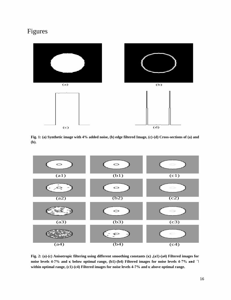
Application of linear gradient filters for delineation of low contrast

regions (case-1) in the presence of noise is illustrated using a

synthetic image shown in Fig. 1(a). The regions correspond to

3

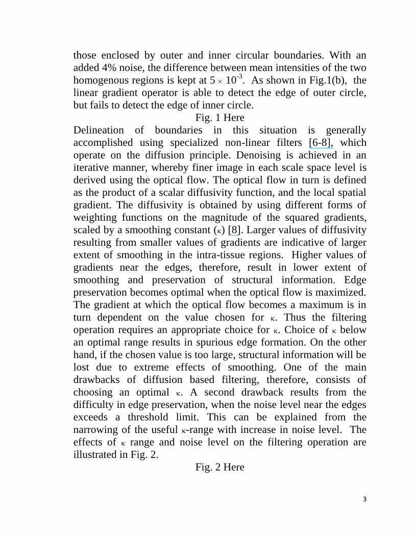
those enclosed by outer and inner circular boundaries. With an

added 4% noise, the difference between mean intensities of the two

homogenous regions is kept at 5 10-3

. As shown in Fig.1(b), the

linear gradient operator is able to detect the edge of outer circle,

but fails to detect the edge of inner circle.

Fig. 1 Here

Delineation of boundaries in this situation is generally

accomplished using specialized non-linear filters [6-8], which

operate on the diffusion principle. Denoising is achieved in an

iterative manner, whereby finer image in each scale space level is

derived using the optical flow. The optical flow in turn is defined

as the product of a scalar diffusivity function, and the local spatial

gradient. The diffusivity is obtained by using different forms of

weighting functions on the magnitude of the squared gradients,

scaled by a smoothing constant () [8]. Larger values of diffusivity

resulting from smaller values of gradients are indicative of larger

extent of smoothing in the intra-tissue regions. Higher values of

gradients near the edges, therefore, result in lower extent of

smoothing and preservation of structural information. Edge

preservation becomes optimal when the optical flow is maximized.

The gradient at which the optical flow becomes a maximum is in

turn dependent on the value chosen for . Thus the filtering

operation requires an appropriate choice for . Choice of below

an optimal range results in spurious edge formation. On the other

hand, if the chosen value is too large, structural information will be

lost due to extreme effects of smoothing. One of the main

drawbacks of diffusion based filtering, therefore, consists of

choosing an optimal . A second drawback results from the

difficulty in edge preservation, when the noise level near the edges

exceeds a threshold limit. This can be explained from the

narrowing of the useful -range with increase in noise level. The

effects of range and noise level on the filtering operation are

illustrated in Fig. 2.

Fig. 2 Here

4

Panels (a)-(c) represent three distinct ranges, and numberings 1-4

correspond to noise levels of 4-7%. The left panels (a1)-(a4)

correspond to values below the optimal range, showing spurious

edge formation with increasing noise levels. The middle and right

panels represent the ideal and supra-threshold ranges. It is seen that

when the noise level exceeds about 6%, the ideal range becomes

too narrow, and begins to exhibit spurious edge formation. Though

diffusion based filter achieves edge preservation and denoising, it

fails to produce sufficient separation between mean intensities of

the two tissue regions. This is important in situations when the

spatial extent of one of the regions is narrow and streaked such as

in angiograms, or spatially distributed in multiple locations and

contained within the other region, such as in multiple-sclerosis.

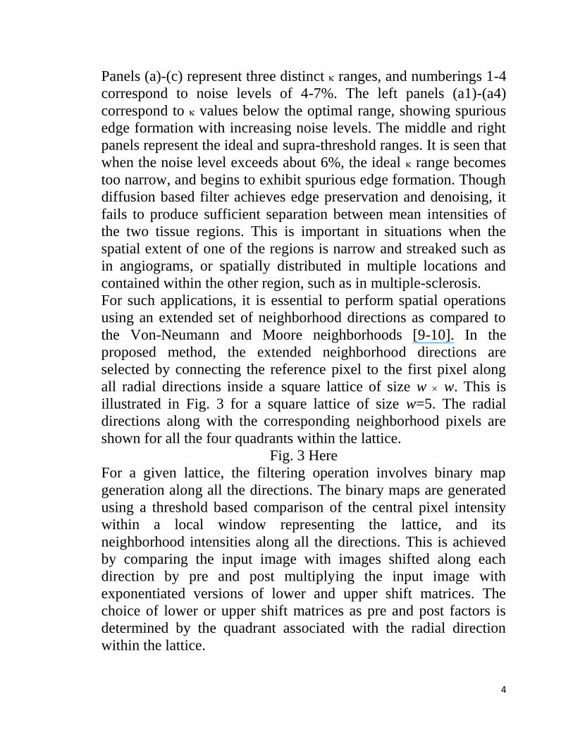
For such applications, it is essential to perform spatial operations

using an extended set of neighborhood directions as compared to

the Von-Neumann and Moore neighborhoods [9-10]. In the

proposed method, the extended neighborhood directions are

selected by connecting the reference pixel to the first pixel along

all radial directions inside a square lattice of size w w. This is

illustrated in Fig. 3 for a square lattice of size w=5. The radial

directions along with the corresponding neighborhood pixels are

shown for all the four quadrants within the lattice.

Fig. 3 Here

For a given lattice, the filtering operation involves binary map

generation along all the directions. The binary maps are generated

using a threshold based comparison of the central pixel intensity

within a local window representing the lattice, and its

neighborhood intensities along all the directions. This is achieved

by comparing the input image with images shifted along each

direction by pre and post multiplying the input image with

exponentiated versions of lower and upper shift matrices. The

choice of lower or upper shift matrices as pre and post factors is

determined by the quadrant associated with the radial direction

within the lattice.

5

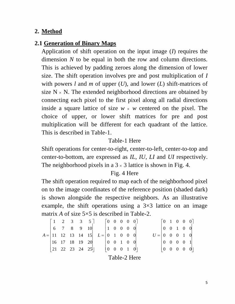
2. Method

2.1 Generation of Binary Maps

Application of shift operation on the input image (I) requires the

dimension N to be equal in both the row and column directions.

This is achieved by padding zeroes along the dimension of lower

size. The shift operation involves pre and post multiplication of I

with powers l and m of upper (U), and lower (L) shift-matrices of

size N N. The extended neighborhood directions are obtained by

connecting each pixel to the first pixel along all radial directions

inside a square lattice of size w w centered on the pixel. The

choice of upper, or lower shift matrices for pre and post

multiplication will be different for each quadrant of the lattice.

This is described in Table-1.

Table-1 Here

Shift operations for center-to-right, center-to-left, center-to-top and

center-to-bottom, are expressed as IL, IU, LI and UI respectively.

The neighborhood pixels in a 3 3 lattice is shown in Fig. 4.

Fig. 4 Here

The shift operation required to map each of the neighborhood pixel

on to the image coordinates of the reference position (shaded dark)

is shown alongside the respective neighbors. As an illustrative

example, the shift operations using a 3×3 lattice on an image

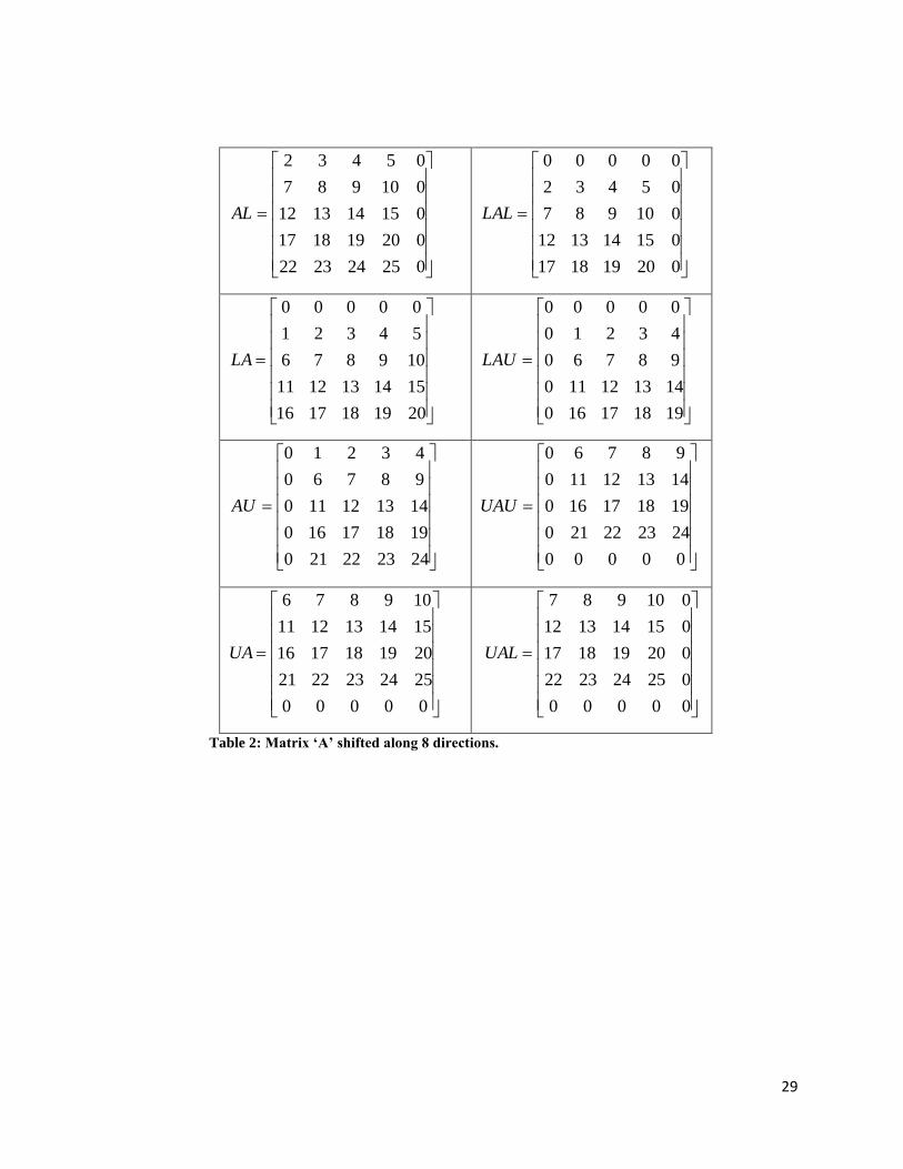
matrix A of size 5×5 is described in Table-2.

2524232221

2019181716

1514131211

109876

53321

A

01000

00100

00010

00001

00000

L

00000

10000

01000

00100

00010

U

Table-2 Here

6

For each radial direction k, the neighborhood pixel mapped on to

the reference position in I is given by

IVquadrantinkdirectionradialforILU

IIIquadrantinkdirectionradialforIUU

IIquadrantinkdirectionradialforIUL

IquadrantinkdirectionradialforILL

J

kk

kk

kk

kk

ml

ml

ml

ml

k

'',

'',

'',

'',

(2)

The binary map (Bk) along kth

direction is obtained using a

threshold based comparison of intensities in the original image I,

and the neighborhood map along kth

direction Jk as

.0

)),(),((1,

otherwise

jiJjiIifjiB

k

k

(3)

where represents the threshold used for binary map generation.

2.2 Computation of Shift-exponents

As shown in Eq. (2), the exponents lk, and mk depend on the radial

direction k, and the lattice size w. Fig. 5(a) shows a lattice with the

reference pixel located at (0, 0) in the local coordinate system. For

any given radial direction originating from the reference pixel, the

immediate neighbor is identified as the first pixel located along

that direction. The exponents of the pre and post shift matrices for

mapping the image coordinates of the immediate neighbor to that

of the reference pixel is obtained using a neighborhood mask E

given by

,0

1),gcd(1,

otherwise

mlifmlE

(4)

for 1 l,m n, where n=(w-1)/2. Positions in E having ones are

considered to be immediate neighbors. Generation of E for a lattice

of size 5 × 5 is illustrated in Fig.5 (b)-(c).

7

Fig. 5 Here

This excludes the immediate neighbors along x and y-directions

with reference to the reference pixel. The shift exponents for these

positions remain independent of w and do not require any special

computational procedure. Therefore, the steps in the current

approach include exponent computation for the remaining

directions only. The procedure for extension of this method to the

remaining quadrants of the lattice is illustrated in Fig. 6.

Fig. 6 Here

Sample neighborhood masks for various lattice sizes are shown in

Table- 3.

Table-3 Here

The number of directions (Nq) in the first quadrant of the lattice, is

therefore obtained by summing the unit elements of the

neighborhood mask,

n

l

n

m

q mlEN1 1

),(

(5)

Considering all four quadrants, the number of immediate neighbors

of any pixel will, therefore, be Nd=4×(Nq+1). Once the shift

exponents are computed, the Nd numbers of binary maps can be

generated as described in Eq. (3).

2.3 Filtering Procedure

A block schematic of the filtering procedure is shown in Fig. 7.

Binary maps are generated for all directions, and threshold for

intensity comparison of the input and shifted images is estimated

using a threshold estimation algorithm, explained in a later section.

Fig. 7 Here

8

The weight for each pixel of the input image is obtained as the

intensity at the corresponding position in the summation of binary

maps (BWI) along all directions

dN

k

kBBWI1 (6)

The filtered image is then estimated as

),(),(),(),( jiBWIjiIjiIjiO

(7)

2.4 Threshold Estimation

The threshold is calculated by first estimating the noise variance

( σ2M ) for a given Region-Of-Interest (ROI), using skewness ( ) of

the intensity distribution of pixels within the ROI. The steps used

for estimation of σ2M is borrowed from [11], and summarized in the

flowchart shown in Fig. 8.

Fig.8 Here

The threshold () is then chosen from a range of values [σ2

M,

CROI], where CROI denotes difference between the mean intensities

of the two tissue regions within the ROI. The effect of choosing a

specific value in this range, on the filtered image is explained in

section 3.2.

3. Result

3.1 Numerical Results

Fig. 9(a) shows a phantom image with two circular edges. The

inner edge is not visible due to the mean intensity difference of 5

10-3

. This image is filtered using different lattice sizes of w=3, 7,

11, and 15. For small values of w, the filter operates as an edge

detector. As w increases, the spread of the edge extends to the

9

centroid of the region having a higher mean intensity. This effect is

illustrated in Figs. 9(g)-(j). The corresponding filtered versions are

shown in panels (b)-(e). It is seen that as w is increased beyond 11,

the edges spread from opposite directions, so as to fill the entire

region with a mean intensity larger than its surrounding pixels. In

the context of medical images, these regions can be likened to

those of small sized lesions, such as multiple sclerosis seen in PD,

or T1-weighted MR images. This is true, especially, for modalities

in which the lesions exhibit a slightly larger intensity than the

surrounding healthy region. As the lesion size increases, the lattice

size required to enhance, or fill the lesion, will accordingly be

higher. Increasing the lattice size is also accompanied by an

increase in the CROI, equivalent to the difference between the mean

intensities of the two regions as evident from panels (i) and (j).

This example illustrates an implementation of case-1, as discussed

section-1.

Fig.9 Here

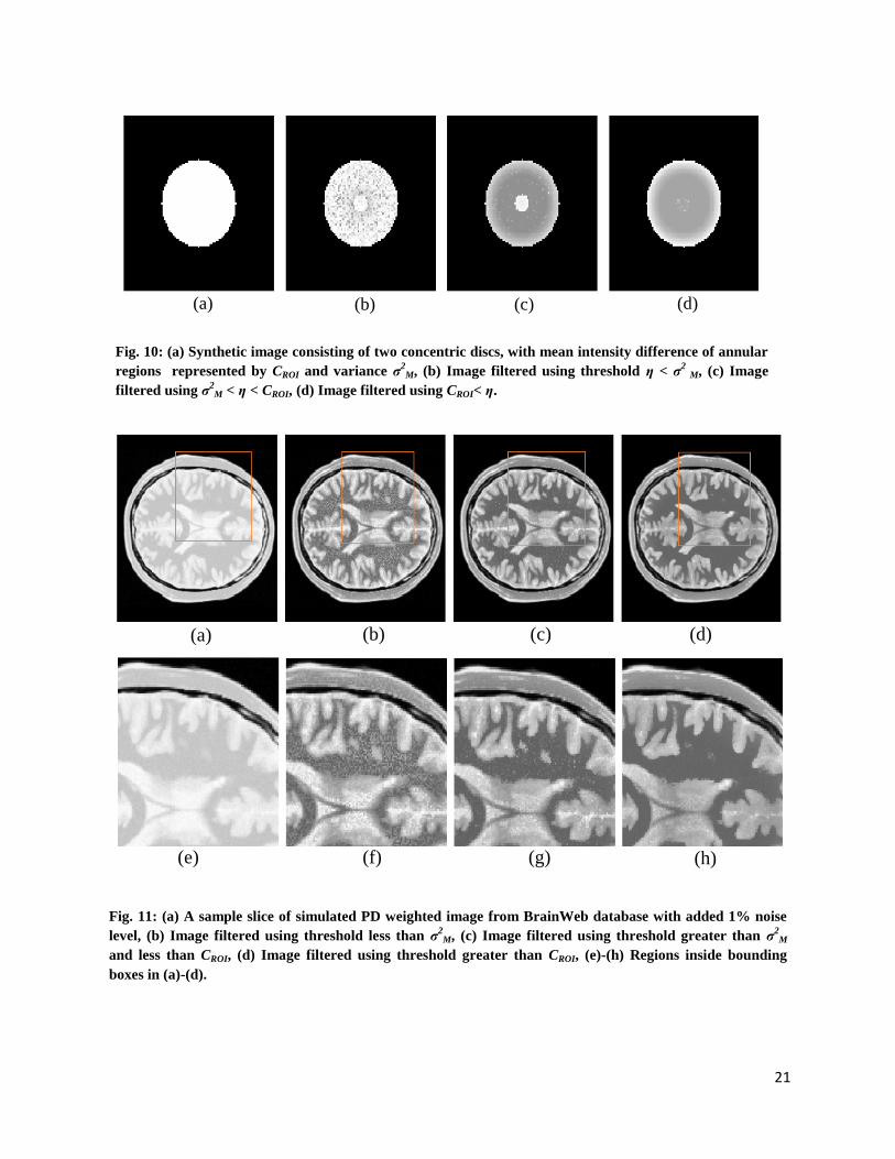
3.2 Effect of

As discussed in section 2.4, the threshold () is selected in such a

way that it should be less than the difference between the means of

two tissue regions in the ROI (CROI), and greater than σ2M. The

effect of choosing an appropriate is illustrated using the phantom

image in Fig. 10, and a sample MR image with MS lesions

obtained from the BrainWeb database [12]. The ROI in Fig. 10 is

chosen to be the circular region, encompassing an inner disk of a

slightly higher mean intensity, as explained earlier in sections-1

and 3.1. For a 1% added noise, the σ2M in the ROI is estimated to

be 4.290310-5

, using the procedure outlined in section 2.4. The

panels (b)-(d) represent filtered images corresponding to < σ2

M,

σ2M < < CROI, and > CROI respectively.

Fig.10 Here

10

The condition < σ2M results in spurious edges as shown in Fig.

10(b). Likewise, for > CROI, the contrast between two regions is

not enhanced as shown in Fig. 10(d). This is easily deduced from

the fact that the weights obtained from binary maps will be close to

zero. The optimal performance is shown in Fig. 10(c). The ROI for

the BrainWeb image is the bounding box shown in red in Fig.

11(a). Filtering is performed on PD images of slice thickness 1mm,

intensity non-uniformity of 20% and different levels of added

noise 1-7% in steps of 2%. The filtered images corresponding to

1% noise level are shown in Figs. (b)-(d) for < σ2M, σ

2M < <

CROI, and > CROI respectively. The insets (f-h) show the filtered

versions of the ROI. The results obtained are identical to the

simulated example in Fig. 10.

Fig.11 Here

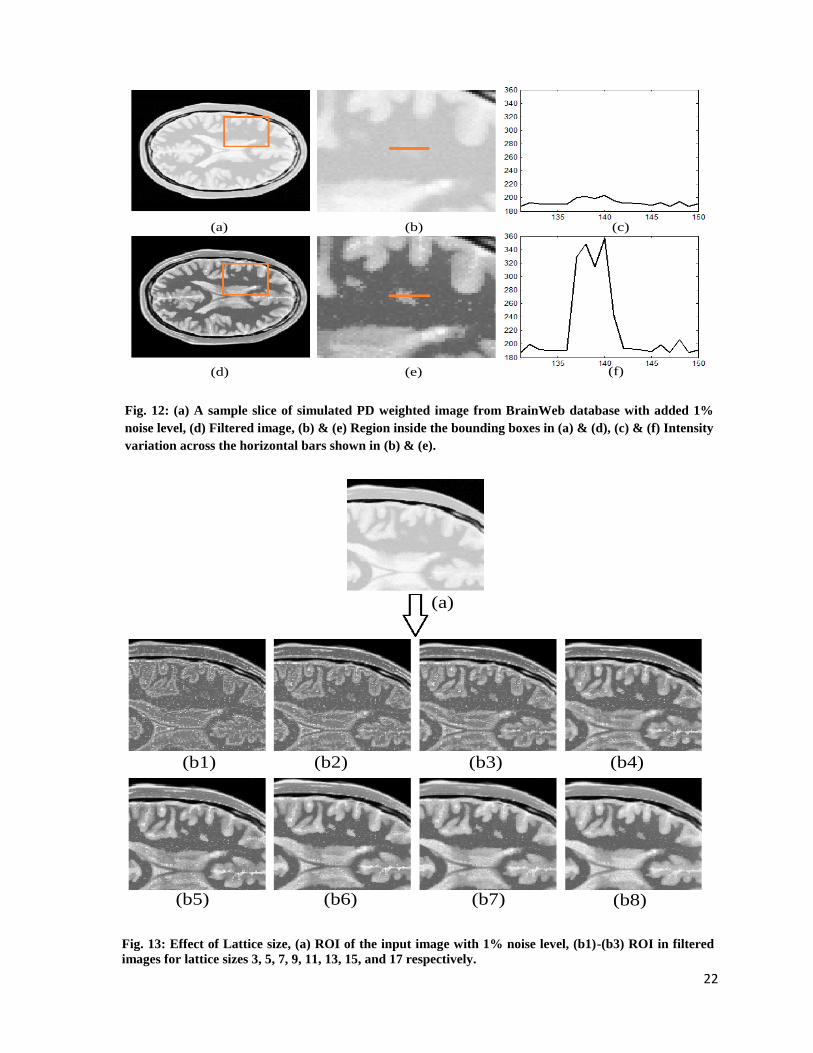
3.3 Application to Simulated Images

In this section, the effect of applying binary weighted maps on

simulated PD weighted images with MS lesions is illustrated.

Sample PD images of slice thickness 1mm, intensity non-

uniformity of 20% and different levels of added noise (1-7 % in

steps of 2%) are taken from BrainWeb database. The lattice size

used for filtering is chosen based on the maximum size of MS

lesions. The threshold is estimated using the estimation procedure

outlined in section 2.4. In the input image shown in Fig. 12(a), the

MS lesions are not clearly visible due to low contrast from the

surrounding tissue. The filtered image is shown in Fig. 12(d). The

panels (b) and (e) show regions within the ROI highlighted by the

bounding boxes in the input and filtered images respectively. The

plots of intensity variation across the lesion in the original and

filtered images are shown in the adjoining panels (c) and (f).

Fig.12 Here

The effect of increasing the lattice size is shown in Fig. 13. It is

seen that for the given ROI of the BrainWeb sample image, an

acceptable performance is achieved for a lattice of 11. With further

11

increase in lattice size, there is no marked difference in

performance.

Fig.13 Here

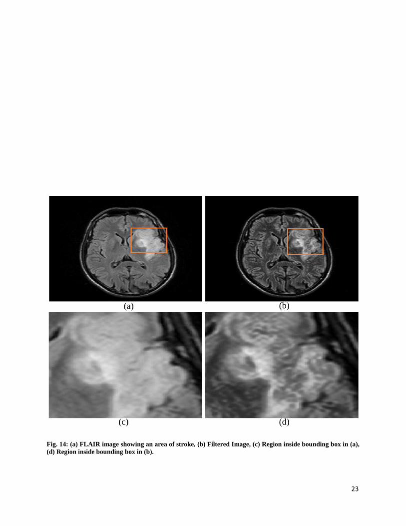
3.4 Application to Clinical images

Fig. 14 illustrates the filtering applied to a sample FLAIR image

acquired on 1.5T clinical MR scanner (Magnetom- Avanto,

Siemens, Erlangen, Germany) with a 12 channel head coil. The

MRI parameters for FLAIR sequence includes the TE : 108

milliseconds; TR : 8140 milliseconds; TI : 2500 milliseconds; field

of view : 230mm; matrix 256 184; 24 slices; 5mm slice thickness,

30% gap). The patient’s MRI FLAIR image shows an infarct in the

left insular cortex and frontal operculum. The ROI indicating the

area of stroke is highlighted using a bounding box in this image.

The regions within the bounding box of the original and filtered

images are shown in panels (c) and (d) respectively. It is seen that

the filtered image highlights the spatial profile of the thrombotic

vasculature. The surrounding regions of edema are seen with

darker shades in the filtered image. After filtration, brain shows

better gray- white distinction. The area of infarct shows various

intensities within, probably representing the extent of infarct

severity. The margins of the infarct are better made out.

Fig.14 Here

Effect of lattice size is shown in Fig. 15. An optimal performance

is achieved for w 15.

Fig. 15 Here

3.5 Performance Characterization

The synthetic image described in section 3.1 is used for calculating

the Contrast-to-Noise Ratio (CNR) for both the binary weighted

filter, and anisotropic filters described by Perona and Malik [6],

and Jiang et al., [8]. CNR between two regions a and b (CNRa/b) is

calculated as (Sa-Sb)/σ, where Sa and Sb refer to the average signal

intensity of brighter, and darker regions respectively. The CNR is

plotted against noise standard deviation (σ) in Fig. 16.

12

Fig.16 Here

For both the proposed and anisotropic filters, the CNR is observed

to decrease with increase in noise variance. The performance of

proposed method is seen to be better when the standard deviation

of intensity variation is less than 0.03 corresponding to a mean

intensity of 0.655. When the standard deviation exceeds 5% of the

mean intensity, a pre-processing step using Non-local means

(NLM) filter [13] is suggested.

Parameters for NLM filtering include the search window size (t),

similarity window size (f) and a weight decay control parameter (h)

[13]. The de-noising capability of NLM filter is controlled by the

third parameter h, identical to the estimated noise variance σ2

M .

The steps for pre-filtering using NLM are shown in Fig. 17.

Fig.17 Here

The result of filtering a BrainWeb image sample with 5% added

noise and 3mm slice thickness is shown in Fig. 18. The panels (a)-

(b) correspond to the noisy input image with 5% added noise,

image processed using NLM filter with search window size t= 5,

similarity window size f =1, and h=11. The image in Fig. 18(b) is

further processed using the proposed filter with a lattice of 17. The

resulting image is shown in panel (c). The zoomed versions of the

ROI are shown in panels (d)-(f).

Fig.18 Here

The MR angiography image in Fig. 19 after filtration, shows an

enhanced version of the peripheral vasculature.

Fig.19 Here

13

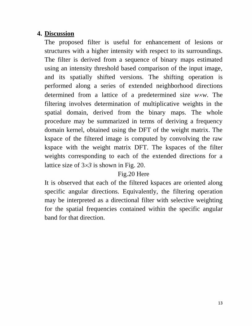
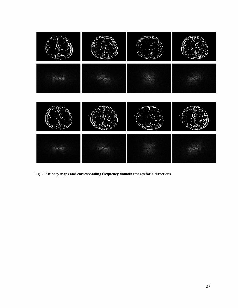
4. Discussion

The proposed filter is useful for enhancement of lesions or

structures with a higher intensity with respect to its surroundings.

The filter is derived from a sequence of binary maps estimated

using an intensity threshold based comparison of the input image,

and its spatially shifted versions. The shifting operation is

performed along a series of extended neighborhood directions

determined from a lattice of a predetermined size ww. The

filtering involves determination of multiplicative weights in the

spatial domain, derived from the binary maps. The whole

procedure may be summarized in terms of deriving a frequency

domain kernel, obtained using the DFT of the weight matrix. The

kspace of the filtered image is computed by convolving the raw

kspace with the weight matrix DFT. The kspaces of the filter

weights corresponding to each of the extended directions for a

lattice size of 33 is shown in Fig. 20.

Fig.20 Here

It is observed that each of the filtered kspaces are oriented along

specific angular directions. Equivalently, the filtering operation

may be interpreted as a directional filter with selective weighting

for the spatial frequencies contained within the specific angular

band for that direction.

14

References

[1] M. Styer, C. B. Uhler, G. Szekely and G. Gerig, “Parametric

estimate of intensity inhomogeneities applied to MRI”. IEEE

Trans. On Med. Img. Vol 19, No. 3, P153-165, March 2000.

[2] J. F. Canny, “Finding edges and lines in images”, Technical

Report AI–TR–720, M.I.T. Artificial Intell. Lab., Cambridge, MA,

1983.

[3] D. Marr and E. C. Hildreth, “Theory of edge detection”, Proc. Roy.

Soc. London Ser. B, vol. 207, pp. 187-217, 1980.

[4] Z. Yu-qian, G. Wei-hua, C. Zhen-cheng, T. Jing-tian, and L. Ling-

yun, “ Medical Images Edge Detection Based on Mathematical

Morphology”, Proceedings of the 2005 IEEE Engineering in

Medicine and Biology 27th

Annual Conference Shanghai, China,

pp. 6492-6495, September 1-4, 2005.

[5] S. Agaian, and A. Almuntashri, “Noise-Resilient Edge Detection

Algorithm for Brain MRI Images”, 31st Annual International

Conference of the IEEE EMBS Minneapolis, Minnesota, USA,

September 2-6, 2009, pp. 3689-3692.

[6] P. Perona and J. Malik, “Scale-Space and Edge Detection Using

Anisotropic Diffusion”, IEEE Trans on Pattern Analysis and

Machine Intelligence, Vol. 12, no. 7,pp. 629-639, July 1990.

[7] G. Gerig, O. Kubler, R. Kikinis and F. A. Jolesz, “Nonlinear

Anisotropic Filtering of MRI Data”, IEEE Trans. On Medical

Imaging, Vol. 11, No. 2, pp. 221-232, June 1992.

[8] D. Jiang, S. B. Fain, G. Tianliang, T. M. Grist and C. A. Mistretta,

“Noise Reduction in MR Angiography with NonLinear

Anisotropic Filtering”, Journal of Magnetic Resonance Imaging,

Vol. 19, No. 5, pp. 632-639, May 2004.

[9] J. Biswapati, P. Pabitra and B. Jaydeb, “New Image Noise

Reduction Schemes Based on Cellular Automata”, International

15

Journal of Soft Computing and Engineering (IJSCE), Vol. 2, No. 2,

pp. 98-103, May 2012.

[10] N. H. Packard and S. Wolfram, “Two dimensional cellular

automata”, Journal of Statistical Physics, Vol. 38, No. 5-6, pp.

901-946, 1985.

[11] J. Rajan, D. Poot, J. Juntu and J. Sijbers, “Noise measurement from

magnitude MRI using local estimates of variance and skewness”,

Physis in Mediceine and Biology, Vol. 55, pp 441-449, 2010.

[12] BrainWeb: Simulated Brian Database,

http://brainweb.bic.mni.mcgill.ca/brainweb/

[13] A. Buades, B. Coll and M. J. Morel, “A non-local algorithm for

image de-noising”, Comp. Vision and Patt. Recog. 2005, IEEE

Computer Society Conference, Vol. 2, pp 60-65, 20-25, June 2005.

16

Figures

(a) (b)

(c) (d)

Fig. 1: (a) Synthetic image with 4% added noise, (b) edge filtered Image, (c)-(d) Cross-sections of (a) and

(b).

(a1) (b1) (c1)

(a2) (b2) (c2)

(a3) (b3) (c3)

(a4) (b4) (c4)

Fig. 2: (a)-(c) Anisotropic filtering using different smoothing constants () ,(a1)-(a4) Filtered images for

noise levels 4-7% and below optimal range, (b1)-(b4) Filtered images for noise levels 4-

within optimal range, (c1)-(c4) Filtered images for noise levels 4-7% and above optimal range.

17

Fig. 3: Extended neighborhood pixels along different directions for a lattice of size 5×5.

18

Fig. 4: Shift operations for mapping neighborhood pixels for a

lattice of size 3×3.

(a) (c)

(b)

Fig. 5: Generation of Neighborhood Mask E. (a) Bounding box showing pixels in the first quadrant of

the square lattice, (b) Local co-ordinates of the first quadrant with corresponding GCD values, (c)

Neighborhood mask E.

19

(a) (b)

(d) (c)

Fig. 6: Procedure for extension of exponent computation to the remaining quadrants of the lattice.

Fig. 7: Block Diagram of the Binary Weighted Filter.

20

Fig. 8: Estimation of Noise variance.

(a) (b) (c) (d) (e)

(f) (g) (h) (i) (j)

Fig. 9: (a) Synthetic image, (b)-(e) Summation of binary maps for lattice size 3, 7, 11 and 15, (f)-(j)

Cross-sections of (a)-(e).

21

(a) (b) (c) (d)

Fig. 10: (a) Synthetic image consisting of two concentric discs, with mean intensity difference of annular

regions represented by CROI and variance σ2

M, (b) Image filtered using threshold η < σ2

M, (c) Image

filtered using σ2

M < η < CROI, (d) Image filtered using CROI< η.

(a) (b) (c) (d)

(h) (g) (f) (e)

Fig. 11: (a) A sample slice of simulated PD weighted image from BrainWeb database with added 1% noise

level, (b) Image filtered using threshold less than σ2

M, (c) Image filtered using threshold greater than σ2M

and less than CROI, (d) Image filtered using threshold greater than CROI, (e)-(h) Regions inside bounding

boxes in (a)-(d).

22

(a) (b) (c)

(e) (f) (d)

Fig. 12: (a) A sample slice of simulated PD weighted image from BrainWeb database with added 1%

noise level, (d) Filtered image, (b) & (e) Region inside the bounding boxes in (a) & (d), (c) & (f) Intensity

variation across the horizontal bars shown in (b) & (e).

(a)

(b1) (b2) (b3) (b4)

(b8) (b7) (b6) (b5)

Fig. 13: Effect of Lattice size, (a) ROI of the input image with 1% noise level, (b1)-(b3) ROI in filtered

images for lattice sizes 3, 5, 7, 9, 11, 13, 15, and 17 respectively.

23

(a) (b)

(d) (c)

Fig. 14: (a) FLAIR image showing an area of stroke, (b) Filtered Image, (c) Region inside bounding box in (a),

(d) Region inside bounding box in (b).

24

(a)

(b1) (b2) (b3) (b4)

(b8) (b7) (b6) (b5)

Fig. 15: Effect of Lattice size, (a) ROI of the FLAIR image, (b1)-(b8) ROI in filtered images for lattice sizes

3, 5, 7, 9, 11, 13, 15, and 17 respectively.

25

Fig. 16: Plots of CNR against noise standard deviation (σ) for the proposed versus Anisotropic filter.

Input

Image

Noise

variance

Estimation

Non-Local

Means

Filter

Proposed

Method

Output

Image

Fig. 17: Pre-filtering using Non-Local Means (NLM) filter.

26

(a) (b) (c)

(f) (e) (d)

Fig. 18: (a) A sample slice of simulated PD weighted image from BrainWeb database with added 5% noise

level, (b) NLM filtered image, (c) The result of proposed binary weighted filter applied to the NLM filtered

input image, (d)-(f) Regions within the bounding boxes in (a)-(c).

(a) (b) (c)

(f) (e) (d)

Fig. 19: (a) A sample slice of MR Angiogram, (b) Filtered image, (d)-(f): Regions within the bounding boxes in

(a) & (b), (c) & (f): Intensity variation across the vertical bars shown in (d) & (e).

27

Fig. 20: Binary maps and corresponding frequency domain images for 8 directions.

28

Tables

Quadrant Shift Operation

Ist

Ll I L

m

IInd

Ll I U

m

IIIrd

Ul I U

m

IVth

Ul I L

m

Table 1: Pre and Post multiplication shift operators for each

quadrant in the lattice.

29

025242322

020191817

015141312

010987

05432

AL

020191817

015141312

010987

05432

00000

LAL

2019181716

1514131211

109876

54321

00000

LA

191817160

141312110

98760

43210

00000

LAU

242322210

191817160

141312110

98760

43210

AU

00000

242322210

191817160

141312110

98760

UAU

00000

2524232221

2019181716

1514131211

109876

UA

00000

025242322

020191817

015141312

010987

UAL

Table 2: Matrix ‘A’ shifted along 8 directions.

30

Table 3: Neighborhood Mask generation for lattice sizes, 3, 5, 7, and 11.