Generalized Equalization Model for Image Enhancement

68 IEEE TRANSACTIONS ON MULTIMEDIA, VOL. 16, NO. 1, JANUARY 2014

Generalized Equalization Modelfor Image Enhancement

Hongteng Xu, Guangtao Zhai, Member, IEEE, Xiaolin Wu, Fellow, IEEE, and Xiaokang Yang, Senior Member, IEEE

Abstract—In this paper, we propose a generalized equalizationmodel for image enhancement. Based on our analysis on the re-lationships between image histogram and contrast enhancement/white balancing, we first establish a generalized equalizationmodelintegrating contrast enhancement and white balancing into a uni-fied framework of convex programming of image histogram. Weshow that many image enhancement tasks can be accomplishedby the proposed model using different configurations of parame-ters. With two defining properties of histogram transform, namelycontrast gain and nonlinearity, the model parameters for differentenhancement applications can be optimized.We then derive an op-timal image enhancement algorithm that theoretically achieves thebest joint contrast enhancement and white balancing result withtrading-off between contrast enhancement and tonal distortion.Subjective and objective experimental results show favorable per-formances of the proposed algorithm in applications of image en-hancement, white balancing and tone correction. Computationalcomplexity of the proposed method is also analyzed.

Index Terms—Contrast enhancement, contrast gain, generalizedequalization, nonlinearity of transform, tone mapping, white bal-ancing.

I. INTRODUCTION

W ITH the fast advance of technologies and the prevalenceof imaging devices, billions of digital images are being

created every day. Due to undesirable light source, unfavor-able weather or failure of the imaging device itself, the contrastand tone of the captured image may not always be satisfactory.Therefore, image enhancement is often required for both theaesthetic and pragmatic purposes. In fact, image enhancementalgorithms have already been widely applied in imaging devicesfor tone mapping. For example, in a typical digital camera, theCCD or CMOS array receives the photons passing through lensand then the charge levels are transformed to the original image.

Manuscript received December 12, 2012; revised May 18, 2013; acceptedJuly 04, 2013. Date of publication September 25, 2013; date of current versionDecember 12, 2013. This work was supported in part by NSFC (60932006,61025005, 61001145, 61129001, 61221001, 61371146) and the 111 Project(B07022).. The associate editor coordinating the review of this manuscript andapproving it for publication was Dr. Xiao-Ping Zhang.H. Xu, G. Zhai, and X. Yang are with the Institute of Image Communica-

tion and Information Processing, Shanghai Jiao Tong University, Shanghai200240, China (e-mail: [email protected]; [email protected];[email protected]).X. Wu is with the Department of Electrical & Computer Engineering, Mc-

Master University, Hamilton, ON L8G 4K1, Canada, and also with the Instituteof Image Communication and Information Processing, Shanghai Jiao Tong Uni-versity, Shanghai 200240, China (e-mail: [email protected]).Color versions of one or more of the figures in this paper are available online

at http://ieeexplore.ieee.org.Digital Object Identifier 10.1109/TMM.2013.2283453

Usually, the original image is stored in RAW format, with abit-length too big for normal displays. So tone mapping tech-niques, e.g. the widely known gamma correction, are used totransfer the image into a suitable dynamic range. More sophis-ticated tone mapping algorithms were developed through theyears, see [2], [8], [12], [29], [33], [34], [43], just to name afew.Generally, tone mapping algorithms can be classified into two

categories by their functionalities during the imaging process.1) White Balancing: Because of the undesirable illuminance

or the physical limitations of inexpensive imaging sensors, thecaptured image may carry obvious color bias.1 To calibratethe color bias of image, we need to estimate the value of lightsource, the problem of which called color constancy [16],[18], [21], [40], [41]. Using a suitable physical imaging model,one can get an approximated illuminance, and then a lineartransform can be applied to map the original image into anideal one.2) Contrast Enhancement: Contrast enhancement algo-

rithms are widely used for the restoration of degraded media,among which global histogram equalization is the most popularchoice. Other variants includes local histogram equalization[42] and the spatial filtering type of methods [11], [14], [27],[32], [39], [44]. For example, in [32] the fractional filter isused to promote the variance of texture so as to enhance theimage. In [31], a texture synthesis based algorithm is proposedfor degraded media, such as old pictures or films. On the otherhand, transform based methods also exist, e.g. curvelet basedalgorithm in [35]. In [44], an adaptive steering regression kernelis proposed to combine image sharpening with denoising.Despite of the abundant literature on image enhancement,

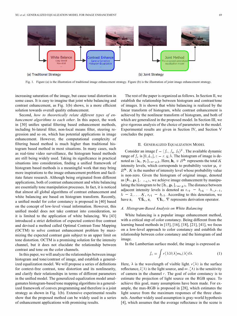
including those representatives listed above, two challengingproblems for image enhancement are still not solved. First, howto achieve contrast enhancement while preserving a good tone.The contrast and tone of an image have mutual influence. Be-cause of the complicated interaction, those algorithms merelyaiming towards contrast enhancement or white balancingcannot provide optimal visual effect. Most, if not all, of currentimage enhancement systems divide white balancing and con-trast enhancement into two separate and independent phases,as Fig. 1(a) shows. This strategy has an obvious drawback:although tone has adjusted in the white balancing phase, con-trast enhancement may undesirably bias it again. This troublehas been observed in many applications, e.g. the de-hazingalgorithms in [26], [37], [38] achieve contrast enhancement by

1In fact, the color bias is caused by tone distortions of the three channels, so“tone” in this paper is referring not only to gray image, but also the hue of colorimage. We will not explicitly discriminate these two concepts in this work.

1520-9210 © 2013 IEEE

XU et al.: GENERALIZED EQUALIZATION MODEL FOR IMAGE ENHANCEMENT 69

Fig. 1. Figure (a) is the illustration of traditional image enhancement strategy. Figure (b) is the illustration of joint image enhancement strategy.

increasing saturation of the image, but cause tonal distortion insome cases. It is easy to imagine that joint white balancing andcontrast enhancement, as Fig. 1(b) shows, is a more efficientsolution towards overall quality enhancement.Second, how to theoretically relate different types of en-

hancement algorithms to each other. In this aspect, the workin [30] unifies spatial filtering based enhancement methods,including bi-lateral filter, non-local means filter, steering re-gression and so on, which has potential applications in imageenhancement. However, the computational complexity offiltering based method is much higher than traditional his-togram based method in most situations. In many cases, suchas real-time video surveillance, the histogram based methodsare still being widely used. Taking its significance in practicalsituations into consideration, finding a unified framework ofhistogram based methods is a meaningful work that may bringmore inspirations to the image enhancement problem and facil-itate future research. Although being originated from differentapplications, both of contrast enhancement and white balancingare essentially tone manipulation processes. In fact, it is noticedthat almost all global algorithms of contrast enhancement andwhite balancing are based on histogram transform. Recently,a unified model for color constancy is proposed in [40] basedon the concept of low-level visual information. However, thisunified model does not take contrast into consideration, soit is limited to the application of white balancing. Wu [43]introduced a strict definition of expected context-free contrastand devised a method called Optimal Contrast-Tone Mapping(OCTM) to solve contrast enhancement problem by maxi-mizing the expected contrast gain subject to an upper limit ontone distortion. OCTM is a promising solution for the intensitychannel, but it does not elucidate the relationship betweencontrast and tone on the color channels.In this paper, we will analyze the relationships between image

histogram and tone/contrast of image, and establish a general-ized equalization model. We will propose a series of definitionsfor context-free contrast, tone distortion and its nonlinearity,and clarify their relationships in terms of different parametersin the unified model. The generalized equalization model amal-gamates histogram-based tone mapping algorithms in a general-ized framework of convex programming and therefore is a jointstrategy as shown in Fig. 1(b). Extensive experimental resultsshow that the proposed method can be widely used in a seriesof enhancement applications with promising results.

The rest of the paper is organized as follows. In Section II, weestablish the relationship between histogram and contrast/toneof images. It is shown that white balancing is realized by thelinear transform of histogram, while contrast enhancement isachieved by the nonlinear transform of histogram, and both ofwhich are generalized in the proposed model. In Section III, wegive rigorous analysis of the choice of parameters in the model.Experimental results are given in Section IV, and Section Vconcludes the paper.

II. GENERALIZED EQUALIZATION MODEL

Consider an image . The available dynamicrange of is , . The histogram of image is de-noted as . Here, represents the totalintensity levels, which corresponds to probability vector

. is the number of intensity level whose probability valueis non-zero. Given the histogram of original image, denotedas , we achieve image enhancement by manipu-lating the histogram to be . The distance betweenadjacent intensity levels is denoted as ,

, . According to this denotation, wehave , . represents derivation operator.

A. Histogram-Based Analysis on White Balancing

White balancing is a popular image enhancement method,with a critical step of color constancy. Being different from thelearning based methods in [15], [16], [18], [21], [41], we focuson a low-level approach to color constancy and establish therelationship between color constancy and the histogram of andimage.In the Lambertian surface model, the image is expressed as

(1)

Here, is the wavelength of visible light. is the surfacereflectance, is the light source, and is the sensitivityof camera in the channel . The goal of color constancy is toestimate the projection of light source on the RGB space. Toachieve this goal, many assumptions have been made. For ex-ample, the max-RGB is proposed in [28], which estimates thelight source from the maximum responses of the three chan-nels. Another widely used assumption is gray-world hypothesis[4], which assumes that the average reflectance in the scene is


achromatic. Recently, these assumptions are unified in [17], asfollows

(2)

Here, is the coordinate of pixel. is an arbitrary positiveconstant and is a parameter. is the normal-ized estimation of light source. When (2) is equivalentto Gray-world assumption while when (2) is equiva-lent to max-RGB. White balancing is achieved by multiplyingthe element of to the corresponding channel of . Because

is the normalized form of white light, themultiplication factor of channel is .From the viewpoint of image histogram, the left side of (2)

can be rewritten as

(3)

where . Eq. (3) reveals the interconnec-tion among white balancing and histogram. Given an image,is calculated as

(4)

As a result, the histogram of white balancing result, denoted as, is computed as follows

(5)

It is obvious that this process is linear. The linearity of the trans-form is the most significant feature of histogram-based whitebalancing algorithm. In the next subsection, we will show thatthis linearity is also an important difference between white bal-ancing and contrast enhancement.

B. Histogram-Based Analysis on Contrast Enhancement

In [43], the expected context-free contrast of image is definedby

(6)

By the definition, the maximum contrast is , which isachieved by a binary black-and-white image; the minimumcontrast is zero when the image is a constant. So, the contrastenhancement is achieved by maximizing (6) in [43], as follows.

(7)

where the first constraint makes sure that the output image stillhas a suitable dynamic range and the second constraint denotesthe minimum distance between adjacent gray levels as .However, although the definition in (6) has obvious statistical

meaning, it is not optimal to be used as objective function di-rectly. Eq. (7) is a linear programming problem whose solutionis sparse—to the maximum probability , the corresponding

, and other . Realizing this problem,another two constraints are added in [43] to suppress artifacts,which makes the model complicated and sensitive to some pre-defined parameters.Before the work in [43], histogram-based algorithm has been

widely used in contrast enhancement. The most commonly usedapproach is histogram equalization [22], which makes the prob-ability density function of enhanced image close to that of uni-form distribution. After equalization, the th intensity level ofnew image, , is

(8)

Here, is a constant. Eq. (8) also gives a relationship betweenhistogram and the distance between adjacent intensity level, asfollowing shows.

(9)

According to (8), (9), histogram equalization is equivalent tosolving following optimization problem.

(10)

Here .The performance of histogram equalization is not optimal in

most situations. The essential reason for its limited performanceis the questionable assumption that the histogram of ideal imageobeys uniform distribution. To get better equalization result, weneed to find a better distribution which is a big challenge. Re-cently, some adaptive histogram equalization methods are pro-posed in [1], [5], [7], [24], [36] but gave neither a clear defi-nition of contrast nor an explicit objective function of contrastenhancement like (7), (10) shows. A common feature of all theenhancement methods mentioned above is that the transform ofhistogram is non-linear, which is different fromwhite balancing.

C. The Proposed Model

The aims of establishing the generalized equalization modelinclude: 1) giving a unified explanation to white balancingproblem and contrast enhancement problem; 2) providingan explicit objective function for these two problems andproposing a joint algorithm for them; 3) controlling the perfor-mance of the algorithm by as few parameters as possible.The proposed model is inspired by (7), (10). Although (7),

(10) seem to be very different, if we regard the order of and


the norm of the objective function as two parameters, and ,(7), (10) are rewritten in a generalized form:

(11)

Both (10) and (7) have interesting relationships with (11). Whenand (or and ), maximum is

reached when , which is equivalent (10). Whenand (or and ), the

solution would be smoother than that of (10). When or, the solution is equivalent to that of (7). Compared

with traditional histogram equalization, (11) is more flexible,because the target histogram does not have to obey uniform dis-tribution. Considering the fact that traditional histogram equal-ization often leads to over-enhanced results, relaxing the con-straints of uniform distribution can suppress over-enhancementeffectively. On the other hand, as long as and in thesuitable range, histogram of the enhanced image can avoid tobe too sparse. As a result, we do not need additional constraintslike OCTM does.According to the analysis above, (11) provides a reasonable

and unified definition with the objective function of contrast en-hancement. We will further take white balancing into the model.Based on (4), (11), we formulate the generalized equalizationmodel mathematically as follows.

(12)

Here, is the original distance between adjacent intensitylevels of the channel . In generalized model, we set the upperbound as the result of white balancing .On the top of (12), we introduce two measures into general-

ized equalization model: the gain of expected context-free con-trast and the nonlinearity of the transform from to , whichare defined as

(13)

If is homogeneous enough, . The larger ,the stronger nonlinearity of the transform. The nonlinearity ofwhite balancing methods is close to 0. On the other hand, thecontrast enhancement methods often have strong nonlinearity,which achieve visible enhancement of contrast. However, sep-arate nonlinear transform of histograms of three channels maycause tone distortion. In the next section, we will theoreticallyprove that the proposed method, with a suitable configurationof parameters, can achieve a best trade-off between contrast en-hancement and tone adjustment.

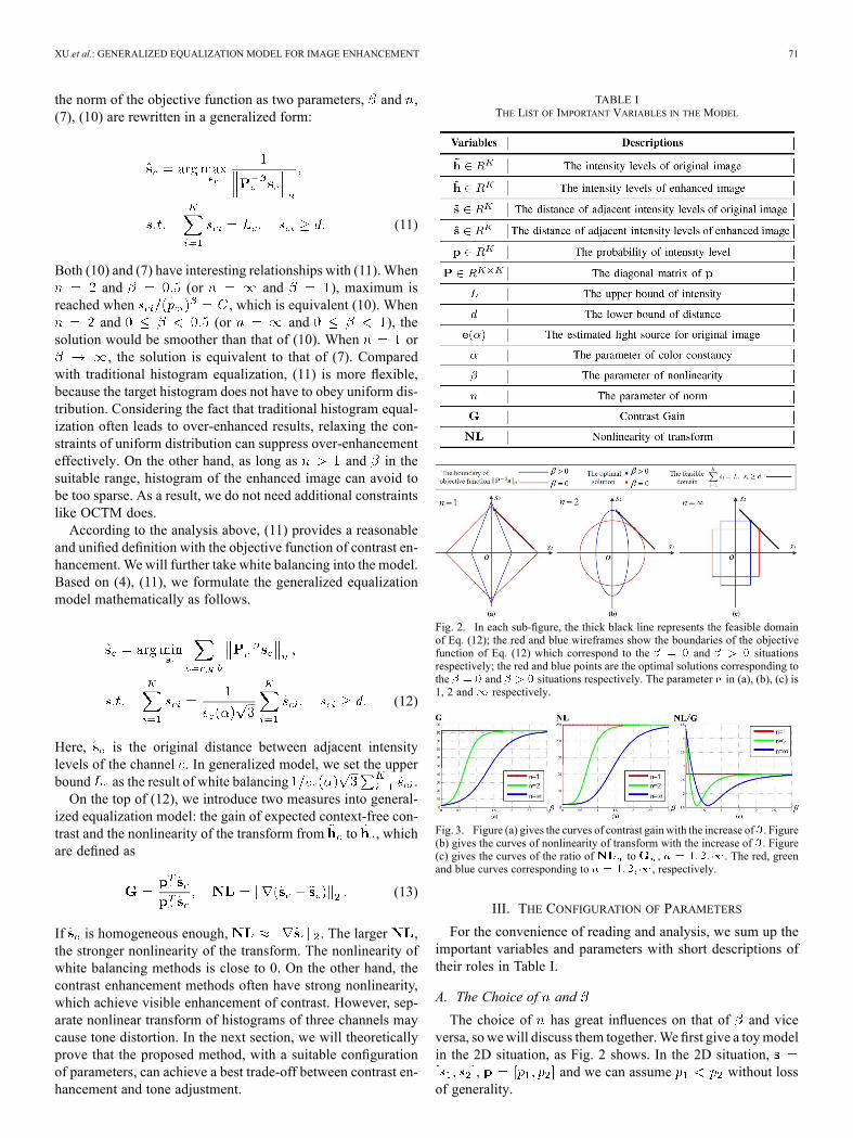
TABLE ITHE LIST OF IMPORTANT VARIABLES IN THE MODEL

Fig. 2. In each sub-figure, the thick black line represents the feasible domainof Eq. (12); the red and blue wireframes show the boundaries of the objectivefunction of Eq. (12) which correspond to the and situationsrespectively; the red and blue points are the optimal solutions corresponding tothe and situations respectively. The parameter in (a), (b), (c) is1, 2 and respectively.

Fig. 3. Figure (a) gives the curves of contrast gain with the increase of . Figure(b) gives the curves of nonlinearity of transform with the increase of . Figure(c) gives the curves of the ratio of to , . The red, greenand blue curves corresponding to , respectively.

III. THE CONFIGURATION OF PARAMETERS

For the convenience of reading and analysis, we sum up theimportant variables and parameters with short descriptions oftheir roles in Table I.

A. The Choice of and

The choice of has great influences on that of and viceversa, sowewill discuss them together.We first give a toymodelin the 2D situation, as Fig. 2 shows. In the 2D situation,

, and we can assume without lossof generality.


Fig. 4. The Figures give the enhancement results and the corresponding histograms with different values.

Fig. 5. Figure (a), (b) and (c) give the contrast gain, the nonlinearity of trans-form and the ratio between them in the -plane respectively. The -axis isfrom 1 to 150 and the -axis is from 0 to 2. The blue region represents lowvalues while the red region represents high values.

TABLE IITHE DIFFERENT CONFIGURATIONS OF PARAMETERS

In (12), determines which Minkowski norm is used whilecontrols the shape of the ball in space. Fig. 2 gives the

boundaries of balls of with different values. When, we have , the ball in the space ( )

is centrosymmetric. In such a situation, the optimal solution of(12) is reached as . We can extend the conclusion tothe general situation and then get following theorem.2

2Detailed proof of Theorem 1 and Theorem 2 are given in the Appendix.

Fig. 6. The red curve corresponds to the processing time of OCTM [43] whilethe blue one corresponds to the processing time of the proposed method.

Fig. 7. The blue crosses show the s for 300 images, and the red points showthe average errors between subjective and .

Theorem 1: In the case of , the minima of isreached when , .


Fig. 8. The columns from left to right are: original images; the histogram equalization results; the enhancement results gotten by CLAHE [9]; the results of OCTM[43]; and the results gotten by the proposed method. Experimental results of other algorithms come from [43] directly.

Theorem 1 tells us that if , the effect of (12) will beequal to adjusting to a same length nomatter what is chosen.In such a situation, has nothing to do with .When , the balls become axial symmetric and the

optimal points move from the center of the feasible domain to itsboundary. In Fig. 2 the optimal solution of is obvious,i.e. as long as , the optimal point is . This meansthat the solution of the form of (12) is equivalent to that of (7),which is sparse. On the other hand, the optimal solutions in theand cases converge to the boundary of the feasible domain

gradually with the increase of . So, we promote the conclusionto the general situation and then get another theorem.Theorem 2: Supposing the sparse solution of (12) with

is . The minima of , , converges to withthe increase of . The rate of convergence of is the squareof the rate of .According to Theorem 2, the convergence point of the solu-

tion in the case of is the same with that of . The

only difference is the convergence rate. Furthermore, in gener-alized equalization model, we get

(14)where is the largest element in and is the expectedcontrast of original image.


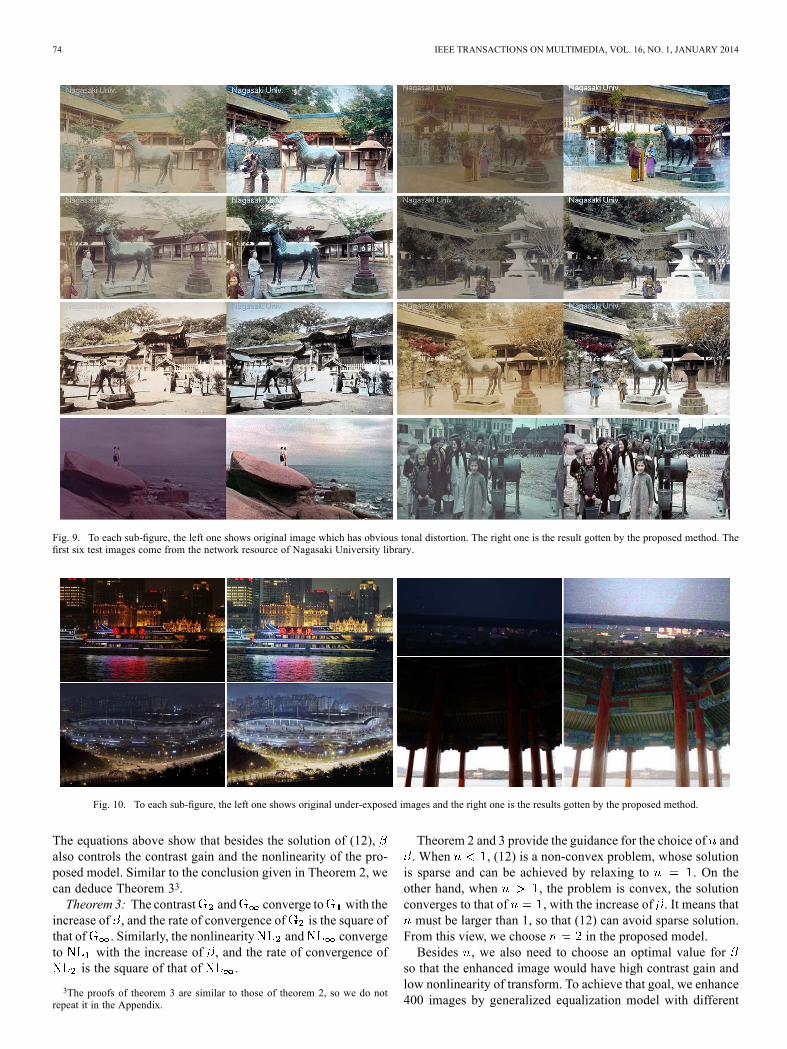
Fig. 9. To each sub-figure, the left one shows original image which has obvious tonal distortion. The right one is the result gotten by the proposed method. Thefirst six test images come from the network resource of Nagasaki University library.

Fig. 10. To each sub-figure, the left one shows original under-exposed images and the right one is the results gotten by the proposed method.

The equations above show that besides the solution of (12),also controls the contrast gain and the nonlinearity of the pro-posed model. Similar to the conclusion given in Theorem 2, wecan deduce Theorem 33.Theorem 3: The contrast and converge to with the

increase of , and the rate of convergence of is the square ofthat of . Similarly, the nonlinearity and convergeto with the increase of , and the rate of convergence of

is the square of that of .

3The proofs of theorem 3 are similar to those of theorem 2, so we do notrepeat it in the Appendix.

Theorem 2 and 3 provide the guidance for the choice of and. When , (12) is a non-convex problem, whose solutionis sparse and can be achieved by relaxing to . On theother hand, when , the problem is convex, the solutionconverges to that of , with the increase of . It means thatmust be larger than 1, so that (12) can avoid sparse solution.

From this view, we choose in the proposed model.Besides , we also need to choose an optimal value for

so that the enhanced image would have high contrast gain andlow nonlinearity of transform. To achieve that goal, we enhance400 images by generalized equalization model with different


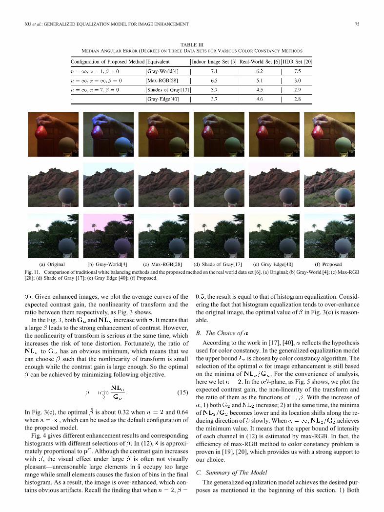
TABLE IIIMEDIAN ANGULAR ERROR (DEGREE) ON THREE DATA SETS FOR VARIOUS COLOR CONSTANCY METHODS

Fig. 11. Comparison of traditional white balancing methods and the proposed method on the real world data set [6]. (a) Original; (b) Gray-World [4]; (c) Max-RGB[28]; (d) Shade of Gray [17]; (e) Gray Edge [40]; (f) Proposed.

. Given enhanced images, we plot the average curves of theexpected contrast gain, the nonlinearity of transform and theratio between them respectively, as Fig. 3 shows.In the Fig. 3, both and increase with . It means that

a large leads to the strong enhancement of contrast. However,the nonlinearity of transform is serious at the same time, whichincreases the risk of tone distortion. Fortunately, the ratio of

to has an obvious minimum, which means that wecan choose such that the nonlinearity of transform is smallenough while the contrast gain is large enough. So the optimalcan be achieved by minimizing following objective.

(15)

In Fig. 3(c), the optimal is about 0.32 when and 0.64when , which can be used as the default configuration ofthe proposed model.Fig. 4 gives different enhancement results and corresponding

histograms with different selections of . In (12), is approxi-mately proportional to . Although the contrast gain increaseswith , the visual effect under large is often not visuallypleasant—unreasonable large elements in occupy too largerange while small elements causes the fusion of bins in the finalhistogram. As a result, the image is over-enhanced, which con-tains obvious artifacts. Recall the finding that when ,

, the result is equal to that of histogram equalization. Consid-ering the fact that histogram equalization tends to over-enhancethe original image, the optimal value of in Fig. 3(c) is reason-able.

B. The Choice of

According to the work in [17], [40], reflects the hypothesisused for color constancy. In the generalized equalization modelthe upper bound is chosen by color constancy algorithm. Theselection of the optimal for image enhancement is still basedon the minima of . For the convenience of analysis,here we let . In the -plane, as Fig. 5 shows, we plot theexpected contrast gain, the non-linearity of the transform andthe ratio of them as the functions of , . With the increase of, 1) both and increase; 2) at the same time, the minimaof becomes lower and its location shifts along the re-ducing direction of slowly. When , achievesthe minimum value. It means that the upper bound of intensityof each channel in (12) is estimated by max-RGB. In fact, theefficiency of max-RGB method to color constancy problem isproven in [19], [20], which provides us with a strong support toour choice.

C. Summary of The Model

The generalized equalization model achieves the desired pur-poses as mentioned in the beginning of this section. 1) Both


Fig. 12. From left to right: Figure (a) includes the original image, the result gotten by the proposed method, the result in [21], and the results gotten by Gray-world,max-RGB, Shade of Gray and Edge-Gray. Figure (b) includes the original images, the results gotten by the proposed method, the results in [41], and the resultsgotten by Gray-world, max-RGB, Shade of Gray and Edge-Gray. Figure (c) includes the raw camera images, the proposed method’s results, the correction resultsbased on measured illuminant, and the results gotten by Gray-world, max-RGB, Shade of Gray and Edge-Gray. The experimental results of other algorithms comefrom [15], [21], [41] directly.

white balancing and contrast enhancement problems can be de-scribed as transforms of the image histogram. If the transformtends to be linear, the result is closer to the white balancing.Meanwhile, if the transform tends to be nonlinear, the resultis closer to contrast enhancement. The generalized equalizationmodel, with suitable parameters, keeps a balance between con-trast enhancement (measured by contrast gain) and tonal dis-tortion (measured by nonlinearity of transform). Moreover, itgives a unified framework accommodating many histogram-based image processing algorithms. Under different configu-rations of parameters, the solution of generalized equalization

model is equivalent to many existing algorithms. Table II4 givesa list of the equivalent algorithms corresponding to differentconfigurations of the model parameters.2) Another advantage of the generalized equalization model

is its high efficiency. Eq. (12) is a convex optimization problemthat can be solved with mature optimization algorithms andpackages. In the case of , the computational complexity ofthe proposed method is . Here is the number of bins in

4When , , in order to get the results of OCTM [43], another twoconstraints of tone should be added. The symbol “-” represents that can bearbitrary positive real number.


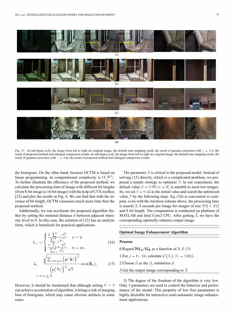
Fig. 13. In sub-figure (a,b), the image from left to right are original image, the default tone mapping result, the result of gamma correction with , theresult of proposed method and enlarged comparison results. In sub-figure (c,d), the image from left to right are original image, the default tone mapping result, theresult of gamma correction with , the result of proposed method and enlarged comparison results.

the histogram. On the other hand, because OCTM is based onlinear programming, its computational complexity is .To further illustrate the efficiency of the proposed method, wecalculate the processing time of image with different bit lengths(from 8-bit image to 16-bit image) with the help of CVX toolbox[23] and plot the results in Fig. 6. We can find that with the in-crease of bit length, OCTM consumes much more time than theproposed method.Additionally, we can accelerate the proposed algorithm fur-

ther by setting the minimal distance between adjacent inten-sity level to 0. In this case, the solution of (12) has an analyticform, which is beneficial for practical applications.

(16)

(17)

However, it should be mentioned that although settingcan achieve acceleration of algorithm, it brings a risk of mergingbins of histogram, which may cause obvious artifacts in somecases.

The parameter is critical to the proposed model. Instead ofsolving (15) directly, which is a complicated problem, we pro-posed a simple strategy to optimize . In our experiment, thedefault value is suitable to most test images.So, we set as the initial value and search the optimizedvalue by the following steps. Eq. (16) is convenient to com-pute, even with the iteration scheme above, the processing timeis merely 2–3 seconds per image for images of size 512 512and 8 bit length. The computation is conducted on platform ofMATLAB and Intel Core2 CPU. After getting , we have thecorresponding optimally enhance output image.

Optimal Image Enhancement Algorithm

Process:

0.Regard as a function of , .

1.For , calculate , .

2.Choose as the minimizes .

3.Get the output image corresponding to .

3) The degree of the freedom of the algorithm is very low.Only 3 parameters are used to control the behavior and perfor-mance of the model. This property of low free parameters ishighly desirable for interactive semi-automatic image enhance-ment applications.


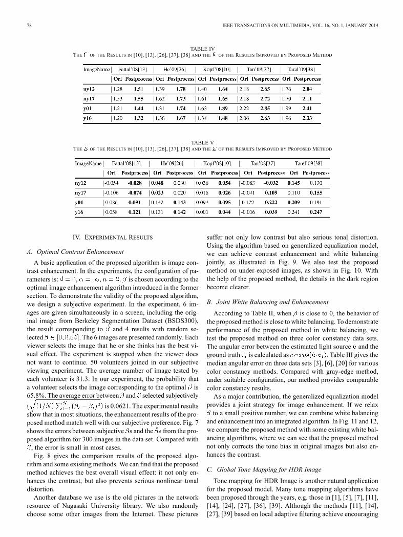
TABLE IVTHE OF THE RESULTS IN [10], [13], [26], [37], [38] AND THE OF THE RESULTS IMPROVED BY PROPOSED METHOD

TABLE VTHE OF THE RESULTS IN [10], [13], [26], [37], [38] AND THE OF THE RESULTS IMPROVED BY PROPOSED METHOD

IV. EXPERIMENTAL RESULTS

A. Optimal Contrast Enhancement

A basic application of the proposed algorithm is image con-trast enhancement. In the experiments, the configuration of pa-rameters is: , , . is chosen according to theoptimal image enhancement algorithm introduced in the formersection. To demonstrate the validity of the proposed algorithm,we design a subjective experiment. In the experiment, 6 im-ages are given simultaneously in a screen, including the orig-inal image from Berkeley Segmentation Dataset (BSDS300),the result corresponding to and 4 results with random se-lected . The 6 images are presented randomly. Eachviewer selects the image that he or she thinks has the best vi-sual effect. The experiment is stopped when the viewer doesnot want to continue. 50 volunteers joined in our subjectiveviewing experiment. The average number of image tested byeach volunteer is 31.3. In our experiment, the probability thata volunteer selects the image corresponding to the optimal is65.8%. The average error between and selected subjectively

is 0.0621. The experimental resultsshow that in most situations, the enhancement results of the pro-posed method match well with our subjective preference. Fig. 7shows the errors between subjective s and the from the pro-posed algorithm for 300 images in the data set. Compared with, the error is small in most cases.Fig. 8 gives the comparison results of the proposed algo-

rithm and some existing methods. We can find that the proposedmethod achieves the best overall visual effect: it not only en-hances the contrast, but also prevents serious nonlinear tonaldistortion.Another database we use is the old pictures in the network

resource of Nagasaki University library. We also randomlychoose some other images from the Internet. These pictures

suffer not only low contrast but also serious tonal distortion.Using the algorithm based on generalized equalization model,we can achieve contrast enhancement and white balancingjointly, as illustrated in Fig. 9. We also test the proposedmethod on under-exposed images, as shown in Fig. 10. Withthe help of the proposed method, the details in the dark regionbecome clearer.

B. Joint White Balancing and Enhancement

According to Table II, when is close to 0, the behavior ofthe proposedmethod is close to white balancing. To demonstrateperformance of the proposed method in white balancing, wetest the proposed method on three color constancy data sets.The angular error between the estimated light source and theground truth is calculated as . Table III gives themedian angular error on three data sets [3], [6], [20] for variouscolor constancy methods. Compared with gray-edge method,under suitable configuration, our method provides comparablecolor constancy results.As a major contribution, the generalized equalization model

provides a joint strategy for image enhancement. If we relaxto a small positive number, we can combine white balancing

and enhancement into an integrated algorithm. In Fig. 11 and 12,we compare the proposed method with some existing white bal-ancing algorithms, where we can see that the proposed methodnot only corrects the tone bias in original images but also en-hances the contrast.

C. Global Tone Mapping for HDR Image

Tone mapping for HDR Image is another natural applicationfor the proposed model. Many tone mapping algorithms havebeen proposed through the years, e.g. those in [1], [5], [7], [11],[14], [24], [27], [36], [39]. Although the methods [11], [14],[27], [39] based on local adaptive filtering achieve encouraging


Fig. 14. Figure (a) gives comparison between de-hazing result of [26] and the result after adding post-processing. Figure (b) gives comparison between de-hazingresult of [38] and the result after adding post-processing. Figure (c) gives comparison between de-hazing result of [10] and the result after adding post-processing.

results, the global method, such as gamma correction, is stillthe most popular choice because of its robustness and lowercomplexity.We test our method on the HDR images captured byNikon D7005 and map them into 8-bit and compare the resultswith those from the default tone mapping process in MATLABand gamma correction.Although the default tone mapping in MATLAB can reveal

some image details, it cannot recover the color of image cor-rectly. In other words, the contrast is enhanced but the tone biasis raised. On the other hand, gamma correction avoids obvioustone bias and protects the color of image but suffers from inap-

5The data set is taken from http://www.cs.sfu.ca/~colour/data/funt_hdr/.

propriate choice of : if is close to 1, the details in the darkregion of image will not be visible, as Fig. 13(a), (b) shows;if is close to 0, the contrast of image will be reduced, asFig. 13(c), (d) shows. Compared with the MATLAB tone map-ping and gamma correction, the proposed model clearly givesmore visually pleasant results, as shown in Fig. 13.

D. Post-Processing for De-hazing Algorithm

The proposed method is also suitable for post-processing ofmany existing enhancement algorithms. For example, althoughthe existing de-hazing algorithms can remove the needlesswhite-light components in the background of the images, they


may lead to tonal distortion in the foreground. So, we can applythe proposed method as a post-processing step of the de-hazingalgorithms to rectify the tonal distortion.To evaluate the performance of our method, we apply the two

blind contrast restoration assessment methods described in [25],namely the increase of the number of visible edge, , and themean of the visibility level, . We denote the number of visibleedge in original image and that in processing result as andrespectively. The increase of visible edge is denoted as

. The larger we get, the better the performanceof contrast enhancement. Similarly, the increase of the valueof also indicates the enhancement of visibility of an image.Because the definition of is out of the range of this paper,we refer the reader to [25] and the code on the website http://perso.lcpc.fr/tarel.jean-philippe/visibility/ for the details of thisdescriptor.Using test images from: http://perso.lcpc.fr/tarel.jean-

philippe/visibility/, we first calculate the values of and forthe de-hazing methods [10], [13], [26], [37], [38]. Then, we usethe proposed method as a post-processing step and calculateand again. Table IV and V give the results of and

respectively.After incorporating the proposed method as post-processing

step, most and all the of de-hazing results are improved.This experimental result indicates that the proposed method canfurther improve the visual results of those de-hazing algorithms.Besides the objective experiment given above, we also design

a subjective view test to verify the human-centered performanceof our proposed model. In the experiment, a hazed image is pro-cessed respectively by two methods—a method selected from[13], [26], [37], [38] and the selected method combined withpost-processing using our proposed model. Then those threeimages are sorted randomly and displayed simultaneously in ascreen. Each viewer selects the image that he/she thinks havingthe best visual effect. The experiment is stopped whenever theviewer does not want to continue. The selection of de-hazingalgorithm is random and unknown for each participant.30 viewers are involved in our experiment. The average

number of image tested by each volunteer is 7.8. In our ex-periment, the probability that volunteers select the imagecorresponding to the method combined with our post-pro-cessing step is 95.8%. This result shows that in most situations,the enhancement results of the proposed method cater oursubjective feelings better. Fig. 14 gives more examples of theprocessing results for the readers’ evaluation.

V. CONCLUSION

In this paper, we analyzed the relationships between imagehistogram and contrast/tone. We established a generalizedequalization model for global image tone mapping. Extensiveexperimental results suggest that the proposed method hasgood performances in many typical applications includingimage contrast enhancement, tone correction, white balancingand post-processing of de-hazed images. In the future, besidesglobal image enhancement, we expect to unify more localimage enhancement methods into the model through localimage feature analysis.

APPENDIX

The Proof of Theorem 1:Proof: When , . Define

as a dimensional vector, which is the op-timal solution of (12). Assume that there exists another vector

satisfying . According to the constraintthat , at least one of the element of is larger than

, which can be labeled as . Then we have

Because is convex, we have

Here is the mean of . As a result, the assumption is false andtherefore this theorem is proven.The Proof of Theorem 2: The rate of convergence of function, whose limit is is defined as

When , is linear convergent to its limit.Proof: We can assume that , ,

without loss of generality. Define the optimal solutions of theand forms of (12) as and . Then we have

Both of them are functions of , whose limits are.

The rates of convergence corresponding to and aredenoted as and respectively. According to the definitionof , we have

Similarly, we can get . Because, both of the solutions converge to linearly, and the

rate of convergence of is the square of the rate of.

REFERENCES

[1] T. Arici, S. Dikbas, and Y. Altunbasak, “A histogram modificationframework and its application for image contrast enhancement,” IEEETrans. Image Process., vol. 18, no. 9, pp. 1921–1935, 2009.

[2] M. Ashikhmin, “A tone mapping algorithm for high contrast images,”in Proc. 13th Eurographics Workshop Rendering, 2002.

[3] K. Barnard, L. Martin, B. Funt, and A. Coath, “A data set for colourresearch,” Color Res. Applicat., vol. 27, no. 3, pp. 147–151, 2002.


[4] G. Buchsbaum, “A spatial processor model for object colour percep-tion,” J. Frank. Inst., vol. 310, 1980.

[5] Z. Chen, B. Abidi, D. Page, and M. Abidi, “Gray-level grouping (glg):An automaticmethod for optimized image contrast enhancement—Parti: The basic method,” IEEE Trans. Image Process., vol. 15, no. 8, pp.2303–2314, 2006.

[6] F. Ciurea and B. Funt, The SunBurst Resort, Scottsdale, AZ, USA, “Alarge image database for color constancy research,” inProc. IS&T/SIDsColor Imaging Conf., 2004, pp. 160–164.

[7] D. Coltuc, P. Bolon, and J.-M. Chassery, “Exact histogram specifi-cation,” IEEE Trans. Image Process., vol. 15, no. 5, pp. 1143–1152,2006.

[8] F. Drago, K. Myszkowski, T. Annen, and N. Chiba, “Adaptive loga-rithmic mapping for displaying high contrast scenes,” in Proc. Com-puter Graphics Forum, 2003, vol. 22, no. 3.

[9] E. D. P. et al., “Contrast limited adaptive histogram image processingto improve the detection of simulated speculations in dense mammo-grams,” J. Digital Imag., vol. 11, no. 4, pp. 193–200, 1998.

[10] J. K. et al., “Deep photo: Model-based photograph enhancement andviewing,” ACM Trans. Graph.—Proc. ACM SIGGRAPH, vol. 27, no.5, 2008.

[11] Z. Farbman, R. Fattal, D. Lischinski, and R. Szeliski, “Edge-preservingdecompositions for multi-scale tone and detail manipulation,” ACMTrans. Graph., vol. 27, no. 3, 2008.

[12] H. Farid, “Blind inverse gamma correction,” IEEE Trans. ImageProcess., vol. 10, no. 10, pp. 1428–1433, 2001.

[13] R. Fattal, “Single image dehazing,” ACM Trans. Graph.—Proc. ACMSIGGRAPH, vol. 27, no. 3, 2008.

[14] R. Fattal, M. Agrawala, and S. Rusinkiewicz, “Multiscale shape anddetail enhancement from multi-light image collections,” ACM Trans.Graph., vol. 26, no. 3, pp. 51–59, 2007.

[15] G. Finlayson and S. Hordley, “A theory of selection for gamut map-ping colour constancy,” in Proc. IEEE Int. Conf. Computer Vision andPattern Recognition, 1998, pp. 60–65.

[16] G. Finlayson, S. Hordley, and P. Hubel, “Colour by correlation: Asimple, unifying approach to colour constancy,” in Proc. IEEE Int.Conf. Computer Vision, 1999, vol. 2, pp. 835–842.

[17] G. Finlayson and E. Trezzi, “Shades of gray and colour constancy,” inProc. IS&T/SID 12th Color Imaging Conf., 2004, pp. 37–41.

[18] D. Forsyth, “A novel algorithm for color constancy,” Int. J. Comput.Vision, vol. 5, no. 1, pp. 5–36, 1990.

[19] B. Funt and L. Shi, “The effect of exposure on maxrgb color con-stancy,” in Proc. SPIE Volume 7527, Human Vision and ElectronicImaging.

[20] B. Funt and L. Shi, “The rehabilitation of maxrgb,” in Proc. IS&T 18thColor Imaging Conf..

[21] P. Gehler, C. Rother, A. Blake, T.Minka, and T. Sharp, “Bayesian colorconstancy revisited,” in Proc. IEEE Int. Conf. Computer Vision andPattern Recognition, 2008, pp. 1–8.

[22] R. C. Gonzalez and R. E. Woods, Digital Image Processing. Beijing,China: Publishing House of Electronics Industry, 2002.

[23] M. Grant and S. Boyd, CVX users guide, Technical report, InformationSystems Laboratory, Department of Electrical Engineering, StanfordUniversity, 2009.

[24] J.-H. Han, S. Yang, and B.-U. Lee, “A novel 3-d color histogram equal-ization method with uniform 1-d gray scale histogram,” IEEE Trans.Image Process., vol. 20, no. 2, pp. 506–512, 2011.

[25] N. Hautière, J.-P. Tarel, D. Aubert, and E. Dumont, “Blind contrastrestoration assessment by gradient rationing at visible edges,” in Proc.Int. Congr. Stereology (ICS’07), Saint Etienne, France, 2007 [Online].Available: http://perso.lcpc.fr/tarel.jean-philippe/publis/ics07.html

[26] K. He, J. Sun, and X. Tang, “Single image haze removal using darkchannel prior,” in Proc. IEEE Int. Conf. Computer Vision and PatternRecognition, 2009, pp. 1956–1963.

[27] K. He, J. Sun, and X. Tang, “Guided image filtering,” in Proc. ECCV,2010.

[28] E. Land and J. McCann, “Lightness and retinex theory,” J. Opt. Soc.Amer. A, vol. 61, no. 1, pp. 1–11, 1971.

[29] P. Ledda, A. Chalmers, T. Troscianko, and H. Seetzen, “Evaluationof tone mapping operators using a high dynamic range display,” ACMTrans. Graph.—Proc. ACM SIGGRAPH, vol. 24, no. 3, 2005.

[30] P. Milanfar, “A tour of modern image filtering: New insights andmethods, both practical and theoretical,” IEEE Signal Process. Mag.,vol. 30, no. 1, pp. 106–128, 2013.

[31] S.-C. Pei, Y.-C. Zeng, and C.-H. Chang, “Virtual restoration of ancientChinese paintings using color contrast enhancement and lacuna texturesynthesis,” IEEE Trans. Image Process., vol. 13, no. 3, pp. 416–429,2004.

[32] Y.-F. Pu, J.-L. Zhou, and X. Yuan, “Fractional differential mask: Afractional differential-based approach for multiscale texture enhance-ment,” IEEE Trans. Image Process., vol. 19, no. 2, pp. 491–511, 2010.

[33] E. Reinhard, M. Stark, P. Shirley, and J. Ferwerda, “Photographic tonereproduction for digital images,” ACM Trans. Graph.—Proc. ACMSIGGRAPH, vol. 21, no. 3, 2002.

[34] Y. Shi, J. Yang, and R. Wu, “Reducing illumination based on nonlineargamma correction,” in Proc. IEEE Int. Conf. Image Processing, 2007,vol. 1, pp. 529–532.

[35] J.-L. Starck, F. Murtagh, E. Candes, and D. Donoho, “Gray and colorimage contrast enhancement by the curvelet transform,” IEEE Trans.Image Process., vol. 12, no. 6, pp. 706–717, 2003.

[36] J. A. Stark, “Adaptive image contrast enhancement using generaliza-tions of histogram equalization,” IEEE Trans. Image Process., vol. 9,no. 5, pp. 889–896, 2000.

[37] R. Tan, “Visibility in bad weather from a single image,” in Proc. IEEEInt. Conf. Computer Vision and Pattern Recognition, 2008, pp. 1–8.

[38] J.-P. Tarel and N. Hautiere, “Fast visibility restoration from a singlecolor or gray level image,” in Proc. IEEE Int. Conf. Computer Vision,2009, pp. 2201–2208.

[39] C. Tomasi and R. Manduchi, “Bilateral filtering for gray and color im-ages,” in Proc. ICCV, 1998.

[40] J. van de Weijer, T. Gevers, and A. Gijsenij, “Edge-based color con-stancy,” IEEE Trans. Image Process., vol. 16, no. 9, pp. 2207–2214,2007.

[41] J. van de Weijer, C. Schmid, and J. Verbeek, “Using high-level visualinformation for color constancy,” in Proc. IEEE Int. Conf. ComputerVision, 2007, pp. 1–8.

[42] Y. Wang, Q. Chen, and B. Zhang, “Image enhancement based on equalarea dualistic sub-image histogram equalization method,” IEEE Trans.Consum. Electron., vol. 45, no. 1, pp. 68–75, 1999.

[43] X. Wu, “A linear programming approach for optimal contrast-tonemapping,” IEEE Trans. Image Process., vol. 20, no. 5, pp. 1262–1272,2010.

[44] X. Zhu and P. Milanfar, “Restoration for weakly blurred and stronglynoisy images,” in Proc. 2011 IEEE Workshop Applications of Com-puter Vision (WACV), 2011, pp. 103–109.

Hongteng Xu received the B.S. degree from TianjinUniversity, Tianjin, China, in 2010. In fall 2010, hejoined in the dual-master program of Georgia Insti-tute of Technology and Shanghai Jiao Tong Univer-sity, and graduated in Spring 2013.Currently, he is a Ph.D. student, School of Elec-

trical and Computer Engineering, Georgia Tech.His research interests include image processing,computer vision, data mining and machine learning.

Guangtao Zhai (M’10) received the B.E. and M.E.degrees from Shandong University, Shandong,China, in 2001 and 2004 and the Ph.D. degree fromShanghai Jiao Tong University, Shanghai, China, in2009.He is currently a research professor at the Institute

of Image Communication and Information Pro-cessing, Shanghai Jiao Tong University, Shanghai,China. From August 2006 to February 2007, he wasa Student Intern with the Institute for InfocommResearch, Singapore. From March 2007 to January

2008, he was a Visiting Student with the School of Computer Engineering,Nanyang Technological University, Singapore. From October 2008 to April2009, he was a Visiting Student with the Department of Electrical and Com-puter Engineering, McMaster University, Hamilton, ON, Canada, where fromJanuary 2010 to March 2012 he was a Postdoctoral Fellow. His research inter-ests include multimedia signal processing and perceptual signal processing.


Xiaolin Wu (M’88–SM’96–F’11) received theB.Sc. degree in computer science from WuhanUniversity, Wuhan, China, in 1982, and the Ph.D.degree in computer science from the University ofCalgary, Calgary, AB, Canada, in 1988. He startedhis academic career in 1988 and has since been onthe faculty of the University of Western Ontario,New York Polytechnic University, and McMasterUniversity, Hamilton, ON, Canada, where he is aProfessor in the Department of Electrical and Com-puter Engineering and holds the NSERC-DALSA

Industrial Research Chair in Digital Cinema. Currently, he is also with the insti-tute of image communication and information processing, Shanghai Jiao TongUniversity, Shanghai, China. His research interests include image processing,multimedia compression, joint source-channel coding, multiple descriptioncoding, and network-aware visual communication. He has published over 180research papers and holds two patents in these fields.Dr. Wu was an Associate Editor of the IEEE TRANSACTIONS ON

MULTIMEDIA. He is an Associate Editor of the IEEE TRANSACTIONS ON

IMAGE PROCESSING.

Xiaokang Yang (M’00–SM’04) received the B. S.degree from Xiamen University, Xiamen, China, in1994, the M. S. degree from Chinese Academy ofSciences, Shanghai, China, in 1997, and the Ph.D. de-gree from Shanghai Jiao Tong University, Shanghai,China, in 2000.He is currently a professor and Vice Dean, School

of Electronic Information and Electrical Engi-neering, and the deputy director of the Institute ofImage Communication and Information Processing,Shanghai Jiao Tong University, Shanghai, China.

From August 2007 to July 2008, he visited the Institute for Computer Science,University of Freiburg, Germany, as an Alexander von Humboldt ResearchFellow. From September 2000 to March 2002, he worked as a ResearchFellow in Centre for Signal Processing, Nanyang Technological University,Singapore. From April 2002 to October 2004, he was a Research Scientist inthe Institute for Infocomm Research, Singapore. He has published over 150refereed papers, and has filed 30 patents. His current research interests includevisual signal processing and communication, media analysis and retrieval, andpattern recognition.He received National Science Fund for Distinguished Young Scholars in

2010, Professorship Award of Shanghai Special Appointment (Eastern Scholar)in 2008, the Microsoft Young Professorship Award in 2006, the Best YoungInvestigator Paper Award at IS&T/SPIE International Conference on VideoCommunication and Image Processing (VCIP2003) and awards from A-STARand Tan Kah Kee foundations. He is currently a member of Editorial Boardof IEEE Signal Processing Letters, Serias Editor of Springer CCIS, a memberof APSIPA, a senior member of IEEE, a member of Visual Signal Processingand Communications (VSPC) Technical Committee of the IEEE Circuitsand Systems Society. He was the special session chair of Perceptual VisualProcessing of IEEE ICME2006. He was the technical program co-chair ofIEEE SiPS2007 and the technical program co-chair of 3DTV workshop injunction with 2010 IEEE International Symposium on Broadband MultimediaSystems and Broadcasting.

Generalized Equalization Model for Image Enhancement

Documents

Transcript of Generalized Equalization Model for Image Enhancement