DETERMINATION AND SIMULATION OF

THE HEAT TRANSFER CHARACTERISTICS

OF ELECTRONIC ASSEMBLIES

FARHAD SARVAR

A thesis submitted in partial fulfilment of the

requirements of the Council for National Academic Awards

for the degree of Doctor of Philosophy

APRIL 1992

Polytechnic of Wales

ACKNOWLEDGMENTS

The author wishes to thank the staff of the Hybrid Electronic Unit of the Radio and Signals

Research Establishment at Malvern for fabricating the test samples used in this project.

Thanks are also due to AGEMA Limited for the loan of their thermal imaging equipment

and the assistance of their representative for temperature measurements on hybrid resistors.

I am indebted to my supervisor Professor P A Witting, head of department of Electronics

and Information Technology at the Polytechnic of Wales, for his helpful guidance,

encouragement and enthusiasm during the course of this investigation.

I would also like to express my gratitude to Dr. N J Poole for his support and many hours

of vigourous and stimulating discussion.

I am grateful to the staff of the Information Technology Centre at the Polytechnic for all

their help with the software content of this project and to the staff of the Media and

Resources for the preparation of the photographs presented in the thesis.

Finally, I wish to thank my wife for her patience and support during the many evenings I

spent working on this thesis.

TABLE OF CONTENTS

ABSTRACT vi

1 INTRODUCTION.......................................................................................... 11.1 Effects of Temperature on Electronic Components ............................ 51.2 Review of Thermal Analysis Techniques ............................................ 81.3 Thermal Analysis and Modelling Using ASTEC3 .............................. 14

2 ASTEC3 SIMULATION PACKAGE .......................................................... 192.1 Introduction ............................................................................................ 19

2.1.1 System Analysis with ASTEC3 ..................................................... 212.1.2 ASTEC3 Data File ...................................................................... 23

2.2 Presentation of ASTEC3 output results for Thermal Systems .......... 262.2.1 Production of Contour and Temperature Distribution Plots .... 28

2.3 Conclusions ............................................................................................. 31

3 HEAT TRANSFER ......................................................................................... 333.1 Conduction ............................................................................................. 333.2 Convection ............................................................................................. 36

3.2.1 Boundary Layer Fundamentals ..................................................... 373.2.1.1 Velocity Boundary Layer ....................................................... 373.2.1.2 Thermal Boundary Layer ...................................................... 393.2.1.3 Laminar and Turbulent Boundary Layers .......................... 39

3.2.2 Empirical Equations ....................................................................... 413.3 Radiation ................................................................................................ 44

3.3.1 View Factor ..................................................................................... 483.3.1.1 Properties of View Factors .................................................... 51

3.4 Conclusions .............................................................................................. 54

4 THERMAL SYSTEM MODELLING ....................................................... 554.1 Introduction ............................................................................................ 554.2 Conduction ............................................................................................ 574.3 Convection ............................................................................................. 584.4 Radiation ............................................................................................... 584.5 ASTEC3 Code-Generation Programs ................................................. 60

4.5.1 Introduction ................................................................................... 604.5.2 Program for 2-D Conduction ........................................................ 62

4.5.3 Program for 3-Dimensional Conduction ..................................... 64

-i-

4.6 Conclusions . .. ..........,.................................. . .................................... 67

5 VALIDATION OF ASTEC3 MODELLING ............................................. 685.1 Introduction ............................................................................................ 685.2 One-dimension ..................................................................................... 69

5.2.1 Conduction only ........................................................................... 69a ASTEC3 Solution .......................................................................... 69b Finite difference solution ............................................................. 69c Analytical Solution ......................................................................... 72

5.2.2 Conduction and Convection ........................................................ 745.3 Two-dimensions .................................................................................... 78

5.3.1 ASTEC3 Solution ......................................................................... 80a Coarse Mesh .................................................................................. 80b Fine Mesh ...................................................................................... 80

5.4 Three-dimensions ................................................................................. 885.5 Efficiency: A combination of Coarse and Fine Mesh Models ............ 885.6 Computing-Time Considerations ......................................................... 945.7 Conclusion............................................................................................... 102

6 EXPERIMENTAL STUDIES IN MACRO-SCALE .................................. 1036.1 Experimental Arrangement ................................................................ 103

6.1.1 Experiment 1 ................................................................................ 1106.1.2 Experiment 2 ................................................................................ 1136.1.3 Experiments .................................................................................. 118

6.2 Conclusions ............................................................................................. 123

7 THERMAL CONDUCTIVITY MEASUREMENTS OF FIBRE-GLASS LAMINATES AND THEIR EFFECT ON SIMULATION .......................... 125

7.1 Introduction ............................................................................................ 1257.2 Thermal Conductivity Normal to the Plane of Glass-FibreLaminates ...................................................................................................... 130

7.2.1 Apparatus and Equations ............................................................. 1317.2.2 Experimental Procedure ............................................................... 133

7.2.2.1 PTFE ....................................................................................... 1347.2.2.2 Glass Fibre Boards ................................................................ 136

7.3 Thermal Conductivity along the plane of the boards ......................... 1367.3.1 Verification of the Technique for the In-Plane Thermal Conductivity Measurement..................................................................... 148

-11-

7.3.2 Improved Experiment for the In-Plane Thermal Conductivity Measurements ......................................................................................... 154

Thermal Conductivity of Air at Low Pressure ................................... 157Heat Transfer Coefficient of Convection .......................................... 158Input Radiation ................................................................................... 159Calculation of the in-plane Thermal Conductivity ........................... 162

7.4 Simulation of original Test configuration using the measured Thermal Conductivities ................................................................................ 1647.5 Conclusions ............................................................................................. 165

8 SCHLIEREN EXPERIMENT FOR VISUALISATION OF NATURALCONVECTION PLUMES ................................................................................. 167

8.1 Introduction ............................................................................................ 1678.2 Theory of Operation .............................................................................. 1688.3 Experiments for the Estimation of the Convection Coefficients ........ 173

8.3.1 Apparatus ....................................................................................... 1748.3.2 Experimental Procedure ............................................................... 1768.3.3 Tests and results ............................................................................. 177

8.4 Determination of the Optimum Mesh Resolution .............................. 1848.5 Determination of heat transfer coefficient values ............................... 1878.6 Simulation of the Original Test Configuration using the OptimisedConvection Coefficients ................................................................................ 1908.7 Conclusions ............................................................................................. 191

9 EXPERIMENTAL MEASUREMENTS AND SIMULATION TESTSON HYBRID CIRCUITS .................................................................................. 193

9.1 Introduction ............................................................................................ 1939.2 Sample Preparations .............................................................................. 1939.3 Temperature Measurement System ..................................................... 196

9.3.1 Emissivity Considerations ............................................................. 1989.3.2 Experiments and Results ............................................................... 199

9.4 ASTEC3 Simulation Model................................................................... 2019.5 Heat Transfer Coefficient of Convection ............................................. 207

9.5.1 Schlieren Experiment .................................................................... 2079.5.2 Optimisation Tests ......................................................................... 211

9.6 Conclusions ............................................................................................. 216

10 DISCUSSIONS AND CONCLUSIONS ...................................................... 218

10.1 Future Work ........................................................................................ 224

-in-

11 REFERENCES ............................................................................................. 228CHAPTER 1 .................................................................................................. 228CHAPTER2 .................................................................................................. 230CHAPTERS .................................................................................................. 231CHAPTER4 .................................................................................................. 231CHAPTERS .................................................................................................. 231CHAPTER6 .................................................................................................. 232CHAPTER? .................................................................................................. 232CHAPTERS .................................................................................................. 233CHAPTER9 .................................................................................................. 233

12 APPENDIXES ............................................................................................... 234APPENDIX 1: Contour Plotting Programs ................................................ 234

Program 1 ................................................................................................. 234

Program 2 ................................................................................................. 235Program3 ................................................................................................. 239

APPENDIX 2: Code Generation Programs ............................................... 245a Two-Dimensional Code-Generation Program ................................... 245b An example of the ouput of the 2-D Code-Generation Program...... 254c Program for Generating the ASTEC3 code for Three-Dimensional Conduction ............................................................................................... 257d Format of Data Files ............................................................................. 265e An example of the output of 3-Dimensional Code-Generation program ................................................................................................... 266

APPENDIX 3: The Analytical Solution For The One-Dimensional Problem (§5.2)................................................................................................ 270APPENDIX 4: Estimation of the Convective and Radiative HeatTransfer Coefficients for Experiment 1 (§6.1.1) ........................................ 272APPENDIX 5: Determination of the Emissivity of Copper surface ......... 275APPENDIX 6: The Raw Results for Thermal ConductivityMeasurement of PTFE Normal to its Plane ............................................... 278APPENDIX 7: The Error Calculations for Thermal conductivity Measurements using the Lees' Disc Apparatus ......................................... 279APPENDIX 8: The Raw Results for Thermal ConductivityMeasurements of FR4 Boards Normal to then* Plane .............................. 281APPENDIX 9: Results of Temperature Measurements at VariousPressures for Determination of Thermal Conductivity Along the Planeof Fibre-Glass Boards (§7.3) ........................................................................ 283

-IV-

APPENDIX 10: Calculation of Heat Transfer Coefficients for theHybrid Carrier ............................................................................................ 294APPENDIX 11: Publications ........................................................................ 296

-v-

ABSTRACT

This research project has developed a computer-assisted methodology whereby the

temporal and spatial distribution of temperature in thick film circuits fabricated on

ceramic substrates may be predicted. The analogy between thermal and electrical

systems is used to define a thermal structure in electrical format which is then simulated

using ASTEC3 electronic analysis package.

Procedures have been developed whereby the three heat transfer mechanisms namely

conduction, convection and radiation may be modelled. Models have also been

proposed which allow the more important sections of a thermal structure to be analysed

in finer detail. These procedures have been used hi the solution of some standard heat

flow problems whose solutions have also been obtained by other more conventional

techniques for comparison. Programs have been developed which facilitate the

presentation of the results in the form of contour-maps or 3-D temperature distribution

plots. Software has also been developed which can generate the electrical equivalent

description of a device in ASTEC3 syntax. Estimates of the computing times required

to carry out electro-thermal simulations of hybrid and VLSI devices have been made.

The predicted computation times are feasible.

Confirmatory experiments have been carried out in large scale using partially heated

samples prepared from printed circuit boards. These were heated electrically and

temperature measurements were made using an infrared thermometer. These structures

were modelled and simulated using ASTEC3 for comparison. It was found that for an

accurate thermal analysis there was a need for reliable data for the thermal conductivity

of the glass-fibre laminate and the heat transfer coefficients of convection. Experiments

were designed to measure the thermal conductivity of the laminates tangential to the

-VI-

plane of the boards. A standard Lees' disc apparatus was also used to measure this

parameter in a direction normal to the boards. A Schlieren optics apparatus was used

to study the convection plumes over the surface of the plates in a horizontal position

with the heated side facing upwards which provided a significant insight into the flow

regime over such surfaces. Values were subsequently determined for the convection

coefficients from the boards. Using the measured thermal conductivities of FR4 boards

and the estimated convection coefficients, excellent agreement was achieved between

the measured and simulated results.

Temperature measurements were also conducted at reduced dimensional scale on

especially designed thick film resistor samples. The samples were fabricated by R.S.R.E

and temperature measurements were carried out using a thermal imaging equipment

manufactured by AGEMA. Again the Schlieren apparatus was used to observe the

convection plumes forming over the devices which led to a better understanding of the

heat transfer mechanism from such devices. These observations were then used to

estimate the natural convection coefficients from the surface of horizontally positioned

resistor samples which were then included in the ASTEC3 model of the devices. The

subsequent ASTEC3 thermal simulation showed an excellent agreement with the

measured temperature profile.

-Vll-

1 INTRODUCTION

The main limitation to the increasing complexity of integrated circuits has been the chip

size. As the necessary chip area increases the production costs also increase and a desired

solution has been not to increase the chip size but to allow a greater density of active

devices on the chip. The prime motivation for the increase in packing density is therefore

the reduction hi the cost of producing such circuits. The semiconductor industry is further

stimulated by the information processing industry constantly requiring systems of higher

performance and speed which can be accomplished by reduction in size and increased

packing density and which in turn reduce the inter-chip interconnection delays [1].

Furthermore, the most unreliable aspect of any system design is the physical connection

and the reliability of electronic systems is approximately inversely proportional to the

number of joints [2]. Component integration has led to the replacement of printed circuit

cards containing many individual circuits (built on chips with smaller numbers of

components) with a single chip. The connection between the circuits is accomplished using

thin film wires on the chip and these are less susceptible to problems with mechanical

vibration, incomplete insertion and dirty contacts normally associated with circuit cards.

The reduction in the number of mechanical connections therefore gives a more reliable

product. The reduction in the physical size of a device however means an increase in

electrical activity within a small area on a chip and consequently to excessive heat

generation within that area. The resulting high temperatures can drastically affect the

performance of a circuit and hence its reliability. There is, therefore, a need for a computer

modelling tool allowing the prediction of the temperature profile on a circuit, preferably

under accurately simulated working condition of electrical activity.

-1-

The transient aspects of the modelling is most crucial for devices operating under pulsed

conditions since in these situations the phasing of the heat dissipation should be taken into

account [3] to reduce the risks of under- or over-estimating the problem. This type of

simulation cannot be carried out without coupling of the electrical and thermal models.

The original objective of this project was to develop a simulation tool capable of

simultaneous analysis of both the electrical and thermal systems. In the event, the initial

simulations indicated that a much closer understanding of the heat loss processes as applied

to microelectronic circuits was needed. As a result the majority of the effort in this work

was directed towards the elucidation of the heat loss mechanisms and further work still

remains to be done to explore the combination of the electrical and thermal analysis.

The work carried out to date and reported in this thesis is as follows:

A modelling process has been developed whereby the thermal characteristics of a

structure can be simulated using an electronic simulation package. To allow the

presentation of the temperature distribution in graphic form, programs have been

developed to produce contour maps of a surface temperature. Also to minimise the

effort involved hi producing an error-free net-list of a structure, software has been

developed to automatically generate such data-files.

To reduce the computation times, techniques were devised and tested whereby the

various sections of a circuit could be simulated at different resolutions.

To demonstrate that ASTEC3 could be used for thermal modelling, standard heat

flow problems were solved using the software and the results were successfully

compared with the solution derived from more conventional techniques.

-2-

To ascertain the validity of the modelling system in a practical situation, experiments

were designed in macro-scale using partially heated PCB plates. The initial simulation

results in this case showed large discrepancies with the measured temperatures. It

was clear that for an accurate simulation, further analysis of the heat flow mechanisms

from these boards was required. Instruments such as the Lees' disc apparatus are

available commercially for the measurement of thermal conductivity in a normal

direction for materials hi the form of thin boards which was subsequently employed

for this purpose. No such apparatus was however found capable of measuring

conductivity hi a direction tangential to the board. A novel experiment was therefore

developed to measure the in-plane thermal conductivity of FR4 boards. Samples of

the insulating board were heated from one end and temperatures measured along the

specimen. This was carried out in a vacuum chamber so as to minimise the effect of

convection which is a difficult process to quantify. These temperatures were then

compared with a finite difference solution of the structure where the thermal

conductivity along the board was varied in the solution until the calculated

temperature profile best match the measured one. The resulting value was then taken

to be the required tangential thermal conductivity. To develop a better understanding

of the heat flow regime and hence the natural convection from partially heated

structures, an optical method was used to observe the plumes forming over such

surfaces. Using the results of these observations and an error optimisation technique,

heat transfer coefficients were estimated for convection. This demonstrated that

certain simplifying assumptions could be made concerning the convection

coefficients. Good agreement between simulation and experiment was obtained.

Having validated the macro-scale model, the modelling system was tested on small

scale devices, namely a hybrid resistor sample. At this scale the measured

temperatures again showed differences with the simulated data which required further

-3-

examination of the convection flow from the packaged hybrid samples. Again it was

demonstrated that (different) simplifying assumptions could be made and good

agreement between simulation and experiment was obtained.

At this point the program of research was terminated and further work will be needed to

deal with the thermal modelling of devices fabricated on semiconducting substrates.

The ASTEC3 electronic simulation program was chosen as a vehicle for such analysis. It

is particularly well suited for thermal simulation of devices as it incorporates two features

of special significance in addition to its highly efficient electronic simulation capabilities.

These are its powerful sub-modelling facility and its ability to handle large sets of first-order

differential equations. The sub-modelling is highly useful hi thermal modelling as a library

of thermal models of standard components may be developed via this facility. These may

then be called up within other circuits with the need of only the outer connections of the

sub-model.

The software also makes it possible to model both thermal and electrical characteristics

of the same device in one simulation. This is made possible by including in the circuit

description file, an additional section describing the electrical equivalent network of the

thermal aspects of the same circuit. The package allows exchange of parameters between

the electrical and thermal sections. The instantaneous heat generation due to the passage

of current is calculated as a parameter in ASTEC3 from the values of the electrical circuit

parameters. This can then be assigned to the heat generator hi the thermal model. In this

way a two-layer combined electro-thermal model is produced.

Modelling procedures are described which can deal with one-, two- and three-dimensional

heat flow situations. One- and two-dimensional models may be used where the heat flow

-4-

within the structure can be approximated to that scheme. It is however shown [4] that

time-dependent problems and devices with very small heat sources cannot be accurately

analysed using one- or two-dimensional models and therefore a three-dimensional

approach has to be taken.

In order to demonstrate the importance of thermal modelling of devices, the following

section is included examining the temperature effects on electronic components.

1.1 Effects of Temperature on Electronic Components

The elevated temperature of a device can cause a variety of strange effects in electronic

circuits. An accelerated corrosion and interfacial diffusion process may be activated at

high temperatures [5] leading to a premature failure of the circuit. Excessive temperatures

may, for example, cause failure in the metallisation layer or bonded interfaces such as wire

bonds and the chip to package bonding of a device. To test the reliability of a device and

for quality control purposes, manufacturers normally rely on accelerated stress testing

techniques. Many chemical and physical processes can be accelerated by temperature. The

reaction rate R at which these processes proceed is related to temperature by the Arrhenius

equation [6]:

1.1

where Ea is the activation energy (in Electron Volts), A: is the Boltzmann constant and T is

the absolute temperature in Kelvin. The results of such tests have shown that the failure

rate of semiconductor devices with temperature follows the same relationship and that

temperature rises as small as 10 "C can reduce the average time that a device functions

before first failure (the mean time to failure) by a factor of two [5,7,8].

-5-

Operating temperature also influences the Performance of the circuit. The changed

characteristics of the components in the hot regions may modify the behaviour of the whole

circuit in such a way that the design specifications are no longer met. P-n junctions, which

are the building blocks of electronic components fabricated on semiconducting substrates,

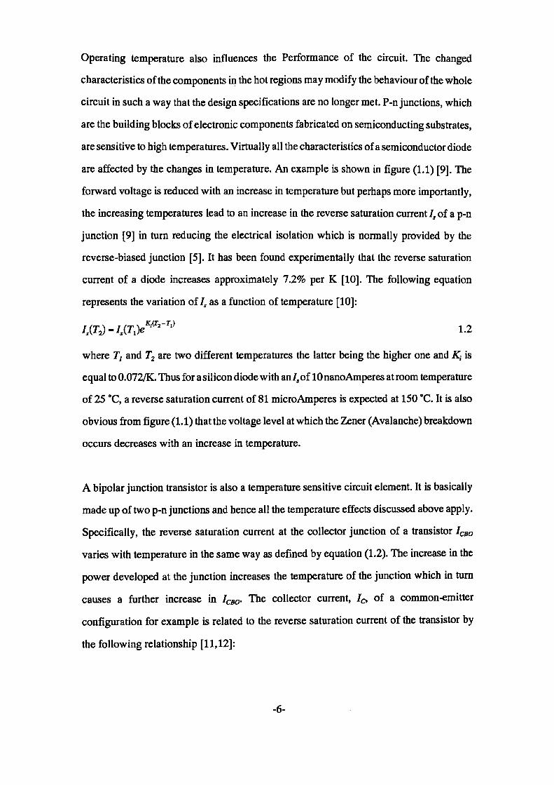
are sensitive to high temperatures. Virtually all the characteristics of a semiconductor diode

are affected by the changes in temperature. An example is shown in figure (1.1) [9]. The

forward voltage is reduced with an increase in temperature but perhaps more importantly,

the increasing temperatures lead to an increase in the reverse saturation current 7, of a p-n

junction [9] in turn reducing the electrical isolation which is normally provided by the

reverse-biased junction [5]. It has been found experimentally that the reverse saturation

current of a diode increases approximately 7.2% per K [10]. The following equation

represents the variation of 7, as a function of temperature [10]:

im-w^-^ 1.2where Tt and T2 are two different temperatures the latter being the higher one and jK, is

equal to 0.072/K. Thus for a silicon diode with an7, of 10 nanoAmperes at room temperature

of 25 °C, a reverse saturation current of 81 microAmperes is expected at 150 *C. It is also

obvious from figure (1.1) that the voltage level at which the Zener (Avalanche) breakdown

occurs decreases with an increase in temperature.

A bipolar junction transistor is also a temperature sensitive circuit element. It is basically

made up of two p-n junctions and hence all the temperature effects discussed above apply.

Specifically, the reverse saturation current at the collector junction of a transistor ICBO

varies with temperature in the same way as defined by equation (1.2). The increase in the

power developed at the junction increases the temperature of the junction which in turn

causes a further increase in ICB0. The collector current, Ic, of a common-emitter

configuration for example is related to the reverse saturation current of the transistor by

the following relationship [11,12]:

-6-

id(m

A) 20

0°C

IOO°

C 25

°C -

75°C

vd (

mV

)

Fig

ure

(1.1

) V

aria

tion

in D

iode

Cha

ract

eris

tics

with

Tem

pera

ture

Cha

nge

Afte

r Boy

lstad

R a

nd N

ashe

lsky

L [9

]

1.3

where fi is the Common-Emitter Forward-Current Amplification Factor of the transistor

[9]. It is therefore clear that an increase in ICBO also increases the collector current. A

regenerative heating cycle may occur at high temperatures (high ambient temperature,

high developed power or perhaps a hot spot on a device) which can result in a phenomenon

referred to as thermal runaway [11,12] and in extreme cases can lead to destruction of the

transistor.

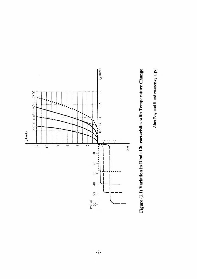
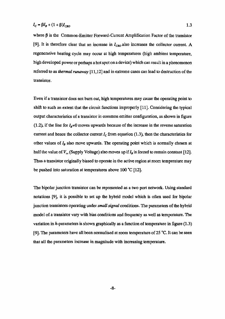
Even if a transistor does not bum out, high temperatures may cause the operating point to

shift to such an extent that the circuit functions improperly [11]. Considering the typical

output characteristics of a transistor in common emitter configuration, as shown in figure

(1.2), if the line for IB=0 moves upwards because of the increase in the reverse saturation

current and hence the collector current Ic from equation (1.3), then the characteristics for

other values of IB also move upwards. The operating point which is normally chosen at

half the value of Vec (Supply Voltage) also moves up if IB is forced to remain constant [12].

Thus a transistor originally biased to operate in the active region at room temperature may

be pushed into saturation at temperatures above 100 "C [12].

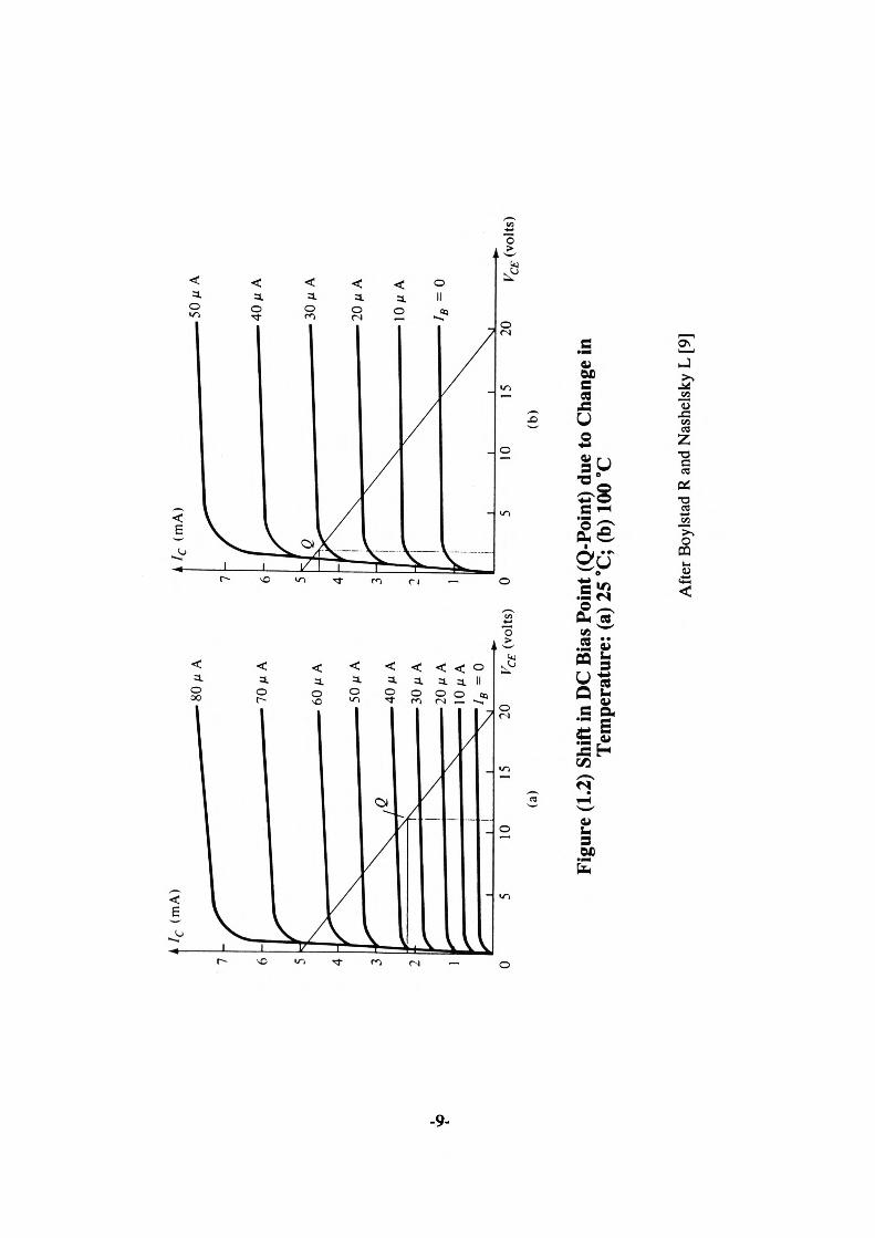
The bipolar junction transistor can be represented as a two port network. Using standard

notations [9], it is possible to set up the hybrid model which is often used for bipolar

junction transistors operating under small signal conditions. The parameters of the hybrid

model of a transistor vary with bias conditions and frequency as well as temperature. The

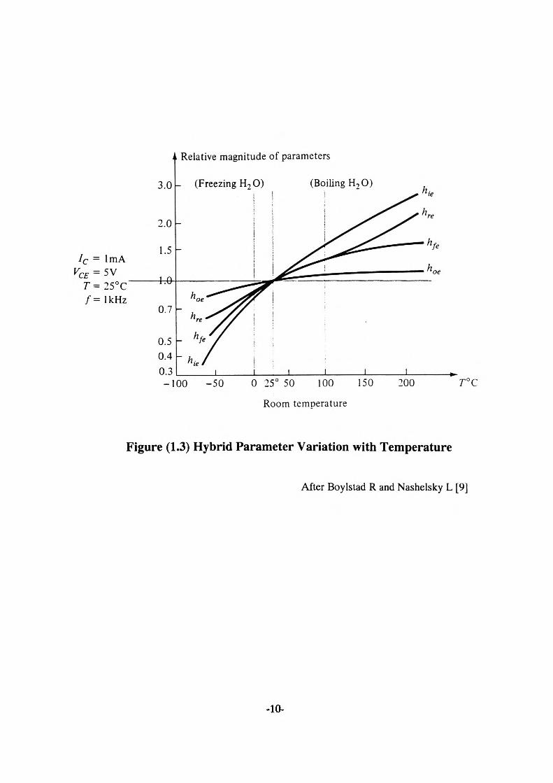
variation in /i-parameters is shown graphically as a function of temperature hi figure (1.3)

[9]. The parameters have all been normalised at room temperature of 25 °C. It can be seen

that all the parameters increase in magnitude with increasing temperature.

-8-

/c (

mA

)

20

V (v

olts)

0

.50/L

t A

• 40

0 f\ " \

"~ \

——

——

— -

10 it

A

——

——

——

——

— 7

0 /i

A

——

——

——

——

— 1

0M A

-— —

——

— /<,

-o

10

15

20

VCE

(vol

ts)

(b)

Figu

re (1

.2) S

hift

in D

C Bi

as P

oint

(Q-P

oint

) due

to C

hang

e in

Te

mpe

ratu

re:

(a) 2

5 °C

; (b)

100

°C

Aft

er B

oyls

tad

R an

d N

ashe

lsky

L [9

]

'. Relative magnitude of parameters

-100 -50 0 25° 50 100 150

Room temperature

200 T°C

Figure (1.3) Hybrid Parameter Variation with Temperature

After Boylstad R and Nashelsky L [9]

-10-

h{e (Input impedance parameter) increases at the greatest rate while hM (Output

conductance) is least affected. hff (forward current gain) changes from 50% of its

normalised value at -50 °C to 150% of its normalised value at +150 "C [9].

In MOS transistors the mobility of the carriers, m in the channel is an inverse function of

the absolute temperature. The mobility at temperature T is related to mobility at room

temperature of 300 K (27 °C) via the empirical relation given below [13]:

(7Y300)"

where a is a constant which lies between 1.0 and 1.5 [13]. Thus a 100 °C temperature rise

would result in approximately 30% fall in carrier mobility. Consequently, for a fixed

applied voltage the drain current ID decreases with an increase with temperature. The

increased temperatures may therefore reduce the switching speeds of these devices [14].

1.2 Review of Thermal Analysis Techniques

The problems outlined above have to be foreseen and prevented at the design stage. The

traditional approach, to construct and test an experimental layout, is obviously costly and

time-consuming and also takes no account of tolerance variations. For many years designers

have faced the problem of predicting temperature rise due to thermal dissipation hi

semiconductor integrated circuits [15,16] and also hybrid microcircuits [17-19], Almost

all the electrical energy consumed by electronic devices is converted directly into heat.

An irreversible dominant heating process occurs when current passes through a material.

This is called Joule Heating and it is proportional to the product of the square of the current

and the electrical resistance of the material to the current flow (?K). A second independent

heating or cooling process which occurs in a single material is called the Thomson Effect

[20]. This appears when an electric current flows through a conductor along which there

-11-

is a temperature gradient [21,22]. This effect is proportional to the product of the current

/ and the temperature gradient dT/dx [21] and therefore reverses when current is reversed.

A Thomson coefficient is defined for a material as the heat evolved when a charge of one

coulomb flows from one point in a material to another at 1 "C lower. Thomson coefficient

which is normally denoted by o has units of Joules and is exceedingly small (in the order

of 10~7 [23] for most metals). For this reason the Thomson Effect will be ignored hi all the

discussions and calculation throughout this thesis.

There is therefore a need for programs which facilitate the prediction of the local

temperature rises in devices. These programs should preferably include both the thermal

and electrical aspects of the design integrated.

A number of papers have been published attempting to deal with the thermal problem in

electronic devices. One of the simplest approaches taken in the modelling of hybrid circuits

is a one-dimensional model [8,24-26] where the heat is assumed to flow from the power

dissipating element in the front to the back side of the substrate. The heat dissipation from

the heat generator is confined to a fixed spreading angle measured from the normal to the

substrate. The angle is taken to be approximately 45° but it is recommended that the angle

should be verified experimentally. An average steady-state thermal resistance analog of

the heat flow is determined by integrating over the thickness of the heat flow path. The

back side is considered to be isothermal and heat losses by convection and radiation from

the surfaces of the device are neglected. The model may be valid to some extent for

substrates of small thermal conductivity such as glass but it is not suitable for ceramic

substrates with relatively high thermal conductivities (around 24 W/mK compared to 1

W/mK for glass) where the lateral heat flux is not negligible. The technique is limited to

steady-state thermal analysis and thermal coupling between different heat generating

-12-

elements is ignored by assuming that the distance between the adjacent elements is

sufficiently large. This may of course be a significant effect in the conductive flow within

a device [27].

In cases where there is considerable lateral heat flow due to high thermal conductivity of

the substrate and the substrate thickness is much smaller than other dimensions, workers

have taken a two-dimensional approach [19,28]. These models assume that the

temperatures on the front and the rear sides of the substrate (top and bottom if placed

horizontally) are identical and neglect temperature gradients perpendicular to the substrate

faces [19]. The two-dimensional model does not however hold for thermal situations where

very small heat sources result hi temperature gradients hi the direction normal to the large

faces [15,29] or where fast thermal transients are present [4]. In such cases the

three-dimensional heat equations have been solved hi the appropriate form to obtain the

temperature distribution hi the device.

Various approaches have been proposed for the solution of the equations defining the heat

flow in devices. A finite-difference method has been presented for two- [30,31] as well as

three-dimensional cases [30], This technique is based on the concept oflumpedparameters.

A device is divided into an array of discrete volumes called nodes and the mass of each

volume is then lumped at a point within the volume it represents [32]. The paths for the

heat flow from one volume to another are represented by conductors joining the appropriate

nodes. Heat balances are subsequently made on each of the nodes giving rise to a system

of linear algebraic equations defining the temperature of each node in terms of the

temperatures of its surrounding nodes. The system of equations may be expressed in matrix

notation asAT=b [33] where A is the matrix including the coefficients of the temperature

terms, T is the required solution vector and b is a column vector of constants. Solutions

of these equations have either been by direct matrix inversion [33] or via iterative techniques

-13-

[28,30,34]. The latter is normally carried out using a relaxation technique which is a method

whereby a temperature is ascribed to each node either by guessing or observation. Upon

substitution of these temperatures a residue is obtained for each nodal equation. The

temperature at the node with the greatest error is then relaxed (corrected) and subsequently

a new error distribution is calculated across the network and the temperature of the node

showing the greatest error is now relaxed. This process is repeated until the residues at

every node reaches a required accuracy. The solution may be slow if a very fine grid is

used in order to obtain more accurate results. This is particularly true in the

three-dimensional cases for which the computing time becomes too large for the method

to be useful [35].

The finite element technique has also been proposed [35,36] for the thermal analysis of

electronic devices. For this method, the structure is divided into a number of small finite

elements which are connected together at some nodes. For each node a heat flow balance

is performed considering all the finite elements connected to it and the solution is expressed

in terms of node temperatures. The advantage of this technique is that it is not geometrically

restrictive [36] and it therefore gives a freedom of choice for the shape of elements [37].

The Separation of variables technique [37,38] has been used by some authors to derive

analytical solutions for heat flow in hybrid [17,27] as well as integrated circuits [39-41].

This approach is used to reach a steady-state solution of the three-dimensional partial

differential equation of heat conduction (Laplace's equation). The following assumptions

are normally made to simplify the thermal problem:

• The lateral dimensions of all the different layers are assumed to be identical, that

is the pattern of these layers is ignored.

• The heat losses due to convection and radiation are neglected from the top face as

-14-

well as the vertical sides of the substrate and the bottom surface of the hybrid is

assumed to be isothermal as it is mounted on to a heat sink.

• The heat is only generated at the top surface and all resistors are taken to be of zero

thickness.

• All layers are of uniform thickness with no voids and they are all rectangular in

shape.

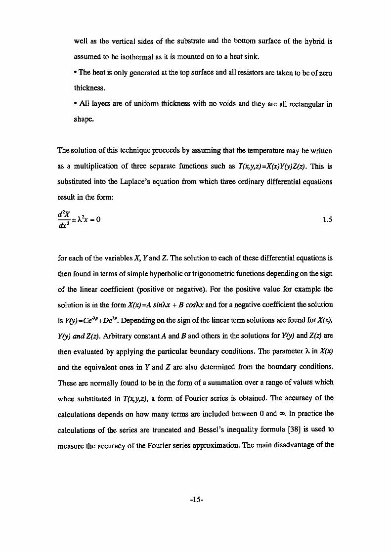
The solution of this technique proceeds by assuming that the temperature may be written

as a multiplication of three separate functions such as T(x,y,z)=X(x)Y(y)Z(z). This is

substituted into the Laplace's equation from which three ordinary differential equations

result in the form:

dbc1.5

for each of the variables X, Y and Z. The solution to each of these differential equations is

then found in terms of simple hyperbolic or trigonometric functions depending on the sign

of the linear coefficient (positive or negative). For the positive value for example the

solution is in the form X(x) =A sirihx + B coshx and for a negative coefficient the solution

is Y(y) =Ce'x> +£>eXy. Depending on the sign of the linear term solutions are found foiX(x),

Y(y) andZ(z). Arbitrary constant A and B and others in the solutions for Y(y) and Z(z) are

then evaluated by applying the particular boundary conditions. The parameter X in X(x)

and the equivalent ones in Y and Z are also determined from the boundary conditions.

These are normally found to be in the form of a summation over a range of values which

when substituted in T(x,y,z), a form of Fourier series is obtained. The accuracy of the

calculations depends on how many terms are included between 0 and «>. In practice the

calculations of the series are truncated and Bessel's inequality formula [38] is used to

measure the accuracy of the Fourier series approximation. The main disadvantage of the

-15-

technique is its limited use [36] and that even for simplest of geometries the solution is

quite complex [37]. The series solution to the equations does not necessarily converge

rapidly and an accurate solution could require evaluation of many terms [36].

Another analytical approach adopted by some workers involves the use of Laplace and

Fourier transform techniques for the solution of the classical transient heat flow equation.

This method has been used for two [35] as well as three-dimensional differential equations.

The solution is found by applying multiple finite Fourier transforms with respect to x and

y and then taking the Laplace transform over the discrete time interval. The resulting

differential equation is then solved for the z variable in the composite structure with the

appropriate boundary conditions. An inverse Laplace transform is subsequently performed

to obtain a relationship for transient temperature in the structure. The accuracy of the

solution depends on the number of terms hi the series. It has been claimed that ±2 °C

truncation error can be achieved using 400 terms [42].

For an accurate thermal analysis of electronic devices, accurate values are required for

various parameters such as the thermal conductivity of the substrate, convection and

radiation coefficients. Perhaps the only parameter for which reliable information may be

available is the thermal conductivity which is normally specified in the manufacturers data

sheets. The convection coefficient hc is the most difficult parameter to quantify [35]. Its

value depends strongly on the nature of the whole surface, the orientation of the substrate

(vertical or horizontal) and the speed of the air flow (natural or forced convection). Perhaps

because of the difficulties in ascertaining an accurate value, some authors [17,25,34] opt

to ignore the effects of convection altogether assuming that these losses are too small

compared to conduction losses. Some workers however include convection in their models

by using values taken from other publications [35] or via a rule of thumb [15,31]. Some

however use a very simplified experimental approach [43] to estimate a uniform convection

-16-

coefficient over the surface. These experiments basically involve the measurement of the

surface and the ambient temperatures followed by a simple energy balance approach [43]

to calculate an average heat transfer coefficient. Empirical relationships have also been

used [18,28,44] to arrive at an average coefficient of convection. The empirical

relationships assume that the rate of convection losses is the same over the whole of the

chip assembly and are derived in various texts each yielding a different heat transfer

coefficient. It is up to the designer to decide which to use in the model.

1.3 Thermal Analysis and Modelling Using ASTEC3

The modelling technique used in this thesis is based on the analogy between thermal and

electrical systems. A thermal structure is divided into an appropriate number of conduction

cells whose thermal resistances may be calculated in the three space directions. Thermal

resistances are also determined for convection and radiation heat losses from the

boundaries. An equivalent electrical network is constructed which is subsequently

simulated using the ASTEC3 electronic simulation package.

Electronic analysis programs have been used in the past for thermal calculations in

microelectronic circuits [45] and other applications [46]. In the case of electronic devices

SPICE2 electronic analysis program has been used as the simulation tool. The method is

limited in its applications as it is only applicable to monolithic integrated circuits [27] and

it is therefore not suitable for thermal analysis of hybrid circuits [27]. The technique does

not include thermal coupling between heat generating elements and it is limited to

steady-state analysis [45]. In one publication [46] thermal analysis of heat exchangers and

control loops of spacelab has been discussed where ASTEC3 is used as the simulation

software.

-17-

The most difficult task in the thermal analysis of devices is the error-free preparation of

the description file especially for very large thermal networks. Software has therefore been

developed which can semi-automatically generate the electrical equivalent circuit of a

thermal structure in ASTEC3 language. Programs have also been developed which make

use of the ASTEC3 output results to plot two-dimensional temperature contour-maps or

three-dimensional surface temperature profiles.

Procedures are also introduced which allow a user to define the more important parts of a

circuit hi finer detail. Interface cells are described which make the coupling of the coarse

and fine mesh areas possible. These procedures are of special importance when simulating

very large circuits as they reduce the computation time required for such simulations.

Studies have been carried out to establish relationships between the size of the circuit and

the CPU time needed for its thermal analysis. These relationships may be used to estimate

the CPU time for a particular thermal simulation.

Verification of the modelling system is established in the first instance by application to

standard heat flow problems. The solutions to these problems are readily available via a

more standard method for comparison.

In practical levels, the accuracy of thermal simulations are limited by the accuracy of the

thermal parameters used. In steady-state analysis these may include thermal conductivity,

emissivity and heat transfer coefficients. In transient simulations the specific heat capacity

of all the materials must also be included hi the list of required parameters. The availability

of such data is also an additional factor since they would have to be measured otherwise.

This problem was encountered in this work during the analysis of a set of preliminary

experiments designed to verify the modelling system.

-18-

2 ASTEC3 SIMULATION PACKAGE

The ASTEC3 software is primarily designed for the analysis of the electrical performance

of circuits and is capable of displaying the results of a simulation in various graphical

formats. For thermal modelling however some of the displaying techniques which are built

into ASTEC3 had to be enhanced to allow the presentation of the results in the form of

temperature contour maps or three dimensional distributions. For this reason a brief

introduction is included in this chapter describing the capabilities of the simulation package.

This is then followed by further sections discussing the software developed to achieve the

displaying enhancement.

2.1 Introduction

ASTEC3 is a powerful analogue circuit analysis package which is capable of performing

transient, AC small signal and DC steady-state simulations [1,2]. ASTEC3 is also suitable

for providing solutions to first order differential equations and any system defined by such

a format can be solved. Since electrical and thermal characteristics of any given network

can be written in terms of analogous differential equations, this allows for the possibility

of simulating both phenomena with ASTEC3.

ASTEC3 has many advantages over other analogue simulators and although other

individual packages may be better than ASTEC3 in certain aspects, ASTEC3 is a package

capable of simulation of both electrical and thermal characteristics of a given circuit and

it is therefore suitable for this investigation. A brief comparison of ASTEC3 with a more

popular circuit simulation package, SPICE, is given below.

-19-

Amongst ASTECS's advantages over SPICE are its speed and efficiency [3] and also the

ease and the speed with which models may be created. Accuracy is also another important

advantage over SPICE, especially in time-dependent simulations [4]. It has been reported

[4] that there is a certain amount of empiricism built into the mathematical formulae used

in SPICE for time-integration which makes it less accurate than ASTEC3. There are also

restrictions in the variables allowed in SPICE since only current and voltage can be made

variable. With ASTEC3 however, any variable is permitted provided that it can be

expressed in the form of a standard FORTRAN equation. This means that parameters such

as temperature and thermal conductivity can be made variables and computed

automatically. There are also other facilities in ASTEC3 which do not exist in SPICE. For

example, the ability to store the final results of a simulation which can then be used as the

starting point for further simulation on the same circuit. This takes away the need for

repeating the whole sequence again. There is also a facility which allows the dynamic

output of the simulation onto the screen. This means that the state of the simulation can

be checked throughout the simulation and if not correct it may be stopped, preventing the

wastage of computing resources and time.

Finally, the most attractive feature of ASTEC3 is its powerful sub-modelling facility. The

simulator allows the description of sub-circuits (so-called models) which can be used within

other models, and the main circuit, many times without the need to write out the sub-circuit

description each time it is employed. These user-defined sub-models can also be stored in

the form of a personalised library. The stored models may then be called up in any future

circuits in the same way as if they had been defined as models hi the description sequence

of the particular ASTEC3 file.

The sub-modelling facility can be of great importance in thermal modelling since it makes

it possible to develop a library of typical components which may then be used in the

-20-

development of more complicated circuits. This makes it possible to hide the details of

the individual thermal/electrical models and greatly simplifies the work of the end-user of

the package.

2.1.1 System Analysis with ASTEC3

In this section a brief description of all the possible forms of simulation will be given with

particular reference to the transient and DC steady-state simulations. These are of particular

importance in thermal simulations of semiconductor devices since they can provide the

user with either the final steady-state temperatures of the device or its transient temperatures

while it is heating up. The latter is especially important since critical temperatures leading

to a device failure may occur well before a steady-state condition has been established.

It is also possible to carry out a statistical simulation on each of the above analyses. This

may be adopted in thermal problems in order to include tolerances in the thermal properties

of the materials. A brief description of these simulations is given below.

DC steady-state

This analysis is used to determine the steady-state values of a linear or non-linear circuit.

For a circuit containing capacitive or inductive components, the steady-state values

correspond to the state after the transients have disappeared and the currents and voltages

reach their equilibrium values.

AC small signal

The AC analysis provides a small signal solution to a linear circuit at a particular frequency.

-21-

If the circuit contains non-linear elements the operating points of the system are first

obtained by an automatic DC steady-state analysis and then small-signal AC analysis is

carried out on a version of the circuit linearised at the calculated operating point using

the stimulus sinusoidal signal supplied by the user.

Transient

The transient simulation routine determines the behaviour of a linear or non-linear network

when subjected to an independent signal which may or may not vary with time. The initial

conditions can either be supplied by the user or can be the DC steady-state values calculated

in a previous simulation.

Statistical

This allows the production of statistical data for DC, AC and Transient simulations by

carrying out a Monte-Carlo analysis [5]. This is a collection of the results of many

simulations on the same circuit but with different, randomly generated, values for specified

components or parameters, taken from a user-specified distribution. These may be based

on component tolerances in the circuit or on parameter tolerances defined in the model

or both. This may be used in thermal problems to specify the variation in the value of

thermal parameters such as thermal conductivity and to study its effect on the results.

The results of such simulations can be presented in three different forms. A scatter diagram

can show the correlation between the relevant parameters; a graph can be plotted showing

the nominal, upper and lower cases; a histogram of the results may be plotted showing the

number of times that a particular quantity has taken a value in a specified range.

-22-

2.1.2 ASTEC3 Data File

A file containing the particular circuit for simulation, normally has three well defined

sections as follows:

Description

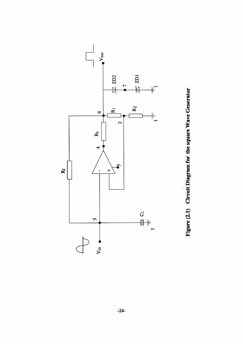
This is the stage where a circuit or system is described in a particular syntax based on a

conventional circuit diagram with the position of each element defined by the nodes at its

connections. This is illustrated in figure (2.1) by means of a simple circuit [6] capable of

producing a square wave (Vout) at its output node if a sinewave (Vin) is applied to its input

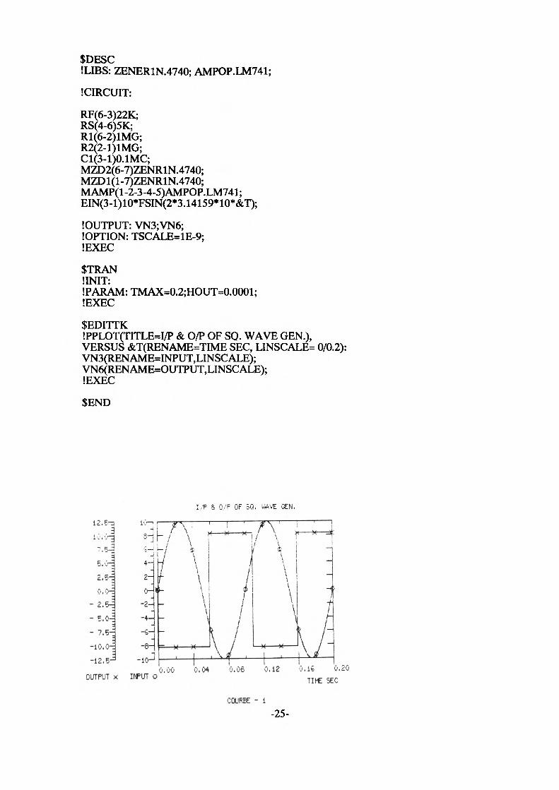
terminals. A listing of the circuit description file and the output produced by ASTEC3 is

shown in figure (2.2).

The circuit components are specified using a keyword (R=resistor, C=capacitor, J=current

source, etc.) followed by an alphanumeric sequence for naming the particular element in

the circuit. This stage includes an"! OUTPUT" sequence in which the required final output

results are declared (eg. VN3 and VN6 in figure (2.2)).

Simulation

In this part of the file, the type of simulation required is specified. The type of simulation

may be one of transient, DC steady-state or AC small signal simulations. It is also possible

to have a single type of simulation or a mixture of all three. There are two sequences

" ! CHANGE" and"! VARY" which allow the simulation of the circuit with parameter values

other than those already given in the description stage.

-23-

'in

•——

——

o

RfH

I-

Rs

fRi R2

I

1

ZD2

ZD1

1 -

Figu

re (2

.1)

Circ

uit D

iagr

am fo

r th

e sq

uare

Wav

e G

ener

ator

$DESCILIBS: ZENER1N.4740; AMPOP.LM741;

1CIRCUIT:

RF(6-3)22K;RS(4-6)5K;R1(6-2)1MG;R2(2-1)1MG;C1(3-1)0.1MC;MZD2(6-7)ZENR1N.4740;MZD1(1-7)ZENR1N.4740;MAMP(l-2-3-4-5)AMPOP.LM741;EIN(3-1)10*FSIN(2*3.14159*10*&T);

IOUTPUT: VN3;VN6; IOPTION: TSCALE=lE-9; 1EXEC

$TRAN UNIT:IPARAM: TMAX=0.2;HOUT=0.0001; IEXEC

!PPLOT(TITLE=I/P & O/P OF SO. WAVE GEN.),VERSUS &T(RENAME=TIME SEC, LINSCALE= 0/0.2):VN3(RENAME=INPUT,LINSCALE);VN6(RENAME=OUTPUT,LINSCALE);IEXEC

$END

I/F & 0/F OF 50, WAVE GEN.

12.5-

3F ,'. r"

£i5~!0.0-:

- 2.5-j

- 5.0-=

- 7.5^

-10.0-:

-12.5-

.; A ! ' i : /Y i : .,-i

4-

2-

O^_

-2—-

-4-

-ioJ

--' \i \ '

/ \\\

\\

/fI1/

/ \/ Y

\\

\\

\0.00 0.04 0.08 0.12

—

Hj

-f

/

\ ^\ J*

0.16 0.20PUT 0

TlhC SEC

COURSE - 1

-25-

If the simulation is of a transient type then the starting point and the length of the simulation

may be declared here as "TMIN" and "TMAX" values.

Presentation of results

This is the final stage where the format of the output results is specified which may be in

the form of graphs or tables of results.

If a statistical analysis is carried out, then the results may be presented in the form of

histograms or scatter diagrams derived from a number of runs. It is also possible to display

an envelope graph showing the nominal, upper and lower performances achieved over

many runs.

There also exists a facility within ASTEC3 which allows the user to store the whole of a

simulation run in a specified file. This file may include tables of results which can then be

used to obtain isothermal maps or temperature distribution plots as will be described in a

later section.

2.2 Presentation of ASTEC3 output results for Thermal Systems

The ASTEC3 package has a very efficient and versatile graphics facility which allows

the presentation of the results of a simulation in various forms. These may be graphs

containing one or more curves from the same, or separate, simulations. In the case of

statistical analysis, histograms, scatter diagrams or even envelope curves may be displayed

representing the upper, lower and the mean values of the results. It is also possible to

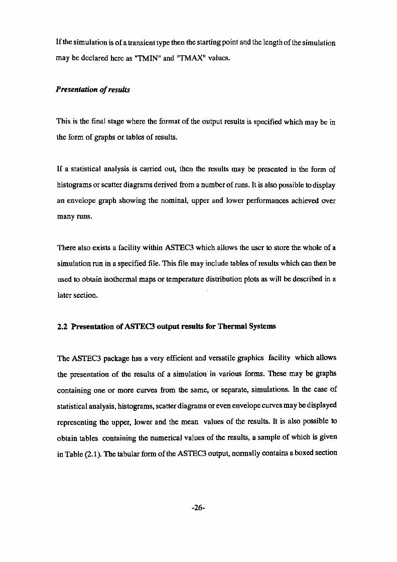
obtain tables containing the numerical values of the results, a sample of which is given

in Table (2.1). The tabular form of the ASTEC3 output, normally contains a boxed section

-26-

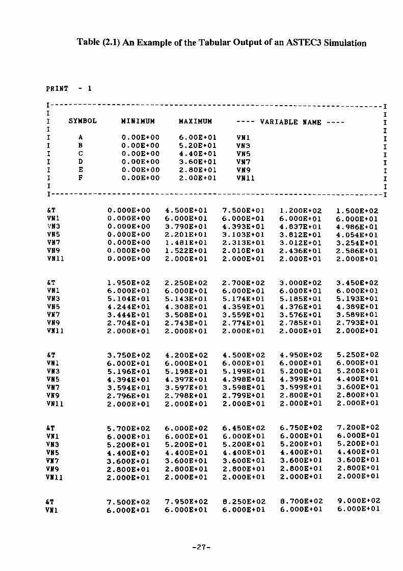
Table (2.1) An Example of the Tabular Output of an ASTEC3 Simulation

PRINT - 1

i-~

I1IIIIIIIIT--

SYMBOL

ABCDEF

MINIMUM

O.OOE+00O.OOE+00O.OOE+00O.OOE+00O.OOE+00O.OOE+00

MAXIMUM

6.00E+015.20E+014.40E+013.60E+012.80E+012.00E+01

---- VARIABLE NAME ----

VN1VN3VN5VN7VN9VN11

----IIIIIIIIIII

____T

&TVN1VN3VN5VN7VN9VN11

&TVN1VN3VN5VN7VN9VN11

&TVN1VN3VN5VN7VN9VN11

&TVN1VN3VN5VN7VN9VNU

&T VN1

O.OOOE+00O.OOOE+00O.OOOE+00O.OOOE+00O.OOOE+00O.OOOE+00O.OOOE+00

1.950E+026.000E+015.104E+014.244E+013.444E+012.704E+012.000E+01

3.750E+026.000E+015.196E+014.394E+013.594E+012.796E+012.000E+01

5.700E+026.000E+015.200E+014.400E+013.600E+012.800E+012.000E+01

7.500E+026.000E+01

4.500E+016.000E+013.790E+012.201E+011.481E+011.522E+012.000E+01

2.250E+026.000E+015.143E+014.308E+013.508E+012.743E+012.000E+01

4.200E+026.000E+015.198E+014.397E+013.597E+012.798E+012.000E+01

6.000E+026.000E+015.200E+014.400E+013.600E+012.800E+012.000E+01

7.950E+026.000E+01

7.500E+016.000E+014.393E+013.103E+012.313E+012.010E+012.000E+01

2.700E+026.000E+015.174E+014.359E+013.559E+012.774E+012.000E+01

4.500E+026.000E+015.199E+014.398E+013.598E+012.799E+012.000E+01

6.450E+026.000E+015.200E+014.400E+013.600E+012.800E+012.000E+01

8.250E+026.000E+01

1.200E+026.000E+014.837E+013.812E+013.012E+012.436E+012.000E+01

3.000E+026.000E+015.185E+014.376E+013.576E+012.785E+012.000E+01

4.950E+026.000E+015.200E+014.399E+013.599E+012.800E+012.000E+01

6.750E+026.000E+015.200E+014.400E+013.600E+012.800E+012.000E+01

8.700E+026.000E+01

1.500E+026.000E+014.986E+014.054E+013.254E+012.586E+012.000E+01

3.450E+026.000E+015.193E+014.389E+013.589E+012.793E+012.000E+01

5.250E+026.000E+015.200E+014.400E+013.600E+012.800E+012.000E+01

7.200E+026.000E+015.200E+014.400E+013.600E+012.800E+012.000E+01

9.000E+026.000E+OI

-27-

at the top of each table which shows the maximum and minimum values of all the logged

variables (voltages at nodes Nl, N2,...etc. in this case). It then gives the transient value of

these variables at equal time intervals in the user-specified time-range. Time is denoted

by the symbol &T and listed at the top row of each column followed by the values of the

outputs at the particular time intervals.

The package is primarily designed for electrical simulations and it lacks the necessary

routines to enable it to produce contour-maps or temperature distribution plots for a thermal

system. It has therefore been necessary to develop additional programs which make use

of the tabular form of ASTEC3 outputs to display the results in the mentioned formats as

detailed below.

2.2.1 Production of Contour and Temperature Distribution Plots

There exists a facility within ASTEC3 which allows the user to store the whole of a

simulation run in a specified file. This file is really a screen-dump of the run and therefore

includes, apart from the tables of results, extra information which should be deleted before

the file can be used in plotting graphs.

As mentioned above the actual tables are normally printed beginning with the symbol

'&T' in the left hand side representing time and ending with the message 'Edit Ended'. A

program has therefore been written in FORTRAN, which scans through the ASTEC3

output file and ignores the additional lines up to the symbol '&T and after 'Edit Ended'.

This program creates a second file containing only the tables. A listing of this program is

given in appendix (1) as program (1).

The output file of program (1) is subsequently analysed using a second program (program

-28-

(2) in appendix (1)) for plotting of the required contour-maps. A brief list of the different

stages of this program are given below:

i) The data file generated by program (1) is scanned and the time-intervals are read and

stored in the array "store_time".

ii) The output values corresponding to each time interval are read and stored in a

two-dimensional array "store_array" along with the corresponding time-interval.

iii) The information concerning the size and location of the point grid is read.

iv) The (x-y) coordinates are generated for the outputs in each time interval. This is carried

out by allocating to the uppermost quantity in the table the coordinate (X0,y0) and the second

output (Xj,y0) until the row ya is complete and then the same at rows y2, y3 and so on.

v) The program asks the user the desired time-difference between the plots.

vi) The appropriate subroutines from the CAD graphics package GINO are initialised

automatically to produce the desired contour-maps for the first time-interval using the

grid generated in section (iv).

vii) The operator is given a few seconds to dump the graph onto a printer before the

contour-map for the next time-interval is displayed.

At present the software uses the CAD package GINO which is only capable of handling

square or rectangular planes with uniform grid pattern superimposed upon them an example

of which is illustrated in figure (2.3).

For the program to operate correctly, the ASTEC3 outputs (normally temperatures at

particular points on a plane although these could be any other parameter with a distribution

over the area) should be arranged in the circuit description file, in order of nodes starting

from the lowest x and y position (Xo,y0 in figure (2.3)) and incremented in the x direction

until the row is complete and then repeated for rows at the next y positions (y,, y2, y3, ...etc.).

-29-

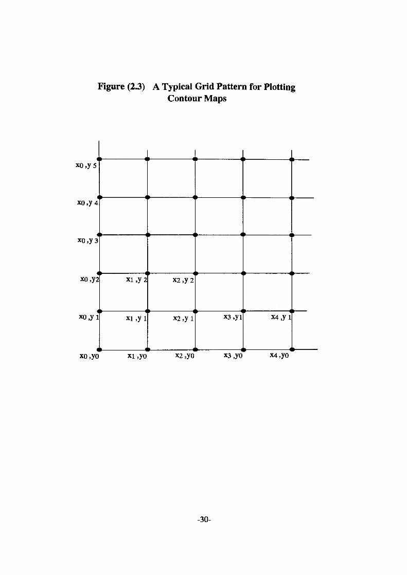
Figure (2.3) A Typical Grid Pattern for Plotting Contour Maps

xo,ys

xo,y4

xo,y3

xo,y2

xo,yi

t

k. ^

» ——————————— 4

» ———————————— «

» ———————————— Ixi,y2

» —————— <xi,yi

i <

1 ^

» ——————— «

» ——————— 4

» ————————— < X2,y2

> ——————— 4X2,y i

i , ,..,,...... ——— <

» —————— i

k ———————— <

» ———————— «

k ———————— <xa.yi

k —————— <

t ——————————— «

» ——————————— «

> ———————————— 4

» —————————— 4

» ——————————— 4x4,yi

» —————— i

t ——

k ————

» ————

» ———

> ———

l —————xo.yo xi,yo X2,yo x4,yo

-30-

The program described above takes into account temperatures at the nodal points in one

fay) §"d to generate the contour map of the plane. This may not be satisfactory where

greater accuracies are required for the temperature profile. This problem may be tackled

in two ways. The first approach may be to use a finer grid for simulation of the structure

which has the disadvantage of having to write a substantially greater data file which in

turn needs greater computer time. This of course become more important when dealing

with larger circuits. A second approach could be to develop the software to utilise the

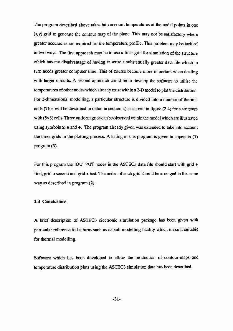
temperatures of other nodes which already exist within a 2-D model to plot the distribution.

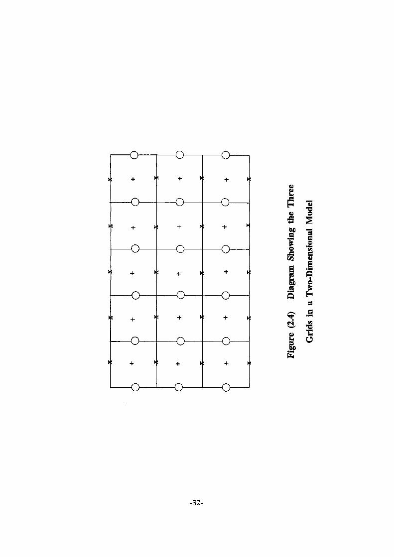
For 2-dimensional modelling, a particular structure is divided into a number of thermal

cells (This will be described in detail in section 4) as shown in figure (2.4) for a structure

with (5x3) cells. Three uniform grids can be observed within the model which are illustrated

using symbols x, o and +. The program already given was extended to take into account

the three grids in the plotting process. A listing of this program is given in appendix (1)

program (3).

For this program the IOUTPUT nodes in the ASTEC3 data file should start with grid +

first, grid o second and grid x last. The nodes of each grid should be arranged in the same

way as described in program (2).

23 Conclusions

A brief description of ASTEC3 electronic simulation package has been given with

particular reference to features such as its sub-modelling facility which make it suitable

for thermal modelling.

Software which has been developed to allow the production of contour-maps and

temperature distribution plots using the ASTEC3 simulation data has been described.

-31-

u>

S)

) +

(T

T

3 +

(—

——

——

X ——

—— :—

— it ——

———

) +

(

) +

(—

——

——

X —

——

—

f :

) +

(

) +

(—

——

— X

——

——

—

) +

(X

——

——

— *

——

——

—

) +

(V

) +

(Y

) +

(

jr

'

)

+

(

——

——

——

X —

——

——

l : 1

Figu

re (

2.4)

Dia

gram

Sho

win

g th

e Th

ree

Grid

s in

a T

wo-

Dim

ensio

nal

Mod

el

3 HEAT TRANSFER

There are three basic processes of heat transfer namely conduction, convection and

radiation. A brief description will be given for each of these processes separately but

bearing in mind that in most problems of practical importance two or sometimes all of

these modes may occur simultaneously.

3.1 Conduction

This is a heat flow mechanism whereby thermal energy is transferred through a material

from a region of high temperature to a region of lower temperature. In metallic conductors

or any other electrically conducting solids, heat is carried through the lattice structure

simultaneously by means of free electrons and vibrational energy (phonons) [1,2]. In

non-metallic or dielectric materials heat is conveyed only by means of phonons [1].

The conduction of thermal energy by lattice waves may be described by considering the

situation of an atom in a crystal vibrating about its equilibrium position. If this atom is

vibrating with an amplitude say a at a temperature T, it exerts decaying periodic forces on

its neighbouring atoms which in turn increase their amplitudes of vibration. This of course

occurs if the other atoms were vibrating with lower amplitudes because of their lower

temperature. If the ends of a solid are kept at different temperatures then heat will flow

from the hot end to the colder end each atom oscillating with smaller and smaller amplitudes

towards the cooler end.

The heat conduction by lattice vibrations is proportional to the mean free path of the

phonons. The thermal conductivity of the material is therefore governed by the distance a

-33-

phonon can travel before it is scattered. If the energy transfer between the atoms of a solid

were purely harmonic, there would be no mutual scattering of phonons [3]. In this case

the scattering process would bedominated by collisions of lattice waves with the boundaries

and lattice imperfections. In solids however, the heating causes a subsequent expansion

of the structure which in turn changes the harmonic nature of the lattice waves. This

anharmonicity then causes collisions between the different phonons and a subsequent

scattering of the waves. Anharmonic interactions are dominant at high temperatures where

the mean free path of the phonons is inversely proportional to the temperature [1]. There

is another scattering process affecting thermal conduction at high temperatures called the

Umklapp process. This is a random process by which the direction of flow of energy is

changed after a phonon-phonon collision [1,3]. Collision of two phonons with wavevectors

Kj and K2 travelling in the positive x direction in a crystal would at low temperatures be

of the form Kj+K2 =K3 where a third phonon is produced travelling in the same general

direction. In the Umklapp process however collision of the energetic phonons gives rise

to a third phonon whose wavevector falls outside the first Brillouin zone. According to

the laws of conservation of momentum in a crystal all meaningful phonon fCs should be

contained in the first zone [3] and therefore the emitted phonon in the Umklapp process

is brought back into the zone by a reversal of direction via Kj+K2=K3 +G where G is a

reciprocal lattice vector.

Conduction in metals is dominated by movement in the solid of the electrons in partially

filled bands although lattice conductivity may occasionally become important in situations

where low temperature, high magnetic fields and large impurity contents exist [4]. The

scattering processes which contribute to lattice resistance to heat conduction in metals may

be due to electron-phonon interactions which is negligible at low temperatures and becomes

important at higher temperatures. The other process is due to scattering of electrons by

lattice defects which is not a temperature dependent process and depends solely on the

-34-

purity of the metal and lattice imperfections.

The basic equations of heat conduction have been well documented [5-7]. In one dimension

the rate of heat transfer through a given area A is given by the Fourier rate equation :

t -^t£where K is the thermal conductivity of the material, T is the temperature and x is the

displacement through the material of area A.

Equation (3.1) assumes that temperature varies only along the x direction and does not

change with time t. This however is not sufficient where the temperature of the solid varies

in the x, y and z directions and with time. The general equation of conduction in three

dimensions for a uniform body with constant thermal conductivity and with heat sources

present within the body [5,8] is given by :

Jerr dT srr\ . „ dTK\ -^ + ^ + ^\+q -PC— 3.2 \dx 2 dy2 dz2 p dt

where q, p and Cp are the heat generation per unit volume, density and the specific heat

capacity of the material respectively.

The terms on the left hand side of equation represent the heat gains by conduction and

generation respectively and the right hand side represents the rate of change of temperature

with time in the solid.

By eliminating the appropriate terms in equation (3.2), suitable relationships can be

obtained defining a particular situation. For example steady-state heat conduction in

2-dimensions with heat generation is of the form:

-35-

r ,l \J A U J »

K\ TT + 7^ +9 =0 3.3 (dx2 dy 2 )

The heat conduction equation may be solved to determine the temperature distribution in

a medium as a function of space and time. For this, a set of boundary conditions and an

initial condition are needed. The latter specifies the temperature distribution in the system

at time t=0 and the former specifies the heat flow or temperature situation at the boundaries.

3.2 Convection

Convection is another mode of heat transfer where heat is exchanged between a solid body

and an adjacent fluid. Heat transfer between the fluid and the solid surface takes place

because of a combination of conduction within the fluid and energy transport which is due

to the fluid motion.

There are two types of convection namely free convection and forced convection. Free

convection takes place as a consequence of density differences caused by temperature

gradients between the fluid and the body and within the fluid itself. Forced convection

occurs when the fluid motion is induced by an external force. The rate of heat flow at the

surface is conventionally described by equation (3.4) [5,6] which is applicable to forced

as well as free convection regimes:

3.4

where A is the solid surface area exposed to the fluids, hc is the convective heat transfer

coefficient and 7} and T, are the fluid and surface temperatures respectively.

-36-

3.2.1 Boundary Layer Fundamentals

When a fluid flows over a body, the velocity and temperature distribution in the vicinity

of the surface influence the heat transfer by convection. In order to simplify the analysis

of convective heat transfer, the boundary layer concept has been introduced [8], There are

essentially two types of boundary layers which form over a surface namely velocity

boundary layer and thermal boundary layer. A brief description of these two kinds of

boundary layers is given in the following sections.

3.2.1.1 Velocity Boundary Layer

The concept of velocity boundary layer may be illustrated by considering the flow past a

plane, stationary plate as shown in figure (3.1). At the leading edge of the plate the fluid

has a velocity Uf which is parallel to the surface. As the fluid moves over the plate, the

fluid viscosity causes the particles near the surface to slow down. The fluid particles in

the immediate vicinity of the surface adhere to it due to the interaction frictional forces

and their velocity reduces to zero [9]. Other fluid molecules trying to slide over these

stationary particles are retarded because of the interaction between the faster and slower

moving particles. This retardation of molecules is reduced to zero at a position far from

the plate where the fluid velocity reaches that of the main fluid velocity Uf. At each location

along the plate there is a distance bv(x) from the surface where the axial velocity component

U approaches 99 percent of Uf. The velocity boundary layer is defined as the locus of the

points where U = 0.99 Uf [8].

Furthermore, as the fluid proceeds along the plate, the shearing forces cause more and

more of the fluid to be slowed down and hence the thickness of the boundary increases

[9]-

-37-

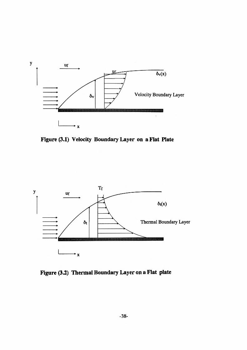
Uf

6v

6v(x)

Velocity Boundary Layer

Figure (3.1) Velocity Boundary Layer on a Flat Plate

TfUf

6t

6t(x)

Thermal Boundary Layer

Figure (3.2) Thermal Boundary Layer on a Flat plate

-38-

3.2.1.2 Thermal Boundary Layer

Analogous to the fluid velocity behaviour, if a flat plate is maintained at a constant

temperature Ts which is different from the main fluid temperature Tfi a thermal boundary

layer develops [9]. The fluid temperature varies from the surface temperature to the free

stream temperature within this boundary layer as shown in figure (3.2). The transition from

the temperature in the boundary layer to the conditions in the main fluid flow takes place

asymptotically [8] and hence the thickness of the thermal boundary layer 6/x) has been

defined similar to the velocity boundary layer as the thickness where the temperature of

the boundary reaches that of the main stream.

The thermal boundary layer contributes the main resistance to heat exchange between the

surface and the fluid. In the immediate vicinity of the surface heat transfer takes place by

way of conduction through the stationary particles in that layer relative to the boundary

[9]. Further away from the surface, the energy transport is aided by the movement of the

fluid. The temperature gradient is quite steep near the surface becoming less steep away

from the wall and levelling out in the main flow.

3.2.1.3 Laminar and Turbulent Boundary Layers

The motion of the fluid in the boundary layer region is in two forms as illustrated in figure

(3.3) for flow over a flat plate. The boundary layer starts at the edge of the plate as a laminar

boundary layer in which the fluid moves in layers, each fluid particle following a smooth

and continuous path. The molecules in these layers behave in an orderly manner and do

not pass each other. In this type of motion the heat exchange is by molecular conduction

within the fluid as well as at the interface between the surface and the fluid [10].

-39-

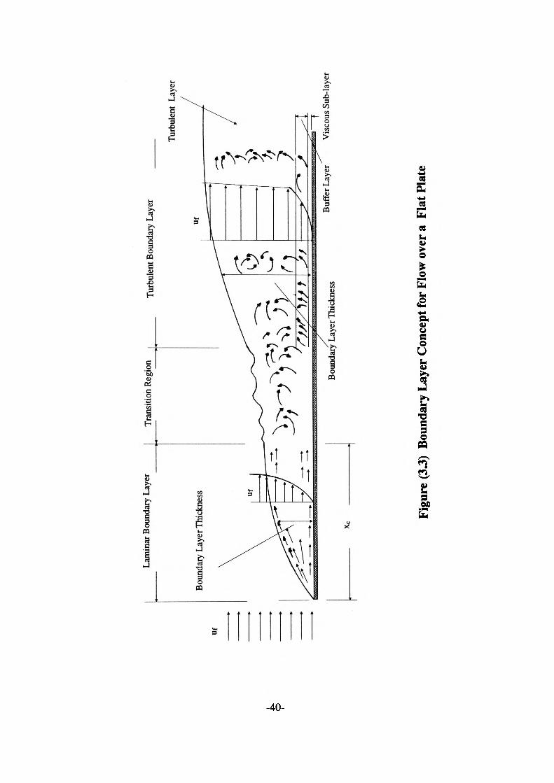
Lam

inar

Bou

ndar

y La

yer

Tran

sitio

n Reg

ion

Turb

ulen

t Bou

ndar

y Lay

er

Uf

Turb

ulen

t La

yer

Boun

dary

Lay

er T

hick

ness

Xc

Boun

dary

Lay

er T

hick

ness

Buffe

r Lay

er

Visc

ous S

ub-la

yer

Figu

re (

3.3)

Bou

ndar

y L

ayer

Con

cept

for

Flow

ove

r a

Fla

t Pla

te

After a transition distance, the flow becomes turbulent where irregular velocity fluctuations

are superimposed on the fluid motion. The turbulent boundary layer consists of three

sections. There exists a very thin layer in the immediate vicinity of the surface called the

viscous sub-layer. Adjacent to this sub-layer there is a region called the buffer layer where

there is a very small, fine-grained turbulence. Following the buffer layer the motion

becomes completely turbulent.

The conduction mechanism in turbulent flows take place by eddies which convey lumps

of fluid across the streamline. These lumps act as carriers of energy by mixing with other

fluid particles.

3.2.2 Empirical Equations

The analysis of convective heat transfer is extremely complicated because of the interaction

between the fluid motion and the temperature field. Therefore the determination of the

temperature distribution in the fluid and hence the true local heat transfer coefficient

involves the solution of the complete fluid mechanics problem in the region near the

surface.

In general this would involve the simultaneous solution of equations for conservation of

mass, momentum and energy and also the equations of state of the fluid [5].

Because of the complexity of the equations of motion and energy, it is extremely difficult

to solve convective heat transfer problems by the above method except for very simple,

idealised situations. Therefore, for most cases of practical interest convective heat transfer

problems have been studied experimentally and the results are then presented hi the form

of empirical equations that involve some dimensionless groups [8].

-41-

Various methods may be employed to arrive at such dimensionless parameters. In one

such method the dimensionless groups can be determined directly from the dimensionless

form of the differential equations of motion and energy [5]. A simpler method however

is the dimensional analysis approach which enables equations to be written relating the

important physical quantities such as the fluid properties in dimensionless groups. Natural

convection is only considered here since throughout this report convection will be assumed

to be of this nature.

Many experiments have been carried out to establish the functional relationships between

the dimensionless parameters for various geometric configurations and planforms [5,6,8].

It has been found for example that hi natural convection relationships of the following

form apply:

Nu - C(GrJPr)n 3.5

where C and n are constants. Nu, Gr and Pr are Nusselt, Grashof and Prandtl numbers

respectively given by:

Nu - hcl/K 3.6

Gr

where the parameters are as given in Table (3.1):

3.7

3.8

Table (3.1)

P8

A7

The coefficient of cubical expansionAcceleration due to gravityCharacteristic length for bodies with geometrically similar shapesThe coefficient of kinematic viscosityCoefficient of dynamic viscosityThe specific heat capacity of the fluidFluid thermal conductivityThe heat transfer coefficientTemperature difference between the surface and the ambient fluid

-42-

The physical significance of Nusselt number may easily be arrived at by writing equation

(3.6) in the following form [11]:

3 - 9

which can be interpreted as the ratio of the heat transfer by convection to heat transfer by

conduction across a fluid layer of thickness /.

Equation (3.8) describing Prandtl number can also be rearranged in the following form

by introducing the fluid density p:

„ PrK K/(pCp ) '

The Prandtl number is then seen to be the ratio of the kinematic viscosity to the thermal

diffusivity. By incorporating these into equation (3.10) the following relationship can be

obtained for the Prandtl number.

Pr = - 3.11 a

Kinematic viscosity v affects the velocity distribution and thermal diffusivity a influences

the temperature profile in the fluid.

Finally, the Grashof number is another dimensionless group defined by equation (3.7). It

has been shown experimentally that this parameter indicates the ratio of the buoyancy

force to the viscous force in natural convection systems [9].

The values of C and n in equation (3.5) are normally quoted for a given range of Rayleigh

number which is a product of Grashof and Prandtl numbers which determines whether the

flow is laminar or turbulent [5,6,8,9]. Laminar flow corresponds to a flow where the fluid

velocities are sufficiently small that the fluid moves in layers parallel to the surface without

-43-

mixing [9]. In contrast, fluid motion in turbulent flow is highly irregular and occurs at

higher fluid velocities where, the mixing of the fluid layers is caused by an oscillatory

motion of the particles normal to the main flow direction [12].

As an example the following relationships have been recommended [5] for uniformly

heated horizontal plates with the heated side facing upwards:

Nu = 0.54(Gr.Pr)1'4 2.6 x 104 < Grfr < 107

Nu - 0.15(Gr J>r)lf3 107 < Gr J>r < 3 x 1010

The various properties are normally taken at a mean film temperature defined as (Ts+Tj)/2

where T, and 7} are the surface and the ambient fluid temperatures.

Once the Nusselt number is determined for a certain situation, an average heat transfer

coefficient can be calculated using a rearranged form of equation (3.6) which is hc =NuK/l.

3.3 Radiation

The third mode of heat transfer is thermal radiation. This is a process in which bodies emit

thermal energy by means of electromagnetic radiation extending from approximately 0.1

to 100 jim wavelength of the electromagnetic spectrum which includes part of the Ultra

Violet and all of the visible and Infra-Red regions. This type of radiation is emitted in all

possible directions and if it strikes another body, it may be partly absorbed, partly reflected

and partly transmitted. The absorbed part of thermal radiation will appear as heat within

the absorbing body.

In contrast to conduction and convection where the transfer of energy from one body to

-44-

another can occur only through a material medium, electromagnetic radiation may pass

from one body to another without the need of a transport medium.

There is a maximum rate at which thermal radiant energy can be emitted and consequently

absorbed by a body at a certain temperature. The surfaces which interchange radiant energy

at such rates are called black bodies and it can be shown [6] that the radiation emitted by

such surfaces at temperature T is given by the Stefan-Boltzmann law:

3.12

where o is the Stefan-Boltzmann constant (5.67xlO~8 WlnfK1), T is the absolute

temperature in Kelvins and Eb is the black-body emissive power. In practice there are no

surfaces that behave as a black-body and the radiation flux emitted by a grey body is

always less than a black-body and is given by:

q - 3- 13

where e is called the emissivity which relates the radiation of the grey surfaces to that of

a black surface.

The fourth power law derived by Stefan-Boltzmann can be used to determine the total

amount of radiation leaving a surface. This concept is however inadequate when dealing

with radiative transfer between bodies where only a portion of the radiation leaving one

surface in a particular direction is intercepted by another. It is therefore necessary to

introduce a quantity called the View or Shape factor which gives the fraction of the total

radiation emitted by a surface which is received by another. Before an attempt is made to

derive a general relationship for the View Factor, basic definitions will be given for Solid

-45-

Angle and Intensity of Radiation.

Solid Angle: The physical significance of solid angle may be illustrated by referring to

figure (3.4) where x is the direction of propagation and dA is a small area normal to * at a

distance r from a point source s. The solid angle to in units of steradians is defined as [9]:

0) = ^- 3.14 r2

using the above definition, for a complete hemispherical shell the solid angle may be

calculated as 2nr*lr* which is equal to 2n steradians.

Intensity of Radiation: The radiation emitted by a surface propagates in all possible

directions and if a small flat area is considered the entire radiation passes through a

hemispherical surface surrounding the emitting area [13] as shown in figure (3.5). The

Intensity of Radiation, /, describes the directional distribution of the radiant energy leaving

a surface or incident upon it. It is defined as the rate of energy emission per unit time of

the emitting surface per unit solid angle subtended at the surface. The variation in the

intensity of radiation for a black-body is expressed by Lambert's Cosine Law which states

that [13]:

3.15

By definition of radiation intensity, the energy dq^ emitted by dA. through a solid angle

d(oN normal to dA is hence given by:

dqN -IN.du>N 3.16

and radiation emitted in an angle 6 through a solid angle du>8:

dqe -Ie.dioQ 3.17

which according to Lambert's Law may be written as :

dqe - IN. cos 6dcoe 3.18

-46-

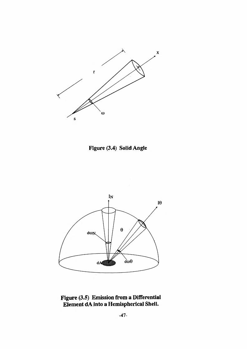
CD

Figure (3.4) Solid Angle

Figure (3.5) Emission from a Differential Element dA into a Hemispherical Shell.

-47-

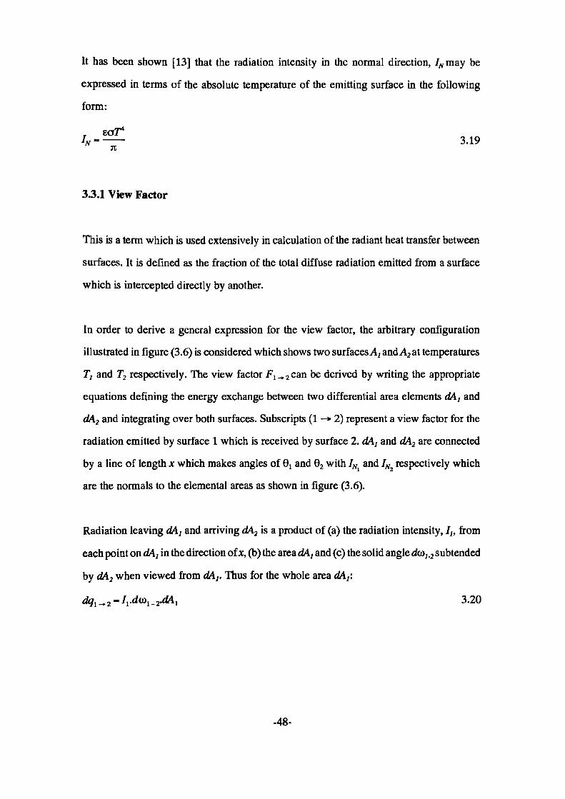
It has been shown [13] that the radiation intensity in the normal direction, IN may be

expressed in terms of the absolute temperature of the emitting surface in the following

form:

. ear4/„-—— 3.19

3.3.1 View Factor

This is a term which is used extensively in calculation of the radiant heat transfer between

surfaces. It is defined as the fraction of the total diffuse radiation emitted from a surface

which is intercepted directly by another.

In order to derive a general expression for the view factor, the arbitrary configuration

illustrated in figure (3.6) is considered which shows two surfaces A1 and A2 at temperatures

Tj and T2 respectively. The view factor Fj_ 2 can be derived by writing the appropriate

equations defining the energy exchange between two differential area elements dAj and

dA2 and integrating over both surfaces. Subscripts (1 -» 2) represent a view factor for the

radiation emitted by surface 1 which is received by surface 2. dA, and dA2 are connected

by a line of length x which makes angles of 0! and 02 with IN and IN respectively which

are the normals to the elemental areas as shown in figure (3.6).

Radiation leaving dA, and arriving dA2 is a product of (a) the radiation intensity, I,, from

each point on dA, in the direction of x, (b) the area dA, and (c) the solid angle du>,.2 subtended

by dA2 when viewed from dA,. Thus for the whole area dA,:

3-20

-48-

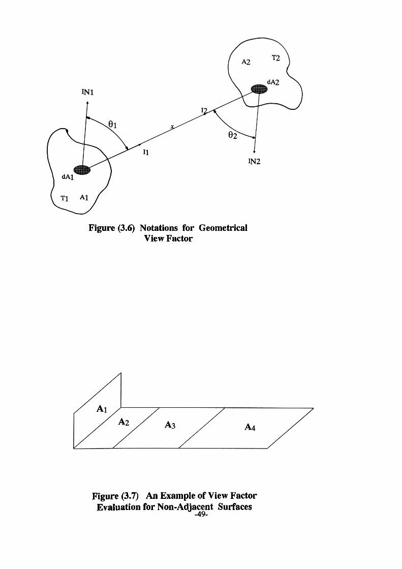
INI

IN2

Figure (3.6) Notations for Geometrical View Factor

Figure (3.7) An Example of View Factor Evaluation for Non-Adjacent Surfaces-49-

By definition of solid angle, dwj.2 is equal to the projected area of the receiving element,

dA2, in a direction normal to the direction of incidence divided by the square of the distance

x. Ij is also equal to IffjCosQ according to Lambert's Law. Therefore d?1 _ 2 becomes :

dA2 cosQ2 <*?!-. 2 -Jocose,. —— r-=.«tti 3'21

X

which may be written as :

cos 6, cos 0,1 -2 - Hl > —— ~2

in a similar manner :

cos0,cos02

3.22

by substituting for IN from equation (3.19) for a black-body with an emissivity (E) of one

and integrating over the two areas the total energy radiated from A, reaching A2 is:

cos 0! cos Q2dAidA2n '

* *nx2 3.24

The total energy emitted by A] is equal to aAjTj4. The View Factor is by definition the

fraction of the total energy emitted by A1 which reaches A2 and therefore:

-^ 3.25-

which by substituting for q\^i becomes :

1 e e cos0,cos0,<i4,£i42 Fl -~ 2 ~°A~\l ————2 3.26

similarly :

r /-COS ,COS 2^! 2 ^^1 f r COS0!-»i"Ti

^2 j JAj A2

-50-

Equations (3.26) and (3.27) may be used to evaluate the shape factor for various surfaces.

It is a very tedious mathematical process involving the double integrals taken over the

surfaces. Even for the simplest of geometries the calculations are quite laborious. Other

workers have carried out such evaluations for most of the significant configurations which

are readily available in various publications. These are normally either in the form of simple

algebraic expressions [9] or in graphic form [9] where with a knowledge of a few

dimensions the view factors can be obtained. More complex situations may generally be

reduced to simpler cases and evaluated using view factor relations which will be given in

the following section.

3.3.1.1 Properties of View Factors

There exist some very useful relationships between the view factors of radiating surfaces

some of which will be given here.

Perhaps the most useful and important property of the shape factors is derived from

equations (3.26) and (3.27) which suggest that:

^1^1-2=^2^2-1 3-28

which is called the reciprocity relationship.

If radiation from a surface i to a surface j is considered where surface; is divided into n

sub-areas(A;yA;y ....,-A^) then the radiation reaching the whole of j is the sum of the

radiation received by its individual parts [9]. Thus:

3-29

-51-

However if the radiating surface is divided into n smaller sections, each radiating to a

surface;, then the shape factor for the whole of surface i to j is given by a summation of

all the individual FA products [9] as :

4^,-fW-; 3.30

Consider the configuration shown in figure (3.7) which illustrates two perpendicular

rectangles with a common edge one of which is divided into three sections. The shape

factors F! _ 4 and F4 _ t for radiation exchange between surfaces Aj and A4 is required.

The shape factors for perpendicular surfaces sharing a common edge are readily available

in various references [9]. Figures may therefore be obtained for shape factors F^j,

According to relation (3.29), the total shape factor from surfaced, to the combined surfaces

of A2, A3 and A4 is the sum of the individual shape factors. Thus:

3.31i -.(2+3+4) - 1 _

Fi-(2+3) = Fi^2 + Fi-3 3.32

by combining equations (3.31) and (3.32) and rearranging for F1 _>4 we get the following

relationship:

F1 _ 4 = F1 _ (2+3+4) -F1 _ (2+3) 3.33

where the two terms on the right hand side of the equation are known.

To derive a relationship forF4 _ 1 use is made of the reciprocity relation given in equation

(3.28) as follows:

-A 3.34

-52-

by substituting for F1 _ 4 from equation (3.33) and rearranging, the shape factor F4 ^ t is

found to be:

A^4-.l =^l/ri-*(2 + 3 + 4)-^'l-(2 + 3)] 3.35

The net radiation exchange between two black surf aces may be determined as follows:

9i -2 -F^jOAX 3.36

fc-i-F^aA^ 3.37

However according to reciprocity relation (3.28) :

3.38

and therefore ^2 -» i becomes:

92-l--AjF1 _ 2°I2 3.39

Thus the net exchange is given by:

3.40

For a black-body at temperature TJt totally enclosed in another much larger surface

maintained at 7^ F1 _ 2 "^2-1 ~ 1 [13] and therefore the net radiant energy exchanged

[14] is given by:

3.41

where A is the surface area of the enclosed body.

For two grey bodies with emissivities of e this becomes:

3.42

Similar to convection, a radiation heat-transfer coefficient hr may be defined [5] as :

-53-

3.43

where T1 and T2 are the temperatures of the two bodies exchanging heat by radiation. hr

may be determined for different surfaces with varying shapes and geometries [5]. By

comparing equations (3.42) and (3.43) the following expression is obtained for the heat

transfer coefficient as :

r) 3.44

3.4 Conclusions

In this chapter the general principles of heat transfer phenomena have been presented. It

was chosen to deal with each of the three modes separately although in most practical

problems at least two of the modes occur simultaneously.

In each section the appropriate equations describing the particular mode were outlined

with particular reference to the equations which will later be used when dealing with various

heat flow situations.

-54-

4 THERMAL SYSTEM MODELLING

4.1 Introduction

The thermal performance of a given system can be written as an electrical analogy by a

suitable change of variables. The simple Ohm's law equation can be compared to equations

(3.1, 3.4 and 3.44) for conductive, convective and radiative heat transfer respectively.

This gives equivalent electrical resistances of:

Axcmduc*m= Kbyte

R - 4 2'^convection L *

4.3

for conductive, convective and radiative processes respectively. The conductive thermal

resistance RcmAK&m is given for a cuboidal portion of a material of thermal conductivity K

and dimensions Ax, Ay and Az as shown in figure (4.1). hc and hr are the convective and

radiative heat transfer coefficients respectively and A is the area.

It can also be seen by comparing the equation for the current in a charging capacitor ( i

= C dV/dt ) with the equation for the rate of change of energy in a volume element AV (q

= pCp&V dT/dt) that an equivalent electrical capacitance can be used to represent the

thermal capacitance of a cell of volume AVof a body given by:

-55-

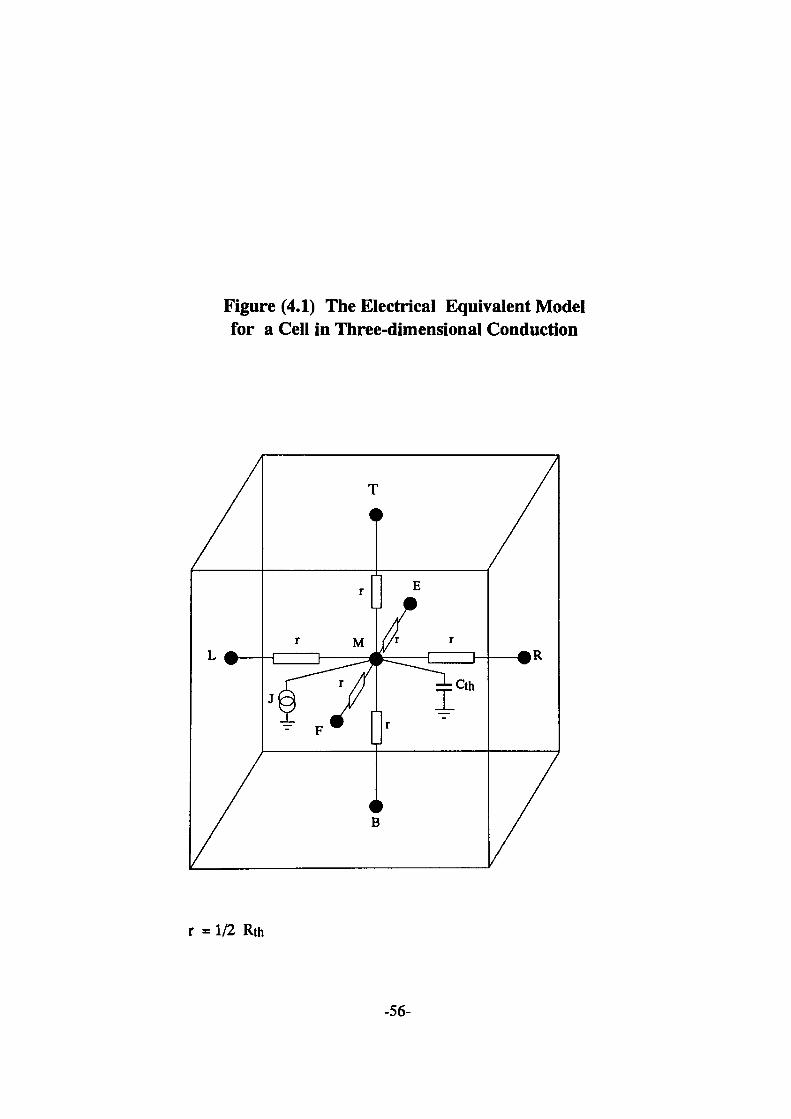
Figure (4.1) The Electrical Equivalent Model for a Cell in Three-dimensional Conduction

r = 1/2 Rth

-56-

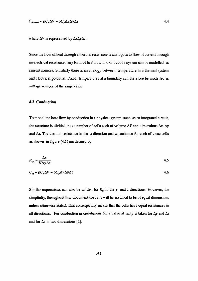
PCpAxAyAz 4.4

where AV is represented by AxAyAz.

Since the flow of heat through a thermal resistance is analogous to flow of current through

an electrical resistance, any form of heat flow into or out of a system can be modelled as

current sources. Similarly there is an analogy between temperature in a thermal system

and electrical potential. Fixed temperatures at a boundary can therefore be modelled as

voltage sources of the same value.

4.2 Conduction

To model the heat flow by conduction in a physical system, such as an integrated circuit,

the structure is divided into a number of cells each of volume AV and dimensions Ax, Ay

and Az. The thermal resistance in the x direction and capacitance for each of these cells

as shown in figure (4.1) are defined by:

Similar expressions can also be written for R^, in the y and z directions. However, for

simplicity, throughout this document the cells will be assumed to be of equal dimensions

unless otherwise stated. This consequently means that the cells have equal resistances in

all directions. For conduction in one-dimension, a value of unity is taken for Ay and Az

and for Az in two dimensions [1].

-57-

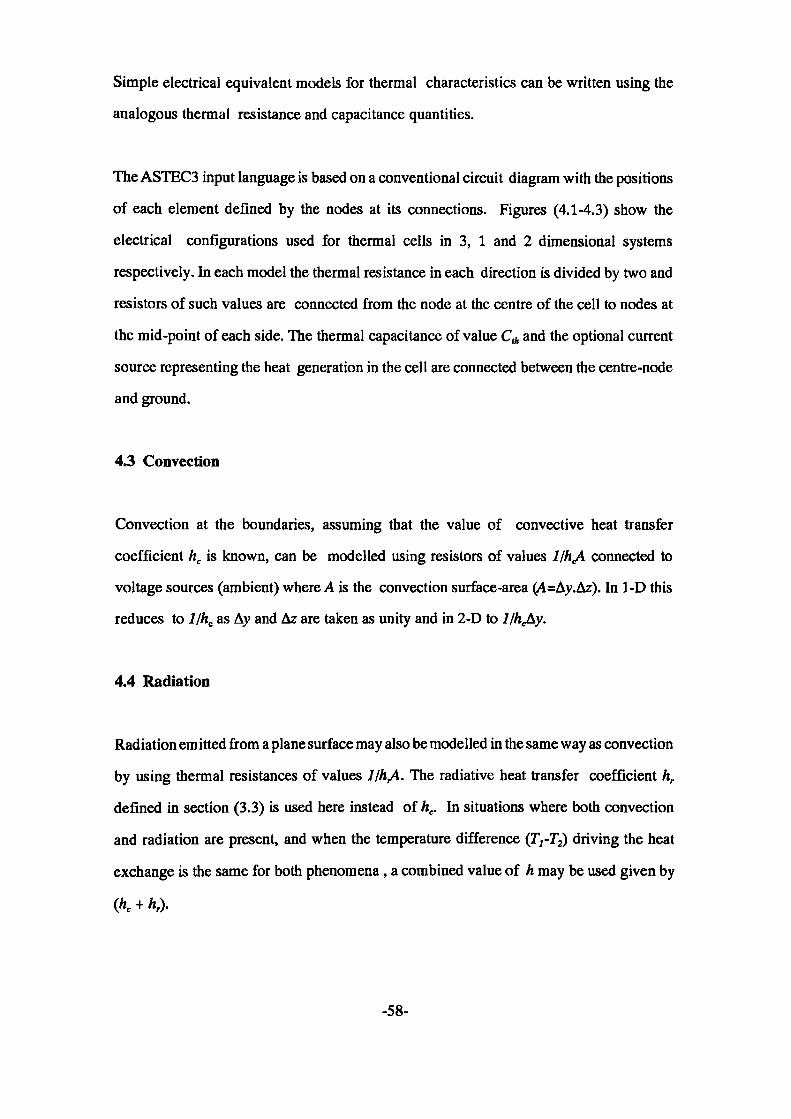
Simple electrical equivalent models for thermal characteristics can be written using the

analogous thermal resistance and capacitance quantities.

The ASTEC3 input language is based on a conventional circuit diagram with the positions

of each element defined by the nodes at its connections. Figures (4.1-4.3) show the

electrical configurations used for thermal cells in 3, 1 and 2 dimensional systems

respectively. In each model the thermal resistance in each direction is divided by two and

resistors of such values are connected from the node at the centre of the cell to nodes at

the mid-point of each side. The thermal capacitance of value Cth and the optional current

source representing the heat generation in the cell are connected between the centre-node

and ground.

4.3 Convection

Convection at the boundaries, assuming that the value of convective heat transfer

coefficient hc is known, can be modelled using resistors of values 1/h^ connected to

voltage sources (ambient) where A is the convection surface-area (A=Ay.Az). In 1-D this

reduces to l/hc as Ay and Az are taken as unity and in 2-D to Hh.Ay.

4.4 Radiation

Radiation emitted from a plane surface may also be modelled in the same way as convection

by using thermal resistances of values l/h,A. The radiative heat transfer coefficient hr

defined in section (3.3) is used here instead of he. In situations where both convection

and radiation are present, and when the temperature difference (T,-T2) driving the heat

exchange is the same for both phenomena, a combined value of h may be used given by

-58-

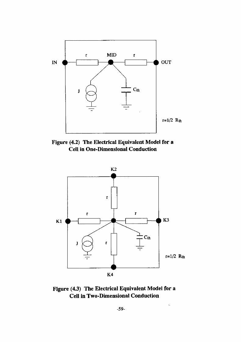
IN OUT

r=l/2 Rth

Figure (4.2) The Electrical Equivalent Model for a Cell in One-Dimensional Conduction

K2

Kl

r=l/2 Rth

K4

Figure (4.3) The Electrical Equivalent Model for a Cell in Two-Dimensional Conduction

-59-

4.5 ASTEC3 Code-Generation Programs

4.5.1 Introduction

For the thermal version of the ASTEC3 modelling package to be of any commercial or

practical interest, it is important for it to be made user-friendly and automated as much as

possible.

The most cumbersome task in thermal simulations is the actual writing of the circuit

description in the ASTEC3 syntax, especially when dealing with a large number of thermal

cells. It was therefore essential to develop the necessary software which would

automatically generate the net-list required for a given thermal structure.

Programs have been developed which generate the electrical equivalent circuit description

for uniform structures. Two programs will be described here the first of which is for

2-dimensional heat conduction and the second for 3-dimensional heat conducting

structures.

It should be mentioned that the user must write a single thermal cell model described in

section (4.2) as a sub-model and store it in his personalised library. This sub-model can

then be called up within the circuit description file. The sub-models for the 2 and 3

dimensional conduction are as follows :

!MODEL2D(L-R-T-B-C-G):PR1;PR2;PC;PJ;RL(L-C)PR1;RR(R-C)PR1;RT(T-C)PR2;RB(B-QPR2;CC(C-G)PC;JC(G-C)PJ;

-60-

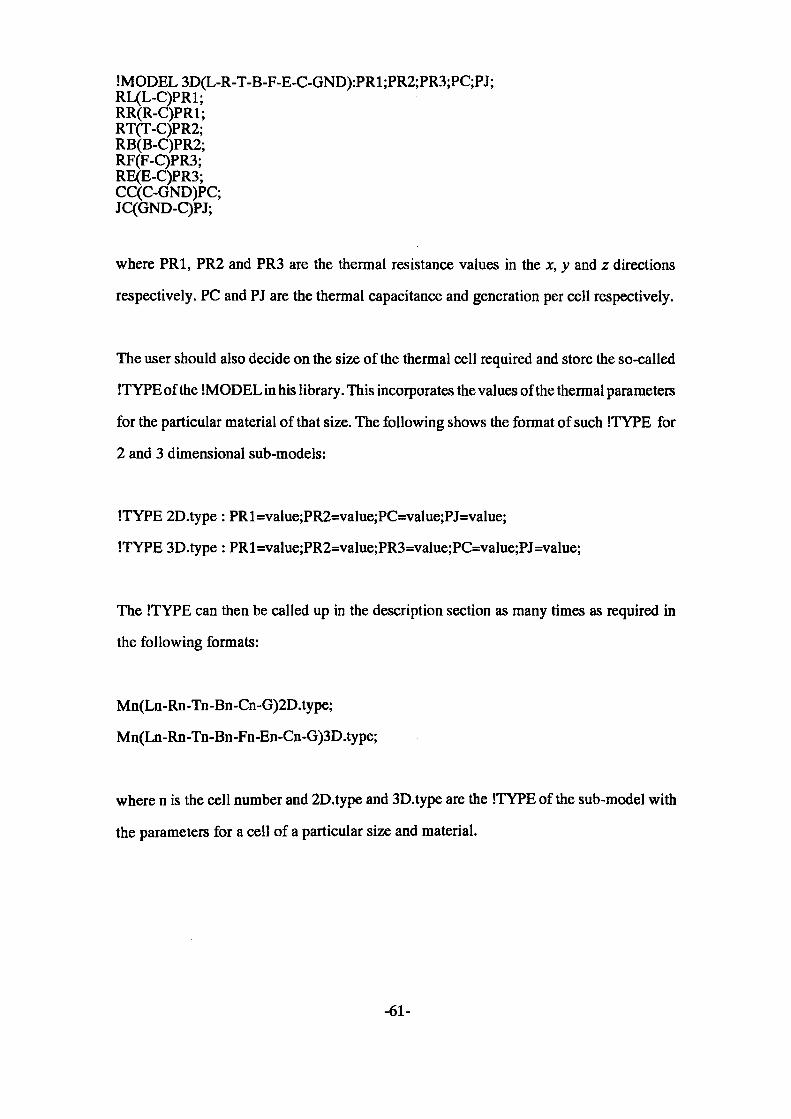
.'MODEL 3D(L-R-T-B-F-E-C-GND):PR1;PR2;PR3;PC;PJ;RL(L-C)PR1;RR(R-C)PR1;RT(T-C)PR2;RB(B-C)PR2;RF(F-C)PR3;RE(E-C)PR3;CC(C-GND)PC;jqGND-C)PJ;

where PR1, PR2 and PR3 are the thermal resistance values in the x, y and z directions

respectively. PC and PJ are the thermal capacitance and generation per cell respectively.

The user should also decide on the size of the thermal cell required and store the so-called

ITYPE of the IMODEL in his library. This incorporates the values of the thermal parameters

for the particular material of that size. The following shows the format of such ITYPE for

2 and 3 dimensional sub-models:

ITYPE 2D.type: PRl=value;PR2=value;PC=value;PJ=value;

ITYPE SD.type : PRl=value;PR2=value;PR3=value;PC=value;PJ=value;

The ITYPE can then be called up in the description section as many times as required in

the following formats:

Mn(Ln-Rn-Tn-Bn-Cn-G)2D.type;

Mn(Ln-Rn-Tn-Bn-Fn-En-Cn-G)3D.type;

where n is the cell number and 2D.type and SD.type are the ITYPE of the sub-model with

the parameters for a cell of a particular size and material.

-61-

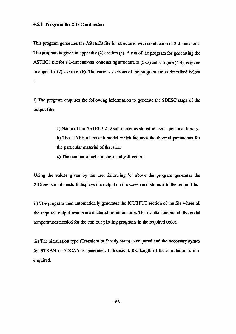
4.5.2 Program for 2-D Conduction

This program generates the ASTEC3 file for structures with conduction in 2-dimensions.

The program is given in appendix (2) section (a). A run of the program for generating the

ASTEC3 file for a 2-dimensional conducting structure of (5x3) cells, figure (4.4), is given

in appendix (2) sections (b). The various sections of the program are as described below

i) The program enquires the following information to generate the $DESC stage of the

output file:

a) Name of the ASTEC3 2-D sub-model as stored in user's personal library.

b) The ITYPE of the sub-model which includes the thermal parameters for

the particular material of that size.

c) The number of cells in the x and y direction.

Using the values given by the user following 'c' above the program generates the

2-Dimensional mesh. It displays the output on the screen and stores it in the output file.

ii) The program then automatically generates the lOUTPUT section of the file where all

the required output results are declared for simulation. The results here are all the nodal

temperatures needed for the contour plotting programs in the required order.

iii) The simulation type (Transient or Steady-state) is enquired and the necessary syntax

for $TRAN or $DCAN is generated. If transient, the length of the simulation is also

enquired.

-62-

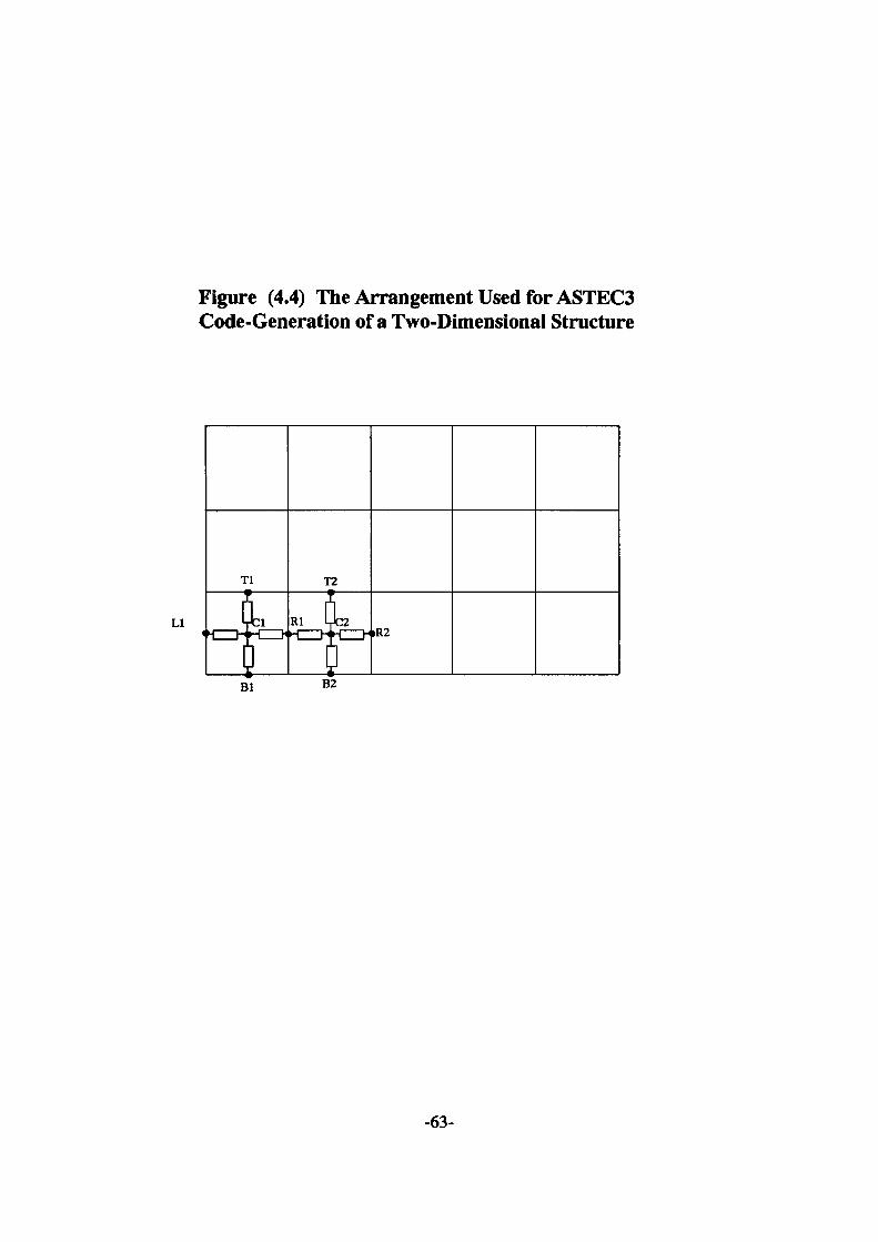
Figure (4.4) The Arrangement Used for ASTEC3 Code-Generation of a Two-Dimensional Structure

Ll

-63-

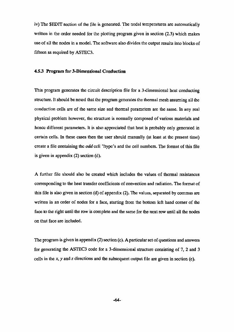
iv) The $EDIT section of the file is generated. The nodal temperatures are automatically

written in the order needed for the plotting program given in section (2.3) which makes

use of all the nodes in a model. The software also divides the output results into blocks of

fifteen as required by ASTEC3.

4.53 Program for 3-Dimensional Conduction

This program generates the circuit description file for a 3-dimensional heat conducting

structure. It should be noted that the program generates the thermal mesh assuming all the

conduction cells are of the same size and thermal parameters are the same. In any real

physical problem however, the structure is normally composed of various materials and

hence different parameters. It is also appreciated that heat is probably only generated in

certain cells. In these cases then the user should manually (at least at the present time)

create a file containing the odd cell 'Itype's and the cell numbers. The format of this file

is given in appendix (2) section (d).

A further file should also be created which includes the values of thermal resistances

corresponding to the heat transfer coefficients of convection and radiation. The format of

this file is also given in section (d) of appendix (2). The values, separated by commas are

written in an order of nodes for a face, starting from the bottom left hand corner of the

face to the right until the row is complete and the same for the next row until all the nodes

on that face are included.

The program is given in appendix (2) section (c). A particular set of questions and answers

for generating the ASTEC3 code for a 3-dimensional structure consisting of 7, 2 and 3

cells in the x, y and z directions and the subsequent output file are given in section (e).

-64-

Various stages of the program are as follows:

i) The program enquires the following information to generate the $DESC stage of the

output file:

a) Name of the ASTEC3 3-D sub-model as stored in user's personal library.

b) The ITYPE of the sub-model which includes the thermal parameters for

the particular material of that size.

c) The number of cells in the x and y and z direction.

d) The name of the file containing the number of those cells with different

ITYPE extension.

e) The name of the file including the combined value for the heat transfer

coefficients of convection and radiation.

ii) Using the information given by the user the program generates the necessary codes for

the $DESC section of the file as shown in the output example in appendix (3) section (e).

Note that in the mesh, the hype name has been changed to the corresponding one in the

given file. A series of resistors is also created with the values supplied in the file for the

heat transfer coefficients.

The remaining stages of the program are very similar to the program for 2-Dimensional

conduction except in (iv) the nodes are in an order for the contour plotting program

described in section (2.3). Here the nodes are chosen to be for the top face of the structure

shown in figure (4.5) which can be easily extended to include any surface.

-65-

Figure (4.5) The Structure Used for Three-Dimensional ASTEC3 Code-Generation

-66-

4.6 Conclusions

In this chapter, procedures have been described for modelling the three heat transfer

mechanisms. An electrical analogy has been employed which allows the simulation of a

thermal structure using the electronic analysis package ASTEC3.

Programs written to semi-automatically generate the electrical equivalent circuit

description of a problem in ASTEC3 syntax have been described. Two programs have

been presented the first of which is for code-generation of two-dimensional conduction

models and second one for three-dimensional heat flow problems.

-67-

5 VALIDATION OF ASTEC3 MODELLING

5.1 Introduction

The principles described in chapter (4) must be verified in the context of ASTEC3

modelling. This is achieved here by applying them to a number of heat flow situations

whose solutions may be determined directly from theory or by a separate, more

conventional, technique. This approach is carried out here for one- and two-dimensional

heat conducting arrangements.

In one-dimension the temperature distribution in a uniform slab is simulated and compared

with the finite-difference and analytical solutions of the same structure. Two cases have

been considered: conduction only and conduction with convection at the boundaries.

To verify the simulation performance in two-dimensional heat conduction, the flow in a

rectangular plate is considered when subjected to a non-uniform external input. The

simulated results are compared with the analytical solution of the problem.

A method will be described which makes it possible to model the more important sections

of a thermal structure in finer detail. Subsequent measurements will demonstrate the

reduction of computation-time when this method is employed.

A further investigation has also been carried out to establish a relationship between the

number of conduction cells and the simulation time. This will allow the prediction of the

computation time needed for a particular thermal structure.

-68-

5.2 One-dimension

5.2.1 Conduction only

As an example consider a slab of width 50 mm with uniform thermal conductivity of 17.3

W/mK and thermal diffusivity of 4.5 \tm2/s where heat is generated at a constant rate of

2.06MW/m3. The temperature distribution in the slab is required when constant temperature

sources at 60 °C and 20 "C are applied to its boundary surfaces.

a ASTEC3 Solution

To achieve an ASTEC3 solution of this problem the slab may be divided into 5 segments

of 10 mm length each. /?(A and Clh are calculated for a one-dimensional cell using equations

(4.5) and (4.6) and five such cells are connected in series as shown in figure (5.1).

The simulation is carried out starting from an initial linear distribution and the

nodal-temperatures are recorded until a steady-state condition is reached. The ASTEC3

results are shown graphically in figure (5.2) which gives the variation of the temperature

distribution in the slab with time.

b Finite difference solution

To validate the ASTEC3 simulation results a finite-difference technique was also used

to determine the temperatures of the four interior nodes from an initial linear steady-state

condition to a final steady state in steps of Af. This is a method by which the partial

differential equation of heat conduction is replaced by a system of linear algebraic

-69-

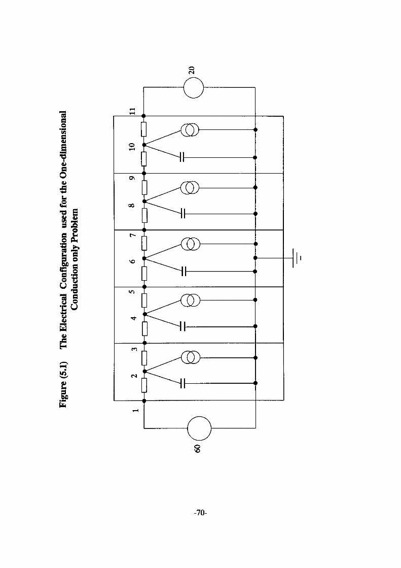
Figu

re (5

.1)

The E

lectr

ical

Conf

igur

atio

n us

ed fo

r the

One

-dim

ensio

nal

Cond

uctio

n on

ly P

robl

em

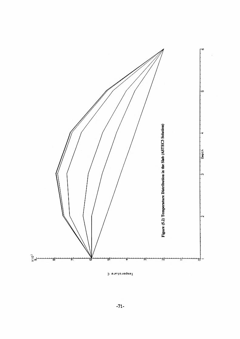
XIO

1

<->

5

e s. o> a IK

figur

e (5

.2) T

empe

ratu

re D

istri

butio

n in

the

Slab

(AST

EC3

Solu

tion)

Dep

th

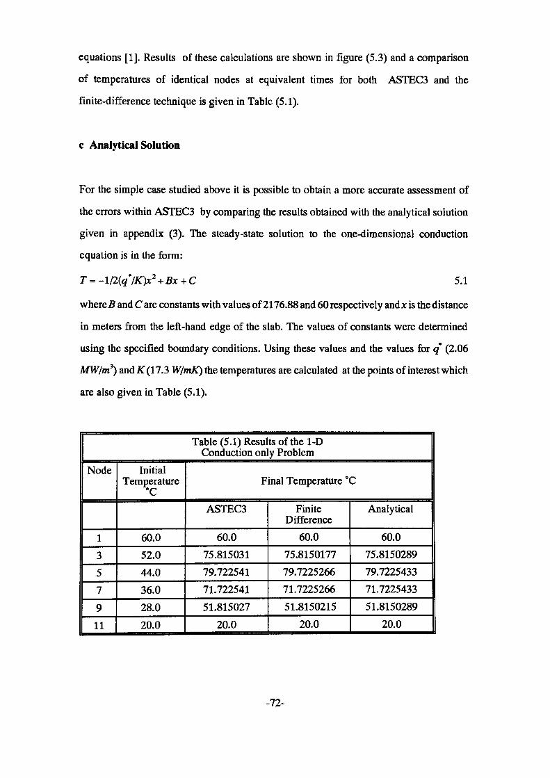
equations [1]. Results of these calculations are shown in figure (5.3) and a comparison

of temperatures of identical nodes at equivalent times for both ASTEC3 and the

finite-difference technique is given in Table (5.1).

c Analytical Solution

For the simple case studied above it is possible to obtain a more accurate assessment of

the errors within ASTEC3 by comparing the results obtained with the analytical solution

given in appendix (3). The steady-state solution to the one-dimensional conduction

equation is in the form:

T = -l/2(q°/K)x2 + Bx + C 5.1

where B and C are constants with values of 2176.88 and 60 respectively and* is the distance

in meters from the left-hand edge of the slab. The values of constants were determined

using the specified boundary conditions. Using these values and the values for q (2.06

MWIm3) and AT (17.3 W/mK) the temperatures are calculated at the points of interest which

are also given in Table (5.1).

Table (5.1) Results of the 1-D Conduction only Problem

Node

1357911

Initial Temperature °C

60.052.044.036.028.020.0

Final Temperature °C

ASTEC3

60.075.81503179.72254171.72254151.815027

20.0

Finite Difference

60.075.815017779.722526671.722526651.8150215

20.0

Analytical

60.075.815028979.722543371.722543351.8150289

20.0

-72-

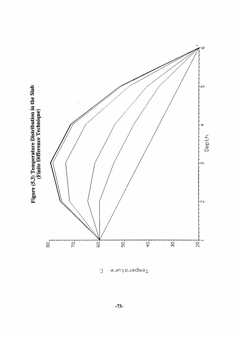
Figu

re (5

.3) T

empe

ratu

re D

istri

butio

n in

the

Slab

(F

inite

Diff

eren

ce T

echn

ique

)

CJ CD 3 d Cb a £ Cb

Dep

th

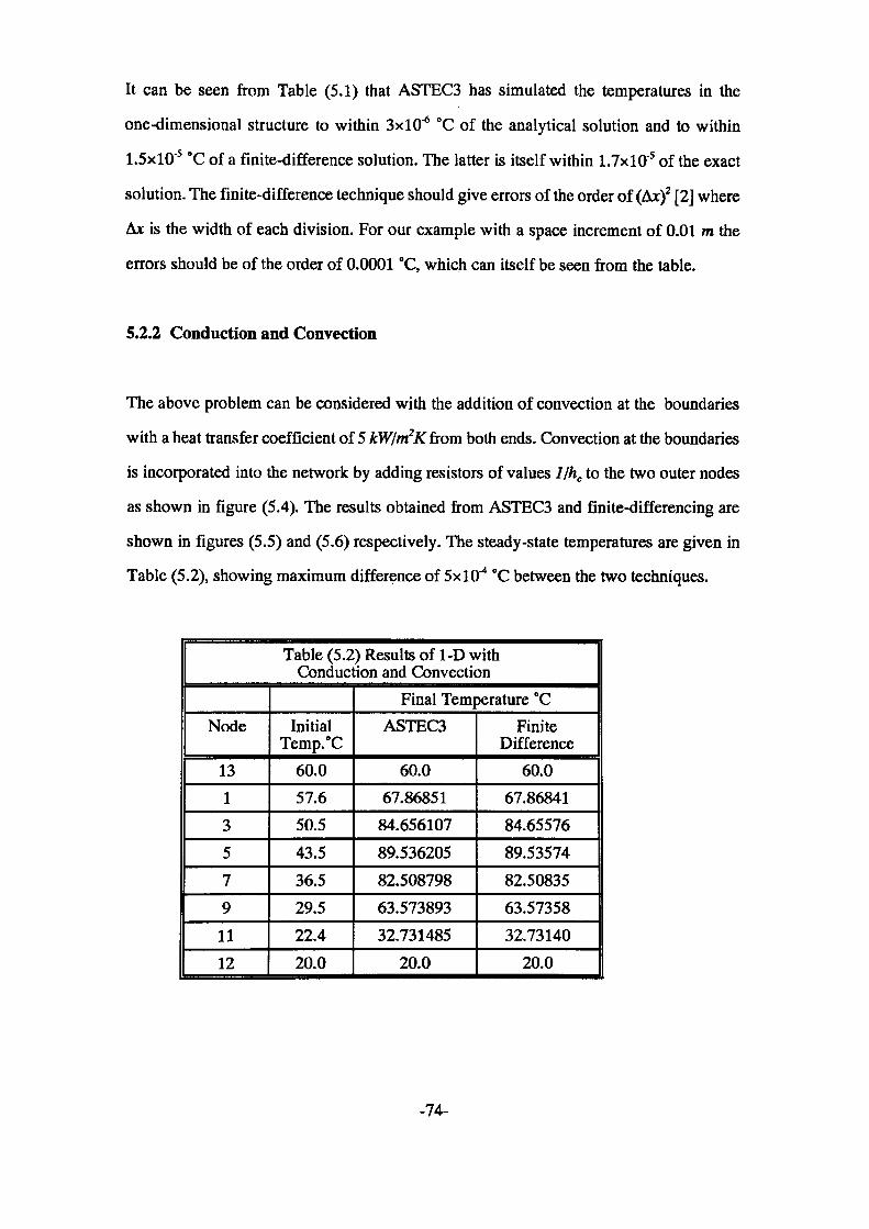
It can be seen from Table (5.1) that ASTEC3 has simulated the temperatures in the

one-dimensional structure to within SxlO"6 °C of the analytical solution and to within

1.5xlO's °C of a finite-difference solution. The latter is itself within 1.7xlO~s of the exact

solution. The finite-difference technique should give errors of the order of (Ax)2 [2] where

Ax is the width of each division. For our example with a space increment of 0.01 m the

errors should be of the order of 0.0001 °C, which can itself be seen from the table.

5.2.2 Conduction and Convection

The above problem can be considered with the addition of convection at the boundaries

with a heat transfer coefficient of 5 kW/m2Kfiom both ends. Convection at the boundaries

is incorporated into the network by adding resistors of values l/hc to the two outer nodes

as shown in figure (5.4). The results obtained from ASTEC3 and finite-differencing are

shown in figures (5.5) and (5.6) respectively. The steady-state temperatures are given in

Table (5.2), showing maximum difference of SxlO"4 °C between the two techniques.

Table (5.2) Results of 1-D with Conduction and Convection

Node

1313579

1112

Initial Temp.°C

60.057.650.543.536.529.522.420.0

Final Temperature °CASTEC3

60.067.86851

84.65610789.53620582.50879863.57389332.731485

20.0

Finite Difference

60.067.8684184.6557689.5357482.5083563.5735832.73140

20.0

-74-

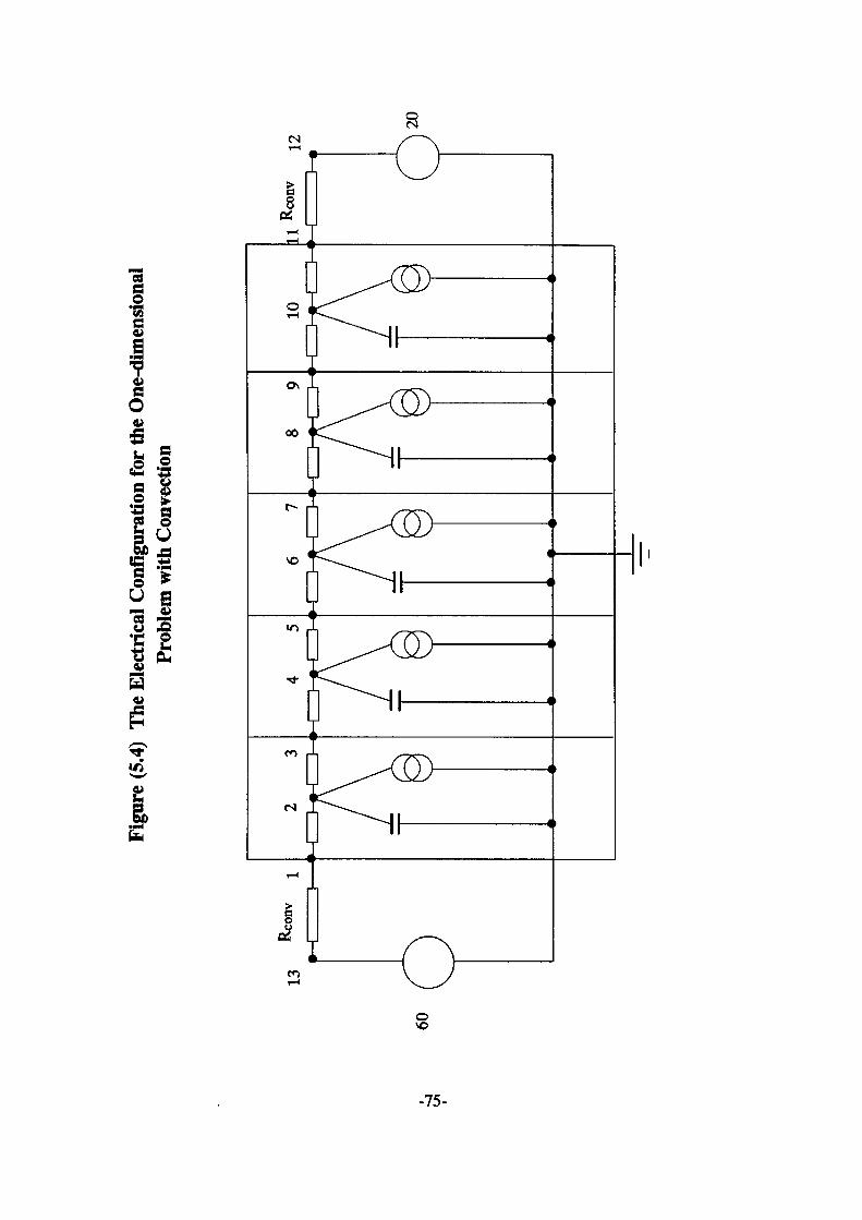
Figu

re (5

.4) T

he E

lect

rical

Con

figur

atio

n fo

r the

One

-dim

ensio

nal

Prob

lem

with

Con

vect

ion

13

60

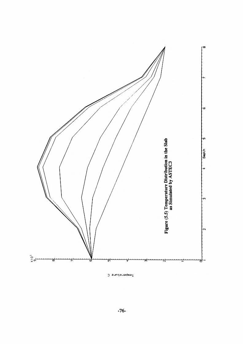
a.

XIO

1

s:

Figu

re (5

.5) T

empe

ratu

re D

istrib

utio

n in

the

Slab

as

Sim

ulat

ed b

y A

STEC

3

•» D

epth

5

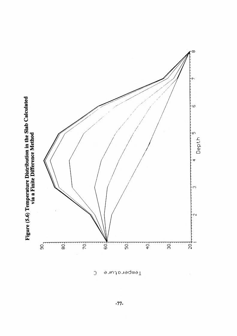
Figu

re (5

.6) T

empe

ratu

re D

istrib

utio

n in

the

Slab

Cal

cula

ted

via

a Fi

nite

Diff

eren

ce M

etho

d

CJ Q; CL E CD

20:

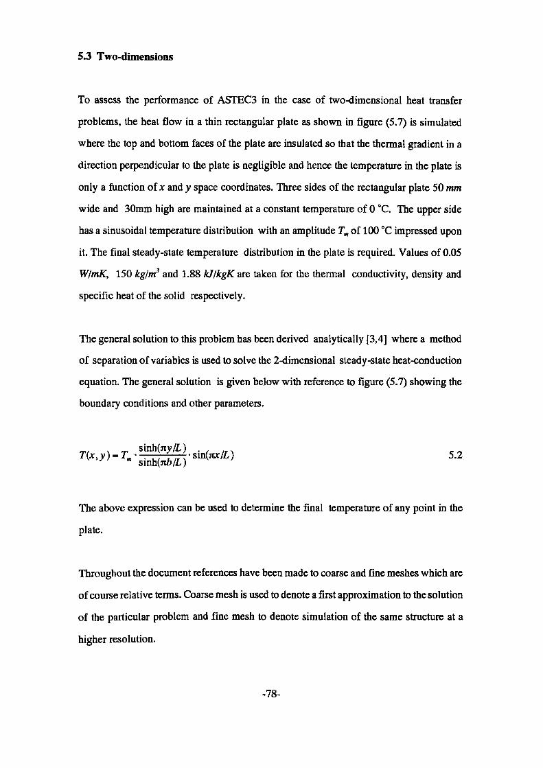
5.3 Two-dimensions

To assess the performance of ASTEC3 in the case of two-dimensional heat transfer

problems, the heat flow in a thin rectangular plate as shown in figure (5.7) is simulated

where the top and bottom faces of the plate are insulated so that the thermal gradient in a

direction perpendicular to the plate is negligible and hence the temperature in the plate is

only a function of x and y space coordinates. Three sides of the rectangular plate 50 mm

wide and 30mm high are maintained at a constant temperature of 0 °C. The upper side

has a sinusoidal temperature distribution with an amplitude Tm of 100 "C impressed upon

it. The final steady-state temperature distribution in the plate is required. Values of 0.05

W/mK, 150 kg/m3 and 1.88 kf/kgK are taken for the thermal conductivity, density and

specific heat of the solid respectively.

The general solution to this problem has been derived analytically [3,4] where a method

of separation of variables is used to solve the 2-dimensional steady-state heat-conduction

equation. The general solution is given below with reference to figure (5.7) showing the

boundary conditions and other parameters.

._5-2The above expression can be used to determine the final temperature of any point in the

plate.

Throughout the document references have been made to coarse and fine meshes which are

of course relative terms. Coarse mesh is used to denote a first approximation to the solution

of the particular problem and fine mesh to denote simulation of the same structure at a

higher resolution.

-78-

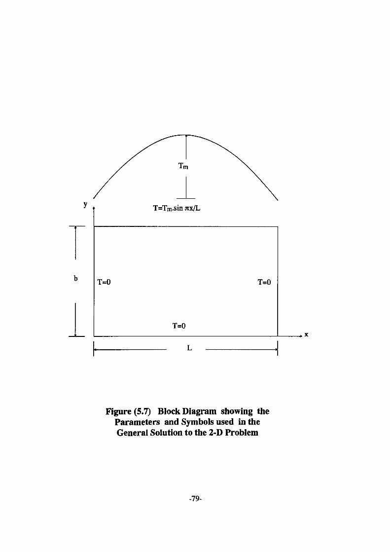
T=Tm.sin jix/L

T=0 T=0

T=0

Figure (5.7) Block Diagram showing the Parameters and Symbols used in the General Solution to the 2-D Problem

-79-

5.3.1 ASTEC3 Solution

a Coarse Mesh

For ASTEC3 modelling, the plate is divided into 15 square cells of dimensions (10 mm x

lOmm).Rth and Clh are calculated using expressions (4.5) and (4.6) and an electrical network

is constructed by connecting 15 such cells as shown in figure (5.8). Average values are

calculated for each segment of the sine function and applied as voltage sources to the 5

nodes on the upper side of the circuit and the outer nodes of the 3 remaining sides are tied

to ground representing a temperature of 0°C. Figure (5.9) in page 84 shows a contour-map

which is plotted using the steady-state temperatures of the mid-nodes of the cells. Note

that figure (5.9) is plotted in such a way that the sinusoidal input to the plate is from the

bottom face and not from the top as illustrated in figure (5.8).

A comparison between the temperatures of the mid-nodes of the cells obtained from the

ASTEC3 and equation (5.2) is given in Table (5.3) in page 83 with reference to figure

(5.8). The errors are in the range of 2.6 °C at the top of the plate to 0.16 "C at the bottom.

The errors associated with these results appear to be higher in the areas where temperature

gradients are relatively higher.

b Fine Mesh

It is postulated that a significant part of the divergence between the exact solution and that

generated by the simulation is caused by the errors involved in approximating the system

with a mesh. These errors should be reduced by using a finer mesh whereby the plate is

divided into smaller cells. This is carried out here by dividing each square cell in the coarse

mesh into 4 smaller ones. ASTEC3's modelling facility can be used here to write a model

-80-

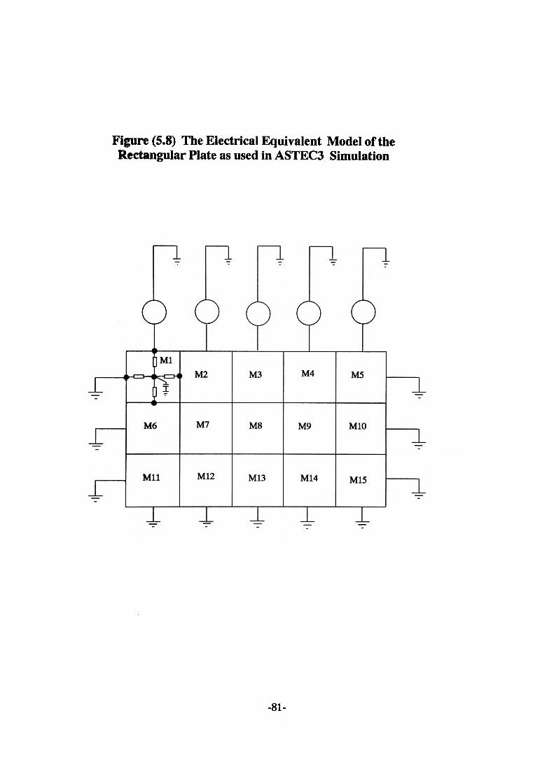
Figure (5.8) The Electrical Equivalent Model of the Rectangular Plate as used in ASTEC3 Simulation

-

c

M(

Ml

j)

JM1

5

$

LI

C, M:

M

M

)>

7

12

1

CM

M

M

)

8

13

CM

MS

M

1

~L

)4

»

14

cM^

M1

Ml

~]

)

D

5

1_L-

±"

-81-

consisting of four 2-D cell-models with appropriate values of Rlh and Cth, connected as

shown in figure (5.10) in page 85. This model is then used to construct an electrical

network in the same way as before. In this case the sinusoidal input is applied at 10 points

instead of 5.

An isothermal map of the plate in the steady-state condition is given in figure (5.11) and

a comparison of the ASTEC3 solution with the exact solution is shown in Table (5.4) in

page 86 with reference to figures (5.8) and (5.10). The contour-map of figure (5.11) also

shows a better and more accurate distribution compared to figure (5.9) since more data

points were available for its description. The accuracy of the simulated temperatures in

the fine mesh solution compared to that obtained via a coarse mesh model is also due to

the sinusoidal input voltage (temperature) to the plate being applied at ten points rather

than five. The ten point distribution is of course a more accurate representation of the sine

input which in turn leads to more accurate simulated temperatures within the plate.

The fine mesh results show errors of 0.8 "C at the top to 0.01 °C at the bottom of the plate.

These results, as anticipated, show a marked reduction in the errors observed with the

coarse mesh model which varied from 2.6 °C at the top to 0.05 °C at the bottom of the

plate. Similar to the coarse mesh model, the errors seem to be higher in the areas with

higher temperature gradients.

-82-

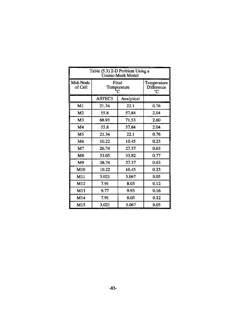
Table (5.3) 2-D Problem Using a Coarse-Mesh Model

Mid-Node of Cell

MlM2M3M4M5M6M7M8M9M10MilM12M13M14M15

Final Temperature *C

ASTEC321.3455.8

68.9355.821.3410.2226.7433.0526.7410.223.0217.919.777.91

3.021

Analytical22.157.8471.5357.8422.110.4527.3733.8227.3710.453.0678.039.938.033.067

Temperature Difference °C

0.762.042.602.040.760.230.630.770.630.230.050.120.160.120.05

-83-

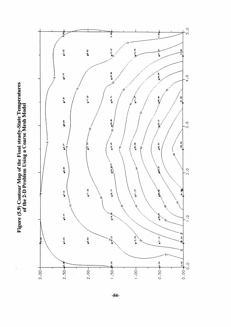
Figu

re (5

.9) C

onto

ur M

ap o

f the

Fin

al s

tead

y-St

ate

Tem

pera

ture

s of

the

2-D

Pro

blem

Usin

g a

Coa

rse

Mes

h M

odel

3.0

0

0.0

00

.0I

.05.0

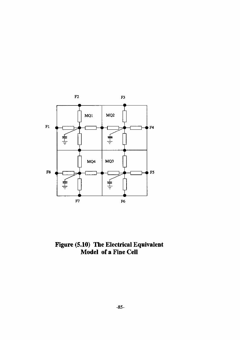
F2 F3

Fl

F8

F7 F6

Figure (5.10) The Electrical Equivalent Model of a Fine Cell

-85-

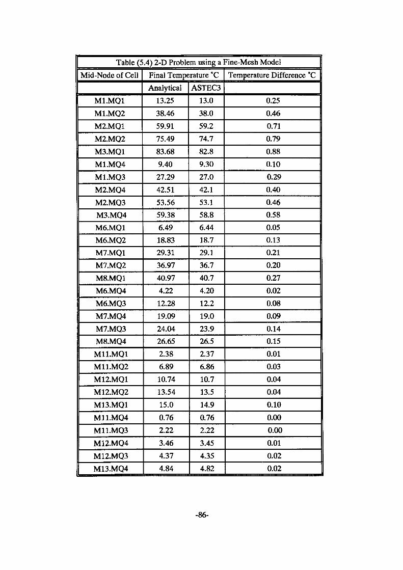
Table (5.4) 2-D Problem using a Fine-Mesh ModelMid-Node of Cell

M1.MQ1M1.MQ2M2.MQ1M2.MQ2M3.MQ1M1.MQ4M1.MQ3M2.MQ4M2.MQ3M3.MQ4M6.MQ1M6.MQ2M7.MQ1M7.MQ2M8.MQ1M6.MQ4M6.MQ3M7.MQ4M7.MQ3M8.MQ4M11.MQ1M11.MQ2M12.MQ1M12.MQ2M13.MQ1M11.MQ4M11.MQ3M12.MQ4M12.MQ3M13.MQ4

Final Temperature °CAnalytical

13.2538.4659.9175.4983.689.4027.2942.5153.5659.386.4918.8329.3136.9740.974.2212.2819.0924.0426.652.386.8910.7413.5415.00.762.223.464.374.84

ASTEC313.038.059.274.782.89.3027.042.153.158.86.4418.729.136.740.74.2012.219.023.926.52.376.8610.713.514.90.762.223.454.354.82

Temperature Difference °C

0.250.460.710.790.880.100.290.400.460.580.050.130.210.200.270.020.080.090.140.150.010.030.040.040.100.000.000.010.020.02

-86-

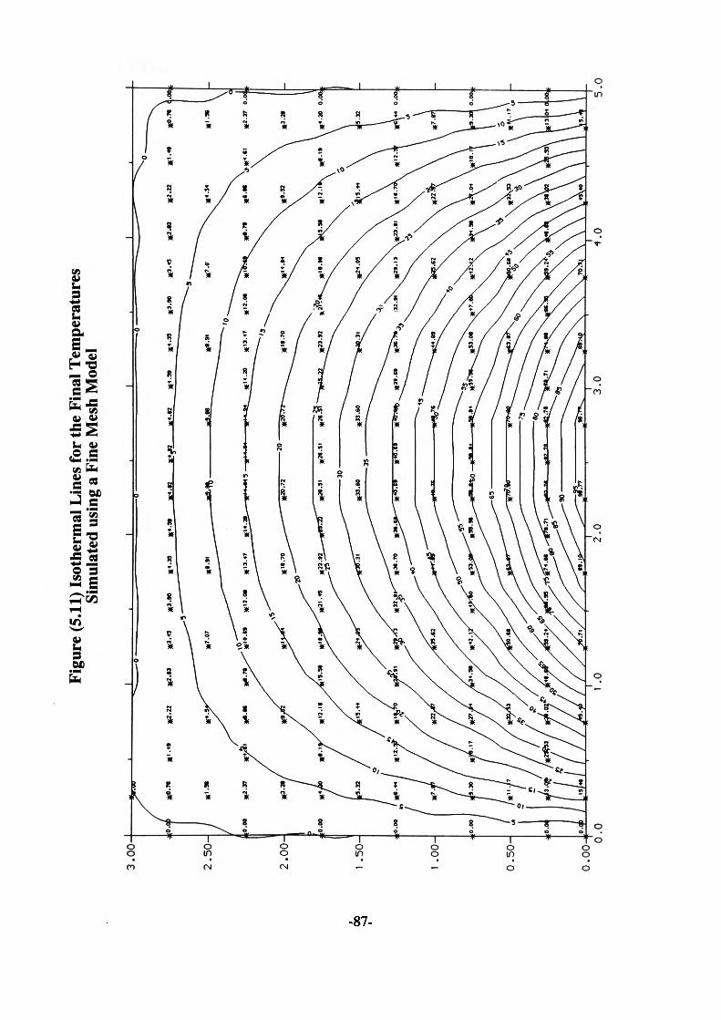
Figu

re (5

.11)

Iso

ther

mal

Lin

es fo

r the

Fin

al T

empe

ratu

res

Sim

ulat

ed u

sing

a Fi

ne M

esh

Mod

el

3.0

0

2.5

0-

2.00

1 .5

0-

1 .0

0-

0.5

0-

0.0

00

.01

.02

.0

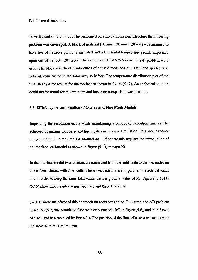
5.4 Three-dimensions

To verify that simulations can be performed on a three dimensional structure the following

problem was envisaged. A block of material (50 mm x 30 mm x 20 mm) was assumed to

have five of its faces perfectly insulated and a sinusoidal temperature profile impressed

upon one of its (30 x 20) faces. The same thermal parameters as the 2-D problem were

used. The block was divided into cubes of equal dimensions of 10 mm and an electrical

network constructed in the same way as before. The temperature distribution plot of the

final steady-state results for the top face is shown in figure (5.12). An analytical solution

could not be found for this problem and hence no comparison was possible.

5.5 Efficiency: A combination of Coarse and Fine Mesh Models

Improving the resolution errors while maintaining a control of execution time can be

achieved by mixing the coarse and fine meshes in the same simulation. This should reduce

the computing time required for simulations. Of course this requires the introduction of

an interface cell-model as shown in figure (5.13) in page 90.

In the interface model two resistors are connected from the mid-node to the two nodes on

those faces shared with fine cells. These two resistors are hi parallel in electrical terms

and in order to keep the same total value, each is given a value of Rth. Figures (5.13) to

(5.15) show models interfacing one, two and three fine cells.

To determine the effect of this approach on accuracy and on CPU time, the 2-D problem

in section (5.2) was simulated first with only one cell, M3 in figure (5.8), and then 3 cells

M2, M3 and M4 replaced by fine cells. The position of the fine cells was chosen to be hi

the areas with maximum error.

-88-

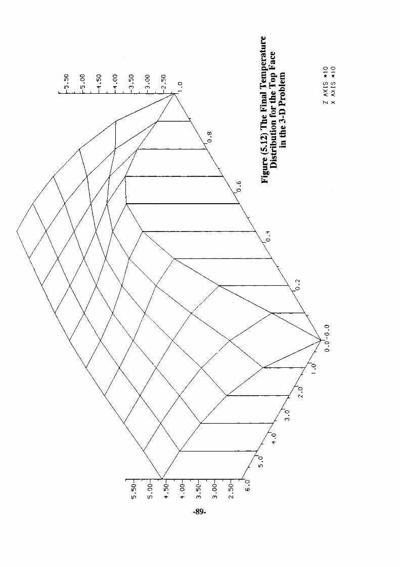
Figu

re (5

.12) T

he F

inal

Tem

pera

ture

Dis

tribu

tion

for t

he T

op F

ace

in th

e 3-

D P

robl

em

I .0

0.0

-0.0

Z A

XIS

*1

0 X

AX

IS

*10

Figu

re (5

.13)

The E

lectr

ical E

quiv

alen

t Mod

el of

a Ce

ll In

terf

acin

g O

ne F

ine C

ell

C4

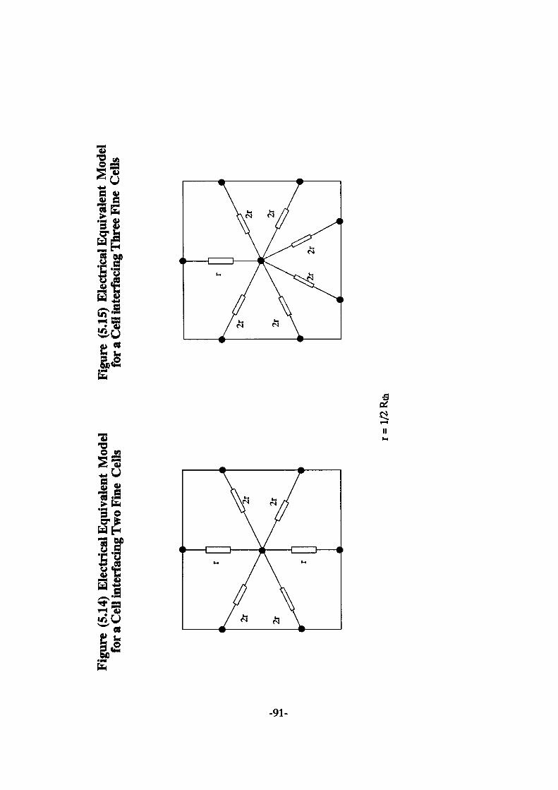
Figu

re (

5.14)

Ele

ctric

al E

quiv

alen

t Mod

el

for a

Cell

inte

rfaci

ng T

wo

Fine

Cel

lsFi

gure

(5.1

5) E

lect

rical

Equ

ival

ent M

odel

fo

r a C

ell in

terfa

cing

Thr

ee F

ine

Cells

r = 1

/2 R

th

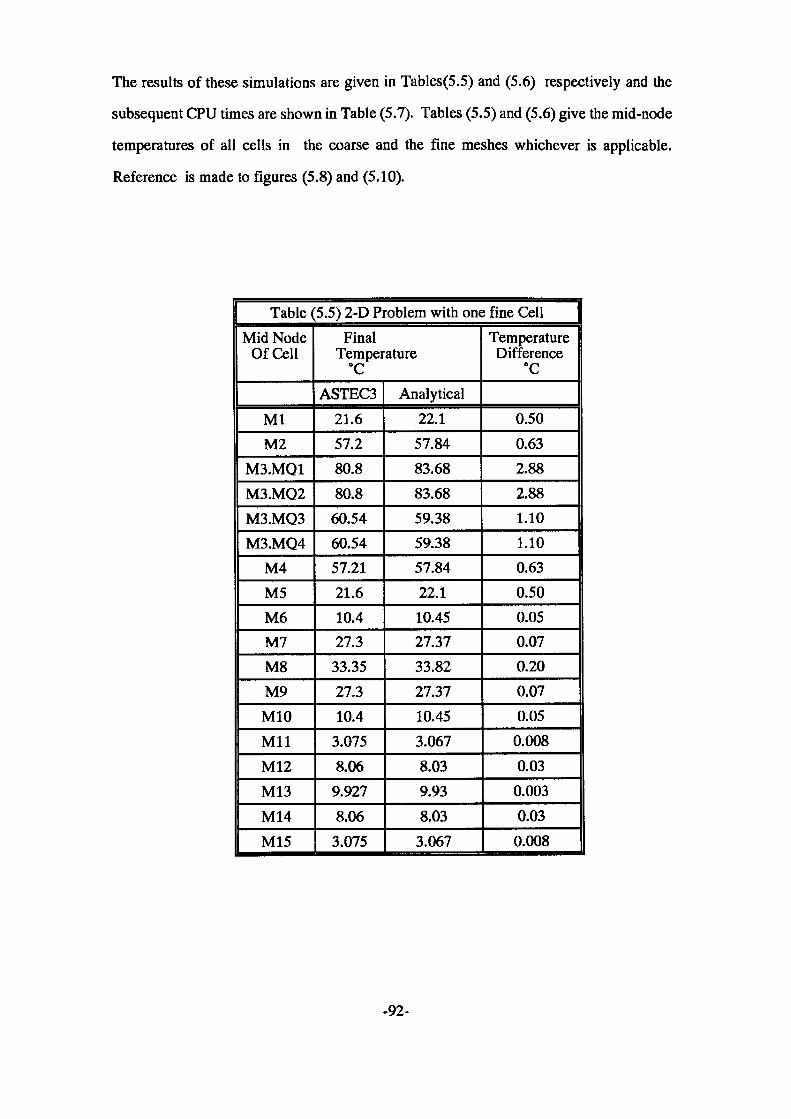
The results of these simulations are given in Tables(5.5) and (5.6) respectively and the

subsequent CPU times are shown in Table (5.7). Tables (5.5) and (5.6) give the mid-node

temperatures of all cells in the coarse and the fine meshes whichever is applicable.

Reference is made to figures (5.8) and (5.10).

Table (5.5) 2-D Problem with one fine CellMid Node

Of Cell

MlM2

M3.MQ1M3.MQ2M3.MQ3M3.MQ4

M4M5M6M7M8M9M10MilM12M13M14M15

Final Temperature °C

ASTEC321.657.280.880.8

60.5460.5457.2121.610.427.3

33.3527.310.4

3.0758.06

9.9278.06

3.075

Analytical22.1

57.8483.6883.6859.3859.3857.8422.110.4527.3733.8227.3710.453.0678.039.938.03

3.067

Temperature Difference °C

0.500.632.882.881.101.100.630.500.050.070.200.070.05

0.0080.03

0.0030.030.008

-92-

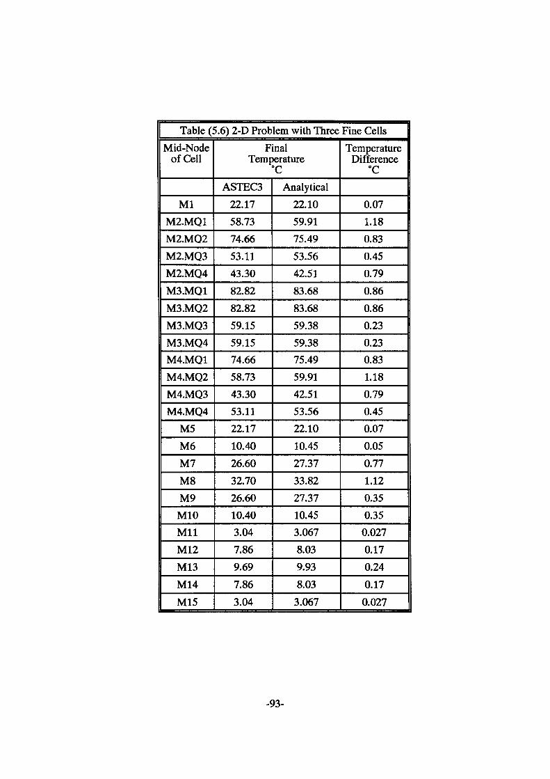
Table (5.6) 2-D Problem with Three Fine CellsMid-Node

of Cell

MlM2.MQ1M2.MQ2M2.MQ3M2.MQ4M3.MQ1M3.MQ2M3.MQ3M3.MQ4M4.MQ1M4.MQ2M4.MQ3M4.MQ4

M5M6M7M8M9M10MilM12M13M14M15

Final Temperature °C

ASTEC322.1758.7374.6653.1143.3082.8282.8259.1559.1574.6658.7343.3053.1122.1710.4026.6032.7026.6010.403.047.869.697.863.04

Analytical22.1059.9175.4953.5642.5183.6883.6859.3859.3875.4959.9142.5153.5622.1010.4527.3733.8227.3710.453.0678.039.938.033.067

Temperature Difference 'C

0.071.180.830.450.790.860.860.230.230.831.180.790.450.070.050.771.120.350.350.0270.170.240.170.027

-93-

Table (5.7) Comparison of CPU Time Requirements for 2-Dimensional Transient Simulations

Model

2-D Coarse Mesh (15 Cells)2-D Fine Mesh (60 Cells)

2-D Mixed Mesh with 1 Fine Cell (18 Cells)2-D Mixed Mesh with 3 Fine Cells (24 Cells)

CPU Time (Seconds)

0.884.411.111.32

The results of the simulations with one fine cell, show an excellent agreement with the

analytical results with errors ranging from a maximum of 2.88 °C in the fine mesh area to

0.003 °C at the bottom of the plate. The errors in the simulated temperature in the fine cells

M3.MQ1 and M3.MQ2 in Table (5.5) seem higher than M3 in Table (5.3). It should be

noted however that these nodes are in a physically different position than M3 in Table

(5.3), situated closer to the edge of the plate and hence see a higher temperature gradient

leading to bigger errors. The results with three fine meshes also show excellent agreement

with the analytical solutions with reduction of errors in the fine mesh areas to a maximum

of 1.18 °C but with a maximum of 0.35 °C in the interface cell M8 at the bottom of the

fine mesh areas. Similar argument to that given above applies to errors in cells M2.MQ1

and M4.MQ2 in Table (5.6) which are also in higher temperature gradient areas.

5.6 Computing-Time Considerations

In order to allow the user to forecast the computer time required for thermal simulations

of the transient type, an attempt was made to derive a relationship between the number of

cells and the CPU time. In the first instance this was only carried out for two-dimensional

modelling.

-94-

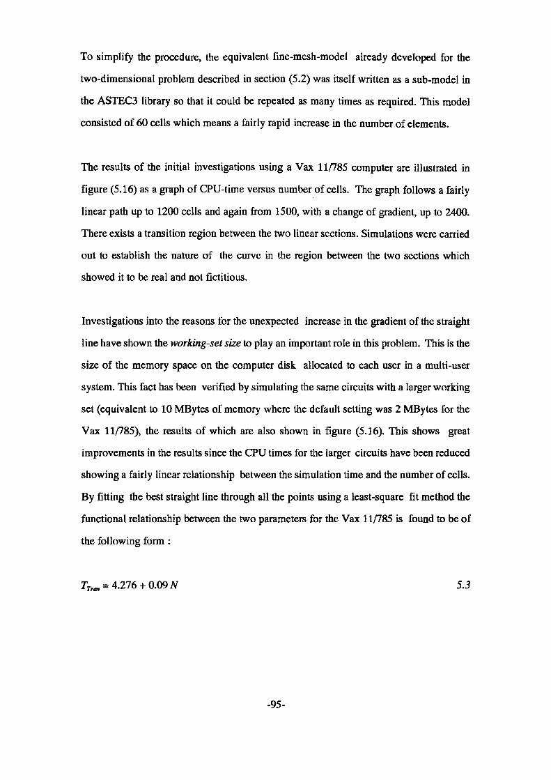
To simplify the procedure, the equivalent fine-mesh-model already developed for the

two-dimensional problem described in section (5.2) was itself written as a sub-model in

the ASTEC3 library so that it could be repeated as many times as required. This model

consisted of 60 cells which means a fairly rapid increase in the number of elements.

The results of the initial investigations using a Vax 11/785 computer are illustrated in

figure (5.16) as a graph of CPU-time versus number of cells. The graph follows a fairly

linear path up to 1200 cells and again from 1500, with a change of gradient, up to 2400.

There exists a transition region between the two linear sections. Simulations were carried

out to establish the nature of the curve in the region between the two sections which

showed it to be real and not fictitious.

Investigations into the reasons for the unexpected increase in the gradient of the straight

line have shown the working-set size to play an important role in this problem. This is the

size of the memory space on the computer disk allocated to each user in a multi-user

system. This fact has been verified by simulating the same circuits with a larger working

set (equivalent to 10 MBytes of memory where the default setting was 2 MBytes for the

Vax 11/785), the results of which are also shown in figure (5.16). This shows great

improvements in the results since the CPU times for the larger circuits have been reduced

showing a fairly linear relationship between the simulation time and the number of cells.

By fitting the best straight line through all the points using a least-square fit method the

functional relationship between the two parameters for the Vax 11/785 is found to be of

the following form :

7 = 4.276 +0.09 JV 5.3

-95-

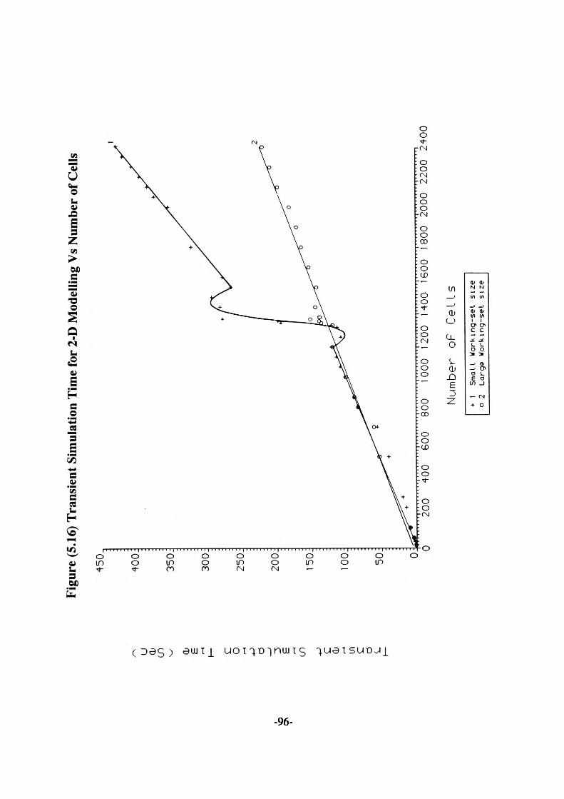
Figu

re (5

.16)

Tra

nsie

nt S

imul

atio

n Ti

me

for

2-D

Mod

ellin

g Vs

Num

ber

of C

ells

u o> CO 0> £ c o 3 £ CO

-^ c c d L

200

400

600

800

1000 1200 1400 1600 1800 2000 2200 2400

Number oF Cells

+ 1

Smal

l Wo

rkin

g-se

t size

o 2

Large

Working-set

size

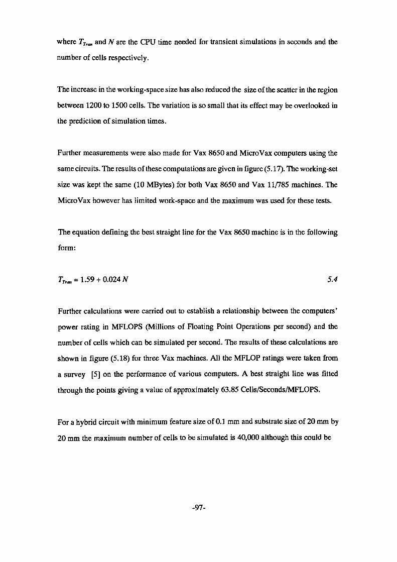
where TTrm and AT are the CPU time needed for transient simulations in seconds and the

number of cells respectively.

The increase in the working-space size has also reduced the size of the scatter in the region

between 1200 to 1500 cells. The variation is so small that its effect may be overlooked in

the prediction of simulation times.

Further measurements were also made for Vax 8650 and MicroVax computers using the

same circuits. The results of these computations are given in figure (5.17). The working-set

size was kept the same (10 MBytes) for both Vax 8650 and Vax 11/785 machines. The

Micro Vax however has limited work-space and the maximum was used for these tests.

The equation defining the best straight line for the Vax 8650 machine is in the following

form:

TTran = 1.59 + 0.024 N 5 A

Further calculations were carried out to establish a relationship between the computers'

power rating in MFLOPS (Millions of Floating Point Operations per second) and the

number of cells which can be simulated per second. The results of these calculations are

shown in figure (5.18) for three Vax machines. All the MFLOP ratings were taken from

a survey [5] on the performance of various computers. A best straight line was fitted

through the points giving a value of approximately 63.85 Cells/Seconds/MFLOPS.

For a hybrid circuit with minimum feature size of 0.1 mm and substrate size of 20 mm by

20 mm the maximum number of cells to be simulated is 40,000 although this could be

-97-

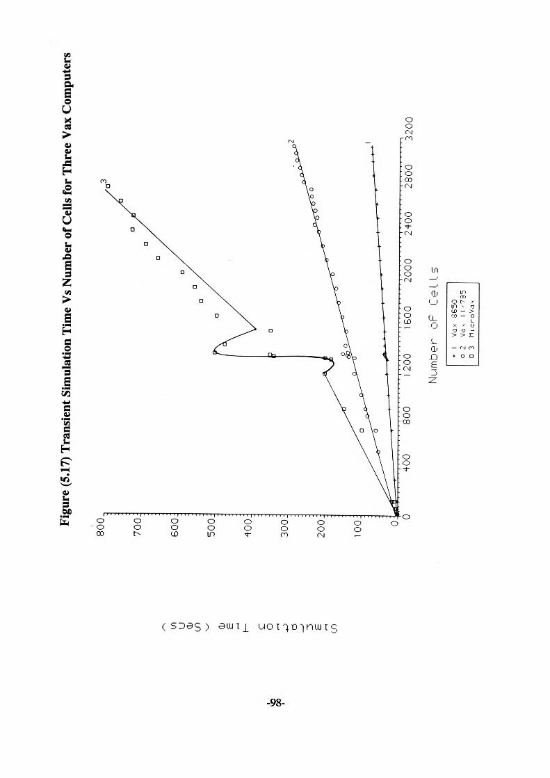
Figu

re (5

.17) T

rans

ient S

imul

atio

n Ti

me V

s Num

ber o

f Cell

s for

Thr

ee V

ax C

ompu

ters

00

in u 0; dJ £ c o 3

E r-*

CO

800,

700J

600J

500

j

400J

300

j

200J OOj

600

2000

2400

2800

3200

Num

ber

oF

Ce

lls

+ 1

Vax

36

50o

2 Va

^ I I

^785

O 3

flic

roV

ax

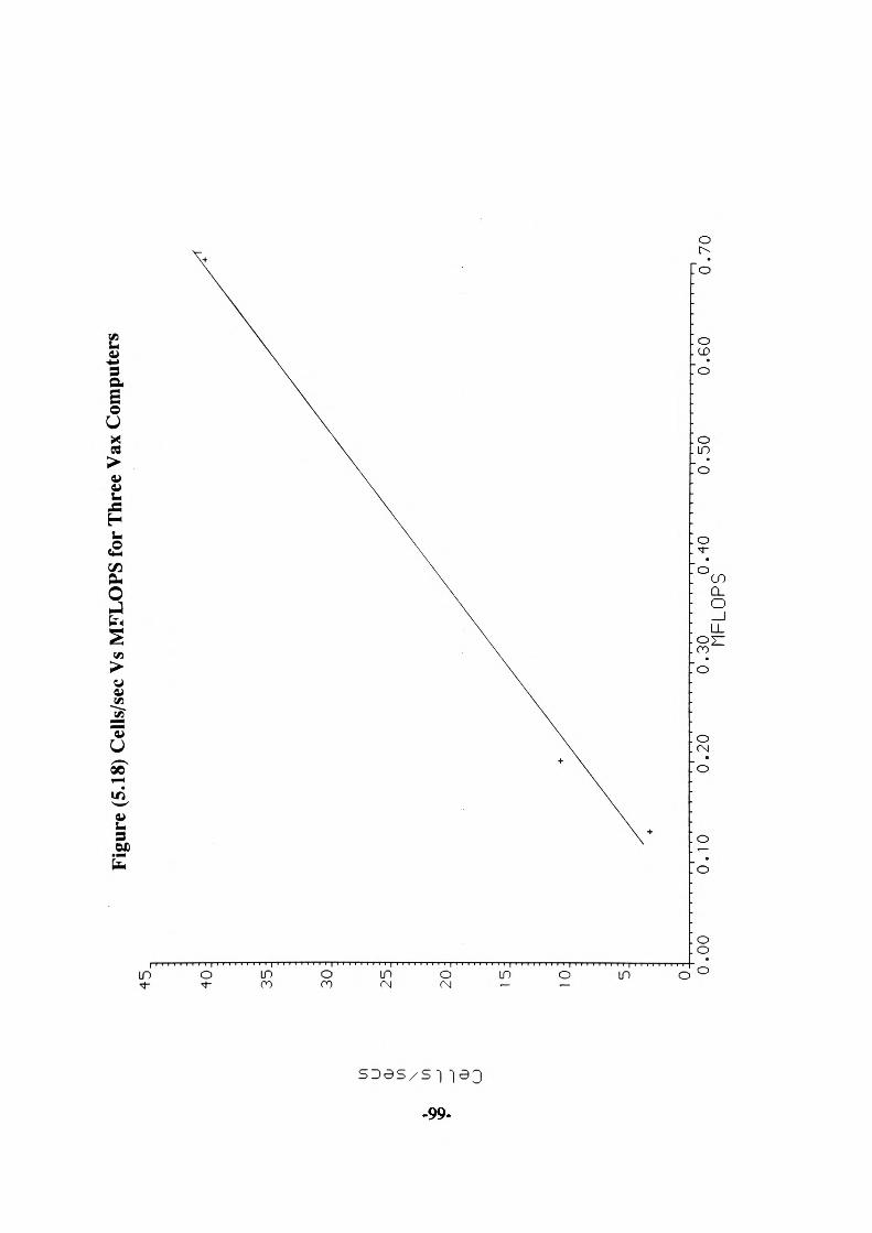
45.

40:

35

:

30:

Figu

re (5

.18)

Cel

ls/se

c V

s MFL

OPS

for T

hree

Vax

Com

pute

rs

1/1 u 0) i/i2

5:

0) o

20

:

15:

10. 0.0

0

0.1

0

0.2

0

0.3

0

0.4

0N

FLO

PS

0.5

00

.60

0.7

0

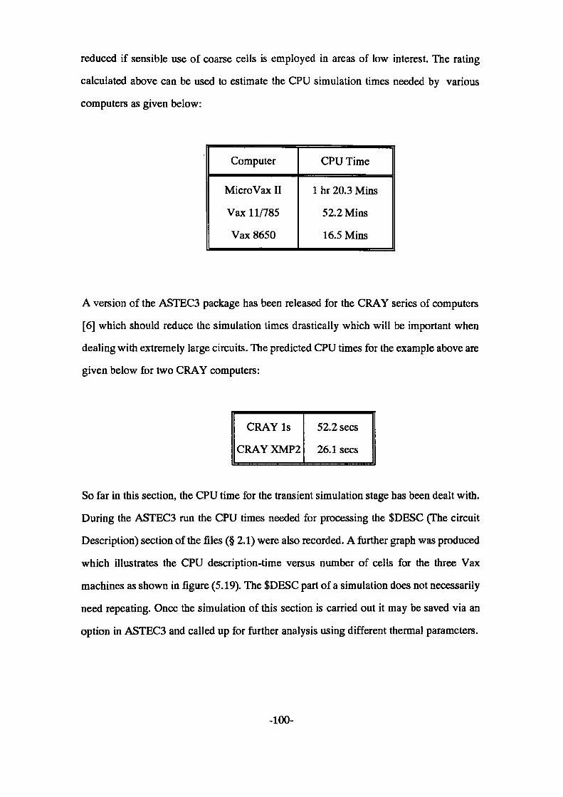
reduced if sensible use of coarse cells is employed in areas of low interest. The rating

calculated above can be used to estimate the CPU simulation times needed by various

computers as given below:

Computer

Micro Vax II

Vax 11/785

Vax 8650

CPU Time

1 hr 20.3 Mins

52.2 Mins

16.5 Mins

A version of the ASTEC3 package has been released for the CRAY series of computers

[6] which should reduce the simulation times drastically which will be important when

dealing with extremely large circuits. The predicted CPU times for the example above are

given below for two CRAY computers:

CRAY Is

CRAYXMP2

52.2 sees

26.1 sees

So far in this section, the CPU time for the transient simulation stage has been dealt with.

During the ASTEC3 run the CPU times needed for processing the $DESC (The circuit

Description) section of the files (§ 2.1) were also recorded. A further graph was produced

which illustrates the CPU description-time versus number of cells for the three Vax

machines as shown in figure (5.19). The $DESC part of a simulation does not necessarily

need repeating. Once the simulation of this section is carried out it may be saved via an

option in ASTEC3 and called up for further analysis using different thermal parameters.

-100-

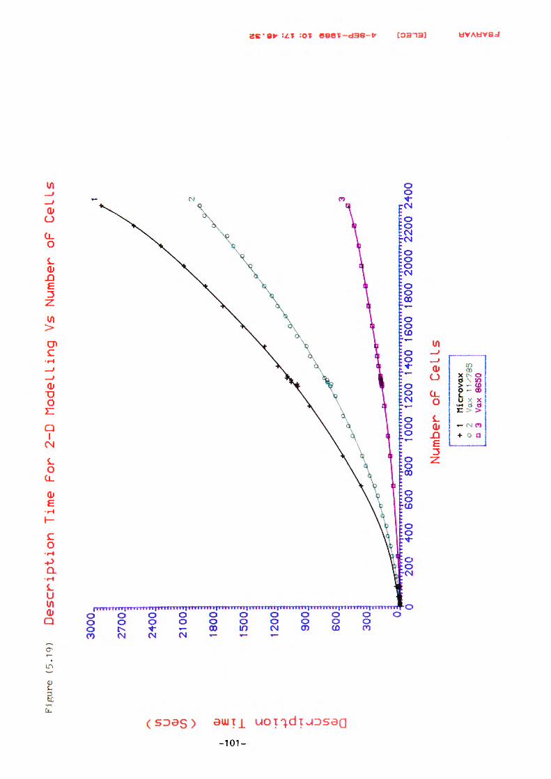
(5.19)

Description Ti

me For

2-D

Mode

l Li

ng Vs Nu

mber

oF Ce

lls

w u Qj OfL

e0

.MT

H

- c o -p Q.

••H L

U CD

Q

3000

.

2700

J

2400

J ;21

00J

1800

J ;

15

00

:

12

00

:

900:

600J

300J

200

400

600

800

1000

12

00 14

00 16

00 18

00 2000 2200 2400

Number oF Cell

s

+ 1

Microvax

o 2

Vax

11^785

a 3

Vax

8650

01 n * o M N * O

«< 9 a u u ttl I i a

5.7 Conclusion

In this section, the ASTEC3 thermal modelling procedures were used for simulation and

prediction of the temperature distributions in one and two-dimensional heat transfer

problems. The numerical results presented for the one-dimensional problem with both

conduction and convection were in excellent agreement with the analytical and finite

difference solutions. The results for the two-dimensional problem using a coarse mesh

showed very good agreement with the analytical solution. The small errors observed were

reduced to negligible margins when a finer mesh was employed.

In order to minimise the computer time required for simulations and hence make it

economically more acceptable, interface models were introduced allowing the mixing of

coarse and fine cells. The tests on these models showed excellent agreement with the

analytical solution and greatly reduced the CPU time when compared with the

full-fme-mesh model.

A great number of simulations were carried out with increasing numbers of thermal cells

using three Vax computers. This was to establish a relationship between the number of

conduction cells and the CPU time needed for simulations. This would in turn enable a

user to predict the CPU time in advance and the relationship between the MFLOPs and

the CPU times. It has also been shown that the computing times are practical for real

situations (Hybrid Circuits).

-102-

6 EXPERIMENTAL STUDIES IN MACRO-SCALE

In chapter (4), a modelling procedure was described whereby the temperature distribution

in thermal systems involving conduction, convection and radiation could be predicted via

a simulation using the ASTEC3 package. This was subsequently used to solve some

standard heat flow problems as given in chapter (5) which showed excellent agreement

with results obtained from alternative, more conventional techniques.

The ASTEC3 heat transfer modelling was used for the simulation of simple experimental

structures. Initially, in order to avoid the problems of measuring surface temperatures of

very small areas, a large scale physical model was used for the experiments. The nature

of these models was similar to that of hybrid circuits with heat generating elements being

mounted in good thermal contact with an insulating substrate.

Experiments will be described where surface temperatures of some copper cladding strips

and plates which may be totally or partially heated were measured. These were then

modelled and simulated using ASTEC3. This demonstrated the extent to which the

idealised heat transfer models developed needed amendment for practical use.

6.1 Experimental Arrangement

In these experiments, a HEIMANN infrared radiation pyrometer type KT14, capable of

measuring between ambient up to 300 °C to an accuracy of 1.5 "C was used to measure

the temperature at various points on the surfaces of some heated samples made of copper

cladding. This is the type of printed circuit board which consists of a very thin layer of

-103-

copper 15 \wi or 35 \un thick (depending on the type of board used) on a fibre-glass base

1.6 mm thick. Electric currents were passed through the copper layer on top, causing a

rise in the temperature of the specimen due to the conversion of electrical to thermal

energy.

The apparatus was placed inside a chamber, a great deal larger than the test specimen. A

larger enclosure was required for the following reason. The sample radiates an energy

density which decreases with distance. The heat transfer coefficients are related to this

energy density and altering the energy density of the immediate surroundings, by means

of a reflected field ( eg. from the walls), would change the heat transfer coefficient. To

overcome this experimental problem the box was made many times larger than the sample

size which allowed the field intensity to decrease proportionally to f2 due to the spreading

of the field and also by e'*" due to attenuation where JA is the absorption coefficient of air

and x is the displacement through the air. The reflected radiation was kept to a minimum

by coating the inside of the chamber with matt black paint.

Furthermore, the size of the box should be large enough for the enclosed ambient air

temperature to be unaffected by the heat input as this would induce irregularities in the

results. This may be checked by calculating the temperature rise in the box due to 6 Watts

of input electrical power which was the maximum power generated within the samples

used in these experiments. Taking a value of 718J/kgK for Cv, the specific heat capacity

of air and 1.15 kg/m3 for its density, for a box with dimensions of (0.9/n x 0.6m x 0.6m)

the temperature rise for an experimental run may be determined from the following

relationship:

-104-

(0.9 x 0.6 x 0.6x1. 15) x 718= n 02°C '

which is sufficiently small compared to the temperature of the strip to be ignored.

The box was also sealed very carefully in order to avoid any draughts from the room. This

in turn allowed the occurrence only of natural convection which is rather simpler to account

for in the calculations than a mixture of natural and forced convections.

A schematic diagram of the apparatus is presented in figure (6.1). A specially designed

holder was used to accommodate the samples. Grooves were cut into two flat pieces of

wood which were fixed parallel to each other onto another flat board. The distance between

the parallel grooves was slightly greater than the length of the copper cladding samples.

The above configuration allowed the specimen boards to be easily inserted into position.

The width of the grooved pieces was made as small as possible to ensure the least contact

between the sample and the rest of the holder assembly in order to minimise the amount

of heat lost by conduction at the grooves.

Figure (6.1) shows a rectangular sample of copper cladding mounted horizontally and

glass wool with thermal conductivity of less than 0.05 W/mK used to insulate the bottom

surface of the strip thus restricting the heat losses by convection and radiation to the top

surface. The sample was heated by passing an electric current through the connections at

the ends of the heated sections.

Initially the current was supplied to the heated areas through fixed points at their ends.

Measurements at various positions showed a non-uniform distribution of temperature over

the surface being cooler towards the comers of the plate. This phenomenon is known as

the crowding effect which occurs when the current is applied in the specific configuration.

-105-

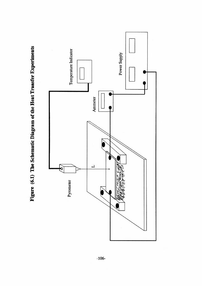
Figu

re (

6.1)

The

Sch

emat

ic D

iagr

am o

f the

Hea

t Tra

nsfe

r Exp

erim

ents

Tem

pera

ture

Indi

cato

r

Since the current is entering the heated strips through a point terminal much smaller than

its width, the electrons travel along the strip to the other terminal in a non-uniform fashion

as shown in figure (6.2). In doing so, the current distribution may even miss parts of the

strip which will not be heated at all. Improvements were therefore made by applying the

current to the islands through a number of wires at each end. Six holes of each 1 mm in

diameter were drilled along the width of each resistor evenly distributed. Wires of

appropriate thickness capable of handling at least 5 amperes were inserted in these holes

and soldered to the copper surface, figure (6.3). These wires were then bunched together

and connected to the main supply line. The above arrangement should in turn establish a

more uniform current distribution and hence a more uniform heating effect in the islands.

The infrared pyrometer was positioned with its axis perpendicular to the plane of the

surface. The distance L between the edge of the lens barrel and the surface was set to

exactly 80 mm as specified by the manufacturers. A specially designed insertion gauge,

figure (6.4) consisting of a flat metal disc and a rod which screws into the centre of the

disc was used for this purpose. The total height of the disc and the rod was adjusted to

exactly 80 mm. The diameter of the rod was 4 mm which made it possible to aim quite

accurately at a certain target position by sliding the flat surface of the disc onto the lens

barrel. The tip of the rod marked the minimum target spot at the proper working distance

of 80 mm.

The pyrometer is designed to respond accurately only for surfaces with emissivities of

nearly 1. To overcome this problem when dealing with copper boards, at positions of

interest, small circular patches of around 4 mm in diameter (focusing area of pyrometer)

were coated with black velvet paint 2010 from 3M. This material is claimed to have an

emissivity of 0.95 [1].

-107-

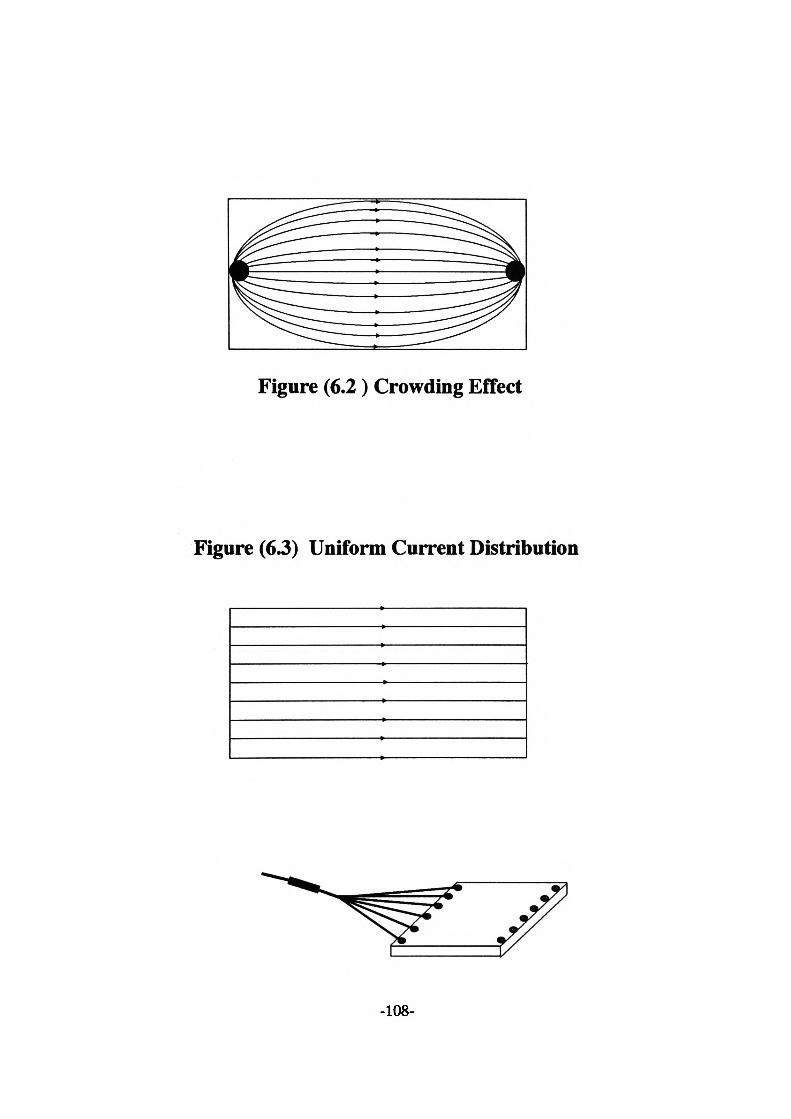
Figure (6.2) Crowding Effect

Figure (6.3) Uniform Current Distribution

-108-

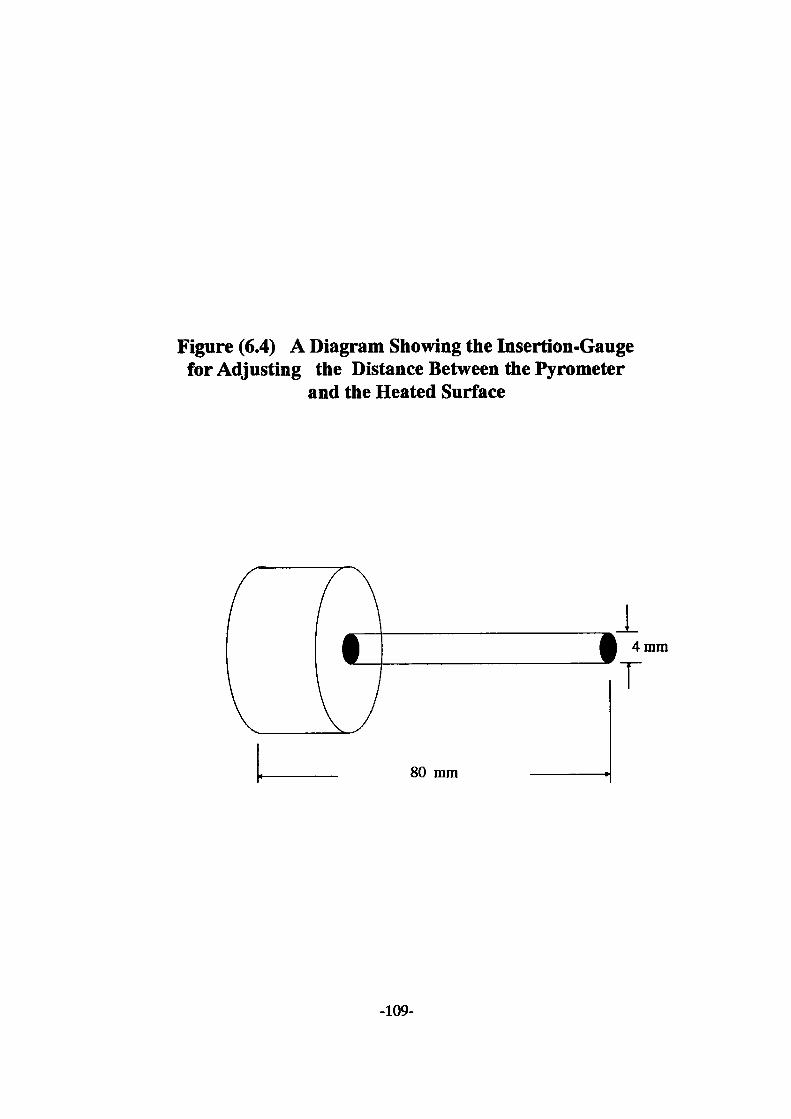
Figure (6.4) A Diagram Showing the Insertion-Gaugefor Adjusting the Distance Between the Pyrometer

and the Heated Surface

14mm

T

80 mm

-109-

Prior to each experimental run, the focusing distanced was checked and the chamber was

sealed carefully for a draft-free atmosphere. The desired currents were selected and after

switching on, the set-up was left to reach a steady-state condition. At this point the surface

and the ambient temperatures were recorded.

A number of confirmatory experiments were carried out as outlined below:

(i) Experiment (1) - A rectangular strip uniformly heated.

(ii) Experiment (2) - A rectangular plate with two electrically heated islands formed

on its conducting layer by cutting grooves in its copper layer. These islands are

electrically isolated from the rest of the plate but thermally connected via the glass

fibre insulating board,

(iii) Experiment (3) - Rectangular plates with only one heated island. One smaller

plate has an island symmetrically situated on it. Three other plates have a heated

island in different positions.

The full details of the above experiments are given in the following sections.

6.1.1 Experiment 1

A rectangular strip of copper cladding (140 mm x 26 mm x 15 \vri) was used as the specimen.

For a current of 30 amperes at an ambient temperature of 23.7 °C a uniform temperature

of 125 °C was measured at all points along the strip.

The thermal characteristics of this experiment were simulated by applying the procedure

described in chapter (4) for three dimensional conduction. The strip was divided into 15

-110-

equal segments, figure (6.5), each a cuboid of dimensions (28mm x 8.67mm x 15 \an). The

thermal resistances in the x, y and z directions and the thermal capacitance of each cell

were calculated using the expressions given in chapter (4).

The rate of heat generation in the strip was calculated assuming that all the electric power

supplied to the strip is converted into thermal energy. Under steady-state conditions then

the total heat generation is simply given by I2R, where / is the current in Amps and R the

electric resistance of the copper plate in Ohms.

Using the values given in the experiment section the total power was calculated as 5.5

Watts. The rate of heat generation in each cell was then the total divided by the number

of segments which in this case gives a value of 366 milliWatts/segment.

To estimate the convective heat transfer coefficient and subsequently the value of thermal

resistance Rconvection for the ASTEC3 model, use was made of the correlations derived by

other workers [2]. These correlations are non-dimensional and for natural convection from

uniformly heated horizontal surfaces are of the form given in section (3.2).

Once the value of the Nusselt number was determined using equation (3.5) in conjunction

with equations (3.7 and 3.8), it was then be used to calculate the value of hc from equation

(3.6) relating the convective heat transfer coefficient to Nusselt number.

Various values have been quoted [2-5] for constant C and the characteristic length / to be

used in equation (3.5). The values of hc arising from these would obviously be different.

For C, values of 0.54 [3,5] and 0.59 [4] are given. For a rectangular plate, either an average

of the two sides [3] or the ratio of the area A over the perimeter p [2,4,5] have been

recommended for /. When tested in the ASTEC3 model however, the correlations

-111-

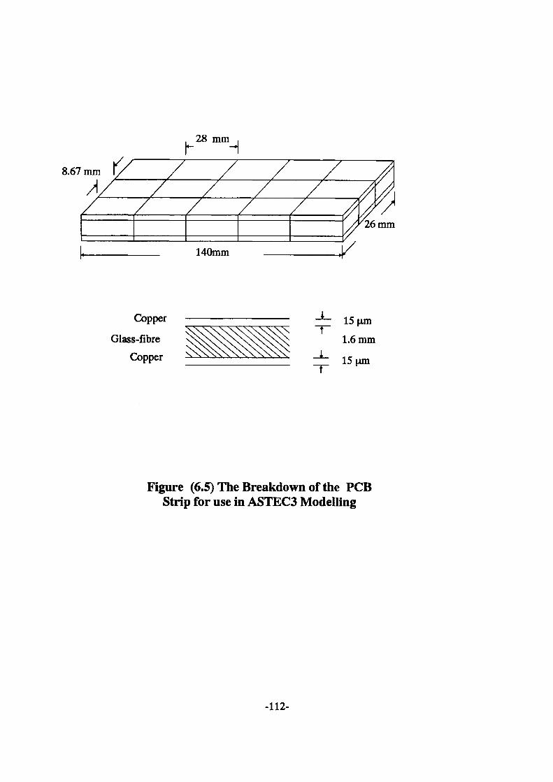
Copper

Glass-fibre Copper

15 1.6mm

15 [Am

Figure (6.5) The Breakdown of the PCB Strip for use in ASTEC3 Modelling

-112-

recommended by Chapman [2] (C=0.54,l=A/p) appeared to yield a value of hc which gave

simulated temperatures closely matched to those measured experimentally. Details of the

calculations are given in appendix (4).

For calculating the heat transfer coefficient of radiation hr using the equations given in

section (3.3), the emissivity of the copper surface was needed. This was estimated via a

method utilising the infrared pyrometer as recommended by the manufacturers of the

thermometer [6]. Aset of experiments was carried out details of which are given in appendix

(5). A value of 0.086 was obtained for the emissivity of the copper clad surface. This value

was subsequently used in appendix (4) for determination of hr

Using a combined convective and radiative heat transfer coefficient of 13.85 W/m2K, the

simulated results showed a uniform temperature of 131 °C along the strip which is in good

agreement and within 4.8% of the 125 "C measured experimentally.

6.1.2 Experiment!

A more complicated system for experimentation was devised where use was made of the

same experimental rig already described in section (6.1). This experiment was designed

taking into account the type of thermal problem which may be encountered when

simulating the thermal characteristics of hybrid microcircuit and semiconductor integrated

circuits.

Hybrid microcircuits are types of device which normally consist of several separate

component parts attached to a ceramic substrate [7] and interconnected either by wire

bonds or suitable metallisation pattern. Considering a very simple case of a hybrid circuit

with two resistors of different values on a substrate, the following specimen was designed

-113-

for experimentation. The copper cladding boards used here onwards were the pre-sensitised

type manufactured by Mica & Micanite of Ireland [8] which can be used easily to form

the required patterns very accurately. The copper layer thicknesses in these boards is given

as 35 \un and the fibre glass is the type FR4 1.6 mm thick.

A rectangular plate of the above material was chosen with dimensions of 140 mm by 120

mm. Two islands were cut into the conducting layer of the board, figure (6.6) but not the

insulation by chemically etching very thin, shallow grooves all the way round the islands,

just enough to isolate them electrically from the rest of the copper. Subsequent checks

were made for no electrical continuity.

Electric currents of 30 and 10 amps were supplied to the larger and the smaller islands

respectively. The set-up was left to reach a steady-state condition and then the infrared

pyrometer was used to measure the surface temperatures at selected points.

An electrical-equivalent circuit model of the system was developed using the procedure

given in section (4) and figure (6.7). Each layer was divided into (6x7) three-dimensional

cells. The fibre glass layer was assumed to be isotropic and a value of 0.343 W/mK was

used for thermal conductivity to calculate the thermal resistances of conduction in this

layer. This figure was experimentally determined via an electrically heated Lees' disc

apparatus details of which will be given in chapter (7).

One major problem here was the estimation of the value of the convective heat transfer

coefficient. Correlations used in section (6.2) are derived for horizontal plates which are

uniformly heated and do not necessarily apply to non-uniform situations. However, for

the first approximation, the plate was divided into six rows along the 120 mm edge and

the same correlations used in experiment (1) were utilised to obtain an average value for

-114-

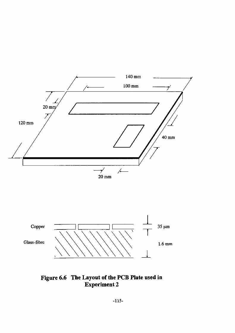
140mm

100mm 7

20mm

Copper

Glass-fibre

J_35

1.6mm

J_

Figure 6.6 The Layout of the PCB Plate used inExperiment 2

-115-

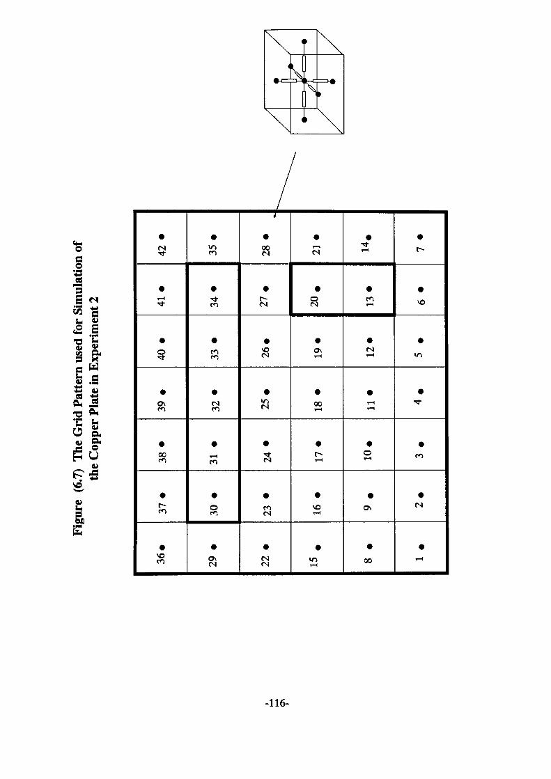
Figu

re (

6.7)

The

Grid

Pat

tern

use

d fo

r Si

mul

atio

n of

th

e Co

pper

Pla

te in

Exp

erim

ent 2

I H-*

h-i ON

36 •

29 •

22 •

15 .

8 •

1 •

37 •

30 •

23 •

16 •

9 •

2.

38 •

31 •

24 •

17 •

10 •

3 •

39 •

32 •

25 •

18 •

11 • 4.

40 •

33 •

26 •

19 •

12 •

5 •

41 •

34 •

27.

20.

13 •

6 •

42 •

35 •

28 •

»

21 •

14.

7 •

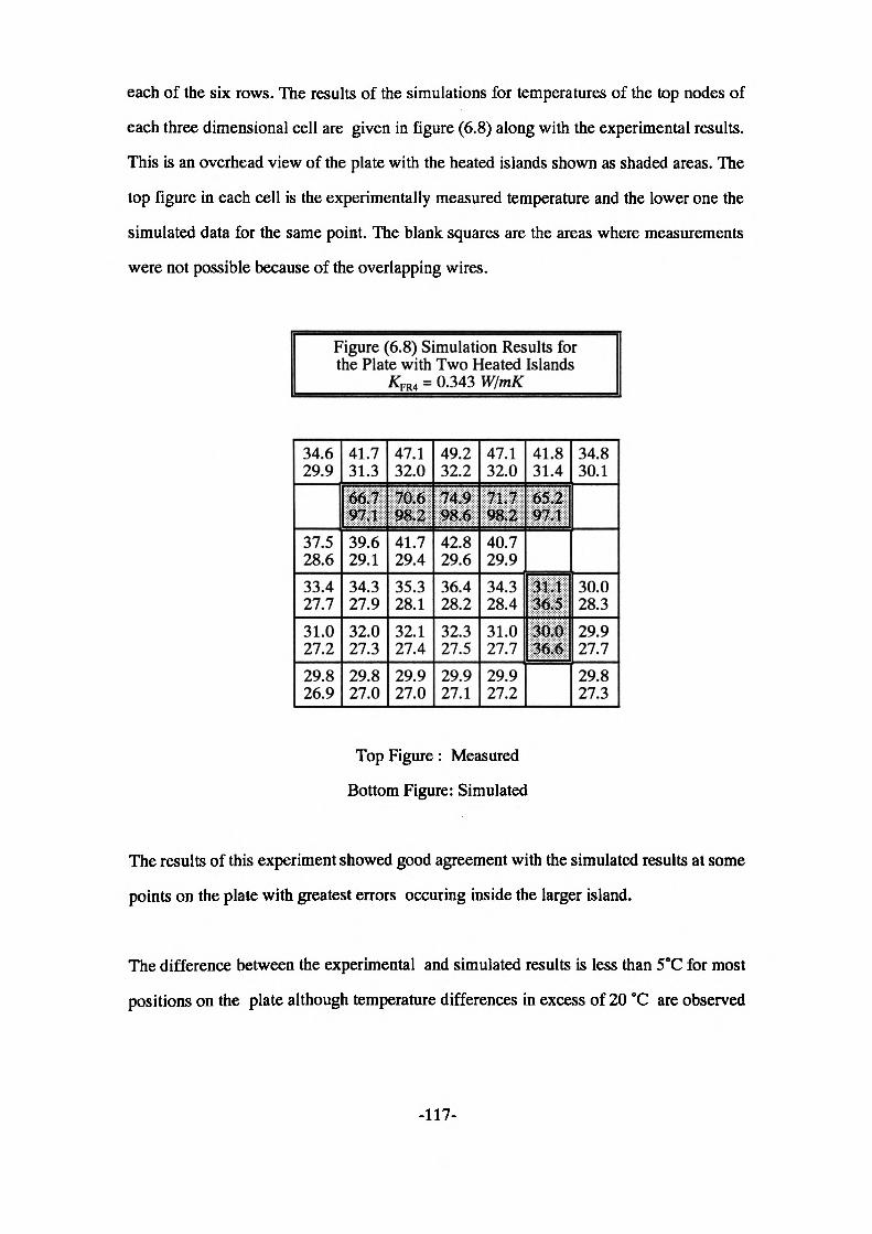
each of the six rows. The results of the simulations for temperatures of the top nodes of

each three dimensional cell are given in figure (6.8) along with the experimental results.

This is an overhead view of the plate with the heated islands shown as shaded areas. The

top figure in each cell is the experimentally measured temperature and the lower one the

simulated data for the same point. The blank squares are the areas where measurements

were not possible because of the overlapping wires.

Figure (6.8) Simulation Results for the Plate with Two Heated Islands

KFR4 = 0.343 W/mK

34.6 29.9

37.5 28.633.4 27.731.027.229.8 26.9

41.7 31.3

1139.6 29.134.3 27.932.0 27.329.8 27.0

47.1 32.0

•41.7 29.435.3 28.132.1 27.429.9 27.0

49.2 32.2iiiii42.8 29.636.4 28.232.3 27.529.927.1

47.1 32.0

S^lsfss

40.7 29.934.3 28.431.027.729.927.2

41.8 31.4

•

$lpp mmmillill!

34.8 30.1

30.0 28.329.927.729.8 27.3

Top Figure : Measured

Bottom Figure: Simulated

The results of this experiment showed good agreement with the simulated results at some

points on the plate with greatest errors occuring inside the larger island.

The difference between the experimental and simulated results is less than 5°C for most

positions on the plate although temperature differences in excess of 20 °C are observed

-117-

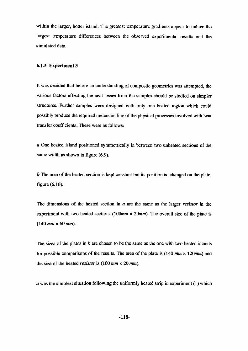
within the larger, hotter island. The greatest temperature gradients appear to induce the

largest temperature differences between the observed experimental results and the

simulated data.

6.13 Experiments

It was decided that before an understanding of composite geometries was attempted, the

various factors affecting the heat losses from the samples should be studied on simpler

structures. Further samples were designed with only one heated region which could

possibly produce the required understanding of the physical processes involved with heat

transfer coefficients. These were as follows:

a One heated island positioned symmetrically in between two unheated sections of the

same width as shown in figure (6.9).

b The area of the heated section is kept constant but its position is changed on the plate,

figure (6.10).

The dimensions of the heated section in a are the same as the larger resistor in the

experiment with two heated sections (100mm x 20mm). The overall size of the plate is

(140 mm x 60 mm).

The sizes of the plates in b are chosen to be the same as the one with two heated islands

for possible comparisons of the results. The area of the plate is (140 mm x 120mm) and

the size of the heated resistor is (100 mm x 20 mm).

a was the simplest situation following the uniformly heated strip in experiment (1) which

-118-

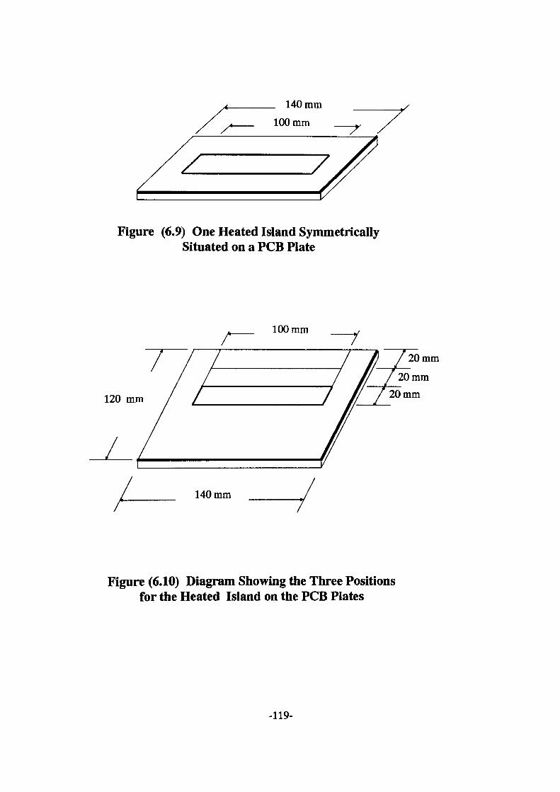
140mm

Figure (6.9) One Heated Island Symmetrically Situated on a PCB Plate

120 mm

100mm

77

7

20mm20mm

20mm

140mm7

Figure (6.10) Diagram Showing the Three Positions for the Heated Island on the PCB Plates

-119-

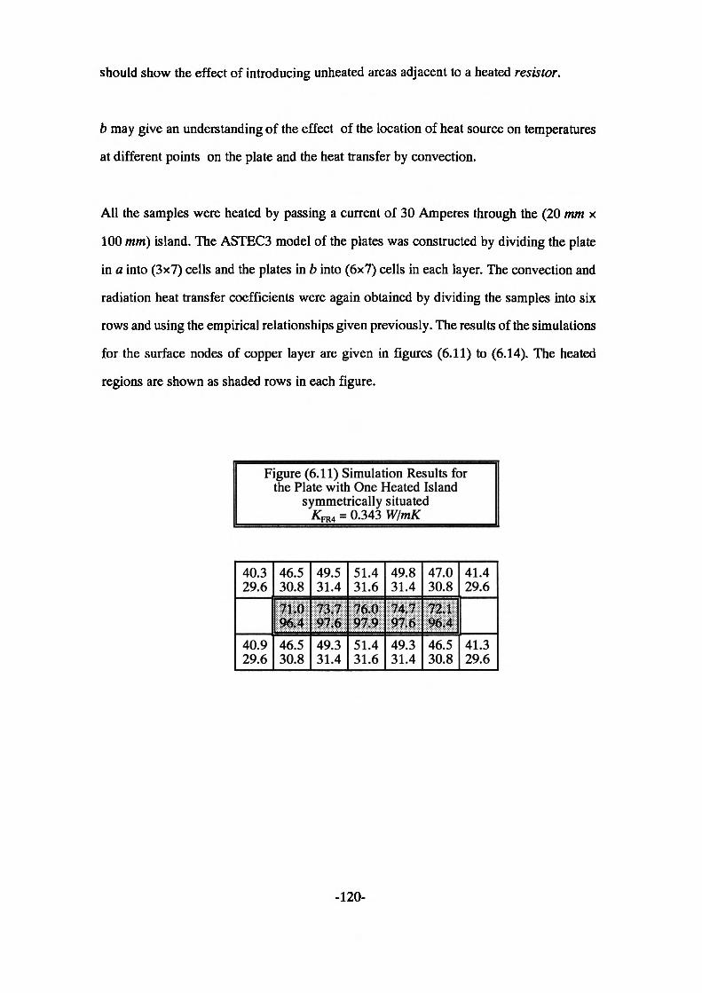
should show the effect of introducing unheated areas adjacent to a heated resistor.

b may give an understanding of the effect of the location of heat source on temperatures

at different points on the plate and the heat transfer by convection.

All the samples were heated by passing a current of 30 Amperes through the (20 mm x

100 mm) island. The ASTEC3 model of the plates was constructed by dividing the plate

in a into (3x7) cells and the plates in b into (6x7) cells in each layer. The convection and

radiation heat transfer coefficients were again obtained by dividing the samples into six

rows and using the empirical relationships given previously. The results of the simulations

for the surface nodes of copper layer are given in figures (6.11) to (6.14). The heated

regions are shown as shaded rows in each figure.

Figure (6.11) Simulation Results forthe Plate with One Heated Island

symmetrically situatedKfM = 0.343 W/mK

40.329.6

46.530.8

49.531.4

51.431.6

49.831.4

47.030.8

41.429.6

40.929.6

46.530.8

49.331.4

51.431.6

49.331.4

46.530.8

41.329.6

-120-

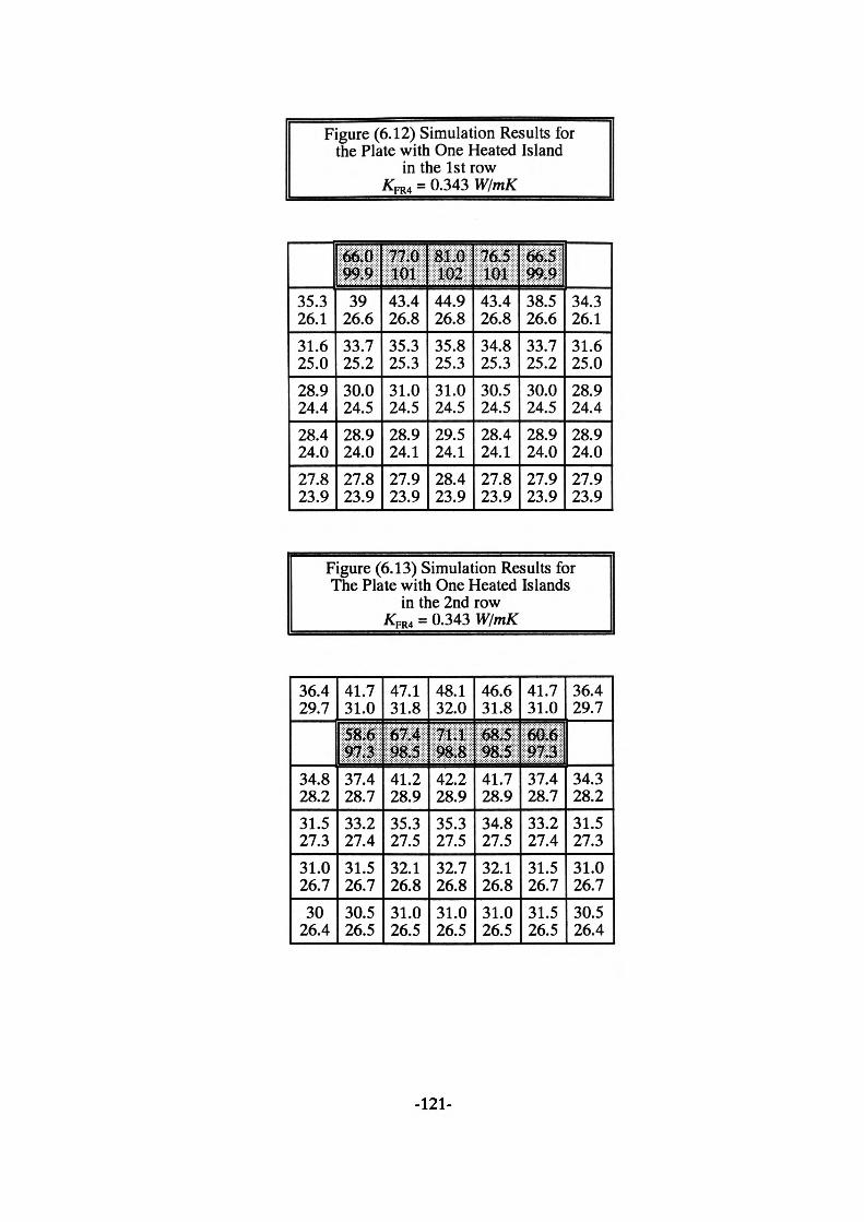
Figure (6.12) Simulation Results for the Plate with One Heated Island

in the 1st row KfR4 = 0.343 W/mK

35.3 26.131.6 25.028.9 24.428.4 24.027.8 23.9

Hill39

26.633.7 25.230.024.528.9 24.027.8 23.9

11143.4 26.835.3 25.331.0 24.528.9 24.127.9 23.9

MWIIP :44.9 26.835.8 25.331.0 24.529.5 24.128.4 23.9

76.5 10143.4 26.834.8 25.330.5 24.528.4 24.127.8 23.9

,M;38.5 26.633.7 25.230.024.528.9 24.027.9 23.9

34.3 26.131.6 25.028.9 24.428.9 24.027.9 23.9

Figure (6.13) Simulation Results for The Plate with One Heated Islands

in the 2nd row/CFR4 = 0.343 W/mK

36.429.7

34.828.231.527.331.026.730

26.4

41.731.0

•|37.428.733.227.431.526.730.526.5

47.131.8

HI41.228.935.327.532.126.831.026.5

48.132.0

H42.228.935.327.532.726.831.026.5

46.631.8

(H41.728.934.827.532.126.831.026.5

41.731.0

ill37.428.733.227.431.526.731.526.5

36.429.7

34.328.231.527.331.026.730.526.4

-121-

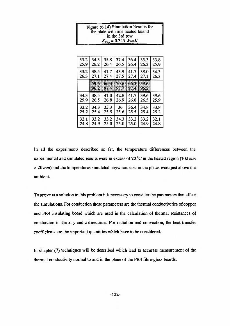
Figure (6.14) Simulation Results for the plate with one heated Island

in the 3rd row KM = 0.343 W/mK

33.2 25.933.2 26.3

34.3 25.933.2 25.232.1 24.8

34.3 26.238.5 27.1

II38.5 26.534.3 25.433.2 24.9

35.8 26.441.7 27.4

tl?,4.

41.0 26.835.3 25.533.2 25.0

37.4 26.543.927.5

9X7:

42.8 26.936

25.634.3 25.0

36.4 26.441.7 27.4

97,441.7 26.836.425.533.2 25.0

35.3 26.238.027.1

mM39.6 26.534.8 25.433.2 24.9

33.8 25.934.3 26.3

39.6 25.933.8 25.232.1 24.8

In all the experiments described so far, the temperature differences between the

experimental and simulated results were in excess of 20 °C in the heated region (100 mm

x 20 mm) and the temperatures simulated anywhere else in the plates were just above the

ambient.

To arrive at a solution to this problem it is necessary to consider the parameters that affect

the simulations. For conduction these parameters are the thermal conductivities of copper

and FR4 insulating board which are used in the calculation of thermal resistances of

conduction in the x, y and z directions. For radiation and convection, the heat transfer

coefficients are the important quantities which have to be considered.

In chapter (7) techniques will be described which lead to accurate measurement of the

thermal conductivity normal to and in the plane of the FR4 fibre-glass boards.

-122-

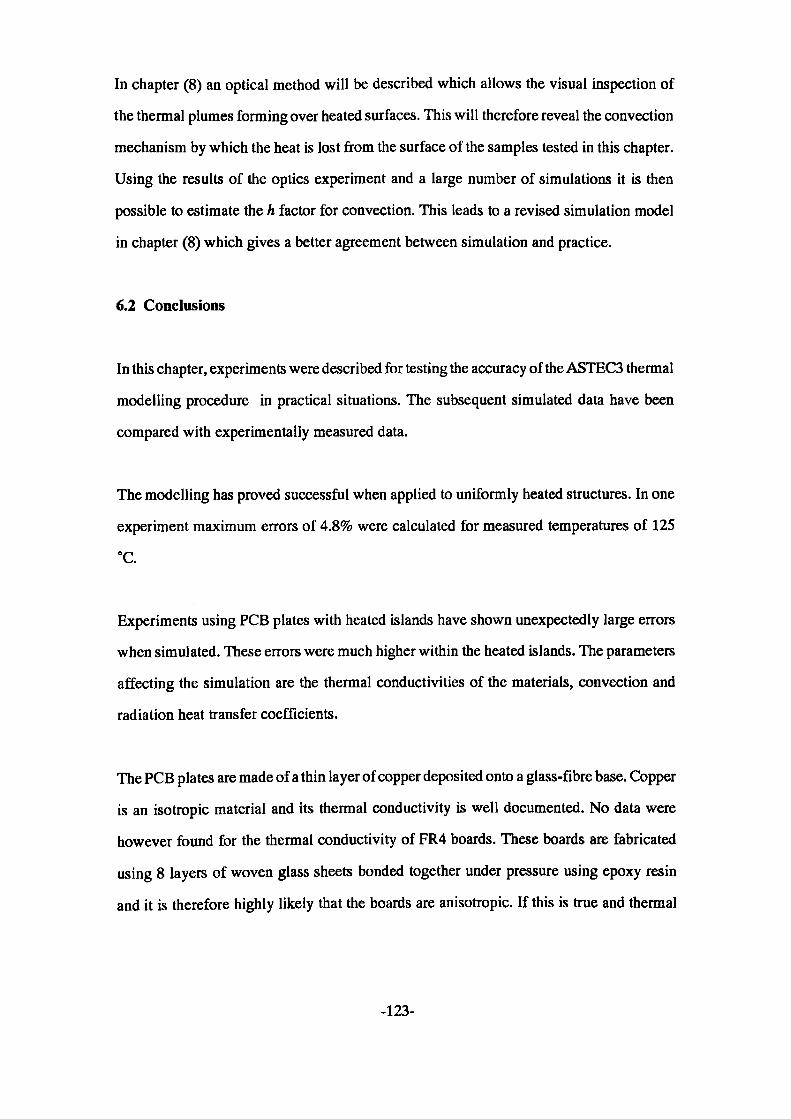
In chapter (8) an optical method will be described which allows the visual inspection of

the thermal plumes forming over heated surfaces. This will therefore reveal the convection

mechanism by which the heat is lost from the surface of the samples tested in this chapter.

Using the results of the optics experiment and a large number of simulations it is then

possible to estimate the h factor for convection. This leads to a revised simulation model

in chapter (8) which gives a better agreement between simulation and practice.

6.2 Conclusions

In this chapter, experiments were described for testing the accuracy of the ASTEC3 thermal

modelling procedure in practical situations. The subsequent simulated data have been

compared with experimentally measured data.

The modelling has proved successful when applied to uniformly heated structures. In one

experiment maximum errors of 4.8% were calculated for measured temperatures of 125

Experiments using PCB plates with heated islands have shown unexpectedly large errors

when simulated. These errors were much higher within the heated islands. The parameters

affecting the simulation are the thermal conductivities of the materials, convection and

radiation heat transfer coefficients.

The PCB plates are made of a thin layer of copper deposited onto a glass-fibre base. Copper

is an isotropic material and its thermal conductivity is well documented. No data were

however found for the thermal conductivity of FR4 boards. These boards are fabricated

using 8 layers of woven glass sheets bonded together under pressure using epoxy resin

and it is therefore highly likely that the boards are anisotropic. If this is true and thermal

-123-

conductivity is higher in the plane of the boards than normal to it, then this could account

for part of the excess temperatures simulated in the heated areas as the heat is obviously

not conducted away. It is therefore crucial that these quantities are measured accurately.

The amount of radiative heat losses is a function of the emissivity of the copper surface

which has already been measured quite accurately in appendix (5) and included in the

ASTEC3 model. This then only leaves the convection losses to be considered.

The convective heat transfer coefficient is a multifunction variable of which position and

temperature are the main factors. In experiments described in previous sections, the

simplified methods used to determine these coefficients do not produce acceptable results

and will therefore have to be modified for a more exact evaluation of the temperature

profile. To produce a more closely matched simulation, a better understanding of the

physical processes involved with heat transfer coefficients is required.

-124-

7 THERMAL CONDUCTIVITY MEASUREMENTS OF

FIBRE-GLASS LAMINATES AND THEIR EFFECT ON

SIMULATION

7.1 Introduction

It has been mentioned in chapter (6) that for accurate simulation of the thermal

characteristics of the two layer PCB structures, precise values of thermal conductivity are

required for both copper and fibre glass layers. Thermal conductivity of copper is well

documented [1] and readily available. No data were however found for thermal

conductivity of FR4 [2] or any other type of epoxy/glass boards and this had to be measured

experimentally.

A rectangular PCB copper cladding board (14 cm x 12 cm) using FR4 epoxy/glass as the

substrate was chosen to demonstrate the effect of thermal conductivity values in the

simulations. This was one of the samples already described in chapter (6). One electrically

isolated island resembling a resistor on a hybrid circuit was cut into the copper layer of

the plate as shown in figure (7.1). This resistor was Joule heated by the passage of an

electric current of 30 amps and the surface temperatures were measured at selected points

along the surface using a HEIMANN Infra red pyrometer type KT14 capable of temperature

readings to an accuracy of 1.5 °C. As the island was electrically isolated heat conduction

from the heated island to its surrounding board was through the fibre-glass substrate only.

An ASTEC3 model of the structure was constructed for simulation purposes using the

procedures given in chapter (4). This was a three-dimensional, two layer model consisting

of the copper and fibre-glass layers. Each layer was divided into (7 x 6) thermal cells of

-125-

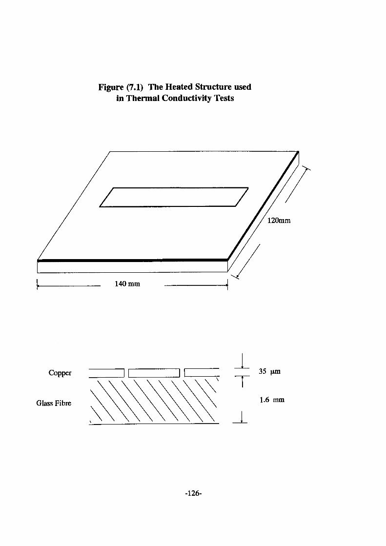
Figure (7.1) The Heated Structure used in Thermal Conductivity Tests

140mm

Copper

Glass Fibre

35

1.6 mm

J.

-126-

(2 cm x 2 cm) dimensions. The full description of the model is given in section (6.1.3). In

the model, thermal conduction in the copper and fibre-glass layers was taken into account.

Convection and radiation from the copper surface were also accounted for and were

calculated using empirical relationships given by other workers [3]. These are very rough

estimates for the heat transfer coefficients and will be dealt with in chapter (8). Their

calculations will not be given in this section since at this stage their values are kept constant

in all the simulations.

Initially the fibre-glass layer was assumed to be isotropic and its thermal conductivity was

measured using a Lees' disc apparatus which will be described in section (7.2). A value

of 0.343 W/mK was found which was subsequently used in the model. The results of the

simulations are given in figure (7.2) along with the measured temperatures. This is an

overhead view of the plate with the heated island in the third row surrounded by double

lines. In each cell the top figure is the measured temperature and the bottom value represents

the simulated top-node temperature.

These show simulated temperatures of greater than 38% above the experimental results

inside the heated island. The temperatures computed anywhere else on the plate are just

above ambient which was measured at 23 °C. These observations lead to the conclusion

that the heat generated in the island was not conducted away and therefore resulted in

excessive temperatures simulated in this area.

-127-

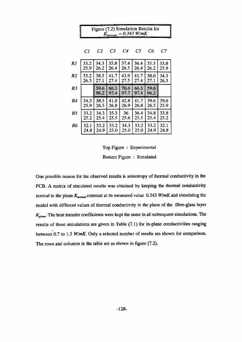
Figure (7.2) Simulation Results for K,sotrooic = 0.343 W/mK

Cl C2 C3 C4 C5 C6 C7

Rl

R2

R3

R4

R5

R6

33.2 25.933.2 26.3

34.3 25.933.2 25.232.1 24.8

34.3 26.238.5 27.1

38.5 26.534.3 25.433.2 24.9

35.8 26.441.7 27.4

41.0 26.835.3 25.533.2 25.0

37.4 26.543.9 27.5

42.8 26.936

25.634.3 25.0

36.4 26.441.7 27.4

41.7 26.836.425.533.2 25.0

35.3 26.238.0 27.1

1139.6 26.534.8 25.433.2 24.9

33.8 25.934.3 26.3

39.6 25.933.8 25.232.1 24.8

Top Figure : Experimental

Bottom Figure : Simulated

One possible reason for the observed results is anisotropy of thermal conductivity in the

PCB. A matrix of simulated results was obtained by keeping the thermal conductivity

normal to the plane £„„„„„, constant at its measured value 0.343 W/mK and simulating the

model with different values of thermal conductivity in the plane of the fibre-glass layer

KplaHe. The heat transfer coefficients were kept the same in all subsequent simulations. The

results of these simulations are given in Table (7.1) for in-plane conductivities ranging

between 0.7 to 1.5 W/mK. Only a selected number of results are shown for comparison.

The rows and columns in the table are as shown in figure (7.2).

-128-

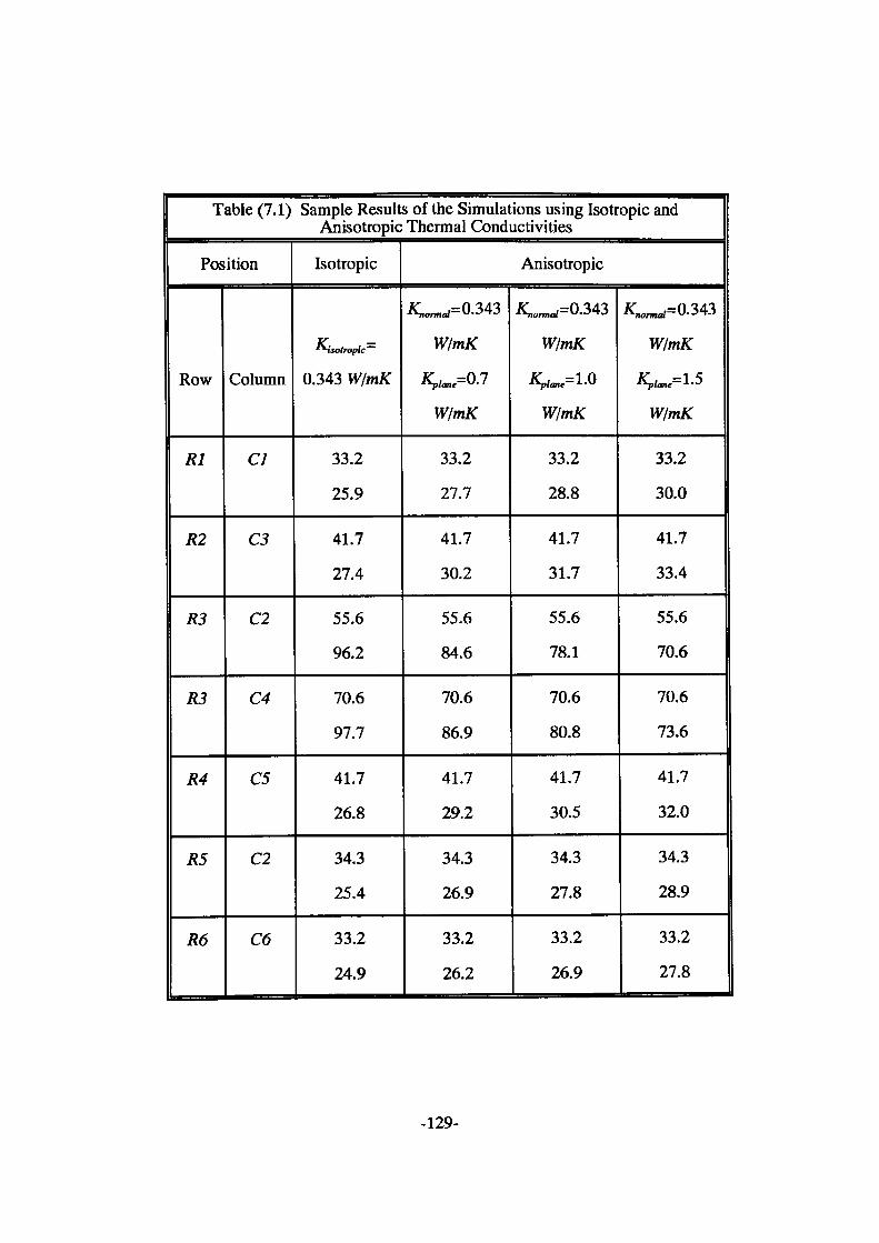
Table (7.1) Sample Results of the Simulations using Isotropic and Anisotropic Thermal Conductivities

Position

Row

Rl

R2

R3

R3

R4

R5

R6

Column

Cl

C3

C2

C4

C5

C2

C6

Isotropic

K**^isotroptc

0.343 W/mK

33.2

25.9

41.7

27.4

55.6

96.2

70.6

97.7

41.7

26.8

34.3

25.4

33.2

24.9

Anisotropic

^^=0.343

W/mK

*W=0.7

W/mK

33.2

27.7

41.7

30.2

55.6

84.6

70.6

86.9

41.7

29.2

34.3

26.9

33.2

26.2

K, —— ,=0.343

W/mK

JW=i.oW/mK

33.2

28.8

41.7

31.7

55.6

78.1

70.6

80.8

41.7

30.5

34.3

27.8

33.2

26.9

K, —— ,=0.343

W/mK

^=1.5

W/mK

33.2

30.0

41.7

33.4

55.6

70.6

70.6

73.6

41.7

32.0

34.3

28.9

33.2

27.8

-129-

It can be seen from Table (7.1) that a closer agreement between the experimental and

simulated results may be obtained with a considerably higher thermal conductivity values

along the plane of the substrate than normal to it. This suggests that the reinforced

fibre-glass substrates are strongly anisotropic. An experiment was therefore proposed to

determine the sensitivity of the results to change in the in-plane thermal conductivity, the

normal conductivity having been measured experimentally.

A standard Lees' disc method [4,5] was used to measure the thermal conductivity of

materials in the shape of thin flat discs in a direction normal to the plane of the boards

(§7.2). This is a method where a disc of the sample and a heater are sandwiched between

three metal slabs and the temperatures of the metal discs are measured. It is then possible

to calculate the thermal conductivity of the sample by equating the amount of input

electrical energy with the heat losses from the system.

A novel technique (§7.3) was devised for measuring the thermal conductivity of these

materials in the plane of theirsurfaces. This technique involves heating rectangular samples

of the material at one end and measuring temperatures at various points along the specimen.

The experimentally measured temperature distribution is then matched to a distribution

obtained from a finite-difference solution, in which only the thermal conductivity value

is unknown, to determine the thermal conductivity of the material.

7.2 Thermal Conductivity Normal to the Plane of Glass-Fibre Laminates

An electrically heated Lees' disc apparatus was used to estimate the thermal conductivity

in a direction normal to the glass fibre boards.

-130-

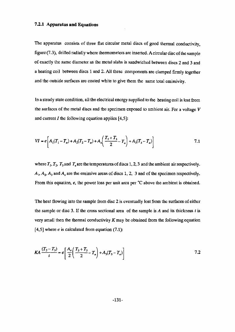
7.2.1 Apparatus and Equations

The apparatus consists of three flat circular metal discs of good thermal conductivity,

figure (7.3), drilled radially where thermometers are inserted. A circular disc of the sample

of exactly the same diameter as the metal slabs is sandwiched between discs 2 and 3 and

a heating coil between discs 1 and 2. All these components are clamped firmly together

and the outside surfaces are coated white to give them the same total emissivity.

In a steady state condition, all the electrical energy supplied to the heating coil is lost from

the surfaces of the metal discs and the specimen exposed to ambient air. For a voltage V

and current / the following equation applies [4,5]:

7.1

where T,, T& T3 and Ta are the temperatures of discs 1,2,3 and the ambient air respectively.

Alt A2, A3 and Ax are the emissive areas of discs 1, 2, 3 and of the specimen respectively.

From this equation, e, the power loss per unit area per °C above the ambient is obtained.

The heat flowing into the sample from disc 2 is eventually lost from the surfaces of either

the sample or disc 3. If the cross sectional area of the sample is A and its thickness t is

very small then the thermal conductivity K may be obtained from the following equation

[4,5] where e is calculated from equation (7.1):

W KA -Ta \+A3(T3 -Ta )\ 7.2

-131-

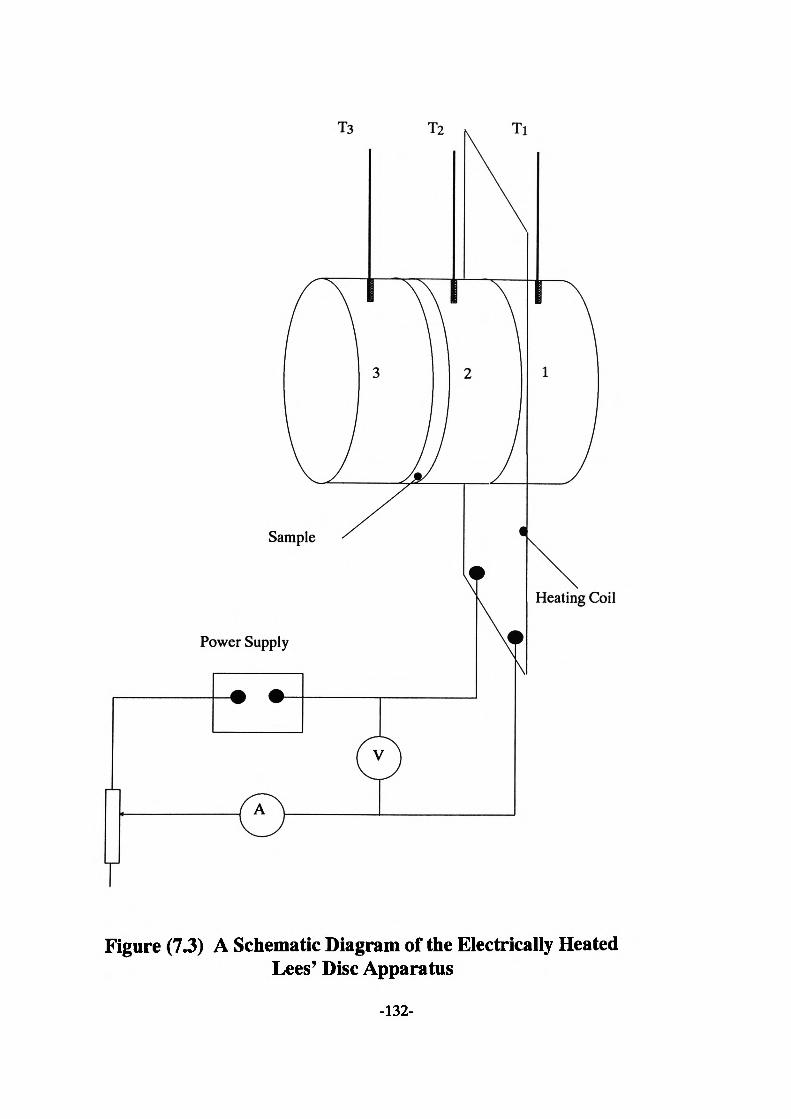
T3 T2 Ti

r

Sample

Power Supply

Heating Coil

Figure (7.3) A Schematic Diagram of the Electrically HeatedLees' Disc Apparatus

-132-

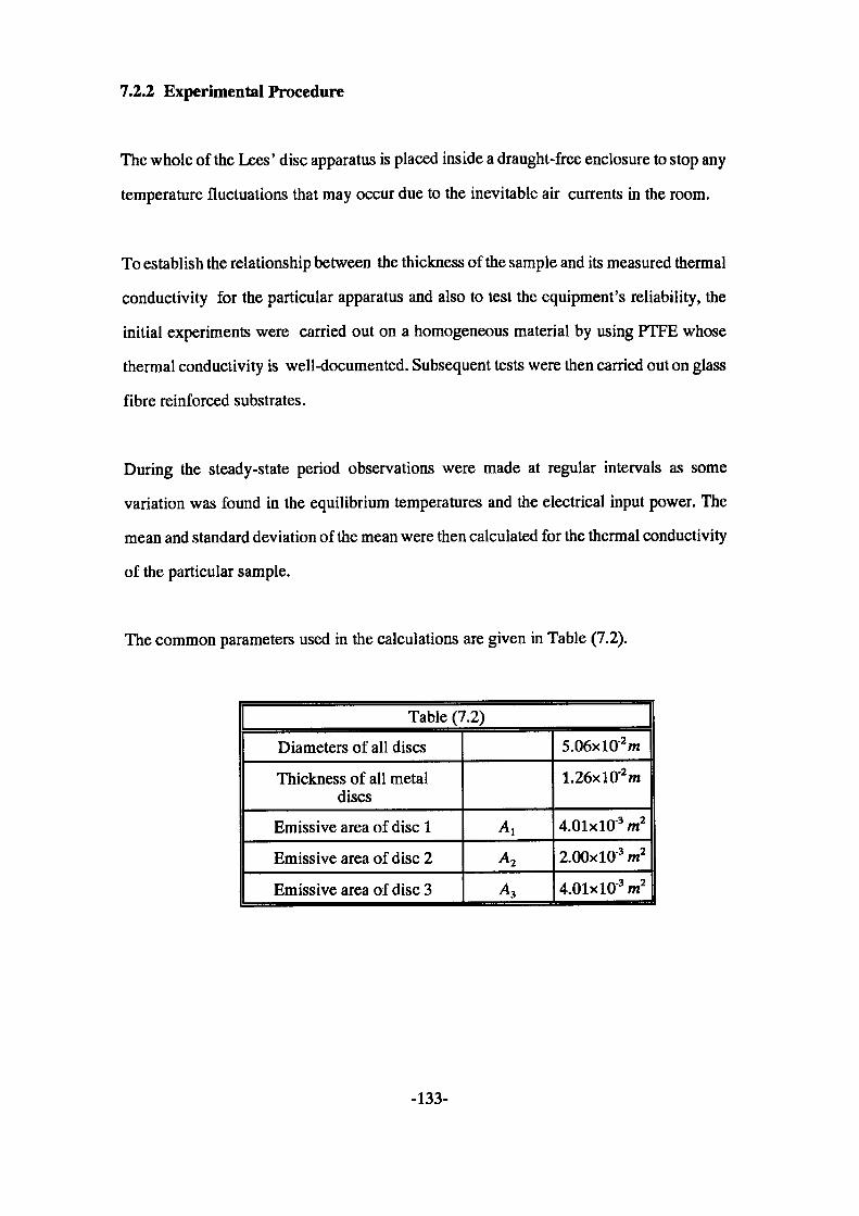
7.2.2 Experimental Procedure

The whole of the Lees' disc apparatus is placed inside a draught-free enclosure to stop any

temperature fluctuations that may occur due to the inevitable air currents in the room.

To establish the relationship between the thickness of the sample and its measured thermal

conductivity for the particular apparatus and also to test the equipment's reliability, the

initial experiments were carried out on a homogeneous material by using PTFE whose

thermal conductivity is well-documented. Subsequent tests were then carried out on glass

fibre reinforced substrates.

During the steady-state period observations were made at regular intervals as some

variation was found in the equilibrium temperatures and the electrical input power. The

mean and standard deviation of the mean were then calculated for the thermal conductivity

of the particular sample.

The common parameters used in the calculations are given in Table (7.2).

Table (7.2)

Diameters of all discs

Thickness of all metal discs

Emissive area of disc 1

Emissive area of disc 2

Emissive area of disc 3

A,

A2

A,

5.06xl(r2 m

1.26xlO'2 m

4.01xlO'3 m2

2.00xl0 3 m24.01X10'3 m2

-133-

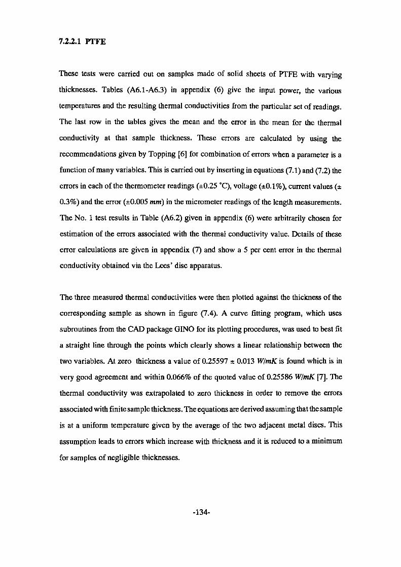
7.2.2.1 PTFE

These tests were carried out on samples made of solid sheets of PTFE with varying

thicknesses. Tables (A6.1-A6.3) in appendix (6) give the input power, the various

temperatures and the resulting thermal conductivities from the particular set of readings.

The last row in the tables gives the mean and the error in the mean for the thermal

conductivity at that sample thickness. These errors are calculated by using the

recommendations given by Topping [6] for combination of errors when a parameter is a

function of many variables. This is carried out by inserting in equations (7.1) and (7.2) the

errors in each of the thermometer readings (±0.25 °C), voltage (±0.1%), current values (±

0.3%) and the error (±0.005 mm) in the micrometer readings of the length measurements.

The No. 1 test results in Table (A6.2) given in appendix (6) were arbitrarily chosen for

estimation of the errors associated with the thermal conductivity value. Details of these

error calculations are given in appendix (7) and show a 5 per cent error in the thermal

conductivity obtained via the Lees' disc apparatus.

The three measured thermal conductivities were then plotted against the thickness of the

corresponding sample as shown in figure (7.4). A curve fitting program, which uses

subroutines from the CAD package GINO for its plotting procedures, was used to best fit

a straight line through the points which clearly shows a linear relationship between the

two variables. At zero thickness a value of 0.25597 ± 0.013 W/mK is found which is in

very good agreement and within 0.066% of the quoted value of 0.25586 W/mK [7]. The

thermal conductivity was extrapolated to zero thickness in order to remove the errors

associated with finite sample thickness. The equations are derived assuming that the sample

is at a uniform temperature given by the average of the two adjacent metal discs. This

assumption leads to errors which increase with thickness and it is reduced to a minimum

for samples of negligible thicknesses.

-134-

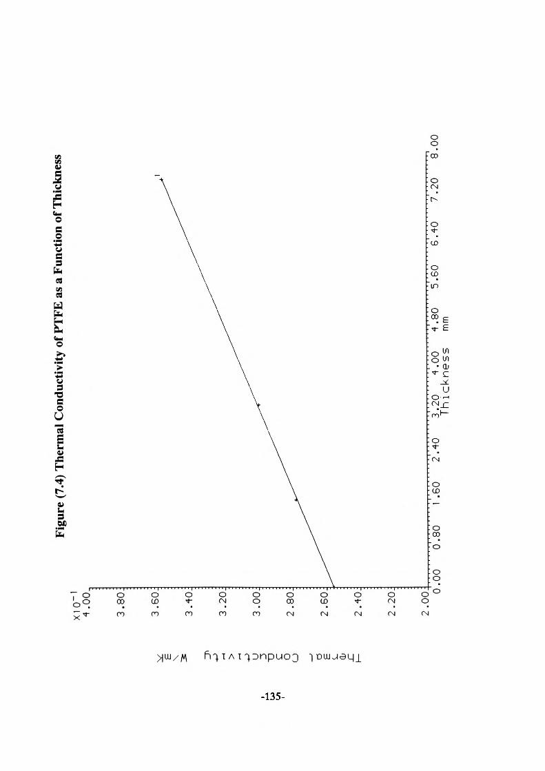
-sei-

Thermal Conductivity W/mK

KJ

K>o

M K)

V CDO O

K) CO CO

co b too o o

U) CO• •-* en o o

cooo o

o- o:

COo

en o

o;

¥~N>

^ On

3 •*3» O

oo o

en•-* o

o o

CD

b o

^4

£H8*

SLnoa c|38,2* wSB ^e

Iss,5i

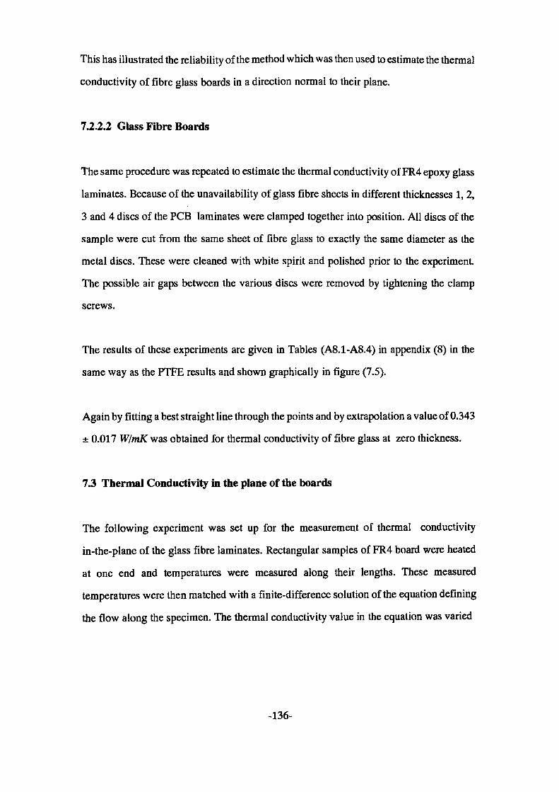
This has illustrated the reliability of the method which was then used to estimate the thermal

conductivity of fibre glass boards in a direction normal to their plane.

7.2.2.2 Glass Fibre Boards

The same procedure was repeated to estimate the thermal conductivity of FR4 epoxy glass

laminates. Because of the unavailability of glass fibre sheets in different thicknesses 1, 2,

3 and 4 discs of the PCB laminates were clamped together into position. All discs of the

sample were cut from the same sheet of fibre glass to exactly the same diameter as the

metal discs. These were cleaned with white spirit and polished prior to the experiment

The possible air gaps between the various discs were removed by tightening the clamp

screws.

The results of these experiments are given in Tables (A8.1-A8.4) in appendix (8) in the

same way as the PTFE results and shown graphically in figure (7.5).

Again by fitting a best straight line through the points and by extrapolation a value of 0.343

± 0.017 W/mK was obtained for thermal conductivity of fibre glass at zero thickness.

7.3 Thermal Conductivity in the plane of the boards

The following experiment was set up for the measurement of thermal conductivity

in-the-plane of the glass fibre laminates. Rectangular samples of FR4 board were heated

at one end and temperatures were measured along their lengths. These measured

temperatures were then matched with a finite-difference solution of the equation defining

the flow along the specimen. The thermal conductivity value in the equation was varied

-136-

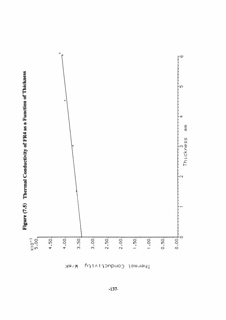
£ \ u 3 TD £ o LJ (Li il

Figu

re (7

.5)

Ther

mal

Con

duct

ivity

of F

R4

as a

Fun

ctio

n of

Thi

ckne

ssX

10~

' 5

.00

,

4.0

0:

3.5

0.

3.0

0:

2.5

0.

2.0

0.

1 .5

0:

1 .O

OJ

0.50

J

0.0

0: 0

Th

ickn

ess

—\ 6m

m

and the resulting temperatures were monitored until the square-root-error between the

measured and the calculated values was minimised. This value of thermal conductivity

was then taken to be that of the test sample. Finite-difference is a method where a particular

structure is divided into small regions called "nodes" and heat balances are made on each

of the nodes. This gives rise to a set of linear algebraic equations which can be solved

simultaneously for the temperatures at the required points. Errors of the order of (Ax/ [8]

are normally expected with the one-dimensional form of this technique, Ax being the space

increment.

The experiment was designed in such a way that the heat flow situation was as simple as

possible to analyse numerically. The samples were heated uniformly along their widths

so that the heat would be travelling along their lengths in a parallel fashion with negligible

flow in the direction normal to the main flow. The chosen samples were of small thickness

and heated around their perimeter at one end to ensure minimal temperature gradients

normal to the faces. Furthermore, the temperatures were determined assuming no

convection or conduction from the surfaces. This was achieved experimentally by

enclosing the specimen in a vacuum chamber and taking results at several pressures, then

extrapolating to zero pressure (perfect vacuum). This left radiation as the only heat loss

mechanism. As energy loss by radiation is a function of the surface emissivity the surface

was coated with a paint of known emissivity.

Also to simplify the situation further all the temperatures were recorded at their steady-state

value. This along with the criteria given above means that a one-dimensional steady-state

heat flow equation with only a radiative heat loss term could be adopted.

Rectangular samples were prepared 15 centimetres long and with varying widths of 3, 4,

5 and 6 centimetres. The copper layer of the PCB boards was chemically etched off except

-138-

for very small circular patches of about 3 mm in diameter along the length of the samples

as shown in figure (7.6). Thermocouples were trapped under a very small amount of solder

at these positions. Solder does not adhere to the thermocouple tips and it is used here merely

to hold the thermocouple tips in good thermal contact with the surface.

Since the emissivity of the boards was unknown, they were coated with black velvet paint

2010 with an emissivity of 0.95 made by 3M [9]. Heating wires were wrapped around the

first 50 mm of each sample and connected to a power supply. The specimen was then

clamped onto a holder and placed inside a steel pressure chamber as shown in figure (7.7).

The inside walls of the vessel were blackened to stop any reflection. The system was

evacuated in order to eliminate the effects of convection and to allow the calculation of

the true value of temperature along the sample when radiation is the only heat loss

mechanism. The thermocouple wires were taken out through a hole on top of the chamber

which was carefully sealed to stop any leakage into the system while pumping down. The

output signals of the thermocouples were fed into an AD595AQ thermocouple amplifier

circuit with an internal cold junction (ice-point) compensator. A calibrated voltmeter

capable of measuring microvolts was subsequently used to monitor the amplified signal

and hence the temperatures along the specimen.

Since zero pressure is almost impossible to achieve the following procedure was carried

out in order to determine the zero pressure temperatures along the samples.

For a constant electrical input power, the variation of steady-state temperatures with

pressure was recorded for each thermocouple. Graphs were produced for temperatures of

each point versus pressure in the vessel. By extrapolation, the values of temperature

corresponding to zero pressure were obtained for each position.

-139-

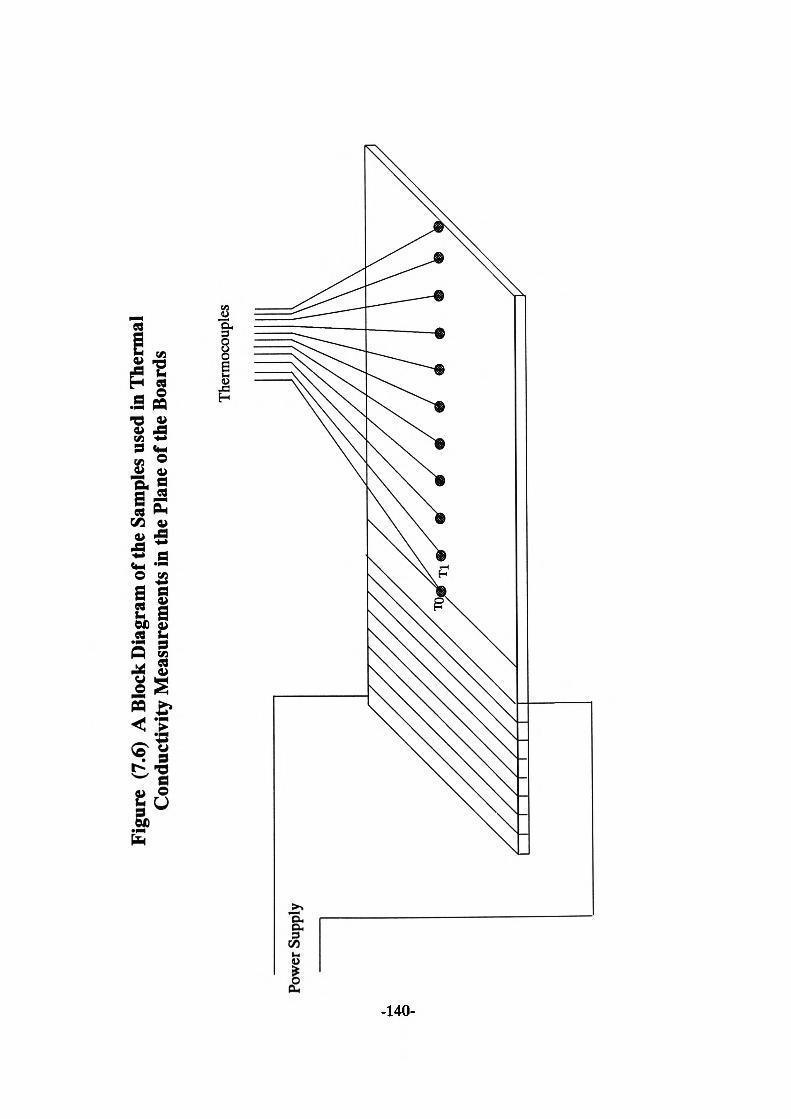
Figu

re (

7.6)

A B

lock

Dia

gram

of t

he S

ampl

es u

sed

in T

herm

al

Con

duct

ivity

Mea

sure

men

ts in

the

Plan

e of

the

Boar

ds

Ther

moc

oupl

es

Powe

r Sup

ply

I I—I o

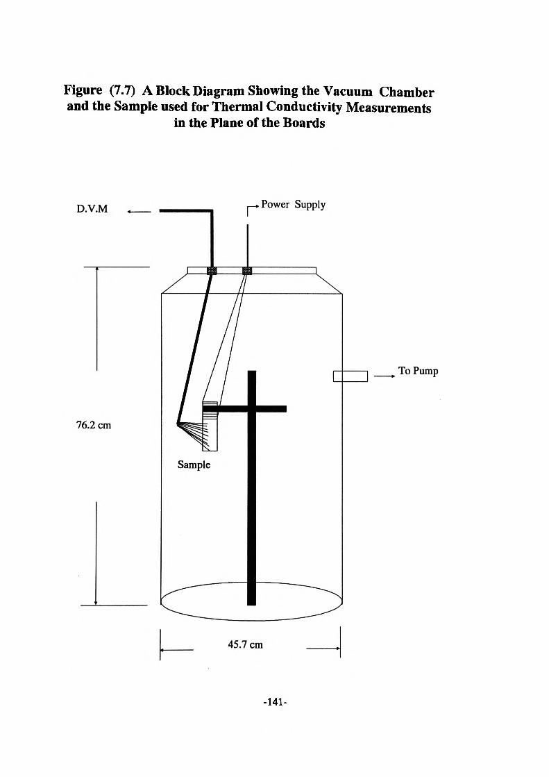
Figure (7.7) A Block Diagram Showing the Vacuum Chamber and the Sample used for Thermal Conductivity Measurements

in the Plane of the Boards

D.V.M Power Supply

76.2 cm

To Pump

45.7 cm

-141-

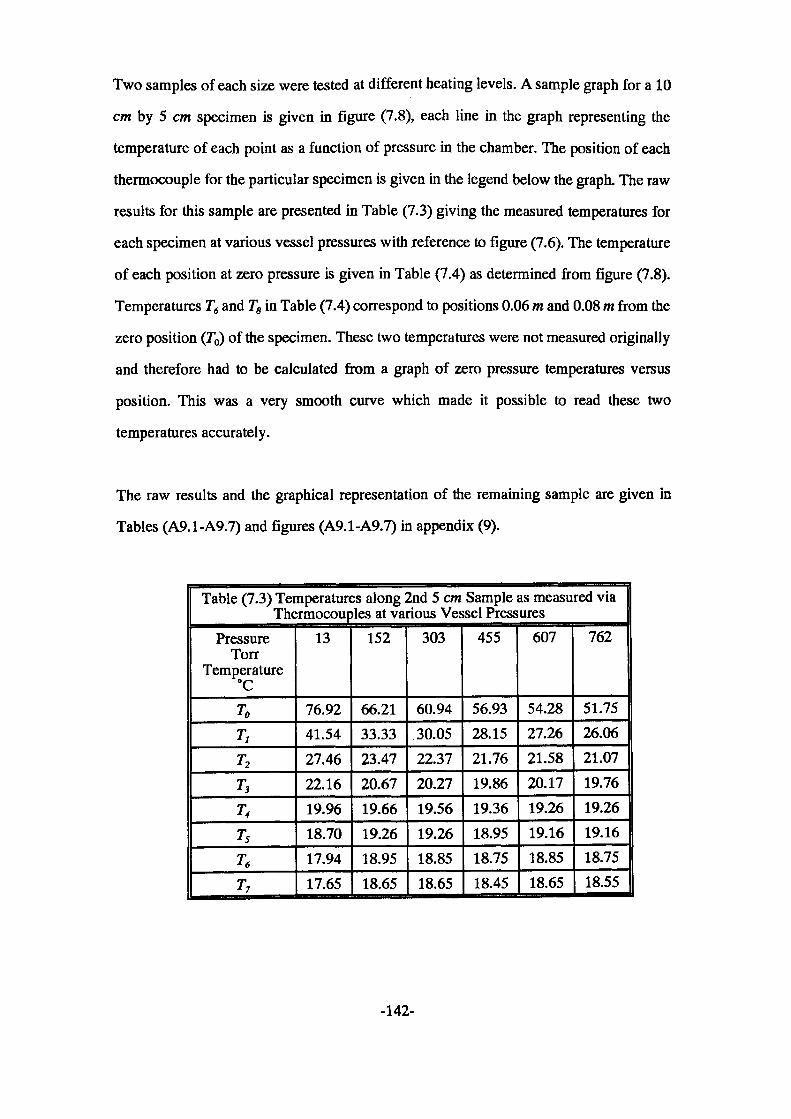
Two samples of each size were tested at different heating levels. A sample graph for a 10

cm by 5 cm specimen is given in figure (7.8), each line in the graph representing the

temperature of each point as a function of pressure in the chamber. The position of each

thermocouple for the particular specimen is given in the legend below the graph. The raw

results for this sample are presented in Table (7.3) giving the measured temperatures for

each specimen at various vessel pressures with reference to figure (7.6). The temperature

of each position at zero pressure is given in Table (7.4) as determined from figure (7.8).

Temperatures T6 and T8 in Table (7.4) correspond to positions 0.06 m and 0.08 m from the

zero position (T0) of the specimen. These two temperatures were not measured originally

and therefore had to be calculated from a graph of zero pressure temperatures versus

position. This was a very smooth curve which made it possible to read these two

temperatures accurately.

The raw results and the graphical representation of the remaining sample are given in

Tables (A9.1-A9.7) and figures (A9.1-A9.7) in appendix (9).

Table (7,3) Temperatures along 2nd 5 cm Sample as measured via Thermocouples at various Vessel Pressures

Pressure Torr

Temperature °C

TOT,T2T3T<T5T6T7

13

76.9241.5427.4622.1619.9618.7017.9417.65

152

66.2133.3323.4720.6719.6619.2618.9518.65

303

60.9430.0522.3720.2719.5619.2618.8518.65

455

56.9328.1521.7619.8619.3618.9518.7518.45

607

54.2827.2621.5820.1719.2619.1618.8518.65

762

51.7526.0621.0719.7619.2619.1618.7518.55

-142-

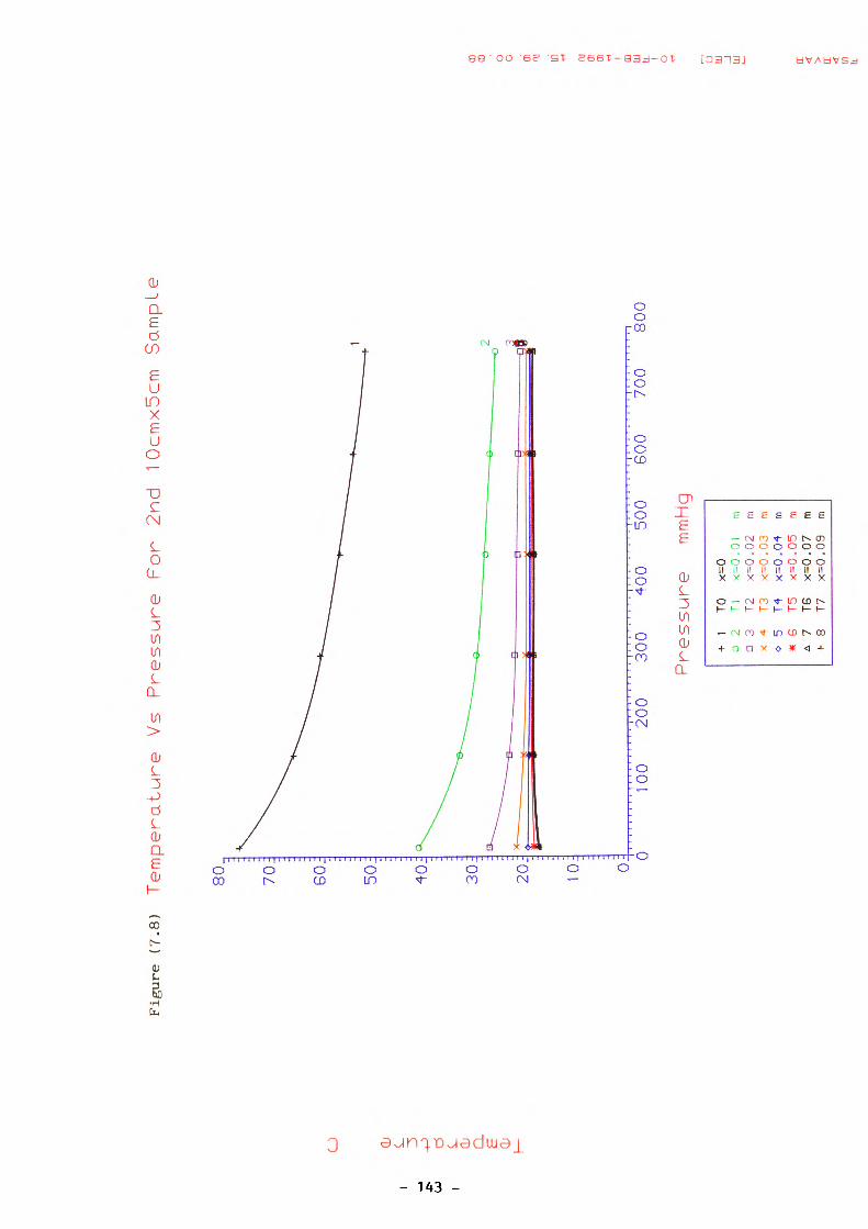
Figu

re

(7.8

) T

em

pe

ratu

re

Vs

Pre

ssure

F

or

2n

d

10cm

xScm

S

am

ple

U) I

CJ CD L CD

CL

E

CD

80

70J

soi

soi

40

:

30J

20;

10: 0

0020

030

040

050

060

070

080

0

Pressure

mmHg

+ o a X o m A 4-

1 2 3 4 5 6 7 8

TO n T2 T3 T4 T5 T6 T7

x=0

x=0

x=0

x^O

x=0

x=0

x=0

x=0

.01

.02

.03

.04

.05

.07

.09

•ii rn m m rn m m

CD O O o o 01 in 0) 0)

^t I CD

111

U_ I O j UJ m u

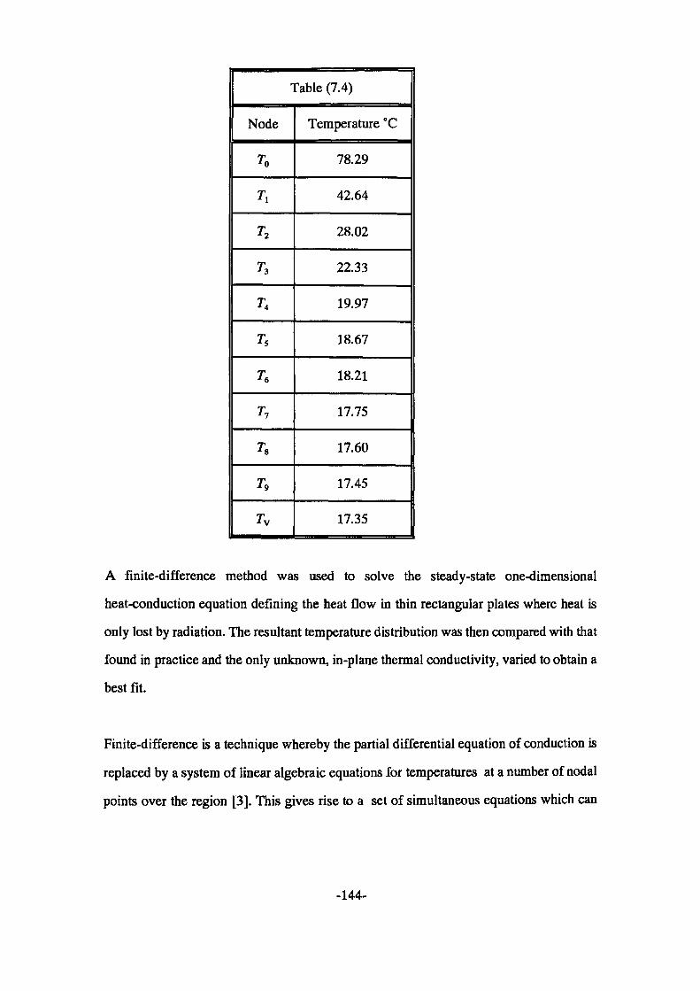
Table (7.4)

Node

TO

TI

T2

T3

T<

Ts

T6

T7

T*

T9

Tv

Temperature °C

78.29

42.64

28.02

22.33

19.97

18.67

18.21

17.75

17.60

17.45

17.35

A finite-difference method was used to solve the steady-state one-dimensional

heat-conduction equation defining the heat flow in thin rectangular plates where heat is

only lost by radiation. The resultant temperature distribution was then compared with that

found in practice and the only unknown, in-plane thermal conductivity, varied to obtain a

best fit.

Finite-difference is a technique whereby the partial differential equation of conduction is

replaced by a system of linear algebraic equations for temperatures at a number of nodal

points over the region [3]. This gives rise to a set of simultaneous equations which can

-144-

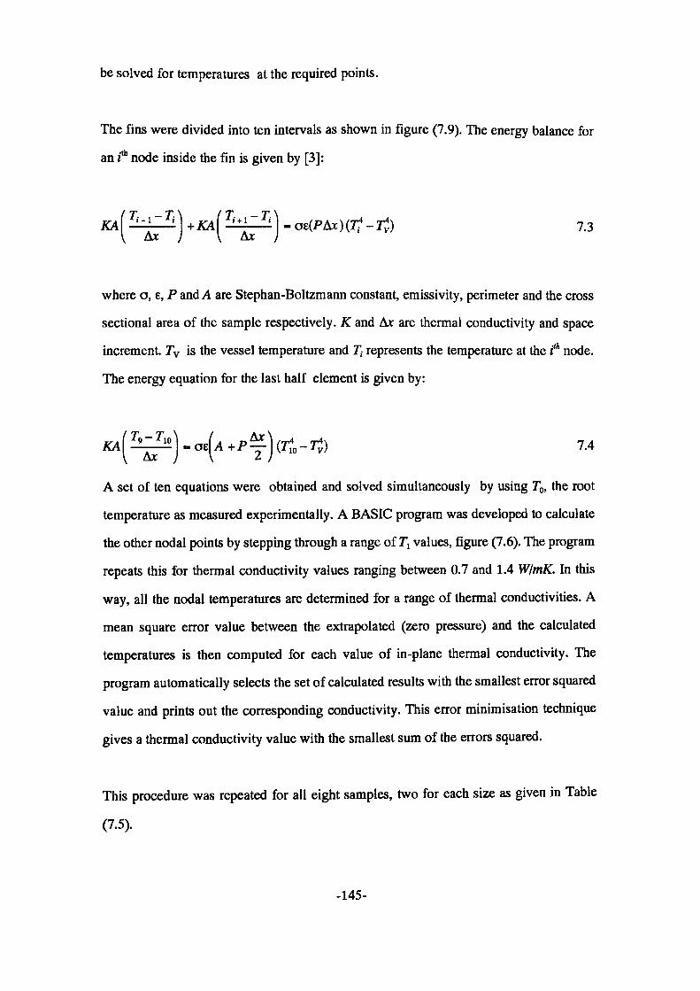
be solved for temperatures at the required points.

The fins were divided into ten intervals as shown in figure (7.9). The energy balance for

an i* node inside the fin is given by [3]:

7.3

where a, e, P and A are Stephan-Boltzmann constant, emissivity, perimeter and the cross

sectional area of the sample respectively. K and Ax are thermal conductivity and space

increment. Tv is the vessel temperature and T{ represents the temperature at the /'* node.

The energy equation for the last half element is given by:

7.4

A set of ten equations were obtained and solved simultaneously by using T0, the root

temperature as measured experimentally. A BASIC program was developed to calculate

the other nodal points by stepping through a range of 7\ values, figure (7.6). The program

repeats this for thermal conductivity values ranging between 0.7 and 1.4 W/mK. In this

way, all the nodal temperatures are determined for a range of thermal conductivities. A

mean square error value between the extrapolated (zero pressure) and the calculated

temperatures is then computed for each value of in-plane thermal conductivity. The

program automatically selects the set of calculated results with the smallest error squared

value and prints out the corresponding conductivity. This error minimisation technique

gives a thermal conductivity value with the smallest sum of the errors squared.

This procedure was repeated for all eight samples, two for each size as given in Table

(7.5).

-145-

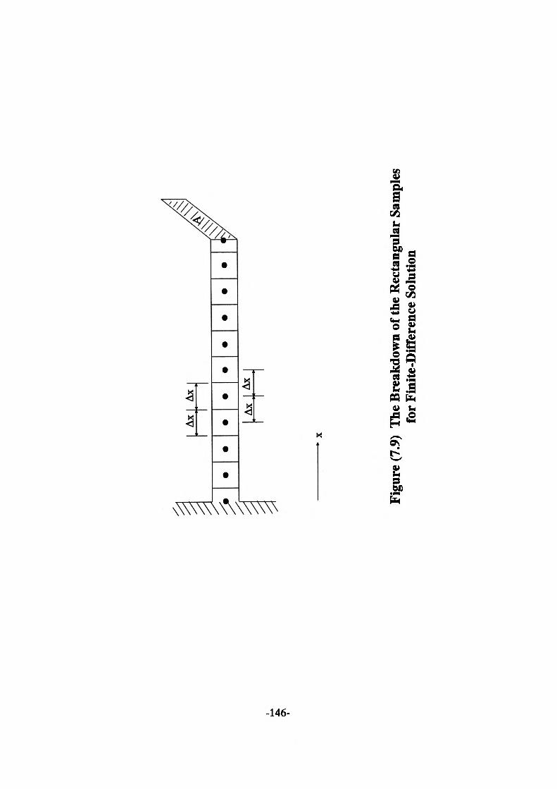
I IAx

Ax

Ax

Figu

re (7

.9) T

he B

reak

down

of t

he R

ecta

ngul

ar S

ampl

es

for F

inite

-Diff

eren

ce S

olut

ion

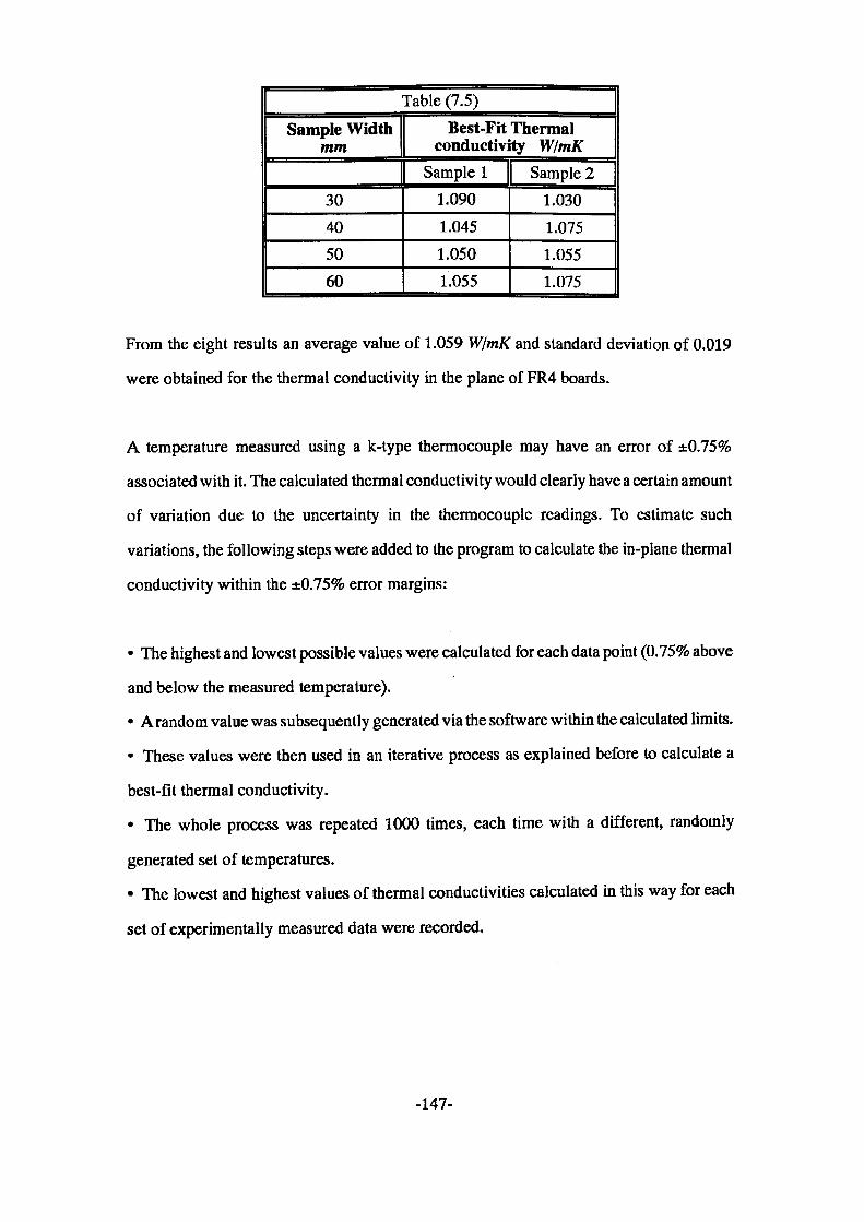
Table (7.5)

Sample Width mm

30405060

Best-Fit Thermal conductivity W/mK

Sample 11.0901.0451.0501.055

Sample 21.0301.0751.0551.075

From the eight results an average value of 1.059 W/mK and standard deviation of 0.019

were obtained for the thermal conductivity in the plane of FR4 boards.

A temperature measured using a k-type thermocouple may have an error of ±0.75%

associated with it. The calculated thermal conductivity would clearly have a certain amount

of variation due to the uncertainty in the thermocouple readings. To estimate such

variations, the following steps were added to the program to calculate the in-plane thermal

conductivity within the ±0.75% error margins:

• The highest and lowest possible values were calculated for each data point (0.75% above

and below the measured temperature).

• A random value was subsequently generated via the software within the calculated limits.

• These values were then used in an iterative process as explained before to calculate a

best-fit thermal conductivity.

• The whole process was repeated 1000 times, each time with a different, randomly

generated set of temperatures.

• The lowest and highest values of thermal conductivities calculated in this way for each

set of experimentally measured data were recorded.

-147-

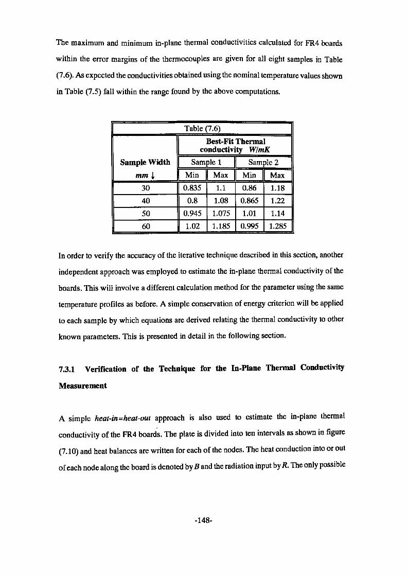
The maximum and minimum in-plane thermal conductivities calculated for FR4 boards

within the error margins of the thermocouples are given for all eight samples in Table

(7.6). As expected the conductivities obtained using the nominal temperature values shown

in Table (7.5) fall within the range found by the above computations.

Sample Widthnun ^

30405060

Table (7.6)Best-Fit Thermal

conductivity W/mKSam

Min0.835

0.80.9451.02

plelMax1.11.081.0751.185

SamMin0.860.8651.01

0.995

ale 2Max1.181.221.141.285

In order to verify the accuracy of the iterative technique described in this section, another

independent approach was employed to estimate the in-plane thermal conductivity of the

boards. This will involve a different calculation method for the parameter using the same

temperature profiles as before. A simple conservation of energy criterion will be applied

to each sample by which equations are derived relating the thermal conductivity to other

known parameters. This is presented in detail in the following section.

7.3.1 Verification of the Technique for the In-Plane Thermal Conductivity

Measurement

A simple heat-in=heat-out approach is also used to estimate the in-plane thermal

conductivity of the FR4 boards. The plate is divided into ten intervals as shown in figure

(7.10) and heat balances are written for each of the nodes. The heat conduction into or out

of each node along the board is denoted by B and the radiation input by R. The only possible

-148-

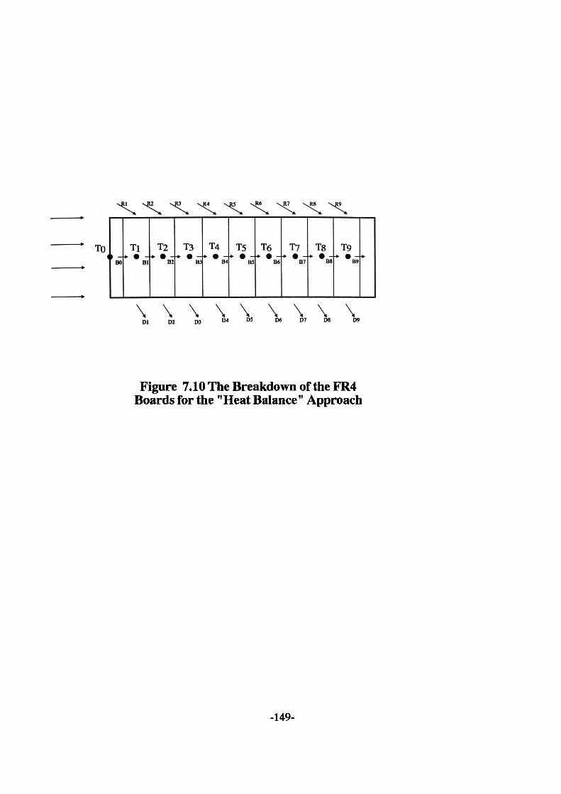
xJU -s^2 x^3 X^M XjU xR* J17

BO

TlBl

T2B2

T3B3

T4B4

T5B5

T6B6

T?B7

T8B8

T9B9

TO

\\\\\\\\\D1 02 D3 D4 D5 D« D7 D8 O9

Figure 7.10 The Breakdown of the FR4 Boards for the "Heat Balance" Approach

-149-

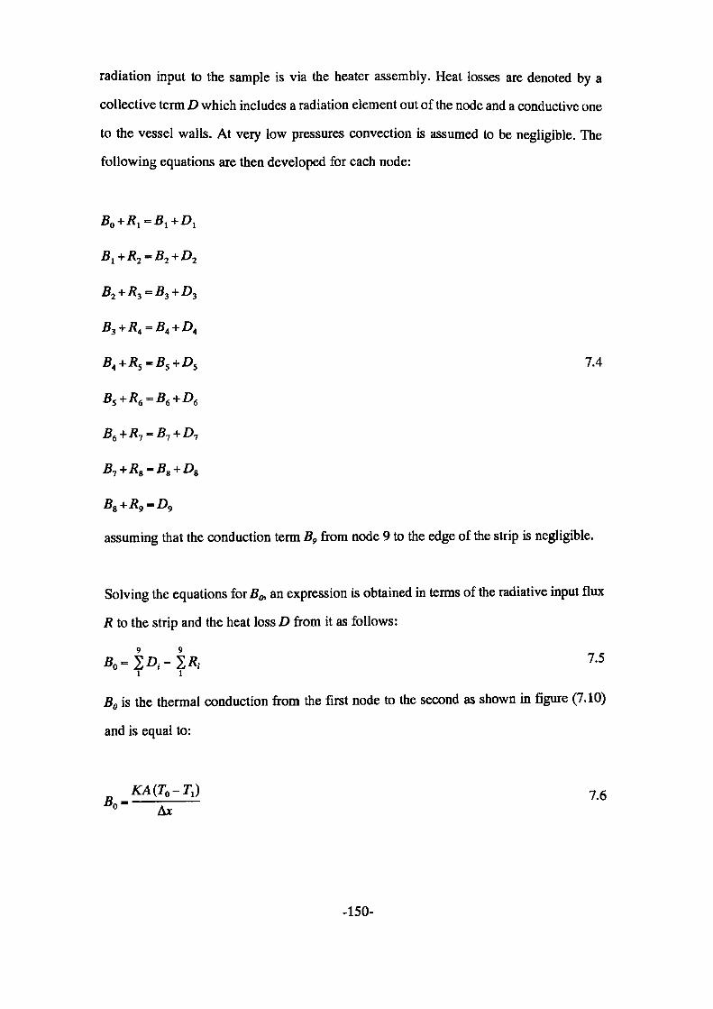
radiation input to the sample is via the heater assembly. Heat losses are denoted by a

collective term D which includes a radiation element out of the node and a conductive one

to the vessel walls. At very low pressures convection is assumed to be negligible. The

following equations are then developed for each node:

B0 + R l =B1 +D,

B4 +RS =B5 + D5 7.4

assuming that the conduction term B9 from node 9 to the edge of the strip is negligible.

Solving the equations for^ an expression is obtained in terms of the radiative input flux

R to the strip and the heat loss D from it as follows:

BO- |D,- |* 7- 5

B0 is the thermal conduction from the first node to the second as shown in figure (7.10)

and is equal to:

Bn ~0 Ax

-150-

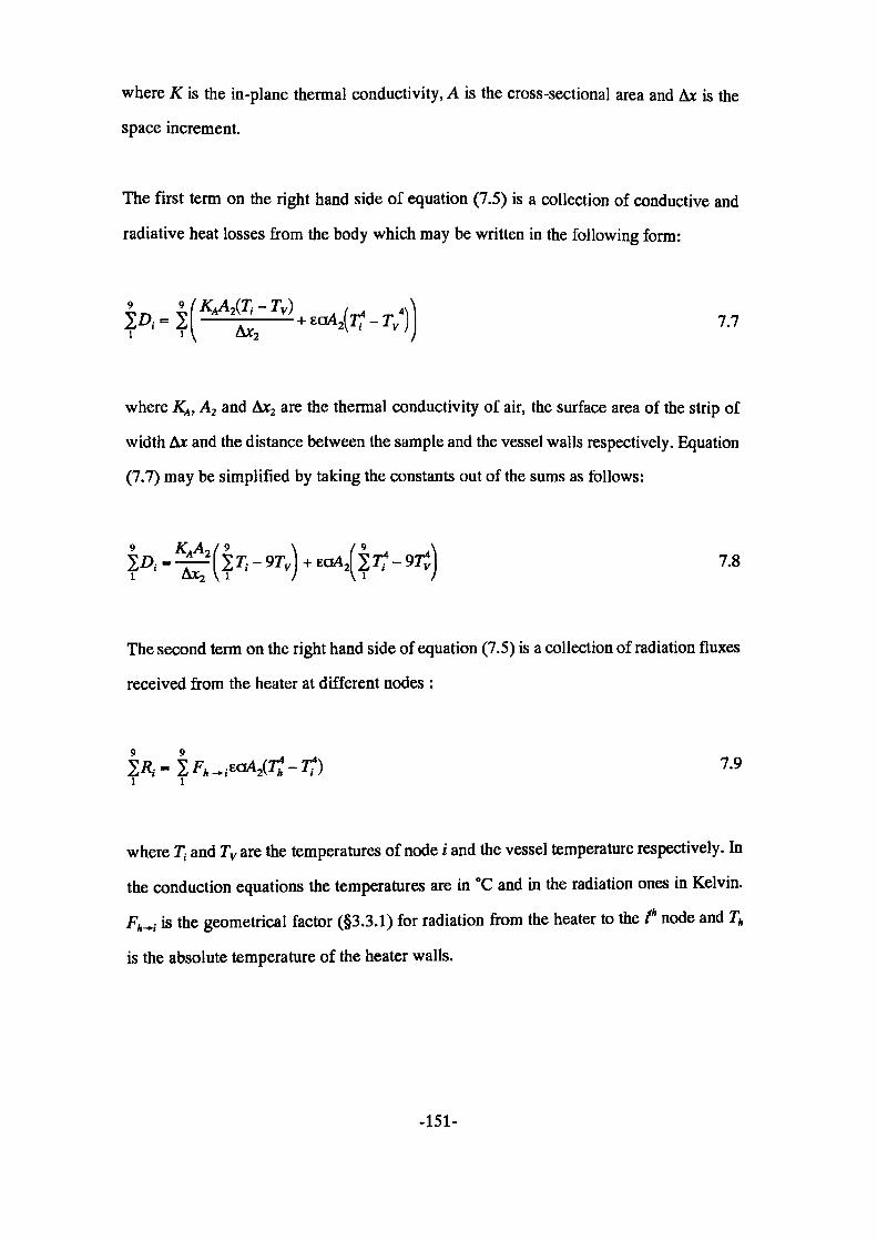
where K is the in-plane thermal conductivity, A is the cross-sectional area and Ax is the

space increment.

The first term on the right hand side of equation (7.5) is a collection of conductive and

radiative heat losses from the body which may be written in the following form:

where KA, A2 and Ax2 are the thermal conductivity of air, the surface area of the strip of

width Ax and the distance between the sample and the vessel walls respectively. Equation

(7.7) may be simplified by taking the constants out of the sums as follows:

7.8

The second term on the right hand side of equation (7.5) is a collection of radiation fluxes

received from the heater at different nodes :

9y. F -EdA (T*4 — 7"?) 7.9 i ~"

where T{ and Tv are the temperatures of node i and the vessel temperature respectively. In

the conduction equations the temperatures are in °C and in the radiation ones in Kelvin.

FA_,- is the geometrical factor (§3.3.1) for radiation from the heater to the /* node and Th

is the absolute temperature of the heater walls.

-151-

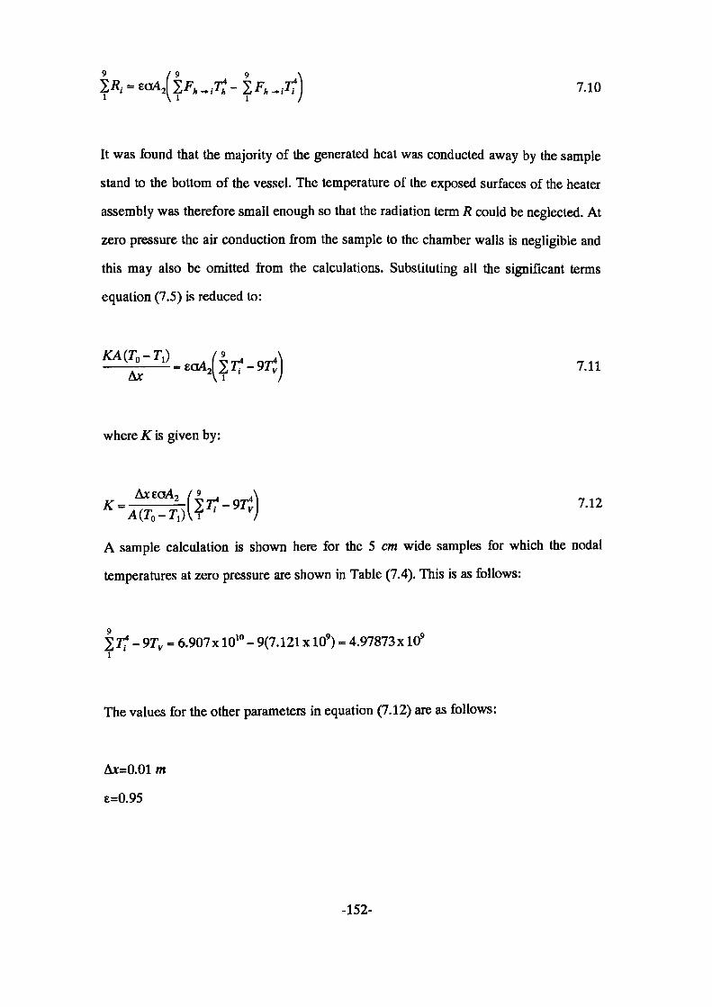
7.10

It was found that the majority of the generated heat was conducted away by the sample

stand to the bottom of the vessel. The temperature of the exposed surfaces of the heater

assembly was therefore small enough so that the radiation term R could be neglected. At

zero pressure the air conduction from the sample to the chamber walls is negligible and

this may also be omitted from the calculations. Substituting all the significant terms

equation (7.5) is reduced to:

7.11

where K is given by:

A sample calculation is shown here for the 5 cm wide samples for which the nodal

temperatures at zero pressure are shown in Table (7.4). This is as follows:

2 T? - 9TV = 6.907x 1010 - 9(7.121 x 109) - 4.97873x 109

The values for the other parameters in equation (7.12) are as follows:

Ax=0.01 m

£=0.95

-152-

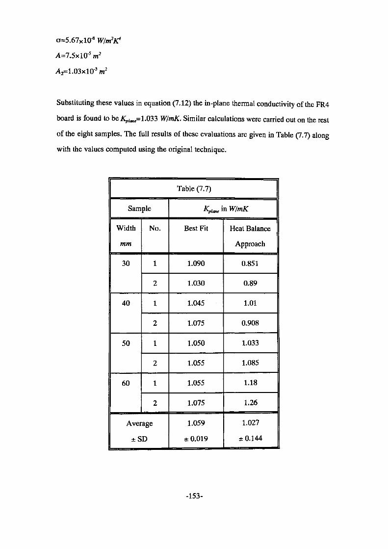
0=5.67X 10-8 Wlm2K*

>U7.5xlO-5 m2

A2=1.03xlO-3 m2

Substituting these values in equation (7.12) the in-plane thermal conductivity of the FR4

board is found to be K^^ 1.033 W/mK. Similar calculations were carried out on the rest

of the eight samples. The full results of these evaluations are given in Table (7.7) along

with the values computed using the original technique.

Table (7.7)

Sample

Width

mm

30

40

50

60

No.

1

2

1

2

1

2

1

2

Average

±SD

/gm, in W/mK

Best Fit

1.090

1.030

1.045

1.075

1.050

1.055

1.055

1.075

1.059

± 0.019

Heat Balance

Approach

0.851

0.89

1.01

0.908

1.033

1.085

1.18

1.26

1.027

± 0.144

-153-

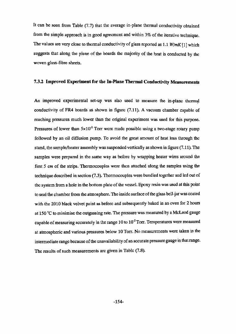
It can be seen from Table (7.7) that the average in-plane thermal conductivity obtained

from the simple approach is in good agreement and within 3% of the iterative technique.

The values are very close to thermal conductivity of glass reported as 1.1 W/mK [1] which

suggests that along the plane of the boards the majority of the heat is conducted by the

woven glass-fibre sheets.

7.3.2 Improved Experiment for the In-Plane Thermal Conductivity Measurements

An improved experimental set-up was also used to measure the in-plane thermal

conductivity of FR4 boards as shown in figure (7.11). A vacuum chamber capable of

reaching pressures much lower than the original experiment was used for this purpose.

Pressures of lower than 5xlO"2 Torr were made possible using a two-stage rotary pump

followed by an oil diffusion pump. To avoid the great amount of heat loss through the

stand, the sample/heater assembly was suspended vertically as shown in figure (7.11). The

samples were prepared in the same way as before by wrapping heater wires around the

first 5 cm of the strips. Thermocouples were then attached along the samples using the

technique described in section (7.3). Thermocouples were bundled together and led out of

the system from a hole in the bottom plate of the vessel. Epoxy resin was used at this point

to seal the chamber from the atmosphere. The inside surface of the glass bell-jar was coated

with the 2010 black velvet paint as before and subsequently baked in an oven for 2 hours

at 150 °C to minimise the outgassing rate. The pressure was measured by a McLeod gauge

capable of measuring accurately in the range 10 to 10 2 Torr. Temperatures were measured

at atmospheric and various pressures below 10 Torr. No measurements were taken in the

intermediate range because of the unavailability of an accurate pressure gauge in that range.

The results of such measurements are given in Table (7.8).

-154-

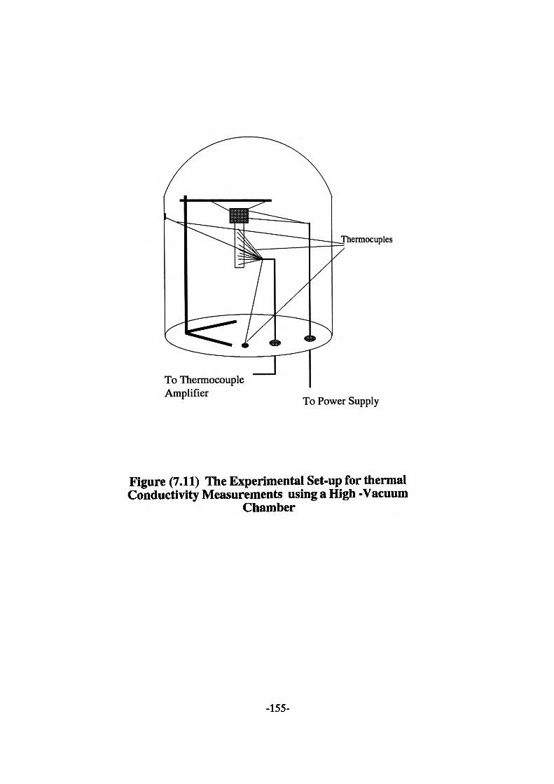
Thermocuples

To Thermocouple Amplifier

To Power Supply

Figure (7.11) The Experimental Set-up for thermal Conductivity Measurements using a High -Vacuum

Chamber

-155-

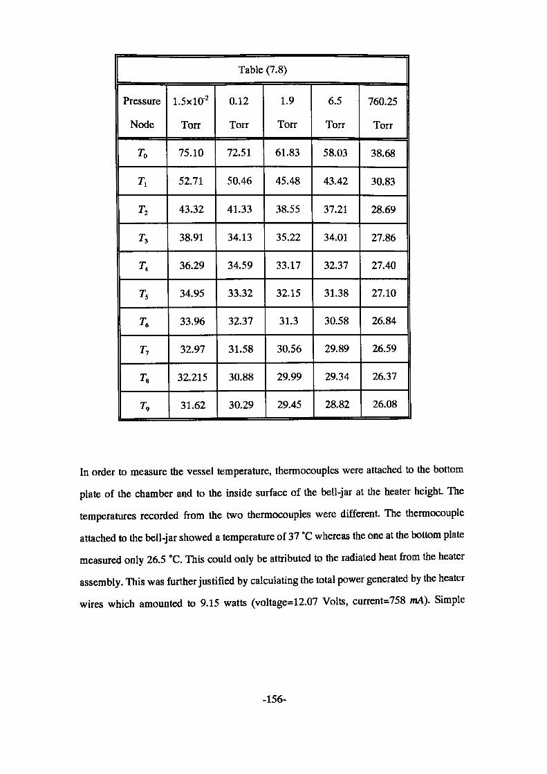
Table (7.8)

Pressure

Node

T0

T,

T2

TI

T<

Ts

T6

T,

Ts

T9

l.SxlO'2

Torr

75.10

52.71

43.32

38.91

36.29

34.95

33.96

32.97

32.215

31.62

0.12

Torr

72.51

50.46

41.33

34.13

34.59

33.32

32.37

31.58

30.88

30.29

1.9

Torr

61.83

45.48

38.55

35.22

33.17

32.15

31.3

30.56

29.99

29.45

6.5

Torr

58.03

43.42

37.21

34.01

32.37

31.38

30.58

29.89

29.34

28.82

760.25

Torr

38.68

30.83

28.69

27.86

27.40

27.10

26.84

26.59

26.37

26.08

In order to measure the vessel temperature, thermocouples were attached to the bottom

plate of the chamber and to the inside surface of the bell-jar at the heater height. The

temperatures recorded from the two thermocouples were different. The thermocouple

attached to the bell-jar showed a temperature of 37 °C whereas the one at the bottom plate

measured only 26.5 "C. This could only be attributed to the radiated heat from the heater

assembly. This was further justified by calculating the total power generated by the heater

wires which amounted to 9.15 watts (voltage=12.07 Volts, current=758 mA). Simple

-156-

calculations show that only a fraction of this power was conducted and radiated away by

the sample (0.9 Watts). At pressures as low as 1.5x10 2, the remaining 8 watts can only be

lost to the bell-jar by radiation and heating of the inside surface.

The calculations of the in-plane thermal conductivity were carried out at the lowest pressure

possible with the current system (ie. 1.5x 10"2 Torr). Even at such high vacuum levels there

may exist some heat losses by convection and conduction through the surrounding air to

the vessel. Therefore calculations are carried out in the following sections to estimate the

thermal conductivity and convection coefficient for the sample. Calculations will also be

presented for the radiation received at the specimen from the heater assembly. This may

be significant, as it was found, by measurement, that the surface of the heater assembly

exposed to the sample was at a temperature of 120 °C.

Thermal Conductivity of Air at Low Pressure

The thermal conductivity K of any gas may be determined from the kinetic theory in the

form [10]:

K = -UmXCv 7.13J

where n, m and X are the number of molecules per unit volume (molecular density), mass

and mean free path of molecules respectively. Cv is the specific heat capacity of the gas at

constant volume.

n and X at a pressure of 10'2 Torr are given as [10] S.SxlO20 molecules per m3 and 5xlO"3

m respectively. It is known [11] that atmospheric air is a mixture of Nitrogen (78.09%),

-157-

Oxygen (20.95%), Argon (0.93%) and Carbon Dioxide (0.03 %). This yields an average

molecular weight of 28.96 for air. According to Avogadro there are 6.022X1023 molecules

per mole of a gas and since there are 28.96 grammes of air per mole, the mass of a molecule

of air may be found by dividing the former to the latter as follows:

• ' ——gmoe = 4.809 x ID'23 g/molecule -= 4.809 x 10'26 kg/molecule 6.022 x 10 molecules /mole °

The specific heat capacities of a gas at constant pressure Cp and at constant volume Cv are

related by [11]:

7.14

where y is 1.4 [11] for diatomic gases such as Nitrogen N2 and Oxygen O2 which are the

largest constituents in a volume of air. The specific heat capacity of air at constant pressure

is l.OOSxlO3 J/kgK and therefore Cv is found from equation (7.14) as 717.85 J/kgK.

Substituting all the values in equation (7.13), a value of 1.9xlO s W/mK is calculated for

the thermal conductivity of air at a pressure of 10"2 Torr.

Heat Transfer Coefficient of Convection

An average value for convection coefficient may be estimated using the simplified

empirical equations of the type shown below [12] recommended for laminar natural

convection from a vertical plate:

-158-

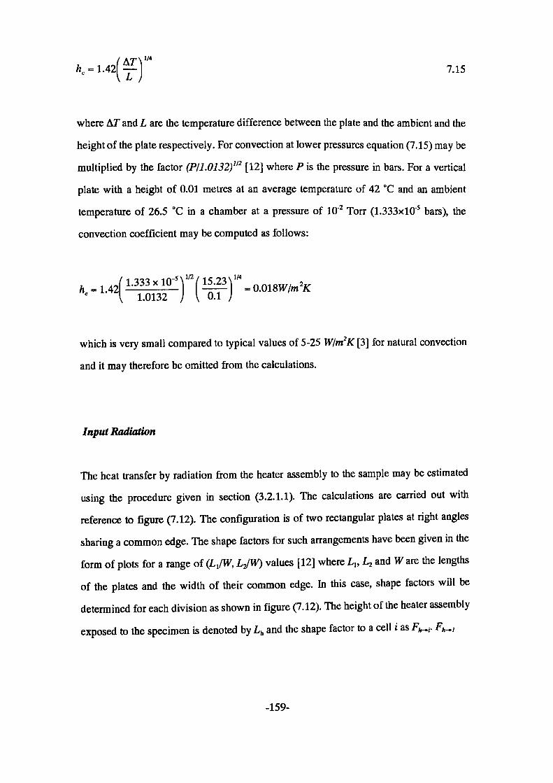
1/47.15

where AT and L are the temperature difference between the plate and the ambient and the

height of the plate respectively. For convection at lower pressures equation (7.15) may be

multiplied by the factor (P/1.0132)"2 [12] where P is the pressure in bars. For a vertical

plate with a height of 0.01 metres at an average temperature of 42 °C and an ambient

temperature of 26.5 °C in a chamber at a pressure of 10"2 Torr (1.333xlO~5 bars), the

convection coefficient may be computed as follows:

which is very small compared to typical values of 5-25 W/m2K [3] for natural convection

and it may therefore be omitted from the calculations.

Input Radiation

The heat transfer by radiation from the heater assembly to the sample may be estimated

using the procedure given hi section (3.2.1.1). The calculations are carried out with

reference to figure (7.12). The configuration is of two rectangular plates at right angles

sharing a common edge. The shape factors for such arrangements have been given in the

form of plots for a range of (LJW, LJW) values [12] where Llt L^ and W are the lengths

of the plates and the width of their common edge. In this case, shape factors will be

determined for each division as shown in figure (7.12). The height of the heater assembly

exposed to the specimen is denoted by Lh and the shape factor to a cell i as Fh^. FA_,

-159-

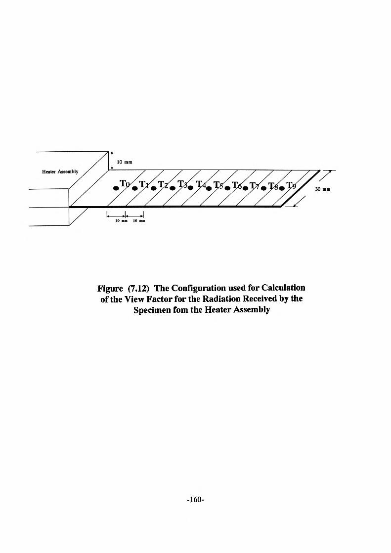
Figure (7.12) The Configuration used for Calculationof the View Factor for the Radiation Received by the

Specimen fom the Heater Assembly

-160-

is calculated as follows:

W 0.03

and:

for which the shape factor is read as [12]:

for division number 2 the following procedure is used (§ 3.2.1.1):

for which :

using relationship (3.29):

-161-

The same procedure may be carried out for the rest of the divisions which shows that

Fh_3 =0.02 and Fh^4 =0.01 and so on approximately halving each time. These are

subsequently used in the calculations of the radiation received at each space increment.

Calculation of the in-plane Thermal Conductivity

Substituting equations (7.6), (7.8) and (7.9) into equation (7.5) the following relationship

is arrived at:

(7,6)

The parameters for the equations are as follows:

KA = 1.9xlQ-5 W/mK

A2 = 0.01x0.63=6.3x10^ m2

= 0.15 m

e = 0.95

a = 5.67X1Q-8

Fh_i = As calculated in previous section

Ax = 0.01 m

These values are substituted in the individual terms in the right and left hand sides of

equation (7.16) as follows:

-162-

Kx 4.5 x!Q-5(75.1- 52.71)

? - I?J - 0.95 x 5.67 x KT8 x 6.3 x 10^(8.03465 x 1010 - 8.397 x 1010)

- 0.122963

Substituting these values in equation (7.16) we get:

O.IK = 1.831 x 1Q-6 + 0.122963 - 0.0181

from which the thermal conductivity K along the plane of the boards is computed as:

K=L0486 W/mK

The results from the new apparatus capable of a high level of vacuum are in very good

agreement with the results obtained from the previous set-up. It has been demonstrated

that the technique by which the zero pressure temperature along the specimen is determined

is valid. Therefore a very good vacuum chamber is not essential for thermal conductivity

measurements although if such a vessel is available, the sequence for determining the zero

pressure temperatures may be omitted from the calculations hence simplifying the

procedure.

-163-

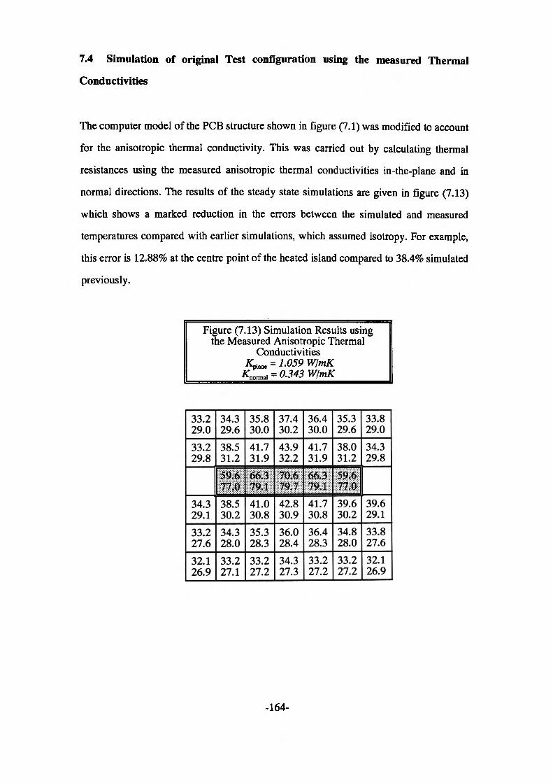
7.4 Simulation of original Test configuration using the measured Thermal

Conductivities

The computer model of the PCB structure shown in figure (7.1) was modified to account

for the anisotropic thermal conductivity. This was carried out by calculating thermal

resistances using the measured anisotropic thermal conductivities in-the-plane and in

normal directions. The results of the steady state simulations are given in figure (7.13)

which shows a marked reduction in the errors between the simulated and measured

temperatures compared with earlier simulations, which assumed isotropy. For example,

this error is 12.88% at the centre point of the heated island compared to 38.4% simulated

previously.

Figure (7.13) Simulation Results using the Measured Anisotropic Thermal

Conductivities AL^ = 1.059 W/mK

= 0.343 W/mK

33.2 29.033.2 29.8

34.3 29.133.2 27.632.1 26.9

34.3 29.638.5 31.2

1138.5 30.234.3 28.033.2 27.1

35.8 30.041.7 31.9n41.0 30.835.3 28.333.2 27.2

37.4 30.243.932.2

42.8 30.936.0 28.434.3 27.3

36.4 30.041.7 31.9

Hi41.7 30.836.4 28.333.2 27.2

35.3 29.638.0 31.2

IJI39.6 30.234.8 28.033.2 27.2

33.8 29.034.3 29.8

39.6 29.133.8 27.632.1 26.9

-164-

7.5 Conclusions

In this chapter the anisotropic thermal conductivity of FR4 epoxy/glass laminates used for

printed circuit boards has been measured. A technique has been described for measuring

thermal conductivity in the plane of a thin flat board. This technique may be used in other

areas of research where thermal conductivity of materials in the form of thin flat boards

is required. An electrically heated Lees' disc apparatus is also used to determine this

quantity in a direction normal to their plane.

PTFE was used as a standard sample to evaluate the reliability of the Lees' disc apparatus.

A value of 0.25597 W/mK± 0.013 was measured which is very close to the quoted value

of 0.25586 W/mK. The subsequent measurements on samples of FR4 laminates yielded

an average value of 0.343 ± 0.017 W/mKfoi the thermal conductivity in a direction normal

to the plane of the boards.

The thermal conductivity in the plane of the boards was measured using a novel technique

involving the use of a vacuum chamber. Two different vacuum vessels were employed for

this purpose. Values of 1.059 W/mK and 1.048 W/mK were obtained using a moderate

vacuum ( around 10 Torr) and a much better vacuum ( 1.5xlO"2 Torr) respectively.

These experiments have demonstrated that the thermal conductivity of these reinforced

boards in a direction tangential to their surfaces is almost three times greater than that

normal to their planes.

The sensitivity of the simulated temperatures to thermal conductivity and heat transfer

coefficients of convection and radiation has been mentioned before. It has been

demonstrated that using the correct values of thermal conductivity of fibre glass the

-165-

simulation errors of nearly 40% have been reduced to around 12%. The remainder of the

discrepancies between the experimental and the simulated temperatures may be due to the

wrong values of heat transfer coefficients. These factors will be investigated in detail in

chapter (8).

-166-

8 SCHLIEREN EXPERIMENT FOR VISUALISATION OF

NATURAL CONVECTION PLUMES

8.1 Introduction

As previously mentioned in chapter (6), the simplified procedure for calculation of heat

transfer coefficient of convection hc has proved unsuccessful. Using the particular method

used in that section a higher value of hc was obtained for the heated island than in the

unheated cooler regions. This of course may not necessarily be true.

From the boundary layer theory the convection mechanism from a surface occurs in two

stages, first via conduction in a thin layer near the surface and then by advection in the

main fluid. The conductive heat loss at any point in the layer adjacent to the surface is a

function of the temperature gradient at that point [1]. Thermal boundary layer thickness

increases as the flow develops inwards from the edge of the plate and accordingly the

magnitude of the temperature gradient and hence the heat transfer by conduction decrease.

The convective heat losses would therefore be higher near the edge of a plate decreasing

towards the centre of the plate.

To investigate the nature of the plumes forming over the composite structures used in the

experiments described in chapter (6) and hence the heat loss mechanism, an optical

technique was utilised. This was a Schlieren method which is used for examination of

refractive index variations in a medium caused by density gradients in that region.

-167-

8.2 Theory of Operation

A Schlieren apparatus is an optical device which was originally developed for observing

the shock waves that form around aerofoils in jet aircraft and bullets in ballistics [2,3].

These shock waves normally form when the flight of these objects is at supersonic speeds.

The Schlieren method allows the observation of the density gradients as variations in the

intensity of illumination. For instance, an increase or decrease in temperature around a

body alters the density of the fluid surrounding that body as a result of which the refractive

index of the fluid in that region changes. This phenomenon then causes a change in the

direction of any light that is passing through the medium and due to variations in the

directions of the light rays, more or less light will pass a knife-edge (cut-off) in the apparatus

and hence lighter/darker regions appear on a viewing screen.

The arrangement of the Schlieren system may be explained by referring to figure (8.1). A

beam of parallel light is obtained by passing the light from a source, s, through a lens LI.

The source is in form of a rectangular cut-out placed at the focus of a lens as shown in

figure (8.1 a). After passing through the test section, the beam of light is focused by a second

lens L2. An image of the source is obtained at the focal plane, p, of lens L2. A portion of

the light is then cut off and the remainder passes through this plane and is directed onto a

screen via an objective lens L3.

The focusing mechanism may be explained in the following fashion considering beams

of projection from given points rather than individual rays. For example, a point, a, in the

source emits a projected beam abc which is focused on, a', at the image plane, p. In the

same way all the other points in the source are focused onto their corresponding points

-168-

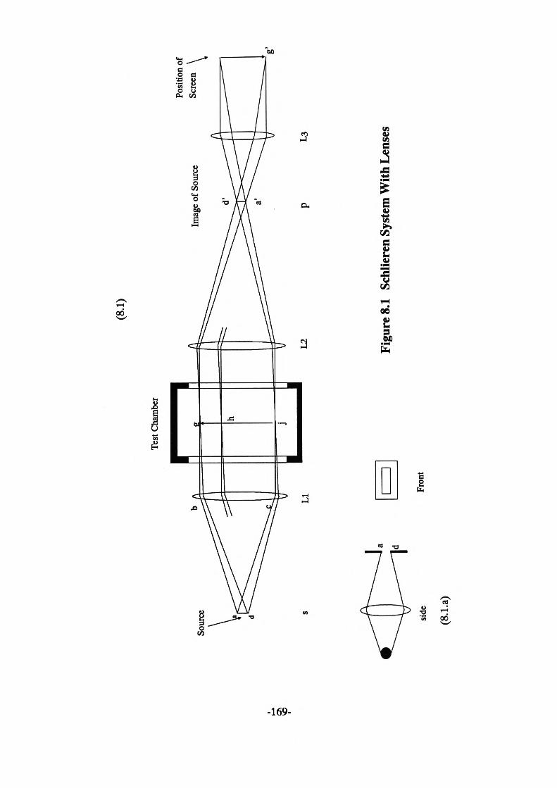
(8.1

)

Sour

ce

Test

Cham

ber

Imag

e of S

ourc

e

L3

Posit

ion

of

Scre

en\

Fron

t

Figu

re 8.

1 Sc

hlier

en S

yste

m W

ith L

ense

s

in p. It should be noted however that each projected beam of light completely fills the

whole of the test section and hence each point in the image receives light from every portion

of the test section.

Furthermore, the light reaching a point, g, in the test section via projection from a and d

namely adg, is transmitted within gd'a', which is focused at, g', on the viewing screen.

This beam passes through the image plane, p, and completely fills it. Other beams from

the test section are also focused at their image points on the screen and can subsequently

an image of the test section is produced there.

As described and shown in figure (8.1) all the beams of light overlap in plane,/?. Therefore

if part of the light is obscured at this plane, only the intensity of the illumination of the

final screen is reduced. All parts are however darkened at the same rate since all the beams

are affected equally.

Now if one of the beams is deflected by a linear angle 6 at the test section due to a refractive

index change, figure (8.2), then it would not overlap the other beams at the focal plane of

L2 and its image point on the screen will be darkened by a different amount which will

result in a darker or lighter point compared with the rest of the field [4]. This of course

depends on the position of the displaced image at the knife edge.

Assuming that the distance along the pencil is f2, the focal length of lens L2, then the

displacement M, figure (8.2), due to angular displacement 0 can be approximated for small

angles as [4,5] :

8.1

-170-

Considering a perpendicular axis, A/, as shown in figure (8.2) could be calculated in a

similar manner.

The knife edge is set parallel to the long side of the slit and hence its image at the plane,

p is as shown in figure (8.3). This leaves a portion h} of the image uncovered. The intensity

of illumination of the screen, /, is therefore proportional to ft; . If a point on the screen then

has an additional illumination A/ imposed upon it (due to the deflected beam) then A/

would be proportional to the displacement Aft. A contrast may then be defined as [4,5]:

A/ Aftc = — = — 8.2 1 ftj

by substituting for Aft in terms of f2 and 6, c becomes:

C ° T~ 8'3

Considering interactions across a test area L it has been shown [4] that for a plane flow

(ie. where conditions are the same in all ^-planes), the angle of deflection 6 after a ray has

passed through a box with density variation in the y direction, figure (8.4), may be given

by the following relationship:

8.4

L represents the total interaction length and is given by the width of the box which is the

distance the rays travel before emerging from the box. p and p^ are parameters which

determine the refractive index and according to:

n •= 1 -4- R — 8 5 P,

p is the actual density and p,is a reference density [4] for the particular gas in the medium

measured at standard conditions which for a temperature of 0 °C, pressure of 760 mmHg

and at a wavelength of 5893 A. R is a dimensionless quantity [4] which for example for

-171-

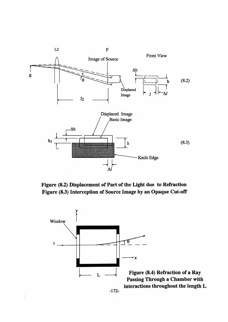
tDisplaced Image

Displaced Image Basic Image

Front View

L——.1h

Knife Edge

(8.2)

(8.3)

Figure (8.2) Displacement of Part of the Light due to Refraction Figure (83) Interception of Source Image by an Opaque Cut-off

Window

-172-

Figure (8.4) Refraction of a RayPassing Through a Chamber with

interactions throughout the length L

air at 5893 .A is equal to 2.92xlO's . It can therefore be seen that the contrast on the screen

is a function of density gradients, density and refractive index in the test section given by:

c -•

An increase or decrease in the intensity of illumination at the viewing screen is directly

proportional to the density changes in the flow.

In order to obtain a large field of view, a large aperture lens would be required [6]. Designers

have therefore developed Schlieren apparatus where lenses are replaced by a system of

mirrors which are cheaper to produce. The internal quality of glass is also not of great

importance in mirrors and at the same time less light is lost in a mirror than in a lens [5].

Of course by using mirrors the chromatic errors normally associated with lenses are avoided

[6].

8.3 Experiments for the Estimation of the Convection Coefficients

A Schlieren apparatus was used to examine the convection plumes forming over the

partially heated PCB boards. This was done in order to ascertain the variation of the

convection coefficient over the surface and how it is possible to simplify the definition of

this parameter in the ASTEC3 thermal model of the structure.

-173-

8.3.1 Apparatus

The apparatus used in this experiment also utilised mirrors. A schematic layout of the

system is shown in figure (8.5). The various components of the apparatus were as follows:

Mirrors

These were very high quality spherical mirrors which were vacuum deposited with very

thin layer of metallic aluminium.

Light source

The light source was a 36 Watt bulb with a single straight axial filament. This is important

since bulbs with V-shaped filaments cannot be used for this application. A condenser lens

and a collimating slit were used to ensure that the bundle of rays passing the cut-off at the

focus of mirror Ml was truly rectangular.

The Cut-off

A razor blade was used for the knife-edge. It was mounted such that it could be positioned

accurately in the focus of mirror M2 using micrometer screws.

Projector Lens and Viewing Screen

A projecting lens L2 was used to direct the image from the cut-off onto a ground glass

screen. A tube between the lens and the screen prevented stray light falling onto it and also

provided a focusing adjustment.

-174-

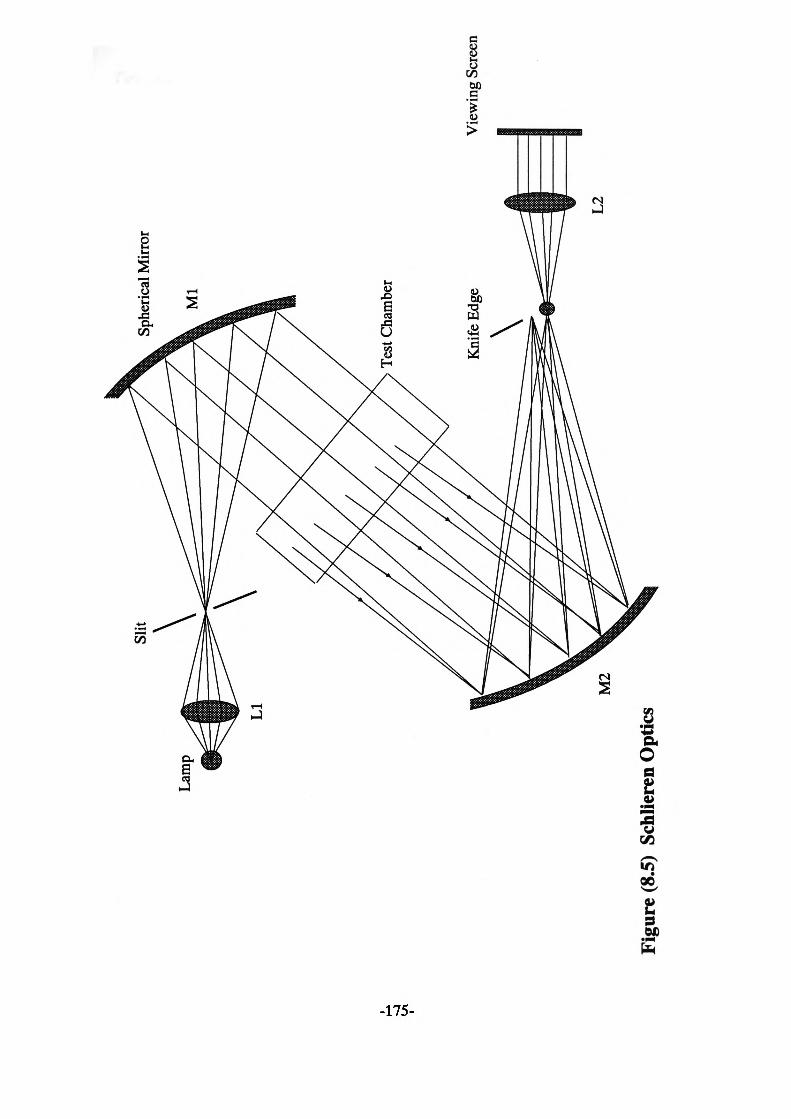
Slit

Lam

p

M2

Sphe

rical

Min

or

Ml

Figu

re (8

.5) S

chlie

ren

Opt

ics

L2

Vie

win

g Sc

reen

Test Section

A box was made almost the same size as the one used for temperature measurements in

chapter (6). It was large enough to stop the plume being affected by reflected fields from

the walls of the chamber. Two square holes were cut into two opposite vertical faces of

the box large enough to allow the parallel beam of light to pass through it. Unused

photographic plates were fixed at these positions and the test chamber was sealed very

carefully to avoid any draughts from the room.

8.3.2 Experimental Procedure

The following steps were taken to set up the system [7]:

a The position of the condenser lens LI with respect to the bulb was adjusted until a sharp

image of the filament was observed on the knife edges of the slit. Micrometer screws were

then used to centralise the slit within the image of the filament.

b The light source assembly was tilted and rotated on its base until the beam emerging

from the slit was horizontal and filled the mirror Ml. The distance between the centre of

the mirror and the slit was then adjusted to the focal length of the mirror.

c The height of mirror Ml was adjusted so that the beam of light deflected was parallel

and passed through the windows of the test box. To check if the beam was parallel and

horizontal, a piece of paper was placed on the window and the attitude of the mirror adjusted

until the disc of light on the paper was circular. The slit assembly was then moved very

slightly backwards and forwards until the diameter of the disc of light was the same as the

mirror.

-176-

d The height of the second mirror at the other side of the test chamber was adjusted so

that the beam of light just filled it.

e The lens L2/screen assembly was positioned so that a clear and bright image could be

viewed on the screen.

/ The focal plane of mirror M2 was found using a piece of paper and the knife-edge

assembly was placed in this position. The cut-off was then used to obscure a portion of

the image at the plane/?. When the set-up was carried out correctly, the illumination of the

picture on the viewing screen was uniform and no matter what proportion of light rays

were obscured it stayed uniform.

8.33 Tests and results

The results from the Schlieren apparatus were in the form of photographs which were taken

from the ground-glass viewing screen. A 35 mm Single Lens Reflex (SLR) camera fitted

with a macro-lens was used for this purpose. The camera was mounted onto a sturdy tripod

to reduce the risk of camera-shake during the long exposures needed for photographing

the fairly dark screen. Furthermore, 400 ASA Black & White films were chosen as a

compromise between the film speed and the subsequent grain size in the final prints.

Some of the enlarged photographs were found to be very faint and in order to enhance the

shape of the plume in the photographs, further processing was carried out on the prints.

A Desk Top Publishing Package called PUBLISHS PAC™ was used for this purpose. This

is a software package which allows any form of print or text to be scanned via a line scanner.

The scanner breaks the image into a number of pixels which can be preset by the user with

a maximum of 300 dpi (Dots Per Inch) as used here. A Black & White bit-map

-177-

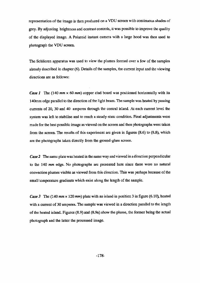
representation of the image is then produced on a VDU screen with continuous shades of

grey. By adjusting brightness and contrast controls, it was possible to improve the quality

of the displayed image. A Polaroid instant camera with a large hood was then used to

photograph the VDU screen.

The Schlieren apparatus was used to view the plumes formed over a few of the samples

already described in chapter (6). Details of the samples, the current input and the viewing

directions are as follows:

Case 1 The (140 mm x 60 mm) copper clad board was positioned horizontally with its

140mm edge parallel to the direction of the light beam. The sample was heated by passing

currents of 20, 30 and 40 amperes through the central island. At each current level the

system was left to stabilise and to reach a steady-state condition. Final adjustments were

made for the best possible image as viewed on the screen and then photographs were taken

from the screen. The results of this experiment are given in figures (8.6) to (8.8), which

are the photographs taken directly from the ground-glass screen.

Case 2 The same plate was heated in the same way and viewed in a direction perpendicular

to the 140 mm edge. No photographs are presented here since there were no natural

convection plumes visible as viewed from this direction. This was perhaps because of the

small temperature gradients which exist along the length of the sample.

Case 3 The (140 mm x 120 mm) plate with an island in position 3 in figure (6.10), heated

with a current of 30 amperes. The sample was viewed in a direction parallel to the length

of the heated island. Figures (8.9) and (8.9a) show the plume, the former being the actual

photograph and the latter the processed image.

-178-

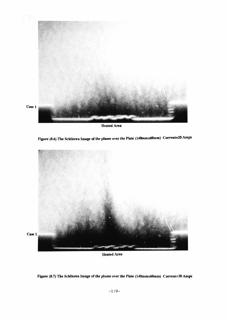
Casel

Heated Area

Figure (8.6) The Schlieren Image of the plume over the Plate (140mmx60mm) Current=20 Amps

Casel

Heated Area

Figure (8.7) The Schlieren Image of the plume over the Plate (140mmx60mm) Current=30 Amps

-179-

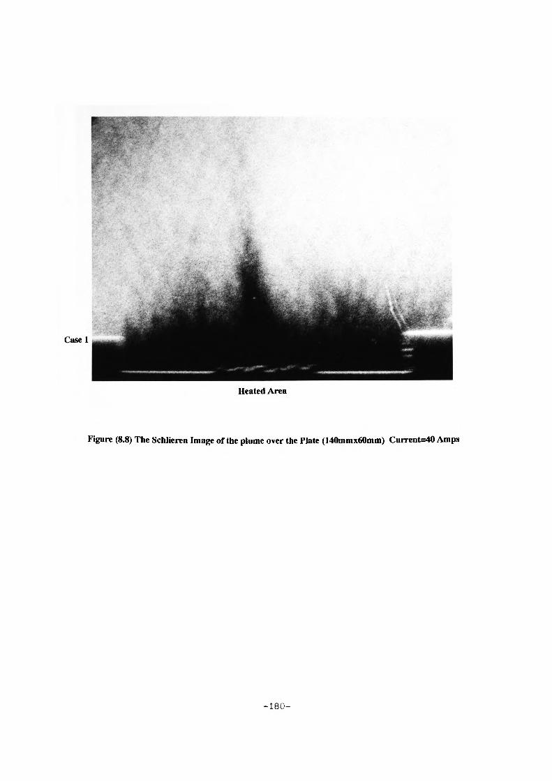
Casel

Heated Area

Figure (8.8) The Schlieren Image of the plume over the Plate (140mmx60nim) Current=40 Amps

-180-

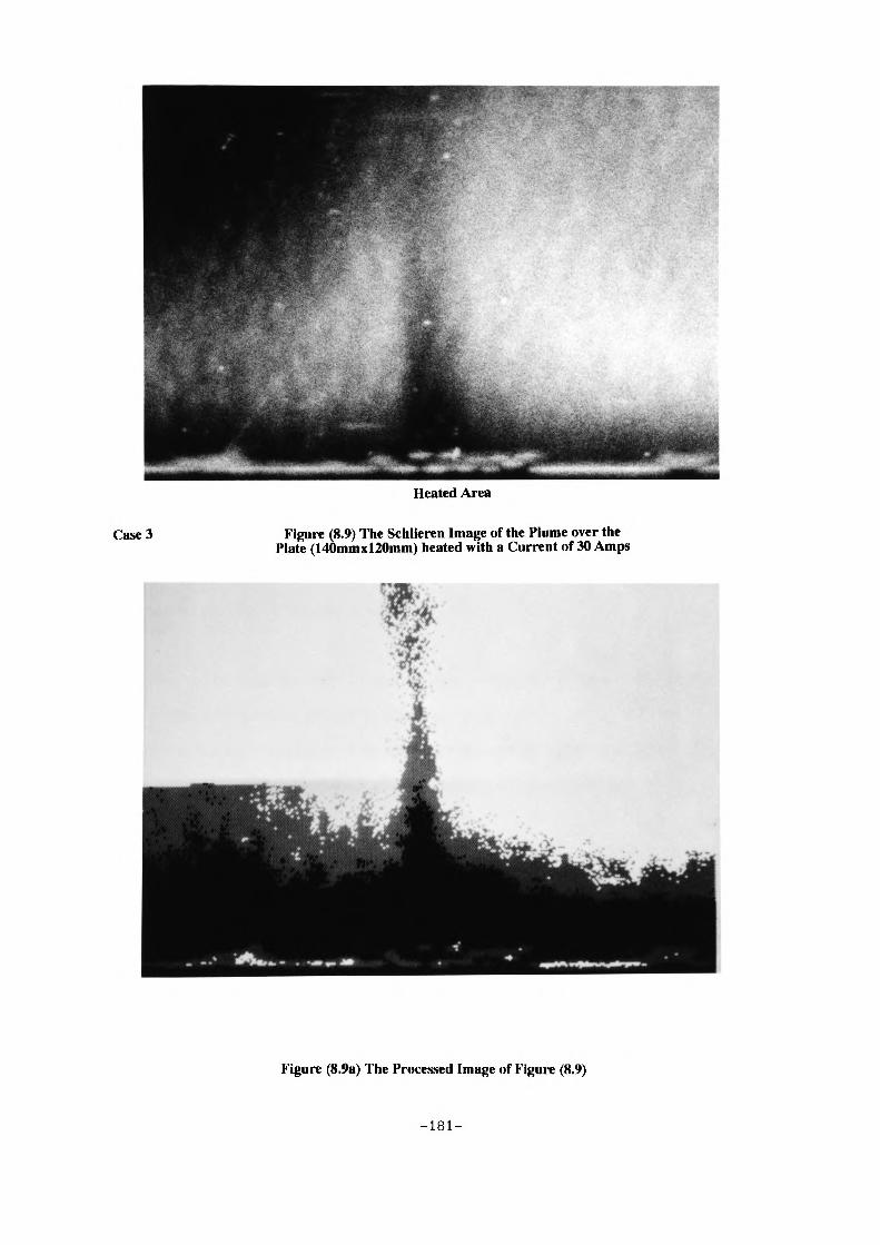
Heated Area

Case 3 Figure (8.9) The Schlieren Image of the Plume over the Plate (140mmxl20mm) heated with a Current of 30 Amps

Figure (8.9a) The Processed Image of Figure (8.9)

-181-

Case 4 The plate with two heated islands as shown in figure (6.6) was heated by passing

currents of 30 and 10 amperes through the (100 mm x 20 mm) and (40 mm x 20 mm) islands

respectively. The corresponding images are given in figures (8.10) and (8.10a).

In case 1 as the current was increased an increase in the thickness of the boundary layer

was observed thought to be due to the increase in the surface temperature. The steady-state

photographs were however similar in that they could all be divided into three main sections.

Two almost horizontal boundary layers extended from the edges of the plates along the

unheated, cooler areas to the edges of the resistor region. The two boundary layers then

met in the middle section and rose in the form of a chimney.

The absence of plume in case 2 seems to be due to the lack of an appreciable temperature

gradient along the plate and hence an observable density gradient.

The observed plume in case 3 above was very similar in nature to that described for case

1 with thinner boundary layers due to lower surface temperatures. These layers met at the

hot resistor and rose in the form of a chimney.

The shape of the boundary layer in case 4 was of similar form to the rest of the samples.

The plume seemed to stay parallel to the plate over the smaller (40 mm x 20 mm) island

which was due to the small size of the island and the corresponding small joule heating in

that region. This was not producing enough heat for a distinct plume rise.

These observations lead to a very important conclusion that for the ASTEC3 simulation

of the thermal behaviour of the heated plates, it is necessary to define only two values of

heat transfer coefficient, one for the unheated areas and one for the resistor area. This will

of course simplify the modelling of the convection part of the heat flow problems.

-182-

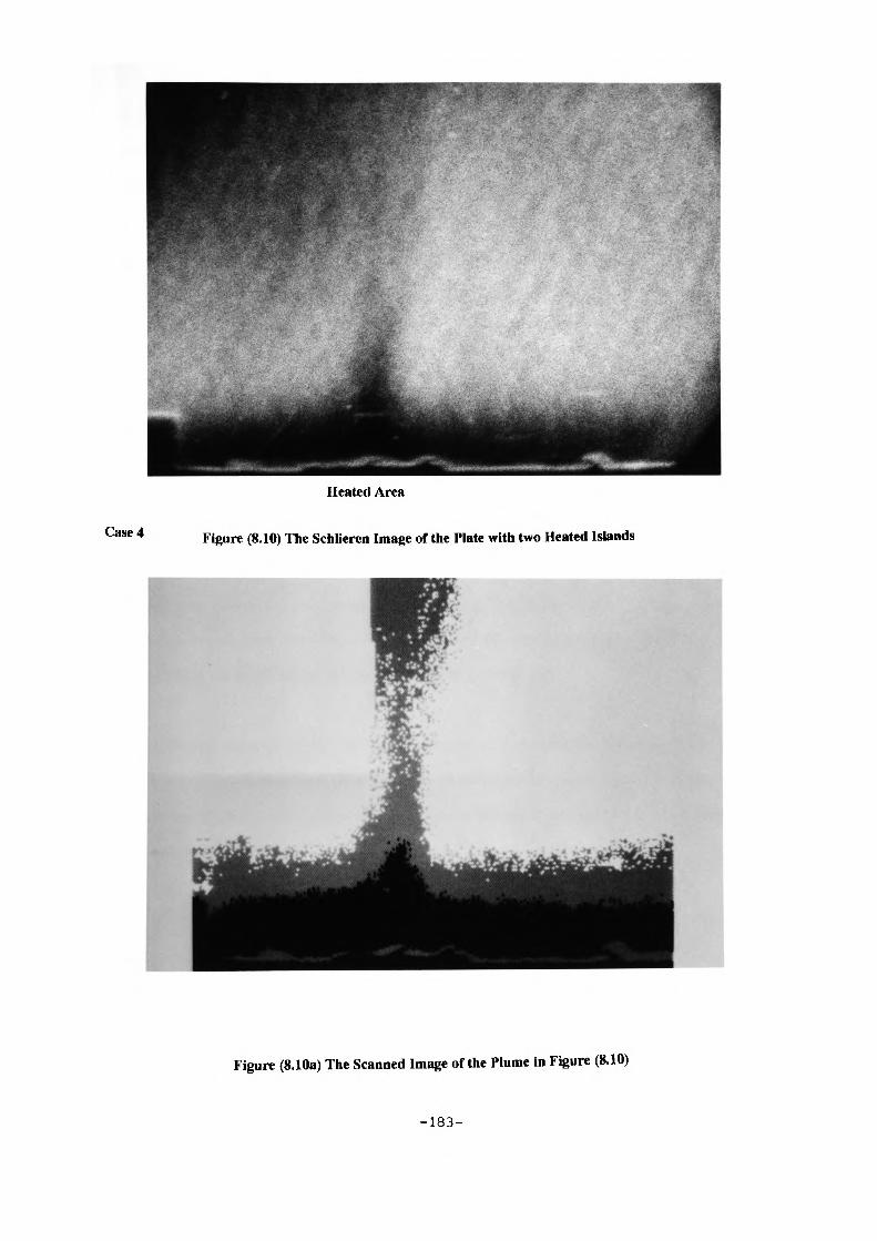
Heated Area

Case 4 Figure (8.10) The Schlieren Image of the Plate with two Heated Islands

Figure (8.10a) The Scanned Image of the Plume in Figure (8.10)

-183-

8.4 Determination of the Optimum Mesh Resolution

A further study was carried out to establish the effect of reducing the size of the thermal

cell used in the modelling of the structure and hence increasing the model resolution. The

(60 mm x 140 mm) plate shown in figure (6.11) with a heated island of dimensions (20

mm x 100 mm) was used for this purpose. The heat transfer coefficients for the losses from

the surface due to convection and radiation were kept the same as those calculated in the

preliminary experiments described in section (6.1.3). These values were acceptable for

this particular test since only the effect of resolution was being studied.

The structure was divided into seven increments in each of the two layers, along the length

of the specimen. The width of the layers (60 mm edge) however was divided into more

and more increments namely 3,9,27 and finally 81 strips. The meshes with 3 and 9 divisions

are shown in (a) and (b) respectively in figure (8.11).

The temperatures of two points were simulated: that of the middle point of the heated strip,

T2, and also the adjacent unheated section, J; as shown in figure (8.11). The simulated

temperatures of these two points were then plotted against the corresponding number of

strips along the width of the sample as shown in figure (8.12).

It can be seen from the graph that the temperatures of these two points vary considerably

as the resolution is increased from very low (3 strips) up to around 27 strips. They then

become asymptotic and around 81 strips the variations in the simulated temperatures

become negligible.

Furthermore, the percentage errors in the simulated temperatures compared with the

experimental results were calculated for the two points T, and T2 in figure (8.11) at each

-184-

60

^-

mmhi

h2

140 mm100mm Wfl

»T2

hi

(a)

3 Divisions T2

(b)

9 Divisions

Figure (8.11) Block Diagram of the Sample used for Simulation Tests at Different Resolutions

-185-

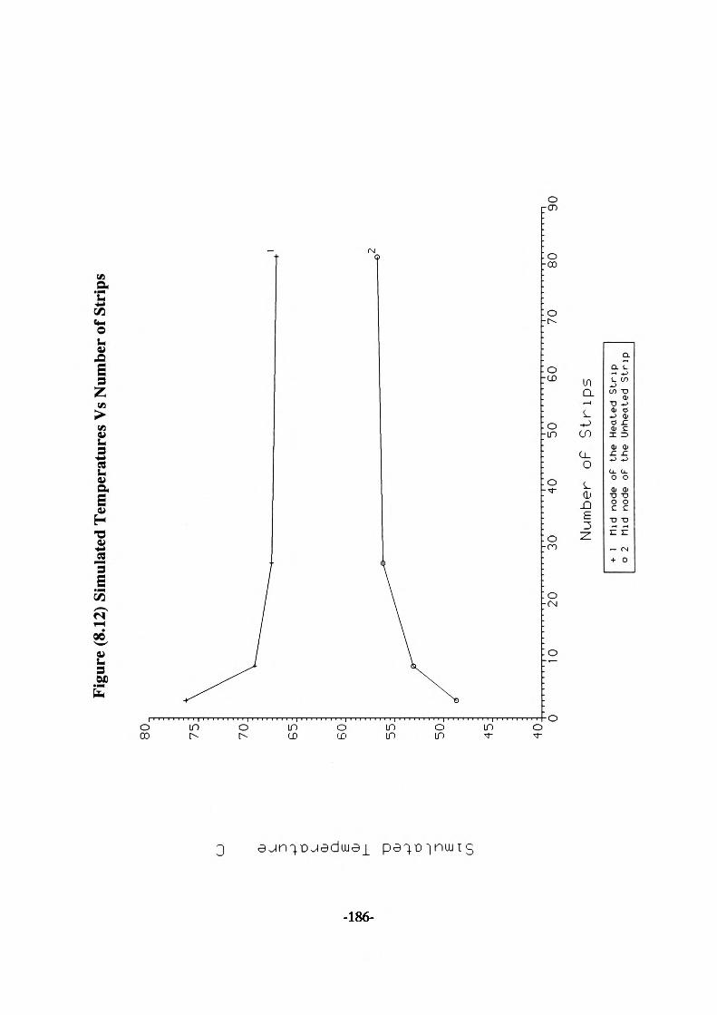
-981-

Simulated TemperatureC

o o--& ui e/1 ui o ui

en en o uioo o

O trs) —

a a3 3 O Oa a rt) fp

o o T> T)

r* r>

1) 11

C X 3 tJ O

O 11 c- aQ. C/1

(/I T•> "D

•o

C 3CT0)

O

COcr*"5t— '

TDUI

o

N> o

COo

.& o

UIo

CD O

V) o

00o

O)-Io

sore'c3 «h*

^Cfl •••

S, 5"

ss 1! 9CA

zc3a-fDno "^»

I01

resolution. The results are shown in figure (8.13) as the percentage error in the results

versus the total number of strips along the 60 mm edge of the plate. These results show

very clearly that the resolution induced errors are reduced to negligible levels when the

number of strips exceeds 27 per island. This is the near optimum resolution which was

used for further experiments.

8.5 Determination of heat transfer coefficient values

Using the optimum resolution level, further tests were carried out to obtain the best values

of heat transfer coefficient for the least error in the simulated results compared to the

experimentally measured temperatures. In all these simulations a value ht is used for the

combined convective and radiative coefficients from the heated region and h2 ioi the

remaining unheated areas. This approach is justified from the Schlieren experimental

results which show an almost laminar flow over the unheated areas of the plate and a sharp

rise in the central heated region leading to the suggestion that the convection coefficients

may be approximated by two values over the surface of the plate. After each simulation a

value was calculated for V%A7\2 + %AjT| where %AT, and %AJ2 are the percentage errors

in T, and T2 compared with experimentally measured values of 76.0 °C and 51.4 "C

respectively for an input current of 30 amps.

The simulations were carried out for hj and h2 values ranging from 0 to 26 W/m2K and a

matrix of error results was obtained for each combination ofhj/h2. In the first instance, the

range was divided into coarse steps of h}/h2 values and using the square-root error as a

guide, the steps were then reduced in the portion of the range where this error was smallest.

This was carried out until the square-root error was reduced to near zero.

The results of the above tests are plotted as shown in figure (8.14) where the x and y axes

-187-

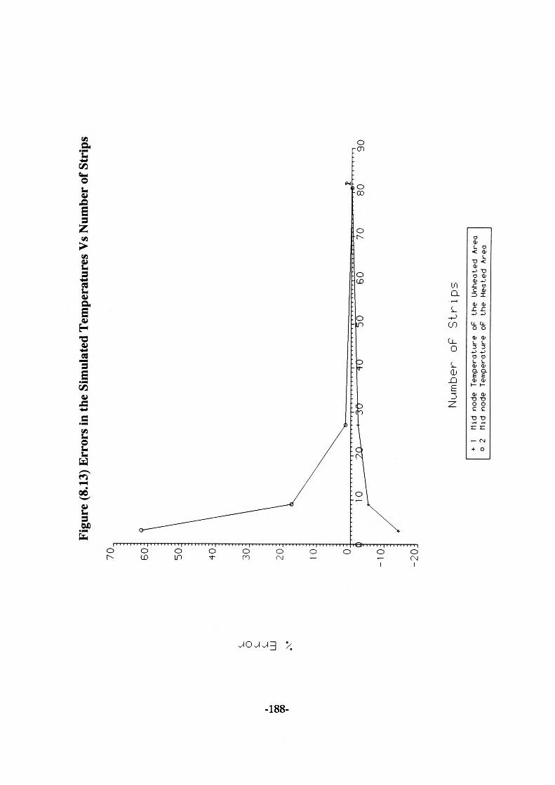
Figu

re (8

.13) E

rror

s in

the S

imul

ated

Tem

pera

ture

s Vs N

umbe

r of S

trip

s

•L

LU

70 eo;

50

:

40.

30J

20:

10

.

Num

ber

oF

Str

ips

+ I

Mid

node

Te

mper

atur

e oF the

Unhe

ated

Area

o 2

Mid

node Te

mper

atur

e oF

th

e Heated Area

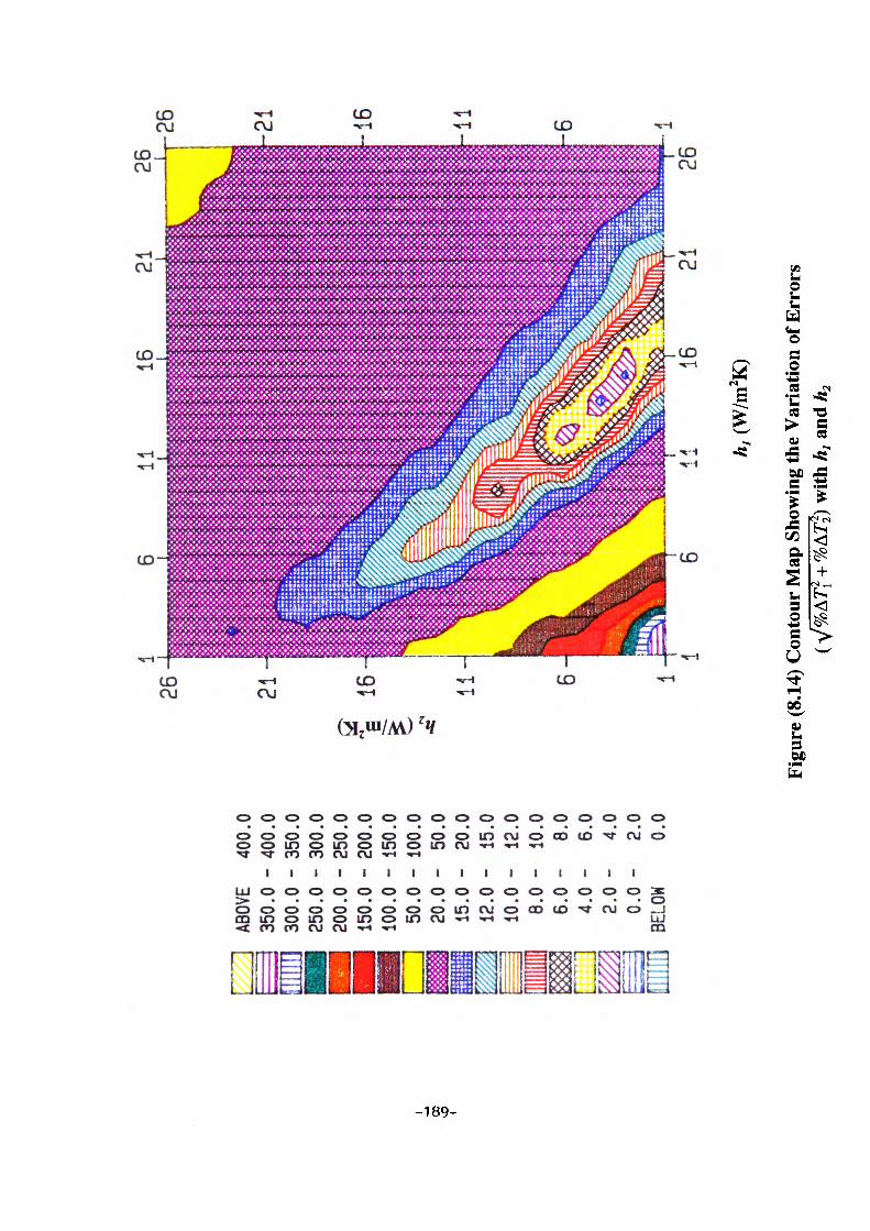
I 00 I

n

ABOV

E 35

0.0

- 300.0

- 25

0.0

- 200.0

- 150.0

-

400.

0

100 50

.020

.015

.012

.010

0 -

0 -

8.0

6.0

4.0

2.0

0.0

BELO

W

400

350

300

250.

020

0.0

150.

010

0.0

50.0

20.0

15.0

12.0

10.0 B.O

6.0

4.0

2.0

0.0

26 21

26

h, (

W/m

2K)

Figu

re (8

.14)

Con

tour

Map

Sho

win

g th

e V

aria

tion

of E

rror

s (V

%A

7fT%

A7?

) w

ith h

f and

h2

are the /J7 and h2 values and the z axis is the error. These plots were obtained using a

graphics package called UNIRAS which is available on the Vax computers. This is a

state-of-the-art graphics system which consists of various subroutine libraries, capable of

producing contour maps and three-dimensional distribution plots. These may be

colour-coded plots with each colour representing a range of values for the parameter in

the z axis.

The ht and Rvalues of 13.5 and 4 W/m2K respectively were found to reduce the square-root

of the sum of the percentage errors to 0.33. This suggests that the heat transfer rate from

the unheated, cooler region in the plate is 3.375 times greater than from the central heated

island.

8.6 Simulation of the Original Test Configuration using the Optimised Convection

Coefficients

An ASTEC3 model of the plate was developed to include the anisotropy in the thermal

conductivity of the fibre glass laminate as found in chapter (7), the optimum resolution

level (81 strips along the width of the plate) and the convection coefficients obtained in

the previous section. A selected number of simulation results are shown in figure (8.15)

relating to the same data points as the original test in figure (6.11). These are the centre

points of the cells if the plate was divided into a (7x3) mesh as in figure (6.11). The top

figure represents the experimentally measured temperature and the bottom figure the

simulated value. The figure in bold gives the percentage error between the measured and

the corresponding simulated temperature for each individual data point.

-190-

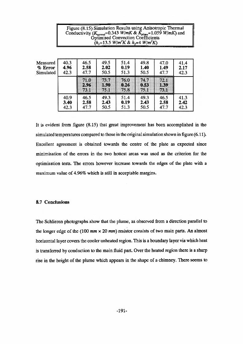
Figure (8.15) Simulation Results using Anisotropic ThermalConductivity (ADonn.,=0.343 W/mK & Ap/(We=1.059 W/mK) and

Optimised Convection Coefficients(h,=l3.5 W/m2K& h2=4 W/m2K)

Measured % Error Simulated

40.34.9642.3

40.93.4042.3

46.52.5847.7

^TKT™46.52.5847.7

49.52.0250.5

::-::::::f£f:S :::::::::

49.32.4350.5

51.40.1951.3

:::: K ::::f5< g:,S:,:

51.40.1951.3

49.81.4050.5

,:«^;|,::,:,:

49.32.4350.5

47.01.4947.7

lilliil:x ''' :^lill

46.52.5847.7

41.42.1742.3

41.32.4242.3

It is evident from figure (8.15) that great improvement has been accomplished in the

simulated temperatures compared to those in the original simulation shown in figure (6.11).

Excellent agreement is obtained towards the centre of the plate as expected since

minimisation of the errors in the two hottest areas was used as the criterion for the

optimisation tests. The errors however increase towards the edges of the plate with a

maximum value of 4.96% which is still in acceptable margins.

8.7 Conclusions

The Schlieren photographs show that the plume, as observed from a direction parallel to

the longer edge of the (100 mm x 20 mm) resistor consists of two main parts. An almost

horizontal layer covers the cooler unheated region. This is a boundary layer via which heat

is transferred by conduction to the main fluid part. Over the heated region there is a sharp

rise in the height of the plume which appears in the shape of a chimney. There seems to

-191-

be no boundary layer present in this section of the plume and no reference has been found

to any work investigating the nature of the flow in the region close to the surface at the

bottom of the chimney.

It may be suggested that the heat loss from the hot region occurs via the particles gaining

energy from the hot surface and bouncing off due to buoyancy forces. This is almost like

pieces of burnt paper and wood in the middle of a bonfire being thrown into the air. The

rate at which this phenomenon may occur is dependent on the number of particles of air

present near the surface which is in turn a function of the density of air in that region. The

air density is of course dependent on the temperature of the air close to the plate which

being high, reduces the number of particles in that vicinity.

From the above analysis it may be concluded that the heat transfer rate and hence the

convective heat transfer coefficient in the central region are much smaller than in the

unheated section which has a conductive boundary layer.

Further evidence has been gained by simulating the original experimental structure (§6.4)

with varying heat transfer coefficient values. It has been shown for instance that for the

(140 mm x 60 mm) plate it is very plausible that a difference may exist between the

convection coefficients in the heated island and the outer unheated region. It is also shown

that a ratio of 3.375 to 1 (unheatedrheated) is a possible ratio for the two coefficients.

Application of this ratio to the original test configuration has produced excellent agreement

with the experimentally measured temperatures. A combination of anisotropic thermal

conductivity, reduction in the thermal cell size and the optimised convection coefficients

has reduced the errors to a minimum of 0.19% around the centre of the plate and a maximum

of 4.96% at one edge.

-192-

9 EXPERIMENTAL MEASUREMENTS AND SIMULATION TESTS

ON HYBRID CIRCUITS

9.1 Introduction

Following the detailed investigations on large scale structures and the successful simulation

results, it was necessary to use the ASTEC3 modelling procedure to study the thermal

characteristics of small scale devices.

In order to investigate the effect of reducing the size of the test structures on simulations,

it was decided to design the hybrid resistor samples using the same patterns as the macro

scale but reduced in size. Royal Signals and Radar Establishment (R.S.R.E) agreed to

manufacture the required samples. The test specimens were designed by using the standard

thick film resistor width of 0.040 inches (1.016 mm) as specified by R.S.R.E. The equivalent

width in macro scale 20 mm. The ratio of these two figures, ie. 1.016/20, was used to scale

all the other dimensions in the reduced case. For example, the hybrid device resembling

the PCB plate (140 mm x 60 mm) with a symmetrically situated island of (100 mm x 20

mm) was scaled to (7.112 mm x 3.048 mm) with a resistor size of (5.08 mm x 1.016 mm).

All the samples (A to E) are illustrated in figure (9.1) with their dimensions.

9.2 Sample Preparations

The resistor samples produced by R.S.R.E were all prepared using the materials given

below. The relevant parameters and production techniques are included where applicable.

-193-

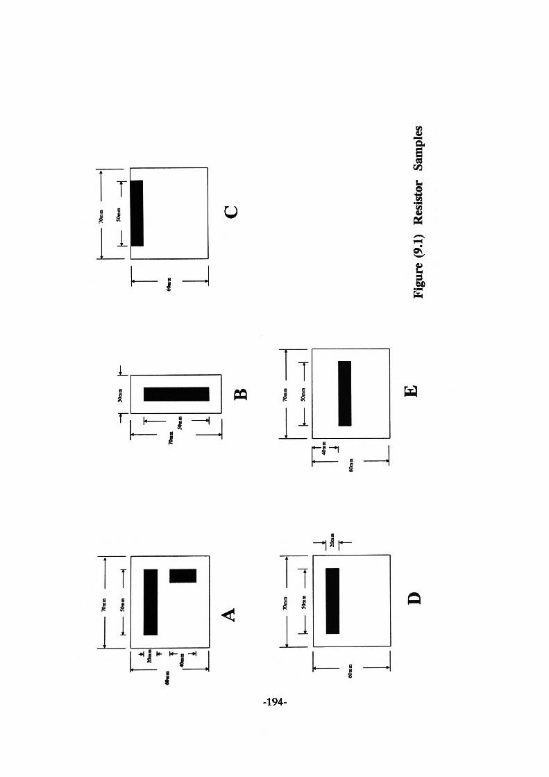
i

20nm T T 1

70mm

50mm

I

—«J

30

mm

U—

T70

mm50

mm 1

B

1

v60

mm

TOmn

50m

n

J 20m:

120mm

70m

in

50m

n

60mm

DE

Figu

re (9

.1)

Resis

tor

Sam

ples

Substrate

White alumina ceramic substrates ( Code No. ADS-96R PER CPC-STD-49) were used

as the base for the resistors [1]. The substrates were 0.025 inch (635 \uri) thick with 96%

concentration of Al2O3 and a thermal conductivity of 20 W/mK at 100 °C [1].

Resistor

Thick film resistor material from the BIROX 1400 series resistor composition made by

Du Pont Electronic Materials [2] was used for this purpose. These materials are produced

with resistivities ranging from 10 Q/square to 1 MQ/square. The 1 fcQ/square type was

chosen by R.S.R.E to match the design specifications. The thermal conductivity of the

1400 series resistor material is related to its resistance varying from 2 W/mK for sheet

resistance of 10 Q/square to 1 W/mK for sheet resistance of 10 MQ/square [3]. The two

parameters have a fairly linear relationship between these two extremes [3] yielding a

thermal conductivity of 1.999 for the 10 &Q/square resistor.

The resistors were printed onto the substrate to 25 ± 3 \un dried print thickness using a

200-mesh stainless steel screen. The prints were allowed to level for 5 to 10 minutes at

room temperature and dried for 15 minutes at 150 °C. The printing was followed by a 60

minute firing cycle with 10 minutes at a peak temperature of 850 °C.

Package

The packages used were of 24-pin type made of black ceramic with 90 % A12O3 purity and

with a thermal conductivity of 24.29 W/mK [4]. The substrates were adhered to the package

using a very thin layer of electrically insulating adhesive made by Ablestic Laboratories.

-195-

This was the Ablebond 41-4 type with a thermal conductivity of 0.52 W/mKat 121 °C [5].

Electrical connections to the chip were made via gold bonding wires which were attached

to the contact pads at the ends of the resistors. Each bond wire was then connected to

another pad on the package using a standard ball-joint bonding technique which was

subsequently routed internally to one of the pins. A typical carrier assembly is shown in

figure (9.2) with the substrate in position.

9.3 Temperature Measurement System

The samples were tested using thermal imaging equipment manufactured by AGEMA.

The particular model was from their Thermovision 800 series comprising an 880 infrared

scanner unit [6] which has an In-Sb liquid Nitrogen-cooled infrared detector. The unit can

be fitted with a wide range of bayonet-mount lenses which make it possible to adapt the

system to different measurement situations. A 38 mm lens with a 20 ° field of view was

found to adequately cover the size of the samples used here.

The Thermovision 880 system is a real-time thermal imaging device capable of surface

temperature measurements and analysis of dynamic and static thermal patterns. The

infrared radiation emitted by the object is detected by the scanner and subsequently

converted into an electrical video signal. The surface of the object is scanned 25 times per

second which produces a real-time TV-like thermal image of the object. A temperature

accuracy of ± 2 % or ± 2 "C is guaranteed by the manufacturers [6].

The thermograms were displayed on a colour video monitor with a colour chart alongside

the image displaying temperature readings in 3 °C intervals as detailed later. If a more

-196-

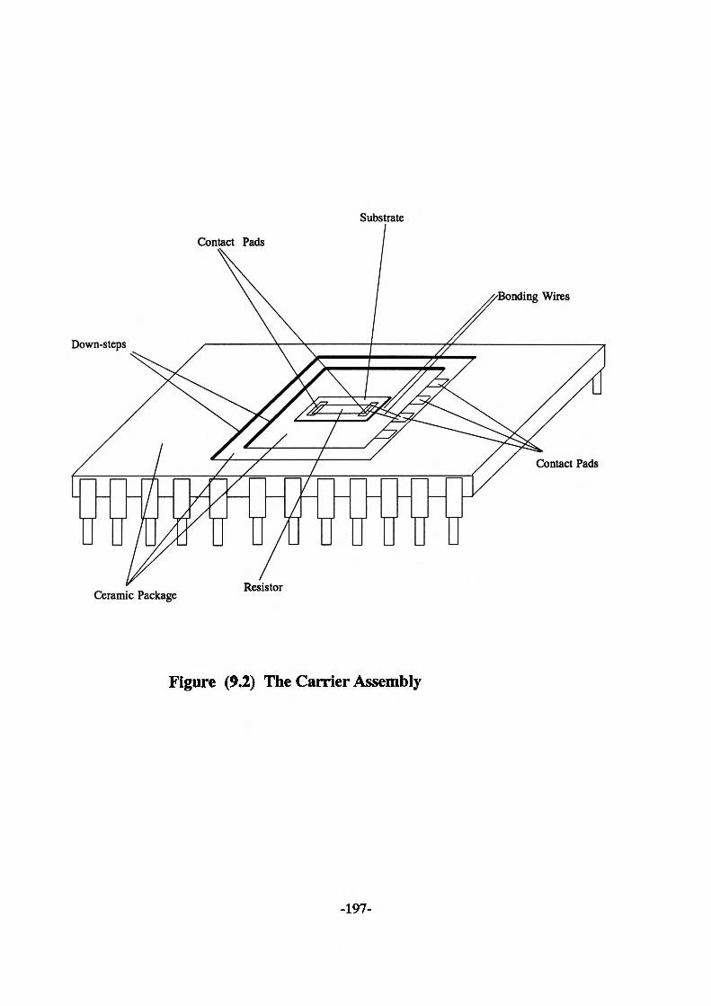
Substrate

Contact Pads

Down-steps

nu/u/ru n u uu uCeramic Package Resistor

nding Wires

Contact Pads

Figure (9.2) The Carrier Assembly

-197-

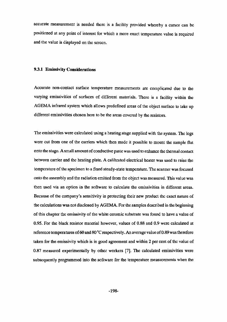
accurate measurement is needed there is a facility provided whereby a cursor can be

positioned at any point of interest for which a more exact temperature value is required

and the value is displayed on the screen.

9.3.1 Emissivity Considerations

Accurate non-contact surface temperature measurements are complicated due to the

varying emissivities of surfaces of different materials. There is a facility within the

AGEMA infrared system which allows predefined areas of the object surface to take up

different emissivities chosen here to be the areas covered by the resistors.

The emissivities were calculated using a heating stage supplied with the system. The legs

were cut from one of the carriers which then made it possible to mount the sample flat

onto the stage. A small amount of conductive paste was used to enhance the thermal contact

between carrier and the heating plate. A calibrated electrical heater was used to raise the

temperature of the specimen to a fixed steady-state temperature. The scanner was focused

onto the assembly and the radiation emitted from the object was measured. This value was

then used via an option hi the software to calculate the emissivities in different areas.

Because of the company's sensitivity in protecting their new product the exact nature of

the calculations was not disclosed by AGEMA. For the samples described in the beginning

of this chapter the emissivity of the white ceramic substrate was found to have a value of

0.95. For the black resistor material however, values of 0.88 and 0.9 were calculated at

reference temperatures of 60 and 80 °C respectively. An average value of 0.89 was therefore

taken for the emissivity which is in good agreement and within 2 per cent of the value of

0.87 measured experimentally by other workers [7]. The calculated emissivities were

subsequently programmed into the software for the temperature measurements when the

-198-

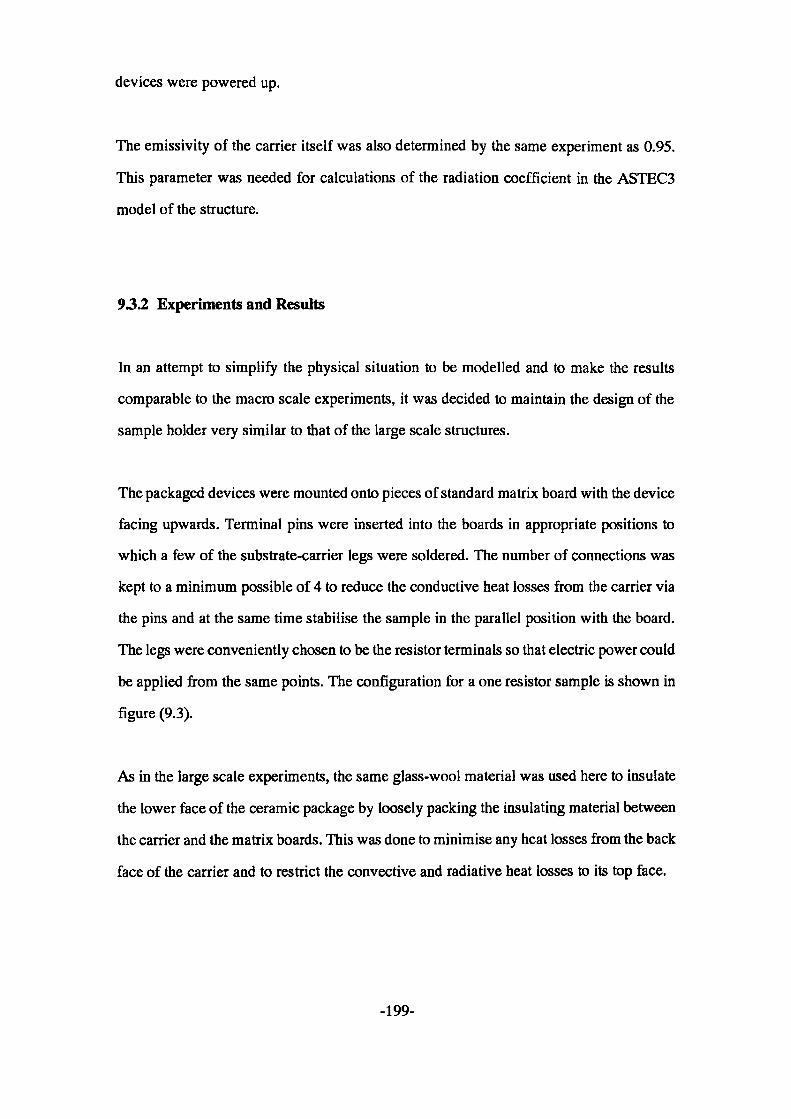
devices were powered up.

The emissivity of the carrier itself was also determined by the same experiment as 0.95.

This parameter was needed for calculations of the radiation coefficient in the ASTEC3

model of the structure.

9.3.2 Experiments and Results

In an attempt to simplify the physical situation to be modelled and to make the results

comparable to the macro scale experiments, it was decided to maintain the design of the

sample holder very similar to that of the large scale structures.

The packaged devices were mounted onto pieces of standard matrix board with the device

facing upwards. Terminal pins were inserted into the boards in appropriate positions to

which a few of the substrate-carrier legs were soldered. The number of connections was

kept to a minimum possible of 4 to reduce the conductive heat losses from the carrier via

the pins and at the same time stabilise the sample in the parallel position with the board.

The legs were conveniently chosen to be the resistor terminals so that electric power could

be applied from the same points. The configuration for a one resistor sample is shown in

figure (9.3).

As in the large scale experiments, the same glass-wool material was used here to insulate

the lower face of the ceramic package by loosely packing the insulating material between

the carrier and the matrix boards. This was done to minimise any heat losses from the back

face of the carrier and to restrict the convective and radiative heat losses to its top face.

-199-

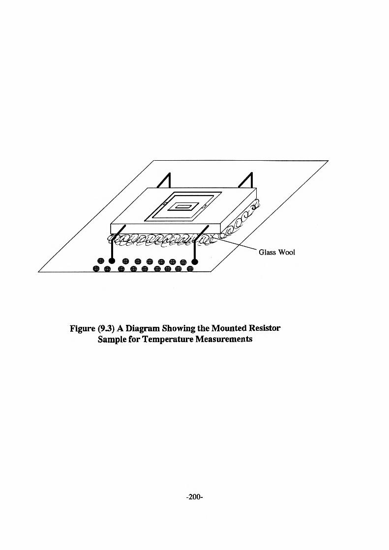
Glass Wool

Figure (9.3) A Diagram Showing the Mounted Resistor Sample for Temperature Measurements

-200-

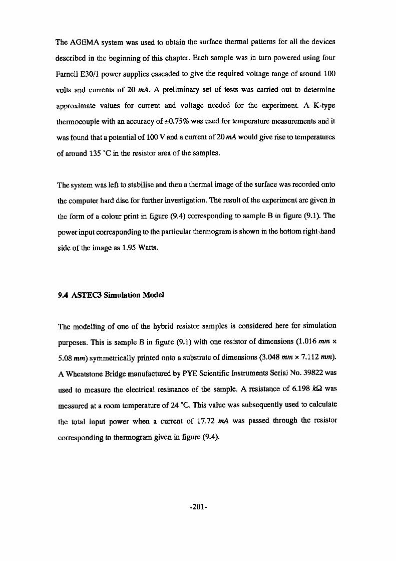
The AGEMA system was used to obtain the surface thermal patterns for all the devices

described in the beginning of this chapter. Each sample was in turn powered using four

Farnell E30/1 power supplies cascaded to give the required voltage range of around 100

volts and currents of 20 mA. A preliminary set of tests was carried out to determine

approximate values for current and voltage needed for the experiment. A K-type

thermocouple with an accuracy of ±0.75% was used for temperature measurements and it

was found that a potential of 100 V and a current of 20 mA would give rise to temperatures

of around 135 °C in the resistor area of the samples.

The system was left to stabilise and then a thermal image of the surface was recorded onto

the computer hard disc for further investigation. The result of the experiment are given in

the form of a colour print in figure (9.4) corresponding to sample B in figure (9.1). The

power input corresponding to the particular thermogram is shown in the bottom right-hand

side of the image as 1.95 Watts.

9.4 ASTEC3 Simulation Model

The modelling of one of the hybrid resistor samples is considered here for simulation

purposes. This is sample B in figure (9.1) with one resistor of dimensions (1.016 mm x

5.08 mm) symmetrically printed onto a substrate of dimensions (3.048 mm x 7.112 mm).

A Wheatstone Bridge manufactured by PYE Scientific Instruments Serial No. 39822 was

used to measure the electrical resistance of the sample. A resistance of 6.198 &Q was

measured at a room temperature of 24 °C. This value was subsequently used to calculate

the total input power when a current of 17.72 mA was passed through the resistor

corresponding to thermogram given in figure (9.4).

-201-

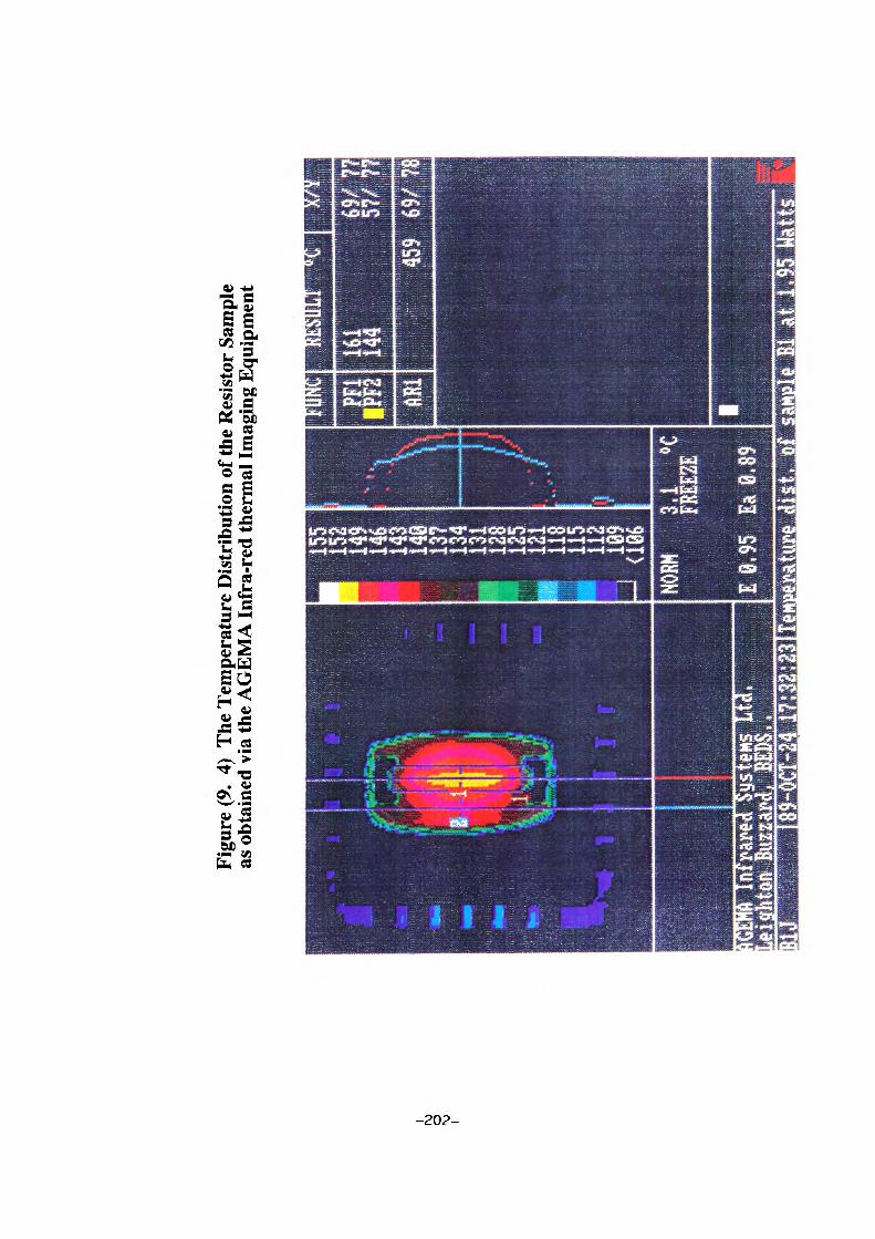
Figu

re (9

. 4)

The

Tem

pera

ture

Dis

tribu

tion

of th

e R

esis

tor S

ampl

e as

obt

aine

d vi

a th

e A

GEM

A In

fra-

red

ther

mal

Imag

ing

Equi

pmen

t

i no

o

An electrical equivalent circuit description of the thermal structure was constructed in

ASTEC3 syntax taking account of the following:

The resistor/substrate combination was modelled using the optimum resolution level

obtained when dealing with the macro scale structure of the same pattern (§ 8.4). ie. 81

and 7 strips along the 3.048 mm and 7.112 mm edges respectively. The arrangement is

shown in figure (9.5) where the resistor layer is modelled as (5x27x1) and the substrate

as (7x27x1) thermal cells. Both layers are modelled as single layers.

Since a very accurate simulation of the carrier was not required it was decided to model

this section of the assembly in the coarsest possible resolution. This would reduce the

number of thermal cells which would in turn reduce the computing-time needed for the

simulations. An ASTEC3 model was therefore generated by constructing a

three-dimensional interface cell (§ 5.4) immediately below the substrate as shown in figure

(9.6). This is effectively a 3-dimensional thermal cell with single resistors (of value .?/2/?rt)

connected from all the faces to the centre-point of the cell apart from the resistor connection

from the top face. This resistor was replaced by 567 resistors joining all the bottom nodes

of the substrate to the centre-node of the interface cell. In electrical terms these resistors

are parallel to each other and hence the value of each resistor was simply calculated by

multiplying the single thermal resistor value (H2R^) by the number of resistors which was

567 in this case.

The model for thermal conduction within the rest of the carrier was then developed using

normal 3-dimensional cells keeping their sizes as large as possible. Figure (9.7) shows a

top view of the carrier illustrating the break-up of the assembly into thermal conduction

cells. For each cell in the model the conduction resistances were calculated using the

equations given in section (4.2) and the corresponding thermal conductivities.

-203-

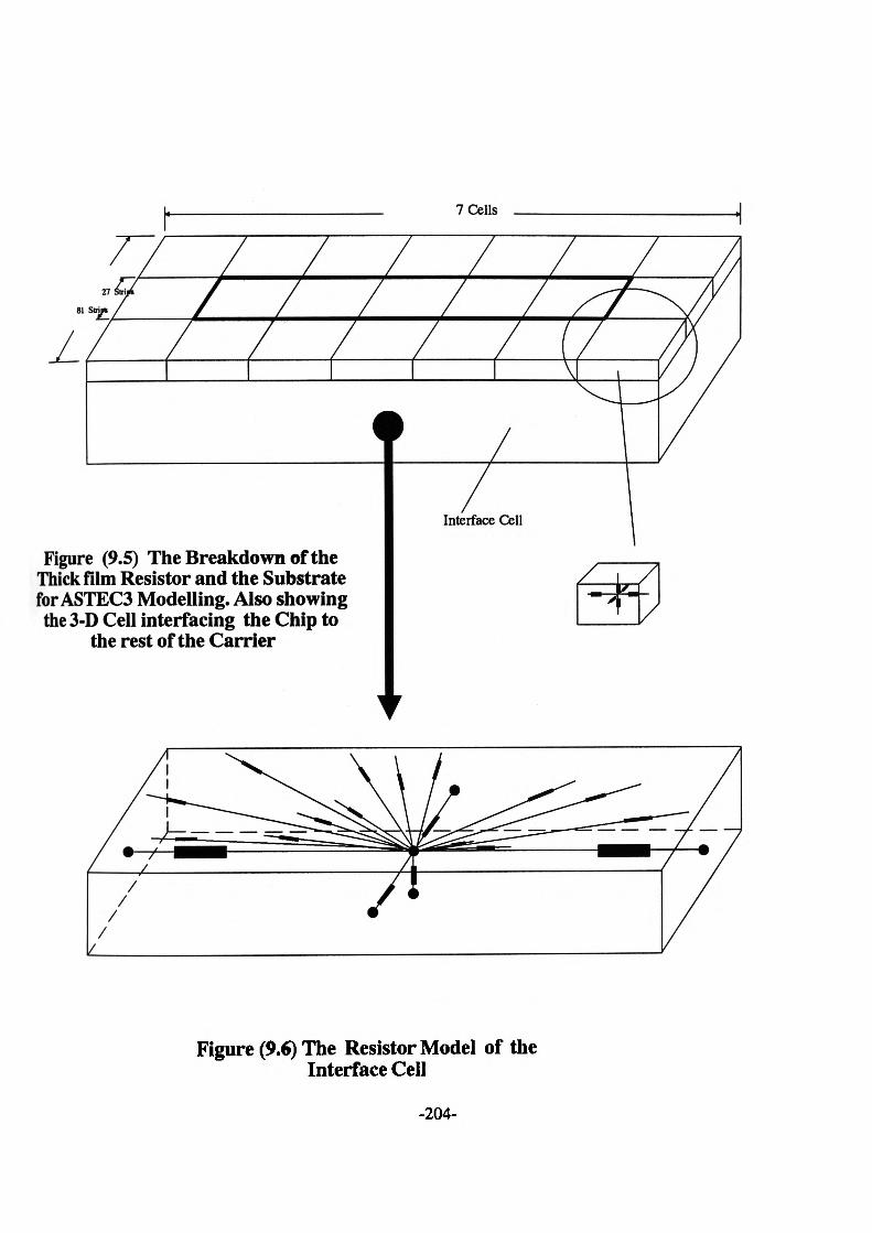
Figure (9.5) The Breakdown of the Thick film Resistor and the Substrate for ASTEC3 Modelling. Also showingthe 3-D Cell interfacing the Chip to

the rest of the Carrier

Interface Cell

XTX

Figure (9.6) The Resistor Model of the Interface Cell

-204-

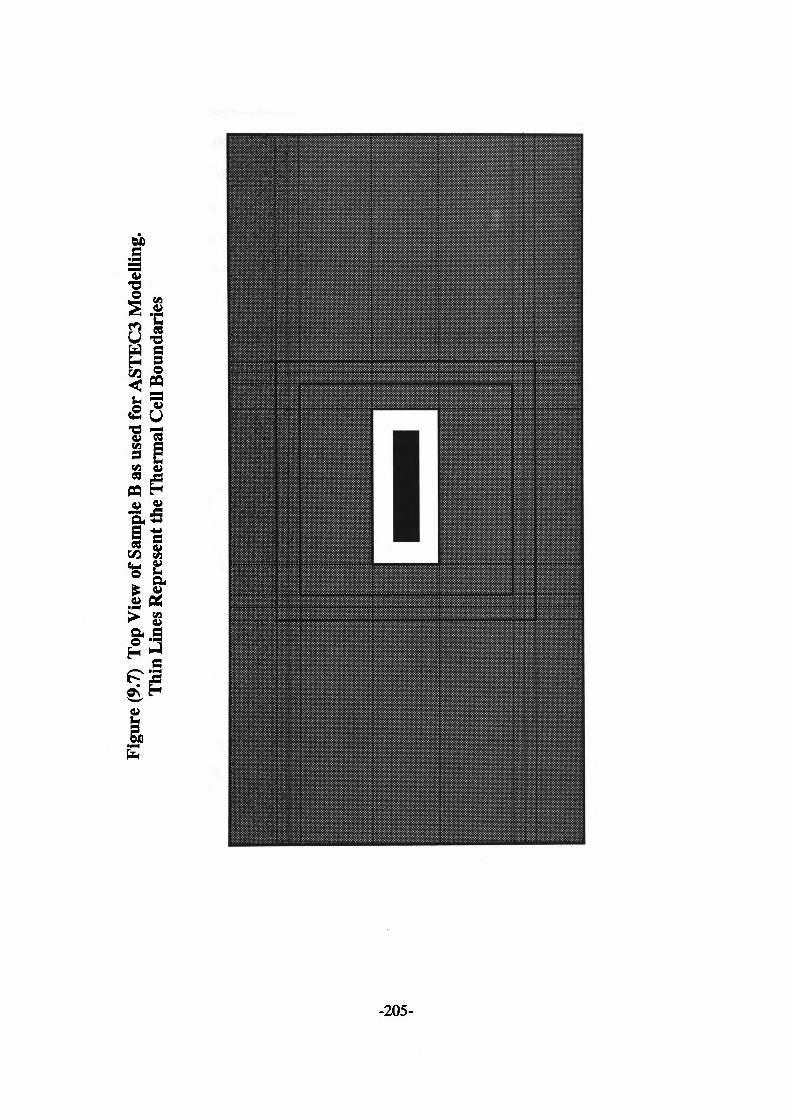
Figu

re (9

.7) T

op V

iew o

f Sam

ple

B as

use

d fo

r AST

EC3

Mod

ellin

g.

Thin

Lin

es R

epre

sent

the

Ther

mal

Cel

l Bou

ndar

ies

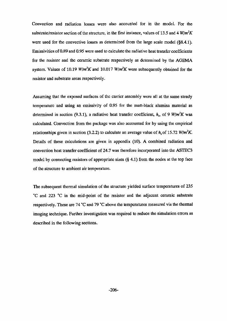
Convection and radiation losses were also accounted for in the model. For the

substrate/resistor section of the structure, in the first instance, values of 13.5 and 4 W/m2K

were used for the convective losses as determined from the large scale model (§8.4.1).

Emissivities of 0.89 and 0.95 were used to calculate the radiative heat transfer coefficients

for the resistor and the ceramic substrate respectively as determined by the AGEMA

system. Values of 10.19 W/m2K and 10.017 W/m2K were subsequently obtained for the

resistor and substrate areas respectively.

Assuming that the exposed surfaces of the carrier assembly were all at the same steady

temperature and using an emissivity of 0.95 for the matt-black alumina material as

determined in section (9.3.1), a radiative heat transfer coefficient, hn of 9 W/m2K was

calculated. Convection from the package was also accounted for by using the empirical

relationships given in section (3.2.2) to calculate an average value of hc of 15.72 W/m2K.

Details of these calculations are given in appendix (10). A combined radiation and

convection heat transfer coefficient of 24.7 was therefore incorporated into the ASTEC3

model by connecting resistors of appropriate sizes (§ 4.1) from the nodes at the top face

of the structure to ambient air temperature.

The subsequent thermal simulation of the structure yielded surface temperatures of 235

°C and 223 °C in the mid-point of the resistor and the adjacent ceramic substrate

respectively. These are 74 °C and 79 °C above the temperatures measured via the thermal

imaging technique. Further investigation was required to reduce the simulation errors as

described in the following sections.

-206-

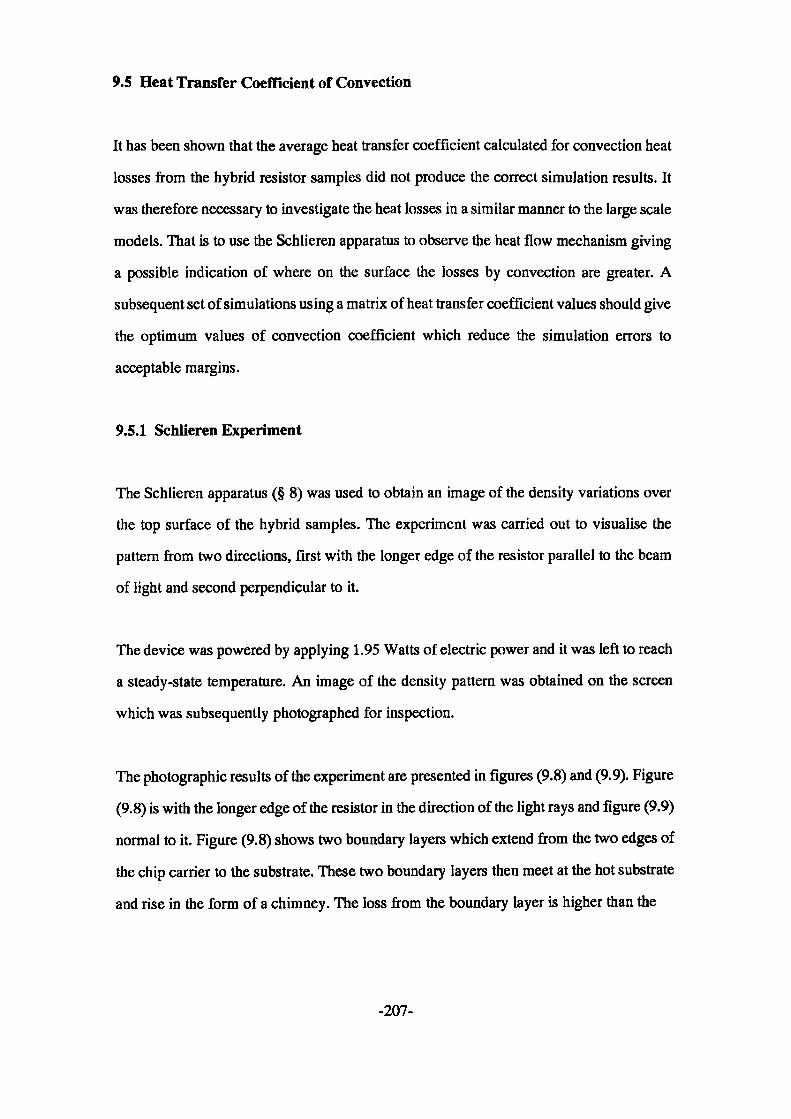
9.5 Heat Transfer Coefficient of Convection

It has been shown that the average heat transfer coefficient calculated for convection heat

losses from the hybrid resistor samples did not produce the correct simulation results. It

was therefore necessary to investigate the heat losses in a similar manner to the large scale

models. That is to use the Schlieren apparatus to observe the heat flow mechanism giving

a possible indication of where on the surface the losses by convection are greater. A

subsequent set of simulations using a matrix of heat transfer coefficient values should give

the optimum values of convection coefficient which reduce the simulation errors to

acceptable margins.

9.5.1 Schlieren Experiment

The Schlieren apparatus (§ 8) was used to obtain an image of the density variations over

the top surface of the hybrid samples. The experiment was carried out to visualise the

pattern from two directions, first with the longer edge of the resistor parallel to the beam

of light and second perpendicular to it.

The device was powered by applying 1.95 Watts of electric power and it was left to reach

a steady-state temperature. An image of the density pattern was obtained on the screen

which was subsequently photographed for inspection.

The photographic results of the experiment are presented in figures (9.8) and (9.9). Figure

(9.8) is with the longer edge of the resistor in the direction of the light rays and figure (9.9)

normal to it. Figure (9.8) shows two boundary layers which extend from the two edges of

the chip carrier to the substrate. These two boundary layers then meet at the hot substrate

and rise in the form of a chimney. The loss from the boundary layer is higher than the

-207-

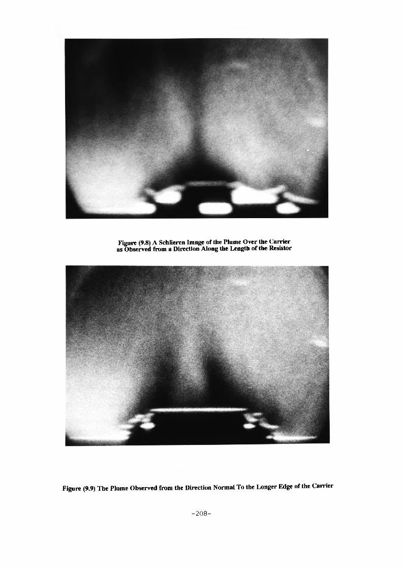
Figure (9.8) A Schlieren Image of the Plume Over the Carrier as Observed from a Direction Along the Length of the Resistor

Figure (9.9) The Plume Observed from the Direction Normal To the Longer Edge of the Carrier

-208-

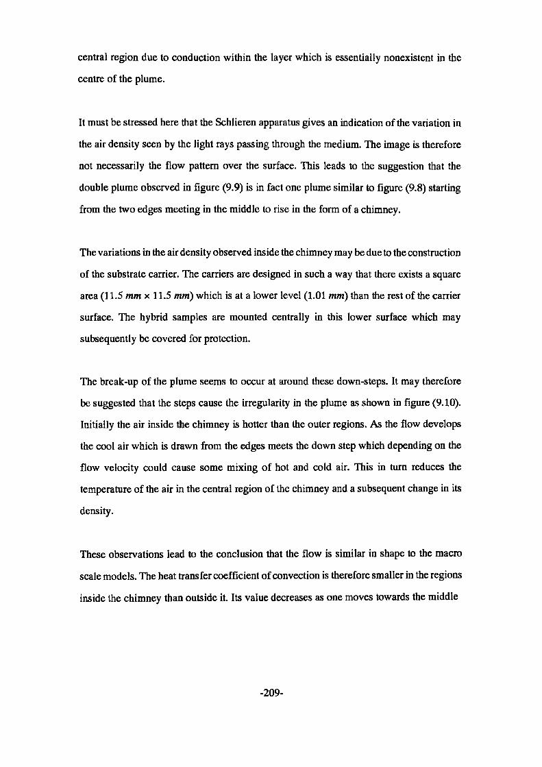
central region due to conduction within the layer which is essentially nonexistent in the

centre of the plume.

It must be stressed here that the Schlieren apparatus gives an indication of the variation in

the air density seen by the light rays passing through the medium. The image is therefore

not necessarily the flow pattern over the surface. This leads to the suggestion that the

double plume observed in figure (9.9) is in fact one plume similar to figure (9.8) starting

from the two edges meeting in the middle to rise in the form of a chimney.

The variations in the air density observed inside the chimney may be due to the construction

of the substrate carrier. The carriers are designed in such a way that there exists a square

area (11.5 mm x 11.5 mm) which is at a lower level (1.01 mm) than the rest of the carrier

surface. The hybrid samples are mounted centrally in this lower surface which may

subsequently be covered for protection.

The break-up of the plume seems to occur at around these down-steps. It may therefore

be suggested that the steps cause the irregularity in the plume as shown in figure (9.10).

Initially the air inside the chimney is hotter than the outer regions. As the flow develops

the cool air which is drawn from the edges meets the down step which depending on the

flow velocity could cause some mixing of hot and cold air. This in turn reduces the

temperature of the air in the central region of the chimney and a subsequent change in its

density.

These observations lead to the conclusion that the flow is similar in shape to the macro

scale models. The heat transfer coefficient of convection is therefore smaller in the regions

inside the chimney than outside it. Its value decreases as one moves towards the middle

-209-

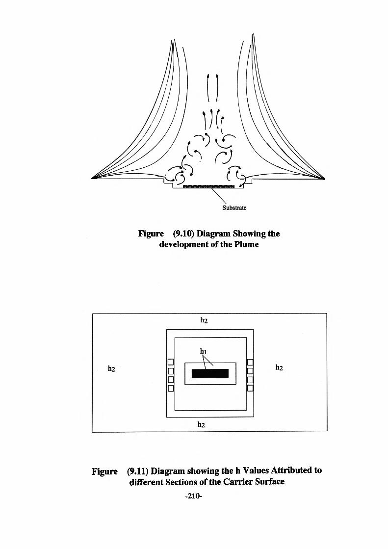
Substrate

Figure (9.10) Diagram Showing the development of the Plume

Figure (9.11) Diagram showing the h Values Attributed to different Sections of the Carrier Surface

-210-

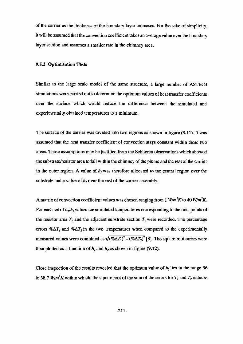
of the carrier as the thickness of the boundary layer increases. For the sake of simplicity,

it will be assumed that the convection coefficient takes an average value over the boundary

layer section and assumes a smaller rate in the chimney area.

9.5.2 Optimisation Tests

Similar to the large scale model of the same structure, a large number of ASTEC3

simulations were carried out to determine the optimum values of heat transfer coefficients

over the surface which would reduce the difference between the simulated and

experimentally obtained temperatures to a minimum.

The surface of the carrier was divided into two regions as shown in figure (9.11). It was

assumed that the heat transfer coefficient of convection stays constant within these two

areas. These assumptions may be justified from the Schlieren observations which showed

the substrate/resistor area to fall within the chimney of the plume and the rest of the carrier

in the outer region. A value of ht was therefore allocated to the central region over the

substrate and a value of h2 over the rest of the carrier assembly.

A matrix of convection coefficient values was chosen ranging from 1 W/m2K to 40 W/m2K.

For each set of hj/h2 values the simulated temperatures corresponding to the mid-points of

the resistor area T1 and the adjacent substrate section J2 were recorded. The percentage

errors %AJ, and %Ar2 in the two temperatures when compared to the experimentally

measured values were combined as V(%A7\)2 + (%Ar2)2 [8]. The square root errors were

then plotted as a function of hj and h2 as shown in figure (9.12).

Close inspection of the results revealed that the optimum value of h2 lies in the range 36

to 38.7 W/m2K within which, the square root of the sum of the errors for T3 and T2 reduces

-211-

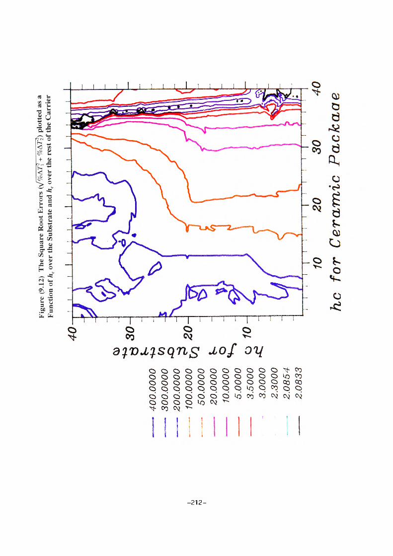
Figu

re (

9.12

) T

he S

quar

e R

oot E

rror

s (V

%A7

? +

%AT

22) p

lott

ed a

s a

Func

tion

of h

c ove

r th

e Su

bstr

ate

and

hc o

ver

the

rest

of t

he C

arri

er

i r\j

400.

0000

300.

0000

200.

0000

100.

0000

50.0

000

20.0

000

10.0

000

5.00

003.

5000

3.00

002.

3000

2.08

542.

0833

10

20

30

40he

for

Cer

amic

Pac

kaae

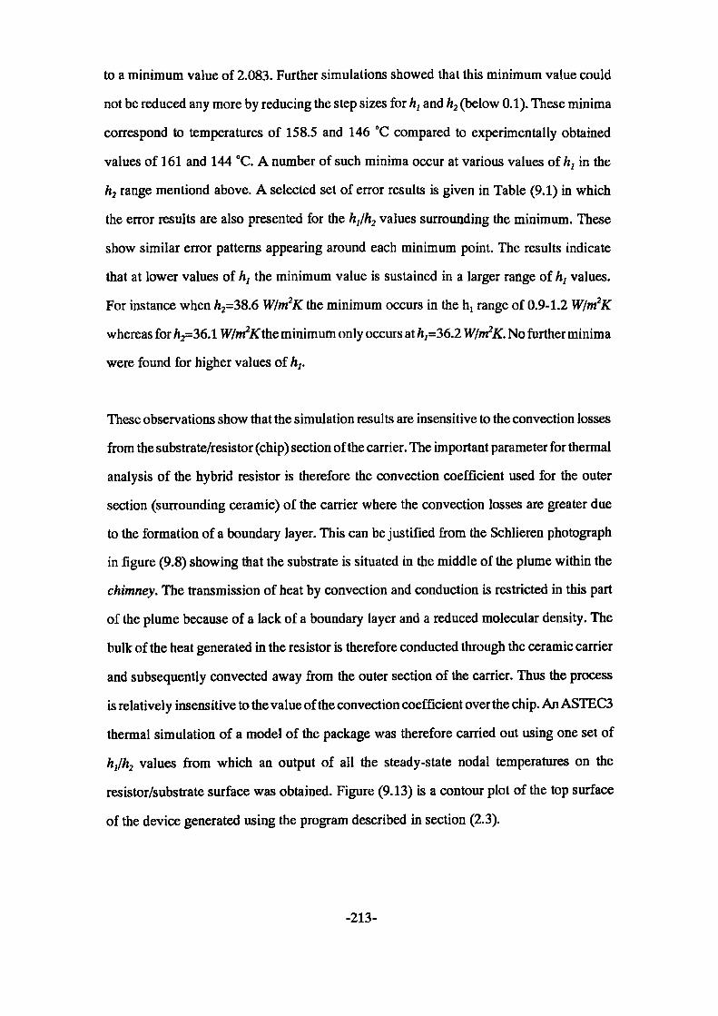
to a minimum value of 2.083. Further simulations showed that this minimum value could

not be reduced any more by reducing the step sizes for h, and h2 (below 0.1). These minima

correspond to temperatures of 158.5 and 146 °C compared to experimentally obtained

values of 161 and 144 °C. A number of such minima occur at various values of h, in the

h2 range mentiond above. A selected set of error results is given in Table (9.1) in which

the error results are also presented for the hj/h2 values surrounding the minimum. These

show similar error patterns appearing around each minimum point. The results indicate

that at lower values of hj the minimum value is sustained in a larger range of ht values.

For instance when ft2=38.6 W/m2K the minimum occurs in the ht range of 0.9-1.2 W/nfK

whereas for fc2=36.1 W/m^the minimum only occurs at hj=36.2 W/m*K. No further minima

were found for higher values of hj.

These observations show that the simulation results are insensitive to the convection losses

from the substrate/resistor (chip) section of the carrier. The important parameter for thermal

analysis of the hybrid resistor is therefore the convection coefficient used for the outer

section (surrounding ceramic) of the carrier where the convection losses are greater due

to the formation of a boundary layer. This can be justified from the Schlieren photograph

in figure (9.8) showing that the substrate is situated in the middle of the plume within the

chimney. The transmission of heat by convection and conduction is restricted in this part

of the plume because of a lack of a boundary layer and a reduced molecular density. The

bulk of the heat generated hi the resistor is therefore conducted through the ceramic carrier

and subsequently converted away from the outer section of the carrier. Thus the process

is relatively insensitive to the value of the convection coefficient over the chip. An ASTEC3

thermal simulation of a model of the package was therefore carried out using one set of

hj/h2 values from which an output of all the steady-state nodal temperatures on the

resistor/substrate surface was obtained. Figure (9.13) is a contour plot of the top surface

of the device generated using the program described in section (2.3).

-213-

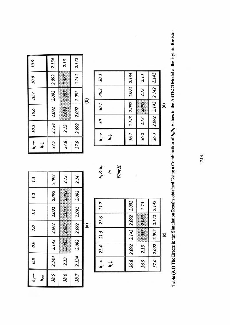
tr 38.5

38.6

38.7

0.8

2.14

3

2.13

2.13

4

0.9

2.14

3

2.09

2

1.0

2.09

2

2.09

2

1.1 2.09

2

mjij

tmm

jif.

^Hlss

i*™

2.09

2

1.2

2.09

2

IB!

2.09

2

(a)

M21

.421

.5

21.6

21.7

1.3

2.09

2

2.13

2.14 h1

&h2

in

Wln

fK

**- M 37.7

37.8

37.9

10.5

2.13

4

2.13

2.09

2

10.6

2.09

2

111

2.09

2

10.7

2.09

2

2.09

2

10.8

2.09

2

ZtfJ

lll

2.14

2

10.9

2.13

4

2.13

2.14

2

(b)

*1- M 36. .7

36.2

36.3

30 2.14

3

2.13

2.09

2

30.1

2.09

2 mi 2.14

2

30.2

2.09

2

2.13

2.14

2

30.3

2.13

4

2.13

2.14

2

(c)

(d)

Tabl

e (9

.1) T

he E

rrors

in th

e Si

mul

atio

n Re

sults

obt

aine

d U

sing

a Com

bina

tion

ofhj

/h2 V

alue

s in

the A

STEC

3 M

odel

of t

he H

ybrid

Res

istor

-214

-

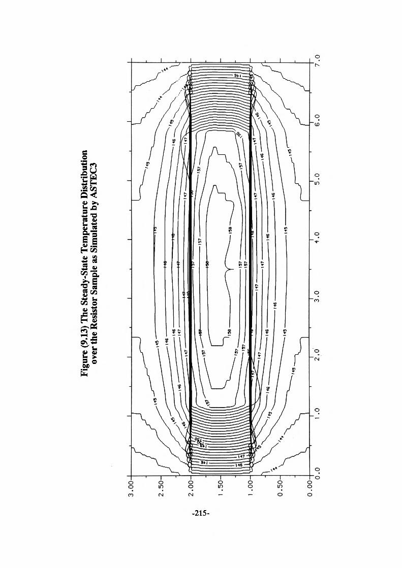
Figu

re (9

.13) T

he S

tead

y-St

ate

Tem

pera

ture

Dist

ribut

ion

over

the R

esist

or S

ampl

e as S

imul

ated

by

ASTE

C3

3.0

0-

2.5

0-

2.0

0-

1 .5

0-

1 .0

0-

0.5

0-

0.0

0- 0

.01

.0i 2,0

3.0

4.0

5.0

6.0

7.0

9.6 Conclusions

The ASTEC3 thermal modelling technique has been applied here for simulation of the

heat flow in a hybrid resistor sample. This was the specimen with a (20 mm x 100 mm)

resistor printed symmetrically onto a (60 mm x 140 mm) substrate. The AGEMA thermal

imaging equipment was used to capture an image of the temperature distribution over the

surface of the device. This showed steady-state temperatures of 161 ± 2 "C at the mid-points

of the resistor and 144 ± 2 °C at the adjacent substrate areas when an electric power of

1.95 Watts were applied to it.

The sample was subsequently modelled and simulated via ASTEC3 package. It was found

that the simulated temperatures were very sensitive to the convective heat transfer

coefficient values. The value of this parameter varies considerably over the surface of the

heated structures. Initial simulations using the average heat transfer coefficients obtained

from the macroscopic case showed temperatures of 235 "C and 223 "C in the resistor and

substrate areas respectively which were evidently excessive. A study of the convective

heat flow over the whole of the carrier assembly using the Schlieren apparatus showed

that the convective losses over the substrate area were much smaller than that of the rest

of the carrier. This was thought to be due to the boundary layer forming over and covering

the large area extending from the edge of the carrier to the substrate causing a great amount

of heat loss by convection. The boundary layers from the two edges meet in the central

region over the substrate rising in the shape of a chimney with a reduced heat loss rate due

to the lack of a boundary layer.

An extensive number of ASTEC3 simulations revealed that the value of convection

coefficient for the outer carrier section lies in a range extending from 36.2 and 38.6 W/m2K

within which the square root error is reduced to 2.083%. The simulation results were found

-216-

to vary very little with the value of the convection coefficient used for the thick

film/substrate section in the ASTEC3 model suggesting that the generated heat is conducted

through the bottom of the substrate and then convected into the atmosphere, thus variation

in the direct chip to atmosphere path has minimal effect on the results.

-217-

10 DISCUSSIONS AND CONCLUSIONS

This thesis has been dealing with one of the major problem areas in the electronic industry.

This is the thermal dissipation problem which is the result of the growing increase in the

packing density of devices fabricated on ceramic substrates namely hybrid circuits. The

initial objectives of the project was to develop a fully interactive computer modelling tool

capable of simultaneous simulation of the electrical and thermal characteristics of hybrid

and semiconductor device. The initial investigation using a macro-scale model however

showed that a better understanding of the heat transfer mechanisms was needed. It was

also found that the thermal conductivity of PCB reinforced laminates was required which

meant that a great deal of effort was concentrated on determination of the conductivity of

FR4 boards and convective heat transfer processes from the plates. A brief outline of the

achievements within the context of the project will be given first and a more detailed

discussion of these will be included later in the section.

• A novel experiment was designed which allowed the measurement of the tangential

thermal conductivity of materials in the shape of a thin flat board. This was subsequently

used to estimate the in-plane conductivity of FR4 insulating boards.

• It was demonstrated, using a Schlieren apparatus and optimisation techniques that the

natural convection coefficient for partially heated boards in a horizontal position with the

heated side facing upwards was much larger on the outside than in the heated region and

that the coefficient may be approximated by two values for thermal analysis. The

convection mechanism from the type of structures described in this thesis has not been

treated by other workers and the results for convection coefficients not presented before.

-218-

• The Schlieren optical apparatus was used to observe the natural convection plumes

forming over a horizontally positioned packaged hybrid resistor sample. It was found that:

a Convection is an important heat transfer mode in the analysis of electronic

devices.

b The convection coefficient may be approximated by two values one for the area

over the chip and the surrounding well and another one for the rest of the assembly.

c The simulation results are quite insensitive to the coefficient value used over the

chip and the well but it is important and high over the ceramic package area.

The Schlieren technique has not in the past been used for the observation of convection

plumes over packaged devices and no account of such analysis is published elsewhere.

• Interface cells have been introduced which make it possible to model via ASTEC3 the

more important sections of a circuit in finer detail reducing computing time and hence

saving resources.

• Software has been developed for producing thermal contour maps from the simulated

temperature data.

• Programs are developed to facilitate the automatic generation of an error-free net-list of

a particular structure.

• CPU time calculations have been carried out to allow the prediction of simulation times.

It has been demonstrated that the simulation times are feasible for hybrid and VLSI circuits.

A more detailed account of the above statements is given below:

-219-

A modelling system has been used which makes use of the analogy between thermal and

electrical systems. A thermal structure is divided into a number of thermal cells and an

electrical equivalent model of the structure is constructed by connecting together the

appropriate number of thermal cells. The circuit is subsequently simulated using ASTEC3

electronic simulation software.

Procedures have been proposed which allow the modelling of the more important areas of

a device in finer details hence giving a more accurate temperature values at such positions.

The connection between the coarse and fine mesh areas is accomplished using special

thermal cells so-called interface cells. This optional facility reduces the computing time

required for a simulation, clearly saving resources when dealing with very large circuits.

Tests have been carried out showing that the introduction of fine mesh areas to a structure

originally simulated via a full coarse mesh model greatly improves the accuracy of the

simulated results.

The most tedious task in the modelling of a structure is the editing of the data file which

includes the net-list for the particular device in ASTEC3 language. Software has therefore

been devised to generate the ASTEC3 codes for a two or three dimensional structure divided

into a uniform mesh. The user is asked a few simple questions such as the output file name,

the number of thermal cells in the x, y and z directions. The type of simulation (transient

or steady-state) and the length of a transient simulation is also inquired. Upon receiving

the answers from the keyboard, the software automatically generates the listing for the

particular structure. This is an important tool for any modelling system since it not only

reduces the cumbersome task of inputting a large amount of data, it also produces an

error-free circuit description which is virtually impossible to create manually for very large

circuits.

-220-

Plotting routines have been developed which make it possible to draw temperature maps

of a heated surface. The nodal temperatures are simulated and stored in a data-file. These

are subsequently read by the program and routines from the GINO CAD package are called

to produce contour-maps or three dimensional temperature distribution plots. The plotting

routines and the ASTEC3 simulations are linked together via a master command file. The

software is designed such that the transient thermal behaviour of a surface can also be

studied by plotting the distributions at the required time steps. At each time step the screen

is cleared and a new plot is generated.

It was important for a user to be able to predict the simulation time needed for thermal

analysis of a particular device. It was also imperative that these simulation times were

realistic. For this reason, tests were carried out which yielded a set of simple relationships

which allow the prediction of the CPU time with a knowledge of the number of thermal

cells. These equation were subsequently used to demonstrate that the CPU time was feasible

for the analysis of a hybrid circuit.

Experiments were designed using Printed Circuit Boards (PCBs) resembling thick film

resistors on ceramic substrates. The specimen were prepared by forming islands in the

copper layer of the PCB plates. These were produced by etching grooves in the copper

layer so that they were electrically isolated from the rest of the copper film but thermally

connected via the insulator. The islands were heated electrically and an infrared pyrometer

was used to measure surface temperatures at selected points. Assuming that the insulating

board was isotropic, the thermal conductivity was measured using a Lees' disc apparatus

which gives this parameter in a direction normal to the plate. The subsequent simulation

of a model of the heated plates showed excessive temperatures within the islands. Further

consideration of the method of fabrication and simulation tests using different values for

the in-plane thermal conductivity of the boards revealed that the thermal conductivity of

-221-

the boards was in fact anisotropic. In the view of the fact that there were no apparatus

available commercially or otherwise capable of measuring the thermal conductivity in the

plane of such boards, an experiment was designed to carry out this task. In brief, the

experiment is carried out hi a vacuum chamber where long rectangular samples of the

insulating board are heated. The heating is applied at one end and steady temperatures are

measured along the length of the specimen. Temperatures of each position are recorded

at various pressures and graphs are produced relating the pressure and the corresponding

temperatures. By extrapolation to zero pressure, a temperature profile is obtained for the

specimen at zero pressure. This is in order to simulate a situation where radiation would

be the only heat loss mechanism from the sample and convection can be ignored since this

is a very difficult process to account for. A finite difference representation of the structure

is then derived in which the thermal conductivity is left as a variable. This is used to

calculate the temperature profiles using a range of thermal conductivities. These are

compared with the measured set of data until a best-match profile is found. The thermal

conductivity yielding the particular temperature distribution is then taken as the thermal

conductivity of the boards. A value of 1.059 ± 0.019 W/mKwas obtained for the in-plane

thermal conductivity of the FR4 boards compared to 0.343 ± 0.017 W/mK in a normal

direction. The subsequent ASTEC3 simulation of the plates displayed a great reduction in

the errors. The devised experiment is a novel one which can be used in other areas of

research where thermal conductivity of materials in the form of a thin board is required.

The final results of the experiment are of course invaluable for anyone dealing with the

thermal aspects of PCB design.

Although the anisotropic conductivities reduced the simulation errors, there were still

errors hi the results due to the averaged convection coefficients used in the model which

were calculated using empirical relationships. A Schlieren optical apparatus was therefore

used to study the natural convection plumes forming over these plates. This is a technique

-222-

whereby a slit/lens combination is used to produce a parallel beam of light which is focussed

to a point via another concave lens. The medium whose refractive index variation is to be

investigated is located in the path of the light beam between the lenses. The variation in

optical path causes the wavefront to be distorted and focussed as such. A knife edge is

then used at the focus to obstruct part of the image and the remainder of is imaged on a

ground-glass screen. The shadows reveal an angular displacement of the rays and it

indicates the rate of change of index across the region concerned. Using this method it was

demonstrated that the heat transfer coefficient of convection over a plate with a centrally

heated island could be approximated to two values. One coefficient value over the heated

island and another over the rest of the plate, the latter being much larger than the former.

Tests also revealed that a ratio of 3.375 to 1 would reduce the simulation errors over two

selected points on the surface to a minimum.

Hybrid resistor samples which resembled the PCB plates were also tested. These were

manufactured by RSRE and temperature measurements were carried out using an AGEMA

thermal imaging equipment. The Schlieren apparatus was again employed to view the heat

flow over the packaged devices. The tests over the resistor sample similar to that used in

macro scale experiment displayed that the convection coefficients could again be

approximated to two values. One coefficient value could be used for convection from the

chip (resistor/substrate) region and another for the rest of the carrier assembly. This was

different from the macro scale situation where the two sections were the heated island and

the unheated surrounding areas of the PCB plate. It was found that a value for the outer

section of the carrier in the range 36.2-38.6 W/m2K reduced the errors in the simulated

temperatures to a minimum. The simulated results and hence the square root errors were

however found to be insensitive to the convection coefficient used in the model for the

resistor/substrate section of the carrier.

-223-

ASTEC3 package is now almost ten years old and with the availability of advanced circuit

analysis packages, it is perhaps advisable for a future user to investigate the possibility of

replacing ASTEC3 with a more user-friendly successor. Such a simulation program should

ideally have the following capabilities:

• It should be an analogue circuit simulator capable of performing AC small signal,

DC steady-state and transient simulations.

• The simulation technique should be fast, efficient and also very accurate.

• The model generation should be simple and possibly automated.

• There should be no restrictions in the variables allowed and also the number of

circuit components.

• It should be possible to store the final results of a simulation so that the circuit may

be analysed again later using different parameter values without the need for repeating

the whole simulation.

• The user should be able to monitor the simulation so that the state of the analysis

can be checked.

•It should have a built-in facility for plotting contour-maps which is important for

thermal modelling.

10.1 Future Work

The code generation software so far developed can only produce the electrical equivalent

circuit of a device if it was divided into a uniform rectangular mesh. It is not capable of

producing the necessary syntax for cases where a mixture of fine and coarse mesh areas

is used. This would have to include the necessary routines for generating the code for the

interface cells. This is an area which needs further development in order to make the

modelling more user-friendly.

-224-

The contour-plotting programs may be extended in the future to display a three-dimensional

temperature map of a device growing with time rather than at each time-step. It may also

be possible to use another plotting package such as UNIRAS which is capable of producing

colour maps making it easier to distinguish between different temperature areas.

The future development of the ASTEC3 thermal modelling software could include building

of a library of thermal modules for typical component structures. These can then be called

up within the description file of more complex circuit arrangements without the need for

generating the code for the particular components. Further tests could also be carried out

to establish whether or how the 2-D simulation times can be used to estimate the simulation

times for a 3-D model.

The coupling of the electrical and thermal analysis of packaged devices was an area which

was not dealt with within the project as was originally intended. This is an avenue which

should be explored fully in the future especially if the transient behaviour of circuits is to

be considered. The description section ($DESC) of the ASTEC3 data file in this case will

have two layers, one describing the electronic components of the circuit and the other will

include the thermal model of the same device. Of course the layer dealing with the thermal

aspect of the device will consist of the thermal model of the chip and that of the package.

The simulation of the circuit would calculate the essential parameters at each time step

which will then be input into the thermal layer for temperature calculations. The heat

transfer coefficients of convection and radiation would be re-adjusted according to the

simulated temperature distribution. Further work should be carried out to establish the

manner by which these coefficients vary over the surface in a transient situation.

Further work could also be carried out to develop a fully interactive structure placement

facility with continuous update of the thermal simulation, thus allowing a user to optimise

-225-

the layout for thermal performance.

So far in this investigation the analysis has been on very simple hybrid resistor sample.

This should be extended to a more complex circuit arrangement and simulation results

verified accordingly. Hybrid microcircuits normally consist of several separate

components attached to a ceramic substrate and interconnected by wire bonds or suitable

metallisation pattern. The individual parts may consist of diffused or thin film components

or one or more monolithic integrated circuits. In dealing with the thermal analysis of such

devices various approaches may be taken depending on the requirements of the design. If

the reliability of the individual microcircuit (an operational amplifier for example) on the

hybrid chip is not in question, then these components may be treated as single point sources

and modelled as such. However if the temperature details of the individual integrated

circuits is required which may be a Medium Scale Integration (MSI) or Large Scale

Integration (LSI) device then these parts may be modelled using a suitable fine grid and

the rest of the hybrid chip modelled using an appropriate coarse mesh, the different grids

connected together via interface cells of the correct type.

Further tests will also be needed to explore the modelling situation hi the case of devices

fabricated on semiconducting substrates. These would initially be on MSI circuits and

extended further to higher density circuits. In dealing with VLSI circuits because of the

very small feature sizes and a very large number of components the model would contain

an extremely large number of thermal cells if a full fine grid was used. In order to save

computer resources, investigations should be carried out to explore the mixing of fine and

coarse mesh areas. To ascertain where on the device finer grids may be needed it would

perhaps be practical to carry out a full coarse mesh simulation to reveal the hotter, more

important sections of the chip. This would then then be followed by a mixed grid simulation.

-226-

To allow temperature measurements from the surface of the resistor samples, the covers

had been removed from the top of the carrier. In the real situations these covers would of

course be in position protecting the chip from possible damage. With the lid in position,

there will be a very small gap of about 1 mm between the chip and the cover. The gap is

so small that when the device is operating, the boundary layers discussed for the de-lidded

situation cannot develop. What can happen is that the generated heat will be conducted

through the trapped air (or whatever the filling) and cause a temperature rise of the cover

and the surrounding carrier sections. The heat is then convected and radiated to the

surroundings. Further work can be carried out to investigate the effect of the lid on the

chip surface temperature. The ceramic lid may be replaced in these investigations with a

material transparent to infrared radiation such as polyethylene [transparent in the range

1.8-5.5 nm] which would allow the measurement of the chip temperature profile with the

lid in position. The Schlieren apparatus could subsequently be used to examine the heat

flow over the carrier with the simulated lid leading to a better understanding of the

convection losses. Further tests can be carried out to determine the heat transfer coefficients

of convection for various devices specified possibly by the geometry, total input power,

etc. Charts may be produced in this way which will allow the thermal designer to select

the optimum values for a new circuit.

-227-

11 REFERENCES

CHAPTER 11. KINNIMENT D J, EDWARDS D A: 'Thermal Design in a Hybrid System with High

Packing Density', IEEE Transactions on Components, Hybrids, and Manufacturing Technology, Volume CHMT-1, No. 2, June 1978, pp. 176-181.

2. HASKARD M R: An Introduction to Application Specific Integrated Circuits, Prentice Hall, Australia, 1990.

3. WITTING P A, SARVAR F, POOLE N J: 'Electro-Thermal Simulation of Hybrid and VLSI Circuits', Digest ofNASECODE Software Forum, Dublin, 1989.

4. DE MEY G: "Thermal Analysis in CAD of Hybrid Circuits', Hybrid Circuits (UK), No.22, May 1991, pp.16-17.

5. MAHLINGAM M : 'Thermal Management in Semiconductor Device Packaging', Proceedings of the IEEE, Volume 73, No. 9, September 1985, pp. 1396-1405.

6. KLINGER D J, NAKADA Y, MENENDEZ MA:AT& T Reliability Manual, Van Nostrand Reinhold, New York, 1990.

7. PECK D S: 'The Analysis of Data from Accelerated Tests', Proceedings of the 9* Reliability Physics Conference, 1971, pp. 69-78.

8. BASLERM: 'Hybrid Thermal Analysis: ADesignTool',HybridCircuitTechnology, pp. 79-84, September 1987.

9. BOYLSTEAD R, NASHELSKY L: Electronic Devices and Circuit Theory, Prentice-Hall Inc., N.J., Third Edition, 1982.

10. SAVANT C J, RODEN M S, CARPENTER G L: Electronic Circuit Design, an Engineering Approach, The Benjamin/Cummings Publishing Company Inc., 1987.

11. SMITH R J: Circuits Devices andSystems, John Wiley & Sons Inc., New York, Third Edition, 1977.

12. MILLMAN J: Microelectronics: Digital and Analog Circuits and Systems, McGraw-Hill Book Company, Singapore, 1986.

13. HODGES D A, JACKSON H G: Analysis of Digital Integrated Circuits, McGraw-Hill, 1983.

14. CARR W N, MIZE J: MOS/LSI Design and Application, New York, McGraw-Hill, 1972.

15. HEIN V L, LENZI V D: 'Thermal Analysis of Substrates and Integrated Circuits', Proceedings of Electronic Component Conference, May 1969, pp. 166-177.

16. SZEKELY Y, SZIRANYI T: 'On the Simulation of 1C Chip Temperature Distribution', Period. Polytech. Electron. Eng. (Hungary), Volume 30, No. 1,1986, pp. 49-53.

-228-

17. DAVID R F: 'Computerised Thermal Analysis of Hybrid Circuits', IEEE Transactions on Parts, Hybrids andPackaging, Vol. PHP-13, No. 3, September 1977 pp. 283-289.

18. GREGORY P: 'Thermal Characteristics of a Hybrid Microcircuit', ll"1 Seminex Conference on Advances in Electronic Components and Systems, 1982 pp.347-57.

19. WEHRHAHN E: 'Temperature Distribution on Substrate of Hybrid Integrated Circuits', 5th European Microelectronics Conference, 1985 pp. 288-295.

20. KIP A F: Fundamentals of Electricity and Magnetism, 2nd Edition, McGraw-Hill Kogakusha Ltd., Tokyo.

21. SPROUL R L: Modern Physics, second Edition, Wiley &Sons, New York, 1966.22. WHITE O M: Essentials of Electricity and Magnetism, McMillan, 1965.23. NOAKES G R: A Text Book of Electricity and Magnetism, McMillan & co. Ltd.,

London, 1950.24. ZIMMER C R: 'Computer Simulation of Hybrid Integrated Circuits Including

Combined Electrical and Thermal Effects', 3rd European Hybrid Microelectronics Conference, Avignon, 1981, pp.44-50.

25. ARKIN O: 'Practical Computer Program for Improved Hybrid Thermal Analysis', Hybrid Circuit Technology, pp. 37-39, November 1986.

26. REED D L, GARTNER B W: 'Thermal Modelling of Hybrid Microelectronics', Spanning the Peaks ofElectrotechnology, IEEE Region 5 Conference, pp. 235-239, 1988.

27. SIBERGOVIC S, BOSNJAK K.M.: 'Computer Application in Thermal Analysis of Microelectronic Circuits', International Colloquium on New Orientations of Passive Components, 1982 pp. 415-418.

28. CASSELMAN G, DE MAY G : 'A Thermal Model for Hybrid Circuits', Hybrid Circuits, No. 10, May 1986, pp.9-13.

29. ROTTIERSL,DEMEYG: 'HotSpotEffectsinHybridCircuits'./JJ^rronsartio/w on Components, Hybrids, and ManufacturingTechnology, Vol. 11, No. 3, September 1988, pp. 274-278.

30. HAMBLING P G, DEAN D J: 'Microcircuit Thermal Design Tables and Computer Program for Two-Dimensional Layouts', Conference on Hybrid Microelectronics, England, September 1975, pp. 191-204.

31. DE MEY G, SCHOOR L V: 'Thermal Analysis of Hybrid Circuits with Mounted Components', Hybrid Circuits, No. 15, January 1988, pp. 28-32.

32. POGSON J T, FRANKLIN J L: 'Analysis and Temperature Control of Hybrid Microcircuits', Transactions of the ASME, Journal of Engineering for Industry, November 1973, pp. 1048-1052.

33. WENTHEN F T: 'Computer Aided Thermal Analysis of Power Semiconductor Devices', IEEE Transactions on Electronic Devices, Volume ED-17, No. 9, September 1970, pp. 765-770.

-229-

34. BILSON R T, ALLEN R W, MCCARTHY J P, STANLEY A J: "Thermal Management Evaluation of Large Size Thick Film Hybrids', Hybrid Circuits, No. 10, May 1986, pp. 65-67.

35. WEHRHAHN E: 'Temperature Distribution on Multilayer Substrates', Proceedings of the 6th European Microelectronics Conference, pp. 264-280, England, June 1987.

36. BARBOU R, MENOZZI G and MOULIN G: 'Temperature Prediction on Hybrid Microelectronics', Proceedings of the 6>k European Microelectronics Conference, pp. 332-339, England, June 1987.

37. BAYLEY F J, OWEN M J, TURNER A B: Heat Transfer, Nelson & Sons Ltd., London, 1972

38. KREYSZIG E: Advanced Engineering Mathematics, Fourth Edition, John Wiley & Sons, New York, 1979.

39. LINDSTED R D, SURTY R J: 'Steady-State Junction Temperature of Semicinductor Chips', IEEE Transactions on Electron Devices, Volume ED-19, No. 1, January 1972, pp. 41-44.

40. LEE C C, PALISOC A L: 'Thermal Analysis of GaAs 1C Devices', IEEE Gallium Arsenide Integrated Circuit Symposium, Technical Digest, 1986, pp. 115-118.

41. CASTELLO R, ANTOGNETTI P: '1C Thermal Modelling', IEEE Journal of Solid State Circuits, June 1978, pp. 146-147.

42. ANTOGNETTI P, BISIO G R, CURATELLI F, PALARA S: 'Three Dimensional Transient Thermal Simulation: Application to Delayed Short Circuit Protection in Power IC's.', IEEE Journal of Solid-State Circuits, Volume SC-15, No.3, pp. 277-281, June 1980.

43. RAMAKRISHNA K: "Thermal Analysis of Composite Multilayer Structures with Multiple Heat Sources', Proceedings of the 2ndIEPS Conference, 1982,281-295.

44. FERRARIS G P, TUDANCA M: 'The Solution of Two-Dimensional Heat Conduction Problems to Predict Operating Temperature and Power Handling Capabilities of Hybrid Circuits', European Hybrid Microelectronics Conference, Ghent, pp. 61-74,1979.

45. ZIMMER C R: 'Electrothermal Analysis of Hybrid Integrated Circuits Using the SPICE II Computer Program', Proceedings of the 32nd Electronic Components Conference, New York, 1982, pp. 24-25.

46. SAULINER J B: 'Description of a Thermal Model Library for Use in Electrical C.A.D. Programs', Proc. Spacecad 79 Computer aided design of Electronics for Space Applications, Bologna, pp. 65-76,19-21 September 1979.

CHAPTER 21. 'ASTEC3 User Manual', SIA Computer Services, London, England, 19842. WITTING P A: 'Electronic Circuit and System Simulation with ASTEC3', Computer

Aided Engineering Journal, 1985, 2,(6), pp. 186-191.

-230-

3. 'Analogue Simulation- ASTEC3 Improves on SPICE', SIA Computer Services, London, England.

4. DWYER P: 'ASTEC3 - An Alternative To SPICE', Electronic Design Products, October 1984 pp. 89-90.

5. MILLER I, FREUND J E: Probability and Statistics for Engineers, New Jersey, Prentice Hall, 1985.

6. SMITH R J: Circuits, Devices, and Systems, 3rd edition, 1976, Wiley and Sons, p. 516.

CHAPTERS1. KITTEL C: Introduction to Solid State Physics, New York, Wiley and Sons, 5th

edition, 1976.2. BACKHURST J R, HARKER J H, PORTER J E: Problems in Heat and Mass

Transfer, London, Arnold, 1974, P.84.3. DEKKER A J: Solid State Physics, London, Macmillan & Co, 1st edition, 1967.4. SPROULL R L: Modern Physics, London, Wiley & Sons, 2nd Edition, 1966.5. CHAPMAN A J: Heat Transfer, New York, McGraw-Hill, 1984.6. HOLMAN J P: Heat Transfer, New York, McGraw-Hill,1981.7. BAYLEY F J, OWEN J M, TURNER A B: Heat Transfer, London, Nelson, 1972.8. OZISIK M N: Basic Heat Transfer, New York, McGraw-Hill, 1977.9. INCORPERA F P, DEWITT D P: Fundamentals of Heat and Mass Transfer, New

York, Wiley and Sons, 1985.10. KREITH F: Principles of Heat Transfer, New York, Harper and Row, 1973.11. OZISIK M N: Heat Transfer: A Basic Approach, McGraw-hill Book Company, 1985.12. JAKOB M: Heat Transfer, Volume 1, Wiley and sons, 1967.13. EASTOP T D, McCONKEY A: Applied Thermodynamics for Engineering

Technologists, New York, Longman, 2nd Edition, 1974.14. ROGERS G F C, MAYHEW Y R: Engineering Thermodynamics Work and Heat

Transfer, 2nd Edition, Longman, 1976.

CHAPTER 41. CHAPMAN A J: Heat Transfer, New York, McGraw-Hill, 1984.

CHAPTERS1. CHAPMAN A J: Heat Transfer, New York, McGraw-Hill, 1984.2. BAYLEY F J, OWEN J M, TURNER A B: Heat Transfer, London, Nelson, 1972,

pp. 90-92.3. HOLMAN J P: Heat Transfer, New York, McGraw-Hill, 5th edition, 1981, pp. 61-65.4. KREITH F: Principles of Heat Transfer, Harper & Row, 3rd edition, 1976,

pp. 87-89.

-231-

5. DONGARRA J J: 'Performance of Various Computers Using Standard Linear Equations Software in a FORTRAN Environment', Proceedings of the 3rd conference on Multiprocessors and Array Processors, Jan 1987, pp. 15-32.

6. Proceedings of the Reunion of the ASTEC Users Club, France, Oct. 1988.

CHAPTER 61. 'Nextel 2010 Coating' Product Performance Bulletin and Application Instructions,

3M Industrial Chemical Products, 3M Head Office, Bracknell, Berks, England.2. CHAPMAN A J: Heat Transfer, New York, McGraw-Hill, 1984.3. OZISIK M N: Basic Heat Transfer, New York, McGraw-Hill, 1977.4. GOLDSTEIN R J, SPARROW E M, JONES D C: 'Natural Convection Mass Transfer

Adjacent to Horizontal Plates', Int. Journal of Heat and Mass Transfer, May 1972 pp. 1025-1034.

5. LLOYD J R, MORAN W R: 'Natural Convection Adjacent to Horizontal Surface of Various Planforms', ASME Journal of Heat Transfer, 1974 pp. 1-5.

6. HEIMANN Radiation Thermometer KT14 Instruction Manual, HEIMANN Gmbh, Infrared Measurements, D-6200 Wiesbaden-Dotzheim, West Germany.

7. BOYLSTAD R, NASHELSKY L: Electronic Devices and Circuit Theory, New Jersey, Prentice-Hall Inc., 1982, p. 488.

8. Private Communication, Mica and Micanite (Ireland) Limited, Mallow, Co. Cork, Ireland.

CHAPTER?1. KAY G W C, LABY T H: Tables of Physics and Chemical Constants, 15th Edition,

Longman Group Limited, 1986, p. 69.2. Private Communication, Mica and Micanite (Ireland) Limited, Mallow, Co. Cork,

Ireland.3. CHAPMAN A J: Heat Transfer, 4th Edition, McGraw-Hill, New York, 1984, p. 131.4. STARLING A J, WOODALL A J: Physics, 2nd Edition, Longmans, 1964,

pp.320-321.5. Equipment Notes No. P28030/1 for Lees' Disc Apparatus from Philip Harris Ltd.

Shenstone, England.6. TOPPING J: Errors of Observation and Their Treatment, 4th Edition, Chapman and

Hall, 1975.7. Data Sheet No. PD4/7/82, Polypenco Engineering Plastics Materials Limited, 76

Bridge Road East, Welwyn Garden City, Herts, England.8. BAYLEY F J, OWEN J M and TURNER A B: Heat Transfer, Nelson and sons

Limited, 1972, pp 90-92.9. 'Nextel 2010 Velvet Coating' Product Performance Bulletin and Application

Instructions, 3M Head Office, Bracknell, Berks, England.

-232-

10. WARD L, BUNN J P: Introduction to the Theory and Practice of High Vacuum Technology, Butterworths & Co. Limited, London, 1967.

11. EASTOP T D, McCONKEY A: Applied Thermodynamics for Engineering Technologists, second Edition, Longman Group Limited, London, 1974.

12. OZISIK M N: Basic Heat Transfer, McGraw-Hill Book Company, New York, 1977.

CHAPTERS1. INCORPERA F P, DEWITT D P: Fundamentals of Heat and Mass Transfer, Wiley

& Sons, Second Edition, 1981.2. JENKINS F A, WHITE H E: Fundamentals of Optics, McGraw-Hill Kogakusha

Limited, Fourth Edition, 1976, p. 604.3. HECHT E: Optics, Addison-Wesley Pub. Co., Second Edition, 1987, p. 577.4. LIEPMANN H W, ROSHKO A: Elements of Gasdynamics, Wiley and Sons Inc.,

New York, 1957, pp. 153-162.5. PANKHURST R C, HOLDER D W: Wind-Tunnel Techniques, Pitman & Sons,

London, 1952, pp. 162-167.6. LONGHURST R S: Geometrical and Physical Optics, Longmans, second Edition,

1968, pp. 336-337.7. 'The SCHLIEREN Apparatus' Instructions Manual No. TE65/A, Flint and Partners

Limited, Fishpond Road, Wokingham, Berkshire, England.

CHAPTER 91. Thick Film Substrates Data Sheet, Design Standard 49, COORS Ceramics Electronics

Limited, 64 Cavendish Way, Southf ield Industrial Estate, Glenrothes, Fife, Scotland.2. Birox* 1400-Series Resistor Compositions for High Performance Hybrid

Microcircuits and Resistor Networks. Data Sheet No. E13361. Du Pont Electronics, Du Pont (UK) Limited, Wedgwood Way, Stevenage, Herts.

3. Private Communication: Du Pont Electronics, Microcircuit & Printed Circuit Materials, Wedgwood Way, Stevenage, Herts, SGl 4QN.

4. Ceramic Packages Data Sheet No. 87C04, SHINKO Electric Industries Co. Limited, Supplied by: Dage (GB) Limited, Rabans Lane, Aylesbury, Bucks, England.

5. Data Sheet for Ablebond 41-4, electrically Insulating Adhesive For Microelectronics, Ablestic Laboratories, 833 West 182nd Street, Gardena, CA 90248, USA.

6. Thermovision 880 SWB Specifications, Publication No. 556556875 Ed. II Eng., AGEMA Infrared Systems Limited, Arden House, Leighton Buzzard, Beds, England.

7. PITT KEG: "The Emissivity of Thick Film Resistor Materials', Proceedings of the Int. Electronic Packaging and Production Conf., U.K., 1980, pp 258-260.

8. CHAPMAN A J: Heat Transfer, New York, McGraw-Hill, 1984.9. TOPPING J: Errors of Observation and Their Treatment, 4th Edition, Chapman and

Hall, 1975.

-233-

12 APPENDIXES

APPENDIX 1: Contour Plotting Programs

Program 1

cc This program reads the output file of an ASTEC3 simulation andc creates another file containing only the tables of results.

CHARACTER*80 INLINE

10 READ(50,100)INLINEIF (INLINE(2:3).NE.'&T') GOTO 10

20 WRITE(51,100)INLINEREAD (50,100,END=999)INLINEIF (INLINE(2:5).NE.'EDIT') GOTO 20

100 FORMAT(A)999 END

-234-

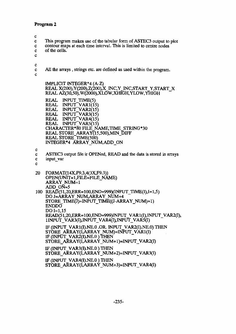
Program 2

cc This program makes use of the tabular form of ASTEC3 output to plotc contour maps at each time interval. This is limited to centre nodesc of the cells.c

cc All the arrays, strings etc. are defined as used within the program.c

IMPLICIT INTEGER*4 (A-Z)REALX(200),Y(200),Z(200),X_INC,Y_INC,START Y,START X REAL AZ(30,50),W(2000),XLOW,XHIGH,YLOW, YHIGHREAL INPUT_TIME(5)REAL INPUT_VAR1(15)REAL INPUT_VAR2(15)REAL INPUT_VAR3(15)REAL INPUT_VAR4(15)REAL INPUT_VAR5(15)CHARACTER*80 FILE_NAME,TIME_STRING*30REAL STORE_ARRAY(15,500),MIN_DIFFREAL STORE_TIME(500)INTEGERS ARRAY_NUM,ADD_ON

cc ASTEC3 output file ir OPENed, READ and the data is stored in arraysc input_varc

20 FORMAT(14X,F9.3,4(3X,F9.3))OPEN(UNIT=1,FILE=FILE_NAME)ARRAY_NUM=1ADD_ON=5

100 READ(51,20,ERR=100,END=999)(INPUT_TIME(I),I=1,5)DO J=ARRAY_NUM,ARRAY_NUM+4STOREjnME(J)=INPUT_TIME((J-ARRAY_NUM)+l)ENDDODO 1=1,15READ(51,20,ERR=100,END=999)INPUT_VAR1(I),INPUT_VAR2(I),1INPUT_VAR3(I),INPUT_VAR4(I),INPUT_VAR5(I)IF (INPUT_VAR1(I).NE.O .OR. INPUT_VAR2(I).NE.O) THEN STORE_ARRAY(I,ARRAY_NUM)=INPUT_VAR1(I) IF (INPUT_VAR2(I).NE.O ) THEN STORE_ARRAY(I,ARRAY_NUM+1)=INPUT_VAR2(I)IF (INPUT_VAR3(I).NE.O ) THEN STORE_ARRAY(I,ARRAY_NUM+2)=INPUT_VAR3(I)IF (INPUT_VAR4(I).NE.O ) THEN STORE_ARRAY(I,ARRAY_NUM+3)=INPUT_VAR4(I)

-235-

IF (INPUT_VAR5(I).NE.O ) THENSTORE_ARRAY(I,ARRAY_NUM+4)=INPUT_VAR5(I)ELSEADD_ON=4ENDIFELSEADD_ON=3ENDIFELSEADD_ON=2ENDIFELSEADD_ON=1ENDIFELSEADD_ON=0ENDIFENDDOARRAY_NUM=ARRAY_NUM+ADD_ONADD_ON=5READ(51,11,END=999)

11 FORMAT(/)GOTO 100

999 CONTINUE1=0

cc The starting point, the number of grid points in the x and y directionsc and the x and y increments are inquired to set up the grid.c

PRINT *,'Please give base value of X'READ(*,*)X(1)PRINT *,'Please give base value of Y'READ(V)Y(1)PRINT *,'Please give number of grids in X'READ(*,*)NUM_XPRINT *,'Please give number of grids in Y'READ(V)NUM_YPRINT *,'Please give X increment'READ(*,*)X_INCPRINT *,'Please give Y increment'READ(V)Y_INC

cc A uniform mesh is generated comprising the centre nodes of all the cellsc

START_Y=Y(1) START_X=X(1) COUNT=1

-236-

DO I=1,NUM_YDO J=1,NUM_XY(COUNT)=START_YIF (J.NE.1) X(COUNT)=X(COUNT-1)+X_INCCOUNT=COUNT+1ENDDOSTART_Y=START_Y+YJNCY(COUNT)=START_YX(COUNT)=START_XENDDODO I=1,COUNT ENDDOPRINT 6

6 FORMAT(1X,'Please give minimum time difference between plots ') READ(*,*)MIN_DIFF

cc All the necessary GINO subroutine are initialised for plotting purposes.c

CALL SETDEV(K) J=-lCALL ERRSWI(J) J=-lCALL ERRMAX(J) DO IZ=1,ARRAY_NUM IF (ILAST_PLOT.EQ.1.OR.1 ABS(STORE_TIME(ILAST_PLOT)-STORE_TIME(IZ)).GE.MIN_DIFF)

THENILAST_PLOT=IZWRITE(TIME_STRING, 1100)STORE_TIME(IZ)

1100FORMAT(lX,F10.0,'Seconds') DO 1=1,15 Z(I)=STORE_ARRAY(I,IZ)ENDDO NW=2000 CALL PICCLENP=NUM_X*NUM_YXLOW=0YLOW=0XHIGH=NUM_X*X_INCYHIGH=NUM_Y*Y_INCCALL TITSTR(TIME_STRING)CALLRANGRD(NP,X,Y,Z,NUM_X,XLOW,XHIGH,NUM_Y,YLOW,1 YHIGH,AZ,NW,W)NCONT=10ISM=1NSYM=-8CALL RANPTS(NSYM)CALLDRACON(NUM_X,XLOW,XHIGH,NUM_Y,YLOW,YHIGH,1 AZ,NCONT,ISM,NW,W)

-237-

CALL CHAMOD CALL WAITENDIFENDDOEND

cc Subroutine 'wait' allows 3 seconds delay between each plot.c

SUBROUTINE WATTIMPLICIT INTEGERS (A-Z)INCLUDE '(SIODEF)'LOGICAL FIRST/.TRUE./CHARACTER TERM*3 /'TT:'/,BUFF*1IF (FIRST) STATUS=SYS$ASSIGN(TERM,CHAN,,)FIRST=.FALSE.FUNC=IO$_READVBLK.OR.IO$M_TIMEDSTATUS=SYS$QIOW(,%VAL(CHAN)5%VAL(FUNC)1 ,,,,BUFF,%VAL(1),%VAL(3),,,)RETURNEND

-238-

Program3

cc This program is designed to make use of the tabular form of ASTEC3 outputc for a particular two-dimensional thermal simulation to plot contour mapsc at each time interval. It generates three uniform grids in 2-D models toc carry out this task. It uses subroutines from GINO CAD package forc plotting.c

cc All the various strings, arrays etc. used in the program are defined.c

IMPLICIT INTEGER*4 (A-Z)REALX(200),Y(200),Z(200),X_INC,Y_INC,START_Y,START_XREALAZ(30,50),W(2000),XLOW,XHIGH)YLOW,YHIGHCHARACTER CHAR*100,BUFFERS*1LOGICAL PLOTTER/.FALSE./REAL INPUT_TIME(5)REAL INPUT_VAR(5)CHARACTER'80 FILE_NAME,TIME_STRING*30,ANS*80REALSTORE_ARRAY(5000,0:200),MIN_DIFFREALSTORE_TIME(5000),START_YN,START_XNCHARACTER* 15 STRINGINTEGER'4 ARRAY_NUM,ADD_ONCOMMON STORE_TIME,LAST_TIME

cc ASTEC3 output file is OPENed, READ and the temperature data is stored inc arrays input_var for each time-interval.c

LAST_TIME=020 FORMAT(A14,F9.3,4(3X,F9.3))

OPEN(UNIT=1,FILE=FILE_NAME)ARRAY_NUM=1ADD_ON=5

100 READ(51,20,END=999)STRING,INPUT_VAR(1),INPUT_VAR(2),1INPUT_VAR(3),INPUT_VAR(4),INPUT_VAR(5)IF (STRING(2:3).EQ.'&T') THENDO ITIME=1,5INPUT TIME(ITIME)=INPUT_VAR(ITIME)ENDDOELSEIF(STRING(2:3).EQ.' ')THENELSEIF (INPUT_TIME(1).NE.O .OR. INPUT_TIME(2).NE.O) THENWHERE I=FIND_ARRAY(INPUT_TIME(1))STORE ARRAY(WHERE_I,0)=STORE_ARRAY(WHERE_I,0)+1STORE~ARRAY(WHERE_I,STORE_ARRAY(WHERE_I,0))=INPUT_VAR(1)IF (INPUT TIME(2).NE.O ) THENWHERE_I=FIND_ARRAY(INPUT_TIME(2))

-239-

STORE_ARRAY(WHERE_I,0)=STORE_ARRAY(WHERE_I,0)+1 STORE_ARRAY(WHERE_I,STORE_ARRAY(WHERE_I,0))=INPUT VAR(2) IF (INPUT_TIME(3).NE.O ) THEN WHERE_I=FIND_ARRAY(INPUT_TIME(3)) STORE_ARRAY(WHERE_I,0)=STORE_ARRAY(WHERE I,0)+l STORE_ARRAY(WHERE_I,STORE_ARRAY(WHERE_I,0))=INPUT_VAR(3)IF (INPUT_TIME(4).NE.O ) THEN WHERE_I=FIND_ARRAY(INPUT_TIME(4)) STORE_ARRAY(WHERE_I,0)=STORE_ARRAY(WHERE_I,0)+1 STORE_ARRAY(WHERE_I,STORE_ARRAY(WHERE_I,0))=INPUT_VAR(4)IF (INPUT_TIME(5).NE.O ) THENWHERE_I=FIND_ARRAY(INPUT_TIME(5))STORE_ARRAY(WHERE_I,0)=STORE_ARRAY(WHERE_I,0)+1STORE_ARRAY(WHERE_I,STORE_ARRAY(WHERE_I,0))=INPUT VAR(5)ELSEADD_ON=4ENDIFELSEADD_ON=3ENDIFELSEADD_ON=2ENDIFELSEADD_ON=1ENDIFELSEADD_ON=0ENDIFENDIF GOTO 100

999 CONTINUE 1=0

cc The program inquires if the user wishes the acquired data to be displayedc for checking the correct operation.

PRINT *,'Do you wish the values to be displayed and filed' PRINT *,'Give filename or return for No' READ(*,1010)ANS

1010FORMAT(A80)IF(ANS(1:10).NE.' ')THENOPEN(UNIT=3,FILE=ANS,RECL=132)DO IOUT=1,LAST_TIME-1WRITE(3,*)' time ',STORE_TIME(IOUT)WRITE(3,*) Temperature :-'ILINE=1DO WHILE (ILINE.LT.STORE_ARRAY(IOUT,0))START=ILINEEND=ILINE+6ILINE=END+1IF (END.GT.STORE_ARRAY(IOUT,0)) END=STORE_ARRAY(IOUT,0)

-240-

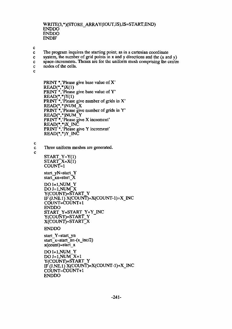
WRITE(3,*)(STORE ARRAY(IOUT,IS),IS=START,END)ENDDOENDDOENDIF

cc The program inquires the starting point; as in a cartesian coordinatec system, the number of grid points in x and y directions and the (x and y)c space-increments. Theses are for the uniform mesh comprising the centrec nodes of the cells.c

PRINT YPlease give base value of X'READ(*,*)X(1)PRINT VPlease give base value of Y'READ(*,*)Y(1)PRINT *,' Please give number of grids in X'READ(*,*)NUM_XPRINT VPlease give number of grids in Y'READ(*,*)NUM_YPRINT *,'Please give X increment'READ(*,*)X_INCPRINT *,'Please give Y increment'READ(*,*)Y_INC

cc Three uniform meshes are generated.c

START_Y=Y(1)START_X=X(1)COUNT=1start_yN=start_Y start_xn=start_XDO I=1,NUM_YDO J=1,NUM_XY(COUNT)=START_YIF (J.NE.1) X(COUNT)=X(COUNT-1)+X_INCCOUNT=COUNT+1ENDDOSTART_Y=START_Y+Y_INCY(COUNT)=START_YX(COUNT)=START_XENDDOstart_Y=start_ynstart_x=start_xn-(x_inc/2)x(count)=start_xDO I=1,NUM_YDOJ=1,NUM_X+1Y(COUNT)=START_YIF (J.NE.1) X(COUNT)=X(COUNT-1)+X_INCCOUNT=COUNT+1ENDDO

-241-

START_Y=START Y+Y INC Y(COUNT)=START_Y ~ X(COUNT)=START_XENDDOstart_Y=start_yn-(y_inc/2)start_x=start_xnx(count)=start_xDO I=1,NUM_YDO J=1,NUM_XY(COUNT)=START_YIF (J.NE.1) X(COUNT)=X(COUNT-1)+X INCCOUNT=COUNT+1ENDDOSTART_Y=START_Y+Y_INCY(COUNT)=START_YX(COUNT)=START_XENDDODO I=1,COUNT ENDDOPRINT 6

6 FORMAT(lX,'Please give minimum time difference between plots ') READ(*,*)MIN_DIFF

cc Various GINO subroutines are initialised for plotting purposes.c

1 CALL SETDEV(K)J=-lCALL ERRSWI(J)J=-lCALL ERRMAX(J)ILAST_PLOT=1DO IZ=1,LAST_TIME-1IF (ILAST_PLOT.EQ.1.OR.1ABS(STORE_TIME(ILAST_PLOT)-STORE_TIME(IZ)).GE.MIN_DIFF)

THENILAST_PLOT=IZWRITE(TIME_STRING,1100)STORE_TIME(IZ)

1100FORMAT(lX,F10.0,'Seconds') DO I=1,STORE_ARRAY(IZ,0) Z(I)=STORE_ARRAY(IZ,I) ENDDO

2 NW=2000CALL PICCLENP=NUM_X*NUM_Y+((NUM_X+1)*NUM_Y)+(NUM_X*(NUM_Y+1))XLOW=0.0YLOW=0.0XHIGH=NUM_X*X_INCYHIGH=NUM_Y*Y_INCCALL TITSTR(TIME_STRING)

-242-

CALLRANGRD(NP,X,Y,Z,NUM_X,XLOW,XHIGH,NUM_Y,1 YLOW,YHIGH,AZ,NW,W)NCONT=10ISM=1CALLDRACON(NUM_X,XLOW,XHIGH,NUM_Y,YLOW,YHIGH,1 AZ,NCONT,ISM,NW,W)CALL CHAMOD

cc WAIT subroutine is called to allow the user a few seconds to decide if ac printout of the particular plot is required.c

IF (.NOT.PLOTER) CALL WAIT(BUFFERS)

cc By pressing the letter 'p' on the keyboard a plot of the contour map isc automatically sent to the printer

IF (BUFFERS.EQ.'P'.OR.BUFFERS.EQ.'p') THENIF (PLOTER) THENCALL DEVENDCALL SETDEV(k)CALL ERRSWI(J)CALL ERRMAX(J)PLOTER=.FALSE.GOTO 2ELSEPRINT V Doing output to the printer'CALL DEVENDKI=9CALL SETDEV(KI)CALL ERRSWI(J)CALL ERRMAX(J)PLOTER=.TRUE.GOTO 2ENDIFENDIFENDIFENDDOEND

cc Subroutine 'wait' allows 3 second delay between each plotc

SUBROUTINE WAIT(BUFFER)IMPLICIT INTEGER*4 (A-Z)INCLUDE '($IODEF)'LOGICAL FIRST/TRUE./CHARACTER TERM*3 /'TT:'/.BUFFER* 1IF (FIRST) STATUS=SYS$ASSIGN(TERM,CHAN,,)FIRST=.FALSE.

-243-

BUFFER = ' 'FUNC=IO$_READVBLK.OR.IO$M_TIMEDSTATUS=SYS$QIOW(,%VAL(CHAN),%VAL(FUNC)1,,,,%REF(BUFFER),%VAL(1),%VAL(3), ) ,)RETURNEND

cc This function looks through the output file and locates the variousc blocks of data for the same time interval.c

INTEGER FUNCTION FIND_ARRAY(TIME)IMPLICIT INTEGER'4 (A-Z)REAL TIMEREAL STORE_TIME(5000)COMMON STORE_TIME,LAST_TIME1=1DO WHILE (I.LE.LAST_TIME.AND.STORE_TIME(I).NE.TIME)1=1+1ENDDOIF (I.LE.LAST_TIME) THENFIND_ARRAY=IELSELAST_TIME=LAST_TIME+1STORE_TIME(LAST_TIME)=TIMEFIND_ARRAY=LAST_TIMEENDIFEND

-244-

APPENDIX 2: Code Generation Programs

a Two-Dimensional Code-Generation Program

cc This program can generate the uniform mesh for a thermal structure withc conduction in 2-dimensions.c

cc Type and lengths and type of all the various characters and strings usedc in the program are defined.c

CHARACTER* 1 LEFT,RIGHT,TOP,BOTTOM,CENTRE,TMP* 180,TMP1 *50,1FILENAME*20,STR1*30,STR2*50,STR3*50,STR4*30,STR5*70,STR6*70,1 TYPE*20,MODEL*20,STR10*100,STR11*100,STR20*50,STR21*50,1 STR31*50,STR32*50,STR25*50,STR26*50INTEGER LEFTN,RIGHTN,TOPN,BOTTOMN,CENTREN,TIME

cc The output file name, the ASTEC3 sub-model and the ITYPE of the sub-modelc are requested.c

WRITE(6,5) 5 FORMAT('$Enter file name for output:')

READ(5,11)FILENAME 11 FORMAT(A20)

OPEN(20,FILE=FILENAME,STATUS='NEW',IOSTAT=IO)WRITE(6,8)

8 FORMAT('$Please give the ASTEC3 subjnodel:') READ(5,11)MODEL

WRITE(6,7)7 FORMAT('$Enter the type_extension for the subjnodel

1 followed by a semicolon :') READ(5,11)TTPE

cc The number of 2-dimensional cells in the x and y directions are requested.c

WRITE(6,1) 1 FORMAT('$Enter number of cells in X - Direction :')

READ(5,200)M 200 FORMAT(IS)

WRITE(6,3) 3 FORMAT('$Enter number of cells in Y - Direction :')

READ(5,200)M1

-245-

cc The codes for $DESC section of ASTEC3 circuit description file arec generated.c

WRITE(20,*)'$DESC' WRITE(20,*)' ' WRITE(6,*)'$DESC' WRITE(6,*)' '

cc The codes are generated for the !LIB sequence which calls up the modelsc from the ASTEC3 library and start the CIRCUIT section.

WRITE(STR10,*)'!LIB:',MODEL,';',MODEL,'.',TYPEJ=lSTR11=' 'DO I=1,LEN(STR10)IF(STR10(I:I).NE.' ')THENSTR11(J:J)=STR10(I:I)J=J+1ENDIFENDDOWRITE(20,*)STR11WRITE(6,*)STR11WRITE(20,*)' '

WRITE(20, *)' !CIRCUIT(G):' WRITE(6,*)' ' WRITE(6,*)'!CIRCUIT(G):' WRITE(6,*)' '

cc The node names in the model and the numbering order are specified.c (eg. cell number 1 has nodes LEFT1 (LI), RIGHT1 (Rl), TOPI (Tl) etc.).

RIGHT='R' TOP=T'

cc Start a loop to generate the code for a 2-D model with M and Ml cells inc the X and Y directions respectively.

DO N=1,M*M1J=MOD(N-1,M)RIGHTN=NTOPN=NIF (J.EQ.O) THENLEFT^'L'

-246-

LEFTN=NELSELEFT='R'LEFTN=N-1END IFIF(N.LE. M)THENBOTTOM='B'BOTTOMN=NELSEBOTTOM='T'BOTTOMN=N-MEND IF

WRITE(TMP) 1000)N,LEFT,LEFTN,RIGHT,RIGHTN,TOP,TOPN, 1BOTTOM,BOTTOMN,N,MODEL,TYPE

'-G)',A10,Y,A10)

J=lTMP1=' 'DO I=1,LEN(TMP)IF (TMP(I:I).NE.' ') THENTMP1(J:J)=TMP(I:I)J=J+1ENDIFENDDO

WRITE(20,*)TMP1WRITE(6,*)TMP1ENDDOPRINT * PRINT*

cc The code for the loutput sequence of ASTEC3 file is generatedc

WRITE(20,*)'!OUTPUT:' WRITE(20,*)' ' WRITE(6,*)' IOUTPUT:' WRITE(6,*)' '

cc A loop to generate the voltages (temperatures) at the CENTRE nodes of eachc cell in the model to be outputed.

DO NUM=1,M*M1 WRITE(STR1, *)'VNC ,NUM,';'

-247-

J=lSTR2=' 'DO I=1,LEN(STR1)IF(STR1(I:I).NE.' ')THENSTR2(J:J)=STR1(I:I)J=J+1ENDIFENDDOWRITE(20,*)STR2WRITE(6,*)STR2ENDDO

cc A loop to generate the voltages (temperatures) at the LEFT nodes of each c cell in the model to be outputed.

WRITE(STR3,*)'VNL',NUM2,';'J=lSTR4=' 'DO I=1,LEN(STR3)IF(STR3(I:I).NE.' ')THENSTR4(J:J)=STR3(I:I)J=J+1ENDIFENDDO

cc A loop to generate the voltages (temperatures) at the RIGHT nodes of each c cell in the model to be outputed. c

WRITE(STR31) *)'VNR',NUM2> VJ=lSTR32=' 'DO I=1,LEN(STR31)IF(STR31(I:I).NE.' ')THENSTR32(J:J)=STR31(I:I)J=J+1ENDIFENDDOK=MOD(NUM2-1,M)IF (K.EQ.O) THENWRITE(20,*)STR4WRITE(6,*)STR4ELSEWRITE(20,*)STR32WRITE(6,*)STR32ENDIFENDDODO NUM3=1,M*M1

-248-

cc A loop to generate the voltages (temperatures) at the BOTTOM nodes of eachc cell in the model to be outputed.

WRITE(STR20,*)'VNB',NUM3,';'STR21=' 'J=lDO I=1,LEN(STR20)IF(STR20(I:I).NE.' ')THENSTR21(J:J)=STR20(I:I)J=J+1ENDIFENDDO

cc A loop to generate the voltages (temperatures) at the TOP nodes of eachc cell in the model to be outputed.

WRITE(STR25,*)'VNT,NUM3,';'STR26=' 'J=lDO I=1,LEN(STR25)IF(STR25(I:I).NE.' ')THENSTR26(J:J)=STR25(I:I)J=J+1ENDIFENDDOIF (NUM3.LE.M) THENWRITE(20,*)STR21WRITE(6,*)STR21ELSEWRITE(20,*)STR26WRITE(6,*)STR26ENDIFENDDO

WRITE(20,*)' ' WRITE(6,*)' 'WRITE(20,*)'!EXEC' WRITE(20,*y ' WRITE(6,*)'!EXEC' WRITE(6,*)' '

c The program inquires whether a steady-state or transient simulation is c required and generates the appropriate codes.

-249-

WRITE(20,*)' 'PRINT *,'Do you require a transient or steady-state simulation'PRINT VType 1 for transient or 2 for steady-state'READ(V)SIM

IF (SIM.EQ.1) THENPRINT *,'Please give the simulation time required'READ(V)TIME

WRITE(20,*)'$TRAN' WRITE(20,*)'!INIT RESET' WRITE(6,*)' ' WRITE(6,*)'$TRAN' WRITE(6,*)'!INIT RESET'

WRITE(STR5,*)'!PARAM: TMAX=',TIME,';'STR6=' 'J=lDO I=1,LEN(STR5)IF(STR5(I:I).NE.' ')THENSTR6(J:J)=STR5(I:I)J=J+1ENDIFENDDOWRITE(20,*)STR6WRITE(6,*)STR6

ELSE IF (SIM.EQ.2) THEN WRITE(20,*)'$DCAN' WRITE(6,*)'$DCAN' ENDIF

WRITE(20,*)'!EXEC' WRITE(20,*)' ' WRITE(6,*)'!EXEC'

cc The codes for the $EDIT part of the file is generated containing thec output results in and order needed for the contour-plotting program.

WRITE(20,*)'$EDIT' WRITE(20,*)' 'WRITE(20,*)'!PRINT.SIMUL1, VERSUS &T:'WRITE(6,*)' ' WRITE(6,*)'$EDIT' WRITE(6,*)' 'WRITE(6, *)' IPRINT.SIMUL1, VERSUS &T: 'IC=16ICOUNT=0DO NUM=1,M*M1

-250-

ICOUNT=ICOUNT+1 IF(ICOUNT.EQ.IC)THENWRITE(20,*)' 'WRITE(20,*)'!PRINT.SIMUL1,VERSUS &T:'WRITE(20,*)' 'WRITE(6,*)' 'WRITE(6,*)'1PRINT.SIMUL1, VERSUS &T:'WRITE(6,*)' 'ICOUNT=1ENDIF

cc generate the code for CENTRE-node temperatures, (eg. VNCl). c

WRITE(STR1,*)'VNC',NUM,YJ=lSTR2=' 'DO I=1,LEN(STR1)IF(STR1(I:I).NE.' ')THENSTR2(J:J)=STR1(I:I)J=J+1ENDIFENDDOWRITE(20,*)STR2WRITE(6,*)STR2ENDDO

DO NUM2=1,M*M1

ICOUNT=ICOUNT+1IF(ICOUNT.EQ.IC)THENWRITE(20,*)' 'WRITE(20,*)' !PRINT.SIMUL1,VERSUS &T:'WRITE(20,*)' 'WRITE(6,*)' 'WRITE(6,*)'!PRINT.SIMUL1, VERSUS &T:'WRITE(6,*)' 'ICOUNT=1ENDIF

cc generate the code for L£FJ-node temperatures, (eg. VNL1).c

WRITE(STR3, *)' VNL',NUM2,';'

J=lSTR4=' 'DO I=1,LEN(STR3)IF(STR3(I:I).NE.' ')THENSTR4(J:J)=STR3(I:I)

-251-

J=J+1ENDIF ENDDO

cc generate the code for RIGHT-oode temperatures, (eg. VNR1).

WRITE(STR31,*)'VNR',NUM2,YJ=lSTR32=' 'DO I=1,LEN(STR31)IF(STR31(I:I).NE.' ')THENSTR32(J:J)=STR31(I:I)J=J+1ENDIFENDDOK=MOD(NUM2-1,M)IF (K.EQ.O) THENWRITE(20,*)STR4WRITE(6,*)STR4ELSEWRITE(20,*)STR32WRITE(6,*)STR32ENDIF ENDDOICOUNT=ICOUNT DO NUM3=1,M*M1ICOUNT=ICOUNT+1IF(ICOUNT.EQ.IC)THENWRITE(20,*)' 'WRITE(20,*)'IPRINT.SIMUL1,VERSUS &T:'WRITE(20,*)' 'WRITE(6,*)' 'WRITE(6,*)'!PRINT.SIMUL1,VERSUS&T:' WRITE(6,*)' 'ICOUNT=1 ENDIF

cc generate the code for BOTTOM-node temperatures, (eg. VNB1).c

WRITE(STR20,*)'VNB',NUM3,';'STR21=' 'J=lDO I=1,LEN(STR20)IF(STR20(I:I).NE.' ')THENSTR21(J:J)=STR20(I:I)

-252-

J=J+1ENDIF ENDDO

cc generate the code for TOP-node temperatures, (eg. VNTl).

WRITE(STR25,*)'VNT,NUM3,';'STR26=' 'J=lDO I=1,LEN(STR25)IF(STR25(I:I).NE.' ')THENSTR26(J:J)=STR25(I:I)J=J+1ENDIFENDDOIF (NUM3.LE.M) THENWRITE(20,*)STR21WRITE(6,*)STR21ELSEWRITE(20,*)STR26 WRITE(6,*)STR26 ENDIFENDDO WRITE(20,*)' '

cc The codes for executing the $EDIT section and ending thec simulation are generated.c

WRITE(20,*)' 'WRITE(20,*)'!EXEC'WRITE(20,*)' 'WRITE(20,*)'$END'WRITE(20,*)' 'WRITE(6,*)' ' WRITE(6,*)'!EXEC' WRITE(6,*)' ' WRITE(6,*)'$END'

END

-253-

b An example of the ouput of the 2-D Code-Generation Program

Questions and Answers for generating a (5x3) mesh

Enter file name for output: F2.DESPlease give the ASTEC3 sub_model: 2DEnter the type_extension for the sub_model followed by a semicolon :S;Enter number of cells in X - Direction :5Enter number of cells in Y - Direction :3

Do you require a transient or steady-state simulationType 1 for transient or 2 for steady-state1Please give the simulation time required2000

The Contents of The Output File F2.DES

$DESC

!LIB:2D;2D.S;

!CIRCUIT(G):

M1(L1-R1-T1-B1-C1-G)2D.S;M2(R1-R2-T2-B2-C2-G)2D.S;M3(R2-R3-T3-B3-C3-G)2D.S;M4(R3-R4-T4-B4-C4-G)2D.S;M5(R4-R5-T5-B5-C5-G)2D.S;M6(L6-R6-T6-T1-C6-G)2D.S;M7(R6-R7-T7-T2-C7-G)2D.S;M8(R7-R8-T8-T3-C8-G)2D.S;M9(R8-R9-T9-T4-C9-G)2D.S;M10(R9-R10-T10-T5-C10-G)2D.S;M11(L11-R11-T11-T6-C11-G)2D.S;M12(R11-R12-T12-T7-C12-G)2D.S;M13(R12-R13-T13-T8-C13-G)2D.S;M14(R13-R14-T14-T9-C14-G)2D.S;M15(R14-R15-T15-T10-C15-G)2D.S;

! OUTPUT:

VNC1; VNC2; VNC3; VNC4; VNC5; VNC6; VNC7; VNC8;

-254-

VNC9; VNC10;VNC11;VNC12;VNC13;VNC14;VNC15;VNL1;VNR2;VNR3;VNR4;VNR5;VNL6;VNR7;VNR8;VNR9;VNR10;VNL11;VNR12;VNR13;VNR14;VNR15;VNB1;VNB2;VNB3;VNB4;VNB5;VNT6;VNT7;VNT8;VNT9;VNT10;VNT11;VNT12;VNT13;VNT14;VNT15;

IEXEC

$TRAN

UNIT RESET !PARAM:TMAX=2000;

IEXEC

$EDIT

!PRINT.SIMUL1,VERSUS &T:

VNC1; VNC2;

-255-

VNC3;VNC4;VNC5;VNC6;VNC7;VNC8;VNC9;VNC10;VNC11;VNC12;VNC13;VNC14;VNC15;

!PRINT.SIMUL1,VERSUS &T:

VNL1;VNR2;VNR3;VNR4;VNR5;VNL6;VNR7;VNR8;VNR9;VNRIO;VNL11;VNR12;VNR13;VNR14;VNR15;

!PRINT.SIMUL1,VERSUS &T:

VNB1;VNB2;VNB3;VNB4;VNB5;VNT6;VNT7;VNT8;VNT9;VNT10;VNT11;VNT12;VNT13;VNT14;VNT15;

IEXEC

SEND

-256-

c Program for Generating the ASTEC3 code for Three-Dimensional Conduction

cc This program generates the electrical equivalent circuit description ofc a uniform thermal structure. It takes into account conduction in 3c directions and in this case convection and radiation from the top surface.ccc The type and sizes of all strings and arrays used within the program arec defined.c

CHARACTER* 1 LEFT,RIGHT,TOP,BOTTOM,CENTRE,TMP* 180,TMP1 *70, 1 FILENAME*20,END*1,FRONT*1,1STR1*55,STR2*50,STR3*50,STR4*50,STR5*50,STR6*50, 1TYPE*20,MODEL*20,STR10*100,STR11*100,STR20*20,STR21*20, 1STR22*20,STR23*20,CTYPE(3000)*4,SP*1,EXT*4,LINE*70,LIN*5,1 SP1*1,LINE1*70,LIN1*6 DIMENSION HC(IOOO)

INTEGER LEFTN,RIGHTN,TOPN,BOTTOMN,CENTREN,FRONTN,ENDN, TIME,X1,X2

cc The output filename is inquired and opened.c

WRITE(6,5) 5 FORMAT('$Enter file name for output:')

READ(5,11)FILENAME 11 FORMAT(A20)

OPEN(20,FILE=FILENAME,STATUS='NEW',IOSTAT=IO)WRITE(6,8)

cc ASTEC3 name for the single cell model and the type of the cell arec inquired. These are as saved in the user's personal library.c

8 FORMAT('$Please give the ASTEC3 subjnodel:') READ(5,11)MODEL

WRITE(6,7) 7 FORMAT('$Enter the type_extension for the subjnodel followed by a

1 semicolon :')READ(5,H)TYPEDO 199 1=1,1000

199 CTYPE(I)=TYPEWRITE(20,*)'$DESC' WRITE(20,*)' '

-257-

WRITE(6,*)'$DESC' WRITE(6,*)' '

cc The !LIB sequence of the ASTEC3 file is generated.c

WRITE(STR10,*)'!LIB:',MODEL,';',MODEL, > .',TYPEJ=lSTR11=' 'DO I=1,LEN(STR10)

IF (STR10(I:I).NE.' ') THENSTR11(J:J)=STR10(I:I)J=J+1ENDIFENDDOWRITE(20,*)STR11WRITE(6,*)STR11

cc The file name containing the cell numbers with different parameter valuesc or heat generation are inquired.lt is subsequently opened and the data isc read. This includes the EXTension of the STYPE of cell.c

WRITE(6,1H)111 FORMAT(' $Enter file name containing the changes :')

READ(5,11)FILENAME

OPEN(22,FILE=FILENAME,STATUS='OLD',IOSTAT=IO)

202 READ(22,256,END=999)EXT 256 FORMAT(A4)

IF(EXT(1:1).EQ.'*')GOTO 999 TYPE *,EXT

cc The model names are written as given in the CIRCUIT description section ofc ASTEC3 file as read from the above file.c

WRITE(STR10,*),MODEL,V,EXTJ=lSTR11=' 'DO I=1,LEN(STR10)IF (STR10(I:I).NE.' ') THENSTR11(J:J)=STR10(I:I)J=J+1ENDIFENDDOWRITE(20,*)STR11WRITE(6,*)STR11

-258-

READ(22,267)LINE 267 FORMAT(A70)

TYPE *,LINE 1=1

203 LIN=LINE(I:I+4)READ(LIN,1020)INDEX,SP

1020FORMAT(I4,A1)1=1+5TYPE *,LIN,'-~> ',INDEX,SPCTYPE(INDEX)=EXTIF(SP.EQ.';')GOTO 202GOTO 203

cc The number of conduction cells in the three directions are inquired.c

999 WRITE(6,1)1 FORMAT('$Enter number of cells in X - Direction :')

READ(5,200)NUM_X 200 FORMAT(IS)

WRITE(6,3)3 FORMAT('$Enter number of cells in Y - Direction :')

READ(5,200)NUM_Y WRITE(6,4)

4 FORMAT('$Enter number of cells in Z - Direction :' ) READ(5,200)NUM_ZWRITE(20,*)' ' WRITE(20,*)'!CIRCUIT(G):' WRITE(20,*)' ' WRITE(6,*)' ' WRITE(6,*)' !CIRCUIT(G):' WRITE(6,*)' '

cc The 3-D mesh is generated by sharing the appropriate nodes between thec adjacent cells.

RIGHT='R'TOP='T'END='E'

DO K=1,NUM_ZDO K1=1,NUM_X*NUM_YN=K1+(K-1)*NUM_X*NUM_YJ=MOD(N-1,NUM_X)RIGHTN=NENDN=N TOPN=NIF (J.EQ.O) THEN LEFT='L' LEFTN=N ELSE

-259-

LEFT='R' LEFTN=N-1 END IFIF ((N-(K-1)*NUM_X*NUM_Y) .LE. NUM_X) THENBOTTOM='B'BOTTOMN=NELSEBOTTOM=T'BOTTOMN=N-NUM_XEND IFIF(N .LE. NUM_X*NUM_Y) THENFRONT='F'FRONTN=NELSEFRONT='E'FRONTN=N-NUM_Y*NUM_XENDIF

WRITE(TMP,1000)N,LEFT,LEFTN,RIGHT,RIGHTN,TOP,TOPN,BOTTOM, 1BOTTOMN,FRONT,FRONTN,END,ENDN,N,MODEL,CTYPE(N)

J=lTMP1=' 'DO I=1,LEN(TMP)IF (TMP(I:I).NE.' ') THENTMP1(J:J)=TMP(I:I)J=J+1ENDIFENDDOWRITE(20,*)TMP1WRITE(6,*)TMP1ENDDOENDDOWRITE(20,*)' '

cc The file name containing the heat transfer coefficients of convection andc radiation is inquired. It is OPENed, READ and the data is processed.c

WRITE(6,211) 21 1 FORMAT('$Enter file name containing heat transfer coeffs: ')

READ(5, 1 1)FILENAMEOPEN(23,FILE=FILENAME,STATUS='OLD',IOSTAT=IO)

357 READ(23,367)LINE1 367 FORMAT(A70)

TYPE *,LINE1 10901=1

DO NUM=1,NUM_Z

-260-

X1=(NUM_X*(NUM_Y-1)+1)+(NUM_X*NUM_Y)*(NUM-1) X2=NUM_X*NUM Y*NUM

303 DON1=X1,X2

LINl=LINEl(I:I+5)READ(LIN1,1030,END=1031)HC1,SP1

1030FORMAT(F5.0,A1) 1031TYPE *,LIN1,'—> ',HC1,SP1

TYPE *,N1HC(N1)=HC1TYPE *,HC(N1),HC11=1+6IF(SP1.EQ.';')THENREAD(23,367)LINE11=1ENDIFENDDOENDDO

cc The codes are genearted for a series of resistances which connect the c appropraiate nodes at the top surface of the structure to the ambient air.

1999DO NUM=1,NUM_ZX1=(NUM_X*(NUM_Y-1)+1)+(NUM_X*NUM_Y)*(NUM-1)X2=NUM_X*NUM_Y*NUMDO NUM_2=X1,X2WRITE(STR1,*)'RT',NUM_2,'(T',NUM_2,'-COM)',HC(NUM_2),';'J=lSTR2=' 'DO I=1,LEN(STR1)IF(STR1(I:I).NE.' ')THENSTR2(J:J)=STR1(I:I)J=J+1ENDIFENDDOWRITE(20,*)STR2 WRITE(6,*)STR2ENDDO ENDDO

WRITE(20,*)' ' WRITE(6,*)' 'WRITE(6,2000)

2000FORMAT('$Please give the ambient temperature :' ) READ(*,*)AMBWRITE(STR1,*)'ECOM(COM-G)',AMB,';'

-261-

J=lSTR2=' 'DO I=1,LEN(STR1)IF(STR1(I:I).NE.' ')THENSTR2(J:J)=STR1(I:I)J=J+1ENDIFENDDOWRITE(20,*)STR2 WRITE(6,*)STR2

PRINT * PRINT *

cc The IOUTPUT sequence of ASTEC3 file is generated. The codes for voltagesc (temperatures) of the nodes at the top surface are generated.

WRITE(20,*)' ' WRITE(20,*)' IOUTPUT:' WRITE(20,*)' 'WRITE(6,*)' ' WRITE(6,*)' IOUTPUT:' WRITE(6,*)' 'DO NUM=1,NUM_ZX1=(NUM_X*(NUM_Y-1)+1)+(NUM_X*NUM_Y)*(NUM-1)X2=NUM_X*NUM_Y*NUMDO NUM_2=X1,X2WRITE(STR1,*)'VNT',NUM_2,';'J=lSTR2=' 'DO I=1,LEN(STR1)IF(STR1(I:I).NE.' ')THENSTR2(J:J)=STR1(I:I)J=J+1ENDIFENDDO

WRITE(20,*)STR2 WRITE(6,*)STR2 ENDDO ENDDOWRITE(20,*)' ' WRITE(6,*)' 'WRITE(20,*)'!EXEC' WRITE(20,*)' ' WRITE(6,*)'!EXEC' WRITE(6,*)' '

-262-

cc The type of simulation (Steady-state or Transient) is inquired and thec appropriate code in ASTEC3 syntax is generated.c

WRITE(20,*)' 'WRITE(6,*)' 'PRINT *,'Do you require a transient or steady-state simulation'PRINT VType 1 for transient or 2 for steady-state'READ(*,*)SIMIF(SIM.EQ.1)THENPRINT VPlease give the simulation time required'READ(*,*)TIMEWRITE(20,*)'$TRAN' WRITE(20,*)'!INIT RESET'WRITE(6,*)'$TRAN' WRITE(6,*)'!INIT RESET'WRITE(STR5,*)'!PARAM: TMAX=',TIME,';'STR6=' 'J=lDO I=1,LEN(STR5)IF(STR5(I:I).NE.' ')THENSTR6(J:J)=STR5(I:I)J=J+1ENDIFENDDOWRITE(20,*)STR6WRITE(6,*)STR6ELSE IF (SIM.EQ.2) THENWRITE(20,*)'$DCAN'WRITE(6,*)'$DCAN'ENDIFWRITE(20,*)'!EXEC'WRITE(6,*)'!EXEC'

cc The $EDIT section of the file is generated which tabulates the required c output results in blocks of fifteen as require by ASTEC3 software. The c following sequence generates the voltages (temperatures) of the top c surface nodes.

WRITE(20,*)' ' WRITE(20,*)'$EDIT' WRITE(20,*)' 'WRITE(20,*)'!PRINT.SIMUL1,VERSUS&T:'WRITE(6,*)' ' WRITE(6,*)'$EDIT' WRITE(6,*)' 'WRITE(6,*)'!PRINT.SIMUL1,VERSUS&T:'

-263-

IC=16DO NUM_5=1,NUM ZX1=(NUM_X*(NUM~Y-1)+1)+(NUM_X*NUM_Y)*(NUM_5-1) X2=NUM_X*NUM Y*NUM_5 ICOUNT=0DO NUM_6=X1,X2 ICOUNT=ICOUNT+1 Z=NUM_X*(NUM_5-1)+ICOUNT IF(Z.EQ.IC)THENWRITE(20,*)''WRITE(20,*)' !PRINT.SIMUL1,VERSUS &T:'WRITE(20,*)' 'WRITE(6,*)' 'WRITE(6,*)' IPRINT.SIMUL1, VERSUS &T:'WRITE(6,*)' 'IC=IC+15 ENDIF

WRITE(STR22,*)'VNT',NUM_6,';'J=lSTR23=' 'DO I=1,LEN(STR22)IF(STR22(I:I).NE.' ')THENSTR23(J:J)=STR22(I:I)J=J+1ENDIFENDDOWRITE(20,*)STR23 WRITE(6,*)STR23 ENDDO ENDDO

cc The IEXEC and $END sequences are generated.c

WRITE(20,*)' ' WRITE(20,*)'!EXEC' WRITE(20,*)' ' WRITE(20,*)'$END' WRITE(6,*)'' WRITE(6,*)'!EXEC' WRITE(6,*)' ' WRITE(6,*)'$END'END

-264-

d Format of Data Files

Format of the file containing the changes hi the cell 'Itype's

NJ; 8, 9, 10, 11, 12, 13, 14, 22, 28, 36, 37, 38, 39, 40, 41, 42;

J;23, 24, 25, 26, 27;

*

Format of the file containing the combined thermal resistances for heat transfer coefficients of convection and radiation

19000,19000,19000,19000,19000,19000,19000,19000;2000,2000,2000,2000,2000,19000,19000,19000,19000,19000,19000,19000,19000;

-265-

e An example of the output of 3-Dimensional Code-Generation program

Questions and Answers for Generating a (7x2x3) 3-D Mesh

Enter file name for output: F3.DESPlease give the ASTEC3 subjnodel: CUBEnter the type_extension for the sub_model followed by a semicolon : F;

Enter file name containing the changes : F3.CHAN

Enter number of cells in the X - Direction : 7 Enter number of cells in the Y - Direction : 2 Enter number of cells in the Z - Direction : 3

Enter file name containing heat transfer coeffe: F3HEAT.DAT

Please give the ambient temperature :25

Do you require a transient or steady-state simulation?Type 1 for transient or 2 for steady-state1

Please give the simulation time required 2000

The Contents of The Output File F3.DES

$DESC

!LIB:CUB;CUB.F;CUB.NJ;CUBJ;

!CIRCUIT(G):

M1(L1-R1-T1-B1-F1-E1-C1-G)CUB.F;M2(R1-R2-T2-B2-F2-E2-C2-G)CUB.F;M3(R2-R3-T3-B3-F3-E3-C3-G)CUB.F;M4(R3-R4-T4-B4-F4-E4-C4-G)CUB.F;M5(R4-R5-T5-B5-F5-E5-C5-G)CUB.F;M6(R5-R6-T6-B6-F6-E6-C6-G)CUB.F;M7(R6-R7-T7-B7-F7-E7-C7-G)CUB.F;M8(L8-R8-T8-T1-F8-E8-C8-G)CUB.NJ;M9(R8-R9-T9-T2-F9-E9-C9-G)CUB.NJ;M10(R9-R10-T10-T3-F10-E10-C10-G)CUB.NJ;M11(R10-R11-T11-T4-F11-E11-C11-G)CUB.NJ;M12(R11-R12-T12-T5-F12-E12-C12-G)CUB.NJ;M13(R12-R13-T13-T6-F13-E13-C13-G)CUB.NJ;M14(R13-R14-T14-T7-F14-E14-C14-G)CUB.NJ;M15(L15-R15-T15-B15-E1-E15-C15-G)CUB.F;M16(R15-R16-T16-B16-E2-E16-C16-G)CUB.F;

-266-

M17(R16-R17-T17-B17-E3-E17-C17-G)CUB.F;M18(R17-R18-T18-B18-E4-E18-C18-G)CUB.F;M19(R18-R19-T19-B19-E5-E19-C19-G)CUB.F;M20(R19-R20-T20-B20-E6-E20-C20-G)CUB.F;M21(R20-R21-T21-B21-E7-E21-C21-G)CUB.F;M22(L22-R22-T22-T15-E8-E22-C22-G)CUB.NJ;M23(R22-R23-T23-T16-E9-E23-C23-G)CUB.J;M24(R23-R24-T24-T17-E10-E24-C24-G)CUB.J;M25(R24-R25-T25-T18-E11-E25-C25-G)CUB.J;M26(R25-R26-T26-T19-E12-E26-C26-G)CUBJ;M27(R26-R27-T27-T20-E13-E27-C27-G)CUBJ;M28(R27-R28-T28-T21-E14-E28-C28-G)CUB.NJ;M29(L29-R29-T29-B29-E15-E29-C29-G)CUB.F;M30(R29-R30-T30-B30-E16-E30-C30-G)CUB.F;M31(R30-R31-T31-B31-E17-E31-C31-G)CUB.F;M32(R31-R32-T32-B32-E18-E32-C32-G)CUB.F;M33(R32-R33-T33-B33-E19-E33-C33-G)CUB.F;M34(R33-R34-T34-B34-E20-E34-C34-G)CUB.F;M35(R34-R35-T35-B35-E21-E35-C35-G)CUB.F;M36(L36-R36-T36-T29-E22-E36-C36-G)CUB.NJ;M37(R36-R37-T37-T30-E23-E37-C37-G)CUB.NJ;M38(R37-R38-T38-T31-E24-E38-C38-G)CUB.NJ;M39(R38-R39-T39-T32-E25-E39-C39-G)CUB.NJ;M40(R39-R40-T40-T33-E26-E40-C40-G)CUB.NJ;M41(R40-R41-T41-T34-E27-E41-C41-G)CUB.NJ;M42(R41-R42-T42-T35-E28-E42-C42-G)CUB.NJ;

RT8(T8-COM)19000.00;RT9(T9-COM)19000.00;RT10(T10-COM)19000.00;RT11(T11-COM)19000.00;RT12(T12-COM)19000.00;RT13(T13-COM)19000.00;RT14(T14-COM)19000.00;RT22(T22-COM)19000.00;RT23(T23-COM)2000.000;RT24(T24-COM)2000.000;RT25(T25-COM)2000.000;RT26(T26-COM)2000.000;RT27(T27-COM)2000.000;RT28(T28-COM)19000.00;RT36(T36-COM)19000.00;RT37(T37-COM)19000.00;RT38(T38-COM)19000.00;RT39(T39-COM)19000.00;RT40(T40-COM)19000.00;RT41(T41-COM)19000.00;RT42(T42-COM)19000.00;

ECOM(COM-G)25.00000;

IOUTPUT:

VNT8;

-267-

VNT9;VNT10; VNT11; VNT12; VNT13; VNT14; VNT22; VNT23; VNT24; VNT25; VNT26; VNT27; VNT28; VNT36; VNT37; VNT38; VNT39; VNT40; VNT41; VNT42;

IEXEC

$TRAN

UNIT RESET !PARAM:TMAX=2000;

1EXEC

$EDIT

!PRINT.SIMUL1,VERSUS &T:

VNT8;VNT9;VNT10;VNT11;VNT12;VNT13;VNT14;VNT22;VNT23;VNT24;VNT25;VNT26;VNT27;VNT28;VNT36;

!PRINT.SIMUL1,VERSUS &T:

VNT37;

-268-

VNT38; VNT39; VNT40; VNT41; VNT42;

IEXEC

SEND

-269-

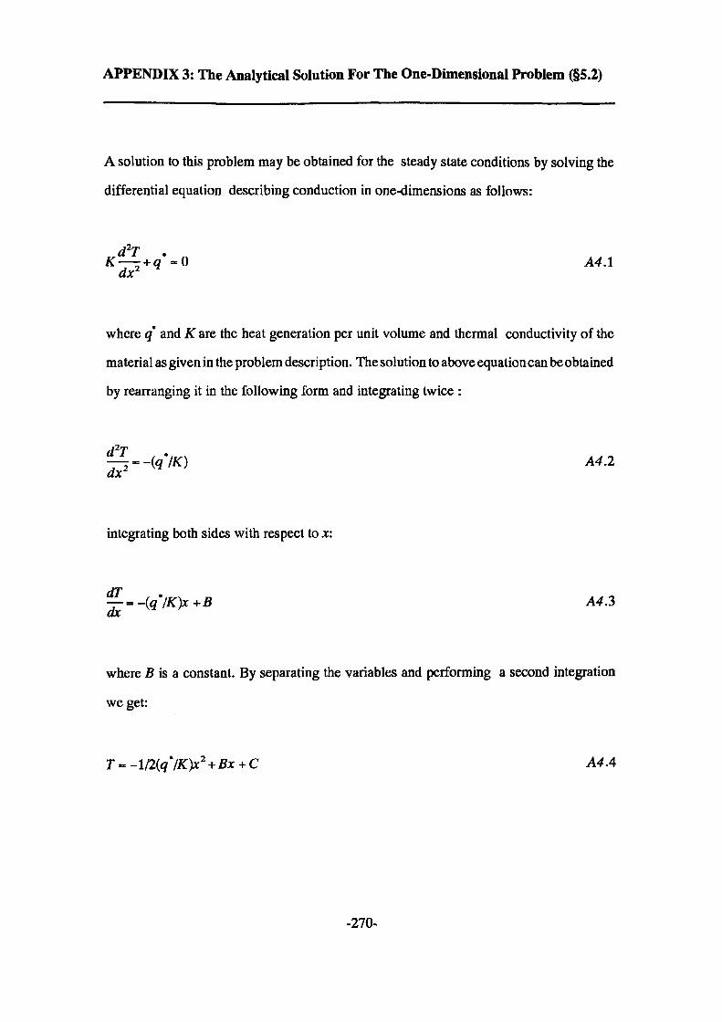
APPENDIX 3: The Analytical Solution For The One-Dimensional Problem (§5.2)

A solution to this problem may be obtained for the steady state conditions by solving the

differential equation describing conduction in one-dimensions as follows:

A4.1 dx2

where q and K are the heat generation per unit volume and thermal conductivity of the

material as given in the problem description. The solution to above equation can be obtained

by rearranging it in the following form and integrating twice :

-(<?*/*) A4.2dx

integrating both sides with respect to x:

A4.3

where B is a constant. By separating the variables and performing a second integration

we get:

T - -l/2(g */K>2 +Bx + C A4A

-270-

Where C is also a constant. The values of B and C can be determined by applying the

following boundary conditions :

T = 60 °C at x = 0

T = 20 °C x = 0.05 m

which gives : B = 2176.8786 and C = 60. The above expression may be used to calculate

final steady-state temperature of any point in the plate.

-271-

APPENDIX 4: Estimation of the Convective and Radiative Heat Transfer Coefficients

for Experiment 1 (§6.1.1)

Two techniques are presented here for calculating the coefficients of convection he and

radiation hr. For the first method use is made of empirical relationships (§3.2.2) to estimate

an average coefficient of convection over the surface and radiation coefficient is calculated

using equation (3.44). The second technique uses a simple heat generated=heat lost

approach where heat losses from the top of the plates and through the insulator is taken

into account. This approach yields a combined convetion/radiation coefficient value.

Method 1

Convection

The convective heat transfer coefficient is calculated here for the copper strip in experiment

1. This is carried out using the recommendations given in Chapman [2] for natural

convection from horizontal surfaces with the heated surface facing upwards. As

recommended, the properties of air are taken at the mean film temperature defined by the

average of the surface and the ambient temperature.

ie. 2} = (T. + TJI2 = 74.35 °C

= 347.5 °K

-272-

The air properties at this temperature are as follows [2]:

v = 20.41 \nm2/sec

K = 29.565 mW/mK

Pr = 0.7065

where K, v and Pr are the thermal conductivity, kinematic viscosity and the Prandtl number

respectively. A characteristic length of / = A/P is used where A and P are the area and

perimeter of the strip which gives a value of 0.011m. The above figures are then used to

evaluate the Rayleigh number defined by the product of Grashof and Prandtl numbers

defined in section (3.2):

Ra = Gr.Pr = ffi&T.Pr/v2 = 6456

This Rayleigh number is in the range for a laminar flow for which the following correlation

is recommended:

Nu = 0.

and since hc = Nu.K/l then

hc = 13.01 W/m2K

-273-

Radiation

The radiative heat transfer coefficient hr as defined in section(3.3) can be determined for

steady-state conditions with values of 23.7 °C and 125 °C for the ambient and surface

temperatures respectively and 0.086 for the emissivity of the surface as calculated

previously. Thus:

h, = 0.84 W/m2K and therefore the total heat transfer coefficient (§4.4) is:

2h=hc + hr = 13.85 WlmK

Method 2

The average heat transfer coefficient over the area of the plate can also be estimated from

the simple equation relating the heat generated and the heat lost in the system. Assuming

that all the electric power is converted into Jule heat it may be written that:

Heat Generated = Heat lost by Convection and Radiation + Heat lost through the insulator

which is:

q = (hc + h,)A (Ts -ty+KA (Ts-Tj/x

where K and x are the thermal conductivity and thickness of the glass wool insulation

material. Substituting values of 0.05 WfmK [2] and 0.035 m for these parameters, a value

of 13.49 is calculated for (hc+hr).

-274-

APPENDIX 5: Determination of the Emissivity of Copper surface

In this technique, a sample of the board is partially coated with matt black lacquer made

by 3M whose emissivity is very nearly 1 [1], The surface is heated and the current outputs

are measured for the coated part (/c) and immediately adjacent to the coated part (Is). A

reading is also taken for the background radiation (7fc) by directing the pyrometer at the

walls of the chamber. The nett current output from the pyrometer is directly proportional

to the emissivity of the surface described by the following relationship:

Is ~ Ib 4<1••-——— A5.1

A piece of copper clad board was partially coated with the paint and heated by passing of

electric current through the copper layer. The specimen was left to reach a steady-state

condition and the pyrometer was used to measure temperature outputs on the coated, bare

copper and the background.These temperatures were then converted into the the

corresponding current outputs using the data supplied by the manufacturers. A graph was

produced from the data supplied shown in figure (A5.1) which made it possible to

accurately carry out the conversions.

The procedure was repeated at increasing electric power inputs and hence increasing

temperature levels. The currents measured and subsequent emissivities are given in Table

(A5.1). The mean and standard deviation from the mean of the results is also given in the

last row of the table.

-275-

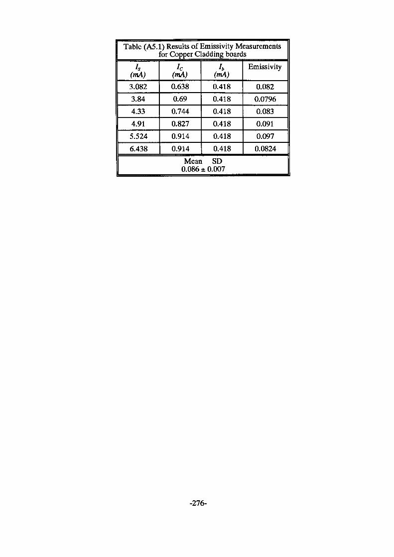
Table (A5.1) Results of Emissivity Measurements for Copper Cladding boards

Is(mA)3.0823.844.334.915.5246.438

Ic(mA)0.6380.690.7440.8270.9140.914

4 (mA)0.4180.4180.4180.4180.4180.418

Emissivity

0.0820.07960.0830.0910.0970.0824

Mean SD 0.086 ± 0.007

-276-

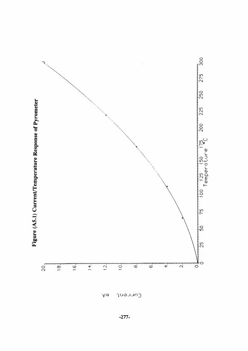
20 is: 16

:

14

:

Figu

re (A

5.1)

Cur

rent

/Tem

pera

ture

Res

pons

e of

Pyr

omet

er

C Cb

12.

10:

LJ

6 4: 2J

0.0

25

50

7510

0 12

5 15

0 17

5 20

0 22

5 25

0 27

5 30

0 T

em

pe

ratu

re

°C

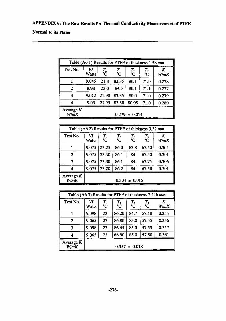
APPENDIX 6: The Raw Results for Thermal Conductivity Measurement of FTFE

Normal to its Plane

Table (A6.1) Results for PTFE of thickness 1.58 mmTest No.

1234

Average K W/mK

VI Watts9.0458.989.0129.03

Ta °C

21.822.021.9021.95

T, °C

83.3584.583.3583.30

T2 °C

80.180.180.080.05

T, °C

71.071.171.071.0

KW/mK0.2780.2770.2790.280

0.279 ± 0.014

Table (A6.2) Results for PTFE of thickness 3.32 mmTest No.

1234

Average K W/mK

VI Watts9.0759.0759.0759.075

Ta °C

23.2523.3023.3023.20

TI °C

86.086.186.186.2

T2 °C

83.8848484

T3 °C

67.5067.5067.7567.50

KW/mK0.3050.3010.3060.301

0.304 ± 0.015

Table (A6.3) Results for PTFE of thickness 7.446 mmTest No.

1234

Average K W/mK

VIWatts9.0989.0659.0989.065

Ta °C

23232323

Tt °C

86.2086.8086.6586.90

T2 °C

84.785.085.085.0

T,°C

57.1057.5557.5557.80

KW/mK0.3540.3560.3570.361

0.357 ± 0.018

-278-

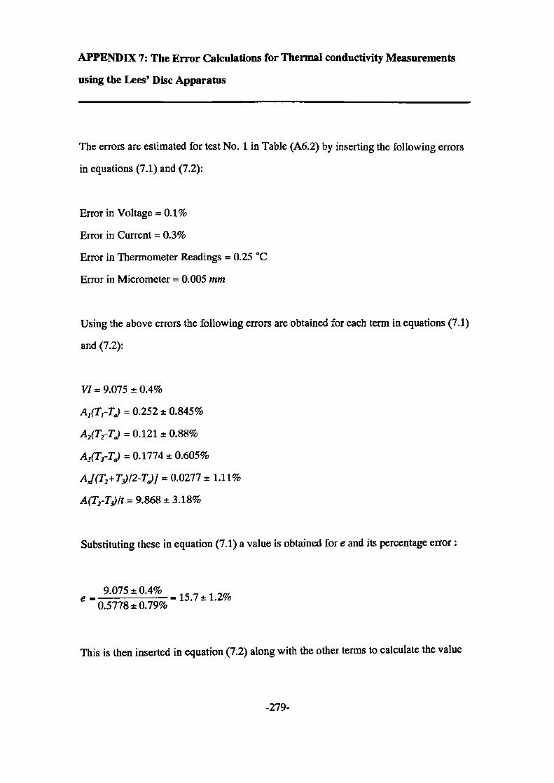
APPENDIX 7: The Error Calculations for Thermal conductivity Measurements

using the Lees' Disc Apparatus

The errors are estimated for test No. 1 in Table (A6.2) by inserting the following errors

in equations (7.1) and (7.2):

Error in Voltage = 0.1%

Error in Current = 0.3%

Error in Thermometer Readings = 0.25 °C

Error in Micrometer = 0.005 mm

Using the above errors the following errors are obtained for each term in equations (7.1)

and (7.2):

VI = 9.075 ±0.4%

Ai(TrTJ = 0.252 ± 0.845%

AJTf-TJ = 0-121 ± 0.88%

A3(T3-TJ = 0.1774 ± 0.605%

AJfc+TJtf-TJJ = 0.0277 ± 1.11%

A(T2-Tj)lt = 9.868 ± 3.18%

Substituting these in equation (7.1) a value is obtained for e and its percentage error :

9.075±0.4% „__ . „ e - ———————— = 15.7 ± 1.2% 0.5778 ±0.79%

This is then inserted in equation (7.2) along with the other terms to calculate the value

-279-

and error in the thermal conductivity K:

(15.7 ± 1.2%) [(0.0138 ± 1.11%) + (0.1774 ±0.605%)] 9.868 ±3.18%

= 0.304 ±5.0%

= 0.304 ±0.015 W/m 2K

-280-

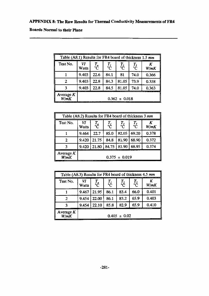
APPENDIX 8: The Raw Results for Thermal Conductivity Measurements of FR4

Boards Normal to their Plane

Table (A8.1) Results for FR4 board of thickness 1.5 mmTest No.

123

Average K W/mK

VIWatts9.4039.4039.403

Ta °C

22.622.822.8

T> °C

84.184.384.5

T2 °C

8181.0581.05

T3 °C

74.073.974.0

KW/mK0.3660.3580.363

0.362 ± 0.018

Table (A8.2) Results for FR4 board of thickness 3 mmTest No.

123

Average K W/mK

VIWatts9.4649.4209.420

Ta °C

22.721.7521.80

Tt °C

85.084.8

84.75

T2 °C

82.0581.9081.90

T3 °C

69.2068.9068.95

KW/mK0.3780.3720.374

0.375 ± 0.019

Table (A8.3) Results for FR4 board of thickness 4.5 mmTest No.

123

Average K W/mK

VI Watts9.4679.4549.454

Ta °C

21.9522.0022.10

Tt °C

86.186.185.8

T2 °C

83.483.282.9

T3 °C

66.065.965.9

K W/mK0.4010.4030.410

0.405 ± 0.02

-281-

Table (A8.4) Results for FR4 board of thickness 6 mm

Test No.

1234

Average K W/mK

VIWatts9.4679.4679.4679.477

r.°c24.424.324.320.9

T, °C

8888.0588.185.25

T2 °C

85.585.6

85.7582.9

T3 °C

6464.0564.261.2

KW/mK0.4120.4110.4120.410

0.411 ± 0.02

-282-

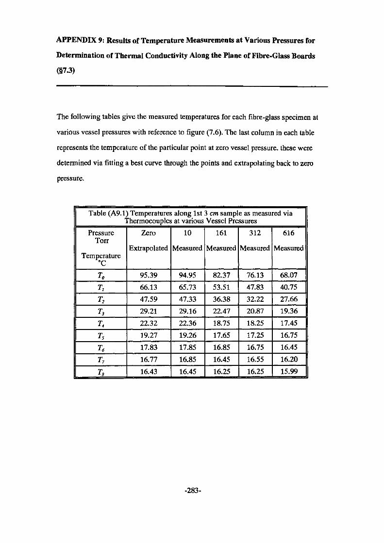
APPENDIX 9: Results of Temperature Measurements at Various Pressures for

Determination of Thermal Conductivity Along the Plane of Fibre-Glass Boards

(§7.3)

The following tables give the measured temperatures for each fibre-glass specimen at

various vessel pressures with reference to figure (7.6). The last column in each table

represents the temperature of the particular point at zero vessel pressure, these were

determined via fitting a best curve through the points and extrapolating back to zero

pressure.

Table (A9.1) Temperatures along 1st 3 cm sample as measured via Thermocouples at various Vessel Pressures

Pressure Torr

Temperature °C

TOT,T2T3T4T5T6T7T8

Zero

Extrapolated

95.3966.1347.5929.2122.3219.2717.8316.7716.43

10

Measured

94.9565.7347.3329.1622.3619.2617.8516.8516.45

161

Measured

82.3753.5136.3822.4718.7517.6516.8516.4516.25

312

Measured

76.1347.8332.2220.8718.2517.2516.7516.5516.25

616

Measured

68.0740.7527.6619.3617.4516.7516.4516.2015.99

-283-

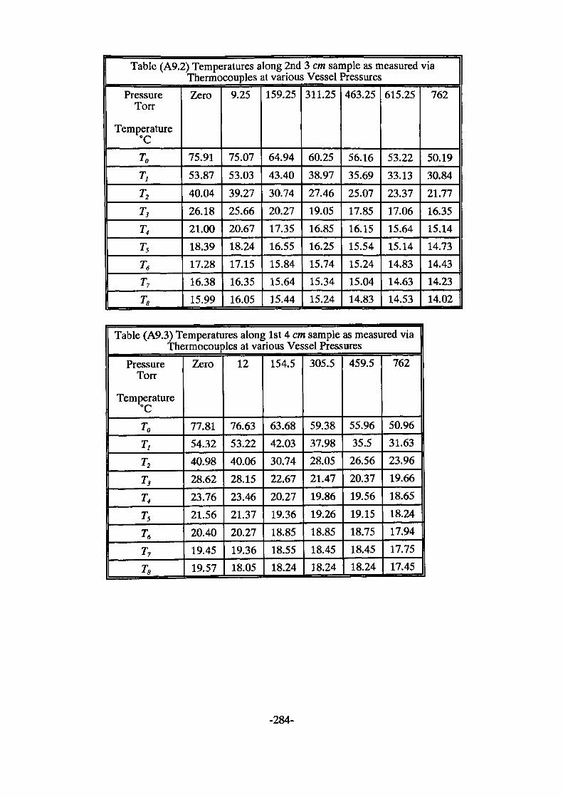
Table (A9.2) Temperatures along 2nd 3 cm sample as measured via Thermocouples at various Vessel Pressures

Pressure Ton-

Temperature °C

T0T>T2T3T4TsT6T7T8

Zero

75.9153.8740.0426.1821.0018.3917.2816.3815.99

9.25

75.0753.0339.2725.6620.6718.2417.1516.3516.05

159.25

64.9443.4030.7420.2717.3516.5515.8415.6415.44

311.25

60.2538.9727.4619.0516.8516.2515.7415.3415.24

463.25

56.1635.6925.0717.8516.1515.5415.2415.0414.83

615.25

53.2233.1323.3717.0615.6415.1414.8314.6314.53

762

50.1930.8421.7716.3515.1414.7314.4314.2314.02

Table (A9.3) Temperatures along 1st 4 cm sample as measured via Thermocouples at various Vessel Pressures

Pressure Ton-

Temperature °C

T0

TtT2T3T4T5T6T7T8

Zero

77.8154.3240.9828.6223.7621.5620.4019.4519.57

12

76.6353.2240.0628.1523.4621.3720.2719.3618.05

154.5

63.6842.0330.7422.6720.2719.3618.8518.5518.24

305.5

59.3837.9828.0521.4719.8619.2618.8518.4518.24

459.5

55.9635.5

26.5620.3719.5619.1518.7518.4518.24

762

50.9631.6323.9619.6618.6518.2417.9417.7517.45

-284-

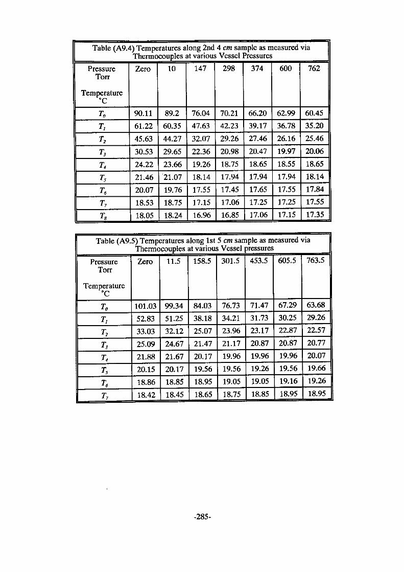
Table (A9.4) Temperatures along 2nd 4 cm sample as measured via Thermocouples at various Vessel Pressures

Pressure Torr

Temperature °C

TO

T,T2T3T4T5T6T7T8

Zero

90.1161.2245.6330.5324.2221.4620.0718.5318.05

10

89.260.3544.2729.6523.6621.0719.7618.7518.24

147

76.0447.6332.0722.3619.2618.1417.5517.1516.96

298

70.2142.2329.2620.9818.7517.9417.4517.0616.85

374

66.2039.1727.4620.4718.6517.9417.6517.2517.06

600

62.9936.7826.1619.9718.5517.9417.5517.2517.15

762

60.4535.2025.4620.0618.6518.1417.8417.5517.35

Table (A9.5) Temperatures along 1st 5 cm sample as measured via Thermocouples at various Vessel pressures

Pressure Ton-

Temperature °C

TOT,T2T3T4T5T6T7

Zero

101.0352.8333.0325.0921.8820.1518.8618.42

11.5

99.3451.2532.1224.6721.6720.1718.8518.45

158.5

84.0338.1825.0721.4720.1719.5618.9518.65

301.5

76.7334.2123.9621.1719.9619.5619.0518.75

453.5

71.4731.7323.1720.8719.9619.2619.0518.85

605.5

67.2930.2522.8720.8719.9619.5619.1618.95

763.5

63.6829.2622.5720.7720.0719.6619.2618.95

-285-

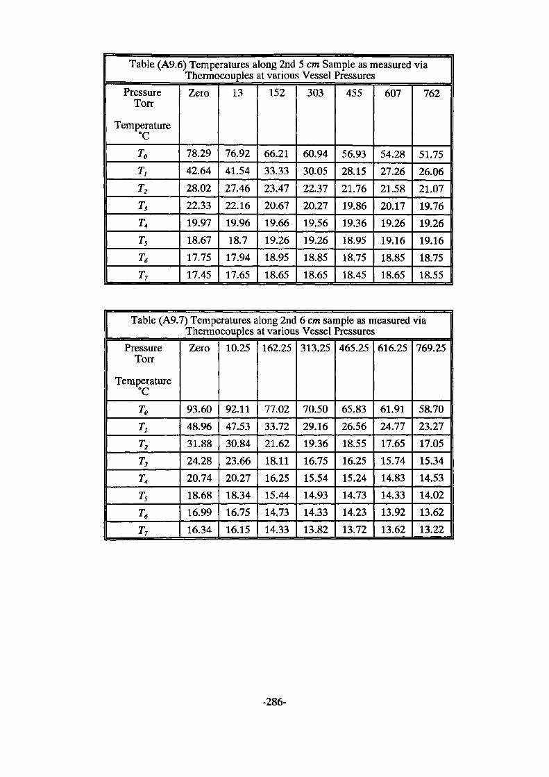
Table (A9.6) Temperatures along 2nd 5 cm Sample as measured via Thermocouples at various Vessel Pressures

Pressure Torr

Temperature °C

TOTtT2T3T4T5T6T7

Zero

78.2942.6428.0222.3319.9718.6717.7517.45

13

76.9241.5427.4622.1619.9618.7

17.9417.65

152

66.2133.3323.4720.6719.6619.2618.9518.65

303

60.9430.0522.3720.2719.5619.2618.8518.65

455

56.9328.1521.7619.8619.3618.9518.7518.45

607

54.2827.2621.5820.1719.2619.1618.8518.65

762

51.7526.0621.0719.7619.2619.1618.7518.55

Table (A9.7) Temperatures along 2nd 6 cm sample as measured via Thermocouples at various Vessel Pressures

Pressure Ton-

Temperature °C

TOT,T2T3T<T5T6T7

Zero

93.6048.9631.8824.2820.7418.6816.9916.34

10.25

92.1147.5330.8423.6620.2718.3416.7516.15

162.25

77.0233.7221.6218.1116.2515.4414.7314.33

313.25

70.5029.1619.3616.7515.5414.9314.3313.82

465.25

65.8326.5618.5516.2515.2414.7314.2313.72

616.25

61.9124.7717.6515.7414.8314.3313.9213.62

769.25

58.7023.2717.0515.3414.5314.0213.6213.22

-286-

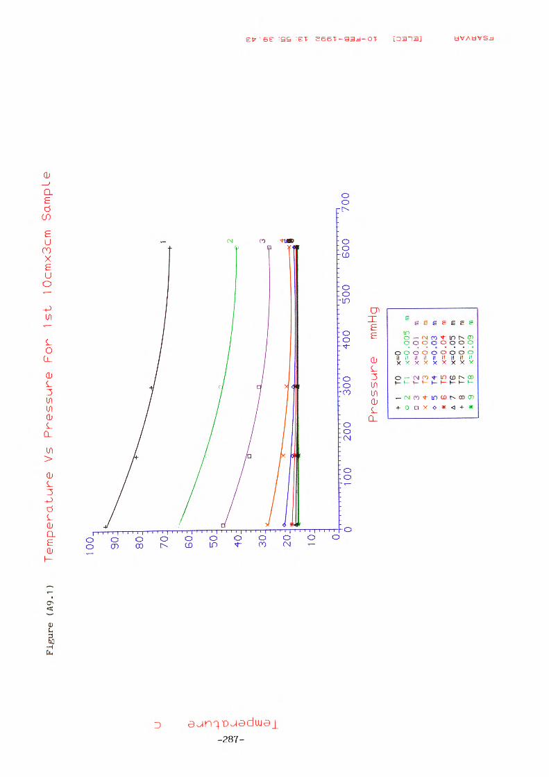
Figu

re (

Ag.

i) T

em

pe

ratu

re

Vs

Pre

ssure

F

or

1st

10cm

x3cm

S

ampl

e

u 0)

Q_

E

0)

00

90:

80:

70:

60:

50:

40:

30:

20:

10: 0:0

100

200

300

400

500

600

700

Pre

ssure

m

mHg

+ o D X O * A + *

1 2 3 4 5 6 7 8 9

TO ri T2 T3 T4 T5 T6 T7 rs

x=0

x-0

x=0

x=0

x=0

x=0

x=0

x=0

<--0

.005

.01

.02

.03

.04

.05

.07

.09

m m m m m m m m

ID

IP ai 01

0) in IL i o o HI j UJ DC

<

> I

< (n u

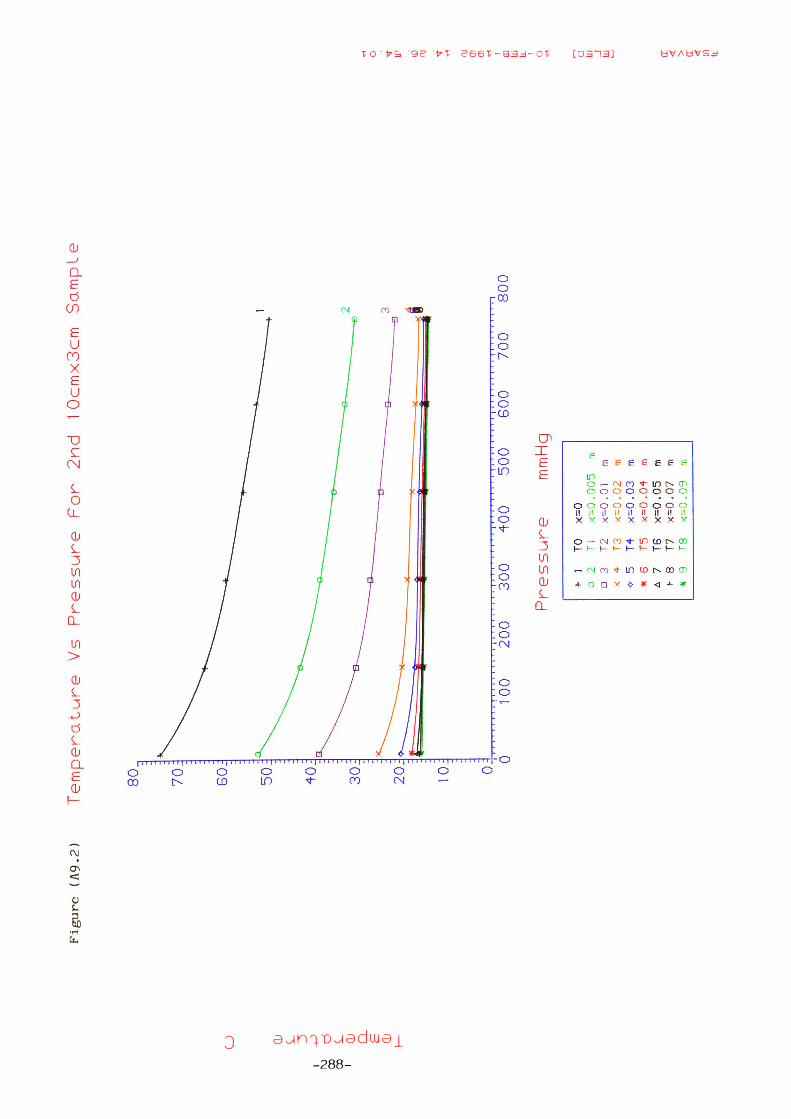
Figu

re

(A9.

2)

Te

mp

era

ture

V

s P

ressu

re

For

2n

d

1 Ocm

xScm

S

am

ple

CJ L 3no 0

0 00 iCD CL E CD

100

200

300

400

500

Pres

sure

mmHg

600

700

800

+ o a X o * A H- <

1 2 3 4 5 6 7 8 9

TO n T2 T3 T4 T5 T6 T7 rs

x=0

x-0

x=0

x=0

x=0

x=0

x=0

x=0

x--0

.005

.01

.02

.03

.04

.05

.07

.09

m m m m m m m Tl

(0

01 ni 0)

0) •H I m UJ u. i o u w J 1U d < > a: < (!) IL

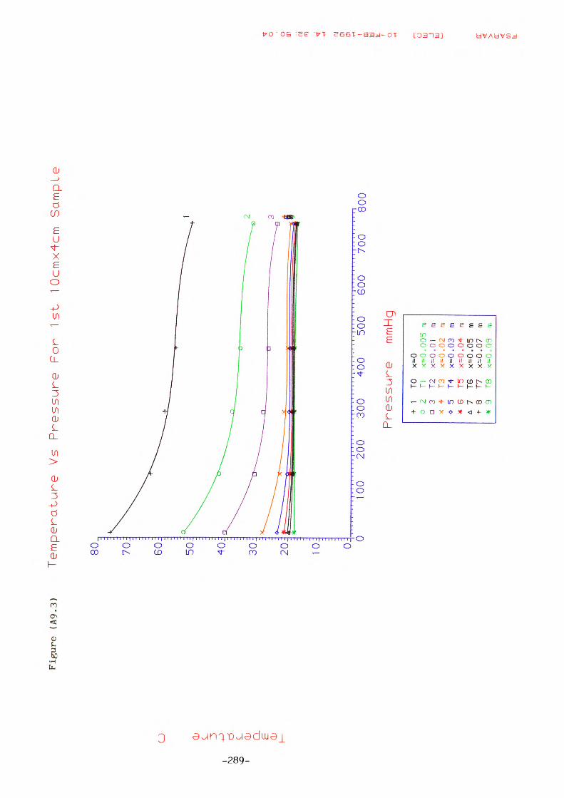
Figu

re

(A9.

3)

Te

mpe

ratu

re

Vs

Pre

ssu

re

For

1st

10cm

x4cm

S

am

ple

oo vO i

CJ Hi L. 3 L Hi CL E Hi

80 70:

eo:

50_

40

;

so:

20: o o

100

200

300

400

500

Pre

ssure

m

mH

g

60

070

0 8

00

+ o n X <> * A + *

1 2 3 4 5 6 7 8 9

TO Tl T2 T3 T4 T5 T6 T7 T8

x=0

x-0

x=0

x=0

x=0

x=0

x=0

x=0

x-0

.005

.01

.02

.03

.04

.05

.07

.09

m m m m m m m n

o 10 0)

0) •H i m UJ lL I o o UJ J UJ d < > a: < (n IL

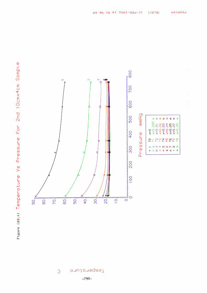
Figu

re

(A9.

4)

Te

mpe

ratu

re

Vs

Pre

ssure

F

or

2nd

10cm

x4cm

S

am

ple

no o i

O a> Oi

CL £

90

80J

70;

GO

l

30J

201 0

100

200

300

400

500

Pre

ssu

re

mm

Hg

600

700

800

+ o a X o * A H- *

1 2 3 4 5 6 7 8 9

TO n T2 T3 T4 T5 T6 T7 T8

x=0

<=-0

x=0

x=0

x=0

x=0

x=0

x=0

x=0

.005

.01

.02

.03

.04

.05

.07

.09

m m m m m m m m

10 IP o IT 0) 01 ri i m UJ u. i o o UJ J Ul I < > a: < <n IL

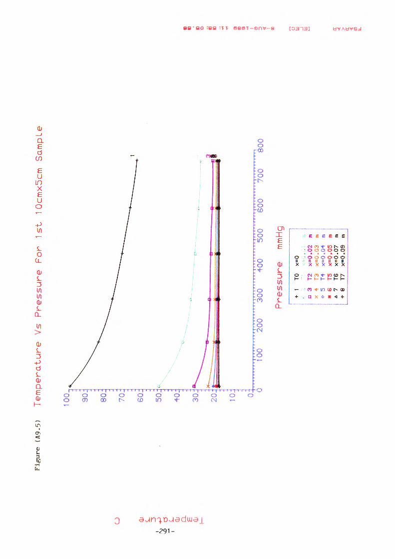
Figu

re (

A9.5

) T

em

pe

ratu

re

Vs

Pre

ssure

F

or

1st

10cm

xScm

S

am

ple

CJ Q; . Q;

CL £

QJ

100 90

:

80:

70:

60:

50:

40:

30:

20: 1 " j 1

1 1 1 1

1 1 1

100

200

300

400

500

Pre

ssure

m

mHg

600

700

800

+ . a X <» m A +

1 3 4 5 6 7 8

TO T2 T3 T4 T5 T6 T7

x=0

x»0

x=0

x=0

x=0

x=0

x=0

e -•

>

.02

.03

.04

.05

.07

.09

m m m m m m

CD

D D o O n a o a Tl I O u bj j m oc D)

U.

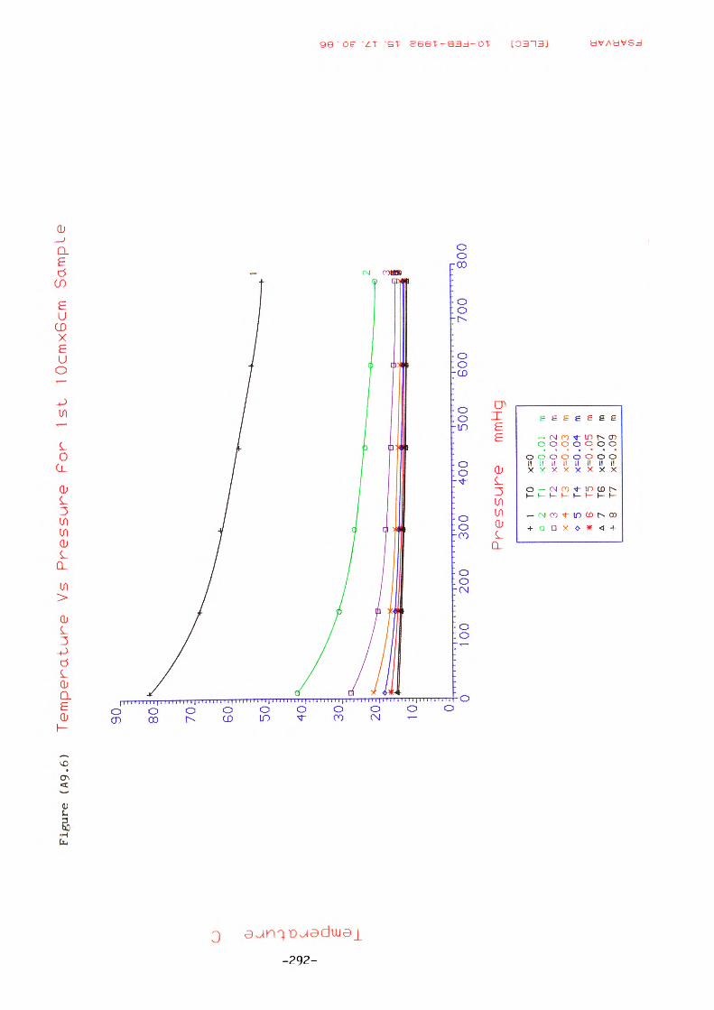
Figu

re

(A9.

6)

Te

mpe

ratu

re

Vs

Pre

ssure

F

or

1st

10cm

xGcm

S

am

ple

r\> i

o Oi d L CU Q.

£ CD

90 80

:

70:

60:

50:

40:

30:

20:

10: o: 0

oo20

030

040

050

060

0 70

080

0

Pre

ssure

m

mH

g

+ o a X 0 * A +

1 2 3 4 5 6 7 8

TO n T2 T3 T4 T5 T6 T7

x=0

x=0

x=0

x=0

x=0

x=0

x=0

x=0

.01

.02

.03

.04

.05

.07

.09

m m m m m m m

(0 CD s ^ ID (M

0) cn UJ

U- i o a tu j UJ cr < > DC

< m IL

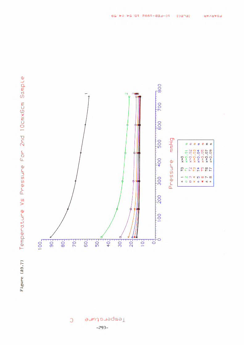
Figu

re

(A9.

7)

Te

mpe

ratu

re

Vs

Pre

ssure

F

or

2nd

10cm

xGcm

S

am

ple

U) I

o CD L

15 Q_

E

Hi

100 90

:

80:

70:

60:

50:

40:

30:

20:

10: 0:0

0020

0 30

040

0 50

060

070

080

0

Pre

ssu

re

mm

Hg

+ o a X o X A f

1 2 3 4 5 6 7 8

TO n T2

T3

T4 T5

T6

T7

x=0

<--o

x=0

x=0

x=0

x=0

x=0

x=0

.01

.02

.03

.04

.05

.07

.09

11 m m m m m m

0) in •7 O •i in in •H

01 en en •H I ffl

UJ

1L U

UJ J UJ U)

ll.

APPENDIX 10: Calculation of Heat Transfer Coefficients for the Hybrid Carrier

Radiation

The radiation coefficient hr \s determined from the following equation (§ 3.3):

Substituting values of 0.95 for emissivity, 120 °C for surface temperature and 23.2 °C for

the ambient temperature a radiation heat transfer coefficient of 9 W/m2K is obtained for

the ceramic package.

Convection

The convective heat transfer coefficient he is calculated using the relationships

recommended in Chapman [8] for natural convection from a horizontal fiat plate with the

heated surface facing upwards. The air properties are taken from the appropriate tables [8]

at the mean film temperature Tf=(T,+Tl)l2 which is 71.6 °C in this case.

Pr=0.707 K=29.32xlQ-i W/mK v=20xlO* m2/sec

The characteristic length is recommended as l=A/p where A and P are the surface area and

perimeter respectively. A width of 0.015 ro and 0.03 m yields a value of 0.005 m for /.

Rayleigh number is defined as:

-294-

Ra =

where =

substituting for all the parameters a value of 608.57 is calculated for Rayleigh number

which is the laminar range [8] for which the following relationship is recommended:

Nu=Q.54Ra1'4 = 2.682

Since he=NuK/l a value of 15.72 W/m2K is obtained for the convective heat transfer

coefficient from the ceramic package.

-295-

APPENDIX 11: Publications

POOLE N J, SARVAR F, WITTING P A and McKENZIE W H: 'Thermal Modelling Using ASTEC3 Software', Int. J. of Numerical Modelling, Volume 1,103-113,1988.

POOLE N J and SARVAR F: 'Fundamentals of Heat Transfer', IEE Colloquium on Thermal Design of Electronic Systems, London, March 1989.

WITTING P A and SARVAR F: 'Electro-thermal Simulation of Hybrid and VLSI Circuits', IEE Colloquium on Thermal Design of Electronic Systems, London, March 1989.

SARVAR F, POOLE N J: 'Simultaneous Modelling of Thermal and Electrical Characteristics Using ASTEC3 Software', Digest of the Nasecode VI Software Forum, Dublin, pp. 149-154,1989.

WITTING P A, SARVAR F, POOLE N J: 'Electro-thermal Simulation of Hybrid and VLSI Circuits', Proceedings of the IASTED Conference, Lugano, June 1989.

SARVAR F, POOLE N J, WITTING P A: 'PCB Glass-Fibre Laminates: Thermal Conductivity Measurements and Their Effect on Simulation', AIME Journal of Electronic Materials, Volume 19, NO. 12,1990.

-296-

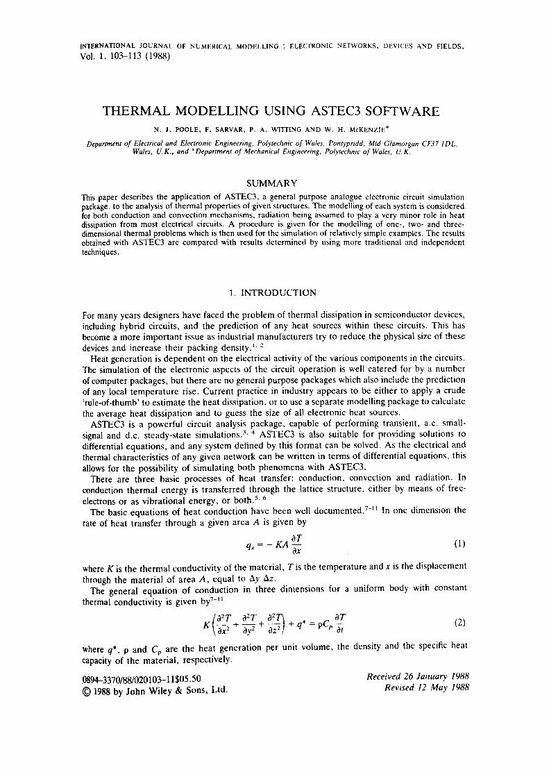
INTERNATIONAL JOURNAL OF NUMERICAL MODELLING : ELECTRONIC NETWORKS, DEVICES AND FIELDS,

Vol. 1, 103-113 (1988)

THERMAL MODELLING USING ASTEC3 SOFTWAREN. J. POOLE, F. SARVAR, P. A. WITTING AND W. H. McKENZIE*

Department of Electrical and Electronic Engineering, Polytechnic of Wales, Pontypridd, Mid Glamorgan CF37 IDL, Wales, U.K., and "Department of Mechanical Engineering, Polytechnic of Wales, U.K.

SUMMARYThis paper describes the application of ASTEC3, a general purpose analogue electronic circuit simulation package, to the analysis of thermal properties of given structures. The modelling of each system is considered for both conduction and convection mechanisms, radiation being assumed to play a very minor role in heat dissipation from most electrical circuits. A procedure is given for the modelling of one-, two- and three- dimensional thermal problems which is then used for the simulation of relatively simple examples. The results obtained with ASTEC3 are compared with results determined by using more traditional and independent techniques.

1. INTRODUCTION

For many years designers have faced the problem of thermal dissipation in semiconductor devices, including hybrid circuits, and the prediction of any heat sources within these circuits. This has become a more important issue as industrial manufacturers try to reduce the physical size of these devices and increase their packing density. 1 - 2

Heat generation is dependent on the electrical activity of the various components in the circuits. The simulation of the electronic aspects of the circuit operation is well catered for by a number of computer packages, but there are no general purpose packages which also include the prediction of any local temperature rise. Current practice in industry appears to be either to apply a crude 'rule-of-thumb' to estimate the heat dissipation, or to use a separate modelling package to calculate the average heat dissipation and to guess the size of all electronic heat sources.

ASTEC3 is a powerful circuit analysis package, capable of performing transient, a.c. small- signal and d.c. steady-state simulations. 3 - 4 ASTEC3 is also suitable for providing solutions to differential equations, and any system defined by this format can be solved. As the electrical and thermal characteristics of any given network can be written in terms of differential equations, this allows for the possibility of simulating both phenomena with ASTEC3.

There are three basic processes of heat transfer: conduction, convection and radiation. In conduction thermal energy is transferred through the lattice structure, either by means of free- electrons or as vibrational energy, or both. 5 - 6

The basic equations of heat conduction have been well documented. 7"" In one dimension the rate of heat transfer through a given area A is given by

where K is the thermal conductivity of the material, Tis the temperature and x is the displacement through the material of area A, equal to Ay Az.

The general equation of conduction in three dimensions for a uniform body with constant thermal conductivity is given by7~"

, „ ar ... < =pC"¥ (2)

where <?*, p and Cp are the heat generation per unit volume, the density and the specific heat capacity of the material, respectively.

.0894-3370/88/020103-1 1$05. 50 Received 26 January 1988 © 1988 by John Wiley & Sons, Ltd. Revised 12 May 1988

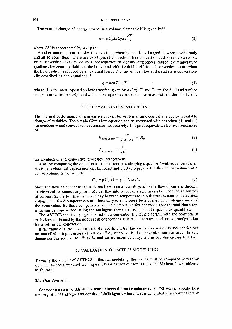
104 N . j. POOLE ET AL.

The rate of change of energy stored in a volume element AK is given by 1

dT(3)

where AK is represented by A*A_yAz.Another mode of heat transfer is convection, whereby heat is exchanged between a solid body

and an adjacent fluid. There are two types of convection: free convection and forced convection. Free convection takes place as a consequence of density differences caused by temperature gradients between the fluid and the body, and with the fluid itself; forced convection occurs when the fluid motion is induced by an external force. The rate of heat flow at the surface is convention­ ally described by the equation7"' '

q = hA(T( - TJ (4)

where A is the area exposed to heat transfer (given by AyAz), T, and Ts are the fluid and surface temperatures, respectively, and h is an average value for the convective heat transfer coefficient.

2. THERMAL SYSTEM MODELLING

The thermal performance of a given system can be written as an electrical analogy by a suitable change of variables. The simple Ohm's law equation can be compared with equations (1) and (4) for conductive and convective heat transfer, respectively. This gives equivalent electrical resistances of

"conduction ~~ js A A ~ "th (-*)

"convection / A \®)

for conductive and convective processes, respectively.Also, by comparing the equation for the current in a charging capacitor 12 with equation (3), an

equivalent electrical capacitance can be found and used to represent the thermal capacitance of a cell of volume AV of a body

Cth = pCp AV=pC p AxAyAz (7)

Since the flow of heat through a thermal resistance is analogous to the flow of current through an electrical resistance, any form of heat flow into or out of a system can be modelled as sources of current. Similarly, there is an analogy between temperature in a thermal system and electrical voltage, and fixed temperatures at a boundary can therefore be modelled as a voltage source of the same value. By these comparisons, simple electrical equivalent models for thermal character­ istics can be constructed, using the analogous thermal resistance and capacitance quantities.

The ASTEC3 input language is based on a conventional circuit diagram, with the positions of each element defined by the nodes at its connections. Figure 1 illustrates the electrical configuration for a cell in 3D conduction.

If the value of convective heat transfer coefficient h is known, convection at the boundaries can be modelled using resistors of values l/HA, where A is the convection surface area. In one dimension this reduces to llh as A_y and Az are taken as unity, and in two dimensions to l//iAy.

3. VALIDATION OF ASTEC3 MODELLING

To verify the validity of ASTEC3 in thermal modelling, the results must be compared with those obtained by some standard techniques. This is carried out for ID, 2D and 3D heat flow problems, as follows.

3.1. One dimension

Consider a slab of width 50 mm with uniform thermal conductivity of 17-3 W/mK, specific heat capacity of 0-444 kJ/kgK and density of 8656 kg/m\ where heat is generated at a constant rate of

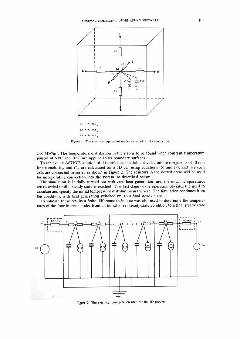
THERMAL MODELLING USING ASTEC3 SOFTWARE 105

rl = S Rth x

r2 = H Rth y

r3 = "i Rth

Figure 1. The electrical equivalent model for a cell in 3D conduction

2-06 MW/m3 . The temperature distribution in the slab is to be found when constant temperature sources at 60°C and 20°C are applied to its boundary surfaces.

To achieve an ASTEC3 solution of this problem, the slab is divided into five segments of 10 mm length each. Rth and C, h are calculated for a ID cell using equations (5) and (7), and five such cells are connected in series as shown in Figure 2. The resistors in the dotted areas will be used for incorporating convection into the system, as described below.

The simulation is initially carried out with zero heat generation, and the nodal temperatures are recorded until a steady state is reached. This first stage of the operation obviates the need to calculate and specify the initial temperature distribution in the slab. The simulation continues from this condition, with heat generation switched on, to a final steady state.

To validate these results a finite-difference technique was also used to determine the tempera­ tures of the four interior nodes from an initial linear steady-state condition to a final steady state

Figure 2. The electrical configuration used for the ID problem

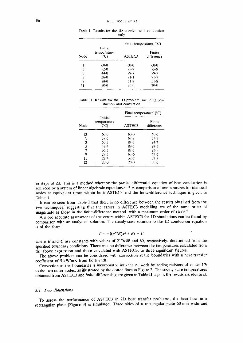
106 N. J. POOLE t'f AL.

Table I. Results for the ID problem with conduction only

Final temperature (°C)

Node

13579

11

Initialtemperature(°C)

60-052-044-036-028-020-0

ASTEC3

60-075-879-771-151-820-0

Finitedifference

60-075-879-771-751-820-0

Table II. Results for the ID problem, including con­ duction and convection

Node

1313579

1112

Initialtemperature(°C)

60-057-650-543-436-529-522-420-0

Final temperature' (°C)

ASTEC3

60-067-984-789-582-563-632-720-0

Finitedifference

60-067-984-789-582-563-632-720-0

in steps of Ar. This is a method whereby the partial differential equation of heat conduction is replaced by a system of linear algebraic equations. 7 ' '' A comparison of temperatures for identical nodes at equivalent times within both ASTEC3 and the finite-difference technique is given in Table I.

It can be seen from Table I that there is no difference between the results obtained from the two techniques, suggesting that the errors in ASTEC3 modelling are of the same order of magnitude as those in the finite-difference method, with a maximum order of (A*)2 . 9

A more accurate assessment of the errors within ASTEC3 for ID simulations can be found by comparison with an analytical solution. The steady-state solution to the ID conduction equation is of the form

T= -$(q*/K)x2 +Bx + C

where B and C are constants with values of 2176-88 and 60, respectively, determined from the specified boundary conditions. There was no difference between the temperatures calculated from the above expression and those calculated with ASTEC3, to three significant figures.

The above problem can be considered with convection at the boundaries with a heat transfer coefficient of 5 kW/mK from both ends.

Convection at the boundaries is incorporated into the network by adding resistors of values \lh to the two outer nodes, as illustrated by the dotted lines in Figure 2. The steady-state temperatures obtained from ASTEC3 and finite-differencing are given in Table II; again, the results are identical.

3.2. Two dimensions

To assess the performance of ASTEC3 in 2D heat transfer problems, the heat flow in a rectangular plate (Figure 3) is simulated. Three sides of a rectangular plate 50 mm wide and

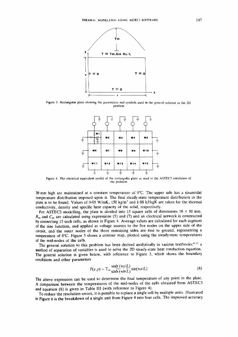
THERMAL MODELLING USING ASTEC1 SOFTWARE 107

T = Tm.Sin nx/L

T = 0 T = 0

T = 0

Figure 3. Rectangular plate showing the parameters and symbols used in the general solution to the 2Dproblem

1

I~

J~

1 Ml

I

Me

M11

M2

M7

M12

M8

M13

MS

M14

MS

M10

MIS

11111Figure 4. The electrical equivalent model of the rectangular plate as used in the ASTEC3 simulation of

the problem

30 mm high are maintained at a constant temperature of 0°C. The upper side has a sinusoidal temperature distribution imposed upon it. The final steady-state temperature distribution in the plate is to be found. Values of 0-05 W/mK, 150 kg/m3 and 1-88 kJ/kgK are taken for the thermal conductivity, density and specific heat capacity of the solid, respectively.

For ASTEC3 modelling, the plate is divided into 15 square cells of dimensions 10 x 10 mm. Rth and Cth are calculated using expressions (5) and (7) and an electrical network is constructed by connecting 15 such cells, as shown in Figure 4. Average values are calculated for each segment of the sine function, and applied as voltage sources to the five nodes on the upper side of the circuit, and the outer nodes of the three remaining sides are tied to ground, representing a temperature of 0°C. Figure 5 shows a contour map, plotted using the steady-state temperatures of the mid-nodes of the cells.

The general solution to this problem has been derived analytically in various textbooks;" " a method of separation of variables is used to solve the 2D steady-state heat conduction equation. The general solution is given below, with reference to Figure 3, which shows the boundary conditions and other parameters

sinh(iry/L) . _ ,., ,g .

The above expression can be used to determine the final temperature of any point in the plate. A comparison between the temperatures of the mid-nodes of the cells obtained from ASTEC3 and equation (8) is given in Table III (with reference to Figure 4).

To reduce the resolution errors, it is possible to replace a single cell by multiple units. Illustrated in Figure 6 is the breakdown of a single unit from Figure 4 into four cells. The improved accuracy

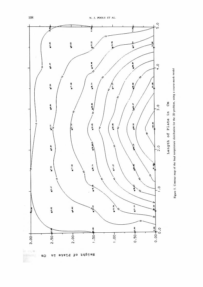
3.0

0

S o c 2

.50

0)

-U

CO u-t o n

2.0

0H

oc m

m

5.0

Leng

th

of

Pla

te

in

Cm

Figu

re 5

. Co

ntou

r m

ap o

f th

e fin

al te

mpe

ratu

re d

istrib

utio

n fo

r th

e 2D

pro

blem

, us

ing

a co

arse

-mes

h m

odel

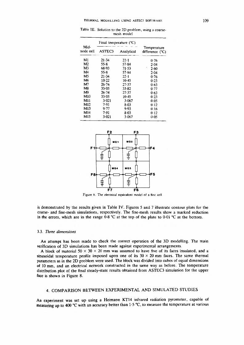
THERMAL MODELLING USING ASTEC3 SOFTWARE

Table III. Solution to the 2D problem, using a coarse- mesh model

109

Mid- node cell

MlM2M3M4M5M6M7M8M9M10MilM12M13M14M15

Final temperature (°C)

ASTEC3

21-3455-868-9355-821-3410-2226-7433-0526-7433-053-0217-919-777-913-021

Analytical

22-157-8471-5357-8422-110-4527-3733-8227-3710-453-0678-039-938-033-067

Temperature difference (°C)

0-762-042-602-040-760-230-630-770-630-230-050-120-160-120-05

F2

F7 F6Figure 6. The electrical equivalent model of a fine cell

is demonstrated by the results given in Table IV. Figures 5 and 7 illustrate contour plots for the coarse- and fine-mesh simulations, respectively. The fine-mesh results show a marked reduction in the errors, which are in the range 0-8 °C at the top of the plate to 0-01 °C at the bottom.

3.3. Three dimensions

An attempt has been made to check the correct operation of the 3D modelling. The main verification of 3D simulations has been made against experimental arrangements.

A block of material 50 X 30 x 20 mm was assumed to have five of its faces insulated, and a sinusoidal temperature profile imposed upon one of its 30 x 20 mm faces. The same thermal parameters as in the 2D problem were used. The block was divided into cubes of equal dimensions of 10 mm, and an electrical network constructed in the same way as before. The temperature distribution plot of the final steady-state results obtained from ASTEC3 simulation for the upper face is shown in Figure 8.

4. COMPARISON BETWEEN EXPERIMENTAL AND SIMULATED STUDIES

An experiment was set up using a Heimann KT14 infrared radiation pyrometer, capable of measuring up to 400 °C with an accuracy better than 1-5 °C, to measure the temperature at various

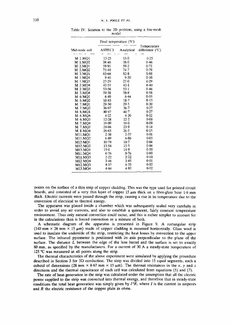
110 N. J. POOLE ET AL.

Table IV. Solution to the 2D problem, using a fine-mesh model

Final temperature (°C)Temperature

Mid-node cell ASTEC3 Analytical difference (°C)

M 1.MQ1M 1.MO2M 2.MQ1M 2.MQ2M 3.MQ1M 1.MQ4M 1.MO3M 2.MQ4M 2.MQ3M 3.MQ4M 6.MQ1M 6.MQ2M 7.MQ1M 7.MQ2M 8.MQ1M 6.MQ4M 6.MQ3M 7.MQ4M 7.MQ3M 8.MQ4M11.MQ1M11.MQ2M12.MQ1M12.MQ2M13.MQ1M11.MQ4M11.MQ3M12.MQ4M12.MQ3M13.MQ4

13-2538-4659-9175-4983-689-40

27-2942-5153-5659-38

6-4918-8329-3036-9740-97

4-2212-2819-0924-0426-65

2-386-89

10-7413-5415-00-762-223-464-374-84

13-038-059-274-782-89-30

27-042-153-158-8

6-4418-729-136-740-7

4-2012-219-023-926-5

2-376-86

10-713-514-90-762-223-454-354-82

0-250-460-710-790-880-100-290-400-460-580-050-130-200-270-270-020-080-090-140-150-010-030-040-040-100-000-000-010-020-02

points on the surface of a thin strip of copper cladding. This was the type used for printed circuit boards, and consisted of a very thin layer of copper 15 (xm thick on a fibre-glass base 1-6 mm thick. Electric currents were passed through the strip, causing a rise in its temperature due to the conversion of electrical to thermal energy.

The apparatus was placed inside a chamber which was subsequently sealed very carefully in order to avoid any air currents, and also to establish a quiescent, fairly constant temperature environment. Thus only natural convection could occur, and this is rather simpler to account for in the calculations than is forced convection or a mixture of both.

A schematic diagram of the apparatus is presented in Figure 9. A rectangular strip (140 mm x 26 mm x 15 |o.m) made of copper cladding is mounted horizontally. Glass wool is used to insulate the underside of the strip, restricting the heat losses by convection to the upper surface. The infrared pyrometer is positioned with its axis perpendicular to the plane of the surface. The distance L between the edge of the lens barrel and the surface is set to exactly 80 mm, as specified by the manufacturers. For a current of 30 A a steady-state temperature of 125 °C was measured at all points along the strip.

The thermal characteristics of the above experiment were simulated by applying the procedure described in Section 3 for 3D conduction. The strip was divided into 15 equal segments, each a cuboid of dimensions (28 mm x 8-67 mm x 15 jim). The thermal resistances in the x, y and z directions and the thermal capacitance of each cell was calculated from equations (5) and (7).

The rate of heat generation in the strip was calculated under the assumption that all the electric power supplied to the strip was converted into thermal energy, and therefore that in steady-state conditions the total heat generation was simply given by 1 2R, where / is the current in amperes and R the electric resistance of the copper plate in ohms.

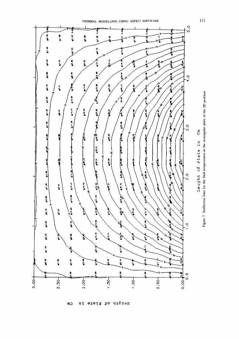
THERMAL MODELLING USING ASTEC3 SOFTWARE 111

_£1£

ou

•H I0) .5

fl t-* «31 i.^ u0 -

*ra

3

3°

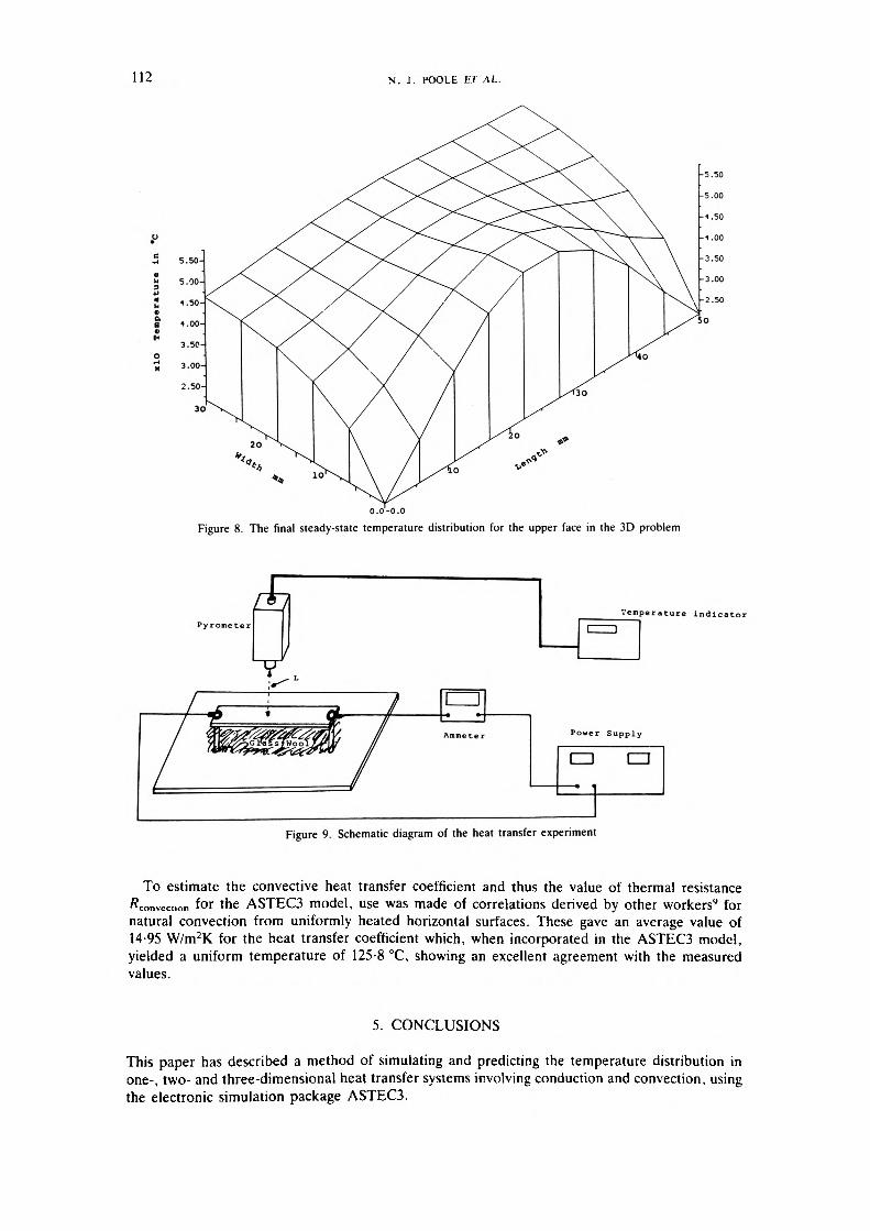
112 N. J. POOLE £J AL.

0.0-0.0

Figure 8. The final steady-state temperature distribution for the upper face in the 3D problem

mperature indicate

Power Supply

CD— 1

cn

Figure 9. Schematic diagram of the heat transfer experiment

To estimate the convective heat transfer coefficient and thus the value of thermal resistance ^convection for the ASTEC3 model, use was made of correlations derived by other workers9 for natural convection from uniformly heated horizontal surfaces. These gave an average value of 14-95 W/m2K for the heat transfer coefficient which, when incorporated in the ASTEC3 model, yielded a uniform temperature of 125-8 °C, showing an excellent agreement with the measured values.

5. CONCLUSIONS

This paper has described a method of simulating and predicting the temperature distribution in one-, two- and three-dimensional heat transfer systems involving conduction and convection, using the electronic simulation package ASTEC3.

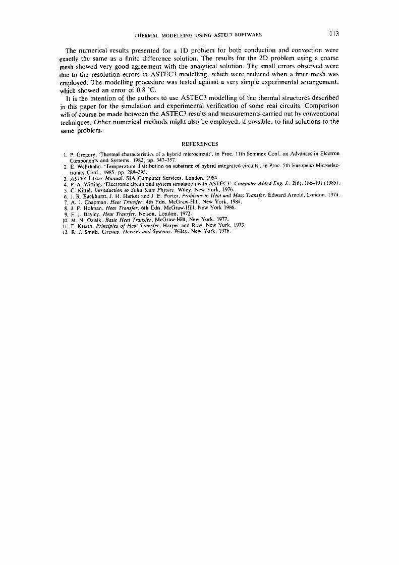
THERMAL MODELLING USING ASTEC3 SOFTWARE 113

The numerical results presented for a ID problem for both conduction and convection were exactly the same as a finite difference solution. The results for the 2D problem using a coarse mesh showed very good agreement with the analytical solution. The small errors observed were due to the resolution errors in ASTEC3 modelling, which were reduced when a finer mesh was employed. The modelling procedure was tested against a very simple experimental arrangement, which showed an error of 0-8 °C.

It is the intention of the authors to use ASTEC3 modelling of the thermal structures described in this paper for the simulation and experimental verification of some real circuits. Comparison will of course be made between the ASTEC3 results and measurements carried out by conventional techniques. Other numerical methods might also be employed, if possible, to find solutions to the same problem.

REFERENCES

1. P. Gregory, Thermal characteristics of a hybrid microcircuit', in Proc. llth Seminex Conf. on Advances in Electron Components and Systems. 1982, pp. 347-357.

2. E. Wehrhahn. 'Temperature distribution on substrate of hybrid integrated circuits', in Proc. 5th European Microelec­ tronics Conf., 1985. pp. 288-295.

3. ASTEC3 User Manual. SIA Computer Services, London. 1984.4. P. A. Witting, 'Electronic circuit and system simulation with ASTEC3'. Computer-Aided Eng. J., 2(6), 186-191 (1985).5. C. Kittel. Introduction to Solid State Physics. Wiley. New York, 1976.6. J. R. Backhurst, J. H. Marker and J. E. Porter, Problems in Heal and Mass Transfer, Edward Arnold. London. 1974.7. A. J. Chapman, Heat Transfer. 4th Edn, McGraw-Hill, New York, 1984. g. J. P. Holman, Heal Transfer. 6th Edn, McGraw-Hill, New York 1986.9. F. J. Bayley, Heal Transfer. Nelson, London, 1972.

10. M. N. Ozisik, Basic Heat Transfer. McGraw-Hill, New York. 1977.11. F. Kreith, Principles of Heat Transfer, Harper and Row. New York, 1973.12. R. J. Smith, Circuits, Devices and Systems. Wiley, New York, 1976.

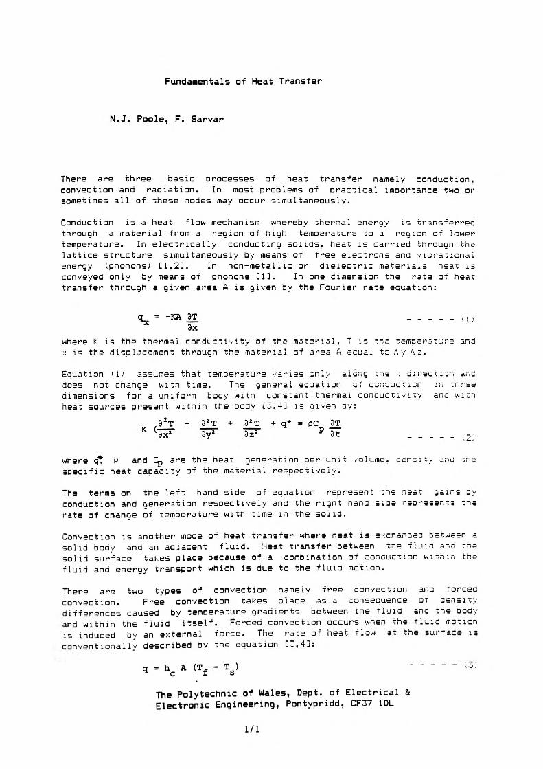
Fundamentals of Heat Transfer

N.J. Poole, F. Sarvar

There are three basic processes of heat transfer namely conduction, convection and radiation. In most problems of oractical importance two or sometimes all of these modes may occur simultaneously.

Conduction is a heat flow mechanism whereby thermal energy is transferred through a material from a region of high temperature to a region of lower temperature. In electrically conducting solids, heat is carried through the lattice structure simultaneously by means of free electrons and vibrationai energy (phonons; Cl,2]. In non-metallic or dielectric materials heat is conveyed only by means of phonons El], In one dimension the rate of heat transfer through a given area A is given by the Fourier rate eauation:

a = -KA 3T _____.,,*V -^— — — — — — \ j. /

^ 3xwhere K is tne thermal conductivity of tne material. T is the temperature and x is the displacement through the material of area A equal to Ay Az.

Eauation (I/ assumes that temperature varies only along ths x direction ana does not change with time. The general eauation of conduction in tnr-ee dimensions for a uniform body with constant thermal conductivity and with heat sources present within the body [3,4] is given by:

,3 2T + 3*T + 3*T + q* = pC 3T K Sx* 3y2 3z 2 P 3t _____ (2 )

where q* P and C^, are the heat generation per unit volume, density ana tne soecific heat capacity of the material respectively.

The terms an the left hand side of equation represent the neat gains by conduction and generation resoectively and the right hand sias rearesents the rate of change of temperature with time in the solid.

Convection is another mode of heat transfer where neat is excnangea between a solid body and an adjacent fluid. Meat transfer oetween tne fluid and the solid surface takes place because of a combination of concuction within the fluid and energy transport which is due to the fluid motion.

There are two types of convection namely free convection ana forced convection. Free convection takes place as a consecuence of density differences caused by temperature gradients between the fluid and tne ocdy and within the fluid itself. Forced convection occurs when the fluid motion is induced bv an external force. The rate of heat flow at the surface is conventionally described by the equation C3.4]:

q = hc A (Tf - Tg )•

The Polytechnic of Wales, Dept. of Electrical Electronic Engineering, Pontypridd, CF37 1DL

1/1

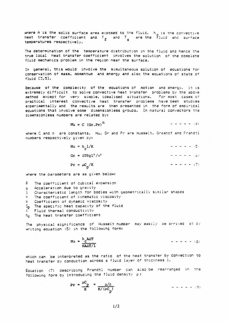
where A is the solid surface area exposed to the fluid, h is tne convective heat transfer coefficient and T_ and T are the fluid ana surface temperatures respectively. S

Tha determination of the temperature distribution in tne fluid and hence tne true local heat transfer coefficient involves the solution of the comoiete fluid mechanics problem in the region near the surface.

In general, this would involve the simultaneous solution of equations for conservation of mass, momentum and energy and also the equations of state of fluid C3,53.

Because of the complexity of the equations of motion and energy. it is extremely difficult to solve convective heat transfer problems by the aocve method except for very simple, idealised situations. For most cases of practical interest convective heat transfer problems have oeen studies experimentally and the results are then presented in the form of empirical equations that involve some dimensionless grouos. In .natural convectors tne dimensionless numbers are related by:

Nu = C (Gr.Pr) n ----- ,4)

where C and n are constants. Nu, Gr and Pr are Nusselt. Grashof and Prandtl numbers respectively given by:

Nu = h 1/K - - - - - >.=;'•• c

Gr = ATSglVv2 _____ . 6)

Pr = UC /K - - - - - \7i P

where the parameters are as given below:

6 The coefficient of cubical expansiong Acceleration due to gravity1 Characteristic lenatn for bodies with geometrically similar snapasv The coefficient of kinematic viscosityU Coefficient of dynamic viscosityCp The specific heat capacity of the fluidK Fluid thermal conauctivityhc The heat transfer coefficient

The ahysical sionificance of Nusselt number may easily oe arrived at oy writing eauation (5) in the following form:

h AATNU = C _____ ,q.

KAAT/1

which can be interpreted as the ratio of the heat transfer by convection to heat transfer by conduction across a fluid layer of thickness 1.

Eauation (7) describing Prandtl number can also be rearranged in tne following form by introducing the fluid density p:

pr = ^ p = U/P K K/(PC )

1/2

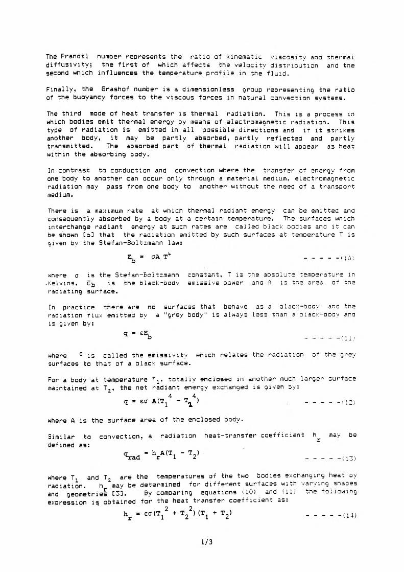
The Prandtl number represents the ratio of kinematic viscosity and thermaldiffusivity; the first of which affects the velocity distribution and tnesecond which influences the temperature profile in the fluid.

Finally, the Grashof number is a dimensionless group reoresenting the ratio of the buoyancy forces to the viscous forces in natural convection systems.

The third mode of heat transfer is thermal radiation. This is a process in which bodies emit thermal energy by means of electromagnetic radiation. This type of radiation is emitted in all possible directions and if it strikes another body, it may be partly absorbed, partly reflected and partly transmitted. The absorbed part of thermal radiation will apoear as heat within the absorbing body.

In contrast to conduction and convection where the transfer of energy from one body to another can occur only through a material medium, electromagnetic radiation may pass from one body to another witnout the need of a transport medium.

There is a maximum rate at which thermal radiant energy can be emitted and consequently absorbed by a body at a certain temperature. The surfaces wnich interchange radiant energy at such rates are called black podies and it can be shown C6] that the radiation emitted by sucn surfaces at temperature T is given by the Stefan-Boltzmann law:

where a is the Stefan-Boitzmann constant, T is the absolute temperature in -Kelvins, E^ is the black-body emissive power ana A is the ares, of the radiating surface.

In practice there are no surfaces that behave as a black-body and the radiation flux emitted by a "grey body" is always less tnan a black-body ana is given by:

q = EEb

where e is called the emissivity which relates the radiation of the grey surfaces to that of a black surface.

For a body at temperature T 1? totally enclosed in another much larger surface maintained at T 2 , the net radiant energy excnanged is given py:

4 4 q = ea ACT. - T ) _ _ _ _ -a2j

where A is the surface area of the enclosed body.

Similar to convection, a radiation heat-transfer coefficient h may Pe defined as:

•(13)

where T, and T, are the temperatures of the two bodies exchanging heat oy radiation. h may be determined for different surfaces with varying snaoes and geometries' C3j. By comparing equations (10) and (ili the following expression is. obtained for the heat transfer coefficient as:

1/3

References

1. KITTEL, C.,: 'Introduction to Solid State Physics', New York, Wiley and Sons, 5th edition, 1976.

2. BACKHURST, J.R., MARKER, J.H. and PORTER, J.E.,: 'Problems in Heat and Mass Transfer', London, Arnold, 1974.

3. CHAPMAN, A.J.: 'Heat Transfer', New York, McSraw-Hili, 1984.

4. KREITH, F.,: 'Principles of Heat Transfer', New York, Harper and Row, 1973.

5. OZISIK, M.N.,: 'Basic Heat Transfer', New York, McSraw-Hill, 1977.

6. HOLMAN, J.P.: 'Heat Transfer', New York, McSraw-Hili, 1981.

1/4

ELECTRO-THERMAL SIMULATION of HYBRID and VLSI CIRCUITS

p A WITTING, F SARVAR

INTRODUCTION

For many years designers of Integra tedC1] and hybrid circuitsC2]C3] have faced the problem of predicting the temperature rise within their devices under operational conditions. This has become a more important issue as the packing density of the devices has increasedCA ] [5 ] . The tendency to carry out ail design work i :- the simulation domain and to then move, without iteration, to the production of finished devices has increased the need for a simulation tool capable of predicting the local temperature within an operational device. It is also important that such a tool should not be over conservative in its predictions, since this could be wastefu1.

Current practice in industry appears to be to either guess at the average heat dissipation in each section of a circuit or to carry out a electrical(only) simulation to determine the average dissipation. These average values of heat dissipation ar-e then input to a quite separate thermal model to predict the temperature rise. Since such methods take no account of the chasing of the heat dissipation it is possible for the predictions to over- or under-est imate the true s i tuat ion. Th i s is Nearly snown by an example system with two heat generating islands. The heat sources are pulsed and in phase (a), pulsed and out of phase (b) and constant (c); all with the same average heat input. The maximum temperatures reached are, however, very different being i79 a C, l" a C and 83°C respectively. This situation will become worse as the devices get smaller and the averaging effect of their thermal mass is less powerful.

The Polytechnic of Wales is currently engaged in a research project to develop a simulation tool which combines tne eiectrica; and thermal simulation functions. The work is based around the Astec3 circuit simulator and relies heavily on the -simple but powerful modelling capabilities of this package. The overall objectives of this project are as foilows:-

1. To develop a method of creating one-. two- and three-dimensional thermal models using Astec3

2. To validate these models against simple macro-scale structures which are amenable to both theoretical and empirical checking

3. To develop a two-layered model capable of combining both the electrical and thermal aspects

4. To produce isothermal contours for the device being simulated

The Polytechnic of Wales, Pontypridd, Mid Glamorgan, CF37 1DL, UK

2/1

5. To estimate the computing resource required to achieve a realistic simulation

6. To develop a means of semi-automaticaI Iy generating the description of the structure to be simulated

7. To carry out simulations of hybrid structures to establish the validity of the modelling procedure at this scale

8. To likewise carry out investigations on integrated circuits

9. To develop interactive input and co1 our - graphic output faci1ities

The final objective represents a major challenge in its own right and work in this area has been deferred to a ruture project. This paper presents the results achieved to date on the first five objecti ves.

VALIDATION of ASTEC3 in THERMAL MODELLING

The methods used to carry out the simulations wiii be discussed in the presentation. The methods have been tested against theoretical predictions for some simple arrangements and good agreement obtained, comparable to that achieved by rini.e difference techniques. These results have been further tested against macro-scale physical systems. For simple arrangements good agree.ment has been obtained, but some anomalies have been observed in more complex situations. Recent work has elaborated the models to remove these anomalies with the result that work will soon commence on hybrid-scale systems.

COMPUTATIONAL ASPECTS

Measurements of computation time demonstrate that. for a given computer system, the computation time is proportional to the number of cells being computed - up to a certain limit imposed by the memory availability in the particular computer. Measurements on three different computers from the DEC vax range of machines indicates that the computation rate (cells per second) is proportional to the computer's power rating in Mflops, being approximately 29.2 ce11/sec/Mf1 op.

A further restriction. in the case of the vax computers, is an limit on the number of equations that may be included in any one model. This is 32,767 corresponding to approximately 3150 2-D cells. It will be seen therefore that there is a strong motivation to reduce the number of cells used. This has lead to the development of mixed-mesh models where fine mesh cell are used in areas of high temperature gradient with a coarser cell structure being used elsewhere. A range of interface cells have been

2/2

developed to permit this mixing.

The specification of the mesh structure for complex systems is clearly time consuming and error prone. A semi-automatic method of producing the required description files has been devised and is in routine use.

CONCLUSION

It has been demonstrated that the simulation of the electrical and thermal aspects of circuit behaviour can be combined via the ASTEC3 software system. The. finer the cell mesh the more 'accurate the results obtained, at the expense of extending the computation. The use of mixed coarse/fine cells reduces this problem and a semi-automatic method of generating the mesh file has been deve1 oped.

The results obtained from the simulations have been shown to correspond to theoretical predictions and, with some reservations, to the experimental situation. However, further work needs to be done on the effects of convection before the method is fully deve1 oped.

The advantage, of the combined simulation is seen to be ^. more realistic estimation of the thermal effects as a result or oein^ able to take account of the phasing of the neat generation processes.

L HEIN V L, LENZI V D:'Thermal Analysis of Substrates ana Integrated Circuits', Proceedings of Electronic Component Conference, May 1969, pp 166-177

2DAVID, R F:'Computerised Thermal Analysis of HybridCircuits', Trans IEEE on Parts, Hybrids and Packaging.vo1 PHP-3, no 3 , Sept 1977, pp 233-289

3 SBERGOVIC S, BOSNJAK K M:'Computer application in Thermal Analysis of Passive Components in Hybrid Microelectronic Circuits. International Colloquium on New Orientations of Passive Components, 1982, p 415

4GREGORY P:'Thermal Characteristics of a Hybrid Mi crocircuit' .Proceedings of 11 th Seminex Conference on Advances in ElectronicComponents and Systems, 1982. pp 3^7-357

5 UEHRHAHN E: 'Temperature Distribution on Substrate of Hybrid Electronic Circuits', Proceedings of the 5'" European Microelectronics Conference. 1985, pp 288-295

2/3

l£CTURE NOTES AND DIGEST OF THE NASECODE VI ASSOCIATED SHORT COURSE AND SOFTWARE FORUM - Edited in W. Crans-DMn (Ireland) IOih-12thJuly 19S9 - Boole Press Ltd.

Simultaneous modelling of thermal and electrical characteristics using

ASTEC 3 software

F. 5ARVAR. N.J. POOLE. AND F.H. wITTING

Department of Electrical ana Electronic Engineering. Polytechnic of iDaies.

f-ontypriaa. Mid Glamorgan CF37 !Di_. wales, u.f.

ABSTRACT

it is difficult for designers to oreaict average te.Tioerature rise aue to thermal

Dissipation in semiconductor integratea circuits ana also hvorio roicrocircuits.

Similarly tne oreaiction ana sucseauent prevention of iocs.iisea nor soots is auite

crucial since tneir effect could very well cause tne failure of tne wnole aevice.

Tnese not soots may also arfect the tolerance of circuit lomDonents wmcn can cause

arastic cnanges in tne aevice characteristics. Tnis has oecome iTiore of an

important issue as inoustriai manufacturers nave tried to reou.ce tne onvsicai sire

of Devices ano tnerefore increase tneir pact me censitv.

Meat generation in electronic circuits :s oecensert on tre siectricai activity of

the various components in tie circu.it. wnii = t tne siTi^istion of the electronic

asoects OT the circuit nceration 1= weii cstere: TO;' D< a numoer cf cor.Duter

Dacrage= mere are no Qen= v ai DU.I-DOSB C'fCraoes u-ncr ?!~c rsciiitate tne Dresiction

OT the local teraoera'ure rise.

*ne ouroose or this '-esgarcri is '? oe 5jis tc c.-ecict Tr.erni«i ana eiect-icai

cnaracter istics of tne Given ae>icss -j.= ini fe siiru:at ion osoage.

These new results snow tnat :t IE c.3 = = i:ie i--< HaTt 1"." TO se user =E a tner.Tia:

simulation oactaoe. using rnese Tecnni^ues it -jiii =jon ce oos = icie to crecict

oevice renaciiitv cue to tnerns; aissioation.

AaTtC;. 1= oarticuiariv uell suitea to tni= rsss- ~= :t incoroorites two features of

soeciai sianificance in aaoition to its nioni- efricient electronic simulation

caoaoi lities. Tnese are its Donerfui SL'.D-mooel ling faciiit. ana its aoility to

nanale large sets of Tirst oraer differential eouations. witnin these eauations

there is no upoer limit to tne numoer cf comoonents tr.at may De used for

simulations.

INTRODUCTION

For manv vears designers nave faced the oroolem of thermal dissipation in

semiconductor devices, inducing nvorio circuits, and tne prediction of any heat

sources within these circuits. This nas become a more important issue as

industrial manufacturers try to reduce the physical size of these devices ana

increase their pacKino aensity [1.23.

149

H69t generation is oeaenoent on trie electrical activity of tne various components

in tne circuits. The simulation or tne electronic asoects OT me circuit ooeratir r.

is well catered Tor oy a number of computer pacnages. out mere are no uenerai

Duroose oacKages which also include the prediction of an, local temoerature ri=e

Current practice in industry appears to oe eitner to apolv a crude r^le-of-thump

to estimate tne heat dissioation or to use a seoarate modelling package to

calculate the average neat dissipation and to guess the size of all electronic heat

sources.

HSTEC3 is a powerful circuit analvsis package, written in Fortran 77. caaaoie of

oerforming transient, s.c. small-signal ana d.c. steady-state simulations [33.

ASTEC3 is also suitable for providing solutions to differential eouations. ana any

system defined By tnis format can De solved. As tne electrical and thermal

characteristics of any given network can be written in terms ot differentia,

eouations. this allows for tne oossiDiiity of simulating Doth Dhenomena with

ASTEC3.

The circuit description is written in A5TEC3 svntav: which is based on a

conventional circuit diagram with tne oosition of each element cefinec! py tne noses

at its connections. H5TEC3 is a software lancuaoe that is cossiple to run on IbM.

.'A* and CRAt mainframe macnines. -.5TEC3 is c-jr-ent;, run on eitner a VH> 11/785 or

a »; A>. 3a5'j. these machines reou irino -.".".'.''."'.".' b-tes of memorv for HSTEC3 ana

i. 'j'X 1 . '.">!' D-.tes nas src-ved suTficitr.T .Tt~-.TiOi" - TC '"un cut" aoo i icat !-•" circuits.

THERMAL SYSTEM MODELLING

Tne pas:c eaustions o~ ne?t trrn = ao-t r.s.e r.==n v-=. 1 coc^mentsd C4j. It is

parameters D'- a suitable cianoe DT ,4.1 'iacier:. ^".".e =ir.nie 'jhr. = i aw ecuation car, oe

compared witn consucti-e anc co!--e:ti-e ~=st t-ansre'". ••esoect i .ei'. T-ns gi.es

ea,u .slent electric?: 'i^istinc-s ••

Ax = Rconduction KAyfiz th

R = 1 convection rr~

for conductive and connective processes, respectively.

The current in a charging capacitor is analogous to the rate of change of energy

stored in a volume element AV giving a thermal capacitance:

C . = PC AV = PC AxAyaz <3) th p p

ISO

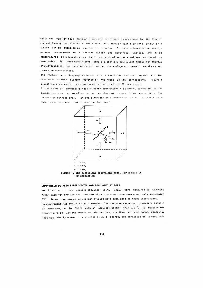
Since the flow of neat through a thermal resistance is analogous to the flow of current through an electrical resistance, an. form of heat flow into or out of a system can be modelled as sources of current. Biiraiariv. there is an analogy Between temperature in a thermal system and electrical voltage. ana fixed temperatures at a Boundary can therefore-De mooeliea as a voltage source of tne same value. By these comoarisons, simois electrical equivalent models for thermal characteristics can oe constructed using the analogous thermal resistance and caoacitance Quantities.The ASTEC3 incut language is based or, a con.-er.ticr.ai circuit diagram, with the DOSltions of each element defined Dy the nodes at its connections. Figure 1 illustrates the electrical confiouration for a cell in 3D conduction. If the value of convective heat transfer coefficient n ls Known, convection at the boundaries can oe modelled using resistors of values i'hn. wne*-e A is the convection surface area. In one dimension tni= reauces to 1-n as A \ and A: are taken as unitv. ana in two dimensions to l-niv.

0

rl - S Rth^

r2 - S nth

rl - S Rch x

Figure 1. The electrical equivalent model for a cell in 3D conduction

COMPARISON BETWEEN EXPERIMENTAL AND SIMULATED STUDIESVerification of tne results obtained using H5TEC3 were compared to standard technidues for one and two dimensional orooiems and have oeen oreviousiv documented [53. Three dimensional simulation studies have oeen used to moaei experiments. An exoenment was set UD using a rieimann fai4 infrared radiation pyrometer, capable of measuring uo to 300t with an accuracy Detter than 1.5 °C. to measure the temperature at various points on the surface of a thin stria of cooper cladding. This was the type used for printed circuit boards, and consisted of a very thin

151

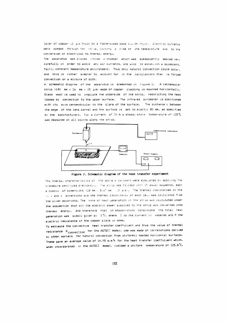
iavsr of copper 10 urn tnici-- on a fiPre-uiaES pase 1.& mm true*;, blectric currents

were passed through tne strip, causing a rise in its temperature due to tne

conversion OT electrical to thermal enerqy.

Tne apparatus was placed insiae a chamber wrucn was supseauentiy sealed very

carefully in order to avoid any air currents, ana also to establish a Quiescent,

fairly constant temperature environment. Thus only natural convection could occur

ana this is rather simpler to account for in the calculations than is forced

convection or a mixture of both.

A schematic diagram of tne apparatus is presented in Figure 2. A rectangular

strio (140 mm x 26 mm :-: 15 urn; maae of copper dadoing is mounted horizontally.

Glass wool is used to insulate tne underside of the strip, restricting the neat

losses by convection to the upper surface. The infrared pyrometer is positioned

with its axis perpendicular to the plane of the surface. The distance L between

the edge of tne lens Parrel and the surface is set to exactly 80 mm. as specified

bv the manufacturers. For a current of 30 A a steaay-stat- temperature of 125 °C

was measured at all points alone the strip.

Figure 2. Schematic diagram of the heat transfer experiment

~ne tnermai cnaracten = t ic= C T t" =>C'C-e e itriiT'^rt *.er= siiT.'jiatec ~-v atpi> ino t~t

proceaure aa=cr-ic.e-3 ore.'iousi,. "ns =-,-\^ WSE cii.iasa ir.ri ir eaual =eQ.T,ents. eacr.

a cuboi'j of cimensionE '.16 T.m E.o" .TUT. .5 UT.'. Tne tr.ermal resistances in tne

v. , ana r direction? and the tnemiai cBipacitance of eacn ceii was cijCLiiatec from

tne given eouations. Tne rate of neat generation i r. tr.e sfio was caiculatea under

tne assumption tnat all tne electric power supoii=a tc tf.e strip was converted into

thermal energy, and tnerefore tnat in steaav-state conoitions tn° total neat

Generation was simply given py I 'ft. where I is the current in affioeres ana R the

electric resistance of tne cooper plate in onms.

To estimate the convective heat transfer coefficient ana tnus tne value of thermal

resistance R t - n f°'" tne ASTEC3 model, use was maae of correlations derived

Bv other workers for natural convection from uniformly heated horizontal surfaces.

These gave an average value of 14.95 ni/m'K for the heat transfer coefficient which.

when incorporatea in the ASTEC3 model, vielaed a uniform temperature of 125.6 C.

152

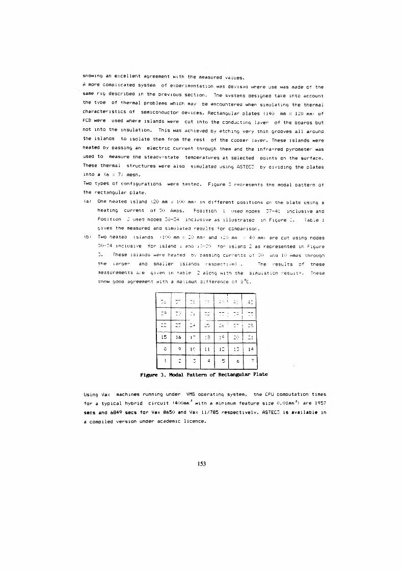
snowing an excellent agreement with the measured values.

A more complicated system pf experimentation was devised where use was made of the same rig described in the previous section. The systems designed take into account the tvpe of thermal problems which mav pe encountered when simulating the tnermal characteristics of semiconductor devices. Rectangular plates '.140 mm x 120 mm.* of PCB were used where islands were cut into the conducting layer of the boaros but not into the insulation. This was achieved PV etchino very thin Grooves all around the islands to isolate them from the rest of the copper layer. These islands were neated by passing an electric current through them and the infra-red pyrometer was used to measure the steadv-state temperatures at selected points on the surface. These thermal structures were also simulated using ASTEC3 Dy dividing the plates into a (6 ;•: 7; mesn.

Two types of configurations were tested. Figure 3 represents tne modal pattern of the rectangular plate.

(a) One heated island i20 mm x 100 mm; in different positions on the plate using a heating current of 30 Amos. Position 1 u.seo nodes 37-41 inclusive and Position 2 used nodes 30-34 inclusive as illustrates in Figu'-e 3. Table 1 gives tne measured ana simulated results for comparison.

tb> Two heated islands ',100 mm • 20 mm' and i20 mm >•• 40 mmj are cut using noces 30-34 inclusive for island 1 ana i3-20 for isianG 2 a= represented in Figure 3. Tnese islands were heated PV Dassir.g currents of 30 ana 10 Amos tnrouon the iargc>- and smaller islands respective! -. Tne results of these measurements a.-e given in tacie 2 along witn the simulation >-esLiit*. Tnese

Figure 3. Modal Pattern of Rectangular Plate

Using Vax machines running under VMS operating system. the CPU computation times for a typical hybrid circuit '400mm witn a minimum feature size 0.01mm 2 ) are 1957 sees and 6B49 sees for Vax 8650 and Vax 11/785 respectively. ASTEC3 is available in a compiled version under academic licence.

153

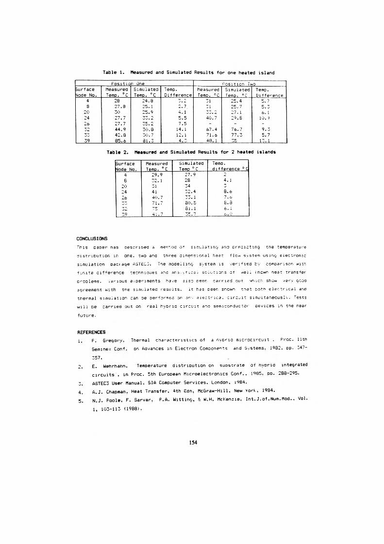
Table 1. Measured and Simulated Results for one heated island

Position oneSurface Mode No.

43

202426T ^v

—'••I'

39

Measured Temp. °C

2827.83027.727.744.942.885.6

Simulated Temp. °C

24.825.125.933. 235.230.830.781.3

Temp. Difference

3. 22.74.15.57.514.112.14.3

Position TwoMeasured Temp. °C

313133 . 240.7-

67.471.648. 1

Simulated Temp . ° C

25.425.727. 12v.S-

76.777.335

Temp. Difference

5.75 . •_•6. 110.9-

9.35.713.1

Table 2. Measured and Simulated Results for 2 heated islands

surface vlode No.

48

20242633^39

Measured Temp. °C

29.932. 1314140.771.77541 .7

Simulated Temp ° C

27.9283432.433. 130.531. 135. 7

Temp, difference ° C

—f

4.138.07.0S.8«j. 1•-• . '.'

CONCLUSIONS

This paper nas aescnoed s metrod of Eirc'-iiatina and predicting tne temperature

ai =trIPUTion in one. two ana three dimensional heat flow system usino electronic

simulation pact:a<je ASTEC3. The modelling system is verified ty comparison with

finite Difference tecnniaaes aria analytical solutions or well mown neat transfer

proBlems. various experiments ha,<e aisr seen carried OUT xnicn show very QOOG

aGreement with tne simulated results. It has Deer, =nown mat totn electrical ano

thermal simulation can oe performea on 5r-- siectrica.i circ-'it simuitaneousi'.. lests

will Pe carrieo out on real hybrid circuit ana semiconductor aevices in tne near

future.

REFERENCES1. F. Greqory. Thermal characteristics of a nvprio microcircuit . F'roc. llth

Semine:-: Conf. on Advances in Electron Components and Systems. 1982. pp. 347-

357.

2. E. Wehrhahn. Temperature distripution on supstrate of hyorid integrated

circuits , in Proc. 5th European Microelectronics Conf.. 1985. PP. 288-295.

~. ASTEC3 User- Manual. SIA Computer Services. London. 1984.

4. A.J. Chapman, Heat Transfer, 4th Edn, McGraw-Hill, New York, 1984.

5. N.J. Poole, F. Sarvar, P.A. Wittinq, & nJ.H. McKenzie. Int. J.of .Num.Mod., Vol.

1, 103-113 (1988).

154

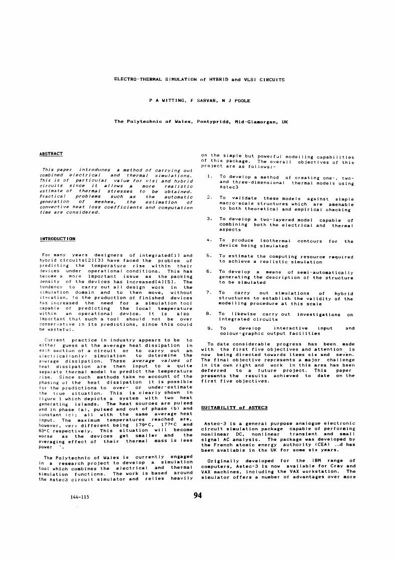
ELECTRO-THERMAL SIMULATION of HYBRID and VLSI CIRCUITS

P A WITTING, F SARVAR, N J POOLE

The Polytechnic of Wales, Pontypridd, Mid-Glamorgan, UK

ABSTRACT

This paper introduces a method of carrying out combined electrical and thermal simulations. This is of particular value for vlsi and hybrid circuits since it allous a more realistic estimate of thermal stresses to be obtained. Practical problems such as the automatic generation of meshes, the estimation of convective heat loss coefficients and computation time are considered.

INTRODUCTION

For many years designers of integrated[1] and hybrid circuits[2]t3] have faced the problem of predicting the temperature rise within their devices under operational conditions. This has become a more Important issue as the packing density of the devices has 1ncreased[4 ] [5 ]. The tendency to carry out all design work in the simulation domain and to then move, without iteration, ^o the production of finished devices has increased the need for a simulation tool capable of predicting the local temperature within an operational device. It is also important that, such a tool should not be over conservative in its predictions, since this could be wastefuI.

Current practice in industry appears to be to either guess at the average heat dissipation in each section of a circuit or to carry out an eleclrica1(only) simulation to determine the average dissipation. These average values of heat dissipation are then input to a quite separate thermal model to predict the temperature rise. Since such methods take no account of the phasing of the heat dissipation it is possible for the predictions to over- or under-estimate the true situation. This is clearly shown in liiiure 1 which depicts a system with two heat generating islands. The heat sources are pulsed and in phase (a), pulsed and out of phase (b) and constant (c): all with the same average heat input. The maximum temperatures reached are, however, very different being 179-C, 177-C and 83-C respectively. This situation will become worse as the devices get smaller and the averaging effect of their thermal mass is less power

The Polytechnic of Wales is currently engaged In a research project to develop a simulation tool which combines the electrical and thermal simulation functions. The work is based around the AstecS circuit simulator and relies heavily

on the simple but powerful modelling capabilities of this package. The overall objectives of this project are as follows:-

1. To develop a method of creating one-, two- and three-dimensional thermal models using Astec3

2. To validate these models against simple macro-scale structures which are amenable to both theoretical and empirical checking

3. To develop a two-layered model capable of combining both the electrical and thermal aspects

To produce isothermal contours for device being simulated

the

5. To estimate the computing resource required to achieve a realistic simulation

6. To develop a means of semi -autonat ica I I y generating the description of the structure to be simulated

7. To carry out simulations of hybrid structures to establish the validity of the modelling procedure at this scale

8. To likewise carry out Investigations on Integrated circuits

9. To develop interactive input co1 our~graphic output facilities

and

To date considerable progress has been made with the first five objectives and attention is now being directed towards items six and seven. The final objective represents a major challenge in its own right and work in this area has been deferred to a future project. This paper presents the results achieved to date on the first five objectives.

SUITABILITY of ASTEC3

Astec-3 is a general purpose analogue electronic circuit simulation package capable of performing nonlinear DC, nonlinear transient and small signal AC analysis. The package was developed by the French atomic energy authority (CEA) ...d has been available In the UK for some six years.

Originally developed for the IBM range of computers, Astec-3 Is now available for Cray and VAX machines, Including the VAX workstation. The simulator offers a number of advantages over more

144-115 94

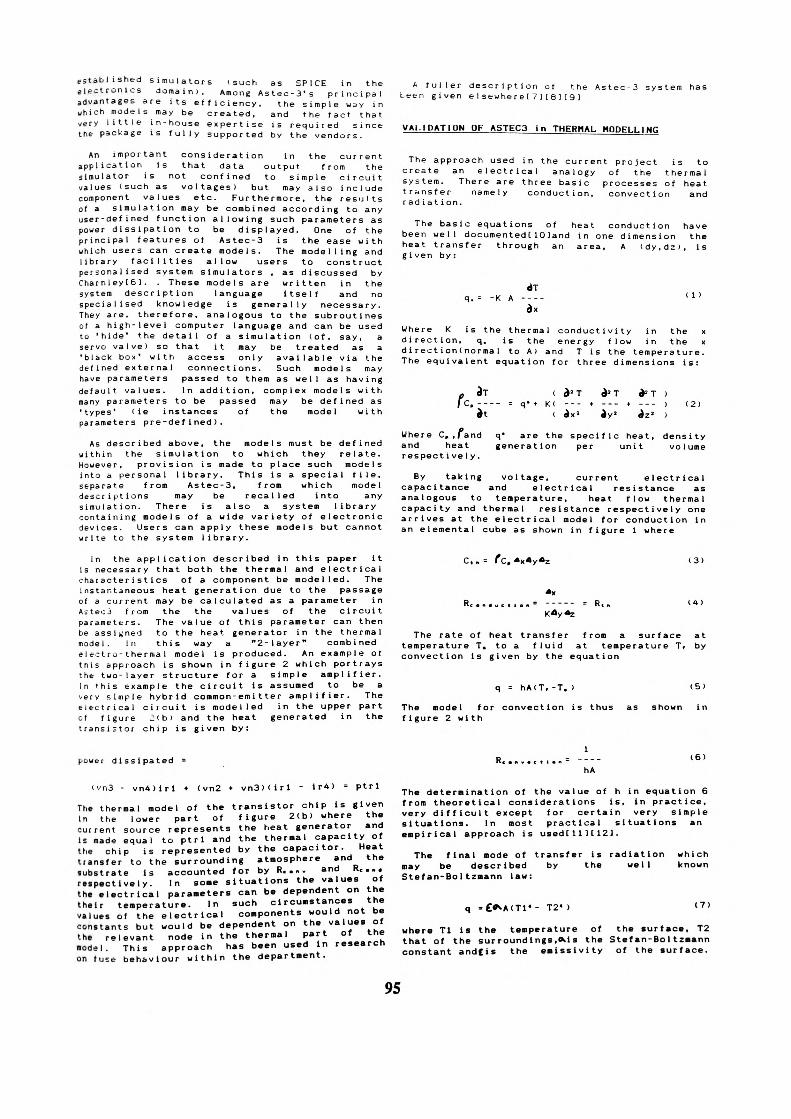
established simulators (such as SPICE in the electronics domain). Among Astec-3's principal advantages are its efficiency, the simple way in M hich models may be created, and the fact that ucry little in-house expertise is required since trie package is fully supported by the vendors.

An important consideration in the current application is that data output from the simulator is not confined to simple circuit values (such as voltages) but may also include component values etc. Furthermore, the results of a simulation may be combined according to any user-defined function allowing such parameters as power dissipation to be displayed. One of the principal features of Astec-3 is the ease with which users can create models. The modelling and library facilities allow users to construct personalised system simulators , as discussed by Char nley[61. . These models are written in the system description language itself and no specialised knowledge is generally necessary. They are, therefore, analogous to the subroutines of a high-level computer language and can be used to 'hide' the detail of a simulation (of, say, a servo valve) so that it may be treated as a 'black box" with access only available via the defined external connections. Such models may have parameters passed to them as well as having default values. In addition, complex models with many parameters to be passed may be defined as 'types' (ie instances of the model with parameters pre-defined).

As described above, the models must be defined within the simulation to which they relate. However, provision is made to place such models into a personal library. This is a special file, separate from Astec-3, from which model descriptions may be recal led into any simulation. There is also a system library containing models of a wide variety of electronic devices. Users can apply these models but cannot write to the system library.

In the application described in this paper it is necessary that both the thermal and electrical char acteristics of a component be model led. The instantaneous heat generation due to the passage of a current may be calculated as a parameter in A; tec 3 from the the values of the circuit parameters. The value of this parameter can then be assigned to the heat generator in the thermal model. In this way a "2-layer" combined electro-therma1 model is produced. An example or this approach is shown in figure 2 which portrays the two-layer structure for a simple amplifier. In this example the circuit is assumed to be a very simple hybrid common-emitter amplifier. The electrical circuit is modelled in the upper part of figure ;:(b) and the heat generated in the transistor chip is given by:

power dissipated -

(vn3 - vnAMrl + (vn2 + vn3)(irl - Ir4) ptrl

The thermal model of the transistor chip is given In the lower part of figure 2(b) where the current source represents the heat generator and is made equal to ptrl and the thermal capacity of the chip is represented by the capacitor. Heat transfer to the surrounding atmosphere and the iubstrate is accounted for by R..». and R.... respectively. In some situations the values of the electrical parameters can be dependent on the their temperature. In such circumstances the v»lues of the electrical components would not be constants but would be dependent on the values of the relevant node in the thermal part of the •odel. This approach has been used in research on fuse behaviour within the department.

A fuller description of the Astec-3 system has teen given eIsewhere[7][81[9]

VALIDATION OF ASTEC3 in THERMAL MODELLING

The approach used in the current project is to create an electrical analogy of the thermal system. There are three basic processes of heat transfer namely conduction, convection and rad iat ion.

The basic equations of heat conduction have been well documentedC10]and in one dimension the heat transfer through an area, A (dy.dz), is given by:

-K A ---- dx

( 1 )

Where K is the thermal conductivity in the x direction, q. is the energy flow in the x directionlnormal to A) and T is the temperature. The equivalent equation for three dimensions is:

TC.; d'TK( (2)

Where C, ,fand q' are the specific heat, density and heat generation per unit volume respective Iy.

By taking voltage, current electrical capacitance and electrical resistance as analogous to temperature, heat flow thermal capacity and thermal resistance respectively one arrives at the electrical model for conduction In an elemental cube as shown in figure 1 where

C., (3)

The rate of heat transfer from a surface at temperature T. to a fluid at temperature T, by convection Is given by the equation

q = hACT, -T. )

The node I for convection is thus figure 2 with

1

hA

(5)

as shown in

(6)

The determination of the value of h in equation 6 from theoretical considerations is. In practice, very difficult except for certain very simple situations. In most practical situations an empirical approach is used[HH12).

The final mode of transfer is radiation which nay be described by the well known Stefan-Boltzmann law:

- T2« (7)

where Tl is the temperature of the surface, T2 that of the surroundings,*is the Stefan-BoItzmann constant andcis the emisslvity of the surface.

95

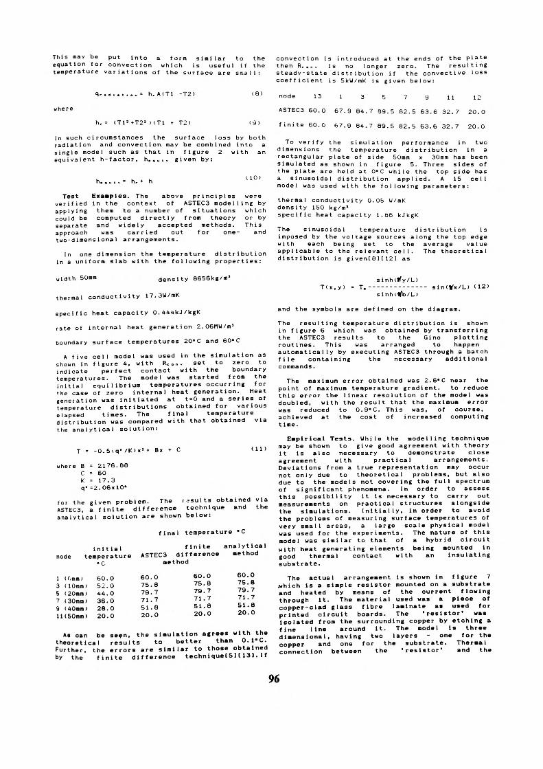
This may be put into a form similar to the equation for convection which is useful if the temperature variations of the surface are small:

, = h, A(T1 -T2)

t\r = (Tl 2 + T2 2 ) (Tl T2> (9)

In such circumstances the surface loss by both radiation and convection, may be combined into a single model such as that in figure 2 with an equivalent h-factor, h.,„i, given by:

h.,. h r • I 10)

Test Examples. The above principles were verified in the context of ASTEC3 modelling by applying them to a number of situations which could be computed directly from theory or by separate and widely accepted methods. This approach was carried out for one- and tuo-dimensionaI arrangements.

In one dimension the temperature distribution in a uniform slab with the following properties:

convection is introduced at the ends of the plate then R«„„, is no longer zero. The resulting steady-state distribution if the convective loss coefficient is BkU/rnK is given below:

node 13 1 3 5 7 9 11 12

ASTEC3 60.0 67.9 84.7 89.5 62.5 63.6 32.7 20.O

finite 60.0 67.9 84.7 89.5 82.5 63.6 32.7 2O.O

To verify the simulation performance in two dimensions the temperature distribution in a rectangular plate of side 50mm x 30mm has been simulated as shown in figure 5. Three sides of the plate are held at 0°C while the top side has a sinusoidal distribution applied. A 15 cell model was used with the following parameters:

thermal conductivity 0.05 U/mKdensity 150 kg/m 1specific heat capacity 1.88 kJkgK

The sinusoidal temperature distribution is imposed by the voltage sources along the top edge with each being set to the average value applicable to the relevant cell. The theoretical distribution is given[6H12] as

width 5Omm density 8656kg/m'

thermal conductivity 17.3U/mK

specific heat capacity O.444kJ/kgK

rate of internal heat generation 2.O6r1W/m 3

boundary surface temperatures 20°C and 60°C

A five cell model was used in the simulation as shown in figure 4, with Rc „„„ set to zero to indicate perfect contact with the boundary temperatures. The model was started from the initial equilibrium temperatures occurring for the case of zero internal heat generation. Heat generation was Initiated at t-0 and a series of temperature distributions obtained for various elapsed times. The final temperature distribution was compared with that obtained via the analytical solution:

T = -O.Siq*/K>x 2 + Bx + C (11)

where B = 2176.88 C = 60 K = 17.3 q- =2.06xlO-

tor the given problem. The results obtained via ASTEC3, a finite difference technique and the analytical solution are shown below:

final temperature °C

initial finite analytical node temperature ASTEC3 difference method

method

1 (Omm i 3 (10mm I 5 (20mm) 7 (30mm) 9 UOmm) ll(50mn)

60.052.044.036.028.020.0

60.0 75.8 79.7 71.7 SI.8 20. O

60.075.879.771.7 SI.820.0

60. O 75.8 79.7 71.7 SI.8 20.0

A9 can be seen, the simulation agrees with the theoretical results to better than 0.1'C. Further, the errors are similar to those obtained by the finite difference techniqueCB)t131.If

T(x,y) = T. •sinh(tfy/L>

sin(1fx/L) < 12)

and the symbols are defined on the diagram.

The resulting temperature distribution is shown in figure 6 which was obtained by transferring the ASTEC3 results to the Gino plotting routines. This was arranged to happen automatically by executing ASTEC3 through a batch file containing the necessary additional commands.

The maximum error obtained was 2.6*C near the point of maximum temperature gradient. to reduce this error the linear resolution of the model was doubled, with the result that the maximum error was reduced to 0.9-C. This was, of course, achieved at the cost of increased computing time.

Empirical Tests. While the modelling technique may be shown to give good agreement with theory it is also necessary to demonstrate close agreement with practical arrangements. Deviations from a true representation may occur not only due to theoretical problems, but also due to the models not covering the full spectrum of significant phenomena. In order to assess this possibility it is necessary to carry out measurements on practical structures alongside the simulations. Initially, In order to avoid the problems of measuring surface temperatures of very small areas, a large scale physical model was used for the experiments. The nature of this model was similar to that of a hybrid circuit with heat generating elements being mounted in good thermal contact with an insulating substrate.

The actual arrangement is shown in figure 7 .which is a simple resistor mounted on a substrate and heated by means of the current flowing through It. The material used was a piece of copper-clad glass fibre laminate as used for printed circuit boards. The 'resistor' was Isolated from the surrounding copper by etching a fine line around it. The model is three dimensional, having two layers - one for the copper and one for the substrate. Thermal connection between the 'resistor 1 and the

96

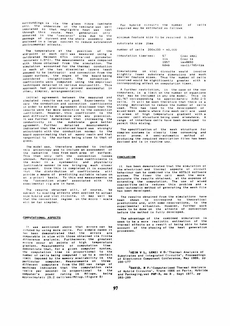
surroundings is via the glass fibre laminate only. the underside of the laminate was well insulated so that negligible heat was lost through this route. Heat generation only occurred in the 'resistor' area due to the passage of current and the whole assembly was enclosed in a large cabinet to reduce extraneous environmental effects.

The temperature at the position of the mid-point ot each cell was measured using a calibrated Heimann KT14 infra-red pyrometer (accuracy 1.5°C). The measurements were compared with those obtained from the simulation. The simulation accounted for the thermal conduction in each of the two dissimilar layers (each assumed to be isotropic) and convection from the copper surface, the edges of the board being considered insignificant. The convection coefficients were computed using the empirical techniques detailed in various sourcesClSJ. This approach had previously proved successful in other, simpler, arrangements[141.

Initial agreement between the measured and simulated results was not good. Experiments to vary the conduction and convection coefficients in order to achieve agreement disclosed that the results were far more sensitive to the convection coefficient. However, this coefficient Is the most difficult to determine with any precision. It was further determined that increasing the conductivity in the substrate gave better agreement. Further detailed measurements indicated that the reinforced board was strongly anisotropic with the conduction normal to the board approximating that of epoxy resin and that tangential to the surface being close to that of glass.

The model was, therefore amended to include this anisotropy and to include an assessment of the radiative loss from each area of surface. This then only left the convection losses unknown. Manipulation of these coefficients in the model in a systematic and physically justityable manner is now bringing much closer agreement. Once this is completed it is expected 'hat the distribution of coefficients will provide a means of predicting suitable values on an a-priori basis. To this end measurements on the 'convection plume' associated with the experimental rig are in hand.

The results obtained will, of course, be subject to scaling effects when applied to actual size hybrid and vlsi circuits, it may well bethat the convection will be far simpler.

it reg ime on the ill

COMPUTATIONAL ASPECTS

It was mentioned above that errors can be educed by using more cells. For simple cases It r>o£ been demonstrated that the errors are comparable in size with those obtained via finite difference analysis. Furthermore, the greatest errors occur at points of high temperature gradient. Measurements of computation time demonstrate that, for a, given computer system, th* computation time is proportional to the number of cells being computed - up to a certain limit Imposed by the memory availability In the particular computer. Measurements on three different computers from the DEC vax range of machines indicates that the computation rate 'cells per second) Is proportional to the computer's power rating in Mflops, being approximately 29.2 ceI I/sec/MfI op.<figure 6)

For hybrid circuits the number of required may be estimated as follows

minimum feature size to be resolved O.lmm

substrate size 20mm

eel Is

number of cells 200x200 = 40,000

computation tin 5711419576649

Cray xmp^:Cray Isvax8650vax1l/765»fpa

Simulations on vlsi circuits would involve slightly lower substrate dimensions and much smaller feature sizes. Thus the number of cells involved would be significantly greater with a corresponding effect on computation times.

A further restriction, in the case of the vax computers, is a limit on the number of equations that may be included in any one model. This is 32,767 corresponding to approximately 315O 2-D cells. It will be seen therefore that there is a strong motivation to reduce the number of cells used. This has lead to the development of mixed-mesh models where fine mesh cell are used in areas of high temperature gradient with a coarser eel I structure being used elsewhere. A range of interface cells have been developed to permit this mixing.

The specification of the mesh structure for complex systems is clearly time consuming and error prone. A semi-automatic method of producing the required description files has been devised and is in routine use.

CONCLUSION

It has been demonstrated that the simulation of the electrical and thermal aspects of circuit behaviour can be combined via the ASTE.C3 software system. The finer the cell mesh the more accurate the results obtained, at the expense of extending the computation. The use of mixed coarse/fine cells reduces this problem and a semi-automatic method of generating the mesh file has been developed.

The results obtained from the simulations have been shown to correspond to theoretical predictions and, with some reservations, to the experimental situation. However, further work needs to be done on the effects of convection before the method is fully developed.

The advantage of the combined simulation is seen to be a more realistic estimation of the thermal effects as a result of being able to take account of the phasing of the heat generation processes.

1 HEIN V L, LENZI V D:'Thermal Analysis of Substrates and Integrated Circuits', Proceedings of Electronic Component Conference, May 1969, pp 166-177

2DAVID, R F:'Computerised Thermal Analysis of Hybrid Circuits', Trans IEEE on Parts, Hybrid* and Packaging,vol PHP-3, no 3 , Sept 1977, pp 283-269

97

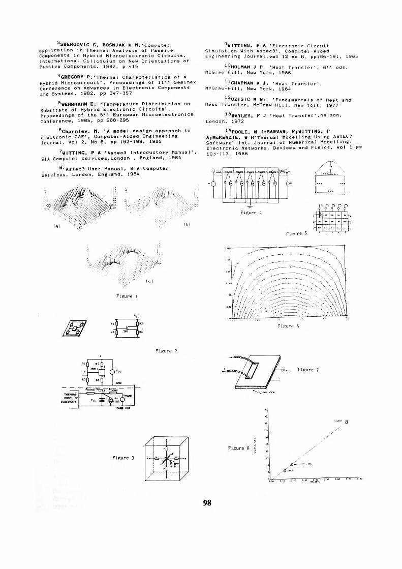
3SBERGOVIC S, BOSNJAK K H:'Computer application in Thermal Analysis of Passive Components in Hybrid Microelectronic Circuits, International Colloquium on New Orientations of Passive Components, 1982, p 415

4GREGORY P:-Thermal Characteristics of a Hybrid Mi crocircuit' , Proceedings of 11'" Seminex Conference on Advances in Electronic Components and Systems, 1982, pp 347-357

5UEHRHAHN E: 'Temperature Distribution on Substrate of Hybrid Electronic Circuits', Proceedings of the 5'" European Microelectronics Conference, 1985, pp 288-295

6Charnley, M. 'A model design approach to electronic CAE", Computer-Aided Engineering Journal, Vo1 2, No 6. pp 192-199, 1985

7UITTING, P A 'Astec3 Introductory Manual 1 , SIA Computer services,London , England, 1984

8> Astec3 User Manual, SIA Computer Services, London, England, 1984

• • ..'•'<'•:'•: : ••'.•f-2££?&i$>': -

(b)

9 WITTING. P A 'Electronic Circuit Simulation Uith Astec3', Computer-Aided Engineering Journal,vo1 12 no 6, pp!86-191, 1985

10HOLMAN J P, 'Heat Transfer', 6'- edn, McGiau-Hill, New York, 1986

UCHAPMAN A J: 'Heat Transfer', McGrau-Hi I I, New York, 1984

12OZISIC M N:, 'Fundamentals of Heat and Mass Transfer, McGraw-Hill, New York, 1977

13 BAYLEY, F J 'Heat Transfer' ,NeI son, London, 1972

lft POOLE, N J;SARVAR, FiWITTING, P A;McKENZlE, W H'Thermal Modelling Using ASTEC3 Software' Int. Journal of Numerical Modelling: Electronic Networks, Devices and Fields, voI I pp 103-113, 1988

Figure

Figure

: ;:;*;i:'-'' (c)

Figure 1

Figure f>

MODE!SUBSTMA:

Figure 3

Figure 2

Figure 7

Figure 8 =

98

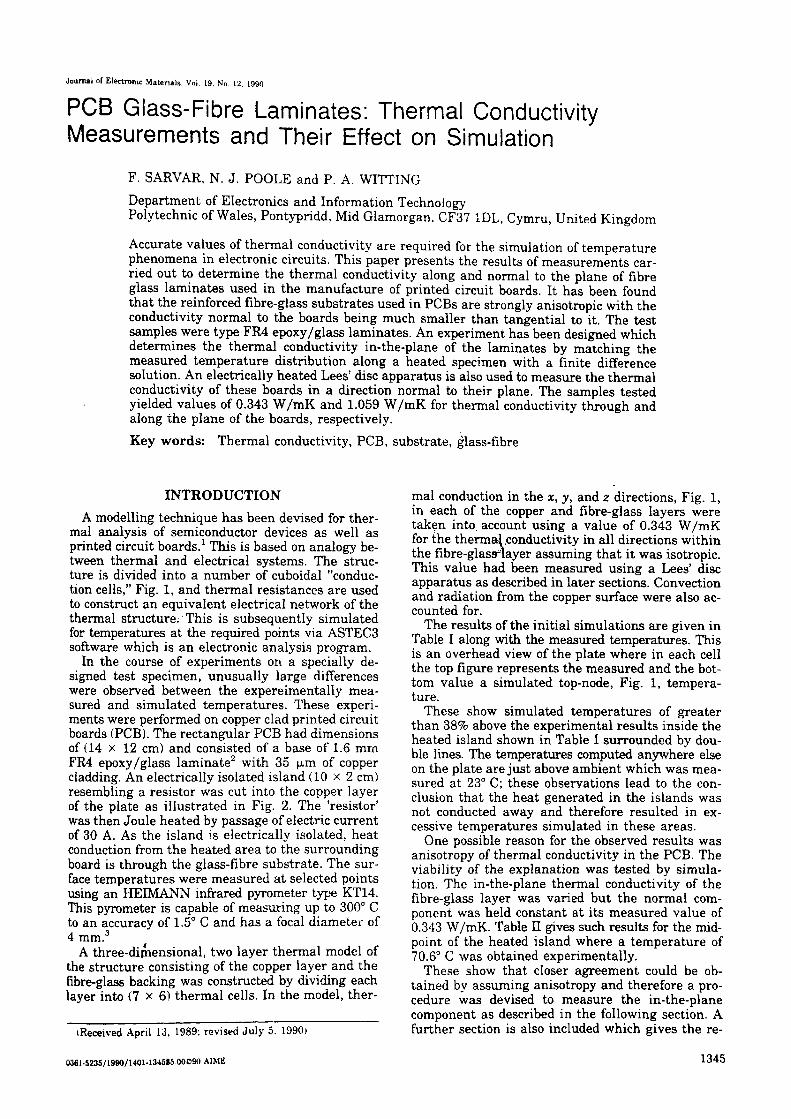
Journal of Electronic Materials, Vol. 19. No. 12. 1990

PCB Glass-Fibre Laminates: Thermal Conductivity Measurements and Their Effect on Simulation

F. SARVAR, N. J. POOLE and P. A. WITTINGDepartment of Electronics and Information TechnologyPolytechnic of Wales, Pontypridd, Mid Glamorgan, CF37 1DL, Cymru, United Kingdom

Accurate values of thermal conductivity are required for the simulation of temperature phenomena in electronic circuits. This paper presents the results of measurements car­ ried out to determine the thermal conductivity along and normal to the plane of fibre glass laminates used in the manufacture of printed circuit boards. It has been found that the reinforced fibre-glass substrates used in PCBs are strongly anisotropic with the conductivity normal to the boards being much smaller than tangential to it. The test samples were type FR4 epoxy/glass laminates. An experiment has been designed which determines the thermal conductivity in-the-plane of the laminates by matching the measured temperature distribution along a heated specimen with a finite difference solution. An electrically heated Lees' disc apparatus is also used to measure the thermal conductivity of these boards in a direction normal to their plane. The samples tested yielded values of 0.343 W/mK and 1.059 W/mK for thermal conductivity through and along the plane of the boards, respectively.Key words: Thermal conductivity, PCB, substrate, glass-fibre

INTRODUCTIONA modelling technique has been devised for ther­

mal analysis of semiconductor devices as well as printed circuit boards. 1 This is based on analogy be­ tween thermal and electrical systems. The struc­ ture is divided into a number of cuboidal "conduc­ tion cells," Fig. 1, and thermal resistances are used to construct an equivalent electrical network of the thermal structure. This is subsequently simulated for temperatures at the required points via ASTEC3 software which is an electronic analysis program.

In the course of experiments on a specially de­ signed test specimen, unusually large differences were observed between the expereimentally mea­ sured and simulated temperatures. These experi­ ments were performed on copper clad printed circuit boards (PCB). The rectangular PCB had dimensions of (14 x 12 cm) and consisted of a base of 1.6 mm FR4 epoxy/glass laminate2 with 35 fim of copper cladding. An electrically isolated island (10 x 2 cm) resembling a resistor was cut into the copper layer of the plate as illustrated in Fig. 2. The 'resistor' was then Joule heated by passage of electric current of 30 A. As the island is electrically isolated, heat conduction from the heated area to the surrounding board is through the glass-fibre substrate. The sur­ face temperatures were measured at selected points using an HEIMANN infrared pyrometer type KT14. This pyrometer is capable of measuring up to 300° C to an accuracy of 1.5° C and has a focal diameter of 4 mm.3

A three-dimensional, two layer thermal model of the structure consisting of the copper layer and the fibre-glass backing was constructed by dividing each layer into (7 x 6) thermal cells. In the model, ther-

iReceived April 13, 1989: revised July 5. 1990)

0361-5235/1990/1401-1345»5.00C90 A1ME

mal conduction in the x, y, and 2 directions, Fig. 1, in each of the copper and fibre-glass layers were taken into, account using a value of 0.343 W/mK for the thermal .conductivity in all directions within the fibre-glassnayer assuming that it was isotropic. This value had been measured using a Lees' disc apparatus as described in later sections. Convection and radiation from the copper surface were also ac­ counted for.

The results of the initial simulations are given in Table I along with the measured temperatures. This is an overhead view of the plate where in each cell the top figure represents the measured and the bot­ tom value a simulated top-node, Fig. 1, tempera­ ture.

These show simulated temperatures of greater than 38% above the experimental results inside the heated island shown in Table I surrounded by dou­ ble lines. The temperatures computed anywhere else on the plate are just above ambient which was mea­ sured at 23° C; these observations lead to the con­ clusion that the heat generated in the islands was not conducted away and therefore resulted in ex­ cessive temperatures simulated in these areas.

One possible reason for the observed results was anisotropy of thermal conductivity in the PCB. The viability of the explanation was tested by simula­ tion. The in-the-plane thermal conductivity of the fibre-glass layer was varied but the normal com­ ponent was held constant at its measured value of 0.343 W/mK. Table II gives such results for the mid­ point of the heated island where a temperature of 70.6° C was obtained experimentally.

These show that closer agreement could be ob­ tained by assuming anisotropy and therefore a pro­ cedure was devised to measure the in-the-plane component as described in the following section. A further section is also included which gives the re-

1345

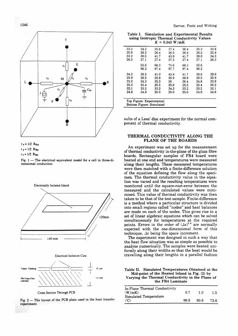
1346 Sarvar, Poole and Witting

Table I. Simulation and Experimental Resultsusing Isotropic Thermal Conductivity Values

K = 0.343 W/mK

r, = 1/2 Ruw r y = 1/2 Rihy r z = 1/2 RuizFig. 1 — The electrical equivalent model for a cell in three-di­ mensional conduction.

Electrically Isolated Island

Electrical Isolation Cuts

Copper Gadding

FR4 Giro Fibre Umiruic

Cross Section Through PCB

Fig. 2 — The layout of the PCB plate used in the heat transfer experiment. •"* .1:-- •

33.225.933.226.3

34.325.933.225.232.124.8

34.326.238.527.155.696.238.526.534.325.433.224.9

35.826.441.727.466.397.441.026.835.325.533.225.0

37.426.543.927.570.697.742.826.93625.634.325.0

36.426.441.727.466.397.441.726.836.425.533.225.0

35.326.238.027.155.696.239.626.534.825.433.224.9

33.825.934.326.3

39.625.933.825.232.124.8

Top Figure: Experimental Bottom Figure: Simulated

suits of a Lees' disc experiment for the normal com­ ponent of thermal conductivity.

THERMAL CONDUCTIVITY ALONG THE PLANE OF THE BOARDS

An experiment was set up for the measurement of thermal conductivity in-the-plane of the glass fibre boards. Rectangular samples of FR4 board were heated at one end and temperatures were measured along their lengths. These measured temperatures were then matched with a finite-difference solution of the equation defining the flow along the speci­ men. The thermal conductivity value in the equa­ tion was varied and the resulting temperatures were monitored until the square-root-error between the measured and the calculated values were mini­ mised. This value of thermal conductivity was then taken to be that of the test sample. Finite-difference is a method where a particular structure is divided into small regions called "nodes" and heat balances are made on each of the nodes. This gives rise to a set of linear algebraic equations which can be solved simultaneously for temperatures at the required points. Errors in the order of (JLc)2 4 are normally expected with the one-dimensional form of this technique, ilx being the space increment.

The experiment was designed in such a way that the heat flow situation was as simple as possible to analyse numerically. The samples were heated uni­ formly along their widths so that the heat would be travelling along their lengths in a parallel fashion

Table II. Simulated Temperatures Obtained at theMid-point of the Heated Island in Fig. (2) by

Varying the Thermal Conductivity in the Plane ofthe FR4 Laminate

In-Plane Thermal Conductivity(W/mK)Simulated Temperaturei°C)

0.7

86.9

1.0

80.8

1.5

73.6

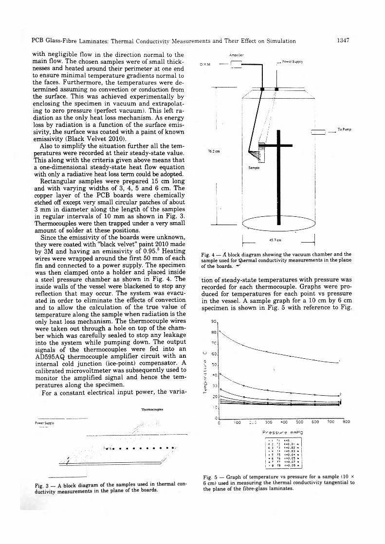
PCB Glass-Fibre Laminates: Thermal Conductivity Measurements and Their Effect on Simulation 1347

with negligible flow in the direction normal to the main flow. The chosen samples were of small thick­ nesses and heated around their perimeter at one end to ensure minimal temperature gradients normal to the faces. Furthermore, the temperatures were de­ termined assuming no convection or conduction from the surface. This was achieved experimentally by enclosing the specimen in vacuum and extrapolat­ ing to zero pressure (perfect vacuum). This left ra­ diation as the only heat loss mechanism. As energy loss by radiation is a function of the surface emis- sivity, the surface was coated with a paint of known emissivity (Black Velvet 2010).

Also to simplify the situation further all the tem­ peratures were recorded at their steady-state value. This along with the criteria given above means that a one-dimensional steady-state heat flow equation with only a radiative heat loss term could be adopted.

Rectangular samples were prepared 15 cm long and with varying widths of 3, 4, 5 and 6 cm. The copper layer of the PCB boards were chemically etched off except very small circular patches of about 3 mm in diameter along the length of the samples in regular intervals of 10 mm as shown in Fig. 3. Thermocouples were then trapped under a very small amount of solder at these positions.

Since the emissivity of the boards were unknown, they were coated with "black velvet" paint 2010 made by 3M and having an emissivity of 0.95. 5 Heating wires were wrapped around the first 50 mm of each fin and connected to a power supply. The specimen was then clamped onto a holder and placed inside a steel pressure chamber as shown in Fig. 4. The inside walls of the vessel were blackened to stop any reflection that may occur. The system was evacu­ ated in order to eliminate the effects of convection and to allow the calculation of the true value of temperature along the sample when radiation is the only heat loss mechanism. The thermocouple wires were taken out through a hole on top of the cham­ ber which was carefully sealed to stop any leakage into the system while pumping down. The output signals of the thermocouples were fed into an AD595AQ thermocouple amplifier circuit with an internal cold junction (ice-point) compensator. A calibrated microvoltmeter was subsequently used to monitor the amplified signal and hence the tem­ peratures along the specimen.

For a constant electrical input power, the varia-

Thermocouples

_, Power Supply

Power Supply

To Pump

Fig. 4 — A block diagram showing the vacuum chamber and the sample used for thermal conductivity measurements in the plane of the boards. ""'

tion of steady-state temperatures with pressure was recorded for each thermocouple. Graphs were pro­ duced for temperatures for each point vs pressure in the vessel. A sample graph for a 10 cm by 6 cm specimen is shown in Fig. 5 with reference to Fig.

100 300 -"00 500 SCO 700 800

Pressure mmMg

0 20 3• 4

0 ?

• 6* 7- 8

134

3i7

8

•0.01•0.02•0.03•0.0*•0.03"0.07•0.09

Fig. 3 — A block diagram of the samples used in thermal con­ ductivity measurements in the plane of the boards.

Fig. 5 — Graph of temperature vs pressure for a sample (10 x 6 cm) used in measuring the thermal conductivity tangential to the plane of the fibre-glass laminates.

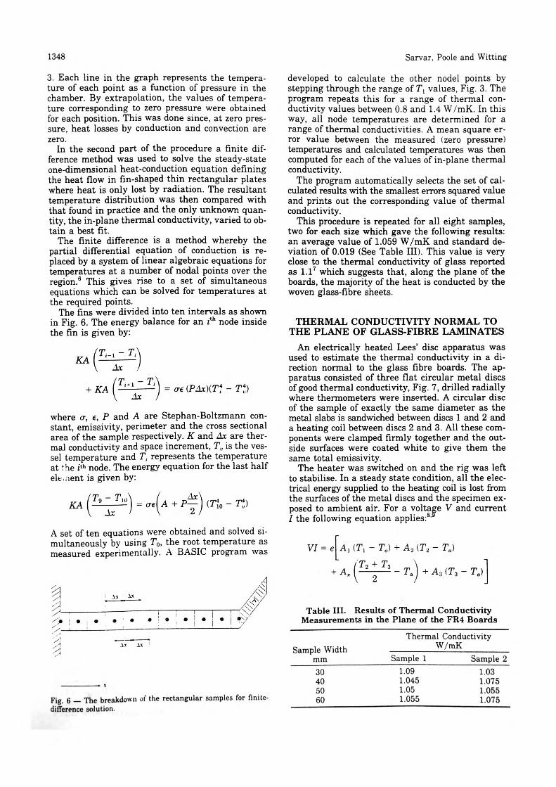
1348 Sarvar, Poole and Witting

3. Each line in the graph represents the tempera­ ture of each point as a function of pressure in the chamber. By extrapolation, the values of tempera­ ture corresponding to zero pressure were obtained for each position. This was done since, at zero pres­ sure, heat losses by conduction and convection are zero.

In the second part of the procedure a finite dif­ ference method was used to solve the steady-state one-dimensional heat-conduction equation defining the heat flow in fin-shaped thin rectangular plates where heat is only lost by radiation. The resultant temperature distribution was then compared with that found in practice and the only unknown quan­ tity, the in-plane thermal conductivity, varied to ob­ tain a best fit.

The finite difference is a method whereby the partial differential equation of conduction is re­ placed by a system of linear algebraic equations for temperatures at a number of nodal points over the region.6 This gives rise to a set of simultaneous equations which can be solved for temperatures at the required points.

The fins were divided into ten intervals as shown in Fig. 6. The energy balance for an ith node inside the fin is given by:

KAT - T•* i-l •* i

Ax

KA±c

= (re

where a, e, P and A are Stephan-Boltzmann con­ stant, emissivity, perimeter and the cross sectional area of the sample respectively. K and Ax are ther­ mal conductivity and space increment, Tv is the ves­ sel temperature and T, represents the temperature at t he ith node. The energy equation for the last half elt.aent is given by:

= o*A + P

A set of ten equations were obtained and solved si­ multaneously by using T0 , the root temperature as measured experimentally. A BASIC program was

i.T A*

Pig e _ The breakdown of the rectangular samples for finite- difference solution.

developed to calculate the other nodel points by stepping through the range of T} values, Fig. 3. The program repeats this for a range of thermal con­ ductivity values between 0.8 and 1.4 W/mK. In this way, all node temperatures are determined for a range of thermal conductivities. A mean square er­ ror value between the measured (zero pressure) temperatures and calculated temperatures was then computed for each of the values of in-plane thermal conductivity.

The program automatically selects the set of cal­ culated results with the smallest errors squared value and prints out the corresponding value of thermal conductivity.

This procedure is repeated for all eight samples, two for each size which gave the following results: an average value of 1.059 W/mK and standard de­ viation of 0.019 (See Table III). This value is very close to the thermal conductivity of glass reported as l.l7 which suggests that, along the plane of the boards, the majority of the heat is conducted by the woven glass-fibre sheets.

THERMAL CONDUCTIVITY NORMAL TO THE PLANE OF GLASS-FIBRE LAMINATES

An electrically heated Lees' disc apparatus was used to estimate the thermal conductivity in a di­ rection normal to the glass fibre boards. The ap­ paratus consisted of three flat circular metal discs of good thermal conductivity, Fig. 7, drilled radially where thermometers were inserted. A circular disc of the sample of exactly the same diameter as the metal slabs is sandwiched between discs 1 and 2 and a heating coil between discs 2 and 3. All these com­ ponents were clamped firmly together and the out­ side surfaces were coated white to give them the same total emissivity.

The heater was switched on and the rig was left to stabilise. In a steady state condition, all the elec­ trical energy supplied to the heating coil is lost from the surfaces of the metal discs and the specimen ex­ posed to ambient air. For a voltage V and current I the following equation applies: 8

-T.

Table III. Results of Thermal Conductivity Measurements in the Plane of the FR4 Boards

Sample Width mm30 40 50 60

Thermal Conductivity W/mK

Sample 11.09 1.045 1.05 1.055

Sample 21.03 1.075 1.055 1.075

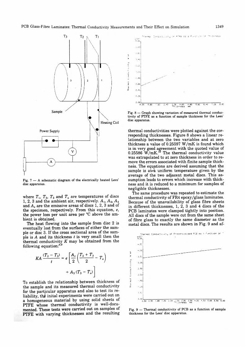
PCB Glass-Fibre Laminates: Thermal Conductivity Measurements and Their Effect on Simulation

T3 T2

1349

Heating Coil

Fig. 7 — A schematic diagram of the electrically heated Lees' disc apparatus.

where T1; T2 , T3 and Ta are temperatures of discs 1, 2, 3 and the ambient air, respectively. AJ, A 2 , A 3 and Ax are the emissive areas of discs 1, 2, 3 and of the specimen, respectively. From this equation, e, the power loss per unit area per °C above the am­ bient is obtained.

The heat flowing into the sample from disc 2 is eventually lost from the surfaces of either the sam­ ple or disc 3. If the cross sectional area of the sam­ ple is A and its thickness t is very small then the thermal conductivity K may be obtained from the following equation:8 '9

A, (T3 - Ta)

To establish the relationship between thickness of the sample and its measured thermal conductivity for the particular apparatus and also to test its re­ liability, thj» inital experiments were carried out on a homogeneous material by using solid sheets of PTFE whose thermal conductivity is well-docu­ mented. These tests were carried out on samples of PTFE with varying thicknesses and the resulting

I2-OoL.

«.00 1.80 5 .60

Fig. 8 — Graph showing variation of measured thermal conduc­ tivity of PTFE as a function of sample thickness for the Lees' disc apparatus.

thermal conductivities were plotted against the cor­ responding thicknesses. Figure 8 shows a linear re­ lationship between the two variables and at zero thickness a value of 0.25597 W/mK is found which is in very good agreement with the quoted value of 0.25586 W/mK."5 The thermal conductivity value was extrapolated to at zero thickness in order to re­ move the errors associated with finite sample thick­ ness. The equations are derived assuming that the sample is at^a uniform temperature given by the average of the two adjacent metal discs. This as­ sumption leads to errors which increase with thick­ ness and it is reduced to a minimum for samples of negligible thicknesses.

The same procedure was repeated to estimate the thermal conductivity of FR4 epoxy/glass laminates. Because of the unavailability of glass fibre sheets in different thicknesses, 1, 2, 3 and 4 discs of the PCB laminates were clamped tightly into position. All discs of the sample were cut from the same sheet of fibre glass to exactly the same diameter as the metal discs. The results are shown in Fig. 9 and af-

" 0.00 0.50' .00 i'.«C :.TO ...'0 I'.OO J.50 <.00 1.50 5.00 5.10 6.00

Fig. 9 — Thermal conductivity of PCB as a function of sample thickness for the Lees' disc apparatus.

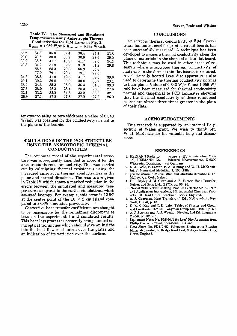
1350 Sarvar, Poole and Witting

Table IV. The Measured and Simulated Temperatures using Anisotropic Thermal

Conductivities for FR4 Layer in Fig. 2, KplaM = 1.059 W/mK Knormal = 0.343 W/mK

33.229.033.229.8

34.329.133.227.632.126.9

34.329.638.531.255.677.038.530.234.328.033.227.1

35.830.041.731.966.379.141.030.835.328.333.227.2

37.430.243.932.270.679.742.830.936.028.434.327.3

36.430.041.731.966.379.141.730.836.428.333.227.2

35.329.638.031.255.677.039.630.234.828.033.227.2

33.829.034.329.8

39.629.133.827.632.126.9

CONCLUSIONSAnisotropic thermal conductivity of FR4 Epoxy/

Glass laminates used for printed circuit boards has been successfully measured. A technique has been developed to measure thermal conductivity along the plane of materials in the shape of a thin flat board. This technique may be used in other areas of re­ search where anisotropic thermal conductivity of materials in the form of thin flat boards is required. An electrically heated Lees' disc apparatus is also used to determine the thermal conductivity normal to their plane. Values of 0.343 W/mK and 1.059 W/ mK have been measured for thermal conductivity normal and tangential to PCB laminates showing that the thermal conductivity of these reinforced boards are almost three times greater in the plain of their flats.

ter extrapolating to zero thickness a value of 0.343 W/mK was obtained for the conductivity normal to the plane of the boards.

SIMULATIONS OF THE PCB STRUCTUREUSING THE ANISOTROPIC THERMAL

CONDUCTIVITIESThe computer model of the experimental struc­

ture was subsequently amended to account for the anisotropic thermal conductivity. This was carried out by calculating thermal resistances using the measured anisotropic thermal conductivities in the plane and normal directions. The results are given in Table IV which shows a marked reduction in the errors between the simulated and measured tem­ peratures compared to the earlier simulations, which assumed isotropy. For example, this error is 12.9% at the centre point of the 10 x 2 cm island com­ pared to 38.4% simulated previously.

Convective heat transfer coefficients are thought to be responsible for the remaining discrepancies between the experimental and simulated results. This heat loss process is presently being studied us­ ing optical techniques which should give an insight into the heat flow mechanism over the plates and an indication of its variation over the surface.

ACKNOWLEDGEMENTSThis research is supported by an internal Poly­

technic of Wales grant. We wish to thank Mr. W. H. McKenzie for his valuable help and discus­sions.

i.REFERENCES

HEIMANN Radiatior rmometer KT14 Instruction Man­ ual, HEIMANN Gm Infrared Measurements, D-6200 Wiesbaden-Dotzheim, -., tst Germany.

2. N. J. Poole, F. Sarvar, P. A. Witting and W. H. McKenzie, Int. J. Numerical Modelling 1, 103 (1988).

3. private communication, Mica and Micanite (Ireland) LTD., Mallow, Co. Cork, Ireland.

4. F. J. Bayley, J. M. Owen and A. B. Turner, Heat Transfer, Nelson and Sons Ltd., (1972), pp. 90-92.

5. 'Nextel 2010 Velvet Coating1 Product Performance Bulletin and Application Instructions, 3M Industrial Chemical Prod­ ucts, 3M Head Office, Bracknell, Berks, England.

6. A. J. Chapman, Heat Transfer, 4th Ed., McGraw-Hill, New York, (1984), p. 131.

7. G. W. C. Kay and T. H. Laby, Tables of Physics and Chem­ ical Constants, 15"1 Ed., Longman Group Ltd., (1986), p. 69.

8. A. J. Starling and A. J. Woodall, Physics, 2nd Ed. Longmans (1964), pp. 320-321.

9. Equipment Notes No. P28030/1 for Lees' Disc Apparatus from Philip Harris Limited, Shenstone, England.

10. Data Sheet No. PD4/7/82, Polypenco Engineering Plastics Materials Limited, 76 Bridge Road East, Welwyn Garden City, Herts, England.