Numerical and experimental study on residual stresses in ...
237
HAL Id: tel-01581004 https://tel.archives-ouvertes.fr/tel-01581004 Submitted on 4 Sep 2017 HAL is a multi-disciplinary open access archive for the deposit and dissemination of sci- entific research documents, whether they are pub- lished or not. The documents may come from teaching and research institutions in France or abroad, or from public or private research centers. L’archive ouverte pluridisciplinaire HAL, est destinée au dépôt et à la diffusion de documents scientifiques de niveau recherche, publiés ou non, émanant des établissements d’enseignement et de recherche français ou étrangers, des laboratoires publics ou privés. Numerical and experimental study on residual stresses in laser beam welding of dual phase DP600 steel plates Shibo Liu To cite this version: Shibo Liu. Numerical and experimental study on residual stresses in laser beam welding of dual phase DP600 steel plates. Mechanical engineering [physics.class-ph]. INSA de Rennes, 2017. English. NNT : 2017ISAR0003. tel-01581004
-
Upload
khangminh22 -
Category
Documents
-
view
1 -
download
0
Transcript of Numerical and experimental study on residual stresses in ...
HAL Id: tel-01581004https://tel.archives-ouvertes.fr/tel-01581004
Submitted on 4 Sep 2017
HAL is a multi-disciplinary open accessarchive for the deposit and dissemination of sci-entific research documents, whether they are pub-lished or not. The documents may come fromteaching and research institutions in France orabroad, or from public or private research centers.
L’archive ouverte pluridisciplinaire HAL, estdestinée au dépôt et à la diffusion de documentsscientifiques de niveau recherche, publiés ou non,émanant des établissements d’enseignement et derecherche français ou étrangers, des laboratoirespublics ou privés.
Numerical and experimental study on residual stressesin laser beam welding of dual phase DP600 steel plates
Shibo Liu
To cite this version:Shibo Liu. Numerical and experimental study on residual stresses in laser beam welding of dualphase DP600 steel plates. Mechanical engineering [physics.class-ph]. INSA de Rennes, 2017. English.�NNT : 2017ISAR0003�. �tel-01581004�
THÈSE INSA Rennessous le sceau de l'Université Bretagne Loire
pour obtenir le titre de
DOCTEUR DE L'INSA RENNESSpécialité: Génie Mécanique
présentée par
Shibo LIUÉCOLE DOCTORALE : SDLMLABORATOIRE : LGCGM
Numerical andexperimental study
on residual stresses inlaser beam welding of
dual phase DP600steel plates
Thèse soutenue le 08/06/2017devant le jury composé de :
Véronique FAVIERProfesseurs des Universités, Arts et Métiers ParisTech - Paris/ PrésidenteLaurent BARRALLIERProfesseurs des Universités, Arts et Métiers ParisTech - Centred'Aix-en-Provence / Rapporteur
Pierre-Yves MANACHProfesseurs des Universités, Université de Bretagne Sud /Rapporteur
Guenael GERMAINMaître de Conférences des Universités HDR, Arts et MétiersParisTech - Centre d'Angers / Examinateur
A�a KOUADRI-HENNIMaître de Conférence des Universités, INSA Rennes /Co-encadrante de thèse
Adinel GAVRUSMaître de Conférence des Universités HDR, INSA Rennes /Directeur de thèse
Ionel NISTORIngénieur Recherche Dr., EDF Lab Paris-Saclay / Invité

Numerical and experimental study onresidual stresses in laser beam welding of dual
phase DP600 steel plates
Shibo LIU
En partenariat avec
Document protégé par les droits d'auteur

Remerciements
I want to thank my parents for their always encouragement and support. Withoutthem, I would not achieve today's outcome. I also thank to China Scholarship Councilfor the �nical support in these years.
I would like to express my sincere gratitude to my supervisor MCF HDR Dr. AdinelGavrus and my co-supervisor MCF Dr. A�a Kouadri-Henni for the continuous supportof my Ph.D study and research, for their patience, motivation, enthusiasm, and immenseknowledge. Their guidance helped me a lot during research and writing of this thesis.
Besides my supervisor and co-supervisor, I would like to thank Pierre-Yves MA-NACH, Professor of Université de Bretagne Sud, and Laurent BARRALLIER, Professorof Arts et Métiers ParisTech - Centre d'Aix-en-Provence, for having accepted the workas reporters.
I also thank the rest of my thesis committee : Véronique FAVIER, Professeurs desUniversités, Arts et Métiers ParisTech - Paris, and Guenael GERMAIN, Maître deConférences des Universités HDR, Arts et Métiers ParisTech - Centre d'Angers for theirwork of examiners. Fulgence RAZAFIMAHERY, Maître de Conférences des Universités,Université de Rennes 1 and Ionel NISTOR Ingénieur Recherche Dr., EDF Lab Paris-Saclay for their encouragement, insightful comments, and great questions.
I also feel grateful to the Mecaproce Team of INSA de Rennes, LGCGM laboratoryand to CEA of Saclay for the experimental measurements. They provide me great favorfor my research work.
I also want to say thanks to my master supervisor Professor Dongjiang Wu for hisscienti�c instructions and kindly help in my development.
I really thank my friends and my love who bring me wonderful times in France.
Finally to all the people who love me and who I love, thank you !
1

2 Remerciements

Table des �gures
1.1 Schematic of Nd :YAG laser oscillator . . . . . . . . . . . . . . . . . . . 24
1.2 Sketch of laser welding system . . . . . . . . . . . . . . . . . . . . . . . . 24
1.3 Three focusing positions of the laser beam . . . . . . . . . . . . . . . . . 25
1.4 DP600 for automotive structural components . . . . . . . . . . . . . . . 26
1.5 Microstructure of dual phase DP600 steel [1] . . . . . . . . . . . . . . . . 27
1.6 Three orders of residual stresses[2] . . . . . . . . . . . . . . . . . . . . . 30
1.7 Thermal stress obtained by dilatation of a clamped bar . . . . . . . . . . 30
1.8 Inner and outer part of a material . . . . . . . . . . . . . . . . . . . . . 31
1.9 Inner part geometry change in two dimension . . . . . . . . . . . . . . . 32
1.10 Sketch of inner part geometry change during heating process . . . . . . . 33
1.11 Sketch of outer part geometry change during heating process . . . . . . 33
1.12 The balance of inner and outer part at the end of heating process . . . . 34
1.13 The con�guration of numerical model . . . . . . . . . . . . . . . . . . . . 36
1.14 The stress tensor and the strain tensor . . . . . . . . . . . . . . . . . . . 37
1.15 Plasticity region . . . . . . . . . . . . . . . . . . . . . . . . . . . . . . . 39
1.16 The surface normal vector direction de�nition in a cartesian coordinatesystem . . . . . . . . . . . . . . . . . . . . . . . . . . . . . . . . . . . . . 42
2.1 The INSTRON tensile test machine (50KN) . . . . . . . . . . . . . . . . 57
2.2 Dimension of Specimen . . . . . . . . . . . . . . . . . . . . . . . . . . . . 58
2.3 The mark points of the tensile specimen . . . . . . . . . . . . . . . . . . 59
2.4 Tensile test of HSLA steel : (a) Force-displacement curve using LVDTsensor, (b) True stress-strain curve using camera measurements . . . . . 59
2.5 True stress-strain curve of dual phase steel DP600 at room temperatureand initial strain rate 8.33×10⁻⁴s−1 . . . . . . . . . . . . . . . . . . . . 61
2.6 The plastic �ow curve of dual phase steel DP600 at room temperatureand initial strain rate 8.33×10⁻⁴s−1 . . . . . . . . . . . . . . . . . . . . 61
2.7 Comparison of Ludwik model and experimental DP600 data . . . . . . . 62
2.8 Comparison of Voce model and experimental DP600 data . . . . . . . . 63
3
4 Table des �gures
2.9 Comparisons of rheological models and experimental DP600 data . . . . 65
2.10 Comparison of rheological models and experimental DP600 data . . . . . 65
2.11 Temperature dependence of experiment data and simulation models . . . 68
2.12 Temperature sensitivity of experiment data and simulation models . . . 70
2.13 True stress-strain curves obtained at di�erent strain rate at room tem-perature . . . . . . . . . . . . . . . . . . . . . . . . . . . . . . . . . . . . 71
2.14 The hardening model describing DP600 dual phase steel plastic behavior 71
2.15 Comparison between experimental data and simulation results of DP600�ow stress at room temperature 20◦C . . . . . . . . . . . . . . . . . . . . 73
2.16 The plastic �ow stress of DP600 dual phase steel at di�erent temperaturesand strain rates . . . . . . . . . . . . . . . . . . . . . . . . . . . . . . . . 73
2.17 The comparison between experimental data from literature [3] and simu-lation results of DP600 dual phase steel general constitutive model . . . 75
2.18 Dimensions of specimen for tensile test . . . . . . . . . . . . . . . . . . . 76
2.19 Yield surface predicted by Hill48 anisotropic model and Von Mises criterion 77
2.20 The computed results of residual stresses based on neutron di�ractionmethod . . . . . . . . . . . . . . . . . . . . . . . . . . . . . . . . . . . . 79
3.1 A cell in analysis zone . . . . . . . . . . . . . . . . . . . . . . . . . . . . 82
3.2 The bulk and the mould wall of the weld . . . . . . . . . . . . . . . . . . 83
3.3 States of a growing grain . . . . . . . . . . . . . . . . . . . . . . . . . . . 84
3.4 The growth direction angle θ . . . . . . . . . . . . . . . . . . . . . . . . 85
3.5 The direction of the grain . . . . . . . . . . . . . . . . . . . . . . . . . . 86
3.6 Parameters in a cell . . . . . . . . . . . . . . . . . . . . . . . . . . . . . 86
3.7 basic iteration rule for each cell . . . . . . . . . . . . . . . . . . . . . . . 87
3.8 Two types of neighborhood of Cellular Automaton . . . . . . . . . . . . 88
3.9 Rule for state change . . . . . . . . . . . . . . . . . . . . . . . . . . . . . 89
3.10 Rule of grain growth . . . . . . . . . . . . . . . . . . . . . . . . . . . . . 90
3.11 �owchart of the microstructure evolution model . . . . . . . . . . . . . . 91
3.12 Conical heat source with Gaussian distribution . . . . . . . . . . . . . . 92
3.13 Selected zone for calculating . . . . . . . . . . . . . . . . . . . . . . . . . 93
3.14 The history temperature of node A . . . . . . . . . . . . . . . . . . . . . 93
3.15 The schematic of distance weighting factor . . . . . . . . . . . . . . . . . 94
3.16 The schematic of linear interpolation . . . . . . . . . . . . . . . . . . . . 95
3.17 Temperature distribution . . . . . . . . . . . . . . . . . . . . . . . . . . 96
3.18 The schematic of calculation of nucleation density [4] . . . . . . . . . . . 97
3.19 The sketch of parameters used in solid fraction computation . . . . . . . 99

Table des �gures 5
3.20 Model of concentration in single cell . . . . . . . . . . . . . . . . . . . . 101
3.21 Schematic diagram of cells contact . . . . . . . . . . . . . . . . . . . . . 103
3.22 Schematic diagram of cells contact . . . . . . . . . . . . . . . . . . . . . 103
3.23 Growth velocity of the interface in a cell . . . . . . . . . . . . . . . . . . 106
3.24 The growth of equiaxed dendrite grain . . . . . . . . . . . . . . . . . . . 108
3.25 The equiaxed dendrite grain of di�erent directions . . . . . . . . . . . . 109
3.26 The growth of column dendrite grains . . . . . . . . . . . . . . . . . . . 110
3.27 The growth of two dendrite grains . . . . . . . . . . . . . . . . . . . . . 111
3.28 The equiaxed dendrite grain growth . . . . . . . . . . . . . . . . . . . . 113
3.29 Nucleation at the corner . . . . . . . . . . . . . . . . . . . . . . . . . . . 114
3.30 Equiaxed grain competition growth of two directions . . . . . . . . . . . 115
3.31 Grains with di�erent growth direction growth at the same speed . . . . 116
3.32 Weld Microstructure Simulation of �ne mesh . . . . . . . . . . . . . . . 117
3.33 Weld Microstructure Simulation with coarse mesh . . . . . . . . . . . . . 118
3.34 Dendrite morphology of 2D simulation and experimental SEM observation119
3.35 Microstructure of FZ and HAZ of DP600 weld cross section . . . . . . . 119
3.36 Microstructure of FZ and HAZ of DP600 weld upper surface . . . . . . . 120
4.1 Linear material constitutive model of DP600 steel . . . . . . . . . . . . . 124
4.2 The shape of heat source and Gauss heat distribution . . . . . . . . . . 125
4.3 The A geometry of welding simulation model . . . . . . . . . . . . . . . 126
4.4 The B geometry of welding simulation model . . . . . . . . . . . . . . . 127
4.5 Boundary conditions of thermal analysis model using B geometry . . . . 128
4.6 Boundary conditions of mechanical analysis model using B geometry . . 128
4.7 Hardening term of material constitutive model . . . . . . . . . . . . . . 130
4.8 Hardening models used in FEM laser welding simulation models . . . . . 130
4.9 Temperature sensitivity term of material constitutive model . . . . . . . 132
4.10 The 4 temperature sensitivity terms used in FEM laser welding simula-tion models . . . . . . . . . . . . . . . . . . . . . . . . . . . . . . . . . . 133
4.11 Temperature sensitivity term of material constitutive model . . . . . . . 134
4.12 The strain rate sensitivity term under di�erent temperatures . . . . . . . 134
4.13 The specimens cut with di�erent angles on dual phase steel DP600 plate 135
4.14 Rolling direction de�ned in numerical laser welding model . . . . . . . . 136
4.15 The CA simulation position in ABAQUS/FEM model . . . . . . . . . . 137
4.16 Temperature history data of 4 points . . . . . . . . . . . . . . . . . . . . 137
4.17 The �owchart of CA-FE model used to simulate residual stresses . . . . 138
4.18 Dendrite grains growth simulation obtained by the CA model . . . . . . 139

6 Table des �gures
5.1 Rectangular type of mesh transition . . . . . . . . . . . . . . . . . . . . 144
5.2 Wedge type of mesh transition . . . . . . . . . . . . . . . . . . . . . . . 144
5.3 Comparison of computation time between wedge type and rectangular type146
5.4 Comparison of computation time of di�erent element type model . . . . 146
5.5 Mesh of longitudinal direction . . . . . . . . . . . . . . . . . . . . . . . . 148
5.6 Residual stress distribution . . . . . . . . . . . . . . . . . . . . . . . . . 149
5.7 Computation time of temperature and stress models . . . . . . . . . . . 149
5.8 Numerical results of temperature range of melting pool heated by laser . 150
5.9 The maximal residual stress of models with di�erent layers . . . . . . . . 150
5.10 Mesh transverse to weld . . . . . . . . . . . . . . . . . . . . . . . . . . . 151
5.11 The comparison of computation time between Model-2x2 and Model-4x4 152
5.12 Residual stress distribution . . . . . . . . . . . . . . . . . . . . . . . . . 153
5.13 Three lines �xed in thickness direction . . . . . . . . . . . . . . . . . . . 153
5.14 Equivalent stress along weld longtitudinal path . . . . . . . . . . . . . . 154
5.15 equivalent stress along transversal path . . . . . . . . . . . . . . . . . . . 154
5.16 σ11 along weld longitudinal path . . . . . . . . . . . . . . . . . . . . . . 155
5.17 σ11 along transversal path . . . . . . . . . . . . . . . . . . . . . . . . . . 155
5.18 σ22 along weld longitudinal path . . . . . . . . . . . . . . . . . . . . . . 156
5.19 σ22 along transversal path . . . . . . . . . . . . . . . . . . . . . . . . . . 156
5.20 The distribution of equivalent residual stresses of welding simulation withdi�erent hardening models . . . . . . . . . . . . . . . . . . . . . . . . . . 157
5.21 The magnitude of equivalent residual stresses of welding simulation withdi�erent hardening models . . . . . . . . . . . . . . . . . . . . . . . . . . 158
5.22 The distribution of σ11 residual stresses of welding simulation with dif-ferent hardening models . . . . . . . . . . . . . . . . . . . . . . . . . . . 159
5.23 The magnitude of σ11 residual stresses of welding simulation with dif-ferent hardening models . . . . . . . . . . . . . . . . . . . . . . . . . . . 160
5.24 The distribution of σ22 residual stresses of welding simulation with dif-ferent hardening models . . . . . . . . . . . . . . . . . . . . . . . . . . . 161
5.25 The magnitude of σ22 residual stresses of welding simulation with dif-ferent hardening models . . . . . . . . . . . . . . . . . . . . . . . . . . . 161
5.26 The distribution of εe11 residual strains of welding simulation with dif-ferent hardening models . . . . . . . . . . . . . . . . . . . . . . . . . . . 162
5.27 The magnitude of εe11 residual strains of welding simulation with di�erenthardening models . . . . . . . . . . . . . . . . . . . . . . . . . . . . . . . 162
5.28 The distribution of εe22 residual strains of welding simulation with dif-ferent hardening models . . . . . . . . . . . . . . . . . . . . . . . . . . . 163

Table des �gures 7
5.29 The magnitude of εe22 residual strains of welding simulation with di�erenthardening models . . . . . . . . . . . . . . . . . . . . . . . . . . . . . . . 164
5.30 The distribution of εp11 residual strains of welding simulation with dif-ferent hardening models . . . . . . . . . . . . . . . . . . . . . . . . . . . 165
5.31 The magnitude of εp11 residual strains of welding simulation with di�erenthardening models . . . . . . . . . . . . . . . . . . . . . . . . . . . . . . . 165
5.32 The distribution of εp22 residual strains of welding simulation with dif-ferent hardening models . . . . . . . . . . . . . . . . . . . . . . . . . . . 166
5.33 The magnitude of εp22 residual strains of welding simulation with di�erenthardening models . . . . . . . . . . . . . . . . . . . . . . . . . . . . . . . 166
5.34 The distribution of εp residual strains of welding simulation with di�erenthardening models . . . . . . . . . . . . . . . . . . . . . . . . . . . . . . . 167
5.35 The magnitude of εp residual strains of welding simulation with di�erenthardening models . . . . . . . . . . . . . . . . . . . . . . . . . . . . . . . 168
5.36 The distribution of equivalent residual stresses of welding simulation with4 di�erent temperature sensitivity terms . . . . . . . . . . . . . . . . . . 169
5.37 The magnitude of equivalent residual stresses of welding simulation mo-dels with 4 di�erent temperature sensitivity terms . . . . . . . . . . . . 169
5.38 The distribution of σ11 residual stresses of welding simulation with 4di�erent temperature sensitivity terms . . . . . . . . . . . . . . . . . . . 170
5.39 The magnitude of σ11 residual stresses of welding simulation models with4 di�erent temperature sensitivity terms . . . . . . . . . . . . . . . . . . 171
5.40 The distribution of σ22 residual stresses of welding simulation with 4di�erent temperature sensitivity terms . . . . . . . . . . . . . . . . . . . 171
5.41 The magnitude of σ22 residual stresses of welding simulation models with4 di�erent temperature sensitivity terms . . . . . . . . . . . . . . . . . . 172
5.42 The distribution of εe11 elastic strains of welding simulation with 4 dif-ferent temperature sensitivity terms . . . . . . . . . . . . . . . . . . . . 173
5.43 The magnitude of εe11 elastic strains of welding simulation models with 4di�erent temperature sensitivity terms . . . . . . . . . . . . . . . . . . . 173
5.44 The distribution of εe22 elastic strains of welding simulation with 4 dif-ferent temperature sensitivity terms . . . . . . . . . . . . . . . . . . . . 174
5.45 The magnitude of εe22 elastic strains of welding simulation models with 4di�erent temperature sensitivity terms . . . . . . . . . . . . . . . . . . . 174
5.46 The distribution of εp11 plastic strains of welding simulation with 4 dif-ferent temperature sensitivity terms . . . . . . . . . . . . . . . . . . . . 175
5.47 The magnitude of εp11 plastic strains of welding simulation models with4 di�erent temperature sensitivity terms . . . . . . . . . . . . . . . . . . 176
5.48 The distribution of εp22 plastic strains of welding simulation with 4 dif-ferent temperature sensitivity terms . . . . . . . . . . . . . . . . . . . . 176

8 Table des �gures
5.49 The magnitude of εp22 plastic strains of welding simulation models with4 di�erent temperature sensitivity terms . . . . . . . . . . . . . . . . . . 177
5.50 The distribution of εp e�ective plastic strains of welding simulation with4 di�erent temperature sensitivity terms . . . . . . . . . . . . . . . . . . 178
5.51 The magnitude of εp e�ective plastic strains of welding simulation modelswith 4 di�erent temperature sensitivity terms . . . . . . . . . . . . . . . 178
5.52 The distribution of equivalent residual stresses of welding simulation mo-dels with and without strain rate in�uence . . . . . . . . . . . . . . . . . 179
5.53 The magnitude of equivalent residual stresses of welding simulation mo-dels with and without strain rate in�uence . . . . . . . . . . . . . . . . . 179
5.54 The distribution of σ11 residual stresses of welding simulation modelswith and without strain rate in�uence . . . . . . . . . . . . . . . . . . . 180
5.55 The magnitude of σ11 residual stresses of welding simulation models withand without strain rate in�uence . . . . . . . . . . . . . . . . . . . . . . 180
5.56 The distribution of σ22 residual stresses of welding simulation modelswith and without strain rate in�uence . . . . . . . . . . . . . . . . . . . 181
5.57 The magnitude of σ22 residual stresses of welding simulation models withand without strain rate in�uence . . . . . . . . . . . . . . . . . . . . . . 181
5.58 The distribution of εe11 elastic strains of welding simulation models withand without strain rate in�uence . . . . . . . . . . . . . . . . . . . . . . 182
5.59 The magnitude of εe11 elastic strains of welding simulation models withand without strain rate in�uence . . . . . . . . . . . . . . . . . . . . . . 182
5.60 The distribution of εe22 elastic strains of welding simulation models withand without strain rate in�uence . . . . . . . . . . . . . . . . . . . . . . 183
5.61 The magnitude of εe22 elastic strains of welding simulation models withand without strain rate in�uence . . . . . . . . . . . . . . . . . . . . . . 183
5.62 The distribution of εp11 plastic strains of welding simulation models withand without strain rate in�uence . . . . . . . . . . . . . . . . . . . . . . 184
5.63 The magnitude of εp11 plastic strains of welding simulation models withand without strain rate in�uence . . . . . . . . . . . . . . . . . . . . . . 184
5.64 The distribution of εp22 plastic strains of welding simulation models withand without strain rate in�uence . . . . . . . . . . . . . . . . . . . . . . 185
5.65 The magnitude of εp22 plastic strains of welding simulation models withand without strain rate in�uence . . . . . . . . . . . . . . . . . . . . . . 185
5.66 The distribution of εp e�ective plastic strains of welding simulation mo-dels with and without strain rate in�uence . . . . . . . . . . . . . . . . . 186
5.67 The magnitude of εp e�ective plastic strains of welding simulation modelswith and without strain rate in�uence . . . . . . . . . . . . . . . . . . . 186

Table des �gures 9
5.68 The distribution of equivalent residual stresses of welding simulation mo-dels with material anisotropy of θ = 0◦, 30◦, 45◦, 60◦, 90◦ and isotropicmaterial . . . . . . . . . . . . . . . . . . . . . . . . . . . . . . . . . . . . 187
5.69 The magnitude of equivalent residual stresses of welding simulation mo-dels with material anisotropy of θ = 0◦, 30◦, 45◦, 60◦, 90◦ and isotropicmaterial . . . . . . . . . . . . . . . . . . . . . . . . . . . . . . . . . . . . 188
5.70 Contour of residual stresses with di�erent material rolling orientations . 189
5.71 Numerical welding residual stresses obtained from di�erent rolling orien-tations . . . . . . . . . . . . . . . . . . . . . . . . . . . . . . . . . . . . . 189
5.72 The distribution of equivalent residual stresses of welding simulation mo-dels with material anisotropy of θ = 0◦, 30◦, 45◦, 60◦, 90◦ and isotropicmaterial . . . . . . . . . . . . . . . . . . . . . . . . . . . . . . . . . . . . 190
5.73 The magnitude of equivalent residual stresses of welding simulation mo-dels with material anisotropy of θ = 0◦, 30◦, 45◦, 60◦, 90◦ and isotropicmaterial . . . . . . . . . . . . . . . . . . . . . . . . . . . . . . . . . . . . 191
5.74 The distribution of equivalent residual stresses of welding simulation mo-dels with all DP600 base metal and with weld material orientations alongwelding direction and obtained by CA model . . . . . . . . . . . . . . . 192
5.75 The magnitude of equivalent residual stresses of welding simulation mo-dels with all DP600 base metal and with weld material orientations alongwelding direction and obtained by CA model . . . . . . . . . . . . . . . 192
5.76 The distribution of equivalent residual stresses of welding simulation mo-dels with all DP600 base metal and with weld material orientations alongwelding direction and obtained by CA model . . . . . . . . . . . . . . . 193
5.77 The magnitude of equivalent residual stresses of welding simulation mo-dels with all DP600 base metal and with weld material orientations alongwelding direction and obtained by CA model . . . . . . . . . . . . . . . 194
5.78 Comparison between the experimental and the numerical residual stresses 195
5.79 The magnitude of equivalent residual stresses of welding simulation consi-dering martensite volume fraction w change . . . . . . . . . . . . . . . . 202
6.1 Figure de l'évolution du matériau lors du processus de soudage . . . . . 204
6.2 La courbe plastique de l'acier dual phase DP600 à température ambianteet la vitesse de déformation initiale de 8.33×10⁻⁴s−1 . . . . . . . . . . . 205
6.3 Comparaison des modèles rhéologiques et des données expérimentalesDP600 . . . . . . . . . . . . . . . . . . . . . . . . . . . . . . . . . . . . . 206
6.4 Dépendance à la température des données expérimentales et des modèlesde simulation . . . . . . . . . . . . . . . . . . . . . . . . . . . . . . . . . 207
6.5 Les courbes plastique de l'acier dual phase DP600 à température di�é-rentes et la vitesse de déformation di�érentes . . . . . . . . . . . . . . . 207
10 Table des �gures
6.6 Surface de �uage prédite par le modèle anisotropique Hill48 et le critèreVon Mises . . . . . . . . . . . . . . . . . . . . . . . . . . . . . . . . . . . 208
6.7 The �owchart of CA-FE model used to simulate residual stresses . . . . 209
6.8 Ordinogramme du modèle d'évolution de la microstructure . . . . . . . . 210
6.9 Simulations numériques de la microstructure par modèle CA . . . . . . . 211
6.10 Microstructure de FZ et HAZ de la section de soudure DP600 et de lasurface supérieure . . . . . . . . . . . . . . . . . . . . . . . . . . . . . . . 211
6.11 La répartition des contraintes résiduelles équivalent de simulation de sou-dage avec 5 modèles de ecrouissage di�érents . . . . . . . . . . . . . . . 213
6.12 La répartition des contraintes résiduelles équivalent des modèles de simu-lation de soudage avec 4 termes de sensibilité à la température di�érents 214
6.13 La répartition des contraintes résiduelles équivalent des modèles de simu-lation de soudage avec et sans in�uence de la vitesse de contrainte . . . 215
6.14 La répartition des contraintes résiduelles équivalentes des modèles de si-mulation de soudage avec une anisotropie matérielle de θ = 0◦, 30◦, 45◦, 60◦, 90◦
et matériel isotrope . . . . . . . . . . . . . . . . . . . . . . . . . . . . . . 216
6.15 La répartition des contraintes résiduelles équivalentes des modèles desimulation de soudage avec tous les métaux de base DP600 et avec desorientations de matériau de soudure le long de la direction de soudage etobtenues par le modèle CA . . . . . . . . . . . . . . . . . . . . . . . . . 217
6.16 Comparaison entre les contraintes résiduelles expérimentales et numériques217
6.17 Les contraintes résiduelles équivalentes de la simulation de soudage entenant compte de la changement de fraction de martensite volumique . . 220
Table des matières
Remerciements 1
Table des �gures 3
Table des matières 11
Introduction générale 19
Introduction 23
1.1 Laser welding . . . . . . . . . . . . . . . . . . . . . . . . . . . . . . . . . 23
1.1.1 Nd :YAG Laser . . . . . . . . . . . . . . . . . . . . . . . . . . . . 23
1.1.2 Sketch of laser welding system . . . . . . . . . . . . . . . . . . . . 24
1.1.3 Laser welding parameters . . . . . . . . . . . . . . . . . . . . . . 25
1.1.3.1 The power . . . . . . . . . . . . . . . . . . . . . . . . . 25
1.1.3.2 The welding speed . . . . . . . . . . . . . . . . . . . . . 25
1.1.3.3 The focusing position . . . . . . . . . . . . . . . . . . . 25
1.1.3.4 The cover gas . . . . . . . . . . . . . . . . . . . . . . . . 26
1.2 Dual phase steel DP600 . . . . . . . . . . . . . . . . . . . . . . . . . . . 26
1.2.1 General information of DP600 . . . . . . . . . . . . . . . . . . . . 26
1.2.2 Applications of DP600 . . . . . . . . . . . . . . . . . . . . . . . . 26
1.2.3 Properties of DP600 . . . . . . . . . . . . . . . . . . . . . . . . . 27
1.2.3.1 Chemical composition of DP600 steel . . . . . . . . . . 27
1.2.3.2 Mechanical properties of DP600 steel . . . . . . . . . . 27
1.2.4 Laser welding DP600 development . . . . . . . . . . . . . . . . . 28
1.3 Residual stresses . . . . . . . . . . . . . . . . . . . . . . . . . . . . . . . 29
1.3.1 The �rst, second and third order of residual stress . . . . . . . . 29
1.3.2 Purpose of research residual stresses . . . . . . . . . . . . . . . . 29
1.3.3 The production mechanism of residual stress in welding . . . . . 29
11

12 Table des matières
1.4 Continuum mechanics description . . . . . . . . . . . . . . . . . . . . . . 35
1.4.1 From physical world to mathematical conception . . . . . . . . . 35
1.4.2 Von Mises e�ective stress and e�ective strain . . . . . . . . . . . 38
1.4.3 Yield criteria . . . . . . . . . . . . . . . . . . . . . . . . . . . . . 38
1.4.4 Elasticity . . . . . . . . . . . . . . . . . . . . . . . . . . . . . . . 40
1.4.4.1 Isotropic linear elasticity . . . . . . . . . . . . . . . . . 40
1.4.4.2 Orthotropic linear elasticity . . . . . . . . . . . . . . . . 41
1.4.5 Plasticity . . . . . . . . . . . . . . . . . . . . . . . . . . . . . . . 45
1.4.5.1 Plastic �ow . . . . . . . . . . . . . . . . . . . . . . . . . 45
1.4.5.2 Anisotropic plastic �ow . . . . . . . . . . . . . . . . . . 46
1.4.5.3 De�ning anisotropic yield behavior on the basis of strainratios (Lankford's r-values) . . . . . . . . . . . . . . . . 47
1.4.6 Material constitutive models . . . . . . . . . . . . . . . . . . . . . 50
1.4.6.1 Hardening . . . . . . . . . . . . . . . . . . . . . . . . . 51
1.4.6.2 Temperature sensitivity . . . . . . . . . . . . . . . . . . 53
1.4.6.3 Strain rate sensitivity . . . . . . . . . . . . . . . . . . . 54
2 Experimental data concerning thermo-mechanical behavior of DP600 57
2.1 Experiment information . . . . . . . . . . . . . . . . . . . . . . . . . . . 57
2.1.1 Equipment introduction . . . . . . . . . . . . . . . . . . . . . . . 57
2.1.2 Material specimens of tensile tests . . . . . . . . . . . . . . . . . 58
2.1.3 Uniaxial tensile testing . . . . . . . . . . . . . . . . . . . . . . . . 58
2.1.4 Rigidity of Machine during tensile tests . . . . . . . . . . . . . . 59
2.2 Material thermo-mechanical constitutive model of DP600 . . . . . . . . 60
2.2.1 Hardening term . . . . . . . . . . . . . . . . . . . . . . . . . . . . 60
2.2.1.1 Ludwik model . . . . . . . . . . . . . . . . . . . . . . . 61
2.2.1.2 Voce model . . . . . . . . . . . . . . . . . . . . . . . . . 62
2.2.1.3 Proposed synthesis model . . . . . . . . . . . . . . . . . 63
2.2.1.4 Synthesis hardening models parameters . . . . . . . . . 66
2.2.2 Temperature sensitivity . . . . . . . . . . . . . . . . . . . . . . . 66
2.2.2.1 Temperature sensitivity of a high strength steel . . . . . 66
2.2.2.2 Temperature sensitivity of dual phase steel DP600 . . . 69
2.2.2.3 Synthesis of DP600 temperature sensitivity models . . . 70
2.2.3 Strain rate sensitivity . . . . . . . . . . . . . . . . . . . . . . . . 70
2.2.3.1 The hardening term for hot rolled DP600 steel . . . . . 70
2.2.3.2 Identi�cation of the strain rate sensitivity based on hot-rolled DP600 dual phase steel . . . . . . . . . . . . . . . 72

Table des matières 13
2.2.3.3 Use of experimental data from literature [3] to identifya larger zone of strain rate sensitivity . . . . . . . . . . 73
2.2.3.4 Strain rate sensitivity of DP600 dual phase steel . . . . 74
2.2.4 Planar anisotropy de�ned by Hill theory . . . . . . . . . . . . . . 74
2.3 Neutron di�raction observation . . . . . . . . . . . . . . . . . . . . . . . 78
3 Cellular Automaton Model 81
3.1 Development of Cellular Automaton model . . . . . . . . . . . . . . . . 81
3.2 Cell . . . . . . . . . . . . . . . . . . . . . . . . . . . . . . . . . . . . . . 82
3.3 States . . . . . . . . . . . . . . . . . . . . . . . . . . . . . . . . . . . . . 82
3.3.1 Bulk, mould and base metal . . . . . . . . . . . . . . . . . . . . . 83
3.3.2 Liquid, growing or solid . . . . . . . . . . . . . . . . . . . . . . . 83
3.3.3 Direction Index . . . . . . . . . . . . . . . . . . . . . . . . . . . . 84
3.4 Parameters . . . . . . . . . . . . . . . . . . . . . . . . . . . . . . . . . . 85
3.4.1 Parameters of the 2D CA model . . . . . . . . . . . . . . . . . . 87
3.5 Operation of update parameters . . . . . . . . . . . . . . . . . . . . . . . 87
3.6 Neighbourhood . . . . . . . . . . . . . . . . . . . . . . . . . . . . . . . . 88
3.7 Rules of CA model . . . . . . . . . . . . . . . . . . . . . . . . . . . . . . 89
3.7.1 Melting rule . . . . . . . . . . . . . . . . . . . . . . . . . . . . . . 89
3.7.2 Grain growth rule . . . . . . . . . . . . . . . . . . . . . . . . . . 89
3.8 Mathematical description of the solidi�cation model . . . . . . . . . . . 90
3.9 Microstructure simulation of weld solidi�cation . . . . . . . . . . . . . . 91
3.9.1 Read temperature database . . . . . . . . . . . . . . . . . . . . . 91
3.9.2 Temperature . . . . . . . . . . . . . . . . . . . . . . . . . . . . . 93
3.9.3 Distance weighting factor for cell temperature computation . . . 94
3.9.4 Linear Interpolation for cell temperature estimation . . . . . . . 95
3.10 Nucleation . . . . . . . . . . . . . . . . . . . . . . . . . . . . . . . . . . . 96
3.10.1 The number of the nucleation . . . . . . . . . . . . . . . . . . . . 96
3.10.2 The position of the nucleation . . . . . . . . . . . . . . . . . . . . 98
3.11 Solid fraction . . . . . . . . . . . . . . . . . . . . . . . . . . . . . . . . . 98
3.11.1 Interface Curvature . . . . . . . . . . . . . . . . . . . . . . . . . . 98
3.12 Interface Concentration . . . . . . . . . . . . . . . . . . . . . . . . . . . 100
3.13 Surface tension anisotropy . . . . . . . . . . . . . . . . . . . . . . . . . . 101
3.14 Di�usion Equation . . . . . . . . . . . . . . . . . . . . . . . . . . . . . . 101
3.14.1 Equation widely accepted . . . . . . . . . . . . . . . . . . . . . . 101
3.14.2 Revised Equation . . . . . . . . . . . . . . . . . . . . . . . . . . . 103
3.15 Growth velocity of the interface . . . . . . . . . . . . . . . . . . . . . . . 105
14 Table des matières
3.15.1 Fick's laws of di�usion . . . . . . . . . . . . . . . . . . . . . . . . 105
3.16 Conservation equation . . . . . . . . . . . . . . . . . . . . . . . . . . . . 105
3.17 Time increment . . . . . . . . . . . . . . . . . . . . . . . . . . . . . . . . 106
3.18 Simulation results . . . . . . . . . . . . . . . . . . . . . . . . . . . . . . . 107
3.18.1 Equiaxed dendrite grain growth . . . . . . . . . . . . . . . . . . . 107
3.18.2 Equiaxed dendrite grain of 48 directions . . . . . . . . . . . . . . 108
3.18.3 Column dendrite grain growth . . . . . . . . . . . . . . . . . . . 109
3.18.4 Two equiaxed dendrite grain growth . . . . . . . . . . . . . . . . 110
3.18.5 Corner Nucleation Growth . . . . . . . . . . . . . . . . . . . . . . 112
3.18.6 The �nal solidi�cation of the liquid . . . . . . . . . . . . . . . . . 113
3.18.7 Dendrite grain growth of two directions . . . . . . . . . . . . . . 114
3.18.8 Equiaxed dendrite grain 12 di�erent directions . . . . . . . . . . 115
3.18.9 Microstructure simulation of weld . . . . . . . . . . . . . . . . . . 116
3.19 Cellular Automaton Simulation validation . . . . . . . . . . . . . . . . . 118
3.19.1 Equiaxed dendrite . . . . . . . . . . . . . . . . . . . . . . . . . . 118
3.19.2 Microstructure of laser welding . . . . . . . . . . . . . . . . . . . 119
3.19.2.1 Weld cross section . . . . . . . . . . . . . . . . . . . . . 119
3.19.2.2 Weld upper surface . . . . . . . . . . . . . . . . . . . . 120
4 Finite Element Model and FEM-CA coupling for numerical simulation of residualstresses 121
4.1 Model Information . . . . . . . . . . . . . . . . . . . . . . . . . . . . . . 121
4.2 Basic material properties . . . . . . . . . . . . . . . . . . . . . . . . . . . 122
4.2.1 Unit system used in ABAQUS/FEM . . . . . . . . . . . . . . . . 122
4.2.2 Conductivity . . . . . . . . . . . . . . . . . . . . . . . . . . . . . 122
4.2.3 Density . . . . . . . . . . . . . . . . . . . . . . . . . . . . . . . . 123
4.2.4 Speci�c Heat . . . . . . . . . . . . . . . . . . . . . . . . . . . . . 123
4.2.5 Elastic property . . . . . . . . . . . . . . . . . . . . . . . . . . . . 123
4.2.6 Plastic property . . . . . . . . . . . . . . . . . . . . . . . . . . . . 124
4.2.7 Expansion . . . . . . . . . . . . . . . . . . . . . . . . . . . . . . . 124
4.2.8 Heat souce model . . . . . . . . . . . . . . . . . . . . . . . . . . . 124
4.3 Model geometry . . . . . . . . . . . . . . . . . . . . . . . . . . . . . . . . 126
4.3.1 A geometry . . . . . . . . . . . . . . . . . . . . . . . . . . . . . . 126
4.3.2 B geometry and mesh method . . . . . . . . . . . . . . . . . . . . 126
4.4 Boundary conditions . . . . . . . . . . . . . . . . . . . . . . . . . . . . . 127
4.4.1 Thermal boundary conditions . . . . . . . . . . . . . . . . . . . . 127
4.4.2 Mechanical boundary conditions . . . . . . . . . . . . . . . . . . 128

Table des matières 15
4.5 Analysis steps . . . . . . . . . . . . . . . . . . . . . . . . . . . . . . . . . 129
4.6 FEM Models with di�erent hardening terms . . . . . . . . . . . . . . . . 129
4.7 FEM Models with di�erent temperature sensitivity terms . . . . . . . . 132
4.8 FEM Models with di�erent strain rate sensitivity terms . . . . . . . . . 133
4.9 FEM Models with di�erent material anisotropy properties . . . . . . . . 135
4.10 Cellular Automaton - Finite Element coupling . . . . . . . . . . . . . . . 136
4.10.1 Base metal elasticity . . . . . . . . . . . . . . . . . . . . . . . . . 136
4.10.2 Weld material elasticity . . . . . . . . . . . . . . . . . . . . . . . 136
5 Numerical simulation results, experimental analysis and discussions 143
5.1 Mesh type . . . . . . . . . . . . . . . . . . . . . . . . . . . . . . . . . . . 143
5.1.1 Rectangular type of mesh transition . . . . . . . . . . . . . . . . 143
5.1.2 Wedge type of mesh transition . . . . . . . . . . . . . . . . . . . 143
5.1.3 Computation time . . . . . . . . . . . . . . . . . . . . . . . . . . 145
5.1.3.1 Comparison between rectangular type and wedge type . 145
5.2 Mesh density . . . . . . . . . . . . . . . . . . . . . . . . . . . . . . . . . 147
5.2.1 Mesh of longitudinal direction . . . . . . . . . . . . . . . . . . . . 147
5.2.2 Mesh of thickness direction . . . . . . . . . . . . . . . . . . . . . 151
5.2.2.1 Thickness section of weld . . . . . . . . . . . . . . . . . 151
5.2.2.2 CPU time . . . . . . . . . . . . . . . . . . . . . . . . . . 151
5.2.2.3 Residual stress distribution . . . . . . . . . . . . . . . . 152
5.3 Boundary condition . . . . . . . . . . . . . . . . . . . . . . . . . . . . . . 153
5.3.1 Constrain position . . . . . . . . . . . . . . . . . . . . . . . . . . 153
5.3.2 Simulation results . . . . . . . . . . . . . . . . . . . . . . . . . . 154
5.3.2.1 Equivalent residual stress . . . . . . . . . . . . . . . . . 154
5.3.2.2 Weld longitudinal direction residual stress . . . . . . . . 155
5.3.2.3 Weld transversal direction residual stress . . . . . . . . 156
5.4 Hardening analysis of DP600 . . . . . . . . . . . . . . . . . . . . . . . . 157
5.4.1 Simulation results of equivalent residual stresses . . . . . . . . . . 157
5.4.2 Simulation results of σ11 residual stresses . . . . . . . . . . . . . 159
5.4.3 Simulation results of σ22 residual stresses . . . . . . . . . . . . . 160
5.4.4 Simulation results of εe11 residual elastic strains . . . . . . . . . . 161
5.4.5 Simulation results of εe22 residual elastic strains . . . . . . . . . . 163
5.4.6 Simulation results of εp11 residual plastic strains . . . . . . . . . . 164
5.4.7 Simulation results of εp22 residual plastic strains . . . . . . . . . . 165
5.4.8 Simulation results of εp residual equivalent plastic strains . . . . 167
5.5 Temperature sensitivity analysis of DP600 . . . . . . . . . . . . . . . . . 168

16 Table des matières
5.5.1 Simulation results of equivalent residual stresses . . . . . . . . . . 168
5.5.2 Simulation results of σ11 residual stresses . . . . . . . . . . . . . 170
5.5.3 Simulation results of σ22 residual stresses . . . . . . . . . . . . . 171
5.5.4 Simulation results of εe11 residual elastic strains . . . . . . . . . . 172
5.5.5 Simulation results of εe22 residual elastic strains . . . . . . . . . . 173
5.5.6 Simulation results of εp11 residual plastic strains . . . . . . . . . . 175
5.5.7 Simulation results of εp22 residual plastic strains . . . . . . . . . . 176
5.5.8 Simulation results of εp equivalent residual strains . . . . . . . . 177
5.6 Strain rate sensitivity analysis of DP600 . . . . . . . . . . . . . . . . . . 179
5.6.1 Simulation results of equivalent residual stresses . . . . . . . . . . 179
5.6.2 Simulation results of σ11 residual stresses . . . . . . . . . . . . . 180
5.6.3 Simulation results of σ22 residual stresses . . . . . . . . . . . . . 181
5.6.4 Simulation results of εe11 residual elastic strains . . . . . . . . . . 182
5.6.5 Simulation results of εe22 residual elastic strains . . . . . . . . . . 183
5.6.6 Simulation results of εp11 residual plastic strains . . . . . . . . . . 184
5.6.7 Simulation results of εp22 residual plastic strains . . . . . . . . . . 185
5.6.8 Simulation results of εp equivalent plastic strains . . . . . . . . . 186
5.7 Plastic planar anisotropy analysis using Hill coe�cients . . . . . . . . . 187
5.7.1 Simulation results of equivalent residual stresses . . . . . . . . . . 187
5.7.2 Simulation results of σ11 and σ22 residual stresses . . . . . . . . . 188
5.7.3 Simulation results of εp residual equivalent plastic strains . . . . 189
5.8 Elastic orthotropic anisotropy analysis using cellular automaton . . . . . 191
5.8.1 Simulation results of equivalent residual stresses . . . . . . . . . . 191
5.8.2 Simulation results of εp residual equivalent plastic strains . . . . 192
5.9 Model validation by experimental analysis . . . . . . . . . . . . . . . . . 193
General Conclusions 197
6 Résumé détaillé - Étude numérique et expérimentale des contraintes résiduellesgénérées lors du soudage laser sur des plaques d'acier dual phase DP600 203
6.1 Introduction . . . . . . . . . . . . . . . . . . . . . . . . . . . . . . . . . . 203
6.2 Chapitre 2 : Données expérimentales concernant le comportement thermo-mécanique de DP600 . . . . . . . . . . . . . . . . . . . . . . . . . . . . . 204
6.2.1 Écrouissage . . . . . . . . . . . . . . . . . . . . . . . . . . . . . . 205
6.2.2 Sensibilité à la température . . . . . . . . . . . . . . . . . . . . . 206
6.2.3 Sensibilité à la vitesse de déformation . . . . . . . . . . . . . . . 207
6.2.4 L'anisotropie planaire dé�nie par la théorie de Hill . . . . . . . . 208

Table des matières 17
6.2.5 Analyse de l'anisotropie orthotrope élastique à l'aide de l'auto-mate cellulaire . . . . . . . . . . . . . . . . . . . . . . . . . . . . 208
6.3 Chapitre 3 : Modèle d'automate cellulaire . . . . . . . . . . . . . . . . . 210
6.4 Chapitre 4 et 5 : ABAQUS/FEM modèles, résultats de simulation etrésultats expérimentaux . . . . . . . . . . . . . . . . . . . . . . . . . . . 212
6.4.1 Informations sur le modèle . . . . . . . . . . . . . . . . . . . . . . 212
6.4.2 Résultats de simulation des modèles de soudage numérique . . . 212
6.4.2.1 Ecrouissage . . . . . . . . . . . . . . . . . . . . . . . . . 212
6.4.2.2 Sensibilité à la température . . . . . . . . . . . . . . . . 213
6.4.2.3 Sensibilité à la vitesse de déformation . . . . . . . . . . 214
6.4.2.4 L'anisotropie plastique . . . . . . . . . . . . . . . . . . . 215
6.4.2.5 L'anisotropie élastique . . . . . . . . . . . . . . . . . . . 216
6.4.2.6 Validation du modêle numérique . . . . . . . . . . . . . 217
6.5 Conclusion . . . . . . . . . . . . . . . . . . . . . . . . . . . . . . . . . . . 218
A List of Publications 221
Appendix 02 221
Bibliographie 228

18 Table des matières
Introduction générale
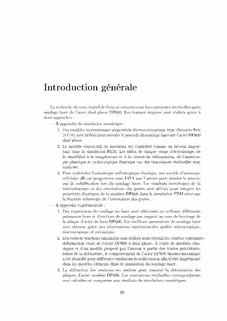
La recherche de cette travail de thèse se concentre sur les contraintes résiduelles aprèssoudage laser de l'acier dual phase DP600. Les travaux majeurs sont réalisés grâce àdeux approches :
� L'approche de simulation numérique :
1. Des modèles incrementaux séquentiels thermo-mécanique type éléments �nis(FEM) sont utilisés pour simuler le procédé du soudage laser sur l'acier DP600dual phase.
2. Le modèle constitutif du matériau est considéré comme un facteur impor-tant dans la simulation FEM. Les e�ets de chaque terme d'écrouissage, dela sensibilité à la température et à la vitesse de déformation, de l'anisotro-pie plastique et orthotropique élastique sur des contraintes résiduelles sontanalysés.
3. Pour rechercher l'anisotropie orthotropique élastique, une modèle d'automatecellulaire 2D est programmé sous JAVA par l'auteur pour simuler le proces-sus de solidi�cation lors du soudage laser. Les résultats numériques de lamicrostructure et des orientations des grains sont utilisés pour integrer lespropriétés élastiques de la soudure DP600 dans la simulation FEM ainsi quela fraction volumique de l'orientation des grains.
� L'approche expérimentale :
1. Des expériences de soudage au laser sont e�ectuées en utilisant di�érentespuissances laser et directions de soudage par rapport au sens de laminage dela plaque d'acier de base DP600. Les meilleurs paramètres de soudage lasersont obtenus grâce aux observations expérimentales qualité microscopique,macroscopique et mécanique.
2. Des tests de tractions uniaxiales sont utilisés pour obtenir les courbes contrainte-déformation vraie de l'acier DP600 à dual phase. À l'aide de modèles clas-siques et d'un modèle proposé par l'auteur à partir des études précédentesissues de la littérature, le comportement de l'acier DP600 thermo-mécaniquea été identi�é pour di�érents conditions de sollicitation a�n d'être implémentédans les modèles éléments �nis de simulation du soudage laser.
3. La di�raction des neutrons est réalisée pour mesurer la déformation desplaques d'acier soudées DP600. Les contraintes résiduelles correspondantessont calculées et comparées aux résultats de simulations numériques.
19

20 Introduction générale
Suivant cette méthodologie de travail, cette thèse est structurée en plusieurs parties :
D'abord une partie d'introduction générale synthétisant, les connaissances actuellesconcernant les contraintes résiduelles lors d'un processus de soudage laser. Les théoriespertinentes utilisées pour étudier le procédé de soudage par laser sont présentés en détailet décrites avec des éléments liés à l'analyse des contraintes résiduelles.
Dans le deuxième chapitre, en tant que facteurs clés dans la simulation des contraintesrésiduelles du processus de soudage laser, le comportement élasto-thermo-plastique del'acier dual phase DP600 est analysé en détail et identi�é par des techniques de régres-sion non-linéaire en partant des donnés expérimentales obtenu lors des essais de tractionuniaxiales.
Dans le troisième chapitre, une modèle numérique d'Automate Cellulaire 2D (CA)programmé sous JAVA a�n de pouvoir simuler la microstructure après soudage laser estétudié ainsi que l'in�uence de la microstructure sur l'anisotropie élastique orthotropiqueest présenté en détail.
Dans le quatrième chapitre, sur la base des modèles constitutifs du matériau iden-ti�és au chapitre 2 et de l'élasticité orthotropique analysée au chapitre 3, les résultatsdes modèles FEM visant à analyser les in�uences de l'écrouissage, de la sensibilité à latempérature, de la sensibilité à la vitesse de déformation, de l'anisotropie plastique etde l'anisotropie orthotropique élastique sont e�ectuées.
Dans le cinquième chapitre, les résultats numériques correspondant aux modèlesFEM du chapitre précédent sont analysés ensemble avec une synthèse de discussionconcernant l'impact de modèles utilisés sur la simulation des contraintes résiduelles lorsdu soudage laser de DP600.
Les principaux résultats de cette thèse sont présentés ci-dessous :
1. L'analyse de l'in�uence de l'écrouissage prouve qu'un petit changement dansle modèle constitutif du matériau peut entraîner une grande di�érence sur lescontraintes résiduelles. Les di�érents modèles constitutifs du matériau reproduc-tible du comportement réel observé lors des essais de traction, présentent lesmêmes in�uences sur la simulation des contraintes résiduelles.
2. La température a une in�uence importante sur les contraintes résiduelles équi-valentes. Le modèle proposé et celui polynomial décrivent bien le comportementà la sensibilité à la température du DP600 et se révèlent avoir des résultats desimulations similaires.
3. La vitesse de la déformation présente une valeur maximale des contraintes rési-duelles et de la déformation tandis que les modèles ne prenant pas en comptel'in�uence de la vitesse de la déformation présente des contraintes résiduelles deplus faibles valeurs aux bord de la zone de soudage et une courbe plutôt stabletout au long de la zone de soudage.
4. L'étude de l'angle entre la direction de laminage et la direction de soudure a miségalement en évidence l'importance de l'orientation de la tôle. Lorsque l'angleest de 45◦, les contraintes résiduelles autour de la soudure sont les plus élevées.

Introduction générale 21
Lorsque l'angle entre le sens du laminage et de soudure est de 90◦, les contraintesrésiduelles autour de la soudure sont les plus faibles.
5. L'anisotropie élastique orthotropique qui prend en compte l'orientation des grainsdont la fraction volumique, obtenue grâce au modèle numérique 2D CA, a peud'in�uence sur les contraintes résiduelles. Ce résultat était attendu car la zonesoudée est très peu texturée et présente une structure équiaxe.
6. En�n, les résultats expérimentaux et ceux obtenus par le couplage des deuxmodèles CA/FEM ont montré de bonnes convergences et permet de con�rmer larobustesse générale du modèle numérique de simulation du procédé de soudagelaser pour estimer les contraintes résiduelles.

22 Introduction générale
Introduction
1.1 Laser welding
Laser is short for �Light Ampli�cation by Stimulated Emission of Radiation� It isan intensive light and is generated by exciting a speci�c material with large energyfrom light, discharge, and so on. Based on the material type, lasers are categorized intosolid-state laser, liquid laser, gas laser and chemical laser.
The �rst ruby laser was built in 1960 by Theodore H. Maiman at Hughes ResearchLaboratories, based on theoretical work of Charles Hard Townes and Arthur LeonardSchawlow [5]. Shortly after that the diode laser was created in 1962 by two US groupsof Robert N. Hall at the General Electric research center [6] and of Marshall Nathanat the IBM T.J. in Watson Research Center [7]. The Nd :YAG laser was �rst inventedby J. E. Geusic et al. at Bell laboratories [8] and the CO2 laser by C.K.N. Patel atBell laboratories. The disk laser concept was proposed in the early 1990s with a �rstindustrial product applied in 2003 [9]. Among these various types of lasers, the Nd :YAGlaser is widely used in welding manufacturing process because of its good compatibilitywith optical �bers and high heat absorption coe�cient with metal.
1.1.1 Nd :YAG Laser
Nd :YAG laser is a kind of solid-state laser. The production of Nd :YAG laser isillustrated in �gure 1.1. A trivalent Nd ion, Nd3+ is doped in YAG material. This isbecause Nd3+ has a energy level structure for four-level model and because YAG crystalis so superior to other laser materials in term of the thermal conductivity.
The pumping and the oscillation wavelength of Nd :YAG laser are 808 nm and 1064nm, respectively. Arranging a number of rod media in the axial direction of the resonatorenables several tenth kW CW oscillation. In fact, a number of companies has realizedproducts of several kW Nd :YAG laser to weld steel and aluminum alloy. The output ofa typical Nd :YAG laser is, however, at most several hundreds W. The typical repetitionrate of Nd :YAG pulsed laser is in the range between several Hz and several kHz. AtQ-switching operation, a high power pulse (several hundreds mJ) of a duration of 10 nsto 50 ns has been generated.
23

24 Introduction
Figure 1.1 � Schematic of Nd :YAG laser oscillator
1.1.2 Sketch of laser welding system
As is seen in �gure 1.2, a sketch is presented in a laser welding system. After ge-nerated in the oscillator, the laser is transported through �ber or lens to the desiredplace. Before use for welding process, the laser beam is focused by lens to get a focuspoint where the power density can be very high to melt, vaporise and even ionize anyexisting material.
Figure 1.2 � Sketch of laser welding system
With di�erent laser beam energy density applied on the material, there are twodi�erent forms of welding : heat conduction welding and deep penetration welding.When the laser beam have a low power density or a high welding speed, the heat

Laser welding 25
conduction welding occurs. When a high power density laser beam is applied to thematerial, absorbed energy can not fully transferred by heat conduction, a part of energyis to vaporise the material and a key hole is formed through which laser penetrate intothe workpiece.
1.1.3 Laser welding parameters
1.1.3.1 The power
The welding power directly in�uences the speci�c energy input expressed per unitvolume of base plate. It is one of the most important parameters of laser welding process.For a given welding condition, as the power of laser beam increases, the geometry ofweld changes from shallow to deep and the welding mode from conduction welding todeep penetration welding. For deep penetration welding, the dimension of a weld willreach a threshold when the power of laser beam increase continuously, because energyinput are absorbed by the plasma of on the keyhole.
1.1.3.2 The welding speed
The welding speeding in�uences the speci�c energy input of base plate. For a givenlaser power, high welding speed can decrease the input energy density applied on thebase plate. In this way, the deep penetration welding can be changed into conductionwelding. With a �xed rate of power input, a high speed will lead the weld to be shallow.Moreover, for a penetration welding, too high speed can result in unstable keyhole anda non-uniform penetration weld. If the welding speed is too low, large amount energyare lost by heat conduction to base metal. It is necessary to balance laser power andwelding speed given process condition.
1.1.3.3 The focusing position
As is seen in �gure 1.3, the focusing position can be expressed by the defocusingamount �D". When D=0, the focal point is at the plate surface. The interaction areaof laser beam applied on the material surface is the smallest. When D>0 or D<0, thefocal point is above or under the plate surface. The interaction area increases as the |D|increase.
Figure 1.3 � Three focusing positions of the laser beam
26 Introduction
1.1.3.4 The cover gas
Argon, helium or nitrogen inert gas are usually used as the cover gas. The covergas is used to protected the weld from rapid oxidation. During welding, the cover gas isblasted on the surface of fusion zone with low pressure �ow volume to shield the weldzone from room oxygen. Welds with cover gas are usually shiny and the mechanicalproperties are not a�ected. The �owing cover gas can take away some amount of heatduring welding, thus reduce the temperature gradient and the thermal load of weldingprocess.
1.2 Dual phase steel DP600
1.2.1 General information of DP600
To relieve energy crisis and environment problems, high strength material is appliedin automotive industries in order to reduce the car weight[10]. As a type of AHSS (ad-vanced high-strength steel), DP600 is widely used in automobile industries. DP meansdual phase steel (martensite + ferrite) and 600 series means that the tensile strengthis over 600 MPa. This steel is a low carbon steel with a soft ferrite matrix containinga hard second phase, mainly islands of martensite (3%-30%) [11]. The hard phase ofmartensite contributes to the high strength while soft ferrite helps to improve ductility[12, 13], which make a good combination of formability and high strength. Compa-red with traditional high-strength low-alloy (HSLA) steels, DP steel has no yield pointelongation and has a higher strain-hardening rate [14]. The high strain-hardening rateenhance the absorption of energy when deformation is happened, which helps decreaseof damage in car collision [15].
1.2.2 Applications of DP600
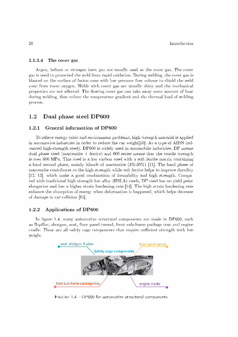
In �gure 1.4, many automotive structural components are made in DP600, suchas B-pillar, shotgun, seat, �oor panel tunnel, front sub-frame package tray and enginecradle. These are all safety cage components that require su�cient strength with lowweight.
Figure 1.4 � DP600 for automotive structural components

Dual phase steel DP600 27
1.2.3 Properties of DP600
The yield and tensile strength of DP 600 steel are primarily determined by thevolume proportion of martensite in the softer ferritic matrix.
Figure 1.5 � Microstructure of dual phase DP600 steel [1]
1.2.3.1 Chemical composition of DP600 steel
The chemical composition of DP600 steel is shown in table 1.1.
Table 1.1 � Chemical composition of DP600 steel [16]DP 600 steel [wt. %]
C Mn Si P S Al N Crmax. 0.2 max. 2.00 max. 0.50 max. 0.090 max. 0.015 min. 0.02 max. 0.012 max. 1.00
1.2.3.2 Mechanical properties of DP600 steel
The general mechanical properties of DP600 steel is shown in table 1.2.
Table 1.2 � Mechanical properties of DP600 steel [16]
Mechanical properties of DP600 steel
Yield strength R p0.2 [MPa] 380-470Strength Rm [MPa] 580-670Maximum R p0.2/Rm proportion 0.70Minimum ductility A5 [%] 24

28 Introduction
1.2.4 Laser welding DP600 development
In the year of 2016, G.C.C. Correard et al. [17] investigated the microstructure ofDP600/DP600 weld and DP600/TRIP750 weld especially on heat a�ected zone (HAZ)by a �ber laser with 1300 W power and 50mm/s welding speed. Martensite is found inweld zone. In HAZ region, martensite and ferrite are observed. The tensile strength ofdi�erent type of DP600 weld joints is about 400 MPa, ranges from 380MPa to 400MPa.Fatigue curves presented a limit at approximately 350 MPa for DP600 steels.
In 2012, Y. Song et al. [18] used Nd :YAG laser to weld DP600 and DX56D steel.The Vickers hardness are tested and based on the mixture rule, the relationship betweenthe micro-Vickers hardness value and material parameters (i.e., the strain hardeningexponent, the strength coe�cient and Young's modulus) was quantitatively built. Atthe same year, M. Hazratinezhad et al. [19] researched the in�uence of Nd :YAG laserpattern on the after welding mechanical property of DP steel. The energy input patternand e�ective peak power density is found to in�uence material strength and high pulseduration lead to coarse grain in HAZ (Heat A�ected Zone).
At year 2010 and 2011, N.Farabi et al. [20, 21, 22] investigated diode laser weldedon DP600/DP600 and DP600/DP980 steel joints. Microstructures, fatigue properties,microhardness pro�les, tensile properties and work hardening characteristics of laserweld joints are studied. Several results are found in their throughout research :
� The welding resulted in a signi�cant increase of hardness in the fusion zone(nearly full martensite is found of DP600/DP980 FZ), but also the formation ofa soft zone in the outer heat-a�ected zone (HAZ). The degree of softening wasfound to be stronger in the DP980 welded joints than in the the DP600 weldedjoints and lead to a signi�cant decrease in the fatigue limit of DP980 softeningzone.
� For DP600 joint, while the ductility decreased after welding, the yield strengthincreased and the ultimate tensile strength remained almost unchanged.
� At higher stress amplitudes, the fatigue life of DP600 is almost the same betweenthe base metal and welded joint. Tensile fracture and fatigue failure occurred atthe outer HAZ. Fatigue crack initiation was from the specimen surface and crackpropagation was characterized by their characteristics..
C. Dharmendra et al. [23] investigated laser welding-brazing DP600/AA6016 withCW Nd :YAG laser. The microstructure and composition analyses of the brazed jointswere examined. The micro-hardness and tensile strength were measured. The laser wel-ding parameters were optimized based on mechanical resistance and thickness of steelseam interface.
M. Xia et al. [24] investigated Nd :YAG laser heat input in�uence on heat a�ectedzone (HAZ) of dual phase steels. Maximum HAZ softening was proportional to themartensite content, and the heat input controlled the completion of softening.
X. Li [25] advocated a technique to stabilize laser lap welding zinc coated DP600 :the technique is addition of a small amount of aluminum to the faying surface region,so that a liquid Al-Zn alloy of high boiling point is formed, thus lowering the Zn vapor

Residual stresses 29
pressure. The comparison of weld surface pro�les and weld interface microstructures,with and without Al foil, are presented to show the good quality of Al added on platesurface.
1.3 Residual stresses
Residual stresses are �self equilibrating internal stresses� existing in a free body withno external forces or constraints on its boundary.
1.3.1 The �rst, second and third order of residual stress
A distinction is made between �rst, second and third order residual stresses (Figure1.6) [2] :
1. First order (σI, macro) : nearly homogeneous across large areas (several grainsof the material). First order residual stresses, σI, extend over macroscopic areasand are averaged stresses over several crystallites.
2. Second order (σII, meso) : nearly homogeneous across smaller areas, of the or-der of some grains or phases of a material. Second order residual stresses, (σII,act between crystallites or crystallite subregions (size approx. 1-0.01 mm) andare averaged within these areas (for instance residual stresses around piled-updislocations or secondary phases).
3. Third order (σIII, micro) : inhomogeneous across submicroscopic areas of thematerial, several atomic distances within a grain. Third order residual stresses,σIII, act between atomic areas (size approx. 10−2 − 10−6 mm ; for instance, theresidual stresses around a single dislocation).
The macroscopic residual stresses are of particular relevance for engineering pur-poses. In this desertation, the objective is focused on the �rst order of residual stresses.
1.3.2 Purpose of research residual stresses
1. Residual stresses superimpose to applied stresses during service life
2. Residual stresses can a�ect the mechanical behavior of a component
3. Residual stresses in�uence the corrosion behavior of the weld part.
Thus, the residual stress evaluation is fundamental to ensure the performance of aproduct.
1.3.3 The production mechanism of residual stress in welding
To better understand the complex welding residual stress, simple cases are analyzed.The production of thermal stress is shown in �gure 1.7. A bar at 20◦C, at 200◦C without

30 Introduction
Figure 1.6 � Three orders of residual stresses[2]
constrain and at 200◦C with constrain is presented. Generally the material increases itsbody volume due to temperature increase, which is usually called thermal expansion.For the bar at 20◦C and at 200◦C without constrain, the bar is at free state with nointernal stress in the bar. For the bar at 200◦C with constrain, the bar is at constrainedstate with internal stress in the bar. This internal stress is called thermal stress and itsmagnitude depend on temperature change and boundary conditions. In a macroscopicpoint of view, the thermal stress can be produced without strain due to the temperaturechange.
Figure 1.7 � Thermal stress obtained by dilatation of a clamped bar

Residual stresses 31
The length at free state of 200◦C is given by :
l1 = l0(1 +α ∆T ) (1.1)
Supposing only elastic behavior, the stress of constrained state at 200◦C is writtenas :
σthermal ≈ −E(l1 − l0l0
)= −Eα∆T (1.2)
Figure 1.8 shows the inner part and outer part of a material. At �rst, the temperatureof the inner part and the outer part is the same. There are no interval and no stressbetween inner and outer part surface. When the temperature of inner part is increasedwhile the temperature of outer remains the same, the inner part tends to expand whilethe outer part tends to remain the same. The con�ict between the two part happens.
Figure 1.8 � Inner and outer part of a material
The inner and outer part is plotted in two dimension to sketch out the geometrychange of inner part (the outer part is also changed but not marked in �gure 1.9). In the�gure, abcd stands for the geometry of inner part at cool state, a"b"c"d" the geometryof inner part of hot state supposing no outer part constrained and a'b'c'd' the geometryof inner part of hot state considering the constrain of outer part.

32 Introduction
Figure 1.9 � Inner part geometry change in two dimension
To analyze the geometry change of inner part during heating process, the geometryof inner part at three states in �gure 1.10 are plotted with the point d, d' and d" atthe same place to illustrate more clearly the volume change of the inner part. First, thegeometry of inner part at cool state abcd is heated. If there is no constrain of outer part,abcd is imagined to expand to a hot state of a"b"c"d". But in reality, the inner partis always constrained by a outer part. Thus, the inner part at cool state abcd expandto a constrained hot state a'b'c'd' , or the inner part at free heated state a"b"c"d" iscompressed to a constrained hot state a'b'c'd'.
During the imagined compressed process, the inner part must take into account anelastic and plastic deformation. Along an horizontal direction, the length change of innerpart can be express as :
∆l = ld”c” − ld′c′ = le + lp (1.3)
where ∆l is the inner part length change when constrained by outer part at heatedstate, le is the elastic deformation length and lp is the plastic deformation length ofinner part.
Corresponding to the inner part, the outer part that has the boundary attached tothe inner part is plotted in �gure 1.11. Due to the expansion of inner part, the outerpart is deformed from state ABCD to A'B'C'D'. If the outer part has no sti�ness, theouter part may be pushed by inner part to the dotted shape. (The maximum volume ofinner part at heated state without constrain).
Residual stresses 33
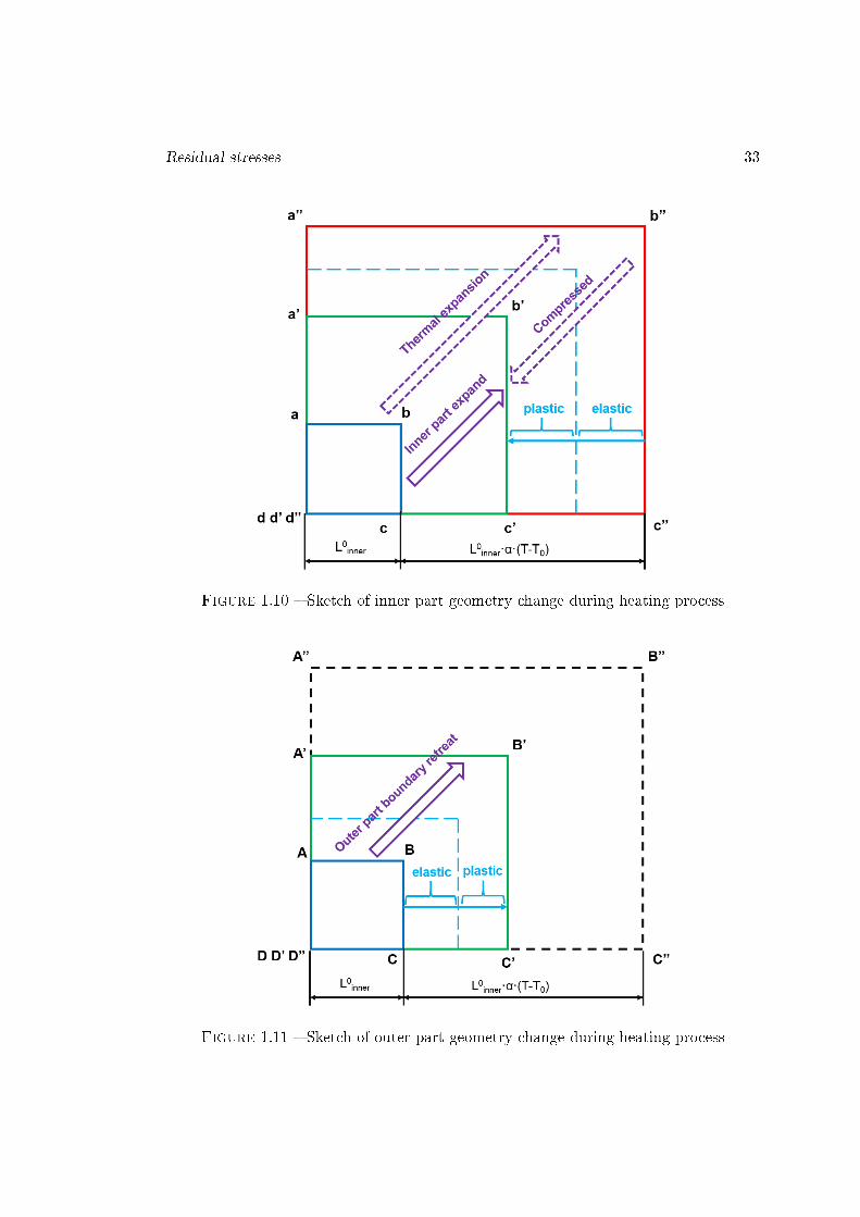
Figure 1.10 � Sketch of inner part geometry change during heating process
Figure 1.11 � Sketch of outer part geometry change during heating process
34 Introduction
This deformation must contains an elastic deformation and may contains a plasticdeformation. In horizontal direction, the length change of outer part can be express as :
∆L = lD′C′ − lDC = Le + Lp (1.4)
where ∆L is the outer part length change when pushed by the inner part expansion,Le is the elastic deformation length and Lp is the plastic deformation length of outerpart.
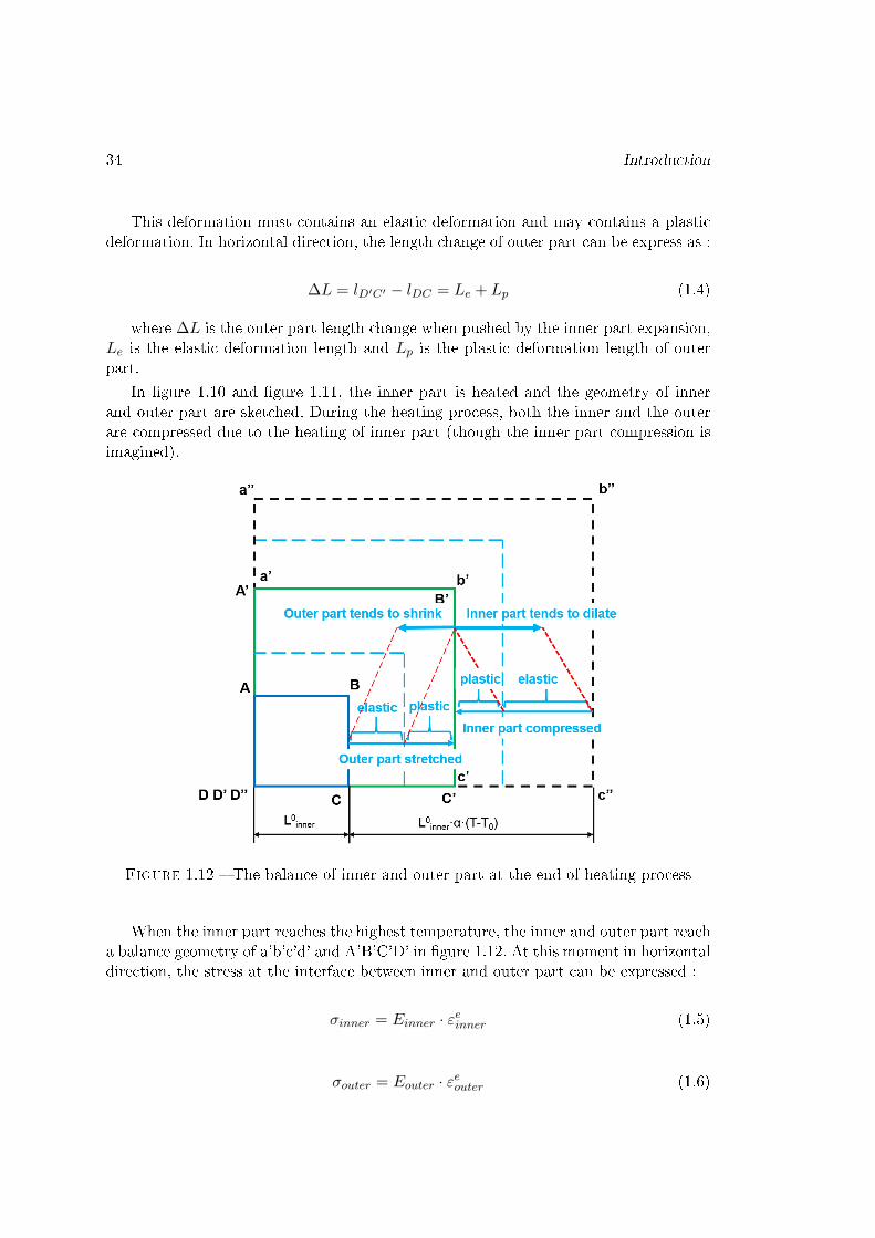
In �gure 1.10 and �gure 1.11, the inner part is heated and the geometry of innerand outer part are sketched. During the heating process, both the inner and the outerare compressed due to the heating of inner part (though the inner part compression isimagined).
Figure 1.12 � The balance of inner and outer part at the end of heating process
When the inner part reaches the highest temperature, the inner and outer part reacha balance geometry of a'b'c'd' and A'B'C'D' in �gure 1.12. At this moment in horizontaldirection, the stress at the interface between inner and outer part can be expressed :
σinner = Einner · εeinner (1.5)
σouter = Eouter · εeouter (1.6)
Continuum mechanics description 35
For laser welding, the heating process is followed by a cooling step. In this simplecase, the heated inner part is cooled. In this cooling process, both inner and outer parttend to return to its original state. The plastic deformation during heating process ispreserved and may be also produced during cooling process. The stress at the interfacebetween a'b'c'd' and A'B'C'D' should be the same and can be computed consideringthe elastic and plastic deformation.
1.4 Continuum mechanics description
The material constitutive model is an important part of numerical mechanical si-mulation. It describes the essential relationship between the strains and the stresses,which is a linear relationship for elastic analyses and a complex nonlinear relationshipfor plastic analyses, involving plastic strain, temperature, strain rate and state variablesdescribing mechanism of deformation at microscopic level.
The elasticity of a material is described in terms of a stress-strain relation. Typically,two types of relation are considered. The �rst type deals with materials that are elasticonly for small strains. The second deals with materials that have large elastic strains. Forsmall strains, the measure of the Cauchy stress is used while the measure of strain is anin�nitesimal strain tensor ; the resulting (predicted) material behavior is termed linearelasticity, which for metallic materials is called the generalized Hooke's law describingboth isotropic and anisotropic elasticity.
In 1867 Tresca published his works [26, 27] on material yielding behavior under va-rious stress states. He used the maximum shear stress as the yield criteria. His systematicexperimental investigations on yielding became a theoretical basis for plasticity investi-gation. After Tresca's work, the Von Mises yield criteria [28] was proposed in 1913. Inprincipal stress space, the yield surface of Tresca criteria is circumscribed by Von Mi-ses's yield criteria. The e�ective Von Mises stress can be viewed as a proportion to theelastic distortional energy which makes Von Mises criteria a more reasonable criteria.Based on Von Mises, Rodney Hill developed several yield criteria [29, 30, 31, 32, 33]for anisotropic plastic deformations which are provided successful in predicting metals,polymers and certain composites. In this work, the Von Mises yield criteria and Hillyield law are used, so a brief description the plasticity including the Von Mises andHill's criteria are introduced below.
1.4.1 From physical world to mathematical conception
To analysis the residual stresses after welding process, the solid dynamics of conti-nuum mechanics are used through a Finite Element Method (FEM) used by the com-mercial software ABAQUS.
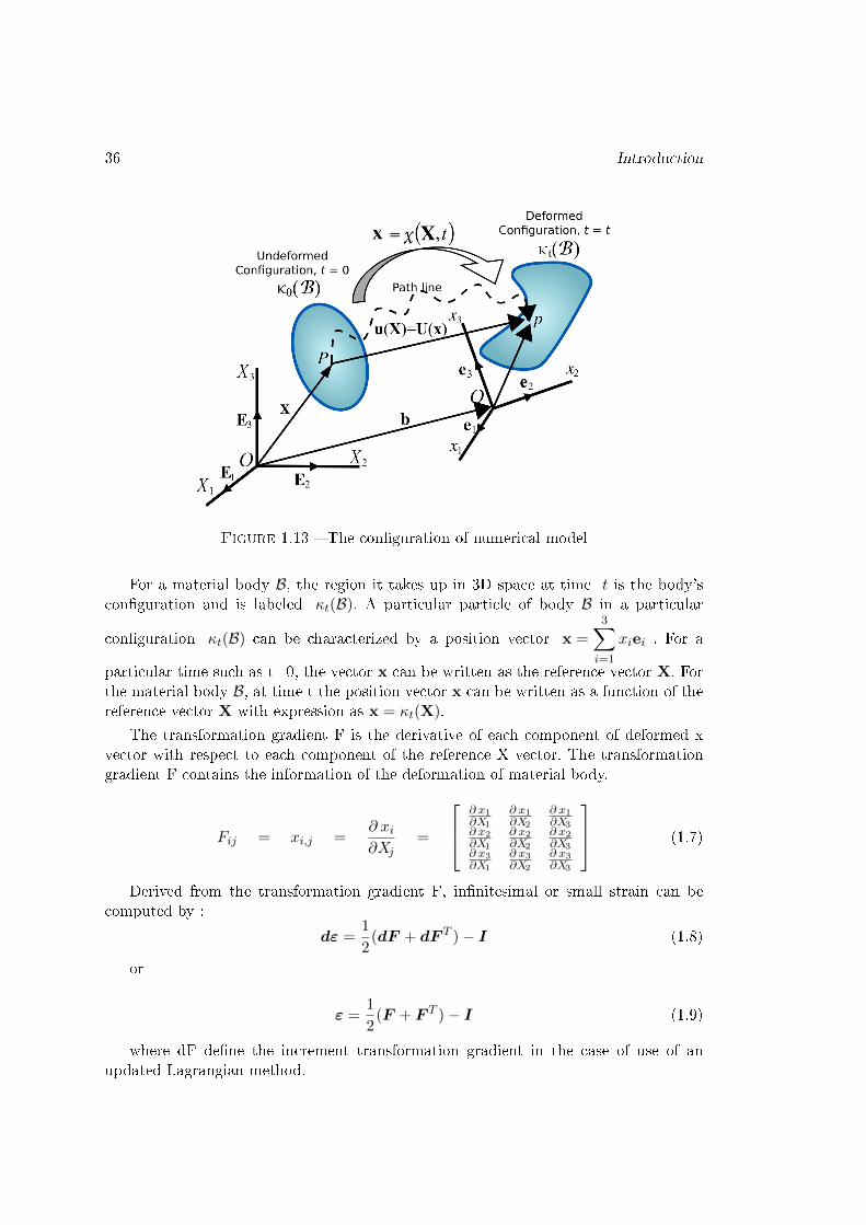
To describe the material mathematical formulations, several basic de�nitions areintroduced according to the �gure 1.13. For more detail informations, please refer tocontinuum mechanics theory.
36 Introduction
Figure 1.13 � The con�guration of numerical model
For a material body B, the region it takes up in 3D space at time t is the body'scon�guration and is labeled κt(B). A particular particle of body B in a particular
con�guration κt(B) can be characterized by a position vector x =3∑i=1
xiei . For a
particular time such as t=0, the vector x can be written as the reference vector X. Forthe material body B, at time t the position vector x can be written as a function of thereference vector X with expression as x = κt(X).
The transformation gradient F is the derivative of each component of deformed xvector with respect to each component of the reference X vector. The transformationgradient F contains the information of the deformation of material body.
Fij = xi,j =∂ xi∂Xj
=
∂ x1∂X1
∂ x1∂X2
∂ x1∂X3
∂ x2∂X1
∂ x2∂X2
∂ x2∂X3
∂ x3∂X1
∂ x3∂X2
∂ x3∂X3
(1.7)
Derived from the transformation gradient F, in�nitesimal or small strain can becomputed by :
dε =1
2(dF + dF T )− I (1.8)
or
ε =1
2(F + F T )− I (1.9)
where dF de�ne the increment transformation gradient in the case of use of anupdated Lagrangian method.
Continuum mechanics description 37
The Lagrangian strain tensor (in�nitestimal deformation) is given as follows :
E =1
2(F · F T )− I (1.10)
For small material deformations, ε =∫dε ≈ E. These equations are generally used
for metallic materials to de�ne a more consistent de�nition of large plastic deformationsusing the evaluation of incremental strain state tensor by dε = dεel + dεpl and F =F elF pl.
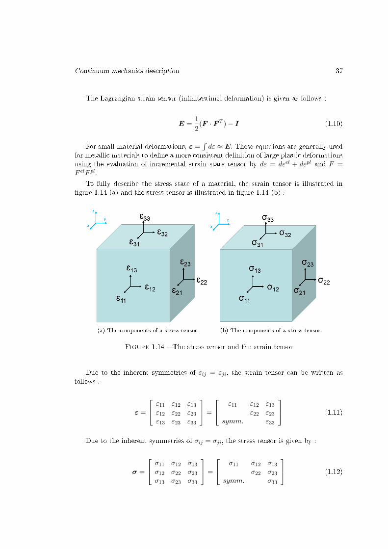
To fully describe the stress state of a material, the strain tensor is illustrated in�gure 1.14 (a) and the stress tensor is illustrated in �gure 1.14 (b) :
(a) The components of a stress tensor (b) The components of a stress tensor
Figure 1.14 � The stress tensor and the strain tensor
Due to the inherent symmetries of εij = εji, the strain tensor can be written asfollows :
ε =
ε11 ε12 ε13
ε12 ε22 ε23
ε13 ε23 ε33
=
ε11 ε12 ε13
ε22 ε23
symm. ε33
(1.11)
Due to the inherent symmetries of σij = σji, the stress tensor is given by :
σ =
σ11 σ12 σ13
σ12 σ22 σ23
σ13 σ23 σ33
=
σ11 σ12 σ13
σ22 σ23
symm. σ33
(1.12)
38 Introduction
1.4.2 Von Mises e�ective stress and e�ective strain
Strain tensor in equation 1.11 and stress tensor in equation 1.12 each have 6 com-ponents of di�erent values, respectively. These values provide the material mechanicalstate under certain circumstances.
To simplify the analysis, a lot of multiaxial yield laws are proposed and among themthe most commonly used is the Von Mises criteria. The Von Mises e�ective stress or theequivalent stress is calculated as follows :
σe =√
12 [(σ11 − σ22)2 + (σ22 − σ33)2 + (σ33 − σ11)2 + 6(σ2
23 + σ231 + σ2
12)]
=√
32(s2
11 + s222 + s2
33 + 2σ223 + 2σ2
31 + 2σ212)
(1.13)
where s is the deviatoric stress term.
The Von Mises in�nitesimal e�ective plastic strain or equivalent plastic strain iscomputed by :
dεpe =
√23(dεp11
2+ dεp22
2+ dεp33
2+ 2dεp23
2+ 2dεp31
2+ 2dεp12
2) (1.14)
Notice that �e�, the subscript of σe and εpe, means e�ective. Using Von Mises e�ective
stress and strain de�nition, complex material stress and strain states with 6 values canbe simpli�ed into only one value, respectively. With this simpli�cation, the uniaxialtensile test can be the reference for yield state for many complex material stress-strainstates.
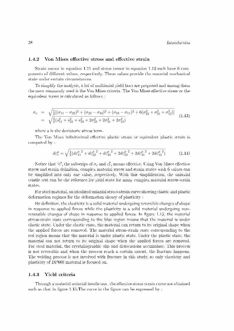
For steel material, an idealized uniaxial stress-strain curve showing elastic and plasticdeformation regimes for the deformation theory of plasticity :
By de�nition, the elasticity is a solid material undergoing reversible changes of shapein response to applied forces while the plasticity is a solid material undergoing non-reversible changes of shape in response to applied forces. In �gure 1.15, the materialstress-strain state corresponding to the blue region means that the material is underelastic state. Under the elastic state, the material can return to its original shape whenthe applied forces are removed. The material stress-strain state corresponding to thered region means that the material is under plastic state. Under the plastic state, thematerial can not return to its original shape when the applied forces are removed.For steel material, the crystallographic slip and dislocations accumulate. This processis not reversible and when the process reach a certain extent, the fracture happens.The welding process is not involved with fracture in this study, so only elasticity andplasticity of DP600 material is focused on.
1.4.3 Yield criteria
Through a material uniaxial tensile test, the e�ective stress-strain curve are obtainedsuch as that in �gure 1.15.The curve in the �gure can be expressed by :
Continuum mechanics description 39
Figure 1.15 � Plasticity region
σyielde = Function(εp
e ) (1.15)
The Von Mises e�ective plastic strain is noted as εpe. The computation method isbased on equation 1.14.
εpe =
∫dεpe (1.16)
According to the material constitutive model used by the numerical simulation andconsidering the deformation history, an e�ective plastic strain εpe and correspondinge�ective stress σe are obtained. Then the computed e�ective stress σe and the yielde�ective stress σyielde of material is compared using yield criteria f :
f = σe − σyielde (1.17)
Based on yield criteria f , the material can be determined to be yield or not in thesimulation.
� If yield criteria f is less than 0, then the material is under elastic state, thematerial is deformed elastically.
� If yield criteria f is equal to 0, then the material is under plastic state, thematerial is deformed plastically.
� The yield criteria f should not be bigger than 0, the plastic �ow will increasethe e�ective plastic strain εpe and then increase the yield e�ective stress σyielde .
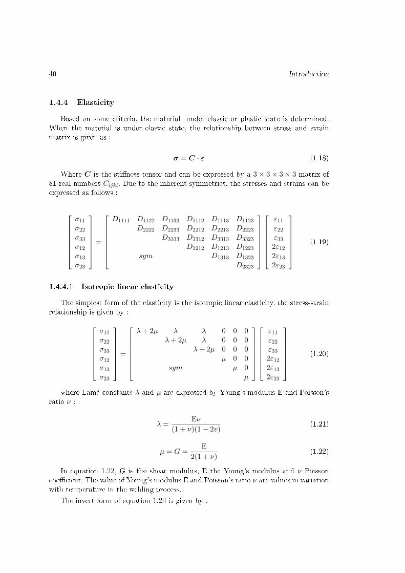
40 Introduction
1.4.4 Elasticity
Based on some criteria, the material under elastic or plastic state is determined.When the material is under elastic state, the relationship between stress and strainmatrix is given as :
σ = C · ε (1.18)
Where C is the sti�ness tensor and can be expressed by a 3 × 3 × 3 × 3 matrix of81 real numbers Cijkl. Due to the inherent symmetries, the stresses and strains can beexpressed as follows :
σ11
σ22
σ33
σ12
σ13
σ23
=
D1111 D1122 D1133 D1112 D1113 D1123
D2222 D2233 D2212 D2213 D2223
D3333 D3312 D3313 D3323
D1212 D1213 D1223
sym D1313 D1323
D2323
ε11
ε22
ε33
2ε12
2ε13
2ε23
(1.19)
1.4.4.1 Isotropic linear elasticity
The simplest form of the elasticity is the isotropic linear elasticity. the stress-strainrelationship is given by :
σ11
σ22
σ33
σ12
σ13
σ23
=
λ+ 2µ λ λ 0 0 0λ+ 2µ λ 0 0 0
λ+ 2µ 0 0 0µ 0 0
sym µ 0µ
ε11
ε22
ε33
2ε12
2ε13
2ε23
(1.20)
where Lamé constants λ and µ are expressed by Young's modulus E and Poisson'sratio ν :
λ =Eν
(1 + ν)(1− 2v)(1.21)
µ = G =E
2(1 + ν)(1.22)
In equation 1.22, G is the shear modulus, E the Young's modulus and ν Poissoncoe�cient. The value of Young's modulus E and Poisson's ratio ν are values in variationwith temperature in the welding process.
The invert form of equation 1.20 is given by :

Continuum mechanics description 41
ε11
ε22
ε33
2ε12
2ε13
2ε23
=1
E
1 −ν −ν−ν 1 −ν−ν −ν 1
2(1 + ν)2(1 + ν)
2(1 + ν)
σ11
σ22
σ33
σ12
σ13
σ23
(1.23)
The isotropic linear elasticity is used in numerical welding simulation except forthe case of elastic orthotropic anisotropy analysis considering phase transformation,material phase mixture and especially grains orientations in the weld. The orthotropicelastic anisotropy analysis is introduced in the next section.
1.4.4.2 Orthotropic linear elasticity
A more complex elasticity is the orthotropic linear elasticity which is de�ned bythree moduli E1, E2, E3, three Poisson's ratios ν12, ν13, ν23 and three shear moduli G12,G13, G23 associated with the material's principal directions.
σ11
σ22
σ33
σ12
σ13
σ23
=
D1111 D1122 D1133 0 0 0D2222 D2233 0 0 0
D3333 0 0 0D1212 0 0
sym D1313 0D2323
ε11
ε22
ε33
2ε12
2ε13
2ε23
(1.24)
where the constants de�ne the D matrix is given by :
D1111 = E1(1− ν23ν32)γ (1.25)
D2222 = E2(1− ν13ν31)γ (1.26)
D3333 = E3(1− ν12ν21)γ (1.27)
D1122 = E1(ν21 + ν31ν23)γ = E2(ν12 + ν32ν13)γ (1.28)
D1133 = E1(ν31 + ν21ν32)γ = E2(ν13 + ν12ν23)γ (1.29)
D2233 = E2(ν32 + ν12ν31)γ = E3(ν23 + ν21ν13)γ (1.30)
D1212 = G12 (1.31)
D1313 = G13 (1.32)
D2323 = G23 (1.33)
where γ is expressed as :
γ =1
1− ν12ν21 − ν23ν32 − ν31ν13 − 2ν21ν32ν13(1.34)
The invert form of equation 1.24 is given by :

42 Introduction
ε11
ε22
ε33
2ε12
2ε13
2ε23
=
1/E1 −ν21/E2 −ν31/E3
−ν12/E1 1/E2 −ν32/E3
−ν13/E1 −ν23/E2 1/E3
1/G12
1/G13
1/G23
σ11
σ22
σ33
σ12
σ13
σ23
(1.35)
The orthotropic linear elasticity is de�ned not only with three moduli E1, E2, E3,three Poisson's ratios ν12, ν13, ν23 and three shear moduli G12, G13, G23, but also byde�nition of the material's principal direction. When the principal direction changesand have angles with 11, 22 and 33 directions, the elastic sti�ness is changed followingformula based on change matrix [34] :
The direction cosine In �gure 1.16, −→on ⊥ 4abc. The angles between the vector −→onand coordinate axises x, y and z are α, β and γ, respectively. It is de�ned that directioncosines (l1, m1, n1) of −→on with respect to axises x, y and z are :
l1 = cosα, m1 = cosβ, n1 = cosγ (1.36)
Figure 1.16 � The surface normal vector direction de�nition in a cartesian coordinatesystem
There are two cartesian coordinate systems, one is named [S] with coordinates (1,2,3)and the other is [K] with (x,y,z). Direction cosines between two coordinate axises areshown in table 1.3.

Continuum mechanics description 43
Table 1.3 � Direction cosines between two coordinate axisesx y z
1 l1 m1 n1
2 l2 m2 n2
3 l3 m3 n3
Transition of stresses in di�erent coordinate systems Stresses[σ
[S]ij
]in coor-
dinate system [S] and[σ
[K]ij
]in [K] can be written as :
[σ
[S]ij
]=
σ1
σ2
σ3
τ23
τ31
τ12
,[σ
[K]ij
]=
σxσyσzτyzτzxτxy
(1.37)
The relation between[σ
[S]ij
]and
[σ
[K]ij
]can be written as :[
σ[S]ij
]= [Aij ]
[σ
[K]ij
](1.38)
where [Aij ]−1 is written by :
[Aij ]−1 =
l21 l22 l23 2l2l3 2l3l1 2l1l2m2
1 m22 m2
3 2m2m3 2m3m1 2m1m2
n21 n2
2 n23 2n2n3 2n3n1 2n1n2
m1n1 m2n2 m3n3 m2n3 +m3n2 m3n1 +m1n3 m1n2 +m2n1
n1l1 n2l2 n3l3 n2l3 + n3l2 n3l1 + n1l3 n1l2 + n2l1l1m1 l2m2 l3m3 l2m3 + l3m2 l3m1 + l1m3 l1m2 + l2m1
(1.39)
Transition of strains in di�erent coordinate systems Strains[ε
[S]ij
]in coordinate
system [S] and[ε
[K]ij
]in [K] can be written as :
[ε
[S]ij
]=
ε1
ε2
ε3
γ23
γ31
γ12
,[ε
[K]ij
]=
εxεyεzγyzγzxγxy
(1.40)
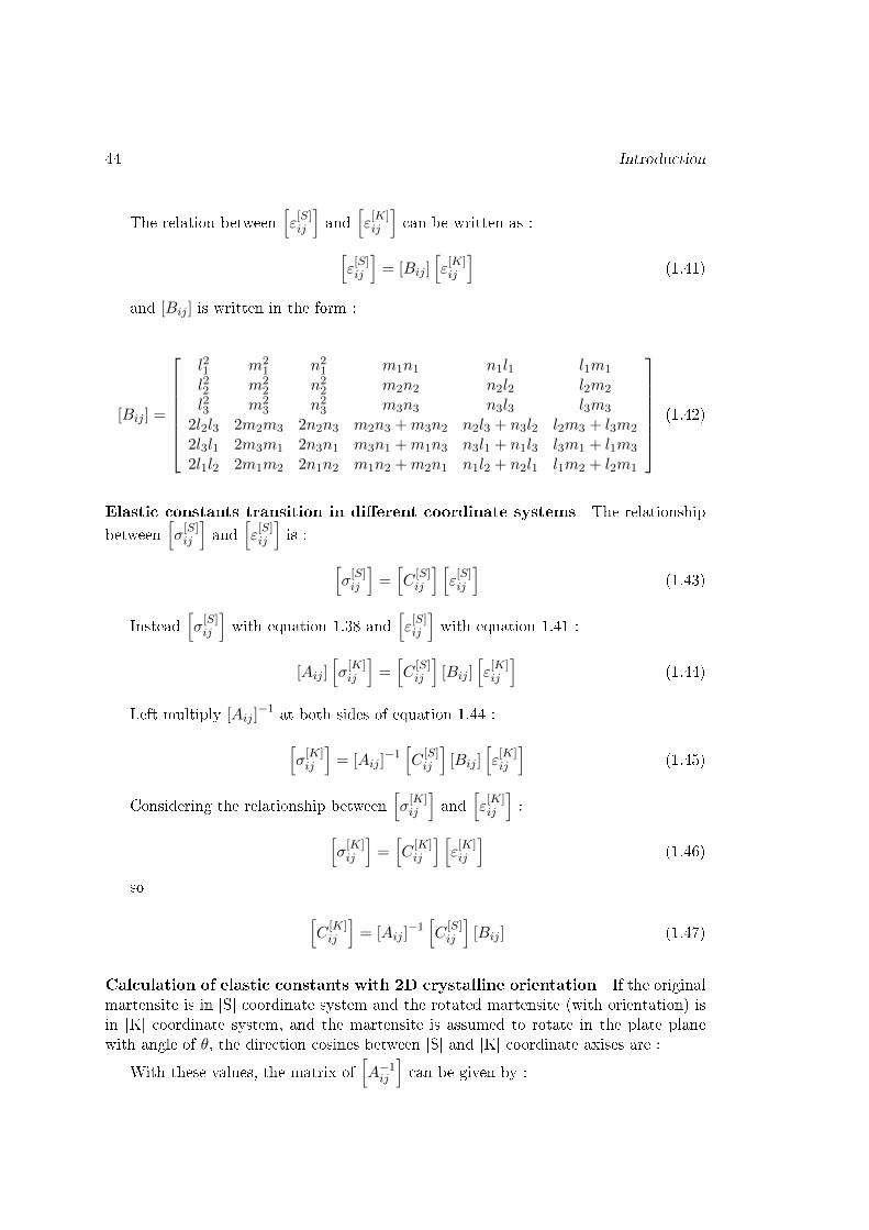
44 Introduction
The relation between[ε
[S]ij
]and
[ε
[K]ij
]can be written as :[
ε[S]ij
]= [Bij ]
[ε
[K]ij
](1.41)
and [Bij ] is written in the form :
[Bij ] =
l21 m21 n2
1 m1n1 n1l1 l1m1
l22 m22 n2
2 m2n2 n2l2 l2m2
l23 m23 n2
3 m3n3 n3l3 l3m3
2l2l3 2m2m3 2n2n3 m2n3 +m3n2 n2l3 + n3l2 l2m3 + l3m2
2l3l1 2m3m1 2n3n1 m3n1 +m1n3 n3l1 + n1l3 l3m1 + l1m3
2l1l2 2m1m2 2n1n2 m1n2 +m2n1 n1l2 + n2l1 l1m2 + l2m1
(1.42)
Elastic constants transition in di�erent coordinate systems The relationshipbetween
[σ
[S]ij
]and
[ε
[S]ij
]is : [
σ[S]ij
]=[C
[S]ij
] [ε
[S]ij
](1.43)
Instead[σ
[S]ij
]with equation 1.38 and
[ε
[S]ij
]with equation 1.41 :
[Aij ][σ
[K]ij
]=[C
[S]ij
][Bij ]
[ε
[K]ij
](1.44)
Left multiply [Aij ]−1 at both sides of equation 1.44 :[
σ[K]ij
]= [Aij ]
−1[C
[S]ij
][Bij ]
[ε
[K]ij
](1.45)
Considering the relationship between[σ
[K]ij
]and
[ε
[K]ij
]:[
σ[K]ij
]=[C
[K]ij
] [ε
[K]ij
](1.46)
so [C
[K]ij
]= [Aij ]
−1[C
[S]ij
][Bij ] (1.47)
Calculation of elastic constants with 2D crystalline orientation If the originalmartensite is in [S] coordinate system and the rotated martensite (with orientation) isin [K] coordinate system, and the martensite is assumed to rotate in the plate planewith angle of θ, the direction cosines between [S] and [K] coordinate axises are :
With these values, the matrix of[A−1ij
]can be given by :
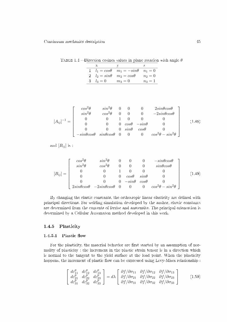
Continuum mechanics description 45
Table 1.4 � Direction cosines values in plane rotation with angle θx y z
1 l1 = cosθ m1 = −sinθ n1 = 02 l2 = sinθ m2 = cosθ n2 = 03 l3 = 0 m3 = 0 n3 = 1
[Aij ]−1 =
cos2θ sin2θ 0 0 0 2sinθcosθsin2θ cos2θ 0 0 0 −2sinθcosθ
0 0 1 0 0 00 0 0 cosθ −sinθ 00 0 0 sinθ cosθ 0
−sinθcosθ sinθcosθ 0 0 0 cos2θ − sin2θ
(1.48)
and [Bij ] is :
[Bij ] =
cos2θ sin2θ 0 0 0 −sinθcosθsin2θ cos2θ 0 0 0 sinθcosθ
0 0 1 0 0 00 0 0 cosθ sinθ 00 0 0 −sinθ cosθ 0
2sinθcosθ −2sinθcosθ 0 0 0 cos2θ − sin2θ
(1.49)
By changing the elastic constants, the orthotropic linear elasticity are de�ned withprincipal directions. For welding simulation developed by the author, elastic constantsare determined from the contents of ferrite and austensite. The principal orientation isdetermined by a Cellular Automaton method developed in this work.
1.4.5 Plasticity
1.4.5.1 Plastic �ow
For the plasticity, the material behavior are �rst started by an assumption of nor-mality of plasticity : the increment in the plastic strain tensor is in a direction whichis normal to the tangent to the yield surface at the load point. When the plasticityhappens, the increment of plastic �ow can be expressed using Levy-Mises relationship :
dεp11 dεp12 dεp13
dεp21 dεp22 dεp23
dεp31 dεp32 dεp33
= dλ
∂f/∂σ11 ∂f/∂σ12 ∂f/∂σ13
∂f/∂σ21 ∂f/∂σ22 ∂f/∂σ23
∂f/∂σ31 ∂f/∂σ32 ∂f/∂σ33
(1.50)

46 Introduction
When we use the Von Mises e�ective stress for computation, then yield criteria f inequation 1.50 can be expressed by :
f = σe − σyielde =√
32(s2
11 + s222 + s2
33 + 2σ223 + 2σ2
31 + 2σ212)− σyielde (1.51)
Substitute equation 1.51 into equation 1.50, the increment of plastic �ow can beexpressed by :
dεp11 dεp12 dεp13
dεp21 dεp22 dεp23
dεp31 dεp32 dεp33
=3
2σedλ
23σ11 − 1
3σ22 − 13σ33 σ12 σ13
σ1223σ22 − 1
3σ11 − 13σ33 σ23
σ13 σ2323σ33 − 1
3σ11 − 13σ22
(1.52)
The equation 1.52 can be simpli�ed using plastic strain εp and deviatoric stress σ′ :
dεp =3
2σedλσ′ (1.53)
In equation 1.50 and 1.52, the plastic multiplier dλ determines the plastic �owamount so that when plastic deformation happens, yield criteria f is always 0.
To compute the plastic multiplier dλ, the yield e�ective stress σyielde in equation 1.17and equation 1.51 plays an important role. The value of the yield e�ective stress σyielde
is based on experiments with respect to plastic strain, temperature and plastic strainrate. The de�nition of σyielde is introduced in detail in the later subsection 1.4.6.
1.4.5.2 Anisotropic plastic �ow
Hill's potential function is a simple extension of the Mises function, which can beexpressed in terms of rectangular Cartesian stress components as
f =√F (σ22 − σ33)2 +G(σ33 − σ11)2 +H(σ11 − σ22)2 + 2Lσ2
23 + 2Mσ231 + 2Nσ2
12 − σe = 0 (1.54)
where F, G, H, L, M, and N are constants obtained by tests of the material indi�erent orientations. They are de�ned as
F =(σyielde )2
2(
1
σ222
+1
σ233
− 1
σ211
) =1
2(
1
R222
+1
R233
− 1
R211
) (1.55)
G =(σyielde )2
2(
1
σ233
+1
σ211
− 1
σ222
) =1
2(
1
R233
+1
R211
− 1
R222
) (1.56)
H =(σyielde )2
2(
1
σ211
+1
σ222
− 1
σ233
) =1
2(
1
R211
+1
R222
− 1
R233
) (1.57)

Continuum mechanics description 47
L =3
2(τyielde
σ23)2 =
3
2R223
(1.58)
M =3
2(τyielde
σ13)2 =
3
2R213
(1.59)
N =3
2(τyielde
σ12)2 =
3
2R212
(1.60)
where each σij is the measured yield stress value when σij is applied as the onlynonzero stress component ; σyielde is the user-de�ned reference yield stress speci�ed forthe metal plasticity de�nition ; R11, R22, R33, R12, R13,and R23 are anisotropic yieldstress ratios ; and τyielde = σyielde /
√3 . The six yield stress ratios are, therefore, de�ned
as follows (in the order in which you must provide them) :
σ11
σyielde
,σ22
σyielde
,σ33
σyielde
,σ12
τyielde
,σ13
τyielde
,σ23
τyielde
Because of the form of the yield function, all of these ratios must be positive. If all theconstants F, G, and H are positive, the yield function is always well-de�ned. However,if one or more of these constants is negative, the yield function may be unde�ned forsome stress states because the quantity under the square root is negative.
The �ow rule is estimated by :
dεpl = dλ∂f
∂σ=dλ
fb (1.61)
where, from the above de�nition of plastic criteria f above,
b =
−G(σ33 − σ11) +H(σ11 − σ22)F (σ22 − σ33)−H(σ11 − σ22)−F (σ22 − σ33) +G(σ33 − σ11)
2Nσ12
2Mσ31
2Lσ23
(1.62)
1.4.5.3 De�ning anisotropic yield behavior on the basis of strain ratios(Lankford's r-values)
In Abaqus [35], Hill's anisotropic plasticity potential is de�ned consisting of ratiosof yield stress in di�erent directions with respect to a reference stress. However, in somecases, such as sheet metal forming applications, it is common to �nd the anisotropicmaterial data given in terms of ratios of width strain to thickness strain. Mathematical

48 Introduction
relationships are then necessary to convert the strain ratios to stress ratios that can beinput into Abaqus.
In sheet metal forming applications we are generally concerned with plane stressconditions. Consider x, y to be the longitudinal (rolling) and respectively transversaldirections in the plane of the sheet where z is the thickness direction. From a designviewpoint, the type of anisotropy usually desired is that in which the sheet is isotropicin the plane and has an increased strength in the thickness direction, which is normallyreferred to as normal anisotropy. Another type of anisotropy is characterized by dif-ferent strengths in di�erent directions in the plane of the sheet, which is called planaranisotropy.
From a simple tensile test performed in the x-direction in the plane of the sheet, the�ow rule for this potential (given above) de�nes the incremental strain ratios (assumingsmall elastic strains) as
dε11 : dε22 : dε33 = G+H : −H : −G (1.63)
Therefore, the ratio of width to thickness strain, often referred to as Lankford'sr-value, is
rx =dε22
dε33=H
G(1.64)
Similarly, for a simple tension test performed in the y-direction in the plane of thesheet, the incremental strain ratios are
dε11 : dε22 : dε33 = −H : F +H : −F (1.65)
and
ry =dε11
dε33=H
F(1.66)
Normal anisotropy A normal anisotropic material is one where rx = ry. If we de�neσ0 in the metal plasticity model to be equal to σ̄11,
R11 = R22 = 1 (1.67)
and, using the relationships above,
R33 =
√rx + 1
2(1.68)
If rx = 1(isotropic material), R33 = 1 and the Mises isotropic plasticity model isrecovered.
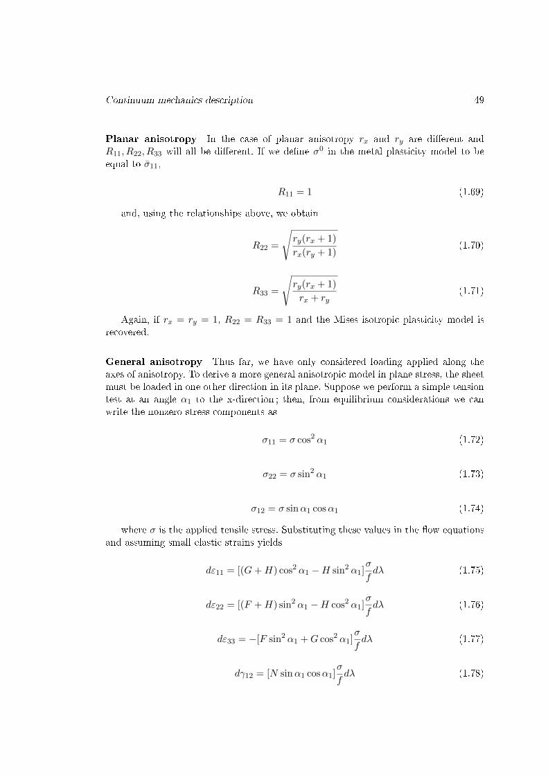
Continuum mechanics description 49
Planar anisotropy In the case of planar anisotropy rx and ry are di�erent andR11, R22, R33 will all be di�erent. If we de�ne σ0 in the metal plasticity model to beequal to σ̄11,
R11 = 1 (1.69)
and, using the relationships above, we obtain
R22 =
√ry(rx + 1)
rx(ry + 1)(1.70)
R33 =
√ry(rx + 1)
rx + ry(1.71)
Again, if rx = ry = 1, R22 = R33 = 1 and the Mises isotropic plasticity model isrecovered.
General anisotropy Thus far, we have only considered loading applied along theaxes of anisotropy. To derive a more general anisotropic model in plane stress, the sheetmust be loaded in one other direction in its plane. Suppose we perform a simple tensiontest at an angle α1 to the x-direction ; then, from equilibrium considerations we canwrite the nonzero stress components as
σ11 = σ cos2 α1 (1.72)
σ22 = σ sin2 α1 (1.73)
σ12 = σ sinα1 cosα1 (1.74)
where σ is the applied tensile stress. Substituting these values in the �ow equationsand assuming small elastic strains yields
dε11 = [(G+H) cos2 α1 −H sin2 α1]σ
fdλ (1.75)
dε22 = [(F +H) sin2 α1 −H cos2 α1]σ
fdλ (1.76)
dε33 = −[F sin2 α1 +G cos2 α1]σ
fdλ (1.77)
dγ12 = [N sinα1 cosα1]σ
fdλ (1.78)
50 Introduction
Assuming small geometrical changes, the width strain increment (the increment ofstrain at right angles to the direction of loading, α1) is written as
dεα1+π2
= dε11 sin2 α1 + dε22 cos2 α1 − 2dγ12 sinα1 cosα1 (1.79)
and Lankford's r-value for loading at an angle α1 is
rα1 =dεα1+π
2
dε33=H + (2N − F −G− 4H) sin2 α1 cos2 α1
F sin2 α1 +G cos2 α1(1.80)
One of the more commonly performed tests is that in which the loading direction isat 45◦. In this case
r45 =2N − (F +G)
2(F +G)orN
G= (r45 +
1
2)(1 +
rxry
) (1.81)
If σ0 is equal to σ11 in the metal plasticity model, R11 = 1. R22, R33 are as de�nedbefore for transverse or planar anisotropy and, using the relationships above,
R12 =
√3(rx + 1)ry
(2r45 + 1)(rx + ry)(1.82)
1.4.6 Material constitutive models
Normally the equation 1.15 �σyielde = Function(εp
e )" is in a general form :
σyielde = σ0 + F(εp
e ) (1.83)
σyielde = σ0 ( ˙̄εp,T) + F(εp
e , ˙̄εp,T) (1.84)
where σ0 is yield stress and F (εpe) is the back stress in function of plastic strain εpe.When the in�uence of strain rate and temperature is considered, the equation 1.83 canbe more complex (equation 1.84). Based on the equation form, the general form understrain rate and temperature in�uence can be sumarized by four categories [36] :
1. Only the yield stress is in�uenced by strain rate sensitivity and temperaturesensitivity, such as the work of Zerilli-Armstrong model for BCC material [37].
σyielde = A (˙̄εp,T) · σ0 + F(εp
e ) (1.85)
2. Only the back stress is in�uenced by strain rate sensitivity and temperaturesensitivity, such as the work of Zerilli-Armstrong model for FCC material [37].
σyielde = σ0 + A (˙̄εp,T) · F(εp
e ) (1.86)
Continuum mechanics description 51
3. Both the yield and the back stress are equally in�uenced by strain rate sensitivityand temperature sensitivity, such as the work of Cowper-Symonds model [38],Johnson-Cook model [39].
σyielde = A (˙̄εp,T) · [σ0 + F(εp
e )] (1.87)
4. The yield and the back stress are in�uenced di�erently by strain rate sensitivityand temperature sensitivity, such as the work of Zhao [40] and Khan-Liang [41].
σyielde = A (˙̄εp,T) · σ0 + B (˙̄εp,T) · F(εp
e ) (1.88)
General constitutive model A proposed constitutive law of A. Gavrus [42, 43, 44,45] developed from physical mechanisms of dislocations kinetics, taking into account amixture Avrami formulation and a material structure evolution at a mesoscopic scale,de�ne in a more general way the constitutive behavior of a large class of metallic alloys,written the equivalent stress variation in the following general form :
σyielde (εp
e , ˙̄ε,T) = H(εpe ) ·G(˙̄ε) · F(T) (1.89)
where the hardening term is H(εpe) = σh(εpe) · (1−ψ) + σs ·ψ, strain rate sensitivityG(˙̄ε) and temperature sensitivity F(T).
The strain rate G an temperature F dependency functions have been also propo-sed in order to generalize classical Cowper-Symonds, Zerilli-Amstrong, Johnson-Cook,Norton-Ho� or Hirt formulations. Concerning this general mesoscopic law proposed byA. Gavrus [42, 43, 44, 45], the hardening term σh can be expressed by Ludwick, Voceor generalized Voce expressions and the material fraction ψ describing the dynamicsoftening phenomena such as : dynamic recovery, dynamic recrystallizations, twinning,respectively phase transition and dual-phase structure material mixture is written inthe following form : ψ = 1−e−r·εsp where r and s can have constant values or strain rateand temperature dependency [46, 42, 43, 44, 45]. The saturated term σs can be regardedgenerally as a constant value or in the case of dual-phase material as a variation withthe plastic strain.
1.4.6.1 Hardening
Mixture model Based on theory of dislocations glides and starting from the mixturemicro-structures formulations proposed by Avrami, the general constitutive rheologicalmodel of equation 1.89 describing the variation of equivalent yield stress σyielde can bewritten for a dual-phase material in the following form :
H(εpe ) = σh(εp
e ) · w + σs(εpe ) · (1− w) (1.90)
where εpe is the cumulated e�ective plastic strain. In equation 1.90, σh(εpe) representsthe hardening component, σs(ε
pe) the softening component and w the material fraction
describing the mixture of the dual-phase material (w=1-ψ is the hardening componentfraction).

52 Introduction
Ludwik model For a material phase such as the martensite one, the material �owstress σyielde can be expressed by the Ludwik hardening model using a classical powerform :
H(εpe ) = σ0 + n1(εp
e )n2 (1.91)
Ludwik model can be interpreted as a particular term of the general constitutiveequation 1.89 de�ned by σh(εp) = σ0 + n1ε
n2p and ψ = 0.
Voce model The Voce law is a good rheological formulation used to describe thematerial recovery (hardening with saturation plateaus) such as the plastic �ow of theferrite. The Voce model can be expressed in the following form :
H(εpe ) = σ0 + n1 ·
[1− e−n2·εpe
](1.92)
In Equation 1.92, n1 + σ0 is the saturation stress and σy is the initial yield stress. Voce
model can be interpreted in term of equation 1.90 at the sum of (n1 +σ0) ·[1− e−n2·εpe
]and σ0 · e−n2·εpe de�ne where σS = n1 + σ0, σh = σ0 and ψ = 1− e−n2·εpe is the dynamicrecovery material fraction.
Sung-Kim-Wagoner model At the year 2010, Sung et al. [47] proposed a �H/Vmodel" (�Hollomon/Voce" model) considering temperature as an in�uence parameteron Hardening term. The �H/V model" Hardening term is given by :
H(εpe ,T ) = p(T)fH + (1− p(T))fV
p(T ) = p1 − p2(T− T0)fH = HHVε
nHVp
fv = VHV(1−AHVe−BHVεp)
(1.93)
where T0 is a reference temperature, and p1, p2, HHV , nHV , VHV , AHV , and BHVare material constants. This model is a particular case of the general constitutive modelof equation 1.89 (ψ = p(T )).
A proposed hardening model According to the above considerations, only mathe-matical improvements of classical hardening laws to �t more accurately the experimentaldata are generally not physically based models. Since DP600 is a dual phase materialcontaining both martensitic and ferritic phases, a proper and physical rheological har-dening model should be de�ned. Based on equation 1.90, using a hardening term H(εpe)de�ned by a mixture Avrami formulation with a Voce model σs describing the ferriticrecovery and the hardening in�uence σh of martensite and introducing the materialfraction w to de�ne the content of martensitic phase, the following synthesis model isproposed :
H(εpe) = w · σh−martensite + (1− w) · σs−ferrite (1.94)
Continuum mechanics description 53
1.4.6.2 Temperature sensitivity
When a material is subjected to a high temperature, its strength tends to drop. Inlaser welding process, this phenomenon has a great e�ect on evaluation of elasto-plasticmaterial behavior. In order to built a �ne welding model and obtain good results of resi-dual stresses, a proper material model taking into account the temperature sensitivity isinvestigated. Several temperature sensitivity models are taken into account and used toanalysis the welding process. A lot of scienti�c works de�ne the temperature sensitivityterm F(T ) in function of the homologous temperature T ∗. Generally the homologoustemperature T ∗ can be de�ned as :
T ∗ =T − Tr
Tmelt − Tr(1.95)
Tmelt, T , Tr are melting, current, and room temperature, respectively. For DP600 steel,Tmelt is supposed to be 1803.15 K and the room temperature is 298.15 K.
Arrhenius model The temperature sensitivity of Arrhenius term ([48]) is expressedby :
F(T ) = exp
(m′Q
RT
)(1.96)
Where R is the universal gas constant, m′ is an adjustable parameter and Q the activa-tion energy. Majority of thermo-mechanical plasticity applications consider a simpli�edexpression using the thermal parameter β = m′Q/R.
Hirt model Similar to Arrhenius model, the Hirt model is de�ned as :
F(T ) = exp(−β′T
)(1.97)
Linear model The linear model can be viewed as an one order Taylor developmentof the exponential Hirt model :
F(T ) = exp(−β′T
)= 1 − β′T + · · · (1.98)
Using �m" for �β′" and �T − Tr" to instead of �T" and avoid the rest, a simple linearmodel can be obtained.
The linear term of temperature sensitivity has been proposed by Hutchison ([49]) in1960s. The material drops linearly with temperature increment.
F(T) = 1−m · (T− Tr) (1.99)
Where m is a material coe�cient and Tr is reference temperature. The linear model issimple in form but not suitable for rapid material strength drop.
54 Introduction
Johnson-Cook model About twenty years later, based on many experimental testsand phenomenological analysis, Johnson-Cook ([39]) proposed a well-founded materialmodel which is still widely used nowadays to describe dynamic forming process. Thetemperature sensitivity term of Johnson-Cook model can well predict the material tem-perature sensitivity below about 1
2Tm but not well above. For Johnson-Cook model, Tris room temperature to de�ne T ∗ in Equation 1.95.
F(T ) = 1− T ∗m (1.100)
Khan model A power function with respect to temperature T is proposed by Khan([50]) as a temperature sensitivity model. For Khan model, Tr is reference temperature,so Khan temperature sensitivity model can use di�erent parameters �m" with di�erenttemperature range. The use of di�erent parameters enable the model to predict materialtemperature sensitivity at high temperature range.
F(T ) =
(Tm − TTm − Tr
)m(1.101)
Chen model The Chen model ([51]) contains the temperature sensitivity term as thefollowing form. The Taylor development of the Chen model is �1 + n · T ∗m + · · · ", sowhen �n" is set to �-1" and the Chen model can be viewed as a �rst order approximationof Johnson-Cook model.
F(T ) = exp(n · T ∗m) (1.102)
Proposed model The proposed model can be viewed as a more general form equationas Johnson-Cook temperature model (k = n = 1).
F(T ) = (1− k · T ∗m)n (1.103)
1.4.6.3 Strain rate sensitivity
The power model The power model known as a Norton one [52] is suitable for lowstrain rates :
G(ε̇) =
(ε̇
ε̇0
)m
(1.104)
where ε̇ and ε̇0 are the current and reference strain rates, m is a material parameter.
The Cowper-Symonds model The Cowper-Symonds model [38] is used for smallstrain rates :
G(ε̇) =
(1 +
ε̇
C
)1/m
or G(ε̇) = 1 +
(ε̇
C
)1/m
(1.105)

Continuum mechanics description 55
where C and m are material parameters.
The Johnson-Cook model Johnson-Cook model [39] is used for high strain rates :
G(ε̇) = 1 + m · ln ε̇ε̇0
(1.106)
As de�ned in the part of power law, ε̇ and ε̇0 are the current and reference strainrates, m is a material parameter.
The general Arcsinus hyperbolic model Starting from the general strain ratesensitivity term proposed by A. Gavrus [42, 43, 44, 45], physically based on kineticsmechanisms of dislocations glides for both static and dynamic loadings, a sinus hyper-bolic strain rate sensitivity is de�ned for describing material behavior for a wide rangeof strain rate (from small to very large value) :
G( ˙̄ε) = 1 +Ash
[1
2( ˙̄ε/ ˙̄ε0)
D], T0 < T < Tm (1.107)
orG( ˙̄ε) = Ash
[e2
( ˙̄ε/ ˙̄ε0)D], 0.3Tm < T < Tm (1.108)
where Ash(x) is the inverse function of sinh(x) and Ash(x) is de�ned as :
Ash(x) = ln(x+
√1 + x2
)(1.109)
It is shown in the work [42, 43, 44, 45] that this proposed law predict Norton power orCowper-Symmonds form for small strain rate and Johnson-Cook form for high strainrate. For the welding simulation, the equation 1.107 is used to describe strain ratesensitivity from room temperature to melting temperature, taking into account gradientsof strain rate between melted region and static solid boundary (BM-Base material).

56 Introduction

Chapitre 2
Experimental data concerningthermo-mechanical behavior ofDP600
2.1 Experiment information
2.1.1 Equipment introduction
The tensile test machine �Instron 3369 J9297� is presented in the �gure 2.1. It iscontrolled by an INSTRON software in the computer. During the tensile test, the forces,displacement and corresponding time are recorded. The original experimental data arethen analyzed so that force-displacement curves can be converted into true stress-strainones. A camera is also used to observe the local deformation of the specimen duringtensile loads.
Figure 2.1 � The INSTRON tensile test machine (50KN)57
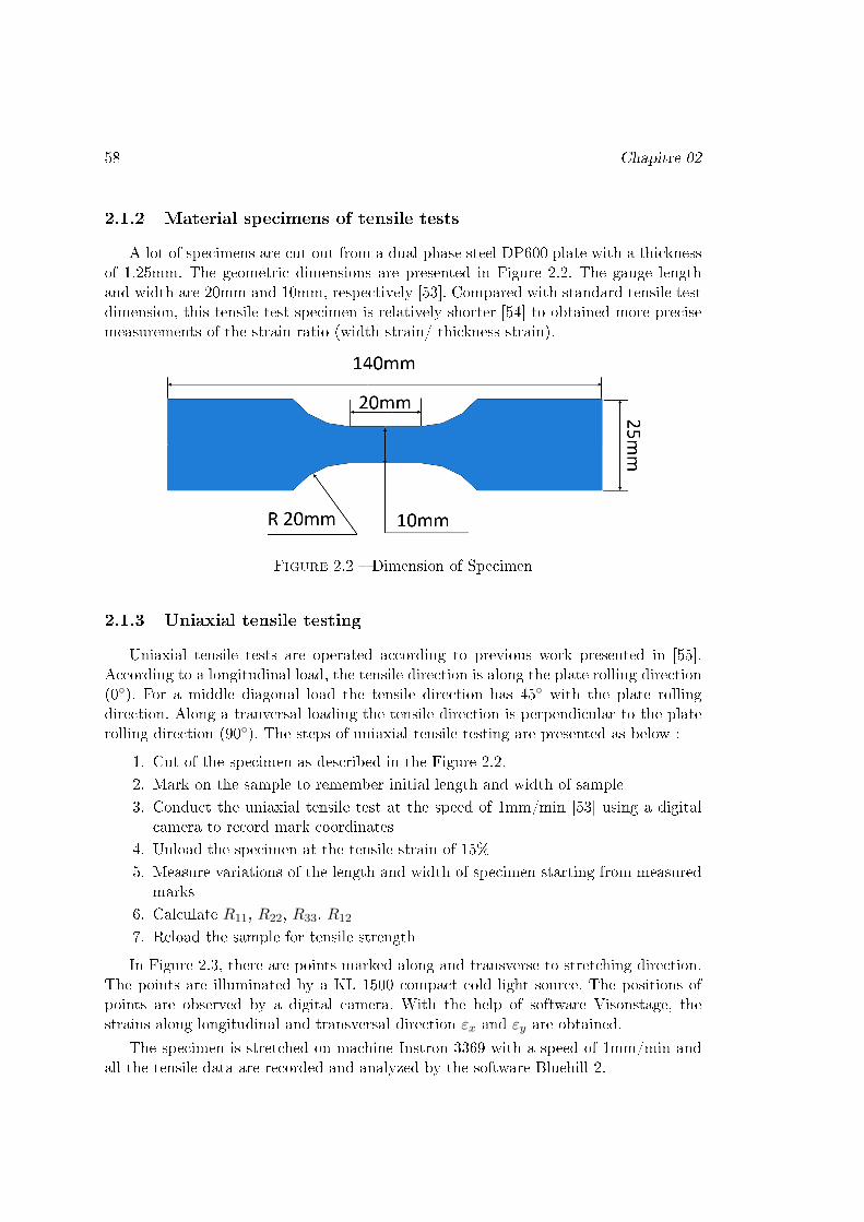
58 Chapitre 02
2.1.2 Material specimens of tensile tests
A lot of specimens are cut out from a dual phase steel DP600 plate with a thicknessof 1.25mm. The geometric dimensions are presented in Figure 2.2. The gauge lengthand width are 20mm and 10mm, respectively [53]. Compared with standard tensile testdimension, this tensile test specimen is relatively shorter [54] to obtained more precisemeasurements of the strain ratio (width strain/ thickness strain).
Figure 2.2 � Dimension of Specimen
2.1.3 Uniaxial tensile testing
Uniaxial tensile tests are operated according to previous work presented in [55].According to a longitudinal load, the tensile direction is along the plate rolling direction(0◦). For a middle diagonal load the tensile direction has 45◦ with the plate rollingdirection. Along a tranversal loading the tensile direction is perpendicular to the platerolling direction (90◦). The steps of uniaxial tensile testing are presented as below :
1. Cut of the specimen as described in the Figure 2.2.2. Mark on the sample to remember initial length and width of sample3. Conduct the uniaxial tensile test at the speed of 1mm/min [53] using a digital
camera to record mark coordinates4. Unload the specimen at the tensile strain of 15%5. Measure variations of the length and width of specimen starting from measured
marks6. Calculate R11, R22, R33, R12
7. Reload the sample for tensile strength
In Figure 2.3, there are points marked along and transverse to stretching direction.The points are illuminated by a KL 1500 compact cold light source. The positions ofpoints are observed by a digital camera. With the help of software Visonstage, thestrains along longitudinal and transversal direction εx and εy are obtained.
The specimen is stretched on machine Instron 3369 with a speed of 1mm/min andall the tensile data are recorded and analyzed by the software Bluehill 2.

Experiment information 59
Figure 2.3 � The mark points of the tensile specimen
2.1.4 Rigidity of Machine during tensile tests
To calculate the rigidity, 6 formula below should be considered :
Ftotal = Fmachine = Fspecimen (2.1)
Fmachine = Kmachine · 4lmachine (2.2)
Fspecimen = Kspecimen · 4lspecimen (2.3)
Ftotal = Ktotal · 4ltotal (2.4)
4 ltotal = 4lmachine +4lspecimen (2.5)
Kspecimen =Especimen · Sspecimen
lspecimen(2.6)
1. In �gure 2.4, with the data detected from tensile test machine and camera, areference high strength low steel (HSLA) with obvious point of elastic limit isused to compute the rigidity of machine :
(a) Force-displacement curve using LVDT sen-sor
(b) true stress-strain curve using camera mea-surements
Figure 2.4 � Tensile test of HSLA steel : (a) Force-displacement curve using LVDTsensor, (b) True stress-strain curve using camera measurements
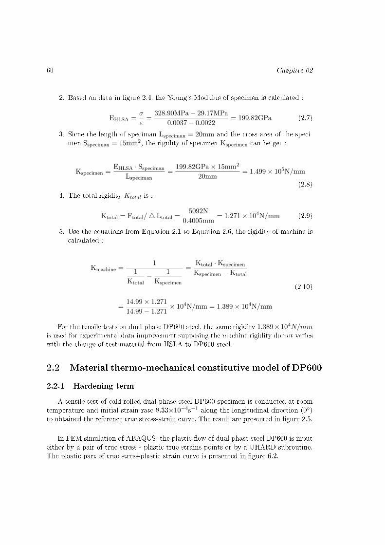
60 Chapitre 02
2. Based on data in �gure 2.4, the Young's Modulus of specimen is calculated :
EHLSA =σ
ε=
328.90MPa− 29.17MPa
0.0037− 0.0022= 199.82GPa (2.7)
3. Sicne the length of speciman Lspeciman = 20mm and the cross-area of the speci-men Sspeciman = 15mm2, the rigidity of specimen Kspecimen can be get :
Kspecimen =EHLSA · Sspeciman
Lspeciman=
199.82GPa× 15mm2
20mm= 1.499× 10⁵N/mm
(2.8)
4. The total rigidity Ktotal is :
Ktotal = Ftotal/4 Ltotal =5092N
0.4005mm= 1.271× 10⁴N/mm (2.9)
5. Use the equations from Equation 2.1 to Equation 2.6, the rigidity of machine iscalculated :
Kmachine =1
1
Ktotal− 1
Kspecimen
=Ktotal ·Kspecimen
Kspecimen −Ktotal
=14.99× 1.271
14.99− 1.271× 10⁴N/mm = 1.389× 10⁴N/mm
(2.10)
For the tensile tests on dual phase DP600 steel, the same rigidity 1.389×10⁴N/mmis used for experimental data improvement supposing the machine rigidity do not varieswith the change of test material from HSLA to DP600 steel.
2.2 Material thermo-mechanical constitutive model of DP600
2.2.1 Hardening term
A tensile test of cold rolled dual phase steel DP600 specimen is conducted at roomtemperature and initial strain rate 8.33×10⁻⁴s−1 along the longitudinal direction (0◦)to obtained the reference true stress-strain curve. The result are presented in �gure 2.5.
In FEM simulation of ABAQUS, the plastic �ow of dual phase steel DP600 is inputeither by a pair of true stress - plastic true strains points or by a UHARD subroutine.The plastic part of true stress-plastic strain curve is presented in �gure 6.2.
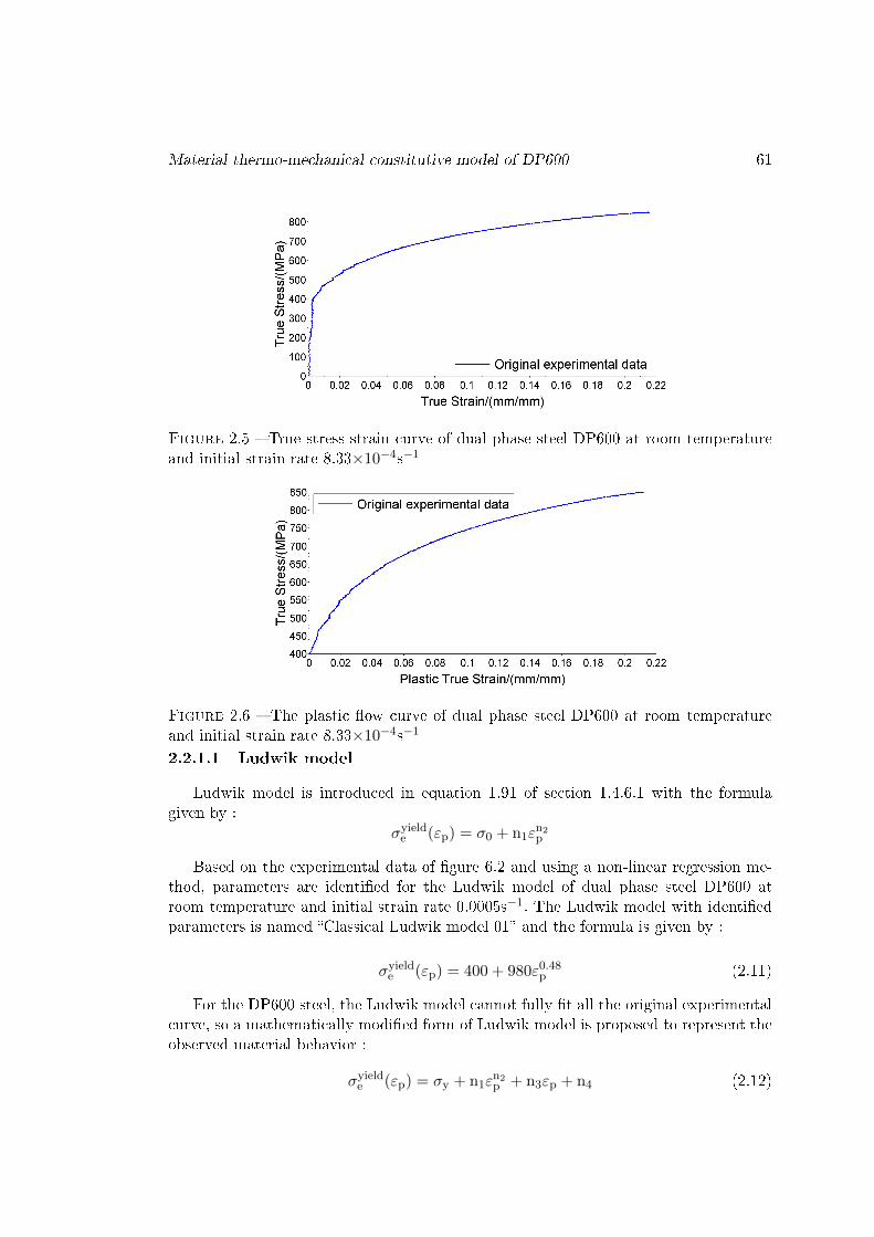
Material thermo-mechanical constitutive model of DP600 61
Figure 2.5 � True stress-strain curve of dual phase steel DP600 at room temperatureand initial strain rate 8.33×10⁻⁴s−1
Figure 2.6 � The plastic �ow curve of dual phase steel DP600 at room temperatureand initial strain rate 8.33×10⁻⁴s−1
2.2.1.1 Ludwik model
Ludwik model is introduced in equation 1.91 of section 1.4.6.1 with the formulagiven by :
σyielde (εp) = σ0 + n1ε
n2p
Based on the experimental data of �gure 6.2 and using a non-linear regression me-thod, parameters are identi�ed for the Ludwik model of dual phase steel DP600 atroom temperature and initial strain rate 0.0005s−1. The Ludwik model with identi�edparameters is named �Classical Ludwik model 01� and the formula is given by :
σyielde (εp) = 400 + 980ε0.48
p (2.11)
For the DP600 steel, the Ludwik model cannot fully �t all the original experimentalcurve, so a mathematically modi�ed form of Ludwik model is proposed to represent theobserved material behavior :
σyielde (εp) = σy + n1ε
n2p + n3εp + n4 (2.12)
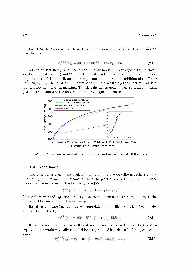
62 Chapitre 02
Based on the experimental data of �gure 6.2, identi�ed �Modi�ed Ludwik model�has the form :
σyielde (εp) = 400 + 1690ε0.5
p − 1240εp − 65 (2.13)
As can be seen in �gure 2.7, �Classical Ludwik model 01" correspond to the classi-cal form (equation 2.11) and �Modi�ed Ludwik model" becomes only a mathematicalimprovement of the Ludwik one. It is important to note that the addition of the linearterm �n3εp+n4" in Equation 2.12 permits to �t more accurately the experimental databut has not any physical meaning. The straight line is used to corresponding to smallplastic strain values of the obtained non-linear regression curve.
Figure 2.7 � Comparison of Ludwik model and experimental DP600 data
2.2.1.2 Voce model
The Voce law is a good rheological formulation used to describe material recovery(hardening with saturation plateaus) such as the plastic �ow of the ferrite. The Vocemodel can be expressed in the following form [56] :
σyielde (εp) = σy + n1 · [1− exp(−n2εp)]
In the framework of equation 1.89, n1 + σy is the saturation stress σs and σy is theinitial yield stress and ψ = 1− exp(−n2εp).
Based on the experimental data of �gure 6.2, the identi�ed �Classical Voce model01� can be written by :
σyielde (εp) = 400 + 555 · [1− exp(−15.5εp)] (2.14)
It can be seen that the plastic �ow stress can not be perfectly �tted by the Voceequation, so a mathematically modi�ed form is proposed in order to �t the experimentalcurve.
σyielde (εp) = σy + n1 · [1− exp(−n2εp)] + n3εp (2.15)
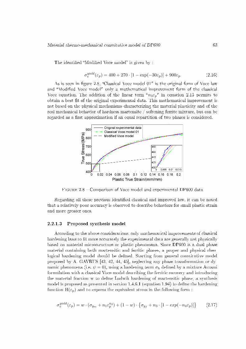
Material thermo-mechanical constitutive model of DP600 63
The identi�ed �Modi�ed Voce model� is given by :
σyielde (εp) = 400 + 270 · [1− exp(−30εp)] + 900εp (2.16)
As is seen in �gure 2.8, �Classical Voce model 01" is the original form of Voce lawand �Modi�ed Voce model" only a mathematical improvement form of the classicalVoce equation. The addition of the linear term �n3εp" in equation 2.15 permits toobtain a best �t of the original experimental data. This mathematical improvement isnot based on the physical mechanisms characterizing the material plasticity and of thereal mechanical behavior of hardness martensite / softening ferrite mixture, but can beregarded as a �rst approximation if an equal repartition of two phases is considered.
Figure 2.8 � Comparison of Voce model and experimental DP600 data
Regarding all these previous identi�ed classical and improved law, it can be notedthat a relatively poor accuracy is observed to describe behaviors for small plastic strainand more greater ones.
2.2.1.3 Proposed synthesis model
According to the above considerations, only mathematical improvements of classicalhardening laws to �t more accurately the experimental data are generally not physicallybased on material microstructure or plastic phenomena. Since DP600 is a dual phasematerial containing both martensitic and ferritic phases, a proper and physical rheo-logical hardening model should be de�ned. Starting from general constitutive modelproposed by A. GAVRUS [43, 42, 44, 45], neglecting any phase transformation or dy-namic phenomena (i.e. ψ = 0), using a hardening term σh de�ned by a mixture Avramiformulation with a classical Voce model describing the ferritic recovery and introducingthe material fraction w to de�ne Ludwik hardening of martensitic phase, a synthesismodel is proposed as presented in section 1.4.6.1 (equation 1.94) to de�ne the hardeningfunction H(εp) and to express the equivalent stress in the following form :
σyielde (εp) = w · (σym + n1εn2p ) + (1− w) ·
{σyf + n3 · [1− exp(−n4εp)]
}(2.17)

64 Chapitre 02
During laser welding material the martensite volume fraction is changed, from expe-rimental point of view, and it is di�cult to estimate the volume fraction of martensite.Dual phase DP600 steel has generally a martensite volume fraction from 0.2 to 0.6.An average value of 0.4 has been considered in a �rst time. Furthermore, experimentaltensile tests for DP600 steel with di�erent martensite fraction must be used to identifyσym and σyf . Here σy = σym = σyf .
Identi�cation with martensite fraction of �w=0.40� A �rstly rough identi�ca-tion for an average value of w equal to 0.4 concerning the martensitic fraction is obtainedin the below equation :
σyielde (εp) = 0.40 · (400 + 1660ε0.63p ) + 0.60 · {400 + 340 · [1− exp(−27.5εp)]} (2.18)
This proposed synthesis model is a mixture of the �Classical Ludwik model 02� andthe �Classical Voce model 02� de�ning respectively hardening of martensite and recoveryof ferrite.
The �Classical Ludwik model 02� is given by :
σyielde (εp) = 400 + 1660ε0.63
p (2.19)
The �Classical Voce model 02� is identi�ed and written by :
σyielde (εp) = 400 + 340 · [1− exp(−27.5εp)] (2.20)
The �gure 2.9 plot the di�erence between the experimental data, the classical Ludwikmodel 02 and the classical Voce model 02 and the proposed synthesis model (identi�edin the plastic strain range of all experimental results i.e. [0, 0.2]). It can be seen theadvantage of the proposed synthesis model to obtain a very good agreement with allexperimental measurements describing the real elasto-plastic behavior of dual phaseDP600 steel, both for plastic strain range [0, 0.05] and [0.05, 0.2] corresponding to alarge class of welding process.
Identi�cation with martensite fraction of �w=0.20� Based on a martensite frac-tion w=2.0 (close to the real value of studied DP600 steel), the parameters of proposedsynthesis model are re-identi�ed. The re-identi�ed parameters of proposed synthesismodel named as "Proposed synthesis model 02" is given by :
σyielde (εp) = 0.20 · (400 + 3411.28ε0.6014p ) + 0.80 · {400 + 234.40 · [1− exp(−27.1092εp)]}
(2.21)
Proposed synthesis model 1 (w=1) is presented as :
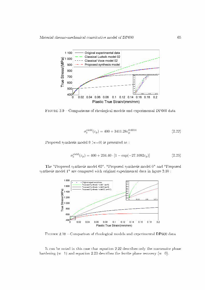
Material thermo-mechanical constitutive model of DP600 65
Figure 2.9 � Comparisons of rheological models and experimental DP600 data
σyielde (εp) = 400 + 3411.28ε0.6014
p (2.22)
Proposed synthesis model 0 (w=0) is presented as :
σyielde (εp) = 400 + 234.40 · [1− exp(−27.1092εp)] (2.23)
The "Proposed synthesis model 02", "Proposed synthesis model 0" and "Proposedsynthesis model 1" are compared with original experimental data in �gure 2.10 :
Figure 2.10 � Comparison of rheological models and experimental DP600 data
It can be noted in this case that equation 2.22 describes only the martensite phasehardening (w=1) and equation 2.23 describes the ferrite phase recovery (w=0).

66 Chapitre 02
2.2.1.4 Synthesis hardening models parameters
Table 2.1 presents all the rheological parameters of DP600 identi�ed for di�erenthardening models. The mathematical form of the hardening models are discussed inthe following parts. It can be noted that the proposed synthesis model equation 2.17describe with a high accuracy the real hardening behavior of the analyzed DP600 dualphase steel.
Table 2.1 � Rheological coe�cients corresponding to di�erent DP600 hardening modelsσy n1 n2 n3 n4 w Equation Nonlinear regression εp range
Classical Ludwik model 01 400 980 0.48 - - - (2.11) [0, 0.2]Classical Ludwik model 02 400 1660 0.63 - - - (2.19) [0, 0.05]Modi�ed Ludwik model 400 1690 0.5 -1240 -65 - (2.13) [0, 0.2]Classical Voce model 01 400 555 15.5 - - - (2.14) [0, 0.2]Classical Voce model 02 400 340 27.5 - - - (2.20) [0, 0.05]Modi�ed Voce model 400 270 30 900 - - (2.16) [0, 0.2]Proposed synthesis model (w=0.4) 400 1660 0.63 340 27.5 0.40 (2.17 et 2.18) [0, 0.2]Proposed synthesis model 02 (w=0.2) 400 3411.3 0.60 234.4 27.1 0.20 (2.17 et 2.21) [0, 0.2]Proposed synthesis model 1 (w=1) 400 3411.3 0.60 234.4 27.1 1 (2.17) -
2.2.2 Temperature sensitivity
2.2.2.1 Temperature sensitivity of a high strength steel
The temperature sensitivity of a high strength steel described in the work of Chen[57] is presented in table 2.2. The thermal softening fraction is the ratio of the stress atelevated temperature to the value at room temperature. The thermal softening fractionis presented with di�erent temperature sensitivity models by setting F(Troom) = 1.
Johnson-Cook temperature sensitivity model Several temperature sensitivitymodel are used to �t the experimental data above. Generally the homologous tempera-ture T ∗ can be de�ned as equation 1.95 :
T ∗ =T − Tr
Tmelt − Tr
Tmelt, T , Tr are melting, current, and room temperature, respectively. For DP600 steel,Tmelt is supposed to be 1803.15 K and the room temperature is 298.15 K.
For Johnson-Cook model [39], Tr is room temperature to de�ne T ∗ in equation 1.100.
F(T ) = 1− T ∗m
To �t the experimental data of table 2.2 obtained, m=1.5 are used. So the Johnson-Cook sensitivity model can be written as :
F(T ) = 1− T ∗1.5 (2.24)
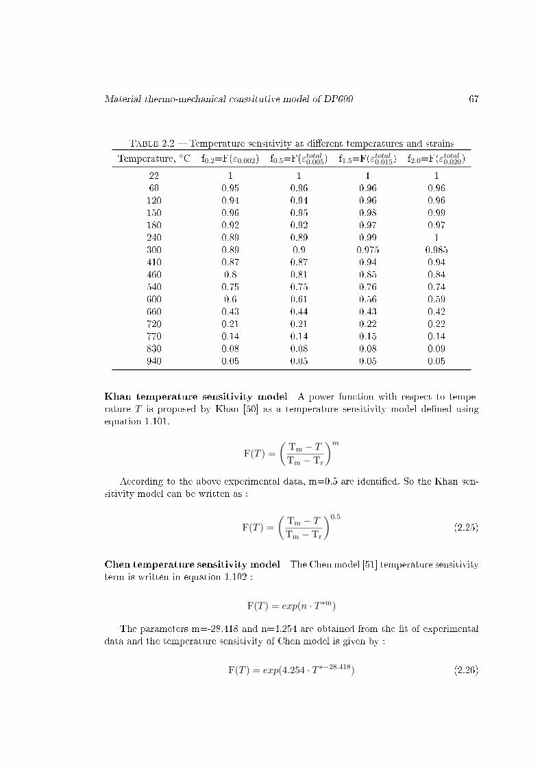
Material thermo-mechanical constitutive model of DP600 67
Table 2.2 � Temperature sensitivity at di�erent temperatures and strains
Temperature, ◦C f0.2=F(ε0.002) f0.5=F(εtotal0.005) f1.5=F(εtotal0.015) f2.0=F(εtotal0.020)
22 1 1 1 160 0.95 0.96 0.96 0.96120 0.94 0.94 0.96 0.96150 0.96 0.95 0.98 0.99180 0.92 0.92 0.97 0.97240 0.89 0.89 0.99 1300 0.89 0.9 0.975 0.985410 0.87 0.87 0.94 0.94460 0.8 0.81 0.85 0.84540 0.75 0.75 0.76 0.74600 0.6 0.61 0.56 0.59660 0.43 0.44 0.43 0.42720 0.21 0.21 0.22 0.22770 0.14 0.14 0.15 0.14830 0.08 0.08 0.08 0.09940 0.05 0.05 0.05 0.05
Khan temperature sensitivity model A power function with respect to tempe-rature T is proposed by Khan [50] as a temperature sensitivity model de�ned usingequation 1.101.
F(T ) =
(Tm − TTm − Tr
)mAccording to the above experimental data, m=0.5 are identi�ed. So the Khan sen-
sitivity model can be written as :
F(T ) =
(Tm − TTm − Tr
)0.5
(2.25)
Chen temperature sensitivity model The Chen model [51] temperature sensitivityterm is written in equation 1.102 :
F(T ) = exp(n · T ∗m)
The parameters m=-28.418 and n=4.254 are obtained from the �t of experimentaldata and the temperature sensitivity of Chen model is given by :
F(T ) = exp(4.254 · T ∗−28.418) (2.26)
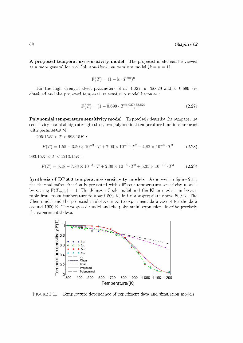
68 Chapitre 02
A proposed temperature sensitivity model The proposed model can be viewedas a more general form of Johnson-Cook temperature model (k = n = 1).
F(T ) = (1− k · T ∗m)n
For the high strength steel, parameters of m=4.027, n=38.629 and k=0.699 areobtained and the proposed temperature senstivity model becomes :
F(T ) = (1− 0.699 · T ∗4.027)38.629 (2.27)
Polynomial temperature sensitivity model To precisely describe the temperaturesensitivity model of high strength steel, two polynominal temperature functions are usedwith parameters of :
295.15K < T < 993.15K :
F (T ) = 1.55− 3.50× 10⁻³ · T + 7.00× 10⁻⁶ · T 2 − 4.82× 10⁻⁹ · T 3 (2.28)
993.15K < T < 1213.15K :
F (T ) = 5.18− 7.83× 10⁻³ · T + 2.30× 10⁻⁶ · T 2 + 5.35× 10⁻¹⁰ · T 3 (2.29)
Synthesis of DP600 temperature sensitivity models As is seen in �gure 2.11,the thermal soften fraction is presented with di�erent temperature sensitivity modelsby setting F(Troom) = 1. The Johnson-Cook model and the Khan model can be sui-table from room temperature to about 800 K, but not appropriate above 800 K. TheChen model and the proposed model are near to experiment data except for the dataaround 1000 K. The proposed model and the polynomial expression describe preciselythe experimental data.
Figure 2.11 � Temperature dependence of experiment data and simulation models

Material thermo-mechanical constitutive model of DP600 69
2.2.2.2 Temperature sensitivity of dual phase steel DP600
According to the work of Aydemir et al. [58], the temperature in�uence on mecha-nical properties of DP600 are measured from 20◦C to 800◦C. The thermal softeningfraction is the ratio of the stress at elevated temperature to that at room temperature.With the yield strength Rp0.2 and ultimate strength Rm of the work of Aydemir et al.,the temperature sensitivity of DP600 plastic hardening model are calculated by :
F(T ) =σT
σ20◦C=
RTp0 .2 + RT
m
R20◦Cp0.2 + R20◦C
m
(2.30)
Table 2.3 � The yield and ultimate strength from literature data [58] and the corres-ponding temperature sensitivity of DP600
Temperature (◦C) 20 200 400 600 700 800
Yield strength Rp0.2 (MPa) 431 413 378 168 84 38Ultimate strength Rm (MPa) 671 630 619 224 110 46Temperature sensitivity F(T ) 1 0.946 0.905 0.356 0.176 0.076
Based on the temperature sensitivity experimental data of Aydemir et al [58], theDP600 temperature sensitivity model are re-identi�ed.
Johnson-Cook temperature sensitivity model The Johnson-Cook temperaturesensitivity model with parameter m=1.5 is also suitable for the dual phase materialDP600 :
F(T ) = 1− T ∗1.5 (2.31)
Khan temperature sensitivity model The Khan temperature sensitivity modelwith parameter m=0.5 is also suitable for the dual phase material DP600 :
F(T ) =
(Tm − TTm − Tr
)0.5
(2.32)
Chen temperature sensitivity model The parameters m=-51.61 and n=4.23 areused to �t the experimental data and the temperature sensitivity of Chen model is givenby :
F(T ) = exp(4.23 · T ∗−51.61) (2.33)
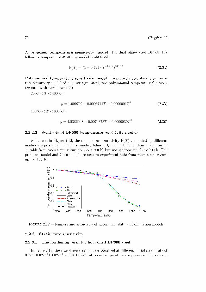
70 Chapitre 02
A proposed temperature sensitivity model For dual phase steel DP600, thefollowing temperature senstivity model is obtained :
F(T ) = (1− 0.491 · T ∗4.212)103.17 (2.34)
Polynominal temperature sensitivity model To precisely describe the tempera-ture sensitivity model of high strength steel, two polynominal temperature functionsare used with parameters of :
20◦C < T < 400◦C :
y = 1.099792− 0.0003741T + 0.0000001T 2 (2.35)
400◦C < T < 800◦C :
y = 4.5386048− 0.0074378T + 0.0000030T 2 (2.36)
2.2.2.3 Synthesis of DP600 temperature sensitivity models
As is seen in Figure 2.12, the temperature sensitivity F(T ) computed by di�erentmodels are presented. The linear model, Johnson-Cook model and Khan model can besuitable from room temperature to about 700 K, but not appropriate above 700 K. Theproposed model and Chen model are near to experiment data from room temperatureup to 1100 K.
Figure 2.12 � Temperature sensitivity of experiment data and simulation models
2.2.3 Strain rate sensitivity
2.2.3.1 The hardening term for hot rolled DP600 steel
In �gure 2.13, the true stress-strain curves obtained at di�erent initial strain rate of0.2s−1,0.02s−1,0.002s−1 and 0.0002s−1 at room temperature are presented. It is shown
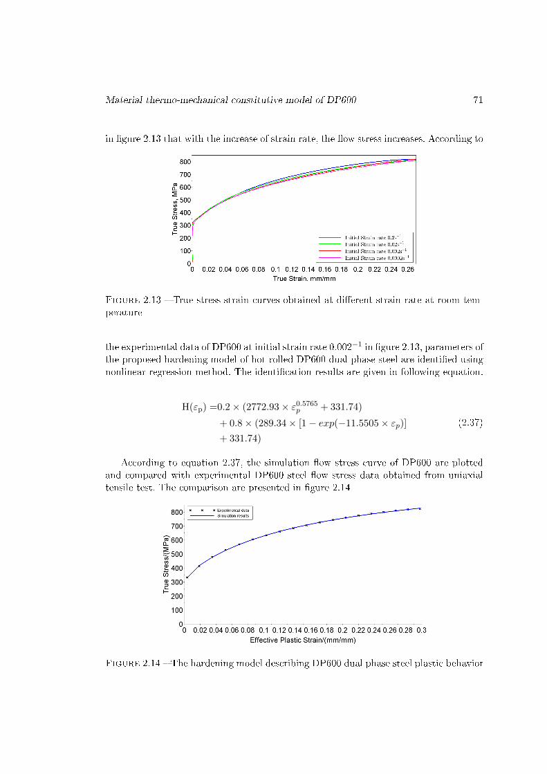
Material thermo-mechanical constitutive model of DP600 71
in �gure 2.13 that with the increase of strain rate, the �ow stress increases. According to
Figure 2.13 � True stress-strain curves obtained at di�erent strain rate at room tem-perature
the experimental data of DP600 at initial strain rate 0.002−1 in �gure 2.13, parameters ofthe proposed hardening model of hot-rolled DP600 dual phase steel are identi�ed usingnonlinear regression method. The identi�cation results are given in following equation.
H(εp) =0.2× (2772.93× ε0.5765p + 331.74)
+ 0.8× (289.34× [1− exp(−11.5505× εp)]+ 331.74)
(2.37)
According to equation 2.37, the simulation �ow stress curve of DP600 are plottedand compared with experimental DP600 steel �ow stress data obtained from uniaxialtensile test. The comparison are presented in �gure 2.14
Figure 2.14 � The hardening model describing DP600 dual phase steel plastic behavior

72 Chapitre 02
It is shown that the hardening model described by equation 2.37 can well predictthe �ow stress of DP600 dual phase steel at room temperature and initial strain rate0.0002s−1 for all range of plastic strain [0,0.3].
2.2.3.2 Identi�cation of the strain rate sensitivity based on hot-rolled DP600dual phase steel
The hardening term can only predict the material behavior of DP600 at particularstrain rate. For material behavior of DP600 at other strain rate, the strain rate sensiti-vity are used to predict the �ow stress change with respect to strain rate change. Basedon the hot-rolled DP600 dual phase steel hardening term, the strain rate sensitivitymodel proposed by A. Gavrus [43, 42] is identi�ed The temperature sensitivity underroom temperature is set to 1. The reference strain rate for the Hardening term is basedon the �ow stress curve at initial strain rate 0.0002s−1. The obtained reference strainrate is 0.997, so approximation ε0 ≈ 1 is used. The result is given in equation 2.38 by :
G(ε̇) = 0.7022851×[1 +Ash
(1
2ε̇
0.0160537)]
(2.38)
Combine the hardening, temperature sensitivity and strain rate sensitivity, theDP600 �ow stress model considering strain, temperature and strain rate are writtenin equation 2.39.
σ(εp,T, ε̇) = { 0.2× (2772.93× ε0.5765p + 331.74) + 0.8× [289.34
× (1− e−11.5505×εp) + 331.74] } × (1− 0.49× T ∗4.21)103.17
× 0.7022851×[1 +Ash(0.5 · ε̇0.0160537
)] (2.39)
According to equation 2.39 that the simulation �ow stress curves are plotted andcompared with experimental data obtained from uniaxial tensile tests. The comparisonsare presented in �gure 2.15.
It is shown from �gure 2.15, the material plasticity model for DP600 dual phase steelpredicts the plastic �ow stress at di�erent strain rate very well for the room temperature.
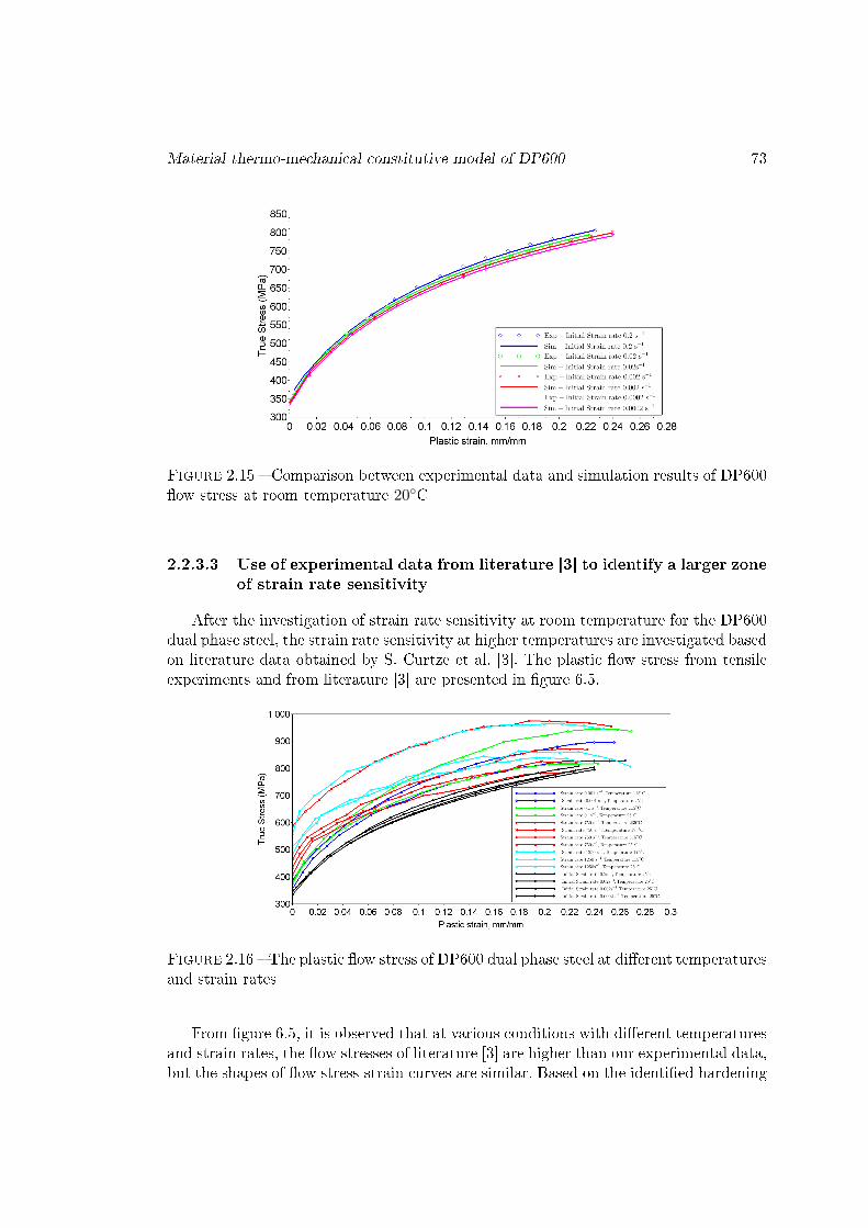
Material thermo-mechanical constitutive model of DP600 73
Figure 2.15 � Comparison between experimental data and simulation results of DP600�ow stress at room temperature 20◦C
2.2.3.3 Use of experimental data from literature [3] to identify a larger zoneof strain rate sensitivity
After the investigation of strain rate sensitivity at room temperature for the DP600dual phase steel, the strain rate sensitivity at higher temperatures are investigated basedon literature data obtained by S. Curtze et al. [3]. The plastic �ow stress from tensileexperiments and from literature [3] are presented in �gure 6.5.
Figure 2.16 � The plastic �ow stress of DP600 dual phase steel at di�erent temperaturesand strain rates
From �gure 6.5, it is observed that at various conditions with di�erent temperaturesand strain rates, the �ow stresses of literature [3] are higher than our experimental data,but the shapes of �ow stress-strain curves are similar. Based on the identi�ed hardening

74 Chapitre 02
term at room temperature of the authors' experimental data, the strain rate sensitivityare identi�ed and discussed below.
2.2.3.4 Strain rate sensitivity of DP600 dual phase steel
Based on all the above data, the following strain rate sensitivity term based on theplastic �ow curves of �gure 6.5 is obtained :
G(ε̇) = 0.8042232×[1 +Ash
(1
2(ε̇/96.077)0.0005410×T−0.1443611
)](2.40)
Using the hardening, the temperature sensitivity and the strain rate sensitivity, theDP600 �ow stress model �nally written by :
σ(εp,T, ε̇) = { 0.2× (2772.93× ε0.5765p + 331.74) + 0.8× [289.34
× (1− e−11.5505×εp) + 331.74] } × (1− 0.49× T ∗4.21)103.17
× 0.8042232×[1 +Ash
(1
2(ε̇/96.077)0.0005410×T−0.1443611
)] (2.41)
The �ow stress simulation results from the DP600 dual phase steel material modelusing the strain rate sensitivity model of equation 2.40 is presented in �gure 2.17.
Though the �ow stresses of DP600 dual phase steel at temperature of 25◦C, 115◦Cand 175◦C with di�erent strain rate of 0.2s−1,0.02s−1,0.002s−1 and 0.0002s−1 have a lotof variations, the identi�ed strain rate material model proposed by A. Gavrus [43, 42]can get a fairly good accordance with acceptable small di�erences.
2.2.4 Planar anisotropy de�ned by Hill theory
For nearly all plate materials, the rolling process would bring anisotropy to the plate.The anisotropy of DP600 steel is considered as planar anisotropy according to Hill-48theory. The Hill's potential function is an extension of the Mises function, which can beexpressed in terms of rectangular Cartesian stress components in equation 1.54 :
f(σ) =[F(σ22 − σ33)2 + G(σ33 − σ11)2 + H(σ11 − σ22)2 + 2Lσ2
23 +2Mσ231 + 2Nσ2
12
]1/2where F, G, H, L, M, and N are the Hill coe�cients obtained by tests of the material
in di�erent orientations. The e�ective stress f(σ) is a scalar that dependent on materialstress state and is a key value de�ning the plastic �ow. Generally it is assumed toestimate this e�ective stress from the equivalent stress corresponding to the plastic�ow curve obtained by tensile tests along the rolling direction. The specimen geometryused for tensile tests is shown in �gure 2.18. The planar anisotropy is estimated using

Material thermo-mechanical constitutive model of DP600 75
(a) 25◦C, 0.001s−1 (b) 25◦C, 0.1s−1
(c) 25◦C, 750s−1 (d) 25◦C, 1250s−1
(e) 115◦C, 0.001s−1 (f) 115◦C, 0.1s−1
(g) 115◦C, 750s−1 (h) 115◦C, 1250s−1
(i) 175◦C, 750s−1 (j) 175◦C, 1250s−1
Figure 2.17 � The comparison between experimental data from literature [3] and si-mulation results of DP600 dual phase steel general constitutive model
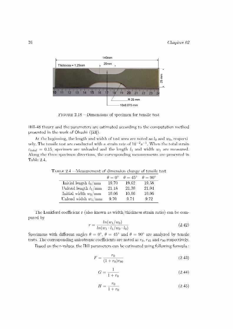
76 Chapitre 02
Figure 2.18 � Dimensions of specimen for tensile test
Hill-48 theory and the parameters are estimated according to the computation methodpresented in the work of Ohashi ([53]).
At the beginning, the length and width of test area are noted as l0 and w0, respecti-vely. The tensile test are conducted with a strain rate of 10−2s−1. When the total strainεtotal = 0.15, specimen are unloaded and the length l1 and width w1 are measured.Along the three specimen directions, the corresponding measurements are presented inTable 2.4.
Table 2.4 � Measurement of dimension change of tensile test
θ = 0◦ θ = 45◦ θ = 90◦
Initial length l0/mm 19.70 19.62 19.58Unload length l1/mm 21.18 21.30 21.04Initial width w0/mm 10.06 10.06 10.06Unload width w1/mm 9.70 9.74 9.72
The Lankford coe�cient r (also known as width/thickness strain ratio) can be com-puted by
r =ln(w1/w0)
ln(w1 · l1/w0 · l0)(2.42)
Specimens with di�erent angles θ = 0◦, θ = 45◦ and θ = 90◦ are analyzed by tensiletests. The corresponding anisotropic coe�cients are noted as r0, r45 and r90 respectively.
Based on the r-values, the Hill parameters can be estimated using following formula :
F =r0
(1 + r0)r90(2.43)
G =1
1 + r0(2.44)
H =r0
1 + r0(2.45)

Material thermo-mechanical constitutive model of DP600 77
N =(1 + 2r45)(r0 + r90)
2(1 + r0)r90(2.46)
For planar anisotropy, if set R11 = 1, the other anisotropic yield stress ratios R22,R33 and R12 are de�ned using the following relationships
R22 =
√r90(r0 + 1)
r0(r90 + 1)(2.47)
R33 =
√r90(r0 + 1)
r0 + r90(2.48)
R12 =
√3(r0 + 1)r90
(2r45 + 1)(r0 + r90)(2.49)
Based on the test results presented in table 2.4 and using the above equations,Lankford coe�cients and Hill's coe�cients of DP600 steel are presented in table 2.5.
Table 2.5 � The Lankford coe�cients and Hill's parameters of DP600 steel
r0 r45 r90 R11 R22 R33 R12
1.0123 0.6487 0.9160 1 0.9748 0.9777 1.1172
F G H N0.5492 0.4969 0.5031 1.2017
Two yield surfaces predicted by Hill48 model and Von Mises criterion of the dualphase steel DP600 sheet are shown in �gure 2.19.
Figure 2.19 � Yield surface predicted by Hill48 anisotropic model and Von Misescriterion
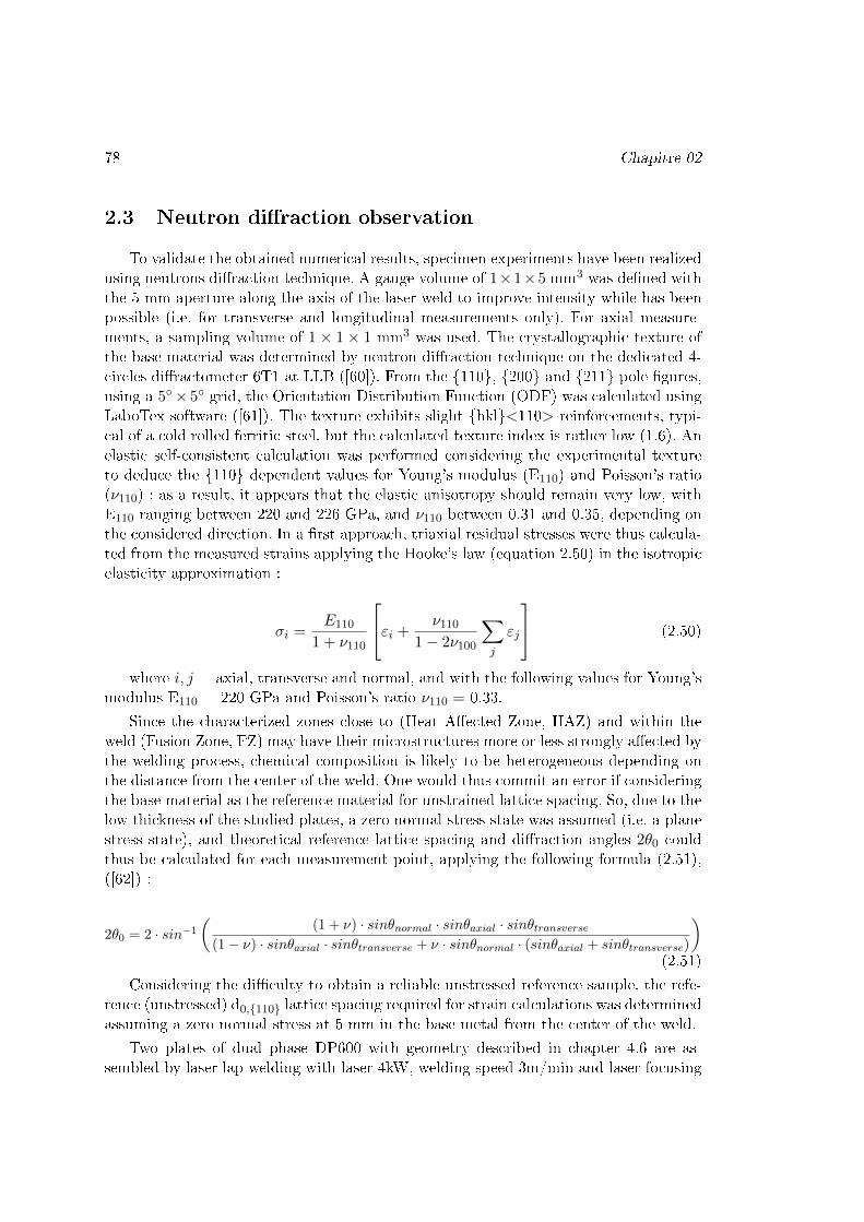
78 Chapitre 02
2.3 Neutron di�raction observation
To validate the obtained numerical results, specimen experiments have been realizedusing neutrons di�raction technique. A gauge volume of 1×1×5 mm3 was de�ned withthe 5 mm aperture along the axis of the laser weld to improve intensity while has beenpossible (i.e. for transverse and longitudinal measurements only). For axial measure-ments, a sampling volume of 1× 1× 1 mm3 was used. The crystallographic texture ofthe base material was determined by neutron di�raction technique on the dedicated 4-circles di�ractometer 6T1 at LLB ([60]). From the {110}, {200} and {211} pole �gures,using a 5◦× 5◦ grid, the Orientation Distribution Function (ODF) was calculated usingLaboTex software ([61]). The texture exhibits slight {hkl}<110> reinforcements, typi-cal of a cold rolled ferritic steel, but the calculated texture index is rather low (1.6). Anelastic self-consistent calculation was performed considering the experimental textureto deduce the {110} dependent values for Young's modulus (E110) and Poisson's ratio(ν110) : as a result, it appears that the elastic anisotropy should remain very low, withE110 ranging between 220 and 226 GPa, and ν110 between 0.31 and 0.35, depending onthe considered direction. In a �rst approach, triaxial residual stresses were thus calcula-ted from the measured strains applying the Hooke's law (equation 2.50) in the isotropicelasticity approximation :
σi =E110
1 + ν110
εi +ν110
1− 2ν100
∑j
εj
(2.50)
where i, j = axial, transverse and normal, and with the following values for Young'smodulus E110 = 220 GPa and Poisson's ratio ν110 = 0.33.
Since the characterized zones close to (Heat A�ected Zone, HAZ) and within theweld (Fusion Zone, FZ) may have their microstructures more or less strongly a�ected bythe welding process, chemical composition is likely to be heterogeneous depending onthe distance from the center of the weld. One would thus commit an error if consideringthe base material as the reference material for unstrained lattice spacing. So, due to thelow thickness of the studied plates, a zero normal stress state was assumed (i.e. a planestress state), and theoretical reference lattice spacing and di�raction angles 2θ0 couldthus be calculated for each measurement point, applying the following formula (2.51),([62]) :
2θ0 = 2 · sin−1
((1 + ν) · sinθnormal · sinθaxial · sinθtransverse
(1− ν) · sinθaxial · sinθtransverse + ν · sinθnormal · (sinθaxial + sinθtransverse)
)(2.51)
Considering the di�culty to obtain a reliable unstressed reference sample, the refe-rence (unstressed) d0,{110} lattice spacing required for strain calculations was determinedassuming a zero normal stress at 5 mm in the base metal from the center of the weld.
Two plates of dual phase DP600 with geometry described in chapter 4.6 are as-sembled by laser lap welding with laser 4kW, welding speed 3m/min and laser focusing
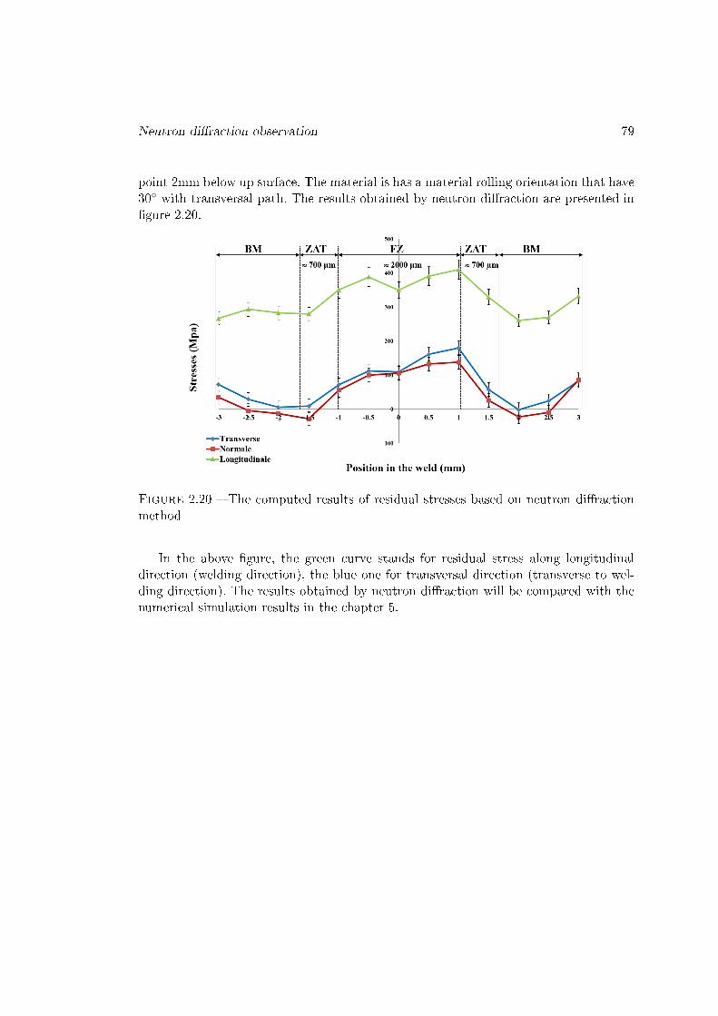
Neutron di�raction observation 79
point 2mm below up surface. The material is has a material rolling orientation that have30◦ with transversal path. The results obtained by neutron di�raction are presented in�gure 2.20.
Figure 2.20 � The computed results of residual stresses based on neutron di�ractionmethod
In the above �gure, the green curve stands for residual stress along longitudinaldirection (welding direction), the blue one for transversal direction (transverse to wel-ding direction). The results obtained by neutron di�raction will be compared with thenumerical simulation results in the chapter 5.

80 Chapitre 02
Chapitre 3
Cellular Automaton Model
In the laser welding of metallic plates, the solidi�cation process o�er the laser fu-sion which plays an important role on microstructure morphology and residual stressesestimation. This chapter present a Cellular Automaton (CA) model used to simulategrowth of dendrite grains, especially concerning martensite phase obtained from fusionsolidi�cation process of dual phase DP600 steel regarded at initial time the base metal.
3.1 Development of Cellular Automaton model
The concept of Cellular Automaton (CA) was �rst discovered by Stanislaw Ulam andJohn Von Neumann, who were both researchers at the Los Alamos National Laboratoryin New Mexico in the 1945 [63]. Ulam was studying the growth of crystals and VonNeumann was imagining a world of self-replicating robots which can build copies ofthemselves. The collision of the two thoughts gives the birth of the CA. At 1970s,a two-dimensional cellular automaton called Conway's Game of Life is created [64].The game greatly simplify Von Neumann's idea and attracted a lot of interest. In 2002,Wolfram published a book [65], A New Kind of Science, which discusses the CA methodin detail.
In brief, Cellular Automaton (CA) is a system made up of many �cell� objects.The cell has a state or many states and some neighborhoods. In the rule de�ned byprogrammers, the CA can iterate on itself. On the whole, the cells can provide andetermined resulted according to the de�ned rules. Because the variation of cells is socomplicated, the CA has the ability to provide us a method to simulate microstructureevolution in a reasonable way.
As a physical and �exible enough model to incorporate the complexity of simulatedphenomena, CA method has been successfully used in the simulation of solidi�cationmicrostructure evolution. Though CA method have many advantages in microstructuresimulation, a major problem hold back the development of CA method. The problemis that the crystallographic axes orientations of dendrite grains are in�uenced by theCA network [66]. In 2008, a limited angles method [67] was proposed which gives the
81
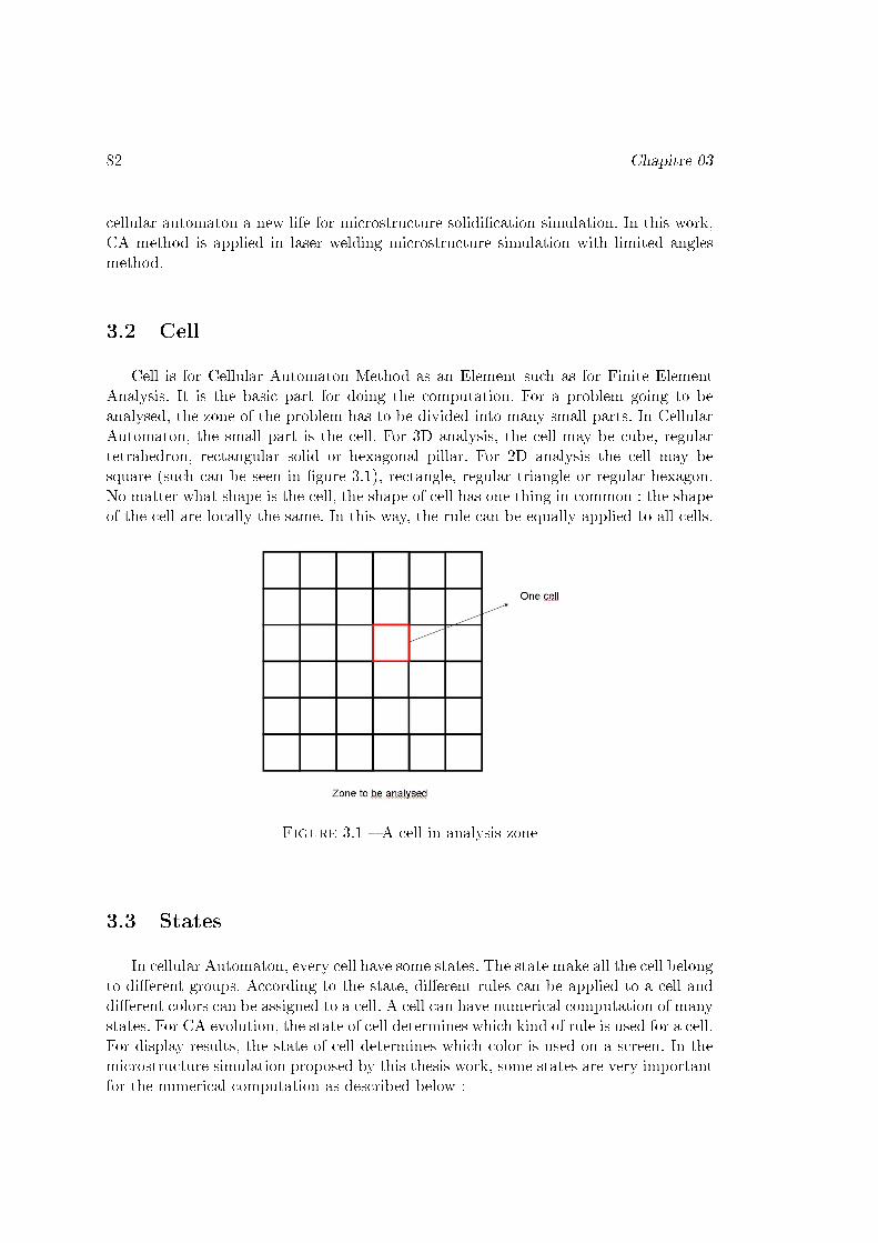
82 Chapitre 03
cellular automaton a new life for microstructure solidi�cation simulation. In this work,CA method is applied in laser welding microstructure simulation with limited anglesmethod.
3.2 Cell
Cell is for Cellular Automaton Method as an Element such as for Finite ElementAnalysis. It is the basic part for doing the computation. For a problem going to beanalysed, the zone of the problem has to be divided into many small parts. In CellularAutomaton, the small part is the cell. For 3D analysis, the cell may be cube, regulartetrahedron, rectangular solid or hexagonal pillar. For 2D analysis the cell may besquare (such can be seen in �gure 3.1), rectangle, regular triangle or regular hexagon.No matter what shape is the cell, the shape of cell has one thing in common : the shapeof the cell are locally the same. In this way, the rule can be equally applied to all cells.
Figure 3.1 � A cell in analysis zone
3.3 States
In cellular Automaton, every cell have some states. The state make all the cell belongto di�erent groups. According to the state, di�erent rules can be applied to a cell anddi�erent colors can be assigned to a cell. A cell can have numerical computation of manystates. For CA evolution, the state of cell determines which kind of rule is used for a cell.For display results, the state of cell determines which color is used on a screen. In themicrostructure simulation proposed by this thesis work, some states are very importantfor the numerical computation as described below :

States 83
3.3.1 Bulk, mould and base metal
The state of cell may be bulk for the melting weld, mould wall for the weld or basemetal. The two state, bulk or mould, di�er the rules of nucleation probability to a cell.The state of bulk or mould or base metal are determined by the temperature historyof the weld. As is generally known, the heterogeneous nucleation is much faster thanan homogeneous nucleation. The energy needed to form a nucleus at a surface is lessthan that in the bulk, so the nucleation probability at the mould wall of weld is muchbigger than the nucleation probability in the bulk. As is seen in the �gure 3.2, the bulkof the weld is red (liquid part), the mould wall is green (semi-solid part), and the basemetal (solid part) that is not melt yet is grey. The green part has the most probabilityto form a nuclei.
Figure 3.2 � The bulk and the mould wall of the weld
3.3.2 Liquid, growing or solid
The state of cell may be solid, growing (at the interface) or liquid. As is seen in�gure 3.3. The color blue means the cell is solidi�ed, the color green means the cell intransition state from liquid to solid and the white part means the cell in melting liquid.In a circle of the program simulation solidi�cation, di�erent computations are used oncells of di�erent state. For example, the nucleation is only used on liquid cells, while thegreen and blue part are free of nucleation consideration. In solidi�cation simulation, thewhite part turns to green, and green part turns to blue if condition is suitable, whichmeans that liquid cell changes to semisolid cell (growing cell or cell at the interface)and semisolid cell changes to solid cell.
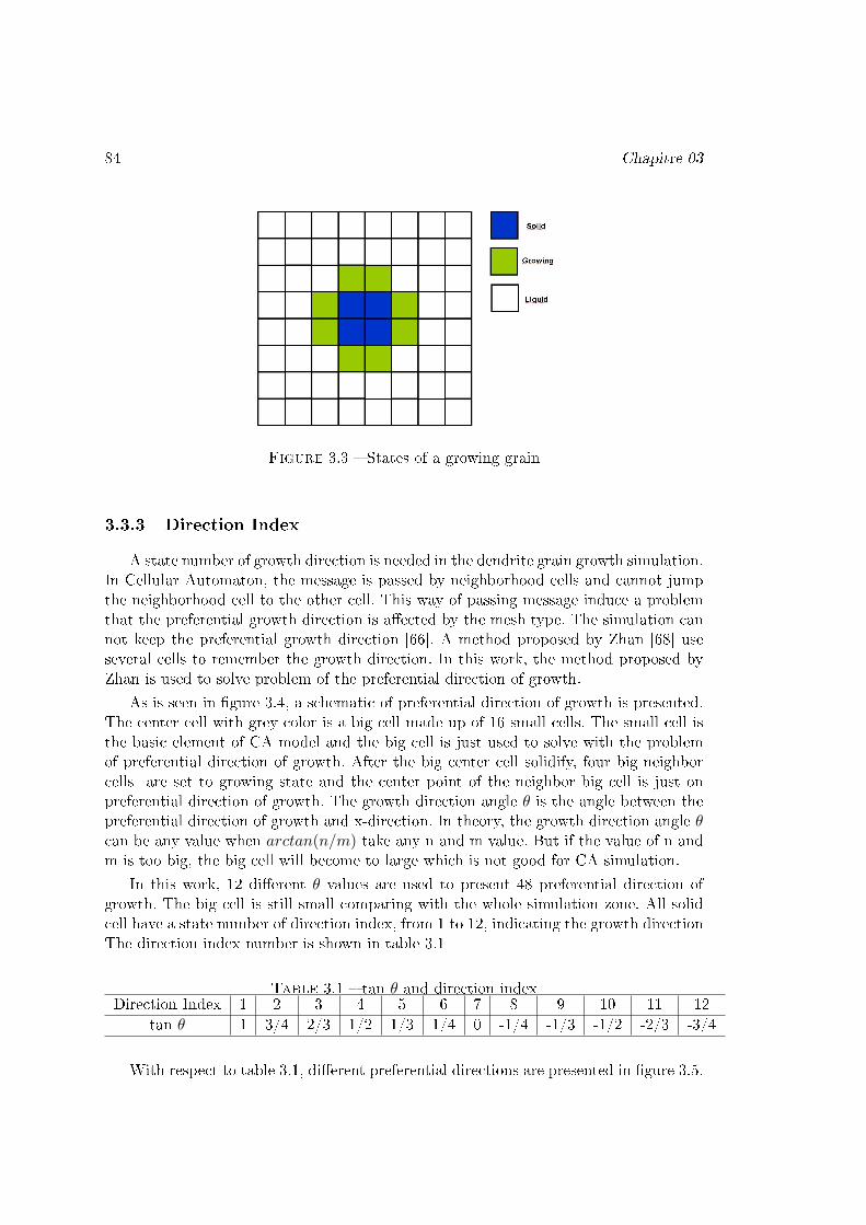
84 Chapitre 03
Figure 3.3 � States of a growing grain
3.3.3 Direction Index
A state number of growth direction is needed in the dendrite grain growth simulation.In Cellular Automaton, the message is passed by neighborhood cells and cannot jumpthe neighborhood cell to the other cell. This way of passing message induce a problemthat the preferential growth direction is a�ected by the mesh type. The simulation cannot keep the preferential growth direction [66]. A method proposed by Zhan [68] useseveral cells to remember the growth direction. In this work, the method proposed byZhan is used to solve problem of the preferential direction of growth.
As is seen in �gure 3.4, a schematic of preferential direction of growth is presented.The center cell with grey color is a big cell made up of 16 small cells. The small cell isthe basic element of CA model and the big cell is just used to solve with the problemof preferential direction of growth. After the big center cell solidify, four big neighborcells are set to growing state and the center point of the neighbor big cell is just onpreferential direction of growth. The growth direction angle θ is the angle between thepreferential direction of growth and x-direction. In theory, the growth direction angle θcan be any value when arctan(n/m) take any n and m value. But if the value of n andm is too big, the big cell will become to large which is not good for CA simulation.
In this work, 12 di�erent θ values are used to present 48 preferential direction ofgrowth. The big cell is still small comparing with the whole simulation zone. All solidcell have a state number of direction index, from 1 to 12, indicating the growth directionThe direction index number is shown in table 3.1
Table 3.1 � tan θ and direction indexDirection Index 1 2 3 4 5 6 7 8 9 10 11 12
tan θ 1 3/4 2/3 1/2 1/3 1/4 0 -1/4 -1/3 -1/2 -2/3 -3/4
With respect to table 3.1, di�erent preferential directions are presented in �gure 3.5.

Parameters 85
Figure 3.4 � The growth direction angle θ
When a small cell nucleates (the cell change its state from liquid to growing), the cellgets a random direction index number marking the preferential direction of growth ofthe grain. With the direction index randomly selected, the nucleation cell change itsown state to growing, together with other small cells, they form a big nucleation cell.All the small cell that is in the zone of the big nucleation cell will change their statefrom liquid to growing. When the big nucleation cell solidify(change state from growingto solid), all the small cells in the big nucleation cell changes their state from liquid tosolid. Meanwhile, according to the direction index, four big cell will nucleation aroundthe solidi�ed big cell. In this way, the dendrite grain grows along a speci�c direction.For 48 directions with 12 direction index numbers, please see the �gure 3.5 below.
3.4 Parameters
Every cell of a CA model contains some parameters regarded as the message of everycell. Focusing on one parameter of one cell, the parameter will be changed step by stepaccording to some rules de�ned by the programmer. In solidi�cation simulation, theserules should re�ects the reality and be reasonable to ensure that the computation ismeaningful.
In the microstructure simulation, the temperature, the solute concentration, the solidfraction, the growing velocity and all the other parameters change according to somerules during the solidi�cation process. For numerical computation, all the parametersare put into a cell and are considered. In �gure 3.6, a small cell contains the parametersof : local cell temperature, concentration of the solution of liquid, concentration of thesolution of solid, solid fraction, interface growth velocity and so on.

86 Chapitre 03
(a) θ = arctan(0) (b) θ = arctan(1) (c) θ = arctan(1/2) (d) θ =arctan(−1/2)
(e) θ = arctan(1/3) (f) θ = arctan(2/3) (g) θ =arctan(−1/3)
(h) θ =arctan(−2/3)
(i) θ = arctan(1/4) (j) θ = arctan(3/4) (k) θ =arctan(−1/4)
(l) θ =arctan(−3/4)
Figure 3.5 � The direction of the grain
Figure 3.6 � Parameters in a cell
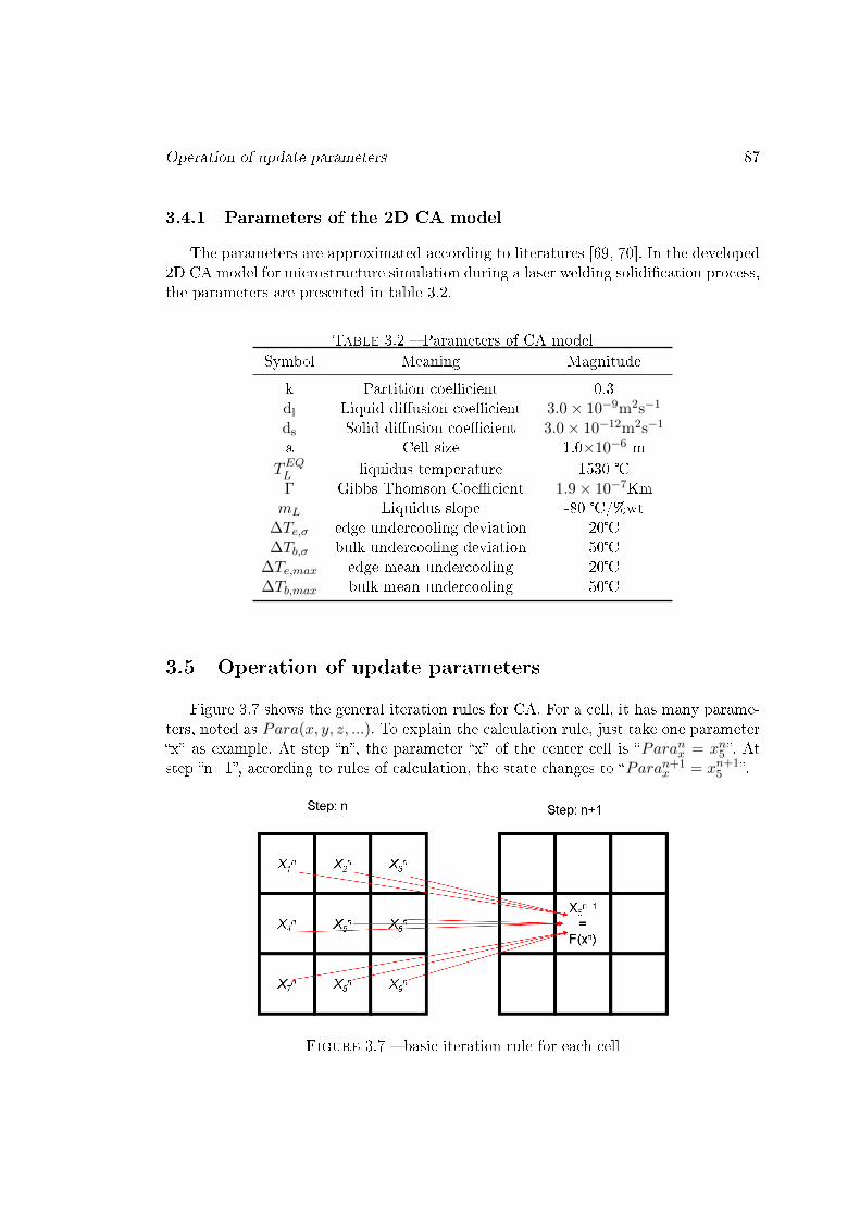
Operation of update parameters 87
3.4.1 Parameters of the 2D CA model
The parameters are approximated according to literatures [69, 70]. In the developed2D CA model for microstructure simulation during a laser welding solidi�cation process,the parameters are presented in table 3.2.
Table 3.2 � Parameters of CA modelSymbol Meaning Magnitude
k Partition coe�cient 0.3dl Liquid di�usion coe�cient 3.0× 10⁻⁹m2s−1
ds Solid di�usion coe�cient 3.0× 10⁻¹²m2s−1
a Cell size 1.0×10⁻⁶ mTEQL liquidus temperature 1530 �
Γ Gibbs Thomson Coe�cient 1.9× 10⁻⁷KmmL Liquidus slope -80 �/%wt
∆Te,σ edge undercooling deviation 20�∆Tb,σ bulk undercooling deviation 50�
∆Te,max edge mean undercooling 20�∆Tb,max bulk mean undercooling 50�
3.5 Operation of update parameters
Figure 3.7 shows the general iteration rules for CA. For a cell, it has many parame-ters, noted as Para(x, y, z, ...). To explain the calculation rule, just take one parameter�x� as example. At step �n�, the parameter �x� of the center cell is �Paranx = xn5 �. Atstep �n+1�, according to rules of calculation, the state changes to �Paran+1
x = xn+15 �.
Figure 3.7 � basic iteration rule for each cell
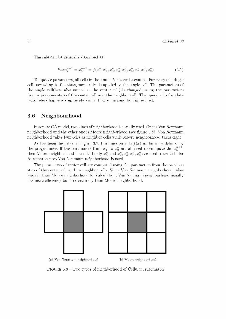
88 Chapitre 03
The rule can be generally described as :
Paran+1x = xn+1
5 = f(xn1 , xn2 , x
n3 , x
n4 , x
n5 , x
n6 , x
n7 , x
n8 , x
n9 ) (3.1)
To update parameters, all cells in the simulation zone is scanned. For every one singlecell, according to the state, some rules is applied to the single cell. The parameters ofthe single cell(here also named as the center cell) is changed, using the parametersfrom a previous step of the center cell and the neighbor cell. The operation of updateparameters happens step by step until that some condition is reached.
3.6 Neighbourhood
In square CA model, two kinds of neighborhood is usually used. One is Von Neumannneighborhood and the other one is Moore neighborhood (see �gure 3.8). Von Neumannneighborhood takes four cells as neighbor cells while Moore neighborhood takes eight.
As has been described in �gure 3.7, the function rule f(x) is the rules de�ned bythe programmer. If the parameters from xn1 to xn9 are all used to compute the xn+1
5 ,then Moore neighborhood is used. If only xn5 and xn2 , x
n4 , x
n6 , x
n8 are used, then Cellular
Automaton uses Von Neumann neighborhood is used.
The parameters of center cell are computed using the parameters from the previousstep of the center cell and its neighbor cells. Since Von Neumann neighborhood takesless cell than Moore neighborhood for calculation, Von Neumann neighborhood usuallyhas more e�ciency but less accuracy than Moore neighborhood.
(a) Von Neumann neighborhood (b) Moore neighborhood
Figure 3.8 � Two types of neighborhood of Cellular Automaton
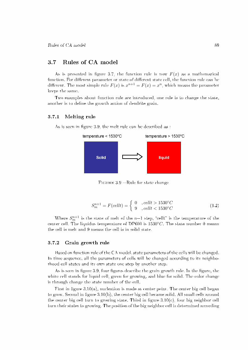
Rules of CA model 89
3.7 Rules of CA model
As is presented in �gure 3.7, the function rule is now F (x) as a mathematicalfunction. For di�erent parameter or state of di�erent state cell, the function rule can bedi�erent. The most simple rule F (x) is xn+1 = F (x) = xn, which means the parameterkeeps the same.
Two examples about function rule are introduced, one rule is to change the state,another is to de�ne the growth action of dendrite grain.
3.7.1 Melting rule
As is seen in �gure 3.9, the melt rule can be described as :
Figure 3.9 � Rule for state change
Sn+1m = F (cellt) =
{0 , cellt > 1530◦C9 , cellt < 1530◦C
(3.2)
Where Sn+1m is the state of melt of the n+1 step, �cellt� is the temperature of the
center cell. The liquidus temperature of DP600 is 1530◦C. The state number 0 meansthe cell is melt and 9 means the cell is in solid state.
3.7.2 Grain growth rule
Based on function rule of the CA model, state parameters of the cells will be changed.In time sequence, all the parameters of cells will be changed according to its neighbo-rhood cell states and its own state one step by another step.
As is seen in �gure 3.9, four �gures describe the grain growth rule. In the �gure, thewhite cell stands for liquid cell, green for growing, and blue for solid. The color changeis through change the state number of the cell.
First in �gure 3.10(a), nucleation is made at center point. The center big cell beganto grow. Second in �gure 3.10(b), the center big cell became solid. All small cells aroundthe center big cell turn to growing state. Third in �gure 3.10(c), four big neighbor cellturn their states to growing. The position of the big neighbor cell is determined according

90 Chapitre 03
to the direction index number. Four in �gure 3.10(d), when four big neighbor cells turnto solid, all small cells around the solid big cell turn to growing state. Based on the waythat four �gures describe, a dendrite grain can grow along a particular direction.
(a) phase 01 (b) phase 02 (c) phase 03 (d) phase 04
Figure 3.10 � Rule of grain growth
3.8 Mathematical description of the solidi�cation model
The �owchart in the �gure 3.11 describes the program procedure of numerical simu-lation concerning the solidi�cation of weld. The temperature database is got from 3DAbaqus Simulation. Tmelt stands for melting temperature. The concentration of all cellsare the same at the beginning.
In the �owchart, a certain step of calculation is performed.
Step 1 : Read temperature. Load temperature data from ABAQUS, compute localtemperature for every cell in the Microstructure Evolution Model.
Step 2 : Determine the cell state. If the cell temperature is above liquidus tempera-ture, then the cell state is liquid. Some cells' state maybe growing because of nucleationor growing calculation. The solid state of cell can be achieved by solidi�cation, whichmeans that fs(fraction solid is equal to 1).
Step 3 : Compute time increase. If temperature of all the cell is above the liquidustemperature, no solidi�cation behavior need to be computed. Calculate time incrementto let temperature drop down.
Step 4 : nucleation. Based on the undercooling degree, the nucleation probability iscomputed and applied to every suitable cell.
Step 5 : Growth. For those cells whose state is growing. The fs(solid fraction) iscomputed, using the velocity value of previous step. If fs(solid fraction) is equal to 1,then the growing cell will change to solid cell.
Step 6 : Curvature and anisotropy. Based on the fs value around the growing cell,the curvature is computed. The curvature is used, same as anisotropy, for calculationinterface concentration of growing cells.
Step 7 : Concentration at the interface. Calculate liquid and solid concentration atthe interface.

Microstructure simulation of weld solidi�cation 91
Figure 3.11 � �owchart of the microstructure evolution model
Step 8 : Concentration di�usion. Calculate the di�usion of concentration for all cells.
Step 9 : Interface growing velocity. Based on the concentration and solid fraction,the growing velocity of interface(or growing) cell is computed.
Step 10 : Time increment Based on the growth velocity, chose an suitable timeincrement for further calculation.
Step 11 : Display the cell state on the screen. Liquid, growing, solid state, index,temperature, concentration, solid fraction and other parameters can be selected to bedisplayed on screen.
After some loop times, all the cell will turn to solid and the program stops.
3.9 Microstructure simulation of weld solidi�cation
3.9.1 Read temperature database
During welding, di�erent part of the weld goes through di�erent heating and co-oling process. The weld temperature distribution �eld is simulated by a Finite ElementAnalysis (FEA) using a conical heat source.
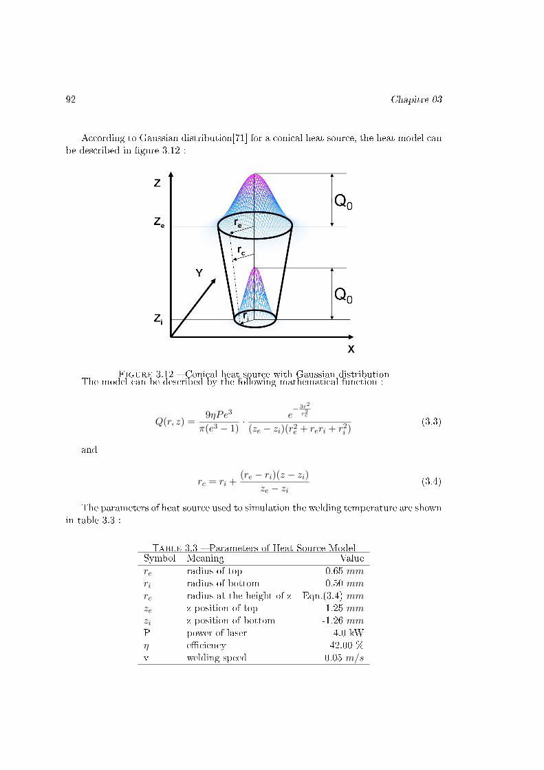
92 Chapitre 03
According to Gaussian distribution[71] for a conical heat source, the heat model canbe described in �gure 3.12 :
Figure 3.12 � Conical heat source with Gaussian distributionThe model can be described by the following mathematical function :
Q(r, z) =9ηPe3
π(e3 − 1)· e
− 3r2
r2c
(ze − zi)(r2e + reri + r2
i )(3.3)
and
rc = ri +(re − ri)(z − zi)
ze − zi(3.4)
The parameters of heat source used to simulation the welding temperature are shownin table 3.3 :
Table 3.3 � Parameters of Heat Source ModelSymbol Meaning Valuere radius of top 0.65 mmri radius of bottom 0.50 mmrc radius at the height of z Eqn.(3.4) mmze z position of top 1.25 mmzi z position of bottom -1.26 mmP power of laser 4.0 kWη e�ciency 42.00 %v welding speed 0.05 m/s

Microstructure simulation of weld solidi�cation 93
During the 2D CA simulation, the temperature of every cell of every step is computedfrom the results of ABAQUS. The ABAQUS temperature simulation result is cut tomany small parts and one of the small part is used by CA model to reduce the computingtimes. The whole weld zone and its heat a�ected zone is too large to compute. To getrid of the long time run in computer, a small zone selected for Cellular Automaton isdepicted in �gure 3.13. The ABCD zone is meshed by 300 × 313 cells, and each cell isdisplayed by a pixel.
Figure 3.13 � Selected zone for calculating
3.9.2 Temperature
After the FEA simulation using ABAQUS software, the computed history of tem-perature during welding are input into CA model. The position of four nodes A, B, C,D and the bigger square nodes E, F, G, H, O, P, Q, R are shown in �gure 3.14. All thetemperature data used by CA model is computed based on the original data of the 12points. There are two kinds of calculation method for cell temperature : one is distanceinterpolation and the other is linear interpolation. The two methods are presented indetail in the following part.
Figure 3.14 � The history temperature of node A
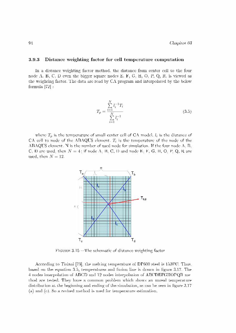
94 Chapitre 03
3.9.3 Distance weighting factor for cell temperature computation
In a distance weighting factor method, the distance from center cell to the fournode A, B, C, D even the bigger square nodes E, F, G, H, O, P, Q, R, is viewed asthe weighting factor. The data are read by CA program and interpolated by the belowformula [72] :
Tp =
N∑i=1
l−1i Ti
N∑i=1
l−1i
(3.5)
where Tp is the temperature of small center cell of CA model. li is the distance ofCA cell to node of the ABAQUS element. Ti is the temperature of the node of theABAQUS element. N is the number of used node for simulation. If the four node A, B,C, D are used, then N = 4 ; if node A, B, C, D and node E, F, G, H, O, P, Q, R areused, then N = 12.
Figure 3.15 � The schematic of distance weighting factor
According to Tiziani [73], the melting temperature of DP600 steel is 1530�. Thus,based on the equation 3.5, temperatures and fusion line is drawn in �gure 3.17. The4 nodes interpolation of ABCD and 12 nodes interpolation of ABCDEFGHOPQR me-thod are tested. They have a common problem which shows an unreal temperaturedistribution at the beginning and ending of the simulation, as can be seen in �gure 3.17(a) and (c). So a revised method is used for temperature estimation.

Microstructure simulation of weld solidi�cation 95
3.9.4 Linear Interpolation for cell temperature estimation
In laser welding, the temperature gradient is very important, so there is a hugedi�erence of temperature history between the outer square nodes E,F,G,H,O,P,Q,Rand nodes A,B,C,D. If used in calculation the cell temperature, the outer square nodeswill have a very strong in�uence. Thus, the revised method only use A,B,C,D four nodedata to compute the district of ABCD.
Figure 3.16 � The schematic of linear interpolation
First, the temperatures of the edge, T(i,0) and T(i,n) are computed.
T(i,0) =i
m(Tb − Ta) + Ta =
i
mTb +
m− im
Ta (3.6)
T(i,n) =i
m(Td − Tc) + Tc =
i
mTd +
m− im
Tc (3.7)
Then the node temperature is interpolated from T(i,0) and T(i,n),
T(i,j) =j
n(T(i,n) − T(i,0)) + T(i,0)
=1
m · n[(m− i)(n− j)Ta + i · (n− j) · Tb
+ (m− i) · j · Tc + i · j · Td]
(3.8)
With the above method, T(i,j), T(i+1,j), T(i,j+1) and T(i+1,j+1) can be estimated.Then the cell temperature t(i,j) is achieved by the function written by :
t(i,j) =1
4(T(i,j) + T(i+1,j) + T(i,j+1) + T(i+1,j+1)) (3.9)
In �gure 3.17, the region with temperature above the melting point is red whilethe region unmelted is black. Sub�gure (a) presents the simulation position of weld.

96 Chapitre 03
In sub�gure (b), areas around A point and C point are melt but the area between Apoint and C point doesn't melt. This doesn't agree with the experiment observation.Sub�gure (c) is the revised result for temperature distribution, compared with sub�gure(b), the sub�gure (c) shows a more reasonable result.
(a) Simulation zone (b) Distance considera-tion
(c) Linear interpolation
Figure 3.17 � Temperature distribution
3.10 Nucleation
3.10.1 The number of the nucleation
According to the nucleation model described by Thevoz et al. [4], the nucleationdensity of the microstructure solidi�cation is shown in �gure 3.18 :
Because concentrations at the mould are di�erent from that in the bulk, the curva-ture undercooling at the mould computed from the concentration will di�er from thecurvature in the bulk. As the undercooling in�uence, the nucleation density at themould will not be same as that in the bulk. Thus, there are two kinds of computationmethods [66]. One is for the mould wall, the other is for the bulk of alloy liquid.
For the mould wall(�s� stands for surface),
δns = ns[∆T + δ(∆T )]− ns∆T =
∫ ∆T+δ(∆T )
∆T
ns,max√2π∆Tσ
e− 1
2(t−∆Ts,max
∆Tσ)2
dt (3.10)
For the bulk of the alloy liquid (�v� stands for volume),
δnv = nv[∆T + δ(∆T )]− nv∆T =
∫ ∆T+δ(∆T )
∆T
nv,max√2π∆Tσ
e− 1
2(t−∆Tv,max
∆Tσ)2
dt (3.11)
In the above formula, ∆T is the whole undercooling of the bulk or the mould wall, itmeans ∆T = Tliq−Tp for mould cells or bulk cells, Tliq is the liquidus temperature in the
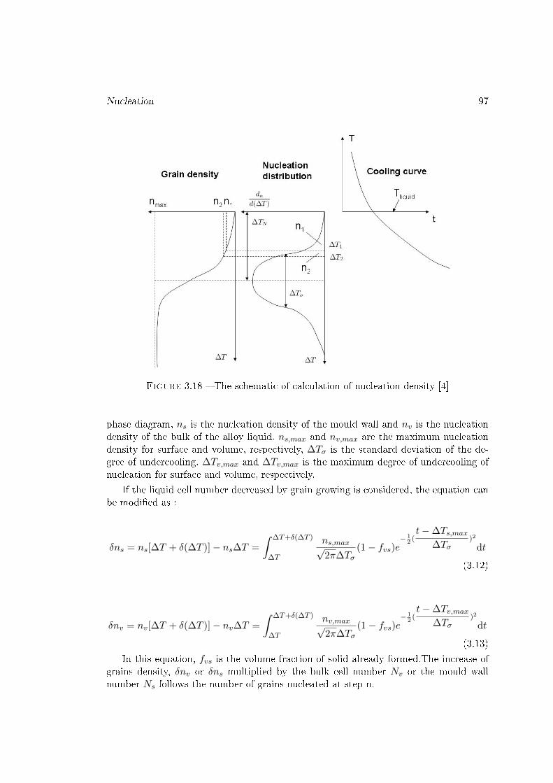
Nucleation 97
Figure 3.18 � The schematic of calculation of nucleation density [4]
phase diagram, ns is the nucleation density of the mould wall and nv is the nucleationdensity of the bulk of the alloy liquid. ns,max and nv,max are the maximum nucleationdensity for surface and volume, respectively, ∆Tσ is the standard deviation of the de-gree of undercooling. ∆Tv,max and ∆Tv,max is the maximum degree of undercooling ofnucleation for surface and volume, respectively.
If the liquid cell number decreased by grain growing is considered, the equation canbe modi�ed as :
δns = ns[∆T + δ(∆T )]− ns∆T =
∫ ∆T+δ(∆T )
∆T
ns,max√2π∆Tσ
(1− fvs)e− 1
2(t−∆Ts,max
∆Tσ)2
dt
(3.12)
δnv = nv[∆T + δ(∆T )]− nv∆T =
∫ ∆T+δ(∆T )
∆T
nv,max√2π∆Tσ
(1− fvs)e− 1
2(t−∆Tv,max
∆Tσ)2
dt
(3.13)
In this equation, fvs is the volume fraction of solid already formed.The increase ofgrains density, δnv or δns multiplied by the bulk cell number Nv or the mould wallnumber Ns follows the number of grains nucleated at step n.
98 Chapitre 03
3.10.2 The position of the nucleation
The nucleation position is chosen among all of the remaining liquid cells at random.The nucleation probabilities for �liquid� cells located in the bulk of the liquid and atthe surface of the mold ( dpe and dpc) to nucleate during each time step are given by
dpe =δNe
Ns(3.14)
and
dpc =δNc
Nv(3.15)
where δNe and δNc are the number of cells at the edge of welding pool ( at themould surface) and in the center of welding pool (in the bulk) at one step. Nv andNs are the number of cells in the bulk and at the mold surface, respectively. Duringthe time step calculation both the mold-surface cells and bulk cells are scanned and arandom number, rand, is generated for each of them (0 ≤ rand ≤ 1). The nucleation ofa �liquid� cell will occur only if rand ≤ dpe or rand ≤ dpc.
3.11 Solid fraction
The solid fraction of growing cells can be determined by [69]
δfs =δt
a
(Vx + Vy − VxVy
δt
a
)(3.16)
Here, a is the mesh size, Vx is the maximum growth velocity of growing cell, δt isthe increment of time.
3.11.1 Interface Curvature
The solid/liquid interface curvature can a�ect the computation of solute concen-tration in the growing cell.An accurate approach for calculating interface curvature isreported by Xin et al. [74] :
K =2∂fs∂x
∂fs∂y
∂2fs∂x∂y −
(∂fs∂y
)2∂2fs∂x2−(∂fs∂x
)2∂2fs∂y2[(
∂fs∂x
)2+(∂fs∂y
)2]3/2
(3.17)
A �nite di�erent method is used to solve the partial derivatives of the solid fractionin the equation (3.17). For every node, for example ua, the value of the node is :
ua =1
4[fs(i− 1, j − 3) + fs(i, j − 3) + fs(i− 1, j − 2) + fs(i, j − 2)] (3.18)
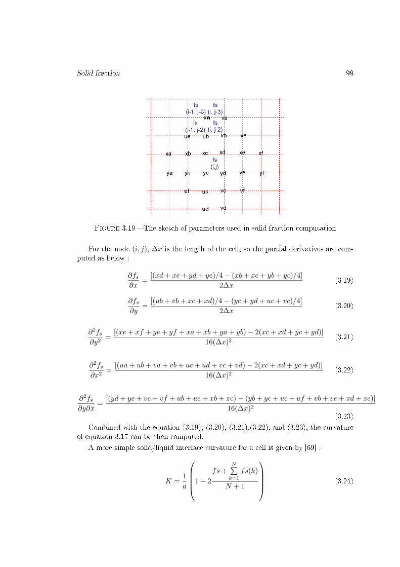
Solid fraction 99
Figure 3.19 � The sketch of parameters used in solid fraction computation
For the node (i, j), ∆x is the length of the cell, so the partial derivatives are com-puted as below :
∂fs∂x
=[(xd+ xe+ yd+ ye)/4− (xb+ xc+ yb+ yc)/4]
2∆x(3.19)
∂fs∂y
=[(ub+ vb+ xc+ xd)/4− (yc+ yd+ uc+ vc)/4]
2∆x(3.20)
∂2fs∂y2
=[(xe+ xf + ye+ yf + xa+ xb+ ya+ yb)− 2(xc+ xd+ yc+ yd)]
16(∆x)2(3.21)
∂2fs∂x2
=[(ua+ ub+ va+ vb+ uc+ ud+ vc+ vd)− 2(xc+ xd+ yc+ yd)]
16(∆x)2(3.22)
∂2fs∂y∂x
=[(yd+ ye+ vc+ vf + ub+ ue+ xb+ xc)− (yb+ yc+ uc+ uf + vb+ ve+ xd+ xe)]
16(∆x)2
(3.23)
Combined with the equation (3.19), (3.20), (3.21),(3.22), and (3.23), the curvatureof equation 3.17 can be then computed.
A more simple solid/liquid interface curvature for a cell is given by [69] :
K =1
a
1− 2
fs+N∑k=1
fs(k)
N + 1
(3.24)

100 Chapitre 03
In the equation (3.24), a is the mesh length of CA model, fs is solid fraction and Nstands for the number of neighbor cells. The result of the curvature calculation rangefrom -1/a to 0 for concave interface and 0 to 1/a for convex interface.
3.12 Interface Concentration
To compute solute concentrations in the growing cells, the interface temperature(T ∗) is �rst given by :
T ∗ = TEQL + (C∗L − C0)mL − Γk̄f(ϕ, θ) (3.25)
Here TEQL is the equilibrium liquidus temperature of the alloy, C∗L is the interfacesolute concentration and C0 is the initial concentration in the material. In the simu-lation, the carbon element equivalent concentration are used to simulate DP600 dualphase steel. mL is the liquidus slope of the phase diagram, k̄ is the mean curvature ofthe S/L interface, Γ is the Gibbs-Thomson coe�cient and f(ϕ, θ) is a coe�cient used toaccount for growth anisotropy where θ is the growth angle (i.e. the angle between thenormal and the x-axis) and ϕ is the preferential crystallographic orientation angle. Inequation 2.20, the third term on the right-hand side is the constitutional undercoolingand the second term on the right-hand side is the curvature undercooling (that reducesthe total undercooling at the dendrite tip, that is, has a stabilizing e�ect on the S/Linterface).
X.H.Zhan point out that [68] the interface temperature is also a�ected by the kineticundercooling
v
µkas an interface dynamic undercooling(∆Tkin). Here v is the growth
velocity, and µk is the coe�cient of dynamic of crystal growth.
So, C∗L can be computed by :
C∗L = C0 +
T ∗ − TEQL + Γk̄ +v
µkmL
(3.26)
In �gure 2.7.1, �S� stands for solid and �L� stands for liquid. The solute concentrationgradient GC can be determined by :
GC =C∗L − CL
(1− fS)∆x/2(3.27)
Here ∆x is the mesh size in the x direction. Then, the solute concentration in liquidcan be expressed as :
CL = C∗L −1− fS
2∆xGC (3.28)

Surface tension anisotropy 101
Figure 3.20 � Model of concentration in single cell
3.13 Surface tension anisotropy
The anisotropy of surface tension [69] is determined from :
f(ϕ, θ) = 1 + δcos(4(ϕ− θ)) (3.29)
Here, δ = 0.04, θ is the angle between growth direction, +x direction and the ϕangle is de�ned by :
ϕ = arcos
(Vx[
V 2x + V 2
y
]1/2)
(3.30)
3.14 Di�usion Equation
3.14.1 Equation widely accepted
After solute concentrations in the growing cells are �rst computed, solute di�usionsin a time step between di�erent cells are estimated.
In the process of growing cells solidi�cation, the solute released by growing cells canbreak the equilibrium and the solute concentration in solid and liquid cells should bedetermined.
At the S/L interface, it can be written :

102 Chapitre 03
C∗S = kC∗L (3.31)
where C∗S is the solute concentration in the solid at the S/L interface and k is thepartition coe�cient.
According to Fick's second law, the partitioning of solute in liquid is given by
∂CL∂t
=∂
∂x(DL
∂CL∂y
) +∂
∂y(DL
∂CL∂x
) (3.32)
Where CL is the solute concentration in liquid and DL is the solute di�usion coef-�cient in liquid.
The partitioning of solute in solid is given by :
∂CS∂t
=∂
∂x(DS
∂CS∂y
) +∂
∂y(DS
∂CS∂x
) (3.33)
Where CS is the solute concentration in solid andDS is the solute di�usion coe�cientin solid.
The partitioning of solute in growing cells is considered as follows. In the simulation,the neighbours of a solid cell can be solid or growing. The neighbours of a liquid cellcan be liquid or growing whereas the neighbours of a growing cell can be solid, liquidand even growing.
Equations (2.25) and (2.26) are used if the computing center is a solid or liquidcell. The neighbours of a solid or liquid cell may be growing. The growing cell is insemisolid state and the solute concentrations in the solid and liquid parts are CgS andCgL respectively. When the growing cell takes part in computation as the neighbour ofa solid cell, the solid concentration CgS is used. When the growing cell takes part incomputation as the neighbour of a liquid cell, the liquid concentration CgL is used.
When the computing center is a growing cell, regardless of the state (i.e. solid, liquidor growing) of the neighbour of the growing cell, the solute concentration of the growingcell can be expressed as an equivalent concentration CE , which is de�ned as :
CE = CL(1− fS) + CSfS = CL[1− (1− k)fS ] (3.34)
where fS is the solid fraction. In the extreme condition, CE is equal to CS when fSis 1, and CE equals CL when fS is zero.
Therefore, the di�usion equations can be expressed by :
∂CE∂t
= ∇(DE∇CE) (3.35)
where CE is the equivalent concentration, which is de�ned by equation (2.27) andDE is the equivalent di�usion coe�cient estimated by :
DE = (1− fS)DL + fSkDSgfs (3.36)
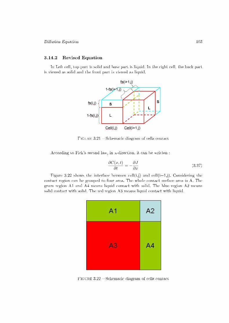
Di�usion Equation 103
3.14.2 Revised Equation
In Left cell, top part is solid and base part is liquid. In the right cell, the back partis viewed as solid and the front part is viewed as liquid.
Figure 3.21 � Schematic diagram of cells contact
According to Fick's second law, in x-direction, it can be written :
∂C(x, t)
∂t= −∂J
∂x(3.37)
Figure 3.22 shows the interface between cell(i,j) and cell(i+1,j). Considering thecontact region can be grouped to four area. The whole contact surface area is A. Thegreen region A1 and A4 means liquid contact with solid. The blue region A2 meanssolid contact with solid. The red region A3 means liquid contact with liquid.
Figure 3.22 � Schematic diagram of cells contact
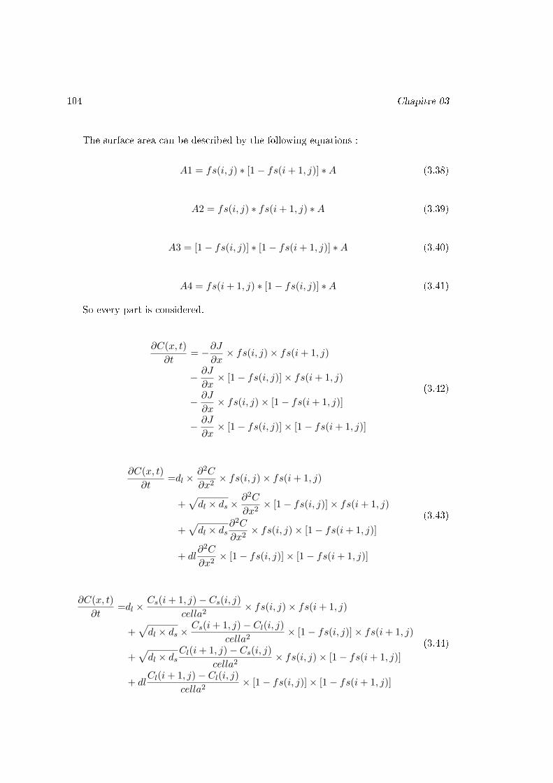
104 Chapitre 03
The surface area can be described by the following equations :
A1 = fs(i, j) ∗ [1− fs(i+ 1, j)] ∗A (3.38)
A2 = fs(i, j) ∗ fs(i+ 1, j) ∗A (3.39)
A3 = [1− fs(i, j)] ∗ [1− fs(i+ 1, j)] ∗A (3.40)
A4 = fs(i+ 1, j) ∗ [1− fs(i, j)] ∗A (3.41)
So every part is considered.
∂C(x, t)
∂t= −∂J
∂x× fs(i, j)× fs(i+ 1, j)
− ∂J
∂x× [1− fs(i, j)]× fs(i+ 1, j)
− ∂J
∂x× fs(i, j)× [1− fs(i+ 1, j)]
− ∂J
∂x× [1− fs(i, j)]× [1− fs(i+ 1, j)]
(3.42)
∂C(x, t)
∂t=dl ×
∂2C
∂x2× fs(i, j)× fs(i+ 1, j)
+√dl × ds ×
∂2C
∂x2× [1− fs(i, j)]× fs(i+ 1, j)
+√dl × ds
∂2C
∂x2× fs(i, j)× [1− fs(i+ 1, j)]
+ dl∂2C
∂x2× [1− fs(i, j)]× [1− fs(i+ 1, j)]
(3.43)
∂C(x, t)
∂t=dl ×
Cs(i+ 1, j)− Cs(i, j)cella2
× fs(i, j)× fs(i+ 1, j)
+√dl × ds ×
Cs(i+ 1, j)− Cl(i, j)cella2
× [1− fs(i, j)]× fs(i+ 1, j)
+√dl × ds
Cl(i+ 1, j)− Cs(i, j)cella2
× fs(i, j)× [1− fs(i+ 1, j)]
+ dlCl(i+ 1, j)− Cl(i, j)
cella2× [1− fs(i, j)]× [1− fs(i+ 1, j)]
(3.44)
Growth velocity of the interface 105
3.15 Growth velocity of the interface
3.15.1 Fick's laws of di�usion
Fick's laws of di�usion is �rst developed by Adolf Fick in 1855. The Fick's lawsdescribe di�usion behavior. Fick's �rst law provide a relationship between di�usive�ux and the concentration gradient under steady state. Fick's second law describes theconcentration �eld evolution with time.
Fick's �rst law assumes that di�usive �ux goes from a area of high concentrationto a area of low concentration and the di�usive rate of �ux is proportional to theconcentration gradient :
J = −D5 φ (3.45)
In the equation, J stands for di�usive �ux. Di�usive �ux means the amount substancegoes through an unit area at an unit time. For the microstructure simulation in thiswork, the unit of di�usive �ux J can be wt%
m2·s
D is the di�usion coe�cient with a unit of m2
s
φ means the amount of substance per unit volume, in this work, unit is wt%m3
5 is gradient operator which can also be written as ∂∂xi
Fick's second law describes the concentration change with time in a �eld. The equa-tion is given as :
∂φ
∂t= D
∂2φ
∂x2i
(3.46)
In the equation, t stands for time and xi means any dimension such as x, y, z, ...For microstructure simulation in CA method, Fick's second law tells that the changeof solute with time in center cell is equal to the addition of �ux in and out of the cellduring the time.
3.16 Conservation equation
In the �gure 3.23, the growing cell and its neighborhood cells in x direction arepresented. The red part of cell is liquid and the blue part is solid. In the �gure, fs(i,j)stands for the solid fraction of cell(i,j).The length of the cell edge are ∆x, ∆y, and ∆z,respectively. The growing velocity of interface in the cell(i,j) is Vx.
In a time step, the solid volume of cell(i,j) increases Vxδ(t)∆y∆z, so the solute inthe cell(i,j) will decrease of Vxδ(t)∆y∆z(C
(i,j)L −C(i,j)
s ). Consideration with Fick's law,the conservation of solute is given by [75] :
Vxδ(t)∆y∆z(C(i,j)L − C(i,j)
s ) = DL∆y∆z∂CL∂x−DS∆y∆z
∂CS∂x
(3.47)
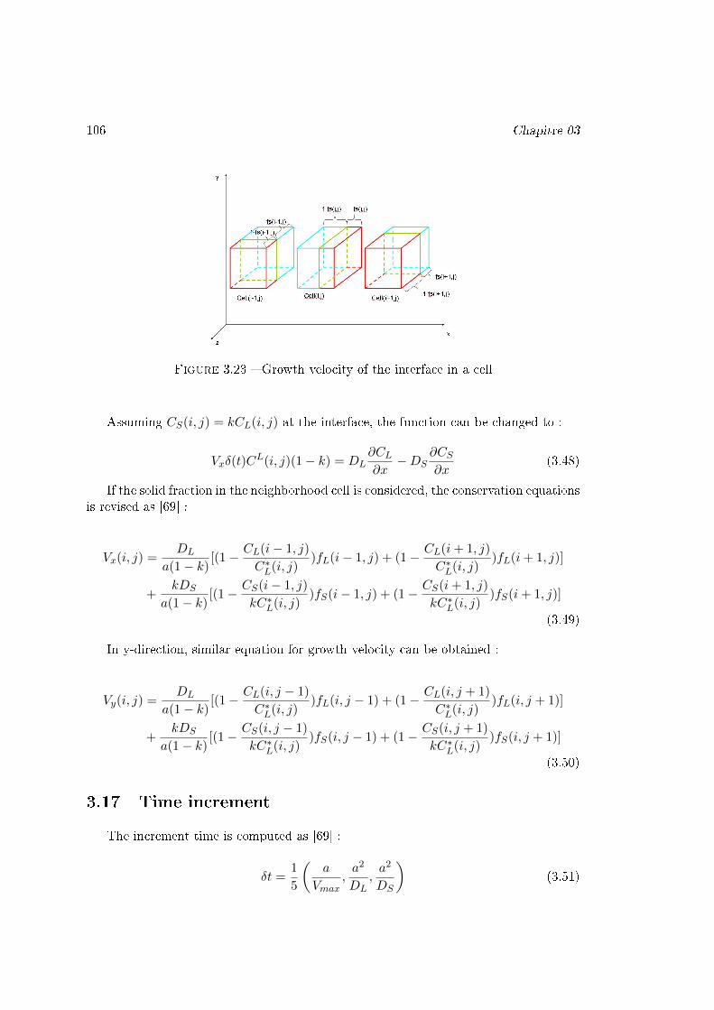
106 Chapitre 03
Figure 3.23 � Growth velocity of the interface in a cell
Assuming CS(i, j) = kCL(i, j) at the interface, the function can be changed to :
Vxδ(t)CL(i, j)(1− k) = DL
∂CL∂x−DS
∂CS∂x
(3.48)
If the solid fraction in the neighborhood cell is considered, the conservation equationsis revised as [69] :
Vx(i, j) =DL
a(1− k)[(1− CL(i− 1, j)
C∗L(i, j))fL(i− 1, j) + (1− CL(i+ 1, j)
C∗L(i, j))fL(i+ 1, j)]
+kDS
a(1− k)[(1− CS(i− 1, j)
kC∗L(i, j))fS(i− 1, j) + (1− CS(i+ 1, j)
kC∗L(i, j))fS(i+ 1, j)]
(3.49)
In y-direction, similar equation for growth velocity can be obtained :
Vy(i, j) =DL
a(1− k)[(1− CL(i, j − 1)
C∗L(i, j))fL(i, j − 1) + (1− CL(i, j + 1)
C∗L(i, j))fL(i, j + 1)]
+kDS
a(1− k)[(1− CS(i, j − 1)
kC∗L(i, j))fS(i, j − 1) + (1− CS(i, j + 1)
kC∗L(i, j))fS(i, j + 1)]
(3.50)
3.17 Time increment
The increment time is computed as [69] :
δt =1
5
(a
Vmax,a2
DL,a2
DS
)(3.51)
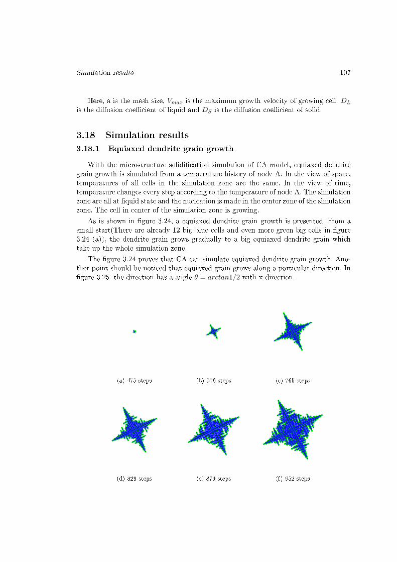
Simulation results 107
Here, a is the mesh size, Vmax is the maximum growth velocity of growing cell. DL
is the di�usion coe�cient of liquid and DS is the di�usion coe�cient of solid.
3.18 Simulation results
3.18.1 Equiaxed dendrite grain growth
With the microstructure solidi�cation simulation of CA model, equiaxed dendritegrain growth is simulated from a temperature history of node A. In the view of space,temperatures of all cells in the simulation zone are the same. In the view of time,temperature changes every step according to the temperature of node A. The simulationzone are all at liquid state and the nucleation is made in the center zone of the simulationzone. The cell in center of the simulation zone is growing.
As is shown in �gure 3.24, a equiaxed dendrite grain growth is presented. From asmall start(There are already 12 big blue cells and even more green big cells in �gure3.24 (a)), the dendrite grain grows gradually to a big equiaxed dendrite grain whichtake up the whole simulation zone.
The �gure 3.24 proves that CA can simulate equiaxed dendrite grain growth. Ano-ther point should be noticed that equiaxed grain grows along a particular direction. In�gure 3.25, the direction has a angle θ = arctan1/2 with x-direction.
(a) 475 steps (b) 576 steps (c) 765 steps
(d) 829 steps (e) 879 steps (f) 952 steps
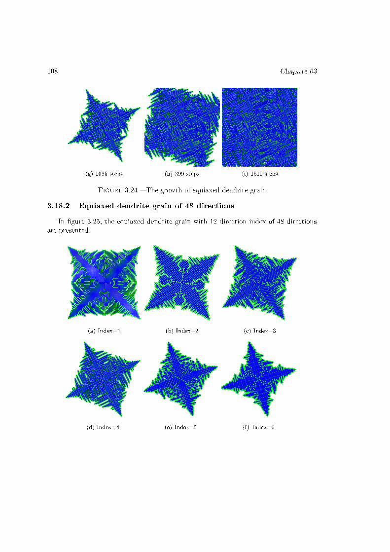
108 Chapitre 03
(g) 1085 steps (h) 399 steps (i) 1810 steps
Figure 3.24 � The growth of equiaxed dendrite grain
3.18.2 Equiaxed dendrite grain of 48 directions
In �gure 3.25, the equiaxed dendrite grain with 12 direction index of 48 directionsare presented.
(a) Index=1 (b) Index=2 (c) Index=3
(d) Index=4 (e) Index=5 (f) Index=6
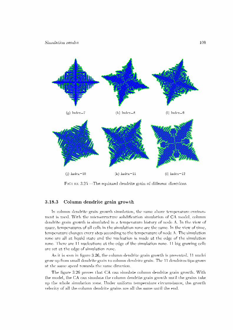
Simulation results 109
(g) Index=7 (h) Index=8 (i) Index=9
(j) Index=10 (k) Index=11 (l) Index=12
Figure 3.25 � The equiaxed dendrite grain of di�erent directions
3.18.3 Column dendrite grain growth
In column dendrite grain growth simulation, the same above temperature environ-ment is used. With the microstructure solidi�cation simulation of CA model, columndendrite grain growth is simulated in a temperature history of node A. In the view ofspace, temperatures of all cells in the simulation zone are the same. In the view of time,temperature changes every step according to the temperature of node A. The simulationzone are all at liquid state and the nucleation is made at the edge of the simulationzone. There are 11 nucleations at the edge of the simulation zone. 11 big growing cellsare set at the edge of simulation zone.
As it is seen in �gure 3.26, the column dendrite grain growth is presented. 11 nucleigrow up from small dendrite grain to column dendrite grain. The 11 dendrites tips growsat the same speed towards the same direction.
The �gure 3.26 proves that CA can simulate column dendrite grain growth. Withthe model, the CA can simulate the column dendrite grain growth until the grains takeup the whole simulation zone. Under uniform temperature circumstance, the growthvelocity of all the column dendrite grains are all the same until the end.
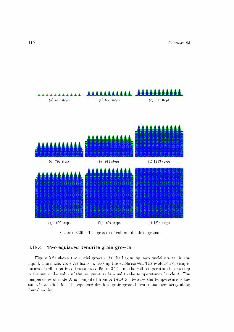
110 Chapitre 03
(a) 468 steps (b) 533 steps (c) 586 steps
(d) 793 steps (e) 971 steps (f) 1233 steps
(g) 1603 steps (h) 1697 steps (i) 1874 steps
Figure 3.26 � The growth of column dendrite grains
3.18.4 Two equiaxed dendrite grain growth
Figure 3.27 shows two nuclei growth. At the beginning, two nuclei are set in theliquid. The nuclei grow gradually to take up the whole screen. The evolution of tempe-rature distribution is as the same as �gure 3.24 : all the cell temperature in one stepis the same, the value of the temperature is equal to the temperature of node A. Thetemperature of node A is computed from ABAQUS. Because the temperature is thesame in all direction, the equiaxed dendrite grain grows in rotational symmetry alongfour direction.
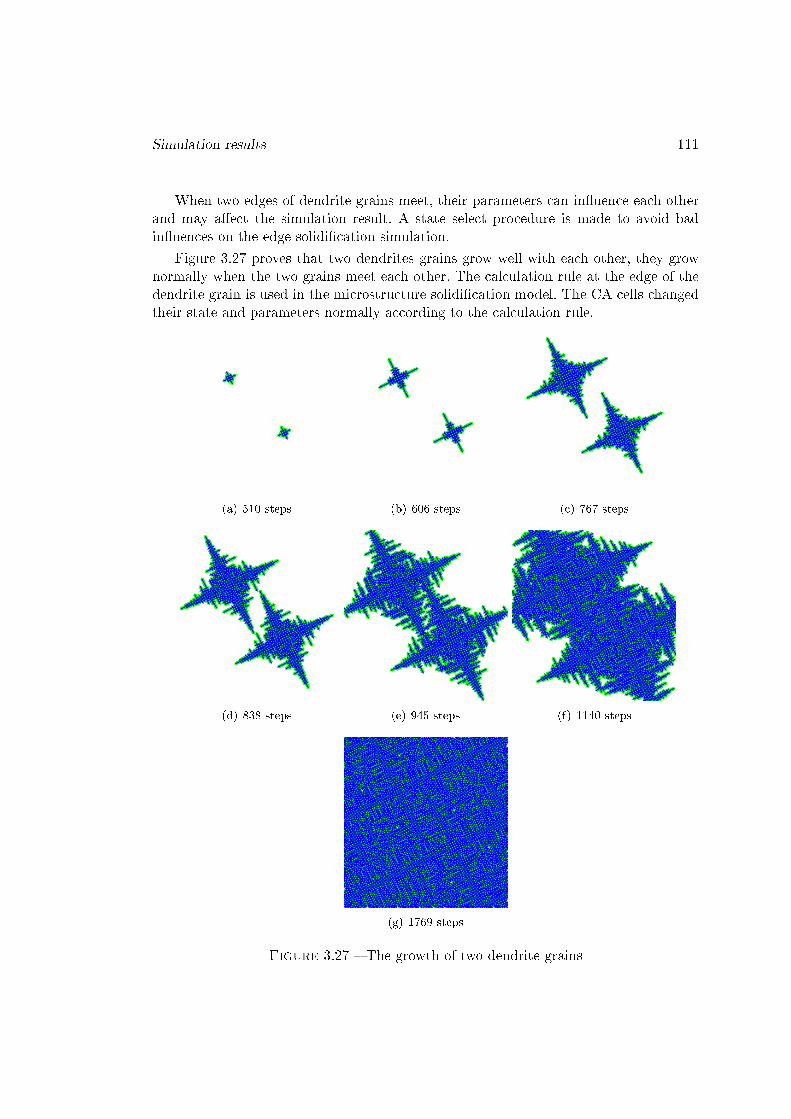
Simulation results 111
When two edges of dendrite grains meet, their parameters can in�uence each otherand may a�ect the simulation result. A state select procedure is made to avoid badin�uences on the edge solidi�cation simulation.
Figure 3.27 proves that two dendrites grains grow well with each other, they grownormally when the two grains meet each other. The calculation rule at the edge of thedendrite grain is used in the microstructure solidi�cation model. The CA cells changedtheir state and parameters normally according to the calculation rule.
(a) 510 steps (b) 606 steps (c) 767 steps
(d) 838 steps (e) 945 steps (f) 1140 steps
(g) 1769 steps
Figure 3.27 � The growth of two dendrite grains
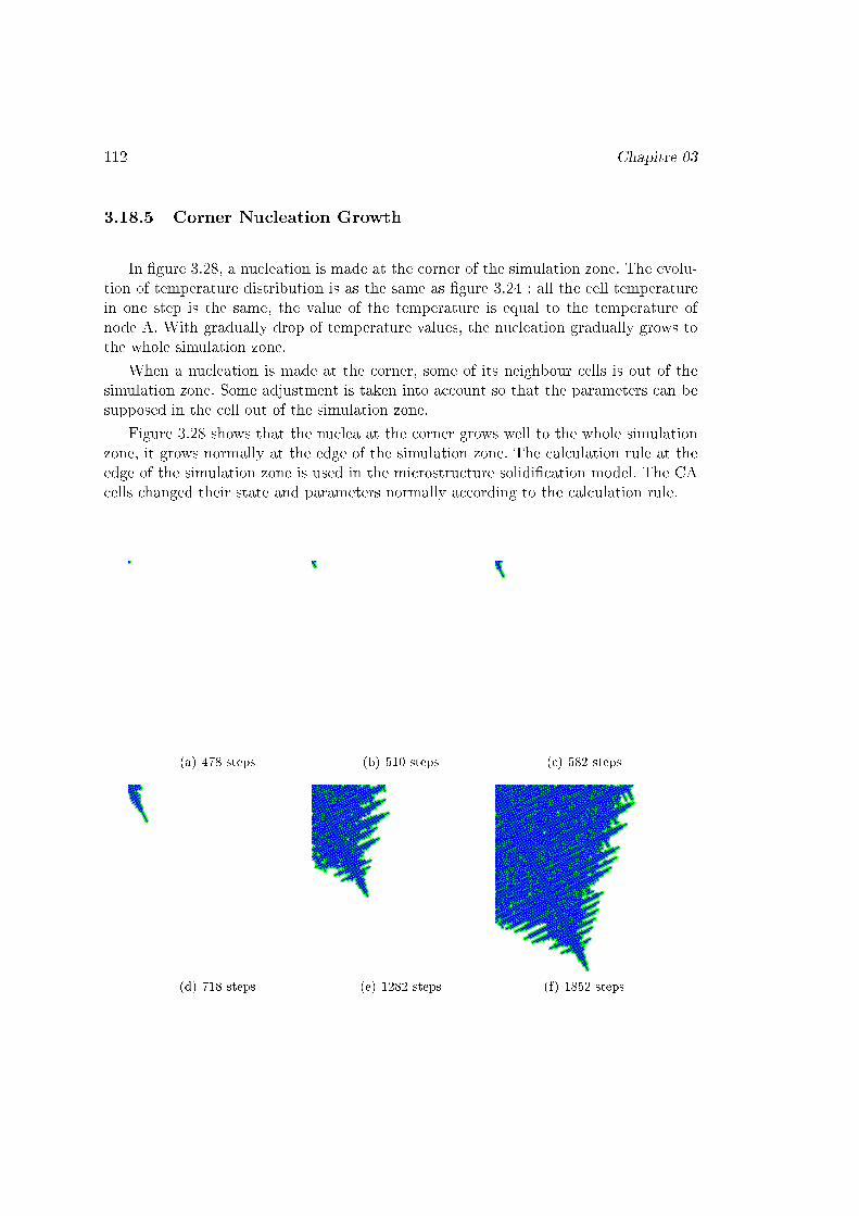
112 Chapitre 03
3.18.5 Corner Nucleation Growth
In �gure 3.28, a nucleation is made at the corner of the simulation zone. The evolu-tion of temperature distribution is as the same as �gure 3.24 : all the cell temperaturein one step is the same, the value of the temperature is equal to the temperature ofnode A. With gradually drop of temperature values, the nucleation gradually grows tothe whole simulation zone.
When a nucleation is made at the corner, some of its neighbour cells is out of thesimulation zone. Some adjustment is taken into account so that the parameters can besupposed in the cell out of the simulation zone.
Figure 3.28 shows that the nuclea at the corner grows well to the whole simulationzone, it grows normally at the edge of the simulation zone. The calculation rule at theedge of the simulation zone is used in the microstructure solidi�cation model. The CAcells changed their state and parameters normally according to the calculation rule.
(a) 478 steps (b) 510 steps (c) 582 steps
(d) 718 steps (e) 1282 steps (f) 1852 steps
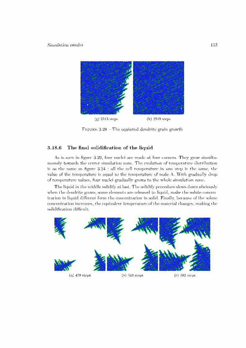
Simulation results 113
(g) 2313 steps (h) 2819 steps
Figure 3.28 � The equiaxed dendrite grain growth
3.18.6 The �nal solidi�cation of the liquid
As is seen in �gure 3.29, four nuclei are made at four corners. They grow simulta-neously towards the center simulation zone. The evolution of temperature distributionis as the same as �gure 3.24 : all the cell temperature in one step is the same, thevalue of the temperature is equal to the temperature of node A. With gradually dropof temperature values, four nuclei gradually grows to the whole simulation zone.
The liquid in the middle solidify at last. The solidify procedure slows down obviouslywhen the dendrite grows, some elements are released to liquid, make the solute concen-tration in liquid di�erent form the concentration in solid. Finally, because of the soluteconcentration increases, the equivalent temperature of the material changes, making thesolidi�cation di�cult.
(a) 478 steps (b) 510 steps (c) 582 steps
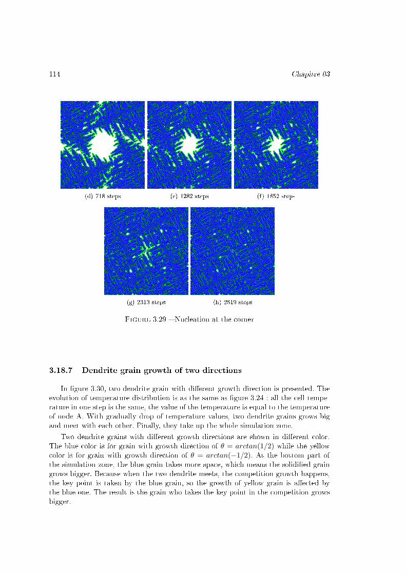
114 Chapitre 03
(d) 718 steps (e) 1282 steps (f) 1852 steps
(g) 2313 steps (h) 2819 steps
Figure 3.29 � Nucleation at the corner
3.18.7 Dendrite grain growth of two directions
In �gure 3.30, two dendrite grain with di�erent growth direction is presented. Theevolution of temperature distribution is as the same as �gure 3.24 : all the cell tempe-rature in one step is the same, the value of the temperature is equal to the temperatureof node A. With gradually drop of temperature values, two dendrite grains grows bigand meet with each other. Finally, they take up the whole simulation zone.
Two dendrite grains with di�erent growth directions are shown in di�erent color.The blue color is for grain with growth direction of θ = arctan(1/2) while the yellowcolor is for grain with growth direction of θ = arctan(−1/2). At the bottom part ofthe simulation zone, the blue grain takes more space, which means the solidi�ed graingrows bigger. Because when the two dendrite meets, the competition growth happens,the key point is taken by the blue grain, so the growth of yellow grain is a�ected bythe blue one. The result is the grain who takes the key point in the competition growsbigger.
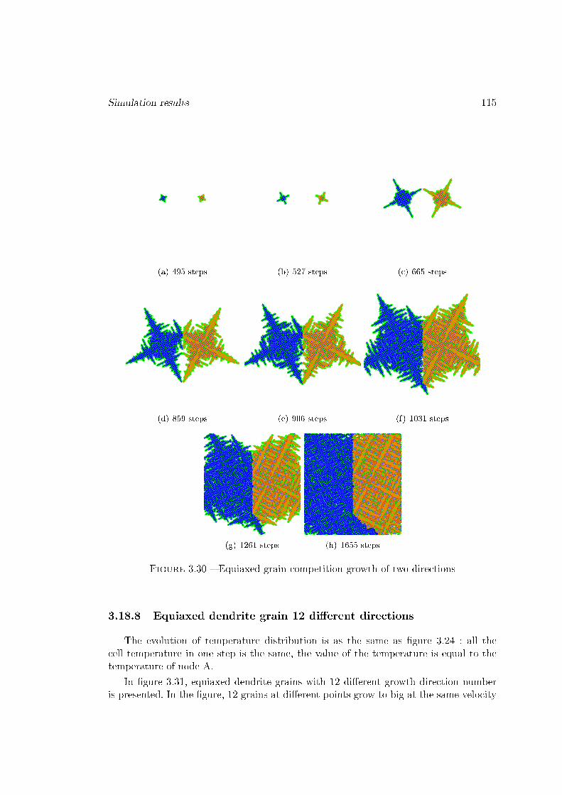
Simulation results 115
(a) 495 steps (b) 527 steps (c) 665 steps
(d) 859 steps (e) 906 steps (f) 1031 steps
(g) 1261 steps (h) 1655 steps
Figure 3.30 � Equiaxed grain competition growth of two directions
3.18.8 Equiaxed dendrite grain 12 di�erent directions
The evolution of temperature distribution is as the same as �gure 3.24 : all thecell temperature in one step is the same, the value of the temperature is equal to thetemperature of node A.
In �gure 3.31, equiaxed dendrite grains with 12 di�erent growth direction numberis presented. In the �gure, 12 grains at di�erent points grow to big at the same velocity

116 Chapitre 03
and �nally they take up the whole simulation zone.
The grains grow smoothly with the other grains with di�erent growth direction. Thegrowth velocity are the same, just the direction is di�erent. In �nal result, some grainsare bigger just because there are more space at the edge.
(a) 399 steps (b) 418 steps (c) 438 steps
(d) 464 steps (e) 491 steps (f) 636 steps
Figure 3.31 � Grains with di�erent growth direction growth at the same speed
3.18.9 Microstructure simulation of weld
Unlike the isotropic temperature distributions used in the former part, those of weldpart are also estimated. The linear interpolation is used for every cell to compute theirown cell temperature. The result shows the corresponding weld microstructure.
As is seen in �gure 3.32, a high resolution ratio is applied to the Weld MicrostructureSimulation Model. Nine pixels are used for one small cell in CA.
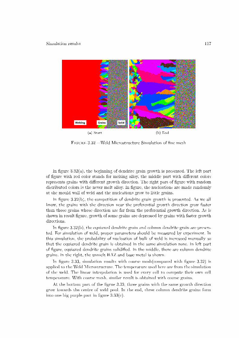
Simulation results 117
(a) Start (b) End
Figure 3.32 � Weld Microstructure Simulation of �ne mesh
In �gure 3.32(a), the beginning of dendrite grain growth is presented. The left partof �gure with red color stands for melting alloy, the middle part with di�erent colorsrepresents grains with di�erent growth direction. The right part of �gure with randomdistributed colors is the never melt alloy. In �gure, the nucleations are made randomlyat the mould wall of weld and the nucleations grow to little grains.
In �gure 3.32(b), the competition of dendrite grain growth is presented. As we allknow, the grains with the direction near the preferential growth direction grow fasterthan those grains whose direction are far from the preferential growth direction. As isshown in result �gure, growth of some grains are depressed by grains with faster growthdirections.
In �gure 3.32(b), the equiaxed dendrite grain and column dendrite grain are presen-ted. For simulation of weld, proper parameters should be measured by experiment. Inthis simulation, the probability of nucleation of bulk of weld is increased manually sothat the equiaxed dendrite grain is obtained in the same simulation zone. In left partof �gure, equiaxed dendrite grains solidi�ed. In the middle, there are column dendritegrains. In the right, the unmelt HAZ and base metal is shown.
In �gure 3.33, simulation results with coarse mesh(compared with �gure 3.32) isapplied to the Weld Microstructure. The temperature used here are from the simulationof the weld. The linear interpolation is used for every cell to compute their own celltemperature. With coarse mesh, similar result is obtained with coarse grains.
At the bottom part of the �grue 3.33, three grains with the same growth directiongrow towards the centre of weld pool. In the end, three column dendrite grains forminto one big purple part in �gure 3.33(c).
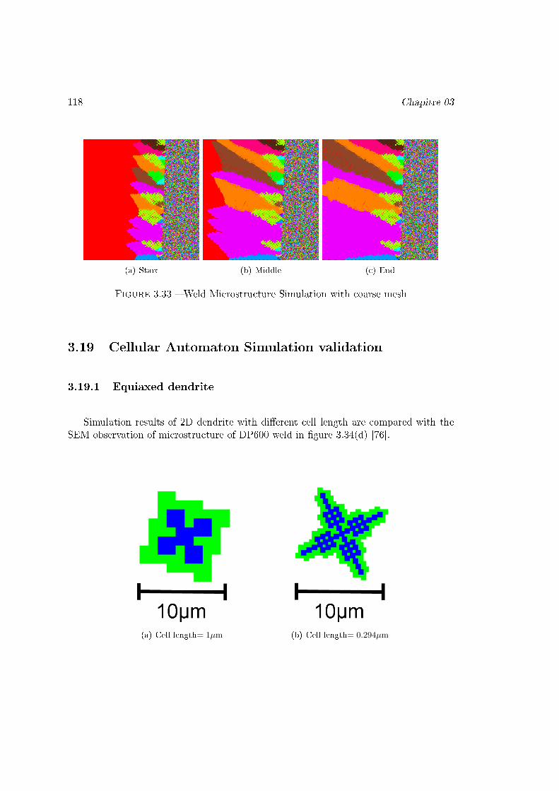
118 Chapitre 03
(a) Start (b) Middle (c) End
Figure 3.33 � Weld Microstructure Simulation with coarse mesh
3.19 Cellular Automaton Simulation validation
3.19.1 Equiaxed dendrite
Simulation results of 2D dendrite with di�erent cell length are compared with theSEM observation of microstructure of DP600 weld in �gure 3.34(d) [76].
(a) Cell length= 1µm (b) Cell length= 0.294µm

Cellular Automaton Simulation validation 119
(c) Cell length= 0.067µm (d) DP600 microstructure [76]
Figure 3.34 � Dendrite morphology of 2D simulation and experimental SEM observa-tion
In microscopic comparison, the equiaxed dendrite morphologies between simulationresult and experimental observation are similar. As the cell length of 2D CA model de-crease, the resolution of simulation increase and more detailed morphologic informationcan be achieved.
3.19.2 Microstructure of laser welding
3.19.2.1 Weld cross section
A laser beam with power of 4KW and welding speed of 3m/min is applied to dualphase steel DP600. The microstructure of laser weld cross section is observed and thecorresponding simulation result is presented in �gure 3.35 :
(a) Optical observation (b) Zoomed zone (c) Simulation result
Figure 3.35 � Microstructure of FZ and HAZ of DP600 weld cross section

120 Chapitre 03
3.19.2.2 Weld upper surface
The microstructure of laser weld cross section is observed and the correspondingsimulation result is presented in �gure 3.36 :
(a) Optical observation (b) Zoomed zone (c) Simulation result
Figure 3.36 � Microstructure of FZ and HAZ of DP600 weld upper surface
Using the temperature interpolation technique, a part of weld zone is simulated andcompared with the optical observation. In a cross-section of weld simulation, dendritewith random orientations grow from the edge to center of the weld have good accordancewith experimental results. At the beginning dendrites has random growth orientation atthe edge, �nally orientations of grains in�uenced by welding temperature distributionand dendrites interaction are similar to experimental observation.

Chapitre 4
Finite Element Model and FEM-CAcoupling for numerical simulation ofresidual stresses
4.1 Model Information
The residual stress analysis uses an incremental sequentially coupled thermal-mechanicalanalysis. The used incremental simulation model consists in two parts :
1. Thermal analysis part� Heat source, heat transfer, radiation and convection are considered to analyze
the thermal data of the model� The computed thermal data is stored in a data �le which is prepared for the
mechanical analysis.
2. Mechanical analysis part� A prede�ned �eld introduced by reading the thermal data of thermal analysis
model is used as thermal load for mechanical analysis .� With the consideration of material properties, such as elastic modulus and
plasticity, the expansion behavior of the material due to temperature increase,the elastic and plastic response of the material, and the relaxation of thematerial at the cooling step are considered to estimate the residual stresses.
The introduction of ABAQUS models will be parted into following sections :
1. Basic material properties. The described properties are used in all the numericalsimulation work.
2. Two Models with di�erent geometries and mesh types. This part introduces thegeometry parameters and mesh information used for laser welding simulationmodel.
121

122 Chapitre 04
3. Important terms of material constitutive model. Several terms are introduced indetail. The information of hardening, temperature sensitivity, strain rate sensi-tivity, elastic and plastic anisotropy via di�erent welding numerical models areintroduced in detail.
4.2 Basic material properties
4.2.1 Unit system used in ABAQUS/FEM
To introduce the material properties, one important thing should be noticed thatthere are no explicit unit system in ABAQUS/FEM. User can select there their favoriteunit system. Usually the IS unit system based on N, m, and s is selected. But forlaser welding process, the author's unit system are based on N, mm, ms. All the otherimportant units can be derived from the basic unit system of N, mm, ms.
Table 4.1 � Unit de�nitionIS unit User de�ned unit
MassN · s2
m=kg
N · (ms)2
mm=g
Energy N ·m = J N ·mm = mJ
Pressure N/m2 = Pa N/mm2 = MPa
Power J/s = W mJ/ms = W
Density kg/m3 g/mm3
4.2.2 Conductivity
The conductivity of material is a temperature dependent parameter, the data ofconductivity is show in Table 4.2 :
Table 4.2 � Conductivity of model [77]
Conductivity (W/(m ·◦ C)) Temperature (◦C)
34.6 034.8 2535 20035 25421.4 110025.5 120060 130070 140070 3000
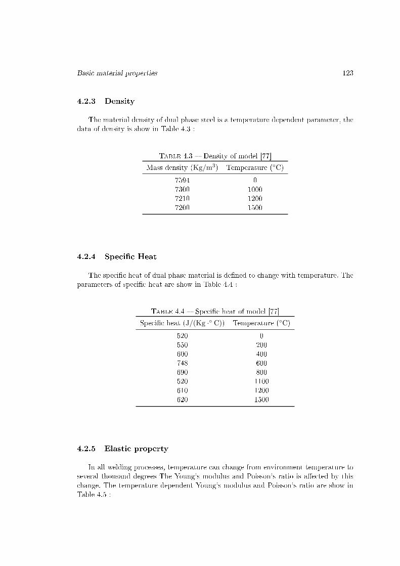
Basic material properties 123
4.2.3 Density
The material density of dual phase steel is a temperature dependent parameter, thedata of density is show in Table 4.3 :
Table 4.3 � Density of model [77]
Mass density (Kg/m3) Temperature (◦C)
7594 07300 10007210 12007200 1500
4.2.4 Speci�c Heat
The speci�c heat of dual phase material is de�ned to change with temperature. Theparameters of speci�c heat are show in Table 4.4 :
Table 4.4 � Speci�c heat of model [77]
Speci�c heat (J/(Kg ·◦ C)) Temperature (◦C)
520 0550 200600 400748 600690 800520 1100610 1200620 1500
4.2.5 Elastic property
In all welding processes, temperature can change from environment temperature toseveral thousand degrees The Young's modulus and Poisson's ratio is a�ected by thischange. The temperature dependent Young's modulus and Poisson's ratio are show inTable 4.5 :

124 Chapitre 04
Table 4.5 � Elastic property of model [77]
Young's modulus (Pa) Poisson's ratio Temperature (◦C)
2.1× 10¹¹ 0.28 01.9× 10¹¹ 0.295 3001.2× 1011 0.31 6003× 1010 0.33 800
4.2.6 Plastic property
A simple linear material constitutive model of DP600 steel is used based on thework of F Ozturk [78] and Ju Chen [57]. The plastic property of DP600 steel is plot-ted in �gure 4.1. This material constitutive model is only used for mesh type, meshdensity and boundary condition analyses. Analyses of material constitutive model ofhardening, temperature and strain rate sensitivity use nonlinear material constitutivemodel identi�ed in chapter 2 and describe in the following part.
Figure 4.1 � Linear material constitutive model of DP600 steel
4.2.7 Expansion
As shown in table 4.6, the expansion coe�cient is also set as a temperature de-pendent parameter :
4.2.8 Heat souce model
The shape of heat source model, Gauss heat distribution and corresponding heatsource parameters are presented in �gure 4.2 and in table 4.7.
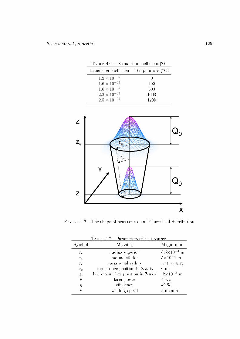
Basic material properties 125
Table 4.6 � Expansion coe�cient [77]
Expansion coe�cient Temperature (◦C)
1.2× 10−05 01.6× 10−05 4001.6× 10−05 8002.2× 10−05 10002.5× 10−05 1200
Figure 4.2 � The shape of heat source and Gauss heat distribution
Table 4.7 � Parameters of heat sourceSymbol Meaning Magnitude
re radius superior 6.5×10⁻⁴ mri radius inferior 5×10⁻⁴ mrc variational radius ri 6 rc 6 reze top surface position in Z axis 0 mzi bottom surface position in Z axis -2×10⁻³ mP laser power 4 Kwη e�ciency 42 %V welding speed 3 m/min
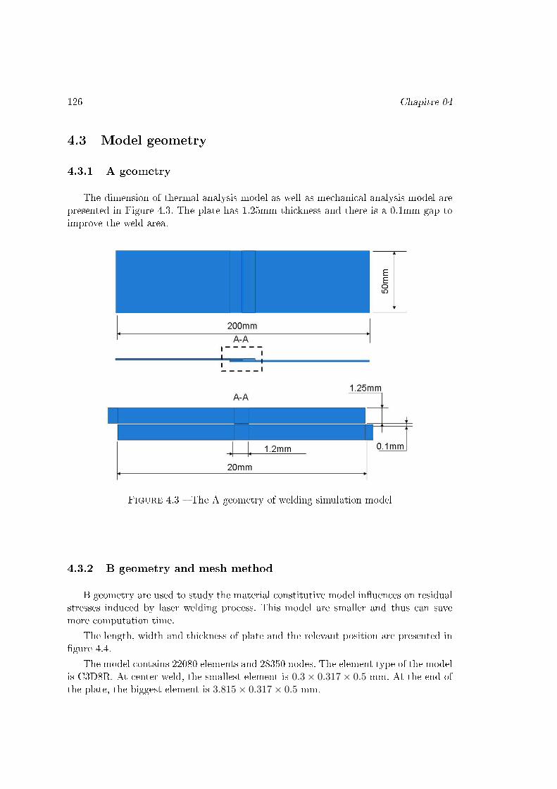
126 Chapitre 04
4.3 Model geometry
4.3.1 A geometry
The dimension of thermal analysis model as well as mechanical analysis model arepresented in Figure 4.3. The plate has 1.25mm thickness and there is a 0.1mm gap toimprove the weld area.
Figure 4.3 � The A geometry of welding simulation model
4.3.2 B geometry and mesh method
B geometry are used to study the material constitutive model in�uences on residualstresses induced by laser welding process. This model are smaller and thus can savemore computation time.
The length, width and thickness of plate and the relevant position are presented in�gure 4.4.
The model contains 22080 elements and 28350 nodes. The element type of the modelis C3D8R. At center weld, the smallest element is 0.3× 0.317× 0.5 mm. At the end ofthe plate, the biggest element is 3.815× 0.317× 0.5 mm.
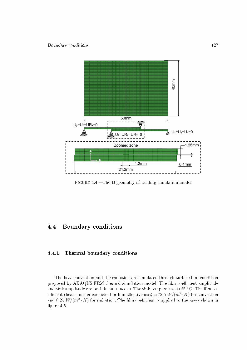
Boundary conditions 127
Figure 4.4 � The B geometry of welding simulation model
4.4 Boundary conditions
4.4.1 Thermal boundary conditions
The heat convection and the radiation are simulated through surface �lm conditionproposed by ABAQUS FEM thermal simulation model. The �lm coe�cient amplitudeand sink amplitude are both instantaneous. The sink temperature is 25 ◦C. The �lm co-e�cient (heat transfer coe�cient or �lm e�ectiveness) is 73.5W/(m2 ·K) for convectionand 0.25 W/(m2 ·K) for radiation. The �lm coe�cient is applied to the areas shown in�gure 4.5.

128 Chapitre 04
Figure 4.5 � Boundary conditions of thermal analysis model using B geometry
4.4.2 Mechanical boundary conditions
In mechanical analysis model, the boundary conditions are de�ned according to thelaser welding process of real experiment. In �gure 4.6, the boundary conditions arepresented. The right end of the plate is �xed while the left surface can move freely in xdirection. Around the weld, the plates are clamped to not move in z direction.
Figure 4.6 � Boundary conditions of mechanical analysis model using B geometry
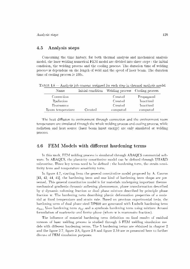
Analysis steps 129
4.5 Analysis steps
Concerning the time history, for both thermal analysis and mechanical analysismodel, the laser welding numerical FEM model are divided into three steps : the initialcondition, the welding process and the cooling process. The duration time of weldingprocess is dependent on the length of weld and the speed of laser beam. The durationtime of cooling process is 100s.
Table 4.8 � Analysis job content assigned for each step in thermal analysis model
Name Initial condition Welding process Cooling process
Convection Created PropagatedRadiation Created InactivedHeatsource Created Inactived
Room temperature Created computed computed
The heat di�usion to environment through convection and the environment roomtemperature are simulated through the whole welding process and cooling process, whileradiation and heat source (laser beam input energy) are only simulated at weldingprocess.
4.6 FEM Models with di�erent hardening terms
In this work, FEM welding process is simulated through ABAQUS commercial soft-ware. In ABAQUS, the plasticity constitutive model can be de�ned through UHARDsubroutine. Three key terms need to be de�ned : the hardening term, the strain sensi-tivity term and temperature sensitivity term.
In �gure 4.7, starting from the general constitutive model proposed by A. Gavrus[43, 42, 44, 45], the hardening term and one kind of hardening term shape are pre-sented. This general constitutive model is for materials undergoing important thermo-mechanical gradients dynamic softening phenomenon, phase transformation describedby ψ dynamic softening fraction or dual phase mixture described by principle phasefraction w. The hardening term describing plastic deformation properties of a mate-rial at �xed temperature and strain rate. Based on previous experimental tests, thehardening term of dual phase steel DP600 are generated with Ludwik hardening termσhm, Voce hardening term σhf and a synthesis hardening term using mixture Avramiformulation of martensite and ferrite phase (where w is martensite fraction).
The in�uence of material hardening term de�nition on �nal results of residualstresses of laser welding process is studied through 5 FEM welding simulation mo-dels with di�erent hardening terms. The 5 hardening terms are obtained in chapter 2and the �gure 2.7, �gure 2.8, �gure 2.9 and �gure 2.10 are re-presented here to furtherdiscuss of FEM simulation purposes.

130 Chapitre 04
Figure 4.7 � Hardening term of material constitutive model
(a) Modi�ed Ludwik model (b) Modi�ed Voce model
(c) Classical Ludwik model 02, classical Vocemodel 02 and proposed synthesis model
(d) Proposed synthesis model 0, model 02 andmodel 1 (w=0, w=0.2 and w=1)
Figure 4.8 � Hardening models used in FEM laser welding simulation models

FEM Models with di�erent hardening terms 131
In �gure 4.8, the modi�ed Ludwik model, the modi�ed Voce model and the propo-sed synthesis model 02 all have good accordance with the original experimental data.The modi�ed Ludwik model, the modi�ed Voce model are not in classical form. Theproposed synthesis model 02 is the synthesis of classical Ludwik model and classicalVoce model. With di�erent mathematical form, the three results in similar stress-straincurves describing the plasticity of dual phase steel DP600. In �gure 4.8 (c) and (d),the classical Ludwik model 02 and the classical Voce model 02 have good accordancewith the original experimental data only in plastic strain range of [0, 0.05] while theproposed synthesis model 02 has good accordance in range of [0, 0.2] and can be usedfor a lot of welding or other dynamic forming processes.
Five hardening models described in chapter 2.2.1.4 are simulated through com-mercial software ABAQUS/FEM. The numerical models are based on basic materialproperties identi�ed in chapter 4.2, B geometry and mesh presented in chapter 4.3.2,boundary conditions detailed in chapter 4.4 and analysis steps described in chapter 4.5.The parameters of the �ve hardening models are reminded in table 4.9.
Table 4.9 � Rheological coe�cients corresponding to di�erent DP600 hardening modelsσy n1 n2 n3 n4 w Equation Nonlinear regression εp range
Classical Ludwik model 01 400 980 0.48 - - - (2.11) [0, 0.2]Classical Ludwik model 02 400 1660 0.63 - - - (2.19) [0, 0.05]Modi�ed Ludwik model 400 1690 0.5 -1240 -65 - (2.13) [0, 0.2]Classical Voce model 01 400 555 15.5 - - - (2.14) [0, 0.2]Classical Voce model 02 400 340 27.5 - - - (2.20) [0, 0.05]Modi�ed Voce model 400 270 30 900 - - (2.16) [0, 0.2]Proposed synthesis model (w=0.4) 400 1660 0.63 340 27.5 0.40 (2.17 et 2.18) [0, 0.2]Proposed synthesis model 02 (w=0.2) 400 3411.3 0.60 234.4 27.1 0.20 (2.17 et 2.21) [0, 0.2]Proposed synthesis model 1 (w=1) 400 3411.3 0.60 234.4 27.1 1 (2.17) -
For the results of hardening models, one should keep in mind that the results willbe revised after the temperature sensitivity is discussed. For the present, the conditionF(298K)=1 and F(1803K)=0.05 are used with a Johnson-Cook temperature sensiti-vity model. It can be noted also here that a constant martensite fraction is used. Thestrain rate sensitivity term G(ε̇) = 1 is used in order to focus the behavior analysison hardening in�uence. In future work, the martensite fraction w during the solidi-�cation should be considered dependent on the temperature in the range of fusiontemperature Tf and ambient temperature T0 using a variation w(T) obtained fromsolid fraction computation of CA model. According to G(ε̇) = 1, the proposed synthe-sis model 02 is written in the form : H(εpe) = w · (400 + 3411.28ε0.6014
p ) + (1 − w) ·{400 + 234.40 · [1− exp(−27.1092εp)]} where identi�cation has made for w=0.2.
By comparing the modi�ed Ludwik model, the modi�ed Voce model and the pro-posed synthesis model 02, the in�uence of constitutive equation form on FEM weldingsimulation results of residual stresses is evaluated. By comparing the classical Ludwikmodel 02, the classical Voce model 02 and the proposed synthesis model 02, the in-�uence of hardening term in the plastic strain range of laser welding on residual stressesof FEM are studied. Results and discussion will be presented in chapter 5.

132 Chapitre 04
4.7 FEMModels with di�erent temperature sensitivity terms
In �gure 4.9, starting from the general constitutive model proposed by A. Gavrus[43, 42, 44, 45], the temperature sensitivity term and its in�uence on the plastic defor-mation properties of a material are presented. The temperature sensitivity term F(T)can in�uence the magnitude of elasto-plastic �ow behavior. The stress-strain curve willbe in�uenced by temperature. Normally, the higher the temperature is, the lower thetemperature sensitivity will be.
Figure 4.9 � Temperature sensitivity term of material constitutive model
Based on temperature sensitivity of a high strength steel in the work of Chen [57],the temperature sensitivity term of dual phase steel DP600 are obtained with Johnson-Cook model, Chen model, a proposed model and a polynomial temperature sensitivityterm. Figure 2.11 are re-presented here to present the di�erence of Johnson-Cook, Chen,proposed and polynomial temperature sensitivity models.
Johnson-Cook temperature sensitivity term use only one parameter to describe thetemperature sensitivity of material. It has a good accordance with experimental datafrom room temperature to about 700K, but not good for temperature bigger than 700K.Chen temperature sensitivity term use two parameters to describe the temperature sen-sitivity of material while the proposed temperature sensitivity term use three. Chenand proposed temperature sensitivity terms are similar in �gure 4.10. Polynomial tem-perature sensitivity term can precisely describe the experimental data but it has to beidenti�ed for every materials and do not have a physical sense.
The 4 temperature sensitivity terms which are used in FEM welding simulation arelisted below :
� Johnson-Cook temperature sensitivity term :
F(T ) = 1− T ∗1.5 (4.1)

FEM Models with di�erent strain rate sensitivity terms 133
Figure 4.10 � The 4 temperature sensitivity terms used in FEM laser welding simula-tion models
� Chen temperature sensitivity term :
F(T ) = exp(4.254 · T ∗−28.418) (4.2)
� Proposed temperature sensitivity term :
F(T ) = (1− 0.699 · T ∗4.027)38.629 (4.3)
� Polynomial temperature sensitivity term :295.15K < T < 993.15K :
F (T ) = 1.55− 3.50× 10⁻³ · T + 7.00× 10⁻⁶ · T 2 − 4.82× 10⁻⁹ · T 3 (4.4)
993.15K < T < 1213.15K :
F (T ) = 5.18− 7.83× 10⁻³ · T + 2.30× 10⁻⁶ · T 2 + 5.35× 10⁻¹⁰ · T 3 (4.5)
Johnson-Cook temperature sensitivity term is similar with polynomial temperaturesensitivity term at low temperature but have obvious di�erence at high temperatureChen and proposed temperature sensitivity model both have di�erence at low and hightemperature with polynomial temperature sensitivity model. The in�uences of tempe-rature sensitivity di�erence on FEM welding simulation results of residual stresses areinvestigated. Results and discussions will be presented in chapter 5.
4.8 FEMModels with di�erent strain rate sensitivity terms
In �gure 4.11, starting from the general constitutive model proposed by A. Gavrus[43, 42, 44, 45], the strain rate sensitivity term and its in�uence on the plastic defor-mation properties of a material are presented. The strain rate sensitivity term G(ε̇) can

134 Chapitre 04
in�uence the magnitude of elasto-plastic �ow behavior. Normally, the higher the strainrate is, the higher the strain rate sensitivity will be.
Figure 4.11 � Temperature sensitivity term of material constitutive model
Based on experimental and literature data [3], the strain rate sensitivity term of dualphase steel DP600 are obtained in section 2.2.3.4. In �gure 4.12, strain rate sensitivityvalues under di�erent temperatures are plotted.
Figure 4.12 � The strain rate sensitivity term under di�erent temperatures
In �gure 4.12, it is shown that the strain rate sensitivity value is around 1 at ambienttemperature. The strain rate sensitivity value will change according to strain rate andtemperature. The strain rate sensitivity used for FEM welding simulation is written inin section 2.2.3.4 and rewritten here derived from proposed Arcsinus hyperbolic strainrate law proposed by A. Gavrus [43, 42, 44, 45] :
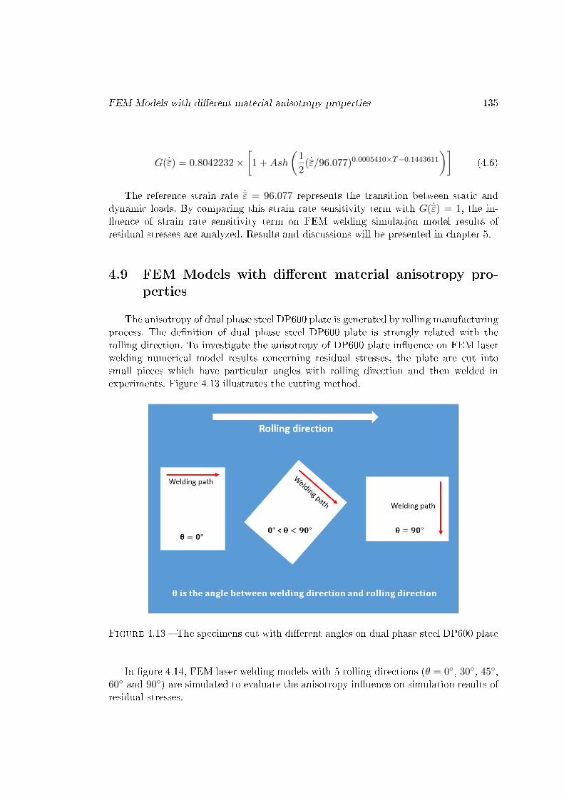
FEM Models with di�erent material anisotropy properties 135
G(ε̇) = 0.8042232×[1 +Ash
(1
2(ε̇/96.077)0.0005410×T−0.1443611
)](4.6)
The reference strain rate ε̇ = 96.077 represents the transition between static anddynamic loads. By comparing this strain rate sensitivity term with G(ε̇) = 1, the in-�uence of strain rate sensitivity term on FEM welding simulation model results ofresidual stresses are analyzed. Results and discussions will be presented in chapter 5.
4.9 FEM Models with di�erent material anisotropy pro-perties
The anisotropy of dual phase steel DP600 plate is generated by rolling manufacturingprocess. The de�nition of dual phase steel DP600 plate is strongly related with therolling direction. To investigate the anisotropy of DP600 plate in�uence on FEM laserwelding numerical model results concerning residual stresses, the plate are cut intosmall pieces which have particular angles with rolling direction and then welded inexperiments. Figure 4.13 illustrates the cutting method.
Figure 4.13 � The specimens cut with di�erent angles on dual phase steel DP600 plate
In �gure 4.14, FEM laser welding models with 5 rolling directions (θ = 0◦, 30◦, 45◦,60◦ and 90◦) are simulated to evaluate the anisotropy in�uence on simulation results ofresidual stresses.
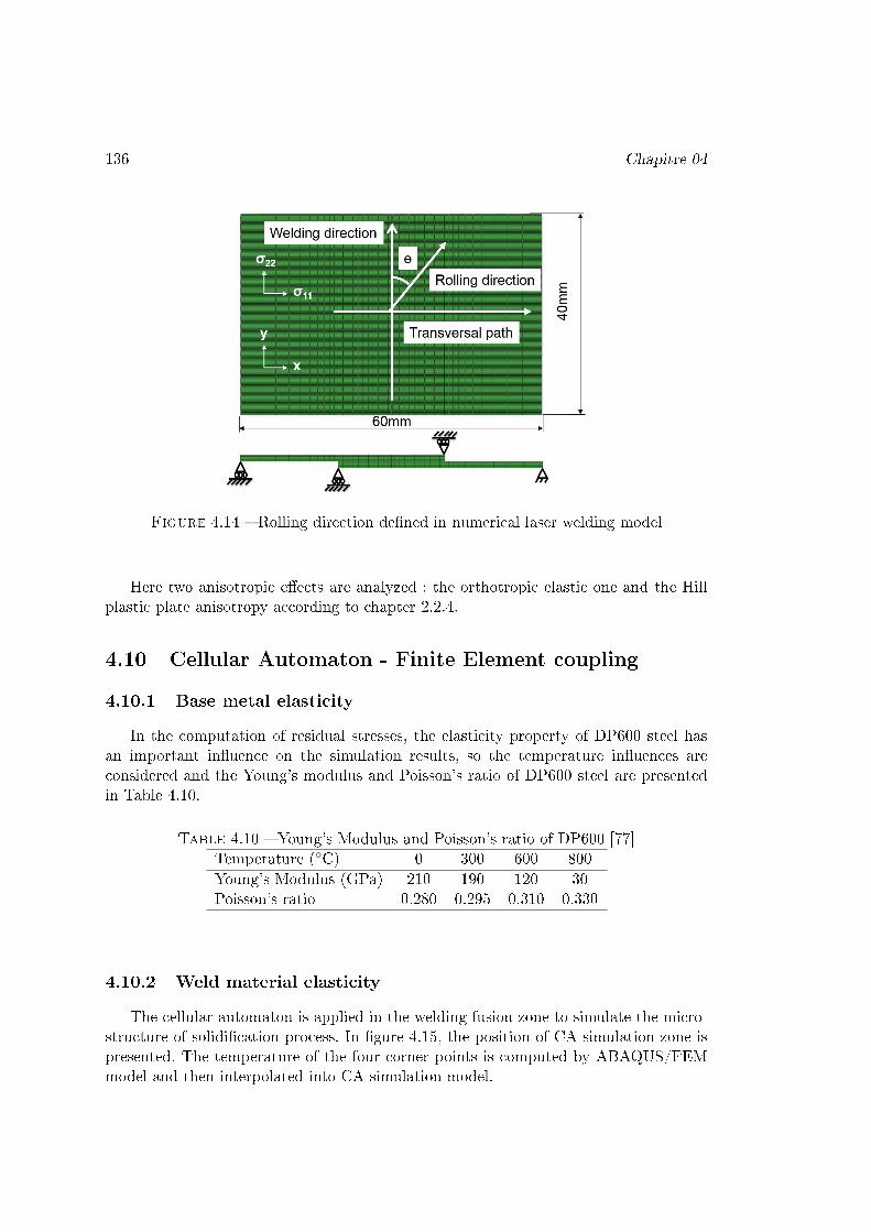
136 Chapitre 04
Figure 4.14 � Rolling direction de�ned in numerical laser welding model
Here two anisotropic e�ects are analyzed : the orthotropic elastic one and the Hillplastic plate anisotropy according to chapter 2.2.4.
4.10 Cellular Automaton - Finite Element coupling
4.10.1 Base metal elasticity
In the computation of residual stresses, the elasticity property of DP600 steel hasan important in�uence on the simulation results, so the temperature in�uences areconsidered and the Young's modulus and Poisson's ratio of DP600 steel are presentedin Table 4.10.
Table 4.10 � Young's Modulus and Poisson's ratio of DP600 [77]Temperature (◦C) 0 300 600 800Young's Modulus (GPa) 210 190 120 30Poisson's ratio 0.280 0.295 0.310 0.330
4.10.2 Weld material elasticity
The cellular automaton is applied in the welding fusion zone to simulate the micro-structure of solidi�cation process. In �gure 4.15, the position of CA simulation zone ispresented. The temperature of the four corner points is computed by ABAQUS/FEMmodel and then interpolated into CA simulation model.

Cellular Automaton - Finite Element coupling 137
Figure 4.15 � The CA simulation position in ABAQUS/FEM model
The results of ABAQUS thermal simulation model is presented in �gure 4.16. Theweld zone experienced a sudden increase and decrease of temperature. The liquid statusof melting pool only last less than 1 second.
Figure 4.16 � Temperature history data of 4 points
In �gure 4.17, the �owchart of CA-FE coupling model for residual stress simulationis shown. The crystalline orientation and orientation fraction is computed based on CAmodel, the results combines with the martensite elastic constants is used to calculate theweld elastic constants that are used in ABAQUS/FEM simulation for residual stresses.
Because of the high cooling rate of laser welding, the face centered cubic austensitein DP600 weld turns to body centered tetragonal martensite in solidi�cation process.This phase transformation phenomenon are observed in many works [21, 79]. Due to the

138 Chapitre 04
Figure 4.17 � The �owchart of CA-FE model used to simulate residual stresses
phase transformation and the grain size decrease, the mechanical properties of the weldmaterial are changed, such as increment of micro-hardness [79, 80, 21, 24]. N.Farabi et al.[22] investigated laser welding on DP600/DP980 steels. Nearly full martensite is foundat FZ (Fusion Zone). The elastic constants of martensite of weld in DP600 are assumedto be the same with those of martensite steel [81]. The martensitic elastic compliance arecomputed based on equation 4.7. If an orthotropic elastic anisotropy is considered, themartensitic elastic compliance Sij which express the relationships between the elasticstrain Voigth vector and the Cauchy stress Voigth vector are computed by :
Sij = C−1ij =
1/E1 −ν21/E2 −ν31/E3
−ν12/E1 1/E2 −ν32/E3
−ν13/E1 −ν23/E2 1/E3
1/G12
1/G13
1/G23
(4.7)
Starting from results obtained in [81] the following values are taking into accountto describe elastic anisotropy of the initial DP600 martensite :
Cij =
268.1 111.2 110.2111.2 268.4 111.0110.2 111.0 267.2
79.0678.72
78.85
(4.8)
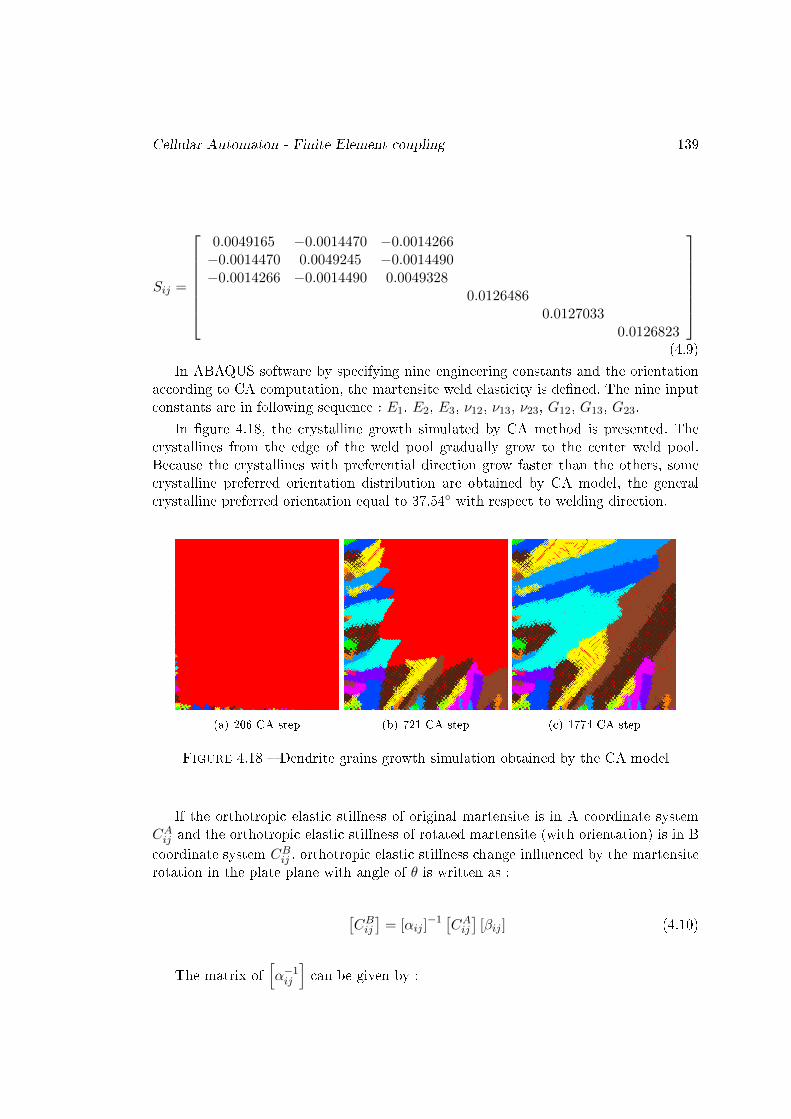
Cellular Automaton - Finite Element coupling 139
Sij =
0.0049165 −0.0014470 −0.0014266−0.0014470 0.0049245 −0.0014490−0.0014266 −0.0014490 0.0049328
0.01264860.0127033
0.0126823
(4.9)
In ABAQUS software by specifying nine engineering constants and the orientationaccording to CA computation, the martensite weld elasticity is de�ned. The nine inputconstants are in following sequence : E1, E2, E3, ν12, ν13, ν23, G12, G13, G23.
In �gure 4.18, the crystalline growth simulated by CA method is presented. Thecrystallines from the edge of the weld pool gradually grow to the center weld pool.Because the crystallines with preferential direction grow faster than the others, somecrystalline preferred orientation distribution are obtained by CA model, the generalcrystalline preferred orientation equal to 37.54◦ with respect to welding direction.
(a) 206 CA step (b) 721 CA step (c) 1774 CA step
Figure 4.18 � Dendrite grains growth simulation obtained by the CA model
If the orthotropic elastic sti�ness of original martensite is in A coordinate systemCAij and the orthotropic elastic sti�ness of rotated martensite (with orientation) is in Bcoordinate system CBij , orthotropic elastic sti�ness change in�uenced by the martensiterotation in the plate plane with angle of θ is written as :
[CBij]
= [αij ]−1 [CAij] [βij ] (4.10)
The matrix of[α−1ij
]can be given by :

140 Chapitre 04
[αij ]−1 =
cos2θ sin2θ 0 0 0 2sinθcosθsin2θ cos2θ 0 0 0 −2sinθcosθ
0 0 1 0 0 00 0 0 cosθ −sinθ 00 0 0 sinθ cosθ 0
−sinθcosθ sinθcosθ 0 0 0 cos2θ − sin2θ
(4.11)
and [βij ] is :
[βij ] =
cos2θ sin2θ 0 0 0 −sinθcosθsin2θ cos2θ 0 0 0 sinθcosθ
0 0 1 0 0 00 0 0 cosθ sinθ 00 0 0 −sinθ cosθ 0
2sinθcosθ −2sinθcosθ 0 0 0 cos2θ − sin2θ
(4.12)
In equation 4.11 and equation 4.12, θ is martensite rotation angle in plane and thedirection cosines between x, y, z axials of A coordinate xA, yA, zA and x, y, z axials ofB coordinate xB, yB, zB are :
Table 4.11 � Direction cosines values in plane rotation with angle θxA yA zA
xB cosθ −sinθ 0yB sinθ cosθ 0zB 0 0 1
The temperature in�uence on elastic constants are considered proportionally thesame as those of DP600 Young's modulus and Poisson's modulus in table 4.10. Linearinterpolation is applied to decrease elastic constants proportionally as the temperatureincreases for 300◦C, 600◦C and 800◦C.
WT
W0=BTB0
(4.13)
Where WT stands for the weld material Young's Modulus and Poisson's ratio valuesof E1, E2, E3, ν12, ν13, ν23, G12, G13 and G23 in table 6.2 at temperature T (T canbe 0◦C, 300◦C, 600◦C and 800◦C) and BT stands for the corresponding base materialYoung's Modulus and Poisson's ratio values in table 4.10. The computed values areshown in table 6.2 and the units of E1, E2, E3, G12, G13 and G23 are of GPa.
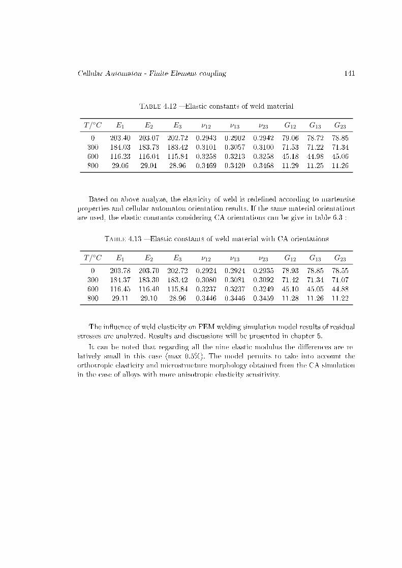
Cellular Automaton - Finite Element coupling 141
Table 4.12 � Elastic constants of weld material
T/◦C E1 E2 E3 ν12 ν13 ν23 G12 G13 G23
0 203.40 203.07 202.72 0.2943 0.2902 0.2942 79.06 78.72 78.85300 184.03 183.73 183.42 0.3101 0.3057 0.3100 71.53 71.22 71.34600 116.23 116.04 115.84 0.3258 0.3213 0.3258 45.18 44.98 45.06800 29.06 29.01 28.96 0.3469 0.3420 0.3468 11.29 11.25 11.26
Based on above analyze, the elasticity of weld is rede�ned according to martensiteproperties and cellular automaton orientation results. If the same material orientationsare used, the elastic constants considering CA orientations can be give in table 6.3 :
Table 4.13 � Elastic constants of weld material with CA orientations
T/◦C E1 E2 E3 ν12 ν13 ν23 G12 G13 G23
0 203.78 203.70 202.72 0.2924 0.2924 0.2935 78.93 78.85 78.55300 184.37 183.30 183.42 0.3080 0.3081 0.3092 71.42 71.34 71.07600 116.45 116.40 115.84 0.3237 0.3237 0.3249 45.10 45.05 44.88800 29.11 29.10 28.96 0.3446 0.3446 0.3459 11.28 11.26 11.22
The in�uence of weld elasticity on FEM welding simulation model results of residualstresses are analyzed. Results and discussions will be presented in chapter 5.
It can be noted that regarding all the nine elastic modulus the di�erences are re-latively small in this case (max 0.5%). The model permits to take into account theorthotropic elasticity and microstructure morphology obtained from the CA simulationin the case of alloys with more anisotropic elasticity sensitivity.

142 Chapitre 04
Chapitre 5
Numerical simulation results,experimental analysis anddiscussions
5.1 Mesh type
As is shown in Figure 5.1 and Figure 5.2, the lap joint is meshed. The fusion zone aremeshed with the maximum mesh density due to big temperature gradient. Except forthe fusion zone(HAZ zone and base metal zone), transition mesh are used to diminishthe computation time. The rectangular model use a rectangular type of mesh transition(Figure 5.1) while wedge model use a wedge type of mesh transition (Figure 5.2).
The weld of the rectangular model and the wedge model both are of 50mm lengthin longitudinal direction and meshed to 40 equal parts with 1.25mm for each part. Thetwo models both have one transition layer. The e�ciency of the two type transitionlayers are investigated.
It should be noted that before discussion of material constitutive model, a simplelinear material constitutive model of DP600 steel is used for mesh type analysis. Thematerial plasticity property are based on the work of F Ozturk [78] and Ju Chen [57].
5.1.1 Rectangular type of mesh transition
In Figure 5.1, the rectangular type of mesh transition is presented.
5.1.2 Wedge type of mesh transition
In Figure 5.2, the wedge type of mesh transition is presented.
143
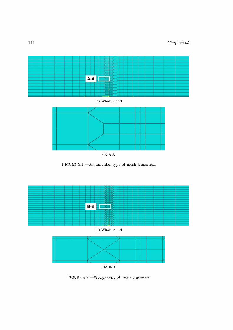
144 Chapitre 05
(a) Whole model
(b) A-A
Figure 5.1 � Rectangular type of mesh transition
(a) Whole model
(b) B-B
Figure 5.2 � Wedge type of mesh transition
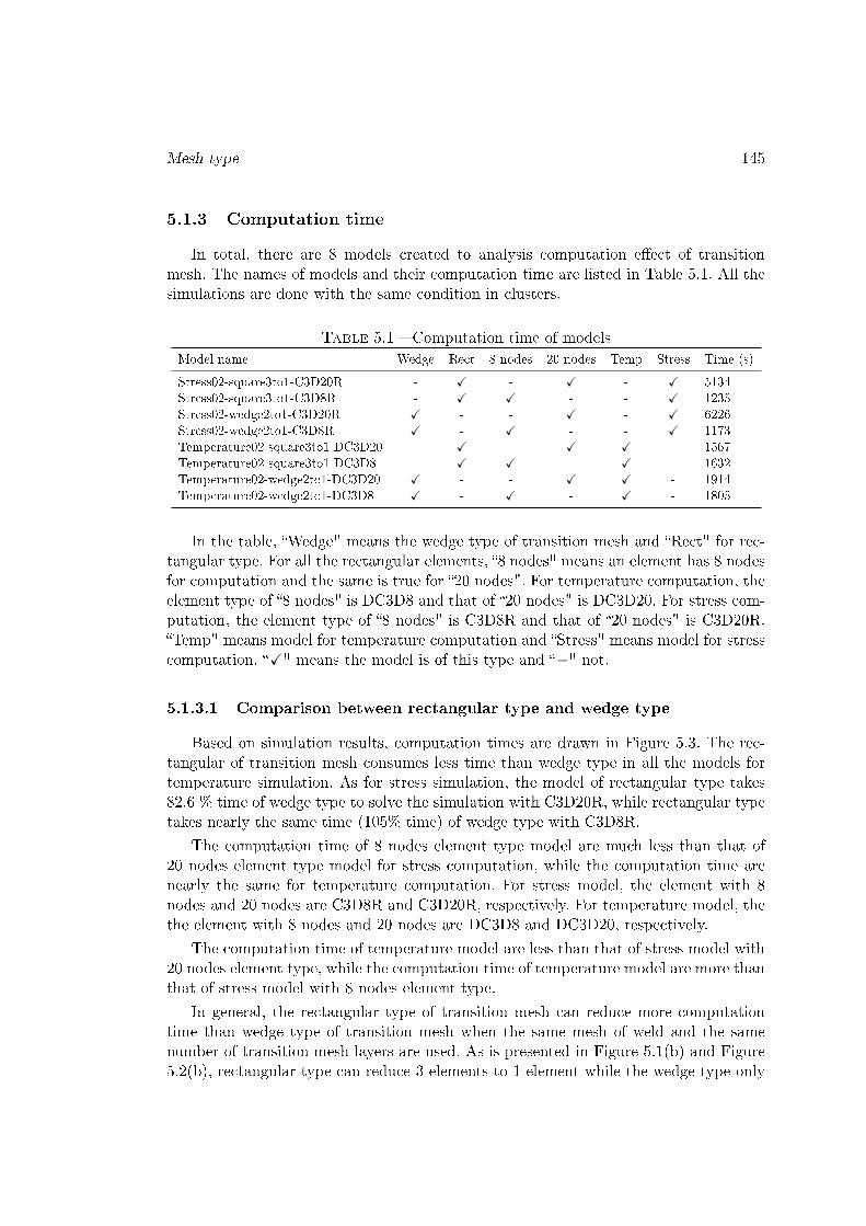
Mesh type 145
5.1.3 Computation time
In total, there are 8 models created to analysis computation e�ect of transitionmesh. The names of models and their computation time are listed in Table 5.1. All thesimulations are done with the same condition in clusters.
Table 5.1 � Computation time of modelsModel name Wedge Rect 8 nodes 20 nodes Temp Stress Time (s)
Stress02-square3to1-C3D20R - X - X - X 5134Stress02-square3to1-C3D8R - X X - - X 1235Stress02-wedge2to1-C3D20R X - - X - X 6226Stress02-wedge2to1-C3D8R X - X - - X 1173Temperature02-square3to1-DC3D20 - X - X X - 1567Temperature02-square3to1-DC3D8 - X X - X - 1632Temperature02-wedge2to1-DC3D20 X - - X X - 1914Temperature02-wedge2to1-DC3D8 X - X - X - 1805
In the table, �Wedge" means the wedge type of transition mesh and �Rect" for rec-tangular type. For all the rectangular elements, �8 nodes" means an element has 8 nodesfor computation and the same is true for �20 nodes". For temperature computation, theelement type of �8 nodes" is DC3D8 and that of �20 nodes" is DC3D20. For stress com-putation, the element type of �8 nodes" is C3D8R and that of �20 nodes" is C3D20R.�Temp" means model for temperature computation and �Stress" means model for stresscomputation. �X" means the model is of this type and �−" not.
5.1.3.1 Comparison between rectangular type and wedge type
Based on simulation results, computation times are drawn in Figure 5.3. The rec-tangular of transition mesh consumes less time than wedge type in all the models fortemperature simulation. As for stress simulation, the model of rectangular type takes82.6 % time of wedge type to solve the simulation with C3D20R, while rectangular typetakes nearly the same time (105% time) of wedge type with C3D8R.
The computation time of 8 nodes element type model are much less than that of20 nodes element type model for stress computation, while the computation time arenearly the same for temperature computation. For stress model, the element with 8nodes and 20 nodes are C3D8R and C3D20R, respectively. For temperature model, thethe element with 8 nodes and 20 nodes are DC3D8 and DC3D20, respectively.
The computation time of temperature model are less than that of stress model with20 nodes element type, while the computation time of temperature model are more thanthat of stress model with 8 nodes element type.
In general, the rectangular type of transition mesh can reduce more computationtime than wedge type of transition mesh when the same mesh of weld and the samenumber of transition mesh layers are used. As is presented in Figure 5.1(b) and Figure5.2(b), rectangular type can reduce 3 elements to 1 element while the wedge type only

146 Chapitre 05
Figure 5.3 � Comparison of computation time between wedge type and rectangulartype
reduce 2 elements to 1 element.
A further compare for element type of stress model is investigated. The transitionlayer is rectangular type and the element type is C3D20, C3D20R, C3D8 and C3D8R,seperately. The computation is done on a computer with 4 CPU of Intel Core i7-4700HQ.
Figure 5.4 � Comparison of computation time of di�erent element type model
As can be seen in Figure 5.4, among all element type models, the model with C3D8Rconsumes the least time.
Based on above analyses, two conclusion are listed below :
� The rectangular type of transition mesh can reduce more computation time thanwedge type of transition mesh when the same mesh of weld and the same number
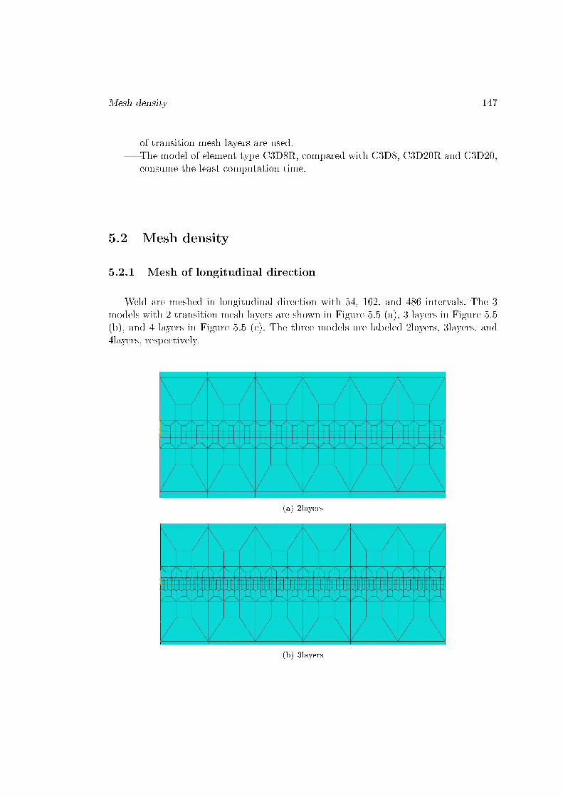
Mesh density 147
of transition mesh layers are used.� The model of element type C3D8R, compared with C3D8, C3D20R and C3D20,
consume the least computation time.
5.2 Mesh density
5.2.1 Mesh of longitudinal direction
Weld are meshed in longitudinal direction with 54, 162, and 486 intervals. The 3models with 2 transition mesh layers are shown in Figure 5.5 (a), 3 layers in Figure 5.5(b), and 4 layers in Figure 5.5 (c). The three models are labeled 2layers, 3layers, and4layers, respectively.
(a) 2layers
(b) 3layers

148 Chapitre 05
(c) 4layers
Figure 5.5 � Mesh of longitudinal direction
The residual stress distributions of models are presented in Figure 5.6. The equiva-lent stress at weld zone is the highest and the equivalent stress decreases outward theweld-transverse in-plate direction. With the intervals increase, the residual stress in thezone adjacent to middle weld increase.
(a) 2layers
(b) 3layers
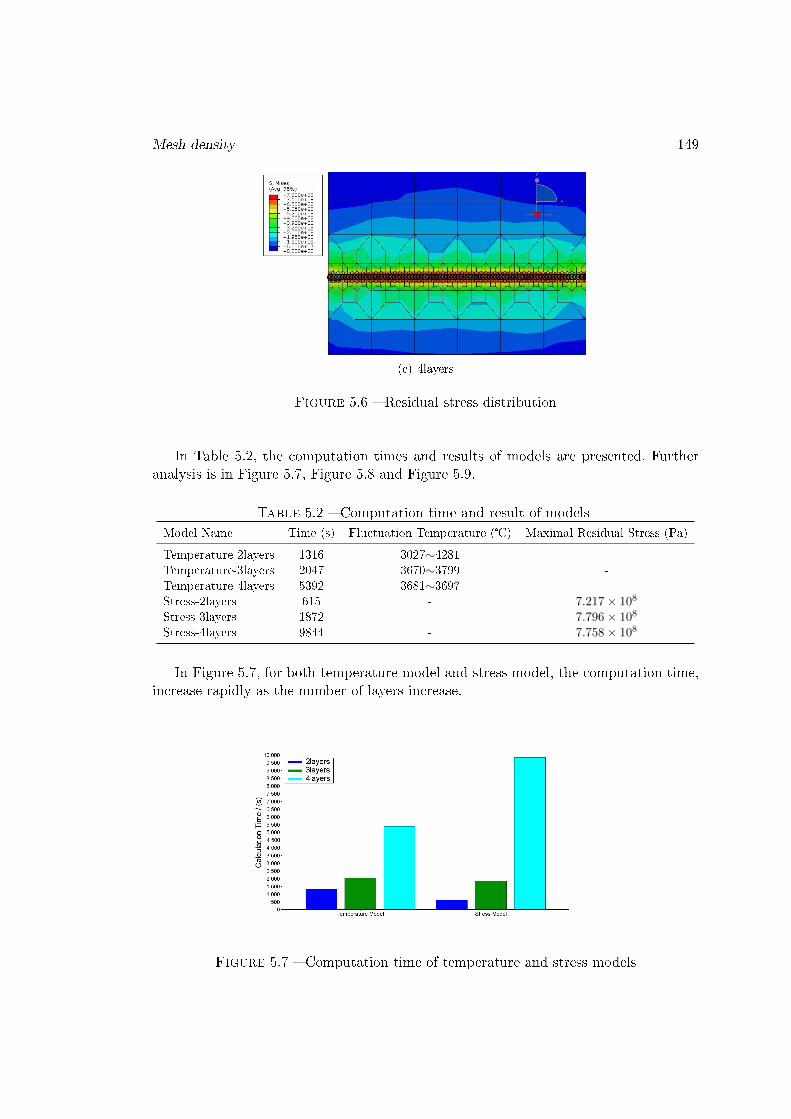
Mesh density 149
(c) 4layers
Figure 5.6 � Residual stress distribution
In Table 5.2, the computation times and results of models are presented. Furtheranalysis is in Figure 5.7, Figure 5.8 and Figure 5.9.
Table 5.2 � Computation time and result of modelsModel Name Time (s) Fluctuation Temperature (�) Maximal Residual Stress (Pa)
Temperature-2layers 1316 3027∼4281 -Temperature-3layers 2047 3670∼3799 -Temperature-4layers 5392 3681∼3697 -Stress-2layers 615 - 7.217× 10⁸
Stress-3layers 1872 - 7.796× 10⁸
Stress-4layers 9844 - 7.758× 10⁸
In Figure 5.7, for both temperature model and stress model, the computation time,increase rapidly as the number of layers increase.
Figure 5.7 � Computation time of temperature and stress models

150 Chapitre 05
From the results of temperature models 2layers, 3layers, and 4layers, the �uctua-tion of the temperature of molten pool are drawn in �gure 5.8. The temperature model2layers has 54 intervals, 3layers 162 intervals, and 4layers 486 intervals. With the num-ber of layers increase, meaning the mesh size decrease, the �uctuation of temperaturedecrease.
Figure 5.8 � Numerical results of temperature range of melting pool heated by laser
The maximal residual stress calculated from the stress models are presented in Figure5.9. The maximal residual stress of the �stress-2layers" model has a big di�erence withresults of �stress-3layers" and �stress-4layers" model. The non correct result may resultfrom the �uctuation of the weld pool temperature. The maximal residual stress of�stress-3layers" model only have a 5% di�erence with the �stress-4layers" model whilethe time consumption of the �stress-3layers" model is only 19% of the �stress-4layers"model.
Figure 5.9 � The maximal residual stress of models with di�erent layers
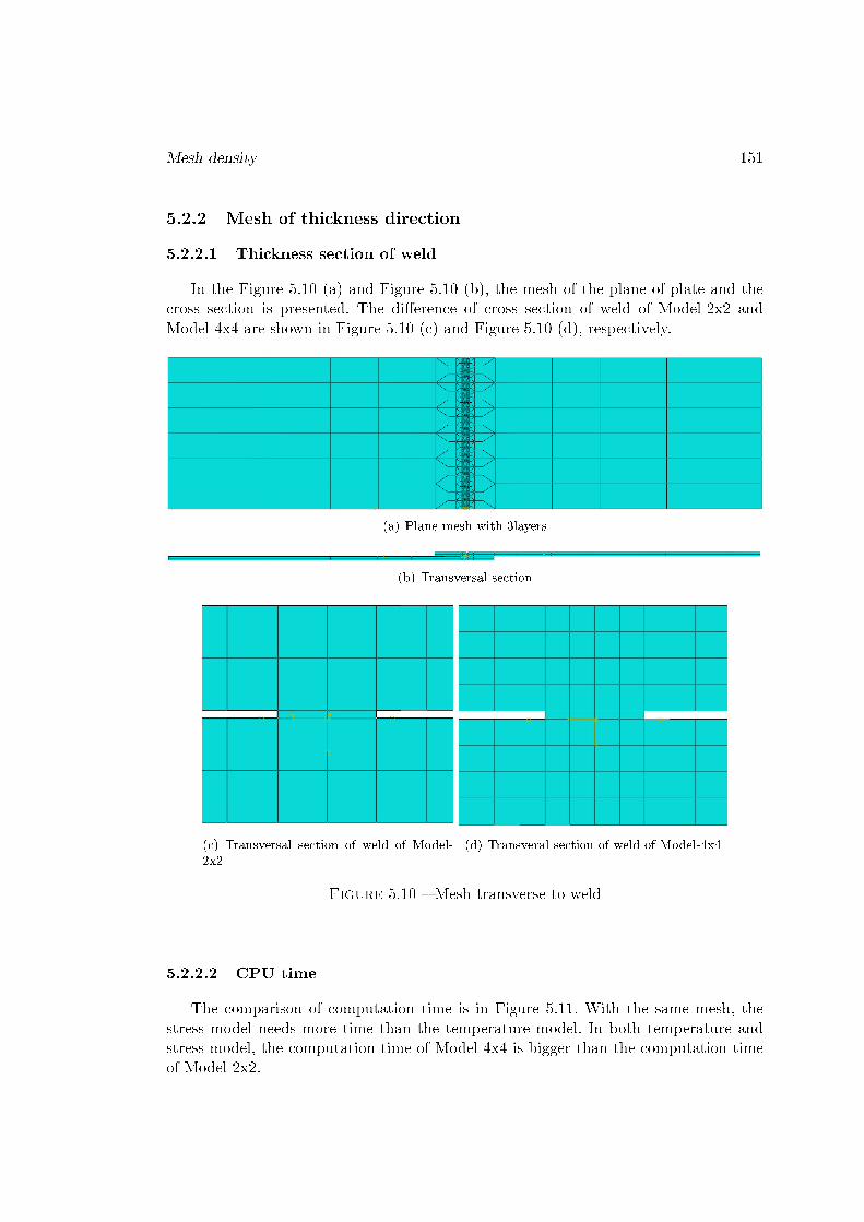
Mesh density 151
5.2.2 Mesh of thickness direction
5.2.2.1 Thickness section of weld
In the Figure 5.10 (a) and Figure 5.10 (b), the mesh of the plane of plate and thecross section is presented. The di�erence of cross section of weld of Model-2x2 andModel-4x4 are shown in Figure 5.10 (c) and Figure 5.10 (d), respectively.
(a) Plane mesh with 3layers
(b) Transversal section
(c) Transversal section of weld of Model-2x2
(d) Transveral section of weld of Model-4x4
Figure 5.10 � Mesh transverse to weld
5.2.2.2 CPU time
The comparison of computation time is in Figure 5.11. With the same mesh, thestress model needs more time than the temperature model. In both temperature andstress model, the computation time of Model-4x4 is bigger than the computation timeof Model-2x2.
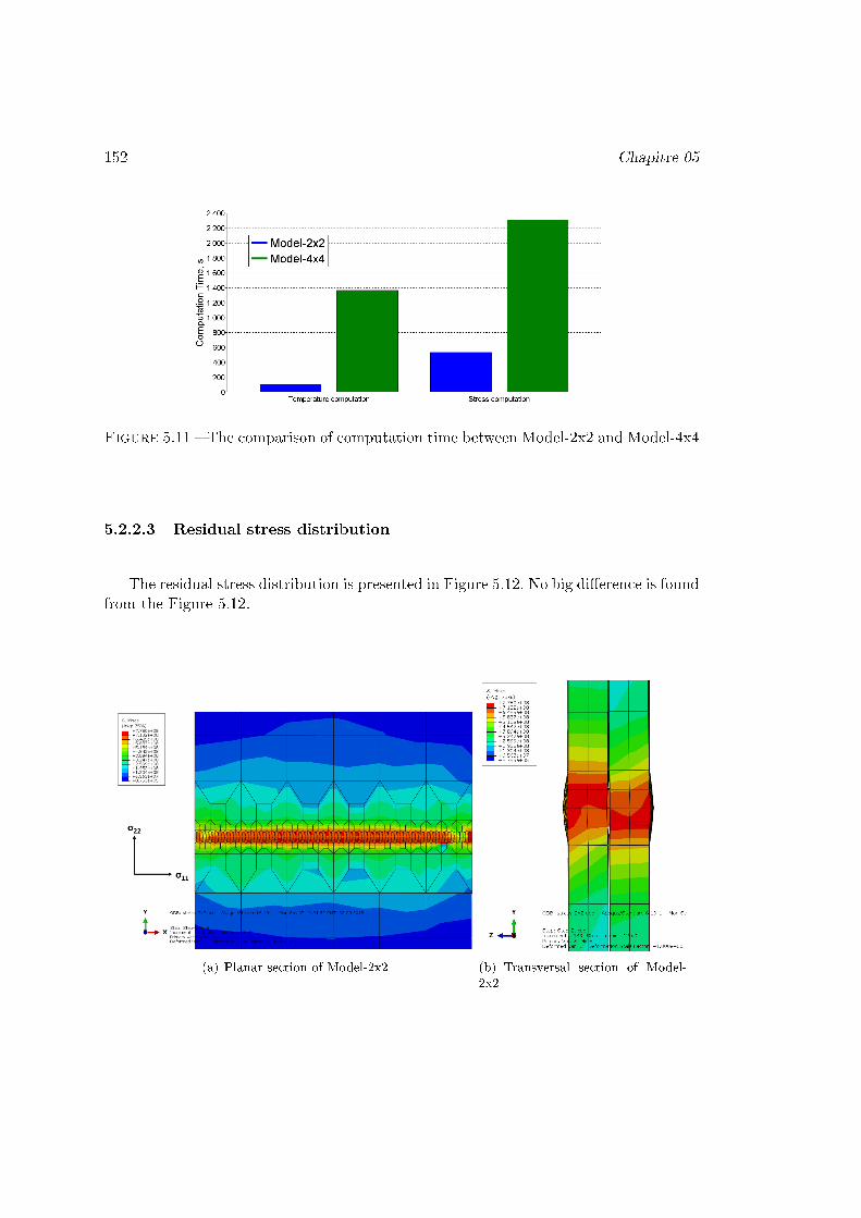
152 Chapitre 05
Figure 5.11 � The comparison of computation time between Model-2x2 and Model-4x4
5.2.2.3 Residual stress distribution
The residual stress distribution is presented in Figure 5.12. No big di�erence is foundfrom the Figure 5.12.
(a) Planar section of Model-2x2 (b) Transversal section of Model-2x2
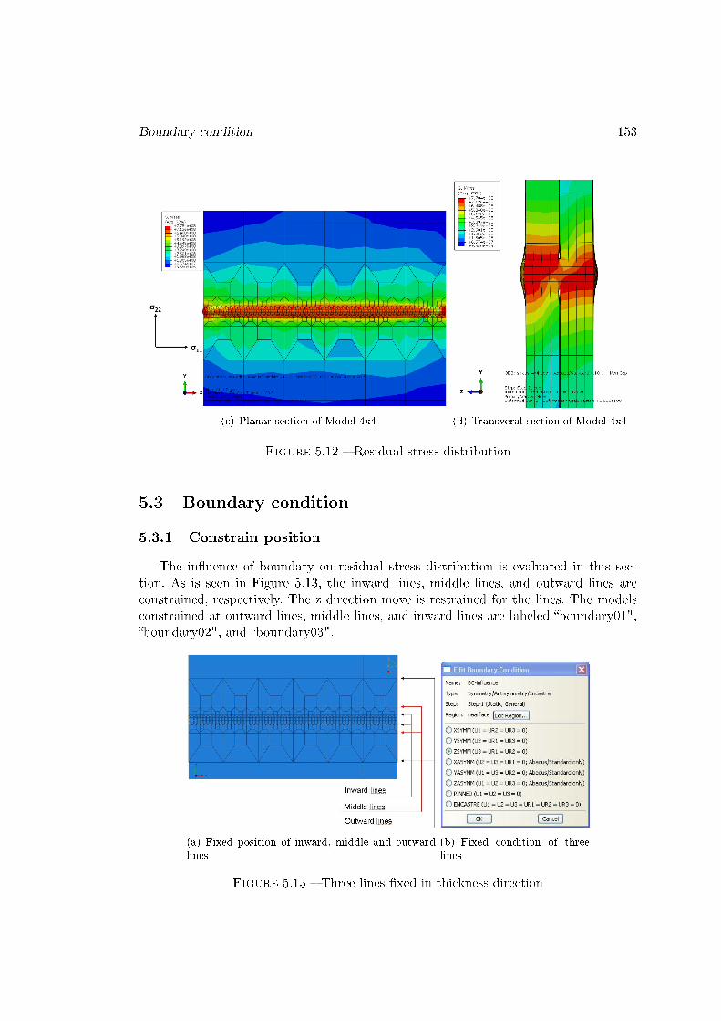
Boundary condition 153
(c) Planar section of Model-4x4 (d) Transveral section of Model-4x4
Figure 5.12 � Residual stress distribution
5.3 Boundary condition
5.3.1 Constrain position
The in�uence of boundary on residual stress distribution is evaluated in this sec-tion. As is seen in Figure 5.13, the inward lines, middle lines, and outward lines areconstrained, respectively. The z direction move is restrained for the lines. The modelsconstrained at outward lines, middle lines, and inward lines are labeled �boundary01",�boundary02", and �boundary03".
(a) Fixed position of inward, middle and outwardlines
(b) Fixed condition of threelines
Figure 5.13 � Three lines �xed in thickness direction

154 Chapitre 05
5.3.2 Simulation results
In the �gure below, �L01-Mises" means the equivalent stress along weld longitudinalpath of model �boundary01". �L" means longtitudinal path and �T" means transversalpath. �01" means model �boundary01", �02" means model �boundary02", and �03" meansmodel �boundary03". �Mises" means the equivalent stress, �σ11" means the residualstress along weld longitudinal direction σ11 and �σ22" means the residual stress alongweld-transversal direction σ22.
5.3.2.1 Equivalent residual stress
In Figure 5.14, equivalent stress along weld longtitudinal path are presented. Themodel �boundary03" with the inward lines constrained has the most stable and thehighest equivalent stress along weld longitudinal path. The equivalent stress of mo-del �boundary02" with the middle lines constrained and model �boundary01" with theoutward lines constrained decrease at the zone of two ends of the weld.
Figure 5.14 � Equivalent stress along weld longtitudinal path
In Figure 5.15, mises stress along transversal path are presented. The mises stressalong transversal path of Model �boundary01", �boundary02", and �boundary03" arenearly the same.
Figure 5.15 � equivalent stress along transversal path

Boundary condition 155
5.3.2.2 Weld longitudinal direction residual stress
In Figure 5.16, σ11 along weld longitudinal path are presented. With the constrainmoves from outer lines to inner lines, the longitudinal residual stress σ11 along weldlongtitudinal path decreases.
Figure 5.16 � σ11 along weld longitudinal path
In Figure 5.17, σ11 along transversal path are presented. With the constrain movesfrom outer lines to inner lines, the longitudinal residual stress σ11 decreases at the weldzone and tends to be the same at the HAZ and base metal. σ11 is tensile residual atweld zone, and compress residual adjacent to the weld zone, and gradually decrease tozero at the zone further than 40mm from the weld.
Figure 5.17 � σ11 along transversal path

156 Chapitre 05
5.3.2.3 Weld transversal direction residual stress
In Figure 5.18, σ22 along weld longitudinal path are presented. With the constrainmoves from outer lines to inner lines, the compress longitudinal residual stress σ22 alongweld longitudinal path increases.
Figure 5.18 � σ22 along weld longitudinal path
In Figure 5.19, σ22 along transversal path are presented. The transversal residualstress σ22 along transversal path of Model �boundary01", �boundary02", and �boun-dary03" are nearly the same.
Figure 5.19 � σ22 along transversal path
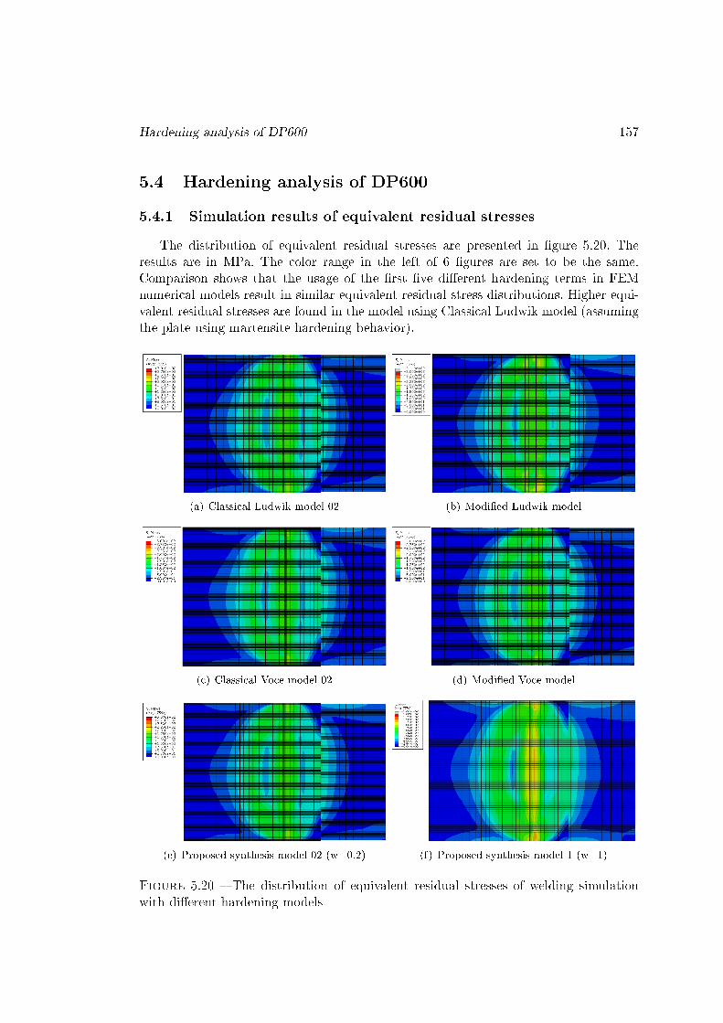
Hardening analysis of DP600 157
5.4 Hardening analysis of DP600
5.4.1 Simulation results of equivalent residual stresses
The distribution of equivalent residual stresses are presented in �gure 5.20. Theresults are in MPa. The color range in the left of 6 �gures are set to be the same.Comparison shows that the usage of the �rst �ve di�erent hardening terms in FEMnumerical models result in similar equivalent residual stress distributions. Higher equi-valent residual stresses are found in the model using Classical Ludwik model (assumingthe plate using martensite hardening behavior).
(a) Classical Ludwik model 02 (b) Modi�ed Ludwik model
(c) Classical Voce model 02 (d) Modi�ed Voce model
(e) Proposed synthesis model 02 (w=0.2) (f) Proposed synthesis model 1 (w=1)
Figure 5.20 � The distribution of equivalent residual stresses of welding simulationwith di�erent hardening models
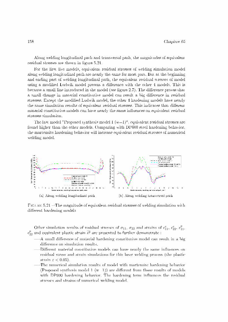
158 Chapitre 05
Along welding longitudinal path and transversal path, the magnitudes of equivalentresidual stresses are shown in �gure 5.21.
For the �rst �ve models, equivalent residual stresses of welding simulation modelalong welding longitudinal path are nearly the same for most part. But at the beginningand ending part of welding longitudinal path, the equivalent residual stresses of modelusing a modi�ed Ludwik model present a di�erence with the other 4 models. This isbecause a small line introduced in the model (see �gure 2.7). The di�erence proves thata small change in material constitutive model can result a big di�erence in residualstresses. Except the modi�ed Ludwik model, the other 4 hardening models have nearlythe same simulation results of equivalent residual stresses. This indicates that di�erentmaterial constitutive models can have nearly the same in�uences on equivalent residualstresses simulation.
The last model "Proposed synthesis model 1 (w=1)", equivalent residual stresses arefound higher than the other models. Comparing with DP600 steel hardening behavior,the martensite hardening behavior will increase equivalent residual stresses of numericalwelding model.
(a) Along welding longitudinal path (b) Along welding transversal path
Figure 5.21 � The magnitude of equivalent residual stresses of welding simulation withdi�erent hardening models
Other simulation results of residual stresses of σ11, σ22 and strains of εe11, εe22, ε
p11,
εp22 and equivalent plastic strain εp are presented to further demonstrate :
� A small di�erence of material hardening constitutive model can result in a bigdi�erence on simulation results.
� Di�erent material constitutive models can have nearly the same in�uences onresidual stress and strain simulations for this laser welding process (the plasticstrain ε < 0.05).
� The numerical simulation results of model with martensite hardening behavior(Proposed synthesis model 1 (w=1)) are di�erent from those results of modelswith DP600 hardening behavior. The hardening term in�uences the residualstresses and strains of numerical welding model.

Hardening analysis of DP600 159
5.4.2 Simulation results of σ11 residual stresses
The distribution of σ11 residual stresses are presented in �gure 5.22. The distributionare similar except �gure 5.22 (b) has some di�erences of red regions.
(a) Classical Ludwik model 02 (b) Modi�ed Ludwik model
(c) Classical Voce model 02 (d) Modi�ed Voce model
(e) Proposed synthesis model 02 (w=0.2) (f) Proposed synthesis model 1 (w=1)
Figure 5.22 � The distribution of σ11 residual stresses of welding simulation withdi�erent hardening models
Along welding longitudinal path and transversal path, the magnitude of σ11 areshown in �gure 5.23. The equivalent residual stresses of model using a modi�ed Ludwikmodel also present a di�erence with the other 4 models.

160 Chapitre 05
(a) Along welding longitudinal path (b) Along welding transversal path
Figure 5.23 � The magnitude of σ11 residual stresses of welding simulation with dif-ferent hardening models
5.4.3 Simulation results of σ22 residual stresses
The distribution of σ22 residual stresses are presented in �gure 5.24.
(a) Classical Ludwik model 02 (b) Modi�ed Ludwik model
(c) Classical Voce model 02 (d) Modi�ed Voce model

Hardening analysis of DP600 161
(e) Proposed synthesis model 02 (w=0.2) (f) Proposed synthesis model 1 (w=1)
Figure 5.24 � The distribution of σ22 residual stresses of welding simulation withdi�erent hardening models
Along welding longitudinal path and transversal path, the magnitude of σ22 areshown in �gure 5.25.
(a) Along welding longitudinal path (b) Along welding transversal path
Figure 5.25 � The magnitude of σ22 residual stresses of welding simulation with dif-ferent hardening models
5.4.4 Simulation results of εe11 residual elastic strains
The distribution of εe11 residual elastic strains are presented in �gure 5.26.
(a) Classical Ludwik model 02 (b) Modi�ed Ludwik model

162 Chapitre 05
(c) Classical Voce model 02 (d) Modi�ed Voce model
(e) Proposed synthesis model 02 (w=0.2) (f) Proposed synthesis model 1 (w=1)
Figure 5.26 � The distribution of εe11 residual strains of welding simulation with dif-ferent hardening models
Along welding longitudinal path and transversal path, the magnitude of εe11 areshown in �gure 5.27.
(a) Along welding longitudinal path (b) Along welding transversal path
Figure 5.27 � The magnitude of εe11 residual strains of welding simulation with di�erenthardening models

Hardening analysis of DP600 163
5.4.5 Simulation results of εe22 residual elastic strains
The distribution of εe22 residual elastic strains are presented in �gure 5.28.
(a) Classical Ludwik model 02 (b) Modi�ed Ludwik model
(c) Classical Voce model 02 (d) Modi�ed Voce model
(e) Proposed synthesis model 02 (w=0.2) (f) Proposed synthesis model 1 (w=1)
Figure 5.28 � The distribution of εe22 residual strains of welding simulation with dif-ferent hardening models
Along welding longitudinal path and transversal path, the magnitude of εe22 areshown in �gure 5.29.

164 Chapitre 05
(a) Along welding longitudinal path (b) Along welding transversal path
Figure 5.29 � The magnitude of εe22 residual strains of welding simulation with di�erenthardening models
5.4.6 Simulation results of εp11 residual plastic strains
The distribution of εp11 residual plastic strains are presented in �gure 5.30.
(a) Classical Ludwik model 02 (b) Modi�ed Ludwik model
(c) Classical Voce model 02 (d) Modi�ed Voce model

Hardening analysis of DP600 165
(e) Proposed synthesis model 02 (w=0.2) (f) Proposed synthesis model 1 (w=1)
Figure 5.30 � The distribution of εp11 residual strains of welding simulation with dif-ferent hardening models
Along welding longitudinal path and transversal path, the magnitude of εp11 areshown in �gure 5.31.
(a) Along welding longitudinal path (b) Along welding transversal path
Figure 5.31 � The magnitude of εp11 residual strains of welding simulation with di�erenthardening models
5.4.7 Simulation results of εp22 residual plastic strains
The distribution of εp22 residual plastic strains are presented in �gure 5.32.
(a) Classical Ludwik model 02 (b) Modi�ed Ludwik model
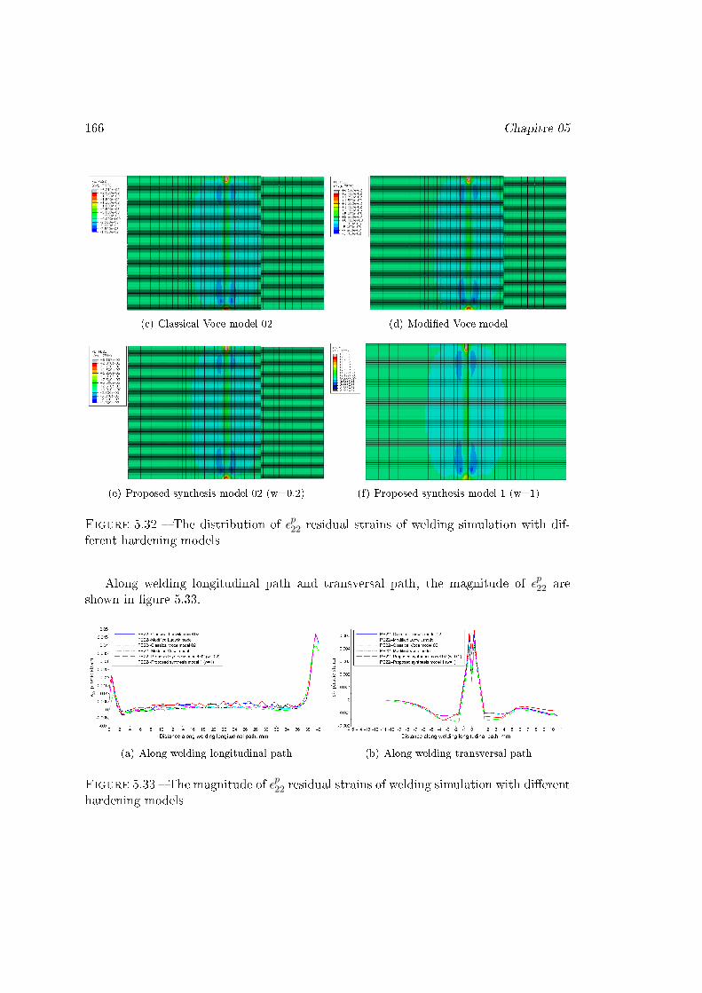
166 Chapitre 05
(c) Classical Voce model 02 (d) Modi�ed Voce model
(e) Proposed synthesis model 02 (w=0.2) (f) Proposed synthesis model 1 (w=1)
Figure 5.32 � The distribution of εp22 residual strains of welding simulation with dif-ferent hardening models
Along welding longitudinal path and transversal path, the magnitude of εp22 areshown in �gure 5.33.
(a) Along welding longitudinal path (b) Along welding transversal path
Figure 5.33 � The magnitude of εp22 residual strains of welding simulation with di�erenthardening models

Hardening analysis of DP600 167
5.4.8 Simulation results of εp residual equivalent plastic strains
The distribution of εp residual equivalent plastic strains are presented in �gure 5.34.
(a) Classical Ludwik model 02 (b) Modi�ed Ludwik model
(c) Classical Voce model 02 (d) Modi�ed Voce model
(e) Proposed synthesis model 02 (w=0.2) (f) Proposed synthesis model 1 (w=1)
Figure 5.34 � The distribution of εp residual strains of welding simulation with di�erenthardening models
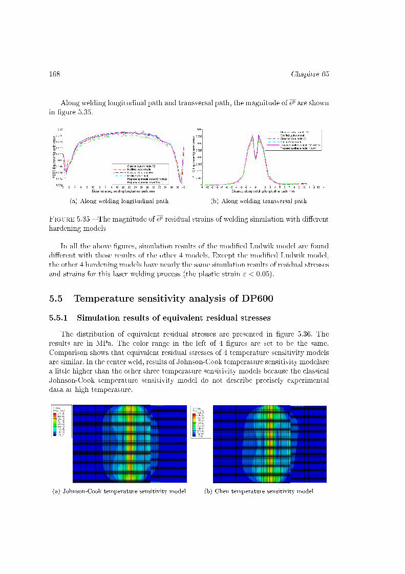
168 Chapitre 05
Along welding longitudinal path and transversal path, the magnitude of εp are shownin �gure 5.35.
(a) Along welding longitudinal path (b) Along welding transversal path
Figure 5.35 � The magnitude of εp residual strains of welding simulation with di�erenthardening models
In all the above �gures, simulation results of the modi�ed Ludwik model are founddi�erent with those results of the other 4 models. Except the modi�ed Ludwik model,the other 4 hardening models have nearly the same simulation results of residual stressesand strains for this laser welding process (the plastic strain ε < 0.05).
5.5 Temperature sensitivity analysis of DP600
5.5.1 Simulation results of equivalent residual stresses
The distribution of equivalent residual stresses are presented in �gure 5.36. Theresults are in MPa. The color range in the left of 4 �gures are set to be the same.Comparison shows that equivalent residual stresses of 4 temperature sensitivity modelsare similar. In the center weld, results of Johnson-Cook temperature sensitivity modelarea little higher than the other three temperature sensitivity models because the classicalJohnson-Cook temperature sensitivity model do not describe precisely experimentaldata at high temperature.
(a) Johnson-Cook temperature sensitivity model (b) Chen temperature sensitivity model
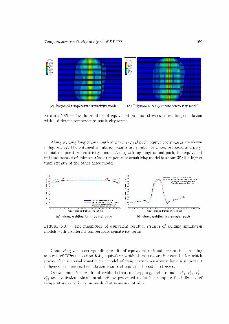
Temperature sensitivity analysis of DP600 169
(c) Proposed temperature sensitivity model (d) Polynomial temperature sensitivity model
Figure 5.36 � The distribution of equivalent residual stresses of welding simulationwith 4 di�erent temperature sensitivity terms
Along welding longitudinal path and transversal path, equivalent stresses are shownin �gure 5.37. The obtained simulation results are similar for Chen, proposed and poly-nomial temperature sensitivity model. Along welding longitudinal path, the equivalentresidual stresses of Johnson-Cook temperature sensitivity model is about 50MPa higherthan stresses of the other three model.
(a) Along welding longitudinal path (b) Along welding transversal path
Figure 5.37 � The magnitude of equivalent residual stresses of welding simulationmodels with 4 di�erent temperature sensitivity terms
Comparing with corresponding results of equivalent residual stresses in hardeninganalysis of DP600 (section 5.4), equivalent residual stresses are increased a lot whichproves that material constitutive model of temperature sensitivity have a importantin�uence on numerical simulation results of equivalent residual stresses.
Other simulation results of residual stresses of σ11, σ22 and strains of εe11, εe22, ε
p11,
εp22 and equivalent plastic strain εp are presented to further compare the in�uence oftemperature sensitivity on residual stresses and strains.
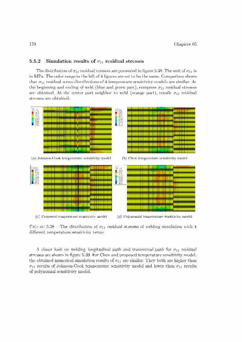
170 Chapitre 05
5.5.2 Simulation results of σ11 residual stresses
The distribution of σ11 residual stresses are presented in �gure 5.38. The unit of σ11 isin MPa. The color range in the left of 4 �gures are set to be the same. Comparison showsthat σ11 residual stress distributions of 4 temperature sensitivity models are similar. Atthe beginning and ending of weld (blue and green part), compress σ11 residual stressesare obtained. At the center part neighbor to weld (orange part), tensile σ11 residualstresses are obtained.
(a) Johnson-Cook temperature sensitivity model (b) Chen temperature sensitivity model
(c) Proposed temperature sensitivity model (d) Polynomial temperature sensitivity model
Figure 5.38 � The distribution of σ11 residual stresses of welding simulation with 4di�erent temperature sensitivity terms
A closer look on welding longitudinal path and transversal path for σ11 residualstresses are shown in �gure 5.39. For Chen and proposed temperature sensitivity model,the obtained numerical simulation results of σ11 are similar. They both are higher thanσ11 results of Johnson-Cook temperature sensitivity model and lower than σ11 resultsof polynomial sensitivity model.

Temperature sensitivity analysis of DP600 171
(a) Along welding longitudinal path (b) Along welding transversal path
Figure 5.39 � The magnitude of σ11 residual stresses of welding simulation modelswith 4 di�erent temperature sensitivity terms
5.5.3 Simulation results of σ22 residual stresses
The distribution of σ22 residual stresses are presented in �gure 5.40. The unit of σ22
is in MPa. The color range in the left of 4 �gures are set to be the same. Comparisonshows that σ22 residual stress distributions of 4 temperature sensitivity models aresimilar. At weld region and the region around weld (orange and green part), tensile σ22
residual stresses are obtained. At the outer part far from weld (blue part), compress σ22
residual stresses are obtained.
(a) Johnson-Cook temperature sensitivity mo-del
(b) Chen temperature sensitivity model
(c) Proposed temperature sensitivity model (d) Polynomial temperature sensitivity model
Figure 5.40 � The distribution of σ22 residual stresses of welding simulation with 4di�erent temperature sensitivity terms

172 Chapitre 05
A closer look on welding longitudinal path and transversal path for σ22 residualstresses are shown in �gure 5.41. For Chen, proposed and polynomial temperature sen-sitivity model, the obtained numerical simulation results of σ22 are similar. At thebeginning and ending part along welding longitudinal path in �gure 5.41 (a), the σ22
results of Johnson-Cook temperature sensitivity model are a little lower than σ22 resultsof the other three temperature sensitivity models.
(a) Along welding longitudinal path (b) Along welding transversal path
Figure 5.41 � The magnitude of σ22 residual stresses of welding simulation modelswith 4 di�erent temperature sensitivity terms
5.5.4 Simulation results of εe11 residual elastic strains
The distribution of εe11 elastic strains are presented in �gure 5.42. The color rangein the left of 4 �gures are set to be the same. Comparison shows that εe11 elastic straindistributions of 4 temperature sensitivity models are similar. At weld region and theregion around weld (blue, green and yellow part), compressible εe11 elastic strains areobtained. At the center plate neighbor to weld (red and orange part), tensile εe11 elasticstrains are obtained.
(a) Johnson-Cook temperature sensitivity model (b) Chen temperature sensitivity model
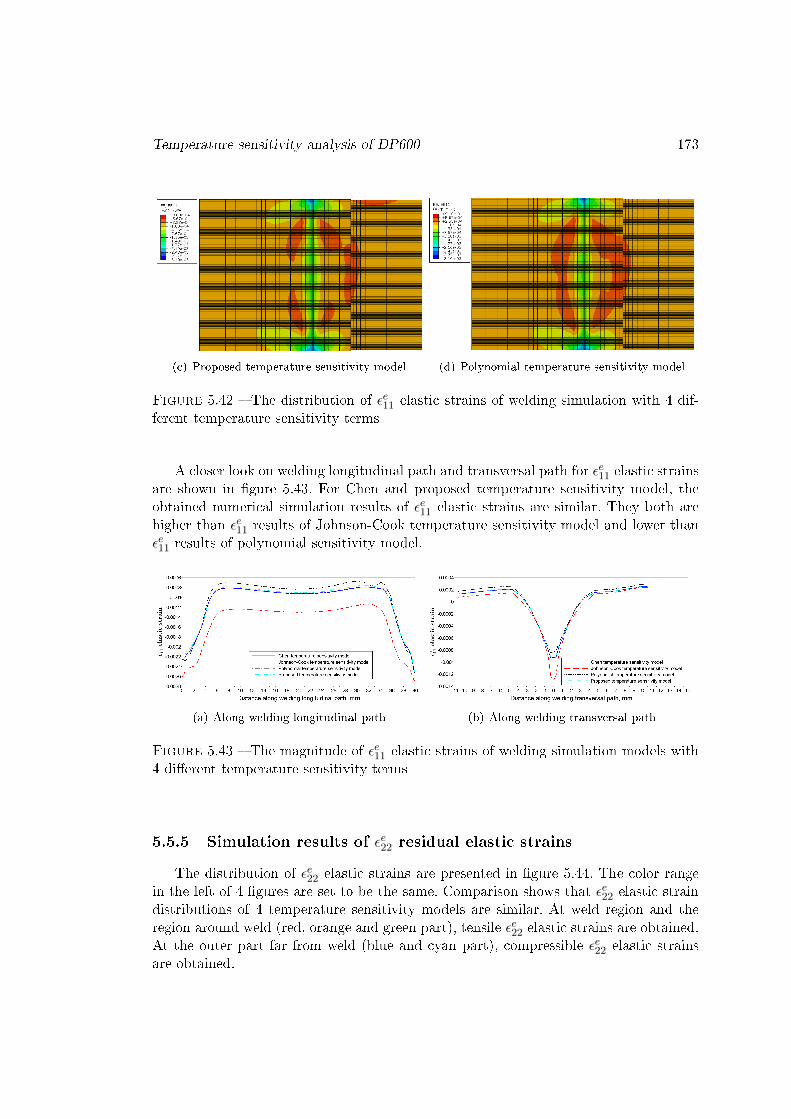
Temperature sensitivity analysis of DP600 173
(c) Proposed temperature sensitivity model (d) Polynomial temperature sensitivity model
Figure 5.42 � The distribution of εe11 elastic strains of welding simulation with 4 dif-ferent temperature sensitivity terms
A closer look on welding longitudinal path and transversal path for εe11 elastic strainsare shown in �gure 5.43. For Chen and proposed temperature sensitivity model, theobtained numerical simulation results of εe11 elastic strains are similar. They both arehigher than εe11 results of Johnson-Cook temperature sensitivity model and lower thanεe11 results of polynomial sensitivity model.
(a) Along welding longitudinal path (b) Along welding transversal path
Figure 5.43 � The magnitude of εe11 elastic strains of welding simulation models with4 di�erent temperature sensitivity terms
5.5.5 Simulation results of εe22 residual elastic strains
The distribution of εe22 elastic strains are presented in �gure 5.44. The color rangein the left of 4 �gures are set to be the same. Comparison shows that εe22 elastic straindistributions of 4 temperature sensitivity models are similar. At weld region and theregion around weld (red, orange and green part), tensile εe22 elastic strains are obtained.At the outer part far from weld (blue and cyan part), compressible εe22 elastic strainsare obtained.
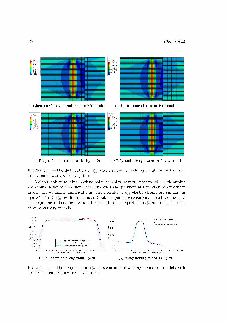
174 Chapitre 05
(a) Johnson-Cook temperature sensitivity model (b) Chen temperature sensitivity model
(c) Proposed temperature sensitivity model (d) Polynomial temperature sensitivity model
Figure 5.44 � The distribution of εe22 elastic strains of welding simulation with 4 dif-ferent temperature sensitivity terms
A closer look on welding longitudinal path and transversal path for εe22 elastic strainsare shown in �gure 5.45. For Chen, proposed and polynomial temperature sensitivitymodel, the obtained numerical simulation results of εe22 elastic strains are similar. In�gure 5.45 (a), εe22 results of Johnson-Cook temperature sensitivity model are lower atthe beginning and ending part and higher in the center part than εe22 results of the otherthree sensitivity models.
(a) Along welding longitudinal path (b) Along welding transversal path
Figure 5.45 � The magnitude of εe22 elastic strains of welding simulation models with4 di�erent temperature sensitivity terms

Temperature sensitivity analysis of DP600 175
5.5.6 Simulation results of εp11 residual plastic strains
The distribution of εp11 plastic strains are presented in �gure 5.46. The color rangein the left of 4 �gures are set to be the same. Comparison shows that εp11 plastic straindistributions of 4 temperature sensitivity models are di�erent. A wider green regionof εp11 plastic strain distributions of Jonhson-Cook temperature sensitivity model arefound than the other three models, a red region which stands for more lower value ofεp11 plastic strain is obtained by Chen temperature sensitivity model .
(a) Johnson-Cook temperature sensitivity model (b) Chen temperature sensitivity model
(c) Proposed temperature sensitivity model (d) Polynomial temperature sensitivity model
Figure 5.46 � The distribution of εp11 plastic strains of welding simulation with 4di�erent temperature sensitivity terms
A closer look on welding longitudinal path and transversal path for εp11 plastic strainsare shown in �gure 5.47. At the weld region and the region around the weld, compressibleεp11 plastic strains are obtained. For Johnson-Cook temperature sensitivity model alongwelding longitudinal and transversal path, the obtained numerical simulation resultsof εp11 plastic strains have a big di�erence with εp11 of polynomial, proposed and Chentemperature sensitivity models. Along welding longitudinal path, εp11 plastic strains ofpolynomial temperature sensitivity model are also di�erent with εp11 of proposed andChen temperature sensitivity models. εp11 of proposed and Chen temperature sensitivitymodels are similar and only a little di�erence is present at the ending part of weld.

176 Chapitre 05
(a) Along welding longitudinal path (b) Along welding transversal path
Figure 5.47 � The magnitude of εp11 plastic strains of welding simulation models with4 di�erent temperature sensitivity terms
5.5.7 Simulation results of εp22 residual plastic strains
The distribution of εp22 plastic strains are presented in �gure 5.48. The color rangein the left of 4 �gures are set to be the same. Comparison shows that εp22 plastic straindistributions of 4 temperature sensitivity models are similar. For all the plate, εp22 plasticstrain distributions are found εp22 = 0 based on �gure 5.49(b) (green region), a lowervalue of εp22 plastic strain is obtained at weld (blue part).
(a) Johnson-Cook temperature sensitivity model (b) Chen temperature sensitivity model
(c) Proposed temperature sensitivity model (d) Polynomial temperature sensitivity model
Figure 5.48 � The distribution of εp22 plastic strains of welding simulation with 4di�erent temperature sensitivity terms

Temperature sensitivity analysis of DP600 177
A closer look on welding longitudinal path and transversal path for εp22 plastic strainsare shown in �gure 5.49. Along welding longitudinal path in �gure 5.49 (a), εp22 plasticstrains of four temperature sensitivity models are around 0 at the center part and havesome di�erences at the beginning and ending part. Along welding transversal path in�gure 5.49 (b), εp22 plastic strains of proposed temperature sensitivity model are moreclosed to polynomial model and have some di�erence with Chen and Johnson-Cooktemperature sensitivity model.
(a) Along welding longitudinal path (b) Along welding transversal path
Figure 5.49 � The magnitude of εp22 plastic strains of welding simulation models with4 di�erent temperature sensitivity terms
5.5.8 Simulation results of εp equivalent residual strains
The distribution of εp e�ective plastic strains are presented in �gure 5.50. The colorrange in the left of 4 �gures are set to be the same. Comparison shows that εp e�ectiveplastic strain distributions of 4 temperature sensitivity models are di�erent. A widergreen region of εp e�ective plastic strain distributions of Jonhson-Cook temperaturesensitivity model are found than the other three models, and red region which standsfor higher value of εp e�ective plastic strain is found at center weld. The red region is alsofound in εp distribution of polynomial temperature sensitivity model. εp distribution ofChen and proposed temperature sensitivity models are similar.
(a) Johnson-Cook temperature sensitivity model (b) Chen temperature sensitivity model

178 Chapitre 05
(c) Proposed temperature sensitivity model (d) Polynomial temperature sensitivity model
Figure 5.50 � The distribution of εp e�ective plastic strains of welding simulation with4 di�erent temperature sensitivity terms
A closer look on welding longitudinal path and transversal path for εp e�ective plasticstrains are shown in �gure 5.51. A big di�erence of εp of Johnson-Cook temperaturesensitivity model is found compared with εp of the other three models. εp of polynomialmodel is similar along longitudinal path but a little di�erent along transversal pathwith εp of proposed and Chen temperature sensitivity model. εp of proposed and Chentemperature sensitivity models are similar.
(a) Along welding longitudinal path (b) Along welding transversal path
Figure 5.51 � The magnitude of εp e�ective plastic strains of welding simulation modelswith 4 di�erent temperature sensitivity terms
In all above �gures, simulation results analyzing temperature sensitivity are founddi�erent with those results analyzing hardening in section 5.4. These comparison provesthat temperature sensitivity has an important in�uence on simulation results of residualstresses and strains in laser welding process.
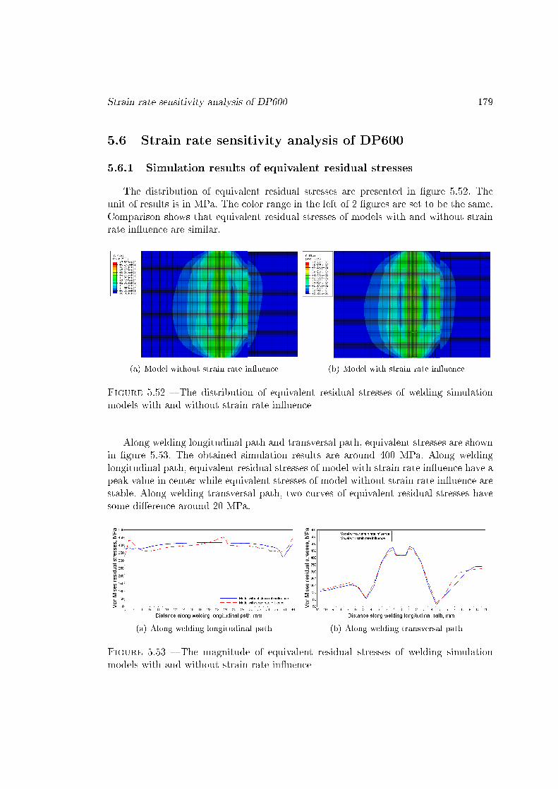
Strain rate sensitivity analysis of DP600 179
5.6 Strain rate sensitivity analysis of DP600
5.6.1 Simulation results of equivalent residual stresses
The distribution of equivalent residual stresses are presented in �gure 5.52. Theunit of results is in MPa. The color range in the left of 2 �gures are set to be the same.Comparison shows that equivalent residual stresses of models with and without strainrate in�uence are similar.
(a) Model without strain rate in�uence (b) Model with strain rate in�uence
Figure 5.52 � The distribution of equivalent residual stresses of welding simulationmodels with and without strain rate in�uence
Along welding longitudinal path and transversal path, equivalent stresses are shownin �gure 5.53. The obtained simulation results are around 400 MPa. Along weldinglongitudinal path, equivalent residual stresses of model with strain rate in�uence have apeak value in center while equivalent stresses of model without strain rate in�uence arestable. Along welding transversal path, two curves of equivalent residual stresses havesome di�erence around 20 MPa.
(a) Along welding longitudinal path (b) Along welding transversal path
Figure 5.53 � The magnitude of equivalent residual stresses of welding simulationmodels with and without strain rate in�uence
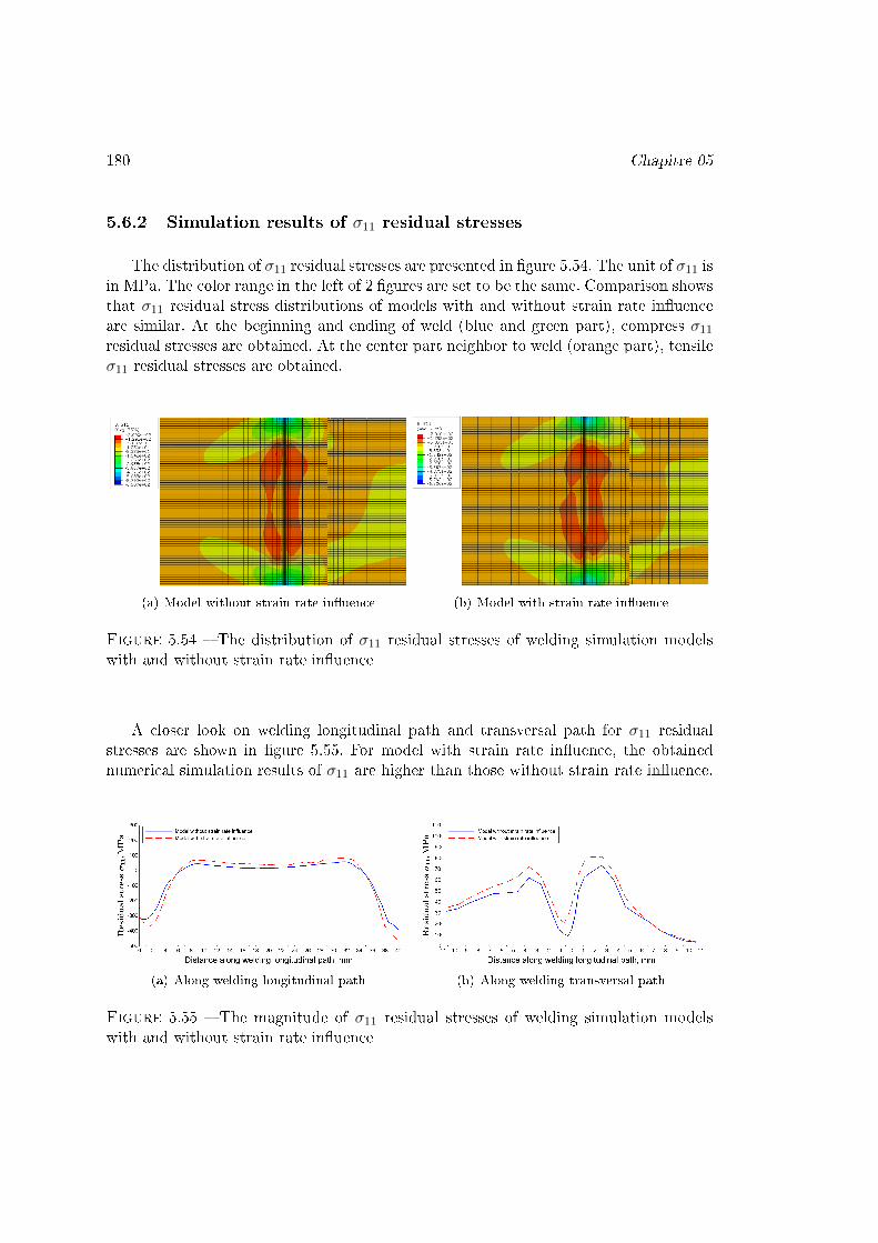
180 Chapitre 05
5.6.2 Simulation results of σ11 residual stresses
The distribution of σ11 residual stresses are presented in �gure 5.54. The unit of σ11 isin MPa. The color range in the left of 2 �gures are set to be the same. Comparison showsthat σ11 residual stress distributions of models with and without strain rate in�uenceare similar. At the beginning and ending of weld (blue and green part), compress σ11
residual stresses are obtained. At the center part neighbor to weld (orange part), tensileσ11 residual stresses are obtained.
(a) Model without strain rate in�uence (b) Model with strain rate in�uence
Figure 5.54 � The distribution of σ11 residual stresses of welding simulation modelswith and without strain rate in�uence
A closer look on welding longitudinal path and transversal path for σ11 residualstresses are shown in �gure 5.55. For model with strain rate in�uence, the obtainednumerical simulation results of σ11 are higher than those without strain rate in�uence.
(a) Along welding longitudinal path (b) Along welding transversal path
Figure 5.55 � The magnitude of σ11 residual stresses of welding simulation modelswith and without strain rate in�uence
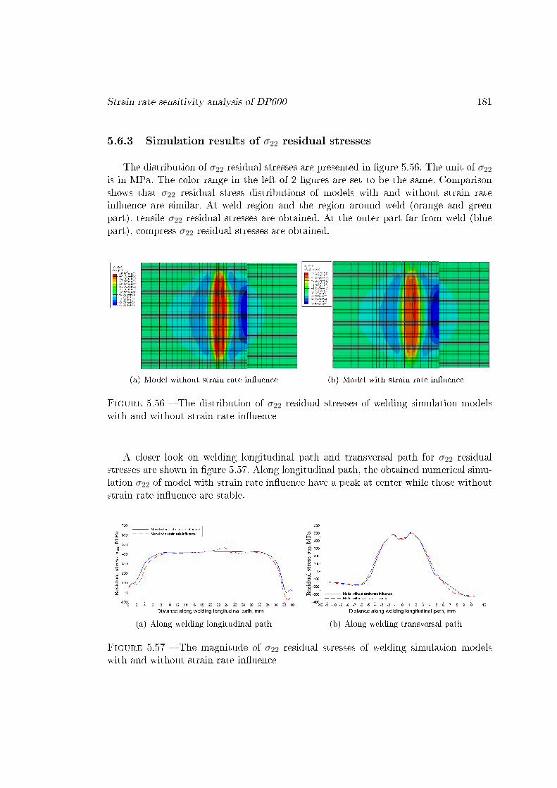
Strain rate sensitivity analysis of DP600 181
5.6.3 Simulation results of σ22 residual stresses
The distribution of σ22 residual stresses are presented in �gure 5.56. The unit of σ22
is in MPa. The color range in the left of 2 �gures are set to be the same. Comparisonshows that σ22 residual stress distributions of models with and without strain ratein�uence are similar. At weld region and the region around weld (orange and greenpart), tensile σ22 residual stresses are obtained. At the outer part far from weld (bluepart), compress σ22 residual stresses are obtained.
(a) Model without strain rate in�uence (b) Model with strain rate in�uence
Figure 5.56 � The distribution of σ22 residual stresses of welding simulation modelswith and without strain rate in�uence
A closer look on welding longitudinal path and transversal path for σ22 residualstresses are shown in �gure 5.57. Along longitudinal path, the obtained numerical simu-lation σ22 of model with strain rate in�uence have a peak at center while those withoutstrain rate in�uence are stable.
(a) Along welding longitudinal path (b) Along welding transversal path
Figure 5.57 � The magnitude of σ22 residual stresses of welding simulation modelswith and without strain rate in�uence
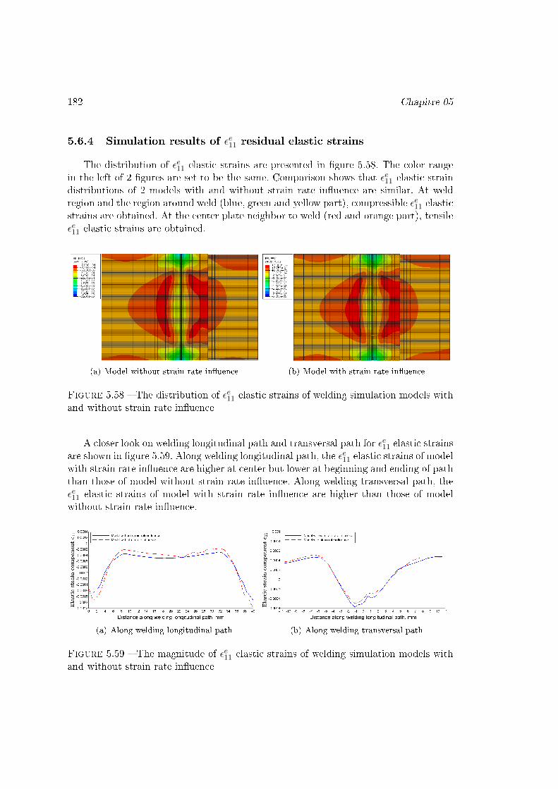
182 Chapitre 05
5.6.4 Simulation results of εe11 residual elastic strains
The distribution of εe11 elastic strains are presented in �gure 5.58. The color rangein the left of 2 �gures are set to be the same. Comparison shows that εe11 elastic straindistributions of 2 models with and without strain rate in�uence are similar. At weldregion and the region around weld (blue, green and yellow part), compressible εe11 elasticstrains are obtained. At the center plate neighbor to weld (red and orange part), tensileεe11 elastic strains are obtained.
(a) Model without strain rate in�uence (b) Model with strain rate in�uence
Figure 5.58 � The distribution of εe11 elastic strains of welding simulation models withand without strain rate in�uence
A closer look on welding longitudinal path and transversal path for εe11 elastic strainsare shown in �gure 5.59. Along welding longitudinal path, the εe11 elastic strains of modelwith strain rate in�uence are higher at center but lower at beginning and ending of paththan those of model without strain rate in�uence. Along welding transversal path, theεe11 elastic strains of model with strain rate in�uence are higher than those of modelwithout strain rate in�uence.
(a) Along welding longitudinal path (b) Along welding transversal path
Figure 5.59 � The magnitude of εe11 elastic strains of welding simulation models withand without strain rate in�uence
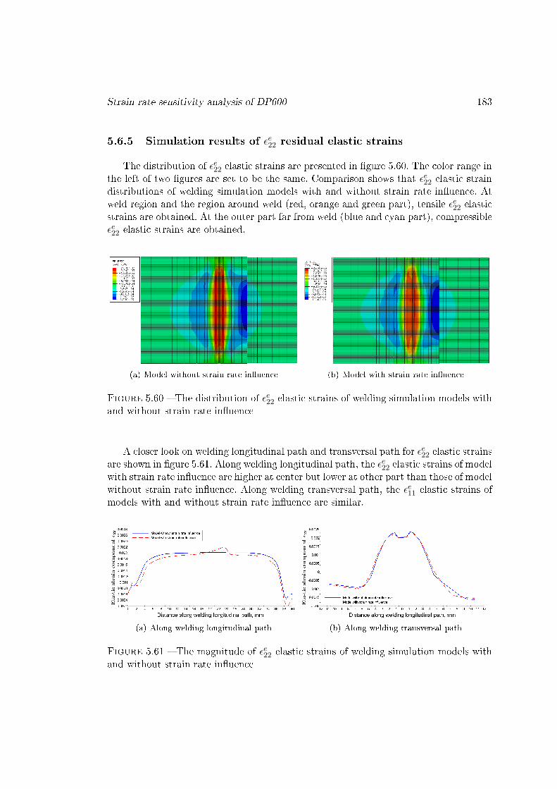
Strain rate sensitivity analysis of DP600 183
5.6.5 Simulation results of εe22 residual elastic strains
The distribution of εe22 elastic strains are presented in �gure 5.60. The color range inthe left of two �gures are set to be the same. Comparison shows that εe22 elastic straindistributions of welding simulation models with and without strain rate in�uence. Atweld region and the region around weld (red, orange and green part), tensile εe22 elasticstrains are obtained. At the outer part far from weld (blue and cyan part), compressibleεe22 elastic strains are obtained.
(a) Model without strain rate in�uence (b) Model with strain rate in�uence
Figure 5.60 � The distribution of εe22 elastic strains of welding simulation models withand without strain rate in�uence
A closer look on welding longitudinal path and transversal path for εe22 elastic strainsare shown in �gure 5.61. Along welding longitudinal path, the εe22 elastic strains of modelwith strain rate in�uence are higher at center but lower at other part than those of modelwithout strain rate in�uence. Along welding transversal path, the εe11 elastic strains ofmodels with and without strain rate in�uence are similar.
(a) Along welding longitudinal path (b) Along welding transversal path
Figure 5.61 � The magnitude of εe22 elastic strains of welding simulation models withand without strain rate in�uence

184 Chapitre 05
5.6.6 Simulation results of εp11 residual plastic strains
The distribution of εp11 plastic strains are presented in �gure 5.62. The color rangein the left of 2 �gures are set to be the same. Comparison shows that εp11 plastic straindistributions of models with and without strain rate in�uence are di�erent. An additio-nal orange region of εp11 plastic strain distributions of model with strain rate in�uenceare found.
(a) Model without strain rate in�uence (b) Model with strain rate in�uence
Figure 5.62 � The distribution of εp11 plastic strains of welding simulation models withand without strain rate in�uence
A closer look on welding longitudinal path and transversal path for εp11 plastic strainsare shown in �gure 5.63. The magnitude of εp11 plastic strains with and without strainrate in�uence have a di�erence around 0.02 for welding longitudinal path. The magni-tude are similar along welding transversal path except a di�erence about 0.01 at weldpart.
(a) Along welding longitudinal path (b) Along welding transversal path
Figure 5.63 � The magnitude of εp11 plastic strains of welding simulation models withand without strain rate in�uence
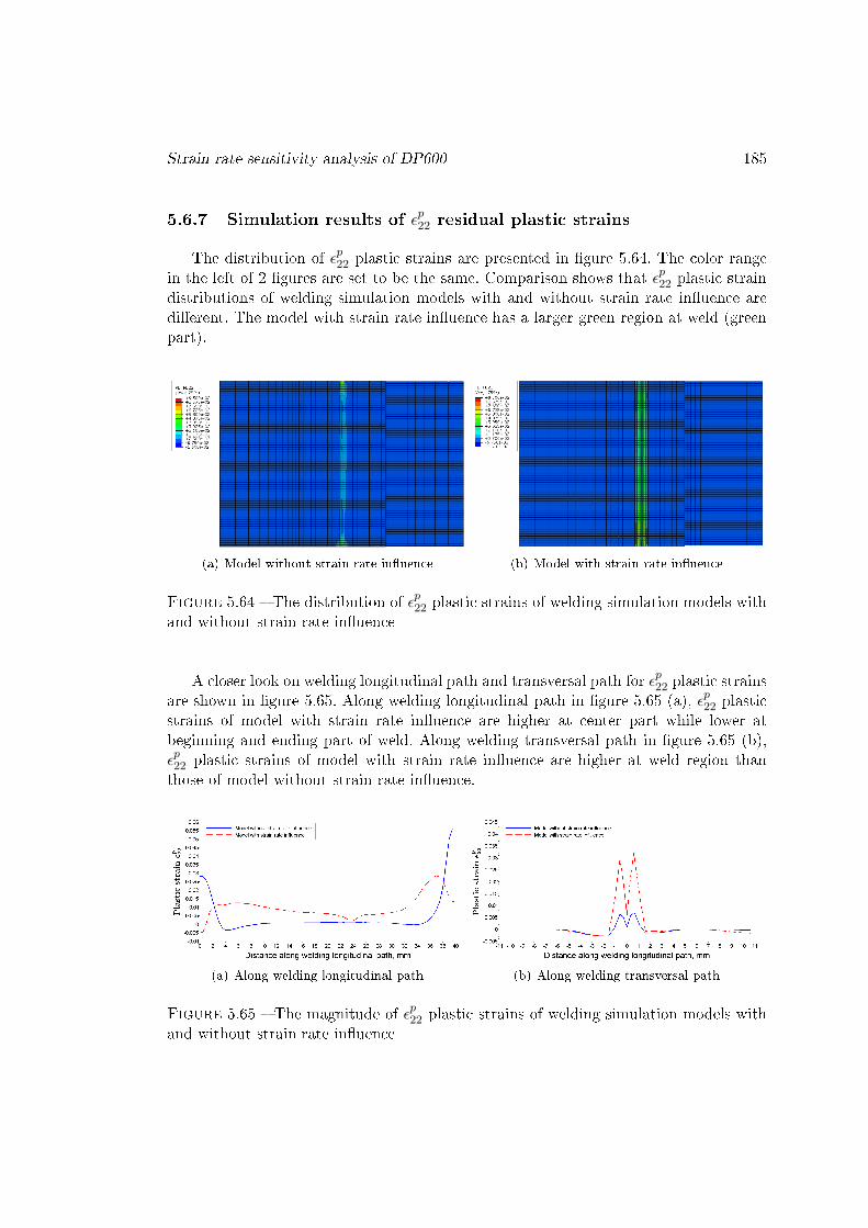
Strain rate sensitivity analysis of DP600 185
5.6.7 Simulation results of εp22 residual plastic strains
The distribution of εp22 plastic strains are presented in �gure 5.64. The color rangein the left of 2 �gures are set to be the same. Comparison shows that εp22 plastic straindistributions of welding simulation models with and without strain rate in�uence aredi�erent. The model with strain rate in�uence has a larger green region at weld (greenpart).
(a) Model without strain rate in�uence (b) Model with strain rate in�uence
Figure 5.64 � The distribution of εp22 plastic strains of welding simulation models withand without strain rate in�uence
A closer look on welding longitudinal path and transversal path for εp22 plastic strainsare shown in �gure 5.65. Along welding longitudinal path in �gure 5.65 (a), εp22 plasticstrains of model with strain rate in�uence are higher at center part while lower atbeginning and ending part of weld. Along welding transversal path in �gure 5.65 (b),εp22 plastic strains of model with strain rate in�uence are higher at weld region thanthose of model without strain rate in�uence.
(a) Along welding longitudinal path (b) Along welding transversal path
Figure 5.65 � The magnitude of εp22 plastic strains of welding simulation models withand without strain rate in�uence

186 Chapitre 05
5.6.8 Simulation results of εp equivalent plastic strains
The distribution of εp e�ective plastic strains are presented in �gure 5.66. The colorrange in the left of 2 �gures are set to be the same. Comparison shows that εp e�ectiveplastic strain distributions are di�erent. For model with strain rate in�uence, a redregion which stands for higher value of εp e�ective plastic strain is found at center weld.
(a) Model without strain rate in�uence (b) Model with strain rate in�uence
Figure 5.66 � The distribution of εp e�ective plastic strains of welding simulationmodels with and without strain rate in�uence
A closer look on welding longitudinal path and transversal path for εp e�ective plasticstrains are shown in �gure 5.67. Along both welding longitudinal and transversal path,εp of model with strain rate in�uence are higher at center part of weld.
(a) Along welding longitudinal path (b) Along welding transversal path
Figure 5.67 � The magnitude of εp e�ective plastic strains of welding simulation modelswith and without strain rate in�uence
In all above �gures, residual stress and strain results of the model considering strainrate sensitivity are di�erent with those no considering strain rate sensitivity. The mostnoticeable in�uence is that the considering strain rate sensitivity will get a peak valueof equivalent stress in the center weld instead of a stable value not considering strainrate sensitivity.

Plastic planar anisotropy analysis using Hill coe�cients 187
5.7 Plastic planar anisotropy analysis using Hill coe�cients
5.7.1 Simulation results of equivalent residual stresses
The distribution of equivalent residual stresses are presented in �gure 5.68. Theunit of results is in MPa. The color range in the left of �gures are set to be the same.Comparison shows that equivalent residual stresses of models with material anisotropyof θ = 0◦, 30◦, 45◦, 60◦, 90◦ and isotropic material are similar.
(a) θ = 0◦ (b) θ = 30◦
(c) θ = 45◦ (d) θ = 60◦
(e) θ = 90◦ (f) Isoropic material
Figure 5.68 � The distribution of equivalent residual stresses of welding simulationmodels with material anisotropy of θ = 0◦, 30◦, 45◦, 60◦, 90◦ and isotropic material

188 Chapitre 05
Along welding longitudinal path and transversal path, equivalent residual stressesare shown in �gure 5.69. The obtained simulation results are around 500 MPa. Alongwelding longitudinal and transversal path, equivalent residual stresses are in�uenced byanisotropy about 70 MPa at weld fusion zone and heat a�ected zone.
(a) Along welding longitudinal path (b) Along welding transversal path
Figure 5.69 � The magnitude of equivalent residual stresses of welding simulationmodels with material anisotropy of θ = 0◦, 30◦, 45◦, 60◦, 90◦ and isotropic material
5.7.2 Simulation results of σ11 and σ22 residual stresses
The contour of residual stresses of two material rolling orientations θ = 0◦ andθ = 90◦ are presented in �gure 5.70. With the material rolling orientation setting fromlongitudinal to transversal direction, the simulated distributions of residual stresses σ11
and σ22 turn over. The distributions of σ11 and σ22 with material rolling orientationθ = 0◦ correspond to the distribution of σ22 and σ11 with material rolling orientationθ = 90◦, respectively.
(a) σ11 with rolling angle θ = 0◦ (b) σ22 with rolling angle θ = 0◦

Plastic planar anisotropy analysis using Hill coe�cients 189
(c) σ11 with rolling angle θ = 90◦ (d) σ22 with rolling angle θ = 90◦
Figure 5.70 � Contour of residual stresses with di�erent material rolling orientations
Residual stresses σ11 and σ22 along transversal path are simulated. Di�erent mate-rial rolling orientations with θ = 0◦ , 45◦ and 90◦ are applied in models. The simulationresults are presented in �gure 5.71. The material rolling orientation in�uence the ma-gnitude of longitudinal and transversal residual stresses.
(a) Residual stresses of transversal direction (b) Residual stresses of longitudinal direction
Figure 5.71 � Numerical welding residual stresses obtained from di�erent rolling orien-tations
5.7.3 Simulation results of εp residual equivalent plastic strains
The distribution of εp residual equivalent strains are presented in �gure 5.72. Thecolor range in the left of �gures are set to be the same. Comparison shows that εp residualequivalent strains of models with material anisotropy of θ = 0◦, 30◦, 45◦, 60◦, 90◦ andisotropic material are similar.

190 Chapitre 05
(a) θ = 0◦ (b) θ = 30◦
(c) θ = 45◦ (d) θ = 60◦
(e) θ = 90◦ (f) Isoropic material
Figure 5.72 � The distribution of equivalent residual stresses of welding simulationmodels with material anisotropy of θ = 0◦, 30◦, 45◦, 60◦, 90◦ and isotropic material
Along welding longitudinal path and transversal path, εp residual equivalent strainsare shown in �gure 5.73. The obtained simulation results are around 0.016 at centerweld. Along welding longitudinal and transversal path, εp residual equivalent strainsare in�uenced by anisotropy about 0.001 at weld fusion zone and heat a�ected zone.
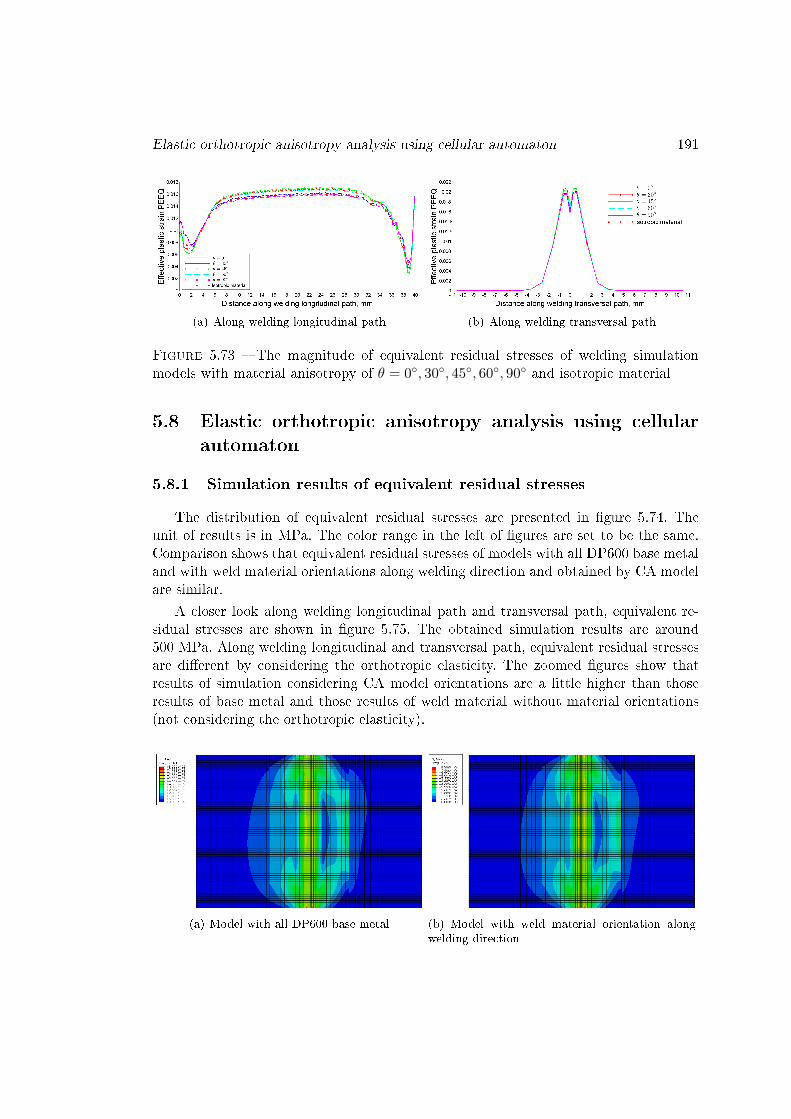
Elastic orthotropic anisotropy analysis using cellular automaton 191
(a) Along welding longitudinal path (b) Along welding transversal path
Figure 5.73 � The magnitude of equivalent residual stresses of welding simulationmodels with material anisotropy of θ = 0◦, 30◦, 45◦, 60◦, 90◦ and isotropic material
5.8 Elastic orthotropic anisotropy analysis using cellularautomaton
5.8.1 Simulation results of equivalent residual stresses
The distribution of equivalent residual stresses are presented in �gure 5.74. Theunit of results is in MPa. The color range in the left of �gures are set to be the same.Comparison shows that equivalent residual stresses of models with all DP600 base metaland with weld material orientations along welding direction and obtained by CA modelare similar.
A closer look along welding longitudinal path and transversal path, equivalent re-sidual stresses are shown in �gure 5.75. The obtained simulation results are around500 MPa. Along welding longitudinal and transversal path, equivalent residual stressesare di�erent by considering the orthotropic elasticity. The zoomed �gures show thatresults of simulation considering CA model orientations are a little higher than thoseresults of base metal and those results of weld material without material orientations(not considering the orthotropic elasticity).
(a) Model with all DP600 base metal (b) Model with weld material orientation alongwelding direction
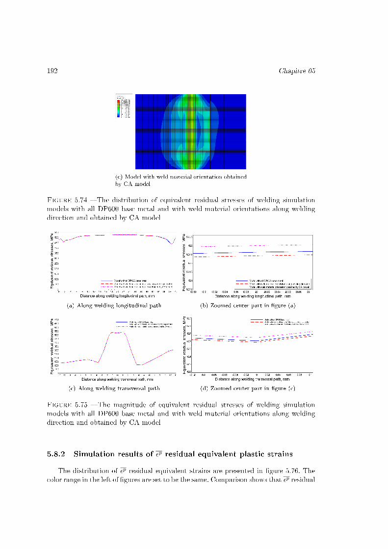
192 Chapitre 05
(c) Model with weld material orientation obtainedby CA model
Figure 5.74 � The distribution of equivalent residual stresses of welding simulationmodels with all DP600 base metal and with weld material orientations along weldingdirection and obtained by CA model
(a) Along welding longitudinal path (b) Zoomed center part in �gure (a)
(c) Along welding transversal path (d) Zoomed center part in �gure (c)
Figure 5.75 � The magnitude of equivalent residual stresses of welding simulationmodels with all DP600 base metal and with weld material orientations along weldingdirection and obtained by CA model
5.8.2 Simulation results of εp residual equivalent plastic strains
The distribution of εp residual equivalent strains are presented in �gure 5.76. Thecolor range in the left of �gures are set to be the same. Comparison shows that εp residual

Model validation by experimental analysis 193
equivalent strains distributions of models with all DP600 base metal and with weldmaterial orientations along welding direction and obtained by CA model are similar.
(a) Model with all DP600 base metal (b) Model with weld material orientation alongwelding direction
(c) Model with weld material orientation obtainedby CA model
Figure 5.76 � The distribution of equivalent residual stresses of welding simulationmodels with all DP600 base metal and with weld material orientations along weldingdirection and obtained by CA model
A closer look along welding longitudinal path and transversal path, εp residual equi-valent strains are shown in �gure 5.77. The obtained simulation results are around 0.016at center weld. Along welding longitudinal and transversal path, εp residual equivalentstrains are di�erent. The zoomed �gures show that results of simulation consideringCA model orientations are a little higher than those results of base metal and thoseresults of weld material without material orientations (not considering the orthotropicelasticity) .
5.9 Model validation by experimental analysis
In the previous analysis, the material constitutive model of strain rate sensitivity andthe orthotropic elastic anisotropy are found to have in�uences but not very big in�uenceson residual stress ans strains of numerical laser welding model. So only the combination

194 Chapitre 05
(a) Along welding longitudinal path (b) Zoomed center part in �gure (a)
(c) Along welding transversal path (d) Zoomed center part in �gure (b)
Figure 5.77 � The magnitude of equivalent residual stresses of welding simulationmodels with all DP600 base metal and with weld material orientations along weldingdirection and obtained by CA model
of hardening, temperature sensitivity and plastic anisotropy material constitutive modelare used in numerical laser welding simulation. The FEM model information can befound in chapter 4.6 with proposed synthesis model, proposed temperature sensitivityand material anisotropy de�ned by Hill theory. The material is assigned a materialrolling orientation that have 30◦ with transversal path.
In �gure 5.78, along the transversal path of weld, experimental and numerical re-sults of residual stresses variations with the di�erent material orientations are shown.The residual stresses of σ11 and σ22 are measured by Neutron Di�raction method alongtransversal path. The simulation results show a good accordance with experiment mea-surements.
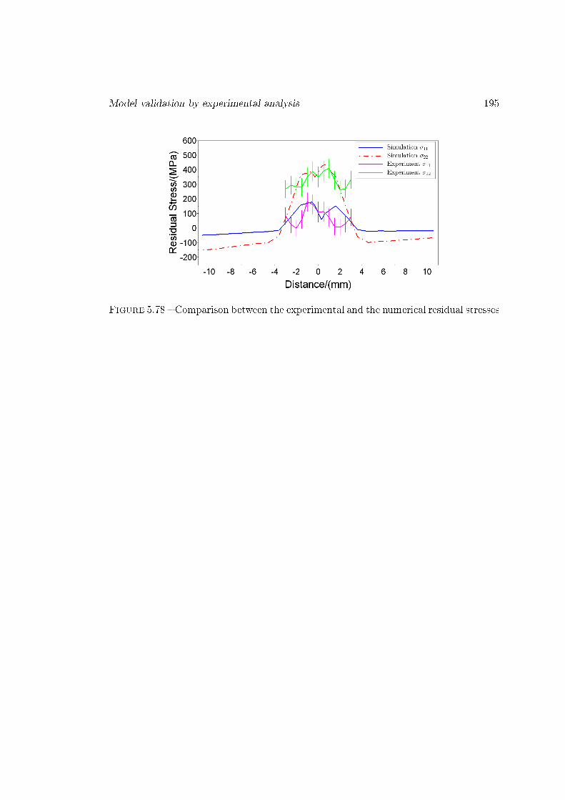
Model validation by experimental analysis 195
Figure 5.78 � Comparison between the experimental and the numerical residual stresses

196 Chapitre 05
General Conclusions
This thesis studies residual stresses produced in Nd :YAG laser beam overlap wel-ding of dual phase DP600 steel plates. The DP600 steel constitutive model is consideredas an important factor in general dynamic forming process and the laser welding nume-rical analysis. Thus a lot of experimental tensile tests are conducted to precisely identifythermo-elasto-plastic behavior of DP600 dual phase steel considering hardening term,strain rate sensitivity, temperature sensitivity, planar plastic anisotropy and orthotro-pic elastic anisotropy. A 2D Cellular Automaton model is introduced to simulate laserwelding solidi�cation process so that the microstructure information are considered forde�ning orthotropic elastic anisotropy and computing residual stresses. FEA numeri-cal simulations are applied based on the identi�ed material constitutive models andcorresponding results are analyzed. Computation of residual stresses through neutrondi�raction are conducted to validate the numerical model and good accordance arefound.
In introduction chapter, laser welding process, DP600 dual phase steel, residualstresses and continuum mechanics are introduced. Laser welding process is widely usedin assembly work of automobile industry. DP600 dual phase steel is a high strengthsteel to reduce automobile weight. Important residual stresses are produced during laserwelding of analyzed dual phase steel. Finite Element Model based on an incrementalsequential coupled elasto-thermo-plastic analysis of commercial code Abaqus toghetherwith speci�c constitutive equations introduced via UMAT subroutine is used to simulateresidual stresses. General information of Nd :YAG laser weld such as its development,mesoscopic mechanism and laser welding parameters are presented. The characteristicsof dual phase DP600 steel such as application area, elastic, thermal, mechanical andchemical properties during a laser welding are described. The orders, research meaningand the production mechanism of residual stress in welding are also taken into account.Mathematical description of yield criteria, elasticity and plasticity are reviewed as abase for this research work.
In chapter 2, material thermo-mechanical constitutive model of DP600 are analyzedbased on a lot of experimental tensile tests. The constitutive model consists of hardeningterm, strain rate sensitivity, temperature sensitivity and anisotropy are identi�ed forDP600 material.
The DP600 hardening term according to Ludwik law, Voce law, a proposed synthesismodel and polynomial equations are studied. It is found that the plastic �ow behavior of
197
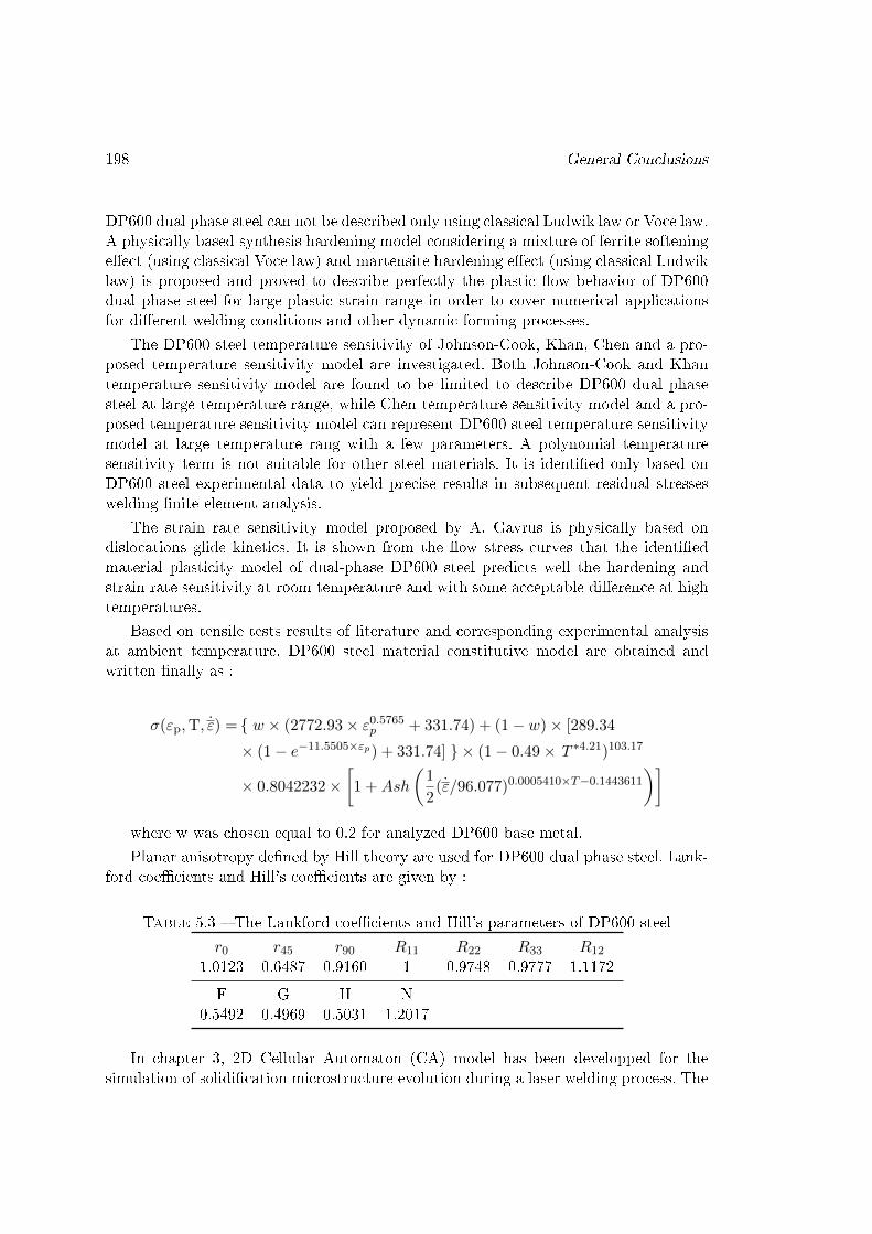
198 General Conclusions
DP600 dual phase steel can not be described only using classical Ludwik law or Voce law.A physically based synthesis hardening model considering a mixture of ferrite softeninge�ect (using classical Voce law) and martensite hardening e�ect (using classical Ludwiklaw) is proposed and proved to describe perfectly the plastic �ow behavior of DP600dual phase steel for large plastic strain range in order to cover numerical applicationsfor di�erent welding conditions and other dynamic forming processes.
The DP600 steel temperature sensitivity of Johnson-Cook, Khan, Chen and a pro-posed temperature sensitivity model are investigated. Both Johnson-Cook and Khantemperature sensitivity model are found to be limited to describe DP600 dual phasesteel at large temperature range, while Chen temperature sensitivity model and a pro-posed temperature sensitivity model can represent DP600 steel temperature sensitivitymodel at large temperature rang with a few parameters. A polynomial temperaturesensitivity term is not suitable for other steel materials. It is identi�ed only based onDP600 steel experimental data to yield precise results in subsequent residual stresseswelding �nite element analysis.
The strain rate sensitivity model proposed by A. Gavrus is physically based ondislocations glide kinetics. It is shown from the �ow stress curves that the identi�edmaterial plasticity model of dual-phase DP600 steel predicts well the hardening andstrain rate sensitivity at room temperature and with some acceptable di�erence at hightemperatures.
Based on tensile tests results of literature and corresponding experimental analysisat ambient temperature, DP600 steel material constitutive model are obtained andwritten �nally as :
σ(εp,T, ε̇) = { w × (2772.93× ε0.5765p + 331.74) + (1− w)× [289.34
× (1− e−11.5505×εp) + 331.74] } × (1− 0.49× T ∗4.21)103.17
× 0.8042232×[1 +Ash
(1
2(ε̇/96.077)0.0005410×T−0.1443611
)]where w was chosen equal to 0.2 for analyzed DP600 base metal.
Planar anisotropy de�ned by Hill theory are used for DP600 dual phase steel. Lank-ford coe�cients and Hill's coe�cients are given by :
Table 5.3 � The Lankford coe�cients and Hill's parameters of DP600 steel
r0 r45 r90 R11 R22 R33 R12
1.0123 0.6487 0.9160 1 0.9748 0.9777 1.1172
F G H N0.5492 0.4969 0.5031 1.2017
In chapter 3, 2D Cellular Automaton (CA) model has been developped for thesimulation of solidi�cation microstructure evolution during a laser welding process. The
General Conclusions 199
temperature �eld of CA are imported from a �nite element analysis model. The analysisfunction of nucleation, solid fraction, interface concentration, surface tension anisotropy,di�usion, interface growth velocity and conservation equations are presented in detail.Starting from initial conditions with di�erent parameters, di�erent results are obtained :
1. In section 3.18.1, CA model results of �gure 3.24 prove that unlike traditionalones, the CA model programed by the author keeps well the growing directionusing limited angles method. The CA model are also able to simulate equiaxeddendrite grain growth.
2. In section 3.18.2, CA model results of �gure 3.25 show that the CA model cansimulate the equiaxed dendrite grain growth with 48 growth directions.
3. In section 3.18.3, CA model results of �gure 3.26 claim that CA can simulatecolumn dendrite grain growth.
4. In section 3.18.4, CA model results of �gure 3.27 make evidence that two den-drite grain grows well with each other, they grow normally when the two grainsdendrite meet each other.
5. In section 3.18.5 and section 3.18.6, CA model results of �gure 3.28 and 3.29mean that the nuclea at the corner grows well to the whole simulation zone, itgrow normally at the edge of the simulation zone.
6. In section 3.18.7, CA model results of �gure 3.30 indicate that CA model cansimulate two equiaxed dendrite grain competition growth.
7. In section 3.18.8, CA model results of �gure 3.31 show that grains grow smoothlywith the other grains with di�erent growth direction.
8. In section 3.18.9 welding temperature environment and random nucleation condi-tions are applied, CA model results of �gure 3.31 present that CA model cansimulate the welding solidi�cation microstructure.
By comparing the dendrite grains growth simulation of CA model during weldingprocess and the corresponding experimental observation of weld microstructures, goodaccordances are found. The microstructure obtained from weld of laser welding DP600steel and those simulated by CA-FE model show similar growth microstructure orien-tations.
In chapter 4, information of �nite element model of laser welding process are presen-ted. Geometry of specimen, heat source, boundary conditions, DP600 dual phase steelmaterial properties such as conductivity, density, speci�c heat, expansion, elasticity andplasticity are introduced. Models analyzing hardening term, strain rate sensitivity, tem-perature sensitivity, plastic anisotropy and elastic anisotropy are described in detail andsimulated. The corresponding results are presented and discussed in chapter 5.
In chapter 5, simulation results of σ11, σ22, equivalent residual stress and εe11, εe22, ε
p11,
εp22 and εp of laser welding DP600 steel process are presented. The in�uence of hardeningterm, strain rate sensitivity, temperature sensitivity and anisotropy on residual stressesare analyzed.

200 General Conclusions
1. Rectangular and wedge type of mesh transition are compared. Rectangular typeof mesh transition is found to save more time than wedge type. Comparingwith C3D8, C3D20 and C3D20R element type, C3D8R element type is found toconsume less computation time.
2. The increment of mesh density in longitudinal direction increase precision of re-sults and computation time. The increment of mesh density in thickness directionis not found obvious di�erence.
3. Di�erent boundary conditions of three clamping distances are simulated. Theequivalent, σ11 and σ22 residual stresses along welding longitudinal and transver-sal path are compared. The equivalent residual stress along welding longitudinalpath is found to be more stable with a small clamping distance. The simulationresults of σ11 and σ22 is smaller with a small clamping distance.
4. In the analysis of hardening constitutive model, the modi�ed Ludwik model havedi�erent simulation results of residual stresses and strains due to a small modi�-cation (a straight line is added). Hardening models identi�ed for DP600 steel areapplied in FEM welding simulation, results of equivalent residual stresses, σ11,σ22, εe11, ε
e22, ε
p11, ε
p22 and εp are compared and similar welding residual stresses
and strains are obtained. A small di�erence of material hardening constitutivemodel is found to result in a big di�erence on simulation results. Di�erent DP600steel constitutive models can have similar numerical simulation results of resi-dual stresses and strains. Martensite hardening behavior using classical Ludwikmodel 03 is applied in numerical simulation model and the simulation results aredi�erent from those results of models with DP600 hardening models.
5. Four temperature sensitivity models identi�ed for DP600 steel are applied inFEM welding simulation, results of equivalent residual stresses, σ11, σ22, εe11, ε
e22,
εp11, εp22 and εp are compared. The Chen, proposed and polynomial temperature
sensitivity models which describe well of DP600 temperature sensitivity beha-vior are found to have similar simulation results of residual stresses and strains.The classical Johnson-Cook temperature sensitivity model which have some dif-ferences with the former three models at high temperature are found to higherequivalent residual stresses and equivalent residual strains. By comparing withresults in the analysis of DP600 steel hardening, temperature sensitivity is foundto have important in�uence on numerical simulation results of residual stressesand strains.
6. Models with and without considering strain rate in�uence on DP600 steel plas-tic material constitutive model are simulated and results of equivalent residualstresses, σ11, σ22, εe11, ε
e22, ε
p11, ε
p22 and εp are compared. Model with considering
strain rate in�uence presents a peak value of residual stress and strain whilemodel without considering strain rate in�uence presents a stable curve alongwelding longitudinal path.
7. Models considering DP600 steel plastic anisotropy are simulated and results ofequivalent residual stresses and εp are compared and found in�uenced by aniso-tropy. When the angle between rolling and welding direction is 45◦, the residual
General Conclusions 201
stresses around weld is found the highest. When the angle between rolling andwelding direction is 90◦, the residual stresses around weld is found the lowest.The material rolling orientation in�uence the magnitude of longitudinal andtransversal residual stresses.
8. Models considering DP600 steel orthotropic elastic anisotropy are simulated andresults of equivalent residual stresses and εp are compared. Simulation results ofstresses and strains are found di�erent. For this material and laser welding condi-tions, considering orthotropic elastic anisotropy with microstructure orientationsis found to increase residual stresses and strains of welding FEM simulation re-sults, though not much.
Finally, specimen experiments have been realized using neutrons di�raction tech-nique. Experimental data is compare with numerical results, a good accordance is foundbetween neutrons di�raction observation data and FEA model simulation results.
At the end of this research work, three interesting areas may be analyzed in thefuture :
1. Instead of a constant value, the martensite fraction w may be de�ned as a func-tion of material position, strain, temperature and strain rate. This analysis canimprove the description of DP600 material constitutive model, especially cor-responding to the thermo-mechanical properties simulation during solidi�cationprocess.
2. Not only dependent on temperature, the elasticity may also take into accountstrain rate in�uence. The investigation of elasticity during laser welding processcan improve the residual stresses prediction.
3. Mechanical response can be introduced in a future 3D CA model to better des-cribe the laser welding process considering thermo-microstructure-mechanicalproperties evolution.
Based on the proposed synthesis hardening term H(εp) = w · (σym + n1εn2p ) + (1−
w) ·{σyf + n3 · [1− exp(−n4εp)]
}by using equation 2.41 and considering the variation
of martensite volume fraction w, the material constitutive model is de�ned with the wvalue setting to 1 at welding area and decrease to 0.2 at the base metal.
In the �gure 5.79, the magnitude of equivalent residual stresses of welding simulationconsidering martensite volume fraction w change is presented and compared with resultsof other hardening models.

202 General Conclusions
(a) Martensite fraction w value change alongwelding transversal path
(b) Equivalent residual stresses along weldinglongitudinal path
(c) Equivalent residual stresses along weldingtransversal path
Figure 5.79 � The magnitude of equivalent residual stresses of welding simulationconsidering martensite volume fraction w change
The numerical simulation results of equivalent residual stresses of the model conside-ring martensite fraction w change (green curves) are di�erent with the DP600 hardeningmodels. The results proves that using the proposed synthesis hardening term, the phasetransformation in�uence on residual stresses can be analyzed. If martensite in the wel-ding area increase, the �nal numerical results of equivalent residual stresses will alsoincrease. But it should be noticed that the numerical results are not real because themartensite fraction w of welding area is not always 1. The martensite fraction w hasvariations during the laser weling process. So in the future research work, strain, tem-perature and strain rate should be considered to de�ne the variation of the martensitefraction w.
Chapitre 6
Résumé détaillé - Étude numériqueet expérimentale des contraintesrésiduelles générées lors du soudagelaser sur des plaques d'acier dualphase DP600
6.1 Introduction
Le laser Nd : YAG a d'abord été inventé par J. E. Geusic et al. dans les laboratoiresde Bell dans les années 1960 [8]. Depuis lors, il est largement utilisé dans les procédés defabrication dans l'industrie grâce à sa polyvalence et à l'utilisation de �bres optiques.Pour l'acier, le laser est devenu incontournable grâce au coe�cient élevé d'absorptionde chaleur pour ce type de matériau.
Pour répondre aux problèmes de crise énergétique et d'environnement, des matériauxcomme les aciers de haute résistance ou haute limite d'élasticité (THR, HLE) sontutilisés dans de nombreuses industries, en particulier l'automobile, a�n de réduire lepoids des voitures [10]. Notre étude porte sur le soudage laser des plaques de l'acier DP600. DP signi�e que l'acier est à dual phase (martensite + ferrite) et la série 600 signi�eque la résistance à la traction est supérieure à 600 MPa. C'est un acier à faible teneuren carbone avec une matrice ferritique ductile contenant une deuxième phase fragile,dont la forme se distingue principalement par des îles de martensite (3 % - 30 %) [11].
Les contraintes résiduelles sont des "contraintes internes auto équilibrantes" exis-tant dans un corps libre sans contraintes extérieures ni contraintes sur les limites. Lescontraintes résiduelles produites dans le processus de soudage au laser peuvent a�ecter lecomportement mécanique et le comportement en corrosion des pièces soudées. L'évalua-tion des contraintes résiduelles est donc fondamentale pour assurer la performance d'un
203

204Résumé détaillé - Étude numérique et expérimentale des contraintes résiduelles générées lors du soudage laser sur des plaques d'acier dual phase DP600
produit, notamment la tenue en service (fatigue). Dans ce sens, le procédé de soudagereste encore un processus complexe : tous les e�ets ne sont pas encore maîtrisés.
Figure 6.1 � Figure de l'évolution du matériau lors du processus de soudage
Pour mieux comprendre le comportement thermo-élasto-plastique de l'acier DP600,nous avons dé�ni et identi�é un modèle constitutif du matériau capable de décrire l'évo-lution de la contrainte équivalente pour une large plage des déformations, températureset vitesses de déformation. Le comportement plastique du DP600 dans l'analyse FEMa été déterminé par la formule ci-dessus. Pour bien prédire le comportement thermo-élasto-plastique de l'acier DP600 σyielde , il est nécessaire d'avoir une description précisesurtout par rapport aux observations expérimentales obtenues lors des essais de traction.
6.2 Chapitre 2 : Données expérimentales concernant le com-portement thermo-mécanique de DP600
La valeur de la contrainte limite équivalente σyielde a été décrite par un modèle consti-tutif prenant en compte le taux d'écrouissage, la sensibilité à la vitesse de déformationet la sensibilité à la température. A l'aide des résultats issus des essais de traction del'acier dual phase DP600, le comportement thermo-mécanique de DP600 a pu être iden-ti�é sur toute la plage de mesure des déformations plastiques (0 - 0.2) et surtout autourde la limite élastique du matériau en utilisant une loi dé�nie à partir des travaux de A.GAVRUS [42, 43, 44, 45] écrité sous la forme :
σyielde = σ(εp
e , ˙̄ε,T) = H(εpe ) ·G(˙̄ε) · F(T) (6.1)
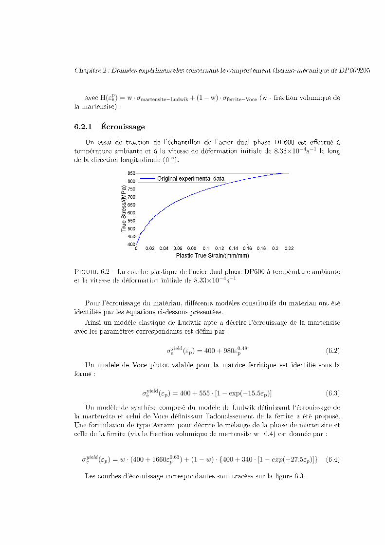
Chapitre 2 : Données expérimentales concernant le comportement thermo-mécanique de DP600205
avec H(εpe ) = w ·σmartensite−Ludwik + (1−w) ·σferrite−Voce (w - fraction volumique de
la martensite).
6.2.1 Écrouissage
Un essai de traction de l'échantillon de l'acier dual phase DP600 est e�ectué àtempérature ambiante et à la vitesse de déformation initiale de 8.33×10⁻⁴s−1 le longde la direction longitudinale (0 ◦).
Figure 6.2 � La courbe plastique de l'acier dual phase DP600 à température ambianteet la vitesse de déformation initiale de 8.33×10⁻⁴s−1
Pour l'écrouissage du matériau, di�érents modèles constitutifs du matériau ont étéidenti�és par les équations ci-dessous présentées.
Ainsi un modèle classique de Ludwik apte a décrire l'écrouissage de la martensiteavec les paramètres correspondants est dé�ni par :
σyielde (εp) = 400 + 980ε0.48
p (6.2)
Un modèle de Voce plutôt valable pour la matrice ferritique est identi�é sous laforme :
σyielde (εp) = 400 + 555 · [1− exp(−15.5εp)] (6.3)
Un modèle de synthèse composé du modèle de Ludwik dé�nissant l'écrouissage dela martensite et celui de Voce dé�nissant l'adoucissement de la ferrite a été proposé.Une formulation de type Avrami pour décrire le mélange de la phase de martensite etcelle de la ferrite (via la fraction volumique de martensite w=0.4) est donnée par :
σyielde (εp) = w · (400 + 1660ε0.63p ) + (1− w) · {400 + 340 · [1− exp(−27.5εp)]} (6.4)
Les courbes d'écrouissage correspondantes sont tracées sur la �gure 6.3.

206Résumé détaillé - Étude numérique et expérimentale des contraintes résiduelles générées lors du soudage laser sur des plaques d'acier dual phase DP600
(a) Modèle avec w = 0.4 (b) Modèle avec w = 0.2
Figure 6.3 � Comparaison des modèles rhéologiques et des données expérimentalesDP600
Par la suite, dans toutes les analyses numériques des di�érents modèles identi�és,nous avons utilisé un taux de martensite de w=0.2 :
σyielde (εp) = w · (400 + 3411.28ε0.6014p ) + (1−w) · {400 + 234.40 · [1− exp(−27.1092εp)]}
6.2.2 Sensibilité à la température
Selon le travail de Aydemir et al. [58], l'in�uence de température sur les propriétésde DP600 est analysée de 20◦C à 800◦C.
Pour étudier la sensibilité à la température de l'acier DP600, nous avons utilisédi�érents modèles issus de la littérature : Johnson-Cook, Khan et Chen. [57].
Le modèle de sensibilité Johnson-Cook [39] a été identi�é sous la forme :
F(T ) = 1− T ∗1.5 (6.5)
Le modèle de sensibilité Khan [50] est écrit comme suit :
F(T ) =
(Tm − TTm − Tr
)0.5
(6.6)
La sensibilité à la température du modèle Chen [51] est donnée par :
F(T ) = exp(4.23 · T ∗−51.61) (6.7)
Dans notre travail, un modèle a été proposé pour décrire la sensibilité à la tempé-rature, identi�é sous la forme suivante :
F(T ) = (1− 0.491 · T ∗4.212)103.17 (6.8)
Les courbes de sensibilité à la température correspondantes sont tracées sur la �gure6.4.
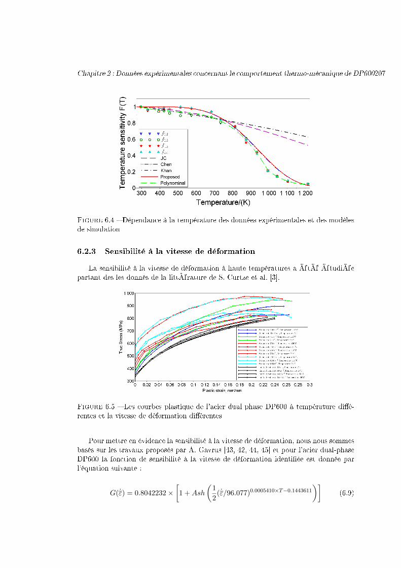
Chapitre 2 : Données expérimentales concernant le comportement thermo-mécanique de DP600207
Figure 6.4 � Dépendance à la température des données expérimentales et des modèlesde simulation
6.2.3 Sensibilité à la vitesse de déformation
La sensibilité à la vitesse de déformation à haute températures a été étudiéepartant des les donnés de la littérature de S. Curtze et al. [3].
Figure 6.5 � Les courbes plastique de l'acier dual phase DP600 à température di�é-rentes et la vitesse de déformation di�érentes
Pour mettre en évidence la sensibilité à la vitesse de déformation, nous nous sommesbasés sur les travaux proposés par A. Gavrus [43, 42, 44, 45] et pour l'acier dual-phaseDP600 la fonction de sensibilité à la vitesse de déformation identi�ée est donnée parl'équation suivante :
G(ε̇) = 0.8042232×[1 +Ash
(1
2(ε̇/96.077)0.0005410×T−0.1443611
)](6.9)
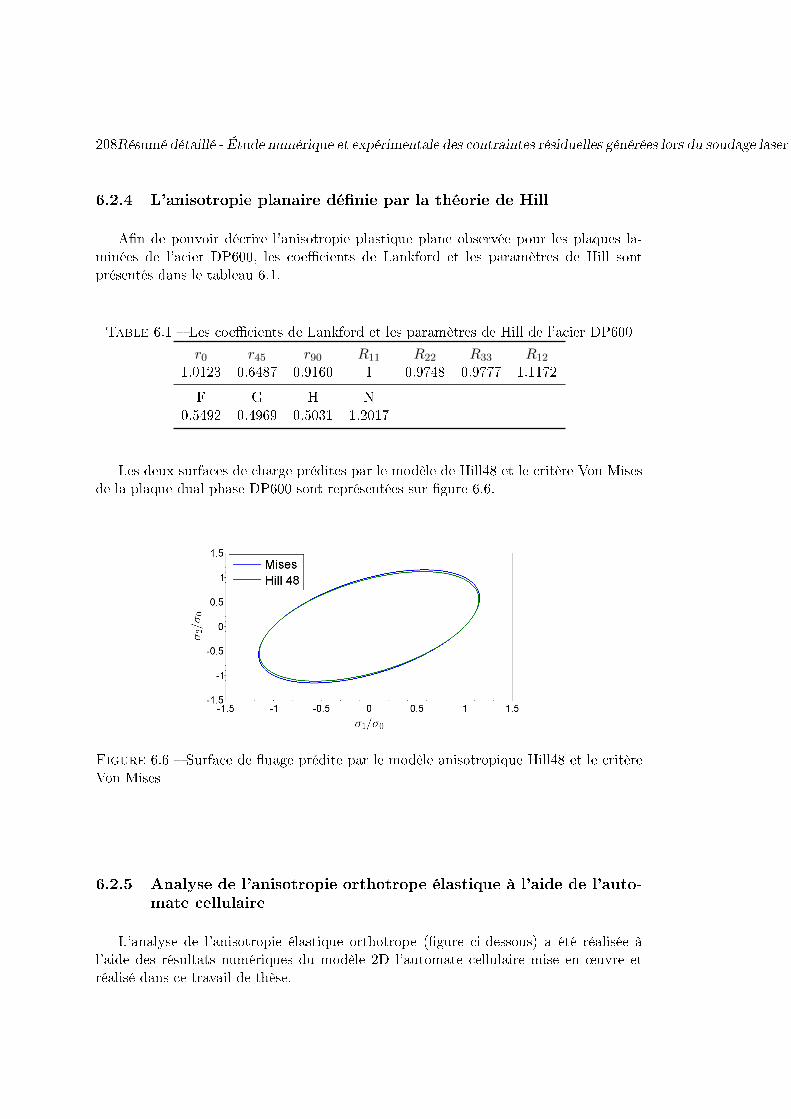
208Résumé détaillé - Étude numérique et expérimentale des contraintes résiduelles générées lors du soudage laser sur des plaques d'acier dual phase DP600
6.2.4 L'anisotropie planaire dé�nie par la théorie de Hill
A�n de pouvoir décrire l'anisotropie plastique plane observée pour les plaques la-minées de l'acier DP600, les coe�cients de Lankford et les paramètres de Hill sontprésentés dans le tableau 6.1.
Table 6.1 � Les coe�cients de Lankford et les paramètres de Hill de l'acier DP600
r0 r45 r90 R11 R22 R33 R12
1.0123 0.6487 0.9160 1 0.9748 0.9777 1.1172
F G H N0.5492 0.4969 0.5031 1.2017
Les deux surfaces de charge prédites par le modèle de Hill48 et le critère Von Misesde la plaque dual phase DP600 sont représentées sur �gure 6.6.
Figure 6.6 � Surface de �uage prédite par le modèle anisotropique Hill48 et le critèreVon Mises
6.2.5 Analyse de l'anisotropie orthotrope élastique à l'aide de l'auto-mate cellulaire
L'analyse de l'anisotropie élastique orthotrope (�gure ci-dessous) a été réalisée àl'aide des résultats numériques du modèle 2D l'automate cellulaire mise en ÷uvre etréalisé dans ce travail de thèse.

Chapitre 2 : Données expérimentales concernant le comportement thermo-mécanique de DP600209
Figure 6.7 � The �owchart of CA-FE model used to simulate residual stresses
La zone soudée est censée être constituée principalement par de la martensite. Aussi,grâce au modèle CA, l'orientation des grains de la martensite a été simulée. De cefait, nous avons tenu compte des nouvelles valeurs liées à la martensite avec prise encompte de l'orientation obtenue par solidi�cation après la phase de mise en fusion :l'élasticité orthotrope en est modi�ée. Les tableaux ci-dessous donnent les valeurs desconstantes élastiques avec et sans prise en compte des orientations des grains de dendritemartensitique. 6.2 6.3.
Table 6.2 � Constantes élastiques du matériau de soudure
T/◦C E1 E2 E3 ν12 ν13 ν23 G12 G13 G23
0 203.40 203.07 202.72 0.2943 0.2902 0.2942 79.06 78.72 78.85300 184.03 183.73 183.42 0.3101 0.3057 0.3100 71.53 71.22 71.34600 116.23 116.04 115.84 0.3258 0.3213 0.3258 45.18 44.98 45.06800 29.06 29.01 28.96 0.3469 0.3420 0.3468 11.29 11.25 11.26
Table 6.3 � Constantes élastiques du matériau de soudure avec des orientations CA
T/◦C E1 E2 E3 ν12 ν13 ν23 G12 G13 G23
0 203.78 203.70 202.72 0.2924 0.2924 0.2935 78.93 78.85 78.55300 184.37 183.30 183.42 0.3080 0.3081 0.3092 71.42 71.34 71.07600 116.45 116.40 115.84 0.3237 0.3237 0.3249 45.10 45.05 44.88800 29.11 29.10 28.96 0.3446 0.3446 0.3459 11.28 11.26 11.22
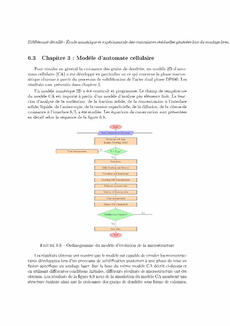
210Résumé détaillé - Étude numérique et expérimentale des contraintes résiduelles générées lors du soudage laser sur des plaques d'acier dual phase DP600
6.3 Chapitre 3 : Modèle d'automate cellulaire
Pour simuler en général la croissance des grains de dendrite, un modèle 2D d'auto-mate cellulaire (CA) a été développé en particulier en ce qui concerne la phase marten-sitique obtenue à partir du processus de solidi�cation de l'acier dual phase DP600. Lesrésultats sont présentés dans chapitre 3.
Un modèle numérique 2D a été construit et programmé. Le champ de températuredu modèle CA est importé à partir d'un modèle d'analyse par éléments �nis. La fonc-tion d'analyse de la nucléation, de la fraction solide, de la concentration à l'interfacesolide/liquide, de l'anisotropie, de la tension super�cielle, de la di�usion, de la vitesse decroissance à l'interface S/L a été étudiée. Les équations de conservation sont présentéesen détail selon la séquence de la �gure 6.8.
Figure 6.8 � Ordinogramme du modèle d'évolution de la microstructure
Les résultats obtenus ont montré que le modèle est capable de simuler les microstruc-tures développées lors d'un processus de solidi�cation posteriori à une phase de mise enfusion spéci�que au soudage laser. Sur la base du même modèle CA décrit ci-dessus eten utilisant di�érentes conditions initiales, di�érents résultats de microstructure ont étéobtenus. Les résultats de la �gure 6.9 issus de la simulation du modèle CA montrent unestructure équiaxe ainsi que la croissance des grains de dendrite sous forme de colonnes.

Chapitre 3 : Modèle d'automate cellulaire 211
(a) Croissance du grain de den-drite Equiaxed
(b) Croissance des grains dedendrite colonne
Figure 6.9 � Simulations numériques de la microstructure par modèle CA
Le modèle simulant les microstructures de soudage a été ainsi validé. Les compa-raisons entre les résultats de simulation et les observations optiques expérimentalesréalisées sur la section transversale de la soudure et la surface supérieure montrent debonnes concordances comme le montre la �gure 6.10 pour
(a) Observation optique de lasection transversale
(b) Résultat de simulation dela section transversale
(c) Observation optique de lasurface supérieure
(d) Observation optique de lasurface supérieure
Figure 6.10 � Microstructure de FZ et HAZ de la section de soudure DP600 et de lasurface supérieure
212Résumé détaillé - Étude numérique et expérimentale des contraintes résiduelles générées lors du soudage laser sur des plaques d'acier dual phase DP600
6.4 Chapitre 4 et 5 : ABAQUS/FEM modèles, résultats desimulation et résultats expérimentaux
6.4.1 Informations sur le modèle
Sur le plan mécanique et sur la base du comportement thermo-mécanique du maté-riau, le modèle FEM a été construit en deux parties :
1. Partie d'analyse thermique� La source de chaleur, le transfert de chaleur, le rayonnement et la convection
ont été pris en compte pour analyser des données thermiques du modèle� Les données thermiques, calculées, ont été utilisées et implémentées pour
dé�nir le comportement mécanique.
2. Partie d'analyse mécanique�� Pour calculer les contraintes résiduelles, nous avons tenu compte des pro-
priétés du matériau dépendantes et indépendantes de la température commel'expansion par exemple, le module élastique et ceux de la plasticité. A par-tir ce cette étude, les contraintes résiduelles ont été calculées à partir de laréponse élasto-plastique du matériau et de la relaxation du matériau lors durefroidissement.
La construction du modèle a été réalisée sur le logiciel ABAQUS en plusieurs sec-tions :
1. Propriétés du matériau de base. Ces propriétés ont été utilisées dans toutes lesanalyses de simulation.
2. Di�érents modèles ont été testés avec di�érentes géométries et types de maillage.Cette partie présente les paramètres de géométrie et les informations de maillageutilisées pour le modèle de simulation de soudage.
3. Par ailleurs, les paramètres importants du modèle constitutif du matériau ontété intégrés dans les modèles : l'écrouissage, la sensibilité à la température, lasensibilité à la vitesse de déformation, l'anisotropie élastique et plastique. Lesrésultats de ces di�érents modèles sont présentés en détail dans le manuscrit.Les résultats nous ont permis de mettre en exergue l'in�uence prépondérante oupas de ces e�ets.
6.4.2 Résultats de simulation des modèles de soudage numérique
6.4.2.1 Ecrouissage
Les e�ets associés à l'in�uence de l'écrouissage sont présentés sur la �gure 6.11.
Le modèle modi�é de Ludwik montrent des di�érences dans les valeurs des contraintesrésiduelles équivalentes (le modèle constitutif de l'écrouissage a une petite modi�cation :
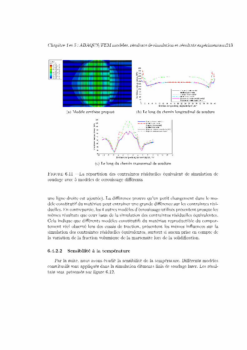
Chapitre 4 et 5 : ABAQUS/FEMmodèles, résultats de simulation et résultats expérimentaux213
(a) Modèle synthèse proposé (b) Le long du chemin longitudinal de soudure
(c) Le long du chemin transversal de soudure
Figure 6.11 � La répartition des contraintes résiduelles équivalent de simulation desoudage avec 5 modèles de ecrouissage di�érents
une ligne droite est ajoutée). La di�érence prouve qu'un petit changement dans le mo-dèle constitutif du matériau peut entraîner une grande di�érence sur les contraintes rési-duelles. En contrepartie, les 4 autres modèles d'écrouissage utilisés présentent presque lesmêmes résultats que ceux issus de la simulation des contraintes résiduelles équivalentes.Cela indique que di�érents modèles constitutifs du matériau reproductible du compor-tement réel observé lors des essais de traction, présentent les mêmes in�uences sur lasimulation des contraintes résiduelles équivalentes, surtout si aucun prise en compte dela variation de la fraction volumique de la martensite lors de la solidi�cation.
6.4.2.2 Sensibilité à la température
Par la suite, nous avons étudié la sensibilité de la température. Di�érents modèlesconstitutifs sont appliqués dans la simulation éléments �nis de soudage laser. Les résul-tats sont présentés sur �gure 6.12.
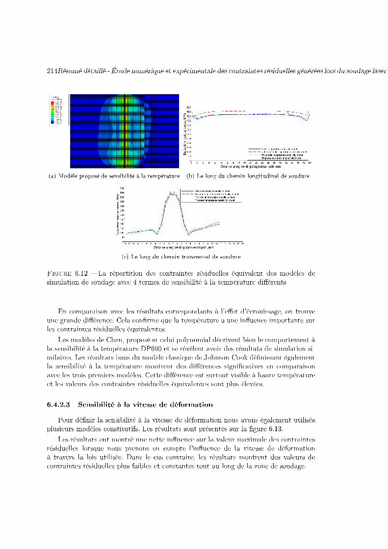
214Résumé détaillé - Étude numérique et expérimentale des contraintes résiduelles générées lors du soudage laser sur des plaques d'acier dual phase DP600
(a) Modèle proposé de sensibilité à la température (b) Le long du chemin longitudinal de soudure
(c) Le long du chemin transversal de soudure
Figure 6.12 � La répartition des contraintes résiduelles équivalent des modèles desimulation de soudage avec 4 termes de sensibilité à la température di�érents
En comparaison avec les résultats correspondants à l'e�et d'écrouissage, on trouveune grande di�érence. Cela con�rme que la température a une in�uence importante surles contraintes résiduelles équivalentes.
Les modèles de Chen, proposé et celui polynomial décrivent bien le comportement àla sensibilité à la température DP600 et se révèlent avoir des résultats de simulation si-milaires. Les résultats issus du modèle classique de Johnson-Cook dé�nissant égalementla sensibilité à la température montrent des di�érences signi�catives en comparaisonavec les trois premiers modèles. Cette di�érence est surtout visible à haute températureet les valeurs des contraintes résiduelles équivalentes sont plus élevées.
6.4.2.3 Sensibilité à la vitesse de déformation
Pour dé�nir la sensibilité à la vitesse de déformation nous avons également utilisésplusieurs modèles constitutifs. Les résultats sont présentés sur la �gure 6.13.
Les résultats ont montré une nette in�uence sur la valeur maximale des contraintesrésiduelles lorsque nous prenons en compte l'in�uence de la vitesse de déformationà travers la lois utilisée. Dans le cas contraire, les résultats montrent des valeurs decontraintes résiduelles plus faibles et constantes tout au long de la zone de soudage.
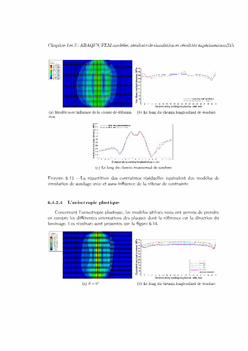
Chapitre 4 et 5 : ABAQUS/FEMmodèles, résultats de simulation et résultats expérimentaux215
(a) Modèle avec in�uence de la vitesse de déforma-tion
(b) Le long du chemin longitudinal de soudure
(c) Le long du chemin transversal de soudure
Figure 6.13 � La répartition des contraintes résiduelles équivalent des modèles desimulation de soudage avec et sans in�uence de la vitesse de contrainte
6.4.2.4 L'anisotropie plastique
Concernant l'anisotropie plastique, les modèles utilisés nous ont permis de prendreen compte les di�érentes orientations des plaques dont la référence est la direction dulaminage. Les résultats sont présentés sur la �gure 6.14.
(a) θ = 0◦ (b) Le long du chemin longitudinal de soudure

216Résumé détaillé - Étude numérique et expérimentale des contraintes résiduelles générées lors du soudage laser sur des plaques d'acier dual phase DP600
(c) Le long du chemin transversal de soudure
Figure 6.14 � La répartition des contraintes résiduelles équivalentes des modèles desimulation de soudage avec une anisotropie matérielle de θ = 0◦, 30◦, 45◦, 60◦, 90◦ etmatériel isotrope
Lorsque l'angle entre la direction de laminage et de soudure est 45◦, les contraintes ré-siduelles autour de la soudure sont les plus élevées. Lorsque l'angle est 90◦, les contraintesrésiduelles autour de la soudure sont les plus faibles. Ces résultats montrent l'impor-tance de l'orientation du matériau de base par rapport à la direction de soudage. Lesrésultats ont montré une répartition di�érente des contraintes résiduelles.
6.4.2.5 L'anisotropie élastique
Du point de vue de l'anisotropie élastique, nous avons introduits l'orientation desgrains dont les résultats sont issus du modèle CA et implémentés dans Abaqus. Lesrésultats sont présentés sur la �gure 6.15.
(a) Modèle avec orientation du matériau de sou-dure obtenu par le modèle CA
(b) Le long du chemin longitudinal de soudure
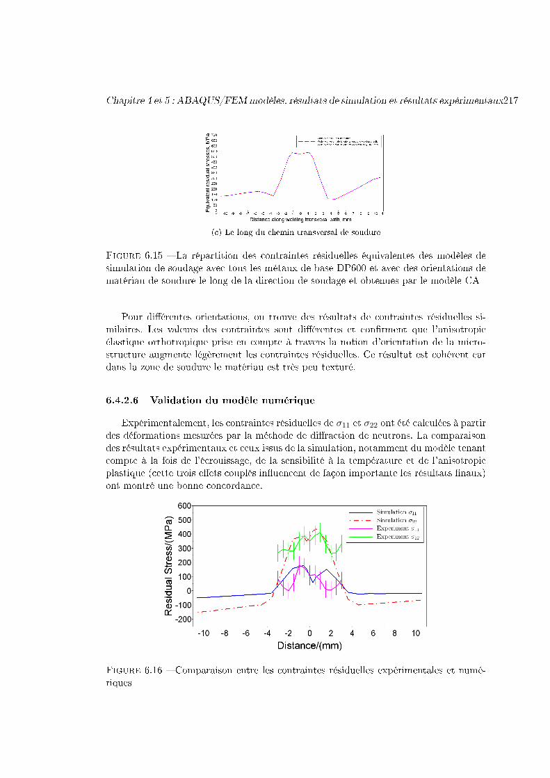
Chapitre 4 et 5 : ABAQUS/FEMmodèles, résultats de simulation et résultats expérimentaux217
(c) Le long du chemin transversal de soudure
Figure 6.15 � La répartition des contraintes résiduelles équivalentes des modèles desimulation de soudage avec tous les métaux de base DP600 et avec des orientations dematériau de soudure le long de la direction de soudage et obtenues par le modèle CA
Pour di�érentes orientations, on trouve des résultats de contraintes résiduelles si-milaires. Les valeurs des contraintes sont di�érentes et con�rment que l'anisotropieélastique orthotropique prise en compte à travers la notion d'orientation de la micro-structure augmente légèrement les contraintes résiduelles. Ce résultat est cohérent cardans la zone de soudure le matériau est très peu texturé.
6.4.2.6 Validation du modêle numérique
Expérimentalement, les contraintes résiduelles de σ11 et σ22 ont été calculées à partirdes déformations mesurées par la méthode de di�raction de neutrons. La comparaisondes résultats expérimentaux et ceux issus de la simulation, notamment du modèle tenantcompte à la fois de l'écrouissage, de la sensibilité à la température et de l'anisotropieplastique (cette trois e�ets couplés in�uencent de façon importante les résultats �naux)ont montré une bonne concordance.
Figure 6.16 � Comparaison entre les contraintes résiduelles expérimentales et numé-riques

218Résumé détaillé - Étude numérique et expérimentale des contraintes résiduelles générées lors du soudage laser sur des plaques d'acier dual phase DP600
6.5 Conclusion
Ainsi l'ensemble de ce travail a été réalisé en plusieurs étapes, en utilisant deuxmodèles numériques de simulations : modèle CA et FEM. Le couplage de ces deuxméthodes nous ont permis d'arriver aux conclusions suivantes :
Le modèle constitutif thermo-mécanique du matériau de DP600 a été analysé sur labase des tests de traction expérimentaux. Le modèle constitutif doit prendre en compteun terme d'écrouissage, la sensibilité à la vitesse de déformation, la sensibilité à latempérature et l'anisotropie plastique et orthotropique élastique de l'acier dual-phaseDP600.
Une méthode de l'automate cellulaire (CA) a été programmée et mise en ÷uvre sousforme d'un modèle numérique 2D. Cette étape nous a permis de simuler l'évolution de lamicrostructure lors solidi�cation suivant le procédé de soudage laser étudié. Le champ detempérature programmé dans le modèle CA est importé à partir d'un modèle d'analysed'éléments �nis. Les di�érents phénomènes apparaissant lors de la solidi�cation commela nucléation, la fraction solide, la concentration à l'interface solide/liquide, l'anisotropiede la tension de surface, la di�usion, la vitesse de croissance à l'interface solide/liquideainsi que des équations de conservation ont été étudié et pris en compte. Les résultatsdu modèle CA ont été comparés aux résultats expérimentaux et nous avons pu montrerune bonne convergence des résultats.
La méthode de simulation par Eléments Finis (FEM), nous a permis de comprendrele comportement thermo-mécanique du matériau étudié. La simulation du procédé desoudage laser ainsi que les lois constitutives du matériaux ont été implémentées. D'unpoint de vue simulation, les e�ets du type d'élément, de la densité du maillage et lesconditions aux limites ont été testés et consolidés. De la même façon le modèle constitutiftemro-élasto-plastique du matériau prenant en compte l'écrouissage, la sensibilité à latempérature et la sensibilité à la vitesse de déformation sur les résultats de simulation descontraintes résiduelles ont été pris en compte et analysés. Le couplage des deux modèlesCA-FE nous a permis aussi d'analyser les e�ets d'anisotropie élastique orthotropesdu matériau soudé sur les l'évolution des contraintes résiduelles. Plusieurs conclusionsimportantes sont synthétisées ici :
1. L'écrouissage : les résultats ont montré une in�uence marquée de l'écrouissagesur les valeurs des contraintes résiduelles.
2. L'étude de la sensibilité à la température a également montré une in�uence im-portante sur les contraintes résiduelles et déformation.
3. La vitesse de la déformation présente une valeur maximale des contraintes rési-duelles et de la déformation tandis que les modèles ne prenant pas en comptel'in�uence de la vitesse de la déformation présente des contraintes résiduelles deplus faible valeurs aux bord de la zone de soudage et une courbe plutôt stabletout au long de la zone de soudage.
4. L'étude de l'angle entre la direction de laminage et la direction de soudure a miségalement en évidence l'importance de l'orientation de la tôle. Lorsque l'angle

Conclusion 219
est de 45◦, les contraintes résiduelles autour de la soudure sont les plus élevées.Lorsque l'angle entre le sens de roulement et de soudure est de 90◦, les contraintesrésiduelles autour de la soudure sont les plus faibles. L'orientation du laminagedu matériau in�ue le niveaux des contraintes résiduelles aussi bien les contraintesrésiduelles longitudinales que transversales.
5. L'anisotropie élastique orthotropique qui prend en compte l'orientation des grainsdont la fraction volumique, obtenue grâce au modèle numérique 2D CA, a peud'in�uence sur les contraintes résiduelles. Ce résultat était attendu car la zonesoudée est très peu texturée.
6. En�n, les résultats expérimentaux et ceux obtenus par le couplage des deuxmodèles CA/FEM ont montré de bonnes convergences et permet de con�rmer larobustesse générale du modèle numérique de simulation du procédé de soudagelaser.
À la �n de ce travail de recherche, trois domaines intéressants peuvent être analysésà l'avenir :
� Au lieu d'une valeur constante, la fraction de martensite w peut être dé�nie enfonction de la position du matériau, de la déformation, de la température et dela vitesse de déformation.
� L'élasticité peut prendre en compte l'in�uence de la température et de la vitessede déformation.
� Une réponse mécanique peut être introduite dans un futur modèle CA 3D pourmieux décrire le processus de soudage laser en considérant l'évolution des pro-priétés thermo-microstructure-mécanique.
Sur la base du terme d'écrouissage de la loi de synthèse proposée H(εp) = w · (σym +n1ε
n2p ) + (1−w) ·
{σyf + n3 · [1− exp(−n4εp)]
}partant d'un modèle constitutif général
(équation 1.89 et 1.90) une variation du taux de martensite peut être prise en comptepar exemple avec une valeur w de 1 à dans la zone de soudage et diminue à 0.2 auniveau du métal de base. Les contraintes résiduelles équivalentes sont présenté dans la�gure 6.17.
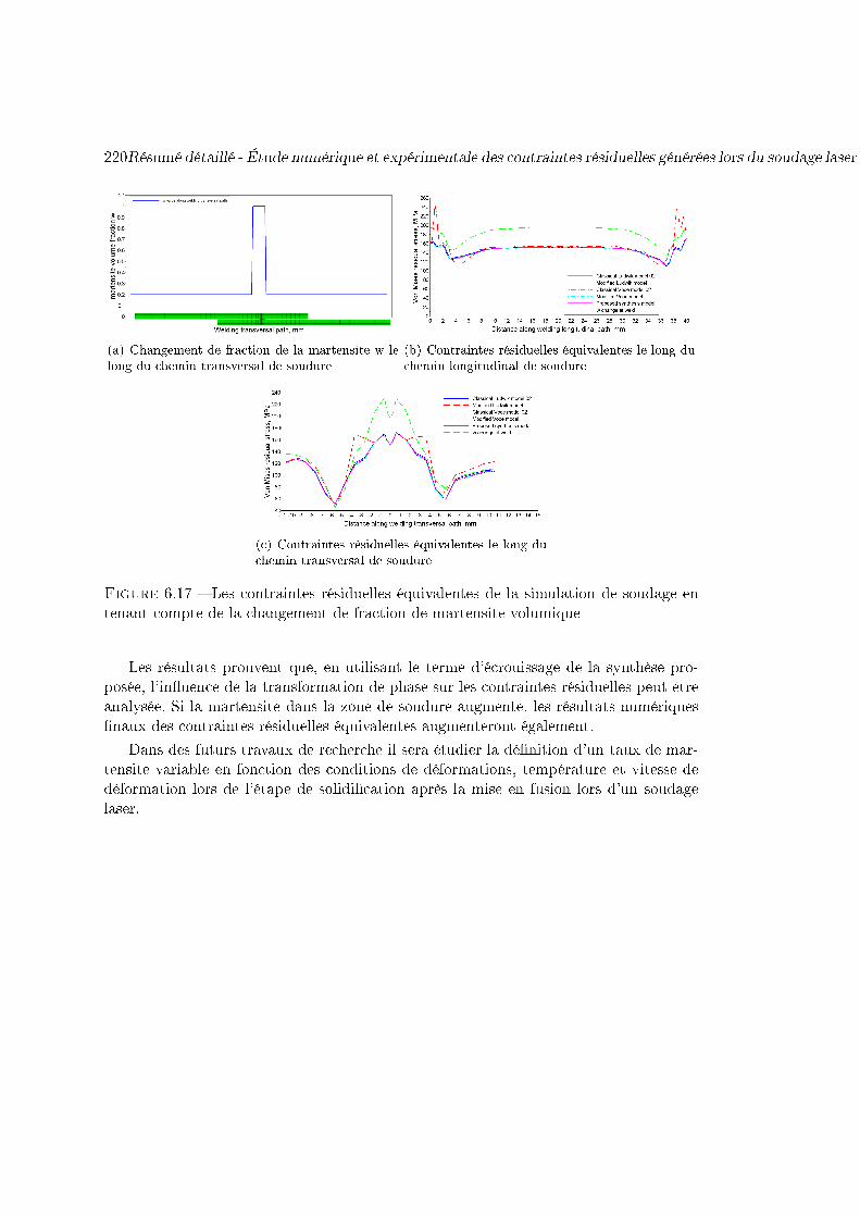
220Résumé détaillé - Étude numérique et expérimentale des contraintes résiduelles générées lors du soudage laser sur des plaques d'acier dual phase DP600
(a) Changement de fraction de la martensite w lelong du chemin transversal de soudure
(b) Contraintes résiduelles équivalentes le long duchemin longitudinal de soudure
(c) Contraintes résiduelles équivalentes le long duchemin transversal de soudure
Figure 6.17 � Les contraintes résiduelles équivalentes de la simulation de soudage entenant compte de la changement de fraction de martensite volumique
Les résultats prouvent que, en utilisant le terme d'écrouissage de la synthèse pro-posée, l'in�uence de la transformation de phase sur les contraintes résiduelles peut êtreanalysée. Si la martensite dans la zone de soudure augmente, les résultats numériques�naux des contraintes résiduelles équivalentes augmenteront également.
Dans des futurs travaux de recherche il sera étudier la dé�nition d'un taux de mar-tensite variable en fonction des conditions de déformations, température et vitesse dedéformation lors de l'étape de solidi�cation après la mise en fusion lors d'un soudagelaser.
Annexe A
List of Publications
Peer-reviewed international journals
[1] Liu S, Kouadri-Henni A, Gavrus A. Numerical simulation and experimental in-vestigation on the residual stresses in a laser beam welded DP600 dual phase steelplate : thermo-mechanical material plasticity model, International journal of Mechani-cal Sciences, 122 (2017) 235 � 243
[2] Liu S, Kouadri-Henni A, Gavrus A. DP600 dual phase steel thermo-elasto-plasticconstitutive model considering strain rate and temperature in�uence on FEM residualstress analysis of laser welding, Journal of Manufacturing Processes (reviewing).
[3]* Liu S, Kouadri-Henni A, Gavrus A. Modeling grain orientation of DP600 steelby Nd :YAG laser welding, MATEC Web of Conferences. EDP Sciences, 2016, 80 :02010. NUMIFORM-2016.
Conference proceedings and scienti�c activities
[1] Liu S, Kouadri-Henni. Numerical simulation on the residual stress of Nd :YAGlaser welding DP600, Simulation Numérique du soudages de AFM 2016.
[2] Liu S, Gavrus A, Kouadri-Henni A. Numerical and experimental research ofresidual stresses in�uenced by anisotropy on laser welding. Journée Manufacturing21,16-18 Nov. 2016.
[3] Liu S, Kouadri-Henni. Gavrus A. Modeling Grain Orientation of LaserWeldingDP600for Residual Stresses. Journée doctorale de INSA Rennes. 12 Jan. 2016.
[4] Liu S, Gavrus A, Kouadri-Henni A. Microstructure simulation of DP600 by laserwelding. Café scienti�c de INSA Rennes. 25 Feb. 2016.
[5] Liu S, Gavrus A, Kouadri-Henni A. Finite element method coupled with a nu-merical cellular automaton model used to simulate the residual stresses of dual phaseDP600 steel Nd :YAG laser welding. Congrès Français Mécanique 2017 (reviewing).
221

222 List of Publications
Bibliographie
[1] ArcelorMittal. Very high strength steels : dual phase steels. Retrieved from cata-logue produit édition européenne, 2008.
[2] Alain Lodini M.E. Fitzpatrick. Analysis of Residual Stress by Di�raction usingNeutron and Synchrotron Radiation. CRC Press, 2003.
[3] S. Curtze, V.-T. Kuokkala, M. Hokka, and P. Peura. Deformation behavior of TRIPand DP steels in tension at di�erent temperatures over a wide range of strain rates.Materials Science and Engineering A, 507 :124�131, 2009.
[4] Ph Thevoz, JL Desbiolles, and M Rappaz. Modeling of equiaxed microstructureformation in casting. Metallurgical Transactions A, 20(2) :311�322, 1989.
[5] Theodore H Maiman. Stimulated optical radiation in ruby. 1960.
[6] Robert N Hall, Gunther E Fenner, JD Kingsley, TJ Soltys, and RO Carlson. Co-herent light emission from GaAs junctions. Physical Review Letters, 9(9) :366,1962.
[7] Marshall I Nathan, William P Dumke, Gerald Burns, Frederick H Dill Jr, andGordon Lasher. Stimulated emission of radiation from GaAs p-n junctions. AppliedPhysics Letters, 1(3) :62�64, 1962.
[8] JE Geusic, HM Marcos, and LeGrand Van Uitert. Laser oscillations in nd-dopedyttrium aluminum, yttrium gallium and gadolinium garnets. Applied Physics Let-ters, 4(10) :182�184, 1964.
[9] Seiji Katayama. Handbook of laser welding technologies. Elsevier, 2013.
[10] Geo�rey Davies. Materials for automobile bodies. Elsevier, Butterworth-Heinemann, 2012.
[11] Marion Calcagnotto, Yoshitaka Adachi, Dirk Ponge, and Dierk Raabe. Deformationand fracture mechanisms in �ne-and ultra�ne-grained ferrite/martensite dual-phasesteels and the e�ect of aging. Acta Materialia,, 59(2) :658�670, 2011.
[12] DL Chen, ZG Wang, XX Jiang, SH Ai, and CH Shih. The dependence of near-threshold fatigue crack growth on microstructure and environment in dual-phasesteels. Mater. Sci. Eng., A,, 108 :141�151, 1989.
[13] Shuang Kuang, Yong-lin Kang, Hao Yu, and Ren-dong Liu. E�ect of continuousannealing parameters on the mechanical properties and microstructures of a coldrolled dual phase steel. Int J. Miner. Metall. Mater., 16(2) :159�164, 2009.
223

224 Bibliographie
[14] JR Fekete and AM Stibich. A comparison of the response of hsla and dual phasesheet in dynamic crush. IBEC,, 01 :3101, 2001.
[15] Olivier Bouaziz, Hatem Zurob, and Mingxin Huang. Driving force and logic ofdevelopment of advanced high strength steels for automotive applications. SteelRes. Int., 84(10) :937�947, 2013.
[16] Milan TUR�A, Jozef ONDRUŠKA, and Petr NESVADBA. Solid state weldingof DP600 to austenitic CrNi steel. METAL, 2010.
[17] GCC Correard, GP Miranda, and MSF Lima. Development of laser beam weldingof advanced high-strength steels. The International Journal of Advanced Manufac-turing Technology, 83(9-12) :1967�1977, 2016.
[18] Yanli Song, Lin Hua, Dongning Chu, and Jian Lan. Characterization of the in-homogeneous constitutive properties of laser welding beams by the micro-vickershardness test and the rule of mixture. Materials and Design, 37 :19�27, 2012.
[19] M. Hazratinezhad, N. B. Mostafa Arab, A. R. Su�zadeh, and M. J. Torkamany.Mechanical and metallurgical properties of pulsed neodymium-doped yttrium alu-minum garnet laser welding of dual phase steels. Materials and Design, 33 :83�87,2012.
[20] N. Farabi, D. L. Chen, and Y. Zhou. Fatigue properties of laser welded dual-phasesteel joints. Procedia Engineering, 2(1) :835�843, 2010.
[21] N. Farabi, D. L. Chen, J. Li, Y. Zhou, and S. J. Dong. Microstructure and mecha-nical properties of laser welded DP600 steel joints. Materials Science and Enginee-ring : A, 527(4 5) :1215�1222, February 2010.
[22] N. Farabi, D. L. Chen, and Y. Zhou. Microstructure and mechanical propertiesof laser welded dissimilar DP600/DP980 dual-phase steel joints. Journal of Alloysand Compounds, 509(3) :982�989, January 2011.
[23] C. Dharmendra, K.P. Rao, J. Wilden, and S. Reich. Study on laser welding-brazingof zinc coated steel to aluminum alloy with a zinc based �ller. Materials Scienceand Engineering : A, 528(3) :1497�1503, 2011.
[24] Mingsheng Xia, Elliot Biro, Zhiling Tian, and Y. Norman Zhou. E�ects of heatinput and martensite on HAZ softening in laser welding of dual phase steels. ISIJInternational, 48(6) :809�814, 2008.
[25] X. Li, S. Lawson, Y. Zhou, and F. Goodwin. Novel technique for laser lap weldingof zinc coated sheet steels. Journal of Laser Applications, 19(4) :259�264, 2007.
[26] H. Tresca. Comptes Rendus Acad. Sci. Paris, 59, 1864.
[27] H. Tresca. Comptes Rendus Acad. Sci. Paris, 64, 1867.
[28] R Von Mises. Gottinger nachrichten. math.-phys, 1913.
[29] R. Hill. A variational principle of maximum plastic work in classical plasticity. TheQuarterly Journal of Mechanics and Applied Mathematics, 1(1) :18�28, 1948.
[30] R Hill. A theory of the yielding and plastic �ow of anisotropic metals. Proceedingsof the Royal Society of London, 193(1033) :281�297, 1948.

Bibliographie 225
[31] L. Bourne and R. Hill. LX. On the correlation of the directional properties ofboiled shee in tension and cupping tests. The London, Edinburgh, and DublinPhilosophical Magazine and Journal of Science, 41(318) :671�681, July 1950.
[32] R. Hill. Theoretical plasticity of textured aggregates. In Mathematical Proceedingsof the Cambridge Philosophical Society, volume 85, pages 179�191. Cambridge UnivPress, 1979.
[33] R. Hill. Constitutive modelling of orthotropic plasticity in sheet metals. Journalof the Mechanics and Physics of Solids, 38(3) :405�417, 1990.
[34] Zheng Lin. Cailiao Tanxing Changshu Zhi Xintan (The new development of elasticconstants). Kexue Chuban She (Science Press), 2011.
[35] H Hibbitt, B Karlsson, and P Sorensen. Abaqus analysis userâ��s manual version6.10. Dassault Systèmes Simulia Corp. : Providence, RI, USA, 2011.
[36] Surajit Kumar Paul. Predicting the �ow behavior of metals under di�erent strainrate and temperature through phenomenological modeling. Computational Mate-rials Science, 65 :91�99, 2012.
[37] Frank J. Zerilli and Ronald W. Armstrong. Dislocation-mechanics-based consti-tutive relations for material dynamics calculations. Journal of Applied Physics,61(5) :1816�, 1987.
[38] G. Rr Cowper and Paul Southworth Symonds. Strain-hardening and strain-ratee�ects in the impact loading of cantilever beams. DTIC Document, pages �, 1957.
[39] Gordon R John and William H Cook. A constitutive model and data for metalssubjected to large strains, high strain rates and high temperatures. Proceedings ofthe 7th International Symposium on Ballistics, 21 :541�547, 1983.
[40] Han Zhao. A constitutive model for metals over a large range of strain rates iden-ti�cation for mild-steel and aluminium sheets. Materials Science and Engineering :A, 230(1-2) :95�99, 1997.
[41] Akhtar S Khan and Riqiang Liang. Behaviors of three bcc metal over a wide rangeof strain rates and temperatures : experiments and modeling. International Journalof Plasticity, 15(10) :1089�1109, 1999.
[42] A Gavrus. Formulation of a new constitutive equation available simultaneously forstatic and dynamic loadings. DYMAT-International Conference on the Mechanicaland Physical Behaviour of Materials under Dynamic Loading, 2 :1239�1244, 2009.
[43] Adinel Gavrus. Constitutive equation for description of metallic materials behaviorduring static and dynamic loadings taking into account important gradients ofplastic deformation. Key Engineering Materials, 504 :697�702, 2012.
[44] Adinel Gavrus, Florina Bucur, Adrian Rotariu, and Sorin Cananau. Analysis ofmetallic materials behavior during severe loadings using a fe modeling of the shpbtest based on a numerical calibration of elastic strains with respect to the rawmeasurements and on the inverse analysis principle. Key Engineering Materials,554 :1133�1146, 2013.

226 Bibliographie
[45] A Gavrus, P Caestecker, E Ragneau, and B Davoodi. Analysis of the dynamicSHPB test using the �nite element simulation. Journal de Physique IV (Procee-dings), 110 :353�358, 2003.
[46] Adinel Gavrus. Identi�cation automatique des parametres rheologiques par analyseinverse. PhD thesis, Ecole Nationale Superieure des Mines de Paris, France, 1996.
[47] Ji Hyun Sung, Ji Hoon Kim, and RH Wagoner. A plastic constitutive equationincorporating strain, strain-rate, and temperature. International Journal of Plas-ticity, 26(12) :1746�1771, 2010.
[48] Dipti Samantaray, Sumantra Mandal, and A.K. Bhaduri. Constitutive analysis topredict high-temperature �ow stress in modi�ed 9Cr-1Mo (p91) steel. Materials &Design, 31(2) :981�984, 2010.
[49] M. M. Hutchison. The temperature dependence of the yield stress of polycrystallineiron. Philosophical Magazine, 8(85) :121�127, 1963.
[50] Akhtar S. Khan, Yeong Sung Suh, and Rehan Kazmi. Quasi-static and dyna-mic loading responses and constitutive modeling of titanium alloys. InternationalJournal of Plasticity, 20(12) :2233�2248, 2004.
[51] Siying Chen, Chenguang Huang, Chunkui Wang, and Zhuping Duan. Mechanicalproperties and constitutive relationships of 30crmnsia steel heated at high rate.Materials Science and Engineering : A, 483-484 :105�108, 2008.
[52] Frederick Harwood Norton. The creep of steel at high temperatures. Number 35.McGraw-Hill Book Company, Incorporated, 1929.
[53] Kazutoshi Ohashi, Hiroshi Utsunomiya, and Ryo Matsumoto. Evaluation of r-value of steels using vickers hardness test. Journal of Physics : Conference Series,379 :012045, 2012.
[54] M Arminjon and B Bacroix. On plastic potentials for anisotropic metals and theirderivation from the texture function. Acta Mechanica, 88(3-4) :219�243, 1991.
[55] W Nasri, A Gavrus, A Kouadri-David, and K Sai. Experimental characterizationand numerical modeling of the three-dimensional anisotropic behavior of a thicksheet aluminum alloy AA2024-T351 using multi-scale approaches. High Perfor-mance and Optimum Design of Structures and Materials II, 166 :163, 2016.
[56] E Voce. A practical strain-hardening function. Metallurgia, 51(307) :219�226, 1955.
[57] Ju Chen, Ben Young, and Brian Uy. Behavior of high strength structural steelat elevated temperatures. Journal of structural engineering, 132(12) :1948�1954,2006.
[58] Bülent Aydemir, Havva Kazdal Zeytin, Gökhan Güven, and Aygun Güngör. In-vestigation of mechanical properties of DP600 steels at elevated temperatures. InISITES2014. Intech, 2014.
[59] Hibbitt, Karlsson, and Sorensen. ABAQUS : Theory Manual, volume 2. Hibbitt,Karlsson & Sorensen, 1997.

Bibliographie 227
[60] Michael T Hutchings, Philip J Withers, Thomas M Holden, and Torben Lorentzen.Introduction to the characterization of residual stress by neutron di�raction. CRCpress, 2005.
[61] K Pawlik and P Ozga. LaboTex : the texture analysis software. Göttinger Arbeitenzur Geologie und Paläontologie, SB4, 1999.
[62] P Staron, M Kocak, S Williams, and A Wescott. Residual stress in friction stir-welded al sheets. Physica B : Condensed Matter, 350(1) :E491�E493, 2004.
[63] S. M. Ulam and J. von Neumann. Random ergodic thorems. Bull. Amer. Math,51 :660, 1945.
[64] John Conway. The game of life. Scienti�c American, 223(4) :4, 1970.
[65] Stephen Wolfram. A new kind of science, volume 5. Wolfram media Champaign,2002.
[66] M. Rappaz and Ch. A. Gandin. Probabilistic modelling of microstructure formationin solidi�cation processes. Acta Metallurgica et Materialia, 41(2) :345�360, 1993.
[67] Xiaohong Zhan, Yanhong Wei, and Zhibo Dong. Cellular automaton simulation ofgrain growth with di�erent orientation angles during solidi�cation process. Journalof Materials Processing Technology, 208(1�3) :1�8, November 2008.
[68] Xiao-Hong Zhan, Zhi-Bo Dong, Yan-Hong Wei, and Yong Wang. Simulation ofcolumnar dendrite grain growth in weld pool of Ni-Cr binary alloy. The ChineseJournal of Nonferrous Metals, 19(8) :1431�1436, 2009.
[69] L. Nastac. Numerical modeling of solidi�cation morphologies and segregation pat-terns in cast dendritic alloys. Acta Materialia, 47(17) :4253�4262, 1999.
[70] W. Wang, P. D. Lee, and M. McLean. A model of solidi�cation microstructuresin nickel-based superalloys : predicting primary dendrite spacing selection. ActaMaterialia, 51(10) :2971�2987, 2003.
[71] Dieter Radaj. Welding residual stresses and distortion. Calculation and measure-ment, DVS-Verlag, Dusseldorf, 2003.
[72] X. H. Zhan, Z. B. Dong, Y. H. Wei, and Y. L. Xu. Dendritic grain growth simulationin weld molten pool based on CA-FD model. Crystal Research and Technology,43(3) :253�259, 2008.
[73] A Tiziani, P Ferro, R Cervo, and M Durante. E�ects of di�erent welding techno-logies on metallurgical anf mechanical properties of dp600 steel welded joints. LaMetallurgia Italiana, 1(1), 2011.
[74] Xin Lin, Lei Wei, Meng Wang, and Wei Dong Huang. A cellular automaton modelwith the lower mesh-induced anisotropy for dendritic solidi�cation of pure sub-stance. Materials Science Forum, 654-656 :1528�1531, 2010.
[75] Y. H. Wei, X. H. Zhan, Z. B. Dong, and L. Yu. Numerical simulation of columnardendritic grain growth during weld solidi�cation process. Science and Technologyof Welding and Joining, 12(2) :138�146, 2007.
228 Bibliographie
[76] M. Marya and X. Q. Gayden. Development of requirements for resistance spotwelding dual-phase (dp600) steels part 1�the causes of interfacial fracture. WeldingJournal,, 84(11) :172�182, 2005.
[77] Chansopheak Seang. Evaluation numérique des contraintes résiduelles appliquée àl'acier DP600 soudé par laser de haute puissance Nd : YAG. PhD thesis, Rennes,INSA, 2013.
[78] F Ozturk, S Toros, and S Kilic. Tensile and spring-back behavior of DP600 advan-ced high strength steel at warm temperatures. Journal of Iron and Steel Research,International, 16(6) :41�46, 2009.
[79] Danyang Dong, Yang Liu, Yuling Yang, Jinfeng Li, Min Ma, and Tao Jiang. Mi-crostructure and dynamic tensile behavior of DP600 dual phase steel joint by laserwelding. Materials Science and Engineering : A, 594 :17�25, January 2014.
[80] Y Y Zhao, Y S Zhang, and W Hu. E�ect of welding speed on microstructure,hardness and tensile properties in laser welding of advanced high strength steel.Science and Technology of Welding and Joining, 18(7) :581�590, October 2013.
[81] Sudook A. Kim and Ward L. Johnson. Elastic constants and internal friction ofmartensitic steel, ferritic-pearlitic steel, and α-iron. Materials Science and Engi-neering : A, 452-453 :633�639, 2007.


N◦ d'ordre : D17-14/17ISAR14Institut National des Sciences Appliques de Rennes20, Avenue des Buttes de Coësmes · CS 70839 · F-35708 Rennes Cedex 7Tel : 02 23 82 00 - Fax : 02 23 23 83 96
Résumé
Le procédé de soudage laser est largement utilisé dans les travauxd'assemblage, en particulier, dans le domaine de l'industrie automobile.L'acier dual phase DP600 est un acier à haute résistance qui permetde réduire le poids de l'automobile dans le cadre de l'allègement desstructures. Notre travail s'est essentiellement basé sur l'évaluation descontraintes résiduelles générées dans l'acier DP600 lors du soudage parlaser. Deux approches ont été réalisées. L'approche expérimentale a étéréalisée à l'aide de méthodes de rayon X et par neutrons pour calculerles contraintes résiduelles. L'approche de simulation a été réalisée parcouplage de di�érentes formulations numériques.
Numériquement, le formalisme de la mécanique continue a été utilisépar des simulations par éléments �nis (FEM) pour analyser etévaluer les contraintes résiduelles. Sur la base de tests de tractionexpérimentaux, le modèle constitutif élasto-thermo-plastique de l'acierDP600 a été identi�é. L'écrouissage du matériau a été étudié par la loide Ludwik et de Voce. A partir de résultats experimentaux, un modèlea été proposé et les résultats analysés en utilisant une loi de mélangemartensite (écrouissage Ludwik) et ferrite (adoucissement de Voce).De même, nous avons étudié la sensibilité à la température en utilisantplusieurs modèles : Johnson-Cook, Khan, Chen. A partir de cetteétude, nous avons proposé un modèle de sensibilité à la température.En�n, un modèle de sensibilité à la déformation plastique, à lavitesse de déformation issu des travaux d'A. Gavrus et un modèled'anisotropie planaire dé�nit par la théorie de Hill ont été ajoutés.
Une méthode d'automate cellulaire (CA) 2D a été programmée poursimuler l'évolution de la microstructure lors de la sali�cation liéeau processus de soudage laser. Dans ce modèle, les phénomènes denucléation avec prise en compte de l'orientation de la croissance, de laconcentration et de la vitesse de croissance à l'interface solide/liquide,l'anisotropie de la tension de surface, de la di�usion, ainsi que lafraction des phases en présence ont été pris en compte. De plus, leséquations de conservation ont été étudiées en détail et analysés. Lesrésultats ainsi que le champ de température issu du modèle FEM ontété importés dans le modèle CA. En comparant la simulation et lesrésultats expérimentaux, de bonnes concordances ont été trouvées.
Par la suite, nous avons réalisés un couplage des deux modèles CAet FEM. Concernant le procédé laser, les résultats du modèle paréléments �nis ont été analysés. La géométrie de l'échantillon, lasource de chaleur, les conditions aux limites, le comportement thermo-mécanique de l'acier dual phase DP600 telles que la conductivité, ladensité, la chaleur spéci�que, l'expansion, l'élasticité et la plasticitésont introduites. Les modèles d'analyse du terme d'écrouissage,de la sensibilité à la vitesse de déformation, de la sensibilité à latempérature, de l'anisotropie plastique et de l'anisotropie élastique ontété simulés. Les fractions volumiques concernant la nature des deuxphases en présence ont été également étudiées.
Les résultats numériques �naux les contraintes résiduelles ont étéétudiées. Les comparaisons avec des mesures expérimentales ontmontré à la fois quels phénomènes étudiés sont prépondérants et lese�ets moins in�uents sur l'évaluation des contraintes résiduelles. Lesrésultats les plus probants ont montré des bonnes convergences entrel'approche numérique et expérimentale. Ces résultats confortent larobustesse du modèle numérique développé.
Mots-clés : Soudage Laser, DP600, Contraintes Résiduelles, Automate
Cellulaire, Ecrouissage, Sensibilité à la Température, Sensibilité à la
vitesse de déformation, Anisotropie, Loi de mélange dual-phase
Abstract
The laser welding process is widely used in assembly work,particularly in the �eld of the automobile industry. The dual phaseDP600 steel is a high-strength steel which reduces the weight ofthe automobile through lightening the structures. Our work wasmainly based on the evaluation of the residual stresses generatedin the DP600 steel during laser welding. Two approaches havebeen developed. The experimental approach was carried out usingX-ray and neutron methods to calculate the residual stresses. Thesimulation approach was realized by coupling di�erent numericalformulations.
Numerically, the theory of continuous mechanics has been usedby �nite element simulations (FEM) to analyze and evaluateresidual stresses. Based on experimental tensile tests, the elasto-thermo-plastic constitutive model of DP600 steel was identi�ed.The material hardening was studied by the law of Ludwik and ofVoce. From experimental results, a model has been proposed andthe results are analyzed by using a mixing law between martensite(Ludwik hardening) and ferrite (Voce softening). Moreover,we have studied temperature sensitivity using several models :Johnson-Cook, Khan, Chen. From this study, we proposed a modelof temperature sensitivity. Finally, a model of sensitivity of plasticstrain and of strain rate according to the work of A. Gavrus and aplanar anisotropy model de�ned by Hill theory were added.
A 2D Cellular Automaton (CA) method has been programmedto simulate the evolution of the microstructure during the laserwelding process. In this model, the nucleation phenomena, theorientation of the growth, the concentration and the growth rateat the solid / liquid interface, the anisotropy of the surface tension,the di�usion as well as the fraction of the phases involved havebeen taken into account. In addition, conservation equations werestudied in detail and analyzed. The results of the temperature�eld from the FEM model were imported into the CA model.By comparing the simulation and the experimental results, goodconcordances were found.
Subsequently, we performed a coupling of the two models CAand FEM. The results of the �nite element model were analyzedfor the laser process. Sample geometry, heat source, boundaryconditions, thermo-mechanical behavior of dual phase DP600 steelsuch as conductivity, density, speci�c heat, expansion, elasticityand plasticity are introduced. The models analyzing the term ofhardening, the strain rate sensitivity, the temperature sensitivity,the plastic anisotropy and the elastic orthotropic anisotropy weresimulated. The voluminal fractions concerning the nature of thetwo phases were also studied.
The �nal numerical results of the residual stresses were stu-died. Comparisons with experimental measurements showedthat some in�uence on residual stresses are preponderant whileother in�uences are less important. The most convincing resultsshowed good convergence between the numerical and experimentalapproach. These results con�rm the validation of the developednumerical model.
Keywords : Laser Welding, DP600, Residual Stress, Cellular Auto-
maton, Hardening, Temperature sensitivity, Strain Rate Sensitivity,
Anisotropy, Mixture dual-phase law.