Stresses and deformation analysis of the storage system ...
71
Master thesis Stresses and deformation analysis of the storage system structure of the Ocean Grazer By Albert Altarriba i Subirana Supervised By prof. dr. A. Vakis MSc Industrial Engineering January 2020
-
Upload
khangminh22 -
Category
Documents
-
view
2 -
download
0
Transcript of Stresses and deformation analysis of the storage system ...

Master thesis
Stresses and deformation analysisof the storage system structure
of the Ocean Grazer
By
Albert Altarriba i Subirana
Supervised By
prof. dr. A. Vakis
MSc Industrial Engineering
January 2020


Abstract
The global warming of the planet, mainly due to the excessive use of fossil fuels, and the con-sequences that are related to this phenomenon have implied a substantial increase in the bet oncleaner and more sustainable energy sources in the last decades. Ocean Grazer is a companycreated at the University of Groningen with the aim of developing technologies that make thistransition possible. One of the elements on which it is carrying out research is an energy storagesystem, which aims to provide the electrical grid with energy coming from the wind and the ocean,with the ability to adapt at all times to the demand of the system.
The aim of this dissertation is to study the stresses and deformations that the structural partof the energy storage system, based on the suction anchoring technology, will have to endure dur-ing the installation stage. To this end, theoretical methods have been studied and used in order tofind the boundary conditions of the system during the installation process; theories and methods ofbasic mechanics and materials resistance are backed by computer-assisted analytical calculationsand simulations, which will be performed to verify the stability and resistance of the structure and,at the same time, optimize its design.
i


Contents1 Introduction 1
1.1 The Ocean Grazer. Description of the system . . . . . . . . . . . . . . . . . . . . . 1
2 Problem analysis 12.1 Problem context . . . . . . . . . . . . . . . . . . . . . . . . . . . . . . . . . . . . . 12.2 Problem definition . . . . . . . . . . . . . . . . . . . . . . . . . . . . . . . . . . . . 2
3 System definition 23.1 System context . . . . . . . . . . . . . . . . . . . . . . . . . . . . . . . . . . . . . . 23.2 Research boundaries . . . . . . . . . . . . . . . . . . . . . . . . . . . . . . . . . . . 3
4 Scope of the thesis. Objectives 44.1 Research statement . . . . . . . . . . . . . . . . . . . . . . . . . . . . . . . . . . . . 44.2 Objectives . . . . . . . . . . . . . . . . . . . . . . . . . . . . . . . . . . . . . . . . . 44.3 Stages of study . . . . . . . . . . . . . . . . . . . . . . . . . . . . . . . . . . . . . . 54.4 Research methodology. Outline for the thesis . . . . . . . . . . . . . . . . . . . . . 6
5 Literature research 75.1 Anchoring classification . . . . . . . . . . . . . . . . . . . . . . . . . . . . . . . . . 7
5.1.1 Foundations for Wind Turbine Generators . . . . . . . . . . . . . . . . . . . 75.2 Suction caissons . . . . . . . . . . . . . . . . . . . . . . . . . . . . . . . . . . . . . . 8
6 Size verification of the suction caisson installed in sand 96.1 Introduction . . . . . . . . . . . . . . . . . . . . . . . . . . . . . . . . . . . . . . . . 96.2 Holding capacity and sizing verification of the suction caissons . . . . . . . . . . . 9
6.2.1 Loads estimation. The Ultimate Limit State . . . . . . . . . . . . . . . . . 96.2.2 Horizontal holding capacity of suction caissons in sand . . . . . . . . . . . . 106.2.3 Vertical holding capacity of suction caissons in sand . . . . . . . . . . . . . 116.2.4 Case study . . . . . . . . . . . . . . . . . . . . . . . . . . . . . . . . . . . . 11
6.3 Self-weight and suction assisted penetration . . . . . . . . . . . . . . . . . . . . . . 126.3.1 Self-weight penetration . . . . . . . . . . . . . . . . . . . . . . . . . . . . . 136.3.2 Suction-assisted penetration . . . . . . . . . . . . . . . . . . . . . . . . . . . 13
7 Suction caisson design 177.1 Theoretical background . . . . . . . . . . . . . . . . . . . . . . . . . . . . . . . . . 17
7.1.1 Structural security . . . . . . . . . . . . . . . . . . . . . . . . . . . . . . . . 177.1.2 The Cross method . . . . . . . . . . . . . . . . . . . . . . . . . . . . . . . . 187.1.3 Determination of the states of stress at critical locations. Failure criterion . 197.1.4 Optimum shape of a profile . . . . . . . . . . . . . . . . . . . . . . . . . . . 217.1.5 Composite profiles . . . . . . . . . . . . . . . . . . . . . . . . . . . . . . . . 21
7.2 Outline for the analysis . . . . . . . . . . . . . . . . . . . . . . . . . . . . . . . . . 227.3 Suction caisson Case I . . . . . . . . . . . . . . . . . . . . . . . . . . . . . . . . . . 22
7.3.1 Design I.0 . . . . . . . . . . . . . . . . . . . . . . . . . . . . . . . . . . . . . 237.3.2 Design I.1 . . . . . . . . . . . . . . . . . . . . . . . . . . . . . . . . . . . . . 237.3.3 Design I.2 . . . . . . . . . . . . . . . . . . . . . . . . . . . . . . . . . . . . . 257.3.4 Design I.3 . . . . . . . . . . . . . . . . . . . . . . . . . . . . . . . . . . . . . 25
7.4 Factorial design . . . . . . . . . . . . . . . . . . . . . . . . . . . . . . . . . . . . . . 297.5 Unions . . . . . . . . . . . . . . . . . . . . . . . . . . . . . . . . . . . . . . . . . . . 337.6 Suction caisson Case II . . . . . . . . . . . . . . . . . . . . . . . . . . . . . . . . . . 367.7 Analytical validation of the models . . . . . . . . . . . . . . . . . . . . . . . . . . . 38
7.7.1 1-compartment case . . . . . . . . . . . . . . . . . . . . . . . . . . . . . . . 397.7.2 5-compartments case . . . . . . . . . . . . . . . . . . . . . . . . . . . . . . . 407.7.3 Results . . . . . . . . . . . . . . . . . . . . . . . . . . . . . . . . . . . . . . 41
ii

8 Discussion and conclusions 438.1 Discussion . . . . . . . . . . . . . . . . . . . . . . . . . . . . . . . . . . . . . . . . . 438.2 Further work . . . . . . . . . . . . . . . . . . . . . . . . . . . . . . . . . . . . . . . 44
8.2.1 Cylindrical suction caisson . . . . . . . . . . . . . . . . . . . . . . . . . . . . 448.2.2 Design I.4 . . . . . . . . . . . . . . . . . . . . . . . . . . . . . . . . . . . . . 448.2.3 Suction caisson life stages other than installation . . . . . . . . . . . . . . . 44
8.3 Conclusions . . . . . . . . . . . . . . . . . . . . . . . . . . . . . . . . . . . . . . . . 45
References 46
Appendices 47A Appendix. Suction caissons calculations literature . . . . . . . . . . . . . . . . . . 47B Appendix. Factorial design runs . . . . . . . . . . . . . . . . . . . . . . . . . . . . 52
iii

List of Figures1 Prototype of bladder functionality . . . . . . . . . . . . . . . . . . . . . . . . . . . 22 Prototype of suction caisson functionality . . . . . . . . . . . . . . . . . . . . . . . 23 Ocean Grazer storage system conceptual design. Module’s section (Ocean Grazer
B.V.) . . . . . . . . . . . . . . . . . . . . . . . . . . . . . . . . . . . . . . . . . . . . 34 Ocean Grazer storage system conceptual design. Overall layout seen from below
(Ocean Grazer B.V.) . . . . . . . . . . . . . . . . . . . . . . . . . . . . . . . . . . . 45 Storage system steel structure (Ocean Grazer B.V.) . . . . . . . . . . . . . . . . . . 46 Stages of suction caisson lifetime (Drawing done with Inkscape version 0.92). . . . 57 Anchoring classification (Pollestad (2015)) . . . . . . . . . . . . . . . . . . . . . . . 78 Common types of foundations used to support WTGs; (a)Gravity-base (b)Monopile
(c) Suction caisson (d)Tripod substructure supported by three driven piles (e)Jacketsubstructure supported by four driven piles (f)Tension leg platform (TLP) anchoredto three driven piles (g)Drag anchors (h) Ballast-stabilised floating spar platformanchored to three suction caissons (Bhattacharya et al. (2017)) . . . . . . . . . . . 7
9 Forces involved in offshore floating windmills anchored to suction caissons (Aranyand Bhattacharya (2018)) . . . . . . . . . . . . . . . . . . . . . . . . . . . . . . . . 9
10 Loads on the anchor lines (Arany and Bhattacharya (2018)) . . . . . . . . . . . . . 1011 Forces acting on suction caissons during the installation stage (Guo and Chu (2014)) 1212 Calculated required suction using equations 9 and 11 for the cases of an effective
weight with values of V′
= 1923kN and V′
= 9429kN respectively . . . . . . . . . 1413 Normalized critical suction versus relative penetration. Homogeneous sand and
layered sand with different ratios LΩ/D (Ibsen and Thilsted (2010)) . . . . . . . . 1514 Suction needed to penetrate a 20m diameter cylindrical suction caisson versus depth 1615 Qualitative representation of the probabilities of obtaining certain values for the so-
licitations and resistance. It is assumed that the correct factoring of each parameterwill always mean that Ed 6 Rd . . . . . . . . . . . . . . . . . . . . . . . . . . . . . 17
16 Structure load combinations and corresponding load factors (γf ) and ResistanceFactors (γR) for Common Structures (ABS (2016)) . . . . . . . . . . . . . . . . . . 18
17 Elastic fixed-end moment of a bar with a uniform distributed load (Lindeburg (1999)) 1918 (a)I-shape profile under bending and compression force. (b)Normal stress due to
bending and compression σx. (c)Composition of both normal and bending stressesleading to a σmax at the lower part in this particular case. A tensile normal forceor a bending force with opposite direction would lead to different results. (Drawingdone with Autocad 2018) . . . . . . . . . . . . . . . . . . . . . . . . . . . . . . . . 19
19 (a)I-shape profile under tangential force. (b)Tangential stress τxz distribution.(c)Tangential stress τxy distribution. (Drawing done with Autocad 2018) . . . . . . 20
20 Calculation of the geometric efficiency of a rectangular shape profile. (Drawing donewith Autocad 2018) . . . . . . . . . . . . . . . . . . . . . . . . . . . . . . . . . . . 21
21 Composite profile. (Drawing done with Autocad 2018) . . . . . . . . . . . . . . . . 2222 Model used in simulation I.0 (drawing from Comsol Multiphysics v5.4) . . . . . . . 2223 Area accounting for each portal frame, defined by the separation s between frames
(Lindeburg (1999)) . . . . . . . . . . . . . . . . . . . . . . . . . . . . . . . . . . . . 2324 Loads applied on the structure in design I.1 . . . . . . . . . . . . . . . . . . . . . . 2325 Diagram of flector moments of design I.1 obtained from Ftools software . . . . . . 2326 Equivalent beam with T-shape profile (Drawing done with Autocad 2018) . . . . . 2427 Detail of the corner singularity. Von Mises stress diagram obtained with Comsol v5.4 2428 Cut section of the design I.2 . . . . . . . . . . . . . . . . . . . . . . . . . . . . . . . 2529 Detail of the reinforcement in design I.2 . . . . . . . . . . . . . . . . . . . . . . . . 2530 Diagram of flector moments of design I.3 obtained from Ftools software . . . . . . 2631 Detail of the Von Mises stress distribution along a beam belonging to the central
frame . . . . . . . . . . . . . . . . . . . . . . . . . . . . . . . . . . . . . . . . . . . 2732 Theoretical End Restraint Coefficients, K (Lindeburg (1999)) . . . . . . . . . . . . 2833 Buckling curves (CEN (2005)) . . . . . . . . . . . . . . . . . . . . . . . . . . . . . . 2834 Cut section of the design I.3 used in the simulation. Symmetry has been applied . 2935 Von Mises stress graph of design I.3 . . . . . . . . . . . . . . . . . . . . . . . . . . 2936 Cube plot of total weights with focus on sand properties, factor A (Drawing done
with Autocad 2018) . . . . . . . . . . . . . . . . . . . . . . . . . . . . . . . . . . . 3237 Interaction of nr. of compartments (B) and spacing of the beams (C) . . . . . . . . 32
iv

38 Interaction of sand properties (A) and nr. of compartments (B) . . . . . . . . . . . 3239 (a)Forces transmitted from the flanges to the web (b)Stiffeners solution (c)’N’ stiff-
ener (UCLM (2005)) . . . . . . . . . . . . . . . . . . . . . . . . . . . . . . . . . . . 3440 FE simulation with Comsol of a connection without stiffeners . . . . . . . . . . . . 3441 FE simulation with Comsol of a connection with stiffeners . . . . . . . . . . . . . . 3442 FE simulation with Comsol of a connection with haunch . . . . . . . . . . . . . . . 3543 FE simulation with Comsol of a connection with haunch and stiffeners . . . . . . . 3544 Maximum equivalent Von Mises stresses in 1-compartment suction caisson with
haunches . . . . . . . . . . . . . . . . . . . . . . . . . . . . . . . . . . . . . . . . . . 3645 Maximum equivalent Von Mises stresses in 5-compartment suction caisson with
haunches . . . . . . . . . . . . . . . . . . . . . . . . . . . . . . . . . . . . . . . . . . 3646 Case II boundary conditions. 1st iteration . . . . . . . . . . . . . . . . . . . . . . . 3747 Case II bending moments diagram. 1st iteration . . . . . . . . . . . . . . . . . . . 3748 Case II normal forces diagram. 1st iteration . . . . . . . . . . . . . . . . . . . . . . 3749 Case II shear forces. 1st diagram . . . . . . . . . . . . . . . . . . . . . . . . . . . . 3750 Case II FE model. Equivalent VM stresses distribution . . . . . . . . . . . . . . . . 3851 Case II FE model. Displacements distribution . . . . . . . . . . . . . . . . . . . . . 3852 FE simulation with Comsol of run 5. Von Misses equivalent stress distribution . . 3953 FE simulation with Comsol of run 5 with haunch reinforcements. Von Misses equiv-
alent stress distribution . . . . . . . . . . . . . . . . . . . . . . . . . . . . . . . . . 3954 Shear force diagram run 5, 1st iteration . . . . . . . . . . . . . . . . . . . . . . . . 3955 Nodes assignation of end bars studied sections . . . . . . . . . . . . . . . . . . . . . 3956 Analysed points of the profile when a shear force is present (drawing done with
Autocad 2018) . . . . . . . . . . . . . . . . . . . . . . . . . . . . . . . . . . . . . . 3957 Shear force diagram run 7, 1st iteration . . . . . . . . . . . . . . . . . . . . . . . . 4058 Nodes assignation of end bars studied sections . . . . . . . . . . . . . . . . . . . . . 4059 Equivalent Von Mises stress distribution of run 5 model . . . . . . . . . . . . . . . 4260 Bending moment diagram run 5, 1st iteration . . . . . . . . . . . . . . . . . . . . . 4261 Detail of the equivalent Von Mises stress distribution of run 5 model, see figure 59 4262 Detail of a possible implementation of a non-uniform reinforcement layout . . . . . 4463 Equilibrium of slice of soil within caisson when pulling it up (Houlsby et al. (2005)) 4864 Equilibrium of slice of soil within caisson during installation (Houlsby and Byrne
(2005)) . . . . . . . . . . . . . . . . . . . . . . . . . . . . . . . . . . . . . . . . . . . 4965 Relative density and effective unit weight. Test CPT.WFS4.28 (Netherlands Enter-
prise Agency (2016)) . . . . . . . . . . . . . . . . . . . . . . . . . . . . . . . . . . 5066 Loading diagram run 1, preliminary stage . . . . . . . . . . . . . . . . . . . . . . . 5267 Bending stress diagram run 1, preliminary stage . . . . . . . . . . . . . . . . . . . 5268 Normal stress diagram run 1, preliminary stage . . . . . . . . . . . . . . . . . . . . 5269 Bending stress diagram run 1, 1st iteration . . . . . . . . . . . . . . . . . . . . . . 5370 Normal stress diagram run 1, 1st iteration . . . . . . . . . . . . . . . . . . . . . . . 5371 Bending stress diagram run 2, preliminary stage . . . . . . . . . . . . . . . . . . . 5372 Normal stress diagram run 2, preliminary stage . . . . . . . . . . . . . . . . . . . . 5373 Bending stress diagram run 2, 1st iteration . . . . . . . . . . . . . . . . . . . . . . 5474 Normal stress diagram run 2, 1st iteration . . . . . . . . . . . . . . . . . . . . . . . 5475 Bending stress diagram run 3, preliminary stage . . . . . . . . . . . . . . . . . . . 5476 Normal stress diagram run 3, preliminary stage . . . . . . . . . . . . . . . . . . . . 5577 Bending stress diagram run 3, 1st iteration . . . . . . . . . . . . . . . . . . . . . . 5578 Normal stress diagram run 3, 1st iteration . . . . . . . . . . . . . . . . . . . . . . . 5579 Bending stress diagram run 4, preliminary stage . . . . . . . . . . . . . . . . . . . 5680 Normal stress diagram run 4, preliminary stage . . . . . . . . . . . . . . . . . . . . 5681 Bending stress diagram run 4, 1st iteration . . . . . . . . . . . . . . . . . . . . . . 5682 Normal stress diagram run 4, 1st iteration . . . . . . . . . . . . . . . . . . . . . . . 5683 Bending stress diagram run 5, preliminary stage . . . . . . . . . . . . . . . . . . . 5784 Normal stress diagram run 5, preliminary stage . . . . . . . . . . . . . . . . . . . . 5785 Bending stress diagram run 5, 1st iteration . . . . . . . . . . . . . . . . . . . . . . 5786 Normal stress diagram run 5, 1st iteration . . . . . . . . . . . . . . . . . . . . . . . 5787 Bending stress diagram run 6, preliminary stage . . . . . . . . . . . . . . . . . . . 5888 Normal stress diagram run 6, preliminary stage . . . . . . . . . . . . . . . . . . . . 5889 Bending stress diagram run 6, 1st iteration . . . . . . . . . . . . . . . . . . . . . . 59
v
90 Normal stress diagram run 6, 1st iteration . . . . . . . . . . . . . . . . . . . . . . . 5991 Bending stress diagram run 7, preliminary stage . . . . . . . . . . . . . . . . . . . 5992 Normal stress diagram run 7, preliminary stage . . . . . . . . . . . . . . . . . . . . 5993 Bending stress diagram run 7, 1st iteration . . . . . . . . . . . . . . . . . . . . . . 6094 Normal stress diagram run 7, 1st iteration . . . . . . . . . . . . . . . . . . . . . . . 6095 Bending stress diagram run 8, preliminary stage . . . . . . . . . . . . . . . . . . . 6096 Normal stress diagram run 8, preliminary stage . . . . . . . . . . . . . . . . . . . . 6197 Bending stress diagram run 8, 1st iteration . . . . . . . . . . . . . . . . . . . . . . 6198 Normal stress diagram run 8, 1st iteration . . . . . . . . . . . . . . . . . . . . . . . 61
vi

List of Tables1 Tools for the development of products . . . . . . . . . . . . . . . . . . . . . . . . . 12 Typical size and skirt length L to diameter D ratio (L/D) values for different suction
foundations applications (Tjelta (2015)) . . . . . . . . . . . . . . . . . . . . . . . . 83 Minimum caisson dimensions for various length to diameter ratios, installed in sand 124 Parameter values used in the implementation of equations 9 and 11, depicted in
figure 12 . . . . . . . . . . . . . . . . . . . . . . . . . . . . . . . . . . . . . . . . . . 145 Geometric efficiencies depending on profile shape. (Drawings done with Autocad
2018) . . . . . . . . . . . . . . . . . . . . . . . . . . . . . . . . . . . . . . . . . . . . 216 Test matrix with coded levels . . . . . . . . . . . . . . . . . . . . . . . . . . . . . . 317 Geometric efficiencies and bars utilization of profiles chosen in the factorial design 318 Data for interaction plot of nr. of compartments versus reinforcements spacing . . 329 Data for interaction plot of sand properties versus nr. of compartments . . . . . . 3210 Higher equivalent Von Mises stresses comparison between FE simulations . . . . . 3411 Values referred to concrete pipe . . . . . . . . . . . . . . . . . . . . . . . . . . . . . 3712 Comparison between FE simulation and theoretical stresses and displacement values
across the run 5 model (1 compartment) . . . . . . . . . . . . . . . . . . . . . . . . 4013 Comparison between FE simulation and theoretical stresses and displacement values
across the run 7 model (5 compartments) . . . . . . . . . . . . . . . . . . . . . . . 4114 Relationship between Relative Density (Dr) and Angle of Internal Friction (φ) in
sand (Lindeburg (1999)) . . . . . . . . . . . . . . . . . . . . . . . . . . . . . . . . . 5115 Factor values used in run 1 . . . . . . . . . . . . . . . . . . . . . . . . . . . . . . . 5216 Factor values used in run 2 . . . . . . . . . . . . . . . . . . . . . . . . . . . . . . . 5317 Factor values used in run 3 . . . . . . . . . . . . . . . . . . . . . . . . . . . . . . . 5418 Factor values used in run 4 . . . . . . . . . . . . . . . . . . . . . . . . . . . . . . . 5519 Factor values used in run 5 . . . . . . . . . . . . . . . . . . . . . . . . . . . . . . . 5720 Factor values used in run 6 . . . . . . . . . . . . . . . . . . . . . . . . . . . . . . . 5821 Factor values used in run 7 . . . . . . . . . . . . . . . . . . . . . . . . . . . . . . . 5922 Factor values used in run 8 . . . . . . . . . . . . . . . . . . . . . . . . . . . . . . . 60
vii

MSc Industrial Engineering - Thesis
1 Introduction
1.1 The Ocean Grazer. Description of the systemThe Ocean Grazer, a Dutch start-up founded in 2016, which has been developed within the Univer-sity of Groningen (RuG) since 2014, is a versatile offshore renewable energy harvesting platformthat integrates various subsystems, based in wave and wind power extraction as well as energystorage on site. The adaptable wave energy converter (WEC), the core of the technology, consistsof a floater blanket on the ocean surface that adapts to the incoming wave features, allowing thisnovel technology, combined with an internal pumping system, to increase the power that can beextracted from the sea waves. Another of the subsystems is the Ocean Battery, an on-site loss-lessenergy storage system, able to control the energy output and adapt to the necessities of the elec-tricity grid.The first concept was based in a large scale wave energy converter designed to be implemented indeep waters like the Atlantic, where most of the ocean power resources worldwide can be found,meaning a greater impact to society. However, in terms of business approach, the current OceanGrazer version will be implemented in shallower waters, such as the North Sea, with the aim ofreleasing these different subsystems so that various configurations and combinations of wind andwave harvesting as well as energy-storage are allowed.
2 Problem analysis
2.1 Problem contextThe Ocean Grazer is an innovative project that works in a vast range of fields with the aim ofdefining the best solutions for its products, by adapting them to the new improvements developedthroughout different iterative steps of the innovative process, carried out by researchers within thecompany. At the moment, the project remains within a laboratory stage, where these outputs aredeveloped by means of conceptualization and materialization design, as well as prototyping. Designand subsequent optimization of models have been performed in order to define and understand thebehaviour of the system while receiving inputs from the environment and how it will adapt to themin the best way, as well as how its output can be maximized and fulfil its expected functions.To date, the storage system version is still being developed. In the process of designing a mechanicalelement or structure, a preliminary design is developed in the first stages in order to approach theproblem in general terms, allowing the researchers to check the convenience of the chosen designparameters and get a first glimpse of the mechanics involved in that very first design. This paper,however, does not start from scratch; the Ocean Grazer company has already been working in adesign. Some of the dimension parameters, which will be detailed later on in the requirementssection, have been mainly determined by the power capacity of the system. However, some of itsfeatures have been defined based in literature and own experience in the field, since exhaustiveresearch has not been previously carried out within the company, or it is investigated at themoment.As in any company which intends to develop a product, one of the most relevant activities arethose related to the performing of prototypes and testing. These can be virtual and physicalrepresentations with the aim of studying the shape, behaviour or its construction.
Table 1: Tools for the development of products
Virtual PhysicalShape CAD model Scale modelBehaviour CAE model PrototypeConstruction CAM model Pre-series
The first step is the use of virtual representation tools, which contribute to the knowledge ofthe product. Different CAD models, with distinct levels of detail, have been implemented. Forinstance, see the one depicted in figure 3.In order to validate the principle of functionality, preliminary prototyping has been carried out. Onthe one hand, a methacrylate structure of the whole module has been build so that the behaviour
1

MSc Industrial Engineering - Thesis
of the flexible reservoir can be tested (see figure 1). A previous version of the storage system hadthe constraint of the bladder suffering a lot of wrinkles while moving. This test allowed to validatethe improvements in the new design.On the other hand, suction anchors testing is also implemented, by means of a methacrylatestructure. The different processes involved in the installation of a suction anchor, as detailed laterin the report, are tested (see figure 2).
Figure 1: Prototype of bladder functionality Figure 2: Prototype of suction caisson functionality
2.2 Problem definitionThe Ocean Grazer team, with M van Rooij as chief technical officer (CTO) and principal problemowner, is interested in proving that the designs that are being developed for the Ocean Grazerstorage system will have the expected performance.Before moving forward in the development of the product, and therefore performing the indispens-able testing in the last stages of the materialization design, simulation is a key step. From thepoint of view of time and cost resources, it is essential to simulate the product until the mostreasonable and possible point.As stated in the previous section, CAD designs and first-stages prototypes have been carried out,but no computer-aided engineering (CAE) simulations are available. In structural mechanics stud-ies, finite element analysis (FEA) are of special interest to evaluate the stresses occurring withinthe element of study under certain boundary conditions.
3 System definitionThis section aims to give a description of the system in order to define the boundaries of theproblem analysed in this report. Based in the problem previously depicted, it is necessary todelimit the system that will be studied, that is the elements that will be taken into account andthose which are out of the scope or unattainable so they will be excluded or will be considered asexternal actors.
3.1 System contextThe Ocean Battery, the energy storage system, consists of a rigid tank at atmospheric pressureand a flexible reservoir - the bladder reservoir. When energy production exceeds the demand, theinternal working fluid (assumed to be water in this paper) will be pushed from the rigid reservoirto the flexible one, this is inflating the bladder, so that the absorbed energy can be accumulatedas potential energy; its deflation by means of the hydrostatic pressure of the ocean, allows theworking fluid to go through a turbine, where the stored potential energy will be transformed intomechanical energy, and thereafter into electricity production, when it is needed. This structurewill be attached to the seabed by means of suction anchoring, a well-known technology that allowsthe storage subsystem to be an independent module that, as specified in section 1.1, is meant tobe combined with the other Ocean Grazer applications, but can also be used in currently workingharvesting plants (i.e. offshore wind farms), storing the production of electricity but also as amooring system (i.e. floating wind turbines).Moreover, with the objective of making the most of the product in terms of versatility and possible
2

MSc Industrial Engineering - Thesis
applications, the problem owners want the suction anchor design to work as an independent an-choring system; thus, the OG storage system could be placed on it, but also, any other structure.The proper definition of each specific case will be done in due course.
Figure 3: Ocean Grazer storage system conceptual design. Module’s section (Ocean Grazer B.V.)
The structure is based in a module intended to allow for different configurations of the storage sys-tem itself, by means of attaching several modules to each other. These modules basically include,among many other structural and functional elements, the steel suction anchor, the rigid tanksmade of concrete, and the flexible bladder made of EPDM synthetic rubber.Unlike most of the cases found in literature, and as it will be detailed later on the following sec-tions, the first design approach for the Ocean Grazer’s suction caisson is in a rectangular shapewith its skirts made of steel, over which the concrete pipes will be attached. They will includesome internal plates and other structural elements in order to provide strength and stiffness tothis vast structure, especially during the installation, to prevent them from bending or buckling.The reasons to conduct research into a new design of the suction caissons to those implementeduntil now are in part economical; thus, instead of cylindrical buckets, we can take advantage of thestorage system layout to convert its bottom profile into the actual anchoring system. Therefore,the skirt of these caissons will be the base of each module.
Although the scope of this paper is to develop the design in function of the results obtainedthrough the simulation analysis, there are several requirements (geometric specifications, mate-rials, etc.) that the design has to meet in order to accomplish its functionality notwithstandingits viability in terms of constructive feasibility and economical profitability. These last issues areout of the scope of this project, but they are not neglected, so the decisions are taken with thosestakeholders involved. The skirt of the suction caissons dimensions are 20 meters both width anddeep, with a thickness of 3cm. The height of the skirt is initially set to 7m. The rigid tanks willhave a cylindrical shape and will be made of concrete with fiber reinforcement. The outer diameteris set to 10m with a thickness of 0.5m.As said above, the design is though to be done in modules to allow for different configurations;however, the Ocean Grazer is working in a layout based in 8 suction anchors attached to eachother, as it is depicted in figure 4, of which 4 have a corner design. With the dimensions previ-ously mentioned, this whole framework has a length and width of 70m at the concrete pipes level.The fact of having not only a suction caisson, but 8 of them, makes the installation process morecontrollable, allowing the structure to penetrate as desired by applying different suction pressuresin each compartment.
3.2 Research boundariesThe system that is taken into consideration in this project is basically the steel suction anchors.The concrete pipes, as well as elements of union between each other, or with other elements areout of the scope.
The flexible bladder will not be of concern in this project because it is considered that, whether
3

MSc Industrial Engineering - Thesis
Figure 4: Ocean Grazer storage system conceptual design. Overalllayout seen from below (Ocean Grazer B.V.)
Figure 5: Storage system steelstructure (Ocean Grazer B.V.)
the flexible reservoir is full or empty, the pressure applied to the outside of the bladder will betotally transmitted to the concrete and steel structures.
The contact between the steel skirts and the soil is known to be of high complexity. The in-teraction between both domains will depend, to a great extend, on the features of the terrainwhere it is installed. Certainly, there is a wide range of possibilities which are determined not onlyby the location, but also affected by the depth, leading to a series of layers of sand and clay withdifferent physical properties. Related to it, phenomena of different nature can arise in the vicinityof the suction caisson, leading to a behaviour of challenging prediction. Therefore, the soil has beenexcluded from the simulation analysis, making the corresponding assumptions or simplifications indue time. Moreover, whenever necessary in analytical calculations, the soil properties used will bethose of sand.The interaction between seawater and the structure will also be simplified, and all forces and mo-ments involved will be considered as external loads applied on the system. Other elements suchas those related to the mooring system, installation or maintenance components will be out of thescope and their effect on the system will be treated with the same approach.
4 Scope of the thesis. Objectives
4.1 Research statementBased on the previous sections, a goal statement is formulated to become the aim of this masterthesis:
Study the mechanics of the Ocean Grazer’s storage system in order to define the optimum designto fulfill its functions.
4.2 ObjectivesTherefore, the research goals can be summarized as follows:
• Analytical study of the structure, taking into account the boundary conditions and theloading capacities, in order to verify the preliminary design, currently being designed byOcean Grazer.
• Construction of a model to simulate the internal stresses and deformations that will occurwithin the main base structure, due to different forces that will be applied on it.
• Contribution to the actual design, by usage of this model, in terms of mechanical performanceunder the expected solicitations, and delivery of design guidelines.
4
MSc Industrial Engineering - Thesis
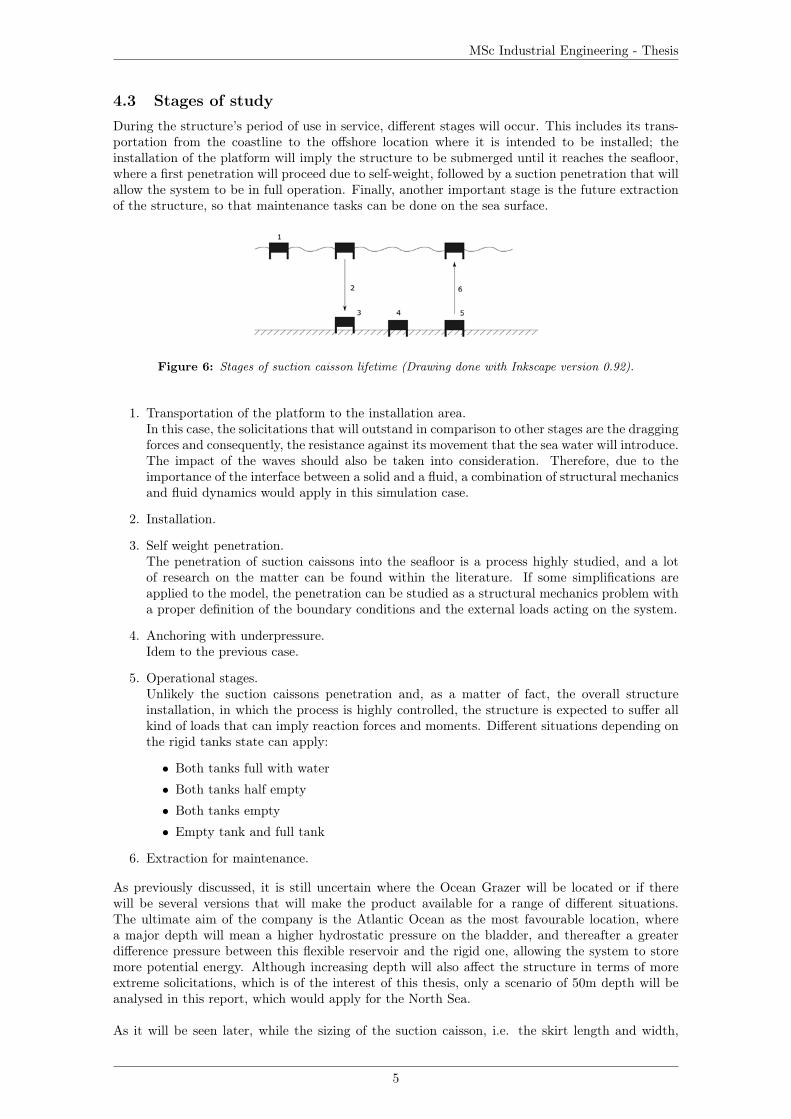
4.3 Stages of studyDuring the structure’s period of use in service, different stages will occur. This includes its trans-portation from the coastline to the offshore location where it is intended to be installed; theinstallation of the platform will imply the structure to be submerged until it reaches the seafloor,where a first penetration will proceed due to self-weight, followed by a suction penetration that willallow the system to be in full operation. Finally, another important stage is the future extractionof the structure, so that maintenance tasks can be done on the sea surface.
Figure 6: Stages of suction caisson lifetime (Drawing done with Inkscape version 0.92).
1. Transportation of the platform to the installation area.In this case, the solicitations that will outstand in comparison to other stages are the draggingforces and consequently, the resistance against its movement that the sea water will introduce.The impact of the waves should also be taken into consideration. Therefore, due to theimportance of the interface between a solid and a fluid, a combination of structural mechanicsand fluid dynamics would apply in this simulation case.
2. Installation.
3. Self weight penetration.The penetration of suction caissons into the seafloor is a process highly studied, and a lotof research on the matter can be found within the literature. If some simplifications areapplied to the model, the penetration can be studied as a structural mechanics problem witha proper definition of the boundary conditions and the external loads acting on the system.
4. Anchoring with underpressure.Idem to the previous case.
5. Operational stages.Unlikely the suction caissons penetration and, as a matter of fact, the overall structureinstallation, in which the process is highly controlled, the structure is expected to suffer allkind of loads that can imply reaction forces and moments. Different situations depending onthe rigid tanks state can apply:
• Both tanks full with water
• Both tanks half empty
• Both tanks empty
• Empty tank and full tank
6. Extraction for maintenance.
As previously discussed, it is still uncertain where the Ocean Grazer will be located or if therewill be several versions that will make the product available for a range of different situations.The ultimate aim of the company is the Atlantic Ocean as the most favourable location, wherea major depth will mean a higher hydrostatic pressure on the bladder, and thereafter a greaterdifference pressure between this flexible reservoir and the rigid one, allowing the system to storemore potential energy. Although increasing depth will also affect the structure in terms of moreextreme solicitations, which is of the interest of this thesis, only a scenario of 50m depth will beanalysed in this report, which would apply for the North Sea.
As it will be seen later, while the sizing of the suction caisson, i.e. the skirt length and width,
5

MSc Industrial Engineering - Thesis
has an influence on the holding capacity, the integrity of the structure will depend on the differentextreme solicitations that will be applied on it.It is easy to see that one of the most extreme cases will be during the suction assisted penetrationwithin the installation process, when there will be a pressure difference between the inside and theoutside of the caisson. This is the case that this thesis will study and analyse.
4.4 Research methodology. Outline for the thesisIn this section, the ways in which the author approached the purpose of exploring the mechanicsof the structure, and indeed the convenience of the design, is described.The analysis carried out can be divided into two types:
• Analytical calculations by means of a theoretical framework: on one hand, calculations basedin methods found in literature related to suction caisson installation procedures that provedto have a high degree of accuracy and that, therefore have been accepted and used by differentauthors; on the other hand, the application of different basic mathematical theories relatedto resistance of materials and structural studies, in bases of verifying the results obtained bythe simulation analysis, mentioned in the next point.
• FE analysis using Comsol Multiphysics version 5.4. A series of simulation tests will be carriedout, starting from basic designs, and subsequently increasing its level of detail and complexity.A Comsol model will be built in order to obtain the desired results while changing differentparameters of interest in terms of boundary conditions and geometric variables.
6

MSc Industrial Engineering - Thesis
5 Literature research
5.1 Anchoring classificationThe anchoring system of most offshore structures can be classified in one of these types:
• Surface gravity anchors or gravity-based structures (GBS): they are very large support struc-tures that sit on the seabed, being hold in place by gravity, and resisting sliding and over-turning loads by friction and soil bearing capacity.
• Drag anchors: consisting of a shank and a fluke. When the anchor is dragged, the fluke digsinto the soil, creating a large holding capacity against horizontal loads.
• Driven piles: cylindrical and hollow steel pipes with a large lengthe to diameter (L/D) ratio,which are drilled or driven into the seabed. Their holding capacity relies on the frictionbetween the pile length and the soil.
• Suction anchors or suction caissons
Figure 7: Anchoring classification (Pollestad (2015))
5.1.1 Foundations for Wind Turbine Generators
Wind turbine generators (WTG) can be supported on various types of foundations, which areshown in figure 8, and that are based on the 4 main typologies that haven been previously de-picted. Figure 8 (a) shows a gravity base foundation, while (b), (d), (e) and (f) are differentimplementations of driven piles; (c) and (h) use suction caissons and type (g) is an example ofdrag anchors (Bhattacharya et al. (2017)).As it will be explained in the next section, suction anchors have been used and combined withother technologies, so other possibilities can be also explored. For instance, tension leg platforms1can be anchored by driven piles (figure 8 (f)), but also with suction caissons.
Figure 8: Common types of foundations used to support WTGs; (a)Gravity-base (b)Monopile (c) Suctioncaisson (d)Tripod substructure supported by three driven piles (e)Jacket substructure supported by fourdriven piles (f)Tension leg platform (TLP) anchored to three driven piles (g)Drag anchors (h) Ballast-stabilised floating spar platform anchored to three suction caissons (Bhattacharya et al. (2017))
1Tension leg platforms (TLP) is a concept which relies on steel cables tensioning a buoyant hull to the seafloorpiling system
7

MSc Industrial Engineering - Thesis
5.2 Suction caissonsSuction caissons are a relatively new form of offshore foundation usually based on large, cylindricalstructures, mainly made of steel, closed at the top and open at the base such as the shape of anupturned bucket. Their principal applications are as a shallow foundation or as an anchoring sys-tem for all kind of designs, including floating structures, in which case the use of suction caissonshas been increasing in recent years for many reasons; for instance, they are easier to install thanimpact-driven piles and can be used in deep water, as well as providing higher load capacities thanfor example, drag embedment anchors; another relevant characteristic is the fact that it can berapidly removed by reversing the installation process, applying an overpressure inside the caissoncavity (Tassoulas et al. (2005)).One main design challenge for this kind of structures is to penetrate the skirt deep enough toobtain the required capacity. That is why they are initially penetrated into the sea-bottom sedi-ments under their own weight, and afterwards pushed to the required depth, applying a differentialpressure inside the cavity by means of pumping water out of the interior. A factor which affectsthe penetration of the suction anchoring is the soil plug formed inside the caisson. When it ispenetrated, soil will move through the open ended rib into the hollow caisson and form soil plug,which adds a resistive force against penetration (Guo and Chu (2014)).
Suction caissons have been used extensively since mid 1990’s for anchoring purposes. For a longtime they were known as suction anchors due to its installation technique—suction-installed; how-ever, experience supports the idea that suction is remarkably important for the holding capacity ofthese foundations during their operational stage. If the structure is totally sealed, suction appearswhen loading is applied. While for soils with high permeability such as sand, this holding capacitycan only be maintained for a short period of time, for low permeability soils like clays, this holdingcapacity can be maintained for years (Tjelta (2015)).
Table 2: Typical size and skirt length L to diameter D ratio (L/D) values for different suction foundationsapplications (Tjelta (2015))
Application Typical diameter (m)Moorings: L/D < 5 4-6Subsea structures: 1 < L/D < 4 5-10Jackets: L/D < 1 8-15Gravity base structures2: L/D 1 to 1 23-35Monopod tower 15-20
Tjelta (2015) gives typical values of size and L/D ratio recommended for different kind of suctionfoundations and its applications, depicted in table 2. The same source also explains the historicevolution of this technology, which is summarized in the following paragraphs.The invention and implementation of suction caissons has slightly evolved from the first mooringtests by Shell in the late 1970’s and its first commercial application at the Gorm field (North Sea,Denmark) in 1981, with twelve suction piles for the anchoring of an oil loading buoy.During the 1990’s suction foundations became a frequently used foundation, specially for the factthat offshore development moved to locations with deeper waters. The Snorre suction foundation(North Sea, Norway) in 1990-1992 was the first TLP foundation to use suction anchors. Alsoduring this decade, the first two jackets which replaced pile foundations with suction caissons wereinstalled for the Draupner "E" Riser Platform and the Sleipner "T" Processing Platform (NorthSea, Norway).From 2000, the high activity in deep waters exponentially increased the number of suction founda-tions used for offshore developments, and in the last decade, suction caissons have been consideredfor the renewable industry. With the objective of provididing practical support and encouragingthe industry to use this technology, the Carbon Trust published the Offshore Wind AcceleratorSuction Installed Caisson Foundation Design Guidelines. Suction caissons can be seen supportingthe 8MW turbines at Vattenfall’s European Offshore Deployment Centre in Scotland and Ørsted’sBorkum Riffgrund 2 in Germany. (Cathie and Irvine (2019)).
2Although gravity-base structures are considered as another type of anchoring, some structures installed inpoor ground conditions are founded on a system of suction caissons. In 1989, the Gullfaks C concrete platform wasinstalled and meant the first time long concrete skirts acting as piles were implemented for a gravity-based structure.(Tjelta (2015))
8

MSc Industrial Engineering - Thesis
6 Size verification of the suction caisson installed in sand
6.1 IntroductionA lot of research has been done and many analytical methods and formulations have been devel-oped by different authors, to firstly approach the forces involved during the installation and usageof the system and predict other variables of interest, when designing the suction caissons, so thattheir integrity will not be compromised in any case. As previously said, this report does not aimto carry out a deep research on the optimization of the suction caisson for the Ocean Grazer interms of the external conditions, but to build a model depending on them and predict the structureperformance. However, the author considers that an estimation of certain parameters is of interest,so that the results obtained in this paper, and consequently, the decisions taken will better fit thereality and therefore will be closer to those implemented in future research. A verification of thesetheories is also out of the scope. All the theories used in the following sections are formulated bytheir authors for the case of a cylindrical caisson. The author of this thesis has adapted them intothe case of a rectangular shape. Thus, the calculations conducted do not seek an exact output butan approximate order of magnitude of some parameters.
6.2 Holding capacity and sizing verification of the suction caissons6.2.1 Loads estimation. The Ultimate Limit State
Due to the inflation and deflation of the flexible bladder, the rigid tanks will contain a certain por-tion of working fluid and the rest will be filled with air at atmospheric pressure. As any other solidsubmerged in water, it will appear a buoyancy force, that can be estimated as the volume of fluiddisplaced. In the particular case of the air cavity, the effect will be considerable since practicallyno weight will go against it. When all that fluid is pumped into the bladder, the rigid cylindricalreservoirs will be totally empty, leading to the most extreme situation. Its value is computed inthe "Vertical load on the anchor" of table 3, along the vertical load due to mooring (Ta sin θa, seenext paragraphs for explanation).
Figure 9: Forces involved in offshore floating windmills anchored to suction caissons (Arany and Bhat-tacharya (2018))
As exposed previously, the storage system is due to perform an additional functionality relatedto the anchoring of other renewable energy harvesting platforms, mainly Floating Offshore WindTurbines (FOWT). Arany and Bhattacharya (2018) provides a simplified approach for finding anupper bound limit for the expected loads that a typical structure of this kind would transfer tothe anchor through a catenary mooring.The maximum load is assumed to be the sum of the wind load, drag and inertia components ofthe wave load, the wind drag on the structural components above water level and the current loadon the floating platform.Arany and Bhattacharya (2018) perform a series of calculations in order to obtain the ultimatelimit state load for the Hywind floating platform, based in Scotland, which consists of five turbines
9

MSc Industrial Engineering - Thesis
of 6 MW each. They conclude that the most extreme situation that the anchor will be subject tois the scenario with the combination of an extreme wave height (which happens every 50 years)and an extreme wind speed with the turbine shut down (also happens every 50 years), with avalue of 23.1MN, applied through the mooring line. This force is applied totally horizontally tothe embedded inverse catenary, located between the seabed and the anchor padeye, which is thedevice placed along the caisson skirt that provides an attachement point to the catenary.As explained in previous sections, this paper does not aim to deeply look into an analytical studyof a suction caisson, let alone a design that could fit in the requirements that a specific FOWTcould demand. That is why the value of 23.1 MW applied through the catenary mooring (Tm infigure 10) is considered a good starting point in the suitability of the caisson design.
Figure 10: Loads on the anchor lines (Arany and Bhattacharya (2018))
The actual load applied on the suction caisson (Ta) is obtained by taking into consideration theload reduction on the inverse caternary from the mudline to the anchor padeye. The anchor padeyetension (Ta) and the angle (θa) can be obtained by solving:
Ta2
(θ2a − θ2
m) = zaQav (1)
TmTa
= eµ(θa−θm) (2)
where
Ta Tension at the anchor padeyeTm Tension at the mudlineθa Angle of the tension at the anchor padeye to horizontalθm Angle of the tension at the mudline to horizontalza Depth of the anchor padeye below mudlineµ Friction coefficient between the forerunner (chain, rope or wire) and the soilQav Average soil resistance between the mudline and the padeye.
For sand, the padeye depth (za) is related to the caisson’s height by za/L = 2/3; in that case θmis considered null, so that the mooring line is transmitting a totally horizontal force Tm; a valueof 0.25 is taken for the friction coefficient µ; the average soil resistance is calculated as:
Qav =1
2AbNcγ
′za (3)
where
Ab effective unit bearing area of the forerunner (according to Arany and Bhattacharya (2018) itequals the diameter of the rope or wire, and 2.5-2.6 times the bar diameter in case of using achain; a value of 1.2 has been considered in these calculations)
Nc bearing capacity factor (a value of 14 has been used)γ
′submerged unit weight of the soil (a value of 8.5 kN/m3 has been used)
6.2.2 Horizontal holding capacity of suction caissons in sand
When anchored in sand, the horizontal capacity of the caisson can be estimated (Chatzivasileiou(2014)) as follows
Hc,sand = LQav =1
2AbNqγ
′L2 ≈ 1
2DoNqγ
′L2 (4)
10

MSc Industrial Engineering - Thesis
where Nq is another bearing capacity factor, which can be obtained as
Nq = eπ tanφ tan2(45o +φ
2) (5)
where φ is the internal angle of friction of the soil, an intrinsic parameter of the sand where thecaisson is anchored (in that case a value of 30o has been taken into account for φ). These and otherparameters will be used again in the calculations of the suction caisson installation, in section 6.3(detailed information about soil parameters has been summarized in appendix A.6).In this case, since the design is not cylindrical but rectangular, the outer diameter Do is approxi-mated with the skirt width (that is Do = wo = lo = 20 meters).
6.2.3 Vertical holding capacity of suction caissons in sand
Vertical holding capacity of a suction anchoring in sand when tensile load is applied very slowlycan be calculated as a fully drained study (Houlsby et al. (2005)). That would be the case ofconcern, since the buoyancy forces, most responsible of the uplift load, change progressively duringthe storage system operational stage.The resistance of the caisson is calculated as the sum of friction on the outside (Qout) and theinside (Qin) of the skirt. These forces are calculated as the shear stress acting on the skirt area ofthe caisson due to its contact with the soil. It is assumed that horizontal effective stress is a factorK times the vertical effective stress. Taking into account the mobilised angle of friction betweenthe caisson wall and the soil (δ), then the shear stress is obtained as σ
′
vK tan δ.The expression that Houlsby et al. (2005) propose is the following:
Vc,sand = Wrt +Wsc
+ γ′Z2o
(exp
(− h
Zo
)− 1 +
(h
Zo
))(K tan δ)oPo
+ γ′Z2i
(exp
(− h
Zi
)− 1 +
(h
Zi
))(K tan δ)iPi
(6)
where
Vc,sand vertical capacity in sand (kN)Wrt Concrete rigid tank weight (kN)Wsc Steel suction caisson weight (kN)
Further detailed information of the obtaining of this formula and the significance of each parametercan be found in appendix A.
6.2.4 Case study
The holding capacity of suction caissons is normally determined in terms of an envelope whichtakes into account both horizontal and vertical load components applied on the anchor, as shownin the following expression (Arany and Bhattacharya (2018)):
FP =
(Hu
Hc
)a+
(VuVc
)b< 1 (7)
where
a = LDo
+ 0.5; b = L3Do
+ 4.5
In this paper, the simplification of considering the outer diameter Do as the skirt width is as-sumed (wo = lo = 20 meters). L is the lenght of the caisson.In equation 7, as explained before, Hc and Vc are the horizontal and vertical capacities respectively,whereas Hu and Vu are the applied loads. FP is the failure criterion so that its maximum valuecan be 1.
The required dimensions of the suction caisson necessary to anchor the storage system of the
11

MSc Industrial Engineering - Thesis
Ocean Grazer as well as other floating platforms are calculated by applying the equations ex-plained in the previous sections and using the parameters showed in the following table.Regarding the method used to calculate the vertical holding capacity, its main limitation is theneed to estimate many input parameters (mainly K, δ, φ and γ
′) from laboratory tests of the soil
in which the caisson is intended to be installed. Therefore, estimates of these parameters are foundbased upon typical values that would imply the most unfavourable results (the values used haveeither been specified in the previous paragraphs or have been included in table 3).
Table 3: Minimum caisson dimensions for various length to diameter ratios, installed in sand
Length-to-width ratio of caisson L/wo 1,222 0,259 0,131Caisson width [m] wo 10 20 30Minimum required length [m] Lmin 12,22 5,18 3,93Wall thickness [m] t 0,02 0,03 0,05Weigth of the caisson [kN] Wrt +Wsc 7027 14055 21085
(K tan)o 0,50 0,50 0,50(K tan)i 0,50 0,50 0,50
Max vertical capacity [kN] Vc 28153 44893 68332Max horizontal capacity [kN] Hc 116782 41968 36236Anchor padeye depth [m] za 8,15 3,45 2,62Angle at the padeye [deg] θa 40,05 16,11 12,12Tension at the padeye [kN] Ta 19396 21532 21910Vertical load on the anchor [kN] Vu = Ta sin θa+buoyancy forces 27977 37034 51432Horizontal load on the anchor [kN] Hu = Ta cos θa 14847 20686 21422
Therefore, for the case of a 20m caisson width, the minimum required length turns out to besomewhat greater than 5m, so that the holding capacity of the anchor is enough. However, severalassumptions and simplifications have been done, and the variation of soil parameters has certainlyproved to change the results. Hence, the premise of a 7m skirt length is assumed.
6.3 Self-weight and suction assisted penetrationOnce the overall geometry has been verified within the previous sections, this chapter turns theattention to the process of installing the structure by means of two stages: self-weight and suctionassisted penetration. The aim of studying these processes is to calculate certain variables relatedto the installation of suction caissons that will be of concern to later simulation processes; amongothers, the self-weight penetration depth, the suction-assisted penetration depth, the suction ap-plied inside the caisson or the suction limit that can be applied are elements of interest.The basic equation for the installation calculations is as follows:
V′+ sAi = Qin +Qout +Qtip (8)
where
Ai Internal plan area of caisson (internal top plate area)Q Resistance forces Suction applied during the suction caisson installation
(pressure outside caisson minus pressure inside caisson)V
′Effective vertical load, taking into account any buoyancy effects
Figure 11: Forces acting on suction caissons during the installation stage (Guo and Chu (2014))
12

MSc Industrial Engineering - Thesis
There are two main types of calculation methods in literature.
• Mechanism-based methods. They are based on using the geotechnical properties of the soiland mechanism-based calculations of the loads on the caisson
• Cone penetration test (CPT) based methods. They use empirical factors applied to CPTmeasurements to convert them to estimates of loads on the caisson.
According to Cathie and Irvine (2019), both approaches often lead to rather similar predictions.In this paper, only methods based in the first type will be presented and used to make the estima-tions. It is assumed that the penetration velocity is constant, and that the driving forces and soilresistance are balanced during the whole installation process.
6.3.1 Self-weight penetration
The self-weight penetration, which occurs in absence of suction, is a crucial part of the installationprocess that creates a seal at the edge of the foundation, allowing the later suction to take place.According to Houlsby and Byrne (2005), the resistance on the caisson can be calculated in a similarapproach as done by Houlsby et al. (2005) to calculate the vertical holding capacity, explained inthe previous sections; thus, as the sum of friction on outside and inside, an the end bearing onthe annulus. In a similar way, the enhancement of vertical stress close to the pile due to frictionalforces is taken into account. In the special case where m is taken as a constant, and uniformstress is assumed within the caisson, the following expression can be formulated to calculate theself-weight penetration depth:
V′
= γ′Z2o
(exp
(h
Zo
)− 1−
(h
Zo
))(K tan δ)o(Po)
+ γ′Z2i
(exp
(h
Zi
)− 1−
(h
Zi
))(K tan δ)i(Pi)
+ σ′
end(Aend)
(9)
where σ′
end can be calculated as:
σ′
end = σ′
voNq + γ′(t− 2x2
t )Nγ where x = t2 +
(σ′vo−σ
′vi)Nq
4γ′Nγif σ
′
vo − σ′
vi <2tNγNq
σ′
end = σ′
voNq + γ′tNγ if σ
′
vo − σ′
vi >2tNγNq
σ′
vo and σ′
vi can be obtained as follows:
σ′
v = γ′Zi
(exp
(z
Zi
)− 1
)(10)
The author has checked if the results obtained with equation 9 are reliable, comparing them to realdata, shown in examples by Houlsby et al. (2005). The assumption of a constant value of m=1.1proves to be correct. The values of self-weight penetration depth will be presented in due course.
6.3.2 Suction-assisted penetration
The suction-assisted penetration is achieved by applying a suction s, that is the pressure withrespect to the ambient seabed water pressure, so that the absolute pressure in the caisson wouldbe pa + γwhw − s, where pa, γw and hw are the atmospheric pressure, the unit weight of waterand the water depth respectively. Continuing with the reference of Houlsby and Byrne (2005), aformulation to calculate the suction applied, depending on the depth, can be done. In this case,this suction generates flow within the soil, where the pore pressure gradients are beneficial for theinstallation process and must be accounted for.In the special case where we assume that the internal vertical effective stress is reduced sufficientlythat the failure mechanism involves movement of soil entirely inwards, m is taken as a constant,and uniform stress is assumed within the caisson, the following expression can be formulated:
V′+ s(Ai) =
(γ
′+as
h
)Z2o
(exp
(h
Zo
)− 1−
(h
Zo
))(K tan δ)o(Po)
+
(γ
′− (1− a)s
h
)Z2i
(exp
(h
Zi
)− 1−
(h
Zi
))(K tan δ)i(Pi)
+
((γ
′− (1− a)s
h
)Zi
(exp
(h
Zi
)− 1
)Nq + γ
′tNγ
)(Aend)
(11)
13

MSc Industrial Engineering - Thesis
The factor a accounts for the fraction of the suction transmitted to the caisson tip. It is a functionof the caisson penetration and soil permeability, and can be obtained with the following expressions:
a =a1kf
(1− a1) + a1kf(12)
where a1 = c0 − c1(1− exp(− hc2D
)); c0 = 0.45; c1 = 0.36; c2 = 0.48; ; kf is the ratio between theinside and the outside permeability (a value of 3 is assumed). The diameter D will be assimilatedto the width and length of the caisson.According to Houlsby and Byrne (2005), more complex variations can be considered but cannotbe solved analytically. Hence, if equation 11 is used, the results vary significantly depending onthe factor m. Comparing results obtained with equation 11 to real data, it has been found that avalue of 1.5 is appropriate. Chatzivasileiou (2014) also concludes that using this value is a goodassumption.
Figure 12: Calculated required suction using equations 9 and 11 for the cases of an effective weight withvalues of V
′= 1923kN and V
′= 9429kN respectively
In figure 12 two cases are depicted, in which the vertical effective weight is set to 1923kN and9429kN respectively (data used in the following sections). The main limitation of applying equa-tions 6.3.1 and 11 is the need of estimating many input parameters, most of them related to thesoil. According to data provided by Houlsby and Byrne (2005), the most onerous soil conditionsare used, so that the worst situation is estimated:
Table 4: Parameter values used in the implementation of equations 9 and 11, depicted in figure 12
Parameter Description Value Units
γ′
Submerged unit weight of the soil 8.5 kN/m3
Ktan δRelation between vertical and horizontal stress, and 0.8angle of friction between steel and soil
Φ Internal angle of friction of the soil 45 [degrees]Nq Bearing capacity factor (overburden) 134.9Nγ Bearing capacity factor (self-weight) 262.7kf Ratio of permeability within caisson to outside caisson 3
14

MSc Industrial Engineering - Thesis
Critical suctionIn sandy soils, the resistance that oppose the skirt’s penetration is remarkably higher than thatencountered in soft clay. That is why there is a need for reduction of the tip resistance, which isachieved by a seepage flow, generated by the pressure difference. This seepage flow is possible inhigh-permeable soils such as sand, and leads to a decrease of effective stresses around the skirt.However, failure during the suction assisted installation phase occurs when certain thresholds areexceeded. Basically, surpassing the critical suction may cause either formation of piping channelsor cavitation of pore water. As proved by Ibsen and Thilsted (2010), the following expressions areaccurate when looking for the critical suction when the installation is in sandy soils:
pcritγ′D
=h
D
( sh
)(13)
where
pcrit critical suctionγ
′submerged unit weight of soil
s seepage lengthh penetrated lengthD suction caisson diameter
The following expression approximates ( sh ) for the installation in homogeneous sand. Equivalentexpressions have been formulated by other authors and lead to similar results.( s
h
)ref
= 2.86− arctan
(4.1
(h
D
)0.8)( π
2.62
)(14)
The following empirical expression is given to approximate ( sh ) in case of having a layered sand,where LΩ is the distance, from the seabed, to a flow boundary. It is assumed that the presence ofsilt layers act as impermeable flow boundaries and change the flow field around the skirt tip as itapproaches the layer, increasing the suction threshold against piping.( s
h
)=( sh
)ref
+ 0.1
(D
LΩ
)(h
LΩ − h
)0.5
(15)
Figure 13 shows the relation between the critical suction pressure and the penetration ratio, forboth homogeneous and layered sand cases. On the one hand, it can be seen that a large ratioLΩ/D means that the silt layer is deep, having little influence on the seepage flow, and therefore,it is assimilated to homogeneous sand. On the other hand, in layered sand cases, it gets to apoint in the penetration ratio (h/D), in which the critical suction grows infinitely. This meansthat the effect of layers of silt is enough to prevent seepage flow to occur, and therefore there is nopossibility of soil failure.
Figure 13: Normalized critical suction versus relative penetration. Homogeneous sand and layered sandwith different ratios LΩ/D (Ibsen and Thilsted (2010))
15

MSc Industrial Engineering - Thesis
Ibsen and Thilsted (2010) compares these empirical curves to actual data obtained by three testswith different soils: homogeneous sand, sand with a silt layer further down the skirt tip, and sandwith silt layers within the penetration depth. They get to the conclusion that a suction close to, oreven higher than the critical suction for the homogeneous case, can be applied without significantconsequences. Also, it is stated that the presence of thin silt layers will increase the suctionthresholds against piping. However, their results also show that the expressions previously shownare a good estimate, at least as a first approach, to the suction needed to overcome the resistanceduring the installation of the buckets. Therefore, equations 13 and 14 are used to predict thesuction that will be required to make the suction anchor to penetrate into the seabed and compareit to the results obtained with equation 11. The assumption of assimilating the system to a 20mdiameter cylindrical caisson is made. (γ
′=8,5 is used)
Figure 14: Suction needed to penetrate a 20m diameter cylindrical suction caisson versus depth
As it is depicted in figure 14, the more penetrated the suction caisson is, the more suction isneeded. The maximum under-pressure (∼ 1bar) will be taken into account at anytime in thefollowing chapters, as a conservative measure.
16

MSc Industrial Engineering - Thesis
7 Suction caisson design
7.1 Theoretical backgroundIn the following subsections, different theories and methodologies are depicted, which will be usedlater on.
7.1.1 Structural security
In mechanical resistance calculations, the safety factor is mainly applied in two ways:
• Multiplying the value of the solicitations or forces acting on a resistant element (Em) by acoefficient greater than 1 (magnification factors). In this case, it is calculated as if the systemwas requested to a greater extent than actually expected (Ed).
• Dividing the favorable properties of the material that determine the design (Rm) by a numbergreater than 1 (reduction factors). In this case, the material is modeled as if it had worseproperties than expected (Rd).
A structure is supposed to satisfy the ultimate limit state criterion if all factored (magnified)stresses (such as bending, shear, tensile or compressive) are below the factored (reduced) resistancescalculated for the section under consideration:
Ed 6 Rd
Figure 15: Qualitative representation of the probabilities of obtaining certain values for the solicitationsand resistance. It is assumed that the correct factoring of each parameter will always mean that Ed 6 Rd
Ultimate limit state (ULS)The definition of the conditions applied on the system is based on the ultimate limit state, thesituation in which the structure loses its ability to carry load in the manner assumed in thestructural design. Depending on the structure type, several organizations deliver guidelines aboutwhich recommended security coefficients and load factors should be applied during the design.According to ABS (2016), in its guide for design criteria in offshore steel structures, the totalfactored load, Fd, used to establish the design load effect, is determined as follows:
Fd = γf,DD + γf,LL+ γf,EE + γf,SS (16)
whereγf,∗ load factor appropriate to the load categories, [*=D,L,E, or S]D value of permanent loadsL value of variable loadsE value of environmental loadsS value of supplementary loads
The following table, extracted from ABS (2016), shows the load factors for both static (ULS-a) and combined loads (ULS-b). Static loads factors should be used when the structure consideredis afloat or resting on the sea bed in calm water. Combined loading factors are used when D, L,and S factors are combined with relevant environmental loading.
17

MSc Industrial Engineering - Thesis
Figure 16: Structure load combinations and corresponding load factors (γf ) and Resistance Factors (γR)for Common Structures (ABS (2016))
Serviceability limit state (SLS)A Serviceability limit state (SLS) is a type of limit state that, if exceeded, produces a loss offunctionality or deterioration of the structure, but not an imminent risk. It normaly deals withissues that could affect such things as:
• Deflections that may alter the effect of the acting forces.
• Excessive vibrations producing discomfort or affecting non-structural components
• Appearance issues
• etc.
This paper will focus its attention particularly in the deflection of the bars and columns. Anotherguideline about offshore standards with the title "Design of offshore steel structures, general - LRFDmethod" provides limiting values for deflection (δmax) criteria (DNV-GL (2016)). For normal steelstructures—without supporting or being made with other brittle materials—the recommendation is
δmax =L
200
where L is the span of the beam/column.
7.1.2 The Cross method
The moment distribution method or also known as Cross method (after Prof. Hardy Cross, whodeveloped it in the 1930s) is an iterative structural analysis method intended for statically inde-terminate (hyperstatic) beams and plane frames. The method includes procedures for cases whenside sway occurs or not. In this thesis, the situation which is considered, with geometric and loadsymmetry, a no side-sway case applies.The moment distribution procedure for a no side-sway frame case is summarized (Lindeburg(1999)):
• Step 1. Draw a line diagram representation of the structure to be analyzed.
• Step 2. Calculate the stiffness for each bar using the following expression:
K =4EI
L(17)
where E is the Young’s modulus, I is the bar inertia and L is the bar length.
• Step 3. Calculate the distribution factor at each end of the bars, recording them on thedrawing (step 1), by means of the following expression:
DFi =Ki∑iKi
(18)
18

MSc Industrial Engineering - Thesis
It is convenient to remember that DF=0 at fixed ends and DF=1 at simple supports. Itwill be considered that the portal frames are fixed at the end of the pillar, where they arepenetrated into the seabed (DF=0 at that points).
• Step 4. Obtain the fixed-end moments (they are tabulated). Record the fixed-end momentson the drawing at the ends of each bar. In this report, only the situation of a uniformdistributed load will be met, the fixed-end moments of which can be calculated as shown infigure 17.
Figure 17: Elastic fixed-end moment of a bar with a uniform distributed load (Lindeburg (1999))
• Step 5. Go to any joint and calculate what is known as the “unbalanced moment”, byadding all the moments at the ends of the bars that meet there. Afterwards, distribute theunbalanced moment to each bar; the distributed moments are equal to the product of theunbalanced moment times the distribution factor (computed in step 3) with the reversedsign.
• Step 6. Carry the distributed moment to the far end of the corresponding bar by multiplyingthe distributed moment by the carryover factor (β). A value of β =0.5 is normally used.
• Step 7. Repeat steps 5 and 6 until the unbalanced moment at the most unbalanced joint isinsignificant (typically, less than 1% of the largest fixed-end moment, calculated in step 4).
• Step 8: Calculate the true moments at each bar end as the sum of moments that have beenrecorded at that end.
In order to easily calculate the moment, as well as the normal and shear force distributions, thesoftware Ftools is used throughout this paper.
7.1.3 Determination of the states of stress at critical locations. Failure criterion
For reasons later explained, an I-beam, also known as H-shaped cross-section, will be used in thestructure reinforcements. That is why the study of the stresses occurring in this kind of profiles isshowed in this section, that is normal and tangential shear stresses (torsional shear stresses are notrelevant in the locations where analytical calculations will be carried out). The horizontal elementsof the I are flanges, and the vertical element is known as the web.
Figure 18: (a)I-shape profile under bending and compression force. (b)Normal stress due to bending andcompression σx. (c)Composition of both normal and bending stresses leading to a σmax at the lower partin this particular case. A tensile normal force or a bending force with opposite direction would lead todifferent results. (Drawing done with Autocad 2018)
19

MSc Industrial Engineering - Thesis
Normal stressDue to tensile/compressive (N) and bending forces (M), normal stress (σ) appear within a barsstructure. The composition of both forces can lead to a asymmetric distribution of the normalstress, which has to be considered when analysing a section (see figure 18).
Tangential stressDue to a tangential force, tangential stresses appear along the section (see figure 19).
Figure 19: (a)I-shape profile under tangential force. (b)Tangential stress τxz distribution. (c)Tangentialstress τxy distribution. (Drawing done with Autocad 2018)
The distribution of τxz, the vertical shear stress, has a great discontinuity in the transition fromthe flange to the web. As it can be seen in figure 19 (b), while in the flanges it is negligible, theweb absorbs most of the T stress. Equation 19 is used to calculate these stresses at a certain point,where the first moment of area, mA
y , is calculated as the area above that point, multiplied by itscentroid.
τxz =Tzm
Ay
Iytw(19)
In addition to the tiny, and therefore negligible, vertical tensions that appear within the flanges,there are other horizontal ones that must be taken into consideration, τxy (see figure 19 (c)).Equation 20 is used to calculate these stresses at a certain point along the flanges, where the firstmoment of area, mA′
y , is calculated as the area of flange from its edge to that point, multiplied byits centroid.
τxy =Tzm
A′
y
Iytf(20)
Failure criterion. Von MisesThis paper will analytically calculate those cases that can be assimilated as simple bending(My + Tz), plus any normal forces (compressive or tensile). In these cases, the stress tensorcan be expressed as:
σ =
σx τxy τxzτxy 0 0τxz 0 0
Since steel will be the material used for the suction caisson, a failure criterion for ductile materialsshould be used.
σeq.V onMises =√σ2x + 3τ2
xy + 3τ2xz 6 σadm
(=σeγR
)(21)
where γR is the reduction factor of the material resistance. As depicted in figure 16, γR = 1.05.
20

MSc Industrial Engineering - Thesis
7.1.4 Optimum shape of a profile
When choosing a bar profile, the optimum situation is that in which the most amount of area isas separated from the bending axis as possible.The geometric efficiency is defined as the profile inertia divided by the ideal profile inertia:
g.eff. =IyIyi
where the ideal inertia is calculated as if the whole area was concentrated at the extremes. Forinstance, in a rectangular shape, applying the Steiner’s theorem:
Iyi = 2
(A
2
(h
2
)2)
=bh3
4; Iy =
1
12bh3; g.eff. =
1
3
where
A Rectangular section areah Rectangular section heightb Rectangular section width
Figure 20: Calculation of the geometric efficiency of a rectangular shape profile. (Drawing done withAutocad 2018)
In table 5, a comparison between the geometric efficiencies of different profiles is depicted. There-fore, an I-shape profile is one of the most efficient profiles. That means that with a lower amountof material (smaller area), the same inertia can be obtained, thus the maximum stresses occurredwithin the section will be the same. That has the interest of this paper, since most of the time,optimizing the design will imply reducing the amount of material used for the structure.
Table 5: Geometric efficiencies depending on profile shape. (Drawings done with Autocad 2018)
Rectangular IPN Circular tub Circular
1/3 2/3 1/2 1/4
7.1.5 Composite profiles
When a profile is made of diverse attached profiles, several parameters happen to be modified.This will be the case, since the external 3cm width steel sheet will have to be taken into accountwhen carrying out the analytical calculations.
21

MSc Industrial Engineering - Thesis
Figure 21: Composite profile. (Drawing done with Autocad 2018)
The neutral axis position varies and can be calculated as follows:
zG =
∑i(zGiAi)∑iAi
(22)
The global inertia will also be affected (zi being the inertia of each profile measured from the lowestsurface of the composite profile):
IG =∑i
Ii +∑i
Ai(zG − zi)2 (23)
7.2 Outline for the analysisThis section pretends to give a clear image of the path that will be followed within this section.As mentioned in section 3, the suction caisson that the Ocean Grazer is developing should be ableto work as an anchoring system not only for the energy storage structure and other harvestingplatforms, but also as an independent suction caisson with multiple applications.The design variations between both versions suggest that they should be divided in the followingsections as different cases:
• Case I. Suction caisson conceived as an independent feature, able to provide anchoring toany application.
• Case II. Suction caisson particularly designed for the Ocean Grazer storage system.
7.3 Suction caisson Case ICase I is the suction anchor though to be as an independent module, able to accommodate anysort of structure.
Figure 22: Model used in simulation I.0 (drawing from Comsol Multiphysics v5.4)
22

MSc Industrial Engineering - Thesis
The initial model is a 20x20x7m caisson with a wall width of 3cm. The vertical effective force(i.e. the own weight minus any buoyancy effects) is estimated in 1923kN, which gives a self-weightpenetration depth of 0,52m (equation and parameters used are detailed in sections 6.3.1 and 6.3.2).
7.3.1 Design I.0
This simulation intends to show that a reinforcement of some kind is needed, so that a structurewith a span of 20 meters can resist. The simulation results at the middle of the span predict a VonMisses stress 10662 MPa and a displacement of 8m.
7.3.2 Design I.1
In order to get more stiffness, a model with transversal fins is analysed. A spacing of 50 cm betweeneach fin is suggested.The system will be assimilated as a rigid structural frame. Equally as a structural analysis, the loadapplied on each beam is assumed to be that applied on the surface defined by the beams spacingdistance (see shaded area in figure 23); in this case, the surface considered will be determined bythe fin spacing. Therefore, the simplification of considering a structure of T-shape beams, eachone placed next to one another, is done. Assuming that the pressure on the walls will be 1,5 bars(150kN/m2), a total 75kN/m will be applied (150kN/m2·0.5m).
Figure 23: Area accounting for eachportal frame, defined by the separation sbetween frames (Lindeburg (1999)) Figure 24: Loads applied on the structure in design I.1
An hyperstatic analysis will be implemented using the Hardy Cross method. Since we have a sym-metrical loading, the analysis will only have what is known as a fundamental state. The penetratedpart of the walls will be considered to be fixed.Figure 25 shows the flector moment distribution obtained from Ftools software (based in the Crossmethod). In the middle point of the beam span (point C), there will be a moment of 1563 kNm,while it will have a maximum value of 2187 kNm at the extremes (points B and D).
Figure 25: Diagram of flector moments of design I.1 obtained from Ftools software
A preliminary design of the fins is set to a 20 cm length and 2 cm width. (A = 190cm2; zG =19, 08cm; Iy = 5622, 15cm4)
23

MSc Industrial Engineering - Thesis
Figure 26: Equivalent beam with T-shape profile (Drawing done with Autocad 2018)
Assuming that simple flexion is applied on the beam, the Navier-Bernoulli law can be applied toobtain the normal stress distribution within the beam profile:
σx,max =−My
Iyzmax (24)
The assumption of simple flexion will particularly not be true at the extreme of the beams, wherea tangential stress will also apply. However, this is a simple calculation that aims to predict theresults later obtained with Comsol.Based on the profile parameters, equation 24 leads to a maximum normal stress of 5303 MPa(tension) at point C, while 7423 MPa (compression) at points B and D.For further comparison and validation of the results found in the previous paragraph, a simulationusing Comsol is carried out. A Von Mises stresses distribution is ploted, obtaining 5537 MPa atpoint C, and 6882 MPa at point C and D. Hence, the results are quite similar to those found ana-lytically. The differences between each other are for various reasons. First of all, the equivalent VonMises stress is calculated as the combination of the normal and tangential stresses in the principaldirections, different in each point. Indeed, in point C, the tangential stress should be null, and thepredominantly value is that of the 1st principal direction. However, values obtained with equation24 did not take into account neither the contribution of normal component on the normal stress,nor the effect of the structure own weight, due to gravity. In points B and D, the differences areeven greater for the fact that tangential stresses are substantial, and the point analysed not beingexactly at the extreme, so that the results where not affected by the singularity at the corner.The concentration of tensions in this point will be discussed later on in this report. Additionally,and as an indication of improving with respect to design I.0, although insufficient, the maximumdisplacement is 431 cm (point C).Therefore, we can conclude that the structural analysis is a correct first approach to predict thestresses that will occur, and hence, determine a design that would fit the requirements.The results found in this design show that the reinforcement has to be improved substantially,which will be discussed in the following section.
Figure 27: Detail of the corner singularity. Von Mises stress diagram obtained with Comsol v5.4
24
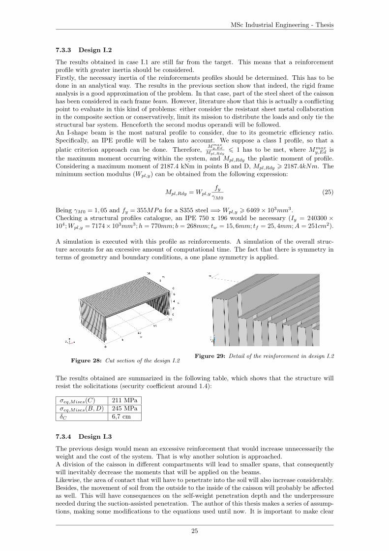
MSc Industrial Engineering - Thesis
7.3.3 Design I.2
The results obtained in case I.1 are still far from the target. This means that a reinforcementprofile with greater inertia should be considered.Firstly, the necessary inertia of the reinforcements profiles should be determined. This has to bedone in an analytical way. The results in the previous section show that indeed, the rigid frameanalysis is a good approximation of the problem. In that case, part of the steel sheet of the caissonhas been considered in each frame beam. However, literature show that this is actually a conflictingpoint to evaluate in this kind of problems: either consider the resistant sheet metal collaborationin the composite section or conservatively, limit its mission to distribute the loads and only tie thestructural bar system. Henceforth the second modus operandi will be followed.An I-shape beam is the most natural profile to consider, due to its geometric efficiency ratio.Specifically, an IPE profile will be taken into account. We suppose a class I profile, so that aplatic criterion approach can be done. Therefore, Mmax
y,Ed
Mpl,Rdy6 1 has to be met, where Mmax
y,Ed isthe maximum moment occurring within the system, and Mpl,Rdy the plastic moment of profile.Considering a maximum moment of 2187.4 kNm in points B and D, Mpl,Rdy > 2187.4kNm. Theminimum section modulus (Wpl,y) can be obtained from the following expression:
Mpl,Rdy = Wpl,yfyγM0
(25)
Being γM0 = 1, 05 and fy = 355MPa for a S355 steel =⇒Wpl,y > 6469× 103mm3.Checking a structural profiles catalogue, an IPE 750 x 196 would be necessary (Iy = 240300 ×104;Wpl,y = 7174× 103mm3;h = 770mm; b = 268mm; tw = 15, 6mm; tf = 25, 4mm;A = 251cm2).
A simulation is executed with this profile as reinforcements. A simulation of the overall struc-ture accounts for an excessive amount of computational time. The fact that there is symmetry interms of geometry and boundary conditions, a one plane symmetry is applied.
Figure 28: Cut section of the design I.2Figure 29: Detail of the reinforcement in design I.2
The results obtained are summarized in the following table, which shows that the structure willresist the solicitations (security coefficient around 1.4):
σeq,Mises(C) 211 MPaσeq,Mises(B,D) 245 MPaδC 6,7 cm
7.3.4 Design I.3
The previous design would mean an excessive reinforcement that would increase unnecessarily theweight and the cost of the system. That is why another solution is approached.A division of the caisson in different compartments will lead to smaller spans, that consequentlywill inevitably decrease the moments that will be applied on the beams.Likewise, the area of contact that will have to penetrate into the soil will also increase considerably.Besides, the movement of soil from the outside to the inside of the caisson will probably be affectedas well. This will have consequences on the self-weight penetration depth and the underpressureneeded during the suction-assisted penetration. The author of this thesis makes a series of assump-tions, making some modifications to the equations used until now. It is important to make clear
25
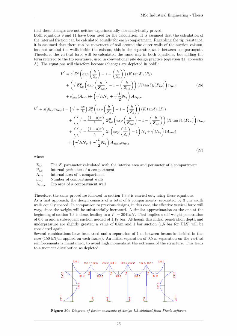
MSc Industrial Engineering - Thesis
that these changes are not neither experimentally nor analytically proved.Both equations 9 and 11 have been used for the calculation. It is assumed that the calculation ofthe internal friction can be calculated equally for each compartment. Regarding the tip resistance,it is assumed that there can be movement of soil around the outer walls of the suction caisson,but not around the walls inside the caisson, this is the separator walls between compartments.Therefore, the vertical force will be calculated the same way in both equations, but adding theterm referred to the tip resistance, used in conventional pile design practice (equation 31, appendixA). The equations will therefore become (changes are depicted in bold):
V′
= γ′Z2o
(exp
(h
Zo
)− 1−
(h
Zo
))(K tan δ)o(Po)
+
(γ
′Z2i,c
(exp
(h
Zi,c
)− 1−
(h
Zi,c
))(K tan δ)i(Pi,c)
)nw,c
+ σ′
end(Aend)+
(γ
′hNq + γ
′ t
2Nγ
)Atip,c
(26)
V′+ s(Ai,cnw,c) =
(γ
′+as
h
)Z2o
(exp
(h
Zo
)− 1−
(h
Zo
))(K tan δ)o(Po)
+
((γ
′− (1− a)s
h
)Z2i,c
(exp
(h
Zi,c
)− 1−
(h
Zi,c
))(K tan δ)i(Pi,c)
)nw,c
+
((γ
′− (1− a)s
h
)Zi
(exp
(h
Zi
)− 1
)Nq + γ
′tNγ
)(Aend)
+
(γ
′hNq + γ
′ t
2Nγ
)Atip,cnw,c
(27)
where
Zi,c The Zi parameter calculated with the interior area and perimeter of a compartmentPi,c Internal perimeter of a compartmentAi,c Internal area of a compartmentnw,c Number of compartment wallsAtip,c Tip area of a compartment wall
Therefore, the same procedure followed in section 7.3.3 is carried out, using these equations.As a first approach, the design consists of a total of 5 compartments, separated by 3 cm widthwalls equally spaced. In comparison to previous designs, in this case, the effective vertical force willvary, since the weight will be substantially increased. A similar approximation as the one at thebeginning of section 7.3 is done, leading to a V
′= 3041kN . That implies a self-weight penetration
of 0,6 m and a subsequent suction needed of 1,18 bar. Although this initial penetration depth andunderpressure are slightly greater, a value of 0,5m and 1 bar suction (1,5 bar for ULS) will beconsidered again.Several combinations have been tried and a separation of 1 m between beams is decided in thiscase (150 kN/m applied on each frame). An initial separation of 0,5 m separation on the verticalreinforcements is maintained, to avoid high moments at the extremes of the structure. This leadsto a moment distribution as depicted:
Figure 30: Diagram of flector moments of design I.3 obtained from Ftools software
26

MSc Industrial Engineering - Thesis
Using equation 25, two different sections will be defined for the two outer frames (considering amaximum moment of 238 kNm) and another one for the three in the middle (maximum momentof 202.2 kNm):
• Two outer frames. IPE O 300. (Iy = 9994× 104;Wpl,y = 743, 8× 103mm3;h = 304mm; b =152mm; tw = 8mm; tf = 12, 7mm;A = 62, 8cm2)
• Three inner frames. IPE 300. (Iy = 8356 × 104;Wpl,y = 628, 4 × 103mm3;h = 300mm; b =150mm; tw = 7, 1mm; tf = 10, 7mm;A = 53, 8cm2)
A Comsol simulation is carried out in order to prove that these profiles will resist the solitations.
Figure 31: Detail of the Von Mises stress distribution along a beam belonging to the central frame
As it can be seen in figure 31, the maximum stress is found at the extremes of the beam, while thisis not that relevant at the middle of the span. In the case of the central frame, the values foundare 198 and 91 MPa, respectively, whereas at the outer frames, the values are 228 and 11 MPa.Therefore, taking into account a S355 steel the security coefficient in these reinforcements is about1,7. Indeed, it is a relatively high value.
Vertical reinforcementsUntil now, only the horizontal reinforcements have been checked. In that case, only the flexiondue to the moments is considered, but the fact that all the walls are fixed makes that a normalforce is also applied on the beams profiles that can induce a flexion, which has been neglected.However, when designing the reinforcements, the possibility of buckling has to be considered. Itwill be done for the vertical reinforcements of this design, and for all reinforcements in the followingsections.Therefore, each column (as said before, a separation of 0,5 m is considered) of the outer walls,is affected by a composite flexion. Specifically, at its base, M=277 kNm and N=312.7 kN (com-pression). Hence, a formula of interaction between the two will be applied (see equation 28, thesignificance of each parameter is detailed in the next paragraphs), taking into account that thiscompression can lead to buckling. The possible lateral overturn phenomenon will not be taken intoaccount.
NEd
χminAfyγM1
+My,Ed
Wpl,yfyγM0
6 1; where χmin = minχy, χz (28)
In that case a HE profile is selected. Although their efficiency is inferior in comparison to IPEand IPN profiles, they have a remarkably higher critical load (Ncr) for the fact that both inertialmoments are more balanced. That is why they are widely used in beams with certain flexionor pillars with moderate compression. Specifically the HEB 240 is used for the outer pillars(Iy = 11260 × 104; Iz = 3923 × 104;Wpl,y = 1053 × 103mm3;h = 240mm; b = 240mm; tw =10mm; tf = 17mm;A = 106cm2).For the buckling phenomena, a theoretical end restraint coefficent K=0.5 is considered as the baris fixed at both extremes (see figure 32 (b)). Thus, the effective length Lcr = KL = L
2 = 6, 5/2 =3, 25m. The Euler’s critical load (Ncr) can be calculated as follows (where E is the Young’s
27

MSc Industrial Engineering - Thesis
modulus, I is the pillar inertia):
Ncr,y =
(π
Lcr
)2
EIpillar,y = 22094× 103N ; Ncr,z =
(π
Lcr
)2
EIpillar,z = 7697× 103N
Figure 32: Theoretical End Restraint Coefficients, K (Lindeburg (1999))
What it is known as the reduced slenderness can be calculated as follows:
λy =
√ApillarfyNcr,y
= 0, 41 (29)
λz =
√ApillarfyNcr,z
= 0, 70
where Apillar is the section area of the pillar profile, fy is the steel yield strength.
Using the calculated reduced slenderness (λ) and the following graph, the buckling coefficient(χ) can be found. (The curves b and c should be used for the y and z axis respectively)
Figure 33: Buckling curves (CEN (2005))
Therefore:χmin = min0, 92; 0, 73 = 0, 73
NEd
χminAfyγM1
+My,Ed
Wpl,yfyγM0
= 0, 12 + 0.78 = 89%
which proves that the profile chosen (HE 240 B) is appropriate. As previously done, a simulationis carried out to prove that the stresses occurring along the structure will not lead to its failure.
28

MSc Industrial Engineering - Thesis
Figure 34: Cut section of the design I.3 used in the simulation. Symmetry has been applied
As expected, the highest stress will occur at the base of the pillars. A value at a height of 0,55mis taken, so that it is not affected by the singularity at exactly 0,5m, where a null prescribeddisplacement has been applied. For the beams used alongside the frames, the values obtained arearound 245 MPa.
Figure 35: Von Mises stress graph of design I.3
7.4 Factorial designThe designs studied until the moment were carried out with boundary conditions and geometricparameters thought for very specific situations. For instance, on the one hand the soil propertieswhere set to those that implied the most extreme solicitations. On the other hand, the separationbetween reinforcement frames was determined for different reasons. However, the variation ofcertain parameters like these would lead to different stresses and indeed, different designs.A factorial design would allow to see which is the effect of each parameter of interest as well as theeventual interaction between each other.A two level factorial design is implemented. Many variables will affect the outcome, but only thosewhich are thought to be more relevant will be considered:
• Soil properties. They will affect the self-weight penetration depth as well as the suctionrequired during the suction-assisted penetration. The following parameters will be takeninto consideration as variable factors (the justification of each choice is backed by theorybriefed in annex A.6):
– Effective unit weight (γ′). Values between 8.19kN/m3 and 10.19kN/m3 account for
very loose sand and very dense sand respectively.
– K tan δ. K parameter and δ are always related to each other - considering them apartwould not make sense. As it is depicted in annex A, there are different approaches to
29

MSc Industrial Engineering - Thesis
calculate the lateral earth pressure coefficient. None of them, however, describes exactlythe situation of a suction caisson installation.
– Angle of internal friction (Φ). Values between 30o and 45o account for very loose sandand very dense sand respectively.
One variable left in the formulation used is the permeability ratio kf . It has been seen thatits variation does not imply a major effect in the results. Furthermore, equally to the otherparameters, its value should be determined by soil testing. A value of 3 is set for this case.
• Number of compartments in which the suction caisson is divided.
• Spacing of the reinforcements.
It is expected that there are no interactions between the soil parameters, so that they have anadditive effect on the resistance against penetration. Therefore, the greater their values are, thegreater the difficulty of the structure to be pushed into the soil. In order to prove such approach,a preliminary factorial study has been carried out with the variables previously depicted:
Factor Name Units Low level (-) High level (+)A Effective unit weight (γ
′) kN/m3 8,19 10,19
B K tan δ - 0.5 0.8C Angle of internal friction (φ) [degrees] 30 45
Therefore, the two-levels factorial design will be implemented with the following factors:
Factor Name Units Low level (-) High level (+)A Sand properties - Loose sand Dense sandB Number of compartments - 1 5C Spacing of the beams m 0.5 1
The total weight of the structure, depending on the design, has been considered as the main re-sponse for the analysis, for the fact that, as previously discussed, a lighter structure is desiredfor economical reasons. Depending on the factors that apply to every case, the best design isconsidered so that the strength and stability of the structure is sufficient to resist the expectedsolicitations. This designs, with their appropriate reinforcement, will have different total weights.
In order to carry out this study, the following steps and considerations will be followed:
1. Setting the relevant factors (A, B and C)
Preliminary stage
2. Assuming a certain preliminary effective vertical weight V′
3. Calculating the initial self-weight penetration depth and suction needed in the suction-assisted penetration stage, by using equations 26 and 27.
4. Obtaining bending and normal forces diagrams, according to the Cross method. The sectionproperties are set to be the same in all bars of the structure.
5. Setting a certain profile for all bars within the structure (i.e. beams and pillars)
6. Verification of the profiles by using equation 28, looking at the critical sections where themost severe stresses occur.
Iteration stages
7. Calculating the volume, and thereafter the new effective vertical weight V′.
8. Idem step 3
9. Equally, the diagrams of bending and normal forces are obtained. However, in this case, eachbar profile is specified, that is their dimensions and therefore, their inertia.
30
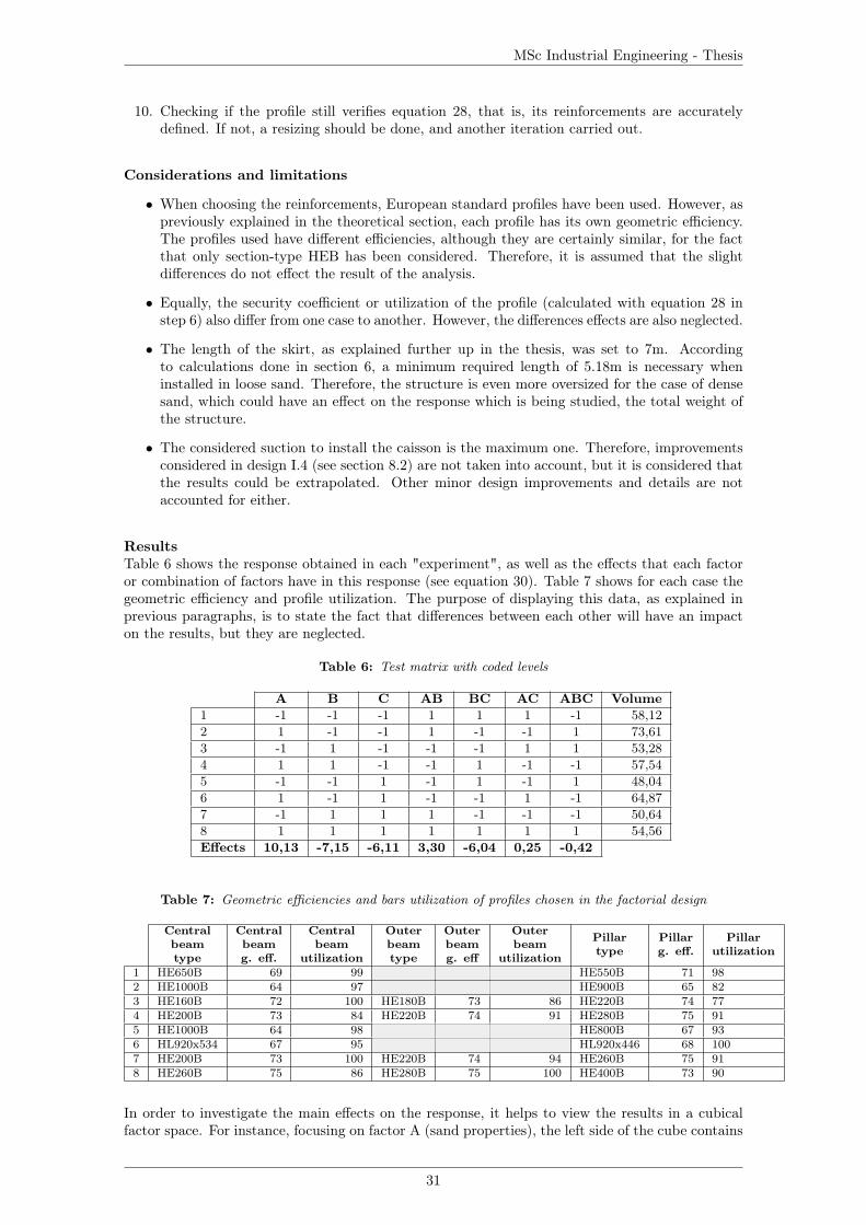
MSc Industrial Engineering - Thesis
10. Checking if the profile still verifies equation 28, that is, its reinforcements are accuratelydefined. If not, a resizing should be done, and another iteration carried out.
Considerations and limitations
• When choosing the reinforcements, European standard profiles have been used. However, aspreviously explained in the theoretical section, each profile has its own geometric efficiency.The profiles used have different efficiencies, although they are certainly similar, for the factthat only section-type HEB has been considered. Therefore, it is assumed that the slightdifferences do not effect the result of the analysis.
• Equally, the security coefficient or utilization of the profile (calculated with equation 28 instep 6) also differ from one case to another. However, the differences effects are also neglected.
• The length of the skirt, as explained further up in the thesis, was set to 7m. Accordingto calculations done in section 6, a minimum required length of 5.18m is necessary wheninstalled in loose sand. Therefore, the structure is even more oversized for the case of densesand, which could have an effect on the response which is being studied, the total weight ofthe structure.
• The considered suction to install the caisson is the maximum one. Therefore, improvementsconsidered in design I.4 (see section 8.2) are not taken into account, but it is considered thatthe results could be extrapolated. Other minor design improvements and details are notaccounted for either.
ResultsTable 6 shows the response obtained in each "experiment", as well as the effects that each factoror combination of factors have in this response (see equation 30). Table 7 shows for each case thegeometric efficiency and profile utilization. The purpose of displaying this data, as explained inprevious paragraphs, is to state the fact that differences between each other will have an impacton the results, but they are neglected.
Table 6: Test matrix with coded levels
A B C AB BC AC ABC Volume1 -1 -1 -1 1 1 1 -1 58,122 1 -1 -1 1 -1 -1 1 73,613 -1 1 -1 -1 -1 1 1 53,284 1 1 -1 -1 1 -1 -1 57,545 -1 -1 1 -1 1 -1 1 48,046 1 -1 1 -1 -1 1 -1 64,877 -1 1 1 1 -1 -1 -1 50,648 1 1 1 1 1 1 1 54,56Effects 10,13 -7,15 -6,11 3,30 -6,04 0,25 -0,42
Table 7: Geometric efficiencies and bars utilization of profiles chosen in the factorial design
Centralbeamtype
Centralbeamg. eff.
Centralbeam
utilization
Outerbeamtype
Outerbeamg. eff
Outerbeam
utilization
Pillartype
Pillarg. eff.
Pillarutilization
1 HE650B 69 99 HE550B 71 982 HE1000B 64 97 HE900B 65 823 HE160B 72 100 HE180B 73 86 HE220B 74 774 HE200B 73 84 HE220B 74 91 HE280B 75 915 HE1000B 64 98 HE800B 67 936 HL920x534 67 95 HL920x446 68 1007 HE200B 73 100 HE220B 74 94 HE260B 75 918 HE260B 75 86 HE280B 75 100 HE400B 73 90
In order to investigate the main effects on the response, it helps to view the results in a cubicalfactor space. For instance, focusing on factor A (sand properties), the left side of the cube contains
31

MSc Industrial Engineering - Thesis
the runs where A is at the minus level, while on the right side, the factor is at the plus level.Calculating the difference of averages of each level is known as the effect of factor A, which can beexpressed as:
Effect =
∑Y+
n+−∑Y−n−
(30)
Figure 36: Cube plot of total weights with focus on sand properties, factor A (Drawing done with Autocad2018)
Equally, this effect is calculated for all factors and combinations of them. The results are shownon the bottom line of table 6. If the effect is positive, it means that increasing that factor willmakes the response (i.e. total weight) to increase, and the other way round when its value isnegative. Notice that the most relevant effects are those of the factors, but also the interactioneffect of BC, which is almost as high as its parents B and C. In other words, the combination ofcompartmentalization (B) and reinforcement spacing (C) produces a big (reducing) impact on totalweight. The opposite effect (weight increase) happens, and to a lesser extent, with the interactionof dense sand (A) and high compartmentalization (B).Interactions occur when the effect of a factor depends on the level of the other, and they cannotbe detected by traditional one-factor-at-a-time (OFAT) experimentation.In this case, tables 8 and 9 show the results for interactions BC and AB. These are actually averagesof data from table 6, where for instance, the first two experiments have both factors B and C attheir low level, with response values of 58.12 and 73.61, which produces an average of 61.81, asshown in table 8.
Table 8: Data for interaction plot of nr. of compart-ments versus reinforcements spacing
B C Volume (Avg)-1 -1 61,811 -1 54,94-1 1 53,571 1 52,6
Table 9: Data for interaction plot of sand propertiesversus nr. of compartments
A B Volume (Avg)-1 -1 49,31751 -1 66,0605-1 1 51,4881 1 56,051
Figure 37: Interaction of nr. of compartments (B)and spacing of the beams (C)
Figure 38: Interaction of sand properties (A) andnr. of compartments (B)
32

MSc Industrial Engineering - Thesis
Notice that the effect of beam spacing (C), depends on the level of factor B (nr. of compartments).For example, when C is 1m (high level), the change in weight is small—from 53.57 to 52.6. How-ever, when the beams are close to one another (C is at low level), the total weight is reducedconsiderably—from 61.81 to 54.94 (see figure 37, obtained with Minitab v18). Therefore, we canconclude that:
• If there is a high number of compartments in which the suction caisson shall be divided →changing the reinforcement spacing has little effect on the total weight of the structure.
• If the caisson is divided into a low number of compartments→ increasing the spacing betweenreinforcements will dramatically reduce the total volume.
A similar situation is depicted for interaction of factors AB (see figure 38, obtained with Minitabv18). Equally:
• If the caisson is divided in a high number of compartments → the fact of being installed indense or loose sand has little effect on the total weight of the structure.
• If the caisson is divided into a low number of compartments→ installing the caisson in loosesand will considerably reduce the total volume, in comparison to a bucket placed in densesand.
7.5 UnionsAs previously discussed, the area concerning the union between the beams and the pillars demandsspecial attention due to the concentration of stresses.Connections are important parts of any metal structure. The mechanical properties of the unionsgreatly influence the strength, rigidity and stability of the structure as a whole.In general, connections classification can be divided into flexible and rigid unions, depending on theability of transmitting a significant moment or not. They could also be classified by the elementstype that they unite—beams and columns mainly. In this case, a rigid union between beams andcolumns shall be designed.In moment resisting connections like this, bolted end plate and welded beam-to-column connec-tions are most commonly used. The welded connections can provide full moment continuity, butare certainly much more expensive to produce, specially on site. This report will not carry outresearch on the the convenience of using one or another in the Ocean Grazer suction caisson;therefore, design procedure of the connection members—let it be either bolts or welding—will notbe implemented. A careful selection of this members can avoid the need for strengthening of thejoint, which leads to a more cost-efficient structure. However, sometimes there is no alternative tostrengthening the connection zones, which can be implemented with a range of stiffeners that willbe detailed and studied in the following paragraphs.
StiffenersA usual simplification in rigid unions calculations consists in assuming that bending and normalforces are absorbed by the profile flanges, while the shear forces by the web.In the connection of figure 39 (a), it can be seen that point D is under the effect of forces F2 andF4, which coming from the flanges of the profiles must be absorbed by a weaker section, such as theweb. These traction or compression forces can induce web yielding or local buckling respectively.These failure modes can be decisive for a connection’s capacity. Therefore, in order to avoid thisconcentration of stresses, the most generalized solution in frames without haunches consists inprolonging the frames of the beam and the column, as indicated in figure 39 (b).
If the ABCD web was not able to withstand the shear stress, the usual solution is to reinforceit with a diagonal stiffener (figure 39 (c)), instead of increasing its thickness.
33

MSc Industrial Engineering - Thesis
Figure 39: (a)Forces transmitted from the flanges to the web (b)Stiffeners solution (c)’N’ stiffener (UCLM(2005))
Several simulations have been carried out in order to see the influence of introducing stiffenersin a beam-to-column connection as strengthening solutions.Firstly, the 5-compartments suction caisson model is approached. Since in this case the span is 4meters, a connection without haunches is firstly considered. Figures 40 and 41 show the compari-son between a connection in which the beam is attached to the column’s flange (as in the rest ofsimulations, a perfect union between solids is assumed), and the same connection reinforced withstiffeners. The higher stress, in both cases occurring at the lowest beam’s flange in its very end,is dramatically reduced when stiffeners are present. For instance, in this case, their values are1029 and 640 MPa respectively. The diagonal or ’N’ stiffener, as previously explained, reduces thestresses occurring within the web, but it has a negligible effect on this maximum stress.
Table 10: Higher equivalent Von Mises stresses comparison between FE simulations
Withoutstiffeners
Withstiffeners
Haunch Haunch + stiffenerlower edge upper edge below edge upper edge
1029.0 MPa 639.75 MPa 260.91 MPa 513.50 MPa 159.39 MPa 343.51 MPa
Figure 40: FE simulation with Comsol of aconnection without stiffeners
Figure 41: FE simulation with Comsol of aconnection with stiffeners
HaunchesAlthough the usage of stiffeners reduces the concentration of stresses, the value encountered in thiscase with certain solicitations is still too high. That is why other solutions are investigated. Infact, in structures with long spans, the usage of other kind of reinforcements—mainly haunches—isrecommended.For portal frame structures, haunched connections at their eaves are widely used. In addition
34

MSc Industrial Engineering - Thesis
to providing increased connection resistances, the haunch increases the moment resistance of thebeam, which would obviously effect the optimization of the design and that will be discussed inlater sections.The haunch adds stiffness to the frame, reducing deflections, and facilitates an efficient momentconnection. It is usually implemented as a triangular cutting placed below the beam at the con-nection to the pillar. Its length will generally be around 10-15% of the span, and is in most casescut from the same section as the beam, or a deeper section.As done with the stiffeners, some preliminary simulations have been carried out to see the im-pact that a haunch has on the stress distribution. The equivalent Von Mises stress distributionof the 5-compartments suction caisson with haunched connection without and with stiffeners isdepicted in figures 42 and 43 respectively. As it should be expected, the maximum stresses arenow concentrated around the haunch edges—values summarized in table 10. For instance, in thiscase, the haunch obviously reduces the stresses that occur within this region, with the stiffenersallowing to decrease this value to 343.51 MPa (close to the target for a S355 steel structure, whereσVM,adm = fy/γR = 355/1.05 = 338MPa).
Figure 42: FE simulation with Comsol of aconnection with haunch
Figure 43: FE simulation with Comsol of aconnection with haunch and stiffeners
Beam-to-column connections with haunch FE simulationsA series of simulations with a parametric sweep of a 1-compartment suction caisson with haunchedbeams has been done to see in which way haunches with different edge lengths effect the results.
Values between 1.5m and 2.5m (with a step increase of 0.2m) were given to both the verticaland horizontal haunch’s edges, getting to 36 combinations in which the stress distribution aroundthe beam-to-column connection was evaluated. Figure 44 shows the results, which have been rear-ranged in order to show those which would be acceptable (that is, with maximum equivalent VonMises stress below the admissible stress σVM,adm)—the first 11 samples.
The results show that when increasing the vertical edge (yh), while setting a fixed value of thehorizontal edge (xh), the haunch’s upper edge will see stresses increasing, in opposition to the areaaround the lower edge, where the stresses will decrease.Moreover, it can be concluded that similar values of (xh) and (yh) will give more stable and lowerstresses. In contrast, highly different edge lengths will make the stresses to concentrate in one ofthe edges; if the reinforcement is vertically skinny, the upper region will have a high concentrationof stresses, while they will appear around the lower area when the haunch has a considerably largerhorizontal edge.
35

MSc Industrial Engineering - Thesis
Figure 44: Maximum equivalent Von Mises stresses in 1-compartment suction caisson with haunches
The same approach has been followed for the case of a 5-compartments suction caissons. A para-metric seep between 0.6m and 1.6m (with a step increase of 0.2m) was implemented for bothvertical and horizontal haunch’s edges. The results are similar, although, as it would be expected,the haunch dimensions can be reduced in comparison to the previous case (see figure 45).
Figure 45: Maximum equivalent Von Mises stresses in 5-compartment suction caisson with haunches
7.6 Suction caisson Case IIThe Case II is the suction caisson version that has been particularly studied and designed by thecompany so far, with the aim of providing an anchoring system for the Ocean Grazer storage sys-tem and other possible applications.The design of each module is the same as Case I, but with a secondary upper portal frame at-tached to the main bucket. This secondary structure is 5 meters high and has a 10 meters span,surrounded by a rigid concrete tank at each side.It is considered that on one hand, the suction pressure will be applied over all the inner surfacesof the caisson, including a quarter of surface of the concrete pipes. On the other hand, the oceanwill make a pressure on the outside surfaces, which will vary with depth. As it has been proceededin Case I, the simplification of considering the same external pressure will be done. Likewise, themaximum suction will always be taken into consideration.Only the steel structure will be considered, and the effect of the concrete pipes will be applied
36

MSc Industrial Engineering - Thesis
as external loads. This loads are simplified as a single vertical force, calculated as the weight ofthe structure and the water contained in it (assumed to be full in the installation process), minusany boundary effects (simplified as the volume of sea water removed). It is indeed an approxima-tion, since a quarter of the pipe external surface will not be in contact with the ocean pressure,but will be under suction pressure. That will probably make this vertical force to increase, and ahorizontal component will appear, which will be applied on the beams of the superior portal frame.
Table 11: Values referred to concrete pipe
Vc[m3] Concrete pipe volume 298Vw[m3] Rigid tank volume 1272VT [m3] Total pipe volume 1571ρc[kg/m
3] Concrete density 2400ρw[kg/m3] Working fluid density 997ρsw[kg/m3] Sea water density 1020Wc[kg] Concrete pipe weight 716283Ww[kg] Working fluid weight 1268528WT [kg] Total weight 1984811FW [kN ] Force due to weight 19471FB [kN ] Buoyancy force 15718FT [kN ] Effective vertical force due to concrete pipes 3753
The same procedure of the factorial design is followed but only for the case of loose sand, 1 mspacing between reinforcements and 1 compartment (which would equal to run 5 of the factorialdesign, where profiles of HE1000B and HE800B have been found necessary for the beams andpillars respectively).
Figure 46: Case II boundary conditions. 1st it-eration
Figure 47: Case II bending moments diagram.1st iteration
Figure 48: Case II normal forces diagram. 1stiteration Figure 49: Case II shear forces. 1st diagram
The profiles that have been determined according to the Cross method are:
• Pillar main portal frame: HE450B with a 88,74% utilization.
• Beam main portal frame: HE500B with a 93.25% utilization. As it can be seen in theforce distribution diagrams showed above, the central part of this beam experience lowersolicitations. However, it has been considered the maximum values found at the extremes todecide the profile.
37

MSc Industrial Engineering - Thesis
• Pillar secondary portal frame: HE360B with a 91.66% utilization.
• Beam secondary portal frame: HE340B with a 96.65% utilization.
Therefore, the profiles found are considerably smaller compared to those found in Case I. That ismainly because the effective vertical stress is higher due to the increased weight of the structure,due to the concrete pipes and the steel buckets. That has an impact in the self-weight penetrationwhich is increased to 3.9m and the suction required in the suction-assisted penetration stage, whichis reduced to 0.83 bar.
Figure 50: Case II FE model. Equivalent VMstresses distribution
Figure 51: Case II FE model. Displacementsdistribution
On the one hand, as it can be seen in figure 50, the stresses along the superior caisson are moreimportant than those occurring within the inferior one. That is probably due to the fact that alarger part of the inferior portal frame has been oversized, as it has been commented before andas it is depicted in the diagrams above. Its highest stresses are around the area of the beam wherethe upper pillars rest, where the highest bending moment occurs.On the other hand, and in accordance with previous designs, haunches have been included in theupper portal frame of the model. The fact that this is a short span case, it could be possible thatsome stiffeners were enough.The deflection diagram has also been included in order to prove that SLS is also met. The superiorbeam, with a maximum deflection of a bit more than 20 mm is far below the admissible value(δmax = 50mm).
7.7 Analytical validation of the modelsThroughout the previous sections, various models have been developed in order to study and designdifferent configurations of the suction caisson of the Ocean Grazer.In this section, a validation of these models will be carried out by means of analytical methodsand calculations, which have been summarized previously in the theoretical background section.Particular cases of the 1-compartment and 5-compartments are looked carefully (run 5 and 7 of thefactorial design, look appendix B for details), in which different points are analysed and comparedto those results obtained with FEA.As it has been previously discussed, the connection between the beam and the pillar has to bestiffened by means of different possible solutions, so that the admissible stress is not surpassedin the surroundings of this area. However, when introducing this elements, the analysis of thestructure is modified. If the distribution of forces (that is axial, shear forces and bending moment)used in the factorial design for these particular cases are to be used, no haunches or stiffeners canbe included in the model. The reason for this is that in order to obtain these forces, calculated withthe Cross method, it has been assumed a uniform profile for each bar (i.e. beams and columns).When haunches are present, the composite profile is modified, and therefore the values of theseforces change. Figures 52 and 53 clearly show that the section at the middle of the beam span seeslower stresses when haunches are included in the design.
38

MSc Industrial Engineering - Thesis
Figure 52: FE simulation with Comsol of run 5.Von Misses equivalent stress distribution
Figure 53: FE simulation with Comsol of run 5with haunch reinforcements. Von Misses equiva-lent stress distribution
7.7.1 1-compartment case
Central section of the beam (Beam - Centre)On the central section of the beam (which has a HE1000B profile), an axial (compression) force(-1102.4 kN) and a bending moment (2346.2 kNm) are applied (see figures 86 and 85, appendixB), while no shear forces are present (see figure 54).
Figure 54: Shear force diagram run 5, 1st itera-tion
Figure 55: Nodes assignation of end bars studiedsections
The results obtained in the FE simulation when no haunches are present in the design, and thoseobtained by analytical calculations are compared. As explained in section 7.1.3, in a compositeprofile like this, where not only the beam but also the 3cm metal sheet is accounted for, the neutralaxis changes its position, resulting in the higher stresses occurring at the lower part of the profile.Thus, that is the point which will always be evaluated.
Figure 56: Analysed points of the profile when a shear force is present (drawing done with Autocad 2018)
Central section of the pillar (Pillar - Centre)Unlike the beam, in that case, a part from a bending moment and normal force, on the centralsection of the pillar (which has a HE800B profile) a shear force is also present. Therefore, 3 pointswill be analysed: point 1 (outer surface of the flange which is situated the furthest from the neutralaxis), point 2 (inner surface of that same flange) and point 3 (central point of the I-shape profileweb). The reason for looking at these points and not others is due to the shear stress distribution,depicted in figure 19. Depending on the magnitude of the shear force and bending moments, thepoint where the maximum stress is occurring will vary.
39
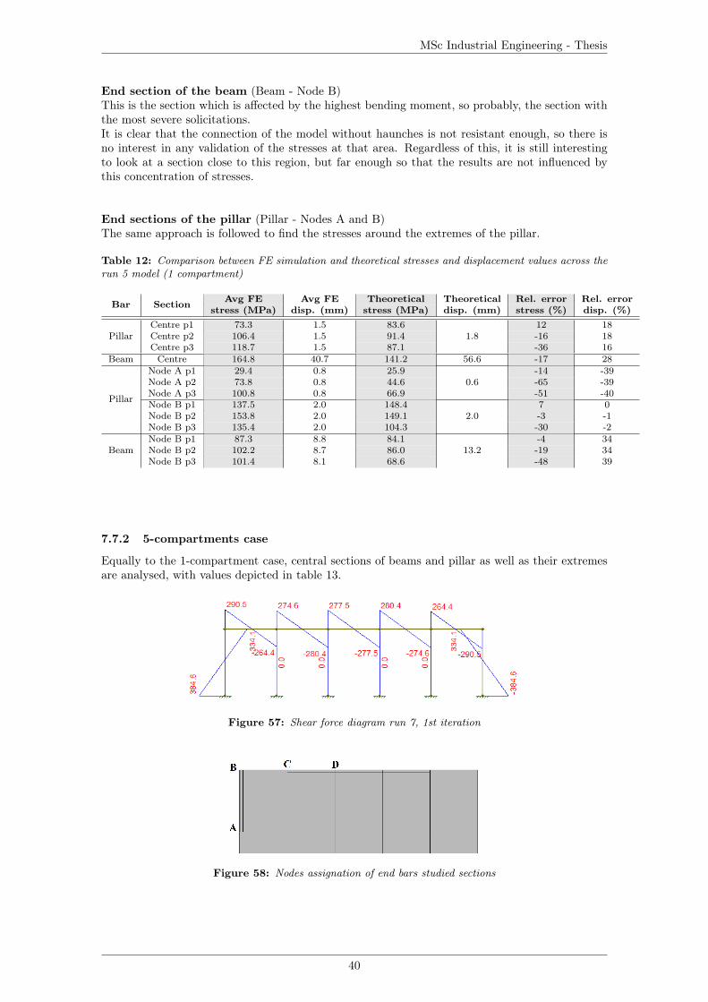
MSc Industrial Engineering - Thesis
End section of the beam (Beam - Node B)This is the section which is affected by the highest bending moment, so probably, the section withthe most severe solicitations.It is clear that the connection of the model without haunches is not resistant enough, so there isno interest in any validation of the stresses at that area. Regardless of this, it is still interestingto look at a section close to this region, but far enough so that the results are not influenced bythis concentration of stresses.
End sections of the pillar (Pillar - Nodes A and B)The same approach is followed to find the stresses around the extremes of the pillar.
Table 12: Comparison between FE simulation and theoretical stresses and displacement values across therun 5 model (1 compartment)
Bar Section Avg FE Avg FE Theoretical Theoretical Rel. error Rel. errorstress (MPa) disp. (mm) stress (MPa) disp. (mm) stress (%) disp. (%)
PillarCentre p1 73.3 1.5 83.6
1.812 18
Centre p2 106.4 1.5 91.4 -16 18Centre p3 118.7 1.5 87.1 -36 16
Beam Centre 164.8 40.7 141.2 56.6 -17 28
Pillar
Node A p1 29.4 0.8 25.90.6
-14 -39Node A p2 73.8 0.8 44.6 -65 -39Node A p3 100.8 0.8 66.9 -51 -40Node B p1 137.5 2.0 148.4
2.07 0
Node B p2 153.8 2.0 149.1 -3 -1Node B p3 135.4 2.0 104.3 -30 -2
BeamNode B p1 87.3 8.8 84.1
13.2-4 34
Node B p2 102.2 8.7 86.0 -19 34Node B p3 101.4 8.1 68.6 -48 39
7.7.2 5-compartments case
Equally to the 1-compartment case, central sections of beams and pillar as well as their extremesare analysed, with values depicted in table 13.
Figure 57: Shear force diagram run 7, 1st iteration
Figure 58: Nodes assignation of end bars studied sections
40

MSc Industrial Engineering - Thesis
Table 13: Comparison between FE simulation and theoretical stresses and displacement values across therun 7 model (5 compartments)
Bar SectionAvg FE Avg FE Theoretical Theoretical Rel. error Rel. errorstress disp. stress disp. stress disp.(MPa) (mm) (MPa) (mm) (%) (%)
Pillar Centre 121.3 7.1 121.8 11.7 0 39Outerbeam
Centre 78.7 3.1 75.9 4.7 -4 34
Innerbeam
Centre 132.3 5.9 126.0 9.6 -5 38
Centralbeam
Centre 119.5 5.3 118.0 8.6 -1 38
Pillar
Node A p1 75.8 2.3 101.72.5
25 8Node A p2 176.7 2.3 134.6 -31 9Node A p3 194.0 2.2 135.4 -43 11Node B p1 28.9 2.8 61.2
4.953 43
Node B p2 134.8 2.8 101.8 -32 44Node B p3 159.0 2.7 115.3 -38 45
Outerbeam
Node B p1 56.3 0.7 68.92.0
18 63Node B p2 149.3 0.7 102.7 -45 63Node B p3 158.8 0.7 111.1 -43 62Node C p1 68.7 1.4 86.7
2.021 31
Node C p2 159.6 1.3 117.9 -35 32Node C p3 168.0 1.3 121.2 -39 34
Innerbeam
Node C p1 76.5 2.1 98.43.2
22 33Node C p2 193.3 2.1 139.6 -38 33Node C p3 204.6 2.1 147.1 -39 34Node D p1 101.1 2.1 111.3
2.79 25
Node D p2 206.8 2.0 150.2 -38 25Node D p3 213.5 2.0 153.7 -39 27
Centralbeam
Node D p1 97.1 1.8 109.82.4
12 26Node D p2 203.6 1.8 147.7 -38 26Node D p3 208.8 1.8 150.7 -39 28
7.7.3 Results
Tables 12 and 13 show the comparison between theoretical and FEA stresses and deflection values.The values of the FE simulations are an average of all the portal frames within the suction caisson.First of all, as explained before, these are not the maximum stresses that occur within the models,since these would be at the connection between beams and columns, which have not been includedin the comparison. Therefore, the stresses showed should easily meet the condition in equation 21;thus the stresses should be no higher than σVM,adm = fy/γR = 355/1.05 = 338MPa.Also, taking into account the SLS limit of δmax = L
200 :
• 1-compartment. The beam, being 20 meters long, should have a deflection no greater than100 mm. The pillar, being 4.5 meters when starting penetrating, a δmax = 22.5mm applies.
• 5-compartment. Every beam, being 4 meters long, should have a deflection no greater than20 mm. The pillar, being 5.2 meters when starting penetrating, a δmax = 25.9mm applies.
As it can be seen, these conditions are met, which also proves the usage of the Cross method andthe whole procedure used throughout this paper to define the different designs is appropriate.
When analyzing the results, it has been seen that while in some sections of the structure (such asthe center of the span), there is a smooth distribution of the stresses in the intersection between theflanges and the web of the I-profile, in other sections, the equivalent V.M stress changes abruptly,with the flanges merely supporting any stresses (such as the section where the bending moment isnul, see figures 59, 60 and 61).This is, in fact, backed by the theoretical analysis. On one hand, when there is a bending momentand normal force applied on the section but no shear force—such as the centre of the span—, thereis a progressive normal stress distribution from the neutral axis to the furthest point of the section(see figure 18); on the other hand, when the tangential force is the dominant—such as the sectionof the beam where there is no bending moment—, the web will see a mostly homogeneous shear
41

MSc Industrial Engineering - Thesis
stress τxz, while the flanges will mainly absorb a neglectable portion of τxz, and τxy, always muchsmaller than the first one.
Figure 59: Equivalent Von Mises stress distribu-tion of run 5 model
Figure 60: Bending moment diagram run 5, 1stiteration
Figure 61: Detail of the equivalent Von Mises stress distribution of run 5 model, see figure 59
In order to show more clearly the comparison between theoretical and FE values, the relative errorshave been calculated, taking the FE values as reference.First of all, if we focus on the stress values, it is clear that when analysing different points of thesame section, point 1 is generally much better predicted than points 2 and 3. That could be dueto the fact that it is a not a symmetrical section, which it makes it harder to foresee. Likewise, itcan be seen that point 1 always has a greater value when analytically calculated, and vice-versafor points 2 and 3.Another conclusion that can be reached is that values in the centre of a bar are anticipated ina better way (especially in the 5-compartments case where absolute errors are no greater than5%, but also in the 1-compartment case, where the relative error of the analysed sections (point1) are as great as 17%). On the contrary, values at the extremes of the beams and columns areworse predicted, which can be explained by various reasons. First of all, it is possible that thestudied section is too close to the connection and therefore, still affected by the concentrationsof stresses. Another reason for this is that when carrying out the theoretical calculations, it hasbeen assumed a frame of 20 meters length and the corresponding height, while it would have beenmore appropriate to take into account the neutral axis. It is possible that the normal and shearforces and bending moments used for the calculations and extracted from the diagrams are notaccurately retrieved.In terms of the deflections, with some exceptions most of the values are certainly badly predicted.When analytically calculated, it is assumed that the structure connections are completely rigid.However, this is not the case when haunches are included, not to mention when no haunches orother types of stiffeners are present, which is the case. That could be an explanation for thesedifferences.
42
MSc Industrial Engineering - Thesis
8 Discussion and conclusions
8.1 DiscussionThis report deals with the search for design solutions for the suction caisson of the Ocean Grazer’sstorage system. First of all, research about this technology has been carried out, confirming thatmost of the cases consider cylindrical suction buckets. Methods found in literature to calculateholding capacity and installation procedures have been studied and adapted to the rectangularshape, taking into account size requirements specified by the company. Obtaining the self-weightpenetration and the suction for the suction-assisted penetration stages will provide the main in-formation for the boundary conditions that will be later used in the design procedure.
Different designs have been developed, dealing with the need for certain types of reinforcements inthe structure, the main core of the thesis. Theoretical methodology of structural mechanics anddesign is depicted and used in order to calculate these reinforcements, assimilated as portal frames.Once the design is decided, FE simulations have been carried out with the aim of validating itsresistance.The first approaches provided information of the amount of stiffness that was needed and provedthat simple plates or T-shape profiles lacked the required inertia and therefore were not a viablesolution. For that reason, it was considered that an I-shape profile was the best approach for thiscase. At the same time, the methods for the suction caisson installation procedure were adaptedagain, to take into account the presence of this reinforcements and their effect on the resistanceagainst penetration into the seabed.While proving that the layout defined until the moment would be appropriate in terms of resistance(missing some details developed later in the report), it was also clear that the amount of requiredreinforcements was certainly high. For that reason a compartmentalization could be a solutionto reduce the size of the profiles. By means of a third modification of the installation proceduremethods, it was proved that indeed, the division of the suction caisson allowed the reinforcementsto be reduced in size. However, it was not clear if these changes had an impact in the amount ofmaterial of the whole structure.The designs done until the moment were based in certain conditions and parameters arbitrarilychosen. A two level factorial design was implemented with soil properties, the number of com-partments and the spacing of the reinforcements as factors. It was concluded that all of them hada remarkable effect on the volume of the structure. It was trivial to see that looser sand woulddecrease the reinforcement, while it was not that straight forward that increasing the number ofcompartments or the distance between reinforcements would also reduce it. However, the factorialdesign allowed to see that some interactions between these factors existed. Beam spacing and loosesand had a remarkable impact on the decrease of volume only when the number of compartmentswas small (i.e. a single caisson).
In the previous designs and procedures, the concentration of stress occurring within the connectionbetween bars was neglected. Stiffeners and haunches are presented as possible solutions. Althoughthe cases analysed implied the need of haunches, stiffeners proved to be good and simpler solu-tions when the solicitations are not that extreme. As said in literature, FE simulations show thathaunches length and height a 10-15% of the span is necessary, with no much differences betweenthe two dimensional parameters.
Without going in depth in it, the analysis of another case has been carried out, where a sec-ondary portal frame was included and the presence of the rigid concrete reservoirs was takeninto account. The fact that the effective vertical force was more than doubled, mainly becauseof the concrete weight, the suction was easier to perform, and therefore, less stiffening was required.
Finally, a validation of the results obtained with FEA have been compared to those calculatedby theoretical methods and calculations.
43

MSc Industrial Engineering - Thesis
8.2 Further workThis thesis is a first glimpse of which are the possibilities for the design of the Ocean Grazer suctioncaisson. Further research that it is considered important in next steps is depicted in the followingsections.
8.2.1 Cylindrical suction caisson
This thesis assumed since its beginning the design that was being developed by Ocean Grazer atthat moment, which is essentially different to the cases found in literature for its rectangular shape.A comparison between a cylindrical and an equivalent rectangular shape could be of the interestof the company in order to make a decision on the convenience of using one or the other.
8.2.2 Design I.4
In this report, the boundary conditions applied on the model have been simplified. As previouslyexplained, in an attempt to make the model more simple and at the same time get conservativeresults, the maximum suction needed is applied at all times. However, this is not what actuallyhappens, making the design oversized. As it can be seen in figure 12, the suction needed at thefirst stages of penetration is much lower, increasing with penetration depth.With the intention of improving the solution, thus using the least amount of material that makesthe structure resistant enough, another approach could be followed.If the loading effects that will occur on the structure along the whole process of penetration areplotted, it can be seen that at the very fist stages, the reinforcement required is much lesser thanthat needed once the caisson is almost anchored. In the latter, however, the skirt will be mainlyburied into the soil.If the load effects on the structure are considered at all times to decide on the reinforcement profiledimensions along the skirt height, this will inevitably lead to an increasing area of the pillars fromthe skirt tip to the top (see figure 62).
Figure 62: Detail of a possible implementation of a non-uniform reinforcement layout
8.2.3 Suction caisson life stages other than installation
As depicted at the beginning of the report, the suction caisson will go through different stages beforeand after its installation. In this report it has been considered that the most severe conditionswhich the structure will suffer will be during the installation procedure. However, the completedesign should include the rest. The operational stage is particularly interesting, probably more inthe light of the holding capacity of the caisson than the resistance of the structure. This thesis hasperformed stationary simulations with perfect anchoring of the suction caisson into the sand, andno relative movement has been considered. This is an idealization that obviously does not reflectthe reality, but it was considered an appropriate simplification for the case that was being studied.However, it would not be the case when analysing the holding capacity, where a model of the soiland its interaction with the suction skirts shall be performed.
44

MSc Industrial Engineering - Thesis
8.3 ConclusionsIn this research project, the study of different design cases of the Ocean Grazer suction caisson havebeen performed, by means of finite elements analysis and backed by theoretical calculations, withthe scope of delivering design guidelines that can be trustfully used and considered in followingstages of the design process. A summery of these guidelines is depicted:
• Information about the type of soil and its properties is essential to know how to proceed inthe calculations of the system’s boundary conditions.
• A rectangular-shape suction caisson with similar dimensions to those required by the OceanGrazer will necessarily need some kind of reinforcement that provides stiffness and resistanceto the structure.
• When installing the suction caisson in uniform sand, several considerations can be done:
– Installation in loose seabeds, compartmentalization of the suction caisson, or increaseof the reinforcement spacing will have an effect on the design, making it lighter andtherefore cheaper to build, but still resistant enough to meet the solicitations.
– If more than one of the variables expressed in the previous paragraph are modified,interactions between them must be taken into account. An increase in the beam spacingor the research of a location with looser sand will have a great impact only when thenumber of compartments in which the suction caisson is divided is low.
• It has been proved that a larger effective force of the structure has a great effect on the instal-lation of the caisson, decreasing the extreme solicitations acting on the structure. Therefore,procedures to increase this force during the installation process (mainly by means of usingtemporal extra weight) could minimize the necessity of over-sizing a structure with a largeamount of reinforcement, only designed with the aim of making possible its installation. Inthat case, and with accordance to the proposed further research, other stages of the suctioncaisson lifetime should be studied, specially its extraction for maintenance.
• The connections between structural elements such as beams and columns need special atten-tion. The concentration of stresses that normally occur in these areas implies the introductionof elements such as stiffeners or haunches. The latter is specially interesting for long spansas this case. A 10-15% length and height is recommended.
45

MSc Industrial Engineering - Thesis
ReferencesABS (2016). Guide for load and resistance factor design (LRFD) criteria for offshore structures.American Bureau of Shipping.
Arany, L. and Bhattacharya, S. (2018). Simplified load estimation and sizing of suction anchorsfor spar buoy type floating offshore wind turbines. (English). Ocean Engineering, 159.
Bhattacharya, S., Nikitas, G., Arany, L., and Nikitas, N. (2017). Soil-structure interactions (ssi)for offshore wind turbines. IET Reference, 1.
Cathie, D. and Irvine, J. (2019). Suction installed caisson foundations for offshore wind: Designguidelines.
CEN (2005). EN 1993-1-1. Eurocode 3: Design of Steel Structures-part 1-1: General rules and rulesfor buildings. European Committee for Standardization - Comité Européen de Normalisation.
Chatzivasileiou, I. G. (2014). Installation of suction caissons in layered sand. assessment of geotech-nical aspects.
DNV-GL (2016). Design of offshore steel structures, general - LRFD method. Det Norske Veritasand Germanischer Lloyd.
Guo, W. and Chu, J. (2014). Suction caisson installation in shallow water: Model tests andprediction.
Houlsby, G. and Byrne, B. (2005). Design procedures for installation of suction caissons in sand.Proceedings of The Institution of Civil Engineers-geotechnical Engineering - PROC INST CIVILENG-GEOTECH E, 158:135–144.
Houlsby, G., Kelly, R., and Byrne, B. (2005). The tensile capacity of suction caissons in sand underrapid loading.
Ibsen, L. and Thilsted, C. (2010). Numerical study of piping limits for suction installation ofoffshore skirted foundations and anchors in layered sand.
Lindeburg, M. R. (1999). Civil Engineering Reference Manual for the PE Exam. ProfessionalPublications, Belmont, CA.
Netherlands Enterprise Agency (2016). Geotechnical Report/Investigation Data. Seafloor In SituTest Locations. Borssele Wind Farm Site IV.
Pollestad, J. (2015). Investigation of suction anchor pullout capacity under undrained conditions.
Tassoulas, J., Maniar, D., and Vásquez, L. (2005). Suction caissons: Finite element modeling.
Tjelta, T. (2015). The suction foundation technology. Frontiers in Offshore Geotechnics III.
UCLM (2005). Tema 3: Tipologia de uniones entre elementos estructurales.
46
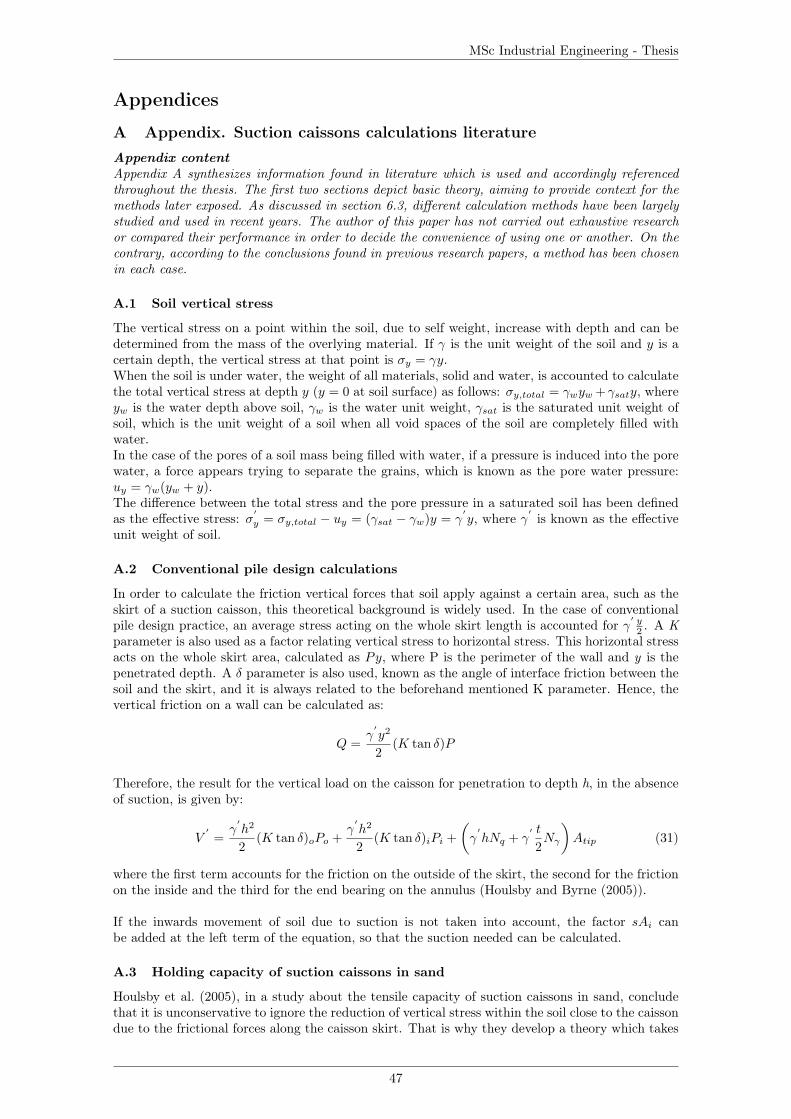
MSc Industrial Engineering - Thesis
Appendices
A Appendix. Suction caissons calculations literatureAppendix contentAppendix A synthesizes information found in literature which is used and accordingly referencedthroughout the thesis. The first two sections depict basic theory, aiming to provide context for themethods later exposed. As discussed in section 6.3, different calculation methods have been largelystudied and used in recent years. The author of this paper has not carried out exhaustive researchor compared their performance in order to decide the convenience of using one or another. On thecontrary, according to the conclusions found in previous research papers, a method has been chosenin each case.
A.1 Soil vertical stress
The vertical stress on a point within the soil, due to self weight, increase with depth and can bedetermined from the mass of the overlying material. If γ is the unit weight of the soil and y is acertain depth, the vertical stress at that point is σy = γy.When the soil is under water, the weight of all materials, solid and water, is accounted to calculatethe total vertical stress at depth y (y = 0 at soil surface) as follows: σy,total = γwyw +γsaty, whereyw is the water depth above soil, γw is the water unit weight, γsat is the saturated unit weight ofsoil, which is the unit weight of a soil when all void spaces of the soil are completely filled withwater.In the case of the pores of a soil mass being filled with water, if a pressure is induced into the porewater, a force appears trying to separate the grains, which is known as the pore water pressure:uy = γw(yw + y).The difference between the total stress and the pore pressure in a saturated soil has been definedas the effective stress: σ
′
y = σy,total − uy = (γsat − γw)y = γ′y, where γ
′is known as the effective
unit weight of soil.
A.2 Conventional pile design calculations
In order to calculate the friction vertical forces that soil apply against a certain area, such as theskirt of a suction caisson, this theoretical background is widely used. In the case of conventionalpile design practice, an average stress acting on the whole skirt length is accounted for γ
′ y2 . A K
parameter is also used as a factor relating vertical stress to horizontal stress. This horizontal stressacts on the whole skirt area, calculated as Py, where P is the perimeter of the wall and y is thepenetrated depth. A δ parameter is also used, known as the angle of interface friction between thesoil and the skirt, and it is always related to the beforehand mentioned K parameter. Hence, thevertical friction on a wall can be calculated as:
Q =γ
′y2
2(K tan δ)P
Therefore, the result for the vertical load on the caisson for penetration to depth h, in the absenceof suction, is given by:
V′
=γ
′h2
2(K tan δ)oPo +
γ′h2
2(K tan δ)iPi +
(γ
′hNq + γ
′ t
2Nγ
)Atip (31)
where the first term accounts for the friction on the outside of the skirt, the second for the frictionon the inside and the third for the end bearing on the annulus (Houlsby and Byrne (2005)).
If the inwards movement of soil due to suction is not taken into account, the factor sAi canbe added at the left term of the equation, so that the suction needed can be calculated.
A.3 Holding capacity of suction caissons in sand
Houlsby et al. (2005), in a study about the tensile capacity of suction caissons in sand, concludethat it is unconservative to ignore the reduction of vertical stress within the soil close to the caissondue to the frictional forces along the caisson skirt. That is why they develop a theory which takes
47
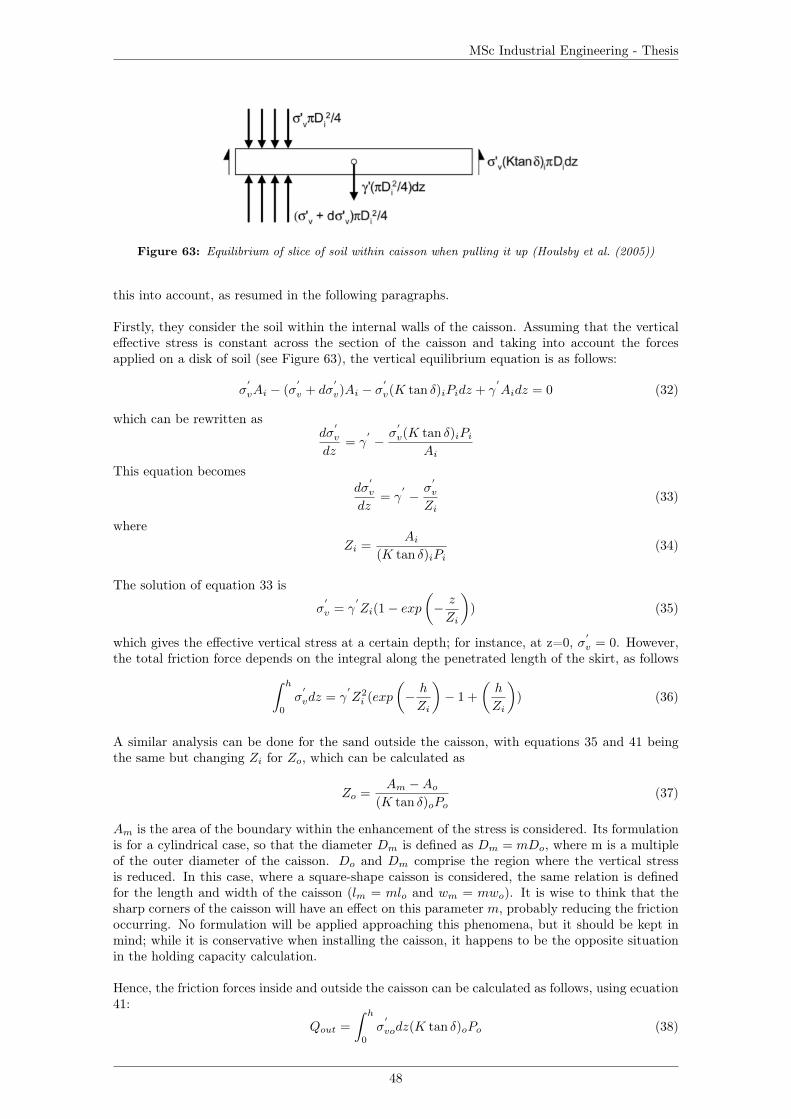
MSc Industrial Engineering - Thesis
Figure 63: Equilibrium of slice of soil within caisson when pulling it up (Houlsby et al. (2005))
this into account, as resumed in the following paragraphs.
Firstly, they consider the soil within the internal walls of the caisson. Assuming that the verticaleffective stress is constant across the section of the caisson and taking into account the forcesapplied on a disk of soil (see Figure 63), the vertical equilibrium equation is as follows:
σ′
vAi − (σ′
v + dσ′
v)Ai − σ′
v(K tan δ)iPidz + γ′Aidz = 0 (32)
which can be rewritten asdσ
′
v
dz= γ
′− σ
′
v(K tan δ)iPiAi
This equation becomesdσ
′
v
dz= γ
′− σ
′
v
Zi(33)
whereZi =
Ai(K tan δ)iPi
(34)
The solution of equation 33 is
σ′
v = γ′Zi(1− exp
(− z
Zi
)) (35)
which gives the effective vertical stress at a certain depth; for instance, at z=0, σ′
v = 0. However,the total friction force depends on the integral along the penetrated length of the skirt, as follows∫ h
0
σ′
vdz = γ′Z2i (exp
(− h
Zi
)− 1 +
(h
Zi
)) (36)
A similar analysis can be done for the sand outside the caisson, with equations 35 and 41 beingthe same but changing Zi for Zo, which can be calculated as
Zo =Am −Ao
(K tan δ)oPo(37)
Am is the area of the boundary within the enhancement of the stress is considered. Its formulationis for a cylindrical case, so that the diameter Dm is defined as Dm = mDo, where m is a multipleof the outer diameter of the caisson. Do and Dm comprise the region where the vertical stressis reduced. In this case, where a square-shape caisson is considered, the same relation is definedfor the length and width of the caisson (lm = mlo and wm = mwo). It is wise to think that thesharp corners of the caisson will have an effect on this parameter m, probably reducing the frictionoccurring. No formulation will be applied approaching this phenomena, but it should be kept inmind; while it is conservative when installing the caisson, it happens to be the opposite situationin the holding capacity calculation.
Hence, the friction forces inside and outside the caisson can be calculated as follows, using ecuation41:
Qout =
∫ h
0
σ′
vodz(K tan δ)oPo (38)
48

MSc Industrial Engineering - Thesis
Qin =
∫ h
0
σ′
vidz(K tan δ)iPi (39)
Therefore, the vertical capacity in sand accounting for the effects of enhancement can be calculatedas (the ocean pressure is not taken into account, but it is a conservative approach):
Vc,sand = Wrt +Wsc +Qout +Qin (40)
Vc,sand vertical capacity in sand (kN)Wrt Concrete rigid tank weight (kN)Wsc Steel suction caisson weight (kN)Qin Friction forces inside the caisson (kN)Qout Friction forces outside the caisson (kN)
Equation 40 can therefore be expressed as:
Vc,sand = Wrt +Wsc
+ γ′Z2o
(exp
(− h
Zo
)− 1 +
(h
Zo
))(K tan δ)oPo
+ γ′Z2i
(exp
(− h
Zi
)− 1 +
(h
Zi
))(K tan δ)iPi
A.4 Suction caisson installation in sand calculations
The same authors (Houlsby and Byrne (2005)), in another document about design procedures forinstallation of suction caissons, present a similar procedure. As shown in figure 64, the equilibriumof forces within a piece of soil is again considered, with the slight difference of the outer frictionhaving the opposite direction.
Figure 64: Equilibrium of slice of soil within caisson during installation (Houlsby and Byrne (2005))
Analogous to the previous section, the equilibrium of forces leads to the following equation:∫ h
0
σ′
vdz = γ′Z2i
(exp
(h
Zi
)− 1−
(h
Zi
))(41)
A part form the friction on the inside and outside of the caisson, an end bearing term is also ac-counted for. Its calculation and the final expressions for the two-phases suction caisson installationprocedure are presented in section 6.3.
A.5 Bearing capacity factors
The Nq and Nγ factors are known as bearing capacity factors, widely used in foundation calcula-tions. There are several formulations to calculate them, which lead to similar results. The onesused in this paper are the following:
• Nq is derived from the Prandtl-Reissner expression:
Nq = eπ tanφ tan2(45 +φ
2) (42)
• Nγ is calculated with Meyerhof (1963) expression:
Nγ = (Nq − 1) tan(1, 4φ) (43)
49
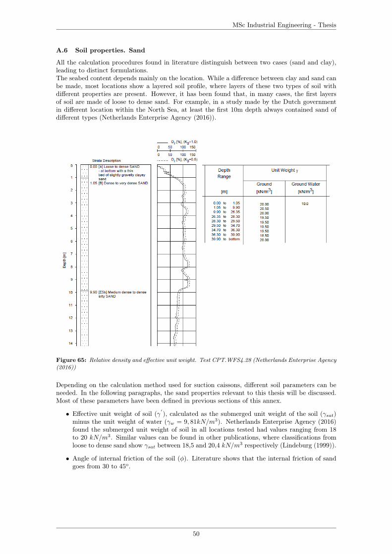
MSc Industrial Engineering - Thesis
A.6 Soil properties. Sand
All the calculation procedures found in literature distinguish between two cases (sand and clay),leading to distinct formulations.The seabed content depends mainly on the location. While a difference between clay and sand canbe made, most locations show a layered soil profile, where layers of these two types of soil withdifferent properties are present. However, it has been found that, in many cases, the first layersof soil are made of loose to dense sand. For example, in a study made by the Dutch governmentin different location within the North Sea, at least the first 10m depth always contained sand ofdifferent types (Netherlands Enterprise Agency (2016)).
Figure 65: Relative density and effective unit weight. Test CPT.WFS4.28 (Netherlands Enterprise Agency(2016))
Depending on the calculation method used for suction caissons, different soil parameters can beneeded. In the following paragraphs, the sand properties relevant to this thesis will be discussed.Most of these parameters have been defined in previous sections of this annex.
• Effective unit weight of soil (γ′), calculated as the submerged unit weight of the soil (γsat)
minus the unit weight of water (γw = 9, 81kN/m3). Netherlands Enterprise Agency (2016)found the submerged unit weight of soil in all locations tested had values ranging from 18to 20 kN/m3. Similar values can be found in other publications, where classifications fromloose to dense sand show γsat between 18,5 and 20,4 kN/m3 respectively (Lindeburg (1999)).
• Angle of internal friction of the soil (φ). Literature shows that the internal friction of sandgoes from 30 to 45o.
50

MSc Industrial Engineering - Thesis
Table 14: Relationship between Relative Density (Dr) and Angle of Internal Friction (φ) in sand (Lin-deburg (1999))
Type of soil Angle of internal friction, (o) Relative density, Dr (%)Meyerhof 1956
very loose sand <30 <20loose sand 30-35 20-40medium sand 35-40 40-60dense sand 40-45 60-80very dense sand >45 >80
As it can be seen from this table, another parameter related to the angle of internal frictionis the relative density, also depicted in figure 65. The same source define the relative densityas the ratio of the difference between the void ratios of a cohesionless soil in its loosest stateand existing natural state to the difference between its void ratio in the loosest and denseststates.
• Interface friction angle (δ), also known as the external or wall friction angle, is the anglebetween the normal of a wall and the direction of the resultant pressure that the soil exertson that wall. It can be estimated as 1
3φ for smooth retaining walls, or 23φ for rougher surfaces.
Values of this angle can be found tabulated for a variety of interface materials. For instance,a steel sheet pile against sand ranges from 11o to 14o.
• Factor relating vertical stress to horizontal stress (K), also known as the lateral earth pres-sure coefficient for soils, it is widely used for retaining walls. Earth pressure is the force perunit area exerted by soil on the retaining wall. Different formulations have been proposedto calculate what it is known as the active earth pressure, the passive earth pressure or theat-rest soil pressure. There are three main earth pressure theories: the Rankine theory, theCoulomb theory and the log-spiral theory.The active earth pressure is present behind a retaining wall that moves away from and ten-sions the remaining soil. A simplified formulation where the backfill is horizontal, the wallface is vertical and the friction between the wall and the soil is disregarded (δ = 0) is:
ka =1
kp= tan2(45o − φ
2) =
1− sin(φ)
1 + sin(φ)
The passive earth pressure is present inf front of a retaining wall that moves toward andcompresses the soil. Equally, an ecuation can be formulated as:
ka =1
ka= tan2(45o +
φ
2) =
1 + sin(φ)
1− sin(φ)
In some cases, the soil is completely confined and the walls do not move, situations knownas "at rest" earth pressure, which can be expressed as:
ko ≈ 1− sin(φ)
• Ratio of permeability within caisson to outside caisson (kf ), calculated as the fraction betweenthe permeability of the soil inside the caisson and outside the caisson (kf = ki/ko). Thisratio will affect the value of the parameter a, which can be obtained as shown in section6.3.2. Depending on the soil and the interaction of this with the structure, different valuescan be used, starting at 1 and up to 5 (Houlsby and Byrne (2005)).
51

MSc Industrial Engineering - Thesis
B Appendix. Factorial design runsAppendix contentAppendix B includes all the data calculated when carrying out the factorial design, the results ofwhich are analysed in section 7.4
B.1 Run 1
Table 15: Factor values used in run 1
A B CSand properties Number of compartments Reinforcement spacing
Loose sand 1 0,5γ
′= 8.19kN/m3
Ktan δ = 0.5φ = 30o
Preliminary stageAn initial value of V
′= 3000kN is set. Using equations 26 and 27, the self-weight penetration
depth and suction needed are calculated: hsw = 2.4m; s = 77.26kPa.
Figure 66: Loading diagram run 1, preliminarystage
The magnifying factor (1.5) as well as thewidth of the structure that accounts for eachframe (the reinforcement spacing. Factor C),will be applied to find the suction that shouldbe considered: s = 77.26 ∗ 1.5 ∗ 0.5 =57.95kPa.
The Cross method (using F-tools software) isapplied in order to find the bending and nor-mal forces diagrams. In this case, since theprofile is still indeterminate, all bars have thesame inertia.As it can be seen in the following figures, the maximum values in each case are:
Beam: M=1725 kNmPillars: M=1725 kNm
Beam: N=643.5 kNPillars: N=579.5 kN
Figure 67: Bending stress diagram run 1, prelimi-nary stage
Figure 68: Normal stress diagram run 1, prelimi-nary stage
Different profiles are set for both the beam and pillars. Using equation 28, the profiles can beverified, calculating the percentage of the structure utilization (which can also be though as thecoefficient of security).
• Beam: HE 650 B. 98%
• Pillars: HE 550 B. 98%
1st iterationWith these profiles, the volume of the whole structure is calculated. Volume=58.12m3, which leads
52
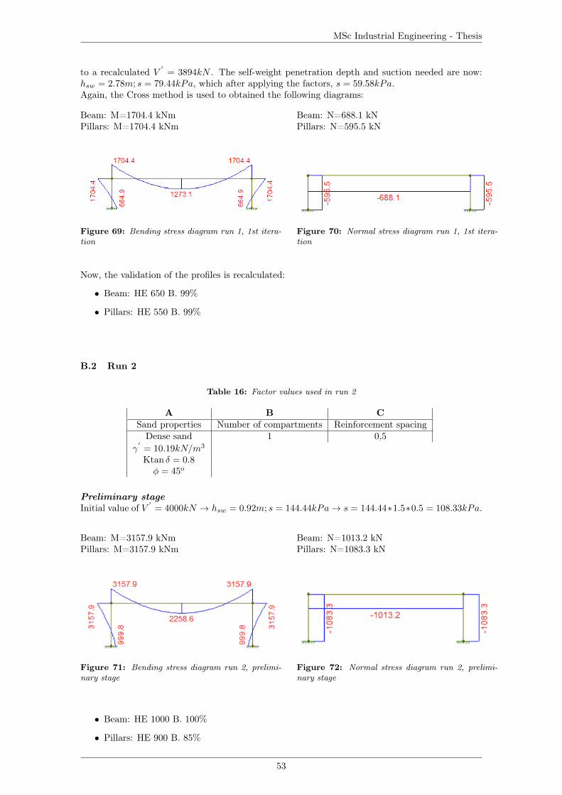
MSc Industrial Engineering - Thesis
to a recalculated V′
= 3894kN . The self-weight penetration depth and suction needed are now:hsw = 2.78m; s = 79.44kPa, which after applying the factors, s = 59.58kPa.Again, the Cross method is used to obtained the following diagrams:
Beam: M=1704.4 kNmPillars: M=1704.4 kNm
Beam: N=688.1 kNPillars: N=595.5 kN
Figure 69: Bending stress diagram run 1, 1st itera-tion
Figure 70: Normal stress diagram run 1, 1st itera-tion
Now, the validation of the profiles is recalculated:
• Beam: HE 650 B. 99%
• Pillars: HE 550 B. 99%
B.2 Run 2
Table 16: Factor values used in run 2
A B CSand properties Number of compartments Reinforcement spacingDense sand 1 0,5
γ′
= 10.19kN/m3
Ktan δ = 0.8φ = 45o
Preliminary stageInitial value of V
′= 4000kN → hsw = 0.92m; s = 144.44kPa→ s = 144.44∗1.5∗0.5 = 108.33kPa.
Beam: M=3157.9 kNmPillars: M=3157.9 kNm
Beam: N=1013.2 kNPillars: N=1083.3 kN
Figure 71: Bending stress diagram run 2, prelimi-nary stage
Figure 72: Normal stress diagram run 2, prelimi-nary stage
• Beam: HE 1000 B. 100%
• Pillars: HE 900 B. 85%
53

MSc Industrial Engineering - Thesis
1st iterationVolume=73.61m3 → V
′= 4932kN .
hsw = 1.1m; s = 144.92kPa → s = 108.69kPa.
Beam: M=3054.5 kNmPillars: M=3054.5 kNm
Beam: N=999.1 kNPillars: N=1086.9 kN
Figure 73: Bending stress diagram run 2, 1st itera-tion
Figure 74: Normal stress diagram run 2, 1st itera-tion
• Beam: HE 1000 B. 97%
• Pillars: HE 900 B. 82%
B.3 Run 3
Table 17: Factor values used in run 3
A B CSand properties Number of compartments Reinforcement spacing
Loose sand 5 0,5γ
′= 8.19kN/m3
Ktan δ = 0.5φ = 30o
Preliminary stageInitial value of V
′= 3000kN .
hsw = 1.7m; s = 101.13kPa → s = 101.13 ∗ 1.5 ∗ 0.5 = 75.85kPa.
Central beams: M=107.8 kNmOuter beams: M=133.2 kNmPillars: M=227.0 kNm
Figure 75: Bending stress diagram run 3, preliminary stage
54

MSc Industrial Engineering - Thesis
Central beams: N=183.5 kNOuter beams: N=187.0 kNPillars: N=162.7 kN
Figure 76: Normal stress diagram run 3, preliminary stage
• Central beams: HE 160 B. 103%
• Outer beams: HE 180 B. 92%
• Pillars: HE 220 B. 88%
1st iterationVolume=53.28m3 → V
′= 3570kN
hsw = 1.87m; s = 103.12kPa → s = 77.34kPa.
Central beams: M=104 kNmOuter beams: M=123.7 kNmPillars: M=195.5 kNm
Figure 77: Bending stress diagram run 3, 1st iteration
Central beams: N=184.4 kNOuter beams: N=184.4 kNPillars: N=160.9 kN
Figure 78: Normal stress diagram run 3, 1st iteration
• Central beams: HE 160 B. 100%
• Outer beams: HE 180 B. 86%
• Pillars: HE 220 B. 77%
B.4 Run 4
Table 18: Factor values used in run 4
A B CSand properties Number of compartments Reinforcement spacingDense sand 5 0,5
γ′
= 10.19kN/m3
Ktan δ = 0.8φ = 45o
55

MSc Industrial Engineering - Thesis
Preliminary stageInitial value of V
′= 3000kN .
hsw = 0.6m; s = 147.8kPa → s = 147.8 ∗ 1.5 ∗ 0.5 = 110.85kPa.
Central beams: M=157.5 kNmOuter beams: M=269 kNmPillars: M=466.1 kNm
Figure 79: Bending stress diagram run 4, preliminary stage
Central beams: N=326.4 kNOuter beams: N=327.5 kNPillars: N=261.7 kN
Figure 80: Normal stress diagram run 4, preliminary stage
• Central beams: HE 200 B. 87%
• Outer beams: HE 220 B. 109%
• Pillars: HE 280 B. 97%
1st iterationVolume=57.54m3 → V
′= 3855kN
hsw = 0.74m; s = 147.72kPa → s = 110.79kPa.
Central beams: M=151 kNmOuter beams: M=221.1 kNmPillars: M=437.7 kNm
Figure 81: Bending stress diagram run 4, 1st iteration
Central beams: N=312.2 kNOuter beams: N=312.2 kNPillars: N=244 kN
Figure 82: Normal stress diagram run 4, 1st iteration
• Central beams: HE 200 B. 84%
56

MSc Industrial Engineering - Thesis
• Outer beams: HE 220 B. 91%
• Pillars: HE 280 B. 91%
B.5 Run 5
Table 19: Factor values used in run 5
A B CSand properties Number of compartments Reinforcement spacing
Loose sand 1 1γ
′= 8.19kN/m3
Ktan δ = 0.5φ = 30o
Preliminary stageInitial value of V
′= 3000kN .
hsw = 2.4m; s = 68.18kPa.s = 68.18 ∗ 1.5 ∗ 1 = 102.27kPa.
Beam: M=3044.3 kNmPillars: M=3044.3 kNm
Beam: N=1135.7 kNPillars: N=1022.7 kN
Figure 83: Bending stress diagram run 5, prelimi-nary stage
Figure 84: Normal stress diagram run 5, prelimi-nary stage
• Beam: HE 1000 B. 100%
• Pillars: HE 800 B. 98%
1st iterationVolume=48.04m3 → V
′= 3219kN .
hsw = 2.5m; s = 69.62kPa → s = 104.43kPa.
Beam: M=2875.3 kNmPillars: M=2875.3 kNm
Beam: N=1102.4 kNPillars: N=1044.3 kN
Figure 85: Bending stress diagram run 5, 1st itera-tion
Figure 86: Normal stress diagram run 5, 1st itera-tion
57

MSc Industrial Engineering - Thesis
• Beam: HE 1000 B. 98%
• Pillars: HE 800 B. 93%
B.6 Run 6
Table 20: Factor values used in run 6
A B CSand properties Number of compartments Reinforcement spacingDense sand 1 1
γ′
= 10.19kN/m3
Ktan δ = 0.8φ = 45o
Preliminary stageInitial value of V
′= 4000kN .
hsw = 0.92m; s = 140.48kPa.s = 140.48 ∗ 1.5 ∗ 1 = 210.72kPa.
Beam: M=6142.6 kNmPillars: M=6142.6 kNm
Beam: N=1970.8 kNPillars: N=2107.2 kN
Figure 87: Bending stress diagram run 6, prelimi-nary stage
Figure 88: Normal stress diagram run 6, prelimi-nary stage
• Beam: HL 920 x 534. 96%
• Pillars: HL 920 x 446. 100%
1st iterationVolume=64.87m3 → V
′= 4346kN .
hsw = 0.99m; s = 140.50kPa → s = 210.75kPa.
Beam: M=6092.2 kNmPillars: M=6092.2 kNm
Beam: N=1955.8 kNPillars: N=2107.5 kN
58

MSc Industrial Engineering - Thesis
Figure 89: Bending stress diagram run 6, 1st itera-tion
Figure 90: Normal stress diagram run 6, 1st itera-tion
• Beam: HL 920 x 534. 95%
• Pillars: HL 920 x 446. 100%
B.7 Run 7
Table 21: Factor values used in run 7
A B CSand properties Number of compartments Reinforcement spacing
Loose sand 5 1γ
′= 8.19kN/m3
Ktan δ = 0.5φ = 30o
Preliminary stageInitial value of V
′= 3000kN .
hsw = 1.71m; s = 92.84kPa → s = 92.84 ∗ 1.5 ∗ 1 = 139.26kPa.
Central beams: M=198 kNmOuter beams: M=237 kNmPillars: M=402.6 kNm
Figure 91: Bending stress diagram run 7, preliminary stage
Central beams: N=329.9 kNOuter beams: N=337 kNPillars: N=296.2 kN
Figure 92: Normal stress diagram run 7, preliminary stage
• Central beams: HE 200 B. 106%
• Outer beams: HE 220 B. 98%
• Pillars: HE 260 B. 102%
59

MSc Industrial Engineering - Thesis
1st iterationVolume=50.64m3 → V
′= 3393kN
hsw = 1.82m; s = 92.49kPa → s = 138.74kPa.
Central beams: M=186.9 kNmOuter beams: M=227.5 kNmPillars: M=358.3 kNm
Figure 93: Bending stress diagram run 7, 1st iteration
Central beams: N=334.1 kNOuter beams: N=334.1 kNPillars: N=290.5 kN
Figure 94: Normal stress diagram run 7, 1st iteration
• Central beams: HE 200 B. 100%
• Outer beams: HE 220 B. 94%
• Pillars: HE 260 B. 91%
B.8 Run 8
Table 22: Factor values used in run 8
A B CSand properties Number of compartments Reinforcement spacingDense sand 5 1
γ′
= 10.19kN/m3
Ktan δ = 0.8φ = 45o
Preliminary stageInitial value of V
′= 3000kN .
hsw = 0.6m; s = 146.59kPa → s = 146.59 ∗ 1.5 ∗ 1 = 219.89kPa.
Central beams: M=312.4 kNmOuter beams: M=524.4 kNmPillars: M=908.4 kNm
Figure 95: Bending stress diagram run 8, preliminary stage
60

MSc Industrial Engineering - Thesis
Central beams: N=640.9 kNOuter beams: N=524.4 kNPillars: N=908.4 kN
Figure 96: Normal stress diagram run 8, preliminary stage
• Central beams: HE 260 B. 90%
• Outer beams: HE 300 B. 97%
• Pillars: HE 400 B. 92%
1st iterationVolume=54.56m3 → V
′= 3656kN
hsw = 0.71m; s = 146.51kPa → s = 219.77kPa.
Central beams: M=299.2 kNmOuter beams: M=440.8 kNmPillars: M=887.7 kNm
Figure 97: Bending stress diagram run 8, 1st iteration
Central beams: N=620.2 kNOuter beams: N=620.1 kNPillars: N=484.5 kN
Figure 98: Normal stress diagram run 8, 1st iteration
• Central beams: HE 260 B. 83%
• Outer beams: HE 280 B. 100%
• Pillars: HE 400 B. 90%
61