University of Tennessee, Knoxville University of Tennessee, Knoxville

TRACE: Tennessee Research and Creative TRACE: Tennessee Research and Creative

Exchange Exchange

Masters Theses Graduate School

8-2010

THERMAL, MAGNETIC, AND MECHANICAL STRESSES AND THERMAL, MAGNETIC, AND MECHANICAL STRESSES AND

STRAINS IN COPPER/CYANATE ESTER CYLINDRICAL COILS – STRAINS IN COPPER/CYANATE ESTER CYLINDRICAL COILS –

EFFECTS OF VARIATIONS IN FIBER VOLUME FRACTION EFFECTS OF VARIATIONS IN FIBER VOLUME FRACTION

Chance Thomas Donahue cdonahue@utk.edu

Follow this and additional works at: https://trace.tennessee.edu/utk_gradthes

Part of the Applied Mechanics Commons

Recommended Citation Recommended Citation Donahue, Chance Thomas, "THERMAL, MAGNETIC, AND MECHANICAL STRESSES AND STRAINS IN COPPER/CYANATE ESTER CYLINDRICAL COILS – EFFECTS OF VARIATIONS IN FIBER VOLUME FRACTION. " Master's Thesis, University of Tennessee, 2010. https://trace.tennessee.edu/utk_gradthes/699

This Thesis is brought to you for free and open access by the Graduate School at TRACE: Tennessee Research and Creative Exchange. It has been accepted for inclusion in Masters Theses by an authorized administrator of TRACE: Tennessee Research and Creative Exchange. For more information, please contact trace@utk.edu.

To the Graduate Council:

I am submitting herewith a thesis written by Chance Thomas Donahue entitled "THERMAL,

MAGNETIC, AND MECHANICAL STRESSES AND STRAINS IN COPPER/CYANATE ESTER

CYLINDRICAL COILS – EFFECTS OF VARIATIONS IN FIBER VOLUME FRACTION." I have

examined the final electronic copy of this thesis for form and content and recommend that it be

accepted in partial fulfillment of the requirements for the degree of Master of Science, with a

major in Mechanical Engineering.

Madhu S. Madhukar, Major Professor

We have read this thesis and recommend its acceptance:

J.A.M. Boulet, John D. Landes

Accepted for the Council:

Carolyn R. Hodges

Vice Provost and Dean of the Graduate School

(Original signatures are on file with official student records.)

To the Graduate Council:

I am submitting herewith a thesis written by Chance Thomas Donahue entitled “Thermal, Magnetic, and

Mechanical Stresses and Strains in Copper/Cyanate Ester Cylindrical Coils – Effects of Variations in Fiber

Volume Fraction.” I have examined the final electronic copy of this thesis for form and content and

recommend that it be accepted in partial fulfillment of the requirements for the degree of Master of

Science, with a major in Mechanical Engineering.

Madhu S. Madhukar

Major Professor

We have read this thesis and

recommend its acceptance:

J.A.M. Boulet

John D. Landes

Accepted for the Council:

Carolyn R. Hodges

Vice Provost and Dean of the Graduate School

(Original signatures are on file with official student records.)

THERMAL, MAGNETIC, AND MECHANICAL STRESSES AND STRAINS IN

COPPER/CYANATE ESTER CYLINDRICAL COILS – EFFECTS OF

VARIATIONS IN FIBER VOLUME FRACTION

A Thesis

Presented for the

Master of Science Degree

The University of Tennessee, Knoxville

Chance Thomas Donahue

August 2010

ii

Copyright © 2010 by Chance Thomas Donahue

All rights reserved.

iii

ACKNOWLEDGEMENTS

I wish to thank all those who helped me complete my Master of Science Degree in Mechanical

Engineering. I would like to thank Dr. Madhukar for his guidance and his effort to teach me about

composite materials, continuum mechanics, mechanics of materials, and sustainable energy concepts.

His many conversations with me have been very helpful to my continued learning. I appreciate his

acceptance of me to the program and for his patient assistance through the whole process.

I also wish to thank Dr. Matthew Hooker of Composite Technologies Development, Inc. His

ready assistance and guidance in the project and the useful data he sent me were invaluable to this

research. The trips he made to the lab were much appreciated and all of his e-mail correspondences to

any question I had were a great asset.

I would like to thank Kevin Freudenberg, Kirk Lowe, and Supratik Datta for their help on using

the finite element analysis software COMSOL. They took time out of their busy schedules to guide me in

the right direction and were patient with my numerous questions. Without them the FEA portion of the

project would have been harder to complete.

The wonderful opportunity to work at the Magnet Development Laboratory was a great

experience. All of the staff there were a huge asset and I learned so much just observing their work.

The facilities at my disposal were phenomenal and the work ethic and eagerness to assist me were much

appreciated. The opportunity to attend meetings and listen to all the knowledge passed on was truly an

honor that I am very grateful for.

I would like to thank Dr. Landes for teaching me about solid mechanics and advanced mechanics

of materials and for his guidance on classes. I would like to thank Dr. Boulet for his guidance on

programs and coursework. I wish to thank all three professors for serving on my committee.

iv

Lastly, I would like to thank my family and my friends, whose suggestions and encouragement

made all of my hard work possible. It is impossible for me to quantify how much they have helped me in

all of my accomplishments.

To every who has helped me along the way, thank you for your time and support.

v

ABSTRACT

Several problems must be solved in the construction, design, and operation of a nuclear fusion reactor.

One of the chief problems in the manufacture of high-powered copper/polymer composite magnets is

the difficulty to precisely control the fiber volume fraction. In this thesis, the effect of variations in fiber

volume fraction on thermal stresses in copper/cyanate ester composite cylinders is investigated. The

cylinder is a composite that uses copper wires that run longitudinally in a cyanate ester resin specifically

developed by Composite Technology Development, Inc. This composite cylinder design is commonly

used in magnets for nuclear fusion reactors. The application of this research is for magnets that use

cylindrical coil geometry such as the Mega Amp Spherical Tokamak (MAST) in the UK. However, most

stellarator magnet designs use complex geometries including the National Compact Stellarator

Experiment (NCSX), and the Quasi-Poloidal Stellarator (QPS). Even though the actual stresses calculated

for the cylindrical geometry may not be directly applicable to these projects, the relationship between

fiber volume fraction and stresses will be useful for any geometry. The effect of fiber volume fraction on

stresses produced by mechanical, thermal and magnetic loads on cylindrical magnet coils is studied

using micromechanics with laminate plate theory (LPT) and finite element analysis (FEA).

Based on the findings of this research, variations in volume fraction do significantly affect the stress

experienced by the composite cylinder. Over a range of volume fractions from 0.3 to 0.5, the LPT results

demonstrate that thermally induced stresses vary approximately 30% while stresses due to pressure

vary negligibly. The FEA shows that magnetic stresses vary much less at around only 5%. FEA results

seem to confirm the LPT model. It was also concluded that the stress in the insulation layers due to all

types of loadings is significant and must be considered when using this system in fusion applications.

vi

TABLE OF CONTENTS

Chapter Page

I. INTRODUCTION ....................................................................................................................... 1

1.1 Energy .............................................................................................................................. 1

1.2 Nuclear Energy ................................................................................................................ 2

1.2.1 MAST Tokamak ........................................................................................................ 2

1.3 Use of Cyanate Ester Resin vs. Epoxy for Tokamak Insulation ........................................ 3

1.4 Effects of Variation in Fiber Volume Fraction ................................................................. 6

II. REVIEW OF LITERATURE ......................................................................................................... 9

2.1 Overview .......................................................................................................................... 9

2.2 Composite Materials ....................................................................................................... 9

2.2.1 Copper Strand Based Composite Materials ........................................................... 10

2.2.2 Cyanate Ester Based Composite Materials ............................................................ 10

2.3 Fiber Volume Fraction Effect on Composite Materials ................................................. 11

2.4 Shells of Revolution ....................................................................................................... 12

2.5 Related Studies .............................................................................................................. 12

III. MATHEMATICAL FORMULATION ........................................................................................ 15

3.1 Overview ........................................................................................................................ 15

3.2 Lamina Level Analysis .................................................................................................... 15

3.2.1 Micromechanics ..................................................................................................... 15

3.2.2 Global Orthotropic Properties ............................................................................... 20

3.2.3 Thermal Properties ................................................................................................ 22

vii

Chapter Page

3.3 Laminate Level Analysis ................................................................................................. 24

3.3.1 Classical Laminate Plate Theory ............................................................................. 24

3.3.2 Laminate Stiffness .................................................................................................. 26

3.3.3 Inclusion of Thermal Loading in Laminate Analysis ............................................... 31

3.4 Magnetic Stress in a Cylinder ........................................................................................ 32

IV. METHODOLOGY .................................................................................................................. 36

4.1 Overview ........................................................................................................................ 36

4.2 Modeling ........................................................................................................................ 36

4.2.1 Lamina Level Analysis ............................................................................................. 39

4.2.2 Laminate Level Analysis ......................................................................................... 39

4.3 MATLAB Programming Environment ............................................................................ 40

4.3.1 Lamina Level Programming .................................................................................... 40

4.3.2 Laminate Level Programming ................................................................................ 41

4.4 Finite Element Analysis of Magnetic Loading ................................................................ 43

4.4.1 Multiphysics Application Modes ............................................................................ 43

4.4.2 Subdomain and Boundary Settings ........................................................................ 46

4.4.3 Meshing and Mesh Settings ................................................................................... 46

4.5 Finite Element Analysis of Magnetic Loading with Rounded Conductor ...................... 48

4.6 Finite Element Analysis of Thermal and Mechanical Loading ....................................... 51

4.6.1 Multiphysics Application Modes ............................................................................ 52

4.6.2 Subdomain and Boundary Settings ........................................................................ 52

4.6.3 Meshing and Mesh Settings ................................................................................... 53

viii

Chapter Page

V. RESULTS AND DISCUSSION .................................................................................................. 55

5.1 Mathematical Modeling ................................................................................................ 55

5.1.1 Lamina Level Analysis Effects ................................................................................. 55

5.1.2 Laminate Level Analysis Effects ............................................................................. 65

5.2 Finite Element Analysis .................................................................................................. 78

5.2.1 Magnetic Stress for Square Conductor .................................................................. 78

5.2.2. Magnetic Stress for Rounded Conductor .............................................................. 91

5.2.3 Thermal Stress and Mechanical Stress .................................................................. 95

VI. CONCLUSIONS AND RECOMMENDATIONS ......................................................................... 98

6.1 Conclusions .................................................................................................................... 98

6.2 Recommendations ....................................................................................................... 100

REFERENCES ........................................................................................................................... 102

APPENDIX ............................................................................................................................... 106

ix

LIST OF TABLES

Table Page

1.1 Comparison of Cyanate Ester and Epoxy Material Properties ......................................... 5

4.1 Input Parameters for Laminate Analysis in MATLAB...................................................... 42

5.1 Material Properties for Lamina Level Analysis ............................................................... 56

5.2 Difference in Material Properties from 0.3 to 0.5 Volume Fractions ............................ 61

5.3 Material Properties for Laminate Level Analysis ............................................................ 66

5.4 Composite Cylinder Specifications ................................................................................. 67

5.5 Summary of Laminate Level Analysis Results for Composite Layers.............................. 77

5.5 Summary of Laminate Level Analysis Results for Insulation Layer ................................ 77

5.7 Maximum Stresses and Displacement for Several Volume Fractions ............................ 90

5.8 Summary of Thermal and Pressure Finite Element Analysis .......................................... 97

x

LIST OF FIGURES

Figure Page

1.1 Worldwide Energy Sources .............................................................................................. 1

1.2 Cutaway View of Conceptual Power Plant Design of MAST Tokamak ............................. 3

1.3 Cure Cycle for CTD-403 ..................................................................................................... 6

1.4 National Compact Stellarator Experiment, a Complex Geometry Coil ............................ 8

3.1 Proposed Methods of Finding Transverse Young’s Modulus E2 ..................................... 18

3.2 Proposed Methods of Finding Shear Modulus G12 ......................................................... 19

3.3 Schematic of Strain Magnification Due to a Transverse Load ........................................ 19

3.4 Global Coordinate System (x,y,z) and Laminate Reference Directions (1,2,3)............... 20

3.5 Proposed Methods of Finding Transverse CTE α2 .......................................................... 24

3.6 Illustration of Kirchhoff’s Hypothesis ............................................................................ 26

3.7 Geometry of an N-Layered Laminate ............................................................................. 27

3.8 Lamina Geometry .......................................................................................................... 28

3.9 Laminate Orientation for 0° and 45° Samples ............................................................... 29

3.10 Earth’s Magnetic Field ................................................................................................... 32

3.11 Geometry for Calculating Magnetic Field at P Due to Current I ................................... 33

3.12 Force Due to a Current Running Through Two Parallel Wires ...................................... 34

3.13 Magnetic Field of a Current-Carrying Solenoid ............................................................. 35

4.1 Copper Conductor Wound in Cylindrical Form ............................................................. 37

4.2 Schematic Showing Fiber Orientation ........................................................................... 38

4.3 Layout of Composite Wires ........................................................................................... 38

4.4 Autodesk Inventor Model of Coil .................................................................................. 44

4.5 Drawing of COMSOL Magnetic Model ........................................................................... 45

4.6 Close-up of the Coil ....................................................................................................... 45

xi

Figure Page

4.7 Editing Toolboxes Used in COMSOL ............................................................................... 47

4.8 Mesh of Coil Geometry .................................................................................................. 47

4.9 Close-Up View of Coil Mesh ........................................................................................... 48

4.10 Photograph of a 2x2 Conductor Assembly ..................................................................... 49

4.11 Magnetic Model with Rounded Edges ........................................................................... 50

4.12 Close-Up of Rounded Edged Magnetic Model ............................................................... 50

4.13 Drawing of COMSOL Thermal and Mechanical Model................................................... 51

4.14 Subdomain Editing Toolbox for 3D Model ..................................................................... 52

4.15 Initial Plane Sketch before Extrusion ............................................................................. 53

4.16 Meshed 3D Coil Geometry ............................................................................................. 54

5.1 Young’s Moduli E1 and E2 with Varying Fiber Volume Fraction...................................... 56

5.2 Poisson’s Ratio ν12 with Varying Fiber Volume Fraction ................................................. 57

5.3 Shear Modulus G12 with Varying Fiber Volume Fraction ................................................ 57

5.4 Variation of Ex as a Function of Orientation Angle θ ...................................................... 59

5.5 Variation of Ey as a Function of Orientation Angle θ ...................................................... 59

5.6 Variation of Gxy as a Function of Orientation Angle θ .................................................... 60

5.7 Variation of νxy as a Function of Orientation Angle θ ..................................................... 60

5.8 Variation of νyx as a Function of Orientation Angle θ ..................................................... 61

5.9 Longitudinal and Transverse CTE’s α1 and α2 with Varying Fiber Volume Fraction ....... 63

5.10 Variation of αx as a Function of Orientation Angle θ ..................................................... 64

5.11 Variation of αy as a Function of Orientation Angle θ ..................................................... 64

5.12 Variation of αxy as a Function of Orientation Angle θ .................................................... 65

5.13 Stress in X Direction Due to Mechanical Loading........................................................... 68

5.14 Stress in Y Direction Due to Mechanical Loading ........................................................... 69

5.15 Stress in X-Y Plane Due to Mechanical Loading ............................................................. 70

5.16 Stress in X Direction Due to Thermal Loading ................................................................ 71

xii

Figure Page

5.17 Stress in Y Direction Due to Thermal Loading ................................................................ 72

5.18 Stress in X-Y Plane Due to Thermal Loading .................................................................. 73

5.19 Stress in X Direction Due to Combined Loading............................................................. 74

5.20 Stress in Y Direction Due to Combined Loading ............................................................. 75

5.21 Stress in X-Y Plane Due to Combined Loading ............................................................... 76

5.22 Surface Magnetic Field .................................................................................................. 79

5.23 Surface Magnetic Flux Density ....................................................................................... 80

5.24 Magnetic Field Lines ....................................................................................................... 80

5.25 Magnetic Field Lines, r Component ............................................................................... 81

5.26 Magnetic Field Lines, z Component ............................................................................... 81

5.27 Stress in the r direction σr .............................................................................................. 83

5.28 Close-up of the End of the Coil for Stress σr .................................................................. 84

5.29 Close-up of the Center of the Coil for Stress σr .............................................................. 84

5.30 Stress in the z direction σz .............................................................................................. 85

5.31 Close-up of the End of the Coil for Stress σz .................................................................. 85

5.32 Close-up of the Center of the Coil for Stress σz .............................................................. 86

5.33 Stress in the φ direction σφ ............................................................................................ 86

5.34 Close-up of the Coil for Stress σφ ................................................................................... 87

5.35 Shear Stress τrz ................................................................................................................ 87

5.36 Close-up of the End of the Coil for Stress τrz .................................................................. 88

5.37 Close-up of the Center of the Coil for Stress τrz ............................................................. 88

5.38 r-direction Displacement dr ............................................................................................ 89

5.39 z-direction Displacement dz ........................................................................................... 89

5.40 Total Displacement dtot................................................................................................... 90

5.41 Stress in the r direction σr for Rounded Edges ............................................................... 93

xiii

Figure Page

5.42 Stress in the z direction σz for Rounded Edges .............................................................. 93

5.43 Stress in the φ direction σφ for Rounded Edges ............................................................. 94

5.44 Shear Stress τrz for Rounded Edges ................................................................................ 94

5.45 Stress with Insulation Boundary Removed .................................................................... 95

5.46 Thermal Stress in the X Direction ................................................................................... 96

5.47 Thermal Stress in the Y Direction ................................................................................... 96

xiv

LIST OF ABBREVIATIONS

NCSX National Compact Stellarator Experiment

QPS Quasi-Poloidal Stellarator

CTD Composite Technology Development, Inc.

FEA Finite Element Analysis

LPT Laminate Plate Theory

CTE Coefficient of Thermal Expansion

MAST Mega Amp Spherical Tokamak

START Small Tight Aspect Ratio Tokamak

ITER International Thermonuclear Experimental Reactor

CE Cyanate Ester

VPI Vacuum Pressure Impregnation

xv

LIST OF SYMBOLS

E1 Elastic Modulus of Composite in Longitudinal Direction

E2 Elastic Modulus of Composite in Transverse Direction

ν12 Poisson's Ratio of Composite

G12 Shear Modulus of Composite

Ef Elastic Modulus of Fiber Material

Em Elastic Modulus of Matrix Material

Gf Shear Modulus of Fiber Material

Gm Shear Modulus of Matrix Material

νf Poisson's Ratio of Fiber Material

νm Poisson's Ratio of Matrix Material

Vf Fiber Volume Fraction of Composite

Vm Matrix Volume Fraction of Composite

Vvoids Void Volume Fraction of Composite

Ex Elastic Modulus of Composite in X Direction

Ey Elastic Modulus of Composite in Y Direction

νxy Poisson's Ratio of Composite in X-Y Plane

Gxy Shear Modulus of Composite in X-Y Plane

θ Fiber Orientation Angle Relative to Reference X Axis

α1 Coefficient of Thermal Expansion in Longitudinal Direction

α2 Coefficient of Thermal Expansion in Transverse Direction

αx Off-Axis Coefficient of Thermal Deformation in X Direction

αy Off-Axis Coefficient of Thermal Deformation in Y Direction

αxy Off-Axis Coefficient of Thermal Deformation in X-Y Direction

1

Chapter I

INTRODUCTION

1.1 Energy

The current world economy is primarily based on energy, and as our need for energy increases with

technology and population, we will need more and more clean, efficient sources of readily available

energy. Energy currently comes from many sources, but the overwhelming majority of our energy

needs are met using fossil fuels, with oil being the leading source of this energy. There is only a finite

amount of these fossil fuels available for use, so research in the area of clean renewable energy is of the

utmost importance. The current picture of our energy needs is quite bleak, since nearly 90% of our

energy comes from nonrenewable fossil fuels, as shown in Figure 1.1.

FIGURE 1.1 Worldwide Energy Sources [1].

2

1.2 Nuclear Energy

At present, the most viable source of clean, efficient, and abundant energy is in nuclear power. Nuclear

energy sources have much less atmospheric pollution, while promising long-term energy production

using less fuel due to the large energy density of nuclear fuels when compared to conventional fossil

fuels. The current production of nuclear energy uses nuclear fission. Fission is the splitting of a large

atom into several smaller, more stable atoms by striking it with a neutron. The resulting products have

slightly less mass than the initial atom because the “missing” mass is converted directly into energy. The

alternative to fission is nuclear fusion. Fusion is the combining of two small atoms (usually hydrogen

isotopes) into a larger atom, with the conversion of some of the mass into energy. The advantage of

fusion over fission is that it has the potential to have an even greater energy density than fissile fuels,

would be completely self-sustaining once initiated, and produces less harmful wastes. However, fusion

has many large obstacles that must be surmounted in order for it to become a viable energy source.

Containment of the fusion reaction is the chief among these, as no current engineering material can

withstand the extreme heat required in a fusion reaction. Naturally occurring fusion in the heart of stars

is contained simply by the gravity of their enormous mass; synthetic reactions currently use high-

powered magnetic fields for containment. The design, production, maintenance, and operation of these

magnetic fields is the primary area of concern for future development of fusion sources of energy, as

these magnetic fields confine and sustain the plasma required for fusion.

1.2.1 MAST Tokamak

The Mega Amp Spherical Tokamak (MAST), shown in Figure 1.2, is a program based in Culham, United

Kingdom, to build a spherical cyanate ester based fusion tokamak as a proof-of-concept test of the

spherical tokamak design [2]. MAST is the successor to the Small Tight Aspect Ratio Tokamak (START)

program and a test model has been successfully built.

3

Figure 1.2 Cutaway View of Conceptual Power Plant Design of MAST Tokamak [2].

The tokamak is a magnetic confinement device that utilizes toroidal magnetic fields produced by an

electric current to confine thermonuclear fusion plasma. It is distinct in its azimuthal symmetry and is

one of the best developed fusion device classes known [3]. The principal objectives for developing the

MAST device are to analyze and optimize key issues for the ITER (originally International Thermonuclear

Experimental Reactor, now just ITER) project and to investigate the viability, longevity, and feasibility of

a spherical design and of tokamaks in general.

1.3 Use of Cyanate Ester Resin vs. Epoxy for Tokamak Insulation

Conventionally, epoxy-based insulation systems have been used in tokamak production and testing.

However, a cyanate ester resin would offer a number of advantages for insulation system application,

including increased high temperature strength, greater radiation resistance, and drastically extended

4

pot life (the length of time that a catalyzed resin system retains a viscosity low enough to be used in

processing) [4]. For these reasons Composite Technologies Development (CTD), Inc. has developed

several cyanate ester based epoxy setups, most notably CTD-403. However, cyanate ester does have its

drawbacks in that very little industrial research has been done, the gelling process is highly exothermic,

the curing process requires that the resin must have no voids, and the resin is sensitive to moisture

absorption and swelling. However, some thermo-mechanical testing and analysis has been performed

by Voss, G. et al [5], and moisture degradation due to moisture effects has been explored in detail by

Morgan, B. et al [6].

There are several key reasons that epoxy-based polymers are not as well suited to fusion insulation.

Cyanate ester exhibits superior material properties to epoxy at critical temperatures necessary for

fusion operation, and especially has much better elevated temperature properties, as is summarized in

Table 1.1 below [5]. In addition to having very good mechanical properties, cyanate ester maintains its

elevated temperature properties much better than epoxy and it demonstrates better resistance to

damage from radiation that is characteristic of nuclear reactors [7]. Cyanate ester also exhibits

improved toughness over epoxy. Significant work is being performed in testing and characterizing this

new material to predict material performance under specific loading and to solidify the superiority of

cyanate ester to epoxy polymers.

The typical cure cycle for CTD-403 cyanate ester is shown in Figure 1.3 below. As can be seen from this

figure, the minimum time required to cure CTD-403 would be about 17 hours, and 22-40 hours is a

typical cure time used in production with soakings at lower temperatures to avoid overheating the coil

and to discourage a runaway exothermic reaction at voids and at rich resin areas [4]. CTD-403 has a

very long pot life compared to other composites and the curing cycle is very straightforward and

consistent.

5

Table 1.1 Comparison of Cyanate Ester and Epoxy Material Properties [4].

Property Test Temp. Unit Cyanate Ester Epoxy Resin

Tensile Strength 21 °C Mpa 80.3 72.6

0.2% Proof Stress 21 °C Mpa 66.7 58.1

Elongation at Failure 21 °C % 2.64 2.9

Tensile Modulus 21 °C GPa 3.49 3.2

Tensile Strength 70 °C Mpa 64.4 (100 °C) 44.5

0.2% Proof Stress 70 °C Mpa 49.0 (100 °C) 36.2

Elongation At Failure 70 °C % 4.8 (100 °C) 3.7

Tensile Modulus 70 °C GPa 2.36 2.16

Flexural Stress at Yield 21 °C Mpa 163.0 120.2

Flexural Modulus 21 °C GPa 3.95 3.39

Compression Modulus 21 °C GPa 3.74 3.39

Max Compression Strength 21 °C Mpa 158.2 118.5

Max Compression Strength 70 °C Mpa 110.9 72.9

Max Compression Strength 100 °C Mpa 87.7 13.0

Fracture Toughness K1c 20 °C MNm-3/2

3.0 2.2

Glass Transition Temp. Tg N/A °C 158 121

Density 20 °C Kg/m3 1239 1207

6

Figure 1.3 Cure Cycle for CTD-403 [6].

1.4 Effects of Variation in Fiber Volume Fraction

In a well-controlled VPI process, the fiber volume fraction will typically only vary by a few percent (±2%

is probably a good estimate). In magnets the challenge is getting uniformly high fiber-volume contents.

That often has more to do with the coil, resin flow path, and how well the coil is wound rather than

problems with the resin processing. Thus you might get 40±2% fiber volume fraction in a coil rather

than 50±2% [8]. The effects of variation in fiber volume fraction are important to characterize; although

local variations are small, throughout the coil, fiber volume fraction can vary by 10% or more and it is

difficult to produce a precise volume fraction throughout.

This research focuses on the effect of variation of fiber volume fraction in a copper/cyanate ester

cylindrical coil on thermal, mechanical, and magnetic stresses and strains. The application of this

research is for magnets that use cylindrical coil geometry such as the Mega Amp Spherical Tokamak

7

(MAST) in the UK. In some stellarator magnet designs, such as the National Compact Stellarator

Experiment (NCSX) (seen in Figure 1.4) and the Quasi-Poloidal Stellarator (QPS), the coil geometries are

complex. While the actual stress values calculated from a simple cylindrical geometry may not be

directly applicable to these more complex shapes, the relationship between fiber volume fraction and

thermal stresses will be useful for any geometry.

The analysis of the composite cylinder was principally achieved through two methods: laminate plate

theory (LPT), and model verification using finite element analysis (FEA). Essentially, the LPT was broken

further into two parts: lamina level analysis and laminate level analysis. The lamina level analysis is

used to determine lamina stiffness as a whole using the properties of the copper strands and the

cyanate ester matrix. Variations in fiber volume fraction were reflected in the stiffness moduli Ex, Ey, Gxy,

and vxy. Also, thermal expansion coefficients of the lamina were calculated from the thermal expansion

coefficients of the copper fiber and polymer matrix. The composite showed strong dependence on fiber

volume fraction variation in that for Ex, Ey, and Gxy increase in volume fraction caused an increase in

these properties; for vxy the opposite trend was found. For the laminate level analysis, the cylinder had

mechanical and thermal loadings applied in order to calculate the stress in the cylinder.

The FEA was used primarily to calculate the stress and strain due to magnetic loading of the cylinder.

This type of loading is complex and would be difficult to calculate with the LPT. However, finite element

simulation took much of the difficulty out of modeling this type of loading. The finite element models

developed are also used to verify the results of the LPT for mechanical and thermal loadings of the

cylinder.

8

Figure 1.4 National Compact Stellarator Experiment, a Complex Geometry Coil [9].

Very little literature is available on the effects on a composite of varying the volume fraction of wires,

and this is a very important parameter to monitor and predict when considering what material to use

and how best to manufacture it. Several models have been developed to help predict exactly how a

copper/cyanate ester composite will behave under varying loads and with varying fiber volume fraction.

These loadings explored are intended to duplicate expected stresses experienced by the coil under a

real duty cycle and should help predict material behavior in a nuclear fusion environment. Once the

models are developed, then all that is needed is to input the specific material properties of the coil and

its behavior can be characterized.

9

Chapter II

REVIEW OF LITERATURE

2.1 Overview

When attempting to describe the performance of a cyanate ester composite, one of the most important

manufacturing variables is the fiber volume fraction [10]. Since the performance of a composite will

depend on the properties of the constituents, namely the wires and the matrix, it is essential to

characterize the effect of varying the mixture of both components in the composite. Once the effect of

fiber volume fraction on stress in the material is understood, then models can be developed to

accurately predict how varying the constituents’ volume fraction will affect the load bearing capacity of

the material. This research will provide an understanding of how the fiber volume fraction affects the

load carrying capacity of a copper/polymer composite cylinder under thermal, mechanical and magnetic

loads.

2.2 Composite Materials

In the broadest sense, the word “composite” denotes something that consists of two or more distinct,

different parts that are combined together. In the context of its use in composite materials (usually just

shortened to composites) a composite is an amalgamation of two (or rarely, more than two) materials

with different properties and natures that allow the attainment of a material with a specific

performance greater than that of the constituents taken separately [10]. The principle advantage of

using a composite over a conventional engineering material is that composite materials usually exhibit

the best qualities of their components and sometimes even possess some qualities neither constituent

had [12]. There are three principle categories of composite materials: fibrous composites, laminated

composites, and particulate composites [11]. Fibrous or fiber-reinforced composites are the most

10

common type and consist of long, continuous fibers imbedded in a polymer matrix. Laminated

composites (not to be confused with laminae) are composed of layers of different materials adhered

together. Particulate or particle-reinforced composites have a matrix like fibrous composites, but rather

than fibers they have particles imbedded in the matrix.

2.2.1 Copper Strand Based Composite Materials

The cyanate ester/copper strand composite that is used in this research is most similar to a fiber-

reinforced composite, but it is not really correct to classify it as such. The role of the copper wires in this

composite is not to strengthen or stiffen the cylinder as is the case for fibrous composites. Copper wires

are the current carriers and the role of the resin is to act as the insulation material and to provide

support to the wires. An important property for the insulation material used in high voltage applications

is the dielectric strength. The dielectric strength of a material is the voltage that will produce a rupture

in the insulation divided by its thickness [6]. CTD-403 possesses a high dielectric strength of 105 kV/mm

giving it superior electrical insulation properties and making it an attractive matrix material to be used in

fusion applications. Furthermore, CE was found to maintain high dielectric strength even when exposed

to high humidity and temperature for prolonged periods of time [6].

2.2.2 Cyanate Ester Based Composite Materials

Cyanate esters have recently emerged as a new class of thermosetting resin that has many applications

to the aerospace and electronics industry [12]. The primary reason that these industries find cyanate

ester to be very attractive is that CE possesses a good combination of high temperature stability and

excellent mechanical properties. Additionally, cyanate esters possess excellent adhesive properties, are

more resistant to the absorption of moisture than comparable thermosetting polymers, and have very

low dielectric constants [13]. The adhesive properties make CE ideal as the matrix in a fiber reinforced

11

composite since the shearing and transverse strength of the material depends largely on the adhesive

ability of the matrix to the wires; additionally, moisture absorption tends to cause materials to swell and

experience a loss in mechanical properties as explored by Morgan, B.I. [6] so low moisture absorption

properties of cyanate esters are very attractive. Cyanate ester possesses a uniquely low cross link

density in its structural makeup making it naturally tougher than most other high-temperature

thermosets [12, 13]. Since fusion composite applications also demand a material with these desirable

qualities, one could add fusion research as an emerging industry that can find many applications for

cyanate ester based composite materials. However, these advantages come at a very high monetary

cost that may not be justified except in the aforementioned industries [13]. Also, the relatively long and

high temperature treatment cycle shown in Figure 1.3 required to cure CE can be seen as a disadvantage

when comparing with epoxy based matrix materials for a composite.

2.3 Fiber Volume Fraction Effect on Composite Materials

The fiber volume fraction, Vf, and is defined as

�� = ���� (2.1)

Where vf is the volume of wires and vc is the total composite volume. The total volume of the composite

is composed of the volume of wires and matrix, and the volume of voids [14]. This equation therefore is

�� + �� + ���� = 1 (2.2)

In vacuum-pressure impregnated coils, the void content in the polymer is considered to be less than 1%

(and is quite often less than 0.5%). Void volume is challenging to measure with absolute certainty

because the void size can be quite small (less than a few microns). Because it is so small, the void

content is generally considered to be zero [8]. It is also not unreasonable to assume that any test article

would have the same void content as a coil, so test data probably is very representative of the values

12

input into a model. For this reason the void fraction in the models developed is set as zero, leading to

the following equation

�� = 1 − �� (2.3)

This assumption will be used in the analysis of cyanate ester/copper composite materials.

2.4 Shells of Revolution

When analyzing the composite cylinder, the pressure vessel may be considered a shell of revolution due

to its curved nature. A shell has all the characteristics of plates, with one additional attribute: curvature.

Shells offer a number of advantages in engineering structures and applications, including their efficiency

of load-bearing behavior, high degree of reserved strength and structural integrity, high strength to

weight ratio, very high stiffness, and effective containment and utilization of space [15]. Although shells

do have these advantages, when considered as a three-dimensional body the calculations involved in

their analysis are generally very difficult and complicated. However, Ventsel [15] has suggested that for

sufficiently thin shells, the analysis can be restricted to the middle surface such that the shell problem

can now be approximated as a two-dimensional thin plate, greatly simplifying the calculations. It is with

this approximation in mind that the theories utilized in the mathematical formulation are developed and

implemented.

2.5 Related Studies

As stated previously, there is not a lot of research available in the area of the performance of a

composite material as fiber volume fraction is varied. Furthermore, there is little in the area of the use

of copper or even metals in general as fiber reinforcement in composite materials, and to the author’s

knowledge no research exists on the effect of fiber volume fraction on cyanate ester composites as

these are a relatively new material class. However, some research has been performed previously.

13

McMillan, J.P. [16] performed a study on the effects of fiber volume fraction on the elastic stability of

specially orthotropic plates. In his findings, McMillan reports that from a micromechanics and structural

analysis standpoint, increasing fiber volume fraction of a composite plate will dramatically increase its

ability to withstand compressive loads. Since his results are for a boron-epoxy composite, and all

composite materials behave differently, one cannot assume that these results are applicable to all fiber-

reinforced composites. However, he does state that increasing the fiber content of a unidirectional,

specially orthotropic and transversely isotropic composite material will increase its elastic stability.

Therefore these trends can be applied to any continuous fiber embedded in an epoxy or epoxy-like

matrix.

Sayre, J.R. [17] performed a study on the effects of fiber volume fraction on mechanical properties of

filament-wound, polypropylene-glass tubes. Sayre performed a study on varying the fiber volume

fraction using three Vf’s: 0.34, 0.37, and 0.46. It was found that the strength and modulus didn’t vary

significantly form one sample to the other. It was also concluded that fiber volume fraction isn’t a

controlling factor in mechanical properties. However, the methods used in reference 17 for controlling

Vf were crude and probably not uniform. Sayre states that the manner used to increase fiber volume

fraction was to simply “squeeze out” polypropylene at the fiber exit. He also states that as he increased

fiber volume fraction, that voids most likely increased in the composite, representing areas of stress

concentration that could promote crack growth and/or reduce the adhesion of the fibers to the matrix.

Upon inspection of Sayre’s results, it was observed that both tensile and flexural properties increased as

volume fraction was increased, but the difference between 0.34 and 0.37 was much more pronounced

than that between 0.37 and 0.46. It can therefore be concluded from Sayre’s results that at lower

volume fractions, increasing the amount of wires has a large effect but as this fiber fraction increases, its

effect on mechanical properties decreases somewhat.

14

Kavuri, H. [18] performed a study on cure behavior and elastic modulus characterization of a QPS coil.

He found that both CTD-404 and CTD-101K resins had low cure stresses but high cool down stresses.

Furthermore, he found that the Young’s modulus for CTD-101K at liquid nitrogen temperatures did not

differ significantly from the value at room temperature. Since CTD-404 is essentially the same as

CTD-403, the results were directly applied to the research presented in this thesis. CTD-101K is an epoxy

based resin so although the results for its analysis are not exactly applicable, they can be held to be

generally true [8].

15

Chapter III

MATHEMATICAL FORMULATION

3.1 Overview

A large portion of the research undertaken involved the application of micromechanics and classical

laminate plate theory to predict the behavior and performance of a cyanate ester/copper composite

material subjected to thermal and mechanical loads. The methodology used is briefly developed in the

preceding sections. Many leading texts in the area of composites, laminates, and plate and shell theory

are used to formulate a process for finding stress and strain in the composite, and to see how varying

fiber volume fraction affects these stresses.

3.2 Lamina Level Analysis

3.2.1 Micromechanics

Micromechanics is the study of a composite material as it pertains to the interaction of the constituents

of the heterogeneous composite [11]. Therefore micromechanics deals with the individual components

of the composite, namely the wires and the matrix, and how their properties can be used to find the

orthotropic behavior of the composite as a whole. Before the overall properties can be found, the

properties of the wires and matrix themselves must be found, namely Ef, Em, Gf, Gm, νf, and νm. Both the

copper wires and the cyanate ester isotropic bulk materials; the shear modulus G for both materials can

be found using the elementary mechanics of materials relation.

� = ��(���) (3.1)

Additionally, the fiber volume fraction Vf and the matrix volume fraction Vm are found using equations

(2.1) and (2.3) as discussed previously. Once the pertinent constituent properties are known and

16

characterized, then properties of the composite material as a whole can be found. Most texts on

composite materials suggest using a mechanics of materials approach to finding these stiffness

constants. Several texts suggest a rule of mixtures expression for the apparent Young’s modulus E1 and

for the Poisson’s ratio ν12, including Hyer [19], Jones [11], Berthelot [10], and Chawla [20]. These

equations are shown below.

�� = �� = ∑ �� = ���� + ���� (3.2)

��� = ���� + ���� (3.3)

These are called rules of mixtures because they are linear relations with respect to the fiber volume

fraction and thus depend solely on the mixture of fibers and matrix. However, these sources suggest

not using the rule of mixtures for the other constants, G12 and ν12. Hyer [19], Tsai [14] and Bertholet [10]

suggest using the following equations.

�� = (���� + ����)�� (3.4)

��� = (���� + ����)�� (3.5)

Gibson [21] proposes that the above standard equations do not correspond well with experimental data

so the equations must be modified. His derivation suggests that transverse and shear moduli are more

accurately functions of the root of fiber volume fraction and advocates the following equations be used.

�� = ��[ 1 − !��" + !����!��#��$�$� %] (3.6)

��� = ��[ 1 − !��" + !����!��#��'�'� %] (3.7)

17

Jones [11] derives the transverse and shear moduli by assuming the same transverse and shear stresses

are experienced by the fibers and matrix, and finds the strain by finding the average stress over the

corresponding volume of material. Since stress and strain are related through the moduli, these moduli

can be solved for in the equations. Therefore Jones has put forward the following nondimensionalized

equations.

�� = �������($�$� ) (3.8)

��� = �������('�'� ) (3.9)

Chawla [20] derives the transverse and shear moduli slightly differently. He starts with the same general

assumptions as Jones, but using the knowledge that experimental results do not follow Jones’ results

exactly, Chawla has provided modified equations describing these constants. Much like Gibson’s results,

Chawla’s models for E2 and G12 depend on the root of Vf rather than volume fraction directly, and he

believes this modification results in better agreement between experimental results and predicted

trends. Therefore Chawla recommends using

�� = ����!��#��$�$� % (3.10)

��� = ����!��#��'�'� % (3.11)

A plot of these various sources’ normalized curves is shown in Figures 3.1 and 3.2. These have both been

normalized in order to make a better comparison. As can be seen, the curves all follow similar trends

except for Gibson and Chawla; however, Hyer and Tsai suggest that their formulas are consistently lower

than experimental data and recommend using partitioning factor to adjust the curves up. In addition,

Gibson justifies his variation because of the over-simplification involved in the rule of mixtures

18

approach. This is because strain in the transverse direction is heterogeneous as is illustrated in Figure

3.3. In slice a-a, the strain will be placed mostly on the matrix since the matrix modulus is less in

magnitude than the fiber modulus. However, slice b-b has no wires in it so the entire load is born by the

resin. This discrepancy in loading because of inherent irregular fiber distribution results in the average

matrix strain in slice b-b being smaller than that of slice a-a. This effect is known as strain magnification

in the matrix. Chawla does not address the issue, and it is observed that he did attempt to rectify the

error in the rule of mixtures model. However, his equations do not follow the other trends, so his

equations are disregarded. Because of this shortcoming in rule of mixtures, and the fact that Hyer and

Tsai also address this issue in a similar manner, Gibson’s equations for E2 and G12 (3.6 and 3.7) are

preferred.

Figure 3.1 Proposed Methods of Finding Transverse Young’s Modulus E2. Gibson’s equation is used in

the analysis instead of those presented by Chawla, Hyer, and Jones.

0 0.1 0.2 0.3 0.4 0.5 0.6 0.7 0.8 0.9 11

1.5

2

2.5

3

3.5

Fiber Volume Fraction

E2/

Em

ChawlaGibson

HyerJones

19

Figure 3.2 Proposed Methods of Finding Shear Modulus G12. Gibson’s equation is used in the analysis

instead of those presented by Chawla, Hyer, and Jones.

Figure 3.3 Schematic of Strain Magnification Due to a Transverse Load [21].

0 0.1 0.2 0.3 0.4 0.5 0.6 0.7 0.8 0.9 11

1.2

1.4

1.6

1.8

2

2.2

2.4

2.6

2.8

3

Fiber Volume Fraction

G12

/Gm

ChawlaGibson

HyerJones

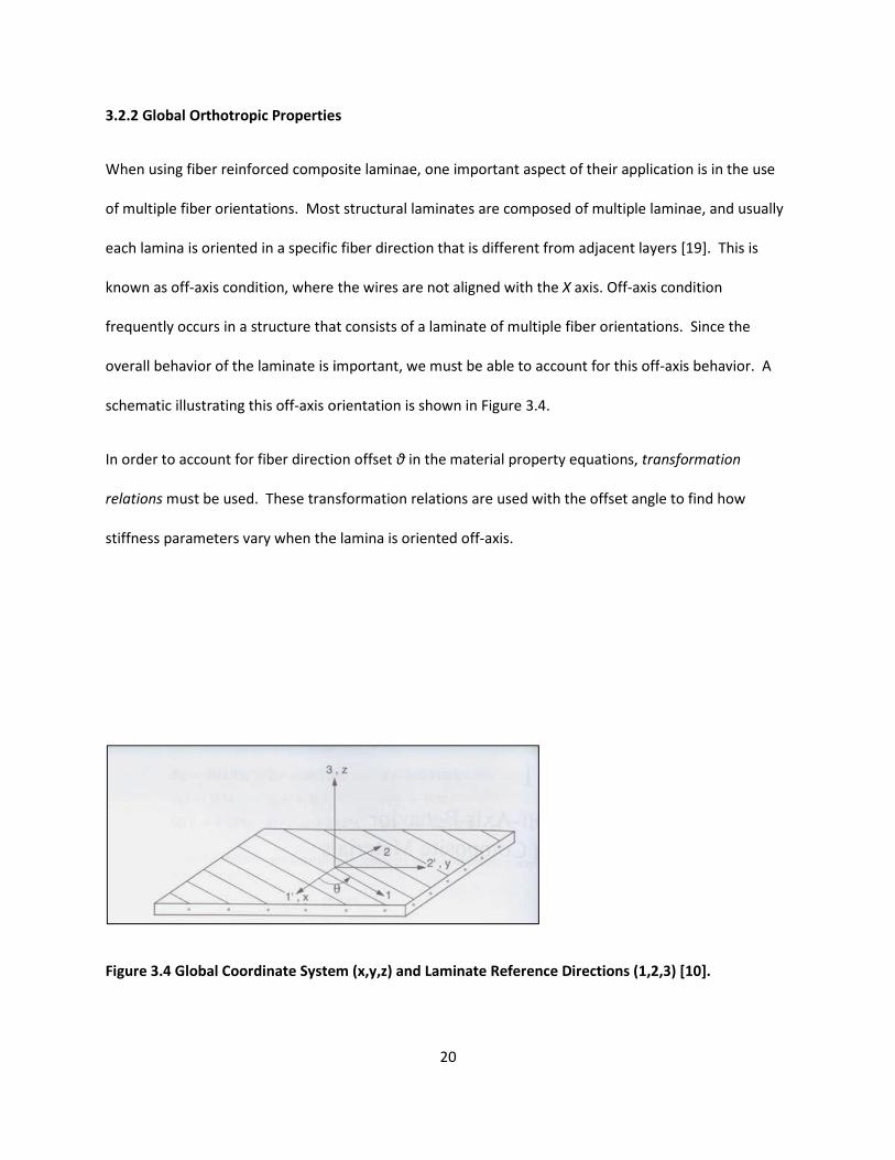
3.2.2 Global Orthotropic Properties

When using fiber reinforced composite laminae, one

of multiple fiber orientations. Most structural laminates are composed of multiple laminae, and usually

each lamina is oriented in a specific fiber direction that is different from adjacent layers [

known as off-axis condition, where the

frequently occurs in a structure that consists of a

overall behavior of the laminate is important, we must be able to account for this off

schematic illustrating this off-axis orientation is shown in Figure

In order to account for fiber direction offset

relations must be used. These transformation relations are used with the offset angle to find how

stiffness parameters vary when the lamina is oriented off

Figure 3.4 Global Coordinate System (x,y,z) and Laminate Reference Directions (1,2,3) [1

20

.2 Global Orthotropic Properties

ced composite laminae, one important aspect of their application is in the use

iber orientations. Most structural laminates are composed of multiple laminae, and usually

oriented in a specific fiber direction that is different from adjacent layers [

axis condition, where the wires are not aligned with the X axis. Off-axis condition

structure that consists of a laminate of multiple fiber orientations.

overall behavior of the laminate is important, we must be able to account for this off-axis behavior. A

orientation is shown in Figure 3.4.

In order to account for fiber direction offset θ in the material property equations, transformation

must be used. These transformation relations are used with the offset angle to find how

stiffness parameters vary when the lamina is oriented off-axis.

.4 Global Coordinate System (x,y,z) and Laminate Reference Directions (1,2,3) [1

important aspect of their application is in the use

iber orientations. Most structural laminates are composed of multiple laminae, and usually

oriented in a specific fiber direction that is different from adjacent layers [19]. This is

axis condition

laminate of multiple fiber orientations. Since the

axis behavior. A

transformation

must be used. These transformation relations are used with the offset angle to find how

.4 Global Coordinate System (x,y,z) and Laminate Reference Directions (1,2,3) [10].

21

Hyer [19] suggests the following standard properties for off-axis orientations.

�( = �1)*+4-+# �1�12−2�12%)*+2-+/02-+�1�2+/04- (3.12)

�1 = �2)*+4-+# �2�12−2�21%)*+2-+/02-+�2�1+/04- (3.13)

�(1 = �12)*+4-++/04-+2[2�12�1 1+2�12"+2�12�2 −1])*+2-+/02- (3.14)

�(1 = �122)*+4-++/04-3−#1+�1�2− �1�12%)*+2-+/02-)*+4-+# �1�12−2�12%)*+2-+/02-+�1�2+/04- (3.15)

�1( = �45(6�78��978)�2��$4$5� $4'5436�48�948

6�78�2 $4'54���4536�48�948�$4$5�978 (3.16)

However, Bertholet [10] and Jones [11] propose

�( = [ ��5 )*+:- + ��4 +/0:- + 2 ��54 − 2 �54�5 3 )*+�-+/0�-]�� (3.17)

�1 = [ ��5 +/0:- + ��4 )*+:- + 2 ��54 − 2 �54�4 3 )*+�-+/0�-]�� (3.18)

�(1 = [2 2 ��5 + ��4 + 4 �54�5 − ��543 )*+�-+/0�- + ��54 (+/0:-+)*+:-)]�� (3.19)

�(1 = �([�54�5 ()*+:- + +/0:-) − 2 ��5 + ��4 − ��543 +/0�-)*+�-] (3.20)

These two methods were compared and gave identical curves for all of the properties shown, except for

the Poisson’s ratio due to stress in the y direction νyx since the other authors do not account for it. In

fact, the corresponding equations in (3.12) through (3.16) and (3.17) through (3.20) not only give

22

identical results, but are the same equations written differently, so they must give the same results. It is

also of note that although Hyer, Berthelot, and Jones derived them, the above equations did not

originate with these authors but are commonly used in micromechanical analysis. Equations (3.12)

through (3.16) are used for the analysis simply due to equation layout preference, but either set of

equations would give the same results and could have been used.

3.2.3 Thermal Properties

In addition to the mechanical properties that relate mechanical strains to stresses, thermal properties of

the composite were also analyzed. The thermal analysis of the laminate was based on finding the

coefficient of thermal expansion (CTE) of the lamina. Similarly to the previous review, thermal

properties were first found for the composite from the properties of the wires and matrix, and then

global laminate properties were developed from these. In Hyer’s [19] model, the composite coefficients

of thermal expansion in the fiber and transverse directions α1 and α2 are found using an alternative rule

of mixtures model similar to that of the transverse modulus. This modified method is used for the same

reason that it is implemented in E2: to account for the interaction between the wires and matrix

elements. Unique strains due to an interaction between the different expansion properties of the wires

and matrix must be built into the model. Because of this, the models are

;� = (=����=���)���=��� �����"����� (3.21)

;� = ;� + ;� − ;�"�� + 2����������5 3 ;� − ;�"(1 − ��)�� (3.22)

For the transverse thermal expansion constant, the final term is an adjustment from the rule of mixtures

equation which is

;� = ;� + ;� − ;�"�� (3.23)

23

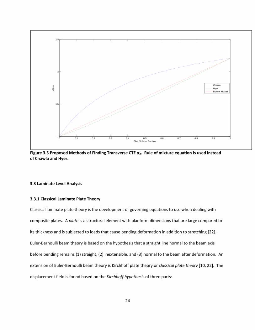
Chawla [20] recommends the following formulas for finding the thermal expansion constants

;� = ����=��(����)��=�������� ����" (3.24)

;� = ;�!�� + ;� 1 − !��"(1 + ���������������) (3.25)

Both authors’ models give the exact same trend for α1; however, they do differ some for transverse

thermal expansion coefficient. Because of this, the trends were compared and are shown in Figure 3.5.

As can be seen in this figure, the adjustments suggested by Hyer are small while those put forward by

Chawla differ greatly from the rule of mixtures plot. Given that Hyer’s equations are linear as is

expected for transverse CTE behavior, and that Chawla’s results previously were disregarded, equations

(3.21) and (3.23) are used for the thermal analysis.

Just as the mechanical properties of a fiber reinforced orthotropic laminate vary with fiber orientation,

the thermal properties as well will change with the fiber direction. Hyer [19] suggests that the

coefficients of thermal deformation in the off-axis system can readily be found by using

;( = ;�)*+�- + ;�+/0�- (3.26)

;1 = ;�+/0�- + ;�)*+�- (3.27)

;(1 = 2(;� − ;�))*+-+/0- (3.28)

As with the mechanical properties, these off-axis thermal properties can be used now to characterize

the behavior of a laminate with multiple fiber orientations.

24

Figure 3.5 Proposed Methods of Finding Transverse CTE α2. Rule of mixture equation is used instead

of Chawla and Hyer.

3.3 Laminate Level Analysis

3.3.1 Classical Laminate Plate Theory

Classical laminate plate theory is the development of governing equations to use when dealing with

composite plates. A plate is a structural element with planform dimensions that are large compared to

its thickness and is subjected to loads that cause bending deformation in addition to stretching [22].

Euler-Bernoulli beam theory is based on the hypothesis that a straight line normal to the beam axis

before bending remains (1) straight, (2) inextensible, and (3) normal to the beam after deformation. An

extension of Euler-Bernoulli beam theory is Kirchhoff plate theory or classical plate theory [10, 22]. The

displacement field is found based on the Kirchhoff hypothesis of three parts:

0 0.1 0.2 0.3 0.4 0.5 0.6 0.7 0.8 0.9 11

1.5

2

2.5

Fiber Volume Fraction

a2/a

m

Chawla

HyerRule of Mixture

25

(1) Straight lines perpendicular to the mid-surface (i.e., transverse normals) before deformation

remain straight after deformation.

(2) The transverse normals do not experience elongation (i.e., they are inextensible).

(3) The transverse normals rotate such that they remain perpendicular to the middle surface after

deformation.

The chief implication of Kirchhoff’s hypothesis is that it vastly simplifies the analysis of plates and thus

plate bending. Since there is no mention of plate material properties, the subject of lines remaining

straight is strictly a kinematic and geometric issue. This is important because it means that if we accept

the validity of the hypothesis, then we assume it is valid for the wide range of complicated material

properties inherent in fiber-reinforced composite materials [19]. A geometric example of the Kirchhoff

hypothesis is shown in Figure 3.6. The plate in part (c) has allowed the lines to distort such that they are

no longer perpendicular to the middle surface, whereas in part (b) the lines are still perpendicular to the

middle surface and thus adhere to Kirchoff’s hypothesis.

Laminate stiffness can be found using Kirchhoff’s hypothesis and another concept that stems from

classical plate theory: classical lamination theory. The key to classical lamination theory is that if the

strains and curvatures of the middle surface - >(, >1, @(1 , A(, A1, A(1 - are found, then the strain

distribution through the thickness of the laminate can be computed [19]. As stated before, this

drastically simplifies the analysis, especially for complicated multi-layered laminates.

26

Figure 3.6 Illustration of Kirchhoff’s Hypothesis [19].

3.3.2 Laminate Stiffness

The starting point for this analysis is to find the laminate stiffness matrix. For the models being

developed, this includes a matrix for both the composite and for the insulation wrap. The compliance

matrix (also known as the reduced stiffness matrix) is representative of the material properties

calculated in the lamina analysis. For an orthotropic material like copper/cyanate ester composite, the

compliance matrix is defined as [19]

B C�C�D��E = FG�� G�� 0G�� G�� 00 0 GIIJ B >�>�@��E (3.29)

27

The reduced stiffness matrix is the 3x3 Q matrix and is used to translate stress from strain. The

components of the reduced stiffness matrix are defined as

G�� = �5���54�45; G�� = �4���54�45; G�� = G�� = �54�4���54�45 = �45�5���54�45; GII = ��� (3.30)

These material properties are of course those of the composite or the insulation, depending on which

layer is being analyzed. In these equations, the material properties are defined above except for ν21

which is given by

��� = �54�4�5 (3.31)

For this analysis, the stress and strain in the layers of the laminate are individually calculated. However,

in order to proceed, the laminate has to be defined as shown in Figure 3.7.

Figure 3.7 Geometry of an N-Layered Laminate [19].

28

As can be seen in this figure, the midline of the laminate is set as the Z-coordinate and the kth

lamina

layer(s) extends from the middle surface. In addition to the coordinate system defined in Figure 3.7, the

orientation of the individual lamina in the laminate must be accounted for in the stiffness matrix. This

angle offset from the principal directions is shown in Figure 3.8. An example of a laminate with several

lamina of different angle orientations is shown in Figure 3.9 below. This illustrates how a laminate can

be arranged using the notation in Figure 3.7. The laminate on the left has what is known as [±45/0]S

orientation where it is arranged symmetrically about the midline, while the right laminate orientation is

written as [±45/0]T. The response of the laminate under a load depends on how it is oriented, and it can

be reasonably shown that the response of these two arrangements will differ even though both are

composed of the same layers.

If the lamina is oriented such that the angle is 0° relative to the coordinate system, then the reduced

stiffness matrix shown above may be used. However, when there is an angle offset a modified matrix,

known as the Q’ matrix, must be used in the equations.

Figure 3.8 Lamina Geometry.

θ Hoop Direction, x

Transverse Direction, y

29

Figure 3.9 Laminate Orientation for 0° and 45° Samples [19].

This matrix is represented as

B C(C1D(1E = KG��L G��L G�ILG��L G��L G�ILG�IL G�IL GIIL M B >(>1@(1E (3.32)

In this equation the Q’xx’s are found using the equations below, where as before θ is the angle offset [3]

Q’11 = Q11cos4θ+Q22sin

4θ+2(Q12+2Q66)sin

2θcos

2θ

Q’22 = Q11sin4θ+Q22cos

4θ+2(Q12+2Q66)sin

2θcos

2θ

Q’66 = (Q11+Q22-2Q12-2Q66)sin2θcos

2θ+Q66(sin

4θ+cos

4θ) (3.33)

Q’12 = (Q11+Q22-4Q66)sin2θcos

2θ+Q12(sin

4θ+cos

4θ)

Q’16 = (Q11-Q12-2Q66)sinθcos3θ-(Q22-Q12-2Q66)(sin

3θ+cosθ)

Q’26 = (Q11-Q12-2Q66)sin3θcosθ-(Q22-Q12-2Q66)(sinθ+cos

3θ)

Once the Q’ matrix was found for each layer, it was used in conjunction with the thickness from the

midpoint of the laminate zk to find some important properties of the material. The extensional stiffness

matrix [A] relates the resultant forces to midplane strains, the bending stiffness matrix [D] relates the

resultant moments to plate curvature, and the coupling matrix [B] implies coupling between bending

and extension of a laminate plate. These are shown below.

30

[N] = NO = ∑ (GOLPQR� )Q(SQ − SQ��) (3.34)

[T] = TO = �� ∑ (GOLPQR� )Q(SQ� − SQ��� ) (3.35)

[U] = UO = �V ∑ (GOLPQR� )Q(SQV − SQ��V ) (3.36)

The loading on the laminate can be broken into two types: forces and moments. For this particular

analysis, the loadings only consist of forces (a pressure loading); therefore, thin-walled pressure vessel

theory is applied to find the force matrix and moment matrix

[W] = X W(W1W(1Y = XZ[\]�0 Y ; [^] = X ^(^1^(1Y = B000E (3.37)

where p is the internal pressure and r is the radius of the middle surface of the laminate. These

quantities can be inserted into the total laminate constitutive equation [19] as

_[W][^]` = a[N] [T][T] [U]b _[>][A] ` or _[>][A]` = a[N] [T][T] [U]b�� _[W][^]` (3.38)

where [>] are the middle surface strains and [A] are the middle surface curvatures defined as

X >(>1@(1 Y =cdedf ghig(g�jg1ghig1 + g�ig( kdl

dm and X A(A1A(1 Y = −

cdedf g4nig(4g4nig142 g4nig(g1kdl

dm (3.39)

Now the Kirchhoff’s hypothesis is utilized along with these middle surface strains and curvatures.

Kirchhoff hypothesis equations are [19]

>((o, p, S) = >((o, p) + SA((o, p) (3.40)

31

>1(o, p, S) = >1(o, p) + SA1(o, p) (3.41)

@(1(o, p, S) = @(1 (o, p) + SA(1 (o, p) (3.42)

Knowing these midplane strains and curvatures, the stress in the kth

lamina of the laminate can be

obtained by substituting into the Kirchhoff hypothesis equation [19]

B C(C1D(1EQ

= KG��L G��L G�ILG��L G��L G�ILG�IL G�IL GIIL MQ

X >(>1@(1 Y + S KG��L G��L G�ILG��L G��L G�ILG�IL G�IL GIIL MQ

X A(A1A(1 Y (3.43)

The stress in each layer is linear with z; since each layer may have a different stiffness matrix, stresses

will be discontinuous at the boundary between laminae.

3.3.3 Inclusion of Thermal Loading in Laminate Analysis

The principle of superposition can be used to include thermal loading in the stress analysis of the

laminated coil. Equations for the off-axis thermal behavior were developed earlier and are represented

in equations (3.26) through (3.28). Utilizing these expressions for αx, αy, and αxy, one can find the

laminate behavior at any offset angle θ.

Once the directional thermal expansion coefficients are found, then they can be superimposed directly

into the strain matrix such that final stress-strain relation for mechanical and thermal loadings on the

coil can be represented as [19]

B C(C1D(1EQ

= KG��L G��L G�ILG��L G��L G�ILG�IL G�IL GIIL MQ

X >(>1@(1 Y + S KG��L G��L G�ILG��L G��L G�ILG�IL G�IL GIIL MQ

X A(A1A(1 Y − Δr KG��L G��L G�ILG��L G��L G�ILG�IL G�IL GIIL MQ

B ;(;1;(1E(3.44)

Or, more concisely

32

B C(C1D(1EQ

= KG��L G��L G�ILG��L G��L G�ILG�IL G�IL GIIL MQ

X >( + SA( − Δr;(>1 + SA1 − Δr;1@(1 + SA(1 − Δr;(1Y (3.45)

3.4 Magnetic Stress in a Cylinder

A magnetic field is produced when a charged particle is moving causing current to flow; this field

occupies the surrounding space and is a separate entity from the electric field. If any other charge or

current is present within this magnetic field, a force is exerted on this charge or current by the field [23].

Magnetism is present in many applications, including the earth’s magnetic field, as shown in Figure 3.10.

When current runs through a straight wire, it will create a magnetic field that can interact with any

charged particle within this field. For a finite length segment of wire, Tipler [25] suggests that the

magnetic field B can be found using the following equation

T = sjt:uv (+/0w� + +/0w�) (3.46)

Figure 3.10 Earth’s Magnetic Field [24].

33

In this equation, µ0 is the permeability of free space, with the value xy = 4z × 10�|r ∙ ~/N = 4z ×10�|W/N�, I is the current in the wire, R is the perpendicular distance to the particle, and w� and w� are

angles between the line perpendicular to the wire and the line from the point P to either end of the

wire. This is illustrated in Figure 3.11 below.

If the wire is very long, then the angles become very nearly 90° so the equation becomes

T = sjt�u] (3.47)

Force due to a magnetic field created by current running in a wire is found using the basic force

equation [25]

�� = ��� × T�� (3.48)

For two parallel conductors carrying currents I and I’, this becomes [23]

� = �L�T = sjtt���u] (3.49)

This is shown in Figure 3.12 below.

Figure 3.11 Geometry for Calculating Magnetic Field at P Due to Current I [26].

34

Figure 3.12 Force Due to a Current Running Through Two Parallel Wires [24].

A current-carrying wound helical coil falls into a special type of conductor called a solenoid. In the case

of this project, the composite cylinder would be considered a solenoid. Due to the axisymmetric, wound

shape of a solenoid, it has an interesting magnetic field. Figure 3.13 shows a current-carrying solenoid

and a typical resulting magnetic field. The magnetic field produced by a solenoid is uniform except at

the ends where it tapers off and loops back inside the coil [27]. However, the forces and by extension

the mechanical stresses in a solenoid are not nearly as uniform.

The mechanical stress in a solenoid occurs because of two opposite effects: interaction between

adjacent turns, and interaction of turns opposite each other. Adjacent turns in a solenoid carry parallel

current traveling in the same direction; therefore they have a force of attraction between them that

causes a compressive stress along the axis of the coil. Conversely, opposite sides of the coil have current

traveling in opposite directions and as such they have a repulsive force that creates tensile stress in the

conductors [23].

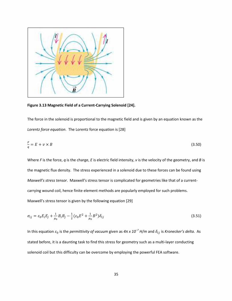
35

Figure 3.13 Magnetic Field of a Current-Carrying Solenoid [24].

The force in the solenoid is proportional to the magnetic field and is given by an equation known as the

Lorentz force equation. The Lorentz force equation is [28]

�� = � + � × T (3.50)

Where F is the force, q is the charge, E is electric field intensity, v is the velocity of the geometry, and B is

the magnetic flux density. The stress experienced in a solenoid due to these forces can be found using

Maxwell’s stress tensor. Maxwell’s stress tensor is complicated for geometries like that of a current-

carrying wound coil, hence finite element methods are popularly employed for such problems.

Maxwell’s stress tensor is given by the following equation [29]

CO = >y��O + �sj TTO − �� (>y�� + �sj T�)�O (3.51)

In this equation >y is the permittivity of vacuum given as 4π x 10−7

H/m and �O is Kronecker’s delta. As

stated before, it is a daunting task to find this stress for geometry such as a multi-layer conducting

solenoid coil but this difficulty can be overcome by employing the powerful FEA software.

36

Chapter IV

METHODOLOGY

4.1 Overview

This phase of the research focuses on the effect of variation in fiber volume fraction on stresses and

strains in a copper/cyanate ester cylindrical coil used for nuclear plasma containment. The first step was

to develop mathematical models to try to accurately predict the effect of varying the fiber volume

fraction of the composite used in the coil. This portion of the research was further broken down into

the lamina level analysis and the laminate level analysis. The mathematical models developed were

then compared to experimental results found from actual samples tested by Composite Technology

Development, Inc. Additionally, finite element models were created to perform magnetic load analysis

and to further verify the results of the mathematical model.

4.2 Modeling

The coil is modeled as a compacted conductor composed of unidirectional copper/cyanate ester

composite. Figure 4.1 shows a graphic of the coil. When wound in a coil like that in Figure 4.1, the wires

will not be parallel to the hoop direction but rather will be oriented at an angle θ from it. This is shown

in Figure 4.2 below. This compacted composite conductor is called the orthotropic lamina at the lamina

level. The composite conductor will be composed of copper wires with cyanate ester matrix filling the

voids in the material, and lapped S2 glass insulation on the outside of the copper sleeve, as shown in

Figure 4.3. When several of these laminas are stacked together with an insulation layer separating

them, this creates what is known as the laminate. This is the terminology used below to distinguish

between these levels of analysis.

37

Figure 4.1 Copper Conductor Wound in Cylindrical Form.

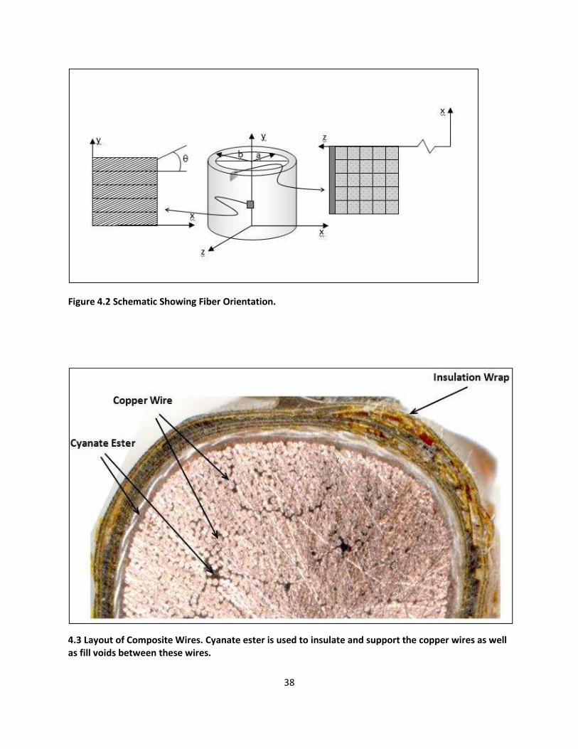
38

Figure 4.2 Schematic Showing Fiber Orientation.

4.3 Layout of Composite Wires. Cyanate ester is used to insulate and support the copper wires as well

as fill voids between these wires.

39

4.2.1 Lamina Level Analysis

Lamina level analysis and laminate level analysis were based on laminate plate theory. In both the

lamina and laminate level analysis, several symbols were used to abbreviate the material properties of

interest, a comprehensive list of which is shown in the List of Symbols on page xv. In the lamina level

portion, the composite was considered to consist of two portions, the cyanate ester polymer matrix, and

the copper wires embedded in this. Each composite lamina was considered to be orthotropic. The

material properties of the wires and the matrix were considerably different. The stiffness values E1, E2,

v12, and G12 were found from micromechanics using the material properties Ef, Em, vf, vm, Gf, and Gm. All

of these equations are a function of the fiber volume fraction of the material, Vf, and the matrix volume

fraction Vm, assumed for this composite to be Vm = 1-Vf since the composite has very few voids as

discussed previously. Then the overall material constants Ex, Ey, Gxy, and vxy were found based on E1, E2,

v12, and G12 and as a function of the fiber orientation angle θ from the reference X-axis. In order to

perform the laminate level analysis, thermal expansion coefficients of the lamina were needed, and

these were included in the lamina level analysis. These were calculated based on the thermal expansion

coefficients of the constituents, copper fiber and polymer matrix.

4.2.2 Laminate Level Analysis

The laminate level analysis was then applied to calculate stress distribution across the thickness of

various laminae. For this we considered the geometry of a composite cylinder with multiple layers of

composite material, insulated from each other with a thin layer of glass cloth/cyanate ester orthotropic

composite. A MATLAB code was developed to predict the stress distribution across the laminate

thickness under various loading conditions. Both mechanical and thermal loadings were considered for

the composite cylinder at the laminate level. The mechanical loading consisted of an internal pressure

applied uniformly to the inside surface of the composite. Although an internal pressure loading inside

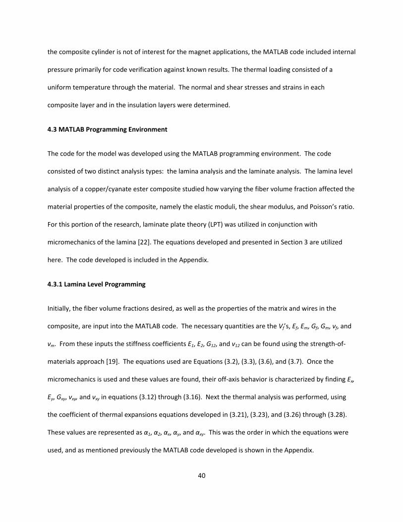
40

the composite cylinder is not of interest for the magnet applications, the MATLAB code included internal

pressure primarily for code verification against known results. The thermal loading consisted of a

uniform temperature through the material. The normal and shear stresses and strains in each

composite layer and in the insulation layers were determined.

4.3 MATLAB Programming Environment

The code for the model was developed using the MATLAB programming environment. The code

consisted of two distinct analysis types: the lamina analysis and the laminate analysis. The lamina level

analysis of a copper/cyanate ester composite studied how varying the fiber volume fraction affected the

material properties of the composite, namely the elastic moduli, the shear modulus, and Poisson’s ratio.

For this portion of the research, laminate plate theory (LPT) was utilized in conjunction with

micromechanics of the lamina [22]. The equations developed and presented in Section 3 are utilized

here. The code developed is included in the Appendix.

4.3.1 Lamina Level Programming

Initially, the fiber volume fractions desired, as well as the properties of the matrix and wires in the

composite, are input into the MATLAB code. The necessary quantities are the Vf’s, Ef, Em, Gf, Gm, νf, and

νm. From these inputs the stiffness coefficients E1, E2, G12, and ν12 can be found using the strength-of-

materials approach [19]. The equations used are Equations (3.2), (3.3), (3.6), and (3.7). Once the

micromechanics is used and these values are found, their off-axis behavior is characterized by finding Ex,

Ey, Gxy, νxy, and νxy in equations (3.12) through (3.16). Next the thermal analysis was performed, using

the coefficient of thermal expansions equations developed in (3.21), (3.23), and (3.26) through (3.28).

These values are represented as α1, α2, αx, αy, and αxy. This was the order in which the equations were

used, and as mentioned previously the MATLAB code developed is shown in the Appendix.

41

4.3.2 Laminate Level Programming

The laminate level model uses the results from the lamina level analysis to predict how a laminate

composed of multiple laminae will perform under a load. Additionally, these laminae will be oriented at

different angles relative to a reference axis. The purpose of the MATLAB programming is to construct

the code to see how a particular laminate will perform using known input parameters, and then it can

be varied to account for virtually any laminate configuration. Since there were many different inputs

required, it was easier to input all of the data as a table in Microsoft Excel and have MATLAB read it.

Therefore, a particular configuration could be set up and then the code would be executed, and the

initial parameters would already be updated. Table 4.1 shows an example configuration.

These inputs are self-explanatory. The number of layers includes the insulation layers, which in the

above example are assumed to be glass cloth. The theory used in the code to develop the laminate level

results is shown in equations (3.29) through (3.45). As can be inferred from the above table, the code

was written to include a high level of flexibility, so that loading, number of layers, layer thicknesses,

angular offsets, and coil dimensions can be varied. This allowed for great control over the input

parameters and ultimately made it easier to explore how varying fiber volume fraction affected the

output stresses.

42

Table 4.1 Input Parameters for Laminate Analysis in MATLAB.

Number of Layers 5

Internal Pressure (kPa) 20

Radius of Pressure Vessel (mm) 450

Temperature Differential ∆T (oC) 20

Coefficient of Thermal Expansion α1 (x10-6

K-1

) 85

Coefficient of Thermal Expansion α2 (x10-6

K-1

) 73

CTE of Glass Cloth αg (x10-6 K-1) 3

Composite Compliance Matrix Qc (GPa) 83.0425 14.4851 0

14.4851 62.9786 0

0 0 1.0624

Glass Cloth Compliance Matrix Qg (GPa) 10 0.2 0

0.2 10 0

0 0 0.5

Thickness of Layers (mm) Angular offset of each layer (Degrees)

3

0

0.5

0

4

10

0.5

0

3 20

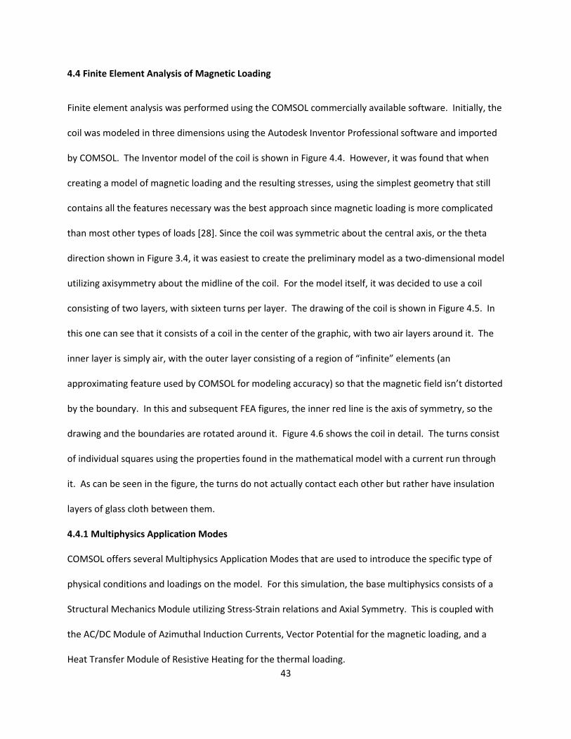
43

4.4 Finite Element Analysis of Magnetic Loading

Finite element analysis was performed using the COMSOL commercially available software. Initially, the

coil was modeled in three dimensions using the Autodesk Inventor Professional software and imported

by COMSOL. The Inventor model of the coil is shown in Figure 4.4. However, it was found that when

creating a model of magnetic loading and the resulting stresses, using the simplest geometry that still

contains all the features necessary was the best approach since magnetic loading is more complicated

than most other types of loads [28]. Since the coil was symmetric about the central axis, or the theta

direction shown in Figure 3.4, it was easiest to create the preliminary model as a two-dimensional model

utilizing axisymmetry about the midline of the coil. For the model itself, it was decided to use a coil

consisting of two layers, with sixteen turns per layer. The drawing of the coil is shown in Figure 4.5. In

this one can see that it consists of a coil in the center of the graphic, with two air layers around it. The

inner layer is simply air, with the outer layer consisting of a region of “infinite” elements (an

approximating feature used by COMSOL for modeling accuracy) so that the magnetic field isn’t distorted

by the boundary. In this and subsequent FEA figures, the inner red line is the axis of symmetry, so the

drawing and the boundaries are rotated around it. Figure 4.6 shows the coil in detail. The turns consist

of individual squares using the properties found in the mathematical model with a current run through

it. As can be seen in the figure, the turns do not actually contact each other but rather have insulation

layers of glass cloth between them.

4.4.1 Multiphysics Application Modes

COMSOL offers several Multiphysics Application Modes that are used to introduce the specific type of

physical conditions and loadings on the model. For this simulation, the base multiphysics consists of a

Structural Mechanics Module utilizing Stress-Strain relations and Axial Symmetry. This is coupled with

the AC/DC Module of Azimuthal Induction Currents, Vector Potential for the magnetic loading, and a

Heat Transfer Module of Resistive Heating for the thermal loading.

44

Figure 4.4 Autodesk Inventor Model of Coil. The coil consists of two composite layers with thin

insulation layers on the outside and between the composite layers.

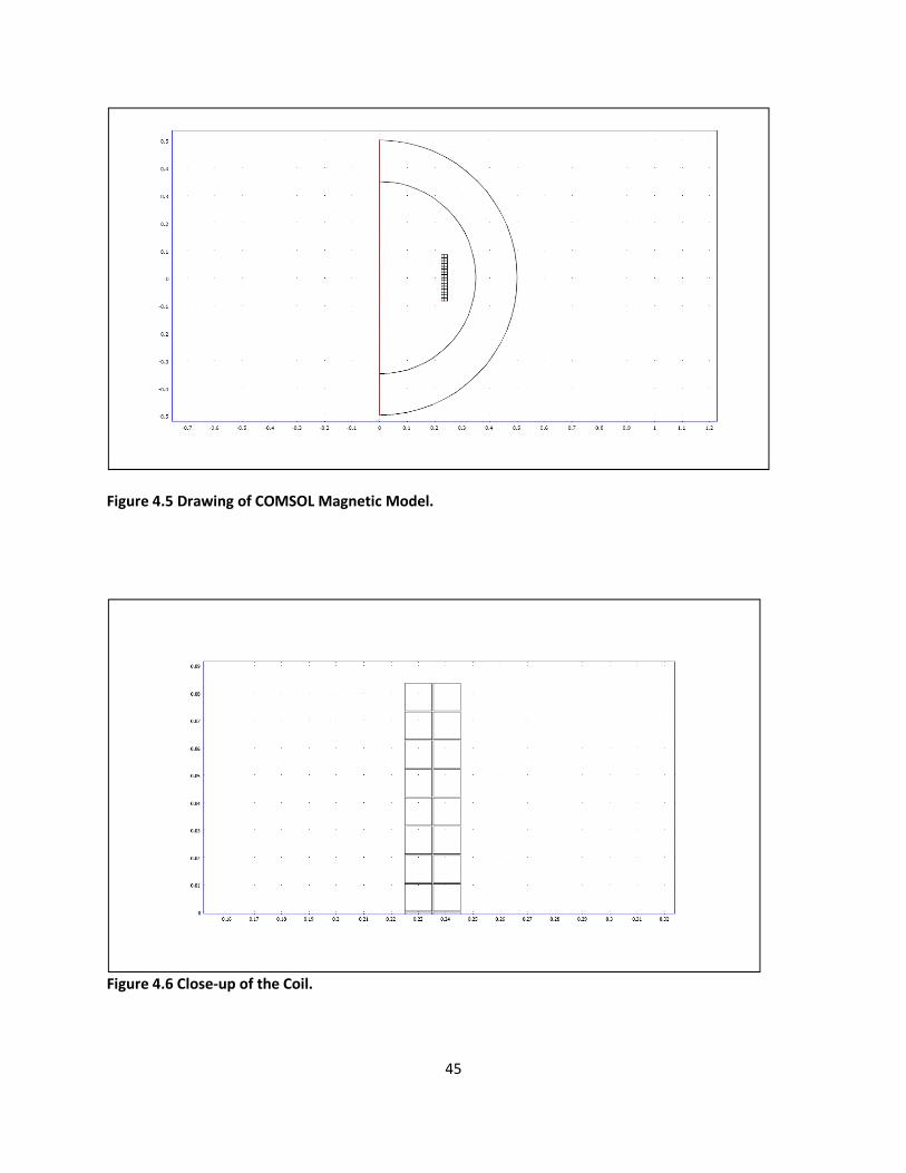
45

Figure 4.5 Drawing of COMSOL Magnetic Model.

Figure 4.6 Close-up of the Coil.

46

4.4.2 Subdomain and Boundary Settings

Once the correct application modes are selected and inserted into the model, then the subdomain and

boundary settings are required in order to couple the models together. This means that the magnetic

loading and the thermal loading must be somehow related to the structural model so that stress and

strain due to these loadings can be found. Figure 4.7 illustrates an example of how dialog boxes are

used for subdomain and boundary editing.

4.4.3 Meshing and Mesh Settings

Once the correct operations, such as coupling loadings, inserting material properties, and grounding the

structural model, were performed, the model could be meshed. Meshing is the term for breaking the

model into discrete elements where the FEA calculations can be performed. The mesh of the model is

shown in Figure 4.8 below. The mesh is automatically generated by the software once it is initialized,

but can be refined and modified by the user for specific purposes. As can be seen below, the mesh is

very fine within and near the coil conductor turns but is much courser farther away from the coil. This is

a memory-saving feature of the software so that areas with a large gradient can be more precisely

modeled while areas with less variation have broader mesh elements, thus preventing unnecessary

calculations from being performed. A close-up view of the coil mesh is shown in Figure 4.9. This

illustrates how corners and other typically higher-stress regions are finely meshed and how the other

areas are not meshed nearly as finely. Once meshing is complete, the model is ready to be solved and

the results analyzed.

47

Figure 4.7 Editing Toolboxes Used in COMSOL. Domains, boundaries, and points can be individually

selected and modified for different loads, constraints, material properties, etc.

Figure 4.8 Mesh of Coil Geometry.

48

Figure 4.9 Close-Up View of Coil Mesh. The mesh is finest at critical points such as corners, different

material contact surfaces, and in very thin insulation layers.

4.5 Finite Element Analysis of Magnetic Loading with Rounded Conductor

When analyzing the results of the magnetic loading analysis using square conductors, two issues were

addressed:

1) Using square conductors that have corresponding sharp edges appear to have a stress

concentration effect in that these edges magnify local stresses.

2) The actual conductors used, though they will ideally be square, in practice will have more

rounded edges.

Figure 4.10 below shows a 2x2 conductor assembly that is used in practice. As can be seen in the image,

the conductors have rounded edges.

49

Figure 4.10 Photograph of a 2x2 Conductor Assembly [8]. Conductors are impregnated with and held

together by CTD-403 resin.

For these reasons, it was decided to make a duplicate FEA model that is identical to the one developed

previously except that the conductors and thus the corresponding insulation wrap layers are more

rounded instead of square. The following is a brief development of the model. An exhaustive study as

was performed on the model in Section 4.4 was not performed on this model; rather it was used to

compare with the former model to see how rounding the edges affected stress and to try to determine

whether eliminating the corners would reduce the stress concentration effect in the model.

The multiphysics for this model are exactly the same as those developed in the previous section. In

order to test whether or not rounding the edges changed the stress, all other factors were held constant

in the new model. Figure 4.11 shows the new FEA model developed, and Figure 4.12 is a close-up of this

model.

50

Figure 4.11 Magnetic Model with Rounded Edges.

Figure 4.12 Close-Up of Rounded Edged Magnetic Model.

51

4.6 Finite Element Analysis of Thermal and Mechanical Loading

In order to verify the laminate level analysis of Section 4.2, a different FEA model was developed to

predict stress from mechanical and thermal loading on the coil. This is a three-dimensional model and

would more accurately portray the loads. This model looks very similar to the Inventor model shown in

Figure 3.7, but for simplicity the layers are modeled as solid rather than with individual turns. The 3D

model of the coil is shown in Figure 4.13. It is not obvious because of their small size, but the coil

consists of two composite layers with insulation between these layers and on the outside of each layer.

The coil is composed of one eighth of a completed coil and is sufficient to approximate the stresses

experienced.

Figure 4.13 Drawing of COMSOL Thermal and Mechanical Model.

52

4.6.1 Multiphysics Application Modes

Unlike the magnetic model, this one was much simpler in that it did not involve coupling multiple

multiphysics application modes together. The only application mode used was Solid, Stress-Strain from

the structural mechanics module. This was used since the applied loads that are analyzed are

mechanical and simply thermal. Since the thermal load is a simple uniform temperature difference, it

can be inserted in the subdomain as a thermal expansion strain.

4.6.2 Subdomain and Boundary Settings

The subdomain settings tool box is used to input the material properties for both the composite and the

insulation. It is also used to apply the thermal load to the model. The boundary settings tool box is used

to identify the planes of symmetry (where the model should extend to complete the cylinder) and to

apply the pressure load. Figure 4.14 shows the subdomain tool box.

Figure 4.14 Subdomain Editing Toolbox for 3D Model. The toolboxes for 3D models are very similar to

those used in 2D models previously.

53

4.6.3 Meshing and Mesh Settings

The mesh for a 3D model is created in a different way than it was for the 2D magnetic model. The vessel

was drawn on a 2D plane, edge-on as shown in Figure 4.15. The curved sections were approximated by

using the 2nd

Degree Bézier Curve function built into COMSOL. Once this was drawn, the model was

meshed using Mapped Mesh Parameters to create a structured 2D mesh. Then this was extruded into a

3D mesh with a set number of elements. Therefore the meshing of the model occurs before the

subdomain and boundary settings are used, which is the reverse of the procedure for the 2D model.

The completed meshed geometry is shown in Figure 4.16.

Figure 4.15 Initial Plane Sketch before Extrusion. The light gray squares represent the mesh elements

to be extruded.

54

Figure 4.16 Meshed 3D Coil Geometry.

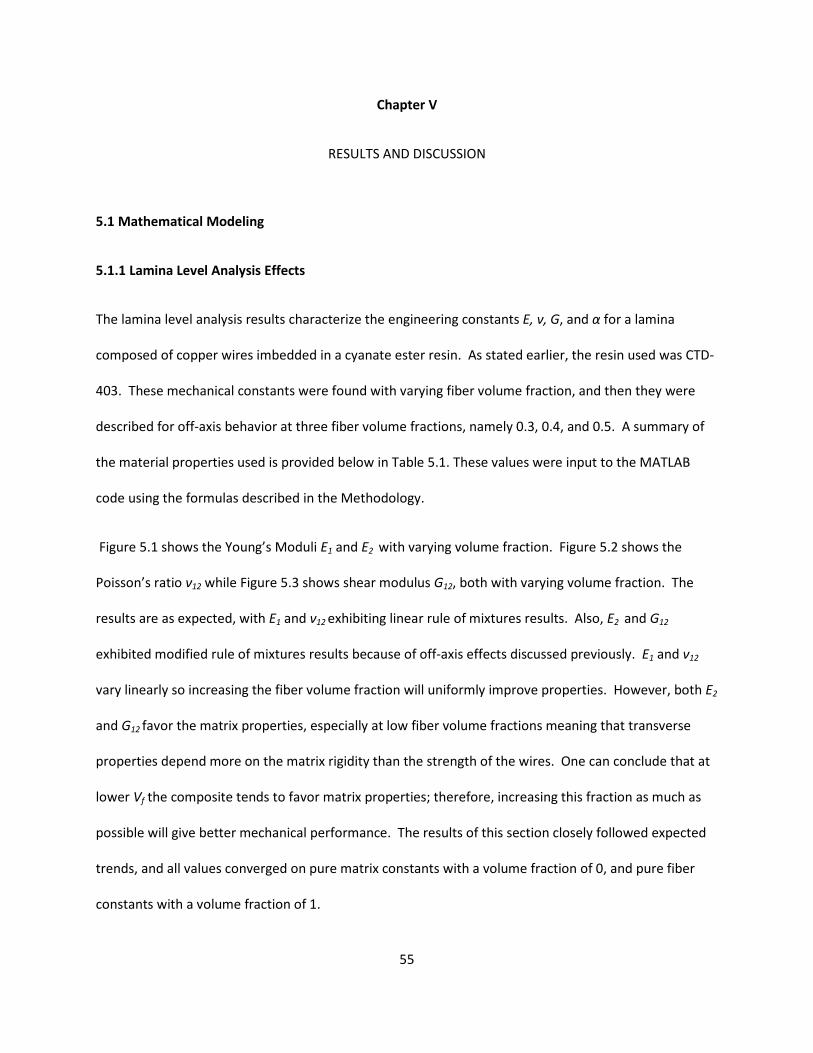
55

Chapter V

RESULTS AND DISCUSSION

5.1 Mathematical Modeling

5.1.1 Lamina Level Analysis Effects

The lamina level analysis results characterize the engineering constants E, ν, G, and α for a lamina

composed of copper wires imbedded in a cyanate ester resin. As stated earlier, the resin used was CTD-

403. These mechanical constants were found with varying fiber volume fraction, and then they were

described for off-axis behavior at three fiber volume fractions, namely 0.3, 0.4, and 0.5. A summary of

the material properties used is provided below in Table 5.1. These values were input to the MATLAB

code using the formulas described in the Methodology.

Figure 5.1 shows the Young’s Moduli E1 and E2 with varying volume fraction. Figure 5.2 shows the

Poisson’s ratio ν12 while Figure 5.3 shows shear modulus G12, both with varying volume fraction. The

results are as expected, with E1 and ν12 exhibiting linear rule of mixtures results. Also, E2 and G12

exhibited modified rule of mixtures results because of off-axis effects discussed previously. E1 and ν12

vary linearly so increasing the fiber volume fraction will uniformly improve properties. However, both E2

and G12 favor the matrix properties, especially at low fiber volume fractions meaning that transverse

properties depend more on the matrix rigidity than the strength of the wires. One can conclude that at

lower Vf the composite tends to favor matrix properties; therefore, increasing this fraction as much as

possible will give better mechanical performance. The results of this section closely followed expected

trends, and all values converged on pure matrix constants with a volume fraction of 0, and pure fiber

constants with a volume fraction of 1.

56

Table 5.1 Material Properties for Lamina Level Analysis.

Copper (Wires) [30, 31] CTD-403 (Matrix) [8] Fiber Volume Fractions

E = 120.7 GPa E = 37.9 GPa Vf1 = 0.3

G = 44.7 GPa G = 15.8 GPa Vf2= 0.4

ν = 0.35 ν = 0.20 Vf3= 0.5

α = 17 x10-6

K-1

α = 52.96 x10-6

K-1

Figure 5.1 Young’s Moduli E1 and E2 with Varying Fiber Volume Fraction. The rule of mixture based

modulus in the longitudinal direction is linear, while the modified equation for transverse modulus

has a parabolic shape.

0 0.1 0.2 0.3 0.4 0.5 0.6 0.7 0.8 0.9 130

40

50

60

70

80

90

100

110

120

130

Fiber Volume Fraction

You

ng's

Mod

ulus

, G

Pa

E1

E2

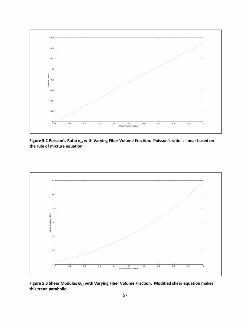
57

Figure 5.2 Poisson’s Ratio ν12 with Varying Fiber Volume Fraction. Poisson’s ratio is linear based on

the rule of mixture equation.

Figure 5.3 Shear Modulus G12 with Varying Fiber Volume Fraction. Modified shear equation makes

this trend parabolic.

0 0.1 0.2 0.3 0.4 0.5 0.6 0.7 0.8 0.9 10.2

0.22

0.24

0.26

0.28

0.3

0.32

0.34

0.36

Fiber Volume Fraction

Poi

sson

's R

atio

0 0.1 0.2 0.3 0.4 0.5 0.6 0.7 0.8 0.9 115

20

25

30

35

40

45

Fiber Volume Fraction

She

ar M

odul

us,

GP

a

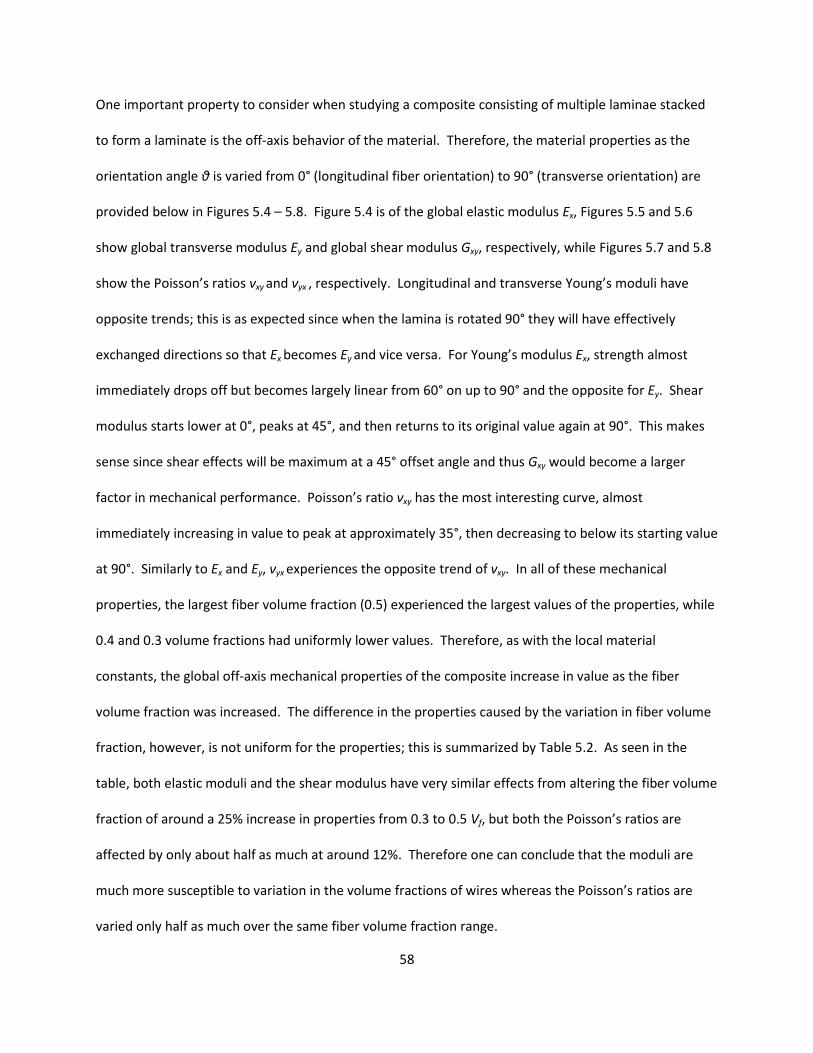
58

One important property to consider when studying a composite consisting of multiple laminae stacked

to form a laminate is the off-axis behavior of the material. Therefore, the material properties as the

orientation angle θ is varied from 0° (longitudinal fiber orientation) to 90° (transverse orientation) are

provided below in Figures 5.4 – 5.8. Figure 5.4 is of the global elastic modulus Ex, Figures 5.5 and 5.6

show global transverse modulus Ey and global shear modulus Gxy, respectively, while Figures 5.7 and 5.8

show the Poisson’s ratios νxy and νyx , respectively. Longitudinal and transverse Young’s moduli have

opposite trends; this is as expected since when the lamina is rotated 90° they will have effectively

exchanged directions so that Ex becomes Ey and vice versa. For Young’s modulus Ex, strength almost

immediately drops off but becomes largely linear from 60° on up to 90° and the opposite for Ey. Shear

modulus starts lower at 0°, peaks at 45°, and then returns to its original value again at 90°. This makes

sense since shear effects will be maximum at a 45° offset angle and thus Gxy would become a larger

factor in mechanical performance. Poisson’s ratio νxy has the most interesting curve, almost

immediately increasing in value to peak at approximately 35°, then decreasing to below its starting value

at 90°. Similarly to Ex and Ey, νyx experiences the opposite trend of νxy. In all of these mechanical

properties, the largest fiber volume fraction (0.5) experienced the largest values of the properties, while

0.4 and 0.3 volume fractions had uniformly lower values. Therefore, as with the local material

constants, the global off-axis mechanical properties of the composite increase in value as the fiber

volume fraction was increased. The difference in the properties caused by the variation in fiber volume

fraction, however, is not uniform for the properties; this is summarized by Table 5.2. As seen in the

table, both elastic moduli and the shear modulus have very similar effects from altering the fiber volume

fraction of around a 25% increase in properties from 0.3 to 0.5 Vf, but both the Poisson’s ratios are

affected by only about half as much at around 12%. Therefore one can conclude that the moduli are

much more susceptible to variation in the volume fractions of wires whereas the Poisson’s ratios are

varied only half as much over the same fiber volume fraction range.

59

Figure 5.4 Variation of Ex as a Function of Orientation Angle θ. Modulus increases uniformly with

volume fraction for all offset angles.

Figure 5.5 Variation of Ey as a Function of Orientation Angle θ. Modulus increases uniformly with

volume fraction for all offset angles.

0 10 20 30 40 50 60 70 80 9050

55

60

65

70

75

80

Orientation Angle Theta (Degrees)

Long

itudi

nal S

tiffn

ess

Mod

ulus

Ex

(GP

a)

Fiber Volume Fraction = 0.3Fiber Volume Fraction = 0.4Fiber Volume Fraction = 0.5

0 10 20 30 40 50 60 70 80 9050

55

60

65

70

75

80

Orientation Angle Theta (Degrees)

Tra

nsve

rse

Stif

fnes

s M

odul

us E

y (G

Pa)

Fiber Volume Fraction = 0.3Fiber Volume Fraction = 0.4Fiber Volume Fraction = 0.5

60

Figure 5.6 Variation of Gxy as a Function of Orientation Angle θ. Modulus increases uniformly with

volume fraction for all offset angles.

Figure 5.7 Variation of νxy as a Function of Orientation Angle θ. Poisson’s ratio increases uniformly

with volume fraction for all offset angles.

0 10 20 30 40 50 60 70 80 9020

21

22

23

24

25

26

27

28

29

Orientation Angle Theta (Degrees)

She

ar S

tiffn

ess

Mod

ulus

Gxy

(G

Pa)

Fiber Volume Fraction = 0.3Fiber Volume Fraction = 0.4Fiber Volume Fraction = 0.5

0 10 20 30 40 50 60 70 80 900.18

0.2

0.22

0.24

0.26

0.28

0.3

0.32

Orientation Angle Theta (Degrees)

Poi

sson

's R

atio

vxy

Fiber Volume Fraction = 0.3Fiber Volume Fraction = 0.4Fiber Volume Fraction = 0.5

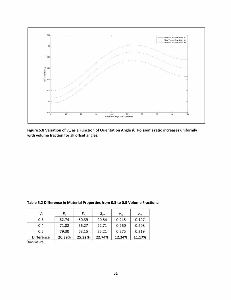
61

Figure 5.8 Variation of νyx as a Function of Orientation Angle θ. Poisson’s ratio increases uniformly

with volume fraction for all offset angles.

Table 5.2 Difference in Material Properties from 0.3 to 0.5 Volume Fractions.

Vf Ex Ey Gxy νxy νyx

0.3 62.74 50.39 20.54 0.245 0.197

0.4 71.02 56.27 22.71 0.260 0.208

0.5 79.30 63.15 25.21 0.275 0.219

Difference 26.39% 25.32% 22.74% 12.24% 11.17% 1Units of GPa.

0 10 20 30 40 50 60 70 80 900.18

0.2

0.22

0.24

0.26

0.28

0.3

0.32

Orientation Angle Theta (Degrees)

Poi

sson

's R

atio

vyx

Fiber Volume Fraction = 0.3Fiber Volume Fraction = 0.4Fiber Volume Fraction = 0.5

62

The thermal property analysis follows a similar pattern to that of the mechanical properties; there is a

local lamina analysis that looks at longitudinal and transverse thermal expansion coefficients α1 and α2,

respectively, and then a global off-axis analysis to determine coefficients of thermal deformation αx, αy,

and αxy. The longitudinal coefficient of thermal expansion α1 and the transverse CTE α2 results are

shown below in Figure 5.9. As with the mechanical properties, the thermal values exhibit full matrix

values at 0 volume fraction, and full fiber values at Vf = 1. However, the curves decrease in value since

the CTE of the matrix is greater than that of the wires. Furthermore, for thermal coefficients the

transverse direction has rule of mixtures linearity and the longitudinal direction displays modified

behavior favoring the wires.

The off-axis behavior of the thermal coefficients was examined next. Figure 5.10 shows the variation in

αx with varying orientation angle and Figure 5.11 shows the variation in αy while orientation angle varies.

Figure 5.12 is an illustration of how increasing angle offset affects coefficient of thermal deformation αxy.

αx and αy both follow a similar pattern to the Young’s modulus values shown in Figures 5.4 and 5.5 as

the trend looks very similar and both are mirror images of each other. The only real difference is that

the curves do not flatten out at the end but rather have a uniform curvature. In these curves the lowest

fiber volume fraction yielded the highest CTE while increasing fiber content led to a decrease in CTEs.

This is to be expected since the wires did have a lower CTE than the matrix, so increasing their volume

fraction should intuitively lead to lower properties. However, this is not quite the case for the off-axis

properties. At 0° and 90° the composite did not experience any shear effects, but once it is off-axis, it

immediately has a coupling CTE value. As expected, this is maximum at 45° and has a uniform inverse

parabolic shape. Because the shear coefficient of thermal expansion is an order of magnitude lower

than either of the other CTEs, its effect would be less of a factor than αx and αy. Interestingly, the

coefficient αxy is unique in that increasing the fiber volume fraction does not appear to uniformly affect

its magnitude like all the other parameters considered so far. As expected, at Vf = 0.5 the shear

63

coefficient was the lowest, but αxy at volume fraction 0.3 is actually lower than that at 0.4. The

differences between Vf = 0.3 and Vf = 0.5 for αx and αy were found to be 17.05% and 20.56%,

respectively, which is comparable to the trend found for the mechanical properties. However, for the

CTE αxy this value was found to be only 5.42%. Such a small variation in αxy suggests that increasing the

volume fraction is not a deciding factor in thermal shear. This result is surprising, but given that the

thermal coefficient αxy is so much lower than the other CTEs, this irregularity does not seem to have

much effect on the overall material behavior.

Figure 5.9 Longitudinal and Transverse CTE’s α1 and α2 with Varying Fiber Volume Fraction. Thermal

constants are opposite of mechanical properties, with linear transverse properties and parabolic

longitudinal properties.

0 0.1 0.2 0.3 0.4 0.5 0.6 0.7 0.8 0.9 115

20

25

30

35

40

45

50

55

Fiber Volume Fraction

Coe

ffic

ient

of

The

rmal

Exp

ansi

on,

x10e

6 (K

- 1)

Logitudinal DirectionTransverse Direction

64

Figure 5.10 Variation of αx as a Function of Orientation Angle θ. CTE decreases uniformly with volume

fraction for all offset angles.

Figure 5.11 Variation of αy as a Function of Orientation Angle θ. CTE decreases uniformly with volume

fraction for all offset angles.

0 10 20 30 40 50 60 70 80 9024

26

28

30

32

34

36

38

40

42

44

Orientation Angle Theta (Degrees)

Coe

ffic

ient

of

The

rmal

Exp

ansi

on a

x (x

10- 6

1/K

)

Fiber Volume Fraction = 0.3Fiber Volume Fraction = 0.4Fiber Volume Fraction = 0.5

0 10 20 30 40 50 60 70 80 9024

26

28

30

32

34

36

38

40

42

44

Orientation Angle Theta (Degrees)

Coe

ffic

ient

of

The

rmal

Exp

ansi

on a

y (x

10- 6

1/K

)

Fiber Volume Fraction = 0.3Fiber Volume Fraction = 0.4Fiber Volume Fraction = 0.5

65

Figure 5.12 Variation of αxy as a Function of Orientation Angle θ. CTE does not vary uniformly for αxy.

5.1.2 Laminate Level Analysis Effects

The laminate level analysis is built upon the results of the lamina level analysis. The results will

characterize the stresses in the laminate due to thermal loading, pressure loading, and a combination of

both. Although there are no closed form equations that directly relate the stress and the fiber volume

fraction, it has been shown previously how varying fiber volume fraction affects the composite material

constants; thus, these constants can be used to observe how the stresses are affected by Vf. The

material properties input into the model for the various fiber volume fractions are shown in Table 5.3.

As previously discussed the mechanical properties are directly proportional to fiber volume fraction,

while the thermal properties experience an inversely proportional trend. These mechanical values were

used to find the compliance matrices for the composite and insulation using the equations in (3.30). The

composite structure analyzed consists of two composite layers with an insulation layer in between.

0 10 20 30 40 50 60 70 80 900

1

2

3

4

5

6

7

8

9

10

Orientation Angle Theta (Degrees)

Coe

ffic

ient

of

The

rmal

Exp

ansi

on a

xy (

x10- 6

1/K

)

Fiber Volume Fraction = 0.3Fiber Volume Fraction = 0.4Fiber Volume Fraction = 0.5

66

Although the properties of the material are outlined in Table 5.3, this tells nothing about the

specifications of the composite cylinder that uses these materials. Table 5.4 shows the various

specifications of the composite cylinder. The pressure and temperature loadings shown are the values

tested.

First, purely mechanical loading was tested for all three fiber volume fractions. This was the pressure

load outlined in Table 5.4 (200 MPa) applied to the inside surface of the cylinder. A plot of the stress in

the cylinder layers for the three fiber volume fractions in the X direction (fiber direction) is shown in

Figure 5.13, while the same plots for the Y direction and shear in the X-Y plane are seen in Figures 5.14

and 5.15, respectively. While altering the fiber volume fraction for the pressure load did little to change

the stress in the composite layers, the main effect was seen in the insulation. The composite stress did

increase slightly with increasing fiber volume fraction, but the stress in the insulation layer actually

decreased for the X and Y directions. The shear in the composite layers was relatively small, and shear

in the insulation increased with increasing Vf.

Table 5.3 Material Properties for Laminate Level Analysis.

Copper/Cyanate Ester Composite

S2 Glass

Insulation [32,33]

Volume Fraction Vf = 0.3 Vf = 0.4 Vf = 0.5 N/A

E1 (GPa) 62.74 71.02 79.30 12.0

E2 (GPa) 50.39 56.27 63.15 20.0

G12 (GPa) 20.54 22.71 25.20 6.0

ν12 0.245 0.260 0.275 0.33

α1 (x 10-6

1/K) 42.17 38.58 34.98 16.5

α2 (x 10-6

1/K) 32.40 28.69 25.74 5.2

67

Table 5.4 Composite Cylinder Specifications [8, 33].

Property Value

Cylinder Inner Diameter 45 cm

Composite Layer Dimensions 1 cm x 1 cm

Insulation Thickness 0.46 mm

Number of Turns 16

Number of Layers 2

Current in the Wires 100 kA

Angle offset of Insulation 18°

Pressure 200 MPa

Temperature Differential 150 K

The next test was performed for a uniform thermal load of 150 K differential through the cylinder. The

results for this are shown in Figures 5.16 through 5.18. A much larger effect of fiber volume fraction was

seen in the longitudinal and transverse stresses for thermal loading, with increasing fiber volume

fraction resulting in an increase in stress in the composite layers and a corresponding decrease in

insulation stress. The final test was simply a combination of pressure and thermal loading and was

performed primarily for the sake of completeness. The results are illustrated in Figures 5.19 through

5.21. This follows the same trends as the pressure loading. A summary of the results is shown in Tables

5.5 and 5.6 below.

Figure 5.13 Stress in X Direction Due to Mechanical Loading.

three fiber volume fractions for a uniform pressure load.

900000000

1.4E+09

1.9E+09

2.4E+09

2.9E+09

3.4E+09

3.9E+09

4.4E+09

-0.015 -0.01

Str

ess

, P

a

68

Direction Due to Mechanical Loading. The curves show changes in stress for

three fiber volume fractions for a uniform pressure load.

0.01 -0.005 0 0.005 0.01

Z-Coordinate of Thickness, m

The curves show changes in stress for

0.01 0.015

Vf = 0.3

Vf = 0.4

Vf = 0.5

Figure 5.14 Stress in Y Direction Due to

three fiber volume fractions for a uniform pressure load.

800000000

1E+09

1.2E+09

1.4E+09

1.6E+09

1.8E+09

2E+09

2.2E+09

-0.015 -0.01

Str

ess

, P

a

69

Direction Due to Mechanical Loading. The curves show changes in stress for

three fiber volume fractions for a uniform pressure load.

0.01 -0.005 0 0.005 0.01

Z-Coordinate of Thickness, m

The curves show changes in stress for

0.01 0.015

Vf = 0.3

Vf = 0.4

Vf = 0.5

Figure 5.15 Stress in X-Y Plane Due to Mechanical Loading.

three fiber volume fractions for a unif

-1.4E+08

-1.2E+08

-1E+08

-80000000

-60000000

-40000000

-20000000

0

20000000

-0.015 -0.01

Str

ess

, P

a

70

Due to Mechanical Loading. The curves show changes in stress for

three fiber volume fractions for a uniform pressure load.

-0.005 0 0.005 0.01

Z-Coordinate of Thickness, m

The curves show changes in stress for

0.01 0.015

Vf = 0.3

Vf = 0.4

Vf = 0.5

Figure 5.16 Stress in X Direction Due to

fiber volume fractions for a uniform

-7E+08

-6E+08

-5E+08

-4E+08

-3E+08

-2E+08

-1E+08

0

-0.015 -0.01

Str

ess

, P

a

71

Direction Due to Thermal Loading. The curves show changes in stress for three

fiber volume fractions for a uniform temperature load.

-0.005 0 0.005 0.01

Z-Coordinate of Thickness, m

The curves show changes in stress for three

0.01 0.015

Vf = 0.3

Vf = 0.4

Vf = 0.5

Figure 5.17 Stress in Y Direction Due to

fiber volume fractions for a uniform

-5E+08

-4.5E+08

-4E+08

-3.5E+08

-3E+08

-2.5E+08

-2E+08

-1.5E+08

-1E+08

-50000000

0

-0.015 -0.01

Str

ess

, P

a

72

Direction Due to Thermal Loading. The curves show changes in stress for three

fiber volume fractions for a uniform temperature load.

0.01 -0.005 0 0.005 0.01

Z-Coordinate of Thickness, m

The curves show changes in stress for three

0.01 0.015

Vf = 0.3

Vf = 0.4

Vf = 0.5

Figure 5.18 Stress in X-Y Plane Due to

fiber volume fractions for a uniform

-1000000

0

1000000

2000000

3000000

4000000

5000000

6000000

-0.015 -0.01

Str

ess

, P

a

73

Due to Thermal Loading. The curves show changes in stress for three

fiber volume fractions for a uniform temperature load.

-0.005 0 0.005 0.01

Z-Coordinate of Thickness, m

The curves show changes in stress for three

0.01 0.015

Vf = 0.3

Vf = 0.4

Vf = 0.5

Figure 5.19 Stress in X Direction Due to

three fiber volume fractions for a combined load of temperature and pressure

500000000

1E+09

1.5E+09

2E+09

2.5E+09

3E+09

3.5E+09

4E+09

4.5E+09

-0.015 -0.01

Str

ess

, P

a

74

Direction Due to Combined Loading. The curves show changes in stress for

combined load of temperature and pressure.

0.01 -0.005 0 0.005 0.01

Z-Coordinate of Thickness, m

The curves show changes in stress for

0.01 0.015

Vf = 0.3

Vf = 0.4

Vf = 0.5

Figure 5.20 Stress in Y Direction Due to

three fiber volume fractions for a combined load of temperature and pressure

800000000

1E+09

1.2E+09

1.4E+09

1.6E+09

1.8E+09

2E+09

-0.015 -0.01

Str

ess

, P

a

75

Direction Due to Combined Loading. The curves show changes in stress for

combined load of temperature and pressure.

0.01 -0.005 0 0.005 0.01

Z-Coordinate of Thickness, m

The curves show changes in stress for

0.01 0.015

Vf = 0.3

Vf = 0.4

Vf = 0.5

Figure 5.21 Stress in X-Y Plane Due to

fiber volume fractions for a combine

-1.3E+08

-1.1E+08

-90000000

-70000000

-50000000

-30000000

-10000000

10000000

-0.015 -0.01

Str

ess

, P

a

76

Due to Combined Loading. The curves show changes in stress for three

combined load of temperature and pressure.

0.01 -0.005 0 0.005 0.01

Z-Coordinate of Thickness, m

The curves show changes in stress for three

0.01 0.015

Vf = 0.3

Vf = 0.4

Vf = 0.5

77

Table 5.5 Summary of Laminate Level Analysis Results for Composite Layers.

Volume

Fraction

Pressure Temperature Combined

Stress σx Stress σy Stress τxy Stress σx Stress σy Stress τxy Stress σx Stress σy Stress τxy

Vf = 0.3 4.47E+09 2.22E+09 3.03E+06 -4.80E+08 -3.39E+08 0.00E+00 3.99E+09 1.88E+09 3.03E+06

Vf = 0.4 4.48E+09 2.23E+09 2.65E+06 -5.50E+08 -3.87E+08 0.00E+00 3.93E+09 1.84E+09 2.65E+06

Vf = 0.5 4.48E+09 2.23E+09 2.33E+06 -6.24E+08 -4.43E+08 0.00E+00 3.86E+09 1.79E+09 2.33E+06

% Change 0.14% 0.28% -23.01% 29.90% 30.69% 0.00% -3.44% -5.19% -23.01% Note: Units of Stress are Pa.

Table 5.6 Summary of Laminate Level Analysis Results for Insulation Layer.

Volume

Fraction

Pressure Temperature Combined

Stress σx Stress σy Stress τxy Stress σx Stress σy Stress τxy Stress σx Stress σy Stress τxy

Vf = 0.3 1.19E+09 1.13E+09 -1.32E+08 -4.50E+07 -3.81E+07 4.88E+06 1.15E+09 1.09E+09 -1.27E+08

Vf = 0.4 1.05E+09 9.84E+08 -1.15E+08 -4.50E+07 -3.81E+07 4.88E+06 1.00E+09 9.46E+08 -1.10E+08

Vf = 0.5 9.22E+08 8.55E+08 -1.01E+08 -4.50E+07 -3.81E+07 4.88E+06 8.77E+08 8.17E+08 -9.65E+07

% Change 22.79% 24.19% 23.01% 0.00% 0.00% 0.00% 23.68% 25.04% 23.90% Note: Units of Stress are Pa.

78

As is illustrated by these tables, the variation in stress as volume fraction was increased from 0.3 to 0.5

is not negligible. Also, one sees that the variation had an effect on the stress in the insulation layers

even though they had the same properties in all three cases. The reason for this is that since the loads

were constant, increasing the fiber volume fraction caused an increase in the load in the composite

layer; the insulation must therefore experience a decrease in load so that the total stress is the same in

the whole laminate. As can be seen in Table 5.5, increasing fiber volume fraction did lead to increases in

stress in the composite; however, the thermal loading produced more than an order of magnitude more

variation than the pressure load. Also, it is observed that in the composite layers the shear stresses

were more than two orders of magnitude smaller than σx and σy shown in Table 5.5. This is attributed to

the fact that the copper wires in the composite layer are oriented in the hoop direction; hence, lower

shear stress is expected. In the insulation layers, the differences in the three stress components (σx, σy,

and τxy) are much more uniform to within 20% of each other. As mentioned earlier, the glass fiber

orientation in the wrapped insulation tape is about 18° from the hoop direction.

5.2 Finite Element Analysis

5.2.1 Magnetic Stress for Square Conductor

The stress experienced by the composite is caused by the magnetic field that is created when current

runs through the continuous copper wires embedded in the cyanate ester resin. Since the load due to a

magnetic field is quite complicated to analyze, COMSOL finite element analysis was used. Standard

inputs typical of fusion reactors were used for this portion of the analysis, and these are the same

numbers shown in Table 5.4. When the material properties are varied, the values in Table 5.3 are used.

First, the magnetic field itself had to be created with the software, and then the forces resultant from

this field were found using a structural mechanics package as outlined in previous sections. The

magnetic field plot is shown in Figure 5.22 below. When analyzing the magnetic stresses in a solenoid,

79

one very important parameter to look at is the magnetic flux density [33]. The magnetic flux density is

the measure of the “flow” of magnetic field through a unit surface area and carries the unit Tesla (T),

where 1 r = 1 P�∙� [23]. A plot of this magnetic flux density is shown in Figure 5.23. As can be seen in

the figure, the maximum flux density experienced by the system is 0.442 T. Another interesting plot to

include is the magnetic field lines generated by the current in the coil. The overall field is again shown in

Figure 5.24. This field is composed of an r-component and a z-component that together make up the

total field. These components are shown in Figures 5.25 and 5.26, respectively. When both of these

fields are combined using superposition, the field in Figure 5.24 is produced. It is also of note that

Figures 5.22 and 5.24 are of the same quantity, except that 5.22 is a surface plot of the magnetic field,

while Figures 5.24 through 5.26 are contour plots of the field lines.

Figure 5.22 Surface Magnetic Field. The magnetic field is strongest at the inside edges of the coil with

a magnitude of �. ��� × ��� ��.

80

Figure 5.23 Surface Magnetic Flux Density. Magnetic flux density and magnetic field are the same

except magnetic flux density is in Tesla. Maximum magnetic flux density is 0.442 T.

Figure 5.24 Magnetic Field Lines. Though the strength is weak for from the coil, the field lines extend

beyond the boundaries of the model.

81

Figure 5.25 Magnetic Field Lines, r Component. This is one component of the normalized magnetic

field.

Figure 5.26 Magnetic Field Lines, z Component. This is one component of the normalized magnetic

field.

82

Now that the magnetic field has been established, its effects on the material such as strain, stress, and

displacement are next explored. The previous magnetic field and flux plots will be the same for all of

the fiber volume fractions because the magnetic properties are independent of Vf. However, the

following table, Table 5.7, is a summary of how the fiber volume fraction affected the stress. The

numbers in the table are derived from the finite element analysis. Stress in the r-direction, denoted as

σr, is illustrated in Figures 5.27 through 5.29. Stress is higher at the ends and the highest stresses are

localized to the corners of the composite and the insulations layers experience a compressive stress.

Stress in the z-direction (σz) is shown below in Figures 5.30 through 5.32. The trend here is similar to the

r-direction, as the stress is tensile at the ends and compressive in the center. However, the z-direction

stresses are much more compressive and the max tensile load is at the inner bottom corner of the fixed

end of the coil. The hoop direction stresses, σφ, are shown in Figures 5.33 and 5.34. These stresses are

much more uniform through the coil and are all tensile, with the composite having a larger stress than

the insulation layers. It would be expected for all these stresses to be tensile as opposite sides of the

coil will all have a repulsive force on them as discussed previously in Section 3.4. Shear stresses τrz are

illustrated in Figures 5.35 through 5.37. This is also a complicated loading where the composite layers

have higher stresses than the insulation does. This also is a very good example of how the corners and

edges of contact between the insulation and composite have stress concentrators where high stresses

are formed at these boundaries, as seen especially in Figure 5.37. Finally, the displacement that the coil

experiences as a result of the magnetic loading is shown in Figures 5.38 through 5.40. Figures 5.38 and

5.39 show the r- and z-direction displacements (respectively) experienced by the geometry, while Figure

5.40 is the superposition of these into the total displacement. The displacement experienced is very

small, and although it is uniform in the z-direction, the r-direction displacement is not uniform and

displaces more in the center. The displacement in the r-direction is all positive, while as expected the z-

displacement is negative due to the compressive forces. The deformed shape of the coil would no

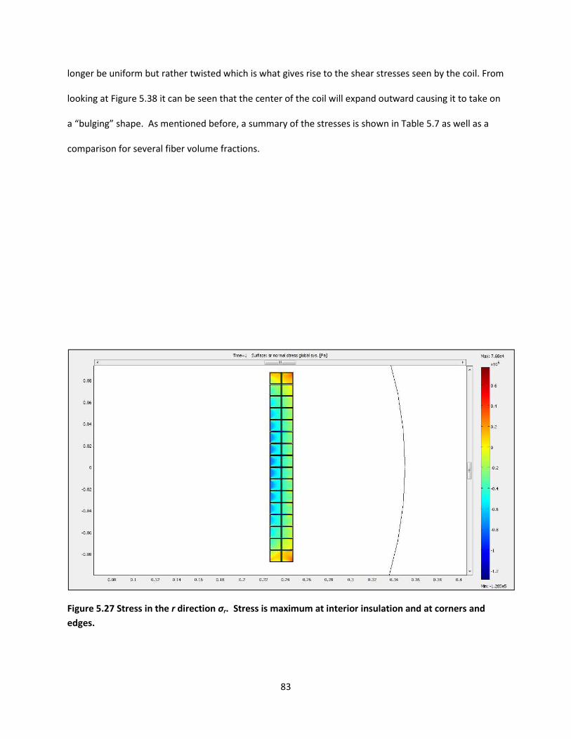
83

longer be uniform but rather twisted which is what gives rise to the shear stresses seen by the coil. From

looking at Figure 5.38 it can be seen that the center of the coil will expand outward causing it to take on

a “bulging” shape. As mentioned before, a summary of the stresses is shown in Table 5.7 as well as a

comparison for several fiber volume fractions.

Figure 5.27 Stress in the r direction σr. Stress is maximum at interior insulation and at corners and

edges.

84

Figure 5.28 Close-up of the End of the Coil for Stress σr. Stress is maximum at interior insulation and

at corners and edges.

Figure 5.29 Close-up of the Center of the Coil for Stress σr. Stress is maximum at interior insulation

and at corners and edges.

85

Figure 5.30 Stress in the z direction σz. Stress is maximum at the bottom inner corner and the inner

center of the coil.

Figure 5.31 Close-up of the End of the Coil for Stress σz. Stress is maximum at the bottom inner corner

and the inner center of the coil.

86

Figure 5.32 Close-up of the Center of the Coil for Stress σz. Stress is maximum at the bottom inner

corner and the inner center of the coil.

Figure 5.33 Stress in the φ direction σφ. Stress is uniform in the composite turns, and in the insulation

layers.

87

Figure 5.34 Close-up of the Coil for Stress σφ. Stress is uniform in the composite turns, and in the

insulation layers.

Figure 5.35 Shear Stress τrz. Shear stress has large stress concentrations in corners and at boundaries

of composite and insulation layers.

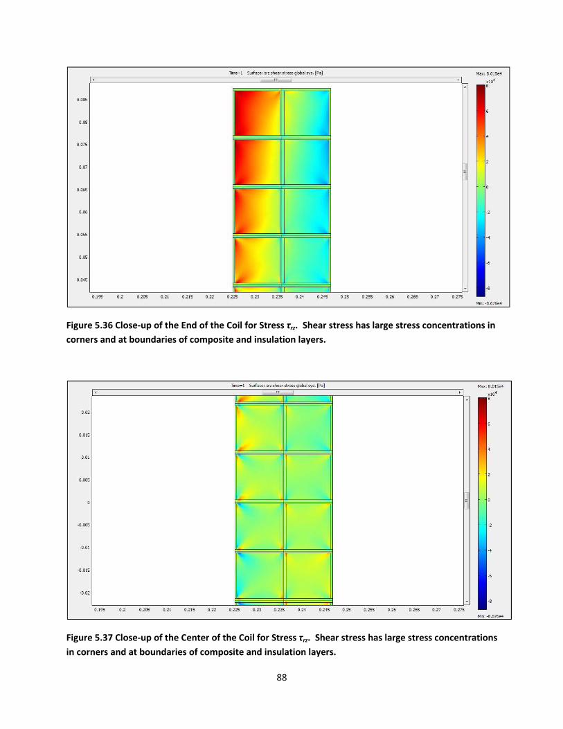
88

Figure 5.36 Close-up of the End of the Coil for Stress τrz. Shear stress has large stress concentrations in

corners and at boundaries of composite and insulation layers.

Figure 5.37 Close-up of the Center of the Coil for Stress τrz. Shear stress has large stress concentrations

in corners and at boundaries of composite and insulation layers.

89

Figure 5.38 r direction Displacement dr. Displacement is maximum at the center, causing a “bulging”

to occur in the center of the coil.

Figure 5.39 z direction Displacement dz. Displacement is maximum at the free end and zero at the

fixed end.

90

Figure 5.40 Total Displacement dtot. This is a superposition of displacement in both directions.

Table 5.7 Maximum Stresses and Displacement for Several Volume Fractions.

Volume Fraction Stress σr Stress σz Stress σφ Stress τrz Displ. dr Displ. dz Total Displ. dt

Vf = 0.3 -1.28E+05 -4.22E+05 6.90E+05 -8.68E+04 2.62E-06 -1.40E-06 2.73E-06

Vf = 0.4 -1.34E+05 -4.35E+05 7.01E+05 -8.68E+04 2.35E-06 -1.30E+06 2.46E+06

Vf = 0.5 -1.38E+05 -4.49E+05 7.12E+05 -8.68E+04 2.13E-06 -1.21E-06 2.24E-06

% Change 7.42% 6.45% 3.09% 0.03% -18.62% -13.54% -18.04% Note: Units of Stress are Pa.

91

The summary of the magnetic stress analysis is shown above in Table 5.7. In general the Results are that

increasing volume fraction has less of an effect on magnetic stresses than it does on thermal and

mechanical stresses. Displacement is by far the most strongly affected quantity, with radial

displacement decreased over 18% and axial displacement decreased over 13%. This is expected because

as the composite stiffens with the addition of more wires, its displacement will be more constrained.

This change in displacement translates into a smaller change in stress seen by the coil. Stress in the r-

direction is most affected at over 7%, and axial stress is similar at almost 6.5%. Hoop stress in the fiber

direction has less than half as much of an effect, and most surprisingly shear stress varies negligibly as

the fiber volume fraction is increased. Again, shear stress is smaller than the other stress components

so it is not as important a factor in the failure of the coil, but it is still surprising that it basically doesn’t

vary with fiber volume fraction.

5.2.2. Magnetic Stress for Rounded Conductor

This section of the analysis was performed solely to test out how much of an effect rounding off the

edges of the magnetic model would have on the stresses experienced by the coil. This was done

because the actual coil will, in practice, have rounded edges, and to investigate just how much of an

effect that the corners have on stress in the cylinder. The magnetic field generated was not exactly the

same because the geometry was altered, but it was very similar. The peak magnetic flux experienced

was found to be 0.439 T for the rounded edged model, and when compared to 0.442 T for the square

model, it is basically the same. The stresses were found to be a bit different, however. Figure 5.41

shows stress in the r-direction of the rounded coil. Stress distribution is very similar to Figure 5.29 in the

conductor and insulation; however, in the insulation transition from rounded to square, a stress

concentration can still be seen. Surprisingly, the magnitude of stress actually went up at the transition

point so the rounded edged model has higher stresses at the critical points than the previous model did.

92

The plot of stress in the z-direction is shown in Figure 5.42 below. Although the original model didn’t

have very much stress concentration effect for σz, Figure 5.42 shows that the new rounded model does

have a significant stress concentration at the same points as in Figure 5.41. Even hoop stress now

experiences a stress concentration that wasn’t previously there as illustrated in Figure 5.43. The final

stress is shear stress in the coil, and it is shown below in Figure 5.44. It can be seen that this stress was

also magnified by rounding the conductors and insulation. These results are surprising and show that

stress concentration actually increased when the edges were removed. The most likely explanation for

this is that the stress is a result of the meeting of the two materials at a point and not because of the

corners. A final test was performed where the insulation layers surrounding the composite were

completely joined to eliminate any corners in the model. This is shown in Figure 5.45. The results are

very convincing, as the stress was not altered at all by this modification.

Of note is the fact that when the insulation is modified to have rounded corners, the material properties

are no longer completely correct. Since the insulation is an orthotropic material, the fiber direction will

slowly change as the insulation travels around the radius. It is possible to make this more accurate in

the FEA software, but this is very difficult and was believed to be beyond the scope of this exercise. In

any case the effect of having incorrect material properties around the radius is probably not significant

and the goal of finding if stress concentration was a factor was still obtained.

93

Figure 5.41 Stress in the r direction σr for Rounded Edges. Stress concentration still occurs at the

intersection of adjacent insulation layers.

Figure 5.42 Stress in the z direction σz for Rounded Edges. Stress concentration still occurs at the

intersection of adjacent insulation layers.

94

Figure 5.43 Stress in the φ direction σφ for Rounded Edges. Stress concentration still occurs at the

intersection of adjacent insulation layers.

Figure 5.44 Shear Stress τrz for Rounded Edges. Stress concentration still occurs at the intersection of

adjacent insulation layers.

95

Figure 5.45 Stress with Insulation Boundary Removed. Stress concentration still occurs at the

intersection of adjacent insulation layers.

5.2.3 Thermal Stress and Mechanical Stress

The final portion of the finite element analysis was to develop a test coil that would model the thermal

and mechanical stresses that were previously found using MATLAB. This model was actually a 3D

representation, but it wasn’t a complete coil but rather just a portion of it. As in the mathematical

model, three types of loads were tested: thermal, mechanical, and a combined load. The same

magnitudes of loadings as the MATLAB portion were used. Figure 5.46 shows the stress in the X-

direction while Figure 5.47 is of stress in the Y-direction, both for a thermal load of ΔT = 150K. Similarly

to the previous findings, the stress is constant in the composite layers and in the insulation layers,

lending some credibility to the assumptions made in the mathematical model. A summary of the results

is shown in Table 5.8 below.

96

Figure 5.46 Thermal Stress in the X Direction. Stress is uniform in composite layers and in the

insulation layers.

Figure 5.47 Thermal Stress in the Y Direction. Stress is uniform in composite layers and in the

insulation layers.

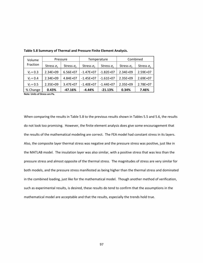
97

Table 5.8 Summary of Thermal and Pressure Finite Element Analysis.

Volume

Fraction

Pressure Temperature Combined

Stress σx Stress σy Stress σx Stress σy Stress σx Stress σy

Vf = 0.3 2.34E+09 6.56E+07 -1.47E+07 -1.82E+07 2.34E+09 2.59E+07

Vf = 0.4 2.34E+09 4.84E+07 -1.45E+07 -1.61E+07 2.35E+09 2.69E+07

Vf = 0.5 2.35E+09 3.47E+07 -1.40E+07 -1.44E+07 2.35E+09 2.78E+07

% Change 0.43% -47.16% -4.44% -21.13% 0.34% 7.46% Note: Units of Stress are Pa.

When comparing the results in Table 5.8 to the previous results shown in Tables 5.5 and 5.6, the results

do not look too promising. However, the finite element analysis does give some encouragement that

the results of the mathematical modeling are correct. The FEA model had constant stress in its layers.

Also, the composite layer thermal stress was negative and the pressure stress was positive, just like in

the MATLAB model. The insulation layer was also similar, with a positive stress that was less than the

pressure stress and almost opposite of the thermal stress. The magnitudes of stress are very similar for

both models, and the pressure stress manifested as being higher than the thermal stress and dominated

in the combined loading, just like for the mathematical model. Though another method of verification,

such as experimental results, is desired, these results do tend to confirm that the assumptions in the

mathematical model are acceptable and that the results, especially the trends hold true.

98

Chapter VI

CONCLUSIONS AND RECOMMENDATIONS

6.1 Conclusions

Cyanate ester resin was specifically designed to replace epoxy as the bonding or matrix material for

copper wires in fusion reactors. Although other areas of application could be used, this was specifically

the focus of the material production and testing of this research. In particular, an investigation into the

effect that varying the volume fraction of wires in the composite had on the performance of the

material was undertaken. This report summarizes and characterizes how one of the most important

parameters of fiber reinforced composite materials, the fiber volume fraction, when altered, will cause

variation in material properties and in stress and strain in the composite cylinder.

Based on laminate plate theory models and finite element analysis, it was found that varying fiber

volume fraction affected both material properties and stresses due to mechanical, thermal, and

magnetic loads. This variation was found not just in the composite itself, but also in the stress seen by

the insulation material.

The major findings of this thesis are concluded as follows:

(1) Increasing fiber volume fraction for a cyanate ester/copper composite results in increased

Young’s moduli, shear modulus, and Poisson’s ratios. In the target range of Vf = 0.3 to 0.5, the

moduli increase almost twice as much as the Poisson’s ratios. The moduli increase in magnitude

by an average of 24.8% whereas the Poisson’s ratios increase by much less, only about 11.7%.

The properties were affected in the sequence Ex, Ey, Gxy, νxy, and νyx where longitudinal modulus

experiences the greatest increase and Poisson’s ratio the least. Thermal expansion coefficients

99

decreased in value as the fiber volume fraction was increased. Both longitudinal and transverse

CTE’s decreased by an average of 18.8% while shear CTE was only decreased by 5.4%.

(2) Varying the properties of the composite affected the load in all the other components as well.

In a multi-layered laminate composed of cyanate ester/copper fiber composite layers with S2

glass cloth insulation in between, the stress in the glass layers as well as the stress in composite

layers is altered by changing the fiber volume fraction of the composite.

(3) For a laminate composed of two cyanate ester impregnated copper composite layers with S2

glass insulation between, under pressure, temperature, and combined loading, the effect of

varying fiber volume fraction was not uniform. Pressure effect is miniscule, but temperature is

altered about 6%.

(4) Insulation experienced an opposite effect from that seen by the composite. It was affected

more than the composite layers by the changes in properties, seeing an almost uniform

decrease of around 20% in stress from volume fraction 0.3 to 0.5.

(5) Corners do not serve as stress concentrators for the magnetic loading in the solenoid; the stress

concentration is rather due to contact between adjacent turns and the contact stress present

when two materials meet. Rounding the corners of the composite and insulation increase the

stresses at these critical points. While rounding the corners did move and possibly spread out

the stress, it did not eliminate the concentration.

(6) The stress that occurs in the insulation, especially due to the compression of the insulation by

adjacent turns, is very important to monitor since the insulation will probably fail before the

composite itself does.

(7) Highest stress for all loading types occurred in the fiber direction. This is fortunate because the

fiber direction has the superior properties due to the increased stiffness inherited by the

composite material from the wires.

100

(8) For the magnetic model, stress in the r-direction was affected more by volume fraction than

stress in the z-direction. Stress in the hoop direction was affected half as much as these, most

likely due to the wires being wound in the hoop direction. Shear stress increase was negligible

with increasing fiber volume fraction.

(9) In general, magnetic stresses are less sensitive to Vf effects than thermal stresses. Stresses

induced by the pressure loading were affected least of all three types of loadings.

6.2 Recommendations

As outlined above, there are methods available to develop mathematical models that describe the

behavior of fiber-reinforced composite materials with a good degree of accuracy. However, in the

course of literature reviews it was observed that relatively little material is available in the area of metal

wires for fiber-reinforced composite materials. Whenever metal is used as the reinforcement, it is

usually in the form of whiskers as discussed previously. However, fusion applications are relatively

unique in that they must have very long, continuous reinforcements because the copper wires carry a

current in them by virtue of their purpose of creating magnetic fields.

Recommendations for future work follow:

(1) Very little literature is available in the use of metals as fiber reinforcement. Therefore, more

research must be performed to characterize material properties when metals such as the

copper used in this research are used for reinforcement purposes. It is believed that the

strength in the fiber (longitudinal) direction would in practice be stronger than the models

predict it to be. Existing models were used in this analysis but the confidence in their

predictions would be stronger if a more complete analysis on this type of composite were

performed.

101

(2) Mathematical models and finite element analysis are only as accurate as the physics they are

based on and the material properties that are input into the model. Therefore it is suggested

that experiments using the composite material with several different fiber volume fractions be

performed to discover and develop material properties used in this analysis. These could be

used to verify the results of the mathematical model as well as to instill more accuracy in the

FEA simulation.

(3) Development and testing of a sample composite cylinder or preferably of several cylinders of

different fiber volume fractions to verify material reaction to loads would be useful.

Furthermore, these cylinders could be loaded to failure under several loads so that a failure

criterion could be used in the models developed in this report.

(4) More extensive finite element analysis is suggested. This could be done to develop a combined

model that incorporates magnetic loads, thermal loads, and pressure loads all together.

Furthermore, a model that incorporates the moisture effects developed in Phase 1 of the

research would be useful.

102

REFERENCES

103

1. IT Power Climate Change Consulting. (2004). [Energy Sources Worldwide Bar Chart 2004.]

Retrieved from http://www.itpi.co.in/Resources/Renewable_energy/Renewable_energy.htm

2. United Kingdom Atomic Energy Authority. (2008). Retrieved from

http://fusion.org.uk/mast/index.html

3. Wesson, J., & Campbell, D.J. (2004). Tokamaks. (3rd ed.). New York: Oxford University Press.

4. Davis, S.R. and Voss, G.M. (2009). Manufacture and test of a prototype cyanate ester coil.

Manuscript funded by United Kingdom Engineering and Physical Sciences Research Council and

by EURATOM.

5. Voss, G., Fabian, P., Feucht, S., Harte, M., & Terry, C. Performance evaluation of cyanate ester

resin. Manuscript funded by the United Kingdom Engineering and Physical Sciences Research

Council and by EURATOM.

6. Morgan, B., Madhukar, M., Walsh, J., Hooker, M., & Grandlienard, S. (2010). Moisture

degradation of cyanate ester/S2 glass composite insulation systems. Journal of Composite

Materials, 44, 821-837.

7. Fabian, P.E., Munshi, N.A., & Denis, R.J. (2001, July). Highly radiation-resistant vacuum

impregnation resin systems for fusion magnet insulation. Paper presented at the meeting of

ICMC, Madison, WI.

8. Hooker, M. Ph.D. Mechanical Engineer. (personal communication, January 2009 – May 2010).

9. National Compact Stellarator Experiment. (2008). [NCSX Machine 2008.] Retrieved from

http://ncsx.pppl.gov/

10. Berthelot, J.M. (1999). Composite materials: Mechanical behavior and structural analysis. New

York: Springer – Verlag New York.

11. Jones, R.M. (1975). Mechanics of composite materials. Washington, D.C.: McGraw – Hill.

104

12. Hillermeier, R.W., & Seferis, J.C. (2000). Environmental effects on thermoplastic and elastomer

toughened cyanate ester composite systems. Journal of Applied Polymer Science, 77, 556-557.

13. Goertzen, W.K., & Kessler, M.R. (2006). Thermal and mechanical evaluation of cyanate ester

composites with low-temperature processability. ScienceDirect. Sponsored by Iowa State

University.

14. Tsai, S.W., & Hahn, H.T. (1980). Introduction to composite materials. Lancaster, PA: Technomic

Publishing.

15. Ventsel, E., & Krauthammer, T. (2001). Thin plates and shells: Theory, analysis, and applications.

New York: Marcel Dekker.

16. McMillan Jr., J.P. (1994). Effects of fiber volume fraction on the elastic stability of specially

orthotropic plates (Master’s thesis). University of Tennessee, Knoxville.

17. Sayre, J. R. (1997). The effects of bias angle and fiber volume fraction on the mechanical

properties of filament-wound, polypropylene-glass tubes (Master’s thesis). University of

Tennessee, Knoxville.

18. Kavuri, H. (2004). Cure behavior study and elastic modulus characterization of resin system of a

quasi poloidal stellarator modular coil (Master’s thesis). University of Tennessee, Knoxville.

19. Hyer, M.W. (1998). Stress analysis of fiber-reinforced composite materials. New York: WCB

McGraw Hill.

20. Chawla, K.K. (1998). Composite materials: Science and engineering. (2nd ed.). New York:

Springer – Verlag New York.

21. Gibson, R.F. (2007) Principles of composite material mechanics. (2nd ed.). CRC Press.

22. Reddy, J.N. (2007) Theory and analysis of elastic plates and shells. (2nd ed.). Boca Raton, FL:

Taylor and Francis Group.

105

23. Young, H.D., & Freedman, R.A. (2004). University physics: With modern physics. (11th ed.). San

Francisco: Pearson Education.

24. San Jose State Department of Physics and Astronomy. (2007). [Physics 51 – Electricity &

Magnetism.] Retrieved from http://www.physics.sjsu.edu/becker/physics51/mag_field.htm

25. Tipler, P.A. (1999). Physics for scientists and engineers. (4th ed.). New York: W.H. Freeman and

Company.

26. Connexions, Rice University. (2010). [Magnetic field due to current in straight wire.] Retrieved

from http://cnx.org/content/m31103/latest/

27. AP Physics, Waterville High School, Waterville, ME. (2006). [The Magnetic Field.] Retrieved from

http://www.apphysics.net/elecmag/magfield.html

28. COMSOL AC/DC Module Documentation. Retrieved from C:\COMSOL35a\doc\acdc\acdcug.pdf

29. Becker, R. (1964). Electromagnetic fields and interactions. New York: Blaisdell Publishing.

30. Norton, R.L. (2006). Machine design: An integrated approach. (3rd ed.). Upper Saddle River,

NJ: Pearson Prentice Hall.

31. Hibbeler, R.C. (2005). Mechanics of materials. (6th ed.). Upper Saddle River, NJ: Pearson

Prentice Hall.

32. Annex to Design Requirements and Guidelines Level 1. Structural Material Database Article 3:

Non-Metalllic Materials Database and Specifications – Electrical Insulation Materials. Provided

by ITER.

33. Freudenberg, K. Mechanical Engineer. (personal communication, July 2009 – April 2010).

106

APPENDIX

107

Principle Code Used in Analysis

% Modeling of the Lamina Level Analysis of a Copper/Cyanate Ester Composite

clear all;

clc;

% First, material properties

% Fiber Volume Fractions

vf1 = 0.3;

vf2 = 0.4;

vf3 = 0.5;

% Fiber and matrix material properties

Ef = 120.7; %(GPa)

Em = 37.9; %(GPa)

Gf = 44.7; %(GPa)

Gm = 15.8; %(GPa)

nuf = 0.35;

num = 0.20;

ctef = 17; %x10e-6 1/K

ctem = 52.96; %x10e-6 1/K

% Micromechanics %

% Loop through both equations to see the trends

n = 1;

for ii = 0:0.01:1

fibervf(n) = ii;

e1(n) = Ef*ii+Em*(1-ii);

e2(n) = Em*((1-sqrt(ii))+(sqrt(ii))/(1-sqrt(ii)*(1-Em/Ef)));

v1(n) = nuf*ii+num*(1-ii);

v2(n) = (v1(n)*e2(n))/e1(n);

g(n) = Gm*((1-sqrt(ii))+(sqrt(ii))/(1-sqrt(ii)*(1-Gm/Gf)));

c1(n) = ((ctef*Ef-ctem*Em)*ii+ctem*Em)/((Ef-Em)*ii+Em);

c2(n) = ctem+(ctef-ctem)*ii;

n = n+1;

end

% Off-axis behavior of Lamina

E1_1 = Ef*vf1+Em*(1-vf1);

E1_2 = Ef*vf2+Em*(1-vf2);

E1_3 = Ef*vf3+Em*(1-vf3);

E2_1 = Em*((1-sqrt(vf1))+(sqrt(vf1))/(1-sqrt(vf1)*(1-Em/Ef)));

E2_2 = Em*((1-sqrt(vf2))+(sqrt(vf2))/(1-sqrt(vf2)*(1-Em/Ef)));

E2_3 = Em*((1-sqrt(vf3))+(sqrt(vf3))/(1-sqrt(vf3)*(1-Em/Ef)));

108

nu12_1 = vf1*nuf+(1-vf1)*num;

nu12_2 = vf2*nuf+(1-vf2)*num;

nu12_3 = vf3*nuf+(1-vf3)*num;

nu21_1 = (nu12_1*E2_1)/E1_1;

nu21_2 = (nu12_2*E2_2)/E1_2;

nu21_3 = (nu12_3*E2_3)/E1_3;

G12_1 = Gm*((1-sqrt(vf1))+(sqrt(vf1))/(1-sqrt(vf1)*(1-Gm/Gf)));

G12_2 = Gm*((1-sqrt(vf2))+(sqrt(vf2))/(1-sqrt(vf2)*(1-Gm/Gf)));

G12_3 = Gm*((1-sqrt(vf3))+(sqrt(vf3))/(1-sqrt(vf3)*(1-Gm/Gf)));

% Thermal Analysis %

% Nonlinear equation for thermal expansion in longitudinal direction

cte1_1 = ctef*vf1+ctem*(1-vf1);

cte1_2 = ctef*vf2+ctem*(1-vf2);

cte1_3 = ctef*vf3+ctem*(1-vf3);

% Rule of mixture for transverse thermal expansion coefficient

cte2_1 = (ctef*ctem)/(vf1*ctem+(1-vf1)*ctef);

cte2_2 = (ctef*ctem)/(vf2*ctem+(1-vf2)*ctef);

cte2_3 = (ctef*ctem)/(vf3*ctem+(1-vf3)*ctef);

% Lamina Level Analysis as a function of theta %

n = 1;

for i = 0:0.5:90

theta(n) = i;

Ex_1(n) = E1_1/((cosd(i))^4+((E1_1/G12_1)-

2*nu12_1)*(cosd(i))^2*(sind(i))^2+(E1_1/E2_1)*(sind(i))^4);

Ex_2(n) = E1_2/((cosd(i))^4+((E1_2/G12_2)-

2*nu12_2)*(cosd(i))^2*(sind(i))^2+(E1_2/E2_2)*(sind(i))^4);

Ex_3(n) = E1_3/((cosd(i))^4+((E1_3/G12_3)-

2*nu12_3)*(cosd(i))^2*(sind(i))^2+(E1_3/E2_3)*(sind(i))^4);

Ey_1(n) = E2_1/((cosd(i))^4+((E2_1/G12_1)-

2*nu21_1)*(cosd(i))^2*(sind(i))^2+(E2_1/E1_1)*(sind(i))^4);

Ey_2(n) = E2_2/((cosd(i))^4+((E2_2/G12_2)-

2*nu21_2)*(cosd(i))^2*(sind(i))^2+(E2_2/E1_2)*(sind(i))^4);

Ey_3(n) = E2_3/((cosd(i))^4+((E2_3/G12_3)-

2*nu21_3)*(cosd(i))^2*(sind(i))^2+(E2_3/E1_3)*(sind(i))^4);

Gxy_1(n) = G12_1/((cosd(i))^4+(sind(i))^4+2*(2*(G12_1/E1_1)*(1+2*nu12_1)+2*(G12_1/E2_1)-

1)*(cosd(i))^2*(sind(i))^2);

Gxy_2(n) = G12_2/((cosd(i))^4+(sind(i))^4+2*(2*(G12_2/E1_2)*(1+2*nu12_2)+2*(G12_2/E2_2)-

1)*(cosd(i))^2*(sind(i))^2);

109

Gxy_3(n) = G12_3/((cosd(i))^4+(sind(i))^4+2*(2*(G12_3/E1_3)*(1+2*nu12_3)+2*(G12_3/E2_3)-

1)*(cosd(i))^2*(sind(i))^2);

nuxy_1(n) = (nu12_1*((cosd(i))^4+(sind(i))^4)-(1+(E1_1/E2_1)-

(E1_1/G12_1))*(cosd(i))^2*(sind(i))^2)/...

((cosd(i))^4+((E1_1/G12_1)-2*nu12_1)*(cosd(i))^2*(sind(i))^2+(E1_1/E2_1)*(sind(i))^4);

nuxy_2(n) = (nu12_2*((cosd(i))^4+(sind(i))^4)-(1+(E1_2/E2_2)-

(E1_2/G12_2))*(cosd(i))^2*(sind(i))^2)/...

((cosd(i))^4+((E1_2/G12_2)-2*nu12_2)*(cosd(i))^2*(sind(i))^2+(E1_2/E2_2)*(sind(i))^4);

nuxy_3(n) = (nu12_3*((cosd(i))^4+(sind(i))^4)-(1+(E1_3/E2_3)-

(E1_3/G12_3))*(cosd(i))^2*(sind(i))^2)/...

((cosd(i))^4+((E1_3/G12_3)-2*nu12_3)*(cosd(i))^2*(sind(i))^2+(E1_3/E2_3)*(sind(i))^4);

nuyx_1(n) = (nu21_1*((cosd(i))^4+(sind(i))^4)-(1+(E2_1/E1_1)-

(E2_1/G12_1))*(cosd(i))^2*(sind(i))^2)/...

((cosd(i))^4+((E2_1/G12_1)-2*nu21_1)*(cosd(i))^2*(sind(i))^2+(E2_1/E1_1)*(sind(i))^4);

nuyx_2(n) = (nu21_2*((cosd(i))^4+(sind(i))^4)-(1+(E2_2/E1_2)-

(E2_2/G12_2))*(cosd(i))^2*(sind(i))^2)/...

((cosd(i))^4+((E2_2/G12_2)-2*nu21_2)*(cosd(i))^2*(sind(i))^2+(E2_2/E1_2)*(sind(i))^4);

nuyx_3(n) = (nu21_3*((cosd(i))^4+(sind(i))^4)-(1+(E2_3/E1_3)-

(E2_3/G12_3))*(cosd(i))^2*(sind(i))^2)/...

((cosd(i))^4+((E2_3/G12_3)-2*nu21_3)*(cosd(i))^2*(sind(i))^2+(E2_3/E1_3)*(sind(i))^4);

ctex_1(n) = cte1_1*(cosd(i))^2+cte2_1*(sind(i))^2;

ctex_2(n) = cte1_2*(cosd(i))^2+cte2_2*(sind(i))^2;

ctex_3(n) = cte1_3*(cosd(i))^2+cte2_3*(sind(i))^2;

ctey_1(n) = cte1_1*(sind(i))^2+cte2_1*(cosd(i))^2;

ctey_2(n) = cte1_2*(sind(i))^2+cte2_2*(cosd(i))^2;

ctey_3(n) = cte1_3*(sind(i))^2+cte2_3*(cosd(i))^2;

ctexy_1(n) = 2*(cte1_1-cte2_1)*cosd(i)*sind(i);

ctexy_2(n) = 2*(cte1_2-cte2_2)*cosd(i)*sind(i);

ctexy_3(n) = 2*(cte1_3-cte2_3)*cosd(i)*sind(i);

n = n+1;

end

% Plot the results

figure(1);

plot(fibervf,e1,fibervf,e2);

xlabel('Fiber Volume Fraction');

ylabel('Young''s Modulus, GPa');

legend('E1','E2','Location','East');

110

figure(2);

plot(fibervf,g);

xlabel('Fiber Volume Fraction');

ylabel('Shear Modulus, GPa');

figure(3);

plot(fibervf,v1);

xlabel('Fiber Volume Fraction');

ylabel('Poisson''s Ratio');

figure(4);

plot(theta,Ex_1,theta,Ex_2,theta,Ex_3);

xlabel('Orientation Angle Theta (Degrees)');

ylabel('Longitudinal Stiffness Modulus Ex (GPa)');

legend('Fiber Volume Fraction = 0.3','Fiber Volume Fraction = 0.4','Fiber Volume Fraction = 0.5');

figure(5);

plot(theta,Ey_1,theta,Ey_2,theta,Ey_3);

xlabel('Orientation Angle Theta (Degrees)');

ylabel('Transverse Stiffness Modulus Ey (GPa)');

legend('Fiber Volume Fraction = 0.3','Fiber Volume Fraction = 0.4','Fiber Volume Fraction =

0.5','Location','Northwest');

figure(6);

plot(theta,Gxy_1,theta,Gxy_2,theta,Gxy_3);

xlabel('Orientation Angle Theta (Degrees)');

ylabel('Shear Stiffness Modulus Gxy (GPa)');

legend('Fiber Volume Fraction = 0.3','Fiber Volume Fraction = 0.4','Fiber Volume Fraction = 0.5');

figure(7);

plot(theta,nuxy_1,theta,nuxy_2,theta,nuxy_3);

xlabel('Orientation Angle Theta (Degrees)');

ylabel('Poisson''s Ratio vxy');

legend('Fiber Volume Fraction = 0.3','Fiber Volume Fraction = 0.4','Fiber Volume Fraction = 0.5');

figure(8);

plot(theta,nuyx_1,theta,nuyx_2,theta,nuyx_3);

xlabel('Orientation Angle Theta (Degrees)');

ylabel('Poisson''s Ratio vyx');

legend('Fiber Volume Fraction = 0.3','Fiber Volume Fraction = 0.4','Fiber Volume Fraction = 0.5');

figure(9);

plot(fibervf,c1,fibervf,c2);

xlabel('Fiber Volume Fraction');

ylabel('Coefficient of Thermal Expansion, x10e6 (K^-1)');

legend('Logitudinal Direction','Transverse Direction');

111

figure(10);

plot(theta,ctex_1,theta,ctex_2,theta,ctex_3);

xlabel('Orientation Angle Theta (Degrees)');

ylabel('Coefficient of Thermal Expansion ax (x10^-6 1/K)');

legend('Fiber Volume Fraction = 0.3','Fiber Volume Fraction = 0.4','Fiber Volume Fraction = 0.5');

figure(11);

plot(theta,ctey_1,theta,ctey_2,theta,ctey_3);

xlabel('Orientation Angle Theta (Degrees)');

ylabel('Coefficient of Thermal Expansion ay (x10^-6 1/K)');

legend('Fiber Volume Fraction = 0.3','Fiber Volume Fraction = 0.4','Fiber Volume Fraction = 0.5',...

'Location','Northwest');

figure(12);

plot(theta,ctexy_1,theta,ctexy_2,theta,ctexy_3);

xlabel('Orientation Angle Theta (Degrees)');

ylabel('Coefficient of Thermal Expansion axy (x10^-6 1/K)');

legend('Fiber Volume Fraction = 0.3','Fiber Volume Fraction = 0.4','Fiber Volume Fraction = 0.5');

% Modeling of Laminate Level Analysis of a Copper/Cyanate Ester Composite %

lay = xlsread('C:\Users\Chance\Documents\Thesis and Research\Matlab Modeling\Input

Data','sheet1','B2'); % Number of layers

% Loop to calculate thickness of each layer (mm)

x = xlsread('C:\Users\Chance\Documents\Thesis and Research\Matlab Modeling\Input

Data','sheet1','G3:G22');

tt = 0;

for i = 1:lay

t(i) = x(i);

tt = tt+t(i);

end

% Loop to calculate z coordinates for each layer (midline = 0)

z(1) = -tt/2;

z(lay+1) = tt/2;

for i = 2:lay

z(i) = z(i-1)+t(i-1);

end

% Stiffness matrix Qij (Qc) and Glass Cloth matrix Qg

qc = xlsread('C:\Users\Chance\Documents\Thesis and Research\Matlab Modeling\Input

Data','sheet1','B17:D19');

qg = xlsread('C:\Users\Chance\Documents\Thesis and Research\Matlab Modeling\Input

Data','sheet1','B20:D22');

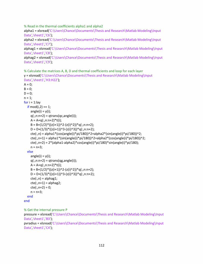
112

% Read in the thermal coefficients alpha1 and alpha2

alpha1 = xlsread('C:\Users\Chance\Documents\Thesis and Research\Matlab Modeling\Input

Data','sheet1','C6');

alpha2 = xlsread('C:\Users\Chance\Documents\Thesis and Research\Matlab Modeling\Input

Data','sheet1','C7');

alphag1 = xlsread('C:\Users\Chance\Documents\Thesis and Research\Matlab Modeling\Input

Data','sheet1','C8');

alphag2 = xlsread('C:\Users\Chance\Documents\Thesis and Research\Matlab Modeling\Input

Data','sheet1','C9');

% Calculate the matrices A, B, D and thermal coefficients and loop for each layer

y = xlsread('C:\Users\Chance\Documents\Thesis and Research\Matlab Modeling\Input

Data','sheet1','H3:H22');

A = 0;

B = 0;

D = 0;

n = 1;

for i = 1:lay

if mod(i,2) == 1;

angle(i) = y(i);

q(:,n:n+2) = qtrans(qc,angle(i));

A = A+q(:,n:n+2)*t(i);

B = B+(1/2)*((z(i+1))^2-(z(i)^2))*q(:,n:n+2);

D = D+(1/3)*((z(i+1))^3-(z(i)^3))*q(:,n:n+2);

cte(:,n) = alpha1*(cos(angle(i)*pi/180))^2+alpha2*(sin(angle(i)*pi/180))^2;

cte(:,n+1) = alpha1*(sin(angle(i)*pi/180))^2+alpha2*(cos(angle(i)*pi/180))^2;

cte(:,n+2) = 2*(alpha1-alpha2)*cos(angle(i)*pi/180)*sin(angle(i)*pi/180);

n = n+3;

else

angle(i) = y(i);

q(:,n:n+2) = qtrans(qg,angle(i));

A = A+q(:,n:n+2)*t(i);

B = B+(1/2)*((z(i+1))^2-(z(i)^2))*q(:,n:n+2);

D = D+(1/3)*((z(i+1))^3-(z(i)^3))*q(:,n:n+2);

cte(:,n) = alphag1;

cte(:,n+1) = alphag2;

cte(:,n+2) = 0;

n = n+3;

end

end

% Get the internal pressure P

pressure = xlsread('C:\Users\Chance\Documents\Thesis and Research\Matlab Modeling\Input

Data','sheet1','B3');

pvradius = xlsread('C:\Users\Chance\Documents\Thesis and Research\Matlab Modeling\Input

Data','sheet1','C4');

113

% N-M matrix

n_m(1,1) = pressure*pvradius;

n_m(2,1) = 0.5*pressure*pvradius;

n_m(3:6,1) = 0;

% A-B-B-D matrix

abbd = A;

abbd(4:6,1:3) = B;

abbd(1:3,4:6) = B;

abbd(4:6,4:6) = D;

% Find e-k matrix

e_k = (inv(abbd))*n_m;

% e_k = [1000e-3 0 0 0 0 0];

% Extract the temperature distribution delta T

dt = xlsread('C:\Users\Chance\Documents\Thesis and Research\Matlab Modeling\Input

Data','sheet1','B5');

% Calculate stresses in each layer and add in thermal stress

f = 1;

g = 1;

cte = cte';

for i = 1:lay

for j = z(i):0.0001:z(i+1)

% stress(:,f) = q(:,g:g+2)*e_k(1:3)+q(:,g:g+2)*j*e_k(4:6)-q(:,g:g+2)*cte(:,g:g+2)*dt;

stress(:,f) = q(:,g:g+2)*(e_k(1:3)+j*e_k(4:6)-dt*cte(g:g+2,:));

thick(f) = j;

f = f+1;

end

g = g+3;

end

% Plot the results

figure(13)

plot(thick,stress(1,:),'r')

xlabel('Z-Coordinate of Thickness, mm')

ylabel('Stress, kPa')

title('Normal Stress in the X-Direction')

figure(14)

plot(thick,stress(2,:),'b')

xlabel('Z-Coordinate of Thickness, mm')

ylabel('Stress, kPa')

title('Normal Stress in the Y-Direction')

114

figure(15)

plot(thick,stress(3,:),'m')

xlabel('Z-Coordinate of Thickness, mm')

ylabel('Stress, kPa')

title('Shear Stress in the XY-Direction')

% check thin-walled vs. thick-walled stress

ro = pvradius+tt/2;

ri = pvradius -tt/2;

pthh = (((ri^2)*pressure)/(ro^2-ri^2))*(1+(ro^2)/(ri^2))*tt;

ptha = (((ri^2)*pressure)/(ro^2-ri^2))*tt;

% End of Program

Function for Transposing Stiffness Matrices

function [q] = qtrans(a,b)

% QTRANS(Q,A) will transpose a 3x3 symmetric orthotropic composite

% stifness matrix Q into another stiffness matrix that corresponds

% to the angle shift A.

b=b*(pi/180)

c(1,1) = a(1,1)*(cos(b))^4+a(2,2)*(sin(b))^4+2*(a(1,2)+2*a(3,3))*((sin(b))^2)*((cos(b))^2)

c(2,2) = a(1,1)*(sin(b))^4+a(2,2)*(cos(b))^4+2*(a(1,2)+2*a(3,3))*((sin(b))^2)*((cos(b))^2)

c(1,2) = (a(1,1)+a(2,2)-4*a(3,3))*((sin(b))^2)*((cos(b))^2)+a(1,2)*(((sin(b))^4)+((cos(b))^4))

c(3,3) = (a(1,1)+a(2,2)-2*a(1,2)-2*a(3,3))*((sin(b))^2)*((cos(b))^2)+a(3,3)*(((sin(b))^4)+((cos(b))^4))

c(1,3) = (a(1,1)-a(1,2)-2*a(3,3))*((sin(b)))*((cos(b))^3)-(a(2,2)-a(1,2)-2*a(3,3))*((sin(b))^3)*(cos(b))

c(2,3) = (a(1,1)-a(1,2)-2*a(3,3))*((sin(b))^3)*((cos(b)))-(a(2,2)-a(1,2)-2*a(3,3))*((sin(b)))*((cos(b))^3)

c(2,1) = c(1,2)

c(3,1) = c(1,3)

c(3,2) = c(2,3)

q = c

115

Code for Finding Reduced Compliance Matrices

clear all;

clc;

% Find the Compliance Matrices for the Materials

% Reduced Stiffness Matrix for Orthotropic Composite

E1 = 130;

E2 = 5;

nu12 = 0.25;

G12 = 10;

nu21 = (nu12*E2)/E1

aaa(1,1) = E1/(1-nu12*nu21)

aaa(1,2) = (nu12*E2)/(1-nu12*nu21)

aaa(2,2) = E2/(1-nu12*nu21)

aaa(3,3) = G12

aaa(2,1) = aaa(1,2)

% Reduced Stiffness Matrix for Insulation

Ec1 = 12;

Ec2 = 20;

nuc12 = 0.33;

Gc12 = 6;

nuc21 = (nuc12*Ec2)/Ec1

bbb(1,1) = Ec1/(1-nuc12*nuc21)

bbb(1,2) = (nuc12*Ec2)/(1-nuc12*nuc21)

bbb(2,2) = Ec2/(1-nuc12*nuc21)

bbb(3,3) = Gc12

bbb(2,1) = bbb(1,2)

% Reduced stiffness isotropic insulation

E = 210;

nu = 0.3;

bbb(1,1) = E/(1-nu^2)

bbb(1,2) = (nu*E)/(1-nu^2)

bbb(2,2) = bbb(1,1)

bbb(3,3) = E/(2*(1+nu))

bbb(2,1) = bbb(1,2)

116

VITA

Chance Thomas Donahue was born on November 12, 1985 in Knoxville, Tennessee. He was raised in

LaFollette, Tennessee where he attended East LaFollette Elementary for grades K – 5th

, LaFollette Middle

School for grades 6th

– 8th

, and went to high school at Campbell County Comprehensive High School. He

graduated Salutatorian in 2004 and began college that fall at the University of Tennessee in Knoxville.

After starting in Aerospace Engineering, he changed curriculum to Mechanical Engineering and

graduated Summa Cum Laude in December of 2008 with his Bachelor of Science in Mechanical

Engineering. During his undergraduate studies, Chance had summer internships at National Coal

Corporation, CEMEX Inc. and Alcoa Inc. He began his graduate studies in January 2009 in Mechanical

Engineering with a concentration of machine design and product development. He worked as a

research assistant to Dr. Madhu S. Madhukar at the Magnet Development Laboratory in collaboration

with UT, Oak Ridge National Laboratory, and Composite Technology Development. He will be

graduating Cum Laude in August 2010 with his Masters of Science in Mechanical Engineering and begin

working in July 2010 for Savannah River Nuclear Solutions, LLC as a maintenance and operations

engineer in Aiken, South Carolina.