
Novel bioreactor design for decolourisation of azo dye effluents
Upload
khangminh22Category
view
1download
0
Design of a Bioreactor to Mimic Hemodynamic Shear Stresses onEndothelial Cells in Microfluidic Systems
by
Noam Saul Lightstone
A thesis submitted in conformity with the requirementsfor the degree of Master’s of Applied Science
Graduate Department of Mechanical and Industrial Engineeringand
The Institute of Biomaterials and Biomedical EngineeringUniversity of Toronto
c© Copyright 2014 by Noam Saul Lightstone

Abstract
Design of a Bioreactor to Mimic Hemodynamic Shear Stresses on Endothelial Cells in Microfluidic Systems
Noam Saul Lightstone
Master’s of Applied Science
Graduate Department of Mechanical and Industrial Engineering
and
The Institute of Biomaterials and Biomedical Engineering
University of Toronto
2014
The mechanisms behind cardiovascular disease (CVD) initiation and progression are not fully elucidated. It
is hypothesized that blood flow patterns regulate endothelial cell (EC) function to affect the progression of
CVDs. A system that subjects ECs to physiologically-relevant shear stress waveforms within microfluidic
devices has not yet been demonstrated, despite the advantages associated with the use of these devices. In
this work, a bioreactor was designed to fulfill this need. Waveforms from regions commonly affected by CVDs
including were derived. Pump motion and fluid flow profiles were validated by actuator motion tracking,
particle image velocimetry, and flowmeters. While several relevant waveforms were successfully replicated,
physiological waveforms could not be produced at physiological frequencies owing to actuator velocity and
accuracy limitations, as well as dampening effects in the system. Overall, this work lays the foundation for
designing a system that provides insight into the role of shear stress in CVD pathogenesis.
ii

Dedication
To the most transformational years of my life thus far.
To all the people who have made it so.
To my strength, perseverance, and desire to succeed and be happy.
And to the continual journey of learning and exploration - may I never stop.
iii

Acknowledgements
This thesis was one of the most challenging accomplishments of my life thus far. It would not have been
completed if it wasn’t for the help of many different people, both from a professional and personal perspec-
tive. I am grateful for all of the help and support I received over the years. I’ll never be able to name every
single person who made a comment or helped guide me to graduation, but I would like to acknowledge some
of the important people in my life who helped complete this work:
First and foremost, I want to thank my co-supervisors: Craig Simmons and Paul Santerre. Thank you
both for your input on refining my thesis and defense presentation, as well as the project throughout. I
would especially like to thank Craig, for his numerous edits on abstracts, reports, and the thesis itself com-
pleted at ungodly hours (on polyphasic sleep), understanding, guidance, meetings upon meetings, and being
a source of support and cheerleading to finish this degree. I could not have asked for someone better.
I would also like to thank my committee members Dr. Lidan You and Dr. David Steinman for their
input and questions that strengthened my thesis. Dr. Steinman thank you for your discussions on “plugs”
and pulsatility, help in my waveform literature search, as well as providing the Womersley analysis code and
running the analysis for me.
Around the labs I worked in, many other students (a.k.a. slaves) taught and helped me, or just commis-
erated with me. Thanks especially to Richard Tam for his help with MatLab, Suthan Srigunapalan for his
introduction to the flow loop which I based my work on, Bodgan Beca for his help on linear actuators, as
well as to all the other Simmons Lab people!
A special mention and thanks to Laura-lee Caruso in the Simmons Lab for teaching me how to make
microdevices and being willing to supply the bulk of the devices I used for my work. As well to the “lab
mom”, Zahra Mirzaei. Thank you Zahra for directing me to find things around the lab, placing orders, being
supportive, pushing me to finish so I can get to my trip, and just being a smiling face in the lab. We are
lucky to have you!
Outside of the Simmons Lab I thank many of the students from the Guenther Lab for their help. I would
especially like to thank Mark Jeronimo, for teaching me how to use the PIV equipment, helping me set it
up, coming in on days for input, not going crazy with all my e-mails and text messages about the laser, and
being a person to bounce ideas off of for troubleshooting. Thanks as well to Phoenix Qing Ba and Zhamak
Abdi for their support and help... and again, commiseration. Thanks also to Lindsey Fiddes for being there
and someone to talk to everyday who was full of positivity. Also to Paige Dickie for being my fellow bribed
student to come to UofT, Digital Dreams partner, and for being an awesome person in general. Thanks also
to Ali Oskooei for talks of the gym late at night while I slaved away at PIV.
On this note, I’d like to thank Dr. Axel Guenther for letting me sit in his lab space and for the use of
iv

the PIV equipment. Much appreciated!
Tomas Bernreiter of the MIE lab staff was very helpful when I was trying to figure out the Alicat
flow meter, in terms of his insight into measurement methods and advice on programming the Arduino
microcontroller. Thanks to Derek Pyne for letting me use the Oscilloscope in the Yu Sun lab. Also, thanks
to Yaaseen Atchia for his workout help, mutual empathy, and mention of LogMeIn which saved me hours of
computation stress with PIV!
Thank you to Neil Hartman, who provided a great deal of support during Alicat troubleshooting. I also
thank Dr. Philippe Sucosky for his permission to use the raw data obtained from his aortic valve simulations.
The support staff at UofT was incredible, and though I can’t mention everyone, I would definitely like to
thank Jeffrey Little and Brenda Fung for their help in planning, committee meetings and defences, as well
as answering administrative and graduation questions. In general, thank you to all of the staff in the MIE
and IBBME graduate offices.
Finally ending the professional portion of gratitudes, I acknowledge the sources who generously funded
my research: NSERC, OGS, CIHR, and the NSERC Create MATCH program.
Now on to the more personal acknowledgements:
I would not be where I am today, graduated and much happier, if it wasn’t for the support of my great
friends. I would literally be a thousand times weaker and not able to push through many things in life
without you. I love each and every one of you and I hope that no matter where we end up in life, we keep
in contact.
My two best friends in Toronto, Kizito Ngoma and Ryan Mulvihill: Though you are younger than me
know that I look up to you in many ways. Some of the things you do astound me and I know you will be
successful in whatever you do in life. I have learned much from being around you, and I thank you for all
your support in tougher times during the past few years... especially when I wouldn’t shut up about this
thesis. I am eternally grateful that I have you guys there as support, and repeat, that I would not be the
man I am today without you. Thank you so much for being the people you are. Rico, for your intelligent
conversations, rap music introductions, and philosophy. Ryan for your positivity, helping me begin my list,
and kindness. You both opened my eyes to many things I never even thought of before, and I have so much
more in my life now than ever. Yes, the bromance is strong.
Many other friends were supportive and have helped shape my life for the better. Even with just a small
dinner, coffee, Skype or a phone conversation, you have each added something to my life, so I thank you:
Rohan Mahimker, Angelo Yogendran, Jibran Sheikh, Matt Spataro, Dima Grafov, Maxim Nazarov, Douglas
Thoms, Nick Semianchuk, Pooyah Tolideh, Andrei Vassallo, Brian Pereira, Tom He, Sepehr Sa, and Geoff
Chan. Thanks for being who you are, each in your own respective way. I wish you nothing but success and
v

happiness for the future.
I met many people while in Toronto who also added to my life, including: Josh Stein, Kevin Singh, Kirill
Rotenberg, Clint Carvalho, Andrew Gappasov, Jeremy Scantlebury (R.I.P.), Nir Hodara, Mike Mitchell,
Samantha Jean, Shawn Goldmintz, John Hamway, Keshav Domun, the members of the UofT Metal Club,
and so many others. To all of you, again, thank you for adding to my life in your own respective ways, either
through your personalities, support, listening, or being people I could enjoy my time with.
Thanks also to my friends back home in Ottawa who were there for me: Eric Hong, Arun Vanapalli, John
and James Vieira, Max Gibson, and especially my best friend, Max Cleary. It was always good seeing all
of you when I went back home, and thanks for all the support over the past years. Also, thanks to Jerome
Choi for expanding my possibilities in terms of trips and Chris Prendergast for helping me open my eyes.
As a special acknowledgement, I wish to thank Maneet Bhatia and Rick Eckley, without whom I would
still be much deeper in negative spaces. Your patience and understanding have put me along a much healthier
path in life which I hope to keep walking and learning from while listening to myself. Thank you for all you
do and know that everyone appreciates all your hard work.
Throughout the past few years I have met many people, but three were very important to me and my
development as an individual: Karyn Raymond, Jessica Chong, and Yang Guo. Each of you entered my
life at different points when I was slowly evolving and changing, but each of you have taught me something
about life and myself that I can never forget or pay you back for. Each of us is not perfect, and I do not
consider our times without bumps or flaws, but I do consider meeting each of you a gift and blessing, and
look at things with positivity and gratitude.
Karyn, you are a very kind hearted and good person in nature. These qualities shined through you the
second I met you, even despite your shyness. How much you cared for people came out when we spent time
together, and I am grateful for that. I know you will find what you are looking for.
Jess, I did not expect to connect with someone as well as you, and yet I did. You are a very passionate
and directed person, who always tried to have a smile on her face. I cherish the connected moments we had,
and the fact that you helped me discover a lot about myself I pushed away, along with crossing off a few
things from my list. You are a truly unique person and I hope that you live the rest of your life in happiness,
connecting with someone equally as unique as you, because you deserve it.
Yang, your ability to make someone feel comfortable is astonishing, as well as how much you care about
other people. The fact that you are able to have deeper conversations yet also be light hearted is an amazing
trait I admire in you. You know a lot about me and my life, and I am grateful for having someone as
supportive and understanding as you enter my life who I wanted to be the same for, especially during the
final months of this thesis. I know that as you go on through life, you will move along your path as well
in self improvement, and become an even stronger version of yourself now, with your unique qualities and
vi

character shining through.
I love each of you very much, and I’m grateful for our time together. Thank you for all your support and
care, and I wish you nothing but happiness.
Finally I wish to thank my family: I thank my extended family, including my Aunts, Uncles, cousins,
and Bubby and Zaidy. I thank my sister Nava, for being awesome (as you are my sister after all so you must
have some of my awesomeness in you) and someone to sit down with from time to time to talk.
But, I would especially like to thank my parents - Leonard and Aviva. Without you, I would not have
been able to experience the things that I have in the past few years which have brought so much happiness
and light into my life. I thank you for your understanding, even when you weren’t clear on what I was doing
or why. I thank you for all your love, support, and guidance throughout the years and for the future.
To everyone I made a personal connection with, I love each and every one of you for what you have brought
into my life, the moments we shared together, and what we did together. Thank you for enriching my time
on this world and my life...
And for helping me finish this thesis.
vii

Contents
1 Introduction and Objectives 1
1.1 Motivating Problem . . . . . . . . . . . . . . . . . . . . . . . . . . . . . . . . . . . . . . . . . 1
1.2 Objective and Aims . . . . . . . . . . . . . . . . . . . . . . . . . . . . . . . . . . . . . . . . . 2
1.3 Thesis Organization . . . . . . . . . . . . . . . . . . . . . . . . . . . . . . . . . . . . . . . . . 3
2 Literature Review 4
2.1 Background . . . . . . . . . . . . . . . . . . . . . . . . . . . . . . . . . . . . . . . . . . . . . . 4
2.1.1 Cardiovascular Disease . . . . . . . . . . . . . . . . . . . . . . . . . . . . . . . . . . . . 4
2.1.2 Endothelial Cells . . . . . . . . . . . . . . . . . . . . . . . . . . . . . . . . . . . . . . . 5
2.1.3 Hemodynamic Stresses and Endothelial Cells . . . . . . . . . . . . . . . . . . . . . . . 6
2.1.4 Anatomy of the Heart and Blood Flow Pattern . . . . . . . . . . . . . . . . . . . . . . 7
2.1.5 Cardiovascular Waveform Structure and the Cardiac Cycle . . . . . . . . . . . . . . . 7
2.1.6 Non-Disturbed and Disturbed Flows in the Cardiovascular System . . . . . . . . . . . 9
2.1.7 Connecting Cardiovascular Disease, Endothelial Cells, and Flow Effects . . . . . . . . 11
2.2 Fluid Flow Principles . . . . . . . . . . . . . . . . . . . . . . . . . . . . . . . . . . . . . . . . . 14
2.2.1 Newtonian versus Non-Newtonian Fluids . . . . . . . . . . . . . . . . . . . . . . . . . 14
2.2.2 Dimensionless Parameters for Flow Characterization . . . . . . . . . . . . . . . . . . . 16
2.2.3 Entrance Length . . . . . . . . . . . . . . . . . . . . . . . . . . . . . . . . . . . . . . . 21
2.2.4 The Navier-Stokes Equations and Several Analytical Solutions . . . . . . . . . . . . . 21
2.2.5 Flow Resistance . . . . . . . . . . . . . . . . . . . . . . . . . . . . . . . . . . . . . . . 28
2.2.6 Wall Shear Stress Estimation Errors in the Parallel Plate Model when Compared to
the Purday Approximation . . . . . . . . . . . . . . . . . . . . . . . . . . . . . . . . . 29
2.2.7 Wall Shear Stress Estimation Errors in the Purday Model when Compared to the
Unsimplified Solution of Rectangular Channel Flow . . . . . . . . . . . . . . . . . . . 30
2.2.8 Flow-Induced Deformation in Microfluidic Systems . . . . . . . . . . . . . . . . . . . . 31
2.3 Bioreactors . . . . . . . . . . . . . . . . . . . . . . . . . . . . . . . . . . . . . . . . . . . . . . 33
viii

2.3.1 Macroscale Flow Bioreactors . . . . . . . . . . . . . . . . . . . . . . . . . . . . . . . . 34
2.3.2 Mesoscale Flow Bioreactors . . . . . . . . . . . . . . . . . . . . . . . . . . . . . . . . . 36
2.3.3 Microscale Flow Bioreactors . . . . . . . . . . . . . . . . . . . . . . . . . . . . . . . . . 40
2.3.4 A Comparison of Flow Bioreactors Based on Scale . . . . . . . . . . . . . . . . . . . . 45
2.3.5 Summary of Limitations of Existing Bioreactors in Literature . . . . . . . . . . . . . . 45
2.4 Flow Measurement . . . . . . . . . . . . . . . . . . . . . . . . . . . . . . . . . . . . . . . . . . 46
2.4.1 Flowmeters . . . . . . . . . . . . . . . . . . . . . . . . . . . . . . . . . . . . . . . . . . 46
2.4.2 Particle Image Velocimetry . . . . . . . . . . . . . . . . . . . . . . . . . . . . . . . . . 49
2.5 Signal Analysis . . . . . . . . . . . . . . . . . . . . . . . . . . . . . . . . . . . . . . . . . . . . 51
2.5.1 Fourier Series . . . . . . . . . . . . . . . . . . . . . . . . . . . . . . . . . . . . . . . . . 51
2.5.2 Fourier Transform . . . . . . . . . . . . . . . . . . . . . . . . . . . . . . . . . . . . . . 52
2.5.3 Nyquist Sampling Theorem . . . . . . . . . . . . . . . . . . . . . . . . . . . . . . . . . 53
2.5.4 Interpolation . . . . . . . . . . . . . . . . . . . . . . . . . . . . . . . . . . . . . . . . . 55
2.5.5 Numerical Integration . . . . . . . . . . . . . . . . . . . . . . . . . . . . . . . . . . . . 55
2.5.6 Mean Squared and Root Mean Squared Errors . . . . . . . . . . . . . . . . . . . . . . 56
3 Flow Waveform Characterization and Analysis 57
3.1 Pseudo-Physiological Waveform Development . . . . . . . . . . . . . . . . . . . . . . . . . . . 57
3.2 Physiological Waveform Development . . . . . . . . . . . . . . . . . . . . . . . . . . . . . . . 58
3.2.1 Physiological Waveform Sourcing and Description . . . . . . . . . . . . . . . . . . . . 58
3.2.2 Fast Fourier Transform and Nyquist Analyses . . . . . . . . . . . . . . . . . . . . . . . 61
3.2.3 Conversion of Physiological Shear Waveforms into Microfluidic Flow Rates . . . . . . 61
4 Bioreactor Design and Model Derivations 65
4.1 Bioreactor Assembly . . . . . . . . . . . . . . . . . . . . . . . . . . . . . . . . . . . . . . . . . 65
4.1.1 Description of Bioreactor Goals and Set-up . . . . . . . . . . . . . . . . . . . . . . . . 65
4.1.2 Bioreactor Design Requirements . . . . . . . . . . . . . . . . . . . . . . . . . . . . . . 67
4.1.3 Selection of Flow Waveform Creation Strategy . . . . . . . . . . . . . . . . . . . . . . 68
4.1.4 Details of Selected Waveform Creation Strategy and Bioreactor Components . . . . . 69
4.2 Syringe Pump and Linear Actuator Testing . . . . . . . . . . . . . . . . . . . . . . . . . . . . 71
4.2.1 MatLab NAVITAR Motion Analysis Protocol . . . . . . . . . . . . . . . . . . . . . . . 71
4.2.2 LabView Programming . . . . . . . . . . . . . . . . . . . . . . . . . . . . . . . . . . . 71
4.2.3 Cole-Parmer Syringe Pump . . . . . . . . . . . . . . . . . . . . . . . . . . . . . . . . . 72
4.2.4 Harvard Apparatus Syringe Pump . . . . . . . . . . . . . . . . . . . . . . . . . . . . . 72
4.2.5 UltraMotion Linear Actuator . . . . . . . . . . . . . . . . . . . . . . . . . . . . . . . . 72
ix

4.2.6 cetoni neMESYS Syringe Pump . . . . . . . . . . . . . . . . . . . . . . . . . . . . . . . 74
4.3 Flowmeter Specification and Standardization . . . . . . . . . . . . . . . . . . . . . . . . . . . 75
4.3.1 Flowmeter Options and Selection . . . . . . . . . . . . . . . . . . . . . . . . . . . . . . 75
4.3.2 Specification of Alicat Flowmeter Scale and Error . . . . . . . . . . . . . . . . . . . . 76
4.4 Assembled Bioreactor Specifications . . . . . . . . . . . . . . . . . . . . . . . . . . . . . . . . 77
4.5 Bioreactor Model Derivations . . . . . . . . . . . . . . . . . . . . . . . . . . . . . . . . . . . . 77
4.5.1 Flow Assumptions . . . . . . . . . . . . . . . . . . . . . . . . . . . . . . . . . . . . . . 77
4.5.2 Pressure Prediction and Deformation Verification inside Microfluidic Channel . . . . . 78
4.5.3 Microfluidic Device Dimension Limits . . . . . . . . . . . . . . . . . . . . . . . . . . . 81
4.5.4 Sufficient Volume Verification for a 1 mL Syringe . . . . . . . . . . . . . . . . . . . . . 82
5 Bioreactor Validation and Results 86
5.1 Validation Using Alicat Flowmeter . . . . . . . . . . . . . . . . . . . . . . . . . . . . . . . . . 86
5.2 Validation Using Particle Image Velocimetry . . . . . . . . . . . . . . . . . . . . . . . . . . . 87
5.2.1 Implementation and Methodology of Validation Using Particle Image Velocimetry . . 87
5.2.2 Sinusoidal Oscillatory Waveform Testing . . . . . . . . . . . . . . . . . . . . . . . . . . 89
5.2.3 Validation of Velocity and Wall Shear Stress Profiles . . . . . . . . . . . . . . . . . . . 98
5.3 Validation Using Sensirion Flowmeter . . . . . . . . . . . . . . . . . . . . . . . . . . . . . . . 100
5.3.1 Calibration Testing . . . . . . . . . . . . . . . . . . . . . . . . . . . . . . . . . . . . . . 101
5.3.2 Verification of Obtaining PIV Results . . . . . . . . . . . . . . . . . . . . . . . . . . . 101
5.3.3 Sinusoidal Oscillatory Flow Testing with Different Waveform Amplitudes and Exam-
ining the Resulting Dampening Behaviour in the System . . . . . . . . . . . . . . . . . 101
5.3.4 Varying Damper Volume and Examining the Resulting Dampening Behaviour in the
System . . . . . . . . . . . . . . . . . . . . . . . . . . . . . . . . . . . . . . . . . . . . 102
5.3.5 Superimposed Sinusoidal Oscillatory Waveform Testing . . . . . . . . . . . . . . . . . 108
5.3.6 Physiological Waveform Flow Testing . . . . . . . . . . . . . . . . . . . . . . . . . . . 109
6 Discussion 114
6.1 Situation Among Current Literature and Novelty of the Approach . . . . . . . . . . . . . . . 115
6.2 Analysis of the System and Value of the Results in Terms of Accuracy . . . . . . . . . . . . . 118
6.2.1 Simplification of In Vivo Hemodynamics and Flow Effects . . . . . . . . . . . . . . . . 118
6.2.2 Accuracy of PIV . . . . . . . . . . . . . . . . . . . . . . . . . . . . . . . . . . . . . . . 120
6.2.3 Accuracy of the neMESYS Linear Actuator . . . . . . . . . . . . . . . . . . . . . . . . 122
6.2.4 Assumptions of Shear Stress Calculations in the Microfluidic Channel . . . . . . . . . 122
6.2.5 Approximation of Sinusoidal Functions as Step Functions . . . . . . . . . . . . . . . . 123
x

6.3 Possible Improvements to the System’s Design . . . . . . . . . . . . . . . . . . . . . . . . . . 124
6.3.1 Discussion and Possible Resolutions of Dampening Effects . . . . . . . . . . . . . . . . 124
6.3.2 Inability of the System to Produce Physiological Waveforms . . . . . . . . . . . . . . . 126
6.3.3 Validation of Pressures within Microfluidic Channel . . . . . . . . . . . . . . . . . . . 129
6.4 Desired versus Achieved Parameter Spaces . . . . . . . . . . . . . . . . . . . . . . . . . . . . . 129
7 Conclusions and Future Recommendations 131
7.1 Conclusions . . . . . . . . . . . . . . . . . . . . . . . . . . . . . . . . . . . . . . . . . . . . . . 131
7.2 Future Recommendations . . . . . . . . . . . . . . . . . . . . . . . . . . . . . . . . . . . . . . 133
Bibliography 135
A Copyright Permissions 144
B MatLab Protocols 146
B.1 Motion Tracking via NAVITAR R© Scope . . . . . . . . . . . . . . . . . . . . . . . . . . . . . . 146
B.2 Fast Fourier Transform Calculations . . . . . . . . . . . . . . . . . . . . . . . . . . . . . . . . 151
B.3 Fourier Series and Coefficient Computation . . . . . . . . . . . . . . . . . . . . . . . . . . . . 152
B.4 Sinc Interpolation . . . . . . . . . . . . . . . . . . . . . . . . . . . . . . . . . . . . . . . . . . . 178
B.5 Calculation of Flow Rate from PIV Data using Purday Approximation . . . . . . . . . . . . . 181
B.6 Calculation of Flow Rate from PIV Data using Rectangular Channel Flow . . . . . . . . . . . 183
B.7 Calculation of Experimental and Theoretical Velocity Profiles from PIV Data . . . . . . . . . 187
B.8 Shear to Flow Waveform Conversion . . . . . . . . . . . . . . . . . . . . . . . . . . . . . . . . 191
B.9 Numerical Integration using Simpson’s Rule . . . . . . . . . . . . . . . . . . . . . . . . . . . . 232
C Womersley Analysis Code 235
D Raw Cardiovascular Shear Waveform Data 250
D.1 PVD Waveform Data . . . . . . . . . . . . . . . . . . . . . . . . . . . . . . . . . . . . . . . . . 250
D.2 CAVD Waveform Data . . . . . . . . . . . . . . . . . . . . . . . . . . . . . . . . . . . . . . . . 274
D.2.1 Aortic-Side . . . . . . . . . . . . . . . . . . . . . . . . . . . . . . . . . . . . . . . . . . 274
D.2.2 Ventricular-Side . . . . . . . . . . . . . . . . . . . . . . . . . . . . . . . . . . . . . . . 276
D.3 Atherosclerosis Waveform Data . . . . . . . . . . . . . . . . . . . . . . . . . . . . . . . . . . . 279
D.3.1 Athero-Prone . . . . . . . . . . . . . . . . . . . . . . . . . . . . . . . . . . . . . . . . . 279
D.3.2 Athero-Protective . . . . . . . . . . . . . . . . . . . . . . . . . . . . . . . . . . . . . . 280
E Testing of UltraMotion Digit Linear Actuator 282
xi

F Validation and Troubleshooting of Alicat Flowmeter 285
F.1 Implementation and Methodology of Validation Using Alicat Flowmeter . . . . . . . . . . . . 285
F.2 Experimental Setups for Flow Testing . . . . . . . . . . . . . . . . . . . . . . . . . . . . . . . 286
F.2.1 Experimental Set-up Using Peristaltic Pump Only . . . . . . . . . . . . . . . . . . . . 286
F.2.2 Experimental Set-up Using neMESYS Only . . . . . . . . . . . . . . . . . . . . . . . . 287
F.2.3 Experimental Set-up Combining Peristaltic and neMESYS . . . . . . . . . . . . . . . . 288
F.3 Data Recording Procedures . . . . . . . . . . . . . . . . . . . . . . . . . . . . . . . . . . . . . 289
F.4 Results from Validation Tests Using Alicat Flowmeter . . . . . . . . . . . . . . . . . . . . . . 289
F.4.1 Qualitative Testing - Constant Flow Using Peristaltic Pump Only . . . . . . . . . . . 289
F.4.2 Qualitative Testing - Constant Flow Using neMESYS Only . . . . . . . . . . . . . . . 290
F.4.3 Quantitative Testing - Constant Flow Using neMESYS Only . . . . . . . . . . . . . . 290
F.4.4 Qualitative Testing - Sinusoidal Flow Using neMESYS Only . . . . . . . . . . . . . . . 290
F.4.5 Qualitative Testing - Sinusoidal Flow Using both Peristaltic and neMESYS . . . . . . 291
F.4.6 Quantitative Testing - Sinusoidal Flow Using neMESYS Only . . . . . . . . . . . . . . 291
F.4.7 Isolation and Troubleshooting of Timing Offset Issues in Data Recording . . . . . . . 293
F.4.8 Isolation and Troubleshooting of Magnitude Offset Issues in Data Recording . . . . . 298
F.5 Timing Offset Issues in Data Recording . . . . . . . . . . . . . . . . . . . . . . . . . . . . . . 304
F.5.1 Evaluating if the waveform period was constant in the experimental data . . . . . . . 304
F.5.2 Examining if an applied impulse change was recorded at the expected time . . . . . . 304
F.5.3 Examining the effects of tubing compliance, and switching from flexible tubing to a
rigid, stainless steel connection from the pump to the flowmeter . . . . . . . . . . . . . 305
F.5.4 Possibility of Syringe Compliance Issues . . . . . . . . . . . . . . . . . . . . . . . . . . 305
F.5.5 Confirming the motion of the neMESYS linear actuator using a NAVITAR scope and
extracting the period of cyclic motion . . . . . . . . . . . . . . . . . . . . . . . . . . . 306
F.5.6 Examination of NAVITAR Timing . . . . . . . . . . . . . . . . . . . . . . . . . . . . . 307
F.5.7 Examination of Hyperterminal Issues . . . . . . . . . . . . . . . . . . . . . . . . . . . . 309
F.5.8 Ramped Flow Test . . . . . . . . . . . . . . . . . . . . . . . . . . . . . . . . . . . . . . 310
F.5.9 Consultation with External Experts . . . . . . . . . . . . . . . . . . . . . . . . . . . . 310
F.5.10 Carrying out various flow tests using the Arduino Uno microcontroller to verify if phase
lag behaviour had been eliminated . . . . . . . . . . . . . . . . . . . . . . . . . . . . . 312
F.6 Isolation and Troubleshooting of Magnitude Offset Issues in Data Recording . . . . . . . . . . 313
F.6.1 Comparison of Peristaltic and neMESYS Results . . . . . . . . . . . . . . . . . . . . . 313
F.6.2 Tubing versus Stainless Steel Connection from neMESYS to Flowmeter . . . . . . . . 314
F.6.3 Period and Increment Testing . . . . . . . . . . . . . . . . . . . . . . . . . . . . . . . . 315
xii

G Programming of Peripheral Devices 323
G.1 Step Motor Driver Interfacing . . . . . . . . . . . . . . . . . . . . . . . . . . . . . . . . . . . . 323
G.2 Step Motor Driver Programming . . . . . . . . . . . . . . . . . . . . . . . . . . . . . . . . . . 324
G.3 Arduino Uno Programming and Connection to Alicat Flowmeter . . . . . . . . . . . . . . . . 324
G.4 Alicat Flowmeter Setup for Experiments - Adaptors and Calibration . . . . . . . . . . . . . . 328
G.5 Hyperterminal Programming Instructions for Alicat Flowmeter . . . . . . . . . . . . . . . . . 329
G.5.1 Configuring Hyperterminal . . . . . . . . . . . . . . . . . . . . . . . . . . . . . . . . . 329
G.5.2 Sending a Script to Hyperterminal to Capture Data to a Text File . . . . . . . . . . . 330
G.6 Sensirion Flowmter Setup . . . . . . . . . . . . . . . . . . . . . . . . . . . . . . . . . . . . . . 332
G.7 neMESYS Setup . . . . . . . . . . . . . . . . . . . . . . . . . . . . . . . . . . . . . . . . . . . 338
G.8 Fire-i and NAVITAR Scope Setup . . . . . . . . . . . . . . . . . . . . . . . . . . . . . . . . . 339
H Particle Image Velocimetry Instructions 341
I Bioreactor Setup and Additional Information 345
I.1 Flow Loop Bill of Materials and Item Schematic . . . . . . . . . . . . . . . . . . . . . . . . . 345
I.2 Loop Setup Instructions . . . . . . . . . . . . . . . . . . . . . . . . . . . . . . . . . . . . . . . 345
J New Linear Actuator Information to Replace neMESYS 350
xiii
List of Tables
1.1 Desired parameter space of the bioreactor. w: channel width, h: channel height, Wo: Womer-
sley number, Re: Reynolds number, Q: flow rate. Definitions of the Womersley and Reynolds
numbers are provided in Chapter 2. . . . . . . . . . . . . . . . . . . . . . . . . . . . . . . . . 3
2.1 Vessel radius, Re, and Wo under rest conditions at heart rate of 60 beats per minute [33]. . . 19
2.2 Shear, pressure, flow, Re, and Wo in various areas of the body associated with common CVDs.
N/A: Not available [13, 27, 34–42]. . . . . . . . . . . . . . . . . . . . . . . . . . . . . . . . . . 20
3.1 Summary of FFT and Nyquist analyses of physiological waveforms. Waveform: the CVD
waveform being analyzed. Time Increment: the time spacing between each data point of
the waveform. Data points: the number of data points comprising the waveform. Maximum
complex amplitude: the resulting maximum complex amplitude value when the FFT of the
waveform is taken. Frequency at Maximum Amplitude: the corresponding frequency at the
maximum complex amplitude. Required Time Increment: the required sampling interval for
reproducing the waveform without signal loss or aliasing using the Nyquist sampling theorem. 62
4.3 Flowmeter options for bioreactor. . . . . . . . . . . . . . . . . . . . . . . . . . . . . . . . . . . 76
4.1 Summary of physiological waveform creation strategies and associated advantages and disad-
vantages, 1 of 2. . . . . . . . . . . . . . . . . . . . . . . . . . . . . . . . . . . . . . . . . . . . 84
4.2 Summary of physiological waveform creation strategies and associated advantages and disad-
vantages, 2 of 2. . . . . . . . . . . . . . . . . . . . . . . . . . . . . . . . . . . . . . . . . . . . 85
4.4 Sufficient volume verification for a 1 mL syringe - volumes input by neMESYS during infuse
steps for each physiological waveform using channel dimensions that include flow rates up to
the maximum allowable value 6 mL/min (width of 2075 µm, height of 225 µm). All volumes
were found to be less than 1 mL. . . . . . . . . . . . . . . . . . . . . . . . . . . . . . . . . . . 85
5.1 Properties of devices used in combined PIV and NAVITAR testing examine flow resistance
effects on neMESYS performance. . . . . . . . . . . . . . . . . . . . . . . . . . . . . . . . . . 94
xiv

5.2 Tubing lengths used in Sensirion flowmeter testing with fully assembled bioreactor. . . . . . . 107
6.1 New continuous flow pump options to replace peristaltic pump and damper. Note: The Cole-
Parmer RK-73100-04 pump can be re-configured with an add-on that allows for a 0.003 - 18
mL/min flow rate range. However, the cost of the part could not be sourced via the company.
It is suggested to inquire with the company about this option before purchasing a new pump. 127
6.2 Options, prices, and details concerning new linear actuator options for creating physiological
waveform using the bioreactor from Shelley Automation. A detailed quote of these items in
included in the thesis (Appendix J). N/A: not applicable. . . . . . . . . . . . . . . . . . . . . 128
6.3 Desired versus obtained parameter space using bioreactor. . . . . . . . . . . . . . . . . . . . . 129
F.1 Data from experiment comparing volume input calculated from theoretical profile and NAV-
ITAR displacement data from the neMESYS and data read from the Alicat flowmeter for
sinusoidal waveforms: The fluid volumes calculated from the theoretical flow and experimen-
tal actuator flow profiles were close, whereas when compared to the volume calculated from
the flowmeter data, the errors increased by an order of magnitude. It was concluded that the
flowmeter was not fit for use in the bioreactor. . . . . . . . . . . . . . . . . . . . . . . . . . . 305
F.2 Data from experiment comparing volume input calculated from theoretical profile and NAV-
ITAR displacement data from the neMESYS and data read from the Alicat flowmeter for
sinusoidal waveforms, 1 of 3. . . . . . . . . . . . . . . . . . . . . . . . . . . . . . . . . . . . . . 306
F.3 Data from experiment comparing volume input calculated from theoretical profile and NAV-
ITAR displacement data from the neMESYS and data read from the Alicat flowmeter for
sinusoidal waveforms, 2 of 3. . . . . . . . . . . . . . . . . . . . . . . . . . . . . . . . . . . . . . 307
F.4 Evaluation of period changes during sinusoidal profile test using neMESYS. . . . . . . . . . . 308
F.5 Data from examining a manually applied impulse change in flow rate using syringe. . . . . . . 309
F.6 Extraction and evaluation of period changes during actuator tracking experiment using neMESYS.310
F.7 Displayed stopwatch time visualized using NAVITAR scope to verify frame rate. . . . . . . . 311
I.1 Bioreactor bill of materials. Item numbers correspond to those depicted in Figure I.1. . . . . 349
xv

List of Figures
2.1 Progression of atherosclerosis - (A) Normal, unblocked vessel, (B) plaque formation begins
leading to partial occlusion, (C) fully occluded vessel leads to flow blockage in vessel. Adapted
from [7]. . . . . . . . . . . . . . . . . . . . . . . . . . . . . . . . . . . . . . . . . . . . . . . . . 5
2.2 Normal aortic valve (A) compared to valve affected by CAVD (B). Valve (B) is characterized
by thickening and calcium deposits (white areas) at the base of the leaflet cusps [10]. . . . . . 5
2.3 Imparted forces acting on the endothelium from blood flow: τ , a shear force, p, a normal or
pressure force, and s, a membrane stretching force. Adapted from Hahn and Schwartz [12]. . 7
2.4 Simplified anatomy of the heart showing blood flow direction [14]. . . . . . . . . . . . . . . . 8
2.5 Typical cardiovascular flow waveforms: the waveforms are pulsatile, unsteady, and bi-directional.
t/T: normalized time scale [15]. . . . . . . . . . . . . . . . . . . . . . . . . . . . . . . . . . . . 9
2.6 Typical non-disturbed (left) versus disturbed (right) waveforms. Non-disturbed waveforms
are associated with high levels of uni-directional shear stress and flow rate. Disturbed flows
on the other hand are low in magnitude, and bi-directional. . . . . . . . . . . . . . . . . . . . 10
2.7 Simplified view of the human cardiovascular system. Disturbed flows preferentially occur at
arterial branches and curvatures, leading to the onset of various CVDs. In this case, the
formation of atherosclerotic plaques (grey shading) leading to atherosclerosis. 1. Aortic sinus,
2. ascending aorta, 3. inner (lesser) curvature of aortic arch, 4. outer (greater) curvature of
aortic arch, 5. innominate artery, 6. right common carotid artery, 7. left common carotid
artery, 8. left subclavian artery, 9. thoracic aorta, 10. renal artery, 11. abdominal aorta, 12.
iliac artery [16]. . . . . . . . . . . . . . . . . . . . . . . . . . . . . . . . . . . . . . . . . . . . . 10
2.8 Depiction of flow separation from an object’s surface (blue line) with the shear stress profile
(in green): A negative pressure gradient exists up to point P, but there is a positive pressure
gradient downstream. The wall shear stress at point S is zero (the separation point), which
continues on to become increasingly negative downstream. The flow direction reverses and a
zone of recirculation appears [17]. . . . . . . . . . . . . . . . . . . . . . . . . . . . . . . . . . . 11
xvi

2.9 Rouleaux formation in blood leading to a rise in viscosity. The rouleaux can be seen as stacks
of linked red blood cells compared to free single cells [30]. . . . . . . . . . . . . . . . . . . . . 15
2.10 Depiction of problem geometry in steady pressure-driven flow between two plates separated
by gap distance h. . . . . . . . . . . . . . . . . . . . . . . . . . . . . . . . . . . . . . . . . . . 22
2.11 Depiction of problem geometry in rectangular duct flow with wall effects for the unsimplified
solution (top panel) and Purday approximation (bottom panel). x, y, and z represent the
co-ordinate axes, with x being aligned with the direction of flow and y and z defining the
cross-section of the channel of width, w, and height, h. The top and bottom panels have their
origins defined differently. The top panel has the y axis aligned horizontally along the bottom
of the channel and z axis oriented vertically upwards when viewing the channel cross-section.
The bottom panel has the z axis aligned horizontally at the channel’s mid-height and the y
axis oriented vertically upwards when viewing the channel cross-section. Adapted from [44]. . 23
2.12 Depiction of problem geometry (top panel) and co-ordinate axes (bottom panel) for rigid tube
Womersley Flow. . . . . . . . . . . . . . . . . . . . . . . . . . . . . . . . . . . . . . . . . . . . 26
2.13 Corollary of flow resistance taken from electrical circuits. Top - fluid network, bottom -
electrical network: Pressure is correlated to voltage and flow rate to current. . . . . . . . . . . 28
2.14 Ratio of the estimations of wall shear stress along the bottom centreline of a rectangular
channel for the parallel plate and Purday approximations at various channel dimensions,
subject to the Purday approximation and design constraints that 1/10 < h/w < 1/2 [48]. The
Purday approximation provides a better estimation of wall shear stress, accounting for wall
effects, and up to a 30% difference can be seen between the two predictions at small channel
widths. . . . . . . . . . . . . . . . . . . . . . . . . . . . . . . . . . . . . . . . . . . . . . . . . . 30
2.15 Ratio of the estimations of wall shear stress along the bottom centreline of a rectangular
channel for the unsimplified solution of rectangular channel flow and the Purday approximation
at various channel dimensions, subject to the design constraint that 1/10 < h/w < 1 [48]. At
the limit of the Purday approximation, when h/w > 1/2, the difference when compared to the
unsimplified solution begins to grow exponentially, up to a maximum of approximately 40%. . 31
2.16 Effects of altering the resistance (top panel) and compliance (bottom panel) on pressure in the
Georgia Tech bioreactor: increasing resistance increases differential pressure and increasing
compliance decreases differential pressure [51]. . . . . . . . . . . . . . . . . . . . . . . . . . . . 33
2.17 Bioreactor used by Narita et al. with balloon pump. Bioreactor components: (1) Balloon
chamber, (2) compliance chamber, (3) culture chamber, and (4) reservoir. The balloon pump
took in air and expelled it controlling the pressure inside the balloon chamber to force media
through the other portions of the bioreactor [52]. . . . . . . . . . . . . . . . . . . . . . . . . . 34
xvii
2.18 Left: bioreactor used by Ruel and Lachance. Bioreactor components: 1) ventricular pump, 2)
valve holder, 3) compliance chamber, 4) variable resistance, 5) reservoir, 6) bi-leaflet unidirec-
tional valve and flowmeter. Right: membrane pump schematic. The culture media chamber
was separated by a deformable membrane which was actuated by a separate air flow at the
bottom of the chamber to create a pulsatile waveform [53]. . . . . . . . . . . . . . . . . . . . . 35
2.19 Schematic of the Georgia Tech pulsatile flow loop. Top: flow loop, bottom: control section of
loop [51]. . . . . . . . . . . . . . . . . . . . . . . . . . . . . . . . . . . . . . . . . . . . . . . . 36
2.20 Cone and plate devices used to shear single layers of cells. Left: cone and plate viscometer,
right: parallel disk viscometer. Adapted from [16]. . . . . . . . . . . . . . . . . . . . . . . . . 37
2.21 Cup and cone bioreactor setup used by Sun et al. Tissue samples were placed into divots
within a plate sandwiched between two rotating cones within a sealed chamber containing cell
culture medium. The top and bottom cones applied different shear stress profiles representing
each side of the aortic valve. (a) Entire bioreactor loop, (b) top view of plate [36]. . . . . . . 38
2.22 Dual pump bioreactor used by Isenberg et al. Overall bioreactor schematic (A) and media
chamber (B) are highlighted. Components of the bioreactor: 1) medium reservoir, 2) peri-
staltic pump, 3) pulse dampeners, 4) pulsatile syringe pump, 5) check valves, 6) pressure
transducer, 7) media chamber, 8) occlusion valve, and 9) flowmeter. The peristaltic pump
continually cycled medium throughout the bioreactor, where the pulsatile nature of the flow
was converted into a steady variant by the pulse dampeners. The syringe pump imparted a
pseudo-physiological flow which was then combined with the steady peristaltic waveform to
be sensed by the biological sample. The flow was then sent back to the original reservoir for
another cycle [4]. . . . . . . . . . . . . . . . . . . . . . . . . . . . . . . . . . . . . . . . . . . . 38
2.23 Schematic (top) and image (bottom) of bioreactor used in the study of Hahn et al. Compo-
nents of the bioreactor: (1) cardiac pump, (2) custom graft chamber, (3) media reservoir,
(4) peristaltic pump, (5) compliance chamber, and (6) check valves. Media was continuously
cycled by a cardiac pump to a chamber containing vascular graft samples fed by a media
reservoir containing cell culture medium. A peristaltic pump also moved flow [19]. . . . . . . 39
2.24 Parallel plate flow chamber. The polycarbonate base plate (top), two gaskets with different
open areas, and the glass slide with EC monolayer (bottom) are held together by a vacuum
suction applied at the perimeter of the slide, forming a channel with a lesser depth at the
entrance, creating a step. Cultured medium enters at inlet port through entrance slit into the
channel and exits through exit slit and outlet port [16]. . . . . . . . . . . . . . . . . . . . . . 41
2.25 Example of a complex multi-channel PDMS device with its size compared to a US dime [74]. 42
xviii
2.26 Multi-force bioreactor used by Estrada et al. Components of the bioreactor: (a) peristaltic
pump, (b) pulmonary compliance, (c) pulmonary resistance, (d) collapsible chamber, (e) one-
way valve, (f) inline flowmeter, (g) cell culture chamber, (h) aortic/systemic compliance, (i)
inline pressure sensor, (j) aortic/systemic resistance, and (k) medium reservoir. The peristaltic
pump moved cell culture medium continuously throughout the bioreactor, where waveform
shape was controlled by upstream and downstream compliance and resistance units. A pneu-
matically actuated collapsible chamber allowed for the control of pulsatility in the system. A
culture chamber with deformable walls allowed for the simulation of membrane deformation
that occurs in vitro [72]. . . . . . . . . . . . . . . . . . . . . . . . . . . . . . . . . . . . . . . . 43
2.27 Left: bioreactor (top panel) and microfluidic co-culture device (bottom panel) used by Scott-
Drechsel et al.. A pulsatile blood pump cycled media throughout the bioreactor, where a
co-culture device housed co-cultured ECs and smooth muscle cells. Right: comparison of
native artery compliance effects and mimicking of these effects by the stiffness chamber used
in the bioreactor. In the compliance chamber, a larger amount of air leads to increased
dampening effects, as the air pressure built up pushes on the flow, decreasing any pulsatile
nature of the flow [76]. . . . . . . . . . . . . . . . . . . . . . . . . . . . . . . . . . . . . . . . . 44
2.28 Schematic of a typical micro PIV setup: A CCD camera captures the image pairs taken by a
laser to visualize flow within a microfluidic device [79]. . . . . . . . . . . . . . . . . . . . . . . 49
2.29 PIV analysis transforming an image pair into velocity vectors: The full width of a microfluidic
channel in a single plane relative to the device’s height is shown in the field of view. The PIV
laser takes two images with one pulse, one at time t and another at time t + ∆t, where ∆t
is specified by the user prior to experimentation. The image at t (1A.) and t + ∆t (1B.) are
divided into equally distributed interrogation windows (whose size is defined by the user, but
usually 64 x 64 pixels2), which undergo statistical calculations to determine the local velocity
vector within each window. This analysis is carried out by examining how the particles within
each window move from 1A. to 1B. The result is the desired field of velocity vectors (if a
correlation between pixels and length has been defined. Otherwise, the analysis results in
pixel displacement which can be converted afterwards) (2.). Scale bar: 66 µm. . . . . . . . . 50
2.30 An example of aliasing: When a 60 Hz cosine signal in time (1.) with a Nyquist Frequency
of 120 Hz is under sampled at 70 Hz (2.), the resulting sampled data seems to construct a 10
Hz cosine signal (3.). Adapted from [80]. . . . . . . . . . . . . . . . . . . . . . . . . . . . . . . 54
3.1 Athero-protective (top panel) and -prone (bottom panel) waveforms extracted from literature
used for further study and the bioreactor [2]. . . . . . . . . . . . . . . . . . . . . . . . . . . . 59
xix

3.2 Disease-protective (ventricular side, top panel) and -prone (aortic side, bottom panel) CAVD
waveforms obtained from literature used for further study and the bioreactor. Cycles continue
until 0.85 s but are zero past what is shown [27]. . . . . . . . . . . . . . . . . . . . . . . . . . 60
3.3 Popliteal artery flow waveform used as input for Womersley analysis (top panel) [82] and
resulting shear waveform (bottom panel) used for further study and the bioreactor. . . . . . . 63
3.4 Parametric analyses of the converted PVD shear waveform into the flow rates required to
obtain the in vivo shear stresses in microfluidic devices. Top panel: varying channel height
while holding channel width constant at w = 1000 µm. Bottom panel: varying channel width
while holding channel height constant at h = 200 µm. Varying channel height had a much
larger effect on the output flow waveforms compared to varying channel width. . . . . . . . . 64
4.1 Schematic depicting overall flow inside the bioreactor: Cell culture media was moved through
the flow circuit by a pumping method that created physiological waveforms to be applied onto
cultured ECs within a microfluidic device, while being continuously re-circulated. . . . . . . . 65
4.2 Schematics of ECs cultured within microfluidic device on microscope slide: overall (top panel),
side (middle panel) and cross-sectional (bottom panel) views. . . . . . . . . . . . . . . . . . . 66
4.3 Flowchart showing steps to move from in vivo to in vitro flow waveform: each step notes
where data is obtained from for the different flow waveforms. . . . . . . . . . . . . . . . . . . 66
4.4 Schematic of the components of the bioreactor: 1. Media reservoir (open to atmosphere for
venting), 2. peristaltic pump, 3. damper, 4. syringe pump, 5. flowmeter, 6. PIV laser, 7.
microfluidic device with cultured endothelial cells. . . . . . . . . . . . . . . . . . . . . . . . . 70
4.5 Components of testing the UltraMotion Digit linear actuator: actuator (top panel), Applied
Motion Si2035 step motor drive (middle panel), and eight lead parallel connection used to
wire the actuator and drive (bottom panel) [87, 88]. . . . . . . . . . . . . . . . . . . . . . . . 73
4.6 Actuator motion test tracked using a 100 ms data point increment sinusoidal waveform and
the neMESYS pump: The theoretical and experimental motion paths matched well except for
a parallax offset, which was shown to not be present in other tests. . . . . . . . . . . . . . . . 75
4.7 Assembled bioreactor in non-recirculatory configuration (outlet of microfluidic device run-
ning to waste beaker instead of back to media reservoir) with major components highlighted:
1. Computer controlling neMESYS and receiving flowmeter data, 2. media reservoir, 3.
peristaltic pump, 4. damper, 5. neMESYS, 6. three-way tee, 7. Sensirion flowmeter, 8.
microfluidic device, 9. waste beaker. . . . . . . . . . . . . . . . . . . . . . . . . . . . . . . . . 77
xx

4.8 ECs experiencing a linearly decreasing pressure along the channel length. A cross-sectional
view of the device is shown: It was essential to realize that the ECs cultured within the
microfluidic device would not be subjected to a uniform pressure throughout the device,
creating a certain amount of heterogeneity in terms of hemodynamic forces applied. The
effects of pressure could be studied by taking cell samples for study from different locations
along the channel length. . . . . . . . . . . . . . . . . . . . . . . . . . . . . . . . . . . . . . . 81
4.9 Maximum micro-channel heights against widths subject to design criteria for bioreactor, as-
suming cell culture media as the fluid. . . . . . . . . . . . . . . . . . . . . . . . . . . . . . . . 82
5.1 Step profile created using neMESYS to resemble a sinusoidal waveform: The neMESYS out-
puts flow rates changing at a maximum of every 100 ms. For sinusoidal profiles, the estimation
is made by keeping flow rate steps constant over every 100 ms interval, constructing a curve
that approximates a sinusoid. . . . . . . . . . . . . . . . . . . . . . . . . . . . . . . . . . . . . 87
5.2 Experimental PIV setup: 1. PCO-imaging SensiCam, 2. Nikon TE 2000-S scope, 3. pulsed
ND:YAG, class 4 laser as part of New Wave Solo III PIV system, 4. computer with DaVis 7.2
software installed. . . . . . . . . . . . . . . . . . . . . . . . . . . . . . . . . . . . . . . . . . . 88
5.3 PIV results of a 1 Hz, pulsatile, sinusoidal waveform applied by the neMESYS: The experi-
mental and theoretical results correlated well. . . . . . . . . . . . . . . . . . . . . . . . . . . . 90
5.4 PIV results of a 1 Hz, oscillatory, sinusoidal waveform applied by the neMESYS using a 5 mL
glass syringe: The experimental results were far removed in terms of amplitude from those
theoretically prescribed. . . . . . . . . . . . . . . . . . . . . . . . . . . . . . . . . . . . . . . . 91
5.5 PIV results of a 1 Hz, oscillatory, sinusoidal waveform applied by the neMESYS using an
alternative flow unit: The experimental results displayed an improvement over the previous
test, in terms of reaching a higher maximum amplitude as well as displaying the symmetric
behaviour expected. . . . . . . . . . . . . . . . . . . . . . . . . . . . . . . . . . . . . . . . . . 91
5.6 PIV results of a 0.1 Hz, oscillatory, sinusoidal waveform applied by the neMESYS: The exper-
imental and theoretical results correlated identically, except for the cases when the actuator
changed direction, where mechanical backlash was prevalent. . . . . . . . . . . . . . . . . . . 92
5.7 PIV results of a 1 Hz, oscillatory, sinusoidal waveform applied by the neMESYS using PEEK
tubing leading from the pump to the microfluidic device: Results did not improve. Hence,
compliance stemming from using flexible tubing was assumed to not be the cause of the
magnitude offset issues in the system. . . . . . . . . . . . . . . . . . . . . . . . . . . . . . . . 93
5.8 Setup of combined PIV and NAVITAR test. The NAVITAR imaged the motion of the
neMESYS actuator leading to a microfluidic device being imaged by PIV: 1. NAVITAR
scope, 2. neMESYS, 3. microfluidic device on Nikon scope stage for PIV imaging. . . . . . . 94
xxi

5.9 NAVITAR displacement results from combined PIV and NAVITAR test using various wave-
forms. Top panel: a 0.1 Hz oscillatory waveform ranging from -1 to 1 mL/min: The experi-
mental and theoretical results matched identically in all cases. Middle panel: a 1 Hz oscillatory
waveform ranging from -1 to 1 mL/min: Slight vertical shifts at a maximum of 20 µm were
seen in the curves throughout the test, but were assumed to be caused by vibrations within
the testing facility. Bottom panel: a 1 Hz pulsatile waveform ranging from 0 to 1 mL/min:
The Device A case seemed to follow the identical motion paths exhibited by the No Device
and Device B cases, but be offset. This was attributed to a shift in the camera’s location, as
Device A was tested following the No Device and Device B cases. . . . . . . . . . . . . . . . . 96
5.10 PIV results from combined PIV and NAVITAR test using 0.1 Hz (top panel) and 1 Hz (middle
panel) oscillatory waveforms ranging from -1 to 1 mL/min along with a 1 Hz pulsatile waveform
ranging from 0 to 1 mL/min (bottom panel): The Device A and B results matched identically,
leading to the conclusion that varying flow resistance did not have a large effect on flow rate
results. . . . . . . . . . . . . . . . . . . . . . . . . . . . . . . . . . . . . . . . . . . . . . . . . . 97
5.11 PIV results of a 1 Hz, oscillatory, sinusoidal waveform applied by the neMESYS using a 2.5
mL glass syringe: While the symmetric behaviour of the oscillatory sinusoid was captured,
the amplitude was far removed from what was desired. . . . . . . . . . . . . . . . . . . . . . . 99
5.12 PIV results of a 1 Hz, oscillatory, sinusoidal waveform applied by the neMESYS using a 1
mL glass syringe. Using this size of syringe resolved the accuracy issues previously observed:
The amplitude issue had been successfully isolated to the syringe type being used affecting
the accuracy of the experimental flow rate output by the neMESYS. . . . . . . . . . . . . . . 99
5.13 Validation of PIV results: Comparison of experimental and theoretical flow profiles at at flow
rates of 1 (A.), -1 (B.), 0,6 (C.), and -0.6 (D.) mL/min during a oscillatory sinusoidal waveform
with an amplitude of 1 mL/min (bottom panel) in a device with channel dimensions of h =
315.494 µm, w = 550 µm, and L = 2.1 cm. Experimental and theoretical velocity profiles
correlated well (top panel). . . . . . . . . . . . . . . . . . . . . . . . . . . . . . . . . . . . . . 100
5.14 Calibration curves of the Sensirion flowmeter using 1 (top panel) and 5 (bottom panel) mL
syringes: Theoretical and experimental flow rates correlated well, and it was decided that
correction of experimental flow rates was not required during further testing. . . . . . . . . . 103
5.15 Examining if the Sensirion flowmeter could accurately measure the final waveform obtained
using PIV: a 1 Hz sinusoidal waveform ranging from -1 to 1 mL/min. The shape and period
of the experimental waveform matched that of the prescribed waveform very well. . . . . . . . 104
xxii

5.16 Examination of dampening effects when testing 1 Hz oscillatory waveforms with different
amplitudes using the bioreactor and 2.5 (top panel) and 5 (bottom panel) mL syringes with the
neMESYS. Legends indicate theoretical waveform amplitude: Significant dampening effects
were seen in the experimental waveforms with minor sensitivity to the prescribed amplitudes. 105
5.17 Comparison of the theoretical and experimental sinusoidal oscillatory waveform amplitudes
due to dampening effects in the bioreactor using 2.5 (top panel) and 5 (bottom panel) mL
syringes for the neMESYS: A strong linear correlation was exhibited by the system. . . . . . 106
5.18 The effect of varying damper volume or free surface level on the output waveforms of the
bioreactor: As expected, more fluid (and less air) in the damper decreased the dampening
effects observed in the system and waveform “smoothness”, which can be observed by com-
paring the regular shape of the 10 mL waveform with the 20 and 26 mL waveforms which
curve slightly to the left at their peak and trough values. . . . . . . . . . . . . . . . . . . . . . 107
5.19 Examining the correlation between damper fluid volume and experimental waveform ampli-
tude: An exponential correlation was exhibited by the system. . . . . . . . . . . . . . . . . . 108
5.20 Superposition testing of constant peristaltic flows and sinusoidal oscillatory waveforms with
amplitudes of 30 mL/min and frequencies of 1 Hz: An approximately constant 250 µL/min
offset was observed between the maximum values of the theoretical and experimental wave-
forms, while the minima aligned well. Peristaltic pump flow rates of 0.5 (top panel), 1 (middle
panel) and 1.5 (bottom panel) mL/min were employed. The expected waveforms were cal-
culated assuming syringe and peristaltic pump flows are independent in terms of dampening
effects using data from Figure 5.16 on p. 105. . . . . . . . . . . . . . . . . . . . . . . . . . . . 111
5.21 Superposition testing of a constant peristaltic flow of 1 mL/min and sinusoidal oscillatory
waveform with amplitude of 30 mL/min and frequency of 0.1 Hz: The offset phenomenon
observed with the 1 Hz superimposed waveform was not present. The expected waveform was
calculated assuming syringe and peristaltic pump flows are independent in terms of dampening
effects. . . . . . . . . . . . . . . . . . . . . . . . . . . . . . . . . . . . . . . . . . . . . . . . . . 112
5.22 Physiological waveform testing using the Sensirion flowmeter: The neMESYS component of
the PVD waveform was tested assuming device dimensions of h = 212.5 µm, w = 1500 µm,
and L = 3 cm. Several details of the prescribed waveform could not be captured: While the
period length and overall shape were represented well in the experimental waveform, finer
details were not correctly replicated along with peak and trough values being misrepresented. 112
xxiii

5.23 Physiological waveform testing using the Sensirion flowmeter: The neMESYS component of
the PVD waveform was tested assuming device dimensions of h = 212.5 µm, w = 1500 µm,
and L = 3 cm and with its time axis extended by a factor of 100. Accurate replication of the
prescribed waveform’s shape, magnitude, and temporal characteristics was achieved compared
to the inaccuracies observed with the 1 Hz variation of the neMESYS component. . . . . . . 113
6.1 Process of phase averaging using PIV: 1. A specific point is marked using external hardware,
such as a pressure sensor which records the point for further external triggering of the PIV
laser at a specific time. Then, the PIV laser is triggered at several time increments from the
pressure sensor point. In each of 2a., 2b. and 2c., the velocity is recorded at the same time
increment over each cycle. This is repeated for however many time increments are desired.
3. Using the recorded data, the entire flow curve is re-constructed at a much faster frequency
than possible without phase averaging. This process assumes a repeated, cyclic waveform. . . 121
6.2 An example of a shear stress profile in a microfluidic channel with dimensions w = 1500 µm
and h = 212.5 µm demonstrating the “core” phenomenon: A 1092 µm wide region in the
centre of the channel is exposed to a constant shear stress (i.e., less than 5% deviation from
the shear stress at the centre of the channel) compared to the smaller regions near the walls
of the channel where the shear stress decreases to zero [91]. . . . . . . . . . . . . . . . . . . . 123
6.3 Possible recirculation zones created within the tee of the bioreactor: The inertia stemming
from the input peristaltic (red) and syringe pumps (blue) caused portions of the fluid (dashed
grey) to travel in unintended paths and create recirculation zones (black). The recirculated
fluid may have accentuated the flow division effect observed with the syringe pump, with its
flow separated between the device (green) and damper (purple), evidenced by the damper free
surface oscillating in phase with the neMESYS actuator movement. The experimental output
was then smaller than that which was theoretically predicted. . . . . . . . . . . . . . . . . . . 125
6.4 Dual pump head or cartridge strategy to create continuous flow using a peristaltic pump:
With the rollers of two heads or cartridges offset by a 90 degree phase angle, the inlet is
split using a Y-connector into the two inlets of the pump and then re-connected at the outlet
(left image). This transforms the discontinuous flow typically associated with a single channel
(Channel A or B) into a continuous variant (Channels A + B) (right image) [103]. . . . . . . 126
E.1 Results from UltraMotion Digit linear actuator test using athero-prone waveform with time
points spaced at 100 ms intervals. . . . . . . . . . . . . . . . . . . . . . . . . . . . . . . . . . . 282
E.2 Results from UltraMotion Digit linear actuator test using ventricular-side CAVD waveform
with time points spaced at 100 ms intervals. . . . . . . . . . . . . . . . . . . . . . . . . . . . . 283
xxiv

E.3 Results from UltraMotion Digit linear actuator test using aortic-side CAVD waveform with
time points spaced at 50 ms intervals. . . . . . . . . . . . . . . . . . . . . . . . . . . . . . . . 283
E.4 Results from UltraMotion Digit linear actuator test using athero-prone waveform with time
points spaced at 50 ms intervals. . . . . . . . . . . . . . . . . . . . . . . . . . . . . . . . . . . 284
E.5 Results from UltraMotion Digit linear actuator test using athero-prone waveform with time
points spaced at 25 ms intervals. . . . . . . . . . . . . . . . . . . . . . . . . . . . . . . . . . . 284
F.1 Pseudo-physiological troubleshooting setup using peristaltic pump only. Main components:
1. Falcon tube containing flow media, 2. peristaltic pump, 3. damper, 4. Arduino Uno
microcontroller, 5. Alicat flowmeter and attachments, 6. waste beaker. . . . . . . . . . . . . . 287
F.2 Pseudo-physiological troubleshooting setup using neMESYS only. Main components: 1. Fal-
con tube containing flow media, 2. neMESYS with syringe and attachments, 3. Alicat flowme-
ter and attachments, 4. waste beaker. Not visible: Arduino Uno microcontroller behind
neMESYS. . . . . . . . . . . . . . . . . . . . . . . . . . . . . . . . . . . . . . . . . . . . . . . . 288
F.3 Pseudo-physiological troubleshooting setup combining peristaltic and neMESYS. Main com-
ponents: 1. Peristaltic pump, 2. damper, 3. neMESYS with syringe and attachments, 4.
tee connector with attachments, 5. Arduino Uno microcontroller, 6. Alicat flowmeter and
attachments. Not visible: waste beaker in line with flow after flowmeter. . . . . . . . . . . . . 289
F.4 Quantitative flow test of constant 1 mL/min flow rate using peristaltic pump: The exper-
imental flow data obtained matched the experimental well within the error bounds of the
flowmeter. . . . . . . . . . . . . . . . . . . . . . . . . . . . . . . . . . . . . . . . . . . . . . . . 290
F.5 Quantitative flow test of constant 0.25 mL/min flow rate using neMESYS: The experimental
flow data obtained matched the experimental well within the error bounds of the flowmeter. . 291
F.6 Quantitative flow test of sinusoidal flow using neMESYS displaying phase shift behaviour.
The three panels show the overall progression of phase lag over time, from being in phase (top
panel), to completely out of phase (middle panel), and returning to being in phase once again
(bottom panel). . . . . . . . . . . . . . . . . . . . . . . . . . . . . . . . . . . . . . . . . . . . . 292
F.7 Employing a slow-phase sinusoidal waveform and measuring the resulting voltage output from
the flowmeter using an oscilloscope: The phase lag behaviour previously seen in acquiring
measurements using Hyperterminal had vanished, leading to the conclusion that it was the
source of the timing issues being examined. . . . . . . . . . . . . . . . . . . . . . . . . . . . . 296
F.8 Employing a square waveform and measuring the resulting voltage output from the flowmeter
using an oscilloscope: The phase lag behaviour previously seen in acquiring measurements
using Hyperterminal had vanished, leading to the conclusion that it was the source of the
timing issues being examined. . . . . . . . . . . . . . . . . . . . . . . . . . . . . . . . . . . . . 297
xxv

F.9 Experimental setup to test the neMESYS using the Arduino Uno. . . . . . . . . . . . . . . . 297
F.10 Focused view of Arduino Uno connected to flowmeter testing the neMESYS. . . . . . . . . . 298
F.11 Slow-phase sinusoidal waveform test (period of 10 s) using the neMESYS and measured with
the Arduino Uno: The phase lag behaviour previously seen with Hyperterminal was resolved
along with finding a more advantageous method of acquiring flow data compared to using an
oscilloscope. . . . . . . . . . . . . . . . . . . . . . . . . . . . . . . . . . . . . . . . . . . . . . . 298
F.12 Square waveform test using neMESYS and measured with the Arduino Uno: The phase
lag behaviour previously seen with Hyperterminal was resolved along with finding a more
advantageous method of acquiring flow data compared to using an oscilloscope. . . . . . . . . 299
F.13 Constant flow rate testing of 1 mL/min to resolve flowmeter magnitude issues using peristaltic
pump: The experimental output was now far removed from the theoretical, which was not
the case when the flowmeter was first tested. . . . . . . . . . . . . . . . . . . . . . . . . . . . 300
F.14 Constant flow rate testing of 1 mL/min to resolve flowmeter magnitude issues using neMESYS:
The experimental output was now far removed from the theoretical, which was not the case
when the flowmeter was first tested. . . . . . . . . . . . . . . . . . . . . . . . . . . . . . . . . 301
F.15 Comparison of the original (left) and new (right) base plates of the neMESYS: The new base
plate supported syringes over a longer length, preventing any movement of the syringe which
could add to flow magnitude errors. . . . . . . . . . . . . . . . . . . . . . . . . . . . . . . . . 301
F.16 Calibration curve for Alicat flowmeter used in superposition experiment and associated cali-
bration equation. . . . . . . . . . . . . . . . . . . . . . . . . . . . . . . . . . . . . . . . . . . . 303
F.17 Results from superposition experiment with a 0.1 Hz sinusoidal waveform and constant 1
mL/min peristaltic pump flow rate being applied: The principle of superposition seemed to
function as predicted, though there was a slight vertical shift in the experimental curve when
compared to what was theoretically predicted. . . . . . . . . . . . . . . . . . . . . . . . . . . . 304
F.18 Experimental results in changing from flexible tubing to SS connector in transition from
neMESYS to flowmeter. . . . . . . . . . . . . . . . . . . . . . . . . . . . . . . . . . . . . . . . 306
F.19 Examination of using a glass syringe instead of a plastic variant on phase lag properties using
the neMESYS. . . . . . . . . . . . . . . . . . . . . . . . . . . . . . . . . . . . . . . . . . . . . 307
F.20 Combined neMESYS actuator motion and flow measurements. . . . . . . . . . . . . . . . . . 308
F.21 One frame showing stopwatch time during NAVITAR frame rate verification experiment. . . 310
F.22 Ramped flow test using neMESYS and oscilloscope to trace flowrate. . . . . . . . . . . . . . . 311
F.23 The Arduino Uno microcontroller compared to a USA quarter [108]. . . . . . . . . . . . . . . 312
F.24 Experimental setup to test the neMESYS with the Arduino Uno. . . . . . . . . . . . . . . . . 312
F.25 Close-up view of Arduino Uno connected to flowmeter testing the neMESYS. . . . . . . . . . 313
xxvi

F.26 0.1 Hz sinusoidal waveform test using neMESYS and measured with Arduino Uno. . . . . . . 313
F.27 Square waveform test using neMESYS and measured with Arduino Uno. . . . . . . . . . . . . 314
F.28 Constant flow rate testing to resolve flowmeter magnitude issues using peristaltic pump. . . . 314
F.29 Constant flow rate testing of flowmeter magnitude issues using SS connection at meter entrance
and neMESYS. . . . . . . . . . . . . . . . . . . . . . . . . . . . . . . . . . . . . . . . . . . . . 315
F.34 Period and increment testing - theoretical period of 10 s and data point increments of 5 s. . . 315
F.30 Long-period sinusoidal waveform testing of flowmeter magnitude issues using tubing at meter
entrance and neMESYS. . . . . . . . . . . . . . . . . . . . . . . . . . . . . . . . . . . . . . . . 316
F.35 Period and increment testing - theoretical period of 10 s and data point increments of 2 s. . . 316
F.31 Long-period sinusoidal waveform testing of flowmeter magnitude issues using SS connection
at meter entrance and neMESYS. . . . . . . . . . . . . . . . . . . . . . . . . . . . . . . . . . . 317
F.36 Period and increment testing - theoretical period of 10 s and data point increments of 1 s. . . 317
F.32 Short-period sinusoidal waveform testing of flowmeter magnitude issues using tubing at meter
entrance and neMESYS. . . . . . . . . . . . . . . . . . . . . . . . . . . . . . . . . . . . . . . . 318
F.37 Period and increment testing - theoretical period of 10 s and data point increments of 0.5 s. . 318
F.33 Short-period sinusoidal waveform testing of flowmeter magnitude issues using SS connection
at meter entrance and neMESYS. . . . . . . . . . . . . . . . . . . . . . . . . . . . . . . . . . . 319
F.38 Period and increment testing - theoretical period of 10 s and data point increments of 0.2 s. . 319
F.39 Period and increment testing - theoretical period of 10 s and data point increments of 0.1 s. . 320
F.40 Period and increment testing - theoretical period of 5 s and data point increments of 2.5 s. . 320
F.41 Period and increment testing - theoretical period of 5 s and data point increments of 1 s. . . 320
F.42 Period and increment testing - theoretical period of 5 s and data point increments of 0.5 s. . 321
F.43 Period and increment testing - theoretical period of 5 s and data point increments of 0.2 s. . 321
F.44 Period and increment testing - theoretical period of 5 s and data point increments of 0.1 s. . 321
F.45 Period and increment testing - theoretical period of 1 s and data point increments of 0.2 s. . 322
G.1 Peripheral (Arduino or oscilloscope) connection points to Alicat flowmeter. 0-5 V signal at
pin #6, and ground signal at pin #8. (Adapted from [109]. . . . . . . . . . . . . . . . . . . . 325
G.2 Sensirion USB485 Sensor Viewer software instructions, 1 of 5. . . . . . . . . . . . . . . . . . . 333
G.3 Sensirion USB485 Sensor Viewer software instructions, 2 of 5. . . . . . . . . . . . . . . . . . . 334
G.4 Sensirion USB485 Sensor Viewer software instructions, 3 of 5. . . . . . . . . . . . . . . . . . . 335
G.5 Sensirion USB485 Sensor Viewer software instructions, 4 of 5. . . . . . . . . . . . . . . . . . . 336
G.6 Sensirion USB485 Sensor Viewer software instructions, 5 of 5. . . . . . . . . . . . . . . . . . . 337
G.7 Bus terminating plug of neMESYS. . . . . . . . . . . . . . . . . . . . . . . . . . . . . . . . . . 338
G.8 Main screen of the Fire-i program and associated settings. . . . . . . . . . . . . . . . . . . . . 339
xxvii

G.9 Video capture screen of the Fire-i program and associated settings. . . . . . . . . . . . . . . . 340
I.1 Schematic of bioreactor and associated components. Item numbers correspond to those listed
in Table I.1. . . . . . . . . . . . . . . . . . . . . . . . . . . . . . . . . . . . . . . . . . . . . . . 348
J.1 Detailed quote from Shelley Automation for new actuator to replace neMESYS, 1 of 3. . . . . 351
J.2 Detailed quote from Shelley Automation for new actuator to replace neMESYS, 2 of 3. . . . . 352
J.3 Detailed quote from Shelley Automation for new actuator to replace neMESYS, 3 of 3. . . . . 353
xxviii

List of Abbreviations and Symbols
A Cross-sectional area of channel
As Cross-sectional area of syringe
Dh Hydraulic diameter
E Young’s modulus
J0 Bessel function of first kind of zeroth order
J1 Bessel function of first kind of first order
Le Entrance length
LRe Characteristic length for Reynolds number calculation
Q Flow rate
Qdeform Flow rate calculated assuming a deformable microchannel
Qrigid Flow rate calculated assuming a rigid microchannel
Qssplateflow Flow rate calculated for steady pressure-driven flow between two plates
Qcardiacaverage Functional average of the flow rate of the in vitro cardiac waveform
Qcardiac Cardiovascular waveform flow rate
R Radius of a flow channel
Rpurday Flow resistance in a rectangular channel governed by the Purday approximation
Ts Time difference between sampled points of a signal
U Scalar of average fluid velocity
W Undeformed microchannel width
xxix

Yi An amount, i, of theoretical data values
∆t Time period (or difference between two time points)
∆x Distance traversed by syringe
∆P Difference in pressure
Γ Boundary of a channel
= Imaginary component of a complex value
Λ Secondary constant resulting from oscillatory Womersley analysis
< Real component of a complex value
α Ratio of channel height to width, the aspect ratio
f Vector of body forces
p Vector of pressures
u Vector of fluid velocity
χ Proportionality constant for entrance length calculations
∂u∂y Shear rate where the dimension, y, is oriented perpendicular to the primary flow direction in one-
dimensional flow (and a two-dimensional flow geometry)
Yi An amount, i, of observed data values
κ PDMS deformation computational simulation correlation coefficient
µ Dynamic viscosity
ω Fundamental circular frequency characteristic of a flow
ρ Fluid density
τN Shear stress of a Newtonian fluid
τφ Wall shear stress obtained from oscillatory Womersley analysis
τs Wall shear stress resulting from steady Womersley analysis
τy Yield stress in the Bingham plastic fluid viscosity model
τNNB Shear stress of a non-Newtonian fluid following the Bingham plastic model
xxx

τNNC Shear stress of a non-Newtonian fluid following the Casson fluid model
τNNP Shear stress of a non-Newtonian fluid obeying a power law
τpwssbc Wall shear stress calculated from Purday analysis at the vertical bottom centreline of a channel
τrwssbc Wall shear stress calculated from unsimplified rectangular channel analysis at the vertical bottom
centreline of a channel
τssplatewss Wall shear stress calculated from steady pressure-driven flow between two plates
τestrada Wall shear stress as calculated in the study of Estrada, et.al.
f(w) Fourier Transform of a function, f(x)
fn Discrete Fourier Transform of a function, f(x)
ζ Primary constant resulting from oscillatory Womersley analysis
a Radius of channel in Womersley analysis
a0 Fourier cosine coefficient of zeroth order
an Fourier cosine coefficient of order n
bn Fourier sine coefficient of order n
c1 Proportionality constant of PDMS deformation
cn Coefficients of sampling polynomial function for discrete Fourier transform
d Flow behaviour index constant of a fluid obeying a non-Newtonian power law
f Friction factor
fc Highest frequency component of a signal
fs Sampling frequency of a signal
h Channel height
h0 Undeformed microchannel height
k Consistency index constant of a fluid obeying a non-Newtonian power law
ks Pressure difference constant resulting from steady Womersley analysis
m Primary empirical constant resulting from Purday analysis
xxxi

n Secondary empirical constant resulting from Purday analysis
p Scalar magnitude of pressure
pφ Oscillatory component of Womersley pressure
ps Steady component of Womersley pressure
q(x) Sampling polynomial function for discrete Fourier transform
qφ Flow rate obtained from oscillatory Womersley analysis
qs Flow rate obtained from steady Womersley analysis
t Time
tfinal End time of a cardiac cycle
tinitial Start time of a cardiac cycle
u Scalar value of fluid velocity
uφ Oscillatory component of Womersley velocity
um Mean velocity
us Steady component of Womersley velocity
umax Maximum velocity
urect Velocity calculated through the unsimplified solution to pressure-driven rectangular channel flow for
PIV validation
v Actuator velocity
w Channel width
Womicro Womersley number based on rectangular microfluidic channels
BD Becton Dickinson and Company
CAD Computer aided design
CAVD Calcific aortic valve disease
CCD Charged-coupled device
CCM Cubic centimetres per minute
xxxii

CFD Computational fluid dynamics
CVD Cardiovascular disease
DFT Discrete Fourier Transform
EC Endothelial cell
FFT Fast Fourier Transform
FT Fourier Transform
MRI Magnetic resonance imaging
MSE Mean squared error
N-S Navier-Stokes
neMESYS The cetoni neMESYS syringe pump
O Order
PAD Peripheral arterial disease
PDMS Polydimethylsiloxane
PIV Particle image velocimetry
PPFC Parallel plate flow chamber
PTFE Polytetrafluoroethylene
PVD Peripheral vascular disease
Rcirc Flow resistance in a circular channel
Rrect Flow resistance in a rectangular channel
Re Reynolds number
RMSE Root mean squared error
SMCs Smooth muscle cells
SS Stainless steel
Wo Womersley number
xxxiii

Chapter 1
Introduction and Objectives
1.1 Motivating Problem
The cardiovascular system is a complex biological marvel that is as of yet, not fully understood. According
to the Public Health Agency of Canada, cardiovascular disease (CVD) represents the greatest percentage of
hospitalizations from all medical diagnoses and is also the second-largest illness-based economic burden in
Canada [1]. It is clear that there is a crucial need for solutions and treatment options for CVD.
In many in vitro studies, it has been demonstrated that various endothelial cell (EC) genes are patho-
physiologically relevant for CVD, and that they are regulated by various hemodynamic forces [2–4]. These
observations suggest that different flow patterns may cause ECs to exhibit different phenotypes which, in
turn, may affect the progression of various diseases. Flows in the cardiovascular system may be divided into
two broad categories: non-disturbed and disturbed. It is hypothesized that blood flow-induced shear stresses
exerted on the ECs in the cardiovascular system influence their biology in a manner that contributes to the
initiation of CVD and its progression. Unfortunately, the mechanisms underpinning these phenomena are
poorly understood and by the time a problem is detected, therapy may only be limited to surgery. Knowledge
of blood flow patterns and their effects on EC phenotypes may enable the early detection of issues within
the cardiovascular system before the onset of various diseases: Through the application of different flow
waveforms on ECs and examining their resulting phenotype, the upregulation of markers associated with
CVD can be correlated to various flow patterns. Visualizing flows via magnetic resonance imaging (MRI) or
Doppler velocity techniques in the vasculature of at risk or elderly individuals in vivo may determine if the
patients are in danger of having CVD.
A platform to study the effects of accurate flow-induced shear stresses on ECs would provide the means
to explore this hypothesis. The effects of blood-flow induced shear stress on EC biology have been examined
using large, macro scale bioreactors. However, these systems can be quite large and cumbersome, and the
1

Chapter 1. Introduction and Objectives 2
entire vascular system is usually modelled, requiring a large number of components. Furthermore, modularity
is much more difficult to achieve when employing a chamber that holds a biological sample: Typically, the
chamber must be custom designed and machined to ensure no leaks occur when it is integrated into the
bioreactor as well as to ensure proper acceptance and support of biological samples, which are often on the
scale of whole tissue.
Microfluidic systems have gained popularity in recent years, and are well-suited to study the shear stress
regulation of ECs in vitro owing to their predictable fluid dynamics, low cost, and potential to improve
experimental throughput and efficiency over traditional macro scale flow bioreactors. Moreover, the ability
to design many different types of devices quickly using software such as AutoCAD and SolidWorks allows
for the testing of different flow problems, geometries representing various areas of the body, as well as the
multiplexing of tests using multiple channels on a single device. New devices can be easily integrated with
modular set-ups that are typically employed in microfluidic testing. This allows for the examination of various
cell cultures, which could encompass different cell types, or those with different properties. New channel
designs can be created to accept any size or shape of cell population, eliminating the aforementioned issues
in macro-scale bioreactors. However, a solution that subjects ECs to physiologically-accurate hemodynamic
waveforms within microfluidic devices encompassing the advantages of microfluidic setups has not yet been
successfully demonstrated.
1.2 Objective and Aims
The overall objective of this project is to create and validate a bioreactor that can accurately mimic a
range of different physiological (or equivalently cardiovascular) waveforms in the cardiovascular system to
be used in experiments with microfluidic devices seeded with ECs. There are two specific aims:
• Aim 1 : Generate a range of physiological shear waveforms representing areas of the vasculature com-
monly affected by CVDs to be used in microfluidic devices representing cardiovascular diseases of
interest: atherosclerosis, calcific aortic valve disease (CAVD), and peripheral arterial or vascular dis-
ease (PAD or PVD).
• Aim 2 : Design, characterize, and validate a bioreactor for the application of these waveforms to
cultured ECs in vitro in typical microfluidic devices (Table 1.1 on p. 3).
Understanding the effects of disturbed flow on ECs can provide insight into the role of flow patterns con-
tributing to the pathogenesis of CVDs and can help to elucidate the phenotypic and functional differences
between quiescent (nonatherogenic/nonthrombogenic) and activated (atherogenic/thrombogenic) ECs.

Chapter 1. Introduction and Objectives 3
Parameter Desired Range
w 25 to 2000 µm
h 100 to 525 µm
Wo 0.0531 to 1.105
Re 14 to 300
Frequency Any frequency up to 1 Hz
Q -0.5 to 4.5 mL/min
Waveform type Physiological
Table 1.1: Desired parameter space of the bioreactor. w: channel width, h: channel height, Wo: Womersleynumber, Re: Reynolds number, Q: flow rate. Definitions of the Womersley and Reynolds numbers areprovided in Chapter 2.
1.3 Thesis Organization
The first chapter presents the motivating problem of the research and a brief summary of the deficiencies
of the current art, along with the thesis objectives. Chapter 2 is a literature review of relevant topics
for the research, providing a summary of various types of CVDs and their relation to flow effects. Fluid
flow principles, bioreactors, flow measurement methods, and signal analysis are also reviewed. Chapter 3
discusses the flow waveforms created and tested. This includes the strategy followed for testing the system
(moving from less complex pseudo-physiological to complex physiological waveforms), as well as the sources
of the waveforms representing the CVDs investigated. The necessary accuracy to replicate these waveforms
using the in vitro system is also determined. Chapter 4 discusses the design of the bioreactor: the layout,
options for creating the flow waveforms, and the selected strategy. Tests to select suitable pumps are also
described. A full bill-of-materials is provided along with a schematic should items need to be re-located.
Moreover, theoretical models of the microfluidic device are provided in order to model the pressures applied
to the ECs within the channel, along with ensuring that channel deformation did not occur. Chapter 5
describes the troubleshooting and implementation of the validation steps for the bioreactor waveforms, and
presents the results from the testing. Chapter 6 is a discussion of the work, including a comparison to
the current literature and the novelty of the approach, sources of error, and possible improvements to the
system’s design. Finally, Chapter 7 provides the conclusions and future recommendations.

Chapter 2
Literature Review
The aim of this chapter is to provide a background of the connection between CVD and fluid mechanics to
demonstrate the importance of further study. Bioreactors currently reported in literature are reviewed and
the deficiencies of the current state of the art are summarized. Measurement of flow waveforms is necessary
to ensure their accuracy, which is of particular importance in a flow bioreactor. Hence, a summary of flow
measurement methods is provided, focusing on different types of flowmeters and particle image velocimetry.
Finally, the area of signal analysis and its associated techniques is discussed.
2.1 Background
2.1.1 Cardiovascular Disease
According to the World Health Organization, CVD is the number one cause of death globally [5]. Not only
is it projected that CVD will remain the single leading cause of death, but also by 2030, it is estimated that
23.3 million individuals will die from CVDs globally per year [5]. There is a crucial need for solutions and
treatment options for various forms of CVD, which include heart diseases (which will not be focused on in
this work) and three important vascular/valvular diseases:
Atherosclerosis is a progressive, degenerative disease that leads to the occlusion of affected vessels and is
the prime cause of strokes. It is characterized by plaques forming beneath the vessel lining within the arterial
walls, which can potentially lead to thrombus formation. The formed thrombus may be loosened through
blood flow creating a free floating clot, which can completely occlude smaller blood vessels downstream of
the original clot location (Figure 2.1) [6].
4

Chapter 2. Literature Review 5
A
B
C
Figure 2.1: Progression of atherosclerosis - (A) Normal, unblocked vessel, (B) plaque formation begins leadingto partial occlusion, (C) fully occluded vessel leads to flow blockage in vessel. Adapted from [7].
Peripheral Vascular and Arterial Disease are manifestations of atherosclerosis, usually in the lower
limbs. In their most severe forms they can involve revascularization, where surgery is performed to restore
blood flow by redirecting blood around the occluded artery [8]. This is known as a vascular graft. Throughout
this thesis, they are labelled together as PVD.
Calcific Aortic Valve Disease involves both sclerosis, or thickening, and calcification of the aortic valve
[9]. Specifically the disease may involve: valve leaflet tissue thickening, the development of calcified nodules
near the leaflet’s surface, and dysfunction and degradation of the endothelium (Figure 2.2). As the aortic
valve thickens and calcifies, movement of the tissue becomes impaired during the cardiac cycle. Calcium
deposits within the valve matrix may prohibit the valve’s leaflets from opening and closing properly, allowing
back flow to occur. Back flow can cause shortness of breath and arrhythmias, vary the pressures within the
heart, and also raise the risk for heart valve infections.
Figure 2.2: Normal aortic valve (A) compared to valve affected by CAVD (B). Valve (B) is characterized bythickening and calcium deposits (white areas) at the base of the leaflet cusps [10].
2.1.2 Endothelial Cells
ECs are specialized epithelial cells that line the interior surface of the entire vasculature and are in contact
with the flowing blood in the body. They are situated within a complex environment, being exposed to

Chapter 2. Literature Review 6
mechanical forces, chemical factors, and signalling mechanisms. Together, ECs form a single layer inside the
vasculature known as the endothelium. The principal roles of the endothelium include many crucial functions
such as the: maintenance of blood homeostasis, regulation of transport across the vessel wall, translation
of mechanical signals from the blood to other regions of the vessel wall, and provision of a smooth, non-
thrombogenic blood-contacting surface [4]. ECs will release locally acting chemical messengers in response
to chemical changes in their environment (such as a reduction in oxygen) or physical changes (such as the
application of fluid-flow induced shear stress). Other functions of ECs include [11]:
• Lining the blood vessel and heart chambers; serving as a physical barrier between the blood and the
remainder of the vessel wall.
• Secretion of vasoactive substances in response to local chemical and physical changes, which cause
vasodilation or vasoconstriction of the underlying smooth muscle.
• Secretion of substances that stimulate new vessel growth and proliferation of smooth muscle cells in
vessel walls.
• Participation in the exchange of materials between the blood and surrounding tissue cells across cap-
illaries through vesicular transport.
• Influencing the formation of platelet plugs, clotting, and clot dissolution.
• Participation in the determination of capillary permeability by contracting to vary the size of the pores
between adjacent endothelial cells.
2.1.3 Hemodynamic Stresses and Endothelial Cells
There are three main forces acting on the endothelium (Figure 2.3 on p. 7):
• A shear force, τ , caused by the friction of the fluid flowing through the vessel parallel to its longitu-
dinal axis.
• A normal force, p, resulting from the blood pressure being exerted normal to the walls of the vessel.
• A stretching force, s, also resulting from the pressure forces.
Macroscopically, these forces distend the vascular wall producing circumferential and longitudinal strains.
On the microscopic level, the forces act directly on the endothelium pressing on and applying both shear and
normal stresses to the luminal surface, while stretching the basement membrane of the ECs. In other words,
each force results in and is linked to an associated hemodynamic stress. In turn, the ECs sense these forces
and alter their morphology. Cellular responses can be envoked by low levels of these forces. For instance,

Chapter 2. Literature Review 7
s
Figure 2.3: Imparted forces acting on the endothelium from blood flow: τ , a shear force, p, a normal orpressure force, and s, a membrane stretching force. Adapted from Hahn and Schwartz [12].
the typical blood pressure in the heart ranges from 80 and 120 mmHg. However, vascular ECs have been
shown to respond to pressures as low as 1.5 cm of water (1.1 × 10⁻³ mmHg) [13].
2.1.4 Anatomy of the Heart and Blood Flow Pattern
The heart is a single organ consisting of two separate pumps on the left and right side (Figure 2.4 on p. 8).
There are four chambers: two ventricles, which pump blood from the heart, and two atria, which receive
blood returning to the heart from the rest of the body and transfer it to the ventricles. Vessels that return
blood from the body to the atria are veins, and those that carry blood from the ventricles are arteries. The
right half of the heart pumps and receives oxygen-poor blood, whereas the left side receives and pumps
oxygen-rich blood [11].
Blood returning from systemic circulation enters the right atrium through the vena cavae. The blood
flows from the right atrium into the right ventricle which is pumped out through the pulmonary artery. Then
from the lungs, oxygenated blood returns to the left atrium via the pulmonary veins, which flows into the
left atrium and subsequently the left ventricle. Blood is carried away from the left ventricle via the aorta.
Flow in the heart is controlled by four one-way valves, which ensure unidirectional flow [11].
2.1.5 Cardiovascular Waveform Structure and the Cardiac Cycle
A typical cardiovascular waveform produced by the heart is cyclic with a period of approximately 1 Hz, and
oscillatory, flowing in both the forward and reverse directions during the cycle and changing its magnitude
constantly (Figure 2.5 on p. 9). The cycle consists of two portions: systole (contraction and emptying) and
diastole (relaxation and filling). When no specific mention is noted, simply stating “systole” or “diastole”

Chapter 2. Literature Review 8
Figure 2.4: Simplified anatomy of the heart showing blood flow direction [14].
refers to ventricular contraction and relaxation, as the atria go through their own systole and diastole as
well. The stages of the cardiac cycle are (referring to both sides of the heart) [11]:
1. Isovolumic contraction - When the ventricular pressure exceeds atrial pressure and the atrioven-
tricular valve close, the ventricular pressure continues to increase until it exceeds the aortic pressure
so that the aortic valve can open. Prior to this event all valves are closed with no blood entering or
exiting the ventricle. Ventricular pressure increases as volume remains constant.
2. Ejection - When ventricular pressure exceeds aortic pressure, the aortic valve opens and blood is
ejected.
3. Isovolumic Relaxation - The aortic valve closes and the atrioventricular valve is not yet open, as
ventricular pressure exceeds atrial pressure. Hence, no blood can enter the left ventricle from the left
atrium. All valves are closed again, and the left ventricle continues to relax as blood pressure falls.
4. Early Rapid Filling - When the ventricular pressure falls below the atrial pressure the atrioventricular
valve opens and ventricular filling occurs again.
5. Diastasis - This is when the initial filling of the ventricles begins to slow down, but it is prior to the
contraction of the atria to complete filling. It is the middle of diastole.
6. Atrial Contraction - Here the atria contract and pump blood while the atrioventricular valves are
opened, though the semilunar valves remain closed.

Chapter 2. Literature Review 9
Figure 2.5: Typical cardiovascular flow waveforms: the waveforms are pulsatile, unsteady, and bi-directional.t/T: normalized time scale [15].
2.1.6 Non-Disturbed and Disturbed Flows in the Cardiovascular System
In the cardiovascular system, flows can be divided into two broad categories (Figure 2.6 on p. 10) [16]:
Non-Disturbed flows occur in straight parts of the arterial tree, where the wall shear stress is generally
high in magnitude and unidirectional. These flows upregulate the expressions of EC genes and proteins that
are protective against CVDs.
Disturbed flows on the other hand typically upregulate EC genes and proteins that promote atheroge-
nesis, the formation of atherosclerotic lesions, and the onset of CAVD. They typically occur:
1. In branches and curves of the arterial tree, including the carotid bifurcations, aortic arch, and branch
points of the coronary, infrarenal, and femoral arteries (atherosclerosis) (Figure 2.7 on p. 10).
2. In arteries caused by surgical interventions such as bypass grafts (PVD).
3. In the aortic valve sinus, and specifically on the aortic side of the valvular leaflets [16] (CAVD).

Chapter 2. Literature Review 10
Flo
w R
ate/
She
ar S
tres
s
Time Time
Flo
w R
ate/
She
ar S
tres
s
Figure 2.6: Typical non-disturbed (left) versus disturbed (right) waveforms. Non-disturbed waveforms areassociated with high levels of uni-directional shear stress and flow rate. Disturbed flows on the other handare low in magnitude, and bi-directional.
Figure 2.7: Simplified view of the human cardiovascular system. Disturbed flows preferentially occur atarterial branches and curvatures, leading to the onset of various CVDs. In this case, the formation ofatherosclerotic plaques (grey shading) leading to atherosclerosis. 1. Aortic sinus, 2. ascending aorta, 3.inner (lesser) curvature of aortic arch, 4. outer (greater) curvature of aortic arch, 5. innominate artery, 6.right common carotid artery, 7. left common carotid artery, 8. left subclavian artery, 9. thoracic aorta, 10.renal artery, 11. abdominal aorta, 12. iliac artery [16].

Chapter 2. Literature Review 11
In general throughout these conditions, disturbed blood flow is non-uniform, irregular, and associated
with a distribution of wall shear stress that is low in magnitude and bi-directional. It also involves recircula-
tion eddies, along with flow separation and reattachment. Briefly, recirculation eddies are zones of swirling
fluid created when a fluid flows past an obstacle. They are also linked with the phenomenon of flow separa-
tion, which occurs when the velocity at the wall of the channel a fluid flows in or at the interface between
a stationary object inside a flowing fluid is zero or negative and an inflection point is created. This is only
possible if a positive pressure gradient exists: At the separation point (where this phenomenon occurs), the
shear stress is zero, and the speed of the fluid relative to the object is zero. The fluid flow becomes detached
from the surface of the object or wall as it is forced to change its direction and takes the form of eddies
(Figure 2.8). The line that separates the flow travelling in the predominant direction to the recirculating
flow is known as the dividing streamline. When this streamline attaches to the wall or object again, the
location at which this occurs is known as the reattachment point, and the phenomenon in general, as flow
reattachment.
Figure 2.8: Depiction of flow separation from an object’s surface (blue line) with the shear stress profile(in green): A negative pressure gradient exists up to point P, but there is a positive pressure gradientdownstream. The wall shear stress at point S is zero (the separation point), which continues on to becomeincreasingly negative downstream. The flow direction reverses and a zone of recirculation appears [17].
2.1.7 Connecting Cardiovascular Disease, Endothelial Cells, and Flow Effects
The mechanical forces associated with blood flow play very important roles in the maintenance, remodelling,
and control of vascular tissue. The maintenance of anti-thrombogenic properties, physiological control of
vessel diameter, regulation of vascular permeability, and pathological consequences of inflammation, wound
healing, and cardiovascular disorders are all influenced by hemodynamic forces acting on the endothelium [4].
More specifically, shear stress has been shown to determine vessel calibre, participate in vascular remodelling,
and pathobiology [18]. When the native hemodynamics become altered, the aforementioned processes may
become inhibited, potentially leading to vascular degradation and disease.
In many in vitro studies, it has been demonstrated that various endothelial cell genes are pathophysiolog-
ically relevant for CVD and are regulated by various hemodynamic forces [2–4]. These observations suggest

Chapter 2. Literature Review 12
that different flow patterns may cause ECs to exhibit different phenotypes which, in turn, may affect the
progression of various diseases. This phenomenon may be observed in each of the three CVDs mentioned:
Atherosclerosis, Endothelial Cells, and Flow Effects
The human vasculature comprises many different geometries with varying properties such as size, radius (if
curved), and length. As atherosclerosis progresses, the geometry is altered from its native state by the forma-
tion of plaque along the vascular wall, and the geometrical anomalies are associated with pathophysiological
hemodynamics and disturbed flows. In turn, these hemodynamics affect EC morphology and function, which
when compared to non-disturbed flows, have been shown to promote the differential regulation of genes as-
sociated with the initiation and progression of atherosclerosis [2]. Arterial levels of shear stress (greater than
15 dyn/cm2) induce endothelial quiescence and an athero-protective gene profile, while the low shear stress
levels (less than 4 dyn/cm2) associated with disturbed flows which are prevalent at athero-prone sites within
the human body stimulate an atherogenic phenotype in ECs [18]. The selection of sites for the onset of
atherosclerotic lesions is attributable, at least in part, to the modification of the local phenotype and func-
tion of vascular ECs by disturbed flows. The local differences in flow patterns and shear stress magnitudes
or gradients may explain the different rates of atherosclerosis progression among different vessels within the
same individual (and even different segments within the same vessel), despite their exposure to the same
systemic risk factors such as exercise level. Advanced lesions in arteries may cause the weakening of the
artery wall, leading to pressure-induced aneurysms and potential rupture [16].
Peripheral Arterial/Vascular Disease, Endothelial Cells, and Flow Effects
With regards to PAD and PVD and focusing on the grafting that is commonly required, two main options
currently exist: synthetic and native autologous vessels. These surgical interventions have been developed
with the aim of restoring blood flow in vascular occlusive diseases. The interventions, however, may induce
regions of disturbed flow or low shear conditions themselves, thus leading to atherosclerotic lesions with poor
blood flow that negatively influence the long-term efficacy of the treatments [16].
When autologous tissue is unavailable, synthetic materials, such as expanded polytetrafluoroethylene
(PTFE) and Dacron are employed during treatment. But, their use is limited to larger vessels greater than
6 mm inner diameter, because of their thrombogenicity and poor elasticity [19]. Moreover, these grafts
are limited to applications such as arteriovenous access for hemodialysis or peripheral arterial bypass above
the knee. The arteriovenous PTFE grafts have a median patency (open to flow) time of only ten months
due to infection, thrombus formation, or intimal hyperplasia that results in occlusion at either the distal
anastomosis (connection site between the graft and native vasculature) or outflow vein [20].
Native vessels, such as autologous saphenous veins and mammary arteries, are currently the preferred

Chapter 2. Literature Review 13
graft materials. They are employed in small diameter (three to four mm) vessel situations, such as below the
knee or coronary artery bypass grafting, because synthetic grafts have extremely low patency rates in these
applications (less than 25% at three years for synthetic grafts compared to greater than 70% for autologous
vascular grafts when used in peripheral and coronary bypass surgeries) [20]. Despite the advantages over
synthetic grafts, the availability of native tissues with the appropriate dimensions is limited for various
applications, and donor site morbidity is a significant complication in these procedures [19]. Producing a
vessel with sufficient mechanical strength at least equivalent to that of a native vessel without relying on
permanent synthetic scaffolds would prove to be extremely beneficial.
Synthetic grafts have been associated with three primary failure modes [21]:
• Acute thrombosis caused by the lack of a functional endothelium.
• Re-stenosis caused by chronic inflammatory responses and compliance mismatch.
• Susceptibility to infection.
Tissue engineered vascular grafts (TEVGs) represent a potential alternative to both native and synthetic
materials, where work has been carried out to overcome the three aforementioned modes of failure. TEVGs
would require a viable endothelium with mechanical properties similar to that of native tissue, but not
contain any foreign materials which initiate inflammatory responses. Diameter-matched conduits free of
existing damage would be created, and this would also eliminate the possible morbidity associated with vein
harvest [21]. However, many technical complications remain to be solved before TEVGs can be considered
as a safe and viable option. First, there is the potential for aneurysmal failure, since the mechanical integrity
of TEVGs is generally less than that of the arteries they replace. Also, the mechanical integrity of the
engineered grafts may not be maintained with time. In addition, many TEVG studies have been plagued in
the in vivo setting by thrombosis and intimal hyperplasia [19].
The demonstration of a stable, non-thrombogenic human endothelium is considered to be one of the four
key criteria to justify a TEVG’s transition to clinical use [21]. As ECs respond to hemodynamic forces in
terms of determining vessel calibre, it is essential that any TEVG must be able to withstand physiological
hemodynamic forces without breakdown of the its extracellular matrix and endothelium. More importantly,
conditioning the TEVG to different hemodynamic waveforms will affect its resultant mechanical properties
and thereby graft patency, as well as provide stimuli for endothelial and extracellular matrix growth during
conditioning and subsequent implantation [20, 22–24].
Calcific Aortic Valve Disease, Endothelial Cells, and Flow Effects
Various experiments have shown that valvular ECs sense mechanical stimuli which may alter tissue properties
and the progression of certain diseases. Studies range from experimental fluid mechanics work using flow
Chapter 2. Literature Review 14
bioreactors on whole aortic valve leaflets [25, 26], to cup and cone plate devices to apply shear on cultured
cells [3], along with computational fluid dynamic simulations [27].
Disturbed flow patterns were found to upregulate inflammatory markers in aortic valve tissue [25, 28].
Specifically, calcium deposits are noted to occur almost exclusively on the aortic surfaces of aortic valve
leaflets, leading to the hypothesis that there are localized flow patterns which promote calcification and the
onset of CAVD [25]. This hypothesis is further supported through differential expression testing of the aortic
and ventricular surfaces of aortic valves, where multiple inhibitors of calcification were expressed less on the
aortic surface [3]. Lipid deposits and calcific lesions in the aortic valve occur preferentially in the fibrosa (the
layer of the valve immediately beneath the endothelium) on the aortic side of the valve, where disturbed
flow patterns are likely to occur [16].
It can be seen that the connection between the phenotypic response of ECs and hemodynamics is of partic-
ular importance in studying CVD. Specifically fluid flow effects on ECs, including those of shear stress, play
an important role in understanding disease pathology.
2.2 Fluid Flow Principles
Before continuing on to describing setups used to study the connection between ECs and shear stress, a
review of important principles in fluid mechanics is provided along with the associated terminology.
2.2.1 Newtonian versus Non-Newtonian Fluids
All fluids may be divided into two categories: Newtonian and non-Newtonian. Newtonian fluids are charac-
terized by a linear relation between shear stress and shear rate by a proportionality constant, known as the
dynamic viscosity, µ. non-Newtonian fluids do not obey this linear relation.
Newtonian Fluids
When a fluid is classified as Newtonian, the governing equations describing the nature of its flow dynamics
simplify greatly, as the viscosities of Newtonian fluids are simplified to be constant at specific temperature
and pressure values. The equation describing the shear stress distribution in a Newtonian fluid (τN ) is given
by
τN = µ∂u
∂y(2.1)
where u is the scalar value of fluid velocity and ∂u∂y the shear rate in the channel where the dimension,
y, is oriented perpendicular to the primary flow direction in one-dimensional flow (and a two-dimensional
geometry).

Chapter 2. Literature Review 15
Non-Newtonian Fluids and a Discussion of Blood Rheology
Complex fluids typically exhibit non-Newtonian behaviour, where viscosity is not constant. A primary
example is blood, whose viscosity depends on three factors:
• Flow rate - Viscosity decreases with increasing flow rate.
• Hematocrit - Viscosity increases with increasing hematocrit (volume percentage of red blood cells).
• Temperature - Viscosity decreases with increasing temperature.
As blood flow slows down or temperature decreases, the red blood cells more readily become clustered and
attach to each other in groups. Equivalently, if there are more red blood cells (hematocrit rises), the same
phenomenon occurs, raising viscosity. This is the formation of rouleaux in the blood, when red blood cells
stack together in long chains (Figure 2.9). It is an indicator of possible infection or disease, and can lead to
poor circulation in the body. The effective increase of the viscosity is caused by the resistance to flow from
the rouleaux groups. When shear is imposed on blood, the rouleaux break up, causing a decrease in the
effective viscosity, leading to the shear thinning behaviour of the fluid (viscosity decreases with increasing
shear stress) [29].
Figure 2.9: Rouleaux formation in blood leading to a rise in viscosity. The rouleaux can be seen as stacks oflinked red blood cells compared to free single cells [30].
Several models have been proposed to model non-Newtonian fluids. One that is quite common is the
power law model where the relation for shear stress, τNNP , is given as
τNNP = k
(∂u
∂y
)d(2.2)
where k and d are constants of proportionality known as the consistency and flow behaviour index, respec-
tively. The flow behaviour index is then combined with shear rate to yield an expression for the apparent

Chapter 2. Literature Review 16
viscosity of a non-Newtonian fluid:
η = k
∣∣∣∣∂u∂y∣∣∣∣d−1
(2.3)
Non-Newtonian fluids are then further sub-divided into two categories based on this model: When d < 1,
the fluids are known as pseudoplastic (shear thinning) and when d > 1, dilatant (shear thickening). Again,
shear thinning behaviour occurs when viscosity decreases with increasing shear stress, and vice versa for
shear thickening behaviour.
Due to the multitude of items than can affect the viscosity of blood, no universally accepted model for
its shear stress distribution exists. However, two related models do form a basis of prediction. First, a fluid
may be classified as a Bingham plastic, in which shear is initially resisted up until exceeding a yield stress,
τy. Shear can then be expressed as
τNNB = τy + µ∂u
∂y(2.4)
This is then extended to the Casson fluid model, which express shear stress using the following equation:
√τNNC =
√τy + k
öu
∂y(2.5)
Experiments have shown the blood behaves as a Newtonian fluid at high shear rates (> 100 s-1). For
flow in large arteries, the viscosity of blood is typically assumed to be 3.5 cP. This assumption does not hold
accurately in the microcirculation (small arteries and capillaries) [31].
2.2.2 Dimensionless Parameters for Flow Characterization
Dimensionless parameters are commonly used in fluid mechanics to model and scale a problem. Correlations
based on these numbers are quite common in applications such as pipe flow, heat transfer, and mass transfer.
They also provide a wealth of information on flow regime and dynamics. Two that are of specific relevance
to this research are the Reynolds and Womersley numbers.
Reynolds Number
The most well known dimensionless parameter is likely the Reynolds number (Re), the value of which
signifies the flow regime of the fluid problem being examined. Re is employed in non-pulsatile, steady flows
and provides the ratio of inertial to viscous forces. It is calculated as
Re =ρULReµ
(2.6)

Chapter 2. Literature Review 17
where ρ is the density of the fluid, U the average fluid velocity in the flow channel, and LRe a characteristic
length or dimension, such as a pipe diameter. Three flow regimes may be described depending on the range
of the Re, at least when referring to pipe flows:
Laminar: Re < 2200
Transitional: 2200 < Re < 2400
Turbulent: Re > 2400
Laminar flow profiles are easily modelled and well defined. Velocity profiles in the laminar regime
have been well characterized by theoretical relations. There are no eddies or vorticies in the flow causing
differences along the flow profile length.
This is the exact opposite of turbulent flow: Turbulent flow is associated with chaos and disorder, where
is it difficult to predict how velocity profiles will appear, even when using computational simulations.
Transitional flows demonstrate a combination of characteristics from both the laminar and turbulent
regimes.
Flow regime plays a critical role in determining EC responses to shear stress. With the exception of flow
through the aortic arch during systole, flow throughout the vasculature is laminar in nature. Moreover, ECs
have markedly different responses to non-laminar flows. Turbulent flow is incapable of inducing changes in
EC orientation and, in most cases, has no effect on EC function. In contrast, laminar flows are capable of
inducing changes in EC orientation, morphology, and function over a range of shear stresses. Undisturbed
laminar flows tend to promote vascular homeostasis, while turbulent flows promote EC proliferation and
apoptosis, and cause ECs to secrete substances that promote vasoconstriction, and coagulation [4]. Most
flows throughout the arterial tree are laminar. Turbulent flow is uncommon but occurs in certain locations
such as the aorta at peak systole and with medical conditions such as aneurysms. Disturbed flows need not
be turbulent to cause the upregulation of genes associated with the onset of various CVDs.
In the current work, ECs were studied in microfluidic channels with rectangular cross-sections and typical
heights of 213 to 316 µm and widths of 550 to 1500 µm. For the typical flow rate employed in this work of 1
mL/min and assuming the working fluid as water at room temperature (ρ = 1000 kg/m3, µ = 8.9×10⁻⁴ Pa·s),
the Reynolds number can be calculated equating the flow rate to be the product of average velocity multiplied
by the cross-sectional area and considering the hydraulic diameter of the channel as the characteristic length
for the Reynolds number equation. In other words:
Re =2ρQ
µ
(1
h+ w
)(2.7)
where h and w are the height and width of the channel, respectively. The range of the Reynolds number is
approximately 20.6 to 49.1, indicating laminar flow.

Chapter 2. Literature Review 18
Womersley Number
In biological flows, especially those in the cardiovascular system, the Womersley number (Wo) is of particular
importance and interest. This parameter can be thought of as the unsteady corollary to the Reynolds number,
providing a ratio of the transient to viscous forces in a flow. Wo is calculated as
Wo = R
√ωρ
µ(2.8)
where R is the radius of the flow channel and ω a fundamental frequency characteristic of the flow in radians
per second (commonly heart rate in the body).
When Wo is less than unity, it means the frequency of pulsations is sufficiently low such that a parabolic
velocity profile has time to develop during each cycle when in a circular channel, and that the flow will be
nearly in phase with the pressure gradient. In such cases, a good approximation of the flow will also be
given by Poiseuille’s Law, using the instantaneous pressure gradient (see Section 2.2.4 on p. 25) for further
details). When Wo is large (ten or higher), it means that the frequency of pulsations is sufficiently large
that the velocity profile is relatively flat or plug-like, and that the mean flow lags the pressure gradient by
approximately ninety degrees [32].
Flows in microdevices with rectangular channels can also be characterized in terms of Wo, but the
expression is different accounting for hydraulic diameter:
Womicro =
(h
1 + hw
)√ωρ
µ(2.9)
For the channel dimension ranges employed in this work (again, typical heights of 213 to 316 µm and
widths of 550 to 1500 µm), assuming water as the working fluid at room temperature, and with a physiological
frequency of 1 Hz corresponding to a circular frequency, ω = 2π rad/s, the range of Womicro is approximately
0.408 to 0.694, indicating the development of a parabolic velocity profile with the flow being nearly in phase
with the pressure gradient.
Hemodynamic Parameter Levels in the Body
Studies of several areas in the body related to this thesis yielded their associated hemodynamic parameter
levels, including: Re, Wo, shear stress, pressure, and flow rate (Tables 2.1 and 2.2).

Chapter 2. Literature Review 19
Vessel Radius (cm) Average Re Wo
Proximal aorta 1.5 1500 21.7
Femoral artery 0.27 180 3.9
Left main coronary artery 0.425 270 6.15
Left anterior descending coronary
artery0.17 80 2.4
Right coronary artery 0.097 233 1.82
Terminal arteries 0.05 17 0.72
Table 2.1: Vessel radius, Re, and Wo under rest conditions at heart rate of 60 beats per minute [33].
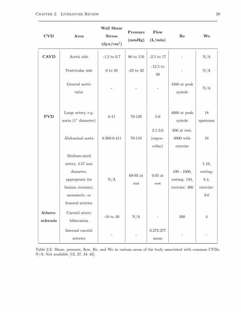
Chapter 2. Literature Review 20
CVD Area
Wall Shear
Stress
(dyn/cm2)
Pressure
(mmHg)
Flow
(L/min)Re Wo
CAVD Aortic side -1.2 to 0.7 80 to 110 -2.5 to 17 - N/A
Ventricular side 0 to 38 -25 to 32-12.5 to
20- N/A
General aortic
valve- - -
4500 at peak
systoleN/A
PVDLarge artery, e.g.
aorta (1” diameter)8-11 70-120 5-6
4000 at peak
systole
18
upstream
Abdominal aorta 0.269-0.411 70-110
2.1-3.6
(supra-
celiac)
600 at rest,
6000 with
exercise
16
Medium-sized
artery, 4.57 mm
diameter,
appropriate for
human coronary,
mesenteric, or
femoral arteries
N/A69-93 at
rest
0.05 at
rest
100 - 1000,
resting: 150,
exercise: 300
1-10,
resting:
6.4,
exercise:
9.0
Athero-
sclerosis
Carotid artery
bifurcation-10 to 30 N/A - 300 4
Internal carotid
arteries- -
0.272-277
mean- -
Table 2.2: Shear, pressure, flow, Re, and Wo in various areas of the body associated with common CVDs.N/A: Not available [13, 27, 34–42].

Chapter 2. Literature Review 21
2.2.3 Entrance Length
When fluid enters into a channel, a thin boundary layer attached to the channel wall develops: The fluid
close to the wall will be experiencing significant viscous effects while the fluid closer to the centreline of the
channel will not, i.e., there is an inviscid core in the velocity profile. In other words when a fluid enters into
a channel, it is not fully developed. As the fluid progresses along the length of the channel, the boundary
layers will increase in thickness until they merge, so that the entire fluid is affected by significant viscous
effects. At this point, the fluid will be fully developed in that the velocity profile will not change along the
length of the channel. This assumes that there are no obstructions, curves, or changes in channel geometry,
which will distort the profile. For channel flow, the entrance length, Le, can be calculated based on channel
height and Re [43]:
Le = χhRe (2.10)
where χ = 0.06 for circular channels and 0.08 for rectangular channels. In the case of experiments involving
microfluidic devices and ECs, the calculation of Le is essential to ensure that the tested ECs are experiencing
the expected shear profile. However, Le is small in microfluidic flows since Re is approximately unity, and h
is typically on the order of hundreds of microns, so this is usually not a large issue.
2.2.4 The Navier-Stokes Equations and Several Analytical Solutions
The Navier-Stokes (N-S) equations are fundamental in solving problems in fluid mechanics. Both the equation
of continuity and equations stemming from Newton’s Second Law (momentum) are assembled into a system
of equations assuming that the flow media behaves as a Newtonian fluid with constant density. In vector
form, the equation of continuity is
∂ρ
∂t+∇ · (ρu) = 0 (2.11)
while the vector form of the momentum equations is given as
ρ∂u
∂t+ ρ(u · ∇)u = −∇p + µ∇2u + f (2.12)
where f is the vector representing all of the body forces acting on the control volume under analysis and u
and p the respective velocity and pressure vectors including the quantities in all co-ordinate directions.
To solve the N-S equations for a given problem, boundary conditions must be prescribed. These are
characteristics of the flow problem involving the velocities, forces, and shear stresses at certain locations in
the channel profile. Only a small number of problems exist that can be solved analytically. Several of those
that are of relevance to this thesis are described:

Chapter 2. Literature Review 22
Steady Pressure-Driven Flow between Two Plates
The steady pressure-driven flow situation between two plates is commonly used to describe flows in rectan-
gular channels (Figure 2.10).
h
y
x
Flow
z
Figure 2.10: Depiction of problem geometry in steady pressure-driven flow between two plates separated bygap distance h.
Assumptions
• The flow is steady, laminar, and fully developed.
• The plates are infinitely wide.
• A pressure gradient is applied along the length of the channel only.
• Body forces are negligible.
• The velocity gradient only exists in the y-direction.
The N-S equations reduce to:
0 = −dpdx
+ µd2u
dy2(2.13)
Boundary conditions
• u(0) = u(h) = 0
Applying the boundary conditions and integrating Equation 2.13 yields:
u(y) = − 1
2µ
dp
dx
(hy − y2
)(2.14)

Chapter 2. Literature Review 23
The resulting flow rate and wall shear stress are calculated, with w representing the width of the channel
into the third co-ordinate direction (z) through:
Qssplateflow = −dpdx
(wh3
12µ
)(2.15)
τssplatewss =6µQssplateflow
wh2(2.16)
This analysis is one-dimensional and does not take into account wall effects resulting from rectangular
channels. While typically employed for analyzing parallel plate flow chambers, there are more accurate
analytical solutions available.
Rectangular Channel Flow with Wall Effects
Rectangular duct flow analysis takes into account wall effects which the previous analysis ignores, in a closed
channel for pressure-driven, steady-state flow (Figure 2.11).
w
h
Flow
y
z
x
w
h
Flow
y
z
x
Figure 2.11: Depiction of problem geometry in rectangular duct flow with wall effects for the unsimplifiedsolution (top panel) and Purday approximation (bottom panel). x, y, and z represent the co-ordinate axes,with x being aligned with the direction of flow and y and z defining the cross-section of the channel of width,w, and height, h. The top and bottom panels have their origins defined differently. The top panel has they axis aligned horizontally along the bottom of the channel and z axis oriented vertically upwards whenviewing the channel cross-section. The bottom panel has the z axis aligned horizontally at the channel’smid-height and the y axis oriented vertically upwards when viewing the channel cross-section. Adapted from[44].

Chapter 2. Literature Review 24
Assumptions
• The flow is two-dimensional, steady, laminar, and fully developed.
• A pressure gradient is applied along the length of the channel only.
• Body forces are negligible.
The N-S equations reduce to:
∂2u
∂y2+∂2u
∂z2= −∆P
µL(2.17)
where ∆P is the pressure difference across the channel.
Boundary conditions
• u(Γ) = 0
where Γ represents the boundary of the rectangular channel.
Tanyeri et al. present the solution to this equation providing the velocity profile at an arbitrary position
in a specified plane along the length of the channel as [45]:
u(y, z) =4h2∆P
π3µL
∞∑n=1,3,5,...
1
n3
[1−
cosh(nπyh
)cosh
(nπw2h
)] sin(nπzh
)(2.18)
The flow rate, Qrect, can then be calculated by integrating Equation 2.18:
Qrect = 2
∫ w/2
0
dy
∫ h
0
dz u(y, z) =h4∆P
12µLα
[1−
∞∑n=1,3,...
192α
(nπ)5tanh
(nπ2α
)](2.19)
where α = hw , the aspect ratio of the channel. The wall shear stress at the bottom of the channel along the
centreline, τrwssbc, is calculated through [46]:
τrwssbc =6µQ
wh3
h− 8h
π2
∞∑k=0
1
(2k + 1)2 cosh[
(2k+1)π2α
]1− 192α
π5
∞∑k=0
tanh[
(2k+1)π2α
](2k + 1)5
−1
(2.20)
Equation 2.18 requires computational solution. Purday proposed an approximation valid for α ≤ 0.5,
which Natarajan and Lakshmanan added empirical constants n and m, yielding [44]:
u
um=
(m+ 1
m
)(n+ 1
n
)[1−
(2y
h
)m] [1−
(2z
w
)n](2.21)
umaxum
=
(m+ 1
m
)(n+ 1
n
)(2.22)

Chapter 2. Literature Review 25
with
m = 1.7 + 0.5α−1.4
and
n =
2 for α ≤ 13
2 + 0.3(α− 1
3
)for α ≥ 1
3
where um and umax are the mean and maximum velocities respectively. um is calculated as
um =Q
wh(2.23)
At the bottom of the channel along the centreline, the wall shear stress (τpwssbc) is calculated through [47]:
τpwssbc =2µQ
wh2
(m+ 1
m
)(n+ 1) (2.24)
Given the inclusion of wall effects and the improved accuracy over the parallel plate results, the expressions
resulting from rectangular channel flow will be used in this thesis. Quantitative evidence of the errors
stemming from using the parallel plate approach as opposed to rectangular channel flow are presented in
Section 2.2.6 on p. 29.
Womersley Flow
Typically, biological flow problems in arteries and veins are solved assuming Womersley flow, which accounts
for the pulsatile nature of cardiovascular flows occurring in a rigid tube (Figure 2.12 on p. 26). The solution
to Womersley flow can be found by decomposing the pressure and velocity into steady and oscillatory parts,
identified by subscripts s and φ, respectively. In other words:
p(z, t) = ps(z) + pφ(z, t) (2.25)
u(z, t) = us(z) + uφ(z, t) (2.26)
When these equations are substituted into Equation 2.12 two relations result: the first leading to a steady-
state solution (i.e. Poiseuille flow) and the second leading to the governing equation for the oscillatory
portion of the flow. The solution methodology can be examined in other references via Fourier analysis and
solving the resulting Bessel equations [32], but the end results are summarized here.

Chapter 2. Literature Review 26
Flow
ra
z
θ
Figure 2.12: Depiction of problem geometry (top panel) and co-ordinate axes (bottom panel) for rigid tubeWomersley Flow.
Steady Womersley Component - Poiseuille Flow
Assumptions
• The flow is steady, laminar, and fully developed.
• A constant pressure gradient is applied along the length of the channel only.
• The radius is constant at a value of a.
• Body forces are negligible, i.e., there are no external forces causing flow rotation implying symmetry
about the longitudinal axis of the vessel
The N-S equations reduce to:
ρuz∂uz∂z
= −∂p∂z
+ µ∇2uz (2.27)

Chapter 2. Literature Review 27
where uz is the velocity in the z-direction.
Boundary conditions
• u(Γ) = 0
where Γ represents the boundary of the vessel. Now, a constant, ks, expressing the pressure difference
between the entrance and exit of the vessel over the length is defined:
ks =ps(l)− ps(0)
l(2.28)
Then, the velocity is given as
us =ks4µ
(r2 − a2
)(2.29)
where a is the radius of the vessel. The flow rate is
qs = −ksπa4
8µ(2.30)
and the wall shear stress is
τs = −4µqsπa3
(2.31)
Many analyses will use the Poiseuille assumption to describe biological flows in vessels. This is a large
over-simplification. The addition of the unsteady Womersley component greatly improves the efficacy and
accuracy of the data obtained from analyses of pulsatile flow problems in circular channels.
Unsteady Womersley Component
Assumptions
All of the assumptions from the steady component still hold, except now:
• The flow is pulsatile.
Then the Navier-Stokes equations reduce to
ρ∂u
∂t+∂p
∂z= µ
(∂2u
∂r2+
1
r
∂u
∂r
)(2.32)
The unsteady pressure difference is represented by kφ(t), and can be decomposed into its exponential form:
kφ(t) = pφ(l, t)− pφ(0, t) = kseiωt = ks (cosωt+ i sinωt) (2.33)

Chapter 2. Literature Review 28
The velocity is then given as
uφ(r, t) =iksa
2
µWo2
(1− J0(ζ)
J0(Λ)
)eiωt (2.34)
where J0 is the Bessel function of first kind of zeroth order, and ζ and Λ are defined, respectively, as
ζ(r) = Λr
a(2.35)
Λ =
(i− 1√
2
)Wo (2.36)
The flow rate is
qφ(t) =iπksa
4
µWo2
(1− 2J1(Λ)
ΛJ0(Λ)
)eiωt (2.37)
and the wall shear stress is
τφ(t) = −ksaΛ
(J1(Λ)
J0(Λ)
)eiωt (2.38)
where J1 is the Bessel function of first kind of order one. The overall solution for Womersley flow may then
be expressed as the superposition of the derived steady and unsteady components.
2.2.5 Flow Resistance
Flow resistance in a fluidic channel is a corollary to the electrical resistance found in a circuit. Fluidically,
the resistance stems from the frictional resistance to flow from the channel walls. The change in pressure is
the product of the flow and resistance, assuming steady flow, just as the change of voltage is the product of
the current and resistance (Figure 2.13).
Q
R
P
P = QR
R
i
V
V = iR
Figure 2.13: Corollary of flow resistance taken from electrical circuits. Top - fluid network, bottom - electricalnetwork: Pressure is correlated to voltage and flow rate to current.

Chapter 2. Literature Review 29
Both rectangular and circular channels have associated expressions for flow resistance. For low aspect
ratios, the expression for flow rate for rectangular channels given by Equation 2.19 on p. 24 becomes
Qrect =h4∆P
12µLα(1− 0.63α) (2.39)
Then, flow resistance in a rectangular channel, Rrect, can be expressed as
Rrect =∆P
Q=
12µLα
h4
1
(1− 0.63α)(2.40)
For circular channels, the expression for flow resistance, Rcirc, is taken from the steady Poiseuille flow
solution using the flow rate expressed in Equation 2.30, yielding:
Rcirc =∆P
Q=
8µL
πa4(2.41)
Flow resistance values can provide quick estimates of how velocities will change within different sized
channels, as well as to what channels a fluid may be biased toward in bifurcating networks. Varying the
resistances between channels in these networks can be strategic for manipulating fluid motion, as a fluid will
tend to travel along the past of least resistance (or the bulk of it if not completely biased toward a single
channel).
2.2.6 Wall Shear Stress Estimation Errors in the Parallel Plate Model when
Compared to the Purday Approximation
Many studies make use of the parallel plate model presented in the previous section to model microfluidic
channels. In this thesis the more accurate Purday model presented that includes edge effects (Equations 2.18
through 2.24) will be employed so long as the validity condition on the aspect ratio, h/w ≤ 0.5, is satisfied.
The two methods of determining wall shear stress will be quantitatively compared to show how accounting
for wall effects using the Purday approximation can significantly affect the calculations.
The ratio of the wall shear stresses (at the channel’s centreline on the vertical bottom) predicted by the
parallel plate assumption and Purday approximation can be written from Equations 2.16 on p. 23 and 2.24
on p. 25 as
τssplatewss
τpwssbc=
6µQwh2
2µQwh2
(m+1m
)(n+ 1)
= 3
[m
(m+ 1)(n+ 1)
](2.42)
The two wall shear stress predictions at the bottom centreline of a rectangular channel can be compared to
obtain characteristic curves providing the differences in the estimations over a range of channel dimensions for
analysis. As was shown for Equation 2.24, the values of m and n depend on the channel dimensions. As the
channel dimensions are varied, the difference between the shear stress values predicted by the two methods

Chapter 2. Literature Review 30
also changes. Comparing the two predictions shows that as the aspect ratio increases, the deviation between
the two methods of calculating shear stress increases. At maximum, there is a 30% difference between the
shear stress values, while at larger channel widths the difference becomes less apparent. However as channel
height increases, even at lower aspect ratios, the error becomes significant (Figure 2.14). It is clear that
taking wall effects into account using the Purday approximation can have a substantial impact on wall shear
stress calculations for devices with high aspect ratios. The Purday approximation provides a simple method
of improving accuracy, but a superior approach is to employ the unsimplified solution of rectangular channel
flow.
0.7
0.75
0.8
0.85
0.9
0.95
0 500 1000 1500 2000 2500
Channel Width (um)
Rat
io o
f P
aral
lel P
late
Ass
um
pti
on
to
Pu
rday
Ap
pro
xim
atio
n
Pre
dic
tio
ns
of
Wal
l Sh
ear
Str
ess
h = 100 um
h = 200 um
h = 300 um
h = 400 um
h = 500 um
Figure 2.14: Ratio of the estimations of wall shear stress along the bottom centreline of a rectangularchannel for the parallel plate and Purday approximations at various channel dimensions, subject to thePurday approximation and design constraints that 1/10 < h/w < 1/2 [48]. The Purday approximationprovides a better estimation of wall shear stress, accounting for wall effects, and up to a 30% difference canbe seen between the two predictions at small channel widths.
2.2.7 Wall Shear Stress Estimation Errors in the Purday Model when Com-
pared to the Unsimplified Solution of Rectangular Channel Flow
While the Purday approximation can be used under the condition that α ≤ 0.5, at times the full solution of
rectangular channel flow must be employed. The ratio of the wall shear stresses (at the channel’s centreline
on the vertical bottom) given by the full solution and the Purday approximation can be written from
Equations 2.20 on p. 24 and 2.24 on p. 25 as
τrwssbc
τpwssbc=
3
h
[m
m+ 1
] [1
n+ 1
]h− 8h
π2
∞∑k=0
1
(2k + 1)2 cosh[
(2k+1)π2α
]1− 192α
π5
∞∑k=0
tanh[
(2k+1)π2α
](2k + 1)5
−1
(2.43)

Chapter 2. Literature Review 31
For low aspect ratios, the two methods of calculating wall shear stress yield nearly identical results. However
as expected, as the aspect ratio increases the difference between the two methods increases, with the Purday
approximation underestimating shear stress. Subject to the device design constraint that 1/10 < h/w < 1
[48], the maximum difference between the wall shear stress calculations is approximately 40% (Figure 2.15).
It is essential to note that at larger aspect ratios the Purday approximation becomes far less applicable and
fails to accurately predict the wall shear stress occurring in rectangular microfluidic channels, as well as what
ECs would sense seeded inside along the bottom wall. Using the Purday approximation to predict wall shear
stress in devices with high aspect ratios can have a large impact on experimental results and provide false
data, in terms of the interplay between shear stress, the mechanobiology of ECs, and the resulting cellular
changes in terms of phenotypic expression.
0.8
0.9
1
1.1
1.2
1.3
1.4
1.5
0 500 1000 1500 2000 2500
Channel Width (um)
Rat
io o
f U
nsi
mp
lifie
d S
olu
tio
n t
o
Pu
rday
Ap
pro
xim
atio
n P
red
icti
on
s o
f W
all S
hea
r S
tres
s
h = 100 um
h = 200 um
h = 300 um
h = 400 um
h = 500 um
Figure 2.15: Ratio of the estimations of wall shear stress along the bottom centreline of a rectangularchannel for the unsimplified solution of rectangular channel flow and the Purday approximation at variouschannel dimensions, subject to the design constraint that 1/10 < h/w < 1 [48]. At the limit of the Purdayapproximation, when h/w > 1/2, the difference when compared to the unsimplified solution begins to growexponentially, up to a maximum of approximately 40%.
2.2.8 Flow-Induced Deformation in Microfluidic Systems
Simple engineering flow systems, such as pipes and ducts composed of metals, are usually considered to be
rigid. However in deformable flow systems, such as a healthy human artery, the pressure caused by the fluid
flow will tend to distend the walls of the flow system. Such is also the case in microfluidic flow chambers
fabricated from PDMS. Not only is there deformation in a flexible, moldable, plastic flow system such as
one that is fabricated from PDMS, but also the deformation changes along the channel in the flow direction
as the pressure varies. These changes in dimensions are important to consider when aiming to reproduce a
specific shear stress, as a dimensional mismatch will cause an error in the calculations. Gervais et al. studied

Chapter 2. Literature Review 32
this phenomena and found that for a given pressure drop, the corresponding flow rate was found to be several
times higher than expected in a non-deforming channel [49]. The following assumptions were made:
• The flow is steady and laminar.
• The bulk properties of PDMS include a low Young’s modulus (0.5-4 MPa) and high Poisson ratio
(ν=0.5, essentially incompressible).
• The microchannels are rectangular.
• The device is bonded to a glass slide which is assumed to be rigid.
• The structural displacement of the PDMS takes place in a semi-infinite medium.
• The deflection of the channel wall is parabolic.
Taking into account the deformation, the actual flow rate through the device, Qdeform, is found to be
Qdeform =h0
4E
48κµ(L− z)
[(1 + κ
p(z)W
Eh0
)4
− 1
](2.44)
where κ is a correlation coefficient of deformation obtained from computational simulations on the order of
one, h0 the undeformed height of the microchannel, L the length of the microchannel, z the distance along
the longitudinal axis, E the elastic modulus, W the width, and p(z) the pressure at the location, z, along
the longitudinal axis. When compared to the flow rate resulting from the simple Poiseuille assumption of
flow in a rectangular channel, the difference in flow rates can be written as
∆Q
Q=Qdeform −Qrigid
Qrigid∝ 3κ
2
∆PW
Eh0(2.45)
As all values in Equation 2.45 are non-zero, it is clear that there will be a difference between assuming rigid
and deformable channels in microfluidic flow. The resulting flow rate can in turn affect shear stress and
pressure predictions, varying what cultured cells within a microfluidic device would be exposed to in terms
of hemodynamics. The maximum height deformation at the mid-width (z = L/2) of the channel is given as
∆hmax =c1pW
E(2.46)
where c1 is a proportionality constant of magnitude order one.
Following a review of principles in fluid mechanics, an overview of bioreactors in the literature is provided
to discuss the deficiencies of the current state of the art.

Chapter 2. Literature Review 33
2.3 Bioreactors
Bioreactors are experimental set-ups that are designed to support and sustain any process which employs
living cells, their organelles, bacteria, and other biological molecules to obtain desired outcomes. Such
outcomes could be the creation of a product to applying forces on living tissue [50]. For the purposes of
this thesis, the term “bioreactor” will refer to experimental setups designed to simulate various in vivo flow
environments found within the human body using laboratory-based equipment. Depending on the situation
being studied, bioreactors can be designed to mimic a wide array of flow-based phenomena, including: flow,
stretch, pressure, perfusion, and shear stress.
In flow bioreactors, both resistance and compliance are altered to create the desired flow waveforms.
Resistance is the impedance to flow, caused by valves, fittings, constrictions, and friction within the system.
Compliance refers to the behaviour caused by air being present in the system, which manifests itself as
bubbles in the flow as well as tubing or flexible material expanding when a flow rate is imposed. Work
carried out by Leo provides a depiction of the effects of altering resistance and compliance, in terms of the
overall pressures throughout a bioreactor [51]. In that research, resistance was varied by opening and closing
a clamp on a flexible portion of tubing, which constricted the flow area. The flow rate would remain constant,
but the velocity would be altered as well as the pressure in the system. Increasing the resistance was shown
to increase the differential pressure. On the other hand, compliance was altered by varying the fluid level in
a compliance chamber, varying the air-to-fluid ratio inside the chamber. Reducing the fluid level (increasing
compliance) reduces differential pressure (Figure 2.16).
Figure 2.16: Effects of altering the resistance (top panel) and compliance (bottom panel) on pressure inthe Georgia Tech bioreactor: increasing resistance increases differential pressure and increasing compliancedecreases differential pressure [51].

Chapter 2. Literature Review 34
This literature review will predominantly focus on bioreactors that are designed to mimic cardiovascular
flow environments (in terms of flow rates and pressures), or apply specific levels of shear stress on tissue
or cultured cells, as these systems are the most relevant to this research. Particular attention is paid to
bioreactors that were created for applications to CVD research. Limitations of the state of the art will also
be discussed.
2.3.1 Macroscale Flow Bioreactors
Mimicking in vivo hemodynamic environments at the macroscale using bioreactors is not a new task and
has been successfully carried out via several methods. Typically, a bioreactor will involve the combination
of a pump, one or several compliance chambers (tanks filled with media to buffer the pumping flow and
pressure), the culture chamber which contains the object (such as a medical device, heart valve, vascular
graft, tissue, or population of cultured cells) being subjected to hemodynamic forces, and several resistance
clamps (valves) to vary pressure and flow independently at several points throughout the flow bioreactor. For
each method, the arrangement of these items may vary. But, the main issue that merits further discussion
is the pump or pumping method which creates the cardiovascular waveform.
Narita et al. made use of an expanding and contracting balloon pump controlled by a computer-based
driving system to study tissue-engineered vascular constructs (Figure 2.17) [52]. The bioreactor could gener-
ate pulsatile flow rates ranging from 0 to 3000 mL/min. As well, the systolic and diastolic pressures ranged
respectively between 0 to 200 mmHg and 0 to 100 mmHg. A large issue was that the shear stress levels that
the bioreactor created ranged between 0.07-0.15 dyn/cm2, whereas physiological shear stresses in a typical
human artery and vein typically range from 10-20 and 1-6 dyn/cm2, respectively [52]. The difference was
explained as being mainly caused by the low viscosity of the culture medium and low flow rate used in the
study.
Figure 2.17: Bioreactor used by Narita et al. with balloon pump. Bioreactor components: (1) Balloonchamber, (2) compliance chamber, (3) culture chamber, and (4) reservoir. The balloon pump took in air andexpelled it controlling the pressure inside the balloon chamber to force media through the other portions ofthe bioreactor [52].

Chapter 2. Literature Review 35
A related method that also makes use of a deforming membrane is a so-called ventricular or membrane
pump, such as one that was used by Ruel and Lachance to test tissue-engineered heart valves (Figure 2.18)
[53]. This bioreactor was designed by first creating a Windkessel model of the system, which converts fluidic
and mechanical components to electrical circuit equivalents using flow resistance equations (as discussed in
Section 2.2.5 on p. 28). The order of accuracy of bioreactors was also discussed, ranging from first order
pulsatile waveforms that can be obtained using a peristaltic pump, to improved accuracy when adding a
compliance chamber, and finally (and most accurately) using a membrane pump with a compliance chamber
and a resistive element. The membrane pump simulates the action of the heart, whereby a flexible membrane
is actuated by a pressurized fluid to displace a certain volume of blood or culture media in the circuit. It
was noted that while the bioreactor produced accurate replication of physiological flows (with a correlation
coefficient of 0.964), the correlation was only very good for pressure (coefficient of 0.783) when compared to
what was predicted by the theoretical Windkessel model. However, no comparison to published standards
was carried out for the Windkessel model. Hence while the correlations may be good, it cannot be said for
certain if the resulting waveforms mimic the in vivo environment accurately without further validation.
Figure 2.18: Left: bioreactor used by Ruel and Lachance. Bioreactor components: 1) ventricular pump, 2)valve holder, 3) compliance chamber, 4) variable resistance, 5) reservoir, 6) bi-leaflet unidirectional valve andflowmeter. Right: membrane pump schematic. The culture media chamber was separated by a deformablemembrane which was actuated by a separate air flow at the bottom of the chamber to create a pulsatilewaveform [53].
It is also worth discussing one of the most heavily referenced macro scale bioreactors that mimics car-
diovascular waveforms: the Georgia Tech Pulse Duplicator, which creates pulsatile waveforms specifically
for heart valve experiments [51]. The setup has been validated and used in many different studies [54–57].
The loop consists of two parts: a pulse generation and delivery system and the flow loop (Figure 2.19 on
p. 36). The pulse generation and delivery system consists of an air compressor, a pneumatic control board,
and a pulse generator. The air compressor delivers compressed air to the pneumatic control board, which
consists of two pneumatic valves and a throttle valve. The length and time delay between the opening and
closing of each pneumatic valve is controlled by a pulse generator and computer. The flow loop comprises

Chapter 2. Literature Review 36
a silicone pumping bulb, a flow transducer, two pressure transducers, a compliance unit, resistance unit, a
reservoir, and the two valve chambers. Compressed air is delivered from the pneumatic loop to the flexible
silicone bulb sealed within an airtight acrylic chamber placed between the aortic and mitral chambers. The
air compresses the silicone bulb. The compliant and resistant units placed downstream of the aortic valve
can be adjusted to obtain accurate simulation of the mitral flow, ventricular and atrial pressures. This can
be accomplished by adjusting the clamp on flexible rubber tubing to control the resistance, and the level of
the solution inside the cylindrical compliance chamber. Pressure and flow transducers were interfaced with
a signal amplifier for real-time visualization.
Figure 2.19: Schematic of the Georgia Tech pulsatile flow loop. Top: flow loop, bottom: control section ofloop [51].
2.3.2 Mesoscale Flow Bioreactors
The term “mesoscale bioreactors” refers to set-ups that are not on the order of size as the aforementioned
macroscale laboratory bench set-ups, but not at the scale of microfluidic devices.
Separate from flow-through type bioreactors connected by tubing and piping, other setups exist that can
apply shear stresses to biological samples, such as cone and plate devices. Typically, a rotating cone causes
fluid to rotate within a container which applies shear stress over a layer of cells, such as in the work of Dai
et al. and Blackman et al. [2, 58]. Such systems can include parallel disks or one cone and one disk with
cells sandwiched between the two (Figure 2.20).

Chapter 2. Literature Review 37
Figure 2.20: Cone and plate devices used to shear single layers of cells. Left: cone and plate viscometer,right: parallel disk viscometer. Adapted from [16].
Parallel disk viscometers do not expose EC monolayers to a uniform level of shear stress, making it
difficult to obtain sufficient sample sizes for genetic analysis. On the other hand, the local relative velocity
and the separation between the cone and plate surfaces in cone and plate viscometers vary linearly with the
radial position, yielding spatially homogeneous shear stress on both surfaces, as well as the fluid in the gap,
making them quite attractive [16]. However, whole pieces of tissue cannot be used due to their associated
thicknesses. To bypass these issues, there is a related system in the work of Sun et al., in which a bioreactor
was used to study the application of ventricular versus aortic side shear stresses on aortic valve cusps using
a cone and plate viscometer. Whole porcine aortic valve leaflet samples were placed in divots within a plate,
and two servo motors drove spinning cones that applied different shear stress waveforms on either side of
the tissue samples [36] (Figure 2.21 on p. 38).
While still in the realm of non-microscale experiments, there are bioreactors that focus on the character-
ization of small-scale vascular grafts. For instance in work by Isenberg et al., the combination of peristaltic
and syringe pumps was used to impart cyclic, sinusoidal flows on ECs to test if they could withstand physi-
ological shear stresses when growing on fibrin-based media-equivalents used for vascular grafts (Figure 2.22
on p. 38) [4].
Referring to Figure 2.22, the pulse dampeners at (3) transformed the pulsatile flow of the peristaltic
pump at (2) into steady, continuous flow. The syringe pump at (4) then imparted an unsteady, sinusoidal
waveform to be superimposed onto the resulting steady peristaltic waveform. A filter on top of the media
reservoir (1) allowed for gas exchange. A simple occlusion valve (8) downstream of the culture chamber (7)
allowed for pressure modulation. Flow and pressure probes connected to a computer via a data-acquisition
card and LabView allowed for data capture. ECs were shown to align with the predominant flow direction
at low flow rates, but in the turbulent flow regime, they did not, as predicted. The authors also expressed
concerns in creating the fibrin-equivalents at sufficient lengths for testing, and with consistent material
properties to systematically investigate the ECs responses to shear stress. Another more crucial concern is
the type waveform that was applied to the ECs in the study: both the pressure and flow waveforms were
sinusoids with a frequency of 1 Hz. Physiological waveforms, while being pulsatile with a 1 Hz frequency,
can be oscillatory (bi-directional), not extend from a mean value by an equal amplitude, and have distinct

Chapter 2. Literature Review 38
peaks and troughs. The 1 Hz sinusoid waveforms in this study, while capturing the temporal component of
a typical cardiovascular waveform, simplify the spatial component or amplitude. With ECs being extremely
sensitive to their hemodynamic environment, applying sinusoidal waveforms may produce different cellular
responses when compared to waveforms that are seen in vivo.
Figure 2.21: Cup and cone bioreactor setup used by Sun et al. Tissue samples were placed into divots withina plate sandwiched between two rotating cones within a sealed chamber containing cell culture medium. Thetop and bottom cones applied different shear stress profiles representing each side of the aortic valve. (a)Entire bioreactor loop, (b) top view of plate [36].
Figure 2.22: Dual pump bioreactor used by Isenberg et al. Overall bioreactor schematic (A) and mediachamber (B) are highlighted. Components of the bioreactor: 1) medium reservoir, 2) peristaltic pump, 3)pulse dampeners, 4) pulsatile syringe pump, 5) check valves, 6) pressure transducer, 7) media chamber,8) occlusion valve, and 9) flowmeter. The peristaltic pump continually cycled medium throughout thebioreactor, where the pulsatile nature of the flow was converted into a steady variant by the pulse dampeners.The syringe pump imparted a pseudo-physiological flow which was then combined with the steady peristalticwaveform to be sensed by the biological sample. The flow was then sent back to the original reservoir foranother cycle [4].

Chapter 2. Literature Review 39
A further option for waveform creation is employing a cardiac pump, which has been specifically designed
to replicate cardiovascular waveforms [59]. These pumps are usually quite expensive, and also have a low
level of customization. A waveform is programmed into the pump, and the user may change the target heart
beats per minute. The output waveform varies according to this parameter in terms of cycling through faster
or slower, but the waveform shape is constant. Such is the case in the study carried out by Hahn et al. [19]:
The research was also within the vascular realm, and employed a strategy related to that of Isenberg et al.
[4]. The study examined the hypothesis of mechanical conditioning being a potential means to enhance the
biochemical and biomechanical properties of tissue engineered vascular grafts. A peristaltic pump created
a base flow rate and was dampened out to continuous flow, following which the pulsatile component of the
flow waveform was supplied using one or more cardiac pumps. The cardiac pumps could be tuned to 60 and
120 bpm to represent the cardiac potential of a human fetus and adult, respectively (Figure 2.23). Flow
rates of 2 mL/s, representative of flow through small diameter blood vessels, were generated, resulting in a
reported mean wall shear stress of 6 dyn/cm2 within the 3 mm inner diameter constructs.
Figure 2.23: Schematic (top) and image (bottom) of bioreactor used in the study of Hahn et al. Componentsof the bioreactor: (1) cardiac pump, (2) custom graft chamber, (3) media reservoir, (4) peristaltic pump, (5)compliance chamber, and (6) check valves. Media was continuously cycled by a cardiac pump to a chambercontaining vascular graft samples fed by a media reservoir containing cell culture medium. A peristalticpump also moved flow [19].
Several issues arise from this bioreactor design: Again, there is no quoted comparison to a reference
waveform to ensure that the obtained flow and pressure profiles are close to physiological conditions. It is
only assumed. Second, the attachment of the vascular constructs into the bioreactor was done assuming
they will remain on their supports through stretched elasticity. While the constructs should remain attached

Chapter 2. Literature Review 40
unless high flow rates are used (which would rupture the supports due to high pressures), a risk still exists.
This risk could be mitigated by experimentally determining when the constructs would become detached
from their supports through the application of increasing flow rates until a burst occurs. Finally, the use
of multiple pulsatile pumps to impart the desired pulsation not only requires a great deal of physical space
(in a crowded environment such as an incubator), but is also expensive. Moreover as previously mentioned,
the degree of customization is severely limited. While the bioreactor employs a compliance chamber, the
waveform output by the cardiac pump itself cannot be varied. This limits the range of studies that can be
carried out. No means of varying resistance is included within the flow loop, further decreasing the amount
of customization possible.
Another device used for mesoscale studies is the parallel plate flow chamber (PPFC) (Figure 2.24 on
p. 41). Here, a pressure difference is created between the inlet and outlet of the chamber, allowing flow to
develop across the surface of cultured cells inside the PPFC. The simple geometry gives rise to predictable
fluid dynamics (obeying the derived fluid profile of steady pressure-driven flow between two plates in Section
2.2.4) allowing for shear stress levels to be easily predicted within the device. Other practical attractions
include homogeneity of the force stimulus, simplicity of the equipment, ease of medium sampling/exchange,
and ease of access to the culture (both physically and for microscope visualization) [16]. The PPFC has been
used in a wide range of studies, not only limited to shear stress-based CVD work [60–65]. While appropriate
for steady flow studies, current in vitro models lack the ability to apply dynamic ranges of shear stress
because flow within the system is commonly generated by a constant pressure difference, syringe pump flow,
or peristaltic pump flow. Moreover when compared to microfluidic devices, the cell culture area is quite
large, which may be in excess for certain experiments, requiring additional materials and media to ensure
the cells remain alive before and during flow experiments.
2.3.3 Microscale Flow Bioreactors
Several bioreactor studies have also examined the effects of hemodynamics on ECs at the microscale. In
microscale systems, flow is applied onto cultured cells in microfluidic devices versus whole tissue in macroscale
systems, such as aortic valve leaflets.
Microfluidic devices are versatile miniaturized flow systems (Figure 2.25 on p. 42). The devices typically
employed for laboratory applications are fabricated using the inexpensive and flexible polymer polydimethyl-
siloxane (PDMS), but higher quality devices can be fabricated from other materials such as glass. The PDMS
versions of the devices are fabricated using the soft lithography process which has been well documented
elsewhere but is briefly summarized in this work for reference [66, 67]:
1. Microfluidic channel design for the device is carried out using CAD software.
2. A transparency is prepared on a high resolution printer to create a photomask.
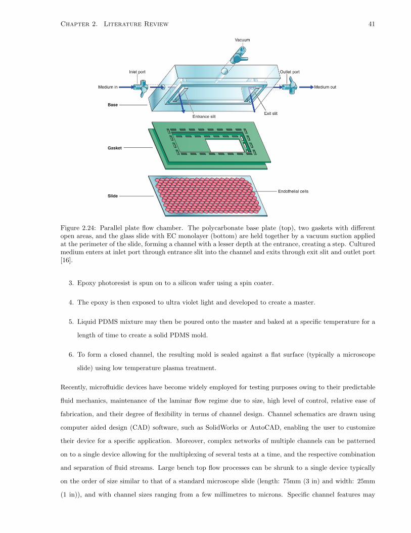
Chapter 2. Literature Review 41
Figure 2.24: Parallel plate flow chamber. The polycarbonate base plate (top), two gaskets with differentopen areas, and the glass slide with EC monolayer (bottom) are held together by a vacuum suction appliedat the perimeter of the slide, forming a channel with a lesser depth at the entrance, creating a step. Culturedmedium enters at inlet port through entrance slit into the channel and exits through exit slit and outlet port[16].
3. Epoxy photoresist is spun on to a silicon wafer using a spin coater.
4. The epoxy is then exposed to ultra violet light and developed to create a master.
5. Liquid PDMS mixture may then be poured onto the master and baked at a specific temperature for a
length of time to create a solid PDMS mold.
6. To form a closed channel, the resulting mold is sealed against a flat surface (typically a microscope
slide) using low temperature plasma treatment.
Recently, microfluidic devices have become widely employed for testing purposes owing to their predictable
fluid mechanics, maintenance of the laminar flow regime due to size, high level of control, relative ease of
fabrication, and their degree of flexibility in terms of channel design. Channel schematics are drawn using
computer aided design (CAD) software, such as SolidWorks or AutoCAD, enabling the user to customize
their device for a specific application. Moreover, complex networks of multiple channels can be patterned
on to a single device allowing for the multiplexing of several tests at a time, and the respective combination
and separation of fluid streams. Large bench top flow processes can be shrunk to a single device typically
on the order of size similar to that of a standard microscope slide (length: 75mm (3 in) and width: 25mm
(1 in)), and with channel sizes ranging from a few millimetres to microns. Specific channel features may

Chapter 2. Literature Review 42
also be created on the size order of microns. For these reasons, microfluidic devices have been employed for
a range of chemical and biological applications, such as cell sorting and separation, the creation of on-chip
or micro-pumps, on-chip valving, chemical detection, chemical assays, cell culture and co-culture, and most
relevant and important to this work, EC shear studies [66–68, 68–73].
Figure 2.25: Example of a complex multi-channel PDMS device with its size compared to a US dime [74].
In work carried out by Estrada et al., the formation of atherosclerotic lesions caused by disturbed and
non-disturbed flows was examined using a bioreactor that was described as being able to apply accurate
pressure, strain, and shear stress on cultured human aortic ECs [72, 75]. The argument presented was that
most bioreactors focus on one of three major forces acting on ECs in vivo, whereas in vivo the complex
interplay between all factors is what leads to the morphological changes in which ECs undergo. The work
focused on conditions in the abdominal aorta in the inferior mesenteric artery, which is associated with a
high incidence of atherosclerotic flow.
The bioreactor consisted of a peristaltic pump to induce flow, a cell culture chamber with a compliant
thin membrane that mimics a vessel’s wall, a pneumatically driven collapsible chamber, and two units each
of tunable resistance and compliance along with a flow control valve and pressure and flow monitors with
data being collected via a LabView protocol on a computer (Figure 2.26 on p. 43).
The collapsible chamber was the primary component introducing pulsatility into the system, representing
left ventricular function. The applied pressure, percentage systolic/diastolic fraction, and frequency could
be manipulated to the amplitude of the pressure and flow waveforms. The tunable compliance and flow
resistance elements upstream of the inlet (pulmonary) and downstream of the outlet of the cell culture
channel (aortic/systemic) allowed for modification of the shape and amplitude of attained pressure and flow
profiles. The one-way valve prevented retrograde flows between the pulsatile and culture chambers.

Chapter 2. Literature Review 43
Figure 2.26: Multi-force bioreactor used by Estrada et al. Components of the bioreactor: (a) peristalticpump, (b) pulmonary compliance, (c) pulmonary resistance, (d) collapsible chamber, (e) one-way valve,(f) inline flowmeter, (g) cell culture chamber, (h) aortic/systemic compliance, (i) inline pressure sensor,(j) aortic/systemic resistance, and (k) medium reservoir. The peristaltic pump moved cell culture mediumcontinuously throughout the bioreactor, where waveform shape was controlled by upstream and downstreamcompliance and resistance units. A pneumatically actuated collapsible chamber allowed for the control ofpulsatility in the system. A culture chamber with deformable walls allowed for the simulation of membranedeformation that occurs in vitro [72].
The bioreactor was reported to replicate typical disturbed and non-disturbed conditions, but several
issues arise from the study. The calculation of shear stress to be applied in the microfluidic devices where
the ECs were cultured was carried out using a model that involves the Womersley number (inside the device)
as a scaling factor, given by
τestrada =Wo√
2
6Qµ
h2w(2.47)
This is a modified form of the parallel plate assumption given by Equation 2.16 on p. 23. It still does not
account for wall effects, and does not change the profile of the parallel plate assumption greatly, as the article
cited a Womersley number ranging between 1.2 to 1.8. Moreover, there is also a large simplification of data
in having two archetypal waveforms represent disturbed versus non-disturbed conditions. Forces can range
between all of strain, pressure, and shear stress within the two flow categories and to reduce the myriad of
conditions to two simple conditions, while convenient, is still a large assumption. The study also claims the
waveforms created “closely match the clinical waveforms reported literature”, but never cite these reference
waveforms or show the comparison being carried out.
Scott-Drechsel et al. studied the effects of pulse flow waves on co-cultured ECs and smooth muscle cells
(SMCs) in a microfluidic device in the context of arterial stiffening, which influences the progression of
vascular diseases [76]. A cardiac pump was used along with a compliance (or so-called stiffness) adjustment
chamber to create various shapes of waveforms acting on the co-culture (Figure 2.27 on p. 44).

Chapter 2. Literature Review 44
Figure 2.27: Left: bioreactor (top panel) and microfluidic co-culture device (bottom panel) used by Scott-Drechsel et al.. A pulsatile blood pump cycled media throughout the bioreactor, where a co-culture devicehoused co-cultured ECs and smooth muscle cells. Right: comparison of native artery compliance effects andmimicking of these effects by the stiffness chamber used in the bioreactor. In the compliance chamber, alarger amount of air leads to increased dampening effects, as the air pressure built up pushes on the flow,decreasing any pulsatile nature of the flow [76].
Both computational and experimental analyses were carried out and compared. Moreover, conditions of
pulsed versus semi-steady flow were applied to the co-culture system, and the cell population in a region of
uniform flow within the microfluidic device was tested in terms of pro-inflammatory expression and smooth
muscle cell proliferation. It was found that the mRNA expressions of two pro-inflammatory markers which
are extremely sensitive to shear, intercellular adhesion molecule 1 and monocyte chemotactic protein-1, were
not found to be statistically different in terms of expression for the two conditions, but both were different
when compared to a zero-flow condition. Pulsed flow yielded an increase in smooth muscle cell proliferation.
The use of a cardiac pump limits extending this study to examine waveforms in other arteries. The specific
artery being modelled was not mentioned either, limiting the range of application of the findings found from
the study.
Work by Chin et al. examined the production of reactive oxygen species in ECs in response to different
shear waveforms and glucose concentrations. This work introduced accurate profiles that were cited and
compared to reference curves through validation by particle image velocimetry [70]. A high-accuracy syringe
pump (the cetoni neMESYS) was connected to a bubble chamber or damper, which then fed into the
microfluidic device used for experimentation. The production of oxygen species were examined along with
mitochondrial morphology. Unfortunately, the shear stress to be produced in the microfluidic device was
predicted using a modified version of the parallel plate assumption (Equation 2.16 on p. 23), which, as
discussed, can be fairly inaccurate.

Chapter 2. Literature Review 45
2.3.4 A Comparison of Flow Bioreactors Based on Scale
Macroscale flow bioreactors are typically designed for a single anatomical area or study, such as the aortic
valve: a component holding the biological tissue being analyzed must be custom-designed so that not only
can the tissue be placed in a flow path, but also that the variation of tissue sizing is accounted for, which
is a large challenge to overcome. The materials are usually selected to be optically transparent for flow
visualization studies (particle image velocimetry, laser Doppler velocimetry, etc.) to allow for validation of
the waveforms created by the bioreactors. The size of these bioreactors can be a burden on laboratory space
and can make incubation studies impossible, unless care is taken. Moreover, the entire vascular system is
usually modelled, requiring a large amount of components and troubleshooting.
Mesoscale bioreactors are typically based on steady flow patterns whose theoretical solutions are well
characterized to aid in analysis (such as parallel plate flow chambers). Large populations of cells may be
studied at once. This has been thought to be advantageous for global population-based studies where it is
desirable to smooth out heterogeneities and also ensure there are sufficient biological products for gene and
protein expression analyses [47].
However, microscale bioreactors provide many advantages over the aforementioned strategies. The ma-
jority of microscale systems are based on microfluidic devices, fabricated using soft lithography techniques
using moldable plastic materials (e.g. PDMS). This technique is cost-effective, quick, and there is the ability
to custom design networks of fluid channels to have multiple fluid streams (or tests) being concurrently done
(multiplexing). Final designs can be translated into more expensive and dimensionally-accurate (e.g. glass)
devices, but PDMS is suitable for the rapid prototyping of design concepts in the laboratory. The small
channel dimensions yield lower reagent use and low Reynolds numbers. This in turn yields a high level of
control over mixing of multi-phase fluids and controllable concentration gradients. Moreover, the ability to
design a new device allows for different studies to be carried out easily versus designing a new bioreactor or
component chamber to accept another tissue or sample type. Macroscale and mesoscale bioreactors often
require maintenance and repair. Microscale approaches allow for disposable use similar to other laboratory
items after experiments (such as plastic flasks). Moreover, these systems provide the option of obtaining
information from single cells when needed, while population averages can be reassembled from the single cell
data if so desired. The advantage of mesoscale bioreactors is becoming less prevalent as microscale bioreactor
setups advance [47].
2.3.5 Summary of Limitations of Existing Bioreactors in Literature
After an overview of the bioreactors that have been designed, there are several key limitations in the current
art. To address these deficiencies, this work aims to design a bioreactor that:
• Allows for multiple flow waveform studies to be carried out with a single experimental setup.

Chapter 2. Literature Review 46
• Does not require the entire vascular system to be modelled.
• Produces specific waveforms, versus creating a system and altering it to create various waveforms
afterwards. The bioreactor design will follow a more targeted approach.
• Compares experimentally obtained flow waveforms with theoretical curves to validate the system.
• Accurately calculates the shear stress that occurs within rectangular microfluidic channels accounting
for wall effects.
2.4 Flow Measurement
Several measurement methods exist that can validate flow waveforms created by bioreactors. The two that
are of relevance to this thesis are flowmeters and particle image velocimetry (PIV) .
2.4.1 Flowmeters
Flowmeters quantify bulk fluid movement using various methods. This review will focus on flowmeters
appropriate for liquids, providing brief descriptions of how each functions [77].
Direct Methods
• Positive Displacement Meter - Fluid flows through the meter to move a component, such as a
reciprocating piston or oscillating disk as it flows through the device. The motion of the component is
translated into a flow rate.
Restriction Based Methods
• Laminar Flow Element - Designed to produce a pressure differential directly proportional to flow
rate. The element contains a metering section with a large number of tubes or passages that each
narrow enough so that the flow through them is laminar, regardless of the flow conditions coming in
to the meter. Hence, flow rate can be calculated according to Poiseuille flow via Equation 2.30. Then,
the flow rate in the element is the sum of the each of the tube flows, and is also a linear function of
pressure drop. Usually, this relation is provided through calibration by the manufacturer, and can be
used over a 10:1 (the maximum flow rate that can be measured accurately is ten times the amount
of the minimum flow rate) range of flow rates. As the relationship between pressure drop and flow
rate for laminar flow is also dependent on viscosity, which is a strong function of temperature, the
fluid temperature must be known to obtain an accurate reading. The element is also light and small,
making it extremely attractive for situations where portability and continuous setup and breakdown
is required.
Chapter 2. Literature Review 47
• Float Meter (Rotameter) - Indicates flow directly for liquids. In operation, a ball or float is carried
upward in a tube by the flowing fluid until the drag force and float weight are in equilibrium. The
meters come factory calibrated for common fluids and flow rate ranges and flow rate can be directly
read off the device.
• Turbine Flow Meter - Contains a free-running vaned impeller mounted in a cylindrical section of
tube. The rate of rotation of the impeller is made to be closely proportional to volume flow rate over a
specified range. Rotational speed of the element can be sensed using a magnetic or modulated carrier
pickup external to the meter. No penetrations or seals in the main line are required. It can also be
used to measure flow rates in corrosive or toxic fluids.
• Vortex Flow Meter - Takes advantage of the fact that a uniform flow will generate a vortex street
when it encounters a bluff body such as a cylinder perpendicular to the flow. A vortex street is a series
of alternating vortices shed from the rear of the body; the alternation generates an oscillating sideways
force on, and therefore oscillation of, the cylinder. The frequency of oscillation in the device is directly
proportional to velocity, and thus provides an indication of its value. However, the velocity profile
does affect the shedding frequency so calibration is required. The cylinder used in a vortex flow meter
is usually quite short in length (10 mm or less) and placed perpendicular to the flow (and for some
devices is not a cylinder at all but some other small bluff object). The oscillation can be measured
using a strain gauge or other sensor. Vortex flow meters can be used over a 20:1 range of flow rates.
• Electromagnetic Flow Meter - Uses the principle of magnetic induction: A magnetic field is created
across a pipe. When a conductive fluid passes through the field, a voltage is generated at right angles
to the field and velocity vectors. Electrodes placed on a pipe diameter are used to detect the resulting
signal voltage. The flowmeter makes use of Faraday’s law, which relates the electromotive force of
a closed circuit to the time rate of change of magnetic flux flowing through the circuit. The signal
voltage is proportional to the average axial velocity when the profile is axisymmetric.
• Magnetic Flow Meter - Also uses the same principle as an electromagnetic flow meter. It may
be used with liquids that have electrical conductivities above 100 microsiemens per metre (where 1
siemen = 1 ampere per volt). The minimum flow speed should be above about 0.3 m/s, but there
are no restrictions on the Reynolds number. The applied magnetic field is pulsed, which allows the
flowmeter to cancel out the effect of stray voltage in the piping system.The flow rate range is usually
quoted at 10:1.
• Ultrasonic Flow Meter - Responds to the average velocity at a pipe cross section. Two principal
types of ultrasonic meters are common: Propagation time (or transit time) is measured for clean liquids,
and reflection frequency shift (Doppler effect) is measured for flows carrying particulates. The speed of

Chapter 2. Literature Review 48
an acoustic wave increases in the flow direction and decreases when transmitted against the flow. For
clean liquids and the transit time flowmeter, an acoustic path inclined to the pipe axis is used to infer
flow velocity. Multiple paths, one moving with flow and one moving against, are used to estimate the
volume flow rate accurately incorporating the distance between receiving and transmitting transducers
and their inclination angle to the pipe axis. The other principal type is the Doppler effect ultrasonic
flow meter, which depends on reflection of sonic waves (in the MHz range) from scattering particles in
the fluid. When the particles move at the flow speed, the frequency shift is proportional to flow speed;
for a suitably chosen path, output is proportional to volume flow rate. One or two transducers may
be used, and the meter may be clamped to the outside of the pipe. Ultrasonic meters may require
calibration in place. For the Doppler effect flowmeter to provide accurate measurements there must
be a high density of sonically reflective items in the fluid, such as fluorescent particles or bubbles.
In contrast, these reflective items reduces the accuracy of measurements obtained with a transit time
flowmeter. The flow rate range is usually 10:1.
• Thermal/Non-Invasive Flowmeter - Uses tiny elements (either hot-wire or hot-film elements)
that are heated electrically. Electronic feedback circuits are used to maintain the temperature of the
element to be constant and to sense the input heating rate needed to accomplish this. The heating
rate is related to the local flow velocity by calibration (a higher velocity leads to more heat transfer),
and knowledge of the fluid’s specific heat and density. The primary advantage of thermal anemometers
is the small size of the sensing element. Sensors as small as 0.002 mm in diameter and 0.1 mm long
are available commercially. Because the thermal mass of such tiny elements is extremely small, their
response to fluctuations in flow velocity is rapid. Insulating coatings may be applied to permit their use
in conductive or corrosive liquids. Because of their fast response and small size, thermal anemometers
are used extensively for research.
At the microscale, several options are not viable mainly due to the low flow rates associated with mi-
crochannel flow. Positive displacement meters require high flow rates to break the moving components free
of tension. Magnetic flowmeters also require high flow rates to create shed vorticies of a reasonable size to
be detected by their sensors. According to technical staff at Cole-Parmer, turbine flow meters require a flow
rate of 13 mL/min, which the flow waveforms used in this thesis did not reach. The most viable option at
the microscale is a thermal/non-invasive flowmeter, due to its ability to be used with low flow applications,
small size, and high sensitivity to fluctuations in flow rate. Laminar flow meters are also a potential, cheaper,
option.

Chapter 2. Literature Review 49
2.4.2 Particle Image Velocimetry
Flowmeters are advangaeous because they provide a direct read out of flow rate within a setup. However,
flowmeters do not provide detailed information concerning the flow profile within channels, which is necessary
to validate predictions of in vitro shear stress. PIV is a particle-based flow imaging technique, which means
that the motion of a fluid under analysis is inferred from the observed velocities of tracer particles which
have been introduced into the flow [78]. The method provides a detailed velocity field over a two-dimensional
plane.
For PIV, a stage is set up with a laser and charged-coupled device (CCD) camera that image a plane
perpendicular to the primary flow direction (Figure 2.28). An area is chosen to extract velocities among
patterns of particles inside a flow channel. Two images are obtained at a known time delay (specified during
PIV set up and governed by laser pulses) and particle position in the two frames is correlated using the CCD
camera [78]. Correlation may be carried out via several different methods, including direct auto-correlation
(longer exposure time), direct cross-correlation (image pairs are compared across the field of view), Young’s
Fringes (where the Fast Fourier Transform of the light waves is carried out, refer to Section 2.5.2 on p. 53
for a discussion of the FFT), and optical correlation (Optical Fourier Transforms are performed). Direct
cross-correlation is most commonly used and will be explained further.
Figure 2.28: Schematic of a typical micro PIV setup: A CCD camera captures the image pairs taken by alaser to visualize flow within a microfluidic device [79].
Particle position is correlated between two separate frames taken during one laser shot, combining its
two pulses, at a time t and t + ∆t, where ∆t was defined during PIV setup. This is why a pulsed laser is
employed in PIV setups, so that two images can be taken quickly one right after another. A seeded flow
with fluorescent particles is introduced into a flow channel, and exposed to the laser light to create sets of
image pairs over a time range of interest. The image pair will display many particles in the flow channel at
t and at a time t + ∆t later. Relative to the time ∆t and flow velocity, the particles have moved a certain
displacement. The field of view is split into interrogation windows of a specified size, with 64 x 64 pixels2
being the typically accepted standard in literature. The other set standard is selecting ∆t such that the
pixel displacements are approximately 1/4 or less than the size of one side of the interrogation window. So

Chapter 2. Literature Review 50
for a 64 x 64 pixels2 size, ∆t should be set so that the displacements are 16 pixels or less, usually, down
to a minimum of 12 pixels. This is desired to increase the chance of locating the same particle in the
same window within a specific image pair. It is possible that during flow several particles may exit one
interrogation window and cross over to another, but the majority will still lie within the same window due
to setting the ∆t at the 1/4 window side size value. Imaging software packages (such as DaVis) examine
all the particle displacements in each window and average them to create a local velocity vector for each
window, calculating the displacements based on statistics. The vectors are assembled for the entire field of
view, creating a vector field of displacement in pixels (Figure 2.29). This can then be converted to a usable
size measurement (such as microns), and further into a velocity by dividing by the value of ∆t.
0.8560
Velocitymm/s
1A.
1B.
2.
Figure 2.29: PIV analysis transforming an image pair into velocity vectors: The full width of a microfluidicchannel in a single plane relative to the device’s height is shown in the field of view. The PIV laser takestwo images with one pulse, one at time t and another at time t+ ∆t, where ∆t is specified by the user priorto experimentation. The image at t (1A.) and t+ ∆t (1B.) are divided into equally distributed interrogationwindows (whose size is defined by the user, but usually 64 x 64 pixels2), which undergo statistical calculationsto determine the local velocity vector within each window. This analysis is carried out by examining howthe particles within each window move from 1A. to 1B. The result is the desired field of velocity vectors (if acorrelation between pixels and length has been defined. Otherwise, the analysis results in pixel displacementwhich can be converted afterwards) (2.). Scale bar: 66 µm.
The window size can be varied for PIV measurements but there are caveats to doing this: A very large
window size decreases resolution and the accuracy of the obtained flow field. However if the window size
becomes very small, the displacements of the particles become on the order of the size of the window creating
a large amount of error. Since ∆t is selected to create displacements on the order of 1/4 of the size of the
Chapter 2. Literature Review 51
interrogation window, as the window size decreases, the displacements become equal to that of the diameter
of the particles. If only one particle is captured within each window, and the particle moves anywhere from
one to greater than one interrogation window over ∆t, the velocity calculations will be inaccurate, and may
not even be able to be carried out.
At the micro-scale, or for micro PIV, two fundamental aspects differentiate it from the macroscale version
[78]:
1. The particles become small relative to the wavelength of illuminating light - Spatial resolutions on
the order of microns are required, requiring particle diameters on the order of 100 to 300 nm. This
diameter range is less than the wavelength of the visible light spectrum, so light scattering techniques
are not adequate. Instead, fluorescent microspheres are commonly employed.
2. Brownian motion of particles becomes a factor - As particle size is reduced, Brownian motion of the
particles can become significant. In other words, the individual particle-fluid and particle-particle
interactions become significant, preventing the particles from following the flow identically. This is
commonly addressed through spatial and/or temporal averaging of measurements.
2.5 Signal Analysis
The area of signal analysis or processing deals with any time- or spatially-varying quantities (signals) that
convey information about the behaviour of some phenomenon as a function of time. The goal may be signal
extraction, improvement, or compression. In other words, the modification of a time-series of data for further
analysis. For the flow and shear waveforms that are used in this thesis, several mathematical techniques
have been employed for their extraction and accurate replication in the bioreactor.
2.5.1 Fourier Series
A Fourier Series is used to decompose periodic functions into an infinite sum of sinusoidal (or equivalently
complex exponential) functions. For some original periodic function, f(x), defined on the range [a, b], the
Fourier Series can be written as:
f(x) =a0
2+
∞∑n=1
[an cos
(nπxL
)+ bn sin
(nπxL
)](2.48)
where L = b−a2 , and an and bn are the Fourier Coefficients of the series. While the series technically
extends to infinity, it may be truncated to any number of terms, but the accuracy of the original waveform’s

Chapter 2. Literature Review 52
reconstruction will decrease. The coefficients are calculated by the following equations with n = 1, 2, 3...:
a0 =1
L
∫ b
a
f(x) dx (2.49)
an =1
L
∫ b
a
f(x) cos(nπxL
)dx (2.50)
bn =1
L
∫ b
a
f(x) sin(nπxL
)dx (2.51)
2.5.2 Fourier Transform
In mathematics, a transform involves any function mapping a set of numbers to another set while preserving
any associated algebraic or geometric structures of the original set.
The Fourier Transform (FT) of a function, f(x), is defined as
f(w) =1√2π
∫ ∞−∞
f(x)e−iwxdx (2.52)
which yields a complex value.
Discrete Fourier Transform
When the data, f(x), being analyzed is not itself a function, but rather a set of uniformly spaced points, the
Discrete Fourier Transform (DFT) is used instead of the FT.
Let f(x) be periodic, and for this example case, of period 2π. It is assumed that N measurements of
f(x) are taken over the interval 0 6 x 6 2π at regularly spaced points. So:
xk =2πk
N(2.53)
with k = 0, 1, ..., N − 1. A sampling polynomial should then be determined such that
q(x) =
N−1∑n=0
cneinxk (2.54)
which interpolates using Equation 2.53 such that f(xk) = q(xk), and where cn are the coefficients of the
sampling polynomial. The DFT is then found to be:
fn = Ncn =
N−1∑k=0
fke−inxk (2.55)
where fk = f(xk), n = 0, ..., N − 1. The DFT yields the frequency spectrum of the input signal.
Chapter 2. Literature Review 53
Fast Fourier Transform
The Fast Fourier Transform (FFT) is a computational algorithm to reduce the amount of work required
to find the FT of an input function. It is readily available in mathematical software packages such as
MatLab. The DFT requires a number of operations on the order (O) of O(N2), while the FFT only requires
O(N) log2N operations. This is quite practical for large N as the FFT breaks down the calculations required
for the DFT into smaller problems: The number of points in the original time signal, N , is chosen such that
N = 2p, where p is an integer, as the number of smaller problems created by the FFT is equal to N/2 of size
2 each. The breakdown process is then repeated p-1 times.
Coefficient Relation Between Fourier Series and Fast Fourier Transform
The coefficients of a function’s Fourier Series, an and bn, can be related to the results obtained from the
FFT of the same function with the following equations:
a0 =1
N<(f1
)(2.56)
an =2
N<(fn+1
)(2.57)
bn =1
N=(fn+1
)(2.58)
where < and = represent the real and imaginary components of a complex value, respectively.
2.5.3 Nyquist Sampling Theorem
Continuous signals are composed of an infinite number of data points, as one can select a small sampling
interval across the range of a given signal. The question then becomes at what frequency do points need to be
sampled along the signal such that the signal can be re-constructed with sufficient accuracy, or equivalently,
to avoid what is known as aliasing: When a signal is under sampled, the experimentally measured signal
may be far different than what was actually being produced. Moreover for a cyclic signal, depending on
where sampling begins during a cycle, the extracted signal may appear differently in terms of appearance.
For example, sampling a cyclically repeating 1 Hz sinusoidal waveform ranging from 0 to 1 s beginning at 0
s will yield different results compared to if sampling began at 0.25 or 0.4 s.
The Nyquist Sampling theorem provides a nominal sampling interval to avoid aliasing. The frequency at
which a signal is sampled at, fs, should be greater than or equal to twice the highest frequency component
of the signal, fc (Figure 2.30 on p. 54). Denoting this mathematically:
fs > 2fc (2.59)

Chapter 2. Literature Review 54
1. 2.
3.
Figure 2.30: An example of aliasing: When a 60 Hz cosine signal in time (1.) with a Nyquist Frequency of120 Hz is under sampled at 70 Hz (2.), the resulting sampled data seems to construct a 10 Hz cosine signal(3.). Adapted from [80].
Combining the DFT and the Nyquist Sampling Theorem
Using a mathematical program such as MatLab, a continuous signal in the time domain, x(t), can be graphed
in terms of its frequency components or its frequency spectrum, x(f), using the DFT. The assumption that
must hold is that the input signal is sampled and finite, and therefore, that there are a finite number of
samples in the discontinuous (sampled) signal. The time between each sample in the x(t) domain, Ts, is given
as fs = 1Ts
. The highest frequency component multiplied by two yields the frequency satisfying the Nyquist
Sampling Theorem. Equivalently, the inverse of this frequency yields the necessary sampling interval. This
allows for the specification of the necessary sampling rate required to re-construct a signal, such as from a
continuous physiological waveform to one that is discretized.

Chapter 2. Literature Review 55
2.5.4 Interpolation
A bandlimited signal may be recovered under several conditions, but most importantly that the average
sampling rate meets or exceeds the Nyquist Frequency. Reconstruction of the signal from non-uniform
samples is usually more difficult than when compared to that of uniform samples.
In mathematics, interpolation is the construction of new data points within a given set of known data
points using curve fitting or regression analysis. Various methods are available, each with its own associated
strengths, weaknesses, and procedures. Examples include: spline fits, Newton’s Method, and Gaussian
interpolation. Sinc interpolation is of particular interest as it results in perfect reconstruction for uniform
sampling of a continuous-time signal, as long as the half sampling period is less than the Nyquist Frequency
[81].
Sinc Interpolation
The normalized sinc function is defined as:
sinc(x) =sin(πx)
πx(2.60)
which is always equal to unity over all real numbers. The continuous function which defines sinc interpolation
is given as
x(t) =
∞∑n=−∞
x[n] · sinc
(t− nTT
)(2.61)
where T is the sampling period used to determine x[n] from the original signal and x(t) is the resulting
reconstructed signal.
2.5.5 Numerical Integration
Numerical integration is a series of techniques used to determine the values of definite integrals, and is
employed when a set of data is discontinuous, i.e., not in the form of a function, such as f(x) = x. For a
sampled signal, this is almost always the case.
Polynomial-Based Integration
A large class of numerical integration methods involves the construction of polynomials. The simplest is a
zeroth order polynomial, also known as the midpoint rule, which evaluates the integral of f(x) from point a
to b as ∫ b
a
f(x) dx ≈ (b− a)f
(a+ b
2
)(2.62)

Chapter 2. Literature Review 56
The accuracy can be increased by using a first order polynomial, yielding the trapezoidal rule:
∫ b
a
f(x) dx ≈ (b− a)f
(f(a) + f(b)
2
)(2.63)
A much more accurate estimation can be obtained by dividing the range over which the function is defined
into a certain number of subintervals, computing approximations for each subinterval, and then summing all
of the results. Simpson’s rule, which uses a polynomial of second order, integrates using n steps and divides
the range into 2n equal subintervals. The integrand of f(x) can then be evaluated as:
∫ b
a
f(x) dx ≈ h
3(y0 + 4y1 + 2y2 + 4y3 + 2y4 + ...+ 4y2n−1 + y2n) (2.64)
where h = b−a2n is the width of each subinterval. y0, y1,...,y2n are the corresponding values at the x co-
ordinates x0, x1,...,x2n. A good approximation of Simpson’s rule can be obtained, assuming n + 1 equally
spaced points, as: ∫ b
a
f(x) dx ≈ h
3(y0 + 2y1 + 4y2 + 4y3 + y4) (2.65)
More complex algorithms exist if intervals between points vary. However, for regularly spaced signals,
Simpson’s rule offers a good approximation in the realm of numerical integration.
2.5.6 Mean Squared and Root Mean Squared Errors
The mean squared and root mean squared errors (MSE and RMSE, respectively) are two methods to measure
the differences between observed and theoretical values. The MSE is based on the square of the error loss,
while the RMSE represents the standard deviation of a sample. Both serve to express the collective errors
in observed data over time into a single value. Conceptually, they can be thought of as constructing an
average error bar that applies to every data point taken within a sample. Given n samples of observed (Yi)
and theoretical (Yi) values, one can express the MSE and RMSE as:
MSE =1
n
n∑i=1
(Yi − Yi
)2
(2.66)
RMSE =√MSE (2.67)

Chapter 3
Flow Waveform Characterization and
Analysis
Prior to the experimental design of the bioreactor, it was essential to decide on the specific flow waveforms
to be replicated by the system as this dictated several requirements, such as what equipment would be
necessary. As well, this step aided in planning the testing of the system.
It was decided to pursue two categories of flow testing: pseudo-physiological and physiological, where the
former was less complex compared to the latter. By gradually increasing the complexity of the waveforms to
be replicated, it allowed for a much easier isolation and location of problems that arose within the system.
This chapter details the development of the flow waveforms to be applied on the ECs in the system.
3.1 Pseudo-Physiological Waveform Development
Three categories of pseudo-physiological waveforms were defined:
1. Constant flows.
2. Sinusoidal flows.
3. Superimposed sinusoidal flows.
Constant flows are self explanatory. Sinusoidal-type flow waveforms were a step closer to being physiolog-
ical. A slow-phase waveform could first be applied (with a long period, i.e. of ten seconds or at a frequency
of 0.1 Hz), moving to one that is of a similar phase to that of a typical cardiac cycle (with a period of one
second or a frequency of 1 Hz). Finally, superimposed sinusoidal waveforms were employed, combining a
constant flow provided by one pump being superimposed with a sinusoidal waveform provided by another
pump; a concept taken to be similar to the to the work of Isenberg et al. [4].
57

Chapter 3. Flow Waveform Characterization and Analysis 58
3.2 Physiological Waveform Development
Three waveforms representing the CVDs studied in this thesis; atherosclerosis, CAVD, and PVD, were
located from various sources in the literature or from collaborators. A literature review was carried out
along with assistance from Dr. David Steinman of the University of Toronto’s Department of Mechanical
and Industrial Engineering and the Sanford Fleming library research staff. The goal was to locate waveforms
based on human biology rather than animal studies, and preferably in the form of shear stresses as opposed
to flow rates to provide an ease of conversion to the flow rates required to replicate the in vivo shear stresses
within the microfluidic channel of the device. Raw shear versus time data of the waveforms can be found in
Appendix D on p. 250.
3.2.1 Physiological Waveform Sourcing and Description
Atherosclerosis
Two waveforms from the study of Dai et al. concerning EC phenotypes being invoked by representative
arterial fluid flows were selected [2]. One represented disease-protective fluid dynamics and the other disease-
prone. These flow patterns represented two distinct regions in the human carotid artery: the carotid sinus
(disease-prone) and the distal internal carotid artery (disease-protective). Both waveforms were extracted
from computational fluid dynamics (CFD) studies. As discussed in Section 2.1.6 on p. 9, the disease-prone
waveforms in atherosclerosis exhibit low levels of bi-directional shear stress, whereas the disease-protective
waveforms exhibit high magnitudes of uni-directional shear stress.
The waveforms were extracted correlating the magnitude scales provided in the original article with the
pixels of captured images of the waveforms at 25 ms increments (Figure 3.1 on p. 59). Sinc interpolation
can be carried out on the waveforms to further increase the number of data points if desired.
CAVD
As per atherosclerosis, two waveforms were extracted representing disease-prone and disease-protective con-
ditions for CAVD. It has been shown in the literature that the genes expressed on the aortic side of the
aortic valve are disease-prone, whereas those expressed in the ventricular side are disease protective [3].
Chandra et al. carried out two-dimensional CFD studies concerning tricuspid aortic valves, examining the
shear stresses at three points along the valve’s leaflet: the tip (or end), the base (attached to the main vessel
wall), and belly (centre portion of the leaflet) [27]. Raw data of the shear stress experienced by aortic valve
leaflets at their base was obtained courtesy of Dr. Phillipe Sucosky of the Department of Aerospace and
Mechanical Engineering at the University of Notre Dame (Figure 3.2 on p. 59). Sinc interpolation can be
carried out on the waveforms to further increase the number of data points if desired.
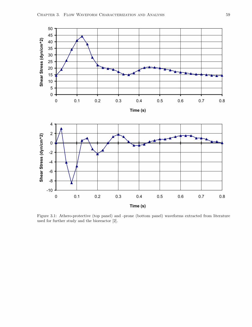
Chapter 3. Flow Waveform Characterization and Analysis 59
0
5
10
15
20
25
30
35
40
45
50
0 0.1 0.2 0.3 0.4 0.5 0.6 0.7 0.8
Time (s)
Sh
ear
Str
ess
(dyn
/cm
^2)
-10
-8
-6
-4
-2
0
2
4
0 0.1 0.2 0.3 0.4 0.5 0.6 0.7 0.8
Time (s)
Sh
ear
Str
ess
(dyn
/cm
^2)
Figure 3.1: Athero-protective (top panel) and -prone (bottom panel) waveforms extracted from literatureused for further study and the bioreactor [2].

Chapter 3. Flow Waveform Characterization and Analysis 60
0.0000
5.0000
10.0000
15.0000
20.0000
25.0000
30.0000
35.0000
40.0000
0 0.1 0.2 0.3 0.4
Time (s)
Sh
ear
Str
ess
(dyn
/cm
^2)
-2.0000
-1.5000
-1.0000
-0.5000
0.0000
0.5000
1.0000
0 0.1 0.2 0.3 0.4
Time (s)
Sh
ear
Str
ess
(dyn
/cm
^2)
Figure 3.2: Disease-protective (ventricular side, top panel) and -prone (aortic side, bottom panel) CAVDwaveforms obtained from literature used for further study and the bioreactor. Cycles continue until 0.85 sbut are zero past what is shown [27].
PVD
Unlike the two previous CVDs, the extraction of a waveform representing PVD was not as straight forward.
It was decided to focus on lower limb arteries as they are commonly affected by diabetes. However, a
waveform of shear stress in a typical artery could not be located. A flow waveform in a popliteal artery
study was employed which measured arterial flow in several patients via two-dimensional cine-mode phase-
contrast magnetic resonance imaging [82]. The waveform was extracted by correlating the magnitude scales
provided in the article with the pixels of captured images of the waveforms. Sinc interpolation was carried
out using a MatLab (MathWorks; Natick, Massachusetts, USA) protocol (provided in Appendix B.4 on

Chapter 3. Flow Waveform Characterization and Analysis 61
p. 178) on the extracted flow waveform to provide data at increments of 0.001 s before carrying out further
analysis (Figure 3.3 on p. 63). A time scale was not provided in the literature, so the total cycle time was
estimated by using the quoted average heart rate of 71 beats per minute (bpm) in the article using the
conversion that cycle time (s) = 60/heart rate (bpm). Following a discussion with an expert in the field (Dr.
David Steinman of the Department of Mechanical and Industrial Engineering at the University of Toronto),
Womersley analysis using an in-house Fortran code (provided courtesy of Dr. Steinman, and which can be
found in Appendix C) was used to convert the flow to the corresponding shear stress magnitudes accounting
for pulsatility effects. To carry out the conversion, the fluid was assumed to have a nominal viscosity of
3.5 cP and density of 1050 kg/m3. The size of the popliteal artery was assumed to be constant, and was
estimated from literature which carried out echo-tracking B-mode ultrasonography to discover arterial sizing
[83]. The popliteal waveform was quoted to be for a patient of an average age of 60, and an age similar to
this was used from the sizing study (66.8 years) to determine vessel size, yielding a diameter value of 8.4
mm. The data was then converted into its Fourier Series up to an accuracy of 400 coefficients using another
MatLab protocol (provided in Appendix B.3 on p. 152). The first 150 coefficients (a limit set by the Fortran
code) were employed to create the resulting shear waveform (Figure 3.3 on p. 63).
3.2.2 Fast Fourier Transform and Nyquist Analyses
To discover at what frequency the developed waveforms needed to be sampled at to avoid data loss, FFT
analysis was carried out using a MatLab protocol (provided in Appendix B.2 on p. 151). The highest
frequency component was then extracted to carry out a Nyquist analysis to determine the required sampling
rate. The analyses showed that the smallest time increment required was 200 ms (Table 3.1 on p. 62).
Therefore, it was concluded that the waveform replicated by the bioreactor must change its magnitude at a
rate of every 200 ms at minimum to ensure sufficient accuracy.
3.2.3 Conversion of Physiological Shear Waveforms into Microfluidic Flow Rates
The derived shear waveforms were then converted into the flow waveforms to re-create the in vivo shear
stresses on the ECs within the microfluidic device. As will be discussed in Chapter 4, the ECs will be laid
down along the vertical bottom of the microfluidic channel coinciding with a glass microscope slide. The
calculated shear values represent the centreline of the vertical bottom. The Purday approximation or full
rectangular channel flow equations were employed (as discussed in the Literature Review in Section 2.2.4
on p. 23), and a custom MatLab program was created to carry out the analysis, which is provided in
Appendix B.8 on p. 191. As expected, variations in height were shown to have much larger effects on the
converted flow waveforms compared to those in width (Figure 3.4 on p. 64).

Chapter 3. Flow Waveform Characterization and Analysis 62
WaveformTime
Increment (s)Data
Points
MaximumComplex
Amplitude
Frequency atMaximumAmplitude
(Hz)
RequiredTime
Increment(s)
Athero-Protective
0.025 33 118.3 2.50 0.200
Athero-Prone
0.025 33 23.9 1.25 0.400
Ventricular-Side,
CAVD0.0100 86 728 1.163 0.423
Aortic-Side,CAVD
0.0100 86 8.51 1.163 0.423
PoplitealArtery, PVD
0.047 19 1195 2.37 0.211
Table 3.1: Summary of FFT and Nyquist analyses of physiological waveforms. Waveform: the CVD waveformbeing analyzed. Time Increment: the time spacing between each data point of the waveform. Data points:the number of data points comprising the waveform. Maximum complex amplitude: the resulting maximumcomplex amplitude value when the FFT of the waveform is taken. Frequency at Maximum Amplitude:the corresponding frequency at the maximum complex amplitude. Required Time Increment: the requiredsampling interval for reproducing the waveform without signal loss or aliasing using the Nyquist samplingtheorem.
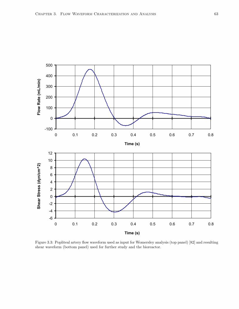
Chapter 3. Flow Waveform Characterization and Analysis 63
-100
0
100
200
300
400
500
0 0.1 0.2 0.3 0.4 0.5 0.6 0.7 0.8
Time (s)
Flo
w R
ate
(mL
/min
)
-6
-4
-2
0
2
4
6
8
10
12
0 0.1 0.2 0.3 0.4 0.5 0.6 0.7 0.8
Time (s)
Sh
ear
Str
ess
(dyn
/cm
^2)
Figure 3.3: Popliteal artery flow waveform used as input for Womersley analysis (top panel) [82] and resultingshear waveform (bottom panel) used for further study and the bioreactor.
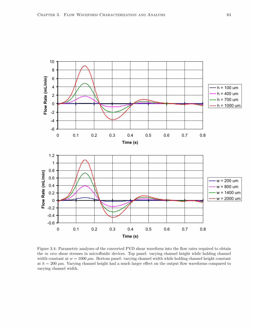
Chapter 3. Flow Waveform Characterization and Analysis 64
-6
-4
-2
0
2
4
6
8
10
0 0.1 0.2 0.3 0.4 0.5 0.6 0.7 0.8
Time (s)
Flo
w R
ate
(mL
/min
)
h = 100 um
h = 400 um
h = 700 um
h = 1000 um
-0.6
-0.4
-0.2
0
0.2
0.4
0.6
0.8
1
1.2
0 0.1 0.2 0.3 0.4 0.5 0.6 0.7 0.8
Time (s)
Flo
w R
ate
(mL
/min
)
w = 200 um
w = 800 um
w = 1400 um
w = 2000 um
Figure 3.4: Parametric analyses of the converted PVD shear waveform into the flow rates required to obtainthe in vivo shear stresses in microfluidic devices. Top panel: varying channel height while holding channelwidth constant at w = 1000 µm. Bottom panel: varying channel width while holding channel height constantat h = 200 µm. Varying channel height had a much larger effect on the output flow waveforms compared tovarying channel width.
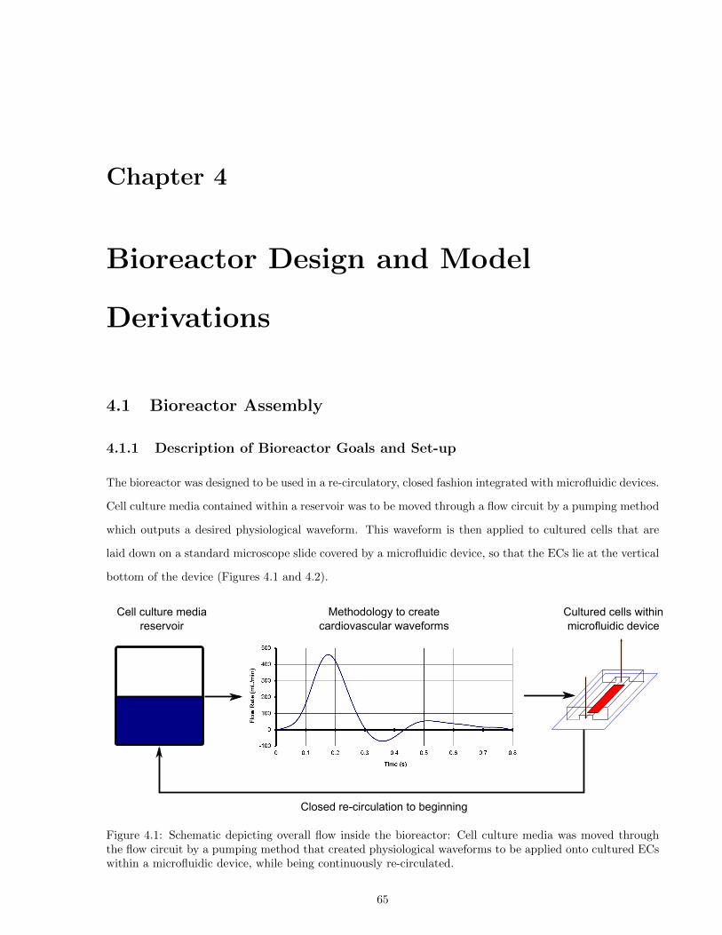
Chapter 4
Bioreactor Design and Model
Derivations
4.1 Bioreactor Assembly
4.1.1 Description of Bioreactor Goals and Set-up
The bioreactor was designed to be used in a re-circulatory, closed fashion integrated with microfluidic devices.
Cell culture media contained within a reservoir was to be moved through a flow circuit by a pumping method
which outputs a desired physiological waveform. This waveform is then applied to cultured cells that are
laid down on a standard microscope slide covered by a microfluidic device, so that the ECs lie at the vertical
bottom of the device (Figures 4.1 and 4.2).
Cell culture mediareservoir
Methodology to createcardiovascular waveforms
Cultured cells withinmicrofluidic device
Closed re-circulation to beginning
Figure 4.1: Schematic depicting overall flow inside the bioreactor: Cell culture media was moved throughthe flow circuit by a pumping method that created physiological waveforms to be applied onto cultured ECswithin a microfluidic device, while being continuously re-circulated.
65

Chapter 4. Bioreactor Design and Model Derivations 66
PDMS Device
EC Layer
Glass Slide
Flow Out
Flow In
Top of PDMS channel
EC layer
Glass slide
Flow
Glass Slide
PDMS Device
Flow (into the page)
EC Layer
Figure 4.2: Schematics of ECs cultured within microfluidic device on microscope slide: overall (top panel),side (middle panel) and cross-sectional (bottom panel) views.
The overall strategy of the setup involved beginning with an in vivo flow waveform and transforming that
into the representative shear waveform applied to ECs in vivo, either through some sort of theoretical analysis
or via previous computational studies that have been carried out. Knowing that it was then necessary to
have the in vivo shear waveform be applied on the ECs in vitro, the in vivo waveform was then transformed
into an in vitro flow waveform to be applied within the microfluidic device on the cultured ECs (Figure 4.3).
Qin vivo τin vivo Qin vitro
CAVD
PVD
Atherosclerosis
ComputationalStudies
MRI Studies
Theoretical Analysis:Purday Approximation
orUnsimplified
Rectangular ChannelFlow
ECs
ComputationalStudies
Theoretical Analysis:Womersley
ComputationalStudies
ComputationalStudies
Pseudo-Physiological
N/AN/A User Defined
Figure 4.3: Flowchart showing steps to move from in vivo to in vitro flow waveform: each step notes wheredata is obtained from for the different flow waveforms.

Chapter 4. Bioreactor Design and Model Derivations 67
4.1.2 Bioreactor Design Requirements
Before beginning design or specification, the bioreactor requirements were described as follows ([84] was used
as a reference). The bioreactor:
• Must be used with a diverse size range of microfluidic devices (i.e. channel dimensions).
• Must have modular capability, i.e. the ability to easily swap different devices in and out for testing.
• Must be able to mimic various physiological waveforms from literature as accurately as possible.
• Must consider flow (shear) as the most important hemodynamic parameter to be accurately replicated,
whereas pressure is secondary and of less importance. Stretch is not to be mimicked at the current
time. Studies have noted that shear stress is more important than pressure or stretch effects in terms
of mechanotransduction and ECs [12], but I provide further justification for this conclusion on the
basis of two main reasons: First, as was discussed in Chapter 2, shear stress has been shown to
play an important role the regulation of the vascular system, from participating in clot formation, to
regulating vascular tone, and regulating transport across vessel walls. More critically, it was noted that
shear stress and the phenotypic response of ECs are connected, which can impact the initiation and
progression of various CVDs. Due to the spatial correlation with regions of disease in CVDs, I believe
that focusing on shear is critical in elucidating CVD disease pathology. The system may be extended
to study the other two stresses at a later point in time (see the Discussion in Chapter 6 for further
details).
• Must be manufactured from components that can withstand autoclave temperature and pressure (120
◦C at 15 psi), as well as resist corrosion within an incubator environment (37 ◦C, 5% CO2 and 100%
humidity).
• Must be manufactured from biocompatible materials that do not leach ions or other elements into the
media.
• Must maintain aseptic conditions during cell culture.
• Must provide gas exchange between incubator and bioreactor environment without compromising steril-
ity, therefore maintaining pH levels of nutrients appropriate to cell culture conditions.
• Must enable the use of microfluidic devices within incubator while equipment is either outside or inside
incubator.
• Must allow for the continuous re-circulation of media after flow over cells in connected microfluidic
device.

Chapter 4. Bioreactor Design and Model Derivations 68
• Must ensure that the total weight of any component required to be inside the incubator during testing
must weigh less than the maximum weight an incubator shelf can support.
4.1.3 Selection of Flow Waveform Creation Strategy
There are three classes of systems to control liquid motion in microfluidic devices. A system may [85]:
1. Use a pressure difference to control the flow rate (i.e. hydrostatic or pressure regulators).
2. Directly impose a flow rate (i.e. syringe pumps).
3. Generate a flow that will depend on the fluidic resistance of the device.
1. Pressure-Based Strategies
Hydrostatic pressure is the simplest way to generate controlled flows in a microfluidic system. A pressure
difference is created by varying the vertical distance of the liquid-to-air interface in different chambers. This
strategy is limited by the Laplace pressure (the difference between the pressure on the outside and inside of
a curved surface caused by the surface tension at the interface of a liquid and that develops at the air-liquid
interface) and which depends on the attraction between the liquid, the atmosphere and the reservoir size
and shape. It should be noted that there is a progressive change in pressure drop as the liquid flows through
one reservoir to the other, resulting in a linear decrease of pressure drop over time.
Pressure regulators may also be used to create flow, but the accuracy of the pressure generated is highly
dependent on the compatibility of all the components involved (chamber, deforming membrane to produce
pressure, and pressure read out) [85]. The major drawback of these systems is the response time being
limited by the mechanical deformation of the membranes in that their material and mechanical properties
define their deformation ability, and hence, the pressures that can be generated [85]. To move past this
disadvantage, a set of electrovalves can be coupled electronically to a pressure sensor, producing a quick
response that can be achieved with microvalves. However, there is a fluctuation associated with the created
pressure which decreases accuracy.
2. Flow-Based Strategies
Syringe pumps were the first flow controllers used in microfluidics. The main advantage of syringe pumps
is their capability of controlling the flow rate across microchannels independently of the fluidic resistance
(the pressure automatically adapts to maintain the flow rate). However, pulsatile flows can be developed
and time is required to stabilize the effective flow rates when compliance in the system is not negligible
[85]. As described in the Literature Review regarding compliance in Section 2.3 on p. 33, a small change in

Chapter 4. Bioreactor Design and Model Derivations 69
dimensions can also vary the pressures within the system which may be a crucial factor in the output results
from biological cell studies if the cell cultures are affected by hemodynamic factors.
3. On-Chip-Based Strategies
Many options exist other than pressure- or flow-based methods that are designed on-chip, or using mi-
crofluidic devices. They range from peristaltic pumps and deforming membranes to create peristaltic flows,
piezo-electric and electro-osmotic pumps. However, these methodologies suffer from a lack of reproducibility
[85].
The resistance-based strategies were eliminated based on the lack of accuracy and reproducibility. Flow-
based strategies were then chosen over pressure-based for several reasons: First, a great deal of flow-based
equipment was readily available in the laboratory versus having to order a whole new array of new compo-
nents, which would have been the case for pressure-based strategies. It was also decided that the fluctuation
in created pressures caused by the components (membrane that drives fluid using pressure and accuracy
of the pressure read out on the controller) involved in creating the flow versus the tuned accuracy of the
flow-based pumps would not be worth addressing, in addition to the programming required to enable the use
of the regulators. Moreover, a flow-based bioreactor already existed in the laboratory [73]. Finally as was
shown in the literature review, flow-based strategies have recently been used to create accurate physiological
waveforms when compared to reference data [70].
Following the literature review of bioreactors provided in the Literature Review in Section 2.3 on p. 33,
a summary of the possibilities for strategies to create the various cardiovascular flows in the flow-based
realm was produced. This included the associated advantages and disadvantages of each strategy (Tables 4.1
and 4.2 on p. 84 and 85, respectively).
4.1.4 Details of Selected Waveform Creation Strategy and Bioreactor Compo-
nents
A combined peristaltic and syringe pump strategy was selected for several reasons: First, this approach built
on and integrated well with the current published steady flow loop system present in the laboratory through
the addition of the syringe pump as well as any other elements needed, such as needle valves, flowmeters,
and pressure sensors [73]. Second, the concept was shown to be applicable in the work of Isenberg et al., but
was missing the accuracy required for obtaining the physiological waveforms [4]. Based on the work of Chin
et al., it was decided that there was a high probability of success following through with this methodology
[70]. Moreover, the approach required few components. Finally in respecting the design requirements as
outlined in Section 4.1.2 on p. 67, the set-up accepted multiple device designs and was modular: the use of
a syringe pump allows for the customization of a waveform to be created in order to mimic flows at various

Chapter 4. Bioreactor Design and Model Derivations 70
vascular sites within the human body.
The setup was designed to consist of the peristaltic and syringe pumps to create the waveforms required,
coupled to one or two dampening reservoir(s) and a culture chamber. An in-line flowmeter was used to be
sourced to ensure that appropriate waveforms were being obtained and that predictions were correct. If a
flowmeter was not used, PIV was instead (Figure 4.4).
Q
1.
2.
7.
5.
4.
3.
6.
Figure 4.4: Schematic of the components of the bioreactor: 1. Media reservoir (open to atmosphere forventing), 2. peristaltic pump, 3. damper, 4. syringe pump, 5. flowmeter, 6. PIV laser, 7. microfluidic devicewith cultured endothelial cells.
The waveform creation strategy involved combining the steady output of the peristaltic pump and one
or two small damper(s) with a syringe pump. To ensure that during experimentation the syringes do not
empty and have to be refilled, it was decided to verify that one syringe pump cycle injects as much fluid into
the system as it extracts. To accomplish this, the functional average of the in vitro flow waveform is found
through
Qcardiacaverage =1
tfinal − tinitial
∫ tfinal
tinitial
Qcardiac(t) dt (4.1)
where tinitial and tfinal are the respective beginning and end times of the cardiac cycle being investigated
and Qcardiac is the cardiovascular flow waveform which is a function of of time. In this sense over each cycle,
the volume input is equal to that being output. The peristaltic pump is then set at this average value, while
the syringe pump is set at a value equal to Qcardiac − Qcardiacaverage. Modelling the union of the damper

Chapter 4. Bioreactor Design and Model Derivations 71
and syringe output as a superposition of the two flows, the original in vitro flow waveform will be recovered
before entering the microfluidic device.
Acceptable peristaltic pumps were already present in the laboratory. However, it was necessary to test
various syringe pumps and linear actuators to ensure sufficient performance characteristics.
4.2 Syringe Pump and Linear Actuator Testing
Several options were tested to specify a pump or linear actuator that could output the required unsteady,
time-varying waveforms for the bioreactor. These options included:
• The Cole-Parmer Model #EW-74901-10 Syringe Pump.
• The Harvard Apparatus PHD Ultra Infusion/Withdrawal Programmable Syringe Pump.
• The creation of a syringe pump in the laboratory with an UltraMotion Digit Linear Actuator, Model
#D-A.083-HT17-2- 1NO-BR/4.
• The cetoni GmbH neMESYS Syringe Pump.
4.2.1 MatLab NAVITAR Motion Analysis Protocol
To test the actuator motion of the pumps or linear actuators, a Matlab protocol was created to track their
movements, as provided in Appendix B.1 on p. 146. A NAVITAR scope with a 12X body scope and macro
ZFL scope attachment (Navitar, Inc; Rochester, NY, USA, respective parts #1-50487AD and #1-6010)
was used to capture a video of the actuators’ motions illuminated using a SCHOTT DCR III light source
(SCHOTT North America Inc.; San Jose, CA, USA), along with a Sony XCD-X710 camera (Sony; Minato,
Tokyo, Japan), and Fire-i software (UniBrain; San Ramon, CA, USA). The created code converts the video
into its constituent picture frames, compares the distance travelled by the actuator from one frame to the
next, and outputs the distance as a number of pixels. By taking a still image with the camera and measuring
a known item in pixels and in metric units, the number of pixels was then converted into a displacement in
µm or mm. The camera frame rate was fixed and set at its maximum of 30 Hz. The distance was finally
output as a displacement from a reference point (defined as the origin). This experimental displacement
could be compared to the theoretical, which was calculated with the methodologies that will be discussed in
Section 4.2.5.
4.2.2 LabView Programming
LabView (National Instruments; Austin, TX, USA) programs were created to control the Cole-Parmer and
Harvard Apparatus syringe pumps. A text file containing a set of flow rates was read in to either program.

Chapter 4. Bioreactor Design and Model Derivations 72
The user could control the time increment between each flow point, i.e., how often the pumps would change
their flow rates.
4.2.3 Cole-Parmer Syringe Pump
The Cole-Parmer Model #EW-74901-10 Syringe Pump (Cole-Parmer; Montreal, QC) was already present
in the laboratory and was tested as the first possibility for creating the necessary flow waveform. As was
discussed, a LabView program was created to test the capabilities of the pump.
It was found that the pump could not reliably and repeatedly alter its flow rate faster than steps of
250 ms and hence, did not meet the 200 ms requirement obtained from the FFT analysis carried out in
Section 3.2.2 on p. 61. Hence, it was discarded as a viable option.
4.2.4 Harvard Apparatus Syringe Pump
The Harvard Apparatus PHD Ultra Infusion/Withdrawal Programmable Syringe Pump (Harvard Apparatus;
Holliston, MA, USA) was thought to be a more viable option, as it is quoted as being able to be programmed
via computer control at time steps as small as 50 ms [86]. The pump was obtained from the laboratory of
Warren Chan at the University of Toronto for testing. Another LabView program was created to test the
capabilities of the device.
It was found that while the pump could change its flow rate quite quickly when running in only one of the
infusion or withdrawal directions, the pump quickly froze when alternating between infusion and withdrawal
directions in succession. As can be seen in the waveforms presented in Section 3.2 on p. 58, the flows alternate
between positive and negative directions requiring a pump that can reliably run bi-directionally. Hence, this
pump was also rejected as a possibility for the bioreactor.
4.2.5 UltraMotion Linear Actuator
It was thought that a syringe pump could be created in the laboratory using the motion of a linear actuator.
An UltraMotion Digit Linear Actuator, Model #D-A.083-HT17-2- 1NO-BR/4 (UltraMotion; Cutchogue,
NY, USA) was connected to a programmable Applied Motion Model #Si2035 step motor drive. Instructions
were sent through the USB port of a computer using Si Programmer software from Applied Motion. Following
previous work carried out by Dobbie, the actuator motor was wired in parallel to the motor drive [87].
Instructions for waveform data points could not be directly programmed as flow rates in this case, and had
to be converted to equivalent distances moved over time. The command “feed to length” in Si Programmer
was employed for each time step. The acceleration, deceleration, velocity, distance, and direction were chosen.
Acceleration and deceleration were maximized for every step to keep lag as low as possible (Figure 4.5).

Chapter 4. Bioreactor Design and Model Derivations 73
Figure 4.5: Components of testing the UltraMotion Digit linear actuator: actuator (top panel), AppliedMotion Si2035 step motor drive (middle panel), and eight lead parallel connection used to wire the actuatorand drive (bottom panel) [87, 88].
To convert the flow rate data into distances and velocities, it was assumed that after the small acceleration
and deceleration portions of each time step that the velocity was constant within, what would be, the syringe
attached to the linear actuator. Also, that there was no loss of speed between the linear actuator and syringe
plunger. Hence, the supplied flow rate is the product of the actuator velocity, v, and cross-sectional of the
syringe, As:
Q = vAs (4.2)
The actuator velocity was then calculated as the distance traversed, ∆x, over a time period, ∆t:
v =∆x
∆t(4.3)
This enabled the conversion of flow rates into equivalent distances (lengths to feed) and velocities at which
to move.
Unfortunately there were several challenges in attempting to employ the linear actuator: The Si Pro-
grammer program only allows for fixed steps of velocity to be input, and not arbitrary set amounts. This

Chapter 4. Bioreactor Design and Model Derivations 74
alters the output flow rate if the velocity used in the calculations is not maintained. On the other hand,
distance travelled may be set arbitrarily (entered via a text box). But, inaccuracy was present again as the
distance is rounded to the nearest 10 µm measurement, which can produce large differences in the output
flow rates, especially when accumulated over time. For example: with a 10 mL Becton-Dickinson plastic
syringe (Becton Dickinson and Company (BD); Mississauga, ON), the inner diameter is 14.5 mm [89]. With
a flow rate of 0.5 mL/min, this translates into the syringe moving 3.03 mm/min via Equation 4.3. This can
be converted to 50 µm/s. Over a 0.1 s time step, a 5 µm displacement should take place, but this can be
offset by a significantly large factor due to the rounding of the displacement value.
Issues were also seen from experimentation. Using the MatLab protocol described in Section 4.2.1, the
experimental displacement of the actuator was compared to that theoretically predicted by Equations 4.2
and 4.3. Experiments with time points spaced at 100, 50, and 25 ms were carried out using a combination
of the athero-prone and aortic- or ventricular-side CAVD waveforms, converted from shear, to flow, to
equivalent displacement values. Tests showed that as time went on the differences between the experimental
results and theoretical predictions of actuator displacement kept growing (Figures E.1 through E.5 on p. 282
through 284). For this reason, it was concluded that the actuator was not outputting the necessary motion
over each cycle, leading to the accumulation of error seen. Hence, it was also deemed as an unviable option
for waveform creation. Appendix E on p. 282 can be consulted for test results.
4.2.6 cetoni neMESYS Syringe Pump
The cetoni neMESYS Syringe Pump (cetoni Automation and Microsystems; Korbussen, Thuringia, Ger-
many) (known from here on as the neMESYS) comes with software capable of programming waveforms at
very high speeds and small time steps and is pulsation free; an essential feature for microfluidic flows [90].
Using the MatLab protocol described in Section 4.2.1 on p. 71, the experimental displacement of the pump’s
actuator was compared to that theoretically predicted by Equations 4.2 and 4.3 on p. 73. A sinusoidal
waveform with a period of 1 s was programmed into the neMESYS with 0.1 s data point increments, similar
to the physiological waveform that would be employed. A small drift between the experimental and the-
oretical results was observed, and it was was assumed to be due to parallax errors, i.e., the camera’s axis
being slightly skewed from following the straight path of the pump’s actuator motion (Figure 4.6 on p. 75).
Separate tests carried out later showed no skewing. It was discovered after that the smallest allowable time
increment for programming was 100 ms. Combining the results of the two experiments, it was concluded
that accurate displacement profiles can be obtained using the neMESYS so long as data points are varied
at increments of 100 ms or larger. Hence, the neMESYS was selected as the option to move forward with
due to its adequate performance and motion characteristics, as seen in the experimental results along with
the time step agreement seen with the FFT analysis carried out in Section 3.2.2 on p. 61. The pump was

Chapter 4. Bioreactor Design and Model Derivations 75
-0.5
0
0.5
1
1.5
2
2.5
3
3.5
0 5 10 15 20 25
Time (s)
Dis
pla
cem
ent
fro
m O
rig
in (
mm
)
Theoretical
Experimental
Figure 4.6: Actuator motion test tracked using a 100 ms data point increment sinusoidal waveform and theneMESYS pump: The theoretical and experimental motion paths matched well except for a parallax offset,which was shown to not be present in other tests.
also readily available in a shared laboratory, and came supplied with customized software which allows for
the creation and selection of flow profiles for arbitrary syringe sizes without the need to manually perform
calculations such as those performed with the Digit linear actuator.
4.3 Flowmeter Specification and Standardization
4.3.1 Flowmeter Options and Selection
A flowmeter was a crucial component in the bioreactor to allow for flow testing and validation and several
options were sourced (Table 4.3 on p. 76). After discussion and deliberation, the Alicat Scientific L-series
flowmeter (Alicat Scientific; Tucson, AZ, USA) was selected due to it being the option with the lowest
cost during initial flowmeter sourcing, being used in a similar previous study that replicated physiological
waveforms using a bioreactor [76], and the rate at which it captures data points being faster than what
was required to maintain the accuracy of physiological waveforms according to the supplier (as analyzed in
Section 3.2.2 on p. 61). After testing, it was determined that the Alicat flowmeter was not suitable for the
application due to accuracy issues (see Section 5.1 on p. 86). The flowmeter was returned and the Sensirion
SLI-2000 was then sourced. The SLI-2000 proved to provide reliable data with much less troubleshooting
and set up requirements.

Chapter 4. Bioreactor Design and Model Derivations 76
Supplier Cost Additional Details
Cole Parmer $1,460Model #RK-32908-44, range of
0-100 mL/min
Omega $1,460
Model #FLR-1600A. Digital
display and output, mostly used
for water-based applications and
not those in the biomedical
realm, range of 4-200 mL/min
Transonic $14,100Used specifically for cardio- and
peri-vascular applications
Alicat Scientific $1,377
L-series liquid flowmeter.
Laminar flow element type.
Used in a similar vascular
bioreactor study with similar
media as used in the laboratory
[76]. Capable of capturing data
at 50 ms time intervals
Sensirion AG $1,290
Model #SLI-2000, range of 0-5
mL/min. Non-invasive. Capable
of capturing data at up to 1 ms
time intervals
Table 4.3: Flowmeter options for bioreactor.
4.3.2 Specification of Alicat Flowmeter Scale and Error
For the Alicat flowmeter, the turn down ratio of the flowmeter was 50:1, which means that dividing the
maximum flow rate the meter is scaled to by fifty yields the minimum flow rate that it can measure. Because
of the wide range of flow rates possible in the bioreactor (depending on waveform selection and device
dimensions), it was decided to fix the waveforms to be used along with specific device dimensions, and
perform testing based on the resulting ranges.
Athero-prone and -protective waveforms were employed (as provided in Section 3.2.1 on p. 58) with
device dimensions being of channel height and width being 212.5 and 1500 µm, respectively. The meter

Chapter 4. Bioreactor Design and Model Derivations 77
was requested to be calibrated to the maximum flow rate seen in the waveforms of 3.5 mL/min which then
corresponded to a minimum measurable flow rate of 0.07 mL/min.
The error on the flowmeter was rated at 2.0% of it’s full range, which corresponds to an error of +/-0.07
mL/min for the specific range selected.
4.4 Assembled Bioreactor Specifications
After all of the bioreactor components were received the bioreactor was assembled (Figure 4.7). A schematic
layout of the assembled bioreactor was created along with a bill of materials corresponding to the item
numbers in the schematic (Figure I.1). Item descriptions and suppliers were also noted as the bioreactor was
assembled (Table I.1). These items can be found in Appendix I.1 on page 345.
1.
2.
3.
4.
9.
8.
7.6.
5.
Figure 4.7: Assembled bioreactor in non-recirculatory configuration (outlet of microfluidic device runningto waste beaker instead of back to media reservoir) with major components highlighted: 1. Computercontrolling neMESYS and receiving flowmeter data, 2. media reservoir, 3. peristaltic pump, 4. damper, 5.neMESYS, 6. three-way tee, 7. Sensirion flowmeter, 8. microfluidic device, 9. waste beaker.
4.5 Bioreactor Model Derivations
4.5.1 Flow Assumptions
Throughout the thesis unless an exception is noted, the flow within the bioreactor tubing and microfluidic
device channel carries the following assumptions:

Chapter 4. Bioreactor Design and Model Derivations 78
• Newtonian - Tests were done using de-ionized or distilled water, which is commonly assumed to be
Newtonian at constant temperatures. Cell culture media which will be used in the bioreactor eventually
may exhibit non-Newtonian characteristics, but was not tested during the course of this thesis.
• Quasi-Steady - Over one time step at the neMESYS pump changes its flow rate, it is assumed that
the flow exhibits quasi-equilibrium behaviour: properties such as velocity, pressure drop and shear
stress of the flow instantaneously change with the alteration of flow rate through each time step.
• Laminar - At the microfluidic scale, Reynolds numbers are on the order of unity, well within the
laminar range.
• Fully developed - All experimental measurements were taken past the entrance length of the mi-
crofluidic devices.
• Isothermal - Temperature was not altered during experiments.
• Constant pressure drop across channel - See explanation for steady flow.
As well, the microfluidic devices only have a single rectangular channel.
4.5.2 Pressure Prediction and Deformation Verification inside Microfluidic Chan-
nel
A theoretical model was created to predict the pressures within the microfluidic device for two primary
reasons: First, to ensure that the pressures exerted on the ECs do not extend far beyond the physiological
range. Second, as discussed in Section 2.2.8 on p. 31, PDMS can bulge and deform, and it was desired
to establish prior to any experimentation if pressures within the device would be far too high and lead to
deformation effects.
Microfluidic Channel Pressure Model
Using the concept of flow resistance (as described in Section 2.2.5 on p. 28), and following through with
the Purday approximation of flow in a rectangular channel as defined in Section 2.2.4 on p. 23, the flow
resistance, Rpurday, becomes
Rpurday =µLf · Re
4ADh2 (4.4)
where A is the cross-sectional area of the channel and Dh the hydraulic diameter, respectively calculated as
A = wh (4.5)
Dh =2wh
w + h(4.6)

Chapter 4. Bioreactor Design and Model Derivations 79
The friction factor and Reynolds number term are calculated following the Purday approximation analysis
of Shah and Lodon as [44]:
f · Re = 24(1− 1.3553α+ 1.9467α2 − 1.7012α3 + 0.9564α4 − 0.2537α5) (4.7)
These equations enable the calculation of pressure drop across the length of the channel given an input flow
waveform.
Examination of Deformation due to Pressure inside Microfluidic Channel
From the work of Gervais et al. [49], the change in flow rate between a rigid and deformable channel can be
written, assuming a worst-case scenario of the empirical constant defined in Equation 2.45 in Section 2.2.8
on p. 32 being equal to unity, through
∆Q
Q=Qdeform −Qrigid
Qrigid=
3
2
∆Pw
Eh0(4.8)
A Microsoft Excel (Microsoft; Redmond, WA, USA) spreadsheet was programmed with the derived pressure
model to convert the flow rates derived from the Purday approximation into associated pressure drops across
the microfluidic device over one simulated cardiac cycle. In work by Srigunapalan et al., which this thesis
builds upon, single channel microfluidic devices had typical dimensions of 1500 µm x 212.5 µm x 3 cm (w
x h x l), and these dimensions were assumed to be standard for experimentation [73]. Pressures can easily
be verified for other devices and dimensions using the Matlab shear to flow conversion protocol (refer to
Appendix B.8 on p. 191) and Microsoft Excel spreadsheet. It is assumed that following the microfluidic
device there is a certain length of exit tubing which returns the fluid back to the media reservoir that is
at atmospheric pressure. Hence, the pressure drop varies according to the length of the exit tubing. The
pressure drop along the tubing can be calculated, assuming Poiseuille flow, from Equation 2.41 on p. 29.
When an extremely long exit tubing length of 30” with an inner diameter of 1.19 mm (equal to that
of Intramedic PE190) and a disproportionately high flow rate of 10 mL/min were selected as a worst case
scenario, the pressure drop across the channel was calculated to be 3296 Pa and the pressure at the channel
entrance 5154 Pa, or 38.7 mmHg, assuming a media viscosity of 0.72 cP [71]. While physiological pressures
in terms of systole and diastole typically range between 80-120 mmHg, the goal was to ensure a pressure
that is not order of magnitudes different than the physiological range. As well, resistance additions to the
bioreactor could vary the pressures while maintaining the flow rates, depending on what is desired.
When substituting the associated 3296 Pa pressure drop into Equation 4.8 assuming a nominal PDMS
elastic modulus of 1 MPa [49], the flow difference equates to 3.49%. In fact, Equaton 4.8 over-estimates the
difference between the rigid and deformable flow rates in this work as the rigid flow estimate is based on

Chapter 4. Bioreactor Design and Model Derivations 80
the Pouseille flow assumption for rectangular channels, which calculates resistance through Equation 2.40
on p. 29. This should be compared to Equation 4.4 on p. 78, which accounts for wall effects, and is much
more accurate.
When employing flow rates far closer to those resulting from the shear to flow conversions (averaging
2 mL/min), the pressure drop across the channel becomes 659 Pa, and the difference between rigid and
deformable flow 0.698%. Compared to the differences that were assumed to arise due to the fluidics, friction,
and pumps, this was concluded to be negligible.
The maximum height deflection can be calculated from Equation 2.46 on p. 32, assuming c1 to be unity,
p as a typical maximum pressure in the channel at the entrance of 1000 Pa, w = 1500 µm, and E = 1 MPa.
The maximum deflection equates to approximately 1.5 µm. The flow rate to create the required in vitro
shear stresses was calculated assuming that no deflection occurs. This value was then used to compare the
shear stress at the vertical bottom centreline of the channel with and without taking into account channel
deflection. For example, the maximum shear stress for the PVD waveform was 1.039 Pa with an associated
flow rate of 0.715 mL/min without accounting for deflection. Accounting for the 1.5 µm deflection in height,
the shear stress becomes 1.025 Pa, representing a negligible variation in shear stress (1.347%). Hence, channel
height deformation was assumed to not affect in vitro shear stress, and was not accounted for in the rest of
the work.
The Difference in Pressures Applied to the ECs along Channel Length
While discussing pressure drops within the microfluidic channel, it was important to realize that the ECs
cultured within the microfluidic device would experience different pressures depending on their location
along the ordinate running parallel with the length of the channel. Considering flow direction, ECs at the
beginning of the channel would experience pressures differing to those at the end of the channel by a factor
calculated through the concept of flow resistance (Section 2.2.5 on p. 28) and Equation 4.4 on p. 78. If a
channel is perfectly rigid the pressure drop varies linearly. Equivalently expressing the pressure gradient in
this scenario as a differential function of the ordinate parallel with the channel length, z:
∂p(z)
∂z=µf · Re
4ADh2 (4.9)
A similar situation results when there is very little deformation experienced, as was shown was the case for
this study. Hence, it was assumed that the ECs in the channel experience a pressure varying linearly with
the channel length ordinate dimension (Figure 4.8 on p. 81). This would be an important item to keep in
mind when analyzing the cell culture after flow experiments. Thus, the pressure difference at any point, (g),

Chapter 4. Bioreactor Design and Model Derivations 81
labelled P (g), may be calculated as
P (g) =µf · Re
4ADh2Q+ P (0) (4.10)
where g is the location of point (g) with reference to the ordinate of the channel length dimension, and P (0)
is the pressure at the channel entrance.
+z
0L z (um)
P(Pa)
g
P(g)
Top of PDMS channel
EC layer
Glass slide
Flow
Figure 4.8: ECs experiencing a linearly decreasing pressure along the channel length. A cross-sectional viewof the device is shown: It was essential to realize that the ECs cultured within the microfluidic device wouldnot be subjected to a uniform pressure throughout the device, creating a certain amount of heterogeneityin terms of hemodynamic forces applied. The effects of pressure could be studied by taking cell samples forstudy from different locations along the channel length.
4.5.3 Microfluidic Device Dimension Limits
Integral in the design of the bioreactor is the discovery of the limits of microchannel dimensions for flow
experiments. While there may be empirical items that must be discovered in experiments, such as at what
flow rates leaks will occur, two numerical criteria were present:
1. The maximum flow rate that the neMESYS can output is approximately 6 mL/min with a 1 mL syringe
(when input into the neMESYS control software).
2. The aspect ratio (height to width) of any channel must be greater than 1:10, with the largest ratio
being 1:1 [48].
Criterion #1 is self explanatory. Criterion #2 stems from preventing channel collapse due to not having
enough support for the structure. Should micro-posts be used within the channel (small post-like structures
along channel length), then this criterion becomes less necessary.

Chapter 4. Bioreactor Design and Model Derivations 82
It was assumed that the fluid viscosity was that of cell culture media, at 0.72 cP [71]. Previous work in the
laboratory carried out by Srigunapalan et al. was used as a basis for selecting size limits, where dimensional
ranges of:
Width: 100 µm to 2 cm
Height: 50 µm to 500 µm
were employed [73]. Choosing to fix width and vary height, the minimum width of 100 µm was first employed.
Flow rates were derived using the MatLab shear calculation protocol (Appendix B.8) until the height to width
ratio being 1:1 was the limiting factor, or a maximum flow rate of 6 mL/min was found. In further detail,
subject to criterion #2, all device heights with a width of 525 µm are usable so long as they are greater
than the 1:10 value required, and less than 1:1. However, if a larger width is used, such as 2000 µm, an
equal height yields a flow rate far greater than the allowed maximum provided by criterion #1. In steps of
25 µm past a width of 525 µm, the maximum heights were calculated to yield maximum flow rates less than
6 mL/min (Figure 4.9).
0
100
200
300
400
500
600
0 500 1000 1500 2000 2500
Channel Width (um)
Ch
ann
el H
eig
ht
(um
)
Figure 4.9: Maximum micro-channel heights against widths subject to design criteria for bioreactor, assumingcell culture media as the fluid.
4.5.4 Sufficient Volume Verification for a 1 mL Syringe
A 1 mL syringe was to be employed with the neMESYS pump to obtain accurate waveforms, as will be
shown in Chapter 5. It was essential to ensure that enough volume would be present in the syringe during
the infuse step (so that the pump is not trying to infuse when there is no media present). The waveforms
that the neMESYS would need to programmed with for each of the physiological waveforms were found using
the MatLab shear calculation protocol (Appendix B.8 on p. 191). The flow waveforms for each maximum
device dimension case presented in Section 4.5.3 on p. 81 were all of similar magnitude. The waveforms

Chapter 4. Bioreactor Design and Model Derivations 83
were obtained at the largest width of the range, 2075 µm, and the corresponding height of 225 µm. As the
volume input was equal to that of the output, all of the negative values over time were set to zero, and the
flow rate curves were integrated over time to calculate the volume input over the infuse portion of the cycle
using Simpson’s Rule. It was found that all volume inputs were less than 1 mL (Table 4.4 on p. 85).

Chapter 4. Bioreactor Design and Model Derivations 84
Strategy Advantages Disadvantages
Balloon Pump• Self-contained lowering
risk of contamination withmedia
• Pressures and flows maybe too high for microflu-idic systems and may causecells to detach
• Cumbersome
• Less fine and precise con-trol over motion
• May not be able to producelow shear stresses
Ventricular Pump• Self-contained lowering
risk of contamination withmedia
• Pressures and flows maybe too high for microflu-idic systems and may causecells to detach
• Less fine and precise con-trol over motion
• May not be able to producelow shear stresses
• Complex design requiredto achieve pumping action
Bulb Pump• Relatively simple set up • High pressures and flows
may be too high for mi-crofluidic systems and maycause cells to detach
• Less fine and precise con-trol over motion
Cup and Cone Device• Accepted standard by lit-
erature for shear stress ap-plication on to cell popula-tions
• Not compatible withmicrofluidic devices andadopted strategy (cellscontained within microflu-idic device)
• Potential issues creatingdiscontinuous shear wave-form on cells
Syringe Pump• Available in laboratory
• Other options com-mercially available iflaboratory versions notsatisfactory
• Possibilities of perfor-mance issues to providesufficient accuracy forwaveform creation
Table 4.1: Summary of physiological waveform creation strategies and associated advantages and disadvan-tages, 1 of 2.

Chapter 4. Bioreactor Design and Model Derivations 85
Strategy Advantages Disadvantages
Peristaltic Pump• Well defined flow
• No programming required
• Available in laboratory
• Inability to create continu-ous flow without additions(compliance chambers ordampers)
• No possibility of produc-ing a customized (physio-logical) waveform on own
Combined Peristaltic and Sy-ringe Pumps • Available in laboratory
Cardiac Pump• No programming required
• Low level of adjustmentand configuration
• Expensive
• Inflexibility in waveformselection
Table 4.2: Summary of physiological waveform creation strategies and associated advantages and disadvan-tages, 2 of 2.
Waveform Volume Input (mL)
Athero-Prone 1.331E-03
Athero-Protective 4.954E-03
Aortic 2.309E-04
Ventricular 1.256E-02
PVD 2.121E-03
Table 4.4: Sufficient volume verification for a 1 mL syringe - volumes input by neMESYS during infusesteps for each physiological waveform using channel dimensions that include flow rates up to the maximumallowable value 6 mL/min (width of 2075 µm, height of 225 µm). All volumes were found to be less than 1mL.

Chapter 5
Bioreactor Validation and Results
This chapter describes the testing, implementation, troubleshooting, and validation of bioreactor flow wave-
form testing. The chapter is divided into three portions of experimentation:
1. Validation using Alicat flowmeter - the first flowmeter acquired which was found to not be usable
for the application.
2. Validation using particle image velocimetry - during the intermittent stages of waiting for a new
flowmeter to arrive, PIV was employed as a validation step and to also obtain detailed velocity profile
data.
3. Validation using Sensirion flowmeter - the second flowmeter acquired.
For all of the proceeding results, it is important to note that the neMESYS created sinusoidal flow
waveforms by approximating the profiles in defined time steps over a specific period (i.e. the waveform
was not continuously interpolated between steps). This created step functions that resembled sinusoids
(Figure 5.1 on p. 87). neMESYS flow waveforms were programmed using proprietary software that came
with the pump (cetoni Automation and Microsystems; Korbussen, Thuringia, Germany), and with successive
data points at 0.1 s time increments unless otherwise noted. As well, unless otherwise noted, microfluidic
devices were fabricated according to standard laboratory procedures documented in other sources [91].
5.1 Validation Using Alicat Flowmeter
Validation of the bioreactor was first carried out using the Alicat flowmeter, as detailed in Section 4.3
on p. 75. Calibration of the flowmeter was tested by applying constant flows using the peristaltic and
neMESYS pumps. Both tests proved to be accurate. However when moving to sinusoidal waveforms, the
shape, magnitude, and temporal characteristics of the experimental flow data were incorrect: the waveforms
86

Chapter 5. Bioreactor Validation and Results 87
Q
t
Theoretical
Step-approximation by neMESYS
Figure 5.1: Step profile created using neMESYS to resemble a sinusoidal waveform: The neMESYS outputsflow rates changing at a maximum of every 100 ms. For sinusoidal profiles, the estimation is made by keepingflow rate steps constant over every 100 ms interval, constructing a curve that approximates a sinusoid.
showed phase shifting behaviour, where the experimental and theoretical data would begin in phase, then
move to be completely out of phase, and then later back in phase again. The expected flow magnitude was
also incorrect. Troubleshooting revealed that the source of the phase lag issues was the recording method,
i.e., using HyperTerminal to stream flow data from the flowmeter. The solution was using an Arduino
Uno microcontroller to read the data directly from the flowmeter. The magnitude issues, however, could
not be solved: Various portions of the experimental setup were changed, the flowmeter was sent back for
recalibration and cleaning, and finally a new unit was ordered in. It was concluded after all this testing that
this specific flowmeter was unacceptable for use for the work.
It was decided to abandon the Alicat flowmeter at this point and source a new model, while concurrently
focusing on a different validation method. PIV was selected as another laboratory had the equipment set up,
personnel were on hand to explain the technique, and detailed information concerning the velocity profile
could be extracted from PIV testing, versus only flow rates when using flowmeters. Further information
concerning the testing of the Alicat flowmeter can be found in Appendix F on p. 285.
5.2 Validation Using Particle Image Velocimetry
5.2.1 Implementation and Methodology of Validation Using Particle Image Ve-
locimetry
Validation of the flow profiles created in the microfluidic channels along with the maximum velocity (to
obtain flow rates) was carried out using micro PIV. A New Wave Solo III PIV system (Electro Scientific

Chapter 5. Bioreactor Validation and Results 88
Industries; Portland, OR, USA) with a pulsed ND:YAG, class 4 laser with a maximum power of 50 mJ and
wavelength of 532 nm were employed. A PCO-imaging SensiCam (PCO AG; Kelheim, Germany) with a
resolution of 1376x1040 pixels2 and pixel size of 6.45x6.45 µm2 was attached to a Nikon TE 2000-S (Nikon;
Shinjuku, Tokyo, Japan) scope for visualization. 64 x 64 pixels2 interrogation windows were employed. In
each experiment, the time constant between laser pulses was set so that the particle displacement ranged
between 12 to 16 pixels. The microscope magnification was fixed at 10X. DaVis 7.2 software (LaVision
GmbH; Goettingen, Germany) was used to record and calculate particle displacements (Figure 5.2). Detailed
instructions for carrying out PIV are provided in Appendix H on p. 341.
1.2.
3.
4.
Figure 5.2: Experimental PIV setup: 1. PCO-imaging SensiCam, 2. Nikon TE 2000-S scope, 3. pulsedND:YAG, class 4 laser as part of New Wave Solo III PIV system, 4. computer with DaVis 7.2 softwareinstalled.
Count subtraction was carried out before calculating displacement vectors to remove any stationary
particles from the analyses. Particle displacements were calculated using DaVis and converted into velocity
vectors by dividing through by the time constant of the laser set in each experiment. Along the direction of
flow, the middle of the channel was imaged to ensure that flow was fully developed, and the mid-plane of
the channel was found by scanning through successive planes to locate the frame which had the maximum
velocity (assuming a parabolic profile in the microfluidic devices, which all had rectangular channels). A 5%
solution of fluorescent microspheres - 1.0 µm FluoSpheres microspheres (Item #F8819, Life Technologies;
Burlington, ON) was combined with de-ionized water for PIV. Data points were taken at a rate of 5 Hz, the
maximum sampling frequency of the system. In all experiments, data was not recorded for at least the first
minute of the pumps running to let the system come to a steady state.
To obtain the flow rate over time for each experiment, the PIV results were imported into MatLab and the
Chapter 5. Bioreactor Validation and Results 89
pivmat package add-on (Frederic Moisy; Orsay Cedex, France) was employed for post-processing. MatLab
protocols were created to find the maximum particle displacement in each analyzed frame of a PIV run and
convert it into the associated maximum velocity (Appendix B.5 on p. 181 and Appendix B.6 on p. 183, for
the Purday approximation and rectangular channel flow). The maximum velocity was then converted into
the flow rate via the Purday approximation in Section 2.2.4 via Equation 2.22 on p. 24 or using the full
solution for pressure-driven rectangular channel flow via Equations 2.18 and 2.19 on p. 24, evaluated at the
midpoint of the channel.
5.2.2 Sinusoidal Oscillatory Waveform Testing
A large amount of troubleshooting was required to obtain accurate, oscillatory waveforms. A waveform
frequency of 1 Hz was desired as this is similar to physiological waveforms. Unless otherwise mentioned,
the microfluidic device employed was a single channel device with a width of 1500 µm, height of 212.5 µm,
and length of 3 cm. The neMESYS was tested in isolation from the peristaltic pump and damper, and was
directly connected to the microfluidic device. The testing steps proceeded as follows:
List of Experiments Carried Out to Obtain Oscillatory Flows using neMESYS Only
1. Ensuring that a pulsatile waveform could be recovered
The first step of PIV testing was examining if a pulsatile (i.e. uni-directional) waveform could be
accurately output using the neMESYS. A pulsatile waveform with a frequency of 1 Hz ranging from 0
to 1 mL/min was programmed into the neMESYS, leading to a microfluidic device connected by PE190
tubing and the adaptors mentioned in Appendix I.1 on p. 345. A 5 mL cetoni glass syringe was used.
The experimental and theoretical results were almost identical (Figure 5.3 on p. 90), demonstrating
that this type of waveform could be accurately replicated by the bioreactor.
2. Ensuring that an oscillatory waveform could be recovered
The next step was examining if an oscillatory (i.e. bi-directional) waveform with the same frequency
could be successfully recovered. An oscillatory waveform with a frequency of 1 Hz ranging from -1 to
1 mL/min was programmed into the neMESYS, using the same setup as described with the pulsatile
waveform. While the theoretical and experimental results matched in terms of temporal spacing (i.e.
the correct number of cycles and no phase shift behaviour occurring), the magnitude of the experimental
results were far removed from the theoretical (Figure 5.4 on p. 91).
3. Troubleshooting the oscillatory waveform, changing the flow unit - problem unresolved
The neMESYS came with two separate flow units that could be attached or detached from the main
control unit of the pump. Only one unit was employed during the previous tests. To examine if
the current unit was faulty, the other unit was tested (Figure 5.5 on p. 91). The output waveform

Chapter 5. Bioreactor Validation and Results 90
showed an improvement not only in terms of bringing the experimental maximum and minimum closer
to the theoretical values, but by also making the waveform symmetric about the origin compared to
the differing magnitudes of the maximum and minimum seen in the 5 mL oscillatory waveform tests
(Figure 5.4 on p. 91). However, the amplitude of the waveform was still small compared to what was
expected: approximately 0.5 mL/min compared to 1 mL/min, and hence, the oscillatory waveform
accuracy issue was still not solved.
At this point, one component in the experimental setup was changed at a time to examine its effects
on the experimental results to troubleshoot the setup.
4. Troubleshooting the oscillatory waveform, varying the waveform frequency from 1 Hz to
0.1 Hz - problem unresolved
It was thought that the actuator of the neMESYS may be being pushed to its limits in terms of how
quickly it could move with a 1 Hz waveform when running in both the infuse and withdraw directions.
The frequency of the waveform was varied from 1 Hz to 0.1 Hz, to examine if a slower waveform
could be accurately replicated. Changing to a slower period (or equivalently frequency) allowed for
the waveform to be almost perfectly re-constructed (Figure 5.6 on p. 92): the measured maximum
and minimum were at the expected magnitude of 1 mL/min and the experimental and theoretical
waveforms matched in terms of magnitude except at the points when the experimental data reached a
value of 0 mL/min, i.e., the actuator changed direction.
0
0.2
0.4
0.6
0.8
1
1.2
0 5 10 15 20
Time (s)
Flo
w R
ate
(mL
/min
)
Theoretical
Experimental
Figure 5.3: PIV results of a 1 Hz, pulsatile, sinusoidal waveform applied by the neMESYS: The experimentaland theoretical results correlated well.

Chapter 5. Bioreactor Validation and Results 91
-1.5
-1
-0.5
0
0.5
1
1.5
0 5 10 15 20
Time (s)
Flo
w R
ate
(mL
/min
)
Theoretical
Experimental
Figure 5.4: PIV results of a 1 Hz, oscillatory, sinusoidal waveform applied by the neMESYS using a 5 mLglass syringe: The experimental results were far removed in terms of amplitude from those theoreticallyprescribed.
-1.5
-1
-0.5
0
0.5
1
1.5
0 2 4 6 8 10
Time (s)
Flo
w R
ate
(mL
/min
)
Theoretical
Experimental
Figure 5.5: PIV results of a 1 Hz, oscillatory, sinusoidal waveform applied by the neMESYS using analternative flow unit: The experimental results displayed an improvement over the previous test, in terms ofreaching a higher maximum amplitude as well as displaying the symmetric behaviour expected.

Chapter 5. Bioreactor Validation and Results 92
-1.5
-1
-0.5
0
0.5
1
1.5
0 5 10 15 20 25
Time (s)
Flo
w R
ate
(mL
/min
)
Theoretical
Experimental
Figure 5.6: PIV results of a 0.1 Hz, oscillatory, sinusoidal waveform applied by the neMESYS: The ex-perimental and theoretical results correlated identically, except for the cases when the actuator changeddirection, where mechanical backlash was prevalent.
It seemed that there were some backlash effects in the pump. Backlash refers to the lost motion in a
mechanism caused by gaps between components. For the neMESYS, this is most likely caused by the
gears that allow the linear actuator to move, with the clearance between the mated gears: The width
between gear teeth on one gear is larger than that on another gear, so when the gears must reverse
direction (i.e. the pump goes from infuse mode, or positive flow rates, to withdraw mode, or negative
flow rates), the small gap is traversed and becomes apparent as a lack of motion in the actuator or
an unexpected change in flow rate. This would explain why when the pump changed direction at the
0 mL/min value, there are discontinuities in the experimental data. While a slower period seemed
to improve magnitude issues (and demonstrate that accurate results could be obtained with other
oscillatory waveforms), backlash was also something to watch for in the system, though it was assumed
that this was inherent and unavoidable in the mechanical components.
5. Troubleshooting the oscillatory waveform, verifying potential operator error - problem
unresolved
To verify that operator error was not an issue, an individual experienced in using the PIV system
set up variations of the previous experiments and results were examined. No change in experimental
results was noted, and hence, operator error was removed as a potential source of error.
6. Troubleshooting the oscillatory waveform, verifying potential tubing compliance issues
by switching to PEEK tubing - problem unresolved
Usually, the tubing leading from the pumps to the microfluidic device in the bioreactor was flexible
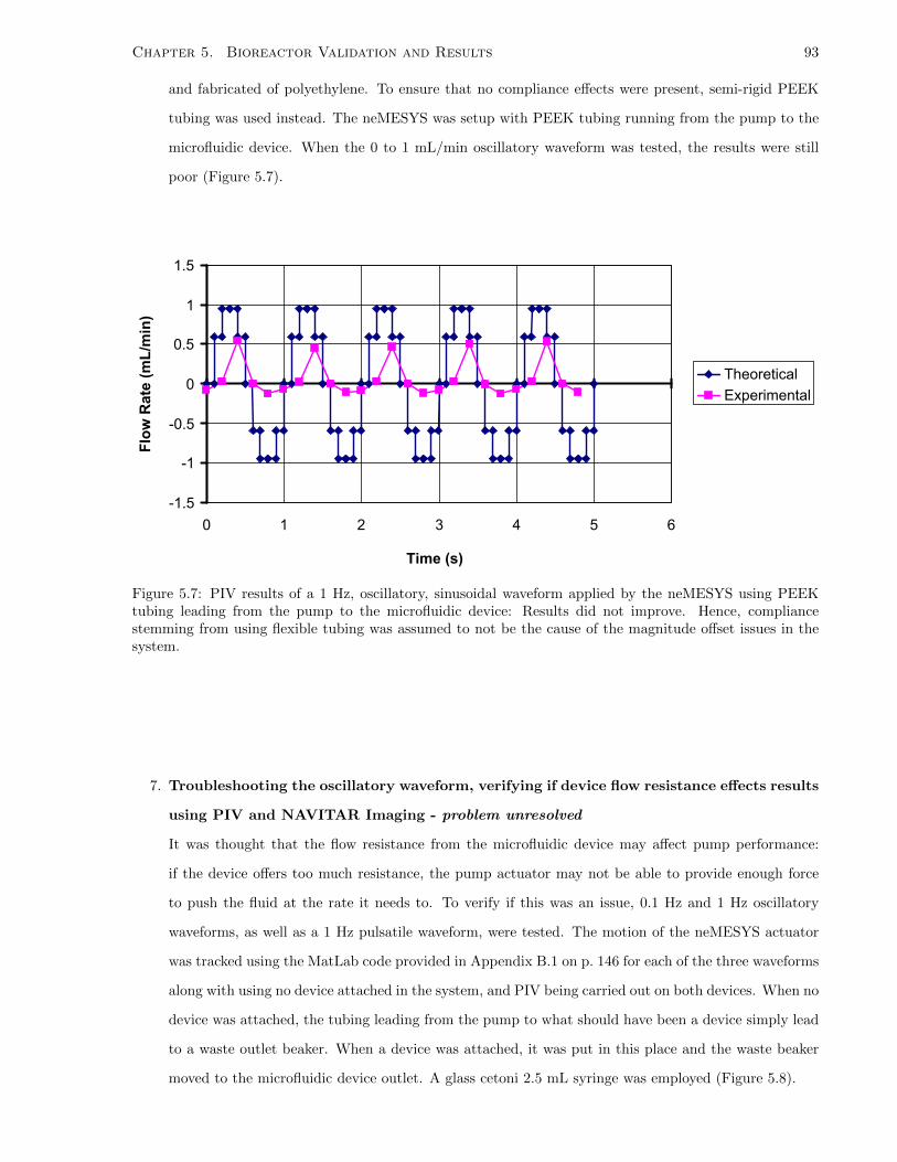
Chapter 5. Bioreactor Validation and Results 93
and fabricated of polyethylene. To ensure that no compliance effects were present, semi-rigid PEEK
tubing was used instead. The neMESYS was setup with PEEK tubing running from the pump to the
microfluidic device. When the 0 to 1 mL/min oscillatory waveform was tested, the results were still
poor (Figure 5.7).
-1.5
-1
-0.5
0
0.5
1
1.5
0 1 2 3 4 5 6
Time (s)
Flo
w R
ate
(mL
/min
)
Theoretical
Experimental
Figure 5.7: PIV results of a 1 Hz, oscillatory, sinusoidal waveform applied by the neMESYS using PEEKtubing leading from the pump to the microfluidic device: Results did not improve. Hence, compliancestemming from using flexible tubing was assumed to not be the cause of the magnitude offset issues in thesystem.
7. Troubleshooting the oscillatory waveform, verifying if device flow resistance effects results
using PIV and NAVITAR Imaging - problem unresolved
It was thought that the flow resistance from the microfluidic device may affect pump performance:
if the device offers too much resistance, the pump actuator may not be able to provide enough force
to push the fluid at the rate it needs to. To verify if this was an issue, 0.1 Hz and 1 Hz oscillatory
waveforms, as well as a 1 Hz pulsatile waveform, were tested. The motion of the neMESYS actuator
was tracked using the MatLab code provided in Appendix B.1 on p. 146 for each of the three waveforms
along with using no device attached in the system, and PIV being carried out on both devices. When no
device was attached, the tubing leading from the pump to what should have been a device simply lead
to a waste outlet beaker. When a device was attached, it was put in this place and the waste beaker
moved to the microfluidic device outlet. A glass cetoni 2.5 mL syringe was employed (Figure 5.8).

Chapter 5. Bioreactor Validation and Results 94
1.
2.
3.
Figure 5.8: Setup of combined PIV and NAVITAR test. The NAVITAR imaged the motion of the neMESYSactuator leading to a microfluidic device being imaged by PIV: 1. NAVITAR scope, 2. neMESYS, 3.microfluidic device on Nikon scope stage for PIV imaging.
The first device was that used in the previous tests. The second device was a device borrowed from
another laboratory. The devices had different dimensions and resistances (Table 5.1 on p. 94). Resis-
tances were calculated with the rectangular channel formula given by Equation 2.40 in Section 2.2.5
on p. 29 and assuming a dynamic water viscosity of 8.9×10⁻⁴ Pa·s.
The NAVITAR displacement results for all three waveforms matched between the three device cases
for the 0.1 Hz oscillatory waveform were essentially identical. With the other two waveforms, minor
differences were seen: For the 1 Hz oscillatory waveform, at times there were maximum offsets between
the curves of 20 µm, but other times not. This was assumed to be caused by vibrations or the entire
frame moving, as the 20 µm shift seemed to displace the entire curve vertically, and not just at a single
point. For the pulsatile waveform, the no device and device B cases matched, but the device A case
was offset, though with the correct shape. It was proposed that the two other cases were tested first
in this experiment, and the actuator stage moved slightly for device A testing (Figure 5.9 on p. 96).
Hence, it was concluded that varying device resistance did not have any affects.
Device Width (µm) Height (µm)Length
(cm)
Resistance
(kg/(s·m4))
A 1500 212.5 3 2.44E10
B 550 315.494 2.1 2.03E10
Table 5.1: Properties of devices used in combined PIV and NAVITAR testing examine flow resistance effectson neMESYS performance.

Chapter 5. Bioreactor Validation and Results 95
The PIV results were more well defined when compared to the NAVITAR data, and provided more
confidence in the same conclusion that varying the devices did not seem to effect the results. Both
Device A and Device B curves matched throughout all the waveforms tested (Figure 5.10 on p. 97).
8. Troubleshooting the oscillatory waveform, switching from a 5 mL to a 2.5 mL syringe -
problem unresolved
A cetoni 2.5 mL glass syringe was put in place of the 5 mL syringe. A smaller diameter syringe
required a larger syringe displacement to obtain the flow rate. If the linear actuator in the syringe
pump carries a small error on the order of microns, this will be magnified in a larger diameter syringe
which moves less than a small diameter variant. This change showed an improvement not only in
terms of bringing the experimental maximum and minimum closer to the theoretical values, but by
also making the waveform symmetric about the origin compared to the differing magnitudes of the
maximum and minimum seen in the 5 mL oscillatory waveform tests (Figure 5.11 on p. 99 compared
to Figure 5.4 on p. 91).
9. Troubleshooting the oscillatory waveform, examining a functional setup and changing the
particle solution - problem unresolved
Making a new solution of fluorescent particles and using the solution that was employed for the working
setup did not produce accurate results.
At this point, another individual in a separate laboratory successfully achieved the oscillatory waveform.
Their setup was analyzed and further troubleshooting was carried out to locate the source(s) of error
in the testing methodology. The device they employed was kept as a constant in all tests. Then,
the fluorescent particle solution, tubing, and syringe were varied one at a time between the testing
equipment that was employed for previous tests and the items used in the working setup. PIV was
carried out on each combination of possible experimental designs.
10. Troubleshooting the oscillatory waveform, examining a functional setup and changing the
tubing to semi-rigid PEEK - problem unresolved
The tubing leading from the neMESYS to the device was changed from flexible polyethylene to semi-
rigid PEEK. The results were still inaccurate.

Chapter 5. Bioreactor Validation and Results 96
-0.10
0.10.20.30.40.50.60.70.80.9
11.11.21.31.41.5
0 5 10 15 20 25 30
Normalized Experiment Time (s)
Dis
pla
cem
ent
fro
m O
rig
in (
mm
)No Device
Device A
Device B
-0.5
0
0.5
1
1.5
2
2.5
3
0 2 4 6 8 10 12
Normalized Experiment Time (s)
Dis
pla
cem
ent
fro
m O
rig
in (
mm
)
No Device
Device A
Device B
-0.1-0.08-0.06-0.04-0.02
00.020.040.060.08
0.10.120.140.160.18
0.2
0 5 10 15 20 25
Normalized Experiment Time (s)
Dis
pla
cem
ent
fro
m O
rig
in (
mm
)
No Device
Device A
Device B
Figure 5.9: NAVITAR displacement results from combined PIV and NAVITAR test using various waveforms.Top panel: a 0.1 Hz oscillatory waveform ranging from -1 to 1 mL/min: The experimental and theoreticalresults matched identically in all cases. Middle panel: a 1 Hz oscillatory waveform ranging from -1 to 1mL/min: Slight vertical shifts at a maximum of 20 µm were seen in the curves throughout the test, but wereassumed to be caused by vibrations within the testing facility. Bottom panel: a 1 Hz pulsatile waveformranging from 0 to 1 mL/min: The Device A case seemed to follow the identical motion paths exhibited bythe No Device and Device B cases, but be offset. This was attributed to a shift in the camera’s location, asDevice A was tested following the No Device and Device B cases.

Chapter 5. Bioreactor Validation and Results 97
-1.5
-1
-0.5
0
0.5
1
1.5
0 5 10 15 20 25
Normalized Experiment Time (s)
Flo
w R
ate
(mL
/min
)
Device A
Device B
-1
-0.5
0
0.5
1
1.5
0 2 4 6 8 10 12
Normalized Experiment Time (s)
Flo
w R
ate
(mL
/min
)
Device A
Device B
0
0.2
0.4
0.6
0.8
1
1.2
0 1 2 3 4 5 6
Normalized Experiment Time (s)
Flo
w R
ate
(mL
/min
)
Device A
Device B
Figure 5.10: PIV results from combined PIV and NAVITAR test using 0.1 Hz (top panel) and 1 Hz (middlepanel) oscillatory waveforms ranging from -1 to 1 mL/min along with a 1 Hz pulsatile waveform ranging from0 to 1 mL/min (bottom panel): The Device A and B results matched identically, leading to the conclusionthat varying flow resistance did not have a large effect on flow rate results.

Chapter 5. Bioreactor Validation and Results 98
11. Troubleshooting the oscillatory waveform, examining a functional setup and changing the
syringe size from 2.5 mL to 1 mL - problem resolved
Finally, it was found that transitioning from a 2.5 mL to a 1 mL syringe (Hamilton Company; Reno,
NV, USA) produced accurate results for the 1 Hz oscillatory waveform. This was tested with the setup
that mimicked the current bioreactor design, and this also produced accurate results with experimental
and theoretical data matching (Figure 5.12 on p. 99).
The conclusion of this validation stage using PIV was that a 1 mL syringe was necessary to be used with
the neMESYS to produce accurate oscillatory sinusoidal waveforms.
5.2.3 Validation of Velocity and Wall Shear Stress Profiles
The velocity profiles given by the Purday approximation and the full solution to pressure-driven rectangular
channel flow were validated using PIV data: The velocities over the entire cross-section of the channel at
the vertical middle plane were found using MatLab and the pivmat add-on. It was assumed that if the
velocity profile in this plane matched the theoretical predictions, the other planes throughout the channel
would follow suit, as would the shear stress derived from the theoretical relations. First, the flow rate for
a specific image was found using the MatLab protocol in Appendix B.6 on p. 183. Then, another MatLab
protocol (Appendix B.7 on p. 187) was written to average the velocities found from the PIV analysis along
each pixel of the channel running perpendicular to the predominant flow direction, to create an average
velocity profile for the entire field of view recorded by PIV. These experimental velocities were then plotted
against the theoretical values obtained from the full solution to pressure-driven rectangular channel flow as
described in Section 2.2.4. A microfluidic device with channel dimensions of h = 315.494 µm, w = 550 µm,
and L = 2.1 cm was employed, and hence the Purday approximation could not be used (since α > 0.5). The
theoretical velocity profile was found by substituting z = h/2 (examining the vertical mid-plane only) into
Equation 2.18 and re-arranging Equation 2.19 to find an expression for pressure drop across the channel in
terms of flow rate. This yields the velocity, urect(y), as:
urect(y) =48Q
π3hw
∞∑n=1,3,5,...
1
n3
[1−
cosh(nπyh
)cosh
(nπw2h
)] sin(nπ
2
)[1−
∞∑n=1,3,5,...
192α
(nπ)5tanh
(nπ2α
)]−1
(5.1)
where in this case, y is the ordinate running along the direction perpendicular to the predominant flow
direction when examining the mid-plane from above. Data from a test of oscillatory flow was employed, with
a sinusoidal shape with an amplitude of 1 mL/min and frequency of 1 Hz. The velocity profiles from four
images were plotted, representing flow rates of 1, -1, 0,6, and -0.6 mL/min, respectively. The experimental
and theoretical results showed excellent correlation in each case (Figure 5.13 on p. 100).

Chapter 5. Bioreactor Validation and Results 99
-1.5
-1
-0.5
0
0.5
1
1.5
0 5 10 15 20 25
Normalized Experiment Time (s)
Flo
w R
ate
(mL
/min
)
Theoretical
Experimental
Figure 5.11: PIV results of a 1 Hz, oscillatory, sinusoidal waveform applied by the neMESYS using a 2.5 mLglass syringe: While the symmetric behaviour of the oscillatory sinusoid was captured, the amplitude wasfar removed from what was desired.
-1.5
-1
-0.5
0
0.5
1
1.5
-1 0 1 2 3 4 5 6
Normalized Experiment Time (s)
Flo
w R
ate
(mL
/min
)
Run 1
Run 2
Run 3
Theoretical
Figure 5.12: PIV results of a 1 Hz, oscillatory, sinusoidal waveform applied by the neMESYS using a 1 mLglass syringe. Using this size of syringe resolved the accuracy issues previously observed: The amplitudeissue had been successfully isolated to the syringe type being used affecting the accuracy of the experimentalflow rate output by the neMESYS.

Chapter 5. Bioreactor Validation and Results 100
-400
-300
-200
-100
0
100
200
300
400
-200 -150 -100 -50 0 50 100 150 200
Velocity (mm/s)
Po
siti
on
fro
m c
entr
e o
f ch
ann
el
alo
ng
wid
th (
um
)
-400
-300
-200
-100
0
100
0 20 40 60 80 100 120 140 160 180 200
Velocity (mm/s)
Experimental (PIV)
Theoretical
-1.5
-1
-0.5
0
0.5
1
1.5
0 0.5 1 1.5 2
Time (s)
Flo
w R
ate
(mL
/min
)
A.
B.
C.
D.
A.B.
C.D.
Figure 5.13: Validation of PIV results: Comparison of experimental and theoretical flow profiles at at flowrates of 1 (A.), -1 (B.), 0,6 (C.), and -0.6 (D.) mL/min during a oscillatory sinusoidal waveform with anamplitude of 1 mL/min (bottom panel) in a device with channel dimensions of h = 315.494 µm, w = 550µm, and L = 2.1 cm. Experimental and theoretical velocity profiles correlated well (top panel).
With the correlation between experimental and theoretical results, it was assumed that the experimental
velocity profile within the channel would match the theoretical predictions, and that the wall shear stress
calculations would be accurate as well, as they are derived from the theoretical versions of the velocity
profiles. After validating the velocity and shear stress profiles, validation studies were transferred to using
the Sensirion flowmeter.
5.3 Validation Using Sensirion Flowmeter
The final validation stage of the bioreactor was carried out using the Sensirion SLI-2000 flowmeter, as detailed
in Section 4.3. This flowmeter performed far superior to the Alicat in terms of not requiring taring during
experimentation, and also being much easier to set up for use with the system. De-ionized water was used as
media for all experiments. Flow rate data was captured using Sensirion RS485 Sensor Viewer proprietary soft-
ware available at: http://www.sensirion.com/en/products/liquid-flow-sensors/download-center/
(Sensirion AG; Westlake Village, CA, USA). In all experiments, data was not recorded for at least the first
minute of the pumps running to let the system come to a steady state (verified visually using the viewer

Chapter 5. Bioreactor Validation and Results 101
software). Instructions concerning flowmeter and software setup can be found in Appendix G.6 on p. 332.
5.3.1 Calibration Testing
The neMESYS was connected to the flowmeter, and the flowmeter outlet to a waste beaker. The damper
and peristaltic pump were not employed. Constant flows were applied to test the accuracy and calibration of
the device. A range of flow rates was employed using 1 and 5 mL glass syringes to test if syringe size would
affect calibration results. 20 s of data was recorded when each constant flow was applied, and the average
values over the experiment time are reported. For both the 1 and 5 mL syringes, the calibration curves were
linear, with correlation coefficients of R2 = 0.99 or higher (Figure 5.14 on p. 103). Based on these results,
no corrections were applied to experimental data from this point due to the small 1% error, which is within
the quoted error specifications of the flowmeter [92].
5.3.2 Verification of Obtaining PIV Results
Before moving on to more advanced waveforms, it was necessary to ensure that the Sensirion flowmeter
could obtain the same results as reported with PIV, namely, being able to accurately measure an oscillatory
sinusoidal waveform ranging from -1 to 1 mL/min with a frequency of 1 Hz. FFT analysis was carried
out on the oscillatory waveform to discover that the minimum sampling frequency should be 500 ms (using
the protocol found in Appendix B.2 on p. 151). Data was oversampled from the flowmeter at a resolution
of 12 bits (data points nominally collected every 5 ms). Test results were identical when a device was or
was not connected in line. In general, the shape of the experimentally measured waveform matched that
of the prescribed waveform very well, with accurate replication of the maximum and minimum flow rates
and only slight deviations due to fluid inertia, i.e., the small steps output from the neMESYS could not
be replicated identically. The period of the experimental waveform also matched that of the theoretical
waveform (Figure 5.15 on p. 104).
The full bioreactor was assembled according to the specifications in Appendix I.1 on p. 345 for the
following tests with a device in line. The bioreactor was run in a non-recirculatory fashion, such that the
device outlet went to a waste beaker instead of back to the media reservoir. A device with dimensions of h =
212.5 µm, w = 1500 µm, and L = 3 cm was employed. Tubing lengths were recorded (Table 5.2 on p. 107).
5.3.3 Sinusoidal Oscillatory Flow Testing with Different Waveform Amplitudes
and Examining the Resulting Dampening Behaviour in the System
When sinusoidal oscillatory flow waveforms with a frequency of 1 Hz and a range of amplitudes were pro-
grammed into the neMESYS, a large dampening effect was observed when comparing the theoretical and
experimental waveforms. This was not expected, but sensible, as the fluid paths of the neMESYS and

Chapter 5. Bioreactor Validation and Results 102
damper are connected in the bioreactor, so they “sense” each other and the damper can affect the neMESYS
waveform output. 1, 2.5, and 5 mL syringes were employed with the neMESYS to test a wide range of
amplitudes. While it was shown from the PIV testing in Section 5.2 that a 1 mL syringe was required
to obtain accurate waveforms, the goal here was not to accurately replicate the prescribed waveforms but
characterize the dampening effects. Theoretical flow rates prescribed to the neMESYS could be used for
calibration based on the experimental results. Data was oversampled from the flowmeter at a resolution of
12 bits (data points nominally collected every 5 ms). With the 1 mL syringe, the tested waveforms were
lightly dampened and insensitive to the prescribed amplitudes. The 2.5 and 5 mL syringe results displayed
large amounts of dampening with minor sensitivity to the prescribed amplitudes (Figure 5.16 on p. 105).
The amplitudes of the theoretical and experimental waveforms were compared for both the 2.5 and 5
mL syringes. Interestingly, a linear correlation was observed between the results for both syringe sizes, with
correlation coefficients of R2 = 0.99 or higher (Figure 5.17 on p. 106).
5.3.4 Varying Damper Volume and Examining the Resulting Dampening Be-
haviour in the System
To further characterize dampening behaviour in the system, the volume of media in the damper (or the
level of the free surface) was varied testing a sinusoidal oscillatory waveform with a frequency of 1 Hz and
amplitude of 30 mL/min. A 5 mL syringe was employed with the neMESYS. Data points were nominally
collected every 10 ms. The minimum damper volume was set at 10 mL as suggested in previous work using
a similar system [73, 91], up to a maximum of 26 mL when fluid spilled out of the inlet of the damper.
Increasing the volume of media in the damper decreased the level of dampening in the output waveform, as
was expected: with more air in the damper, a greater amount of compression is possible in the system and
more specifically, on the air in the damper. During experimentation, the damper free surface height oscillated
in phase with the neMESYS infuse and withdrawal pattern when applying an oscillatory waveform, so it was
sensible that the amount of air would affect the output of the bioreactor, even when only the neMESYS was
operated. Varying the damper volume did not have an effect on period but, as expected, a larger amount
of air in the damper “smoothened” out the resultant waveforms, whereas a lower amount lead to distortion
(Figure 5.18 on p. 107). A higher damper volume of media lead to a faster time for the system to come to a
steady state, but the experimental waveform had a large amount of pulsatility. A lower media volume lead
to a much smoother flow, with the time to reach steady state being a minute or less. The relation between
damper volume and waveform amplitude was shown to be exponential in nature (Figure 5.19 on p. 108).

Chapter 5. Bioreactor Validation and Results 103
y = 1.047x
R2 = 0.994
0.000
0.050
0.100
0.150
0.200
0.250
0.300
0.350
0 0.05 0.1 0.15 0.2 0.25 0.3 0.35
Theoretical Flow Rate (mL/min)
Exp
erim
enta
l Flo
w R
ate
(mL
/min
)
Calibration Data
Linear(Calibration Data)
y = 1.0101x
R2 = 0.9997
0.000
0.500
1.000
1.500
2.000
2.500
3.000
3.500
0 0.5 1 1.5 2 2.5 3 3.5
Theoretical Flow Rate (mL/min)
Exp
erim
enta
l Flo
w R
ate
(mL
/min
)
Calibration Data
Linear(Calibration Data)
Figure 5.14: Calibration curves of the Sensirion flowmeter using 1 (top panel) and 5 (bottom panel) mLsyringes: Theoretical and experimental flow rates correlated well, and it was decided that correction ofexperimental flow rates was not required during further testing.

Chapter 5. Bioreactor Validation and Results 104
-1.5
-1
-0.5
0
0.5
1
1.5
0 2 4 6 8 10
Time (s)
Flo
w R
ate
(mL
/min
)
Theoretical
Experimental
Figure 5.15: Examining if the Sensirion flowmeter could accurately measure the final waveform obtained usingPIV: a 1 Hz sinusoidal waveform ranging from -1 to 1 mL/min. The shape and period of the experimentalwaveform matched that of the prescribed waveform very well.

Chapter 5. Bioreactor Validation and Results 105
-0.2
-0.15
-0.1
-0.05
0
0.05
0.1
0.15
0.2
0 2 4 6 8 10
Time (s)
Flo
w R
ate
(mL
/min
)
6 mL/min
8 mL/min
10 mL/min
12 mL/min
14 mL/min
-0.5
-0.4
-0.3
-0.2
-0.1
0
0.1
0.2
0.3
0.4
0.5
0 2 4 6 8 10
Time (s)
Flo
w R
ate
(mL
/min
)
15 mL/min
20 mL/min25 mL/min
30 mL/min
Figure 5.16: Examination of dampening effects when testing 1 Hz oscillatory waveforms with different am-plitudes using the bioreactor and 2.5 (top panel) and 5 (bottom panel) mL syringes with the neMESYS.Legends indicate theoretical waveform amplitude: Significant dampening effects were seen in the experimen-tal waveforms with minor sensitivity to the prescribed amplitudes.

Chapter 5. Bioreactor Validation and Results 106
y = 0.014x - 0.046
R2 = 0.9899
0
0.02
0.04
0.06
0.08
0.1
0.12
0.14
0.16
5 7 9 11 13 15
Theoretical Waveform Amplitude (mL/min)
Exp
erim
enta
l Wav
efo
rm A
mp
litu
de
(mL
/min
)
Amplitude Data
Linear (Amplitude Data)
y = 0.0198x - 0.168
R2 = 0.9986
0
0.05
0.1
0.15
0.2
0.25
0.3
0.35
0.4
0.45
0.5
15 20 25 30
Theoretical Waveform Amplitude (mL/min)
Exp
erim
enta
l Wav
efo
rm A
mp
litu
de
(mL
/min
)
Amplitude Data
Linear (Amplitude Data)
Figure 5.17: Comparison of the theoretical and experimental sinusoidal oscillatory waveform amplitudesdue to dampening effects in the bioreactor using 2.5 (top panel) and 5 (bottom panel) mL syringes for theneMESYS: A strong linear correlation was exhibited by the system.

Chapter 5. Bioreactor Validation and Results 107
Section Tubing Type Length
Peristaltic pump to damper Masterflex #13 25”
Damper to tee Masterflex #25 3”
neMESYS to tee Intramedic PE60 5-1/8”
neMESYS to tee Masterflex #25 1”
Tee to flowmeter Masterflex #25 1-3/4”
Flowmeter to device Masterflex #25 1-1/4”
Flowmeter to device Intramedic PE60 5-1/8”
Device to waste beaker Intramedic PE190 9”
Table 5.2: Tubing lengths used in Sensirion flowmeter testing with fully assembled bioreactor.
-4
-3
-2
-1
0
1
2
3
4
0 2 4 6 8 10
Time (s)
Flo
w R
ate
(mL
/min
)
Volume: 10 mL,Height: 1.8 cm
Volume: 20 mL,Height: 3.6 cm
Volume: 26 mL,Height: 5.3 cm
Figure 5.18: The effect of varying damper volume or free surface level on the output waveforms of thebioreactor: As expected, more fluid (and less air) in the damper decreased the dampening effects observedin the system and waveform “smoothness”, which can be observed by comparing the regular shape of the 10mL waveform with the 20 and 26 mL waveforms which curve slightly to the left at their peak and troughvalues.

Chapter 5. Bioreactor Validation and Results 108
y = 0.0846e0.134x
R2 = 0.9717
0
0.5
1
1.5
2
2.5
3
3.5
10 15 20 25 30
Damper Volume (mL)
Exp
erim
enta
l Wav
efo
rm A
mp
litu
de
(mL
/min
)
Amplitude Data
Expon. (Amplitude Data)
Figure 5.19: Examining the correlation between damper fluid volume and experimental waveform amplitude:An exponential correlation was exhibited by the system.
5.3.5 Superimposed Sinusoidal Oscillatory Waveform Testing
Constant peristaltic flows of 0.5, 1, and 1.5 mL/min were then superimposed over sinusoidal oscillatory
waveforms with amplitudes of 30 mL/min from the neMESYS using a 5 mL syringe. From Figure 5.16, the
theoretical oscillatory waveform that should have been obtained accounting for dampening was extracted,
yielding a sinusoidal waveform with an amplitude of 0.4 mL/min. This was superimposed over the various
constant offsets representing the peristaltic pump flows, providing final theoretical superimposed sinusoidal
waveforms with maximum flow rates of 0.9, 1.4, and 1.9 mL/min.
While the periods of the experimental and theoretical waveforms correlated well, the maximum values
of the experimental waveforms were greater than theoretical predictions, while the minima were recorded
as predicted. The offset between the theoretical and experimental waveforms at their maxima was approxi-
mately constant at a value of 250 µL/min. Varying the peristaltic pump flow rate seemed to have no effect
on this offset (Figure 5.20 on p. 111).
0.1 Hz sinusoidal oscillatory waveforms were tested and recorded at a resolution of 13 bits (data points
nominally collected every 10 ms) with only the neMESYS operating but attached to the rest of the bioreactor.
Then, a theoretical 30 mL/min sinusoidal oscillatory waveform was superimposed over a constant peristaltic
flow of 1 mL/min taking into account measured dampening effects. The offset phenomenon vanished and
the prescribed and experimental waveforms correlated well (Figure 5.21 on p. 112).
It was concluded that at higher frequencies, the neMESYS cannot accurately replicate the instructions
programmed by the user. Hence, superimposed sinusoidal waveforms could only be achieved at lower fre-
quencies.

Chapter 5. Bioreactor Validation and Results 109
5.3.6 Physiological Waveform Flow Testing
After testing superimposed sinusoidal oscillatory waveforms, physiological waveforms were examined. The
neMESYS was connected to the flowmeter, and the flowmeter outlet to a waste beaker. The damper and
peristaltic pump were not employed, as primarily, the neMESYS was being tested in terms of its actuator’s
ability to keep up with velocity commands to replicate the physiological waveforms. Data was oversampled
from the flowmeter at a resolution of 12 bits (data points nominally collected every 5 ms). The neMESYS
component of the PVD waveform specified in Section 3.2.1 on p. 60 was calculated using the MatLab protocol
detailed in Appendix B.8 on p. 191, assuming device dimensions of h = 212.5 µm, w = 1500 µm, and L =
3 cm, and employed for testing. While the period length and overall shape of the theoretical waveform was
captured, the magnitude offset between the experimental and theoretical waveforms was large: the maximum
value in the experimental waveform was 0.15 mL/min compared to the expected 0.30 mL/min value. The
minimum experimental value was -0.06 mL/min compared to the expected -0.32 mL/min value (Figure 5.22
on p. 112). It was clear that the dampening was not symmetric, compared to the sinusoidal oscillatory
waveforms tested in Section 5.3.3 on p. 101 where both the maximum and minimum values of the waveforms
were dampened to the same magnitude.
To further characterize this error, the waveform had its time axis extended by a factor of 100 making
the period length 80 s. The waveform was tested and an accurate replication of the shape, magnitude, and
temporal characteristics of the theoretical waveform was obtained (Figure 5.23 on p. 113).
With all the troubleshooting previously carried out and extending the waveform so as to make directional
changes of the neMESYS linear actuator more gradual, it was concluded at this point that the limits of the
neMESYS had been reached. The neMESYS is highly customizable, where arbitrary waveforms of any
shape can be programmed into its proprietary software with the smallest change between each value within
a flow waveform being 0.1 s. However, testing revealed that even when programming these waveforms, it
does not necessarily guarantee that the neMESYS can output the desired flow waveform due to limitations
in the speed of the linear actuator as well as the force that can be applied. Specifically, rapid changes in
direction seemed to cause issues with the pump, in terms of backlash and not being able to keep up with
the provided velocity commands. A new linear actuator or syringe pump should be sourced to ensure the
accurate production of the physiological waveforms. The CAVD and atherosclerosis waveforms were not
tested, as the waveforms have similarly large gradients in flow rate.
Furthermore while correlations can mitigate the effects of dampening seen in the system by enabling the
prediction of experimental waveform amplitudes with sinusoidal waveforms, this is not an acceptable method
for the irregular, physiological waveforms, as physiological waveform testing displayed unsymmetric damping
when comparing the maximum and minimum values of the experimental values. Moreover, dampening issues
were also shown to produce temporal offsets in several of the experimental flow waveforms. Hence, it was

Chapter 5. Bioreactor Validation and Results 110
also concluded that methods for reducing compliance in the system were necessary. It is suggested that the
damper used to create continuous flow from the peristaltic pump should be replaced via other methods, or,
the peristaltic pump and damper should be completely replaced with a pump that produces continuous flow
without requiring any additional components. In the next chapter, these issues are further highlighted and
discussed in greater detail.

Chapter 5. Bioreactor Validation and Results 111
0
0.2
0.4
0.6
0.8
1
1.2
1.4
0 2 4 6 8 10
Time (s)
Flo
w R
ate
(mL
/min
)
Expected
Experimental
0.4
0.6
0.8
1
1.2
1.4
1.6
1.8
0 2 4 6 8 10
Time (s)
Flo
w R
ate
(mL
/min
)
Expected
Experimental
1
1.2
1.4
1.6
1.8
2
2.2
2.4
0 2 4 6 8 10
Time (s)
Flo
w R
ate
(mL
/min
)
Expected
Experimental
Figure 5.20: Superposition testing of constant peristaltic flows and sinusoidal oscillatory waveforms withamplitudes of 30 mL/min and frequencies of 1 Hz: An approximately constant 250 µL/min offset wasobserved between the maximum values of the theoretical and experimental waveforms, while the minimaaligned well. Peristaltic pump flow rates of 0.5 (top panel), 1 (middle panel) and 1.5 (bottom panel)mL/min were employed. The expected waveforms were calculated assuming syringe and peristaltic pumpflows are independent in terms of dampening effects using data from Figure 5.16 on p. 105.

Chapter 5. Bioreactor Validation and Results 112
-4
-3
-2
-1
0
1
2
3
4
5
6
0 10 20 30 40 50 60 70
Time (s)
Flo
w R
ate
(mL
/min
)
Expected
Experimental
Figure 5.21: Superposition testing of a constant peristaltic flow of 1 mL/min and sinusoidal oscillatorywaveform with amplitude of 30 mL/min and frequency of 0.1 Hz: The offset phenomenon observed with the1 Hz superimposed waveform was not present. The expected waveform was calculated assuming syringe andperistaltic pump flows are independent in terms of dampening effects.
-0.4
-0.3
-0.2
-0.1
0
0.1
0.2
0.3
0.4
0 0.5 1 1.5 2
Time (s)
Flo
w R
ate
(mL
/min
)
Theoretical
Experimental
Figure 5.22: Physiological waveform testing using the Sensirion flowmeter: The neMESYS component ofthe PVD waveform was tested assuming device dimensions of h = 212.5 µm, w = 1500 µm, and L = 3 cm.Several details of the prescribed waveform could not be captured: While the period length and overall shapewere represented well in the experimental waveform, finer details were not correctly replicated along withpeak and trough values being misrepresented.

Chapter 5. Bioreactor Validation and Results 113
-0.4
-0.2
0
0.2
0.4
0.6
0.8
0 50 100 150 200
Time (s)
Flo
w R
ate
(mL
/min
)
Theoretical
Experimental
Figure 5.23: Physiological waveform testing using the Sensirion flowmeter: The neMESYS component ofthe PVD waveform was tested assuming device dimensions of h = 212.5 µm, w = 1500 µm, and L = 3 cmand with its time axis extended by a factor of 100. Accurate replication of the prescribed waveform’s shape,magnitude, and temporal characteristics was achieved compared to the inaccuracies observed with the 1 Hzvariation of the neMESYS component.

Chapter 6
Discussion
This work has focused on the design of a novel bioreactor to apply physiological shear waveforms on ECs in
microfluidic devices. Several useful results emerged:
• The agreement between experimental velocity profiles measured with PIV when compared to theoretical
predictions.
• The demonstration of syringe size having a large impact on the accuracy of flow profiles created by a
syringe pump.
• The ability of the flow system to accurately replicate a sinusoidal oscillatory waveform when the
neMESYS is tested in isolation from the rest of the bioreactor, and the relationships observed in
correlating experimental sinusoidal oscillatory waveform amplitude to theoretical waveform amplitude
(linear) and damper media volume (exponential).
More work is required to accurately replicate physiological shear waveforms owing to the dampening be-
haviour observed in the system, and the inability of the neMESYS to produce accurate physiological profiles.
Further discussion of this research is separated into four areas:
1. Situation of the research among current literature and novelty of the approach.
2. Analysis of the system and value of the results in terms of their accuracy.
3. Possible improvements to the system’s design.
4. Desired versus achieved parameter spaces.
114

Chapter 6. Discussion 115
6.1 Situation Among Current Literature and Novelty of the Ap-
proach
Creating a bioreactor to mimic a physiological waveform has been successfully carried out in previous studies.
However, there have been limitations in terms of the accuracy and efficacy of the systems. The system
designed in this research has attempted to encompass the following improvements upon the studies reported
in the literature:
1. Experimental data was compared to reference literature in order to obtain accurate phys-
iological waveforms
Many studies have labelled flows that have been created by bioreactors as physiological, but the experi-
mental waveforms were not compared to reference literature, limiting the confidence in the results that
were obtained [4, 36, 52, 53, 72]. Even for work where cardiac pumps were employed, which should
mimic at least one specific physiological waveform reasonably well, comparisons were not provided
[19]. Other research simulated versions of physiological waveforms that were supposed to approximate
the properties seen in vivo, but without any comparison to the literature, there was no substantiated
quantification in terms of accuracy [72, 93]. While the limitations of the current system are acknowl-
edged in terms of not creating physiological waveforms, this work attempted to follow an approach
that could eventually create waveforms that are tailored toward specific reference cardiovascular flows:
By selecting waveforms to mimic physiological conditions (Section 3.2.1 on p. 58), calculating the min-
imum sample rate required to maintain the signals and its properties without loss (via FFT analysis,
Section 3.2.2 on p. 61), and continuously comparing results to literature, with further improvements
to the system, it is hypothesized that accurate waveforms will be replicated.
2. The entire vascular system was not required to be modelled
Bioreactors can contain many components to create a physiological waveform, in an attempt to mimic
lumped portions of the vascular system, such as upstream and downstream vascular resistances and
compliances. The most well known is the Georgia Tech Pulse Duplicator [54–57]. Other studies, such as
that of Estrada et al. have followed this approach [72]. The current thesis work attempts to minimize
the components necessary to achieve the desired waveform. In this regard, it was shown that the
inclusion of components such as dampers which typically mimic compliance can cause experimental
design issues, offsetting the accuracy of the anticipated results.
3. The bioreactor allows for multiple flow waveform studies to be carried out with a single
experimental setup
A myopic approach is typically followed in the literature, where only one or a select few waveforms can

Chapter 6. Discussion 116
be created by a bioreactor. Specifically, when using waveform production methods such as a cardiac
pump, due to the programmed nature of the device, only so much alteration of the output waveform is
possible, as the waveform shape is constant in terms of peaks and troughs [19, 76]. It has been shown,
however, that just in examining three types of CVDs (atherosclerosis, PVD, and CAVD), physiological
waveforms throughout different areas of the human vasculature can be drastically different, in terms
magnitude, slope, number of oscillations per one cycle, and direction. While the current work focused
on the creation of five waveforms representing three CVDs, based on the approach that was followed,
there is a possibility for replicating many other different waveforms, which can involve different heart
arrhythmias, CVDs, and areas of the body. As well, the described system enables one to arbitrarily
vary a waveform to reflect a pathophysiological state, and enable the study of its effects on the cultured
cells within the microfluidic device.
4. The wall shear stress occurring within microfluidic devices was accurately calculated
In response to disturbed flows, CVDs are initiated and progress due to the alteration of EC phenotype.
ECs begin to respond to external forces at very low levels of stress, such as vascular ECs at pressures
of 1.1 × 10⁻³ mmHg [13]. Many studies have employed the parallel-plate flow approximation (or
steady-pressure driven flow between two plates, refer to Section 2.2.4 on p. 22) to predict the shear
stress that ECs will be subjected to in vitro [93–96]. Others have used variants of this approximation
with correction factors [72, 76]. It was shown in Section 2.2.6 that the exclusion of wall effects when
calculating the shear stress exerted on ECs in rectangular channels can lead to errors as high as 30%. In
the current thesis, relations that accurately model the shear stress that is exprienced within rectangular
channels have been used while other simplified versions were disregarded. The one approximation used
was the Purday approximation, and this was discussed in Section 2.2.4 on p. 23. This was employed
when the error was not high, such as in the case of the device typically tested, which had dimensions of
w = 1500 µm and h = 212.5 µm, which carries as associated error of approximately 4% when compared
to the unsimplified solution for rectangular channel flow (refer to Section 2.2.7 on p. 30). Hence, the
model improved upon the accuracy of shear stress prediction and applied it for microfluidic cell culture
studies.
5. The bioreactor was designed to be employed at the microscale
The generation of physiological waveforms at the macro- and mesoscales is not novel and has been
well documented in the literature. However, as previously discussed, each carries its own associated
disadvantages: Macroscale systems can be quite large and cumbersome, and for both macro- and
mesoscale setups, modularity is difficult to accomplish: For macroscale flow bioreactors, machining is
typically required such that a chamber is designed to contain biological samples and not allow leaks
to occur [51–57]. It is difficult to use multiple types of tissue, organs, or cell types, unless separate

Chapter 6. Discussion 117
chambers are constructed to accept each. At the mesoscale, this limitation is less of an issue with
PPFCs being able to accept multiple cell types [60–65], along with cup and cone bioreactors which not
only accept different cell types, but also tissue samples [2, 36, 58]. However, setups at the microscale
overcome the aforementioned disadvantages at the macroscale and also provide superiority to mesoscale
approaches. Specifically, the foot print of devices is small, with typical devices being on the order of the
size of a microscope slide, or less, and the size of bioreactors at the microscale decreases significantly:
not only are the larger components that are required with macroscale systems now unnecessary, but at
the microscale, much smaller pressures and velocities are required to achieve the same flow properties
(namely shear stress) in a typical device. This decrease in pressure and velocity requirements leads to
less pumping power required, and hence, driving methods with a smaller foot print as well. The other
extremely attractive feature of microfluidic bioreactors is that of modularity. Typically, microfluidic
devices are “plug and play”, as the devices are attached via union-type connectors to tubing, and can
be easily removed and exchanged for other devices. Not only does this encourage quick turn around
in terms of experiments, but cleaning of a culture chamber is unnecessary as typically, microfluidic
devices are batched produced and a new device can simply be substituted instead of the used variant.
Moreover, this exchange of devices allows for different device designs to be used, ranging from simple
geometries to complex multi-channel designs.
Bioreactors that take advantages of these factors and apply physiological shear stresses on ECs at
the microscale have been reported [70, 72, 76], but none of these have combined the comparison of
experimental results to reference literature along with the accurate calculation of shear stress being
applied to ECs in vitro.
6. The bioreactor is modular, and multiple microfluidic device dimensions are accepted
Modularity in microscale setups is one of the most attractive features of working within the size
range. Not only can devices be quickly exchanged, but most of the setup is disposable (i.e. the
tubing connecting all the different components and the device itself), or easily sterilizable for re-use by
autoclave, if the designers have taken this into account (i.e. the union adaptors and various fittings).
Such advantages are not usually present at the macro- and mesoscales where more cleaning may be
involved, and certainly with large scale tubing and piping, disposal is not a viable option. Moreover
at the macroscale, experiments can be postponed for indefinite periods of time should maintenance
be required for unique and critical components, such as custom designed culture chambers. With
microfluidics, a new device is simply put in place of the other. This is also attractive for the culture
and growth of cells. Instead of relying on a single sample, multiple cell populations can be cultured
should one fail, perish, or not be usable.
In terms of the devices themselves, the modularity of bioreactors at the microscale allows for different

Chapter 6. Discussion 118
types to be tested. In this study, only single channel devices were employed, and with only two sizes
throughout the experiments. However, the system was designed to incorporate devices with a large
array of possible sizes, and provided methods to accurately calculate the required flow rates to obtain
shear stresses over this range. Moreover, more complex device designs can be employed, such as those
with multi-channel networks, to those with geometrical features attempting to mimic different areas
of the body. This allows for many possibilities in terms of expansion of the current research not only
in the realm of CVDs and ECs, but to different diseases and cell populations.
6.2 Analysis of the System and Value of the Results in Terms of
Accuracy
An analysis of the system and results obtained from this work along with their accuracy is essential to discuss
possible limitations and improvements.
6.2.1 Simplification of In Vivo Hemodynamics and Flow Effects
This work made three important simplifications in terms of in vivo hemodynamics and fluid flow effects:
1. Only shear was attempted to be mimicked by the bioreactor. Hemodynamic effects from pressure and
membrane stretch were not analyzed.
2. The in vivo vascular geometry, levels of dimensionless parameters (such as the Reynolds and Womersley
numbers), and local fluid flow effects (flow recirculation, separation, and reattachment) were not taken
into consideration.
3. Five waveforms were employed to represent three different CVDs: two represent the disease-prone and
disease-protective states of atherosclerosis and CAVD, respectively, while another represented PVD.
As was discussed in Section 2.1.3 on p. 6, the endothelium experiences complex hemodynamic forces,
including friction, pressure, and strain or stretching. The interplay between these forces along with the
biochemical signalling and environment of the vasculature affects EC morphology, which can, in turn, affect
vessel calibre, angiogenesis and atherogenesis, as well as the presence or levels of chemical messengers [11].
The exclusion of any of the above stresses from the in vitro environment will affect the output results and
their accuracy. However, as was discussed when setting the bioreactor design requirements in Section 4.1.2
on p. 67, shear stress has been shown to play a prominent role in regulating the vascular system and hence
was the focus of attention here. More critically, it was noted that shear stress and the phenotypic response
of ECs are correlated, which can impact the initiation and progression of various CVDs. Just as in the
examination of the generated waveforms of the bioreactor, the work here began with the simplest approach

Chapter 6. Discussion 119
(replicating one form of stress accurately) before moving on to replicate other forms. With the design of the
current bioreactor, such extensions can be easily imagined. For example: the use of membrane type devices
where ECs are grown on deformable membranes and subjected to fluid flow [72, 73]. These devices can be
designed and simply integrated due to the modular nature of the bioreactor. While studies have begun to
consider multi-force bioreactors to study EC response, such as that in the work of Estrada et al. and Smits
et al., suffered from not using physiologically accurate shear stress profiles relevant to CVDs when compared
to reference literature [72, 93]. It was desirable to first obtain accurate physiological shear stress data before
proceeding on to examine the more complex nature of the vascular environment.
In terms of the in vivo environment, many traits of the fluid flow were simplified in creating an in
vitro version. First, the vascular geometry and levels of associated dimensionless parameters in the areas
of the body being analyzed were not taken into account. Typically, for accurate flow modelling, one must
perform a dimensional analysis of the problem and compare it to the model being created to maintain flow
properties. This is done by matching the dimensionless parameters between the two cases. However in this
work, the latter was not carried out. It is foreseeable, given the ease of customization and design that comes
with microfluidic devices, that certain geometrical properties of the body could be effectively scaled down
and modelled, such as vessel curvature. However, the microfabrication technology is not at a point where
accurate three-dimensional models can be obtained in the devices, such as if the aorta was to be modelled.
A device could be designed that varies its cross-section to represent, for example, a vessel blockage
stemming from atherosclerosis in a curving channel that accurately mimics the geometry of the in vivo
environment, at least in two dimensions. Such scaling would require the matching of dimensional parameters
associated with the flow, such as the Reynolds and Womersley numbers along with the Dean number. This
can present an issue, as Reynolds numbers at the microfluidic scale are typically on the order of unity, and
depending on what portion of the vascular tree is examined, it may be impossible to maintain dimensional
accuracy between all of the dimensional parameters. For instance, this would be the case when examining
the aorta given its turbulent flow at peak systole.
The constraint of low Reynolds numbers in microfluidic devices also places another caveat on the design:
It was discussed in Section 2.2.2 on p. 16 that flow regime plays a critical role in determining EC response to
shear stress: While most flows in the vascular system are laminar, non-laminar flows promote EC proliferation
and apoptosis, along with vasoconstriction and coagulation. Microfluidic experiments examining if these
effects occur in vitro are not possible due to the low Reynolds numbers, as the sizing places limits on
the magnitude of Re values possible [4]. Moreover in not maintaining dimensional accuracy, it has been
impossible to capture the local fluid flow effects that may exist in vivo: As discussed in Section 2.1.6 on
p. 9, disturbed flow upregulates genes associated with CVD initiation and progression, not only due to the
low magnitude and bi-directionality of the associated shear stresses, but also due to phenomena such as flow

Chapter 6. Discussion 120
recirculation, separation, and reattachment. While the magnitude of the physiological shear stresses has
been attempted to be re-created in this work, the flow phenomena have not. Advanced device design, such
as the inclusion of a step near the entrance of the microchannel, could be tested and integrated to re-create
such phenomena as has been previously reported in the literature [97].
With regards to the physiological waveforms themselves, five were selected from the literature to repre-
sent the three CVDs that were the focus of this study: atherosclerosis, CAVD, and CVD. Specifically for
atherosclerosis and CAVD, each had their own associated waveform pair with one representing a disease-
prone and one representing a disease-protective state. The simplifications carried by using this approach
are important to note but necessary: In the in vivo environment, their are a vast number of vessels. While
some are more prone to disease than others, it is impossible to select one to fully characterize the nature
of a disease. The local environment in each vessel, while exhibiting the typical characteristics of disturbed
flow, may be different in terms of local flow effects and shear stress magnitudes. As previously discussed,
local flow effects and dimensionless parameters will also vary depending upon what area of the body is
examined. Such is also the case with CAVD: Even in being localized to a specific region such as the aortic
valve, compared to examining the entire vasculature, it is a large simplification to limit the study to specific
waveforms. These waveforms can also vary dynamically at times during an individual’s life, not remaining
constant: As a disease progresses the waveforms may change in shape. While selecting areas to examine,
especially with regards to atherosclerosis and PAD/PVD, may be a simplification of the flow problem at
hand, it is a large improvement over using steady flow [24, 91, 98] or sinusoidal waveforms [4] to study shear
stress effects on cell cultures. Moreover, at least in capturing the nature of disturbed versus non-disturbed
flows, conclusions may be drawn in terms of how each affects ECs.
6.2.2 Accuracy of PIV
The PIV data may be scrutinized in terms of accuracy: It was noted that the system’s laser could only fire
at a pulse rate of 5 Hz or every 200 ms, and only up to a maximum of approximately one minute’s worth of
data. It may be argued that this is not a sufficient frequency to obtain reliable waveforms. In other words,
more data points through each cycle are required to construct an accurate flow profile, and over a longer
period of time. Given that the minimum sampling frequency of the 1Hz, 1 mL/min oscillatory waveform
was calculated to be 50 ms, this is especially prevalent. What can be done to overcome this limitation of
frequency is what is known as “phase averaging” [99, 100]. In simplified phase averaging, a specific point in
a cycle is recorded through some means, usually via a pressure sensor. For example with a sinusoidal curve,
the maximum flow rate will correspond to the maximum pressure in the channel, and when the pressure
curve is examined via a sensor, this point can be extracted. From this recorded point, an external trigger
can fire the PIV laser at the required time (connected to the pressure sensor via a programming method

Chapter 6. Discussion 121
such as LabView), and measurements of velocity can be taken repeatedly over several cycles at different time
displacements from the point, constructing an elongated flow curve over time. In this sense, not only are
there more data points along each cycle, but also the total experiment time may be increased (Figure 6.1).
Further operations and more complex components of phase averaging are possible, such as in applications
involving turbulent flow, but these were deemed unnecessary for the current work. This approach would
provide more confidence in the output flow profiles from PIV if required.
u
t
P
u
t t
u
t
u
u
t1.
2b.
3.
2a. 2c.
Figure 6.1: Process of phase averaging using PIV: 1. A specific point is marked using external hardware,such as a pressure sensor which records the point for further external triggering of the PIV laser at a specifictime. Then, the PIV laser is triggered at several time increments from the pressure sensor point. In each of2a., 2b. and 2c., the velocity is recorded at the same time increment over each cycle. This is repeated forhowever many time increments are desired. 3. Using the recorded data, the entire flow curve is re-constructedat a much faster frequency than possible without phase averaging. This process assumes a repeated, cyclicwaveform.
For validation of the velocity and shear profiles obtained from the work, the centre channel was focused
on and shown to match theoretical predictions. It was then concluded that the rest of the profile would
follow suit. Only the centre plane was measured and quantified because it can be easily obtained through
experimentation: a range of depths can be scanned through using the PIV microscope and measurements
taken. A parabolic pattern can be seen in the measurements due to the nature of the channel geometry,
and hence, the maximum velocity (in between two planes with lower velocities) correlates to the channel
of maximum flow. The actual depth the microscope image moves when adjusting the focus is not known.
However, this can be obtained by placing a mark at the bottom of the microfluidic channel (the glass slide),
then measuring up to the plane of maximum flow, and correlating this distance (half of the channel height)
to the increment of microscope adjustment. For the PIV system that was employed, the controller dial was
Chapter 6. Discussion 122
graduated into 1% increments. This could be used to obtain velocity measurements in a desired number of
planes to create a three-dimensional velocity profile, which can be compared to the theoretical version for
improved confidence in results. Furthermore, comparing the experimentally derived and prescribed wave-
forms for the accurate 1 mL/min sinusoidal oscillatory test results, the RMSE was calculated yielding a value
of 0.238 mL/min, which is fairly high at 24% of the waveform amplitude. This is counter-intuitive as the
plotted waveform shape seemed to match of the theoretical (Figure 5.12 on p. 99). However, nearly exact
correlation between the experimental and prescribed waveforms testing the same 1 mL/min sinusoidal oscil-
latory waveform but using the flowmeter instead of PIV proved that the flow waveform in the microchannel
was correct (Figure 5.15 on p. 104).
6.2.3 Accuracy of the neMESYS Linear Actuator
Another point worth noting is why the change to a 1 mL syringe produced the accurate oscillatory profiles
when no other alteration to the experiment would. If the neMESYS linear actuator carries a constant error
in motion of 1 µm, this error will be seen much more with a larger syringe than a smaller one: To produce
the same flow rate, a larger syringe moves much less due to its increased cross-sectional area, which implies
than a small error can greatly impact the output flow. For a smaller syringe which traverses a much larger
distance compared to a large syringe for the same flow rate, the same level of error will not impact results
to the same extent. Hence, when moving to a smaller syringe, I was able to ensure that any motion error
in the neMESYS was far less prevalent, as can be clearly seen in the increasing accuracy of the output flow
profiles in changing from a 5 mL (Figure 5.4 on p. 91), to a 2.5 mL (Figure 5.11 on p. 99), and finally to the
accurate 1 mL (Figure 5.12 on p. 99) syringe.
6.2.4 Assumptions of Shear Stress Calculations in the Microfluidic Channel
The vertical bottom centreline expressions for calculating shear stress were employed to convert the in vivo
shear waveforms to the required in vitro flows to obtain the identical shear stresses within the microfluidic
channel. However, the shear stress varies across the width of the channel. It can be noted that to the
parabolic nature of the velocity profile, shear stress is nearly uniform in the centre “core” of the channel’s
width, where velocity is approximately constant. This is especially prevalent in wider channels (Figure 6.2
on p. 123). I justify the calculation decision by assuming that after flow testing, cells will be extracted and
analyzed from this “core” region, defined where there is less than 5% deviation from the maximum shear
stress.
Moreover, the topology of ECs within the microfluidic channel can also affect the local shear stress
distribution. ECs are not flat with a typical cell height of 2.5 µm [101]. However, I employed the shear stress
values coinciding with the vertical bottom of the microfluidic channel. I justify this decision by noting that

Chapter 6. Discussion 123
due to the use of a monolayer of ECs, the height of the monolayer is negligible compared to the height of
the channel (i.e. the 2.5 µm cell height is approximately 1% of the 212.5 µm height of the channel typically
tested in this work). Research has shown that the variations of shear stress can be large when examining
specific cells in a monolayer of ECs [102]. However, the normalized shear stress over the cell layer will not be
vastly different than the vertical bottom when, as is common practice, topographical features are ignored.
Figure 6.2: An example of a shear stress profile in a microfluidic channel with dimensions w = 1500 µm andh = 212.5 µm demonstrating the “core” phenomenon: A 1092 µm wide region in the centre of the channelis exposed to a constant shear stress (i.e., less than 5% deviation from the shear stress at the centre of thechannel) compared to the smaller regions near the walls of the channel where the shear stress decreases tozero [91].
6.2.5 Approximation of Sinusoidal Functions as Step Functions
At the beginning of the results section in Chapter 5, it was discussed how the neMESYS approximates
sinusoidal waveforms as step functions, as the pump does not interpolate between steps for continuous
movement (see Figure 5.1 on p. 87). This can lead to an error in the volume input or output, depending
on how the step approximation is carried out. Analyzing the final sinusoidal waveforms employed in this
study (oscillatory variants), theoretically, the volume input should be exactly equal to the volume output.
When the integral of the step approximation of the 1 mL/min waveform is taken using Simpson’s Rule over
a single 1 s cycle, the result is 0 mL as expected. With amplitudes higher than unity, errors in volume were
found to be on the order of E-19 mL, which are excellent results given the approximation. Moreover due
to fluid inertia and play in the neMESYS actuator, the small steps of the neMESYS could not have been
completely replicated unless the system was ideal. Hence, the step approximation of the sinusoidal curves
became more continuous in that the fluid almost never came to a continuous velocity during testing (see
Figure 5.16 on p. 105 for a typical example). The step versions of the sinusoidal functions were in steps of 0.1
s, higher than the required Nyquist frequency of 0.5 s obtained from FFT analysis (Appendix B.2 on p. 151).

Chapter 6. Discussion 124
The RMSE was calculated for a typical step approximation, the 1 mL/min sinusoidal oscillatory waveform,
yielding 2.31E-7 mL/min; a very small amount of error when compared to the amplitude of the waveform
(2.31E-5%). However even with these considerations, it is important to note that the step versions cannot
replicate the exact dynamics of actual sinusoidal functions, and introduce higher frequency components in
the flow waveform compared to the continuous functions.
6.3 Possible Improvements to the System’s Design
Several alterations can be made to improve the design of the current system:
6.3.1 Discussion and Possible Resolutions of Dampening Effects
Dampening issues in the system originated from compliance, due exclusively to the damper in the system.
While the periods of the experimentally measured waveforms matched those of the prescribed waveforms,
consequences of dampening were clearly observed in terms of decreased amplitudes in oscillatory waveform
testing using the Sensirion flowmeter (Figure 5.16 on p. 105). Moreover, the waveforms were also quite erratic
in appearance: those measured by the flowmeter when the neMESYS was directly connected appeared much
smoother than when the entire bioreactor was assembled (compare the tested PVD waveform in Figure 5.22
on p. 112 to the dampened oscillatory curves in Figure 5.16 on p. 105). As well, output waveforms may have
been affected by the tee: As the flow was imparted from the syringe pump, the flow may have split between
the two other paths of the tee, dampening the expected output. In phase oscillation of the media’s free
surface within the damper provides evidence for this hypothesis, such that flow moves towards the damper.
Flow recirculation and dead zones may have occurred as well: Peristaltic and syringe pump flows may have
combined to create recirculation zones inside the tee due to fluid inertia from the two pumps forcing fluid
along certain paths. This, again, decreases the expected output at the outlet of the tee (Figure 6.3 on p. 125).
While a linear relationship was observed between the theoretical and experimental amplitudes of si-
nusoidal oscillatory waveforms due to dampening effects (Figure 5.17 on p. 106), physiological waveform
testing demonstrated non-symmetric dampening when comparing the theoretical and experimental maxima
and minima, making this type of correlation unsatisfactory for correction purposes.
To decrease dampening effects in the system, it is suggested that three possible paths for improvement
be considered:
1. Employ different dampening strategies other than the damper used in this work.
2. Replace the peristaltic pump and damper with a continuous pump.
3. Mathematically model the system and predict how additions can counteract the current behaviour.

Chapter 6. Discussion 125
Peristaltic
Syringe
Output
Theoretical
Experimental
Backflow todamper
Figure 6.3: Possible recirculation zones created within the tee of the bioreactor: The inertia stemming fromthe input peristaltic (red) and syringe pumps (blue) caused portions of the fluid (dashed grey) to travel inunintended paths and create recirculation zones (black). The recirculated fluid may have accentuated theflow division effect observed with the syringe pump, with its flow separated between the device (green) anddamper (purple), evidenced by the damper free surface oscillating in phase with the neMESYS actuatormovement. The experimental output was then smaller than that which was theoretically predicted.
1. Employ different dampening strategies other than the damper used in this work
While dampening pulsatile peristaltic pump flow to a continuous variant was carried out using a damper
in previous work [73, 91], several other strategies may be employed which would negate the need for
the type of damper used in this work:
(a) A larger tubing diameter could be employed to decrease the revolution speed and amount of
oscillation in the output waveform. However, there would still be large gaps between each fluid
“slug” expelled by the pump, so this would only be a partial strategy in eliminating pulsation.
(b) Employing a pump head with a large number of rollers: The current pump head used in the
laboratory, an EasyLoad II Model #77202-60 pump head, has four rollers. Other variants may be
purchased with up to eight rollers, which would decrease the amount of time between successive
fluid “slugs” being expelled by the peristaltic pump. Possibilities include a direct attachment six
roller head (item #RK-07535-04. Cole-Parmer; Montreal, QC) or eight roller head and cartridge
(items #RK-07519-20 and #RK-07519-75. Cole-Parmer; Montreal, QC).
(c) Offset the rollers of multiple heads by a 90 degree phase angle: By employing two cartridges (item
noted in the previous paragraph) in opposite directions or manually adjusting the rollers of two
pump heads such that they are separated by a 90 degree phase angle, the number of roller heads is
effectively doubled. However in addition to this step, one must employ a Y-connector to split the
inlet tube between the two sets of rollers and then re-combine the two paths into a single outlet
after being run through the pump. This creates a much smoother variant of flow, and offsets the
gaps in fluid “slugs” typically present with peristaltic pumps (Figure 6.4 on p. 126).
It is believed that option #3 can provide continuous flow, and would be fairly inexpensive to test:

Chapter 6. Discussion 126
Figure 6.4: Dual pump head or cartridge strategy to create continuous flow using a peristaltic pump: Withthe rollers of two heads or cartridges offset by a 90 degree phase angle, the inlet is split using a Y-connectorinto the two inlets of the pump and then re-connected at the outlet (left image). This transforms thediscontinuous flow typically associated with a single channel (Channel A or B) into a continuous variant(Channels A + B) (right image) [103].
plastic Y-connectors would be required along with the associated tubing. Then, new pump heads may
be required, which can be returned if they do not provide the desired continuous flow.
2. Replace the peristaltic pump and damper with a continuous pump
Another option is replacing the peristaltic pump and damper completely with a pump that outputs
continuous flow. Suppliers were contacted and options were noted (Table 6.1 on p. 127). It is recom-
mended that the RK-73100-04 from Cole-Parmer for it’s price point with reference to all of the other
options and inclusion of a controller. Other less expensive options may be viable but would require
the sourcing of a seperate controller.
3. Mathematically model the system and predict how additions can counteract the current
behaviour
The other possibility is to mathematically model the system behaviour. Using the resistance equations
and pressure model found in Chapter 4 and taking into account air compression inside the damper, one
could model the system and predict how alterations to the system design would affect the output flow
rate. Such design alterations could include the addition of components, such as dampers downstream of
the device to vary the compliance, or occlusion valves to vary the resistance. Creating a set equations
that model the expected response to varying inputs such as number of dampers, damper water height,
and resistances using a software package such as MatLab could prove to be advantageous for design.
6.3.2 Inability of the System to Produce Physiological Waveforms
The other main issue with the current system is the fact that, as shown in Section 5.3.6, the neMESYS could
not output accurate physiological waveform profiles, even before being combined with the peristaltic pump.
In discussion with cetoni, it was recommended that the pump be sent back for to be recalibration to be
non-geared or direct-drive, as a gearing ratio of 14:1 is currently in place. The direct-drive would eliminate
potential backlash issues causing the neMESYS to miss certain portions of the physiological profile, in terms

Chapter 6. Discussion 127
SupplierItem Number or
DescriptionCost ($) Details
Cole-Parmer;
Montreal,QC
RK-73100-04 $2,975
0.3 - 18 mL/min. Wetted materials:316 SS, tungsten carbide, aluminium,
PTFE graphite, and Viton wettedparts (all sterilizable by autoclave).
Analog drive. Comes with controller.
Cole-Parmer;
Montreal,QC
RK-73100-54 $12,420
0.003 - 18 mL/min. Wetted materials:316 SS, tungsten carbide, PTFE
graphite, and Viton (all sterilizable byautoclave). Digital drive. Comes with
controller.
VissersSalesCorp.;
AnnacisIsland,
BC
MZR-2921 M2.1 (pump),MZR-xx21/xx42 M2.1
(manifold adapter), S-ND(controller)
$2,175, $241,$2,500, and $203for power supplyand connectioncables. Total:
$5,119
Flow rate: 0.3 - 18 mL/min. Wettedmaterials: 316 SS, tungsten carbide,
ceramic, epoxy resin.
VikingPump
Canada;Windsor,
ON
GA.X21JFSE $1,168.180 - 10 mL/min. Gears fabricated fromPEEK and motor body from 316 SS.
Table 6.1: New continuous flow pump options to replace peristaltic pump and damper. Note: The Cole-Parmer RK-73100-04 pump can be re-configured with an add-on that allows for a 0.003 - 18 mL/min flowrate range. However, the cost of the part could not be sourced via the company. It is suggested to inquirewith the company about this option before purchasing a new pump.
of not being able to move quick enough. The advantage of the direct drive configuration is that the maximum
actuator velocity significantly increases from 6.33 to 89.00 mm/s, and and as a result, so do the maximum
flow rates that can be output [90]. However, the maximum force that the syringe pump can apply is reduced
from 390 to 40 N, which may cause accuracy issues if there is too much back pressure in the system as the
pump may not be able to apply enough force to move the fluid to create a specified flow rate. It was desired
to send one of the existing units away for alteration but this was deemed unacceptable by other users of the
pump. As of writing, a new direct-drive unit would cost approximately $5,000 US, which cannot be returned
if the issue is not solved.
There are two alternatives: a new syringe pump or linear actuator can be sourced or an entirely new
pumping methodology must be found. It is our recommendation that the approach presented in this work
need not be abandoned and another pump or actuator can be located. In discussion with several suppliers,
two possible solutions were provided by Parker Motion and its Toronto-based supplier Shelley Automation:
• The first option involves the use of a positional stage driven by a lead screw-type linear actuator. This
is a similar type of actuator as the UltraMotion Digit actuator tested in this work (Section 4.2.5 on
p. 72). However, the maximum speed of the Shelley Automation actuator is nearly twice that of the
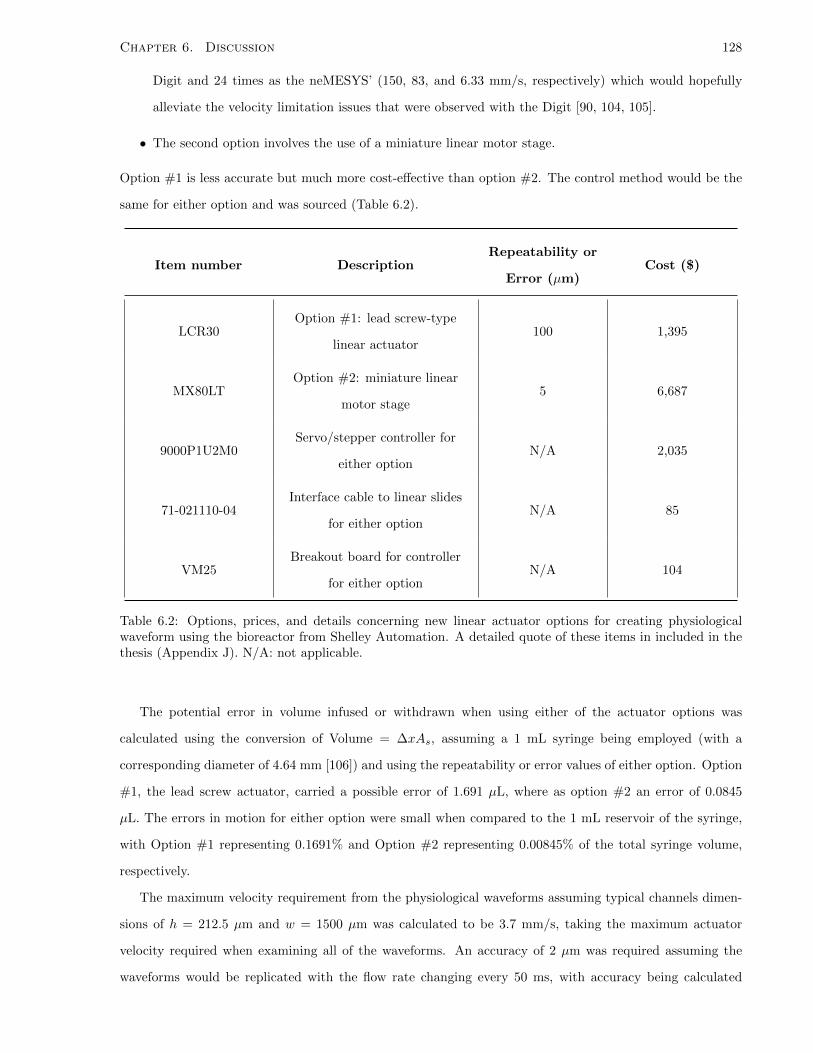
Chapter 6. Discussion 128
Digit and 24 times as the neMESYS’ (150, 83, and 6.33 mm/s, respectively) which would hopefully
alleviate the velocity limitation issues that were observed with the Digit [90, 104, 105].
• The second option involves the use of a miniature linear motor stage.
Option #1 is less accurate but much more cost-effective than option #2. The control method would be the
same for either option and was sourced (Table 6.2).
Item number DescriptionRepeatability or
Error (µm)Cost ($)
LCR30Option #1: lead screw-type
linear actuator100 1,395
MX80LTOption #2: miniature linear
motor stage5 6,687
9000P1U2M0Servo/stepper controller for
either optionN/A 2,035
71-021110-04Interface cable to linear slides
for either optionN/A 85
VM25Breakout board for controller
for either optionN/A 104
Table 6.2: Options, prices, and details concerning new linear actuator options for creating physiologicalwaveform using the bioreactor from Shelley Automation. A detailed quote of these items in included in thethesis (Appendix J). N/A: not applicable.
The potential error in volume infused or withdrawn when using either of the actuator options was
calculated using the conversion of Volume = ∆xAs, assuming a 1 mL syringe being employed (with a
corresponding diameter of 4.64 mm [106]) and using the repeatability or error values of either option. Option
#1, the lead screw actuator, carried a possible error of 1.691 µL, where as option #2 an error of 0.0845
µL. The errors in motion for either option were small when compared to the 1 mL reservoir of the syringe,
with Option #1 representing 0.1691% and Option #2 representing 0.00845% of the total syringe volume,
respectively.
The maximum velocity requirement from the physiological waveforms assuming typical channels dimen-
sions of h = 212.5 µm and w = 1500 µm was calculated to be 3.7 mm/s, taking the maximum actuator
velocity required when examining all of the waveforms. An accuracy of 2 µm was required assuming the
waveforms would be replicated with the flow rate changing every 50 ms, with accuracy being calculated

Chapter 6. Discussion 129
as the minimum displacement required between each change in flow rate to create the desired flow profile.
Based on these options, the miniature linear motor stage would seem to be the most viable option.
The choice of which method to proceed with is to the future designers. The syringe would need to be
connected to the actuator which would involve a simple rig design, as either method employs a flat stage for
mounting purposes.
6.3.3 Validation of Pressures within Microfluidic Channel
To validate the microfluidic channel model predictions of pressures presented in Section 4.5.2 on p. 78, pres-
sure sensors could be incorporated at the entrance and exit to the device. This would ensure that pressures
are within physiological range. A pressure sensor which would suit this need is the Dwyer Instruments model
#673-3 (Dwyer Instruments; Michigan City, IN; USA), which measures pressures within the range of 0-5 psi
(0-260 mmHg).
6.4 Desired versus Achieved Parameter Spaces
While a range of parameters were desired to be replicated with the bioreactor, the full range of several could
not be successfully replicated as prescribed in the objectives of Chapter 1 (Table 1.1 on p. 3). The desired
versus obtained parameter spaces were compared (Table 6.3).
Parameter Desired Range Tested and Achieved Range
w 25 to 2000 µm 550 and 1500 µm
h 100 to 525 µm 212.5 and 315.494 µm
Wo 0.0531 to 1.105 0.408 and 0.694
Re 14 to 300 20.6 and 49.1
Frequency Any frequency up to 1 HzCertain waveforms at 1 Hz, most at
slower frequencies
Q -0.5 to 4.5 mL/min
0.1 to 2.1 mL/min at 1 Hz and -3 to 5mL/min at 0.1 Hz
sinusoidal/pseudo-physiological. -0.35 to0.6 mL/min at 0.0125 Hz physiological.
Waveformtype
Physiological Sinusoidal/pseudo-physiological
Table 6.3: Desired versus obtained parameter space using bioreactor.
The range of dimensions possible was specified in Section 4.5.3 on p.81. Only two devices were tested in
this work: one of dimensions h = 212.5 µm and w = 1500 µm, and the other of h = 315.494 µm and w = 550
µm. It was shown in Table 5.1 on p. 94 that this selection of dimensions does not vary device resistance by a
large amount. Moreover as can be seen from the calculation of Wo and Re in Table 6.3 (with Re calculated

Chapter 6. Discussion 130
assuming a typical flow rate employed in this work of 1 mL/min), these channel dimensions do not produce
a large selection of the desired parameter space. Most troubleshooting was done with devices with typical
dimensions of h = 212.5 µm and w = 1500 µm and hence, a multitude of devices were not employed during
testing. Further experiment could provide an increased range of tested dimensions. However, the most
important features of the bioreactor were explored using just these two devices: The desired Womersley
number range is within the parabolic profile range versus the “plug” flow range, so it was assumed that no
large deviations in results would occur if higher Womersley numbers were tested. The same applies for the
Reynolds number, with the desired range lying within the laminar flow regime. For both the Womersley and
Reynolds numbers, the tested devices encompassed the associated regimes. Furthermore, it was discovered
that certain features of the equipment prohibited physiological frequency testing of waveforms, so using
multiple devices would have not provided additional information.
The main numerical parameter range that must be achieved is that of flow rate. It is essential to ensure
that the flow rate range can be obtained for physiological waveforms at physiological frequencies. Once the
performance issues associated with the damper and syringe pump are solved, multiple devices should be
tested to ensure that the entire parameter range can be achieved with the system.

Chapter 7
Conclusions and Future
Recommendations
7.1 Conclusions
In this work, a bioreactor was designed to apply physiological shear stresses that would in the future,
enable the study of ECs cultured in microfluidic devices. A solution was designed that incorporated several
advantages not reported in the literature. The system and strategy:
1. Compared experimental data that was obtained to reference literature to ensure accurate physiological
waveforms.
2. Did not require the entire vascular system to be modelled.
3. Allowed for multiple flow waveform studies to be carried out using a single experimental setup.
4. Incorporated the accurate calculation of shear stress that would be experienced by cultured ECs in
microfluidic devices.
5. Was based at the microscale, making use of the flexibility and small foot print associated with mi-
crofluidic devices.
6. Was based on ensuring a modular approach, allowing for the quick and easy exchange of different
components, mainly using different devices.
In terms of the specific aims noted in Chapter 1, Aim 1 was successfully accomplished: a number
of shear waveforms were successfully generated to mimic three CVDs of interest: atherosclerosis, CAVD,
and PAD/PVD. The waveforms were sourced from literature or created via in vivo flow waveforms in the
131
Chapter 7. Conclusions and Future Recommendations 132
literature using Womersley rigid tube analysis. The in vivo shear waveforms were converted into the in vitro
flow waveforms required to re-create the in vivo shear stresses within the microfluidic devices on the ECs in
vitro.
Aim 2 involved the design, characterization, and validation of a bioreactor to apply the aforementioned
shear waveforms on cultured ECs in microfluidic devices. A combined peristaltic and syringe pump approach
was selected to create the waveforms, superimposing two flows together. To ensure that the syringe never
ran out of media, the peristaltic pump flow rate was set as the average of the physiological waveform, and the
syringe pump output the physiological waveform with its average flow rate subtracted. The cetoni neMESYS
was selected as the method of creating the unsteady waveform. The velocity and shear stress profiles within
a tested microfluidic device were validated using PIV, with a nearly identical match between experimental
results and theoretical predictions. After many rounds of troubleshooting, it was found using PIV that
syringe sizes of 1 mL or less were required with the neMESYS to obtain accurate, sinusoidal oscillatory
flow profiles. The pump’s motion was tracked using a MatLab protocol, and the recorded displacement
agreed with the theoretical predictions of the necessary motion to produce the physiological waveforms.
The bioreactor was able to output pseudo-physiological sinusoidal waveforms at low frequencies, but not
sinusoidal and physiological waveforms at physiological frequencies due to significant dampening effects.
Additionally, the physiological waveforms were not only dampened, but finer details of the waveforms could
not be captured using the neMESYS due to actuator velocity limitations that were not observed during
mechanical motion testing. Suggestions were made to increase the accuracy of the system by using several
strategies to reduce dampening with the system as is, replacing the peristaltic pump and damper with a new
continuous pump, and using a new linear actuator to produce accurate physiological profiles.
In summary, the system improved on the state of the art. With the ability to program arbitrary waveforms
for replication on ECs in vitro, geometrical features observed in vivo do not need to be replicated and
accounted for in microfluidic channel design. Moreover, a shear stress waveform for the popliteal artery,
which is commonly affected by PVD, was defined using Womersley analysis. This has not been carried
out in the literature for bioreactor EC studies. The current system can apply physiological waveforms at
low frequencies and oscillatory sinusoidal waveforms at physiological frequencies. Super-imposed sinusoidal
waveforms can be created, but are limited in terms of the range of flow rates that can be created owing to
dampening effects in the system.
Overall, this work began the development of a novel, expandable, and multi-use bioreactor which will
aid in researching the role of flow patterns contributing to the pathogenesis of CVDs, specifically when
examining the functional and phenotypic properties of ECs.

Chapter 7. Conclusions and Future Recommendations 133
7.2 Future Recommendations
Before moving on to other applications, the bioreactor must be further designed to successfully achieve
physiological waveforms. As discussed in Section 6.3 on p. 124, immediate improvements to the system
can be achieved by testing several methods of reducing dampening in the system without using a damper,
replacing the peristaltic pump and damper with a continuous flow pump, or using mathematical models to
predict and correct the dampening behaviour observed in the system. The neMESYS should also be replaced
with a different linear actuator. Moreover, the equipment should be tested within an incubator environment
to examine the effects of temperature on fluid flow, as well as using cell culture media instead of water.
Pressure sensors could be purchased to ensure that the microfluidic channel pressure model is correct, and
pressures are within physiological range.
Once these factors have been examined, several other areas are possible for expanding the bioreactor’s
use:
• As previously discussed, the use of microfluidic devices allows for multiple designs to be tested, which
can include experiments that examine the effects of wall effects (rectangular versus circular) and channel
dimensions on cultured cells when exposed to fluid flow, as well as incorporating complex or multi-
channel device designs, including geometrical “bumps” and raised features to mimic, for example,
atherosclerotic plaques, or to induce mixing.
• Cultured cells can be examined in terms of how they respond to different hemodynamic stimuli. Not
only can physiological waveforms be applied to ECs, but different cell types can be employed. For
example, flow waveforms can be applied to stem cells to characterize their preferred differentiation (if
any exists) into different lineages when exposed to several waveforms.
• Drug or reagent effects on cultured cells may be examined by installing a bypass line (a simple tee
junction, where one end contains a syringe with a loaded drug for injection into the bioreactor circu-
lation).
• Recently it was shown that cultured ECs respond quite differently in cup and cone devices and PPFCs
compared to microfluidic devices when exposed to shear stress: In cup and cone devices and PPFCs,
ECs align parallel to the predominant direction of flow and shear stress. However in microfluidic
devices, they were shown to align perpendicular to the predominant flow direction with the application
of steady shear stress [91]. The bioreactor could be employed to examine if the same phenomenon
would occur with ECs exposed to physiological and pulsatile shear stresses, and moreover, different
shear waveforms.
• It was decided to focus only on hemodynamic shear stress for replication with the bioreactor. However,

Chapter 7. Conclusions and Future Recommendations 134
both pressure and membrane stretch could be incorporated into testing. The effects of altering pressure
on ECs can be examined by applying a constant flow throughout the bioreactor, implying constant
shear stress on the ECs. The pressure within the device was shown to vary along the device length, via
the pressure model discussed in Section 4.5.2 on p. 78. Samples of ECs can be extracted at different
points along the channel, which would incorporate a constant, controlled shear stress while varying
the pressure. Membrane stretch could be incorporated using flexible-membrane devices, which have
been documented in the literature [73, 91]. The incorporation of all three hemodynamic stresses acting
on the endothelium has begun to be examined in the literature, but not with physiological waveforms
that have been demonstrated to be accurate [4, 36, 52, 53, 72, 72, 93]. Doing so would represent an
extremely important and novel study, in terms of attempting to mimic the in vivo environment as
accurately as possible.
• While variants of water-based solutions were tested throughout this thesis, eventually cell culture
media is to be employed. It is possible that non-Newtonian effects may come into play, as cell culture
media typically contains additives, such as proteins. The media’s viscosity can be characterized before
being employed in the flow loop. If it turns out to be non-Newtonian, a flow analysis of the system
(incorporating non-Newtonian variations of the N-S equations) should be carried out.
• Computational simulations (with software such as COMSOL) could broaden the scope of this research
as well as validate experimental results. Should complex channel geometries be tested, the flow patterns
in the device could be predicted. This may also be necessary in determining exact pressures applied
to ECs within simple or complex designs. Specifically if Non-Newtonian behaviour is established to
be prevalent, computational simulations are necessary to predict the levels of shear stress, pressure,
and flow within the channel. Fluid structure interaction studies could extend simulations to verifying
channel deformation and examining the stretch of ECs if cultured on membrane-type devices.
• Finally if possible, or desired, dimensional analysis can be carried out between the physiological flow
problem and the microfluidic device model to establish similitude, matching all of the dimensionless
parameters, or as many as possible.

Bibliography
[1] Public Health Agency of Canada. (2009) Cardiovascular disease morbidity, mortality and risk
factors surveillance information. [Online]. Available: http://www.phac-aspc.gc.ca/cd-mc/cvd-mcv/
cvdmmrf-mmmcvfr-eng.php
[2] G. Dai, M. R. Kaazempur-Mofrad, S. Natarajan, Y. Zhang, S. Vaughn, B. R. Blackman, R. D. Kamm,
G. Garcıa-Cardena, and M. A. Gimbrone, “Distinct endothelial phenotypes evoked by arterial wave-
forms derived from atherosclerosis-susceptible and -resistant regions of human vasculature,” Proceedings
of the National Academy of Sciences of the United States of America, vol. 101, pp. 14 871–6, 2004.
[3] C. A. Simmons, G. R. Grant, E. Manduchi, and P. F. Davies, “Spatial heterogeneity of endothelial
phenotypes correlates with side-specific vulnerability to calcification in normal porcine aortic valves,”
Circulation research, vol. 96, pp. 792–9, 2005.
[4] B. C. Isenberg, C. Williams, and R. T. Tranquillo, “Endothelialization and flow conditioning of fibrin-
based media-equivalents,” Annals of biomedical engineering, vol. 34, pp. 971–85, 2006.
[5] World Health Organization. (2012) Cardiovascular diseases (CVDs). [Online]. Available: http:
//www.who.int/mediacentre/factsheets/fs317/en/index.html
[6] R. Kell and L. Sherwood, Human physiology - from cells to systems, A. Williams, Ed. Nelson Education
Ltd., 2010.
[7] OmniMedicalSearch.com. (2011) Conditions & diseases: cardiovascular system. [Online]. Available:
http://www.omnimedicalsearch.com/conditions-diseases/atherosclerosis-introduction-types.html
[8] M. Lovell, K. Harris, T. Forbes, G. Twillman, B. Abramson, M. H. Criqui, P. Schroeder, E. R. Mohler,
and A. T. Hirsch, “Peripheral arterial disease: lack of awareness in Canada,” Canadian journal of
cardiology, vol. 25, pp. 39–45, 2009.
[9] V. L. Roger, A. Go, D. Lloyd-Jones, R. Adams, J. Berry, T. Brown, M. Carnethon, S. Dai, G. de Si-
mone, E. Ford, C. Fox, H. Fullerton, C. Gillespie, K. Greenlund, S. Hailpern, J. Heit, P. Ho, V. Howard,
B. Kissela, S. Kittner, D. Lackland, J. Lichtman, L. Lisabeth, D. Makuc, G. Marcus, A. Marelli,
D. Matchar, M. McDermott, J. Meigs, C. Moy, D. Mozaffarian, M. Mussolino, G. Nichol, N. Paynter,
W. Rosamond, P. Sorlie, R. Stafford, T. Turan, M. Turner, N. Wong, and J. Wylie-Rosett, “Heart
135

BIBLIOGRAPHY 136
disease and stroke statistics–2011 update: a report from the American Heart Association,” Circulation
research, vol. 123, pp. e18–e209, 2011.
[10] J. Chen, M. Manning, A. Frazier, J. Jeudy, and C. White, “CT angiography of the cardiac valves:
normal, diseased, and postoperative appearances,” Radiographics, vol. 29, pp. 1393–412, 2009.
[11] L. Sherwood and R. Kell, Human physiology - from cells to systems. Nelson Education Ltd., 2009.
[12] C. Hahn and M. A. Schwartz, “Mechanotransduction in vascular physiology and atherogenesis,” Nature
reviews – molecular cell biology, vol. 10, pp. 53–62, 2009.
[13] M. A. Gimbrone and P. I. Lelkes, Mechanical forces and the endothelium. Overseas Publishers Asso-
ciation, 1999.
[14] T. Gallant. (n.d.) Heart anatomy. Kennebecasis Valley High School. [Online]. Available:
http://kvhs.nbed.nb.ca/gallant/biology/heart.html
[15] P. M. McGah, D. F. Leotta, K. W. Beach, R. E. Zierler, J. J. Riley, and A. Aliseda, “Hemodynamic
conditions in a failing peripheral artery bypass graft.” Journal of vascular surgery, vol. 56, pp. 403–9,
2012.
[16] J. Chiu and S. Chien, “Effects of disturbed flow on vascular endothelium : pathophysiological basis
and clinical perspectives,” Physiological Reviews, vol. 91, pp. 327–387, 2011.
[17] University of Sydney. (2005) Aerodynamics for students - separation of flow. [Online].
Available: http://www-mdp.eng.cam.ac.uk/web/library/enginfo/aerothermal dvd only/aero/fprops/
introvisc/node9.html
[18] A. M. Malek, S. L. Alper, and S. Izumo, “Hemodynamic shear stress and its role in atherosclerosis,”
Journal of the American Medical Association, vol. 282, pp. 2035–2042, 1999.
[19] M. S. Hahn, M. K. McHale, E. Wang, R. H. Schmedlen, and J. L. West, “Physiologic pulsatile flow
bioreactor conditioning of poly(ethylene glycol)-based tissue engineered vascular grafts,” Annals of
biomedical engineering, vol. 35, pp. 190–200, 2007.
[20] S. Dahl, A. Kypson, J. Lawson, J. Blum, J. Strader, Y. Li, R. Manson, W. Tente, L. DiBernardo,
M. Hensley, R. Carter, T. Williams, H. Prichard, M. Dey, K. Begelman, and L. Niklason, “Readily
available tissue-engineered vascular grafts,” Science translational medicine, vol. 3, pp. 68–79, 2011.
[21] N. L’Heureux, N. Dusserre, A. Marini, S. Garrido, L. de la Fuente, and T. McAllister, “Technology
insight: the evolution of tissue-engineered vascular grafts–from research to clinical practice,”
Nature clinical practice – cardiovascular medicine, vol. 4, pp. 389–95, 2007. [Online]. Available:
http://www.ncbi.nlm.nih.gov/pubmed/17589429
[22] S. P. Hoerstrup, G. Zund, R. Sodian, A. M. Schnell, J. Grunenfelder, and M. I. Turina, “Tissue
engineering of small caliber vascular grafts,” European journal of cardio-thoracic surgery, vol. 20, pp.
164–9, 2001.

BIBLIOGRAPHY 137
[23] B. C. Isenberg, C. Williams, and R. T. Tranquillo, “Small-diameter artificial arteries engineered in
vitro,” Circulation research, vol. 98, pp. 25–35, 2006.
[24] H. Inoguchi, T. Tanaka, Y. Maehara, and T. Matsuda, “The effect of gradually graded shear stress on
the morphological integrity of a HUVEC-seeded compliant small-diameter vascular graft,” Biomateri-
als, vol. 28, pp. 486–95, 2007.
[25] C. H. Yap, N. Saikrishnan, G. Tamilselvan, and A. P. Yoganathan, “Experimental measurement of
dynamic fluid shear stress on the aortic surface of the aortic valve leaflet,” Biomechanics and modeling
in mechanobiology, vol. 11, pp. 171–82, 2012.
[26] C. H. Yap, N. Saikrishnan, and A. P. Yoganathan, “Experimental measurement of dynamic fluid
shear stress on the ventricular surface of the aortic valve leaflet,” Biomechanics and modeling in
mechanobiology, vol. 11, pp. 231–44, 2012.
[27] S. Chandra, N. Rajamannan, and P. Sucosky, “Computational assessment of bicuspid aortic valve wall-
shear stress: implications for calcific aortic valve disease,” Biomechanics and modeling in mechanobi-
ology, vol. 11, pp. 1085–96, 2012.
[28] J. Butcher and R. Nerem, “Valvular endothelial cells and the mechanoregulation of valvular pathology,”
Philosophical transactions of the Royal Society of London. Series B, biological sciences, vol. 362, pp.
1445–57, 2007.
[29] C. R. Ethier and C. A. Simmons, Introductory biomechanics - from cells to organisms. Cambridge
University Press, 2007.
[30] University of Utah – Health Sciences Library. (n.d.) Hematopathology – rouleaux formation. [Online].
Available: http://library.med.utah.edu/WebPath/HEMEHTML/HEME007.html
[31] S. E. R. Krishnan B. Chandran, Ajit P. Yoganathan, Biofluid mechanics - the human circulation.
CRC Press, 2007.
[32] M. Zamir, The physics of pulsatile flow. Springer-Verlag, 2000.
[33] G. Truskey, F. Yuan, and D. Katz, Transport phenomena in biological systems, Second, Ed. Pearson
Prentice Hall Bioengineering, 2009.
[34] Lancashire and South Cumbria Cardiac Network. (n.d.) Normal and abnormal intracardiac pressures.
[Online]. Available: http://lane.stanford.edu/portals/cvicu/HCP CV Tab 1/Intracardiac Pressures.
[35] D. N. Ku, “Blood flow in arteries,” Annual Review of Fluid Mechanics, vol. 29, pp. 399–434, 1997.
[36] L. Sun, N. M. Rajamannan, and P. Sucosky, “Design and validation of a novel bioreactor to subject
aortic valve leaflets to side-specific shear stress,” Annals of biomedical engineering, vol. 39, pp. 2174–85,
2011.
[37] E. M. Pedersen, S. Oyre, M. Agerbaek, I. B. Kristensen, S. Ringgaard, P. Boesiger, and W. P.

BIBLIOGRAPHY 138
Paaske, “Distribution of early atherosclerotic lesions in the human abdominal aorta correlates with
wall shear stresses measured in vivo,” European journal of vascular and endovascular surgery, vol. 18,
pp. 328–33, 1999. [Online]. Available: http://www.ncbi.nlm.nih.gov/pubmed/10550268
[38] T. G. Papaioannou and C. Stefanadis, “Vascular wall shear stress: basic principles and
methods,” Hellenic journal of cardiology, vol. 46, pp. 9–15, 2005. [Online]. Available:
http://www.ncbi.nlm.nih.gov/pubmed/15807389
[39] K. Chandran, “Flow dynamics in the human aorta,” in Biomechanical systems - techniques and appli-
cations, volume II: cardiovascular techniques. CRC Press, 2000.
[40] C. Cheng, R. Herfkens, and C. Taylor, “Comparison of abdominal aortic hemodynamics between men
and women at rest and during lower limb exercise,” Journal of vascular surgery, vol. 37, pp. 118–23,
2003.
[41] A. Javadzadegan, A. S. C. Yong, M. Chang, A. C. C. Ng, J. Yiannikas, M. K. C. Ng, M. Behnia, and
L. Kritharides, “Flow recirculation zone length and shear rate are differentially affected by stenosis
severity in human coronary arteries,” American journal of physiology – heart and circulatory physiology,
vol. 304, pp. H559–66, 2013. [Online]. Available: http://www.ncbi.nlm.nih.gov/pubmed/23241317
[42] M. D. Ford, N. Alperin, S. H. Lee, D. W. Holdsworth, and D. A. Steinman, “Characterization of
volumetric flow rate waveforms in the normal internal carotid and vertebral arteries,” Physiological
measurement, vol. 26, pp. 477–88, 2005. [Online]. Available: http://www.ncbi.nlm.nih.gov/pubmed/
15886442
[43] E. W. K. Young and C. A. Simmons, “Macro- and microscale fluid flow systems for endothelial cell
biology,” Lab on a chip, vol. 10, pp. 143–60, 2010.
[44] R. Shah and A. Lodon, Laminar flow forced convection in ducts. Academic Press, 1978.
[45] M. Tanyeri, M. Ranka, and C. M. Schroeder, “Supplementary material: A microfluidic-based hydro-
dynamic trap: Design and implementation,” Lab on a Chip, vol. 11, pp. 1–7, 2011.
[46] D. Xing, C. Yan, C. Wang, and L. Sun, “A theoretical analysis about the effect of aspect ratio on
single-phase laminar flow in rectangular ducts,” Progress in nuclear energy, vol. 65, pp. 1–7, 2013.
[47] E. W. K. Young, “Accessible microfluidic devices for studying endothelial cell biology,” Ph.D. disser-
tation, University of Toronto, 2009.
[48] Stanford Microfluidics Foundry. (n.d.) Designing your own device: basic design rules. [Online].
Available: http://www.stanford.edu/group/foundry/Basic%20Design%20Rules.html
[49] T. Gervais, J. El-Ali, A. Gunther, and K. F. Jensen, “Flow-induced deformation of shallow microfluidic
channels,” Lab on a chip, vol. 6, pp. 500–7, 2006.
[50] IUPAC. Iupac compendium of chemical terminology - bioreactor. [Online]. Available: http:
//goldbook.iupac.org/B00662.html

BIBLIOGRAPHY 139
[51] H. L. Leo, “An in vitro investigation of the flow fields through bileaflet and polymeric prosthetic heart
valves,” Ph.D. dissertation, Georgia Institute of Technology, 2005.
[52] Y. Narita, K. I. Hata, H. Kagami, A. Usui, M. Ueda, and Y. Ueda, “Novel pulse duplicating bioreactor
system for tissue-engineered vascular construct,” Tissue engineering, vol. 10, pp. 1224–33, 2004.
[53] J. Ruel and G. Lachance, “A new bioreactor for the development of tissue-engineered heart valves,”
Annals of biomedical engineering, vol. 37, pp. 674–681, 2009.
[54] H. A. Simon, H.-L. Leo, J. Carberry, and A. P. Yoganathan, “Comparison of the hinge flow fields of two
bileaflet mechanical heart valves under aortic and mitral conditions,” Annals of biomedical engineering,
vol. 32, pp. 1607–17, 2004.
[55] H.-L. Leo, H. Simon, J. Carberry, S.-C. Lee, and A. P. Yoganathan, “A Comparison of Flow Field
Structures of Two Tri-Leaflet Polymeric Heart Valves,” Annals of Biomedical Engineering, vol. 33, pp.
429–443, 2005.
[56] H. L. Leo, L. P. Dasi, J. Carberry, H. A. Simon, and A. P. Yoganathan, “Fluid dynamic assessment
of three polymeric heart valves using particle image velocimetry,” Annals of biomedical engineering,
vol. 34, pp. 936–52, 2006.
[57] L. P. Dasi, L. Ge, H. A. Simon, F. Sotiropoulos, and A. P. Yoganathan, “Vorticity dynamics of a
bileaflet mechanical heart valve in an axisymmetric aorta,” Physics of Fluids, vol. 19, pp. 067 105–1–
067 105–17, 2007.
[58] B. Blackman, K. Barbee, and L. Thibault, “In vitro cell shearing device to investigate the dynamic
response of cells in a controlled hydrodynamic environment,” Annals of biomedical engineering, vol. 28,
pp. 363–72, 2000.
[59] Harvard Apparatus. (n.d.) Pulsatile blood pumps. [Online]. Available: http://www.harvardapparatus.
com/webapp/wcs/stores/servlet/haisku1 10001 11051 44023 -1 HAI ProductDetail N 37295
[60] P. Charoenphol, S. Mocherla, D. Bouis, K. Namdee, D. Pinsky, and O. Eniola-Adefeso, “Targeting
therapeutics to the vascular wall in atherosclerosis-Carrier size matters,” Atherosclerosis, vol. 217, pp.
364–370, 2011.
[61] G. Rainger and G. Nash, “Cellular pathology of atherosclerosis - Smooth muscle cells prime cocultured
endothelial cells for enhanced leukocyte adhesion,” Circulation research, vol. 88, pp. 615–622, 2001.
[62] S. Coleman, “The development of an in vitro flow simulation device to study the effects of arterial
shear stress profiles on endothelial cells,” Master’s thesis, Georgia Institute of Technology and Emory
University, 2005.
[63] D. E. Hoehn, “The effect of shear stress magnitude on aortic valve inflammation,” Master’s thesis,
University of Notre Dame, 2010.
[64] C. J. Holliday, R. F. Ankeny, H. Jo, and R. M. Nerem, “Discovery of shear- and side-specific mRNAs

BIBLIOGRAPHY 140
and miRNAs in human aortic valvular endothelial cells,” American journal of physiology – heart and
circulatory physiology, vol. 301, pp. H856–H867, 2011.
[65] W. O. Lane, A. E. Jantzen, T. A. Carlon, R. M. Jamiolkowski, J. E. Grenet, M. M. Ley, J. M. Haseltine,
L. J. Galinat, F.-H. Lin, J. D. Allen, G. A. Truskey, and H. E. Achneck, “Parallel-plate flow chamber
and continuous flow circuit to evaluate endothelial progenitor cells under laminar flow shear stress,”
Journal of visualized experiments, vol. 59, p. 3349, 2012.
[66] R. S. Kane, A. D. Stroock, N. L. Jeon, D. E. Ingber, and G. M. Whitesides, “Soft lithography and
microfluidics,” in Optical biosensors: present and future, 1st ed. Jordan Hill, Oxford: Elsevier B.V.,
2008, ch. 18, pp. 571–595.
[67] J. C. Mcdonald, D. C. Duffy, J. R. Anderson, and D. T. Chiu, “Fabrication of microfluidic systems in
poly ( dimethylsiloxane ),” Electrophoresis, vol. 21, pp. 27–40, 2000.
[68] G. M. Whitesides, E. Ostuni, S. Takayama, X. Jiang, and D. E. Ingber, “Soft lithography in biology
and biochemistry,” Annual review of biomedical engineering, vol. 3, pp. 335–73, 2001. [Online].
Available: http://www.ncbi.nlm.nih.gov/pubmed/11447067
[69] Y. Xia and G. M. Whitesides, “Soft lithography,” Annual review of materials science, vol. 28, pp.
153–184, 1998.
[70] L. Chin, J. Yu, Y. Fu, T. Yu, A. Liu, and K. Luo, “Production of reactive oxygen species in endothelial
cells under different pulsatile shear stresses and glucose concentrations,” Lab on a chip, vol. 11, pp.
1856–63, 2011.
[71] E. W. K. Young, A. R. Wheeler, and C. A. Simmons, “Matrix-dependent adhesion of vascular and
valvular endothelial cells in microfluidic channels,” Lab on a chip, vol. 7, pp. 1759–66, 2007.
[72] R. Estrada, G. A. Giridharan, M.-D. Nguyen, S. D. Prabhu, and P. Sethu, “Microfluidic endothelial
cell culture model to replicate disturbed flow conditions seen in atherosclerosis susceptible regions,”
Biomicrofluidics, vol. 5, pp. 32 006–11, 2011.
[73] S. Srigunapalan, C. Lam, A. R. Wheeler, and C. A. Simmons, “A microfluidic membrane device to
mimic critical components of the vascular microenvironment,” Biomicrofluidics, vol. 5, pp. 013 409–1–9,
2011.
[74] A. M. Jakubek. (2009) Music-powered lab-on-a-chip promises easier health screening.
Popular Science. [Online]. Available: http://www.popsci.com/gear-amp-gadgets/article/2009-07/
musical-chip-means-portable-flu-kits-are-just-around-corner?dom=PSC&loc=recent&lnk=7&con=
musicpowered-labonachip-promises-easier-health-screening
[75] R. Estrada, G. A. Giridharan, M.-D. Nguyen, T. J. Roussel, M. Shakeri, V. Parichehreh, S. D. Prabhu,
and P. Sethu, “Endothelial cell culture model for replication of physiological profiles of pressure, flow,
stretch, and shear stress in vitro,” Analytical chemistry, vol. 83, pp. 3170–7, 2011.

BIBLIOGRAPHY 141
[76] D. Scott-Drechsel, Z. Su, K. Hunter, M. Li, R. Shandas, and W. Tan, “A new flow co-culture system
for studying mechanobiology effects of pulse flow waves,” Cytotechnology, vol. 64, 2012.
[77] P. J. Pritchard, Fox and McDonald’s Introduction to Fluid Mechanics. John Wiley & Sons, Inc., 2011.
[78] D. Sinton, “Microscale flow visualization,” Microfluidics and nanofluidics, vol. 1, pp. 2–21, 2004.
[79] M. M. Mielnik, “Micro-PIV and its application to some BioMEMS related microfluidic flows,” Ph.D.
dissertation, Norwegian University of Science and Technology, 2005.
[80] S. Eddins. (2010) Aliasing and a sampled cosine signal. [Online]. Available: http://blogs.mathworks.
com/steve/2010/03/03/aliasing-and-a-sampled-cosine-signal/
[81] S. Maymon, A. V. Oppenheim, and L. Fellow, “Sinc interpolation of nonuniform samples,” IEEE
Transactions on Signal Processing, vol. 59, pp. 4745–4758, 2011.
[82] E. Suzuki, T. Yoshimura, Y. Omura, M. Sakaguchi, Y. Nishio, H. Maegawa, A. Hisatomi, K. Fujimoto,
J. Takeda, and A. Kashiwagi, “Higher arterial stiffness , greater peripheral vascular resistance and
lower blood flow in lower-leg arteries are associated with long-term hyperglycaemia in type 2 diabetic
patients with normal ankle-brachial index,” Diabetes/metabolism research and reviews, vol. 25, pp.
363–369, 2009.
[83] T. Sandgren, B. Sonesson, A. R. Ahlgren, and T. Lanne, “Factors predicting the diameter of the
popliteal artery in healthy humans,” Journal of vascular surgery, vol. 28, pp. 284–9, 1998.
[84] B. Beca, “A platform for high-throughput mechanobiological stimulation of engineered microtissues
a platform for high-throughput mechanobiological stimulation of engineered microtissues,” Master’s
thesis, University of Toronto, 2012.
[85] elveflow. (n.d.) Flow control in microfluidic devices. [Online]. Available: http://www.elveflow.com/
microfluidic-reviews-and-tutorials/nanofluidics-microfluidics-and-millifluidics
[86] Harvard Apparatus. (n.d.) Standard infuse/withdraw phd ultra syringe pumps. [Online]. Avail-
able: http://www.harvardapparatus.com/webapp/wcs/stores/servlet/product 11051 10001 62851 -1
HAI ProductDetail
[87] B. E. Dobbie, “Mechanical design of a cell stretching bioreactor system for aortic valve mechanobiology
research,” Master’s thesis, University of Toronto, 2009.
[88] D. R. Watt, “The effects of mechanical loading on the local myofibrogenic differentiation of aortic valve
interstitial cells,” Master’s thesis, University of Toronto, 2008.
[89] Harvard Apparatus. (n.d.) Common syringe data - diameter and plunger surface area. [On-
line]. Available: http://www.harvardapparatus.com/hapdfs/HAI DOCCAT 4/Syringe%20Selection%
20Guide.pdf
[90] cetoni GmbH. (2012) Syringe pump neMESYS technics. [Online]. Available: http://www.cetoni.de/
englisch/products/syringepump nemesys technic.html

BIBLIOGRAPHY 142
[91] S. Srigunapalan, “Development and characterization of microfluidic platforms for endothelial cell biol-
ogy,” Ph.D. dissertation, University of Toronto, 2013.
[92] Sensirion AG. (2012) Sli liquid flow meter. [Online]. Avail-
able: http://www.sensirion.com/fileadmin/user upload/customers/sensirion/Dokumente/
LiquidFlow/Sensirion Liquid Flow SLI Datasheet V1.pdf
[93] A. Smits, A. Driessen-Mol, C. Bouten, and F. Baaijens, “A mesofluidics-based test platform for sys-
tematic development of scaffolds for in situ cardiovascular tissue engineering,” Tissue engineering, part
C – methods, vol. 18, 2012.
[94] E. Martines, K. McGhee, C. Wilkinson, and A. Curtis, “A parallel-plate flow chamber to study initial
cell adhesion on a nanofeatured surface,” IEEE transactions on nanobioscience, vol. 3, pp. 90–5, 2004.
[95] J. T. Patton, D. G. Menter, D. M. Benson, G. L. Nicolson, and L. V. McIntire, “Computerized analysis
of tumor cells flowing in a parallel plate chamber to determine their adhesion stabilization lag time,”
Cell motility and the cytoskeleton, vol. 26, pp. 88–98, 1993.
[96] J. A. McCann, S. D. Peterson, M. W. Plesniak, T. J. Webster, and K. M. Haberstroh, “Non-uniform
flow behavior in a parallel plate flow chamber alters endothelial cell responses,” Annals of Biomedical
Engineering, vol. 33, pp. 328–336, 2005.
[97] O. Baysal, N. Erbas, and M. Koklu, “Control of separated flow past a backward facing step in a
microchannel,” Microfluidics and Nanofluidics, vol. 1, pp. 86–92, 2004.
[98] J. Butcher and R. Nerem, “Valvular endothelial cells regulate the phenotype of interstitial cells in
co-culture: effects of steady shear stress,” Tissue engineering, vol. 12, pp. 905–15, 2006.
[99] R. Perrin, E. Cid, S. Cazin, A. Sevrain, M. Braza, F. Moradei, and G. Harran, “Phase-averaged
measurements of the turbulence properties in the near wake of a circular cylinder at high Reynolds
number by 2C-PIV and 3C-PIV,” Experiments in fluids, vol. 42, pp. 93–109, 2006.
[100] J. Sung and J. Y. Yoo, “Three-dimensional phase averaging of time-resolved PIV measurement data,”
Measurement Science and Technology, vol. 12, pp. 655–662, 2001.
[101] P. Uttayarat, M. Chen, M. Li, F. D. Allen, R. J. Composto, P. I. Lelkes, P. Uttayarat, M. Chen,
M. Li, A. Fd, C. Rj, and L. Pi, “Microtopography and flow modulate the direction of endothelial
cell migration,” American journal of physiology – heart and circulatory physiology, vol. 19104, pp.
1027–1035, 2008.
[102] K. Barbee, T. Mundel, R. Lal, and P. Davies, “Subcellular distribution of shear stress at the surface
of flow-aligned and nonaligned endothelial monolayers,” The American journal of physiology, vol. 268,
pp. H1765–72, 1995.
[103] Cole-Parmer. (2013) Cole-parmer virtual print catalog - masterflex pump heads. [Online]. Available:
http://www.coleparmer.ca/Virtual-Catalog/US/1516

BIBLIOGRAPHY 143
[104] Parker Motion. (2013) Lcr series positioners. [Online]. Available: http://divapps.parker.com/divapps/
emn/pdf/LCR/LCRBrochure2.pdf
[105] UltraMotion. (n.d.) The digit. [Online]. Available: http://www.ultramotion.com/products/digit.php
[106] Harvard Apparatus. (n.d.) Syringe selection guide. [Online]. Available: http://www.harvardapparatus.
com/hapdfs/HAI DOCCAT 4/Syringe%20Selection%20Guide.pdf
[107] Hewlett-Packard Computers. (2002) Hp printers - a comparison of data transmission speeds: serial,
parallel, usb (1.1 and 2.0) and ethernet. [Online]. Available: http://h20565.www2.hp.com/portal/site/
hpsc/template.PAGE/public/kb/docDisplay/?sp4ts.oid=27718&spf p.tpst=kbDocDisplay&spf p.
prp kbDocDisplay=wsrp-navigationalState%3DdocId%253Demr na-bpm06333-4
[108] sparkfun Electronics. (n.d.) Arduino Uno - R3. [Online]. Available: https://www.sparkfun.com/
products/11021
[109] Alicat Scientific. (2012) Alicat scientific precision water flow meter/controller - operating manual. [On-
line]. Available: http://www.alicat.com/documents/manuals/Liquid Flow Meter Controller Manual.

Appendix A
Copyright Permissions
• [4] - Permission obtained for reprinting from RightsLink, license #3310970285956. Originally published
in Annals of Biomedical Engineering.
• [10] - Permission obtained for reprinting from the Radiological Society of North America. Originally
published in RadioGraphics.
• [12] - Originally published in Nature reviews - Molecular Cell Biology.
• [15] - Permission obtained for reprinting from RightsLink, license #3311010463584. Originally pub-
lished in Journal of Vascular Surgery.
• [19] - Permission obtained for reprinting from RightsLink, license #3310970294864. Originally pub-
lished in Annals of Biomedical Engineering.
• [36] - Permission obtained for reprinting from RightsLink, license #3310961253768. Originally pub-
lished in Annals of Biomedical Engineering.
• [52] - Originally published in Tissue Engineering, Part A.
• [53] - Permission obtained for reprinting from RightsLink, license #3310920766893. Originally pub-
lished in Annals of Biomedical Engineering.
• [72] - Permission obtained for reprinting from RightsLink, license #3311000667218. Originally pub-
lished in Biomicrofluidics.
• [76] - Permission obtained for reprinting from RightsLink, license #3311000677590. Originally pub-
lished in Cytotechnology.
• CVD shear stress data found in Appendix D obtained courtesy of Dr. Phillipe Sucosky of the University
of Notre-Dame and re-used with permission.
144

Appendix A. Copyright Permissions 145
• Custom Womersley analysis code found in Appendix C obtained courtesy of Dr. David Steinman of
the University of Toronto and re-used with permission.
Appendix B
MatLab Protocols
MatLab R© was used extensively during this thesis. The following codes were used for various portions of the
research.
B.1 Motion Tracking via NAVITAR R© Scope
This protocol enabled the tracking of a moving edge during actuator and pump testing. Detailed instructions
concerning NAVITAR R© scope and Fire-i R© program setup can be found in Appendix G.8 on p. 339. To
produce a usable set of data, the following instructions should be followed:
1. Setup experiment as desired with the item to be tracked directly under the NAVITAR R© scope.
2. Connect the supplied Firewire R© cable from the computer to the NAVITAR R© scope.
3. Open the Fire-I R© (unibrain; San Ramon, CA, USA) software.
4. Set the desired frame rate (30.0 Hz is the default used. Note: this must be changed in the supplied
motiontrack.m MatLab R© protocol if altered).
5. Move the scope and item around, adjusting zoom and magnification distances until the item can be
visibly seen. Ensure the Preview checkbox is the only item selected and click Start to view what the
scope is imaging.
6. Run through the motion of the item, ensuring the zoom is acceptable for the experiment and the item
will not leave the field of view.
7. Once satisfied, check the Frame Capture box to take a picture of the item.
8. Measure the item captured using a set of Vernier Callipers and a characteristic dimension available,
such as length, width, or whatever has been imaged by the scope.
146

Appendix B. MatLab Protocols 147
9. Open the image and find the start and end points of the same measurement, correlated to pixel
measurements. Microsoft Paint R© (Microsoft; Redmond, WA, USA) can be used by examining the
pixel tracker in the bottom bar of the application.
10. Record the pixel length of the measurement. This combined with the Vernier measurement should be in-
serted into the pix to mm value found in the motiontrack.m protocol, with the Vernier measurement in
mm entered as the first number and the pixel measurement as the second. i.e., pix to mm=vernier/pixel.
11. Run the experiment as desired. Check the Video Capture box to record a video.
12. Extract .JPEG stills of each frame of the recorded movie using VirtualDub R© , which may be obtained
from virtualdub.org.
13. Open VirtualDub R© and then the recorded movie. Navigate to File, Export, Image Sequence.
14. Ensure the output format is JPEG. Choose the file properties desired and click OK.
15. Once the extraction has finished, place the motiontrack.m file in the same folder as the extracted
images.
16. Prior to running through the entire images, one can test the settings required using the houghlineoneim-
age.m protocol.
17. Place this file along with one image in a folder.
18. Run the protocol. The original image should appear on screen with a straight line drawn as desired.
19. If the line is not straight or does not appear, change the FillGap and MinLength variables in the code
until the desired result is achieved.
20. Open MatLab R© and the motiontrack.m file. Run the protocol and wait for the data to be analyzed.
21. Once complete, the variable time displacement will have two columns of numbers: the left most being
the time between successive frames, and the right most being the displacement from the origin in mm.
This data can then be copied for further analysis.
houghlineoneimage.m
%Program that can be used to test Hough Line line finding before running
%through an entire stack of images
I = imread(’testbinaryconvert.jpeg’);
conv=im2bw(I,.4);

Appendix B. MatLab Protocols 148
BW=edge(conv,’canny’);
[H,theta,rho] = hough(BW)
P = houghpeaks(H,1);
%CHANGE THESE VALUES IF DESIRED
lines = houghlines(BW,theta,rho,P,’FillGap’,1024,’MinLength’,40);
figure, imshow(I), hold on
max len = 0;
for k = 1:length(lines)
xy = [lines(k).point1; lines(k).point2];
plot(xy(:,1),xy(:,2),’LineWidth’,2,’Color’,’green’);
% Plot beginnings and ends of lines
plot(xy(1,1),xy(1,2),’x’,’LineWidth’,2,’Color’,’yellow’);
plot(xy(2,1),xy(2,2),’x’,’LineWidth’,2,’Color’,’red’);
% Determine the endpoints of the longest line segment
len = norm(lines(k).point1 - lines(k).point2);
if ( len >max len)
max len = len;
xy long = xy;
end
end
% highlight the longest line segment
plot(xy long(:,1),xy long(:,2),’LineWidth’,2,’Color’,’cyan’);
motiontrack.m
%Original line find code from http://matlab.izmiran.ru/help/toolbox/images/enhanc11.html
%File indexing from http://blogs.mathworks.com/steve/2006/06/06/batch-processing/ for for
%loop with images.
%Note: Search sweeps and finds one line. If only one line in view, OK, but
%multiple lines in view has not been taken care of at this point
%(unneccesary).

Appendix B. MatLab Protocols 149
clear all;
clc;
%Camera frame rate (Hz)
f=30;
%Calculate time increments of images (s)
T=1/f;
%FOR NEMESYS
%{
%1 pixel = how many mm?
%From standardization image, x=[510,1000] is the mover which is 4mm. So
%4mm=(1000-510)pix=490pix. So have 3.96mm/490pix
%}
pix to mm=3.96/490;
%Read in and count all files with .jpeg extension
files=dir(’*.jpeg’);
%Declare array of x co-ordinates of lines
x coor=zeros(numel(files),1);
%Do for each file
for a = 1:numel(files)
I = imread(files(a).name);
conv=im2bw(I,.4);
BW=edge(conv,’canny’);
[H,theta,rho] = hough(BW);
%Find one peak
P = houghpeaks(H,1);
%Grab the lines corresponding to the found peak, make it quite long
%corresponding to edge (fillgap) so that any multiple lines found join to
%one. Ensure this value is the size of the y dimension of the picture
lines = houghlines(BW,theta,rho,P,’FillGap’,1024,’MinLength’,40);

Appendix B. MatLab Protocols 150
%Write the x coor
x coor(a) = [lines(1).point1(1)];
end
%Now calculate displacement from origin
%Let pixel at first image be the origin
x origin=x coor(1);
%Calculate displacement matrix in pixels relative to fixed origin, subtract in this order since a
%forward pusher movement means a decrease in pixels at least for the
%Nemesys. This may shift for another pump, try to standardize. i.e. forward
%means moving to the left of the screen.
displacement from origin=x origin-x coor;
%Convert displacement pixels to mm
displacement from origin=displacement from origin*pix to mm;
%Input delete all first zeros algorithm until only one left. Count five
%non-zero numbers, then go (in case one value is off using the Hough
%Transform)
%However, this may change since some waveforms start at 0 and hold, some
%start at a non-zero number. It must be altered to suit the waveform.
%Initialize when to know what element in the matrix
k=1;
place counter=0;
%Initialize to know how many non-zero values there are
value counter=0;
for k = 1:numel(files)
if displacement from origin(k) =0
value counter=value counter+1;
else
value counter=0;

Appendix B. MatLab Protocols 151
end
if value counter==5
place counter=k;
break;
end
end
%Delete the unwanted values
displacement from origin=displacement from origin(k-5:numel(files));
%Create time/displacement matrix
time displacement=zeros(numel(displacement from origin),2);
for a = 1:numel(displacement from origin)
time displacement(a,1)=T*(a-1);
time displacement(a,2)=displacement from origin(a);
end
B.2 Fast Fourier Transform Calculations
This protocol computed the Fast Fourier Transform of an input waveform.
%Script that takes the FFT of an input waveform
%The waveform, x, must be defined, as well as the time increment between
%each point, ts. The function outputs a matrix with left column being
%frequency and right column magnitude of the FFT
function [B] = feb282013fft(x,ts)
global fftmatrix;
%Number of samples

Appendix B. MatLab Protocols 152
N=numel(x);
%Frequency of sampling
fs=1/ts;
%Maximum time
tmax=(N-1)*ts;
%Produce time and frequency ranges
t=0:ts:tmax;
f=-fs/2:fs/(N-1):fs/2;
%FFT, plot magnitude vs. frequency
z=fftshift(fft(x));
plot(f,abs(z));
xlabel(’Frequency (Hz)’); ylabel(’Complex Magnitude’);
set(gca,’FontSize’,12)
h=get(gca,’xlabel’)
set(h, ’FontSize’, 30)
set(h,’FontWeight’,’bold’)
grid;
f=f’;
%Produce frequency versus norm of the FFT to find the Nyquist Frequency
A=[f abs(z)];
fftmatrix=A;
assignin(’base’,’fmatrix’,fftmatrix)
B=A;
B.3 Fourier Series and Coefficient Computation
This protocol produced the Fourier Coefficients of the PVD waveform for use in the Womersley analysis.

Appendix B. MatLab Protocols 153
clear all;
clc;
% initializations
% ===============
% number of discrete data
m = 10 ;
N = (2ˆm) ; %The interval on 0 to L, L being time period length
L=0.8;
%Dt = L/N ;
T=L;
inc=0.001;
%T = N*Dt ;
% fundamental frequency
ffreq = 2*pi/T ; %t = linspace(0,T,N+1) ;
%The PVD waveform flow rate values at each discrete time point
f=[0
0.328840788
0.666509637
1.012604854
1.366739486
1.728544002
2.097668976
2.47378776
2.856599133
3.24582993
3.641237628
4.042612887
4.449782042
4.862609527
5.281000229
5.704901769
6.134306689
6.569254544

Appendix B. MatLab Protocols 154
7.009833896
7.45618419
7.908497519
8.367020254
8.832054554
9.303959722
9.783153427
10.27011277
10.76537518
11.2695392
11.78326499
12.3072748
12.8423532
13.38934705
13.94916548
14.52277945
15.11122134
15.71558421
16.3370209
16.97674294
17.63601934
18.31617505
19.01858931
19.74469387
20.49597086
21.27395063
22.08020933
22.91636631
23.7840814
24.68505193
25.62100965
26.59371749
27.60496613
28.65657045

Appendix B. MatLab Protocols 155
29.75036579
30.88820419
32.07195033
33.30347753
34.58466352
35.91738615
37.30351899
38.7449269
40.24346148
41.80095642
43.41922293
45.10004497
46.84517457
48.65632706
50.53517634
52.48335012
54.50242517
56.59392264
58.75930336
60.99996324
63.31722869
65.71235214
68.18650763
70.7407865
73.37619317
76.09364106
78.8939486
81.77783546
84.7459188
87.79870979
90.93661024
94.15990943
97.46878111
100.8632807

Appendix B. MatLab Protocols 156
104.3433426
107.9087781
111.5592729
115.294385
119.1135437
123.0160474
127.0010625
131.0676228
135.2146283
139.4408448
143.7449039
148.1253028
152.5804045
157.1084388
161.7075023
166.3755605
171.110448
175.9098711
180.7714091
185.6925163
190.6705247
195.7026467
200.7859772
205.9174977
211.0940789
216.3124845
221.569375
226.8613116
232.1847606
237.5360975
242.9116118
248.3075119
253.7199297
259.144926

Appendix B. MatLab Protocols 157
264.5784957
270.0165731
275.4550376
280.8897194
286.3164051
291.7308436
297.1287524
302.5058233
307.8577285
313.1801269
318.4686704
323.7190098
328.9268015
334.0877131
339.1974304
344.251663
349.2461507
354.1766695
359.0390381
363.8291233
368.5428462
373.1761879
377.7251957
382.1859877
386.5547593
390.8277878
395.001438
399.0721669
403.0365288
406.8911799
410.6328825
414.2585098
417.7650497
421.1496087

Appendix B. MatLab Protocols 158
424.4094154
427.5418245
430.5443193
433.4145152
436.1501623
438.7491481
441.2094992
443.5293841
445.7071144
447.7411466
449.6300834
451.3726746
452.9678178
454.4145593
455.712094
456.8597655
457.8570661
458.7036361
459.3992633
459.9438817
460.337571
460.5805543
460.6731974
460.6160063
460.4096255
460.0548354
459.5525504
458.9038158
458.109805
457.1718167
456.0912718
454.8697096
453.5087848
452.0102637

Appendix B. MatLab Protocols 159
450.3760204
448.608033
446.7083795
444.6792339
442.5228617
440.2416159
437.8379324
435.3143258
432.6733849
429.9177678
427.050198
424.0734592
420.9903908
417.8038836
414.5168749
411.132344
407.6533075
404.0828149
400.4239439
396.679796
392.8534922
388.9481684
384.9669713
380.9130539
376.7895719
372.599679
368.3465234
364.0332438
359.6629656
355.2387975
350.7638277
346.2411207
341.6737139
337.0646148

Appendix B. MatLab Protocols 160
332.4167976
327.7332005
323.0167231
318.2702236
313.4965168
308.6983712
303.8785074
299.0395959
294.1842552
289.3150502
284.4344907
279.5450299
274.6490634
269.7489277
264.8468995
259.9451949
255.0459687
250.1513138
245.2632609
240.3837779
235.5147704
230.658081
225.8154897
220.9887144
216.1794104
211.389172
206.6195318
201.8719624
197.1478763
192.4486275
187.7755115
183.1297671
178.5125771
173.9250692

Appendix B. MatLab Protocols 161
169.3683178
164.8433444
160.3511198
155.8925648
151.4685518
147.0799062
142.7274079
138.4117929
134.1337544
129.8939447
125.6929766
121.5314251
117.4098285
113.3286905
109.2884815
105.2896399
101.3325739
97.41766318
93.54525987
89.71569037
85.92925668
82.18623783
78.48689119
74.83145387
71.22014394
67.65316178
64.1306912
60.65290067
57.21994442
53.83196351
50.48908688
47.19143232
43.93910739
40.7322103

Appendix B. MatLab Protocols 162
37.57083077
34.45505076
31.38494522
28.36058277
25.3820263
22.44933355
19.56255765
16.72174755
13.9269485
11.17820235
8.475547942
5.819021369
3.208656198
0.64448368
-1.873467105
-4.345169132
-6.770597362
-9.149728705
-11.48254202
-13.76901813
-16.00913991
-18.20289238
-20.3502628
-22.45124083
-24.50581871
-26.51399144
-28.475757
-30.39111657
-32.26007478
-34.08263998
-35.85882449
-37.58864492
-39.27212241
-40.909283

Appendix B. MatLab Protocols 163
-42.50015786
-44.04478364
-45.54320279
-46.99546384
-48.40162172
-49.7617381
-51.07588165
-52.34412836
-53.56656185
-54.74327362
-55.87436338
-56.95993927
-58.00011818
-58.99502593
-59.94479757
-60.84957759
-61.70952013
-62.52478917
-63.29555875
-64.02201315
-64.70434701
-65.34276551
-65.93748453
-66.4887307
-66.99674158
-67.46176572
-67.88406271
-68.26390332
-68.60156947
-68.89735433
-69.1515623
-69.36450904
-69.53652148
-69.6679378

Appendix B. MatLab Protocols 164
-69.75910737
-69.81039077
-69.82215971
-69.79479697
-69.72869633
-69.62426252
-69.48191109
-69.30206834
-69.08517121
-68.83166716
-68.54201404
-68.21668
-67.8561433
-67.4608922
-67.03142482
-66.56824895
-66.07188193
-65.54285045
-64.98169041
-64.3889467
-63.76517308
-63.11093195
-62.42679418
-61.71333891
-60.97115334
-60.20083257
-59.40297935
-58.5782039
-57.72712367
-56.85036316
-55.94855367
-55.02233308
-54.07234561
-53.09924163

Appendix B. MatLab Protocols 165
-52.10367736
-51.08631468
-50.04782085
-48.98886828
-47.91013425
-46.81230066
-45.69605377
-44.56208391
-43.41108521
-42.24375532
-41.06079511
-39.86290838
-38.65080154
-37.42518335
-36.18676454
-34.93625751
-33.67437604
-32.40183489
-31.11934951
-29.82763568
-28.52740913
-27.21938519
-25.90427845
-24.58280235
-23.25566882
-21.92358788
-20.58726726
-19.24741199
-17.90472403
-16.55990182
-15.21363989
-13.86662845
-12.51955297
-11.17309374

Appendix B. MatLab Protocols 166
-9.827925492
-8.484716911
-7.144130259
-5.806820926
-4.47343701
-3.144618883
-1.820998772
-0.503200334
0.80816177
2.112482282
3.40916577
4.697627029
5.977291487
7.247595599
8.507987233
9.757926054
10.99688389
12.2243451
13.43980691
14.64277977
15.83278768
17.00936846
18.17207413
19.32047112
20.45414059
21.57267865
22.67569663
23.76282127
24.83369496
25.88797589
26.92533825
27.94547233
28.9480847
29.93289832

Appendix B. MatLab Protocols 167
30.89965257
31.84810338
32.77802325
33.68920127
34.58144318
35.45457126
36.30842438
37.14285793
37.95774369
38.7529698
39.52844061
40.28407652
41.0198139
41.7356048
42.43141688
43.10723309
43.76305151
44.39888505
45.01476124
45.61072189
46.18682284
46.74313361
47.27973712
47.79672932
48.29421882
48.77232659
49.23118553
49.67094013
50.09174606
50.49376975
50.87718805
51.24218774
51.5889652
51.9177259

Appendix B. MatLab Protocols 168
52.22868406
52.5220622
52.79809067
53.05700731
53.29905696
53.52449106
53.73356725
53.92654892
54.10370484
54.26530871
54.4116388
54.54297754
54.65961114
54.76182919
54.84992434
54.92419188
54.98492944
55.03243664
55.06701472
55.08896629
55.09859496
55.09620507
55.08210142
55.05658898
55.01997261
54.97255687
54.9146457
54.84654229
54.76854877
54.68096608
54.58409374
54.4782297
54.36367015
54.24070934

Appendix B. MatLab Protocols 169
54.10963949
53.9707506
53.82433034
53.67066394
53.51003405
53.34272066
53.16900099
52.98914938
52.80343727
52.61213303
52.41550195
52.21380615
52.00730452
51.79625262
51.58090267
51.36150345
51.13830027
50.91153487
50.6814454
50.44826635
50.21222849
49.97355879
49.73248038
49.48921247
49.24397028
48.99696498
48.74840359
48.49848894
48.24741955
47.99538954
47.74258858
47.48920175
47.23540948
46.98138739

Appendix B. MatLab Protocols 170
46.72730624
46.4733318
46.21962472
45.96634041
45.71362894
45.4616349
45.21049729
44.96034936
44.71131849
44.46352609
44.21708744
43.97211155
43.72870106
43.48695209
43.24695412
43.00878987
42.77253521
42.53825898
42.30602295
42.07588169
41.84788247
41.62206521
41.39846237
41.17709889
40.95799218
40.74115202
40.52658055
40.31427229
40.10421409
39.89638517
39.69075716
39.48729413
39.28595265
39.08668189

Appendix B. MatLab Protocols 171
38.88942371
38.6941128
38.50067677
38.30903636
38.1191056
37.93079201
37.7439968
37.55861513
37.3745364
37.19164444
37.00981792
36.82893059
36.64885165
36.46944613
36.29057522
36.11209671
35.93386537
35.75573344
35.57755098
35.39916641
35.22042698
35.04117921
34.86126944
34.6805443
34.49885126
34.31603916
34.13195871
33.94646305
33.75940828
33.57065404
33.38006399
33.1875064
32.99285465
32.79598782

Appendix B. MatLab Protocols 172
32.59679113
32.39515651
32.19098312
31.98417777
31.77465546
31.56233982
31.34716353
31.12906878
30.90800761
30.68394237
30.45684597
30.22670228
29.99350637
29.75726482
29.51799591
29.27572981
29.03050881
28.78238737
28.53143223
28.2777225
28.02134961
27.76241735
27.50104175
27.23735098
26.97148522
26.70359645
26.43384822
26.1624154
25.8894838
25.61524986
25.33992025
25.06371139
24.78684901
24.5095676

Appendix B. MatLab Protocols 173
24.23210987
23.95472612
23.67767365
23.40121605
23.12562255
22.85116723
22.57812829
22.30678727
22.0374282
21.77033681
21.5057996
21.24410305
20.98553264
20.73037201
20.478902
20.23139972
19.98813765
19.74938268
19.51539518
19.28642809
19.06272594
18.84452401
18.63204737
18.42551002
18.22511404
18.03104868
17.84348964
17.66259819
17.48852045
17.32138668
17.16131056
17.00838855
16.86269929
16.72430305

Appendix B. MatLab Protocols 174
16.59324119
16.46953572
16.35318888
16.24418278
16.14247911
16.04801889
15.96072229
15.88048852
15.80719576
15.74070115
15.68084092
15.62743044
15.58026452
15.53911758
15.50374406
15.47387881
15.44923751
15.42951728
15.41439719
15.40353902
15.3965879
15.39317316
15.39290914
15.39539612
15.40022126
15.40695963
15.41517527
15.42442233
15.4342462
15.44418471
15.45376944
15.46252692
15.46997999
15.47564916

Appendix B. MatLab Protocols 175
15.47905393
15.47971424
15.47715183
15.4708917
15.46046354
15.44540314
15.42525388
15.39956812
15.36790865
15.32985013
15.28498042
15.23290205
15.17323349
15.10561053
15.02968754
14.94513872
14.8516593
14.74896673
14.63680173
14.5149294
14.38314016
14.2412507
14.08910484
13.92657435
13.75355958
13.56999022
13.37582576
13.17105602
12.95570156
12.72981395
12.49347603
12.24680203
11.98993761
11.72305982

Appendix B. MatLab Protocols 176
11.44637696
11.16012836
10.86458403
10.56004426
10.24683911
9.925327792
9.595898018
9.258965177
8.914971488
8.564385042
8.207698767
7.84542931
7.478115838
7.10631877
6.730618435
6.35161366
5.969920296
5.586169684
5.201007063
4.81508993
4.429086353
4.04367324
3.659534575
3.27735962
2.897841098
2.521673348
2.14955047
1.782164466
1.420203369
1.064349389
0.715277055
0.373651385
0.040126071
-0.284658303

Appendix B. MatLab Protocols 177
0
];
%FFT declarations
N=length(f)-1;
fhat = f ;
fhat(1) = (f(1)+f(N+1))/2 ;
fhat(N+1) = [] ;
F = fft(fhat,N) ;
% use only the first half of the DFTs
% ==================================
F=F(1:N/2) ;
k=0:(N/2-1) ;
% in units of rads/sec
omega=k*ffreq ; % extracting the Fourier coefficients
A = 2*real(F)/N ;
A(1)= A(1)/2 ;
B =-2*imag(F)/N ;
%Plot to show how many Fourier Coefficients to use, as graph dies off
%shows usefulness of inclusion of more terms
%
figure();
power = sqrt(A.2 +B.2);
plot(power)
axis([0 100 0 10])
%
t=0:inc:T;

Appendix B. MatLab Protocols 178
%Plot;
figure();
%Limit the number of terms in FS
NFS = 399;
fapprox = A(1)*ones(size(t)) ;
for k=1:NFS
fapprox = fapprox + A(k+1)*cos(omega(k+1)*t)...
+ B(k+1)*sin(omega(k+1)*t);
end
%Plot the original waveform and the Fourier Series approximation
plot(t,fapprox,’g’,t,f,’r’);
legend([’N = ’ num2str(NFS),’ Terms Fourier Series Approximation’],’Original Waveform’);
xlabel(’Time(msec)’); ylabel(’Flow Rate(mL/min)’); title(’Flow Rate vs. Time’);
B.4 Sinc Interpolation
This protocol carried out Sinc interpolation on input waveforms.
function [yi, ypi] = sincdint(x, y, xi, c)
% SINCDINT 1-D piecewise discrete sinc interpolation
% SINCDINT(X,Y,XI,C) interpolates to find YI, the values of the
% underlying function Y at the points in the array XI, using
% piecewise discrete sinc interpolation. X and Y must be vectors
% of length N.
%
% C specifies the amount of signal mirroring. It can be:
% 0 : No mirroring (default)
% 1 : Forward mirroring
% 2 : Backward and forward mirroring
% [YI,YPI] = SINCDINT() also returns the interpolated derivative

Appendix B. MatLab Protocols 179
% of the underlying function Y at points XI.
% See also interpft.
% Joe Henning - Fall 2011
if (nargin <4)
c = 0;
end
n = length(x);
% Find the period of the undersampled signal
T = x(2) - x(1);
if (c == 1)
temp x = x;
for k = 1:n-1
temp x = [temp x x(n)+T*k];
end
temp y = [y fliplr(y(1:length(y)-1))];
x = temp x;
y = temp y;
n = length(x);
elseif (c == 2)
temp x = [];
for k = 1:n-1
temp x = [temp x x(1)-T*(n-k)];
end
temp x = [temp x x];
for k = 1:n-1
temp x = [temp x x(n)+T*k];
end
temp y = [fliplr(y(2:length(y))) y fliplr(y(1:length(y)-1))];
x = temp x;
y = temp y;

Appendix B. MatLab Protocols 180
n = length(x);
end
for i = 1:length(xi)
% Find the right place in the table by means of a bisection.
klo = 1;
khi = n;
while (khi-klo >1)
k = fix((khi+klo)/2.0);
if (x(k) >xi(i))
khi = k;
else
klo = k;
end
end
h = x(khi) - x(klo);
if (h == 0.0)
fprintf(’??? Bad x input to sincdint. x values must be distinct’);
yi(i) = NaN;
ypi(i) = NaN;
continue;
end
% Evaluate discrete sinc
yi(i) = 0;
ypi(i) = 0;
for k = 1:n
yi(i) = yi(i) + y(k)*sincd((1/T)*(xi(i)-x(k)),n);
ypi(i) = ypi(i) + y(k)*(sincd((1/T)*(xi(i)-x(k)),n) + (1/T)*coscd((1/T)*(xi(i)-x(k)),n));
end
end
function y = sincd(x,n)

Appendix B. MatLab Protocols 181
% normalized discrete sinc function
i = find(x == 0);
x(i) = 1; % Don’t need this if divide-by-zero warning is off
if (rem(n,2) == 0)
y = (sin(pi*(n+1)*x/n)./(n*sin(pi*x/n)) + sin(pi*(n-1)*x/n)./(n*sin(pi*x/n)))/2.0;
else
y = sin(pi*x)./(n*sin(pi*x/n));
end
y(i) = 1;
function y = coscd(x,n)
% derivative of normalized discrete sinc function
i = find(x == 0);
x(i) = 1; % Don’t need this if divide-by-zero warning is off
if (rem(n,2) == 0)
y = (sin(pi*x/n).*(cos(pi*(n+1)*x/n)*pi*(n+1) + cos(pi*(n-1)*x/n)*pi*(n-1)) - cos(pi*x/n)*pi*(sin(pi*(n+1)*x/n)
+ sin(pi*(n-1)*x/n)))./(2*n*n*sin(pi*x/n).*sin(pi*x/n));
else
y = (pi*n*cos(pi*x).*sin(pi*x/n) - pi*sin(pi*x).*cos(pi*x/n))./(n*n*sin(pi*x/n).*sin(pi*x/n));
end
y(i) = 0;
B.5 Calculation of Flow Rate from PIV Data using Purday Ap-
proximation
The following protocol calculated flow rate in the microfluidic channels using data obtained from PIV using
the Purday approximation.
%Program uses the maximum velocity obtained from PIV to calculate the flow
%rate
%Define time step (us)
time step=90;

Appendix B. MatLab Protocols 182
%Channel width (um)
w=1500;
%Channel height (um)
h=212.5;
%Read in the image vectors
v=loadvec(’*.vc7’);
%For each time step/file:
%Access the x-component of velocity data, vx and find the maximum velocity
%Average the velocity data along each column to represent a global average
%for the divided pixel down the image window. Store in an array
maximum velocity=zeros(1,numel(v));
for i = 1 : numel(v)
%Average each column and store in a row each
average velocity along y=mean(v(i).vx,1);
%account for negatives (oscillatory flow)
avg=mean(average velocity along y);
if avg¿0
maximum velocity(i)=max(average velocity along y);
else
maximum velocity(i)=min(average velocity along y);
end
end
%Comes out currently in units of pixels
%Multiply by pixel to micron scaling factor for 10x magnification lens.
%Number of microns/pixels
pixel to micron=550/839.75;
%So now in units of microns
maximum velocity=maximum velocity*pixel to micron;
%Convert to m
maximum velocity=maximum velocity*10ˆ-6;

Appendix B. MatLab Protocols 183
%Divide by time step to get velocity in m/s
maximum velocity=maximum velocity/(time step*10ˆ-6);
%Calculate channel area (in mˆ2)
A=w*h*(10ˆ-6)ˆ2;
%Calculate flow rate through Purday Approximation - Calculate n and m as
%well
alpha=h/w;
%Calculate n
if alpha ¿= (1/3);
n=2+0.3*(alpha-(1/3));
else
n=2;
end
%Calculate m
m=1.7+0.5*alphaˆ-1.4;
%Flow rate in mˆ3/s
Q=(m/(m+1))*(n/(n+1))*A*maximum velocity;
%Convert to ml/min
Q=Q*60*10ˆ3*10ˆ3;
B.6 Calculation of Flow Rate from PIV Data using Rectangular
Channel Flow
The following protocol calculated flow rate in the microfluidic channels using data obtained from PIV using
the rectangular channel flow equations.

Appendix B. MatLab Protocols 184
%Calculates flow rate from velocity according to the exact solution of
%rectangular channel flow
%Enter everything as u:m/s, W,H: micron, L: mm
function[q]=profilecalc(W,H,L)
%Definitions, converting to standard SI
%Width
w=W*10ˆ-6;
%Height
h=H*10ˆ-6;
%Length
l=L*10ˆ-3;
%Viscosity
mu=8.9*10ˆ-4;
%Aspect ratio
a=h/w;
%Velocity
u=zeros;
sum=0;
term=0;
%Define time step (us)
time step=55;
%Read in the image vectors
v=loadvec(’*.vc7’);
%For each time step/file:
%Access the x-component of velocity data, vx and find the maximum velocity
%Average the velocity data along each column to represent a global average
%for the divided pixel down the image window. Store in an array
maximum velocity=zeros(1,numel(v));

Appendix B. MatLab Protocols 185
for i = 1 : numel(v)
%Average each column and store in a row each
average velocity along y=mean(v(i).vx,1);
%account for negatives (oscillatory flow)
avg=mean(average velocity along y);
if avg¿0
maximum velocity(i)=max(average velocity along y);
else
maximum velocity(i)=min(average velocity along y);
end
end
%Before Mark’s oscillatory/pulsatile flow changes
%
for i = 1 : numel(v)
%Average each column and store in a row each
average velocity along y=mean(v(i).vx,1);
%Maximum velocity
maximum velocity(i)=max(average velocity along y);
end
%
%Comes out currently in units of pixels
%Multiply by pixel to micron scaling factor for 10x magnification lens.
%Number of microns/pixels
pixel to micron=550/839.75;
%So now in units of microns
maximum velocity=maximum velocity*pixel to micron;
%Convert to m
maximum velocity=maximum velocity*10ˆ-6;

Appendix B. MatLab Protocols 186
%Divide by time step to get velocity in m/s
maximum velocity=maximum velocity/(time step*10ˆ-6);
u=maximum velocity;
%Calculate the bracketed term in the flow rate equation
for m=1:2:19
t=((192*a)/(m*pi)ˆ5)*tanh((m*pi)/(2*a));
term=term+t;
end
Tterm=1-term;
%Calculate the sum term in the velocity expression, assuming we are using
%maximum velocities from PIV analysis at mid-channel, with z=h/2 and y=0.
%We here assume that we correctly found the correct z-plane while scanning
%with microscope, and the PIV analysis uses a maximum velocity value in
%middle of channel but this is theoretically the case
for k=1:2:19
s=(1/kˆ3)*(1-(1/(cosh(k*pi*w/(2*h)))))*sind(k*180/2);
sum=sum+s;
end
Hterm=sum;
%Now find the flow rate in mˆ3/s
q=(u*piˆ3*Tterm*w*h)/(48*Hterm);
%Convert to ml/min
q=q*1000*1000*60;
q=q’;

Appendix B. MatLab Protocols 187
B.7 Calculation of Experimental and Theoretical Velocity Profiles
from PIV Data
The following protocol takes channel dimension data along with the flow rate of the image being analyzed
obtained from the previous protocols, and compares the experimental and theoretical (obtained from rect-
angular channel flow, see Section 2.2.4 on p. 23) velocity profiles.
%Calculates velocities from PIV data, Purday, and full rectangular solution
%and presents them for graphing. Use one image at a time.
%Enter everything as u:m/s, W,H: micron, L: mm, Q:mL/min
%u purday not included as output
function[u piv,u full,z,pivcoor]=pivprofilevalidation(W,H,L,Q)
%Definitions, converting to standard SI
%Width
w=W*10ˆ-6;
%Height
h=H*10ˆ-6;
%Length
l=L*10ˆ-3;
%Viscosity
mu=8.9*10ˆ-4;
%Aspect ratio
alpha=h/w;
%Velocity
u=zeros;
%FLow rate
Q=Q*10ˆ-6/60;
sum=0;
term=0;
%For the PIV data
%Define time step (us)

Appendix B. MatLab Protocols 188
time step=55;
%Read in the image vector, change to what is being analyzed.
v=loadvec(’B00015.VC7’);
%Find the average velocity across the entire channel from PIV data
average velocity along y=mean(v.vx,1);
u piv=average velocity along y;
%Comes out currently in units of pixels
%Multiply by pixel to micron scaling factor for 10x magnification lens.
%Number of microns/pixels
pixel to micron=550/839.75;
%So now in units of microns
u piv=u piv*pixel to micron;
%Convert to m/s
u piv=u piv*10ˆ-6;
%Divide by time step to get velocity in m/s
u piv=u piv/(time step*10ˆ-6);
%Now in mm/s
u piv=u piv’;
u piv=u piv*1000;
%Read in and store the PIV co-ordinates in y-dir
pivcoor=v.y(1,:);
%Convert to micron
pivcoor=pivcoor*pixel to micron;
%Convert to m
pivcoor=pivcoor*10ˆ-6;
%Since DaVis puts the ordinate axes at the top left of the viewing
%window, the coordinates must be normalized so that the origin falls
%in the middle of the profile

Appendix B. MatLab Protocols 189
%Subtract off the first value to make about zero, multiplied by a
%certain factor
pivcoor=pivcoor-3.75*pivcoor(1);
%Now make it symmetric
pivcoor=pivcoor-max(pivcoor)/2;
%Now calculate based on full solution
%Calculate over half width in steps of 1um
z=0:1*10ˆ-6:w/2;
z=z’;
%Calculate the bracketed term in the flow rate equation
for m=1:2:19
t=((192*alpha)/(m*pi)ˆ5)*tanh((m*pi)/(2*alpha));
term=term+t;
end
Tterm=1-term;
%Calculate the sum term in the velocity expression, assuming we are using
%maximum velocities from PIV analysis at mid-channel, with z=h/2 and y=0.
%We here assume that we correctly found the correct z-plane while scanning
%with microscope, and the PIV analysis uses a maximum velocity value in
%middle of channel but this is theoretically the case
Hterm=size(z);
for i=1:1:size(z)
g=z(i);
sum=0;
for k=1:2:19
s=(1/kˆ3)*(1-(cosh(k*pi*g/h)/(cosh(k*pi*w/(2*h)))))*sind(k*180/2);
sum=sum+s;
end
Hterm(i)=sum;
end

Appendix B. MatLab Protocols 190
%The velocity
for i=1:1:size(z)
u full(i)=48*Q/(piˆ3*h*w)*(1/Tterm)*Hterm(i);
end
%In mm/s
u full=u full’*1000;
%Flip the matricies upside down and append to the full ones. Make the z
%value negative to represent the other half of the velocity profile
u full=[u full;flipud(u full)];
z=[z;-flipud(z)];
%Have z and pivcoorin um for plotting
z=z*10ˆ6;
pivcoor=pivcoor*10ˆ6;
%Plot the profiles
plot(u full,z,u piv,pivcoor)
%Purday approximation is not applicable for the channel that was analyzed but is included in case re-
quired. It would have to incorporated into plotting as well
%
%Calculate velocities based on Purday approximation
%Calculate n
if alpha >= (1/3);
n=2+0.3*(alpha-(1/3));
else
n=2;
end
%Calculate m
m=1.7+0.5*alphaˆ-1.4;
%u purday=size(z);

Appendix B. MatLab Protocols 191
for i=1:1:size(z)
g=z(i);
u purday(i)=(Q/(w*h))*((m+1)/m)*((n+1)/n)*(1-(2*g/w)ˆn);
end
%In mm/s
u purday=u purday’*1000;
%
B.8 Shear to Flow Waveform Conversion
The following protocol converted the associated shear waveforms to the desired flow waveforms based on
inputted micro-channel dimensions using the Purday Approximation. The program outputs both the car-
diovascular waveform, as well as the waveform the syringe pump should be programmed with. Note that
the averaging is done assuming that the waveforms can be re-created using the data as in (for instance at
25 ms intervals using the athero-prone and -protective waveforms. Should this not be the case, for example
in using the neMESYS where only 100 ms intervals were possible, the data should be re-input in this form,
and the calculations run again.
%*************Flow rate calculation for all waveforms. Program
%automatically decides if Purday approximation can be employed or
%rectangular channel flow analysis is necessary.
%THIS ASSUMES WE ARE LOOKING AT THE BOTTOM CENTRELINE OF THE CHANNEL IN
%TERMS OF SHEAR STRESS CALCULATIONS.
%Clear command window and declarations
clear all;
clc;
%Microfluidic dimensioning
%width in microns
width=1500;
%height in microns
height=212.5;

Appendix B. MatLab Protocols 192
%Fluid properties
%Viscosity(Pa.s)
mu=0.72*10ˆ-3;
%Corresponding shear stress at the time matrix’s, t, points (dyn/cmˆ2)
%Note valvular data corresponds to Belly
%Shear data in Pa
%Protective/Prone - 25ms data, athero
%Aortic/Ventricular - 10ms data, cavd
%PVD - 1ms data, pvd
shear protective=[14.47368421
18.94736842
25.78947368
34.21052632
41.05263158
44.21052632
38.15789474
28.15789474
22.36842105
20.26315789
19.73684211
18.94736842
17.10526316
15.26315789
15
16.31578947
18.42105263
20.26315789
20.78947368
20.52631579
20
19.21052632
18.42105263

Appendix B. MatLab Protocols 193
17.36842105
16.84210526
16.31578947
15.78947368
15.26315789
15.26315789
15
14.47368421
14.21052632
13.94736842
];
shear prone=[0
3.076923077
-4.102564103
-8.461538462
-4.871794872
0.512820513
1.025641026
-1.282051282
-2.307692308
-1.538461538
0
1.282051282
1.794871795
1.282051282
0.256410256
-0.512820513
-0.512820513
-0.256410256
0.256410256
0.512820513
0.769230769
0.769230769

Appendix B. MatLab Protocols 194
1.025641026
1.282051282
1.538461538
1.538461538
1.538461538
1.025641026
1.025641026
0.769230769
0.256410256
0.256410256
0
];
shear ventricular=[6.3303
6.5828
7.0474
14.668
29.3188
37.7158
37.3725
32.9553
34.0425
37.9424
35.8073
30.7421
31.2986
34.5896
33.4349
29.9982
29.8814
31.8398
31.6054
29.2345
28.383

Appendix B. MatLab Protocols 195
29.4764
29.9706
28.8513
28.0517
27.8614
27.2917
26.1743
25.0674
24.0615
22.7393
0
0
0
0
0
0
0
0
0
0
0
0
0
0
0
0
0
0
0
0
0
0
0
0

Appendix B. MatLab Protocols 196
0
0
0
0
0
0
0
0
0
0
0
0
0
0
0
0
0
0
0
0
0
0
0
0
0
0
0
0
0
0
0
];
shear aortic=[-0.0341
Appendix B. MatLab Protocols 197
-0.0107
0.693
-0.7362
0.0065
-0.7032
-1.7873
-1.1798
0.6332
0.1245
-1.4931
-1.185
0.6279
0.1457
-1.1976
-1.071
0.1935
0.1632
-0.6685
-0.8754
-0.1539
0.116
-0.2391
-0.2536
-0.0163
0.0231
-0.0998
-0.158
-0.1165
-0.0404
-0.1377
0
0
0
0

Appendix B. MatLab Protocols 198
0
0
0
0
0
0
0
0
0
0
0
0
0
0
0
0
0
0
0
0
0
0
0
0
0
0
0
0
0
0
0
0
0
0

Appendix B. MatLab Protocols 199
0
0
0
0
0
0
0
0
0
0
0
0
0
0
0
0
0
];
shear pvd=[
-0.382396501
-0.328392805
-0.279230357
-0.237105377
-0.201095922
-0.167702973
-0.136667311
-0.111953542
-0.093935811
-0.07540384
-0.049670817
-0.019528575
0.006234648
0.02379686

Appendix B. MatLab Protocols 200
0.038380165
0.05753795
0.082458086
0.106798548
0.124327204
0.136981056
0.152979573
0.176203469
0.201118572
0.220788082
0.235811805
0.251096424
0.268016883
0.28591549
0.307574013
0.334934488
0.361446003
0.378171839
0.387783868
0.40324046
0.430686501
0.462258215
0.488642219
0.510421543
0.532976003
0.557803861
0.584166893
0.613224446
0.645086417
0.676435825
0.705837325
0.73721861
0.773841295
0.812968074

Appendix B. MatLab Protocols 201
0.850595752
0.887637884
0.927476043
0.970892078
1.016706507
1.063944536
1.11108022
1.157569119
1.207885883
1.26768213
1.333251636
1.392704776
1.442570216
1.495387718
1.563718018
1.643239142
1.720005344
1.789130913
1.857415913
1.931438097
2.012137865
2.098501834
2.187961316
2.27517005
2.358574406
2.446005446
2.545386508
2.651875505
2.753449431
2.848127662
2.94583849
3.053251107
3.166761633
3.281686531

Appendix B. MatLab Protocols 202
3.398238042
3.515557139
3.629571839
3.741607592
3.860911509
3.992386915
4.127830282
4.255739556
4.375958704
4.499024214
4.632935763
4.774952691
4.915674368
5.048821687
5.177683943
5.312005711
5.456681088
5.604719585
5.745267611
5.877536609
6.011266958
6.153429014
6.300894547
6.44729972
6.59017819
6.728906659
6.862556474
6.994089764
7.130797341
7.27530494
7.420132996
7.556073826
7.683103102
7.808888301

Appendix B. MatLab Protocols 203
7.938905712
8.071426378
8.200599863
8.322187245
8.437927546
8.55496142
8.677649429
8.799860107
8.910718894
9.008918796
9.105003849
9.207167517
9.311777395
9.411277579
9.50368409
9.589542207
9.667191762
9.738262723
9.810924224
9.889229793
9.964359316
10.02542061
10.07476258
10.12306601
10.17284672
10.21745146
10.2546706
10.28957943
10.32312002
10.34847806
10.36231308
10.37076072
10.37984089
10.38709983

Appendix B. MatLab Protocols 204
10.38701258
10.37912112
10.36651089
10.35033201
10.3297154
10.30358222
10.27041913
10.22951725
10.18408116
10.13890597
10.09303618
10.03951652
9.97461813
9.902824044
9.829718769
9.754964231
9.675574813
9.591538771
9.503786435
9.410511671
9.310262355
9.205882334
9.100540942
8.992112426
8.876759692
8.756126131
8.635360864
8.514489897
8.387755072
8.252617901
8.114224988
7.978017391
7.841738487
7.69893384

Appendix B. MatLab Protocols 205
7.548415577
7.39612893
7.246957089
7.09840519
6.944787221
6.785324688
6.624431843
6.464409769
6.302266136
6.135665468
5.96832238
5.805323077
5.644768306
5.478949486
5.304216595
5.126285008
4.954044466
4.790223887
4.629079375
4.461899871
4.284908683
4.10339838
3.927928103
3.764085713
3.605912558
3.441904067
3.267707229
3.090356994
2.919586192
2.757862844
2.599936323
2.439446986
2.27454088
2.10866921

Appendix B. MatLab Protocols 206
1.947126224
1.791754969
1.638805596
1.483408335
1.325778782
1.170968746
1.022604759
0.879232182
0.736716953
0.592014731
0.445087766
0.299664936
0.161215818
0.030837683
-0.097731799
-0.230879118
-0.365924011
-0.494619327
-0.615421506
-0.735443514
-0.858894076
-0.980807786
-1.095730168
-1.20594888
-1.316240576
-1.425974409
-1.532243616
-1.636460053
-1.741235193
-1.843741967
-1.939092151
-2.028954302
-2.120156163
-2.214686749

Appendix B. MatLab Protocols 207
-2.306877664
-2.391742533
-2.471436468
-2.5515574
-2.634087631
-2.715841887
-2.792119014
-2.861016405
-2.925494511
-2.991510307
-3.062702068
-3.136369401
-3.20520052
-3.263342472
-3.311640861
-3.35828076
-3.413177876
-3.478291862
-3.543256526
-3.594619389
-3.630921617
-3.664519256
-3.706720576
-3.755938391
-3.803367687
-3.844947387
-3.882364503
-3.91674399
-3.948109337
-3.978703742
-4.010448268
-4.040744026
-4.066604561
-4.091431581

Appendix B. MatLab Protocols 208
-4.120797847
-4.152121249
-4.176029681
-4.189275792
-4.199839124
-4.216732739
-4.239909657
-4.262654546
-4.279416454
-4.28894711
-4.293672591
-4.298828424
-4.309141766
-4.323489342
-4.335117229
-4.339188374
-4.338016441
-4.337437606
-4.340033978
-4.343520414
-4.3440766
-4.340075922
-4.333939425
-4.330224809
-4.330057031
-4.328114156
-4.318321765
-4.30221671
-4.287709744
-4.279179887
-4.2731105
-4.264250958
-4.251322788
-4.234804158
Appendix B. MatLab Protocols 209
-4.214377129
-4.192053364
-4.173294892
-4.160234177
-4.146574493
-4.124591318
-4.095803049
-4.069525585
-4.050318305
-4.031814856
-4.005255524
-3.97099516
-3.938072829
-3.912911091
-3.891791976
-3.865928924
-3.831927778
-3.794305972
-3.75855909
-3.725475692
-3.693195114
-3.660690552
-3.626619777
-3.588657381
-3.547813389
-3.509704187
-3.476335565
-3.440170077
-3.393655173
-3.342538944
-3.300319169
-3.269157674
-3.235974447
-3.19071201

Appendix B. MatLab Protocols 210
-3.138906212
-3.0905944
-3.045568531
-2.998222284
-2.95038277
-2.908420535
-2.870203115
-2.825584108
-2.770755781
-2.713469499
-2.661964024
-2.615816555
-2.570481134
-2.524228804
-2.47650925
-2.424752947
-2.368161268
-2.311650962
-2.260792273
-2.214236264
-2.165697951
-2.112802432
-2.05925761
-2.007743747
-1.955462297
-1.899425965
-1.842522218
-1.790081378
-1.742064018
-1.693213638
-1.640683037
-1.586660047
-1.532552328
-1.476173728

Appendix B. MatLab Protocols 211
-1.417920203
-1.364257936
-1.319183411
-1.275798414
-1.223683065
-1.163256809
-1.105125762
-1.055069894
-1.007715259
-0.957002538
-0.904785682
-0.854896753
-0.805870206
-0.755146579
-0.704807165
-0.656908927
-0.607984725
-0.555000283
-0.502874867
-0.458295288
-0.418525079
-0.37429364
-0.322995372
-0.271451308
-0.225440579
-0.183481699
-0.141938071
-0.099646991
-0.055920565
-0.010023925
0.035224252
0.07501795
0.11012224
0.14766519

Appendix B. MatLab Protocols 212
0.191335409
0.235715332
0.273876546
0.306598382
0.339948547
0.376837161
0.415041998
0.451510326
0.484966193
0.51567217
0.545660055
0.577838289
0.61226727
0.644641804
0.671297609
0.694611267
0.720584214
0.75135898
0.782584232
0.808504328
0.828204876
0.846439041
0.86881985
0.895962212
0.922506445
0.942722073
0.956872509
0.970514577
0.987940888
1.008476134
1.028930847
1.046657481
1.059895203
1.06890239

Appendix B. MatLab Protocols 213
1.077898672
1.091966897
1.109764837
1.123267649
1.128035074
1.130268206
1.139235126
1.154867046
1.167879945
1.171553454
1.168925205
1.167908467
1.173012288
1.182797968
1.192450263
1.197089338
1.194630544
1.187588882
1.181983403
1.183022791
1.190315282
1.196736164
1.193967819
1.18181143
1.170740568
1.170724629
1.177566635
1.176564158
1.162068937
1.146390878
1.143400227
1.149141606
1.147474727
1.132296647

Appendix B. MatLab Protocols 214
1.114313312
1.105174418
1.103876652
1.101781938
1.093716826
1.080023586
1.063569551
1.049441765
1.042672743
1.041285215
1.03541884
1.018705588
0.997645195
0.983962022
0.979455492
0.974369287
0.96074987
0.941816908
0.92631166
0.917567046
0.91095238
0.900282508
0.884204297
0.866336729
0.850818898
0.838728781
0.828733378
0.819380567
0.809178797
0.795699475
0.77794264
0.759748743
0.746886006
0.739283124

Appendix B. MatLab Protocols 215
0.729860685
0.713863847
0.695810044
0.683277831
0.676301602
0.667742383
0.652893989
0.634177461
0.61673605
0.603921969
0.596798934
0.593012174
0.585400065
0.567514879
0.543207973
0.525570261
0.521896751
0.523385785
0.515321513
0.495394464
0.475490065
0.4651784
0.460442013
0.452027923
0.439133308
0.428306564
0.421389896
0.412418781
0.397981444
0.383876307
0.376836323
0.373948016
0.366394629
0.352207282

Appendix B. MatLab Protocols 216
0.33905261
0.333361565
0.331818842
0.326229302
0.313547766
0.298253919
0.286861761
0.282355231
0.282638777
0.282284764
0.276559324
0.265058948
0.251380808
0.239604437
0.232454558
0.231405942
0.234780806
0.235894855
0.228042823
0.213120605
0.200798954
0.19693166
0.197256312
0.195510577
0.192207019
0.190473028
0.187999135
0.180355147
0.169695342
0.163088226
0.16275938
0.16428197
0.163873429
0.161490975

Appendix B. MatLab Protocols 217
0.156867
0.149196168
0.14178036
0.14023512
0.143919535
0.144931239
0.138706658
0.13040414
0.127233127
0.128738939
0.128990607
0.125279347
0.120325687
0.11722598
0.116023009
0.114888826
0.112541605
0.109256503
0.106207129
0.103680385
0.10057145
0.096902974
0.095102711
0.095981031
0.095189117
0.088539217
0.079801314
0.076996897
0.080268577
0.080621751
0.073299059
0.065145025
0.06365683
0.06517187

Appendix B. MatLab Protocols 218
0.06107472
0.051581814
0.045002381
0.044762458
0.045276699
0.041421988
0.035045567
0.029426666
0.023380769
0.015211635
0.008596969
0.008544119
0.012218467
0.009484517
-0.004549313
-0.021174482
-0.027119712
-0.021392594
-0.017506006
-0.026564366
-0.043103967
-0.052980247
-0.052044043
-0.050091941
-0.056752746
-0.070362936
-0.08232638
-0.086946999
-0.085046908
-0.082799515
-0.088458683
-0.104583033
-0.12172496
-0.126427791

Appendix B. MatLab Protocols 219
-0.118595053
-0.113876283
-0.124127548
-0.14227279
-0.153059268
-0.152738811
-0.150040094
-0.151961996
-0.158012088
-0.1662131
-0.175447627
-0.181828242
-0.181326585
-0.177553247
-0.179598466
-0.189807786
-0.199715105
-0.201062366
-0.195957706
-0.193017389
-0.197016389
-0.205208173
-0.211482249
-0.211842133
-0.207332248
-0.203019502
-0.203172181
-0.207127558
-0.210621545
-0.210358972
-0.206257627
-0.201069078
-0.199207575
-0.202978397

Appendix B. MatLab Protocols 220
-0.207531904
-0.203757728
-0.190575373
-0.179923957
-0.182642807
-0.19255432
-0.193380629
-0.180626948
-0.166923642
-0.163844068
-0.167633345
-0.167353993
-0.159686517
-0.149785071
-0.142509357
-0.138815714
-0.137835049
-0.137121152
-0.132605394
-0.122652775
-0.111414134
-0.104926979
-0.104430355
-0.105390887
-0.102345707
-0.093524754
-0.08222068
-0.074485253
-0.07368495
-0.076298099
-0.075183212
-0.067604658
-0.057785423
-0.051137201

Appendix B. MatLab Protocols 221
-0.049024031
-0.049898157
-0.05159943
-0.051067573
-0.04574564
-0.037886057
-0.03389964
-0.036623524
-0.041100693
-0.041251693
-0.037934713
-0.036766975
-0.039794537
-0.04351083
-0.044527568
-0.043696226
-0.044036816
-0.047118067
-0.052611135
-0.059808831
-0.067887365
-0.074648837
-0.076993541
-0.07485101
-0.074299019
-0.082902699
-0.100084892
-0.115805735
-0.122156989
-0.12291367
-0.127114004
-0.136523021
-0.146060389
-0.154324317

Appendix B. MatLab Protocols 222
-0.165397696
-0.179969257
-0.192962022
-0.201987665
-0.210684462
-0.221087566
-0.230002475
-0.236573519
-0.246333193
-0.262948295
-0.281691667
-0.295947804
-0.305090892
-0.311751697
-0.316979675
-0.323137983
-0.335649224
-0.355487351
-0.374578024
-0.385031462
-0.389032979
-0.393714837
-0.400924278
-0.408815738
-0.419056936
-0.433933015
-0.44915975
-0.457744136
-0.45957376
-0.460137495
-0.462037587
-0.465493823
-0.474590772
-0.492699942

Appendix B. MatLab Protocols 223
-0.511109434
-0.51184011
-0.485040854
-0.437453007
-0.382394823
];
%Begin calculations
%Convert width and height to SI units (metres)
w=width/10ˆ6;
h=height/10ˆ6;
%Calculate exponents for Purday (if can be used)
alpha=h/w;
%Calculate n
if alpha >= (1/3);
n=2+0.3*(alpha-(1/3));
else
n=2;
end
%Calculate m
m=1.7+0.5*alphaˆ-1.4;
%Calculate for all shears
%Athero-protective
tstart=0;
%End time of cycle
tend = 0.8;
%Time increment (ms) of input data;
tincrement=25;

Appendix B. MatLab Protocols 224
t=[tstart:(tincrement/1000):tend];
%Convert shear to Pa
shear pa protective=shear protective*0.1;
%If aspect ratio < 0.5, use Purday
if alpha < 0.5
%Calculate flow rate based on Purday approximation (mˆ3/s)
flow m3s protective=shear pa protective/(n+1)*(m/(m+1))*w*hˆ2/(2*mu);
%Otherwise use the Full Profile method
else
%Definitions for Full rectangular profile
term=0;
Tterm=0;
Tauterm=0;
tautermtemp=0;
ttemp=0;
for m=0:1:20
ttemp=(tanh(((2*m+1)*pi)/(2*alpha)))/((2*m+1)ˆ5);
term=term+ttemp;
end
Tterm=1-(((192*alpha)/piˆ5)*term);
for k=0:1:20
tautermtemp=1/((2*k+1)ˆ2*cosh(((2*k+1)*pi)/(2*alpha)));
Tauterm=Tauterm+tautermtemp;
end
%Flow in mˆ3/s
flow m3s protective=((hˆ3*w*Tterm*shear pa protective)/(6*mu))*(1/(h-(((8*h)/piˆ2)*Tauterm)));
end

Appendix B. MatLab Protocols 225
%Convert flow rate to (mL/min)
flow mlmin protective=flow m3s protective*10ˆ6*60;
%Call protocol that uses Simpsons rule to calculate the numerical integral of the flow
%waveform function
I=simpsons(flow mlmin protective,tstart,tend,[]);
%Now calculate the average
flow average protective=1/(tend-tstart)*I;
%Calculate syringe pump flow
flow syringe protective=flow mlmin protective-flow average protective;
flow syringe protective=flow syringe protective’;
%Time/flow matrix for syringe pump
format long;
syringe flow matrix protective=[t(1,:)’,flow syringe protective(1,:)’];
flow mlmin protective=flow mlmin protective’;
flow matrix protective = [t(1,:)’,flow mlmin protective(1,:)’];
%Athero-prone
%Convert shear to Pa
shear pa prone=shear prone*0.1;
%If aspect ratio < 0.5, use Purday
if alpha < 0.5
%Calculate flow rate based on Purday approximation (mˆ3/s)
flow m3s prone=shear pa prone/(n+1)*(m/(m+1))*w*hˆ2/(2*mu);
%Otherwise use the Full Profile method
else
%Definitions for Full rectangular profile

Appendix B. MatLab Protocols 226
term=0;
Tterm=0;
Tauterm=0;
tautermtemp=0;
ttemp=0;
for m=0:1:20
ttemp=(tanh(((2*m+1)*pi)/(2*alpha)))/((2*m+1)ˆ5);
term=term+ttemp;
end
Tterm=1-(((192*alpha)/piˆ5)*term);
for k=0:1:20
tautermtemp=1/((2*k+1)ˆ2*cosh(((2*k+1)*pi)/(2*alpha)));
Tauterm=Tauterm+tautermtemp;
end
%Flow in mˆ3/s
flow m3s prone=((hˆ3*w*Tterm*shear pa protective)/(6*mu))*(1/(h-(((8*h)/piˆ2)*Tauterm)));
end
%Convert flow rate to (mL/min)
flow mlmin prone=flow m3s prone*10ˆ6*60;
%Call protocol that uses Simpsons rule to calculate the numerical integral of the flow
%waveform function
I=simpsons(flow mlmin prone,tstart,tend,[]);
%Now calculate the average
flow average prone=1/(tend-tstart)*I;
%Calculate syringe pump flow
flow syringe prone=flow mlmin prone-flow average prone;

Appendix B. MatLab Protocols 227
flow syringe prone=flow syringe prone’;
%Time/flow matrix for syringe pump
format long;
syringe flow matrix prone=[t(1,:)’,flow syringe prone(1,:)’];
flow mlmin prone=flow mlmin prone’;
flow matrix prone = [t(1,:)’,flow mlmin prone(1,:)’];
%Valvular-aortic
tstart=0;
%End time of cycle
tend = 0.85;
%Time increment (ms) of input data;
tincrement=10;
t=[tstart:(tincrement/1000):tend];
%Convert shear to Pa
shear pa aortic=shear aortic*0.1;
%If aspect ratio < 0.5, use Purday
if alpha < 0.5
%Calculate flow rate based on Purday approximation (mˆ3/s)
flow m3s aortic=shear pa aortic/(n+1)*(m/(m+1))*w*hˆ2/(2*mu);
%Otherwise use the Full Profile method
else
%Definitions for Full rectangular profile
term=0;
Tterm=0;
Tauterm=0;
tautermtemp=0;
ttemp=0;

Appendix B. MatLab Protocols 228
for m=0:1:20
ttemp=(tanh(((2*m+1)*pi)/(2*alpha)))/((2*m+1)ˆ5);
term=term+ttemp;
end
Tterm=1-(((192*alpha)/piˆ5)*term);
for k=0:1:20
tautermtemp=1/((2*k+1)ˆ2*cosh(((2*k+1)*pi)/(2*alpha)));
Tauterm=Tauterm+tautermtemp;
end
%Flow in mˆ3/s
flow m3s aortic=((hˆ3*w*Tterm*shear pa aortic)/(6*mu))*(1/(h-(((8*h)/piˆ2)*Tauterm)));
end
%Convert flow rate to (mL/min)
flow mlmin aortic=flow m3s aortic*10ˆ6*60;
%Call protocol that uses Simpsons rule to calculate the numerical integral of the flow
%waveform function
I=simpsons(flow mlmin aortic,tstart,tend,[]);
%Now calculate the average
flow average aortic=1/(tend-tstart)*I;
%Calculate syringe pump flow
flow syringe aortic=flow mlmin aortic-flow average aortic;
flow syringe aortic=flow syringe aortic’;
%Time/flow matrix for syringe pump
format long;
syringe flow matrix aortic=[t(1,:)’,flow syringe aortic(1,:)’];

Appendix B. MatLab Protocols 229
flow mlmin aortic=flow mlmin aortic’;
flow matrix aortic = [t(1,:)’,flow mlmin aortic(1,:)’];
%Valvular-ventricular
%Convert shear to Pa
shear pa ventricular=shear ventricular*0.1;
%If aspect ratio < 0.5, use Purday
if alpha < 0.5
%Calculate flow rate based on Purday approximation (mˆ3/s)
flow m3s ventricular=shear pa ventricular/(n+1)*(m/(m+1))*w*hˆ2/(2*mu);
%Otherwise use the Full Profile method
else
%Definitions for Full rectangular profile
term=0;
Tterm=0;
Tauterm=0;
tautermtemp=0;
ttemp=0;
for m=0:1:20
ttemp=(tanh(((2*m+1)*pi)/(2*alpha)))/((2*m+1)ˆ5);
term=term+ttemp;
end
Tterm=1-(((192*alpha)/piˆ5)*term);
for k=0:1:20
tautermtemp=1/((2*k+1)ˆ2*cosh(((2*k+1)*pi)/(2*alpha)));
Tauterm=Tauterm+tautermtemp;
end

Appendix B. MatLab Protocols 230
%Flow in mˆ3/s
flow m3s ventricular=((hˆ3*w*Tterm*shear pa ventricular)/(6*mu))*(1/(h-(((8*h)/piˆ2)*Tauterm)));
end
%Convert flow rate to (mL/min)
flow mlmin ventricular=flow m3s ventricular*10ˆ6*60;
%Call protocol that uses Simpsons rule to calculate the numerical integral of the flow
%waveform function
I=simpsons(flow mlmin ventricular,tstart,tend,[]);
%Now calculate the average
flow average ventricular=1/(tend-tstart)*I;
%Calculate syringe pump flow
flow syringe ventricular=flow mlmin ventricular-flow average ventricular;
flow syringe ventricular=flow syringe ventricular’;
%Time/flow matrix for syringe pump
format long;
syringe flow matrix ventricular=[t(1,:)’,flow syringe ventricular(1,:)’];
flow mlmin ventricular=flow mlmin ventricular’;
flow matrix ventricular = [t(1,:)’,flow mlmin ventricular(1,:)’];
%PVD
tstart=0;
%End time of cycle
tend = 0.8;
%Time increment (ms) of input data;
tincrement=1;
t=[tstart:(tincrement/1000):tend];

Appendix B. MatLab Protocols 231
%Convert shear to Pa
shear pa pvd=shear pvd*0.1;
%If aspect ratio < 0.5, use Purday
if alpha < 0.5
%Calculate flow rate based on Purday approximation (mˆ3/s)
flow m3s pvd=shear pa pvd/(n+1)*(m/(m+1))*w*hˆ2/(2*mu);
%Otherwise use the Full Profile method
else
%Definitions for Full rectangular profile
term=0;
Tterm=0;
Tauterm=0;
tautermtemp=0;
ttemp=0;
for m=0:1:20
ttemp=(tanh(((2*m+1)*pi)/(2*alpha)))/((2*m+1)ˆ5);
term=term+ttemp;
end
Tterm=1-(((192*alpha)/piˆ5)*term);
for k=0:1:20
tautermtemp=1/((2*k+1)ˆ2*cosh(((2*k+1)*pi)/(2*alpha)));
Tauterm=Tauterm+tautermtemp;
end
%Flow in mˆ3/s
flow m3s pvd=((hˆ3*w*Tterm*shear pa pvd)/(6*mu))*(1/(h-(((8*h)/piˆ2)*Tauterm)));
end
%Convert flow rate to (mL/min)
flow mlmin pvd=flow m3s pvd*10ˆ6*60;
%Call protocol that uses Simpsons rule to calculate the numerical integral of the flow
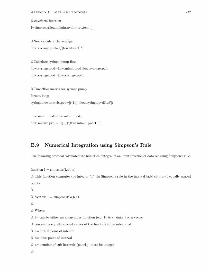
Appendix B. MatLab Protocols 232
%waveform function
I=simpsons(flow mlmin pvd,tstart,tend,[]);
%Now calculate the average
flow average pvd=1/(tend-tstart)*I;
%Calculate syringe pump flow
flow syringe pvd=flow mlmin pvd-flow average pvd;
flow syringe pvd=flow syringe pvd’;
%Time/flow matrix for syringe pump
format long;
syringe flow matrix pvd=[t(1,:)’,flow syringe pvd(1,:)’];
flow mlmin pvd=flow mlmin pvd’;
flow matrix pvd = [t(1,:)’,flow mlmin pvd(1,:)’];
B.9 Numerical Integration using Simpson’s Rule
The following protocol calculated the numerical integral of an input function or data set using Simpson’s rule.
function I = simpsons(f,a,b,n)
% This function computes the integral ”I” via Simpson’s rule in the interval [a,b] with n+1 equally spaced
points
%
% Syntax: I = simpsons(f,a,b,n)
%
% Where,
% f= can be either an anonymous function (e.g. f=@(x) sin(x)) or a vector
% containing equally spaced values of the function to be integrated
% a= Initial point of interval
% b= Last point of interval
% n= number of sub-intervals (panels), must be integer
%

Appendix B. MatLab Protocols 233
% Written by Juan Camilo Medina - The University of Notre Dame
% 09/2010 (copyright Dr. Simpson)
%
%
% Example 1:
%
% Suppose you want to integrate a function f(x) in the interval [-1,1].
% You also want 3 integration points (2 panels) evenly distributed through the
% domain (you can select more point for better accuracy).
% Thus:
%
% f=@(x) ((x-1).*x./2).*((x-1).*x./2);
% I=simpsons(f,-1,1,2)
%
%
% Example 2:
%
% Suppose you want to integrate a function f(x) in the interval [-1,1].
% You know some values of the function f(x) between the given interval,
% those are fi= 1,0.518,0.230,0.078,0.014,0,0.006,0.014,0.014,0.006,0
% Thus:
%
% fi= [1 0.518 0.230 0.078 0.014 0 0.006 0.014 0.014 0.006 0];
% I=simpsons(fi,-1,1,[])
%
% note that there is no need to provide the number of intervals (panels) ”n”,
% since they are implicitly specified by the number of elements in the
% vector fi
if numel(f)¿1 % If the input provided is a vector
n=numel(f)-1; h=(b-a)/n;
I= h/3*(f(1)+2*sum(f(3:2:end-2))+4*sum(f(2:2:end))+f(end));
else % If the input provided is an anonymous function
h=(b-a)/n; xi=a:h:b;

Appendix B. MatLab Protocols 234
I= h/3*(f(xi(1))+2*sum(f(xi(3:2:end-2)))+4*sum(f(xi(2:2:end)))+f(xi(end)));
end

Appendix C
Womersley Analysis Code
The following Fortran code was provided and used by Dr. David Steinman to carry out the Womersley
analysis on the PVD flow data.
womernoam.f **Contains the code necessary to carry out Womersley analysis with input from the second
file, noampopliteal.cfg. The output is the normalized flow and wall shear stress waveforms to the Posueille
values of flow and wall shear stress. Multiplying either output by these items provides either flow rate or
shear stress in physical units.
implicit real (a-h,o-y), complex (z), integer(i-n)
dimension ccoef(0:1000),scoef(0:1000)
read(5,*) nt,alpha,nf,(ccoef(i),scoef(i),i=0,nf)
write(6,’(a,f9.6)’) ’# alpha = ’,alpha
write(6,’(a)’) ’VARIABLES=time,q,wss,u0’
do 10 i=0,nt
t = 1.0*i/nt
call womer(alpha,nf,ccoef,scoef,t,q,wss,u0)
write(6,900) t,q,wss,u0
10 continue
900 format(f13.6,1x,f13.6,1x,f13.6,1x,f13.6)
stop
end
235

Appendix C. Womersley Analysis Code 236
* **********************************************************************
subroutine womer(alpha,nf,ccoef,scoef,t,q,wss,u0)
* **********************************************************************
real alpha,ccoef(0:1000),scoef(0:1000),t,q,wss,u0
integer nf
* **********************************************************************
complex zi,zk,zt,za,zf10,zq,zu0,zwss,zbes
real pi
zi = (0.0,1.0)
pi = 3.1415926535
q = ccoef(0)/ccoef(0)
u0 = 2.0*ccoef(0)/ccoef(0)
wss = 4.0*ccoef(0)/ccoef(0)/4.0
do 10 k=1,nf
zk = 2.0*pi*zi*k
zt = zk*t
za = alpha*sqrt(1.0*k)*zi*csqrt(zi)
zf10 = 2.0*zbes(1,za)/zbes(0,za)/za
zq = (ccoef(k)-zi*scoef(k))*cexp(zt)/ccoef(0)
zu0 = zq*(1.0-1.0/zbes(0,za))/(1.0-zf10)
zwss = -zq*za*zbes(1,za)/zbes(0,za)/(1.0-zf10)/4.0
q = q+real(zq)
wss = wss+real(zwss)
u0 = u0+real(zu0)
10 continue
end
complex function zbes(n,y)
complex z,zarg,y
integer i,n
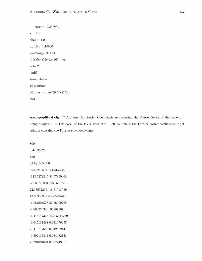
Appendix C. Womersley Analysis Code 237
zarg = -0.25*y*y
z = 1.0
zbes = 1.0
do 10 i=1,10000
z=z*zarg/i/(i+n)
if (cabs(z).le.1.e-20) then
goto 20
endif
zbes=zbes+z
10 continue
20 zbes = zbes*(0.5*y)**n
end
noampopliteal.cfg **Contains the Fourier Coefficients representing the Fourier Series of the waveform
being analyzed. In this case, of the PVD waveform. Left column is the Fourier cosine coefficients, right
column contains the Fourier sine coefficients.
800
6.44695826
150
83.68106529 0
35.52250501 114.3153987
-123.5272245 53.57850468
-22.30779804 -73.05527261
22.33052269 -16.71513089
13.50908982 4.982960787
-1.187904578 5.956009265
-3.06023638 0.93887967
-1.445147335 -0.205014739
-0.645131488 0.041976095
-0.415717685 0.042892141
-0.302133344 0.034482123
-0.234031694 0.027749511

Appendix C. Womersley Analysis Code 238
-0.188651555 0.022966458
-0.156310124 0.019556922
-0.132165758 0.017059374
-0.11351757 0.015171585
-0.098734724 0.013701306
-0.086771856 0.012525012
-0.076926976 0.011561588
-0.068710838 0.010756415
-0.061771979 0.010071773
-0.055851479 0.009480972
-0.050754498 0.008964685
-0.046331726 0.008508618
-0.042466924 0.008101992
-0.039068341 0.007736525
-0.036062667 0.007405754
-0.033390683 0.007104554
-0.031004084 0.006828806
-0.028863117 0.00657516
-0.026934802 0.006340856
-0.025191581 0.0061236
-0.023610262 0.005921464
-0.022171216 0.005732818
-0.020857724 0.005556266
-0.019655477 0.005390612
-0.018552163 0.005234816
-0.017537141 0.005087977
-0.016601171 0.004949302
-0.015736202 0.004818095
-0.014935186 0.004693739
-0.013501 0.004463451
-0.012857555 0.004356593
-0.012257325 0.004254719
-0.011696509 0.004157476
-0.011171715 0.004064543

Appendix C. Womersley Analysis Code 239
-0.010679909 0.003975629
-0.010218374 0.003890469
-0.009784666 0.003808823
-0.009376585 0.003730471
-0.008992143 0.003655209
-0.008629543 0.003582854
-0.008287157 0.003513234
-0.007963506 0.003446193
-0.007657242 0.003381584
-0.00736714 0.003319275
-0.007092079 0.003259141
-0.006831035 0.003201067
-0.006583068 0.003144944
-0.006347318 0.003090674
-0.006122994 0.003038164
-0.005909368 0.002987326
-0.005705768 0.002938079
-0.005511576 0.002890348
-0.00532622 0.002844062
-0.005149171 0.002799154
-0.00497994 0.002755561
-0.004818072 0.002713225
-0.004663146 0.002672089
-0.004514769 0.002632104
-0.004372578 0.002593218
-0.004236232 0.002555386
-0.004105416 0.002518564
-0.003979834 0.002482711
-0.003859211 0.002447787
-0.003743289 0.002413756
-0.003631825 0.002380583
-0.003524595 0.002348234
-0.003421387 0.002316678
-0.003322002 0.002285886

Appendix C. Womersley Analysis Code 240
-0.003226253 0.002255827
-0.003133966 0.002226476
-0.003044974 0.002197808
-0.002959124 0.002169796
-0.002876269 0.002142419
-0.002796271 0.002115653
-0.002719001 0.002089478
-0.002644336 0.002063874
-0.00257216 0.00203882
-0.002502364 0.002014299
-0.002434844 0.001990294
-0.002369503 0.001966787
-0.002306249 0.001943761
-0.002244992 0.001921203
-0.00218565 0.001899096
-0.002128145 0.001877427
-0.002072401 0.001856183
-0.002018347 0.001835349
-0.001965916 0.001814914
-0.001915043 0.001794866
-0.001865668 0.001775193
-0.001817732 0.001755884
-0.00177118 0.001736929
-0.00172596 0.001718317
-0.001682021 0.001700038
-0.001639315 0.001682083
-0.001597797 0.001664443
-0.001557424 0.001647109
-0.001518153 0.001630073
-0.001479946 0.001613327
-0.001442764 0.001596862
-0.001406571 0.001580671
-0.001371332 0.001564747
-0.001337014 0.001549083

Appendix C. Womersley Analysis Code 241
-0.001303586 0.001533671
-0.001271018 0.001518507
-0.001239279 0.001503582
-0.001208343 0.001488891
-0.001178182 0.001474428
-0.001148772 0.001460188
-0.001120087 0.001446165
-0.001092104 0.001432352
-0.0010648 0.001418747
-0.001038154 0.001405342
-0.001012145 0.001392134
-0.000986753 0.001379118
-0.000961959 0.001366289
-0.000937744 0.001353642
-0.000914091 0.001341174
-0.000890982 0.001328881
-0.0008684 0.001316758
-0.000846331 0.001304801
-0.000824759 0.001293007
-0.000803669 0.001281372
-0.000783047 0.001269893
-0.00076288 0.001258565
-0.000743154 0.001247386
-0.000723857 0.001236353
-0.000704976 0.001225462
-0.0006865 0.00121471
-0.000668417 0.001204095
-0.000650717 0.001193613
-0.000633388 0.001183261
-0.000616421 0.001173037
-0.000599807 0.001162938
-0.000583534 0.001152962
-0.000567594 0.001143105
-0.000551979 0.001133366

Appendix C. Womersley Analysis Code 242
-0.000536679 0.001123743
-5.22E-04 0.001114232
-5.07E-04 0.001104831
-4.93E-04 0.001095539
-4.78E-04 0.001086354
-4.65E-04 0.001077272
-4.51E-04 0.001068292
-4.38E-04 0.001059413
-4.25E-04 0.001050632
-4.12E-04 0.001041947
-3.99E-04 0.001033356
-3.87E-04 0.001024858
-3.75E-04 0.001016451
-3.63E-04 0.001008133
-3.51E-04 0.000999902
-3.40E-04 0.000991758
-3.29E-04 0.000983697
-3.18E-04 0.00097572
-3.07E-04 0.000967824
-2.96E-04 0.000960007
-2.86E-04 0.000952269
-2.76E-04 0.000944607
-2.66E-04 0.000937022
-2.56E-04 0.00092951
-2.46E-04 0.000922071
-2.36E-04 0.000914704
-2.27E-04 0.000907407
-2.18E-04 0.00090018
-2.09E-04 0.00089302
-2.00E-04 0.000885927
-1.91E-04 0.000878899
-1.83E-04 0.000871936
-1.74E-04 0.000865037
-1.66E-04 0.0008582

Appendix C. Womersley Analysis Code 243
-1.58E-04 0.000851424
-1.50E-04 0.000844708
-1.42E-04 0.000838051
-1.34E-04 0.000831453
-0.000126408 0.000824912
-0.000118898 0.000818427
-0.00011151 0.000811998
-0.000104243 0.000805623
-9.71E-05 0.000799302
-9.01E-05 0.000793033
-8.31E-05 0.000786817
-7.63E-05 0.000780651
-6.96E-05 0.000774536
-6.30E-05 0.000768471
-5.65E-05 0.000762454
-5.01E-05 0.000756484
-4.39E-05 0.000750562
-3.77E-05 0.000744687
-3.16E-05 0.000738857
-2.56E-05 0.000733072
-1.97E-05 0.000727332
-1.38E-05 0.000721635
-8.11E-06 0.000715981
-2.47E-06 0.000710369
3.09E-06 0.000704799
8.56E-06 0.00069927
1.39E-05 0.000693781
1.93E-05 0.000688332
2.45E-05 0.000682922
2.96E-05 0.000677551
3.47E-05 0.000672218
3.97E-05 0.000666922
4.46E-05 0.000661663
4.95E-05 0.000656441

Appendix C. Womersley Analysis Code 244
5.43E-05 0.000651254
5.90E-05 0.000646103
6.36E-05 0.000640986
6.82E-05 0.000635904
7.27E-05 0.000630855
7.71E-05 0.00062584
8.15E-05 0.000620857
8.58E-05 0.000615907
9.01E-05 0.000610989
9.43E-05 0.000606102
9.84E-05 0.000601246
0.000102492 0.00059642
0.000106508 0.000591625
0.000110467 0.000586859
0.000114371 0.000582123
0.000118219 0.000577415
0.000122012 0.000572736
0.000125753 0.000568084
0.000129441 0.000563461
0.000133078 0.000558864
0.000136664 0.000554294
0.0001402 0.000549751
0.000143686 0.000545234
0.000147125 0.000540743
0.000150516 0.000536277
0.000153859 0.000531836
0.000157157 0.00052742
0.00016041 0.000523028
0.000163617 0.00051866
0.000166781 0.000514316
0.000169901 0.000509995
0.000172978 0.000505697
0.000176013 0.000501422
0.000179007 0.000497169

Appendix C. Womersley Analysis Code 245
0.00018196 0.000492939
0.000184873 0.00048873
0.000187746 0.000484543
0.00019058 0.000480377
0.000193375 0.000476232
0.000196133 0.000472107
0.000198853 0.000468003
0.000201536 0.000463919
0.000204183 0.000459855
0.000206794 0.00045581
0.00020937 0.000451784
0.000211911 0.000447778
0.000214417 0.00044379
0.00021689 0.000439821
0.000219329 0.00043587
0.000221735 0.000431937
0.000224109 0.000428022
0.000226451 0.000424125
0.000228761 0.000420244
0.000231039 0.000416381
0.000233287 0.000412534
0.000235505 0.000408705
0.000237692 0.000404891
0.00023985 0.000401094
0.000241979 0.000397312
0.000244078 0.000393547
0.00024615 0.000389796
0.000248193 0.000386061
0.000250208 0.000382341
0.000252196 0.000378636
0.000254156 0.000374946
0.00025609 0.00037127
0.000257998 0.000367609
0.000259879 0.000363961

Appendix C. Womersley Analysis Code 246
0.000261735 0.000360328
0.000263565 0.000356708
0.000265369 0.000353101
0.000267149 0.000349508
0.000268905 0.000345928
0.000270636 0.000342361
0.000272343 0.000338807
0.000274026 0.000335265
0.000275685 0.000331736
0.000277322 0.000328219
0.000278935 0.000324714
0.000280526 0.000321221
0.000282095 0.00031774
0.000283641 0.00031427
0.000285165 0.000310812
0.000286667 0.000307365
0.000288148 0.000303929
0.000289608 0.000300504
0.000291046 0.00029709
0.000292464 0.000293686
0.000293861 0.000290293
0.000295238 0.00028691
0.000296595 0.000283537
0.000297931 0.000280175
0.000299248 0.000276822
0.000300545 0.000273479
0.000301823 0.000270145
0.000303081 0.000266821
0.000304321 0.000263506
0.000305541 0.0002602
0.000306743 0.000256904
0.000307927 0.000253616
0.000309092 0.000250337
0.000310239 0.000247066

Appendix C. Womersley Analysis Code 247
0.000311368 0.000243804
0.000312479 0.00024055
0.000313573 0.000237305
0.000314649 0.000234067
0.000315708 0.000230837
0.000316749 0.000227616
0.000317773 0.000224401
0.000318781 0.000221195
0.000319772 0.000217996
0.000320746 0.000214804
0.000321703 0.000211619
0.000322644 0.000208442
0.000323569 0.000205271
0.000324478 0.000202107
0.000325371 0.00019895
0.000326248 0.000195799
0.000327109 0.000192655
0.000327954 0.000189517
0.000328784 0.000186386
0.000329599 0.00018326
0.000330398 0.000180141
0.000331182 0.000177027
0.000331952 0.000173919
0.000332706 0.000170817
0.000333445 0.00016772
0.000334169 0.000164629
0.000334879 0.000161543
0.000335574 0.000158463
0.000336255 0.000155387
0.000336921 0.000152317
0.000337573 0.000149251
0.00033821 0.00014619
0.000338834 0.000143134
0.000339443 0.000140082

Appendix C. Womersley Analysis Code 248
0.000340039 0.000137035
0.00034062 0.000133993
0.000341188 0.000130954
0.000341742 0.00012792
0.000342282 0.00012489
0.000342808 0.000121863
0.000343321 0.000118841
0.000343821 0.000115822
0.000344307 0.000112807
0.000344779 0.000109796
0.000345239 0.000106788
0.000345685 0.000103783
0.000346118 0.000100782
0.000346538 9.78E-05
0.000346944 9.48E-05
0.000347338 9.18E-05
0.000347719 8.88E-05
0.000348086 8.58E-05
0.000348441 8.28E-05
0.000348783 7.99E-05
0.000349112 7.69E-05
0.000349429 7.39E-05
0.000349732 7.09E-05
0.000350023 6.80E-05
0.000350302 6.50E-05
0.000350568 6.20E-05
0.000350821 5.91E-05
0.000351061 5.61E-05
0.00035129 5.31E-05
0.000351505 5.02E-05
0.000351708 4.72E-05
0.000351899 4.42E-05
0.000352077 4.13E-05
0.000352243 3.83E-05

Appendix C. Womersley Analysis Code 249
0.000352397 3.54E-05
0.000352538 3.24E-05
0.000352667 2.95E-05
0.000352783 2.65E-05
0.000352888 2.36E-05
0.00035298 2.06E-05
0.000353059 1.77E-05
0.000353127 1.47E-05
0.000353182 1.18E-05
0.000353225 8.84E-06
0.000353255 5.89E-06
0.000353274 2.95E-06

Appendix D
Raw Cardiovascular Shear Waveform
Data
D.1 PVD Waveform Data
Note that this is the waveform after carrying out sinc interpolation.
Time (s) Shear Stress (dyn/cm2) 0 -0.382396501
0.001 -0.328392805
0.002 -0.279230357
0.003 -0.237105377
0.004 -0.201095922
0.005 -0.167702973
0.006 -0.136667311
0.007 -0.111953542
0.008 -0.093935811
0.009 -0.07540384
0.01 -0.049670817
0.011 -0.019528575
0.012 0.006234648
0.013 0.02379686
0.014 0.038380165
0.015 0.05753795
0.016 0.082458086
0.017 0.106798548
250

Appendix D. Raw Cardiovascular Shear Waveform Data 251
0.018 0.124327204
0.019 0.136981056
0.02 0.152979573
0.021 0.176203469
0.022 0.201118572
0.023 0.220788082
0.024 0.235811805
0.025 0.251096424
0.026 0.268016883
0.027 0.28591549
0.028 0.307574013
0.029 0.334934488
0.03 0.361446003
0.031 0.378171839
0.032 0.387783868
0.033 0.40324046
0.034 0.430686501
0.035 0.462258215
0.036 0.488642219
0.037 0.510421543
0.038 0.532976003
0.039 0.557803861
0.04 0.584166893
0.041 0.613224446
0.042 0.645086417
0.043 0.676435825
0.044 0.705837325
0.045 0.73721861
0.046 0.773841295
0.047 0.812968074
0.048 0.850595752
0.049 0.887637884
0.05 0.927476043
0.051 0.970892078

Appendix D. Raw Cardiovascular Shear Waveform Data 252
0.052 1.016706507
0.053 1.063944536
0.054 1.11108022
0.055 1.157569119
0.056 1.207885883
0.057 1.26768213
0.058 1.333251636
0.059 1.392704776
0.06 1.442570216
0.061 1.495387718
0.062 1.563718018
0.063 1.643239142
0.064 1.720005344
0.065 1.789130913
0.066 1.857415913
0.067 1.931438097
0.068 2.012137865
0.069 2.098501834
0.07 2.187961316
0.071 2.27517005
0.072 2.358574406
0.073 2.446005446
0.074 2.545386508
0.075 2.651875505
0.076 2.753449431
0.077 2.848127662
0.078 2.94583849
0.079 3.053251107
0.08 3.166761633
0.081 3.281686531
0.082 3.398238042
0.083 3.515557139
0.084 3.629571839
0.085 3.741607592

Appendix D. Raw Cardiovascular Shear Waveform Data 253
0.086 3.860911509
0.087 3.992386915
0.088 4.127830282
0.089 4.255739556
0.09 4.375958704
0.091 4.499024214
0.092 4.632935763
0.093 4.774952691
0.094 4.915674368
0.095 5.048821687
0.096 5.177683943
0.097 5.312005711
0.098 5.456681088
0.099 5.604719585
0.1 5.745267611
0.101 5.877536609
0.102 6.011266958
0.103 6.153429014
0.104 6.300894547
0.105 6.44729972
0.106 6.59017819
0.107 6.728906659
0.108 6.862556474
0.109 6.994089764
0.11 7.130797341
0.111 7.27530494
0.112 7.420132996
0.113 7.556073826
0.114 7.683103102
0.115 7.808888301
0.116 7.938905712
0.117 8.071426378
0.118 8.200599863
0.119 8.322187245

Appendix D. Raw Cardiovascular Shear Waveform Data 254
0.12 8.437927546
0.121 8.55496142
0.122 8.677649429
0.123 8.799860107
0.124 8.910718894
0.125 9.008918796
0.126 9.105003849
0.127 9.207167517
0.128 9.311777395
0.129 9.411277579
0.13 9.50368409
0.131 9.589542207
0.132 9.667191762
0.133 9.738262723
0.134 9.810924224
0.135 9.889229793
0.136 9.964359316
0.137 10.02542061
0.138 10.07476258
0.139 10.12306601
0.14 10.17284672
0.141 10.21745146
0.142 10.2546706
0.143 10.28957943
0.144 10.32312002
0.145 10.34847806
0.146 10.36231308
0.147 10.37076072
0.148 10.37984089
0.149 10.38709983
0.15 10.38701258
0.151 10.37912112
0.152 10.36651089
0.153 10.35033201

Appendix D. Raw Cardiovascular Shear Waveform Data 255
0.154 10.3297154
0.155 10.30358222
0.156 10.27041913
0.157 10.22951725
0.158 10.18408116
0.159 10.13890597
0.16 10.09303618
0.161 10.03951652
0.162 9.97461813
0.163 9.902824044
0.164 9.829718769
0.165 9.754964231
0.166 9.675574813
0.167 9.591538771
0.168 9.503786435
0.169 9.410511671
0.17 9.310262355
0.171 9.205882334
0.172 9.100540942
0.173 8.992112426
0.174 8.876759692
0.175 8.756126131
0.176 8.635360864
0.177 8.514489897
0.178 8.387755072
0.179 8.252617901
0.18 8.114224988
0.181 7.978017391
0.182 7.841738487
0.183 7.69893384
0.184 7.548415577
0.185 7.39612893
0.186 7.246957089
0.187 7.09840519

Appendix D. Raw Cardiovascular Shear Waveform Data 256
0.188 6.944787221
0.189 6.785324688
0.19 6.624431843
0.191 6.464409769
0.192 6.302266136
0.193 6.135665468
0.194 5.96832238
0.195 5.805323077
0.196 5.644768306
0.197 5.478949486
0.198 5.304216595
0.199 5.126285008
0.2 4.954044466
0.201 4.790223887
0.202 4.629079375
0.203 4.461899871
0.204 4.284908683
0.205 4.10339838
0.206 3.927928103
0.207 3.764085713
0.208 3.605912558
0.209 3.441904067
0.21 3.267707229
0.211 3.090356994
0.212 2.919586192
0.213 2.757862844
0.214 2.599936323
0.215 2.439446986
0.216 2.27454088
0.217 2.10866921
0.218 1.947126224
0.219 1.791754969
0.22 1.638805596
0.221 1.483408335

Appendix D. Raw Cardiovascular Shear Waveform Data 257
0.222 1.325778782
0.223 1.170968746
0.224 1.022604759
0.225 0.879232182
0.226 0.736716953
0.227 0.592014731
0.228 0.445087766
0.229 0.299664936
0.23 0.161215818
0.231 0.030837683
0.232 -0.097731799
0.233 -0.230879118
0.234 -0.365924011
0.235 -0.494619327
0.236 -0.615421506
0.237 -0.735443514
0.238 -0.858894076
0.239 -0.980807786
0.24 -1.095730168
0.241 -1.20594888
0.242 -1.316240576
0.243 -1.425974409
0.244 -1.532243616
0.245 -1.636460053
0.246 -1.741235193
0.247 -1.843741967
0.248 -1.939092151
0.249 -2.028954302
0.25 -2.120156163
0.251 -2.214686749
0.252 -2.306877664
0.253 -2.391742533
0.254 -2.471436468
0.255 -2.5515574

Appendix D. Raw Cardiovascular Shear Waveform Data 258
0.256 -2.634087631
0.257 -2.715841887
0.258 -2.792119014
0.259 -2.861016405
0.26 -2.925494511
0.261 -2.991510307
0.262 -3.062702068
0.263 -3.136369401
0.264 -3.20520052
0.265 -3.263342472
0.266 -3.311640861
0.267 -3.35828076
0.268 -3.413177876
0.269 -3.478291862
0.27 -3.543256526
0.271 -3.594619389
0.272 -3.630921617
0.273 -3.664519256
0.274 -3.706720576
0.275 -3.755938391
0.276 -3.803367687
0.277 -3.844947387
0.278 -3.882364503
0.279 -3.91674399
0.28 -3.948109337
0.281 -3.978703742
0.282 -4.010448268
0.283 -4.040744026
0.284 -4.066604561
0.285 -4.091431581
0.286 -4.120797847
0.287 -4.152121249
0.288 -4.176029681
0.289 -4.189275792

Appendix D. Raw Cardiovascular Shear Waveform Data 259
0.29 -4.199839124
0.291 -4.216732739
0.292 -4.239909657
0.293 -4.262654546
0.294 -4.279416454
0.295 -4.28894711
0.296 -4.293672591
0.297 -4.298828424
0.298 -4.309141766
0.299 -4.323489342
0.3 -4.335117229
0.301 -4.339188374
0.302 -4.338016441
0.303 -4.337437606
0.304 -4.340033978
0.305 -4.343520414
0.306 -4.3440766
0.307 -4.340075922
0.308 -4.333939425
0.309 -4.330224809
0.31 -4.330057031
0.311 -4.328114156
0.312 -4.318321765
0.313 -4.30221671
0.314 -4.287709744
0.315 -4.279179887
0.316 -4.2731105
0.317 -4.264250958
0.318 -4.251322788
0.319 -4.234804158
0.32 -4.214377129
0.321 -4.192053364
0.322 -4.173294892
0.323 -4.160234177

Appendix D. Raw Cardiovascular Shear Waveform Data 260
0.324 -4.146574493
0.325 -4.124591318
0.326 -4.095803049
0.327 -4.069525585
0.328 -4.050318305
0.329 -4.031814856
0.33 -4.005255524
0.331 -3.97099516
0.332 -3.938072829
0.333 -3.912911091
0.334 -3.891791976
0.335 -3.865928924
0.336 -3.831927778
0.337 -3.794305972
0.338 -3.75855909
0.339 -3.725475692
0.34 -3.693195114
0.341 -3.660690552
0.342 -3.626619777
0.343 -3.588657381
0.344 -3.547813389
0.345 -3.509704187
0.346 -3.476335565
0.347 -3.440170077
0.348 -3.393655173
0.349 -3.342538944
0.35 -3.300319169
0.351 -3.269157674
0.352 -3.235974447
0.353 -3.19071201
0.354 -3.138906212
0.355 -3.0905944
0.356 -3.045568531
0.357 -2.998222284

Appendix D. Raw Cardiovascular Shear Waveform Data 261
0.358 -2.95038277
0.359 -2.908420535
0.36 -2.870203115
0.361 -2.825584108
0.362 -2.770755781
0.363 -2.713469499
0.364 -2.661964024
0.365 -2.615816555
0.366 -2.570481134
0.367 -2.524228804
0.368 -2.47650925
0.369 -2.424752947
0.37 -2.368161268
0.371 -2.311650962
0.372 -2.260792273
0.373 -2.214236264
0.374 -2.165697951
0.375 -2.112802432
0.376 -2.05925761
0.377 -2.007743747
0.378 -1.955462297
0.379 -1.899425965
0.38 -1.842522218
0.381 -1.790081378
0.382 -1.742064018
0.383 -1.693213638
0.384 -1.640683037
0.385 -1.586660047
0.386 -1.532552328
0.387 -1.476173728
0.388 -1.417920203
0.389 -1.364257936
0.39 -1.319183411
0.391 -1.275798414

Appendix D. Raw Cardiovascular Shear Waveform Data 262
0.392 -1.223683065
0.393 -1.163256809
0.394 -1.105125762
0.395 -1.055069894
0.396 -1.007715259
0.397 -0.957002538
0.398 -0.904785682
0.399 -0.854896753
0.4 -0.805870206
0.401 -0.755146579
0.402 -0.704807165
0.403 -0.656908927
0.404 -0.607984725
0.405 -0.555000283
0.406 -0.502874867
0.407 -0.458295288
0.408 -0.418525079
0.409 -0.37429364
0.41 -0.322995372
0.411 -0.271451308
0.412 -0.225440579
0.413 -0.183481699
0.414 -0.141938071
0.415 -0.099646991
0.416 -0.055920565
0.417 -0.010023925
0.418 0.035224252
0.419 0.07501795
0.42 0.11012224
0.421 0.14766519
0.422 0.191335409
0.423 0.235715332
0.424 0.273876546
0.425 0.306598382

Appendix D. Raw Cardiovascular Shear Waveform Data 263
0.426 0.339948547
0.427 0.376837161
0.428 0.415041998
0.429 0.451510326
0.43 0.484966193
0.431 0.51567217
0.432 0.545660055
0.433 0.577838289
0.434 0.61226727
0.435 0.644641804
0.436 0.671297609
0.437 0.694611267
0.438 0.720584214
0.439 0.75135898
0.44 0.782584232
0.441 0.808504328
0.442 0.828204876
0.443 0.846439041
0.444 0.86881985
0.445 0.895962212
0.446 0.922506445
0.447 0.942722073
0.448 0.956872509
0.449 0.970514577
0.45 0.987940888
0.451 1.008476134
0.452 1.028930847
0.453 1.046657481
0.454 1.059895203
0.455 1.06890239
0.456 1.077898672
0.457 1.091966897
0.458 1.109764837
0.459 1.123267649
Appendix D. Raw Cardiovascular Shear Waveform Data 264
0.46 1.128035074
0.461 1.130268206
0.462 1.139235126
0.463 1.154867046
0.464 1.167879945
0.465 1.171553454
0.466 1.168925205
0.467 1.167908467
0.468 1.173012288
0.469 1.182797968
0.47 1.192450263
0.471 1.197089338
0.472 1.194630544
0.473 1.187588882
0.474 1.181983403
0.475 1.183022791
0.476 1.190315282
0.477 1.196736164
0.478 1.193967819
0.479 1.18181143
0.48 1.170740568
0.481 1.170724629
0.482 1.177566635
0.483 1.176564158
0.484 1.162068937
0.485 1.146390878
0.486 1.143400227
0.487 1.149141606
0.488 1.147474727
0.489 1.132296647
0.49 1.114313312
0.491 1.105174418
0.492 1.103876652
0.493 1.101781938

Appendix D. Raw Cardiovascular Shear Waveform Data 265
0.494 1.093716826
0.495 1.080023586
0.496 1.063569551
0.497 1.049441765
0.498 1.042672743
0.499 1.041285215
0.5 1.03541884
0.501 1.018705588
0.502 0.997645195
0.503 0.983962022
0.504 0.979455492
0.505 0.974369287
0.506 0.96074987
0.507 0.941816908
0.508 0.92631166
0.509 0.917567046
0.51 0.91095238
0.511 0.900282508
0.512 0.884204297
0.513 0.866336729
0.514 0.850818898
0.515 0.838728781
0.516 0.828733378
0.517 0.819380567
0.518 0.809178797
0.519 0.795699475
0.52 0.77794264
0.521 0.759748743
0.522 0.746886006
0.523 0.739283124
0.524 0.729860685
0.525 0.713863847
0.526 0.695810044
0.527 0.683277831

Appendix D. Raw Cardiovascular Shear Waveform Data 266
0.528 0.676301602
0.529 0.667742383
0.53 0.652893989
0.531 0.634177461
0.532 0.61673605
0.533 0.603921969
0.534 0.596798934
0.535 0.593012174
0.536 0.585400065
0.537 0.567514879
0.538 0.543207973
0.539 0.525570261
0.54 0.521896751
0.541 0.523385785
0.542 0.515321513
0.543 0.495394464
0.544 0.475490065
0.545 0.4651784
0.546 0.460442013
0.547 0.452027923
0.548 0.439133308
0.549 0.428306564
0.55 0.421389896
0.551 0.412418781
0.552 0.397981444
0.553 0.383876307
0.554 0.376836323
0.555 0.373948016
0.556 0.366394629
0.557 0.352207282
0.558 0.33905261
0.559 0.333361565
0.56 0.331818842
0.561 0.326229302

Appendix D. Raw Cardiovascular Shear Waveform Data 267
0.562 0.313547766
0.563 0.298253919
0.564 0.286861761
0.565 0.282355231
0.566 0.282638777
0.567 0.282284764
0.568 0.276559324
0.569 0.265058948
0.57 0.251380808
0.571 0.239604437
0.572 0.232454558
0.573 0.231405942
0.574 0.234780806
0.575 0.235894855
0.576 0.228042823
0.577 0.213120605
0.578 0.200798954
0.579 0.19693166
0.58 0.197256312
0.581 0.195510577
0.582 0.192207019
0.583 0.190473028
0.584 0.187999135
0.585 0.180355147
0.586 0.169695342
0.587 0.163088226
0.588 0.16275938
0.589 0.16428197
0.59 0.163873429
0.591 0.161490975
0.592 0.156867
0.593 0.149196168
0.594 0.14178036
0.595 0.14023512

Appendix D. Raw Cardiovascular Shear Waveform Data 268
0.596 0.143919535
0.597 0.144931239
0.598 0.138706658
0.599 0.13040414
0.6 0.127233127
0.601 0.128738939
0.602 0.128990607
0.603 0.125279347
0.604 0.120325687
0.605 0.11722598
0.606 0.116023009
0.607 0.114888826
0.608 0.112541605
0.609 0.109256503
0.61 0.106207129
0.611 0.103680385
0.612 0.10057145
0.613 0.096902974
0.614 0.095102711
0.615 0.095981031
0.616 0.095189117
0.617 0.088539217
0.618 0.079801314
0.619 0.076996897
0.62 0.080268577
0.621 0.080621751
0.622 0.073299059
0.623 0.065145025
0.624 0.06365683
0.625 0.06517187
0.626 0.06107472
0.627 0.051581814
0.628 0.045002381
0.629 0.044762458

Appendix D. Raw Cardiovascular Shear Waveform Data 269
0.63 0.045276699
0.631 0.041421988
0.632 0.035045567
0.633 0.029426666
0.634 0.023380769
0.635 0.015211635
0.636 0.008596969
0.637 0.008544119
0.638 0.012218467
0.639 0.009484517
0.64 -0.004549313
0.641 -0.021174482
0.642 -0.027119712
0.643 -0.021392594
0.644 -0.017506006
0.645 -0.026564366
0.646 -0.043103967
0.647 -0.052980247
0.648 -0.052044043
0.649 -0.050091941
0.65 -0.056752746
0.651 -0.070362936
0.652 -0.08232638
0.653 -0.086946999
0.654 -0.085046908
0.655 -0.082799515
0.656 -0.088458683
0.657 -0.104583033
0.658 -0.12172496
0.659 -0.126427791
0.66 -0.118595053
0.661 -0.113876283
0.662 -0.124127548
0.663 -0.14227279

Appendix D. Raw Cardiovascular Shear Waveform Data 270
0.664 -0.153059268
0.665 -0.152738811
0.666 -0.150040094
0.667 -0.151961996
0.668 -0.158012088
0.669 -0.1662131
0.67 -0.175447627
0.671 -0.181828242
0.672 -0.181326585
0.673 -0.177553247
0.674 -0.179598466
0.675 -0.189807786
0.676 -0.199715105
0.677 -0.201062366
0.678 -0.195957706
0.679 -0.193017389
0.68 -0.197016389
0.681 -0.205208173
0.682 -0.211482249
0.683 -0.211842133
0.684 -0.207332248
0.685 -0.203019502
0.686 -0.203172181
0.687 -0.207127558
0.688 -0.210621545
0.689 -0.210358972
0.69 -0.206257627
0.691 -0.201069078
0.692 -0.199207575
0.693 -0.202978397
0.694 -0.207531904
0.695 -0.203757728
0.696 -0.190575373
0.697 -0.179923957

Appendix D. Raw Cardiovascular Shear Waveform Data 271
0.698 -0.182642807
0.699 -0.19255432
0.7 -0.193380629
0.701 -0.180626948
0.702 -0.166923642
0.703 -0.163844068
0.704 -0.167633345
0.705 -0.167353993
0.706 -0.159686517
0.707 -0.149785071
0.708 -0.142509357
0.709 -0.138815714
0.71 -0.137835049
0.711 -0.137121152
0.712 -0.132605394
0.713 -0.122652775
0.714 -0.111414134
0.715 -0.104926979
0.716 -0.104430355
0.717 -0.105390887
0.718 -0.102345707
0.719 -0.093524754
0.72 -0.08222068
0.721 -0.074485253
0.722 -0.07368495
0.723 -0.076298099
0.724 -0.075183212
0.725 -0.067604658
0.726 -0.057785423
0.727 -0.051137201
0.728 -0.049024031
0.729 -0.049898157
0.73 -0.05159943
0.731 -0.051067573

Appendix D. Raw Cardiovascular Shear Waveform Data 272
0.732 -0.04574564
0.733 -0.037886057
0.734 -0.03389964
0.735 -0.036623524
0.736 -0.041100693
0.737 -0.041251693
0.738 -0.037934713
0.739 -0.036766975
0.74 -0.039794537
0.741 -0.04351083
0.742 -0.044527568
0.743 -0.043696226
0.744 -0.044036816
0.745 -0.047118067
0.746 -0.052611135
0.747 -0.059808831
0.748 -0.067887365
0.749 -0.074648837
0.75 -0.076993541
0.751 -0.07485101
0.752 -0.074299019
0.753 -0.082902699
0.754 -0.100084892
0.755 -0.115805735
0.756 -0.122156989
0.757 -0.12291367
0.758 -0.127114004
0.759 -0.136523021
0.76 -0.146060389
0.761 -0.154324317
0.762 -0.165397696
0.763 -0.179969257
0.764 -0.192962022
0.765 -0.201987665

Appendix D. Raw Cardiovascular Shear Waveform Data 273
0.766 -0.210684462
0.767 -0.221087566
0.768 -0.230002475
0.769 -0.236573519
0.77 -0.246333193
0.771 -0.262948295
0.772 -0.281691667
0.773 -0.295947804
0.774 -0.305090892
0.775 -0.311751697
0.776 -0.316979675
0.777 -0.323137983
0.778 -0.335649224
0.779 -0.355487351
0.78 -0.374578024
0.781 -0.385031462
0.782 -0.389032979
0.783 -0.393714837
0.784 -0.400924278
0.785 -0.408815738
0.786 -0.419056936
0.787 -0.433933015
0.788 -0.44915975
0.789 -0.457744136
0.79 -0.45957376
0.791 -0.460137495
0.792 -0.462037587
0.793 -0.465493823
0.794 -0.474590772
0.795 -0.492699942
0.796 -0.511109434
0.797 -0.51184011
0.798 -0.485040854
0.799 -0.437453007

Appendix D. Raw Cardiovascular Shear Waveform Data 274
0.8 -0.382394823
D.2 CAVD Waveform Data
Raw numerical CAVD data was provided courtesy of Dr. Phillipe Sucosky at the University of Notre Dame,
Indiana, United States.
D.2.1 Aortic-Side
Time (s) Shear Stress (dyn/cm2)
0 -0.0341
0.01 -0.0107
0.02 0.6930
0.03 -0.7362
0.04 0.0065
0.05 -0.7032
0.06 -1.7873
0.07 -1.1798
0.08 0.6332
0.09 0.1245
0.1 -1.4931
0.11 -1.1850
0.12 0.6279
0.13 0.1457
0.14 -1.1976
0.15 -1.0710
0.16 0.1935
0.17 0.1632
0.18 -0.6685
0.19 -0.8754
0.2 -0.1539
0.21 0.1160
0.22 -0.2391
0.23 -0.2536

Appendix D. Raw Cardiovascular Shear Waveform Data 275
0.24 -0.0163
0.25 0.0231
0.26 -0.0998
0.27 -0.1580
0.28 -0.1165
0.29 -0.0404
0.3 -0.1377
0.31 0.0000
0.32 0.0000
0.33 0.0000
0.34 0.0000
0.35 0.0000
0.36 0.0000
0.37 0.0000
0.38 0.0000
0.39 0.0000
0.4 0.0000
0.41 0.0000
0.42 0.0000
0.43 0.0000
0.44 0.0000
0.45 0.0000
0.46 0.0000
0.47 0.0000
0.48 0.0000
0.49 0.0000
0.5 0.0000
0.51 0.0000
0.52 0.0000
0.53 0.0000
0.54 0.0000
0.55 0.0000
0.56 0.0000
0.57 0.0000

Appendix D. Raw Cardiovascular Shear Waveform Data 276
0.58 0.0000
0.59 0.0000
0.6 0.0000
0.61 0.0000
0.62 0.0000
0.63 0.0000
0.64 0.0000
0.65 0.0000
0.66 0.0000
0.67 0.0000
0.68 0.0000
0.69 0.0000
0.7 0.0000
0.71 0.0000
0.72 0.0000
0.73 0.0000
0.74 0.0000
0.75 0.0000
0.76 0.0000
0.77 0.0000
0.78 0.0000
0.79 0.0000
0.8 0.0000
0.81 0.0000
0.82 0.0000
0.83 0.0000
0.84 0.0000
0.85 -0.0341
D.2.2 Ventricular-Side
Time (s) Shear Stress (dyn/cm2)
0 6.3303
0.01 6.5828

Appendix D. Raw Cardiovascular Shear Waveform Data 277
0.02 7.0474
0.03 14.6680
0.04 29.3188
0.05 37.7158
0.06 37.3725
0.07 32.9553
0.08 34.0425
0.09 37.9424
0.1 35.8073
0.11 30.7421
0.12 31.2986
0.13 34.5896
0.14 33.4349
0.15 29.9982
0.16 29.8814
0.17 31.8398
0.18 31.6054
0.19 29.2345
0.2 28.3830
0.21 29.4764
0.22 29.9706
0.23 28.8513
0.24 28.0517
0.25 27.8614
0.26 27.2917
0.27 26.1743
0.28 25.0674
0.29 24.0615
0.3 22.7393
0.31 0.0000
0.32 0.0000
0.33 0.0000
0.34 0.0000
0.35 0.0000

Appendix D. Raw Cardiovascular Shear Waveform Data 278
0.36 0.0000
0.37 0.0000
0.38 0.0000
0.39 0.0000
0.4 0.0000
0.41 0.0000
0.42 0.0000
0.43 0.0000
0.44 0.0000
0.45 0.0000
0.46 0.0000
0.47 0.0000
0.48 0.0000
0.49 0.0000
0.5 0.0000
0.51 0.0000
0.52 0.0000
0.53 0.0000
0.54 0.0000
0.55 0.0000
0.56 0.0000
0.57 0.0000
0.58 0.0000
0.59 0.0000
0.6 0.0000
0.61 0.0000
0.62 0.0000
0.63 0.0000
0.64 0.0000
0.65 0.0000
0.66 0.0000
0.67 0.0000
0.68 0.0000
0.69 0.0000

Appendix D. Raw Cardiovascular Shear Waveform Data 279
0.7 0.0000
0.71 0.0000
0.72 0.0000
0.73 0.0000
0.74 0.0000
0.75 0.0000
0.76 0.0000
0.77 0.0000
0.78 0.0000
0.79 0.0000
0.8 0.0000
0.81 0.0000
0.82 0.0000
0.83 0.0000
0.84 0.0000
0.85 6.3303
D.3 Atherosclerosis Waveform Data
D.3.1 Athero-Prone
Time (s) Shear Stress (dyn/cm2)
0 0
0.025 3.076923077
0.05 -4.102564103
0.075 -8.461538462
0.1 -4.871794872
0.125 0.512820513
0.15 1.025641026
0.175 -1.282051282
0.2 -2.307692308
0.225 -1.538461538
0.25 0
0.275 1.282051282

Appendix D. Raw Cardiovascular Shear Waveform Data 280
0.3 1.794871795
0.325 1.282051282
0.35 0.256410256
0.375 -0.512820513
0.4 -0.512820513
0.425 -0.256410256
0.45 0.256410256
0.475 0.512820513
0.5 0.769230769
0.525 0.769230769
0.55 1.025641026
0.575 1.282051282
0.6 1.538461538
0.625 1.538461538
0.65 1.538461538
0.675 1.025641026
0.7 1.025641026
0.725 0.769230769
0.75 0.256410256
0.775 0.256410256
0.8 0
D.3.2 Athero-Protective
Time (s) Shear Stress (dyn/cm2)
0 14.47368421
0.025 18.94736842
0.05 25.78947368
0.075 34.21052632
0.1 41.05263158
0.125 44.21052632
0.15 38.15789474
0.175 28.15789474
0.2 22.36842105

Appendix D. Raw Cardiovascular Shear Waveform Data 281
0.225 20.26315789
0.25 19.73684211
0.275 18.94736842
0.3 17.10526316
0.325 15.26315789
0.35 15
0.375 16.31578947
0.4 18.42105263
0.425 20.26315789
0.45 20.78947368
0.475 20.52631579
0.5 20
0.525 19.21052632
0.55 18.42105263
0.575 17.36842105
0.6 16.84210526
0.625 16.31578947
0.65 15.78947368
0.675 15.26315789
0.7 15.26315789
0.725 15
0.75 14.47368421
0.775 14.21052632
0.8 14.47368421

Appendix E
Testing of UltraMotion Digit Linear
Actuator
The following are the results of testing the Ultramotion Digit Linear Actuator when being considered for
use in the bioreactor.
-0.5
0
0.5
1
1.5
2
2.5
3
3.5
4
4.5
0 5 10 15 20 25 30 35
Time (s)
Dis
pla
cem
ent
fro
m O
rig
in (
mm
)
Theoretical
Experimental
Figure E.1: Results from UltraMotion Digit linear actuator test using athero-prone waveform with timepoints spaced at 100 ms intervals.
282

Appendix E. Testing of UltraMotion Digit Linear Actuator 283
-20
0
20
40
60
80
100
120
140
160
0 5 10 15 20 25 30
Time (s)
Dis
pla
cem
ent
fro
m O
rig
in (
um
)
Theoretical
Experimental
Figure E.2: Results from UltraMotion Digit linear actuator test using ventricular-side CAVD waveform withtime points spaced at 100 ms intervals.
-160
-140
-120
-100
-80
-60
-40
-20
0
20
0 2 4 6 8 10 12 14 16
Time (s)
Dis
pla
cem
ent
fro
m O
rig
in (
um
)
Theoretical
Experimental
Figure E.3: Results from UltraMotion Digit linear actuator test using aortic-side CAVD waveform with timepoints spaced at 50 ms intervals.

Appendix E. Testing of UltraMotion Digit Linear Actuator 284
-2000
0
2000
4000
6000
8000
10000
12000
0 2 4 6 8 10 12 14 16 18
Time (s)
Dis
pla
cem
ent
fro
m O
rig
in (
um
)
Theoretical
Experimental
Figure E.4: Results from UltraMotion Digit linear actuator test using athero-prone waveform with timepoints spaced at 50 ms intervals.
-180
-160
-140
-120
-100
-80
-60
-40
-20
0
20
40
0 5 10 15 20 25
Time (s)
Dis
pla
cem
ent
fro
m O
rig
in (
um
)
Theoretical
Experimental
Figure E.5: Results from UltraMotion Digit linear actuator test using athero-prone waveform with timepoints spaced at 25 ms intervals.

Appendix F
Validation and Troubleshooting of
Alicat Flowmeter
Validation of the bioreactor was first carried out using the Alicat flowmeter, as presented in Section 4.3 on
p. 75, was carried out by following a strategy of moving from simple to complex waveforms. Two types of
flows were employed:
1. Constant Flow - Refers to a constant flow of 1 mL/min being prescribed using either the peristaltic
or neMESYS pumps. Only one pump was connected at a time for these tests, which were primarily
carried out to ensure that the flowmeter was reading flow rates correctly.
2. Sinusoidal Flow - Various sinusoidal flows were employed, beginning with slow-phase (long periods,
at approximately ten seconds or a frequency of 0.1 Hz) moving to quicker-phase (shorter periods, at
approximately one second or a frequency of 1 Hz) mimicking a cardiac cycle. The amplitude of the
waveforms was 1 or 2 mL/min depending on the test.
F.1 Implementation and Methodology of Validation Using Alicat
Flowmeter
Validation tests were either qualitative or quantitative: Qualitative tests involved examining the visual
movement of the fluid inside a microfluidic device using a NAVITAR scope, SCHOTT light source, Sony
XCD-X710 camera, and Fire-i software. A combination (one or two) of the pumps were connected to the
system along with a microfluidic device. A solution of 0.1% 1.0 µm FluoSpheres microspheres (Item #F8819,
Life Technologies; Burlington, ON) and distilled water was combined and employed as the medium so that
upon capturing a video, particle movement representing bulk fluid motion could be visually inspected to
285

Appendix F. Validation and Troubleshooting of Alicat Flowmeter 286
determine if the fluid was moving as desired. On the other hand, quantitative tests involved examining
the numerical flow rate values obtained from applying flow waveforms to the system when the flowmeter was
installed. Distilled water was used as a fluid. A microfluidic device was not connected, and the fluid was
simply allowed to drain into a waste beaker.
The tests proceeded as follows:
1. Qualitative - Test constant flow using peristaltic pump.
2. Quantitative - Test constant flow using peristaltic pump.
3. Qualitative - Test constant flow using neMESYS.
4. Quantitative - Test constant flow using neMESYS.
5. Qualitative - Test sinusoidal flow using using neMESYS only.
6. Qualitative - Test sinusoidal flow using using both peristaltic and neMESYS pumps.
7. Quantitative - Test sinusoidal flow using neMESYS.
8. Quantitative - Test sinusoidal flow using using both peristaltic and neMESYS pumps.
F.2 Experimental Setups for Flow Testing
The following section details the experimental layout of the testing that was carried out during the validation
of the system using the Alicat flowmeter. Detailed instructions of how to attach components together,
assemble the setup in the correct order, fill the setup with media, and install the flowmeter may be found
in Appendices I.2, G.4, and G.3 on p. 345, 328, and 324, respectively. These set-ups remained consistent
for all the tests that will be described in this Chapter unless otherwise noted. The flowmeter was placed in
a vertical orientation at the suggestion of Alicat Scientific to trap and remove bubbles from the system.
F.2.1 Experimental Set-up Using Peristaltic Pump Only
A standard laboratory beaker was filled with media to flow through the setup. Typically a 400 mL beaker
was employed with a 50 mL Falcon tube (Becton Dickinson and Company; Missisauga, ON). A small length
of MasterFlex #13 tubing (Cole-Parmer; Montreal, QC) was run between the beaker and in through the
EasyLoad II Model #77202-60 pump head of the Masterflex L/S: Digital Economy Drive peristaltic pump
(Cole-Parmer; Montreal, QC). The tubing was then fitted into the highest port of the small laboratory
damper (custom machined in-house, refer to [91]) held in place by a Styrofoam stage. A small length of
Masterflex PharMed #25 BPT tubing (Cole-Parmer; Montreal, QC) was fitted onto the end of the damper at
the exit, with a 3/16” to 1/16” tubing connector (Cole-Parmer; Montreal, QC) at its other end. Intramedic

Appendix F. Validation and Troubleshooting of Alicat Flowmeter 287
PE60 tubing (Becton Dickinson and Company; Missisauga, ON) was run between this connector, and then
a small length of Intramedic PE190 tubing (Becton Dickinson and Company; Missisauga, ON) was fit over
the PE60 leading to the entrance of the flowmeter. The flowmeter used 10-32 external thread to 1/32” inner
diameter tubing barbs and 1/8” NPT adaptors (beswick engineering; Greenland, NH, USA). From the exit
of the flowmeter, a section of PE190 tubing was run into a waste media beaker for collection (Figure F.1).
2.
1.3.
5.
6.4.
Figure F.1: Pseudo-physiological troubleshooting setup using peristaltic pump only. Main components: 1.Falcon tube containing flow media, 2. peristaltic pump, 3. damper, 4. Arduino Uno microcontroller, 5.Alicat flowmeter and attachments, 6. waste beaker.
F.2.2 Experimental Set-up Using neMESYS Only
A glass syringe sourced from cetoni was loaded into the neMESYS syringe pump. A 1/4-28 UNF to luer-lock
adaptor (Cole-Parmer; Montreal, QC) was fastened to the end of the syringe. Then, this was either connected
to a 18G x 1 PrecisionGlide needle (Becton Dickinson and Company; Missisauga, ON) and a length of PE190
tubing was run to the flowmeter via the same procedure as described for the peristaltic pump. Or, male
and female adaptors were employed (McMasterr-Carr; Aurora, OH, USA) to create a connection from the
luer-lock end of the syringe adaptor to the 1/8” NPT port at the entry to the flowmeter. At the exit of the
flowmeter PE190 tubing was once again run to a waste media beaker for collection (Figure F.2).

Appendix F. Validation and Troubleshooting of Alicat Flowmeter 288
2.
1.
3.
4.
Figure F.2: Pseudo-physiological troubleshooting setup using neMESYS only. Main components: 1. Falcontube containing flow media, 2. neMESYS with syringe and attachments, 3. Alicat flowmeter and attach-ments, 4. waste beaker. Not visible: Arduino Uno microcontroller behind neMESYS.
F.2.3 Experimental Set-up Combining Peristaltic and neMESYS
When the two pumps were combined and a microfluidic device incorporated (if desired), the length of
Masterflex PharMed #25 BPT tubing from the peristaltic pump was directly attached to a 3/16” three-way-
tee (Cole-Parmer; Montreal, QC). A 21G x 1-1/2 PrecisionGlide needle (Becton Dickinson and Company;
Missisauga, ON) was fixed to the luer-lock adaptor at the neMESYS, and a small length of PE60 tubing
was then fitted into a 3/16” to 1/16” tubing connector, which was then connected to additional PE190 and
MasterFlex #25 tubing and the second port of the three-way tee. The last port of the tee had another length
of MasterFlex #25 tubing and a 3/16” to 1/16” tubing connector attached. PE60 tubing was run from the
connector, then a small amount of PE190 was fitted over it. A blue ferrule half union and peek union
adaptor (Upchurch Scientific; Oak Harbor, WA, USA) were fixed onto the PE190 tubing, with matching
parts on the tubing at the entrance of the microfluidic device. These parts were also fixed at the exit, with
a length of PE190 tubing running either to a waste collection beaker, or to the initial media source. If a
microfluidic device was not employed, the tubing from the flowmeter outlet simply went to an exit waste
beaker (Figure F.3).

Appendix F. Validation and Troubleshooting of Alicat Flowmeter 289
3.
1.
2. 4.
5.
6.
Figure F.3: Pseudo-physiological troubleshooting setup combining peristaltic and neMESYS. Main compo-nents: 1. Peristaltic pump, 2. damper, 3. neMESYS with syringe and attachments, 4. tee connector withattachments, 5. Arduino Uno microcontroller, 6. Alicat flowmeter and attachments. Not visible: wastebeaker in line with flow after flowmeter.
F.3 Data Recording Procedures
Initially, quantitative data from the flowmeter was acquired using a supplied cable connecting the data port
of the flowmeter to the USB port of the computer via a male 8 pin mini Din to female DB9 cable and USB
to RS232 converter (Alicat Scientific; Tucson, AZ, USA). However, as will be discussed in the Sections that
follow, this approach was abandoned in favour of using a microcontroller. An Arduino Uno (Creatron Inc.;
Toronto, ON) was programmed to record the flow data using a customized code (provided in Appendix G.3)
and a serial data to text program, RS232 port logger (Eltima Software; Bellevue, WA, USA) was employed
to transfer the acquired flowmeter data to a computer for data analysis. Teflon shielded signal wire was
soldered to pin headers (Active Surplus; Toronto, ON) to connect the microcontroller to the flowmeter.
Detailed instructions concerning flowmeter setup and data recording are provided in Appendix G.
F.4 Results from Validation Tests Using Alicat Flowmeter
F.4.1 Qualitative Testing - Constant Flow Using Peristaltic Pump Only
When running the qualitative test using the peristaltic pump at a constant flow rate of 1 mL/min, the
particles seemed to flow at a regular velocity. It was assumed that the fluid was moving as prescribed.

Appendix F. Validation and Troubleshooting of Alicat Flowmeter 290
Quantitative Testing - Constant Flow Using Peristaltic Pump Only
The flowmeter was attached to the set up. This experiment also served as a check to ensure that the
flowmeter unit was calibrated properly. A flow of 1 mL/min was prescribed to the peristaltic pump. A
variety of tubing lengths at the exit of the flowmeter were employed along with a waste beaker either in a
horizontal or vertical configuration. The results were all nearly identical providing a good match between
experimental and theoretical results, where the experimental data was well within the error limits of the
flowmeter (Figure F.4).
0.92
0.94
0.96
0.98
1
1.02
1.04
1.06
1.08
0 50 100 150 200
Time (s)
Flo
w R
ate
(mL
/min
) Theoretical
Experimental
Maximum ofFlow Error
Minimum ofFlow Error
Figure F.4: Quantitative flow test of constant 1 mL/min flow rate using peristaltic pump: The experimentalflow data obtained matched the experimental well within the error bounds of the flowmeter.
F.4.2 Qualitative Testing - Constant Flow Using neMESYS Only
When running the qualitative test using the neMESYS at a constant flow rate of 1 mL/min, the particles
seemed to flow at a regular velocity. It was assumed that the fluid was moving as prescribed.
F.4.3 Quantitative Testing - Constant Flow Using neMESYS Only
A flow of 0.25 mL/min was prescribed to the neMESYS. The collected experimental data from the flowmeter
was well within the error limits (Figure F.5).
F.4.4 Qualitative Testing - Sinusoidal Flow Using neMESYS Only
When running the qualitative test using the neMESYS using various sinusoidal waveforms, the particles
seemed to oscillate back and forth within the channel in a pulsatile manner. It was assumed that the fluid
was moving as prescribed.

Appendix F. Validation and Troubleshooting of Alicat Flowmeter 291
0.15
0.17
0.19
0.21
0.23
0.25
0.27
0.29
0.31
0.33
0 20 40 60 80 100
Time (s)
Flo
w R
ate
(mL
/min
)Experimental
Theoretical
Minimum ofFlow Error
Maximum ofFlow Error
Figure F.5: Quantitative flow test of constant 0.25 mL/min flow rate using neMESYS: The experimentalflow data obtained matched the experimental well within the error bounds of the flowmeter.
F.4.5 Qualitative Testing - Sinusoidal Flow Using both Peristaltic and neMESYS
When running the qualitative test with both pumps, a constant flow rate was applied using the peristaltic
pump while a sinusoidal waveform was applied using the neMESYS. When examined, the particles seemed
to oscillate back and forth within the channel in a pulsatile manner, while continually moving forward at
zero-points within the sinusoidal cycle. It was assumed that the fluid was moving as prescribed.
F.4.6 Quantitative Testing - Sinusoidal Flow Using neMESYS Only
A simple sinusoidal waveform was then tested using the neMESYS. The waveform was prescribed to range
between 0 and 2 mL/min, with data points changing every 0.5 s, with a period of 10 s. A Becton-Dickinson
plastic 10 mL syringe was employed. Experimental and theoretical data were matched in terms of time by
aligning the first maximum experimental flow rate value obtained over a period with that in the theoretical
data.
While the magnitude differences between the experimental and theoretical flow rates were initially quite
close to each other, they began to show a marked difference as the experiment progressed. However a more
pressing issue was that the two waveforms seemed to drift in terms of a constantly increasing time difference
every cycle: At first the waveforms were perfectly in phase, then drifted to become completely out of phase,
continuing later on to become nearly in phase again (Figure F.6).

Appendix F. Validation and Troubleshooting of Alicat Flowmeter 292
0
0.5
1
1.5
2
2.5
0 20 40 60 80 100
Time (s)
Flo
w R
ate
(mL
/min
)
Theoretical
Experimental
0
0.5
1
1.5
2
2.5
100 120 140 160 180 200
Time (s)
Flo
w R
ate
(mL
/min
)
Theoretical
Experimental
0
0.5
1
1.5
2
2.5
200 220 240 260 280 300
Time (s)
Flo
w R
ate
(mL
/min
)
Theoretical
Experimental
Figure F.6: Quantitative flow test of sinusoidal flow using neMESYS displaying phase shift behaviour.The three panels show the overall progression of phase lag over time, from being in phase (top panel), tocompletely out of phase (middle panel), and returning to being in phase once again (bottom panel).
It was decided to first focus on the more pressing matter of the phase-shift behaviour exhibited by the
flow waveforms by examining the data and changing some of the parameters of the experimental setup to
isolate the issue(s) causing the errors. Then, the magnitude issues would be examined.
During the various stages of troubleshooting, both cetoni GmbH and Alicat Scientific were contacted
regularly. The troubleshooting steps are presented along with reasons for testing and conclusions. Detailed
information regarding each step, including experimental setup, results, analyses, and figures can be found in

Appendix F. Validation and Troubleshooting of Alicat Flowmeter 293
Appendices F.5 and F.6.
F.4.7 Isolation and Troubleshooting of Timing Offset Issues in Data Recording
The timing offset issues could have been due to:
1. Timing and lag issues with the neMESYS, or
2. Timing and lag issues with how the flowmeter reported data.
Multiple tests were carried out to verify where the timing offset issues were stemming from by changing one
item within the experimental setup at a time. Trapped bubbles were also considered as a possible source of
error. However, in verifying that no air was present in the lines and assuming water was incompressible at
the velocities the fluid was travelling at during the experiments, this was discounted.
1. Evaluating if the waveform period was constant in the experimental data - problem un-
resolved
It was first decided to determine if the period of the prescribed waveform was changing throughout the
tests. If the period of the waveform was constant though there was a timing offset, this would mean
that the issue would most likely stem from a data recording error: the waveform was achieving the
desired shape, but a continuously growing lag may be present due to data transfer issues. The time
difference between successive maxima in a sinusoidal waveform were examined. The test showed that
the period was constant, and only differed in some cases by a single time step (0.5 s). It was concluded
that additional testing was required to locate the source of timing error.
2. Examining if an applied impulse change was recorded at the expected time - problem
unresolved
To determine if flow rates were being changed at expected times, data was collected over time while
a constant flow rate was being applied manually using a syringe. At a pre-determined time the flow
rate was changed to a high value. The time to apply this high flow rate was timed using an external
bench top timer. Afterwards, the recorded data was examined extracting the associated time stamp
produced by the computer at the flow rate increase to verify if the event occurred at the same time
when comparing the bench top timer.
It was found that for an applied impulse, the recorded data showed that the flow rate increased at the
expected time. This would seem to imply that there should be no lag between when the flow rate was
changing at the pump and what was recorded by the computer.
3. Examining the effects of tubing compliance, and switching from flexible tubing to a rigid,
stainless steel connection from the pump to the flowmeter - problem unresolved

Appendix F. Validation and Troubleshooting of Alicat Flowmeter 294
It was thought that the flexible tubing used between the neMESYS and the flowmeter might have been
exhibiting compliant behaviour, in terms of expanding under applied flows and altering the expected
time at which a flow is to be recorded. To examine if this was occurring, a union of stainless steel (SS)
threaded male 1/8” male NPT to luer-lock and female-to-female luer-lock adaptors was employed to
connect the neMESYS to the flowmeter instead of flexible tubing. The same phase shift behaviour was
still observed, eliminating the possibility of the flexible tubing being the main cause of the time offset
in the recorded data.
4. Confirming the motion of the neMESYS linear actuator using a NAVITAR scope and
extracting the period of cyclic motion - problem unresolved
It was hypothesized that the linear actuator driving the neMESYS may not have been moving properly.
To examine if this was the case, the MatLab motion tracking algorithm used to survey linear actuator
options was employed (as detailed in Appendix B.1) along with the NAVITAR scope. A sinusoidal
waveform ranging from 0 to 2 mL/min with a 10 s period was employed together with the flowmeter.
Previous tests confirmed that the data output from the flowmeter seemed to have a constant period.
This test would corroborate that mechanical motion also had a constant period, and that the neMESYS
actuator motion was not changing over time.
The experimentally recorded and theoretically prescribed flow rates were presented along with the
amplitude of the actuator displacement from the origin. While the experimental and theoretical flow
rates still exhibited the previously observed phase lag behaviour, the time difference between the
actuator motion and theoretical flow rate curves seemed to be constant and non-varying.
Then, the time between successive cycles was then extracted from the actuator motion data to verify
if the period was changing over time. The motion data was examined and the maximum displacement
from the origin was found, recording the first time this event occurred during each cycle. When the full
data range was examined, two far data points were selected to average out sampling errors. Between
two time points of 250 s and 490 s, the average period, taking into account the number of cycles
between the two selected data points, was found to be exactly 10 s as prescribed. This confirmed that
the period was not changing as the actuator moved over time.
5. Verifying that the NAVITAR frame rate was correct, ensuring no offset was occurring -
problem unresolved
In terms of experimental setup, the last potential issue that was identified was that the NAVITAR
scope frame rate may be offset or the images were being received by the computer with a certain lag.
This may alter the actuator motion that was imaged. To ensure that the frame rate was as prescribed
(30 Hz), the progression of time from a standard stop watch was imaged using the NAVITAR for

Appendix F. Validation and Troubleshooting of Alicat Flowmeter 295
approximately one minute. The theoretical time displayed by the stopwatch was then compared to
the progression of frames in a recorded movie. Still images of the movie were tracked and extracted
using VirtualDub (virtualdub.org). The frame number and displayed time were extracted, and the
experimental frame rate was calculated over approximately 70 frames to average out sampling error.
The experimental frame rate was found to be 0.0328 s or 30.5 Hz, which when compared to the
theoretical value, yields a percent difference of 1.6%. With this low of an error value, it was assumed
that the NAVITAR was being triggered properly and that the timing was accurate.
As the flowmeter and pump seemed to be functioning correctly in terms of timing, attention was turned
to the recording methodology (at this time, using Hyperterminal). Hyperterminal was selected as the
default method of collecting flow data over time, as instructions for its use were included in the supplied
flowmeter manual (available at: http://www.alicat.com/documents/manuals/Liquid_Flow_Meter_
Controller_Manual.pdf). It was thought that altering the data collection method could potentially
solve the phase lag issues. Two options were considered:
(a) Using an oscilloscope
(b) Using a microcontroller
Both an oscilloscope and a microcontroller do not rely on serial communication from a computer to
relay recorded data. Rather, analog electrical signals (in terms of voltages) can be read directly. This
eliminates potential data lag issues in the flowmeter having to convert its electrical signal to flow rates,
and then sending this data to be read via the serial port on a computer. This process of analog to
digital conversion can be a source of timing errors: serial communication is known to be much slower
when compared to other forms of communication, such as USB and Firewire, but the RS232 protocol is
included on most measurement equipment as the archaic technology is still used in many laboratories.
An oscilloscope measures data via electrical clips and data is streamed directly on screen, assuming
a stand alone unit. However, a microcontroller is typically connected to a computer similarly as a
flowmeter is. The difference between instruments such as a flowmeter and a microcontroller is that a
microcontroller is typically connected to a USB port, whereas even with a serial-to-USB converter, the
flowmeter may still be limited to serial port technology and speeds: the transmission speed on a PC
serial port is typically 57.3 kilobytes per second, whereas for a standard USB 2.0 port the speed can be
up to 480 megabytes per second, which represents an approximately 8400 times increase in transmission
speed [107]. Certain flowmeters use newer, faster RS485 technology, which does not exhibit these lag
issues. such as the Sensirion flowmeter sourced after the Alicat, which was quoted to reliably achieve
data collection at 1 ms intervals [92].
For these reasons and after discussion with several external experts, another group who used the same

Appendix F. Validation and Troubleshooting of Alicat Flowmeter 296
flowmeter model on a similar bioreactor set-up [76] and Alicat Scientific, both an oscilloscope and
microcontroller were sourced for testing.
6. Using an oscilloscope to measure flow signal and test if phase shift behaviour was still
present - problem resolved
A LeCroy WaveSurfer 424 (Teledyne LeCroy; Chestnut Ridge, NY, USA) oscilloscope was connected
to the flowmeter via alligator clips and wires connected to the 0-5 V (#6) and ground (#8) pins on the
flowmeter, as described in Appendix G.3. First, a 0.1 Hz sinusoidal waveform was applied. Then, a
square waveform. The flow rate values were converted into their corresponding voltages knowing that
the flowmeter linearly scales based on its full flow rate and voltage range values. For the particular
flowmeter used, the full range was 3.5 mL/min with an associated voltage value of 5 V. Conversion
was carried out using the following equation:
Flow Rate
3.5 mL/min=
Voltage
5 V(F.1)
Using an oscilloscope seemed to eliminate the phase lag issues seen previously between the experimental
and theoretical waveforms (Figures F.7 and F.8). It was concluded that using Hyperterminal and the
computer serial port to capture flow data were the items causing the phase shift behaviour.
Figure F.7: Employing a slow-phase sinusoidal waveform and measuring the resulting voltage output fromthe flowmeter using an oscilloscope: The phase lag behaviour previously seen in acquiring measurementsusing Hyperterminal had vanished, leading to the conclusion that it was the source of the timing issues beingexamined.
While using an oscilloscope seemed to solve the phase lag behaviour issue, acquiring an oscilloscope was
problematic: the laboratory was not equipped with a unit, and one had been borrowed from another
laboratory. The unit was cumbersome and very difficult to regularly obtain for experiments.
This also led to the idea of using a microcontroller to record data. Thomas Bernreiter of the Department
of Mechanical and Industrial Engineering at the University of Toronto was consulted and suggested the

Appendix F. Validation and Troubleshooting of Alicat Flowmeter 297
Figure F.8: Employing a square waveform and measuring the resulting voltage output from the flowmeter us-ing an oscilloscope: The phase lag behaviour previously seen in acquiring measurements using Hyperterminalhad vanished, leading to the conclusion that it was the source of the timing issues being examined.
Arduino Uno for its price, accuracy, and ease of open-source programming. As well, the microcontroller
is far more accurate compared to an oscilloscope in terms of resolution. The unit was programmed
with the help of Mr. Bernreiter and the code is included in Appendix G.3.
7. Carrying out various flow tests using the Arduino Uno microcontroller to verify if phase
lag behaviour had been eliminated - problem resolved
The Uno was employed for several rounds of flow testing (Figure F.9 and Figure F.10). First, a sinusoid
with a period of 10 s was applied using the neMESYS. Then, a square wave ranging between 0 and 0.5
mL/min was applied. It was found that there did not seem to be any time-lag or phase shift behaviour
occurring (Figure F.11). A square waveform was then applied. Again, no time lag behaviour was
Figure F.9: Experimental setup to test the neMESYS using the Arduino Uno.
observed, though some magnitude offset issues were present (Figure F.12).
The Uno was selected as the method of recording flow data for future experiments when using the Alicat
flowmeter.

Appendix F. Validation and Troubleshooting of Alicat Flowmeter 298
Figure F.10: Focused view of Arduino Uno connected to flowmeter testing the neMESYS.
0
0.2
0.4
0.6
0.8
1
1.2
0 20 40 60 80 100 120
Time (s)
Flo
w R
ate
(mL
/min
)
Theoretical
Experimental
Figure F.11: Slow-phase sinusoidal waveform test (period of 10 s) using the neMESYS and measured withthe Arduino Uno: The phase lag behaviour previously seen with Hyperterminal was resolved along withfinding a more advantageous method of acquiring flow data compared to using an oscilloscope.
F.4.8 Isolation and Troubleshooting of Magnitude Offset Issues in Data Record-
ing
Following solving the time offset issue seen in the recorded data, the discrepancies observed in the magnitude
of the experimental data when compared to what was expected were examined.
1. Re-testing constant flows of 1 mL/min with the peristaltic and neMESYS - problem
unresolved
Constant flow rates of 1 mL/min were tested when the flowmeter first arrived as detailed in Section F.1,
and the experimental and theoretical results matched well. It was decided to run these experiments
again. When tested, the experimental output showed incorrect flow rates out of the acceptable error
bounds of the flowmeter (+/- 0.7 mL/min) (Figures F.13 and F.14). It was assumed that the flowmeter

Appendix F. Validation and Troubleshooting of Alicat Flowmeter 299
0
0.1
0.2
0.3
0.4
0.5
0.6
0.7
0 100 200 300 400 500
Time (s)
Flo
w R
ate
(mL
/min
)
Theoretical
Experimental
Figure F.12: Square waveform test using neMESYS and measured with the Arduino Uno: The phase lagbehaviour previously seen with Hyperterminal was resolved along with finding a more advantageous methodof acquiring flow data compared to using an oscilloscope.
had become uncalibrated, though several other tests were carried out before this conclusion was drawn.
2. Checking for compliance issues with neMESYS setup by comparing flexible tubing and a
stainless steel connection being used with various waveforms - problem unresolved
To examine if compliance effects were altering flowmeter results, several waveforms were tested using
the neMESYS using in one case, flexible tubing, and in another case, a stainless steel connection as
detailed previously. A 1 mL/min constant flow waveform and 0.1 and 1 Hz sinusoidal waveforms with
an amplitude of 1 mL/min and a minimum of 0 mL/min were employed. In each case, the experimental
results were nearly identical when using flexible tubing or the stainless steel connection. Hence, it was
determined that compliance effects were not causing magnitude offset issues.
3. Varying flowmeter back pressure - problem unresolved
Alicat Scientific suggested increasing the back pressure to the flowmeter, i.e., such that the pressure
downstream of the flowmeter is greater than just atmospheric pressure, as the flowmeter requires a
certain amount of back pressure to function correctly. Adding a flow restriction or having the unit
lower in elevation with respect to the downstream components are viable methods of accomplishing
this. In the case of this test, raising the beaker which held the waste media after it flowed through
the setup increased the back pressure. No visible change in the recorded flow rates was seen after the
system came to steady state, so this was also removed as a possible reason for magnitude offset issues.
4. Changing neMESYS base plate - problem unresolved

Appendix F. Validation and Troubleshooting of Alicat Flowmeter 300
0
0.2
0.4
0.6
0.8
1
1.2
1.4
0 10 20 30 40 50 60
Time (s)
Flo
w R
ate
(mL
/min
)
Theoretical
Experimental
Figure F.13: Constant flow rate testing of 1 mL/min to resolve flowmeter magnitude issues using peristalticpump: The experimental output was now far removed from the theoretical, which was not the case whenthe flowmeter was first tested.
At the suggestion of cetoni, the base plate of the neMESYS was exchanged for one that supported the
syringe over a longer distance (Figure F.15). The new plate was used for all Alicat troubleshooting
experiments from this point onward, but initial tests did not show any change in experimental results
in terms of yielding correct magnitudes.
5. Sending flowmeter away for re-calibration and cleaning - problem unresolved
After trying all of the requested troubleshooting steps suggested by cetoni and Alicat Scientific, the
flowmeter was sent back to Alicat Scientific for re-calibration and cleaning. It was reported that at full
scale, the device was reading +0.148 mL/min above the actual flow rate. The meter was re-calibrated.
As well to reduce the pressure drop across the meter, the flow body size was increased from 5 cm3/min
(CCM) to 10 CCM. This involved changing to a larger flow stack: The meter is based on laminar
flow and differential pressure technology, and uses stainless steel plates stacked on top of each other.
The 10 CCM model has twice the number of elements as the 5 CCM model, reducing the pressure
drop through the device. This decrease in pressure drop decreases flow resistance stemming from the
flowmeter, as well as the back pressure required to operate the device.
6. Graduated cylinder test using peristaltic pump and re-calibrated flowmeter - problem
unresolved
The flowmeter was returned and a test was run to examine its capabilities. A 1 mL/min flow rate was
applied using the peristaltic pump dampened out to steady flow. A graduated cylinder was used at
the outlet of the tubing to ensure that the pump was not mis-calibrated. The test was run twice for a

Appendix F. Validation and Troubleshooting of Alicat Flowmeter 301
0
0.2
0.4
0.6
0.8
1
1.2
1.4
1.6
1.8
0 20 40 60 80 100 120
Time (s)
Flo
w R
ate
(mL
/min
)
Theoretical
Experimental
Figure F.14: Constant flow rate testing of 1 mL/min to resolve flowmeter magnitude issues using neMESYS:The experimental output was now far removed from the theoretical, which was not the case when theflowmeter was first tested.
period of ten minutes each time.
Both times, the graduated cylinder read 11.0 +/- 0.4 mL. However, the flowmeter read an average
of 0.7 mL/min the first test, and 1.4 mL/min the second test. Both tests were done right after one
another without changing the experimental setup whatsoever.
Due to these results after re-calibration, the flowmeter was deemed unacceptable for use and a new
flowmeter was obtained from Alicat Scientific.
7. Testing various sinusoidal waveforms with different periods and increments at which data
points were changed - problem unresolved
Figure F.15: Comparison of the original (left) and new (right) base plates of the neMESYS: The new baseplate supported syringes over a longer length, preventing any movement of the syringe which could add toflow magnitude errors.

Appendix F. Validation and Troubleshooting of Alicat Flowmeter 302
To decide whether the speed at which the input waveform to the flowmeter was causing magnitude
offset issues, the period and data point increment of the input flow waveform were both varied in
a series of experiments. The neMESYS was employed and a microfluidic device was not connected.
Sinusoidal waveforms with periods of 1, 5, and 10 s were tested, with data point increments of 0.1, 0.2,
0.5, 1, 2.5, and 5 s selected, depending on which waveform was being examined.
At a period of 10 s, excellent correlations were seen between experimental and theoretical data. However
at higher frequencies, magnitude offset issues occurred, such as the experimental data not reaching
the intended maximum and the minimum, and the experimental maximum being larger than the
theoretical. While all the tested theoretical and experimental waveforms matched respectively in
terms of their temporal data (how many periods there should be and where the peaks and troughs
of the waveforms occurred), higher frequency waveforms could not be accurately measured using the
Alicat flowmeter.
8. Testing the principle of superposition using a 0.1 Hz sinusoidal waveform - problem un-
resolved
Though the flowmeter was unable to measure a small 1 Hz frequency sinusoidal wave form accurately,
it could measure a slower 0.1 Hz waveform. The bioreactor was assembled according to the items listed
in Appendix I.1 along with the flowmeter to verify if the bioreactor methodology of superposition
functioned as predicted. A microfluidic device was not connected.
A calibration curve was created using a range of flow rates applied by the neMESYS and peristaltic
pumps to correlate experimentally measured and theoretical flow rates (Figure F.16). A 1 mL/min
constant flow rate was applied using the peristaltic pump and a sinusoidal waveform ranging from
0 to 1 mL/min with a frequency of 0.1 Hz was employed. The theoretical and experimental results
matched closely except for slight deviations at the lower range of the waveforms (Figure F.17). This
experiment was done to verify that at least the principle of the bioreactor would feasibly work, even if
not at the correct frequency.
9. Comparing expected flow volume results from flowmeter and NAVITAR actuator dis-
placement - problem unresolved
To confirm the accuracy of flowmeter measurements, 5 s sinusoidal waveforms ranging from 0 to 1
mL/min with data points spaced at 0.1 and 0.2 s (labelled as P5I0.1 and P5I0.2, respectively) were pro-
grammed into the neMESYS. The NAVITAR and MatLab motion tracking algorithm (Appendix B.1)
visualized the motion of the pump actuator when a 5 mL glass cetoni syringe filled with fluid along
with all the tubing and fittings required leading up to the flowmeter were attached. The flowmeter
drained into a waste beaker, as a microfluidic device was not connected for this particular test. Each

Appendix F. Validation and Troubleshooting of Alicat Flowmeter 303
y = 0.8659x
0
0.5
1
1.5
2
2.5
0 0.5 1 1.5 2 2.5 3
Theoretical Flow Rate (mL/min)
Exp
erim
enta
l Flo
w R
ate
(mL
/min
)Raw Data
Linear (Raw Data)
Figure F.16: Calibration curve for Alicat flowmeter used in superposition experiment and associated cali-bration equation.
waveform was tested twice.
The volume input by the pump for each waveform was calculated according to the theoretical profile,
NAVITAR displacement data, and flowmeter measurements. For the theoretical profile and flowmeter
measurements, the volume input was calculated by multiplying the time increment by the flow rate
during that increment and summing over all increments. For the NAVITAR data, the output dis-
placement was in absolute terms from a defined origin. Hence, the data is output as the total volume
displaced (since a displacement of zero means the actuator has not moved from the origin, and there-
fore, no volume has been input or withdrawn from the flow loop). The displacement was multiplied
by the stroke length characteristics of the syringe: the 5 mL syringe had a stroke length of 60 mm,
providing a mL to mm conversion factor for the NAVITAR displacement data.
It was found that the theoretical volume input matched closely with the volume input calculated from
the NAVITAR data, with percent differences on the order of 1% except for one run with a percent
difference of 3.62%. The differences between the theoretical volume input and flowmeter volume input
data were quite high however, with a minimum error of 11.04%, and a maximum error of 37.17%
(Table F.1). Confidence was high in the motion of the NAVITAR being correct due to previous work
with the system by the laboratory. However, the flowmeter was displaying further inaccuracies.
The following are extra testing protocols and results from testing and troubleshooting the Alicat flowme-
ter. However at this point, it was known that the Alicat flowmeter was not suitable for the application.
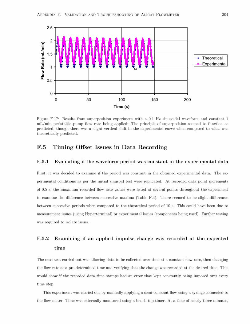
Appendix F. Validation and Troubleshooting of Alicat Flowmeter 304
0
0.5
1
1.5
2
2.5
0 50 100 150 200
Time (s)
Flo
w R
ate
(mL
/min
)
Theoretical
Experimental14
Figure F.17: Results from superposition experiment with a 0.1 Hz sinusoidal waveform and constant 1mL/min peristaltic pump flow rate being applied: The principle of superposition seemed to function aspredicted, though there was a slight vertical shift in the experimental curve when compared to what wastheoretically predicted.
F.5 Timing Offset Issues in Data Recording
F.5.1 Evaluating if the waveform period was constant in the experimental data
First, it was decided to examine if the period was constant in the obtained experimental data. The ex-
perimental conditions as per the initial sinusoid test were replicated. At recorded data point increments
of 0.5 s, the maximum recorded flow rate values were listed at several points throughout the experiment
to examine the difference between successive maxima (Table F.4). There seemed to be slight differences
between successive periods when compared to the theoretical period of 10 s. This could have been due to
measurement issues (using Hyperterminal) or experimental issues (components being used). Further testing
was required to isolate issues.
F.5.2 Examining if an applied impulse change was recorded at the expected
time
The next test carried out was allowing data to be collected over time at a constant flow rate, then changing
the flow rate at a pre-determined time and verifying that the change was recorded at the desired time. This
would show if the recorded data time stamps had an error that kept constantly being imposed over every
time step.
This experiment was carried out by manually applying a semi-constant flow using a syringe connected to
the flow meter. Time was externally monitored using a bench-top timer. At a time of nearly three minutes,

Appendix F. Validation and Troubleshooting of Alicat Flowmeter 305
Profile
Percent Differencebetween VolumesDetermined by
Theoretical FlowProfile and
Actuator Motion
Percent Differencebetween VolumesDetermined by
Theoretical FlowProfile and
Flowmeter Data
Percent Differencebetween VolumesDetermined by
Actuator Motionand Flowmeter
Data
P5I0.2,run 1
1.22% 11.0% 12.1%
P5I0.2,run 2
1.58% 21.1% 22.3%
P5I0.1,run 1
1.95% 37.2% 38.4%
P5I0.1,run 2
3.62% 26.8% 24.1%
Table F.1: Data from experiment comparing volume input calculated from theoretical profile and NAVITARdisplacement data from the neMESYS and data read from the Alicat flowmeter for sinusoidal waveforms:The fluid volumes calculated from the theoretical flow and experimental actuator flow profiles were close,whereas when compared to the volume calculated from the flowmeter data, the errors increased by an orderof magnitude. It was concluded that the flowmeter was not fit for use in the bioreactor.
the flow was changed. Examining the output data it was found that this was recorded as desired (Table F.5).
F.5.3 Examining the effects of tubing compliance, and switching from flexi-
ble tubing to a rigid, stainless steel connection from the pump to the
flowmeter
Compliance, or flexibility and expansion/compression properties, in tubing has been known to affect the
desired results in bioreactors at times.
To examine if this was occurring, a union of a SS threaded male 1/8” male NPT to luer-lock and female-
to-female luer-lock adaptors was employed to connect the neMESYS to the flowmeter instead of flexible
tubing. The same phase shift behaviour is exhibited (Figure F.18), eliminating the possibility of the flexible
tubing being the main cause of the time lag.
F.5.4 Possibility of Syringe Compliance Issues
As per the plastic tubing, using a plastic syringe may have also caused compliance issues. A 1 mL glass
syringe (Hamilton Company; Reno, NV, USA) was employed. A smaller periodical sinusoid wave was tested
(1 s). Collected data displayed not only a marked magnitude issue, but also the same phase lag issue as
previously seen (Figure F.19).

Appendix F. Validation and Troubleshooting of Alicat Flowmeter 306
Profile
Experiment RunTime from
Actuator Data(s)
Volume InputCalculated fromActuator Motion
(mL)
Volume InputCalculated fromFlowmeter Data
(mL)
Volume InputCalculated fromTheoretical Flow
Profile (mL)
P5I0.2,run 1
24.7 0.210 0.184 0.207
P5I0.2,run 2
24.2 0.209 0.162 0.206
P5I0.1,run 1
23.8 0.209 0.129 0.205
P5I0.1,run 2
27.8 0.236 0.179 0.245
Table F.2: Data from experiment comparing volume input calculated from theoretical profile and NAVITARdisplacement data from the neMESYS and data read from the Alicat flowmeter for sinusoidal waveforms, 1of 3.
Figure F.18: Experimental results in changing from flexible tubing to SS connector in transition fromneMESYS to flowmeter.
F.5.5 Confirming the motion of the neMESYS linear actuator using a NAVI-
TAR scope and extracting the period of cyclic motion
It was hypothesized that the linear actuator driving the neMESYS may not have been moving properly. To
examine if this was the case, the MatLab motion tracking algorithm used to survey linear actuator options
was employed (as detailed in Appendix B.1). A sinusoid with a 10 s period was applied.
The experimentally and theoretically recorded flow rates were collected and presented along with the
amplitude of actuator displacement from the origin (Figure F.20). While the experimental and theoretical
flow rates still exhibited the phase lag behaviour, the time difference between the actuator motion and
theoretical flow rate curves seemed to be constant and not varying.
The time between successive cycles was then extracted from the actuator motion data to verify if the
period was changing over time (a selection of data is provided in Table F.6). In examining the data, the
maximum displacement from the origin was found and the first time this occurred during each cycle was
recorded. There are marginal errors present, such as one selected cycle displaying a period of 11 s.
When the full data range was examined, two far data points were selected to average out sampling errors.

Appendix F. Validation and Troubleshooting of Alicat Flowmeter 307
Profile
Volume InputCalculated fromActuator Motion
per UnitExperiment Time
(mL/s)
Volume InputCalculated fromFlowmeter Data
per UnitExperiment Time
(mL/s)
Volume InputCalculated fromTheoretical FlowProfile per Unit
Experiment Time(mL/s)
P5I0.2,run 1
8.487E-03 7.46E-03 8.38E-03
P5I0.2,run 2
8.634E-03 6.71E-03 8.50E-03
P5I0.1,run 1
8.779E-03 5.41E-03 8.61E-03
P5I0.1,run 2
8.480E-03 6.44E-03 8.80E-03
Table F.3: Data from experiment comparing volume input calculated from theoretical profile and NAVITARdisplacement data from the neMESYS and data read from the Alicat flowmeter for sinusoidal waveforms, 2of 3.
Figure F.19: Examination of using a glass syringe instead of a plastic variant on phase lag properties usingthe neMESYS.
Between two time points of 250 s and 490 s, approximately 24 cycles occurred, which can be seen by visually
counting the peaks in Figure F.20. The average period was then calculated as
Average Period =Time Frame
Number of Cycles=
490− 250 s
24= 10 s (F.2)
which is the exact same as the prescribed period of the theoretical waveform. This showed that the linear
actuator was most likely performing as desired.
F.5.6 Examination of NAVITAR Timing
To ensure that the NAVITAR scope was imaging the motion of the actuator correctly (i.e. the frame rate
was not offset), the progression of time from a standard stop watch was imaged using the NAVITAR for

Appendix F. Validation and Troubleshooting of Alicat Flowmeter 308
Time (s)Maximum Flow Rate During
Period (mL/min)Period (Current and Last Maximum)
(s)
1 2.023 N/A
10.5 2.016 9.5
20.5 1.994 10
30 2.016 9.5
39.5 1.989 9.5
49.5 1.99 10
292.5 1.911 N/A
302 1.906 9.5
312 1.904 10
321.5 1.915 9.5
331 1.902 9.5
487 2.029 N/A
496.5 2.033 9.5
506 2.036 9.5
Table F.4: Evaluation of period changes during sinusoidal profile test using neMESYS.
Figure F.20: Combined neMESYS actuator motion and flow measurements.
approximately one minute (Figure F.21). The theoretical time displayed by the stopwatch was then compared
to the progression of frames in a recorded movie. Still images of the movie were tracked and extracted using
VirtualDub (virtualdub.org). The movie frame number and displayed time during the first two seconds was
then tabulated for analysis (Table F.7). Using the tabulated range of data to average out single frame
sampling errors, the experimental frame rate can be calculated as
Frame Rate =Time Frame
Number of Frames=
2.08− 0.31 s
112− 59 + 1≈ 0.0328 s (F.3)
The percent difference between the experimental value and the theoretical value (of 1/30 s) is 1.6%, which
is negligible. Taking a larger sample size near the end of the movie at frame 1326 and a time of 42.47 s
yielded an experimental frame rate of 0.0332 s when compared to frame 59 at a time of 0.31 s, which yields a

Appendix F. Validation and Troubleshooting of Alicat Flowmeter 309
Time (s) Time (min)Flow Rate(mL/min)
... ... ...
170 2.833333333 1.358
170.5 2.841666667 1.329
171 2.85 1.245
171.5 2.858333333 1.219
172 2.866666667 1.211
172.5 2.875 1.218
173 2.883333333 1.22
173.5 2.891666667 1.246
174 2.9 1.234
174.5 2.908333333 1.203
175 2.916666667 1.252
175.5 2.925 1.274
176 2.933333333 1.294
176.5 2.941666667 1.279
177 2.95 1.254
177.5 2.958333333 1.299
178 2.966666667 1.298
178.5 2.975 +04.028 VOV
179 2.983333333 +04.480 VOV
179.5 2.991666667 +04.480 VOV
180 3 +04.480 VOV
180.5 3.008333333 +04.480 VOV
181 3.016666667 +04.480 VOV
Table F.5: Data from examining a manually applied impulse change in flow rate using syringe.
percent error of 0.4%. With these low error values, it was assumed that the NAVITAR was being triggered
properly and timing was accurate.
F.5.7 Examination of Hyperterminal Issues
Hyperterminal was selected as the default method of collecting flow data over time as instructions for its
use were included in the supplied flowmeter manual (available at: http://www.alicat.com/documents/
manuals/Liquid_Flow_Meter_Controller_Manual.pdf). It was thought that there may have been com-
munication issues in using the program along with its connection via the serial port of the computer. Two
options that were examined to replace its use were an oscilloscope and a microcontroller.

Appendix F. Validation and Troubleshooting of Alicat Flowmeter 310
Time (s)Maximum Displacement During
Period (mL/min)Period (Current and Last Point) (s)
6.766667 2.780265655 N/A
15.86667 2.780265655 9.1
25.76667 2.780265655 9.9
35.93333 2.780265655 10.16667
101.8333 2.780265655 N/A
112.8333 2.780265655 11
216.7 2.780265655 N/A
226.6333 2.780265655 9.933333
236.6333 2.780265655 10
316.6667 2.780265655 N/A
326.6333 2.780265655 9.966667
336.7333 2.780265655 10.1
346.6333 2.780265655 9.9
Table F.6: Extraction and evaluation of period changes during actuator tracking experiment using neMESYS.
Figure F.21: One frame showing stopwatch time during NAVITAR frame rate verification experiment.
F.5.8 Ramped Flow Test
Alicat Scientific requested for a test that used Hyperterminal, and involved applying a steadily increasing
ramp signal. A flow waveform ranging from 0 to 3.5 mL/min varied at 0.5 mL/min increments every minute
was applied using the neMESYS and a BD 20 mL plastic syringe, and measured at 5 s intervals (Figure F.22).
Ignoring any magnitude issues, a small offset was noted in the time it took for the experimental and theoretical
signals to match up when the flow changed. This also led to the conclusion that Hyperterminal was not an
accurate data recording method.
F.5.9 Consultation with External Experts
While the oscilloscope was a viable option to remedy the time lag issue, the laboratory was not equipped
with a unit and was borrowing one off time from the Yu Sun laboratory at the University of Toronto. The
unit was cumbersome and very hard to regularly obtain for experiments.

Appendix F. Validation and Troubleshooting of Alicat Flowmeter 311
Frame Stopwatch Time (s)
59 0.31
... ...
63 0.44
... ...
71 0.63
... ...
86 1.21
... ...
112 2.08
Table F.7: Displayed stopwatch time visualized using NAVITAR scope to verify frame rate.
Figure F.22: Ramped flow test using neMESYS and oscilloscope to trace flowrate.
Two external experts were consulted for assistance. The first, Dr. Thomas Ewart, provided feedback on
signal analysis, circuit design, and experimental set-up, as well as the possibility of another oscilloscope being
loaned. This seemed as though it was a possible option. However, Dr. Ewart also suggested the possibility
of using some sort of microcontroller to obtain voltage data from the flowmeter and then subsequently
transform this data into flow rate information.
When searching for other oscilloscope options, Thomas Bernreiter of the Department of Mechanical and
Industrial Engineering at the University of Toronto was consulted and also suggested the use of a microcon-
troller, specifically the Arduino Uno (Figure F.23) for its price, accuracy, and ease of open-source program-
ming. As well, the microcontroller is far more accurate compared to an oscilloscope in terms of resolution.
The unit was programmed with the help of Mr. Bernreiter and the code is included in Appendix G.3.

Appendix F. Validation and Troubleshooting of Alicat Flowmeter 312
Figure F.23: The Arduino Uno microcontroller compared to a USA quarter [108].
F.5.10 Carrying out various flow tests using the Arduino Uno microcontroller
to verify if phase lag behaviour had been eliminated
The Uno was employed for several rounds of flow testing (Figure F.24 and Figure F.25). First, a sinusoid
with a period of 10 s was applied using the neMESYS. Then, a square wave ranging between 0 and 0.5
mL/min was applied. It was found that there did not seem to be any time-lag or phase shift behaviour
occurring (Figure F.26). A square waveform was then applied. Again, no time-lag behaviour was observed,
Figure F.24: Experimental setup to test the neMESYS with the Arduino Uno.
though some magnitude offset issues are present (Figure F.12).
Following these experiments, it was determined that the use of Hyperterminal was the most likely cause
of the time-lag behaviour and the Arduino Uno had provided a remedy to the issue at hand.

Appendix F. Validation and Troubleshooting of Alicat Flowmeter 313
Figure F.25: Close-up view of Arduino Uno connected to flowmeter testing the neMESYS.
Figure F.26: 0.1 Hz sinusoidal waveform test using neMESYS and measured with Arduino Uno.
F.6 Isolation and Troubleshooting of Magnitude Offset Issues in
Data Recording
Following the solution of the time-lag issue, the problem of the offset of the recorded flow magnitude was
examined. It was possible that either or both of the flowmeter and neMESYS were causing discrepancies
between the experimental and theoretical results.
F.6.1 Comparison of Peristaltic and neMESYS Results
To decide on the possibility of the neMESYS not producing accurate flow profiles, identical constant flow
tests were run comparing the results from the neMESYS to the peristaltic pump in the laboratory. The
peristaltic pump had shown excellent matching between experimental and theoretical data in a constant
flow rate test, as described in Section F.4.1. If the results between the proven, accurate peristaltic and
neMESYS agreed, the problem would be isolated to the flowmeter or something related to the experimental
set-up linked to the meter.
The peristaltic pump was first tested by setting it to apply a constant flow of 1 mL/min. Flexible tubing
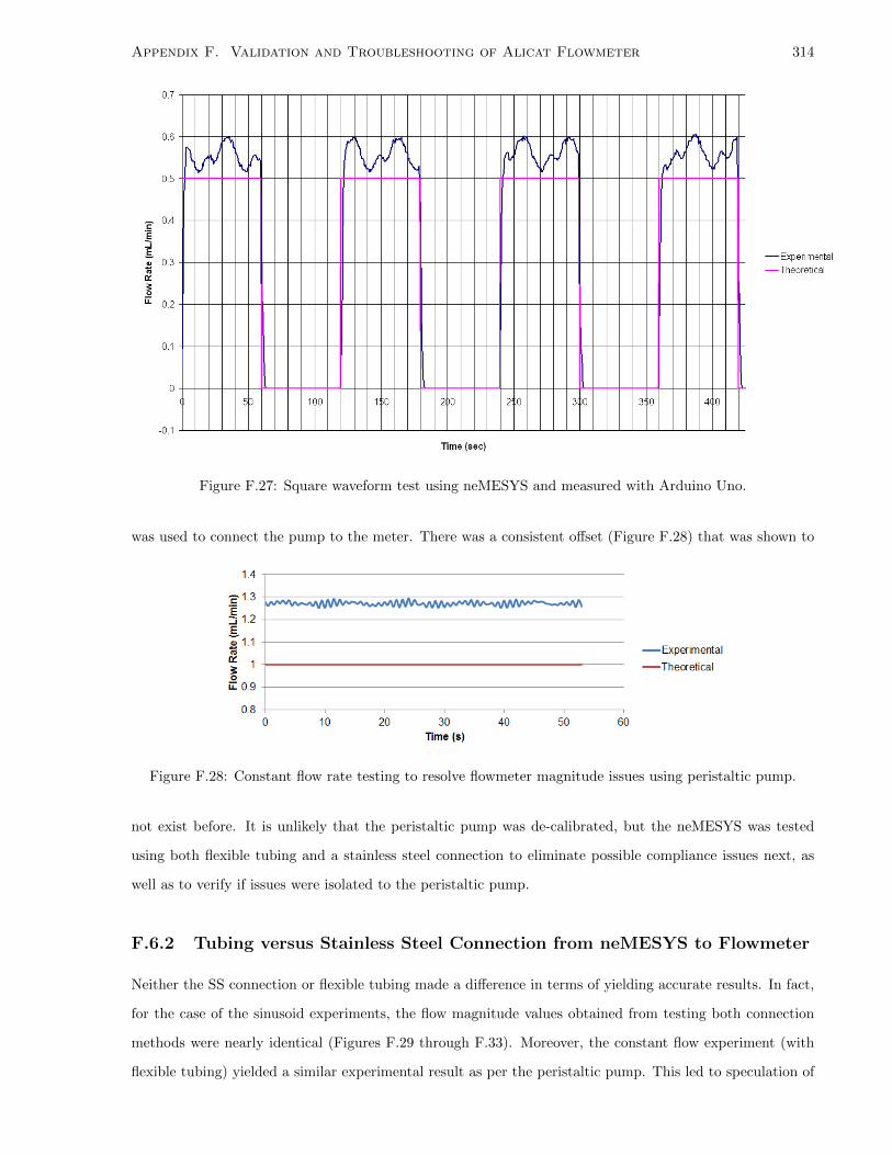
Appendix F. Validation and Troubleshooting of Alicat Flowmeter 314
Figure F.27: Square waveform test using neMESYS and measured with Arduino Uno.
was used to connect the pump to the meter. There was a consistent offset (Figure F.28) that was shown to
Figure F.28: Constant flow rate testing to resolve flowmeter magnitude issues using peristaltic pump.
not exist before. It is unlikely that the peristaltic pump was de-calibrated, but the neMESYS was tested
using both flexible tubing and a stainless steel connection to eliminate possible compliance issues next, as
well as to verify if issues were isolated to the peristaltic pump.
F.6.2 Tubing versus Stainless Steel Connection from neMESYS to Flowmeter
Neither the SS connection or flexible tubing made a difference in terms of yielding accurate results. In fact,
for the case of the sinusoid experiments, the flow magnitude values obtained from testing both connection
methods were nearly identical (Figures F.29 through F.33). Moreover, the constant flow experiment (with
flexible tubing) yielded a similar experimental result as per the peristaltic pump. This led to speculation of

Appendix F. Validation and Troubleshooting of Alicat Flowmeter 315
the flowmeter being the cause of the magnitude issues.
Figure F.29: Constant flow rate testing of flowmeter magnitude issues using SS connection at meter entranceand neMESYS.
F.6.3 Period and Increment Testing
A variety of waveforms in terms of period and increments at which the flow rates were varied within the
waveform were tested to examine the ability of the flowmeter to produce the expected waveforms. It was
found that at periods of 5 s or less, experimental waveform magnitude did not match that of theoretical
(Figures F.34 through F.45).
0
0.2
0.4
0.6
0.8
1
1.2
0 5 10 15 20 25 30 35
Time (s)
Flo
w R
ate
(mL
/min
)
Theoretical
Experimental
Figure F.34: Period and increment testing - theoretical period of 10 s and data point increments of 5 s.

Appendix F. Validation and Troubleshooting of Alicat Flowmeter 316
Figure F.30: Long-period sinusoidal waveform testing of flowmeter magnitude issues using tubing at meterentrance and neMESYS.
0
0.2
0.4
0.6
0.8
1
1.2
0 10 20 30 40 50 60
Time (s)
Flo
w R
ate
(mL
/min
)
Theoretical
Experimental
Figure F.35: Period and increment testing - theoretical period of 10 s and data point increments of 2 s.

Appendix F. Validation and Troubleshooting of Alicat Flowmeter 317
Figure F.31: Long-period sinusoidal waveform testing of flowmeter magnitude issues using SS connection atmeter entrance and neMESYS.
0
0.2
0.4
0.6
0.8
1
1.2
0 10 20 30 40 50 60
Time (s)
Flo
w R
ate
(mL
/min
)
Theoretical
Experimental
Figure F.36: Period and increment testing - theoretical period of 10 s and data point increments of 1 s.

Appendix F. Validation and Troubleshooting of Alicat Flowmeter 318
Figure F.32: Short-period sinusoidal waveform testing of flowmeter magnitude issues using tubing at meterentrance and neMESYS.
0
0.2
0.4
0.6
0.8
1
1.2
0 5 10 15 20 25 30 35 40
Time (s)
Flo
w R
ate
(mL
/min
)
Theoretical
Experimental
Figure F.37: Period and increment testing - theoretical period of 10 s and data point increments of 0.5 s.

Appendix F. Validation and Troubleshooting of Alicat Flowmeter 319
Figure F.33: Short-period sinusoidal waveform testing of flowmeter magnitude issues using SS connection atmeter entrance and neMESYS.
0
0.2
0.4
0.6
0.8
1
1.2
0 10 20 30 40 50 60
Time (s)
Flo
w R
ate
(mL
/min
)
Theoretical
Experimental
Figure F.38: Period and increment testing - theoretical period of 10 s and data point increments of 0.2 s.

Appendix F. Validation and Troubleshooting of Alicat Flowmeter 320
0
0.2
0.4
0.6
0.8
1
1.2
0 10 20 30 40 50 60
Time (s)
Flo
w R
ate
(mL
/min
)Theoretical
Experimental
Figure F.39: Period and increment testing - theoretical period of 10 s and data point increments of 0.1 s.
0
0.2
0.4
0.6
0.8
1
1.2
0 10 20 30 40 50 60
Time (s)
Flo
w R
ate
(mL
/min
)
Theoretical
Experimental
Figure F.40: Period and increment testing - theoretical period of 5 s and data point increments of 2.5 s.
0
0.1
0.2
0.3
0.4
0.5
0.6
0.7
0.8
0.9
1
0 5 10 15 20 25 30 35 40
Time (s)
Flo
w R
ate
(mL
/min
)
Theoretical
Experimental
Figure F.41: Period and increment testing - theoretical period of 5 s and data point increments of 1 s.
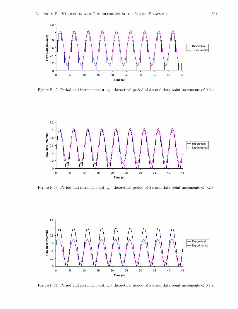
Appendix F. Validation and Troubleshooting of Alicat Flowmeter 321
0
0.2
0.4
0.6
0.8
1
1.2
0 5 10 15 20 25 30 35 40 45
Time (s)
Flo
w R
ate
(mL
/min
)Theoretical
Experimental
Figure F.42: Period and increment testing - theoretical period of 5 s and data point increments of 0.5 s.
0
0.2
0.4
0.6
0.8
1
1.2
0 5 10 15 20 25 30 35 40 45
Time (s)
Flo
w R
ate
(mL
/min
)
Theoretical
Experimental
Figure F.43: Period and increment testing - theoretical period of 5 s and data point increments of 0.2 s.
0
0.2
0.4
0.6
0.8
1
1.2
0 5 10 15 20 25 30 35 40 45
Time (s)
Flo
w R
ate
(mL
/min
)
Theoretical
Experimental
Figure F.44: Period and increment testing - theoretical period of 5 s and data point increments of 0.1 s.

Appendix F. Validation and Troubleshooting of Alicat Flowmeter 322
0
0.2
0.4
0.6
0.8
1
1.2
0 5 10 15 20 25 30
Time (s)
Flo
w R
ate
(mL
/min
)Theoretical
Experimental
Figure F.45: Period and increment testing - theoretical period of 1 s and data point increments of 0.2 s.
Due to unsolvable magnitude issues, the Alicat flowmeter was abandoned in favour of employing PIV
and the Sensirion flowmeter.

Appendix G
Programming of Peripheral Devices
Note: These instructions were adapted from those originally written by Beca [84].
Appendicies G.1 and G.2 outline the steps taken to interface the step motor driver, which controlled the
stepper motor, with a personal computer. This enabled the programming of different loading profiles into
the driver that were transmitted to the stepper motor.
G.1 Step Motor Driver Interfacing
1. Connect the supplied step motor driver cable (Model RS-232 PC/MMI, Applied Motion; Watsonville,
CA, USA) to a USB-to-serial DB39 adaptor cable (CablesToGo; Moraine, OH, USA) and install the
appropriate driver (drivers found at: https://www.cablestogo.com/help/tech_support.asp# under
Drivers and manuals link).
2. IMPORTANT: Before proceeding further, ensure that the motor leads are connected to the step motor
driver and that the USB-to-serial DB39 adaptor cable is connected to the RS-232 PC/MMI cable.
3. To interface the motor driver with a PC, download SiProgrammer (software found at: http://www.
applied-motion.com/products/software/si-programmer).
4. Install and open SiProgrammer (a prompt may appear saying that a communication error has occurred.
Click OK until it disappears).
5. Connect the USB-to-serial DB39 adaptor cable to a USB port on the PC.
6. Supply power to the step motor driver.
7. Select the appropriate COM port corresponding to the USB port and ensure that the right motor
driver version is displayed (Si2035 in this case). The COM port can be verified by navigating to the
Windows Control Panel, under System, then by going to Device Manager).
323

Appendix G. Programming of Peripheral Devices 324
8. Once power is supplied to the step motor driver, it will automatically start running the last program
that was downloaded into it. To stop the motor, click Upload.
G.2 Step Motor Driver Programming
1. To enter the first line of the program, click the downward arrow beside the number 1.
2. A menu appears that outlines a number of programming options. Click Feed to Length to open a
submenu that allows for the control of rotation speed, acceleration, etc.
3. Set the direction in the Direction option. Depending upon whether infuse or withdrawal is desired this
will either be clockwise (CW) or counter-clockwise (CCW).
4. To enter the second programming line, click the downward arrow beside the number 2.
5. Repeat steps 2-4 for any amount of program steps as desired.
6. After entering all of the necessary programming steps and if a loop is desired, click the downward
arrow beside the last step.
7. Select the programming option Go To.
8. A menu appears that prompts the user to enter the number of a programming line. Enter number 1.
This creates a program loop.
9. Turn the Idle Current option to 100% in the main menu and change the current value to 0.7 A/Phase.
10. Click Download to download the program into the step motor driver.
11. To test the program, click Execute.
To disconnect the motor, perform the aforementioned connecting sequence backwards. To run the motor
during an experiment, ensure the appropriate program is downloaded into the step motor driver, and power
up the driver, which will turn on the motor. Connection to a PC is not required during biological experiments.
G.3 Arduino Uno Programming and Connection to Alicat Flowme-
ter
An Ardiuno Uno was used to measure flow data in the bioreactor. The following details its programming,
as well as the code used to acquire the data.
1. Download the Ardiuno software from the Arduino website, found at: http://www.arduino.cc.

Appendix G. Programming of Peripheral Devices 325
2. Open the downloaded file and install the software and associated drivers.
3. Connect the Arduino Uno microcontroller to the computer via a USB Type A Male to Type B Female
cable (Canada Computers; Toronto, ON).
4. Open the Arduino software program via the desktop shortcut.
5. Open the flowdata.ino program file, or re-enter the code as supplied in this section.
6. Download the text/serial port writing program, RS232 Data Logger, found at: http://www.eltima.
com/products/rs232-data-logger/.
7. Install RS232 Data Logger.
8. Using electrical wires (preferably shielded), connect the Arduino and flowmeter as shown in Figure G.1.
Open the RS232 Data Logger program.
Figure G.1: Peripheral (Arduino or oscilloscope) connection points to Alicat flowmeter. 0-5 V signal at pin#6, and ground signal at pin #8. (Adapted from [109].
9. Ensure that the COM port matches what the Arduino Uno is connected to (which can be verified under
System, then by going to Device Manager in the Windows Control Panel). Also ensure that the baud
rate matches that selected on the Alicat flow meter and in the flowdata.ino program (see comments in
the program of where this value can be selected and changed and the Alicat flowmeter manual available
at: http://www.alicat.com/documents/manuals/Liquid_Flow_Meter_Controller_Manual.pdf).
10. Go back to the Arduino software, and ensure all values match the desired experiment settings (baud
rate, data collection interval, etc.).
11. Click the upload button to send the code to the Arduino Uno.
12. Once this has been completed, start recording data using the RS232 Data Logger program by selecting
file to record to.

Appendix G. Programming of Peripheral Devices 326
13. Once satisfied with the data or time line of the experiment, stop recording using the Data Logger
program. One can then navigate to the created file and open it to see two columns: At the left are the
time points, and at the right are the associated flow values at each time point.
flowdata.ino
/*
Analog input, analog output, serial output
Reads an analog input pin, at a predefined frequency
Also prints the results to the serial monitor.
* Sensor connected to analog pin 0 and ground
created 30 May. 2013
Built upon example code
by Tom Igoe
This example code is in the public domain.
According to tom bernretier can use this code reliably up to 50Hz
*/
// These constants won’t change. They’re used to give names
// to the pins used:
const int analogInPin = A0; // Analog input pin that the potentiometer is attached to
int sensorValue = 0; // value read from the pot
double voltageValue = 0; //voltage value
double flowValue = 0; //flow value
double timesec = 0; // time in seconds
unsigned long time = 0, sampletime = 0; // value of millis since board start
void setup()

Appendix G. Programming of Peripheral Devices 327
// initialize serial communications at 256000 bps:
Serial.begin(256000);
void loop()
// read the analog in value after a desired amount of time has passed:
// Time increment right now 10ms
if (millis() - sampletime >= 10)
sampletime += 10;
time=millis();
sensorValue = analogRead(analogInPin);
/*Covert to a voltage by dividing sensor value (in bytes) by 1023, the total number of bytes in the 10
bit Arduino system (2ˆ10 bytes-1), multiplied by voltage scaler (5V),
the operating voltage of the Arduino
To figure out how big a number we can store in a 2 byte-sized box use a calculator and take 2 to the
power of the number of bits
(since each bit can store 2 values, 0 or 1). Then we subtract 1 because like in the car odometer, you can’t
actually display the final value, 10000.
So, in this case the largest number is 216 - 1 = 65535. Since the number we’re trying to store (102400) is
larger than that, we see that ”rollover.”
http://www.ladyada.net/learn/arduino/lesson4.html
*/
//1023.0 and 5.0 to make sure it’s a float, otherwise reads as an integer
voltageValue=sensorValue/1023.0*5.0;
//3.5 mL/min flow range and 5V
flowValue=voltageValue*3.5/5.0;
timesec=time/1000.0;
// print the results to the serial monitor:
//Serial.print(”sensor voltage = ” );
//Serial.print(voltageValue);

Appendix G. Programming of Peripheral Devices 328
//Serial.print(” �Millis = ”);
//Serial.println(time);
//Prints time and voltage value in columns that can be imported to Excel
Serial.print(timesec,DEC);
Serial.print(”�”);
Serial.print(flowValue,DEC);
Serial.println();
G.4 Alicat Flowmeter Setup for Experiments - Adaptors and Cal-
ibration
Each time the flowmeter is connected, the following procedure should be followed:
1. Remove the red particle-filter attachments from the inlet and outlet ports of the flowmeter.
2. Plug in the 24 V power adaptor (Alicat Scientific; Tucson, AZ, USA) into the power port of the Alicat
at the top of the meter and into a standard wall outlet.
3. Wait at least one minute for the reading of the flowmeter to become constant (reach steady-state).
4. Once it seems that the meter reading is not changing, press the Tare button at the top right of the
meter display.
5. Attach two sets of a 10-32 internal thread to 1/8” NPT adaptor and 10-32 external thread to barb for
1/32” tube (beswick engineering; Greenland, NH, USA) together.
6. Wrap teflon tape (seal tape) around the NPT threads of the beswick assembly. Leave two threads
uncovered by the tape. Wrap the teflon tape around the body twice, in the same directon as one would
tighten the fitting.
7. Screw one set into the inlet and one into the outlet of the flowmeter.
8. Tighten the sets to the flowmeter using a wrench.
9. Connect the tubing on either sides of the flowmeter.
10. Connect the meter for data logging, if desired, as detailed in Appendix G.3.

Appendix G. Programming of Peripheral Devices 329
11. Begin flowing fluid through the meter.
12. Once fluid is flowing through the outlet tubing of the meter, open the bleed ports (small hex screws
on the front face of the flowmeter) of the meter.
13. Begin with the bleed port closest to the inlet side of the meter. Loosen the screw using a 3/32” Allen
key until fluid begins to visibly run from the screw. Gently tap the unit using the handle or soft edge
of a tool, such as a screwdriver.
14. Tighten the screw back.
15. Repeat the previous steps with the outlet bleed port.
16. Stop the flow.
17. Let the reading on the flowmeter reach a steady-state value, such that it is not changing, or changing
within +/- 0.07 mL/min.
18. Tare the flowmeter by pressing the top right button on the flowmeter display.
19. The flowmeter is now calibrated and ready for use.
G.5 Hyperterminal Programming Instructions for Alicat Flowme-
ter
The following are adapted instructions from the Alicat Scientific L-Series Flowmeter operating manual
on how to set up Hypterminal to read in flow data from the meter. The reader is invited to refer to
the flowmeter manual (available at: http://www.alicat.com/documents/manuals/Liquid_Flow_Meter_
Controller_Manual.pdf) for additional details.
G.5.1 Configuring Hyperterminal
1. Connect the male 8 pin mini Din to female DB9 cable, item #MD8DB9, and USB to RS232 converter
together (Alicat Scientific; Tucson, AZ, USA) from the meter data port to a computer USB port.
2. Open the HyperTerminal RS-232 / RS-485 terminal program (installed under the “Accessories” menu
on most Microsoft Windows operating systems). If Hypterminal is not installed, it can be downloaded
at: http://ituploads.com/microsoft/hyperterminal-for-windows-7-vista/.
3. Select Properties from the file menu.

Appendix G. Programming of Peripheral Devices 330
4. Click on the Configure button under the Connect To tab. Be sure the program is set for: 19,200 baud
(or matches the baud rate selected in the RS-232 / RS-485 communications menu on the meter) and
an 8-N-1-None (8 Data Bits, No Parity, 1 Stop Bit, and no Flow Control) protocol.
5. One can check if the COM port choice is correct by opening the Windows control panel (navigate
to Start, Settings, Control Panel), going to System, then Device Manager, and looking under the
Communication Ports list.
6. Under the Settings tab, make sure the Terminal Emulation is set to ANSI or Auto Detect.
7. Click on the ASCII Setup button and be sure the Send Line Ends with Line Feeds box is not checked
and the Echo Typed Characters Locally box and the Append Line Feeds to Incoming Lines boxes are
checked. Settings not mentioned here are normally acceptable in their default positions.
8. Save the settings, close HyperTerminal, and re-open it.
9. In Polling Mode, the screen should be blank except the blinking cursor. In order to get the data
streaming to the screen, hit the Enter key several times to clear any extraneous information. Type
*@ = @ followed by Enter (or using the RS-232 / RS-485 communication select menu, select @ as
identifier and exit the screen). If data still does not appear, check all the connections and COM port
assignments.
G.5.2 Sending a Script to Hyperterminal to Capture Data to a Text File
1. Open a text editing program, such as Microsoft Word.
2. Set the CAPS lock on.
3. Beginning at the top of the page, type A<Enter> repeatedly. Using Microsoft Word, one can tell
how many lines are written by the line count at the bottom of the screen. The number of lines will
correspond to the total number of times the flow device will be polled, and thus the total number of
lines of data it will produce For example:
A
A
A
A
A
A
will yield a total of six lines of data from the flow meter. The time between each line will be set in
HyperTerminal.

Appendix G. Programming of Peripheral Devices 331
4. When finished writing the lines desired, go to the File menu and select Save. In the save dialog box,
enter a path and file name as desired and in the Save as Type box, select the plain text (.txt) option.
It is important that it be saved as a generic text file for HyperTerminal to read it correctly.
5. Click Save.
6. A file conversion box will appear. In the End Lines With drop down box, select CR Only. Everything
else can be left as default.
7. Click OK.
8. Close the file and exit the text editing program.
9. Open HyperTerminal and establish communication with the flowmeter as outlined in Appendix G.5.
10. Set the flow device to Polling Mode as described in Appendix G.5. Each time one types A<Enter>,
the meter should return one line of data to the screen.
11. Go to the File menu in HyperTerminal and select Properties.
12. Select the Settings tab.
13. Click on the ASCII Setup button.
14. The Line Delay box is defaulted to 0 milliseconds. This is where it will be decided how often a line
will be read from the script file created. 1000 milliseconds is one second, so if a line of data is desired
every 30 seconds, enter 30000 into the box.
15. When the desired value has been entered, click on OK and OK in the Properties dialog box.
16. Go the Transfer menu and select Send Text File... (NOTE: NOT Send File...).
17. Browse and select the text “script” file created.
18. Click Open.
19. The program will begin “executing” the script file, reading one line at a time with the line delay you
specified and the flow device will respond by sending one line of data for each poll it receives, when it
receives it.
20. To capture the data, select Capture Text from the Transfer Menu. Type in the path and file name
desired. Push the start button.
21. When the data collection period is complete or is desired to be terminated, select Capture Text from
the Transfer Menu and select Stop from the sub-menu that appears.

Appendix G. Programming of Peripheral Devices 332
22. Data that is selected and copied, either directly from HyperTerminal or from a text file can be pasted
directly into Excel.
23. When the data is pasted it will all be in the selected column. Select Text to Columns... under the
Data menu in Excel and a Text to Columns Wizard (dialog box) will appear. Make sure that Fixed
Width is selected under Original Data Type in the first dialog box and click Next.
24. In the second dialog box, set the column widths as desired, but the default is usually acceptable. Click
on Next again.
25. In the third dialog box, make sure the column data format is set to General, and click Finish.
26. Once the data is in this format, it can be graphed or manipulated as desired.
G.6 Sensirion Flowmter Setup
The following details how to use the Sensirion flowmeter.
1. Detach the safety/air plugs from the flowmeter port ends.
2. Install the desired connectors on to the inlet and outlet ports of the flowmeter. For the bioreactor, the
connectors are 3/16” to 1/4-28 flat bottom style (Item #30704-88. Cole-Parmer; Montreal, QC).
3. Connect the flowmeter into the bioreactor.
4. Attach the RS485 to USB cable supplied with the flowmeter to the unit as well as to a computer
running the Sensirion USB RS485 Sensor Viewer software, available for download at: http://www.
sensirion.com/en/products/liquid-flow-sensors/download-center/.
5. Open the Sensor Viewer software, and select the USB port the flowmeter is attached to. This can be
verified under System, then by going to Device Manager in the Windows Control Panel.
6. Once the flowmeter has been located and the software identifies it, the main terminal window appears
showing a graph and several options. Instructions from the SLI-2000 manual about this window and
the software is provided, as this is not available online unless requested from the company (Figures G.2
through G.6). Typically, all default values may be kept other than selecting a file to record to and the
resolution, which varies how often data is recorded and is up to the user.
7. Once an experiment has started to run, click the Run, then Start Logging buttons to record flow data.
When finished, click Stop Logging and Stop.
8. Sensirion can be contacted to acquire the manual or for support should additional information be
required.
Appendix G. Programming of Peripheral Devices 333
Figure G.2: Sensirion USB485 Sensor Viewer software instructions, 1 of 5.

Appendix G. Programming of Peripheral Devices 334
Figure G.3: Sensirion USB485 Sensor Viewer software instructions, 2 of 5.

Appendix G. Programming of Peripheral Devices 335
Figure G.4: Sensirion USB485 Sensor Viewer software instructions, 3 of 5.

Appendix G. Programming of Peripheral Devices 336
Figure G.5: Sensirion USB485 Sensor Viewer software instructions, 4 of 5.

Appendix G. Programming of Peripheral Devices 337
Figure G.6: Sensirion USB485 Sensor Viewer software instructions, 5 of 5.

Appendix G. Programming of Peripheral Devices 338
G.7 neMESYS Setup
The following details how to setup the neMESYS. Detailed information can be found in the pump man-
ual, which can be viewed at: http://www.cetoni.de/fileadmin/user_upload/Documents/neMESYS_V2_
Manual_Hardware_en.pdf.
1. Insert the software CD associated with the neMESYS and install the pump software.
2. Re-start the computer.
3. Connect the bus-terminating plug into the dosing unit of the neMESYS, as shown in Figure G.7.
Figure G.7: Bus terminating plug of neMESYS.
4. Connect a male type-B USB to male type-A USB cable to the computer the software was installed on
and the pump.
5. Connect the power cable of the pump to a standard wall outlet.
6. Turn the pump on, by flipping the large red switch at the back of the pump.
7. If there is an error recognizing the pump USB driver, download and install the driver from: http:
//www.ixxat.com/download_vci_v3_en.html. Dis-connnect the pump, re-start the computer, then
re-connect the pump and turn it back on.
8. Open the neMESYS control program from the Start Menu.
9. Click the Search Device button (magnifying glass icon) at the top left of the program.
10. Follow the instructions found in the manual to select a syringe type.
11. Click the Reference Move button.
12. Once the actuator has moved to the ordinate and stopped, click the Re-fill button beside the window
where the flow rate can be selected and wait for the actuator to move to its other extreme position.
13. Manually fill the syringe with media.
14. Follow the instructions found in the manual to load the syringe into the pump.
15. As well, follow the instructions as to creating a flow profile or applying another type of flow.

Appendix G. Programming of Peripheral Devices 339
G.8 Fire-i and NAVITAR Scope Setup
This section details the use of the Fire-i program to control the NAVITAR scope for capturing images and
movies to use with the line tracking program or for imaging purposes.
1. Connect the Firewire cable to the NAVITAR scope.
2. Open Fire-i R©.
3. Ensure the settings are as shown in Figure G.8.
Figure G.8: Main screen of the Fire-i program and associated settings.
4. Click Start to see a preview of the viewing window, and move the object being imaged such that it is
captured within the view.
5. To take a still frame, check the box next to Frame Capture. Clicking on the text will bring up a window
allowing the user to define where the photo is saved.
6. Click Start. Allow the camera to capture images for at least five seconds.
7. Close the viewing window and navigate to the folder selected for image capture to acquire the image.
8. To take a movie, click the Video Capture checkbox.
9. Click the Video Capture text and a dialog box will open. Ensure that the settings are as shown in
Figure G.9, and select a folder to save the video to.
10. Click Run.
11. Once satisfied, close the viewing window and navigate to the folder selected for video capture to acquire
the video
.

Appendix G. Programming of Peripheral Devices 340
Figure G.9: Video capture screen of the Fire-i program and associated settings.

Appendix H
Particle Image Velocimetry
Instructions
The following details the use of the PIV equipment. Following the acquisition of data, files may be analyzed
as described in Section 5.2 on p. 87.
1. Turn on the interlock by flipping the switch to “I”. The interlock is the sign signifying that a laser is
in use in the PIV area, located outside the curtained area.
2. Place the microfluidic device that contains the channel to be imaged on the microscope stage.
3. Open the DaVis program on the PIV computer.
4. Create a New Project, ensuring the project type is set to PIV.
5. Fabricate a 5% flurorescent bead and de-ionized water solution.
6. Set up all equipment in terms of pumps and tubing as desired around the PIV area, beginning with
the neMESYS.
7. Initialize the neMESYS following the instructions provided in Appendix G.7 on p. 338.
8. Fill the syringe with the bead solution and and attach it to the neMESYS and associated tubing. The
neMESYS is used to carry out PIV calibration, while the peristaltic pump can be connected later. DO
NOT connect the peristaltic pump or damper in line with the neMESYS at this point.
9. Ensure that the microscope is set on the correct filter. This can be verified by ensuring that a small
green dot appears on the microfluidic device when the objective is moved to the middle of the channel.
10. Ensure that a 10X objective is being used with the microscope.
341

Appendix H. Particle Image Velocimetry Instructions 342
11. Locate the channel in the microscope field of view: Turn on the microscope light and switch the
microscope settings to bino (knob for this choice located on the front of the microscope) and eye (knob
for this choice located on the front of the right side of the microscope). Ensure that a portion of the
channel is clearly in focus.
12. Switch the microscope settings back to confocal (instead of bino) and side (instead of eye).
13. Turn the key on the PIV laser box on the floor, and press the Start button.
14. Wait 5 seconds. Then press, one after the other, the buttons lined up 3 in a row horizontally to enable
EXT, EXT, and HIGH.
15. Wait 10 seconds for all lights to stop flashing on the PIV box. Then, press the Laser and Emission
Fire buttons simultaneously.
16. Run flow with the neMESYS until the bead solution can be visually seen to fill the channel and all
tubing.
17. Click New on the DaVis window, at the top left of the screen.
18. Navigate to Device, Recording, Timing, Trigger Rate, and set to 5 Hz.
19. Navigate to Device, Recording, Laser Control, and set to on.
20. Turn off all of the lights in the PIV room and ensure that the curtains are closed.
21. Click the Grab button.
22. Use the microscope stage control and scroll to the the vertical top of the channel (when looking down
on to the device and considering the plane view).
23. Ensure this top channel line is horizontally straight by rotating the PCO imaging (blue) camera,
attached to the microscope on its left.
24. Ensure that the laser is firing into the mid-section along length of channel, i.e., it is past the entrance
length.
25. Scroll down to find the vertical middle of the channel. If the channel is wider than the field of view,
use a particle on screen as a marker with the knowledge that approximately 850 pixels represents 550
microns. Stop once the middle has been located.
26. Now locate the horizontal mid-section of channel (in the plane of moving the microscope stage vertically
up and down). This is done by finding the plane with the maximum velocity, with knowledge that
the velocity profile is parabolic inside a rectangular channel. Different planes must be examined and
tested sequentially.
Appendix H. Particle Image Velocimetry Instructions 343
27. Go to timing and under Reference Time 1 change the dt to a start value, for example 100 µs.
28. Start the flow at the maximum flow rate that will be tested, for instance, the maximum of a sinusoidal
waveform. The maximum flow rate is what is used to calibrate the PIV setup for velocity.
29. After allowing 10 s for steady state to be achieved, click take. Focus on a particle on screen and
measure the displacement by scrolling through the two images and clicking, holding and dragging on
the screen to draw a displacement line. A displacement of 12-16 pixels is desired, and this is read out
at the bottom right of the program. Vary the dt to achieve this displacement, where a longer dt will
increase displacement, and a shorter dt will decrease displacement.
30. Stop the flow.
31. For the typical device dimensions employed in this thesis of width 1500 µm and height 212.5 µm, dt
should be set at 90 µs for a maximum flow rate of 1 mL/min. The dt can be scaled proportionally to
the maximum flow rate. For example with the aforementioned device dimensions, dt would be 9000 µs
for a maximum flow rate of 0.01 mL/min.
32. Once the dt choice is acceptable, scan sequentially up and down the channel by increments of 10 scales
on the microscope side. Start with as many measurements as desired in both directions. A good way to
track the measurements is to name them focus XX, where XX is the increment. This can be changed
under Acquisition, Recording Sequence, Name.
33. Under Acquisition, Image Acquisition, change number of images to 3.
34. Start the flow, and keep clicking Start Recording while scrolling through the increments until the
desired amount of measurements are taken.
35. Click Close.
36. Batch process all data. Click Batch, right click operation list #3 - vector statistics: vector field result,
and enable if not enabled already.
37. Click Start Processing, and repeat for all measurements taken.
38. Once complete, go back to the project window and expand all the focus XX trees. Look under to find
TimeMeanQF vector - the average velocity vector measurement.
39. Pick a point to measure consistently between all experiments and note down the velocity at this point
among all focus measurements.
40. Examine the pattern of how the velocity changes as the focus number changes. If an easily identifiable
parabolic distribution is observed, then the plane with the maximum velocity can be found. If no

Appendix H. Particle Image Velocimetry Instructions 344
pattern can be easily extracted, observe the pattern of altering focus number and the resultant velocity.
Re-do the measurements beginning at the extreme focus values as necessary until the plane of maximum
velocity can be found.
41. Set to the focus number of maximum velocity.
42. Delete all of the focus files.
43. Setup the rest of the pumps and flow network as desired.
44. Disable the operation list #3 item that was enabled previously for Batch Processing.
45. Run the tests as desired, varying the number of images as necessary for recording purposes.
46. Flush the device with de-ionized water then air when finished using a syringe.

Appendix I
Bioreactor Setup and Additional
Information
I.1 Flow Loop Bill of Materials and Item Schematic
A schematic layout of the assembled bioreactor was created along with a bill of materials corresponding to
the item numbers in the schematic (Figure I.1 on p. 348). Item descriptions and suppliers were also noted as
the bioreactor was assembled (Table I.1 on p. 349). All items are inert and biocompatible, and if possible,
were sourced to be sterilizable by autoclave.
I.2 Loop Setup Instructions
The following details the steps necessary to assemble the entire bioreactor to perform flow experiments.
1. Collect all items listed in the bill of materials as provided in Table I.1 on p. 349 and shown in Figure I.1
on p. 348. The assembled bioreactor is shown in Figure 4.7 on p. 77. Typical tubing lengths that are
suggested to be used can be found in Table 5.2 on p. 107.
2. Connect reservoir, peristaltic pump, and associated tubing up to damper, but do not attach the tubing
to the damper yet. The Falcon tube sits in a glass beaker for stabilization purposes.
3. Ensure a drilled falcon tube cap is accessible containing two holes: one for large Masterflex #13 size,
and one for PE190.
4. Add media into the reservoir and screw the drilled falcon cap on.
5. Place the Masterflex #13 tubing through the pump head ensuring proper alignment (the tubing must
be in the “V-notches” of the pump head), and snap the pump head lever shut on the tubing.
345

Appendix I. Bioreactor Setup and Additional Information 346
6. Turn on the pump to prime the tubing full of media. Ensure the pump is set up to use a #13 tubing
size.
7. Connect the exit tubing of the damper (Masterflex #25).
8. Fold back the exit tubing of the damper and tape this tubing to the damper body. This prevents media
from flowing out of the damper during filling.
9. Add media into the damper at the top inlet side using a syringe. Ensure that the fluid level in the
damper is between half way full, and at least above the exit spout (approximately 10 mL).
10. Connect the primed tubing to the inlet port of the damper.
11. Run the peristaltic pump for a short amount of time, then unfold the damper outlet tubing for priming.
12. Once media begins to leak out of the tubing, stop the flow, and attach the tee.
13. Run the peristaltic pump again until media comes out both ends of the tee. Stop the flow.
14. Set up the syringe pump as detailed in Appendix G.7 on p. 338, and also all tubing up to the tee.
15. Prime the syringe pump tubing full of media until media leaks out of the Masterflex #25 tubing that
is to be connected from the syringe pump to the tee.
16. Connect the aforementioned section of tubing to the tee.
17. Run both the syringe and peristaltic pumps in unison until media leaks from the syringe pump Mas-
terflex #25 tubing. The syringe pump can be run at a low flow rate to not use a large amount of media
from the syringe. Stop the flows.
18. Connect the syringe pump Masterflex #25 tubing on to the open end of the tee.
19. Run the pumps again until media comes out of the aforementioned section of tubing. Stop the flows.
20. Ensure that no bubbles are present in the tee.
21. Connect the flowmeter with associated adaptors to the tee and with tubing running from flowmeter
exit to microfluidic device. However, do not connect to the microfluidic device yet.
22. Start the flow until media is exiting the open end of the tubing. Stop the flows.
23. Inject ethanol through the outlet portion of the tubing contained on the microfluidic device, ensuring
media fills to the very top of the tubing end and also that the syringe is below the air-liquid interface.

Appendix I. Bioreactor Setup and Additional Information 347
24. Place the lock nut and ferrule onto each inlet and outlet port of the microfluidic device. Add ethanol
into the unions and allow them to wet through the union port to the other side. Screw the union onto
the device end first, forming a media connection to prevent bubbles. Once all unions are in place, add
more ethanol into the unions, then screw in and tighten the lock nuts from the two ends of the tubing
assembly.
25. Check all connections for tight seals.
26. Run both pumps at low speeds again to ensure everything is connected properly. If leaks occur, check
seals again, or use tape or epoxy to plug holes (such as between PE60 to PE190 interfaces or connector
to tubing attachment points).
27. Let the ethanol exit the microfluidic device being substituted for media into a waste container.
28. Once all ethanol has exited the flow system, connect the last section of tubing exiting the microfluidic
device back to the reservoir. Note: ensure the tubing end is below the free surface otherwise perturba-
tions will result in the flowmeter measurements as droplets form and exit the tubing when suspended
in mid-air.
29. Once satisfied, begin the flow experiment as desired.

Appendix I. Bioreactor Setup and Additional Information 348
neMESYS
Arduino
1.
2.
3.
4.2. 5.
6.
7.
a.10.
9.
13.14.15.18.
16.
19.
a.20.
8.
Sensirion
11.
12.
17.
a.
8.
8.
Figure I.1: Schematic of bioreactor and associated components. Item numbers correspond to those listed inTable I.1.

Appendix I. Bioreactor Setup and Additional Information 349
Item Supplier Description
1 Becton, Dickinson and Company(BD); Mississauga, ON
Laboratory glass beaker and BD Falcon 50 mL tube
2 Cole-Parmer; Montreal, QC Masterflex Tygon tubing. Item #06419-13
3 Cole-Parmer; Montreal, QC Masterflex L/S: Digital Economy Drive peristalticpump #07551-10, EasyLoad II Model #77202-60pump head
4 Custom machined - University ofToronto
Glass damper: inner diameter of 2.4 cm, height of5.5 cm (refer to [91])
5 Cole-Parmer; Montreal, QC Masterflex PharMed BPT tubing. Item #06508-25
6 Cole-Parmer; Montreal, QC 3/16” three-way-tee connector. Item #FSSP9718810
7 Cole-Parmer; Montreal, QC 3/16” to 1/16” tubing connector. Item#FSSP9718099
8 Becton Dickinson and Company(BD); Missisauga, ON
Intramedic PE60 tubing. Item #427416
9 Becton Dickinson and Company(BD); Missisauga, ON
Intramedic PE190 tubing. Item #427436
10 N/A Microfluidic device
11 Upchurch Scientific; Oak Harvor,WA, USA
Female luer lock to female 1/4-28 UNF adaptor.Item #P-658
12 Cole-Parmer; Montreal, QC 3/16” to 1/4-28 flat bottom adaptor. Item #30704-88
13 Becton, Dickinson and Company(BD); Missisauga, ON
21G x 1-1/2 PrecisionGlide needle (for use with PE60tubing). Item #305167
13 Becton, Dickinson and Company(BD); Missisauga, ON
18G x 1 PrecisionGlide needle (for use with PE190tubing). Item #305195
14 Cole-Parmer; Montreal, QC 1/4-28 UNF to luer-lock adaptor. Item #45513-81
15 cetoni Automation andMicrosystems; Korbussen,Thuringia, Germany
Glass syringes, various sizes: 2.5, 5, 10, and 25 mL.Respective items #M1101000028, #M1101000009,#M1101000029, #M1101000030
15 Hamilton Company; Reno, NV,USA
1 mL glass syringe
16 cetoni Automation andMicrosystems; Korbussen,Thuringia, Germany
neMESYS pump with low-pressure flow unit
17 Sensirion AG; Westlake Village,CA, USA
Flowmeter. Item #SLI-2000
18 N/A Computer
19 Upchurch Scientific; Oak Habor,WA, USA
Peek union assembly, 020 thru 1/16”. Item#29008654
20 Upchurch Scientific; Oak Habor,WA, USA
Blue ferrule half union 1/16” adaptor. Item #P-200x
Table I.1: Bioreactor bill of materials. Item numbers correspond to those depicted in Figure I.1.

Appendix J
New Linear Actuator Information to
Replace neMESYS
The following pages included a detailed quote of the possible options sourced from Shelley Automation to
replace the neMESYS for physiological waveform creation.
350

Appendix J. New Linear Actuator Information to Replace neMESYS 351�������������� �� �������������������������� �!��"�#$���%��&��'%���(����%�����)*+��!,�#��-&���./-�.�� �/,../012332!�� �#��-&���./4*�*�� �����5 ����6�7�8�� �(%9�:5 ����6�7�8�;<=>? ;@ABCDEFBGH;=I;<=E=AG=;;;? ? ;;JKL>?;;?MGGA>;NOKBP>?Q=KO;RBSTGFG=AD;A=KOUPBSTGFG=ADVOKBPUWG=E=AG=UXK?? YT=AD>??;JE=O>;;ZBXTKDP;ZBXTKDP; ;YT>;[\]_;\\a\];DLG>;? ;bKGD>;;Q=C;cd;ce]f;DOKBP>; OBXTKDPUOBXTKDPVFTDPPDHUX=O; JKL>;[ggg_;gggagggg; ; ;;hijklmnmopqrqqostuvwxyz{|x}~m��m}�{�w}�utt��q; ;YKSD;];=I;f???�����??�������?��?���?������������?�����?�?���?����?�?������?��?������?����?������������?�����?��?�������?���?���?�������?��?��?����������?�?����?����?�������?��?�����?���?��?�?��������?����������?�����?���?����������?��?���?�����?���������???�������? ?¡?���������?����?�������?������???¢£¤¥ ¦§©¥ª«¬®°±²©±«³¥ ¦±°®¥µ³¬®§¥¡? ¶· ¹º¶�¡º»»¼º¡½º¾¾¿¡ÀÁ¶¹Ã¹?ÄÅÆÇ? ¶· ?ÈÉÊÆ? ¹º?ËÉÌÆ¥£ËÍɪ? ¶�¡º?Î?¡º?¿¿?¶ÁÃϾ· ÁÐ?Ð�¼Ñ?��¶��Á?¿�¼� ?¿�Ò�¼?£ËÍÌÆÇ¥ÇƪӣԥÕÄÄÖ? ¼º¡½º?Î?¡½º?¿¿?¼ Ã×Á¶?ØÆÍËɪӥ£¤¦Æ? ¾?Î?¾ÙÒà Á?Ã�¶?�Áà ��Ú¾?ƪÌÉËŪÄƪ£ÍÇ¥¦ËÅ£Æ £ÉŪ? ¾?Î?¾¼ �Û?¾Áö?×Á ¾���?ܾ¼ÏÝ?ÄÅ£Å˥ɪÞÅËÄÍ£ÉŪ? ¿¡ÀÁÂ?Î?�Á¿Ã?¡À?¾¼ÁÛÛÁ ?¿¼ ?Ð�¼Ñ?½ºº?¶��Á?Á�·�ÏÁ ?ÔÅÄƥͪ¥Æª¥ÅÞ¥£ËÍÌÆǥŦ£ÉŪ? ¶¹?Î?¹?Û�Û?¾������?ÜÂ?��·�?¡?����Ý?ÍĦÇÉÞÉÆ˥Ŧ£ÉŪ? ù?Î?ÛÂ?¾¼ÁÛÛÁ ?Ï �×Áßÿ۶���Á ?Ðß¡¿?÷ ?·Ã�¶Á?¾Á¼?? à¡á¹â½�ºº???????????? ? ? ã äåæçèçéæêããFigure J.1: Detailed quote from Shelley Automation for new actuator to replace neMESYS, 1 of 3.

Appendix J. New Linear Actuator Information to Replace neMESYS 352����������������� �������� ���������������� ���������� !�"#�"�$� ��"!��%&$����'� ()*+�,+-(�../'0��1(+234-5'6�')'7����8�9� ,+-�:�'2+���,��;�<�=��&�� ��:����> ? ���@��A����"8���B#�� /'�:�*���<��� �����(�����C�D����E"D"� � 0���:�0����FGHHI�J�� � ��FGH1HI�%�K9��L#�"�$ � 1(+2�:���0 �M:N<�O�1�P<�?�QJ�R )�1����>����ST%U�$$�9�E�!��"�$� 3�:�1��������? � ���3:1M����<��"V"��9�E"$����W$!�&��� 4-�:�+H'�� >����5�?�<X� ���W$8"��$D�$��9�L#�"�$ �5'�:�7���A��A�N � ?M��"V"��9�YD#9"Z"���L#�"�$ �6�'�:�R )�2+:60�/ � ��<�7��;��/� ;�[�R�<�> �\�(�A��L�U���L#�"�$ � )'�:�G��6AA � ���<��� ��?�]T��L��U�V�$�9"�B� 7'�:�G��):�1��� �X��� ���� _a*bH++����N���P��M���� ��?��P�;��c�Q�X<A�?X���?���M����<<�Q ���>�����<<���� ;���M�����������P < �\���dX ��AH�������� ���������� !�"#�"�$� ��"!��%&$����e� f+++�'g�(+��7��;��J?�������>�����<<���57������4�M������ ������>��6A;��>�A�>�����<�����X��?��<��?��?�������>M�A�?��> � >�� ��?� h�i�jklmjj�����e� b':+�'''+:+-�c������>��>�P<�����< �����?< A�?� h�nlmjj�����e� R(�2�o���p�X��P���A�����>�����<<��� h�ejqmjj�������G���?r��'H� �X�Q <<��<?����dX �����>�X�<�������Q���?X��< �?�PX��\�X���\�M�;���M�?���<���A\����\�X����> < �\H�,M��;�<����?���dX ��A������-�R/1������M��>�����<<�����A����A?>��Q�?\?������A��-�R/1���A�*+�R/������M��< �����������?\?��������5����A?a��( >M��<�4H�( >M��<a��H�4��H�7�� ���(�� ���1�����<�4�� ����J,�� ����7M�<<�\�c�AX?�� �<�6X����� ������Figure J.2: Detailed quote from Shelley Automation for new actuator to replace neMESYS, 2 of 3.

Appendix J. New Linear Actuator Information to Replace neMESYS 353���������������� �� ������ ���� ����� ������ ������������������� ������������ ������������������� ������� ��!!�� "���# ��$$ ����!!�������� ����� ��!!�� ������������ �$�����%��������& ��� ������������ ������������� ����������"�'� �� �� �����(�����$�%���� �������� �$����� � ������� �� � �� ��� �� ���� �)�� *�������� ������������ �������� ���� !����������������� ����� �� ������ ���� ��������������������� ��� � ! ���$��!�+� �� %�,����������-���!������,��"��+����� ������������ ���� ���%! ����$����� ������������ ������ � �!�� ���%�+� �� %�,����������-���!������,��"�� �. $�����* �!���� ������ ���� ����� ������ /�-��������� �������0�����������������123�.���4������2��������������������$���56���%�"�*�7 ��89+*�:�'+*;� 7������ � ���������� "�'�%! ���� �!�/�< ��56���%��2"-"0"�. ��� �%���! �!�%����%��� ����� !���"��1�7 ��� ��� �%���� ���� � �������� ��-=2"�2�����/��1 � ����>7�� ��� 7� ��� ��������� ��������� ���� 7�������� "�2�� ����������!�� � ���� ������ ���� �� �� �� �"�����������Figure J.3: Detailed quote from Shelley Automation for new actuator to replace neMESYS, 3 of 3.
Copyright © 2022 FDOKUMEN