Hemodynamic Traveling Waves in Human Visual Cortex

Hemodynamic Traveling Waves in Human Visual CortexKevin M. Aquino1*, Mark M. Schira2,3, P. A. Robinson1,4, Peter M. Drysdale1,4, Michael Breakspear5,6,7,8

1 School of Physics, University of Sydney, New South Wales, Australia, 2 Neuroscience Research Australia, Randwick, New South Wales, Australia, 3 School of Psychology,

University of New South Wales, Kensington, New South Wales, Australia, 4 Brain Dynamics Center, Sydney Medical School – Western, University of Sydney, New South

Wales, Australia, 5 Queensland Institute of Medical Research, Herston, Queensland, Australia, 6 School of Psychiatry, University of New South Wales, Sydney, New South

Wales, Australia, 7 The Black Dog Institute, Sydney, New South Wales, Australia, 8 The Royal Brisbane and Women’s Hospital, Brisbane, Queensland, Australia

Abstract

Functional MRI (fMRI) experiments rely on precise characterization of the blood oxygen level dependent (BOLD) signal. Asthe spatial resolution of fMRI reaches the sub-millimeter range, the need for quantitative modelling of spatiotemporalproperties of this hemodynamic signal has become pressing. Here, we find that a detailed physiologically-based model ofspatiotemporal BOLD responses predicts traveling waves with velocities and spatial ranges in empirically observable ranges.Two measurable parameters, related to physiology, characterize these waves: wave velocity and damping rate. To test thesepredictions, high-resolution fMRI data are acquired from subjects viewing discrete visual stimuli. Predictions and experimentshow strong agreement, in particular confirming BOLD waves propagating for at least 5–10 mm across the cortical surfaceat speeds of 2–12 mm s-1. These observations enable fundamentally new approaches to fMRI analysis, crucial for fMRI dataacquired at high spatial resolution.

Citation: Aquino KM, Schira MM, Robinson PA, Drysdale PM, Breakspear M (2012) Hemodynamic Traveling Waves in Human Visual Cortex. PLoS Comput Biol 8(3):e1002435. doi:10.1371/journal.pcbi.1002435

Editor: Nikolaus Kriegeskorte, Medical Research Council, United Kingdom

Received October 20, 2011; Accepted February 6, 2012; Published March 22, 2012

Copyright: � 2012 Aquino et al. This is an open-access article distributed under the terms of the Creative Commons Attribution License, which permitsunrestricted use, distribution, and reproduction in any medium, provided the original author and source are credited.

Funding: The Australian Research Council (FF0883155, DP0877816, and TS0669860), the Westmead Millennium Institute, University of New South Wales GoldstarGrant (PS22962), and the Brain Network Recovery Group Grant (JSMF22002082) supported this work. MB and MS acknowledge the support of Brain NRGJSMF22002082. MB also acknowledges the support of the Australian Research Council and NHMRC. The funders had no role in study design, data collection andanalysis, decision to publish, or preparation of the manuscript.

Competing Interests: The authors have declared that no competing interests exist.

* E-mail: [email protected]

Introduction

Functional magnetic resonance imaging (fMRI) experiments have

substantially advanced our understanding of the structure and function

of the human brain [1]. Hemodynamic responses to neuronal activity

are observed experimentally in fMRI data via the blood oxygenation

dependent (BOLD) signal, which provides a noninvasive measure of

neuronal activity. Understanding the mechanisms that drive this

BOLD response, combined with detailed characterization of its spatial

and temporal properties, is fundamental for accurately inferring the

underlying neuronal activity [2]. Such an understanding has clear

benefits for many areas of neuroscience, particularly those concerned

with detailed functional mapping of the cortex [3], those using

multivariate classifiers that implicitly incorporate the spatial distribution

of BOLD [4,5], and those that focus on understanding and modeling

spatiotemporal cortical activity [6–10].

The temporal properties of the hemodynamic BOLD response

have been well characterized by existing physiologically based

models, such as the balloon model [11–14]. Although the spatial

response of BOLD has been characterized experimentally via

hemodynamic point spread functions [15–18], it is commonly

agreed that the spatial and spatiotemporal properties are relatively

poorly understood [19,20].

Many studies work from the premise that the hemodynamic

BOLD response is space-time separable, i.e. is the product of a

temporal HRF and a simple Gaussian spatial kernel. The latter

assumed as a simple ansatz or ascribed to diffusive effects, for

example [21]. This approach raises the following concerns: (i)

since the temporal dynamics of the HRF is the focus of most

theoretical analyses, e.g. the balloon model, this precludes

dynamics that couple space and time, dismissing whole classes of

dynamics, such as waves; (ii) in practice, employing a static spatial

filter then convolving with a temporal HRF on a voxel-wise basis

neglects non-separable interactions between neighboring voxels;

and (iii) calculating temporal correlations between voxels then

assumes that the hemodynamic processes responsible for the signal

occur on scales smaller than the resolution of the measurements.

In summary, neglecting spatial effects such as voxel-voxel

interactions and boundary conditions (e.g., blood outflow from

one voxel must enter neighboring ones) ignores important

phenomena and physical constraints that could be used to increase

signal to noise ratios and to improve inferences of neural activity

and its spatial structure. These constraints are becoming

increasingly relevant, as advances in hardware and software

improve the spatial resolution of fMRI by reducing voxel sizes.

While treating spatial hemodynamics as a Gaussian is a

reasonable first approximation [15–20,22], this requires spatio-

temporal BOLD dynamics, such as spatially delayed activity to be

attributed solely to the underlying neuronal activity, without

hemodynamic effects from neighboring tissue, an assumption that

may not be valid. In this limit, BOLD measurements would simply

impose a spatial low-pass filter of neuronal activity [20]. Several

studies have already presented results that challenge this

assumption, most strikingly by demonstrating reliable classification

of neuronal structures such as ocular dominance or orientation

columns [4,5] on scales significantly smaller than the resolution of

the fMRI protocols used [4,5,19,23,24]. Although there are

suggestions that the organization of orientation columns may have

PLoS Computational Biology | www.ploscompbiol.org 1 March 2012 | Volume 8 | Issue 3 | e1002435

low spatial frequency components, hemodynamics may also

contribute to this effect. Going in the opposite direction, as voxels

decrease in size, they must eventually become smaller in linear

extent than the hemodynamic response, and thus become highly

interdependent. Recent studies [20,25–27], have highlighted how

BOLD responses involve active changes in cortical vasculature,

and hence reflect their mechanical and other spatiotemporal

response properties, with spatial scales that are at least partly

distinct from the scales of the underlying neuronal activity [20].

Given the above points, the mapping between neuronal activity

and the spatially extended BOLD response cannot be assumed to

be a spatially local temporal convolution [20], but should rather be

treated in a comprehensive framework that accounts for both

spatial and temporal properties and their interactions. A recent

theoretical approach [25] treats cortical vessels as pores penetrat-

ing the cortical tissue and draws on a rich framework of methods

developed in geophysics [28] to derive a physiologically based

approximation of the hemodynamics. This model is expressed in

terms of a closed set of dynamical equations that reduces to the

familiar balloon model [25] in the appropriate limit where spatial

effects are averaged over each voxel. It analyzes the spatiotem-

poral hemodynamic response by modeling the coupled changes in

blood flow, pressure, volume, and oxygenation levels that occur in

response to neural activity.

The objective of the present work is to make and empirically test

novel predictions of the model, focusing particularly on spatio-

temporal dynamics. We first predict the quantitative spatiotem-

poral hemodynamic response function (stHRF) for physiologically

plausible parameters. We find that the model predicts a local

response and damped traveling waves, whose speed and range are

potentially observable with current high resolution fMRI. Second,

we acquire and characterize such high resolution fMRI data from

subjects viewing a visual stimulus designed to excite spatially

localized neuronal activity in primary visual cortex. We observe

hemodynamic waves in these experimental data, whose charac-

teristics confirm our theoretical predictions of wave ranges,

damping rates, and speeds, and constrain the physiological

parameters of the model.

Results

Theoretical prediction: Spatiotemporal hemodynamicresponse function

Cortical hemodynamics and the resulting BOLD signal are

modeled by incorporating the physiological properties of cortical

vasculature into the theory of fluid flow through a porous elastic

medium. The pores are the dense elastic cortical vasculature that

penetrate the bulk cortical tissue [25]. In response to a rise in

neural activity, local arterial inflow increases, deforming surround-

ing tissue and thus exerting outward pressure on neighboring

tissue. The model predicts coupled dynamical changes in pressure,

blood volume, and deoxyhemoglobin (dHb) content in the two-

dimensional sheet comprising the cortex and its vascular layer

(Figure 1). We refer the reader to the Methods for full details of

the model.

Here we linearize this model and derive the stHRF, which is the

BOLD response due to a spatially point-like, brief increase in

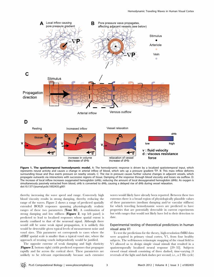
neuronal activity. The main stages of this response are as follows:

An increase in neuronal activity z(r,t) occurs, as a function of time t

and position r on the cortical sheet. This causes relaxation of the

smooth arterial muscles (mediated by astrocytes), inducing an

increased influx of blood (Figure 1A) increasing local vessel

volume and pressure. Blood then flows to regions of lower

pressure, resulting in a redistribution of pressure through the

medium (Figure 1B). These pressure changes induce further

blood volume changes in adjacent cortical tissue. As a conse-

quence of conservation of mass and momentum, this results in

local changes of blood velocity in this adjacent tissue (Figure 1C).

As these coupled changes propagate outwards, the viscous

properties of blood lead to damping of their amplitude

(Figures 1C, D). This is accompanied by outflows to draining

veins, reducing vessel volume, and thus yielding further dissipa-

tion. Although these two sources of dissipation occur at small

scales, they are reflected in the larger scale dynamics of the system.

Together, the above processes result in the propagation of

pressure changes that travel beyond the ,1 mm range of direct

blood flow between adjacent arterioles and venules. In our theory,

the time required for changes in directly coupled adjacent tissue to

occur is comparable to the time it takes for the blood to transit the

gray matter (,1 s). Consequently, these considerations predict

propagation speeds of order 1 mm/s.

During the change in vessel volume, local deoxyhemoglobin

(dHb) content also changes (Figure 1D). The influx of arterial

blood increases the content of oxygenated hemoglobin (oHb),

hence reducing local dHb concentration. Further reductions occur

by the removal of dHb by local outflow. As this process occurs,

oxygen diffuses passively into the cortical tissue, converting oHb to

dHb. Together, these processes result in an initial decrease of local

dHb concentration followed by a delayed increase.

The BOLD signal thus reflects the net change of blood volume

and dHb content. In the case of a spatiotemporally localized

neural activation, the predicted BOLD response is given by the

stHRF, expressed in Eqs. 1–5 of the Methods. The response to a

more general stimulus is obtained by convolving the stimulus with

the stHRF, as discussed in Text S1. Critically, the predicted

stHRF (Eq. 5) implies that the hemodynamic response contains a

component that propagates as damped traveling waves over spatial

scales potentially far greater than those of the neural signal that

generated them. In other words, our model predicts that even if

neuronal activity is restricted to a very small patch of cortex, it will

cause changes in the BOLD signal that propagate for several

millimeters over a few seconds.

The precise quantitative properties of the predicted BOLD

signal depend on several key physiological parameters that can be

experimentally determined. Our analysis (Figure 2) indicates that

the average vascular stiffness and the rate of damping due to blood

viscosity and outflow at boundaries are the most critical

parameters (see Table S1 in Text S1 for a complete list of

parameters). High stiffness results in a rapid return to equilibrium,

Author Summary

Functional magnetic resonance imaging (fMRI) experi-ments have advanced our understanding of the structureand function of the human brain. Dynamic changes in theflow and concentration of oxygen in blood are observedexperimentally in fMRI data via the blood oxygen leveldependent (BOLD) signal. Since neuronal activity inducesthis hemodynamic response, the BOLD signal provides anoninvasive measure of neuronal activity. Understandingthe mechanisms that drive this BOLD response isfundamental for accurately inferring the underlyingneuronal activity. The goal of this study is to systematicallypredict spatiotemporal hemodynamics from a biophysicalmodel, then test these in a high resolution fMRI study ofthe visual cortex. Using this theory, we predict andempirically confirm the existence of hemodynamic wavesin cortex – a striking and novel finding.

Hemodynamic Traveling Waves in Human Visual Cortex


thereby increasing the wave speed and range. Conversely high

blood viscosity results in strong damping, thereby reducing the

range of the waves. Figure 2 shows a range of predicted spatially

extended BOLD responses spanning physiologically realistic

ranges of these two parameters (Text S1). A combination of

strong damping and low stiffness (Figure 2, top left panel) is

predicted to lead to localized responses whose spatial extent is

mostly confined to that of the neuronal signal. Although there

would still be some weak signal propagation, it is unlikely this

would be detectable given typical levels of measurement noise and

voxel sizes. This parameter set corresponds to cases where the

stHRF spatial scale is smaller than a typical voxel size, where the

approach of treating voxels independently would be justified.

The opposite extreme of weak damping and high elasticity

(Figure 2, bottom right) yields predicted responses that propagate

rapidly and far across the cortical sheet. These parameters are

unlikely to be relevant experimentally because such extensive

waves would likely have already been reported. Between these two

extremes there is a broad region of physiologically plausible values

of these parameters (medium damping and/or vascular stiffness)

for which traveling hemodynamic waves are predicted to have

properties that are potentially detectable in current experiments

but with ranges that would not likely have led to their detection to

date.

Experimental testing of theoretical predictions in humanvisual area V1

To test the predictions for the theory, high-resolution fMRI data

were acquired in primary visual cortex, V1, from four healthy

subjects. The well-known retinotopic mapping of the visual field to

V1 allowed us to design simple visual stimuli that resulted in a

spatiotemporally localized neural response [29–32]. Subjects

viewed visual stimuli consisting of three dashed, time-varying (4

reversals of the light and dark dashes per second; i.e., a 2 Hz cycle)

Figure 1. The spatiotemporal hemodynamic model. A: The hemodynamic response is driven by a localized spatiotemporal input, whichrepresents neural activity and causes a change in arterial inflow of blood, which sets up a pressure gradient =P. B: This mass inflow deformssurrounding tissue and thus exerts pressure on nearby vessels. C: The rise in pressure causes further volume changes in adjacent vessels, whichpropagate outwards via interactions with successive regions of tissue. Damping of the response through blood viscosity and losses via outflow. D:The increase of local inflow increases oxygenated hemoglobin (oHb), reducing the amount of local deoxygenated hemoglobin (dHb). As oxygen issimultaneously passively extracted from blood, oHb is converted to dHb, causing a delayed rise of dHb during vessel relaxation.doi:10.1371/journal.pcbi.1002435.g001



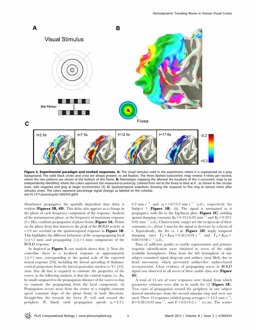
concentric rings at eccentricities of 0.6u, 1.6u, and 3u (Figure 3A).

Subjects were instructed to focus at the center of the screen and

perform a simple fixation task (see Methods).

These concentric visual stimuli resulted in strong BOLD

modulations in early visual cortex, as seen in the example in

Figure 3C. As a result of the retinotopic projection from visual

field to early cortex (Figure 3B), these concentric rings are

projected to lines on the cortical surface, one for each eccentricity.

We find that the maximum BOLD modulation occurs on these

lines, and that signal modulations weaken away from these peak

responses. The three rings were presented at the same time.

However, since the hemodynamic responses of the last two rings

were not sufficiently separated on the cortex (in all subjects), we

focus on the responses to the most inner ring, which was clearly

separated (see Methods) from the responses of the other rings. The

spatiotemporal evoked response is shown in a series of snapshots at

different times t with respect to the stimulus onset (Figure 3C).

Early responses (t = 2.5 s) are restricted to the central region (red)

on these surface patches. As time progresses the BOLD signal near

the center rises, and locations successively further from the center

demonstrate increasingly delayed rises at t = 2.5–7.5 s. Finally,

outward propagation of positive modulation in the periphery

continues, while central responses decrease until they display the

well known negative phase of the local post-stimulus undershoot at

t = 12.5–17.6 s.

BOLD waves on the cortical surfaceThe outward propagation (Figure 3C), discussed in the

previous section, suggests the possibility of a traveling wave

response, propagating normal to the centerline of the underlying

neuronal response. We now focus on characterizing this response.

Because stimulation of an isoeccentric curve in the visual field

excites an approximately straight line of neurons in V1 [33],

normal directions are clearly identifiable on a flattened cortex. We

thus estimate the centerline of the primary isoeccentric response in

a flattened representation of V1 (Figures 4A,B), and average the

signal change over all points the same distance from this centerline

(Figure 4B) (see Methods). Repeating this at various distances x

and times t reveals the average spatiotemporal response

(Figure 4C). Although the signal has been low-pass filtered in

the time domain, and averaged along the direction parallel to the

stimulus centerline, it is crucial to note that no spatial smoothing

has been performed in the x direction.

The response has two characteristic spatial scales. Near the

center (|x|,1 mm), a local response occurs, with a range similar

to that of the expected neural response and whose time variation is

similar to that predicted by the (purely temporal) balloon model.

However, outside this region, the response propagates outward for

several mm, with the peak response occurring steadily later as |x|

increases (Figure 4D). At |x| = 5 mm the response is delayed,

reaching its peak just as the central response |x|,1 mm reverses

sign (Figures 4D,E). Furthermore, the amplitude of the

propagating response decreases with |x| until it reaches the

background level beyond |x| = 5 mm.

Quantifying the spatiotemporal responseThe above features of the BOLD signal modulations confirm

the qualitative theoretical predictions of the spatiotemporal model.

The theory also makes quantitative predictions of the waves’

propagation speed, range, and damping rate. We next test these

predictions and estimate the corresponding parameters through

more detailed quantification of the empirical response.

To estimate the speed of wave propagation, phase fronts of the

BOLD signal were estimated (see Methods). As the hemodynamic

Figure 2. Predicted responses vs. x and t for a range of physiologically plausible values of of nb and C. Each column represents aparticular nb – as labeled at the top, while each row corresponds to a different C – as labeled at the left.doi:10.1371/journal.pcbi.1002435.g002



disturbance propagates, the spatially dependent time delay is

evident (Figures 3B, 4D). This delay also appears as a change in

the phase of each frequency component of the response. Analysis

of the instantaneous phase, at the frequency of maximum response

(0.1 Hz), confirms propagation of phase fronts (Figure 5A). Points

on the phase front that intersects the peak of the BOLD activity at

x = 0 are overlaid on the spatiotemporal response in Figure 5B.

This highlights the different behaviors of the nonpropagating local

(|x|,1 mm) and propagating (|x|.1 mm) components of the

BOLD response.

As depicted in Figure 5, our analysis shows that: (i) Near the

centerline there is a localized response at approximately

|x|,1 mm, corresponding to the spatial scale of the expected

neural response [34], including the lateral spreading of thalamo-

cortical projections from the lateral geniculate nucleus to V1 [35].

(note that all that is required to estimate the properties of the

waves, in the following analysis, is that the central region, i.e. Dx,

be small compared to the propagation distance of the waves so that

we separate the propagating from the local component). (ii)

Propagation occurs away from the center at a roughly constant

speed (constant slope of the phase front) in both directions.

Straight-line fits towards the fovea (F, red) and toward the

periphery (P, black) yield propagation speeds vF = 2.36

0.2 mm s21 and vP = 1.860.2 mm s21 (s.d.), respectively for

Subject 1 (Figure 5B). (iii) The signal is attenuated as it

propagates, with fits to the log-linear plots (Figure 5C) yielding

spatial damping constants KP = 0.3360.02 mm21 and KF = 0.396

0.02 mm21 (s.d.). Characteristic ranges are the reciprocals of these

constants; i.e., about 3 mm for the signal to decrease by a factor of

e. Equivalently, the fits vs. t in (Figure 5D) imply temporal

damping rates CP = KPvP = 0.5660.04 s21 and CF = KFvF =

0.8660.08 s21 (s.d.).

Data of sufficient quality to enable segmentation and primary

response identification were obtained in seven of the eight

available hemispheres. Data from the left hemisphere of one

subject contained signal drop-out and artifact, most likely due to

head movement, which prevented artifact-free surface-based

reconstruction. Clear evidence of propagating waves in BOLD

signal was observed in all seven of these usable data sets (FigureS5).

A total of 14 sets of wave responses were found, from which

parameter estimates were able to be made for 12 (Figure 5E).

Two cases of propagation toward the periphery in one subject

showed interference from the second stimulus ring and were not

used. These 12 responses yielded group averages v = 462 mm s21,

K = 0.2860.03 mm21, and C= 0.860.2 s21 (s.e.m). The scatter

Figure 3. Experimental paradigm and evoked responses. A: The visual stimulus used in the experiment, where it is superposed on a graybackground. The solid black circles and cross are always present, to aid fixation. The three dashed isoeccentric rings reverse 4 times per second,where the two patterns are shown at the bottom of this frame. B: Retinotopic mapping the allowed the locations of the 3 concentric rings to beindependently identified, where the colors represent the measured eccentricity, colored from red at the fovea to blue at 6u, as shown in the circularinset, with magenta and gray at larger eccentricities [3]. C: Spatiotemporal snapshots showing the response to first ring at various times afterstimulus onset. The colors represent percentage signal change, as labeled on the colorbar.doi:10.1371/journal.pcbi.1002435.g003



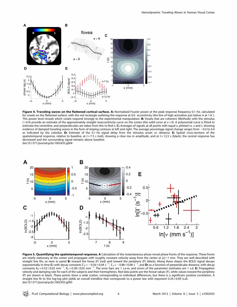
Figure 4. Traveling waves on the flattened cortical surface. A: Normalized Fourier power at the peak response frequency 0.1 Hz, calculatedfor voxels on the flattened surface, with the red rectangle outlining the response at 0.6u eccentricity (the line of high activation just below is at 1.6u).This power level reveals which voxels respond strongly to the experimental manipulation. B: Voxels that are coherent (Methods) with the stimulus(.0.4) provide an estimate of the approximately straight isoeccentricity curve on the cortex (the solid curve at x = 0). A polynomial curve is fitted toestimate the centerline, and perpendiculars are taken from this to find x. C: Averages of signals at all points with equal x, plotted vs. x and t, showingevidence of damped traveling waves in the form of sloping contours at left and right. The average percentage signal change ranges from 20.4 to 0.4as indicated by the colorbar. D: Estimate of the 0.1 Hz signal delay from the stimulus onset vs. distance. E: Spatial cross-sections of thespatiotemporal response, relative to baseline, at t = 7.5 s (red), showing a clear rise in amplitude, and at t = 12.5 s (black), the central response hasdecreased and the surrounding signal remains above baseline.doi:10.1371/journal.pcbi.1002435.g004

Figure 5. Quantifying the spatiotemporal response. A Calculation of the instantaneous phase reveal phase fronts of the response. These frontsare nearly stationary at the center and propagate with roughly constant velocity away from the center at |x|.1 mm. They are well described withstraight line fits, as seen in panel B: toward the fovea (F) (red) and toward the periphery (P) (black). Along these slopes the BOLD signal decaysexponentially in time C: with decay constants CP = 20.5660.04 s21, CF = 20.8660.08 s21, and D: as a function of perpendicular distance, with decayconstants KP = 0.3260.02 mm21, KF = 0.3860.02 mm21. The error bars are 1 s.e.m, and errors of the parameter estimates are 1 s.d. E: Propagationvelocity and damping rate for each of the subjects and their hemispheres. Red data points are the foveal values (F), while values toward the periphery(P) are shown in black. These points show a wide scatter, corresponding to individual differences, but there is a significant positive correlation. Astraight line fit to this log-log plot yields an overall trendline that corresponds to a power law with exponent 0.2460.09 (s.d).doi:10.1371/journal.pcbi.1002435.g005



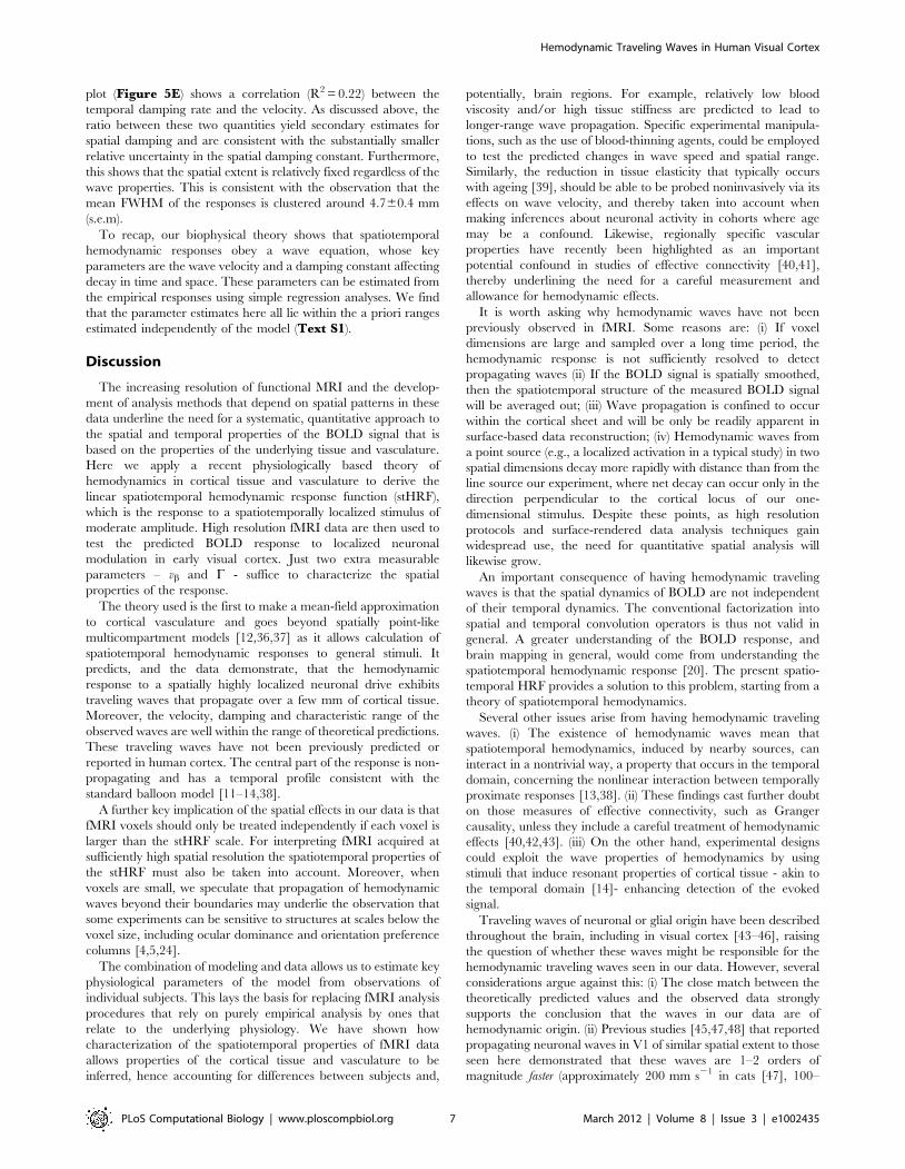
plot (Figure 5E) shows a correlation (R2 = 0.22) between the

temporal damping rate and the velocity. As discussed above, the

ratio between these two quantities yield secondary estimates for

spatial damping and are consistent with the substantially smaller

relative uncertainty in the spatial damping constant. Furthermore,

this shows that the spatial extent is relatively fixed regardless of the

wave properties. This is consistent with the observation that the

mean FWHM of the responses is clustered around 4.760.4 mm

(s.e.m).

To recap, our biophysical theory shows that spatiotemporal

hemodynamic responses obey a wave equation, whose key

parameters are the wave velocity and a damping constant affecting

decay in time and space. These parameters can be estimated from

the empirical responses using simple regression analyses. We find

that the parameter estimates here all lie within the a priori ranges

estimated independently of the model (Text S1).

Discussion

The increasing resolution of functional MRI and the develop-

ment of analysis methods that depend on spatial patterns in these

data underline the need for a systematic, quantitative approach to

the spatial and temporal properties of the BOLD signal that is

based on the properties of the underlying tissue and vasculature.

Here we apply a recent physiologically based theory of

hemodynamics in cortical tissue and vasculature to derive the

linear spatiotemporal hemodynamic response function (stHRF),

which is the response to a spatiotemporally localized stimulus of

moderate amplitude. High resolution fMRI data are then used to

test the predicted BOLD response to localized neuronal

modulation in early visual cortex. Just two extra measurable

parameters – vb and C - suffice to characterize the spatial

properties of the response.

The theory used is the first to make a mean-field approximation

to cortical vasculature and goes beyond spatially point-like

multicompartment models [12,36,37] as it allows calculation of

spatiotemporal hemodynamic responses to general stimuli. It

predicts, and the data demonstrate, that the hemodynamic

response to a spatially highly localized neuronal drive exhibits

traveling waves that propagate over a few mm of cortical tissue.

Moreover, the velocity, damping and characteristic range of the

observed waves are well within the range of theoretical predictions.

These traveling waves have not been previously predicted or

reported in human cortex. The central part of the response is non-

propagating and has a temporal profile consistent with the

standard balloon model [11–14,38].

A further key implication of the spatial effects in our data is that

fMRI voxels should only be treated independently if each voxel is

larger than the stHRF scale. For interpreting fMRI acquired at

sufficiently high spatial resolution the spatiotemporal properties of

the stHRF must also be taken into account. Moreover, when

voxels are small, we speculate that propagation of hemodynamic

waves beyond their boundaries may underlie the observation that

some experiments can be sensitive to structures at scales below the

voxel size, including ocular dominance and orientation preference

columns [4,5,24].

The combination of modeling and data allows us to estimate key

physiological parameters of the model from observations of

individual subjects. This lays the basis for replacing fMRI analysis

procedures that rely on purely empirical analysis by ones that

relate to the underlying physiology. We have shown how

characterization of the spatiotemporal properties of fMRI data

allows properties of the cortical tissue and vasculature to be

inferred, hence accounting for differences between subjects and,

potentially, brain regions. For example, relatively low blood

viscosity and/or high tissue stiffness are predicted to lead to

longer-range wave propagation. Specific experimental manipula-

tions, such as the use of blood-thinning agents, could be employed

to test the predicted changes in wave speed and spatial range.

Similarly, the reduction in tissue elasticity that typically occurs

with ageing [39], should be able to be probed noninvasively via its

effects on wave velocity, and thereby taken into account when

making inferences about neuronal activity in cohorts where age

may be a confound. Likewise, regionally specific vascular

properties have recently been highlighted as an important

potential confound in studies of effective connectivity [40,41],

thereby underlining the need for a careful measurement and

allowance for hemodynamic effects.

It is worth asking why hemodynamic waves have not been

previously observed in fMRI. Some reasons are: (i) If voxel

dimensions are large and sampled over a long time period, the

hemodynamic response is not sufficiently resolved to detect

propagating waves (ii) If the BOLD signal is spatially smoothed,

then the spatiotemporal structure of the measured BOLD signal

will be averaged out; (iii) Wave propagation is confined to occur

within the cortical sheet and will be only be readily apparent in

surface-based data reconstruction; (iv) Hemodynamic waves from

a point source (e.g., a localized activation in a typical study) in two

spatial dimensions decay more rapidly with distance than from the

line source our experiment, where net decay can occur only in the

direction perpendicular to the cortical locus of our one-

dimensional stimulus. Despite these points, as high resolution

protocols and surface-rendered data analysis techniques gain

widespread use, the need for quantitative spatial analysis will

likewise grow.

An important consequence of having hemodynamic traveling

waves is that the spatial dynamics of BOLD are not independent

of their temporal dynamics. The conventional factorization into

spatial and temporal convolution operators is thus not valid in

general. A greater understanding of the BOLD response, and

brain mapping in general, would come from understanding the

spatiotemporal hemodynamic response [20]. The present spatio-

temporal HRF provides a solution to this problem, starting from a

theory of spatiotemporal hemodynamics.

Several other issues arise from having hemodynamic traveling

waves. (i) The existence of hemodynamic waves mean that

spatiotemporal hemodynamics, induced by nearby sources, can

interact in a nontrivial way, a property that occurs in the temporal

domain, concerning the nonlinear interaction between temporally

proximate responses [13,38]. (ii) These findings cast further doubt

on those measures of effective connectivity, such as Granger

causality, unless they include a careful treatment of hemodynamic

effects [40,42,43]. (iii) On the other hand, experimental designs

could exploit the wave properties of hemodynamics by using

stimuli that induce resonant properties of cortical tissue - akin to

the temporal domain [14]- enhancing detection of the evoked

signal.

Traveling waves of neuronal or glial origin have been described

throughout the brain, including in visual cortex [43–46], raising

the question of whether these waves might be responsible for the

hemodynamic traveling waves seen in our data. However, several

considerations argue against this: (i) The close match between the

theoretically predicted values and the observed data strongly

supports the conclusion that the waves in our data are of

hemodynamic origin. (ii) Previous studies [45,47,48] that reported

propagating neuronal waves in V1 of similar spatial extent to those

seen here demonstrated that these waves are 1–2 orders of

magnitude faster (approximately 200 mm s21 in cats [47], 100–



250 mm s21 in primates [45] and 50–70 mm s21 in rats [48]),

and waves in cortical white matter travel even faster [43].

Likewise, although the spatial scales may be similar to those

presently reported, the diffusion of nitrous oxide - which mediates

the coupling between neuronal activity and vasodilation - occurs

too rapidly to explain our results [21]. (iii) Another possible source

of propagating signal of possible relevance are calcium waves

traveling via astrocytes because these mediate the neuronal signal

in vasodilation. However, these calcium waves travel at

,10 mm s21 [49], which is 2 orders of magnitude slower that the

waves reported here.

Although hemodynamic waves have not been characterized,

detected, or previously modeled, existing work has detailed some

spatiotemporal properties of the BOLD response. Previous studies

have demonstrated hemodynamic contributions to spatiotemporal

BOLD response, including: the effect of draining veins [50,51]

which induces a latent BOLD signal due to these veins; effects

across vascular layers [52,53] that induce layer dependent delays

of the BOLD response; and general effects of the vascular network

[43] that cause delayed BOLD responses across extensive brain

regions. Studies have also implemented ways to minimize such

effects to improve spatial specificity of functional activations

[43,50]. The hemodynamic waves are different from the

mentioned phenomena in that they exhibit propagation across

the cortical surface. As the waves pass through they induce

changes in arterioles, capillaries, and venules – not reliant on

overall drainage by large veins. The possible interplay of these

effects will be subject to future modeling and experimental work.

In summary, with advances in imaging technology and data

analysis, intervoxel effects will become more pronounced,

demanding spatiotemporal analyses based on the underlying brain

structure and hemodynamics. By verifying a model that enables

such analysis, the present paper opens the way to new fMRI

probes of brain activity. These new possibilities include experi-

ments using spatial deconvolution to discriminate between neural

and hemodynamic contributions to the spatiotemporal BOLD

response evoked by complex sensory stimuli. An important

potential application would be to disentangle negative components

of the BOLD response from surround inhibition in the visual

cortex. Our analysis also affords novel insights and physiological

information on neurovasculature, a subject of particular signifi-

cance to ageing and vascular health. Finally, the combination of

the present stHRF with spatially embedded neural field models [8]

would allow a systematic and integrated computational framework

for inferring dynamic activity in underlying neuronal populations

from fMRI data.

Methods

The methods used in this study are threefold: (i) Derivation of a

theoretical spatiotemporal hemodynamic response function

(stHRF) from a physiologically based model of cortical hemody-

namics; (ii) Execution of a customized experimental protocol for

the acquisition and preprocessing of high resolution fMRI data on

the response to spatially localized visual stimuli; and (iii) Model-

based analysis of these data and explicit comparison with the

predicted stHRF, including inference of underlying cortical

hemodynamic parameters.

Theoretical predictionThe theoretical prediction of the stHRF is derived from a

physiologically-based model for spatiotemporal hemodynamics

[25]. This model treats brain tissue as a poroelastic medium, with

interconnected pores representing the cortical vasculature. The

governing equations are a set of nonlinear partial differential

equations that connect blood flow velocity v, mass density

contributed by blood (i.e. the part of the total density contributed

by blood as opposed to tissue) j, deoxygenated hemoglobin

concentration Q, and blood pressure P due to an increase in

arterial flow F caused by an increase neural activity z, as a function

of time t and position on the cortex r. Although we describe

changes in blood volume throughout the text, we model changes

in j - which is closely related to the fractional volume of blood in

tissue: j/rf, where rf is the density of blood itself. These model

equations were recently derived and explained in a separate paper

[25]. We provide a synopsis here and apply this with appropriate

boundary conditions (Text S1) to calculate the stHRF and derive

a hemodynamic wave equation.

The dynamics of flow F(r,t) are modeled as a damped harmonic

oscillator [13] driven by neural activity z(r,t):

d2F(r,t)

dt2zk

dF (r,t)

dtzc F (r,t){F0½ �~z(r,t): ð1Þ

The dynamics in Eq. 1 are parameterized by the signal decay rate

k, the flow-dependent elimination constant c and the resting flow

F0. The neural activity z(r,t) drives a distribution of arterial control

sites (see Figure S1), as described further in Text S1.

The vascular response due to this increase in arterial flow is then

constrained by physical laws, including conservation laws. Firstly,

the conservation of blood mass is embodied by

rf +:v(r,t)zLj(r,t)

Lt~rf F (r,t){cPP(r,t)½ �, ð2Þ

where cP is a proportionality constant. This conservation law

describes how the rate of change of local blood mass density hj/ht

is determined by the local divergence of the flow rf=N(v), the

source of mass due to the average inflow of blood F, and the

average venous outflow of blood cPP. These latter source/sink

terms are mean-field terms that describe the average spatiotem-

poral hemodynamic processes (For more details see the Text S1on the derivation of these terms).

The rate at which blood travels through the vasculature

depends on the elastic response of cortical vessels. This process

must conserve momentum, expressed as

rf

Lv(r,t)

Lt~{ c1+P j(r,t)½ �zD v(r,t){vF (r,t){vP(r,t)½ �f g, ð3Þ

where P is the average pore pressure, D parameterizes damping

due to blood viscosity, and c1/rf is the constant of proportionality

between pressure gradient and acceleration in the porous medium.

This equation describes how forces are directed down pressure

gradients, causing blood to accelerate toward regions of lower

pressure. These velocity changes are resisted by blood viscosity

leading to the resistive term D(v-vF - vP) where vF and vP are the

blood velocities at inflow and outflow, respectively (Text S1). The

average pressure is related to the elastic properties of blood vessels

by the constitutive equation,

P(r,t)~c2j(r,t)b, ð4Þ

where the elasticity of blood vessels is parameterized by the Grubb

exponent 1/b (see Table S1 in Text S1) and a proportionality

constant c2, as in previous empirical studies of cerebral blood flow

[54].



As changes in local blood volume occur, oxygen diffuses into

cortical tissue because of the increased partial pressure of oxygen.

This process produces blood deoxyhemoglobin (dHb) - whose

concentration is represented by Q - from oxygenated hemoglobin.

The local concentration of hemoglobin in tissue is a fixed

proportion y (in mmol kg21), of local blood density in tissue,

and is thus expressed as yj. Hence, the difference yj - Q is the

amount of oxygenated hemoglobin. If g is the fractional rate at

which oxygen passes from oxygenated hemoglobin to cortical

tissue, the flow of dHb obeys a conservation equation, similar to

Eq. 2 for the conservation of blood mass:

LQ(r,t)

Ltz+: Q(r,t) v(r,t){vF (r,t){vP(r,t)½ �f g

~ yj(r,t){Q(r,t)½ �g{Q(r,t)

j(r,t)=rf

cPP(r,t),

ð5Þ

where the difference term (yj - Q)g on the right hand side

introduces the source of dHb, in which dHb is convereted to oHb

at a rate g, and the term –QPcP/(jrf) represents the rate of

reduction of dHb concentration due to blood outflow. This

assumes that the blood is well mixed so the concentration leaving a

vascular unit is Q/(jrf) at a rate of average venous blood outflow

cPP (Text S1). As in Eq. 2, the net outflow rate, here dHb =N(Qv),

is balanced by local changes in content, here hQ/ht.

Finally, the measured BOLD signal y is predicted by a recent

semi-empirical relation [55] between tissue blood volume content

j/rf and dHb content Q to be

y(r,t)~V0 k1 1{Q(r,t)

Q0

� �zk2 1{

Q(r,t)rf V0

j(r,t)Q0

� �zk3 1{

j(r,t)

rf V0

!" #,ð6Þ

where V0 is the resting total volume, Q0 is the resting fraction of

dHb, and the constants k1, k2, and k3 depend on the acquisition

parameters, including field strength and echo time.

Calculation of the stHRF. Eq. 1–6 are a closed set of

nonlinear partial differential equations which describe the

hemodynamics in response to an arbitrary neural signal z(r,t).

To probe their fundamentals, we analyze their predicted

spatiotemporal hemodynamic response function (stHRF) to a

spatiotemporally localized stimulus, from which responses to

general stimuli can be derived.

Provided the amplitude of neural activity is not too large, the

model’s response is approximately linear. Therefore, the hemo-

dynamic variables henceforth represent linear perturbations from

the steady state of hemodynamics. We thus approximate the

hemodynamic response by linearizing the system 1–6 and arrive at

the hemodynamic wave equation

L2j(r,t)

Lt2z2C

Lj(r,t)

Lt{n2

b+2j(r,t)~rf F (r,t), ð7Þ

where C is the damping parameter and nb is the propagation

velocity. This equation predicts waves of j in response to an

increase in local activity F. The damping parameter is given by

2C= b/t+D/rf and shows that dissipation of j waves is due to

viscous damping, D/rf,and blood outflow b/t at boundaries,

which also dissipates wave amplitude. This equation represents the

dominant factor that determines the traveling-wave part of the

hemodynamic response (the rest of the equations are detailed in

Text S1). Ranges for nb and C are of the order of mm s21 and

s21, respectively (Text S1).

Fourier methods are next used to calculate a set of transfer

functions, TLz, which describe the ratio of the response of a

hemodynamic quantity L (i.e., Q, j, y, or F) at a given spatial

frequency (i.e., wave vector) k and temporal angular frequency v,

to the change in neural activity signal z(k,v). These transfer

functions act as spatiotemporal filters and can be used to derive the

BOLD frequency response to an arbitrary neural input. Hence,

this includes the impulse response from a spatiotemporal neural

input; i.e. the spatiotemporal HRF. This transfer function Tyz

maps from neural activity z(r,t), to BOLD signal y(r,t). The

predicted experimental response y(r,t) is given by the inverse

Fourier transform of the product of the transfer function in TextS1: Eq. S17 and the Fourier transform of the neural activity

z(k,v). To predict our experimental design we approximate the

distribution of the evoked spatial neural activity as a Gaussian with

a standard deviation of 1 mm in the x direction (Text S1: Eq.S22), to represent the spatial spread of the expected neural

response [34]. The temporal neural response is simply the block

design of the visual stimulus delivered in the experiment.

General MRI proceduresBy restricting the fMRI scans to the occipital pole, we achieved

a resolution of 1.561.561.5 mm3 and 2 s TR echoplanar images

(EPI). The stimulus onset was dephased by 250 ms per block for 8

blocks to further increase the effective time resolution. These EPI

data were then coregistered to a high-resolution T1-weighted

anatomical scan, acquired at 0.7560.7560.75 mm3, so that the

spatiotemporal resolution was effectively resampled to

250 ms6(0.7560.7560.75) mm3. Furthermore, these mappings

were restricted to the gray matter by segmenting the anatomical

data into gray and white matter. Finally, functional retinotopic

scans were used to map out the expected cortical positions in the

visual cortex of each subject [3]. Data were acquired on a Philips

3 T Achieva Series MRI machine equipped with Quasar Dual

gradient system and an eight-channel head coil.

SubjectsFive healthy subjects (two female) ranging from 21 to 30 years

participated in this study. The study protocols were approved by

ethics boards of the University of New South Wales and

Neuroscience Research Australia (formerly the Prince of Wales

Medical Research Institute).

Visual paradigmParticipants viewed visual stimuli via a mirror mounted on the

head coil at a viewing distance of 1.5 m, resulting in a display

spanning a diameter of 11u (or 5.5u in eccentricity). The visual

paradigm was prepared with PresentationH software. Stimulus

duration and fMRI pulse timing were logged with 0.1 ms

accuracy. The stimulus consisted of 3 concentric rings simulta-

neously presented at 0.6u, 1.6u, and 3u eccentricity, presented in a

block paradigm. (on for 8 s and off for 12.25 s). Each annulus was

only 1 pixel wide (roughly 0.014u visual angle).

As known from retinotopic studies, isoeccentric lines in the

visual field map to approximately straight lines in primary visual

cortex. This stimulus was chosen to exploit this property,

optimizing the identification of the primary response and

secondary changes in BOLD signal in the orthogonal direction.

During the ‘on’ state, the annuli were divided into black and

gray dashes that reversed roles 4 times per second (i.e., in a 2 Hz

cycle). During the ‘off’ state, the annuli remained black (FigureS2). To improve visual fixation, a black fixation cross extended

across the entire screen, 4 black circles were permanently present,

and a pseudorandomly flickering fixation dot fluctuated between



red, green, and blue [56]. Subjects reported that they were able to

maintain alertness and attend to the fixation cross throughout data

acquisition.

Note that off blocks were 12.25 s in duration, ensuring that the

evoked response was effectively sampled at 250 ms. Each fMRI

session consisted of 8 stimulus blocks, consisting of 80+1 fMRI

volumes (the extra scan was due to the delayed onset) plus an

additional 7 ‘off’ scans prior to the first block. Hence each session

contained 88 fMRI volumes, a running time of 176 s, 14 such

sessions were acquired from each subject.

To improve timing accuracy and synchronization we used a

monitor refresh rate of 60 Hz for the visual display, and a TR of

2006 ms, rather than 2000 ms, to compensate for system delays.

The remaining variability of the stimulus onset precision was

logged and used for modeling the experimental design during data

analysis.

Functional data and preprocessingTo achieve high resolution, speed, and minimize distortions, we

used a SENSE [57] accelerated echoplanar imaging (EPI)

sequence. Great care was taken to minimize distortion, and each

subject’s data were carefully investigated to ensure distortion was

minimal. Functional data were acquired in 29 1.5 mm slices for all

but one subject, for whom there were 28 slices, with a 1926192

matrix, 230 mm field of view, and a SENSE factor of 2.3.

Functional data were motion corrected and slice scan-time

corrected using SPM5 (SPM software package, http://www.fil.ion.

ucl.ac.uk/spm/), then imported into the mrVista- Toolbox

(http://white.stanford.edu/software/) for further processing and

analysis. The fMRI data were transformed and analyzed in three

different spaces: Firstly, the original planar space of the data

acquisition, secondly, the 3 dimensional space defined by the high

resolution T1 anatomy scans into which the data were aligned,

transformed, and spatially up-sampled and finally for a flattened

representation of the visual cortex, with maps of phase of the fMRI

signals at the left and right occipital pole. Apart from the spatial

up-sampling and mapping, no further preprocessing of the data in

the spatial dimension was performed. The temporal time series of

each voxel were low-pass filtered with a third order Butterworth

filter below 0.1 Hz. Furthermore, although there were three

concentric rings, we focus only on the 0.6u ring closest to the fovea

when analyzing the spatiotemporal hemodynamic response as this

was clearly spatially distinct whereas there was some overlap in

responses to the furthest two rings (1.6u, and 3u).

Distance measurementsDistance measurements were made along the cortical surface

using meshes generated by the segmentation on each subject. A

shortest path algorithm (in the VISTA software) was used to

determine these distances on the surface.

Isoeccentric averagingWhen a stimulus excites a line of cortex, as in the present case,

the hemodynamic response depends only on time and the

perpendicular distance x from that line. To analyze these

dependences, we estimated the location of the centerline of the

primary response on the flattened surface, then measured the

average BOLD signal at various distances orthogonal to this

response as a function of time since stimulus onset. This was

achieved in five steps (see Text S1 for further details):

I. Voxels with stimulus-related signal change were deemed

to be those with signal fluctuations above a normalized

temporal Fourier power of 40% relative to the total power

at the peak stimulus response frequency bin of 0.1 Hz.

II. Voxels within the primary visual cortex and at the

approximate locations corresponding to the visual stimulus

of 0.6u eccentricity were identified using a previously

acquired retinotopic map as a spatial prior (Figure 4Aand Figure S3).

III. A polynomial was fitted to the spatially distributed voxels

fulfilling these criteria (Figure 4B), and is an estimate of

the centerline of the response. The order of this

polynomial was estimated using the Aikake Information

[58] criterion (see Text S1 and Figure S4).

IV. The distance x was found by constructing lines orthogonal

to the centerline, extending 10 mm either side of it

(Figure 4B) and measuring distances along them. Positive

x was chosen to be toward the fovea.

V. The spatiotemporal responses y(r,t) at all points with a

given value of x were averaged at each time t to obtain

y(x,t) (Figure 4B).

Phase estimates with the Hilbert transformAs a hemodynamic disturbance travels, the BOLD signal phase

depends on x and t. Phase fronts enable any wave propagation to

be tracked at large |x|. To obtain phase estimates from the signal

y(x,t), we first constructed the analytic signal [59],

as(x,t)~y(x,t)ziHt y(x,t)½ �, ð8Þ

where

Ht y(x,t)½ �~ 1

p

ðy(x,t0)

t{t0dt0, ð9Þ

is the temporal Hilbert transform [59]. The phase Q(x,t) is then

given by

Q(x,t)~ arg as(x,t)½ �, ð10Þ

where arg is the complex argument. Maps of this phase are shown

in Figure 5A as well as in the Supplementary text for all the data

sets. Constant-phase lines represent the phase fronts of the BOLD

signal.

Estimation of physiological parameters from dataThe empirical estimates for the properties of the wave fronts

were calculated from the phase fronts emerging from the peak of

the BOLD signal at x = 0 (Figure 5B). From here, the two

principal characteristics of the spatiotemporal response can be

identified, the local response, close to x = 0, as a region of near-

uniform phase spanning |x|,1 mm, and the propagating

component heading away from these regions at |x|.1 mm (see

Figure 5B and Text S1). This is consistent with the expected

neural point spread function estimated from independent

physiological data [34]. Straight-line fits to this propagating

region, as shown in Figure 5B, yielded estimates of the wave

velocity nb.

The BOLD signal was measured at each point on the phase

front as a function of time (Figure 5C) and space (Figure 5D).

Transformation to logarithmic scales yielded approximately

straight line plots, suggesting exponential decay of BOLD signal

in space and time. Linear regression then yielded rate constants of



temporal and spatial signal decay. Estimation of the standard error

of these linear regressions provided error estimates for these

parameters (see Text S1).

Supporting Information

Figure S1 The geometrical space for the hemodynamicresponse function. The center of this corresponds to a small

area that contains various flow control sides that all contribute to

the injection of mass into the system.

(TIFF)

Figure S2 The visual stimulus presented to subjects inthe scanner. The three rings;1,2, & 3 in the figure, were located

at 0.6u, 1.6u, and 3u eccentricity respectively. These rings flickered

back and forth with four reversals per second during the stimulus

on phase. These rings were overlaid on a grey background and

fixation grid consisting of rings and lines (in dark grey) that were

always present. The sizes of the rings and the lines are exaggerated

for clarity, and in the experimental design were 1 pixel wide. The

intensities of the light and dark grays are also exaggerated on the

spatial oscillation on each ring: 1, 2, & 3, and shown below on the

2 Hz flicker panel. During the off phase rings 1,2, & 3 were set at

the luminosity of the fixation grid. Not shown here is the fixation

task, which was a small square at the centre which pseudor-

andomly osciallated between red, green and blue. Lumonisty

values were measured at: 1.16106 cd/m2 and 36105 cd/m2 for

the light and dark grays respectively. The background gray was

measured at 66105 cd/m2, and the dark stimulus fixation lines

were measured at 1.56105 cd/m2. These lumonisity values were

measured with a Minolta � CS-100 photometer under conditions

matching those of the subjects in the scanner.

(TIFF)

Figure S3 Thresholding the data in V1. A: Frequency

responses in all voxels in the occipital pole for each subject,

denoted by SXH, (where X is subject number and H is the

hemisphere), where the peak at is in red of all subjects. B: The

spatial distribution of the Fourier peak frequency response, at

0.1 Hz, where the colors represent normalized power shown in the

colorbar. These show the first ring (0.6u eccentricity and red band

closest to the centre) in all subjects with the outer two rings, in

most cases, combining. These panels are masked to only include

V1 which is overlaid on the flattened occipital pole. C: The

complementary eccentricity retinotopic map for each subject, with

the colors representing the eccentricity in the visual field, indicated

by the filled circle, where the centre represents the fovea the colors

extend out radially to the periphery at 5.5u of eccentricity. Both B

and C colormaps are overlaid on a curvature map of the cortex,

where the intensities represent cortical curvature going from high

in black to low in white.

(TIFF)

Figure S4 Fitting the stimulus centerline for all subjectsand hemispheres. On the left of each panel is the Akaike

Information Criteria (AIC) vs. the degree of the polynomial fitted to the

thresholded voxels. On the right the polynomial fit at the minimal AIC

with corresponding orthogonal lines. In Subject 1, right at high orders,

orthogonal lines highly intersected so that the sampling data was

effectively reduced significantly. This mean that the minimal AIC was

not optimal in this dataset, therefore the choice was made to choose the

first significant drop in AIC from the previous order, n = 3.

(TIFF)

Figure S5 Spatiotemporal responses and parameterestimates for each subject and hemisphere. The procedure

is that used to obtain Figure 5 of the main text, as described there. A:The instantaneous phase. B: Spatiotemporal response, with estimated

wave fronts overlaid in black toward the periphery (x,0) and in red

towards the fovea (x.0). C: Amplitude vs. x. D: amplitude vs. t. The

peripheral estimates for S3 left and right hemispheres contained few

data points due to interference between the response from the ring at

the next eccentricity, and are thus omitted from the subsequent analysis

(see Figure S3). The errors quoted for parameter estimates

throughout this manuscript are 1 standard deviation, estimated from

linear regression fits to the data.

(TIFF)

Text S1 We present the full linearized model (with thedescriptions of the boundary conditions, and how theequations were linearized) and detail the completemodel parameters and estimate their values. We also

provide extra details of the polynomial fitting routines shown in

Figures 4 and S4.

(PDF)

Acknowledgments

We thank J. Roberts for helpful remarks on the manuscript.

Author Contributions

Conceived and designed the experiments: KMA MMS MB PAR.

Performed the experiments: KMA MMS. Analyzed the data: KMA

MMS MB. Contributed reagents/materials/analysis tools: KMA MMS

MB. Wrote the paper: KMA MMS PAR MB. Made the theoretical

predictions: KMA PMD PAR.

References

1. Friston KJ (2009) Modalities, Modes, and Models in Functional Neuroimaging.

Science 326: 399–403.

2. Logothetis NK, Pauls J, Augath M, Trinath T, Oeltermann A (2001)

Neurophysiological investigation of the basis of the fMRI signal. Nature 412:

150–157.

3. Schira MM, Tyler CW, Breakspear M, Spehar B (2009) The foveal confluence

in human visual cortex. J Neurosci 29: 9050–9058.

4. Kamitani Y, Tong F (2005) Decoding the visual and subjective contents of the

human brain. Nat Neurosci 8: 679–685.

5. Haynes JD, Rees G (2005) Predicting the orientation of invisible stimuli from

activity in human primary visual cortex. Nat Neurosci 8: 686–691.

6. Breakspear M, Bullmore E, Aquino K, Dass P, Williams LM (2006) The

multiscale properties of evoked cortical activity. Neuroimage 30: 1230–1242.

7. Stephan KE, Kasper L, Harrison LM, Daunizeau J, Ouden HEM, et al. (2008)

Nonlinear dynamic causal models for fMRI. Neuroimage 42: 649–662.

8. Robinson PA (2001) Prediction of electroencephalographic spectra from

neurophysiology. Phys Rev E 63: 021903.

9. Daunizeau J, Kiebel SJ, Friston KJ (2009) Dynamic causal modelling of

distributed electromagnetic responses. Neuroimage 47: 590–601.

10. Breakspear M, Jirsa V, Deco G (2010) Computational models of the brain: From

structure to function. Neuroimage 52: 727–730.

11. Buxton R, Wong E, Frank L (1998) Dynamics of Blood Flow and Oxygenation

Changes During Brain Activation: The Balloon Model. Magn Reson Med 39:

855–864.

12. Mandeville JB, Marota JJA, Ayata C, Zaharchuk G, Moskowitz, et al. (1998)

Evidence of a cerebrovascular postarteriole windkessel with delayed compliance.

J Cereb Blood Flow Metab 19: 679–689.

13. Friston K, Mechelli A, Turner R, Price C (2000) Nonlinear Responses in fMRI:

The Balloon Model, Volterra Kernels, and Other Hemodynamics. Neuroimage

12: 466–477.

14. Robinson PA, Drysdale PM, Van der Merwe H, Kriakou E, Rigozzi MK, et al.

(2006) BOLD responses to stimuli: Dependence on frequency, stimulus form,

amplitude, and repetition rate. Neuroimage 38: 387–401.

15. Engel SA, Glover GH, Wandell GH (1997) Retinotopic organization in human visual

cortex and the spatial precision of functional MRI. Cereb Cortex 7: 181–192.

16. Parkes LM, Schwarzbach JV, Bouts AA, Deckers RhR, Pullens P, et al. (2005)

Quantifying the spatial resolution of the gradient echo and spin echo BOLD

response at 3 Tesla. Magn Reson Med 54: 1465–1472.



17. Menon RS, Goodyear BG (1999) Submillimeter Functional Localization in

Human Striate Cortex Using BOLD Contrast at 4 Tesla: Implications for theVascular Point-Spread Function. Magn Reson Med 41: 2350–235.

18. Shmuel A, Yacoub E, Chaimow D, Logothetis NK, Ugurbil K (2007) Spatio-

temporal point-spread function of fMRI signal in human gray matter at 7 Tesla.Neuroimage 35: 539–552.

19. Ugurbil K, Toth L, Kim DS (2003) How accurate is magnetic resonanceimaging of brain function? Trends Neurosci 26: 108–114.

20. Kriegeskorte N, Cusack R, Bandettini P (2010) How does an fMRI voxel sample

the neuronal activity pattern: Compact-kernel or complex spatiotemporal filter?Neuroimage 49: 1965–1976.

21. Friston KJ (1995) Regulation of rCBF by Diffusible Signals: An Analysis ofConstraints on Diffusion and Elimination. Hum Brain Mapp 3: 56–65.

22. Logothetis NK, Wandell BA (2004) Interpreting the BOLD signal. Annu RevPhysiol 66: 735–769.

23. Haynes JD, Rees G (2006) Decoding mental states from brain activity in

humans. Nat Rev Neurosci 7: 523–534.24. Swisher JD, Gatenby JC, Gore JC, Wolfe BA, Moon CH, et al. (2010) Multiscale

Pattern Analysis of Orientation-Selective Activity in the Primary Visual Cortex.J Neurosci 30: 325–330.

25. Drysdale P, Huber JP, Robinson PA, Aquino KM (2010) Spatiotemporal BOLD

hemodynamics from a poroelastic hemodynamic model. J Theor Biol 265:524–534.

26. Gardner JL (2010) Is cortical vasculature functionally organized? Neuroimage49: 1953–1956.

27. Shmuel A (2002) Sustained Negative BOLD, Blood Flow and OxygenConsumption Response and Its Coupling to the Positive Response in the

Human Brain. Neuron 36: 1195–1210.

28. Wang H (2000) Theory of Linear Poroelasticity with Applications forGeomechanics and Hydrogeology. New Jersey: Princeton University Press.

29. Hubel DH, Wiesel TN (1995) Receptive fields, binocular interaction andfunctional architecture in the cat’s visual cortex. J Physiol (Lond) 160: 106–154.

30. Sereno MI, Dale AM, Reppas JB, Kwong KK, Belliveau JW, et al. (1995)

Borders of multiple visual areas in human revealed by functional magneticresonance imaging. Science 268: 889–893.

31. Blasdel G, Campbell D (2001) Functional Retinotopy of Monkey Visual Cortex.J Neurosci 21: 8286–8301.

32. Schira MM, Wade AR, Tyler CW (2007) Two-dimensional mapping of thecentral and parafoveal visual field to human visual cortex. J Neurophysiol 97:

4284–4295.

33. Tootell RB, Silverman MS, Switkes E, De Valois RL (1982) Deoxyglucoseanalysis of retinotopic organization in primate striate cortex. Science 26:

902–904.34. Vanduffel W, Tootell RB, Schoups AA, Orban GA (2002) The organization of

orientation selectivity throughout macaque visual cortex. Cereb Cortex 12:

647–662.35. Steriade M, Jones EG, McCormick DA (1997) Thalamus. Volume I:

Organisation and Function. Oxford: Elsevier Science Ltd..36. Boas DA, Jones SR, Devor A, Huppert TJ, Dale AM (2008) A vascular

anatomical network model of the spatio-temporal response to brain activation.NeuroImage 40: 1116–1129.

37. Zheng Y, Johnston D, Berwick J, Chen D, Billings S, et al. (2005) A three-

compartment model of the hemodynamic response and oxygen delivery to brain.Neuroimage 28: 925–939.

38. Buxton RB, Uludag KM, Dubowitz DJ, Liu TT (2004) Modeling thehemodynamic response to brain activation. NeuroImage 23: S220–S233.

39. Kotsis V, Stabouli S (2011) Arterial Stiffness, Vascular Aging, and Intracranial

Large Artery Disease. J Hypertens 24: 252.

40. Friston K (2009) Causal Modelling and Brain Connectivity in FunctionalMagnetic Resonance Imaging. PLoS Biol 7: 220–225.

41. David O, Guillemain I, Saillet S, Reyt S, Deransart C, et al. (2008) IdentifyingNeural Drivers with Functional MRI: An Electrophysiological Validation. PLoS

Biol 6: 2683–2697.

42. Roebroeck A, Formisano E, Goebel R (2011) The identification of interactingnetworks in the brain using fMRI: Model selection, causality and deconvolution.

NeuroImage 58: 296–302.

43. Chang C, Thomason ME, Glover GH (2008) Mapping and correction of

vascular hemodynamic latency in the BOLD signal. Neuroimage 43: 90–102.

44. Nunez PL (1995) Neocortical Dynamics and Human EEG Rhythms. Oxford:Oxford University Press.

45. Grinvald A, Lieke EE, Frostig RD, Hildesheim R (1994) Cortical Point-SpreadFunction and Long-Range Lateral Interactions Revealed by Real-Time Optical

Imaging of Macaque Monkey Primary Visual Cortex Activity. J Neurosci 14:2545–2568.

46. Dahlem MA, Hadjikhani N (2009) Migraine Aura: Retracting Particle-Like

Waves in Weakly Susceptible Cortex. PLoS ONE 4: e5007.

47. Benucci A, Frazor RA, Carandini M (2007) Standing Waves and Traveling

Waves Distinguish Two Circuits in Visual Cortex. Neuron 55: 103–117.

48. Xu W, Huang X, Takagaki K, Wu JY (2007) Compression and Reflection ofVisually Evoked Cortical Waves. Neuron 55: 119–129.

49. Peters O, Schipke CG, Hashimoto Y, Kettenmann H (2003) DifferentMechanisms Promote astrocyte Ca2 waves and spreading depression in the

mouse neocortex. J Neurosci 23: 9888–9896.

50. Lee AT, Glover GH, Meyer CH (1995) Discrimination of Large Venous Vesselsin Time-Course Spiral Blood-Oxygen-Level-Dependent Magnetic- Resonance

Functional Neuroimaging. Magn Reson Med 33: 745–754.

51. Bianciardi M, Fukunaga M, van Gelderen P, de Zwart JA, Duyn JH (2011)

Negative BOLD-fMRI signals in large cerebral veins. J Cereb Blood FlowMetab 31: 401–412.

52. Tian P, Teng IC, May LD, Kurz R, Lu K (2010) Cortical depth-specific

microvascular dilation underlies laminar differences in blood oxygenation level-

dependent functional MRI signal. Proc Natl Acad Sci U S A 34: 15246–15251.

53. Hirano Y, Stefanovic B, Silva AC (2011) Spatiotemporal Evolution of the fMRIResponse to Ultrashort Stimuli. J Neurosci 31: 1440–1447.

54. Grubb R, Raichle M, Eichling J, Ter-Pogossian M (1974) The Effects of

Changes in PaCO2 Cerebral Blood Volume, Blood Flow, and Vascular Mean

Transit Time. Stroke 5: 630–639.

55. Stephan KE, Weiskopf N, Drysdale PM, Robinson PA, Friston KJ (2007)Comparing hemodynamic models with D.C.M. Neuroimage 38: 387–401.

56. Tyler CW, Likova LT, Chen CC, Kontsevich LL, Schira MM, et al. (2005)

Extended Concepts of Occipital Retinotopy. Curr Med Imaging Rev 1:

319–329.

57. Pruessmann KP, Weiger M, Scheidegger MB, Boesiger P (1999) SENSE:Sensitivity encoding for fast MRI. Mag Reson Med 42: 952–962.

58. Akaike H (1974) A new look at the statistical model identification. IEEE Trans

Automat Contr 19: 716–723.

59. Cohen L (1995) Time-frequency analysis. New Jersey: Prentice Hall PTR.



Hemodynamic Traveling Waves in Human Visual Cortex

Documents

Transcript of Hemodynamic Traveling Waves in Human Visual Cortex