Department of Computer ScienceGeorge Mason University Technical Reports

4400 University Drive MS#4A5Fairfax, VA 22030-4444 USAhttp://cs.gmu.edu/ 703-993-1530

Bounty Hunters as Dynamic Traveling Repairmen

Drew Wickedwicke@gmu.edu

Ermo Weiewei@cs.gmu.edu

Sean Lukesean@cs.gmu.edu

Technical Report GMU-CS-TR-2018-2

Abstract

Vehicle routing problems such as the multiagent Dy-namic Traveling Repariman Problem (DTRP) are of in-terest to many fields and of increasing practical impor-tance in light of advances in autonomous vehicles. DTRPis NP-hard, making approximation methods attractive.However current heuristic approaches do not adequatelyconsider issues special to DTRP, such as fairness andvariance, discontiguous-space scenarios, or approachesto equitably partitioning the task space. We tackle thisproblem in a novel way, using a multiagent task alloca-tion technique called bounty hunting. In bounty hunt-ing, agents compete to perform tasks non-exclusively inreturn for reward, and rapidly learn which agents aremore adept at various tasks than others, divvying upthe task space. We demonstrate that bounty hunting canperform efficiently in discontiguous environments, andcan improve the bias and variance of the system whileminimally affecting average waiting time. We show thatBounty Hunting Pareto dominates the current state-of-the-art heuristic, and is particularly good in large-scalescenarios.

1 Introduction

In this paper we discuss a new approach to the dis-tributed or multi-agent version of the dynamic travelingrepairman problem or DTRP [1]. In the DTRP, one or moreagents are tasked to travel to and from various locationsin order to service customers. The goal is to minimize theaverage waiting time of the customers. While abstract,the DTRP is applicable to a wide and increasing rangeof real-world problems, notably in routing, autonomousvehicles, and logistics.

The DTRP is NP-hard and so much of the literaturehas focused on heuristic approximation methods. Sur-prisingly, one of the most popular and best-performingsingle-agent-case solutions is to simply follow a nearestneighbor policy [2]. In the distributed case, it has been

proven that by equitably partitioning the space into k re-gions, each assigned to a unique agent, and by followingsome optimal single agent policy, the overall system willbe near optimal in general [14].

Unfortunately very little research has been done inbuilding equitable partitions. Current approaches at-tempt an equitable partition of the space by running adistributed gradient descent algorithm on the weightsof a power diagram [13]. These methods assume thatthe agents are resources to be allocated to the generatedregions, and that the agents share internal informationbetween themselves in order to create the equitable parti-tions. This may fail if not all the agents are following thesame algorithm, or are otherwise unwilling or unable toshare information.

Additionally, these methods assume a contiguousspace, and while some of the current algorithms func-tion in other spaces, current theory does not address thissituation. However in many real world scenarios therewill be spaces where no tasks are generated, creatingdiscontiguous task regions.

Finally, and critically, these methods have only fo-cused on the efficiency of the system (in the form of aver-age waiting time) but not the variance, which can con-tribute to the perception of a longer waiting time [9].Unfortunately work on studying variance even in thesingle agent case has been limited [8]. Furthermore, fair-ness (for example, the order of task completion) has notbeen studied in this setting and no formal fairness metrichas been proposed. However, fairness is an importantconcern in many similar areas, such as in schedulingqueues [19]; and in real-world scenarios to which theDTRP may be applied, particularly involving humans.

Bounty Hunting We will demonstrate the use ofbounty hunting as an effective alternative heuristic solu-tion to the DTRP. Bounty Hunting is a novel counterpartto the use of auctions in multiagent task allocation [16]in which a bail bondsman offers an ever-increasing bounty(or reward) for various tasks up for grabs, and multi-ple bounty hunters compete to complete these tasks. The

1

bounty on a task is rewarded only to the bounty hunterwho completes it first. There is no task exclusivity: mul-tiple bounty hunters can commit to the same task at thesame time. Although, tasks can not be simultaneouslyserviced by more than one agent. For purposes of theDTRP, this means that our bounty hunting variation willnot partition the space at all, unlike previous methods.

Bounty hunting only works if each agent can adaptso as to learn which tasks are worth pursuing. At thatpoint they will have largely ceded tasks to one another,effectively (in the DTRP case) creating a loose partition ofthe space. However this partition is dynamic, soft, andfluid, allowing for flexibility that the hard-partitioningmethods cannot provide. Furthermore this approachworks better if the bounty hunters are equipped with theability to signal to other bounty hunters that they intendto work on specific tasks.

The bail bondsman gradually increases the bounty onan outstanding task until it is completed. We argue thatthe rate at which this bounty increases can act as a tuningknob for the variance in the average waiting time of thetasks, and will show how changing this rate affects bothefficiency and fairness, allowing the designer to tune thesystem for the task at hand.

In this paper we will begin by describing the prob-lem and past approaches to solving it. We will thenpresent our version of the bounty hunting model andsignaling method, and show that in the single-agentcase it can be straightforwardly made equivalent to thenearest-neighbor method in terms of efficiency. We de-fine several ways to measure both the efficiency andfairness of the system, and then perform a number ofexperiments to show the advantages of bounty hunting.Our experiments will first show how bounty huntingcan be equivalent to nearest-neighbor in the single-agentcase, while being tunable for both efficiency and fairness.We will then move to the multiagent case, showing howour partition-free approach can significantly outperformexisting hard-partitioned distributed methods.

2 The Multiagent DynamicTraveling Repairman Problem

In the multiagent DTRP we define a set M of magents, each with point locations at time t, as H(t) =〈h1(t), ..., hm(t)〉. Each task i has a location li and anidentical and independently distributed service timewith mean s. Tasks are generated by a Poisson pointprocess with a Poisson rate λ and a location uniformlydistributed on a convex space G of area G. The load fac-tor, or the percent of time an agent spends servicing atask, is given by ρ = sλ

m . The system is defined to be inheavy load when ρ → 1 and in low load when ρ → 0.Agents move at constant velocity v within G. Tasks areremoved after an agent arrives to the task and services it.An agent may work on only one task at a time. The time

from the arrival of the task to its completion is Ti. Thesystem objective is to minimize the average wait time ofthe tasks, T = limi→∞E[Ti].

Work has been done to characterize the expected wait-ing time of the tasks for a variety of single and multiplevehicle algorithms. In [1] it was shown that the aver-age waiting time, in heavy load conditions, is boundedbelow as:

T ≥ λG4v(1− ρ)2

Further, the bound may be written, for particular γthat is determined for a specific policy µ, as:

T ∼ γ2µ

λGv(1− ρ)2

Values for γ have been analytically provided for anumber of different policies [2]. However, the nearestneighbor policy has no fixed value for γ and it has onlybeen possible to experimentally determine its value [4].

The bounds in heavy load have been extended to themultiagent setting [3]. There are two main ways of divid-ing up the problem between the agents. First, the Poissonprocess can be equally divided between the agents. Inthis case, it is easy to see that:

T ∼ γ2µ

λGmv2(1− ρ)2

However, this method does not scale as the numberof agents increases. Another popular approach has beento equitably partition the space, assign each agent to aregion, and have each agent service the tasks in its regionusing a single agent policy. In this case we have:

T ∼ γ2µ

λGm2v2(1− ρ)2 (1)

Because both the area and the Poisson point processare divided equally between the agents, the methodscales with the number of agents [3].

3 Related Work

The DTRP has a number of practical applications includ-ing fleet routing of repair and utility vehicles [13, 5]. Bert-simas and van Ryzin formalized a number of algorithmsfor solving the problem in the single vehicle scenario [1].They showed that the DTRP is related to queuing theoryand provided bounds for the average wait time in bothheavy and light load situations. Further, they experimen-tally found the Nearest Neighbor approach outperformsa TSP approach, which has theoretical guarantees for γthat NN does not. They state that NN is not fair becauseit does not follow a First Come First Serve (FCFS) policy,and does not repeatedly return to a single location [2].

2

Single agent DTRP has been further studied in var-ious conditions and settings. For example, a new ap-proach, PART-n-TSP, reduces the variance of the waitingtime in mid-range loads [8]. The DTRP has also been ex-tended to include deadlines for tasks, with upper boundson competitive ratios given for certain algorithms [10].DTRP has also been studied for networks rather thanEuclidean space [20].

DTRP is normally extended to the multi-vehicle (multi-agent) case by partitioning the space into regions, andrunning single vehicle policies, one vehicle per region [3].There exists a generalized form of the problem withdemand locations and service times based on arbitrarycontinuous distributions [4]. Equitably partitioning thespace has also been generalized by performing gradientdescent on the weights in power diagrams [13, 14].

Dynamic multiagent task allocation bears many simi-larities to the multiagent DTRP and methods in this areamay prove fruitful. Such approaches include auctions [6]and bounty hunting [16, 18, 17]. However to date mar-ket, auction, or economic based approaches (in whichbounty hunting falls) have not been studied in the DTRP.However, there has been work done in a related problem,the k-TRP, where tasks are not dynamically generatedand the agents may bid for the tasks in an auction [11].

Many of the approaches to the DTRP have been basedon scheduling disciplines such as FCFS (First ComeFirst Served) and its SJN (Shortest Job Next) equivalent,namely Nearest Neighbor. Bounty hunting is closely re-lated to another scheduling discipline, Highest ResponseRatio Next (HRRN) [7]. This method works by schedul-ing jobs with the highest priority where the priority isdefined as:

Priority =Waiting Time

Estimated Run Time+ 1

This ratio has since been used as a slowdown metric,and is very similar to the bounty metric used in [16].Recently the HRRN has been extended to be preemp-tive, which is again similar to bounty hunting with taskabandonment [15, 18].

4 Methods

4.1 Bounty Hunting Model

The bounty hunting model has previously been studiedand formally defined for the dynamic multiagent taskallocation problem [16, 18].

Bondsman The bondsman, who may be distributedamong the tasks, acts to set the base bounty and thebounty rate for the tasks. The base bounty, B0 is thebounty assigned to the task at time step zero, and thebounty rate R is the rate at which the bounty rises withtime. Therefore, the bounty associated with a particular

task at time step t is B(t) = B0 + Rt. The bounty ratemay be a function; however, we restrict ourselves to aconstant R ≥ 0.

When setting the base bounty, the bondsman mustconsider the resource cost of the bounty hunters. Onesuch resource is fuel. The fuel resource costs bountyhunters C f per unit of travel. Therefore, the base bounty

should be conservatively set to B0 > C f‖G‖

v where ‖G‖vis the maximum number of units a bounty hunter maytravel.

In addition, the bondsman must set the bounty rateR. To provide guidance on setting the bounty rate weassume the bounty hunters choose to pursue tasks soas to maximize their bounty per time step and are nothyperstrategic (assumed in previous literature in bountyhunting [16]). We recognize that the nearest neighbor al-gorithm in the single agent case has been experimentallyshown to produce near optimal results [1]. Therefore, itwould be ideal to motivate the bounty hunters to followa nearest neighbor policy.

We let I(t) be the set of tasks available at time t. As-sume we have a single bounty hunter whose location attime t is h1(t), and that the distance between task i ∈ I(t)and the agent is defined to be di = ‖li − h1(t)‖.

Definition 1. Nearest Neighbor Policy

argmini∈I(t)

di (2)

Definition 2. Greedy Bounty Hunter Policy

argmaxi∈I(t)

Ui(t)

Ui(t) =B(t)− C f di

di + s

(3)

To motivate the bounty hunters to follow the nearestneighbor policy we make the following proposition.

Proposition 1. Let B0 > C f‖G‖

v , R = 0, and let there bea single bounty hunter following the greedy bounty hunterpolicy, then the bounty hunter will be incentivized to servicetasks with a nearest neighbor policy.

To prove this we derive the nearest neighbor policyfrom the greedy bounty hunter policy. To simplify theequations we can assume without loss of generality thatv = 1.0.

Proof. First, we convert the maximization problem of thebounty hunter to a minimization problem

argmaxi∈I(t)

Ui(t) = argmini∈I(t)

−B(t)− C f di

di + s (4)

Now we assume that there are two tasks 1 and 2 thathave utility −U1 < −U2. The agent will then choose to

3

vie for task 1 according to Equation (4). We prove belowthat by setting B(t) = B0 for all tasks we have:

−B(t)− C f d1

d1 + s< −

B(t)− C f d2

d2 + sB(t)− C f d1

d1 + s>

B(t)− C f d2

d2 + s(B(t)− C f d1)(d2 + s) > (B(t)− C f d2)(d1 + s)

B(t)d2 − C f d1 s > B(t)d1 − C f d2 s

d2 > d1

(5)

Therefore, the task with the minimum distance d1 ischosen by the nearest neighbor policy. It follows thatby choosing the task with the highest bounty per timestep that the agents will choose the task that is closest tothem and therefore are following the nearest neighborpolicy:

argmaxi∈I(t)

Ui(t) = argmini∈I(t)

−Ui(t) = argmini∈I(t)

di (6)

We have shown that the bounty hunters will follow anearest neighbor policy when the bounty rate is zero andthe base bounty is fixed. However, when the bounty rateis set to some value other than zero the bounty hunterswill no longer follow a nearest neighbor policy. If thebounty rate is set to some positive value, greedy bountyhunters will be incentivized to follow a policy similar innature to both the nearest neighbor and FCFS policies.We will study this behavior in terms of variance in theaverage waiting time and fairness with respect to a FCFSpolicy with experiments in Section 6.

Bounty Hunter Learning and Communication Here,we consider how the bounty hunters learn when to sig-nal to the other agents that they are attempting a task.Bounty hunters decide what task to work towards ateach time step, and may abandon a task that they areworking on or traveling toward in order to undertakeanother task. They keep track of the distance to the taskthat they were traveling toward when they abandon thetask, in order to develop an expected distance. Thisdistance indicates the range at which it becomes moreprobable that the agent will complete the task withoutabandoning it. For each agent j the set of distances atwhich agents will abandon tasks is defined as Dj and theaverage distance is defined as:

E[Dj] =1|Dj| ∑

d∈Dj

d

The bounty hunters then use this value to determinewhen to signal to other agents that they are pursuing atask i (where li is the location of task i):

‖h(t)− li‖ ≤ E[Dj]

Specifically, when the distance between the agent andthe task is less than or equal to the point of average taskabandonment, the agent will signal to nearby agentstheir intention of completing the task i. Initially E[Dj] isset to zero and only after agents abandon tasks do thoseagents signal. Signaling gives a more reliable indicationof the agent’s intentions while allowing the agents tohave the freedom to abandon tasks.

The bounty hunters use these signals and past inter-action with agents in order to determine the probabilityof successfully completing the task. Because the agentsare operating in a dynamic environment, exponentialaveraging is used to learn this value:

Yk ← (1− β)Yk + βy

where y is 0 if the agent did not complete the task whenagent k completed the task, and β = .99. Regardlessof outcome the agent will increase the probability ofsuccess with all agents using the same update again, thistime with β = .001 and y = 1.0. This has the effectof making agents slowly more optimistic about beatingother agents to tasks. Such an effect is useful when thereis an agent that has signaled the task but has possiblystopped working [16].

We can then calculate the probability of successfullycompleting the given task, based on the agents that havesignaled that task or nearby tasks. Let ij be the task thatagent j signaled and let the set of agents Z be defined as:

Z = {∀k 6= j|ij = ik, ‖lik − lij‖ < ‖hj(t)− lij‖}

Then we can calculate, using this set of agents, theprobability of successfully completing the task:

α = ∏k∈Z

Yk

Using the above we can then calculate expectedbounty received for task i for agent j:

Ui(t) = α

(Bi(t)− Ci

‖hj(t)− li‖+ s+ R

)where the cost is defined as Ci = C f ‖h(t)− li‖, the priceof fuel is C f , the agent’s current location h(t), and thetask location is li. The average service time for the job islearned through exponential averaging s = (1− ψ)s +ψs, where s is the service time of the finished job, and ψis the learning rate (in our experiments ψ = 0.05).

When agents arrive to a task, they work on the taskuntil they finish it. The set of available tasks is definedas I(t). At each time step the agents calculate which taskthey will travel toward as I∗(t) or, if they are workingon a task, whether they continue to work on the task by:

I∗(t) = argmax∀i∈I(t)

Ui(t)

Therefore, the bounty hunters learn not to go aftertasks other agents have signaled while maximizing theirtotal expected bounty per time step.

4

4.2 Equitable Partitions Nearest Neighbor

For this method we split the area G into m equitable par-titions and assign each agent to a partition. Because weconsider uniformly distributed tasks in a square regionwe are able to manually partition the space. However, ifthe tasks are distributed by some other distribution ina convex space then the space may be equitably parti-tioned through a gradient descent algorithm of a powerdiagram as defined in [13]. Then, each agent followsthe single agent nearest neighbor policy, as defined inDefinition 1, with the ability to abandon tasks.

5 Evaluation Metrics

In order to evaluate bounty hunting as an adaptivemethod for the multiagent DTRP, we propose a num-ber of metrics.

Average Waiting Time of Tasks

Definition 3. Average Waiting Time

E[T](t) =1|K(t)| ∑

x∈K(t)Tx (7)

K(t) is the set of completed tasks at time step t andwaiting time for some task x is Tx = Wx + sx. Wx is thetime the task waited until it was serviced and sx is thetime it took to be serviced.

The experimental system time can be modeled byEquation (1). However, the value for γ is not knownand is thought to be analytically intractable for the near-est neighbor policy [4]. Therefore, we must experimen-tally determine the value. The value of γ will pro-vide evidence to support the claim that although thebounty hunters are not explicitly equitably partitioningthe space they are modeled by the same formula.

Variance

Definition 4. Variance of the Average Waiting Time

Var(t) =1

|K(t)| − 1 ∑k∈K

(Tk − E[T](t))2 (8)

Where K(t) is the set of tasks that have been com-pleted by time step t and Tk is the waiting time for taskk. Variance enables us to examine another dimensionof the efficiency of the system. Additionally, as we willsee in Section 6 it helps us to understand the role of thebounty rate.

No theoretical bounds have been established for vari-ance. With variance, however, we are able to betterexperimentally demonstrate the usefulness of a bountyrate.

Fairness Another metric we are interested in is thefairness of the system. In many scenarios we may bewilling to sacrifice efficiency in order to service tasks thathave been waiting a long time. The FCFS policy has beenclaimed to be fair [1]. We base our fairness metric on acomparison of the agent’s actual decision to the decisionhad the agent followed a FCFS policy.

Definition 5. Fairness

Fair(x) = Wx/W∗ (9)

Where x is the task that the agent has chosen, Wx isthe time the task has been waiting at the moment of thedecision, and the waiting time of the longest waitingtask is W∗. Therefore, an agent’s decision is consideredto be completely fair when Fair(x) = 1 and the agentservices the task that has been waiting the longest. Thedecision is completely unfair when Fair(x) = 0 and theagent services the task that has been waiting the leastamount of time.

We can then obtain the average fairness of the systemby averaging the fairness of all of the decisions:

E[Fair] =1|A| ∑

j∈A

1|Kj| ∑

x∈Kj

Fair(x)

Where we have the set of agents A and Kj is the set oftasks that agent j has completed.

We restate fairness in terms of bias, a common metricin machine learning algorithms. Bias is the distance fromcomplete fairness to the expected fairness:

Bias = 1− E[Fair]

The decision making is more biased when decisionsare less fair and less biased when the decisions are morefair. Bias → 1 when the decision function completestasks in a last in first out fashion and Bias → 0 whenprocessing tasks in a FCFS manner.

Total Error We are interested in the trade-off betweenbias and variance and minimizing the total error, wherethe total error is defined as:

Total Error = Bias2 + Var(t)

With this measure we are able to analyze the effect ofdifferent values for the bounty rate on the average waittime of the tasks within the system.

Total Average Bounty Available The total outstand-ing bounty available in the environment can act as ameasure for the efficiency of the system. In the DTRP weare able to provide a bound on the outstanding bountyin the system based on the bound on the system timeand Little’s Law.

B ∼ B0N + RTN = B0Tλ + RT2λ (10)

5

1000 2000 3000 4000 5000 6000G

m2v2(1 )2

0

1000

2000

3000

4000

5000

6000

7000

Expe

rimen

tal T

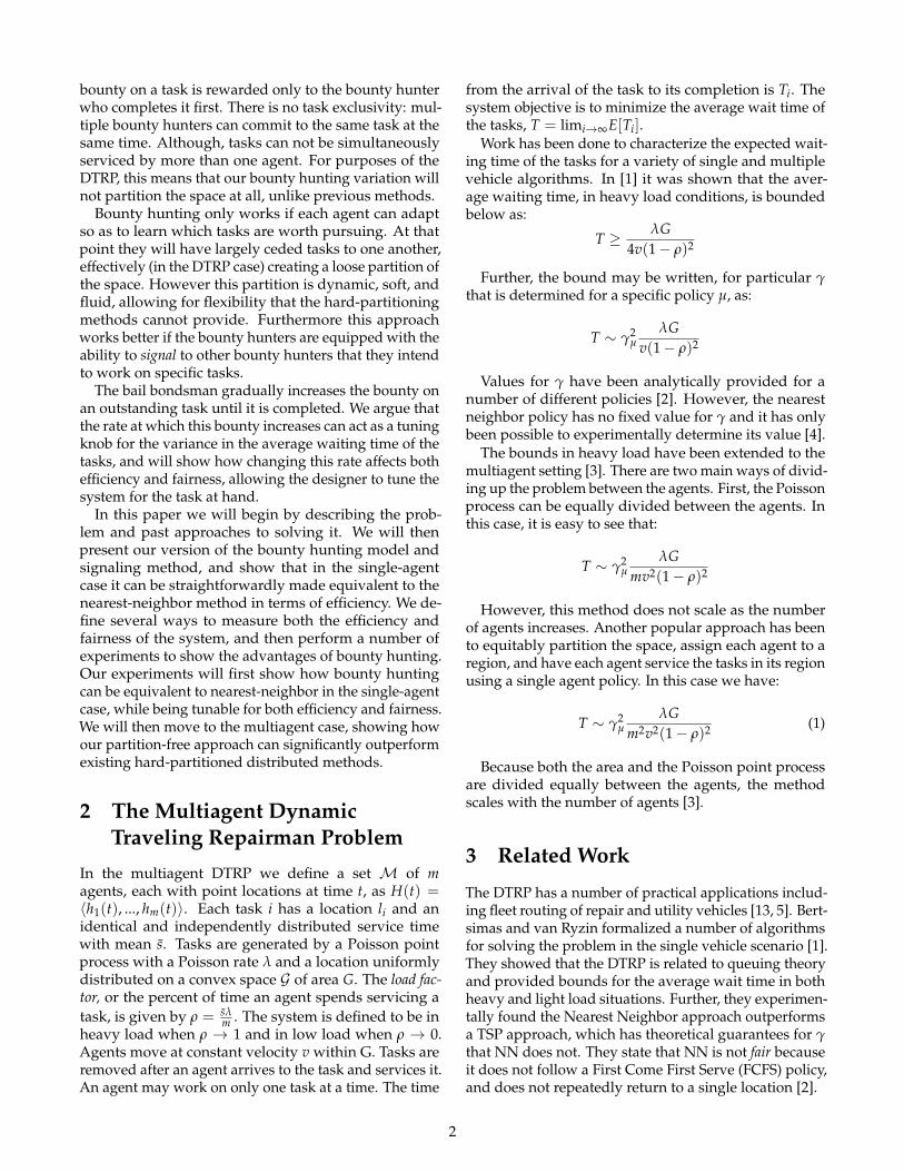
Single Agent 40x40 Contiguous Space with No FuelBounty rate 0.0 = 0.5552 slope = 0.3082Bounty rate 1.0E-4 = 0.5549 slope = 0.3080Bounty rate 0.001 = 0.5467 slope = 0.2989Bounty rate 0.01 = 0.5630 slope = 0.3170Bounty rate 0.1 = 0.8473 slope = 0.7179Bounty rate 1.0 = 1.1766 slope = 1.3844Bounty rate 5.0 = 1.1649 slope = 1.3571Nearest Neighbor = 0.5473 slope = 0.2995

Figure 1: Contiguous Task Experiment: One agent40×40 area with no fuel, 300,000 steps.

where N is the number of tasks in the system on average,which can be estimated through Little’s Law N = λT.However, because the bounty hunters complete tasks ina nearest neighbor or nearest neighbor-like discipline,and the value for T is analytically intractable, we canonly use this for known values of γ [4]. We are inter-ested in studying this value in order to show that theamount of bounty in the system is bounded in terms ofthe average waiting time of the tasks.

6 Experiments

The tasks were generated in a continuous environmentbased on a Poisson point process with average time be-tween tasks λ. Tasks were distributed uniformly ran-domly within the space defined by the experiment andthe service time for each task was generated by a geomet-ric distribution with a mean s specific to each experiment.The agents may overlap with other agents or tasks andmoved with a velocity of v = 0.7. The agents traveled tothe tasks and upon arrival serviced the task.

Agents were positioned at time step zero at a depot.Depots were locations in the environment where agentscould purchased fuel or return to if no tasks were avail-able to complete. For experiments where fuel was con-sidered we set the unit cost of fuel C f = 1.0 where thecurrency used was the bounty that the agent had ob-tained by completing tasks. In scenarios where fuel wasused the agents had a fuel capacity of 3000 and startedwith a full tank along with a starting balance of 1000units of bounty. Each time step that the agent moved inthe environment would use a single unit of fuel. Whenthe agent had only enough fuel to return to the depotthe agent would refuel by returning and purchasing themax amount of fuel that they had currency for. It takes asingle time step to refuel and we assume there was no

0.0 0.0001 0.001 0.01 0.1 1.0 5.0Bounty Rate

0.1

0.2

0.3

0.4

0.5

0.6

0.7

0.8

Norm

alize

d Er

ror

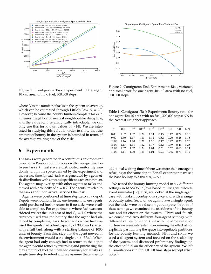
Single Agent Contiguous Space Bias-Variance Plotbias^2variancetotal error

Figure 2: Contiguous Task Experiment: Bias, variance,and total error for one agent 40×40 area with no fuel,300,000 steps.

Table 1: Contiguous Task Experiment: Bounty ratio forone agent 40×40 area with no fuel, 300,000 steps; NN isthe Nearest Neighbor approach.

R

s 0.0 10−4 10−3 10−2 10−1 1.0 5.0 NN

8.00 1.07 1.07 1.22 1.14 0.45 0.17 0.24 1.159.00 1.30 1.17 1.13 1.12 0.52 0.20 0.28 1.15

10.00 1.16 1.20 1.21 1.26 0.47 0.27 0.36 1.2511.00 1.17 1.11 1.12 1.17 0.42 0.39 0.46 1.2512.00 1.07 1.07 1.24 1.04 0.51 0.52 0.60 1.1413.00 1.11 1.00 1.11 1.04 0.93 0.66 0.71 1.12

additional waiting time if there was more than one agentrefueling at the same depot. For all experiments we setthe base bounty to a fixed B0 = 500.

We tested the bounty hunting model in six differentsettings in MASON, a Java based multiagent discreteevent simulator [12]. First, we looked at the single agentcase with tasks in contiguous space and with a rangeof bounty rates. Second, we again have a single agent,but the tasks were in a discontiguous space. In both ofthese settings we examined the usefulness of the bountyrate and its effects on the system. Third and fourth,we considered two different four-agent settings withdifferent values for λ and s but with the same value forρ. Here we were interested in examining the effect of notexplicitly partitioning the space into equitable partitionsfor the bounty hunting method. Fifth and sixth, weused a 64 agent system and focused on the scalabilityof the system, and discussed preliminary findings onthe effect of fuel on the efficiency of the system. We leftall simulations run for 300,000 time steps (except whennoted).

6

Figure 3: Discontiguous Task Space. One agent in thetop left 40×40 area, after 600,000 time steps when s = 8.

6.1 Single Agent

We examine two single agent environments in order toillustrate why the bounty rate is important.

Contiguous space For this experiment we verified thata bounty rate of zero is equivalent to the NN approachby comparing the value of γ. We then examined theeffect of the bounty rate on the bias and variance. Wecompared the theory and actual total average bountyavailable in the system.

We had a single agent with start position locatedat the depot at (0,0), the center of the 40×40 environ-ment. We set ρ = 0.8125, 0.75, 0.6875, 0.625, 0.5625, 0.5based on λ = 1

16 = .0625 and mean job lengths = 13, 12, 11, 10, 9, 8. We set the bounty rate to R =0, 0.0001, 0.001, 0.01, 0.1, 1, 5. We repeated the simulation40 times for each value of ρ and bounty rate.

Results In Figure 1 we plot the experimentally ob-tained average waiting time T against λG

m2v2(1−ρ)2 for arange of bounty rates alongside the NN approach. Wecan see that the bounty hunting approach with zerobounty had a γ value within 1% of the nearest neighborapproach.

Next, we consider in Figure 2 how the bounty rateeffected the bias and variance of the system. To plot thiswe averaged the bias and variance for each s and thennormalized the values. As the bounty rate increasedthe bias decreased and the variance decreased and thenincreased, but the total error was minimized when thebounty rate R was 5. However, when the bounty rateR ≥ 0.1, the expected waiting time increased. Therefore,there was a trade-off between average waiting time, andthe bias and variance.

Each entry in the bounty table in Table 1 is the ratio ofthe total bounty in the system at time step 300,000 aver-aged over 40 trials to B. We calculated B based on thevalues for γ found in Figure 1. Values greater than onemeant that B underestimated the bounty in the systemand when the ratio was less than one B overestimated

Table 2: Discontiguous Task Experiment: Average wait-ing time for the Nearest Neighbor approach and BountyHunting with a bounty rate of 5.0.

s Nearest Neighbor Bounty Hunting

8.00 9305.95 2325.559.00 12211.07 3189.18

10.00 16086.59 4617.2011.00 21221.22 7123.0512.00 27554.38 11684.9313.00 39723.68 21157.16

the actual average. We see that B gave a very large over-estimate when the bounty rate was one and was close tocorrect when the bounty rate was ≤ 10−4.

Discontiguous Tasks This experiment illustrated therole that the bounty rate plays in an environment wherethe nearest neighbor approach struggles.

For this experiment the bounty rate was set to five.We created two regions of 40×40 that were centered at(20,20) and (150,150) as illustrated in Figure 3. Therewere two depots at the centers of the two regions andthe agent started in the region centered at (20,20). Taskswere generated with the same ρ values as above, but eachregion had a mean task generation rate of λ1 = λ2 = 1

32which due to the property of Poisson processes had anoverall generation rate λ = 1

16 . This experiment was runfor 1,000,000 time steps rather than 300,000 due to thelarger area in which the agents operate.

Results As we see in Table 2 the nearest neighbor ap-proach performed very poorly compared to the bountyhunting approach. This was because the bounty ratemotivated the agents to more frequently service tasksthat were further away.

6.2 Four Agents

Next we considered two different four-agent cases wherewe adjusted the values for λ and s to see whether bountyhunting could match and improve on the NN approachwith equitable partitions.

Rapid Task Generation Here the environment was an80×80 square, and in order to maintain the same valuefor ρ we set λ = 1

4 and used the same values for s. Thedepots were located at (20, 20), (60, 20), (20, 60), and (60,60) and each agent started at a different depot. The spacewas split into four, 40×40 square regions with the depotat the center of the region. Each nearest neighbor agentwas assigned to service the tasks that were generatedwithin its assigned region.

7

1000 2000 3000 4000 5000 6000G

m2v2(1 )2

0

1000

2000

3000

4000

5000

6000

7000

Expe

rimen

tal T

Four Agents 80x80 = . 25 with No FuelBounty rate 0.0 = 0.5686 slope = 0.3233Bounty rate 1.0E-4 = 0.5594 slope = 0.3130Bounty rate 0.001 = 0.5607 slope = 0.3144Bounty rate 0.01 = 0.5598 slope = 0.3134Bounty rate 0.1 = 0.8046 slope = 0.6474Bounty rate 1.0 = 1.1497 slope = 1.3219Bounty rate 5.0 = 1.1548 slope = 1.3336Nearest Neighbor = 0.5535 slope = 0.3064

Figure 4: Rapid Task Generation Experiment: FourAgent, λ = 1

4 , 80×80 area with no fuel, 300,000 steps.

This experiment focused on whether explicitly split-ting the space into equitable partitions is necessary orwhether a different approach could produce similar re-sults.

Results In Figure 4 we plot the experimentally ob-tained waiting time in order to acquire the value of γ foreach setting. We see that the bounty hunting approachdid similarly to the nearest neighbor approach.

Slow Task Generation Again we considered an 80×80environment with four agents, but we set λ = 1

20 andwe set the mean service times to s = 65, 60, 55, 50, 45, 40.Therefore, we were still using the same value for ρ, butwith different values for λ and s. The agents and depotswere all located in the same manner as in the previousexperiment.

In this experiment, we examined a scenario in whichexplicitly splitting up the space performed poorly, tosee whether our alternative approach could improveperformance.

Results As we can see in Figure 5 the value for γ forthe nearest neighbor approach was significantly greaterthan that of the bounty hunting approach with a bountyrate less than one. This meant that we could achievesuperior results to the NN with equitable partitions.

6.3 Sixty Four Agents

Based on Equation (1), by equitably partitioning thespace the system will scale as the number of agentsincreases. However, because we did not theoreticallyprove that the agents were equitably partitioning thespace we demonstrated empirically that the averagewaiting time continued to be similar to or outperformed

0 200 400 600 800 1000 1200G

m2v2(1 )2

0

500

1000

1500

2000

Expe

rimen

tal T

Four Agents 80x80 = 0.05 with No FuelBounty rate 0.0 = 0.7042 slope = 0.4960Bounty rate 1.0E-4 = 0.6776 slope = 0.4591Bounty rate 0.001 = 0.6746 slope = 0.4551Bounty rate 0.01 = 0.6756 slope = 0.4564Bounty rate 0.1 = 0.7344 slope = 0.5393Bounty rate 1.0 = 1.2954 slope = 1.6780Bounty rate 5.0 = 1.4062 slope = 1.9774Nearest Neighbor = 0.8337 slope = 0.6951

Figure 5: Slow Task Generation Experiment: Four Agent,λ = 1

20 , 80×80 area with no fuel, 300,000 steps.

equitable partitions. The following two experimentssought to do this in addition to examining the impact offuel.

In order for the system to scale we had to limit thecommunication between the agents. Specifically, thebounty hunters could only communicate with otheragents within a radius of 40 units, and were aware oftasks within a radius of 40.

Without Fuel We made an 8×8 grid of evenly spaceddepots (each depot centered in a 40×40 area). Forthis experiment we increased the size of the environ-ment to a 320×320 area and we set λ = 64

80 = 0.8and s = 65, 60, 55, 50, 45, 40. Therefore, we maintainedthe same load factor values as in previous experiments:ρ = 0.8125, 0.75, 0.6875, 0.625, 0.5625, 0.5.

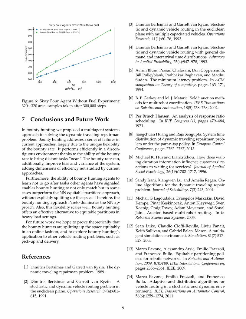
Results We see in Figure 6 that not only did the systemscale, but the value of γ was dependent on the valuesfor λ and s. As expected, the bounty hunting approachoutperformed the NN approach as we have a similarsetting to that in Figure 5.

With Fuel We performed the same experiment exceptthe agents had a fuel capacity of 3000 and a startingbounty balance of 1000.

Results The case where the agents were given unlim-ited fuel capacity and the case where the agents hada fuel capacity of 3000 units produced similar results.Even with a large number of agents, as long as we hadenough depots and the agents did not need to make fre-quent trips to the depot to refuel, the system time wasnot degraded compared to NN.

8

200 400 600 800 1000 1200G

m2v2(1 )2

100

200

300

400

500

600

700

800

900Ex

perim

enta

l TSixty Four Agents 320x320 with No Fuel

Bounty rate 0.0 = 0.6238 slope = 0.3891Nearest Neighbor = 0.8409 slope = 0.7071

Figure 6: Sixty Four Agent Without Fuel Experiment:320×320 area, samples taken after 300,000 steps.

7 Conclusions and Future Work

In bounty hunting we proposed a multiagent systemsapproach to solving the dynamic traveling repairmanproblem. Bounty hunting addresses a series of failures incurrent approaches, largely due to the unique flexibilityof the bounty rate. It performs efficiently in a discon-tiguous environment thanks to the ability of the bountyrate to bring distant tasks “near.” The bounty rate can,additionally, improve bias and variance of the system,adding dimensions of efficiency not studied by currentapproaches.

Furthermore, the ability of bounty hunting agents tolearn not to go after tasks other agents have signaledenables bounty hunting to not only match but in somecases outperform the NN equitable partitions approach,without explicitly splitting up the space. Therefore, thebounty hunting approach Pareto dominates the NN ap-proach. Also, this flexibility scales well. Bounty huntingoffers an effective alternative to equitable partitions inheavy load settings.

For future work we hope to prove theoretically thatthe bounty hunters are splitting up the space equitablyin an online fashion, and to explore bounty hunting’sapplication to other vehicle routing problems, such aspick-up and delivery.

References

[1] Dimitris Bertsimas and Garrett van Ryzin. The dy-namic traveling repairman problem. 1989.

[2] Dimitris Bertsimas and Garrett van Ryzin. Astochastic and dynamic vehicle routing problem inthe euclidean plane. Operations Research, 39(4):601–615, 1991.

[3] Dimitris Bertsimas and Garrett van Ryzin. Stochas-tic and dynamic vehicle routing in the euclideanplane with multiple capacitated vehicles. OperationsResearch, 41(1):60–76, 1993.

[4] Dimitris Bertsimas and Garrett van Ryzin. Stochas-tic and dynamic vehicle routing with general de-mand and interarrival time distributions. Advancesin Applied Probability, 25(4):947–978, 1993.

[5] Avrim Blum, Prasad Chalasani, Don Coppersmith,Bill Pulleyblank, Prabhakar Raghavan, and MadhuSudan. The minimum latency problem. In ACMsymposium on Theory of computing, pages 163–171,1994.

[6] B. P. Gerkey and M. J. Mataric. Sold!: auction meth-ods for multirobot coordination. IEEE Transactionson Robotics and Automation, 18(5):758–768, 2002.

[7] Per Brinch Hansen. An analysis of response ratioscheduling. In IFIP Congress (1), pages 479–484,1971.

[8] Jiangchuan Huang and Raja Sengupta. System timedistribution of dynamic traveling repairman prob-lem under the part-n-tsp policy. In European ControlConference, pages 2762–2767, 2015.

[9] Michael K. Hui and Lianxi Zhou. How does wait-ing duration information influence customers’ re-actions to waiting for services? Journal of AppliedSocial Psychology, 26(19):1702–1717, 1996.

[10] Sandy Irani, Xiangwen Lu, and Amelia Regan. On-line algorithms for the dynamic traveling repairproblem. Journal of Scheduling, 7(3):243, 2004.

[11] Michail G Lagoudakis, Evangelos Markakis, DavidKempe, Pinar Keskinocak, Anton Kleywegt, SvenKoenig, Craig Tovey, Adam Meyerson, and SonalJain. Auction-based multi-robot routing. In InRobotics: Science and Systems, 2005.

[12] Sean Luke, Claudio Cioffi-Revilla, Liviu Panait,Keith Sullivan, and Gabriel Balan. Mason: A multia-gent simulation environment. Simulation, 81(7):517–527, 2005.

[13] Marco Pavone, Alessandro Arsie, Emilio Frazzoli,and Francesco Bullo. Equitable partitioning poli-cies for robotic networks. In Robotics and Automa-tion, 2009. ICRA’09. IEEE International Conference on,pages 2356–2361. IEEE, 2009.

[14] Marco Pavone, Emilio Frazzoli, and FrancescoBullo. Adaptive and distributed algorithms forvehicle routing in a stochastic and dynamic envi-ronment. IEEE Transactions on Automatic Control,56(6):1259–1274, 2011.

9

[15] GA Shidali, SB Junaidu, and SE Abdullahi. A newhybrid process scheduling algorithm (pre-emptivemodified highest response ratio next). ComputerScience and Engineering, 5(1):1–7, 2015.

[16] Drew Wicke, David Freelan, and Sean Luke. Bountyhunters and multiagent task allocation. In Interna-tional Conference on Autonomous Agents and Multia-gent Systems, 2015.

[17] Drew Wicke and Sean Luke. Bounty hunting andhuman-agent group task allocation. In AAAI FallSymposium on Human-Agent Groups: Studies, Algo-rithms and Challenges, 2017.

[18] Drew Wicke, Ermo Wei, and Sean Luke. Throwingin the towel: Faithless bounty hunters as a task allo-cation mechanism. IJCAI workshop on Interactionswith Mixed Agent Types, 2016.

[19] Adam Wierman. Fairness and classifications. ACMSIGMETRICS Performance Evaluation Review, 34(4):4–12, 2007.

[20] Haiping Xu. Optimal policies for stochastic and dy-namic vehicle routing problems. PhD thesis, Mas-sachusetts Institute of Technology, 1994.

10