Proceeding of 2013 IAHR World Congress

ABSTRACT: Riverbed is likely to be damaged in the natural conditions or due to human activities,

which results in river morphology changed, and even the presence of extreme cases, such as crack or

geological fault due to earthquake. Thus, riverbed evolution is different from natural evolution owing to

flow structure around the damaged zone has changed. In order to facilitate research in this paper, the post-

damaged riverbed is simplified as a triangular pit which has a steep slope appeared on the riverbed. This

paper presents the investigation on riverbed evolution behavior in the vicinity of the pit in different flow

conditions by experiments and numerical simulations. This study mainly focuses on explaining the

mechanism of pit migration by measuring the shapes of the pit in different time during its development

and numerical simulating the flow field in corresponding moment. Two kinds of flow conditions are

included in experiments, clear-water and live-bed conditions. The experimental result under the former

condition shows that the migration of pit is not obvious; the phenomenon in the latter condition shows

that the upstream side slope of the pit moves forward and the downstream side slope is eroded, and the

retrogressive erosion to upstream is not found. A vertical Two-dimensional standard k-ε turbulent model

is used and its validation is achieved against experimental results of velocity field measured by an

acoustic Doppler velocimeter (ADV). The results of the numerical simulation show that the longitudinal

vortex in the pit hole develops to the bottom with migration of the pit and the velocity is small (<0.1m/s)

in the pit hole. The maximum value of bed-shear stress amplification appears at the upstream and

downstream ends of the pit. This paper only analyzes one post-damaged riverbed form, for other riverbed

forms in different flow and sediment conditions, this problem needs further studying.

KEY WORDS: Post-damaged riverbed, Evolution, Steep slope, Two-dimensional model, Shear stress.

1 INTRODUCTION

The post-damaged riverbed can be divided into two cases according to the causes, one is that

riverbed is damaged in the natural conditions, such as trench, crack or geological fault which usually has

a sharp longitudinal slope due to earthquake; the other case is man-made damage, such as sand and gravel

mining from riverbed for construction projects. Researches about this problem mainly focus on the latter

case, Lee et al. (1993) investigated the migration behavior of several rectangular pits of different sizes

composed of uniform bed material by a series of experiments, they distinguished two different periods in

the process of the pit migration, namely convection period and diffusion period, and empirical equations

for maximum scour depth and migration speed of the pits were obtained. Neyshabouri, Farhadzadeh &

Amini (2002) also reported an experimental study on the migration of rectangular mining pits and

variation of longitudinal profile in channel bed composed of uniform sediments, they concentrated on the

Experimental and Numerical Investigation of Riverbed Evolution in Post-Damaged Conditions Jinzhao Li

Ph.D. Student, Beijing Jiaotong University, Beijing 100044, China. Email: 12115290@bjtu.edu.cn

Meilan Qi

Professor, Beijing Jiaotong University, Beijing 100044, China. Email: mlqi@bjtu.edu.cn

Yakun Jin

Graduate Student, Beijing Jiaotong University, Beijing 100044, China. Email: 11121260@bjtu.edu.cn

2

influence of length/width ratio of the pit to the migration speed. The results showed the effect of width is

more important than the effect of length. Gill (1994) presented an approximately theoretical solution for

the behavior of the mining pits of regular geometrical shape using the one-dimensional St. Venant’s

equations of motion, but these theoretical solutions were only applicable to equilibrium condition of

sediment flow. Ribberink, Roos & Hulscher (2005) provided analytical formulas for the migration

velocity and infill time of trenches in the marine environment, using a harmonic analysis of simplified

one-dimensional basic equations for the morphodynamics system, and the results showed that damping

dominates the shortest trench, while migration and damping occur simultaneously for the long trench. Wu

& Wang (2008) simulated the flow through an initially dry mining pit and the associated morphology

changes using the generalized one-dimensional shallow water equations and nonequilibrum sediment

transport equations, the results showed the most significant erosions occur at the upstream and

downstream ends of the pit due to headcut and tailcut respectively. Azar, Namaee & Rostami (2012)

simulated the variation of bed profile due to mining pit using one-dimensional hydraulic engineering

software (HEC-RAS). Chen & Liu (2009) compared two commonly used hydrodynamic and sediment

transport model, HEC-RAS and CCHE2D (a depth-averaged two-dimensional model developed at the

University of Mississippi), and the results showed that the latter model was more robust in simulating

flood zone coverage, non-uniform sediment sorting, and channel geomorphologic changes.

In this paper, the former case, a steep longitudinal slope and small length/depth ratio of the pit, was

investigated. The post-damaged riverbed was simplified as a triangular pit appeared on the riverbed for

facilitating study. The following aims to illustrate the relationship between the hydrodynamic parameters

of the flow around the pit and the shape of the pit during its development. Two kinds of flow conditions

are considered, clear-water and live-bed condition. The riverbed evolution behaviors around the pit in

different flow conditions are presented by measuring riverbed elevation in different period. The flow field

in corresponding moment is calculated by numerical simulating (a vertical 2-D standard k-ε turbulent

model) which has been validated against experimental results of velocity field measured by an acoustic

Doppler velocimeter (ADV).

2 FLUME EXPERIMENTS

2.1 Experimental Apparatus

The experiments in this study were conducted in a circulating flume in which the slope is adjustable,

6m long, 25cm wide and 25cm deep. A false floor was installed in the flume leaving a

40cm×25cm×10cm recess in which sediments were placed, ensuring the enough thickness of sediment

used in live-bed experiment. A PVC grille at the inlet section was used to stabilize flow and an adjustable

weir at the downstream end of the flume was used to control the depth of flow. The flow discharge was

monitored using an electromagnetic meter and the accuracy is ±0.01m3/h. The water depth and bed

morphology were monitored by a non-contract ultrasonic elevation meter, the accuracy is ±0.01mm. An

acoustic Doppler velocimeter (ADV) was used which has a sampling rate and volume of 200Hz and

0.09cm3 respectively.

2.2 Calibration Test

The purpose of this test is to examine the accuracy of the experimental instruments, especially the

acoustic Doppler velocimeter (ADV). The test is a rigid-bed experiment which means there’s no layer of

sand on the bottom of the flume (smooth-bed).

The water depth was maintained at 10cm and the approach flow velocity at V=25.7cm/s which was

obtained from integration of velocity profile. The longitudinal slope of channel was fixed as 0.0002. The

test was conducted under the sub-critical (Fr=0.26) and uniform flow. The velocity measurements were

made by ADV in the longitudinal symmetrical line of the flume.

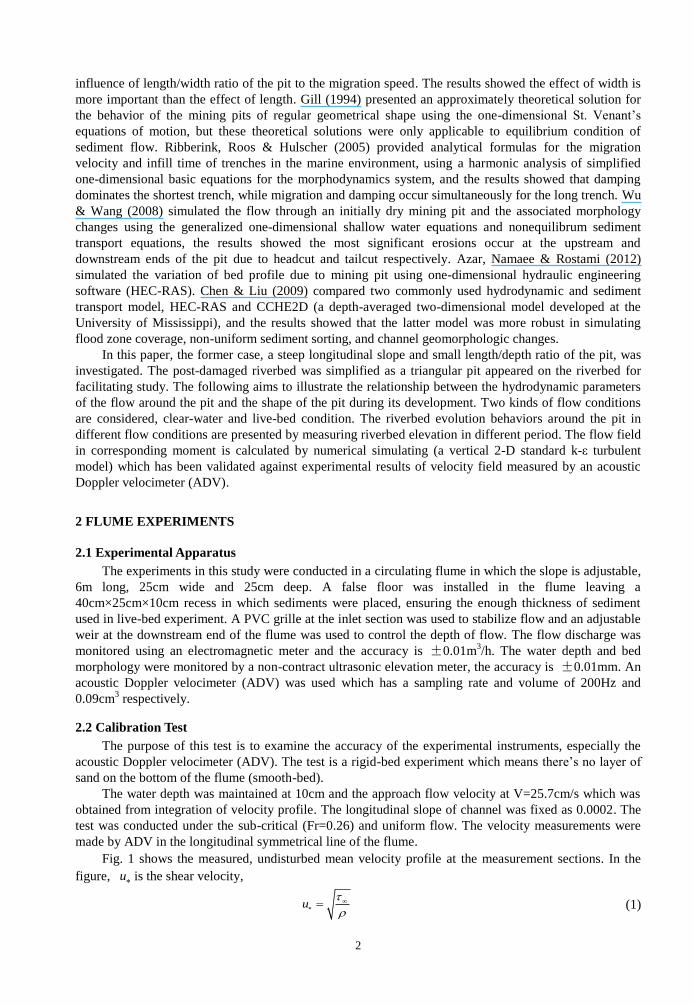
Fig. 1 shows the measured, undisturbed mean velocity profile at the measurement sections. In the

figure, u is the shear velocity,

u

(1)

3

and y

is the normalized distance from the bed,

*yuy

(2)

herein,

is the undisturbed bed shear stress, is the fluid density and is the kinematic

viscosity.

Fig. 1 illustrates the mean velocity profile can be approximated by the logarithmic law,

*

2.5ln( ) 4.5u

yu

(3)

which means there’s a good agreement between the measurement data and the theoretical result.

Figure 1 Undisturbed velocity profile for the smooth bed, *u =1.04cm/s

2.3 Migration Experiments

The purpose of these experiments are to investigate the migration of pit with sharp slope (exceeding

the angle of repose) in two flow conditions, one is clear-water condition which means the flow approach

velocity is smaller than critical velocity for the initiation of sediment motion; the other is in live-bed

regime when the shear stress induced by the water flow exceeds the critical shear stress of the bed

material.

The experimental flow conditions in this test are summarized in table 1, where i is bed longitudinal

slope; Q is the inflow discharge; u is mean velocity obtained from integration of velocity profile; cu

is the incipient velocity of sediment; Re is the Reynolds number; Fr is the Froude number; D and L are

the depth and length (along the flow direction) of the pit respectively. The bed material consisted of a

cohesionless, uniform sand with a median particle size of D50=0.6mm and a specific gravity of 2.65. The

geometric standard deviation of the bed material was σ=1.483. In this experiment, flow condition in run 1

is in clear-water regime and run 2 is in live-bed regime.

Table 1 Flow conditions for the experiments

Run i Q (m3/h) h(m) u (m/s) c

u (m/s) Re Fr D（cm） L（cm）

1 1/5000 11.27 0.06 0.21 0.24 52500 0.274 4 4

2 1/2000 13.65 0.05 0.303 0.235 15150 0.786 4.3 5

For creating the pit, a cubic metal mold with desired dimensions was used and was put into the

desired location. For prevention of moving bed materials, water with low speed entered into the flume.

Afterwards, the flow depth increased gently until to the required depth, then removed the metal mould.

The pit was located about 3m away from the flume entrance. During the experiments, the discharge was

kept constant and the channel bed elevation around the pit was measured in different moment until the

shape of the pit reached an equilibrium state.

0.01

0.1

1

10

0 10 20 30 40

y(c

m)

u(cm/s)

*/ 2.5ln( ) 4.5u u y

4

2.3.1 Clear-water experiment

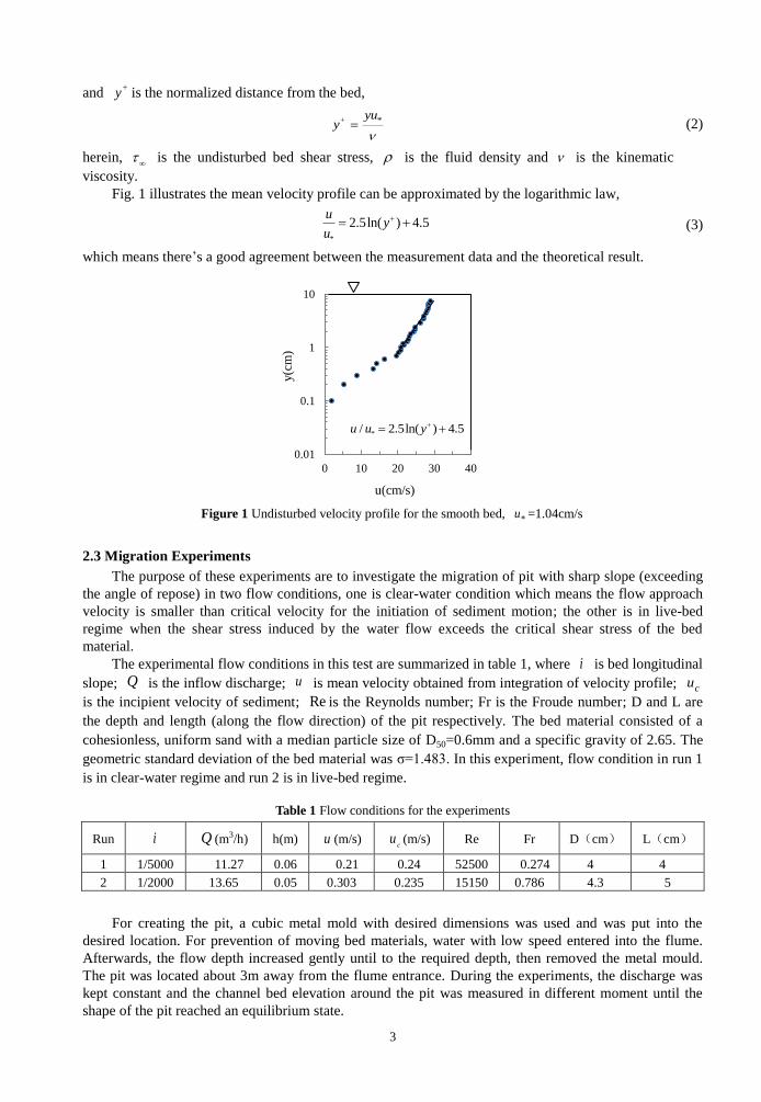
Fig. 2 shows the migration of pit in clear-water condition. The result reveals the most significant

erosions occur at the upstream and downstream ends of the pit at the beginning period (0~5min) when the

transient flow through a dry pit.

After the pit hole is filled up with water (5min~55min), the migration of the pit is not obvious in

clear-water regime and the retrogressive erosion to upstream is not found. Moreover, the morphological

time scale of the evolution is small and reaches an equilibrium state soon. Another phenomenon is the

slope of the upstream side (22o) is greater than the downstream (16

o), which means the tailcut (7cm from

the pit to downstream) is greater than headcut (5cm from the pit to upstream)

Figure 2 Bed longitudinal profile and pit variation with time in clear-water condition.

2.3.2 Live-bed experiment

Live-bed experiment means that the sand on the riverbed is mobile due to the flow approach velocity

is larger than critical velocity for the initiation of sediment motion. Since no sediment was supplied from

upstream, the experiment was conducted in a nonequilibrium condition.

Fig. 3 shows that the temporal variation of the bed elevation around the pit is obvious in live-bed

conditions. The upstream slope of the pit moves forward and the downstream slope is eroded, a steep

upstream slope and a more gentle downstream slope slowly develops. This is because most of the

incoming sediment deposits in the pit hole and the water entering downstream channel is almost clear,

thus, erosion to downstream occurs and gradually extends downstream. The slope of the pit hole in the

upstream side is approximately equal to the angle of repose 32 . It can be also observed that the

lowest point of the pit does not move downstream and the behavior of infilling dominates the pit’s

development.

Figure 3 Bed longitudinal profile and pit variation with time in live-bed condition

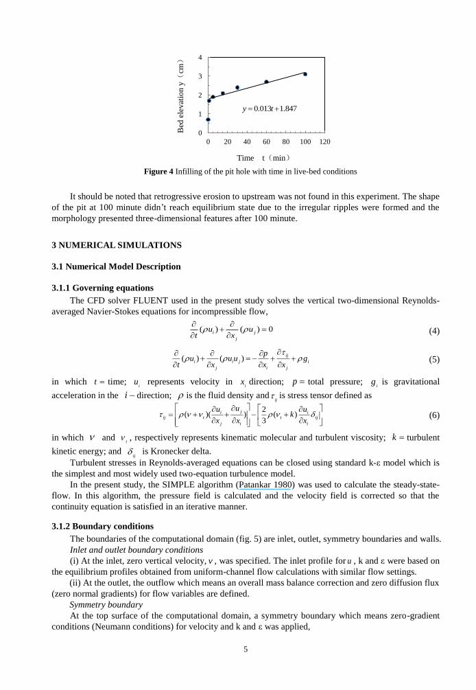
Fig. 4 shows that the variation of bed elevation at the lowest point of the pit (x=0) with time. It can

be observed that the infilling phenomenon is significant, infilling velocity is high, at the beginning period

for the transient flow through a dry pit (0~1min). After the pit hole is filled up with water (1min~100min),

the infilling velocity is approximately constant for the relation between the bed elevation y and time t is

approximately linear.

0

1

2

3

4

5

6

7

-5 -4 -3 -2 -1 0 1 2 3 4 5 6 7

Bed

lev

el(c

m)

x(cm)

Orig.pit

5min

15min

35min

55min

0

1

2

3

4

5

6

-7 -5 -3 -1 1 3 5 7 9 11 13

Bed

lev

el(c

m)

x(cm)

Orig.pit

1min

5min

15min

30min

5

Figure 4 Infilling of the pit hole with time in live-bed conditions

It should be noted that retrogressive erosion to upstream was not found in this experiment. The shape

of the pit at 100 minute didn’t reach equilibrium state due to the irregular ripples were formed and the

morphology presented three-dimensional features after 100 minute.

3 NUMERICAL SIMULATIONS

3.1 Numerical Model Description

3.1.1 Governing equations

The CFD solver FLUENT used in the present study solves the vertical two-dimensional Reynolds-

averaged Navier-Stokes equations for incompressible flow,

( ) ( ) 0i j

j

u ut x

(4)

( ) ( )ij

i i j i

j i j

pu u u g

t x x x

(5)

in which t time; i

u represents velocity in i

x direction; p total pressure; i

g is gravitational

acceleration in the i direction; is the fluid density andij is stress tensor defined as

2

( )( ) ( )3

ji iij t t ij

j i i

uu uk

x x x

(6)

in which and t

, respectively represents kinematic molecular and turbulent viscosity; k turbulent

kinetic energy; and ij

is Kronecker delta.

Turbulent stresses in Reynolds-averaged equations can be closed using standard k-ε model which is

the simplest and most widely used two-equation turbulence model.

In the present study, the SIMPLE algorithm (Patankar 1980) was used to calculate the steady-state-

flow. In this algorithm, the pressure field is calculated and the velocity field is corrected so that the

continuity equation is satisfied in an iterative manner.

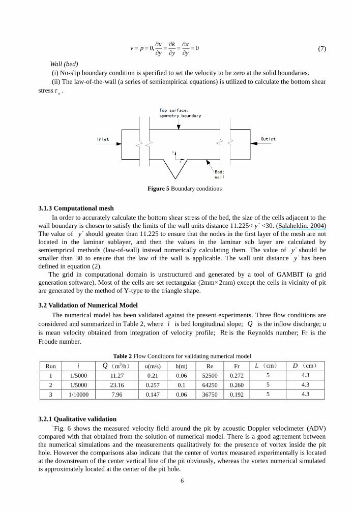
3.1.2 Boundary conditions

The boundaries of the computational domain (fig. 5) are inlet, outlet, symmetry boundaries and walls.

Inlet and outlet boundary conditions

(i) At the inlet, zero vertical velocity, v , was specified. The inlet profile for u , k and ε were based on

the equilibrium profiles obtained from uniform-channel flow calculations with similar flow settings.

(ii) At the outlet, the outflow which means an overall mass balance correction and zero diffusion flux

(zero normal gradients) for flow variables are defined.

Symmetry boundary

At the top surface of the computational domain, a symmetry boundary which means zero-gradient

conditions (Neumann conditions) for velocity and k and ε was applied,

0

1

2

3

4

0 20 40 60 80 100 120

Bed

ele

vat

ion

y（

cm）

Time t（min）

0.013 1.847y t

6

0, 0u k

v py y y

(7)

Wall (bed) (i) No-slip boundary condition is specified to set the velocity to be zero at the solid boundaries.

(ii) The law-of-the-wall (a series of semiempirical equations) is utilized to calculate the bottom shear

stressw

.

Figure 5 Boundary conditions

3.1.3 Computational mesh

In order to accurately calculate the bottom shear stress of the bed, the size of the cells adjacent to the

wall boundary is chosen to satisfy the limits of the wall units distance 11.225< y

<30. (Salaheldin. 2004)

The value of y

should greater than 11.225 to ensure that the nodes in the first layer of the mesh are not

located in the laminar sublayer, and then the values in the laminar sub layer are calculated by

semiemprical methods (law-of-wall) instead numerically calculating them. The value of y

should be

smaller than 30 to ensure that the law of the wall is applicable. The wall unit distance y

has been

defined in equation (2).

The grid in computational domain is unstructured and generated by a tool of GAMBIT (a grid

generation software). Most of the cells are set rectangular (2mm2mm) except the cells in vicinity of pit

are generated by the method of Y-type to the triangle shape.

3.2 Validation of Numerical Model

The numerical model has been validated against the present experiments. Three flow conditions are

considered and summarized in Table 2, where i is bed longitudinal slope; Q is the inflow discharge; u

is mean velocity obtained from integration of velocity profile; Re is the Reynolds number; Fr is the

Froude number.

Table 2 Flow Conditions for validating numerical model

Run i Q （m3/h） u(m/s) h(m) Re Fr L （cm） D （cm）

1 1/5000 11.27 0.21 0.06 52500 0.272 5 4.3

2 1/5000 23.16 0.257 0.1 64250 0.260 5 4.3

3 1/10000 7.96 0.147 0.06 36750 0.192 5 4.3

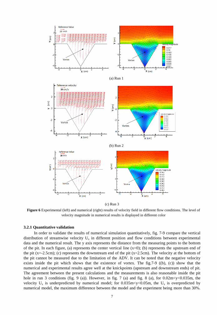
3.2.1 Qualitative validation

`Fig. 6 shows the measured velocity field around the pit by acoustic Doppler velocimeter (ADV)

compared with that obtained from the solution of numerical model. There is a good agreement between

the numerical simulations and the measurements qualitatively for the presence of vortex inside the pit

hole. However the comparisons also indicate that the center of vortex measured experimentally is located

at the downstream of the center vertical line of the pit obviously, whereas the vortex numerical simulated

is approximately located at the center of the pit hole.

7

(a) Run 1

(b) Run 2

(c) Run 3

Figure 6 Experimental (left) and numerical (right) results of velocity field in different flow conditions. The level of

velocity magnitude in numerical results is displayed in different color

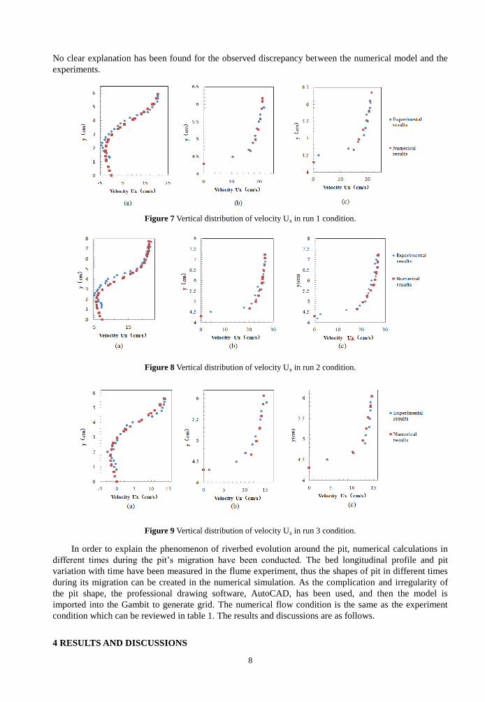
3.2.1 Quantitative validation

In order to validate the results of numerical simulation quantitatively, fig. 7-9 compare the vertical

distribution of streamwise velocity Ux in different position and flow conditions between experimental

data and the numerical result. The y axis represents the distance from the measuring points to the bottom

of the pit. In each figure, (a) represents the center vertical line (x=0); (b) represents the upstream end of

the pit (x=-2.5cm); (c) represents the downstream end of the pit (x=2.5cm). The velocity at the bottom of

the pit cannot be measured due to the limitation of the ADV. It can be noted that the negative velocity

exists inside the pit which shows that the existence of vortex. The fig.7-9 ((b), (c)) show that the

numerical and experimental results agree well at the knickpoints (upstream and downstream ends) of pit.

The agreement between the present calculations and the measurements is also reasonable inside the pit

hole in run 3 conditions (fig. 9 (a)). However, in fig. 7 (a) and fig. 8 (a), for 0.02m<y<0.035m, the

velocity Ux is underpredicted by numerical model; for 0.035m<y<0.05m, the Ux is overpredicted by

numerical model, the maximum difference between the model and the experiment being more than 30%.

8

No clear explanation has been found for the observed discrepancy between the numerical model and the

experiments.

Figure 7 Vertical distribution of velocity Ux in run 1 condition.

Figure 8 Vertical distribution of velocity Ux in run 2 condition.

Figure 9 Vertical distribution of velocity Ux in run 3 condition.

In order to explain the phenomenon of riverbed evolution around the pit, numerical calculations in

different times during the pit’s migration have been conducted. The bed longitudinal profile and pit

variation with time have been measured in the flume experiment, thus the shapes of pit in different times

during its migration can be created in the numerical simulation. As the complication and irregularity of

the pit shape, the professional drawing software, AutoCAD, has been used, and then the model is

imported into the Gambit to generate grid. The numerical flow condition is the same as the experiment

condition which can be reviewed in table 1. The results and discussions are as follows.

4 RESULTS AND DISCUSSIONS

9

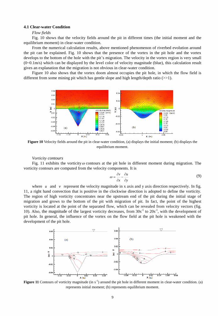
4.1 Clear-water Condition

Flow fields

Fig. 10 shows that the velocity fields around the pit in different times (the initial moment and the

equilibrium moment) in clear-water condition.

From the numerical calculation results, above mentioned phenomenon of riverbed evolution around

the pit can be explained. Fig. 10 shows that the presence of the vortex in the pit hole and the vortex

develops to the bottom of the hole with the pit’s migration. The velocity in the vortex region is very small

(0~0.1m/s) which can be displayed by the level color of velocity magnitude (blue), this calculation result

gives an explanation that the migration is not obvious in clear-water condition.

Figure 10 also shows that the vortex doom almost occupies the pit hole, in which the flow field is

different from some mining pit which has gentle slope and high length/depth ratio (>>1).

Figure 10 Velocity fields around the pit in clear-water condition, (a) displays the initial moment; (b) displays the

equilibrium moment.

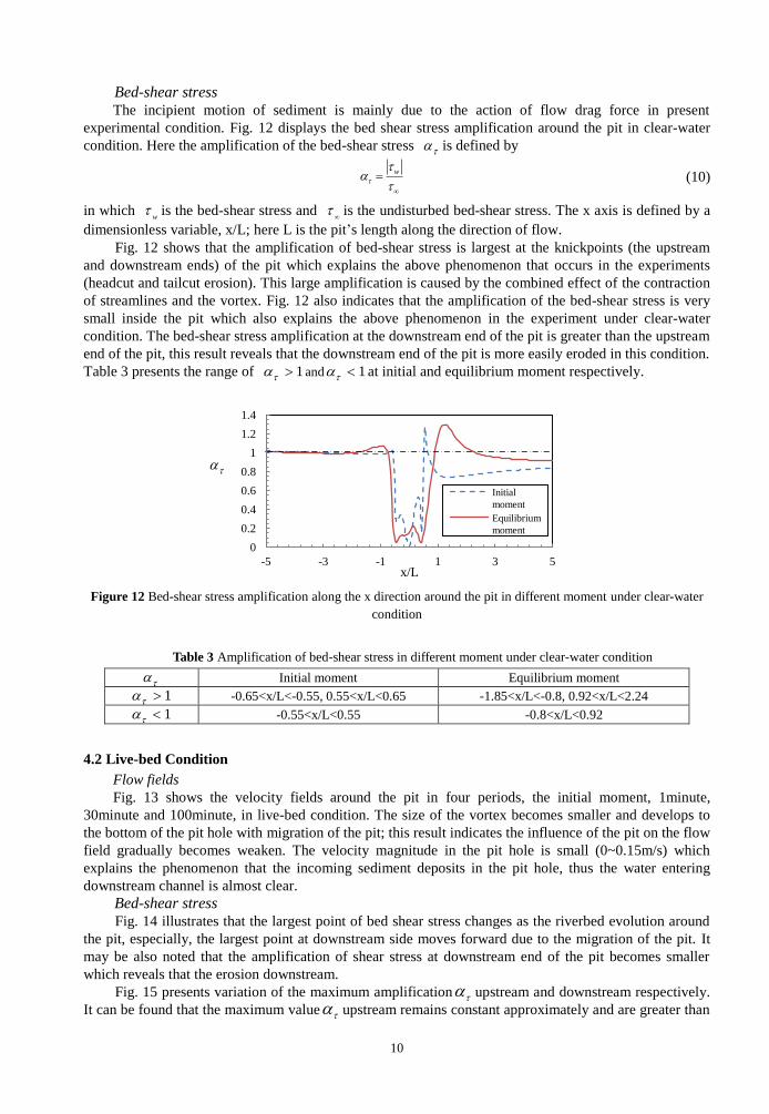
Vorticity contours Fig. 11 exhibits the vorticity contours at the pit hole in different moment during migration. The

vorticity contours are computed from the velocity components. It is

v u

x y

(9)

where u and v represent the velocity magnitude in x axis and y axis direction respectively. In fig.

11, a right hand convection that is positive in the clockwise direction is adopted to define the vorticity.

The region of high vorticity concentrates near the upstream end of the pit during the initial stage of

migration and grows to the bottom of the pit with migration of pit. In fact, the point of the highest

vorticity is located at the point of the separated flow, which can be revealed from velocity vectors (fig.

10). Also, the magnitude of the largest vorticity decreases, from 30s-1

to 20s-1

, with the development of

pit hole. In general, the influence of the vortex on the flow field at the pit hole is weakened with the

development of the pit hole.

Figure 11 Contours of vorticity magnitude (in s-1) around the pit hole in different moment in clear-water condition. (a)

represents initial moment; (b) represents equilibrium moment.

10

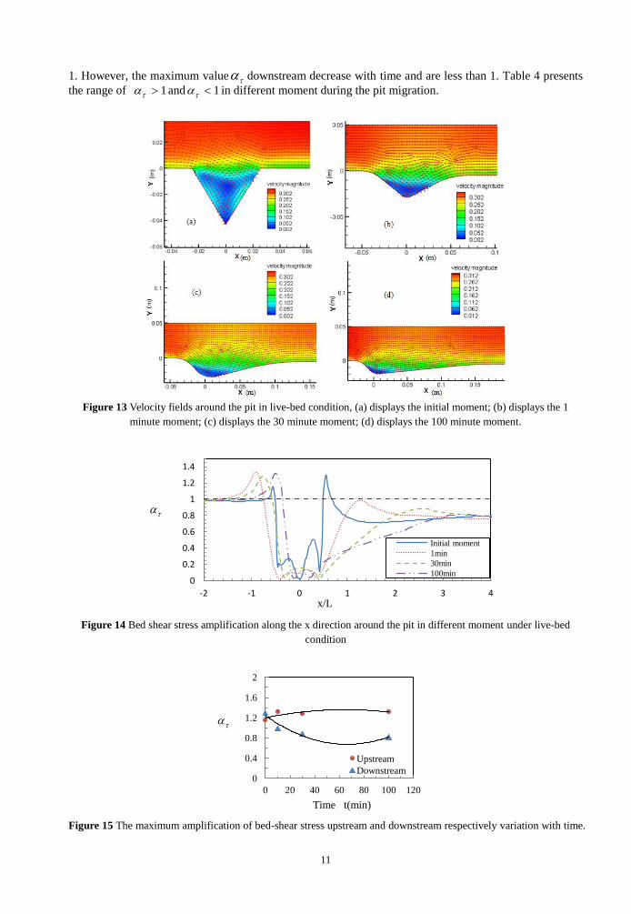
Bed-shear stress

The incipient motion of sediment is mainly due to the action of flow drag force in present

experimental condition. Fig. 12 displays the bed shear stress amplification around the pit in clear-water

condition. Here the amplification of the bed-shear stress is defined by

w

(10)

in which w

is the bed-shear stress and

is the undisturbed bed-shear stress. The x axis is defined by a

dimensionless variable, x/L; here L is the pit’s length along the direction of flow.

Fig. 12 shows that the amplification of bed-shear stress is largest at the knickpoints (the upstream

and downstream ends) of the pit which explains the above phenomenon that occurs in the experiments

(headcut and tailcut erosion). This large amplification is caused by the combined effect of the contraction

of streamlines and the vortex. Fig. 12 also indicates that the amplification of the bed-shear stress is very

small inside the pit which also explains the above phenomenon in the experiment under clear-water

condition. The bed-shear stress amplification at the downstream end of the pit is greater than the upstream

end of the pit, this result reveals that the downstream end of the pit is more easily eroded in this condition.

Table 3 presents the range of 1 and 1 at initial and equilibrium moment respectively.

Figure 12 Bed-shear stress amplification along the x direction around the pit in different moment under clear-water

condition

Table 3 Amplification of bed-shear stress in different moment under clear-water condition

Initial moment Equilibrium moment

1 -0.65<x/L<-0.55, 0.55<x/L<0.65 -1.85<x/L<-0.8, 0.92<x/L<2.24

1 -0.55<x/L<0.55 -0.8<x/L<0.92

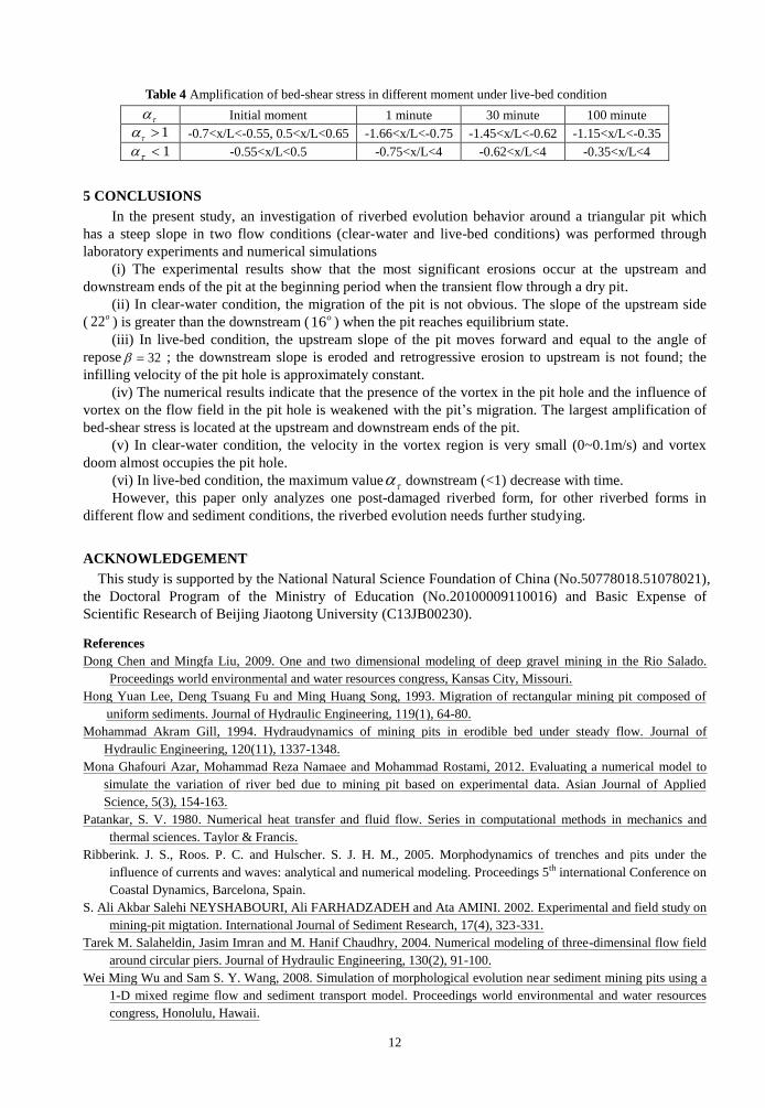
4.2 Live-bed Condition

Flow fields

Fig. 13 shows the velocity fields around the pit in four periods, the initial moment, 1minute,

30minute and 100minute, in live-bed condition. The size of the vortex becomes smaller and develops to

the bottom of the pit hole with migration of the pit; this result indicates the influence of the pit on the flow

field gradually becomes weaken. The velocity magnitude in the pit hole is small (0~0.15m/s) which

explains the phenomenon that the incoming sediment deposits in the pit hole, thus the water entering

downstream channel is almost clear.

Bed-shear stress

Fig. 14 illustrates that the largest point of bed shear stress changes as the riverbed evolution around

the pit, especially, the largest point at downstream side moves forward due to the migration of the pit. It

may be also noted that the amplification of shear stress at downstream end of the pit becomes smaller

which reveals that the erosion downstream.

Fig. 15 presents variation of the maximum amplification upstream and downstream respectively.

It can be found that the maximum value upstream remains constant approximately and are greater than

0

0.2

0.4

0.6

0.8

1

1.2

1.4

-5 -3 -1 1 3 5 x/L

Initial

moment

Equilibrium

moment

11

1. However, the maximum value downstream decrease with time and are less than 1. Table 4 presents

the range of 1 and 1 in different moment during the pit migration.

Figure 13 Velocity fields around the pit in live-bed condition, (a) displays the initial moment; (b) displays the 1

minute moment; (c) displays the 30 minute moment; (d) displays the 100 minute moment.

Figure 14 Bed shear stress amplification along the x direction around the pit in different moment under live-bed

condition

Figure 15 The maximum amplification of bed-shear stress upstream and downstream respectively variation with time.

0

0.2

0.4

0.6

0.8

1

1.2

1.4

-2 -1 0 1 2 3 4 x/L

Initial moment

1min

30min

100min

0

0.4

0.8

1.2

1.6

2

0 20 40 60 80 100 120

Time t(min)

Upstream

Downstream

12

Table 4 Amplification of bed-shear stress in different moment under live-bed condition

Initial moment 1 minute 30 minute 100 minute

1 -0.7<x/L<-0.55, 0.5<x/L<0.65 -1.66<x/L<-0.75 -1.45<x/L<-0.62 -1.15<x/L<-0.35

1 -0.55<x/L<0.5 -0.75<x/L<4 -0.62<x/L<4 -0.35<x/L<4

5 CONCLUSIONS

In the present study, an investigation of riverbed evolution behavior around a triangular pit which

has a steep slope in two flow conditions (clear-water and live-bed conditions) was performed through

laboratory experiments and numerical simulations

(i) The experimental results show that the most significant erosions occur at the upstream and

downstream ends of the pit at the beginning period when the transient flow through a dry pit.

(ii) In clear-water condition, the migration of the pit is not obvious. The slope of the upstream side

( 22o) is greater than the downstream (16o ) when the pit reaches equilibrium state.

(iii) In live-bed condition, the upstream slope of the pit moves forward and equal to the angle of

repose 32 ; the downstream slope is eroded and retrogressive erosion to upstream is not found; the

infilling velocity of the pit hole is approximately constant.

(iv) The numerical results indicate that the presence of the vortex in the pit hole and the influence of

vortex on the flow field in the pit hole is weakened with the pit’s migration. The largest amplification of

bed-shear stress is located at the upstream and downstream ends of the pit.

(v) In clear-water condition, the velocity in the vortex region is very small (0~0.1m/s) and vortex

doom almost occupies the pit hole.

(vi) In live-bed condition, the maximum value downstream (<1) decrease with time.

However, this paper only analyzes one post-damaged riverbed form, for other riverbed forms in

different flow and sediment conditions, the riverbed evolution needs further studying.

ACKNOWLEDGEMENT

This study is supported by the National Natural Science Foundation of China (No.50778018.51078021),

the Doctoral Program of the Ministry of Education (No.20100009110016) and Basic Expense of

Scientific Research of Beijing Jiaotong University (C13JB00230).

References

Dong Chen and Mingfa Liu, 2009. One and two dimensional modeling of deep gravel mining in the Rio Salado.

Proceedings world environmental and water resources congress, Kansas City, Missouri.

Hong Yuan Lee, Deng Tsuang Fu and Ming Huang Song, 1993. Migration of rectangular mining pit composed of

uniform sediments. Journal of Hydraulic Engineering, 119(1), 64-80.

Mohammad Akram Gill, 1994. Hydraudynamics of mining pits in erodible bed under steady flow. Journal of

Hydraulic Engineering, 120(11), 1337-1348.

Mona Ghafouri Azar, Mohammad Reza Namaee and Mohammad Rostami, 2012. Evaluating a numerical model to

simulate the variation of river bed due to mining pit based on experimental data. Asian Journal of Applied

Science, 5(3), 154-163.

Patankar, S. V. 1980. Numerical heat transfer and fluid flow. Series in computational methods in mechanics and

thermal sciences. Taylor & Francis.

Ribberink. J. S., Roos. P. C. and Hulscher. S. J. H. M., 2005. Morphodynamics of trenches and pits under the

influence of currents and waves: analytical and numerical modeling. Proceedings 5th international Conference on

Coastal Dynamics, Barcelona, Spain.

S. Ali Akbar Salehi NEYSHABOURI, Ali FARHADZADEH and Ata AMINI. 2002. Experimental and field study on

mining-pit migtation. International Journal of Sediment Research, 17(4), 323-331.

Tarek M. Salaheldin, Jasim Imran and M. Hanif Chaudhry, 2004. Numerical modeling of three-dimensinal flow field

around circular piers. Journal of Hydraulic Engineering, 130(2), 91-100.

Wei Ming Wu and Sam S. Y. Wang, 2008. Simulation of morphological evolution near sediment mining pits using a

1-D mixed regime flow and sediment transport model. Proceedings world environmental and water resources

congress, Honolulu, Hawaii.