Simultaneous H-infinity vibration control of fluid/plate

system via reduced-order controller

Bogdan Robu, Lucie Baudouin, Christophe Prieur, Denis Arzelier

To cite this version:

Bogdan Robu, Lucie Baudouin, Christophe Prieur, Denis Arzelier. Simultaneous H-infinityvibration control of fluid/plate system via reduced-order controller. IEEE Transactions onControl Systems Technology, Institute of Electrical and Electronics Engineers (IEEE), 2012, 20(3), pp.700-711. <hal-00584343>

HAL Id: hal-00584343

https://hal.archives-ouvertes.fr/hal-00584343

Submitted on 11 Apr 2011

HAL is a multi-disciplinary open accessarchive for the deposit and dissemination of sci-entific research documents, whether they are pub-lished or not. The documents may come fromteaching and research institutions in France orabroad, or from public or private research centers.

L’archive ouverte pluridisciplinaire HAL, estdestinee au depot et a la diffusion de documentsscientifiques de niveau recherche, publies ou non,emanant des etablissements d’enseignement et derecherche francais ou etrangers, des laboratoirespublics ou prives.

Simultaneous H∞ vibration control of fluid/plate system via

reduced-order controller

Bogdan Robu; Lucie Baudouin; Christophe Prieur and Denis Arzelier ∗

April 11, 2011

Abstract

We consider the problem of the active reduction of structural vibrations of a plane winginduced by the sloshing of large masses of fuel inside partly full tank. This study focuses on anexperimental device composed of an aluminum rectangular plate equipped with piezoelectricpatches at the clamped end and with a cylindrical tip-tank, more or less filled with liquidat the opposite free end. The control is performed through piezoelectric actuators and themain difficulty comes from the complex coupling between the flexible modes of the wing andthe sloshing modes of the fuel. First, a partial derivative equation model and then a finite- dimensional approximation, calculated using the first 5 structural modes of the plate andthe first 2 liquid sloshing modes, is established. Second, after a model matching procedure,a simultaneous H∞ control problem associated to the vibration attenuation problem for twodifferent fillings of the tank is stated. Due to the large scale of the synthesis model andto the simultaneous performance requirements, a reduced-order H∞ controller is computedwith HIFOO 2.0 package and is compared with individual designs for different filling levels.Experimental results are finally provided illustrating the relevance of the chosen strategy.

Keywords. Partial differential equation, flexible system, fluid/plate system, H∞ control, HIFOO.

1 Introduction

As commercial transport aircraft designs become larger and more flexible, the impact of aeroelasticvibration of the flight dynamics grows in prominence. See e.g. [45], [2], [12] or even [24] for airplanesand see [39] for helicopter dynamics. Moreover for space applications, the interaction of flexiblemodes and sloshing modes disturbs the dynamics (see [10]).

For applications in aeronautics, it is crucial to attenuate the plane wing’s vibrations when thewing is in interaction with the movement of the fuel inside of it. Smart materials are used formany applications for instance in civil engineering. Thus flexible structures, which are equippedwith piezoelectric patches, occupy a major place in the control research area. Their capability ofattenuating the vibrations and measuring the deformation is described in [3, 4, 14] and [41] amongother references. In the present paper, it is shown how piezoelectric devices can be useful forvibration control in aeronautics.

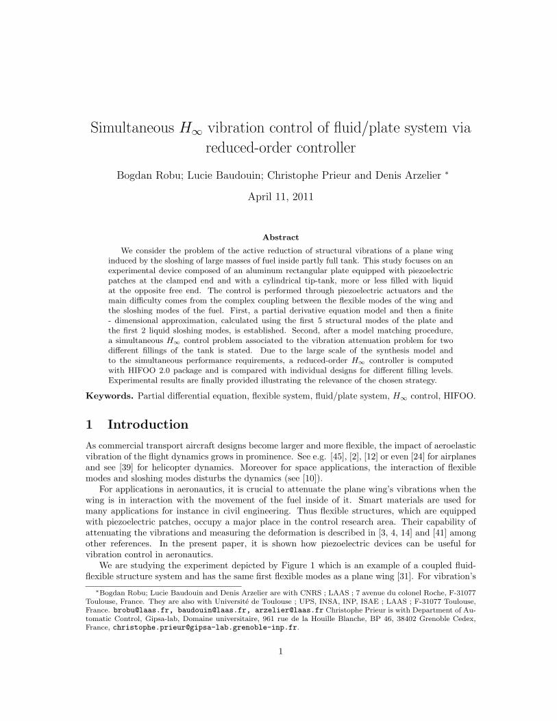
We are studying the experiment depicted by Figure 1 which is an example of a coupled fluid-flexible structure system and has the same first flexible modes as a plane wing [31]. For vibration’s

∗Bogdan Robu; Lucie Baudouin and Denis Arzelier are with CNRS ; LAAS ; 7 avenue du colonel Roche, F-31077

Toulouse, France. They are also with Universite de Toulouse ; UPS, INSA, INP, ISAE ; LAAS ; F-31077 Toulouse,

France. brobu@laas.fr, baudouin@laas.fr, arzelier@laas.fr Christophe Prieur is with Department of Au-

tomatic Control, Gipsa-lab, Domaine universitaire, 961 rue de la Houille Blanche, BP 46, 38402 Grenoble Cedex,

France, christophe.prieur@gipsa-lab.grenoble-inp.fr.

1

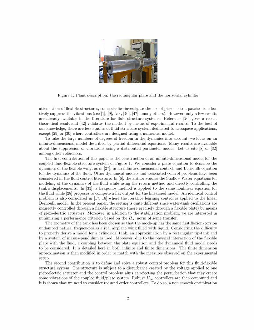
Figure 1: Plant description: the rectangular plate and the horizontal cylinder

attenuation of flexible structures, some studies investigate the use of piezoelectric patches to effec-tively suppress the vibrations (see [1], [9], [20], [46], [47] among others). However, only a few resultsare already available in the literature for fluid-structure systems. Reference [26] gives a recenttheoretical result and [42] validates the method by means of experimental results. To the best ofour knowledge, there are less studies of fluid-structure system dedicated to aerospace applications,except [29] or [30] where controllers are designed using a numerical model.

To take the large numbers of degrees of freedom in the dynamics into account, we focus on aninfinite-dimensional model described by partial differential equations. Many results are availableabout the suppression of vibrations using a distributed parameter model. Let us cite [8] or [32]among other references.

The first contribution of this paper is the construction of an infinite-dimensional model for thecoupled fluid-flexible structure system of Figure 1. We consider a plate equation to describe thedynamics of the flexible wing, as in [27], in an infinite-dimensional context, and Bernoulli equationfor the dynamics of the fluid. Other dynamical models and associated control problems have beenconsidered in the fluid control literature. In [6], the author studies the Shallow Water equations formodeling of the dynamics of the fluid while using the return method and directly controlling thetank’s displacements. In [33], a Lyapunov method is applied to the same nonlinear equation forthe fluid while [28] proposes to compute a flat output for the linearized model. An identical controlproblem is also considered in [17, 16] where the iterative learning control is applied to the linearBernoulli model. In the present paper, the setting is quite different since water-tank oscillations areindirectly controlled through a flexible structure (more precisely through a flexible plate) by meansof piezoelectric actuators. Moreover, in addition to the stabilization problem, we are interested inminimizing a performance criterion based on the H∞ norm of some transfer.

The geometry of the tank has been chosen so that the mock-up has the same first flexion/torsionundamped natural frequencies as a real airplane wing filled with liquid. Considering the difficultyto properly derive a model for a cylindrical tank, an approximation by a rectangular tip-tank andby a system of masses-pendulum is used. Moreover, due to the physical interaction of the flexibleplate with the fluid, a coupling between the plate equation and the dynamical fluid model needsto be considered. It is detailed here in both infinite and finite dimensions. The finite dimensionapproximation is then modified in order to match with the measures observed on the experimentalsetup.

The second contribution is to define and solve a robust control problem for this fluid-flexiblestructure system. The structure is subject to a disturbance created by the voltage applied to onepiezoelectric actuator and the control problem aims at rejecting the perturbation that may createsome vibrations of the coupled fluid/plate system. Robust H∞ controllers are then computed andit is shown that we need to consider reduced order controllers. To do so, a non smooth optimization

2

approach proposed in the HIFOO package is used [18]. It has also the interest of allowing the com-putation of a unique controller for several fillings of the tank, by solving a simultaneous H∞ optimalcontrol problem. Finally, some experiments on the real setup are presented and the relevance of thestabilizing controller to suppress the vibrations of the fluid-structure system is shown. To avoid aspillover effect when closing the loop, a suitable filter is also defined in the standard control problem(see [20]).

The paper is organized as follows. The plant under consideration, equipped with piezoelectricpatches (sensors and actuators) along with the control objectives are detailed in Section 2. In Section3 the fluid/plate model of the system is established. In Section 4, first the model matching problemis solved, second a full-order robust controller and then a reduced-order one using HIFOO packageare computed. Finally, the effectiveness of the robust controller of reduced order is checked onvarious experiments. Section V comprises some concluding remarks and Section VI some technicaldevelopments.

2 Problem statement and control objectives

2.1 Plant description

The plant to be controlled is located at ISAE-ENSICA, Toulouse, France and has been constructedto have the vibration frequencies of a real plane wing filled with fuel in its tip-tank [31].

The device is composed of an aluminium rectangular plate and a plexiglas horizontal cylindricaltip-tank filled with liquid (see Figures 1 and 2).

wx

O y

z

Figure 2: Deformation of the rectangular plate (1st mode)The length of the plate is along the horizontal axis and the width along the vertical one. The

plate is clamped on one end and free on the three other sides. The characteristics of the aluminiumplate are given in Table 1.

Plate length L 1.36 mPlate width l 0.16 m

Plate thickness h 0.005 mPlate density ρ 2970 kg m−3

Plate Young modulus Y 75 GPaPlate Poisson coefficient ν 0.33

Table 1: Plate characteristics

The two piezoelectric actuators made from PZT (Lead zirconate titanate) are bonded next tothe plate clamped side. Two sensors (made from PVDF - Polyvinylidene fluoride), are located onthe opposite side of the plate with respect to the actuators. The characteristics of the collocatedsensors and actuators are given in Table 2.

The tank is centered at 1.28 m from the plate clamped side and is symmetrically spread alongthe horizontal axis. Due to the configuration of the whole system (see Figure 2), the tank undergoes

3

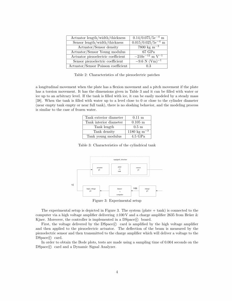
Actuator length/width/thickness 0.14/0.075/5e−4 mSensor length/width/thickness 0.015/0.025/5e−4 m

Actuator/Sensor density 7800 kg m−3

Actuator/Sensor Young modulus 67 GPaActuator piezoelectric coefficient −210e−12 m V−1

Sensor piezoelectric coefficient −9.6 N (Vm)−1

Actuator/Sensor Poisson coefficient 0.3

Table 2: Characteristics of the piezoelectric patches

a longitudinal movement when the plate has a flexion movement and a pitch movement if the platehas a torsion movement. It has the dimensions given in Table 3 and it can be filled with water orice up to an arbitrary level. If the tank is filled with ice, it can be easily modeled by a steady mass[38]. When the tank is filled with water up to a level close to 0 or close to the cylinder diameter(near empty tank empty or near full tank), there is no sloshing behavior, and the modeling processis similar to the case of frozen water.

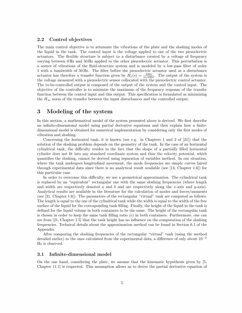
Tank exterior diameter 0.11 mTank interior diameter 0.105 m

Tank length 0.5 mTank density 1180 kg m−3

Tank young modulus 4.5 GPa

Table 3: Characteristics of the cylindrical tank

dspace

computer

+

+1

plate

tank

sensor

p1

actuator

p2

high_voltage

p4

charge

p3

equipped_structure

vmvi

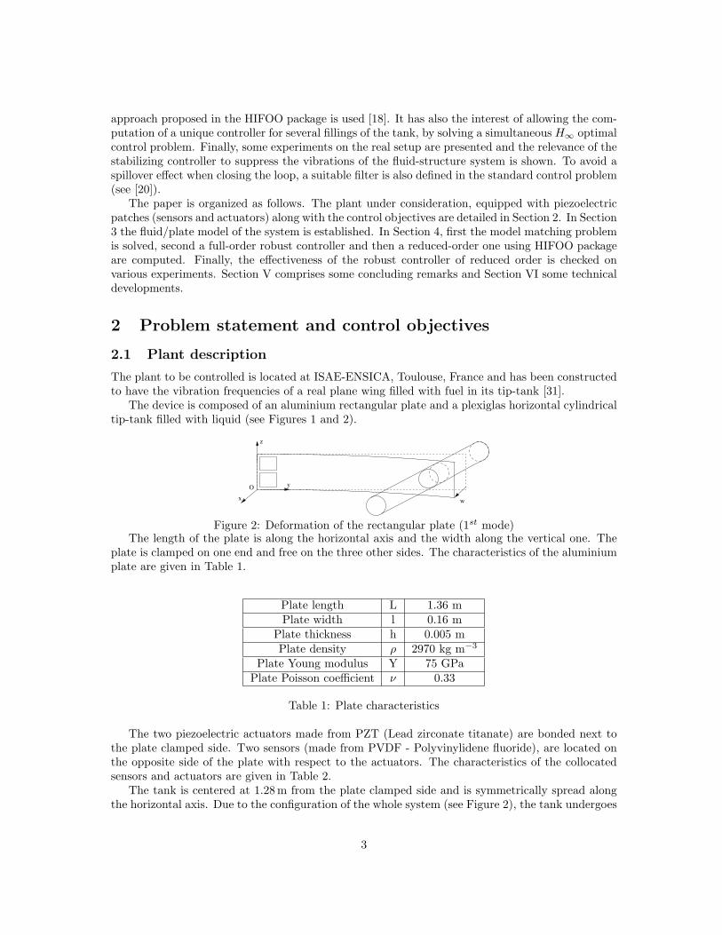
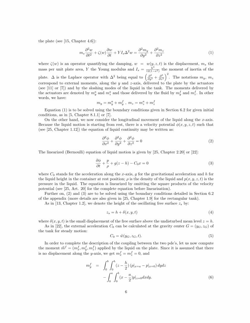
Figure 3: Experimental setup

The experimental setup is depicted in Figure 3. The system (plate + tank) is connected to thecomputer via a high voltage amplifier delivering ±100 V and a charge amplifier 2635 from Bruer &Kjaer. Moreover, the controller is implemented in a DSpace c© board.

First, the voltage delivered by the DSpace c© card is amplified by the high voltage amplifierand then applied to the piezoelectric actuator. The deflection of the beam is measured by thepiezoelectric sensor and then transmitted to the charge amplifier which will deliver a voltage to theDSpace c© card.

In order to obtain the Bode plots, tests are made using a sampling time of 0.004 seconds on theDSpace c© card and a Dynamic Signal Analyzer.

4

2.2 Control objectives

The main control objective is to attenuate the vibrations of the plate and the sloshing modes ofthe liquid in the tank. The control input is the voltage applied to one of the two piezoelectricactuators. The flexible structure is subject to a disturbance created by a voltage of frequencyvarying between 0 Hz and 50 Hz applied to the other piezoelectric actuator. This perturbation isa source of vibrations of the fluid-structure system and is modeled by a low-pass filter of order1 with a bandwidth of 50 Hz. The filter before the piezoelectric actuator used as a disturbanceactuator has therefore a transfer function given by H1(s) = 100π

s+100π. The output of the system is

the voltage measured with a piezoelectric sensor collocated with the piezoelectric control actuator.The to-be-controlled output is composed of the output of the system and the control input. Theobjective of the controller is to minimize the maximum of the frequency response of the transferfunction between the control input and this output. This specification is formulated as minimizingthe H∞ norm of the transfer between the input disturbances and the controlled output.

3 Modeling of the system

In this section, a mathematical model of the system presented above is derived. We first describean infinite-dimensional model using partial derivative equations and then explain how a finite-dimensional model is obtained for numerical implementation by considering only the first modes ofvibration and sloshing.

Concerning the horizontal tank, it is known (see e.g. in Chapters 1 and 2 of [21]) that thesolution of the sloshing problem depends on the geometry of the tank. In the case of an horizontalcylindrical tank, the difficulty resides in the fact that the shape of a partially filled horizontalcylinder does not fit into any standard coordinate system and thus the velocity potential, whichquantifies the sloshing, cannot be derived using separation of variables method. In our situation,where the tank undergoes longitudinal movement, the mode frequencies are simply curves fairedthrough experimental data since there is no analytical result available (see [13, Chapter 1.6]) forthis particular case.

In order to overcome this difficulty, we use a geometrical approximation. The cylindrical tankis replaced by an “equivalent” rectangular one with the same sloshing frequencies (where lengthand width are respectively denoted a and b and are respectively along the x-axis and y-axis).Analytical results are available in the literature for the calculation of modes and forces/moments(see [21, Chapter 1.6]). The parameters of the rectangular “virtual” tank are computed as follows:The length is equal to the one of the cylindrical tank while the width is equal to the width of the freesurface of the liquid for the corresponding tank filling. Finally, the height of the liquid in the tank isdefined for the liquid volume in both containers to be the same. The height of the rectangular tankis chosen in order to keep the same tank filling ratio (e) in both containers. Furthermore, one cansee from [21, Chapter 1.5] that the tank height has no influence on the computation of the sloshingfrequencies. Technical details about the approximation method can be found in Section 6.1 of theAppendix.

After comparing the sloshing frequencies of the rectangular “virtual” tank (using the methoddetailed earlier) to the ones calculated from the experimental data, a difference of only about 10−2

Hz is observed.

3.1 Infinite-dimensional model

On the one hand, considering the plate, we assume that the kinematic hypothesis given by [5,Chapter 11.1] is respected. This assumption allows us to derive the partial derivative equation of

5

the plate (see [15, Chapter 4.6]):

ms

∂2w

∂t2+ ζ(w)

∂w

∂t+ Y Is∆

2w =∂2my

∂y2+

∂2mz

∂z2(1)

where ζ(w) is an operator quantifying the damping, w = w(y, z, t) is the displacement, ms the

mass per unit plate area, Y the Young modulus and Is = h3

12(1−ν2) the moment of inertia of the

plate. ∆ is the Laplace operator with ∆2 being equal to(

∂2

∂y2 + ∂2

∂z2

)2

. The notations my, mz

correspond to external moments, along the y and z-axis, delivered to the plate by the actuators(see [11] or [7]) and by the sloshing modes of the liquid in the tank. The moments delivered bythe actuators are denoted by ma

y and maz and those delivered by the fluid by mf

y and mfz . In other

words, we have:my = ma

y + mfy , mz = ma

z + mfz

Equation (1) is to be solved using the boundary conditions given in Section 6.2 for given initialconditions, as in [5, Chapter 8.1.1] or [7].

On the other hand, we now consider the longitudinal movement of the liquid along the x-axis.Because the liquid motion is starting from rest, there is a velocity potential φ(x, y, z, t) such that(see [25, Chapter 1.12]) the equation of liquid continuity may be written as:

∂2φ

∂x2+

∂2φ

∂y2+

∂2φ

∂z2= 0 (2)

The linearized (Bernoulli) equation of liquid motion is given by [25, Chapter 2.20] or [22]:

∂φ

∂t+

p

ρ+ g(z − h) − C0x = 0 (3)

where C0 stands for the acceleration along the x-axis, g for the gravitational acceleration and h forthe liquid height in the container at rest position; ρ is the density of the liquid and p(x, y, z, t) is thepressure in the liquid. The equation is linearized by omitting the square products of the velocitypotential (see [25, Art. 20] for the complete equation before linearisation).

Further on, (2) and (3) are to be solved using the boundary conditions detailed in Section 6.2of the appendix (more details are also given in [25, Chapter 1.9] for the rectangular tank).

As in [13, Chapter 1.2], we denote the height of the oscillating free surface zs by:

zs = h + δ(x, y, t) (4)

where δ(x, y, t) is the small displacement of the free surface above the undisturbed mean level z = h.As in [22], the external acceleration C0 can be calculated at the gravity center G = (yG, zG) of

the tank for steady motion:C0 = w(yG, zG, t). (5)

In order to complete the description of the coupling between the two pde’s, let us now computethe moment ~mf = (mf

x, mfy , mf

z ) applied by the liquid on the plate. Since it is assumed that there

is no displacement along the y-axis, we get mfx = mf

z = 0, and

mfy =

∫ b

0

∫ h

0

(z −h

2) (p|x=a − p|x=0) dydz

−

∫ a

0

∫ b

0

(x −a

2)p|z=0dxdy. (6)

6

The second contribution to the whole moment is due to the voltage applied by the piezoelectricpatches (see references [11, 23]). As our experimental setup is not symmetric with respect to thex-axis (the actuators are only on one side of the plate), the position of the neutral fiber needs tobe recalculated. We finally get that:

may(y, z, t) = ma

z(y, z, t) = KaVa(t) if (y, z) ∈ A= 0 else

(7)

where A = (ya1, ya2)× (za1, za2) is the square delimited by the surface of the actuator and Ka is aparameter depending on the actuator/plate geometry and on the position of the neutral fiber (see[23]).

The piezoelectric sensor delivers a voltage Vc given by:

Vc = Kc

∫ yc2

yc1

∫ zc2

zc1

(∂2w

∂y2+

∂2w

∂z2)dydz (8)

where Kc is a parameter depending on the piezoelectric characteristics and on the capacity of thecharge amplifier. yc1, yc2, zc1, zc2 define the extremities of the piezoelectric sensor.

The perturbation entry, defined as a noise on the perturbation actuator glued next to thecontrolled actuator, creates a momentum similar to (7):

mpy(y, z, t) = mp

z(y, z, t) = KpWp(t) (9)

where Wp is a noise with a frequency of 50Hz.

3.2 Finite-dimensional approximation

In order to compute an approximation of the previous infinite-dimensional model, it is needed todescribe an appropriate basis in which the solution of the partial derivative equation may be written.This issue is well covered in the literature (see for example [15, Chapter 5.2] for the plate and [22]for the liquid sloshing) thus it will be detailed only in the appendix (see Section 6.3 below). Thisallows us to compute a finite-dimensional approximation of the model.

Knowing that the influence of system’s modes is inversely proportional to the mode’s frequency,the approximation of the displacement by the first N modes of the system may be justified. Thederivation of the finite-dimensional approximation of our model is now detailed. We aim at de-scribing a state space model where the state vector should gather the first N vibration modes ofthe plate and the first M 6= N sloshing modes of the tank.

3.2.1 Plate model

In this section, we calculate the finite-dimensional approximation of size N of (1) for the rectangularplate, doing a truncation of the equation (33) at n = N .

The approximation of the influence of the tank on the plate will be considered in Section 3.2.3.We write:

{

Xp(t) = ApXp(t) + Bpu(t)y(t) = CpXp(t)

(10)

where Xp =(

q1 ω1q1 · · · ˙qN ωNqN

)

- the qn being the same as in (33) - is the state spacevector. u(t) stands for the voltage applied to the piezoelectric patch and y(t) is the voltage deliveredby the piezoelectric sensor.

7

In (10), the dynamic matrix Ap is written as:

Ap =

Ap10 · · · 0

0 Ap2· · · 0

· · ·0 0 · · · ApN

(11)

with Apn=

(

−2ζnωn −ωn

ωn 0

)

for every n from 1 to N .

The angular frequency of the nth mode is ωn in [rad s−1] given in [5, Chapter 11] and ζpnis the

damping factor. The experiments have shown that the damping is not constant for every vibrationmode but it depends on the quality factor which is different for every structure mode. For a giveninput voltage, we measure the quality vector and then identify the damping by analogy to a secondorder system with damping [40].

For the control matrix Bp, we use (1) and (7), and we integrate on the surface A of the actuator.Thus we get:

Bp = (bp1, 0, ..., bpn

, 0, ..., bpN, 0)T (12)

where

bpn= Kb(Y

′

in(ya2) − Y ′

in(ya1))

∫ za2

za1

Zjn(z)dz

+Kb(Z′

jn(za2) − Z ′

jn(za1))

∫ ya2

ya1

Yin(y)dy

Here in and jn are the specific deformation modes of the plate along y and z-axis. Moreover, theHeaviside step is used here to suggest that the moment generated by the actuator is different thanzero only under the actuator. More details of the derivation are given in Section 6.4 of the appendix.

The output matrix Cp is calculated with (8) and the new position of the neutral fiber:

Cp = (0, cp1, ..., 0, cpk

, ..., 0, cpN) (13)

where

cpn= Kc

ωpn

(

(Y ′

in(yc2) − Y ′

in(yc1))

∫ zc2

zc1

Zjn(z)dz

+(Z ′

jn(zc2) − Z ′

jn(zc1))

∫ yc2

yc1

Yin(y)dy

)

and Kc is the same parameter depending on the sensor/plate geometry and on the position of theneutral fiber as in (8). Here also, the Heaviside step is used to infer that the sensor senses the platedeformation which is only under it. The computation method is similar to the one of the controlmatrix from Section 6.4.

3.2.2 Liquid model

In this section, we calculate the finite-dimensional approximation of the tank’s sloshing using amechanical approach.

With the geometrical parameters of the rectangular tank, one can calculate the movementequations of the liquid and the boundary conditions (see [25, Chapter 17]). The approximationgiven by [22] may be used to model the sloshing. Indeed we consider a finite number of masspendulum systems, each corresponding to a sloshing mode, which will exert on the tank the sameforce and moment as the sloshing liquid does (one can see for instance that for each odd integer i

of (36) or (37) in the appendix corresponds to a mass-pendulum systems of index k = 1 · · ·M).

8

The state-space representation is then easily obtained using the pendulum equation under ex-ternal acceleration [21]:

θk + 2ξθ

√

g

lkθk +

g

lkθk = −

1

lkC0 (14)

where θm is the angle of the mth pendulum compared to its equilibrium position, lk its length andξθ is the value of the damping fixed at 0.01.

Choosing the state space vector for the liquid sloshing equal to

Xθ =(

θ1

√

gl1

θ1 · · · ˙θM

√

glM

θM

)T

,

the dynamic equation, for the general case of an input uacc, is:

Xθ = AθXθ + Bθuacc (15)

where the matrix Aθ computed from (14) for each k is:

Aθ =

Aθ10 · · · 0

0 Aθ2· · · 0

· · ·0 0 · · · AθM

(16)

with Aθk=

−2ξθ

√

glk

−√

glk

√

glk

0

.

In the case of the control matrix Bθ the construction is also straightforward by consideringuacc = C0 as the control variable:

Bθ = (bθ1, 0, ..., bθk

, 0, ..., bθM, 0)T (17)

where bθk=

(

− 1lk

0

)

.

3.2.3 Model coupling

Plate influence on the rectangular tank The influence of the plate on the movement of thefluid is given by (5) which is expressed using the Ritz functions as (see (33)):

C0 =

N∑

n=1

Yin(yG)Zjn

(zG).qn(t) (18)

TakingKG = (Yi1(yG)Zj1(zG), 0, · · · , YiN

(yG)ZjN(zG), 0)

this equation is equivalent to:

C0 = KG

(

q1(t) ω1q1(t) · · · qN (t) ωN ˙qN (t))T

. (19)

Since(

q1(t) ω1q1(t) · · · qN (t) ωN ˙qN (t))T

= Xp is the derivative of the state space vectorof the rectangular plate, using (10) we obtain

C0 = KGApXp + KGBpu. (20)

9

Using now (16), (17) and (20), equation (15) becomes:

Xθ = AθXθ + Bθ(KGApXp + KGBpu). (21)

This equation describes the coupling between the movement of the plate and the movement ofthe pendulum mass systems, that is to say the movement of the liquid in the tank.

Tank’s influence on the rectangular plate The liquid sloshing is viewed by the plate as aperturbation that comes into the state space representation by means of a matrix Aθp:

{

Xp = ApXp + Bpu + AθpXθ

y = CpXp(22)

(see paragraph 3.2.1). For the calculation of the perturbation matrix Aθp, an identical approach asin the case of the control matrix Bp has been followed.

The external moment applied to the tank due to the movement of the fluid is computed in (38).Due to our choice of the physical parameters of the pendulum, the moment from the liquid sloshingequals the moment due to the movement of all mass-pendulum systems. The external momentwritten for M mass-pendulum system is

Mθp =

M∑

k=1

mkLklkθk

where lkθk is the total acceleration due to pendulum oscillations and plate movement. Using (16),the expression of Mθp can be rewritten as:

Mθp = (m1l1L1, 0, · · · , mM lMLM , 0) AθXθ. (23)

In similar way as the computation of the control matrix Bp given by (12), using (6) and in-tegrating on a small square (y1G, z1G) × (y2G, z2G) around the point G, we get that the matrixAθp ∈ R

2N×2M is given by:

Aθp =(

aTθp1

0 . . . aTθpn

0 . . . aTθpN

0)T

(24)

where aθpn∈ R

2M is given by

aθpn= Kθp

(

(Y ′

in(y2G) − Y ′

in(y1G))

∫ z2G

z1G

Zjn(z)dz

+(Z ′

jn(z2G) − Z ′

jn(z1G))

∫ y2G

y1G

Yin(y)dy

)

andKθp = (m1l1L1, 0, · · · , mklkLk, 0, · · · , mM lMLM , 0) Aθ.

3.3 Complete Model

From (21) and (22), one can write the complete state-space model of the experimental setup.As previously stated, in the presentation of the complete model, we consider the case of N Ritzfunctions and M mass-pendulum systems. For the complete system, the state space vector is:

X =

(

Xp

Xθ

)

.

10

Combining all the matrices leads to the following finite-dimensional approximation using the state-space representation:

X =

(

Ap Aθp

Apθ Aθ

)

X +

(

Bp

Bpθ

)

u +

(

Bw

0

)

w

z =

(

Cp 0

0 0

)

X +

(

01

)

u

y =(

Cp 0)

X.

(25)

where Apθ = BθKGAp, Bpθ = BθKGBp and 0 denotes null matrices of appropriate dimensions.Bw is the perturbation matrix computed from (9) using the same methodology as Bp.

As stated earlier in (25), y stands for the measured output (the voltage measured through thepiezoelectric sensor), u is the control input (the voltage applied to the piezoelectric actuator), z

stands for the output to be controlled and is composed in this case of y and u. Finally, w is thedisturbance input (not to be confused with the plate’s displacement) and is generated by the voltageapplied to the piezoelectric actuator used as source of disturbances.

4 Controller synthesis

The system model (25) is established for the first N modes of the plate and for the first M modesof the liquid sloshing. As it is observed in Section 4.1 below, this choice allows to consider theflexional and torsional deformation of the plate. Besides, it is shown in [19] that the first modescontain the main part of the energy of the deformation of the flexible structure. Moreover, usingthe energy approach from [43], it is possible to check that the first five modes contain almost allthe energy of the structure. Since the objective is to control the flexional deformation but also thetorsional modes of the plate, the number of modes considered is also chosen so that torsion modesare included. Therefore the controller will be computed with N = 5 and M = 2. So Xp ∈ R

2N andXl ∈ R

2M and the total state space vector X belongs to R14.

4.1 Model matching

The complete system model from (25) was validated in [35] by a comparison of a time-responsefor a given initial deformation of the plate. However, in order to obtain a model which providesa good match of the measured frequency response, some adjustments are required by consideringthe Bode plots. This adaptation is done following a trial-and-error method (first the frequenciesare matched and then is the damping). Other methods are possible for flexible structures (see e.g.,[36] and references therein).

This model matching is necessary since some mechanical elements are not well known and havenot been taken into account in the modeling. These elements include the circular ring used to attachthe tank on the plate, the dynamical behavior of the piezoelectric patches, the non-homogeneity ofthe plate and the weight of the tank.

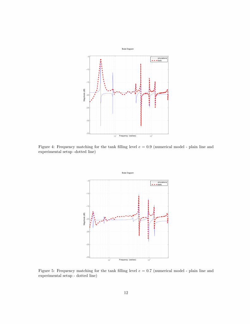
As a first step of the model matching, the frequencies of the plate are adjusted. A bigger amountof liquid will be sensed by the plate as an increase of the total mass of the plate and this will leadto (see [5, Chapter 11]) a shift towards zero of all the mode frequencies. A second step of the modelmatching is the adding of a static gain that corresponds to the high frequency modes neglectedduring the model reduction static correction [37]. This allows to get a more realistic model at lowfrequencies. The comparison of the bode plots for e = 0.7 and e = 0.9 on Figures 4 and 5 showsthat the model, for e = 0.7 is quite accurate with respect to the real data while there is somediscrepancy in the amplitude of the first sloshing mode for e = 0.9.

11

101

102

−35

−30

−25

−20

−15

−10

−5

Magnitude (

dB

)

Bode Diagram

Frequency (rad/sec)

simulations

tests

Figure 4: Frequency matching for the tank filling level e = 0.9 (numerical model - plain line andexperimental setup -dotted line)

101

102

−35

−30

−25

−20

−15

−10

−5

Magnitude (

dB

)

Bode Diagram

Frequency (rad/sec)

simulations

tests

Figure 5: Frequency matching for the tank filling level e = 0.7 (numerical model - plain line andexperimental setup - dotted line)

12

In the considered figures, the first peak corresponds to the first flexional mode of the plate(0.625 Hz) and the second peak to the first sloshing mode (1.25 Hz for e = 0.7 and 1.415 Hz fore = 0.9) in the tank. The next four peaks are respectively representing: The first torsional mode(the third peak) (6.38 Hz) and the second (8.75 Hz), third (14.45 Hz) and fourth (21.50 Hz) flexionalmodes of the plate. The second mode of the liquid sloshing (1.99 Hz for e = 0.7 and 2.15 Hz fore = 0.9) cannot be identified on the Bode diagrams due to its very small amplitude.

4.2 Robust H∞ control problem

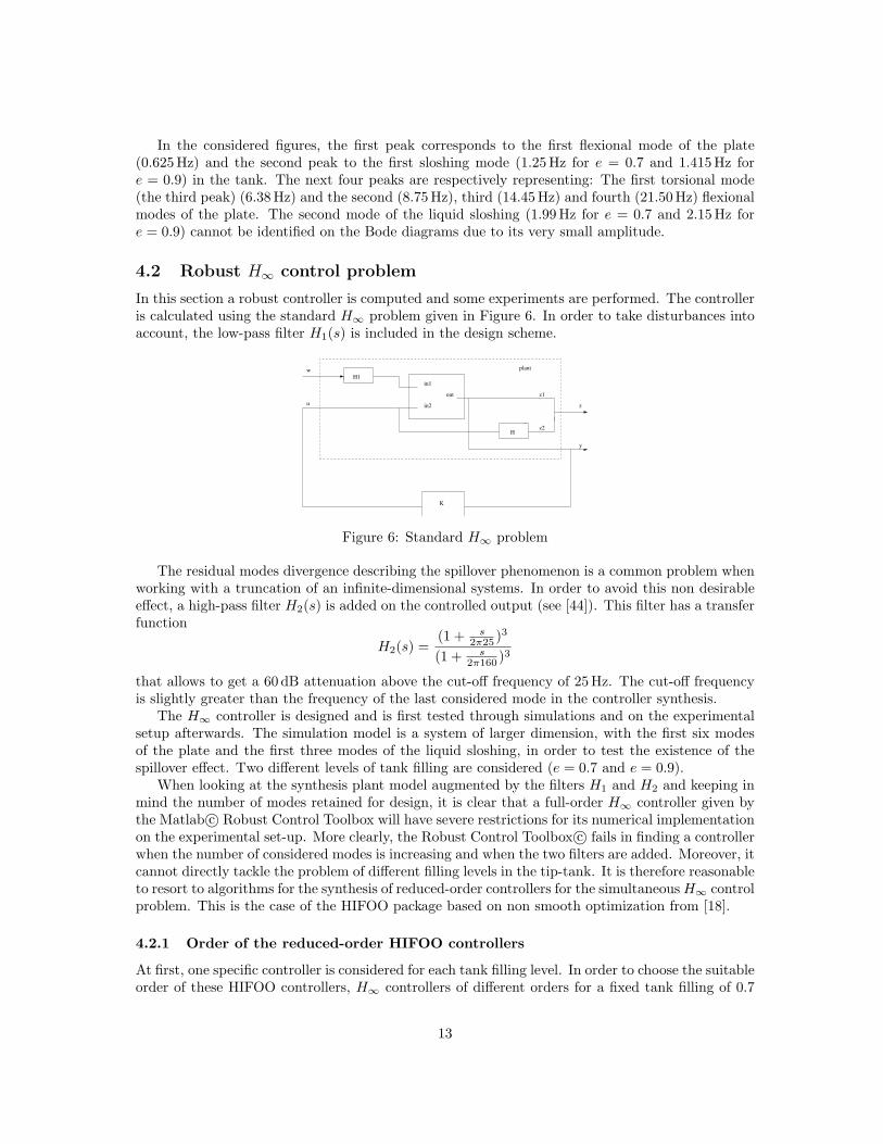
In this section a robust controller is computed and some experiments are performed. The controlleris calculated using the standard H∞ problem given in Figure 6. In order to take disturbances intoaccount, the low-pass filter H1(s) is included in the design scheme.

H1

K

H

u

z1

w

z

y

plant

z2

in2

in1

out

Figure 6: Standard H∞ problem

The residual modes divergence describing the spillover phenomenon is a common problem whenworking with a truncation of an infinite-dimensional systems. In order to avoid this non desirableeffect, a high-pass filter H2(s) is added on the controlled output (see [44]). This filter has a transferfunction

H2(s) =(1 + s

2π25 )3

(1 + s2π160 )3

that allows to get a 60 dB attenuation above the cut-off frequency of 25Hz. The cut-off frequencyis slightly greater than the frequency of the last considered mode in the controller synthesis.

The H∞ controller is designed and is first tested through simulations and on the experimentalsetup afterwards. The simulation model is a system of larger dimension, with the first six modesof the plate and the first three modes of the liquid sloshing, in order to test the existence of thespillover effect. Two different levels of tank filling are considered (e = 0.7 and e = 0.9).

When looking at the synthesis plant model augmented by the filters H1 and H2 and keeping inmind the number of modes retained for design, it is clear that a full-order H∞ controller given bythe Matlab c© Robust Control Toolbox will have severe restrictions for its numerical implementationon the experimental set-up. More clearly, the Robust Control Toolbox c© fails in finding a controllerwhen the number of considered modes is increasing and when the two filters are added. Moreover, itcannot directly tackle the problem of different filling levels in the tip-tank. It is therefore reasonableto resort to algorithms for the synthesis of reduced-order controllers for the simultaneous H∞ controlproblem. This is the case of the HIFOO package based on non smooth optimization from [18].

4.2.1 Order of the reduced-order HIFOO controllers

At first, one specific controller is considered for each tank filling level. In order to choose the suitableorder of these HIFOO controllers, H∞ controllers of different orders for a fixed tank filling of 0.7

13

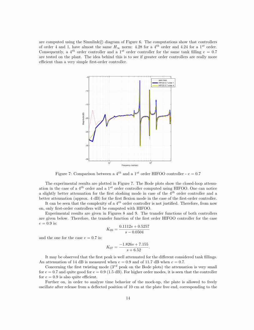
are computed using the Simulink c© diagram of Figure 6. The computations show that controllersof order 4 and 1, have almost the same H∞ norm: 4.28 for a 4th order and 4.24 for a 1st order.Consequently, a 4th order controller and a 1st order controller for the same tank filling e = 0.7are tested on the plant. The idea behind this is to see if greater order controllers are really moreefficient than a very simple first-order controller.

101

102

−35

−30

−25

−20

−15

−10

−5

Frequency (rad/sec)

Magnitude(d

B)

open loop

HIFOO 0.7 order 1

HIFOO 0.7 order 4

Figure 7: Comparison between a 4th and a 1st order HIFOO controller - e = 0.7

The experimental results are plotted in Figure 7. The Bode plots show the closed-loop attenu-ation in the case of a 4th order and a 1st order controller computed using HIFOO. One can noticea slightly better attenuation for the first sloshing mode in case of the 4th order controller and abetter attenuation (approx. 4 dB) for the first flexion mode in the case of the first-order controller.

It can be seen that the complexity of a 4th order controller is not justified. Therefore, from nowon, only first-order controllers will be computed with HIFOO.

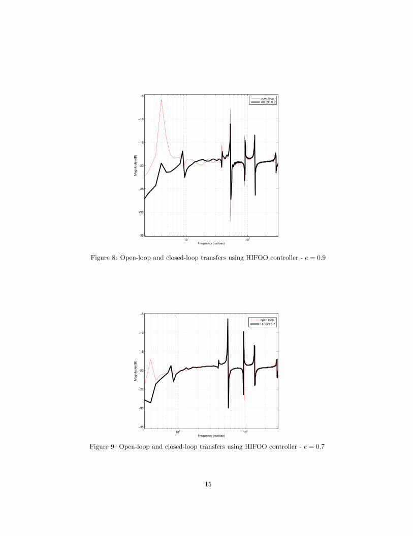
Experimental results are given in Figures 8 and 9. The transfer functions of both controllersare given below. Therefore, the transfer function of the first order HIFOO controller for the casee = 0.9 is:

K09 =0.1112s + 0.5257

s − 0.0504

and the one for the case e = 0.7 is:

K07 =−1.826s + 7.155

s + 6.52.

It may be observed that the first peak is well attenuated for the different considered tank fillings.An attenuation of 14 dB is measured when e = 0.9 and of 11.7 dB when e = 0.7.

Concerning the first twisting mode (3rd peak on the Bode plots) the attenuation is very smallfor e = 0.7 and quite good for e = 0.9 (1.5 dB). For higher order modes, it is seen that the controllerfor e = 0.9 is also quite efficient.

Further on, in order to analyze time behavior of the mock-up, the plate is allowed to freelyoscillate after release from a deflected position of 10 cm at the plate free end, corresponding to the

14

101

102

−35

−30

−25

−20

−15

−10

−5

Frequency (rad/sec)

Magnitude (

dB

)

open loop

HIFOO 0.9

Figure 8: Open-loop and closed-loop transfers using HIFOO controller - e = 0.9

101

102

−35

−30

−25

−20

−15

−10

−5

Frequency (rad/sec)

Magnitude(d

B)

open loop

HIFOO 0.7

Figure 9: Open-loop and closed-loop transfers using HIFOO controller - e = 0.7

15

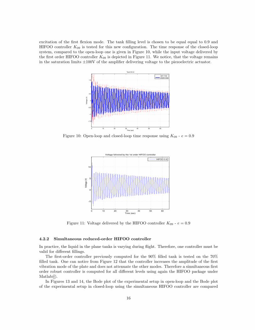
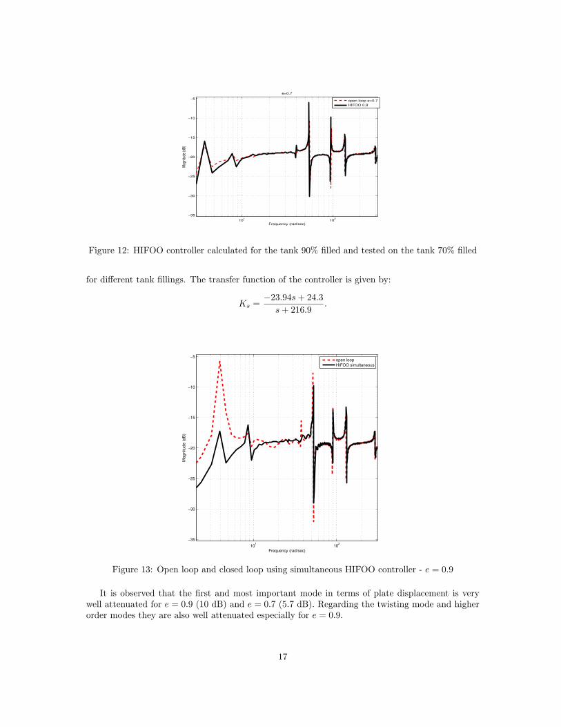
excitation of the first flexion mode. The tank filling level is chosen to be equal equal to 0.9 andHIFOO controller K09 is tested for this new configuration. The time response of the closed-loopsystem, compared to the open-loop one is given in Figure 10, while the input voltage delivered bythe first order HIFOO controller K09 is depicted in Figure 11. We notice, that the voltage remainsin the saturation limits ±100V of the amplifier delivering voltage to the piezoelectric actuator.

0 10 20 30 40 50 60

−1.5

−1

−0.5

0

0.5

1

1.5

Time (sec)

Voltage (

V)

Tank fill 0.9

open−loop

closed−loop

Figure 10: Open-loop and closed-loop time response using K09 - e = 0.9

0 10 20 30 40 50 60

−5

0

5

10

Time (sec)

Vol

tage

(V

)

Voltage felivered by the 1st order HIFOO controller

HIFOO 0.9

Figure 11: Voltage delivered by the HIFOO controller K09 - e = 0.9

4.2.2 Simultaneous reduced-order HIFOO controller

In practice, the liquid in the plane tanks is varying during flight. Therefore, one controller must bevalid for different fillings.

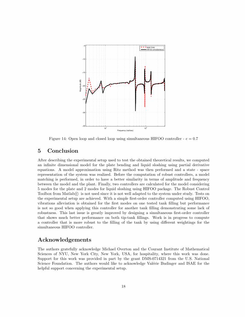
The first-order controller previously computed for the 90% filled tank is tested on the 70%filled tank. One can notice from Figure 12 that the controller increases the amplitude of the firstvibration mode of the plate and does not attenuate the other modes. Therefore a simultaneous firstorder robust controller is computed for all different levels using again the HIFOO package underMatlab c©.

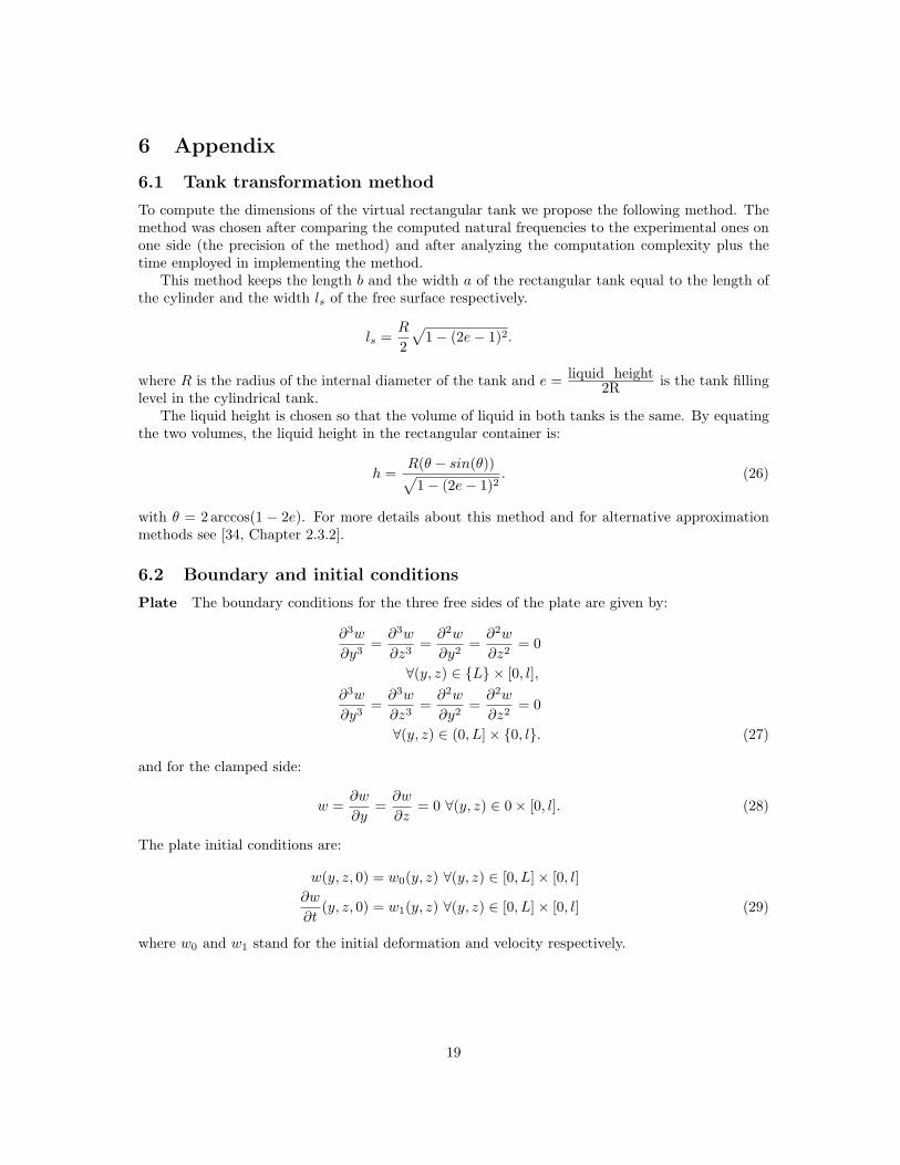
In Figures 13 and 14, the Bode plot of the experimental setup in open-loop and the Bode plotof the experimental setup in closed-loop using the simultaneous HIFOO controller are compared

16

101

102

−35

−30

−25

−20

−15

−10

−5

Frequency (rad/sec)

Mag

nitu

de (d

B)

e=0.7

open loop e=0.7

HIFOO 0.9

Figure 12: HIFOO controller calculated for the tank 90% filled and tested on the tank 70% filled

for different tank fillings. The transfer function of the controller is given by:

Ks =−23.94s + 24.3

s + 216.9.

101

102

−35

−30

−25

−20

−15

−10

−5

Frequency (rad/sec)

Magnitude (

dB

)

open loop

HIFOO simultaneous

Figure 13: Open loop and closed loop using simultaneous HIFOO controller - e = 0.9

It is observed that the first and most important mode in terms of plate displacement is verywell attenuated for e = 0.9 (10 dB) and e = 0.7 (5.7 dB). Regarding the twisting mode and higherorder modes they are also well attenuated especially for e = 0.9.

17

101

102

−35

−30

−25

−20

−15

−10

−5

Frequency (rad/sec)

Magnitude (

dB

)

open loop

HIFOO simultaneous

Figure 14: Open loop and closed loop using simultaneous HIFOO controller - e = 0.7

5 Conclusion

After describing the experimental setup used to test the obtained theoretical results, we computedan infinite dimensional model for the plate bending and liquid sloshing using partial derivativeequations. A model approximation using Ritz method was then performed and a state - spacerepresentation of the system was realized. Before the computation of robust controllers, a modelmatching is performed, in order to have a better similarity in terms of amplitude and frequencybetween the model and the plant. Finally, two controllers are calculated for the model considering5 modes for the plate and 2 modes for liquid sloshing using HIFOO package. The Robust ControlToolbox from Matlab c© is not used since it is not well adapted to the system under study. Tests onthe experimental setup are achieved. With a simple first-order controller computed using HIFOO,vibrations alleviation is obtained for the first modes on one tested tank filling but performanceis not so good when applying this controller for another tank filling demonstrating some lack ofrobustness. This last issue is greatly improved by designing a simultaneous first-order controllerthat shows much better performance on both tip-tank fillings. Work is in progress to computea controller that is more robust to the filling of the tank by using different weightings for thesimultaneous HIFOO controller.

Acknowledgements

The authors gratefully acknowledge Michael Overton and the Courant Institute of MathematicalSciences of NYU, New York City, New York, USA, for hospitality, where this work was done.Support for this work was provided in part by the grant DMS-0714321 from the U.S. NationalScience Foundation. The authors would like to acknowledge Valerie Budinger and ISAE for thehelpful support concerning the experimental setup.

18

6 Appendix

6.1 Tank transformation method

To compute the dimensions of the virtual rectangular tank we propose the following method. Themethod was chosen after comparing the computed natural frequencies to the experimental ones onone side (the precision of the method) and after analyzing the computation complexity plus thetime employed in implementing the method.

This method keeps the length b and the width a of the rectangular tank equal to the length ofthe cylinder and the width ls of the free surface respectively.

ls =R

2

√

1 − (2e − 1)2.

where R is the radius of the internal diameter of the tank and e =liquid height

2R is the tank fillinglevel in the cylindrical tank.

The liquid height is chosen so that the volume of liquid in both tanks is the same. By equatingthe two volumes, the liquid height in the rectangular container is:

h =R(θ − sin(θ))

√

1 − (2e − 1)2. (26)

with θ = 2 arccos(1 − 2e). For more details about this method and for alternative approximationmethods see [34, Chapter 2.3.2].

6.2 Boundary and initial conditions

Plate The boundary conditions for the three free sides of the plate are given by:

∂3w

∂y3=

∂3w

∂z3=

∂2w

∂y2=

∂2w

∂z2= 0

∀(y, z) ∈ {L} × [0, l],

∂3w

∂y3=

∂3w

∂z3=

∂2w

∂y2=

∂2w

∂z2= 0

∀(y, z) ∈ (0, L] × {0, l}. (27)

and for the clamped side:

w =∂w

∂y=

∂w

∂z= 0 ∀(y, z) ∈ 0 × [0, l]. (28)

The plate initial conditions are:

w(y, z, 0) = w0(y, z) ∀(y, z) ∈ [0, L] × [0, l]

∂w

∂t(y, z, 0) = w1(y, z) ∀(y, z) ∈ [0, L] × [0, l] (29)

where w0 and w1 stand for the initial deformation and velocity respectively.

19

Tank with liquid The boundary conditions for the tank with liquid are:

∂φ

∂x= 0,

∂φ

∂y= 0,

∂φ

∂z= 0 on the tank walls

∂δ

∂t=

∂φ

∂zfor z = zs (30)

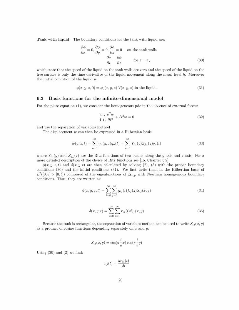
which state that the speed of the liquid on the tank walls are zero and the speed of the liquid on thefree surface is only the time derivative of the liquid movement along the mean level h. Moreoverthe initial condition of the liquid is:

φ(x, y, z, 0) = φ0(x, y, z) ∀(x, y, z) in the liquid. (31)

6.3 Basis functions for the infinite-dimensional model

For the plate equation (1), we consider the homogeneous pde in the absence of external forces:

ms

Y Is

∂2w

∂t2+ ∆2w = 0 (32)

and use the separation of variables method.The displacement w can then be expressed in a Hilbertian basis:

w(y, z, t) =

∞∑

n=1

ηn(y, z)qn(t) =

∞∑

n=1

Yin(y)Zjn

(z)qn(t) (33)

where Yin(y) and Zjn

(z) are the Ritz functions of two beams along the y-axis and z-axis. For amore detailed description of the choice of Ritz functions see [15, Chapter 5.2].

φ(x, y, z, t) and δ(x, y, t) are then calculated by solving (2), (3) with the proper boundaryconditions (30) and the initial conditions (31). We first write them in the Hilbertian basis ofL2([0, a] × [0, b]) composed of the eigenfunctions of ∆x,y with Newman homogeneous boundaryconditions. Thus, they are written as:

φ(x, y, z, t) =∞∑

i=0

∞∑

j=0

gij(t)fij(z)Sij(x, y) (34)

δ(x, y, t) =

∞∑

i=0

∞∑

j=0

rij(t)Sij(x, y) (35)

Because the tank is rectangular, the separation of variables method can be used to write Sij(x, y)as a product of cosine functions depending separately on x and y:

Sij(x, y) = cos(πi

ax) cos(π

i

by)

Using (30) and (2) we find:

gij(t) =drij(t)

dt

20

fij(z) =cosh(Υijz)

Υij sinh(Υijh)

where Υij = π ia

+ π jb.

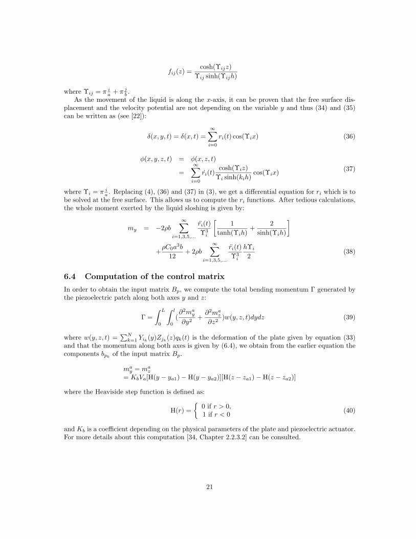
As the movement of the liquid is along the x-axis, it can be proven that the free surface dis-placement and the velocity potential are not depending on the variable y and thus (34) and (35)can be written as (see [22]):

δ(x, y, t) = δ(x, t) =

∞∑

i=0

ri(t) cos(Υix) (36)

φ(x, y, z, t) = φ(x, z, t)

=

∞∑

i=0

ri(t)cosh(Υiz)

Υi sinh(kih)cos(Υix)

(37)

where Υi = π ia. Replacing (4), (36) and (37) in (3), we get a differential equation for ri which is to

be solved at the free surface. This allows us to compute the ri functions. After tedious calculations,the whole moment exerted by the liquid sloshing is given by:

my = −2ρb

∞∑

i=1,3,5,...

ri(t)

Υ3i

[

1

tanh(Υih)+

2

sinh(Υih)

]

+ρC0a

3b

12+ 2ρb

∞∑

i=1,3,5,...

ri(t)

Υ3i

hΥi

2(38)

6.4 Computation of the control matrix

In order to obtain the input matrix Bp, we compute the total bending momentum Γ generated bythe piezoelectric patch along both axes y and z:

Γ =

∫ L

0

∫ l

0

(∂2ma

y

∂y2+

∂2maz

∂z2)w(y, z, t)dydz (39)

where w(y, z, t) =∑N

k=1 Yik(y)Zjk

(z)qk(t) is the deformation of the plate given by equation (33)and that the momentum along both axes is given by (6.4), we obtain from the earlier equation thecomponents bpk

of the input matrix Bp.

may = ma

z

= KbVa[H(y − ya1) − H(y − ya2)][H(z − za1) − H(z − za2)]

where the Heaviside step function is defined as:

H(r) =

{

0 if r > 0,

1 if r < 0(40)

and Kb is a coefficient depending on the physical parameters of the plate and piezoelectric actuator.For more details about this computation [34, Chapter 2.2.3.2] can be consulted.

21

References

[1] B.P. Baillargeon and S.S. Vel. Active vibration suppression of sandwich beams using piezoelectricshear actuators: Experiments and numerical simulations. Journal of Intelligent Material Systems andStructures, 16(6):517–530, 2005.

[2] J. Becker. Active buffeting vibration alleviation demonstration of intelligent aircraft structure forvibration & dynamic load alleviation. In Proceedings of the US-Europe Workshop on Sensors andSmart Structures Technology, pages 9–18, Commo and Soma Lombardo, Italy, April 2002.

[3] J. Becker and W.G. Luber. Comparison of piezoelectric systems and aerodynamic systems for aircraftvibration alleviation. In Smart Structures and Materials, pages 9–18, San Diego, CA, March 1998.

[4] B. Bhikkaji, S. O. R. Moheimani, and I. R. Petersen. Multivariable integral control of resonantstructures. In Proceedings of the 47th IEEE Conference on Decision and Control, pages 3743–3748,Cancum, Mexico, December 2008.

[5] R. D. Blevins. Formulas for natural frequency and mode shape. Krieger publishing company, Florida,1995.

[6] J.-M. Coron. Local controllability of a 1-D tank containing a fluid modeled by the shallow waterequations. 8:513–554, 2002.

[7] E. Crepeau and C. Prieur. Control of a clamped-free beam by a piezoelectric actuator. ESAIM:Control, Optim. Cal. Var., 12:545–563, 2006.

[8] M.A. Demetriou and F. Fahroo. An adaptive control scheme for a class of second order distributedparameter systems with structured perturbations. In Proceedings of the 43rd IEEE Conference onDecision and Control, pages 1520–1525, Atlantis, Bahamas, December 2004.

[9] K.K. Denoyer and M.K. Kwak. Dynamic modelling and vibration suppression of a swelling stuctureutilizing piezoelectric sensors and actuators. Journal of Sound and Vibration, 189(1):13–31, January1996.

[10] J.J. Deyst. Effects of structural flexibility on entry vehicle control systems. Technical Report NASASP-8016, Nasa, Space Vehicle Design Criteria, April 1969.

[11] E.K. Dimitriadis, C.R. Fuller, and C.A. Rogers. Piezoelectric actuators for distributed vibrationexcitation of thin plates. Journal of Vibrational Acoustics, 113:100–107, 1991.

[12] C. S. Buttrill D.L. Raney, E. B. Jackson and W. M. Adams. The impact of structural vibrationon flying qualities of a supersonic transport. In AIAA Atmospheric Flight Mechanics Conference,Montreal, Canada, 2001.

[13] F.T. Dodge. The new ”dynamic behavior of liquids in moving containers”. Technical report, SouthwestResearch Institute, San Antonio, Texas, 2000.

[14] A.J. Fleming and S.O. Reza Moheimani. Optimal impedance design for piezoelectric vibration control.In Proceedings of the 43rd IEEE Conference on Decision and Control, pages 2596–2601, Atlantis,Bahamas, December 2004.

[15] M. Geradin and D. Rixen. Mechanical Vibrations: theory and application to structural dynamics.Masson, 1994.

[16] M. Grundelius. Iterative optimal control of liquid slosh in an industrial packaging machine. In Decisionand Control, 2000. Proceedings of the 39th IEEE Conference on, volume 4, pages 3427–3432, Sydney,Australia, 2000.

[17] M. Grundelius and B. Bernhardsson. Constrained iterative learning control of liquid slosh in anindustrial packaging machine. In Decision and Control, 2000. Proceedings of the 39th IEEE Conferenceon, volume 5, pages 4544–4549, Sydney, Australia, 2000.

[18] S. Gumussoy, D. Henrion, M. Millstone, and M.L. Overton. Multiobjective robust control with HIFOO2.0. In Proceedings of the IFAC Symposium on Robust Control Design, Haifa, Israel, June 2009.

[19] D. Halim and S.O.R. Moheimani. An optimization approach to optimal placement of collocated piezo-electric actuators and sensors on a thin plate. Mechatronics, 13(1):27–47, February 2003.

22

[20] J.K. Hwang, C.-H. Choi, C.K. Song, and J.M. Lee. Robust LQG control of an all-clamped thinplate with piezoelectric actuators/sensors. IEEE/ASME Transactions on Mechatronics, 2(3):205–212,September 1997.

[21] R. A. Ibrahim. Liquid sloshing dynamics. Cambridge Univ. Press, 2005.

[22] R.S. Khandelwal and N.C. Nigam. A mechanical model for liquid sloshing in a rectangular container.Journal of the institution of engineers, India, 69:152–156, 1989.

[23] S.J. Kim and J.D. Jones. Influence of piezo-actuator thickness on the active vibration control of acantilever beam. Journal of Intelligent Material Systems and Structures, 6:610–623, 1995.

[24] F. Kubica and C. Le Garrec. European patent office: ”procede et dispositif pour reduire les mouvementsvibratoires d’un fuselage d’un aeronef”. Technical report, AIRBUS France, May 2003.

[25] Sir H. Lamb. Hydrodynamics. Cambridge Mathematical Library, 1995.

[26] I. Lasiecka and A. Tuffaha. Boundary feedback control in fluid-structure interactions. In Proceedingsof the 47th IEEE Conference on Decision and Control, pages 203–208, Cancun, Mexico, December2008.

[27] Y. K. Lee and D. Halim. Vibration control experiments on a piezoelectric laminate plate using spatialfeedforward control approach. In Proceedings of the 43rd IEEE Conference on Decision and Control,pages 2403–2408, Atlantis, Bahamas, December 2004.

[28] N. Petit and P. Rouchon. Dynamics and solutions to some control problems for water-tank systems.IEEE Transactions on Automatic Control, 47(4):594 –609, 2002.

[29] V. Pommier-Budinger, M. Budinger, P. Lever, J. Richelot, and J. Bordeneuve-Guibe. FEM design ofa piezoelectric active control structure. application to an aircraft wing model. In Proceedings of theInternational Conference on Noise and Vibration Engineering, Leuven, Belgium, September 2004.

[30] V. Pommier-Budinger, Y. Janat, D. Nelson-Gruel, P. Lanusse, and A. Oustaloup. Fractional robustcontrol with iso-damping property. In Proceedings of the 2008 American Control Conference, pages4954–4959, Seattle, WA, June 2008.

[31] V. Pommier-Budinger, J. Richelot, and J. Bordeneuve-Guibe. Active control of a structure withsloshing phenomena. In Proceedings of the IFAC Conference on Mechatronic Systems, Heidelberg,Germany, 2006.

[32] R. Potami, M. A. Demetriou, and K. M. Grigoriadis. Actuator switching for vibration control ofspatially distributed systems. Proceedings of the 2007 American Control Conference, pages 4981–4986,New York, NY, July 11-13, 2007.

[33] C. Prieur and J. de Halleux. Stabilization of a 1-D tank containing a fluid modeled by the shallowwater equations. Systems and Control Letters, 52(3-4):167–178, 2004.

[34] B. Robu. Active vibration control of a fluid/plate system. PhD thesis, Universite de Toulouse, France,http://www.gipsa-lab.fr/∼christophe.prieur/thesis-robu.pdf, 2010.

[35] B. Robu, L. Baudouin, and C. Prieur. A controlled distributed parameter model for a fluid-flexiblestructure system: numerical simulations and experiment validations. In Proceedings of the 48th IEEEConference on Decision and Control and 28th Chinese Control Conference, pages 5532–5537, Shanghai,P.R. China, December 2009.

[36] C. Roos. Generation of flexible aircraft lft models for robustness analysis. In Proceedings of the 6thIFAC Symposium on Robust Control Design, pages 349–354, Haifa, Israel, June 2009.

[37] S. Rubin. Improved component-mode representation for structural dynamic analysis. AIAA Journal,13(8):995–1006, 1975.

[38] J.-S. Schotte and R. Ohayon. Various modelling levels to represent internal liquid behavior in thevibration analysis of complex structures. Journal of Comput. Methods Appl. Mech. Engrg., 198:1913–1925, 2009.

[39] J. Shaw and N. Albion. Active control of the helicopter rotor for vibration reduction. Journal AmericanHelicopter Society 26, 26:32–40, July 1981.

23

[40] W.C. Siebert. Circuits, Signals, and Systems. The MIT Press, 1998.

[41] H. Sun, Z. Yang, KX. Li, B. Li, J. Xie, D. Wu, and LL. Zhang. Vibration suppression of a hard diskdriver actuator arm using piezoelectric shunt damping with a topology-optimized PZT transducer.Journal of Smart Materials and Structures, 18(6), June 2009.

[42] T. Terasawa, C. Sakai, H. Ohmori, and A. Sano. Adaptive identification of MR damper for vibrationcontrol. In Proceedings of the 43rd IEEE Conference on Decision and Control, pages 2297–2303,Atlantis, Bahamas, December 2004.

[43] S. Tliba and H. Abou-Kandil. H∞ control design for active vibration damping of flexible structureusing piezoelectric transducers. In Proceedings of the 4th IFAC Symposium on Robust Control Design,Milan, Italy, June 2003.

[44] S. Tliba, H. Abou-Kandil, and C. Prieur. Active vibration damping of a smart flexible structure usingpiezoelectric transducers: H∞ design and experimental results. In Proceedings of the 16th IFAC WorldCongress, Praha, Czech Republic, July 2005.

[45] B. A. Winther, P. J. Goggin, and J. R. Dykman. Reduced-order dynamic aeroelastic model developmentand integration with nonlinear simulation. In AIAA/ASME/ASCE/AHS/ASC. Structures, StructuralDynamics, and Materials Conference, volume 37, pages 833–839, Long Beach, CA, 2000.

[46] K. Yamada, H. Matsuhisa, and H. Utsuno. Hybrid vibration suppression of multiple vibration modesof flexible structures using piezoelectric elements and analog circuit. In Proceedings of World Forumon Smart Materials and Smart Structures Technology, pages 317–318, P. R. China, May 2007.

[47] J. Zhang, L. He, E. Wang, and R. Gao. Active vibration control of flexible structures using piezoelectricmaterials. In Proceedings of the 2009 International Conference on Advanced Computer Control, pages540–545, Shenyang, P.R. China, January 2009.

24