2-D differential quadrature solution for vibration analysis of functionally graded conical,...

ARTICLE IN PRESS

Contents lists available at ScienceDirect

Journal of Sound and Vibration

Journal of Sound and Vibration 328 (2009) 259–290

0022-46

doi:10.1

� Cor

E-m

journal homepage: www.elsevier.com/locate/jsvi

2-D differential quadrature solution for vibration analysisof functionally graded conical, cylindrical shell and annularplate structures

Francesco Tornabene a, Erasmo Viola a,�, Daniel J. Inman b

a DISTART Department, Faculty of Engineering, University of Bologna, Italyb Center of Intelligent Material Systems and Structures, Virginia Polytechnic Institute and State University, USA

a r t i c l e i n f o

Article history:

Received 11 December 2007

Received in revised form

12 June 2009

Accepted 24 July 2009

Handling Editor: A.V. MetrikineAvailable online 10 September 2009

0X/$ - see front matter & 2009 Elsevier Ltd.

016/j.jsv.2009.07.031

responding author. Tel.: +39 051 209 3510; fax

ail address: [email protected] (E

a b s t r a c t

This paper focuses on the dynamic behavior of functionally graded conical, cylindrical

shells and annular plates. The last two structures are obtained as special cases of the

conical shell formulation. The first-order shear deformation theory (FSDT) is used to

analyze the above moderately thick structural elements. The treatment is developed

within the theory of linear elasticity, when materials are assumed to be isotropic and

inhomogeneous through the thickness direction. The two-constituent functionally

graded shell consists of ceramic and metal that are graded through the thickness, from

one surface of the shell to the other. Two different power-law distributions are

considered for the ceramic volume fraction. The homogeneous isotropic material is

inferred as a special case of functionally graded materials (FGM). The governing

equations of motion, expressed as functions of five kinematic parameters, are

discretized by means of the generalized differential quadrature (GDQ) method. The

discretization of the system leads to a standard linear eigenvalue problem, where two

independent variables are involved without using the Fourier modal expansion

methodology. For the homogeneous isotropic special case, numerical solutions are

compared with the ones obtained using commercial programs such as Abaqus, Ansys,

Nastran, Straus, Pro/Mechanica. Very good agreement is observed. Furthermore, the

convergence rate of natural frequencies is shown to be very fast and the stability of the

numerical methodology is very good. Different typologies of non-uniform grid point

distributions are considered. Finally, for the functionally graded material case numerical

results illustrate the influence of the power-law exponent and of the power-law

distribution choice on the mechanical behavior of shell structures.

& 2009 Elsevier Ltd. All rights reserved.

1. Introduction

Thin and thick shells have been widespread in many fields of engineering because they give rise to optimum conditions fordynamic behavior, strength and stability. These structures support applied external forces efficiently by virtue of their geometricalshape. In other words, shells are much stronger and stiffer than other structural shapes. The vibration effects on shell structurescaused by different phenomena can be of serious consequence for their strength and safety. Therefore, an accurate frequency andmode shape determination is of considerable importance for the technical design of these structural elements.

All rights reserved.

: +39 051 209 3495.

. Viola).

www.sciencedirect.com/science/journal/yjsvi

www.elsevier.com/locate/jsvi

dx.doi.org/10.1016/j.jsv.2009.07.031

mailto:[email protected]

ARTICLE IN PRESS

F. Tornabene et al. / Journal of Sound and Vibration 328 (2009) 259–290260

As for many other shape kinds, conical, cylindrical shells and annular plates are very common structural elements. So,the purpose of this paper is to study the dynamic behavior of these structures derived from shells of revolution.

There are various 2-D theories of thin shells, which are used to approximate the real 3D problem. In the last 50 years,refined 2-D linear theories of thin shells have been developed including important contributions by Sanders [1], Flugge [2],Novozhilov [3], Vlasov [4], Kraus [5], Leissa [6] and Niordson [7]. In these refined shell theories, deformation is based on theKirchhoff-Love assumption. Based on the Kirchhoff-Love shell theory, named classical shell theory (CST), many researchesanalyzed various characteristics of thin conical shell structures [8–15].

Simple and accurate theories for thick shells have been developed [5,16–18]. With respect to thin shells, the thick shelltheories take the transverse shear deformation and rotary inertia into account. The transverse shear deformation has beenincorporated into shell theories by following the work of Reissner [19]. The present work is just based on the first-ordershear deformation theory. The geometric model refers to a moderately thick shell, and the effects of transverse sheardeformation as well as rotary inertia are taken into account. Several studies have been presented earlier for the vibrationanalysis of such revolution shells and the most popular numerical tool in carrying out these analyses is currently the finiteelement method [16–18]. The generalized collocation method based on the ring element method has also been applied.With regard to the latter method, each static and kinematic variable is transformed into a theoretically infinite Fourierseries of harmonic components, with respect to the circumferential coordinates [20–23]. In a panel, however, it is notpossible to perform such a reduction operation, and the 2-D field must be dealt with directly. In this paper, the governingequations of motion are a set of five 2-D partial differential equations with variable coefficients. These fundamentalequations are expressed in terms of kinematic parameters and can be obtained by combining the three basic sets ofequations, namely balance, congruence and constitutive equations.

Referring to the formulation of dynamic equilibrium in terms of harmonic amplitudes of mid-surface displacements androtations, in this paper the system of second-order linear partial differential equations is solved without resorting to the1-D formulation of the dynamic equilibrium of the shell. Now, the discretization of the system leads to a standard lineareigenvalue problem, where two independent variables are involved. In this way, it is possible to compute the completeassessment of the modal shapes corresponding to natural frequencies of panel structures. It should be noted that there iscomparatively little literature available for these structures, compared to literature on the free vibration analysis ofcomplete shells of revolution. Complete revolution shells are obtained as special cases of shell panels by satisfying thekinematic and physical compatibility at the common meridian with W ¼ 0;2p.

As regards material advances, functionally graded materials (FGM) are a class of composites that have a smooth andcontinuous variation of material properties from one surface to another and thus can alleviate stress concentrations foundin laminated composites.

In this study, ceramic–metallic graded shells of revolution with two different power-law variations of the volumefraction of constituents in the thickness direction are considered. The effect of the power-law exponent and distributionchoice on the mechanical behavior of functionally graded shells is investigated. Some researchers analyzed variouscharacteristics of functionally graded structures [18,24–36]. However, this paper is motivated by the lack of studies foundin the literature addressing to the free vibration analysis of functionally graded conical, cylindrical shells and annular platesand to the effect of the power-law distribution choice on their mechanical behavior.

The solution is obtained by using the numerical technique termed generalized differential quadrature (GDQ) method,which leads to a generalized eigenvalue problem. The main features of the numerical technique under discussion areillustrated in Section 3, while mathematical fundamentals and recent developments of the GDQ method as well as its majorapplications in engineering are discussed in detail by Shu [37]. The solution is given in terms of generalized displacementcomponents of the points lying on the middle surface of the shell. Then, in order to verify the accuracy of this method,numerical results for the isotropic and homogeneous material case will also be computed by using commercial programs.Different typologies of grid point distribution are also considered, and their effect on solution accuracy is investigated. Theconvergence and stability of some natural frequencies for the considered structures with different boundary conditions arereported. For the worked out examples, the approximate solutions show good convergence characteristics and appear to beaccurate when tested by comparison with each other.

It can be pointed out that in this paper the numerical statement of the problem does not involve any variationalformulation, but deals directly with the governing equations of motion, which are directly transformed in one step toobtain the final algebraic form. Moreover, a linear eigenvalue problem involving two independent variables over a 2-Ddomain is solved. As shown in the literature [38–43], the GDQ technique is a global method, which can obtain very accuratenumerical results by using a considerably small number of grid points.

2. Basic governing equations

2.1. Shell geometry and kinematic equations

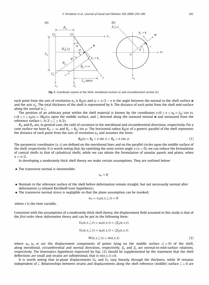
The geometry of shells considered hereafter is a surface of revolution. The notation for the coordinates is shown in Fig. 1for a generic conical shell. The coordinates along the meridional and circumferential directions are x and s, respectively. a isa semi-vertex angle of the cone while Rb is the shift of the axis x03 with reference to the axis of revolution x3. The distance of

ARTICLE IN PRESS

Fig. 1. Coordinate system of the shell: meridional section (a) and circumferential section (b).

F. Tornabene et al. / Journal of Sound and Vibration 328 (2009) 259–290 261

each point from the axis of revolution x3 is R0ðxÞ and j ¼ p=2� a is the angle between the normal to the shell surface nand the axis x03. The total thickness of the shell is represented by h. The distance of each point from the shell mid-surfacealong the normal is z.

The position of an arbitrary point within the shell material is known by the coordinates x ð0 � x � x0 ¼ L0= cos aÞ,s ð0 � s � s0ðxÞ ¼ WR0ðxÞÞ upon the middle surface, and z directed along the outward normal n and measured from thereference surface ð�h=2 � z � h=2Þ.

Rj and RW are, in general case, the radii of curvature in the meridional and circumferential directions, respectively. For acone surface we have Rj ¼ 1 and RW ¼ R0= sin j. The horizontal radius R0ðxÞ of a generic parallel of the shell representsthe distance of each point from the axis of revolution x3 and assumes the form:

R0ðxÞ ¼ Rb þ x sin a ¼ Rb þ x cos j (1)

The parametric coordinates (x, s) are defined on the meridional lines and on the parallel circles upon the middle surface ofthe shell, respectively. It is worth noting that, by vanishing the semi-vertex angle a (a ¼ 0), we can reduce the formulationof conical shells to that of cylindrical shells, while we can obtain the formulation of annular panels and plates, whena ¼ p=2.

In developing a moderately thick shell theory we make certain assumptions. They are outlined below:

�

wh

The transverse normal is inextensible:

�n � 0

�
Normals to the reference surface of the shell before deformation remain straight, but not necessarily normal afterdeformation (a relaxed Kirchhoff-Love hypothesis). � The transverse normal stress is negligible so that the plane assumption can be invoked:
sn ¼ snðx; s; z; tÞ ¼ 0

ere t is the time variable.

Consistent with the assumptions of a moderately thick shell theory, the displacement field assumed in this study is that ofthe first-order shear deformation theory and can be put in the following form:

Uxðx; s; z; tÞ ¼ uxðx; s; tÞ þ zbxðx; s; tÞ

Usðx; s; z; tÞ ¼ usðx; s; tÞ þ zbsðx; s; tÞ

Wðx; s; z; tÞ ¼ wðx; s; tÞ (2)

where ux; us; w are the displacement components of points lying on the middle surface ðz ¼ 0Þ of the shell,along meridional, circumferential and normal directions, respectively. bx and bs are normal-to-mid-surface rotations,respectively. The kinematics hypothesis expressed by Eqs. (2) should be supplemented by the statement that the shelldeflections are small and strains are infinitesimal, that is wðx; s; tÞ5h.

It is worth noting that in-plane displacements Ux and Us vary linearly through the thickness, while W remainsindependent of z. Relationships between strains and displacements along the shell reference (middle) surface z ¼ 0 are

ARTICLE IN PRESS


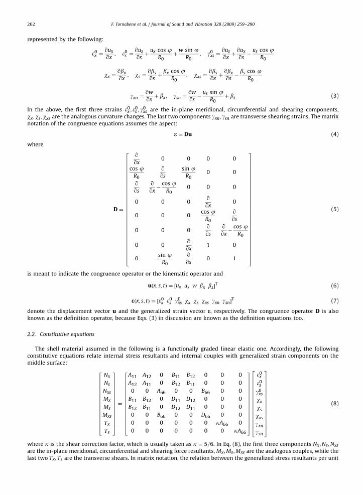
represented by the following:

�0x ¼

qux

qx; �0

s ¼qus

qsþ

ux cos jR0

þw sin j

R0; g0

xs ¼qus

qxþqux

qs�

us cos jR0

wx ¼qbx

qx; ws ¼

qbs

qsþbx cos j

R0; wxs ¼

qbs

qxþqbx

qs�bs cos j

R0

gxn ¼qw

qxþ bx; gsn ¼

qw

qs�

us sin jR0

þ bs (3)

In the above, the first three strains �0x ; �

0s ; g0

xs are the in-plane meridional, circumferential and shearing components,wx;ws;wxs are the analogous curvature changes. The last two components gxn; gsn are transverse shearing strains. The matrixnotation of the congruence equations assumes the aspect:

e ¼ Du (4)

where

D ¼

qqx

0 0 0 0

cos jR0

qqs

sin jR0

0 0

qqs

qqx�

cos jR0

0 0 0

0 0 0qqx

0

0 0 0cos j

R0

qqs

0 0 0qqs

qqx�

cos jR0

0 0qqx

1 0

0 �sin j

R0

qqs

0 1

26666666666666666666666666666664

37777777777777777777777777777775

(5)

is meant to indicate the congruence operator or the kinematic operator and

uðx; s; tÞ ¼ ½ux us w bx bs�T (6)

eðx; s; tÞ ¼ ½�0x �

0s g0

xs wx ws wxs gxn gsn�T (7)

denote the displacement vector u and the generalized strain vector e, respectively. The congruence operator D is alsoknown as the definition operator, because Eqs. (3) in discussion are known as the definition equations too.

2.2. Constitutive equations

The shell material assumed in the following is a functionally graded linear elastic one. Accordingly, the followingconstitutive equations relate internal stress resultants and internal couples with generalized strain components on themiddle surface:

Nx

Ns

Nxs

Mx

Ms

Mxs

Tx

Ts

2666666666666664

3777777777777775

¼

A11 A12 0 B11 B12 0 0 0

A12 A11 0 B12 B11 0 0 0

0 0 A66 0 0 B66 0 0

B11 B12 0 D11 D12 0 0 0

B12 B11 0 D12 D11 0 0 0

0 0 B66 0 0 D66 0 0

0 0 0 0 0 0 kA66 0

0 0 0 0 0 0 0 kA66

2666666666666664

3777777777777775

�0x

�0s

g0xs

wx

ws

wxs

gxn

gsn

26666666666666664

37777777777777775

(8)

where k is the shear correction factor, which is usually taken as k ¼ 5=6. In Eq. (8), the first three components Nx;Ns;Nxs

are the in-plane meridional, circumferential and shearing force resultants, Mx;Ms;Mxs are the analogous couples, while thelast two Tx; Ts are the transverse shears. In matrix notation, the relation between the generalized stress resultants per unit

ARTICLE IN PRESS


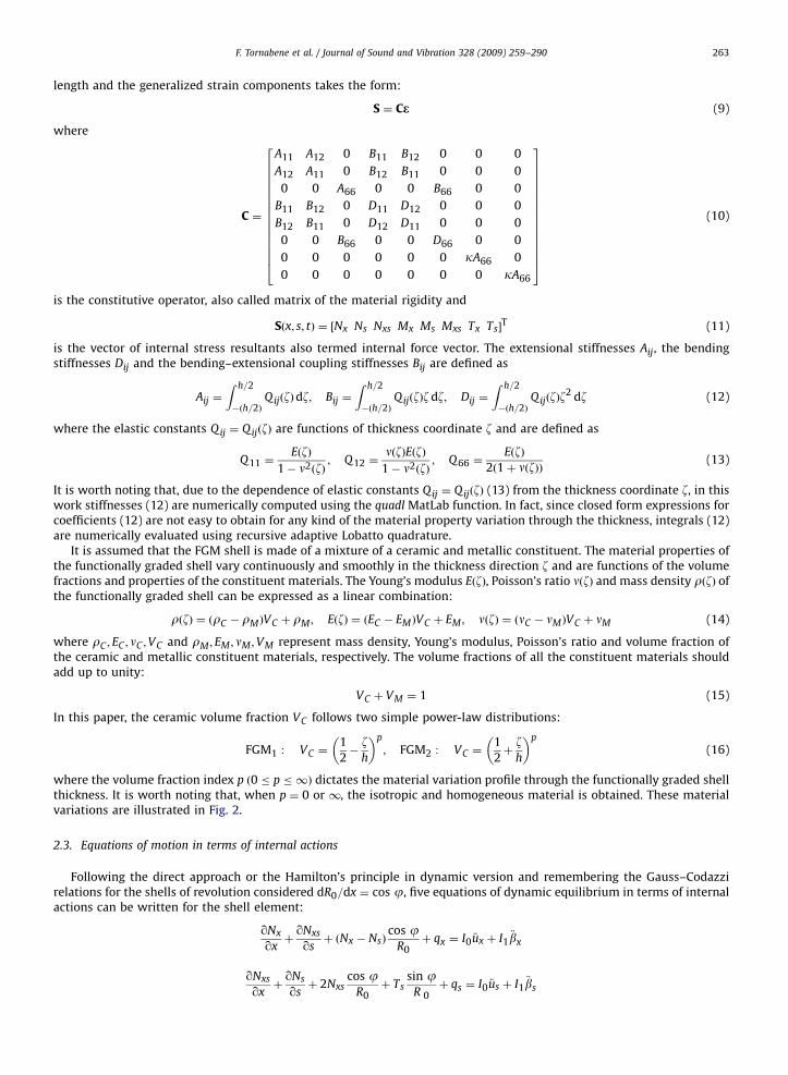
length and the generalized strain components takes the form:

S ¼ Ce (9)

where

C ¼

A11 A12 0 B11 B12 0 0 0

A12 A11 0 B12 B11 0 0 0

0 0 A66 0 0 B66 0 0

B11 B12 0 D11 D12 0 0 0

B12 B11 0 D12 D11 0 0 0

0 0 B66 0 0 D66 0 0

0 0 0 0 0 0 kA66 0

0 0 0 0 0 0 0 kA66

2666666666666664

3777777777777775

(10)

is the constitutive operator, also called matrix of the material rigidity and

Sðx; s; tÞ ¼ ½Nx Ns Nxs Mx Ms Mxs Tx Ts�T (11)

is the vector of internal stress resultants also termed internal force vector. The extensional stiffnesses Aij, the bendingstiffnesses Dij and the bending–extensional coupling stiffnesses Bij are defined as

Aij ¼

Z h=2

�ðh=2ÞQijðzÞdz; Bij ¼

Z h=2

�ðh=2ÞQijðzÞzdz; Dij ¼

Z h=2

�ðh=2ÞQijðzÞz

2 dz (12)

where the elastic constants Qij ¼ QijðzÞ are functions of thickness coordinate z and are defined as

Q11 ¼EðzÞ

1� n2ðzÞ; Q12 ¼

nðzÞEðzÞ1� n2ðzÞ

; Q66 ¼EðzÞ

2ð1þ nðzÞÞ (13)

It is worth noting that, due to the dependence of elastic constants Qij ¼ QijðzÞ (13) from the thickness coordinate z, in thiswork stiffnesses (12) are numerically computed using the quadl MatLab function. In fact, since closed form expressions forcoefficients (12) are not easy to obtain for any kind of the material property variation through the thickness, integrals (12)are numerically evaluated using recursive adaptive Lobatto quadrature.

It is assumed that the FGM shell is made of a mixture of a ceramic and metallic constituent. The material properties ofthe functionally graded shell vary continuously and smoothly in the thickness direction z and are functions of the volumefractions and properties of the constituent materials. The Young’s modulus EðzÞ, Poisson’s ratio nðzÞ and mass density rðzÞ ofthe functionally graded shell can be expressed as a linear combination:

rðzÞ ¼ ðrC � rMÞVC þ rM ; EðzÞ ¼ ðEC � EMÞVC þ EM ; nðzÞ ¼ ðnC � nMÞVC þ nM (14)

where rC ; EC ; nC ;VC and rM ; EM ; nM ;VM represent mass density, Young’s modulus, Poisson’s ratio and volume fraction ofthe ceramic and metallic constituent materials, respectively. The volume fractions of all the constituent materials shouldadd up to unity:

VC þ VM ¼ 1 (15)

In this paper, the ceramic volume fraction VC follows two simple power-law distributions:

FGM1 : VC ¼1

2�zh

� �p

; FGM2 : VC ¼1

2þzh

� �p

(16)

where the volume fraction index p ð0 � p � 1Þ dictates the material variation profile through the functionally graded shellthickness. It is worth noting that, when p ¼ 0 or 1, the isotropic and homogeneous material is obtained. These materialvariations are illustrated in Fig. 2.

2.3. Equations of motion in terms of internal actions

Following the direct approach or the Hamilton’s principle in dynamic version and remembering the Gauss–Codazzirelations for the shells of revolution considered dR0=dx ¼ cos j, five equations of dynamic equilibrium in terms of internalactions can be written for the shell element:

qNx

qxþqNxs

qsþ ðNx � NsÞ

cos jR0þ qx ¼ I0 €ux þ I1

€bx

qNxs

qxþqNs

qsþ 2Nxs

cos jR0þ Ts

sin jR 0þ qs ¼ I0 €us þ I1

€bs

ARTICLE IN PRESS

Fig. 2. Variation of the ceramic volume fraction VC through the thickness for different values of power-law index p: (a) FGM1 distribution and (b) FGM2

distribution.


qTx

qxþqTs

qsþ Tx

cos jR 0� Ns

sin jR0þ qn ¼ I0 €w

qMx

qxþqMxs

qsþ ðMx �MsÞ

cos jR0� Tx þmx ¼ I1 €ux þ I2

€bx

qMxs

qxþqMs

qsþ 2Mxs

cos jR0� Ts þms ¼ I1 €us þ I2

€bs (17)

where

Ii ¼

Z h=2

�h=2rðzÞzi 1þ

zRW

� �dz; i ¼ 0;1;2 (18)

are the mass inertias. The first three equations (17) represent translational equilibriums along meridional, circumferentialand normal directions, while the last two are rotational equilibrium equations about the x and s directions.

Equations of motion or dynamic equilibrium equations (17) can be written in the operatorial form:

D�S ¼ q�qKqt

or D�S ¼ f (19)

where

qðx; s; tÞ ¼ ½qx qs qn mx ms�T (20)

Kðx; s; tÞ ¼M _u (21)

are the distributed external load and the momentum vectors, respectively, and

M ¼

I0 0 0 I1 0

0 I0 0 0 I1

0 0 I0 0 0

I1 0 0 I2 0

0 I1 0 0 I2

26666664

37777775

(22)

is the mass matrix, while

_uðx; s; tÞ ¼qqt½ux us w bx bs�

T (23)

is the derivative of the displacement vector u with respect to the variable t, that is the vector velocity.

ARTICLE IN PRESS


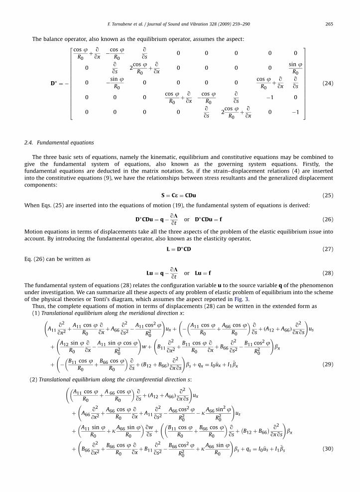
The balance operator, also known as the equilibrium operator, assumes the aspect:

D� ¼ �

cos jR0þ

qqx�

cos jR0

qqs

0 0 0 0 0

0qqs

2cos j

R0þ

qqx

0 0 0 0sin j

R0

0 �sin j

R00 0 0 0

cos jR0þ

qqx

qqs

0 0 0cos j

R0þ

qqx�

cos jR0

qqs

�1 0

0 0 0 0qqs

2cos j

R0þ

qqx

0 �1

2666666666666666664

3777777777777777775

(24)

2.4. Fundamental equations

The three basic sets of equations, namely the kinematic, equilibrium and constitutive equations may be combined togive the fundamental system of equations, also known as the governing system equations. Firstly, thefundamental equations are deducted in the matrix notation. So, if the strain–displacement relations (4) are insertedinto the constitutive equations (9), we have the relationships between stress resultants and the generalized displacementcomponents:

S ¼ Ce ¼ CDu (25)

When Eqs. (25) are inserted into the equations of motion (19), the fundamental system of equations is derived:

D�CDu ¼ q�qKqt

or D�CDu ¼ f (26)

Motion equations in terms of displacements take all the three aspects of the problem of the elastic equilibrium issue intoaccount. By introducing the fundamental operator, also known as the elasticity operator,

L ¼ D�CD (27)

Eq. (26) can be written as

Lu ¼ q�qKqt

or Lu ¼ f (28)

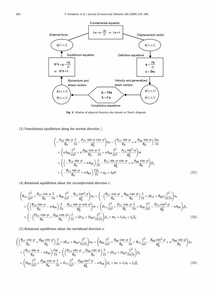
The fundamental system of equations (28) relates the configuration variable u to the source variable q of the phenomenonunder investigation. We can summarize all these aspects of any problem of elastic problem of equilibrium into the schemeof the physical theories or Tonti’s diagram, which assumes the aspect reported in Fig. 3.

Thus, the complete equations of motion in terms of displacements (28) can be written in the extended form as(1) Translational equilibrium along the meridional direction x:

A11q2

qx2þ

A11 cos jR0

qqxþ A66

q2

qs2�

A11 cos2 jR2

0

!ux þ �

A11 cos jR0

þA66 cos j

R0

� �qqsþ ðA12 þ A66Þ

q2

qxqs

!us

þA12 sin j

R0

qqx�

A11 sin j cos jR2

0

!wþ B11

q2

qx2þ

B11 cos jR0

qqxþ B66

q2

qs2�

B11 cos2 jR2

0

!bx

þ �B11 cos j

R0þ

B66 cos jR0

� �qqsþ ðB12 þ B66Þ

q2

qxqs

!bs þ qx ¼ I0 €ux þ I1

€bx (29)

(2) Translational equilibrium along the circumferential direction s:

A11 cos jR0

þA 66 cos j

R0

� �qqsþ ðA12 þ A66Þ

q2

qxqs

!ux

þ A66q2

@x2þ

A66 cos jR0

qqxþ A11

q2

qs2�

A66 cos2 jR2

0

� kA66 sin2 jR2

0

!us

þA11 sin j

R0þ kA66 sin j

R0

� �qw

qsþ

B11 cos jR0

þB66 cos j

R0

� �qqsþ B12 þ B66� � q2

qxqs

!bx

þ B66q2

qx2þ

B66 cos jR0

qqxþ B11

q2

qs2�

B66 cos2 jR2

0

þ kA66 sin jR0

!bs þ qs ¼ I0 €us þ I1

€bs (30)

ARTICLE IN PRESS

Fig. 3. Scheme of physical theories also known as Tonti’s diagram.


(3) Translational equilibrium along the normal direction z:

�A12 sin j

R0

qqx�

A11 sin j cos jR2

0

!ux �

A11 sin jR0

þ kA66 sin jR0

� �qus

qs

þ kA66q2

qx2þ kA66 cos j

R0

qqxþ kA66

q2

qs2�

A11 sin2 jR2

0

!w

þ �B12 sin j

R0þ kA66

� �qqx�

B11 sin j cos jR2

0

þ kA66 cos jR0

!bx

þ �B11 sin j

R0þ kA66

� �qbs

qsþ qn ¼ I0 €w (31)

(4) Rotational equilibrium about the circumferential direction s:

B11q2

qx2þ

B11 cos jR0

qqxþ B66

q2

qs2�

B11 cos2 jR2

0

!ux þ �

B11 cos jR0

þB66 cos j

R0


q2

qxqs

!us

þB12 sin j

R0� kA66

� �qqx�

B11 sin j cos jR2

0

!wþ D11

q2

qx2þ

D11 cos jR0

qqxþ D66

q2

qs2�

D11 cos2 jR2

0

� kA66

!bx

þ �D11 cos j

R0þ

D66 cos jR0

� �qqsþ ðD12 þ D66Þ

q2

qxqs

!bs þmx ¼ I1 €ux þ I2

€bx (32)

(5) Rotational equilibrium about the meridional direction x:

B11 cos jR0

þB66 cos j

R0


q2

qxqs

!ux þ B66

q2

qx2þ

B66 cos jR0

qqxþ B11

q2

qs2�

B66 cos2 jR2

0

þ kA66 sin jR0

!us

þB11 sin j

R0� kA44

� �qw

qsþ

D11 cos jR0

þD66 cos j

R0

� �qqsþ ðD12 þ D66Þ

q2

qxqs

!bx

þ D66q2

qx2þ

D66 cos jR0

qqxþ D11

q2

qs2�

D66 cos2 jR2

0

� kA66

!bs þms ¼ I1 €us þ I2

€bs (33)

ARTICLE IN PRESS


2.5. Boundary and compatibility conditions

In the following, three kinds of boundary conditions are considered, namely the fully clamped edge boundary condition(C), the simply supported edge boundary condition (S) and the free edge boundary condition (F). The equations describingthe boundary conditions can be written as follows:

Clamped edge boundary condition (C):

ux ¼ us ¼ w ¼ bx ¼ bs ¼ 0 at x ¼ 0 or x ¼ x0; 0 � s � s0 (34)

ux ¼ us ¼ w ¼ bx ¼ bs ¼ 0 at s ¼ 0 or s ¼ s0; 0 � x � x0 (35)

Simply supported edge boundary condition (S):

ux ¼ us ¼ w ¼ bs ¼ 0; Mx ¼ 0 at x ¼ 0 or x ¼ x0; 0 � s � s0 (36)

ux ¼ us ¼ w ¼ bx ¼ 0; Ms ¼ 0 at s ¼ 0 or s ¼ s0; 0 � x � x0 (37)

Free edge boundary condition (F):

Nx ¼ Nxs ¼ Tx ¼ Mx ¼ Mxs ¼ 0 at x ¼ 0 or x ¼ x0; 0 � s � s0 (38)

Ns ¼ Nxs ¼ Ts ¼ Ms ¼ Mxs ¼ 0 at s ¼ 0 or s ¼ s0; 0 � x � x0 (39)

In addition to the external boundary conditions, the kinematic and physical compatibility should be satisfied at the commonmeridian with s ¼ 0;2pR0, if we want to consider a complete shell of revolution. The kinematic compatibility conditionsinclude the continuity of displacements. The physical compatibility conditions can only be the five continuous conditionsfor the generalized stress resultants. To consider complete revolution conical, cylindrical shells and annular platescharacterized by s0 ¼ 2pR0, it is necessary to implement the kinematic and physical compatibility conditions between thetwo meridians with s ¼ 0 and s0 ¼ 2pR0:

Kinematic compatibility conditions:

uxðx;0; tÞ ¼ uxðx; s0; tÞ;usðx;0; tÞ ¼ usðx; s0; tÞ;wðx;0; tÞ ¼ wðx; s0; tÞ;

bxðx;0; tÞ ¼ bxðx; s0; tÞ;bsðx;0; tÞ ¼ bsðx; s0; tÞ0 � x � x0 (40)

Physical compatibility conditions:

Nsðx;0; tÞ ¼ Nsðx; s0; tÞ;Nxsðx;0; tÞ ¼ Nxsðx; s0; tÞ; Tsðx;0; tÞ ¼ Tsðx; s0; tÞ;

Msðx;0; tÞ ¼ Msðx; s0; tÞ;Mxsðx;0; tÞ ¼ Mxsðx; s0; tÞ0 � x � x0 (41)

3. Generalized differential quadrature method review

The GDQ method will be used to discretize the derivatives in the governing equations and the boundary conditions. TheGDQ approach was developed by Shu [44] to improve the differential quadrature technique [45,46] for the computation ofweighting coefficients, entering into the linear algebraic system of equations obtained from the discretization of thedifferential equation system, which can model the physical problem considered. The differential quadrature methodologyhas been applied in many fields of structural mechanics, as shown in the literature [38,47–51]. The essence of thedifferential quadrature method is that the partial derivative of a smooth function with respect to a variable is approximatedby a weighted sum of function values at all discrete points in that direction. Its weighting coefficients are not related to anyspecial problem and only depend on the grid points and the derivative order. In this methodology, an arbitrary griddistribution can be chosen without any limitation.

The GDQ method is based on the analysis of a high-order polynomial approximation and the analysis of a linear vectorspace [37]. For a general problem, it may not be possible to express the solution of the corresponding partial differentialequation in a closed form. This solution function can be approximated by the two following types of functionapproximation: high-order polynomial approximation and Fourier series expansion (harmonic functions). It is well knownthat a smooth function in a domain can be accurately approximated by a high-order polynomial in accordance with theWeierstrass polynomial approximation theorem. In fact, from the Weierstrass theorem, if f ðxÞ is a real valued continuousfunction defined in the closed interval ½a; b�, then there exists a sequence of polynomials PrðxÞ which converges to f ðxÞ

uniformly as r goes to infinity. In practical applications, a truncated finite polynomial may be used. Thus, if f ðxÞ representsthe solution of a partial differential equation, then it can be approximated by a polynomial of a degree less than or equal toN � 1, for N large enough. The conventional form of this approximation is

f ðxÞ ffi PNðxÞ ¼XNj¼1

djpjðxÞ (42)

ARTICLE IN PRESS


where dj is a constant. Then it is easy to show that the polynomial PNðxÞ constitutes an N-dimensional linear vector spaceVN with respect to the operation of vector addition and scalar multiplication. Obviously, in the linear vector space VN , pjðxÞ

is a set of base vectors. It can be seen that, in the linear polynomial vector space, there exist several sets of base polynomialsand each set of base polynomials can be expressed uniquely by another set of base polynomials in the space. Using vectorspace analysis, the method for computing the weighting coefficients can be generalized by a proper choice of basepolynomials in a linear vector space. For generality, the Lagrange interpolation polynomials are chosen as the basepolynomials. As a result, the weighting coefficients of the first-order derivative are computed by a simple algebraicformulation without any restriction on the choice of the grid points, while the weighting coefficients of the second andhigher order derivatives are given by a recurrence relationship.

When the Lagrange interpolated polynomials are assumed as a set of vector space base functions, the approximation ofthe function f ðxÞ can be written as

f ðxÞ ffiXNj¼1

pjðxÞf ðxjÞ (43)

where N is the number of grid points in the whole domain, xj, j ¼ 1;2; . . . ;N, are the coordinates of grid points in thevariable domain and f ðxjÞ are the function values at the grid points. pjðxÞ are the Lagrange interpolated polynomials, whichcan be defined by the following formula:

pjðxÞ ¼LðxÞ

ðx� xjÞLð1ÞðxjÞ

; j ¼ 1;2; . . . ;N (44)

where

LðxÞ ¼YNi¼1

ðx� xiÞ; Lð1ÞðxjÞ ¼YN

i¼1;iaj

ðxj � xiÞ (45)

Differentiating Eq. (43) with respect to x and evaluating the first derivative at a certain point of the function domain, it ispossible to obtain:

f ð1ÞðxiÞ ffiXNj¼1

pð1ÞjðxiÞf ðxjÞ ¼

XNj¼1

Bð1Þij

f ðxjÞ; i ¼ 1;2; . . . ;N (46)

where Bð1Þij

are the GDQ weighting coefficients of the first-order derivative and xi denote the coordinates of the grid points.In particular, it is worth noting that the weighting coefficients of the first-order derivative can be computed as

pð1ÞjðxiÞ ¼ Bð1Þ

ij¼

Lð1ÞðxiÞ

ðxi � xjÞLð1ÞðxjÞ

; i; j ¼ 1;2; . . . ;N; iaj (47)

From Eq. (47), Bð1ÞijðiajÞ can be easily computed. However, the calculation of Bð1Þ

iiis not easy to compute. According to the

analysis of a linear vector space, one set of base functions can be expressed uniquely by a linear sum of another set of basefunctions. Thus, if one set of base polynomials satisfy a linear equation like (46), so does another set of base polynomials. As

a consequence, the equation system for determining Bð1Þij

and derived from the Lagrange interpolation polynomials should

be equivalent to that derived from another set of base polynomials, i.e. pjðxÞ ¼ xj�1, j ¼ 1;2; . . . ;N. Thus, Bð1Þij

satisfies the

following equation, which is obtained by the base polynomials pjðxÞ ¼ xj�1, when j ¼ 1:

XNj¼1

Bð1Þij¼ 0 ) Bð1Þ

ii¼ �

XNj¼1;jai

Bð1Þij; i; j ¼ 1;2; . . . ;N (48)

Eqs. (47) and (48) are two formulations to compute the weighting coefficients Bð1Þij

. It should be noted that, in the development

of these formulations, two sets of base polynomials were used in the linear polynomial vector space VN . Finally, the n-th order

derivative of function f ðxÞ with respect to x at grid points xi, can be approximated by the GDQ approach:

dnf ðxÞ

dxn

��x¼xi

¼XNj¼1

BðnÞij

f ðxjÞ; i ¼ 1;2; :::;N (49)

where BðnÞij

are the weighting coefficients of the n-th order derivative. Similar to the first-order derivative and according to

the polynomial approximation and the analysis of a linear vector space, it is possible to determine a recurrence relationshipto compute the second and higher order derivatives. Thus, the weighting coefficients can be generated by the following

ARTICLE IN PRESS


recurrent formulation:

BðnÞij¼ n Bðn�1Þ

iiBð1Þ

ij�Bðn�1Þ

ij

xi � xj

0@

1A; iaj; n ¼ 2;3; . . . ;N � 1; i; j ¼ 1;2; . . . ;N (50)

XNj¼1

BðnÞij¼ 0 ) BðnÞ

ii¼ �

XNj¼1;jai

BðnÞij; n ¼ 2;3; . . . ;N � 1; i; j ¼ 1;2; . . . ;N (51)

It is obvious from the above equations that the weighting coefficients of the second and higher order derivatives can bedetermined from those of the first-order derivative. Furthermore, it is interesting to note that, the preceding coefficients

BðnÞij

are dependent on the derivative order n, on the grid point distribution xj, j ¼ 1;2; . . . ;N, and on the specific point xi,

where the derivative is computed. There is no need to obtain the weighting coefficients from a set of algebraic equationswhich could be ill-conditioned when the number of grid points is large. The merit of the explicit formulae (47), (48), (50)and (51) is that highly accurate weighting coefficients may be determined for any number of arbitrarily spaced samplingpoints. Furthermore, this set of expressions for the determination of the weighting coefficients is so compact and simplethat it is very easy to implement them in formulating and programming, because of the recurrence feature.

3.1. Grid distributions

Another important point for successful application of the GDQ method is how to distribute the grid points. The gridpoint distribution also plays an essential role in determining the accuracy, the convergence speed and the stability of theGDQ method. In this paper, the effects of the grid point distribution will be investigated for the vibration analysis of conical,cylindrical shells and annular plates. The natural and simplest choice of the grid points through the computational domainis the one having equally spaced points in the coordinate direction of the computational domain. However, it isdemonstrated that non-uniform grid distribution usually yields better results than equally spaced distribution. Quan andChang [52,53] compared numerically the performances of the often-used non-uniform meshes and concluded that the gridpoints originating from the Chebyshev polynomials of the first kind are optimum in all the cases examined there. The zerosof orthogonal polynomials are the rational basis for the grid points. Shu [44] used a choice which gives better results thanthe zeros of Chebyshev and Legendre polynomials. Bert and Malik [38] indicated that the preferred type of grid pointschanges with problems of interest and recommended the use of Chebyshev–Gauss–Lobatto grid for the structuralmechanics computation. With Lagrange interpolating polynomials, the rule of Chebyshev–Gauss–Lobatto (C–G–L)sampling points proves efficient for numerical reasons [54] and for such a collocation the approximation error of thedependent variables decreases as the number of nodes increases. In this study, different grid point distributions areconsidered to investigate their effect on the GDQ solution accuracy, convergence speed and stability.

The typical distributions of grid points, which are commonly used in the literature, in normalized form are reported asfollows:

Equally spaced or uniform distribution (Uni)

ri ¼i� 1

N � 1; i ¼ 1;2; . . . ;N (52)

Roots of Chebyshev polynomials of the first kind (C I1)

ri ¼gi � g1

gN � g1; gi ¼ cos

2i� 1

2N

� �p

� �; i ¼ 1;2; . . . ;N (53)

Roots of Chebyshev polynomials of the second kind (C II1)

ri ¼gi � g1

gN � g1; gi ¼ cos

ipN þ 1

� �; i ¼ 1;2; . . . ;N (54)

Roots of Legendre polynomials (Leg)

ri ¼gi � g1

gN � g1; gi ¼ 1�

1

8N2þ

1

8N3

� �cos

4i� 1

4N þ 2p

� �; i ¼ 1;2; . . . ;N (55)

Quadratic sampling points distribution (Quad)

ri ¼

2i� 1

N � 1

� �2

i ¼ 1;2; . . . ;N þ 1

2

�2i� 1

N � 1

� �2

þ 4i� 1

N � 1

� �� 1

!i ¼

N þ 1

2

� �þ 1; . . . ;N

8>>>>><>>>>>:

(56)

ARTICLE IN PRESS

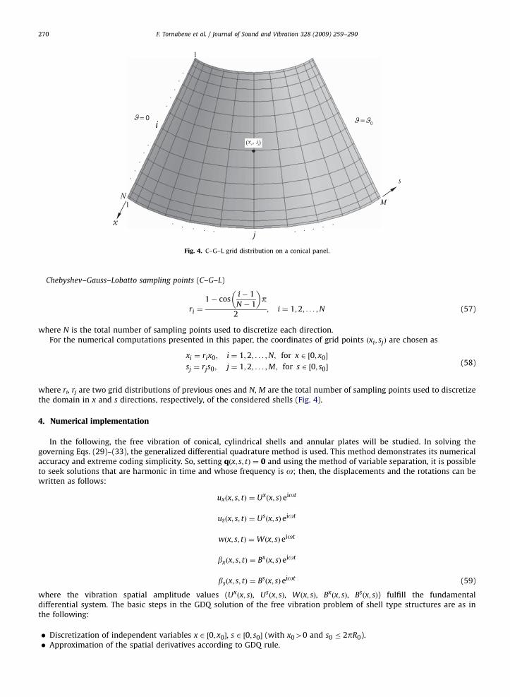
Fig. 4. C–G–L grid distribution on a conical panel.


Chebyshev–Gauss–Lobatto sampling points (C–G–L)

ri ¼

1� cosi� 1

N � 1

� �p

2; i ¼ 1;2; . . . ;N (57)

where N is the total number of sampling points used to discretize each direction.For the numerical computations presented in this paper, the coordinates of grid points ðxi; sjÞ are chosen as

xi ¼ rix0; i ¼ 1;2; . . . ;N; for x 2 ½0; x0�

sj ¼ rjs0; j ¼ 1;2; . . . ;M; for s 2 ½0; s0�(58)

where ri, rj are two grid distributions of previous ones and N, M are the total number of sampling points used to discretizethe domain in x and s directions, respectively, of the considered shells (Fig. 4).

4. Numerical implementation

In the following, the free vibration of conical, cylindrical shells and annular plates will be studied. In solving thegoverning Eqs. (29)–(33), the generalized differential quadrature method is used. This method demonstrates its numericalaccuracy and extreme coding simplicity. So, setting qðx; s; tÞ ¼ 0 and using the method of variable separation, it is possibleto seek solutions that are harmonic in time and whose frequency is o; then, the displacements and the rotations can bewritten as follows:

uxðx; s; tÞ ¼ Uxðx; sÞ eiot

usðx; s; tÞ ¼ Usðx; sÞ eiot

wðx; s; tÞ ¼Wðx; sÞ eiot

bxðx; s; tÞ ¼ Bxðx; sÞ eiot

bsðx; s; tÞ ¼ Bsðx; sÞ eiot (59)

where the vibration spatial amplitude values (Uxðx; sÞ, Usðx; sÞ, Wðx; sÞ, Bxðx; sÞ, Bsðx; sÞ) fulfill the fundamentaldifferential system. The basic steps in the GDQ solution of the free vibration problem of shell type structures are as inthe following:

�
Discretization of independent variables x 2 ½0; x0�, s 2 ½0; s0� (with x040 and s0 � 2pR0). � Approximation of the spatial derivatives according to GDQ rule.

ARTICLE IN PRESS


�
Transformation of the differential governing systems (29), (30), (31), (32), and (33) into linear eigenvalue problems forthe natural frequencies. The boundary and compatibility conditions are imposed in the sampling points correspondingto the boundary. All these relations are imposed point-wise. These resulting equations constitute a well-posedeigenvalue problem where the number of equations is identical to the number of unknowns. � Solution of the previously stated discrete system in terms of natural frequencies and mode shape components. For each
mode, local values of dependent variables are used to obtain the complete assessment of the deformedconfiguration.

4.1. Discretization of motion equations

The GDQ procedure enable one to write the equations of motion in discrete form, transforming each space derivativeinto a weighted sum of node values of dependent variables. Each approximate equation is valid in a single sampling point.The governing equations can be discretized as

(1) Translational equilibrium along the meridional direction x:

A11

XNk¼1

Bxð2Þik

Uxkj þ

A11 cos ji

R0i

XNk¼1

Bxð1Þik

Uxkj þ A66

XMm¼1

Bsð2Þjm

Uxim �

A11 cos2 ji

R20i

Uxij

�A11 cos ji

R0iþ

A66 cos ji

R0i

� � XMm¼1

Bsð1Þjm

Usim þ ðA12 þ A66Þ

XNk¼1

Bxð1Þik

XMm¼1

Bsð1Þjm

Uskm

þA12 sin ji

R0i

XNk¼1

Bxð1Þik

Wkj �A11 sin ji cos ji

R20i

Wij þ B11

XNk¼1

Bxð2Þik

Bxkj þ

B11 cos ji

R0i

XNk¼1

Bxð1Þik

Bxkj

þ B66

XMm¼1

Bsð2Þjm

Bxim �

B11 cos2 ji

R20i

Bxij �

B11 cos ji

R0iþ

B66 cos ji

R0i

� � XMm¼1

Bsð1Þjm

Bsim

þ ðB12 þ B66ÞXNk¼1

Bxð1Þik

XMm¼1

Bsð1Þjm

Bskm ¼ �o

2ðI0Uxij þ I1Bx

ijÞ (60)

(2) Translational equilibrium along the circumferential direction s:

A11 cos ji

R0iþ

A66 cos ji

R0i

� � XMm¼1

Bsð1Þjm

Uxim þ ðA12 þ A66Þ

XNk¼1

Bxð1Þik

XMm¼1

Bsð1Þjm

Uxkm þ A66

XNk¼1

Bxð2Þik

Uskj

þA66 cos ji

R0i

XNk¼1

Bxð1Þik

Uskj þ A11

XMm¼1

Bsð2Þjm

Usim �

A66 cos2 ji

R20i

þ kA66 sin2 ji

R20i

!Us

ij

þA11 sin ji

R0iþ kA66 sin ji

R0i

� � XMm¼1

Bsð1Þjm

Wim þB11 cos ji

R0iþ

B66 cos ji

R0i

� � XMm¼1

Bsð1Þjm

Bxim

þ ðB12 þ B66ÞXNk¼1

Bxð1Þik

XMm¼1

Bsð1Þjm

Bxkm þ B66

XNk¼1

Bxð2Þik

Bskj þ

B66 cos ji

R0i

XNk¼1

Bxð1Þik

Bskj

þ B11

XMm¼1

Bsð2Þjm

Bsim �

B66 cos2 ji

R20i

� kA66 sin ji

R0i

!Bs

ij ¼ �o2ðI0Us

ij þ I1BsijÞ (61)

(3) Translational equilibrium along the normal direction z:

�A12 sin ji

R0i

XNk¼1

Bxð1Þik

Uxkj �

A11 sin ji cos ji

R20i

Uxij �

A11 sin ji

R0iþ kA66 sin ji

R0i

� � XMm¼1

Bsð1Þjm

Usim

þ kA66

XNk¼1

Bxð2Þik

Wkj þ kA66 cos ji

R0i

XNk¼1

Bxð1Þik

Wkj þ kA66

XMm¼1

Bsð2Þjm

Wim �A11 sin2 ji

R20i

Wij

�B12 sin ji

R0i� kA66

� �XNk¼1

Bxð1Þik

Bxkj �

B11 sin ji cos ji

R20i

� kA66 cos ji

R0i

!Bx

ij

�B11 sin ji

R0i� kA66

� � XMm¼1

Bsð1Þjm

Bsim ¼ �o

2I0Wij (62)

ARTICLE IN PRESS


(4) Rotational equilibrium about the circumferential direction s:

B11

XNk¼1

Bxð2Þik

Uxkj þ

B11 cos ji

R0i

XNk¼1

Bxð1Þik

Uxkj þ B66

XMm¼1

Bsð2Þjm

Uxim �

B11 cos2 ji

R20i

Uxij

�B11 cos ji

R0iþ

B66 cos ji

R0i

� � XMm¼1

Bsð1Þjm

Usim þ ðB12 þ B66Þ

XNk¼1

Bxð1Þik

XMm¼1

Bsð1Þjm

Uskm

þB12 sin ji

R0i� kA66

� �XNk¼1

Bxð1Þik

Wkj �B11 sin ji cos ji

R20i

Wij þ D11

XNk¼1

Bxð2Þik

Bxkj

þD11 cos ji

R0i

XNk¼1

Bxð1Þik

Bxkj þ D66

XMm¼1

Bsð2Þjm

Bxim �

D11 cos2 ji

R20i

þ kA66

!Bx

ij

�D11 cos ji

R0iþ

D66 cos ji

R0i

� � XMm¼1

Bsð1Þjm

Bsim þ ðD12 þ D66Þ

XNk¼1

Bxð1Þik

XMm¼1

Bsð1Þjm

Bskm

¼ �o2ðI1Uxij þ I2Bx

ijÞ (63)

(5) Rotational equilibrium about the meridional direction x:

B11 cos ji

R0iþ

B66 cos ji

R0i

� � XMm¼1

Bsð1Þjm

Uxim þ ðB12 þ B66Þ

XNk¼1

Bxð1Þik

XMm¼1

Bsð1Þjm

Uxkm þ B66

XNk¼1

Bxð2Þik

Uskj

þB66 cos ji

R0i

XNk¼1

Bxð1Þik

Uskj þ B11

XMm¼1

Bsð2Þjm

Usim �

B66 cos2 ji

R20i

� kA66 sin ji

R0i

!Us

ij

þB11 sin ji

R0i� kA66

� � XMm¼1

Bsð1Þjm

Wim þD11 cos ji

R0iþ

D66 cos ji

R0i

� � XMm¼1

Bsð1Þjm

Bxim

þ ðD12 þ D66ÞXNk¼1

Bxð1Þik

XMm¼1

Bsð1Þjm

Bxkm þ D66

XNk¼1

Bxð2Þik

Bskj þ

D66 cos ji

R0i

XNk¼1

Bxð1Þik

Bskj

þ D11

XMm¼1

Bsð2Þjm

Bsim �

D66 cos2 ji

R20i

þ kA66

!Bs

ij ¼ �o2ðI1Us

ij þ I2BsijÞ (64)

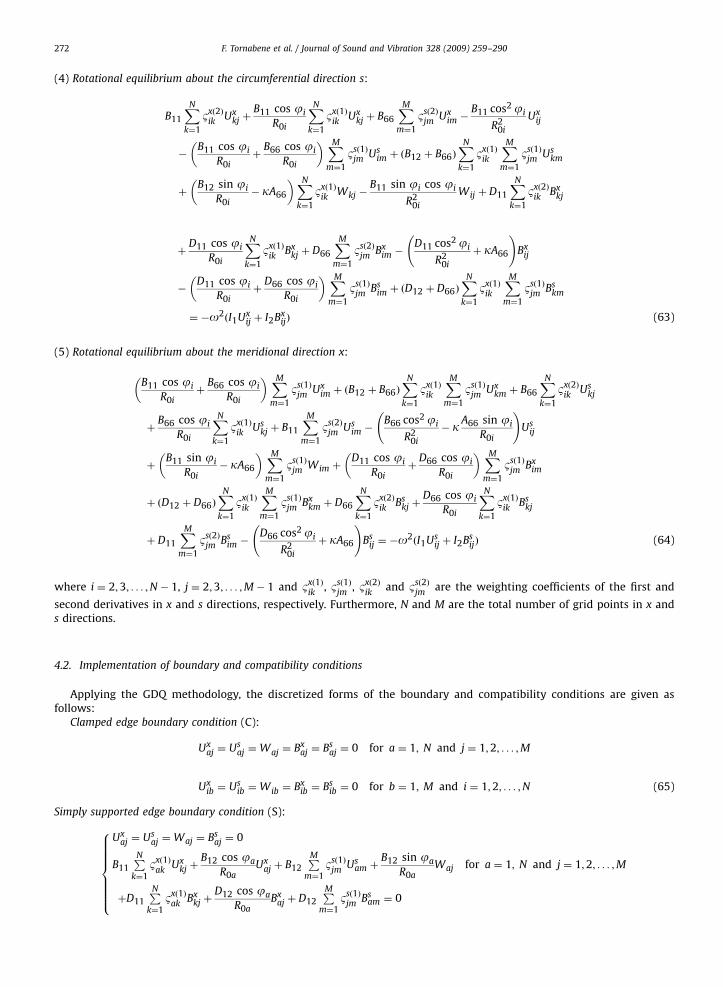
where i ¼ 2;3; . . . ;N � 1, j ¼ 2;3; . . . ;M � 1 and Bxð1Þik

, Bsð1Þjm

, Bxð2Þik

and Bsð2Þjm

are the weighting coefficients of the first and

second derivatives in x and s directions, respectively. Furthermore, N and M are the total number of grid points in x ands directions.

4.2. Implementation of boundary and compatibility conditions

Applying the GDQ methodology, the discretized forms of the boundary and compatibility conditions are given asfollows:

Clamped edge boundary condition (C):

Uxaj ¼ Us

aj ¼Waj ¼ Bxaj ¼ Bs

aj ¼ 0 for a ¼ 1; N and j ¼ 1;2; . . . ;M

Uxib ¼ Us

ib ¼Wib ¼ Bxib ¼ Bs

ib ¼ 0 for b ¼ 1; M and i ¼ 1;2; . . . ;N (65)

Simply supported edge boundary condition (S):

Uxaj ¼ Us

aj ¼Waj ¼ Bsaj ¼ 0

B11PN

k¼1Bxð1Þ

akUx

kj þB12 cos ja

R0aUx

aj þ B12PM

m¼1Bsð1Þ

jmUs

am þB12 sin ja

R0aWaj for a ¼ 1; N and j ¼ 1;2; . . . ;M

þD11PN

k¼1Bxð1Þ

akBx

kj þD12 cos ja

R0aBx

aj þ D12PM

m¼1Bsð1Þ

jmBs

am ¼ 0

8>>>>>>><>>>>>>>:

ARTICLE IN PRESS


Uxib ¼ Us

ib ¼Wib ¼ Bxib ¼ 0

B12PN

k¼1Bxð1Þ

ikUx

kb þB11 cos ji

R0iUx

ib þ B11PM

m¼1Bsð1Þ

bmUs

im þB11 sin ji

R0iWib for b ¼ 1; M and i ¼ 1;2; . . . ;N

þD12PN

k¼1Bxð1Þ

ikBx

kb þD11 cos ji

R0iBx

ib þ D11PM

m¼1Bsð1Þ

bmBs

im ¼ 0

8>>>>>>><>>>>>>>:

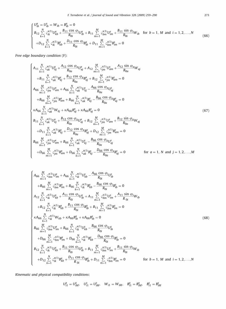
(66)

Free edge boundary condition (F):

A11PN

k¼1Bxð1Þ

akUx

kj þA12 cos ja

R0aUx

aj þ A12PM

m¼1Bsð1Þ

jmUs

am þA12 sin ja

R0aWaj

þB11PN

k¼1Bxð1Þ

akBx

kj þB12 cos ja

R0aBx

aj þ B12PM

m¼1Bsð1Þ

jmBs

am ¼ 0

A66PM

m¼1Bsð1Þ

jmUx

am þ A66PN

k¼1Bxð1Þ

akUs

kj �A66 cos ja

R0aUs

aj

þB66PM

m¼1Bsð1Þ

jmBx

am þ B66PN

k¼1Bxð1Þ

akBs

kj �B66 cos ja

R0aBs

aj ¼ 0

kA66PN

k¼1Bxð1Þ

akWkj þ kA66Bx

aj þ kA66Bsaj ¼ 0

B11PN

k¼1Bxð1Þ

akUx

kj þB12 cos ja

R0aUx

aj þ B12PM

m¼1Bsð1Þ

jmUs

am þB12 sin ja

R0aWaj

þD11PN

k¼1Bxð1Þ

akBx

kj þD12 cos ja

R0aBx

aj þ D12PM

m¼1Bsð1Þ

jmBs

am ¼ 0

B66PM

m¼1Bsð1Þ

jmUx

am þ B66PN

k¼1Bxð1Þ

akUs

kj �B66 cos ja

R0aUs

aj

þD66PM

m¼1Bsð1Þ

jmBx

am þ D66PN

k¼1Bxð1Þ

akBs

kj �D66 cos ja

R0aBs

aj ¼ 0 for a ¼ 1; N and j ¼ 1;2; . . . ;M

8>>>>>>>>>>>>>>>>>>>>>>>>>>>>>>>>>>>>>>>>>>><>>>>>>>>>>>>>>>>>>>>>>>>>>>>>>>>>>>>>>>>>>>:

(67)

A66PM

m¼1Bsð1Þ

bmUx

im þ A66PN

k¼1Bxð1Þ

ikUs

kb �A66 cos ji

R0iUs

ib

þB66PM

m¼1Bsð1Þ

bmBx

im þ B66PN

k¼1Bxð1Þ

ikBs

kb �B66 cos ji

R0iBs

ib ¼ 0

A12PN

k¼1Bxð1Þ

ikUx

kb þA11 cos ji

R0iUx

ib þ A11PM

m¼1Bsð1Þ

bmUs

im þA11 sin ji

R 0iWib

þB12PN

k¼1Bxð1Þ

ikBx

kb þB11 cos ji

R0iBx

ib þ B11PM

m¼1Bsð1Þ

bmBs

im ¼ 0

kA66PN

k¼1Bxð1Þ

ikWkb þ kA66Bx

ib þ kA66Bsib ¼ 0

B66PM

m¼1Bsð1Þ

bmUx

im þ B66PN

k¼1Bxð1Þ

ikUs

kb �B66 cos ji

R0iUs

ib

þD66PM

m¼1Bsð1Þ

bmBx

im þ D66PN

k¼1Bxð1Þ

ikBs

kb �D66 cos ji

R0iBs

ib ¼ 0

B12PN

k¼1Bxð1Þ

ikUx

kb þB11 cos ji

R0iUx

ib þ B11PM

m¼1Bsð1Þ

bmUs

im þB11 sin ji

R0iWib

þD12PN

k¼1Bxð1Þ

ikBx

kb þD11 cos ji

R 0iBx

ib þ D11PM

m¼1Bsð1Þ

bmBs

im ¼ 0 for b ¼ 1; M and i ¼ 1;2; . . . ;N

8>>>>>>>>>>>>>>>>>>>>>>>>>>>>>>>>>>>>>>>>>>><>>>>>>>>>>>>>>>>>>>>>>>>>>>>>>>>>>>>>>>>>>>:

(68)

Kinematic and physical compatibility conditions:

Uxi1 ¼ Ux

iM ; Usi1 ¼ Us

iM ; Wi1 ¼WiM ; Bxi1 ¼ Bx

iM ; Bsi1 ¼ Bs

iM

ARTICLE IN PRESS


A66PM

m¼1Bsð1Þ

1m Uxim þ A66

PNk¼1

Bxð1Þik

Usk1 �

A66 cos ji

R0iUs

i1

þB66PM

m¼1Bsð1Þ

1m Bxim þ B66

PNk¼1

Bxð1Þik

Bsk1 �

B66 cos ji

R0iBs

i1

¼ A66PM

m¼1Bsð1Þ

MmUxim þ A66

PNk¼1

Bxð1Þik

UskM �

A66 cos ji

R0iUs

iM

þB66PM

m¼1Bsð1Þ

MmBxim þ B66

PNk¼1

Bxð1Þik

BskM �

B66 cos ji

R0iBs

iM

A12PN

k¼1Bxð1Þ

ikUx

k1 þA22 cos ji

R0iUx

i1 þ A11PM

m¼1Bsð1Þ

1m Usim þ

A11 sin ji

R0iWi1

þB12PN

k¼1Bxð1Þ

ikBx

k1 þB11 cos ji

R0iBx

i1 þ B11PM

m¼1Bsð1Þ

1m Bsim

¼ A12PN

k¼1Bxð1Þ

ikUx

kM þA11 cos ji

R0iUx

iM þ A11PM

m¼1Bsð1Þ

MmUsim þ

A11 sinji

R0iWiM

þB12PN

k¼1Bxð1Þ

ikBx

kM þB11 cos ji

R0iBx

iM þ B11PM

m¼1Bsð1Þ

MmBsim

kA66PN

k¼1Bxð1Þ

ikWk1 þ kA66Bx

i1 þ kA66Bsi1

¼ kA66PN

k¼1Bxð1Þ

ikWkM þ kA66Bx

iM þ kA66BsiM

B66PM

m¼1Bsð1Þ

1m Ujimþ B66

PNk¼1

Bxð1Þik

Usk1 �

B66 cos ji

R0iUs

i1

þD66PM

m¼1Bsð1Þ

1m Bxim þ D66

PNk¼1

Bxð1Þik

Bsk1 �

D66 cos ji

R0iBs

i1

¼ B66PM

m¼1Bsð1Þ

MmUxim þ B66

PNk¼1

Bxð1Þik

UskM �

B66 cos ji

R0iUs

iM

þD66PM

m¼1Bsð1Þ

MmBxim þ D66

PNk¼1

Bxð1Þik

BskM �

D66 cos ji

R0iBs

iM

B12PN

k¼1Bxð1Þ

ikUx

k1 þB11 cos ji

R0iUx

i1 þ B11PM

m¼1Bsð1Þ

1m Usim þ

B11 sin ji

R0iWi1

þD12PN

k¼1Bxð1Þ

ikBx

k1 þD11 cos ji

R0iBx

i1 þ D11PM

m¼1Bsð1Þ

1m Bsim

¼ B12PN

k¼1Bxð1Þ

ikUx

kM þB11 cos ji

R0iUx

iM þ B11PM

m¼1Bsð1Þ

MmUsim þ

B11 sin ji

R0iWiM

þD12PN

k¼1Bxð1Þ

ikBx

kM þD11 cos ji

R0iBx

iM þ D11PM

m¼1Bsð1Þ

MmBsim for i ¼ 2; . . . ;N � 1

8>>>>>>>>>>>>>>>>>>>>>>>>>>>>>>>>>>>>>>>>>>>>>>>>>>>>>>>>>>>>>>>>>>>>>>>>>>>>>>>>>>>>>>>>>>>>><>>>>>>>>>>>>>>>>>>>>>>>>>>>>>>>>>>>>>>>>>>>>>>>>>>>>>>>>>>>>>>>>>>>>>>>>>>>>>>>>>>>>>>>>>>>>>:

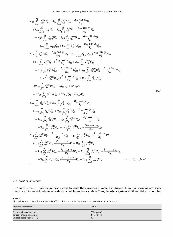
(69)

4.3. Solution procedure

Applying the GDQ procedure enables one to write the equations of motion in discrete form, transforming any spacederivative into a weighted sum of node values of dependent variables. Thus, the whole system of differential equations has

Table 1Physical parameters used in the analysis of free vibrations of the homogeneous isotropic structures ðp ¼ 1Þ.

Physical parameter Value

Density of mass r ¼ rM 7800 kg/m3

Young’s modulus E ¼ EM 2.11011 Pa

Poisson coefficient n ¼ nM 0.3

ARTICLE IN PRESS

Table 2The first 10 frequencies for the conical panel C–F–F–F.

Frequencies (Hz) GDQ method Abaqus Ansys Nastran Straus Pro/Mechanica

f 1 76.80 77.06 77.12 77.23 76.99 77.06

f 2 106.53 106.84 107.15 106.92 106.89 106.82

f 3 152.17 152.54 152.63 152.82 152.14 152.54

f 4 187.12 187.94 188.31 188.57 187.64 187.92

f 5 248.57 249.37 250.60 250.21 249.39 249.30

f 6 262.12 261.46 262.79 262.36 261.40 261.45

f 7 308.50 308.37 308.97 309.19 307.24 308.34

f 8 345.90 346.86 348.48 348.68 346.45 346.86

f 9 380.15 379.80 382.67 381.47 380.08 379.99

f 10 400.73 401.52 404.08 403.66 401.78 401.50

Table 3The first 10 frequencies for the cylindrical panel C–F–F–F.


f 1 58.32 58.91 58.84 59.01 58.97 58.92

f 2 90.62 91.82 91.94 91.84 91.77 91.79

f 3 146.35 144.59 145.21 144.99 145.08 144.59

f 4 230.72 232.46 233.09 233.32 232.34 232.46

f 5 263.63 266.07 267.33 267.19 266.62 266.07

f 6 278.56 278.88 278.98 278.78 278.47 278.69

f 7 339.43 338.80 342.11 340.93 341.58 338.81

f 8 430.81 427.44 429.12 428.59 427.02 427.25

f 9 489.26 488.07 493.18 491.86 491.01 488.22

f 10 511.30 512.94 517.49 517.13 514.68 513.06

Table 4The first 10 frequencies for the annular panel C–F–F–F.


f 1 60.36 60.37 60.44 60.42 60.40 60.42

f 2 131.86 131.82 132.12 132.22 132.01 132.07

f 3 241.48 241.51 242.79 242.64 242.29 241.75

f 4 278.48 278.50 280.06 279.76 279.36 278.75

f 5 363.05 363.07 365.49 365.56 364.81 363.60

f 6 410.96 410.89 414.08 413.56 412.09 411.89

f 7 544.02 544.04 549.38 548.91 547.93 544.62

f 8 597.35 597.44 603.81 602.43 599.55 599.12

f 9 681.37 681.43 689.79 688.57 686.32 682.03

f 10 754.15 754.21 763.97 763.10 760.43 755.49

Table 5The first 10 frequencies for the conical dome C–F.


f 1 200.69 200.52 200.59 200.74 200.29 200.47

f 2 200.69 200.52 200.59 200.74 200.29 200.47

f 3 221.65 221.28 221.82 221.52 221.26 221.32

f 4 221.65 221.28 221.82 221.52 221.26 221.34

f 5 274.77 275.35 275.35 274.55 274.71 274.96

f 6 274.77 275.35 275.35 274.55 274.71 275.07

f 7 308.30 308.38 308.26 308.24 308.05 308.22

f 8 308.30 308.38 308.26 308.24 308.05 308.22

f 9 341.16 340.08 340.53 340.49 339.52 340.04

f 10 341.16 340.08 340.53 340.49 339.52 340.05


ARTICLE IN PRESS

Table 6The first 10 frequencies for the cylinder C–F.


f 1 146.17 144.82 145.02 144.96 144.88 144.81

f 2 146.17 144.82 145.02 144.96 144.88 144.81

f 3 210.32 208.81 209.58 209.45 209.52 208.82

f 4 210.32 208.81 209.58 209.45 209.52 208.83

f 5 242.55 242.61 242.69 242.43 242.53 242.42

f 6 242.55 242.61 242.69 242.43 242.53 242.42

f 7 366.58 365.52 367.97 367.57 367.72 365.58

f 8 366.58 365.52 367.97 367.57 367.72 365.60

f 9 401.91 403.17 402.74 402.42 402.78 402.45

f 10 412.36 408.28 411.12 409.57 410.08 408.25

Table 7The first 10 frequencies for the annular plate C–F.


f 1 67.03 67.03 67.09 67.07 67.07 67.02

f 2 121.86 121.86 122.02 122.08 122.01 121.99

f 3 121.86 121.86 122.02 122.08 122.01 121.99

f 4 203.17 203.17 203.71 203.63 203.70 203.18

f 5 203.17 203.17 203.71 203.63 203.70 203.18

f 6 283.85 283.85 285.44 285.22 285.19 283.85

f 7 302.85 302.85 304.12 303.81 304.09 302.91

f 8 302.85 302.85 304.12 303.81 304.09 302.91

f 9 340.65 340.65 342.59 342.54 342.33 341.12

f 10 340.65 340.65 342.59 342.54 342.33 341.12

Table 8The first 10 frequencies for conical shells characterized by different boundary conditions.

Frequencies (Hz) Conical panel Conical dome

C–F–C–F F–S–F–S S–S–F–F C–C S–S C–S

f 1 122.73 74.28 90.92 227.59 208.69 225.59

f 2 135.28 125.33 170.04 227.59 208.69 225.59

f 3 241.48 224.79 232.33 239.71 222.70 234.82

f 4 256.59 258.79 272.43 239.71 222.70 234.82

f 5 287.24 288.70 312.85 275.27 250.33 275.11

f 6 293.42 327.04 324.61 275.27 250.33 275.11

f 7 381.19 360.93 374.71 333.69 318.11 331.96

f 8 421.65 388.22 411.13 333.69 318.11 331.96

f 9 463.67 444.46 454.88 350.59 318.66 350.58

f 10 494.98 480.42 488.36 350.59 318.66 350.58

Table 9The first 10 frequencies for cylindrical shells characterized by different boundary conditions.

Frequencies (Hz) Cylindrical panel Cylinder


f 1 204.87 168.18 76.18 360.36 331.15 344.78

f 2 222.97 364.40 188.14 360.36 331.15 344.78

f 3 383.58 407.33 232.26 375.86 348.46 361.52

f 4 441.11 421.67 285.37 375.86 348.46 361.52

f 5 467.98 634.29 428.84 463.29 440.86 451.18

f 6 474.78 651.69 467.63 463.29 440.86 451.18

f 7 715.01 717.89 537.52 523.55 508.07 515.53

f 8 719.14 781.15 573.73 523.55 508.07 515.53

f 9 725.44 792.79 673.55 646.56 596.25 628.74

f 10 736.76 806.95 731.76 646.56 596.25 628.74


ARTICLE IN PRESS

Table 10The first 10 frequencies for annular plates characterized by different boundary conditions.

Frequencies (Hz) Annular panel Annular plate


f 1 235.47 13.52 57.68 238.05 115.42 182.68

f 2 249.30 76.326 150.27 246.01 129.88 196.69

f 3 307.53 159.11 233.13 246.01 129.88 196.69

f 4 424.25 167.87 288.57 275.54 175.58 242.03

f 5 592.67 287.65 401.53 275.54 175.58 242.03

f 6 628.39 315.23 456.92 335.89 250.65 319.28

f 7 648.64 399.78 588.04 335.89 250.65 319.28

f 8 729.72 434.01 619.55 427.31 347.67 421.25

f 9 795.34 505.97 650.91 427.31 347.67 421.25

f 10 876.77 604.97 763.19 542.01 432.75 540.29

Mode shape 1 Mode shape 2 Mode shape 3


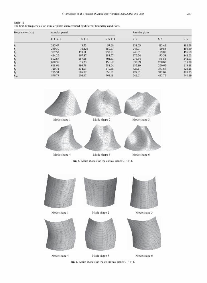
Fig. 5. Mode shapes for the conical panel C–F–F–F.



Fig. 6. Mode shapes for the cylindrical panel C–F–F–F.


ARTICLE IN PRESS

Mode shapes 1-2 Mode shapes 3-4 Mode shapes 5-6

Mode shapes 7-8 Mode shape 9 Mode shapes 10-11

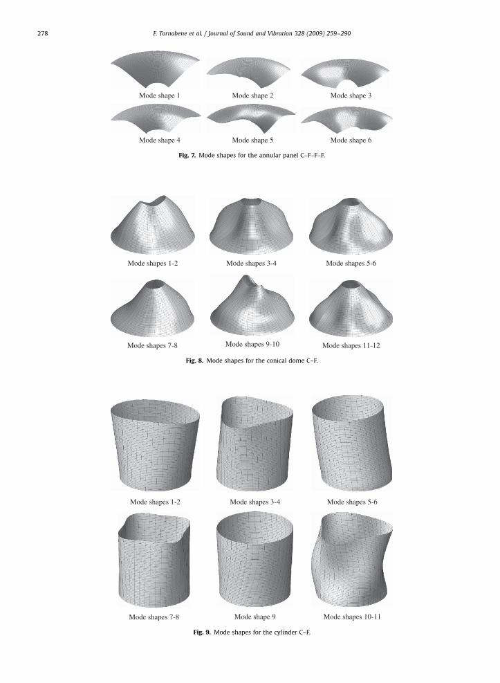
Fig. 9. Mode shapes for the cylinder C–F.



Fig. 8. Mode shapes for the conical dome C–F.



Fig. 7. Mode shapes for the annular panel C–F–F–F.


ARTICLE IN PRESS

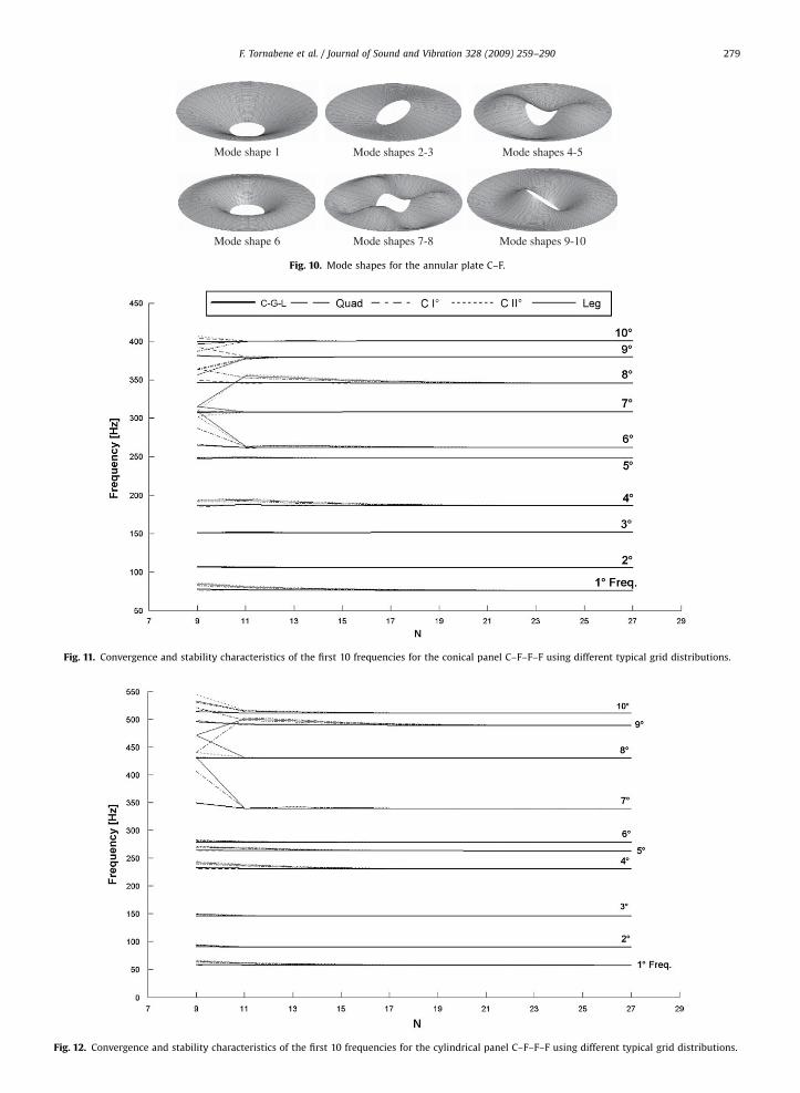
Fig. 11. Convergence and stability characteristics of the first 10 frequencies for the conical panel C–F–F–F using different typical grid distributions.

Fig. 12. Convergence and stability characteristics of the first 10 frequencies for the cylindrical panel C–F–F–F using different typical grid distributions.

Mode shape 1 Mode shapes 2-3 Mode shapes 4-5

Mode shape 6 Mode shapes 7-8 Mode shapes 9-10

Fig. 10. Mode shapes for the annular plate C–F.


ARTICLE IN PRESS


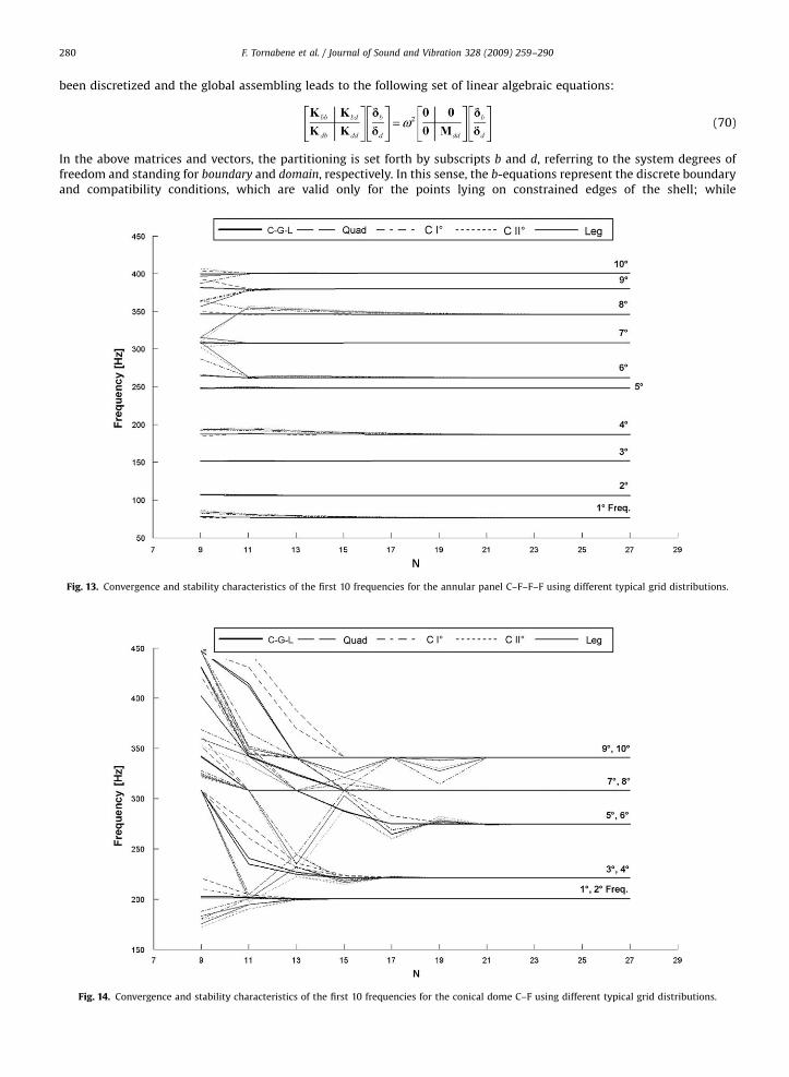
been discretized and the global assembling leads to the following set of linear algebraic equations:

(70)

In the above matrices and vectors, the partitioning is set forth by subscripts b and d, referring to the system degrees offreedom and standing for boundary and domain, respectively. In this sense, the b-equations represent the discrete boundaryand compatibility conditions, which are valid only for the points lying on constrained edges of the shell; while

Fig. 13. Convergence and stability characteristics of the first 10 frequencies for the annular panel C–F–F–F using different typical grid distributions.

Fig. 14. Convergence and stability characteristics of the first 10 frequencies for the conical dome C–F using different typical grid distributions.

ARTICLE IN PRESS


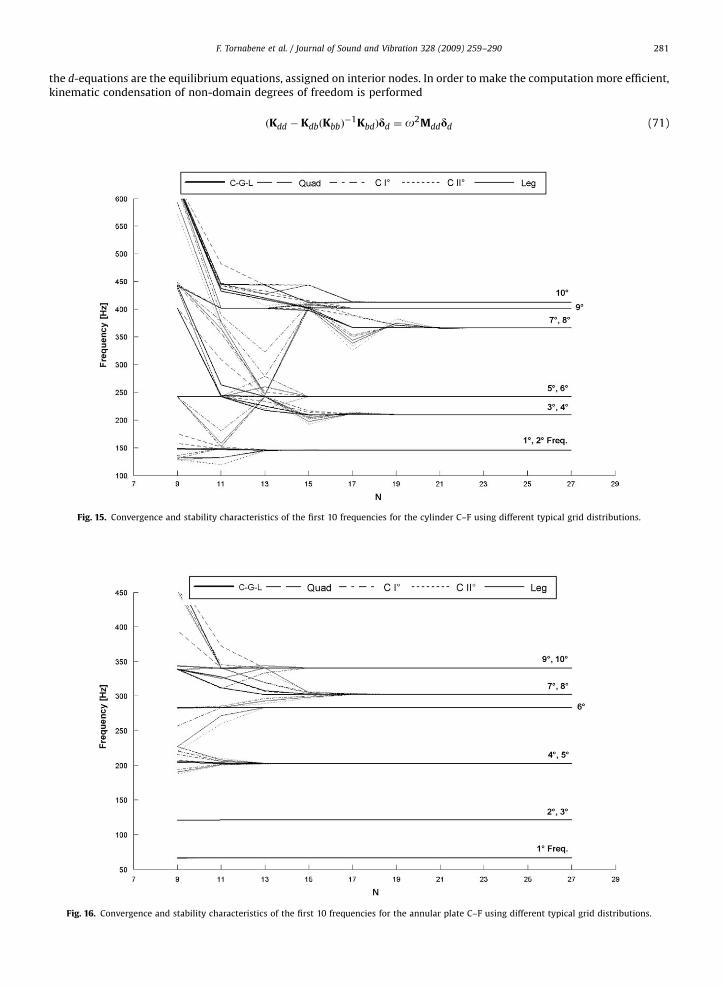
the d-equations are the equilibrium equations, assigned on interior nodes. In order to make the computation more efficient,kinematic condensation of non-domain degrees of freedom is performed

ðKdd � KdbðKbbÞ�1KbdÞdd ¼ o2Mdddd (71)

Fig. 15. Convergence and stability characteristics of the first 10 frequencies for the cylinder C–F using different typical grid distributions.

Fig. 16. Convergence and stability characteristics of the first 10 frequencies for the annular plate C–F using different typical grid distributions.

ARTICLE IN PRESS


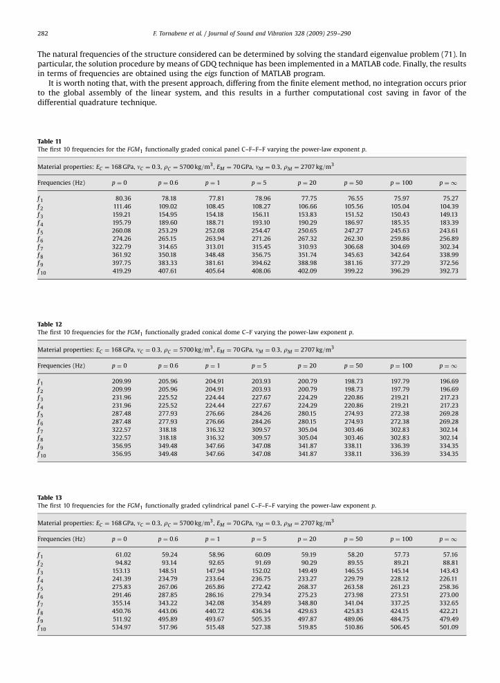
The natural frequencies of the structure considered can be determined by solving the standard eigenvalue problem (71). Inparticular, the solution procedure by means of GDQ technique has been implemented in a MATLAB code. Finally, the resultsin terms of frequencies are obtained using the eigs function of MATLAB program.

It is worth noting that, with the present approach, differing from the finite element method, no integration occurs priorto the global assembly of the linear system, and this results in a further computational cost saving in favor of thedifferential quadrature technique.

Table 11The first 10 frequencies for the FGM1 functionally graded conical panel C–F–F–F varying the power-law exponent p.

Material properties: EC ¼ 168 GPa, nC ¼ 0:3, rC ¼ 5700 kg=m3, EM ¼ 70 GPa, nM ¼ 0:3, rM ¼ 2707 kg=m3

Frequencies (Hz) p ¼ 0 p ¼ 0:6 p ¼ 1 p ¼ 5 p ¼ 20 p ¼ 50 p ¼ 100 p ¼ 1

f 1 80.36 78.18 77.81 78.96 77.75 76.55 75.97 75.27

f 2 111.46 109.02 108.45 108.27 106.66 105.56 105.04 104.39

f 3 159.21 154.95 154.18 156.11 153.83 151.52 150.43 149.13

f 4 195.79 189.60 188.71 193.10 190.29 186.97 185.35 183.39

f 5 260.08 253.29 252.08 254.47 250.65 247.27 245.63 243.61

f 6 274.26 265.15 263.94 271.26 267.32 262.30 259.86 256.89

f 7 322.79 314.65 313.01 315.45 310.93 306.68 304.69 302.34

f 8 361.92 350.18 348.48 356.75 351.74 345.63 342.64 338.99

f 9 397.75 383.33 381.61 394.62 388.98 381.16 377.29 372.56

f 10 419.29 407.61 405.64 408.06 402.09 399.22 396.29 392.73

Table 12The first 10 frequencies for the FGM1 functionally graded conical dome C–F varying the power-law exponent p.



f 1 209.99 205.96 204.91 203.93 200.79 198.73 197.79 196.69

f 2 209.99 205.96 204.91 203.93 200.79 198.73 197.79 196.69

f 3 231.96 225.52 224.44 227.67 224.29 220.86 219.21 217.23

f 4 231.96 225.52 224.44 227.67 224.29 220.86 219.21 217.23

f 5 287.48 277.93 276.66 284.26 280.15 274.93 272.38 269.28

f 6 287.48 277.93 276.66 284.26 280.15 274.93 272.38 269.28

f 7 322.57 318.18 316.32 309.57 305.04 303.46 302.83 302.14

f 8 322.57 318.18 316.32 309.57 305.04 303.46 302.83 302.14

f 9 356.95 349.48 347.66 347.08 341.87 338.11 336.39 334.35

f 10 356.95 349.48 347.66 347.08 341.87 338.11 336.39 334.35

Table 13The first 10 frequencies for the FGM1 functionally graded cylindrical panel C–F–F–F varying the power-law exponent p.



f 1 61.02 59.24 58.96 60.09 59.19 58.20 57.73 57.16

f 2 94.82 93.14 92.65 91.69 90.29 89.55 89.21 88.81

f 3 153.13 148.51 147.94 152.02 149.49 146.55 145.14 143.43

f 4 241.39 234.79 233.64 236.75 233.27 229.79 228.12 226.11

f 5 275.83 267.06 265.86 272.42 268.37 263.58 261.23 258.36

f 6 291.46 287.85 286.16 279.34 275.23 273.98 273.51 273.00

f 7 355.14 343.22 342.08 354.89 348.80 341.04 337.25 332.65

f 8 450.76 443.06 440.72 436.34 429.63 425.83 424.15 422.21

f 9 511.92 495.89 493.67 505.35 497.87 489.06 484.75 479.49

f 10 534.97 517.96 515.48 527.38 519.85 510.86 506.45 501.09

ARTICLE IN PRESS


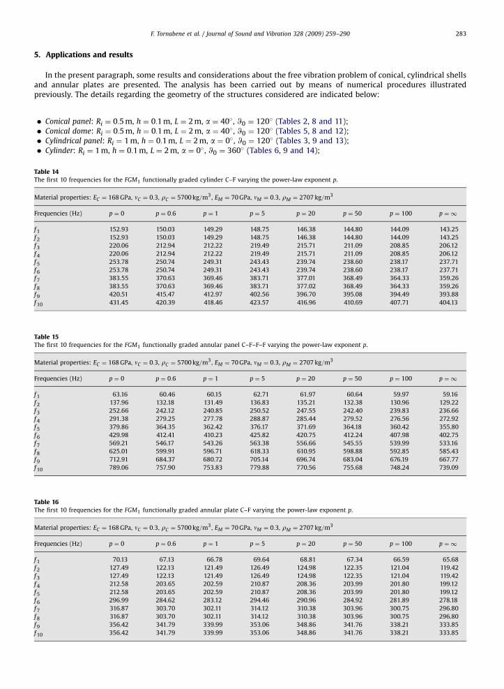
5. Applications and results

In the present paragraph, some results and considerations about the free vibration problem of conical, cylindrical shellsand annular plates are presented. The analysis has been carried out by means of numerical procedures illustratedpreviously. The details regarding the geometry of the structures considered are indicated below:

�

TabThe

Ma

Fre

f 1

f 2

f 3

f 4

f 5

f 6

f 7

f 8

f 9

f 10

TabThe

Ma

Fre

f 1

f 2

f 3

f 4

f 5

f 6

f 7

f 8

f 9

f 10

TabThe

Ma

Fre

f 1

f 2

f 3

f 4

f 5

f 6

f 7

f 8

f 9

f 10

Conical panel: Ri ¼ 0:5 m, h ¼ 0:1 m, L ¼ 2 m, a ¼ 40, W0 ¼ 120 (Tables 2, 8 and 11);
� Conical dome: Ri ¼ 0:5 m, h ¼ 0:1 m, L ¼ 2 m, a ¼ 40, W0 ¼ 120 (Tables 5, 8 and 12); � Cylindrical panel: Ri ¼ 1 m, h ¼ 0:1 m, L ¼ 2 m, a ¼ 0, W0 ¼ 120 (Tables 3, 9 and 13); � Cylinder: Ri ¼ 1 m, h ¼ 0:1 m, L ¼ 2 m, a ¼ 0, W0 ¼ 360 (Tables 6, 9 and 14);
le 14first 10 frequencies for the FGM1 functionally graded cylinder C–F varying the power-law exponent p.

terial properties: EC ¼ 168 GPa, nC ¼ 0:3, rC ¼ 5700 kg=m3, EM ¼ 70 GPa, nM ¼ 0:3, rM ¼ 2707 kg=m3

quencies (Hz) p ¼ 0 p ¼ 0:6 p ¼ 1 p ¼ 5 p ¼ 20 p ¼ 50 p ¼ 100 p ¼ 1

152.93 150.03 149.29 148.75 146.38 144.80 144.09 143.25

152.93 150.03 149.29 148.75 146.38 144.80 144.09 143.25

220.06 212.94 212.22 219.49 215.71 211.09 208.85 206.12

220.06 212.94 212.22 219.49 215.71 211.09 208.85 206.12

253.78 250.74 249.31 243.43 239.74 238.60 238.17 237.71

253.78 250.74 249.31 243.43 239.74 238.60 238.17 237.71

383.55 370.63 369.46 383.71 377.01 368.49 364.33 359.26

383.55 370.63 369.46 383.71 377.02 368.49 364.33 359.26

420.51 415.47 412.97 402.56 396.70 395.08 394.49 393.88

431.45 420.39 418.46 423.57 416.96 410.69 407.71 404.13

le 15first 10 frequencies for the FGM1 functionally graded annular panel C–F–F–F varying the power-law exponent p.



63.16 60.46 60.15 62.71 61.97 60.64 59.97 59.16

137.96 132.18 131.49 136.83 135.21 132.38 130.96 129.22

252.66 242.12 240.85 250.52 247.55 242.40 239.83 236.66

291.38 279.25 277.78 288.87 285.44 279.52 276.56 272.92

379.86 364.35 362.42 376.17 371.69 364.18 360.42 355.80

429.98 412.41 410.23 425.82 420.75 412.24 407.98 402.75

569.21 546.17 543.26 563.38 556.66 545.55 539.99 533.16

625.01 599.91 596.71 618.33 610.95 598.88 592.85 585.43

712.91 684.37 680.72 705.14 696.74 683.04 676.19 667.77

789.06 757.90 753.83 779.88 770.56 755.68 748.24 739.09

le 16first 10 frequencies for the FGM1 functionally graded annular plate C–F varying the power-law exponent p.



70.13 67.13 66.78 69.64 68.81 67.34 66.59 65.68

127.49 122.13 121.49 126.49 124.98 122.35 121.04 119.42

127.49 122.13 121.49 126.49 124.98 122.35 121.04 119.42

212.58 203.65 202.59 210.87 208.36 203.99 201.80 199.12

212.58 203.65 202.59 210.87 208.36 203.99 201.80 199.12

296.99 284.62 283.12 294.46 290.96 284.92 281.89 278.18

316.87 303.70 302.11 314.12 310.38 303.96 300.75 296.80

316.87 303.70 302.11 314.12 310.38 303.96 300.75 296.80

356.42 341.79 339.99 353.06 348.86 341.76 338.21 333.85

356.42 341.79 339.99 353.06 348.86 341.76 338.21 333.85

ARTICLE IN PRESS


�

Figpan

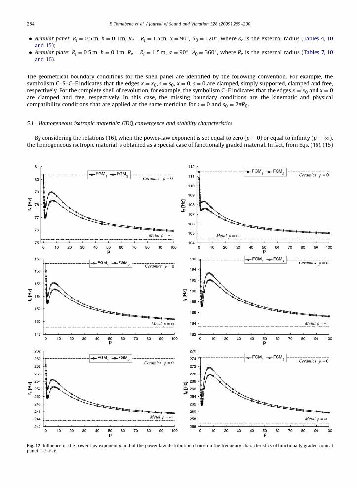
Annular panel: Ri ¼ 0:5 m, h ¼ 0:1 m, Re � Ri ¼ 1:5 m, a ¼ 90, W0 ¼ 120, where Re is the external radius (Tables 4, 10and 15);
� Annular plate: Ri ¼ 0:5 m, h ¼ 0:1 m, Re � Ri ¼ 1:5 m, a ¼ 90, W0 ¼ 360, where Re is the external radius (Tables 7, 10
and 16).

The geometrical boundary conditions for the shell panel are identified by the following convention. For example, thesymbolism C–S–C–F indicates that the edges x ¼ x0, s ¼ s0, x ¼ 0, s ¼ 0 are clamped, simply supported, clamped and free,respectively. For the complete shell of revolution, for example, the symbolism C–F indicates that the edges x ¼ x0 and x ¼ 0are clamped and free, respectively. In this case, the missing boundary conditions are the kinematic and physicalcompatibility conditions that are applied at the same meridian for s ¼ 0 and s0 ¼ 2pR0.

5.1. Homogeneous isotropic materials: GDQ convergence and stability characteristics

By considering the relations (16), when the power-law exponent is set equal to zero (p ¼ 0) or equal to infinity (p ¼N),the homogeneous isotropic material is obtained as a special case of functionally graded material. In fact, from Eqs. (16), (15)

. 17. Influence of the power-law exponent p and of the power-law distribution choice on the frequency characteristics of functionally graded conical

el C–F–F–F.

ARTICLE IN PRESS


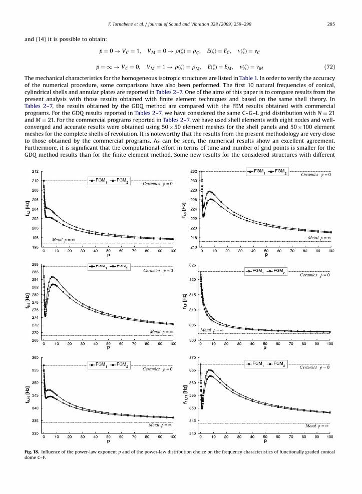
and (14) it is possible to obtain:

p ¼ 0! VC ¼ 1; VM ¼ 0! rðzÞ ¼ rC ; EðzÞ ¼ EC ; nðzÞ ¼ nC

p ¼ 1! VC ¼ 0; VM ¼ 1! rðzÞ ¼ rM ; EðzÞ ¼ EM ; nðzÞ ¼ nM (72)

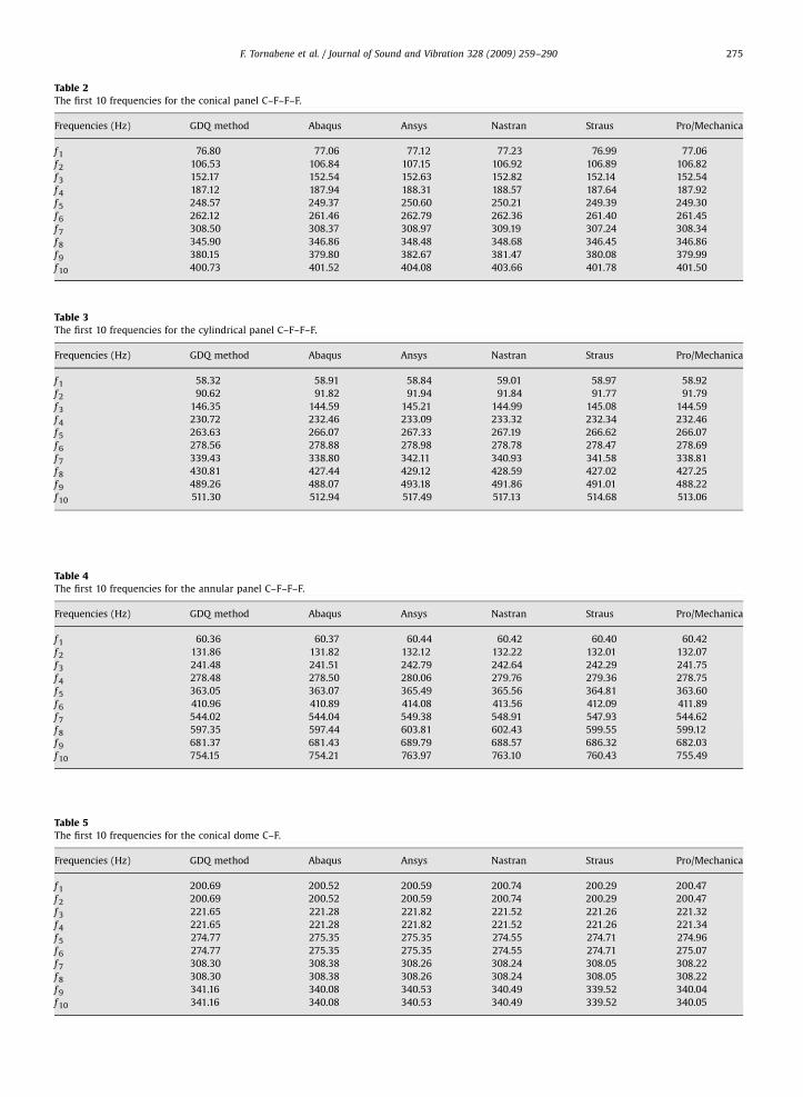
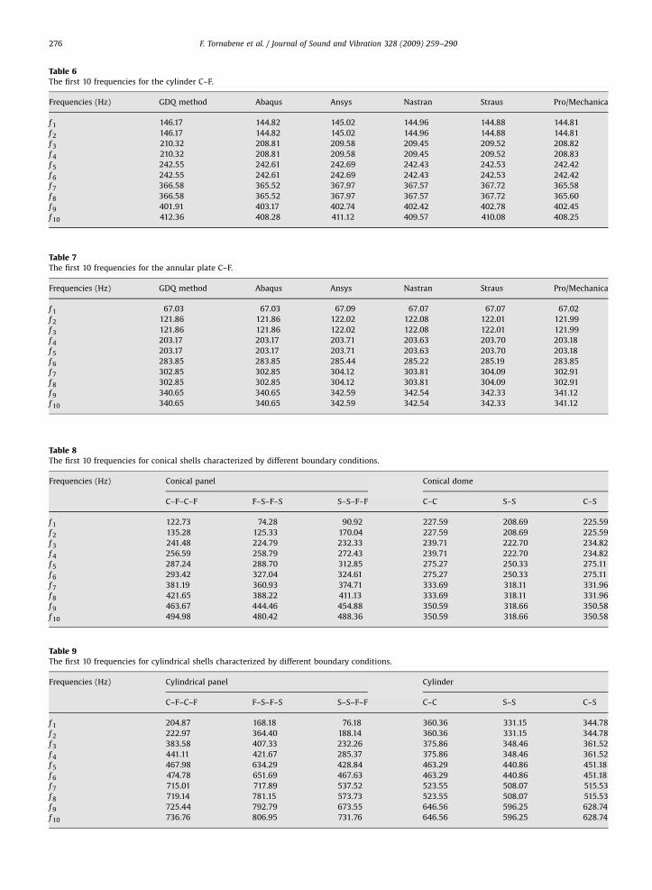
The mechanical characteristics for the homogeneous isotropic structures are listed in Table 1. In order to verify the accuracyof the numerical procedure, some comparisons have also been performed. The first 10 natural frequencies of conical,cylindrical shells and annular plates are reported in Tables 2–7. One of the aims of this paper is to compare results from thepresent analysis with those results obtained with finite element techniques and based on the same shell theory. InTables 2–7, the results obtained by the GDQ method are compared with the FEM results obtained with commercialprograms. For the GDQ results reported in Tables 2–7, we have considered the same C–G–L grid distribution with N ¼ 21and M ¼ 21. For the commercial programs reported in Tables 2–7, we have used shell elements with eight nodes and well-converged and accurate results were obtained using 5050 element meshes for the shell panels and 50100 elementmeshes for the complete shells of revolution. It is noteworthy that the results from the present methodology are very closeto those obtained by the commercial programs. As can be seen, the numerical results show an excellent agreement.Furthermore, it is significant that the computational effort in terms of time and number of grid points is smaller for theGDQ method results than for the finite element method. Some new results for the considered structures with different

Fig. 18. Influence of the power-law exponent p and of the power-law distribution choice on the frequency characteristics of functionally graded conical

dome C–F.

ARTICLE IN PRESS


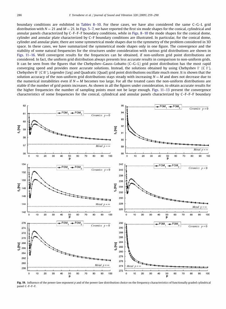
boundary conditions are exhibited in Tables 8–10. For these cases, we have also considered the same C–G–L griddistribution with N ¼ 21 and M ¼ 21. In Figs. 5–7, we have reported the first six mode shapes for the conical, cylindrical andannular panels characterized by C–F–F–F boundary conditions, while in Figs. 8–10 the mode shapes for the conical dome,cylinder and annular plate characterized by C–F boundary conditions are illustrated. In particular, for the conical dome,cylinder and annular plate, there are some symmetrical mode shapes due to the symmetry of the problem considered in 3Dspace. In these cases, we have summarized the symmetrical mode shapes only in one figure. The convergence and thestability of some natural frequencies for the structures under consideration with various grid distributions are shown inFigs. 11–16. Well convergent results for the frequencies can be obtained, if non-uniform grid point distributions areconsidered. In fact, the uniform grid distribution always presents less accurate results in comparison to non-uniform grids.It can be seen from the figures that the Chebyshev–Gauss–Lobatto (C–G–L) grid point distribution has the most rapidconverging speed and provides more accurate solutions. Instead, the solutions obtained by using Chebyshev I1 (C I1),Chebyshev II1 (C II1), Legendre (Leg) and Quadratic (Quad) grid point distributions oscillate much more. It is shown that thesolution accuracy of the non-uniform grid distributions stays steady with increasing N ¼ M and does not decrease due tothe numerical instabilities even if N ¼ M becomes too large. For all the treated cases the non-uniform distributions arestable if the number of grid points increases. As shown in all the figures under consideration, to obtain accurate results forthe higher frequencies the number of sampling points must not be large enough. Figs. 11–13 present the convergencecharacteristics of some frequencies for the conical, cylindrical and annular panels characterized by C–F–F–F boundary

Fig. 19. Influence of the power-law exponent p and of the power-law distribution choice on the frequency characteristics of functionally graded cylindrical

panel C–F–F–F.

ARTICLE IN PRESS


conditions, while Figs. 14–16 show the convergence characteristics of some frequencies for the conical dome, cylinder andannular plate characterized by C–F boundary conditions. The boundary conditions influence the convergence and stabilitycharacteristics. In fact, it can be seen from these figures that the solutions for the conical, cylindrical and annular panelshave the most rapid converging speed and provide more accurate results with a lower number of sampling points. Paneltype structures yield very accurate results for the considered frequencies using the C–G–L grid distribution withN ¼ M ¼ 17. Instead, the worked solutions for the conical dome, cylinder and annular plate oscillate much more and requirea larger number of sampling points. In these cases, compatibility conditions are introduced and must be implemented tosolve the complete shell of revolution problem. To obtain accurate results for the higher frequencies, it is necessary to use aC–G–L grid distribution with N ¼ M ¼ 21 sampling points. In fact, these frequencies show the slower convergence rate. It isworth noting that, using all the non-uniform grid distributions, the methodology presents good stability and convergingcharacteristics. Furthermore, the accuracy depends on the number of sampling points used.

5.2. Functionally graded materials

In the present paragraph, some results and considerations about the free vibration problem of FGM shells are presented.Regarding the functionally graded materials, their two constituents are taken to be zirconia (ceramic) and aluminum(metal), as can be seen from the mechanical characteristics listed in Tables 11–16. The details regarding the geometry of the

Fig. 20. Influence of the power-law exponent p and of the power-law distribution choice on the frequency characteristics of functionally graded cylinder

C–F.

ARTICLE IN PRESS

Fig. 21. Influence of the power-law exponent p and of the power-law distribution choice on the frequency characteristics of functionally graded annular

panel C–F–F–F.


structures are presented previously. For the GDQ results, we have considered the Chebyshev–Gauss–Lobatto (C–G–L) griddistribution with N ¼ M ¼ 31. Tables 11–16 illustrate the results obtained using various values of the power-law exponent p

(i.e. p ¼ 0 ceramic rich and p ¼N metallic rich) for the FGM1 power-law distribution. These tables show how by varyingthe power-law index p of the volume fraction VC it is possible to modify natural frequencies of FGM shells. The influence ofthe index p on the vibration frequencies is shown in Figs. 17–22. As can be seen from the figures, natural frequencies of FGMshell panels present an intermediate value between the natural frequencies of the limit cases of homogeneous shell panelsof zirconia (p ¼ 0) and of aluminum (p ¼N), as expected. It is interesting to note that the frequencies attain a minimumvalue for a shell made only of metal, due to the fact that aluminum has a much smaller Young’s modulus that zirconia. Inparticular, it can be noted that the most of frequencies exhibits a fast descending behavior from the ceramic limit case(p ¼ 0) varying the power-law index from p ¼ 0 to 1, while for values of p greater than unity frequencies increase until amaximum value. After this maximum, frequencies slowly decrease by increasing the power-law exponent p and tend to themetallic limit case (p ¼N). This is expected because the more p increases the more the ceramic content is low and the FGMshell approaches the case of the fully metallic shell. The behavior described above is not present in all the frequencies anddepends on the type of vibration mode. It is worth noting that in Figs. 18–20 some frequencies do not present thecharacteristic knee described above, but decrease gradually from the ceramic limit case (p ¼ 0) to the metallic limit case(p ¼N) by increasing the power-law exponent p. In particular, the types of vibration mode that present this monotonegradually decrease of frequency are torsional and bending mode shapes, while the circumferential and radial mode shapesare characterized by a knee, as can be seen by comparing the mode shapes in Figs. 5–10 with Figs. 17–22. For examples, thefrequencies f7, f8 of the conical dome of Fig. 18 and f5, f6 of the cylinder of Fig. 20 correspond to bending mode shapes as canbe observed from Figs. 8 and 9, respectively, while the frequency f9 of the cylinder of Fig. 20 correspond to a torsional modeshape as can be inferred from Fig. 9.

Furthermore, Figs. 17–22 also show the effect of the power-law distribution choice on the frequency parameters. As canbe seen, the FGM1 power-law frequency curves are always over the FGM2 power-law frequency curves for any value of p.Moreover, the distance between these two curves increases with increasing the shell thickness because of the curvature ofthe shell. In fact, for curved shells it is important from dynamic vibration point of view to know if the top surface of theshell ðz ¼ h=2Þ is ceramic or metallic rich and if the bottom surface ðz ¼ �h=2Þ is metallic or ceramic rich.

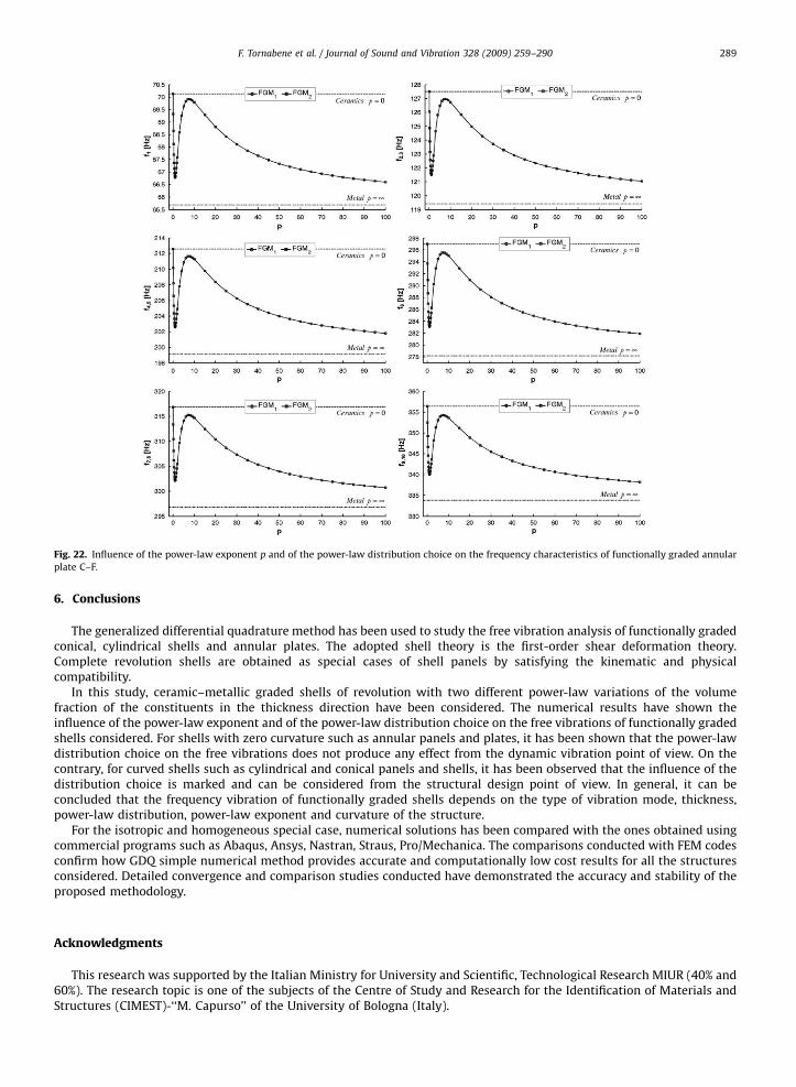
ARTICLE IN PRESS

Fig. 22. Influence of the power-law exponent p and of the power-law distribution choice on the frequency characteristics of functionally graded annular

plate C–F.


6. Conclusions

The generalized differential quadrature method has been used to study the free vibration analysis of functionally gradedconical, cylindrical shells and annular plates. The adopted shell theory is the first-order shear deformation theory.Complete revolution shells are obtained as special cases of shell panels by satisfying the kinematic and physicalcompatibility.

In this study, ceramic–metallic graded shells of revolution with two different power-law variations of the volumefraction of the constituents in the thickness direction have been considered. The numerical results have shown theinfluence of the power-law exponent and of the power-law distribution choice on the free vibrations of functionally gradedshells considered. For shells with zero curvature such as annular panels and plates, it has been shown that the power-lawdistribution choice on the free vibrations does not produce any effect from the dynamic vibration point of view. On thecontrary, for curved shells such as cylindrical and conical panels and shells, it has been observed that the influence of thedistribution choice is marked and can be considered from the structural design point of view. In general, it can beconcluded that the frequency vibration of functionally graded shells depends on the type of vibration mode, thickness,power-law distribution, power-law exponent and curvature of the structure.

For the isotropic and homogeneous special case, numerical solutions has been compared with the ones obtained usingcommercial programs such as Abaqus, Ansys, Nastran, Straus, Pro/Mechanica. The comparisons conducted with FEM codesconfirm how GDQ simple numerical method provides accurate and computationally low cost results for all the structuresconsidered. Detailed convergence and comparison studies conducted have demonstrated the accuracy and stability of theproposed methodology.

Acknowledgments

This research was supported by the Italian Ministry for University and Scientific, Technological Research MIUR (40% and60%). The research topic is one of the subjects of the Centre of Study and Research for the Identification of Materials andStructures (CIMEST)-‘‘M. Capurso’’ of the University of Bologna (Italy).

ARTICLE IN PRESS


References

[1] J.L. Sanders, An improved first approximation theory of thin shells, NASA TR-R24, Washington, DC, 1959.[2] W. Flugge, Stresses in Shells, Springer, New York, 1960.[3] V.V. Novozhilov, Thin Shell Theory, P. Noordhoff, Groningen, 1964.[4] V.Z. Vlasov, General theory of shells and its application in engineering, NASA TTF-99, Washington, DC, 1964.[5] H. Kraus, Thin Elastic Shells, Wiley, New York, 1967.[6] A.W. Leissa, Vibration of shells, NASA SP-288, Washington, DC, 1973.[7] F.I. Niordson, Shell Theory, North-Holland, Amsterdam, 1985.[8] C. Shu, An efficient approach for free vibration analysis of conical shells, Int. J. Mech. Sci. 38 (1996) 935–949.[9] K.Y. Lam, L. Hua, Vibration analysis of a rotating truncated circular conical shell, Int. J. Solids Struct. 34 (1997) 2183–2197.

[10] L. Hua, K.Y. Lam, Frequency characteristics of a thin rotating cylindrical shell using the generalized differential quadrature method, Int. J. Mech. Sci. 40(1998) 443–459.

[11] T.Y. Ng, H. Li, K.Y. Lam, C.T. Loy, Parametric instability of conical shells by the generalized differential quadrature method, Int. J. Numer. Meth. Eng. 44(1999) 819–837.

[12] L. Hua, K.Y. Lam, The generalized quadrature method for frequency analysis of a rotating conical shell with initial pressure, Int. J. Numer. Meth. Eng. 48(2000) 1703–1722.

[13] K.Y. Lam, L. Hua, Influence of initial pressure on frequency characteristics of a rotating truncated circular conical shell, Int. J. Mech. Sci. 42 (2000)213–236.

[14] L. Hua, K.Y. Lam, Orthotropic influence on frequency characteristics of rotating composite laminated conical shell by the generalized differentialquadrature method, Int. J. Solids Struct. 38 (2001) 3995–4015.

[15] K.Y. Lam, H. Li, T.Y. Ng, C.F. Chua, Generalized differential quadrature method for the free vibration of truncated conical panels, J. Sound Vib. 251(2002) 329–348.

[16] P.L. Gould, Finite Element Analysis of Shells of Revolution, Pitman Publishing, Boston, 1984.[17] P.L. Gould, Analysis of Plates and Shells, Prentice-Hall, New Jersey, 1999.[18] J.N. Reddy, Mechanics of Laminated Composites Plates and Shells, CRC Press, New York, 2003.[19] E. Reissner, The effect of transverse shear deformation on the bending of elastic plates, J. Appl. Mech. ASME 12 (1945) 66–77.[20] C. Shu, Free vibration analysis of composite laminated conical shells by generalized differential quadrature, J. Sound Vib. 194 (1996) 587–604.[21] C.P. Wu, C.Y. Lee, Differential quadrature solution for the free vibration analysis of laminated conical shells with variable stiffness, Int. J. Mech. Sci. 43

(2001) 1853–1869.[22] E. Viola, E. Artioli, The G.D.Q. method for the harmonic dynamic analysis of rotational shell structural elements, Struct. Eng. Mech. 17 (2004) 789–817.[23] E. Artioli, E. Viola, Static analysis of shear-deformable shells of revolution via G.D.Q. method, Struct. Eng. Mech. 19 (2005) 459–475.[24] C.T. Loy, J.N. Lam, J.N. Reddy, Vibration of functionally graded cylindrical shells, Int. J. Mech. Sci. 41 (1999) 309–324.[25] C.P. Wu, Y.H. Tsai, Asymptotic DQ solutions of functionally graded annular spherical shells, Eur. J. Mech. A Solid 23 (2004) 283–299.[26] I. Elishakoff, C. Gentilini, E. Viola, Forced vibrations of functionally graded plates in the three-dimensional setting, AIAA J. 43 (2005) 2000–2007.[27] I. Elishakoff, C. Gentilini, E. Viola, Three-dimensional analysis of an all-around clamped plate made of functionally graded materials, Acta Mech. 180

(2005) 21–36.[28] B.P. Patel, S.S. Gupta, M.S. Loknath, C.P. Kadu, Free vibration analysis of functionally graded elliptical cylindrical shells using higher-order theory,

Compos. Struct. 69 (2005) 259–270.[29] S. Abrate, Free vibration, buckling, and static deflection of functionally graded plates, Compos. Sci. Technol. 66 (2006) 2383–2394.[30] R.K. Bhangale, R.K. Ganesan, C. Padmanabhan, Linear thermo-elastic buckling and free vibration behavior of FG truncated conical shell, J. Sound Vib.

292 (2006) 341–371.[31] A.M. Zenkour, Generalized shear deformation theory for bending analysis of functionally graded plates, Appl. Math. Model. 30 (2006) 67–84.[32] J.L. Pelletier, S.S. Vel, An exact solution for the steady-state thermoelastic response of functionally graded orthotropic cylindrical shells, Int. J. Solids

Struct. 43 (2006) 1131–1158.[33] R.A. Arciniega, J.N. Reddy, Large deformation analysis of functionally graded shells, Int. J. Solids Struct. 44 (2007) 2036–2052.[34] C.M.C. Roque, A.J.M. Ferreira, R.M.N. Jorge, A radial basis function for the free vibration analysis of functionally graded plates using refined theory,

J. Sound Vib. 300 (2007) 1048–1070.[35] A.H. Sofiyev, The buckling of functionally graded truncated conical shells under dynamic axial loading, J. Sound Vib. 305 (2007) 808–826.[36] J. Yang, H.S. Shen, Free vibration and parametric resonance of shear deformable functionally graded cylindrical panels, J. Sound Vib. 261 (2007)

871–893.[37] C. Shu, Differential Quadrature and Its Application in Engineering, Springer, Berlin, 2000.[38] C. Bert, M. Malik, Differential quadrature method in computational mechanics, Appl. Mech. Rev. 49 (1996) 1–27.[39] E. Viola, F. Tornabene, Vibration analysis of damaged circular arches with varying cross-section, Struct. Integr. Durab. (SID-SDHM) 1 (2005) 155–169.[40] E. Viola, F. Tornabene, Vibration analysis of conical shell structures using GDQ method, Far East J. Appl. Math. 25 (2006) 23–39.[41] F. Tornabene, Modellazione e Soluzione di Strutture a Guscio in Materiale Anisotropo, PhD Thesis, University of Bologna—DISTART Department, 2007.[42] F. Tornabene, E. Viola, Vibration analysis of spherical structural elements using the GDQ method, Comput. Math. Appl. 53 (2007) 1538–1560.[43] E. Viola, M. Dilena, F. Tornabene, Analytical and numerical results for vibration analysis of multi-stepped and multi-damaged circular arches, J. Sound

Vib. 299 (2007) 143–163.[44] C. Shu, Generalized Differential-integral Quadrature and Application to the Simulation of Incompressible Viscous Flows Including Parallel

Computation, PhD Thesis, University of Glasgow, 1991.[45] R. Bellman, J. Casti, Differential quadrature and long-term integration, J. Math. Anal. Appl. 34 (1971) 235–238.[46] R. Bellman, B.G. Kashef, J. Casti, Differential quadrature: a technique for the rapid solution of nonlinear partial differential equations, J. Comput. Phys.

10 (1972) 40–52.[47] F. Civan, C.M. Sliepcevich, Differential quadrature for multi-dimensional problems, J. Math. Anal. Appl. 101 (1984) 423–443.[48] C.W. Bert, S.K. Jang, A.G. Striz, Two new approximate methods for analyzing free vibration of structural components, AIAA J. 26 (1988) 612–618.[49] S. Jang, C. Bert, A.G. Striz, Application of differential quadrature to static analysis of structural components, Int. J. Numer. Meth. Eng. 28 (1989)

561–577.[50] C. Shu, W. Chen, On optimal selection of interior points for applying discretized boundary conditions in DQ vibration analysis of beams and plates,

J. Sound Vib. 222 (1999) 239–257.[51] G. Karami, P. Malekzadeh, Application of a new differential quadrature methodology for free vibration analysis of plates, Int. J. Numer. Meth. Eng. 56

(2003) 847–868.[52] J.R. Quan, C.T. Chang, New insights in solving distributed system equations by the quadrature method—I. Analysis, Comput. Chem. Eng. 13 (1989)

779–788.[53] J.R. Quan, C.T. Chang, New insights in solving distributed system equations by the quadrature method—II. Numerical experiments, Comput. Chem.

Eng. 13 (1989) 1017–1024.[54] C. Shu, W. Chen, H. Xue, H. Du, Numerical study of grid distribution effect on accuracy of DQ analysis of beams and plates by error estimation of

derivative approximation, Int. J. Numer. Meth. Eng. 51 (2001) 159–179.

2-D differential quadrature solution for vibration analysis of functionally graded conical,...

Documents

Transcript of 2-D differential quadrature solution for vibration analysis of functionally graded conical,...