The annular-sum and Hale-McClellan methods of 3D wavefield extrapolation

3D wavefield extrapolation

CREWES Research Report — Volume 18 (2006) 1

The annular-sum and Hale-McClellan methods of 3D wavefield extrapolation

Gary F. Margrave, Saleh M. Al Saleh, Michael P. Lamoureux and Wentao Sun

ABSTRACT A new theory of efficient 3D wavefield extrapolation, patterned after the established

Hale-McClellan theory, is presented. The new method uses annular-sum filters, operators that compute the sum over a specific annulus of all wavefield samples at each point, weighted by the radial samples of the 3D wavefield extrapolation operator. In contrast, the Hale-McClellan algorithm uses samples of the 2D wavefield extrapolation operator to weight the wavefield as filtered by McClellan filters. The latter are shown to be a type of annular-sum filter that incorporates an additional approximate 45 degree phase rotation and an amplitude decay. The annular-sum filters can be computed exactly in the 2D Fourier domain by multiplication by a Bessel function. They can also be computed approximately, but accurately, by spatial convolution with a small spatial operator. The annular-sum filters are used to formulate the Wiener least-squares design problem for 2D circularly symmetric filters as a standard matrix-vector problem that can be solved by standard solvers. The elements of the radial convolution matrix are shown to be the result of annular-sum filters applied to the 2D impulse response of one of the circularly symmetric filters.

INTRODUCTION In the space-frequency domain, wavefield extrapolation in the z direction formulates

as a spatial convolution, at constant frequency, over the spatial coordinates transverse to z. In a 2D theory, this is a 1D spatial convolution of the wavefield extrapolation operator, w , with a monochromatic wavefield. In a 3D theory, a 2D convolution with a different operator, W , must be performed. The 2D and 3D extrapolation operators are known exactly for a homogeneous medium and, for the variable velocity setting, it is common to assume that these operators can be applied at any spatial location with the local wavespeed, a method called hereafter the locally homogeneous assumption. The 2D and 3D extrapolation operators are most easily expressed in the transverse-wavenumber and temporal frequency domain as

( ) ( )2 2ˆ , , expW k z i z k ξΔ = Δ −ξ (1)

where for 2D 2 21ξ ξ= and for 3D 2 2 2

1 2ξ ξ ξ= + in which 1ξ and 2ξ are the wavenumbers associated with the transverse spatial coordinates. Also in equation (1), /k vω= where ω is temporal frequency and v is velocity or wavespeed. (More careful theory requires that equation (1) be specified for the possible square-root branches but for now this simple expression suffices.) Thus w is the 1D inverse Fourier transform of equation (1) over 1ξ ξ= , and W is the 2D inverse Fourier transform of equation (1) over

( )1 2,ξ ξ=ξ . The realization that the 2D and 3D operators are related by the assignment 2 2 2

1 1 2ξ ξ ξ→ + is at the heart of the popular Hale-McClellan algorithm for 3D wavefield

Margrave et al.

2 CREWES Research Report — Volume 18 (2006)

extrapolation (Hale, 1991b). This, together with the observation that the filter depends only on the square of the wavenumber, led Hale to deduce the 3D wavefield extrapolation formula

( ) ( ) ( )( ) ( )( )0 1 1, , , , , , , ,N Nz z w z w m z w m zψ ω ψ ω ψ ω ψ ω+Δ ≈ + • + + •x x x x (2)

where ( ), ,zψ ωx is the 3D seismic wavefield, ( )1 2,x x=x denotes the transverse spatial

coordinates, [ ], 0,jw j N∈ are the coefficients of the 2D wavefield extrapolator, and the subscript j indicates the lag of the coefficient from the center of the operator. Also, the

jm are coefficients of filters called McClellan filters, and • denotes 2D spatial

convolution over ( )1 2,x x=x . At first glance, the advantage of equation (2) might not be apparent since the entire extrapolation operation must be a single 2D spatial convolution of the 3D wavefield extrapolator, W , with the wavefield, and equation (2) has N 2D convolutions. However, the velocity dependence of the operator means that in general the wavefield extrapolation convolution is nonstationary while the convolutions in equation (2) are explicitly stationary. This is a big advantage. A second point is that equation (2) requires only the spatial samples of a 2D operator, not a 3D operator, and these are more easily found. As Hale (1991a) showed, the design of stable wavefield extrapolators in the space-frequency domain is a challenging task and it is an advantage to not have to repeat this process in 3D when it has already been done in 2D.

While equation (2) was not given explicitly in Hale’s paper, it is clearly implied by the text, and its validity is not in doubt. The purpose of this paper is to shed light on the physical meaning of Hale’s formula, and to present an alternative, although similar, formula which has a clear, direct, physical interpretation. Through this understanding it is possible that new insights and algorithms might emerge. In the next section our alternative formula is derived by exploiting the circular symmetry of the 3D extrapolation operator. Our formula uses the radial samples of the 3D wavefield extrapolator as weighting terms for a series of stationary filters. However, these filters are not the McClellan filters but are a related operator which we call an annular-sum filter. Then the design of a stable 3D wavefield extrapolator is formulated as a simple least-squares problem using annular-sum filters. In this approach a radial convolution matrix, analogous to but different from the familiar Toeplitz matrix, is developed. In the subsequent section, a series of numerical examples are presented, and the annular-sum filters are contrasted with the McClellan filters. The implementation of approximate annular-sum filters by spatial convolution is examined. Finally the utility of the radial convolution matrix is demonstrated with an example from wavefield extrapolator theory.

THEORY

Wavefield extrapolation using the locally homogeneous model is most easily expressed using the GPSPI (generalized phase-shift plus interpolation) formula in the space-frequency domain (e.g. Margrave et al. 2006). In 3D the formula is



( ) ( ) ( )( )2

, , , , , ,z z z W k z dψ ω ψ ω+Δ = − Δ∫x u x u x u , (3)

where ( ), ,zψ ωx is the space-frequency domain wavefield, ω is the temporal frequency,

( )1 2,x x=x denotes the transverse spatial direction, ( )1 2,u u=u are the transverse spatial directions of integration, 1 2d du du=u , zΔ is the depth step, and the wavefield extrapolation operator is

( )( ) ( )( )2

,2

1 ˆ, , , ,4

iW k z W k z e dξπ

−− Δ = Δ∫ ξ x-ux u x ξ x , (4)

where ( )1 2,ξ ξ=ξ is the wavenumber vector dual to x , and

( )( ) ( )( ),ˆ , , zik k zW k z e ΔΔ = x ξξ x , (5)

( )( )( ) ( )

( ) ( )

2 22 2

2 22 2

,,

,z

k kk k

i k k

ξ ξ

ξ ξ

⎧⎪ − >⎪⎪⎪=⎨⎪⎪ − ≥⎪⎪⎩

x xx ξ

x x , (6)

( )( )

kvω

=xx

. (7)

The wavefield extrapolator of equation (4) is known exactly and is given by

( )( )

2 2

2 2 2 2, , 1

2ik zik z iW k z e

z k zρρ

π ρ ρ+Δ

⎛ ⎞⎟Δ ⎜ ⎟⎜Δ =− + ⎟⎜ ⎟⎜ ⎟+Δ ⎟⎜ +Δ⎝ ⎠, (8)

where ( ) ( )( ), , , ,W k z W k zρ Δ = − Δx u x , and

( ) ( )2 21 1 2 2x u x uρ= − = − + −x u is the radial coordinate at constant z.

In two spatial dimensions, the corresponding formula to equation (8) is

( ) ( ) ( )1 2 21 112 2

1

, , zw k z ik H k zz

Δρ Δ ρ Δρ Δ

= − ++

, (9)

where ( ) ( )11H u is the first-order Hankel function of the first kind and

( )21 1 1 1 1x u x uρ = − = − . For large values of its argument, the Hankel function admits

a simple approximation (e.g. Gradshteyn and Ryzhik, 1980) which gives the far-field approximation

Margrave et al.


( )( )

2 21 / 4

1 3/ 4 2 22 211

3, , 12 8

i k zk z iw k z ek zz

ρ Δ πΔρ Δπ ρ Δρ Δ

⎡ ⎤+ −⎢ ⎥⎣ ⎦⎡ ⎤⎢ ⎥≈ +⎢ ⎥++ ⎣ ⎦

. (10)

Comparing equations (8) and (10) shows that the essential difference between the 2D and 3D extrapolators is a / 4π phase shift and a different dependence on inverse distance. The 3D operator decays as inverse distance squared while in 2D the decay is less strong, being inverse distance to the 3/2 power. (More detail on these operators can be found in many places, e.g. Margrave and Daley (2001).)

Next, Theorem 1 is presented, demonstrating a formula with resemblance to equation (2) but different in detail and, in principle, exact.

Theorem 1: Let the radial coordinate be broken into a countable infinity of finite intervals, 0 1 2 1: 0, , , , ,n nρ ρ ρ ρ ρ ρ +

⎡ ⎤= ∞⎣ ⎦ . Then the 3D wavefield extrapolator of equation (3) can be re-expressed as

( ) ( )( ) ( )0

, , , , , ,n nn

z z W k z zψ ω ρ ψ ω∞

=

′+Δ = Δ∑x x x (11)

where 1,n n nρ ρ ρ +⎡ ⎤′ ∈ ⎣ ⎦ ,

( ) ( ) ( )1

, , , ,n nn z I I zρ ρψ ω ψ ω+

= − •x x , (12)

• denotes 2D convolution over the transverse coordinates and

( )0

1,, 0; 0

0, otherwisen

nI n Iρ ρ

ρ⎧⎪ ≤⎪= > =⎨⎪⎪⎩

xx (13)

is the indicator function of the disk of radius ρ . The quantities ( ), ,n zψ ωx are called

annular sums and give the sum (integral) of ( ), ,zψ ωx over the annular region

1,n nρ ρ ρ +⎡ ⎤∈ ⎣ ⎦ for each point x .

Proof:

Consider the computation of equation (3) at a single output point which can be taken to be the origin ( )0,0=x . For this single point, ( )1 0,0k vω −= is a constant and then, by equation (4), the wavefield extrapolation operator depends only upon the radial distance ρ . Expressing the integration in polar coordinates gives

( )( ) ( )( ) ( )2

0,0 , , , , , , ,z z z W k z d dψ ω ψ ρ θ ω ρ ρ ρ θ+Δ = Δ∫ (14)

which becomes



( )( ) ( ) ( )( )2

0 00,0 , , , , , , ,z z W k z z d d

πψ ω ρ ψ ρ θ ω θ ρ ρ

∞ ⎡ ⎤+Δ = Δ ⎢ ⎥

⎢ ⎥⎣ ⎦∫ ∫ (15)

or

( )( ) ( ) ( )0

0,0 , , , , , ,z z W k z z dψ ω ρ ψ ρ ω ρ ρ∞

+Δ = Δ∫ (16)

where

( ) ( )( )2

0, , , , ,z z d

πψ ρ ω ψ ρ θ ω θ= ∫ . (17)

Equation (16) is a simple 1-D integration which admits a numerical evaluation by a straight-forward Riemann sum, provided that ( ), ,zψ ρ ω can be easily obtained.

Let the range of integration in (16) be broken into the intervals, [ ]0 1 2: 0, , , ,nρ ρ ρ ρ ρ= ∞ so that

( )( ) ( ) ( )1

0

0,0 , , , , , ,n

nn

z z W k z z dρ

ρψ ω ρ ψ ρ ω ρ ρ

+∞

=

+Δ = Δ∑∫ . (18)

By the mean-value theorem, there exists some 1,n n nρ ρ ρ +⎡ ⎤′ ∈ ⎣ ⎦ in each interval such that

( ) ( ) ( ) ( )1 1

, , , , , , , ,n n

n nnW k z z d W k z z d

ρ ρ

ρ ρρ ψ ρ ω ρ ρ ρ ψ ρ ω ρ ρ

+ +′Δ = Δ∫ ∫ (19)

so that

( )( ) ( ) ( )1

0

0,0 , , , , , ,n

nn

n

z z W k z z dρ

ρψ ω ρ ψ ρ ω ρ ρ

+∞

=

′+Δ = Δ∑ ∫ . (20)

The data integral in equation (20), which is called ( ),n zψ ω , is

( ) ( ) ( )( )1 1 2

0, , , , , ,

n n

n nn z z d z d d

ρ ρ π

ρ ρψ ω ψ ρ ω ρ ρ ψ ρ θ ω ρ ρ θ

+ +

= =∫ ∫ ∫ , (21)

which is just the integral of the data over the annulus defined by 1,n nρ ρ ρ +⎡ ⎤∈ ⎣ ⎦ . To see

this more clearly, note that if Cψ= (a constant) over this annulus, then it immediately results that ( )2 2

1n n n Cψ π ρ ρ+= − where the term preceding C is just the area of the annulus. Furthermore, 0ψ= everywhere in the annulus except for a small region of area A where 1ψ= , then n Aψ = . So equation (20) becomes

( )( ) ( ) ( )0

0,0 , , , , ,n nn

z z W k z zψ ω ρ ψ ω∞

=

′+Δ = Δ∑ (22)

where the annular sums, ( ),n zψ ω , are given by equation (21).

Margrave et al.


Equation (22) was computed explicitly for the point at the origin but it generalizes immediately to any other point since the ( ),n zψ ω are geometrically defined as annular

sums about the point in question. So, let ( ), ,n zψ ωx be the annular sums at any point x

and let ( )( ), ,W k zρ′ Δx be the nonstationary Wavefield extrapolator coefficients. (In the special case of stationarity, the extrapolator is independent of x .) Thus equation (11) is the immediate generalization of equation (22).

Finally, the ( ), ,n zψ ωx can be computed with a 2D convolution. Just as convolution in 1D with a boxcar function produces a new function whose values are the sum of the input values over the length of the boxcar, then so can the annular sums be computed by 2D convolution of the input wavefield with the indicator function of each annulus. Since the indicator function of the annulus is just the indicator function for the outer disk minus that for the inner, equation (12) results. ■

While equation (11) bears formal resemblance to the Hale-McClellan formula (equation (2)), the former is potentially exact, although not computable, due to the infinite sum and the indefiniteness of the points nρ′ . Theorem 2 gives a computable approximation to equation (11) and increases the correspondence with Hale-McClellan.

Theorem 2: Let ( )( ), , 0,1, 2,nW k z n NΔ =x … be the radial samples of an

approximate wavefield extrapolation operator corresponding to radii nr n x= Δ , where xΔ is the spatial grid size of the sampled wavefield. It is assumed that N has been

chosen sufficiently large and the sampled operator has been adequately stabilized. Then equation (11) admits the approximation

( ) ( )( ) ( )0

, , , , ,N

n nn

z z W k z zψ ω ψ ω=

+Δ ≈ Δ∑x x x (23)

where the annular boundaries are given by [ ] 02 1 , 1, , 0

2nn x n Nρ ρ−

= Δ ∈ = .

Proof:

Using the annular boundaries stated in the theorem, then each inner annulus [ ]0 1,ρ ρ is actually a small disk containing only one data point. However, it is incorrect to assume the data is constant across this disk. The remaining annular boundaries fall midway between each radial operator sample. If the radial intervals are small, then a reasonable approximation is

( ) ( )( ) ( )1, , / 2, , , , 0n n n nW k z W k z W k z nρ ρ ρ +′ Δ ≈ + Δ = Δ > .

The result follows directly. ■



Having established equation (23) as an alternative to equation (2), it is now appropriate to give a more explicit formula for computing the annular-sum filters. Theorem 3 gives an exact result for the computation of the annular-sum filters in the Fourier domain.

Theorem 3: The annular sums ( ), ,n zψ ωx of equation (12) can be computed in the transverse spatial wavenumber domain by the formula

( )( ) ( )( )( )( )

( )( )( )( )

12 21/ 2 1/ 2

12 21/ 2

ˆ ˆ , , , 0, ,

ˆ , , , 0

n x n x

n

x

F I I F z nz

F I F z n

ψ ωψ ω

ψ ω

−+ Δ − Δ

−Δ

⎧⎪ − >⎪⎪⎪=⎨⎪⎪ =⎪⎪⎩

xx

x, (24)

where 2 :F →T Tx k is the 2D Fourier transform and

( ) ( )1 2ˆ JIρ

ρ πρ=

ξξ

ξ (25)

is the 2D Fourier transform of the indicator function of the disk, and 1J is the first order Bessel function. If the annular thickness is sufficiently small, then the ( ), ,n zψ ωx can be more directly calculated from

( ) ( )( )( )12 2

ˆ, , , ,n n xz xF I F zδψ ω ψ ω−Δ≈Δx x (26)

where

( ) ( )0ˆ 2 2I Jδρ πρ πρ=ξ ξ (27)

in which 0J is the zero-order Bessel function and

( )Iδρ δ ρ= −x . (28)

Proof:

Bracewell (2000, p338) gives the 2D Fourier transform of the indicator function of a disk of radius ρ as

( ) ( )1 2ˆ JIρ

ρ πρ=

ξξ

ξ (29)

so the first result follows immediately from the convolution theorem. For the second case, consider

Margrave et al.


( ) ( )( ) ( )1 12 2ˆ ˆ

ρ ρ ρ

ρ ρ π ρ ρ ξ ρ πρ ξ

ξ ξ+Δ

+Δ +Δ− = −

J JI I . (30)

which manipulates as

( ) ( )( ) ( )1 12 2 2 2ˆ ˆ

2 2ρ ρ ρ

π ξ ρ ρ π ρ ρ ξ π ξ ρ πρ ξρξ π ξ ρ π ξ ρ+Δ

⎡ ⎤+Δ +ΔΔ ⎢ ⎥− = −⎢ ⎥Δ Δ⎢ ⎥⎣ ⎦

J JI I (31)

( ) ( ) ( )2

21 0 0

ˆ ˆ 2 2π ξ ρ

π ξ ρ

ρ ρ ρρ ρ

πρ π ξ ρ ρξ ξ

==

+Δ

⎡ ⎤Δ ∂ Δ ⎡ ⎤⎢ ⎥− ≈ = = Δ⎣ ⎦⎢ ⎥∂⎣ ⎦

uu

I I uJ u uJ u Ju

.(32)

This also follows from physical reasoning by modeling the annulus as ( )ρδ ρΔ −x and,

according to Bracewell, the Fourier transform of ( )δρ δ ρ= −I x is given by

( ) ( )0ˆ 2 2δρ πρ πρ ξ=I Jξ . (33)

■

Thus the annular-sum filters, which are given by xIδρΔ in the space domain, can be computed precisely in the Fourier domain by multiplication by

( ) ( )0ˆ 2 2xI x Jδρ π ρ πρ ξΔ = Δξ . In Theorem 4, the annular-sum filters are employed,

together with equation (23), to formulate the FOCI 3D operator design equation as a standard least-squares problem. In particular, it is shown that the radial samples of the result of the 2D convolution of two circularly symmetric 2D functions are related to the radial samples of the input functions by a particular matrix equation. The matrix involved, the radial convolution matrix, is the generalization of a Toeplitz matrix familiar from the 1D case.

Theorem 4: Consider the FOCI operator design problem for 3D wavefield extrapolation. This poses as

( ) ( )( )12

ˆ/ 2 / 2η

−• Δ = ΔWI W z F W z (34)

where ( )/ 2W zΔ is an approximate, windowed (e.g. compactly supported of radial

length J+1 ) operator for a half-step, ( )ˆ / 2W zΔ is the exact half-step operator in the

Fourier domain, • denotes 2D spatial convolution, [ ]0, 2η ∈ , and WI is to be determined such that equation (34) holds in the least squares sense. Then, in the discrete setting using a square spatial grid of size xΔ , WI is a solution to the following matrix equation



00 01 0 00

110 11 11

220 21 2

0 1

M

M

M

MN

N N NM

W W W AWI

AW W WWI

AW W W

WIAW W W

⎡ ⎤ ⎡ ⎤⎢ ⎥ ⎢ ⎥⎡ ⎤⎢ ⎥⎢ ⎥⎢ ⎥⎢ ⎥ ⎢ ⎥⎢ ⎥⎢ ⎥ ⎢ ⎥⎢ ⎥⎢ ⎥ = ⎢ ⎥⎢ ⎥⎢ ⎥ ⎢ ⎥⎢ ⎥⎢ ⎥ ⎢ ⎥⎢ ⎥⎢ ⎥ ⎢ ⎥ ⎢ ⎥⎢ ⎥ ⎣ ⎦ ⎢ ⎥⎢ ⎥ ⎣ ⎦⎣ ⎦

(35)

where [ ], 0,mWI m M∈ are the radial samples of WI , nA are the radial samples of

( )( )12

ˆ / 2F W zη

− Δ , N J M= + , and n mW are annular sums computed from the 2D

impulse response of ( )/ 2W zΔ such that m xΔ is the annular radius and n xΔ is the radial distance from the center of the impulse response. The matrix whose elements are

n mW will be called a radial convolution matrix.

Proof: Clearly, since both ( )/ 2W zΔ and ( )( )12

ˆ / 2F W zη

− Δ are functions only of

radius, then so must WI be. Equation (11) is actually a prescription for the 2D convolution of any radial function with an arbitrary wavefield. By

( ) ( )/ 2 , , / 2W z W k zρΔ = Δ we mean the 2D, circularly symmetric impulse response of

the approximate half-step operator. Let ( )/ 2W zΔ play the role of the wavefield and applying equation (11) in this case leads to

( ) ( ) ( )0

m mm

WI W Aρ∞

=

=∑ x x (36)

where we have used

( ) ( )12

ˆA F Wη

−=x . (37)

Equation (36) gives the convolution at all positions in the plane; however, since the result is a function of radius only, this is redundant. Let ( ):nA A n x= = Δx x be the radial

samples of ( )A x for [ ]0,n N∈ and also truncate the sum in equation (36) at m M= to get

0

M

m n m nm

WI W A=

=∑ (38)

where ( )m mWI WI ρ= and ( )n m mW W n x= = Δx . Equation (38) is equivalent to equation (35). ■

Margrave et al.


EXAMPLES OF ANNULAR-SUM FILTERS The purpose of these examples is to illustrate the basic behavior of the annular-sum

algorithm, as represented by equation (23), and to compare it with the Hale-McClellan method as represented by equation (2). Hale (1991b) implemented equation (2) using approximate filters whose impulse response was prescribed in the space domain. However, here the McClellan filters were implemented with an exact Fourier domain expression (also given by Hale) as

( )( ) ( )( )( )12 2, , cos 2 , ,jm z F j x F zψ ω π ξ ψ ω−• = Δx x . (39)

Thus

( )ˆ cos 2jm j xπ ξ= Δ (40)

while for the kth annular-sum filter, ka , using equation (26),

( )20ˆ 2 2ja j x J j xπ π= Δ Δ ξ . (41)

At this time, the mathematical relation between these results will not be investigated, only numerical comparisons are shown. Nevertheless, some insight is gained by noting

that ( )02~ cos

4J π

θ θπθ

⎛ ⎞⎟⎜ − ⎟⎜ ⎟⎜⎝ ⎠ for large θ . Thus, scale factors aside, the ˆ ja decay as

1/ 2ξ − and are phase shifted by / 4π while the ˆ jm do not decay at all. While the terms

( )ja r j xδ= − Δ are known precisely in the space domain, the inverse Fourier transform of equation (40) has no known analytic expression.

Implementation and cost of annular-sum filters

Figure 1 shows the response of an input field, containing four unit impulses, to a disk-sum filter and three different methods of implementing an annular-sum filter. The disk sum filter (Figure 1a) is simply the application of equation (25) as a Fourier multiplier (however, see Figure 3 and below). The four initial impulses were at the precise centers of the four disks. As with all examples in this paper, the spatial grid was square with

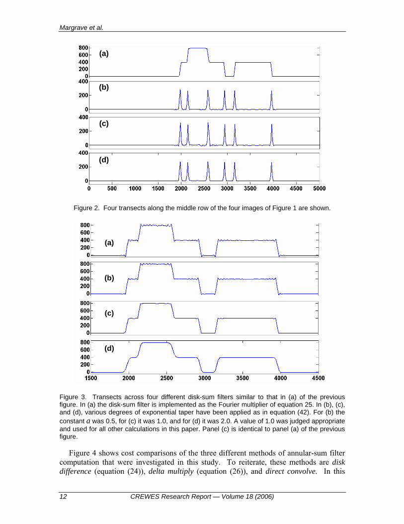
20 mxΔ = . In Figure 1b is the result of an annular-sum filter applied to the same input field where the filter was implemented as in equation (24) by the difference of two disk filters whose radii differed by one sample. Figure 1c shows the result when the annular-sum filter is implemented with equation (26), that is as a single Fourier multiplier corresponding to a annular Dirac delta. In Figure 1d is the result of a 2D spatial convolution with an approximate impulse response of the annular-sum filter. The design of this spatial filter is discussed more below. Figure 2 shows a series of transects across the images in the corresponding panels of Figure 1. The three different annular-sum filters give very similar results with very little obvious preference for one or the other. However, as will be seen, the direct convolution method is often far faster.

Direct implementation of the disk-sum filter by using equation (25) as a Fourier multiplier has bothersome Gibbs effect oscillations at the disk boundaries as shown in



Figure 3a. An easy way to control these effects is to introduce a Gaussian taper in the Fourier domain, which corresponds to a Gaussian convolution in the space domain. That is, equation (25) can be modified to give

( ) ( ) ( )( )21 2ˆ exp 2J

I a xρ

ρ πρ= − Δ

ξξ ξ

ξ (42)

where a is an adjustable scalar controlling the Gaussian width. When 1a = , the Gaussian half-width is equal to the Nyquist spatial wavenumber. Figures 3b, 3c, and 3d show the result of disk-sum filters using equation (42) with values of 0.5,1.0, 2.0a = respectively. The Gaussian taper clearly is able to control the Gibb’s effect and a value of 1a = was chosen as optimal and used for all examples in this paper. The various annular-sum filters and the McClellan filters were also similarly tapered.

(a) (b)

(c) (d)

(a) (b)

(c) (d)

Figure 1. The response of 4 impulses to the application of a disk-sum filter of radius 400m is shown in (a). The original impulses were located at the centers of each disk. The filter was accomplished as a Fourier multiplier. The result of 3 different annular-sum filters applied to the same impulses are shown in (b), (c), and (d). In (b) the annular-sum filter was the difference of two disk-sum filters as in (a), differing in radius by 1 sample. In (c) the filter was a radial delta function implemented as a Fourier multiplier, and in (d) the filter was a direct convolution (in space) with the approximate impulse response of the exact annular-sum filter.

Margrave et al.


(a)

(b)

(c)

(d)

(a)

(b)

(c)

(d)

Figure 2. Four transects along the middle row of the four images of Figure 1 are shown.

(a)

(b)

(c)

(d)

(a)

(b)

(c)

(d)

Figure 3. Transects across four different disk-sum filters similar to that in (a) of the previous figure. In (a) the disk-sum filter is implemented as the Fourier multiplier of equation 25. In (b), (c), and (d), various degrees of exponential taper have been applied as in equation (42). For (b) the constant a was 0.5, for (c) it was 1.0, and for (d) it was 2.0. A value of 1.0 was judged appropriate and used for all other calculations in this paper. Panel (c) is identical to panel (a) of the previous figure.

Figure 4 shows cost comparisons of the three different methods of annular-sum filter computation that were investigated in this study. To reiterate, these methods are disk difference (equation (24)), delta multiply (equation (26)), and direct convolve. In this



latter case, the approximate impulse response of the disk difference filter is captured and applied with a 2D spatial convolution. The approximate impulse response was estimated by the steps

(i) a test field, whose size is double that of the desired annulus, is generated as all zeros except for a single live sample in the precise center.

(ii) the annular-sum filter of equation (24) (disk difference) is applied

(iii) any negative samples in the resulting impulse response are zeroed.

The last step was deduced from empirical testing and gives a significantly improved filter.

The cost comparisons in Figure 4 are simply MATLAB computation times for the filter application times. The horizontal axis labeled “number of points” refers to the number of points in the field to which the filters were applied, not to the filters themselves. The actual size of the 2D field is the square of the value given on the x axis. The size of the annulus was 400m as before, and with a spatial sample interval of 20m, this means that 21 points are required to span the diameter of the annulus. The direct convolution method is the fastest for all but the smallest n, and the difference becomes extremely significant for large n. The slope of the curves for disk difference and delta multiply are both slightly greater than 2 in Figure 4b. This is consistent with the expectation of ( )logO N N where 2N n= , with n being the value on the x axis. That the cost of the direct convolve method seems essentially independent of n is somewhat counterintuitive but may reflect the efficiencies of the MATLAB 2D convolution function. That the cost is much lower than the other methods is expected since the fixed size of the direct-convolve filter is, in this case, 81 points, which is smaller than all but the first grid tested. It is anticipated that direct convolution will be the method of choice in 3D migration applications since generally very short Wavefield extrapolation operators (<20 points) will be used.

(a) (b)(a) (b)

Figure 4. Computation cost estimates are shown for the three different annular-sum filter implementations discussed in the text as a function of dataset size. The radius of the annular-sum filter was held constant (at 400 m) and the dataset size was increased through n=[64,128, 256, 512, 1024]. Here n refers to the single dimension of an n-by-n 2D dataset.

Margrave et al.


Basic properties of annular-sum filters Figure 5 shows the results of applying three iterations of an 800 m radius annular-sum

filter. The input field, Figure 5a, was a radially symmetric sinc function designed with a period of 10 times the spatial sample size, or 200 m in this case. Figures 5b, 5c, and 5d show one, two, and three applications of the 800 m radius annular-sum filter. Each panel of this figure has been independently scaled because the annular-sum filter weights each input point with its associated area, which is this case is roughly 2 ~ 400xΔ . Displayed in true relative scale, only the fourth panel would be visible on a plot of limited dynamic range. This areal scaling effect of the annular-sum filters is discussed just following equation (21).

To understand Figure 5, consider that the annular-sum filter is a kind of generalized Radon transform where the summation curves are circles. Thus, the value at any point in Figure 5b is the summation around an annulus, one sample wide, centered at the corresponding point in Figure 5a. Thus the dark ring in Figure 5b indicates all those points that are precisely 800 m from the largest sample in Figure 5a, which is the center point. In Figure 5c, there are two sets of preferred points that are 800 m from the large ring in Figure 5b. The point at the center shows very high amplitude for this reason while the ring of points 1600 m from the center of the original sinc function is also indicated. The point at the center is the strongest because of the areal scaling effect mentioned previously. Similar considerations afford an interpretation of Figure 5d.

Figure 6 shows the effect of applying annular-sum filters of different radius to the same input field. In this case, the input (Figure 6a) is the superposition of two radial sinc functions like that of the previous figure but with one sinc displaced from the center so that the field is no longer circularly symmetric about its center. Shown in Figures 5b, 5c, and 5d are the result of 100 m, 500 m, and 800 m. The dark rings in each figure are the loci of points whose distance from the center of either sinc functions equals the radius of the filter.

Figure 7 is similar to Figure 6 except that the second sinc function has been built with a period of 60 m so that it is sampled only 3 times per period by the 20 m grid. The short wavelength sinc function maintains its form and sharpness in each panel, indicating that the annular-sum filters are performing well with near Nyquist sampling.



(a) (b)

(c) (d)

(a) (b)

(c) (d)

Figure 5. A radial sinc function, of period 200 m, having ten discrete samples per period, is shown in (a) while (b) shows the result of convolution of (a) with an annular-sum filter of radius 800m. In (c) is the result of the same 800 m annular-sum filter applied to (b) and in (d) is the result of the same annular-sum filter applied to (c). All four plots are independently scaled.

Margrave et al.


(a) (b)

(c) (d)

(a) (b)

(c) (d)

Figure 6. Linear superposition of two radial sinc functions, both of period 200 m, is shown in (a) while (b) shows the result of convolution of (a) with an annular-sum filter of radius 100m. In (c) and (d) are the results of 500 m and 800 m annular-sum filters applied to (a). The four plots are scaled independently.



(a) (b)

(c) (d)

(a) (b)

(c) (d)

Figure 7. Linear superposition of two radial sinc functions, one of period 200 m and the other of period 60 m, is shown in (a). With a spatial grid size of 20 m the latter has only 3 samples per period. Panels (b) , (c) and (d) are the results of 100 m, 500 m and 800 m annular-sum filters applied to (a). The four plots are scaled independently.

Comparison of annular-sum and Hale-McClellan filters As previously noted, the Hale-McClellan filters correspond to multiplication by a

cosine in the Fourier domain (equation (40)) while the annular-sum filters require multiplication by a zero-order Bessel function (equation (41). As was also noted, the Bessel function has an asymptotic form of a phase-shifted cosine with radial wavenumber decay. These mathematical observations help the interpretation of the numerical results presented here.

Figure 8 shows a comparison between the impulse responses of the annular-sum filters and the Hale-McClellan filters for the problem of Figure 1. On this , it is reasonable to suppose that the Hale-McClellan filters are also annular filters, although not strictly summation filters. The annular-sum filters are essentially positive everywhere, while the Hale-McClellan filters have an obvious trough on the inside of each circle. In Figure 9, a transect across each panel of Figure 8 reveals the detailed structure. The overall much larger amplitude of the annular-sum filters is a simple consequence of the 2xΔ factor in equation (41), which in this case has the value 400. More interesting is the clear phase rotation present in the Hale-McClellan filter

Margrave et al.


(a) (b)(a) (b)

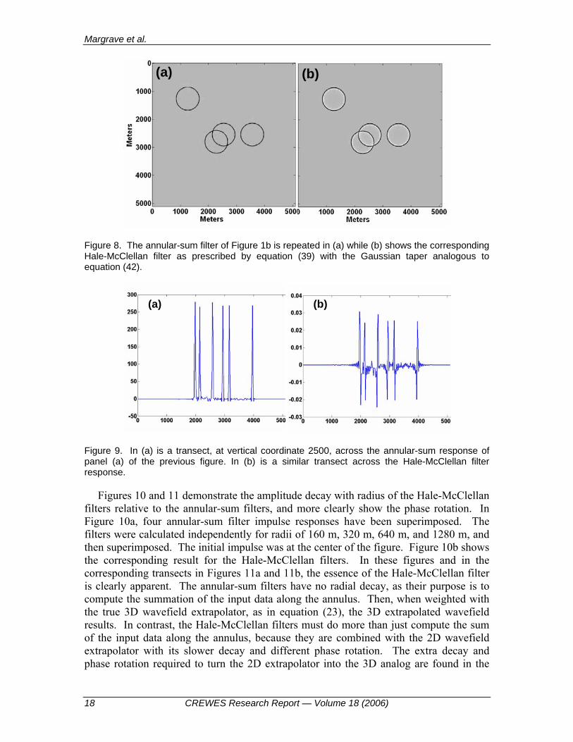
Figure 8. The annular-sum filter of Figure 1b is repeated in (a) while (b) shows the corresponding Hale-McClellan filter as prescribed by equation (39) with the Gaussian taper analogous to equation (42).

(a) (b)(a)(a) (b)(b)

Figure 9. In (a) is a transect, at vertical coordinate 2500, across the annular-sum response of panel (a) of the previous figure. In (b) is a similar transect across the Hale-McClellan filter response.

Figures 10 and 11 demonstrate the amplitude decay with radius of the Hale-McClellan filters relative to the annular-sum filters, and more clearly show the phase rotation. In Figure 10a, four annular-sum filter impulse responses have been superimposed. The filters were calculated independently for radii of 160 m, 320 m, 640 m, and 1280 m, and then superimposed. The initial impulse was at the center of the figure. Figure 10b shows the corresponding result for the Hale-McClellan filters. In these figures and in the corresponding transects in Figures 11a and 11b, the essence of the Hale-McClellan filter is clearly apparent. The annular-sum filters have no radial decay, as their purpose is to compute the summation of the input data along the annulus. Then, when weighted with the true 3D wavefield extrapolator, as in equation (23), the 3D extrapolated wavefield results. In contrast, the Hale-McClellan filters must do more than just compute the sum of the input data along the annulus, because they are combined with the 2D wavefield extrapolator with its slower decay and different phase rotation. The extra decay and phase rotation required to turn the 2D extrapolator into the 3D analog are found in the



Hale-McClellan filters. Remarkably, with suitably designed 2D and 3D extrapolators, equations (23) and (2) are equivalent.

(a) (b)(a) (b)

Figure 10. Panel (a) shows the superposition of 4 different annular-sum filter impulse responses for radii 160 , 320, 640, and 1280 m. Panel (b) is the corresponding Hale-McClellan filter response.

(a)

(b)

(a)

(b)

Figure 11. Panel (a) shows a transect, from the panel center to the right along the horizontal axis, across the annular-sum filter result in panel (a) of the previous figure. Panel (b) shows the analogous result for the Hale-McClellan filters in panel (b) of the previous figure.

Testing 2D convolution via annular-sum filters

In this section, simulations of 2D convolution are presented using annular-sum filters as directly expressed in equation (23). That the direct convolution method will be much faster in practice is not in doubt given the evidence of Figure 4. This provides incentive to develop a high fidelity, compactly supported, space domain approximation, called a ,

Margrave et al.


to the annular-sum filter, whose Fourier transform is given by equation (41). The 2D convolution is calculated with equation (23), using specific test functions for W , to test several different strategies for constructing a .

A simple, direct construction method is to capture the impulse response of the Fourier algorithm with a window. In Figure 12 a simple test of a the most direct method of constructing a , that is to simply capture the impulse response, is shown. For this case W was taken to be a 21 point boxcar, which means that the resulting convolution should reconstruct the disks of Figure 1a when applied to the same input field containing four impulses. To construct a , the exact Fourier operator was applied to an impulse centered in a number field twice as large as the largest expected annulus. Let this be called the IFC (inverse Fourier capture) method, referred to as IFCa . The resulting operator was used directly in 2D convolutions. In Figure 12a, the result of the convolution using equation (23) with the Fourier algorithm is shown while in Figure 12b the result from IFCa is shown. The Fourier algorithm has reproduced the disks essentially exactly, with a slight Gibbs ripple. This is actually a very difficult test, in some ways more difficult than wavefield extrapolation because W is discontinuous, and the results in Figure 12a-b show a very high fidelity algorithm. In contrast, IFCa has not done nearly as well, with numerous artifacts, including the large negative troughs preceding each disk.

(a)

(b)

(c)

(d)

(a)

(b)

(c)

(d)

Figure 12. Recreation of a disks via annular convolution (compare Figure 1a). In (a) the annular sums were generated with the full Fourier routine, and (b) shows a transect across (a) along the middle row. In (c) the annular sums were generated with the Inverse Fourier Capture method described in the text. A transect across (c) is shown in (d).

The result in Figure 12 motivates possible adjustments of the IFC method. In Figure 13a-b is the result using the IFC method with the addition of zeroing any negative samples in IFCa , which is called the IFCZ method. The negative shadows around the disks are removed, but at the expense of an unacceptable artifact in the center. Figure 13c-d shows the result of applying a Gaussian taper to the samples of IFCa that are beyond each annulus, and is called the IFCG. It is likely that IFCGa would prove more acceptable than either IFCa or IFCZa in practice, but we would like better still.



(a)

(b)

(c)

(d)

(a)

(b)

(c)

(d)

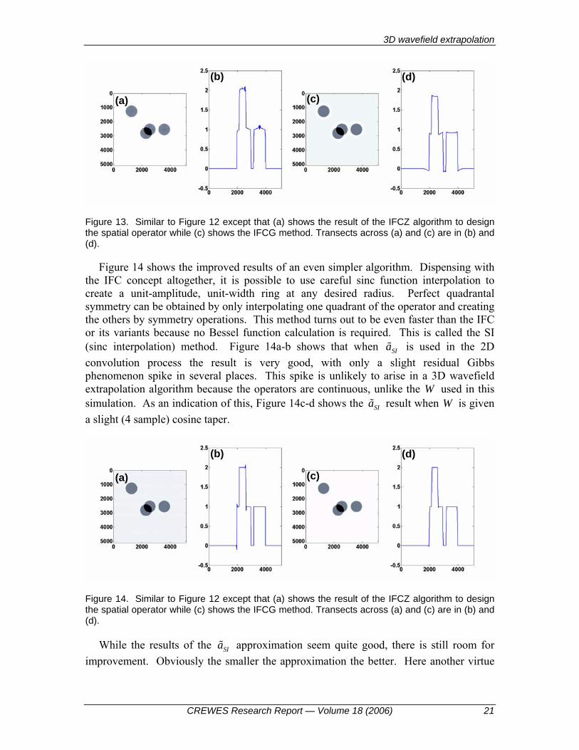
Figure 13. Similar to Figure 12 except that (a) shows the result of the IFCZ algorithm to design the spatial operator while (c) shows the IFCG method. Transects across (a) and (c) are in (b) and (d).

Figure 14 shows the improved results of an even simpler algorithm. Dispensing with the IFC concept altogether, it is possible to use careful sinc function interpolation to create a unit-amplitude, unit-width ring at any desired radius. Perfect quadrantal symmetry can be obtained by only interpolating one quadrant of the operator and creating the others by symmetry operations. This method turns out to be even faster than the IFC or its variants because no Bessel function calculation is required. This is called the SI (sinc interpolation) method. Figure 14a-b shows that when SIa is used in the 2D convolution process the result is very good, with only a slight residual Gibbs phenomenon spike in several places. This spike is unlikely to arise in a 3D wavefield extrapolation algorithm because the operators are continuous, unlike the W used in this simulation. As an indication of this, Figure 14c-d shows the SIa result when W is given a slight (4 sample) cosine taper.

(a)

(b)

(c)

(d)

(a)

(b)

(c)

(d)

Figure 14. Similar to Figure 12 except that (a) shows the result of the IFCZ algorithm to design the spatial operator while (c) shows the IFCG method. Transects across (a) and (c) are in (b) and (d).

While the results of the SIa approximation seem quite good, there is still room for improvement. Obviously the smaller the approximation the better. Here another virtue

Margrave et al.


of the Hale-McClellan algorithm is worth mentioning. It turns out that the McClellan filters obey the recursion

1 1 22j j jm m m m− −= • − , (43)

which means that all of the McClellan filters can be generated from repeated convolutions with 1m which is a very small operator. At present, it is not known whether the ja satisfy a similar recurrence relation or not.

Designing the 3D operator If the annular-sum method is to be used, then a method to design a stable, compactly

supported approximation to the 3D homogeneous wavefield extrapolator is required. For the FOCI algorithm, there are at least two possibilities: (i) the McClellan transform, and (ii) inverting the radial convolution matrix, which means solving equation (35).

In the first case, this is straight forward although the work is not yet completed and not reported here All that is required is a 2D wavefield extrapolation operator, w , that is sufficiently stable, and the McClellan transform turns this into a circularly symmetric 3D operator, W . This is done with the three steps (i) forward Fourier transform

( ) ( )ˆw x w ξ→ , (ii) interpolate onto a radial grid ( ) ( )2 21 2

ˆˆ ˆw w Wξ ξ ξ→ + = , (iii) inverse

2D Fourier transform ( ) ( )2 2 2 21 2 1 2W W x xξ ξ+ → + . In step (iii) the inverse 2D Fourier

transform could be replaced by a Hankel transform. This method will be reported on at a later date.

In the second case, the radial samples of the 3D operator can potentially be designed directly by solving a least-squares problem. This least-squares problem is posed by equation (35) and requires an estimate of an unstable forward operator for a half-step and a right-hand-side which is a suitably band-limited delta function. Investigation into this possibility is not yet satisfactory, and full reporting is also postponed. However, enough progress has been made to illustrate the use and potential of the radial convolution matrix.

Consider a 3D wavefield extrapolator for a step / 2zΔ , ( ), , / 2)W k zρ Δ , as expressed by equation (8). It is a straightforward exercise of Fourier transformation to show that when this operator is convolved with itself, the result is a 3D wavefield extrapolator for step zΔ , ( ), , )W k zρ Δ . Since equation (35) was derived as the convolution of two radially symmetric operators, a version of it applies in this case, given by



( )( )

( )

( )( )

( )

000 01 0 0

1 110 11 1

0 1

/ 2

/ 2

/ 2

M

M

NMN N NM

W zW W W W zW z W zW W W

W zW zW W W

⎡ ⎤ ⎡ ⎤Δ ⎡ ⎤Δ⎢ ⎥ ⎢ ⎥ ⎢ ⎥⎢ ⎥ ⎢ ⎥ ⎢ ⎥Δ Δ⎢ ⎥ ⎢ ⎥ ⎢ ⎥⎢ ⎥ =⎢ ⎥ ⎢ ⎥⎢ ⎥ ⎢ ⎥ ⎢ ⎥⎢ ⎥ ⎢ ⎥ ⎢ ⎥⎢ ⎥ Δ⎢ ⎥Δ ⎢ ⎥⎣ ⎦⎢ ⎥ ⎣ ⎦⎣ ⎦

. (44)

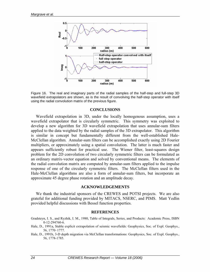
As described in the proof of Theorem 4, the elements of the radial convolution matrix are computed by applying annular-sum filters to the 2D impulse response of ( ), , / 2)W k zρ Δ . Each row of the matrix contains annular-sums computed at a fixed radius from the operator center and of each possible radius. Figure 15 shows the radial convolution matrix in this case, and it is definitely not Toeplitz (constant diagonal). Figure 16 shows the result of the auto-convolution of ( ), , / 2)W k zρ Δ , and it is an extremely good match

for ( ), , )W k zρ Δ . The 31 point half-step operator becomes 61 points long after autoconvolution, and there are no discernable discrepancies until well into the second 31 points.

(a) (b)(a) (b)

Figure 15. The real part of the radial convolution matrix for ( ), , / 2)W k zρ Δ is shown in (a) and the imaginary part in (b).

Margrave et al.


Figure 16. The real and imaginary parts of the radial samples of the half-step and full-step 3D wavefield extrapolators are shown, as is the result of convolving the half-step operator with itself using the radial convolution matrix of the previous figure.

CONCLUSIONS Wavefield extrapolation in 3D, under the locally homogenous assumption, uses a

wavefield extrapolator that is circularly symmetric. This symmetry was exploited to develop a new algorithm for 3D wavefield extrapolation that uses annular-sum filters applied to the data weighted by the radial samples of the 3D extrapolator. This algorithm is similar in concept but fundamentally different from the well-established Hale-McClellan algorithm. Annular-sum filters can be accomplished exactly using 2D Fourier multipliers, or approximately using a spatial convolution. The latter is much faster and appears sufficiently robust for practical use. The Wiener filter, least-squares design problem for the 2D convolution of two circularly symmetric filters can be formulated as an ordinary matrix-vector equation and solved by conventional means. The elements of the radial convolution matrix are computed by annular-sum filters applied to the impulse response of one of the circularly symmetric filters. The McClellan filters used in the Hale-McClellan algorithms are also a form of annular-sum filters, but incorporate an approximate 45 degree phase rotation and an amplitude decay.

ACKNOWLEDGEMENTS

We thank the industrial sponsors of the CREWES and POTSI projects. We are also grateful for additional funding provided by MITACS, NSERC, and PIMS. Matt Yedlin provided helpful discussions with Bessel function properties.

REFERENCES Gradsteyn, I. S., and Ryzhik, I. M., 1980, Table of Integrals, Series, and Products: Academic Press, ISBN

0-12-294760-6. Hale, D., 1991a, Stable explicit extrapolation of seismic wavefields: Geophysics, Soc. of Expl. Geophys.,

56, 1770–1777. Hale, D., 1991b, 3-D depth migration via McClellan transformations: Geophysics, Soc. of Expl. Geophys.,

56, 1778-1785.



Margrave, G. F. and Daley, P. F., 2001, Recursive Kirchhoff wavefield extrapolation: in the 13th Annual Research Report of the CREWES Project.

Margrave, G. F., Geiger, H. D., Al-Saleh, S. M., and Lamoureux, M. P., 2006, Improving explicit seismic depth migration with a stabilizing Wiener filter and spatial resampling: Geophysics, 71, S111-S120.

The annular-sum and Hale-McClellan methods of 3D wavefield extrapolation

Documents

Transcript of The annular-sum and Hale-McClellan methods of 3D wavefield extrapolation