Seismic wavefield simulation by a modifiedfinite element method with a perfectlymatched layer absorbing boundary

Weijuan Meng1,2,3 and Li-Yun Fu1

1Key Laboratory of Earth and Planetary Physics, Institute of Geology and Geophysics, Chinese Academyof Sciences, Beijing 100029, People’s Republic of China2University of Chinese Academy of Sciences, Beijing 100049, People’s Republic of China

E-mail: mwj@mail.iggcas.ac.cn

Received 25 September 2016, revised 13 March 2017Accepted for publication 4 April 2017Published 13 June 2017

AbstractThe finite element method is a very important tool for modeling seismic wave propagation incomplex media, but it usually consumes a large amount of memory which significantly decreasescomputational efficiency when solving large-scale seismic problems. Here, a modified finite elementmethod (MFEM) is proposed to improve efficiency. Triangular elements are employed to mesh thetopography and the discontinuous interface more flexibly. In the two-dimensional case, the Jacobianmatrix is obtained by using three controlling points instead of all nodes in each element with MFEM,which separates the Jacobian matrix from the stiffness matrix. The kernel matrices of the stiffnessmatrix rather than the global matrix are stored, and memory requirements are thus reducedsignificantly. Meanwhile, the element-by-element scheme is adopted to spare large sparse matricesand make the program easily parallelized. A second-order perfectly matched layer (PML) is alsoimplemented to eliminate artificial reflections. Finally, the accuracy and efficiency of our algorithmare validated by numerical tests.

Keywords: numerical simulation, finite element method, storage scheme, element-by-element,PML absorbing boundary condition

1. Introduction

Investigation of the wavefield from the earth’s interior as wellas the interpretation of seismic data networks have been majorproblems. Therefore, the numerical simulation of seismicwave propagation is very important in the seismology (Kellyet al 1976, Komatitsch and Tromp 2002).

Ongoing computer hardware improvements in recent dec-ades have provided the possibility of extracting more informa-tion from real seismic data. Widely used methods for solvingseismic wave equations include the finite difference method(FDM) (Alford et al 1974, Virieux 1984, 1986, Bohlenand Saenger 2006), the pseudo spectral method (PSM)(Fornberg 1988, Liu et al 2013), the finite element method(FEM) (Padovani et al 1994, Liu et al 2014a), the spectralelement method (SEM) (Komatitsch and Vilotte 1998,

Komatitsch and Tromp 2002, 2003, Komatitsch et al 2010) andother optimized methods (Yang et al 2009). The FDM is mostwidely used due to its high efficiency and easy implementation.However, the conventional FDM has some disadvantages inpractical modeling. Firstly, severe numerical dispersion occurswhen a coarse grid is used or a high velocity contrast exists.Secondly, rugged surfaces are hard to subdivide directly and afree surface boundary condition cannot be satisfied naturallyand needs to be dealt with by extra equations and otherspecial schemes (Kelly et al 1976, Moczo et al 2000, Liet al 2010, 2011, 2012, Zhang and Shen 2010, Zhang et al 2012,Wang et al 2014). The PSM is a global method with goodprecision and little numerical dispersion. However, it may yieldnumerical instability in a strongly heterogeneous medium and isstill incapable of handling complex geological geometriesor free boundary conditions (Fornberg 1988, Tessmer andKosloff 1994, Liu et al 2013). The FEM overcomes someshortcomings of previous methods. It is applicable to various

Journal of Geophysics and Engineering

J. Geophys. Eng. 14 (2017) 852–864 (13pp) https://doi.org/10.1088/1742-2140/aa6b31

3 Author to whom any correspondence should be addressed.

1742-2132/17/040852+13$33.00 © 2017 Sinopec Geophysical Research Institute Printed in the UK852

Dow

nloaded from https://academ

ic.oup.com/jge/article/14/4/852/5107940 by guest on 22 January 2022

geometrical models and naturally satisfies the free boundarycondition. However, the large memory requirements decrease itscomputational efficiency (Marfurt 1984, Padovani et al 1994,Zhang et al 2002, Liu et al 2014a). The SEM, known as thehigh-order FEM, also needs a large amount of computer mem-ory. One benefit of SEM with Legendre polynomials is that theinterpolation points are consistent with the integral points, whichleads to a diagonal mass matrix. Another is that a spectral-likeconvergence rate can be achieved because the orthogonalpolynomials are used in the space domain. Therefore, it has highcomputational accuracy and efficiency in modeling seismicwave (Komatitsch and Vilotte 1998, Chaljub et al 2007,Komatitsch et al 2010). However, the rectangular elements (two-dimensional, 2D) and hexahedral elements (three-dimensional,3D) used in conventional SEM can hardly subdivide the com-plex model (Liu et al 2014).

In the classical FEM either the consistent mass matrix or thestiffness matrix takes up most computer memory and decreasescomputational efficiency dramatically. The original mass matrix,also known as the consistent mass matrix, is non-diagonal andconsumes a large amount of computer memory (Marfurt 1984,Padovani et al 1994). Based on the law of mass conservation,the whole mass of each element is dispersed along its nodes.Then, the consistent mass matrix is transformed into a lumpedmass matrix, which is a diagonal matrix (Richter 1994, Liuet al 2014b). Such special treatment of the mass matrix avoidsthe need to solve a large-scale sparse system of equations andsubstantially increases the computational efficiency of the FEM.

Each discrete point in the computational domain of the FEMis only connected with the points in the surrounding elements.Thus, most zero elements are in each row of the stiffness matrixand the non-zero ones tend to be distributed around the maindiagonal of the stiffness matrix (Jiang and Pang 1979). Constantbandwidth storage is a simple and common way to store thestiffness matrix (Cuthill and McKee 1969, Gibbs et al 1976). Inthis scheme, only the elements inside the semi-bandwidth of thestiffness matrix are stored and the zero elements outside can beneglected. The drawback of this storage mode is that a largenumber of zero elements are stored inside the semi-bandwidth. Inorder to reduce storage requirements, some data-compressionstorage techniques, such as the compressed sparse row (CSR)method (Liu et al 2013), are introduced. In the CSR method,only non-zero elements in each row of the stiffness matrix arestored in three one-dimensional arrays. Therefore, computermemory and computational cost can both be reduced. All theseprevious methods cannot avoid storing the large sparse stiffnessmatrix. Thus, the storage costs of these methods may still beunaffordable in solving large-scale problems. Liu et al (2014a)introduced the kernel matrices storage (KMS) method in whichonly the kernel matrices of the global matrix are stored and theassembly of a large global stiffness matrix can be avoided. Thematrix–vector products are calculated element-by-element, simi-lar to the discontinuous Galerkin methods (Hesthaven andWarburton 2008, He et al 2015). At the cost of a small increasein float-point computation time, the storage memory for the KMSmethod can be significantly reduced. However, KMS is onlyapplicable to consistent elements and is less effective in complex

models with irregular interfaces, and thus requires furtherimprovement.

This paper is organized as follows. In the next section, theimproved version of KMS method, called the modified finiteelement method (MFEM), is proposed. The lumped massmatrix, the second-order perfectly matched layer (PML)absorbing boundary condition and updating of the wavefieldare also presented. Then the accuracy and efficiency of theMFEM are investigated in a simple homogeneous medium bycomparison with different storage schemes and other classicalmethods such as conventional FEM and SEM. In addition, theeffectiveness of different-order MFEMs are also benchmarkedin a two-layered model with inclined interfaces and a ruggedsurface model. Finally, the computational accuracy and effi-ciency of the MFEM are discussed.

2. Theoretical method

2.1. Elastic wave equation

The elastic wave equation is used to describe the propagationof aseismic wave through the solid earth. Considering anisotropic elastic medium, the 2D elastic wave equation isgiven by (Ma et al 2011, Liu et al 2015b)

uu u f

t, 1

2

2r l m m¶¶

= + ⋅ + ⋅ +(( ) ) ( ) ( )

where u and f are the displacement vector and source term,respectively, r is mass density and l and m are Laméconstants.

Multiplying the above equation by a test function, inte-grating over the whole domain Ω and applying the method ofweighted residuals, the weak form of equation (1) yields

uv x u v x

u v x f v x

td d

: d d , 2

2

2ò òò ò

r l m

m

¶¶

⋅ = + ⋅ ⋅

+ + ⋅

W W

W W

( )( )( )

( ) ( ) ( )

where v is an arbitrary time-independent vector and x is theCartesian coordinate.

We subdivide the domain Ω into N non-overlappingelements, and equation (2) can be written as

MU KU F

M

KK KK K

K

K

K

K

d

2 d

d

d

2 d

3

e

N

e

N

x x z z

x z z x

x z z x

x x z z

T

11 12

21 22

11T T

12T T

21T T

22T T

e

e

e

e

e

e

ò

ò

ò

ò

ò

å

å

r f f

l m f f m f f

l f f m f f

m f f l f f

m f f l m f f

= +

= W

=

= - + + W

= - + W

= - + W

= - + + W

W

W

W

W

W

W

⎧

⎨

⎪⎪⎪⎪⎪⎪⎪⎪

⎩

⎪⎪⎪⎪⎪⎪⎪⎪

⎡⎣⎢

⎤⎦⎥

[ ] [ ]

( )[ ] [ ] [ ] [ ]

[ ] [ ] [ ] [ ]

[ ] [ ] [ ] [ ]

[ ] [ ] ( )[ ] [ ]

( )

853

J. Geophys. Eng. 14 (2017) 852 W Meng and L-Y Fu

Dow

nloaded from https://academ

ic.oup.com/jge/article/14/4/852/5107940 by guest on 22 January 2022

where U is the displacement vector, M is the consistent massmatrix, K is the assembled stiffness matrix and F is the sourcevector.

For regular quadrilateral elements, each stiffness kernelmatrix is identical in all the same shape elements, and only four

kernels, d ,x xT

eò f f WW

[ ] [ ] d ,z zT

eò f f WW

[ ] [ ] dx zT

eò f f WW

[ ] [ ]

and d ,z xT

eò f f WW

[ ] [ ] of an element stiffness matrix instead of a

huge global matrix are stored. A detailed description can befound in Liu et al (2014a). However, in order to simulate seis-mic wave propagation in complex structures we need to inves-tigate this problem with triangular subdivision further. Differenttriangular elements have different Jacobian matrices that connectthe physical coordinates with the local coordinates. Therefore,we only need to calculate Jacobian matrices over all elementsand store them in advance.

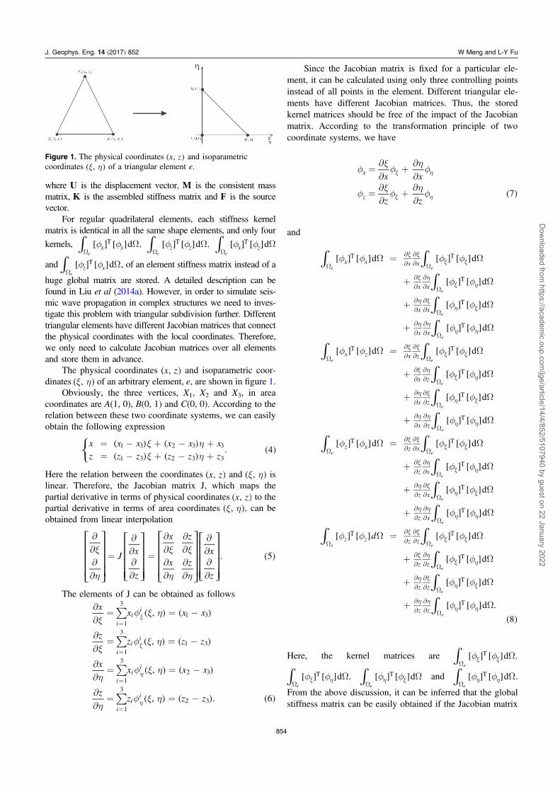
The physical coordinates x z,( ) and isoparametric coor-dinates ,x h( ) of an arbitrary element, e, are shown in figure 1.

Obviously, the three vertices, X1, X2 and X3, in areacoordinates are A(1, 0), B(0, 1) and C(0, 0). According to therelation between these two coordinate systems, we can easilyobtain the following expression

x x x x x xz z z z z z

. 41 3 2 3 3

1 3 2 3 3

x hx h

= - + - += - + - +

⎧⎨⎩( ) ( )( ) ( )

( )

Here the relation between the coordinates x z,( ) and ,x h( ) islinear. Therefore, the Jacobian matrix J, which maps thepartial derivative in terms of physical coordinates x z,( ) to thepartial derivative in terms of area coordinates , ,x h( ) can beobtained from linear interpolation

J x

z

x z

x zx

z

. 5x

h

x x

h h

¶¶¶¶

=

¶¶¶¶

=

¶¶

¶¶

¶¶

¶¶

¶¶¶¶

⎡

⎣

⎢⎢⎢⎢

⎤

⎦

⎥⎥⎥⎥

⎡

⎣

⎢⎢⎢⎢

⎤

⎦

⎥⎥⎥⎥

⎡

⎣

⎢⎢⎢⎢

⎤

⎦

⎥⎥⎥⎥

⎡

⎣

⎢⎢⎢⎢

⎤

⎦

⎥⎥⎥⎥( )

The elements of J can be obtained as followsx

x x x

zz z z

xx x x

zz z z

,

,

,

, . 6

ii

i

ii

i

ii

i

ii

i

1

3

1 3

1

3

1 3

1

3

2 3

1

3

2 3

å

å

å

å

xf x h

xf x h

hf x h

hf x h

¶¶

= = -

¶¶

= = -

¶¶

= = -

¶¶

= = -

x

x

h

h

=

=

=

=

( ) ( )

( ) ( )

( ) ( )

( ) ( ) ( )

Since the Jacobian matrix is fixed for a particular ele-ment, it can be calculated usingonly three controlling pointsinstead of all points in the element. Different triangular ele-ments have different Jacobian matrices. Thus, the storedkernel matrices should be free of the impact of the Jacobianmatrix. According to the transformation principle of twocoordinate systems, we have

x x

z z7

x

z

fxf

hf

fxf

hf

=¶¶

+¶¶

=¶¶

+¶¶

x h

x h ( )

and

d

d d

d

d

d

d d

d

d

d

d d

d

d

d

d

d

d

d .

8

x x x x

x x

x x

x x

x z x z

x z

x z

x z

z x z x

z x

z x

z x

z z z z

z z

z z

z z

T T

T

T

T

T T

T

T

T

T T

T

T

T

T T

T

T

T

e e

e

e

e

e e

e

e

e

e e

e

e

e

e e

e

e

e

ò ò

ò

ò

ò

ò ò

ò

ò

ò

ò ò

ò

ò

ò

ò ò

ò

ò

ò

f f f f

f f

f f

f f

f f f f

f f

f f

f f

f f f f

f f

f f

f f

f f f f

f f

f f

f f

W = W

+ W

+ W

+ W

W = W

+ W

+ W

+ W

W = W

+ W

+ W

+ W

W = W

+ W

+ W

+ W

x xx x

x hx h

h xh x

h hh h

x xx x

x hx h

h xh x

h hh h

x xx x

x hx h

h xh x

h hh h

x xx x

x hx h

h xh x

h hh h

W

¶¶

¶¶ W

¶¶

¶¶ W

¶¶

¶¶ W

¶¶

¶¶ W

W

¶¶

¶¶ W

¶¶

¶¶ W

¶¶

¶¶ W

¶¶

¶¶ W

W

¶¶

¶¶ W

¶¶

¶¶ W

¶¶

¶¶ W

¶¶

¶¶ W

W

¶¶

¶¶ W

¶¶

¶¶ W

¶¶

¶¶ W

¶¶

¶¶ W

[ ] [ ] [ ] [ ]

[ ] [ ]

[ ] [ ]

[ ] [ ]

[ ] [ ] [ ] [ ]

[ ] [ ]

[ ] [ ]

[ ] [ ]

[ ] [ ] [ ] [ ]

[ ] [ ]

[ ] [ ]

[ ] [ ]

[ ] [ ] [ ] [ ]

[ ] [ ]

[ ] [ ]

[ ] [ ]( )

Here, the kernel matrices are d ,T

eò f f Wx xW

[ ] [ ]

d ,T

eò f f Wx hW

[ ] [ ] dT

eò f f Wh xW

[ ] [ ] and d .T

eò f f Wh hW

[ ] [ ]

From the above discussion, it can be inferred that the globalstiffness matrix can be easily obtained if the Jacobian matrix

Figure 1. The physical coordinates x z,( ) and isoparametriccoordinates ,x h( ) of a triangular element e.

854

J. Geophys. Eng. 14 (2017) 852 W Meng and L-Y Fu

Dow

nloaded from https://academ

ic.oup.com/jge/article/14/4/852/5107940 by guest on 22 January 2022

of triangular elements as well as the kernel matrices arecalculated in advance.

2.2. Lumped mass matrix

The consistent mass matrix constructed from the classical finiteelement equations is non-diagonal and requires the solution ofa large sparse linear system of equations. However, based onthe principle of mass conservation, the non-diagonal consistentmass matrices can be lumped into a diagonal mass matrix withthe lumped mass technique (Archer and Whalen 2005,Wu 2006). The formula for diagonalizing the mass matrixM inequation (3) is given by (Liu et al 2014b)

M M M M . 9ii iii j

ijj

jjd åå å=

⎛⎝⎜⎜

⎞⎠⎟⎟

⎛⎝⎜⎜

⎞⎠⎟⎟ ( )

Because of the diagonal property of the lumped massmatrix, the wavefields can be updated by explicit recursionand the efficiency of the FEM can be improved significantly.However, when the mesh size is much less than the seismicwavelength and the accuracy of numerical integration isadequate, the numerical precision of the FEM with thelumped mass matrix is of the same order as that with theconsistent mass matrix. Here, we do not discuss the num-erical precision specifically and just test the accuracy of ourmethod by comparing it with analytical solutions or othermethods. More details can be found in the papers of Wu(2006) or Liu et al (2013).

2.3. PML absorbing boundary condition

In order to eliminate artificial reflections, the PML for second-order elastic wave equations is adopted (Komatitsch andTromp 2003, Liu et al 2012).

From equation (1), the source-free elastic wave equationcan be rewritten in the following form:

u

t x

u

x

u

z

z

u

x

u

z

u

t x

u

x

u

z

z

u

x

u

z

2

2

.

10

x x z

z x

z z x

x z

2

2

2

2

r l m l

m

r m

l l m

¶¶

=¶¶

+¶¶

+¶¶

+¶¶

¶¶

+¶¶

¶¶

=¶¶

¶¶

+¶¶

+¶¶

¶¶

+ +¶¶

⎧

⎨

⎪⎪⎪⎪⎪

⎩

⎪⎪⎪⎪⎪

⎡⎣⎢

⎤⎦⎥

⎡⎣⎢

⎛⎝⎜

⎞⎠⎟

⎤⎦⎥

⎡⎣⎢

⎛⎝⎜

⎞⎠⎟

⎤⎦⎥

⎡⎣⎢

⎤⎦⎥

( )

( )

( )

In complex stretched coordinates (Collino and Tsogka 2001),equation (10) can be rewritten as

Ud x x d x

U

x d z

U

z

d z z d x

U

x

d z

U

z

Ud x x d x

U

x

d z

U

z

d z z d x

U

x

d z

U

z

ii

i2

i

i

i

i

i

i

i

i

i

i

ii

i

i

i

i

i

i

i

i

i

2i

i

11

xx x

x

z

z

z x

z

z

x

zx x

z

z

x

z x

x

z

z

2

2

r ww

wl m

ww

lw

w

ww

mw

w

ww

r ww

wm

ww

ww

ww

lw

w

l mw

w

=+

¶¶

++

´¶¶

++

¶¶

++

¶¶ +

¶¶

++

¶¶

=+

¶¶ +

¶¶

++

¶¶

++

¶¶ +

¶¶

+ ++

¶¶

⎧

⎨

⎪⎪⎪⎪⎪⎪⎪⎪⎪⎪⎪⎪

⎩

⎪⎪⎪⎪⎪⎪⎪⎪⎪⎪⎪⎪

⎡⎣⎢

⎤⎦⎥

⎡⎣⎢

⎛⎝⎜

⎞⎠⎟

⎤⎦⎥

⎡⎣⎢

⎛⎝⎜

⎞⎠⎟

⎤⎦⎥

⎡⎣⎢

⎤⎦⎥

( )( )

( )( )

( )

( ) ( )

( )

( )( ) ( )

( )

( ) ( )

( )( )

( )

where i 1= - is the imaginary unit,w is the angular frequencyandUx andUz are the Fourier transforms of ux and uz with respectto time, respectively. d xx ( ) and d zz ( ) are the dampingcoefficients in the PML region, which are described in detail inthe appendix. After splitting each displacement component intothree terms and transforming the terms back into the time domain,we get

d x ux

u

xP

d z uz

u

zP

d x d z u

x

u

z z

u

x

d x P d xu

x

d z P d zu

z

2

2

12

t x xx

xx

t z xx

xz

t x t z x

z z

t x xx xx

t z xz zx

21

22

3

r l m r

r m r

r

l m

r l m

r m

¶ + =¶¶

+¶¶

+

¶ + =¶¶

¶¶

+

¶ + ¶ +

=¶¶

¶¶

+¶¶

¶¶

¶ + = - + ¢ ¶¶

¶ + = - ¢ ¶¶

⎧

⎨

⎪⎪⎪⎪⎪⎪⎪

⎩

⎪⎪⎪⎪⎪⎪⎪

⎡⎣⎢

⎤⎦⎥

⎡⎣⎢

⎤⎦⎥

⎡⎣⎢

⎤⎦⎥

⎡⎣⎢

⎤⎦⎥

[ ( )] ( )

[ ( )]

[ ( )][ ( )]

[ ( )] ( ) ( )

[ ( )] ( )

( )

d z uz

u

zP

d x ux

u

xP

d x d z u

x

u

z z

u

x

d z P d zu

z

d x P d xu

x

2

2

13

t z zz

zz

t x zz

zx

t x t z z

z z

t z zz zz

t x zx xz

21

22

3

r l m r

r m r

r

m l

r l m

r m

¶ + =¶¶

+¶¶

+

¶ + =¶¶

¶¶

+

¶ + ¶ +

=¶¶

¶¶

+¶¶

¶¶

¶ + = - + ¢ ¶¶

¶ + = - ¢ ¶¶

⎧

⎨

⎪⎪⎪⎪⎪⎪⎪

⎩

⎪⎪⎪⎪⎪⎪⎪

⎡⎣⎢

⎤⎦⎥

⎡⎣⎢

⎤⎦⎥

⎡⎣⎢

⎤⎦⎥

⎡⎣⎢

⎤⎦⎥

[ ( )] ( )

[ ( )]

[ ( )][ ( )]

[ ( )] ( ) ( )

[ ( )] ( )

( )

855

J. Geophys. Eng. 14 (2017) 852 W Meng and L-Y Fu

Dow

nloaded from https://academ

ic.oup.com/jge/article/14/4/852/5107940 by guest on 22 January 2022

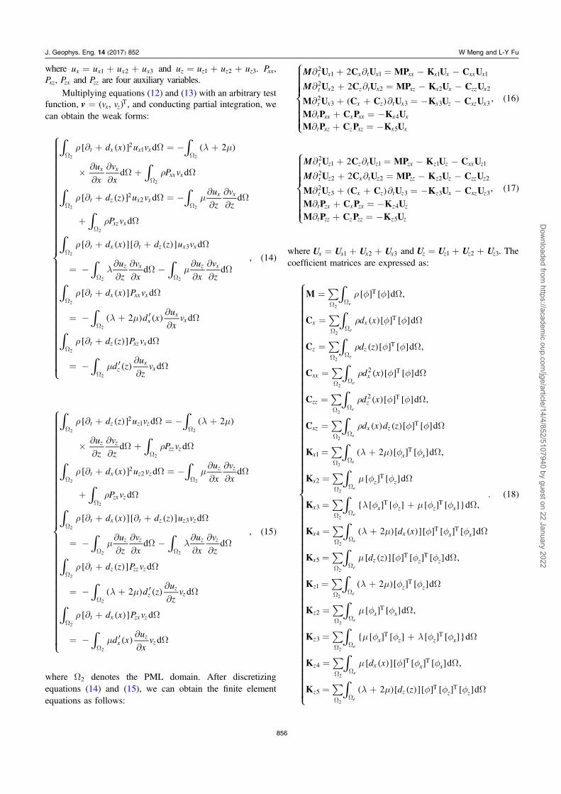
where u u u ux x x x1 2 3= + + and u u u u .z z z z1 2 3= + + P ,xx

P ,xz Pzx and Pzz are four auxiliary variables.

Multiplying equations (12) and (13) with an arbitrary testfunction, v v v, ,x z

T= ( ) and conducting partial integration, wecan obtain the weak forms:

d x u v

u

x

v

xP v

d z u vu

z

v

z

P v

d x d z u v

u

z

v

x

u

x

v

z

d x P v

d xu

xv

d z P v

d zu

zv

d 2

d d

d d

d

d

d d

d

2 d

d

d

, 14

t x x x

x xxx x

t z x xx x

xz x

t x t z x x

z x z x

t x xx x

xx

x

t z xz x

zx

x

21

22

3

2 2

2

2 2

2

2

2 2

2

2

2

2

ò ò

ò

ò ò

ò

ò

ò ò

ò

ò

ò

ò

r l m

r

r m

r

r

l m

r

l m

r

m

¶ + W = - +

´¶¶

¶¶

W + W

¶ + W = -¶¶

¶¶

W

+ W

¶ + ¶ + W

= -¶¶

¶¶

W -¶¶

¶¶

W

¶ + W

= - + ¢ ¶¶

W

¶ + W

= - ¢ ¶¶

W

W W

W

W W

W

W

W W

W

W

W

W

⎧

⎨

⎪⎪⎪⎪⎪⎪⎪⎪⎪⎪⎪⎪

⎩

⎪⎪⎪⎪⎪⎪⎪⎪⎪⎪⎪⎪

[ ( )] ( )

[ ( )]

[ ( )][ ( )]

[ ( )]

( ) ( )

[ ( )]

( )

( )

d z u v

u

z

v

zP v

d x u vu

x

v

x

P v

d x d z u v

u

z

v

x

u

x

v

z

d z P v

d zu

zv

d x P v

d xu

xv

d 2

d d

d d

d

d

d d

d

2 d

d

d

, 15

t z z z

z zzz z

t x z zz z

zx z

t x t z z z

z z z z

t z zz z

zz

z

t x zx z

xz

z

21

22

3

2 2

2

2 2

2

2

2 2

2

2

2

2

ò ò

ò

ò ò

ò

ò

ò ò

ò

ò

ò

ò

r l m

r

r m

r

r

m l

r

l m

r

m

¶ + W = - +

´¶¶

¶¶

W + W

¶ + W = -¶¶

¶¶

W

+ W

¶ + ¶ + W

= -¶¶

¶¶

W -¶¶

¶¶

W

¶ + W

= - + ¢ ¶¶

W

¶ + W

= - ¢ ¶¶

W

W W

W

W W

W

W

W W

W

W

W

W

⎧

⎨

⎪⎪⎪⎪⎪⎪⎪⎪⎪⎪⎪⎪

⎩

⎪⎪⎪⎪⎪⎪⎪⎪⎪⎪⎪⎪

[ ( )] ( )

[ ( )]

[ ( )][ ( )]

[ ( )]

( ) ( )

[ ( )]

( )

( )

where 2W denotes the PML domain. After discretizingequations (14) and (15), we can obtain the finite elementequations as follows:

M

M

U C U MP K U C U

U C U MP K U C U

M U C C U K U C UM P C P K UM P C P K U

2

2, 16

t x x t x xx x x xx x

t x z t x xz x x zz x

t x x z t x x z xz x

t xx x xx x x

t xz z xz x x

21 1 1 1

22 2 2 2

23 3 3 3

4

5

¶ + ¶ = - -

¶ + ¶ = - -

¶ + + ¶ = - -¶ + = -¶ + = -

⎧

⎨⎪⎪⎪

⎩⎪⎪⎪

( ) ( )

M

M

U C U MP K U C U

U C U MP K U C U

M U C C U K U C UM P C P K UM P C P K U

2

2, 17

t z z t z zx z z xx z

t z x t z zz z z zz z

t z x z t z z x xz z

t zx x zx z z

t zz z zz z z

21 1 1 1

22 2 2 2

23 3 3 3

4

5

¶ + ¶ = - -

¶ + ¶ = - -

¶ + + ¶ = - -¶ + = -¶ + = -

⎧

⎨⎪⎪⎪

⎩⎪⎪⎪

( ) ( )

where U U U Ux x x x1 2 3= + + and U U U U .z z z z1 2 3= + + Thecoefficient matrices are expressed as:

d x

d z

d x

d x

d x d z

d x

d z

d x

d z

M

C

C

C

C

C

K

K

K

K

K

K

K

K

K

K

d ,

d

d ,

d

d ,

d

2 d ,

d

d ,

2 d

d ,

2 d

d ,

d

d ,

2 d

. 18

x x

z z

xx x

zz z

xz x z

x x x

x z z

x x z z x

x x x x

x z z z

z z z

z x x

z x z z x

z x x x

z z z z

T

T

T

2 T

2 T

T

1T

2T

3T T

4T T

5T T

1T

2T

3T T

4T T

5T T

e

e

e

e

e

e

e

e

e

e

e

e

e

e

e

e

2

2

2

2

2

2

2

2

2

2

2

2

2

2

2

2

ò

ò

ò

ò

ò

ò

ò

ò

ò

ò

ò

ò

ò

ò

ò

ò

å

å

å

å

å

å

å

å

å

å

å

å

å

å

å

å

r f f

r f f

r f f

r f f

r f f

r f f

l m f f

m f f

l f f m f f

l m f f f

m f f f

l m f f

m f f

m f f l f f

m f f f

l m f f f

= W

= W

= W

= W

= W

= W

= + W

= W

= + W

= + W

= W

= + W

= W

= + W

= W

= + W

W W

W W

W W

W W

W W

W W

W W

W W

W W

W W

W W

W W

W W

W W

W W

W W

⎧

⎨

⎪⎪⎪⎪⎪⎪⎪⎪⎪⎪⎪⎪⎪⎪⎪⎪⎪⎪⎪⎪⎪⎪

⎩

⎪⎪⎪⎪⎪⎪⎪⎪⎪⎪⎪⎪⎪⎪⎪⎪⎪⎪⎪⎪⎪⎪

[ ] [ ]

( )[ ] [ ]

( )[ ] [ ]

( )[ ] [ ]

( )[ ] [ ]

( ) ( )[ ] [ ]

( )[ ] [ ]

[ ] [ ]

{ [ ] [ ] [ ] [ ]}

( )[ ( )][ ] [ ] [ ]

[ ( )][ ] [ ] [ ]

( )[ ] [ ]

[ ] [ ]

{ [ ] [ ] [ ] [ ]}

[ ( )][ ] [ ] [ ]

( )[ ( )][ ] [ ] [ ]

( )

856

J. Geophys. Eng. 14 (2017) 852 W Meng and L-Y Fu

Dow

nloaded from https://academ

ic.oup.com/jge/article/14/4/852/5107940 by guest on 22 January 2022

2.4. Updating the wavefield

There are many methods for temporal discretization, such asthe Lax–Wendroff method (Chen 2009), the Runge–Kuttamethod (Yang et al 2009), the Newmark method (Komatitschand Tromp 2002, Liu et al 2014) and symplectic schemes(Ma et al 2011, Liu et al 2015a). Among these methods, thesecond-order Lax–Wendroff method, also known as thecentral difference method, is employed due to its simplicityand high efficiency:

tU M KU F U U2 . 19t t t t t t2 1= D + + -+D

--D( ) ( ) ( )( ) ( ) ( ) ( )

3. Numerical experiments

3.1. A simple homogeneous model

First, we use a homogeneous medium to investigate thevalidity and the accuracy of the MFEM. The size of the modelis 1000 m×1000 m, and the thickness of the PML absorbingboundary is 100 m. The velocities of P- and S-waves are

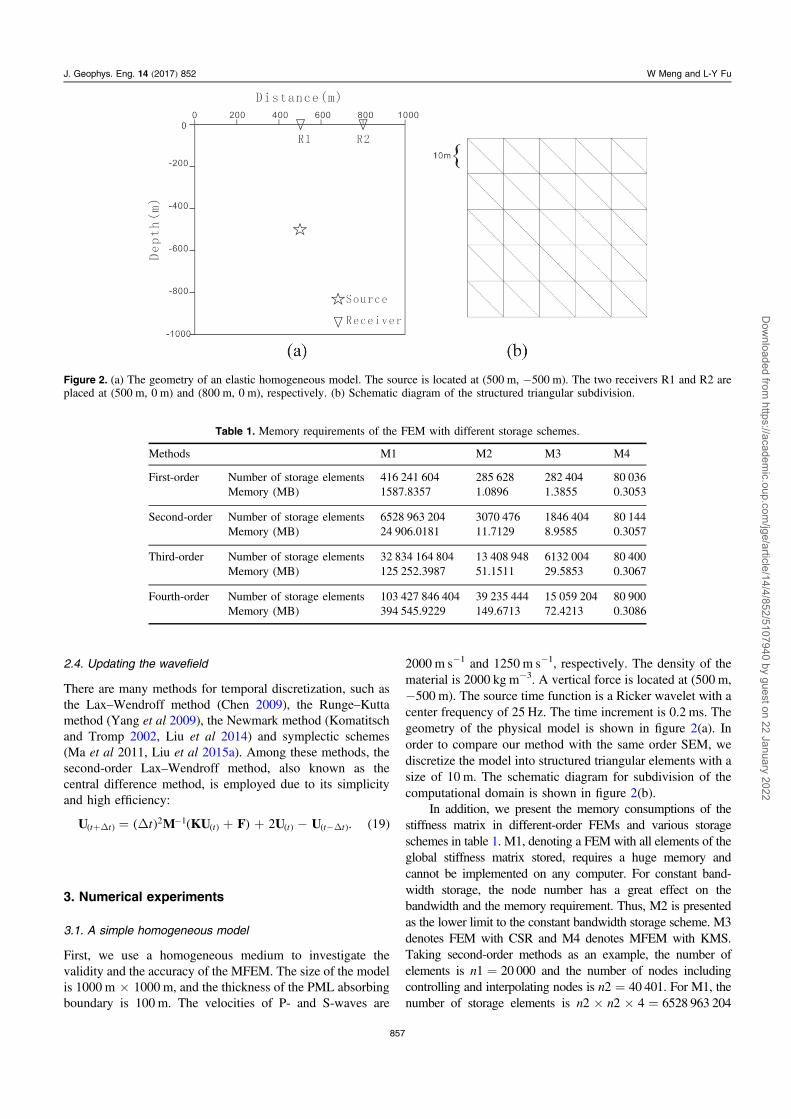
2000 m s−1 and 1250 m s−1, respectively. The density of thematerial is 2000 kg m−3. A vertical force is located at (500 m,−500 m). The source time function is a Ricker wavelet with acenter frequency of 25 Hz. The time increment is 0.2 ms. Thegeometry of the physical model is shown in figure 2(a). Inorder to compare our method with the same order SEM, wediscretize the model into structured triangular elements with asize of 10 m. The schematic diagram for subdivision of thecomputational domain is shown in figure 2(b).

In addition, we present the memory consumptions of thestiffness matrix in different-order FEMs and various storageschemes in table 1. M1, denoting a FEM with all elements of theglobal stiffness matrix stored, requires a huge memory andcannot be implemented on any computer. For constant band-width storage, the node number has a great effect on thebandwidth and the memory requirement. Thus, M2 is presentedas the lower limit to the constant bandwidth storage scheme. M3denotes FEM with CSR and M4 denotes MFEM with KMS.Taking second-order methods as an example, the number ofelements is n1=20 000 and the number of nodes includingcontrolling and interpolating nodes is n2=40 401. For M1, thenumber of storage elements is n2×n2×4=6528 963 204

Figure 2. (a) The geometry of an elastic homogeneous model. The source is located at (500 m, −500 m). The two receivers R1 and R2 areplaced at (500 m, 0 m) and (800 m, 0 m), respectively. (b) Schematic diagram of the structured triangular subdivision.

Table 1. Memory requirements of the FEM with different storage schemes.

Methods M1 M2 M3 M4

First-order Number of storage elements 416 241 604 285 628 282 404 80 036Memory (MB) 1587.8357 1.0896 1.3855 0.3053

Second-order Number of storage elements 6528 963 204 3070 476 1846 404 80 144Memory (MB) 24 906.0181 11.7129 8.9585 0.3057

Third-order Number of storage elements 32 834 164 804 13 408 948 6132 004 80 400Memory (MB) 125 252.3987 51.1511 29.5853 0.3067

Fourth-order Number of storage elements 103 427 846 404 39 235 444 15 059 204 80 900Memory (MB) 394 545.9229 149.6713 72.4213 0.3086

857

J. Geophys. Eng. 14 (2017) 852 W Meng and L-Y Fu

Dow

nloaded from https://academ

ic.oup.com/jge/article/14/4/852/5107940 by guest on 22 January 2022

and the memory cost is 6528 963 204×4≈249 06.0181MBin single precision storage. For M2, the bandwidth ofthe stiffness matrix is nb=19. The number of storageelements is nb×n2×4=3070 476 and the memory cost is3070 476×4≈11.7129MB. For M3, the numbers of the rowsthat include six, nine and nineteen non-zero elements are 402,29 802, 396 and 9801. Thus, the number of storage elements,including non-zero elements over all rows, is 1846 404, and thememory cost for storing these non-zero ones by using the threearrays is 1846 404×(4+1)+(n2+1)×4≈8.9585MB.For M4, the number of nodes in each element is n=6. The

number of storage elements is (n1×4) + (n×n×4) =80 144 and the memory cost is 80 144×4≈0.3057MB.Compared with the memory requirements of constant bandwidthstorage and CSR, M4 can save a significant amount of memory.

When the order increases from one to four, the memorycost of the stiffness matrix will increase by 15.69, 78.88 and248.48 times for M1, by 10.75, 46.95 and 137.37 times forM2, 6.47, 21.35, by 52.27 times for M3 and by about 1 timefor M4. The memory cost of the constant bandwidth storagemethod falls between M1 and M2. Therefore, for the constantbandwidth storage method and M3, the computational points

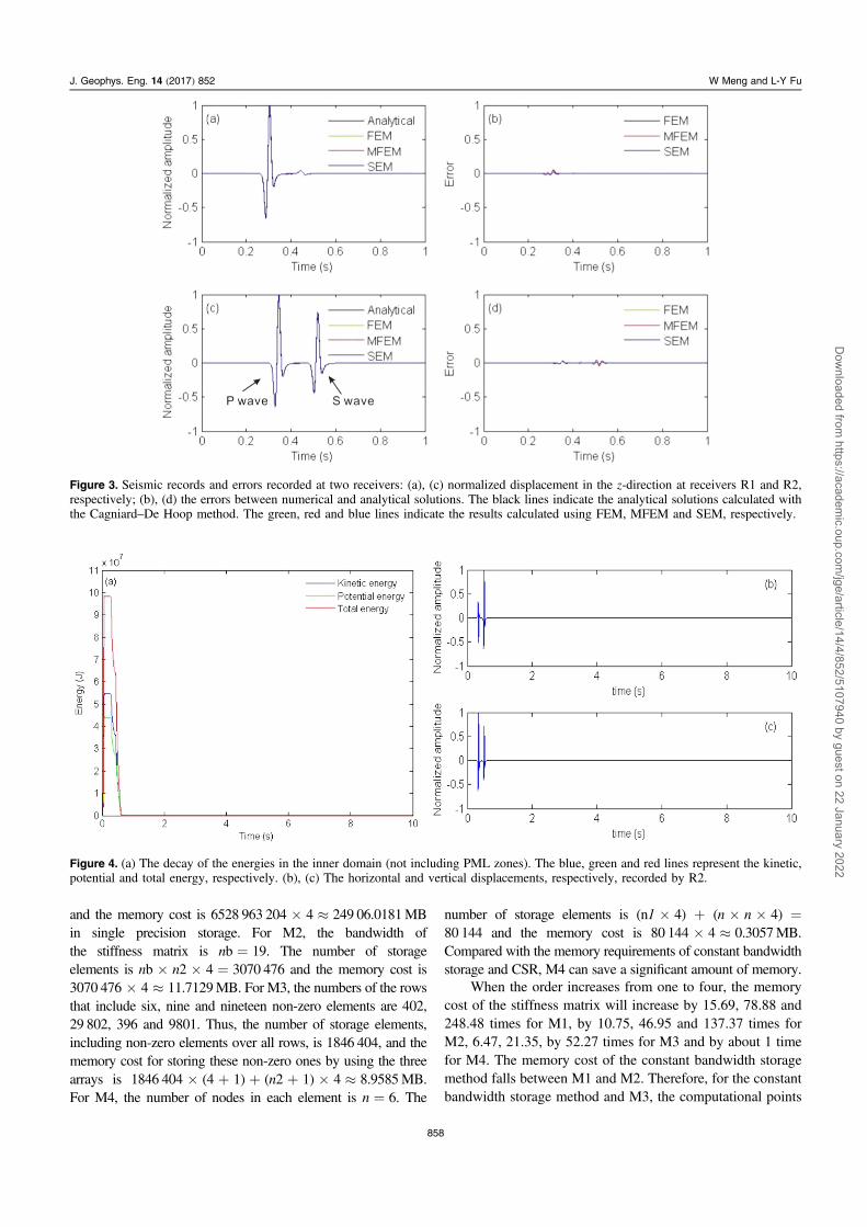
Figure 3. Seismic records and errors recorded at two receivers: (a), (c) normalized displacement in the z-direction at receivers R1 and R2,respectively; (b), (d) the errors between numerical and analytical solutions. The black lines indicate the analytical solutions calculated withthe Cagniard–De Hoop method. The green, red and blue lines indicate the results calculated using FEM, MFEM and SEM, respectively.

Figure 4. (a) The decay of the energies in the inner domain (not including PML zones). The blue, green and red lines represent the kinetic,potential and total energy, respectively. (b), (c) The horizontal and vertical displacements, respectively, recorded by R2.

858

J. Geophys. Eng. 14 (2017) 852 W Meng and L-Y Fu

Dow

nloaded from https://academ

ic.oup.com/jge/article/14/4/852/5107940 by guest on 22 January 2022

and memory requirements of the stiffness matrix will increaserapidly with increasing numerical order. For M4, only thekernel matrices of elements include more nodes and thus theincrease in memory requirements will be trivial.

Simulation of seismic wave propagation is performed onthe same computer with three numerical methods includingthe FEM, MFEM, and SEM, which are third-order in space.The computational domain is subdivided into quadrilateralelements in the SEM with a side length of 10 m and triangularelements in the FEM and MFEM with a right side length of10 m. Figure 3 shows seismic waveforms and errors recordedin the two receivers. The black lines indicate the analyticalsolutions generated by the Cagniard–De Hoop method (DeHoop 1960), and the other lines indicate the results fromFEM, MFEM and SEM. As shown in figure 3, the amplitudeand arrival time of the P- and S-waves are accurate, whichmeans that the results calculated using the MFEM and theother methods are consistent with the analytical solutions inthe homogeneous model. The maximum norm of errors inFEM, MFEM and SEM are 0.0504, 0.0513 and 0.0207,respectively, at receiver R1 (figure 3(b)). At receiver R2(figure 3(d)), the errors are 0.0473, 0.0458 and 0.0195,respectively. The results of FEM and SEM with triangularelements are less accurate than those with quadrilateral ele-ments (Liu et al 2014). Therefore, the above error analysesare reasonable.

As shown in figure 4(a), the performance and numericalstability of the PML are tested at long times period by mea-suring the decay of kinetic, potential and total energy versustime. The seismic records of R2 are presented in figures 4(b)and (c). The total energy is defined as (Shi et al 2012)

E1

2: d . 202ò r u s e= + W

W ( ) ( )

We present the evolution of energy over 5×104 time steps(10 s). As the source loads over time, the kinetic, potentialand total energy significantly increase and remain unchangedfrom 0.016 to 0.27 s. The energy of the P- and S-wavesdecreases quickly at about 0.28 s and 0.43 s, at which thewaves propagate gradually away from the computationaldomain. The energy decreases approximately to zero and theseismic records of R2 are close to zero after about 0.64 s,which shows the good performance and stability of the PMLwithout apparent artificial reflection energy at long times.

Table 2 shows the computational efficiency of the third-and fourth-order FEM, MFEM and SEM in the homogeneousmodel. The stiffness matrices are stored with the CSR schemein FEM and SEM but with the KMS scheme in MFEM.

Despite including the computation of PML and other addi-tional costs, MFEM has the smallest memory requirement. Inthe third-order case, the memory for MFEM is about 0.46times that for FEM and 0.34 times that for SEM. In thefourth-order case, the memory for MFEM is about 0.41 timesthat for FEM and 0.28 times that for SEM. In the MFEM, theJacobian matrices of elements and the kernel matrices arestored ahead and then the equations are resolved element-by-element. Therefore, the MFEM needs extra CPU time (about10% more than for FEM). The CPU time for MFEM is stillless than that for high-order SEM. These conclusions areconsistent with the results of Liu et al (2014a), in which onlyelements of the same shape, namely regular quadrilateralelements, are investigated.

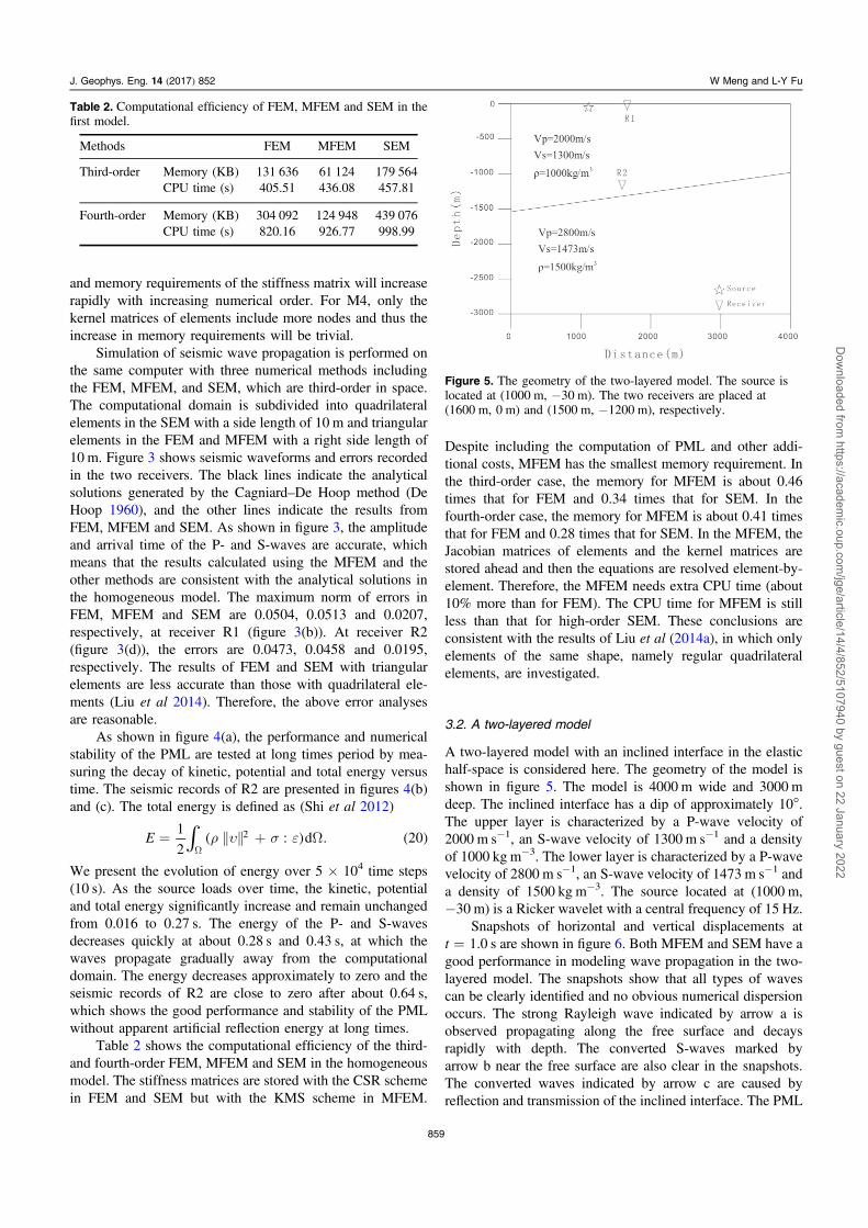
3.2. A two-layered model

A two-layered model with an inclined interface in the elastichalf-space is considered here. The geometry of the model isshown in figure 5. The model is 4000 m wide and 3000 mdeep. The inclined interface has a dip of approximately 10°.The upper layer is characterized by a P-wave velocity of2000 m s−1, an S-wave velocity of 1300 m s−1 and a densityof 1000 kg m−3. The lower layer is characterized by a P-wavevelocity of 2800 m s−1, an S-wave velocity of 1473 m s−1 anda density of 1500 kg m−3. The source located at (1000 m,−30 m) is a Ricker wavelet with a central frequency of 15 Hz.

Snapshots of horizontal and vertical displacements att=1.0 s are shown in figure 6. Both MFEM and SEM have agood performance in modeling wave propagation in the two-layered model. The snapshots show that all types of wavescan be clearly identified and no obvious numerical dispersionoccurs. The strong Rayleigh wave indicated by arrow a isobserved propagating along the free surface and decaysrapidly with depth. The converted S-waves marked byarrow b near the free surface are also clear in the snapshots.The converted waves indicated by arrow c are caused byreflection and transmission of the inclined interface. The PML

Table 2. Computational efficiency of FEM, MFEM and SEM in thefirst model.

Methods FEM MFEM SEM

Third-order Memory (KB) 131 636 61 124 179 564CPU time (s) 405.51 436.08 457.81

Fourth-order Memory (KB) 304 092 124 948 439 076CPU time (s) 820.16 926.77 998.99

Figure 5. The geometry of the two-layered model. The source islocated at (1000 m, −30 m). The two receivers are placed at(1600 m, 0 m) and (1500 m, −1200 m), respectively.

859

J. Geophys. Eng. 14 (2017) 852 W Meng and L-Y Fu

Dow

nloaded from https://academ

ic.oup.com/jge/article/14/4/852/5107940 by guest on 22 January 2022

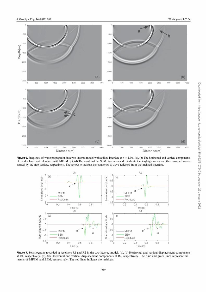
Figure 6. Snapshots of wave propagation in a two-layered model with a tilted interface at t=1.0 s. (a), (b) The horizontal and vertical componentsof the displacement calculated with MFEM. (c), (d) The results of the SEM. Arrows a and b indicate the Rayleigh waves and the converted wavescaused by the free surface, respectively. The arrows c indicate the converted S-wave reflected from the inclined interface.

Figure 7. Seismograms recorded at receivers R1 and R2 in the two-layered model. (a), (b) Horizontal and vertical displacement componentsat R1, respectively. (c), (d) Horizontal and vertical displacement components at R2, respectively. The blue and green lines represent theresults of MFEM and SEM, respectively. The red lines indicate the residuals.

860

J. Geophys. Eng. 14 (2017) 852 W Meng and L-Y Fu

Dow

nloaded from https://academ

ic.oup.com/jge/article/14/4/852/5107940 by guest on 22 January 2022

absorbing boundary attenuates the waves propagating rapidlyacross the left boundary and thus no artificial reflectionoccurs.

The seismograms recorded at the receivers are shown infigure 7. The fluctuation of the Rayleigh wave denoted byarrow a is observed at receiver R1. Arrows b and c indicatethe head wave and the converted S-wave reflected from theinclined interface, respectively. The results of the MFEMare in good agreement with those of the SEM. The residualsare less than 1% and are thus negligible. However, the MFEMhas an advantage over the SEM in computational efficiency(table 3). It is observed that although the CPU time requiredby the MFEM approximates to that by the SEM, the memorycost in the MFEM is only about 20% of that in the SEM.

3.3. A rugged surface model

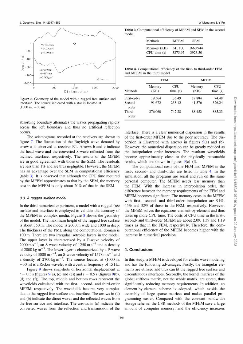
In the third numerical experiment, a model with a rugged freesurface and interface is employed to validate the accuracy ofthe MFEM in complex media. Figure 8 shows the geometryof the model. The maximum height of the rugged free surfaceis about 350 m. The model is 2000 m wide and 1000 m deep.The thickness of the PML along the computational domain is100 m. There are two irregular isotropic layers in the model.The upper layer is characterized by a P-wave velocity of2000 m s−1, an S-wave velocity of 1250 m s−1 and a densityof 2000 kg m−3. The lower layer is characterized by a P-wavevelocity of 3000 m s−1, an S-wave velocity of 1578 m s−1 anda density of 2700 kg m−3. The source located at (1000 m,−30 m) is a Ricker wavelet with a central frequency of 15 Hz.

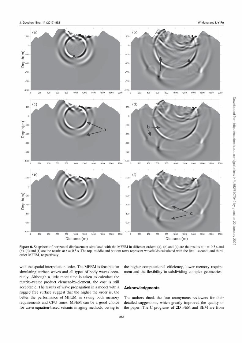
Figure 9 shows snapshots of horizontal displacement att=0.3 s (figures 9(a), (c) and (e)) and t=0.5 s (figures 9(b),(d) and (f)). The top, middle and bottom rows represent thewavefields calculated with the first-, second- and third-orderMFEM, respectively. The wavefields become very complexdue to the rugged free surface and interface. The arrows in (a)and (b) indicate the direct waves and the reflected waves fromthe free surface and interface. The arrows in (c) indicate theconverted waves from the reflection and transmission of the

interface. There is a clear numerical dispersion in the resultsof the first-order MFEM due to the poor accuracy. The dis-persion is illustrated with arrows in figures 9(a) and (b).However, the numerical dispersion can be greatly reduced asthe interpolation order increases. The resultant wavefieldsbecome approximately close to the physically reasonableresults, which are shown in figures 9(c)–(f).

The computational costs of the FEM and MFEM in thefirst-, second- and third-order are listed in table 4. In thesimulation, all the programs are serial and run on the samepersonal computer. The MFEM needs less memory thanthe FEM. With the increase in interpolation order, thedifference between the memory requirements of the FEM andMFEM becomes significant. The memory costs in the MFEMwith first-, second- and third-order interpolation are 91%,45% and 32% of those in the FEM, respectively. However,the MFEM solves the equations element-by-element and thustakes up more CPU time. The costs of CPU time in the first-,second- and third-order MFEM are about 2.09, 1.39 and 1.19times as that in the FEM, respectively. Therefore, the com-putational efficiency of the MFEM becomes higher with theincrease in numerical precision.

4. Conclusions

In this study, a MFEM is developed for elastic wave modelingand has the following advantages. Firstly, the triangular ele-ments are utilized and thus can fit the rugged free surface anddiscontinuous interfaces. Secondly, the kernel matrices of theglobal stiffness matrix, not the whole matrix, are stored, thussignificantly reducing memory requirements. In addition, anelement-by-element scheme is adopted, which avoids theassembly of large sparse matrices and makes parallel pro-gramming easier. Compared with the constant bandwidthstorage scheme, the CSR methods of the MFEM save a largeamount of computer memory, and the efficiency increases

Table 3. Computational efficiency of MFEM and SEM in the secondmodel.

Methods MFEM SEM

Memory (KB) 341 100 1660 944CPU time (s) 3875.97 3923.30

Figure 8. Geometry of the model with a rugged free surface andinterface. The source indicated with a star is located at(1000 m, −30 m).

Table 4. Computational efficiency of the first- to third-order FEMand MFEM in the third model.

FEM MFEM

MethodsMemory(KB)

CPUtime (s)

Memory(KB)

CPUtime (s)

First-order 19 564 35.49 17 884 74.48Second-order

91 672 233.12 41 576 326.24

Third-order

276 060 742.28 88 452 885.33

861

J. Geophys. Eng. 14 (2017) 852 W Meng and L-Y Fu

Dow

nloaded from https://academ

ic.oup.com/jge/article/14/4/852/5107940 by guest on 22 January 2022

with the spatial interpolation order. The MFEM is feasible forsimulating surface waves and all types of body waves accu-rately. Although a little more time is taken to calculate thematrix–vector product element-by-element, the cost is stillacceptable. The results of wave propagation in a model with arugged free surface suggest that the higher the order is, thebetter the performance ofMFEM in saving both memoryrequirements and CPU times. MFEM can be a good choicefor wave equation-based seismic imaging methods, owing to

the higher computational efficiency, lower memory require-ment and the flexibility in subdividing complex geometries.

Acknowledgments

The authors thank the four anonymous reviewers for theirdetailed suggestions, which greatly improved the quality ofthe paper. The C programs of 2D FEM and SEM are from

Figure 9. Snapshots of horizontal displacement simulated with the MFEM in different orders: (a), (c) and (e) are the results at t=0.3 s and(b), (d) and (f) are the results at t=0.5 s. The top, middle and bottom rows represent wavefields calculated with the first-, second- and third-order MFEM, respectively.

862

J. Geophys. Eng. 14 (2017) 852 W Meng and L-Y Fu

Dow

nloaded from https://academ

ic.oup.com/jge/article/14/4/852/5107940 by guest on 22 January 2022

Dr Shaolin Liu. This research was supported by the NaturalScience Foundation of China (grant no. 41130418) and theNational High Technology Research and Development Pro-gram (863 Program) of China (grant no. 2013AA064202).

Appendix

The empirical expressions for the damping coefficients, d xx ( )and d z ,z ( ) are given by Collino and Tsogka (2001)

d x n RV x

d z n RV z

1 log2

1 log2

xP

zP

2

2

d d

d d

= - + ⋅ ⋅ ⋅

= - + ⋅ ⋅ ⋅

⎜ ⎟

⎜ ⎟

⎧⎨⎪⎪

⎩⎪⎪

⎛⎝

⎞⎠

⎛⎝

⎞⎠

( ) ( ) ( )

( ) ( ) ( )

where d is the thickness of the PML absorbing layer, x or z isthe distance to the computational boundary in the PMLregion, n is a constant that controls the attenuation rate (whichgenerally takes a value of 2 or 3) and R is the theoreticalreflection coefficient which ranges from 10−6 to 10−2 ingeneral.

References

Alford R M, Kelly K R and Boore D M 1974 Accuracy of finite-difference modeling of the acoustic wave equation Geophysics39 834–42

Archer G C and Whalen T M 2005 Development of rotationallyconsistent diagonal mass matrices for plate and beam elementsComput. Methods Appl. Mech. Eng. 194 675–89

Bohlen T and Saenger E H 2006 Accuracy of heterogeneousstaggered-grid finite-difference modeling of Rayleigh wavesGeophysics 71 T109–15

Chaljub E, Komatitsch D, Vilotte J P, Capdeville Y, Valette B andFesta G 2007 Spectral-element analysis in seismology Adv.Geophys. 48 365–419

Chen J B 2009 Lax–Wendroff and Nyström methods for seismicmodeling Geophys. Prospect. 57 931–41

Collino F and Tsogka C 2001 Application of the perfectly matchedabsorbing layer model to the linear elastodynamic problem inanisotropic heterogeneous media Geophysics 66 294–307

Cuthill E and McKee J 1969 Reducing the bandwidth of sparsesymmetric matrices Proc. 1969 24th Natl Conf. of the ACMpp 157–72

De Hoop A T 1960 A modification of Cagniard’s method for solvingseismic pulse problems Appl. Sci. Res. 8 349–56

Fornberg B 1988 The pseudospectral method: accuraterepresentation of interfaces in elastic wave calculationsGeophysics 53 625–37

Gibbs N E, Poole W G and Stockmeyer P K 1976 An algorithm forreducing the bandwidth and profile of a sparse matrix SIAM J.Numer. Anal. 13 236–50

Hesthaven J S and Warburton T 2008 Nodal Discontinuous GalerkinMethods: Algorithms, Analysis, and Applications (New York:Springer)

He X, Yang D and Wu H 2015 A weighted Runge–Kuttadiscontinuous Galerkin method for wavefield modelingGeophys. J. Int. 200 1389–410

Jiang L and Pang Z 1979 The Method and the Theoretical Basis ofthe Finite Element (Beijing: People’s Education Press) (inChinese)

Kelly K R, Ward R W, Treitel S and Alford R M 1976 Syntheticseismograms: a finite-difference approach Geophysics 41 2–27

Komatitsch D and Vilotte J P 1998 The spectral element method: anefficient tool to simulate the seismic response of 2D and 3Dgeological structures Bull. Seismol. Soc. Am. 88 368–92

Komatitsch D and Tromp J 2002 Spectral-element simulations ofglobal seismic wave propagation—I validation Geophys. J. Int.149 390–412

Komatitsch D and Tromp J 2003 A perfectly matched layerabsorbing boundary condition for the second-order seismicwave equation Geophys. J. Int. 154 146–53

Komatitsch D, Erlebacher G, Göddeke D and Michéa D 2010 High-order finite-element seismic wave propagation modeling withMPI on a large GPU cluster J. Comput. Phys. 229 7692–714

Li X F, Zhu T, Zhang M G and Long G H 2010 Seismic scalar waveequation with variable coefficients modeling by a newconvolutional differentiator Comput. Phys. Commun. 1811850–8

Li X F, Li Y Q, Zhang M G and Zhu T 2011 Scalar seismic-waveequation modeling by a multisymplectic discrete singularconvolution differentiator method Bull. Seismol. Soc. Am. 1011710–8

Li X F, Wang W S, Lu M W, Zhang M G and Li Y Q 2012Structure-preserving modeling for elastic waves: a symplecticdiscrete singular convolution differentiator method Geophys. J.Int. 188 1382–92

Liu S L, Li X F, Wang W S and Liu Y S 2014a A mixed-grid finiteelement method with PML absorbing boundary conditions forseismic wave modeling J. Geophys. Eng. 11 055009

Liu S L, Li X F, Liu Y S, Zhu T and Zhang M G 2014b Dispersionanalysis of triangle-based finite element method for acousticand elastic wave simulation Chin. J. Geophys. 57 2620–30 (inChinese)

Liu S L, Li X F, Wang W S and Zhu T 2015a A symplectic RKNscheme for solving elastic wave equations Chin. J. Geophys.58 1355–66 (in Chinese)

Liu S L, Li X F, Wang W S and Zhu T 2015b Source wavefieldreconstruction using a linear combination of the boundarywavefield in reverse time migration Geophysics 80S203–12

Liu Y S, Liu S L, Zhang M G and Ma D T 2012 An improvedperfectly matched layer absorbing boundary condition forsecond order elastic wave equation Prog. Geophys. 272113–22

Liu Y S, Teng J W, Liu S L and Xu T 2013 Explicit finite elementmethod with triangle meshes stored by sparse format and itsperfectly matched layers absorbing boundary condition Chin.J. Geophys. 56 3085–99 (in Chinese)

Liu Y, Teng J, Lan H, Si X and Ma X 2014 A comparative study offinite element and spectral element methods in seismicwavefield modeling Geophysics 79 T91–104

Ma X, Yang D and Liu F 2011 A nearly analytic symplecticallypartitioned Runge–Kutta method for 2D seismic waveequations Geophys. J. Int. 187 480–96

Marfurt K J 1984 Accuracy of finite-difference and finite-elementmodeling of the scalar and elastic wave equations Geophysics49 533–49

Moczo P, Kristek J and Halada L 2000 3D fourth-order staggered-grid finite-difference schemes: stability and grid dispersionBull. Seismol. Soc. Am. 90 587–603

Padovani E, Priolo E and Seriani G 1994 Low and high order finiteelement method: experience in seismic modeling J. Comput.Acoust. 2 371–422

Richter G R 1994 An explicit finite element method for the waveequation Appl. Numer. Math. 16 65–80

Shi R, Wang S and Zhao J 2012 An unsplit complex-frequency-shifted PML based on matched Z-transform for FDTDmodeling of seismic wave equations J. Geophys. Eng. 9218–29

863

J. Geophys. Eng. 14 (2017) 852 W Meng and L-Y Fu

Dow

nloaded from https://academ

ic.oup.com/jge/article/14/4/852/5107940 by guest on 22 January 2022

Tessmer E and Kosloff D 1994 3D elastic modeling with surfacetopography by a Chebychev spectral method Geophysics 59464–73

Virieux J 1984 SH-wave propagation in heterogeneous media: velocity–stress finite-difference method Geophysics 49 1933–42

Virieux J 1986 P-SV wave propagation in heterogeneous media:velocity-stress finite-difference method Geophysics 51 889–901

Wang Y, Liang W, Nashed Z, Li X, Liang G and Yang C 2014 Seismicmodeling by optimizing regularized staggered-grid finite-differenceoperators using a time-space-domain dispersion-relationship-preserving method Geophysics 79 T277–85

Wu S R 2006 Lumped mass matrix in explicit finite element methodfor transient dynamics of elasticity Comput. Methods Appl.Mech. Eng. 195 5983–94

Yang D, Wang N, Chen S and Song G 2009 An explicit methodbased on the implicit Runge–Kutta algorithm for solving waveequations Bull. Seismol. Soc. Am. 993340–54

Zhang M G, Wang M Y, Li X F, Yang X C and Wang L 2002 Finiteelement forward modeling of anisotropic elastic waves Prog.Geophys. 17 384–9 (in Chinese)

Zhang W and Shen Y 2010 Unsplit complex frequency shifted PMLimplementation using auxiliary differential equation forseismic wave modeling Geophysics 75 T141–54

Zhang W, Zhang Z and Chen X 2012 Three-dimensional elasticwave numerical modeling in the presence of surfacetopography by a collocated-grid finite-difference method oncurvilinear grids Geophys. J. Int. 190 358–78

864

J. Geophys. Eng. 14 (2017) 852 W Meng and L-Y Fu

Dow

nloaded from https://academ

ic.oup.com/jge/article/14/4/852/5107940 by guest on 22 January 2022