1

TYING A WELL TO SEISMIC

2

Compiled by : maryam seyed mahmoudi Thanks a lot from dr. salehiKharazmi univercity of tehran

msmahmoudi1392@gmail.com Fall, 2014

Outline

3

- introduction -Comparing well with seismic data -Measurements In Time and In Depth -The Modeling Process of synthetic trace - blocked sonic log - Discussion 1 -Dynamic time warping - LSIM- Discussion 2

introductionReliable well-seismic tying is a crucial step in seismic interpretation to correlate subsurface geologyto observed seismic data..

4

F(1)

the tying procedure depend on:

*- the availability of high quality logs

*-the estimation of a suitable wavelet

and*-the interpreter’s experience.

5

THE PROBLEM OF TYING WELL TO SEISMIC DATA

Geophysicists are interested in knowing a

sprecisely as possible the locationin depth of geologic horizons to

determine where to dril

6

7

Measurements In Time and In Depth Well-seismic ties allow well data, measured in units of depth to be compared to seismic data, measured in units of time

Comparison of Seismic and Well Data•Seismic Data

•Samples area and volume•Low frequency 5 - 60 Hz•Vertical resolution 15 - 100 m

•Horizontal resolution 150 - 1000 m

•Measures seismic amplitude, phase, continuity, horizontal & vertical velocities

•Time measurement

8

Well Data•Samples point along wellbore •High frequency,10,000 - 20,000 Hz•Vertical resolution 2 cm - 2 m•Horizontal resolution 0.5 cm – 6m •Measures vertical velocity, density, resistivity, radioactivity, , rock and fluid properties from cores•Depth measurement

The Modeling Process of synthetic trace

9

F(2)

•The synthetic trace is compared to the real seismic data

collected near the well location

10

F(3)

Seismic-Well Tie Flow-Chart11

FL ch(1)

Blocked sonic log

12

The sonic log the sonic log,which

involves defining discrete intervals on the log over

which a constant interval transit

time (ITT), which corresponds to a constant

interval velocity, is an acceptable

approximation for the actual velocity character

of the log

13

Using a blocked sonic logtying a well to time

processed seismic data using a blocked sonic log

for a case a vertical seismic

profile, is available

14

five reflectionsnumbered 1–5 are annotated for correlation to the. well.(Case Study : Desoto Canyon / on the 269 no.1 )

1)reflection 1 corresponding to the base of the Neogene clastic section.1,2,4) Note that reflections 1, 2, and 4 are peaks, 3) is a trough,5) is the peak in a symmetric peak-over-trough pair.Or it might be a tuned response.

15

F(4)

with blocked values for the sonic log shown in blue. ITT values for the blocked sonic log are listed inTable 2

16

F(5)

Depth and blocked soniclog data for the well

17

T(2)

18

The results

are shown in Table 3, and the resulting interval velocity depth plot is shown in F(6). F(6) ,

T(3)

19

F( 7). Final correlation of blocked log intervals A through D well to reflections 1–5 on the 3D PSTM line having graphically stretched the sonic log interval by interval from depth to time.(Case Study : Desoto Canyon / on the 269 no.1 )

F(7)

20

Discussion 1

for the following reasons the lack of

biostratigraphic data for the well

precludes assignment of formation tops

to individual reflections as part of the well tie):

21

1) The blocking of the sonic log is reasonable in view of the overall log character.

2) the interval velocities calculated from the ITT values on the blocked sonic log

22

3) The log markers converted to time using the interval

velocities derived from

the blocked sonic log correlate well with the prominent

reflections on the seismic data

•4) The log markerscan be confidently

correlated to the seismic data

without need for excessive adjustment of the blocked log values

23

this is an acceptable well-to-seismic tiegiven the available

dataand

using the procedure

24

Dynamic time warping(DTW)

25

DTWUsing dynamic time warping,a

fast algorithm that optimally aligns two

sequences, we shift and warp a synthetic seismogram

tomatch a seismic trace to

produce a well tie and time-depth function.

26

27

The first alternative to perform the automated tying is based on dynamic time warping (DTW)(Herrera and Van der Baan, 2012a, 2014) and the second

approach faces the nonlinearity correction usingthe local similarity attribute (LSIM) (Fomel, 2007a).

28

F(9)

29

These methods produced a guided stretching and

squeezing in time series based on a correlation technique establish a

point-for-point correlation between

traces.(Liner and Clapp (2004)

30

F(10)

Correlation cofficient

Having two (time-dependent) sequences both of length n, the correlation coefficient is

An alternative to crosscorrelation is to find the Euclidean distance (L2-norm) between the two time series

The optimal path that minimizes the total warping cost (Berndt and Clifford, 1994) is

The LSIM starts with the observation that thesquared correlation coefficient can be split as the product of two factors

31

(1)

(2)

(3)

(4)

Quality control: The relative velocity change

32

Both methods create a warping function w(t) that maps the synthetic trace into the seismic traces bythe following transformation:

(5) , (6)

•The warping function produced by the local

similaritymethod has been smoothed by the shaping filters

(Fomel, 2007b).

33

We apply both approaches, DTW and

LSIM, to obtain

well-seismic ties

34

35

Seismic section with study well annotated at CDP 39. The inset shows the synthetic seismogram with the initial manual correlation of 0.77 in the time window 800-114ms.F(11)

36

Figure 11 shows a seismic section with one well at CDP

39. The well-seismic

Tie for this well is shown in the inset figure. We scanned the seismic

section to find the best matching location, following White and Simm

(2003),which is at CDP 41.

The generated synthetic trace (red) and

the corresponding seismic trace (blue) have been

exported for post processing.

37

the seismic trace has been shortened

to the well log length. Also,

both signals have been

standardized in amplitude.

38

Figure shows how the synthetic(upper trace) and seismic traces (lowertrace) match after constrained DTWwith a warping window r = 10.

F(12)

39

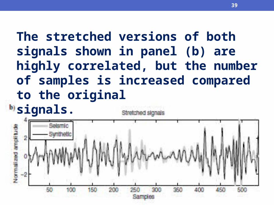
The stretched versions of both signals shown in panel (b) are highly correlated, but the number of samples is increased compared to the originalsignals.

40

the alignment process to a limited window. This reduces the freedom of the warping path to align events within a limited distance.The estimated warping path is shown in Figure 13, where we used r =10 samples to limit the maximum amount of permitted point-to-point shifting

F(13)

41

The LSIM performs an automatic squeezing and stretching of the synthetic trace with respect to the seismic trace while computing the local correlation.This process leads to a local-similarity scan.

The red color indicates high similarity, and from these pick values, we estimate the relative stretch measure s(t), represented as a black curve in F(14)

42

Quality control Figure 15a shows the relative stretch

(dwdt) ∕for both methods. The LSIM method

(in black bold) shows few variations, while the DTW result

(dashed line) shows reliable

stability in the bottom half

of the display, i.e.,

F(15)

little change between the synthetic and the seismic trace.

43

These variations are reflected

in the velocity changes shown Figure 15b.

The original sonic log (thick gray)

is almost overlapped by the LSIM result (black

line), with little difference

only at the initialsamples. DTW (dashed line

as expected, producesmore changes in the velocity curve in the

areas

44

Discussion2

Well-seismic ties are challenging due to the

highnumber of subjective decisions and pattern

recognitiontasks involved.

45

1)First, an appropriate wavelet is to be estimated.

2) Then, choose the correct wavelet polarity.

3) Next, apply a global bulk shift, for stance, via a simple correlation; this precludes having large warping windows in DTW and produces faster convergence in LSIM.

46

4) For DTW, slowly increase the length of the warping window until the quality-control procedure indicates unrealistic stretching and squeezing results.

5) In LSIM, adjust the regularization parameter to generate a smooth relative stretch curve controlling the deviation from unity

47

Recap: Flow Chart

FL ch(2)

48

Thanks a lot from dr.ehsan salehi

And mis. Najar ms.engineer in oil expoloration

49

Refrences:Automatic approaches for seismic to well tying(Roberto H. Herrera1, Sergey Fomel2, and Mirko van der Baan1)

Tutorial: Tying a well to seismic using a blocked sonic log (Donald A. Herro)

Automatically tying well logs to seismic dataAndrew Mu˜noz & Dave Hale

WELL(LOG)SYNTHETIC SEISMOGRAM AND TIES TOSEISMIC(compiled by from Fred W Schroeder,AAPG)