Uncertainty around the Mean Utility Assessment

Accounting for Mapping Extrapolation:

Application to Prostate Cancer ∗

Carole Siani †a Christian de Peretti b Christel Castelli c

Tu Phung d Jean-Pierre Daures c,f Gerard Duru e

November 11, 2010

a Research Laboratory in Knowledge Engineering (ERIC, EA3083), Institut des SciencesPharmaceutiques et Biologiques (ISPB), University Claude Bernard Lyon 1, Universityof Lyon, France.

b Laboratory of Actuarial and Financial Sciences (SAF, EA2429), Institute of Financialand Insurance Sciences (ISFA School), University Claude Bernard Lyon 1, University ofLyon, France.

c Departement Biostatistique Epidemiologie clinique Sante Publique et Information Medicale(BESPIM), Centre Hospitalier Universitaire, Nımes, France.

d Institut Universitaire de Recherche Clinique, laboratoire de biostatistique, Universite deMontpellier 1, France.

f Laboratoire Epidemiologie et Biostatistique, Institut Universitaire de Recherche Clinique,Montpellier, France.

e Cyklad, France.

Abstract

In cost-effectiveness analysis, one or more medical treatment(s) were comparedwith a standard treatment on the two-fold basis of cost and utility. Since thehealth utility measure is not necessarily available for the entire sample, this utilitymeasure is often extrapolated from a technical or medical questionnaire through amapping function. In the literature this mapping is not accounted for when uncer-tainty is handled, leading to wrong decision-making with serious consequence onthe patient’s health. The purpose of this paper is then to build a confidence intervalaround the mean utility measure, accounting for the uncertainty coming from the

∗The authors would like to thank IReSP and DGS, DREES-MiRe, InVS, HAS, CANAM, AFSSAPS,Inserm for funding this project. They also thank Institut de Recherche en Sante Publique (IReSP) andits director Alfred Spira for inviting them to the IReSP’s seminar in Paris, 1st June 2010. Finally, theauthors would like to give thanks to Mathea Orsini for her help with the data.

†Correspondence to: Carole Siani, Batiment d’odontologie, 11 Rue Guillaume Paradin, 69372 Lyoncedex 08, France. Tel: +33 (0)4 78 77 10 50. Fax: +33 (0)4 72 43 10 44 . Email: carole.siani@univ-lyon1.fr.Web: recherche.univ-lyon2.fr/eric/82-Carole-Siani.html.

1

questionnaire extrapolation. Analytic and nonparametric bootstrap procedures areproposed. An extension of the methodologies to the Incremental Cost-Utility Ratiois proposed in Appendix.

J.E.L. Classification: C13, C15, [C44]; I19.

Keywords: mapping, mean utility prediction, uncertainty, bootstrap.

1 Introduction

In cost-effectiveness analysis (CEA), one or more medical treatment(s) are comparedwith a standard treatment on the two-fold basis of cost and medical effectiveness bydecision-makers. Only recently, the health utility has been taken into account insteadof the sole effectiveness. Since collecting utility data is time consuming and human re-source demanding, the utility data are often collected on a sub-sample, conversely to theother data such as cost data. Since the utility measure is not necessarily available forthe entire sample, the utility measure is often extrapolated from a questionnaire thatis not based on any utility principle such as clinical data of patient characteristics orself-reply questionnaires on quality of life. In practice, the utility is measured on a smallsub-sample, whereas a technical questionnaire is collected from all the patients. A map-ping is estimated between the utility measure and the questionnaire on the sub-sample.Then, the utility value is predicted for the other patients, extrapolating the questionnaireusing the estimated mapping. For instance, the mapping techniques are often used inRheumatoid Arthritis, where the EuroQol EQ-5D measure is extrapolated from the HAQor DAS28 scores (see Ariza-Ariza et al. [2006], Nord et al. [1992], Longworth et al. [2005]).For other examples, see among others Torrance [1976], Krabbe et al. [1997], Dolan andSutton [1997], O’Leary et al. [1995], Torrance et al. [1996].

We will show that decision-making based on utility values interpolated from mappingis not reliable if the mapping is not accounted for. On a medical point of view, whenestimating the mean utility of a treatment, it is important to get an accurate confidenceinterval, since these classical methods can lead to wrong positive decisions.

The purpose of this paper is then to build a confidence interval around the mean utilitymeasure, accounting for the uncertainty coming from the questionnaire extrapolation.We point out that if the extrapolated utility values are used to compute a confidenceinterval as if they were the observed values, this procedure dramatically decreases theconfidence interval so that the conclusion is not reliable since the uncertainty is largelyunderestimated. This spurious decrease in uncertainty is not accounted for in the studiesof the literature and in the CEAs conducted in the pharmaceutical industry. Furthermore,decision-making follows from these results.

In this paper, analytic and nonparametric bootstrap procedures are proposed to ac-count for the questionnaire extrapolation procedure to build the confidence interval forthe mean utility. The performance of the methods is assessed via Monte Carlo experi-ments for various sample sizes and models. Finally, an out of sample validation is carriedout to check the performance of the various methods on prostate cancer data. In addition,an extension of the methodologies to the Incremental Cost-Utility Ratio is proposed inAppendix B.

All the programs are written and run with Gauss software r©: the confidence intervaland Monte Carlo procedures, the regressions on data, as well as the out of sample val-

2

idation. The Gauss procedures are available at: http://recherche.univ-lyon2.fr/eric/82-Carole-Siani.html.

The remainder of this paper is organized as follows. section 2 describes the variousmapping methods of the literature. section 3 proposes several methods to handle un-certainty around the mean utility. section 4 provides the Monte Carlo results for theperformance of the methods. section 5 provides an application to prostate cancer as wellas an out of sample validation. Finally, section 6 concludes. In addition, Appendix Bproposes an extension of the methodologies to the Incremental Cost-Utility Ratio.

2 Mapping methods in the literature

In this section, mapping methods of the literature used in various medical situations arepresented.

2.1 Notations

1. Preference-based single index measure:

(a) U : overall score, which is rescaled to [0,1].

(b) Uk, k = 1, . . . , K: the level of the index dimensions.

2. Non-preference based condition-specific instrument:

(a) X: overall score,

(b) Xd, d = 1, . . . , nD: the score of the instrument domains,

(c) Zi, i = 1, . . . , nI : the level of the instrument items, which can be discretevariables,

(d) Ii,z, i = 1, . . . , nI , z ∈ E: a dummy variable that = 1 when the level of theinstrument item i is z. E is the set of values for z.

3. other independent variables:

(a) W : row vector of patient characteristics such as age, age squared, sex or others.

The paper of Tsuchiya et al. [2002] is presented first. The authors convert Asthma Qualityof Life Questionnaire (AQLQ) - a non-preference-based QOL instrument for asthma -into EQ-5D indices - a preference-based generic instrument -. They propose a simpletransformation (linear), multi-linear regressions over the various domains or items. Theyare presented below.

2.2 Simple linear regression mapping

U = α + βX + Wω + u (1)

α and β are parameters, and ω is a column vector of parameters.

3

2.3 Multi-linear regression mapping

U = δ0 + δ1X1 + . . . + δnDXnD

+ Wω⋆ + v (2)

U = ι0 + ι1Z1 + . . . + ιnIZnI

+ Wω⋆⋆ + w (3)

U = ι′0 +

nI∑

i=1

ι′iZi +

nI∑

i=1

nI∑

j=1

ι′ijZiZj + Wω′ + w′ (4)

Models 1–4 are estimated using ordinary least squares (OLS), and the independent vari-ables are treated as continuous.

U = ι′′0 +

nI∑

i=1

∑

z∈E\last element of E

ι′′i,zIi,z + Wω′′ + w′′ (5)

Model 5 continues to use OLS, but now the independent variables Ii,z are treated ascategorical variables (with possibly continuous variables W ).

2.4 Multiple linear regressions

Uk = ιk,0 + ιk,1Z1 + . . . + ιk,nIZnI

+ Wωk + wk, k = 1, . . . , K (6)

Again, OLS is used, and both the dependent U and the independent variables are treatedas continuous. 1

2.5 Power models

In Stevens et al. [2006], Shmueli [2007], the authors propose mapping between VisualAnalogue Scale and Standard Gamble data. They assume a model of the following form:

Uis = f(Xis) + εis (7)

where i represents an individual and s represents a health state. 2 The authors assumethat the transformation function f( . ) do not vary across individuals and that they areindependence across observations. They assume the errors are normally distributed:

εis ∼ N(µi, σ2i )

Linear, quadratic, cubic and power functions are estimated. The linear and power modelsare estimated using the disvalue form, where disvalue =(1-value) and disutility =(1-utility). Since the utility measure belongs to [0,1]; the quadratic and cubic models usethe value form and are constrained to pass through 0 and 1. To allow for this constraint,the quadratic model is estimated as:

U − X2 = α(X − X2)

1In practice, if Zi are discrete, the model is a mixture of discrete and continuous variables.2s belongs to an (a priori) infinite continuous set, since for an analogical scale all the values are

allowed. Otherwise, we are limited to some integer numbers.

4

and the cubic model is estimated as:

U − X3 = α(X − X3) + β(X2 − X3)

where U is the utility, X is the overall score of the instrument, and α and β are parametersto be estimated.

The constraints to pass through 0 and 1 should also be applied to the previous models.However, they are not necessarily respected by the data in practice. In addition, the errorterms u are out of this restriction. Consequently, we prefer not to impose them, and toestimate the following models:

Quadratic: U = α + βX + γX2 + Wω + u (8)

Cubic: U = α + βX + γX2 + δX3 + Wω + u (9)

2.6 Generalised linear model (GLM)

The dependent variable U is transformed into an s-shaped non-linear variable that ap-proaches 1, but does not reach it. The logit transformation can be applied. The obviousshortcoming of this in the context of Tsuchiya et al. [2002] is that there are many re-sponses with observed EQ-5D index of 1.00, and the transformation will imply droppingthese observations (because the transformed values approach infinity). Tsuchiya et al.[2002] accommodated this by standardising the raw EQ-5D indices to the range [0,1],based on an artificial range, say, [-0.5, +1.1], and then transforming this. In their paper,Tsuchiya et al. [2002], given the additional complication, the arbitrary nature of the stan-dardisation and the transformation, and the fact that the maximum predicted EQ-5Dindices of the simple linear models hardly exceed 1.00, the associated benefits of GLMdo not seem to outweigh its costs. Therefore Tsuchiya et al. [2002] decided not to useGLM. Another way to overcome this problem would be to manage the 1’s as 1− ε in thelogistic model, with ε converging to 0.

3 Methods for calculating the mean utility confidence

interval

Beresniak et al. [2007] first criticised the use of mapping in cost-utility analysis since theuncertainty is not accounted for in usual methods.

In their papers, Stevens et al. [2006], Shmueli [2007], Salomon and Murray [2004],Longworth et al. [2005] report the prediction of their models for the mean utility. How-ever, no confidence interval of this prediction is given. The absolute error of the modelis provided, but again, it does not correspond to an estimate error of the mean.

In their paper, Rivero-Arias et al. [2009] also report the mean utility on the out ofsample. They provide a confidence region for the mean utility. They argue that “Interms of predicting uncertainty around EQ-5D mean estimates, their model estimatedtighter 95% CIs than the actual 95% CIs.” However, these confidence intervals areunderestimated (see Table 1).

The paper of Merkesdal et al. [2010] can also be cited. It deals with rheumatoidarthritis. The HAQ score changes are mapped to related health utility states expressedin QALYs gained. For this transformation, a standardised formula was used according to

5

the most published cost-effectiveness models in RA. In the base case scenario, the formulaby Bansback et al. [2005] (female) was applied:

QoL = 0.76 − 0.28 ∗ HAQ − 0.05 ∗ Female. (10)

The utility estimates of the model result are provided in terms of QALYs for each sequenceof treatment with a confidence interval. It should be noted that it is impossible toget a confidence interval from Equation 10. Thus, the confidence interval provided byMerkesdal et al. [2010] should come from the mapped values, and should be under-valuated. In addition, the authors provide a cost-effectiveness acceptability curve, whichshould be wrong for the same reason.

Consequently, in this paper, we propose a method to provide the confidence intervalof the mean utility.

3.1 Statistical properties of the utility measure

Assumption 1: Utility

It is assumed that the utility measures ui follow independent random variableswith [0, 1] support and with distribution denoted DU as follows:

Ui ∼ independent DU(µU , σ2U), (11)

where i denotes the individuals, µU the mean, and σ2U the variance.

Since the support of the random variable Ui is finite, all the moments of the distributionare finite. Since the true mean corresponding to the theoretical population is unknown,the mean utility can be estimated as follows, on the basis of data collected from groupsof patients, each undergoing one of the forms of therapy (one group consisting of nindividuals):

U =1

n

n∑

i=1

Ui. (12)

Under Assumption 1, and applying the Central Limit Theorem (CLT), we obtain:

U ∼ N

(µU ,

1

nσ2

U

). (13)

Assumption 2: Mapping

It is assumed that the utility measure can be explained by some variables X.

Ui = f(Xi; β) + εi, (14)

εi ∼ N(0, σ2ε), (15)

where f is a function that depends on a parameter vector β, and εi is inde-pendent of X. For simplicitys sake, at a first stage, it can be assumed that fis linear: Ui = Xiβ + εi. Thus, µU = E(Xi)β, and σ2

U = β′V (X)β + σ2ε .

6

Let us consider an “in sample” with individuals i = 1, . . . , n where the utility measure isknown, and an “out of sample” with individuals i = n + 1, . . . , n + m where the utilityvalue is unknown.

The aim of mapping is to assess the out of sample mean utility µUout= E(Uout). In the

linear case, µUout= E(Xout)β, where Xout is the matrix of independent variables for

the out of sample. The estimator for the mean utility generally used is:

µUout=

1

m

n+m∑

i=n+1

Ui =1

m

n+m∑

i=n+1

Xiβin = Xoutβin =1

mι′mXout(X

′inXin)−1X ′

inUin,

where Ui are the out of sample predicted values for the utility measure, βin is the es-timate of β using the mapping on the in sample, ιm = (1, . . . , 1)′, Xin is the matrix ofindependent variables for the in sample, Uin are the utility measures for the in sample,and ′ denote the transpose. It should be noted that:

µUout=

1

mιmXoutβ +

1

mιmXout(X

′inXin)−1X ′

inεin.

Then, we have the following properties: E(µUout) = E(Xout)β. Thus, the estimator

µUoutis unbiased, and can be used to assess the mean utility. However, in order to take

a decision, the uncertainty has to be accounted for.

3.2 “Naive” confidence interval

A naive, and wrong, way to compute the variance of µUoutwould be:

V Naive(µUout

)=

1

m

[1

m − 1

n+m∑

i=n+1

(Ui − µUout

)2]

. (16)

We report here the confidence interval that is provided by Rivero-Arias et al. [2009]. Anaive way to provide a (1 − α) confidence interval is:

CINaiveµU

(1 − α) =

[µUout

± Φ−1(1 − α

2

) √V Naive

(µUout

)], (17)

7

where Φ is the cumulative distribution function of a standard normal random variable.

3.3 Analytic confidence interval

In the case of a linear model, we derived the variance of µUout, which can be estimated

as follows:

V(µUout

)=

1

mβ′inΩX βin + σ2

εinXout(X

′inXin)−1X ′

out. (18)

See proof in Appendix, section A. It should be noted that

V(µUout

)= V Naive

(µUout

)+ σ2

εinXout(X

′inXin)−1X ′

out. (19)

Thus, the term σ2εin

Xout(X′inXin)−1X ′

out is missing in Equation 16. The asymptotic

(1 − α) confidence interval is:

CIAnalyticµU

(1 − α) =

[µUout

± Φ−1(1 − α

2

) √V

(µUout

)]. (20)

This analytic confidence interval is restricted to a linear framework with Gaussian errorterms. It can easily be extended to a nonlinear framework, using an Edgeworth expan-sion, but it will be an approximation. Consequently, we prefer to develop a bootstrapmethodology, which will account for any nonlinear specification (such as logistic specifi-cation for instance). In addition, if a nonparametric version of bootstrap method is used,non-Gaussian distributed error terms can also be accounted for.

3.4 Nonparametric bootstrap confidence interval

In this subsection, we propose a methodology for building a confidence interval basedon the nonparametric bootstrap technique. For a general presentation of the percentile-tmethod, see Hall [1992], Davidson and MacKinnon [1993], Efron and Tibshirani [1993],Hjorth [1994], and Shao and Tu [1995].

First, a particular mapping model has to be chosen. Let us denote it:

U = f(X; β) + ε, (21)

where X is a regressor matrix, and the function f is known and is parametric in the sensethat it depends on a parameter vector β. The confidence interval is built as follows:

1. Equation 21 is estimated using appropriate methods such as OLS, Nonlinear LeastSquares, Maximum Likelihood, . . . , leading to βin, εin, and Uout.

2. µUoutand s =

√V

(µUout

)are computed using the original dataset.

3. A bootstrap Data Generating Process (DGP) has to be defined. It may be eitherparametric or semi-parametric, characterized by βin and by any other relevantestimates, such as the error variance σ2

in, that may be needed. In a general case,we propose:

U bi = f

(Xi, βin

)+ εb

i , (22)

8

for i = 1, . . . , n. In the case of linear modelling, the DGP is restricted to:

U bi = Xiβin + εb

i , (23)

The distribution of εbi will be discussed in the last paragraph of this section.

4. B bootstrap samples are generated, (U bi )

ni=1, b = 1, . . . , B.

5. For each of these, an estimate µbUout

and its standard error sb are computed in

exactly the same as for µUoutand s from the original data. Then the bootstrap

“t-statistic” is computed:

τ b =µb

Uout− µUoutsb

.

6. The asymmetric equal-tail bootstrap confidence interval can be written as:

CIBootstrapµU

(1 − α) =[µUout

− s · F−1(1 − α

2), µUout

− s · F−1(α

2)], (24)

where F is the Empirical Distribution Function of the B bootstrap statistics τ b.

We consider the following way of generating the bootstrap residuals εbi (see Weber [1984]).

The εbi are generated by independent uniform draws with replacement among the vector

with the typical element εi constructed as follows:

1. Calculate (PX)i,i, i = 1, . . . , n, the diagonal elements of the projection matrix onX.

2. Calculate εi√1−(PX)i,i

, ∀i = 1, . . . , n.

3. Re-centre the vector that results.

4. Rescale it so that it has the variance σ2ε .

This makes it possible to correct the heteroskedasticity in the residuals due to the regres-sors.

4 Performance of the methods: Monte Carlo exper-

iments

In this section, the performance of the various methods is examined using Monte Carloexperiments.

4.1 Monte Carlo methodology

Data Generating Processes (DGP) are used to generate simulated data samples. Thevarious methods are applied to each simulated sample j = 1, . . . , S, where S is thenumber of Monte Carlo replications in an experiment. It is examined if each confidenceinterval number j contains or not the true value µU of the mean utility (which is known,

9

since the DGP is known, conversely to real data). The coverage c of the confidenceintervals can be estimated as follows:

c =1

S

S∑

j=1

I (µU ∈ Intervalj) . (25)

The standard deviation of this Monte Carlo estimate of the coverage is equal to√

1Sc(1 − c),

where c is the coverage.In our Monte Carlo experiments, we choose the confidence level 1 − α is equal to

0.95. The number of bootstrap replications is B = 999. The number of Monte Carloreplications is S = 10, 000. If the true coverage c = 0.95, the standard deviation of theMonte Carlo estimate of the coverage is 0.002179. At worst (when c = 0.5) the standarddeviation is 0.005. Several values for the in sample size n and the out of sample size mare chosen. Small values for n and large values for m are chosen to reflect the case wherethe utility is assessed only on a small sub-sample, and then extrapolated to the otherpatients.

4.2 Data Generating Process

A variety of DGP are proposed to check the robustness of the methods: linear, nonlinear,with Gaussian and non-Gaussian error terms.

4.2.1 Linear Case

Ui = β0 + β1 · X1i + β2 · X2i + εi, (26)

X1i ∼ i.i.d.U([0, 1]), (27)

X2i ∼ i.i.d.B(0.5, 3), (28)

εi ∼ i.i.d.N(0, σ2). (29)

The parameters values are set to: β0 = 0.1, β1 = 0.6, β2 = 0.2, σ = 0.3. We haveE(Ui) = 0.7.

4.2.2 Random Linear Case

The model is the same, but the parameters vary randomly across the Monte Carlo repli-cations:

β0 ∼ i.i.d.N(0.1, 0.12), (30)

β1 ∼ i.i.d.N(0.6, 0.62), (31)

β2 ∼ i.i.d.N(0.2, 0.22), (32)

σ ∼ i.i.d.U([0.3 · 0.5, 0.3 · 1.5]). (33)

4.2.3 Non-Gaussian Random Linear Case

The model is the same as in Equation 26–Equation 28, but the error terms follow theuniform distribution:

εi ∼ i.i.d.U([−0.6, 0.6]). (34)

10

4.2.4 Nonlinear Case

Ui = F [β0 + β1 · X1i + β2 · X2i + εi] (35)

X1i ∼ i.i.d.U([0, 1]) (36)

X2i ∼ i.i.d.B(0.5, 3) (37)

εi ∼ i.i.d.N(0, σ2) (38)

The parameters values are set to: β0 = −0.6, β1 = 0.6, β2 = 0.2, σ = 0.3. We haveE(Ui) = 0.5.

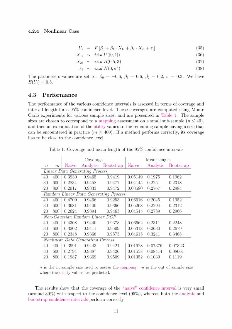
4.3 Performance

The performance of the various confidence intervals is assessed in terms of coverage andinterval length for a 95% confidence level. These coverages are computed using MonteCarlo experiments for various sample sizes, and are presented in Table 1. The samplesizes are chosen to correspond to a mapping assessment on a small sub-sample (n ≤ 40),and then an extrapolation of the utility values to the remaining sample having a size thatcan be encountered in practice (m ≥ 400). If a method performs correctly, its coveragehas to be close to the confidence level.

Table 1: Coverage and mean length of the 95% confidence intervals

Coverage Mean lengthn m Naive Analytic Bootstrap Naive Analytic Bootstrap

Linear Data Generating Process40 400 0.3930 0.9465 0.9419 0.05149 0.1975 0.196230 600 0.2834 0.9458 0.9477 0.04145 0.2251 0.231820 800 0.2017 0.9333 0.9472 0.03580 0.2767 0.2984Random Linear Data Generating Process40 400 0.4709 0.9466 0.9253 0.06616 0.2045 0.195230 600 0.3681 0.9400 0.9366 0.05268 0.2294 0.231220 800 0.2624 0.9394 0.9463 0.04545 0.2789 0.2966Non-Gaussian Random Linear DGP40 400 0.4308 0.9440 0.9378 0.06662 0.2311 0.224830 600 0.3202 0.9411 0.9509 0.05318 0.2630 0.267920 800 0.2348 0.9366 0.9573 0.04615 0.3241 0.3468Nonlinear Data Generating Process40 400 0.3991 0.9443 0.9421 0.01928 0.07376 0.0732330 600 0.2794 0.9387 0.9426 0.01558 0.08414 0.0866120 800 0.1987 0.9369 0.9509 0.01352 0.1039 0.1119

n is the in sample size used to assess the mapping. m is the out of sample sizewhere the utility values are predicted.

The results show that the coverage of the “naive” confidence interval is very small(around 30%) with respect to the confidence level (95%), whereas both the analytic andbootstrap confidence intervals perform correctly.

11

5 Application to Prostate Cancer

The above methodologies are then applied to data collected from a longitudinal prospec-tive cohort study evaluating patients’ health-related quality of life after treatment forprostate cancer. Several centres in the Herault and Gard regions participated in thestudy. It has been financed by the French National Institute of Cancer (INCa).

5.1 Data description

Data on patients’ health-related quality of life were repeatedly collected 4 times. Thefirst time was done after diagnosis of prostate cancer and before treatment. The sec-ond, third and fourth times were respectively 2 months, 6 months and 12 months aftertreatment, respectively. The treatment under consideration here is laparoscopic radicalprostatectomy for which there are 116 patients. The utility of patients’ own health statewas evaluated directly by Standard Gamble method. The health related quality of lifeinformation was evaluated by several multidimensional auto-administered quality of lifequestionnaires. There were two generic questionnaires (EQ-5D and SF-36), one cancerspecific quality of life questionnaire (EORTC-QLQ C30), one prostate cancer specificquestionnaire (EORTC-PR25) and 3 prostate cancer – related symptoms questionnaire(ICS, IIEF, and IPSS).

The dependent variable of the model is the SG score. The independent variablesincluded in the study are the following:

• The QLQ-C30 questionnaire, including

– the Global health status (GS),

– the Functional scales (FS) with the Physical Functioning (CF), the Role func-tioning (CT), the emotional functioning (EM), the Cognitive functioning (CC)and the social functioning (CS) scores,

– and the Symptom scales (SyS) with the Fatigue (FA), Nausea and vomiting(NV), Pain (DOU), Dyspnoea (DY), Insomnia (IN), Appetite loss (MA), Con-stipation (CO), Diarrhoea (DI) and Financial difficulties (DF) scores.

• IPSS and IIEF-5 questionnaires.

• The SF-36 questionnaire, including

– the Physical Composite Score (PCS),

– and the Mental Composite Score (MCS).

• The Visual Analogic Scales (VAS).

• Some individual characteristics: age and Prostate Specific Antigen (PSA) of thepatients. 3

3Since the gender is necessarily “male”, thus, the sex variable is not included.

12

5.2 Link between the explanatory variables and the utility mea-sure

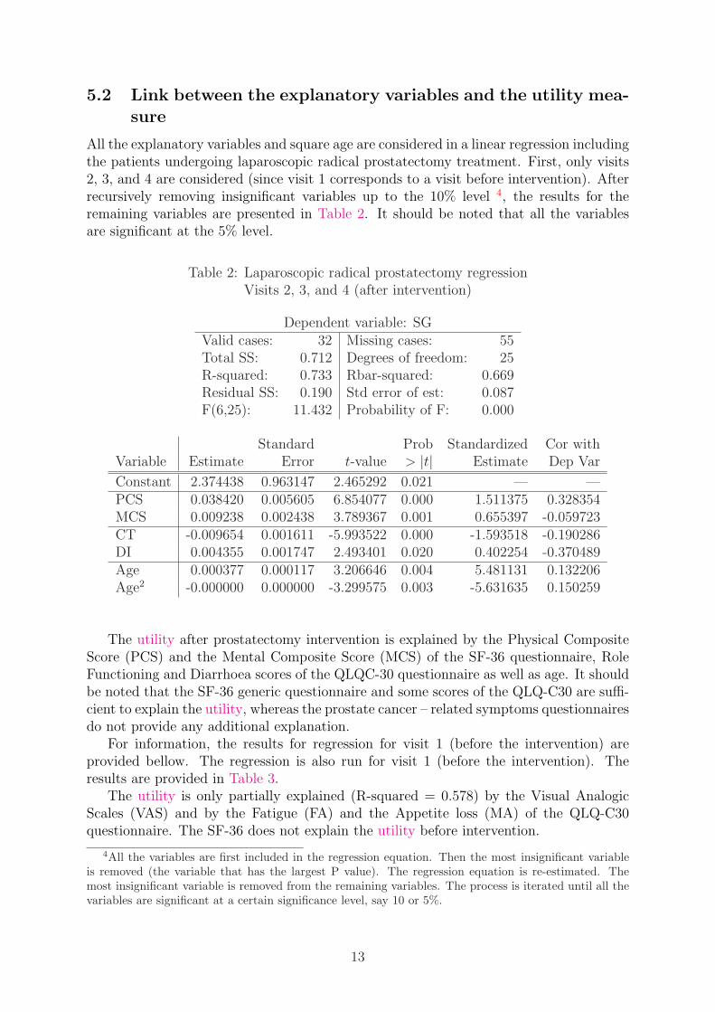
All the explanatory variables and square age are considered in a linear regression includingthe patients undergoing laparoscopic radical prostatectomy treatment. First, only visits2, 3, and 4 are considered (since visit 1 corresponds to a visit before intervention). Afterrecursively removing insignificant variables up to the 10% level 4, the results for theremaining variables are presented in Table 2. It should be noted that all the variablesare significant at the 5% level.

Table 2: Laparoscopic radical prostatectomy regressionVisits 2, 3, and 4 (after intervention)

Dependent variable: SGValid cases: 32 Missing cases: 55Total SS: 0.712 Degrees of freedom: 25R-squared: 0.733 Rbar-squared: 0.669Residual SS: 0.190 Std error of est: 0.087F(6,25): 11.432 Probability of F: 0.000

Standard Prob Standardized Cor withVariable Estimate Error t-value > |t| Estimate Dep Var

Constant 2.374438 0.963147 2.465292 0.021 — —PCS 0.038420 0.005605 6.854077 0.000 1.511375 0.328354MCS 0.009238 0.002438 3.789367 0.001 0.655397 -0.059723CT -0.009654 0.001611 -5.993522 0.000 -1.593518 -0.190286DI 0.004355 0.001747 2.493401 0.020 0.402254 -0.370489Age 0.000377 0.000117 3.206646 0.004 5.481131 0.132206Age2 -0.000000 0.000000 -3.299575 0.003 -5.631635 0.150259

The utility after prostatectomy intervention is explained by the Physical CompositeScore (PCS) and the Mental Composite Score (MCS) of the SF-36 questionnaire, RoleFunctioning and Diarrhoea scores of the QLQC-30 questionnaire as well as age. It shouldbe noted that the SF-36 generic questionnaire and some scores of the QLQ-C30 are suffi-cient to explain the utility, whereas the prostate cancer – related symptoms questionnairesdo not provide any additional explanation.

For information, the results for regression for visit 1 (before the intervention) areprovided bellow. The regression is also run for visit 1 (before the intervention). Theresults are provided in Table 3.

The utility is only partially explained (R-squared = 0.578) by the Visual AnalogicScales (VAS) and by the Fatigue (FA) and the Appetite loss (MA) of the QLQ-C30questionnaire. The SF-36 does not explain the utility before intervention.

4All the variables are first included in the regression equation. Then the most insignificant variableis removed (the variable that has the largest P value). The regression equation is re-estimated. Themost insignificant variable is removed from the remaining variables. The process is iterated until all thevariables are significant at a certain significance level, say 10 or 5%.

13

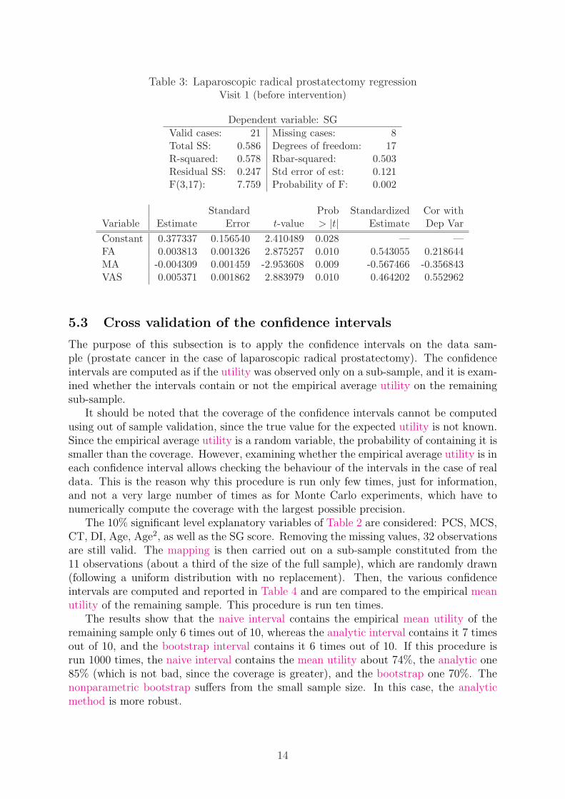
Table 3: Laparoscopic radical prostatectomy regressionVisit 1 (before intervention)

Dependent variable: SG

Valid cases: 21 Missing cases: 8Total SS: 0.586 Degrees of freedom: 17R-squared: 0.578 Rbar-squared: 0.503Residual SS: 0.247 Std error of est: 0.121F(3,17): 7.759 Probability of F: 0.002

Standard Prob Standardized Cor withVariable Estimate Error t-value > |t| Estimate Dep Var

Constant 0.377337 0.156540 2.410489 0.028 — —FA 0.003813 0.001326 2.875257 0.010 0.543055 0.218644MA -0.004309 0.001459 -2.953608 0.009 -0.567466 -0.356843VAS 0.005371 0.001862 2.883979 0.010 0.464202 0.552962

5.3 Cross validation of the confidence intervals

The purpose of this subsection is to apply the confidence intervals on the data sam-ple (prostate cancer in the case of laparoscopic radical prostatectomy). The confidenceintervals are computed as if the utility was observed only on a sub-sample, and it is exam-ined whether the intervals contain or not the empirical average utility on the remainingsub-sample.

It should be noted that the coverage of the confidence intervals cannot be computedusing out of sample validation, since the true value for the expected utility is not known.Since the empirical average utility is a random variable, the probability of containing it issmaller than the coverage. However, examining whether the empirical average utility is ineach confidence interval allows checking the behaviour of the intervals in the case of realdata. This is the reason why this procedure is run only few times, just for information,and not a very large number of times as for Monte Carlo experiments, which have tonumerically compute the coverage with the largest possible precision.

The 10% significant level explanatory variables of Table 2 are considered: PCS, MCS,CT, DI, Age, Age2, as well as the SG score. Removing the missing values, 32 observationsare still valid. The mapping is then carried out on a sub-sample constituted from the11 observations (about a third of the size of the full sample), which are randomly drawn(following a uniform distribution with no replacement). Then, the various confidenceintervals are computed and reported in Table 4 and are compared to the empirical meanutility of the remaining sample. This procedure is run ten times.

The results show that the naive interval contains the empirical mean utility of theremaining sample only 6 times out of 10, whereas the analytic interval contains it 7 timesout of 10, and the bootstrap interval contains it 6 times out of 10. If this procedure isrun 1000 times, the naive interval contains the mean utility about 74%, the analytic one85% (which is not bad, since the coverage is greater), and the bootstrap one 70%. Thenonparametric bootstrap suffers from the small sample size. In this case, the analyticmethod is more robust.

14

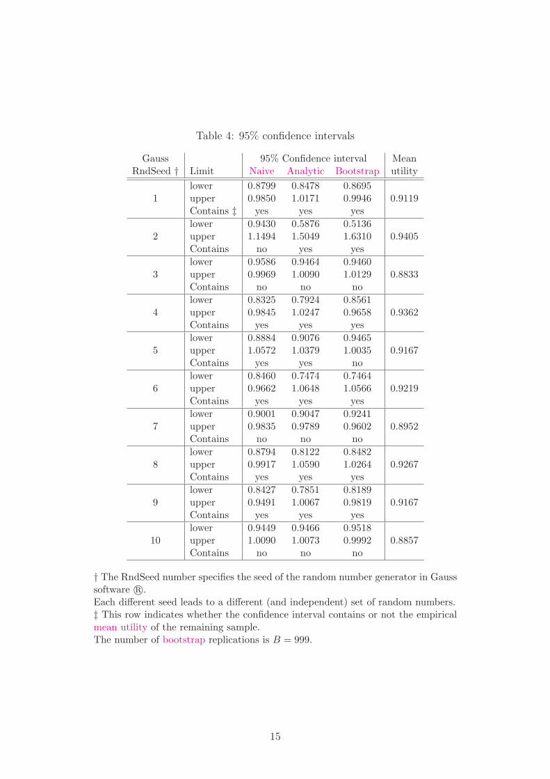
Table 4: 95% confidence intervals

Gauss 95% Confidence interval MeanRndSeed † Limit Naive Analytic Bootstrap utility

lower 0.8799 0.8478 0.86951 upper 0.9850 1.0171 0.9946 0.9119

Contains ‡ yes yes yes

lower 0.9430 0.5876 0.51362 upper 1.1494 1.5049 1.6310 0.9405

Contains no yes yes

lower 0.9586 0.9464 0.94603 upper 0.9969 1.0090 1.0129 0.8833

Contains no no no

lower 0.8325 0.7924 0.85614 upper 0.9845 1.0247 0.9658 0.9362

Contains yes yes yes

lower 0.8884 0.9076 0.94655 upper 1.0572 1.0379 1.0035 0.9167

Contains yes yes no

lower 0.8460 0.7474 0.74646 upper 0.9662 1.0648 1.0566 0.9219

Contains yes yes yes

lower 0.9001 0.9047 0.92417 upper 0.9835 0.9789 0.9602 0.8952

Contains no no no

lower 0.8794 0.8122 0.84828 upper 0.9917 1.0590 1.0264 0.9267

Contains yes yes yes

lower 0.8427 0.7851 0.81899 upper 0.9491 1.0067 0.9819 0.9167

Contains yes yes yes

lower 0.9449 0.9466 0.951810 upper 1.0090 1.0073 0.9992 0.8857

Contains no no no

† The RndSeed number specifies the seed of the random number generator in Gausssoftware r©.Each different seed leads to a different (and independent) set of random numbers.‡ This row indicates whether the confidence interval contains or not the empiricalmean utility of the remaining sample.The number of bootstrap replications is B = 999.

15

6 Discussion and conclusion

On a medical point of view, when estimating the mean utility of a treatment, it is im-portant to get an accurate confidence interval. Indeed, the final purpose is to carry outa cost-utility analysis (using for instance the incremental cost-utility ratio -ICUR-).

In CUA, the classical methods do not account for the mapping phenomenon. Wehave shown that decision-making based on utility values interpolated from mapping isnot reliable if the mapping is not accounted for : a “naive interval” (which does notaccount for mapping) would lead to a serious mistake: the coverage is between 20% and40% for a 95% confidence level! Then, the utility can be greatly under or over evaluated.These methods can lead to wrong positive decisions. In addition, it is often possible todetermine any sub-groups of patients for which a new treatment is more effective (interms of utility) than the standard treatment (for instance a sub-group for which thedisease if more serious). Thus, in these cases, it is essential to account for the uncertaintydue to mapping to get an accurate confidence interval with respect to the risk of coverageα.

Our analytic and bootstrap procedures, integrating the mapping, provide very accu-rate results. Monte Carlo experiments show that the analytic and bootstrap 95% confi-dence intervals display coverage between 94% and 96% for various sample sizes, with areasonable interval length. In addition, the cross validation from the laparoscopic radicalprostatectomy data shows similar results in terms of coverage.

In the example of the prostate cancer, the utility after prostatectomy interventionis explained by the Physical Composite Score (PCS) and the Mental Composite Score(MCS) of the SF-36 questionnaire, Role Functioning and Diarrhoea scores of the QLQC-30 questionnaire as well as age. These results have to be interpreted with caution becauseof the small number of patients for which we have all the information. In addition, in ourmodel, to increase the number of observations, we had to consider that the visits wereindependent, which is not necessarily true in practice. However, the large place taken upby the SF36, and completed by any scores of the QLQC-30, is coherent. Nevertheless,any items, characteristic of the consequences of an intervention on the prostate, do notappear.

These methodologies can b extended to the Incremental Cost-Utility Ratio. This al-lows to directly do the cost-utility analysis on the basis of cost and utility simultaneously.Appendix B proposes an extension of the methodologies to the Incremental Cost-UtilityRatio.

16

Appendix

A Proof of the analytic confidence interval

Assume the following linear model:

Ui = Xiβ + εi.

Let the in sample be denoted: i = 1, . . . , n, and the out of sample be denoted: i =n + 1, . . . , n + m.

The aim is to assess the out of sample mean utility:

µUout= E(Uout,i) = E(Xout,i)β.

The estimator of µUoutis:

µUout= Xoutβin =

1

mι′mXout(X

′inXin)−1X ′

inUin,

where ιm = (1, . . . , 1)′. It can be noted that:

µUout=

1

mιmXoutβ +

1

mιmXout(X

′inXin)−1X ′

inεin. (39)

Then, the estimator has the following properties.

A.1 Bias

E(µUout) = E(Xout)β, the estimator is unbiased.

A.2 Variance

V (µUout) = V (Xoutβin).

From Equation 39, we have:

V(µUout

)= V

[Xoutβ + Xout(X

′inXin)−1X ′

inεin]

(40)

= V[Xoutβ

]+ V

[Xout(X

′inXin)−1X ′

inεin]

+2 · cov[Xoutβ, Xout(X

′inXin)−1X ′

inεin]

(41)

= A + B + 2 · C (42)

A =1

mβ′V (Xout,iβ) =

1

mβ′ΩXβ (43)

B = E[Xout(X

′inXin)−1X ′

inεinε′inXin(X ′inXin)−1X ′

out]

−E

[Xout(X

′inXin)−1X ′

inεin]2

(44)

= EE

[Xout(X

′inXin)−1X ′

inεinε′inXin(X ′inXin)−1X ′

out|X]

−E

E

[Xout(X

′inXin)−1X ′

inεin|X]2

(45)

= EXout(X

′inXin)−1X ′

inE[εinε′in|X

]Xin(X ′

inXin)−1X ′out

−E

Xout(X

′inXin)−1X ′

inE[εin|X

]2(46)

17

Since E[εinε′in|X

]= σ2

εIn and E[εin|X

]= 0, then

B = σ2εE

Xout(X

′inXin)−1X ′

out

(47)

C = E[XoutβXout(X

′inXin)−1X ′

inεin]

−E[Xoutβ

]· E

[Xout(X

′inXin)−1X ′

inεin]

(48)

= 0 (49)

V(µUout

)=

1

mβ′ΩXβ + σ2

εEXout(X

′inXin)−1X ′

out

. (50)

It should be noted that Xout(X′inXin)−1X ′

out = O(

1n

). Then, as n −→ ∞ and m −→

∞, V(µUout

)−→ 0.

A.3 Confidence interval

In practice, this variance can be estimated as follows:

V(µUout

)=

1

mβ′inΩX βin + σ2

εinXout(X

′inXin)−1X ′

out,

where ΩX is estimated on the whole sample rather than only on Xout to increase theprecision.

18

B Extension of the methodologies to the Incremental

Cost-Utility Ratio

B.1 Background: the incremental cost-utility ratio

B.1.1 Definition and estimation

In economic evaluations, an ICUR statistic in which a new therapy (T = 1) is comparedwith a standard therapy (T = 0) is defined by:

ICUR =µ1

C − µ0C

µ1U − µ0

U

, (51)

where µ is the true mean value of (subscripts) costs (C) and utility (U) for treatmentsnumber 1 and number 0. Since the true means corresponding to the theoretical populationare not known, the ICUR can be estimated as follows, on the basis of data collected fromtwo groups of patients, each undergoing one of the forms of therapy (group number 1,consisting of n1 individuals, underwent treatment (T = 1) and group number 0, consistingof n0 individuals 5, underwent treatment (T = 0)):

ICUR =C1 − C0

U1 − U0=

∆C

∆U, (52)

where C1, C0 are the sample mean of the costs and U1, U0 in the two treatment armsare the sample mean of utility.

B.1.2 Assumptions and statistical properties

Assumption 3: Utility distribution

It is assumed that the utilities of treatment T = 0, 1 follow independent randomvariables with [0, 1] support and with distribution DT

U as follows:

UTi ∼ DT

U(µTU , σT

U

2), (53)

where i denotes the individuals.

Since the support is finite, all the moments of the distribution are finite.

Assumption 4: Mapping

It is assumed that the utility measure can be explained by some variables X.

UTi = f(XT

i , εTi ; βT ), (54)

εTi ∼ N(0, σ2

ε), (55)

where f is a function that depends on a parameter vector βT , and εTi inde-

pendent of XT . It should be noted that βT is specific to the treatment.

Let us consider an “in-sample” where the utility measure is known be denoted: i =1, . . . , nT , and an “out-of-sample” where the utility is unknown be denoted: i = nT +1, . . . , nT + mT . The aim of mapping is to assess the out-of-sample mean utility:

µUT

out= E(UT

out) = E(f(XT

i,out, εT

i,out; βT )).

5n1 is generally different from n0.

19

Assumption 5: Cost distribution

It is assumed that the costs of treatment T = 0, 1 follow independent randomvariables with (0, +∞) support and with distribution DT

C as follows:

CTi ∼ DT

C(µTC , σT

C

2), (56)

where σTC

2< ∞. i denotes the individuals.

Assumption 6: Cost-Utility link

It is assumed that the utility measure and the cost are correlated for individuali and treatment T :

Cov(UTi , CT

i ) = σTUC (57)

Although the data in question do not follow normal distributions, we can generallyapply the Central Limit Theorem (CLT), partly thanks to the fact that each sequence ofpairs of random variables (C1

i , U1i )i=1,···,n1 , (C0

i , U0i )i=1,···,n0 is independent and identically

distributed (because the data were obtained in a randomised trial). Therefore, C1, C0,U1 and U0 are asymptotically normally distributed, and the same applies for ∆C and∆E as the difference between normally distributed variables. 6

B.1.3 Linear approximation of the mapping

Utility modeling and estimate

If a first order approximation of the function f in Equation 54 is computed, it can beassumed that UT is approximated by:

UTi = XT

i βT + εTi , (58)

where the constant term is assumed to be contained in XT . Thus,

µUT

out= E(XT

i,out)βT .

The estimator usually used is:

µUT

out=

1

mT

nT +mT∑

i=nT +1

UTi =

1

mT

nT +mT∑

i=nT +1

XTi βT

in = XT

outβT

in (59)

where Ui are the out-of-sample predicted values for the utility measure, βT

in = (XT ′

inXT

in)−1XT ′

inUT

inthe in-sample estimate of βT , and ιm = (1, . . . , 1)′. It should be noted that:

µUT

out=

1

mTι′mXT

outβT +

1

mTι′mXT

out(XT ′

inXT

in)−1XT ′

inεT

in. (60)

Then, we have the following properties: E(µUT

out) = E(XT

out)βT . The estimator is

unbiased, and can be used to assess the mean utility. However, to take a decision, theuncertainty has to be accounted for. The problem, which will be handle in subsection B.2,is to estimate the variance of µUT

out.

6The estimated ICUR does not necessarily have a defined mean or a defined variance, mainly owingto the fact that the denominator of the ratio can be statistically close to zero. In this case, the estimatedICUR will be very large (so that it is statistically close to infinite) or indeterminate, depending onwhether ∆C is also statistically close to zero, and the distribution of the estimated ICUR will be closeto a Cauchy distribution (whose moments are infinite).

20

Cost estimate

The out-of-sample mean cost can be estimated as follows:

CT

out =1

mT

nT +mT∑

i=nT +1

CTi . (61)

Under Assumption 6, and applying the Central Limit Theorem (CLT) as nT −→ ∞, weobtain:

CT

out ∼ N

(µT

C ,1

nTσT

C

2)

. (62)

The variance of CTi can be estimated as follows:

(σT

Cout

)2

=1

mT

nT +mT∑

i=nT +1

(CT

i − CT

out). (63)

Utility-Cost link modeling and estimate

σTUC = Cov(XT

i1, CTi )β1 + · · · + Cov(XT

iK , CTi )βK + Cov(εT

i , CTi ), (64)

where K is the number of explanatory variables, X0 corresponds to the constant term.Let us denote Cov(XT

ik, CTi ) = γT

k , (γT1 , . . . , γT

K) = γT , and Cov(εTi , CT

i ) = γε. It shouldbe noted that Cov(εT

i , CTi ) is not necessarily equal to 0, since among two individuals that

have the same characteristics, if one has a random problem that causes its health status,it will also causes the corresponding cost. The covariance vector can be estimated asfollows:

γT =1

mT

mT∑

i=nT +1

(XTi − ιmT XT )′(Ci − C), (65)

where ιmT = (1, . . . , 1), XT = 1mT

∑mT

i=nT +1 XTi , and C = 1

mT

∑mT

i=nT +1 Ci.

B.2 Confidence region for the ICUR

B.2.1 Case of no mapping: Fieller’s method

Why Fieller’s method?

Siani and Moatti [2003] analyzed all the method of the literature for calculating a con-fidence region for the incremental cost effectiveness ration (ICER): box method, deltamethod, ellipse method, Fieller’s method, classical bootstrap method, and “re-ordered”bootstrap method. They found that the only two methods that are reliable are Fieller’smethod and the “re-ordered” bootstrap method. Siani et al. [2004], Siani and de Peretti[2010] then focused on the performance of Fieller’s and “reordered” bootstrap methodsin the problematic cases, frequently occurring in practice, of the difference between av-erage effects of the two treatments approaching statistically zero or of the (mean costsdifference, mean effects difference) pair also approaching statistically zero using MonteCarlo simulations. Their Monte Carlo simulations show that the non-reordered bootstrapmethod performs worse than Fieller’s method in these problematic cases. They also con-firm that the reordered bootstrap method and Fieller’s method have similar performance

21

most of the time. Nevertheless, their Monte Carlo simulations show that in any extremecases Fieller’s method performs significantly better than reordered bootstrap method. 7

When no mapping is used to assess the utility measure, the statistical properties of theICUR are similar to the ones of the ICER. Thus Fieller’s method should also over-performthe other methods for the ICUR.

General theory

This analytic method is based on the joint distribution function of the (mean costs dif-ference, mean effects difference) pair, which is assumed to follow a bivariate Gaussiandistribution. The method involves calculating confidence regions using the pivotal func-tion technique, which consists of solving a second degree equation for the ICER. Webriefly recall the general context of Fieller’s theorem Fieller [1954] (see also Heitjan[2000]). Fieller’s theorem has been considered in the univariate case Fieller [1940b,a],Finney [1978] and in the multivariate case Volund [1980], Zerbe et al. [1982], Laska et al.[1985]. It is assumed here that X1 and X2 are two random normally distributed variablessuch that:

X ∼ N(η, Ω) with X =

(X1

X2

), η =

(η1

η2

)and Ω =

(ω2

1 ω12

ω12 ω22

), (66)

and it is proposed to determine a (1 − α) confidence region for η1

η2

. For this purpose, we

draw up the (statistic) Z = X1 − ρX2 and we note that:

Z ∼ N(0, ω21 + ρ2ω2

2 − 2ρ ω12) under the assumption that ρ is equal toη1

η2

.

Therefore, we have:Z2

ω21 + ρ2ω2

2 − 2ρ ω12

∼ χ2(1), (67)

⇒ P

((X1 − ρX2)

2

ω21 + ρ2ω2

2 − 2ρ ω12

≤ k1−α

)= 1 − α ,

where k1−α is the (1 − α) quantile of the chi-squared distribution with one degree offreedom. To find the (1 − α) confidence region for η1

η2

, the following inequation must besolved:

Q(ρ) ≤ 0, (68)

whereQ(ρ) = xρ2 + yρ + z, (69)

with x = X22 − k1−αω2

2, y = 2(k1−αω12 − X1X2) and z = X21 − k1−αω2

1. If the variancesand covariances are unknown (for example in the case of small sample size), they can bereplaced by their estimators, in which case k1−α is interpreted as the (1 − α) quantile ofan F distribution with the appropriate degrees of freedom.

7Previous Monte Carlo studies of the Literature which compared the performances of Fieller’s andbootstrap methods, concluded that they had similar performance for calculating confidence regions forthe incremental cost-effectiveness ratio. However, these studies do not clearly mention whether they dealwith reordered or non-reordered bootstrap methods and we will clarify this point. In addition, in thesestudies, the number of simulations used was insufficient to provide a great accuracy, the simulated datadealt with were often configured in such a way that they were sufficiently far from problematic cases, themiscoverage was measured calculating the mean miscoverage on several Data Generating Process, givingthe impression that all the methods have similar performance, and consequently, no reliable conclusioncan be drawn from these results.

22

Application to the ICER

We assume that (CT , ET ) are vector random variables with mean (µTC , µT

E), variance((σT

C)2, (σTE)2

)and covariance σT

CE for T = 0, 1. The variables used in Fieller’s methodcorrespond to the following values:

X1 = ∆C,

X2 = ∆E,

ω21 = σ0

C

2/n0 + σ1

C

2/n1,

ω22 = σ0

E

2/n0 + σ1

E

2/n1,

ω12 = σ0CE/n0 + σ1

CE/n1.

After solving the inequation 68, (1−α) confidence regions for the ICER can have differentforms. Depending on the sign of x, defined in Equation 69, and depending on the signof the discriminant ∆ of the polynomial function Q, the various forms of the confidenceregion obtained with Fieller’s method are shown in Table 5. RL and RU are the roots of

Table 5: Form of the confidence region

∆ < 0 ∆ = 0 ∆ > 0x > 0 impossible impossible

[RL, RU

]

Q convex case casex = 0 impossible R

Q linear case[RL, +∞

)if y < 0

x < 0 R R (−∞, RU ] ∪ [RL, +∞)Q concave

the polynomial function Q, given by the following formulas:

RL =X1X2 − k1−αω12 −

√(k1−αω12 − X1X2)2 − (X2

2 − k1−αω22)(X

21 − k1−αω2

1)

X22 − k1−αω2

2

, (70)

RU =X1X2 − k1−αω12 +

√(k1−αω12 − X1X2)2 − (X2

2 − k1−αω22)(X

21 − k1−αω2

1)

X22 − k1−αω2

2

. (71)

If x > 0, we have RL < RU , otherwise if x < 0, we have RL > RU . Lastly, if x = 0, thenRL = RU . It should be noted that the condition x < 0 corresponds to the case in whichµ∆E is not significantly different from zero at level α, and geometrically, the (∆C, ∆E)pair is close to the vertical axis. The sign of x determines the statistical distance betweenthe mean effects difference and zero. As regards the sign of ∆, it measures the statisticaldistance between the (mean costs difference, mean effects difference) and the origin of theCE plane (see theorem 2). A detailed analyze of all the cases can be get under requestto the authors.

23

B.2.2 Case of mapping: various proposals

“Naive” confidence region

A naive, and wrong, way to compute the variance of µUT

outwould be:

V Naive(µUT

out

)=

1

mT

1

mT − 1

nT +mT∑

i=nT +1

(UT

i − µUT

out

)2

, (72)

and the covariance between µUT

outand CT

out:

CovNaive

(µUT

out, CT

out

)=

1

mT

1

mT − 2

nT +mT∑

i=nT +1

(UT

i − µUT

out

) (CT

i − CT) . (73)

The standard deviation in Equation 72 seems to be used in Rivero-Arias et al. [2009]to compute the confidence interval for the mean utility. A naive way to provide a (1 −α)-confidence region for the ICUR is to provide the following moments to the Fieller’smethod:

X1 = ∆C = C1out − C0

out, (74)

X2 = ∆U = µU1

out− µU0

out, (75)

ω21 =

(σ1

Cout

)2

/n1 +(σ0

Cout

)2

/n0, (76)

ω22 = V Naive

(µU1

out

)+ V Naive

(µU0

out

), (77)

ω12 = CovNaive

(µU1

out, C1

out

)+ Cov

Naive(µU0

out, C0

out

). (78)

The confidence region for the ICUR is then given by Table 5, Equation 70, and Equa-tion 71 when using the moments above.

Analytic confidence region

In the case of a linear approximation, the variance of µUoutcan be estimated as follows:

V(µUT

out

)=

1

mTβT

in′ΩXT

outβT

in + σ2εT

inXT

out(XT

in′XT

in)−1XT

out′. (79)

The proof can be get under request to the authors. It should be noted that

V(µUT

out

)= V Naive

(µUT

out

)+ σ2

εT

inXT

out(XT

in′XT

in)−1XT

out′. (80)

In Equation 72, the term σ2εT

inXT

out(XT

in′XT

in)−1XT

out′ is missing. The covariance between

µUT

outand CT

out can be estimated as follows:

Cov(µUT

out, CT

out

)=

1

mTγT

out′βT

in. (81)

24

The proof can be get under request to the authors. The confidence region for the ICUR isthen given by Table 5, Equation 70, and Equation 71 when using the following moments:

X1 = ∆C = C1out − C0

out, (82)

X2 = ∆U = µU1

out− µU0

out, (83)

ω21 =

(σ1

Cout

)2

/n1 +(σ0

Cout

)2

/n0, (84)

ω22 = V

(µU1

out

)+ V

(µU0

out

), (85)

ω12 = Cov(µU1

out, C1

out

)+ Cov

(µU0

out, C0

out

). (86)

These analytic confidence region is restricted to a linear framework with Gaussianerror terms. It can easily be extended to a nonlinear framework, using an Edgeworth ex-pansion, but it will be an approximation. Consequently, we prefer to propose a bootstrapmethodology, which will account for nonlinear specification, which may be used (suchas logistic specification for instance). In addition, using nonparametric bootstrap, errorterms with non-Gaussian distribution can also be accounted for.

Nonparametric bootstrap confidence region

In this subsection, we propose a methodology for building a confidence region based onthe nonparametric bootstrap technique to compute the moments of the estimators. For ageneral presentation of the percentile-t method, see Hall [1992], Davidson and MacKinnon[1993], Efron and Tibshirani [1993], Hjorth [1994], and Shao and Tu [1995]. A mappingmodel is chosen:

UTi = f(XT

i , εTi ; βT ), (87)

CTi = g(UT

i , νTi ; βT

C), (88)

where XT is a regressor matrix, and the functions f and g are known and are parametricin the sense that they depend on a parameter vector βT or βT

C . εTi and νT

i are not assumedto be Gaussian. V (εT

i ) = (σTε )2, and V (νT

i ) = (σTν )2. The confidence region is built as

follows:

1. Equation 87 and Equation 88 are estimated, providing βT

in, εT

in, (σTε )2, βT

C,in, νT

in,

and (σTν )2.

2. A bootstrap Data Generating Process (DGP) has to be defined. It may be eitherparametric or semiparametric, characterized by βin, βT

C,in, and by any other relevant

estimates that may be needed. In a general case, we propose:

UT,bi = f(XT,b

i , εT,bi ; βT

in), (89)

CT,bi = g(UT,b

i , νT,bi ; βT

C,in), (90)

XT,bi ∼ i.i.d. uniform distribution on XT

i , (91)

for T = 1, 0 and i = 1, . . . , nT . The distribution of εbi will be discussed later. f and

g have to be chosen. For simplicitys sake, a linear model is chosen here:

UT,bi = XT,b

i βT

in + εT,bi , (92)

CT,bi = UT,b

i βT

C,in + νT,bi , (93)

25

where XT is assumed to contain the constant term, but a more specific nonlinearmodel can be chosen in practice in accordance with the data.

3. B bootstrap samples are generated:

(XT,bi )nT +mT

i=1 , (UT,bi )nT

i=1, (CT,bi )nT +mT

i=1 ,

for T = 1, 0 and b = 1, . . . , B.

4. For each of these samples, we compute βT

in -denoted βT,b

in -, ∆U b = µU

1,b

out− µ

U0,b

out=

X1,b

outβ1,b

in − X0,b

outβ0,b

in and ∆Cb = C1,b

out − C0,b

out.

5. The variance-covariance matrix of X1 = ∆C = C1out − C0

out and X2 = ∆U =µU1

out− µU0

outis then computed as follows:

ω21 =

1

B

B∑

b=1

(∆Cb − ∆C

)2, (94)

ω22 =

1

B

B∑

b=1

(∆U b − ∆U

)2

, (95)

ω12 =1

B

B∑

b=1

(∆Cb − ∆C

) (∆U b − ∆U

). (96)

6. The confidence region is obtained by applying Fieller’s method to the momentscomputed using bootstrap techniques.

We consider the following way of generating the bootstrap residuals εT,bi and νT,b

i (seeWeber Weber [1984]). The εT,b

i are generated by independent uniform draws with re-placement among the vector with the typical element εT

i constructed as follows:

1. Calculate (PXT )i,i, i = 1, . . . , nT , the diagonal elements of the projection matrix onXT .

2. CalculateεTi√

1−(PXT )i,i

, ∀i = 1, . . . , nT .

3. Recenter the vector that results.

4. Rescale it so that it has the variance (σTε )2.

This permits to correct the heteroskedasticity in the residuals due to the regressors. Thesame procedure is applied for νT,b

i .

B.3 Performance of the methods: Monte Carlo experiments

Data Generating Process (DGP) are use to generate simulated data samples. The meth-ods are applied to each simulated sample j = 1, . . . , S , and it is examined if eachconfidence region j contains or not the true value ICUR of the ratio (which is known,

26

since the DGP is known, conversely to real data). The coverage c of the confidence regionscan be estimated as follow:

c =1

S

S∑

j=1

I (µU ∈ Intervalj) . (97)

The standard deviation of this Monte Carlo estimate of the coverage is√

1Sc(1 − c), where

c is the true coverage.In our Monte Carlo experiments, we choose the confidence level 1 − α = 0.95. The

number of bootstrap replications is B = 999. The number of Monte Carlo replicationsis S = 10, 000. If the true coverage c = 0.95, the standard deviation of the Monte Carloestimate of the coverage is 0.002179. At most (where c = 0.5) the standard deviation is0.005. Several values for nT and mT are chosen. Small values for nT and large valuesfor mT are first allow to reflect the case where the utility is assessed only on a smallsubsample, and then extrapolated to the other patients.

B.3.1 Data Generating Process

A variety of DGP are proposed to check the robustness of the methods: linear, nonlinear,with non-Gaussian error terms.

Linear Case

UTi = βT

0 + βT1 · XT

1i + β2 · XT2i + εT

i , (98)

CTi = βT

C,0 + βTC,1 · UT

i + νTi , (99)

XT1i ∼ i.i.d.U([0, 1]), (100)

XT2i ∼ i.i.d.B(0.5, 3), (101)

εTi ∼ i.i.d.N(0, (σT

ε )2), (102)

νTi ∼ i.i.d.N(0, (σT

ν )2). (103)

The parameters values are set to:β1

0 = 0.2, β11 = 0.7, β1

2 = 0.3, σ1ε = 0.15, β1

C,0 = 0.35, β1C,1 = 0.5, σ1

ν = 0.15.β0

0 = 0, β01 = 0.5, β0

2 = 0.1, σ0ε = 0.15, β0

C,0 = 0.35, β0C,1 = 0.5, σ0

ν = 0.15.We have E(U1

i ) = 1, E(C1i ) = 0.85, E(U0

i ) = 0.4, E(C0i ) = 0.55, ICUR = 0.5.

Random Linear Case

The model is the same, but the parameters vary randomly across the Monte Carlo repli-cations:

β10 ∼ i.i.d.N(0.2, 0.22) , β0

0 ∼ i.i.d.N(0, 02), (104)

β11 ∼ i.i.d.N(0.7, 0.72) , β0

1 ∼ i.i.d.N(0.5, 0.52), (105)

β12 ∼ i.i.d.N(0.3, 0.32) , β0

2 ∼ i.i.d.N(0.1, 0.12), (106)

σ1ε ∼ i.i.d.U([0.15 · 0.5, 0.15 · 1.5]) , σ0

ε ∼ i.i.d.U([0.15 · 0.5, 0.15 · 1.5]), (107)

β1C,0 ∼ i.i.d.N(0.35, 0.352) , β0

C,0 ∼ i.i.d.N(0.35, 0.352), (108)

β1C,1 ∼ i.i.d.N(0.5, 0.52) , β0

C,1 ∼ i.i.d.N(0.5, 0.52), (109)

σ1ν ∼ i.i.d.U([0.15 · 0.5, 0.15 · 1.5]) , σ0

ν ∼ i.i.d.U([0.15 · 0.5, 0.15 · 1.5]). (110)

27

We have E(UTi |βT ) = (1, 0.5, 1.5)βT , E(CT

i |βT , βTC) =

(1, E(UT

i |βT ))βT

C .

Non-Gaussian Random Linear Case

The model is the same as in Equation 98–Equation 101, but the error terms follow theuniform distribution:

εTi ∼ i.i.d.U([−2, 2]) ∗ σT

ε , (111)

νTi ∼ i.i.d.U([−2, 2]) ∗ σT

ν . (112)

The parameters follow the same distributions as in Equation 104–Equation 110. Then,we also have E(UT

i |βT ) = (1, 0.5, 1.5)βT , E(CTi |βT , βT

C) =(1, E(UT

i |βT ))βT

C .

Nonlinear Case

UTi = F [β0 + β1 · X1i + β2 · X2i + εi] (113)

CTi =

(βT

C,0 + UTi βT

C,1

)χ2(1) (114)

F is the cumulative distribution function of a normal variable. The parameters valuesare set to:β1

0 = −0.5, β11 = 0.7, β1

2 = 0.3, σ1ε = 0.3, β1

C,0 = 0.25, β1C,1 = 0.5.

β00 = −0.7, β0

1 = 0.5, β02 = 0.1, σ0

ε = 0.3, β0C,0 = 0.25, β0

C,1 = 0.5.We have E(U1

i ) = 0.61791142, E(C1i ) = 0.55895571, E(U0

i ) = 0.38208858, E(C0i ) =

0.44104429, ICUR = 0.5.

B.3.2 Performance

The coverage of the various confidence regions, computed via Monte Carlo experimentsfor various samples sizes, are presented in Table 6. The sizes are chosen to correspondto a mapping assessment on a small subsample, and then an extrapolation of the utilityvalues to the remaining sample of sizes that can be encountered in practice. The resultsshow that the coverage of the “naive” confidence region is small (down to 60% dependingon the sample sizes) with respect to the confidence level (95%), whereas both the analyticand bootstrap confidence regions perform correctly.

28

Table 6: Coverage and mean length of the 95% confidence intervals

Coverage Mean anglenT mT Naive Analytic Bootstrap Naive Analytic BootstrapLinear Data Generating Process40 400 0.9239 0.9818 0.9818 0.0929 0.1309 0.127530 600 0.7892 0.9620 0.9567 0.0761 0.1322 0.127320 800 0.6659 0.9598 0.9471 0.0659 0.1501 0.1403

Random Linear Data Generating Process80 40 0.9593 0.9679 0.9685 0.4240 0.4538 0.4518

100 100 0.9417 0.9616 0.9616 0.2848 0.3104 0.310240 400 0.8348 0.9667 0.9605 0.1324 0.2337 0.226530 600 0.7495 0.9620 0.9523 0.1101 0.2520 0.240620 800 0.6349 0.9540 0.9437 0.0826 0.2519 0.2319

Non-Gaussian Random Linear DGP40 400 0.8000 0.9538 0.9495 0.1457 0.2666 0.259130 600 0.7057 0.9577 0.9498 0.1010 0.2624 0.251120 800 0.6112 0.9461 0.9381 0.0872 0.3170 0.2886

Nonlinear Data Generating Process40 400 0.9512 0.9580 0.9321 0.7086 0.7383 0.716430 600 0.9382 0.9559 0.9171 0.5827 0.6292 0.598920 800 0.9230 0.9483 0.9207 0.5119 0.5967 0.5608

nT is the in sample size used to assess the mapping. mT is the out of sample sizewhere the utility values are predicted.

29

References

R. Ariza-Ariza, B. Hernandez-Cruz, B. Carmona, M. D. Ruiz-Montesinos, J. Bal-lina, F. Navarro-Sarabia, The Costs, and Quality of Life in Rheumatoid ArthritisStudy Group. Assessing utility values in rheumatoid arthritis: A comparison betweentime trade-off and the euroqol. Arthritis and Rheumatism (Arthritis Care and Re-search), 55(5):751–756, October 15 2006. DOI 10.1002/art.22226, American College ofRheumatology. 1

N. Bansback, A. Brennan, and O. Ghatnekar. Cost-effectiveness of adalimumab in thetreatment of patients with moderate to severe rheumatoid arthritis in sweden. Ann.Rheum. Dis., 64:995–1002, 2005. 3

A. Beresniak, A.S. Russell, B. Haraoui, L. Bessette, C. Bombardier, and G. Duru. Ad-vantages and limitations of utility assessment methods in ra. Journal of Rheumatology,34(11):2193–2200, 2007. 3

R. Davidson and J. G. MacKinnon. Estimation and inference in economics. OxfordUniversity Press, New York, 1993. 3.4, B.2.2

P. Dolan and M. Sutton. Mapping visual analogue scale health state valuations ontostandard gamble and time trade-off values. Soc Sci Med, 44(10):1519–1530, 1997. 1

B. Efron and R. J. Tibshirani. An Introduction to the Bootstrap, volume 57 of Monographson Statistics and Applied Probability. Chapman and Hall, London, 1993. 3.4, B.2.2

E. C. Fieller. Some problems in interval estimation. Journal of the Royal StatisticalSociety, Series B, 16:175–183, 1954. 7

E.C. Fieller. The biological standardization of insulin. Journal of the Royal StatisticalSociety, 137:1–53, 1940a. 7

E.C. Fieller. A fundamental formula in the statistics of the biological assay, and someapplications. Quarterly Journal of Pharmacy and Pharmacology, 17:117–123, 1940b.7

D.J. Finney. Statistical methods in biological assay. Macmillan, 1978. New York. 7

P. Hall. The Bootstrap and Edgeworth Expansion. Springer-Verlag, New York, 1992. 3.4,B.2.2

D.F. Heitjan. Fieller’s method and net health benefits. Health Economics, 9:327–335,2000. 7

J. S. U. Hjorth. Computer Intensive Statistical Methods. Chapman and Hall, London,1994. 3.4, B.2.2

P. F. Krabbe, M. L. Essink-Bot, and G. J. Bonsel. The comparability and reliability offive health-state valuation methods. Soc Sci Med, 45(11):1641–1652, 1997. 1

E.M. Laska, H.B. Kushner, and M. Meisner. Reader reaction: multivariate bioassay.Biometrics, 41:547–554, 1985. 7

30

L. Longworth, M. Buxton, M. Sculpher, and D. H. Smith. Estimating utility data fromclinical indicators for patients with stable angina. Eur J Health Econom, 6:347–353,2005. 1, 3

S. Merkesdal, T Kirchhoff, D. Wolka, G. Ladinek, A. Kielhorn, and A. Rubbert-Roth.Cost-effectiveness analysis of rituximab treatment in patients in germany with rheuma-toid arthritis after etanercept-failure. Eur J Health Econ, 11:95–104, 2010. DOI10.1007/s10198-009-0205-y. 3, 3

E. Nord, J. Richardson, and K. Macarounas-Kirchmann. Social evaluation of healthcare versus personal evaluation of health states: Evidence on the validity of four healthstate scaling instruments using norvegian and australian survey data. Centre for HealthProgram Evaluation (CHPE), Working Paper 23, September 1992. 1

J. F. O’Leary, D. L. Fairclough, M. K. Jankowski, and J. C. Weeks. Comparison of timetrade-off utilities and rating scale values of cancer patients and their relatives: evidencefor a possible plateau relationship. Med Decis Making, 15(2):132–137, 1995. 1

O. Rivero-Arias, M. Ouellet, A. Gray, J. Wolstenholme, P. M. Rothwell, and R. Luengo-Fernandez. Mapping the modified rankin scale (mrs) measurement into the genericeuroqol (eq-5d) health outcome. In 7th World Congress on Health Economics, volumeHarmonizing Health and Economics, Beijing, China, July 12–15 2009. InternationalHealth Economics Association. Poster presentation. 3, 3.2, B.2.2

J. A. Salomon and C. J. L. Murray. A multi-method approach to measuring health-statevaluations. Health Economics, 13:281–290, 2004. Published online 20 June 2003 inWiley InterScience (www.interscience.wiley.com). DOI:10.1002/hec.834. 3

J. Shao and D. Tu. The Jackknife and Bootstrap. Springer-Verlag, New York, 1995. 3.4,B.2.2

A. Shmueli. It might be premature to reject the assumption of a power curve relationshipbetween vas and sg data: Three comments on stevens, mccabe and braziers mappingbetween vas and sg data; results from the uk hui index 2 valuation survey. HealthEconomics, 16(in press):755–758, 2007. Published online 18 December 2006 in WileyInterScience (www.interscience.wiley.com). DOI: 10.1002/hec.1188. 2.5, 3

C. Siani and C. de Peretti. Are fieller’s and bootstrap methods really equivalent for cal-culating confidence regions for ratios. Health, Decision and Management, forthcoming,2010. B.2.1

C. Siani, C. de Peretti, and J. P. Moatti. Rehabilitating the confidence region for icersand which method to use: Fieller or re-ordered bootstrap? Applied Health Economicsand Health Policy, 3(1):S62–S63, 2004. supplement. B.2.1

C. Siani and J.-P. Moatti. Quelles methodes de calcul des regions de confiance du ratiocout-efficacite incremental choisir ? Revue d’Epidemiologie et de Sante Publique, 51:255–276, 2003. B.2.1

K. J. Stevens, C. J. McCabe, and J. E. Brazier. Mapping between visual analogue scaleand standard gamble data; results from the uk health utilities index 2 valuation survey.Health Econ., Health Economics Letters, 15:527–533, 2006. Published online 3 January

31

2006 in Wiley InterScience (www.interscience.wiley.com). DOI:10.1002/hec.1076. 2.5,3

G. W. Torrance. Social preferences for health states: an empirical evaluation of threemeasurement techniques. Socio-Econ Planning Sci, 10(3):129–136, 1976. 1

G. W. Torrance, D. H. Feeny, W. J. Furlong, R. D. Barr, Y. Zhang, and Q. Wang.Multiattribute utility function for a comprehensive health status classification system.health utilities index mark 2. Med Care, 34(7):702–722, 1996. 1

A. Tsuchiya, J. Brazier, E. McColl, and D. Parkin. Deriving preference-based singleindices from non-preference based condition-specific instruments: Converting aqlq intoeq5d indices. Sheffield Health Economics Group, Discussion Paper Series Ref: 02/1;The University of Sheffield, ScHARR, School of Health and Related Research, May2002. 2.1, 2.6

A. Volund. Multivariate bioassay. Biometrics, 36:225–236, 1980. 7

N.C. Weber. On resampling techniques for regression models. Statistics and ProbabilityLetters, 2:275–278, 1984. 3.4, B.2.2

E.M. Zerbe, G.O.and Laska, M. Meisner, and H.B. Kushner. On multivariate confidenceregions and simultaneous confidence limits for ratios. Communications in Statistics,Theory and Methods, 11:2401–2425, 1982. 7

32