INTERNATIONAL JOURNAL FOR NUMERICAL METHODS IN ENGINEERING, VOL. 36,2851-2860 (1993)

AN IMPROVED NUMERICAL METHOD TO FIND PARAMETERS USING EXPERIMENTAL DATA

IHTZAZ QAMAR A N D S WILAYAT HUSAIN

Dr. A. Q. Khan Research Lahoratoriea, P.O. Box. 502, Rawalpindi, Pakistan

SUMMARY

In this paper we describe a numerical method to determine adjustable parameters in a mathematical model using experimental data. This is basically an improvement over our earlier method which was based on the idea that the area under the experimental curve must be equal to the integral of the function used. The improvement used is the addition of an area correction factor which estimates the necessary difference that must exist between the numerically evaluated and the true area. This correction surprisingly eliminates the use of integral with the result that the two areas being equaliLed are both numerically evaluated, one using the experimental data points and the other using the fitted function values. It is shown that the application of the area correction factor significantly improves the accuracy of the adjusted parameters. The method has been compared with the well-known method of least squares for few selected cases involving variety of functions. It is seen that our method shows convergence for a wider range of initial guesses as compared to the method of least squares. The superiority of our method becomes evident when more than two non-linear parameters are involved.

INTRODUCTION

Mathematical modelling is a n essential tool utilized to gather a better understanding of the processes occurring in nature. The phenomena under investigation arc analysed mathematically and models are proposed. These models generally contain certain adjustable parameters which must be determined accurately to gain useful information from the model. A common practice is to perform the experiments in conjunction with the modelling and then use the experimental results to adjust the model parameters. The adjustment of parameters boils down to a curve- fitting problem where numerical values of the parameters are determined which give the best fit between the model and the experimental results. Therefore, the curve-fitting problem is basically an inverse problem. As discussed by Beck and Blackwell' there are two general classes of inverse problems, parameter estimation and function estimation. Parameter estimation technique is used where the functional form having a limited number of parameters is known and the parameters are determined from experimental data. Most frequent engineering applications include deter- mination of activation energy from chemical kinetics data,2 various thermal properties such as diffusivity and conductivity from thermal history,' corrosion parameters from electrochemical measurement^,^ etc. If the number of parameters involved is large the problem becomes that of a function estimation. A well-known case would be the inverse heat conduction problem where surface heat flux, varying with time, is estimated from transient heat conduction data,

The curve fitting is generally performed using the method of least squares. Fo r models which are linear in parameters, the method of least squares is easy to implement. However, for non-linear models this method poses serious convergence problems. In our earlier paper4 we have

0029-598 1/93/162851-10$10.00 0 1993 by John Wiley & Sons, Ltd.

Received 2 April 1992 Revised 17 February 1993

2852 1. QAMAR AND S. W. HUSAIN

presented a new approach to determine parameters from experimental data. In the present work we describe an improved version of this method. In order to show the performance of the improved method, we have applied the method to various test cases. The results are compared with those obtained using the method of least squares. In a future publication we will present our results in detail showing that the present method can easily be applied to solve function estimation problems such as the inverse heat conduction problem. In this paper we present the application of our method to parameter estimation only.

THE PROPOSED METHOD

We assume that the experimental data consist of N pairs of (x, y ) points and is to be represented by a mathematical model of the form

Y = F ( x , Q j ) (1)

where aj ( , j = 1 ,2 ,3 , . . . , M ) are the parameters to be determined. The error between the fitted and the experimental points is generally represented as

N

In the method of ordinary least squares, the error, E, is minimized with respect to all the adjustable parameters. The set of equations to be solved is obtained by differentiating equation (2) with respect to each parameter:

Our method is based on the idea that the area under the experimental curve should be equal to the integral of the model equation. The first relationship is again the minimization of error which, however, is applied to one parameter only:

dE H , r , = O *a1

(4)

For the rest of the equations, the domain of the experimental data is divided into M - 1 parts and for each part the area under the experimental curve is equated to the integral of the function for that part:

H k + , = A , - F(x,uj)dX=O, ( k = 1 , 2 , . . . , M - 1 ) ( 5 ) I= where the indices s and e mark the start and the end of the kth part. The area Ak is determinined numerically using the trapezoidal rule as

e - 1 Y i + l + Yi

A k = c (k = 1,2,. . . ,M - 1) i = s L

Note that the evaluation of the area Ak does not depend on the values of the parameters a,. On the other hand, the integral is evaluated analytically for a given set of parameters and is independent of the experimental data. The system of equations, H,, expressed by equations (4) and (5) is then solved simultaneously to determine the parameters.

It should be realized that the use of equation (5) may lead to certain degree of error in the computed values of the parameters. According to equation (9, the numerical area should

USING EXPERIMENTAL DATA TO FIND PARAMETERS 2853

exactly be equal to the analytical area, i.e. the value of the integral. As the numerical area is calculated using trapezoidal rule, equation (5) holds true only if the function F ( x , a, j happens to be a straight line. In general, the two areas will be different and forcing them to be equal leads to an error in the results. To circumvent this discrepancy we estimate the difference that must exist between the two areas and equation ( 5 ) is then modified to account lor the difference. The difference in the areas, A&, for every part, is computed using the following equation:

The first term on the right-hand side of the equality is the trapezoial area for the kth part computed by evaluating the fitted values of the function instead of using the experimental yi values. The second term is the analytical area. The area difference AAk is thus an estimate of the deviation in the two areas and will be used to rectify the discrepancy in equation ( 5 ) as shown below:

X e

Hk+l = Ak - F ( x , aj)dx - A 4 = 0 (k = 1, . . .2, . . . , M - 1) (8)

Inserting equations (6) and (7) into equation (8) we get

(k = 1,2, . . . , M - 1) (9) The result is quite surprising as it does not involve the integral. The final equation is basically the difference between two numerically evaluated areas, one using experimental values, y;s, and the other using the function values, F ( x i , aj)'s.

Note that these two areas can be calculated using any numerical technique such as Simpson's rules, etc. The only restriction is to apply the same rule for both the areas. If trapezoidal rule is used with equally spaced data points, equation (9) is further simplified as shown below:

The expression is now simply the sum of the error between the mid-points. The solution algorithm to solve the above set of equations consists of the following steps:

1 . Input N pairs of ( x i , yi) experimental data. 2. Divide the data points into M - 1 parts where M is the number of adjustable parameters. 3. Assume a guess for aj parameters. 4. Compute function values F ( x i , a j ) for each x i . 5 . Compute H I in equation (4) and H2 to HM in equation (9) 6. The system of simultaneous equations obtained in step 5 is solved using Newton-Raphson

method. This is done by solving the following matrix system:

2854 1. QAMAR A N D S. W. HIJSAIN

All the partial derivatives are computed numerically using central differences.

Update the guess using the following relations: 7. The solution vector provides the necessary improvement in the guess for the next iteration.

a, +- a, + AaJ

8. Repeat steps 4-7 until values of H i s are less than a user-defined tolerance. This then provides the values of the fitted parameters.

RESULTS AND DISCUSSION

We have applied the present method to various types of functions such as exponential, trigono- metric, etc., involving two, three or more adjustable parameters. In the following we examine only the intrinsic behaviour of the method using the exact hypothetical data which is generated using assumed values of parameters. These exact data are used to calculate the values of parameters by our method which are then compared with the method of least squares.

Efec t oj the area correction

exponential function with two parameters: Let us first examine the advantage of using the idea of area correction. For this we use a simple

y = al exp(a,x)

with a, = - 1.0 and a2 = 5.0. The domain, x, is varied from 0 to 1. First we use the method without the area correction, i.e. equations (4) and (5 ) . The results obtained are shown in Figure 1 where the percentage deviation in the computed parameters is shown as a function of the number of data points. It is seen that the deviation in the computed parameters may be significant if the number of data points is not sufficiently large, i.e. when the points are not closely spaced. This is due to the fact that when the interval between the successive data points is large, the numerical area using the trapezoidal rule is significantly different than the true value of the integral. Since the method tries to equalize the two areas, the parameters are accordingly adjusted. Therefore, the resulting parameters differ from their true values. It is clear from Figure

i 40

0 10 20 30 40 50

N

Figure I . Percentage deviation in the fitted parameters using the method without area correction. The function used is Y a1 exp(a2x)

USING LXPFRIMENTAL D A T A TO FIND PARAMETERS 2855

1 that the deviation in a , is much less than that in a 2 . This is because the integral of the curve being used here is more sensitive to changes in u2 as compared to a , .

When the method is used with area correction, i.e. equations (4) and (9), the exact values of the parameters are obtained regardless of the number of data points. This is due to the fact that in order to equalize the two areas, a correction is being made in the numerical area rather than forcing the parameters to adjust the integral. In fact, integral of the function is not even used in the final expression which simply involves two numerically integrated areas. The elimination of the integral is a significant feature since now the functions which are not integrable can be handled easily. In addition, it should be noted that equation (9) is easier to implement as compared to equation (5).

After establishing the importance of the area correction we now compare this method with the method of least squares for few test cases. For the sake of comparison, the solution of equations obtained in the method of least squares is also carried out using Newton-Raphson’s method.

Comparison with the method of least squares

Test cme I. Here again, we use a simple exponential function with two parameters:

y = a , exp(a2x)

with a l = 1.0 and a2 = - 1.0. The domain, x, is varied from 0 to 1 with 10 equally spaced data points. We have tested the methods for a large number of initial guesses and the results are graphically summarized in Figure 2. Figure 2(a) depicts the regions where the present method converges t o true values of the parameters. The same for the method of least squares is shown in Figure 2(b). It is seen that the method of least squares converges only in a narrow range in the vicinity of the true values. On the other hand, our method shows convergence in a wide range. Note that the range of convergence for a , extends beyond the limits shown in both directions.

3

2

1

a 0

-1

-2

-3

N

-3 L -3 -2 -1 0 1 2 3 -3 -1 1 3

(4 81 (b) a1

Figure 2. The range of the initial guesses of the parameters for which the convergence is obtained using (a) the present method, (b) the method of the least squares. The function used is y = a, exp(a,x) with the true values of the parameters

being a , = 1.0 and u2 = - 1.0

2856 1. QAMAR AND S. W. HUSAIN

2

1.5

$ 1

0.5

0

2

1.5

$ 1

0.5

0 0 0.5 1 1.5 2 0 0.5 1 1.5 2

( 4 a1 (b) a,

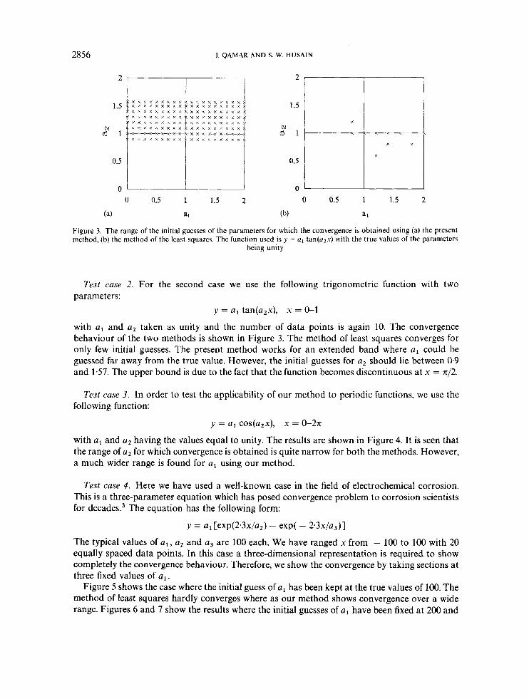
Figure 3. The range of the initial guesses of the parameters for which the convergence is obtained using (a) the present method, (b) the method of the least squares. The function used is J J = u1 tan(u2x) with the true values of the parameters

being unity

Test case 2. For the second case we use the following trigonometric function with two parameters:

y = a, tan(a,x), x = &1

with al and az taken as unity and the number of data points is again 10. The convergence behaviour of the two methods is shown in Figure 3. The method of least squares converges for only few initial guesses. The present method works for an extended band where a, could be guessed far away from the true value. However, the initial guesses for a2 should lie between 0.9 and 1-57. The upper bound is due to the fact that the function becomes discontinuous at x = 4 2 .

Test case 3 . In order to test the applicability of our method to periodic functions, we use the following function:

y = a, cos(a2x), x = 0-271

with a, and a2 having the values equal to unity. The results are shown in Figure 4. It is seen that the range of a2 for which convergence is obtained is quite narrow for both the methods. However, a much wider range is found for a, using our method.

Test case 4. Here we have used a well-known case in the field of electrochemical corrosion. This is a three-parameter equation which has posed convergence problem to corrosion scientists for decade^.^ The equation has the following form:

y = a, [exp(2.3x/a2) - exp( - 2-3x/a3)]

The typical values of a,, a, and a3 are 100 each. We have ranged x from - 100 to 100 with 20 equally spaced data points. In this case a three-dimensional representation is required to show completely the convergence behaviour. Therefore, we show the convergence by taking sections at three fixed values of al .

Figure 5 shows the case where the initial guess of a, has been kept at the true values of 100. The method of least squares hardly converges where as our method shows convergence over a wide range. Figures 6 and 7 show the results where the initial guesses of a, have been fixed at 200 and

USING EXPERIMENTAL DATA TO FIND PARAMETERS

0.5

0

2857

i i 1

2

1.5

N a 1

0.5

0

x x x x x x x x x x x x x x x x x x X x --x-x-x-x-x-x-x x-x-x- x X-v-v-x-x-x-x-x-x x x x x x x x x x x X x X X x X X X X x -3

-300 -150 0 150 300 -300 -150 0 150 300

( 4 a1 6) a1

Figure 4. The range of the initial guesses of the parameters for which the convergence is obtained using (a) the present method, (b) the method of the least squares. The function used is y = a , cos(u2xj with the true values of the parameters

being unity

210

160

2 110

60

10

210

160

(0" 110

60

10 10 60 110 160 210 10 60 110 160 210

(a) a2 (b) a2

Figure 5 . The convergence pattern for the function y = a , [exp(2.3uja2) - exp( - 2.3x/a3)] with the initial guess for a, fixed at the true value of 100.0 using (a) the present method, (b) the method of the least squares

50, respectively. Note that the results shown are for our method only since the method of least squares does not converge at all. This case elucidates that the method of least squares is plagued by serious convergence problems when the function contains non-linear parameters.

Rate of convergence

The present method converges quite rapidly and true values are obtained within few iterations. Table I shows, for the test case 1, that the error E decreases rapidly with the number of iterations. Similar rates are observed for the other test cases. It should be pointed out that the rates of convergence using the method of least squares are comparable.

The final error for the present method as well as for the method of least squares is quite small since exact data have been used in all the test cases and the convergence is obtained to the true values of the parameters. This may not be the case when real data are used since it would contain

2858 I. QAMAR AND S. W. HUSAIN

210

1 60

60 x x

x x x x x

10 60 110 160 210

a2

Figure 6 The convergence pattern for the function J = a, Cexp(2 3x/a2) - exp( - 2 3i/a,)] with the initial gueTs for a, fixed at 2000 using the present method The method of least squares does not converge at all

210

160

(do 110

60

10

x x x x x x x x x x x x x x x x x

I X I

10 60 110 160 210

a2

Figure 7. The convergence pattern for the function y = al [exp(2.3x/a2) - exp( - 2.3xja3)] with the initial guess for a , fixed a t 50.0 using the present method. The method of least squares does not converge at all

Table I. Rate of convergence for the test case 1 show- ing the error after each iteration. The initial guesses for the parameters a, and u2 are 3.0 and - 3.0 and the

true values are 1-0 and - 1.0 respectively

Iteration number a, a2 Error, E

0 3-0000 - 3.0000 7.3 x 10" 1 0-5160 - 1.2315 1 . 4 ~ 10' 2 1.0732 - 1-1066 1.3 x lo-' 3 0.9981 - 0.9997 1 . 7 ~

5 1.OOOO - 1.0000 8 . 9 ~ 4 0.9999 - 0.9999 9.3 x

USING EXPFRIMFNTAI. DATA TO k I N D PARAMETERS 2859

-3 -1 1 3

al

Figure 8. The range of the in~tial guesses of the parameters for which the convergence is obtained when the error is minimized with respect to the parameter u z . Compare this with Figure 2(a) where the error is minimized with respect lo

the parameter a,

some inaccuracies due to experimental errors. The effect of such random experimental errors would be addressed in our future publication.

Cuse of lineur coeficients

After establishing the superior convergence properties of our method for functions with non-linear coefficients, we now describe the situation for linear coefficients. In such cases the system of simultaneous equations obtained is linear with respect to the unknown parameters and a direct solution is possible thus eliminating the iterative process. Note that same is true for the method of least squares and hence it is expected that the two methods would have similar behaviour. We have tested our method for a large number of linear systems including poly- nomials with unlimited number of unknown parameters and always obtain the correct values of the parameters. The method of least squares is known to give correct values for linear systems. Our method therefore bchaves as good as the method of least squares for this case.

Selection of parameters

In the results presented so far we have used the parameter a, to minimize the sum of squares of the error as stated in equation (4). The remaining equations used in the Newton Raphson method are obtained by differentiating equation (9) with respect to the rest of the parameters. Although the use of a, in equation (4) is arbitrary and any one of the parameters can be used, the preferred choice may vary from function to function. The results for such an exercise using thc test case 1 are shown in Figure 8. This figure shows the convergence range when u2 is used in equation (4). Note that the region of convergence has considerably shrunk as compared to the one shown in Figure 2(a) where a, has been used in equation (4). This decline in the performance is related to the fact that now we arc applying the least-squares criterion a non-linear parameter. We therefore recommend that equation (4) should be applied on a linear parameter.

CONCLUSIONS

1. The present method which incorporates the area correction factor provides more accurate values of the adjusted parameters as compared to our previous method which simply equated the numerical area under the experimental curve with the integral of the function.

2860 1. QAMAR A N D S. W. HUSAIN

2. The proposed method exhibits quadratic rate of convergence. 3. The performance of our method is comparable to that of the method of least squares for the

case of linear parameters. 4. Our method shows better performance than the method of least squares for the case of

non-linear parameters as it converges over a wider range of initial guesses. The difference in behaviour becomes more pronounced as the number of parameters is increased.

5 . In our method, the error is minimized with respect to one parameter only. The convergence behaviour of our method is better if this parameter is linear.

REFERENCES

1. J. V. Beck and B. Blackwell, ‘Inverse Problems’, in W. J. Minkowycz, E. M. Sparrow, G. E. Schneider and R. H.

2. J. H. Haberman and Y. K. Rao, ‘Chemiccrl dissolution of lead blasifurnace accretions with potassium carbonate in the

3. 1. Qamar and S. W. Husain, ‘New computational method to determine Tafel slopes and corrosion rates from electrode

4. I . Qamar and S. W. Husain, ‘A numerical approach to find parameters using experimental data’, Commun. Appl.

Pletcher (eds.), Handhok of Numeriral Heat Transfer, Wiley, New York, 1988.

presenre of carbon’, Can. Metall. Q., 27, 247-251 (1988).

kinetic measurements’, Rr. Corros. J., 25, 202-204 (1990).

Numer. Methods, 7, 259-263 (1991).