Improved constraints on cosmological parameters from Type Ia supernova data
24
Mon. Not. R. Astron. Soc. 000, 000–000 (0000) Printed 9 August 2011 (MN L A T E X style file v2.2) Improved constraints on cosmological parameters from SNIa data M.C. March 1? , R. Trotta 1,2 , P. Berkes 3 , G.D. Starkman 4 , and P.M. Vaudrevange 4,5 1 Imperial College London, Astrophysics Group, Blackett Laboratory, Prince Consort Road, London SW7 2AZ, UK 2 African Institute for Mathematical Sciences, 6 Melrose Rd, Muizenberg, 7945, Cape Town, South Africa 3 Brandeis University, Volen Center for Complex Systems, 415 South Street, Waltham, MA 02454-9110, USA 4 CERCA & Department of Physics, Case Western Reserve University, 10900 Euclid Ave, Cleveland, OH 44106, USA 5 DESY, Notkestrasse 85, 22607 Hamburg, Germany 9 August 2011, preprint: DESY-11-023 ABSTRACT We present a new method based on a Bayesian hierarchical model to extract con- straints on cosmological parameters from SNIa data obtained with the SALT-II lightcurve fitter. We demonstrate with simulated data sets that our method delivers tighter statistical constraints on the cosmological parameters over 90% of the time, that it reduces statitical bias typically by a factor ∼ 2 - 3 and that it has better coverage properties than the usual χ 2 approach. As a further benefit, a full posterior probability distribution for the dispersion of the intrinsic magnitude of SNe is ob- tained. We apply this method to recent SNIa data, and by combining them with CMB and BAO data we obtain Ω m =0.28 ± 0.02, Ω Λ =0.73 ± 0.01 (assuming w = -1) and Ω m =0.28 ± 0.01,w = -0.90 ± 0.05 (assuming flatness; statistical uncertainties only). We constrain the intrinsic dispersion of the B-band magnitude of the SNIa population, obtaining σ int μ =0.13 ± 0.01 [mag]. Applications to systematic uncertainties will be discussed in a forthcoming paper. Key words: Supernovae type Ia, Bayesian statistics, cosmological parameters, sys- tematic errors, intrinsic dispersion. 1 INTRODUCTION Since the late 1990s when the Supernova Cosmology Project and the High-Z Supernova Search Team presented evidence that the expansion of the universe is accelerating (Riess et al. 1998; Perlmutter et al. 1999), observations of Type Ia supernovae (SNIa) has been seen as one of our most important tools for measuring the cosmic expansion as a function of time. Since a precise measurement of the evolution of the scale factor is likely the key to characterizing the dark energy or establishing that General Relativity must be modified on cosmological scales, the limited data that our universe affords us must be used to the greatest possible advantage. One important element of that task is the most careful possible statistical analysis of the data. Here we report how an improved statistical approach to SNIa data, with, in particular, more consistent treatment of uncertainties, leads to significant improvements in both the precision and accuracy of inferred cosmological parameters. The fundamental assumption underlying the past and proposed use of Type Ia supernovae to measure the expansion history is that they are “standardizable candles”. Type Ia supernovae occur when material accreting onto a white dwarf from a companion drives the mass of the white dwarf above the maximum that can be supported by electron degeneracy pressure, the Chandrasekhar limit of about 1.4 solar masses. This triggers the collapse of the star and the explosive onset of carbon fusion, in turn powering the supernova explosion. Because the collapse happens at a particular critical mass, all Type Ia supernovae are similar. Nevertheless, variability in several factors, including composition, rotation rate, and accretion rate, can lead to measurable differences in supernova observables as a function of time. Indeed, the intrinsic magnitude of the nearby ? Corresponding author: [email protected] c 0000 RAS arXiv:1102.3237v4 [astro-ph.CO] 8 Aug 2011
Transcript of Improved constraints on cosmological parameters from Type Ia supernova data
Mon. Not. R. Astron. Soc. 000, 000–000 (0000) Printed 9 August 2011 (MN LATEX style file v2.2)
Improved constraints on cosmological parameters fromSNIa data
M.C. March1?, R. Trotta1,2, P. Berkes3, G.D. Starkman4, and P.M. Vaudrevange4,51Imperial College London, Astrophysics Group, Blackett Laboratory, Prince Consort Road, London SW7 2AZ, UK2African Institute for Mathematical Sciences, 6 Melrose Rd, Muizenberg, 7945, Cape Town, South Africa3Brandeis University, Volen Center for Complex Systems, 415 South Street, Waltham, MA 02454-9110, USA4CERCA & Department of Physics, Case Western Reserve University, 10900 Euclid Ave, Cleveland, OH 44106, USA5DESY, Notkestrasse 85, 22607 Hamburg, Germany
9 August 2011, preprint: DESY-11-023
ABSTRACT
We present a new method based on a Bayesian hierarchical model to extract con-straints on cosmological parameters from SNIa data obtained with the SALT-IIlightcurve fitter. We demonstrate with simulated data sets that our method deliverstighter statistical constraints on the cosmological parameters over 90% of the time,that it reduces statitical bias typically by a factor ∼ 2 − 3 and that it has bettercoverage properties than the usual χ2 approach. As a further benefit, a full posteriorprobability distribution for the dispersion of the intrinsic magnitude of SNe is ob-tained. We apply this method to recent SNIa data, and by combining them with CMBand BAO data we obtain Ωm = 0.28± 0.02,ΩΛ = 0.73± 0.01 (assuming w = −1) andΩm = 0.28± 0.01, w = −0.90± 0.05 (assuming flatness; statistical uncertainties only).We constrain the intrinsic dispersion of the B-band magnitude of the SNIa population,obtaining σint
µ = 0.13 ± 0.01 [mag]. Applications to systematic uncertainties will bediscussed in a forthcoming paper.
Key words: Supernovae type Ia, Bayesian statistics, cosmological parameters, sys-tematic errors, intrinsic dispersion.
1 INTRODUCTION
Since the late 1990s when the Supernova Cosmology Project and the High-Z Supernova Search Team presented evidence that
the expansion of the universe is accelerating (Riess et al. 1998; Perlmutter et al. 1999), observations of Type Ia supernovae
(SNIa) has been seen as one of our most important tools for measuring the cosmic expansion as a function of time. Since
a precise measurement of the evolution of the scale factor is likely the key to characterizing the dark energy or establishing
that General Relativity must be modified on cosmological scales, the limited data that our universe affords us must be used
to the greatest possible advantage. One important element of that task is the most careful possible statistical analysis of the
data. Here we report how an improved statistical approach to SNIa data, with, in particular, more consistent treatment of
uncertainties, leads to significant improvements in both the precision and accuracy of inferred cosmological parameters.
The fundamental assumption underlying the past and proposed use of Type Ia supernovae to measure the expansion
history is that they are “standardizable candles”. Type Ia supernovae occur when material accreting onto a white dwarf from
a companion drives the mass of the white dwarf above the maximum that can be supported by electron degeneracy pressure,
the Chandrasekhar limit of about 1.4 solar masses. This triggers the collapse of the star and the explosive onset of carbon
fusion, in turn powering the supernova explosion. Because the collapse happens at a particular critical mass, all Type Ia
supernovae are similar. Nevertheless, variability in several factors, including composition, rotation rate, and accretion rate,
can lead to measurable differences in supernova observables as a function of time. Indeed, the intrinsic magnitude of the nearby
? Corresponding author: [email protected]
c© 0000 RAS
arX
iv:1
102.
3237
v4 [
astr
o-ph
.CO
] 8
Aug
201
1

2 March et al
Type Ia supernovae, the distances to which are known via independent means, exhibit a fairly large scatter. Fortunately, this
scatter can be reduced by applying the so-called “Phillips corrections” – phenomenological correlations between the intrinsic
magnitude of SNIa and their colour as well as between their intrinsic magnitudes and the time scale for the decline of their
luminosity (Phillips 1993; Phillips et al. 1999). Such corrections are derived from multi-wavelength observations of the SNIa
lightcurves (i.e., their apparent brightness as a function of time). Fortuitously, they make SNIa into standardizable candles
– in other words, having measured the colour and light curve of a SNIa, one can infer its intrinsic magnitude with relatively
low scatter, typically in the range 0.1 − 0.2 mag. Observations of SNIa at a range of redshifts can then be used to measure
the evolution of luminosity distance as a function of redshift, and thence infer the evolution of the scale factor, assuming that
the intrinsic properties of SNIa do not themselves evolve (an assumption that has to be carefully checked).
The SNIa sample which is used to measure distances in the Universe has grown massively thanks to a world-wide
observational effort (Astier et al. 2006; Wood-Vasey et al. 2007; Amanullah et al. 2010; Kowalski et al. 2008; Kessler et al.
2009a; Freedman et al. 2009; Contreras et al. 2010; Balland et al. 2009; Bailey et al. 2008; Hicken et al. 2009). Presently,
several hundred SNIa have been observed, a sample which is set to increase by an order of magnitude in the next 5 years
or so. As observations have become more accurate and refined, discrepancies in their modeling have come into focus. Two
main methods have emerged to perform the lightcurve fit and derive cosmological parameter constraints. The Multi-Colour
Lightcurve Shape (MLCS) (Jha, Riess & Kirshner 2007) strategy is to simultaneously infer the Phillips corrections and the
cosmological parameters of interest, applying a Bayesian prior to the parameter controlling extinction. The SALT and SALT-
II (Guy et al., 2007) methodology splits the process in two steps. First, Phillips corrections are derived from the lightcurve
data; the cosmological parameters are then constrained in a separate inference step. As the supernova sample has grown and
improved, the tension between the results of the two methods has increased.
Despite the past and anticipated improvements in the supernova sample, the crucial inference step of deriving cosmological
constraints from the SALT-II lightcurve fits has remained largely unchanged. For details of how the cosmology fitting is
currently done, see for example (Astier et al. 2006; Kowalski et al. 2008; Amanullah et al. 2010; Conley et al. 2011). As
currently used, it suffers from several shortcomings, such as not allowing for rigorous model checking, and not providing a
rigorous framework for the evaluation of systematic uncertainties. The purpose of this paper is to introduce a statistically
principled, rigorous, Bayesian hierarchical model for cosmological parameter fitting to SNIa data from SALT-II lightcurve
fits. In particular the method addresses identified shortcomings of standard chi-squared approaches – notably, it properly
accounts for the dependence of the errors in the distance moduli of the supernovae on fitted parameters. It also treats more
carefully the uncertainty on the Phillips colour correction parameter, escaping the pontetial bias caused by the fact that the
error is comparable to the width of the distribution of its value.
We will show that our new method delivers considerably tighter statistical constraints on the parameters of interest, while
giving a framework for the full propagation of systematic uncertainties to the final inferences. (This will be explored in an
upcoming work.) We also apply our Bayesian hierarchical model to current SNIa data, and derive new cosmological constraints
from them. We derive the intrinsic scatter in the SNIa absolute magnitude and obtain a statistically sound uncertainty on its
value.
This paper is organized as follows: in section 2 we review the standard method used to perform cosmological fits from
SALT-II lightcurve results and we describe its limitations. We then present a new, fully Bayesian method, which we test on
simulated data in section 3, where detailed comparisons of the performance of our new method with the standard approach
are presented. We apply our new method to current SN data in section 4 and give our conclusions in section 5.
2 COSMOLOGY FROM SALT-II LIGHTCURVE FITS
2.1 Definition of the inference problem
Several methods are available to fit SNe lightcurves, including the MLCS method, the ∆m15 method, CMAGIC, (Wang et al.,
2003; Conley et al., 2006) SALT, SALT-II and others. Recently, a sophisticated Bayesian hierarchical method to fit optical and
infrared lightcurve data has been proposed by Mandel et al. (2009, 2010). As mentioned above, MLCS fits the cosmological
parameters at the same time as the parameters controlling the lightcurve fits. The SALT and SALT-II methods, on the
contrary, first fit to the SNe lightcurves three parameters controlling the SN magnitude, the stretch and colour corrections.
From those fits, the cosmological parameters are then fitted in a second, separate step. In this paper, we will consider the
SALT-II method (although our discussion is equally applicable to SALT), and focus on the second step in the procedure,
namely the extraction of cosmological parameters from the fitted lightcurves. We briefly summarize below the lightcurve
fitting step, on which our method builds.
The rest-frame flux at wavelength λ and time t is fitted with the expression
dFrest
dλ(t, λ) = x0 [M0(t, λ) + x1M1(t, λ)] exp (c · CL(λ)) , (1)
where M0,M1, CL are functions determined from a training process, while the fitted parameters are x0 (which controls
c© 0000 RAS, MNRAS 000, 000–000
Improved constraints from SNIa 3
the overall flux normalization), x1 (the stretch parameter) and c (the colour correction parameter). The B-band apparent
magnitude m∗B is related to x0 by the expression
m∗B = −2.5 log
[x0
∫dλM0(t = 0, λ)TB(λ)
], (2)
where TB(λ) is the transmission curve for the observer’s B-band, and t = 0 is by convention the time of peak luminosity. After
fitting the SNIa lightcurve data with SALT-II algorithm, e.g. Kessler et al. (2009a) report the best-fit values for m∗B , x1, c,
the best-fit redshift z of each SNIa and a covariance matrix Ci for each SN, describing the covariance between m∗B , x1, c from
the fit, of the form
Ci =
σ2m∗
Bi σm∗
Bi,x1i σm∗
Bi,ci
σm∗Bi,x1i σ2
x1i σx1i,ciσm∗
Bi,ci σx1i,ci σ2
ci
. (3)
Let us denote the result of the SALT-II lightcurve fitting procedure for each SN as
Di = zi, m∗Bi, x1i, ci, Ci. (4)
(where i runs through the n SNe in the sample, and measured quantities are denoted by a hat). We assume (as it is implicitly
done in the literature) that the distribution of m∗Bi, x1i, ci is a multi-normal Gaussian with covariance matrix Ci.
The distance modulus µi for each SN (i.e., the difference between its apparent B–band magnitude and its absolute
magnitude) is modeled as:
µi = m∗Bi −Mi + α · x1i − β · ci (5)
where Mi is the (unknown) B-band absolute magnitude of the SN, while α, β are nuisance parameters controlling the stretch
and colour correction (so-called “Phillips corrections”), respectively, which have to be determined from the data at the same
time as the parameters of interest. The purpose of applying the Phillips corrections is to reduce the scatter in the distance
modulus of the supernovae, so they can be used as almost standard candles. However, even after applying the corrections, some
intrinsic dispersion in magnitude is expected to remain. Such intrinsic dispersion can have physical origin (e.g., host galaxies
properties such as mass (Kelly et al. 2010; Sullivan et al. 2011) and star formation rate (Sullivan et al. 2006), host galaxy
reddening (Mandel et al. 2010), possible SNe Ia evolution (Gonzalez-Gaitan et al. 2011), etc) or be associated with undetected
or underestimated systematic errors in the surveys. Below, we show how to include the intrinsic dispersion explicitly in the
statistical model.
Turning now to the theoretical predictions, the cosmological parameters we are interested in constraining are
C = Ωm,ΩΛ or w, h (6)
where Ωm is the matter density (in units of the critical energy density), ΩΛ is the dark energy density, w is the dark energy
equation of state (taken to be redshift-independent, although this assumption can easily be generalized) and h is defined as
H0 = 100hkm/s/Mpc, where H0 is the value of the Hubble constant today1. The curvature parameter Ωκ is related to the
matter and dark energy densities by the constraint equation
Ωκ = 1− Ωm − ΩΛ. (7)
In the following, we shall consider either a Universe with non-zero curvature (with Ωκ 6= 0 and an appropriate prior) but
where the dark energy is assumed to be a cosmological constant, i.e. with w = −1 (the ΛCDM model), or a flat Universe
where the effective equation of state parameter is allowed to depart from the cosmological constant value, i.e. Ωκ = 0, w 6= −1
(the wCDM model).
In a Friedman-Robertson-Walker cosmology defined by the parameters C , the distance modulus to a SN at redshift zi is
given by
µi = µ(zi,C ) = 5 log
[DL(zi,C )
Mpc
]+ 25, (8)
where DL denotes the luminosity distance to the SN. This can be rewritten as
µi = η + 5 log dL(zi,Ωm,ΩΛ, w), (9)
where
η = −5 log100h
c+ 25 (10)
and c is the speed of light in km/s. We have defined the dimensionless luminosity distance (with DL = c/H0dL, where c is
1 The Hubble parameter h actually plays the role of a nuisance parameter, as it cannot be constrained by distance modulus measurements
independently unless the absolute magnitude of the SNe is known, for the two quantities are perfectly degenerate.
c© 0000 RAS, MNRAS 000, 000–000
4 March et al
the speed of light)
dL(z,Ωm,ΩΛ, w) =(1 + z)√|Ωκ|
sinn√|Ωκ|
∫ z
0
dz′[(1 + z′)3Ωm + Ωde(z′) + (1 + z′)2Ωκ
]−1/2 (11)
with the dark energy density parameter
Ωde(z) = ΩΛ exp
(3
∫ z
0
1 + w(x)
1 + xdx
). (12)
In the above equation, we have been completely general about the functional form of the dark energy equation of state, w(z).
In the rest of this work, however, we will make the further assumption that w is constant with redshift, i.e., w(z) = w. We
have defined the function sinn(x) = x, sin(x), sinh(x) for a flat Universe (Ωκ = 0), a closed Universe (Ωκ < 0) or an open
Universe, respectively.
The problem is now to infer, given data D in Eq. (4), the values (and uncertainties) of the cosmological parameters C ,
as well as the nuisance parameters α, β, appearing in Eq. (5) and any further parameter describing the SNe population and
its intrinsic scatter. Before building a full Bayesian hierarchical model to solve this problem, we briefly describe the usual
approach and its shortcomings.
2.2 Shortcomings of the usual χ2 method
The usual analysis (e.g., Astier et al. (2006); Kowalski et al. (2008); Kessler et al. (2009a); Conley et al. (2011)) defines a χ2
statistics as follows:
χ2µ =
∑i
(µi − µobsi )2
σ2µi
. (13)
where µi is given by Eq. (9) as a function of the cosmological parameters and the “observed” distance modulus µobsi is obtained
by replacing in Eq. (5) the best-fit values for the colour and stretch correction and B-band magnitude from the SALT-II
output (denoted by hats). Furthermore, the intrinsic magnitude for each SN, Mi, is replaced by a global parameter M , which
represents the mean intrinsic magnitude of all SNe in the sample:
µobsi = m∗Bi −M + α · x1i − β · ci , (14)
where the mean intrinsic magnitude M is unknown. The variance σ2µi comprises several sources of uncertainty, which are
added in quadrature:
σ2µi = (σfit
µi)2 + (σzµi)
2 + (σintµ )2, (15)
where σfitµi is the statistical uncertainty from the SALT-II lightcurve fit,(
σfitµi
)2
= ΨT CiΨ (16)
where Ψ = (1, α,−β) and Ci is the covariance matrix given in Eq. (3). σzµi is the uncertainty on the SN redshift from
spectroscopic measurements and peculiar velocities of and within the host galaxy; finally, σintµ is an unknown parameter
describing the SN intrinsic dispersion. Further discussions of the unknown σintµ estimation problem, see (Blondin,Mandel&
Kirshner 2011; Kim 2011; Vishwakarma& Narlikar 2011). As mentioned above, ideally σintµ is a single quantity that encapsulates
the remaining intrinsic dispersion in the SNIa sample, folding in all of the residual scatter due to physical effects not well
captured by the Phillips corrections. However, observational uncertainties such as the estimation of photometric errors can
lead to a variation of σintµ sample by sample (for which there is a growing body of evidence). While we do not consider the
latter scenario in this paper, it is important to keep in mind that describing the whole SN population with a single scatter
parameter σintµ is likely to be an oversimplification.
Further error terms are added in quadrature to the total variance, describing uncertainties arising from dispersion due to
lensing, Milky Way dust extinction, photometric zero-point calibration, etc. In this work, we do not deal with such systematic
uncertainties, though they can be included in our method and we comment further on this below.
The cosmological parameter fit proceeds by minimizing the χ2 in Eq. (13), simultaneously fitting the cosmological pa-
rameters, α, β and the mean intrinsic SN magnitude M . The value of σintµ is adjusted to obtain χ2
µ/dof ∼ 1 (usually on a
sample-by-sample basis), often rejecting individual SNe with a residual pull larger than some arbitrarily chosen cut-off. It was
recognized early that fitting the numerator and denominator of Eq. (13) iteratively leads to a large “bias” in the recovered
value of β (Kowalski et al. 2008; Astier et al. 2006; Wang et al. 2006). This has been traced back to the fact that the error
on the colour correction parameter ci is as large as or larger than the width of the distribution of values of ci, especially
for high-redshift SNe. This is a crucial observation, which constitutes the cornerstone of our Bayesian hierarchical model,
as explained below. We demonstrate that an appropriate modeling of the distribution of values of ci leads to an effective
likelihood that replaces the χ2 of Eq. (13). With this effective likelihood and appropriate Bayesian priors, all parameters can
c© 0000 RAS, MNRAS 000, 000–000

Improved constraints from SNIa 5
be recovered without bias. If instead one adopts a properly normalized likelihood function, i.e., replacing the χ2 of Eq. (13)
with
L = L0 exp
(−1
2χ2µ
)(17)
(with the pre-factor L0 chosen so that the likelihood function integrates to unity in data space), marginalization over α, β
leads to catastrophic biases in the recovered values (up to ∼ 6σ in some numerical tests we performed). This is a strong hint
that the naive form of the likelihood function above is incorrect for this problem. The effective likelihood we derive below
solves this problem.
The standard approach to cosmological parameters fitting outlined above adopted in most of the literature to date has
several shortcomings, which can be summarized as follows:
(i) The expression for the χ2, Eq. (13), has no fundamental statistical justification, but is based on a heuristic derivation.
The fundamental problem with Eq. (13) is that some of the parameters being fitted (namely, α, β) control both the location
and the dispersion of the χ2 expression, as they appear both in the numerator and the denominator, via the (σfitµi)
2 term.
Therefore, the statistical problem is one of jointly estimating both the location and the variance. We show below how this
can be tackled using a principled statistical approach.
(ii) Adjusting σintµ to obtain the desired goodness-of-fit is problematic, as it does not allow one to carry out any further
goodness-of-fit test on the model itself, for obviously the variance has been adjusted to achieve a good fit by construction.
This means that model checking is by construction not possible with this form of the likelihood function.
(iii) It would be interesting to obtain not just a point estimate for σintµ , but an actual probability distribution for it, as
well. This would allow consistency checks e.g. among different surveys, to verify whether the recovered intrinsic dispersions
are mutually compatible (within errorbars). This is currently not possible given the standard χ2 method. A more easily
generalizable approach is desirable, that would allow one to test the hypothesis of multiple SNe populations with different
values of intrinsic dispersion, for example as a consequence of evolution with redshift, or correlated with host galaxy properties.
Current practice is to split the full SN sample in subsamples (e.g., low- and high-redshift, or for different values of the colour
correction) and check for the consistency of the recovered values from each of the subsamples. Our method allows for a more
systematic approach to this kind of important model checking procedure.
(iv) It is common in the literature to obtain inferences on the parameters of interest by minimizing (i.e., profiling) over
nuisance parameters entering in Eq. (13). This is in general much more computationally costly than marginalization from e.g.
MCMC samples (Feroz et al. 2011). There are also examples where some nuisance parameters are marginalized over, while
others are maximised (Astier et al. 2006), which is statistically inconsistent and should best be avoided. It should also be
noted that maximisation and marginalization do not in general yield the same errors on the parameters of interest when the
distribution is non-Gaussian. From a computational perspective, it would be advantageous to adopt a fully Bayesian method,
which can be used in conjunction with fast and efficient MCMC and nested sampling techniques for the exploration of the
parameter space. This would also allow one to adopt Bayesian model selection methods (which cannot currently be used with
the standard χ2 approach as they require the full marginalization of parameters to compute the Bayesian evidence).
(v) The treatment of systematic errors is being given great attention in the recent literature (see e.g. Nordin et al. (2008)),
but the impact of various systematics on the final inference for the interesting parameters, C , has often been propagated in
an approximate way (e.g., Kessler et al. (2009a), Appendix F). As we are entering an epoch when SN cosmology is likely to be
increasingly dominated by systematic errors, it would be desirable to have a consistent way to include sources of systematic
uncertainties in the cosmological fit and to propagate the associated error consistently on the cosmological parameters. The
inclusion in the analysis pipeline of systematic error parameters has been hampered so far by the fact that this increases
the number of parameters being fitted above the limit of what current methods can handle. However, if a fully Bayesian
expression for the likelihood function was available, one could then draw on the considerable power of Bayesian methods (such
as MCMC, or nested sampling) which can efficiently handle larger parameter spaces.
Motivated by the above problems and limitations of the current standard method, we now proceed to develop in the next
section a fully Bayesian formalism from first principles, leading to the formulation of a new effective likelihood which will
overcome, as will be shown below, the above problems. A more intuitive understanding of our procedure can be acquired from
the simpler toy problem described in Appendix B.
2.3 The Bayesian hierarchical model
We now turn to developing a Bayesian hierarchical model (BHM) for the SNe data from SALT-II lightcurve fits. The same
general linear regression problem with unknown variance has been addressed by Kelly (2007), and applied in that paper
to X-ray spectral slope fitting. The gist of our method is shown in the graphical network of Fig. 1, which displays the
probabilistic and deterministic connection between variables. The fundamental idea is that we introduce a new layer of
so-called “latent” variables – that is, quantities which describe the “true” value of the corresponding variables, and which
c© 0000 RAS, MNRAS 000, 000–000
6 March et al
x?, Rx C α, β M0, σintµ c?, Rc
x1i zi µi Mi ci
m∗Bi
x1i zi m∗Bi ci
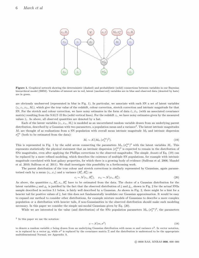
Figure 1. Graphical network showing the deterministic (dashed) and probabilistic (solid) connections between variables in our Bayesian
hierarchical model (BHM). Variables of interest are in red, latent (unobserved) variables are in blue and observed data (denoted by hats)are in green.
are obviously unobserved (represented in blue in Fig. 1). In particular, we associate with each SN a set of latent variables
(zi, ci, x1i,Mi), which give the true value of the redshift, colour correction, stretch correction and intrinsic magnitude for that
SN. For the stretch and colour correction, we have noisy estimates in the form of data ci, x1i (with an associated covariance
matrix) resulting from the SALT-II fits (solid vertical lines). For the redshift zi, we have noisy estimates given by the measured
values zi. As above, all observed quantities are denoted by a hat.
Each of the latent variables (ci, x1i,Mi) is modeled as an uncorrelated random variable drawn from an underlying parent
distribution, described by a Gaussian with two parameters, a population mean and a variance2. The latent intrinsic magnitudes
Mi are thought of as realizations from a SN population with overall mean intrinsic magnitude M0 and intrinsic dispersion
σintµ (both to be estimated from the data):
Mi ∼ N (M0, (σintµ )2). (19)
This is represented in Fig. 1 by the solid arrow connecting the parameters M0, (σintµ )2 with the latent variables Mi. This
represents statistically the physical statement that an intrinsic dispersion (σintµ )2 is expected to remain in the distribution of
SNe magnitudes, even after applying the Phillips corrections to the observed magnitudes. The simple Ansatz of Eq. (19) can
be replaced by a more refined modeling, which describes the existence of multiple SN populations, for example with intrinsic
magnitude correlated with host galaxy properties, for which there is a growing body of evidence (Sullivan et al. 2006; Mandel
et al. 2010; Sullivan et al. 2011). We shall investigate this possibility in a forthcoming work.
The parent distribution of the true colour and stretch corrections is similarly represented by Gaussians, again parame-
terised each by a mean (c?, x?) and a variance (R2c , R
2x) as
ci ∼ N (c?, R2c), x1i ∼ N (x?, R
2x). (20)
As above, the quantities c?, R2c , x?, R
2x have to be estimated from the data. The choice of a Gaussian distribution for the
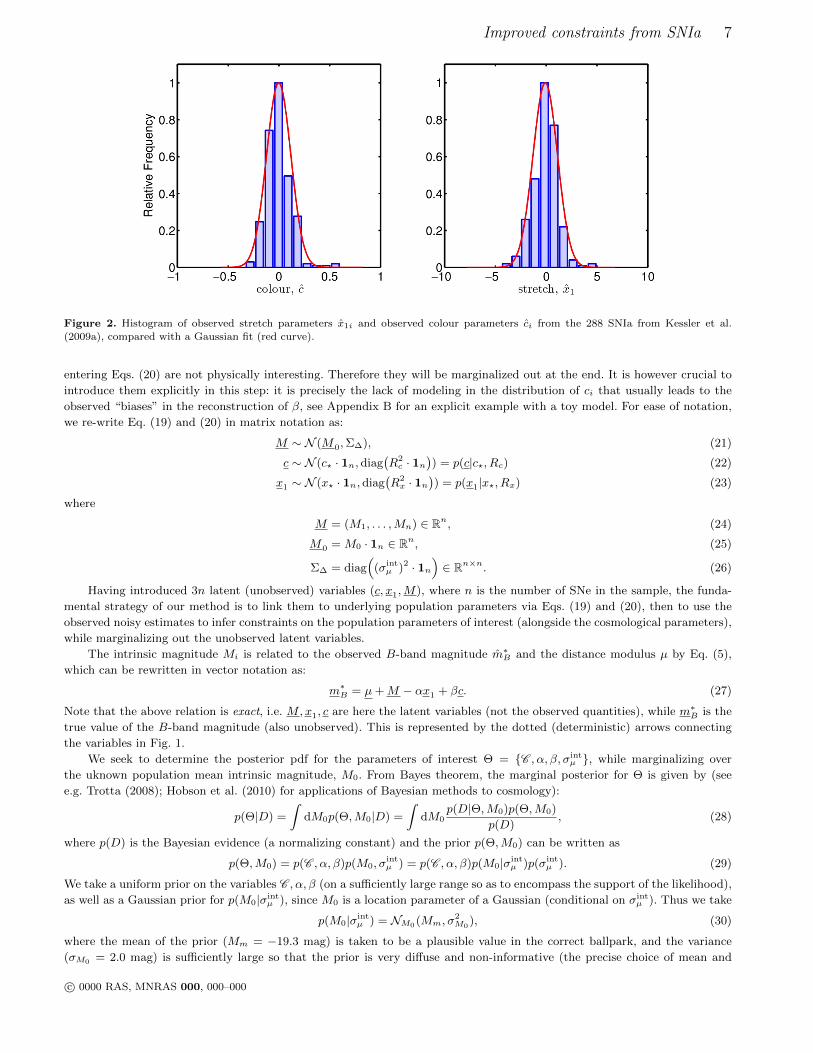
latent variables c and x1 is justified by the fact that the observed distribution of c and x1, shown in Fig. 2 for the actual SNIa
sample described in section 3.1 below, is fairly well described by a Gaussian. As shown in Fig. 2, there might be a hint for a
heavier tail for positive values of c, but this does not fundamentally invalidate our Gaussian approximation. It would be easy
to expand our method to consider other distributions, for example mixture models of Gaussians to describe a more complex
population or a distribution with heavier tails, if non-Gaussianities in the observed distribution should make such modeling
necessary. In this paper we consider the simple uni-modal Gaussians given by Eq. (20).
While we are interested in the value (and distribution) of the SNe population parameters M0, (σintµ )2, the parameters
2 In this paper we use the notation:
x ∼ N (m,σ2) (18)
to denote a random variable x being drawn from an underlying Gaussian distribution with mean m and variance σ2. In vector notation,
m is replaced by a vector m, while σ2 is replaced by the covariance matrix Σ and the distribution is understood to be the appropriate
multidimensional Normal, see Appendix A.
c© 0000 RAS, MNRAS 000, 000–000
Improved constraints from SNIa 7
Figure 2. Histogram of observed stretch parameters x1i and observed colour parameters ci from the 288 SNIa from Kessler et al.
(2009a), compared with a Gaussian fit (red curve).
entering Eqs. (20) are not physically interesting. Therefore they will be marginalized out at the end. It is however crucial to
introduce them explicitly in this step: it is precisely the lack of modeling in the distribution of ci that usually leads to the
observed “biases” in the reconstruction of β, see Appendix B for an explicit example with a toy model. For ease of notation,
we re-write Eq. (19) and (20) in matrix notation as:
M ∼ N (M0,Σ∆), (21)
c ∼ N (c? · 1n, diag(R2c · 1n
)) = p(c|c?, Rc) (22)
x1 ∼ N (x? · 1n, diag(R2x · 1n
)) = p(x1|x?, Rx) (23)
where
M = (M1, . . . ,Mn) ∈ Rn, (24)
M0 = M0 · 1n ∈ Rn, (25)
Σ∆ = diag(
(σintµ )2 · 1n
)∈ Rn×n. (26)
Having introduced 3n latent (unobserved) variables (c, x1,M), where n is the number of SNe in the sample, the funda-
mental strategy of our method is to link them to underlying population parameters via Eqs. (19) and (20), then to use the
observed noisy estimates to infer constraints on the population parameters of interest (alongside the cosmological parameters),
while marginalizing out the unobserved latent variables.
The intrinsic magnitude Mi is related to the observed B-band magnitude m∗B and the distance modulus µ by Eq. (5),
which can be rewritten in vector notation as:
m∗B = µ+M − αx1 + βc. (27)
Note that the above relation is exact, i.e. M,x1, c are here the latent variables (not the observed quantities), while m∗B is the
true value of the B-band magnitude (also unobserved). This is represented by the dotted (deterministic) arrows connecting
the variables in Fig. 1.
We seek to determine the posterior pdf for the parameters of interest Θ = C , α, β, σintµ , while marginalizing over
the uknown population mean intrinsic magnitude, M0. From Bayes theorem, the marginal posterior for Θ is given by (see
e.g. Trotta (2008); Hobson et al. (2010) for applications of Bayesian methods to cosmology):
p(Θ|D) =
∫dM0p(Θ,M0|D) =
∫dM0
p(D|Θ,M0)p(Θ,M0)
p(D), (28)
where p(D) is the Bayesian evidence (a normalizing constant) and the prior p(Θ,M0) can be written as
p(Θ,M0) = p(C , α, β)p(M0, σintµ ) = p(C , α, β)p(M0|σint
µ )p(σintµ ). (29)
We take a uniform prior on the variables C , α, β (on a sufficiently large range so as to encompass the support of the likelihood),
as well as a Gaussian prior for p(M0|σintµ ), since M0 is a location parameter of a Gaussian (conditional on σint
µ ). Thus we take
p(M0|σintµ ) = NM0(Mm, σ
2M0
), (30)
where the mean of the prior (Mm = −19.3 mag) is taken to be a plausible value in the correct ballpark, and the variance
(σM0 = 2.0 mag) is sufficiently large so that the prior is very diffuse and non-informative (the precise choice of mean and
c© 0000 RAS, MNRAS 000, 000–000

8 March et al
variance for this prior does not impact on our numerical results). Finally, the appropriate prior for σintµ is a Jeffreys’ prior,
i.e., uniform in log σintµ , as σint
µ is a scale parameter, see e.g. Box & Tiao (1992). Although the intrinsic magnitude M0 and
the Hubble constant H0 are perfectly degenerate as far as SNIa data are concerned, we do not bundle them together in a
single parameter but treat them separately with distinct priors, as we are interested in separating out the variability due to
the distribution of the SNIa intrinsic magnitude.
We now proceed to manipulate further the likelihood, p(D|Θ,M0) = p(c, x1, m∗B |Θ,M0):
p(c, x1, m∗B |Θ,M0) =
∫dc dx1 dM p(c, x1, m
∗B |c, x1,M,Θ,M0)p(c, x1,M |Θ,M0) (31)
=
∫dc dx1 dM p(c, x1, m
∗B |c, x1,M,Θ)
×∫
dRc dRx dc? dx? p(c|c?, Rc)p(x1|x?, Rx)p(M |M0, σintµ )p(Rc)p(Rx)p(c?)p(x?) (32)
In the first line, we have introduced a set of 3n latent variables, c, x1,M, which describe the true value of the colour,
stretch and intrinsic magnitude for each SNIa. Clearly, as those variables are unobserved, we need to marginalize over them.
In the second line, we have replaced p(c, x1,M |Θ,M0) by the distributions of the latent c, x1,M given by the probabilistic
relationships of Eq. (21) and Eqs. (22–23), obtained by marginalizing out the population parameters Rc, Rx, c?, x?:
p(c, x1,M |Θ,M0) =
∫dRc dRx dc? dx? p(c|c?, Rc)p(x1|x?, Rx)p(M |M0, σ
intµ )p(Rc)p(Rx)p(c?)p(x?). (33)
(we have also dropped M0 from the likelihood, as conditioning on M0 is irrelevant if the latent M are given). If we further
marginalize over M0 (as in Eq. (28), including the prior on M0), the expression for the effective likelihood, Eq. (32), then
becomes:
p(c, x1, m∗B |Θ) =
∫dc dx1 dM p(c, x1, m
∗B |c, x1,M,Θ)
×∫
dRc dRx dc? dx? dM0 p(c|c?, Rc)p(x1|x?, Rx)p(M |M0, σintµ )p(Rc)p(Rx)p(c?)p(x?)p(M0|σint
µ ) (34)
The term p(c, x1, m∗B |c, x1,M,Θ) is the conditional probability of observing values c, x1, m
∗B if the latent (true) value
of c, x1,M and of the other cosmological parameters were known. From Fig. 1, m∗B is connected only deterministically to all
other variables and parameters, via Eq. (27). Thus we can replace m∗B = µ+M − α · x1 + β · c and write
p(c, x1, m∗B |c, x1,M,Θ) =
n∏i=1
N (µi +Mi − α · x1i + β · ci, Ci) (35)
= |2πΣC |−12 exp
(−1
2[(X −X0)TΣ−1
C (X −X0)]
)(36)
where µi ≡ µi(zi,Θ) and we have defined
X = X1, . . . , Xn ∈ R3n, X0 = X0,1, . . . , X0,n ∈ R3n, (37)
Xi = ci, x1,i, (Mi − αx1,i + βci) ∈ R3, X0,i = ci, x1,i, m∗Bi − µi ∈ R3, (38)
as well as the 3n× 3n block covariance matrix3
ΣC =
C1 0 0 0
0 C2 0 0
0 0. . . 0
0 0 0 Cn
. (39)
Finally we explicitly include redshift uncertainties in our formalism. The observed apparent magnitude, m∗B , on the
left-hand-side of Eq. (35), is the value at the observed redshift, z. However, µ in Eq. (35) should be evaluated at the true
(unknown) redshift, z. As above, the redshift uncertainty is included by introducing the latent variables z and integrating
over them:
p(c, x1,M |c, x1,M,Θ) =
∫dz p(c, x1,M |c, x1,M, z,Θ)p(z|z) (40)
where we model the redshift errors p(z|z) as Gaussians:
z ∼ N (z,Σz) (41)
3 Notice that we neglect correlations between different SNIa, which is reflected in the fact that ΣC takes a block-diagonal form. It would
be however very easy to add arbitrary cross-correlations to our formalism (e.g., coming from correlated systematic within survey, forexample zero point calibration) by adding such non-block diagonal correlations to Eq. (39).
c© 0000 RAS, MNRAS 000, 000–000
Improved constraints from SNIa 9
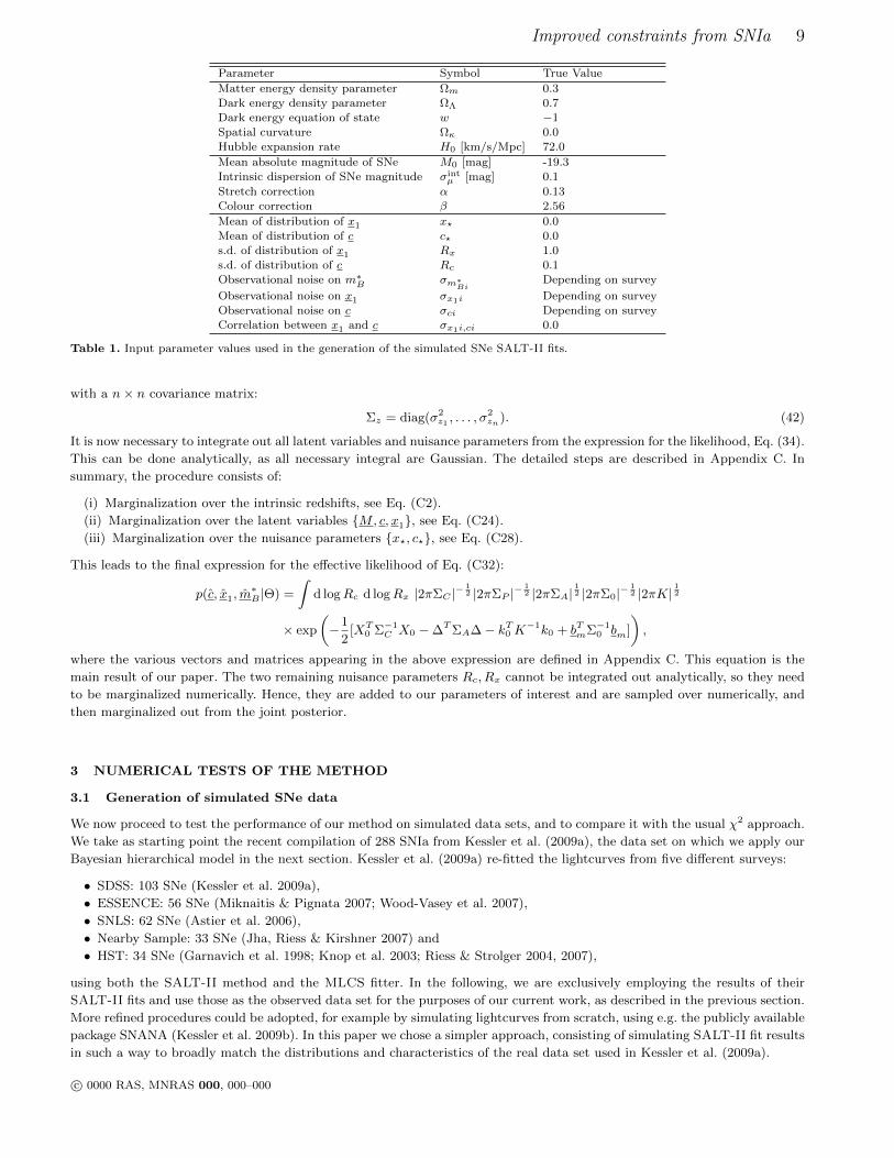
Parameter Symbol True Value
Matter energy density parameter Ωm 0.3Dark energy density parameter ΩΛ 0.7
Dark energy equation of state w −1
Spatial curvature Ωκ 0.0Hubble expansion rate H0 [km/s/Mpc] 72.0
Mean absolute magnitude of SNe M0 [mag] -19.3
Intrinsic dispersion of SNe magnitude σintµ [mag] 0.1
Stretch correction α 0.13
Colour correction β 2.56
Mean of distribution of x1 x? 0.0Mean of distribution of c c? 0.0
s.d. of distribution of x1 Rx 1.0
s.d. of distribution of c Rc 0.1Observational noise on m∗B σm∗
BiDepending on survey
Observational noise on x1 σx1i Depending on surveyObservational noise on c σci Depending on survey
Correlation between x1 and c σx1i,ci 0.0
Table 1. Input parameter values used in the generation of the simulated SNe SALT-II fits.
with a n× n covariance matrix:
Σz = diag(σ2z1 , . . . , σ
2zn). (42)
It is now necessary to integrate out all latent variables and nuisance parameters from the expression for the likelihood, Eq. (34).
This can be done analytically, as all necessary integral are Gaussian. The detailed steps are described in Appendix C. In
summary, the procedure consists of:
(i) Marginalization over the intrinsic redshifts, see Eq. (C2).
(ii) Marginalization over the latent variables M, c, x1, see Eq. (C24).
(iii) Marginalization over the nuisance parameters x?, c?, see Eq. (C28).
This leads to the final expression for the effective likelihood of Eq. (C32):
p(c, x1, m∗B |Θ) =
∫d logRc d logRx |2πΣC |−
12 |2πΣP |−
12 |2πΣA|
12 |2πΣ0|−
12 |2πK|
12
× exp
(−1
2[XT
0 Σ−1C X0 −∆TΣA∆− kT0 K−1k0 + bTmΣ−1
0 bm]
),
where the various vectors and matrices appearing in the above expression are defined in Appendix C. This equation is the
main result of our paper. The two remaining nuisance parameters Rc, Rx cannot be integrated out analytically, so they need
to be marginalized numerically. Hence, they are added to our parameters of interest and are sampled over numerically, and
then marginalized out from the joint posterior.
3 NUMERICAL TESTS OF THE METHOD
3.1 Generation of simulated SNe data
We now proceed to test the performance of our method on simulated data sets, and to compare it with the usual χ2 approach.
We take as starting point the recent compilation of 288 SNIa from Kessler et al. (2009a), the data set on which we apply our
Bayesian hierarchical model in the next section. Kessler et al. (2009a) re-fitted the lightcurves from five different surveys:
• SDSS: 103 SNe (Kessler et al. 2009a),
• ESSENCE: 56 SNe (Miknaitis & Pignata 2007; Wood-Vasey et al. 2007),
• SNLS: 62 SNe (Astier et al. 2006),
• Nearby Sample: 33 SNe (Jha, Riess & Kirshner 2007) and
• HST: 34 SNe (Garnavich et al. 1998; Knop et al. 2003; Riess & Strolger 2004, 2007),
using both the SALT-II method and the MLCS fitter. In the following, we are exclusively employing the results of their
SALT-II fits and use those as the observed data set for the purposes of our current work, as described in the previous section.
More refined procedures could be adopted, for example by simulating lightcurves from scratch, using e.g. the publicly available
package SNANA (Kessler et al. 2009b). In this paper we chose a simpler approach, consisting of simulating SALT-II fit results
in such a way to broadly match the distributions and characteristics of the real data set used in Kessler et al. (2009a).
c© 0000 RAS, MNRAS 000, 000–000
10 March et al
0.5 1 1.515
20
25
z
mB
0.5 1 1.5−5
0
5
10
z
x1(stretch)
0.5 1 1.5−0.5
0
0.5
z
c(colour)
0.1 0.20
1
2
3
σc
σ x1
0 1 2 30
0.1
0.2
σx1
σ mB
0 0.1 0.20
0.1
0.2
σc
σ mB
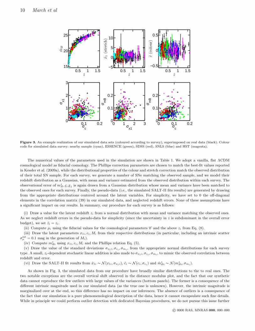
Figure 3. An example realization of our simulated data sets (coloured according to survey), superimposed on real data (black). Colour
code for simulated data survey: nearby sample (cyan), ESSENCE (green), SDSS (red), SNLS (blue) and HST (magenta).
The numerical values of the parameters used in the simulation are shown in Table 1. We adopt a vanilla, flat ΛCDM
cosmological model as fiducial cosmology. The Phillips correction parameters are chosen to match the best-fit values reported
in Kessler et al. (2009a), while the distributional properties of the colour and stretch correction match the observed distribution
of their total SN sample. For each survey, we generate a number of SNe matching the observed sample, and we model their
redshift distribution as a Gaussian, with mean and variance estimated from the observed distribution within each survey. The
observational error of m∗B , c, x1 is again drawn from a Gaussian distribution whose mean and variance have been matched to
the observed ones for each survey. Finally, the pseudo-data (i.e., the simulated SALT-II fits results) are generated by drawing
from the appropriate distributions centered around the latent variables. For simplicity, we have set to 0 the off-diagonal
elements in the correlation matrix (39) in our simulated data, and neglected redshift errors. None of these assumptions have
a significant impact on our results. In summary, our procedure for each survey is as follows:
(i) Draw a value for the latent redshift zi from a normal distribution with mean and variance matching the observed ones.
As we neglect redshift errors in the pseudo-data for simplicity (since the uncertainty in z is subdominant in the overall error
budget), we set zi = zi.
(ii) Compute µi using the fiducial values for the cosmological parameters C and the above zi from Eq. (8).
(iii) Draw the latent parameters x1i, ci,Mi from their respective distributions (in particular, including an intrinsic scatter
σintµ = 0.1 mag in the generation of Mi).
(iv) Compute m∗Bi using x1i, ci,Mi and the Phillips relation Eq. (5).
(v) Draw the value of the standard deviations σx1i, σci , σmi , from the appropriate normal distributions for each survey
type. A small, zi-dependent stochastic linear addition is also made to σx1i, σci , σmi , to mimic the observed correlation between
redshift and error.
(vi) Draw the SALT-II fit results from x1i ∼ N (x1i, σx1i), ci ∼ N (ci, σci) and m∗Bi ∼ N (m∗Bi, σmi).
As shown in Fig. 3, the simulated data from our procedure have broadly similar distributions to the to real ones. The
two notable exceptions are the overall vertical shift observed in the distance modulus plot, and the fact that our synthetic
data cannot reproduce the few outliers with large values of the variances (bottom panels). The former is a consequence of the
different intrinsic magnitude used in our simulated data (as the true one is unknown). However, the intrinsic magnitude is
marginalized over at the end, so this difference has no impact on our inferences. The absence of outliers is a consequence of
the fact that our simulation is a pure phenomenological description of the data, hence it cannot encapsulate such fine details.
While in principle we could perform outlier detection with dedicated Bayesian procedures, we do not pursue this issue further
c© 0000 RAS, MNRAS 000, 000–000

Improved constraints from SNIa 11
Parameter ΛCDM wCDM
Ωm Uniform: U(0.0, 1.0) Uniform: U(0.0, 1.0)Ωκ Uniform: U(−1.0, 1.0) Fixed: 0
w Fixed: −1 Uniform: U(−4, 0)
H0 [km/s/Mpc] N (72, 82) N (72, 82)
Common priors
σintµ [mag] Uniform on log σint
µ : U(−3.0, 0.0)
M0 [mag] Uniform: U(−20.3,−18.3)α Uniform: U(0.0, 1.0)
β Uniform: U(0.0, 4.0)
Rc Uniform on logRc: U(−5.0, 2.0)Rx Uniform on logRc: U(−5.0, 2.0)
Table 2. Priors on our model’s parameters used when evaluating the posterior distribution. Ranges for the uniform priors have been
chosen so as to generously bracket plausible values of the corresponding quantities.
in this paper. We stress once more that the purpose of our simulations is not to obtain realistic SNIa data. Instead, they
should only provide us with useful mock data sets coming from a known model so that we can test our procedure. More
sophisticated tests based on more realistically generated data (e.g., from SNANA) are left for future work.
3.2 Numerical sampling
After analytical marginalization of the latent variables, we are left with the following 8 parameters entering the effective
likelihood of Eq. (43):
Ωm,Ωκ or w,H0, σintµ , α, β,Rc, Rx . (43)
As mentioned above, in keeping with the literature we only consider either flat Universes with a possible w 6= −1 (the ΛCDM
model), or curved Universes with a cosmological constant (w = −1, the wCDM model). Of course it is possible to relax those
assumptions and consider more complicated cosmologies with a larger number of free parameters if one so wishes (notably
including evolution in the dark energy equation of state).
Of the parameters listed in Eq. (43), the quantities Rc, Rx are of no interest and will be marginalized over. As for the
remaining parameters, we are interested in building their marginal 1 and 2-dimensional posterior distributions. This is done by
plugging the likelihood (43) into the posterior of Eq. (28), with priors on the parameters chosen according to Table 2. We use a
Gaussian prior on the Hubble parameter H0 = 72±8 km/s/Mpc from local determinations of the Hubble constant (Freedman
et al. 2001). However, as H0 is degenerate with the intrinsic population absolute magnitude M0 (which is marginalized over
at the end), replacing this Gaussian prior with a less informative prior H0[km/s/Mpc] ∼ U(20, 100) has no influence on our
results.
Numerical sampling of the posterior is carried out via a nested sampling algorithm (Skilling 2004, 2006; Feroz & Hobson
2008; Feroz et al. 2009). Although the original motivation for nested sampling was to compute the Bayesian evidence, the
recent development of the MultiNest algorithm (Feroz & Hobson 2008; Feroz et al. 2009) has delivered an extremely powerful
and versatile algorithm that has been demonstrated to be able to deal with extremely complex likelihood surfaces in hun-
dreds of dimensions exhibiting multiple peaks. As samples from the posterior are generated as a by-product of the evidence
computation, nested sampling can also be used to obtain parameter constraints in the same run as computing the Bayesian
evidence. In this paper we adopt the publicly available MultiNest algorithm (Feroz & Hobson 2008) to obtain samples from
the posterior distribution of Eq. (28). We use 4000 live points and a tolerance parameter 0.1, resulting in about 8 × 10⁵
likelihood evaluations.4
We also wish to compare the performance of our BHM with the usually adopted χ2 minimization procedure. To this end,
we fit the pseudo-data using the χ2 expression of Eq. (13). In order to mimic what is done in the literature as closely as possible,
we first fix a value of σintµ . Then, we simultaneously minimize the χ2 w.r.t. the fit parameters ϑ = Ωm,Ωκ or w,H0,M0, α, β,
as described below. We then evaluate the χ2/dof from the resulting best fit point, and we adjust σintµ to obtain χ2/dof = 1.
We then repeat the above minimization over ϑ for this new value of σintµ , and iterate the procedure. Once we have obtained
the global best fit point, we derive 1- and 2-dimensional confidence intervals on the parameters by profiling (i.e., maximising
over the other parameters) over the likelihood
L(ϑ) = exp
(−1
2χ(ϑ)2
), (44)
with χ2 given by Eq. (13). According to Wilks’ theorem, approximate confidence intervals are obtained from the profile
4 A Fortran code implementing our method is available from the authors upon request.
c© 0000 RAS, MNRAS 000, 000–000
12 March et al
0 0.2 0.4 0.60
0.5
1
ΩM
ΩΛ
Flat Universe
0 0.2 0.4 0.6
−2
−1
0
w
ΛCDM
ΩM
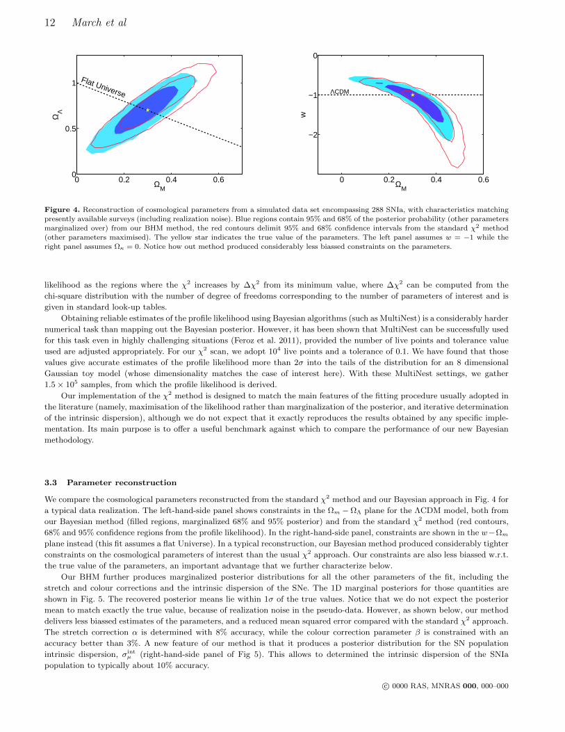
Figure 4. Reconstruction of cosmological parameters from a simulated data set encompassing 288 SNIa, with characteristics matchingpresently available surveys (including realization noise). Blue regions contain 95% and 68% of the posterior probability (other parameters
marginalized over) from our BHM method, the red contours delimit 95% and 68% confidence intervals from the standard χ2 method
(other parameters maximised). The yellow star indicates the true value of the parameters. The left panel assumes w = −1 while theright panel assumes Ωκ = 0. Notice how out method produced considerably less biassed constraints on the parameters.
likelihood as the regions where the χ2 increases by ∆χ2 from its minimum value, where ∆χ2 can be computed from the
chi-square distribution with the number of degree of freedoms corresponding to the number of parameters of interest and is
given in standard look-up tables.
Obtaining reliable estimates of the profile likelihood using Bayesian algorithms (such as MultiNest) is a considerably harder
numerical task than mapping out the Bayesian posterior. However, it has been shown that MultiNest can be successfully used
for this task even in highly challenging situations (Feroz et al. 2011), provided the number of live points and tolerance value
used are adjusted appropriately. For our χ2 scan, we adopt 104 live points and a tolerance of 0.1. We have found that those
values give accurate estimates of the profile likelihood more than 2σ into the tails of the distribution for an 8 dimensional
Gaussian toy model (whose dimensionality matches the case of interest here). With these MultiNest settings, we gather
1.5× 10⁵ samples, from which the profile likelihood is derived.
Our implementation of the χ2 method is designed to match the main features of the fitting procedure usually adopted in
the literature (namely, maximisation of the likelihood rather than marginalization of the posterior, and iterative determination
of the intrinsic dispersion), although we do not expect that it exactly reproduces the results obtained by any specific imple-
mentation. Its main purpose is to offer a useful benchmark against which to compare the performance of our new Bayesian
methodology.
3.3 Parameter reconstruction
We compare the cosmological parameters reconstructed from the standard χ2 method and our Bayesian approach in Fig. 4 for
a typical data realization. The left-hand-side panel shows constraints in the Ωm −ΩΛ plane for the ΛCDM model, both from
our Bayesian method (filled regions, marginalized 68% and 95% posterior) and from the standard χ2 method (red contours,
68% and 95% confidence regions from the profile likelihood). In the right-hand-side panel, constraints are shown in the w−Ωmplane instead (this fit assumes a flat Universe). In a typical reconstruction, our Bayesian method produced considerably tighter
constraints on the cosmological parameters of interest than the usual χ2 approach. Our constraints are also less biassed w.r.t.
the true value of the parameters, an important advantage that we further characterize below.
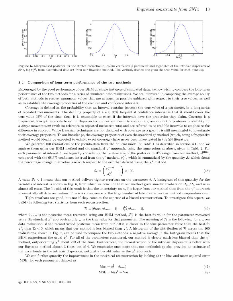
Our BHM further produces marginalized posterior distributions for all the other parameters of the fit, including the
stretch and colour corrections and the intrinsic dispersion of the SNe. The 1D marginal posteriors for those quantities are
shown in Fig. 5. The recovered posterior means lie within 1σ of the true values. Notice that we do not expect the posterior
mean to match exactly the true value, because of realization noise in the pseudo-data. However, as shown below, our method
delivers less biassed estimates of the parameters, and a reduced mean squared error compared with the standard χ2 approach.
The stretch correction α is determined with 8% accuracy, while the colour correction parameter β is constrained with an
accuracy better than 3%. A new feature of our method is that it produces a posterior distribution for the SN population
intrinsic dispersion, σintµ (right-hand-side panel of Fig 5). This allows to determined the intrinsic dispersion of the SNIa
population to typically about 10% accuracy.
c© 0000 RAS, MNRAS 000, 000–000
Improved constraints from SNIa 13
0.06 0.08 0.1 0.12 0.14 0.16 0.180
0.2
0.4
0.6
0.8
1
α
post
erio
r de
nsity
2.2 2.4 2.6 2.8 30
0.2
0.4
0.6
0.8
1
β
post
erio
r de
nsity
−2.6 −2.4 −2.2 −20
0.2
0.4
0.6
0.8
1
Ln σµint
post
erio
r de
nsity
Figure 5. Marginalised posterior for the stretch correction α, colour correction β parameter and logarithm of the intrinsic dispersion of
SNe, log σintµ , from a simulated data set from our Bayesian method. The vertical, dashed line gives the true value for each quantity.
3.4 Comparison of long-term performance of the two methods
Encouraged by the good performance of our BHM on single instances of simulated data, we now wish to compare the long-term
performance of the two methods for a series of simulated data realizations. We are interested in comparing the average ability
of both methods to recover parameter values that are as much as possible unbiased with respect to their true values, as well
as to establish the coverage properties of the credible and confidence intervals.
Coverage is defined as the probability that an interval contains (covers) the true value of a parameter, in a long series
of repeated measurements. The defining property of a e.g. 95% frequentist confidence interval is that it should cover the
true value 95% of the time; thus, it is reasonable to check if the intervals have the properties they claim. Coverage is a
frequentist concept: intervals based on Bayesian techniques are meant to contain a given amount of posterior probability for
a single measurement (with no reference to repeated measurements) and are referred to as credible intervals to emphasize the
difference in concept. While Bayesian techniques are not designed with coverage as a goal, it is still meaningful to investigate
their coverage properties. To our knowledge, the coverage properties of even the standard χ2 method (which, being a frequentist
method would ideally be expected to exhibit exact coverage) have never been investigated in the SN literature.
We generate 100 realizations of the pseudo-data from the fiducial model of Table 1 as described in section 3.1, and we
analyze them using our BHM method and the standard χ2 approach, using the same priors as above, given in Table 2. For
each parameter of interest θ, we begin by considering the relative size of the posterior 68.3% range from out method, σBHMθ ,
compared with the 68.3% confidence interval from the χ2 method, σχ2
θ , which is summarized by the quantity Sθ which shows
the percentage change in errorbar size with respect to the errorbar derived using the χ2 method
Sθ ≡
(σBHMθ
σχ2
θ
− 1
)× 100. (45)
A value Sθ < 1 means that our method delivers tighter errorbars on the parameter θ. A histogram of this quantity for the
variables of interest is shown in Fig. 6, from which we conclude that our method gives smaller errobars on Ωm,ΩΛ and w in
almost all cases. The flip side of this result is that the uncertainty on α, β is larger from our method than from the χ2 approach
in essentially all data realization. This is a consequence of the large number of latent variables our method marginalizes over.
Tight errorbars are good, but not if they come at the expense of a biased reconstruction. To investigate this aspect, we
build the following test statistics from each reconstruction:
Tθ ≡ |θBHM/θtrue − 1| − |θbfχ2/θtrue − 1|, (46)
where θBHM is the posterior mean recovered using our BHM method, θbfχ2 is the best-fit value for the parameter recovered
using the standard χ2 approach and θtrue is the true value for that parameter. The meaning of Tθ is the following: for a given
data realization, if the reconstructed posterior mean from our BHM is closer to the true parameter value than the best-fit
χ2, then Tθ < 0, which means that our method is less biassed than χ2. A histogram of the distribution of Tθ across the 100
realizations, shown in Fig. 7, can be used to compare the two methods: a negative average in the histogram means that the
BHM outperforms the usual χ2. For all of the parameters considered, our method is clearly much less biassed than the χ2
method, outperforming χ2 about 2/3 of the time. Furthermore, the reconstruction of the intrinsic dispersion is better with
our Bayesian method almost 3 times out of 4. We emphasize once more that our methodology also provides an estimate of
the uncertainty in the intrinsic dispersion, not just a best-fit value as the χ2 approach.
We can further quantify the improvement in the statistical reconstruction by looking at the bias and mean squared error
(MSE) for each parameter, defined as
bias = 〈θ − θtrue〉 (47)
MSE = bias2 + Var, (48)
c© 0000 RAS, MNRAS 000, 000–000
14 March et al
Parameter Bias Mean squared error
Bayesian χ2 Improvement Bayesian χ2 Improvement
ΛCDM Ωm -0.0188 -0.0183 1.0 0.0082 0.0147 1.8
ΩΛ -0.0328 -0.0223 0.7 0.0307 0.0458 1.5
α 0.0012 0.0032 2.6 0.0001 0.0002 1.4β 0.0202 0.0482 2.4 0.0118 0.0163 1.4
σintµ -0.0515 -0.1636 3.1 0.0261 0.0678 2.6
wCDM Ωm -0.0177 -0.0494 2.8 0.0072 0.0207 2.9ΩΛ 0.0177 0.0494 2.8 0.0072 0.0207 2.9
w -0.0852 -0.0111 0.1 0.0884 0.1420 1.6
α 0.0013 0.0032 2.5 0.0001 0.0002 1.5β 0.0198 0.0464 2.3 0.0118 0.0161 1.4
σintµ -0.0514 -0.1632 3.2 0.0262 0.0676 2.6
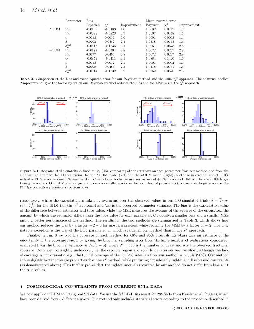
Table 3. Comparison of the bias and mean squared error for our Bayesian method and the usual χ2 approach. The columns labelled
“Improvement” give the factor by which our Bayesian method reduces the bias and the MSE w.r.t. the χ2 approach.
−100% −50% 0% 50% 100%0
10
20
30
40
Change in errorbar size for ΩM
97% of trials errorbar is reduced
Fre
quen
cy
σBHM< σχ2
σBHM> σχ2
Λ CDM
−100% −50% 0% 50% 100%0
10
20
30
40
50
Change in errorbar size for ΩΛ
98% of trials errorbar is reduced
−100% −50% 0% 50% 100%0
20
40
60
Change in errorbar size for α
1% of trials errorbar is reduced
Fre
quen
cy
−100% −50% 0% 50% 100%0
20
40
60
Change in errorbar size for β
0% of trials errorbar is reduced
−100% −50% 0% 50% 100%0
5
10
15
20
Change in errorbar size for ΩM
79% of trials errorbar is reduced
Fre
quen
cy
σBHM< σχ2
σBHM> σχ2
wCDM
−100% −50% 0% 50% 100%0
5
10
15
20
25
Change in errorbar size for w
68% of trials errorbar is reduced
−100% −50% 0% 50% 100%0
20
40
60
Change in errorbar size for α
1% of trials errorbar is reduced
Fre
quen
cy
−100% −50% 0% 50% 100%0
20
40
60
Change in errorbar size for β
1% of trials errorbar is reduced
Figure 6. Histograms of the quantity defined in Eq. (45), comparing of the errorbars on each parameter from our method and from thestandard χ2 approach for 100 realization, for the ΛCDM model (left) and the wCDM model (right). A change in errorbar size of −10%
indicates BHM errorbars are 10% smaller than χ2 errorbars. A change in errorbar size of +10% indicates BHM errorbars are 10% larger
than χ2 errorbars. Our BHM method generally delivers smaller errors on the cosmological parameters (top row) but larger errors on thePhillips correction parameters (bottom row).
respectively, where the expectation is taken by averaging over the observed values in our 100 simulated trials, θ = θBHM
(θ = θbfχ2) for the BHM (for the χ2 approach) and Var is the observed parameter variance. The bias is the expectation value
of the difference between estimator and true value, while the MSE measures the average of the squares of the errors, i.e., the
amount by which the estimator differs from the true value for each parameter. Obviously, a smaller bias and a smaller MSE
imply a better performance of the method. The results for the two methods are summarized in Table 3, which shows how
our method reduces the bias by a factor ∼ 2− 3 for most parameters, while reducing the MSE by a factor of ∼ 2. The only
notable exception is the bias of the EOS parameter w, which is larger in our method than in the χ2 approach.
Finally, in Fig. 8 we plot the coverage of each method for 68% and 95% intervals. Errobars give an estimate of the
uncertainty of the coverage result, by giving the binomial sampling error from the finite number of realizations considered,
evaluated from the binomial variance as Np(1 − p), where N = 100 is the number of trials and p is the observed fractional
coverage. Both method slightly undercover, i.e. the credible region and confidence intervals are too short, although the lack
of coverage is not dramatic: e.g., the typical coverage of the 1σ (2σ) intervals from our method is ∼ 60% (90%). Our method
shows slightly better coverage properties than the χ2 method, while producing considerably tighter and less biassed constraints
(as demonstrated above). This further proves that the tighter intervals recovered by our method do not suffer from bias w.r.t
the true values.
4 COSMOLOGICAL CONSTRAINTS FROM CURRENT SNIA DATA
We now apply our BHM to fitting real SN data. We use the SALT-II fits result for 288 SNIa from Kessler et al. (2009a), which
have been derived from 5 different surveys. Our method only includes statistical errors according to the procedure described in
c© 0000 RAS, MNRAS 000, 000–000

Improved constraints from SNIa 15
−0.5 0 0.50
5
10
15
20
25
63% < 0
Test statistics for ΩM
Fre
quen
cy
−0.5 0 0.50
10
20
30
64% < 0
Test statistics for ΩΛ
Λ CDM
−0.1 0 0.10
5
10
15
20
60% < 0
Test statistics for α
Fre
quen
cy
−0.05 0 0.050
5
10
15
20
25
57% < 0
Test statistics for β−0.1 0 0.1
0
5
10
15
20
2575% < 0
Test statistics for Ln σµint
−0.5 0 0.50
5
10
15
20
25
73% < 0
Test statistics for ΩM
Fre
quen
cy
−0.5 0 0.50
10
20
30
40
73% < 0
Test statistics for ΩΛ
wCDM
−0.5 0 0.50
5
10
15
20
25
63% < 0
Test statistics for w
−0.1 0 0.10
10
20
30
63% < 0
Test statistics for α
Fre
quen
cy
−0.05 0 0.050
5
10
15
20
25
59% < 0
Test statistics for β−0.2 0 0.2
0
10
20
30
75% < 0
Test statistics for Ln σµint
Figure 7. Histograms of the test statistics defined in Eq. (46), comparing the long-term performance of the two methods for theparameters of interest in the ΛCDM model (left) and the wCDM model (right). A predominantly negative value of the test statistics
means that our method gives a parameter reconstruction that is closer to the true value than the usual χ2, i.e., less biassed. For the
cosmological parameters (top row), our method outperforms χ2 about 2 times out of 3.
0
10
20
30
40
50
60
70
80
90
100
ΩM
ΩΛ
Ωκ
α β σµint
% o
f sam
ples
with
in s
peci
fied
No
of σ
of t
rue
val.
1 σ
2 σ
0
10
20
30
40
50
60
70
80
90
100
ΩM
ΩΛ
w α β σµint
% o
f sam
ples
with
in s
peci
fied
No
of σ
of t
rue
val.
1 σ
2 σ
Figure 8. Coverage of our method (blue) and standard χ2 (red) for 68% (solid) and 95% (dashed) intervals, from 100 realizationsof pseudo-data for the ΛCDM model (left) and the wCDM model (right). While both methods show significant undercoverage for all
parameters, our method has a comparable coverage to the standard χ2, except for w. Coverage values for the intrinsic dispersion σintµ
are not available from the χ2 method, as it does not produce an error estimate for this quantity.
section 2.3, coming from redshift uncertainties (arising from spectroscopic errors and peculiar velocities), intrinsic dispersion
(which is determined from the data) and full error propagation of the SALT-II fit results. Systematic uncertainties play an
important role in SNIa cosmology fitting, and (although not included in this study) can also be treated in our formalism in a
fully consistent way. We comment on this aspect further below, though we leave a complete exploration of systematics with
our BHM to a future, dedicated work (March et al. 2011).
We show in Fig. 9 the constraints on the cosmological parameters Ωm − ΩΛ (left panel, assuming w = −1) and w − Ωm(right panel, assuming Ωκ = 0) obtained with our method. All other parameters have been marginalized over. In order to
be consistent with the literature, we have taken a non-informative prior on H0, uniform in the range [20, 100] km/s/Mpc.
The figure also compares our results with the statistical contours from Kessler et al. (2009a), obtained using the χ2 method.
(Notice that we compare with the contours including only statistical uncertainties for consistency.) In Fig. 10 we combine
our SNIa constraints with Cosmic Microwave Background (CMB) data from WMAP 5-yrs measurements (Komatsu et al.
2009) and Baryonic Acoustic Oscillations (BAO) constraints from the Sloan Digital Sky Survey LRG sample (Eisenstein et al.
2005), using the same method as Kessler et al. (2009a). The combined SNIa, CMB and BAO statistical constraints result in
Ωm = 0.28± 0.02,ΩΛ = 0.73± 0.01 (for the ΛCDM model) and Ωm = 0.28± 0.01, w = −0.90± 0.05 (68.3% credible intervals)
for the wCDM model. Although the statistical uncertainties are comparable to the results by Kessler et al. (2009a) from the
same sample, our posterior mean values present shifts of up to ∼ 2σ compared to the results obtained using the standard
c© 0000 RAS, MNRAS 000, 000–000

16 March et al
ΩM
ΩΛ
Flat Universe
No Big
Ban
g
0 0.2 0.4 0.6 0.8 10
0.5
1
1.5
0 0.2 0.4 0.6 0.8 1−2
−1.5
−1
−0.5
0
ΩM
w
ΛCDM Universe
Figure 9. Constraints on the cosmological parameters Ωm,ΩΛ (left panel, assuming w = −1) and w,Ωm (right panel, assuming Ωκ = 0)from our Bayesian method (light/dark blue regions, 68% and 95% marginalized posterior), compared with the statistical errors from the
usual χ2 approach (yellow/red regions, same significance level; from Kessler at al. (2009a)). The yellow star gives the posterior mean
from our analysis.
χ2 approach. This is a fairly significant shift, which can be attributed to our improved statistical method, which exhibits a
reduced bias w.r.t. the χ2 approach.
Fig. 11 shows the 1d marginalized posterior distributions for the Phillips correction parameters and for the intrinsic
dispersion. All parameters are well constrained by the posterior, and we find α = 0.12± 0.02, β = 2.7± 0.1 and a value of the
intrinsic dispersion (for the whole sample) σintµ = 0.13± 0.01 mag.
Kessler et al. (2009a) find values for the intrinsic dispersion ranging from 0.08 (for SDSS-II) to 0.23 (for the HST sample),
but their χ2 method does not allow them to derive an error on those determinations. With our method, it would be easy to
derive constraints on the intrinsic dispersion of each survey – all one needs to do is to replace Eq. (19) with a corresponding
expression for each survey. This introduces one pair of population parameters (M0, σintµ ) for each survey. In the same way, one
could study whether the intrinsic dispersion evolves with redshift. We leave a detailed study of these issues to a future work.
The value of α found in Kessler et al. (2009a) is in the range 0.10 − 0.12, depending of the details of the assumptions
made, with a typical statistical uncertainty of order ∼ 0.015. These results are comparable with our own. As for the colour
correction parameter β, constraints from Kessler et al. (2009a) vary in the range 2.46 − 2.66, with a statistical uncertainty
of order 0.1 − 0.2. This stronger dependence on the details of the analysis seems to point to a larger impact of systematic
uncertainties for β, which is confirmed by evidence of evolution with redshift of the value of β (Kessler et al. (2009a), Fig. 39).
Our method can be employed to carry out a rigorous assessment of the evolution with redshift of colour corrections. A possible
strategy would be to replace β with a vector of parameters β1, β2, . . . , with each element describing the colour correction in
a different redshift bin. The analysis proceeds then as above, and it produces posterior distributions for the components of
β, which allows to check the hypothesis of evolution. Finally, in such an analysis the marginalized constraints on all other
parameters (including the cosmological parameters of interest) would automatically include the full uncertainty propagation
from the colour correction evolution, without the need for further ad hoc inflation of the errorbars. These kind of tests will
be pursued in a forthcoming publication (March et al. 2011).
5 CONCLUSIONS
We have presented a statistically principled approach for the rigorous analysis of SALT-II SNIa lightcurve fits, based on a
Bayesian hierarchical model. The main novelty of our method is that it produces an effective likelihood that propagates uncer-
tainties in a fully consistent way. We have introduced an explicit statistical modeling of the intrinsic magnitude distribution of
the SNIa population, which for the first time allows one to derive a full posterior distribution of the SNIa intrinsic dispersion.
We have tested our method using simulated data sets and found that it compares favourably with the standard χ2
approach, both on individual data realizations and in the long term performance. Statistical constraints on cosmological
parameters are significantly improved, while in a series of 100 simulated data sets our method outperforms the χ2 approach
at least 2 times out of 3 for the parameters of interest. We have also demonstrated that our method is less biassed and has
better coverage properties than the usual approach.
We applied our methodology to a sample of 288 SNIa from multiple surveys. We find that the flat ΛCDM model is
still in good agreement with the data, even under our improved analysis. However, the posterior mean for the cosmological
c© 0000 RAS, MNRAS 000, 000–000

Improved constraints from SNIa 17
ΩM
ΩΛ
Flat Universe
No Big
Ban
g
0 0.2 0.4 0.6 0.8 10
0.5
1
1.5
ΩM
w
Λ CDM Universe
0 0.2 0.4 0.6 0.8 1−2
−1.5
−1
−0.5
0
Figure 10. Combined constraints on the cosmological parameters Ωm,ΩΛ (left panel, assuming w = −1) and w,Ωm (right panel,assuming Ωκ = 0) from SNIa, CMB and BAO data. Red contours give 68% and 95% regions from CMB alone, green contours from BAO
alone, blue contours from SNIa alone from our Bayesian method. The filled regions delimit 68% and 95% combined constraints, with the
yellow star indicating the posterior mean.
0.08 0.1 0.12 0.14 0.160
0.2
0.4
0.6
0.8
1
α
Pos
terio
r de
nsity
2.4 2.6 2.8 3 3.20
0.2
0.4
0.6
0.8
1
β
Pos
terio
r de
nsity
−1 −0.95 −0.9 −0.85 −0.80
0.2
0.4
0.6
0.8
1
Log10
σintµ
Pos
terio
r de
nsity
Figure 11. Marginalised posterior for the stretch correction α, colour correction β parameter and logarithm of the intrinsic dispersionof SNe, log σint
µ from current SNIa data.
parameters exhibit up to 2σ shifts w.r.t. results obtained with the conventional χ2 approach. This is a consequence of our
improved statistical analysis, which benefits from a reduced bias in estimating the parameters.
While in this paper we have only discussed statistical constraints, our method offers a new, fully consistent way of including
systematic uncertainties in the fit. As our method is fully Bayesian, it can be used in conjunction with fast and efficient Bayesian
sampling algorithms, such as MCMC and nested sampling. This will allow to enlarge the number of parameters controlling
systematic effects that can be included in the analysis, thus taking SNIa cosmological parameter fitting to a new level of
statistical sophistication. The power of our method as applied to systematic errors analysis will be presented in a forthcoming,
dedicated work.
At a time when SNIa constraints are entering a new level of precision, and with a tenfold increase in the sample size
expected over the next few years, we believe it is timely to upgrade the cosmological data analysis pipeline in order to extract
the most information from present and upcoming SNIa data. This paper represents a first step in this direction.
Acknowledgments This work was partially supported by travel grants by the Royal Astronomical Society and by the Royal
Society. RT would like to thank the Volen Center for Complex Systems and the African Institute for Mathematical Sciences
for hospitality. MCM would like to thank CWRU for hospitality. PMV, GDS and PB would like to thank Imperial College for
hospitality. MCM was partially supported by a Royal Astronomical Society grant. GDS and PV were supported by a grant
from the US-DOE to the CWRU theory group, and by NASA grant NNX07AG89G to GDS. PV was supported by CWRU’s
College of Arts and Sciences. We would like to thank Bruce Bassett, Ariel Goobar, Josh Frieman, Andrew Jaffe, Marek
Kowalski, Tom Loredo, Louis Lyons, Kaisey Mandel, Mathew Smith, Mark Sullivan, for useful discussions and Alex Conley,
Rick Kessler, David van Dyke for comments on an earlier draft. The use of Imperial College London’s High Performance
Computing service is gratefully acknowledged.
c© 0000 RAS, MNRAS 000, 000–000
18 March et al
REFERENCES
Amanullah R., et al., 2010, Astrophys. J., 716, 712Andreon S., 2006, Mon. Not. R. Astron. Soc., 369, 2, 969-975Andreon S., Hurn M. A., 2010, Mon. Not. R. Astron. Soc., 404, 1922Astier P., et al., 2006, Astron. Astrophys., 447, 31Bailey S., et al., 2008, arXiv:0810.3499Balland C., et al., 2009, Astronomy & Astrophysics, 507, 85Box G. E. P., Tiao G. C., 1992, Bayesian Inference in Statistical Analysis. John Wiley & Sons, Chicester, UKA. Conley, J. Guy, M. Sullivan, N. Regnault, P. Astier, C. Balland, S. Basa, R. G. Carlberg et al., Astrophys. J.Suppl. 192, 1 (2011).
Contreras C., et al., 2010, Astrophys. J., 139, 519D’Agostini G., 2005, arXiv:physics/0511182v1Eisenstein D. J., et al., 2005, Astrophys. J., 633, 560Feroz F., Cranmer K., Hobson M., de Austri R. R., Trotta R., 2011, arXiv:1101.3296Feroz F., Hobson M. P., 2008, Mon. Not. R. Astron. Soc., 384, 449Feroz F., Hobson M. P., Bridges M., 2009, Mon. Not. R. Astron. Soc., 398, 1601F. Feroz, K. Cranmer, M. Hobson, R. Ruiz de Austri and R. Trotta, preprint: 1101.3296 [hep-ph].Freedman W. L., Burns C. R., Phillips M., Wyatt P., Persson S., et al., 2009, Astrophys.J., 704, 1036Freedman W. L., et al., 2001, Astrophys. J., 553, 47Garnavich P. M., Kirshner R. P., Challis P. a., 1998, Astrophys. J. L., 493, L53+Gonzalez-Gaitan S., Perrett K., Sullivan M., Conley A., Howell D., et al., 2011, Astrophys.J., 727, 107Gull S., 1989, in Skilling J., ed., , Maximum entropy and Bayesian methods. Kluwer Academic, pp 511–518Hicken M., et al., 2009, Astrophys. J., 700, 331Hobson M., Jaffe A., Liddle A., Mukherjee P., Parkinson D. R., eds, 2010, Bayesian Methods in Cosmology. Cam-bridge University Press
Hogg D. W., Bovy J., Lang D., 2010, arXiv:1008.4686Jha S., Riess A. G., Kirshner R. P., 2007, Astrophys. J., 659, 122Kelly B. C., 2007, Astrophys.J., 665, 1489Kelly P. L., Hicken M., Burke D. L., Mandel K. S., Kirshner R. P., 2010, Astrophys.J., 715, 743Kessler R., et al., 2009a, Astrophys. J. S., 185, 32Kessler R., et al., 2009b, arXiv:0908.4280Knop R. A., Aldering G., Amanullah R., Astier P., 2003, Astrophys. J., 598, 102Komatsu E., et al., 2009, Astrophys.J.Suppl., 180, 330Kowalski M., et al., 2008, Astrophys. J., 686, 749Mandel K. S., Narayan G., Kirshner R. P., 2010, arXiv:1011.5910Mandel K. S., Wood-Vasey W., Friedman A. S., Kirshner R. P., 2009, Astrophys.J., 704, 629March M., et al., 2011, in preparationMiknaitis G., et al., 2007, Astrophys. J., 666, 674Nordin J., Goobar A., Jonsson J., 2008, JCAP, 0802, 008Perlmutter S., et al., 1999, Astrophys. J., 517, 565Phillips M., 1993, Astrophys.J., 413, L105Phillips M., Lira P., Suntzeff N., Schommer R., Hamuy M., et al., 1999, Astron.J., 118, 1766Riess A. G., et al., 1998, Astron. J., 116, 1009Riess A. G., Strolger L., 2004, Astrophys. J., 607, 665Riess A. G., Strolger L., 2007, Astrophys. J., 659, 98Skilling J., 2004, in R. Fischer, R. Preuss, & U. V. Toussaint ed., American Institute of Physics Conference SeriesVol. 735 of American Institute of Physics Conference Series, Nested Sampling. pp 395–405
Skilling J., 2006, Bayesian Analysis, 1, 833Sullivan M., et al., 2006, Astrophys. J., 648, 868M. Sullivan, J. Guy, A. Conley, N. Regnault, P. Astier, C. Balland, S. Basa, R. G. Carlberg et al., [arXiv:1104.1444[astro-ph.CO]].
Trotta R., 2008, Contemp.Phys., 49, 71Wang L.-F., et al., 2006, Astrophys. J., 641, 50Wood-Vasey W. M., Miknaitis G., Stubbs C. W., 2007, Astrophys. J, 666, 694Jha, S., Riess, A. G., Kirshner, R. P.,2007,Astrophys. J,659,122Guy J., et al., 2007 Astron. Astrophys., 466,11
c© 0000 RAS, MNRAS 000, 000–000

Improved constraints from SNIa 19
Wang L., et al., 2003, Astrophys. J., 590, 944Conley A., 2006, Astrophys. J., 644,1Blondin S., Mandel K. S., Kirshner, R. P.,2011, Astron. Astrophys.,526,81Kim A. G.,2011, Pub. Am. Soc. Pacific., 123 900 230Gopal Vishwakarma R., Narlikar J. V., 2011, R. Astron. Astrop.,10,1195
APPENDIX A: NOTATION
For reference, we collect here a few useful formulas relating to Gaussian integrals. Use the notation x ∼ Nx(µ,Σ) to denote
that the random variable x is drawn from a Normal distribution of mean µ and inverse covariance matrix Σ, given by
p(x) =1
|2πΣ|1/2exp
[−1
2(x− µ)TΣ−1(x− µ)
]. (A1)
In performing Gaussian integrals, it is also convenient to recall that:
Nx(µ1,Σ1) · Nx(µ
2,Σ2) = f0 · Nx(µ
f,Σf ) (A2)
where
f0 = Nµ1(µ
2, (Σ1 + Σ2)) (A3)
µf
= (Σ−11 + Σ−1
2 )−1(Σ−11 µ
1+ Σ−1
2 µ2) (A4)
Σf = (Σ−11 + Σ−1
2 )−1. (A5)
Finally, the integral of the multidimensional Gaussian of Eq. (A1) over all space is unity.
APPENDIX B: TOY MODEL FOR GENERAL LINEAR FITTING
We can get an intuitive understanding of the central ingredient in our Bayesian hierarchical method by considering a simpler
toy model, which highlights the salient features of the problem.
As mentioned in section 2.2, several authors have observed in the past that the spread of fit values for the colour correction,
c, is of the same order as the size of the statistical uncertainty on the values themselves. This leads to a bias in the best-fit
value of β obtained from minimizing the χ2 in Eq. (13). The quantity β gives the slope of the linear relationship between c
and µ, see Eq. (27). In the usual χ2 approach, the latent (true) c are replaced by the observed value, c, as in Eq. (14). If
the statistical uncertainty in the independent variable, c, is as large as the spread of its values, the best-fit slope obtained
from minimizing the χ2 may be biased, as the large uncertainty in the actual location of the independent variable leads to
confusion as to the value of the slope. The (Bayesian) solution to this problem is to determine the spread of the independent
variable directly from the data, and to marginalize over it with an appropriate prior. This gives the most general solution to
the problem of linear fitting with errors in both the independent and dependent variable, as shown by Gull (1989). Recent
literature in cosmology and astronomy (D’Agostini 2005; Hogg et al. 2010) addresses linear fitting, but not this general case,
which has been treated before in Kelly (2007) (see also Andreon (2006); Andreon & Hurn (2010) for related examples). In
this short appendix, we will analyse the toy model of fitting a linear function, and compare the performance of a BHM and
the χ2 approach.
B1 Bayesian linear fitting in the presence of large x and y uncertainties
In this subsection, we give a short review of the results of Gull (1989). The simplest toy model which illustrates the methodology
we adopt in our paper is shown by the graphical network of Fig. B1. A linear relationship is assumed between the latent
variables xi and yi, described by a slope a and intercept b (which are collectively denoted as a parameter vector θ):
yi = axi + b. (B1)
The observed values for the dependent and independent variables are denoted by hats (xi, yi, i = 1, . . . , N), and they are
obtained from the latent values under the assumption of Gaussian noise (with known variances σ2x, σ
2y):
xi ∼ N (xi, σ2x) and yi ∼ N (yi, σ
2y). (B2)
c© 0000 RAS, MNRAS 000, 000–000
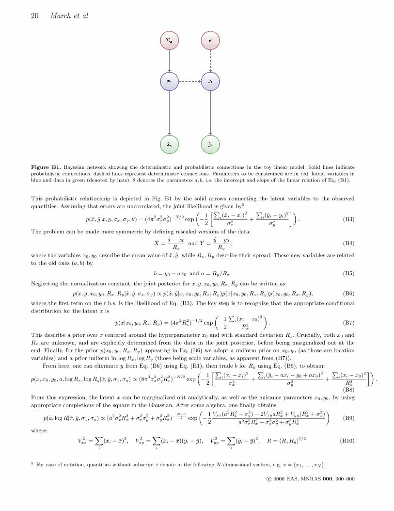
20 March et al
Figure B1. Bayesian network showing the deterministic and probabilistic connections in the toy linear model. Solid lines indicate
probabilistic connections, dashed lines represent deterministic connections. Parameters to be constrained are in red, latent variables in
blue and data in green (denoted by hats). θ denotes the parameters a, b, i.e. the intercept and slope of the linear relation of Eq. (B1).
This probabilistic relationship is depicted in Fig. B1 by the solid arrows connecting the latent variables to the observed
quantities. Assuming that errors are uncorrelated, the joint likelihood is given by5
p(x, y|x, y, σx, σy, θ) = (4π2σ2xσ
2y)−N/2 exp
(−1
2
[∑i(xi − xi)
2
σ2x
+
∑i(yi − yi)
2
σ2y
]). (B3)
The problem can be made more symmetric by defining rescaled versions of the data:
X =x− x0
Rxand Y =
y − y0
Ry, (B4)
where the variables x0, y0 describe the mean value of x, y, while Rx, Ry describe their spread. These new variables are related
to the old ones (a, b) by
b = y0 − ax0 and a = Ry/Rx. (B5)
Neglecting the normalization constant, the joint posterior for x, y, x0, y0, Rx, Ry can be written as:
p(x, y, x0, y0, Rx, Ry|x, y, σx, σy) ∝ p(x, y|x, x0, y0, Rx, Ry)p(x|x0, y0, Rx, Ry)p(x0, y0, Rx, Ry), (B6)
where the first term on the r.h.s. is the likelihood of Eq. (B3). The key step is to recognize that the appropriate conditional
distribution for the latent x is
p(x|x0, y0, Rx, Ry) = (4π2R2x)−1/2 exp
(−1
2
∑i(xi − x0)2
R2x
). (B7)
This describe a prior over x centered around the hyperparameter x0 and with standard deviation Rx. Crucially, both x0 and
Rx are unknown, and are explicitly determined from the data in the joint posterior, before being marginalized out at the
end. Finally, for the prior p(x0, y0, Rx, Ry) appearing in Eq. (B6) we adopt a uniform prior on x0, y0 (as those are location
variables) and a prior uniform in logRx, logRy (those being scale variables, as apparent from (B7)).
From here, one can eliminate y from Eq. (B6) using Eq. (B1), then trade b for Ry using Eq. (B5), to obtain:
p(x, x0, y0, a, logRx, logRy|x, y, σx, σy) ∝ (8π3σ2xσ
2yR
2x)−N/2 exp
(−1
2
[∑i(xi − xi)
2
σ2x
+
∑i(yi − axi − y0 + ax0)2
σ2y
+
∑i(xi − x0)2
R2x
]).
(B8)
From this expression, the latent x can be marginalized out analytically, as well as the nuisance parameters x0, y0, by using
appropriate completions of the square in the Gaussian. After some algebra, one finally obtains
p(a, logR|x, y, σx, σy) ∝ (a2σ2xR
2x + σ2
xσ2y + σ2
yR2x)−
N−12 exp
(−1
2
Vxx(a2R2x + σ2
y)− 2VxyaR2x + Vyy(R2
x + σ2x)
a2σ2xR2
x + σ2xσ2
y + σ2yR2
x
)(B9)
where:
V 2xx =
∑i
(xi − x)2, V 2xy =
∑i
(xi − x)(yi − y), V 2yy =
∑i
(yi − y)2, R = (RxRy)1/2. (B10)
5 For ease of notation, quantities without subscript i denote in the following N -dimensional vectors, e.g. x = x1, . . . , xN.
c© 0000 RAS, MNRAS 000, 000–000
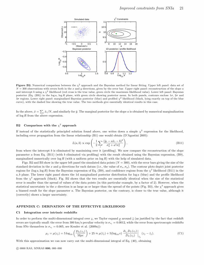
Improved constraints from SNIa 21
0.8 0.9 1 1.1 1.20
0.5
1
Log10
a
1D posterior / profile likelihood
Log10
a
Log 10
R
Bayesian posterior
0.5 1 1.5
−0.6
−0.5
−0.4
−0.3
a
b
χ2 Constraints
8 10 12 14 16 189
9.5
10
10.5
11
−1 −0.5 0 0.5 16
8
10
12
14
Observed x
Obs
erve
d y
Simulated data
Figure B2. Numerical comparison between the χ2 approach and the Bayesian method for linear fitting. Upper left panel: data set of
N = 300 observations with errors both in the x and y directions, given by the error bar. Upper right panel: reconstruction of the slope a
and intercept b using a χ2 likelihood (red cross is the true value, green circle the maximum likelihood value). Lower left panel: Bayesianposterior (Eq. (B9)) in the log a, logR plane, with green circle showing posterior mean. In both panels, contours enclose 1σ, 2σ and
3σ regions. Lower right panel: marginalized Bayesian posterior (blue) and profiled χ2 likelihood (black, lying exactly on top of the bluecurve), with the dashed line showing the true value. The two methods give essentially identical results in this case.
In the above, x =∑i xi/N , and similarly for y. The marginal posterior for the slope a is obtained by numerical marginalization
of logR from the above expression.
B2 Comparison with the χ2 approach
If instead of the statistically principled solution found above, one writes down a simple χ2 expression for the likelihood,
including error propagation from the linear relationship (B1) one would obtain (D’Agostini 2005):
L(a, b) ∝ exp
(−1
2
∑i
(yi − axi − b)2
σ2y + a2σ2
x
), (B11)
from where the intercept b is eliminated by maximising over it (profiling). We now compare the reconstruction of the slope
parameter a from Eq. (B11) (with b eliminated via profiling) with the result obtained using the Bayesian expression, (B9),
marginalized numerically over logR (with a uniform prior on logR) with the help of simulated data.
Figs. B2 and B3 show in the upper left panel the simulated data points (N = 300), with the error bars giving the size of the
standard deviation in the x and y directions for each datum (i.e., the value of σx, σy). The contour plots depict joint posterior
regions for (log a, logR) from the Bayesian expression of Eq. (B9), and confidence regions from the χ2 likelihood (B11) in the
a, b plane. The lower right panel shows the 1d marginalized posterior distribution for log a (blue) and the profile likelihood
from the χ2 approach (black). Fig. B2 shows that the two results are essentially identical when the size of the statistical
error is smaller than the spread of values of the data points (in this particular example, by a factor of 2). However, when the
statistical uncertainty in the x direction is as large as or larger than the spread of the points (Fig. B3), the χ2 approach gives
a biassed result for the slope parameter a. The Bayesian posterior, on the contrary, is closer to the true value, although it
(correctly) shows a larger uncertainty.
APPENDIX C: DERIVATION OF THE EFFECTIVE LIKELIHOOD
C1 Integration over intrinsic redshifts
In order to perform the multi-dimensional integral over z, we Taylor expand µ around z (as justified by the fact that redshift
errors are typically small: the error from 300 km/s peculiar velocity is σzi = 0.0012, while the error from spectroscopic redshifts
from SNe themselves is σzi = 0.005, see Kessler et al. (2009a)):
µj = µ(zj) = 5 log10
(DL(zj)
Mpc
)+ 25 ≈ µ(zj) + 5(log10 e)
∂zjDL(zj)
DL(zj)
∣∣∣∣zj
(zj − zj). (C1)
With this approximation we can now carry out the multi-dimensional integral of Eq. (40), obtaining
c© 0000 RAS, MNRAS 000, 000–000
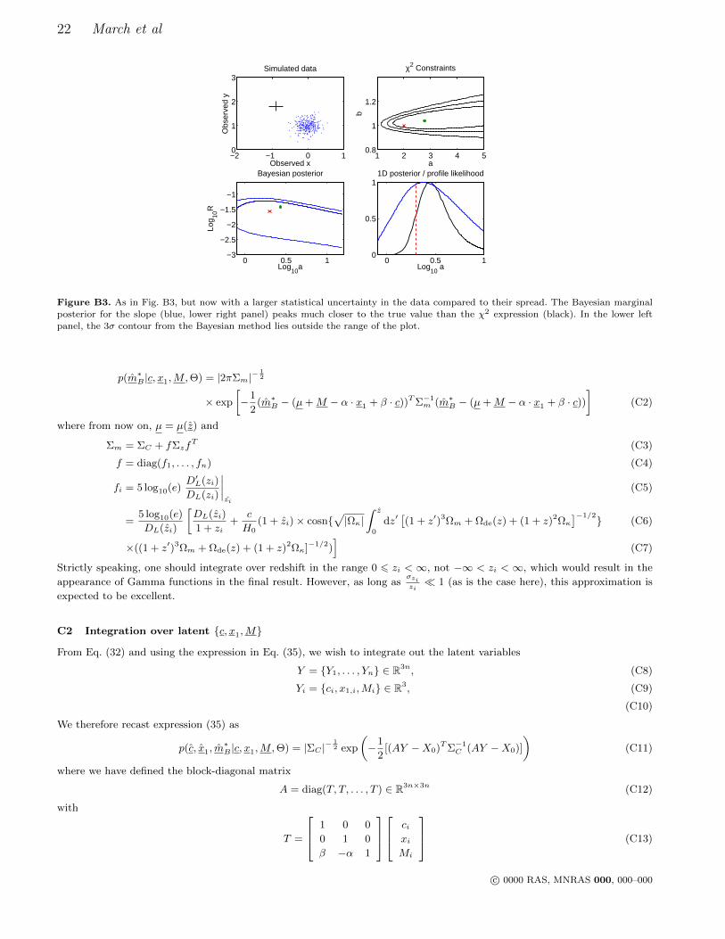
22 March et al
0 0.5 10
0.5
1
Log10
a
1D posterior / profile likelihood
Log10
a
Log 10
R
Bayesian posterior
0 0.5 1−3
−2.5
−2
−1.5
−1
a
b
χ2 Constraints
1 2 3 4 50.8
1
1.2
−2 −1 0 10
1
2
3
Observed x
Obs
erve
d y
Simulated data
Figure B3. As in Fig. B3, but now with a larger statistical uncertainty in the data compared to their spread. The Bayesian marginal
posterior for the slope (blue, lower right panel) peaks much closer to the true value than the χ2 expression (black). In the lower left
panel, the 3σ contour from the Bayesian method lies outside the range of the plot.
p(m∗B |c, x1,M,Θ) = |2πΣm|−12
× exp
[−1
2(m∗B − (µ+M − α · x1 + β · c))TΣ−1
m (m∗B − (µ+M − α · x1 + β · c))]
(C2)
where from now on, µ = µ(z) and
Σm = ΣC + fΣzfT (C3)
f = diag(f1, . . . , fn) (C4)
fi = 5 log10(e)D′L(zi)
DL(zi)
∣∣∣∣zi
(C5)
=5 log10(e)
DL(zi)
[DL(zi)
1 + zi+
c
H0(1 + zi)× cosn
√|Ωκ|
∫ z
0
dz′[(1 + z′)3Ωm + Ωde(z) + (1 + z)2Ωκ
]−1/2 (C6)
×((1 + z′)3Ωm + Ωde(z) + (1 + z)2Ωκ]−1/2)]
(C7)
Strictly speaking, one should integrate over redshift in the range 0 6 zi < ∞, not −∞ < zi < ∞, which would result in the
appearance of Gamma functions in the final result. However, as long asσzizi 1 (as is the case here), this approximation is
expected to be excellent.
C2 Integration over latent c, x1,M
From Eq. (32) and using the expression in Eq. (35), we wish to integrate out the latent variables
Y = Y1, . . . , Yn ∈ R3n, (C8)
Yi = ci, x1,i,Mi ∈ R3, (C9)
(C10)
We therefore recast expression (35) as
p(c, x1, m∗B |c, x1,M,Θ) = |ΣC |−
12 exp
(−1
2[(AY −X0)TΣ−1
C (AY −X0)]
)(C11)
where we have defined the block-diagonal matrix
A = diag(T, T, . . . , T ) ∈ R3n×3n (C12)
with
T =
1 0 0
0 1 0
β −α 1
ci
xiMi
(C13)
c© 0000 RAS, MNRAS 000, 000–000

Improved constraints from SNIa 23
The prior terms appearing in Eq. (34), namely p(c|c?, Rc)p(x1|x?, Rx)p(M |M0, σintµ ), may be written as:
p(c|c?, Rc)p(x1|x?, Rx)p(M |M0, σintµ ) = |2πΣP |−
12 exp
(−1
2[(Y − Y∗)TΣ−1
P (Y − Y∗)])
(C14)
where
S−1 = diag(R−2c , R−2
x , (σintµ )−2
)∈ R3×3, Σ−1
P = diag(S−1, S−1, . . . , S−1) ∈ R3n×3n, (C15)
Y∗ = J · b ∈ R3n×1, (C16)
J =
1 0 0
0 1 0
0 0 1...
......
1 0 0
0 1 0
0 0 1
∈ R3n×3, (C17)
b =
c∗x∗M0
∈ R3×1. (C18)
Now the integral over dY = dc dx1 dM in Eq. (34) can be performed, giving:∫dY p(c, x1, m
∗B |c, x1,M,Θ)p(c|c?, Rc)p(x1|x?, Rx)p(M |M0, σ
intµ ) =
= |2πΣC |−12 |2πΣP |−
12 |2πΣA|
12 exp
(−1
2[XT
0 Σ−1C X0 − Y T0 Σ−1
A Y0 + Y T∗ Σ−1P Y∗]
)(C19)
where
Σ−1A = ATΣ−1
C A+ Σ−1P ∈ R3n×3n, (C20)
Σ−1A Y0 = ATΣ−1
C X0 + Σ−1P Y∗, (C21)
Y0 = ΣA(ATΣ−1C X0 + Σ−1
P Y∗)ΣA(∆ + Σ−1P Y∗), (C22)
∆ = ATΣ−1C X0 ∈ R3n×1. (C23)
Substituting Eq. (C19) back into Eq. (34) gives:
p(c, x1, m∗B |Θ) =
∫dRc dRx dc? dx? |2πΣC |−
12 |2πΣP |−
12 |2πΣA|
12
× exp
(−1
2[XT
0 Σ−1C X0 − Y T0 Σ−1
A Y0 + Y T∗ Σ−1P Y∗]
)× p(Rc)p(Rx)p(c?)p(x?)p(M0|σint
µ ). (C24)
C3 Integration over population variables c?, x?,M0
The priors on the population variables b = c?, x?,M0 in Eq. (C24) can be written as:
p(b) = p(c?)p(x?)p(M0|σintµ ) = |2πΣ0|−
12 exp
(−1
2(b− bm)TΣ−1
0 (b− bm)
)(C25)
where
Σ−10 =
1/σ2c∗ 0 0
0 1/σ2x∗ 0
0 0 1/σ2M0
(C26)
and
bm =
0
0
Mm
∈ R3×1 (C27)
c© 0000 RAS, MNRAS 000, 000–000
24 March et al
Thus Eq. (C24) can be written as:
p(c, x1, m∗B |Θ) =
∫dRc dRx db |2πΣC |−
12 |2πΣP |−
12 |2πΣA|
12 |2πΣ0|−
12 p(Rc)p(Rx)
× exp
(−1
2[XT
0 Σ−1C X0 − (ΣA(∆ + Σ−1
P J · b))TΣ−1A (ΣA(∆ + Σ−1
P J · b)) + bTJTΣ−1P Jb+ (b− bm)TΣ−1
0 (b− bm)]
)=
∫dRc dRx |2πΣC |−
12 |2πΣP |−
12 |2πΣA|−
12 |2πΣ0|−
12 p(Rc)p(Rx)
× exp
(−1
2[XT
0 Σ−1C X0 −∆TΣA∆− kT0 K−1k0 + bTmΣ−1
0 bm]
)∫db exp
(−1
2[(b− k0)TK−1(b− k0)]
)(C28)
where
K−1 = −JTΣ−1P ΣAΣ−1
P J + JTΣ−1P J + Σ−1
0 ∈ R3×3, (C29)
K−1k0 = JTΣ−1P ΣA∆ + Σ−1
0 bm ∈ R3×1, (C30)
k0 = K(JTΣ−1P ΣA∆ + Σ−1
0 bm). (C31)
We can now carry out the Gaussian integral over b in Eq. (C24), obtaining our final expression for the effective likelihood,
p(c, x1, m∗B |Θ) =
∫d logRc d logRx |2πΣC |−
12 |2πΣP |−
12 |2πΣA|
12 |2πΣ0|−
12 |2πK|
12
× exp
(−1
2[XT
0 Σ−1C X0 −∆TΣA∆− kT0 K−1k0 + bTmΣ−1
0 bm]
), (C32)
where we have chosen an improper Jeffreys’ prior for the scale variables Rc, Rx:
p(Rc) ∝ R−1c ⇒ p(Rc)dRc ∝ d logRc, (C33)
and analogously for Rx. These two remaining nuisance parameters cannot be integrated out analytically, so they need to be
marginalized numerically. Hence, Rc, Rx are added to our parameters of interest and are sampled over numerically, and then
marginalized out from the joint posterior.
c© 0000 RAS, MNRAS 000, 000–000