water

Article

Experimental and Numerical Analysis of aDam-Break Flow through Different ContractionGeometries of the Channel

Selahattin Kocaman 1,* , Hasan Güzel 1, Stefania Evangelista 2 , Hatice Ozmen-Cagatay 3 andGiacomo Viccione 4

1 Department of Civil Engineering, Iskenderun Technical University, Iskenderun 31200, Turkey;hasan.guzel@iste.edu.tr

2 Civil and Mechanical Engineering Department, University of Cassino and Southern Lazio,03043 Cassino (FR), Italy; s.evangelista@unicas.it

3 Department of Civil Engineering, Cukurova University, Adana 01330, Turkey; hatmen@cu.edu.tr4 Department of Civil Engineering, University of Salerno, 84084 Fisciano, Italy; gviccion@unisa.it* Correspondence: selahattin.kocaman@iste.edu.tr

Received: 1 March 2020; Accepted: 12 April 2020; Published: 15 April 2020�����������������

Abstract: Dam-break wave propagation usually occurs over irregular topography, due for exampleto natural contraction-expansion of the river bed and to the presence of natural or artificial obstacles.Due to limited available dam-break real-case data, laboratory and numerical modeling studies aresignificant for understanding this type of complex flow problems. To contribute to the related field,a dam-break flow over a channel with a contracting reach was investigated experimentally andnumerically. Laboratory tests were carried out in a smooth rectangular channel with a horizontaldry bed for three different lateral contraction geometries. A non-intrusive digital imaging techniquewas utilized to analyze the dam-break wave propagation. Free surface profiles and time variation ofwater levels in selected sections were obtained directly from three synchronized CCD video camerarecords through a virtual wave probe. The experimental results were compared against the numericalsolution of VOF (Volume of Fluid)-based Shallow Water Equations (SWEs) and Reynolds-AveragedNavier-Stokes (RANS) equations with the k-ε turbulence model. Good agreements were obtainedbetween computed and measured results. However, the RANS solution shows a better correspondencewith the experimental results compared with the SWEs one. The presented new experimental data canbe used to validate numerical models for the simulation of dam-break flows over irregular topography.

Keywords: contraction; dam-break; unsteady flow; RANS; SWEs; CFD

1. Introduction

Dam breaks can cause rapid floods downstream, with catastrophic consequences in terms ofloss of lives and damages of properties and natural habitats, which can be minimized by forecastingthe hazards. The dam-break wave propagation usually occurs over a downstream bottom withirregular topography, resulting for example from natural contraction-expansion and meandering ofriver channels and presence of artificial (buildings, bridges) or natural (debris, dikes, trees) obstacles.The channel geometry affects the modality of the wave propagation [1–4], whose prediction is a lotmore complicated the more complex the geometry is. Topography is, in fact, a determining factorfor the flow regime: in the presence of a contraction, for example, prominent hydraulic jumps andnegative surges arise, making more difficult the evaluation of time evolution of water depths andpositive and negative wave-front celerities, crucial for flood risk assessment and management. Due

Water 2020, 12, 1124; doi:10.3390/w12041124 www.mdpi.com/journal/water

Water 2020, 12, 1124 2 of 22

to limited available dam-break real-case data [5,6], laboratory and numerical modeling studies aresignificant for understanding this type of complex flow problems [7–9].

The analysis of the literature shows several laboratory experiments aimed at investigating thepropagation of a dam-break flow over irregular flumes [2,3,10–16]. The galloping progresses inthe evolution of the imaging technology have led to a wiser use of the digital image processing inlaboratory experimental measurements of dam-break flows [17–20], with significant contribution tobetter understand the physics of real processes [21,22].

Investigation of dam-break flows over complex topography can be performed through numericalanalysis and validated through the comparison of numerical solutions obtained with different methodsagainst experimental data [23–28]. Most of previous works simulated the dam-break flow throughthe Shallow Water Equations (SWEs) [2,29–32]. The complete 3D Reynolds-Averaged Navier-Stokes(RANS) equations involving the turbulence modeling can more accurately describe the dam-breakwave propagation over complex topography [27,28,33,34]. Recently, 3D VOF (Volume of Fluid) basedCFD (Computational Fluid Dynamics) modeling software, such as FLOW-3D (Flow-Science Co, NewMexico, NM, USA) have been widely applied to the simulation of unsteady free-surface flows and alsotested on dam-break flows [35–40].

The present research focuses on the dam-break flood wave propagation over the downstreamchannel, characterized by abruptly varying cross-sections. The resulting channel contractioncorresponds to the valley contraction in real stream beds, which induces sudden alteration in theflow behavior, with shock and development of hydraulic jump and wave reflections [41]. Hence,experiments were executed in a prismatic rectangular channel with an initially dry horizontal bottomfor three different contraction geometries. Two different symmetrical trapezoidal-shaped and onetriangular-shaped obstacles were installed on the side walls to produce an abrupt contraction inthe channel cross section. These particular test cases were constructed to examine the influenceof topographical contraction on the formation and reflection of the dam-break wave propagatingdownstream. In a previous work [42] the effect of an abrupt contraction (triangular one) wasinvestigated, through laboratory experiments and numerical RANS simulations. The trapezoidalshape of the lateral contraction was considered, instead, in Ozmen-Cagatay and Kocaman [15]. In thepresent work, three different geometries of the contraction were compared, in order to highlight howa slow or an abrupt change in the cross section, as well as the entity of the contraction slope, mayhave different effects on the wave propagation. Experimental measurements were carried out througha virtual wave probe based on a non-intrusive digital image analysis technique, which permits oneto collect data, avoiding any flow disturbance. Specifically, continuous free-surface profiles over thedownstream channel at different times and water level time histories at four points were obtained fromvideo images recorded by three synchronous cameras. Experimental data were then compared againstCFD results utilizing VOF-based (RANS) with k-ε turbulence model and SWEs approach, respectively.

2. Experimental Facility and Measuring Technique

The laboratory tests were performed at the Hydraulic Laboratory of the Civil EngineeringDepartment at Cukurova University, Adana, Turkey, in a rectangular horizontal channel, made of glasswalls and bottom, having the following dimensions: length 8.90 m, width 0.30 m and height 0.34 m(Figure 1). The upstream reservoir was formed by a vertical gate representing the dam, positionedat a distance of 4.65 m from the upstream boundary wall, and it was filled with water up to a levelh0 = 0.25 m in the initial condition; the downstream part of the channel, 4.25 m long, was initially dryand left open in order for the flow to fall freely with no reflection. The water in the reservoir wascolored with food dye with the aim of an easier identification of the free surface profiles and evaluationof the behavior of the dam-break flow from the recorded video frames. The obstacles installed to formthe local contraction in the channel were made of Plexiglas and were located at a specific distancedownstream of the dam on both sidewalls symmetrically. Three different geometries of the contractionwere built, namely Triangular, Trapezoidal-A and Trapezoidal-B, dimensions and shapes of which can

Water 2020, 12, 1124 3 of 22

be seen in Figure 2. The different shapes were selected in order to represent transition from smooth tosudden contraction. The lengths of the obstacles (0.95 m), the maximum contraction width (0.10 m)and the distance from the gate (1.52 m) were chosen equally in order to compare contraction effects.

Water 2020, 12, x FOR PEER REVIEW 3 of 23

transition from smooth to sudden contraction. The lengths of the obstacles (0.95 m), the maximum contraction width (0.10 m) and the distance from the gate (1.52 m) were chosen equally in order to compare contraction effects.

In Figure 1, the Trapezoidal-A obstacles are shown. Different distances of the obstacles from the gate, between 1.52 m and 2.47 m, were investigated in Ozmen-Cagatay and Kocaman [15].

Figure 1. Laboratory set-up: (a) Longitudinal view A-A, (b) Top view, (lengths in (cm), Trapezoidal-A contraction).

Figure 2. Geometries and dimensions (lengths in (cm)) of the different contractions chosen for the experiments.

To represent the dam-break, the instantaneous removal of the gate in the vertical direction was guaranteed by an ad-hoc designed mechanism [37]. During the test, the release of a weight located 1.50 m above the floor, allowed the 4-mm thick gate to be instantaneously removed (opening time estimated from the recorded video between 0.06 and 0.08 s, shorter than 1.25(h0/g)1/2 = 0.2 s, where h0 is the initial water level in the reservoir and g is gravity [43]).

An advanced digital image processing measurement technique [21] was exploited satisfactorily to determine free surface profiles at specific times and water level time histories at fixed sections. The digital instrumentation for the image analysis consisted of three CCD (Charged Coupled Device) cameras, a computer and a frame grabber card for the simultaneous transfer to the computer, and a combination of the synchronous images recorded by the three adjacent cameras. With this system, the evolutions of the free surface profiles along all the different parts of the downstream channel were synchronously recorded and a full panoramic view of the flow was obtained, without test repetitions after changing the positions of the cameras, unlike other measuring techniques usually adopted in most previous experimental works (e.g., [3,15,21]). The experiments were repeated anyways three times for each scenario, in order to guarantee the generality of the results, obtained as the average of all the records.

The raw images were acquired as 768 × 576 pixels at 50 frames/s. Distortion of the images, due to the wide-angle lens use, was corrected through a planer checkerboard formed by 42 uniform black and white 0.1 × 0.1 m squares. In order to calibrate each camera, 25 selected pictures of the board were processed by the software “Camera Calibration Toolbox for Matlab” (Jean-Yves Bouguet, California Institute of Technology, Pasadena, Canada) To correct the distortions, the spatial calibration parameters were estimated by matching the predetermined coordinates of the board corners on pictures obtained by different viewpoints of the board. The details of the raw images of

Figure 1. Laboratory set-up: (a) Longitudinal view A-A, (b) Top view, (lengths in (cm), Trapezoidal-Acontraction).

Water 2020, 12, x FOR PEER REVIEW 3 of 23

transition from smooth to sudden contraction. The lengths of the obstacles (0.95 m), the maximum contraction width (0.10 m) and the distance from the gate (1.52 m) were chosen equally in order to compare contraction effects.

In Figure 1, the Trapezoidal-A obstacles are shown. Different distances of the obstacles from the gate, between 1.52 m and 2.47 m, were investigated in Ozmen-Cagatay and Kocaman [15].

Figure 1. Laboratory set-up: (a) Longitudinal view A-A, (b) Top view, (lengths in (cm), Trapezoidal-A contraction).

Figure 2. Geometries and dimensions (lengths in (cm)) of the different contractions chosen for the experiments.

To represent the dam-break, the instantaneous removal of the gate in the vertical direction was guaranteed by an ad-hoc designed mechanism [37]. During the test, the release of a weight located 1.50 m above the floor, allowed the 4-mm thick gate to be instantaneously removed (opening time estimated from the recorded video between 0.06 and 0.08 s, shorter than 1.25(h0/g)1/2 = 0.2 s, where h0 is the initial water level in the reservoir and g is gravity [43]).

An advanced digital image processing measurement technique [21] was exploited satisfactorily to determine free surface profiles at specific times and water level time histories at fixed sections. The digital instrumentation for the image analysis consisted of three CCD (Charged Coupled Device) cameras, a computer and a frame grabber card for the simultaneous transfer to the computer, and a combination of the synchronous images recorded by the three adjacent cameras. With this system, the evolutions of the free surface profiles along all the different parts of the downstream channel were synchronously recorded and a full panoramic view of the flow was obtained, without test repetitions after changing the positions of the cameras, unlike other measuring techniques usually adopted in most previous experimental works (e.g., [3,15,21]). The experiments were repeated anyways three times for each scenario, in order to guarantee the generality of the results, obtained as the average of all the records.

The raw images were acquired as 768 × 576 pixels at 50 frames/s. Distortion of the images, due to the wide-angle lens use, was corrected through a planer checkerboard formed by 42 uniform black and white 0.1 × 0.1 m squares. In order to calibrate each camera, 25 selected pictures of the board were processed by the software “Camera Calibration Toolbox for Matlab” (Jean-Yves Bouguet, California Institute of Technology, Pasadena, Canada) To correct the distortions, the spatial calibration parameters were estimated by matching the predetermined coordinates of the board corners on pictures obtained by different viewpoints of the board. The details of the raw images of

Figure 2. Geometries and dimensions (lengths in (cm)) of the different contractions chosen forthe experiments.

In Figure 1, the Trapezoidal-A obstacles are shown. Different distances of the obstacles from thegate, between 1.52 m and 2.47 m, were investigated in Ozmen-Cagatay and Kocaman [15].

To represent the dam-break, the instantaneous removal of the gate in the vertical direction wasguaranteed by an ad-hoc designed mechanism [37]. During the test, the release of a weight located1.50 m above the floor, allowed the 4-mm thick gate to be instantaneously removed (opening timeestimated from the recorded video between 0.06 and 0.08 s, shorter than 1.25(h0/g)1/2 = 0.2 s, where h0

is the initial water level in the reservoir and g is gravity [43]).An advanced digital image processing measurement technique [21] was exploited satisfactorily

to determine free surface profiles at specific times and water level time histories at fixed sections.The digital instrumentation for the image analysis consisted of three CCD (Charged Coupled Device)cameras, a computer and a frame grabber card for the simultaneous transfer to the computer, and acombination of the synchronous images recorded by the three adjacent cameras. With this system, theevolutions of the free surface profiles along all the different parts of the downstream channel weresynchronously recorded and a full panoramic view of the flow was obtained, without test repetitionsafter changing the positions of the cameras, unlike other measuring techniques usually adopted inmost previous experimental works (e.g., [3,15,21]). The experiments were repeated anyways threetimes for each scenario, in order to guarantee the generality of the results, obtained as the average ofall the records.

The raw images were acquired as 768 × 576 pixels at 50 frames/s. Distortion of the images, due tothe wide-angle lens use, was corrected through a planer checkerboard formed by 42 uniform black andwhite 0.1 × 0.1 m squares. In order to calibrate each camera, 25 selected pictures of the board wereprocessed by the software “Camera Calibration Toolbox for Matlab” (Jean-Yves Bouguet, CaliforniaInstitute of Technology, Pasadena, Canada) To correct the distortions, the spatial calibration parameters

Water 2020, 12, 1124 4 of 22

were estimated by matching the predetermined coordinates of the board corners on pictures obtainedby different viewpoints of the board. The details of the raw images of the channel, including the barreldistortion and a calibrated image, can be found in Kocaman and Ozmen-Cagatay [21,42], together witha better description of the image processing for reconstruction of the water surface edge, also in theregions with significant air entrainment. After the calibration process, the images corresponding tothe same time obtained from adjacent synchronous cameras were automatically merged to provide acomplete view of the free-surface profile based on predetermined stitching coordinates on the images.

A virtual wave probe was used to determine water level changes with time. Using thismeasurement technique, water depth histories can be obtained at any selected point of the flowfrom recorded video frames using image processing techniques non-intrusively, without any physicalinstrument requirement. Moreover, the desired number of vertical lines representing the virtual waveprobe can be placed on the recorded images. The location of the water free surface is determinedprecisely and objectively using an edge detection algorithm after appropriate filtering and sharpeningprocess of images. The abrupt variations of adjacent pixel colors in-line with vertical virtual probe onthe digital images are evaluated as an edge. Subsequent images were automatically processed throughthe same procedure and then the calibrated pixel coordinates were converted into metric values toobtain water depth evolutions with time. For each experiment, 900 video frames were analyzed for18 s.

3. Numerical Simulations

The commercially available CFD program FLOW-3D [44] was used for the numerical simulationsof the same scenarios observed during laboratory experiments. The numerical solutions wereobtained with two different approaches, RANS (with k-ε turbulent model) and SWEs, and solved bya Finite-Volume formulation on a structured staggered Finite-Difference grid using VOF for the freesurface computation.

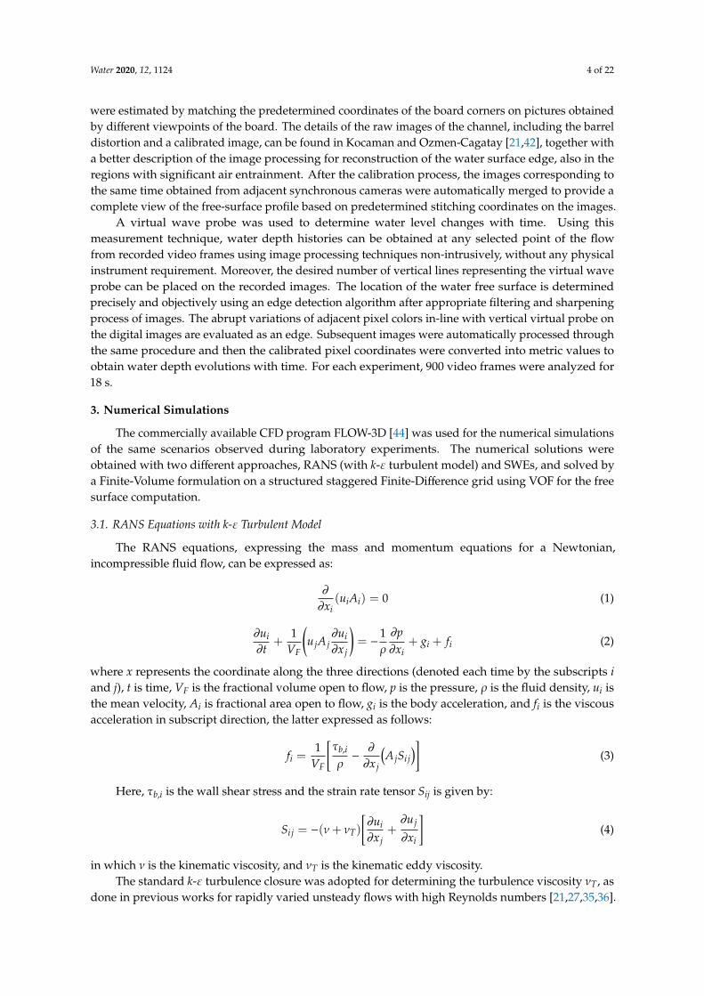
3.1. RANS Equations with k-ε Turbulent Model

The RANS equations, expressing the mass and momentum equations for a Newtonian,incompressible fluid flow, can be expressed as:

∂∂xi

(uiAi) = 0 (1)

∂ui∂t

+1

VF

(u jA j

∂ui∂x j

)= −

1ρ

∂p∂xi

+ gi + fi (2)

where x represents the coordinate along the three directions (denoted each time by the subscripts iand j), t is time, VF is the fractional volume open to flow, p is the pressure, ρ is the fluid density, ui isthe mean velocity, Ai is fractional area open to flow, gi is the body acceleration, and fi is the viscousacceleration in subscript direction, the latter expressed as follows:

fi =1

VF

[τb,i

ρ−

∂∂x j

(A jSi j

)](3)

Here, τb,i is the wall shear stress and the strain rate tensor Sij is given by:

Si j = −(ν+ νT)

[∂ui∂x j

+∂u j

∂xi

](4)

in which ν is the kinematic viscosity, and νT is the kinematic eddy viscosity.The standard k-ε turbulence closure was adopted for determining the turbulence viscosity νT, as

done in previous works for rapidly varied unsteady flows with high Reynolds numbers [21,27,35,36].

Water 2020, 12, 1124 5 of 22

In this model, turbulence eddy viscosity is computed using turbulence kinetic energy k and turbulentdissipation rate ε per unit fluid mass as νT = Cµk2/ε, with Cµ as empirical coefficient [45].

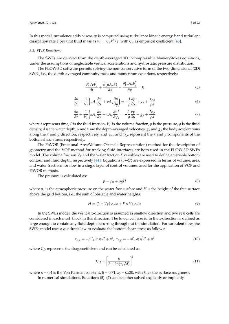
3.2. SWE Equations

The SWEs are derived from the depth-averaged 3D incompressible Navier-Stokes equations,under the assumptions of neglectable vertical accelerations and hydrostatic pressure distribution.

The FLOW-3D software permits solving the non-conservative form of the two-dimensional (2D)SWEs, i.e., the depth-averaged continuity mass and momentum equations, respectively:

∂(VFF)∂t

+∂(uAxF)∂x

+∂(vAyF

)∂y

= 0 (5)

∂u∂t

+1

VF

(uAx

∂u∂x

+ vAy∂u∂y

)= −

1ρ

∂p∂x

+ gx +τb,x

ρd(6)

∂v∂t

+1

VF

(uAx

∂v∂x

+ vAy∂v∂y

)= −

1ρ

∂p∂y

+ gy +τb,y

ρd(7)

where t represents time, F is the fluid fraction, VF is the volume fraction, p is the pressure, ρ is the fluiddensity, d is the water depth, u and v are the depth-averaged velocities, gx and gy the body accelerationsalong the x and y direction, respectively, and τb,x and τb,y represent the x and y components of thebottom shear stress, respectively.

The FAVOR (Fractional Area/Volume Obstacle Representation) method for the description ofgeometry and the VOF method for tracking fluid interfaces are both used in the FLOW-3D SWEsmodel. The volume fraction VF and the water fraction F variables are used to define a variable bottomcontour and fluid depth, respectively [44]. Equations (5)–(7) are expressed in terms of volume, area,and water fractions for flow in a single layer of control volumes used for the application of VOF andFAVOR methods.

The pressure is calculated as:p = p0 + ρgH (8)

where p0 is the atmospheric pressure on the water free surface and H is the height of the free surfaceabove the grid bottom, i.e., the sum of obstacle and water heights:

H = (1−VF) × δz + F×VF × δz (9)

In the SWEs model, the vertical z-direction is assumed as shallow direction and two real cells areconsidered in each mesh block in this direction. The lower cell size δz in the z-direction is defined aslarge enough to contain any fluid depth occurring throughout the simulation. For turbulent flow, theSWEs model uses a quadratic law to evaluate the bottom shear stress as follows:

τb,x = −ρCDu√

u2 + v2, τb,y = −ρCDv√

u2 + v2 (10)

where CD represents the drag coefficient and can be calculated as:

CD =

[κ

B + ln(z0/d)

]2

(11)

where κ = 0.4 is the Von Karman constant, B = 0.71, z0 = ks/30, with ks as the surface roughness.In numerical simulations, Equations (5)–(7) can be either solved explicitly or implicitly.

Water 2020, 12, 1124 6 of 22

3.3. Solution Domain, Boundary and Initial Conditions

The computational domain was reduced to only the longitudinal half channel, due to the symmetrywith respect to the central longitudinal section. A solution domain of length 8.90 m, width 0.15 m andheight 0.30 m was, therefore, defined.

The upstream boundary was specified as “wall” (no flow entering the reservoir), whereas thedownstream one was set as “outflow” (channel kept open downstream). The top boundary waslabeled as “pressure”, and “zero shear stress” and “constant atmospheric pressure” were defined astop boundary conditions at the free surface [44,46]. The channel sidewall and the bottom were set aswalls as well and assumed as smooth, with the choice of no-slip condition, and consequent zero valuefor tangential and normal velocities at the solid boundary, whereas logarithmic velocity distributions(wall function) in the boundary layer are provided by the applied k-ε turbulence closure model.

Wall roughness was not taken into consideration given the negligible material roughness ofthe experimental set-up which was used for validation of the numerical solutions. However, thelogarithmic velocity profile is used by RANS to calculate the shear stress at all no-slip wall boundariesin conjunction with the turbulence closure model. In the present study, the turbulent mixing length wasdynamically computed. Otherwise, when flow is turbulent, SWEs uses the quadratic law to computebottom shear stress using Equation (10). In the SWEs simulations, the drag coefficient should bedetermined for bottom shear stress. It was taken as its default value of 0.0026 in the current study. Theeffect of the drag coefficient on the water levels for SWEs results and the effect of different turbulentmodels and turbulent mixing length should also be considered as a future study for dam-break flowswith high turbulence such as in the present study.

The computational domain was subdivided into a mesh of fixed square cells using Cartesiancoordinates. After a grid sensitivity analysis, a uniform mesh size of 0.005 m was selected, in threedirections for 3D RANS model and in two directions for the SWEs model for the whole computationaldomain. Herein, a minimum of two real cells had to be defined in each mesh block in the z-direction toapply VOF in the SWEs model. The software allowed dividing z-axis horizontally into two layers, witha lower layer of 0.27 m (size sufficient to contain all the water in the layer through the simulation) andan upper layer of 0.30 m. The total number of cells was approximately 3,200,000 for RANS and 106,800for SWEs. The time step ∆t was calculated automatically by the CFD package, FLOW-3D, according tothe CFL (Courant-Friedrichs-Lewy) criterion.

When modeling strongly unsteady flows, including prominent hydraulic jumps and wavebreaking in FLOW-3D using SWEs, a second-order monotonicity preserving momentum advectionapproximation was required to ensure robust and accurate results. For RANS simulations, instead,first-order momentum advection approximation was sufficient. The implicit scheme was used to solvethe equations in both numerical models.

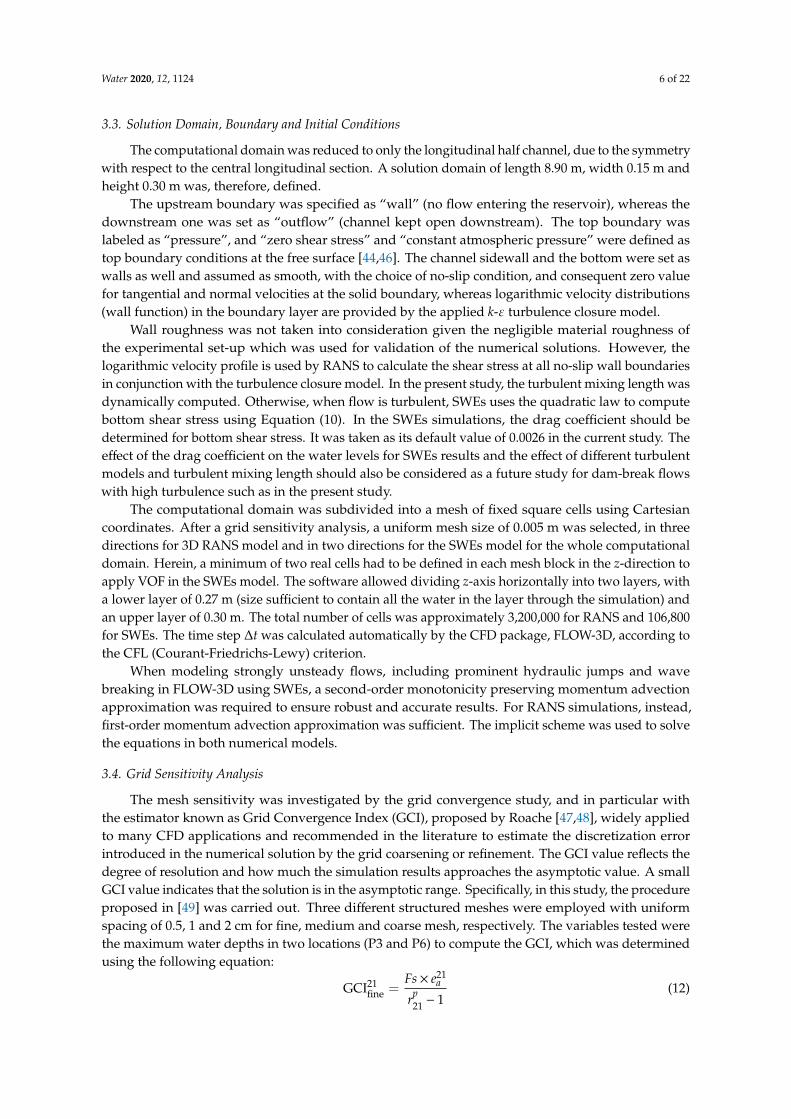
3.4. Grid Sensitivity Analysis

The mesh sensitivity was investigated by the grid convergence study, and in particular withthe estimator known as Grid Convergence Index (GCI), proposed by Roache [47,48], widely appliedto many CFD applications and recommended in the literature to estimate the discretization errorintroduced in the numerical solution by the grid coarsening or refinement. The GCI value reflects thedegree of resolution and how much the simulation results approaches the asymptotic value. A smallGCI value indicates that the solution is in the asymptotic range. Specifically, in this study, the procedureproposed in [49] was carried out. Three different structured meshes were employed with uniformspacing of 0.5, 1 and 2 cm for fine, medium and coarse mesh, respectively. The variables tested werethe maximum water depths in two locations (P3 and P6) to compute the GCI, which was determinedusing the following equation:

GCI21fine =

Fs× e21a

rp21 − 1

(12)

Water 2020, 12, 1124 7 of 22

Here, Fs represents the safety factor. When using three different meshes, it is recommended totake the value of Fs = 1.25. The approximate relative error e21

a was calculated as follows:

e21a =

∣∣∣∣∣∣φ1 −φ2

φ1

∣∣∣∣∣∣ (13)

where φi (i = 1,2,3) represents the maximum water depths for fine, medium and coarse meshes,respectively. The variable r is the ratio of the mesh size between the coarse and fine meshes (r21 = h2/h1

and r32 = h3/h2) and h is the mesh size. Here, this ratio was chosen as constant: r21 = r32 = 2. Theapparent order of convergence p can be calculated as follows:

p =1

ln(r21)ln|ε32/ε21| (14)

where ε is error between two adjacent meshes: ε32 = φ3 −φ2, ε21 = φ2 −φ1. In addition, extrapolatedvalues and extrapolated relative error can be obtained as follows, respectively:

φ21ext =

(rp

21φ1 −φ2)/(rp

21 − 1)

(15)

e21ext =

∣∣∣∣∣∣φ12ext −φ1

φ12ext

∣∣∣∣∣∣ (16)

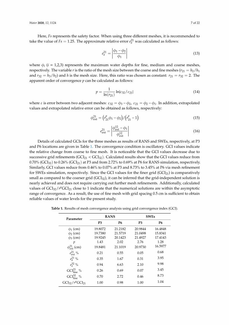
Details of calculated GCIs for the three meshes as results of RANS and SWEs, respectively, at P3and P6 locations are given in Table 1. The convergence condition is oscillatory. GCI values indicatethe relative change from coarse to fine mesh. It is noticeable that the GCI values decrease due tosuccessive grid refinements (GCI21 < GCI32). Calculated results show that the GCI values reduce from0.70% (GCI32) to 0.26% (GCI21) at P3 and from 2.72% to 0.69% at P6 for RANS simulation, respectively.Similarly, GCI values reduce from 0.46% to 0.07% at P3 and 8.73% to 3.45% at P6 via mesh refinementfor SWEs simulation, respectively. Since the GCI values for the finer grid (GCI21) is comparativelysmall as compared to the coarser grid (GCI32), it can be inferred that the grid-independent solution isnearly achieved and does not require carrying out further mesh refinements. Additionally, calculatedvalues of GCI32/rpGCI21 close to 1 indicate that the numerical solutions are within the asymptoticrange of convergence. As a result, the use of fine mesh with grid spacing 0.5 cm is sufficient to obtainreliable values of water levels for the present study.

Table 1. Results of mesh convergence analysis using grid convergence index (GCI).

ParameterRANS SWEs

P3 P6 P3 P6

φ1 (cm) 19.8072 21.2182 20.9844 16.4848φ2 (cm) 19.7380 21.5719 21.0498 15.8341φ3 (cm) 19.9245 20.1423 21.4927 17.4143

p 1.43 2.02 2.76 1.28φ21

ext (cm) 19.8481 21.1019 20.9730 16.5977

e21ext % 0.21 0.55 0.05 0.68

e21a % 0.35 1.67 0.31 3.95

e32a % 0.94 6.63 2.10 9.98

GCI21fine % 0.26 0.69 0.07 3.45

GCI32fine % 0.70 2.72 0.46 8.73

GCI32/rpGCI21 1.00 0.98 1.00 1.04

Water 2020, 12, 1124 8 of 22

4. Results and Discussion

4.1. Comparison of Experimental data for Different Contraction Geometries

The dam-break flow originates right after the gate lifting, when it starts rapidly propagatingon the dry channel, recorded all along the channel through the transparent glass walls by the threesynchronous CCD cameras. Once the wave reaches the contracted section, the wave is partiallyreflected, thus inducing the formation of a negative bore moving upward, while the rest of the flowmoves downward. In Figure 3, images obtained from the experiments conducted for the three differentcontractions, respectively, at different times after the gate opening are compared. The dashed linesindicate the borders of the contraction zone for all three cases. The blue line in the pictures is thesupporting strut for the glass channel walls.

As shown in the images at t = 1.8 s (Figure 3a), the water level starts to rise at the points wherethe flood wave encounters the narrowest section, being it constricted by the local contraction; intenseturbulence mixing is evident on the free surface, with strong air entrainment into the flow, and anegative bore of water-air swelling starts to move upward with rising depth. In the case of Trapezoidal-Bcontraction, for which the minimum section is reached earlier than with the other contractions, thewater level rises faster. In addition, as a result of the flow sudden expansion downstream of thecontraction, a significant formation of air bubbles is detected, differently from the other cases. On theother side, for the Triangular contraction, the rise in the water level is slower, being the narrowestsection reached at a bigger distance, and a very small amount of air bubbles forms. At t = 2.4 s(Figure 3b), the negative wave is moving upward with rising water depth. In the case of Trapezoidal-Bcontraction, the surge wave moves upward with significant air entrainment in front of the wave. Forthe Triangular case, the water surface slope continues to increase in the narrowing section and there isalmost no air entrainment. For the Trapezoidal-A contraction, the water surface has a bumpy shapewith a maximum water level in the middle of the narrowing section, and significant air entrainmentoccurs in front of the reflected wave. At t = 3.0 s (Figure 3c), the water surface has a bumpy appearanceat the narrowing section for the Triangular contraction, but there is still no significant air entrainment atthe upfront wave surface. The reflected wave in the Trapezoidal-B case moves little ahead and strongair entrainment is observed compared to Trapezoidal-A. These reflection waves can be considereda moving hydraulic jump. At t = 4.5 s (Figure 3d), for the Triangular case, the reflected wave is stillpropagating, with still little air entrainment in front of the wave compared to Trapezoidal-A andTrapezoidal-B; the reflected water wave moves slowly compared to the others. In all three cases, thewater surface has a horizontal profile between the wave front and the first narrowed section, and thewater level decreases rapidly after the contraction zone. In addition, the water surface slope in thenarrowest region decreases from Triangular to Trapezoidal-B contraction, i.e., with the slope of thecontraction. As a result, in the case of Trapezoidal-B, it can be said that stronger reflections occur withthe passage of the flood wave, there is significant air entrainment in front of the surge wave, and thewave front moves faster upward, compared to Trapezoidal-A and even more compared to Triangularcontractions. The reason for this behavior can be ascribed to the fact that in the Trapezoidal-B case, theflow cross-section has a more rigid transition due to the higher slope of the contracting obstacles andthe shorter tapered upstream section, resulting in an earlier encounter with the narrowest opening,compared to the other cases. On the other hand, in the Triangular contraction case, the transition fromthe full cross-section to the narrowest section is smoother, the flow is more slowly constricted at thelocal contraction entrance, the wave front jams and runs up the channel sidewalls with less impact,and the water reflection remains smaller.

Water 2020, 12, 1124 9 of 22

Water 2020, 12, x FOR PEER REVIEW 9 of 23

Figure 3. Comparison of test images for 3 different contraction conditions (dashed lines highlights the contraction position) in terms of water profiles at different times: (a) 1.8 s, (b) 2.4 s, (c) 3.0 s, (d) 4.5 s, respectively, after the gate opening.

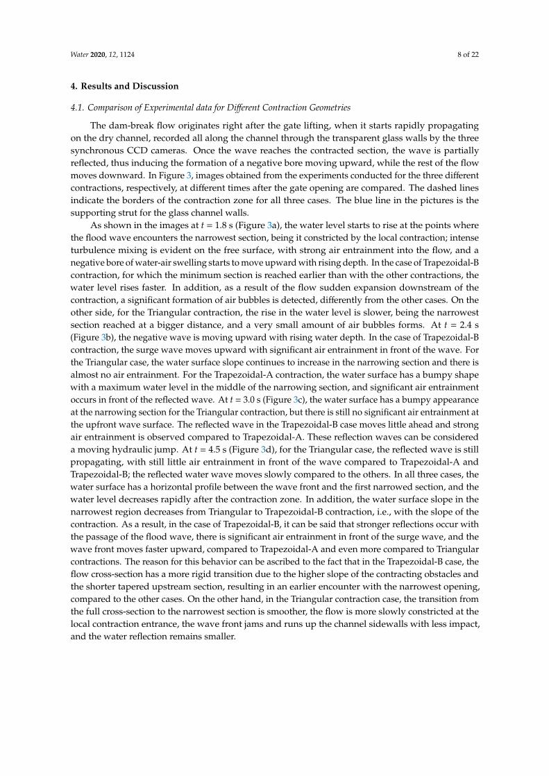
Besides the water surface profiles at different times, time variation of water levels was also measured at four different points in the three cases using the virtual wave probe. The measurement points (Figure 4) were selected, respectively as follows: right upstream of the dam (P1), right downstream of the dam (P2), at half distance between the dam location and the contraction (P3), and at the starting point of the contraction (P4).

Figure 3. Comparison of test images for 3 different contraction conditions (dashed lines highlights thecontraction position) in terms of water profiles at different times: (a) 1.8 s, (b) 2.4 s, (c) 3.0 s, (d) 4.5 s,respectively, after the gate opening.

Besides the water surface profiles at different times, time variation of water levels was alsomeasured at four different points in the three cases using the virtual wave probe. The measurementpoints (Figure 4) were selected, respectively as follows: right upstream of the dam (P1), right

Water 2020, 12, 1124 10 of 22

downstream of the dam (P2), at half distance between the dam location and the contraction (P3), andat the starting point of the contraction (P4).Water 2020, 12, x FOR PEER REVIEW 10 of 23

Figure 4. Measurement points for all cases: P1, P2, P3 and P4.

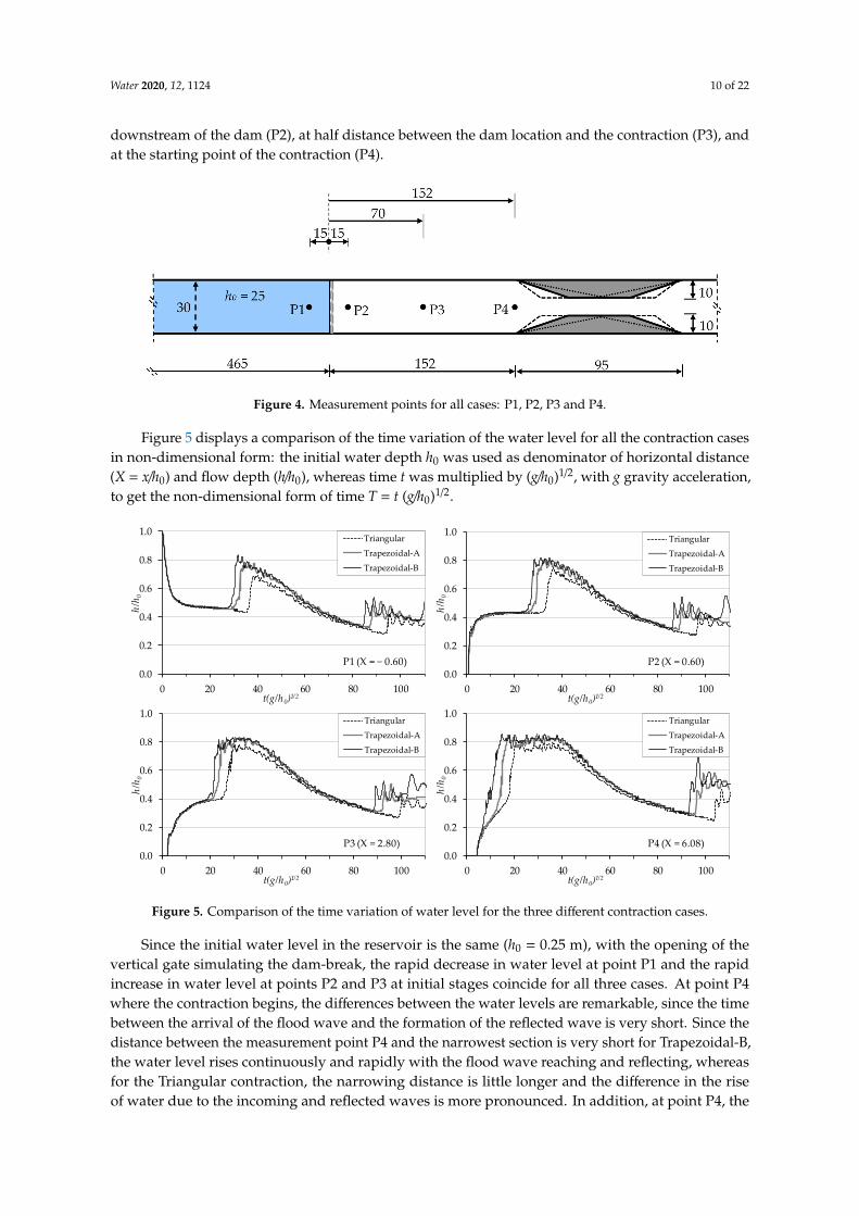
Figure 5 displays a comparison of the time variation of the water level for all the contraction cases in non-dimensional form: the initial water depth h0 was used as denominator of horizontal distance (X = x/h0) and flow depth (h/h0), whereas time t was multiplied by (g/h0)1/2, with g gravity acceleration, to get the non-dimensional form of time T = t (g/h0)1/2.

Figure 5. Comparison of the time variation of water level for the three different contraction cases.

Since the initial water level in the reservoir is the same (ℎ = 0.25 m), with the opening of the vertical gate simulating the dam-break, the rapid decrease in water level at point P1 and the rapid increase in water level at points P2 and P3 at initial stages coincide for all three cases. At point P4 where the contraction begins, the differences between the water levels are remarkable, since the time between the arrival of the flood wave and the formation of the reflected wave is very short. Since the distance between the measurement point P4 and the narrowest section is very short for Trapezoidal-B, the water level rises continuously and rapidly with the flood wave reaching and reflecting, whereas for the Triangular contraction, the narrowing distance is little longer and the difference in the rise of water due to the incoming and reflected waves is more pronounced. In addition, at point P4, the non-dimensional time T to reach the maximum height of water level is 10.52 for the Trapezoidal-B, 13.53 for the Trapezoidal-A and 16.91 for the Triangular case, respectively, i.e., in the Triangular contraction is longer than in the other cases. The maximum water levels were observed at the narrowest section for all cases. The measured non-dimensional maximum water height h/h0 is 0.85 for Trapezoidal-B, 0.84 for Trapezoidal-A and 0.81 for Triangular contraction, i.e., it is higher, since it is reached with

0.0

0.2

0.4

0.6

0.8

1.0

0 20 40 60 80 100

h/h 0

t(g/h0)1/2

P4 (X = 6.08)

Triangular

Trapezoidal-A

Trapezoidal-B

0.0

0.2

0.4

0.6

0.8

1.0

0 20 40 60 80 100

h/h 0

t(g/h0)1/2

P2 (X = 0.60)

Triangular

Trapezoidal-A

Trapezoidal-B

0.0

0.2

0.4

0.6

0.8

1.0

0 20 40 60 80 100

h/h 0

t(g/h0)1/2

P3 (X = 2.80)

Triangular

Trapezoidal-A

Trapezoidal-B

0.0

0.2

0.4

0.6

0.8

1.0

0 20 40 60 80 100

h/h 0

t(g/h0)1/2

P1 (X = − 0.60)

Triangular

Trapezoidal-A

Trapezoidal-B

Figure 4. Measurement points for all cases: P1, P2, P3 and P4.

Figure 5 displays a comparison of the time variation of the water level for all the contraction casesin non-dimensional form: the initial water depth h0 was used as denominator of horizontal distance(X = x/h0) and flow depth (h/h0), whereas time t was multiplied by (g/h0)1/2, with g gravity acceleration,to get the non-dimensional form of time T = t (g/h0)1/2.

Water 2020, 12, x FOR PEER REVIEW 10 of 23

Figure 4. Measurement points for all cases: P1, P2, P3 and P4.

Figure 5 displays a comparison of the time variation of the water level for all the contraction cases in non-dimensional form: the initial water depth h0 was used as denominator of horizontal distance (X = x/h0) and flow depth (h/h0), whereas time t was multiplied by (g/h0)1/2, with g gravity acceleration, to get the non-dimensional form of time T = t (g/h0)1/2.

Figure 5. Comparison of the time variation of water level for the three different contraction cases.

Since the initial water level in the reservoir is the same (ℎ = 0.25 m), with the opening of the vertical gate simulating the dam-break, the rapid decrease in water level at point P1 and the rapid increase in water level at points P2 and P3 at initial stages coincide for all three cases. At point P4 where the contraction begins, the differences between the water levels are remarkable, since the time between the arrival of the flood wave and the formation of the reflected wave is very short. Since the distance between the measurement point P4 and the narrowest section is very short for Trapezoidal-B, the water level rises continuously and rapidly with the flood wave reaching and reflecting, whereas for the Triangular contraction, the narrowing distance is little longer and the difference in the rise of water due to the incoming and reflected waves is more pronounced. In addition, at point P4, the non-dimensional time T to reach the maximum height of water level is 10.52 for the Trapezoidal-B, 13.53 for the Trapezoidal-A and 16.91 for the Triangular case, respectively, i.e., in the Triangular contraction is longer than in the other cases. The maximum water levels were observed at the narrowest section for all cases. The measured non-dimensional maximum water height h/h0 is 0.85 for Trapezoidal-B, 0.84 for Trapezoidal-A and 0.81 for Triangular contraction, i.e., it is higher, since it is reached with

0.0

0.2

0.4

0.6

0.8

1.0

0 20 40 60 80 100

h/h 0

t(g/h0)1/2

P4 (X = 6.08)

Triangular

Trapezoidal-A

Trapezoidal-B

0.0

0.2

0.4

0.6

0.8

1.0

0 20 40 60 80 100

h/h 0

t(g/h0)1/2

P2 (X = 0.60)

Triangular

Trapezoidal-A

Trapezoidal-B

0.0

0.2

0.4

0.6

0.8

1.0

0 20 40 60 80 100

h/h 0

t(g/h0)1/2

P3 (X = 2.80)

Triangular

Trapezoidal-A

Trapezoidal-B

0.0

0.2

0.4

0.6

0.8

1.0

0 20 40 60 80 100

h/h 0

t(g/h0)1/2

P1 (X = − 0.60)

Triangular

Trapezoidal-A

Trapezoidal-B

Figure 5. Comparison of the time variation of water level for the three different contraction cases.

Since the initial water level in the reservoir is the same (h0 = 0.25 m), with the opening of thevertical gate simulating the dam-break, the rapid decrease in water level at point P1 and the rapidincrease in water level at points P2 and P3 at initial stages coincide for all three cases. At point P4where the contraction begins, the differences between the water levels are remarkable, since the timebetween the arrival of the flood wave and the formation of the reflected wave is very short. Since thedistance between the measurement point P4 and the narrowest section is very short for Trapezoidal-B,the water level rises continuously and rapidly with the flood wave reaching and reflecting, whereasfor the Triangular contraction, the narrowing distance is little longer and the difference in the riseof water due to the incoming and reflected waves is more pronounced. In addition, at point P4, the

Water 2020, 12, 1124 11 of 22

non-dimensional time T to reach the maximum height of water level is 10.52 for the Trapezoidal-B, 13.53for the Trapezoidal-A and 16.91 for the Triangular case, respectively, i.e., in the Triangular contractionis longer than in the other cases. The maximum water levels were observed at the narrowest section forall cases. The measured non-dimensional maximum water height h/h0 is 0.85 for Trapezoidal-B, 0.84 forTrapezoidal-A and 0.81 for Triangular contraction, i.e., it is higher, since it is reached with more abruptcontraction, in the Trapezoidal-B case. Similar results are obtained observing the graphs of P1, P2 andP3 points. With the Trapezoidal-B contraction, the reflected wave reaches these points earlier and themeasured maximum height is higher compared to the other cases; the water level in the upstreamsections of the contraction increases significantly with the formation of a negative surge (reflected)wave in all cases. Due to finite reservoir length, the flow rate of the incoming flow decreases after awhile and the water accumulated upstream of the contraction also gradually decreases. The reflectedwave moving upwards is again reflected from the vertical wall at the upstream end of the channel, anda wave train which moves again downstream is formed. In the plots, while water levels are decreasing,a sudden rise and fluctuation of water levels are observed. The comparison of the reflected wavesfor all cases shows that the wave reflected in the Trapezoidal-B case is faster than in the other cases.In addition, during the passage of the wave reflected from the upstream channel boundary through thecontracted section, the water level increases considerably, especially for the Trapezoidal-B case (beforeT = 100). Then, the wave reflected from the upstream end of the channel is reflected again from thenarrowed sections and starts to move again in the upstream direction. This situation can be seen in theTrapezoidal-B curve at T = 105 for points P2 and P3. In general, when the dam-break wave encountersa cross-sectional change during its propagation, while a part of the flow passes through the existingopening, the rest of it is reflected in the contracted section and forms a reflected wave moving upwardbetween the contraction and the upstream end of the channel until the water completely discharges.As a result, when the dam-break flood wave encounters quite abrupt transitions along its path, strongerreflections, higher water levels and mixed flow conditions occur upstream of the narrowing section.The small oscillations observed in the experimental reconstruction of the water level time histories(Figure 5) with the specific image analysis measuring technique described above are not only the resultof the strong reflections of propagating waves upward and downward and their interferences, buteven more a result of the mixed flow conditions which occur in such strongly unsteady flows.

4.2. Comparison between Experimental and Numerical Results for Trapezoidal-A Case

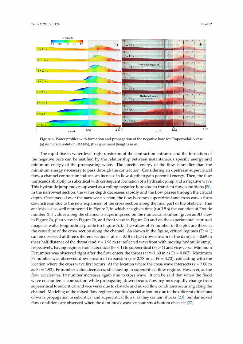
Figure 6 displays, for the Trapezoidal-A case, the comparison between the numerical resultsobtained by CFD simulation of RANS (Figure 6a) and the experimental flow picture frames captured forthe time interval 1.5–4.0 s (Figure 6b). The two frames at corresponding times are in good agreement.

The selected times from 1.5 s to 4.0 s permit one to analyze the formation and propagation of thenegative bore. The dashed lines indicate borders of the local contraction and of the 0.65 m long narrowthroat. As already seen in Figure 3 for all cases, with the sudden opening of the gate, the flow startspropagating; when the traveling wave front reaches the local contraction, at first the flow cross-sectionis constricted at the entrance before jamming and running up the sidewalls (t = 1.5 s). The water levelsharply increases up to the entrance of the narrow throat at times t = 1.5–1.8 s, and intense turbulencemixing, with air entrainment into the flow, is noticed on the free surface. At time t = 2.1 s, the negativebore crest starts moving upstream with rising depth. When the bore crest leaves the contraction region(t = 2.4 s), a reflected negative wave moving upwards forms (t = 2.7 s). In this way, the flood wavemoving downwards encounters the negative wave, thus forming a prominent hydraulic jump at thecontraction entrance.

Water 2020, 12, 1124 12 of 22

Water 2020, 12, x FOR PEER REVIEW 11 of 23

more abrupt contraction, in the Trapezoidal-B case. Similar results are obtained observing the graphs of P1, P2 and P3 points. With the Trapezoidal-B contraction, the reflected wave reaches these points earlier and the measured maximum height is higher compared to the other cases; the water level in the upstream sections of the contraction increases significantly with the formation of a negative surge (reflected) wave in all cases. Due to finite reservoir length, the flow rate of the incoming flow decreases after a while and the water accumulated upstream of the contraction also gradually decreases. The reflected wave moving upwards is again reflected from the vertical wall at the upstream end of the channel, and a wave train which moves again downstream is formed. In the plots, while water levels are decreasing, a sudden rise and fluctuation of water levels are observed. The comparison of the reflected waves for all cases shows that the wave reflected in the Trapezoidal-B case is faster than in the other cases. In addition, during the passage of the wave reflected from the upstream channel boundary through the contracted section, the water level increases considerably, especially for the Trapezoidal-B case (before T = 100). Then, the wave reflected from the upstream end of the channel is reflected again from the narrowed sections and starts to move again in the upstream direction. This situation can be seen in the Trapezoidal-B curve at T = 105 for points P2 and P3. In general, when the dam-break wave encounters a cross-sectional change during its propagation, while a part of the flow passes through the existing opening, the rest of it is reflected in the contracted section and forms a reflected wave moving upward between the contraction and the upstream end of the channel until the water completely discharges. As a result, when the dam-break flood wave encounters quite abrupt transitions along its path, stronger reflections, higher water levels and mixed flow conditions occur upstream of the narrowing section. The small oscillations observed in the experimental reconstruction of the water level time histories (Figure 5) with the specific image analysis measuring technique described above are not only the result of the strong reflections of propagating waves upward and downward and their interferences, but even more a result of the mixed flow conditions which occur in such strongly unsteady flows.

4.2. Comparison between Experimental and Numerical Results for Trapezoidal-A Case

Figure 6 displays, for the Trapezoidal-A case, the comparison between the numerical results obtained by CFD simulation of RANS (Figure 6a) and the experimental flow picture frames captured for the time interval 1.5–4.0 s (Figure 6b). The two frames at corresponding times are in good agreement.

Figure 6. Water profiles with formation and propagation of the negative bore for Trapezoidal-A case: (a) numerical solution (RANS), (b) experiment (lengths in m).

Figure 6. Water profiles with formation and propagation of the negative bore for Trapezoidal-A case:(a) numerical solution (RANS), (b) experiment (lengths in m).

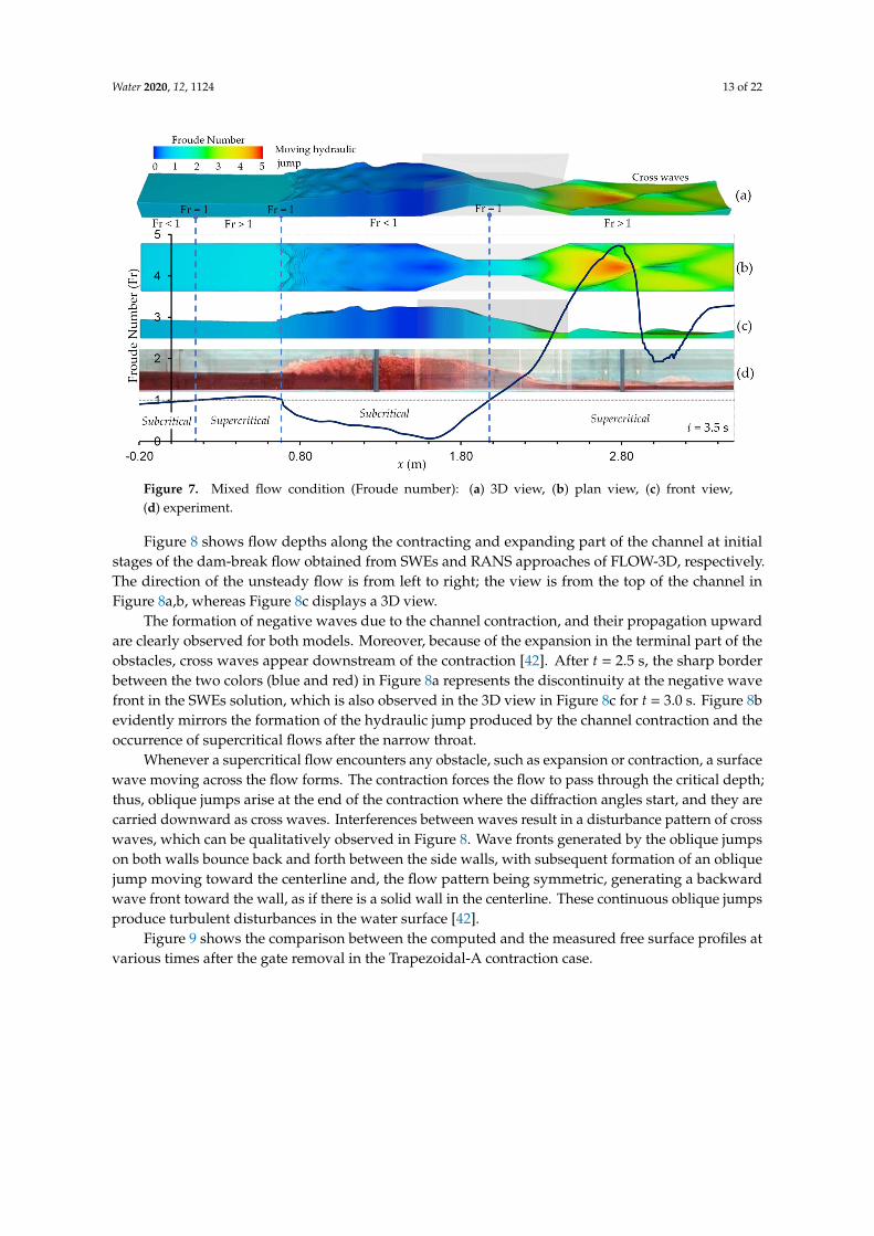
The rapid rise in water level right upstream of the contraction entrance and the formation ofthe negative bore can be justified by the relationship between instantaneous specific energy andminimum energy of the propagating wave. The specific energy of the flow is smaller than theminimum energy necessary to pass through the contraction. Considering an upstream supercriticalflow, a channel contraction induces an increase in flow depth to gain potential energy. Then, the flowtranscends abruptly to subcritical with consequent formation of a hydraulic jump and a negative wave.This hydraulic jump moves upward as a rolling negative bore due to transient flow conditions [50].In the narrowest section, the water depth decreases rapidly and the flow passes through the criticaldepth. Once passed over the narrowest section, the flow becomes supercritical and cross waves formdownstream due to the new expansion of the cross section along the final part of the obstacle. Thisanalysis is also well represented in Figure 7, in which at a given time (t = 3.5 s) the variation of Froudenumber (Fr) values along the channel is superimposed on the numerical solution (given as 3D viewin Figure 7a, plan view in Figure 7b, and front view in Figure 7c) and on the experimental capturedimage as water longitudinal profile (in Figure 7d). The values of Fr number in the plot are those atthe centerline of the cross section along the channel. As shown in the figure, critical regimes (Fr = 1)can be observed at three different sections: at x = 0.18 m (just downstream of the dam), x = 0.69 m(near half-distance of the throat) and x = 1.98 m (at reflected wavefront with moving hydraulic jump),respectively, having regimes from subcritical (Fr < 1) to supercritical (Fr > 1) and vice-versa. MinimumFr number was observed right after the flow enters the throat (at x=1.60 m as Fr = 0.067). MaximumFr number was observed downstream of expansion (x = 2.78 m as Fr = 4.72), coinciding with thelocation where the cross wave first occurs. At the location where the cross wave intersects (x = 3.00 mas Fr = 1.92), Fr number value decreases, still staying in supercritical flow regime. However, as theflow accelerates, Fr number increases again due to cross wave. It can be said that when the floodwave encounters a contraction while propagating downstream, flow regimes rapidly change fromsupercritical to subcritical and vice versa due to obstacle and mixed flow conditions occurring along thechannel. Modeling of the mixed flow regimes requires special attention due to the different directionsof wave propagation in subcritical and supercritical flows, as they contain shocks [23]. Similar mixedflow conditions are observed when the dam-break wave encounters a bottom obstacle [27].

Water 2020, 12, 1124 13 of 22

Water 2020, 12, x FOR PEER REVIEW 13 of 23

Figure 7. Mixed flow condition (Froude number): (a) 3D view, (b) plan view, (c) front view, (d) experiment.

Figure 8 shows flow depths along the contracting and expanding part of the channel at initial stages of the dam-break flow obtained from SWEs and RANS approaches of FLOW-3D, respectively. The direction of the unsteady flow is from left to right; the view is from the top of the channel in Figure 8a,b, whereas Figure 8c displays a 3D view.

Figure 7. Mixed flow condition (Froude number): (a) 3D view, (b) plan view, (c) front view,(d) experiment.

Figure 8 shows flow depths along the contracting and expanding part of the channel at initialstages of the dam-break flow obtained from SWEs and RANS approaches of FLOW-3D, respectively.The direction of the unsteady flow is from left to right; the view is from the top of the channel inFigure 8a,b, whereas Figure 8c displays a 3D view.

The formation of negative waves due to the channel contraction, and their propagation upwardare clearly observed for both models. Moreover, because of the expansion in the terminal part of theobstacles, cross waves appear downstream of the contraction [42]. After t = 2.5 s, the sharp borderbetween the two colors (blue and red) in Figure 8a represents the discontinuity at the negative wavefront in the SWEs solution, which is also observed in the 3D view in Figure 8c for t = 3.0 s. Figure 8bevidently mirrors the formation of the hydraulic jump produced by the channel contraction and theoccurrence of supercritical flows after the narrow throat.

Whenever a supercritical flow encounters any obstacle, such as expansion or contraction, a surfacewave moving across the flow forms. The contraction forces the flow to pass through the critical depth;thus, oblique jumps arise at the end of the contraction where the diffraction angles start, and they arecarried downward as cross waves. Interferences between waves result in a disturbance pattern of crosswaves, which can be qualitatively observed in Figure 8. Wave fronts generated by the oblique jumpson both walls bounce back and forth between the side walls, with subsequent formation of an obliquejump moving toward the centerline and, the flow pattern being symmetric, generating a backwardwave front toward the wall, as if there is a solid wall in the centerline. These continuous oblique jumpsproduce turbulent disturbances in the water surface [42].

Figure 9 shows the comparison between the computed and the measured free surface profiles atvarious times after the gate removal in the Trapezoidal-A contraction case.

Water 2020, 12, 1124 14 of 22Water 2020, 12, x FOR PEER REVIEW 14 of 23

Figure 8. Comparison of flow depths at initial stages of the dam-break process, calculated, respectively, for Trapezoidal-A case by: (a) SWEs and (b) RANS simulations every 0.5 s from 1.0 to 3.0 s in plan-view (c) 3D-view of SWEs and RANS results at 3.0 s after the gate removal.

The formation of negative waves due to the channel contraction, and their propagation upward are clearly observed for both models. Moreover, because of the expansion in the terminal part of the obstacles, cross waves appear downstream of the contraction [42]. After t = 2.5 s, the sharp border between the two colors (blue and red) in Figure 8a represents the discontinuity at the negative wave front in the SWEs solution, which is also observed in the 3D view in Figure 8c for t = 3.0 s. Figure 8b evidently mirrors the formation of the hydraulic jump produced by the channel contraction and the occurrence of supercritical flows after the narrow throat.

Whenever a supercritical flow encounters any obstacle, such as expansion or contraction, a surface wave moving across the flow forms. The contraction forces the flow to pass through the critical depth; thus, oblique jumps arise at the end of the contraction where the diffraction angles start, and they are carried downward as cross waves. Interferences between waves result in a disturbance pattern of cross waves, which can be qualitatively observed in Figure 8. Wave fronts generated by the oblique jumps on both walls bounce back and forth between the side walls, with subsequent formation of an oblique jump moving toward the centerline and, the flow pattern being

Figure 8. Comparison of flow depths at initial stages of the dam-break process, calculated, respectively,for Trapezoidal-A case by: (a) SWEs and (b) RANS simulations every 0.5 s from 1.0 to 3.0 s in plan-view(c) 3D-view of SWEs and RANS results at 3.0 s after the gate removal.

The borders of the contraction region are X = 6.08 and X = 9.88, indicated with dashed lines onthe graphs, together with the borders of the throat. Again, it can be noticed that when the propagatingdam-break wave approaches the contraction (T = 11.28), the water level upstream rises abruptly and anegative wave is formed. A satisfactory accordance between measured and both computed profilescan be observed at X < 5 at times T = 11.28–15.03. A little discrepancy is noticed between experimentaland RANS solved numerical free-surface profiles between X = 6 and about X = 9, whereas the SWEssolution shows more discrepancies and underestimates water depths as well as the negative wavefront speed. The formation of the strong hydraulic jump causes here random oscillations. Free surfaceprofiles can be nearly predicted by both numerical simulations after T = 18.79, except for the appearanceof a discontinuity on the negative wave front in the SWEs solutions. The overall disagreement of theSWEs solution is most probably caused by the assumption of neglectable vertical acceleration andhydrostatic pressure distribution [2].

Water 2020, 12, 1124 15 of 22

Water 2020, 12, x FOR PEER REVIEW 15 of 23

symmetric, generating a backward wave front toward the wall, as if there is a solid wall in the centerline. These continuous oblique jumps produce turbulent disturbances in the water surface [42].

Figure 9 shows the comparison between the computed and the measured free surface profiles at various times after the gate removal in the Trapezoidal-A contraction case.

Figure 9. Comparison between numerically computed and experimentally measured free surface profiles over time for Trapezoidal-A contraction case.

The borders of the contraction region are X = 6.08 and X = 9.88, indicated with dashed lines on the graphs, together with the borders of the throat. Again, it can be noticed that when the propagating dam-break wave approaches the contraction (T = 11.28), the water level upstream rises abruptly and a negative wave is formed. A satisfactory accordance between measured and both computed profiles can be observed at X < 5 at times T = 11.28–15.03. A little discrepancy is noticed between experimental and RANS solved numerical free-surface profiles between X = 6 and about X = 9, whereas the SWEs solution shows more discrepancies and underestimates water depths as well as the negative wave front speed. The formation of the strong hydraulic jump causes here random oscillations. Free surface profiles can be nearly predicted by both numerical simulations after T = 18.79, except for the appearance of a discontinuity on the negative wave front in the SWEs solutions. The overall disagreement of the SWEs solution is most probably caused by the assumption of neglectable vertical acceleration and hydrostatic pressure distribution [2].

When the formation of the negative wave is fully completed (i.e., at times T ≥ 21.92), the free surface becomes more stable and a better correspondence is observed between the measured profiles

0.0

0.2

0.4

0.6

0.8

1.0

0 2 4 6 8 10

h/h 0

x/h0

T = 46.98

RANSSWEExperiment

0.0

0.2

0.4

0.6

0.8

1.0

0 2 4 6 8 10

h/h 0

x/h0

T = 21.92

RANSSWEsExperiment

0.0

0.2

0.4

0.6

0.8

1.0

0 2 4 6 8 10

h/h 0

x/h0

T = 40.72

RANSSWEExperiment

0.0

0.2

0.4

0.6

0.8

1.0

0 2 4 6 8 10

h/h 0

x/h0

T = 18.79

RANSSWEsExperiment

0.0

0.2

0.4

0.6

0.8

1.0

0 2 4 6 8 10

h/h 0

x/h0

T = 34.45

RANSSWEExperiment

0.0

0.2

0.4

0.6

0.8

1.0

0 2 4 6 8 10

h/h 0

x/h0

T = 16.91

RANSSWEsExperiment

0.0

0.2

0.4

0.6

0.8

1.0

0 2 4 6 8 10

h/h 0

x/h0

T = 31.32

RANSSWEExperiment

0.0

0.2

0.4

0.6

0.8

1.0

0 2 4 6 8 10

h/h 0

x/h0

T = 15.03

RANSSWEsExperiment

0.0

0.2

0.4

0.6

0.8

1.0

0 2 4 6 8 10

h/h 0

x/h0

T = 28.19

RANSSWEExperiment

0.0

0.2

0.4

0.6

0.8

1.0

0 2 4 6 8 10

h/h 0

x/h0

T = 13.15

RANSSWEsExperiment

0.0

0.2

0.4

0.6

0.8

1.0

0 2 4 6 8 10

h/h 0

x/h0

T = 25.06

RANSSWEsExperiment

0.0

0.2

0.4

0.6

0.8

1.0

0 2 4 6 8 10

h/h 0

x/h0

T = 11.28

RANSSWEsExperiment

Figure 9. Comparison between numerically computed and experimentally measured free surfaceprofiles over time for Trapezoidal-A contraction case.

When the formation of the negative wave is fully completed (i.e., at times T ≥ 21.92), the freesurface becomes more stable and a better correspondence is observed between the measured profilesand those computed by RANS. While the RANS model slightly underestimates the maximum waterlevels for T ≥ 21.92, the SWEs solution overestimates them.

The present investigation analyzes the capability of the two models to simulate dam-break flowsin real-case topography. It is shown that the solution of the VOF-based RANS numerical modelwell describes well the propagation of the negative wave induced by the strong reflection of thedam-break flow against the abruptly changing topography with a reasonable accuracy, but it needsmore computational time. On the other hand, the SWEs simulation shows a little disagreement but itprovides an advantage in requiring less computational time, which would be even more importantfor real-case real-scale applications. The run-times were approximately 53 min in SWEs and 46 hin RANS for 20 s solution time, respectively, on a computer equipped with Intel Core i7 2.8 GHz16 GB RAM. Hence, SWE-based numerical models are still preferable over RANS-based models forlarge computational domains where the vertical acceleration is insignificant compared to the lesscomputational efforts and time. Fine meshes can be necessary in numerical simulations to representirregular topographies and to obtain more accurate results. On the other hand, more computationalefforts and times are required for 3-D solutions of large-scale real-case dam-break problems in thepresence of artificial and natural obstacles such as bridges, buildings, dikes, and trees [39,51,52].

Water 2020, 12, 1124 16 of 22

In order to model flow around 3D structures such as bridges using fine mesh to capture localizedflow details, the hybrid models combining RANS-based 3D flow and shallow water models in onesimulation can also be used to reduce the computation time [44].

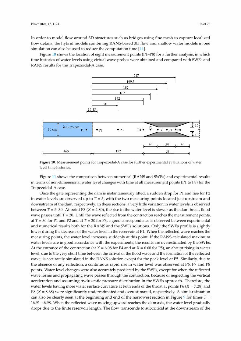
Figure 10 shows the location of eight measurement points (P1–P8) for a further analysis, in whichtime histories of water levels using virtual wave probes were obtained and compared with SWEs andRANS results for the Trapezoidal-A case.

Water 2020, 12, x FOR PEER REVIEW 16 of 23

and those computed by RANS. While the RANS model slightly underestimates the maximum water levels for T ≥ 21.92, the SWEs solution overestimates them.

The present investigation analyzes the capability of the two models to simulate dam-break flows in real-case topography. It is shown that the solution of the VOF-based RANS numerical model well describes well the propagation of the negative wave induced by the strong reflection of the dam-break flow against the abruptly changing topography with a reasonable accuracy, but it needs more computational time. On the other hand, the SWEs simulation shows a little disagreement but it provides an advantage in requiring less computational time, which would be even more important for real-case real-scale applications. The run-times were approximately 53 min in SWEs and 46 h in RANS for 20 s solution time, respectively, on a computer equipped with Intel Core i7 2.8 GHz 16 GB RAM. Hence, SWE-based numerical models are still preferable over RANS-based models for large computational domains where the vertical acceleration is insignificant compared to the less computational efforts and time. Fine meshes can be necessary in numerical simulations to represent irregular topographies and to obtain more accurate results. On the other hand, more computational efforts and times are required for 3-D solutions of large-scale real-case dam-break problems in the presence of artificial and natural obstacles such as bridges, buildings, dikes, and trees [39,51,52]. In order to model flow around 3D structures such as bridges using fine mesh to capture localized flow details, the hybrid models combining RANS-based 3D flow and shallow water models in one simulation can also be used to reduce the computation time [44].

Figure 10 shows the location of eight measurement points (P1–P8) for a further analysis, in which time histories of water levels using virtual wave probes were obtained and compared with SWEs and RANS results for the Trapezoidal-A case.

Figure 10. Measurement points for Trapezoidal-A case for further experimental evaluations of water level time histories.

Figure 11 shows the comparison between numerical (RANS and SWEs) and experimental results in terms of non-dimensional water level changes with time at all measurement points (P1 to P8) for the Trapezoidal-A case.

Figure 10. Measurement points for Trapezoidal-A case for further experimental evaluations of waterlevel time histories.

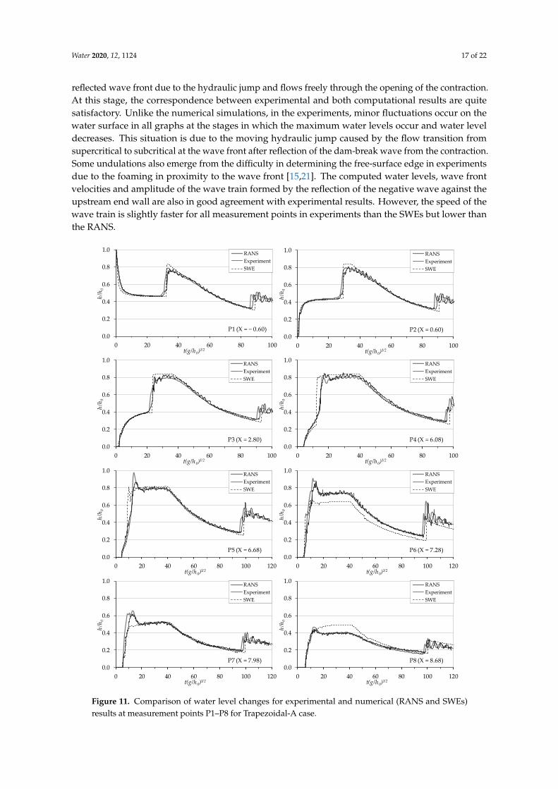
Figure 11 shows the comparison between numerical (RANS and SWEs) and experimental resultsin terms of non-dimensional water level changes with time at all measurement points (P1 to P8) for theTrapezoidal-A case.

Once the gate representing the dam is instantaneously lifted, a sudden drop for P1 and rise for P2in water levels are observed up to T = 5, with the two measuring points located just upstream anddownstream of the dam, respectively. In these sections, a very little variation in water levels is observedbetween T = 5–30. At point P3 (X = 2.80), the rise in the water level is slower as the dam-break floodwave passes until T = 20. Until the wave reflected from the contraction reaches the measurement points,at T = 30 for P1 and P2 and at T = 20 for P3, a good correspondence is observed between experimentaland numerical results both for the RANS and the SWEs solutions. Only the SWEs profile is slightlylower during the decrease of the water level in the reservoir at P1. When the reflected wave reaches themeasuring points, the water level increases suddenly at this point. If the RANS-calculated maximumwater levels are in good accordance with the experiments, the results are overestimated by the SWEs.At the entrance of the contraction (at X = 6.08 for P4 and at X = 6.68 for P5), an abrupt rising in waterlevel, due to the very short time between the arrival of the flood wave and the formation of the reflectedwave, is accurately simulated in the RANS solution except for the peak level at P5. Similarly, due tothe absence of any reflection, a continuous rapid rise in water level was observed at P6, P7 and P8points. Water-level changes were also accurately predicted by the SWEs, except for when the reflectedwave forms and propagating wave passes through the contraction, because of neglecting the verticalacceleration and assuming hydrostatic pressure distribution in the SWEs approach. Therefore, thewater levels having more water surface curvature at both ends of the throat at points P6 (X = 7.28) andP8 (X = 8.68) were significantly underestimated and overestimated, respectively. A similar situationcan also be clearly seen at the beginning and end of the narrowest section in Figure 9 for times T =

16.91–46.98. When the reflected wave moving upward reaches the dam axis, the water level graduallydrops due to the finite reservoir length. The flow transcends to subcritical at the downstream of the

Water 2020, 12, 1124 17 of 22

reflected wave front due to the hydraulic jump and flows freely through the opening of the contraction.At this stage, the correspondence between experimental and both computational results are quitesatisfactory. Unlike the numerical simulations, in the experiments, minor fluctuations occur on thewater surface in all graphs at the stages in which the maximum water levels occur and water leveldecreases. This situation is due to the moving hydraulic jump caused by the flow transition fromsupercritical to subcritical at the wave front after reflection of the dam-break wave from the contraction.Some undulations also emerge from the difficulty in determining the free-surface edge in experimentsdue to the foaming in proximity to the wave front [15,21]. The computed water levels, wave frontvelocities and amplitude of the wave train formed by the reflection of the negative wave against theupstream end wall are also in good agreement with experimental results. However, the speed of thewave train is slightly faster for all measurement points in experiments than the SWEs but lower thanthe RANS.Water 2020, 12, x FOR PEER REVIEW 17 of 23

Figure 11. Comparison of water level changes for experimental and numerical (RANS and SWEs) results at measurement points P1–P8 for Trapezoidal-A case.

Once the gate representing the dam is instantaneously lifted, a sudden drop for P1 and rise for P2 in water levels are observed up to T = 5, with the two measuring points located just upstream and downstream of the dam, respectively. In these sections, a very little variation in water levels is observed between T = 5–30. At point P3 (X = 2.80), the rise in the water level is slower as the dam-break flood wave passes until T = 20. Until the wave reflected from the contraction reaches the measurement points, at T = 30 for P1 and P2 and at T = 20 for P3, a good correspondence is observed between experimental and numerical results both for the RANS and the SWEs solutions. Only the SWEs profile is slightly lower during the decrease of the water level in the reservoir at P1. When the reflected wave reaches the measuring points, the water level increases suddenly at this point. If the

0.0

0.2

0.4

0.6

0.8

1.0

0 20 40 60 80 100 120

h/h 0

t(g/h0)1/2

P8 (X = 8.68)

RANSExperimentSWE

0.0

0.2

0.4

0.6

0.8

1.0

0 20 40 60 80 100 120

h/h 0

t(g/h0)1/2

P6 (X = 7.28)

RANSExperimentSWE

0.0

0.2

0.4

0.6

0.8

1.0

0 20 40 60 80 100

h/h 0

t(g/h0)1/2

P4 (X = 6.08)

RANSExperimentSWE

0.0

0.2

0.4

0.6

0.8

1.0

0 20 40 60 80 100

h/h 0

t(g/h0)1/2

P2 (X = 0.60)

RANSExperimentSWE

0.0

0.2

0.4

0.6

0.8

1.0

0 20 40 60 80 100

h/h 0

t(g/h0)1/2

P3 (X = 2.80)

RANSExperimentSWE

0.0

0.2

0.4

0.6

0.8

1.0

0 20 40 60 80 100 120

h/h 0

t(g/h0)1/2

P5 (X = 6.68)

RANSExperimentSWE

0.0

0.2

0.4

0.6

0.8

1.0

0 20 40 60 80 100 120

h/h 0

t(g/h0)1/2

P7 (X = 7.98)

RANSExperimentSWE

0.0

0.2

0.4

0.6

0.8

1.0

0 20 40 60 80 100

h/h 0

t(g/h0)1/2

P1 (X = − 0.60)

RANSExperimentSWE

Figure 11. Comparison of water level changes for experimental and numerical (RANS and SWEs)results at measurement points P1–P8 for Trapezoidal-A case.

Water 2020, 12, 1124 18 of 22

The RANS model uses the sum of viscous and turbulent shear stresses with turbulence models,whereas the SWEs use an empirical equation to calculate bottom shear stress for turbulent flows.Therefore, when comparing RANS and SWEs results in terms of water-level measurements, it shouldbe taken into consideration that energy losses between the two models are handled with differentapproaches. The SWEs in FLOW-3D do not include any viscosity term nor use any of the turbulentmodels, but rely on the empirical expression based on a quadratic law given in Equation (10) tocalculate energy loss for turbulent flow. The calculation of bottom shear stress requires the definitionof a drag coefficient CD, which can be selected as a constant (as we did, assigning the value of 0.0026,according to the manual suggestions) or let it be calculated from the software for a component, basedon its surface roughness, using Equation (11). Preliminary sensitivity studies showed that the use of aconstant value CD = 0.0026 or of a value of CD calculated based on the surface roughness ks = 0.00015cm did not change much the results in terms of water depths. A sensitivity analysis of the calibrationparameter, evaluating the effect of different CD values, was also performed, proving no significanteffects in maximum wave heights and speed of reflected wave fronts. This is probably due to the lowroughness of bottom and walls of the channel, which were made of glass. An accurate determinationof the CD coefficient might be necessary for surfaces with different roughness.

The dam-break wave propagation analyzed here is a strongly unsteady flow characterized byhigh turbulence, mixed flow and steep water surface fronts (shocks). In this situation, the hypothesesof hydrostatic distribution of pressures and neglectable vertical components of both velocity andacceleration, on which the SWEs are based, are not satisfied and can lead to not completely satisfactoryresults, differently from a fully 3D model like RANS, which is certainly more suitable. However, duringthe transition of the wave, water levels are excessive only in a certain period of time in the SWEs results.In the 3D RANS model energy losses are fully calculated via shear stress expressions with viscosityand turbulent viscosity by using k-ε turbulent model. For a more coherent comparison between SWEsand RANS, which is not a priority here, it might be better to evaluate at each time step water levelsalso in the SWEs model, including the period of time in which the hydraulic jump (shock) occurs.

Error analysis was performed making use of the three following measures of the differencesbetween model (RANS and SWEs) predicted yp and experimental observed values y0 for n samples:

• Root Mean Square Error (RMSE)

RMSE =

√√1n

n∑i=1

(yo − yp

)2(17)

• Mean Absolute Percent Error (MAPE)

MAPE% =100n×

n∑i=1

∣∣∣∣∣ yo − yp

y0

∣∣∣∣∣ (18)

• Mean Absolute Error (MAE)

MAE =1n

n∑i=1

∣∣∣yo − yp∣∣∣ (19)

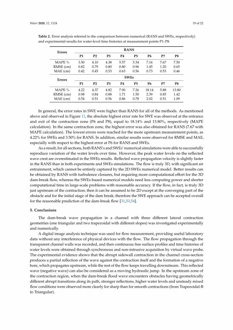
Referring, for example, to the data reported in Figure 11 (water level time histories), the threeerrors are reported for the measuring points P1–P8 in Table 2. Errors were calculated for 900 (18/0.02)different values for a total of 18 s at 0.02 s intervals.

Water 2020, 12, 1124 19 of 22

Table 2. Error analysis referred to the comparison between numerical (RANS and SWEs, respectively)and experimental results for water-level time histories at measurement points P1–P8.

ErrorsRANS

P1 P2 P3 P4 P5 P6 P7 P8

MAPE % 3.50 4.10 4.38 5.57 5.34 7.16 7.67 7.50RMSE (cm) 0.82 0.79 0.80 0.80 0.96 1.45 1.20 0.65MAE (cm) 0.42 0.45 0.53 0.63 0.56 0.73 0.53 0.46

ErrorsSWEs

P1 P2 P3 P4 P5 P6 P7 P8

MAPE % 4.22 4.37 4.82 7.90 7.26 18.14 5.88 13.80RMSE (cm) 0.98 0.84 0.88 1.71 1.50 2.39 0.85 1.42MAE (cm) 0.54 0.51 0.56 0.86 0.78 2.02 0.51 1.09

In general, the error rates in SWE were higher than RANS for all of the methods. As mentionedabove and observed in Figure 11, the absolute highest error rate for SWE was observed at the entranceand exit of the contraction zone (P6 and P8), equal to 18.14% and 13.80%, respectively (MAPEcalculation). In the same contraction zone, the highest error was also obtained for RANS (7.67 withMAPE calculation). The lowest errors were reached for the more upstream measurement points, as4.22% for SWEs and 3.50% for RANS. In addition, similar results were observed for RMSE and MAE,especially with respect to the highest error at P6 for RANS and SWEs.

As a result, for all sections, both RANS’s and SWEs’ numerical simulations were able to successfullyreproduce variation of the water levels over time. However, the peak water levels on the reflectedwave crest are overestimated in the SWEs results. Reflected wave propagation velocity is slightly fasterin the RANS than in both experiments and SWEs simulations. The flow is truly 3D, with significant airentrainment, which cannot be entirely captured by the 2D SWEs numerical model. Better results canbe obtained by RANS with turbulence closures, but requiring more computational effort for the 3Ddam-break flow, whereas the SWEs-based numerical models need less computing power and shortercomputational time in large-scale problems with reasonable accuracy. If the flow, in fact, is truly 3Djust upstream of the contraction, then it can be assumed to be 2D except at the converging part of theobstacle and for the initial stage of the dam break; therefore the SWE approach can be accepted overallfor the reasonable prediction of the dam-break flow [31,53,54].

5. Conclusions

The dam-break wave propagation in a channel with three different lateral contractiongeometries (one triangular and two trapezoidal with different slopes) was investigated experimentallyand numerically.

A digital image analysis technique was used for flow measurement, providing useful laboratorydata without any interference of physical devices with the flow. The flow propagation through thetransparent channel walls was recorded, and then continuous free surface profiles and time histories ofwater levels were obtained through synchronous and non-intrusive acquisition by virtual wave probe.The experimental evidence shows that the abrupt sidewall contraction in the channel cross-sectionproduces a partial reflection of the wave against the contraction itself and the formation of a negativebore, which propagates upstream, while the rest of the flow keeps travelling downstream. This reflectedwave (negative wave) can also be considered as a moving hydraulic jump. In the upstream zone ofthe contraction region, when the dam-break flood wave encounters obstacles having geometricallydifferent abrupt transitions along its path, stronger reflections, higher water levels and unsteady mixedflow conditions were observed more clearly for sharp than for smooth contractions (from Trapezoidal-Bto Triangular).

Water 2020, 12, 1124 20 of 22

The laboratory data were compared against the SWEs and 3D RANS (with the k-ε turbulenceclosure model) numerical simulation results, obtained through a VOF-based commercially availableCFD program, FLOW-3D. There is a very satisfactory accordance between measured data and RANSnumerical results, while the SWEs solution shows little discrepancies at early stages of the reflectedwave formation. Despite inaccurate prediction of the negative bore formation and overestimation ofthe peak water levels, the SWEs model is still capable of predicting the free surface profiles with anacceptable level. Although the RANS based numerical models with turbulence closures give betterresults for 3-D dam-break flow over the irregular domains, the SWEs-based numerical models needless computing power and give faster results in large scale problems with reasonable accuracy.

Owing to the fact that limited field data available for dam-break flows, the present newexperimental data give a contribution to the understanding of the effect of a dam-break wavepropagation over an abruptly varying downstream topography. Although the laboratory investigatedscenarios (e.g., the rectangular channel) are often far from reality (e.g., a real river bed), in fact, resultsobtained from small-scales tests conducted in a protected and controlled environment can be useful fora deeper comprehension of the real processes and for the validation of simulation numerical models,also in large-scale scenarios for real-time defense systems. Results confirm that simplified SWEs-basedmodels can be used for analyzing a large number of scenarios, but they have to be integrated withmore complete RANS simulations for more accurate results.

Author Contributions: Conceptualization, S.K., H.G. and H.O.-C.; methodology, S.K., H.G., H.O.-C. and S.E;software, S.K., S.E and G.V.; validation, S.K., S.E. and G.V.; formal analysis, S.K., S.E. and G.V.; investigation, S.K.,H.O.-C. and H.G; resources, S.K., H.G. and H.O.-C.; data collection and processing, S.K. and S.E.; writing—originaldraft preparation, S.K., H.G and S.E.; writing—review and editing, H.O.-C., S.E. and G.V.; visualization, S.K., S.E.and H.G.; supervision, S.K.; project administration, S.K. All authors have read and agreed to the published versionof the manuscript.

Funding: This research received no external funding.

Conflicts of Interest: The authors declare no conflict of interest.

References

1. de Marinis, G.; Di Cristo, C.; Evangelista, S.; Leopardi, A. Dam break waves on stepped bottom. In Proceedingsof the XXXIII IAHR Int. Biennal Congress, Vancouver, BC, Canada, 8–14 August 2009; pp. 1262–1268.

2. Evangelista, S.; Altinakar, M.S.; Di Cristo, C.; Leopardi, A. Simulation of dam-break waves on movable bedsusing a multi-stage centered scheme. Int. J. Sediment Res. 2013, 28, 269–284. [CrossRef]

3. Ozmen-Cagatay, H.; Kocaman, S.; Guzel, H. Investigation of dam-break flood waves in a dry channel with ahump. HydroResearch 2014, 8, 304–315. [CrossRef]

4. Wang, B.; Zhang, J.; Chen, Y.; Peng, Y.; Liu, X.; Liu, W. Comparison of measured dam-break flood waves intriangular and rectangular channels. J. Hydrol. 2019, 575, 690–703. [CrossRef]

5. Valiani, A.; Caleffi, V.; Zanni, A. Case Study: Malpasset Dam-break simulation using a two-dimensionalfinite volume method. J. Hydraul. Eng. 2002, 128, 460–472. [CrossRef]

6. Gallegos, H.A.; Schubert, J.E.; Sanders, B.F. Two-dimensional, high-resolution modeling of urban dam-breakflooding: A case study of Baldwin Hills, California. Adv. Water Resour. 2009, 32, 1323–1335. [CrossRef]

7. Prestininzi, P. Suitability of the diffusive model for dam break simulation: Application to a CADAMexperiment. J. Hydrol. 2008, 361, 172–185. [CrossRef]

8. Haltas, I.; Tayfur, G.; Elçi, S. Sebnem Two-dimensional numerical modeling of flood wave propagation in anurban area due to Ürkmez dam-break, Izmir, Turkey. Nat. Hazards 2016, 81, 2103–2119. [CrossRef]

9. Güney, M.S.; Tayfur, G.; Bombar, G.; Elçi, S. Distorted physical model to study sudden partial dam breakflows in an urban area. J. Hydraul. Eng. 2014, 140, 05014006. [CrossRef]

10. Miller, S.; Chaudhry, M.H. Dam-break flows in curved channel. J. Hydraul. Eng. 1989, 115, 1465–1478.[CrossRef]

11. Bell, S.W.; Elliot, R.C.; Chaudhry, M.H. Experimental results of two-dimensional dam-break flows. J. Hydraul.Res. 1992, 30, 225–252. [CrossRef]

12. Ostapenko, V.V. Dam-break flows over a bottom step. J. Appl. Mech. Tech. Phys. 2003, 44, 495–505. [CrossRef]

Water 2020, 12, 1124 21 of 22

13. Soares-Frazao, S. Experiments of dam-break wave over a triangular bottom sill. J. Hydraul. Res. 2007, 45,19–26. [CrossRef]

14. Soares-Frazao, S.; Zech, Y. Experimental study of dam-break flow against an isolated obstacle. J. Hydraul.Res. 2007, 45, 27–36. [CrossRef]

15. Ozmen-Cagatay, H.; Kocaman, S. Investigation of dam-break flow over abruptly contracting channel withtrapezoidal-shaped lateral obstacles. J. Fluids Eng. 2012, 134, 081204. [CrossRef]

16. Bellos, C.V.; Soulis, V.; Sakkas, J.G. Experimental investigation of two-dimensional dam-break induced flows.J. Hydraul. Res. 1992, 30, 47–63. [CrossRef]

17. Cochard, S.; Ancey, C. Tracking the free surface of time-dependent flows: Image processing for the dam-breakproblem. Exp. Fluids 2007, 44, 59–71. [CrossRef]

18. Aureli, F.; Maranzoni, A.; Mignosa, P.; Ziveri, C. Dam-break flows: Acquisition of experimental data throughan imaging technique and 2D numerical modeling. J. Hydraul. Eng. 2008, 134, 1089–1101. [CrossRef]

19. Aureli, F.; Maranzoni, A.; Mignosa, P.; Ziveri, C. An image processing technique for measuring free surfaceof dam-break flows. Exp. Fluids 2010, 50, 665–675. [CrossRef]

20. Liu, W.; Wang, B.; Chen, Y.; Wu, C.; Liu, X. Assessing the analytical solution of one-dimensional gravitywave model equations using dam-break experimental measurements. Water 2018, 10, 1261. [CrossRef]

21. Kocaman, S.; Ozmen-Cagatay, H. Investigation of dam-break induced shock waves impact on a vertical wall.J. Hydrol. 2015, 525, 1–12. [CrossRef]

22. Wang, B.; Liu, W.; Wang, W.; Zhang, J.; Chen, Y.; Peng, Y.; Liu, X.; Yang, S. Experimental and numericalinvestigations of similarity for dam-break flows on wet bed. J. Hydrol. 2020, 583, 124598. [CrossRef]

23. Mohapatra, P.; Bhallamudi, S.M. Computation of a dam-break flood wave in channel transitions. Adv. WaterResour. 1996, 19, 181–187. [CrossRef]

24. García-Navarro, P.; Fras, A.; Villanueva, I. Dam-break flow simulation: Some results for one-dimensionalmodels of real cases. J. Hydrol. 1999, 216, 227–247. [CrossRef]

25. Brufau, P.; Vázquez-Cendón, M.E.; García-Navarro, P. A numerical model for the flooding and drying ofirregular domains. Int. J. Numer. Methods Fluids 2002, 39, 247–275. [CrossRef]

26. Gottardi, G.; Venutelli, M. Central scheme for two-dimensional dam-break flow simulation. Adv. WaterResour. 2004, 27, 259–268. [CrossRef]

27. Ozmen-Cagatay, H.; Kocaman, S. Dam-break flow in the presence of obstacle: Experiment and CFDsimulation. Eng. Appl. Comput. Fluid Mech. 2011, 5, 541–552. [CrossRef]

28. Marsooli, R.; Wu, W. Three-dimensional numerical modeling of dam-break flows with sediment transportover movable beds. J. Hydraul. Eng. 2015, 141, 04014066. [CrossRef]

29. Liang, D.; Falconer, R.; Lin, B. Comparison between TVD-MacCormack and ADI-type solvers of the shallowwater equations. Adv. Water Resour. 2006, 29, 1833–1845. [CrossRef]

30. Liang, Q.; Marche, F. Numerical resolution of well-balanced shallow water equations with complex sourceterms. Adv. Water Resour. 2009, 32, 873–884. [CrossRef]

31. Evangelista, S. Experiments and numerical simulations of dike erosion due to a wave impact. Water 2015, 7,5831–5848. [CrossRef]

32. Erduran, K.S.; Kutija, V.; Hewett, C.J.M. Performance of finite volume solutions to the shallow water equationswith shock-capturing schemes. Int. J. Numer. Methods Fluids 2002, 40, 1237–1273. [CrossRef]

33. Shigematsu, T.; Liu, P.; Oda, K. Numerical modeling of the initial stages of dam-break waves. J. Hydraul. Res.2004, 2, 183–195. [CrossRef]

34. Biscarini, C.; Di Francesco, S.; Ridolfi, E.; Manciola, P. On the simulation of floods in a narrow bending valley:The malpasset dam break case study. Water 2016, 8, 545. [CrossRef]

35. Vasquez, J.A.; Roncal, J.J. Testing River2D and Flow-3D for sudden dam-break flow simulations. InProceedings of the C.D.A. Annual Conference, Whistler, BC, Canada, 3–8 October 2009; pp. 44–55.

36. Biscarini, C.; Di Francesco, S.; Manciola, P. CFD modelling approach for dam break flow studies. Hydrol.Earth Syst. Sci. 2010, 14, 705–718. [CrossRef]

37. Ozmen-Cagatay, H.; Kocaman, S. Dam-break flows during initial stage using SWE and RANS approaches. J.Hydraul. Res. 2010, 48, 603–611. [CrossRef]

38. Marsooli, R.; Wu, W. 3-D finite-volume model of dam-break flow over uneven beds based on VOF method.Adv. Water Resour. 2014, 70, 104–117. [CrossRef]

Water 2020, 12, 1124 22 of 22

39. Quecedo, M.; Pastor, M.J.; Herreros, M.; Fernández-Merodo, J.A.; Zhang, Q. Comparison of two mathematicalmodels for solving the dam break problem using the FEM method. Comput. Methods Appl. Mech. Eng. 2005,194, 3984–4005. [CrossRef]

40. Ye, Z.; Zhao, X. Investigation of water-water interface in dam break flow with a wet bed. J. Hydrol. 2017, 548,104–120. [CrossRef]

41. Liang, Q. Simulation of shallow flows in nonuniform open channels. J. Fluids Eng. 2008, 130, 011205.[CrossRef]

42. Kocaman, S.; Ozmen-Cagatay, H. The effect of lateral channel contraction on dam break flows: Laboratoryexperiment. J. Hydrol. 2012, 432, 145–153. [CrossRef]

43. Lauber, G.; Hager, W.H. Experiments to dambreak wave: Horizontal channel. J. Hydraul. Res. 1998, 36,291–307. [CrossRef]

44. Flow Science Inc. Flow-3D Users Manual; Flow Science Inc.: Santa Fe, NM, USA, 2016.45. Launder, B.E.; Spalding, D. The numerical computation of turbulent flows. Comput. Methods Appl. Mech.

Eng. 1974, 3, 269–289. [CrossRef]46. Hirt, C.; Nichols, B. Volume of fluid (VOF) method for the dynamics of free boundaries. J. Comput. Phys.

1981, 39, 201–225. [CrossRef]47. Roache, P.J. Perspective: A method for uniform reporting of grid refinement studies. J. Fluids Eng. 1994, 116,

405–413. [CrossRef]48. Roache, P.J. Verification and Validation in Computational Science and Engineering; Hermosa publishers: Socorro,

NM, USA, 1998.49. Celik, I.B.; Ghia, U.; Roache, P.J.; Freitas, C.J.; Coleman, H.; Raad, P.E.; Coleman, H.P. Procedure of estimation

and reporting of uncertainty due to discretization in CFD applications. J. Fluids Eng. 2008, 130, 078001.50. Chanson, H. Unsteady turbulence in tidal bores: Effects of bed roughness. J. Waterw. Port, Coastal, Ocean Eng.

2010, 136, 247–256. [CrossRef]51. Zhang, S.-H.; Xia, Z.; Yuan, R.; Jiang, X. Parallel computation of a dam-break flow model using OpenMP on

a multi-core computer. J. Hydrol. 2014, 512, 126–133. [CrossRef]52. Peng, Y.; Diao, W.; Zhang, X.; Zhang, C.; Yang, S. Three-dimensional numerical method for simulating

large-scale freewater surface by massive parallel computing on a GPU. Water 2019, 11, 2121. [CrossRef]53. Evangelista, S.; Greco, M.; Iervolino, M.; Leopardi, A.; Vacca, A. A new algorithm for bank-failure mechanisms

in 2D morphodynamic models with unstructured grids. Int. J. Sediment Res. 2015, 30, 382–391. [CrossRef]54. Di Cristo, C.; Evangelista, S.; Greco, M.; Iervolino, M.; Leopardi, A.; Vacca, A. Dam-break waves over an

erodible embankment: Experiments and simulations. J. Hydraul. Res. 2017, 56, 196–210. [CrossRef]

© 2020 by the authors. Licensee MDPI, Basel, Switzerland. This article is an open accessarticle distributed under the terms and conditions of the Creative Commons Attribution(CC BY) license (http://creativecommons.org/licenses/by/4.0/).