Static Aeroelastic and Longitudinal Trim Model of Flexible ...
Upload
independentCategory
view
2download
0
ARTICLE IN PRESS
0376-0421/$ - se
doi:10.1016/j.pa
�CorrespondE-mail addr1Present addr
Progress in Aerospace Sciences 40 (2004) 535–558
www.elsevier.com/locate/pacrosci
Fluid–structure interaction for aeroelastic applications
Ramji Kamakoti, Wei Shyy�,1
Department of Mechanical and Aerospace Engineering, University of Florida, 231 MAE-A, P.O. Box 116250, Gainesville,
FL 32611-6250, USA
Available online 8 March 2005
Abstract
The interaction between a flexible structure and the surrounding fluid gives rise to a variety of phenomena with
applications in many areas, such as, stability analysis of airplane wings, turbomachinery design, design of bridges, and
the flow of blood through arteries. Studying these phenomena requires modeling of both fluid and structure. Many
approaches in computational aeroelasticity seek to synthesize independent computational approaches for the
aerodynamic and the structural dynamic subsystems. This strategy is known to be fraught with complications
associated with the interaction between the two simulation modules. The task is to choosing the appropriate models for
fluid and structure based on the application, and to develop an efficient interface to couple the two models. In the
present article, we review the recent advancements in the field of fluid–structure interaction, with specific attention to
aeroelastic applications. One of the key aspects to developing a robust coupled aeroelastic model is the presence of an
efficient moving grid technique to account for structural deformations. Several such techniques are reviewed in this
paper. Also, the time scales associated with fluid–structure interaction problems can be very different; hence,
appropriate time stepping strategies and/or sub-cycling procedures within the individual field need to be devised. The
flutter predictions performed on an AGARD 445.6 wing at different Mach numbers are selected to highlight the state-
of-the-art computational and modeling issues.
r 2005 Elsevier Ltd. All rights reserved.
Contents
1. Introduction . . . . . . . . . . . . . . . . . . . . . . . . . . . . . . . . . . . . . . . . . . . . . . . . . . . . . . . . . . . . . . . . . . . . 536
2. Range of computational aeroelastic models . . . . . . . . . . . . . . . . . . . . . . . . . . . . . . . . . . . . . . . . . . . . . . 537
2.1. Fully coupled model . . . . . . . . . . . . . . . . . . . . . . . . . . . . . . . . . . . . . . . . . . . . . . . . . . . . . . . . . . 537
2.2. Loosely coupled model . . . . . . . . . . . . . . . . . . . . . . . . . . . . . . . . . . . . . . . . . . . . . . . . . . . . . . . . 538
2.3. Closely coupled model . . . . . . . . . . . . . . . . . . . . . . . . . . . . . . . . . . . . . . . . . . . . . . . . . . . . . . . . 538
3. Fluid solver. . . . . . . . . . . . . . . . . . . . . . . . . . . . . . . . . . . . . . . . . . . . . . . . . . . . . . . . . . . . . . . . . . . . . 539
3.1. Governing equations for fluid equations . . . . . . . . . . . . . . . . . . . . . . . . . . . . . . . . . . . . . . . . . . . . 540
3.2. Navier–Stokes fluid flow solver . . . . . . . . . . . . . . . . . . . . . . . . . . . . . . . . . . . . . . . . . . . . . . . . . . 541
3.3. The geometric conservation law. . . . . . . . . . . . . . . . . . . . . . . . . . . . . . . . . . . . . . . . . . . . . . . . . . 542
3.4. Turbulence modeling . . . . . . . . . . . . . . . . . . . . . . . . . . . . . . . . . . . . . . . . . . . . . . . . . . . . . . . . . 542
e front matter r 2005 Elsevier Ltd. All rights reserved.
erosci.2005.01.001
ing author. Tel.: +1352 392 7303; fax: +1 352 392 0961.
ess: [email protected] (W. Shyy).
ess. Department of Aerospace Engineering, The University of Michigan, Ann. Arbor, MI 48109-2140, USA.
ARTICLE IN PRESS
Nomenclature
b semi-root chord
Cp pressure coefficient
Dt time step, tnþ1 � tn
E Young’s modulus of the beam
G viscous term
g specific heat ratio
H stagnation enthalpy
I moment of inertia about beam’s cross
section
J Jacobian of the inverse transformation
k turbulent kinetic energy
M Mach number
m mass ratio of the wing
p pressure
q structural displacement vector
y torsional displacement of structure
RðtÞ aerodynamic forces at a given time, t
r density of fluid
u Cartesian velocity component
U curvilinear velocity component
Uf flutter speed index
8 volume of element
w vertical deflection of structure
ws local velocity of cell boundary_x; _y; _z grid velocity in the respective directions
Z generalized displacement of structure
R. Kamakoti, W. Shyy / Progress in Aerospace Sciences 40 (2004) 535–558536
4. Structure solver . . . . . . . . . . . . . . . . . . . . . . . . . . . . . . . . . . . . . . . . . . . . . . . . . . . . . . . . . . . . . . . . . . 543
4.1. Modal equations of motion. . . . . . . . . . . . . . . . . . . . . . . . . . . . . . . . . . . . . . . . . . . . . . . . . . . . . 543
4.2. Newmark integration method . . . . . . . . . . . . . . . . . . . . . . . . . . . . . . . . . . . . . . . . . . . . . . . . . . . 544
5. Moving grid technique . . . . . . . . . . . . . . . . . . . . . . . . . . . . . . . . . . . . . . . . . . . . . . . . . . . . . . . . . . . . . 545
6. Interfacing procedure for fluid and structure solvers . . . . . . . . . . . . . . . . . . . . . . . . . . . . . . . . . . . . . . . . 546
7. Aeroelastic computations using AGARD 445.6 wing . . . . . . . . . . . . . . . . . . . . . . . . . . . . . . . . . . . . . . . 549
7.1. Computational procedure . . . . . . . . . . . . . . . . . . . . . . . . . . . . . . . . . . . . . . . . . . . . . . . . . . . . . . 549
7.2. Computational setup . . . . . . . . . . . . . . . . . . . . . . . . . . . . . . . . . . . . . . . . . . . . . . . . . . . . . . . . . 549
7.2.1. Geometry definition . . . . . . . . . . . . . . . . . . . . . . . . . . . . . . . . . . . . . . . . . . . . . . . . . . . . 549
7.2.2. CFD grid . . . . . . . . . . . . . . . . . . . . . . . . . . . . . . . . . . . . . . . . . . . . . . . . . . . . . . . . . . . 549
7.2.3. Structure grid . . . . . . . . . . . . . . . . . . . . . . . . . . . . . . . . . . . . . . . . . . . . . . . . . . . . . . . . 549
7.3. Time scales and choice of time step size for the coupled problem . . . . . . . . . . . . . . . . . . . . . . . . . . 550
7.4. Flutter boundary prediction for AGARD wing. . . . . . . . . . . . . . . . . . . . . . . . . . . . . . . . . . . . . . . 552
8. Conclusions. . . . . . . . . . . . . . . . . . . . . . . . . . . . . . . . . . . . . . . . . . . . . . . . . . . . . . . . . . . . . . . . . . . . . 555
References . . . . . . . . . . . . . . . . . . . . . . . . . . . . . . . . . . . . . . . . . . . . . . . . . . . . . . . . . . . . . . . . . . . . . . . . . 556
1. Introduction
The term computational aeroelasticity (CAE) gener-
ally refers to coupling high-level computational fluid
dynamic (CFD) methods with structural dynamic tools
to perform aeroelastic analysis [1,2]. Recently, CAE has
gained interest as considerable progress has been made
in CFD, computational structural dynamics (CSD), and
in computer technologies [3]. While computational
methods that study different aspects of aeroelastic
response have been studied for some time, numerous
open research issues remain to be resolved. For example,
many approaches in computational aeroelasticity seek to
synthesize independent computational approaches for
the aerodynamic and the structural dynamic subsystems.
This strategy is known to be fraught with complications
associated with the interaction between the two simula-
tion modules. Some of the issues arise from the fact that
CFD and CSD mesh systems are quite different.
Frequently, the former uses an Eulerian or spatially
fixed-coordinate system, while the latter uses a Lagran-
gian or material fixed-coordinate system. Hence, care
must be taken to develop a suitable interfacing
technique between the two modules. Also, the time
scales can be very different for the two modules;
hence one must be careful while performing coupled
calculations.
In this review, the fluid–structure interaction problem
[4] will be illustrated using the AGARD 445.6 wing by
predicting its flutter boundary. This configuration was
chosen because extensive research has been done in the
field of aeroelasticity using this model. Several flow
solvers, ranging from transonic small disturbance (TSD)
models to full three-dimensional Navier–Stokes solver
and its thin layer approximations have been coupled to
the normal modes of the structure to determine the
flutter boundary for the AGARD wing geometry.
Particularly, the interest lies in predicting the transonic
dip as this has given researchers numerous problems in
the past. This dip is important as it helps determine the
minimum velocity at which flutter can occur across the
flight envelope of a vehicle. Both linear and nonlinear
ARTICLE IN PRESSR. Kamakoti, W. Shyy / Progress in Aerospace Sciences 40 (2004) 535–558 537
aerodynamic models have been employed to determine
the flutter boundary. Linear analysis using transonic
small disturbance model (CAP-TSD, [5]) was found to
predict the flutter boundaries accurately at subsonic and
supersonic speeds but failed to predict the dip,
accurately, at transonic Mach numbers. Specifically,
linear analysis was found to be under-conservative in the
transonic speed regime, where it predicted a significantly
higher flutter speed. This is attributed to the highly
nonlinear effects arising from the formation and
disappearance of shock waves at this Mach number
regime as the wing undergoes unsteady, flexible motion.
Inclusion of viscous effects to the transonic small
disturbance model (CAP-TSDV, [6]) increased the
predictive capability of the model at transonic
Mach numbers.
Within nonlinear models, one can use both inviscid as
well as viscous analysis to determine the flutter
boundary. The flutter boundary obtained by solving
the unsteady Euler aerodynamics equation of motion
coupled to the normal modes of the structure (CFL3D-
Euler, [7]) was found to be over-conservative, predicting
a significantly lower flutter speed. Viscous effects such as
boundary layer thickening and/or flow separation due to
shock waves were found to be important factors in
determining the transonic dip accurately [8]. It was
shown that the inclusion of viscous effects was found to
improve the prediction of transonic dip [9–11].
Lee-Rausch and Batina [9] coupled an unsteady thin-
layer approximation of the Navier–Stokes equations
with the normal modes of structure. A moving mesh
method based on spring analogy was incorporated to
account for grid movement after each time step.
Gordnier and Melville [10] coupled an unsteady
compressible Navier–Stokes model with normal modes
of structure using a Beam-Warming type implicit time
marching scheme with sub-iterations. An overset grid
approach with algebraic mesh deformation method was
used to account for grid movement. The geometric
conservation law, which takes care of certain geometric
quantities associated with mesh movement, was invoked
as well. Liu et al. [11] coupled an unsteady RANS
(Reynolds-averaged Navier–Stokes) model with normal
modes of structure to predict the flutter boundary for
the AGARD wing. Spring analogy along with transfinite
interpolation technique was used to move the multi-
block mesh. An implicit time stepping scheme using sub-
iterations was employed here. Significant improvement
was observed for supersonic speed regimes while using
nonlinear viscous models.
Not all of the above-mentioned models incorporated
all the features essential in producing a robust CAE
model Recently, Kamakoti et al. [12–14] improved the
computational capability by incorporating all of the
features to predict the flutter boundary for an AGARD
445.6 wing at subsonic, transonic and supersonic
numbers. The aim of this paper is to review the recent
progress in the field of CAE with special interest in
analyzing closely coupled aeroelastic solvers between
Navier–Stokes flow solvers and linear structure models.
This paper will be organized as follows. In Section 2, a
review of the various classes of CAE is presented, which
includes the fully, loosely and closely coupled models.
The theoretical and numerical formulation pertaining to
the flow solver is presented in Section 3. This is followed
by the description of the structure solver in Section 4.
Section 5 focuses on the moving grid modules necessary
to account for structural deformation after every time
instant. The coupling procedure, including the necessary
interpolation and extrapolation techniques, is discussed
in Section 6. The computational setup along with
flutter results for the AGARD wing will be presented
in Section 7.
2. Range of computational aeroelastic models
Computational aeroelasticity can be classified broadly
under three major categories: fully coupled, closely
coupled, and loosely coupled analyses. Before looking at
the various CAE models in detail, it is useful to look at
the generalized equations of motion [8] to explain CAE
methodologies better.
½M�f €qðtÞg þ ½C�f _qðtÞg þ ½K �fqðtÞg ¼ fF ðtÞg, (1)
fwðx; y; z; tÞg ¼XN
i¼1
qiðtÞffiðx; y; zÞg. (2)
Here, fwðx; y; z; tÞgis the structural displacement at anytime instant and position and fqðtÞg is the generalized
displacement vector. The matrices ½M�; ½C�; ½K� are the
generalized mass, damping, and stiffness matrices;
respectively and fi are the normal modes of the
structure, with N being the total number of modes of
the structure. The term on the right-hand side of Eq. (1),
fF ðtÞg; is the generalized force vector, which is respon-sible for linking the unsteady aerodynamics and inertial
loads with the structural dynamics. Eq. (1) shows that
there are distinct terms representing the structures,
aerodynamics, and dynamics disciplines. This gives us
the flexibility in choosing different methods for any
particular system. For example, linear structural models
can be coupled with a 3-D unsteady RANS model, to
develop a CAE model without actually changing the
overall formulation of the equations of motion. Some of
these models are discussed next.
2.1. Fully coupled model
In this kind of approach, the governing equations
are reformulated by combining fluid and structural
ARTICLE IN PRESSR. Kamakoti, W. Shyy / Progress in Aerospace Sciences 40 (2004) 535–558538
equations of motion, which are then solved and
integrated in time simultaneously. While using a fully
coupled procedure, one must deal with fluid equations in
an Eulerian reference system, and structural equations in
a Lagrangian system. This leads to the matrices being
orders of magnitude stiffer for structure systems as
compared to fluid systems, thereby making it virtually
impossible to solve the equations using a monolithic
computational scheme for large-scale problems. Initi-
ally, Guruswamy and Byun [15,16] combined Euler flow
equations with plate finite-element structures; and later
combined the Navier–Stokes equations with shell finite-
element structure to perform fluid–structure calcula-
tions. They used a domain decomposition method,
wherein fluids and structures are solved in separate
modules. On the same note, Garcia and Guruswamy [17]
computed the transonic aeroelastic response of 3-D
wings by coupling a nonlinear-beam finite-element
model with Navier–Stokes equations. This kind of fully
coupled method has limitations on grid size, and is
currently limited to 2-D problems as they can be
computationally expensive.
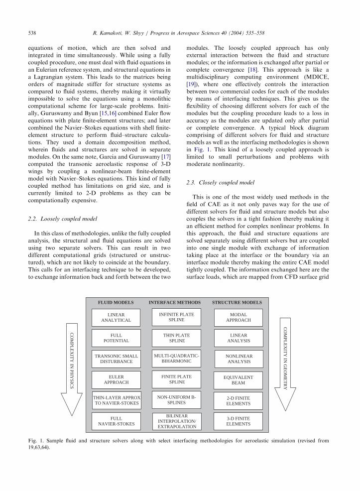
2.2. Loosely coupled model
In this class of methodologies, unlike the fully coupled
analysis, the structural and fluid equations are solved
using two separate solvers. This can result in two
different computational grids (structured or unstruc-
tured), which are not likely to coincide at the boundary.
This calls for an interfacing technique to be developed,
to exchange information back and forth between the two
LINEAR ANALYTICAL
THIN-LAYER APPROX TO NAVIER-STOKES
EULER APPROACH
FULL POTENTIAL
TRANSONIC SMALL DISTURBANCE
FLUID MODELS INTERFACE MET
NON-UNIFORSPLINES
FINITE PLA SPLINE
INFINITE PLSPLINE
THIN PLAT SPLINE
MULTI-QUADRBIHARMON
FULL NAVIER-STOKES
BILINEARINTERPOLATEXTRAPOLA
CO
MPL
EX
ITY
IN PH
YSIC
S
Fig. 1. Sample fluid and structure solvers along with select interf
19,63,64).
modules. The loosely coupled approach has only
external interaction between the fluid and structure
modules; or the information is exchanged after partial or
complete convergence [18]. This approach is like a
multidisciplinary computing environment (MDICE,
[19]), where one effectively controls the interaction
between two commercial codes for each of the modules
by means of interfacing techniques. This gives us the
flexibility of choosing different solvers for each of the
modules but the coupling procedure leads to a loss in
accuracy as the modules are updated only after partial
or complete convergence. A typical block diagram
comprising of different solvers for fluid and structure
models as well as the interfacing methodologies is shown
in Fig. 1. This kind of a loosely coupled approach is
limited to small perturbations and problems with
moderate nonlinearity.
2.3. Closely coupled model
This is one of the most widely used methods in the
field of CAE as it not only paves way for the use of
different solvers for fluid and structure models but also
couples the solvers in a tight fashion thereby making it
an efficient method for complex nonlinear problems. In
this approach, the fluid and structure equations are
solved separately using different solvers but are coupled
into one single module with exchange of information
taking place at the interface or the boundary via an
interface module thereby making the entire CAE model
tightly coupled. The information exchanged here are the
surface loads, which are mapped from CFD surface grid
LINEAR ANALYSIS
MODAL APPROACH
3-D FINITE ELEMENTS
2-D FINITE ELEMENTS
EQUIVALENT BEAM
HODS STRUCTURE MODELS
M B-
TE
ATE
E
ATIC-IC
NONLINEAR ANALYSIS
ION/
TION
CO
MPL
EX
ITY
IN G
EO
ME
TR
Y
acing methodologies for aeroelastic simulation (revised from
ARTICLE IN PRESSR. Kamakoti, W. Shyy / Progress in Aerospace Sciences 40 (2004) 535–558 539
onto the structure dynamics grid; and the displacement
field, which are mapped from structure dynamics grid
onto CFD surface grid. The transfer of surface
displacement back to the CFD module implies deforma-
tion of the CFD surface mesh and this calls for a moving
boundary technique to enable re-meshing the entire
CFD domain as we march in time. This can cause
potential problems for multi-block grids with complex
geometries and will be looked at in-depth in the
forthcoming sections.
Several models have been combined for individual
modules to arrive at a closely coupled model. From the
fluids perspective, models ranging from simple potential
flow models to complex 3-D RANS models have been
used. On the other hand, models ranging from linear
beam finite elements to nonlinear solid finite elements
have been used for structure module. The fluid and
structure models are interlinked via necessary interfa-
cing techniques, the complexity of which depends on
what two models are used for the individual modules. A
brief summary of some of the models that have been
developed in the past will be described next.
Cunningham et al. [20] developed a computational
scheme to perform transonic aeroelastic analysis by
coupling TSD potential flow equations (CAP-TSD) with
the natural vibrational modes of the structure. Viscous
effects were later incorporated into the flow solver by
including an inverse integral boundary layer model. The
equations of motion were solved on a sheared Cartesian
grid where the lifting surfaces were modeled as thin
plates. This kind of approach simplified the task of
generating grids and no moving boundary algorithm
was required as the surface velocity boundary condition
was applied at a mean plane. This technique of using
TSD formulation failed in the presence of a strong shock
or when viscous effects were dominant. To overcome
this, Schuster et al. [21] came up with a model that uses a
3-D flow solver coupled with a linear structure model to
study the aeroelastic analysis of a fighter aircraft
(ENS3DAE). Thin layer approximations to the full
three-dimensional compressible RANS equations were
used. The linear generalized mode shapes were used to
model the structure. A Beam-Warming implicit scheme
was employed for temporal integration. A grid motion
algorithm that uses an algebraic shearing technique was
introduced to account for the grid movement. A similar
method (CFL3DAE), developed by Lee-Rausch and
Batina [7,9], couples a linear, normal mode structural
dynamics model with the thin-layer three-dimensional
compressible RANS model. Time marching was accom-
plished by means of a second order accurate backward
time differencing scheme. A pseudo-time sub-iteration
method was introduced to expedite the convergence at
each time step. A moving mesh algorithm based on
spring analogy was used here. This model was used
to predict the wing flutter boundary. Reviews of the
above-mentioned models, such as, CAP-TSD,
ENS3DAE and CFL3DAE, have been reviewed by
Bennett and Edwards [22] and Huttsell et al. [23].
Liu et al. [11,24] presented an integrated CFD–CSD
code for flutter calculations based on a parallel, multi-
block, multi-grid flow solver for solving the full
Navier–Stokes equations. The flow solver is strongly
coupled with the structural modal dynamics equations.
A dual time-stepping scheme was introduced to enable
simultaneous integration of flow and structural equa-
tions without a time delay. A moving mesh method
based on transfinite interpolation (TFI, [25]) and spring
analogy [26] was also incorporated in the code. Message
passing interface (MPI) was used to enable data transfer
between the two modules. The method was used to
perform static aeroelastic analysis and wing flutter
computations on the AGARD 445.6 wing [11,27].
A three-field formulation for solving transient non-
linear aeroelastic problems was suggested by Farhat et
al. [28] where they used an Arbitrary Lagrangian and
Eulerian (ALE) method for solving the equations on a
deforming mesh system. In the case of ALE formula-
tion, separate set of equations are specified for grid
movement that are directly coupled with the ALE flow
equations. The fluid and structure equations are coupled
by the interface conditions. Unstructured meshes were
used for both fluid and structure solver. Farhat and
Lesoinne [29] improved upon the existing serial and
parallel algorithms for nonlinear transient aeroelastic
problems.
Recently, Kamakoti et al. [12,13] developed a closely
coupled CAE model based on a three-dimensional,
multi-block, structured CFD solver for the RANS
equations. Structural modal dynamic equations were
solved simultaneously and were strongly coupled with
the flow equations using fully implicit (iterative) and
semi-implicit (non-iterative) time-marching methods. A
linear structure model based on beam finite elements was
employed to perform flutter analysis on the AGARD
445.6 wing. The flow solver used was based on the full 3-
D RANS equations with well-validated turbulence
models. A suitable method to evaluate Jacobians via
the geometric conservation law was invoked in the
model as well. The solver also has capabilities to include
effects for multi-block moving boundary treatment
based on master/slave concepts and transfinite inter-
polation techniques. Robust interfacing techniques were
also embedded in the coupled solver to account for
transfer of information between the two modules.
3. Fluid solver
In this section, the description of the flow solver,
including the governing equations and overview of
ARTICLE IN PRESSR. Kamakoti, W. Shyy / Progress in Aerospace Sciences 40 (2004) 535–558540
different algorithms for steady and unsteady flows, is
presented.
3.1. Governing equations for fluid equations
The three-dimensional compressible Navier–Stokes
equations in curvilinear coordinates, written in strong
conservative form, read as follows
qðJrÞqt
þqqx
ðrUÞ þqqZ
ðrV Þ þqqz
ðrW Þ ¼ 0, (3)
qðJruÞ
qtþ
qqx
ðrUuÞ þqqZ
ðrVuÞ þqqz
ðrWuÞ
¼ � f 11qp
qxþ f 21
qp
qZþ f 31
qp
qz
� �
þqqx
GJ
q11qu
qxþ q12
qu
qZþ q13
qu
qz
� �� �
þqqZ
GJ
q21qu
qxþ q22
qu
qZþ q23
qu
qz
� �� �
þqqz
GJ
q31qu
qxþ q32
qu
qZþ q33
qu
qz
� �� �, ð4Þ
qðJrvÞ
qtþ
qqx
ðrUvÞ þqqZ
ðrVvÞ þqqz
ðrWvÞ
¼ � f 12qp
qxþ f 22
qp
qZþ f 32
qp
qz
� �
þqqx
GJ
q11qv
qxþ q12
qv
qZþ q13
qv
qz
� �� �
þqqZ
GJ
q21qv
qxþ q22
qv
qZþ q23
qv
qz
� �� �
þqqz
GJ
q31qv
qxþ q32
qv
qZþ q33
qv
qz
� �� �, ð5Þ
qðJrwÞ
qtþ
qqx
ðrUwÞ þqqZ
ðrVwÞ þqqz
ðrWwÞ
¼ � f 13qp
qxþ f 23
qp
qZþ f 33
qp
qz
� �
þqqx
GJ
q11qw
qxþ q12
qw
qZþ q13
qw
qz
� �� �
þqqZ
GJ
q21qw
qxþ q22
qw
qZþ q23
qw
qz
� �� �
þqqz
GJ
q31qw
qxþ q32
qw
qZþ q33
qw
qz
� �� �, ð6Þ
qðJrHÞ
qtþ
qqx
ðrUHÞ þqqZ
ðrVHÞ þqqz
ðrWHÞ
¼qqx
Gh
Jq11
qh
qxþ q12
qh
qZþ q13
qh
qz
� �� �
þqqZ
Gh
Jq21
qh
qxþ q22
qh
qZþ q23
qh
qz
� �� �
þqqz
Gh
Jq31
qh
qxþ q32
qh
qZþ q33
qh
qz
� �� �
þqqx
Gk
Jq11
qk
qxþ q12
qk
qZþ q13
qk
qz
� �� �
þqqZ
Gk
Jq21
qk
qxþ q22
qk
qZþ q23
qk
qz
� �� �
þqqz
Gk
Jq31
qk
qxþ q32
qk
qZþ q33
qk
qz
� �� �þ F, ð7Þ
where, u is the Cartesian velocity component, p is the
pressure, H is the stagnation enthalpy, h is the specific
enthalpy, G accounts for viscosity and F is the
dissipation function.
q11 ¼ f 211 þ f 212 þ f 213,
q12 ¼ q21 ¼ f 11f 21 þ f 12f 22 þ f 13f 23,
q22 ¼ f 221 þ f 222 þ f 223,
q13 ¼ q31 ¼ f 11f 31 þ f 12f 32 þ f 13f 31,
q33 ¼ f 231 þ f 232 þ f 233,
q23 ¼ q32 ¼ f 31f 21 þ f 32f 22 þ f 13f 23, ð8Þ
where f ij ’s are the metric terms arising from the
transformation of coordinates from Cartesian to curvi-
linear system, and J is the Jacobian given by
J ¼ xxyZzz þ xzyxizZ þ xZyzzx
� xxyzzx � xzyZzx � xZyxzz. ð9Þ
Here, U, V and W are the components of the
contravariant velocity, given by
U ¼ f 11ðu � _xÞ þ f 12ðv � _yÞ þ f 13ðw � _zÞ,
V ¼ f 21ðu � _xÞ þ f 22ðv � _yÞ þ f 23ðw � _zÞ,
W ¼ f 31ðu � _xÞ þ f 32ðv � _yÞ þ f 33ðw � _zÞ, (10)
where _x; _y and _z are the grid velocities that are
approximated by a first-order backward time difference
scheme given by
_x ¼x � x0
Dt_y ¼
y � y0
Dt_z ¼
z � z0
Dt. (11)
Here, Dt is the time step size of the flow solver and the
superscript 0 refers to the previous time step. When
performing computations on a fixed grid, the grid
velocities, _x; _y; and _z; are zero but this is not the casewhile performing computations on a grid that moves
with respect to time. In such cases, care must be taken to
preserve the geometric conservation law (GCL) as
originally formulated by Thomas and Lombard [30].
This will be discussed at length shortly.
ARTICLE IN PRESSR. Kamakoti, W. Shyy / Progress in Aerospace Sciences 40 (2004) 535–558 541
3.2. Navier–Stokes fluid flow solver
Several algorithms have been developed in the past to
solve the governing equations pertaining to fluids. A
time-linearized or dynamically linear model was initially
employed, in which a steady-state nonlinear solution is
used as a starting point; then a small dynamic
perturbation about this steady flow is considered, and
all subsequent flow variables and shock motion are
assumed to vary in a linear fashion. This model leads to
an order of magnitude reduction in computer resources
compared to the nonlinear model, and was found to be
sufficient for many problems. However, this method was
found to be less useful for turbomachinery problems.
This approach was then extended to determine a full
dynamically nonlinear solution, which involves solving a
nonlinear convected-wave equation for potential flow or
Euler or Navier–Stokes models. Either finite-difference
or finite-volume schemes in spatial variables was used to
convert the system of partial difference equations to
ordinary differential equations. Additional models must
be developed to account for turbulence flow features,
and for transition from laminar to turbulent flows.
Typically, algorithms for the Navier–Stokes equations
[32,33] can be broadly classified into either density- or
pressure-based methods. For both of these approaches,
the velocity field is obtained via the momentum
equations. In density-based methods, the continuity
equation is used to obtain density and the pressure is
extracted through the equation of state. It is usually
employed for compressible flows when the density is not
a constant in the continuity equation. The system of
equations is usually solved simultaneously. This method
can be extended to incompressible flows as well for low
Mach number regime. On the other hand; the pressure-
based method was initially developed for incompressible
flows [34]. In this method, the pressure is obtained via a
pressure or a pressure correction equation, which is
formulated by manipulating the continuity and momen-
tum equations.
The solution procedure for pressure-based methods is
typically sequential in nature, and hence, can adapt to a
varying number of equations without reformulating the
entire algorithm. This method can be extended to
compressible flows by taking into account the depen-
dence of density on pressure through the equation of
state [33,35]. One of the algorithms that were originally
developed for these pressure-based flow solvers was
based on SIMPLE (Semi-implicit pressure-linked equa-
tions) family of algorithms [31]. This method was
originally developed for incompressible flows and it
has been extended to solve compressible flows by
modifying the pressure correction equation to include
the effects of density on pressure [36]. Additionally, the
algorithm has been extended to body-fitted curvilinear
coordinates in order to handle arbitrarily-shaped flow
boundaries. This approach can handle flows at all speeds
without any fundamentally different treatment for any
particular flow regime. This procedure was found to be
an efficient method predominantly for steady state
computations. A modification to the SIMPLE algo-
rithm, SIMPLEC (SIMPLE-Consistent, [33]), was found
to be a robust algorithm for steady-state computations
as well. It is very similar to the SIMPLE algorithm
except for some less-significant terms omitted in the
velocity correction equations. This family of algorithms
can be extended for unsteady flow computations in a
straightforward manner using time-stepping schemes
such as the implicit or explicit Euler scheme, the
Crank–Nicolson scheme, etc. But the iterative nature
of the SIMPLE algorithm within a given time step can
make the procedure very time-consuming for unsteady
computations. An efficient method for unsteady com-
putations was proposed by Issa [37]. It is based on an
operator-splitting procedure such as the Pressure-Im-
plicit Splitting of Operators (PISO) algorithm. It was
initially proposed for Cartesian grids and primarily for
incompressible flows. It was later modified to include
compressibility effects and reformulated in curvilinear
coordinates [38]. The algorithm involves a series of
predictor and corrector steps to solve for velocity and
other scalar variables by ensuring the fact that the
splitting error is less than the discretization error. This
form of method obviates the need to iterate within a
time step thereby making the algorithm efficient for time
dependent computations. A detailed procedure of the
algorithms can be found in Thakur et al. [35].
Typically, computations can be performed using
either a staggered grid arrangement or a non-staggered
or collocated grid arrangement. In the former arrange-
ment, the velocities are stored at the cell face, rather
than at the cell centers for the collocated arrangement.
This makes the collocated grid system easier to use but it
does require some interpolation procedure to evaluate
the contravariant velocities at the cell faces. One such
interpolation scheme devised is the momentum inter-
polation scheme, proposed by Rhie and Chow [38]. Such
an interpolation scheme was proposed with steady-state
computations in mind. For unsteady computations, the
interpolation procedure introduces the time step size
factor into the formulation and there might be situations
when one might be forced to use a small time step size
based on the stability condition of the time marching
procedure. It has been shown previously [39–41] that a
small time step leads to minor oscillations in pressure
and velocity field while using the original Rhie–Chow
momentum interpolation method. Several authors
[39–41] proposed modified momentum interpolation
schemes to calculate cell-face velocity to eliminate the
effect of time step size on the solution. It was originally
proposed for Cartesian grid systems. Kamakoti et al.
[13] extended the method to make it suitable for
ARTICLE IN PRESSR. Kamakoti, W. Shyy / Progress in Aerospace Sciences 40 (2004) 535–558542
curvilinear grids, which meant calculating contravariant
velocities in an appropriate manner from the Cartesian
velocity components at the cell faces. The method was
validated using both Cartesian and curvilinear grid test
cases and satisfactory results were obtained using both
grids [13].
3.3. The geometric conservation law
While transforming coordinates from Cartesian to
curvilinear systems, the Jacobian matrix is introduced.
The determinant of this Jacobian matrix represents the
cell volume in the transformed coordinates. In moving
grid problems, since the grid moves, this Jacobian
associated with each cell element must be updated in a
consistent fashion. This is done via the geometric
conservation law, originally proposed by Thomas and
Lombard [30]. The GCL is derived from the conserva-
tion of mass by setting r ¼ 1 and v ¼ 0: It can bewritten as
d
dt
ZV
d8 ¼
ZS
ws dS, (12)
where ws is local velocity of cell boundary. The GCL can
be stated as the change in volume of each control
volume between two time instants, tn and tnþ1; must beequal to the volume swept by the cell boundary during
that time Dt ¼ tnþ1 � tn:The above expression is referred to as the integral
form of GCL. A differential statement of the GCL can
be derived from the integral statement of GCL. We first
perform a transformation from the Cartesian coordinate
system (x, y, z) to the body-fitted coordinate system (x;Z; z), which leads to the following form of the integralstatement:
d
dt
ZV
J dxdZdz ¼Z
V
ðr:wsÞJ dxdZdz. (13)
Here, J represents the volume element in the
transformed coordinate system hence each node is
associated with a particular value of J. Therefore, the
computed value of Jmust be consistent with the value of
DV implied by the numerical scheme used for solving the
flow equations. Earlier, arbitrary procedures were used
to compute J, for e.g., instantaneous mesh distribution
at a given time instant was used to evaluate J at that
particular time, which lead to an erroneous solution.
Expanding the right-hand side of Eq. (13) and after
performing necessary manipulations, we arrive at the
following form for the differential statement of GCL.
Jt þ ðxtÞx þ ðZtÞZ þ ðztÞz ¼ 0, (14)
where, xt; Zt; zt are the metric terms given by
xt ¼ �½ _xðyZzz � yzzZÞ þ _yðzZxz � zzxZÞ þ _zðxZyz � xzyZÞ�,
Zt ¼ �½ _xðyzzx � yxzzÞ þ _yðzzxx � zxxzÞ þ _zðxzyx � xxyzÞ�,
zt ¼ �½ _xðyxzZ � yZzxÞ þ _yðzxxZ � zZxxÞ þ _zðxxyZ � xZyxÞ�.
(15)
Eq. (14) is solved numerically to update the Jacobian
values at each time step. It should be noted that since
GCL arises due to the numerical procedures devised
based on grid movement, its implications are expected to
be scheme dependent. Alternative forms of the GCL
have been implemented over the years to study its
impact on solution accuracy. Thomas and Lombard
implemented the GCL for density-based finite difference
schemes on structured meshes by updating the value of
the Jacobian at each time step. Shyy et al. [42,43]
implemented the GCL along the lines of Thomas and
Lombard for pressure-based finite volume schemes by
updating the Jacobian values after every time step using
a first-order backward Euler time-integration scheme.
Lesoinne and Farhat [44] developed a first order, time
accurate scheme preserving the GCL using the density-
based ALE finite volume as well as finite element schemes
on unstructured grids. Koobus and Farhat [45] pro-
posed a GCL scheme for second-order time-accurate
density-based ALE finite volume schemes. Farhat et al.
[46] summarized six different time-integration schemes
based on ALE formulation, some of them preserving the
GCL, and showed the impact the different schemes have
on solution accuracy. In this effort, we assess selected
approaches for multi-block structured grids based on
finite volume formulation and do a comparative study on
these methods. Most previously conducted studies
employed the density-based fluid flow solver; in the
present effort, the pressure-based fluid flow solver
[31,35,42] is utilized. The implications of different
implementation of GCL and the fluid flow solver are
of main interest. In this regard, four different time-
integration schemes for evaluating the Jacobian values
were investigated by Kamakoti and Shyy [47]: first-order
implicit scheme, first-order time-averaged scheme, sec-
ond-order implicit scheme and a second-order time-
averaged scheme. They concluded, using several test
cases [12,13], that a scheme consistent with the choice of
time marching scheme used for flow solver provides the
most accurate and consistent way of evaluating the
Jacobian values.
3.4. Turbulence modeling
The most widely employed two-equation model,
namely, the k-� model is used for turbulent computa-tions. Since the standard k-� model is only valid in fullyturbulent regions, it requires additional modeling near
wall regions or in the no-slip regions. Near wall
boundaries, the local Reynolds number is of the order
of one and hence viscous effects are more dominant,

ARTICLE IN PRESSR. Kamakoti, W. Shyy / Progress in Aerospace Sciences 40 (2004) 535–558 543
hence the k-� model cannot be used as it is formulatedbased on the assumption of high Reynolds number. Two
approaches have been proposed to handle near-wall
effects, one being the low Reynolds number model and
the other being wall-function method [48]. The former
method requires a very fine grid resolution near the wall
and hence makes the computations expensive. The latter
method is based on the assumption that there exists local
equilibrium between production and dissipation of
turbulent kinetic energy. It has been proven to be an
accurate and robust approximation. This technique uses
the law of the wall as the constitutive relation between
the velocity and the surface shear stress. The detailed
formulation of the model can be found in Shyy et al.
[49]. While using wall functions method, we need to
ensure that the node next to the wall boundary is in the
log layer. Since we use a moving grid formulation, we
need to ensure this is the case for all time steps in spite of
grid movement. This is controlled by the rigidity of mesh
movement, which is addressed in the moving grid
algorithm. A variation to the k-� model, a filter-basedk-� model [50], was investigated to improve upon thepredictive capability of the standard k-� two-equationmodel. In RANS computations, the true resolution is
not only dictated by the mesh size but also by the
magnitude of eddy viscosity. These in turn affect the
local Reynolds number, which needs to be Oð1Þ
magnitude in order to resolve the flow structure
satisfactorily. Also, one should note that an excessive
eddy viscosity could smear out the flow structures within
the reach of a grid resolution. In such cases, the effective
viscosity in the model should be reduced to resolve the
structures satisfactorily. To achieve this, a filter is
imposed on the turbulence model via eddy viscosity,
which does not resolve structures smaller than the filter
size. The filter size is chosen based on the maximum grid
size in the domain. Further details about the model can
be found in Johansen et al. [50].
4. Structure solver
There are several ways to model a structure, from 3-D
finite elements to simplified beam elements and modal
analysis [51]. The complexity of the model depends on
the kind of finite element model that one uses and the
number of degrees of freedom associated with the
element. Since the aim of this paper is to address the
interaction of a complex fluid solver with a simplified
structure solver, the structure solver is modeled using
beam finite elements with only linear effects considered
[52]. This simplification allows for a good description of
the motion of the wing, without being computationally
hampered by complex nonlinear effects. Since the wing
is modeled as a linear structure, it is possible to model
the deformations as a summation of different modes of
deformation without looking at the complex interaction
of the modes. To this end, the structure or the wing is
modeled as a linear finite element structure that can
undergo bending and torsion. The Bernoulli–Euler beam
theory is enforced, which means the cross-sections
remain rigid, thereby uncoupling the bending and
torsional displacements.
The linear finite element that we choose to model the
wing is a beam that has mass, stiffness, and damping
matrices of the actual wing. Thus, the deformations
become that of a Bernoulli–Euler beam bending and
torsion, the equations for which reads as
d2
dx2EId2w
dx2
� �¼ f , (16)
where f is the distributed loading (force per unit length)
acting in the same direction as the out-of-plane
displacement (w), E is the Young’s modulus of the
beam, and I is the area moment of inertia of the beam’s
cross section. Since, the cross sections of the wing are
assumed to be rigid, there is a point at which the vertical
displacement of the beam is a result of only the bending
of the wing. This point is where the elastic axis of the
wing intersects the cross section. The generalized
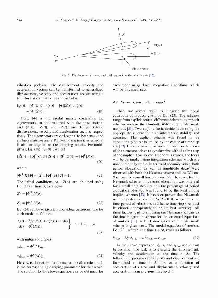
displacements from bending and torsion are measured
from this point. This has been depicted in Fig. 2.
To find the equations of motion, Lagrange’s equation
was used. The equations take the form given by
d
dt
qT
q _q
� ��qT
qqþqV
qq¼ �
qF
q _qþ Q, (17)
where q represents the generalized displacements,
vertical and torsional displacements, F represent the
Rayleigh dissipation function, and Q represents the
generalized forces. The kinetic energy and the potential
energy of the wing are given by T and V, respectively.
The generalized coordinates for the wing are functions
of the position of the cross section along the span of the
wing and time. Here, the generalized coordinates are
referred to as w, representing the classical generalized
coordinates of bending, and y; representing the classicalgeneralized coordinates of torsion. The equations of
motion that govern the structural dynamics of the wing
take the well-known form [53] given by
½M�f €qðtÞg þ ½C�f _qðtÞg þ ½K �fqðtÞg ¼ fRðtÞg, (18)
where RðtÞ is a vector containing the aerodynamic forces
associated with aerodynamic loads; and fqðtÞg; f _qðtÞg;and f €qðtÞg are the displacement, velocity and accelerationvectors of the finite element assembly, respectively.
4.1. Modal equations of motion
The equation of motion of the structure, given by
Eq. (18), can be solved using modal approach by
composing the solution with the eigenvectors of the
ARTICLE IN PRESS
Z
Xw (y,t)
θ (y,t)
Elastic Axis
Fig. 2. Displacements measured with respect to the elastic axis [12].
R. Kamakoti, W. Shyy / Progress in Aerospace Sciences 40 (2004) 535–558544
vibration problem. The displacement, velocity and
acceleration vectors can be transformed to generalized
displacement, velocity and acceleration vectors using a
transformation matrix, as shown below
fqðtÞg ¼ ½F�fZðtÞg; f _qðtÞg ¼ ½F�f _ZðtÞg; f €qðtÞg
¼ ½F�f €ZðtÞg. ð19Þ
Here, ½F� is the modal matrix containing the
eigenvectors, orthonormalized with the mass matrix,
and fZðtÞg; f _ZðtÞg; and f €ZðtÞg are the generalized
displacement, velocity and acceleration vectors, respec-
tively. The eigenvectors are orthogonal to both mass and
stiffness matrices and if Rayleigh damping is assumed, it
is also orthogonal to the damping matrix. Pre-multi-
plying Eq. (18) by ½F�T; we get
f €ZðtÞg þ ½F�T½C�½F�f _ZðtÞg þ ½O2�fZðtÞg ¼ ½F�TfRðtÞg,
(20)
where
½F�T½K�½F� ¼ ½O2�; ½F�T½M�½F� ¼ 1. (21)
The initial conditions on fZðtÞg are obtained using
Eq. (19) at time 0, as follows
Z0 ¼ ½F�T½M�q0,
_Z0 ¼ ½F�T½M� _q0. (22)
Eq. (20) can be written as n individual equations, one for
each mode, as follows
€ziðtÞ þ 2xioi €ziðtÞ þ o2i ziðtÞ ¼ riðtÞ
riðtÞ ¼ FTi fRðtÞg
)i ¼ 1; 2; . . . ; n
(23)
with initial conditions
xijt¼0 ¼ FTi ½M�q0,
_xijt¼0 ¼ FTi ½M� _q0. (24)
Here oi is the natural frequency for the ith mode and xi
is the corresponding damping parameter for that mode.
The solution to the above equation can be obtained for
each mode using direct integration algorithms, which
will be discussed next.
4.2. Newmark integration method
There are several ways to integrate the modal
equations of motion given by Eq. (23). The schemes
range from explicit central difference schemes to implicit
schemes such as the Houbolt, Wilson-y and Newmarkmethods [53]. Two major criteria decide in choosing the
appropriate scheme for time integration: stability and
accuracy. The explicit scheme was found to be
conditionally stable is limited by the choice of time step
size [52]. Hence, one may be forced to perform iterations
of the structure solver to synchronize with the time step
of the implicit flow solver. Due to this reason, the focus
will be on implicit time integration schemes, which are
unconditionally stable. In terms of accuracy issues, both
period elongation as well as amplitude decay were
observed with both the Houbolt scheme and the Wilson-
y scheme for a small time step size [53]. However, for theNewmark scheme, only period elongation was observed
for a small time step size and the percentage of period
elongation observed was found to be the least among
implicit schemes [53]. It has been proven that Newmark
method performs best for Dt=To0:01; where T is the
time period of vibrations and hence time step size must
be chosen appropriately to obtain best accuracy. All
these factors lead to choosing the Newmark scheme as
the time integration scheme for the structural equations
of motion [13]. A brief description of the Newmark
scheme is given next. The modal equation of motion,
Eq. (23), written at a time t þ Dt; reads as follows
€ztþDt þ 2xo€ztþDt þ o2ztþDt ¼ rtþDt. (25)
In the above expression, x; o; and rtþDt are known
beforehand. The task is to evaluate the displacement,
velocity and acceleration at the time t þ Dt: Thefollowing expressions for velocity and displacement are
formulated at time t þ Dt first as a function of
acceleration at t þ Dt and displacement, velocity and
acceleration from previous time level t.
ARTICLE IN PRESSR. Kamakoti, W. Shyy / Progress in Aerospace Sciences 40 (2004) 535–558 545
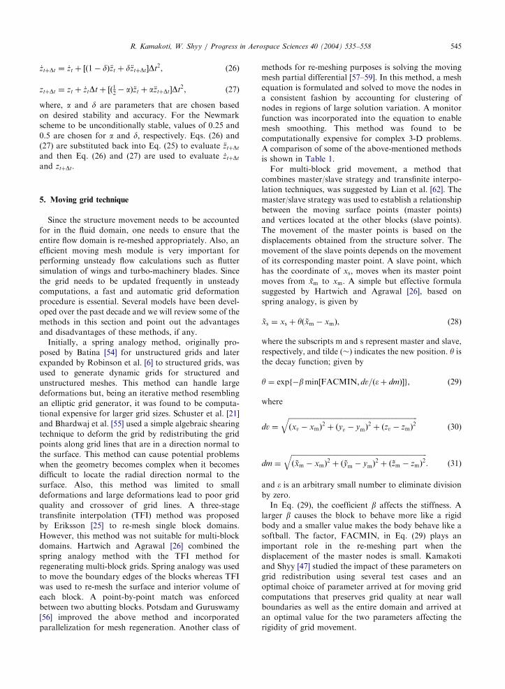
_ztþDt ¼ _zt þ ½ð1� dÞ€zt þ d€ztþDt�Dt2, (26)
ztþDt ¼ zt þ _ztDt þ ½ð12� aÞ€zt þ a€ztþDt�Dt2, (27)
where, a and d are parameters that are chosen basedon desired stability and accuracy. For the Newmark
scheme to be unconditionally stable, values of 0.25 and
0.5 are chosen for a and d; respectively. Eqs. (26) and(27) are substituted back into Eq. (25) to evaluate €ztþDt
and then Eq. (26) and (27) are used to evaluate _ztþDt
and ztþDt:
5. Moving grid technique
Since the structure movement needs to be accounted
for in the fluid domain, one needs to ensure that the
entire flow domain is re-meshed appropriately. Also, an
efficient moving mesh module is very important for
performing unsteady flow calculations such as flutter
simulation of wings and turbo-machinery blades. Since
the grid needs to be updated frequently in unsteady
computations, a fast and automatic grid deformation
procedure is essential. Several models have been devel-
oped over the past decade and we will review some of the
methods in this section and point out the advantages
and disadvantages of these methods, if any.
Initially, a spring analogy method, originally pro-
posed by Batina [54] for unstructured grids and later
expanded by Robinson et al. [6] to structured grids, was
used to generate dynamic grids for structured and
unstructured meshes. This method can handle large
deformations but, being an iterative method resembling
an elliptic grid generator, it was found to be computa-
tional expensive for larger grid sizes. Schuster et al. [21]
and Bhardwaj et al. [55] used a simple algebraic shearing
technique to deform the grid by redistributing the grid
points along grid lines that are in a direction normal to
the surface. This method can cause potential problems
when the geometry becomes complex when it becomes
difficult to locate the radial direction normal to the
surface. Also, this method was limited to small
deformations and large deformations lead to poor grid
quality and crossover of grid lines. A three-stage
transfinite interpolation (TFI) method was proposed
by Eriksson [25] to re-mesh single block domains.
However, this method was not suitable for multi-block
domains. Hartwich and Agrawal [26] combined the
spring analogy method with the TFI method for
regenerating multi-block grids. Spring analogy was used
to move the boundary edges of the blocks whereas TFI
was used to re-mesh the surface and interior volume of
each block. A point-by-point match was enforced
between two abutting blocks. Potsdam and Guruswamy
[56] improved the above method and incorporated
parallelization for mesh regeneration. Another class of
methods for re-meshing purposes is solving the moving
mesh partial differential [57–59]. In this method, a mesh
equation is formulated and solved to move the nodes in
a consistent fashion by accounting for clustering of
nodes in regions of large solution variation. A monitor
function was incorporated into the equation to enable
mesh smoothing. This method was found to be
computationally expensive for complex 3-D problems.
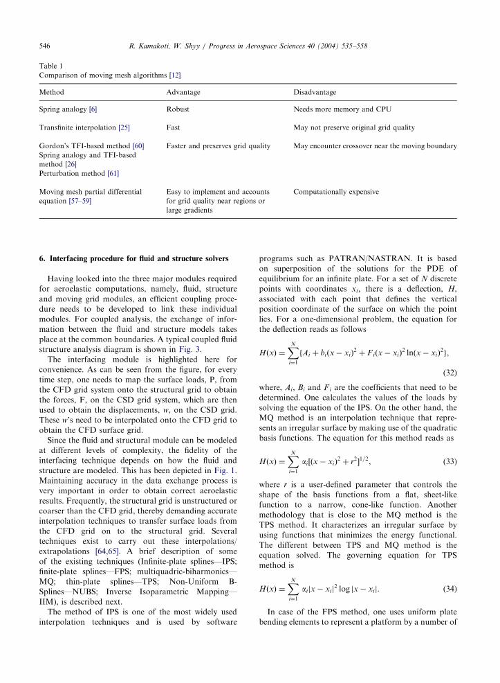
A comparison of some of the above-mentioned methods
is shown in Table 1.
For multi-block grid movement, a method that
combines master/slave strategy and transfinite interpo-
lation techniques, was suggested by Lian et al. [62]. The
master/slave strategy was used to establish a relationship
between the moving surface points (master points)
and vertices located at the other blocks (slave points).
The movement of the master points is based on the
displacements obtained from the structure solver. The
movement of the slave points depends on the movement
of its corresponding master point. A slave point, which
has the coordinate of xs; moves when its master pointmoves from x̄m to xm: A simple but effective formulasuggested by Hartwich and Agrawal [26], based on
spring analogy, is given by
~xs ¼ xs þ yð ~xm � xmÞ, (28)
where the subscripts m and s represent master and slave,
respectively, and tilde ( ) indicates the new position. y isthe decay function; given by
y ¼ expf�bmin½FACMIN; dv=ð�þ dmÞ�g, (29)
where
dv ¼
ffiffiffiffiffiffiffiffiffiffiffiffiffiffiffiffiffiffiffiffiffiffiffiffiffiffiffiffiffiffiffiffiffiffiffiffiffiffiffiffiffiffiffiffiffiffiffiffiffiffiffiffiffiffiffiffiffiffiffiffiffiffiffiffiffiffiffiffiffiffiffiffiffiffiðxv � xmÞ
2þ ðyv � ymÞ
2þ ðzv � zmÞ
2
q(30)
dm ¼
ffiffiffiffiffiffiffiffiffiffiffiffiffiffiffiffiffiffiffiffiffiffiffiffiffiffiffiffiffiffiffiffiffiffiffiffiffiffiffiffiffiffiffiffiffiffiffiffiffiffiffiffiffiffiffiffiffiffiffiffiffiffiffiffiffiffiffiffiffiffiffiffiffiffiffiffiffiffið ~xm � xmÞ
2þ ð ~ym � ymÞ
2þ ð~zm � zmÞ
2
q. (31)
and � is an arbitrary small number to eliminate divisionby zero.
In Eq. (29), the coefficient b affects the stiffness. Alarger b causes the block to behave more like a rigidbody and a smaller value makes the body behave like a
softball. The factor, FACMIN, in Eq. (29) plays an
important role in the re-meshing part when the
displacement of the master nodes is small. Kamakoti
and Shyy [47] studied the impact of these parameters on
grid redistribution using several test cases and an
optimal choice of parameter arrived at for moving grid
computations that preserves grid quality at near wall
boundaries as well as the entire domain and arrived at
an optimal value for the two parameters affecting the
rigidity of grid movement.
ARTICLE IN PRESS
Table 1
Comparison of moving mesh algorithms [12]
Method Advantage Disadvantage
Spring analogy [6] Robust Needs more memory and CPU
Transfinite interpolation [25] Fast May not preserve original grid quality
Gordon’s TFI-based method [60] Faster and preserves grid quality May encounter crossover near the moving boundary
Spring analogy and TFI-based
method [26]
Perturbation method [61]
Moving mesh partial differential
equation [57–59]
Easy to implement and accounts
for grid quality near regions or
large gradients
Computationally expensive
R. Kamakoti, W. Shyy / Progress in Aerospace Sciences 40 (2004) 535–558546
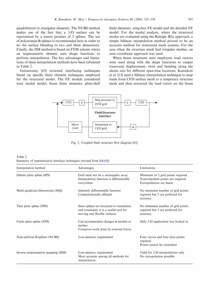
6. Interfacing procedure for fluid and structure solvers
Having looked into the three major modules required
for aeroelastic computations, namely, fluid, structure
and moving grid modules, an efficient coupling proce-
dure needs to be developed to link these individual
modules. For coupled analysis, the exchange of infor-
mation between the fluid and structure models takes
place at the common boundaries. A typical coupled fluid
structure analysis diagram is shown in Fig. 3.
The interfacing module is highlighted here for
convenience. As can be seen from the figure, for every
time step, one needs to map the surface loads, P, from
the CFD grid system onto the structural grid to obtain
the forces, F, on the CSD grid system, which are then
used to obtain the displacements, w, on the CSD grid.
These w’s need to be interpolated onto the CFD grid to
obtain the CFD surface grid.
Since the fluid and structural module can be modeled
at different levels of complexity, the fidelity of the
interfacing technique depends on how the fluid and
structure are modeled. This has been depicted in Fig. 1.
Maintaining accuracy in the data exchange process is
very important in order to obtain correct aeroelastic
results. Frequently, the structural grid is unstructured or
coarser than the CFD grid, thereby demanding accurate
interpolation techniques to transfer surface loads from
the CFD grid on to the structural grid. Several
techniques exist to carry out these interpolations/
extrapolations [64,65]. A brief description of some
of the existing techniques (Infinite-plate splines—IPS;
finite-plate splines—FPS; multiquadric-biharmonics—
MQ; thin-plate splines—TPS; Non-Uniform B-
Splines—NUBS; Inverse Isoparametric Mapping—
IIM), is described next.
The method of IPS is one of the most widely used
interpolation techniques and is used by software
programs such as PATRAN/NASTRAN. It is based
on superposition of the solutions for the PDE of
equilibrium for an infinite plate. For a set of N discrete
points with coordinates xi; there is a deflection, H,
associated with each point that defines the vertical
position coordinate of the surface on which the point
lies. For a one-dimensional problem, the equation for
the deflection reads as follows
HðxÞ ¼XN
i¼1
fAi þ biðx � xiÞ2þ Fiðx � xiÞ
2 lnðx � xiÞ2g,
(32)
where, Ai; Bi and Fi are the coefficients that need to be
determined. One calculates the values of the loads by
solving the equation of the IPS. On the other hand, the
MQ method is an interpolation technique that repre-
sents an irregular surface by making use of the quadratic
basis functions. The equation for this method reads as
HðxÞ ¼XN
i¼1
ai½ðx � xiÞ2þ r2�1=2, (33)
where r is a user-defined parameter that controls the
shape of the basis functions from a flat, sheet-like
function to a narrow, cone-like function. Another
methodology that is close to the MQ method is the
TPS method. It characterizes an irregular surface by
using functions that minimizes the energy functional.
The different between TPS and MQ method is the
equation solved. The governing equation for TPS
method is
HðxÞ ¼XN
i¼1
aijx � xij2 log jx � xij. (34)
In case of the FPS method, one uses uniform plate
bending elements to represent a platform by a number of
ARTICLE IN PRESSR. Kamakoti, W. Shyy / Progress in Aerospace Sciences 40 (2004) 535–558 547
quadrilateral or triangular elements. The NUBS method
makes use of the fact that a 3-D surface can be
represented by a tensor product of 2 splines. The use
of polynomial B-splines is recommended here in order to
do the surface blending in two and three dimensions.
Finally, the IIM method is based on FEM scheme where
an isoparametric element uses shape functions to
perform interpolation. The key advantages and limita-
tions of these interpolation methods have been tabulated
in Table 2.
Guruswamy [63] reviewed interfacing techniques
based on specific finite element techniques employed
for the structural model. The FE models considered
were modal model, beam finite elements, plate/shell
Table 2
Summary of representative interface techniques (revised from [64,65])
Interpolation method Advantages
Infinite plate spline (IPS) Grid need not be a rec
Interpolation function
everywhere
Multi-quadratic-biharmonic (MQ) Infinitely differentiable
Computationally efficie
Thin plate spline (TPS) Since splines are invaria
and rotational, it is a u
moving and flexible su
Finite plate spline (FPS) Can accommodate chan
meshes
Conserves work done b
Non-uniform B-splines (NUBS) Low-memory requirem
Inverse isoparametric mapping (IIM) Low-memory requirem
Most accurate among
interpolation
CFD P Map pressuFEM grid
InterpolateCFD grid
Move Grid
Fluid/StruInterfac
Fig. 3. Coupled fluid–struct
finite elements, wing-box FE model and the detailed FE
model. For the modal analysis, where the structural
modes are evaluated using the Raleigh–Ritz approach, a
simple bilinear interpolation method proved to be an
accurate method for structured mesh systems. For the
case when the structure mesh had irregular meshes, an
area coordinate approach was used.
When beam structures were employed, load vectors
were used along with the shape functions to output
transverse displacement, twist and bending along the
elastic axis for different span-wise locations. Kamakoti
et al. [13] used a bilinear interpolation technique to map
loads from CFD surface mesh to a temporary structure
mesh and then extracted the load vector on the beam
Limitations
tangular array Minimum of 3 grid points required
is differentiable Noncoincident points are required
Extrapolations are linear
function
nt
No minimum number of grid points
required but 3 are preferred for
accuracy
nt to translation
seful tool for
rfaces
No minimum number of grid points
required but 3 are preferred for
accuracy
ges in models or Only 2-D application was looked at
y external forces
ent Four curves and four data points
required
Points cannot be coincident
ent Valid for 2-D interpolations only
all methods for No extrapolation possible
Fre to
to
CSD
cture e
W
ure flow diagram [63].
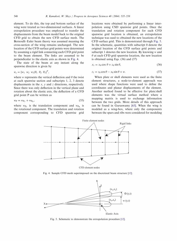
ARTICLE IN PRESSR. Kamakoti, W. Shyy / Progress in Aerospace Sciences 40 (2004) 535–558548
element. To do this, the top and bottom surface of the
wing were treated as two-dimensional surfaces. A linear
extrapolation procedure was employed to transfer the
displacements from the beam model back to the original
CFD grid to obtain the new CFD surface mesh. The
Bernoulli–Euler beam theory was assumed meaning the
cross-section of the wing remains unchanged. The new
location of the CFD surface grid points were determined
by assuming a rigid link connecting each CFD grid point
to the beam element. The links are assumed to be
perpendicular to the elastic axis as shown in Fig. 4.
The state of the beam at any instant along the
spanwise direction is given by
ws ¼ fw1 w2 w3jy1 y2 y3gT,
where w represents the vertical deflection and y the twistat each spanwise section and subscripts 1, 2, 3 denote
displacements in the x, y and z directions, respectively.
Since there was only deflection in the vertical plane and
rotation about the elastic axis, the deflection of a CFD
grid point P can be written as
wP ¼ wPT þ wPR , (35)
where wPT is the translation component and wPR is
the rotational component. The translation and rotation
component corresponding to CFD spanwise grid
X
Fig. 5. Schematic to demonstrate th
Finite el
CFD eleme
. . .
...
. . .
Fig. 4. Sample CFD mesh superimposed o
locations were obtained by performing a linear inter-
polation using CSD spanwise grid points. Once the
translation and rotation component for each CFD
spanwise grid location is obtained, an extrapolation
technique was used to obtained the new locations of the
CFD surface grid. This is demonstrated through Fig. 5.
In the schematic, quantities with subscript 0 denote the
original location of the CFD surface grid points and
subscript 1 denotes the new location. By knowing w and
y at each CFD grid spanwise location, the new locationis obtained using Eqs. (36) and (37)
x1 ¼ x0 cos yþ z0 sin y, (36)
z1 ¼ z0 cos y� x0 sin yþ w. (37)
When plate or shell elements were used as the finite
element structures, a node-to-element approach was
used where shape functions were used to define the
coordinates and planar displacements of the element.
Another method found to be effective for plate/shell
elements was the virtual surface method where a
mapping matrix is used to exchange information
between the two grids. More details of this approach
can be found in Guruswamy [63]. When the wing is
modeled as a wing-box, where only the components
between the spars and ribs were considered for modeling
Z
w (y,t)
Θ (y,t)
(xo,zo)
(x1,z1)
Elastic Axis
e extrapolation procedure [12].
ement nodes
nt nodes
Rigid links
. . . .
...
. . . .
n the discretized beam structure [12].
ARTICLE IN PRESSR. Kamakoti, W. Shyy / Progress in Aerospace Sciences 40 (2004) 535–558 549
purposes, a discrepancy might occur as there is a
discontinuity in surface at the leading and trailing
edges. In such cases, forces were lumped onto structural
nodes and bending and twisting moment conservation
is enforced. Deflection at the FEM nodes were
obtained by using transformation functions by assuming
that the wing is chordwise rigid. Brown [66] proposed a
method that combines the node-to-element approach
used for plate/shell FE and the lumped method for
wing-box structures. For detailed FE models, where
the interior of the FE grid could be irregular and
the surface elements could take both triangular and
quadrilateral elements, the area coordinate method
of the virtual surface method was found to be an
efficient one.
7. Aeroelastic computations using AGARD 445.6 wing
In this section, the computational procedure, includ-
ing the computational setup, for performing fluid–struc-
ture interaction computations will be discussed. The
different methodologies will be discussed by applying
the methodology to predict the flutter boundary for a
three-dimensional wing geometry.
7.1. Computational procedure
The overall procedure for carrying out computational
aeroelastic computations can be divided into the
following major steps.
1.
Constructing the geometry for aeroelastic computa-tions and also to supply appropriate boundary
conditions and initial conditions.
2.
Perform steady-state CFD computation to obtaininitial guess for starting coupled computations.
3.
Perform unsteady CFD computations using steadystate result as initial guess and obtain necessary
aerodynamic forces on the surface of the wing.
4.
Map aerodynamic forces onto the structural mesh.5.
Perform CSD computation to obtain the deformationof the geometry.
6.
Map the displacements onto CFD surface grid.7.
Re-mesh CFD grid based on the deformationobtained from the CSD calculations using the moving
boundary module.
8.
Repeat steps 3–7 using current solution as the initialguess for the subsequent steps.
A closer look at the above-mentioned steps along with
the grid generation details and time scale issues
concerned with the different solvers will be looked
at next.
7.2. Computational setup
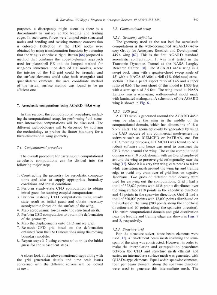
7.2.1. Geometry definition
The geometry used as the test bed for aeroelastic
computations is the well-documented AGARD (Advi-
sory Group for Aerospace Research and Development)
445.6 wing [67]. This is the first AGARD standard
aeroelastic configuration. It was first tested in the
Transonic Dynamics Tunnel at the NASA Langley
Research Center [68]. The AGARD 445.6 wing is a
swept back wing with a quarter-chord sweep angle of
45� with a NACA 65A004 airfoil (4% thickness) cross-
section. It has a panel aspect ratio of 1.65 and a taper
ratio of 0.66. The root chord of this model is 1.833 feet
with a semi-span of 2.5 feet. The wing tested at NASA
Langley was a semi-span, wall-mounted model made
with laminated mahogany. A schematic of the AGARD
wing is shown in Fig. 6.
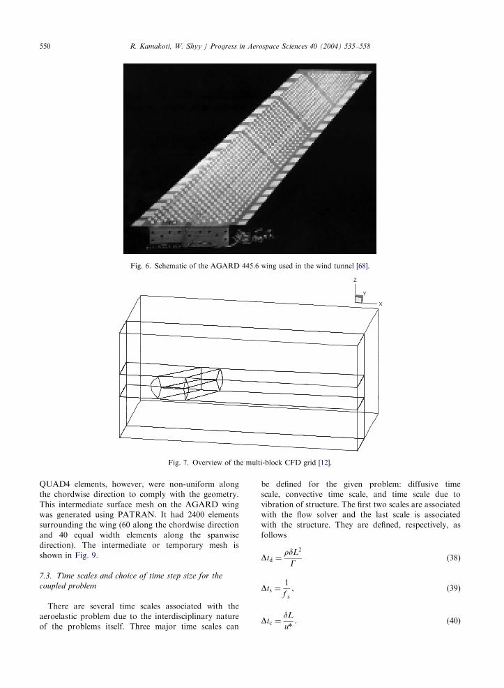
7.2.2. CFD grid
A CFD mesh is generated around the AGARD 445.6
wing by placing the wing in the middle of the
computational domain, which has dimensions of 18�
9� 9 units. The geometry could be generated by using
the CAD module of any commercial mesh-generating
software such as ICEMCFD or PATRAN, etc. For
CFD meshing purposes, ICEMCFD was found to be a
robust software and hence was used to construct the
CFD mesh around the wing. The entire computational
domain was a 10 block domain with an O-grid employed
around the wing to preserve grid orthogonality near the
wing [12]. Since it is a very thin wing, care needs to taken
while generating mesh around the wing tip and trailing
edge to avoid any cross-over of grid lines or negative
Jacobians. Two grids of different mesh density were
used for carrying out the computations: Grid I had a
total of 322,622 points with 4838 points distributed over
the wing surface (118 points in the chordwise direction
and 41 points in the spanwise direction); Grid II had a
total of 800,000 points with 12,000 points distributed on
the surface of the wing (200 points along the chordwise
direction and 60 points along the spanwise direction).
The entire computational domain and grid distribution
near the leading and trailing edges are shown in Figs. 7
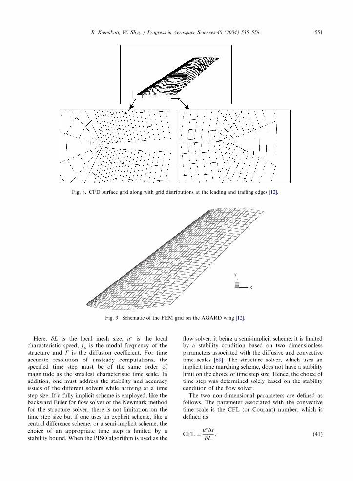
and 8, respectively.
7.2.3. Structure grid
For the structure solver, since beam elements were
used [12], a ten-element beam mesh spanning the semi-
span of the wing was constructed. However, in order to
make the interpolation and extrapolation procedures
between the CFD and structure mesh efficient and
easier, an intermediate surface mesh was generated with
QUAD4-type elements. Equal width spanwise elements,
four per beam element, along the spanwise direction
were used to generate this intermediate mesh. The
ARTICLE IN PRESS
Y
X
Z
Fig. 7. Overview of the multi-block CFD grid [12].
Fig. 6. Schematic of the AGARD 445.6 wing used in the wind tunnel [68].
R. Kamakoti, W. Shyy / Progress in Aerospace Sciences 40 (2004) 535–558550
QUAD4 elements, however, were non-uniform along
the chordwise direction to comply with the geometry.
This intermediate surface mesh on the AGARD wing
was generated using PATRAN. It had 2400 elements
surrounding the wing (60 along the chordwise direction
and 40 equal width elements along the spanwise
direction). The intermediate or temporary mesh is
shown in Fig. 9.
7.3. Time scales and choice of time step size for the
coupled problem
There are several time scales associated with the
aeroelastic problem due to the interdisciplinary nature
of the problems itself. Three major time scales can
be defined for the given problem: diffusive time
scale, convective time scale, and time scale due to
vibration of structure. The first two scales are associated
with the flow solver and the last scale is associated
with the structure. They are defined, respectively, as
follows
Dtd ¼rdL2
G(38)
Dts ¼1
f s, (39)
Dtc ¼dL
un. (40)
ARTICLE IN PRESS
X
YZ
Fig. 9. Schematic of the FEM grid on the AGARD wing [12].
Fig. 8. CFD surface grid along with grid distributions at the leading and trailing edges [12].
R. Kamakoti, W. Shyy / Progress in Aerospace Sciences 40 (2004) 535–558 551
Here, dL is the local mesh size, u� is the local
characteristic speed, f s is the modal frequency of the
structure and G is the diffusion coefficient. For time
accurate resolution of unsteady computations, the
specified time step must be of the same order of
magnitude as the smallest characteristic time scale. In
addition, one must address the stability and accuracy
issues of the different solvers while arriving at a time
step size. If a fully implicit scheme is employed, like the
backward Euler for flow solver or the Newmark method
for the structure solver, there is not limitation on the
time step size but if one uses an explicit scheme, like a
central difference scheme, or a semi-implicit scheme, the
choice of an appropriate time step is limited by a
stability bound. When the PISO algorithm is used as the
flow solver, it being a semi-implicit scheme, it is limited
by a stability condition based on two dimensionless
parameters associated with the diffusive and convective
time scales [69]. The structure solver, which uses an
implicit time marching scheme, does not have a stability
limit on the choice of time step size. Hence, the choice of
time step was determined solely based on the stability
condition of the flow solver.
The two non-dimensional parameters are defined as
follows. The parameter associated with the convective
time scale is the CFL (or Courant) number, which is
defined as
CFL ¼u�Dt
dL. (41)
ARTICLE IN PRESSR. Kamakoti, W. Shyy / Progress in Aerospace Sciences 40 (2004) 535–558552
In curvilinear coordinates, the CFL number can be
written as
CFL ¼Dt
JmaxðU ;V ;W Þ, (42)
where J is the Jacobian and U, V, W are the
contravariant velocities. The corresponding dimension-
less parameter for the diffusion time scale is given by
D ¼GDt
rdL2, (43)
which, written in curvilinear coordinates, reads as
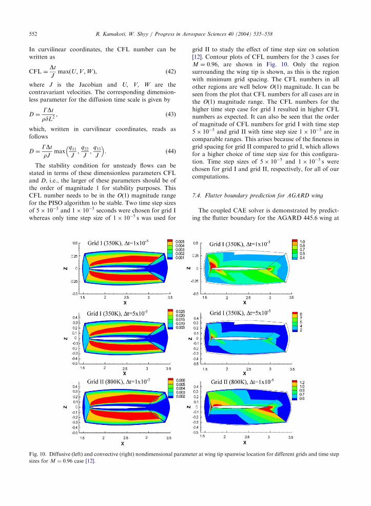
follows
D ¼GDt
rJmax
q11J
;q22J
;q33J
�. (44)
The stability condition for unsteady flows can be
stated in terms of these dimensionless parameters CFL
and D, i.e., the larger of these parameters should be of
the order of magnitude 1 for stability purposes. This
CFL number needs to be in the Oð1Þ magnitude range
for the PISO algorithm to be stable. Two time step sizes
of 5� 10�5 and 1� 10�5 seconds were chosen for grid I
whereas only time step size of 1� 10�5 s was used for
Fig. 10. Diffusive (left) and convective (right) nondimensional parame
sizes for M ¼ 0:96 case [12].
grid II to study the effect of time step size on solution
[12]. Contour plots of CFL numbers for the 3 cases for
M ¼ 0:96; are shown in Fig. 10. Only the region
surrounding the wing tip is shown, as this is the region
with minimum grid spacing. The CFL numbers in all
other regions are well below Oð1Þ magnitude. It can be
seen from the plot that CFL numbers for all cases are in
the Oð1Þ magnitude range. The CFL numbers for the
higher time step case for grid I resulted in higher CFL
numbers as expected. It can also be seen that the order
of magnitude of CFL numbers for grid I with time step
5� 10�5 and grid II with time step size 1� 10�5 are in
comparable ranges. This arises because of the fineness in
grid spacing for grid II compared to grid I, which allows
for a higher choice of time step size for this configura-
tion. Time step sizes of 5� 10�5 and 1� 10�5 s were
chosen for grid I and grid II, respectively, for all of our
computations.
7.4. Flutter boundary prediction for AGARD wing
The coupled CAE solver is demonstrated by predict-
ing the flutter boundary for the AGARD 445.6 wing at
ter at wing tip spanwise location for different grids and time step
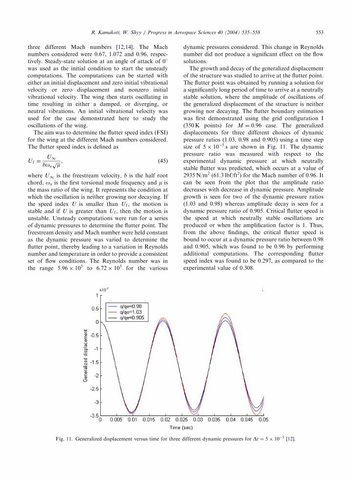
ARTICLE IN PRESSR. Kamakoti, W. Shyy / Progress in Aerospace Sciences 40 (2004) 535–558 553
three different Mach numbers [12,14]. The Mach
numbers considered were 0.67, 1.072 and 0.96, respec-
tively. Steady-state solution at an angle of attack of 0�
was used as the initial condition to start the unsteady
computations. The computations can be started with
either an initial displacement and zero initial vibrational
velocity or zero displacement and nonzero initial
vibrational velocity. The wing then starts oscillating in
time resulting in either a damped, or diverging, or
neutral vibrations. An initial vibrational velocity was
used for the case demonstrated here to study the
oscillations of the wing.
The aim was to determine the flutter speed index (FSI)
for the wing at the different Mach numbers considered.
The flutter speed index is defined as
U f ¼U1
boaffiffiffim
p , (45)
where U1 is the freestream velocity, b is the half root
chord, oa is the first torsional mode frequency and m isthe mass ratio of the wing. It represents the condition at
which the oscillation is neither growing nor decaying. If
the speed index U is smaller than U f ; the motion isstable and if U is greater than U f ; then the motion isunstable. Unsteady computations were run for a series
of dynamic pressures to determine the flutter point. The
freestream density and Mach number were held constant
as the dynamic pressure was varied to determine the
flutter point, thereby leading to a variation in Reynolds
number and temperature in order to provide a consistent
set of flow conditions. The Reynolds number was in
the range 5:96� 105 to 6:72� 105 for the various
Fig. 11. Generalized displacement versus time for three
dynamic pressures considered. This change in Reynolds
number did not produce a significant effect on the flow
solutions.
The growth and decay of the generalized displacement
of the structure was studied to arrive at the flutter point.
The flutter point was obtained by running a solution for
a significantly long period of time to arrive at a neutrally
stable solution, where the amplitude of oscillations of
the generalized displacement of the structure is neither
growing nor decaying. The flutter boundary estimation
was first demonstrated using the grid configuration I
(350K points) for M ¼ 0:96 case. The generalizeddisplacements for three different choices of dynamic
pressure ratios (1.03, 0.98 and 0.905) using a time step
size of 5� 10�5 s are shown in Fig. 11. The dynamic
pressure ratio was measured with respect to the
experimental dynamic pressure at which neutrally
stable flutter was predicted, which occurs at a value of
2935N/m2 (61.3 lbf/ft2) for the Mach number of 0.96. It
can be seen from the plot that the amplitude ratio
decreases with decrease in dynamic pressure. Amplitude
growth is seen for two of the dynamic pressure ratios
(1.03 and 0.98) whereas amplitude decay is seen for a
dynamic pressure ratio of 0.905. Critical flutter speed is
the speed at which neutrally stable oscillations are
produced or when the amplification factor is 1. Thus,
from the above findings, the critical flutter speed is
bound to occur at a dynamic pressure ratio between 0.98
and 0.905, which was found to be 0.96 by performing
additional computations. The corresponding flutter
speed index was found to be 0.297, as compared to the
experimental value of 0.308.
different dynamic pressures for Dt ¼ 5� 10�5 [12].
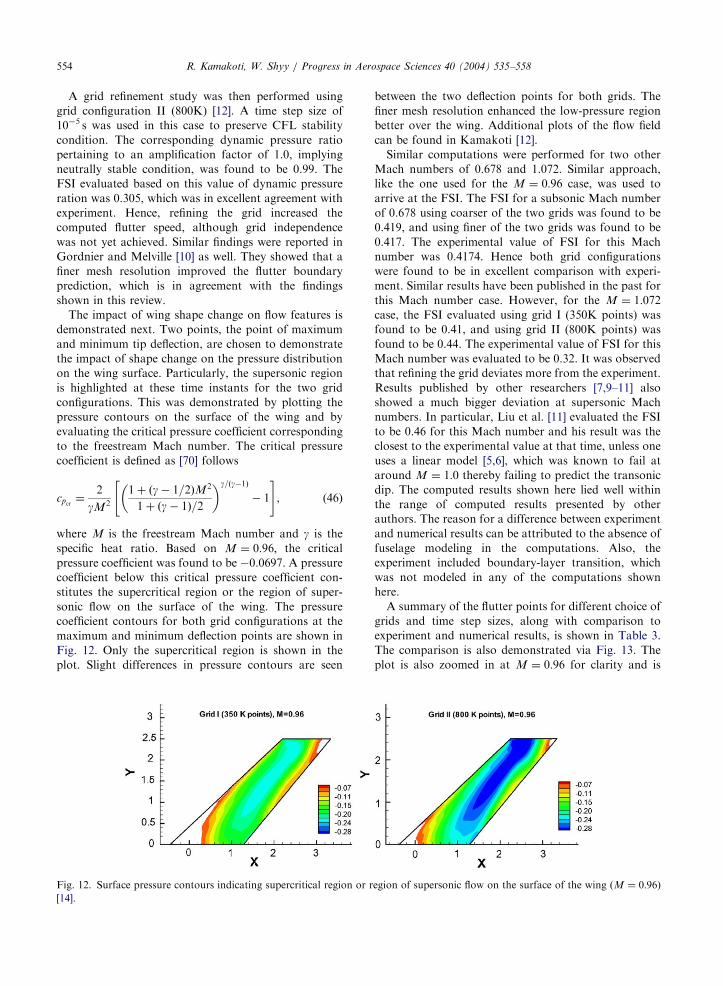
ARTICLE IN PRESSR. Kamakoti, W. Shyy / Progress in Aerospace Sciences 40 (2004) 535–558554
A grid refinement study was then performed using
grid configuration II (800K) [12]. A time step size of
10�5 s was used in this case to preserve CFL stability
condition. The corresponding dynamic pressure ratio
pertaining to an amplification factor of 1.0, implying
neutrally stable condition, was found to be 0.99. The
FSI evaluated based on this value of dynamic pressure
ration was 0.305, which was in excellent agreement with
experiment. Hence, refining the grid increased the
computed flutter speed, although grid independence
was not yet achieved. Similar findings were reported in
Gordnier and Melville [10] as well. They showed that a
finer mesh resolution improved the flutter boundary
prediction, which is in agreement with the findings
shown in this review.
The impact of wing shape change on flow features is
demonstrated next. Two points, the point of maximum
and minimum tip deflection, are chosen to demonstrate
the impact of shape change on the pressure distribution
on the wing surface. Particularly, the supersonic region
is highlighted at these time instants for the two grid
configurations. This was demonstrated by plotting the
pressure contours on the surface of the wing and by
evaluating the critical pressure coefficient corresponding
to the freestream Mach number. The critical pressure
coefficient is defined as [70] follows
cpcr ¼2
gM2
1þ ðg� 1=2ÞM2
1þ ðg� 1Þ=2
� �g=ðg�1Þ
� 1
" #, (46)
where M is the freestream Mach number and g is thespecific heat ratio. Based on M ¼ 0:96; the criticalpressure coefficient was found to be �0.0697. A pressure
coefficient below this critical pressure coefficient con-
stitutes the supercritical region or the region of super-
sonic flow on the surface of the wing. The pressure
coefficient contours for both grid configurations at the
maximum and minimum deflection points are shown in
Fig. 12. Only the supercritical region is shown in the
plot. Slight differences in pressure contours are seen
Fig. 12. Surface pressure contours indicating supercritical region or r
[14].
between the two deflection points for both grids. The
finer mesh resolution enhanced the low-pressure region
better over the wing. Additional plots of the flow field
can be found in Kamakoti [12].
Similar computations were performed for two other
Mach numbers of 0.678 and 1.072. Similar approach,
like the one used for the M ¼ 0:96 case, was used toarrive at the FSI. The FSI for a subsonic Mach number
of 0.678 using coarser of the two grids was found to be
0.419, and using finer of the two grids was found to be
0.417. The experimental value of FSI for this Mach
number was 0.4174. Hence both grid configurations
were found to be in excellent comparison with experi-
ment. Similar results have been published in the past for
this Mach number case. However, for the M ¼ 1:072case, the FSI evaluated using grid I (350K points) was
found to be 0.41, and using grid II (800K points) was
found to be 0.44. The experimental value of FSI for this
Mach number was evaluated to be 0.32. It was observed
that refining the grid deviates more from the experiment.
Results published by other researchers [7,9–11] also
showed a much bigger deviation at supersonic Mach
numbers. In particular, Liu et al. [11] evaluated the FSI
to be 0.46 for this Mach number and his result was the
closest to the experimental value at that time, unless one
uses a linear model [5,6], which was known to fail at
around M ¼ 1:0 thereby failing to predict the transonicdip. The computed results shown here lied well within
the range of computed results presented by other
authors. The reason for a difference between experiment
and numerical results can be attributed to the absence of
fuselage modeling in the computations. Also, the
experiment included boundary-layer transition, which
was not modeled in any of the computations shown
here.
A summary of the flutter points for different choice of
grids and time step sizes, along with comparison to
experiment and numerical results, is shown in Table 3.
The comparison is also demonstrated via Fig. 13. The
plot is also zoomed in at M ¼ 0:96 for clarity and is
egion of supersonic flow on the surface of the wing ðM ¼ 0:96Þ

ARTICLE IN PRESS
Table 3
Comparison of critical flutter speed and dynamic pressure with
experiment and other numerical results
Mach
number
Model FSI
0.678 Experiment [68] 0.4174
Euler and normal modes [7] 0.417
TSD-linear and normal modes [6] 0.430
RANS and beam (modes) with GCL
[12]
0.419
RANS and beam (modes) with GCL
[14]
0.417
0.96 Experiment [68] 0.3095
Euler and normal modes [7] 0.275
NS and normal modes [9] 0.294
TSD-nonlinear and normal modes [22] 0.284
RANS and normal modes [11] 0.300
NS and normal modes with GCL [10] 0.319
RANS and beam (modes) with GCL
[12]
0.297
RANS and beam (modes) with GCL
[12]
0.305
1.072 Experiment [68] 0.3201
Euler and normal modes [7] 0.466
TSD-linear and normal modes [6] 0.340
RANS and normal modes [11] 0.460
RANS and beam (modes) with GCL
[12]
0.410
RANS and beam (modes) with GCL
[14]
0.440
0.2
0.3
0.4
0.5
0.6
0.7
0.4 0.5 0.6 0.7 0Mach n
FS
I
Experiment [68]
TSD-linear and normal modes
Euler normal modes [7]NS and normal mdoes [9]
RANS and normal modes [11]
NSand normal modes with GC
RANSand beam (modes) withRANSand beam (modes) with
Fig. 13. Summary of flutter speed index pre
R. Kamakoti, W. Shyy / Progress in Aerospace Sciences 40 (2004) 535–558 555
shown in Fig. 14. It can be observed from the figure that
the approach presented here compared reasonably well
with both experimental as well as prior numerical results
in spite of the simplicity of the structure model used and
the first-order accuracy of the flow solver.
8. Conclusions
Recent advances in the field of computational
aeroelasticity were reviewed. Particularly, the three
major models pertaining to CAE, namely, flow solver,
structure solver and moving mesh algorithm, were
studied in depth thereby giving a flair for arriving at
suitable models for performing fluid–structure interac-
tion calculations. Specifically, a closely-coupled ap-
proach was discussed in detail as it was found to be an
efficient and accurate way to couple flow and structure
solvers. It also gives us the flexibility in choosing
different solvers for fluids and structures depending on
the complexity of the applications looked at. In this
review, the emphasis is on the interaction between a
complex flow solver and a simplified structure model.
Such a model is used as a basis to probe into the various
issues involved with developing a computational aero-
elastic module.
The advantages of using a non-iterative flow solver
were discussed. Also, the different time scales associated
with the different solvers and how they impact on the
choice of time step size of the overall computations were
studied. The importance of having a robust moving
mesh module was reviewed in detail. The impact of
different parameters associated with the moving mesh
module was also highlighted.
Since the computations need to be performed on a
dynamically moving mesh, the geometric properties
.8 0.9 1 1.1 1.2umber
[6]
L [10]
GCL [12] GCL [14]
diction for AGARD 445.6 wing [14].
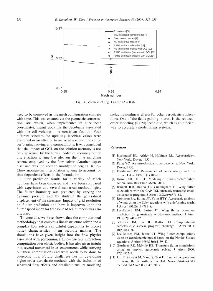
ARTICLE IN PRESS
0.27
0.32
0.37
0.95 0.96 0.97Mach number
FS
I
Experiment [68]
TSD-linearand normal modes [6]
Euler normal modes [7]
NS and normal modes [9]
RANS and normal modes [11]NS and normal modes with GCL [10]
RANS and beam (modes) with GCL [12]
RANS and beam (modes) with GCL [14]
Fig. 14. Zoom in of Fig. 13 near M ¼ 0:96:
R. Kamakoti, W. Shyy / Progress in Aerospace Sciences 40 (2004) 535–558556
need to be conserved as the mesh configuration changes
with time. This was ensured via the geometric conserva-
tion law, which, when implemented in curvilinear
coordinates, meant updating the Jacobians associated
with the cell volumes in a consistent fashion. Four
different schemes for updating Jacobian values were
examined in an attempt to arrive at a robust choice for
performing moving grid computations. It was concluded
that the impact of GCL on the solution accuracy is not
only governed by the formal order of accuracy of the
discretization scheme but also on the time marching
scheme employed by the flow solver. Another aspect
discussed was the need to modify the original Rhie–-
Chow momentum interpolation scheme to account for
time-dependent effects in the formulation.
Flutter prediction results for a variety of Mach
numbers have been discussed and have been compared
with experiment and several numerical methodologies.
The flutter boundary was predicted by varying the
dynamic pressure and by studying the generalized
displacement of the structure. Impact of grid resolution
on flutter prediction and how it improves upon the
flutter speed index for transonic Mach numbers was also
discussed.
To conclude, we have shown that the computational
methodology that couples a linear structure solver and a
complex flow solver can exhibit capabilities to predict
flutter characteristics in an accurate manner. The
simulations have given insight into the flow physics
associated with performing a fluid–structure interaction
computation over elastic bodies. It has also given insight
into several numerical issues encountered while carrying
out these computations and what needs to be done to
overcome this. Future challenges lies in developing
higher-order aeroelastic methods with the inclusion of
separated flow effects and detailed structure modeling
including nonlinear effects for other aeroelastic applica-
tions. One of the fields gaining interest is the reduced-
order modeling (ROM) technique, which is an efficient
way to accurately model larger systems.
References
[1] Bisplingoff RL, Ashley H, Halfman RL. Aeroelasticity.
New York: Dover; 1955.
[2] Fung YC. An introduction to aeroelasticity. New York:
Dover; 1955.
[3] Friedmann PP. Renaissance of aeroelasticity and its
future. J Airc 1999;36(1):105–21.
[4] Dowell EH, Hall KC. Modeling of fluid–structure inter-
action. Ann Rev Fluid Mech, 2001.
[5] Bennett RM, Batina JT, Cunningham H. Wing-flutter
calculations with the CAP-TSD unsteady transonic small-
disturbance program. J Aircr 1989;26(9):876–82.
[6] Robinson BA, Batina JT, Yang HTY. Aeroelastic analysis
of wings using the Euler equations with a deforming mesh.
J Aircr 1991;28(11):781–8.
[7] Lee-Rausch EM, Batina JT. Wing flutter boundary
prediction using unsteady aerodynamic method. J Aircr
1995;32(2):416–22.
[8] Schuster DM, Liu DD, Huttsell LJ. Computational
aeroelasticity: success, progress, challenge. J Aircr 2003;
40(5):843–56.
[9] Lee-Rausch EM, Batina JT. Wing flutter computations
using an aerodynamic model based on the Navier–Stokes
equations. J Aircr 1996;33(6):1139–47.
[10] Gordnier RE, Melville RB. Transonic flutter simulations
using an implicit aeroelastic solver. J Aircr 2000;
37(5):872–9.
[11] Liu F, Sadeghi M, Yang S, Tsai H. Parallel computation
of wing flutter with a coupled Navier–Stokes/CSD
method. AIAA-2003-1347, 2003.
ARTICLE IN PRESSR. Kamakoti, W. Shyy / Progress in Aerospace Sciences 40 (2004) 535–558 557
[12] Kamakoti R. Computational aeroelasticity using a pres-
sure-based flow solver. PhD dissertation, University of
Florida, Gainesville, 2004.
[13] Kamakoti R, Shyy W, Thakur S, Sankar B. Time
dependent RANS computations for an aeroelastic wing.
AIAA-2004-0886, 2004.
[14] Kamakoti R, Shyy W. Flutter prediction over three-
dimensional wing geometry, 2005, to be published.
[15] Guruswamy GP, Byun C. Direct coupling of Euler flow
equations with plate finite element structures. AIAA J
1994;33(2):375–7.
[16] Guruswamy GP, Byun C. Fluid–structure interactions
using Navier–Stokes flow equations coupled with shell
finite element structures. AIAA-93-3087, 1993.
[17] Garica JA, Guruswamy GP. Aeroelastic analysis of
transonic wings using Navier–Stokes equations and a
nonlinear beam finite element model. AIAA-99-1215,
1999.
[18] Smith MJ, Schuster DM, Huttsell L, Buxton B. Develop-
ment of an Euler/Navier–Stokes aeroelastic method for
three-dimensional vehicles with multiple flexible surfaces.
AIAA-96-1513-CP, 1996.
[19] Seigel JM, Parthasarathy V, Kingsley GM, Dionne PJ,
Harrand VJ, Luker JJ. Application of a multi-
disciplinary computing environment (MDICE) for
loosely coupled fluid–structural analysis. AIAA-98-4865,
1998.
[20] Cunningham HJ, Batina JT, Bennett RM. Modern wing
flutter analysis by computational fluid dynamics methods.
J Aircr 1988;25(10):962–8.
[21] Schuster DM, Vadyak J, Atta E. Static aeroelastic analysis
of fighter aircraft using a three-dimensional Navier–Stokes
algorithm. J Aircr 1990;27(9):820–5.
[22] Bennett RM, Edwards JW. An overview of recent
developments in computational aeroelasticity. AIAA-98-
2421, 1998.
[23] Huttsell L, Schuster D, Volk J, Giesing J, Love M.
Evaluation of computational aeroelasticity codes for loads
and flutter. AIAA-2001-0569, 2001.
[24] Liu F, Cai J, Zhu Y, Wong ASF, Tsai HM. Calculation of
wing flutter by a coupled CFD–CSD method. AIAA-2000-
0907, 2000.
[25] Eriksson LE. Generation of boundary-conformation grids
around wing-body configurations using transfinite inter-
polation. AIAA J 1982;20(10):1313–20.
[26] Hartwich PM, Agrawal S. Method for perturbing multi-
block patched grids in aeroelastic and design optimization
applications. AIAA Paper 97-2038, 1997.
[27] Cai J, Liu F, Tsai HM. Static aero-elastic computation
with a coupled CFD and CSD method. AIAA-2001-0717,
2001.
[28] Farhat C, Pierson K, Degand C. CFD based simulation of
the unsteady aeroelastic response of a maneuvering
vehicle. AIAA-2000-0899, 2000.
[29] Farhat C, Lesoinne M. Two efficient staggered algorithms
for the serial and parallel solution of three-dimensional
nonlinear transient aeroelastic problems. Comput Meth-
ods Appl Mech Eng 2000;182:499–515.
[30] Thomas PD, Lombard K. Geometric conservation law and
its application to flow computations on moving grids.
AIAA J 1979;17(10):1030–7.
[31] Patankar SV. Numerical heat transfer and fluid flow.
Washington, DC: Hemisphere; 1980.
[32] Ferziger JH, Peric M. Computational methods for fluid
dynamics, 3rd ed. New York: Springer; 2002.
[33] Versteeg HK, Malalasekera. An introduction to computa-
tional fluid dynamics. Harlow, England: Longman Scien-
tific and Technical; 1995.
[34] Shyy W. Computational modeling for fluid flow and
interfacial transport. Amsterdam: Elsevier; 1994.
[35] Thakur S, Wright J, Shyy W. STREAM: a computational
fluid dynamics and heat transfer Navier–Stokes solver:
theory and applications. Gainesville, FL: Streamline
Numerics, Inc; 2002.
[36] Shyy W, Braaten ME. Application of a generalized
pressure correction algorithm for flows in complicated
geometries. In: Baysal O, editor. Advances and applica-
tions in computational fluid dynamics. New York: ASME;
1988. p. 109–19.
[37] Issa RI. Solution of the implicitly discretised fluid flow
equations by operator-splitting. J Comp Phys 1985;
62:40–65.
[38] Rhie CM, Chow WL. Numerical study of the turbulent
flow past an airfoil with trailing edge separation. AIAA J
1983;21(11):1525–35.
[39] Choi SK. Note on the use of momentum interpolation
method for unsteady flows. Numer Heat Transfer Part A
1999;36:545–50.
[40] Yu B, Kawaguchi Y, Tao WQ, Ozoe H. Checkerboard
pressure predictions due to underrelaxation factor and
time step size for a nonstaggered grid with momentum
interpolation method. Numer Heat Transfer Part B
2002;41:85–94.
[41] Yu B, Tao WQ, Wei JJ, Kawaguchi Y, Tagawa T, Ozoe H.
Discussion on momentum interpolation method for
collocated grids of incompressible flow. Numerical Heat
Transfer Part B 2002;42:141–66.
[42] Shyy W, Udaykumar HS, Rao MM, Smith RW. Compu-
tational fluid dynamics with moving boundaries. London:
Taylor and Francis; 1996.
[43] Shyy W, Francois M, Udaykumar HS, N’dri N, Tran-Son-
Tay R. Moving boundaries in micro-scale biofluid
dynamics. Appl Mech Rev 2001;54:419–53.
[44] Lesoinne M, Farhat C. Geometric conservation laws for
flow problems with moving boundaries and deformable
meshes, and their impact on aeroelastic computations.
Comput Methods Appl Mech Eng 1996;134:71–90.
[45] Koobus B, Farhat C. Second-order time-accurate and
geometrically conservative implicit schemes for flow
computations on unstructured dynamic meshes. Comput
Methods Appl Mech Eng 1999;170:103–29.
[46] Farhat C, Geuzaine P, Grandmont C. The discrete
geometric conservation law and the nonlinear stability of
ALE schemes for the solution of flow problems on moving
grids. J Comput Phys 2001;174:669–94.
[47] Kamakoti R, Shyy W. Moving grid computations for
turbulent, aeroelastic flows. AIAA-2003-3719, 2003.
[48] Launder BE, Spalding DB. The numerical computations of
turbulent flows. Comput Methods Appl Mech Eng
1974;3:269–89.
[49] Shyy W, Thakur SS, Ouyang H, Liu J, Blosch E.
Computational techniques for complex transport
ARTICLE IN PRESSR. Kamakoti, W. Shyy / Progress in Aerospace Sciences 40 (2004) 535–558558
phenomena. New York: Cambridge University Press;
1997.
[50] Johansen ST, Wu J, Shyy W. Filter-based unsteady RANS
computations. Int J Heat Fluid Flow 2004;25:10–21.
[51] Cook RD, Malkus DS, Plesha ME. Concepts and
applications of finite element analysis, 2nd ed. New York:
Wiley; 1999.
[52] Kamakoti R, Lian Y, Regisford S, Kurdila A, Shyy W.
Computational aeroelasticity using a pressure-based sol-
ver. AIAA-2002-0869, 2002.
[53] Bathe K-J. Finite element procedures. Englewood Cliffs,
NJ: Prentice-Hall; 1996.
[54] Batina JT. Unsteady Euler algorithm with unstructured
dynamic mesh for complex-aircraft aeroelastic analysis.
AIAA-89-1189, 1989.
[55] Bhardwaj MK, Kapania K, Reichenbach E, Guruswamy
GP. Computational fluid dynamics/computational struc-
tural dynamics interaction methodology for aircraft wings.
AIAA J 1998;36(12):2179–86.
[56] Potsdam MA, Guruswamy GP. A parallel multiblock
mesh movement scheme for complex aeroelastic applica-
tions. AIAA-2001-0716, 2001.
[57] Huang W, Ren Y, Russell RD. Moving mesh methods
based on moving mesh partial differential equations.
J Comput Phys 1994;113:279–90.
[58] Huang W, Russell RD. Moving mesh strategy based on a
gradient flow equation for two-dimensional problems.
SIAM J Sci Comput 1999;20(3):998–1015.
[59] Huang W. Practical aspects of formulation and solution of
moving mesh partial differential equations. J Comput Phys
2001;171:753–75.
[60] Wong A, Tsai H, Cai J, Zhu, Y, Liu F. Unsteady flow
calculations with a moving mesh algorithm. AIAA-2000-
1002, 2000.
[61] Reuther J, Jameson A, Farmer J, Martinelli L, Saunders
D. Aerodynamics shape optimization of complex aircraft
configurations via an adjoint formulation. AIAA-96-0094,
1996.
[62] Lian Y, Shyy W, Viieru D, Zhang B. Membrane wing
aerodynamics for micro aerial vehicles. Prog Aerospace Sci
2003;39:425–65.
[63] Guruswamy GP. A review of numerical fluids/structures
interface methods for computations using high-fidelity
equations. Comput Struct 2002;80:31–41.
[64] Smith MJ, Cesnik CES, Hodges DH, Moran KJ. An
evaluation of computational algorithms to interface
between CFD and CSD methodologies. AIAA-96-1400,
1996.
[65] Smith MJ, Hodges DH, Cesnik CES. Evaluation of
computational algorithms suitable for fluid–structure
interactions. J Aircr 2000;37(2):282–94.
[66] Brown SA. Displacement extrapolation for CFD+CSD
aeroelastic analysis. AIAA-97-1090, 1997.
[67] Yates Jr EC. AGARD standard aeroelastic configuration
for dynamic response. Candidate Configuration I-Wing
445.6, NASA TM 100492, 1987.
[68] Yates Jr EC, Land NS, Foughner Jr JT. Measured and
calculated subsonic and transonic flutter characteristics of
a 45� sweptback wing planform in air and in Freon-12 in
the Langley Transonic Dynamics Tunnel, AGARD TN D-
1616, 1963.
[69] Thakur S, Wright J. A multiblock operator-splitting
algorithm for unsteady flows at all speeds in complex
geometries. Int J Num Methods Fluids 2004;46:
383–413.
[70] Anderson JD. Modern compressible flow with a
historical perspective. New York: McGraw-Hill College;
2002.
Copyright © 2022 FDOKUMEN