1

AEROELASTIC BEHAVIOUR OF A GYROPLANE ROTOR

IN AXIAL DESCENT AND FORWARD FLIGHT

J. Trchalík*, E. A. Gillies

†, D. G. Thomson

‡

* PhD Research Student,

CAA ARB Sponsored ‘Aeroelastic Modelling of Gyroplane Rotors’

Research Project, email: jtrchali@aero.gla.ac.uk

† Lecturer of Low-Speed Aerodynamics and Aeroelasticity,

email: ericg@aero.gla.ac.uk

‡ Senior lecturer, Head of the Department,

email:d.thomson@aero.gla.ac.uk

Department of Aerospace Engineering

University of Glasgow

Glasgow, G12 8QQ

Keywords: Gyroplane, autogyro, aeroelasticity, rotor, rotor blade, rotorcraft, stability, axial

flight, forward flight

Abstract. A mathematical model was created to simulate aeroelastic behaviour of a rotor during

autorotation. Aeroelastic Model of a Rotor in Autorotation (AMRA) captures both bending and

twist of the blade and hence it can investigate couplings between blade flapping, torsion and rotor

speed. The rotor blades were assumed to be perfectly rigid, i.e. flapping angle and blade twist due

to torsion are constant along the blade span. Aeromechanical behaviour of a rotor during both

axial flight and forward flight in autorotation were investigated.

Significant part of the research was focused on investigation of the effect of different values of

torsional and flexural stiffness of the blade on stability of the autorotation. Special care was taken

of mutual relations between blade twist, blade flap and rotor speed. Calculations were carried out

for several different positions of centre of gravity in order to determine stability boundary of the

rotor. It was found that the aeroelastic behaviour of a rotor in autorotation is affected by strong

coupling between blade twist and rotor speed. The results obtained with the aid of the model

demonstrate the special characteristics of autorotative regime. Coupled rotor speed/flap/twist

oscillations (flutter) occur if torsional stiffness of the blade is lower than a critical value. This

instability is unique to the gyroplane as it differs from both helicopter rotor flutter and fixed-wing

flutter.

Effects of gust loads on the rotor and corresponding disturbances in flap and twist of the blade

were investigated for different blade configurations. In many cases, the results demonstrate auto-

stabilizing effect of coupling between blade twist and rotor speed. Parametric studies of influence

of gyroplane rotor design on its performance were also accomplished. Simulations were executed

for different blade incidence angles and various linear twist of the blade. The effect of blade tip

mass and its different location along the blade span on gyroplane rotor performance was

investigated also.

2

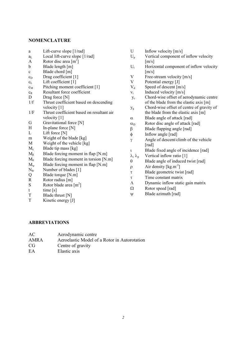
NOMENCLATURE

a Lift-curve slope [1/rad]

aL Local lift-curve slope [1/rad]

A Rotor disc area [m2]

b Blade length [m]

c Blade chord [m]

cD Drag coefficient [1]

cL Lift coefficient [1]

cM Pitching moment coefficient [1]

cR Resultant force coefficient

D Drag force [N]

1/f Thrust coefficient based on descending

velocity [1]

1/F Thrust coefficient based on resultant air

velocity [1]

G Gravitational force [N]

H In-plane force [N]

L Lift force [N]

m Weight of the blade [kg]

M Weight of the vehicle [kg]

Mc Blade tip mass [kg]

Mβ Blade forcing moment in flap [N.m]

Mθ Blade forcing moment in torsion [N.m]

Mψ Blade forcing moment in flap [N.m]

NB Number of blades [1]

Q Blade torque [N.m]

R Rotor radius [m]

S Rotor blade area [m2]

t time [s]

T Blade thrust [N]

T Kinetic energy [J]

U Inflow velocity [m/s]

Up Vertical component of inflow velocity

[m/s]

Ut Horizontal component of inflow velocity

[m/s]

V Free-stream velocity [m/s]

V Potential energy [J]

Vd Speed of descent [m/s]

vi Induced velocity [m/s]

yc Chord-wise offset of aerodynamic centre

of the blade from the elastic axis [m]

yg Chord-wise offset of centre of gravity of

the blade from the elastic axis [m]

α Blade angle of attack [rad]

αD Rotor disc angle of attack [rad]

β Blade flapping angle [rad]

φ Inflow angle [rad]

γ Angle of descent/climb of the vehicle

[rad]

ι Blade fixed angle of incidence [rad]

λ, λp Vertical inflow ratio [1]

θ Blade angle of induced twist [rad]

ρ Air density [kg.m-3]

τ Blade geometric twist [rad]

τ Time constant matrix

Λ Dynamic inflow static gain matrix

Ω Rotor speed [rad]

ψ Blade azimuth [rad]

ABBREVIATIONS

AC Aerodynamic centre

AMRA Aeroelastic Model of a Rotor in Autorotation

CG Centre of gravity

EA Elastic axis

3

1. INTRODUCTION

The gyroplane represents the first successful rotorcraft design and it paved the way for the

development of helicopter during 1940s. Further development of the gyroplane was ceased

during following decades as helicopter became more successful. Interest in this type of aircraft as

a recreational vehicle was resurrected in recent years thanks to simplicity of its design and low

operational costs.

Unfortunately, autogyros, or gyroplanes, have been involved in number of fatal accidents during

last two decades1. Sudden loss of rotor speed or mechanical failures of the rotor blades as

delamination were involved in many of the accidents. Very little data on gyroplane flight

mechanics and handling qualities are available in the literature. This forced the UK Civil

Aviation Authority (CAA) to investigate these problems by contracting the Department of

Aerospace Engineering, University of Glasgow to investigate aerodynamics and flight mechanics

of a gyroplane.1-4

The cause of the high accident rate of gyroplanes still remains unclear. Rotor aeroelastic

instability has not yet been investigated as a possible cause of some the accidents and it is the aim

of the present work to investigate this possibility. This paper shows preliminary results of a CAA

funded project on “Aeroelasticity of Gyroplane Rotors”.

The aim of the investigation is to identify flight conditions or configurations of the rotor that

might have catastrophic consequences and work out basic design criteria for gyroplane blades.

Resulting aeromechanical model of gyroplane rotor blade can be also used for prediction of

stability of new or modified gyroplane rotor configurations.

4

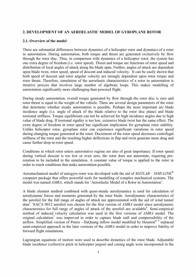
2. DEVELOPMENT OF AN AEROELASTIC MODEL OF GYROPLANE ROTOR

2.1. Overview of the model

There are substantial differences between dynamics of a helicopter rotor and dynamics of a rotor

in autorotation. During autorotation, both torque and thrust are generated exclusively by flow

through the rotor disc. Thus, in comparison with dynamics of a helicopter rotor, the system has

one extra degree of freedom (i.e. rotor speed). Thrust and torque are functions of rotor speed and

distribution of local angles of attack along the blade span. Further, angles of attack are dependent

upon blade twist, rotor speed, speed of descent and induced velocity. It can be easily shown that

both speed of descent and rotor angular velocity are strongly dependent upon rotor torque and

rotor thrust. Therefore, simulation of the aeroelastic characteristics of a rotor in autorotation is

iterative process that involves large number of algebraic loops. This makes modelling of

autorotation significantly more challenging than powered flight.

During steady autorotation, overall torque generated by flow through the rotor disc is zero and

rotor thrust is equal to the weight of the vehicle. There are several design parameters of the rotor

that determine whether steady autorotation is possible. Perhaps the most important are blade

incidence angle (i.e. angle of attack of the blade relative to the rotor disc plane) and blade

torsional stiffness. Torque equilibrium can not be achieved for high incidence angles due to high

value of blade drag. If torsional rigidity is too low, extensive blade twist has the same effect. The

extra degree of freedom in rotor speed has significant implication for gyroplane rotor stability.

Unlike helicopter rotor, gyroplane rotor can experience significant variations in rotor speed

during changing torque generated at the rotor. Decrement of the rotor speed decreases centrifugal

stiffness of the rotor and the resulting higher deflections in flap and twist generate more drag and

cause further drop in rotor speed.

Conditions in which rotor enters autorotative regime are also of great importance. If rotor speed

during vertical descent is too low or even zero, the rotor does not autorotate, requiring pre-

rotation to be included in the simulation. A constant value of torque is applied to the rotor in

order to reach conditions that make autorotation possible.

Aeromechanical model of autogyro rotor was developed with the aid of MATLAB – SIMULINK®

computer package that offers powerful tools for modelling of complex mechanical systems. The

model was named AMRA, which stands for ‘Aeroelastic Model of a Rotor in Autorotation’.

A blade element method combined with quasi-steady aerodynamics is used for calculation of

aerodynamic forces and moments generated by the rotor blade. Aerodynamic characteristics of

the aerofoil for the full range of angles of attack are approximated with the aid of wind tunnel

data5. NACA 0012 aerofoil was chosen for the first version of AMRA model since aerodynamic

characteristics for full range of angles of attack of the aerofoil are available6. Semi-empirical

method of induced velocity calculation was used in the first versions of AMRA model. The

original calculation7 was improved in order to capture blade stall and compressibility of the

airflow. Simplified version of Peters - HaQuang inflow model modified by Houston8, 9 replaced

semi-empirical approach in the later versions of the AMRA model in order to improve fidelity of

forward flight simulations.

Lagrangian equations of motion were used to describe dynamics of the rotor blade. Adjustable

blade incidence (collective pitch in helicopter jargon) and coning angle were incorporated in the

5

dynamic model of the blade. The rotor is assumed to have no lag hinge since it has extra degree

of freedom in azimuth. Chord-wise locations of elastic axis (EA), centre of gravity (CG) and

aerodynamic centre (AC) can be set in each span-wise station. Values of flexural and torsional

rigidity of the blade can be set to investigate behaviour of the rotor for different physical

properties of the blades. AMRA model also allows placement of single concentrated mass at any

span-wise station of the blade.

2.2. Aerodynamic model of rotor in autorotation

During autorotation, the flow through the rotor has opposite direction than in the case of powered

flight of a helicopter. Thus, blade aerodynamic angle of attack has to be expressed in different

form

Aα θ φ= + , (2.1)

where inflow angle is

p

T

Uarctg

Uφ

=

. (2.2)

Local values of vertical and horizontal components of inflow velocity (U) have to be calculated

in order to determine aerodynamic angle of attack of any blade section. Inflow velocity is a

function of angle of attack of the rotor disc that is given by sum of incidence angle of the rotor

disc ι (i.e. angle between rotor disc plane and the horizontal) and pitch angle of the vehicle γ (see Eq.(2.3)). During axial flight, rotor disc angle of attack is 90deg.

D

d

h

Varctg

V

α ι γ

γ

= +

=

(2.3)

Leishman10 shows that, if quasi-steady flow is considered, lift coefficient of oscillating wing

section can be described as follows

1 2

2 2

2

EA

l

cy

h cc a

cV V

αα

− ≈ + + −

& &. (2.4)

Previous equation can be rewritten so as to describe quasi-steady aerodynamics of a rotor blade

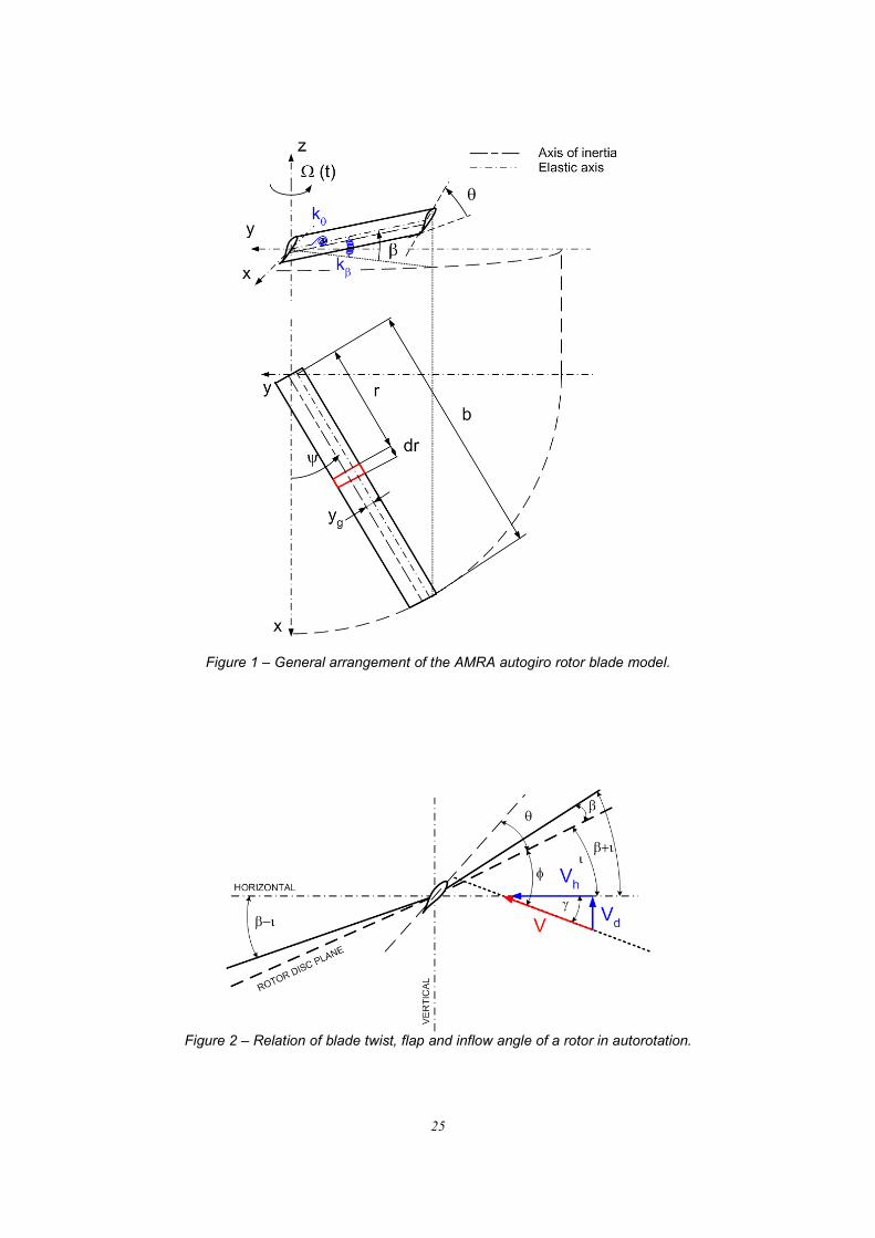
more clearly and to match with coordinate system orientation of the model (see Fig.1)

3

4l EA

r cc a y

r r

β θθ φ ≈ + − − − Ω Ω

& &

. (2.5)

6

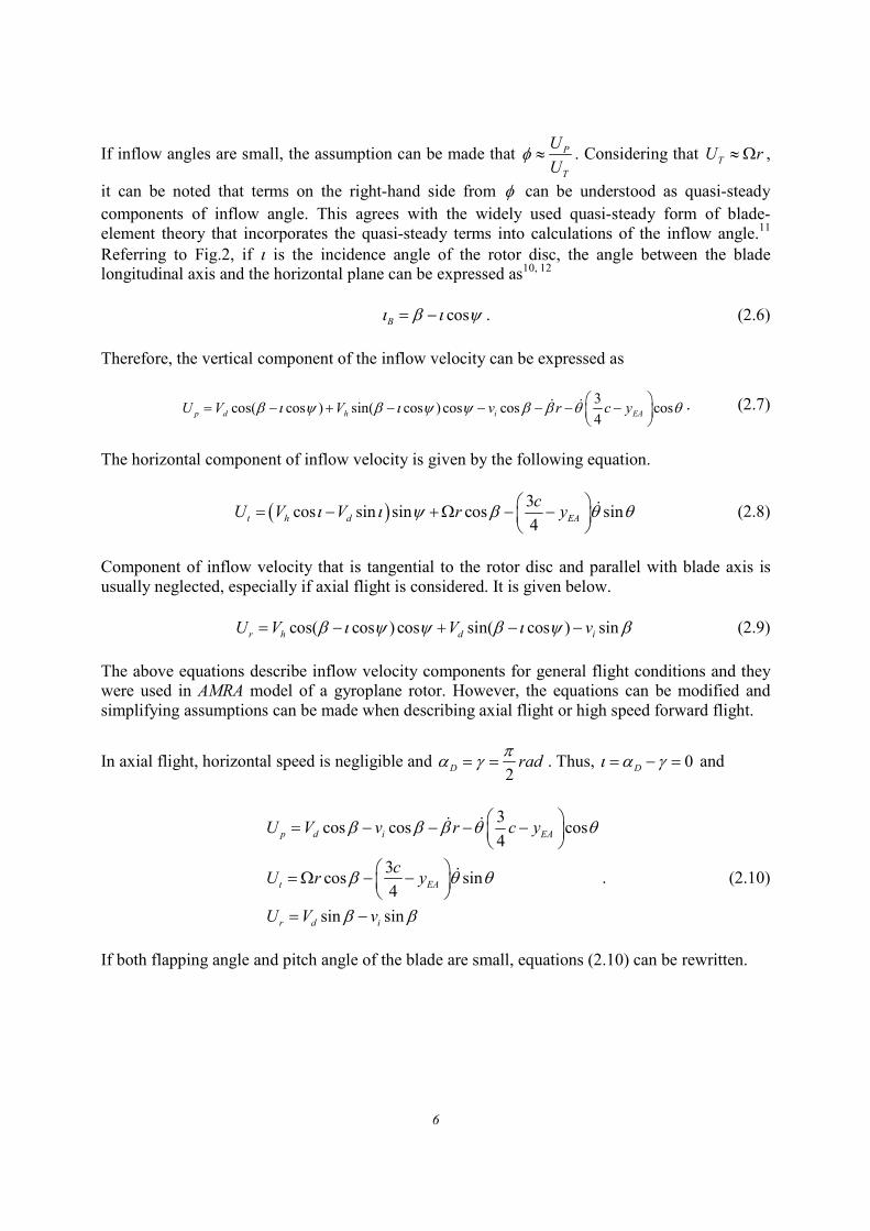
If inflow angles are small, the assumption can be made that P

T

U

Uφ ≈ . Considering that TU r≈ Ω ,

it can be noted that terms on the right-hand side from φ can be understood as quasi-steady components of inflow angle. This agrees with the widely used quasi-steady form of blade-

element theory that incorporates the quasi-steady terms into calculations of the inflow angle.11

Referring to Fig.2, if ι is the incidence angle of the rotor disc, the angle between the blade longitudinal axis and the horizontal plane can be expressed as10, 12

cosBι β ι ψ= − . (2.6)

Therefore, the vertical component of the inflow velocity can be expressed as

3cos( cos ) sin( cos ) cos cos cos

4p d h i EAU V V v r c yβ ι ψ β ι ψ ψ β β θ θ = − + − − − − −

& & . (2.7)

The horizontal component of inflow velocity is given by the following equation.

( ) 3cos sin sin cos sin

4t h d EA

cU V V r yι ι ψ β θ θ = − +Ω − −

& (2.8)

Component of inflow velocity that is tangential to the rotor disc and parallel with blade axis is

usually neglected, especially if axial flight is considered. It is given below.

cos( cos ) cos sin( cos ) sinr h d iU V V vβ ι ψ ψ β ι ψ β= − + − − (2.9)

The above equations describe inflow velocity components for general flight conditions and they

were used in AMRA model of a gyroplane rotor. However, the equations can be modified and

simplifying assumptions can be made when describing axial flight or high speed forward flight.

In axial flight, horizontal speed is negligible and 2

D radπ

α γ= = . Thus, 0Dι α γ= − = and

3cos cos cos

4

3cos sin

4

sin sin

p d i EA

t EA

r d i

U V v r c y

cU r y

U V v

β β β θ θ

β θ θ

β β

= − − − −

= Ω − −

= −

& &

& . (2.10)

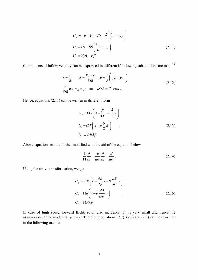
If both flapping angle and pitch angle of the blade are small, equations (2.10) can be rewritten.

7

3

4

3

4

p i d EA

t EA

r d i

U v V r c y

cU r y

U V v

β θ

θθ

β β

= − + − − −

= Ω − −

= −

& &

& (2.11)

Components of inflow velocity can be expressed in different if following substitutions are made13

1 3

4

cos cos

d iEA

D D

V vrx y c y

R R R

VR V

R

λ

α µ µ α

− = = = − Ω

= ⇒ Ω =Ω

. (2.12)

Hence, equations (2.11) can be written in different form

p

t

r

U R x y

U R x y

U R

β θλ

θθ

λβ

= Ω − − Ω Ω

= Ω − Ω = Ω

& &

&

. (2.13)

Above equations can be further modified with the aid of the equation below

1 d dt d d

dt d dt dψ ψ= =

Ω. (2.14)

Using the above transformation, we get

p

t

r

d dU R x y

d d

dU R x y

d

U R

β θλ θ

ψ ψ

θθ

ψ

λβ

= Ω − −

= Ω −

= Ω

. (2.15)

In case of high speed forward flight, rotor disc incidence (ι ) is very small and hence the assumption can be made that

Dα γ≈ . Therefore, equations (2.7), (2.8) and (2.9) can be rewritten

in the following manner

8

3cos sin cos cos cos

4

3sin cos sin

4

sin cos cos sin

p d h i EA

t h EA

r d h i

U V V v r c y

U V r c y

U V V v

β β ψ β β θ θ

ψ β θ θ

β β ψ β

= + − − − −

= + Ω − −

= + −

& &

& . (2.16)

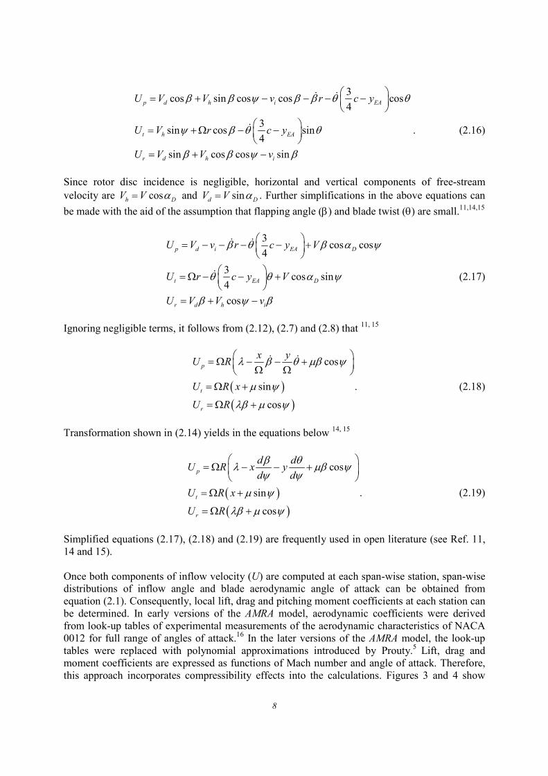
Since rotor disc incidence is negligible, horizontal and vertical components of free-stream

velocity are cosh DV V α= and sind DV V α= . Further simplifications in the above equations can

be made with the aid of the assumption that flapping angle (β) and blade twist (θ) are small.11,14,15

3cos cos

4

3cos sin

4

cos

p d i EA D

t EA D

r d h i

U V v r c y V

U r c y V

U V V v

β θ β α ψ

θ θ α ψ

β ψ β

= − − − − +

= Ω − − +

= + −

& &

& (2.17)

Ignoring negligible terms, it follows from (2.12), (2.7) and (2.8) that 11, 15

( )( )

cos

sin

cos

p

t

r

x yU R

U R x

U R

λ β θ µβ ψ

µ ψ

λβ µ ψ

= Ω − − + Ω Ω = Ω +

= Ω +

& &

. (2.18)

Transformation shown in (2.14) yields in the equations below 14, 15

( )( )

cos

sin

cos

p

t

r

d dU R x y

d d

U R x

U R

β θλ µβ ψ

ψ ψ

µ ψ

λβ µ ψ

= Ω − − +

= Ω +

= Ω +

. (2.19)

Simplified equations (2.17), (2.18) and (2.19) are frequently used in open literature (see Ref. 11,

14 and 15).

Once both components of inflow velocity (U) are computed at each span-wise station, span-wise

distributions of inflow angle and blade aerodynamic angle of attack can be obtained from

equation (2.1). Consequently, local lift, drag and pitching moment coefficients at each station can

be determined. In early versions of the AMRA model, aerodynamic coefficients were derived

from look-up tables of experimental measurements of the aerodynamic characteristics of NACA

0012 for full range of angles of attack.16 In the later versions of the AMRA model, the look-up

tables were replaced with polynomial approximations introduced by Prouty.5 Lift, drag and

moment coefficients are expressed as functions of Mach number and angle of attack. Therefore,

this approach incorporates compressibility effects into the calculations. Figures 3 and 4 show

9

trends of lift coefficient and drag coefficient of NACA 0012 obtained with the aid of Prouty’s

polynomial approximation.

When the values of aerodynamic coefficients at all span-wise stations are obtained, the forces

generated by the blade can be calculated.

2 2 2 2

/ 4

1 1 1

2 2 2L D c MdL c U cdx dD c U cdx dM c U c dxρ ρ ρ= = = (2.20)

It can be seen from equations (2.10) that inflow velocity does not depend upon azimuth in axial

flight. This symmetry makes modelling of axial flight much easier since model of single blade

can be created and resulting aerodynamic forces can be obtained by multiplying of blade lift, drag

and pitching moment by number of blades (NB).

/ 4 / 4,B Bl B Bl c B c BlL N L D N D M N M= = = (2.21)

In forward flight, inflow angle of the blade is a function of azimuth. Therefore, assumption of

uniform rotor disc loading cannot be made.

( ) ( ) ( )/ 4 / 4, / 4,

1 1 1

B B BN N N

Bl B Bl Bl B Bl c c Bl B c Bl

l l l

L L N L D D N D M M N Mψ ψ ψ= = =

= ≠ = ≠ = ≠∑ ∑ ∑

(2.22)

2.3. Inflow model

Many models of helicopter aerodynamics utilise momentum theory for computation of induced

velocity. However, for small negative values of speed of climb, momentum theory fails to

estimate induced velocity correctly (see Fig.5). Therefore, classical momentum theory cannot be

used for calculation of induced velocity of autorotating rotor.

i) Axial flight

Early versions of the AMRA model used a semi-empirical method computation of induced

velocity.7 The model uses combination of classical theory of blade aerodynamics and

experimental data to estimate values of both induced velocity and speed of descent from the value

of vertical component of inflow velocity (Up). The original method published in Ref. 7 was

improved in order to include the effects of blade stall and compressibility.

The relationship between speed of descent and vertical component of speed of descent is given by

empirical relation of thrust coefficient based on resultant air velocity 1

F and thrust coefficient

based on descending velocity 1

f.

10

2 2

2 2

2

21

21

p

d

p

d

R U

F T

R V

f T

Uf

F V

π ρ

π ρ

=

=

=

(2.23)

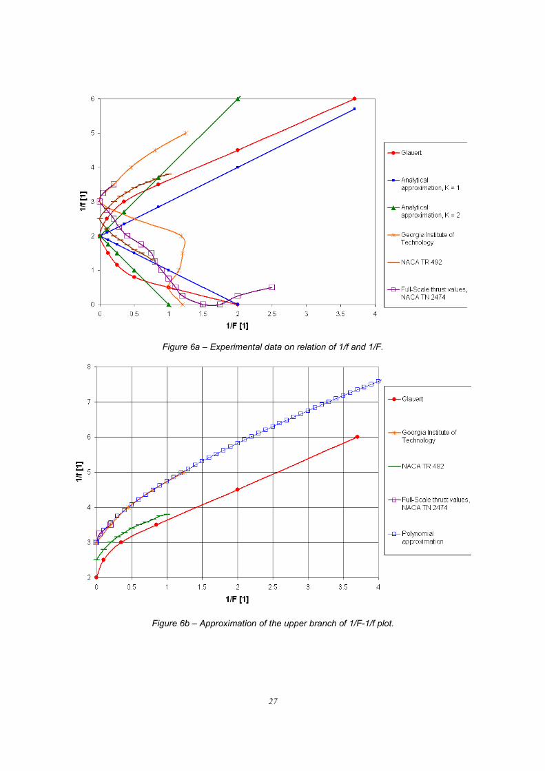
Several experimental measurements of these coefficients were carried out and the results

published in open literature.7, 9, 10, 11 Data from these experiments are summarised in Fig.6a. Full-

scale experimental results from NACA Technical Note no. 247413 were used in the AMRA model.

The upper branch of the 1/F – 1/f plot corresponds to the windmill brake state7 (Up > 0) and the

experimental results published in Ref.13 can be approximated in the following manner (see

Fig.6b)

0.71 1

2.2 3f F

= +

(2.24)

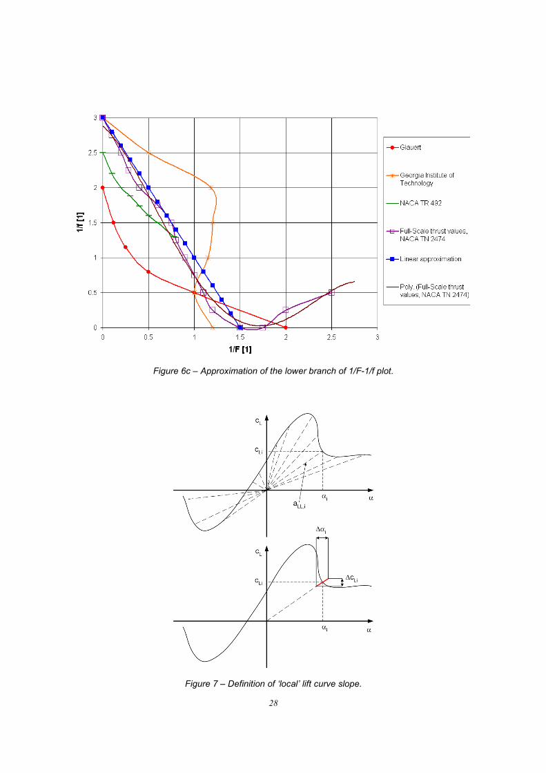
The lower branch of the 1/F – 1/f plot corresponds to the vortex-ring state7 (Up < 0) and two

different formulas can be used to approximate the experimental results (see Fig.6c)

4 3 2

1 23

1 1 1 1 10.3207 1.846 2.5336 1.1336 2.8834

f F

or

f F F F F

= −

= − + − − +

(2.25)

It can be shown7 that Up can be calculated with the aid of vertical inflow ratio.

2

2 4

24

3 3 2 2 4

p p d i

De DeL L L

B e

p

L De

U R V v

c ca a a Q

N R c

a c

λ

θ θρ

λ

= Ω = −

− + − − − − Ω =−

(2.26)

While linear lift curve and a parabolic drag curve were used in the original semi-empirical

method, an approach that allows capture of the effects of blade stall was developed and used in

the model. The constant lift-curve slope, which was used in Ref. 7, was replaced by ‘local’ lift

curve slope (aL) and parabolic approximation of drag curve was substituted for value of cD

obtained from experimental data. Local lift curve slope represents slope of imaginary linear lift

curve that contains the point [αi, cL, i]. The variable does not have any physical significance and it

is merely used to introduce stall effect into the inflow model.

11

,

, ( )L i

L i

i

ca f α

α= = (2.27)

Figure 7 shows that different value of aL is allocated to each point of lift curve ( La a≡ before

stall if the blade section is symmetrical). Since step size of the simulation is very low, this

approach induces much lower error that linear lift curve approach.

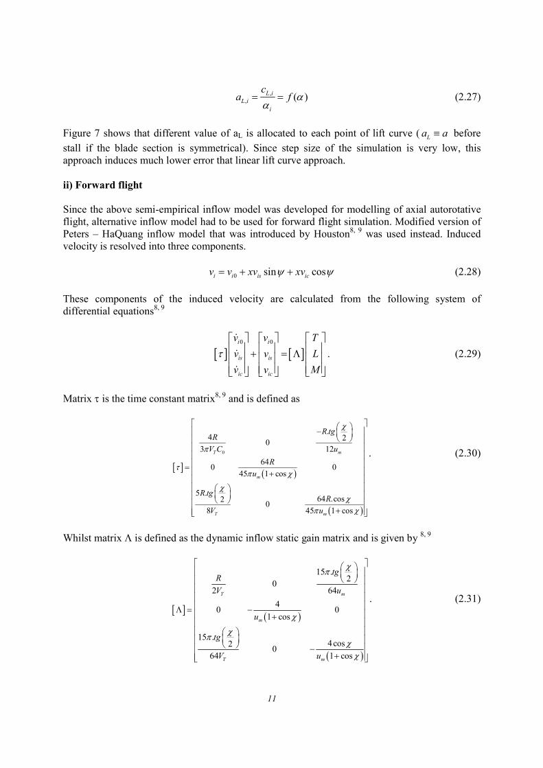
ii) Forward flight

Since the above semi-empirical inflow model was developed for modelling of axial autorotative

flight, alternative inflow model had to be used for forward flight simulation. Modified version of

Peters – HaQuang inflow model that was introduced by Houston8, 9 was used instead. Induced

velocity is resolved into three components.

0 sin cosi i is icv v xv xvψ ψ= + + (2.28)

These components of the induced velocity are calculated from the following system of

differential equations8, 9

[ ] [ ]0 0i i

is is

ic ic

v v T

v v L

v v M

τ + = Λ

&

&

&

. (2.29)

Matrix τ is the time constant matrix8, 9 and is defined as

[ ]( )

( )

0

.4 2

03 12

640 0

45 1 cos

5 .64 .cos2

08 45 1 cos

T m

m

T m

R tgR

V C u

R

u

R tgR

V u

χ

π

τπ χ

χχ

π χ

−

= +

+

. (2.30)

Whilst matrix Λ is defined as the dynamic inflow static gain matrix and is given by 8, 9

[ ]

( )

( )

15 .2

02 64

40 0

1 cos

15 .4cos2

064 1 cos

T m

m

T m

tgR

V u

u

tg

V u

χπ

χ

χπ

χχ

Λ = − +

−+

. (2.31)

12

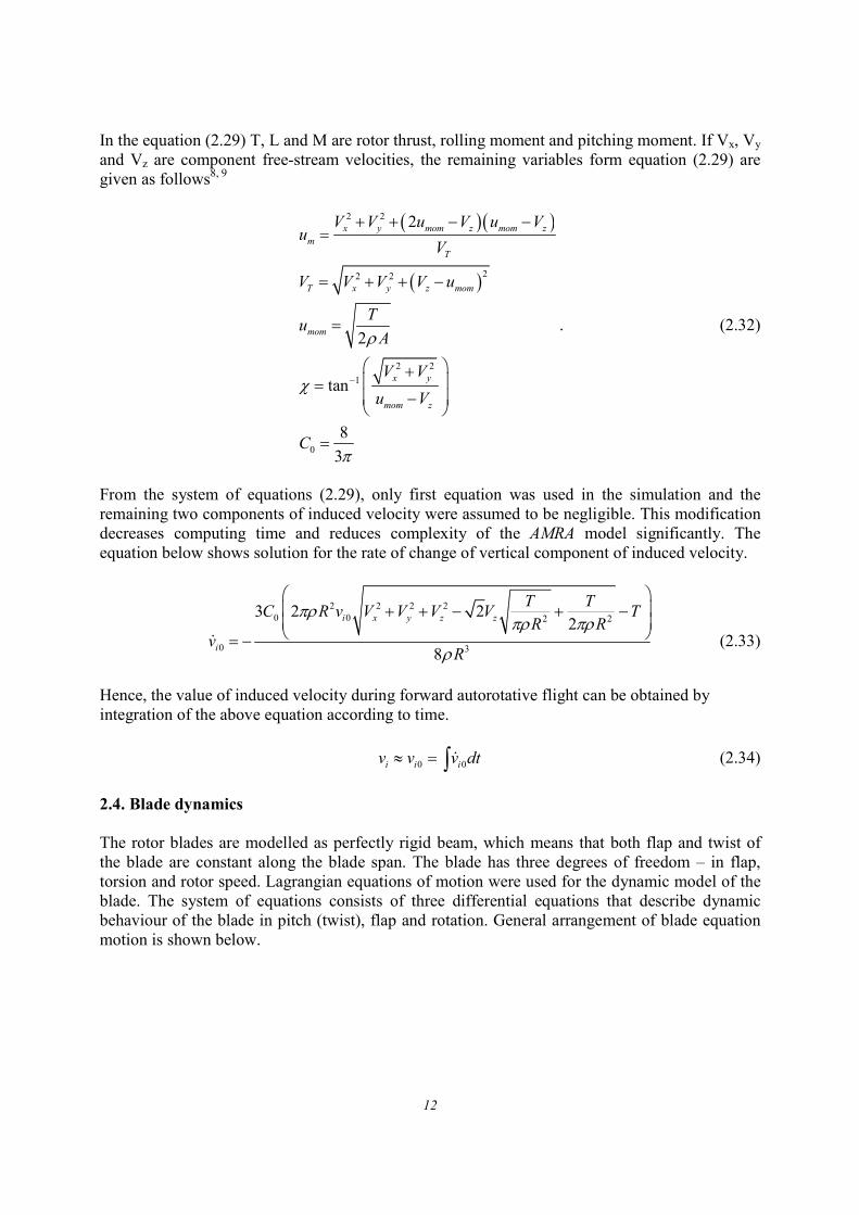
In the equation (2.29) T, L and M are rotor thrust, rolling moment and pitching moment. If Vx, Vy

and Vz are component free-stream velocities, the remaining variables form equation (2.29) are

given as follows8, 9

( )( )

( )

2 2

22 2

2 2

1

0

2

2

tan

8

3

x y mom z mom z

m

T

T x y z mom

mom

x y

mom z

V V u V u Vu

V

V V V V u

Tu

A

V V

u V

C

ρ

χ

π

−

+ + − −=

= + + −

=

+ = −

=

. (2.32)

From the system of equations (2.29), only first equation was used in the simulation and the

remaining two components of induced velocity were assumed to be negligible. This modification

decreases computing time and reduces complexity of the AMRA model significantly. The

equation below shows solution for the rate of change of vertical component of induced velocity.

2 2 2 2

0 0 2 2

0 3

3 2 22

8

i x y z z

i

T TC R v V V V V T

R Rv

R

πρπρ πρ

ρ

+ + − + − = −& (2.33)

Hence, the value of induced velocity during forward autorotative flight can be obtained by

integration of the above equation according to time.

0 0i i iv v v dt≈ = ∫ & (2.34)

2.4. Blade dynamics

The rotor blades are modelled as perfectly rigid beam, which means that both flap and twist of

the blade are constant along the blade span. The blade has three degrees of freedom – in flap,

torsion and rotor speed. Lagrangian equations of motion were used for the dynamic model of the

blade. The system of equations consists of three differential equations that describe dynamic

behaviour of the blade in pitch (twist), flap and rotation. General arrangement of blade equation

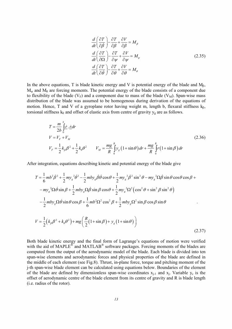
motion is shown below.

13

d T T VM

dt

d T T VM

dt

d T T VM

dt

β

ψ

θ

β β β

ψ ψ

θ θ θ

∂ ∂ ∂− + = ∂ ∂ ∂

∂ ∂ ∂ − + = ∂Ω ∂ ∂

∂ ∂ ∂ − + = ∂ ∂ ∂

&

&

(2.35)

In the above equations, T is blade kinetic energy and V is potential energy of the blade and Mβ,

Mψ and Mθ are forcing moments. The potential energy of the blade consists of a component due

to flexibility of the blade (VF) and a component due to mass of the blade (VM). Span-wise mass

distribution of the blade was assumed to be homogenous during derivation of the equations of

motion. Hence, T and V of a gyroplane rotor having weight m, length b, flexural stiffness kβ,

torsional stiffness kθ and offset of elastic axis from centre of gravity yg are as follows.

( ) ( )

0

2 2

0 0

.2

1 11 sin 1 sin

2 2

b

F M

R R

F M g

mT r rdr

b

V V V

mg mgV k k V y dr r dr

R Rβ θβ θ θ β

=

= +

= + = + + +

∫

∫ ∫

& &

(2.36)

After integration, equations describing kinetic and potential energy of the blade give

( )

( )

2 2 2 2 2 2 2 2

2 2 2 2 2 2

2 2 2 2

2 2

1 1 1 1cos sin sin cos cos

6 2 2 2

1 1sin sin cos cos sin sin

2 2

1 1 1sin cos cos sin cos sin

2 6 2

11 si

2 2

g g g g

g g g

g g

T mb my mby my my

my mby my

mby mb mby

RV k k mgβ θ

β θ βθ θ β θ β θ θ β

θ β β β θ θ β θ

θ θ β β β β θ

β θ

= + − + − Ω +

− Ω + Ω + Ω +

− Ω + Ω + Ω

= + + +

& & & & & &

& &

&

( ) ( )n 1 sing

yβ θ + +

.

(2.37)

Both blade kinetic energy and the final form of Lagrange’s equations of motion were verified

with the aid of MAPLE® and MATLAB® software packages. Forcing moments of the blades are

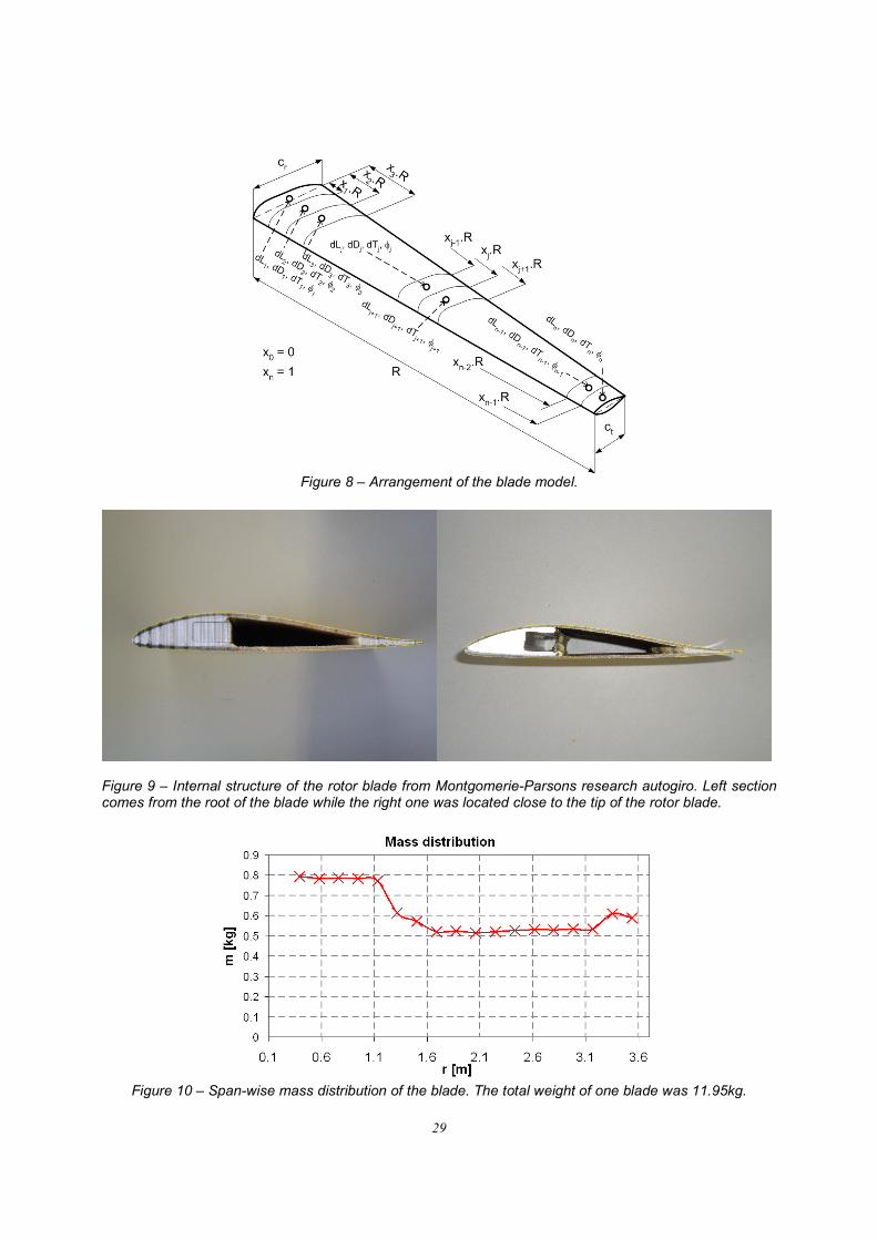
computed from the output of the aerodynamic model of the blade. Each blade is divided into ten

span-wise elements and aerodynamic forces and physical properties of the blade are defined in

the middle of each element (see Fig.8). Thrust, in-plane force, torque and pitching moment of the

j-th span-wise blade element can be calculated using equations below. Boundaries of the element

of the blade are defined by dimensionless span-wise coordinates xj-1 and xj. Variable yc is the

offset of aerodynamic centre of the blade element from its centre of gravity and R is blade length

(i.e. radius of the rotor).

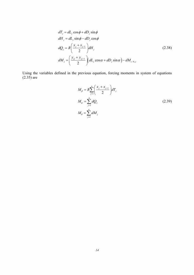
14

( )

1

1

/ 4,

cos sin

sin cos

2

cos sin2

j j j

j j j

j j

j j

cj cj

j j j c j

dT dL dD

dH dL dD

x xdQ R dH

y ydM dL dD dM

φ φ

φ φ

α α

−

−

= +

= −

+ =

+

= + −

(2.38)

Using the variables defined in the previous equation, forcing moments in system of equations

(2.35) are

1

1

1

1

2

nj j

j

j

n

j

j

n

j

j

x xM R dT

M dQ

M dM

β

ψ

θ

−

=

=

=

+ =

=

=

∑

∑

∑

(2.39)

15

3. EXPERIMENTAL MEASUREMENTS OF BLADE PROPERTIES

Since majority of gyroplane rotor blades are manufactured by small private companies, it is

relatively difficult to get any information of structural properties of these blades. A couple of

blades from the Montgomerie-Parsons autogyro were subjected to a series of experiments in

order to assess its physical properties and mass distribution. Data gathered during the

experiments were used as input values of the simulations.

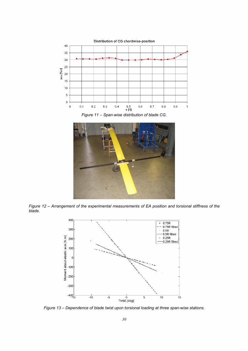
The first blade was cut up into 20 sections and each was measured and weighed so as to ascertain

span-wise mass distribution of the blade. Chord-wise position of centre of gravity was also

estimated for each blade element from the arrangement of internal structure of each blade section

(i.e. position and size of the spar, thickness of the skin and distribution of potential filling

material).

Figure 9 shows the internal structure of the blade at blade root and at the tip. It can be seen that

both mass distribution and chord-wise positions of CG are mainly given by span-wise

distribution of the spar. Span-wise distributions of blade mass and CG locations that were

obtained from the experiments are depicted in Fig.10 and Fig.11.

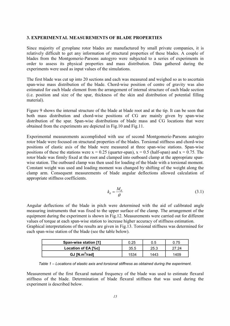
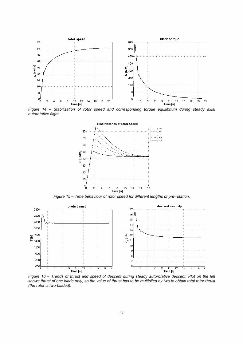
Experimental measurements accomplished with use of second Montgomerie-Parsons autogiro

rotor blade were focused on structural properties of the blades. Torsional stiffness and chord-wise

positions of elastic axis of the blade were measured at three span-wise stations. Span-wise

positions of these the stations were x = 0.25 (quarter-span), x = 0.5 (half-span) and x = 0.75. The

rotor blade was firmly fixed at the root and clamped into outboard clamp at the appropriate span-

wise station. The outboard clamp was then used for loading of the blade with a torsional moment.

Constant weight was used and loading moment was changed by shifting of the weight along the

clamp arm. Consequent measurements of blade angular deflections allowed calculation of

appropriate stiffness coefficients.

M

k θθ θ

= (3.1)

Angular deflections of the blade in pitch were determined with the aid of calibrated angle

measuring instruments that was fixed to the upper surface of the clamp. The arrangement of the

equipment during the experiment is shown in Fig.12. Measurements were carried out for different

values of torque at each span-wise station to increase higher accuracy of stiffness estimation.

Graphical interpretations of the results are given in Fig.13. Torsional stiffness was determined for

each span-wise station of the blade (see the table below).

Span-wise station [1] 0.25 0.5 0.75

Location of EA [%c] 35.5 25.3 27.24

GJ [N.m2/rad] 1534 1443 1409

Table 1 – Locations of elastic axis and torsional stiffness as obtained during the experiment.

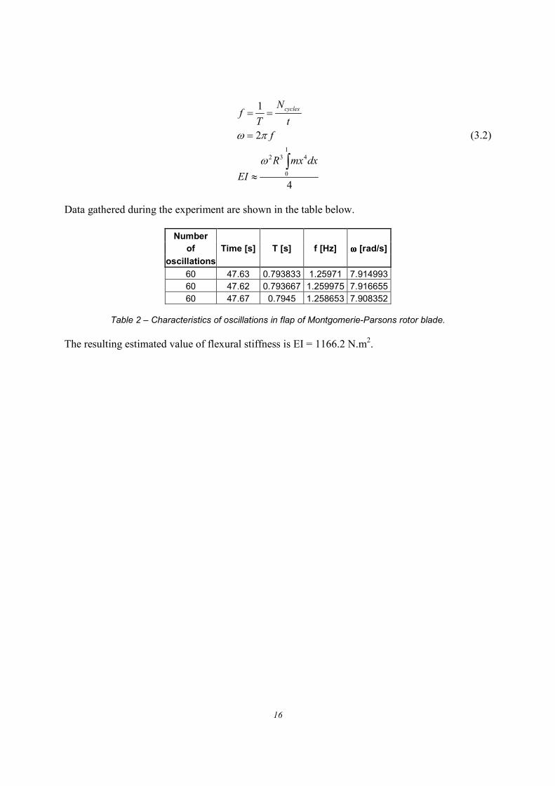
Measurement of the first flexural natural frequency of the blade was used to estimate flexural

stiffness of the blade. Determination of blade flexural stiffness that was used during the

experiment is described below.

16

1

2 3 4

0

1

2

4

cyclesNf

T t

f

R mx dx

EI

ω π

ω

= =

=

≈∫

(3.2)

Data gathered during the experiment are shown in the table below.

Number

of Time [s] T [s] f [Hz] ωωωω [rad/s] oscillations

60 47.63 0.793833 1.25971 7.914993

60 47.62 0.793667 1.259975 7.916655

60 47.67 0.7945 1.258653 7.908352

Table 2 – Characteristics of oscillations in flap of Montgomerie-Parsons rotor blade.

The resulting estimated value of flexural stiffness is EI = 1166.2 N.m2.

17

4. SIMULATION OF AUTOROTATIVE AXIAL FLIGHT

4.1. Initial observations and verification

Series of simulations of aeromechanical behaviour of a gyroplane rotor in axial autorotative flight

was performed. The input parameters of the simulations can be found in Table 3. Simulations of a

gyroplane rotor in steady autorotative descent have revealed that the AMRA model captures all

key features of the system. The rotor speed has to be increased by application of external torque

during pre-rotation. Once the rotor speed reaches sufficient value, the external torque is removed

and the system enters autorotative regime. Both acceleration of the rotor from lower rotor speed

and transition from helicopter regime (i.e. deceleration from higher rotor speed, see Fig.14) can

be demonstrated by the simulation (see Fig.15). Note that rotor speed always stabilises at the

same value once steady autorotation is established since its configuration did not change.

PARAMETER VALUE

Blade length (R) 3.63m

Blade chord (c) 0.2m

Chord-wise position of EA (yEA) 0.08m = 40%c

Chord-wise position of CG (yCG) 0.066m = 33%c

Chord-wise position of AC (yAC) 0.05m = 25%c

Offset of CG from EA (yg) 0.014m

Offset of AC from EA (yc) 0.03m

Blade weight (m) 13kg

Number of blades (NB) 2

Blade fixed incidence angle 0 rad

Span-wise distribution of blade geometric twist ε = 0 rad Weight of the autogyro (M) 400kg

Blade torsional stiffness coefficient (kθ) 1600N.m2/rad

Blade flexural stiffness coefficient (kβ) 1200N.m2

Blade section geometry NACA 0012

Torque used for pre-rotation (QPR) 2000N.m

Table 3 – Input parameters of the simulations.

It should be noted that rotor speed in autorotation is much lower than rotor speed of helicopter

rotor during flight. It can be seen from Fig.14 that the rotor speed is stabilized and the system

reaches torque equilibrium within few seconds. At this point, the total thrust of the rotor is in

balance with the weight of the vehicle and the value of speed of descent is approximately 11.5m/s

(see Fig.16). The value of speed of descent agrees with the results of experimental flight

measurements that were carried out by NACA and several other research bodies.10,12

The

equation below shows empirical relationship of disc loading of an autogiro and speed of descent

that was derived from the experimental results.10, 12

1.212 /dV T A≈ (4.1)

Weight of the vehicle is M = 400kg and rotor radius is R = 3.63m, hence rotor disc loading is T/A

= 96N.m-2 and equation (4.1) gives speed of descent Vd = 11.8m/s.

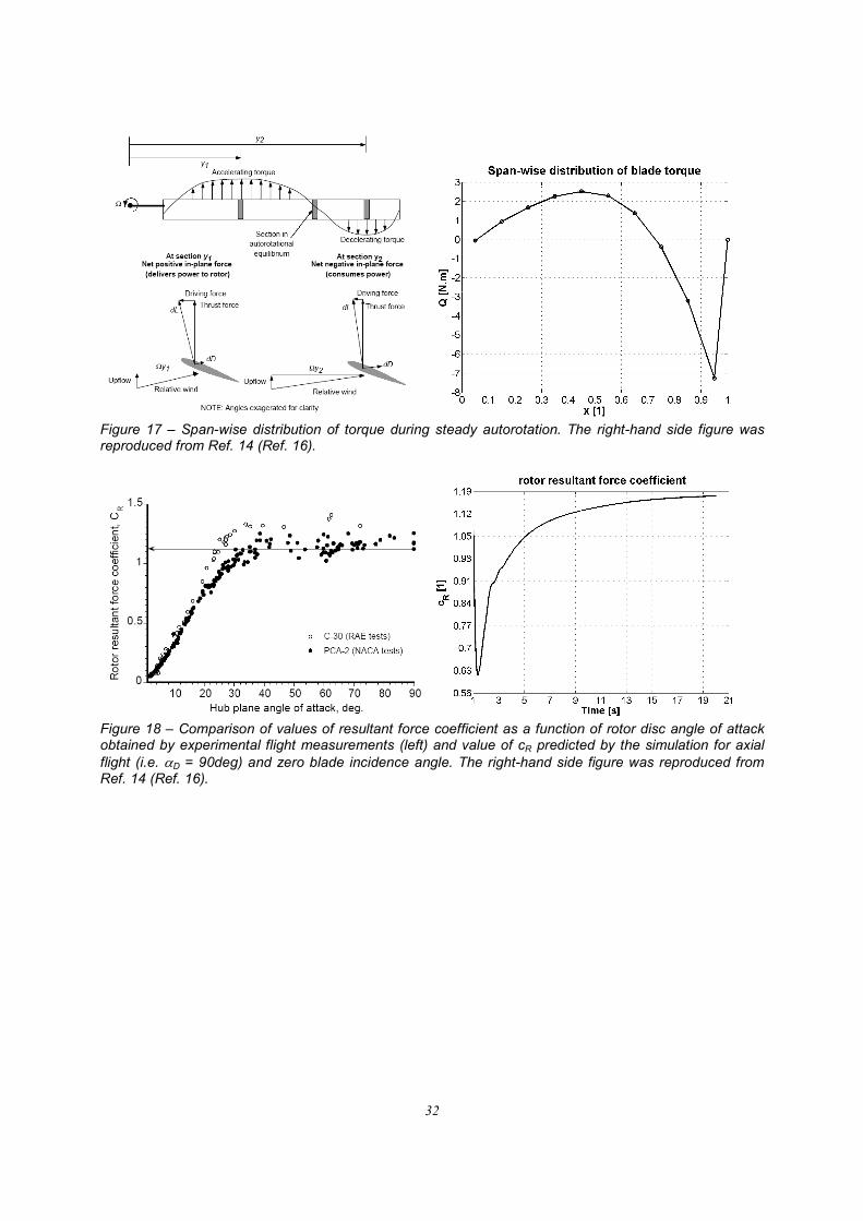
A characteristic span-wise distribution of blade torque for a rotor in the autorotative regime is

observed. The inboard part of the blade generates positive torque and the outboard part of the

blade generates negative torque. In steady autorotation, the total value of torque generated by the

18

blade is zero. Figure 17 shows a comparison of span-wise distribution of torque obtained from

the simulation and torque distribution as described in open literature.10, 12

The so-called coefficient of resultant force is another important characteristic of autorotative

regime.10, 12

It is defined by

2

2 2

2 2

2R

h d

Rc

V A

R L D

V V V

ρ=

= +

= +

. (4.2)

Previous research involving experimental flight measurements10, 12

found that cR on typical rotor

of an autogyro during steady autorotative flight at large rotor disc angles of attack (αD > 30deg)

is about 1.25. It is important to realize that the majority of gyroplane rotors have very small or

zero fixed blade angle of incidence (in effect a collective pitch setting, in helicopter jargon). The

value of cR is different for non-zero blade angles of incidence as it is shown later in this paper.

Figure 18 shows a comparison of experimental values of cR10, 12 and the outcome of the

simulation. The AMRA model predicts value of cR to be 1.19.

4.2. Parametric studies

A series of parametric studies of basic rotor designs were undertaken in order to gain more

knowledge about the influence of different design parameters of a gyroplane rotor on its

performance.

i) Blade fixed incidence

Experimental investigations of gyroplane aerodynamics revealed that range of blade fixed

incidence angle (collective pitch), for which steady autorotation is sustainable, is limited.10, 12

Results obtained from the AMRA model correlate with conclusions of experimental

measurements. The model shows that excessive values of blade collective pitch cause stall of the

inboard regions of the blade (i.e. driving region), hence torque equilibrium is not possible. As a

result, rotor speed decreases rapidly, thrust decreases and velocity of descent increases.

Comparison of the autorotational diagram12 and output from the AMRA model (see Fig.19) shows

that the simulation correctly estimates critical blade pitch to be about 0.2rad.

In the case of negative value of blade fixed incidence angle, the rotor speed is significantly higher

than for zero or small positive value of the angle and torque equilibrium is established. However,

this configuration of autogyro rotor is not practical since speed of descent during steady

autorotation is very high.

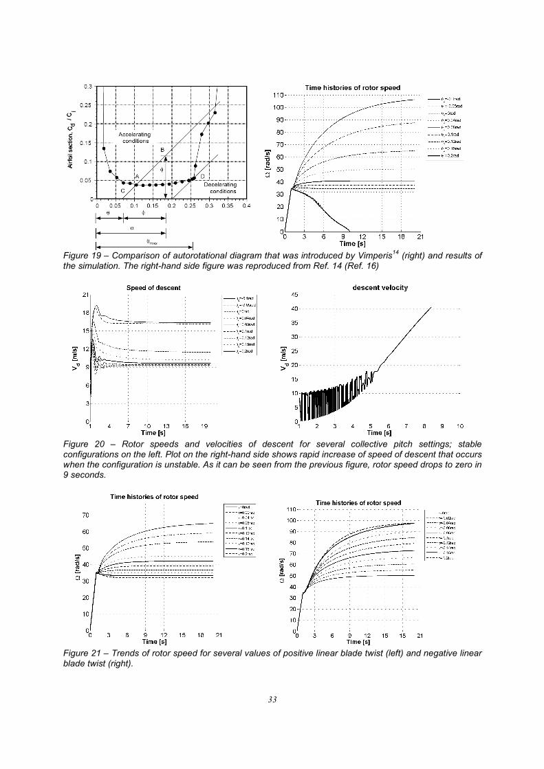
ii) Blade twist

A parametric study was performed to establish the influence of blade twist. The conclusions are

very similar to those obtained during the study dealing with varying blade incidence angle - i.e.

steady autorotation is possible only for moderate values of blade twist. However, the limity value

19

of linear blade twist is higher as it affects mainly the outboard part of the blade where inflow

angle is relatively small (see Fig.21). It can be noted that, in analogy with the study of the effect

of blade incidence angle, negative twist of the blade increases both rotor speed and velocity of

descent.

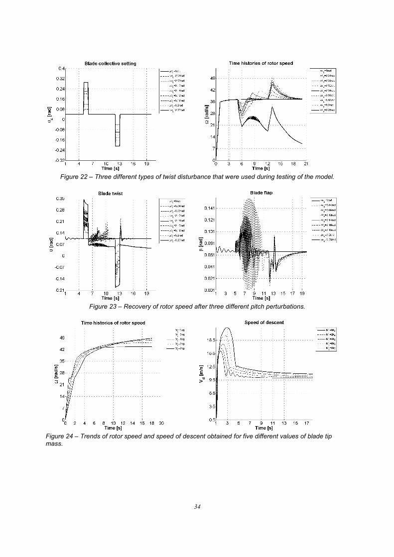
Provided that rotor speed is high enough and the rotor blade is in stable configuration,

autorotation is a very stable flight regime. Simulations were carried out for several different

magnitudes of twist disturbance to study the ability of a rotor in autorotation to recover from a

gust. The effect of a gust was modelled as a step input in collective pitch. Figures 22 and 23

depict clearly that, if the blade is in stable configuration, coupling between rotor speed, blade

twist and flap return have strong auto-stabilizing characteristics. The rotor speed recovers even if

the magnitude of the disturbance is relatively high. Computations have also demonstrated that the

rotor is not able to reach steady autorotation if rotor speed is too low. The highest twist deflection

leads to significant decrease of rotor speed that results in stall of significant part of the blade.

Stable autorotation is not re-established since the lift drops and drag increases considerably

behind the stall point.

iii) Blade tip mass

Blade tip mass is frequently used to increase moment of inertia of gyroplane rotor blades. Higher

moment of inertia further improves the stability of autorotation and therefore decreases

probability of abrupt loss of rotor speed due to a gust or poor piloting. Computation for several

different values of blade tip mass were undertaken to establish how sensitive autorotative state is

to changes in this parameter. The concentrated mass was placed at the local elastic axis in order

not to affect blade pitch dynamics. The outcome of the simulations is shown in Fig.24. It can be

seen that the tip mass increases rotor speed as anticipated.

Results of the simulations have demonstrated that the effect of coupling between blade twist and

rotor speed is very significant due to strong influence of blade incidence angle on both torque and

thrust of the blade. Therefore, the conclusion can be drawn that the value of blade torsional

stiffness is the key parameter of any gyroplane blade design. Together with chord-wise location

of the elastic axis and centre of gravity, flexural stiffness has the decisive effect on aeroelastic

stability of a rotor in autorotation. Further investigations have shown that blade flexural stiffness

plays rather inferior role in this case due to centrifugal stiffening.

4.3. Stability boundary

In order to investigate rotor stability boundary in torsion, simulations for various torsional

stiffness, chord-wise positions of centre of gravity (CG) and chord-wise positions of elastic axis

(EA) were carried out.

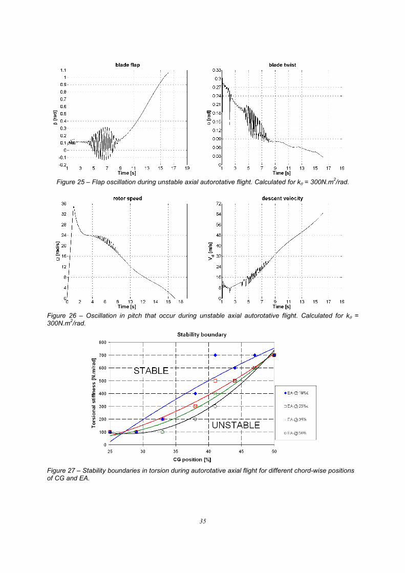
The results of the simulations have revealed that low torsional stiffness of the blade leads to an

aeroelastic instability (flutter) that comes through as coupled rotor speed / pitch / flap oscillations

(see Fig.25 and 26). These oscillations result in catastrophic decrease of rotor speed as is shown

in Fig.26. This is demonstration of strong rotor speed / pitch / flap that exists only during

autorotation. Decrement of the rotor speed decreases centrifugal stiffness of the rotor and the

resulting higher deflections in flap and twist generate more drag and cause further drop in rotor

speed. As it can be seen in Fig.26, reduction of rotor speed from a steady value to zero takes only

few seconds and the speed of descent increases to unacceptable value during this time. This type

20

of flutter seems to be unique for rotor in autorotation since it differs from both helicopter rotor

flutter and flutter of a fixed wing.

It can be seen from figures 27 and 28 that position of CG aft EA is destabilizing, which agrees

both with theory of aeroelasticity and experiments. Chord-wise position of CG seems to have

much stronger influence on the stability of autorotation than chord-wise position of EA. It is

probably caused by the fact that the offset of aerodynamic centre (AC) from EA (i.e. the arm of

forcing torsional moment) is another factor influencing stability the shape of boundary and it is a

function of chord-wise location of EA.

c AC EA

g CG EA

y y y

y y y

= −

= − (4.3)

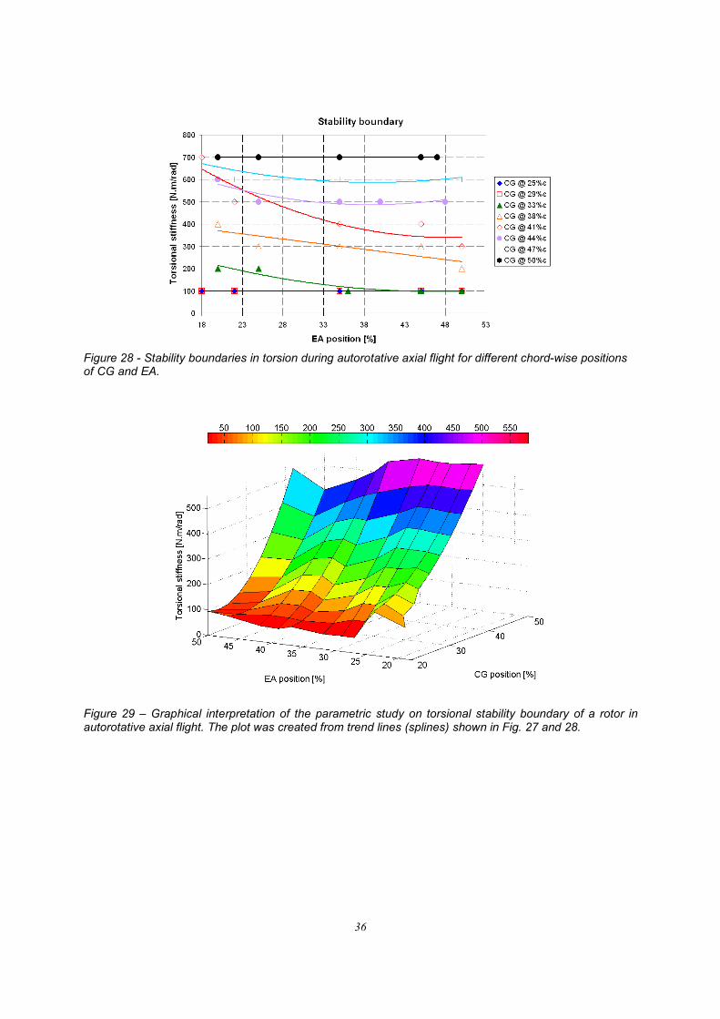
All results of the investigations can be summarised in 3-D chart that comprises change of the

stability boundary due to both variation of CG position and variation of EA position (see Fig. 29

and 30).

21

5. SIMULATION OF AUTOROTATIVE FORWARD FLIGHT

Since gyroplanes operate mostly in forward flight regime, modelling of forward autorotative

flight represents the key task in investigation of aeroelastic behaviour of a gyroplane rotor blade.

In comparison to the simulation of axial autorotative flight, simulation of forward flight in

autorotation induces some complication. Both direction and value of the inflow velocity are

functions of azimuth if horizontal speed is not zero (see equations (2.7) and (2.8)). This means

that there is no torque equilibrium during steady forward flight and the value of torque oscillates

around the zero value (see Fig.31). The amount of vibrations induced by the rotor blade during

steady forward flight is therefore significantly higher than in axial descent. In addition, free-

stream velocity at the advancing side of the rotor disc is higher, and thus the values of the forcing

moments are higher too. It can be expected that gyroplane rotor blade in the forward flight regime

is more prone to undergo aeroelastic instability than the same blade during axial autorotative

flight.

5.1. Parametric studies

i) Chord-wise position of CG and EA

Computations carried out with the aid of the latest version of the AMRA model have shown that

the rotor suffers of aeroelastic instability if CG lies aft EA. The model has also predicted that

fixed incidence angle of the blade (collective pitch) has very strong influence on shape of

torsional stability boundary. In order to gain more knowledge about the problem, parametric

study focused on the effect of position of blade CG and EA was performed. Computations for EA

at 35%c and different chord-wise locations of CG and values of torsional stiffness kθ were

undertaken. Since most of parameters in forward autorotative flight have harmonic behaviour, the

results are presented in the form of boundaries of their trends. This approach allows comparison

of multiple data sets in one plot. Figures 31 and 32 show an example of results of the simulations

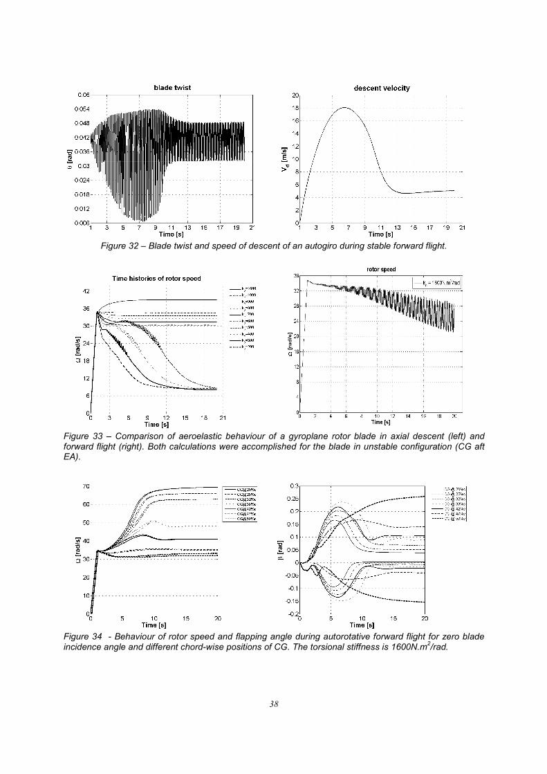
obtained from forward autorotative flight in stable configuration (Vh = 50m/s, CG ahead of EA).

Comparison of time behaviours of rotor speed of a rotor blade in unstable configuration (CG at

45%c and EA at 35%c) during autorotative axial descent and forward flight is depicted in Fig.33.

Blade incidence angle is set to 0.04rad for both axial flight and forward flight. Note that in the

case of axial descent, blade oscillations and decrease of rotor speed occur at much lower torsional

stiffness than during forward flight. In forward flight, oscillations develop even for realistic value

of torsional stiffness obtained during experimental measurements of blade structural properties

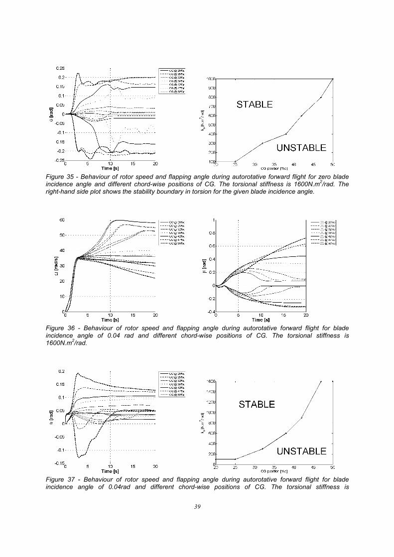
(kθ = 1600N.m2/rad). Figures 34 - 37 compare estimations of the behaviour of the rotor during

forward flight for zero blade incidence angle and blade incidence angle θc = 0.04rad. The influence of blade incidence in forward autorotative flight seems to be even stronger than during

axial descent. Stability boundaries obtained for forward flight regime are given in Fig. 35 and 37.

Corresponding data for autorotative vertical flight can be found in Fig.27.

ii) Blade fixed incidence angle

Figures 38 and 39 show results of a series of simulations to investigate the effect of blade

incidence angle alone (without change of chord-wise location of CG). Again, blade incidence

angle seems to have a strongly destabilizing effect. Another set of calculations was carried out for

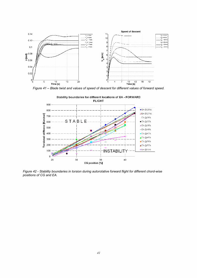
different values of horizontal speed. It can be seen from Fig.40 and 41 that both flapping and

22

torsion of the blade increases with rise of horizontal speed. Rotor speed, however, does not

change since the configuration of the rotor remains unchanged.

5.2. Stability boundary of a rotor blade in autorotative forward flight

Similarly as in case of axial flight in autorotation, simulations for various torsional stiffness,

chord-wise positions of centre of gravity (CG) and chord-wise positions of elastic axis (EA) were

performed.

The results of the simulations have shown that location of CG aft EA leads to torsional

oscillations that are combined with oscillations in blade flap and rotor speed. Mean value of rotor

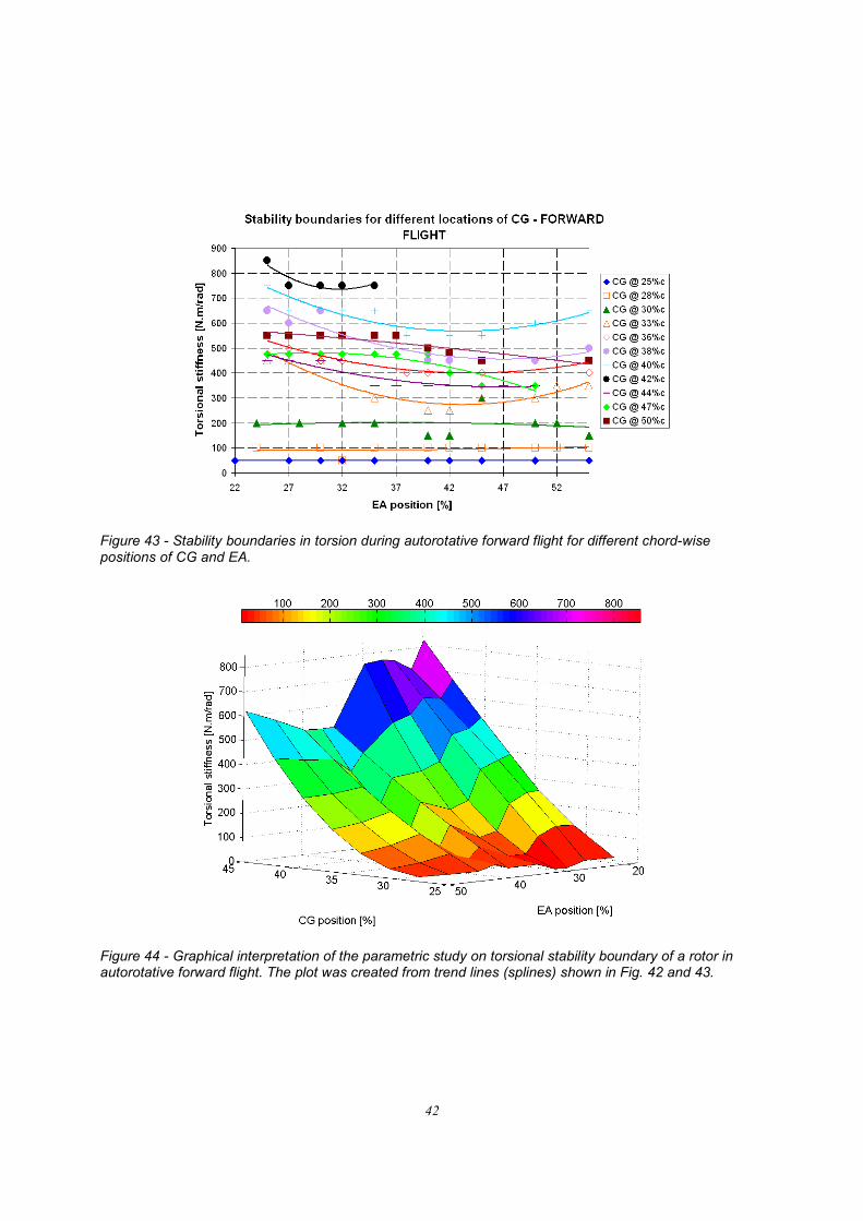
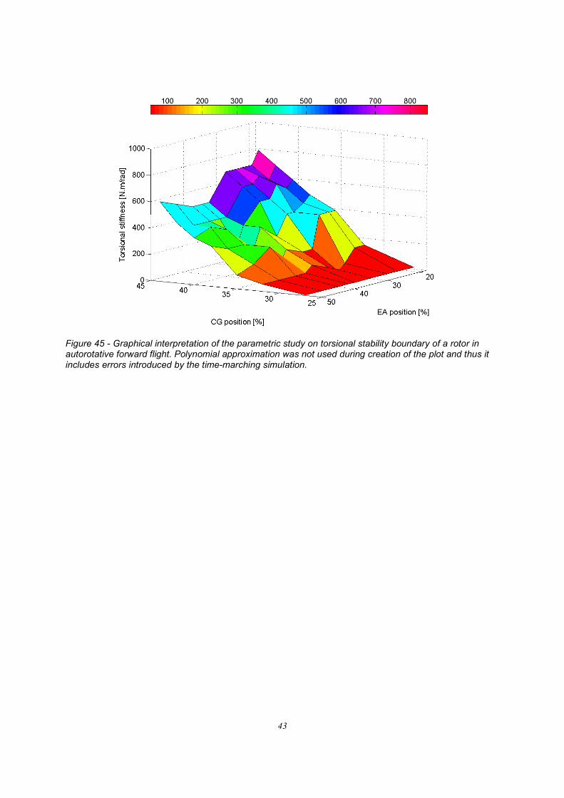
speed decreases due to higher drag of the rotor blade (see Fig. 36 and 37). Figures 42 – 45 show

resulting stability boundaries of the rotor and corresponding 3D stability plots. Again, it can be

noted that blade oscillations and decrease of the rotor speed occur for higher values of blade

torsional stiffness than in axial flight. Conclusion can be made that the auto-stabilising effect of

pitch-flap-rotor speed coupling is relatively strong during axial descent, but is suppressed by

flow-induced oscillations in forward flight.

23

6. CONCLUSIONS

An aeromechanical model of a gyroplane rotor AMRA was developed and used in predicting the

aeroelastic behaviour of a rotor. Both regimes were investigated – autorotative axial flight

(vertical descent) and forward flight in autorotation. Simulations have shown that autorotation is

a complex aeromechanical process with auto-stabilizing characteristics. It was found that blade

twist / rotor speed coupling has major effect on stability of autorotation when the rotor is in a

stable configuration.

In order to obtain input parameters for the structural model of the blade, a series of experimental

measurements were carried out. Blade mass distribution, position of elastic axis, span-wise

distribution of CG and torsional and flexural stiffness was determined during the experiments.

Results from the AMRA model were verified and found to be in a good agreement with both

existing theory of aeroelasticity and experimental measurements. Several parametric studies were

performed so as to gain more knowledge on the effect of blade geometry and structural properties

on performance of the rotor during autorotation.

Occurrence of a type of flutter that is unique for autorotating rotor was discovered during

simulation of unsteady axial descent in autorotation. This aeroelastic instability is driven by blade

pitch / flap / rotor speed coupling and differs from both flutter of a helicopter rotor and flutter of a

fixed wing. The instability results in catastrophic decrease of the rotor speed and significant

increase of speed of descent.

Preliminary results of simulation of gyroplane rotor in forward flight were obtained and analysed.

The AMRA model suggests that positive blade twist has adverse effect on performance of the

rotor during autorotative forward flight. Very low positive or zero fixed blade incidence angle

and moderate amount of blade tip mass seem to be beneficial for performance of a rotor in

autorotation. Low negative value of blade linear twist can also improve its behaviour as it

decreases angle of attack of the outboard part of the blade which is the source of negative torque

during autorotation.

More powerful structural model of gyroplane blade that will utilise finite element method (FEM)

will be developed in the next stage of the project. It will be coupled with RASCAL advanced

rotor blade aerodynamic model developed by Dr Houston from Department of Aerospace

Engineering, University of Glasgow.20

24

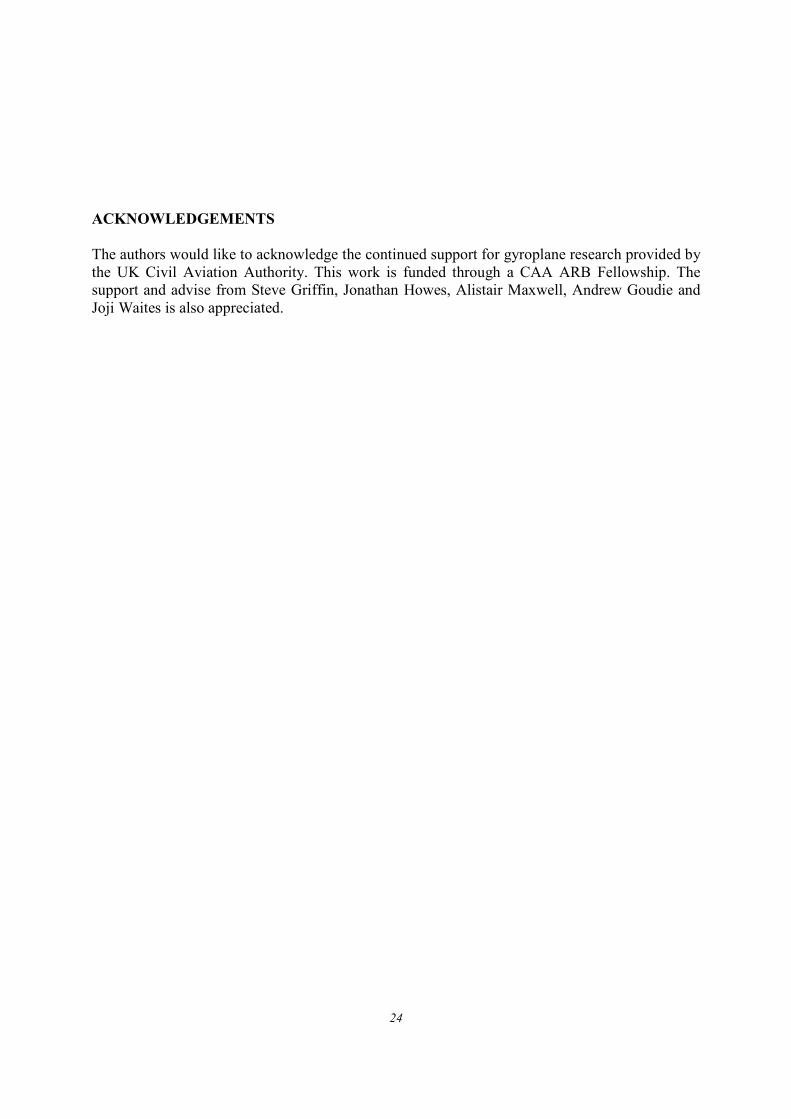
ACKNOWLEDGEMENTS

The authors would like to acknowledge the continued support for gyroplane research provided by

the UK Civil Aviation Authority. This work is funded through a CAA ARB Fellowship. The

support and advise from Steve Griffin, Jonathan Howes, Alistair Maxwell, Andrew Goudie and

Joji Waites is also appreciated.

25

Figure 1 – General arrangement of the AMRA autogiro rotor blade model.

Figure 2 – Relation of blade twist, flap and inflow angle of a rotor in autorotation.

26

Figure 3 – Trends of NACA 0012 lift coefficient obtained for different values of Mach number. Obtained with the aid of approach described in Ref.5.

Figure 4 - Trends of NACA 0012 drag coefficient obtained for different values of Mach number. Obtained with the aid of approach described in Ref.5.

Figure 5 – Induced velocity relations in vertical flight (speed of climb on the x-axis, induced velocity on the y-axis). Reproduced from Ref. 23.

27

Figure 6a – Experimental data on relation of 1/f and 1/F.

Figure 6b – Approximation of the upper branch of 1/F-1/f plot.

28

Figure 6c – Approximation of the lower branch of 1/F-1/f plot.

Figure 7 – Definition of ‘local’ lift curve slope.

29

Figure 8 – Arrangement of the blade model.

Figure 9 – Internal structure of the rotor blade from Montgomerie-Parsons research autogiro. Left section comes from the root of the blade while the right one was located close to the tip of the rotor blade.

Figure 10 – Span-wise mass distribution of the blade. The total weight of one blade was 11.95kg.

30

Figure 11 – Span-wise distribution of blade CG.

Figure 12 – Arrangement of the experimental measurements of EA position and torsional stiffness of the blade.

Figure 13 – Dependence of blade twist upon torsional loading at three span-wise stations.

31

Figure 14 – Stabilization of rotor speed and corresponding torque equilibrium during steady axial autorotative flight.

Figure 15 – Time behaviour of rotor speed for different lengths of pre-rotation.

Figure 16 – Trends of thrust and speed of descent during steady autorotative descent. Plot on the left shows thrust of one blade only, so the value of thrust has to be multiplied by two to obtain total rotor thrust (the rotor is two-bladed).

32

Figure 17 – Span-wise distribution of torque during steady autorotation. The right-hand side figure was reproduced from Ref. 14 (Ref. 16).

Figure 18 – Comparison of values of resultant force coefficient as a function of rotor disc angle of attack obtained by experimental flight measurements (left) and value of cR predicted by the simulation for axial

flight (i.e. αD = 90deg) and zero blade incidence angle. The right-hand side figure was reproduced from Ref. 14 (Ref. 16).

33

Figure 19 – Comparison of autorotational diagram that was introduced by Vimperis

14 (right) and results of

the simulation. The right-hand side figure was reproduced from Ref. 14 (Ref. 16)

Figure 20 – Rotor speeds and velocities of descent for several collective pitch settings; stable configurations on the left. Plot on the right-hand side shows rapid increase of speed of descent that occurs when the configuration is unstable. As it can be seen from the previous figure, rotor speed drops to zero in 9 seconds.

Figure 21 – Trends of rotor speed for several values of positive linear blade twist (left) and negative linear blade twist (right).

34

Figure 22 – Three different types of twist disturbance that were used during testing of the model.

Figure 23 – Recovery of rotor speed after three different pitch perturbations.

Figure 24 – Trends of rotor speed and speed of descent obtained for five different values of blade tip mass.

35

Figure 25 – Flap oscillation during unstable axial autorotative flight. Calculated for kθ = 300N.m

2/rad.

Figure 26 – Oscillation in pitch that occur during unstable axial autorotative flight. Calculated for kθ = 300N.m

2/rad.

Figure 27 – Stability boundaries in torsion during autorotative axial flight for different chord-wise positions of CG and EA.

36

Figure 28 - Stability boundaries in torsion during autorotative axial flight for different chord-wise positions of CG and EA.

Figure 29 – Graphical interpretation of the parametric study on torsional stability boundary of a rotor in autorotative axial flight. The plot was created from trend lines (splines) shown in Fig. 27 and 28.

37

Figure 30 - Graphical interpretation of the parametric study on torsional stability boundary of a rotor in autorotative axial flight. Polynomial approximation was not used during creation of the plot and thus it includes errors introduced by the time-marching simulation.

Figure 31 – Rotor speed and blade flap angle in stable forward flight.

38

Figure 32 – Blade twist and speed of descent of an autogiro during stable forward flight.

Figure 33 – Comparison of aeroelastic behaviour of a gyroplane rotor blade in axial descent (left) and forward flight (right). Both calculations were accomplished for the blade in unstable configuration (CG aft EA).

Figure 34 - Behaviour of rotor speed and flapping angle during autorotative forward flight for zero blade incidence angle and different chord-wise positions of CG. The torsional stiffness is 1600N.m

2/rad.

39

Figure 35 - Behaviour of rotor speed and flapping angle during autorotative forward flight for zero blade incidence angle and different chord-wise positions of CG. The torsional stiffness is 1600N.m

2/rad. The

right-hand side plot shows the stability boundary in torsion for the given blade incidence angle.

Figure 36 - Behaviour of rotor speed and flapping angle during autorotative forward flight for blade incidence angle of 0.04 rad and different chord-wise positions of CG. The torsional stiffness is 1600N.m

2/rad.

Figure 37 - Behaviour of rotor speed and flapping angle during autorotative forward flight for blade incidence angle of 0.04rad and different chord-wise positions of CG. The torsional stiffness is

40

1600N.m2/rad. The right-hand side plot shows the stability boundary in torsion for the given blade

incidence angle.

Figure 38 – The effect of blade incidence angle (collective pitch) on aeroelastic behaviour of a gyroplane rotor in forward flight.

Figure 39 – Twist of the blade obtained for different values of blade incidence angle (i.e. collective pitch).

Figure 40 – The effect of the value of forward speed on rotor speed and flapping angle of the blade.

41

Figure 41 – Blade twist and values of speed of descent for different values of forward speed.

Figure 42 - Stability boundaries in torsion during autorotative forward flight for different chord-wise positions of CG and EA.

42

Figure 43 - Stability boundaries in torsion during autorotative forward flight for different chord-wise positions of CG and EA.

Figure 44 - Graphical interpretation of the parametric study on torsional stability boundary of a rotor in autorotative forward flight. The plot was created from trend lines (splines) shown in Fig. 42 and 43.

43

Figure 45 - Graphical interpretation of the parametric study on torsional stability boundary of a rotor in autorotative forward flight. Polynomial approximation was not used during creation of the plot and thus it includes errors introduced by the time-marching simulation.

44

7. REFERENCES

[1] Thomson, D.G., Houston, S.S., Spathopoulos, V. M., “Experiments in Autogiro Airworthiness for Improved

Handling Qualities”, Journal of American Helicopter Society, Pg. 295, No. 4, Vol. 50, October 2005.

[2] Houston, S. S., “Longitudinal Stability of Gyroplanes”, The Aeronautical Journal, Vol. 100 (991), 1996, pp.

1-6.

[3] Houston, S. S.: “Identification of Autogiro Longitudinal Stability and Control Characteristics”, Journal of

Guidance, Control and Dynamics, Vol. 21, No. 3, 1998, pp. 391-399.

[4] Coton, F., Smrcek, L., Patek, Z., “Aerodynamic Characteristics of a Gyroplane Configuration”, Journal of

Aircraft, Vol. 35, No. 2, 1998, p. 274 – 279.

[5] Prouty, R. W., “Helicopter Performance, Stability and Control”, Robert E. Krieger Publishing Co., Malabar,

FA, USA, 1990.

[6] Sheldahl, R. E., Klimas, P. C., “Aerodynamic Characteristics of Seven Aerofoil Sections Through 180

Degrees Angle of Attack for Use in Aerodynamic Analysis of Vertical Axis Wind Turbines”, SAND80-

2114, Sandia National Laboratories, Albuquerque, New Mexico, USA, 1981.

[7] Nikolsky, A.A., Seckel, E., “An Analytical Study of the Steady Vertical Descent in Autorotation of Single-

Rotor Helicopters”, NACA TN 1906, Washington, 1949.

[8] Houston, S. S., “Modelling and Analysis of Helicopter Flight Mechanics in Autorotation”, Journal of

Aircraft, Vol. 40, No. 4, 2003.

[9] Spathopoulos, V. McI., “The Assessment of a Rotorcraft Simulation Model in Autorotation by Means of

Flight Testing a Light Gyroplane”, PhD Thesis, Department of Aerospace Engineering, University of

Glasgow, 2001.

[10] Leishman, J.G., “Principles of Helicopter Aerodynamics”, Cambridge University Press, 2nd Edition, 2006,

pp.428-431. ISBN 0-521-85860-7

[11] Wheatley, J.B., “An Aerodynamic Analysis of the Autogiro Rotor with a Comparison between Calculated

and Experimental Results,” NACA TR 487.

[12] Leishman, J.G., “The Development of the Autogiro: A Technical Perspective”, Journal of Aircraft, Vol. 41,

(2), 2004, pp. 765-781.

[13] Bramwell, A. R. S. et al, “Bramwell’s Helicopter Dynamics”, 2nd edition, Butterworth-Heinemann, 2001.

ISBN 0-7506-5075-3

[14] Sissingh, G., “Contribution to the Aerodynamics of Rotating-Wing Aircraft,” NACA TM 921

[15] Wheatley, J.B., “The Aerodynamic Analysis of the Gyroplane Rotating-Wing System,” NACA TN 492,

Langley Memorial Aeronautical Laboratory, 1934.

[16] www.cyberiad.net/foildata.htm The data were synthesized from a combination of experimental results

published in [20] and computer calculations.

[17] Wheatley, B., Bioletti, C., “Wind-Tunnel Tests of a 10-foot-diameter Gyroplane Rotor”, NACA TR 536.

[18] Wheatley, B., Bioletti, C., “Wind-Tunnel Tests of a 10-foot-diameter Gyroplane Rotors”, NACA TR 552.

[19] Wheatley, B., Hood, M. J., “Full-Scale Wind-Tunnel Tests of a PCA-2 Autogiro Rotor”, NACA TR 515.

45

[20] Houston, S.S., “Validation of a non-linear individual blade flight dynamics model using a perturbation

method”, The Aeronautical Journal of the Royal Aeronautical Society, Vol.98, No.977, Aug-Sep. 1994.

[21] Carpenter, P.J., “Lift and Profile-drag Characteristics of an NACA 0012 Airfoil Section as Derived from

Measured Helicopter-rotor Hovering Performance”, NACA TN 4357, Langley Memorial Aeronautical

Laboratory, Langley Field, VA, USA, 1958.

[22] Wheatley, J.B., “An Aerodynamic Analysis of the Gyroplane Rotating-Wing System”, NACA TR 487,

Langley Memorial Aeronautical Laboratory, Langley Field, VA, USA, 1934.

[23] Wheatley, J.B., “An Aerodynamic Analysis of the Autogiro Rotor with a Comparison between Calculated

and Experimental Results”, NACA TR 487.

[24] Castles, W., Gray, R.B., “Empirical Relation Between Induced Velocity, Thrust and Rate of Descent of a

Helicopter Rotor as Determined by Wind-Tunnel Tests on Four Model Rotors”, NACA TN 2474,

Washington, 1951.

[25] Brown, R. E., Houston, S. S., “CFD-based Simulation and Experiment in Helicopter Aeromechanics”,

published at www.ae.ic.uk/research/rotorcraft/pubs.