Static Aeroelastic and Longitudinal Trim Model of Flexible ...

Static Aeroelastic and Longitudinal Trim Model of FlexibleWing Aircraft Using Finite-Element Vortex-Lattice Coupled

Solution

Eric Ting∗

Stinger Ghaffarian Technologies, Inc., Moffett Field, CA 94035Nhan Nguyen†

NASA Ames Research Center, Moffett Field, CA 94035Khanh Trinh‡

Stinger Ghaffarian Technologies, Inc., Moffett Field, CA 94035

This paper presents a static aeroelastic model and longitudinal trim model for the analysis of a flexiblewing transport aircraft. The static aeroelastic model is built using a structural model based on finite-elementmodeling and coupled to an aerodynamic model that uses vortex-lattice solution. An automatic geometrygeneration tool is used to close the loop between the structural and aerodynamic models. The aeroelasticmodel is extended for the development of a three degree-of-freedom longitudinal trim model for an aircraftwith flexible wings. The resulting flexible aircraft longitudinal trim model is used to simultaneously computethe static aeroelastic shape for the aircraft model and the longitudinal state inputs to maintain an aircraft trimstate. The framework is applied to an aircraft model based on the NASA Generic Transport Model (GTM) withwing structures allowed to flexibly deformed referred to as the Elastically Shaped Aircraft Concept (ESAC).The ESAC wing mass and stiffness properties are based on a baseline “stiff” values representative of currentgeneration transport aircraft.

I. Introduction

In recent years, considerable attention within the aircraft design industry has been directed at incorporating lighter

weight materials in the construction of aircraft structures. These efforts target reduction of aircraft weight, which

translates into a lower lift requirement and in turn, reduces induced drag and thrust requirements. Usage of modern

light-weight materials such as advanced composites has been adopted for use in the design of new aircraft. These

materials are able to provide weight savings while maintaining the same load-carrying capacity as older material

selections, also allowing the structural rigidity of the designs to be reduced. It becomes increasingly important for

these modern designs to take into account the aeroelastic interactions between flight aerodynamics and the flexible

aircraft structures within flight. Understanding and modeling these interactions can aid engineers in the analysis of

design selections incorporating these lighter weight materials.

In 2010, a conceptual study titled “Elastically Shaped Future Air Vehicle Concept”1 was conducted to investigate

the benefits of several advanced aircraft concepts over a conventional design. The study showed that there exists

potential benefits in shaping wing surface aeroelastic deformation actively in flight with active control. The possibility

of increasing aerodynamic efficiency by using active wing shaping for modern wing structures with reduced structural

flexibility was realized. Development of modeling tools that can be used to investigate flexible wing aircraft and

their aeroelastic behavior is emphasized in order to pursue these areas of research. These tools can also lead the way

to flexible wing design optimization and the development of novel control surfaces to achieve active wing shaping,

such as the Variable Camber Continuous Trailing Edge Flap system being investigated in a joint effort by NASA and

Boeing.2, 3

∗Engineer, Intelligent Systems Division, [email protected]†Research Scientist, Intelligent Systems Division, [email protected], AIAA Associate Fellow‡Engineer, Intelligent Systems Division, [email protected]

1 of 29

American Institute of Aeronautics and Astronautics

This paper outlines the development of a static aeroelasticity model and a three degree-of-freedom longitudinal trim

model for an aircraft with flexible wing structures. The static aeroelasticity model utilizes a one-dimensional structural

model of the the wing structure as a beam in coupled bending-torsion.4, 5 The aeroelastic model also takes into account

engine thrust forces and the effect of aero-propulsive-elasticity.5 Previous studies have utilized the Galerkin method4, 6

to formulate a discretized weak-form solution to the structural equations. The similar numerical technique of finite-

element method (FEM)7–9 utilizing shape functions will be used in this study, as approached by previous work.5 An

aeroelastic model is generated by coupling an aerodynamic model based off vortex-lattice data with the structural

model through a geometry modeling tool that can create aeroelastically deformed aircraft models.

A three degree-of-freedom longitudinal trim model is developed as an extension of the static aeroelastic model.

The aircraft’s trim state is determined by balancing the longitudinal forces and moments on the flexible wing aircraft

such that equilibrium is obtained. The trim model uses a standard Newton’s method approach to solve the aircraft’s

equilibrium equations in the aircraft stability axes, while accounting for aeroelastic deflections. The modeling capabil-

ity allows for the longitudinal states and the wing aeroelastic shape at trim to be determined. A comparison between a

rigid wing aircraft and the effect of incorporating aeroelastic effects can be conducted.

The static aeroelasticity and the three degree-of-freedom longitudinal trim model are applied to various different

aircraft models. The models are based on the NASA Generic Transport Model (GTM), which is a transport aircraft

airframe similar in class to the Boeing 757.10 A simplified model based upon the planform and the characteristics of the

jig-shape wing is developed, called the “Idealized Wing Alone” model. Validation of the developed static aeroelastic

framework is conducted using the Idealized Wing Alone model and the results are compared against NASTRAN

aeroelastic results provided by Boeing Research and Technology.2 A full aircraft model with fuselage, tails, and

engines referred to as the Elastically Shaped Aircraft Concept (ESAC) is utilized. The ESAC model can utilize a rigid

wing model or wing model where aeroelastic deformation is considered. For the flexible wing model, the ESAC model

utilizes mass and stiffness values representative of the GTM wing. The static aeroelastic framework is applied to the

ESAC, and the resulting model is extended to develop the trim solution capable of handling wing aeroelasticity.

II. Aircraft Models

A. Elastically Shaped Aircraft Concept

The Elastically Shaped Aircraft Concept (ESAC) is a model of a complete, typical, transport aircraft configuration.

It is developed based upon the NASA Generic Transport Model (GTM),10 which represents a notional single-aisle,

mid-size, 200-passenger aircraft. The GTM is a research platform that includes a wind tunnel model and a remotely

piloted vehicle. An extensive wind tunnel aerodynamic database10 also exists for the GTM configuration lending

itself for understanding and validation of results. Figure 1 is an illustration of the GTM planform. The benchmark

configuration represents one of the most common types of transport aircraft in the commercial aviation sector that

provides short-to-medium range, 3000 nautical mile, passenger carrying capacities.

Figure 1. Benchmark GTM Planform

2 of 29


The geometry of the ESAC is obtained by scaling up the geometry of GTM wind tunnel model by a scale of 200:11.

In the aeroelastic model, the jig-shape wings of the ESAC can be analyzed using a rigid model or be allowed to freely

deform based on reference wing stiffness values. The equivalent beam model for the wing and the aircraft mass

and baseline stiffness values are built using a component-based approach. The aircraft is divided into the following

components: fuselage, wings, horizontal tails, vertical tail, engines, operational empty weight (or OEW equipment),

and typical load including passengers, cargo, and fuel. The fuselage, wings, horizontal tails, and vertical tail are

modeled as shell structures with constant wall thicknesses.11

B. Idealized Wing Alone Planform Model

Development of the Idealized Wing Alone model is conducted using the undeformed jig-shape wing of the ESAC.

Using the geometric wing pre-twist, measurements of mean camber line, and planform shape, the removal of the

fuselage, tails, engines, and pylons allows for the construction of the wing alone model. This wing alone model is

idealized as a surface with no thickness, and the wing root is extended from the planform of the original wing to the

aircraft centerline. The idealized surface can then be twisted based on the jig-shape geometry wing pre-twist, or shaped

based on camber line measurements. The resulting Idealized Wing Alone model represents only a wing surface, and

the jig-shape’s inherent twist and camber can be individually activated on the model for incremental analysis of their

effect on static aeroelasticity.

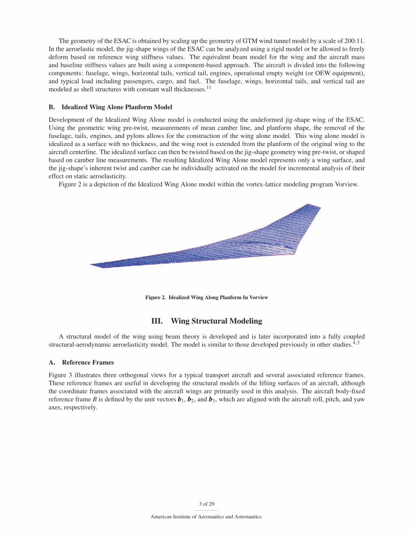
Figure 2 is a depiction of the Idealized Wing Alone model within the vortex-lattice modeling program Vorview.

Figure 2. Idealized Wing Along Planform In Vorview

III. Wing Structural Modeling

A structural model of the wing using beam theory is developed and is later incorporated into a fully coupled

structural-aerodynamic aeroelasticity model. The model is similar to those developed previously in other studies.4, 5

A. Reference Frames

Figure 3 illustrates three orthogonal views for a typical transport aircraft and several associated reference frames.

These reference frames are useful in developing the structural models of the lifting surfaces of an aircraft, although

the coordinate frames associated with the aircraft wings are primarily used in this analysis. The aircraft body-fixed

reference frame B is defined by the unit vectors bbb1, bbb2, and bbb3, which are aligned with the aircraft roll, pitch, and yaw

axes, respectively.

3 of 29


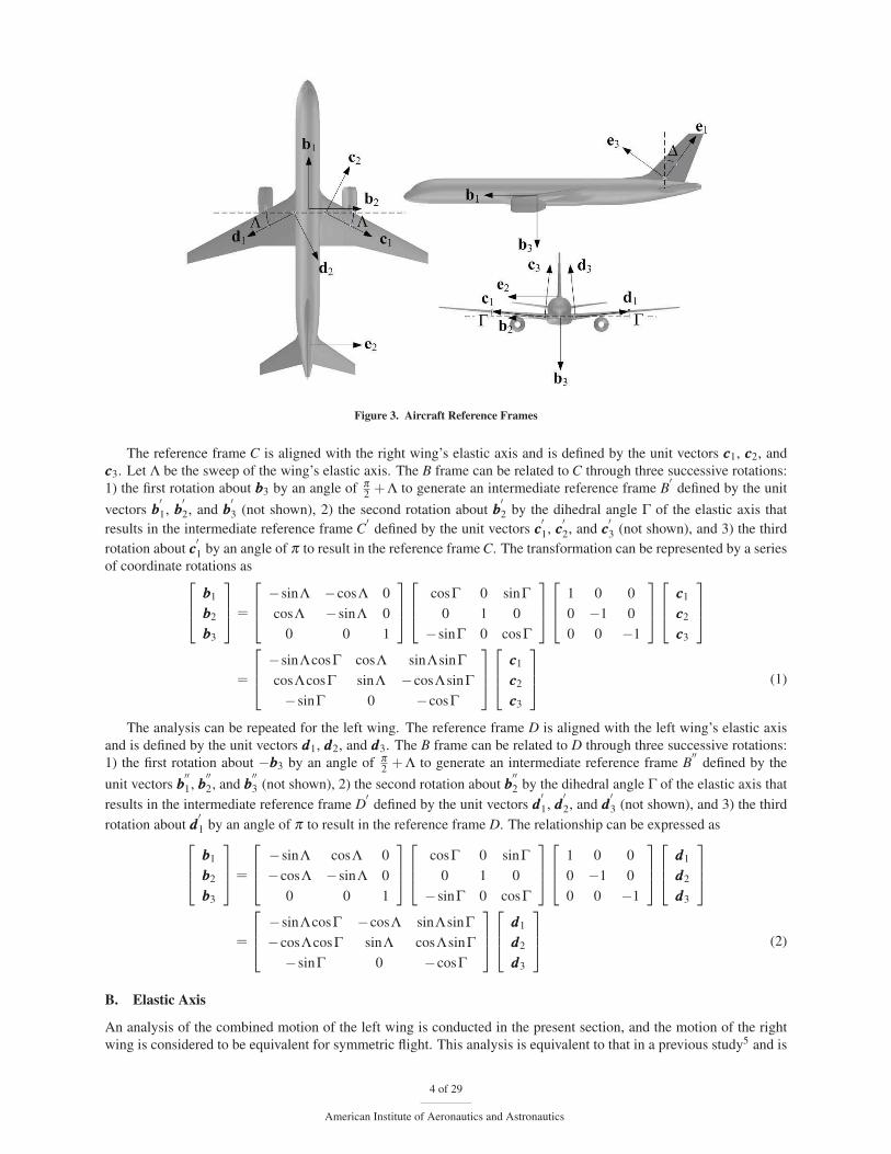
Figure 3. Aircraft Reference Frames

The reference frame C is aligned with the right wing’s elastic axis and is defined by the unit vectors ccc1, ccc2, and

ccc3. Let Λ be the sweep of the wing’s elastic axis. The B frame can be related to C through three successive rotations:

1) the first rotation about bbb3 by an angle of π2 + Λ to generate an intermediate reference frame B

′defined by the unit

vectors bbb′1, bbb

′2, and bbb

′3 (not shown), 2) the second rotation about bbb

′2 by the dihedral angle Γ of the elastic axis that

results in the intermediate reference frame C′

defined by the unit vectors ccc′1, ccc

′2, and ccc

′3 (not shown), and 3) the third

rotation about ccc′1 by an angle of π to result in the reference frame C. The transformation can be represented by a series

of coordinate rotations as⎡⎢⎣ bbb1

bbb2

bbb3

⎤⎥⎦=

⎡⎢⎣ −sinΛ −cosΛ 0

cosΛ −sinΛ 0

0 0 1

⎤⎥⎦⎡⎢⎣ cosΓ 0 sinΓ

0 1 0

−sinΓ 0 cosΓ

⎤⎥⎦⎡⎢⎣ 1 0 0

0 −1 0

0 0 −1

⎤⎥⎦⎡⎢⎣ ccc1

ccc2

ccc3

⎤⎥⎦

=

⎡⎢⎣ −sinΛcosΓ cosΛ sinΛsinΓ

cosΛcosΓ sinΛ −cosΛsinΓ−sinΓ 0 −cosΓ

⎤⎥⎦⎡⎢⎣ ccc1

ccc2

ccc3

⎤⎥⎦ (1)

The analysis can be repeated for the left wing. The reference frame D is aligned with the left wing’s elastic axis

and is defined by the unit vectors ddd1, ddd2, and ddd3. The B frame can be related to D through three successive rotations:

1) the first rotation about −bbb3 by an angle of π2 + Λ to generate an intermediate reference frame B

′′defined by the

unit vectors bbb′′1, bbb

′′2, and bbb

′′3 (not shown), 2) the second rotation about bbb

′′2 by the dihedral angle Γ of the elastic axis that

results in the intermediate reference frame D′

defined by the unit vectors ddd′1, ddd

′2, and ddd

′3 (not shown), and 3) the third

rotation about ddd′1 by an angle of π to result in the reference frame D. The relationship can be expressed as⎡

⎢⎣ bbb1

bbb2

bbb3

⎤⎥⎦=

⎡⎢⎣ −sinΛ cosΛ 0

−cosΛ −sinΛ 0

0 0 1

⎤⎥⎦⎡⎢⎣ cosΓ 0 sinΓ

0 1 0

−sinΓ 0 cosΓ

⎤⎥⎦⎡⎢⎣ 1 0 0

0 −1 0

0 0 −1

⎤⎥⎦⎡⎢⎣ ddd1

ddd2

ddd3

⎤⎥⎦

=

⎡⎢⎣ −sinΛcosΓ −cosΛ sinΛsinΓ

−cosΛcosΓ sinΛ cosΛsinΓ−sinΓ 0 −cosΓ

⎤⎥⎦⎡⎢⎣ ddd1

ddd2

ddd3

⎤⎥⎦ (2)

B. Elastic Axis

An analysis of the combined motion of the left wing is conducted in the present section, and the motion of the right

wing is considered to be equivalent for symmetric flight. This analysis is equivalent to that in a previous study5 and is

4 of 29


included for completeness.

Let x represent the coordinate along the elastic axis of a wing running from root to tip. The wing pre-twist angle

γ(x) thus represents the incidence of the airfoil section at the corresponding elastic axis coordinate. A typical wing pre-

twist varies from nose-up at the wing root to nose-down at the wing tip and is commonly referred to as a “wash-out”

twist distribution.

The internal structure of a wing is typically composed of a complex arrangement of load carrying spars and wing

boxes that carry the stresses and strains introduced by aerodynamic forces and aeroelastic deflections. For this analysis,

an equivalent beam approach is used which models the wing’s elastic behavior using equivalent stiffness properties. It

is a common approach in analyzing aeroelastic deflections7 and can be used to analyze high aspect ratio wings with

good accuracy. The effect of wing curvature is ignored and straight beam theory is used to model the wing deflection.

The axial or extensional deflection of a wing is also generally very small and is neglected.

Figure 4. Left Wing Reference Frame

Consider an airfoil section on the left wing as shown in Fig. 4 undergoing bending and torsional deflections. Let

(x,y,z) be the coordinates of point Q on the wing airfoil section. The undeformed local airfoil coordinates of point Q

are [yz

]=

[cosγ −sinγsinγ cosγ

][ηξ

](3)

where η and ξ are the local airfoil coordinates, and γ is the wing section pre-twist angle, positive nose-down.12 The

wing pre-twist is defined with respect to the elastic axis of the wing.

Differentiating with respect to x gives[yx

zx

]= γ

′[

−sinγ −cosγcosγ −sinγ

][ηξ

]=

[−zγ ′

yγ ′

](4)

Let Θ be a torsional twist angle about the x-axis, positive nose-down, and let W and V be flapwise and chordwise

bending deflections of point Q, respectively. Then, the rotation angle due to the elastic deformation can be expressed

as

φφφ(x, t) = Θddd1 −Wxddd2 +Vxddd3 (5)

where the subscript x denotes the partial derivatives of Θ, W , and V with respect to x.

Let (x1,y1,z1) be the coordinates of point Q on the airfoil in the reference frame D with aeroelastic deformation.

The coordinates (x1,y1,z1) are computed using the small angle approximation as⎡⎢⎣ x1(x, t)

y1(x, t)z1(x, t)

⎤⎥⎦=

⎡⎢⎣ x

y+Vz+w

⎤⎥⎦+

⎡⎢⎣ φφφ × (yddd2 + zddd3).ddd1

φφφ × (yddd2 + zddd3).ddd2

φφφ × (yddd2 + zddd3).ddd3

⎤⎥⎦=

⎡⎢⎣ x− yVx − zWx

y+V − zΘz+W + yΘ

⎤⎥⎦ (6)

5 of 29


Differentiating x1, y1, and z1 with respect to x yields⎡⎢⎣ x1,x

y1,x

z1,x

⎤⎥⎦=

⎡⎢⎣ 1− yVxx + zγ ′

Vx − zWxx − yγ ′Wx

−zγ ′+Vx − zΘx − yγ ′Θ

yγ ′+Wx + yΘx − zγ ′Θ

⎤⎥⎦ (7)

Neglecting the transverse shear effect, the longitudinal strain is computed as13

ε =ds1 −ds

ds=

s1,x

sx−1 (8)

where

sx =√

1+ y2x + z2

x =√

1+(y2 + z2)(γ ′)2 (9)

s1,x =√

x21,x + y2

1,x + z21,x

=√

s2x −2yVxx −2zWxx +2(y2 + z2)γ ′Θx +(x1,x −1)2 +(y1,x + zγ ′)2 +(z1,x − yγ ′)2 (10)

Ignoring the second-order terms and using the Taylor series expansion, s1,x is approximated as

s1,x ≈ sx +−yVxx − zWxx +(y2 + z2)γ ′Θx

sx

The longitudinal strain is then obtained as

ε =−yVxx − zWxx +(y2 + z2)γ ′Θx

s2x

≈−y[1+(y2 + z2)(γ

′)2]

Vxx − z[1+(y2 + z2)(γ

′)2]

Wxx +(y2 + z2)γ′y[1+(y2 + z2)(γ

′)2]

Θx (11)

For a small wing twist angle γ , (γ ′)2 ≈ 0. Then

ε = −yVxx − zWxx +(y2 + z2)γ′Θx (12)

The moments acting on the wing are then obtained as13

⎡⎢⎣ Mx

My

Mz

⎤⎥⎦=

⎡⎢⎣ GJΘx

0

0

⎤⎥⎦+ˆ ˆ

Eε

⎡⎢⎣ (y2 + z2)(γ ′

+Θx)−z−y

⎤⎥⎦dydz (13)

=

⎡⎢⎣ GJ +EB1(γ

′)2 −EB2γ ′ −EB3γ ′

−EB2γ ′EIyy −EIyz

−EB3γ ′ −EIyz EIzz

⎤⎥⎦⎡⎢⎣ Θx

Wxx

Vxx

⎤⎥⎦ (14)

where E is the Young’s modulus; G is the shear modulus; γ ′is the derivative of the wing pre-twist angle; Iyy, Iyz, and

Izz are the section area moments of inertia about the flapwise axis; J is the torsional constant; and B1, B2, and B3 are

the bending-torsion coupling constants which are defined as⎡⎢⎣ B1

B2

B3

⎤⎥⎦=ˆ ˆ

(y2 + z2)

⎡⎢⎣ y2 + z2

zy

⎤⎥⎦dydz (15)

The strain analysis shows that, for a pre-twisted wing, the bending deflections are coupled to the torsional deflection

via the slope of the wing pre-twist angle. This coupling can be significant if the wash-out slope γ ′is dominant as in

highly twisted wings such as turbomachinery blades.

6 of 29


C. Coupled Bending-Torsion Equations

Without considering chordwise bending of the wing, the equilibrium conditions for bending and torsion are expressed

as13

∂Mx

∂x= −mx (16)

∂ 2My

∂x= fz − ∂my

∂x(17)

where mx is the pitching moment per unit span about the elastic axis, fz is the lift force per unit span, and my is the

bending moment per unit span about the flapwise axis of the wing.

1. Aerodynamic Forces and Moments

Because the structural modeling is intended for use in a static aeroelasticity model, a steady-state aerodynamics model

is used. Aerodynamic information can be obtained through vortex-lattice modeling to develop the forces and moments

for coupled bending-torsion of a flexible wing.

Figure 5. Airfoil Forces and Moments

Neglecting the effect of downwash that is caused due to lift generation over a three-dimensional finite-wing, the

sectional lift coefficient for an airfoil cross section, assuming linear aerodynamics, is as follows:

cL(x) = cLα (x)αc(x) (18)

where αc is known as the aeroelastic angle of attack and comprises of the rigid-body angle of attack and the contri-

bution due to aeroelastic deformation. Note that αc is defined relative to the elastic axis of the wing and cL is the

sectional lift coefficient in the wing reference frame.

Let α be the aircraft’s rigid-body angle of attack and αe be the effect on the local angle of attack due to aeroelastic

deformation at the aerodynamic center of the airfoil section. Note that these values α , αe are defined relative to the

aircraft pitch axis, not the elastic axis.

αc(x) =α +αe(x)

cosΛ(19)

cLr(x) = cL0+ cLα (x)

αcosΛ

(20)

cLe(x) = cLα (x)αe(x)cosΛ

(21)

where cL0is the zero angle of attack lift coefficient for the airfoil section.

It is also important to note that the elastic contribution to the local aeroelastic angle of attack, αe, can be used to

characterize an aeroelastic deformation. Given a deformation characterized by elastic axis twist Θ and vertical bending

slope Wx, the elastic contribution to the aeroelastic angle of attack can be calculated as

αe(x) = −Θ(x)cosΛcosΓ−Wx(x)sinΛ (22)

where αe is about the aircraft pitch axis.

The steady-state drag coefficient can be modeled by a parabolic drag polar as

cD(x) = cD0(x)+ k(x)c2

L(x) (23)

7 of 29


where cD0is the section parasite drag coefficient and k is the section drag polar parameter. This can be expressed in

terms of rigid-body and aeroelastic contributions:

cD(x) = cDr(x)+ cDe(x) (24)

cDr(x) = cD0(x)+ k(x)c2

Lr (25)

cDe(x) = k(x)cLe(x) [2cLr(x)+ cLe(x)] (26)

The pitching moment coefficient about the aircraft pitch axis can be computed as

cm(x) = cmac(x)+e(x)c(x)

cL(x)cosΛ (27)

where e is the location of the aerodynamic center relative to the elastic axis defined in the streamwise direction

perpendicular to the pitch axis, positive when the aerodynamic center is forward of the elastic axis, and cmac is defined

about the pitch axis, positive nose-up.

The lift force, drag force, and pitching moment about the aircraft pitch axis are expressed as

l = cLq∞ cosΛc (28)

d = cDq∞ cosΛc (29)

m = cmq∞c2 (30)

where cosΛ takes into account the correction due to the elastic axis sweep, but is not needed in the pitch moment

calculation since Eq. 27 is already about the pitch axis.

The forces and moments in the local coordinate reference frame are obtained as

f ax = (l cosα +d sinα)Γ+(d cosα − l sinα)sinΛ (31)

f ay = (d cosα − l sinα)cosΛ (32)

f az = l cosα +d sinα − (d cosα − l sinα)sinΛΓ (33)

max = −mcosΛ (34)

may = msinΛ (35)

maz = mcosΛΓ (36)

For a model with only flapwise bending and torsion considered, the beam deflection analysis is affected only by

the terms f az , ma

x , and may . The aerodynamic force and moment terms are thus considered to be

f az ≈ cLq∞ cos2 Λc (37)

max ≈−cmq∞ cos2 Λc2 (38)

∂may

∂x≈ ∂cm

∂xq∞ sinΛcosΛc2 (39)

where an additional cosΛ term is introduced due to the change in direction of q∞ due to sweep.

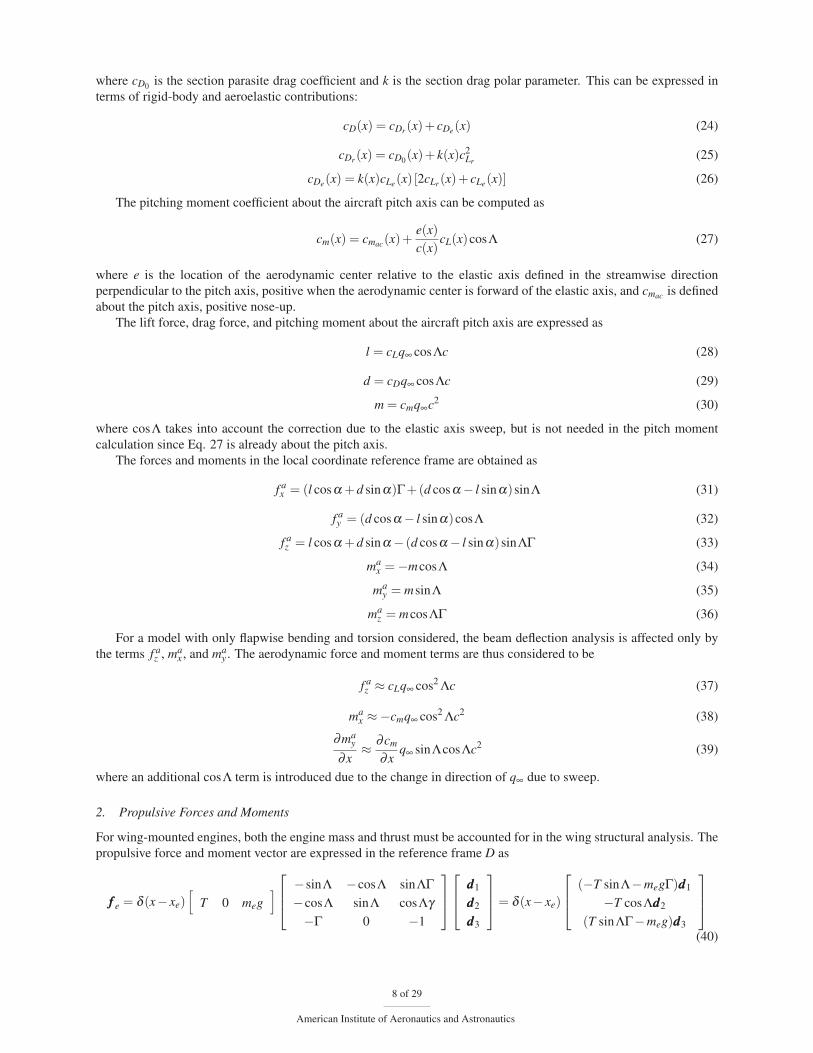
2. Propulsive Forces and Moments

For wing-mounted engines, both the engine mass and thrust must be accounted for in the wing structural analysis. The

propulsive force and moment vector are expressed in the reference frame D as

fff e = δ (x− xe)[

T 0 meg]⎡⎢⎣ −sinΛ −cosΛ sinΛΓ

−cosΛ sinΛ cosΛγ−Γ 0 −1

⎤⎥⎦⎡⎢⎣ ddd1

ddd2

ddd3

⎤⎥⎦= δ (x− xe)

⎡⎢⎣ (−T sinΛ−megΓ)ddd1

−T cosΛddd2

(T sinΛΓ−meg)ddd3

⎤⎥⎦(40)

8 of 29


mmme = rrre × fff e = (xeddd1 − yeddd2 − zeddd3)× fff e = δ (x− xe)

⎡⎢⎣ (−Tye sinΛΓ−T ze cosΛ+megye)ddd1

(−Tye sinΛΓ+megxe +T ze sinΛ+megyeΓ)ddd2

(−T xe cosΛΓ−Tye sinΛ−megyeΓ)ddd3

⎤⎥⎦ (41)

where T is the engine thrust, me is the engine mass, (xe,ye,ze) is the coordinate of the engine thrust center such that yeis positive forward of the elastic axis and ze is positive below the elastic axis, and δ (x− xe) is the Dirac delta function

such that ˆδ (x− xe) f (x)dx = f (xe) (42)

Transforming into the local coordinate reference frame, the propulsive forces and moments are given by

f ex = δ (x− xe) [−T sinΛ−megΓ+(T sinΛΓ−meg)Wx] (43)

f ey = δ (x− xe) [−T cosΛ+(T sinΛΓ−meg)(Θ+ γ)] (44)

f ez = δ (x− xe) [T sinΛΓ−meg+T cosΛ(Θ+ γ)+(T sinΛ+megΓ)Wx] (45)

mex = δ (x− xe) [−Tye sinΛΓ−T ze cosΛ+megye − (T xe cosΛ+Tye sinΛ+megyeΓ)Wx] (46)

mey = δ (x− xe) [−T xe sinΛΓ+megxe +T ze sinΛ+megzeΓ− (T xe cosΛ+Tye sinΛ+megyeΓ)(Θ+ γ)] (47)

mez = δ (x− xe) [−T xe cosΛ−Tye sinΛ−megyeΓ+T xe sinΛΓ−megxe −T ze sinΛ−megzeΓ)(Θ+ γ)

+(Tye sinΛΓ+T ze cosΛ−megye)Wx] (48)

The partial derivatives of the moment components are

∂mex

∂x= −δ (x− xe)(T xe cosΛ+Tye sinΛ+megyeΓ)Wxx (49)

∂mey

∂x= −δ (x− xe)(T xe cosΛ+Tye sinΛ+megyeΓ)(Θx + γ

′) (50)

∂mez

∂x= −δ (x− xe)

[(T xe sinΛΓ−megxe −T ze sinΛ−megzeΓ)(Θx + γ

′)

+(Tye sinΛΓ+T ze cosΛ−megyeΓ)Wxx] (51)

3. Summary of Coupled Bending-Torsion Partial Differential Equations

The force and moment equations due to aerodynamics and propulsive sources and inertial effects are formulated.

fz = f az + f e

z −mg−mWtt +mecgΘtt +δ (x− xe)(−meWtt +meyeΘtt) (52)

mx = max +me

x +mgecg +mecgWtt −mr2k Θtt +δ (x− xe)

[meyeWtt −me(y2

e + z2e)Θtt

](53)

∂my

∂x=

∂may

∂x+

∂mey

∂x(54)

Inserting Eq. 13 and the force and moment terms into the governing equilibrium equations, Eqs. 16 and 17, the

following equations which describe the coupled bending and torsion motion of the wing can be formulated:

∂ 2

∂x2(−EB2γ

′Θx +EIyyWxx) =

−mWtt +mecgΘtt −mg+ cLq∞ cos2 Λc− ∂cm

∂xtanΛq∞ cos2 Λc2

+δ (x− xe)(−mewtt +meyeΘtt)+δ (x− xe) [T sinΛΓ−meg+(T sinΛ+megΓ)Wx +T cosΛ(Θ+ γ)]

+δ (x− xe)(T xe cosΛ+Tye sinΛ+megyeΓ)(Θx + γ′)

+δ (x− xe)(−Tye sinΛΓ−T ze cosΛ+megye)[Wxx(Θ+ γ)+Wx(Θx + γ

′)]

(55)

∂∂x

{[GJ +EB1(γ

′)2]

Θx −EB2γ′Wxx

}=

mr2k Θtt −mecgWtt −mgecg + cmq∞ cos2 Λc2 +δ (x− xe)

[me(y2

e + z2e)Θtt −meyeWtt

]−δ (x− xe) [−Tye sinΛΓ −T ze cosΛ+megye − (T xe cosΛ+Tye sinΛ+megyeΓ)Wx] (56)

9 of 29


IV. Finite-Element Modeling

The development of the coupled bending-torsion partial differential equations allows for wing bending and tor-

sional deflections to be solved. FEM,8 a numerical technique that uses locally-defined basis functions to numerically

approximate the solution of the governing partial differential equations, is used. The wing structure is discretized into

n equally spaced one-dimensional beam elements, and FEM is applied. The bending and torsional deflections can be

approximated as

Θ(x, t) =n

∑i=1

Θi(x, t) (57)

W (x, t) =n

∑i=1

Wi(x, t) (58)

where i refers to the i-th element.

For each element, the bending and torsional deflections are approximated as

Θi(x, t) = ψiθ1i(t)+ψ2(x)θ2i(t) =[

ψ1(x) ψ2(x)][ θ1i(t)

θ2i(t)

]= Nθ (x)θi(t) (59)

Wi(x, t) =[

φ1(x)w1i(t)+φ2(x)w′1i(t)+φ3(x)w2i(t)+φ4(x)w

′2i(t)

]

=[

φ1(x) φ2(x) φ3(x) φ4(x)]⎡⎢⎢⎢⎣

w1i(t)w

′1i(t)

w2i(t)w

′2i(t)

⎤⎥⎥⎥⎦= Nw(x)wi(t) (60)

where the subscripts 1 and 2 denote values at nodes 1 and 2, and ψ j(x), j = 1,2 and φk(x), k = 1,2,3,4 are the linear

and Hermite polynomial shape functions

ψ1(x) = 1− xl

(61)

ψ2(x) =xl

(62)

φ1(x) = 1−3(xl)2 +2(

xl)3 (63)

φ2(x) = l[x

l−2(

xl)2 +(

xl)3]

(64)

φ3(x) = 3(xl)2 −2(

xl)3 (65)

φ4(x) = l[−(

xl)2 +(

xl)3]

(66)

where x ∈ [0,1] is the local coordinate and l = Ln is the element length.

The weak-form integral expressions of the coupled bending-torsion partial differential equations are obtained by

multiplying the equations by NTθ (x) and NT

w(x) and then integrating over the wing span. This yields

n

∑i=0

ˆ l

0

NTθ

ddx

{[GJ +EB1(γ

′)2]

N′θ θi −EB2γ

′N

′′wwi

}dx =

n

∑i=1

ˆ l

0

NTθ (cmc)q∞ cos2 Λcdx+

n

∑i=1

ˆ l

0

NTθ (−mgecg +mr2

k Nθ θi −mecgNwwi)dx

+n

∑i=1

NTθ[me(y2

e + z2e)Nθ θi −meyeNwwi

]x=xe

+

n

∑i=1

NTθ

[Tye sinΛΓ+T ze cosΛ−megye +(T xe cosΛ+Tye sinΛ+megyeΓ)N

′wwi

]x=xe (67)

10 of 29


n

∑i=0

ˆ l

0

NTw

d2

dx2(−EB2γ

′N

′θ θi +EIyyN

′′wwi)dx =

n

∑i=1

ˆ l

0

NTw

(cL − dcm

dxtanΛc

)q∞ cos2 Λcdx+

n

∑i=1

NTw(−ρgA−ρANwwi +ρAecgNθ θi)dx

+n

∑i=1

NTw

[−meNwwi +meyeNθ θi +T sinΛΓ−meg+T cosΛ(Nθ θi + γ)+(T sinΛ+megΓ)N

′wwi

]x=xe

+n

∑i=1

NTw

[(T xe cosΛ+Tye sinΛ+megyeΓ)(N

′θ θi + γ

′)]

x=xe(68)

The expressions on the left hand sides can be integrated by parts upon enforcing the boundary conditions resulting

inˆ l

0

NTθ

ddx

{[GJ +EB1(γ

′)2]

N′θ θi −EB2γ

′N

′′wwi

}dx = −

ˆ l

0

N′Tθ

{[GJ +EB1(γ

′)2]

N′θ θi −EB2γ

′N

′′wwi

}dx (69)

ˆ l

0

NTw

d2

dx2(−EB2γ

′N

′θ θi +EIyyN

′′wwi)dx =

ˆ l

0

N′′Tw (−EB2γ

′N

′θ θi +EIyyN

′′wwi)dx (70)

The elemental mass matrix, stiffness matrix, and force vector are then established as

Mi =ˆ l

0

m

[r2

k NTθ Nθ −ecgNT

θ Nw

−ecgNTwNθ NT

wNw

]dx+me

[(y2

e + z2e)N

Tθ Nθ −yeNT

θ Nw

−yeNTwNθ NT

wNw

]x=xe

(71)

Ki =ˆ l

0

[ [GJ +EB1(γ

′)2]

N′Tθ N

′θ −EB2γ ′

N′Tθ N

′′w

−EB2γ ′N

′′Tw N

′θ EIyyN

′′Tw N

′′w

]dx

+

[0 (T xe cosΛ+Tye sinΛ+megyeΓ)NT

θ N′w

−T cosΛNTwNθ − (T xe cosΛ+Tye sinΛ+megyeΓ)NT

wN′θ −(T sinΛ+megΓ)NT

wN′w

]x=xe

(72)

Fi =ˆ l

0

mg

[ecgNT

θ−NT

w

]dx+

ˆ l

0

([−cmcNT

θcLNT

w

]+

[0

cmc tanΛN′Tw

])q∞ cos2 Λcdx

+

[0

cmc tanΛNTw

]l

0

q∞ cos2 Λcdx

+

[−(Tye sinΛΓ+T ze cosΛ−megye)NT

θ[T sinΛΓ−meg+T cosΛγ +(T xe cosΛ+Tye sinΛ+megyeΓ)γ ′]

NTw

]x=xe

(73)

The globally assembled system is described by the matrix equation

Mxe +Kxe = F (74)

where xe =[

θ1 w1 w′1 θ2 w2 w

′2 . . . θi wi w

′i . . . θn+1 wn+1 w

′n+1

]T.

Equation 74 represents the governing equation for solving the structural deflection of a flexible wing given aero-

dynamic and propulsive force and moment inputs. By setting xe = 000, the equilibrium solution can be obtained through

inverting the stiffness matrix and pre-multiplying the force matrix. This represents the static structural deflection of

the wing based on the prescribed load input at that flight condition.

xe = K−1F (75)

Information extracted from the wing solution state vector xe is used to characterize the wing’s structural deflection

along the elastic axis of the wing Θ and W . It can also be used to calculate the elastic contribution to the aeroelastic

angle of attack αe in Eq. 22.

11 of 29


V. Vortex-Lattice Aerodynamic Modeling

Vorview is a computational tool used for aerodynamic modeling of aircraft configurations using vortex-lattice

method.14 Based on lifting line aerodynamic theory, Vorview provides a rapid method for estimating aerodynamic

force and moment coefficients. Input vehicle geometries are discretized within Vorview into a series of panels which

are then represented by placement of spanwise and chordwise locations of bound or horseshoe vortices. Vorview

computes the vehicle aerodynamics in both the longitudinal and lateral directions independently, and these can be

combined to produce the overall aerodynamic characteristics of the vehicle at any arbitrary angle of attack and angle

of sideslip.

Vorview is considered a medium fidelity tool, and limitations associated with vortex-lattice modeling in general

apply to Vorview aerodynamic analysis. The drag prediction by Vorview is most reliable only for induced drag

prediction due to the inviscid nature of any vortex-lattice method. Prediction of viscous drag due to boundary layer

separation and wave drag due to shock-induced boundary layer separation are generally not conducted by vortex-

lattice, and viscous drag must be estimated using other methods.

In addition to force and moment analysis, Vorview can provide a rapid estimation of aerodynamic derivatives

including dynamic derivatives due to angular rates. These aerodynamic stability and control derivatives are useful in

analyzing the stability and handling characteristics of an aircraft configuration. Owing to the computationally efficient

vortex-lattice method, aerodynamic derivatives can be estimated in Vorview fairly quickly. A flight dynamic model

for a given vehicle configuration can be easily developed with Vorview, using the results from these stability and

handling analyses. Vorview has been validated by both wind tunnel data10 as well as the NASA Cart3D tool,15 which

is a high-fidelity inviscid (Euler) CFD analysis code targeted at analyzing aircraft performance in conceptual and

preliminary aerodynamic design. In general, both Vorview and Cart3D seem to have similar predictive capabilities

when compressibility is not a factor.

Figure 6 illustrates an aerodynamic model of the GTM in Vorview.

Figure 6. GTM Aircraft Model in Vorview

In this study, Vorview will be used as the primary tool for conducting aerodynamic modeling for the aircraft

configurations. Total aircraft characteristics as well as sectional data along the aircraft wing surfaces can be post-

processed from Vorview.

VI. Parasitic Drag Modeling

Due to the inviscid nature of vortex-lattice drag estimates, a conceptual parasitic drag model will be utilized for

development of the longitudinal trim model. This is necessary for realistic trim thrust values to be calculated, which

must take into account viscous drag over the ESAC model’s airframe.

12 of 29


The skin friction model for all the surfaces will be done by calculating the arc lengths of the surfaces along the

direction of flow and treating those lengths as flat plate surfaces. For airfoil surfaces, the arc lengths can be divided into

top and bottom arc surfaces. For revolved surfaces, the model will calculate the skin friction coefficients by revolving

the mean arc lengths.

The Reynold’s number for an arc length c is calculated as

Rec =ρV c

μ(76)

A critical Reynold’s number Rexc is assumed to be Rexc = 600,000. This critical Reynold’s number is used to

calculate the critical length as

xc =Rexc μ

ρV(77)

The kinematic viscosity model is calculated in lb-s

ft2by the Sutherland’s viscosity model:

μ = 0.3170×10−10T32

(734.7

T +216

)(78)

The revised skin friction coefficient for a single arc length is calculated as

c f =1.328√

Rexc

xc

c︸︷︷︸c f ,laminar

+0.072Re−0.2c −0.072

xc

cRe−0.2

xc︸︷︷︸c f ,turbulent

(79)

The total skin friction coefficient for the aircraft components can then be formulated by integrating the skin friction

coefficients either over the entire span of a wing, or the entire revolution of a surface.

If pressure drag is to be conceptually estimated as well, then a form factor for the wing needs to be estimated. A

form factor FF can can be defined for a wing surface as16

FF =(

1+0.6

(x/c)m

( tc

)+100

( tc

)4)(

1.34M0.18(cosΛm)0.28)

(80)

where tc is the maximum thickness of the airfoil,

( xc

)m is the location of the airfoil maximum thickness point, and Λm

is the sweep of the maximum-thickness line.

For bodies of revolution, the form factor is evaluated as16

FF =(

1+60

f 3+

f400

)(81)

where f is a fineness ratio given by f = l√4π Amax

and Amax is the largest cross-sectional area perpendicular to the flow.

The total parasitic drag coefficient including skin-friction and pressure drag due to separation and the supervelocity

effect is calculated as16

CD0= ∑ Cf (FF)(Q)Swet

Sre f(82)

where all the components’ contributions to parasitic drag are summed up. The value Swet represents the wetted surface

area of the component, and Q represents an interference factor.

The parasite drag modeling method introduced here is also used to develop the wing’s spanwise parasitic drag

coefficients used in Eq. 23 of the aeroelastic model.

VII. Automated Geometry Modeling Tool

An automated geometry generation tool is developed in Matlab and is used to close the loop between the structural

and aerodynamic modeling needed to generate an aeroelastic model. The geometry generation tool uses structural

deflection data that is computed by the FEM model and applies it to the undeformed aircraft wing geometry to reflect

static aeroelastic deflections. The vehicle geometry modeler directly outputs a geometry input file that can be read by

Vorview when computing an aeroelastic solution.

13 of 29


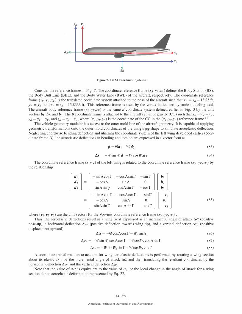
Figure 7. GTM Coordinate Systems

Consider the reference frames in Fig. 7. The coordinate reference frame (xA,yA,zA) defines the Body Station (BS),

the Body Butt Line (BBL), and the Body Water Line (BWL) of the aircraft, respectively. The coordinate reference

frame (xV ,yV ,zV ) is the translated coordinate system attached to the nose of the aircraft such that xV = xB −13.25 ft,

yV = yB, and zV = zB − 15.8333 ft. This reference frame is used by the vortex-lattice aerodynamic modeling tool.

The aircraft body reference frame (xB,yB,zB) is the same B coordinate system defined earlier in Fig. 3 by the unit

vectors bbb1, bbb2, and bbb3. The B coordinate frame is attached to the aircraft center of gravity (CG) such that xB = xV −xV ,

yB = yV − yV , and zB = zV − zV , where (xV , yV,zV ) is the coordinate of the CG in the (xV ,yV,zV ) reference frame.11

The vehicle geometry modeler has access to the outer mold line of the aircraft geometry. It is capable of applying

geometric transformations onto the outer mold coordinates of the wing’s jig-shape to simulate aeroelastic deflection.

Neglecting chordwise bending deflection and utilizing the coordinate system of the left wing developed earlier (coor-

dinate frame D), the aeroelastic deflections in bending and torsion are expressed in a vector form as

φφφ = Θddd1 −Wxddd2 (83)

ΔΔΔrrr = −W sinWxddd1 +W cosWxddd3 (84)

The coordinate reference frame (x,y,z) of the left wing is related to the coordinate reference frame (xV ,yV ,zV ) by

the relationship ⎡⎢⎣ ddd1

ddd2

ddd3

⎤⎥⎦=

⎡⎢⎣ −sinΛcosΓ −cosΛsinΓ −sinΓ

−cosΛ sinΛ 0

sinΛsinγ cosΛsinΓ −cosΓ

⎤⎥⎦⎡⎢⎣ bbb1

bbb2

bbb3

⎤⎥⎦

=

⎡⎢⎣ −sinΛcosΓ −cosΛcosΓ −sinΓ

−cosΛ sinΛ 0

sinΛsinΓ cosΛsinΓ −cosΓ

⎤⎥⎦⎡⎢⎣ −vvv1

vvv2

−vvv3

⎤⎥⎦ (85)

where (vvv1,vvv2,vvv3) are the unit vectors for the Vorview coordinate reference frame (xV ,yV ,zV ) .

Thus, the aeroelastic deflections result in a wing twist expressed as an incremental angle of attack Δα (positive

nose-up), a horizontal deflection ΔyV (positive deflection towards wing tip), and a vertical deflection ΔzV (positive

displacement upward):

Δα = −ΘcosΛcosΓ−Wx sinΛ (86)

ΔyV = −W sinWx cosΛcosΓ−W cosWx cosΛsinΓ (87)

Δzv = −W sinWx sinΓ+W cosWx cosΓ (88)

A coordinate transformation to account for wing aeroelastic deflections is performed by rotating a wing section

about its elastic axis by the incremental angle of attack Δα and then translating the resultant coordinates by the

horizontal deflection ΔyV and the vertical deflection ΔzV .

Note that the value of Δα is equivalent to the value of αe, or the local change in the angle of attack for a wing

section due to aeroelastic deformation represented by Eq. 22.

14 of 29


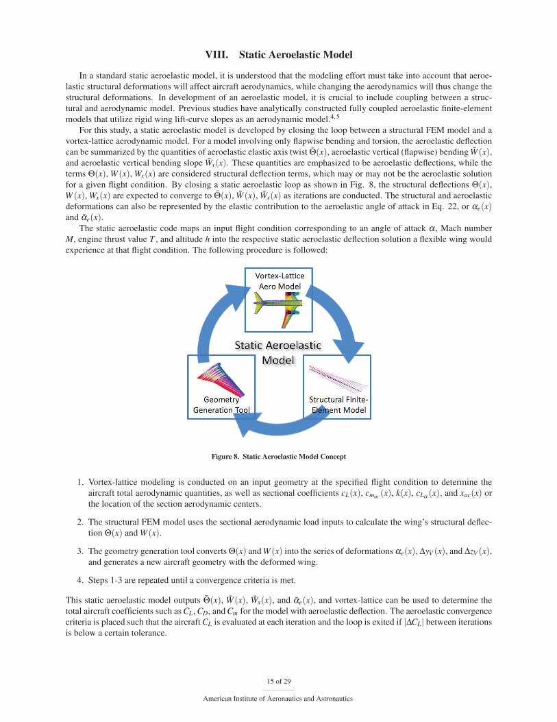
VIII. Static Aeroelastic Model

In a standard static aeroelastic model, it is understood that the modeling effort must take into account that aeroe-

lastic structural deformations will affect aircraft aerodynamics, while changing the aerodynamics will thus change the

structural deformations. In development of an aeroelastic model, it is crucial to include coupling between a struc-

tural and aerodynamic model. Previous studies have analytically constructed fully coupled aeroelastic finite-element

models that utilize rigid wing lift-curve slopes as an aerodynamic model.4, 5

For this study, a static aeroelastic model is developed by closing the loop between a structural FEM model and a

vortex-lattice aerodynamic model. For a model involving only flapwise bending and torsion, the aeroelastic deflection

can be summarized by the quantities of aeroelastic elastic axis twist Θ(x), aeroelastic vertical (flapwise) bending W (x),and aeroelastic vertical bending slope Wx(x). These quantities are emphasized to be aeroelastic deflections, while the

terms Θ(x), W (x), Wx(x) are considered structural deflection terms, which may or may not be the aeroelastic solution

for a given flight condition. By closing a static aeroelastic loop as shown in Fig. 8, the structural deflections Θ(x),W (x), Wx(x) are expected to converge to Θ(x), W (x), Wx(x) as iterations are conducted. The structural and aeroelastic

deformations can also be represented by the elastic contribution to the aeroelastic angle of attack in Eq. 22, or αe(x)and αe(x).

The static aeroelastic code maps an input flight condition corresponding to an angle of attack α , Mach number

M, engine thrust value T , and altitude h into the respective static aeroelastic deflection solution a flexible wing would

experience at that flight condition. The following procedure is followed:

Figure 8. Static Aeroelastic Model Concept

1. Vortex-lattice modeling is conducted on an input geometry at the specified flight condition to determine the

aircraft total aerodynamic quantities, as well as sectional coefficients cL(x), cmac(x), k(x), cLα (x), and xac(x) or

the location of the section aerodynamic centers.

2. The structural FEM model uses the sectional aerodynamic load inputs to calculate the wing’s structural deflec-

tion Θ(x) and W (x).

3. The geometry generation tool converts Θ(x) and W (x) into the series of deformations αe(x), ΔyV (x), and ΔzV (x),and generates a new aircraft geometry with the deformed wing.

4. Steps 1-3 are repeated until a convergence criteria is met.

This static aeroelastic model outputs Θ(x), W (x), Wx(x), and αe(x), and vortex-lattice can be used to determine the

total aircraft coefficients such as CL, CD, and Cm for the model with aeroelastic deflection. The aeroelastic convergence

criteria is placed such that the aircraft CL is evaluated at each iteration and the loop is exited if |ΔCL| between iterations

is below a certain tolerance.

15 of 29


IX. Longitudinal Trim Model

The condition known as “trim” refers to the condition where an aircraft is in a state of constant velocity equilibrium.

For longitudinal trim, this formulates a three degree-of-freedom system where the input variables are the aircraft’s

angle of attack α , the elevator deflection δe (positive deflection is downward deflection), and the engine thrust T .

The forces and moments are developed in the aircraft stability axes shown in Fig. 9. Only symmetric flight within

a vertical plane of a non-rotating flat Earth is considered.

Figure 9. Aircraft Longitudinal Forces and Axes

The body-fixed coordinate system is consistent with the previous usages of the B coordinate frame, while the

stability or wind axes are represented by (xS,yS,zS) where xS is in the direction of Va, the aircraft velocity. The axis

yh represents a vector parallel to the flat Earth surface and perpendicular to the aircraft vertical altitude. The value γgrepresents the aircraft glide path angle, and the pitch angle θp is defined as the angle between the aircraft forward body

axis and the horizontal yh direction. The aircraft is modeled to experience a lift force L, drag force D, weight W , and

pitching moment M acting at the aircraft CG. The equilibrium equations in the stability axes are:

∑FxS = 2T cos(α + ε)−D−W sin(γ) = 0 (89)

∑FzS = 2T sin(α + ε)+L−W cos(γ) = 0 (90)

∑MyS = M +2T ze cosε +2T xe sinε = 0 (91)

where the value T represents a single engine’s thrust value and hence a factor of 2 appears in the equations of motion.

The value ε is the engine mount angle, positive upwards.

The equations are expanded using non-dimensional coefficients:

fxS = 2T cos(α + ε)− (CDr +CDe +CDδeδe)q∞Sre f −W sinγg = 0 (92)

fzS = 2T sin(α + ε)+(CLr +CLe +CLδeδe)q∞Sre f −W cosγg = 0 (93)

myS = (Cmr +Cme +Cmδeδe)q∞Sre f c+2T ze cosε +2T xe sinε = 0 (94)

Let the static aeroelastic deformation be represented by αe = αe(yS,α,T ), a function of the wing spanwise station

yS, the aircraft angle of attack α , and the engine thrust T . For a model with wing flexibility, it must be taken into

16 of 29


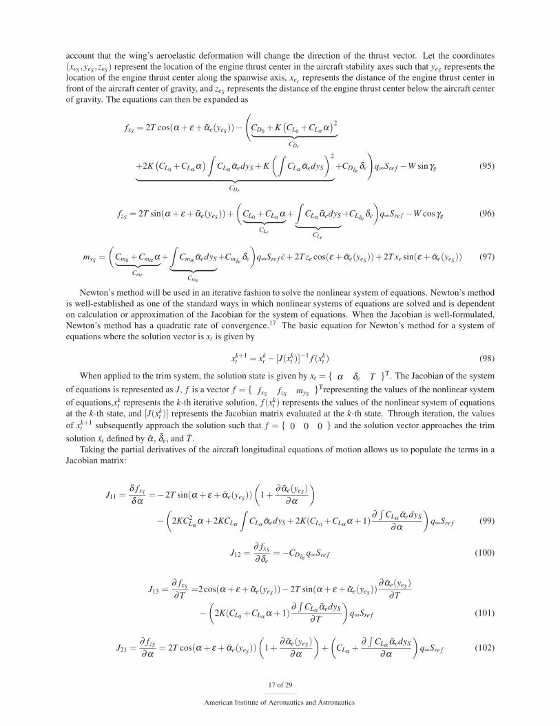
account that the wing’s aeroelastic deformation will change the direction of the thrust vector. Let the coordinates

(xeS ,yeS ,zeS) represent the location of the engine thrust center in the aircraft stability axes such that yeS represents the

location of the engine thrust center along the spanwise axis, xes represents the distance of the engine thrust center in

front of the aircraft center of gravity, and zeS represents the distance of the engine thrust center below the aircraft center

of gravity. The equations can then be expanded as

fxS = 2T cos(α + ε + αe(yeS))−(

CD0+K

(CL0

+CLα α)2︸︷︷︸

CDr

+2K(CL0

+CLα α)ˆ

CLα αedyS +K(ˆ

CLα αedyS

)2

︸︷︷︸CDe

+CDδeδe

)q∞Sre f −W sinγg (95)

fzS = 2T sin(α + ε + αe(yeS))+(

CL0+CLα α︸︷︷︸CLr

+ˆ

CLα αedyS︸︷︷︸CLe

+CLδeδe

)q∞Sre f −W cosγg (96)

myS =(

Cm0+Cmα α︸︷︷︸Cmr

+ˆ

Cmα αedyS︸︷︷︸Cme

+Cmδeδe

)q∞Sre f c+2T ze cos(ε + αe(yeS))+2T xe sin(ε + αe(yeS)) (97)

Newton’s method will be used in an iterative fashion to solve the nonlinear system of equations. Newton’s method

is well-established as one of the standard ways in which nonlinear systems of equations are solved and is dependent

on calculation or approximation of the Jacobian for the system of equations. When the Jacobian is well-formulated,

Newton’s method has a quadratic rate of convergence.17 The basic equation for Newton’s method for a system of

equations where the solution vector is xt is given by

xk+1t = xk

t − [J(xkt )]

−1 f (xkt ) (98)

When applied to the trim system, the solution state is given by xt = { α δe T }T. The Jacobian of the system

of equations is represented as J, f is a vector f = { fxS fzS myS}Trepresenting the values of the nonlinear system

of equations,xkt represents the k-th iterative solution, f (xk

t ) represents the values of the nonlinear system of equations

at the k-th state, and [J(xkt )] represents the Jacobian matrix evaluated at the k-th state. Through iteration, the values

of xk+1t subsequently approach the solution such that f = { 0 0 0 } and the solution vector approaches the trim

solution xt defined by α , δe, and T .

Taking the partial derivatives of the aircraft longitudinal equations of motion allows us to populate the terms in a

Jacobian matrix:

J11 =δ fxS

δα=−2T sin(α + ε + αe(yeS))

(1+

∂ αe(yeS)∂α

)

−(

2KC2Lα α +2KCLα

ˆCLα αedyS +2K(CL0

+CLα α +1)∂´

CLα αedyS

∂α

)q∞Sre f (99)

J12 =∂ fxS

∂δe= −CDδe

q∞Sre f (100)

J13 =∂ fxS

∂T=2cos(α + ε + αe(yeS))−2T sin(α + ε + αe(yeS))

∂ αe(yeS)∂T

−(

2K(CL0+CLα α +1)

∂´

CLα αedyS

∂T

)q∞Sre f (101)

J21 =∂ fzS

∂α= 2T cos(α + ε + αe(yeS))

(1+

∂ αe(yeS)∂α

)+(

CLα +∂´

CLα αedyS

∂α

)q∞Sre f (102)

17 of 29


J22 =∂ fzS

∂δe= CLδe

q∞Sre f (103)

J23 =∂ fzS

∂T= 2sin(α + ε + αe(yeS))+2cos(α + ε + αe(yeS))

∂ αe(yeS)∂T

+∂´

CLα αedyS

∂Tq∞Sre f (104)

J31 =∂myS

∂α=Cmα q∞Sre f c+

∂´

Cmα αedyS

∂αq∞Sre f c

−2T ze sin(ε + αe(yeS))∂ αe(yeS)

∂T+2T xe cos(ε + αe(yeS))

∂ αe(yeS)∂T

(105)

J32 =∂myS

∂δe= Cmδe

q∞Sre f c (106)

J33 =∂myS

∂T=2(cos(ε + αe(yeS))zeS + sin(ε + αe(yeS))xeS

)+

∂´

Cmα αe(yeS)dy∂T

q∞Sre f c

+2T(cos(ε + αe(yeS))xeS − sin(ε + αe(yeS))zeS

) ∂ αe(yeS)∂T

+2T(

cos(ε + αe(yeS))∂ zeS

∂T+ sin(ε + αe(yeS))

∂xeS

∂T

)(107)

The elastic terms in the Jacobian, which require running a static aeroelastic sensitivity study to α and T at each

iteration, can be costly to calculate. Therefore, for the scope of this study, these terms are not used in approximation of

the Jacobian. The value of 2KC2Lα α is also approximated as the value CDα , which is rapidly estimated by vortex-lattice

code. As a trade-off in using these simplifications, the convergence rate of the trim algorithm is expected to decrease.

The Jacobian for the system becomes:

J =

⎡⎢⎣ −2T sin(α + ε)−CDα q∞Sre f −CDδe

q∞Sre f 2cos(α + ε)2T cos(α + ε)+CLα q∞Sre f CLδe

q∞Sre f 2sin(α + ε)Cmα q∞Sre f c Cmδe

q∞Sre f c 2(cos(ε)zeS + sin(ε)xeS)

⎤⎥⎦ (108)

The static aeroelastic framework in Fig. 8 is augmented with an additional step in which the Newton’s method

trim procedure is added within the structural-aerodynamic loops. The resulting framework is represented in Fig. 10.

Figure 10. Static Aeroelastic Longitudinal Trim Model

Additional steps and modifications are added to the static aeroelastic approach to generate the aeroelastic trim

procedure:

18 of 29


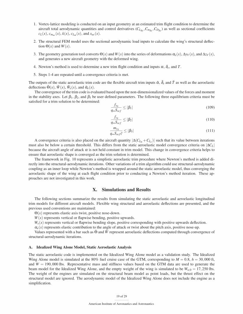
1. Vortex-lattice modeling is conducted on an input geometry at an estimated trim flight condition to determine the

aircraft total aerodynamic quantities and control derivatives (CLδe ,Cmδe ,CDδe ) as well as sectional coefficients

cL(x), cmac(x), k(x), cLα (x), and xac(x).

2. The structural FEM model uses the sectional aerodynamic load inputs to calculate the wing’s structural deflec-

tion Θ(x) and W (x).

3. The geometry generation tool converts Θ(x) and W (x) into the series of deformations αe(x), ΔyV (x), and ΔzV (x),and generates a new aircraft geometry with the deformed wing.

4. Newton’s method is used to determine a new trim flight condition and inputs α , δe, and T .

5. Steps 1-4 are repeated until a convergence criteria is met.

The outputs of the static aeroelastic trim code are the flexible aircraft trim inputs α , δe and T as well as the aeroelastic

deflections Θ(x), W (x), Wx(x), and αe(x).The convergence of the trim code is evaluated based upon the non-dimensionalized values of the forces and moment

in the stability axes. Let β1, β2, and β3 be user defined parameters. The following three equilibrium criteria must be

satisfied for a trim solution to be determined:fxS

q∞Sre f≤ |β1| (109)

fzS

q∞Sre f≤ |β2| (110)

myS

q∞Sre f c≤ |β3| (111)

A convergence criteria is also placed on the aircraft quantity |Δ(CL0+CLe)| such that its value between iterations

must also be below a certain threshold. This differs from the static aeroelastic model convergence criteria on |ΔCL|because the aircraft angle of attack α is not held constant in trim model. This change in convergence criteria helps to

ensure that aeroelastic shape is converged as the trim solution is determined.

The framework in Fig. 10 represents a simplistic aeroelastic trim procedure where Newton’s method is added di-

rectly into the structural-aerodynamic iterations. Other variations of a trim algorithm could use structural-aerodynamic

coupling as an inner loop while Newton’s method is wrapped around the static aeroelastic model, thus converging the

aeroelastic shape of the wing at each flight condition prior to conducting a Newton’s method iteration. These ap-

proaches are not investigated in this work.

X. Simulations and Results

The following sections summarize the results from simulating the static aeroelastic and aeroelastic longitudinal

trim models for different aircraft models. Flexible wing structural and aeroelastic deflections are presented, and the

previous used conventions are maintained:

Θ(x) represents elastic axis twist, positive nose-down.

W (x) represents vertical or flapwise bending, positive upwards.

Wx(x) represents vertical or flapwise bending slope, positive corresponding with positive upwards deflection.

αe(x) represents elastic contribution to the angle of attack or twist about the pitch axis, positive nose-up.

Values represented with a bar such as Θ and W represent aeroelastic deflections computed through convergence of

structural-aerodynamic iterations.

A. Idealized Wing Alone Model, Static Aeroelastic Analysis

The static aeroelastic code is implemented on the Idealized Wing Alone model as a validation study. The Idealized

Wing Alone model is simulated at the 80% fuel cruise case of the GTM, corresponding to M = 0.8, h = 30,000 ft,

and W = 190,000 lbs. Representative mass and stiffness values based on the GTM data are used to generate the

beam model for the Idealized Wing Alone, and the empty weight of the wing is simulated to be Ww,0 = 17,250 lbs.

The weight of the engines are simulated on the structural beam model as point loads, but the thrust effect on the

structural model are ignored. The aerodynamic model of the Idealized Wing Alone does not include the engine as a

simplification.

19 of 29


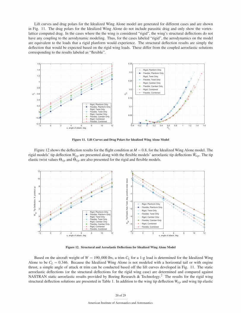
Lift curves and drag polars for the Idealized Wing Alone model are generated for different cases and are shown

in Fig. 11. The drag polars for the Idealized Wing Alone do not include parasitic drag and only show the vortex-

lattice computed drag. In the cases where the the wing is considered “rigid”, the wing’s structural deflections do not

have any coupling to the aerodynamic modeling. Thus, for the cases labeled “rigid”, the aerodynamics on the model

are equivalent to the loads that a rigid planform would experience. The structural deflection results are simply the

deflection that would be expected based on the rigid wing loads. These differ from the coupled aeroelastic solutions

corresponding to the results labeled as “flexible”.

−2 0 2 4 6 8 10 12−0.4

−0.2

0

0.2

0.4

0.6

0.8

1

1.2

1.4

1.6

α, angle of attack, deg

CL

Rigid, Planform OnlyFlexible, Planform OnlyRigid, Twist OnlyFlexible, Twist OnlyRigid, Camber OnlyFlexible, Camber OnlyRigid, CombinedFlexible, Combined

−0.4 −0.2 0 0.2 0.4 0.6 0.8 1 1.2 1.4 1.60

0.05

0.1

0.15

0.2

0.25

0.3

0.35

CL

CD


Figure 11. Lift Curves and Drag Polars for Idealized Wing Alone Model

Figure 12 shows the deflection results for the flight condition at M = 0.8, for the Idealized Wing Alone model. The

rigid models’ tip deflection Wtip are presented along with the flexible models’ aeroelastic tip deflections Wtip. The tip

elastic twist values Θtip and Θtip are also presented for the rigid and flexible models.

−2 0 2 4 6 8 10 12−4

−2

0

2

4

6

8

10

12


Wtip

, Tip

Def

lect

ion,

ft, p

ositi

ve u

p


−2 0 2 4 6 8 10 12−6

−5

−4

−3

−2

−1

0

1

2


Θtip

, Tip

Ela

stic

Axi

s Tw

ist,

deg,

pos

itive

nos

e−do

wn


Figure 12. Structural and Aeroelastic Deflections for Idealized Wing Alone Model

Based on the aircraft weight of W = 190,000 lbs, a trim CL for a 1-g load is determined for the Idealized Wing

Alone to be CL = 0.346. Because the Idealized Wing Alone is not modeled with a horizontal tail or with engine

thrust, a simple angle of attack α trim can be conducted based off the lift curves developed in Fig. 11. The static

aeroelastic deflections (or the structural deflections for the rigid wing case) are determined and compared against

NASTRAN static aeroelastic results provided by Boeing Research & Technology.2 The results for the rigid wing

structural deflection solutions are presented in Table 1. In addition to the wing tip deflection Wtip and wing tip elastic

20 of 29


axis twist Θtip, the value of the elastic contribution to angle of attack αe,tip is also provided representing the amount

of twist of the wing tip about the pitch axis.

Planform Only Wing Alone Model NASTRANAbsolute

Difference

α , deg 3.20 3.15 0.05

Wtip, in 24.34 22.42 1.92

Θtip, deg −1.43 −1.12 0.31

αe,tip, deg −0.25 −0.36 0.11

With Twist Wing Alone Model NASTRANAbsolute

Difference

α , deg 2.33 2.27 0.06

Wtip, in 16.97 15.12 1.85

Θtip, deg −1.06 −0.80 0.26

αe,tip, deg −0.07 −0.16 0.09

With Camber Wing Alone Model NASTRANAbsolute

Difference

α , deg 1.28 1.16 0.21

Wtip, in 26.50 28.28 1.78

Θtip, deg −0.05 0.19 0.24

αe,tip, deg −1.64 −1.94 0.30

Combined Wing Alone Model NASTRANAbsolute

Difference

α , deg 0.41 0.29 0.12

Wtip, in 19.05 20.99 1.94

Θtip, deg 0.32 0.51 0.19

αe,tip, deg −1.46 −1.74 0.28

Table 1. Structural Deflection (Rigid Wing) Results for Idealized Wing Alone, h = 30,000 ft

The structural deflection results for the Idealized Wing Alone model when only the rigid wing loads are considered

are in good agreement between the aeroelastic model and the NASTRAN results. The percent differences in tip

deflection between the Idealized Wing Alone model and the NASTRAN results are 8.56%, 12.2%, 6.29%, and 9.24%

respectively for the planform only model, planform and twist, planform and camber, and combined models. Wing tip

twist agrees where the absolute differences of Θtip ≤ |0.31◦| and αe,tip ≤ |0.30◦| are observed for elastic axis twist and

pitch axis twist, respectively.

The effects of adding twist, camber, and twist and camber on the aeroelastic model with no coupling serve as

confirmation of expected aerodynamic behavior. Because the angle of attack α is adjusted to maintain the total load

of W = 190,000 lbs, the effect of twist, camber, and both combined acts only to redistribute the lift load along the

planform of the wing. With just the planform, the angle of attack to maintain CL = 0.346 is α = 3.20◦. With twist

enabled, the angle of attack decreases to α = 2.33◦. The decrease in angle of attack is expected due to the positive

nose-up twist of the jig-shape at the root which increases the net lift on the planform. The wash-out of the wing twist

shifts the lift distribution towards the root, and thus, a decrease in the tip deflection Wtip and more nose-down tip twist

Θtip are observed. The introduction of camber also significantly affects the angle of attack for CL = 0.346. It is known

from aerodynamics that camber significantly increases the lift on airfoil sections and also introduces moment about

the airfoil aerodynamic center. Because the cambered wing is able to generate much more lift than the flat planform,

the angle of attack needed to maintain the 1-g lift load is only α = 1.28◦, much less than the planform only. The

21 of 29


tip twist Θtip also becomes more nose-down. This is expected, as typical cambered aircraft wings have negative cmac

which twists the airfoil sections nose-down.

The structural deflection results without aeroelastic coupling are recomputed for an altitude of h = 35,000 ft (CL =0.437) and the results are summarized in Table 2.


Difference

α , deg 4.04 3.98 0.06

Wtip, in 24.34 22.42 1.92

Θtip, deg −1.43 −1.12 0.31

αe,tip, deg −0.25 −0.36 0.11


Difference

α , deg 3.17 3.09 0.08

Wtip, in 18.53 16.63 1.90

Θtip, deg −1.14 −0.86 0.28

αe,tip, deg −0.10 −0.20 0.10


Difference

α , deg 2.12 1.99 0.13

Wtip, in 26.03 27.07 1.04

Θtip, deg −0.34 −0.08 0.26

αe,tip, deg −1.35 −1.61 0.26


Difference

α , deg 1.25 1.10 0.15

Wtip, in 20.18 21.28 1.10

Θtip, deg −0.04 0.18 0.22

αe,tip, deg −1.21 −1.46 0.25

Table 2. Structural Deflection (Rigid Wing) Results for Idealized Wing Alone, h = 35,000 ft

Good agreement still exists at the increased altitude of h = 35,000 ft between the developed aeroelastic model

and NASTRAN results for the Idealized Wing Alone model when only the rigid wing loads are considered. Percent

differences of 8.56%, 11.4%, 3.84%, and 5.26% respectively for the planform only model, planform and twist, plan-

form and camber, and combined models are observed between the wing tip deflection Wtip results with the developed

aeroelastic model and NASTRAN. Absolute differences of Θtip ≤ |0.31◦| and αe,tip ≤ |0.26◦| are observed for wing

tip elastic axis twist and pitch axis twist, respectively.

The aerodynamic trends observed for the Idealized Wing Alone model with the rigid wing at h = 30,000 ft are

consistent with the results at h = 35,000 ft. The addition of twist, camber, and twist and camber to the planform

increases the lift generated by the model and subsequently reduces the angle of attack α needed to maintain a load of

CL = 0.346.

22 of 29


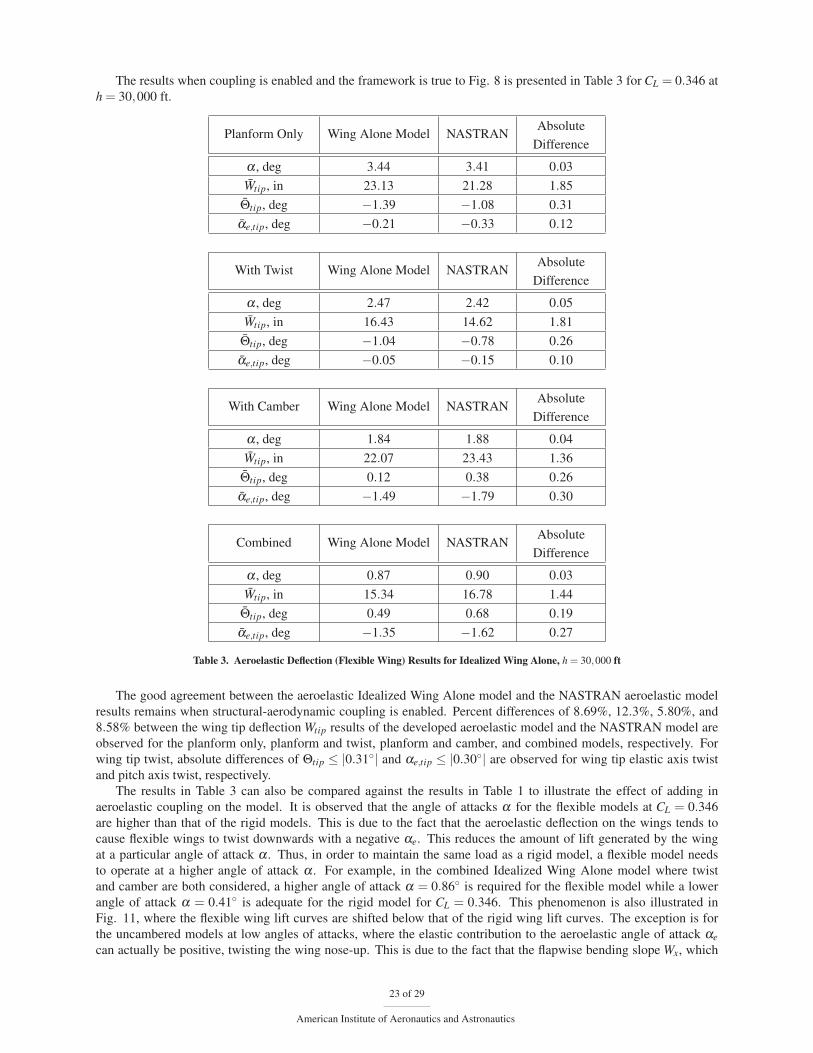
The results when coupling is enabled and the framework is true to Fig. 8 is presented in Table 3 for CL = 0.346 at

h = 30,000 ft.


Difference

α , deg 3.44 3.41 0.03

Wtip, in 23.13 21.28 1.85

Θtip, deg −1.39 −1.08 0.31

αe,tip, deg −0.21 −0.33 0.12


Difference

α , deg 2.47 2.42 0.05

Wtip, in 16.43 14.62 1.81

Θtip, deg −1.04 −0.78 0.26

αe,tip, deg −0.05 −0.15 0.10


Difference

α , deg 1.84 1.88 0.04

Wtip, in 22.07 23.43 1.36

Θtip, deg 0.12 0.38 0.26

αe,tip, deg −1.49 −1.79 0.30


Difference

α , deg 0.87 0.90 0.03

Wtip, in 15.34 16.78 1.44

Θtip, deg 0.49 0.68 0.19

αe,tip, deg −1.35 −1.62 0.27

Table 3. Aeroelastic Deflection (Flexible Wing) Results for Idealized Wing Alone, h = 30,000 ft

The good agreement between the aeroelastic Idealized Wing Alone model and the NASTRAN aeroelastic model

results remains when structural-aerodynamic coupling is enabled. Percent differences of 8.69%, 12.3%, 5.80%, and

8.58% between the wing tip deflection Wtip results of the developed aeroelastic model and the NASTRAN model are

observed for the planform only, planform and twist, planform and camber, and combined models, respectively. For

wing tip twist, absolute differences of Θtip ≤ |0.31◦| and αe,tip ≤ |0.30◦| are observed for wing tip elastic axis twist

and pitch axis twist, respectively.

The results in Table 3 can also be compared against the results in Table 1 to illustrate the effect of adding in

aeroelastic coupling on the model. It is observed that the angle of attacks α for the flexible models at CL = 0.346

are higher than that of the rigid models. This is due to the fact that the aeroelastic deflection on the wings tends to

cause flexible wings to twist downwards with a negative αe. This reduces the amount of lift generated by the wing

at a particular angle of attack α . Thus, in order to maintain the same load as a rigid model, a flexible model needs

to operate at a higher angle of attack α . For example, in the combined Idealized Wing Alone model where twist

and camber are both considered, a higher angle of attack α = 0.86◦ is required for the flexible model while a lower

angle of attack α = 0.41◦ is adequate for the rigid model for CL = 0.346. This phenomenon is also illustrated in

Fig. 11, where the flexible wing lift curves are shifted below that of the rigid wing lift curves. The exception is for

the uncambered models at low angles of attacks, where the elastic contribution to the aeroelastic angle of attack αecan actually be positive, twisting the wing nose-up. This is due to the fact that the flapwise bending slope Wx, which

23 of 29


generally contributes to the nose-down elastic twist of the wing, is very low at these flight conditions.

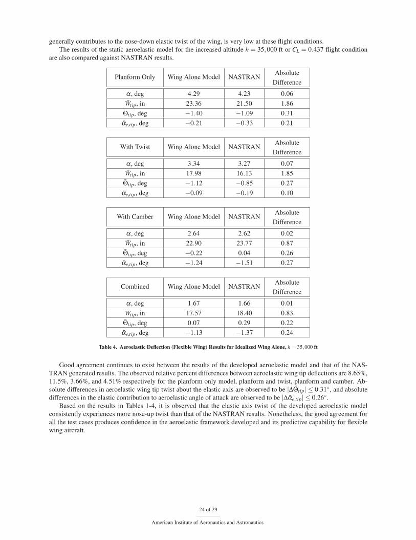
The results of the static aeroelastic model for the increased altitude h = 35,000 ft or CL = 0.437 flight condition

are also compared against NASTRAN results.


Difference

α , deg 4.29 4.23 0.06

Wtip, in 23.36 21.50 1.86

Θtip, deg −1.40 −1.09 0.31

αe,tip, deg −0.21 −0.33 0.21


Difference

α , deg 3.34 3.27 0.07

Wtip, in 17.98 16.13 1.85

Θtip, deg −1.12 −0.85 0.27

αe,tip, deg −0.09 −0.19 0.10


Difference

α , deg 2.64 2.62 0.02

Wtip, in 22.90 23.77 0.87

Θtip, deg −0.22 0.04 0.26

αe,tip, deg −1.24 −1.51 0.27


Difference

α , deg 1.67 1.66 0.01

Wtip, in 17.57 18.40 0.83

Θtip, deg 0.07 0.29 0.22

αe,tip, deg −1.13 −1.37 0.24

Table 4. Aeroelastic Deflection (Flexible Wing) Results for Idealized Wing Alone, h = 35,000 ft

Good agreement continues to exist between the results of the developed aeroelastic model and that of the NAS-

TRAN generated results. The observed relative percent differences between aeroelastic wing tip deflections are 8.65%,

11.5%, 3.66%, and 4.51% respectively for the planform only model, planform and twist, planform and camber. Ab-

solute differences in aeroelastic wing tip twist about the elastic axis are observed to be |ΔΘtip| ≤ 0.31◦, and absolute

differences in the elastic contribution to aeroelastic angle of attack are observed to be |Δαe,tip| ≤ 0.26◦.

Based on the results in Tables 1-4, it is observed that the elastic axis twist of the developed aeroelastic model

consistently experiences more nose-up twist than that of the NASTRAN results. Nonetheless, the good agreement for

all the test cases produces confidence in the aeroelastic framework developed and its predictive capability for flexible

wing aircraft.

24 of 29


B. ESAC Model, Static Aeroelastic and Longitudinal Trim Analysis

With preliminary validation of the aeroelastic modeling completed, the static aeroelastic framework is extended to

that of the ESAC. The ESAC model is representative of a full aircraft configuration with engine nacelles, pylons, tail

surfaces, and fuselage present in the modeling.

Two independent and separate cruise conditions are simulated with the ESAC, representing different possible de-

sign cruise condition candidates. The weight model is also adjusted based on the different candidate cruise conditions.

• A first cruise condition is simulated at M = 0.8, h = 30,000 ft, where the 80% fuel case of the aircraft is

W = 190,000 lbs and the empty wing mass is Ww,0 = 17,250 lbs. The design lift coefficient in this case is

CL = 0.346.

• A second cruise condition is simulated at M = 0.8, h = 36,000 ft, where the 80% fuel case of the aircraft is

W = 210,000 lbs and the empty wing mass is Ww,0 = 13,000 lbs. The design lift coefficient for this case is

CL = 0.510.

For the cruise flight conditions, the parasitic drag coefficient is built up using a critical Reynold’s number of Rec =600,000. The results are presented in Table 5.

h = 30,000 ft

Component Cf CD0

Wings 0.0037 0.0054

Fuselage 0.0042 0.0047

Horizontal Tail 0.0010 0.0015

Vertical Tail 0.0008 0.0011

Engine Nacelles+Pylons 0.0004 0.0010

Total 0.0102 0.0137

h = 36,000 ft

Component Cf CD0

Wings 0.0038 0.0056

Fuselage 0.0044 0.0049

Horizontal Tail 0.0011 0.0015

Vertical Tail 0.0008 0.0012

Engine Nacelles+Pylons 0.0005 0.0011

Total 0.0106 0.0142

Table 5. Parasite Drag Build-Up At Cruise Conditions

Initially neglecting thrust and its effect on the aeroelastic deformation, the lift curve and drag polars for the ESAC

are generated and shown in Fig. 13. Note that now the drag polar includes the conceptually estimated parasitic drag

coefficient.

−2 0 2 4 6 8 10 12−0.2

0

0.2

0.4

0.6

0.8

1

1.2

1.4

1.6


CL

Rigid Wing, Both Cruise ConditionsFlexible, Cruise Condition #1Flexible, Cruise Condition #2

−0.2 0 0.2 0.4 0.6 0.8 1 1.2 1.4 1.60

0.05

0.1

0.15

0.2

0.25

CL

CD

Rigid Wing, Cruise Condition #1Flexible, Cruise Condition #1Rigid Wing, Cruise Condition #2Flexible, Cruise Condition #2

Figure 13. Lift Curves and Drag Polars for ESAC Model, No Thrust or Control Deflection

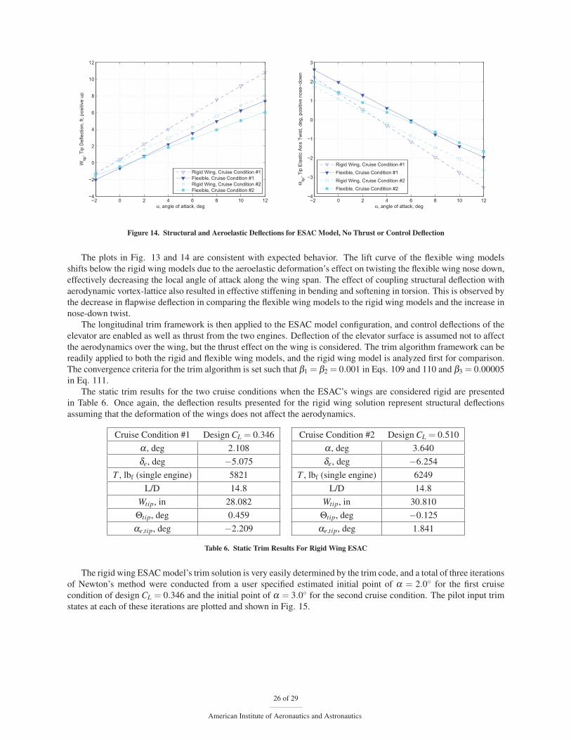
The tip deflection, Wtip for the rigid model and Wtip for the flexible model, and tip elastic axis twist, Θtip for the

rigid model and Θtip for the flexible model, at the two different flight conditions are shown in Fig. 14.

25 of 29


−2 0 2 4 6 8 10 12−4

−2

0

2

4

6

8

10

12


Wtip

, Tip

Def

lect

ion,

ft, p

ositi

ve u

p


−2 0 2 4 6 8 10 12−4

−3

−2

−1

0

1

2

3


Θtip

, Tip

Ela

stic

Axi

s Tw

ist,

deg,

pos

itive

nos

e−do

wn


Figure 14. Structural and Aeroelastic Deflections for ESAC Model, No Thrust or Control Deflection

The plots in Fig. 13 and 14 are consistent with expected behavior. The lift curve of the flexible wing models

shifts below the rigid wing models due to the aeroelastic deformation’s effect on twisting the flexible wing nose down,

effectively decreasing the local angle of attack along the wing span. The effect of coupling structural deflection with

aerodynamic vortex-lattice also resulted in effective stiffening in bending and softening in torsion. This is observed by

the decrease in flapwise deflection in comparing the flexible wing models to the rigid wing models and the increase in

nose-down twist.

The longitudinal trim framework is then applied to the ESAC model configuration, and control deflections of the

elevator are enabled as well as thrust from the two engines. Deflection of the elevator surface is assumed not to affect

the aerodynamics over the wing, but the thrust effect on the wing is considered. The trim algorithm framework can be

readily applied to both the rigid and flexible wing models, and the rigid wing model is analyzed first for comparison.

The convergence criteria for the trim algorithm is set such that β1 = β2 = 0.001 in Eqs. 109 and 110 and β3 = 0.00005

in Eq. 111.

The static trim results for the two cruise conditions when the ESAC’s wings are considered rigid are presented

in Table 6. Once again, the deflection results presented for the rigid wing solution represent structural deflections

assuming that the deformation of the wings does not affect the aerodynamics.

Cruise Condition #1 Design CL = 0.346

α , deg 2.108

δe, deg −5.075

T , lbf (single engine) 5821

L/D 14.8

Wtip, in 28.082

Θtip, deg 0.459

αe,tip, deg −2.209


α , deg 3.640

δe, deg −6.254


L/D 14.8

Wtip, in 30.810

Θtip, deg −0.125

αe,tip, deg 1.841

Table 6. Static Trim Results For Rigid Wing ESAC

The rigid wing ESAC model’s trim solution is very easily determined by the trim code, and a total of three iterations

of Newton’s method were conducted from a user specified estimated initial point of α = 2.0◦ for the first cruise

condition of design CL = 0.346 and the initial point of α = 3.0◦ for the second cruise condition. The pilot input trim

states at each of these iterations are plotted and shown in Fig. 15.

26 of 29


1 2 32

2.05

2.1

2.15

Iteration Number

α

1 2 3−6

−4

−2

0

Iteration Number

δ e

1 2 30

2000

4000

6000

Iteration Number

T

Cruise Condition #1, Design CL = 0.346

1 2 33

3.5

4

Iteration Number

α

1 2 3−10

−5

0

Iteration Number

δ e

1 2 30

5000

10000

Iteration Number

T


Figure 15. Static Trim Iteration Data for Rigid Wing ESAC

The longitudinal trim code is then run on the ESAC with fully flexible wings. The trim solution is determined, and

the results are summarized in Table 7.


α , deg 3.747

δe, deg −6.798


L/D 11.4

Wtip, in 24.645

Θtip, deg 0.643



α , deg 5.160

δe, deg −7.880


L/D 11.9

Wtip, in 28.469

Θtip, deg 0.014


Table 7. Static Trim Results For Flexible Wing ESAC

Due to the flexibility of the wing, the trim code takes longer to converge, with 20 iterations for the design CL =0.346, and 14 iterations for the design CL = 0.510. The pilot input trim states at each of these iterations are plotted in

Fig. 16. As expected, the trim angle of attacks α for the flexible models are higher than that of the rigid models due

to the effect of the aeroelastic bending and torsion on the aeroelastic angle of attack.

Because the flexible trim case also involves determining the coupled aeroelastic wing deformation, plots of the

evolution of the tip deformation are shown in Fig. 17, where Wtip is plotted in feet and Θtip is plotted in degrees. It is

observed that the aeroelastic deformation of the model converges alongside the solution of the static trim inputs.

27 of 29


1 2 3 4 5 6 7 8 9 10 11 12 13 14 15 16 17 18 19 202

3

4

Iteration Number

α

1 2 3 4 5 6 7 8 9 10 11 12 13 14 15 16 17 18 19 20−10

−5

0

Iteration Number

δ e

1 2 3 4 5 6 7 8 9 10 11 12 13 14 15 16 17 18 19 200

5000

10000

Iteration Number

T


1 2 3 4 5 6 7 8 9 10 11 12 13 143

4

5

6

Iteration Number

α

1 2 3 4 5 6 7 8 9 10 11 12 13 14−8

−6

−4

−2

0

Iteration Number

δ e

1 2 3 4 5 6 7 8 9 10 11 12 13 140

2000

4000

6000

8000

Iteration Number

T


Figure 16. Static Trim Iteration Data for Flexible Wing ESAC

1 2 3 4 5 6 7 8 9 10 11 12 13 14 15 16 17 18 19 200

1

2

3

Iteration Number

Wtip

1 2 3 4 5 6 7 8 9 10 11 12 13 14 15 16 17 18 19 200

0.5

1

1.5

Iteration Number

Θtip

1 2 3 4 5 6 7 8 9 10 11 12 13 14 15 16 17 18 19 20−2.5

−2

−1.5

Iteration Number

α etip


1 2 3 4 5 6 7 8 9 10 11 12 13 141

1.5

2

2.5

3

Iteration Number

Wtip

1 2 3 4 5 6 7 8 9 10 11 12 13 14−0.5

0

0.5

Iteration Number

Θtip

1 2 3 4 5 6 7 8 9 10 11 12 13 14−2

−1.5

−1

Iteration Number

α etip


Figure 17. Static Trim Deflection Iteration Data for Flexible Wing ESAC

XI. Conclusions

This study presents the development of a static aeroelastic model and a static three degree-of-freedom longitudinal

aeroelastic trim model capable of analyzing flexible wing aircraft. The aeroelastic model is developed by coupling

equivalent beam wing structural models in the loop with vortex-lattice aerodynamic modeling. The static aeroelastic

code is capable of generating flexible wing aircraft configurations and characterizing aeroelastic deformations. Utiliz-

ing converged aeroelastic geometry, flexible aircraft lift curves and drag polars can be generated exploring the effect of

flexibility enabled models. The coupled finite-element vortex-lattice aeroelastic model is validated against NASTRAN

aeroelasticity results for a simplified Idealized Wing Alone model for various test cases, including systematically ana-

28 of 29


lyzing the model planform only, with only added twist, with only added camber, and both added. The static aeroelastic

model is extended to develop an aeroelastic three degree-of-freedom longitudinal trim model for a full aircraft config-

uration with horizontal tail, elevator, and engines. The trim algorithm uses Newton’s method which is inserted in the

static aeroelastic approach to iterate pilot trim inputs and to solve the flight condition until convergence is achieved.

This framework is readily applied for the flexible wing models investigated in this study, but could be improved in the

future for highly flexible wings. Future study of an aeroelastic trim model where Newton’s method is wrapped around

an inner loop static aeroelastic model can be investigated. In addition, different approaches for estimating the Jacobian

and variations to Newton’s method can possibly increase the convergence rate of the longitudinal trim model.

XII. Acknowledgments

The authors wish to acknowledge Mr. John Dykman of Boeing Research & Technology in Seal Beach, CA for

providing insight and the NASTRAN results used in development of the models. The authors would also like to

thank the NASA Aeronautics Research Mission Directorate (ARMD) Fixed Wing Project under the Fundamental

Aeronautics Program for providing the funding to support this work.

References1Nguyen, N., “NASA Innovation Fund 2010 Project: Elastically Shaped Future Air Vehicle Concept,” NASA Internal Report Submitted to

NASA Innovative Partnerships Program Office, October 8, 2010.2Boeing Report No. 2010X0015, "Development of Variable Camber Continuous Trailing Edge Flap System,” submitted to NASA ARMD

Fixed Wing Project, October 4, 2012.3Urnes, Sr., J., Nguyen, N., Ippolito, C., Totah, J., Trinh, K., Ting, E., “A Mission-Adaptive Variable Camber Flap Control System to Optimize

High Lift and Cruise Lift-to-Drag Ratios of Future N+3 Transport Aircraft,” 51st AIAA Aerospace Sciences Meeting, AIAA-2013-0214, January

2013.4Nguyen, N., Trinh, K., Frost S., and Reynolds, K., “Coupled Aeroelastic Vortex Lattice Modeling of Flexible Aircraft,” AIAA Applied

Aerodynamics Conference, AIAA-2011-3021, June 2011.5Nguyen, N., Trinh, K., Nguyen, D., Tuzcu, I., “Nonlinear Aeroelasticty of Flexible Wing Structure Coupled with Aircraft Flight Dynamics,”

AIAA Structures, Structural Dynamics, and Materials Conference, AIAA-2012-1792, April 2012.6Meirovitch, L., Fundamentals of Vibrations, McGraw-Hill Higher Education, 2001.7Hodges, D.H. and Pierce, G.A., Introduction to Structural Dynamics and Aeroelasticity, Cambridge University Press, 2002.8Hughes, T., The Finite Element Method: Linear Static and Dynamic Finite Element Analysis, Prentice Hall, Inc., 1987.9Craig, Jr., R.R. and Kurdila, A.J., Fundamentals of Structural Dynamics, Second Edition, John Wiley & Sons, Inc., 2006.

10Jordan, T. L., Langford, W. M., Belcastro, C. M., Foster, J. M., Shah, G. H., Howland, G., and Kidd, R., “Development of a Dynamically

Scaled Generic Transport Model Testbest for Flight Research Experiments,” AUVSI Unmanned Unlimited, Arlington, VA, 2004.11Nguyen, N., Nelson, A., and Pulliam, T., “Damage Adaptive Control System Research Report,” Internal NASA Report, April 2006.12Nguyen, N., “Integrated Flight Dynamics Modeling of Flexible Aircraft with Inertial Force-Propulsion - Aeroelastic Couplings,” 46th AIAA

Aerospace Sciences Meeting and Exhibit, AIAA-2008-194, January 2008.13Houbolt, J. C and Brooks, G. W., “Differential Equations of Motion for Combined Flapwise Bending, Chordwise Bending, and Torsion of

Twisted Nonuniform Rotor Blades,” NACA Technical Note 3905, February 1957.14Miranda, L.R., Elliot, R.D., and Baker, W.M., “A Generalized Vortex Lattice Method for Subsonic and Supersonic Flow Applications,”

NASA CR-2865, 1977.15Aftosmis, M.J., Berger, M.J., and Melton, J.E., “Robust and Efficient CartesianMesh Generation for Component- Based Geometry,” AIAA

Journal, Vol. 36, No. 6, 1998, pp. 953-960.16Raymer, D. P., Aircraft Design: A Conceptual Approach, American Institue of Aeronautics and Astronautics, 1989.17Pozrikidis, C., Numerical Computation in Science and Engineering, Oxford University Press, Inc., 1998.

29 of 29


Static Aeroelastic and Longitudinal Trim Model of Flexible ...

Documents

Transcript of Static Aeroelastic and Longitudinal Trim Model of Flexible ...