The order of convergence of Eigenfrequencies in finite element approximations of fluid-structure...

MATHEMATICS OF COMPUTATIONVolume 65, Number 216October 1996, Pages 1463–1475

THE ORDER OF CONVERGENCE OF EIGENFREQUENCIES

IN FINITE ELEMENT APPROXIMATIONS

OF FLUID-STRUCTURE INTERACTION PROBLEMS

RODOLFO RODRIGUEZ AND JORGE E. SOLOMIN

Abstract. In this paper we prove a double order for the convergence of eigen-frequencies in fluid-structure vibration problems. We improve estimates givenrecently for compressible and incompressible fluids. To do this, we extendclassical results on finite element spectral approximation to nonconformingmethods for noncompact operators.

1. Introduction

This paper deals with the approximation of eigenfrequencies in vibration prob-lems for coupled systems with fluid-structure interaction. Such problems have beenconsidered in several recent papers. A survey of current results and references canbe found in [12].

In particular, we consider the interior elastoacoustics problem consisting of de-termining the vibration modes of an elastic solid containing a fluid. Different for-mulations have been proposed to solve this problem (see [6, 11, 14]). A pure dis-placement formulation yields a simple eigenvalue problem; however, spurious modesarise when standard finite element methods are applied to it (see [11]). Recently,several methods to avoid these spurious modes have been proposed (see [2, 3, 8]).

In [2] a finite element method consisting of Raviart-Thomas elements for thedisplacements of the fluid and standard Courant elements for those of the solid isintroduced for the case of a compressible fluid. A weak coupling between both typeof elements along the interface is imposed. In [3] this method has been adapted todeal with incompressible fluids. Both procedures yield nonconforming methods toapproximate the eigenvalue problem for the noncompact operators present in theformulation.

It is well known, in the case of conforming approximations of compact operators,that the order of convergence for the eigenvalues doubles that for the eigenfunc-tions (see, for instance, [1]). In [10] the same result is proved to be valid even fornoncompact operators under reasonable assumptions. A similar analysis is con-tained in [13] for nonconforming approximations of compact operators. None ofthese theories cover the situations considered in [2] and [3].

Received by the editor January 30, 1995.1991 Mathematics Subject Classification. Primary 65N25, 65N30; Secondary 70J30, 73K70,

76Q05.Key words and phrases. Fluid-structure, eigenvalue problems.Partially supported by Consejo Nacional de Investigaciones Cientıficas y Tecnicas, Argentina.

c©1996 American Mathematical Society

1463

License or copyright restrictions may apply to redistribution; see http://www.ams.org/journal-terms-of-use

1464 RODOLFO RODRIGUEZ AND JORGE E. SOLOMIN

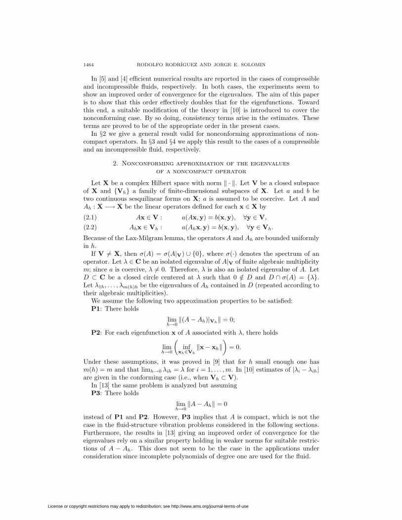
In [5] and [4] efficient numerical results are reported in the cases of compressibleand incompressible fluids, respectively. In both cases, the experiments seem toshow an improved order of convergence for the eigenvalues. The aim of this paperis to show that this order effectively doubles that for the eigenfunctions. Towardthis end, a suitable modification of the theory in [10] is introduced to cover thenonconforming case. By so doing, consistency terms arise in the estimates. Theseterms are proved to be of the appropriate order in the present cases.

In §2 we give a general result valid for nonconforming approximations of non-compact operators. In §3 and §4 we apply this result to the cases of a compressibleand an incompressible fluid, respectively.

2. Nonconforming approximation of the eigenvalues

of a noncompact operator

Let X be a complex Hilbert space with norm ‖ · ‖. Let V be a closed subspaceof X and Vh a family of finite-dimensional subspaces of X. Let a and b betwo continuous sesquilinear forms on X; a is assumed to be coercive. Let A andAh : X −→ X be the linear operators defined for each x ∈ X by

Ax ∈ V : a(Ax,y) = b(x,y), ∀y ∈ V,(2.1)

Ahx ∈ Vh : a(Ahx,y) = b(x,y), ∀y ∈ Vh.(2.2)

Because of the Lax-Milgram lemma, the operatorsA and Ah are bounded uniformlyin h.

If V 6= X, then σ(A) = σ(A|V) ∪ 0, where σ(·) denotes the spectrum of anoperator. Let λ ∈ C be an isolated eigenvalue of A|V of finite algebraic multiplicitym; since a is coercive, λ 6= 0. Therefore, λ is also an isolated eigenvalue of A. LetD ⊂ C be a closed circle centered at λ such that 0 /∈ D and D ∩ σ(A) = λ.Let λ1h, . . . , λm(h)h be the eigenvalues of Ah contained in D (repeated according totheir algebraic multiplicities).

We assume the following two approximation properties to be satisfied:P1: There holds

limh→0‖(A−Ah)|Vh

‖ = 0;

P2: For each eigenfunction x of A associated with λ, there holds

limh→0

(inf

xh∈Vh

‖x− xh‖)

= 0.

Under these assumptions, it was proved in [9] that for h small enough one hasm(h) = m and that limh→0 λih = λ for i = 1, . . . ,m. In [10] estimates of |λi − λih|are given in the conforming case (i.e., when Vh ⊂ V).

In [13] the same problem is analyzed but assumingP3: There holds

limh→0‖A−Ah‖ = 0

instead of P1 and P2. However, P3 implies that A is compact, which is not thecase in the fluid-structure vibration problems considered in the following sections.Furthermore, the results in [13] giving an improved order of convergence for theeigenvalues rely on a similar property holding in weaker norms for suitable restric-tions of A − Ah. This does not seem to be the case in the applications underconsideration since incomplete polynomials of degree one are used for the fluid.


ORDER OF CONVERGENCE OF EIGENFREQUENCIES 1465

The results in [9] could be extended to the nonconforming case (i.e., Vh 6⊂ V).However for the estimators therein to be useful, the eigenfunctions of the adjointoperator A∗ with respect to a need to be smooth. To avoid this drawback, insteadof the adjoints A∗ and A∗h, we consider as in [13] the bounded operators A∗ andA∗h : X −→ X defined by

A∗x ∈ V : a(y, A∗x) = b(y,x), ∀y ∈ V,(2.3)

A∗hx ∈ Vh : a(y, A∗hx) = b(y,x), ∀y ∈ Vh.(2.4)

Then λ is an eigenvalue of A∗ with the same multiplicity m as that of λ (see [13]).Analogously, for h small enough, λ1h, . . . , λmh are the eigenvalues of A∗h belongingto D := µ ∈ C : µ ∈ D.

We assume for A∗ and A∗h approximation properties analogous to P1 and P2,namely,

P1∗: There holds

limh→0‖(A∗ −A∗h)|Vh

‖ = 0;

P2∗: For each eigenfunction x of A∗ associated with λ, there holds

limh→0

(inf

xh∈Vh

‖x− xh‖)

= 0.

Let Πh and Π∗h : X −→ X be the projectors with range Vh defined bya(x − Πhx ,y) = 0, ∀y ∈ Vh, and a(y,x − Π∗hx) = 0, ∀y ∈ Vh, respec-tively. Since a is continuous and coercive, Πh and Π∗h are bounded uniformlyin h. Let Bh := AhΠh : X −→ X. Notice that σ(Ah) = σ(Bh) and that,for any nonzero eigenvalue, the corresponding invariant subspaces coincide. LetB∗h := A∗hΠ∗h : X −→ X.

Let E : X −→ X be the spectral projector of A relative to the isolated eigenvalueλ. Let Fh : X −→ X be the spectral projector of Bh relative to its eigenvaluesλ1h, . . . , λmh. It can be proved as in Lemma 1 of [10] that there exists h0 > 0 suchthat

∥∥(z −Bh)−1∥∥ is bounded for h ≤ h0 and z ∈ ∂D; consequently, for h small

enough, the spectral projectors Fh are bounded uniformly in h. Let E∗ and F∗h bethe spectral projector of A∗ and B∗h relative to λ and λ1h, . . . , λmh, respectively.

We remark that B∗h turns out to be the actual adjoint of Bh with respect to a.In fact, for all x and y ∈ X,

a(Bhx,y) = a(AhΠhx,y) = a(AhΠhx,Π∗hy) = b(Πhx,Π∗hy)

and, analogously, a(x, B∗hy) = b(Πhx,Π∗hy). Therefore, the spectral projectorF∗h is also the adjoint of Fh.

For Y and Z closed subspaces of X, let

δ(Y,Z) := supy∈Y‖y‖=1

(infz∈Z‖y − z‖

)

and

δ(Y,Z) := max δ(Y,Z), δ(Z,Y) .

Let γh

:= δ(E(X),Vh) and γ∗h := δ(E∗(X),Vh). Because of P2 and P2∗, wehave γ

h→ 0 and γ∗h → 0 as h → 0. Since a is coercive and continuous, there

holds∥∥(I −Πh)|E(X)

∥∥ ≤ Cγh

and∥∥(I −Π∗h)|E∗(X)

∥∥ ≤ Cγ∗h . From now on, C



denotes a generic constant not necessarily the same at each occurrence but alwaysindependent of h.

For h sufficiently small, we have the following results:

Lemma 2.1. There holds∥∥(E − Fh)|E(X)

∥∥ ≤ C ∥∥(A−Bh)|E(X)

∥∥ ,∥∥(E∗ − F∗h)|E∗(X)

∥∥ ≤ C ∥∥(A∗ −B∗h)|E∗(X)

∥∥ .Proof. The proof is identical to that of Lemma 3 in [10].

Let δh

:= γh

+‖(A−Ah)|Vh‖ and δ∗h := γ∗h +‖(A∗ −A∗h)|Vh

‖. Because of P1and P2 (resp. P1∗ and P2∗) we have δ

h→ 0 and δ∗h → 0 as h→ 0.

Lemma 2.2. There holds ∥∥(A−Bh)|E(X)

∥∥ ≤ Cδh,∥∥(A∗ −B∗h)|E∗(X)

∥∥ ≤ Cδ∗h .Proof. Let x ∈ E(X) with ‖x‖ = 1; we have

‖(A−Bh)x‖ ≤ ‖A(I −Πh)x‖+ ‖(A−Ah)Πhx‖≤ ‖A‖ ‖(I −Πh)x‖+ ‖(A−Ah)|Vh

‖ ‖Πhx‖≤ C (γ

h+ ‖(A−Ah)|Vh

‖) = Cδh,

and an analogous proof is valid for the second estimate of the theorem.

Let Λh := Fh|E(X) : E(X) −→ Fh(X).

Lemma 2.3. The operator Λh is bijective and∥∥Λ−1

h

∥∥ is bounded in h.

Proof. See the proof of Theorem 1 in [10].

Theorem 2.1. There holds

δ (Fh(X), E(X)) ≤ Cδh.

Proof. The proof is identical to that of Theorem 1 in [10].

Let A := A|E(X) : E(X) −→ E(X) and Bh := Λ−1h BhΛh : E(X) −→ E(X). The

operator A has a unique eigenvalue λ of algebraic multiplicity m; the operator Bhhas the eigenvalues λ1h, . . . , λmh.

Consider the following consistency terms:

Mh = supx∈E(X)‖x‖=1

supy∈E∗(X)‖y‖=1

[a(Ax,Π∗hy) − b(x,Π∗hy)

],

M∗h = supx∈E(X)‖x‖=1


[a(Πhx, A∗y)− b(Πhx,y)

].

It is clear that Mh = M∗h = 0 for conforming methods. In general, we have thefollowing result, which can be seen to be an extension to the nonconforming caseof Theorem 2 in [10].

Theorem 2.2. There holds∥∥∥A− Bh∥∥∥ ≤ C (δhδ∗h +Mh +M∗h) .



Proof. We easily see that∥∥∥A− Bh∥∥∥ = supx∈E(X)‖x‖=1

∥∥∥(A− Bh)x∥∥∥

≤ C supx∈E(X)‖x‖=1

supy∈V‖y‖=1

a(

(A− Bh)x,y)

= C supx∈E(X)‖x‖=1


a(

(A− Bh)x,y).(2.5)

By using that(Λ−1h Fh − I

)A|E(X) = 0 and that Bh commutes with its spectral

projector Fh, it is straightforward to prove that

A− Bh = (A−Bh) |E(X) +(Λ−1h Fh − I

)(A−Bh) |E(X).(2.6)

Let x ∈ E(X) and y ∈ E∗(X) with ‖x‖ = ‖y‖ = 1. Since Fh(Λ−1h Fh − I

)= 0

and F∗h is the adjoint of Fh with respect to a, we have

|a((Λ−1h Fh − I)(A−Bh)x,y)|

=∣∣a ((Λ−1

h Fh − I) (A−Bh) x, (I − F∗h) y)∣∣

≤ ‖a‖∥∥Λ−1

h Fh − I∥∥∥∥(A−Bh)|E(X)

∥∥∥∥(I − F∗h) |E∗h(X)

∥∥≤ Cδ

hδ∗h ,

(2.7)

where we have used Lemmas 2.1, 2.2 and 2.3 and the fact that Fh is boundedindependently of h.

On the other hand,

a(

(A−Bh) x,y)

= a(

(A−Bh) x,Π∗hy)

+ a(

(A−Bh) x, (I −Π∗h)y).(2.8)

By using Lemma 2.2 we may bound the second term in the right-hand side of (2.8):∣∣∣a( (A−Bh) x, (I −Π∗h)y)∣∣∣ ≤ ‖a‖ ∥∥(A−Bh)|E(X)

∥∥∥∥(I −Π∗h)|E∗h(X)

∥∥≤ Cδ

hγ∗h ,

(2.9)

whereas for the first term we have

a(

(A−Bh) x,Π∗hy)

= a(

(A−Ah) x,Π∗hy)

+ a(

(Ah −Bh) x,Π∗hy).(2.10)

Now, ∣∣∣a( (A−Ah) x,Π∗hy)∣∣∣= ∣∣∣a (Ax,Π∗hy)−b (x,Π∗hy)

∣∣∣≤Mh(2.11)

and

a(

(Ah −Bh) x,Π∗hy)

= a(Ah(I −Πh)x,Π∗hy

)= b(

(I −Πh)x,Π∗hy)

= b(

(I −Πh)x,y)− b(

(I − Πh)x, (I −Π∗h)y).(2.12)

The second term in the right-hand side of (2.12) can be easily bounded by∣∣∣b((I −Πh)x, (I −Π∗h)y)∣∣∣ ≤ ‖b‖ ∥∥(I −Πh)|E(X)

∥∥∥∥(I −Π∗h)|E∗h(X)

∥∥≤ Cγ

hγ∗h ,

(2.13)



and for the first term we have

b(

(I −Πh)x,y)

= a(x, A∗y)− b(Πhx,y)

= a(

(I −Πh)x, A∗y)

+[a(Πhx, A∗y)− b(Πhx,y)

].(2.14)

Finally, for the first term on the right of (2.14) we have that∣∣∣a((I −Πh)x, A∗y)∣∣∣ =

∣∣∣a((I − Πh)x, (I −Π∗h)A∗y)∣∣∣

≤ ‖a‖∥∥(I −Πh)|E(X)

∥∥∥∥(I −Π∗h)|E∗h(X)

∥∥ ‖A∗‖ ≤ Cγhγ∗h(2.15)

whereas for the second term we have∣∣∣a(Πhx, A∗y)− b(Πhx,y)∣∣∣ ≤M∗h.(2.16)

Now the theorem is a consequence of formulae (2.5) to (2.16).

By using the previous theorem, we deduce the following result about the approx-imation of the eigenvalue λ:

Theorem 2.3. We have∣∣∣∣∣λ− 1

m

m∑i=1

λih

∣∣∣∣∣ ≤ C (δhδ∗h +Mh +M∗h)(2.17)

and

maxi=1,...,m

|λ− λih| ≤ C (δhδ∗h +Mh +M∗h)1/α ,(2.18)

where α is the ascent of the eigenvalue λ of A (i.e., α is the least positive integer

such that Ker((λ− A)α) = Ker((λ− A)α+1)).

Proof. (2.17) is a direct consequence of Theorem 2.2 and the continuity of the tracefor finite-dimensional operators. (2.18) is an application of well-known results formatrices (see, for instance, [16]).

We remark that if A|E(X) is diagonalizable, then α = 1 and so we have esti-mates of the same order for the convergence of all the approximate eigenvaluesλ1h, . . . , λmh. This is the case in the applications considered in the following sec-tions, where A|V : V −→ V is selfadjoint with respect to a.

3. Approximation of eigenfrequencies in a fluid-structure problem

We consider the problem of determining the vibration modes of an ideal (inviscid)barotropic fluid contained in a linear elastic structure. We take as a model problemthe case of a vessel completely filled by the fluid. We restrict ourselves to the2D case and assume polygonal boundaries and interfaces. This problem has beenanalyzed in [2], where a nonoptimal rate of convergence for the eigenfrequencieshas been proved.

Let ΩF

and ΩS

be the domains occupied by the fluid and the solid, respectively,as in Figure 1. We assume Ω

Fto be simply connected but not necessarily convex.

By ΓI we denote the interface between the solid and the fluid, and by ν its unitnormal vector pointing outward from Ω

F. The exterior boundary of the solid is the

union of ΓD

and ΓN

: the structure is fixed along ΓD

and free of stress along ΓN

; letη denote the unit outward normal vector along ΓN .



.

.

.

.

.

.

.

.

.

.

.

.

.

.

.

.

.

.

.

.

.

.

.

.

.

.

.

.

.

.

.

.

.

.

.

.

.

.

.

.

.

.

.

.

.

.

.

.

.

.

.

.

.

.

.

.

.

.

.

.

.

.

.

.

.

.

.

.

.

.

.

.

.

.

.

.

.

.

.

.

.

.

.

.

.

.

.

.

.

.

.

.

.

.

.

.

.

.

.

.

.

.

.

.

.

.

.

.

.

.

.

.

.

.

.

.

.

.

.

.

.

.

.

.

.

.

.

.

.

.

.

.

.

.

.

.

.

.

.

.

.

.

.

.

.

.

.

.

.

.

.

.

.

.

.

.

.

.

.

.

.

.

.

.

.

.

.

.

.

.

.

.

.

.

.

.

.

.

.

.

.

.

.

.

.

.

.

.

.

.

.

.

.

.

.

.

.

.

.

.

.

.

.

.

.

.

.

.

.

.

.

.

.

.

.

.

.

.

.

.

.

.

.

.

.

- η

- ν

ΩF

ΩS

ΓD

ΓN

ΓI

Figure 1. Fluid and solid domains

Henceforth, we use the standard notation for Sobolev spaces, norms and semi-norms.

Let X := H(div,ΩF) ×

[H1

ΓD

(ΩS)]2

(H1Γ

D(Ω

S) being the subspace of functions

in H1(ΩS) vanishing on ΓD) endowed with the H(div,ΩF) ×[H1(ΩS)

]2norm,

which we denote by ‖(u,v)‖. Let V be the closed subspace of X defined byV := (u,v) ∈ X : u · ν = v · ν on Γ

I. Let a0 and b be the continuous, sym-

metric and positive bilinear forms on X given by

a0 ((u,v), (φ,ψ)) :=

∫Ω

F

ρFc2 div u divφ+

∫Ω

S

σ(v) : ε(ψ),

b ((u,v), (φ,ψ)) :=

∫Ω

F

ρFu · φ+

∫Ω

S

ρSv ·ψ,

where σ(v) : ε(ψ) denotes the tensorial product between the strain tensor εij(ψ) :=12

(∂ψi∂xj

+∂ψj∂xi

)and the stress tensor σij(v) := λS

∑2k=1 εkk(v)δij + 2µSεij(v) (λS

and µS

being the Lame coefficients of the structure); ρS

and ρF

are the densities ofthe solid and the fluid, respectively, and c is the acoustic speed in the fluid.

The classical acoustic approximation for the small-amplitude motions yields thefollowing eigenvalue problem for the vibration modes of the coupled system (see[2]):

VP0: Find λ ∈ R and (u,v) ∈ V, (u,v) 6= (0,0), such that

a0 ((u,v), (φ,ψ)) = λb ((u,v), (φ,ψ)) , ∀(φ,ψ) ∈ V.

Here, ω =√λ is the frequency of the eigenmode, and u and v are the displacements

in the fluid and in the solid, respectively.There exist eigenmodes of problem VP0 which do not induce vibrations into

the solid. They are pure rotational motions of the fluid and correspond to theeigenvalue λ = 0. It is proved in [2] that the corresponding eigenspace is K :=

( curl ξ,0), ξ ∈ H10 (Ω

F)

. Therefore, the bilinear form a0 is not coercive. How-ever, a := a0 + b is coercive and can be used instead. The eigenvalue problemassociated with a is:

VP: Find λ ∈ R and (u,v) ∈ V, (u,v) 6= (0,0), such that

a ((u,v), (φ,ψ)) = λb ((u,v), (φ,ψ)) , ∀(φ,ψ) ∈ V.



As in the previous section, we consider the bounded linear operator A : X −→ Xdefined by A(u,v) ∈ V and

a (A(u,v), (φ,ψ)) = b ((u,v), (φ,ψ)) , ∀(φ,ψ) ∈ V.

Since a and b are symmetric, A|V is selfadjoint with respect to a. Clearly,(λ, (u,v)) is an eigenpair of A|V if and only if ( 1

λ , (u,v)) is a solution of VP

which, in turn, is equivalent to ( 1λ − 1, (u,v)) being a solution of VP0.

The operator A|V is not compact; in fact, λ = 1 is an eigenvalue of A|V withinfinite-dimensional eigenspace K. Nevertheless, AK⊥ is compact. This is usedin [2] to show that the spectrum of A|V consists of the eigenvalue λ = 1 and asequence of finite-multiplicity eigenvalues λn : n ∈N ⊂ (0, 1) converging to 0.Each eigenvector (un,vn) associated with λn ∈ (0, 1) satisfies curlun = 0. Further-more, additional smoothness can be proved for these eigenmodes. In particular, thefollowing a priori estimate will be used below to estimate the consistency terms.

Theorem 3.1. Let (u,v) be an eigenfunction of A with corresponding eigenvalue

λ ∈ (0, 1). Then u ∈ [Hα(ΩF)]

2, v ∈

[H1+β(Ω

S)]2

, div u ∈ H1+α(ΩF) and

‖u‖[Hα(ΩF

)]2 + ‖v‖[H1+β(ΩS

)]2 + ‖ div u‖H1+α(ΩF

) ≤ C‖(u,v)‖,

with α ∈ (1/2, 1] and β ∈ (0, 1] and with C a positive constant.

Proof. This is a straightforward extension of the proof of Theorem 2.6 in [2]. Astherein, the constants α and β only depend on the data of the problem. Moreprecisely, α = 1 if Ω

Fis convex, and α = π

θ , with θ the largest reentrant corner ofΩ

F, otherwise. On the other hand, β ∈ (0, 1] depends on the reentrant corners of

∂ΩS , on the angles between ΓN and ΓD and on the Lame coefficients λS and µS .

The eigenfunctions in K are not physically relevant since they induce neithervibrations into the structure nor gradients of pressure into the fluid. However,a suitable numerical approximation should be such that the discrete eigenspaceassociated with λ = 1 be large enough as to approximate the whole K as themeshsize goes to zero. Otherwise, spurious modes may appear. This is the case,for instance, when continuous piecewise linear finite elements are used for both, thefluid and the solid (see [11]).

To avoid such spurious modes, the following approach is considered in [2]. LetTh be a family of regular triangulations of Ω

F∪Ω

Ssuch that every triangle is com-

pletely contained either in ΩF or in ΩS . For each component of the displacementsin the solid, standard piecewise linear finite element spaces are used:

Lh(ΩS) :=

v ∈ H1(Ω

S) : v|T ∈ P1(T ), ∀T ∈ Th, T ⊂ Ω

S

.

For the displacements in the fluid, the lowest-order Raviart-Thomas spaces [15] areused:

Rh(ΩF) := u ∈ H(div,Ω

F) : u|T ∈ R0(T ), ∀T ∈ Th, T ⊂ Ω

F ,

where

R0(T ) :=u ∈ P1(T )2 : u(x, y) = (a+ bx, c+ by), a, b, c ∈ R

.

The degrees of freedom in Rh(ΩF) are the (constant) values of the normal compo-

nent of u along each edge of the triangulation. The discrete analogue of X is

Xh :=

(u,v) ∈ Rh(ΩF)× [Lh(ΩS)]2

: v|ΓD

= 0.



The intersections V ∩Xh are not suitable finite element spaces to approximateV. In fact, any function of these spaces has constant normal components alongeach segment of Γ

Iand, hence, only functions in V with the same property could

be well approximated. Instead, we use

Vh :=

(u,v) ∈ Xh :

∫`

(u · ν − v · ν) = 0, ∀` edge of Th, ` ⊂ ΓI

.

We remark that for (u,v) ∈ Vh, u·ν and v ·ν coincide at the midpoint of each edge` ⊂ ΓI but, in general, they do not coincide on the whole edge. Hence, Vh 6⊂ V;that is, the method turns out to be nonconforming.

As in the previous section, we consider the linear operator Ah : X −→ X definedby Ah(u,v) ∈ Vh and

a (Ah(u,v), (φ,ψ)) = b ((u,v), (φ,ψ)) , ∀(φ,ψ) ∈ Vh.

Properties P1 and P2 in the previous section have been proved in [2] for thisfinite element approximation. More precisely:

P1: There exist positive constants C and h0 such that, if h ≤ h0, then

‖(A−Ah)|Vh‖ ≤ Chγ .

P2: For each eigenfunction (u,v) of A associated with λ ∈ (0, 1) with ‖(u,v)‖ =1, there exist positive constants C and h0 such that, if h ≤ h0, then

inf(uh,vh)∈Vh

‖(u,v)− (uh,vh)‖ ≤ Chγ .

In both cases, γ := minα, β with α and β the constants arising in Theorem 3.1.Obviously, properties P1∗ and P2∗ are equally valid. In fact, since a and b aresymmetric, then A∗ and A∗h, as defined in (2.3) and (2.4), coincide with A and Ah,respectively.

The spectrum ofAh furnishes the approximation of the spectrum of A|V analyzedin [2]. The following results are proved therein. First, the eigenspace associatedwith λ = 1 is well represented in this discretization:

Theorem 3.2. λ = 1 is an eigenvalue of Ah and its eigenspace is K ∩Vh.

Secondly, there are no spurious eigenvalues for h small enough:

Theorem 3.3. Let J be a closed interval such that J ∩ σ(A) = ∅. There existshJ > 0 such that, if h ≤ hJ , then J ∩ σ(Ah) = ∅.

Let λ ∈ (0, 1) be an eigenvalue of A with multiplicity m. As in the previoussection, let E(X) denote the eigenspace of A associated with λ. Since P1 and P2are fulfilled, for h small enough there are exactly m eigenvalues of Ah, λ1h, . . . , λmh,(repeated according to their multiplicities) converging to λ. Let Fh(X) denote theeigenspace of Ah associated with them. Theorem 2.1 can be rewritten in thiscontext:

Theorem 3.4. There exist positive constants C and h0 such that, for h ≤ h0,

δ (E(X), Fh(X)) ≤ Chγ ,with γ := minα, β and α and β as in Theorem 3.1.

In order to analyze the convergence of the λih’s by means of Theorem 2.3, we needto bound the consistency terms. Notice that Mh and M∗h also coincide because ofthe symmetry of a and b.



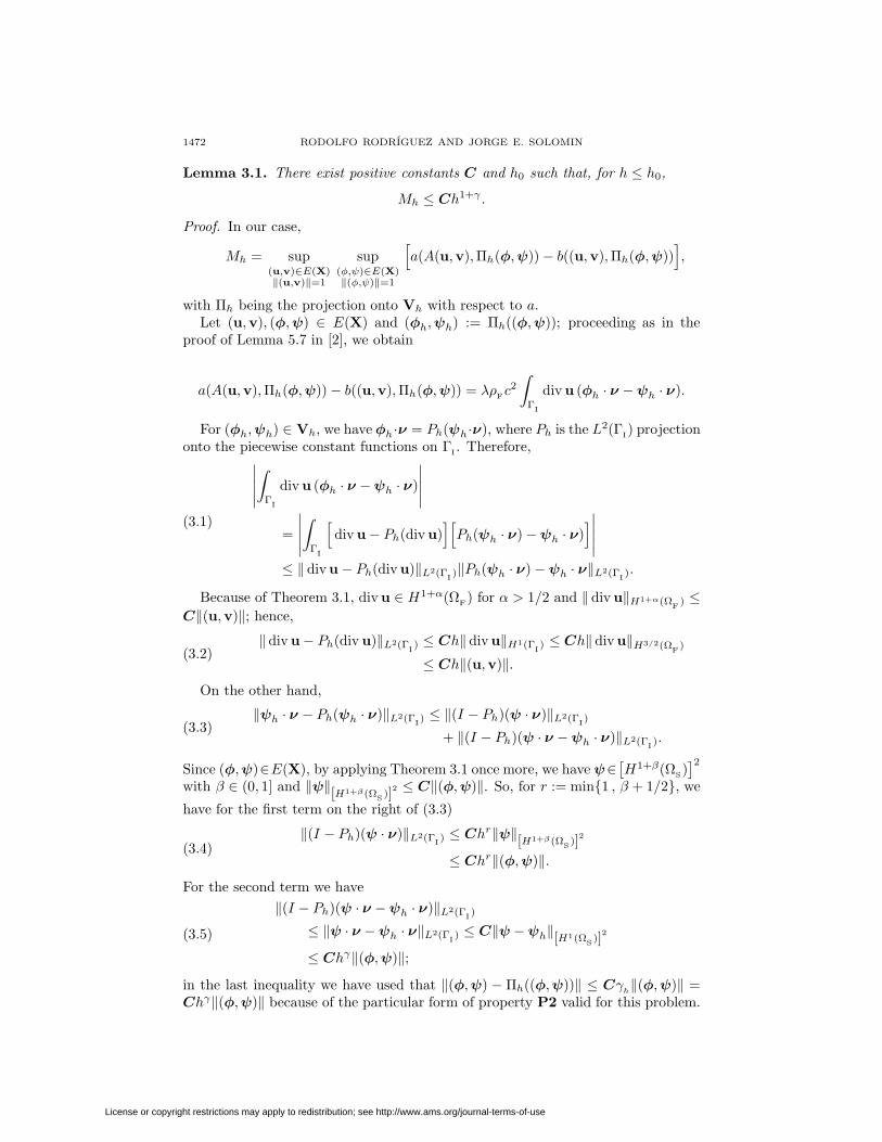
Lemma 3.1. There exist positive constants C and h0 such that, for h ≤ h0,

Mh ≤ Ch1+γ .

Proof. In our case,

Mh = sup(u,v)∈E(X)‖(u,v)‖=1

sup(φ,ψ)∈E(X)‖(φ,ψ)‖=1

[a(A(u,v),Πh(φ,ψ))− b((u,v),Πh(φ,ψ))

],

with Πh being the projection onto Vh with respect to a.Let (u,v), (φ,ψ) ∈ E(X) and (φh,ψh) := Πh((φ,ψ)); proceeding as in the

proof of Lemma 5.7 in [2], we obtain

a(A(u,v),Πh(φ,ψ))− b((u,v),Πh(φ,ψ)) = λρFc2∫

ΓI

div u (φh · ν −ψh · ν).

For (φh,ψh) ∈ Vh, we have φh ·ν = Ph(ψh·ν), where Ph is the L2(ΓI) projection

onto the piecewise constant functions on ΓI. Therefore,∣∣∣∣∣

∫Γ

I

div u (φh · ν −ψh · ν)

∣∣∣∣∣=

∣∣∣∣∣∫

ΓI

[div u− Ph(div u)

][Ph(ψh · ν)−ψh · ν)

]∣∣∣∣∣≤ ‖ div u− Ph(div u)‖L2(Γ

I)‖Ph(ψh · ν)−ψh · ν‖L2(Γ

I).

(3.1)

Because of Theorem 3.1, div u ∈ H1+α(ΩF) for α > 1/2 and ‖ div u‖H1+α(ΩF

) ≤C‖(u,v)‖; hence,

‖ div u− Ph(div u)‖L2(ΓI) ≤ Ch‖ div u‖H1(Γ

I) ≤ Ch‖ div u‖H3/2(Ω

F)

≤ Ch‖(u,v)‖.(3.2)

On the other hand,

‖ψh · ν − Ph(ψh · ν)‖L2(ΓI) ≤ ‖(I − Ph)(ψ · ν)‖L2(Γ

I)

+ ‖(I − Ph)(ψ · ν −ψh · ν)‖L2(ΓI).

(3.3)

Since (φ,ψ)∈E(X), by applying Theorem 3.1 once more, we have ψ∈[H1+β(ΩS)

]2with β ∈ (0, 1] and ‖ψ‖[H1+β(Ω

S)]

2 ≤ C‖(φ,ψ)‖. So, for r := min1 , β + 1/2, we

have for the first term on the right of (3.3)

‖(I − Ph)(ψ · ν)‖L2(ΓI) ≤ Chr‖ψ‖[H1+β(Ω

S)]

2

≤ Chr‖(φ,ψ)‖.(3.4)

For the second term we have

‖(I − Ph)(ψ · ν −ψh · ν)‖L2(ΓI)

≤ ‖ψ · ν −ψh · ν‖L2(ΓI) ≤ C‖ψ −ψh‖[H1(Ω

S)]

2

≤ Chγ‖(φ,ψ)‖;(3.5)

in the last inequality we have used that ‖(φ,ψ) − Πh((φ,ψ))‖ ≤ Cγh‖(φ,ψ)‖ =

Chγ‖(φ,ψ)‖ because of the particular form of property P2 valid for this problem.



Now, since γ = minα, β ≤ r, we have that (3.3), (3.4) and (3.5) yield

‖ψh · ν − Ph(ψh · ν)‖L2(ΓI) ≤ Chγ‖(φ,ψ)‖,

which together with (3.1) and (3.2) shows that∣∣∣∣∣∫

ΓI

div u (φh · ν −ψh · ν)

∣∣∣∣∣ ≤ Ch1+γ‖(u,v)‖‖(φ,ψ)‖,

proving the lemma.

Now, we conclude the main theorem of this section.


maxi=1,...,m

|λ− λih| ≤ Ch2γ

with γ := minα, β and α and β as in Theorem 3.1.

Proof. This is a direct application of Theorem 2.3, Lemma 3.1 and the propertiesP1 and P2 valid for this problem.

Theorem 3.5 shows that the order of convergence for the eigenvalues doublesthat for the eigenfunctions. Numerical evidence of this improved order had beenreported in [5]; however, to the authors’ knowledge, it has not been proved be-fore. Furthermore, since ours is a nonconforming approximation of a noncompactoperator, neither the theory in [10] nor that in [13] covers this case.

4. The incompressible case

In [3], it has been proved that the method in [2] described in the previous sectioncan be adapted to the case of an incompressible fluid. A problem with such a fluidcan be thought of as a limit case of that with a compressible one as the acousticspeed c goes to ∞.

For a perfectly incompressible fluid, the divergence of its displacements vanishesand hence it is convenient to consider the pressure of the fluid as a new variable.In this way we obtain a variational problem for the vibration modes of an elasticvessel completely filled with the fluid (as in Figure 1):

VPI: Find λ ∈ R and (u,v, p) ∈ V × L2(ΩF), (u,v, p) 6= (0,0, 0), such that

a ((u,v), (φ,ψ))−∫

ΩF

p divφ = λb ((u,v), (φ,ψ)) , ∀(φ,ψ) ∈ V,

−∫

ΩF

q div u = 0, ∀q ∈ L2(ΩF),

with p being the pressure into the fluid and with the same notation as in §3, exceptfor the bilinear form a which, in this case, is defined by

a ((u,v), (φ,ψ)) :=

∫Ω

S

σ(v) : ε(ψ), (u,v), (φ,ψ) ∈ X.

In [3], VPI is shown to be a well-posed mixed problem in the sense that thebilinear forms involved satisfy the standard Brezzi conditions (see, for instance,[7]). Proceeding as in [3], we can eliminate the pressure p in VPI, and the followingequivalent eigenvalue problem is obtained:



IP: Find λ ∈ R and (u,v) ∈W, (u,v) 6= (0,0), such that

a ((u,v), (φ,ψ)) = λb ((u,v), (φ,ψ)) , ∀(φ,ψ) ∈W,

where W := (u,v) ∈ V : div u = 0 in ΩF.

Let A : X −→ X be defined by A(u,v) ∈W and

a (A(u,v), (φ,ψ)) = b ((u,v), (φ,ψ)) , ∀(φ,ψ) ∈W.

All the results of the previous section regarding the spectrum and eigenfunctions ofA remain valid in this case, with V substituted by W and VP by IP. In particular,the analogue of Theorem 3.1 is the following (see [3]):

Theorem 4.1. Let (u,v) be an eigenfunction of A with corresponding eigenvalueλ ∈ (0, 1). Let p ∈ L2(Ω

F) be such that

(1λ , (u,v, p)

)is a solution of VPI. Then

u ∈ [Hα(ΩF)]

2, v ∈

[H1+β(Ω

S)]2

, p ∈ H1+α(ΩF) and

‖u‖[Hα(ΩF

)]2 + ‖v‖[H1+β(Ω

S)]

2 + ‖p‖H1+α(ΩF

) ≤ C‖(u,v)‖,

with α ∈ (1/2, 1] and β ∈ (0, 1] and with C a positive constant.

The finite element spaces introduced in §3 are also useful in the incompressiblecase. Furthermore, let Wh := (u,v) ∈ Vh : div u = 0 in Ω

F. Let Ah : X −→ X

be defined by Ah(u,v) ∈Wh and

a (Ah(u,v), (φ,ψ)) = b ((u,v), (φ,ψ)) , ∀(φ,ψ) ∈Wh.

In [3] it is shown that the spectrum and the eigenfunctions of Ah approximatethose of A; implementation issues and numerical experiments are reported in [4].Notice that, in particular, the restriction div u = 0 in the definition of Wh is easyto deal with, since Wh = ( curl ξ,v) ∈ Vh : ξ ∈ Lh(ΩF).

Properties P1 and P2 as in the previous section are shown to remain valid in theincompressible case in [3]; these properties are used therein to show the analoguesof Theorem 3.2 (with K ∩Wh instead of K ∩Vh) and Theorem 3.3.

Given λ ∈ (0, 1), an eigenvalue of A of multiplicity m, for h small enough thereexist m eigenvalues of Ah, λ1h, . . . , λmh, (repeated according to their multiplicities)converging to λ. Let E(X) and Fh(X) denote the respective eigenspaces. Theorem3.4 is also valid in the incompressible case (see [3]).

As a consequence, P2 is also valid with Vh substituted by Wh. Property P1 isobviously valid for Wh ⊂ Vh. Lemma 3.1 is valid too in the incompressible case;in fact, its proof reduces to that of the compressible case by substituting div u byp and by using Theorem 4.1 to bound ‖p‖H3/2(Ω

F) in the analogue of (3.2).

Therefore, we may conclude, also in the incompressible case, that there is adouble order of convergence for the eigenvalues:


maxi=1,...,m

|λ− λih| ≤ Ch2γ

with γ := minα, β and α and β as in Theorem 4.1.



References

1. I. Babuska and J. Osborn, Eigenvalue problems, in Handbook of Numerical Analysis, Vol. II(ed. P. G. Ciarlet and J. L. Lions) North Holland, Amsterdam, 1991. CMP 91:14

2. A. Bermudez, R. Duran, M.A. Muschietti, R. Rodrıguez and J. Solomin, Finite elementvibration analysis of fluid-solid systems without spurious modes, SIAM J. Numer. Anal., 32(1995), 1280–1295. CMP 95:15

3. A. Bermudez, R. Duran and R. Rodrıguez, Finite element analysis of compressible and in-compressible fluid-solid systems, Math. Comp. (submitted)

4. A. Bermudez, R. Duran and R. Rodrıguez, Finite element solution of incompressible fluid-structure vibration problems, Internat. J. Numer. Methods Engrg. (submitted)

5. A. Bermudez and R. Rodrıguez, Finite element computation of the vibration modes of afluid-solid system, Comp. Methods in Appl. Mech. and Eng., 119 (1994) pp. 355-370. MR95j:73064

6. J. Boujot, Mathematical formulation of fluid-structure interaction problems, M2AN, 21 (1987)239-260. MR 88j:73032

7. F. Brezzi, M. Fortin, Mixed and Hybrid Finite Element Methods, Springer-Verlag, New York,1991. MR 92d:65187

8. H. C. Chen and R. L. Taylor, Vibration analysis of fluid-solid systems using a finite elementdisplacement formulation, Internat. J. Numer. Meth. Eng., 29 (1990) 683-698.

9. J. Descloux, N. Nassif and J. Rappaz, On spectral approximation. Part I: The problem ofconvergence., R.A.I.R.O. Anal. Numer., 12 (1978) 97-112. MR 58:3404a

10. J. Descloux, N. Nassif and J. Rappaz, On spectral approximation. Part 2: Error estimatesfor the Galerkin methods, R.A.I.R.O. Anal. Numer., 12 (1978) 113-119. MR 58:34046

11. M. Hamdi, Y. Ouset and G. Verchery, A displacement method for the analysis of vibrationsof coupled fluid-structure systems, Internat. J. Numer. Methods Eng., 13 (1978) 139-150.

12. H.J-P. Morand and R. Ohayon, Interactions fluides-structures, Recherches en MathematiquesAppliquees, 23, Masson, Paris, 1992. MR 93m:73031

13. B. Mercier, J. Osborn, J. Rappaz and P. A. Raviart, Eigenvalue approximation by mixed andhybrid methods, Math. Comp., 36 (1981) 427-453. MR 82b:65108

14. L. Olson and K. Bathe, Analysis of fluid-structure interactions. A direct symmetric coupledformulation based on the fluid velocity potential, Comp. Struct., 21 (1985) 21-32.

15. P. A. Raviart and J. M. Thomas, A mixed finite element method for second order ellipticproblems, Mathematical Aspects of Finite Element Methods. Lecture Notes in Mathematics,606, Springer-Verlag, Berlin, Heidelberg, New York, 1977, 292-315. MR 58:3547

16. J. H. Wilkinson, The algebraic eigenvalue problem, Clarendon Press, Oxford, 1965.

Departamento de Ingenieria Matematica, Universidad de Concepcion, Casilla 4009,

Concepcion, Chile

E-mail address: [email protected]

Departamento de Matematica, Facultad de Ciencias Exactas, Universidad Nacional

de La Plata, C.C. 172, 1900 La Plata, Argentina

E-mail address: [email protected]


The order of convergence of Eigenfrequencies in finite element approximations of fluid-structure...

Documents

Transcript of The order of convergence of Eigenfrequencies in finite element approximations of fluid-structure...