Regional Convergence in Latin America

WP/06/125

Regional Convergence in Latin America

Maria Isabel Serra Maria Fernanda Pazmino

Genevieve Lindow Bennett Sutton

Gustavo Ramirez

© 2006 International Monetary Fund WP/06/125

IMF Working Paper

Western Hemisphere Department

Regional Convergence in Latin America

Prepared by Maria Isabel Serra, Maria Fernanda Pazmino, Genevieve Lindow,

Bennett Sutton, and Gustavo Ramirez1

Authorized for distribution by Timothy D. Lane

May 2006

Abstract

This Working Paper should not be reported as representing the views of the IMF. The views expressed in this Working Paper are those of the author(s) and do not necessarily represent those of the IMF or IMF policy. Working Papers describe research in progress by the author(s) and are published to elicit comments and to further debate.

This paper presents empirical evidence on convergence of per capita output for regions within six large middle-income Latin American countries: Argentina, Brazil, Chile, Colombia, Mexico, and Peru. It explores the role played by several exogenous sectoral shocks and differences in steady states within each country. It finds that poor and rich regions within each country converged at very low rates over the past three decades. It also finds evidence of regional “convergence clubs” within Brazil and Peru— the estimated speeds of convergence for these countries more than double after controlling for different subnational levels of steady state. For the latter countries and Chile, convergence is also higher after controlling for sector-specific shocks. Finally, results show that national disparities in per capita output increased temporarily after each country pursued trade liberalization. JEL Classification Numbers: C21, O47, O56, R11 Keywords: growth, convergence, regional disparities, Argentina, Brazil, Chile, Colombia,

Mexico, Peru Author(s) E-Mail Address: [email protected], [email protected], [email protected],

[email protected], [email protected]

1 This paper received insightful comments from Timothy Lane, Martin Cerisola and Ricardo Adrogue through its preparation. The authors are also grateful to Christopher Towe, Paul Cashin, Xavier Sala-i-Martin, and the participants in the seminar presented at the IMF Western Hemisphere Department for their comments. Any errors are those of the authors.

- 2 -

Contents Page

I. Introduction ........................................................................................................................... 3 II. Methodology ........................................................................................................................ 4 III. Summary Results for Latin America .................................................................................. 5 IV. Country-By-Country Results .............................................................................................. 6

A. Argentina.......................................................................................................................... 6 B. Brazil ................................................................................................................................ 8 C. Chile ............................................................................................................................... 12 D. Colombia........................................................................................................................ 15 E. Mexico............................................................................................................................ 17 F. Peru ................................................................................................................................. 20

V. Conclusions........................................................................................................................ 22 Appendix: Data Sources and Definitions.................................................................................23 References................................................................................................................................26

Figures 1. Per Capita GDP Relative to the United States .......................................................................3 2. Regional Disparities and Trade Liberalization ......................................................................6 3. Argentina: Per Capita GDP Growth ......................................................................................7 4. Argentina: Convergence 19702001 .......................................................................................7 5. Argentina: σ-convergence......................................................................................................8 6. Brazil: Per Capita GDP Growth.............................................................................................9 7. Brazil: Convergence 1970-2003 ..........................................................................................10 8. Brazil: “Convergence Clubs” 1970-2003 ............................................................................11 9. Brazil: σ-convergence..........................................................................................................12 10. Chile: Per Capita GDP Growth..........................................................................................12 11. Chile: Convergence 1960-2001 .........................................................................................13 12. Chile: σ-convergence .........................................................................................................14 13. Colombia: Per Capita GDP Growth...................................................................................15 14a. Colombia: Convergence 1950-1992 ................................................................................16 14b. Colombia: Convergence 1990-2002 ................................................................................16 15. Colombia: σ-convergence..................................................................................................17 16. Mexico: Per Capita GDP Growth ......................................................................................17 17. Mexico: Convergence 1970-2003......................................................................................18 18. Mexico: σ-convergence .....................................................................................................20 19. Peru: Per Capita GDP Growth ...........................................................................................20 20. Peru: Convergence 1970-2001...........................................................................................21 21. Peru: σ-convergence ..........................................................................................................22 Tables 1. Latin American Countries: Summary Results .......................................................................5 2. Argentina: Regresion Results ................................................................................................8 3. Brazil: Regresion Results.....................................................................................................10 4. Chile: Regresion Results......................................................................................................14 5. Colombia: Regresion Results...............................................................................................16 6. Mexico: Regresion Results ..................................................................................................19 7. Peru: Regresion Results .......................................................................................................21

- 3 -

I. INTRODUCTION

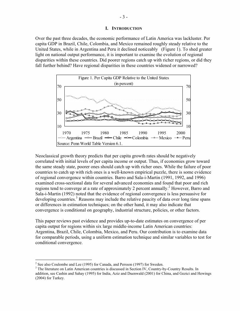
Over the past three decades, the economic performance of Latin America was lackluster. Per capita GDP in Brazil, Chile, Colombia, and Mexico remained roughly steady relative to the United States, while in Argentina and Peru it declined noticeably (Figure 1). To shed greater light on national output performance, it is important to examine the evolution of regional disparities within these countries. Did poorer regions catch up with richer regions, or did they fall further behind? Have regional disparities in these countries widened or narrowed?

10

30

50

70

1970 1975 1980 1985 1990 1995 200010

30

50

70

Argentina Brazil Chile Colombia Mexico Peru

Figure 1. Per Capita GDP Relative to the United States(in percent)

Source: Penn World Table Version 6.1. Neoclassical growth theory predicts that per capita growth rates should be negatively correlated with initial levels of per capita income or output. Thus, if economies grow toward the same steady state, poorer ones should catch up with richer ones. While the failure of poor countries to catch up with rich ones is a well-known empirical puzzle, there is some evidence of regional convergence within countries. Barro and Sala-i-Martin (1991, 1992, and 1996) examined cross-sectional data for several advanced economies and found that poor and rich regions tend to converge at a rate of approximately 2 percent annually.2 However, Barro and Sala-i-Martin (1992) noted that the evidence of regional convergence is less persuasive for developing countries.3 Reasons may include the relative paucity of data over long time spans or differences in estimation techniques; on the other hand, it may also indicate that convergence is conditional on geography, industrial structure, policies, or other factors. This paper reviews past evidence and provides up-to-date estimates on convergence of per capita output for regions within six large middle-income Latin American countries: Argentina, Brazil, Chile, Colombia, Mexico, and Peru. Our contribution is to examine data for comparable periods, using a uniform estimation technique and similar variables to test for conditional convergence.

2 See also Coulombe and Lee (1995) for Canada, and Persson (1997) for Sweden. 3 The literature on Latin American countries is discussed in Section IV, Country-by-Country Results. In addition, see Cashin and Sahay (1995) for India, Aziz and Duenwald (2001) for China, and Gezici and Hewings (2004) for Turkey.

- 4 -

The structure of this paper is as follows. Section II describes the methodology used in convergence analysis. Section III discusses common findings for the six Latin American countries. Section IV presents our results country-by-country. Section V concludes.

II. METHODOLOGY

The neoclassical growth model of Solow (1956) and Swan (1956), based on the assumption of diminishing returns to scale, implies conditional convergence of per capita output: per capita growth decreases as an economy approaches its steady state level of output. Thus, among economies that converge to the same steady state, this model implies absolute convergence of per capita output: poorer economies catch up with richer ones. Following Barro and Sala-i-Martin (2004), the following univariate regression equation is derived from the neoclassical model:

( ) ( ) ( )[ ] ( ) iTTitT

Titit yTeyyT εα β +⋅−−=⋅ −−

− log/1/log/1 (1) where subscripts i and t denote region and time, T is the period length, and y is per capita output. Thus, the dependent variable is the average annual growth rate of per capita output in region i over T years and the independent variable is the initial level of per capita output. Assuming that the coefficient α is constant across regions, the coefficient β represents the speed of absolute convergence—the rate at which the gap between poor and rich regions closes. Initially, we estimate absolute β-convergence for each country. This recognizes that within a country, there is likely to be greater labor and capital mobility and greater homogeneity of policies and preferences than across countries. In addition, we test for conditional β-convergence to see whether regions within countries converge to different steady states. The simplest way to address this possibility is by introducing regional dummies to equation (1).4 In this case, conditional β-convergence represents the average speed at which regions approach their different subnational steady states. Furthermore, we attempt to account for differences in sectoral structure which may condition regions’ growth and, if omitted, would be captured by the error term and cause heteroscedasticity. Following Barro and Sala-i-Martin (2004), in addition to regional dummies, we add Sit to equation (1),

( )[ ]TyyS TjtjtTijt

n

jit −−=⋅Σ= log

1ω (2)

where the subscript j denotes the sector, ωijt-T is the initial weight of sector j’s output in total output of state i, which multiplies the annual growth rate of sector j’s national output, yj. Sectoral variables can be included for agriculture, manufacturing, services, and mining.5

4 See Data Appendix for details on regional dummies used for each country. 5 See Data Appendix for details on structural variables used for each country.

- 5 -

Finally, we examine whether regions within a country have experienced σ-convergence—whether the standard deviation of the level of per capita output declines over time. It is worth noting that β-convergence is a necessary, but not sufficient, condition for σ-convergence. The dispersion in the level of per capita output decreases (σ-convergence) only when poor regions grow faster than rich ones (absolute β-convergence), but if poor regions grow too quickly their per capita output could outstrip that in richer regions and increase the dispersion of per capita output.

III. SUMMARY RESULTS FOR LATIN AMERICA

The results suggest that there is limited evidence of regional convergence over the past 30 years within the Latin American countries examined. In the cases of Chile, Colombia, and Peru, there is some sign of absolute β-convergence (Table 1, column I), but the estimated speeds of convergence are low.6 For example, in the case of Chile, the rate of convergence is 1.2 percent—well below the 2 percent rate often found for advanced economies—implying that it would take nearly 60 years to close half the gap between regions within the country. Brazil displayed an even slower speed of convergence, and the regions within Argentina and Mexico are estimated to have experienced no convergence at all.

(IV)

β Prob. Adj. R2 β Prob. Adj. R2 β Prob. Adj. R2 σ3/

Argentina (1970-2001) 0.0050 0.2283 0.0179 0.0143 0.2141 0.0304 0.58-0.59Brazil (1970-2003) 0.0064 0.0161 0.0923 0.0163 0.0077 0.3900 0.0272 0.0139 0.4157 0.62-0.58Chile (1970-2000) 0.0122 0.0490 0.3400 0.0145 0.0100 0.6390 0.0173 0.0180 0.6320 0.53-0.44Colombia (1970-1990) 0.0262 0.0353 0.1387 0.0223 0.2209 0.2126 0.38-0.40Colombia (1990-2002) 0.0084 0.0000 0.2334 0.0106 0.1820 0.3952 0.0044 0.5771 0.3207 0.67-0.61Mexico (1970-2003) 0.0019 0.5760 -0.023 0.0005 0.9180 -0.083 0.0056 0.2550 -0.073 0.41-0.45Peru (1970-2001) 0.0110 0.0390 0.2120 0.0226 0.0030 0.8140 0.0309 0.0750 0.7790 0.65-0.53

Table 1. Latin American Countries: Summary Results1/ 2/

(I) (II) (III)

Basic Equation With Regional DummiesWith Regional Dummies

and Sector Variables

1/ Estimator: Nonlinear Least Squares (Newey-West).2/ See Country-by-Country Results for details on sample size, dummy and sector variables.3/ Standard deviation of per capita GDP. Regions within some of these countries, notably Brazil and Peru, seem to have formed “convergence clubs.” In particular, the estimates tend to be more supportive of β-convergence once regional dummies are included, and the speed of convergence is higher (Table 1, column II). For example, in Brazil, the β coefficient rises from 0.6 percent to 1.6 percent with the inclusion of regional dummies, and in Peru, the coefficient doubles from 1.1 percent to 2.3 percent.

6 In line with Table 1, rank correlation tests suggest that there is a negative association between initial income and subsequent economic growth for Colombia and Peru at 5 percent level of significance and for Brazil and Chile at 10 percent level of significance. Correlation coefficients for Argentina and Mexico were not significant.

- 6 -

Differences in the structure of the economy also seem to affect convergence rates in some countries, notably Brazil, Chile, and Peru. In these cases, including sectoral variables tends to increase the estimated speed of β-convergence (Table 1, column III). For example, in Brazil, the coefficient β rises to 2.8 percent once we control for exogenous output shocks in agriculture and manufacturing. In Peru, it increases to 3.9 percent after accounting for shocks in agriculture, mining, and manufacturing. In Chile, the speed of convergence also rises controlling for shocks in the mining sector. An examination of the standard deviation of per capita output also provides evidence of only modest regional σ-convergence (Table 1, column IV). Interestingly, it suggests that output disparities tended to rise in the aftermath of trade liberalization (Figure 2). For instance, after Chile liberalized in 1975-79, regional disparities increased for about 5 years, but subsequently narrowed. Argentina, Brazil, Colombia, Mexico, and Peru undertook trade reforms in the early 1990s and also experienced a temporary increase in disparities within sub-national regions. Prior to liberalizing trade (1991), Mexico had been experiencing both β- and σ-convergence; however, after liberalization regional disparities increased and β-divergence was found to be 1.4 percent. Although in these countries aggregate growth accelerated after trade liberalization, these results may suggest wide discrepancies in the benefit of reforms across different regions within a country.

0.3

0.5

0.7

-15 -10 -5 0 5 10 150.3

0.5

0.7

Argentina Brazil Chile Colombia Mexico Peru

before trade liberalization after trade liberalization

Figure 2. Regional Disparities and Trade Liberalization(standard deviation of regional per capita GDP)

Source: authors' calculations.

IV. COUNTRY-BY-COUNTRY RESULTS

A. Argentina

From 1970 to 2004, Argentina’s per capita GDP grew at an average annual rate of ½ percent. This meager performance has been associated with extremely high volatility, with severe economic crises followed by recoveries (Figure 3). Argentine provinces have experienced similar patterns of unstable growth.

- 7 -

Figure 3. Argentina: Per Capita GDP Growth(in percent)

-16

-8

0

8

16

1970 1975 1980 1985 1990 1995 2000-16

-8

0

8

16

There is no evidence of convergence among Argentine provinces. Figure 4 does not suggest a significant negative correlation between the initial level of per capita GDP and growth for the period between 1970 and 2001. Accordingly, estimates for the speed of β-convergence suggest that, within Argentina’s 24 provinces and Federal Capital, poor provinces did not catch up with rich ones. For the 31-year period and for sub-periods of 10 years, the estimated speeds of absolute convergence yielded insignificant coefficients (Table 2, column I). In addition, there is no evidence of conditional convergence either within subnational regions, or if accounting for structural shocks. To test for conditional convergence, we include dummy variables for provinces in the North, Center, and South, but the estimated coefficients were still not significant (Table 2, column II). Even accounting for shocks in manufacturing, there is no evidence of convergence (Table 2, column III). Our findings for Argentina conform to those found in previous studies by Garrido et al. (2000), Marina (2000), and Figueras et al. (2003).7

TU TFSE SF

SC

SL

SJ

STRN

NQ

MI

MZ

LR

LPJYFO

ER CH

CC

CRCB

CT

BA

CF

-1

0

1

2

3

4

7 8 9 10Log of initial per capita GDPPe

riod

Ave

rage

Ann

ual G

row

th R

ate

(in p

erce

nt)

Figure 4. Argentina: Convergence 1970-2001

Note: See list of abbreviations in the appendix. 7 It is worth noting that although convergence is not found for per capita output in Argentina, Marina (2000) found evidence of convergence in wage levels for 1984-98.

- 8 -

β Prob. Adj. R2 β Prob. Adj. R2 β Prob. Adj. R2

1970-2001 0.0050 0.2283 0.0179 0.0143 0.2141 0.03041970-1980 0.0015 0.8076 -0.0423 0.0048 0.6400 0.12751980-1990 0.0146 0.3198 0.0464 0.0056 0.7665 0.03881990-2000 0.0038 0.7910 -0.0344 0.0202 0.2896 0.2195 0.0203 0.3598 0.1785

2/ Sample size: 23 provinces and Federal Capital.

4/ Includes 3 regional dummies and one sector variable for manufacturing.3/ Includes 3 regional dummies: North, Center, and South.

Basic Equation With Regional Dummies3/With Regional Dummies

and Sector Variables4/

1/ Estimator: Nonlinear Least Squares (Newey West).

Table 2. Argentina: Regression Results1/ 2/

(I) (II) (III)

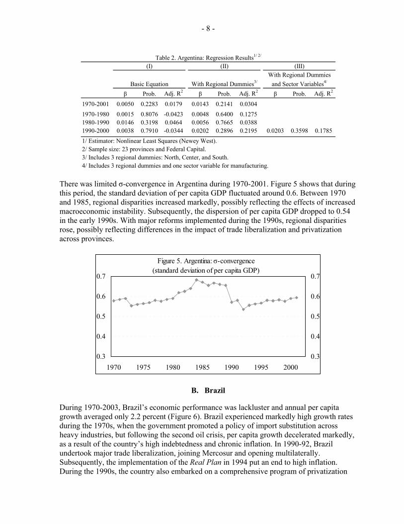
There was limited σ-convergence in Argentina during 1970-2001. Figure 5 shows that during this period, the standard deviation of per capita GDP fluctuated around 0.6. Between 1970 and 1985, regional disparities increased markedly, possibly reflecting the effects of increased macroeconomic instability. Subsequently, the dispersion of per capita GDP dropped to 0.54 in the early 1990s. With major reforms implemented during the 1990s, regional disparities rose, possibly reflecting differences in the impact of trade liberalization and privatization across provinces.

Figure 5. Argentina: σ-convergence(standard deviation of per capita GDP)

0.3

0.4

0.5

0.6

0.7

1970 1975 1980 1985 1990 1995 20000.3

0.4

0.5

0.6

0.7

B. Brazil

During 1970-2003, Brazil’s economic performance was lackluster and annual per capita growth averaged only 2.2 percent (Figure 6). Brazil experienced markedly high growth rates during the 1970s, when the government promoted a policy of import substitution across heavy industries, but following the second oil crisis, per capita growth decelerated markedly, as a result of the country’s high indebtedness and chronic inflation. In 1990-92, Brazil undertook major trade liberalization, joining Mercosur and opening multilaterally. Subsequently, the implementation of the Real Plan in 1994 put an end to high inflation. During the 1990s, the country also embarked on a comprehensive program of privatization

- 9 -

and deregulation. However, per capita growth failed to accelerate significantly, possibly reflecting a variety of factors including high fiscal burden, growing indebtedness, and an overvalued real exchange rate8. Following a balance of payments crisis in the late 1990s, Brazil implemented a major fiscal adjustment and related reforms and adopted inflation targeting and a flexible exchange rate regime.

Figure 6. Brazil: Per Capita GDP Growth(in percent)

-16

-8

0

8

16

1970 1975 1980 1985 1990 1995 2000-16

-8

0

8

16

Against this backdrop, regional disparities in Brazil remained significant. Figure 7 illustrates the negative correlation between initial GDP per capita and growth in 1970-2003. As a result of the expansion of the manufacturing industry to the South and the agriculture frontier to the Midwest, states in those regions experienced the highest growth rates, such that their average per capita GDP almost matched that of São Paulo and Rio de Janeiro by 2003. States in the Northeast, where approximately 30 percent of the population resides, also experienced stronger-than-average growth. Nevertheless, in 2003, per capita GDP in São Paulo and Rio de Janeiro was still four to ten times as high as in Brazil’s poorest states. States in the North region grew below the already modest national average, with the exception of Amazonas, Brazil’s fastest growing state due to the rise of the electronics industry in Manaus’ duty free zone.

8 See Adrogue, Cerisola, and Gelos (2006).

- 10 -

DF

GOMT

RS

SCPR

SPRJ

ESMGBA

SEAL PE

PBRN

CEPIMA

AP

PA

RR

AM

AC RO

2

3

4

5

6

7

6 7 8 9

Figure 7. Brazil: Convergence 1970-2003

Log of initial per capita GDPPerio

d A

vera

ge A

nnua

l Gro

wth

Rat

e(in

per

cent

)

Note: See list of abbreviations in the appendix.

The estimated speed at which poor states caught up with rich states is low. For 1970-2003, the rate of absolute β-convergence is estimated to be only 0.6 percent (Table 3, column I). At this rate, it would take 108 years for half of the gap between rich and poor states to disappear. Ellery and Ferreira (1996) estimated the speed of absolute convergence within Brazilian states for 1970-1990 to be 1.3 percent (equivalent to a 53-year half-life). Their estimates are higher than those presented in this paper possibly due to the difference in the timeframe.9 For 1970-2000, Da Mata et al. (2005) estimated the speed of absolute convergence within 123 Brazilian municipalities to be 2 percent. This suggests that, even though convergence is found to be very slow at the state level, poor urban areas caught up with rich urban areas at a higher speed. In contrast with our findings, the latter indicates that less-urban states, for example those in the North region, were the ones that were left behind.


1970-2003 0.0064 0.0161 0.0923 0.0163 0.0077 0.3900 0.0272 0.0139 0.41571970-1980 0.0101 0.0097 0.0507 0.0320 0.0008 0.3441 0.0414 0.0109 0.37131980-1990 0.0055 0.3280 0.0055 0.0070 0.5327 0.3259 0.0342 0.0257 0.58611990-2000 0.0008 0.7973 -0.0424 0.0076 0.3421 -0.1777 0.0272 0.2244 0.2460

2/ Sample size: 25 states (Goiás includes Tocantins and Mato Grosso includes Mato Grosso do Sul).3/ Includes five regional dummies.4/ Includes five regional dummies and two sector variables for agriculture and manufacturing.




Table 3. Brazil: Regression Results1/ 2/

(I) (II) (III)

Regional disparities appear to have narrowed at higher rates within “convergence clubs.” Including dummy variables for Brazil’s five sub-national regions, the estimated coefficient β 9 However, this might also be the case because they estimated real GDP figures for 1990 based on the increase in state’s collection of local VAT, as an attempt to overcome the changes in methodology of the GDP series (see Appendix I on data description). As they point out, the latter makes the strong assumption that growth in GDP corresponds to growth in collection of local VAT.

- 11 -

rises to 1.6 percent (Table 3, column II). The estimated coefficients on the dummies are highly significant, conforming to the existence of five sub-national levels of steady state to which states within each region appear to have converged. Figure 8 also points out to the existence of different levels of steady state. The North and Northeast regions, comprising 15 states, seem to constitute a single “convergence club”. Within the Midwest, South, and Southeast regions convergence appears to have been also stronger. The overall gap between poor states (in the northern regions) and rich states has improved little over the years. Evidence on the existence of “convergence clubs” was also found by Da Mata et al. (2005).

ROAC

AM

RR

PA

AP

MAPI CE

RNPB

PEALSEBA MG

ES

RJ SP

PRSC

RS

MTGO

DF

2

3

4

5

6

7

6 7 8 9

North andNortheast

South, Southeastand Midwest

Figure 8. Brazil: "Convergence Clubs" 1970-2003


d A

vera

ge A

nnua

l Gro

wth

Rat

e(in

per

cent

)


The estimated speed of convergence rises when accounting for structural shocks in the agricultural and manufacturing sectors. Conditional on both structural variables and regional dummies, β-convergence increases to 2.7 percent, with all coefficients being significant (Table 3, column III). Thus, differences in resource endowments in each state suggest different paths of conditional convergence and help to explain why poorer states tend to catch up with richer states at very slow rates.10 Brazilian states also display little evidence of σ-convergence. The standard deviation of per capita GDP among Brazilian states decreased very modestly from 0.62 in 1970 to 0.58 in 2003 (Figure 9). During the 1970s, there is evidence of relatively stronger σ-convergence, which conforms to the higher estimates of β-convergence found for that period (Table 3). Evidence for the 1980s is mixed; the standard deviation of per capita GDP points to divergence in the first half of the decade and then convergence in the second half. For that period, there is no support for absolute convergence or convergence conditional to regional dummies, but the speed of convergence is estimated to be 3.4 percent and statistically significant once we control for structural shocks. Finally, in the 1990s, after trade liberalization, there is evidence of σ-divergence, as the dispersion of per capita GDP rose throughout the decade; meanwhile, estimates for β were statistically insignificant.

10 In addition to agriculture and manufacturing, other sectors were taken into consideration, but were excluded from the reported regressions because their coefficients were not significant.

- 12 -

Figure 9. Brazil: σ-convergence(standard deviation of per capita GDP)

0.3

0.4

0.5

0.6

0.7

1970 1975 1980 1985 1990 1995 20000.3

0.4

0.5

0.6

0.7

C. Chile

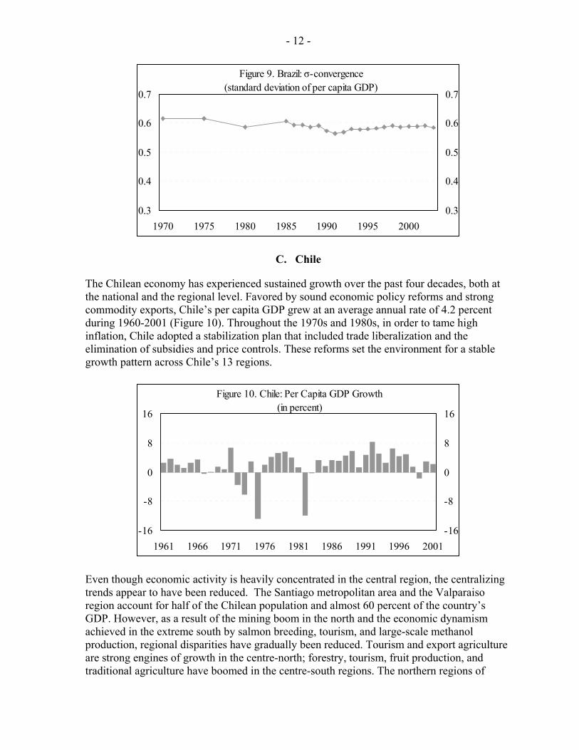
The Chilean economy has experienced sustained growth over the past four decades, both at the national and the regional level. Favored by sound economic policy reforms and strong commodity exports, Chile’s per capita GDP grew at an average annual rate of 4.2 percent during 1960-2001 (Figure 10). Throughout the 1970s and 1980s, in order to tame high inflation, Chile adopted a stabilization plan that included trade liberalization and the elimination of subsidies and price controls. These reforms set the environment for a stable growth pattern across Chile’s 13 regions.

Figure 10. Chile: Per Capita GDP Growth(in percent)

-16

-8

0

8

16

1961 1966 1971 1976 1981 1986 1991 1996 2001-16

-8

0

8

16

Even though economic activity is heavily concentrated in the central region, the centralizing trends appear to have been reduced. The Santiago metropolitan area and the Valparaiso region account for half of the Chilean population and almost 60 percent of the country’s GDP. However, as a result of the mining boom in the north and the economic dynamism achieved in the extreme south by salmon breeding, tourism, and large-scale methanol production, regional disparities have gradually been reduced. Tourism and export agriculture are strong engines of growth in the centre-north; forestry, tourism, fruit production, and traditional agriculture have boomed in the centre-south regions. The northern regions of

- 13 -

Tarapaca, Antofagasta, Atacama, and Coquimbo in 2001 accounted for 16 percent of the national GDP, compared to only 10 percent in 1972. On the other hand, the metropolitan area and the Valparaiso region decreased their joint share over total GDP from 61 percent in 1972 to 57 percent in 2001. Consistent with the de-centralization process, poor regions grew at higher rates than richer ones. Figure 11 shows a negative correlation between the initial level per capita GDP and growth among regions in Chile. For 1960-2001, the estimated average annual rate of absolute convergence is 1.2 percent (Table 4, column I). Such speed of convergence is quite slow, as it implies a half-life of approximately 56 years. The speed of absolute convergence obtained is broadly consistent with previous studies, even though most of the past analyses used a different methodology—panel data linear least square estimations—to provide evidence on convergence (Diaz 2003). It was found that when geographic and structural differences are taken into account, the speed of β-convergence increases but only marginally (Table 4, columns II and III). The latter estimates are slightly lower than the results obtained in previous studies by Duncan (2005), Diaz (2003), Aroca (2000), where the speed of conditional convergence varies between 2 and 4 percent. Other studies also found the speed of convergence of regional per capita income to be higher than that of per capita output, but both are still low compared to developed countries (Duncan 2005).

MAG

AYSLLGARA

BIO

MAU

OHGSAN

VAL

COQ

ATA

ANT

TRA

0.00.51.01.52.02.53.03.5

12.5 13.0 13.5 14.0 14.5 15.0

Figure 11. Chile: Convergence 1960-2001


d A

vera

ge A

nnua

l Gro

wth

Rat

e(in

per

cent

)


- 14 -


1960-2001 0.0123 0.0380 0.4120 0.0143 0.0280 0.4770 0.0184 0.0500 0.47201960-1970 0.0153 0.1080 0.1770 0.0139 0.1800 0.0380 0.0190 0.1750 -0.01901970-1980 0.0073 0.1170 0.1500 0.0082 0.0810 0.2190 0.0112 0.0610 0.22901980-1990 0.0150 0.0070 0.4940 0.0149 0.0170 0.3840 0.0212 0.0040 0.56901990-2001 0.0050 0.6450 -0.0680 0.0111 0.1980 0.4800 0.0164 0.1740 0.4620

2/ Sample size: 13 states.

Table 4. Chile: Regression Results1/ 2/

(I) (II) (III)




3/ Includes thre regional dummies.4/ Includes three regional dummies and one sector variable for mining.

Chile’s regions also display evidence of σ-convergence. From 1960 to 2001, the standard deviation of per capita GDP across regions fell from 0.59 to 0.44 (Figure 12). Regional disparities were significantly reduced in the earlier period of 1960-1975, dropping to 0.43. The speed of conditional convergence during the 1960s and early 1970s was also higher; estimated to be 1.9 percent for 1960-1970 and 4.9 percent for 1970-197511. After trade liberalization reforms were introduced during 1975-1980, there was a short period when disparities across regions increased. However, they continued to decrease through the 1980s and early 1990s—period during which conditional convergence was found to be 2.1 percent. Finally, in the late 1990s there is evidence of σ-divergence, as the standard deviation of per capita GDP increased to 1976 levels. Apparently, the latter started to revert in 2000.

Figure 12. Chile: σ-convergence(standard deviation of per capita GDP)

0.3

0.4

0.5

0.6

0.7

1960 1965 1970 1975 1980 1985 1990 1995 20000.3

0.4

0.5

0.6

0.7

These findings suggest that regions in Chile converged to a common level of per capita GDP. The speed at which poorer regions caught up with the richer regions varies across periods, with higher β found in the 1960s, 1970s, and 1980s, than in the 1990s. Even though the speed at which regions converged increases when we account for regional and structural

11 The results of this estimation are not shown in Table 3, but were statistically significant at the 1 percent level.

- 15 -

differences, the change in the speed of convergence is not as sharp as in other countries. This suggests that the 13 Chilean regions are converging to similar levels of steady states.

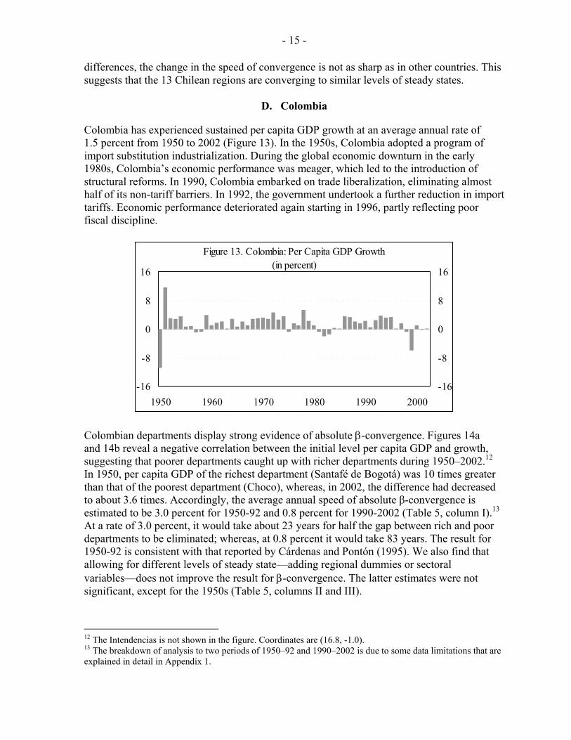
D. Colombia

Colombia has experienced sustained per capita GDP growth at an average annual rate of 1.5 percent from 1950 to 2002 (Figure 13). In the 1950s, Colombia adopted a program of import substitution industrialization. During the global economic downturn in the early 1980s, Colombia’s economic performance was meager, which led to the introduction of structural reforms. In 1990, Colombia embarked on trade liberalization, eliminating almost half of its non-tariff barriers. In 1992, the government undertook a further reduction in import tariffs. Economic performance deteriorated again starting in 1996, partly reflecting poor fiscal discipline.

Figure 13. Colombia: Per Capita GDP Growth(in percent)

-16

-8

0

8

16

1950 1960 1970 1980 1990 2000-16

-8

0

8

16

Colombian departments display strong evidence of absolute β-convergence. Figures 14a and 14b reveal a negative correlation between the initial level per capita GDP and growth, suggesting that poorer departments caught up with richer departments during 1950–2002.12 In 1950, per capita GDP of the richest department (Santafé de Bogotá) was 10 times greater than that of the poorest department (Choco), whereas, in 2002, the difference had decreased to about 3.6 times. Accordingly, the average annual speed of absolute β-convergence is estimated to be 3.0 percent for 1950-92 and 0.8 percent for 1990-2002 (Table 5, column I).13 At a rate of 3.0 percent, it would take about 23 years for half the gap between rich and poor departments to be eliminated; whereas, at 0.8 percent it would take 83 years. The result for 1950-92 is consistent with that reported by Cárdenas and Pontón (1995). We also find that allowing for different levels of steady state—adding regional dummies or sectoral variables—does not improve the result for β-convergence. The latter estimates were not significant, except for the 1950s (Table 5, columns II and III).

12 The Intendencias is not shown in the figure. Coordinates are (16.8, -1.0). 13 The breakdown of analysis to two periods of 1950–92 and 1990–2002 is due to some data limitations that are explained in detail in Appendix 1.

- 16 -

INT

VALTOL

SUC

SAN

DC

RISQUI

NSANAR

METMAG

LAG

HUI

CUN

CORCHO

CES

CAUCAL

BOYBOL

ATL

ANT

-10123456

7.5 8.5 9.5 10.5

Figure 14a. Colombia: Convergence 1950-1992

Log of initial per capita GDP

Perio

d A

vera

ge A

nnua

l G

row

th R

ate

(in p

erce

nt)


ANTATLBOLBOY

CALCAU CES

CHO

COR

CUNHUI

LAG

MAGMET

NAR

NSAQUI

RIS DC

SAN

SUC

TOL

VAL

-1

0

1

2

3

4

13.3 13.6 13.9 14.2 14.5 14.8

Figure 14b. Colombia: Convergence 1990-2002

Log of initial per capita GDP

Perio

d A

vera

ge A

nnua

l G

row

th R

ate

(in p

erce

nt)


(In 1975 prices)1950-1992 0.0302 0.0442 0.4280 0.0341 0.2238 0.53311950-1960 0.0557 0.0007 0.5503 0.0609 0.0081 0.68541960-1970 0.0085 0.6064 -0.0194 -0.0083 0.0858 0.81821970-1980 0.0286 0.0396 0.0823 0.0342 0.1909 0.24311980-1990 0.0173 0.1923 0.0149 0.0120 0.4217 -0.0242 0.0101 0.3483 0.6652

(In 1994 prices)1990-2002 0.0084 0.0000 0.2334 0.0106 0.1820 0.3952 0.0044 0.5771 0.32071995-2002 0.0077 0.0030 0.0790 0.0105 0.3991 0.1698 0.0129 0.2620 0.15601990-1995 0.0097 0.0004 0.1404 0.0133 0.2336 0.1117 -0.0018 0.9149 0.1146

2/ Sample size: 24 observations.3/ Six regional dummy variables (for atlantic, capital, central, eastern, pacific, and southern).4/ Sectors used were agriculture, manufacturing industry, and commerce.

Table 5. Colombia: Regression Results, 1950-20021/ 2/

(I) (II) (III)




Regional disparities in Colombia diminished in 1950-92 and 1990-2002. Figure 15 illustrates the decrease in the standard deviation of per capita GDP among departments in 1950-92, as a whole, and during 1990-2002. A dramatic reduction of disparities occurred during the 1950s, which might be associated with Colombia’s adoption of import substituting industrialization. This reduction in regional disparities is consistent with the high speed of absolute β-convergence, 5.6 percent, for 1950-60. Subsequently, however, the standard deviation in per capita GDP among the departments followed an upward trend. Accordingly, there is no evidence of β-convergence for 1960-92. Thus, the high speed of convergence found for 1950-92 is chiefly a result of the pronounced improvement in regional disparities in the 1950s. The dispersion of per capita GDP began to ease back in 1992 and has followed a downward trend since then.

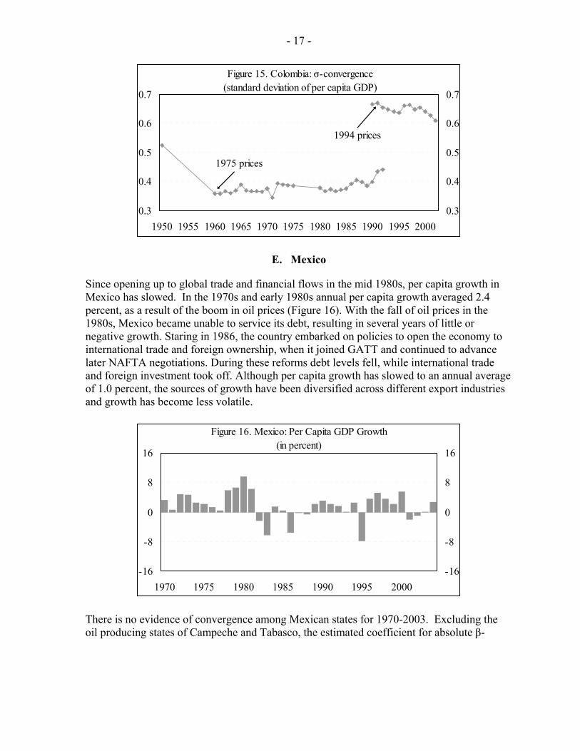
- 17 -

Figure 15. Colombia: σ-convergence(standard deviation of per capita GDP)

0.3

0.4

0.5

0.6

0.7

1950 1955 1960 1965 1970 1975 1980 1985 1990 1995 20000.3

0.4

0.5

0.6

0.7

1994 prices

1975 prices

E. Mexico

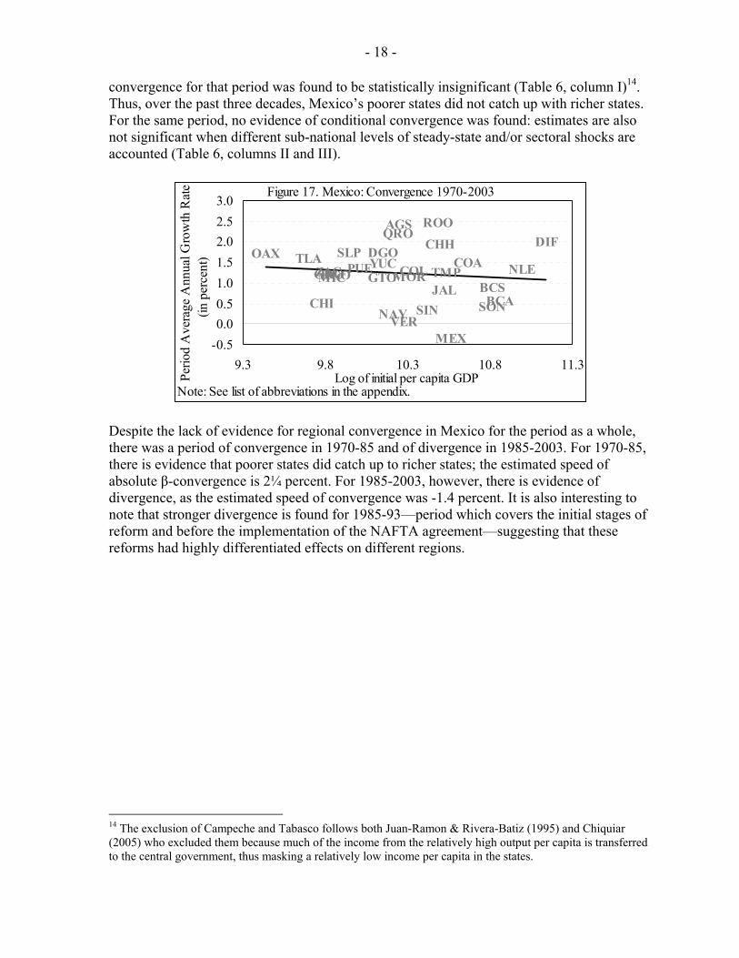
Since opening up to global trade and financial flows in the mid 1980s, per capita growth in Mexico has slowed. In the 1970s and early 1980s annual per capita growth averaged 2.4 percent, as a result of the boom in oil prices (Figure 16). With the fall of oil prices in the 1980s, Mexico became unable to service its debt, resulting in several years of little or negative growth. Staring in 1986, the country embarked on policies to open the economy to international trade and foreign ownership, when it joined GATT and continued to advance later NAFTA negotiations. During these reforms debt levels fell, while international trade and foreign investment took off. Although per capita growth has slowed to an annual average of 1.0 percent, the sources of growth have been diversified across different export industries and growth has become less volatile.

-16

-8

0

8

16

1970 1975 1980 1985 1990 1995 2000-16

-8

0

8

16

Figure 16. Mexico: Per Capita GDP Growth(in percent)

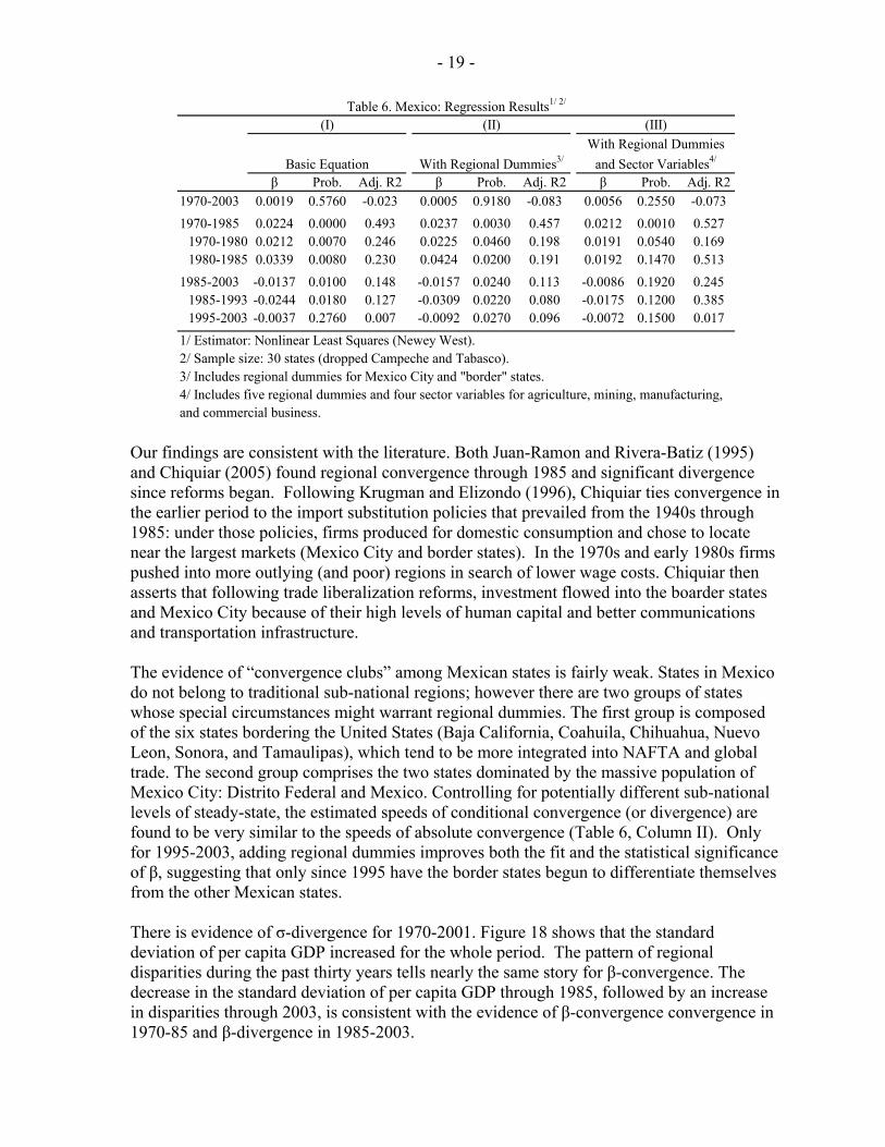
There is no evidence of convergence among Mexican states for 1970-2003. Excluding the oil producing states of Campeche and Tabasco, the estimated coefficient for absolute β-

- 18 -

convergence for that period was found to be statistically insignificant (Table 6, column I)14. Thus, over the past three decades, Mexico’s poorer states did not catch up with richer states. For the same period, no evidence of conditional convergence was found: estimates are also not significant when different sub-national levels of steady-state and/or sectoral shocks are accounted (Table 6, columns II and III).

OAX TLA

CHI

ZACGROMICHGO

SLPPUE

GTOYUCDGO

NAY

QROAGS

VER

MORCOL

SIN

ROOCHH

JALTMP

MEX

COA

SONBCS

BCA

NLE

DIF

-0.50.00.51.01.52.02.53.0

9.3 9.8 10.3 10.8 11.3

Figure 17. Mexico: Convergence 1970-2003


d A

vera

ge A

nnua

l Gro

wth

Rat

e(in

per

cent

)


Despite the lack of evidence for regional convergence in Mexico for the period as a whole, there was a period of convergence in 1970-85 and of divergence in 1985-2003. For 1970-85, there is evidence that poorer states did catch up to richer states; the estimated speed of absolute β-convergence is 2¼ percent. For 1985-2003, however, there is evidence of divergence, as the estimated speed of convergence was -1.4 percent. It is also interesting to note that stronger divergence is found for 1985-93—period which covers the initial stages of reform and before the implementation of the NAFTA agreement—suggesting that these reforms had highly differentiated effects on different regions.

14 The exclusion of Campeche and Tabasco follows both Juan-Ramon & Rivera-Batiz (1995) and Chiquiar (2005) who excluded them because much of the income from the relatively high output per capita is transferred to the central government, thus masking a relatively low income per capita in the states.

- 19 -

β Prob. Adj. R2 β Prob. Adj. R2 β Prob. Adj. R21970-2003 0.0019 0.5760 -0.023 0.0005 0.9180 -0.083 0.0056 0.2550 -0.0731970-1985 0.0224 0.0000 0.493 0.0237 0.0030 0.457 0.0212 0.0010 0.527

1970-1980 0.0212 0.0070 0.246 0.0225 0.0460 0.198 0.0191 0.0540 0.1691980-1985 0.0339 0.0080 0.230 0.0424 0.0200 0.191 0.0192 0.1470 0.513

1985-2003 -0.0137 0.0100 0.148 -0.0157 0.0240 0.113 -0.0086 0.1920 0.2451985-1993 -0.0244 0.0180 0.127 -0.0309 0.0220 0.080 -0.0175 0.1200 0.3851995-2003 -0.0037 0.2760 0.007 -0.0092 0.0270 0.096 -0.0072 0.1500 0.017

and commercial business.

2/ Sample size: 30 states (dropped Campeche and Tabasco).

Table 6. Mexico: Regression Results1/ 2/

(I) (II) (III)




3/ Includes regional dummies for Mexico City and "border" states.4/ Includes five regional dummies and four sector variables for agriculture, mining, manufacturing,

Our findings are consistent with the literature. Both Juan-Ramon and Rivera-Batiz (1995) and Chiquiar (2005) found regional convergence through 1985 and significant divergence since reforms began. Following Krugman and Elizondo (1996), Chiquiar ties convergence in the earlier period to the import substitution policies that prevailed from the 1940s through 1985: under those policies, firms produced for domestic consumption and chose to locate near the largest markets (Mexico City and border states). In the 1970s and early 1980s firms pushed into more outlying (and poor) regions in search of lower wage costs. Chiquiar then asserts that following trade liberalization reforms, investment flowed into the boarder states and Mexico City because of their high levels of human capital and better communications and transportation infrastructure. The evidence of “convergence clubs” among Mexican states is fairly weak. States in Mexico do not belong to traditional sub-national regions; however there are two groups of states whose special circumstances might warrant regional dummies. The first group is composed of the six states bordering the United States (Baja California, Coahuila, Chihuahua, Nuevo Leon, Sonora, and Tamaulipas), which tend to be more integrated into NAFTA and global trade. The second group comprises the two states dominated by the massive population of Mexico City: Distrito Federal and Mexico. Controlling for potentially different sub-national levels of steady-state, the estimated speeds of conditional convergence (or divergence) are found to be very similar to the speeds of absolute convergence (Table 6, Column II). Only for 1995-2003, adding regional dummies improves both the fit and the statistical significance of β, suggesting that only since 1995 have the border states begun to differentiate themselves from the other Mexican states. There is evidence of σ-divergence for 1970-2001. Figure 18 shows that the standard deviation of per capita GDP increased for the whole period. The pattern of regional disparities during the past thirty years tells nearly the same story for β-convergence. The decrease in the standard deviation of per capita GDP through 1985, followed by an increase in disparities through 2003, is consistent with the evidence of β-convergence convergence in 1970-85 and β-divergence in 1985-2003.

- 20 -

0.3

0.4

0.5

0.6

0.7

1970 1975 1980 1985 1990 1995 20000.3

0.4

0.5

0.6

0.7

Figure 18. Mexico: σ-convergence(standard deviation of per capita GDP)

F. Peru

Peru experienced modest economic growth in the last three decades. In 1970-2001, average growth of per capita GDP was only 0.1 percent (Figure 19), mainly due to unstable economic and political conditions. During the 1970s, the Peruvian economy was stagnant and characterized by increased nationalization, high spending, and foreign borrowing. With the return of democracy in the 1980s there were some attempts to introduce market friendly reforms; however, these failed mostly due to the debt crisis, the effects of the El Niño, and political violence. The reforms implemented in the mid and late 1980s failed to stabilize the economy and in 1990, the rate of inflation exceeded 7500 percent. In the early 1990s, a radical program of economic stabilization, trade liberalization, and structural reforms was launched. High inflation was brought under control and growth picked up until 1997. The 1997-98 international financial crises, coupled with another severe El Niño phenomenon, led the economy once again to stagnation.

Figure 19. Peru: Per Capita GDP Growth(in percent)

-16

-8

0

8

16

1970 1975 1980 1985 1990 1995 2000-16

-8

0

8

16

Growth performance across Peruvian regions varied considerably. There is a relatively modern sector on the coastal plains and a subsistence sector inland. Moreover, the copper and

- 21 -

zinc mines are located in the southern regions of Moquegua and Tacna. While Moquegua experienced growth well above the national average, at an annual rate of 6.2 percent in 1970-2001, Apurimac, located in the interior, grew only 0.04 percent. There is evidence that Peru’s poorer regions caught up with the richer regions, albeit at a slow pace. Figure 20 reveal a negative correlation between the initial level of per capita GDP and growth for 1970-2001. Accordingly, the estimated speed of absolute β-convergence is 1.1 percent. At such rate, it would take about 63 years for half of the regional gap to disappear (Table 7, column I). Among the very few other studies on regional convergence for Peru, Odar (2002 and 2001) estimates a much lower rate of absolute convergence.

Figure 20. Peru: Convergence 1970-2001

AMZANC

APU

AREAYA

CMA

CUZHVC

HNC

ICA

JUNLIBLAM

LYC

LOR

MDD

MOQ

PAS

PIU

PUNSMT

TCNTUM

-2.0

-1.0

0.0

1.0

2.0

3.0

7.0 7.5 8.0 8.5 9.0 9.5Log of initial per capita GDPPe

riod

Ave

rage

Ann

ual G

row

th R

ate

(in p

erce

nt)



1970-2001 0.0110 0.0390 0.2120 0.0226 0.0030 0.8140 0.0309 0.0750 0.77901970-1980 0.0262 0.1030 0.1130 0.1003 0.0040 0.7860 0.1419 0.0930 0.78601980-1990 0.0185 0.0120 0.2670 0.0482 0.1260 0.2370 0.0572 0.2640 0.04801990-2000 0.0018 0.8290 -0.0450 0.0060 0.7800 0.3310 0.0179 0.5580 0.2560

and manufacturing.

Table 7. Peru: Regression Results1/ 2/


3/ Includes eight regional dummies.4/ Includes eight regional dummies and two sector variables for agriculture, mining,

(I) (II) (III)



2/ Sample size: 23 states (Ucayali was included under the department of Loreto).

There is strong evidence of “convergence clubs” for Peruvian regions. Odar (2001 and 2002) found that the speed at of convergence increases significantly when the eight regional clusters are taken into account. Accordingly, accounting for the same eight sub-national groups of regions, we find convergence to be approximately 2.3 percent (Table 7, column II). The latter estimate suggests that Peruvian regions converge faster to sub-national levels of steady state than to one common long term level of per capita output.

- 22 -

The speed of convergence increases further when accounting for structural shocks in the economy. Controlling for shocks in agriculture, mining, and industry, the estimated speed of conditional convergence increases to 3.1 percent (Table 7, column III). It is important to note that even though the data suggests that there is conditional convergence among the regions in Peru, the coefficients of the structural variables are not always statistically significant. There is also evidence of σ-convergence within Peru. Regional disparities improved over the past three decades (Figure 21). The standard deviation of per capita GDP fell from 0.61 in 1970 to its lowest, 0.48, in 1998. The level of dispersion is significantly reduced during the early 1970s and the 1980s, coinciding with the implementation of policies characterized by higher spending (wages were raised and food subsidies were increased) and increased national control of natural resources and industrial partnership. Results in Table 7 confirm that regions converged at very high rates during the 1970s and 1980s. Since 2001, regional disparities have increased somewhat.

Figure 21. Peru: σ-convergence(standard deviation of per capita GDP)

0.3

0.4

0.5

0.6

0.7

1970 1975 1980 1985 1990 1995 20000.3

0.4

0.5

0.6

0.7

V. CONCLUSIONS

The results presented in this paper demonstrate the variety of regional convergence patterns in Latin America. While convergence is found within some countries, at least among particular “clubs” of regions, in other cases regional convergence is either very slow or absent. The lack of regional convergence, in turn, might be a major factor underlying the persistence of income inequality within the countries examined. It is also important to the understanding of growth experiences which are usually examined only at the national level. This suggests that it is important to take account of the regional dimension in devising policies to promote growth and reduce poverty. Another noteworthy result is that, in all countries, regional disparities increased, at least temporarily, after trade liberalization. This suggests that the winners and losers from trade liberalization may have been geographically concentrated, and that in Latin America the initial benefits may have tended to favor higher-output regions. This concentration of benefits would need to be taken into account in designing social safety nets to mitigate the potentially adverse effects of reforms, particularly within a federal state.

- 23 - APPENDIX

APPENDIX: DATA SOURCES AND DEFINITIONS

Argentina. Data on real per capita GDP are available for 1970-97 from ProvInfo. Nominal per capita GDP for 1990-2001 is available from INDEC. Real figures for the latter period are calculated using the national GDP deflator. Data are available for the country’s 23 provinces and Capital Federal. Sectoral GDP and deflator are available for 1990-2001. Three regional dummies are created for the northern, center, and southern provinces. Other ways to group the provinces were tested but the coefficients of the dummies were also not significant.

Center SouthCatamarca (CT) Misiones (MI) Capital Federal (CF) Chubut (CH)Corrientes (CR) Salta (ST) Buenos Aires (BA) La Pampa (LP)

Chaco (CC) San Juan (SJ) Córdoba (CB) Neuquén (NQ)Entre Ríos (ER) San Luis (SL) Mendoza (MZ) Río Negro (RN)Formosa (FO) Santa Fe (SF) Santa Cruz (SC)

Jujuy (JY) Santiago del Estero Tierra del Fuego (TF)La Rioja (LR) Tucumán (TU)

NorthRegional Dummies for Argentine Provinces

Brazil. Data on population and nominal GDP by states are available since 1970 from IBGE. For 1970-80, GDP figures are available for every five years and are calculated based on factor costs. For 1985-2002, GDP figures are available on an annual basis and are calculated based on market prices. Real GDP (in 2000 prices) is calculated using price indices for each state for 1985-2002. For 1970-80, price indices by state are not available, thus we use the national GDP deflator to compute real GDP. Out of 27 existing states, our sample contains 25 observations. Data for Tocantins is only available starting in 1999, when the state was emancipated from Goiás. Thus, we treat the two states as one by adding up their populations and GDPs. For similar reasons, the states of Mato Grosso and Mato Grosso Sul are also treated as one. Brazilian states are grouped into five regions for the purpose of constructing regional dummy variables. This classification is broadly in line with the official classification used by IBGE. The only exception to it being that Tocantins, which is currently part of the North region, here falls into the Midwest region since it was incorporated to Goiás.

North Northeast Southeast South MidwestRondônia (RO) Maranhão (MA) Minas Gerais (MG) Paraná (PR) Mato Grosso (MT)

Acre (AC) Piauí (PI) Espírito Santo (ES) Santa Catarina (SC) (incl. M.G. do Sul)Amazonas (AM) Ceará (CE) Rio de Janeiro (RJ) Rio Grande do S. (RS) Goiás (GO)

Roraima (RR) Rio Grande do N. (RN) São Paulo (SP) (incl.Tocantins)Pará (PA) Paraíba (PB) Distrito Federal (DF)

Amapá (AM) Pernambuco (PE)Alagoas (AL)Sergipe (SE)Bahia (BA)

Brazilian States by Regions

Chile. Regional data are available for 1960-2002 from MIDEPLAN, which recently compiled four different series that existed for different base years (1965, 1977, 1986, and 1996). Data exist for the country’s twelve regions and the metropolitan area of Santiago,

- 24 - APPENDIX

which we group into three sub-national regions for the purpose of constructing regional dummies—north, center, and south—assuming that regions around the metropolitan area of Santiago (in the center) might converge to different steady states than those further away from the capital city.

Region I Region II Region IIII de Tarapacá (TRA) V de Valparaíso (VAL) VIII del Bío-Bío (BIO)

II de Antofagasta (ANT) Met. de Santiago (SAN) IX de La Araucanía (ARA)III de Atacama (ATA) VI de O'Higgins (OHG) X de Los Lagos (LLG)

IV de Coquimbo (COQ) VII del Maule (MAU) XI de Aysén (AYS)XII de Magallanes (MAG)

Regional Dummies for Chilean Regions

Colombia. Real per capita GDP is available for 1950-92 in 1975 prices and for 1990-2002 in 1994 prices, both from DANE. The series based on 1975 prices and those based on 1994 are calculated using different methodologies and yield to very different growth rates; thus, cannot be compiled in a longer series for 1950-2002 by rebasing the series. Our sample contains 24 observations; 23 departments plus an aggregated group of new departments called Intendencias. This group of former intendencias and comisarias, which were formally recognized as departments in the early 1990s, includes Amazonas, Arauca, Caquetá, Casanare, Guainia, Guaviare, Putumayo, San Andrés y Providencia, Vaupés, and Vichada. We define six regional dummies for states in the atlantic, central, eastern, and pacific regions, for the capital district of Bogotá (DC) and for the Indendencias.

Atlantic Central Eastern PacificAtlántico (ATL) Antioquía (ANT) Boyacá (BOY) Cauca (CAU)Bolívar (BOL) Caldas (CAL) Cundinamarca (CUN) Chocó (CHO)César (CES) Huila (HUI) Norte de Santander (NSA) Nariño (NAR)

Córdoba (COR) Meta (MET) Santander (SAN) Valle del Cauca (VAL)La Guajira (LAG) Quindío (QUI)Magdalena (MAG) Risaralda (RIS)

Sucre (SUC) Tolima (TOL)

Colombian Provinces by Regions

Mexico. State level data on nominal GDP and population were gathered from INEGI. Nominal GDP is deflated by the national GDP deflator. State population estimates were only available for 1970, 1980, 1990, 1995, and 2000. We estimate state population for 1985 and 1993 by interpolated growth rates. For year 2003 population was estimated assuming constant population growth equal to that between 1995 and 2000. Campeche and Tabasco, oil producing states, were excluded from the dataset. This follows the Mexican convergence literature which notes that high output per capita does correspond to a higher standard of living as much of the oil revenue is transferred to the central government. Peru. Data on regional GDP is available from INEI. The data is presented in two different base years (1979 and 1994) and was complied by converting it to a common base year (1994) using the Rate of Change Method (Vernon (2004)). The sample contains 23 departments. Ucayali is included under Loreto. As in other studies, Lima and El Callao are considered

- 25 - APPENDIX

together as one department. Regional dummies were created by grouping the departments into eight sub-regions following the analysis previously set by Odar (2002).

Region I Region II Region III Region IVAmazonas (AMZ) Apurimac (APU) Arequipa (ARE) Cajamarca (CMA)

Ancash (ANC) Ayacucho (AYA) Loreto (LOR) Cuzco (CUZ)Huanuco (HNC) Madre de Dios (MDD) Huancavelica (HVC)

San Martin (SMT) Pasco (PAS) Puno (PUN)Region V Region VI Region VII Region VIII

Ica (ICA) Lima y Callao (LYC) Piura (PIU) Moquegua (MOQ)Junin (JUN Tacna (TCN) Tumbes (TUM)

La Libertad (LIB)Lamba Yeque (LAN)

Peruvian States by Regions

- 26 -

REFERENCES

Adrogue, Ricardo, Martin Cerisola, and Gaston Gelos, 2006, “Brazil’s Long-Term Growth Performance—Trying to Explain the Puzzle” (unpublished; Washington: International Monetary Fund).

Aroca, Patricio, and Mariano Bosch, 2000, “Crecimiento, Convergencia, y Espacio en las

Regiones Chilenas: 1960-1998,” Estudios de Economía, Vol 27, pp. 199-224, Universidad Católica del Norte.

Aziz, Jahangir, and Christoph Duenwald, 2001, “China’s Provincial Growth Dynamics,”

IMF Working Paper 01/3 (Washington: International Monetary Fund). Baron, Juan David, Gerson Javier Pérez V., and Peter Rowland, 2003, “A Regional

Economic Policy for Colombia,” Banco de la República, Borradores de Economia No. 314.

Barro, Robert, and Xavier Sala-i-Martin, 1992, “Convergence,” Journal of Political

Economy, Vol. 100, No. 2, pp. 223-51. ———, 2004, Economic Growth, 2nd edition (Cambridge, Massachusetts: MIT Press). Cárdenas, Mauricio, and Adriana Pontón, 1995, “Growth and Convergence in Colombia:

1950-1990,” Journal of Development Economics, Vol. 47, pp. 5-37. Cárdenas, Mauricio, 2001, “Economic Growth in Colombia: A Reversal of Fortune?”

Working Paper No. 83, pp. 1-4 (Cambridge, Massachusetts: Center for International Development at Harvard University).

Cashin, Paul, and Ratna Sahay, 1995, “Internal Migration, Centre-State Grants, and

Economic Growth in the States of India,” IMF Working Paper 95/66 (Washington: International Monetary Fund).

Chiquiar, Daniel, 2005, “Why Mexico’s Regional Income Convergence Broke Down,”

Journal of Development Economics, Vol. 77, pp. 257-75. Chumacero, R., 2002, “Is There Enough Evidence against Absolute Convergence?” Central

Bank of Chile Working Paper, No. 176. Clavijo, Sergio, 2003, “Growth and Productivty in Colombia,” Banco de la República. Coulombe, Serge, and Frank C. Lee, 1995, “Convergence Across Canadian Provinces, 1961

to 1991,” Canadian Journal of Economics, Vol. 28, No. 4a, pp. 886-98 Díaz, Rodrigo, and Patricio Meller, 2003, “Crecimiento Económico Regional en Chile:

Convergencia?” Working Paper, No. 180, Centro de Economía Aplicada, Universidad de Chile.

- 27 -

Diaz, V. Javier, 2004, “Empalem Series de PIB Regionales 1960-2001, Base 1996,” Ministerio de Planificación y Cooperación, Santiago de Chile.

Da Mata, Daniel., Uwe Deichmann, J. Vernon Henderson, Somik V. Lall, and Hyoung Gun

Wang, 2005 “Examining the Growth Patterns of Brazilian Cities,” World Bank Policy Research Working Paper, No. 3724 (Washington: World Bank).

Ellery, Roberto, and Pedro Ferreira, 1996, “Convergência entre a Renda Per-Capita dos

Estados Brasileiros,” Revista de Econometria, Vol. 16, No.1, pp. 83-104. Duncan, R., and J.R. Fuentes, 2005, “Convergencia Regional en Chile: Nuevos Tests, Viejos

Resultados,” Central Bank of Chile Working Paper, No. 313. Figueras, Alberto, José Luis Arrufat, and P.J. Regis, 2003, “El Fenómeno de la

Convergencia Regional: Una Contribución,” Paper 1803, Annual Meetings of the Asociacion Argentina de Economía Política (AAEP).

Garrido, Nicolás, Adriana Marina, and Daniel Sotelsek, , “Crecimiento y Convergencia. Un

Ejercicio Empírico sobre las Regiones Españolas y las Provincias Argentinas,” Asociacion Argentina de Economía Política (AAEP).

Gezici, Ferhan, and Geoffrey J.D. Hewings, 2004, “Regional Convergence and the Economic

Performance of Peripheral Areas in Turkey,” Review of Urban & Regional Development Studies, Vol. 16, pp. 113.

Heston, Alan, Robert Summers, and Bettina Aten, 2002, Penn World Table Version 6.1,

Center for International Comparisons at the University of Pennsylvania (CICUP). Juan-Ramón, V. Hugo, and Luis A. Rivera-Batiz, 1996, “Regional Growth in Mexico: 1970-

93,” IMF Working Paper 96/92 (Washington: International Monetary Fund). Krugman, Paul, and Raul Livas Elizondo, 1996, “Trade Policy and the Third World

Metropolis,” Journal of Development Economics, Vol. 49, pp. 138-50. Marina, Adriana, 2002, “Economic Convergence of the First and Second Moment in

Provinces of Argentina,” Estudios de Economía, Vol.27, pp.259-77. Odar, Juan Carlos, 2002, “Convergence and Polarization: The Peruvian Case: 1961-96”

(unpublished; Helsinki: World Institute for Development Economics Research). Persson, J., 1997, “Convergence across the Swedish Counties, 1911-93,” European

Economic Review, vol. 41, pp. 1835-52. Sala-i-Martin, Xavier, 1996, “The Classical Approach to Convergence Analysis”, Economic

Journal, vol. 106, no. 437, pp. 1019-36. Soto, R., and A. Torche, 2004, “Spatial Inequality, Migration, and Economic Growth in

Chile,” Pontificia Universidad Católica de Chile, Working Paper, No.274.

Regional Convergence in Latin America

Documents

Transcript of Regional Convergence in Latin America