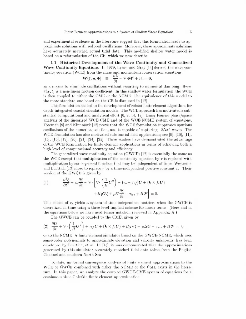
FINITE ELEMENT APPROXIMATIONS TO THE SYSTEM OFSHALLOW WATER EQUATIONS, PART I: CONTINUOUS TIME APRIORI ERROR ESTIMATES �S. CHIPPADAz , C. N. DAWSONz , M. L. MARTINEZy , AND M. F. WHEELERzTICAM Technical Report TR 95-18This paper appears in SINUM 35(1998), No.2 pp.692-711Abstract. Various sophisticated �nite element models for surface water ow based on theshallow water equations exist in the literature. Gray, Kolar, Luettich, Lynch and Westerink havedeveloped a hydrodynamic model based on the generalized wave continuity equation (GWCE) for-mulation, and have formulated a Galerkin �nite element procedure based on combining the GWCEwith the nonconservative momentum equations. Numerical experiments suggest that this methodis robust, accurate and suppresses spurious oscillations which plague other models. We analyze aslightly modi�ed Galerkin model which uses the conservative momentum equations (CME). For thisGWCE-CME system of equations, we present a continous-time a priori error estimate based on anL2 projection.Key words. shallow water equations, surface water ow, mass conservation, momentum con-servation, �nite element method, a priori error estimateAMS subject classi�cations. 35Q35, 35L65 65N30, 65N151. Introduction. In recent years, there has been much interest in the numeri-cal solutions of the shallow water equations. Simulation of shallow water systems canserve numerous purposes. First, it can serve as means for modeling tidal uctuationsfor those interested in capturing tidal energy for commercial purposes. Second, thesesimulations can be used to compute tidal ranges and surges such as tsunamis andhurricanes caused by extreme earthquake and storm events. This information can beused in the development planning of coastal areas. Finally, the shallow water hydro-dynamic model can be coupled to a transport model in considering ow and transportphenomenon, thus making it possible to study remediation options for polluted baysand estuaries, to predict the impact of commercial projects on �sheries, to modelfreshwater-saltwater interactions, and to study allocation of allowable discharges bymunicipalities and by industry in meeting water quality controls.The 2-dimensional shallow water equations are obtained by depth (or vertical)averaging of the continuum mass and momentum balances given by the 3-dimensionalincompressible Navier-Stokes equations. Shallow water equations can be used to study ow in uid domains whose bathymetric depth is much smaller than the characteristiclength scale in the horizontal direction. We denote by �(x; t) the free surface elevationover a reference plane and by hb(x) the bathymetric depth under that reference planeso that H(x; t) = � + hb is the total water column (see Figure 1). Also, we denoteby u(x; t) = [u(x; t) v(x; t)]T the depth-averaged horizontal velocities. Letting U =uH, the 2-dimensional governing equations, in operator form [12], are the primitivecontinuity equation (CE) L(�;u;hb) � @�@t +r�U = 0;� This work was supported in part by National Science Foundation, Project No. DMS-9408151.y Department of Computational and Applied Mathematics-MS 134; Rice University; 6100 MainStreet; Houston, TX 77005-1892z Center for SubsurfaceModeling - C0200; Texas Institute for Computational and Applied Math-ematics; The University of Texas at Austin; Austin, TX 78712.1

2 Chippada, Dawson, Mart��nez, WheelerFig. 1. De�nition of elevation and bathymetryξ

Bottom sea bed

hband the primitive non-conservative momentumequations (NCME), as derived by Wes-terink et al [26],M(�;u; �) � @@tu+ (u�r)u + �bfu + k � fcu+gr� � �H�U � 1H �ws +F = 0;where � = (hb; �bf ; fc; g; �; �ws; pa; �). In particular, �bf (�;u) is a bottom frictionfunction, k is a unit vector in the vertical direction, fc is the Coriolis parameter, g isacceleration due to gravity, � is the horizontal eddy di�usion/dispersion coe�cient,�ws is the applied free surface wind stress relative to the reference density of water,and F = (rpa � gr�), where pa(x; t) is the atmospheric pressure at the free surfacerelative to the reference density of water, and �(x; t) is the Newtonian equilibrium tidepotential relative to the e�ective Earth elasticity factor. We will treat �bf ; �ws; fc; paand � as data. Moreover, we will treat the di�usion coe�cient � as a constant.The primitive conservative momentum equations (CME) are derived from theNCME as Mc � HM+ uL = 0:The numerical procedure used to solve the shallow water equations must resolvethe physics of the problem without introducing spurious oscillations or excessive nu-merical di�usion. Westerink et al [26] note a need for greater grid re�nement nearland boundaries to resolve important processes and to prevent energy from aliasing.Permitting a high degree of grid exibility, the �nite element method is a good can-didate.There has been substantial e�ort over the past two decades in applying �niteelement methods to the CE coupled with either the NCME or the CME. Early �niteelement simulations of shallow water systems were plagued by spurious oscillations.Various methods were introduced to eliminate these oscillations through arti�cial dif-fusion [17, 22]. These methods were generally unsuccessful due to excessive dampingof physical components of the solution. Recently, Agoshkov et al [2, 4, 3] have inves-tigated a �nite element approximation, where the velocity �eld is approximated bypiecewise linear polynomials and the elevation is approximated by the same functionsplus some additional ones. They have studied the e�ects of various boundary con-ditions, and proven stability of various time discretization schemes for a continuityequation-momentum equation system. In this paper, we will examine a �nite elementapproximation to a modi�ed shallow water model described below. Computational

Finite Element Approximations to a System of Shallow Water Equations 3and experimental evidence in the literature suggest that this formulation leads to ap-proximate solutions with reduced oscillations. Moreover, these approximate solutionshave accurately matched actual tidal data. This modi�ed shallow water model isbased on a reformulation of the CE, which we now describe.1.1. Historical Development of the Wave Continuity and GeneralizedWave Continuity Equations. In 1979, Lynch and Gray [14] derived the wave con-tinuity equation (WCE) from the mass and momentum conservation equations,W(�;u; �) � @L@t �r�Mc + �L = 0;as a means to eliminate oscillations without resorting to numerical damping. Here,� (x; t) is a non-linear friction coe�cient. In this shallow water formulation, the WCEis then coupled to either the CME or the NCME. The equivalence of this model tothe more standard one based on the CE is discussed in [12].This formulation has led to the development of robust �nite element algorithms fordepth-integrated coastal circulation models. The WCE approach has motivated a sub-stantial computational and analytical e�ort [6, 8, 14, 18]. Using Fourier phase/spaceanalysis of the linearized WCE-CME and of the WCE-NCME system of equations,Foreman [8] and Kinnmark [12] prove that the WCE formulation suppresses spuriousoscillations of the numerical solution, and is capable of capturing \2�x" waves. TheWCE formulation has also motivated substantial �eld applications; see [9], [10], [11],[15], [16], [19], [20], [21], [24], [25]. These studies have demonstrated the advantageof the WCE formulation for �nite element applications in terms of achieving both ahigh level of computational accuracy and e�ciency.The generalized wave continuity equation (GWCE) [12] is essentially the same asthe WCE except that multiplication of the continuity equation by � is replaced withmultiplication by some general function that may be independent of time. Westerinkand Luettich [13] chose to replace � by a time-independent positive constant ��. Theirversion of the GWCE is given by@2�@t2 + �� @�@t �r� �r�� 1HU2�� (�� � �bf )U + (k � fcU )(1) +Hgr� + �r@�@t � �ws +HF� = 0:This choice of �� yields a system of time-independent matrices when the GWCE isdiscretized in time using a three-level implicit scheme for linear terms. (Here and inthe equations below we have used tensor notation reviewed in Appendix A.)The GWCE can be coupled to the CME, given by@U@t +r�� 1HU2�+ �bfU + (k � fcU ) +Hgr� � ��U � �ws +HF = 0;(2)or to the NCME. A �nite element simulator based on the GWCE-NCME, which usessame-order polynomials to approximate elevation and velocity unknowns, has beendeveloped by Luettich, et al. In [13], it was demonstrated that the approximationsgenerated by this simulator accurately matched tidal data taken from the EnglishChannel and southern North Sea.To date, no formal convergence analysis of �nite element approximations to theWCE or GWCE combined with either the NCME or the CME exists in the litera-ture. In this paper, we analyze the coupled GWCE-CME system of equations for acontinuous time Galerkin �nite element approximation.

4 Chippada, Dawson, Mart��nez, WheelerThe rest of this paper is outlined as follows. In section 2 we detail the assumptionswe will need in our analysis. We also introduce the weak formulation associated withthe GWCE-CME system of equations. In section 3, we introduce the �nite elementapproximation to the weak solution.In the derivation of an error estimate, we investigated various types of projections,such as the L2; elliptic, and parabolic projections. Because of the highly nonlinearnature of the coupled system of equations (1)-(2), we found these projections all ledto suboptimal estimates. To that end, we present, in section 4, the simplest derivationof an a priori error estimate based on an L2 projection.2. Preliminaries.2.1. Notation and De�nitions. For the purpose of our analysis, we de�nesome notation used throughout the rest of this paper.Let be a bounded polygonal domain in IR2 and x= (x1; x2) 2 IR2:The L2 inner product is denoted by('; !) = Z ' � ! dx; '; ! 2 [L2()]n;where \�" here refers to either multiplication, dot product, or double dot product asappropriate. We denote the L2 norm by jj'jj = jj'jjL2() = ('; ')1=2 : In IRn; � =(�1; : : : ; �n) is an n-tuple with nonnegative integer components,D� = D�11 � � �D�nn = @�1@x�11 � � � @�n@x�nnand j�j =Pni=1�i:For ` any nonnegative integer, letH` � f' 2 L2() j D�' 2 L2() for j�j � `gbe the Sobolev space with normjj'jjH`() = 0@Xj�j�` jjD�� jj2L2()1A1=2 :Additionally, H10() denotes the subspace of H1() obtained by completing C10 ()with respect to the norm jj�jjH1() ; where C10 () is the set of in�nitely di�erentiablefunctions with compact support in :Moreover, let W1̀ � f' 2 L1() j D�' 2 L1() for j�j � `gbe the Sobolev space with normjj'jjW1̀() = maxj�j�` jjD�' jjL1() :For relevant properties of these spaces, please refer to [1].Observe, for instance, that H` are spaces of IR-valued functions. Spaces of IRn-valued functions will be denoted in boldface type, but their norms will not be distin-guished. Thus, L2() = [L2()]n has norm jj'jj2 =Pni=1 jj'ijj2; H1() = [H1()]nhas norm jj'jj2H1() =Pni=1Pj�j�1 jjD�'ijj2; etc.For X, a normed space with norm jj � jjX and a map f: [0; T ]! X, de�ne

Finite Element Approximations to a System of Shallow Water Equations 5jjf jj2L2((0;T );X) = Z T0 jjf(�; t)jj2X dt;jjf jjL1((0;T );X) = sup0�t�T jjf(�; t)jjX:Finally, we let K;Ki; (i = 0; 1; 2; ::) and � be generic constants not necessarily thesame at every occurrence.2.2. Variational Formulation. We will consider the coupled system given bythe GWCE-CME described in Section 1, with the following homogeneous Dirichletboundary conditions for simplicity�(x; t) = 0;u(x; t) = 0; �x 2 @; t > 0;(3)and with the compatible initial conditions�(x; 0) = �0(x);@�@t (x; 0) = �1(x);u(x; 0) = u0(x); 9=;x 2 �;(4)where @ is the boundary of � IR2 and � = [@. Extensions to more general landand sea boundary conditions will be treated in a later paper. As noted in Kinnmark[12], the condition necessary for the solution of the GWCE-CME system of equationsto be the same as the solution of the primitive form is that�1(x) = �r�U(x; 0):The weak form of this system is the following: For t 2 (0; T ], �nd �(x; t) 2 H10()and U (x; t) 2H10() such that�@2�@t2 ; v�+ ���@�@t ; v�+�r�� 1HU2� ;rv�| {z }(a) +((�bf � ��)U ;rv)(5) + (k � fcU ;rv) + (Hgr�;rv) + ��r@�@t ;rv�� (�ws;rv) + (HF ;rv) = 0; 8v 2 H10(); t > 0;�@U@t ;w�+�r�� 1HU2� ;w�| {z }(b) +(�bfU ;w) + (k � fcU ;w) + (Hgr�;w)(6) +� (rU ;rw)� (�ws;w) + (HF ;w) = 0; 8w 2H10(); t > 0;with initial conditions(�(x; 0); v) = (�0(x); v); 8v 2 H10();(@�@t (x; 0); v) = (�1(x); v); 8v 2 H10();(U (x; 0);w) = (U0(x);w); 8w 2H10():(7)Here, we have set U0 = u0H0:

6 Chippada, Dawson, Mart��nez, Wheeler2.3. Some Assumptions. Our analysis requires that we make certain physi-cally reasonable assumptions about the solutions and the data. First, we assume for(x; t) 2 �� (0; T ]A1 the solutions (�, U ) to (5)-(7) exist and are unique,A2 9 positive constants H� and H� such that H� � H(x; t) � H�,A3 the velocities u(x; t); v(x; t) are bounded,A4 @@xihb(x) is bounded.Assumption A2 is obvious from Figure 1. Dimensional analysis as explained in [23]accounts for assumption A3. Second, we assume that for (x; t) 2 �� (0; T ]A5 9 positive constants � and � such that � � ghb(x) � �;A6 9 non-negative constants �� and �� such that �� � �bf � ��;A7 (�bf � ��) is bounded,A8 9 non-negative constants f� and f� such that f� � fc � f�,A9 � is a positive constant,A10 rpa(x; t) and r�(x; t) are bounded.Finally, we make the following smoothness assumptions on the initial data and on thesolutions:A11 �0(x); �1(x) 2 H10(),A12 U0(x) 2H10(),A13 H(x; �) 2 H10() \H`() \W11(); t 2 (0; T ),A14 U (x; �) 2H10() \H`() \W11(); t 2 (0; T ),where ` is a positive integer de�ned below.3. Finite Element Approximation.3.1. The Continuous-Time Galerkin Approximation. Let T be a quasi-uniform triangulation of into elements Ei; i = 1; : : : ;m; with diam(Ei) = hi andh = maxi hi: Let Sh denote a �nite dimensional subspace of H10() de�ned on thistriangulation consisting of piecewise polynomials of degree at most (s1 � 1). De�neH() = H10()\H`(), and assume Sh satis�es the standard approximation propertyinf'2Sh jjv � 'jjHs0 () � K0h`�s0 jjvjjH`() ; v 2 H();(8)and the inverse assumptionsjj'jjH`�s0 () � K0 jj'jjL2() h�(`�s0);jj'jjL1() � K0 jj'jjL2() h�1;jjr'jjL1() � K0 jjr'jjL2() h�1; 9=; ' 2 Sh();(9)for 0� s0 � k; s0 � `� s1; with k de�ned from 0� k � (s1 � 1); and where K0 is aconstant independent of h and v.We de�ne the continuous-time Galerkin approximations to �;U to be the map-pings �h(x; t) 2 Sh;Uh(x; t) 2 Sh for each t > 0 satisfying�@2�h@t2 ; v�+ �� �@�h@t ; v�+�r�� 1HhUh2� ;rv�| {z }(a0) +((�bf � ��)Uh;rv)(10) + (k � fcUh;rv) + (Hhgr�h;rv) + ��r@�h@t ;rv�� (�ws;rv) + (HhF ;rv) = 0; 8v 2 Sh();

Finite Element Approximations to a System of Shallow Water Equations 7�@Uh@t ;w�+ �r�� 1HhUh2� ;w�| {z }(b0) +(�bfUh;w) + (k � fcUh;w) + (Hhgr�h;w)(11) +� (rUh;rw) � (�ws;w) + (HhF ;rv) = 0; 8w 2 Sh();with boundary conditions�h(x; t) = 0;Uh(x; t) = 0; � x 2 @; t > 0;(12)and with initial conditions(�h(x; 0); v) = (�0(x); v); 8v 2 Sh();(@�h@t (x; 0); v) = (�1(x); v); 8v 2 Sh();(Uh(x; 0);w) = (U0(x);w); 8w 2 Sh():(13)Here, Hh(x; t) = hb(x) + �h(x; t).4. A Priori Error Estimate. We will compare our �nite element approxima-tions �h and Uh, satisfying (10){(13), to L2 projections e� and eU satisfying�(� � e�)(�; t); v� = 0; 8v 2 Sh; t � 0;�(U � eU )(�; t);w� = 0; 8w 2 Sh; t � 0:(14)For the purpose of succinctness in the rest of the paper, we de�ne( � = � � e�; = �h � e�;� = U � eU ; � = Uh � eU :(15)Clearly, � � �h = � � and U � Uh = � � �: We shall call � and � the projectionerrors and we shall call and � the a�ne errors.The following results are standard.Lemma 4.1. Let 0 � s0 � k; s0 � ` � s1; 0 � k � (s1 � 1); and H() =H10() \ H`(): Let � 2 L2 ((0; T );H()) and U 2 L2 ((0; T );H()) and let (e�; eU)be the corresponding L2 projections de�ned by (14). And let � and � be de�ned asabove.If for some integer | � 0@|�@t| 2 L2 ((0; T );H()) ; @|U@t| ;2 L2 ((0; T );H()) ;then @|e�@t| 2 L2 �(0; T );Sh()� ; @| eU@t| 2 L2 �(0; T );Sh()� ;and ������� @@t�| �������L2((0;T );Hs()) � K0hq�s ������� @@t�| �������L2((0;T );Hq()) ;������� @@t�| �������L2((0;T );Hs()) � K0hq�s ������� @@t�| q������L2((0;T );Hq())

8 Chippada, Dawson, Mart��nez, Wheelerfor some constant K0 independent of �; q; h; `; where q = min(`; s1):We will also need the following result.Lemma 4.2. e�; eU and their �rst-order spatial derivatives are bounded above inL1 ((0; T );L1()) by a positive constant K�.Proof. See [5] Corollary 4.8.9.Before proceeding, it will be necessary to make certain assumptions about theGalerkin approximations. We employ an argument similar to that made in [7] tohandle nonlinearities. In particular, we will assume that the Galerkin approximationsare bounded by some constant in order to derive the a priori error estimate. Thenwe will show for su�ciently small h, in the case of polynomials of degree at least two(s1 � 3), that we can remove the estimates' dependence on the assumed bound ofthe approximations, being dependent instead on a smaller bound on the comparisonprojections.To that end, we assume that, givenK� de�ned in Lemma 4.2, 9 positive constantsC� � H�2 and C� � 2K� such thatB1 C� � Hh(x; t) � C�; andB2 jjUhjjL1((0;T );L1()) � C�:The following lemma will be needed when we bound the right-hand sides of (18),(19), and (20).Lemma 4.3. Let AssumptionsA2, B1 hold. There exists constants K1(C�);K2(C�)such that ��������UH � UhHh �������� � K1 (jj�jj+ jj jj) +K2 (jj�jj+ jj�jj) :Proof.��������UH � UhHh �������� = ��������U (Hh �H) + (U � Uh)HHHh ��������� �������� UHHh ��������L1() jjHh �Hjj+ �������� 1Hh ��������L1() jjU �Uhjj= K1 jj�h � �jj+K2 jjU �Uhjj :Assumptions A2, B1 are used to get the �rst part of the inequality and assumptionB1 is used to get the second part of the inequality.4.1. Error Estimate. In order to obtain an error estimate for (� � �h) and(U � Uh), we must �rst obtain an estimate on the a�ne error terms (�h � e�) and(Uh � eq). Then, with the approximation result stated in Lemma 4.1 and with theestimate on the a�ne error to be obtained in the proof of Theorem 4.4, an applicationof the triangle inequality will yield an estimate for (� � �h) and (U � Uh).It will be useful to employ the following expansion of terms (a){(b) in (5){(6):r�� 1HU2� = �UH �rU�+ (r�U)UH � (rhb�U ) UH2 � (r��U ) UH2 :Similarly, the expansion of terms (a'){(b') in (10){(11) givesr�� 1HhUh2� = �UhHh �rUh�+ (r�Uh)UhHh � (rhb�Uh) UhHh2 � (r�h�Uh) UhHh2 :

Finite Element Approximations to a System of Shallow Water Equations 9Subtract (5) from (10) and (6) from (11), using the fact that we can write�UhHh �r(Uh � eU )�� �UH �rU�+�UhHh �r eU�= �UhHh �r����UH �r(U � eU )�� ��UH � UhHh � �r eU�= �UhHh �r����UH �r�����UH � UhHh � �r eU� ;r�(Uh � eU )UhHh � (r�U ) UH + �r� eU� UhHh= (r��)UhHh � (r��)UH � (r� eU ) �UH � UhHh � ;�r(�h � e�)�Uh� UhHh2 � (r��U ) UH2 + (re��Uh) UhHh2= (r �Uh) UhHh2 � (r��U ) UH2 �re��(�UH �2 � �UhHh �2) ;andHhgr(�h � e�)�Hgr� +Hhgre� = Hhgr �Hgr(� � e�) � (H �Hh)gre�= Hhgr �Hgr� � �gre� + gre�:Consequently, we obtain the following GWCE-CME error equations:�@2 @t2 ; v�+ ���@ @t ; v�+ ��UhHh �r�� ;rv�+ �(r��) UhHh ;rv�(16) +�(r �Uh) UhHh2 ;rv�+ ((�bf � ��)�;rv) + (k � fc�;rv) + (Hhgr ;rv)+��r@ @t ;rv�+ ( F ;rv)= ��UH �r�� ;rv�+��UH � UhHh � �r eU ;rv�+ �(r��)UH ;rv�+�(r� eU ) �UH � UhHh � ;rv�+ rhb�(�UH�2 ��UhHh�2) ;rv!+�(r��U ) UH2 ;rv�+ re��(�UH�2 ��UhHh�2) ;rv!+ ((�bf � ��)�;rv)+ (k � fc�;rv) + (Hgr�;rv) + ��gre�;rv�� � gre�;rv�+��r@�@t ;rv�+ (�F ;rv) ; 8v 2 Sh(); t > 0:

10 Chippada, Dawson, Mart��nez, Wheeler�@�@t ;w�+ ��UhHh �r�� ;w�+�(r��) UhHh ;w�+�(r �Uh) UhHh2 ;w�(17) + (�bf�;w) + (k � fc�;w) + (Hhgr ;w) + � (r�;rw) + ( F ;w)= ��UH �r�� ;w�+��UH � UhHh � �r eU ;w�+ �(r��)UH ;w�+�(r� eU ) �UH � UhHh � ;w�+ rhb�(�UH�2 ��UhHh�2) ;w!+�(r��U ) UH2 ;w�+ re��(�UH�2 � �UhHh�2) ;w! + (�bf�;w)+ (k � fc�;w) + (Hgr�;w) + ��gre�;w�� � gre�;w�+� (r�;rw) + (�F ;w) 8w 2 Sh(); t > 0:4.1.1. Choice of Test Functions and their Manipulation. We now choosespecial test functions to obtain the a�ne error estimate. Let r be a positive constantto be chosen. We let v1(�; t) = R Tt e�rs (�; s)ds and v2(�; t) = R Tt e�rs @@t (�; s)ds bethe test functions in (16). And, we let w=� be the test function in (17).First, we will investigate the use of v1 and v2 as the test functions in (16) followedby temporally integrating over (0; T ]. Note that v1(�; T )=0, v2(�; T )=0. Also recallthat given &, the following relations hold: �@&@t ; &�= 12 ddt �jj&jj2� and 12 ddt �e�rt jj&jj2�=12e�rt ddt �jj&jj2�� r2e�rt jj&jj2 :Now, consider the �rst two terms of (16). When v = v1; we obtain, upon inte-grating by parts,Z T0 �@2 @t2 ; v1� dt = � Z T0 �@ @t ; @v1@t � dt+ �@ @t ; v1�����T0 = Z T0 e�rt�@ @t ; � dt= 12 Z T0 ddt �e�rt jj jj2� dt+ r2 Z T0 e�rt jj jj2dt= 12e�rT jj (�; T )jj2 + r2 Z T0 e�rt jj jj2dtand �� Z T0 �@ @t ; v1� dt = ��� Z T0 � ; @v1@t � dt = �� Z T0 e�rt jj jj2dt:We also have from the di�usion term upon integrating by parts in time:� Z T0 �r@ @t ;rv1� dt = � Z T0 e�rt jjr jj2dt:We are also able to manipulate part of the eighth term in (16) by using thede�nition of v1 as follows:Z T0 (ghbr ;rv1) dt = �12 Z T0 ert ddt (ghbrv1;rv1) dt= �12 Z T0 ddt �ert ������pghbrv1������2� dt + r2 Z T0 ert ������pghbrv1������2dt

Finite Element Approximations to a System of Shallow Water Equations 11� �2 jjrv1(x; 0)jj2 + r �2 Z T0 ert jjrv1jj2dt:Similarly, using v = v2 as the test function in (16) followed by temporally inte-grating over (0; T ] yieldsZ T0 �@2 @t2 ; v2� dt = � Z T0 �@ @t ; @v2@t � dt = Z T0 e�rt ��������@ @t ��������2dt;�� Z T0 �@ @t ; v2� dt = ��� Z T0 � ; @v2@t � dt = �� Z T0 e�rt � ; @ @t � dt= ��2 e�rT jj (�; T )jj2 + �� r2 Z T0 e�rt jj jj2dt:The �rst equality below follows from the de�nition of v2:� Z T0 �r@ @t ;rv2� dt = ��2 Z T0 ert ddt (rv2;rv2) dt= ��2 Z T0 ddt �ert jjrv2jj2� dt + r�2 Z T0 ert jjrv2jj2dt= �2 jjrv2(x; 0)jj2 + r�2 Z T0 ert jjrv2jj2dt:The temporal integration of terms �@�@t ;�� ; (�bf�;�) ; � (r�;r�) in (17) are straight-forward.4.1.2. Bounding theGWCE Error Equations. Using v1(�; t)= R Tt e�rs (�; s)dsas the test function in (16), integrating in time over (0; T ], and using the relationsabove yields12e�rT jj (�; T )jj2+ (r + 2��)2 Z T0 e�rt jj jj2dt+ �2 jjrv1(x; 0)jj2(18) +r �2 Z T0 ert jjrv1jj2dt+ � Z T0 e�rt jjr jj2dt� � Z T0 ��UhHh �r�� ;rv1� dt � Z T0 �(r��)UhHh ;rv1� dt+ Z T0 �(r �Uh) UhHh2 ;rv1� dt� Z T0 ((�bf � ��)�;rv1) dt� Z T0 (k � fc�;rv1) dt � Z T0 (�hgr ;rv1) dt + Z T0 ( F ;rv1) dt+ Z T0 ��UH �r�� ;rv1� dt+ Z T0 ��UH � UhHh � �r eU ;rv1� dt+ Z T0 �(r��)UH ;rv1� dt+ Z T0 �(r� eU ) �UH � UhHh � ;rv1� dt+ Z T0 rhb�(�UH �2 � �UhHh �2) ;rv1! dt+ Z T0 �(r��U ) UH2 ;rv1� dt

12 Chippada, Dawson, Mart��nez, Wheeler+ Z T0 re��(�UH �2 � �UhHh �2) ;rv1! dt+ Z T0 ((�bf � ��)�;rv1) dt+ Z T0 (k � fc�;rv1) dt+ Z T0 (Hgr�;rv1) dt+ Z T0 ��gre�;rv1� dt� Z T0 � gre�;rv1� dt + � Z T0 �r@�@t ;rv1� dt+ Z T0 (�F ;rv1) dt= (A1 + � � �+ A7) + (P1 + � � �+ P14) :Here, A denotes an a�ne error term and P denotes a projection error term.We will explore the nonlinear terms appearing in the right-hand side of (18) inmore detail. It will be implicitly understood that we use either the the H�older In-equality or the Arithmetic Geometric Mean Inequality or both in the treatment of thea�ne and projection error terms. We will explicitly mention additional justi�cationsin the derivation of bounds for these terms.From Assumptions A9, B1 B2, there exists K3 = K3 (�;C�; C�) and K4 =K4 (�;C�; C�) with which we obtain the following bounds on A1, A2 and on A3 :A1 = � Z T0 ��UhHh �r�� ;rv1� dt � � Z T0 e�rt jjr�jj2dt +K3 Z T0 ert jjrv1jj2dt;A2 = � Z T0 �(r��)UhHh ;rv1� dt � � Z T0 e�rt jjr�jj2dt+K3 Z T0 ert jjrv1jj2dt;A3 = Z T0 �(r �Uh) UhHh2 ;rv1� dt � � Z T0 e�rt jjr jj2dt +K4 Z T0 ert jjrv1jj2dt:From Assumption A7, there exists K5 = K5 �jj�bf � ��jjL1((0;T );L1())� suchthat we obtain a bound on A4:A4 = � Z T0 ((�bf � ��)�;rv1) dt � K Z T0 e�rt jj�jj2dt +K5 Z T0 ert jjrv1jj2dt:FromAssumptionA8, there existsK6 = K6 (f�) such that we obtain the followingbound on A5 :A5 = � Z T0 (k � fc�;rv1) dt � K Z T0 e�rt jj�jj2dt+K6 Z T0 ert jjrv1jj2dt:From Assumptions A9, B1, there exists K7 = K7 (�;C�) such that bound forA6 is as follows:A6 = � Z T0 (�hgr ;rv1) dt � � Z T0 e�rt jjr jj2dt+K7 Z T0 ert jjrv1jj2dt:From AssumptionA10, there exists K8 = K8 ���; jjF jjL1((0;T );L1())� such thatthe bound for A7 is as follows:A7 = Z T0 ( F ;rv1) dt � � Z T0 e�rt jj jj2dt +K8 Z T0 ert jjrv1jj2dt:

Finite Element Approximations to a System of Shallow Water Equations 13From Assumptions A2, A3, there exists K9 = K9�������UH ������L1((0;T );L1())� sothat we obtain the following upper bound on the projection error terms P1 and P3:P1 = Z T0 ��UH �r�� ;rv1� dt � K9 jjr�jj2L2((0;T );L2()) +K Z T0 ert jjrv1jj2dt;P3 = Z T0 �(r��)UH ;rv1� dt � K9 jjr�jj2L2((0;T );L2()) +K Z T0 ert jjrv1jj2dt:From Lemma 4.3, and Lemma 4.2, there exists K10 = K10 (��;K1;K2;K�) suchthat the bounds for P2 and P4 are as follows:P2 = Z T0 ��UH � UhHh � �r eU ;rv1� dt � K Z T0 e�rt jj�jj2dt+ � Z T0 e�rt jj jj2dt+K Z T0 e�rt jj�jj2dt+K Z T0 e�rt jj�jj2dt+K10 Z T0 ert jjrv1jj2dt;P3 = Z T0 �(r� eU ) �UH � UhHh � ;rv1� dt � K jj�jj2L2((0;T );L2()) + � Z T0 e�rt jj jj2dt+K jj�jj2L2((0;T );L2()) +K jj�jj2L2((0;T );L2()) +K10 Z T0 ert jjrv1jj2dt:From Lemma 4.3, Lemma 4.2 and Assumptions A2, A3, A4, B1, B2, thereexists K11 = K11 ���;K1;K2; jjrhbjjL1((0;T );L1()) ; C�; C�� such that the bound forP5 is as follows:P5 = Z T0 rhb�(�UH �2 � �UhHh �2) ;rv1! dt= Z T0 �rhb���UH � UhHh ��UH + UhHh � + �UhU �UUhHHh �� ;rv1� dt� K jj�jj2L2((0;T );L2()) + � Z T0 e�rt jj jj2dt +K jj�jj2L2((0;T );L2())+K jj�jj2L2((0;T );L2()) +K11 Z T0 ert jjrv1jj2dt:From Assumption A2,A3, there exists K12 = K12�������u2H2 ������L1((0;T );L1())� suchthat we obtain the following upper bound on the projection error term P6:P6 = Z T0 �(r��U ) UH2 ;rv1� dt � K jjr�jj2L2((0;T );L2()) +K12 Z T0 ert jjrv1jj2dt:From Lemma 4.3, Lemma 4.2, and Assumptions A2, A3, B1, B2, there existsK13 = K13 (��;K1;K2; C�; C�;K�) such that the bound for P7 is given byP7 = Z T0 re��(�UH �2 � �UhHh �2) ;rv1! dt= Z T0 �re����UH � UhHh � �UH + UhHh �+ �UhU � UUhHHh �� ;rv1� dt

14 Chippada, Dawson, Mart��nez, Wheeler� K Z T0 e�rt jj�jj2dt + � Z T0 e�rt jj jj2dt+K Z T0 e�rt jj�jj2dt+K Z T0 e�rt jj�jj2dt+K13 Z T0 ert jjrv1jj2dt:Term P8 is treated similarly to A4 and term P9 is treated similarly to A5 if, for both,we treat � like �.From Assumption A2, there exists K14 = K14 �jjHgjjL1((0;T );L1())� such thatwe obtain the the following upper bound on the projection error term P10:P10 = Z T0 (Hgr�;rv1) dt � K jjr�jj2L2((0;T );L2()) +K14 Z T0 ert jjrv1jj2dt:From Lemma 4.2, there exists K15 = K15 (K�) and K16 = K16 (��;K�) such thatwe obtain the following bounds on P11 and on P12 :P11 = Z T0 ��gre�;rv1� dt � K Z T0 e�rt jj�jj2dt+K15 Z T0 ert jjrv1jj2dtP12 = � Z T0 � gre�;rv1� dt � � Z T0 e�rt jj jj2dt+K16 Z T0 ert jjrv1jj2dt:Obtaining a bound on P13 is straightforward:P13 = � Z T0 �r@�@t ;rv1� dt � K ��������r@�@t ��������2L2((0;T );L2()) +K17 Z T0 ert jjrv1jj2dt:Finally, term P14 is treated similarly to A7:Using v2(�; t)=R Tt e�rs @@t (�; s)ds as the test function in (16), integrating in timeover (0; T ], and using the relations above yieldsZ T0 e�rt ��������@ @t ��������2dt+ e�rT ��2 jj (�; T )jj2+ r ��2 Z T0 e�rt jj jj2dt(19) +�2 jjrv2(x; 0)jj2 + r�2 Z T0 ert jjrv2jj2dt= � Z T0 ��UhHh �r�� ;rv2� dt � Z T0 �(r��)UhHh ;rv2� dt+ Z T0 �(r �Uh) UhHh2 ;rv2� dt� Z T0 ((�bf � ��)�;rv2) dt� Z T0 (k � fc�;rv2) dt � Z T0 (Hhgr ;rv2) dt+ Z T0 ( F ;rv2) dt+ Z T0 ��UH �r�� ;rv2� dt+ Z T0 ��UH � UhHh � �r eU ;rv2� dt+ Z T0 �(r��)UH ;rv2� dt+ Z T0 �(r� eU ) �UH � UhHh � ;rv2� dt+ Z T0 rhb�(�UH �2 � �UhHh �2) ;rv2! dt+ Z T0 �(r��U ) UH2 ;rv2� dt

Finite Element Approximations to a System of Shallow Water Equations 15+ Z T0 re��(�UH �2 � �UhHh �2) ;rv2! dt+ Z T0 ((�bf � ��)�;rv2) dt+ Z T0 (k � fc�;rv2) dt+ Z T0 (Hgr�;rv) dt + Z T0 ��gre�;rv2� dt� Z T0 � gre�;rv2� dt + � Z T0 �r@�@t ;rv2� dt+ Z T0 (�F ;rv2) dt= �cA1 + � � �+ cA7�+ �cP1 + � � �+dP14� :The terms on the right-hand side of the inequality are handled as in (18). Notethat term cA6 di�ers from A6 by one term. From Assumptions A2, A9, there existsK18 = K18 (C�) such that the the upper bound on cA6 is as followscA6 = � Z T0 (Hhgr ;rv2) dt � � Z T0 e�rt jjr jj2dt+K18 Z T0 ert jjrv2jj2dt:4.1.3. Bounding the CME Error Equation. Using w = � as the test func-tion in (17) followed by integration in time over (0; T ], yields12 jj�(�; T )jj2+ � jjr�jj2L2((0;T );L2()) + ����p�bf �����2L2((0;T );L2())(20)� � Z T0 ��UhHh �r�� ;�� dt� Z T0 �(r��)UhHh ;�� dt+ Z T0 �(r �Uh) UhHh2 ;�� dt� Z T0 (Hhgr ;�) dt + Z T0 ( F ;�) dt+ Z T0 ��UH �r�� ;�� dt + Z T0 ��UH � UhHh � �r eU ;�� dt+ Z T0 �(r��)UH ;�� dt+ Z T0 �(r� eU ) �UH � UhHh � ;�� dt+ Z T0 rhb�(�UH �2 � �UhHh �2) ;�! dt+ Z T0 �(r��U ) UH2 ;�� dt+ Z T0 re��(�UH �2 � �UhHh �2) ;�! dt+ �� Z T0 (�;�)| {z }0 by (14)j dt+ Z T0 (k � fc�;�) dt + Z T0 (Hgr�;�) dt + Z T0 ��gre�;�� dt� Z T0 � gre�;�� dt+ � Z T0 (r�;r�) dt+ Z T0 (�F ;�) dt= �fA1 + fA2 + fA3�+ �fA6 + fA7�+ �fP1 + � � �+ fP7�+ �fP9 + � � �+gP14� :The terms on the right-hand side of the inequality are handled as in (18). Again,observe that term fA6 di�ers from A6 by one component and is thus treated similarlyto cA6 in (19). Also, the treatment of term gP13 di�ers slightly from the treatment ofthe corresponding terms in the previous equations:gP13 = � Z T0 (r�;r�) dt � K19 jjr�jj2L2((0;T );L2()) + � jjr�jj2L2((0;T );L2()) :

16 Chippada, Dawson, Mart��nez, Wheeler4.1.4. Bounding the Sum of the Error Equations. We observe that theright-hand-side of (18) can be bounded by� Z T0 e�rt jj jj2dt + � Z T0 e�rt jjr jj2dt+Kv1 Z T0 ert jjrv1jj2dt+K jj�jj2L2((0;T );L2())(21) +� jjr�jj2L2((0;T );L2()) +K jj�jj2L2((0;T );L2()) +K jjr�jj2L2((0;T );L2())+K ��������r@�@t ��������2L2((0;T );L2()) +K jj�jj2L2((0;T );L2()) +K jjr�jj2L2((0;T );L2())where Kv1 = Kv1 (K1; : : : ;K17) :The right-hand-side of (19) can be bounded by� Z T0 e�rt jj jj2dt + � Z T0 e�rt jjr jj2dt+Kv2 Z T0 ert jjrv2jj2dt+K jj�jj2L2((0;T );L2())(22) +K jjr�jj2L2((0;T );L2()) +K jj�jj2L2((0;T );L2()) +K jjr�jj2L2((0;T );L2())+K ��������r@�@t ��������2L2((0;T );L2()) +K jj�jj2L2((0;T );L2()) +K jjr�jj2L2((0;T );L2())where Kv2 = Kv2 (K1; : : : ;K6;K8; : : : ;K18) :Finally, the right-hand-side of (20) can be bounded by� Z T0 e�rt jj jj2dt+ � Z T0 e�rt jjr jj2dt +Kw Z T0 ert jj�jj2dt(23) +K jj�jj2L2((0;T );L2()) + � jjr�jj2L2((0;T );L2()) +K jj�jj2L2((0;T );L2())+K jjr�jj2L2((0;T );L2()) +K jj�jj2L2((0;T );L2()) +K jjr�jj2L2((0;T );L2())where Kw = Kw (K1; : : : ;K4;K8; : : : ;K16;K18;K19) :Now choose r = maxf2Kv1= �; 2Kv2=�g ; such thatr1 = �r �2 �Kv1� � 0and r2 = �r�2 �Kv2� � 0:Then, summing (18), (19), and (20), using the above choice for r; and usingbounds (21), (22), and (23) yieldsr(�� + 1)2 Z T0 e�rt jj jj2dt+ ��� + 12 � e�rT jj (�; T )jj2(24) + Z T0 e�rt ��������@ @t ��������2dt+ �2 Z T0 e�rt jjr jj2dt + �2 jjrv1(x; 0)jj2| {z }A+ �2 jjrv2(x; 0)jj2| {z }B +r1 Z T0 ert jjrv1jj2dt| {z }C +r2 Z T0 ert jjrv2jj2dt| {z }D

Finite Element Approximations to a System of Shallow Water Equations 17+12 jj�(�; T )jj2 + ����p�bf �����2L2((0;T );L2()) + �2 jjr�jj2L2((0;T );L2())� K jj�jj2L2((0;T );L2()) +K jjr�jj2L2((0;T );L2()) +K ��������r@�@t ��������2L2((0;T );L2())+K jj�jj2L2((0;T );L2()) +K jjr�jj2L2((0;T );L2()) +K20 jj�jj2L2((0;T );L2())where K20 = KwerT +K.From (24), we havejj�(�; T )jj2 � 2K jj�jj2L2((0;T );L2()) + 2K jjr�jj2L2((0;T );L2())(25) +2K ��������r@�@t ��������2L2((0;T );L2()) + 2K jj�jj2L2((0;T );L2())+2K jjr�jj2L2((0;T );L2()) + 2K20 jj�jj2L2((0;T );L2()) :Applying Gronwall's Lemma to (25) yieldsjj�(�; T )jj2 � 2K21 nK jj�jj2L2((0;T );H1())(26) +K ��������r@�@t ��������2L2((0;T );L2()) +K jj�jj2L2((0;T );H1())) ;where K21 = e2K20T :We now return to (24) to bound it above and below. Let �1 = minf�; r(��+ 1)g;observe that terms A;B;C;D are all non-negative, and use (26) to obtain,12e�rT "(�� + 1) jj (�; T )jj2 + 2 ��������@ @t ��������2L2((0;T );L2()) + �1 jj jj2L2((0;T );H1())(27) + jj�(�; T )jj2 + 2 ����p�bf �����2L2((0;T );L2()) + � jjr�jj2L2((0;T );L2())i� (1 + 2K20K21K)K njj�jj2L2((0;T );H1())+ ��������r@�@t ��������2L2((0;T );L2()) + jj�jj2L2((0;T );H1())) :Now, letting � = minf (�� + 1) ; 2; �1; 1; �g and multiplying through by 2erT ; weobtain jj (�; T )jj2 + ��������@ @t ��������2L2((0;T );L2()) + jj jj2L2((0;T );H1())(28) + jj�(�; T )jj2 + ����p�bf �����2L2((0;T );L2()) + jjr�jj2L2((0;T );L2())� K22(jj�jj2L2((0;T );H1()) + ��������r@�@t ��������2L2((0;T );L2()) + jj�jj2L2((0;T );H1()))withK22 = 2erT (1+2K20K21K)K� :Observe thatK22 depends on r; s1; T , and onK�; C�; C�.Use the approximation result stated in Lemma 4.1,jj�jjL2((0;T );H1()) ; ��������r@�@t ��������L2((0;T );L2()) ; jj�jjL2((0;T );H1()) � K0h`�1;

18 Chippada, Dawson, Mart��nez, Wheelerto obtainjj (�; T )jj+ ��������@ @t ��������L2((0;T );L2()) + jj jjL2((0;T );H1())(29) + jj�(�; T )jj+ ����p�bf �����L2((0;T );L2()) + jjr�jjL2((0;T );L2()) � K23h`�1where K23 � K0pK22.Finally, applying the triangle inequality to the projection error and to the a�neerror (29) yields the following error estimate.Theorem 4.4 (A Priori Error Estimate). Let 0 � s0 � k; s0 � ` � s1; 0�k � (s1 � 1); and let H = H10() \ H`(). Let (�;U ) be the solution to (5)-(7).Let (�h;Uh) be the Galerkin approximations to (�;U). If �(t) 2 H() \ W11();,U (t) 2 H() \W11(); for each t; if �h(t) 2 Sh(), Uh(t) 2 Sh() for eacht; and suppose that assumptions A2{A10 and B1, B2 hold; then, 9 a constant�K = �K(T; s1; r;K�; C�; C�) such that�������� @@t (� � �h)��������L2((0;T );L2()) + jj (� � �h)(�; T ) jj+ jj� � �hjjL2((0;T );H1())(30) + jj (U �Uh)(�; T ) jj+ ����p�bf (U � Uh)����L2((0;T );L2())+ jjrU �rUhjjL2((0;T );L2()) � �Kh`�1:Moreover, for h su�ciently small and s1 � 3 thenjj�hjjL1((0;T );L1()) + jjUhjjL1((0;T );L1()) < 2K� � C�;and �h > H�2 � C�:Thus, the dependence of �K on C�; C� is removed.4.1.5. Boundedness of Approximations. The proof of the theorem is nowcomplete in the case of linears since we assumed that B1, B2 holds for this case.We now complete the proof of the theorem in the case of at least quadraticpolynomials (s1 � 3).From the inverse assumptions, the boundedness of the L2 projection and a�neerror estimate (29), we obtainjjUhjjL1((0;T );L1()) � ������Uh � eU ������L1((0;T );L1()) + ������ eU ������L1((0;T );L1())� K0h�1 ������Uh � eU ������L1((0;T );L2()) +K�� K0h�1K23h`�1 +K�= K24h`�2 +K�For h su�ciently small, viz, h`�2 < K�K24 , we getjjUhjj2L1((0;T );L1()) < 2K� � C�:The upper bound for Hh(x; t) is shown similarly.

Finite Element Approximations to a System of Shallow Water Equations 19To get the lower bound for Hh(x; t), use Assumption A2, inverse assumptions,and estimates on the a�ne and projection errors.Hh = H � (H �Hh) = H � � + � H� �K25h`�2:For h su�ciently,small, viz. h`�2 < H�2K25 ; we getHh > H�2 � C�:Thus for the case of quadratics and higher, there exists a �K bounded aboveindependent of C�; C�:This completes the proof of the theorem.5. Conclusions. We have analyzed a full nonlinear coupled GWCE-CME sys-tem of equations. Making physically-realistic assumptions, we derived an a priori errorestimate for the Galerkin �nite element approximation to the solution of GWCE-CMEsystem of equations, in weak form, by using an L2 projection. This led to a subop-timal estimate. That is, if we use continuous, piecewise polynomials of degree s1 � 1to approximate the elevation and velocity unknowns on a mesh with grid-spacing h,then the approximations tend to the solutions of the weak form like hs1�1. To ourknowledge, our error analysis of a system of shallow water equations is the �rst of itskind.6. Acknowledgments. The authors thank Martha Carey and Amr Elbakry fortheir valuable feedback, as well as the referees for their helpful comments.

20 Chippada, Dawson, Mart��nez, WheelerA. Review of Tensor Notation. Let '; 2 IR2.The dyadic product is de�ned as (' )ij = 'i j : Thus,'2 = � '21 '1'2'2'1 '22 � :The dot product of a tensor with a vector is the usual matrix-vector multiplicationresult [M �$]i =PjMij$j :The scalar product (or double-dot product) of two tensors is de�ned as S:T =Pi;j SijTij:The gradient of a vector is de�ned as fr'gij = @'j@xi : For example,r' = @'1@x1 @'2@x1@'1@x2 @'2@x2 ! :The divergence of a tensor is de�ned as [r�S]j =Pi @@xiSij : Thus,r�r' = 0@ @2'1@x21 + @2'1@x22@2'2@x21 + @2'2@x22 1A = 4'14'2 ! :Observe that (r':r') = � @@x1'1�2 + � @@x2'1�2 + � @@x1'2�2 + � @@x2'2�2 andthat r�(r�'2) = @2@x21'21 + @2@x1@x2 ('2'1) + @2@x2@x1 ('1'2) + @2@x22'22:REFERENCES[1] R. A. Adams, Sobolev Spaces, vol. 65 of Pure and Applied Mathematics, Academic Press, NewYork, 1978.[2] V. I. Agoshkov, E. Ovchinnikov, A. Quarteroni, and F. Saleri, Modi�ed �nite elementapproximation to shallow water equations and stability results, in Finite Elements in Fluids:New Trends and Applications, K. Morgan, E. O~nate, J. Periaux, J. Peraire, and O. C.Zienkiewicz, eds., Centro Internacional de M�etodos Num�ericos en Ingenier��a, Wales, 1993,Pineridge Press, pp. 1020{1025.[3] , Recent developments in the numerical simulation of shallow water equations II: Tem-poral discretization, Mathematical Models and Methods in Applied Sciences, 4 (1994),pp. 533{556.[4] V. I. Agoshkov, A. Quarteroni, and F. Saleri, Recent developments in the numericalsimulation of shallow water equations I: Boundary conditions, Applied Numerical Mathe-matics, 15 (1994), pp. 175{200.[5] S. C. Brenner and L. R. Scott, The Mathematical Theory of Element Methods, vol. 15 ofTexts in Applied Mathematics, Springer-Verlag, New York, 1994.[6] J. Drolet and W. G. Gray, On the well-posedness of some wave formulations of the shallowwater equations, Advances in Water Resources, 11 (1988), pp. 84{91.[7] R. E. Ewing and M. F. Wheeler, Galerkin methods for miscible displacement problems inporous media, SIAM Journal of Numerical Analysis, 17 (1980), pp. 351{365.[8] M. G. G. Foreman, An analysis of the \wave equation model" for �nite element tidal com-putations, Computational Physics, 52 (1983), pp. 290{312.[9] , A comparison of tidal models for the southwest coast of Vancouver Island, in Compu-tational Methods in Water Resources: Proceedings of the VII International Conference,MIT, USA, June 1988, M. A. C. et al, ed., Amsterdam, 1988, Elsevier.[10] W. G. Gray, A �nite element study of tidal ow data for the North Sea and English Channel,Advances in Water Resources, 12 (1989), pp. 143{154.

Finite Element Approximations to a System of Shallow Water Equations 21[11] W. G. Gray, J. Drolet, and I. P. E. Kinnmark, A simulation of tidal ow in the southernpart of the North Sea and the English Channel, Advances in Water Resources, 10 (1987),pp. 131{137.[12] I. P. E. Kinnmark, The Shallow Water Wave Equations: Formulation, Analysis and Appli-cations, vol. 15 of Lecture Notes in Engineering, Springer-Verlag, New York, 1985.[13] R. A. Luettich, J. J. Westerink, and N. W. Scheffner, ADCIRC: An advanced three-dimensional circulation model for shelves, coasts, and estuaries, Tech. Report 1, Depart-ment of the Army, U.S. Army Corps of Engineers,Washington,D.C. 20314-1000,December1991.[14] D. R. Lynch and W. G. Gray, A wave equation model for �nite element tidal computations,Computers and Fluids, 7 (1979), pp. 207{228.[15] D. R. Lynch and F. E. Werner, Three-dimensional hydrodynamics on �nite elements, partII: Nonlinear time-stepping model, International Journal for Numerical Methods in Fluids,12 (1991), pp. 507{534.[16] D. R. Lynch, F. E. Werner, J. M. Molines, and M. Fornerino, Tidal dynamics in acoupled ocean/lake system, Estuarine, Coastal and Shelf Science, 31 (1990), pp. 319{343.[17] P. W. Partridge and C. A. Brebbia, Quadratic �nite elements in shallow water problems,ASCE Journal of Hydraulic Engineering, 102 (1976), pp. 1299{1313.[18] R. A. Walters, Numerically induced oscillations in �nite element approximations to theshallow water equations, International Journal for Numerical Methods in Fluids, 3 (1983),pp. 591{604.[19] , A model for tides and currents in the English Channel and southern North Sea, Ad-vances in Water Resources, 10 (1987), pp. 138{148.[20] , A �nite element model for tides and currents with �eld applications, Communicationsin Numerical Methods in Engineering, 4 (1988), pp. 401{441.[21] R. A. Walters and F. E. Werner, A comparison of two �nite element models of tidal hydro-dynamics using a North Sea data set, Advances in Water Resources, 12 (1989), pp. 184{193.[22] J. D. Wang and J. J. Connor, Mathematical modeling of near coastal circulation, Tech.Report 200, MIT Parsons Laboratory, Cambridge, MA, 1975.[23] T. Weiyan, Shallow Water Hydrodynamics, vol. 55 of Elsevier Oceanography Series, Elsevier,Amsterdam, 1992.[24] F. E. Werner and D. R. Lynch, Field veri�cation of wave equation tidal dynamics inthe English Channel and southern North Sea, Advances in Water Resources, 10 (1987),pp. 115{130.[25] , Harmonic structure of English Channel/Southern Bight tides from a wave equationsimulation, Advances in Water Resources, 12 (1989), pp. 121{142.[26] J. J. Westerink, R. A. Luettich, A. M. Baptista, N. W. Scheffner, and P. Farrar,Tide and storm surge predictions in the Gulf of Mexico using a wave-continuity equation�nite element model, in Estuarine and Coastal Modeling: Proceedings of the 2nd Interna-tional Conference, e. a. Malcolm L. Spaulding, ed., New York, 1992, American Society ofCivil Engineers.