Aeroelastic stability analysis using stochastic structural modifications

L.J. Adamsona,∗, S. Ficheraa, J.E. Mottersheada

aSchool of Engineering, University of Liverpool, Liverpool L69 3GH, United Kingdom

Abstract

An experimental-based approach to flutter speed uncertainty quantification in aeroelastic systems is devel-oped. The proposed technique considers uncertainty from a post-manufacture perspective. Variability dueto manufacturing tolerances, damage and degradation is formulated as a stochastic structural modificationto a single set of measured receptance data. The Sherman-Morrison formula is exploited so that the proba-bility of flutter is evaluated either from parameter bounds or by using a first-order reliability method. Theadvantage of the formulation is that there is no requirement to model either the structure or aerodynamics,thereby avoiding model-form and parameter uncertainties. Numerical examples are provided, which demon-strate the efficiency of the method when compared to conventional Monte-Carlo simulation (MCS). Themethod is also demonstrated in experimental examples and it is shown to be eminently practical since thedata required for MCS is generally not available in industrial practice.

Keywords: Aeroelasticity, Structural modification, Receptance, Uncertainty quantification

1. Introduction

Aerostructures are becoming increasingly lightweight and flexible thanks to the advent of compositematerials with high specific strengths [1]. Although advantageous in terms of aerodynamic and fuel efficiency[2], this can lead to undesired aeroelastic phenomena that potentially compromise the safety of aircraft.One such phenomena is that of flutter, which is an unstable, self-excited vibration caused by the transferof energy from the air to the structure [3, 4]. Flutter is particularly dangerous since it can cause largestructural deflections that expedite fatigue or even result in catastrophic structural failure [5]. It is crucial,therefore, that the conditions at which flutter occurs are accurately predicted.

Conventionally, the conditions that enable flutter to arise have been determined by means of computa-tional modelling. In this approach, a finite-element model of the structure is coupled with an aerodynamicmodel and an eigenvalue analysis is performed [6]. Although well established and widely used, this methodrequires knowledge of both the model-form and its corresponding parameters. In practice, such knowledgeis not known exactly and is merely estimated. Consequently, there is always a discrepancy between the trueand estimated flutter conditions.

In recent years, uncertainty quantification (UQ) techniques have been used in aeroelastic systems in orderto approach the problem of flutter prediction from a probabilistic perspective [7, 8, 9, 10, 11]. Castraveteand Ibrahim [12] first considered the effect of random stiffness parameters on the flutter speed by use ofa Karhunen-Love expansion. Both a perturbation approach and Monte-Carlo simulations were used tocompute the probability of aeroelastic instability. Likewise, Khodaparast et al. [13] considered the problemof uncertainty quantification using a first- and second-order perturbation method that relied upon a responsesurface, which took the form of a multivariate polynomial. Manan and Cooper [14], Scarth et al. [15] andGeorgiou et al. [16] all used a polynomial chaos expansion, constructed by Latin Hypercube sampling,

∗Corresponding author.Email addresses: l.j.adamson@liverpool.ac.uk (L.J. Adamson), sebastiano.fichera@liverpool.ac.uk (S. Fichera),

j.e.mottershead@liverpool.ac.uk (J.E. Mottershead)

Preprint submitted to Journal of Sound and Vibration March 31, 2020

to create a surrogate model of the flutter speed variability, which arose from variable material and lay-upproperties in composite materials. A Monte-Carlo simulation was then performed on the surrogate model,which was shown to significantly reduce computational time compared to direct Monte-Carlo. Allen andMaute [17] and Nikbay and Kuru [18] used a first-order reliability method to quantify variable aeroelasticresponses and further used this to perform a reliability-based optimisation.

Although well-established, UQ in aeroelasticity has thus far concentrated primarily on introducing un-certainty into numerical models. This may be thought of as quantifying uncertainty during the design phase,i.e. pre-manufacture. To the best of the present authors’ knowledge, little research effort has been given tosimulating the effect of uncertainty post-manufacture. Such uncertainty may arise from: i) manufacturingtolerances, and ii) damage and degradation of structural components. This is the subject of the presentwork.

In this paper, uncertainty is modelled as a direct structural modification [19, 20, 21, 22, 23, 24, 25] to asingle set of receptances, which may be measured experimentally by means of conventional modal testing [26].In this way, there is no need to model the structure, aerodynamics, nor their interaction since experimentaldata is used directly. The structural modification is represented as a stochastic matrix, which containsrandom mass, stiffness and damping parameters [27]. Assuming that the system (both the structure andcoupled aerodynamics) is linear, the characteristic equation of the modified system is then obtained by usingthe Sherman-Morrison formula [28] in an iterative way. When the modification is single-rank and arises froma single mechanical element, it is shown that a graphical method can be used to determine the values ofthe random parameter that lead to flutter. The probability of flutter, in this case, is then evaluated simplyby integrating the probability density function of the random parameter in the regions that lead to flutter.When the modification arises from more than one mechanical element, it is shown that the characteristicequation of the modified system can be projected onto the joint distribution of the random parameters andspecific regions integrated in order to find the probability of flutter. To simplify the integration, it is shownthat a first-order reliability method [29] can be used, which is computationally efficient. In contrast withconventional techniques, this method does not provide a direct estimate of the flutter speed probabilitydistribution. Instead, it estimates the likelihood of flutter arising at a given airspeed. This allows for aQuantitative Risk Assessment (QRA) to be performed, for instance, in decision-making safety systems.

2. Structural modification theory in aeroelasticity

Consider a general n-degree-of-freedom, linear aeroelastic system governed by

Mq(t) + Cq(t) + Kq(t) = fa(t) (1)

where M,C,K ∈ Rn×n are the structural mass, damping and stiffness matrices respectively; q(t) ∈ Rn isthe vector of degrees-of-freedom; and fa(t) ∈ Rn is the external load arising from the aerodynamics. Takingthe Laplace transform and dropping the initial value terms gives that(

s2M + sC + K)q(s) = fa(s) (2)

where s ∈ C is the complex variable.According to Roger [30], the aerodynamic load may be approximated by a rational transfer function, so

thatfa(s) = Qa(s, v)q(s) (3)

where Qa(s, v) ∈ Cn×n is the ‘aerodynamic dynamic stiffness’ or ‘aerodynamic transfer matrix’, and v isthe free-stream speed. It is shown in [30] that the aerodynamic transfer matrix may be expanded into thesum of contributory steady and unsteady aerodynamic matrix terms. However, in the proceeding analysis,there is no need to perform such an expansion since the form given in Eq. 3 is used directly; that is, thereis no requirement to model the aerodynamics explicitly, regardless of the degree of unsteadiness.

Substituting Eq. 3 into Eq. 2 yields

(Zs(s)−Qa(s, v)) q(s) = 0 (4)

2

whereZs(s) = s2M + sC + K (5)

is the structural dynamic stiffness matrix. The characteristic equation of the aeroelastic system is thus givenby

det (Zs(s)−Qa(s, v)) = 0 (6)

and the values of s that satisfy Eq. 6 are the system’s poles. Due to the dependency of the aerodynamics onv, the poles vary with the free-stream speed. The first speed at which one or more poles become unstable isdenoted the flutter speed vf . At this point, one or more pole pairs lie precisely on the imaginary axis andso

det (Zs(iω)−Qa(iω, vf )) = 0 (7)

When the internal structural properties1 are modified so that the mass, stiffness or damping changes,Eq. 4 becomes

(Zs(s) + ∆Zs(s)−Qa(s, v)) q(s) = 0 (8)

where∆Zs(s) = s2∆M + s∆C + ∆K (9)

is the structural modification term. In the remainder of this work, it is assumed that the modification canbe parameterised by a vector θ ∈ Rp of p random variables, so that

∆Zs(s,θ) = s2∆M(θ) + s∆C(θ) + ∆K(θ) (10)

Replacing the structural modification term of Eq. 8 with the parameterised form of Eq. 10 and pre-multiplying by

Hs+a(s, v) = (Zs(s)−Qa(s, v))−1

(11)

gives that(I + Hs+a(s, v)∆Zs(s,θ)) q(s) = 0 (12)

The characteristic equation of the aeroelastic system with a stochastic structural modification is therefore

det (I + Hs+a(s, v)∆Zs(s,θ)) = 0 (13)

In the modified system, the poles vary according to both the free-stream speed and the random parameters.Consequently, the poles at any given speed are not singular points but are instead clusters in the complexplane.

The receptance matrix is used directly in the above formulation. This means that there is no need toconstruct a numerical model of the system since receptances can be collected experimentally by means ofmodal testing, as will be shown later.

2.1. Problem formulation

For safety reasons, the maximum operating speed of an aircraft is always set below the calculated flutterspeed. For example, Federal Aviation Administration regulations mandate a 15% factor of safety [31]. AsPettit [8] discusses, these margins of safety are chosen empirically and have little physical basis. Instead, ithas been suggested that a probabilistic-based approach may used to define the probability of flutter at somegiven airspeed. In terms of receptances, the problem is formulated in two ways:

1. What structural modification would cause the system to enter flutter at some given speed below thenominal flutter speed?

2. What is the probability of flutter due to a structural modification if the probability distributions ofthe random parameters are known?

1This condition implies that the external geometry of the aerofoil remains unchanged.

3

3. Rank-one, single-element modification

When the structural modification is rank-one and arises from a single mechanical element, i.e. a singlemass, spring or damper, Eq. 10 can be written in the form

∆Zs(s, θ) = b(s, θ)eeT (14)

where e ∈ Rn is a vector with unit entries corresponding to the coordinates of the modification, andb(s, θ) ∈ C is the dynamic stiffness of the modification element [19]. The element’s dynamic stiffness mayalways be separated so that

b(s, θ) = θg(s) (15)

where θ ∈ R is the random mass, stiffness or damping parameter; and g(s) ∈ C is some function of thecomplex variable. For example, a random mass modification is of the form

b(s,m) = m× s2

Therefore, the structural modification matrix may be written as

∆Zs(s, θ) = θg(s)eeT (16)

Since Eq. 16 is always rank-one, the Sherman-Morrison formula [32] can be used to express the receptancematrix of the modified system in terms of the original unmodified receptance matrix, so that

Hs+a(s, v,θ) = Hs+a(s, v)− θg(s)Hs+a(s, v)eeTHs+a(s, v)

1 + θg(s)eTHs+a(s, v)e(17)

where Hs+a(s, v,θ) is the receptance matrix of the modified system. By inspection, therefore, the charac-teristic equation of the modified system is

1 + θg(s)eTHs+a(s, v)e = 0 (18)

Re-arranging Eq. 18 in terms of the random parameter gives that

θ = − 1

g(s)eTHs+a(s, v)e(19)

As discussed in Section 2, one or more pole pairs lie precisely on the imaginary axis (s = iω) at the fluttercondition and therefore a modification that causes this must satisfy

θ = − 1

g(iω)eTHs+a(iω, v)e(20)

Initially, the value of ω at which the pole pair(s) lie is unknown. However, for physically-meaningful solutions,the random parameter must be purely real. Therefore, only values of ω for which

Im(g(iω)eTHs+a(iω, v)e

)= 0 (21)

are valid.The number of solutions to Eq. 20 determines the number of times that a pole pair crosses the imaginary

axis as the random parameter is changed. Therefore, it is equivalent to the number of times for which thesystem transitions from stable to unstable, or vice versa. Given that the original unmodified system is stable,the unstable parameter solutions can be determined easily, as demonstrated in Fig. 1. The probability offlutter is evaluated by integrating the probability density function of the random parameter across theunstable regions.

4

Figure 1: Example of stable and unstable parameters bounds.

4. Multiple-rank, multiple-element modification

Suppose that there are p random mechanical elements that act as a stochastic modification. The struc-tural modification matrix may be written as

∆Zs(s,θ) =

p∑i=1

θigi(s)eieTi (22)

In general, the modification is rank-m (1 ≤ m ≤ n). However, it may be separated into the sum ofcontributory rank-one elements, as in Eq. 22. By defining

Ak = Zs(s)−Qa(s, v) +

k−1∑i=1

θigi(s)eieTi (23)

the modified receptance matrix is expressed as

Hs+a(s, v,θ) =(Ap + θpgp(s)epe

Tp

)−1(24)

Since Eq. 24 is the inverse of a rank-one modification, the Sherman-Morrison formula can again be utilisedso that

Hs+a(s, v,θ) = A−1p −θpgp(s)A

−1p epe

Tp A−1p

1 + θpgp(s)eTp A−1p ep(25)

and hence the characteristic equation of the modified system is

1 + θpgp(s)eTp A−1p ep = 0 (26)

Since

A−1p =(Ap−1 + θp−1gp−1(s)ep−1e

Tp−1)−1

(27)

A−1p−1 =(Ap−2 + θp−2gp−2(s)ep−2e

Tp−2)−1

(28)

...

A−12 =(Zs(s)−Qa(s, v) + θ1g1(s)e1e

T1

)−1(29)

and(Zs(s)−Qa(s, v))

−1= Hs+a(s, v) (30)

the Sherman-Morrison formula can be used iteratively in order to find the characteristic equation of thegeneral multiple-rank modified system in terms of the original measured receptance matrix.

Repeated use of the Sherman-Morrison formula eventually leads to the general form of the characteristicequation, which is

1 +

p∑i1=1

θi1fi1(s) +

p∑i1=1

p∑i2=1i2 6=i1

θi1θi2fi1,i2(s) + · · · = 0 (31)

5

where fij (s) are functions that depend on the original measured receptances. As discussed previously, theflutter condition requires that one or more pole pairs lie precisely on the imaginary axis and therefore, bysubstituting s = iω into Eq. 31, the modification must satisfy

1 +

p∑i1=1

θi1fi1(iω) +

p∑i1=1

p∑i2=1i2 6=i1

θi1θi2fi1,i2(iω) + · · · = 0 (32)

The left-hand side of Eq. 32 is referred to as the non-standardised limit-state function L(θ1, . . . , θp, ω)hereinafter and is geometrically equivalent to a hyper-plane in the θ1, . . . , θp, ω space. In the above analysis,it has been assumed that each modification parameter may be written as a rank-one modification andthat the scalar dynamic stiffness contribution of each random parameter is a linear function of the randomparameter. In simple mass, spring or damper modifications, this is valid. However, in more complexmodifications, this is not necessarily true. A more generalised approach is presented in the Appendix todeal with such cases; although it is important to note that the overall method remains unchanged and leadsto a limit-state function that is similar to the one given in Eq. 32.

To simplify and make universal the proceeding analysis, a Rosenblatt transformation [33] is applied toeach random parameter, such that

θ1θ2...

θp

=

Φ−1 (F1(θ1))

Φ−1(F2|1(θ2|θ1)

)...

Φ−1(Fp|p−1,...,1(θp|θp−1, . . . , θ1)

) (33)

and θ1θ2...θp

=

F−11

(Φ(θ1)

)F−12|1

(Φ(θ2)|θ1)

)...

F−1p|p−1,...,1

(Φ(θp)|θp−1, . . . , θ1)

)

(34)

where θi is the standardised random parameter; Φ and Φ−1 is the forward and inverse unit variance,zero mean normal cumulative distribution function; and Fp|p−1,...,1 and F−1p|p−1,...,1 are the forward and

inverse cumulative distribution functions of the conditional random variable θp|θp−1, . . . , θ1. This serves tostandardise the distribution of the random parameters so that they are normal, zero mean and unit variance.Using Eq. 34 in Eq. 32 allows the non-standardised limit-state function to be expressed in terms of thestandardised parameters. The resulting hyper-surface, when expressed in terms of the standardised variables,is referred to as the standardised limit-state function L(θ1, . . . , θp, ω). At each frequency ω, the standardisedlimit-state function gives the combination of standardised parameters that causes one or more pole pairs tolie exactly on the imaginary axis. Since Eq. 32 involves complex receptance terms, the parameter solutionsmay be complex. Therefore, for physically-meaningful solutions, one must impose the constraint that theparameters are real. This reduces the number of parameter solutions. For example, in the case of tworandom parameters, the hyper-surface reduces to a curve in the θ1, θ2, ω space, as illustrated in Fig. 2.

At each frequency ω, the standardised limit-state function may be projected from the θ1, . . . , θp, ω space

to the θ1, . . . , θp space. The resulting projection is named the projected, standardised limit-state function

L(θ1, . . . , θp) and bisects the θ1, . . . , θp space. Since the limit-state function is defined as the combinationof parameters that causes one or more poles to lie on the imaginary axis, at any frequency ω, the bisectedregions in this projected space represent parameter combinations that cause the poles of the system to beeither in the left- or right-hand side of the complex plane. Therefore, the projection divides the θ1, . . . , θpspace into regions that keep the system stable or make the system unstable; the regions are denoted S andU for the stable and unstable regions respectively. Since the unmodified system is inherently stable, it is

6

Figure 2: Standardised limit-state function for two parameters.

concluded that the region that encapsulates the origin is S. The above concepts are also illustrated, againfor the case of two parameters, in Fig. 2.

The probability of flutter can now be found simply by integrating the joint distribution of the randomparameters across the unstable region,

p(flutter) =

∫ ∫· · ·∫Uf(θ1, θ2, . . . , θp)dθ1dθ2 . . . dθp (35)

where f(θ1, θ2, . . . , θp)is the joint distribution of the standardised random parameters, which is a p-multivariate,zero mean, unit variance normal distribution.

4.1. First-Order Reliability Estimation of the Probability of Flutter

Evaluating Eq. 35 is often time-consuming and can require significant computational effort when thenumber of random parameters is large. Therefore, it is usually more suitable to estimate the probability offlutter by other means. Here, a first-order reliability method [29] is used.

Let the most-probable point θ∗

=(θ∗1 , . . . , θ

∗p, ω∗)T

be defined as the point on the standardised limit-

state function L(θ1, . . . , θp, ω) that minimises R =√θ21 + · · ·+ θ2p. The smallest value of R is equal to the

Euclidean distance from the origin of the θ1, . . . , θp space to the closest point on the projected, standardisedlimit-state function, as shown in Fig. 2. By definition of R, the vector from the origin to the most-probablepoint lies perpendicular to the tangent of the limit-state function at the most-probable point.

If the projected, standardised limit-state function is well approximated by a hyper-plane, or line in thecase of two random parameters, the probability of flutter may be evaluated simply by

p(flutter) = 1− Φ(R) (36)

where Φ(R) is the cumulative distribution function of the standardised Gaussian evaluated at the most-probable point.

The above method provides a fast and easy method to evaluate the probability of flutter for multipleelement modifications. However, it should be noted that the method has two main drawbacks: i) it is usuallynecessary to determine the most-probable point by means of computational optimisation since analyticexpressions of the projected limit-state function are seldom available, and ii) there is no guarantee, ingeneral, that the projected, standardised limit-state function is well approximated as first order. If thefunction is highly nonlinear, the method may yield erroneous estimates of the probability. However, we notein passing that a second- or higher-order reliability method [29] may be suitable in these situations.

7

5. Numerical examples

The methods developed in Sections 2, 3 and 4 are now applied on a two-degree-of-freedom, pitch-plunge,numerical aeroelastic model. The model is based on that of Theodorsen [34], which models unsteadyaerodynamics using a potential flow approach. The equations of motion are given by

(Ms + ρMa) q + (Cs + ρvCa) q +(Ks + ρv2Ka

)q = 0 (37)

where

Ms =

(M SαSα Iα

),Cs =

(ch 00 cα

),Ks =

(kh 00 kα

),Ma = πb2Sp

(1 −ab−ab b2

(a2 + 1

8

))Ca = πbSp

(2C(k) b+ 2b

(12 − a

)C(k)

−2b(12 + a

)C(k) b2

(12 − a

)− 2b2

(14 − a

2)C(k)

),

Ka = 2πbSp

(0 C(k)0 −b

(12 + a

)C(k)

),q =

(hα

)It is to be noted that the original theory presented in [34] is based on an airfoil with unit span. Therefore,the parameter Sp is used here to scale the aerodynamics to an arbitrary airfoil with span Sp.

The term C(k) is named the Theodorsen function and is a complex function of the reduced frequency

k =ωb

v(38)

The analytic form of the Theodorsen function is

C(k) =H

(2)1 (k)

H(2)1 (k) + iH

(2)0 (k)

(39)

where H(2)ν (k) are Hankel functions of the second kind. However, it is approximated here, using the work

of Jones [35], by

C(k) = 1− 0.165

1− 0.0455ik

− 0.335

1− 0.3ik

(40)

By taking the Laplace transform of Eq. 37 and inverting, the receptance matrix of the system is givenby

Hs+a(s, v) =((Ms + ρMa) s2 + (Cs + ρvCa) s+

(Ks + ρv2Ka

))−1(41)

The nominal structural and aerodynamic parameters are given in Table 1. The flutter speed with thenominal parameters is 14.9 m/s. In the examples that follow, all random modifications are taken aboutthe system at a free-stream speed of 12.7 m/s, which represents a 15% margin from the unmodified flutterspeed.

5.1. Example 1: Single-rank, single-element modification

Suppose firstly that the plunge spring is variable about the nominal value. The scalar modification termis written as

b(iω, θ) = kh

and hence, from Eq. 20, the spring modification required to cause flutter is

kh = − 1

eTHs+a(iω, v)e

Since the plunge spring acts as a direct modification at the first coordinate of the system,

eT =(1 0

)8

Parameter Value UnitM 14.1 kgSα 0.0900 kg mIα 0.0353 kg m2

ch 10.0 N s m−1

cα 0.0450 N m s rad−1

kh 5150 N m−1

kα 34.2 N m rad−1

a -0.12 -b 0.15 mρ 1.225 kg m−3

Sp 1.2 m

Table 1: Nominal structural and aerodynamic parameters.

and so

kh = − 1

h11(iω, v)(42)

Figure 3 shows the Bode plot of the receptance h11 at 12.7 m/s. For real solutions of the stiffnessparameter, the phase of the receptance must be 0 ± nπ. The only frequencies at which this is true is ω =0.00, 3.92 and 4.89 Hz. The corresponding parameter solutions at these frequencies, according to Eq. 42,are kh = -5150, 2478 and 8389 N/m respectively. The three solutions indicate the points where one of the

0 1 2 3 4 5 6 7

10-4

10-2

Ma

gn

itu

de

(m

/N)

0 1 2 3 4 5 6 7

Frequency (Hz)

-4

-2

0

2

4

Ph

ase

(ra

d)

Figure 3: Bode plot of h11 at 12.7 m/s.

pole pairs lies exactly on the imaginary axis. Therefore, there are three crossing points of the poles with theimaginary axis. Since it is known that the poles originally lie in the stable region of the complex plane, it isconcluded that the solution with the lowest magnitude (2478 N/m) is the solution that first produces flutterand causes the poles to enter the unstable region. The next highest solution (8389 N/m) represents themodification that causes the pole to become stable again. Modifications greater than this value, therefore,do not cause the system to become unstable. The final solution (-5150 N/m) is identically equal to thenominal plunge stiffness. Of course, the system becomes marginally stable if the plunge spring is completelyremoved.

9

The above points are illustrated by means of root locus, for the unstable pole, in Fig. 4. The blue pointindicates the position of the pole before modification. The red points show the points at which the systemtransitions from stable to unstable, and vice versa.

-1.5 -1 -0.5 0 0.5 1

Re( )

16

18

20

22

24

26

28

30

32

34Im

()

Figure 4: Modification root locus of the unstable pole.

To verify that the new flutter speed is as predicted, the 2478 N/m modification is added and the polesare computed. The modified poles at this point are λ1,2 = 0.04± 24.7i, λ3,4 = −3.70± 25.5i. Note here thatthe real part of the first pole pair is not identically equal to zero due to numerical error. The new modifiedFRF is also shown in Fig. 5 and indicates a sharp peak at the resonant frequency belonging to the newflutter condition.

0 1 2 3 4 5 6 710

-5

100

Ma

gn

itu

de

(m

/N)

0 1 2 3 4 5 6 7

Frequency (Hz)

-4

-2

0

2

4

Ph

ase

(ra

d)

Figure 5: Modified FRF at 12.7 m/s.

With knowledge of the distribution of the stiffness modification, the probability of flutter is simply

10

evaluated byP (flutter) = P (2478 ≤ kh ≤ 8389) + P (kh ≤ −5150) (43)

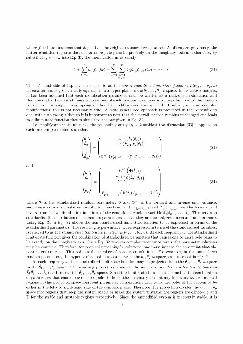
5.2. Example 2: Multiple-rank, multiple-element modification

In this second example, the plunge mass coefficient and the pitch moment of inertia coefficient areuncertain. The structural modification matrix is written as

∆Zs(s, θ) = Mhs2e1e

T1 + Iαs

2e2eT2 (44)

where

eT1 =(1 0

)eT2 =

(0 1

)For the sake of brevity, it is assumed that both random parameters have a normal distribution, with pa-rameters given in Table 2, and are independent of each other.

Parameter Mean Standard Deviation

Mh 0 1.5 kg

Iα 0 0.006 kg m2

Table 2: Uncertain parameters (Example 2).

Using the Sherman-Morrison formula iteratively, the characteristic equation of the modified system is

1 + h11(s)Mhs2 + h22(s)Iαs

2 + mhIαs4 (h11(s)h22(s)− h12(s)h21(s)) = 0

and hence the non-standardised limit-state function is given by

L = 1− h11(iω)Mhω2 − h22(iω)Iαω

2 + mhIαω4 (h11(iω)h22(iω)− h12(iω)h21(iω))

Since the random parameters are already normal, zero-mean, they may be easily standardised according to2

Mh =Mh√

Var[Mh], Iα =

Iα√Var[Iα]

The standardised limit-state function is then found by substituting the above standardised parameters intothe non-standardised limit-state function, so that

L = 1− h11√

Var[Mh]Mhω2 − h22

√Var[Iα]Iαω

2 +

√Var[Mh]Var[Iα]MhIαω

4 (h11h22 − h12h21)

where the receptances are evaluated at s = iω.

The most-probable point θ∗

is found by means of an optimisation problem defined by

minω,Mh,Iα

R =

√M2h + I2α

s.t. L = 0

2It is to be noted that application of the Rosenblatt transformation would yield the same result. However, for the sake ofbrevity, this is not shown.

11

In this work, the TOMLAB Optimisation for MATLAB package was used to solve the constrained, nonlinearoptimisation problem using a gradient-based approach. After 37 iterations, from the initial set (−1, 1, 24)T ,the most-probable point was found to be (−1.122, 1.3244, 22.0572)T , which corresponds to an R value of1.74. Using Eq. 36, the probability of flutter was calculated as 0.0409. The time taken to estimate ofthe probability of flutter depends almost solely on the time taken to find the most probable point. In thisparticular case, the total time taken was 0.23 seconds on a standard desktop computer.

Figure 6 shows the projected, standardised limit-state function for the two random parameters. Between-3 and +3 standard deviations of the random parameters, the projected function is well approximated aslinear and hence the estimate of the probability is likely to be accurate. Also, the most probable point onthe curve, indicated by the red circle, matches that found by the optimisation.

Figure 6: Projected, standardised limit-state function (Example 2).

The results obtained above were verified independently by a Monte-Carlo simulation on the model.Using 1,000,000 samples, the probability of flutter was calculated as 0.0407. This matched closely the valueobtained by a first-order reliability approach, with only a 0.5% error. Overall, the time taken to completethe MCS was 82 seconds, which was significantly greater than that of the first-order reliability method.

6. Experimental case study

6.1. Experimental setup

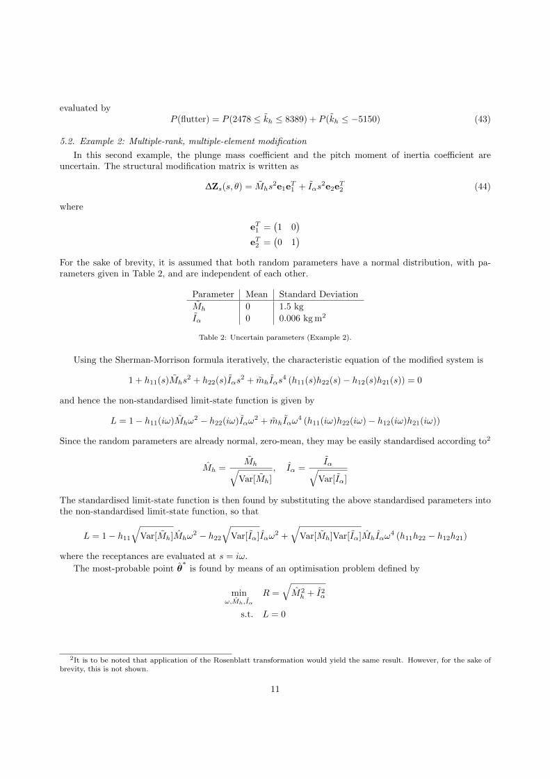
The methods developed were implemented on an experimental pitch-plunge aeroelastic model, which isshown in Fig. 7. The model consists of two main assemblies: i) the aerofoil, which is mounted to a test sectioninside the University of Liverpool’s low-speed wind-tunnel; and ii) the external support structure. Theaerofoil itself consists of five 3D-printed NACA0018 aerodynamic sectors with geometries and arrangementsas shown in Fig. 8. Each sector is connected to two aluminium spars, which run perpendicular to thespan, by bolts located in the centre of each sector. The cross section of each spar is designed so that thereis negligible twisting or bending across the aerofoil. The total span and chord length is 1.2m and 0.3mrespectively. The external support structure consists of a series of vertical and horizontal linkages thatallow the aerofoil to move rigidly in both a vertical, or plunge, motion and a rotational, or pitch, motionabout a so-called elastic axis. Two independent cantilever beams are connected in the pitch and plungedegrees-of-freedom and act as spring elements.

12

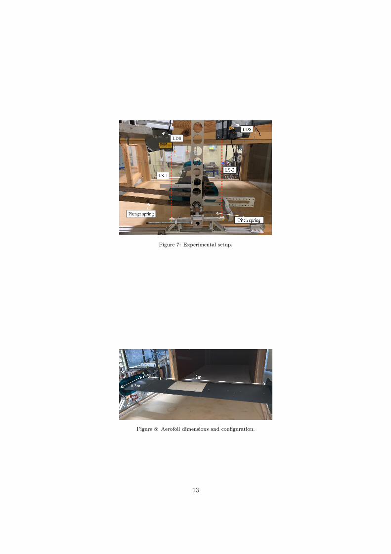
Figure 7: Experimental setup.

Figure 8: Aerofoil dimensions and configuration.

13

Frequency response functions were collected from the system by means of stepped-sine testing between2-7 Hz using an Siemens PLM data acquisition system. A force transducer was attached to the structure attwo points (one after the other) and was connected to an electro-mechanical shaker by means of a stinger,as shown in Fig. 9. The locations of the shaker were chosen so that both the pitch and plunge degreesof freedom were sufficiently excited during testing. Moreover, the use of two input locations allowed forany physical modification to be simulated, as will be demonstrated later. The stinger, which was 1mm indiameter and made from stainless steel, was chosen to minimise the effect of any additional pitch stiffnessintroduced by the attachment of the shaker. At the same locations as the force transducers, two highprecision LK-500 Keyence laser displacement sensors (LDS) were used to read the position of the systemand hence receptances collected were of the form

H(s, v) =

(h11(s, v) h12(s, v)h21(s, v) h22(s, v)

)(45)

where hij(s, v) represents the receptance measurement at laser i due to a force at location j.

Figure 9: Modal shaker, stinger and load cell arrangement for stepped-sine testing.

6.2. Single-rank, single-element modification

6.2.1. Modification model

First, a single-element, rank-one modification was considered. The modification was the addition of a 1kg mass to a fixed bar protruding from the elastic axis, as shown in Fig. 10. The distance from the centreof the mass to the elastic axis was equal to the distance from the elastic axis to the position of the laserreading 2 (LS2). In this way, the modification acted as a point mass collocated with position 2 and thusonly h22(s, v) receptances were required.

From Eq. 15, the scalar modification term is

b(s) = ms2 (46)

and so the modified receptance is related to the original receptance, using the Sherman-Morrison formula,by

h22(s, v) = h22(s, v)− ms2h22(s, v)2

1 +ms2h22(s, v)(47)

where h(s) is the receptance of the modified system and h(s) is the original receptance, before modification.The corresponding frequency response function of the modified system is given by substituting s = iω intoEq. 47.

14

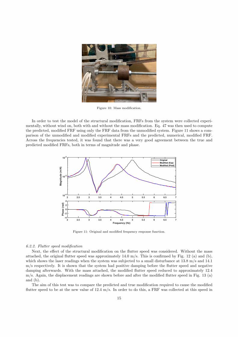
Figure 10: Mass modification.

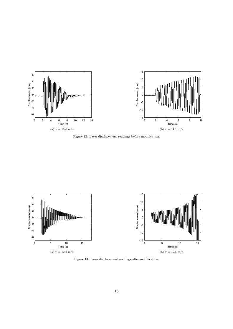
In order to test the model of the structural modification, FRFs from the system were collected experi-mentally, without wind on, both with and without the mass modification. Eq. 47 was then used to computethe predicted, modified FRF using only the FRF data from the unmodified system. Figure 11 shows a com-parison of the unmodified and modified experimental FRFs and the predicted, numerical, modified FRF.Across the frequencies tested, it was found that there was a very good agreement between the true andpredicted modified FRFs, both in terms of magnitude and phase.

2 2.5 3 3.5 4 4.5 5 5.5 6 6.5 710

-4

10-3

10-2

Mag

nit

ud

e (

m/N

)

Original

Modified (Exp)

Modified (Pred)

2 2.5 3 3.5 4 4.5 5 5.5 6 6.5 7

Frequency (Hz)

-4

-2

0

2

4

Ph

ase (

rad

)

Figure 11: Original and modified frequency response function.

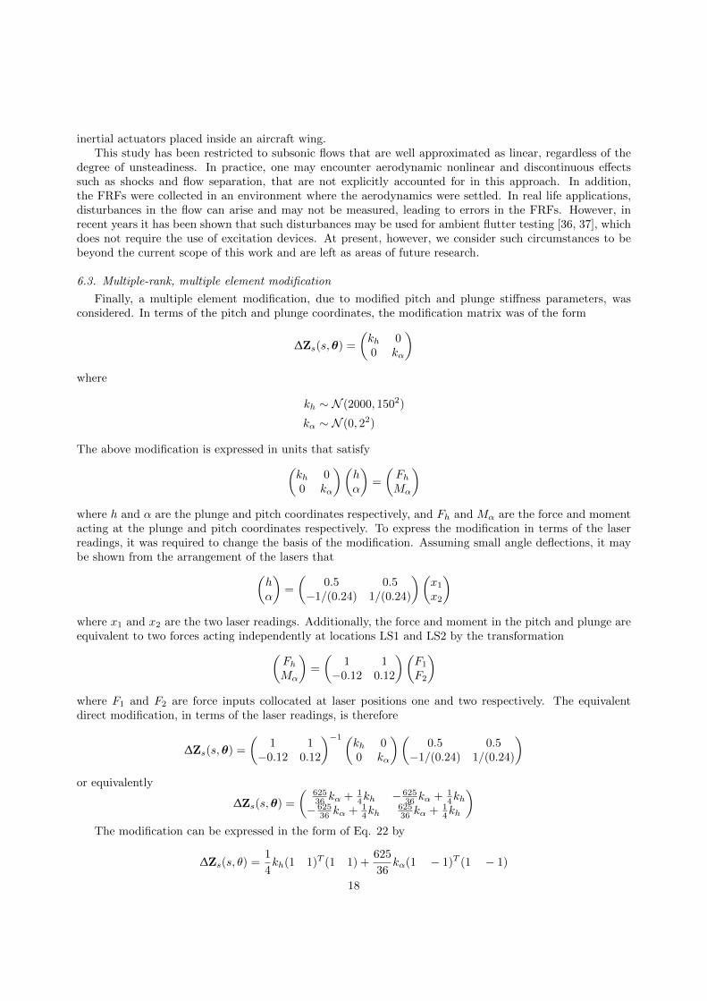
6.2.2. Flutter speed modification

Next, the effect of the structural modification on the flutter speed was considered. Without the massattached, the original flutter speed was approximately 14.0 m/s. This is confirmed by Fig. 12 (a) and (b),which shows the laser readings when the system was subjected to a small disturbance at 13.8 m/s and 14.1m/s respectively. It is shown that the system had positive damping before the flutter speed and negativedamping afterwards. With the mass attached, the modified flutter speed reduced to approximately 12.4m/s. Again, the displacement readings are shown before and after the modified flutter speed in Fig. 13 (a)and (b).

The aim of this test was to compare the predicted and true modification required to cause the modifiedflutter speed to be at the new value of 12.4 m/s. In order to do this, a FRF was collected at this speed in

15

0 2 4 6 8 10 12 14

Time (s)

-6

-4

-2

0

2

4

6

Dis

pla

cem

en

t (m

m)

(a) v = 13.8 m/s

0 2 4 6 8 10

Time (s)

-15

-10

-5

0

5

10

15

Dis

pla

cem

en

t (m

m)

(b) v = 14.1 m/s

Figure 12: Laser displacement readings before modification.

0 5 10 15

Time (s)

-6

-4

-2

0

2

4

6

Dis

pla

cem

en

t (m

m)

(a) v = 12.2 m/s

0 5 10 15

Time (s)

-15

-10

-5

0

5

10

15

Dis

pla

cem

en

t (m

m)

(b) v = 12.5 m/s

Figure 13: Laser displacement readings after modification.

16

the unmodified system and is shown in Fig. 14. According to Eq. 20, the structural modification requiredto cause flutter at this speed is

m =1

ω2h22(iω)

For purely real solutions of the mass modification, it is necessary to choose values of ω for which thereceptance h22(iω) was real; or in other words, the phase of h22(iω) had to be 0 ± nπ. The only valuesof ω for which this was true were 16.7 rad/s (2.66 Hz) and 19.3 rad/s (3.08 Hz). At 19.3 rad/s, the FRFmagnitude was 2.73×10−3m/N and so the predicted mass modification at this frequency was 0.98 kg. Thismatched very closely to the true modification (1 kg), with an error of 2%. It is noted in passing here thatthe other solution, corresponding to 16.7 rad/s, yielded a solution that rendered the system stable again,although this was not considered due to the large mass required (4 kg), which would have damaged the pitchsprings.

2 2.5 3 3.5 4 4.5 5 5.5 6 6.5 710

-4

10-3

10-2

Ma

gn

itu

de

(m

/N)

2 2.5 3 3.5 4 4.5 5 5.5 6 6.5 7

Frequency (Hz)

-4

-2

0

2

4

Ph

as

e (

rad

)

Figure 14: Unmodified receptance at v=12.4 m/s.

Finally, to verify the above solution, a fast Fourier transform (FFT) of the time series corresponding tothe modification at v = 12.5 m/s (Fig. 13 (b)) was computed. As shown in Fig. 15, the peak of the FFT isat 3.31Hz, which gives a 6.9 % error from the predicted frequency of 3.08Hz.

0 1 2 3 4 5 6 7 8 9 10

Frequency (Hz)

0

1

2

3

4

|FF

T| (m

m)

Figure 15: FFT of the time signal of the modified system at v=12.5 m/s.

In this particular example, the shaker used for FRF measurements was placed outside of the wind-tunnel(see Fig. 9) and therefore did not affect the aerodynamics. In practical applications, one may consider using

17

inertial actuators placed inside an aircraft wing.This study has been restricted to subsonic flows that are well approximated as linear, regardless of the

degree of unsteadiness. In practice, one may encounter aerodynamic nonlinear and discontinuous effectssuch as shocks and flow separation, that are not explicitly accounted for in this approach. In addition,the FRFs were collected in an environment where the aerodynamics were settled. In real life applications,disturbances in the flow can arise and may not be measured, leading to errors in the FRFs. However, inrecent years it has been shown that such disturbances may be used for ambient flutter testing [36, 37], whichdoes not require the use of excitation devices. At present, however, we consider such circumstances to bebeyond the current scope of this work and are left as areas of future research.

6.3. Multiple-rank, multiple element modification

Finally, a multiple element modification, due to modified pitch and plunge stiffness parameters, wasconsidered. In terms of the pitch and plunge coordinates, the modification matrix was of the form

∆Zs(s,θ) =

(kh 00 kα

)where

kh ∼ N (2000, 1502)

kα ∼ N (0, 22)

The above modification is expressed in units that satisfy(kh 00 kα

)(hα

)=

(FhMα

)where h and α are the plunge and pitch coordinates respectively, and Fh and Mα are the force and momentacting at the plunge and pitch coordinates respectively. To express the modification in terms of the laserreadings, it was required to change the basis of the modification. Assuming small angle deflections, it maybe shown from the arrangement of the lasers that(

hα

)=

(0.5 0.5

−1/(0.24) 1/(0.24)

)(x1x2

)where x1 and x2 are the two laser readings. Additionally, the force and moment in the pitch and plunge areequivalent to two forces acting independently at locations LS1 and LS2 by the transformation(

FhMα

)=

(1 1

−0.12 0.12

)(F1

F2

)where F1 and F2 are force inputs collocated at laser positions one and two respectively. The equivalentdirect modification, in terms of the laser readings, is therefore

∆Zs(s,θ) =

(1 1

−0.12 0.12

)−1(kh 00 kα

)(0.5 0.5

−1/(0.24) 1/(0.24)

)or equivalently

∆Zs(s,θ) =

(62536 kα + 1

4kh − 62536 kα + 1

4kh− 625

36 kα + 14kh

62536 kα + 1

4kh

)The modification can be expressed in the form of Eq. 22 by

∆Zs(s, θ) =1

4kh(1 1)T (1 1) +

625

36kα(1 − 1)T (1 − 1)

18

and hence the Sherman-Morrison formula was used iteratively to obtain the characteristic equation of themodified system, which was

1 +1

4kh(h11 + h12 + h21 + h22) +

625

36kα(h11 − h12 − h21 + h22) +

625

36kαkh(h11h22 − h12h21) = 0 (48)

The non-standardised limit-state function is then given by evaluating the receptances at s = iω. Thestandardised limit-state function is obtained by first normalising the random variables by

kh =kh − E[kh]√

Var[kh], kα =

kα − E[kα]√Var[kα]

and then substituting this form into the non-standardised limit-state function.Frequency response functions were collected from the unmodified system at 12.4 m/s. Due to measure-

ment noise, the FRFs were fitted with rational transfer functions using SDTools. The measured and fittedFRFs are shown in Fig. 16.

2 3 4 5 6 710-4

10-3

10-2

Mag

nit

ud

e (

m/N

)

Measured

Fitted

2 3 4 5 6 7

Frequency (Hz)

-4

-2

0

Ph

ase (

rad

)

(a) h11

2 3 4 5 6 710-4

10-3

10-2

Mag

nit

ud

e (

m/N

)

2 3 4 5 6 7

Frequency (Hz)

-10123

Ph

ase (

rad

)

(b) h12

2 3 4 5 6 7

10-4

10-2

Mag

nit

ud

e (

m/N

)

2 3 4 5 6 7

Frequency (Hz)

-4-2024

Ph

ase (

rad

)

(c) h21

2 3 4 5 6 710-4

10-3

10-2

Ma

gn

itu

de (

m/N

)

2 3 4 5 6 7

Frequency (Hz)

-4

-2

0

2

Ph

ase (

rad

)

(d) h22

Figure 16: Measured and fitted FRFs at v = 12.4 m/s.

The projected, standardised limit-state function is illustrated in Fig. 17. As shown, the projectedfunction is well approximated by a first-order approximation and thus it is concluded that a first-orderreliability method will give a reasonably accurate prediction of the probability of flutter.

Using the same optimisation procedure as in Section 5.2, the most-probable point (MPP) is found to be(0.1509,−1.7237, 22.6862)T , which matches that obtained from Fig. 17. The R value at the MPP is 1.73 andtherefore the probability of flutter is calculated as 0.0418. We note in passing here that this result cannot

19

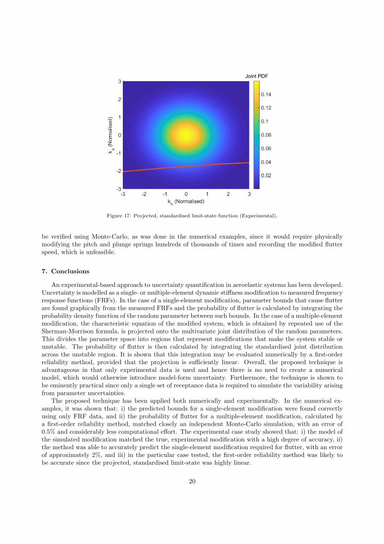
Figure 17: Projected, standardised limit-state function (Experimental).

be verified using Monte-Carlo, as was done in the numerical examples, since it would require physicallymodifying the pitch and plunge springs hundreds of thousands of times and recording the modified flutterspeed, which is unfeasible.

7. Conclusions

An experimental-based approach to uncertainty quantification in aeroelastic systems has been developed.Uncertainty is modelled as a single- or multiple-element dynamic stiffness modification to measured frequencyresponse functions (FRFs). In the case of a single-element modification, parameter bounds that cause flutterare found graphically from the measured FRFs and the probability of flutter is calculated by integrating theprobability density function of the random parameter between such bounds. In the case of a multiple-elementmodification, the characteristic equation of the modified system, which is obtained by repeated use of theSherman-Morrison formula, is projected onto the multivariate joint distribution of the random parameters.This divides the parameter space into regions that represent modifications that make the system stable orunstable. The probability of flutter is then calculated by integrating the standardised joint distributionacross the unstable region. It is shown that this integration may be evaluated numerically by a first-orderreliability method, provided that the projection is sufficiently linear. Overall, the proposed technique isadvantageous in that only experimental data is used and hence there is no need to create a numericalmodel, which would otherwise introduce model-form uncertainty. Furthermore, the technique is shown tobe eminently practical since only a single set of receptance data is required to simulate the variability arisingfrom parameter uncertainties.

The proposed technique has been applied both numerically and experimentally. In the numerical ex-amples, it was shown that: i) the predicted bounds for a single-element modification were found correctlyusing only FRF data, and ii) the probability of flutter for a multiple-element modification, calculated bya first-order reliability method, matched closely an independent Monte-Carlo simulation, with an error of0.5% and considerably less computational effort. The experimental case study showed that: i) the model ofthe simulated modification matched the true, experimental modification with a high degree of accuracy, ii)the method was able to accurately predict the single-element modification required for flutter, with an errorof approximately 2%, and iii) in the particular case tested, the first-order reliability method was likely tobe accurate since the projected, standardised limit-state was highly linear.

20

In this research, it has been assumed that the system is linear, both in terms of the structure andaerodynamics. In real-life systems this may not be true and the measured FRFs could exhibit nonlinearbehaviour. The effect of this, and potential solutions, will be considered in future research.

Acknowledgements

The authors gratefully acknowledge the financial support provided by the Engineering and PhysicalSciences Research Council (EPSRC) grant EP/N017897/1. LJA also acknowledges the support provided bythe Engineering and Physical Sciences Research Council (EPSRC) Doctoral Training Scholarship.

Appendix - Generalised modification theory

Let the modification matrix be decomposed as the sum of contributory matrices that are functions ofeach random parameter, so that

∆Zs(s,θ) =

p∑i=1

∆Zs(s, θi) (A.1)

In general, the modification belonging to each parameter θi is rank-m (1 ≤ m ≤ n). However, they may beseparated into the sum of contributory rank-one elements by

∆Zs(s, θi) =

ni∑j=1

hi,j(θi)gi,j(s)ei,jeTi,j (A.2)

where ni is the total number of rank-one decompositions of each matrix ∆Zs(s, θi) and hi,j(θi) is some,potentially nonlinear, function of the random parameter. This leads to the general form

∆Zs(s,θ) =

p∑i=1

ni∑j=1

hi,j(θi)gi,j(s)ei,jeTi,j (A.3)

which is the sum of rank-one modifications. One may now proceed with the analysis presented in Section 4but noting, however, that the new limit state function is now of the form

1 +

N∑i1=1

hi1(θ)fi1(iω) +

N∑i1=1

N∑i2=1i2 6=i1

hi1(θ)hi2(θ)fi1,i2(iω) + · · · = 0 (A.4)

where N is the total number of rank-one modifications.

References

[1] E. Livne, Future of Airplane Aeroelasticity, Journal of Aircraft 40 (6) (2008) 1066–1092 (2008).[2] P. P. Friedmann, Renaissance of Aeroelasticity and Its Future, Journal of Aircraft 36 (1) (1999) 105–121 (1999).[3] E. H. Dowell, A Modern Course in Aeroelasticity, 5th Edition, Vol. 217 of Solid Mechanics and Its Applications, Springer,

2015 (2015).[4] D. H. Hodges, G. A. Pierce, Introduction to Structural Dynamics and Aeroelasticity, 2nd Edition, Cambridge University

Press, Cambridge, 2011 (2011).[5] J. R. Wright, J. E. Cooper, Introduction to Aeroelasticity and Loads, 2nd Edition, Wiley, Chichester, 2014 (2014).[6] H. J. Hassig, An approximate true damping solution of the flutter equation by determinant iteration., Journal of Aircraft

8 (11) (1971) 885–889 (1971).[7] Y. Dai, C. Yang, Methods and advances in the study of aeroelasticity with uncertainties, Chinese Journal of Aeronautics

27 (3) (2014) 461–474 (2014).[8] C. L. Pettit, Uncertainty Quantification in Aeroelasticity: Recent Results and Research Challenges, Journal of Aircraft

41 (5) (2004) 1217–1229 (2004).

21

[9] P. Beran, B. Stanford, Uncertainty Quantification in Aeroelasticity, in: H. Bijl, D. Lucor, S. Mishra, C. Schwab (Eds.),Lecture Notes in Computational Science and Engineering, Springer, Cham, 2013, Ch. Uncertaint, pp. 59–103 (2013).

[10] P. Beran, B. Stanford, C. Schrock, Uncertainty Quantification in Aeroelasticity, Annual Review of Fluid Mechanics 49 (1)(2016) 361–386 (2016).

[11] J.-C. Chassaing, C. T. Nitschke, A. Vincenti, P. Cinnella, D. Lucor, Advances in parametric and model-form uncertaintyquantification in canonical aeroelastic systems, Journal AerospaceLab ONERA 14 (14) (2018) 1–19 (2018).

[12] S. C. Castravete, R. A. Ibrahim, Effect of Stiffness Uncertainties on the Flutter of a Cantilever Wing, AIAA Journal 46 (4)(2008) 925–935 (2008).

[13] H. H. Khodaparast, J. E. Mottershead, K. J. Badcock, Propagation of structural uncertainty to linear aeroelastic stability,Computers and Structures 88 (3-4) (2010) 223–236 (2010).

[14] A. Manan, J. Cooper, Design of Composite Wings Including Uncertainties: A Probabilistic Approach, Journal of Aircraft46 (2) (2009) 601–607 (2009).

[15] C. Scarth, J. E. Cooper, P. M. Weaver, G. H. Silva, Uncertainty quantification of aeroelastic stability of composite platewings using lamination parameters, Composite Structures 116 (1) (2014) 84–93 (2014).

[16] G. Georgiou, A. Manan, J. E. Cooper, Modeling composite wing aeroelastic behavior with uncertain damage severity andmaterial properties, Mechanical Systems and Signal Processing 32 (2012) 32–43 (2012).

[17] M. Allen, K. Maute, Reliability-based design optimization of aeroelastic structures, Structural and MultidisciplinaryOptimization 27 (4) (2004) 228–242 (2004).

[18] M. Nikbay, M. N. Kuru, Reliability Based Multidisciplinary Optimization of Aeroelastic Systems with Structural andAerodynamic Uncertainties, Journal of Aircraft 50 (3) (2013) 708–715 (2013).

[19] J. E. Mottershead, Y. M. Ram, Inverse eigenvalue problems in vibration absorption: Passive modification and activecontrol, Mechanical Systems and Signal Processing 20 (1) (2006) 5–44 (2006).

[20] I. Bucher, S. Braun, The structural modification inverse problem: an exact solution, Mechanical Systems and SignalProcessing 7 (3) (1992) 217–238 (1992).

[21] Y. M. Ram, J. J. Blech, The dynamic behavior of a vibratory system after modification, Journal of Sound and Vibration150 (3) (1991) 357–370 (1991).

[22] S. H. Tsai, H. Ouyang, J. Y. Chang, Inverse structural modifications of a geared rotor-bearing system for frequencyassignment using measured receptances, Mechanical Systems and Signal Processing 110 (2018) 59–72 (2018).

[23] J. He, Structural modification, Philosophical Transactions: Mathematical, Physical and Engineering Sciences 359 (1778)(2001) 187–204 (2001).

[24] J. T. Weissenburger, Effect of Local Modifications on the Vibration Characteristics of Linear Systems, Journal of AppliedMechanics 35 (2) (1967) 327–332 (1967).

[25] A. Kyprianou, J. E. Mottershead, H. Ouyang, Structural modification. Part 2: Assignment of natural frequencies andantiresonances by an added beam, Journal of Sound and Vibration 284 (1-2) (2005) 267–281 (2005).

[26] D. J. Ewins, Modal Testing: Theory, Practice and Application, 2nd Edition, Research Studies Press, Baldock, Hertford-shire, England, 2000 (2000).

[27] L. J. Adamson, S. Fichera, B. Mokrani, J. E. Mottershead, Pole placement in uncertain dynamic systems by varianceminimisation, Mechanical Systems and Signal Processing 127 (2019) 290–305 (2019).

[28] J. Sherman, W. Morrison, Adjustment of an inverse matrix corresponding to a change in one element of a given matrix,The Annals of Mathematical Statistics 21 (1) (1950) 124–127 (1950).

[29] S.-K. Choi, R. V. Grandhi, R. A. Canfield, Reliability-based Structural Design, Springer, London, 2007 (2007).[30] K. L. Roger, Airplane math modelling methods for active control design, Tech. rep., AGARD (1977).[31] Aeroelastic Stability Substantiation of Transport Category Airplanes (AC 25.629-1B), Tech. rep., Federal Aviation Ad-

ministration (2014).[32] G. H. Golub, C. F. Van Loan, Matrix Computations, 4th Edition, The John Hopkins University Press, Baltimore, Mary-

land, 2013 (2013).[33] M. Rosenblatt, Remarks on a Multivariate Transformation, The Annals of Mathematical Statistics 23 (3) (1952) 470–472

(1952).[34] T. Theodorsen, General Theory of Aerodynamic Instability and the Mechanism of Flutter, Tech. rep., National Advisory

Committee for Aeronautics (1949).[35] R. T. Jones, Operational treatment of the nonuniform-lift theory in airplane dynamics, Tech. rep., National Advisory

Committee for Aeronautics (1938).[36] J. Cooper, Flutter testing using ambient excitation, in: Proceedings of ISMA 2018 - International Conference on Noise

and Vibration Engineering and USD 2018 - International Conference on Uncertainty in Structural Dynamics, 2018, pp.3353–3364 (2018).

[37] G. Jelicic, J. Schwochow, Y. Govers, A. Hebler, M. Boswald, Real-time assessment of flutter stability based on automatedoutput-only modal analysis, in: Proceedings of ISMA 2014 - International Conference on Noise and Vibration Engineeringand USD 2014 - International Conference on Uncertainty in Structural Dynamics, 2014, pp. 3633–3646 (2014).

22