Fluid structure interaction (FSI) of the left ventricle (LV) in ...

Fluid Structure Interaction (FSI) of the

Left Ventricle (LV) in Developing the

Next Generation Ventricular Assist

Device (VAD) System

A thesis submitted in fulfilments of the requirements for

the degree of

Doctor of Philosophy

By

MD. SHAMSUL AREFIN

Faculty of Science, Engineering and Technology

Bio-mechanical and Tissue Engineering Group

Swinburne University of Technology

2015

II

ABSTRACT

This thesis represents the formal documentation for a Doctoral research program

undertaken at the Swinburne University of Technology in Melbourne Australia,

between the years of 2011 and 2014. The broad objective of the Doctoral research was

to apply innovative engineering approaches to analyze the Left Ventricle (LV) of the

human heart in order to provide the underpinning knowledge required to develop a

"next generation" Ventricular Assist Device (VAD). Also, it was possible to gain better

understanding of the dynamics of the LV (filling phase) for the first time by numerical

modelling based on general conditions, by varying the angles between the aortic and

mitral orifices and by applying the elastic modulus and friction co-efficient.

It was well established that a lack of natural blood circulation resulted in various cardiac

diseases. These diseases indisputably influenced the overall functionalities of the

cardiac structure and were a primary factor in cardiac related mortality. The LV of the

heart is its most significant compartment which helps circulate blood to the end organs

of the body. However, the natural performance of the LV decays due to aging and/or

weakened heart muscles and hence, various cardiac diseases can arise. In general, in

these circumstances the treatments in common use at the time this research commenced

were based on the use of ventricular assist devices (VADs), which were implanted

within patients. Over the years, research had demonstrated significant improvements in

VADs but various limitations still resulted in developing diseases/infections inside

patients. The literature review undertaken in this Doctoral program uncovered no

evidence of VADs that could prevent infections from arising.

In this Doctoral research, the long term focus was on providing the underlying

engineering analysis that would facilitate the development of a “next generation VAD”

which would be highly flexible and be able minimize potential complications -

specifically diseases and infections. In order to develop a next generation VAD, it was

critically important to determine the hemodynamic forces and structural

deformation/displacement of the LV during various physiological conditions. Moreover,

to achieve this, the reviewed research literature indicated that the utilization of a

numerical technique could provide an ideal tool to determine these properties. Hence,

III

the prime focus of this Doctoral research was eyed on the numerical investigations

required to determine hemodynamic parameters and the structural changes in a

"physiologically correct" LV model.

The Fluid Structure Interaction (FSI) scheme was determined to be an appropriate

means of investigating and determining the functionalities of the LV during various

physiological conditions. Hemodynamic features, such as:

• The flow pattern, including the vortex characteristics

• Changes in the intraventricular pressure (Ip)

• Wall Shear Stress (WSS) distributions

• Structural changes, using Total Mesh Displacement (TMD)

could be determined readily via this numerical technique, and in a cost-effective

manner. Once these values are determined they can then be incorporated into a

prototype of a next generation VAD. This prototype can successfully impersonate the

synchronization of the natural heartbeat.

In order to gain a greater understanding of the analysis prior to application into an LV

model, the numerical technique was initially applied to:

• The Internal Thoracic Artery- Left Anterior Descending (ITA-LAD) bypass

graft by varying the degrees of LAD-stenosis (0%, 30%, 50% and 75%)

• An Abdominal Aortic Aneurysm (AAA)

The application of the FSI technique in these two models (ITA-LAD and AAA)

generated substantial knowledge on the utilization of grid independency testing; suitable

boundary conditions, and different flow properties. This knowledge and data were then

applied on the LV model.

The FSI technique was then applied to an anatomically correct 3D LV model during the

filling phase. In doing so, Navier-Stoke’s equations and Arbitrary Lagrangian Eulerian

IV

(ALE) methods were coupled for the fluid and solid domains of the ventricle model.

Subsequently, hemodynamic parameters, such as:

• Velocity mapping including the vortex characteristics

• WSS distributions

• Ip distributions

• TMD distributions

were investigated and determined. In this thesis, the results are then presented, including

a discussion on how these parameters can influence the LV during diastole. Also, these

substantial findings were effective in understanding the natural rhythm of the LV and

would be important to the development of a next generation VAD device.

Simulations were also executed on the LV model by varying the angles between the

mitral and aortic orifices (50°, 55° and 60°) during the filling phase. Similar boundary

conditions and mathematical approaches were utilized to investigate and determine the

hemodynamic parameters and structural changes of the LV. These findings from this

thesis are novel and have not been investigated before, would be particularly useful in

the development of a next generation VAD.

The influences of the friction co-efficient and elastic modulus of the 3D LV model

during diastole were also investigated. Additionally, required mathematical approaches

and computational procedures were applied to study the hemodynamics and

physiological variations of the structure. Also, by varying the friction co-efficient and

elastic modulus for the first time to the best of our knowledge, Dilated Cardiomyopathy

(DCM) - a critical heart disease - could potentially be identified. Knowledge of this

disease condition would provide valuable data in developing a VAD device.

Overall, all the simulations were analyzed in detail and validated against previously

published research. Finally, overall conclusions are presented in this thesis, together

with potential future research directions.

V

ACKNOWLEDGEMENTS

I would like to express my gratitude to my principal co-ordinating supervisor Professor

Yosry Morsi, for his encouragement, inspiration, guidance and advice during the entire

research project. It would have been impossible to complete the work without his clear

supervision. Also, it has been my honour to work beside him and I am very grateful for

his support throughout the research. I would also like to thank my co-supervisor

Associate Professor Richard Manasseh for his valuable suggestions during my research.

Special thanks to two undergraduate group students, composed of students Wajid

Baryalai, Yining Wang, Abdul A. AlMalki, Majid B. Masoud, Ahmed S. Alrashdi,

Abdulhakim S. Almutarrid, Ahmed A. Aldhahri and Khaled A. Alenezi for their efforts

and help in developing a model/prototype of the next generation VAD device.

I am extremely thankful to Swinburne University of Technology for supporting me

financially by means of scholarship during my research.

Also, I would like to convey my gratitude to my colleagues, especially Himani

Mazumder and Arafat Ahmed for their assistance in technical knowledge and software

proficiency throughout the research.

Last but not the least, I would like to convey my gratitude to all my friends in the

biomechanical and tissue engineering group researchers whose friendship and assistance

alleviated my work and made my time enjoyable.

Finally, I also wish to convey my perpetual gratitude to my mother, father, brothers and

other family members for their everlasting support and belief during my research

program.

VI

This Thesis is Dedicated to

My Beloved Parents & Brothers

VII

DECLARATION

I declare that this thesis represents my own work and contains no material which has

been accepted for the award of any other degree, diploma or qualification in any

university except where due reference has been made in the text of the dissertation. To

the best of my knowledge and belief this thesis contains no material published or

written by other person except where due acknowledgement has been made.

Signed: …………………………… Date:

MD. SHAMSUL AREFIN

VIII

TABLE OF CONTENTS

ABSTRACT ..................................................................................................................... II

ACKNOWLEDGEMENTS ............................................................................................. V

DECLARATION .......................................................................................................... VII

TABLE OF CONTENTS ............................................................................................. VIII

LIST OF FIGURES ...................................................................................................... XV

LIST OF TABLES .................................................................................................... XVIII

LIST OF ABBREVIATIONS ....................................................................................... XX

Chapter 1 ........................................................................................................................... 1

Introduction ................................................................................................................... 1

1.1 Objectives of the Thesis ...................................................................................... 2

1.2 Detailed Background Study ................................................................................ 3

1.2.1 General .................................................................................................... 3

1.2.2 Overview of Cardiac Structure ................................................................ 3

1.2.3 Overview of Blood Flow ......................................................................... 5

1.2.4 Overview of Cardiac Cycle ..................................................................... 7

1.2.4.1 General ............................................................................................... 7

1.2.4.2 First Diastole Phase ............................................................................ 8

1.2.4.3 First Systole Phase .............................................................................. 8

1.2.4.4 Second Diastole Phase ........................................................................ 9

1.2.4.5 Second Systole Phase ......................................................................... 9

1.2.5 Synopsis of Heart Valves and its Diseases ............................................ 12

1.2.6 Synopsis of Arterial System .................................................................. 16

1.2.7 Overview of Cardiovascular Diseases (CVD) ....................................... 17

1.2.7.1 General Discussion ........................................................................... 17

1.2.7.2 Heart Failure ..................................................................................... 18

1.2.7.3 Coronary Heart Disease (CHD) ........................................................ 20

1.2.8 Current Treatments for Heart Diseases ................................................. 21

1.2.9 Overview of Ventricular Assist Devices (VADs) ................................. 23

1.2.10 Limitations of the Existing VAD System Technologies ................... 25

IX

1.2.11 Recent Advancements of the VAD Devices and the Need for A "Next

Generation" VAD System ................................................................................... 26

1.3 Specific Objectives of the Research.................................................................. 30

1.4 Overview of Methodology and Experimentation Methods .............................. 32

1.5 Specific Contributions of Research Program .................................................... 34

1.6 Structure of Thesis ............................................................................................ 35

Chapter 2 ......................................................................................................................... 37

Literature Review into the Left Ventricle: Experimental and Computational Approaches .................................................................................................................. 37

2.1 Overview ........................................................................................................... 38

2.2 Introduction ....................................................................................................... 40

2.3 Analysis on the Experimental Approaches of LV ............................................ 43

2.4 Analysis of Numerical Approaches using CFD/FSI for an Ideal LV ............... 55

2.5 Analysis of Experimental and Computational Approaches of the Diseased LV:

Dilated Cardiomyopathy (DCM) ............................................................................ 73

2.6 Summary ........................................................................................................... 82

Chapter 3 ......................................................................................................................... 84

Numerical Experimentation of Coronary Artery Bypass Graft and Abdominal Aortic Aneurysm Model ......................................................................................................... 84

3.1 Overview ........................................................................................................... 85

3.2 Review of Literature pertaining to the Bypass Graft ........................................ 86

3.3 Mathematical Procedure, Solver and Output Settings ...................................... 90

3.4 Case Study I: ITA-LAD Bypass Graft .............................................................. 94

3.4.1 Geometry ............................................................................................... 94

3.4.2 Meshing Configurations and Mesh Independency Testing ................... 96

3.4.3 Required Boundary Conditions ............................................................. 97

3.4.4 Simulation Results ............................................................................... 100

3.4.4.1 Velocity Distributions .................................................................... 100

3.4.4.2 Wall Shear Stress (WSS) Distributions .......................................... 107

3.4.4.3 Spatial Wall Shear Stress (WSS) Distributions .............................. 113

3.4.4.4 Structure Simulation using Total Mesh Displacement (TMD) ...... 119

3.4.5 Discussions on ITA-LAD for different degree of LAD-stenosis ........ 124

X

3.4.5.1 Variations of the hemodynamics inside the bypass graft using

velocity mapping ........................................................................................... 124

3.4.5.2 The effects of Wall Shear Stress (WSS) inside the bypass graft using

WSS distributions.......................................................................................... 126

3.4.5.3 The effects of the wall shear stress (WSS) inside the bypass graft

using spatial wall shear stress (WSS) distributions....................................... 127

3.4.5.4 Structure simulation of the bypass graft for different degree of LAD-

stenosis using total mesh displacement (TMD) ............................................ 128

3.5 Abdominal Aortic Aneurysm (AAA) ............................................................. 130

3.6 Literature Review of Abdominal Aortic Aneurysm (AAA) ........................... 132

3.7 Case Study II: abdominal aortic aneurysm (AAA) ......................................... 136

3.7.1 Geometry ............................................................................................. 136

3.7.2 Meshing Configurations and Mesh Independency Testing ................. 138

3.7.3 Required Boundary Conditions ........................................................... 139

3.7.4 Simulation Results ............................................................................... 141

3.7.4.1 Velocity Mapping ........................................................................... 141

3.7.4.2 Wall shear stress (WSS) distributions ............................................ 144

3.7.4.3 Total mesh displacement (TMD) distributions............................... 146

3.7.5 Discussion ........................................................................................... 149

3.7.5.1 Influence of flow dynamics of the AAA using velocity vectors .... 149

3.7.5.2 Influence of wall shear stress (WSS) of the AAA using WSS

distributions ................................................................................................... 150

3.7.5.3 Influence of the structral displacement of the AAA using total mesh

displacemnt (TMD) distributions .................................................................. 152

3.8 Summary of Results and Conclusions ............................................................ 154

Chapter 4 ....................................................................................................................... 156

Numerical Studies of the Left Ventricle during Diastole Phase: General Conditions ................................................................................................................................... 156

4.1 Overview ......................................................................................................... 157

4.2 Introduction ..................................................................................................... 158

4.3 Computational Approaches ............................................................................. 159

4.3.1 Overview ............................................................................................. 159

XI

4.3.2 Geometry ............................................................................................. 159

4.3.3 Meshing Information and Mesh Independency Trials ........................ 162

4.3.4 Required Boundary Conditions ........................................................... 163

4.4 Simulation Results and Discussions ............................................................... 165

4.4.1 Overview ............................................................................................. 165

4.4.2 Distributions of Pressure ..................................................................... 165

4.4.3 Distributions of Wall Shear Stress (WSS) .......................................... 172

4.4.4 Distributions of Velocity ..................................................................... 177

4.4.5 Structure Simulation using Total Mesh Displacement (TMD) ........... 186

4.5 Summary ......................................................................................................... 192

Chapter 5 ....................................................................................................................... 194

Numerical Analysis of the Left Ventricle during Diastole Phase: Angular Variations between the Mitral and Aortic Orifice ...................................................................... 194

5.1 Overview ......................................................................................................... 195

5.2 Introduction ..................................................................................................... 196


5.3.1 Overview ............................................................................................. 197

5.3.2 Geometry Extraction ........................................................................... 197

5.3.3 Meshing Statistics and Mesh Independency Trials ............................. 199

5.3.3 Boundary Conditions ........................................................................... 201

5.4 Simulation Results .......................................................................................... 202

5.4.1 Overview ............................................................................................. 202

5.4.2 Distributions of Velocity ..................................................................... 202

5.4.2.1 Angular Difference of 50° .............................................................. 202



5.4.3 Wall Shear Stress (WSS) Distributions ............................................... 216




XII

5.4.4 Distributions of Pressure ..................................................................... 228




5.4.5 Structure Simulations using Total Mesh Displacement (TMD) .......... 242




5.5 Discussion ....................................................................................................... 257

5.5.1 Influence of flow dynamics for 50°, 55° and 60° between the mitral and

aortic orifice using velocity mapping ................................................................ 257

5.5.2 Influence of intra-ventricular wall shear stress (WSS) for 50°, 55° and

60° between the mitral and aortic orifice using WSS distributions .................. 258

5.5.3 Influence of intra-ventricular pressure (Ip) for 50°, 55° and 60° between

the mitral and aortic orifice using pressure distributions .................................. 260

5.5.4 Influence of structure simulation for 50°, 55° and 60° between the

mitral and aortic orifice using total mesh displacement (TMD) ....................... 261

5.6 Summary ......................................................................................................... 263

Chapter 6 ....................................................................................................................... 265

Numerical Analysis of the Left Ventricle during Diastole Phase: The Influence of Friction Co-efficient and Elastic Modulus ................................................................ 265

6.1 Overview ......................................................................................................... 266

6.2 Introduction ..................................................................................................... 267


6.3.1 Geometry Extraction ........................................................................... 268

6.3.2 Meshing Statistics and Mesh Independency Trials ............................. 268

6.3.3 Boundary Conditions ........................................................................... 270

6.4 Simulation Results .......................................................................................... 273

6.4.1 Overview ............................................................................................. 273

6.4.2 The influence of friction coefficient and elastic modulus of the LV

using wall shear stress (WSS) distributions ...................................................... 273

XIII

6.4.2.1 Elastic modulus of 0.35 MPa ......................................................... 273

6.4.2.2 Elastic modulus of 0.7 MPa ........................................................... 276


6.4.3 The influence of friction coefficient and elastic modulus using

intraventricular pressure (Ip) distributions ........................................................ 281




6.4.4 The influence of friction coefficient and elastic modulus using velocity

mapping ............................................................................................................. 289


6.4.4.2 Elastic modulus of 0.7MPa ............................................................ 292


6.4.5 The influence of friction coefficient and elastic modulus structure

simulation using total mesh displacement (TMD) ............................................ 297

6.4.5.1 Elastic modulus of 0.35MPa .......................................................... 297

6.4.5.2 Elastic modulus of 0.7MPa ............................................................ 299


6.5 Discussion ....................................................................................................... 303

6.5.1 The influence of Cf and elastic modulus on the LV using WSS

distributions ....................................................................................................... 303

6.5.2 The influence of Cf and elastic modulus on the LV using Ip

distributions ....................................................................................................... 305

6.5.3 The influence of Cf and elastic modulus on the LV using velocity

mapping ............................................................................................................. 306

6.5.4 The influence of Cf and elastic modulus on the LV structure simulation

using total mesh displacement (TMD) .............................................................. 308

6.6 Summary ......................................................................................................... 310

Chapter 7 ....................................................................................................................... 312

Conclusions and Future Directions ........................................................................... 312

7.1 Overall Conclusions of the Dissertation ......................................................... 313

7.2 Clinical Implications ....................................................................................... 318

XIV

7.2.1 Overview ............................................................................................. 318

7.2.2 Significance of the next generation VAD system ............................... 318

7.2.3 Significance of the CABG and aortic aneurysm models ..................... 319

7.2.4 Significance of the LV model.............................................................. 320

7.3 Future Directions and Recommendations ....................................................... 323

7.3.1 Overview ............................................................................................. 323

7.3.2 Experimental Requirements for VAD Prototype [including the works

from two undergraduate groups] ....................................................................... 323

7.3.3 Experimental Requirements of the LV Model .................................... 324

7.3.4 Computational and Experimental Requirements of the CABG and

Aortic Aneurysm Model ................................................................................... 325

7.3.5 Computational Requirements of the LV Model .................................. 327

Appendix ....................................................................................................................... 329

1. Variations in the velocity distributions of AAA ............................................... 329

2. Variations in the WSS of AAA ......................................................................... 330

3. Variations in the structural displacement using TMD of AAA ........................ 331

4. Experimental VAD prototype design – using DC motor and wireless technology

............................................................................................................................... 332

5. Experimental VAD prototype design – using steel wings and wireless

technology ............................................................................................................. 333

List of Publications ....................................................................................................... 335

XV

LIST OF FIGURES

Figure 1.1 Major elements of the human heart (Bianco, 2000) .................................... 4

Figure 1.2 Human heart (Medic, 2011) .......................................................................... 5

Figure 1.3 Cross-section of the heart for different pressure values (Laizzo, 2009,

Dreamstime, 2013) ........................................................................................................... 6

Figure 1.4 Blood flow pattern (Bailey, 2011).................................................................. 8

Figure 1.5 Cardiac cycles (Physiology, 2013) ............................................................... 10

Figure 1.6 Left ventricle volume and pressure (Klabunde, 2011)................................ 11

Figure 1.7 Illustration of heart valves (Sentara, 2014) ................................................ 13

Figure 1.8 Illustration of the main layers of the coronary artery (Do, 2012) ............. 17

Figure 1.9 Illustration of heart failure (Mattox, 2013) ................................................ 19

Figure 1.10 Coronary disease (Health, 2012) ............................................................... 21

Figure 1.11 Illustration of heart transplant (Staff, 2012) ............................................ 22

Figure 1.12 Left Ventricular Assist Device (Bouthillet, 2011) ..................................... 23

Figure 1.13 The MYO-VAD (Ostrovsky, 2006)............................................................. 28

Figure 3.1 Illustration of the flow chart utilized during the entire simulation

procedure (Arefin and Morsi, 2014, Owida et al., 2012) .............................................. 93

Figure 3.2 Cross sectional view of the ITA-LAD bypass graft (75% LAD-stenosis) (a):

Ideal 3D model (SolidWorks 2012) (b): The model utilized in simulations (SolidWorks

2012) ............................................................................................................................... 95

Figure 3.3 Meshing independency testing .................................................................... 97

Figure 3.4 Inlet velocities for the ITA-LAD bypass graft (Ding et al., 2012) .............. 98

Figure 3.5 Velocity mapping of the ITA-LAD bypass graft for the (a) 0%, (b) 30%, (c)

50% and (d) 75%LAD-stenosis .................................................................................... 105

Figure 3.6 Distributions of WSS for different degrees of LAD-stenosis (0%, 30%, 50%

and 75%) ....................................................................................................................... 111

Figure 3.7 Spatial WSS distributions using Line A, Line B and line C .................... 113

Figure 3.8 Spatial WSS distributions of Line A, Line B and Line C for (a) 0% (b) 30%

(c) 50% and (d) 75% LAD-stenosis ............................................................................. 117

Figure 3.9 Structure simulation using total mesh displacement (TMD) for (a) 0% (b)

30% (c) 50% and (d) 75% LAD-stenosis ..................................................................... 122

Figure 3.10 Location of abdominal aortic aneurysm (AAA) (Stern) ......................... 131

XVI

Figure 3.11 (a) Cross-sectional geometry of an axisymmetric AAA (using SolidWorks

2012) (b) Detailed dimensions of the AAA (using SolidWorks 2012) (Li, 2005) ....... 137

Figure 3.12 Mesh independency testing using line control properties ...................... 139

Figure 3.13 Inlet velocity waveform (Li, 2005) ........................................................... 140

Figure 3.14 Actual outlet pressure waveform (Li, 2005) ............................................ 140

Figure 3.15 Simplified outlet pressure waveform utilized in the simulations ........... 140

Figure 3.16 Velocity distributions of the AAA in different time steps ....................... 143

Figure 3.17 WSS distributions of the AAA in different time steps ............................. 145

Figure 3.18 Structural displacement using total mesh displacement (TMD)

distributions .................................................................................................................. 148

Figure 4.1 (a) Dimensions of the LV used for the simulations (SolidWorks 2010) (b)

Geometric construction of the LV model (SolidWorks 2010) (Arefin and Morsi, 2014)

....................................................................................................................................... 161

Figure 4.2 Mesh independency trials (Arefin and Morsi, 2014) ................................ 163

Figure 4.3 Transmitral flow velocity (U) against time (t) waveform, implemented in

the inlet region (Arefin and Morsi, 2014) ................................................................... 164

Figure 4.4 Changes in the Ip for various time steps during diastolic flow conditions

(Arefin and Morsi, 2014) ............................................................................................. 169

Figure 4.5 Distributions of WSS during the filling phase .......................................... 175

Figure 4.6 Illustration of velocity distributions during diastolic flow conditions

(Arefin and Morsi, 2014) ............................................................................................. 184

Figure 4.7 Illustration of total mesh displacement (TMD) during diastolic flow

conditions (Arefin and Morsi, 2014) ........................................................................... 190

Figure 5.1 LV Model with the angular differences of (a) 50°, (b) 55° and (c) 60°

between the inlet and outlet (SolidWorks 2012) .......................................................... 199

Figure 5.2 Mesh independency trial using fluid flow velocity ................................... 200

Figure 5.3 Velocity mapping for the angular difference of 50° ................................. 206



Figure 5.6 Wall shear stress (WSS) distributions for the angular difference of 50° 219



XVII

Figure 5.9 Intra-ventricular pressure (Ip) distributions for the angular difference of

50° ................................................................................................................................. 231


55° ................................................................................................................................. 236


60° ................................................................................................................................. 241

Figure 5.12 Total mesh displacement (TMD) distributions for the angular difference

of 50° ............................................................................................................................. 246


of 55° ............................................................................................................................. 250


of 60° ............................................................................................................................. 255

Figure 6.1 Mesh independency trial by using fluid velocity....................................... 269

Figure 6.2 WSS distributions for 0.35 MPa ................................................................ 275

Figure 6.3 WSS distributions for 0.7 MPa .................................................................. 278

Figure 6.4 WSS distributions for 1.4 MPa .................................................................. 280

Figure 6.5 Ip distributions for the elastic modulus of 0.35MPa ................................ 283

Figure 6.6 Ip distributions for the elastic modulus of 0.7MPa .................................. 285

Figure 6.7 Ip distributions for the elastic modulus of 1.4MPa .................................. 288

Figure 6.8 Velocity distributions for the elastic modulus of 0.35MPa ...................... 291

Figure 6.9 Velocity distributions for the elastic modulus of 0.7MPa ........................ 293

Figure 6.10 Velocity distributions for the elastic modulus of 1.4MPa ...................... 296

Figure 6.11 TMD distributions for the elastic modulus of 0.35MPa ......................... 298

Figure 6.12 TMD distributions for the elastic modulus of 0.7MPa ........................... 300

Figure 6.13 TMD distributions for the elastic modulus of 1.4MPa ........................... 302

XVIII

LIST OF TABLES

Table 1.1 Overall status of the chambers of the heart (Bronzino, 2006) ....................... 7

Table 1.2 LV volume and pressure in different phase-conditions (Klabunde, 2011) .. 11

Table 1.3 Summary of heart valve diseases and medications ....................................... 13

Table 2.1 Primary investigations on LV flow dynamics (experimental) ...................... 50

Table 2.2 Left Ventricle researches and its configurations .......................................... 67

Table 2.3 Primary investigations on DCM .................................................................... 78

Table 3.1 Observations pertaining to figure 3.5 .......................................................... 105




Table 3.5 Time step observations ................................................................................. 124

Table 3.6 Time step observations ................................................................................. 126

Table 3.7 Summary of the whole work (CABG and AAA) ......................................... 154

Table 4.1 Sequence of events pertaining to figure 4.4 ................................................ 169

Table 4.2 Summary of time-step observations relating to figure 4.5.......................... 176

Table 4.3 Time-step observations pertaining to figure 4.6 ......................................... 184








Table 5.8 Observations pertaining to figure 5.10 ........................................................ 236

Table 5.9 Observations pertaining to figure 5.11 ........................................................ 241

Table 5.10 Observations pertaining to figure 5.12 ...................................................... 246



Table 6.1 Computations of Cf ...................................................................................... 271



XIX

Table 6.4 Observations pertaining to figure 6.4.......................................................... 281






Table 6.10 Observations pertaining to figure 6.10...................................................... 296




Table 7.1 Overall features of the simulated models .................................................... 322

XX

LIST OF ABBREVIATIONS

AAA = Abdominal Aortic Aneurysm

AV = Aortic Valve

CABG = Coronary Artery Bypass Graft

BSM = Bjork-ShileyMonostrut

EDV = End-diastolic Volume

EDP = End-diastolic Pressure

ESPVR = End-systolic Pressure-Volume Relationship

FSI = Fluid Structure Interaction

ITA = Internal Thoracic Artery

MV = Mitral Valve

LA = Left Atrium

LAD = Left Anterior Descending

LV = Left Ventricle

PA = Pulmonary Artery

RV = Right Ventricle

RA = Right Atrium

VAD = Ventricular Assist Device

1

Chapter 1

Introduction

2

1.1 Objectives of the Thesis

The objective of this thesis is to document a Doctoral research program that was

undertaken between 2011 and 2014 in the Faculty of Science, Engineering and

Technology (FSET) at Swinburne University of Technology in Melbourne, Australia.

The primary purpose of the research program was to investigate engineering issues

associated with the development of a "next generation" Ventricular Assist Device

(VAD) system driven by a wireless controller. The key elements of this Doctoral

research program involved a detailed analysis of the hemodynamic forces and the

structure deformation of the Left Ventricle (LV) during different physiological

conditions.

More specifically, the primary focus of this research was to determine precisely the:

• Flow dynamics

• Shear stress

• Pressure

exerted on the ventricle endocardium and the degree of structural displacement of the

left ventricle. This knowledge would subsequently assist in the design of a next

generation VAD.

At the time this research commenced, there were many VADs available for patients but

a number of complications relating to their use had been uncovered. These are

documented in this thesis. The broader objective of this research was to create a

knowledge foundation that would enable a next generation VAD to be developed to

assist people who have a weak heart muscle and/or a cardiac structure with insufficient

strength to circulate the required amount of blood to the entire body.

3

1.2 Detailed Background Study

1.2.1 General

This section provides general background information on the research work, as well as

the impetus for the research that was undertaken and the need to develop a next

generation VAD system. Firstly, overviews of the cardiac structure and its components;

cardiac diseases; current treatments and VAD system are presented. Subsequently,

limitations of existing technologies (VADs) are highlighted and finally, recent

advancements and the need for a next generation VAD are documented.

1.2.2 Overview of Cardiac Structure

The human cardiovascular system is composed of a conically-formed pumping-organ

(the heart); blood and blood vessels which act as a branching network throughout the

whole body. The heart weighs approximately 0.33 kilogram for an adult male and 0.28

kilogram for adult female. In a given day, a healthy heart beats approximately a hundred

thousand times and pumps/drives around two thousand gallons of blood every day

(Bronzino 1999, Bronzino, 2006, Morsi, 2011, Bender, 1992).

Precisely, the heart is located between the 3rd and 6th ribs, inside the centre of the

thoracic cavity; it is suspended by its links to the great vessels and surrounded by a

rubbery sac - the pericardium (Laizzo, 2009, Bronzino 1999, Bronzino, 2006). See

Figure 1.1, which shows an overview diagram of the relevant elements.

4

Figure 1.1 Major elements of the human heart (Bianco, 2000)

Humans have a comparatively thick-walled pericardium compared to general

mammalian animals (e.g., canine, porcine or bovine) (Laizzo, 2009). A very small

quantity of fluid can be found inside the sac. This is referred to as pericardial fluid and

lubricates the outer part of the heart and allows it to move fluidly during a heartbeat.

The muscle tissue inside the ventricle walls is referred to as the myocardium, and the

inner layer and outer layer of the myocardium is known as the endocardium and

epicardium accordingly (Laizzo, 2009, Li, 2011).

Consequently, the heart is separated by a hard muscular wall, namely the interatrial-

interventricular septum, into a semi-circular shaped right part and cylindrically shaped

left part. Both parts function as a pump except that they are joined in series (Bronzino,

2006, Bronzino 1999). These two parts are separated into two main chambers, atriums

(upper portion) and ventricles (lower portions). Both of these are further separated into

two more chambers right atrium (upper chamber), left atrium (lower chamber) and right

ventricle, left ventricle. Figure 1.2 shows the construction of the human heart (Medic,

2011, Bronzino 1999, Bronzino, 2006, Bender, 1992, Morsi, 2011, Li, 2011).

5

Figure 1.2 Human heart (Medic, 2011)

The left atrium and left ventricle are accountable for the whole-body/systemic

circulation and the right atrium and right ventricle are accountable for the pulmonary

blood circulation. The primary task for the atriums is to gather the blood while the

ventricles are responsible for driving that blood through the heart valves. The blood

flow inside the heart is kept unidirectional by the four valves which always open and

close synchronously. Entering from the veins, the blood move into the heart via the

right atrium and then the heart begins its function cycle. However, the entering blood

transports a large amount of carbon dioxide, whereas the quantity of oxygen is

relatively low as the body tissue engross it completely (Li, 2011, Bender, 1992, Morsi,

2011).

1.2.3 Overview of Blood Flow

As noted in Section 1.2.2, the left part of the heart, including left atrium and left

ventricle push oxygen enriched blood via the semilunar aortic valve into systemic blood

circulation. The blood is then carried out through various areas of the cells throughout

the body and then comes back to the right side of the heart, where the amount of oxygen

6

in the blood is very low but enriched in carbon dioxide. The right atrium and the right

ventricle of the heart push the deoxygenated blood, via the pulmonary heart valve, to the

pulmonary blood circulation that drives the carbon dioxide enriched blood into the

lungs. The various elements are shown in Figure 1.3. In the lungs, the deoxygenated

blood is purified into the oxygenated blood and then this oxygen enriched blood is

driven to the left part of the heart again. Due to the physiological proximity of the heart

to the lungs, both the right atrium and right ventricle do not need to function very

strongly to pump the blood throughout the pulmonary blood circulation (Bronzino,

2006, Laizzo, 2009).

When the pressure of the ventricles is high and when it surpasses the pressure of the

pulmonary artery and/or aorta, then the blood is pushed out from the ventricle. This

functional cardiac phase is represented as systole. Now, when the myocytes in the

ventricle are at rest, (i.e., the ventricle pressure drops lower than that of the atria) the

atrioventricular valves open and then the ventricles replenish. This cardiac phase is

represented as diastole (Laizzo, 2009). The various status parameters associated with

the heart are listed in Table 1.1, abstracted from Bronzino (2006).

Figure 1.3 Cross-section of the heart for different pressure values (Laizzo, 2009,

Dreamstime, 2013)

7

Table 1.1 Overall status of the chambers of the heart (Bronzino, 2006) Chambers of the heart Wall thickness

(centimetre)

Volume of blood

(litres)

Pressure

(kilopascals)

Left atrium 0.3 0.045 0-3.33

Right atrium 0.2 0.063 0-1.33

Left ventricle Inconsistent,

maximum 1.2

0.1 18.67

Right ventricle 0.4 0.13 5.33

1.2.4 Overview of Cardiac Cycle

1.2.4.1 General

The cardiac cycle demonstrates consecutive events, which appear for a single cycle of a

heartbeat. This is the result of the sequence of events having occurred as the heart beats.

The cardiac cycle consists of two phases, identified as the Diastole and Systole phases

(Morsi, 2011, Bailey, 2011, Bijlani and Manjunatha, 2011).

Figure 1.4 demonstrates the total blood flow pattern, which shows the path of the blood

when it arrives into the heart and is squeezed out to the lungs. Subsequently, this blood

goes back to the heart and is squeezed out again to the whole body. The first and second

diastole phases always happen together and it is similar for the first and second systole

phases (Bailey, 2011).

8

Figure 1.4 Blood flow pattern (Bailey, 2011)

1.2.4.2 First Diastole Phase

During this phase, the atria and ventricles are relaxed/rested and the atrioventricular

valves (AV) (tricuspid and mitral) are opened. Superior and the inferior vena cava

contain de-oxygenated blood. This blood drifts into the right atrium. The blood then

flows through to the ventricles by the open atrioventricular valves. The Sinuatrial Node

(SA) starts pushing the atria to contract. Then, the right ventricle is filled up with blood

from the right atrium, and the tricuspid valve prevents backflow into the right atrium

(Bailey, 2011).

1.2.4.3 First Systole Phase

In the first systole phase, the Purkinje fibres provide stimulation to the right ventricle

and cause it to contract. In this phase, the atrioventricular and the semilunar valves

(aortic and pulmonary) are open and closed respectively. The pulmonary artery then

contains the deoxygenated blood and the pulmonary valve precludes the backflow into

9

the right ventricle. After that, the blood is passed to the lungs by the pulmonary artery.

In the lungs, the blood is purified with the oxygen and is then carried back to the left

atrium. This process is conducted by the pulmonary veins (Bailey, 2011).

1.2.4.4 Second Diastole Phase

During the second diastole phase, the semilunar and the atrioventricular valves are

closed and opened accordingly. The left atrium is gaining blood from the pulmonary

veins and at the same time, right atrium gains the blood form the vena cava. Then the

SA node again starts signalling the atria to contract. As a result, the left ventricle is

filled with blood from the left atrium. In this phase, the mitral valve averts the blood

from coming back into the left atrium (Bailey, 2011).

1.2.4.5 Second Systole Phase

During this phase, the atrioventricular and the semilunar valves are closed and opened

accordingly. The Purkinje fibres trigger the left ventricle, and it begins to contract. The

aorta receives the oxygenated blood and the backflow is prevented by the aortic valve

into the left ventricle. The aorta then spreads the oxygenated blood to the whole body

and the deoxygenated blood flows back to the heart via the vena cava (Bailey, 2011).

The various pressures for each phase are shown in Figure 1.5.

10

Figure 1.5 Cardiac cycles (Physiology, 2013)

Depending on a person’s age, the heart can contract 60-140 times a minute, each time it

is stimulated by an electrical impulse. Each contraction of the ventricles is referred to as

a single heartbeat. The ventricles start contracting a fraction of a second later than the

atria. As a result, the ventricles gain the blood from the atria before the ventricles can

start contracting. However, if any abnormal functioning occurs in the conduction system

of the heart, it can cause the heart to beat too slow or too fast, and can result in an

asymmetrical heart rate, referred to as arrhythmia (Pitigalaarachchi, 2011).

Subsequently, in the case of the Left Ventricle (LV), volume and pressure can be

summarized as per Table 1.2, (derived from Figure 1.6) (Klabunde, 2011).

11

(a) (b)

Figure 1.6 Left ventricle volume and pressure (Klabunde, 2011)

Table 1.2 LV volume and pressure in different phase-conditions (Klabunde, 2011)

Phases Situation of LV Pressure Situation of LV volume Ventricular

Filling (D)

(Phase a)

Point 1, where the mitral valve starts

closing, defines the pressure at the

completion of ventricular filling.

This point indicates the End Diastolic

Pressure (EDP).

At this point, the pressure is

approximately 10 mmHg.

Point 1, same as the EDP, also

indicates volume at the

completion of ventricular filling

and referred to as End Diastolic

Volume (EDV).

Here the volume is around 120

ml.

Isovolumetric

Contraction

(S) (Phase b)

When the ventricles start the

isovolumetric-contraction, then the

mitral valves close completely and

the pressure rises.

It can be examined at point 2, where

the aortic valve starts to open.

The pressure at this point is just

below 100 mmHg.

It can be also seen at point 2,

where there is no effect on the

volume, because all the valves

are closed.

So the volume would be same

as point 1 of around 120 ml.

Ejection (S)

(Phase c)

Aortic valve opens (point 2), when

the LV pressure surpasses the aortic

diastolic pressure and as a result,

ejection (phase c) starts.

Throughout this phase the LV

pressure rises to its highest rate (peak

Comparing to the same situation

of this phase in case of volume;

the volume starts dropping at

point 2 to point 3.

The lowest volume can be

12

systolic pressure) and then drops due

to the relaxation of the ventricle

(point 3).

The maximum pressure can be

obtained around 120 mmHg.

obtained around 50 ml.

Isovolumetric

Relaxation

(D) (Phase d)

At point 3, aortic valve starts to close

and that is why the ejection phase

stops.

The ventricle rests isovolumetrically

and as a result, the pressure falls.

The pressure at this stage is just

above 100 mmHg (point 3).

When the pressure drops lower than

the left atrial pressure (point 4),

ventricle starts to fill.

At the beginning, pressure starts to

drop due to the filling of ventricle

and when it is complete, then the

pressure and volume rises steadily.

When the ventricle rests

isovolumetrically, then the

volume stays unaffected, as all

valves are closed.

The volume at this stage is

known as End Systolic Volume

(ESV). The volume is around

50 ml.

1.2.5 Synopsis of Heart Valves and its Diseases

When the RA contracts/squeezes blood is then pushed inside the RV via the tricuspid

valve. At the same time as the right atrium contracts, blood is driven through the

pulmonary valve and passed to the lungs. In the lungs, the blood is purified and then the

oxygen-enriched blood containing low level of carbon dioxide comes back into the LA.

Next, this oxygen enriched blood is driven through the MV into the left ventricle after

the contraction of the LA. Coming from the left atrium, the blood is then propelled

through the aortic valve out to the rest of the body. The primary principle of these four

valves is to assist the blood flow normally in the heart. Naturally, humans have two

types of valves, bicuspid and tricuspid, which possess the number of leaflets inside the

valve. The key features of these valves are that they are unidirectional, and prevent

blood going back (this process is known as regurgitation) from one section to another

within the heart (Bender, 1992, Morsi, 2011).

13

There are four valves all total inside the human heart (Figure 1.7); two of these are

semilunar valves and the other two are atrioventricular valves. The semilunar heart

valves are further divided into the pulmonary and aortic valve and the atrioventricular

valves are divided into the tricuspid and mitral valves (Lanza et al., 2007).

Figure 1.7 Illustration of heart valves (Sentara, 2014)

Table 1.3 summarizes the various diseases and remedies as abstracted from various

references.

Table 1.3 Summary of heart valve diseases and medications Valve

Diseases

Causes and Effects Disease Indications Medications/Remedy References

Aortic

Regurgitati

on (AR)

1. Affects the aortic root,

valve leaflets and the

valve outlets; due to

annular

widening/prolapse of the

valve.

2. Increased

hypertension, higher

blood pressure and

elevated after-load.

Acute tiredness, briefness

in breathes, chest pain,

weakness, inflamed

feet/ankle and so on.

Using medicine, such as:

diuretics and blood

pressure medicine and

also the repair and

replacement of the

valve.

(Drugs, 2012,

Morsi, 2011,

Shipton and

Wahba, 2001,

Disease,

HealthCentral,

2014, Pick,

2012a)

14

Aortic

Stenosis

(AS)

The left ventricular free

wall and the inter-

ventricular septum are

hardened.

Briefness in breathe,

dizziness, coughing,

inflamed feet/ankle, heart

murmurs, extreme

urination and many more.

1. Replacement of aortic

valve is used after the

symptoms are matured.

2. Balloon vulvoplasty is

used if the patient is

unable for surgery

Mitral

Regurgitati

on (MR)

1. The LV, LA, PA and

RV are expanded.

2. Mitral valve prolapse

is the most frequent

anatomical defects,

responsible for this.

3. Severe regurgitation is

generally initiated by

myocardial infraction

Breathing complications,

exhaustion (mostly while

performing exercise),

cough, palpitations of the

heart, inflamed feet/ankle,

extreme urination and

various disorders.

1. It can be an

asymptomatic disease,

which might recover

rapidly for some

patients.

2. Echocardiogram helps

to determine the

acuteness of this disease.

3. Transesophageal

echocardiogram, MRI,

stress echo or cardiac

catheterization are also

useful to identify the

valve dysfunction,

cardiac injury and

suggested

medication/surgery.

(HealthCentral,

2013a, Shipton

and Wahba,

2001, Disease,

Pick, 2012b,

MeDIndia,

2014)

Mitral

Stenosis

(MS)

1. The LA, PA and RV

are expanded.

2. Overflow of blood in

PA and RV.

3. Rheumatic fever.

High pressure, lungs-

hardening and breathing-

complications, fatigue,

palpitations and many

more.

1. Mostly depends on

patient’s conditions.

2. Catheterization

techniques,

Percutaneous balloon

valvuloplasty and Mitral

balloon valvuloplasty

techniques are used

depending on the

patient’s conditions.

Tricuspid

Regurgitati

on (TR)

1. RA expands and the

blood pressure inside

RA also elevates.

2. Right part of the heart

carrying contagious

endocarditis triggers the

TR.

1. TR might not produce

any indications if the

patients do not have

pulmonary hypertension.

2. If the pulmonary

hypertension and medium-

acute TR be present all

1. Treatments might not

be required if there are

few or no indications,

but for acute indications,

hospitalization might be

necessary.

2.

(HealthCentral,

2010, Pick,

2007, Wang

and Bashore,

2009, Roberts

and

Buchbinder,

15

3. Bulge of RV, MS and

MR elevate the risk of

TR.

4. Rheumatic fever,

carcinoid tumours,

marfan disorder,

rheumatoid arthritis,

heart valve infections

and so on.

along then, exhaustion,

feebleness, reduced

urination, inflamed

feet/ankle and abdomen

and other indications

might take place.

Swelling/inflammation

can be cured by

diuretics.

3. Some patients might

require the rare

operation to

substitute/repair the

diseased valve and it is

performed only when

another heart valve (e.g.

mitral valve

replacement) needs to be

substituted.

1972, Barbour

and Roberts,

1986,

HealthCentral,

2013b,

HeartValveSurg

ery, 2012,

Roberts and

Sjoerdsma,

1964,

Shmookler et

al., 1977)

Tricuspid

Stenosis

(TS)

1. RA expands, but RV

does not acquire

sufficient blood and

remains small. So, the

cardiac output of the

blood reduces.

2. Rheumatic

fever/disease, carcinoid

heart disease, tumour or

connective tissue

diseases and others.

Drowsiness, tenderness,

trembling feeling in the

neck, palpitation, ache in

the right part (upper) of

the abdomen and many

more.

1. Basically TS does not

need any treatment, but

it mostly depends on the

acuteness of the disease.

2. General treatment

could be monitoring the

condition of patients,

medications and surgery

(if needed).

3. Chest X-ray,

electrocardiogram and

an echocardiogram are

useful to diagnose.

Moreover, cardiac

catheterization can be

used to carry out the

surgery.

Pulmonic

Regurgitati

on (PR)

1. Iatrogenic sources,

pulmonary hypertension

or the dilation of the

core PA, distorted or

stiffened pulmonary

valve.

2. Rarely, it can occur

due to endocarditis or

carcinoid heart disease.

Exhaustion, breathing

complications, chest ache,

palpation, expanded liver,

inflamed legs/feet,

cyanosis and so on.

Echocardiogram and

MRI are very useful to

diagnose and to decide

the requirement and

timing of the

operation/substitution.

(Shmookler et

al., 1977, Wang

and Bashore,

2009, Hospital,

2013, PSC,

2008, Virginia,

2013)

Pulmonic 1. Congenital heart Hurried/speedy breathing, 1. Chest X-ray,

16

Stenosis

(PS)

disease itself or

accumulated with

cardiovascular

congenital deficiency.

2. Irregular enhancement

of the pulmonary valve

during the first 8 weeks

of the fetal development.

3. Bacterial endocarditis

could occur.

breathing complications,

exhaustion, palpations,

inflamed feet, ankles, face,

eyelids, abdomen etc.

electrocardiogram,

echocardiogram, and

cardiac catheterization

could be used for the

diagnosis purpose.

2. Mild stenosis

generally does not need

any medication but the

medium-critical stenosis

is cured with the repair

of the diseased valve

(which includes

valvuplasty, valvotomy,

patch enlargement,

pulmonary valve

replacement).

1.2.6 Synopsis of Arterial System

The circulatory system of the human body contains the heart and blood vessels. The

blood vessels encompass the arteries, veins and capillaries. The heart helps circulating

the blood through the vessels, which contain the oxygenated blood, essential nutrients

for different organs, tissues and cells inside the body (Do, 2012).

A nutrition-bearing artery is made up of three distinct layers (Figure 1.8):

• The Intima

• The Media

• The Adventitia

These individual layers contain an exclusive constituent of cells and matrix (Do, 2012).

17

Figure 1.8 Illustration of the main layers of the coronary artery (Do, 2012)

The innermost layer is known as the tunica intima, which is a monolayer made up of

endothelial cells (EC). A sub-endothelium layer (where the matrix is enriched with

protein), consists of proteoglycan and the collagen that is located under the

endothelium. The mid layer is known as the media or tunica media, which largely

contains the smooth muscle cells and some scattered elastic connective tissue of varying

quantity. Finally, the outer/external wall encompassing the tunica media is known as the

adventitia (Do, 2012). Diseases related to coronary artery disease/coronary heart disease

are briefly described in the Section 1.2.7.

1.2.7 Overview of Cardiovascular Diseases (CVD)

1.2.7.1 General Discussion

Cardiovascular disease (CVD) is an expression that relates to every possible syndrome

and disorder of the heart and blood vessel system. It mostly causes damage to the veins

and arteries which pass to and from the heart. The National Health and Medical

Research Council (NHMRC) in Australia spent $439.5 million for research into CVD

between the years of 2000 to 2007 (Council, 2014).

18

CVD encompasses all the diseases as well as the stipulations of the cardiac structure

and blood vessels system. By far, it is the primary cause of mortality in Australia

including 45,600 deaths during the year of 2011. Overall CVD afflicts over 3.7 million

Australian inhabitants and precludes 1.4 million Australians from leading a normal life

(Council, 2014). Moreover, in underdeveloped countries the mortality rate from CVD is

found to be approximately 80% and the rate is rapidly rising. In developed countries, on

the other hand, age-related CVD-deaths reduced by 50% between the years 1960 to

2010 (Emeto et al., 2011).

Also, CVD is often diagnosed in advanced stages, which is why it can be dangerous.

For this reason alone, where detected early, suitable drug therapies are implemented at

the onset, to block the disease’s progression (Emeto et al., 2011).

Another issue with CVD is that it is a primary source of mortality for the Hemodialysis

(HD) patients. This is due to a combination of blood pressure, disturbed lipid

metabolism, oxidative stress, micro inflammation, hyperhomocysteinemia, anaemia,

secondary hyperparathyroidism and vascular shunt flow (Petrovi et al., 2011).

Additionally, when the high blood pressure is found to be the cause of the heart disease,

it is termed as hypertensive heart disease (Badii, 2012).

1.2.7.2 Heart Failure

Heart Failure (Figure 1.9) is a common disease which occurs due to lack of proper

physical functioning as the balance within the body is hindered, causing the patient to

expire. Heart failure generally represents the disorder which can occur due to any

functional dysfunction, which damages the capability and/or natural rhythms of the

ventricle to expand and contract. As a result, heart failure causes a lack of blood

circulation, increases lung pressure, decreases the level of enriched oxygenated blood

and death results (Hunt et al., 2009, Baryalai et al., 2011). In Australia alone, more than

380,000 people are susceptible to a heart attack at any time and each year approximately

55,000 people actually experience a heart attack (Foundation).

19

Figure 1.9 Illustration of heart failure (Mattox, 2013)

There are a number of different types of heart failure:

(i) Dilated Cardiomyopathy

The leading and most significant kind heart failure is Dilated

Cardiomyopathy. This causes the heart ventricles to become soft and

widened, resulting in a weakened heart. In addition, because of this

condition, the heart rate will try to facilitate the required cardiac output

as the stroke volume falls down (Peschar et al., 2004, Baryalai et al.,

2011).

If the necessary output is not met, the body will become starved of

nutrient enriched arterial blood, essential for vital organs. On the other

hand, the same symptoms of dilated cardiomyopathy can be observed;

that is, the pressure levels in the heart and lungs are increased, and is

20

identified as Congestive Herat Failure (Hunt et al., 2009, Baryalai et al.,

2011).

(ii) Hypertrophic Cardiomyopathy

When the heart muscle becomes thick, it causes the ventricles to solidify,

and is identified as Hypertrophic Cardiomyopathy. The solidifying of the

cardiac muscles can also responsible for the impediment of the left

ventricle, similar to the Aortic Stenosis (Fogoros, 2014a, Baryalai et al.,

2011).

(iii) Diastolic Dysfunction

The third most common kind of heart failure is Diastolic Dysfunction,

which is due to the irregular thickening of the ventricles and aberrant

filling of the ventricle during the filling phase. Higher blood pressure,

hypertrophic cardiomyopathy, coronary artery diseases, obesity and

many other causes can instigate this disease (Fogoros, 2014b, Baryalai et

al., 2011).

1.2.7.3 Coronary Heart Disease (CHD)

When the coronary arteries (which deliver blood and oxygen to the heart muscle) are

blocked with an oily substance known as ‘plaque’ or ‘atheroma’, this is identified as

Coronary Heart Disease (CHD) - see Figure 1.10. Plaque builds up along the

inner/internal wall of the arteries, affecting them to become thin, thus resulting in the

blood’s inability to pass properly within the arteries. This problem is known as

‘atherosclerosis’(Channel, 2014). CHD is one of the leading causes of deaths in the

world and one of the crucial factors for CHD is atherosclerosis (Basçiftçi and Incekara,

2011). Approximately 1.4 million Australian people suffer CHD and this disease is

responsible for the death of approximately 59 people per day (Foundation).

21

Figure 1.10 Coronary disease (Health, 2012)

1.2.8 Current Treatments for Heart Diseases

Heart failure itself is a serious issue which can be mitigated as time goes by. Some of

these diseases can be prevented by following a recommended course of treatment. In

addition, when the heart muscle becomes weakened, there are numerous treatments

available which can alleviate the symptoms and halt or decelerate the slow decline of

the situation (Center, 2014).

Xu et al. (2011) showed that the quantification of coronary arterial stenosis is effective

in the diagnosis of coronary heart disease (Xu et al., 2011). In another study, Petrovi et

al. (2011) noted that the process for lowering the cardiovascular death rate for

Hemodialysis (HD) patients must contain initial recognition of very high-risk patients;

permanent assessment dialysis suitability, and electrolyte stability (Petrovi et al., 2011).

Also, Lavu et al. (2011) reported that gene therapy could be an ideal treatment for

ischemic heart disease in humans in the near future (Lavu et al., 2011). Moreover,

related to the valvular diseases, Morsi, 2011 observed that the treatment lies in either

22

the valve replacement or substitution of the valve using mechanical or tissue valves

(Morsi, 2011).

The term Heart Transplant (See Figure 1.11), refers to a surgical procedure for replacing

a patient’s unhealthy heart with a healthy one from a deceased donor. It is the final stage

in saving a patient’s life, and it is done only when medical options and other serious

surgeries are unsuccessful. Patients must undergo a rigorous selection procedure, as the

number of donor hearts available for transplant are limited (National Heart, 2012).

Figure 1.11 Illustration of heart transplant (Staff, 2012)

There are of course numerous problems with heart transplants. Boucek et al. 2008 noted

that children and infants receiving an orthotropic heart transplant possess a higher risk

of death at the time of the procedure (Boucek et al., 2008). More pragmatically,

however, the perpetual scarcity of available donors for transplantation beckons a greater

focus on the implantation/insertion of Left Ventricular Assist Devices (LVADs)

(Agarwal and High, 2012).

Moreover, stem cell technologies could also be the basis of next generation tools to

assist heart failure patients. Mozes, 2011 reported that by utilizing stem cells, it was

23

possible to reduce the size of the expanded cardiac structure, but that more work was

required in this field (Mozes, 2011).

1.2.9 Overview of Ventricular Assist Devices (VADs)

A Ventricular Assist Device (VAD) is a type of mechanical pump that acts as a

ventricle and returns general hemodynamic and end-organ blood flow - see Figure 1.12.

The left ventricle of the heart is the targeted region for artificial assistance, as the left

ventricle plays a significant role in the provision of oxygen-rich blood to the body and is

also more prone to degradation from various diseases. Between 1998 and 2001, Left

Ventricular Assist Devices (LVADs) were accepted as a replacement therapy or bridge

to transplantation therapy (BTT). However, there are three important factors that create

peri-operative difficulties: (Goldstein et al., 1998, Rose et al., 2001, Awad et al., 2010).

• Native heart failure containing inferior organ impairment

• The implanted devices, having an enduring effect

• Surgical Procedures, comprising cardiopulmonary bypass (CPB)

Figure 1.12 Left Ventricular Assist Device (Bouthillet, 2011)

24

Subsequently, the primary goal of the VAD system is to help carrying the blood from

the lower chamber (ventricles) and then assist in pumping blood into the whole body,

including the vital organs. The VAD is effective when the ventricles of the human heart

do not work appropriately.

The fundamental components of a VAD system include:

• A small tube, which takes the blood from the heart to the pump

• Another tube, which removes the blood from the pump to the recipient’s body

• A power source

The power source is attached to a control unit, which mainly supervises the VAD’s

operation system. When the power is minimal or if the device is not functioning

properly, then this control unit also provides warnings or alarms (Institute, 2012).

Recent improvements in LVAD technologies, including refinements in patient selection

and management have vastly improved the survival rate (Moazami, 2011). These

modern VAD systems, being smaller in size and equipped with many options, deliver a

suitable replacement and, at the same time, also decrease the death rate for the patients

who are on the transplant waiting list (Garbade et al., 2011).

There are various kinds of VADs. Some of them generate the pulsating flow like the

heart, while others can provide a consistent flow of blood. It is possible that, when the

blood movement is consistent, then the recipients might not feel the usual pulse.

However, their body will still be receiving the blood which is necessary for the body to

function (Institute, 2012).

There are essentially two types of VADs:

• Left ventricular assist devices (LVADs)

• Right ventricular assist devices (RVADs)

25

When these two VADs are utilized together, then the resulting technology is referred to

as a biventricular assist device (BIVAD) (Institute, 2012).

The LVADs are the most popular type of VADs and their main function is to aid the

pumping of blood from the left ventricle to the aorta. RVADs are utilized to aid

pumping the blood from the right ventricle into the pulmonary artery. Finally, a BIVAD

might be employed when the two ventricles do not function properly to meet the general

requirements for the body. When the patient is in this kind of situation, then one other

treatment is considered, a total artificial heart (TAH), which substitutes the ventricles

(Institute, 2012).

1.2.10 Limitations of the Existing VAD System Technologies

While VADs offer a lifeline for some patients, they are also responsible for causing

various complicating issues. These issues relate to (Goldstein et al., 1998, Friedman et

al., 2011, Pamboukian, 2011):

• Device size

• Device durability

• Driveline infections

• Open chest surgery

• Right sided heart failure

• Thromboembolism

• Thrombotic and bleeding complications

Moreover for the implantation of LVADs, haemolysis has been an issue containing the

centrifugal and axial-flow for the LVADs. However, in patients, it did not show

evidence of any medical problem when the LVADs were implanted (Goldstein et al.,

1998). The problems with VADs can therefore be significant when these devices are

implanted inside the human body.

26

The broad objectives of this Doctoral research are to undertake engineering analysis and

developments that may reduce the risks associated with VAD systems and to enable

them operate more safely. In order to do that, FSI of the LV have been utilized during

the filling phase for different physiological conditions, which are analyzed and

discussed extensively in Chapter 4, Chapter 5 and Chapter 6.

1.2.11 Recent Advancements of the VAD Devices and the Need for A "Next Generation"

VAD System

At the time this Doctoral research commenced, significant developments in mechanical

VADs had been achieved, especially for the patients with severe heart failure.

Specifically, a high degree of stability in the VADs; simple pumping mechanisms

without bearings (or, at least, with few bearings), and continually improving valves

have been the prime developments in this field. At the time of compiling this

dissertation, various devices, such as (Molina and Boyce, 2013):

• HeartMate II

• HeartWare HVAD

• Jarvik 2000

• Micromed CardioVascular HeartAssist 5

• Synergy LVAD

were available and operational for heart failure patients.

Moreover, a range of different LVADs, such as (Molina and Boyce, 2013):

• HeartMate III

• HeartMateX

• HeartWare MVAD

27

were in the pipeline for the acute heart failure patients.

All the current devices offered flexibility but further improvements in LVAD

technologies, including much smaller and more robust pumps, will aid patients

extensively. Additionally, the removal of driveline wires, combined with upgraded

VAD pumps, less invasive surgical procedures and inclusion of wireless technology

will enhance the advancements of these devices in upcoming years (Molina and Boyce,

2013). Also, three different generations of LVAD devices have been obtained (Garbade

et al., 2011, Rodriguez et al., 2013):

First Generation: Uses pulsatile pump to generate the blood flow. These generation

VAD devices contain several moving parts. Examples are: HeartMate I, HeartMate

XVE etc.

Second Generation: Uses continuous blood pumping (axial pumps). Examples are:

HeartMate II, jarvik 2000 etc.

Third Generation: Contains non-contacting bearings and continuous flow pumps

(centrifugal pumps). Examples are: HeartWare LVAD, HeartMate III etc.

Detailed discussion concerning the different generation and improvement of VADs can

be found in (Goldstein et al., 1998, Farrar et al., 2007, Frazier et al., 1998, Burke et al.,

2001, Slaughter, 2010, Partyka and Taylor, 2014, Nguyen and Thourani, 2010, Hoshi et

al., 2006, Timms, 2011).

In relation to the improvement of VAD devices, it was reported by Ostrovsky, 2006 that

the New York-based Myotech Cardiovascular was testing devices with an enclosure/cup

around the heart to assist it in expanding/contracting synchronously with the natural

rhythm of the human body - see Figure 1.13. This device contains a smaller exterior

drive unit and stretchable polymer enclosure which can be implanted outside the heart

within three minutes. However, the developments did not discuss the use of wireless

technology (Ostrovsky, 2006).

28

Figure 1.13 The MYO-VAD (Ostrovsky, 2006)

More recently, Miller (2012) reported that with the aid of a "next generation" wireless-

power transfer system, it would be possible to facilitate improved VADs and artificial-

heart-development (Miller, 2012). However, wireless technology had been introduced

by Leviticus Cardio (Cardio, 2014) where they developed the wireless coplanar energy

transfer (CET) system which provided the daily requirements of energy for VADs. They

noted that their pioneering CET would be particularly useful for patients because it is

minimally sensitive to body movement; had minimal risk involved in skin heating and

was straightforward to implant (Cardio, 2014).

In another study, Waters et al. (2011) introduced the Free-Range Resonant Electrical

Energy Delivery (FREE-D) System, and experimented with the axial VAD and

VentrAssist VAD. They demonstrated that these VADs could be operated wirelessly

using the FREE-D system (Waters et al., 2012). However, for further utilization with

the VADs, the FREE-D system needed to incorporate single frequency operation and

advanced resonators which could be implanted efficiently and effectively (Waters et al.,

2013).

29

Subsequently, Kim et al. 2012 investigated the wireless power transmission between a

source and connected cardiac implant (Kim et al., 2012). Moreover, Ho et al. 2013

discussed the concept of midfield wireless powering and demonstrated it for a heart-

implant (Ho et al., 2013).

The introduction of wireless electricity (Glass and Ponsford, 2014) as the energy source;

wireless technology for the medical devices/implants (HospiMedica, 2012, Hartford,

2013) and even wireless charging (Sahota, 2013) will play a vital role in the

advancement of the different medical devices/implants in the future.

The detailed literature review in this thesis will show that although many researchers are

working on VADs to reduce mortality rates, a great deal of additional research, over a

number of fields, will be required in order to make a successful "next generation" VAD

device that provides a quantum leap over the currently available devices.

30

1.3 Specific Objectives of the Research

In Section 1.1, it was noted that the basic objectives of this Doctoral research program

were to investigate engineering issues associated with the development of a "next

generation" Ventricular Assist Device (VAD) system driven by a wireless controller.

Pursuant to this, a number of specific research objectives were identified, that is:

The development of a numerical analysis technique to model the

physiologically correct left ventricle and determine the hemodynamic forces

and the structural displacement.

The definition of the correct geometry of the left ventricle.

The determination of the required boundary conditions and heart cycle

(transmitral velocity) to calculate the required hemodynamic and structural

properties.

To verify and validate the results either by physical observations or

comparisons with existing published information.

To conduct numerical analysis of the Internal Thoracic Artery (ITA)-Left

Anterior Descending (LAD) bypass graft using fluid structure interaction

(FSI) to study the variations of the hemodynamics and structural properties.

To perform the FSI procedure for the Abdominal Aortic Aneurysm (AAA) to

identify the variations in the flow pattern and structural displacements.

To determine the hemodynamic and physiological effects by varying the

angles between the mitral and aortic orifices of the left ventricle using FSI.

To determine the significance of the friction coefficient and elastic modulus

on the left ventricle using FSI.

31

Finally, the objective was to determine the benefits and limitations of the work that was

conducted in this Doctoral research.

32

1.4 Overview of Methodology and Experimentation Methods

The long term goal for this research is to provide analysis to facilitate the development

of a "next generation" VAD system which can be controlled using wireless

technologies. However, in order to construct such a device it is necessary to obtain

engineering data on

• Velocity profile

• The shear stress

• Intraventricular pressure

• Degree of deformation of the cardiac structure

Therefore during the course of this Doctoral research, computational approaches using

the FSI were utilized on left ventricle (LV) to determine the flow dynamics,

intraventricular pressure distributions, wall shear and the deformation of the structure

during different heart cycles. In doing so, as mentioned in the objectives, a

physiologically correct geometry of the LV had to be identified. After that, required

boundary conditions had to be provided and required parameters were simulated.

However, before performing the numerical investigations on the LV, computational

studies using FSI had to be performed on the ITA-LAD (Internal Thoracic Artery- Left

Anterior Descending) and the results then verified. This study focused on the flow

pattern, changes in the wall shear and the structural displacement/deformation by

varying the degree of LAD-stenosis (0%, 30%, 50% and 75%). This investigation

provided an overall understanding related to the coronary artery diseases/coronary heart

diseases.

Similarly, numerical investigations were employed using FSI on the Abdominal Aortic

Aneurysm (AAA) to understand and determine the flow pattern, variations in the wall

shear and the deformation/displacement of the AAA-structure during different cardiac

cycles. As noted earlier, for both cases, physiologically correct geometries were

defined, required boundary conditions were provided and the simulations performed.

33

Moreover, simulations were performed on the flow dynamics, intraventricular pressure

distributions, changes in the wall shear and structural displacement of the LV, by

varying the angles between the mitral and aortic orifices of the LV during different

cardiac cycles. Once again, the geometry of the LV was defined, required boundary

conditions were applied and the simulations performed.

Furthermore, the friction co-efficient and elastic modulus of the LV during different

cardiac conditions, were analyzed. In doing so, similar approaches were undertaken to

determine the complete nature and physiological characteristics of the LV. By changing

the friction co-efficient and elastic modulus of the LV, the conditions for the dilated

cardiomyopathy (DCM) of the LV could be identified.

It also needs to be noted that different experimental approaches were undertaken by

involving undergraduate students from Swinburne University to construct a prototype of

the next generation VAD device. Therefore, a brief description of this is provided in

chapter 7.

All these numerical investigations provide useful insights on the LV in various

conditions and the data will be helpful in developing a next generation VAD model.

34

1.5 Specific Contributions of Research Program

It is believed that this Doctoral research program has made a number of specific

contributions of knowledge to the field. These include:

• A comprehensive review of literature into the fields of experimental and

computational studies both for the general LV and diseased LV (dilated

cardiomyopathy).

• The development of detailed models pertaining to the LV (general conditions,

by varying the angles and by changing the friction co-efficient and elastic

modulus), ITA-LAD bypass graft and AAA.

• Determination of benefits and limitations of the models and testing regimes

outlined in this thesis.

• Based on the end point and limitations of the research documented herein, an

identification of new areas of research to further the field.

35

1.6 Structure of Thesis

This thesis has seven chapters, six of which follow on from this introduction.

Specifically, these chapters are summarized as follows:

• Chapter 2 provides detailed discussions on the experimental and numerical

approaches (fluid structure interaction/computational fluid dynamics) of the left

ventricle and dilated cardiomyopathy that have been presented.

• Chapter 3 represents the numerical investigations of the ITA-LAD bypass graft

and AAA using FSI in terms of hemodynamic optimizations and structural

displacements. Using the available literatures, different boundary conditions and

assumptions have been utilized and the effects have been analysed. Also, this

chapter is helpful to build up more confidences on the FSI scheme.

• Chapter 4 contains the computational procedure of the left ventricle using FSI in

general conditions during the filling phase. Hemodynamic data and structural

displacements have been determined and analysed.

• Chapter 5 documents the computational procedures using FSI that were carried

out to determine the effects of the hemodynamics and physiological properties

of the left ventricle by varying the angles between the mitral and aortic orifices.

The results were discussed and analyzed during the diastolic wave conditions.

This numerical data would be useful in developing a wireless VAD even if the

angular variations exist.

• Chapter 6 determines and analyses the effects of the friction coefficient and

elastic modulus on the left ventricle during the filling phase. This chapter

provides the information for the diseased LV (dilated cardiomyopathy).

• Chapter 7 provides a synopsis of the whole work along with the clinical

implications, limitations and future directions. One should note that, four

different experimental approaches for developing the wireless VAD have been

36

enlisted in this chapter where two initial approaches have been conducted for the

demonstration purpose only and the other two with the assistance of the

undergraduate students.

37

Chapter 2

Literature Review into the Left Ventricle:

Experimental and Computational Approaches

38

2.1 Overview

The primary objective of this literature review was to determine the current state of

research in the fields of:

• Disease conditions (Dilated Cardiomyopathy (DCM)) of the left ventricle

• Experimental approaches

• Computational approaches

Based on previously published research outcomes and future directions identified from

learned researchers in the field, this literature review also provided the impetus for the

research directions in this Doctoral program. Specifically, the following areas were

investigated in the review and are documented herein:

(i) Historical perspective and overview of the Left Ventricle– this was

undertaken to get an insight into the significance of this research in the

overall totality of research that had been conducted to date.

(ii) Literature into Left Ventricle based on general conditions (experimental and

computational methods). Publications in this field were carefully analyzed in

order to determine the current state of research and to obtain related

hemodynamic and structural detail.

(iii) Literature related to the Left Ventricle based on the diseased condition

(Dilated Cardiomyopathy (DCM)). Publications related to this field were

thoroughly investigated in order to determine the significance of this

research and to obtain related hemodynamical and structural information for

the LV.

In Chapter 1, the cardiac structure and its components; related diseases and available

treatments were documented but some of the reviews related to general background

were included in order to provide a basic insight into the area.

39

More specifically, in relation to this Doctoral research, detailed analyses of past

research efforts were beneficial to executing fluid structure integration (FSI)

simulations, because the geometry and required boundary conditions had to be obtained

from the previous research studies.

Finally, limitations from earlier published research are highlighted herein and attempts

were made to address these during the simulation procedures. These review components

are documented in Sections 2.3 - 2.5. At the end of each section, tables (2.1, 2.2, and

2.3) are provided to get a clear view of the previous studies and their limitations.

40

2.2 Introduction

The human heart is a multifaceted, three dimensional (3D) structure which provides

circulation to the entire body (Watanabe et al., 2004). Heart diseases are self-evidently

major factors in human morbidity and hence research into the field is extensive.

Specifically, a substantial knowledge, based on cardiac models, for both normal and

diseased hearts was required to accomplish suitable outcomes in basic and clinical

cardiac investigations (Vadakkumpadan et al., 2010).

Various experimental and numerical simulations had been conducted before this

Doctoral research commenced but many vital challenges remained. Firstly, these related

to the incorporation of simulation insights into devices which could assist cardiac

patients having weaker heart muscles. Secondly, challenges remained in achieving an

entire hemodynamic analysis inside an anatomically correct left ventricle (LV) of the

heart.

Although ventricular assist devices (VADs) were utilized for the heart failure but in

Chapter 1 it was noted that these devices had numerous complications. At the time this

Doctoral research commenced, no comprehensive device had been completed and made

available to minimize the risk of driveline infection in the VAD. This Doctoral research

therefore aimed to conduct engineering analysis that would facilitate development of a

wireless cardiac assist device which would benefit patients having weaker heart muscle

and other cardiac related diseases - for example, dilated cardiomyopathy (DCM).

Moreover, to develop the engineering models it was essential to identify/collect and

collate real data in terms of:

• Amount of wall shear on exerted endocardium

• Correct physiological properties - fluid flow velocity including the formation of

vortices, pressure inside the ventricle and their influence on physiological

properties of the heart muscle

• Structural variations of the ventricle

41

The physiological conditions of dilated cardiomyopathy (DCM) were particularly

severe for aged persons. Therefore, real data also had to be acquired for the total

hemodynamic and physiological properties of the LV during DCM. In this context,

computational approaches using computational fluid dynamics (CFD)/FSI could assess

these numerical investigations and become effective in determining and understanding

the correct physiological functioning of the cardiac model (Vadakkumpadan et al.,

2010).

The development of the cardiac assist model and the need for this device could be

divided into three sections, specifically:

• Experimental

• Numerical

• DCM investigations for the left ventricle

Detailed investigations, based on general experimental approaches, were examined in

the course of the literature review. In most cases, general qualitative hemodynamic

analyses had been performed by various researchers but, at the time of conducting this

Doctoral research, they were yet to develop a complete wireless cardiac assist device.

In order to understand hemodynamic features correctly, computational fluid dynamics

(CFD) and fluid structure integration (FSI) were alternative approaches needed to

examine the detailed functionalities of the LV. The entire geometry of the LV, together

with various physiological effects and coupling between the blood flow and the

structure deformation, were computed inside virtual surroundings. The flow pattern,

generation of vortices and changes in the intraventricular pressure and wall shear were

analysed using both simplified geometry and by obtaining actual geometry by using

various imaging tools, such as magnetic resonance imaging (MRI), echocardiography.

Earlier researchers had proved that applying ideal/simplified geometry could produce

realistic results and hence, the primary focus was to determine the:

42

• Flow pattern

• Intraventricular pressure changes

• Displacement/deformation of the LV

under various physiological conditions.

The sections which follow, review the developments and achievements in LV

hemodynamic analysis in three main areas:

• Experimental approaches

• Uses of computational approaches on an ideal LV

• Uses of computational approaches on the diseased LV, DCM

43

2.3 Analysis on the Experimental Approaches of LV

A novel approach (flow-pulse method) to determine the ventricular functionalities

inside the LV chamber was demonstrated by Hunter et al., 1979, using 11 individual

canine LVs during the systolic condition. A latex balloon was placed inside the LV

through the mitral annulus and the balloon was also attached to a hydraulic servo

system. Authors noted that by using this method it was possible to determine the

variation in the intraventricular pressure during systole. Therefore, the flow-pulse

method was very effective in investigating intraventricular pressure during the ejection

phase. Though this study was based on isovolumetric conditions, other physiological

conditions needed to be assessed thoroughly (Hunter et al., 1979).

In the same year, Suga et al., 1979, investigated the influence of pressure and volume

during systole on the end-systolic pressure and permanent end-systolic volume in the

LV of canine hearts. 25 trials were conducted on individual canine LVs and a thin latex

balloon was positioned inside the LV during the experiments. After the completion of

systole, stroke volume (SV) by end-diastolic volume (EDV) could be evaluated more

precisely by end-systolic pressure than systolic volume and pressure (Suga et al., 1979).

Instantaneous pressure (P) inside the dog LV was evaluated by instantaneous volume

(V) of the ventricle-lumen. Also, in order to determine the supplementary causes of P at

specific V, a fixed volume was assigned to the ventricle at specific time during the heart

cycle while the end-diastolic volume (EDV) and ejection velocity were varied. During

the experiment, the LV was fitted with a thin latex balloon and a tiny pressure gauge

was positioned in the apical region of the ventricle. Results demonstrated that any given

time and volume, pressure was found decreasing with a rise in ejection velocity (Suga et

al., 1980).

Sunagawa et al., 1982(a), subsequently investigated the end-systolic pressure-volume

relationship (ESPVR) with a variation in the coronary arterial pressure (CAP) in 10

excised canine LVs. A laboratory setup was established by using servo-pumps acting as

a feed-back loop, oxygenator for support dogs. The results from this study indicated that

ESPVR was moderately linear within the physiological load-range and non-linear in the

44

low load-range. However, authors noted that precise physiological boundary conditions

needed to be included on the coronary feedback loop on ESPVR (Sunagawa et al.,

1982b).

In the same year, Sunagawa et al., 1982(b), introduced a microprocessor based system

to investigate the pressure-volume relationship, where the servo-pump was regulated by

microprocessor oriented end-device which was able to generate infinite volume

waveforms unlike the analog control unit (Sunagawa et al., 1982a). Again, this group

also investigated and demonstrated the effect of LV-interaction with arterial load in

excised canine hearts. This proposed model was only applicable when the LV was

functioning as usual (Sunagawa et al., 1983).

Later, the same group examined ESPVR based on the influence of canine heart rate. A

similar laboratory setup was established and a water filled latex balloon was positioned

inside the canine LV through a metal ring in the mitral orifice. Results demonstrated

that the dissimilarity in the response of ESPVR to altering of the rate of heart could be

very effective to add to diagnostic data for patients. However, researchers restricted

controlled conditions to analysis of undamaged animal hearts. Various controlled

factors such as, reflex action and variation in CAP could also alter the heart rate

(Maughan et al., 1985).

A flow-clamp study using excised rabbit hearts based on the influence of LV internal

resistance and the flow properties including flow duration, initial volume,

ejected/systolic volume and total volume at a specified time was conducted by Vaartjes

and Boom, 1987. 15 rabbits were used for this experiment where the left atrium was

ajar, mitral valve (MV) leaflets were removed and LV was directly used excised from

the rabbit heart. Results demonstrated that ejection flow evaluated from the LV

pressure-continuous flow relation did not depend on the magnitude of pressure (P),

volume (V) and time (t). However, data based on the pressure-flow relation was

considered only for continuous flow. If the flow was not continuous, the characteristics

would have been different (Vaartjes and Boom, 1987).

45

Later, Nikolic et al., 1990, studied the influence of early diastolic filling during the

myocardial relaxation inside a raw canine LV. During their investigations LV diastolic

volume was adjusted by using a remote-controlled, customized, prosthetic mitral valve,

and a controller was placed outside the ventricle to input the correct physiological

signal. Authors noted that myocardial relaxation was influenced by diastole condition

and because of that, the time period elevated. So this condition represented as a function

of ventricle volume and time and it was a critical factor in adjusting the pressure-

volume relationship (Nikolic et al., 1990).

Mouret et al., 2000, developed a dual activation simulator (DAS) in order to investigate

the flow dynamics inside the LV. The design incorporated the LV, left atrium and the

aorta which were made from silicon. Bjork-Shiley valves were used both for the mitral

and aortic orifice. Researchers indicated that their experimental trials could implement

in vivo investigations clinically (Mouret et al., 2000).

Consequently, a new mechanical heart valve (MHV) (Triflow) was used to study the

flow pattern in the aortic opening of the LV using digital particle image velocitmetry

(DPIV). This new MHV contained three leaflets arranged in symmetric positions, and

the LV was constructed as a straight-tube and transparent. From the analysis, it was

seen that the new MHV demonstrated excellent compliance, similar to the aortic heart

valve, and small vortex wakes were found in the LV chamber behind the valve leaflets.

However LV was considered as a translucent pipe/tube and its physiological properties

were neglected during the experiment (Brucker et al., 2002). The same group previously

worked on Bjork-ShileyMonostrut (BSM) and Sorin-Bicarbon (SB) heart valves using

video-oriented DPIV technique, but the experimental approach also lacked proper LV

data (Brücker, 1997).

Pantalos et al., 2004, developed the mock circulation system which incorporated the left

atrium, left ventricle and systemic and coronary compliances to examine ventricular

assist devices (VADs). This mock circulatory system was also utilized to determine the

capability of the mock left ventricle to imitate the Frank-Starling response/effect of the

ideal, dysfunctional heart and cardiac recovery states. During the tests, the left atrium

was made of flexible polyurethane, left ventricle with flexible, segmented polyurethane

46

sac and customized tri-leaflet polyurethane valves were placed in the outflow tract.

Authors noted that the mock vasculature could be formed to imitate the physiological

properties of the general vasculature, but this system would not be able to perform trials

with in vivo models (Pantalos et al., 2004). Also:

• Testing of mono and biventricular assist devices using Computer controlled

mock circulatory system (Ferrari et al., 1998)

• Electrical circuit of 3-component LV model (WIJKSTRA and BOOM, 1989)

• Hemodynamics and P-V relation for the continuous and pulsatile VADs using

mock circulatory system (Koenig et al., 2004)

• Elastance mock ventricle system (Colacino et al., 2008, Baloa et al., 2001)

• In vitro mock cardiovascular system with LV(Furusato et al., 2007)

• Color M mode Doppler with experimental setup (Steen and Steen, 1994)

• Mock circulatory loop for the left atrium, left ventricle and pulmonary

circulation (Tanné et al., 2010).

Pierrakos et al., 2005, examined the hemodynamics of two different valves, namely:

• Anatomical and anti-anatomical position/design of the St. Jude Medical (SJM)

bi-leaflet valve

• SJM biocor porcine valve inside the flexible and transparent LV by employing

time-resolved digital particle image velocimetry (TRDPIV)

Development and merging of vortices mainly affected the contraction and extraction of

the LV. From the analysis it was determined that the anatomical structure demonstrated

slower filling phenomena whereas the anti-anatomical and porcine structures had

quicker development times (Pierrakos et al., 2005).

Subsequently, Cenedese et al., 2005 analyzed the flow dynamics experimentally in the

LV including the effect of the tilting-disk valve in the mitral orifice during the whole

cardiac cycle. For the experiment, a Plexiglas compartment, filled with water and

transparent silicon rubber LV, was submerged. The flow pattern was studied by varying

the heart rate and stroke volume. Results from this experimental study were very

47

effective in categorizing the primary characteristics of the flow dynamics in the LV.

Results demonstrated that two vortices were seen to be formed, and were propagating

diagonally inside the LV chamber, near the apical region. In the ventricle model, wall

motion was enforced outwardly and the ratio between the diameter of the LV and the

dimension of the mitral valve was higher than the actual values (Cenedese et al., 2005).

After that, Domenichini et al., 2007 investigated the flow dynamics both experimentally

and numerically in the LV during the whole cardiac cycle. The flow pattern was

analyzed based on the vortex pattern by using 3D numerical approach. For the

experimental setup a model LV was made using transparent silicon rubber, positioned

within a Plexiglas compartment, which was attached with a piston-cylinder mechanism-

the compartment was filled with water. Results between the numerical and experimental

approaches were inline, and it was found that the ring shaped vortex intermixed with the

adjacent ventricle wall. However, the shape of the LV was slightly different as used in

simulation and experimental studies. A few key parameters were neglected in the LV, as

the mitral valve was considered fixed and fully opened (Domenichini et al., 2007).

A mock circulatory system was also utilized by Gregory et al., 2009 to investigate and

assess the functionalities of the cardiac assist device of a dilated cardiomyopathy-heart.

A CT scan was used to develop the image and then mould of the LV with dilated

cardiomyopathy. The LV sac was semi-transparent and compressible (made from

silicon) and used in experimental and simulation approaches. Results indicated that the

inclusion of pulmonary blood flow into the mock system was required to imitate the

flow dynamics of the LV. However, intraventricular pressure was found negative during

the end-systolic condition of the simulation with the flow rate of 5 l/min (Gregory et al.,

2009).

In another study, Querzoli et al., 2010 assessed the flow distribution by implementing

three different valves in the mitral opening during the whole cardiac cycle. At first, the

mitral opening was set with a fuse valve (top hat inflow) which was fully opened and

without modeling the leaflets and chordate tendinae. Subsequently, mono-leaflet and bi-

leaflet mechanical valves were positioned in the mitral opening respectively. Results

demonstrated that from the investigation of turbulence data, the mono-leaflet valve

48

provided much higher turbulence concentration compared to the bi-leaflet valve, but in

the case of the fuse valve, no complete transition of turbulence was found. Also,

analysis of the flow distribution showed that the variations in the inflow velocity highly

influenced the coherent structures in the LV chamber- which were formed during the

initial diastolic phase and the inflow wave due to the atrial contraction at the end

diastolic phase (Querzoli et al., 2010). A similar study was also conducted by this group

(Fortini et al., 2008).

Yokoyama et al., 2010, developed a new pulse duplicator to examine the functionalities

of the ventricular assist devices (which could be either pulsatile or continuous) by

utilizing the pressure-volume (p-v) curve of the general heart. The tests were performed

using the LV which was made of soft latex rubber and a mono-leaflet tilting disk valve

was placed in the mitral orifice and a bi-leaflet SJM valve was positioned in the aortic

orifice during the entire heart cycle. The trials of this pulse duplicator were very

effective and useful (Yokoyama et al., 2010).

In another study, Fortini et al., 2010 examined the 3D velocity pattern throughout the

ventricle filling wave and investigated the flow pattern which was achieved from the

velocity measurement in the LV model. This velocity measurement was executed by a

feature tracking algorithm. The same LV model, with flexible and transparent silicon

rubber, was used for the tests. Results showed that an enlarged vortex in the posterior

side of the LV wall shifted towards the apical region and the flow distribution was

found to be asymmetric during the filling wave, similar to some LV disease states

(Fortini et al., 2010).

Adib et al., 2012, briefly reviewed the flow dynamics through the valve leaflets inside

the LV. Authors noted that the experimental models had limitations mostly based on the

physical setups and the outcomes. For instance, lack of ability to influence the system

pressure and continuous flow pattern was one of the critical complications. Therefore,

further investigations were still required for the experimental approaches (Adib et al.,

2012).

49

Moreover, Espa et al., 2012, experimentally investigated the flow dynamics of the LV

during the entire heart cycle. The ventricle sac was silicon made and transparent and

two check-valves were positioned in both the mitral and aortic opening. Velocity

distributions were determined both in the Lagrangian and Eulerian methods by using

image analysis. From this investigation, authors reported that by using these methods

the complex phenomenon of the intraventricular flow pattern could be easily clarified.

Also, different cross-sectional planes were taken to analyze the 3D characteristics of the

flow pattern completely. However during the study, valve leaflets were not considered

(Espa et al., 2012).

In another study, (Vukićević et al., 2012) designed an asymmetric mechanical heart

valve (MHV) model including the asymmetrical leaflets and extended central orifice.

The same configurations for the LV model were used, along with the asymmetric MHV

leaflets during the subsequent experiment. The Feature Tracking imaging tool was

utilized to analyze the flow pattern and the influence of the inlet (mitral) and outlet

(aortic) valves. It was found that the existence of leaflets, which were not symmetrically

placed in the mitral opening, elevated the propagation of the inflow jet which matched

closely with the general flow dynamics. However, the primary limitations were the poor

quality manufacturing of the valve models and the fact that a considerable analysis

between the symmetric and asymmetric MHV was required (Vukićević et al., 2012).

The hemodynamics of the LV, during the entire heart cycle, using an experimental

approach were investigated by the same group (Espa et al., 2013). This heart cycle was

generated by using a linear motor; the LV sac was constructed using transparent silicon

rubber and a one-way hydraulic valve was placed in the mitral opening. The transparent

sac was very effective in capturing the flow pattern inside the LV by using an image

processing tool, Feature Tracking. The particle displacement and the changes in the

velocity vectors, including the evaluation and merging of vortices, were observed.

Results demonstrated that for every filling wave a ring-shaped vortex was developed,

and this vortex ring was correlated to two vorticity-peaks on the measured plane. These

vortices were found propagating towards the apical region of the LV. The viscous shear

stress was also determined, as it was expected to be a critical factor for destroying the

blood cells (Espa et al., 2013).

50

Various conditions for the LV flow dynamics using experimental approaches are listed

in Table 2.1, abstracted from various references (as cited therein).

Table 2.1 Primary investigations on LV flow dynamics (experimental) References LV

Conditions

Valve

Conditions

Test Trials

(LVs)

Findings Limitations

Hunter et al.

1979

Latex balloon Chordae

tendineae was

cut off from

MV

Canine Determined

intraventricular

pressure during

ejection

Only based on

isovolumetric

conditions

Suga et al. 1979 Thin/slim

latex balloon

Canine Stroke volume

evaluated with a

fixed EDV

EDP value not more

than 25 mm Hg

Suga et al. 1980 Thin/slim

latex balloon

Canine Pressure

decreased with

the rise in

ejection velocity

LV volume was

fixed at certain time,

but EDV and

ejection velocity

varied

Sunagawa et al.

1982 (a)

Thin balloon Canine ESPVR was

determined

Only in isovolumic

contractions

Sunagawa et al.

1982 (b)

Latex balloon Canine Servo-pump

controlled by

microprocessor

based computer

Sunagawa et al.

1983

Thin balloon

attached to a

plastic adaptor

Canine To determine

the influence of

LV-interaction

with arterial

load

Only suitable when

LV was functioning

naturally

Maughan et al.

1985

Latex balloon Metal ring in

mitral orifice

Canine Evaluated data

could be useful

to add

diagnostic

information

Restricted controlled

conditions

Vaartjes and

Boom, 1987

Rabbit LV Valve leaflets

were removed

Rabbit LV pressure-

flow relation did

Only continuous

flow was considered

51

from MV not depend on

P, V and t

Wijkstra and

Boom, 1989

Rabbit LV Aortic valve Rabbit With small

propagation of

flows, P could

surpass

isovolumic P

Continuation of

super-activation

mechanism was not

thoroughly

investigated

Nikolic et al.

1990

Canine LV Customized

prosthetic MV

Canine Myocardial

relaxation

varied due to

diastole

More precise

structures of

relaxation-state

should be

experimented

Steen and Steen,

1994

Rubber

balloon

Experimental

setup

The size of the

mitral orifice

was evaluated,

which phase

was

manipulated the

flow dynamics

during diastole

Brucker, 1997 Axial-

symmetric

flow conduit

Tested BSM

and SB heart

valves

Mock-circuit

loop

Using phase-

shifted DPIV,

flow

propagation was

studied

Proper LV data

needed

Ferrari et al.

1998

Mock-circuit

system

Computer-

controlled mono

and bi-VAD

investigations

The influence of

system control unit

on ventricle needed

to be improved

Mouret et al.

2000

Silicon LV

structure

Bjork-Shiley

valves for MV

and AV

Mock loop

system

DAS was very

effective to

determine the

effect of flow

dynamics in LV

Simplified

physiological

structures

Baloa et al.

2001

Single

chamber fluid

circuit

Polyurethane

tri-leaflet

valve and

resistance

needle valve

Mock circuit

system

(elastance)

Elastance-

oriented system

mimicked the

functionalities

of natural heart

Simplified fluid

dynamic

characteristics was

considered

52

Brucker et al.

2002

Clear, straight

tube

Triflo AV Mock circuit

system

Triflo

demonstrated

good agreement

with natural

aortic valve and

its properties

Correct LV cavity

and its physiological

properties were

neglected

Pantalos et al.

2004

Flexible,

segmented

polyurethane

cavity

customized

tri-leaflet

polyurethane

AV

Mock

circulation

procedure

system

Mock

circulatory

system

developed and

verified to

assess VAD

functionalities

Not planned for in

vivo trials

Koenig et al.

2004

Flexible,

polymer

cavity

Prosthetic MV

and AV

Mock

circulation

Significance of

the dissimilarity

between

continuous and

pulsatile assist

devices

Mock system,

unable to imitate

nurohemoral

reaction, tissular

characteristics or

genetic

characteristics

Pierrakos et al.

2005

Flexible,

transparent

silicone LV

St. Jude

Medical

(SJM) bi-

leaflet valve,

SJM biocor

porcine valve

Mock

circulatory

loop

Anatomical

valve

demonstrated

slower filling

phenomena than

anti-anatomical

valve

Velocity vectors

were restricted to a

plane

Cenedese et al.

2005

Transparent,

silicon rubber

LV

Tilting-disk

valve in mitral

position

Laboratory

setup

Two vortices

were

propagating

diagonally

Physiological

properties of the LV

wall was somewhat

restricted

Furusato et al.

2007

Silicon LV Mock

circulatory

system

Peak flow rate

was observed

during lower

systolic fraction

No information

regarding valves

Domenichini et

al. 2007

Transparent

silicon rubber

LV

Two, one-way

valves in

mitral and

aortic orifices

Experimental

setup

Ring shaped

vortex

intermixed with

the ventricle

MV was considered

fixed and open

53

wall

Colacino et al.

2008

Screw driven

piston-

cylinder LV

Passive

spring-plate

MV and AV

Mock

circulatory

system

Capable of

imitating

elastance

physiology of

LV

Conditions of the

valves needed to be

upgraded

Fortini et al.

2008

Flexible, clear

and silicone

rubber LV

One-way AV

and check

valve, BSM

and Bicarbon

MV

Laboratory

model

Generation of

vortices is an

important

characteristics

in diastole

Gregory et al.

2009

Semi-

transparent

compressible,

silicon LV

Mock

circulatory

system

Could help

reducing

stagnation and

thrombosis of

VAD cannula

Lower shore

hardness silicone

and LV wall

thickness decreased

Tanne et al.

2010

Deformable,

silicon mold

LV

MV, AV Mock

circulatory

system

Ventricle can

atrial volume

can be

manipulated

Shape of the left

atrium was slightly

modified and mitral

conduit was

considered circular

Querzoli et al.

2010

Flexible,

transparent

and conical

LV from

silicone

rubber

Check valve

(AV), check

valve, BSM

and bicarbon

valves (MV)

Experimental

model

Differences in

the inflow

velocity

substantially

influenced the

coherent

structures in LV

Simplified LV

cavity was

considered

Yokoyama et al.

2010

Soft latex

rubber LV

mono-leaflet

tilting disk

valve (MV),

bi-leaflet SJM

valve (AV)

Pulse

duplicator

To assess

cardiac

dynamics/functi

onalities

Fortini et al.

2010

Deformable,

clear silicon

rubber LV

cavity

One-way MV

and AV

Laboratory

model

Generation of

vortex shedding

and its influence

Simplified LV

structure

Adib et al. 2012 Concisely reviewed the flow dynamics through

the valve leaflets inside the LV

Lack of ability to influence the system

pressure and continuous flow pattern

54

are one of the critical complications

which needs to be highlighted

Espa et al. 2012 Flexible,

transparent

silicone LV

Check valves

for AV and

MV

Laboratory

model

Complex

phenomenon of

the

intraventricular

flow pattern

could be easily

explain

No valve leaflets

were considered

Vukicevic et al.

2012

Flexible,

transparent

silicone LV

Mono and bi-

leaflet MHV

Experimental

model

Valve leaflets

elevated the

propagation of

the inflow jet

Poor quality

manufacturing of the

valve models

Espa et al. 2013 Transparent

silicon rubber

One-way

hydraulic

valve

Experimental

setup

Viscous shear

stress was

determined

55

2.4 Analysis of Numerical Approaches using CFD/FSI for an Ideal LV

The flow dynamics inside the LV were investigated by Bellhouse, 1972, where in the

development and merging of vortices during the filling wave were analysed. He noted

that because of the shape of his LV-model, the vortex was not symmetrical and

expansion of the model LV eradicated the vortex pattern (Bellhouse, 1972). In 1981,

Reul and his team examined the flow pattern in the LV by initiating a resilient pressure

gradient during the flow deceleration (Reul et al., 1981). Later, these findings were

verified by using colour Doppler mapping and Magnetic Resonance Imaging (MRI)

(Kim et al., 1994, Kim et al., 1995, Firstenberg et al., 2000, Tonti et al., 2001, Baccani

et al., 2003).

In 1993, Owen examined the effect of variation in the LV pressure during the filling

wave, where it was found that minimum pressure at the ventricle-base was higher than

the ventricle-apex. In doing so, a numerical model was developed including the atrium

and ventricle, which were represented as distensible cylinder/container during the early

diastolic filling. Owen noted that this model was not aimed to obtain results

quantitatively but to gain comprehensive knowledge on the functional behaviour of the

LV filling. Results indicated that the observation could be justified as the inflow

velocity wave moved from the basal region to the apical region of the ventricle. After

reaching the ventricle apex, the flow was reflected back to the base. Although Owen

clarified the findings, based on the intraventricular pressure change, he used a

cylindrical structure for the atrium and ventricle. Moreover, the effect of LV wall

properties and the coupling procedure were excluded (Owen, 1993).

In order to perform a 3D simulation during the ejection of the LV, Taylor et al. 1994

developed a LV model by using computational fluid mechanics. A spherical LV model

was utilized to determine the 3D flow pattern and the pressure distribution. Although

they computed the simulation during the ejection phase, they did not report any detailed

investigation in terms of formation of vortices. Moreover, the required physiological

properties of the LV wall were omitted (Taylor et al., 1994).

56

In the following year, the same group improved on their previous work by taking a

realistic human LV model which was cast from a canine heart. The authors presented a

casting technique in order to develop a LV model and also 3D simulation of the flow

dynamics and variations in the pressure distribution during systole. However, they noted

that future investigations would be to determine the influence of myocardial infracted

zones in the cardiac wall and to simulate the flow pattern (Taylor and Yamaguchi,

1995).

Jones and Metaxas (1998), using CFD solver, examined the blood flow pattern into the

ventricle chamber (LV). They used MRI-SPAMM (Spatial Modulation of the

Magnetization) to extract the wall motion of the LV and then this was used as the

boundary condition in the simulation. It was the first time that an exact boundary

condition had been utilized in a patient-specific case (Jones and Metaxas, 1998).

In 1999, Vierendeels and his group developed a 2D computer model of a canine left

ventricle and simulated the flow dynamics during the filling wave. The influence on the

flow pattern, including the formation of vortices and the changes in the intraventricular

pressure, were reported in the study. Results demonstrated the F-wave generated due to

the reflection of the intraventricular pressure at the apical region. Moreover, the flow

velocities were found to be much higher compared to the wave propagation velocity.

However, during the simulation, mitral valve annulus was considered immovable, so the

subsequent nodes were fixed and the apical motion was restricted as well (Vierendeels

et al., 1999).

McQueen and Peskin, 2000, were famous for their development of the “Immersed

Boundary Method”, a numerical method which concurrently calculated the fluid/blood

motion and the elastic-boundary motion (or wall) submerged in and creating an effect

while interacting with the fluid. They were mainly focused on the behaviour of the

blood flow inside the human heart and to develop a method, which utilized the forces

evolving from a submerged boundary. However they noted that a lack of effective

interactive visualisations turned out to be their main problem. In addition, illustrating a

complete velocity distribution was found arduous and while demonstrating a small area

of a velocity field it was also complicated to compute vector components in the

57

direction, for the display monitor. Their medium-term aims were to examine some

disease conditions and to construct some prosthetic devices, specifically prosthetic

valves. The long term objectives were to calculate the flow behaviour inside the heart in

real time and, at the same time, to be capable of modifying the structure and functioning

properties of the model. McQueen and Peskin concluded that once they completed their

goals, this approach/method would then be very helpful to diagnose and to assist in

medical treatment, but it would require noteworthy advancements in end device power,

computing algorithms and higher imaging quality (McQueen and Peskin, 2000).

Utilizing the immersed boundary technique, Lemmon and Yoganathan, 2000, made a

computational model and deployed it into the thin-walled human left heart model under

appropriate flow conditions in order to investigate physiological flow conditions by

considering irregular diastolic dysfunctions. The authors considered changes in

ventricle stiffness and the volume of blood flow inside the LV and from the simulations,

they noted that the amount of blood flow reduced with an increase in ventricular

dysfunction and increase in ventricle stiffness (Lemmon and Yoganathan, 2000).

Vierendeels et al., 2000, improved their own previous study (Vierendeels et al., 1999)

by utilising the Immersed Boundary technique which was acquired from a study of

McQueen and Peskin, 2000. The authors investigated the intraventricular flow and

pressure gradients during diastole, based on a 2D axisymmetric simplified CAD model.

They stated that the generation of vortices were evident during the acceleration phases

of the diastolic wave and while it was in the diastasis phase, the vortices were enlarged

inside the ventricle. Although they demonstrated the pressure distribution and flow

dynamics in the LV but they did not consider the regional dissimilarities in the Young’s

modulus and thickness of the LV. Moreover, the effect in the flow dynamic with the

change in the angle between the mitral and aortic orifice were not computed

(Vierendeels et al., 2000).

In another study, Kilner and his team, 2000 investigated the axisymmetrical blood flow

directions inside the atria and ventricular cavities, obtained from the magnetic resonance

velocity mapping. They concluded that asymmetries in the ventricular cavity hold

fluidic and dynamic advantages (Kilner et al., 2000).

58

Saber et al., 2001, developed a methodology to simulate the flow pattern inside the LV

by using the combination of CFD and magnetic resonance imaging (MRI). In order to

perform CFD, the geometry of the LV was developed by employing an MRI of the

heart. Authors demonstrated the physiological changes in the LV, including the

contraction and expansion and flow dynamics inside the ventricle, incorporating the

formation of vortices and swirling features. Although the results were in line,

qualitatively, with previous research, the simulation of the velocity distribution was

restricted due to a lack of anatomical data related to the valve orifices (Saber et al.,

2001).

Watanabe et al., 2002, simulated the pumping characteristics of the human LV by using

the FSI finite element (FE) scheme, adding the dissemination of the excitation and

excitation-contraction (E-C) coupling method for discrete cardiac myocytes in the

subcellular level. The authors presumed that the inertia between the model wall and the

fluid were minimal. FSI was limited on the model boundary and because of this, the

kinematics of the fluid were eradicated from the FSI scheme. Also, a finite element

method (FEM) code was built to characterize the cardiac muscles (Watanabe et al.,

2002).

In 2000, a 3D in vivo flow pattern/characteristics and pressure distribution inside the

human LV using the combination of velocity field measurements and the computational

fluid dynamics was demonstrated by the Ebbers et al. They noted that the velocity and

pressure distributions offered substantial insights into ideal cardiac pressure dynamics.

Also, the in vivo measurement and visualization of these 3D velocity and pressure fields

could prove very useful in order to establish the total functionalities of the heart both for

the normal and diseased persons (Ebbers et al., 2002).

In 2002, Verdnock and Vierendeels observed the hydrodynamical mechanism inside a

simplified canine LV flow pattern was the propagation of the vortex during the 3D

filling cycle. They also investigated the correlation between the centre of the vortex and

location of the maximum flow velocity during diastole. However, the position of the

59

mitral annulus was considered stationary during the simulation (Verdonck and

Vierendeels, 2002).

Using CFD, the hemodynamics of the 3D LV model, including the formation of vortices

and the intraventricular pressure distribution during early diastole, was examined by

Nakamura et al., 2002. The authors confirmed that the transmitral velocity was

responsible for developing a vortex ring which elongated from the anterior side to the

posterior side in the ventricle chamber. Also, the vortices kept the flow pattern linear to

the apical region of the ventricle. However, during their investigation they assumed that

the ventricle-wall movement was not dependent on its flow pattern inside the chamber

(Nakamura et al., 2002). This work was further modified and updated by Nakamura et

al., 2003, to determine the primary features of the interaventricular pressure distribution

and the flow pattern during the filling wave. They demonstrated that the annular vortex

caused the inflow fluid path to be narrowed and thus the velocity of the fluid elevated

while flowing through this annular vortex. An echocardiographic test was conducted to

compare/match the results due to the transmitral fluid flow and the generation of the

vortices. Once again, they assumed an ideal LV geometry and the physiological

properties of the LV, including the twisting motion of the LV, were restricted

(Nakamura et al., 2003).

Subsequently, it was observed that a non-parallel/asynchronous electrical trigger could

lead to different irregularities in perfusion and pumping operations. For this reason,

Usyk and McCulloch, 2003, employed an electromechanical model in order to examine

the functioning effects of the distorted cardiac series by using a 3D canine ventricular

wall model. The authors found significant differences in delay times which were due to

numerous issues including discrepancy in local anatomy and end-diastolic strain and

stress. They concluded that these essential 3D ventricular features were responsible for

producing a series of fibre shortening, which yielded erratic replacement for regional

depolarization or electromechanical activation inside the undamaged ventricle (Usyk

and McCulloch, 2003).

In 2003, Kerckhoffs and his team, using a simplified canine model for pacing at the left

ventricle free wall and right ventricle apex, simulated using myofiber alignments the

60

depolarization time and shortening in the LV. The results demonstrated that early

shortening was evident during the isovolumic contraction/systole period and during the

late depolarization areas, myofibers were found lengthened. However, with the

exclusion of the right ventricle in the left ventricle free wall pacing, the depolarization

timing results were affected (Kerckhoffs et al., 2003).

After improving the work from (Saber et al., 2001), Saber et al., 2003 demonstrated the

flow dynamics of the LV, including the generation of vortices during the entire cardiac

cycle, using a combination of CFD and magnetic resonance imaging (MRI) scan of the

LV. The results showed that the development of the coherent vortex was identified near

the mitral orifice and, during the end-diastolic phase, an elongated vortex was formed in

the anterior region of the LV. Although they verified the results with MR data and other

experimental studies, due to the limitations of the MR data, especially for the valves,

they did not incorporate the detail physiological properties of the LV (Saber et al.,

2003).

In other work, Long et al., 2003, studied the influence of various boundary conditions

for the LV flow. They also developed a new hybrid approach in the inlet region in order

to examine different operational inlet boundary conditions. This approach amalgamated

the required velocity profile in the majority of the inlet region and required pressure

distribution to the rest of the inlet area in order to accomplish global mass conservation.

Simulations were employed with their projected approach and using the pure pressure

boundary approach. Based on comparisons and investigations on optimal and prime

areas, the authors noted that CFD simulations were very sensitive to imposed boundary

conditions in the filling phase inside the LV. With the change in the inlet area, however,

the flow pattern and the inflow profiles varied inconsistently (Long et al., 2003).

In 2004, Watanabe and his team developed their earlier work (Watanabe et al., 2002)

further in order to associate the sub-cellular molecular actions in the functioning

procedure of the heart. They prepared a 3D simulation technique where the objective

was to integrate the combination of contraction and expansion mechanisms along with

their proliferation in the cellular level physiology where they had conducted simulations

using the FSI scheme on the human LV using the FE (Finite Element) procedure. The

61

behaviour of the fluid flow inside the cavity, along with the effects on the cavity wall,

were simulated by using an electrical analogue to characterize the pulmonary

circulation. The left atrium (LA) was employed as a preload and the Windkessel model

utilized as afterload. They effectively imitated the biphasic filling flow and atrial

contraction allied to earlier research and other clinical findings. Wave propagation

velocity was investigated further using the FSI scheme and the authors noted that this

scheme could be an ideal source for correlating molecular disorders and clinical

irregularities. Conversely, due to the lack of computational power at the time the

research was conducted, LA was developed using electrical circuit which would

definitely limit the proper physiological conditions (Watanabe et al., 2004).

Verhey and Nathan, 2004, discussed a technique regarding the transfer of data of a LV

obtained from the transesophageal echocardiography (TEE) into a finite element

analysis software package, namely ABAQUS. The authors demonstrated the direction

of pressure exerted from the LV wall for both the filling wave and systole (Verhey and

Nathan, 2004).

In 2004, McCulloch also reviewed examples of computational biology in terms of:

• Computational models which were effective for different interacting features

within biochemical systems.

• Structurally detailed models which were valuable for interacting within

biological organizations, including molecules to organisms and assimilation of

data in clinical and laboratory works.

These types of features were described utilizing cardiac E-C coupling and the

electromechanics of the complete heart, both in ideal and disease stages (McCulloch,

2004).

Subsequently, an electromechanical model of the heart was deployed by Sermesant et

al., 2005, where they represented the MRI imaging method in vivo to:

62

• Examine the heart

• Develop a standard cardiac structure

• Develop mathematical equations to perform the simulation of electromechanical

characteristics of the model

• Match the general cardiac structure with the patient-cardiac model and the data

assimilation techniques to determine the contraction of the cardiac structure

However they noted that the long term goal would be to investigate the cardiac structure

of a patient experiencing electrophysiology studies (Sermesant et al., 2005).

The findings from previous studies were utilised by Cheng et al., 2005, where they

investigated the flow dynamics during the filling phase of a simplified LV structure.

During the computational approach, they analysed the variation in the pressure

distribution and velocity distribution, including the development and merging of

vortices. It was noted that flow patterns during the late diastole were inconsistent in

different computational and experimental approaches. Inclusion of real LV wall

properties and changes in angle between the inlet and outlet of the LV were neglected

(Cheng et al., 2005).

In another study, Domenichini et al., 2005 examined the numerical approach of the 3D

flow dynamics inside the simplified LV model using a prolate spheroid structure during

the filling phase. To identify and understand the primary fluid phenomena and

physiological characteristics inside the enlarging LV of healthy young adults, they

analysed the values of the geometrical and flow pattern parameters, including

generation and evolution of vortices. Results indicated that when the value of the

Strouhal Number was minimal, weak turbulence was seen developed by the flow

dynamics. However, they considered the quiescent flow as a preliminary boundary

condition during the computational approach and also they did not consider the

variation in angles between the mitral and aortic orifice in the LV (Domenichini et al.,

2005).

Pedrizzetti and Domenichini, 2005 investigated the intraventricular blood flow inside

the human LV by utilizing prolate spheroid geometry, where the model wall could be

63

"moved along" with time. The authors also analysed the flow patterns including the

evolution of vortices and they verified the findings, similar to the physiological

structure of the ventricle. Additionally they noted that, because of cardiac diseases

and/or due to substitution of valves, pumping efficiency could decrease more than 10%

and therefore that cardiac muscles were essential to supplement the functioning

efficiency (Pedrizzetti and Domenichini, 2005).

Although their primary work was basically focusing on physiological properties and

fluid flow inside the ventricle cavity, in 2006, Formaggia and others documented a

unique methodology, simulating the arterial network with minimal computational costs.

Their primary interest was in the coupling mechanisms between the LV and the arterial

network due to their significance in physio-pathology. However, the authors noted that

their future work would be highlighting different pathological cases, defining the wave

reflections provoked by the existing endoprosthesis, or by means of implementing

bypass in a surgery. Additionally, they noted that representing the detailed

functionalities of the heart (encompassing the venous system) and aging consequences

as well as triggering the electrical initiation of myocardium would need to be taken into

account as well (Formaggia et al., 2006).

Lee et al., 2009 reviewed the advancements and applications of the coupling

mechanisms within the entire heart, including the ventricle contraction, expansion,

excitation and the flow dynamics in the coronary artery. The authors investigated the

influence of the coupling mechanics in order to determine the entire cardiac

functionalities, but they noted that further investigation was required:

• On the hemodynamics

• To construct a physiological model of a cardiac anatomy

• To improve the additional coupling methods

so that these schemes could become more robust and efficient to deliver the necessary

insights of cardiac physiology (Lee et al., 2009).

64

Vadakkummpadan et al., 2010, reviewed earlier investigations into developing

computational models of the whole heart and then illustrated a processing pipeline

which was utilized to form the:

• Normal mouse, rabbit, canine, human hearts

• Weakened canine heart, infracted/diseased rabbit and canine cardiac structures

They generated these models from high resolution 3D structural magnetic resonance

(MR) and diffusion tensor magnetic resonance (DTMR) image tools ex vivo. They

concluded that although their generated models offered substantial structural features it

would take a significant amount of time to develop (Vadakkumpadan et al., 2010).

A 3D electromechanical model for the LV was constructed by Keldermann et al., 2010,

where the authors studied the influence of the effects of the electrical wave and

mechanical contraction. However, they used limited experimental results in order to

characterize desired mechanical feedback and also ignored the variation in the angles

between the mitral and aortic orifice (Keldermann et al., 2010).

In 2011, Gurev and his researchers presented an innovative method in order to produce

a precise anatomical model of the heart using imaging tools such as, higher MR

(Magnetic Resonance) resolution and DTMR (diffusion tensor magnetic resonance)

cardiac images. By using their methodology, they were able to produce the finite

element models consisting of normal canine, deteriorated canine and human ventricles,

but the normal canine model was further utilized to reproduce and analyse physiological

behaviour, signifying the effectiveness of their electromechanical model. Although they

generated the electromechanical model of the canine ventricle, in order to reduce the

computational effort, weak coupling was used. Also, they did not consider any angular

variation in the mitral and aortic orifice where the change in the hemodynamic

behaviour might affect or change the total physiological properties (Gurev et al., 2011).

Nordsletten et al., 2011, reviewed the entire mathematical framework in order to

characterize the contraction and expansion of the heart ventricles and the correlation

behind these mechanics, including the functionalities of the ventricle; 3D flow

65

dynamics; coronary blood flow; electrical activation, and in clinical applications. The

authors noted that further investigation and research were still required based on the

physiological characteristics - for example, detection of ischemia; advancements in

diagnosis tools and to characterize influences after cardiac surgery and/or ventricle

pacing (Nordsletten et al., 2011).

Mihalef et al., 2011 demonstrated a patient-specific model which included the entire

human heart. The cardiac structured incorporated all four chambers and the associated

valves; the aorta, and the pulmonary artery. The authors performed a CFD simulation

based on the hemodynamics flow pattern during the complete cardiac cycle. Later, the

simulation results were matched with the 4D flow pattern, which was acquired from the

phase contrast MRI (Mihalef et al., 2011). A 4D velocity distribution in the ventricle

chamber and the great vessels was reviewed and examined by Markl et al. 2011 (Markl

et al., 2011).

Sugiura et al., 2012 reviewed and analyzed the fundamental mechanisms and

characteristics to determine not only the multi-scale properties but also the significance

of the multi-physics properties of cardiac simulation, including the effect of molecular

and cellular features along with the characterization of the required electrophysiology

and the flow dynamics. The authors noted that it would be highly costly to construct a

heart model with all these features but they had developed a sample model. However,

the required characteristics, such as metabolism, would be included in a future model

which might be an ideal tool for clinical applications. Also, because of the restrictions

in computational power, almost every cardiac structure deployed the lumped parameter

structure in the case of cellular models. Although the capability of advanced-computer

systems was progressing rapidly, it was still very complicated to model the entire

cardiac structure including the features of the myocyte. This will require a large number

of degrees of freedom and was under development (Sugiura et al., 2012).

In another study, Lassila et al., 2012 implemented a novel method for a computational

approach and data assimilation inside the 3D LV during an entire heartbeat. Also, they

linked the LV with a 1D interaction of the arterial model in order to determine the flow

dynamics and pressure distribution, both in the LV and the arterial system and therefore

66

achieving a multi-scale structure. It was noted that his model could be effective for

clinical applications using patient-specific data and also by incorporating other multi-

scale and multi-physics properties (Lassila et al., 2012).

Lee and Sotiropoulos, 2013, presented an innovative cell-activation oriented structure in

order to simulate the physiological effect of the LV during the entire cardiac cycle.

Using FSI, the physiological characteristics of the LV wall motion were utilized to

simulate between the flow pattern and the influence of the bi-leaflet mechanical heart

valve (BMHV) inserted into the aortic orifice. They demonstrated that the model was

efficient in determining the influence of fibre deformation characteristics. However,

during the study, the mitral valve was considered fully open as the researchers did not

consider the influence of the mitral valve (Le and Sotiropoulos, 2013).

Consequently, Adib et al., 2013 examined the flow behaviour and the mitral valve

leaflet in the LV, during the diastolic condition, by considering simplified 2D heart

valve leaflets using FSI. They simulated the displacement and velocity pattern for four

different shapes of the valve leaflets and concluded that the triangle-leaflet

demonstrated maximum displacement and change in the velocity. The generation of

vortex was also evident under the valve leaflets. Even though these researchers

performed the FSI on the valve leaflets, they did not consider the effect of the ventricle

wall during the flow dynamics and a highly simplified LV geometry was adopted (Adib

et al., 2013).

In another study, Arefin and Morsi, 2014 studied the hemodynamics features by using

FSI during the diastolic flow conditions. Changes in the flow dynamics including the

overall characteristics of the vortices, wall shear stress (WSS) and intraventricular

pressure along with the deformation of the ventricle were simulated and determined

(Arefin and Morsi, 2014).

Table 2.2 encapsulates different LV flow conditions using computational approaches as

summarized and tabulated from various references.

67

Table 2.2 Left Ventricle researches and its configurations

References Fluid

State

Viscosity Limitations and

Challenges

Findings

Bellhouse,

1972

Expansion of LV eradicated

the vortex

Reul et al.

1981

3.6 cp LV wall properties were

not fully described

Developed vortices might

not affect the valve closure

procedure

Owen, 1993 Cylindrical LV model and

required LV wall

properties were excluded

Flow propagation inside the

LV due to change in

intraventricular pressure

Taylor et al.

1994

Newtonian,

homogeneou

s and

incompressi

ble

Formation of vortices and

LV wall properties were

not discussed

To compare simulation data

with different imaging

techniques

Kim et al.

1994

Doppler echocardiography Anaesthesia affected the

non-physiological

variables, as flow velocity,

heart rate and blood

pressure

Filling pattern inside the LV

during diastole were

affected by LV flow

dynamics

Kim et al.

1995

Magnetic resonance velocity

mapping

Vortex movement was

only measured in x-y plane

Sizeable counter clockwise

vortex inside LV was

reported

Taylor and

Yamaguchi,

1995

Newtonian,

homogeneou

s and

incompressi

ble

LV was considered hollow Formation of 3-D vortices

Jones and

Metaxas,

1998

Newtonian Vortex-phenomenon was

not discussed

Patient-specific LV flow

dynamics was simulated

Vierendeels et

al. 1999

Newtonian Mitral annulus was

inflexible and LV apical

movement was restricted

Generation of F-wave and

the influence of slower

relaxation and elevated

stiffness

Firstenberg et

al. 2000

Colour Doppler LV inflow wave was

considered laminar

Combination of complex

image processing method

and Eulerian equation to

68

investigate diastolic

pressure gradient

Vierendeels et

al. 2000

Newtonian 2.5431026

m2/s

Required LV wall

properties were neglected

including the variation in

wall thickness

Vortices developed during

the acceleration phases of

the diastolic wave and it

enlarged during diastasis

Lemmon and

Yoganathan,

2000

Physiological detail was

not fully included by these

coupled models (Lee et al.

2009)

The amount of blood flow

reduced with the rise in

ventricular dysfunction and

increase in ventricle

stiffness

Kilner et al.

2000

Different functional data

would be required to build

a reliable model (Lee et al.

2009)

Twisting and asymmetries

of the cardiac structure

provided substantial

functional advantages

McQueen and

Peskin, 2000

Newtonian

fluid

Interaction between the

fluid and leaflet motion of

the valves were highly

complicated to simulate

and lack of quality

graphics made it harder to

analyze

Flow pattern inside the

cardiac structure of human

Saber et al.

2001

Newtonian fluid; MRI Simulation of the velocity

distribution was restricted

Successfully generated 3D

systole and diastole

conditions of LV

Watanabe et

al. 2002

Viscosity 4.71 E-3 Pa Inertias between the model

wall and the fluid were

minimal and FSI was

limited on the model

boundary

To simulate the LV

contraction and the flow

dynamics inside LV FSI

code has been generated

Ebbers et al.

2002

Newtonian

fluid

0.004

Ns/m2

Spatial resolution was

somewhat restricted and

inadequate to evaluate

viscous resistance

Velocity and the pressure

distributions offered

considerable details in an

ideal cardiac structure

Verdnock and

Vierendeels,

2002

Color M-mode Doppler

echocardiograms

Location of the mitral

annulus was considered

inflexible

Hydrodynamical procedure

inside the canine LV flow

pattern is similar to the

propagation of the vortex in

the LV

69

Nakamura et

al. 2002

Newtonian,

homogeneous

and

incompressibl

e

3.5 E-3 Pa.s LV wall movement was

not dependent on its flow

dynamics inside the cavity

Transmitral velocity was

responsible for the

generation of vortex ring

and the vortices followed

linear flow pattern towards

apex

Nakamura et

al. 2003

Newtonian,

homogeneous

and

incompressibl

e

0.035

g/(cm.s)

Simplified LV model and

proper physiological

properties were neglected

Annular vortex inside LV

was responsible for the

inflow fluid path to be

narrowed and thus the

velocity of the fluid

elevated

Baccani et al.

2003

Newtonian, M-mode

representation

Axisymmetric assumption

of the geometry could not

illustrate 3D flow

dynamics

Multifaceted adhesive

vortices were found to be

developed due to the

moving/flexible valve

Usyk and

McCulloch,

2003

Considered a constant

interval in between

electrical initiation and

contraction

Validation of numerical

results and evaluation of LV

depolarization developing

in 40 to 55 msec

Long et al.

2003

Incompressibl

e Newtonian

0.004 Pa s Due to the change in the

inlet orifice, flow

dynamics varied

inconstantly

Pressure-regions were

affected by flow dynamics

in the hybrid boundary

states

Kerckhoffs et

al. 2003

Depolarization timing was

affected due to the

exclusion of RV in left

ventricle free wall pacing

Early shortening was

evident during the

isovolumic contraction

period and in late

depolarization areas,

myofibers were found

lengthened

Saber et al.

2003

Homogeneous

and

Newtonian

4

E-3 Pa.s

Detailed physiological

properties of the LV were

not considered

Development of the vortex

was located near the mitral

orifice and during the end-

diastolic phase an elongated

vortex was developed in the

anterior section of the LV

Watanabe et

al. 2004

Newtonian 4.71*10-3

Pa.s

LA model was developed

using electrical circuit

A finite element (FE) code

was developed and

70

because of lack of

computational power

implemented to simulate the

systole and diastole of the

LV, incorporated with LA

electrical analog and

pulmonary flow dynamics

McCulloch,

2004

[Review]

Verhey and

Nathan, 2004

3D transesophagealecho

cardiography (TEE)

Required substantial

validation procedure

including the pre, post and

bypass surgery using MRI

and compare between

them

For detailed intraoperative

investigation in LV, 3

factors namely, realistic

model data, LV pressure

and tissue elastance data

were required

Sermesant et

al. 2005

MRI Highly challenging to

investigate the invertibility

properties using data

assimilation method

Using data assimilation

technique, it was possible to

evaluate the contractility

from particular

displacements

Pedrizzetti

and

Domenichini,

2005

Newtonian 3*10-6 m2/s

(kinematic)

Mitral valve was

considered circular,

stationary and open

Flow energy dissipation

was seen decreasing related

to the anatomical

conditions

Domenichini

et al. 2005

Quiescent flow was

considered at the

beginning of the

simulation

Weak turbulence was seen

developed at low Strouhal

number

Cheng et al.

2005

Newtonian 0.00316

Pa·s

Simplified LV geometry

and uniform transmitral

flow velocity

Changes in the

intraventricular pressure

and velocity was obtained

and demonstrated in LV

cavity during ventricular

expansion

Formaggia et

al. 2006

Newtonian Movement of the vessel in

the arterial network was

restricted only in radial

direction and the flow was

considered axi-symmetric

Coupling between LV and

the arterial network have

been simulated due to its

significance in patho-

physiology with lower

computational expense

J. Lee et al. [Review]

71

2009

Vadakkummp

adan et al.

2010

Magnetic resonance (MR)

and diffusion tensor magnetic

resonance (DTMR)

Higher time required to

produce the models

Different animal models

were used to characterize

substantial structural

features for simulation of

the cardiac

electromechanical models

Keldermann

et al. 2010

Limited experimental data

was taken to characterize

electromechanical

feedback and only fibre

orientations was

considered in the model

3D electromehcanical

model of LV was developed

to investigate the electrical

proliferation and

physiological/mechanical

contraction

Gurev et al.

2011

Higher MR (Magnetic

Resonance) resolution and

DTMR (diffusion tensor

magnetic resonance)

No strong coupling

between electrical and

mechanical components

Cardiac cell membrane,

myofilament dynamics,

electrical wave, ventricle

shortening and

hemodynamics were

included in the

electromehanical model to

simulate the electrical and

physiological/mechanical

actions of the ventricles

Nordsletten et

al. 2011

[Review]

Mihalef et al.

2011

Newtonian 4m Pa.s Patient oriented heart model

was utilized to as an input

to 3D Navier-Stokes solver,

which provided realistic

flow pattern

Markl et al.

2011

4D Phase contrast

cardiovascular magnetic

resonance (CMR)

Substantial amount of time

was required to obtain and

investigate 4D velocity

components

Non-invasive 4D

measurements of

hemodynamics inside the

heart and great vessels

demonstrated substantial

insights over 2D and 3D

techniques

Sugiura et al.

2012

Required higher

computational power and

Constructed an electro-

mechano-hemodynamic

72

degrees of freedom cardiac structure prototype

Lassil aet al.

2012

Newtonian 0.035

g/cm/s

More precise data on LV

structure and accurate

calibration were required

Development and

investigation

ofhemodynamics using

mathematical multi-scale

structure by including 3D

LV model and 1D arterial

network

Lee and

Sotiropoulos,

2013

Incompressibl

e, Newtonian

3.33 E-6

m2/w

Influence of mitral valve

was not considered

To simulate hemodynamics

and the influence of the bi-

leaflet mechanical heart

valve (BMHV) positioned

into the aortic orifice

Adib et al.

2013

Incompressibl

e, Newtonian

2.70 E-3

Pa.s

LV wall effect was

neglected

Triangular leaflet

demonstrated maximum

velocity distribution and

displacement variation

Arefin et al.

2014

Newtonian 0.0035 Pa.s No valvular effects have

been included and only

filling phase has been

considered

Magnitude of the WSS,

intraventricular pressure,

flow pattern and structural

displacement have been

determined

73

2.5 Analysis of Experimental and Computational Approaches of the Diseased LV:

Dilated Cardiomyopathy (DCM)

Dilated heart failure generally characterises the LV diastolic pressure to increase

because of the lack of supply of blood to the whole body during systole. Grossman et

al., 1979, investigated other parameters, such as LV relaxation rate and diastolic

compliance, on eight people who were affected by cardiomyopathy in order to observe

whether these parameters could cause the diastolic pressure to elevate inside the LV.

Results indicated that LV relaxation in the early diastolic period reduced in

cardiomyopathy and this deficiency was due to a reduction in LV compliance

(Grossman et al., 1979).

Takenaka et al., 1986 also determined the significance of the LV filling with DCM

using pulse Doppler echocardiography. This study involved:

• 21 patients having DCM and mitral regurgitation (MR)

• 12 patients having only DCM without MR

• 19 healthy patients

Irregularities in the peak inflow velocity wave were identified from the investigation in

DCM patients with no MR. However, these irregularities were not found in the patients

containing both DCM and MR. So, it was concluded that MR substantially affected the

LV diastolic irregularities in DCM patients (Takenaka et al., 1986).

Jacobs et al., 1990 examined the pulsed-wave and colour Doppler measurement in 48

patients having DCM - 14 additional patients (in healthy condition) were utilized as a

reference. The results indicated that quick transmitral flow propagation starting from the

base to the apex of LV was observed in the healthy subjects. However, DCM-patients

lacked this phenomenon and delayed flow propagation was found in DCM conditions.

Also, the time differences of the inflow velocity in DCM patients were found to be

higher than the normal subjects. Moreover, in DCM cases, the apical velocities were

substantially elevated and the outflow velocity was decelerated (Jacobs et al., 1990).

Echocardiographic measurement was also utilized by various authors to determine the

74

functional behaviour and mitral regurgitation of the LV during the cardiac cycle

(Vanoverschelde et al., 1990, Kŭtova et al., 1981, Cioffi et al., 2005, Zhang et al., 2013,

Levisman, 1977 ).

Levin et al., 1996 reported that a 19 year old patient having heart failure, due to DCM,

was being assisted with the left ventricular assist device (LVAD) for approximately 183

days. However, when heart transplantation was planned for that patient, it was observed

that the patient’s heart came back to normal size and shape, general ejection fraction

and other functionalities. Therefore, that LVAD was explanted and the transplantation

was not executed. However, at a later stage, the heart enlarged, the ejection fraction was

abnormal and the patient died because of the heart failure intensified deeply by a

systemic viral illness infection. Because of this, the authors noted that these findings

might become useful in terms of the treatment procedure (Levin et al., 1996).

Loebe et al., 1997 reported that LVAD had assisted in a 36 year patient having DCM

for approximately 795 days. Throughout this period, functional repossession of the

cardiac structure was observed. When a donor was found for the heart transplantation,

LVAD was explanted from the patient and the surgery was performed. Following

surgery, the physical condition of the patient was found satisfactory and he was

discharged afterwards (Loebe et al., 1997).

Hetzer et al., 1999 investigated the significance of the ventricular assist device and/or

replacement of VAD pumps after an "assisting time" of 26 months on 19 patients

containing uncontrollable end-stage DCM. During their analysis

• 7 patients were found rebuilding their cardiac functionalities beyond 8 months

• 5 patients fewer than 5 months’ time.

• 5 patients died because of heart failure within 4-8 months’ time

• 2 patients died from other than cardiac related complications

The authors concluded that long-term retrieval can be achieved by ventricle-unloading

in a group of patients containing acute dilated cardiomyopathy (Hetzer et al., 1999).

75

Baccani et al., 2002, demonstrated a comprehensive analysis of the flow dynamics

inside the simplified LV model during the filling phase. The flow pattern had been

examined for both the normal and dilated ventricle. However, during the numerical

simulation, the flow pattern was considered axisymmetric and the mitral valve was

assumed fixed. For the normal case, the formation of a wake vortex during the early

filling wave was identified. During the simulation of the dilated ventricle, the thickness

of the LV wall increased, which resulted in a delayed separation of the wake vortex; the

flow velocity decreased and the vortex stagnated for a longer period of time close to the

apical region of the ventricle (Baccani et al., 2002).

Yotti et al., 2005 studied the influence of diastolic suction in patients with DCM by

using colour M-mode Doppler images. Diastolic suction is known to be a key factor in

animal trials for the early diastolic wave in the LV and it was related to the development

of a diastolic intraventricular pressure gradient (DIVPG) between the apical and basal

region of the LV during the early filling wave. Initially, authors performed and

validated this method on animals to evaluate the spatio-temporal distribution of DIVPG

using Doppler images. Subsequently, the authors used 40 patients with DCM and 20

healthy people for this study. Results demonstrated that the maximum DIVPD (diastolic

intraventricular pressure gradient and difference) was below 0.5 in the DCM patients

relative to the healthy people. Also, DCM patients displayed uncharacteristically

reduced diastolic suction. However, for acute DCM, the percentage of error, due to 1-D

Doppler image simplification, might be significant (Yotti et al., 2005).

Liden et al. (2007) studied the effect of LVAD device-weaning in 18 patients as a

bridge-to-transplantation. A four months follow-up was conducted and the patients were

frequently monitored with right heart catheterization and Doppler echocardiography. It

was found that three patients were able to accomplish the conditions required for

cardiac retrieval and the LVADs were explanted, but the process was unsuccessful as

the diseases reoccurred or they needed transplantation. Therefore, the authors claimed

that patients having acute heart failure were unlikely to demonstrate substantial

recovery of cardiac functionalities following the use of LVAD (Liden et al., 2007).

76

In another study, the effect of the formation of vortex using the left ventricle assist

device (LVAD) in a dysfunctional ventricle had been investigated by Loerakker et al.,

2008. An axisymmetric flow pattern of the LV model was considered and it was linked

with a lumped parameter model to accomplish the flow circulation. Computational

simulations were executed both in ideal and dilated conditions (DCM). It was found that

the magnitude of the primary vortex was significantly lower in the DCM ventricle than

the ideal case. Also, the LVAD was responsible for elevating the magnitude of the

vortex and was also responsible for diminishing the vortex much more quickly. The

authors used a simplified LV cavity for the computational approaches (Loerakker et al.,

2008).

Thomas et al., 2009 discussed the critical features of echocardiography in the

assessment and management of cardiomyopathy. The authors suggested that the people

who are presumed to have heart failure should undergo complete echocardiographic

assessment in order to diagnose DCM and other cardiac diseases including valve

diseases. By using the standard echocardiographic and ultrasound technique along with

the usage of modern technologies, such as:

• Tissue-Doppler imaging

• Strain analysis

• 3D echocardiographic assessment

greater insights could be obtained for pathological reports which might be effective for

cardiomyopathy patients (Thomas et al., 2009).

Jefferies and Towbin, 2010 discussed the fundamental characterization of the DCM and

its influence in heart failure. Although the outcomes in DCM had enhanced, the general

consequences still needed to be improved, especially for patients having non-ischemia

diseases. Because of this, gene-based therapies, including the gene-therapy, stem cell

treatment and other targeted therapies were in progress (Jefferies and Towbin, 2010).

DCM and its categories and the influence of myocardial collagen in the development of

DCM were further discussed by (Maron et al., 2006, Elliott et al., 2007, Hershberger

and Morales, 2013, Gunja-Smith et al., 1996).

77

Chan et al., 2012 examined the influence of size and shape of the simplified left

ventricle model in terms of the formation of vortices and the variation in the

intraventricular pressure gradient (IVPG) during the entire cardiac cycle. They used two

different methods namely:

• Geometry-prescribed

• FSI

in the normal and dilated ventricle. Results demonstrated that the magnitude of the

vortices and IVPG were greatly reduced inside the dilated LV which, in turn, elevated

the possibility of thrombus development and weakened flow propagation. Also, they

suggested that the FSI technique is the best possible option in order to investigate

dysfunction and certain predictive features of the LV. However, a simplified LV model

with DCM was considered for all the simulations (B. T. Chan et al., 2012).

The same group, Chan et al., 2013 further investigated sensitivity analysis in a dilated

(DCM) LV by using the FSI. During the work they examined the influence of the

idiopathic and ischemic DCM inside the LV in terms of the flow pattern and the

variation in the myocardial wall stress. Additionally, key factors which were responsible

for DCM were also examined, including the velocity of the peak E-wave, variation on

the myocardial-wall features and so on. The flow dynamics inside the ventricle and the

twisting of the myocardial wall were highly reduced compared to a healthy case. Also,

from the sensitivity analysis, it was demonstrated that flow velocity significantly

reduced with the rise in the ventricle stiffness. The analysis might provide

comprehensive data but by using an axisymmetrical model of the LV, intraventricular

flow dynamics and the formation of vortices might be influenced. Future studies would

need to use an asymmetrical LV model or any other patient-specific geometry (Chan et

al., 2013a).

Once again, the same group, Chan et al., 2013 reviewed computational approaches

(CFD/FSI) inside the heart with DCM. They noted that because of the limitations on the

imaging tools, CFD provides a better option for investigating and determining the entire

78

functionalities of the heart and its disease conditions. Moreover, from their discussions,

they noted that initial recognition of the diseases; enhancement of the assisting devices,

and other restorative features can be accelerated by using CFD analysis (Chan et al.,

2013b).

Mangual et al., 2013 studied the DCM affected LV flow pattern numerically compared

to the LV in the ideal condition. The computational approach was conducted by

combining the 3D echocardiographic technique and the equations for the flow

movement inside the LV. Results indicated that the flow pattern for the DCM-LV was

significantly different to that of the healthy LV in terms of the formation of vortices,

because those developed vortices were very weak in the enlarged DCM ventricle. Also,

the DCM and the healthy LV flow dynamics had differences in vortex-formation time

and energy dissipation. However, valvular effect, as well as the mitral and aortic valve

were neglected, and a limited frame rate for the 3D echocardiographic imaging was

utilized during the investigation (Mangual et al., 2013).

Table 2.3 summarizes the DCM conditions for the LV using both the experimental and

numerical approaches as enlisted from various references.

Table 2.3 Primary investigations on DCM Authors Methods Features Findings Limitations

Levisman,

1977

Echocardiography

and cardiac

catheterization

Observed the LV

conditions

including mitral

regurgitation (MR)

of 18 patients

6 patients were found

with minor or no

regurgitation and 12

patients with medium

or acute

Septal motion with

higher MR were not

visible using

echocardiography

Grossman et

al. 1979

Echocardiogram 8 patients with

severe congestive

heart failure due to

cardiomyopathy

LV relaxation rate in

the early diastolic

period decreased

Kutova et

al. 1981

Echocardiography 25 patients with

congestive

cardiomyopathy

and MR

Differences were

observed compared to

the usual

echocardiographic

results

Difficult to

discriminate between

the rheumatic mitral

deficiency and mitral

deficiency

Takenaka et Pulse Doppler 21 patients with LV diastolic Doppler LV indicators

79

al. 1986 echocardiography DCM and MR, 12

patients only with

DCM and 19

normal people

irregularities were

affected by MR in

DCM patients

were yet to be

determined clinically

Jacobs et al.

1990

Pulsed-wave and

colour Doppler

measurement

48 DCM patients

and 14 healthy

people

Delayed flow

propagation, from base

to apex was observed

in DCM patients

Vanoversch

elde et al.

1990

Pulsed wave

Doppler and M-

mode

echocardiography

34 patients with

DCM

LV filling was

influenced by left atrial

pressure (LAP) and

MR

Lack of invasive

assessment of LAP

Levin et al.

1996

Assisted with

LVAD for 183

days

19-year old patient

with DCM

LVAD was explanted

as the patient was

recovering

Patient died because of

heart failure

Gunja-Smith

et al. 1996

Human tissue

from the DCM-

hearts

Significance of

DCM in abundance

of collagen

Collagen increased two

times in ventricle wall

and four times overall

in amount

Coronary artery

dysfunction and other

infracted areas were

debarred

Loebe et al.

1997

Assisted with

LVAD

36 years-old DCM

patient

LVAD was explanted

when a donor was

found for heart-

transplantation

Hetzer et al.

1999

Observation of

VAD and/or

change of VAD

pumps after 26

months

19 patients (23-65

years) with end-

stage DCM

Overall 12 patients

were found recovering

and 7 patients died

To characterize the

patients who could be

able to recover their

normal functionalities

Baccani et

al. 2002

Numerical

simulation of

Navier-Stokes

equation

Flow pattern for the

normal and DCM

LV

thickness of the LV

wall increased, inflow

velocity decreased,

vortex stagnated much

longer

Flow pattern was

considered

axisymmetric and

mitral valve was

assumed fixed

Yotti et al.

2005

Colour Doppler

M-mode

recordings

40 DCM patients

and 20 healthy

people

Maximum DIVPD

(diastolic

intraventricular

pressure gradient and

difference) < 0.5 in

DCM patients

1-D Doppler trajectory

was assumed in Euler’s

equation and the error

was much higher

80

Cioffi et al.

2005

Colour Doppler 175 patients, aged >

70 years with

chronic heart failure

(CHF)

Negative correlation

between

MR and hospitalization

for deteriorating CHF

Patients with heart

valve diseases, severe

myocarditis and other

related diseases were

not considered

Maron et al.

2006

Detailed definitions and classifications of

primary and secondary cardiomyopathies

Correlation and

development molecular

genetics including the

ion channelopathies in

primary

cardiomyopathies

However,

channelopathies might

not provide suitable

explanation as

cardiomyopathies

(Elliott et al. 2007)

Elliott et al.

2007

Classified into morphological and

functional phenotypes and each of them

was sub-grouped into

familial and non-familial forms

Leaving and directing

the differences between

primary and secondary

cardiomyopathies into

more specific reasons

Limited to document

the causes of various

cardiomyopathies due

to similar genetic

metamorphosis genetic

Liden et al.

2007

Doppler

echocardio

graphy and

right heart

catheteriza

tion

15 patients with HeratMate

VE and 3 patients with

Jarvik 2000

Patients with acute

heart failure doubtful to

demonstrate substantial

cardiac recovery using

LVADs

The functionalities of

bridge to recovery for

the mechanical aiding

devices are unclassified

Loerakker et

al. 2008

Lumped

parameter

model and

a

computatio

nal model

of LV

Effect of LVAD on

vortices in normal and

DCM

Strength of primary

vortex in DCM is

lower than normal LV

Simplified LV chamber

Thomas et

al. 2009

Role of echocardiography in assessment

of DCM

Precise

pathophysiological data

can be obtained using

tissue-Doppler, strain

analysis and 3D

echocardiography

Capability and

reproducibility might

be a limiting factor for

tissue Doppler

Jefferies

and Towbin,

2010

Primary characteristics of DCM and its

effect in heart failure

Clinical characteristics,

genetics

and contributing

Stem-cell treatment for

end-stage DCM

resulted some

81

mechanisms,

diagnostic approaches,

treatments of

primary and secondary

DCM

controversies but it

was still in research

Chan et al.

2012

Geometry-

prescribed

and fluid

structure

interaction

(FSI)

simulation

To examine the flow

dynamics in DCM LV

during filling wave

Magnitude of the

intraventricular

vortices and

intraventricular

pressure gradient

reduced

Simplified LV

geometry

Chan et al.

2013

FSI

simulation

Sensitivity analysis

including the effect of

DCM inside the LV in

terms of the

intraventricular flow

pattern and change in wall

stress

Flow velocity notably

decreased with the rise

in the ventricle

stiffness

Simplified LV model

Chan et al.

2013

Review on the current diagnostic

approaches including the computational

simulations in DCM heart during diastole

and entire heart cycle

Computational

methods could play a

significant role to

detect early-stage

diseases

Generally assumptions

were considered during

computational

simulations

Zhang et al.

2013

Echocardio

graphy,

vector flow

mapping

51 patients having

coronary artery disease and

ejection fraction (EF)>

50%, 70 patients with 13

coronary disease and 57

DCM and EF< 50% and

62 normal people

Evolution of vortices

strongly correlated

with LV dimensions

and functionalities/

characteristics

3D intraventricular

flow data was taken

from the long axis due

to the effect of mitral

and aortic openings

Mangual et

al. 2013

3D

echocardio

graphy and

computatio

nal

approaches

20 normal people and 8

DCM patients

Generated vortices

were very weak in

DCM LV than normal

LV

Data was taken from

very few inhabitants

and the data on heart

valves were neglected

Hershberger

and

DCM characteristics and classifications,

primary reasons, diagnosis processes and

82

Morales,

2013

treatments

2.6 Summary

From the literature review it became evident that precise hemodynamic characteristics,

as well as the coupling between the fluid forces and the anatomical deformation of the

left ventricle, were imperative in the investigation of the cardiac diseases. However, the

literature revealed that evaluating and detecting such information in vivo had proven to

be highly complex. Moreover, no such research work was uncovered which could assist

patients having problems with an enlarged heart; driveline infections of VADs or other

cardiac diseases (e.g., dilated cardiomyopathy).

Hence, in this Doctoral research, an experimental work program was developed, based

on a cardiac assist device, which may ultimately be able to assist cardiomyopathy

patients and other patients whose heart muscles were weak and did not expand and

contract properly. At the time of compiling this dissertation, this assist device

development work was still in progress. However, with the assistance of undergraduate

students, it was possible to successfully demonstrate wireless expansion and contraction

(this is briefly documented in Chapter 7 and appendix).

In order to successfully complete the entire features of this cardiac assist device,

detailed numerical investigations, with realistic anatomical details, and complete

simulations of the left ventricle were espoused to evaluate the real data on the

hemodynamic forces including:

• Fluid and structural forces

• Wall shear

• Flow dynamics and vortex pattern

• Changes in the intraventricular pressure pattern inside the LV cavity

during the diastole condition.

83

The reviewed literature clearly suggested that numerous research efforts had been made

into the hemodynamic characteristics of the LV but a complete hemodynamic analysis

was still missing, both for the normal and diseased LV.

Therefore, this research aimed to simulate the hemodynamic forces by changing the

friction co-efficient and ventricular wall thickness during diastole. Also, the flow

patterns, changes in the intraventricular pressure, and the deformation of the LV wall,

were computed by varying the angles between the mitral and aortic orifice of the left

ventricle. This analysis provided substantial insights into the flow dynamics of the LV,

due to differences in cardiac structures and diseases. Also, the data arising from this

analysis would facilitate a greater focus in terms of a cardiac assist device.

It can be seen from the literature and the Tables 2.1, 2.2 and 2.3 that a simplified

geometry of the LV models was able to produce realistic results. One therefore

concludes that physiologically correct waveforms and realistic structures are the nuts

and bolts for effectively determining hemodynamic forces and flow dynamics inside the

LV. Moreover, a Fluid structure Interaction (FSI) tool had been utilized to analyse the

deformation and hemodynamic forces in many cases reported in the literature. Hence, in

this Doctoral research, during the numerical simulations, simplified and anatomically

correct LV geometry was used and the results were investigated and determined

accordingly using Fluid Structure Interaction (FSI) scheme. This is documented

throughout the remainder of this thesis.

84

Chapter 3

Numerical Experimentation of Coronary Artery

Bypass Graft and Abdominal Aortic Aneurysm

Model

85

3.1 Overview

The primary objective of the research processes documented in this chapter was to

become familiar with applications of the Fluid Structure Interaction (FSI) scheme.

Hence, two case studies were undertaken to develop knowledge in the field of FSI. The

case studies were performed by using three dimensional (3D) models of the:

• Coronary Artery Bypass Graft (CABG) with four different degree of stenosis:

o 0%

o 30%

o 50%

o 75%

• Abdominal Aortic Aneurysm (AAA)

During the case studies, the results were tabulated and analysed in terms of:

• Flow dynamics

• Wall shear stress (WSS)

• Deformation of the solid domain

In doing so, the results were compared and discussed in relation to previously published

results. During the simulations, suitable boundary conditions for both the solid domains

and fluid domains for both models were applied. Also, the Navier-Stokes equations and

the Arbitrary Lagrangian Eulerian (ALE) formulation were utilized to couple the fluid

and solid regions of the simulated models.

The work documented in this chapter was effective in developing knowledge in the

utilization of numerical techniques and also for quantitative and qualitative research in

the field of cardiology. Specifically, in relation to the objectives of this Doctoral

research, the analysis and discussion of these case studies proved to be highly useful in

performing the required FSI simulations on the Left Ventricle (LV) model, detailed in

Chapter 4 of this thesis.

Finally, this chapter concludes by specifying the significance and the utilization of FSI

and the lessons learned throughout the simulations.

86

3.2 Review of Literature pertaining to the Bypass Graft

The utilization of the Internal Thoracic Artery (ITA)/Internal Mammary Artery (IMA),

containing the Left Internal Thoracic Artery (LITA) - Left Anterior Descending (LAD)

anastomosis, elevates the rate of survival of patients in bypass surgery. The LITA in

Coronary Artery Bypass Grafting (CABG) is also extensively recognised due to its

exceptional and enduring patency rate (Ochi, 2006). The CABG procedure proved to be

very effective for re-establishing blood flow inside moderately or fully blocked arteries

(Kouhi, 2011).

The CABG procedure utilizes an autologous vein or any prosthetic channel/pipe

inserted into the closest/ proximal and remote/distal diseased segment of the artery, with

the target of restoring hemodynamics because of myocardial infarction. The parameters

for hemodynamic forces, such as wall shear stress (WSS), applied on the endothelial

cells, oscillatory shear index (OSI) and temporal and spatial wall shear stress gradients

(WSSG) are the most significant elements that can influence the patency rate of the

CABG. Nowadays, the most common operative approach for myocardial

revascularization involves an ITA connected with one or more Saphenous Vein Grafts

(SVG). To elevate the rate of survival of patients, an unobstructed LAD coronary artery,

including ITA, is required for surgery (Mohr and Kramer, 2006, Otaki et al., 1994,

Swillens et al., 2012, Kouhi, 2011, Kouhi et al., 2008).

Hemodynamic investigations of the CABG had been studied by using Computational

Fluid Dynamics (CFD) methods and also by utilizing experimental and imaging

techniques (Freshwater IJ, 2006, Owida et al., 2010, Zhang et al., 2008). These

methods/techniques require successful detections of various features, such as:

• Blood flow fields

• Wall shear stress and gradients

• Deformation of the artery and graft junction incorporating the degree of

compliance divergence

87

All these features were broadly investigated and analysed by (Kouhi et al., 2008,

Freshwater IJ, 2006, Do, 2012).

The CFD technique was also used by Ethier et al., 1998 and the authors concluded that

low and oscillatory WSS areas were the most crucial positions for Intimal Hyperplasia

(IH) and were repeatedly seen in distal anastomosis (Ethier et al., 1998). Also,

Goubertis et al., 2001 determined the impact of the lower WSS area in graft-failure

inside a saphenous vein, including varicose saphenous veins by employing CFD

(Goubergrits et al., 2001).

In another study, Freshwater et al., 2006, studied the significance of anastomotic angles

(20˚, 40˚ and 60˚) on flow dynamics and WSS distribution of the LIMA-LAD bypass

graft. The CFD method was used for the simulations and the authors concluded that

both the 60˚ (high) and 20˚ (low) anatomosis angles were linked to elevate flow

disturbance which might be responsible for crucial development of IH (Freshwater IJ,

2006). Moreover, Sankarnarayan et al., 2006, studied the flow dynamics inside a CABG

(out-of-plane) by utilizing CFD and they found a substantial effect which could affect

the graft patency. However, during the simulation, elasticity/flexibility of the wall and

the non-Newtonian flow properties, were neglected (Sankaranarayanan et al., 2006).

Siddique et al., 2009, examined the influence of the non-Newtonian characteristics of

the blood and pulsatality on the flow pattern of an artery comprising stenosis (Siddiqui

et al., 2009).

Subsequently, a large volume of numerical and experimental investigations of CABG

have been documented, mainly in the flow dynamics and the inflexible arterial wall, due

to the complexity of coupled fluid-structure deformation (Zarins et al., 1983, Taylor et

al., 1998, Deplano and Siouffi, 1999, Bertolotti and Deplano, 2000, Bertolotti et al.,

2001, Cole et al., 2002, Politis et al., 2008). However, this postulation was only suitable

for those states where the deformation of the structure did not affect the flow dynamics

(Kouhi, 2011, Perktold and Rappitsch, 1995). Moreover, the flow pattern and wall shear

stress in the end-to-side and side-to-side anastomosis of the CABG were studied by

Frauenfelder et al., 2007. Although the authors considered patient-specific data, the

simulations were carried out only for two patients, which somewhat restricted the

88

impact of clinical outcomes (Frauenfelder et al., 2007). Later, Nordgaard et al., 2010,

analyzed the influence of the competitive flow on WSS inside the LIMA-LAD porcine

model. They concluded that the flow pattern in the graft was particularly reliant/

dependent on the degree/scale of competitive flow. However, they utilized a simplified

geometry and boundary conditions for the simulations (Nordgaard et al., 2010).

Swillens et al., 2012, in a similar LIMA-LAD model, which was extracted from a pig,

studied hemodynamic influences, including the WSS and pressure at the distal area of

the LAD by varying the degree of LAD-stenosis. Although they concluded that a lower

degree of LAD-stenosis was connected with higher competitive flow and lower WSS in

the LIMA, they only considered simplified boundary conditions during the simulations

(Swillens et al., 2012). Also, Berger et al., 2004, studied the influence of lifelong

patency of the IMA tubes with clinical and angiographic data/statistics. There were

some limitations on obtaining related patient data but the findings indicated that the

lifelong patency rate of IMA grafts was minimum when the patient’s vessel/tube was

somewhat stenosed (Berger et al., 2004). Moreover, Sankaran et al., 2012, simulated the

flow pattern of a patient-specific CABG model using an implicitly coupled multiscale

structure to execute CFD simulations. During the simulations, the inflexible walls of the

structure were considered (Sankaran et al., 2012).

In another study, Morsi et al., 2012, demonstrated the directional movement of the

arterial wall of the CABG, along with its maximum deformation, by using FSI during

one cardiac cycle. For the simulations the authors considered the CABG with 20˚

anatomosis angle and graft-artery ratio of 1.6. The findings suggested that the simulated

data could be very effective for graft designers and/or surgeons/doctors, including the

selection of different bio-materials for the grafts. For the simulation, the authors

emphasized the use of FSI to determine the deformation of the structure, which could

influence the overall results (Morsi et al., 2012). In the same year, Kabinejadian and

Ghista, 2012, introduced an innovative design for the CABG which comprises the

coupled end-to-side and side-to-side anastomoses. The design offered effective flow

dynamics and WSS distributions when compared with the regular end-to-side

anatomosis. For the simulation, a two-way FSI technique had been utilized. However,

89

during the simulation, cardiac motion was not considered (Kabinejadian and Ghista,

2012).

Consequently Ding et al., 2012 investigated the influence of the flow dynamics in an

ITA-LAD bypass graft comprising various degree of LAD-stenosis using CFD. From

the analysis, the authors demonstrated that a bypass graft surgery might be required

when the degree of LAD-stenosis was found to be more than 75%. However during the

simulation, proper physiological and hemodynamic parameters were discarded (Ding et

al., 2012). Subsequently, Lassila et al., 2013, examined the inverse complications which

arose in the flow dynamics of a bypass graft (Lassila et al., 2013). Also, Sabik et al.,

2013, investigated the influence of the re-operative CABG of the LITA-LAD graft and

they stated that re-operative LITA-LAD bypass grafting was low risk. However, during

the study they did not incorporated angiographic patency data (Sabik et al., 2013).

The above mentioned investigations focused on the general flow dynamics inside the

CABG with varying degree of success. However, a complete analysis of the

hemodynamic forces and physiological variations of the model, which also

encompasses the relationship between the degrees of LAD-stenosis (0% or no stenosis,

30%, 50% and 75% stenosis) in the ITA-LAD bypass graft, was not thoroughly

covered.

For these reasons, in Section 3.3, the hemodynamic forces are described in terms of:

• Velocity distributions


• Structural displacement of the bypass graft model

with the correlation between the various degrees of LAD-stenosis in the ITA-LAD

bypass graft under different physiological conditions. In doing so, Arbitrary Lagrangian

Eulerian (ALE) equations were utilized for the FSI analysis of the 3D non-linear,

realistic bypass graft model.

90

3.3 Mathematical Procedure, Solver and Output Settings

The ANSYS software system was deployed to derive the fundamental solutions of the

3D time-dependent equations, which were based on the finite volume method and

various coupled iterative solver equations. The general conditions of the flow related

problems were computed by the exploitation of the principles of the conservation of

mass equations, momentum equations and energy equations. All the primary/governing

equations were mathematically discreted based on finite element methods. Also, during

the simulation, the Navier-Stokes equations were utilized in the simulation for the time-

dependent and incompressible viscous fluids, which were coupled with the continuity

equation, as per (Temam, 2001, Arefin and Morsi, 2014, Do, 2012, de Vecchi et al.,

2014, Pierrakos and Vlachos, 2006):

(3.1)

Equation of momentum:

(3.2)

Subsequently, the kinetic energy (Ek(t)), at an instant time (t):

( ) ( ) ( ) d 2

tk Ω⋅= ∫Ω

tvtvE ρ (3.3)

Viscous energy (Ev(t)), at an instant time (t):

( ) (3.4) dt d : t xT

v Ω∇∇= ∫∫Ω

ννµ xE

Where:

• ρ is the density of the fluid density.

0ˆ =∇⋅−⋅∇+∂∂ ρρ uU

t

( ) gSUuUut

U ρ+⋅∇=∇⋅−⊗⋅∇+∂∂ ˆ

91

• U and S denote the momentum and the Cauchy stress tensor respectively.

• g represents the gravity vector, u denotes the velocity vector; is the mesh

velocity vector.

• µ denotes the viscosity, v represents the velocity of the blood and Ω denotes the

antisymmetric sections of the velocity gradient tensor for the centre of the

vortex.

More details can be found in (Krittian et al., 2010, Tay et al., 2011). Moreover, the

energy transfer characteristics of the flow dynamics inside the cavity can be determined

further by utilizing work-energy equation, which were comprehensively analysed in

(Khalafvand, 2013, Hung et al., 2008). Consequently, the equation of motion for

displacement, utilized for elastics in the solid domain (Fluent, 2013, Arefin and Morsi,

2014):

(3.5) 0 f =+⋅∇ σ

Where, σ and f represent the stress tensor and the body force respectively.

Subsequently, by assuming insignificant deformation, the stress tensor equation is

characterized as (Fluent, 2013, Arefin and Morsi, 2014):

(3.6) I )T-(T 2-1

E - )I ) tr(2-1v(

1E 0α

υεε

υυσ +

+=

Where

• E represents the Young’s modulus.

• υ denotes the Poisson’s ratio.

• T is the temperature.

• T0 represents the reference temperature and T=T0.

• I denotes the unit tensor.

In this investigation, the Arbitrary Lagrangian Eulerian (ALE) finite element based

approach was adapted for the viscous fluid, which is non-linear, on a large surface wave

function. Subsequently, when the ALE method was compared to its Eulerian

u

92

equivalents it provided complete solution correctness for structures which could deform

and contain fluid. The detailed description on ALE, based on the Navier-Stoke equation,

was based on the information provided in (Huerta and Liu, 1998, Donea et al., 2004,

Temam, 2001, Souli et al., 2000, Arefin and Morsi, 2014).

The flow chart of Figure 3.1 shows that convergence occurs for the unidirectional FSI

approach for the conditions provided in the simulation. The algorithm of Semi-Implicit

Method of Pressure Linked Equations (SIMPLE) was used here to determine the

equations of mass and momentum. This flow chart was applicable until convergence of

the simulation occurred (Lemmon and Yoganathan, 2000, Patankar and Spalding, 1972,

Arefin and Morsi, 2014, Owida et al., 2012).

93

Structure Displacement

Forces

No

Yes

No

Yes

Figure 3.1 Illustration of the flow chart utilized during the entire simulation

procedure (Arefin and Morsi, 2014, Owida et al., 2012)

ANSYS 14.5 was utilized for the entire simulation, where the following approaches

were followed:

• Initially, all the required boundary conditions were provided.

• Subsequently, suitable meshing was employed.

• A coupling procedure was selected.

Start

FSI Simulation

ANSYS Structural

Solver

ANSYS Fluid

Solver

Solution

Converged?

Solution Complete?

Result Analysis

94

3.4 Case Study I: ITA-LAD Bypass Graft

3.4.1 Geometry

The 3D cross-sectional model of the ITA-LAD bypass graft, created using SolidWorks

2012, is demonstrated in Figure 3.2 (a), which characterizes the ideal human

anastomosis of the bypass graft. Figure 3.2 (b) demonstrates the detailed measurements

of the bypass graft using similar CAD (Computer-Aided Design) software. The

following parameters were used in modelling:

• The length of the native stenosed LAD coronary artery was taken to be 134 mm

with a diameter of 4 mm.

• The anastomosis angle was taken to be 45°, and the stenosis was assumed to be

located at 25.67 mm from the anastomosis angle.

• The length of the anastomosed ITA was considered to be 67.59 mm on the

longer side of the ITA, rear to the anastomosis angle and 61.19 mm close to the

anastomosis angle.

• The diameter of the ITA was taken to be 4.40 mm.

• The length of the stenosed LAD, starting from the diameter to the anastomosis

region, was taken to be 38.47 mm.

• The vessel thickness of the bypass graft was considered to be 1mm.

All the parameters closely matched those in the models of (Ding et al., 2012, Kouhi,

2011).

95

(a)

(b)

Figure 3.2 Cross sectional view of the ITA-LAD bypass graft (75% LAD-stenosis) (a):

Ideal 3D model (SolidWorks 2012) (b): The model utilized in simulations (SolidWorks

2012)

96

3.4.2 Meshing Configurations and Mesh Independency Testing

The CAD model of the bypass graft was imported/ transferred to ANSYS 14.5, where

the meshing was executed and the obligatory boundary conditions were applied. For the

meshing, "Mapped Face Meshing" was performed separately for both the solid and fluid

regions of the structure. Also, line control properties were utilized to determine the

discrepancies in the fluid velocity. Subsequently, a mesh independency test was

executed by utilizing these line control properties, where the differences in the flow

velocity were compared for successive nodes and elements (Kouhi, 2011). The changes

in the flow velocity were determined until convergence.

Figure 3.3 demonstrates the mesh independency test based on the variations in the fluid

velocity. Four different mesh types (coarse, medium and fine and coarse refinement)

were selected and changed during the simulations. It was validated that 22289 nodes

and 11546 elements were considered to be suitable for the solid region, and 18355

nodes and 85966 elements for the fluid region. Also, during the simulation, all these

nodes and elements were obtained from the medium mesh type. Moreover, the

convergence criterion for the fluid flow was considered to be 10-4 and 10-2 for the

coupling data transfer.

97

Figure 3.3 Meshing independency testing

3.4.3 Required Boundary Conditions

Boundary conditions are one of the preliminary conditions for executing the desired

simulations. Therefore, for this simulation, initially the flow velocity was provided at

the inlet region of the ITA and LAD. These blood flow velocity profiles were obtained

from in vivo trials/testing of 18 pigs, as reported in (Ding et al., 2012).The flow profiles

were categorized into four different inlet velocities according to various levels of LAD-

stenosis, specifically:

• 0%

• 30%

• 50%

• 75%.

Figure 3.4 demonstrates the flow profiles for various degrees of stenosis in the ITA-

LAD bypass graft. For the four different types of inlet velocities, the X-axis represents

the time (t) in seconds and Y-axis represents the velocity in m/s. A curve-fitting

0

0.05

0.1

0.15

0.2

0.25

0.3

0.35

0 0.05 0.1 0.15

Velo

city

[m/s

]

Z [m]

Mesh Type-Coarse

Mesh Type-Medium

Mesh Type-Fine

Mesh Type-CoarseRefinement

98

technique was utilized to obtain these inlet velocities from the velocities provided in

(Ding et al., 2012). All the velocities were in line with the reported velocities from Ding

et al., 2012, except for the LAD 50%, due to the variations in the original one. The total

time duration for the simulation was taken to be 0.8 s (Ding et al., 2012).

Figure 3.4 Inlet velocities for the ITA-LAD bypass graft (Ding et al., 2012)

99

Subsequently (Ding et al., 2012, Lassila et al., 2012, Kouhi, 2011),

• Once the inlet velocities were provided in the bypass graft, the density and the

viscosity of the fluid were provided with the value of 1050 kg/m3 and 0.0035

Pa•s respectively.

• The arterial wall was considered to be isotropic and homogeneous with a

Poisson’s ratio of 0.49.

• Newtonian fluid flow was considered during the simulations, including the no-

slip boundary conditions.

• The flow was considered to be laminar.

• Relative pressure in the outlet was set to 0 Pa and the circumferential faces in

the inlets and outlet were fixed.

• For the coupling data transfer control, under relaxation factor was set to 0.75.

• A Cylindrical Support on the CABG (except the toe and heel) was employed,

where only the tangential direction was considered fixed and the radial and

axial directions were considered free. This was due to higher variations in the

inlet velocities.

Young’s Modulus, was obtained from the following equation (Olufsen, 1999, Kouhi,

2011):

𝐸ℎ𝑟0

= 𝑘1 × 𝑒𝑥𝑝(𝑘2𝑟0) + 𝑘3 (3.7)

Where,

• r0 denoted the diameter of the artery (distal area)

• h denoted the wall thickness

• 𝑘1 = 2 × 107 𝑔 𝑠2. 𝑐𝑚⁄

• 𝑘2 = −22.53 𝑐𝑚−1

• 𝑘3 = 8.652 × 105 𝑔 𝑠2. 𝑐𝑚⁄

100

Moreover, it is to be noted that blood’s rheological model usually differ from person to

person and therefore it is not possible to incorporate all the required parameters which

are associated in a model. Reynolds number is one such parameter which is generally

utilized in determining the influence of the turbulence of the flow dynamics. Reynolds

number can be determined using (Do, 2012, Vimmr and Jonášová, 2010):

𝑅𝑒 = 𝜌𝑉𝐷𝐻𝜇

(3.8)

Where,

• Re denoted the Reynolds number

• ρ denoted the density (kg/m3) of the fluid

• μ represented the dynamic viscosity (kg/m.s) of the fluid

• DH was the hydraulic diameter (m2)

• V denoted the mean velocity of the fluid (m/s)

3.4.4 Simulation Results

3.4.4.1 Velocity Distributions

The results are presented in terms of velocity distributions, including:

• The generation of vortices inside the artery

• Wall shear stress (WSS) distributions

• Structural displacement by using total mesh displacement (TMD)

for four different degree of LAD-stenosis in the ITA-LAD bypass graft.

Figures in 3.5 demonstrate the flow dynamics inside the ITA-LAD bypass for different

flow patterns of the LAD-stenosis (0%, 30%, 50% and 75%) in four different time

101

steps. Velocity mapping was utilized to characterize the discrepancies in the flow

distributions, which were mapped on the YZ cross-sectional plane of the bypass graft.

This cross-sectional plane was employed in the middle of the bypass graft structure,

where the plane contained the inlet regions of the ITA and the LAD, incorporating the

anastomosis and the distal LAD (Ding et al., 2012).

Apparently, because of various inlet flow velocities for different degree of LAD-

stenosis, discrepancies in the flow pattern were observed inside the bypass graft.

Subsequently, with the elevation in the degree of LAD-stenosis, the magnitude of the

inflow wave decelerated in the proximal area of the LAD but increased in the ITA

(Ding et al., 2012). Table 3.1 summarizes the observations from the results.

0.05s

0.3 s

102

0.55 s

0.75 s

(a) 0% LAD-stenosis

0.05 s

0.3 s

LAD-stenosis

LAD-stenosis

103

0.55 s

0.75 s

(b) 30% LAD-stenosis

0.05 s

0.3 s

LAD-stenosis

LAD-stenosis

LAD-stenosis

LAD-stenosis

104

0.55 s

0.75 s

(c) 50% LAD-stenosis

0.05 s

0.3 s

LAD-stenosis

Stagnation

LAD-stenosis Stagnation

LAD-stenosis

LAD-stenosis

105

0.55 s

0.75 s

(d) 75% LAD-stenosis Figure 3.5 Velocity mapping of the ITA-LAD bypass graft for the (a) 0%, (b) 30%, (c)

50% and (d) 75%LAD-stenosis

Table 3.1 Observations pertaining to figure 3.5

% Stenosis Observations 0% Reverse-flow/flow separation into the graft artery was evident during the flow pattern.

During the time step of t= 0.05 s, the magnitudes of the velocity through the ITA and

LAD region are 0 m/s and around 0.23 m/s respectively. During this time step, a

reverse flow was observed through the ITA region. Subsequently, the rate of flow

through the ITA and LAD was found to be in the forward direction during the time step

of 0.3 s. With the progression of the time step, t= 0.55 s the magnitude of the velocity

for the ITA increased to approximately 0.19 m/s and with the incoming jet from the

proximal LAD, maximum magnitude of velocity around 6.69E-1 m/s was found to be

close to the anastomosis angle in the distal LAD region. Once again, with the

deceleration in the inlet velocity through the ITA (around -0.18 m/s) and LAD region

(around 0.22 m/s), a reverse flow is observed in the ITA region. Consequently, the

magnitude of the flow velocity reduces through the distal LAD region of the host

artery.

LAD-stenosis

Stagnation

LAD-stenosis

Stagnation

106

30% During the time step of t= 0.05 s the magnitudes of the inlet jet velocity were found to

be around 0.15 m/s and 0.13 m/s through the ITA and LAD region accordingly. Due to

the stenosis in the proximal LAD of the host artery, a slight disturbance in the general

flow pattern was observed near the anatomosis region close to the heel but the direction

of the flow pattern was found to be forward. A disturbance in the flow was also

observed close to the heel during the time step of t= 0.3 s. During the time step of t=

0.55 s the magnitude of the inlet velocity through the ITA increased to approximately

0.225 m/s and maximum flow velocity of around 6.69E-1 m/s was found to be just

beside the anastomosis region of the distal LAD region. During the time step of t= 0.75

s the magnitude of the velocity of the ITA, with a value of around 0.22 m/s, was found

to be higher than the velocity of the LAD, with a value of around 0.12 m/s. Hence, the

magnitude of the velocity was found to be slightly higher close to the arterial wall of

the host artery with a value of around 4.46E-1 m/s, but the magnitude was lower

compared to the previous time step (t= 0.55 s).

50% The magnitude of the velocity through the ITA and LAD were found to be around 0.13

m/s and 0.031 m/s accordingly during the time step of t= 0.05 s. With the increase in

the degree of the stenosis in the proximal LAD region, the magnitude of the flow

velocity through the LAD region decreased and a disturbance in the anastomosis angle

of the bypass was observed with the time step of t= 0.05 s. Also, with the time step t=

0.3 s, the rate of flow somewhat increased through the ITA and decelerated through the

LAD region. Therefore, the rate of flow was found to be forward through the inlet of

the ITA region. Again, with the elevation in the inlet velocity through the ITA

(approximately 0.42 m/s) compared to the LAD velocity of around 0.04 m/s during the

time step of t= 0.55 s, maximum magnitude of the flow velocity was found to be

around 7.33E-1 m/s close to the arterial wall of the distal LAD region. However, with

the deceleration in the ITA velocity (around 0.2 m/s) during the time step of t= 0.75 s,

a disturbance in the flow pattern near the anastomosis angle was observed,

incorporating the re-circulation/ formation of ring shaped vortex close to the vicinity of

the anatomosis region of the arterial wall.

75% An inlet velocity of around 0.021 m/s for the 75% LAD-stenosis and a very weak ring

shaped vortex was seen developed near the vicinity of the anastomosis region of the

artery wall. Simultaneously, a higher flow rate was observed through the ITA region

and through the distal LAD region of the host artery. Also, due to the higher flow rate

through the ITA region, the direction of the rate of flow was found to be forward

towards the outlet region. Moreover, a small ring-shaped and clockwise (CW) vortex

was found to be developed close to the arterial wall in the anastomosis region.

107

Subsequently, with a rise in the inflow velocity through the ITA, with a magnitude of

around 0.52 m/s, maximum flow velocity with a value of approximately 8.92E-1 m/s

was found to be close to the arterial wall of the distal LAD. Later, with the time step t=

0.75 s, the magnitude of the inlet velocity through the ITA decelerated (approximately

0.25 m/s) and hence, a disturbance in the flow pattern near the anastomosis angle was

observed, where a strong ring shaped vortex was formed in the vicinity of the artery

wall in the anastomosis region.

3.4.4.2 Wall Shear Stress (WSS) Distributions

Figure 3.6 illustrates the variations of the wall shear stress (WSS) inside the bypass

graft for different levels of LAD-stenosis (0%, 30%, 50% and 75%) during a cardiac

cycle. It was decided that the effect of the wall motion, during a cardiac cycle for

various LAD-stenosis levels should be investigated. In so doing, WSS was considered

on the outer surface of the bypass graft. Also, the required boundary conditions were

implemented and the inlet velocities through the ITA and LAD were provided (Figure

3.4). Additionally, spatial WSS distributions are documented in Section 3.4.4.3. Table

3.2 summarizes the observations.

0.05 s

108

0.3 s

0.55 s

0.75 s

(a) 0% LAD-stenosis

0.05 s

109

0.3 s

0.55 s

0.75 s


0.05 s

110

0.3 s

0.55 s

0.75 s


0.05 s

111

0.3 s

0.55 s

0.75 s

(d) 75% LAD-stenosis Figure 3.6 Distributions of WSS for different degrees of LAD-stenosis (0%, 30%, 50%

and 75%)


% Stenosis Observations 0% The magnitude of the WSS was found to be slightly higher close to the inlet region of

the proximal LAD and close to the toe (t= 0.05 s). This can be explained with the higher

magnitude of inlet velocity through the LAD region compared to its ITA region, hence a

somewhat higher magnitude of WSS could be found in the LAD region. Later, during

the time step of t= 0.3 s, a slightly higher magnitude of WSS was found in the distal

112

LAD but comparatively lower magnitude of WSS both in the ITA and LAD region.

Once again, during the time step of t= 0.55 s, the magnitude of the inlet velocity through

the ITA elevated and hence higher magnitude of WSS with the value of around 7.9 Pa

could be found in the distal LAD region. Afterwards with the time step of t= 0.75 s, the

magnitude of the inlet velocities through the ITA and LAD regions decreased and hence

the influence of the WSS was found to be lower again compared with the previous time

step of t= 0.55 s.

30% A lower magnitude of inlet velocity entered through the ITA and LAD region during the

time step of t= 0.05 s. At that time, a slightly higher magnitude of WSS was found to be

near the toe of the bypass graft. Once again, during the time step of t= 0.3 s, the

magnitude of the inlet velocity decelerated and hence a lower magnitude of the WSS was

seen on the bypass graft. Later during the time step t= 0.55 s, the magnitude of the WSS

was found to be moderately higher on the distal LAD due to higher inlet velocity

through the ITA and LAD region. Also, a maximum magnitude of around 6.32 Pa was

found to be close to the toe of the bypass graft. After that with the progression in the

time step to t= 0.75 s, a higher magnitude of WSS was still found to be near the toe due

to the inlet velocity through the ITA region.

50% Due to the minimal inlet velocity through the inlet regions of the ITA and LAD during

the time step of t= 0.05 s, a lower magnitude of WSS was found to be both on the ITA

and proximal LAD, but slightly higher magnitude of WSS was found to be on the distal

LAD. During the time step of t= 0.3 s, the magnitude of the inlet velocity through the

ITA accelerated and through LAD it decelerated. Hence, the magnitude of the WSS was

found to be moderately higher in the ITA region compared to its LAD region. Later on,

the magnitude of the WSS was found to be much higher on the ITA, anastomosis region

and on the distal LAD during the time step of t=0.55 s. This could be attributed to the

fact that due to a much higher inlet velocity through the ITA, the magnitude of the WSS

elevated and simultaneously, it increased on the anastomosis region and on host artery. It

is noteworthy that the maximum magnitude of WSS was found to be around 1.58E1 Pa

on the toe close to the anastomosis region. During the time step of t= 0.75 s, the

magnitude of the WSS on the inlet region of the ITA and distal LAD decreased due to

much lower input velocity wave from the ITA region compared to its previous time step

of t= 0.55 s.

75% During the time step of t= 0.05 s, the magnitude of the WSS on the ITA was moderately

higher than its proximal LAD, due to a lower magnitude of the inlet velocity. Later, with

the increase in velocity of the ITA and decrease in the LAD region (t= 0.3 s), the

magnitude of the WSS on the ITA region was somewhat higher compared to its LAD

region. With the time step of t= 0.55 s, the flow rate through the ITA region increased

113

even more, which resulted the elevation in the magnitude of the WSS on the ITA region,

anastomosis region and on the distal LAD. Specifically, maximum magnitude of around

1.42E1 Pa was found to be near the anastomosis region on the distal LAD. Also, at the

same time step, the magnitude of the inflow velocity through the LAD region increased

but it was minimal. Once again, during the time step of t= 0.75 s, the magnitude of the

inlet velocity through the ITA and LAD region decelerated and therefore the magnitude

of the WSS on the graft artery and on the distal LAD including the anastomosis region

also decreased.

3.4.4.3 Spatial Wall Shear Stress (WSS) Distributions

In addition to the variations of the WSS distributions during different time steps of a

cardiac cycle, as reported in Section 3.4.4.2, three specific locations of the bypass graft

were considered to further analyse the discrepancies of the WSS distributions. In order

to characterize the spatial WSS distributions of the bypass graft for different degrees of

LAD-stenosis, three lines (line A, line B and line C) were chosen to investigate the

significance of the WSS during a cardiac cycle. Figure 3.7 represents the lines on the

bypass graft for spatial WSS distributions and Figure 3.8 demonstrates the variations of

WSS using Line A (toe), Line B (heel) and Line C (bed) for all stenosis levels (30%,

50% and 75%) and the no stenosis cases. The observations are summarized in Table 3.3.

Figure 3.7 Spatial WSS distributions using Line A, Line B and line C

114

(i) Line A

(ii) Line B

(iii) Line C

0

1

2

3

4

5

6

7

8

0.07 0.075 0.08 0.085 0.09

WSS

[Pa]

Z [m]

0.05 s

0.3 s

0.55 s

0.75 s

0

0.5

1

1.5

2

2.5

3

3.5

4

4.5

0.09 0.095 0.1 0.105 0.11

WSS

[Pa]

Z [m]

0.05 s

0.3 s

0.55 s

0.75 s

0

0.5

1

1.5

2

2.5

3

3.5

4

0 0.05 0.1 0.15

WSS

[Pa]

Z [m]

0.05 s

0.3 s

0.55 s

0.75 s

115

(a) 0% LAD-stenosis

(i) Line A (30%)

(ii) Line B (30%)

(iii) Line C (30%)


0

1

2

3

4

5

6

0.07 0.075 0.08 0.085 0.09

WSS

[Pa]

Z [m]

0.05 s

0.3 s

0.55 s

0.75 s

0

0.5

1

1.5

2

2.5

0.09 0.095 0.1 0.105 0.11

WSS

[Pa]

Z [m]

0.05 s

0.3 s

0.55 s

0.75 s

0

0.5

1

1.5

2

2.5

3

3.5

0 0.05 0.1 0.15

WSS

[Pa]

Z [m]

0.05 s

0.3 s

0.55 s

0.75 s

116

(i) Line A (50%)

(ii) Line B (50%)

(iii) Line C (50%)


-2

0

2

4

6

8

10

0.07 0.075 0.08 0.085 0.09

WSS

[Pa]

Z [m]

0.05 s

0.3 s

0.55 s

0.75 s

0

0.1

0.2

0.3

0.4

0.5

0.6

0.09 0.095 0.1 0.105 0.11

WSS

[Pa]

Z [m]

0.05 s

0.3 s

0.55 s

0.75 s

-2

0

2

4

6

8

10

12

0 0.05 0.1 0.15

WSS

[Pa]

Z [m]

0.05 s

0.3 s

0.55 s

0.75 s

117

(i) Line A (75%)

(ii) Line B (75%)

(iii) Line C (75%)

(d) 75% LAD-stenosis

Figure 3.8 Spatial WSS distributions of Line A, Line B and Line C for (a) 0% (b) 30%

(c) 50% and (d) 75% LAD-stenosis

-2

0

2

4

6

8

10

12

0.07 0.075 0.08 0.085 0.09

WSS

[Pa]

Z [m]

0.05 s

0.3 s

0.55 s

0.75 s

00.05

0.10.15

0.20.25

0.30.35

0.40.45

0.09 0.095 0.1 0.105 0.11

WSS

[Pa]

Z [m]

0.05 s

0.3 s

0.55 s

0.75 s

-2

0

2

4

6

8

10

12

0 0.05 0.1 0.15

WSS

[Pa]

Z [m]

0.05 s

0.3 s

0.55 s

0.75 s

118


% Stenosis Observations 0% A maximum magnitude of approximately 6.8 Pa, during the time step of t= 0.55 s, was

obtained from the line A or toe of the bypass graft. Once again, this was due to the

higher inlet flow velocity through the ITA and LAD. Specifically for this no-stenosis

case during this time step, a higher flow rate entered through the proximal LAD and with

the mixture of the flow velocity coming from the ITA. Overall, from the graphical

representation of line A, due to the variations in the inlet velocities through the ITA and

LAD region, a higher magnitude of WSS was found to be on the toe of the bypass graft.

Subsequently, due to lower inlet velocity, WSS decreased. Similarly, from line B, a

maximum magnitude of 4.1 Pa was found to be on the heel of the bypass graft during the

time step of t= 0.55 s due to the higher flow rate from the inlets. However, during the

time step of t= 0.3 s, a much lower magnitude of WSS could be found on line B. From

line C, a maximum magnitude of the WSS of approximately 3.75 Pa (t= 0.55 s) was

found to be near the anastomosis region on the bed of the bypass graft. Also, during the

time step of t= 0.75 s the WSS was found to be lowest near the anastomosis region of the

bed.

30% A maximum magnitude of approximately 5.4 Pa during the time step of t= 0.55 s was

found to be on the toe (line A) of the bypass graft. Once more, higher magnitudes of

inlet flow velocities elevated the magnitude of the WSS on the toe. Also during the time

step of t= 0.3 s, with minimal inlet velocity, the magnitude of the WSS decreased (line

A). Likewise for line B, a maximum magnitude of WSS was found to be around 2 Pa

during the time step of t= 0.55 s on the heel of the bypass graft. This was due to the

higher inflow velocity through the inlets. Conversely, with the decrease in the inlet wave

WSS decelerated. Moreover, due to the higher inlet flow velocity during the time step of

t= 0.55 s, a maximum magnitude of 3.1 Pa was found to be near the anastomosis region

of the bed (line C). Also from line C it was evident that due to the 30% stenosis inside

the proximal LAD, the inlet flow velocity was hindered and specifically, during the time

step of t= 0.3 s, a lower magnitude of WSS was observed on the bed due to minimal inlet

flow velocity.

50% From line A, a much higher magnitude of the WSS with a value of approximately 9 Pa

could be found during the time step of t= 0.55 s on the toe of the bypass graft. With the

increased degree of stenosis, the overall flow rate through the LAD region minimized

and due to higher inlet flow velocity through the ITA region, maximum magnitude was

obtained on the toe of the artery. Similarly, from line B, a maximum magnitude of WSS

(0.55 Pa) was found to be on the heel during the time step of t= 0.55 s due to higher

119

inflow velocity. Also, from line C, during the time step of t= 0.55 s, a significant

elevation in the magnitude of the WSS with a value of around 11 Pa was found to be on

the bed of the artery near the anastomosis region. This can be ascribed to the fact that,

because of much higher inlet flow velocity during this time step, a maximum magnitude

of WSS was found to be on the anastomosis region. Also, due to lower inflow velocity

(t= 0.05 s) the magnitude of the WSS was found to be lowest.

75% Once again, a maximum magnitude of approximately 10 Pa (t= 0.55 s) was found to be

on the toe (line A) because of the higher inlet flow velocity, especially from ITA region.

Also, with the deceleration in the inlet flow velocity the magnitude of the WSS

decreased. Likewise, from line B, a maximum magnitude of approximately 0.41 Pa was

found to be near the heel of the proximal LAD during the time step of t= 0.55 s. Once

more, on the bed of the artery, a maximum magnitude of around 10.8 Pa was found

during the time step of t= 0.55 s. Also, with the deceleration in the inlet wave and due to

the stenosis inside the proximal LAD, the lowest magnitude of WSS was found to be on

the bed during the time step of t= 0.05 s.

3.4.4.4 Structure Simulation using Total Mesh Displacement (TMD)

The images in Figure 3.9 demonstrate the changes in the displacement of the bypass

graft for different degrees of LAD-stenosis (0%, 30%, 50% and 75%) for three different

time steps. Table 3.4 summarizes the observations. Variations in the displacement of the

structure for different degrees of LAD-stenosis were determined using TMD. Similar

boundary conditions and inlet waveforms (Figure 3.4), which are primarily employed

for the velocity mapping and WSS distributions were used. The changes in the

magnitude of the TMD were observed on the outer surface of the bypass graft. Also, an

XY plane was selected with a distance of 0.0913175 m in the Z-direction of the

anastomosis region, so that the discrepancies due to different inlet velocity waveforms

were mapped on this plane.

120

0.3 s

0.55 s

0.75 s

(a) 0% LAD-stenosis

0.3 s

121

0.55 s

0.75 s


0.3 s

0.55 s

122

0.75 s


0.3 s

0.55 s

0.75 s

(d) 75% LAD-stenosis Figure 3.9 Structure simulation using total mesh displacement (TMD) for (a) 0% (b)

30% (c) 50% and (d) 75% LAD-stenosis

123


% Stenosis Observations 0% With the propagation of the fluid inside the bypass graft through the ITA and proximal

LAD, the magnitude of the displacement varied accordingly. During the time step of t=

0.3 s for 0% or no-stenosis, a much higher magnitude of displacement could be found on

the distal LAD. However, the changes in the displacement of the ITA and proximal LAD

were minimal due to minimal inlet flow velocity. During the time step of t= 0.55 s a

maximum magnitude of around 6.25E-6 m could be found on the distal LAD close to the

outlet region. From the XY plane, a slightly higher magnitude of displacement could be

found on the LAD region compared to its ITA. During the time step of t= 0.75 s the

magnitude of the displacement on the bypass graft was found to be minimal because of

lower inflow velocity through the inlets.

30% A much higher magnitude of displacement was found to be on the distal LAD and heel

of the bypass graft during the time step of t= 0.3 s. Moreover, with the time step of t=

0.55 s the magnitude of the inlet velocity rose both through the ITA and LAD region.

With this higher flow propagation, a maximum magnitude of around 3.75E-6 m could be

found on the anastomosis region close to the heel of the bypass graft. Also, from the XY

plane, a slightly higher magnitude of displacement was observed near the anastomosis

region. During the time step of t= 0. 75 s the magnitude of the displacement was

observed to be lower both in the ITA and LAD region. This was once again due to

minimal flow velocity through the inlet region. However, a slightly higher magnitude of

the displacement could be found on the arterial wall of the distal LAD close to the outlet

region.

50% During the time step of t= 0.3 s, a somewhat higher magnitude of displacement was

found to be on the heel compared to its inlets (ITA and proximal LAD). Due to the

higher flow velocity though the ITA region, a slightly higher magnitude of displacement

was found on the ITA region/ heel (XY-plane). Consequently, during the time step of t=

0.55 s, due to higher inlet flow velocity maximum magnitude of around 1.25E-5 m was

found near the heel of the bypass graft. Also, a much higher magnitude of displacement

was found on the ITA region compared to its proximal LAD. Again, with the time step

of t= 0.75 s a much higher magnitude of displacement was found on the arterial wall of

the distal LAD close to the outlet region. At the same time step, displacement of the ITA

was moderately higher compared to its LAD (XY-plane).

75% During the time step of t= 0.3 s, a much higher magnitude of the displacement was found

to be around the outlet region. During the time step of t= 0.55 s a much higher

magnitude of displacement was found to be on the heel and on the ITA region. During

124

this time step, a much higher flow velocity entered through the ITA compared to its

stenosed LAD. With the time step of t= 0.75 s, a maximum magnitude of around 1.25E-5

m was found to be on the distal LAD and around the outlet region. Also from the XY

plane, a much lower magnitude of displacement was found to be on the anastomosis

region as the magnitude of the inlet waveform decelerated through the ITA and LAD

region.

3.4.5 Discussions on ITA-LAD for different degree of LAD-stenosis

3.4.5.1 Variations of the hemodynamics inside the bypass graft using velocity mapping

The changes in the flow pattern, including the generation, development, merging and

shifting of vortices during a complete heart cycle in the ITA-LAD bypass graft were

demonstrated and determined using velocity vectors. During the simulations, different

rates of flow through the ITA-LAD bypass graft were implemented for different degrees

of LAD-stenosis in order to understand and determine the hemodynamical conditions of

the bypass grafts. Hence, due to different inlet flow rates, variations in the flow patterns

are observed through the ITA and LAD region and, as a result, separation of flow,

formation of vortices and other phenomena are also observed. Moreover, from the

simulations it became evident that higher degree of LAD-stenosis decreased the flow

dynamics through the proximal LAD (Ding et al., 2012). The observations are

summarized in Table 3.5.

Table 3.5 Time step observations

Time Step Observations t= 0.05 s The flow direction through the ITA region was found to be reversed for the 0% LAD-

stenosis. This phenomenon can be explained in that, with the higher inlet velocity of the

proximal LAD compared to its ITA and also the negative velocity gradient for the ITA,

there was a separation of the flow and reverse directional flow was found at the ITA

region. However during the same time step, the direction of the flow was found to be

forward for the 30%, 50% and 75% LAD-stenosis levels. It needs to be noted that

disturbance in the flow pattern was observed close to the heel near the anastomosis

region, both for the 50% and 75% LAD-stenosis.

125

t= 0.3 s The direction of the flow was found to be forward for all four LAD-stenosis. With the

increase in the degree of LAD-stenosis, the rate of flow through the proximal LAD

decelerated. Therefore:

• A deceleration in the flow pattern (30%, 50% and 75%)

• Dominance of the flow through the ITA region (30%, 50% and 75%)

• Disturbance of flow near the heel in the anastomosis region (50% and 75%)

• Generation of a weak ring shaped and CW vortex in the anastomosis region of

the proximal LAD (75%)

were observed during this time step.

t= 0.55 s The direction of the flow pattern was found to be forward once again for all cases of

LAD-stenosis. With the elevation in the rate of flow through the ITA region and due to

the increase in the degree of LAD stenosis, a much higher flow velocity was found in

the distal LAD. Precisely, a much higher velocity was observed for the 75% LAD-

stenosis compared to 50%, 30% and 0% LAD-stenosis. Although a smooth flow profile

was observed in the bypass graft for the 0% and 30% LAD-stenosis, but for the 50%

and 75% LAD-stenosis, a fluid stagnation was found just beside the toe close to the

arterial wall of the distal LAD. This could be attributed to the fact that, due to higher

flow velocity through the ITA region, the rate of flow was found to be higher through

the distal LAD and hence, due to the anastomosis angle of the ITA, stagnation was

found close to the arterial wall. Also, because of the dominance of the flow rate through

the ITA region, a slight disturbance/hindrance in the flow pattern was observed near the

anastomosis region for the 75% LAD-stenosis, though the rate of flow through the

proximal LAD was minimal. Also, for the similar LAD-stenosis, the previous weak

vortex slightly merged with the inlet velocity through the LAD region.

t= 0.75 s A reverse-direction flow pattern was obtained once again for the 0% LAD-stenosis.

This could be ascribed to the fact that due to negative flow velocity through the ITA

and much higher flow rate through the proximal LAD, a reverse direction in the flow

pattern was observed through the ITA region. However, the direction of flow was

found to be forward in the bypass graft for all the stenosed cases. Once more, a smooth

flow profile was observed in the bypass graft of the 30% LAD-stenosis. Also, similar to

the previous time step (t= 0.55 s) a stagnation was found to be near the arterial wall of

the distal LAD, both for the 50% and 75% LAD-stenosis. Moreover, because of

minimal flow velocity through the LAD region, the weak ring shaped CW vortex was

seen once again near the arterial wall of the anastomosis region, but the location of the

vortex is shifted slightly towards the distal LAD region.

126

From Table 3.5, it can be noted that the general trend for the flow pattern, including:

• The disturbance of the flow

• Generation, merging and shifting of vortices

• Changes in the direction of the flow pattern inside the bypass graft

for the different degrees of LAD-stenosis coincided well with previously documented

investigations (Ding et al., 2012, Kouhi, 2011, Freshwater IJ, 2006).

3.4.5.2 The effects of Wall Shear Stress (WSS) inside the bypass graft using WSS

distributions

The variations in the WSS during different time steps are provided in table 3.6.

Table 3.6 Time step observations

Time Step Observations t= 0.05 s At the onset of the simulation (t= 0.05 s), the magnitude of the WSS was mostly

observed on:

• The LAD (0% stenosis)

• Toe (30% and 50% stenosis)

• ITA (75% stenosis)

Due to the variations in the inlet velocities through the ITA and LAD region for

different degrees of LAD-stenosis, the magnitude of the WSS varied accordingly.

Specifically, for the 0% stenosis in the proximal LAD, higher magnitudes of WSS were

found on the host artery. However, with the rise in the degree of stenosis inside the host

artery (LAD), much lower magnitudes of WSS were found on the LAD wall.

Moreover, for the 30% and 50% stenosis, WSS was found to be moderately higher on

the toe compared to its inlets, but for the 75% stenosis slightly higher WSS can be

found on the ITA and near the toe region of the bypass graft. So, with the rise in the

degree of LAD-stenosis during this time step, higher magnitudes of WSS were found

on the ITA region (75% LAD-stenosis).

t= 0.3 s During this time step, moderately higher magnitudes of WSS were found on the outlet

region/distal LAD of the bypass artery for the 0%ALD-stenosis. This can be explained

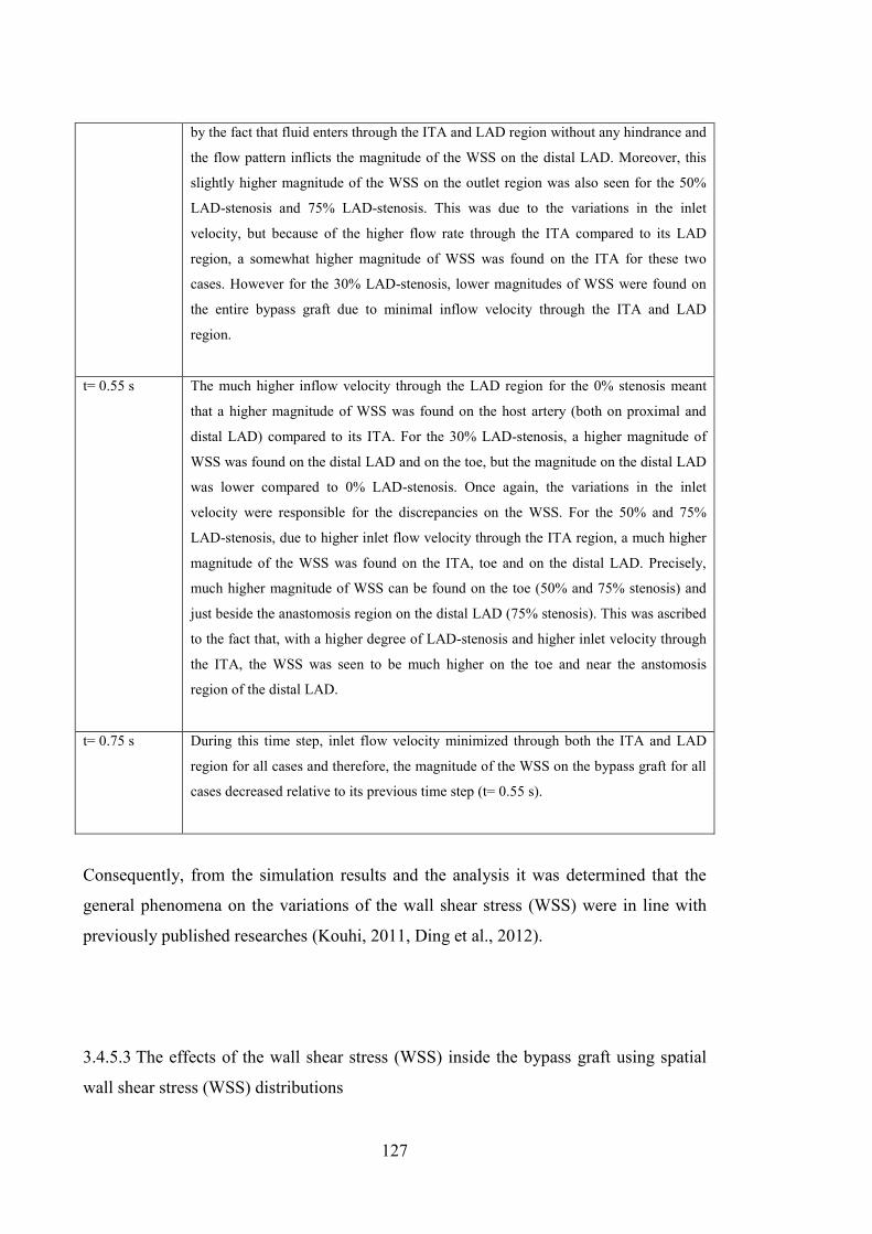
127

by the fact that fluid enters through the ITA and LAD region without any hindrance and

the flow pattern inflicts the magnitude of the WSS on the distal LAD. Moreover, this

slightly higher magnitude of the WSS on the outlet region was also seen for the 50%

LAD-stenosis and 75% LAD-stenosis. This was due to the variations in the inlet

velocity, but because of the higher flow rate through the ITA compared to its LAD

region, a somewhat higher magnitude of WSS was found on the ITA for these two

cases. However for the 30% LAD-stenosis, lower magnitudes of WSS were found on

the entire bypass graft due to minimal inflow velocity through the ITA and LAD

region.

t= 0.55 s The much higher inflow velocity through the LAD region for the 0% stenosis meant

that a higher magnitude of WSS was found on the host artery (both on proximal and

distal LAD) compared to its ITA. For the 30% LAD-stenosis, a higher magnitude of

WSS was found on the distal LAD and on the toe, but the magnitude on the distal LAD

was lower compared to 0% LAD-stenosis. Once again, the variations in the inlet

velocity were responsible for the discrepancies on the WSS. For the 50% and 75%

LAD-stenosis, due to higher inlet flow velocity through the ITA region, a much higher

magnitude of the WSS was found on the ITA, toe and on the distal LAD. Precisely,

much higher magnitude of WSS can be found on the toe (50% and 75% stenosis) and

just beside the anastomosis region on the distal LAD (75% stenosis). This was ascribed

to the fact that, with a higher degree of LAD-stenosis and higher inlet velocity through

the ITA, the WSS was seen to be much higher on the toe and near the anstomosis

region of the distal LAD.

t= 0.75 s During this time step, inlet flow velocity minimized through both the ITA and LAD

region for all cases and therefore, the magnitude of the WSS on the bypass graft for all

cases decreased relative to its previous time step (t= 0.55 s).

Consequently, from the simulation results and the analysis it was determined that the

general phenomena on the variations of the wall shear stress (WSS) were in line with

previously published researches (Kouhi, 2011, Ding et al., 2012).

3.4.5.3 The effects of the wall shear stress (WSS) inside the bypass graft using spatial

wall shear stress (WSS) distributions

128

From the graphical representations of the line A (toe), line B (heel) and line C (bed), the

variations in the WSS in different time steps were obtained for different inlet velocities

through the ITA and proximal LAD, for different degrees of stenosis. In general, for all

cases of line A, the maximum magnitude was found to be near the toe of the artery

during the time step of t= 0.55 s. This could be explained by the fact that a much higher

magnitude of inlet velocity was found to be entering through the ITA and LAD region

during this time step. However, due to the LAD-stenosis, the propagation of the flow

was obstructed inside the proximal LAD, but with higher inflow velocity through the

ITA region (for different degrees of LAD-stenosis), a much higher magnitude was

obtained on the toe of the bypass graft. Conversely, with a lower magnitude of inlet

velocity WSS decreased.

Subsequently, similar phenomena were observed for line B for different LAD-stenosis

levels. Once again, with the aid of higher inflow velocity (t= 0.55 s), a maximum

magnitude of WSS was found to be on the heel of the proximal LAD. Although higher

magnitude of WSS was found during this time step, but it needs to be noted that with

the increase in the degree of LAD-stenosis, the magnitude of the WSS on the heel

decreased.

Likewise, a maximum magnitude of WSS was found to be on the bed (line C) during

the time step of t= 0.55 s. Once again this was due to the higher inlet flow velocity,

which helped elevate the magnitude of WSS. Also, with lower inflow velocity, the

magnitude minimized.

So, the general trends of the variations of the spatial WSS distributions were in line with

the investigations from (Kouhi, 2011).

3.4.5.4 Structure simulation of the bypass graft for different degree of LAD-stenosis

using total mesh displacement (TMD)

129

During the time step of t= 0.3 s, due to minimal inlet flow velocity for all cases, the

magnitude of the displacement on the ITA and LAD were found to be minimal.

However, moderately higher magnitudes of displacement were found to be on the distal

LAD for all cases and around the outlet region (75%) during this time step. This can be

ascribed to the fact that, due to the propagation velocity through the inlet region,

volume inside the bypass graft rose and in turn, the magnitude of the displacement on

the distal LAD elevated.

Subsequently, with the time step of t= 0.55 s, much higher inlet flow velocities entered

through the ITA and LAD region. A maximum magnitude of displacement was found to

be on the distal LAD (0%), but from the simulated results it was observed that the

increase in the degree of the maximum magnitude of displacement was found to be on

the heel (30%, 50% and 75%). Also, due to higher inlet flow velocity (ITA and LAD),

the volume inside the inlets increased. Hence, during this time step, maximum

displacements on the ITA and proximal LAD were obtained for 50% LAD-stenosis.

At a time step of t= 0.75 s, magnitudes of the inlet velocities became minimal for all

cases compared to the previous time step of t= 0.55 s. During this time step, a much

lower magnitude on the entire bypass graft was found for the no-stenosis case.

However, for the stenosed cases, a slightly higher magnitude on the distal LAD (30%),

both on the ITA and distal LAD (55%) and maximum magnitude of displacement

around the outlet region and on the distal LAD (75%) were found. These phenomena

can be attributed to the fact that due to the minimal inlet velocity through the ITA and

LAD, magnitude of the displacement decreased (0%) as the volume inside the graft

provided very little displacement on the arterial wall. Also, for the stenosed cases,

because of the variations of the inlet velocities through the ITA and LAD, the volume

inside the ITA (55% and 75%) and on the distal LAD (30%, 55% and 75%) rose and

this consecutively increased the magnitude of the displacements.

130

3.5 Abdominal Aortic Aneurysm (AAA)

In general, an aneurysm indicates the ballooning/swelling of a local blood vessel above

half of its nominal diameter leading to a risk of unexpected rupture. There are various

factors responsible for producing aneurysms such as:

• Blood vessel deterioration

• Diseases

• Unexpected/sudden injuries

• Birth driven factors

Even though aneurysms can be developed in any blood vessels, four different types of

aneurysms can create critical risks (Li, 2005), specifically:

• Brain aneurysms

• Thoracic aortic aneurysms

• Dissecting aortic aneurysms

• Abdominal aortic aneurysms (AAA)

AAA is located in the abdominal aorta, which is below the renal arteries and above the

iliac bifurcation (Figure 3.10). Aged people (60 years or more) are much prone to AAA

diseases. Also, 90% of AAA are found to be between the renal arteries and iliac

bifurcation (Li, 2005).

131

Figure 3.10 Location of abdominal aortic aneurysm (AAA) (Stern)

132

3.6 Literature Review of Abdominal Aortic Aneurysm (AAA)

Various computational approaches had been conducted which focused on the

hemodynamics and wall shear stress analysis of the AAA models - both clinically and

laboratory-based - along with different computational approaches (Li, 2005). For

instance, Peattie et al., 1994, examined the steady flow through some polyvinyl chloride

models of aneurysms and the flow dynamics were determined by using colour Doppler

imaging. They noted that for lower flow rates, smooth and laminar flow patterns were

observed. Also, for higher rates of flow, the flow pattern was found to be intermittent,

fluctuating/random and turbulent (Peattie et al., 1994).

In another study, Yamada et al., 1994, investigated the mechanical features of the

expansion and rupture of the AAA. The researchers noted that intrinsic (maximum

diameter and wall thickness) and external (blood pressure) factors highly influenced the

deformation and stress distributions in the AAA. The results stated that the rise in the

intrinsic and external factors requirements elevated the wall stress because of the

expansion of the aneurysm (Yamada et al., 1994).

In the year 2000, Raghavan and Vorp (2000), constructed the finite strain structure of

the AAA by utilizing experimental results. They noted that their model was suitable for

the AAA stress analysis and it could also be effective for developing a biomechanical

tool which could clinically assist AAA affected patients. However during this

investigation, a simplified model of AAA was utilized (Raghavan and Vorp, 2000). The

same research group Raghavan et al., 2000 non-invasively examined the wall stress

distributions of a 3D model of the AAA during systolic blood pressure. Data was

obtained from six patients with AAA and one patient with non-aneurysmal aorta using

spiral CT images. However, during their analysis, the wall thickness was considered

uniform and invariable (Raghavan et al., 2000).

Hua et al., 2001, noted that simple geometric features were not reliable in estimating

AAA wall stresses (Hua and Mower, 2001). Subsequently, Elger et al., 1996, also

worked on the wall stresses of the AAA and determined the correlation between the

variations of stresses exerted on the wall and the shape of AAA (Elger et al., 1996).

133

Thubrikar et al., 2001, noted that in order to determine the rupture of an AAA, it was

essential to identify the primary features responsible for this. In doing so, the authors

examined the wall stresses in a clinical model of AAA and they concluded that the

rupture of the AAA was presumably to take place inside the internal surface of the wall

(Thubrikar et al., 2001a). In another study Thubrikar et al., 2001, examined the

mechanical properties/characteristics of aneurysms in various sections of the AAA.

From the results they identified the various yield stress, yield strains and other

mechanical features possessed in various sections of the AAA (Thubrikar et al., 2001b).

Sonesson et al., 1997, also studied the mechanical features of the aneurysm aorta and

they concluded that the AAA was the simplified process of a vasculature with

significant symptoms in the abdominal aorta (Sonesson et al., 1997).

Fillinger et al., 2002, determined the in vivo AAA wall stresses for ruptured and

symptomatic cases, and concluded that this stress analysis was viable. This might play a

significant role in detecting an AAA rupture-threat (Fillinger et al., 2002). The same

group extended their research and investigated the rupture-threat over time where the

patients were being monitored (Fillinger et al., 2003).

In 2005, Li and Kleinstreuer (2005) worked on AAA wall stresses and proposed a new

wall stress equation for the aneurysm-rupture (Li and Kleinstreuer, 2005). The same

group utilized FSI on AAA structure including variable neck and bifurcation angle to

investigate the effects of hemodynamics and wall stress (Li and Kleinstreuer, 2006) -

similarly with (Pelerin et al., 2006). The influence of the asymmetry and wall thickness

of the AAA were studied by Scotti et al., 2005 (Scotti et al., 2005). Moreover,

investigations on wall stresses and hemodynamics inside the AAA were also conducted

by the same research group (Scotti et al., 2008). Xenos et al., 2010, once again utilized

the FSI technique to study the development of aneurismal disease by considering the

iliac bifurcation and AAA neck angle (Xenos, 2010).

In another study, Georgakarakos et al., 2011, noted that the conventional norm of

maximum diameter was not enough to distinguish a small AAA, which may be likely to

rupture or expand quickly, but wall stress might play a significant role in such cases.

134

Hence, these researchers reviewed the significance of geometric-characteristics in

possible rupture or expansion, and the necessity for further assessment and validation of

geometric features (Georgakarakos et al., 2011).

Maksymowicz et al., 2011, noted that with the existing medical knowledge it was not

possible to avert the formation and progression of AAA since the pathogenesis of this

disease was unidentified. Therefore, the authors reviewed the three crucial factors which

were related with the development of AAA, such as (Sonesson et al., 1997, Shteinberg

et al., 2000, Maksymowicz et al., 2011):

• Maximum diameter

• Growth/ expansion rate

• Mural thrombus existence

They also stated that there could be multiple causes for the generation of AAA which

include (Sonesson et al., 1997, Shteinberg et al., 2000, Maksymowicz et al., 2011):

• Genetic

• Anatomic

• Hemodynamical

• Biomechanical

• Environmental issues such as smoking,

• Inflammatory/provocative

• Atherosclerotic

Martufi and Gasser, 2013, reviewed the functionalities of the biomechanical modelling

in the rupture-threat-evaluation for the AAA and they noted that the evaluation was

effective for patients as it aspired to preclude aneurysms from being ruptured, not

including a needless number of repair intercessions (Martufi and Gasser, 2013).

Another review was conducted by Kleinstreuer et al., 2013 based on the rupture risk-

threat-evaluation and surgical restoration of AAA. However, during their investigations

they noted that the Fluid Structure Interaction (FSI) for patient-specific AAA cases

135

vastly enhanced the accuracy of rupture occurrences (Kleinstreuer et al., 2013).

Subsequently, Soudah et al., 2013 exploited the computational fluid dynamics

modelling (CFD) of a 3D AAA model using hemodynamic loads. The authors noted

that AAA rupture was a multifaceted condition-which relied on the:

• Maximum diameter

• Internal pressure

• Wall stress

• Asymmetry

• Saccular manifestation

and so on (Soudah et al., 2013). Also, Giuma et al., 2013, employed FSI of the AAA

and highlighted the significance of geometric parameters in predicting the maximum

wall stresses (Giuma et al., 2013).

Svensjo et al., 2014, reported a population-oriented group-study where people had been

asked for the aortic ultrasound test at the age 65 and asked to be monitored once again

at the age of 70. They stated that the development of AAA was quite usual among

people incorporating an aortic diameter less than 30 mm (Svensjö et al., 2014).

In summary, researchers had studied the general flow pattern and wall stresses of an

AAA with different degrees of accomplishment. However, a complete investigation,

based on the hemodynamic and structural displacement of an AAA model needed to be

assessed thoroughly. In so doing, the hemodynamic forces inside the AAA were

analysed and demonstrated by utilizing velocity mapping and WSS distributions.

Structural displacements were demonstrated by employing total mesh displacement

(TMD) under different physiological conditions. Moreover, during the computational

approaches, Arbitrary Lagrangian Eulerian (ALE) equations were implemented for FSI-

analysis of the 3D axisymmetric AAA model.

136

3.7 Case Study II: abdominal aortic aneurysm (AAA)

3.7.1 Geometry

Figure 3.11 (a) represents a 3D axisymmetric model of the AAA, created using

SolidWorks 2012. This illustrates the ideal aortic aneurysm in the abdomen (AAA) of a

human body. Also, Figure 3.11 (b) demonstrates the detailed dimensions of the AAA by

utilizing the similar CAD software. For the following figures

• The diameter of the proximal neck was considered to be 20 mm.

• The iliac bifurcation artery 12 mm.

• The aneurysm wall 60 mm.

• The length of the neck aorta (proximal neck) was 20 mm.

• The aneurysm wall was 80 mm.

• The iliac bifurcation artery (distal neck) was 41 mm.

• The wall thickness of the neck aorta and aneurysm wall was considered to be

1.50 mm each.

• The iliac bifurcation artery was 1 mm.

• The iliac bifurcation artery angle was assumed to be 60°.

All the geometric parameters match closely with the models of (Li, 2005, Xenos, 2010,

Li and Kleinstreuer, 2006, Thubrikar et al., 2001a).

137

(a)

(b)

Figure 3.11 (a) Cross-sectional geometry of an axisymmetric AAA (using SolidWorks

2012) (b) Detailed dimensions of the AAA (using SolidWorks 2012) (Li, 2005)

138

3.7.2 Meshing Configurations and Mesh Independency Testing

In a similar approach to that deployed for the bypass graft model, after constructing the

3D AAA model in the CAD software, it was then imported to ANSYS 14.5, where a

suitable meshing was implemented and mandatory boundary conditions were provided.

Once again, “Mapped Face Meshing” was executed individually for both the solid and

fluid domain. Moreover, line control properties were applied in order to find the

variations in the velocity of the fluid. Subsequently, by implementing these line control

properties, mesh independency testing was carried out to determine and compare the

discrepancies in the fluid velocity for consecutive nodes and elements, until the velocity

converged (Kouhi, 2011).

The mesh independency testing is demonstrated in Figure 3.12 which was obtained

from the discrepancies in the fluid velocity. Moreover, three different mesh types

(coarse, medium and fine) were chosen and varied during the simulations. It should be

noted that, 28205 nodes and 15291 elements were considered to be apposite and

validated for the solid region, and 12706 nodes and 46557 elements, for the fluid region.

Also, for the solid domain refinement of the distal neck of the iliac bifurcation was

employed. Furthermore, from the simulations all these nodes and elements were

selected from the coarse mesh type. Once more, the convergence conditions for the fluid

flow were considered to be 10-4 and 10-2 for the coupling data transfer.

139

Figure 3.12 Mesh independency testing using line control properties


Once again, similar to the simulations of the bypass graft, compulsory boundary

conditions had to be assigned to perform the desired simulations. During the simulation,

the inlet flow velocity was provided through the neck aorta (proximal neck) and the

outlet pressure waveform was provided through the iliac bifurcation arteries (and/or

distal neck) of the AAA. Figure 3.13 and figure 3.14 represent the velocity and pressure

waveforms through the inlet and outlet accordingly and the waveforms closely matched

with the previous investigations of (Li and Kleinstreuer, 2006, Li, 2005, Xenos, 2010).

For the inlet velocity waveform, the X-axis represents the time (t) in seconds and the Y-

axis represents the velocity (V) in m/s. Also, for the outlet waveform, the X-axis

represents the time (t) in seconds and the Y-axis represents the pressure (P) in mmHg.

In order to simplify the simulation and to avoid geometric inflation (Xenos, 2010), the

outlet pressure waveform was modified and is illustrated in Figure 3.15.

0

0.2

0.4

0.6

0.8

1

1.2

1.4

5.20E-055.30E-055.40E-055.50E-055.60E-055.70E-05

Velo

city

, V [m

/s]

Z [m]

Coarse refinementmesh

Medium mesh

Fine mesh

140

Figure 3.13 Inlet velocity waveform (Li, 2005)

Figure 3.14 Actual outlet pressure waveform (Li, 2005)

Figure 3.15 Simplified outlet pressure waveform utilized in the simulations

-0.1

0

0.1

0.2

0.3

0.4

0.5

0 0.5 1 1.5

Velo

city

, V (m

/s)

t (s)

Inlet velocity

0

20

40

60

80

100

120

140

0 0.5 1 1.5

Pres

sure

, P (m

mHg

)

t (s)

Outlet…

0

20

40

60

80

100

120

140

0 0.5 1 1.5

Pres

sure

, P (m

mHg

)

t (s)

Simplified outletpressure

141

After providing the required inlet and outlet waveforms, the density and viscosity of the

liquid/fluid were assigned with the value of 1050 kg/m3 and 0.0035 Pa•s accordingly.

Li, 2005, reported that experimental information suggested that the elastic modulus for

the aneurysm was much higher than that of a healthy artery (neck and iliac bifurcation).

Therefore, the elastic modulus for the aneurysm was considered to be 4.66 MPa and for

the healthy artery it was 1.2 MPa. Also, Poisson’s ratio for the aneurysm wall and

healthy artery were considered to be 0.45 and 0.49 respectively. Also, the

circumferential faces of the inlet and the outlet were considered fixed during the

simulation. Similar to the bypass simulations, the AAA wall was assumed to be

isotropic and homogeneous. Moreover, Newtonian fluid flow was considered during the

simulations including the no-slip boundary conditions. Also, the flow was assumed to

be laminar (Li, 2005, Xenos, 2010, Di Martino et al., 2001, Li and Kleinstreuer, 2006,

Soudah et al., 2013, Pelerin et al., 2006). Once again, for coupling data transfer control,

under relaxation, the factor had been set to 0.75.

3.7.4 Simulation Results

3.7.4.1 Velocity Mapping

Simulation results are illustrated by utilizing velocity mapping, which incorporates:

• The generation, development, shifting and merging of vortices inside the

aneurysm

• Distributions of wall shear stress (WSS)

• Structural displacement in terms of total mesh displacement (TMD)

during a complete cardiac cycle.

Figures in 3.16 illustrate the flow pattern inside the aneurysm in ten different time steps.

Velocity vectors were utilized to characterize the variations in the flow dynamics, which

142

were mapped on the XY cross-sectional plane of the AAA. This plane was set in the

middle of the AAA where the plane consisted of inlet, outlets and the aneurysm.

0.025 s 0.05 s

0.1 s

0.15 s 0.2s

143

0.275 s

0.5 s

Figure 3.16 Velocity distributions of the AAA in different time steps

At the beginning of the simulation, the jet started to enter through the distal neck of the

outlet regions inside the aneurysm body (t= 0.025 s). This was due to higher outlet

velocity compared to the inlet. With an increase in the time step (t= 0.05 s) the

exit/outlet velocity rose and therefore, a higher magnitude of velocity entered through

the distal neck. During this time step, two ring shaped vortices started to develop close

to the distal neck of the aneurysm wall. Subsequently, this clockwise (CW) ring shaped

vortex on the right-side and counter clockwise (CCW) ring shaped vortex on the left-

side were found to be elongating close to the distal neck (t= 0.1 s). During this exact

144

time step, the magnitude of the outlet velocity was still found to be higher than that of

inlet.

During the time step of t= 0.15 s the inlet velocity started to rise and the fluid entered

through the proximal neck of the aneurysm. At the same time step, the magnitude of the

velocity through the iliac bifurcation was found to be slightly decelerating compared to

the previous time step. Simultaneously, the primary vortices shifted their location and

moved towards the centre of the aneurysm body. Later, with the time step of t= 0.2 s, a

maximum magnitude of velocity, around 1.4 m/s, was found to be entering through the

distal neck. The inlet velocity with a magnitude of around 0.42 m/s (from Figure 3.13)

started to enter through the proximal neck. During this time step, the vortices slightly

expanded and reached toward the core of the aneurysm.

Consequently, with a higher magnitude of the inlet velocity through the proximal neck

(t= 0.275 s), a CCW ring shaped vortex developed on the right-side and a CW ring

shaped vortex on the left side, close to the proximal neck of the aneurysm. However,

with the progression in the time step, the magnitudes of the inlet and outlet start to

decrease. Precisely, during the time step of t= 0.5 s, with lower inlet and outlet velocity,

the secondary vortices expanded slightly but the primary vortices shifted their locations

once again close to the wall and started to merge. Later, with lower magnitudes of inlet

and outlet velocities (t= 0.7 s, 0.9 s and 1 s; please see in Appendix, Figure A-1), both

the primary and secondary vortices (all four) started to amalgamate with the progression

of the time steps.

3.7.4.2 Wall shear stress (WSS) distributions

All the illustrations in Figures 3.17 demonstrate the wall shear stress (WSS) inside the

aneurysm during a cardiac cycle. The wall motion during this cardiac cycle had to be

determined and in doing so, WSS was considered on the exterior surface of the

aneurysm wall for ten different time steps.

145

0.025 s 0.05 s

0.1 s 0.15 s

0.2 s 0.275 s

Figure 3.17 WSS distributions of the AAA in different time steps

146

As demonstrated in the Section 4.7.3.1, at the beginning of the simulation (t= 0.025 s),

the magnitude of the inflow velocity through the distal neck was much higher than at

the proximal neck. During this time step, a much higher magnitude of WSS was found

on the distal neck compared to its proximal neck. After that, with a rise in the inflow

velocity through the bifurcation (t= 0.05 s), the magnitude of the WSS on the distal neck

elevated and also the WSS of the iliac arteries/outlet regions rose compared to the

previous time step. During the time step of t= 0.1 s, the magnitude of the WSS was

found to be almost identical with the previous time step (t= 0.05 s). At the same time

step, a much higher magnitude of WSS was found on the distal neck compared to its

iliac arteries. With further progression of the time step, t= 0.15 s, the inlet jet started to

enter through the proximal neck and hence slight variations of the WSS were found on

the neck artery. Also, during this time step the magnitude of the WSS on the distal neck

was found to be decreasing compared to the previous time step (t= 0.1 s).

During the time step of t= 0.2 s, a maximum magnitude of WSS, approximately 1.2 E1

Pa was found to be on the distal neck of the aneurysm. Simultaneously, the magnitude

of the WSS on the proximal neck was found to be moderately higher when compared to

its previous time step, but this magnitude was much lower than that of the distal neck.

During the time step of t= 0.275 s, both the magnitude of the WSS on the proximal neck

and distal neck started to decline. During the time steps of t= 0.5 s, 0.7 s, 0.9 s and 1 s,

no significant variations of the WSS were identified on the AAA (Please see in

Appendix, Figure A-2).

3.7.4.3 Total mesh displacement (TMD) distributions

Figure 3.18 illustrates the variations of the structural displacement of the aneurysm

during a cardiac cycle in ten different time steps. Changes in the displacement of the

aneurysm-model during the cardiac cycle were determined using total mesh

147

displacement (TMD) distributions. In doing so, TMD had been considered on the outer

surface of the aneurysm body.

0.025 s 0.05 s

0.1 s 0.15 s

0.2 s 0.275 s

148

0.5 s

Figure 3.18 Structural displacement using total mesh displacement (TMD)

distributions

At the onset of the simulation (t= 0.025 s), the change in the displacement was found to

be minimal in the vicinity of the iliac bifurcation arteries, due to lower inflow waveform

through the iliac bifurcation arteries. With a rise in the inflow velocity through the distal

neck, variations in the magnitude of the displacement were evident on the aneurysm

wall and on the distal neck. Later, during the time step of t= 0.1 s, the magnitude of the

displacement on the aneurysm wall close to the distal neck was found to be increasing

and simultaneously, a higher magnitude of displacement was evident in the vicinity of

the bifurcation arteries.

During the time step of t= 0.15 s, the rate of flow through the proximal neck accelerated

and the magnitude of the displacement tended to increase on the aneurysm wall close to

the neck artery. However, the magnitude of the displacement close to the distal neck

was found to be increasing.

At the time step of t= 0.2 s the flow rate through the distal and proximal neck

accelerated and the magnitude of the displacement was still found to be moderately

higher close to the distal neck of the aneurysm. When the inflow velocity through the

proximal and distal neck decelerated (t= 0.275 s), a higher magnitude of displacement

149

was still found to be on the aneurysm wall close to the distal neck. Moreover, during the

time step of t= 0.5 s, a maximum displacement of approximately 2.3E-3 m was found

on the aneurysm wall close to the distal neck. Similarly, during the time steps of t= 0.7

s, 0.9 s and 1 s, a much higher magnitude of the displacement was found to be on the

aneurysm wall near the distal neck (please see in Appendix, Figure A-3).

3.7.5 Discussion

3.7.5.1 Influence of flow dynamics of the AAA using velocity vectors

At the onset of the simulation, a much higher magnitude of velocity flow started to enter

through the bifurcation towards the centre of the aneurysm. During the time step of t=

0.05 s, two ring shaped symmetric vortices (CW vortex on right-side and CCW vortex

on left side) developed close to the distal neck. With a rise in the inflow velocity

through the iliac artery (t= 0.1 s), the primary vortices were expanded and shifted their

position slightly upwards. It should be noted that, during this time step, the generation

of the CW vortex on the right-side and CCW vortex on the left-side contradicted with

the findings from (Li, 2005) who found that a CW vortex originated on the left-side and

CCW on the right-side. This can be attributed to the fact that due to the smaller diameter

of the distal neck and because of a much higher flow velocity through the bifurcation

CW and CCW, symmetric vortices originated and elongated on the right-side and left-

side accordingly. At the same time step, minimal inflow velocity starts to enter through

the inlet region of the aneurysm.

During the time step of t= 0.15 s, the inlet velocity started to rise but the inflow velocity

through the distal neck was much higher than its inlet. At the same time, the primary

symmetric vortices expanded longitudinally and shifted their position towards the centre

of the aneurysm. With further progression in the time step (t= 0.2 s), both the inflow

velocity through the proximal neck (inlet region) and distal neck (iliac

artery/bifurcation) rose. Simultaneously, the primary vortices were found to be at the

core of the aneurysm body. However, due to different parameters of the inlet and outlet

150

waveform, two vortices still existed during this particular time step - this was different

to the findings from (Li, 2005).

After reaching a peak of the inlet velocity (through proximal neck), flow started to

decelerate and during the time step of t= 0. 275 s another pair of symmetric ring shaped

vortices, which were CCW on the right-side and CW on the left-side, were seen

originating close to the proximal neck. The generation and direction of the vortices was

in line with the results from (Li, 2005). This can be attributed to the fact that, with the

higher inlet diameter (proximal neck) and higher magnitude of the inlet jet, the direction

of these two symmetric vortices also completely matched with the findings from (Li,

2005).

The magnitude of the inflow velocity through the inlet and outlet region started to

decelerate in subsequent time steps (t= 0.5 s, 0.7 s, 0.9 s and 1 s). Specifically, during

the time step of 0.5 s, the secondary vortices close to the proximal neck elongated

slightly and shifted their location downwards. The primary vortices changed their

position once again and moved closer to the wall. Later, during the time steps of t= 0.7

s, 0.9 s and 1 s, the primary vortex started to amalgamate, and the secondary vortex

(only right-side) merged also.

Although there were some discrepancies inside the flow dynamics of the aneurysm

during a cardiac cycle, the general trend of the flow dynamics, including the generation,

development, merging and shifting of vortices was in line with the findings from (Li,

2005, Xenos, 2010).

3.7.5.2 Influence of wall shear stress (WSS) of the AAA using WSS distributions

Once again because of the higher inflow velocity through the distal neck during the time

step of t= 0.025 s, a much higher magnitude of the WSS was found on the distal neck of

the aneurysm. Also, due to negative inlet velocity through the proximal neck, no

significant variations of the WSS were found on the neck artery. Subsequently, the

151

magnitude of the WSS on the distal neck was found to be increasing during the time

step of t= 0.05 s, due to the rise in the inflow velocity through the iliac artery. Hence,

the magnitudes of the WSS on the iliac arteries were also found to be elevating during

this exact time step.

During the time step of t= 0.1 s, a higher magnitude of WSS was found on the distal

neck but still due to the negative inflow velocity through the proximal neck, no

variations in the WSS on the proximal neck were found. However, due to higher flow

waves through the iliac arteries, the effect of WSS was found on the bifurcation artery.

Moreover, with the time step of t= 0.15 s, the magnitude of the inflow velocity through

the proximal neck started to rise and hence the discrepancy of the WSS could be found

on the proximal neck. Concurrently, due to a lower inflow wave through the distal neck,

the magnitude of the WSS on the distal neck was found to be decelerating, compared to

the previous time step, but the magnitude was still higher than that of proximal neck.

Also, the effects of the WSS on the iliac arteries are found to be minimizing during this

time step.

Once again, with the rise in the inflow velocity through the proximal and distal neck (t=

0.2 s) of the aneurysm, the magnitudes of the WSS on both the proximal and distal neck

were found to be elevating compared to the previous time steps. Also, the effect of the

WSS was found once more on the iliac bifurcation arteries. However, during the time

step of t= 0.275 s, the magnitude of the inflow wave through the inlet and iliac artery

started to decelerate and because of that, the magnitude of the WSS on both the neck

artery and distal neck were found to be decelerating. Additionally, the effects of the

WSS on the iliac arteries decelerated due to lower inflow waves through the outlet

region. Moreover, during the time steps of t= 0.5 s, 0.7 s, 0.9 s and 1 s the magnitude of

the WSS was found to be minimal because of the lower inflow wave through the

proximal and distal neck.

152

3.7.5.3 Influence of the structral displacement of the AAA using total mesh displacemnt

(TMD) distributions

At the beginning of the simulation (t= 0.025 s), the inflow wave started to enter through

the iliac arteries and therefore the magnitude of the displacement tended to be slightly

higher in the vicinity of the bifurcation arteries. With the progression of the time step

(t= 0.05 s), the inflow wave through the bifurcation arteries rose and a higher magnitude

of displacement was found on the aneurysm wall. This can be attributed to the fact that

due to the rise in the inflow wave through the iliac arteries, the jet started to propagate

from the distal neck towards the proximal neck. Hence, the volume inside the aneurysm

increased, which consecutively increased the magnitude of the displacement inside the

AAA.

During the time step of t= 0.1 s, a much higher magnitude of inflow wave started to

enter through the distal neck and the volume inside the aneurysm increased. Later, with

the time step of t= 0.15 s, the inflow wave through the proximal neck started to enter

and the volume inside the aneurysm increased. With the jet entering both the proximal

and distal neck, the volume inside the aneurysm rose and a higher magnitude of

displacement was found on the aneurysm wall close to the distal neck.

Once again, with the time step of t= 0.2 s the magnitude of the inflow jet both the

proximal and distal neck increased and therefore the volume increased. Also, a much

higher magnitude of displacement was still found to be on the aneurysm wall near the

distal neck. After that, the magnitude of the inflow wave started to decelerate (t= 0.275

s and 0.5 s) through the proximal and distal neck but, due to the increased volume inside

the aneurysm, a much higher magnitude of displacement was found on the aneurysm

wall. Precisely, during the time step of t= 0.5 s, a maximum magnitude of displacement

was found to be around 0.0023 m which was close to the value of 0.0016 m for the

symmetric aneurysm as reported by (Li, 2005).

Due to the variations in the outlet waveform and variations in the geometric parameters

of the AAA, the magnitude of the displacement varied. Once more, with lower inflow

velocity through the proximal and distal neck and increased volume inside the

153

aneurysm, a higher magnitude of displacement was still evident on the aneurysm wall,

near the distal neck.

It should be noted from the simulation results that, during all the assigned time steps,

the magnitude of the displacement was found to be higher in the vicinity of the

bifurcation arteries. This could be ascribed to the fact that, because of higher inflow

wave through the iliac arteries, with the bifurcation angle (β) inflow wave entered

through the arteries and combined in the vicinity of the bifurcation arteries. Hence, the

magnitudes of the displacement during all time steps were found to be much higher.

154

3.8 Summary of Results and Conclusions

Table 3.7 summarizes the whole work (CABG and AAA), as presented in this chapter.

Table 3.7 Summary of the whole work (CABG and AAA) Case

Studies

Mesh

Independ

ency

Testing

Boundary

Conditions

Simulations Findings

CABG

with0%,

30%, 50%

and 75%

LAD-

stenosis

Yes (i) Inlet

velocities

obtained from

pigs (Ding et al.,

2012)

(ii) Laminar;

fluid density

and the

viscosity of

1050 kg/m3 and

0.0035 Pa•s

accordingly

(i) Flow

dynamics

(ii) WSS

analysis

including

spatial WSS

distributions

(iii)

Deformation

of the solid

domain

using TMD

(i) Reverse flow direction for the 0% LAD-

stenosis but forward for the stenosed cases (30%,

50% and 75%) during t= 0.05 s

(ii) Disturbance of the flow and generation of

vortices were mostly observed in the anstomosis

region

(iii) Higher WSS were found near the

anastomosis region, toe and on the arterial wall

close to the anastomosis region

(iv) Maximum magnitude of WSS were found

mainly on the anatomosis region (Line C)

(v) With rise in the inlet flow velocity magnitude

of WSS tends to rise

(vi) For the 75% LAD-stenosis maximum

magnitude of displacement was found to be on

the distal LAD and close to the outlet region (t=

0.75 s)

AAA Yes (i) Outlet

pressure

waveform

(ii) Laminar;

fluid density

and the

viscosity of

1050 kg/m3 and

0.0035 Pa•s

respectively

(i) Flow

dynamics

(ii) WSS

analysis

(iii)

Deformation

of the

structure

using TMD

(i) Due to smaller diameter of the distal neck

than its proximal neck and higher magnitude of

inflow jet entering through the iliac arteries, CW

and CCW symmetric primary vortices were seen

developed and elongated on the right-side and

left-side of the aneurysm accordingly

(ii) With the rise in the inflow waveform, the

magnitude of the WSS elevated. However, with

minimal inflow waveform through the proximal

and distal neck, no significant variations in the

wall shear were seen on the AAA

(iii) The magnitude of displacement is always

found to be higher on the vicinity of the iliac

155

arteries even though the magnitudes varied with

different time steps

From the comprehensive investigations and simulation results detailed in this chapter,

the importance and applications of the FSI scheme were achieved. Specifically, the

necessity for:

• Grid independency testing

• Required physiological parameters/ boundary conditions for the solid and

fluid domains

• Physiologically correct pulsatile flow conditions through the inlet and outlet

regions

were learned. The manner in which these factors could change the general outcomes of

simulations (case studies) were analysed and discussed. The applications of different

numerical methods (Navier-Stokes equations and ALE); the variations in the simulations

using the under-relaxation factors and the extractions of the inlet and outlet flow

patterns, along with the appropriate boundary conditions were noted. The obtained

results and detailed analysis from the case studies, in terms of flow dynamics, WSS

analysis and the deformation of the solid domain, provided substantial insights into the

hemodynamics and structural changes of the coupled models.

In conclusion, during the numerical simulations (CABG and AAA), simplified and

anatomically correct geometries were deployed and the results were studied and

analyzed accordingly by employing a Fluid Structure Interaction (FSI) scheme. After

gathering the required information on the FSI and the applications of this scheme, the

approach was then utilized on a realistic model of the Left Ventricle (LV), presented in

Chapter 4.

156

Chapter 4

Numerical Studies of the Left Ventricle during

Diastole Phase: General Conditions

157

4.1 Overview

The primary objective of the research, documented in this chapter, was to determine and

analyze the hemodynamic characteristics and structural variations of the anatomically

correct 3D model of the left ventricle (LV) during diastolic flow conditions. The entire

simulations for the LV were computed using the Fluid Structure Interaction (FSI)

technique. During the simulations, the results were analyzed and are discussed, herein,

in terms of:

• Flow dynamics

• Intraventricular pressure (Ip) distributions


• Deformation of the solid domain

Throughout the simulations, the required boundary conditions were applied. More

precisely, the transmitral flow velocity (U) in the inlet region was provided and in a

similar approach to that documented in Chapter 3, the Navier-Stokes equations and the

Arbitrary Lagrangian Eulerian (ALE) methods were used in order to couple the fluid

and solid domains of the LV model. The results were then studied and compared with

previously published results.

This chapter concludes by providing the findings from the simulations, which could be

particularly useful in the development of a next generation ventricular assist device

(VAD) system. Moreover, these numerical simulations provided a clear view of

hemodynamic features and structural changes which could be beneficial for future,

ongoing research, as presented in Chapter 5 and Chapter 6.

The research work documented in this chapter was extracted from the following

publication:

M. S. Arefin and Y. Morsi, Fluid structure interaction (FSI) simulation of the left

ventricle (LV) during the early filling wave (E-wave), diastasis and atrial

contraction wave (A-wave), Australas Phys Eng Sci Med, 37(2), 2014. DOI:

10.1007/s13246-014-0250-4

158

4.2 Introduction

As noted in the literature review of Chapter 2, a computational approach, using a

Computational Fluid dynamics (CFD)/Fluid Structure Interaction (FSI) scheme could be

utilized for computing the hemodynamic and physiological variations of the LV. It was

also evident from the literature that this simulation method was well established in

terms of understanding and determining the flow dynamics and physiological variations

of a simulated structure (Reul et al., 1981, McQueen and Peskin, 2000, Lemmon and

Yoganathan, 2000).

Earlier researchers had generally placed emphasis on the general flow dynamics of the

LV model, with varying degrees of accomplishment, but a comprehensive analysis of

the flow dynamics and physiological variations of the simulated model was not

thoroughly explained. In this regard, this chapter documents the utilization of the fluid

structure interaction (FSI) scheme in order to understand and determine the

hemodynamic forces and structural variations of a realistic, 3D model of the LV during

the diastolic conditions/filling phase under different physiological states. Therefore:

• Changes in the Ip

• Variations in the flow pattern, including the changing, shifting and merging of

vortices

• Differences in the wall shear stress (WSS)

under various physiological conditions are documented and discussed. Additionally, the

structural displacement of the LV model is also explained, using the total mesh

displacement during the filling phase. Conclusions are presented at the end of this

chapter, where the hemodynamic and physiological states are thoroughly explained

during diastolic flow conditions.

159

4.3 Computational Approaches

4.3.1 Overview

In this section, the details of the LV geometry are described and the various

measurement parameters are presented. Subsequently, the required boundary conditions

and inlet velocity waveform are executed. Once all the required features are provided,

the:

• Distributions of intraventricular pressure (Ip)

• Velocity pattern


• Variations in structural displacement

are observed and documented.

4.3.2 Geometry

A three dimensional (3D), physiologically realistic left ventricle model of the heart was

developed using CAD software (SolidWorks 2010) (figure 4.1). This structure was

modelled by considering the entire physiological characteristics/measurements of the

LV, with the aid of magnetic resonance imaging (MRI) data and additional required

information that was extracted from medical textbooks. These recommended

measurements/dimensions matched closely with the practical LV models, as stated in

(Arefin and Morsi, 2014, Bronzino 1999, Bronzino, 2006, Zheng et al., 2012, Saber et

al., 2001).

A simplified LV structure was utilized for the simulations. However, the literature

suggested that if the essential physiological and hemodynamic boundary conditions

were assigned properly, then a simplified model could still produce valid results, which

could be readily related to the physical behaviour of a real LV (Cheng et al., 2005,

160

Nakamura et al., 2002, Zheng et al., 2012, Watanabe et al., 2004, Arefin and Morsi,

2014).

The shape of the employed LV model was an ellipsoidal, which is exhibited in Figure

4.1, with the values of (Arefin and Morsi, 2014, Cheng et al., 2005):

• 0.7 cm starting from the topmost part of the LV (inlet/mitral orifice) to the

lowermost part of the model.

• 3.6 cm from the right-side of the LV to the left-side.

Moreover, in a similar approach to LV geometry as Cheng et al., 2005 (Arefin and

Morsi, 2014, Cheng et al., 2005):

• The diameter of the mitral valve was taken to be 2.5 cm in the inlet region, by

assuming the mitral valve completely open.

• The diameter of aortic valve was set to 2.1 cm in the outlet region, which was

considered completely closed during the total simulations.

• The wall of the LV model was presumed to comprise a uniform wall thickness,

where the magnitude of the wall thickness was 0.1 cm.

161

(a)

(b)

Figure 4.1 (a) Dimensions of the LV used for the simulations (SolidWorks 2010) (b)

Geometric construction of the LV model (SolidWorks 2010) (Arefin and Morsi, 2014)

162

4.3.3 Meshing Information and Mesh Independency Trials

In a similar approach to the meshing technique documented in Chapter 4, a CAD model

of the LV was introduced into ANSYS 15.0 and after importing, the required meshing

was performed and the essential boundary conditions were assigned. For these LV

simulations, “Mapped Face Meshing” was implemented separately, both for the solid

and the fluid regions of the LV. Once again, line control properties were applied and the

discrepancies in the fluid velocity were observed and determined. Hence, mesh

independency trials were executed by utilizing the changes in the flow velocity for

consequent nodes and elements (Kouhi, 2011, Arefin and Morsi, 2014). These changes

were determined until the flow velocities converged.

Figure 4.2 demonstrates the mesh independency trials using flow velocity. During the

testing, three different mesh categories were selected:

• Coarse

• Medium

• Fine

From testing, it was determined that, for the structural domain:

• 19706 nodes

• 10058 elements

were required for accuracy. For the fluid domain:

• 138311 nodes

• 746829 elements

were considered for accuracy purposes. Subsequent nodes and elements were selected

for the medium mesh type for the entire simulations. Moreover, the convergence

criterion for the fluid was considered to be 10-4 and for the coupling data transfer, it was

considered to be 10-2 (Arefin and Morsi, 2014).

163

Figure 4.2 Mesh independency trials (Arefin and Morsi, 2014)


The flow velocity for the inlet region was ascertained using a lumped parameter model.

This data was clinically extracted from a young and healthy person. Also, the acquired

data was customized further, using the model of Waite et al. 2000 (Arefin and Morsi,

2014, Cheng et al., 2005, Waite et al., 2000).

Figure 4.3 shows the transmitral flow velocity, U (in m/s) on the X-axis and the time, t

(in seconds) on the Y-axis. This transmitral flow velocity was provided at the inlet of

the model during the simulation. However, in order to implement the velocity

waveform, a curve-fitting procedure was used and the extracted waveform matched

96% with the actual curve, which was acquired from (Arefin and Morsi, 2014, Cheng et

al., 2005, Waite et al., 2000).

0

0.1

0.2

0.3

0.4

0.5

0.6

0.7

0.8

0 0.02 0.04 0.06 0.08

Velo

city

, V [m

/s]

Axial Position, Y [m]

Mesh Type-Coarse

Mesh Type-Medium

Mesh Type-Fine

164

Figure 4.3 Transmitral flow velocity (U) against time (t) waveform, implemented in

the inlet region (Arefin and Morsi, 2014)

The LV wall was considered to be isotropic and homogeneous, including the density of

the LV wall, which was set to be 1.2 g/cm3 and having an elastic modulus of 0.7 MPa

and a Poisson’s Ratio of 0.4. Newtonian fluid flow was considered for the entire

simulation, including:

• A density of 1050 kg/m3

• A viscosity of 0.0035 Pa.s

incorporating no-slip boundary conditions and the flow property was considered to be

laminar. Also, the outlet section and the circumferential face of the inlet were

considered fixed during the whole simulations. Entire simulations were executed on an

Intel® Xeon® processor of 3.07 GHz (Arefin and Morsi, 2014, Cheng et al., 2005,

Lassila et al., 2012, Vierendeels et al., 1999, Saber et al., 2003). For coupling data

transfer control, the under relaxation factor was fixed to 0.75.

165

4.4 Simulation Results and Discussions

4.4.1 Overview

The results and discussions are presented in this section, using

• Intraventricular pressure distribution (Ip)

• Wall Shear Stress (WSS)

• Flow dynamics, including the generation, development, merging and shifting of

vortices during the filling phase

Additionally, variations to the LV structure using total mesh displacement (TMD) were

also considered during the diastolic flow conditions (Arefin and Morsi, 2014).

4.4.2 Distributions of Pressure

It can be observed from Figure 4.3, that the transmitral flow profile (U) is composed of

two peaks, which are:

• At time t= 0.08s, where the flow velocity U is around 0.8 m/s.

• At time t= 0.44s, where the flow profile U is nearly 0.4 m/s.

The first peak was recognized as the early filling wave (E-wave), which resulted from

the resting-period of the LV, due to the flow of blood entering from the left atrium to

the ventricle and the latter peak was known as the atrial contraction wave (A-wave),

which was responsible for applying pressure on the atria. Subsequently, in-between

these two peaks, the middle phase of the flow profile (around 0.22<t<0.3s) was

recognized as the diastasis or slow filling or relaxed filling period (Arefin and Morsi,

2014, Cheng et al., 2005).

166

Figure 4.4 shows the pressure distribution into the interior section of the LV, where the

changes in the intraventricular pressure (Ip) were differentiated by implementing an XY

cross-sectional plane throughout the diastolic flow conditions. These variations in the Ip

were demonstrated for fourteen different states of the transmitral waveform. During the

simulation, the inlet was considered fully open and the outlet was considered fully-

closed, as noted in Section 4.3.2 (Cheng et al., 2005, Arefin and Morsi, 2014).

(a) t= 0.025s (b) t= 0.05s

(c) t=0.075 s (d) t= 0.125 s

167

(e) t= 0.15s (f) t= 0.2 s

(g) t= 0.225s (h) t= 0.275 s

168

(i) t= 0.35 s (j) t=0.375s

(k) t= 0.425 s (l) t= 0.45 s

169

(m) t= 0.475s (n) t=0.5s

Figure 4.4 Changes in the Ip for various time steps during diastolic flow conditions

(Arefin and Morsi, 2014)

From the images in Figure 4.4, from the initiation of the diastolic flow conditions, Table

4.1 summarizes the sequence of events that took place.

Table 4.1 Sequence of events pertaining to figure 4.4 Time Observations

t= 0.025 s Fluid starts to move into the cavity of the LV through the inlet/ mitral orifice. After

starting to fill the cavity; when t= 0.025s, the inlet velocity was determined to be

approximately 0.3 m/s and the basal pressure (which was close to the inlet region) was

observed to be much higher in magnitude relative to the apical pressure of the LV. At

this period of time, a negative pressure gradient was developed in the ventricle apex

and this occurred because the inlet velocity/flow velocity had not yet reached the apical

region of the LV.

t=0.05 s The chamber started to fill with the rise in the inlet velocity waveform and the negative

pressure gradient in the ventricle apex began to disappear.

t= 0.075 s When the inlet velocity (when U= 0.8 m/s) reached its first peak (with the time t=

170

0.075s, Peak of the E-wave) the intraventricular pressure elevated in the LV cavity and

the resultant Ip was found to approximately 5.4E2 Pa in the apical region of the LV.

Additionally, it was also observed that during the peak of the E-wave, the ventricle

apex had higher intraventricular pressure than the base of the LV. Moreover, a small

vortex was detected near the outlet region of the LV (Arefin and Morsi, 2014).

t= 0.125 s Once the inflow velocity reached the peak E-wave, it started to decline and a vortex

was seen formed close to the outlet tract. During the same time step, Ip in the apical

region was found to be much higher relatively than its basal region.

t= 0.15 s With a deceleration in the inflow velocity, around 0.5 m/s when t= 0.15 s, the changes

in the intraventricular pressure were still much higher in the apical region of the

ventricle compared to its basal region. At this time the vortex, which was located

previously close to the outlet region, started to expand its shape and size and changed

its position into the centre of the cavity. Also, when the Ip reached the ventricle apex,

the tip of the LV wall produced a non-negative reflection back to its inlet velocity

wave. Hence, the intermingling of these two waves raised the apical pressure, which

was recognized as the F-wave (Arefin and Morsi, 2014, Cheng et al., 2005, Vierendeels

et al., 1999).

t= 0.2 s With further decrease in the inlet velocity (around 2 m/s, t= 0.2 s) the primary vortex

reached almost to the core of the cavity and a small vortex was seen formed near the

dead-end of the outlet region. Although the magnitude of the Ip tends to be higher in

the ventricle apex and base but the magnitude minimized compared with the previous

time step, as the inflow velocity enters into the diastasis period.

t= 0.225 s When it came into the diastasis phase, the magnitude of the transmitral flow velocity

decreased and therefore, the variations in the intraventricular pressure were apparent

inside the LV chamber. At 0.225 s, the magnitude of the inflow wave was 0.1 m/s and

during this time step, higher intraventricular pressure in the cavity was found compared

to the basal pressure.

t= 0.275 s The development of the vortex was evident and was located in the core of the LV

chamber. At the same time, the small vortex began to merge inside the cavity. As the

inflow waveform was still low, the primary vortex tended to enlarge in the centre of the

cavity.

t= 0.35 s Initially, with the elevation in the inlet velocity, the primary vortex tended to merge

with the propagation of the flow. At this time step, basal pressure was found to be

171

somewhat higher than the apical pressure.

t= 0.375 s

t= 0.425 s

t= 0.45 s

With the elevation in the inlet velocity, the magnitude of the Ip at the base of the LV

started to rise again more than that of the LV apex. A second vortex was seen appearing

close to the outlet region and the core vortex began to amalgamate with the inlet wave.

Thus, when the inlet velocity elevated, the vortex began to merge in the ventricle cavity

(Arefin and Morsi, 2014). Consequently, at the beginning of the A-wave, the

magnitude of the pressure at the ventricle base started to increase again when compared

with the apical pressure, but when it touched the pinnacle of the A-wave, the magnitude

of the apical pressure became higher when compared with the pressure at the base of

the LV.

t= 0.475 s The inflow wave decelerated again and the basal pressure decreased simultaneously.

t= 0.5 s At the end of the inflow velocity the magnitude of the Ip at the base was found to be

somewhat higher but the magnitude was still much lower compared to the pressure at

the ventricle apex (Arefin and Morsi, 2014).

All these findings and the general trends of the Ip pressure distributions (with the

variations in the magnitude of Ip starting from the ventricle base to the apex),

generation, development and merging of vortices during the diastolic flow wave inside

the LV chamber, matched closely with the findings from previously published research

(Arefin and Morsi, 2014, Cheng et al., 2005, Vierendeels et al., 1999, Nakamura et al.,

2002).

Additionally, it was noted that the Ip could be determined during the diastolic flow

conditions by three different approaches:

• Using mean pulmonary wedge pressure (MPWP)/ mean left atrial (LA) pressure.

• End-diastolic pressure of the LV (LEDP), which occurs after the onset of A-

wave.

• Pre-A LV diastolic pressure.

172

The transmitral waveform played a significant role for the LV diastolic flow

propagations and changes in the Ip (Arefin and Morsi, 2014, Courtois et al., 1988,

Nagueh et al., 2009).

4.4.3 Distributions of Wall Shear Stress (WSS)

Wall Shear Stress (WSS) was determined in order to investigate its influence on the

motion of the ventricle wall. WSS was observed on the outer surface of the ventricle

wall, demonstrated in Figure 4.5 for the filling phase. Similar to the intraventricular

pressure distribution, fourteen different time steps were chosen for the variations in the

WSS distributions.

(a) t= 0.025 s (b) t= 0.05 s

173

(c) t=0.075 s (d) t= 0.125 s

(e) t= 0.15s (f) t= 0.2 s

174

(g) t= 0.225s (h) t= 0.275 s

(i) t= 0.35 s (j) t=0.375s

175

(k) t= 0.425 s (l) t= 0.45 s

(m) t= 0.475s (n) t=0.5s

Figure 4.5 Distributions of WSS during the filling phase

The images in Figure 4.5 represent the variations in the WSS during the changes in the

transmitral flow velocity. The sequence of events is summarized in Table 4.2.

176

Table 4.2 Summary of time-step observations relating to figure 4.5 Time Observations

t= 0.025 s As the transmitral flow wave entered through the inlet region, the magnitude of the wall

shear in ventricle base started to increase. At the same time, the wall shear in the apical

region of the ventricle varied very little as the inlet velocity had not yet reached its

apex. At the side of the inlet tract, WSS tended to be much higher due to the

propagation of the inflow jet.

t= 0.05 s The WSS rose in the side of the inlet tract with the elevation in the transmitral velocity.

During the exact time step, the magnitude of the wall shear in the basal region

increased with the rise in the inflow waveform.

t= 0.075 s When the inflow velocity reached the pinnacle of the E-wave, the maximum jet flowed

through the inlet region and therefore the magnitude of WSS in the basal region

elevated once again. Also, the magnitude slightly increased in the apical region, but

maximum WSS could be found at the side of the inlet region.

t= 0.125 s After reaching the peak of the E-wave, transmitral flow velocity decelerated and

simultaneously, WSS decreased both in the basal region and apical region of the LV.

Also, the shear stress effect at the side of the inlet wall tended to decrease. At the same

time step, the magnitude of the wall shear was much higher near the dead-end of the

outlet tract. This could be attributed to the fact that the fluid which existed inside the

LV cavity which created pressure on the ventricle wall and also the development of

vortex (as reported in Section 4.4.2), which could contribute to elevating the WSS near

the outlet region.

t= 0.15 s With further decrease in the inflow velocity, the magnitudes of the WSS in the ventricle

base and apex reduced.

t= 0.2 s As the inlet velocity was very low, WSS in the apical region reduced significantly

compared to its previous time step. WSS in the basal region reduced as well but the rate

was found to be minimal.

t= 0.225 s

t= 0.275 s

As the inlet waveform entered into the diastasis phase; the magnitude of the WSS in the

ventricle base reduced slightly but the magnitude in the ventricle apex increased. This

can be ascribed to the fact that, during the diastasis period, the fluid inside the chamber

tended to be in the centre and the apex of the ventricle and, therefore, WSS in the apical

region elevated. However, with the progression in the diastasis period, WSS tended to

rise in the basal region of the LV due to the inflow velocity waveform (Figure 4.3).

177

t= 0.35 s

t= 0.375 s

Once again, elevation in the inflow jet increased the magnitude of the WSS in the basal

region compared to its apical region. As the transmitral velocity increased, WSS in the

basal region decreased. This could be attributed to the inflow jet creating pressure

directly on the inlet region and hence, the reduction of the WSS in the basal region was

observed. Conversely, the maximum magnitude of the WSS was located at the side of

the inlet region.

t= 0.425 s

t= 0.45 s

t= 0.475 s

A much higher magnitude in the inlet was observed at the peak of the A-wave. After

reaching the peak of the A-wave, the inflow jet decelerated once more and the

magnitude of the WSS decreased in the inlet region.

t= 0.5 s At the end of the filling phase, WSS in the apical region and the basal region was found

slightly increasing relative to previous time steps.

The magnitudes of the WSS during the peak E-wave, diastasis and A-wave were

obtained in the ventricle apex and were approximately 4 Pa, 1.38 Pa and 1.63 Pa

respectively. In the ventricle base they were 5.7 Pa, 1.4 Pa and 2 Pa respectively

(Arefin and Morsi, 2014).

4.4.4 Distributions of Velocity

The primary features of the velocity mapping inside the cavity are demonstrated in

figure 4.6. The XY cross-sectional plane was set in the LV model and by using the

velocity vectors during the diastolic flow conditions, the variations in the flow pattern

were determined. Similar to the distribution of pressure, the flow pattern is also

illustrated for fourteen different time steps by considering the inlet, which is fully open,

and the outlet, which is completely closed, during the diastolic flow conditions (Arefin

and Morsi, 2014).

178

(a) t= 0.025 s (b) t= 0.05 s

(c) t=0.075s (d) t= 0.1s

179

(d) t= 0.125 s

(e) t= 0.15s

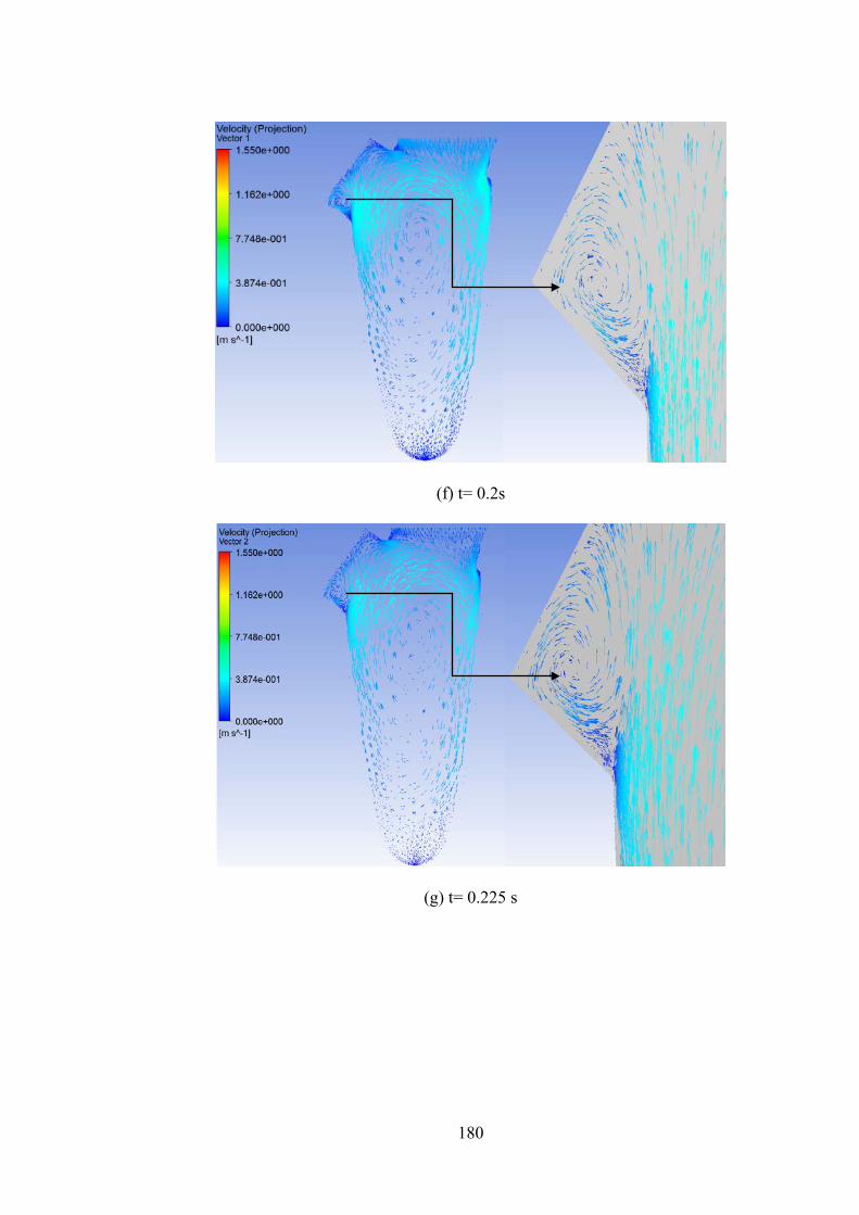
180

(f) t= 0.2s

(g) t= 0.225 s

181

(h) t= 0.275 s

(i) t= 0.3s

182

(j) t= 0.375 s

(k) t= 0.4s

183

(l) t= 0.45 s

(m) t= 0.475s

184

(n) t= 0.5s

Figure 4.6 Illustration of velocity distributions during diastolic flow conditions

(Arefin and Morsi, 2014)

The time-step observations pertaining to Figure 4.6 are contained in Table 4.3.

Table 4.3 Time-step observations pertaining to figure 4.6 Time Observations

t= 0.025 s At the initiation of the diastolic phase (Figure 4.6), the fluid started to enter the LV

chamber and it began to fill.

t= 0.05 s Due to the rise in the inflow jet a clockwise (CW) ring shaped vortex was seen forming

near the outlet tract.

t= 0.075 s The inlet velocity reached the pinnacle of the E-wave with a magnitude of approximately

0.8 m/s. At this time, maximum inflow velocity entered through the mitral orifice/ inlet

and the jet maintained its flow from the basal region of the LV to the apical region. Due to

this flow of E-wave, the ring shaped, CW vortex changed its location/ shifted its position

slightly downwards but still remained near the outlet tract. Also, the magnitude of flow

velocity was found to be higher in the anterior section of the LV cavity compared to its

posterior region from the mitral orifice. Once the inflow velocity reached the peak of the

185

E-wave it started to decelerate. Because of this, the adherence vortex, which was

developed previously, changed its place a little from the dead-end of the outflow tract and

started to expand simultaneously (Arefin and Morsi, 2014).

t= 0.125 s After reaching the pinnacle of the E-wave, inflow velocity minimized and the vortex

moved towards the core of the LV chamber.

t= 0.15 s The primary ring shaped, CW vortex shifted once more and elongated into the mid of the

LV but a second vortex, which was ring shaped but counter clockwise (CCW), developed

near the dead-end of the outlet region.

t= 0.2 s The inlet flow velocity of 0.2 m/s decelerated further and, as shown in Figure 4.6 (f), the

shape of the vortex enlarged and changed its position to the core of the cavity.

t= 0.225 s The primary vortex was found at the core of the chamber and the secondary/CCW vortex

tended to increase in size and shape.

t= 0.275 s

t= 0.3 s

The primary vortex slightly moved in the anterior direction as the inflow velocity was

minimal and the secondary vortex elongated but stayed close to the outlet tract.

Subsequently, at the end of the diastasis, this ring shaped vortex began to elongate once

more but, at the same time step, an additional counter-clockwise (CCW) vortex originated

at the anterior position of the outlet region, which also enlarged simultaneously (Arefin

and Morsi, 2014).

t= 0.375 s With the rise in the inflow jet, the primary vortex shifted its position again in the core of

the chamber and the CCW vortex was slightly enlarged near the outlet region.

t= 0.4 s

t= 0.45 s

A third vortex, which was ring shaped and CW, developed in the vicinity of the mitral

orifice and the aortic orifice. At the pinnacle of the A-wave, the inlet flow velocity began

to rise once more and because of this, the fundamental/primary vortex began to

amalgamate in the LV cavity. Simultaneously, the third vortex started to enlarge and shift

its position towards the centre of the LV and the second vortex tended to reduce its size

and shape.

t= 0.475 s After touching the peak of the A-wave, the inflow velocity started to decelerates again and

the second vortex stayed in the close outlet tract. However, the ineffective/weak third

vortex once again moved its position slightly to the core of the LV.

t=0.5 s At the end of the A-wave the feeble third vortex completely amalgamated with the

186

propagation of the inlet flow velocity but a primary ring-shaped vortex was formulated

once again at the core of the cavity. The magnitude of the maximum flow velocity of 1.55

m/s was acquired during the filling cycle (Arefin and Morsi, 2014).

The general trends concerning the flow characteristics, formation and/or evolution,

shifting, amalgamation/merging of vortices once again matched closely with previously

published research (Arefin and Morsi, 2014, Cheng et al., 2005, Watanabe et al., 2004,

Nakamura et al., 2002, Vierendeels et al., 1999, Lassila et al., 2012, Verdonck and

Vierendeels, 2002).

Although, the evolution of vortices from the simulations were in line with the results

observed from Cheng et al., 2005, the simulated results here did not directly coincide

with the developments of the vortices reported from the same group. This can be

ascribed to the fact that, in the late diastolic phase, the flow pattern could be altered

because of the utilization of different computational/simulation methods (Arefin and

Morsi, 2014, Cheng et al., 2005).

4.4.5 Structure Simulation using Total Mesh Displacement (TMD)

Similar to the pressure and the velocity distributions of the LV cavity, TMD was also

determined by considering the XY cross sectional plane inside the chamber. Figure 4.7

illustrates the variations in the TMD by taking the wide-open inlet/ mitral orifice and

fully closed outlet/ aortic orifice during the filling phase (Arefin and Morsi, 2014).

187

(a) t= 0.025 s (b) t= 0.05 s

(c) t= 0.075s (d) t= 0.125 s

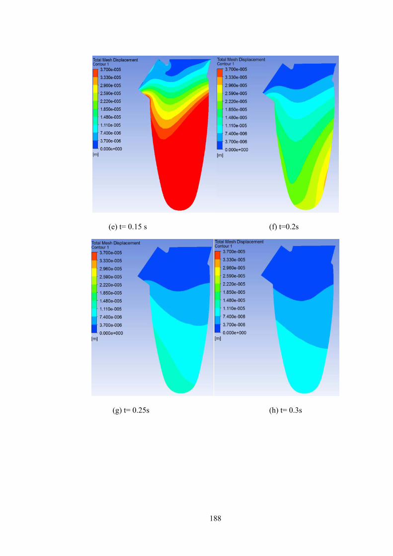
188

(e) t= 0.15 s (f) t=0.2s

(g) t= 0.25s (h) t= 0.3s

189

(i) t= 0.325 s (j) t= 0.375 s

(k) t=0.4s (l) t= 0.45 s

190

(m) t= 0.475s (n) t=0.5s

Figure 4.7 Illustration of total mesh displacement (TMD) during diastolic flow

conditions (Arefin and Morsi, 2014)

From the images in Figure 4.7; at the beginning of the filling phase, the volume in the

LV cavity started to increase with the progression of the flow propagation. For instance,

at the onset of the filling wave, the LV chamber was empty and with the rise in the

inflow velocity, the cavity started to fill. During the pinnacle of the E-wave, the jet

progressed through the inlet of the LV with maximum flow velocity and because of this,

a much higher magnitude of displacement was obtained in the ventricle apex compared

to the ventricle base. The magnitude in the apical region of the LV remained higher due

to the intraventricular pressure developed on the LV wall.

As soon as the inflow velocity wave entered into the diastasis phase, the value of the

TMD decreased in the tip of the ventricle, compared to its previous time steps (t= 0.2 s).

During the time step t= 0.25 s the displacement changed from the posterior section of

the LV to the anterior section in the ventricle apex, as shown in the ventricle-contour

(Figure 4.7 (g)) (Arefin and Morsi, 2014). At the end of the diastasis stage, the

magnitude of the displacement was found to be minimal due to the lower inlet velocity.

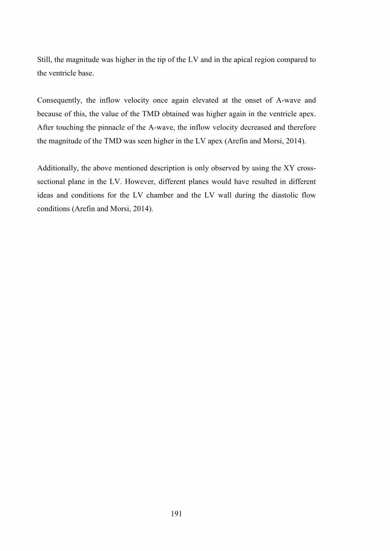
191

Still, the magnitude was higher in the tip of the LV and in the apical region compared to

the ventricle base.

Consequently, the inflow velocity once again elevated at the onset of A-wave and

because of this, the value of the TMD obtained was higher again in the ventricle apex.

After touching the pinnacle of the A-wave, the inflow velocity decreased and therefore

the magnitude of the TMD was seen higher in the LV apex (Arefin and Morsi, 2014).

Additionally, the above mentioned description is only observed by using the XY cross-

sectional plane in the LV. However, different planes would have resulted in different

ideas and conditions for the LV chamber and the LV wall during the diastolic flow

conditions (Arefin and Morsi, 2014).

192

4.5 Summary

The simulations indicated that the variations in the Ip within the chamber of the LV

occurred due to the changes in the LV wall during the E-wave and the A-wave. Also,

the value of the Ip in the ventricle apex was much higher compared to the Ip in the

ventricle base during the pinnacle of the early filling wave; atrial contraction wave, and

the diastasis. The basal pressure was higher at the onset of the early filling wave and the

atrial contraction wave. The development and merging of vortices were evident during

the filling phase inside the cavity of the LV (Arefin and Morsi, 2014).

WSS increased with the rise in the inflow velocity of the early filling wave and atrial

contraction phase, but vice-versa during the slow filling phase/diastasis (Arefin and

Morsi, 2014). During the filling phase, the fluid inside the ventricle chamber was

thought to be responsible for developing WSS. Moreover, similar effects had also been

found in the structure simulations of the LV where, with the rise in the inlet waveform

elevated and during the deceleration of the inflow velocity, the magnitudes of the

displacement were observed to be reduced.

The evolution of vortices, including the development, shifting and amalgamation, were

observed inside the LV cavity during various time steps of the inlet flow propagation.

However, it was determined that by using different simulation/ computational

approaches the results could vary during the late-diastolic period (Arefin and Morsi,

2014).

All these cardiac conditions were generally in line with previously published research

and clinical results. Also the outcomes of this simulation provided useful insights into

physiological and hemodynamical variations, which included (Arefin and Morsi, 2014):

• The flow pattern

• Distribution of Ip

• Distribution of WSS

• The structural displacement during the filling conditions

193

From these investigations, it was determined that (Arefin and Morsi, 2014):

• The maximum value of the intraventricular pressure (Ip) was 5.4E2 Pa

• The magnitude of WSS was 5.7 Pa

• The flow velocity was 1.55 m/s

• The maximum amount of displacement in the LV apex was found to be 3.7E-5

m during the pinnacle of the early filling wave

This investigation and the magnitudes of various parameters during the diastolic

conditions will be helpful in developing next generation VAD system.

194

Chapter 5

Numerical Analysis of the Left Ventricle during

Diastole Phase: Angular Variations between the

Mitral and Aortic Orifice

195

5.1 Overview

The main objective of the research documented in this chapter was to determine the

significance of the hemodynamic characteristics and the physiological alterations of the

left ventricle (LV), by varying the angles between the aortic and the mitral orifice

during the filling phase. During the simulations, three different angles were considered

and varied, as:

• 50°

• 55°

• 60°

Once again, similar to the simulations in Chapter 3 and Chapter 4, Fluid Structure

Interaction (FSI) was utilized and the results were also exhibited and analyzed in terms

of:

• Flow pattern



• Deformation of the structure

The 3D LV model and the required boundary conditions used here were similar to

Chapter 4. Again, similar to Chapter 3 and Chapter 4, the Navier-Stokes equations and

the Arbitrary Lagrangian Eulerian (ALE) methods were utilized to couple the fluid and

solid domains of the geometry. Subsequently, the simulated results were analyzed and

compared with previously published research work.

This chapter concludes by providing the findings from the simulations, which highlight

the significance of the hemodynamic features and structural changes brought about by

changing the degree of mitral and aortic orifices. As with previous analyses, these

would be useful for the development of a next generation VAD device.

196

5.2 Introduction

It was well-known that a small variation in the LV structure could change the overall

hemodynamic performance. Even though there were various imaging tools available

which could specify the qualitative differences in the flow dynamics inside the cavity of

the LV, the hemodynamic features achieved by varying the angles between the mitral

and aortic orifice still had to be investigated. In this research, the angles between the

mitral and aortic orifice were varied to 50°, 55° and 60° and the overall changes in the

structural and hemodynamic changes are described.

From the previous investigations in Chapter 3 and Chapter 4, it was evident that the

utilization of the FSI method was well established and offered significant features that

would enable researchers to determine and understand various physiological and clinical

aspects of the simulated models. The FSI technique was employed here in order to

determine the physiological and clinical significance of different angular variations in

the inlet and outlet region of the 3D, physiologically correct LV during filling

conditions.

During the application of these numerical approaches, an analysis of:

• The flow dynamics, including the evolution, merging and shifting of vortices

• Pressure distributions

• Wall Shear Stress (WSS) distributions

• Structural variations using Total Mesh Displacement (TMD) characteristics

was undertaken and documented. The primary features of the hemodynamic behaviour

and physiological displacement during diastolic conditions are subsequently

highlighted.

197


5.3.1 Overview

The LV geometry deployed here for all the simulations was similar to the one

documented in Chapter 4 but here the angles between the mitral and aortic orifices were

varied (50°, 55° and 60°). Once the required geometry was selected, boundary

conditions and inlet velocity wave/transmitral velocity profile (U) parameters similar to

those in Chapter 4 were implemented on the LV model. Subsequently, pressure

distributions, velocity distributions, WSS distributions and structural displacement were

investigated and determined.

5.3.2 Geometry Extraction

As noted above, a similar geometry of the LV to that illustrated in Chapter 4 [Figure 4.1

(a) and Figure 4.1 (b)], was utilized here for the simulations. Also, it was already proven

that by providing suitable boundary conditions and physiological parameters, a

simplified geometry could produce accurate results (Arefin and Morsi, 2014, Nakamura

et al., 2002, Watanabe et al., 2004, Cheng et al., 2005, Zheng et al., 2012). This

geometry was varied angularly between the mitral and the aortic orifices (50°, 55° and

60°) using SolidWorks 2012. Figure 5.1 demonstrates the LV model with the angular

discrepancies of 50°, 55° and 60° between the inlet and outlet.

198

(a)

(b)

199

(c)

Figure 5.1 LV Model with the angular differences of (a) 50°, (b) 55° and (c) 60°

between the inlet and outlet (SolidWorks 2012)

5.3.3 Meshing Statistics and Mesh Independency Trials

Once again, after a model was developed using SolidWorks 2012, it was then

introduced into ANSYS 14.5. Suitable meshing was then implemented and required

boundary conditions were allotted. For the current simulations, the “Tetrahedrons

Method using Patch Conforming Algorithm” was implemented for the solid and fluid

domains separately. Again, line control properties were utilized, similar to the research

documented in Chapter 4, to observe the differences in the flow velocity (Arefin and

Morsi, 2014, Kouhi, 2011).

Consequently, a mesh independency trial was executed using these line control

parameters and the variations in the fluid velocity were determined for successive nodes

and elements, both for the solid and fluid domains until convergence was achieved.

Figure 5.2 demonstrates the mesh independency trials by implementing the fluid

200

velocity. In this trial, three different meshing categories (coarse, medium and fine) were

chosen. After implementing these categories it was verified that:

• 5436 nodes

• 2743 elements

were assumed to be ideal for the solid region and:

• 2467 nodes

• 1331 elements

were considered to be ideal for the fluid domain. These nodes and elements were chosen

for the medium type of mesh. Also, the convergence criterion for the fluid was taken to

be 10-4 and for the coupling data transfer it was assumed to be 10-2, similar to the

simulations documented in Chapter 4 (Arefin and Morsi, 2014).

Figure 5.2 Mesh independency trial using fluid flow velocity

0

0.1

0.2

0.3

0.4

0.5

0.6

0.7

0.8

0 0.02 0.04 0.06 0.08

Mesh Type-Coarse

Mesh Type-Fine

Mesh Type-Medium

201

5.3.3 Boundary Conditions

Transmitral flow velocity (U in m/s) was provided through the inlet region for all three

geometries. Moreover, the boundary conditions for the solid and fluid region remained

similar, as reported in Chapter4 (Figure 4.3), for the simulations (Arefin and Morsi,

2014). Moreover, with the inlet velocity profile, three states of the filling phase were

identified, as described in Chapter 4. These comprised:

• Two peaks, being the early filling wave (E-wave, at t= 0.08 s) and atrial

contraction wave (A-wave, at t= 0.44 s) with the velocity of 0.8 m/s and 0.4 m/s

correspondingly.

• In between the two peaks, the middle phase was recognized as the diastasis/slow

filling phase (0.22<t<0.3s) (Vierendeels et al., 1999, Cheng et al., 2005, Arefin

and Morsi, 2014).

As per the boundary details utilized in Chapter 4, the ventricle wall was considered to

be homogeneous and isotropic, with:

• A density of 1.2 g/cm3

• Elastic modulus of 0.7 MPa

• Poisson’s Ratio with the magnitude of 0.4

Also, during the simulations, Newtonian fluid flow was considered incorporating:

• Fluid density of 1050 kg/m3

• Viscosity of 0.0035 Pa.s

which also comprised no-slip boundary conditions. The flow property was assumed to

be laminar (Vierendeels et al., 1999, Cheng et al., 2005, Lassila et al., 2012, Arefin and

Morsi, 2014, Saber et al., 2003). Once again, for the coupling data transfer control, the

under relaxation factor was fixed to 0.75.

202

5.4 Simulation Results

5.4.1 Overview

The results are shown here in the form of velocity distributions incorporating:

• The evolution, merging and shifting of vortices

• Intraventricular pressure distributions (Ip)

• Distribution of wall Shear Stress (WSS)

• Variations in the structural displacement using total mesh displacement (TMD)

during the filling phase

5.4.2 Distributions of Velocity

5.4.2.1 Angular Difference of 50°

The images in Figure 5.3 illustrate the flow/hemodynamic characteristics inside the

chamber of the LV during the diastolic flow conditions. Velocity mapping was utilized

to epitomize the variations in the flow pattern, where the velocity vectors were plotted

on the XY cross-sectional plane of the LV, for the angular difference of 50°. The flow

profiles are illustrated by taking the mitral orifice wide open and the outlet region

completely closed. Fourteen different time steps are presented here, which were

obtained from the alterations in the inlet velocity waveform (U). Table 5.1 presents the

summary of the results during three states.

203

0.025s 0.05 s

0.075s 0.125s

204

0.175s 0.2s

0.25 s 0.275 s

205

0.3 s 0.35 s

0.4 s 0.45 s

206

0.475 s 0.5 s

Figure 5.3 Velocity mapping for the angular difference of 50°

Table 5.1 Observations pertaining to figure 5.3 Conditions Observations

E-wave During the initiation of the filling cycle, fluid began to flow concurrently through the

inlet into the LV cavity. Initially, the inflow velocity was minimal and when it reached

the pinnacle of the E-wave the maximum inflow velocity flowed through the wide open

inlet and the fluid rapidly started to flow from the basal region to the apical region of the

LV. During this time step, the flow velocity magnitude was higher relative to the

posterior position from the inlet region of the LV. Once it touched the pinnacle of the E-

wave, the inflow velocity began to decrease and during that time, fluid inside the

chamber started to develop a wake vortex near the vicinity of the mitral and aortic

orifice. A maximum velocity of 8.96E-1 m/s was found to be at the basal region of the

LV during the time step of t= 0.075s (close to peak E-wave). After touching the pinnacle

of the E-wave, the velocity of the inflow jet started to decrease and hence the magnitude

in the basal region started to decrease as well. The vortex was found to be enlarging and

shifting its position slightly towards the middle of the cavity (t= 0.125 s). With a further

decrease in the inlet velocity (when t= 0.175 s and t= 0.2 s) the primary vortex was still

found to be elongating and moving towards the centre of the chamber.

Diastasis When the inlet velocity entered into the diastasis period, inflow velocity was minimal

and therefore a change in the vortex location was observed inside the cavity. During that

207

time (t= 0.25 s), the vortex changes its location from the basal region into the core of the

chamber. The maximum velocity was found to be approximately 3E-1 m/s around the

core of the vortex.

A-wave At the onset of the A-wave (t= 0.3 s), the inflow velocity started to increase and

subsequently, with the rise in the inflow velocity (t= 0.35 s), due to the atrial contraction

wave, this vortex slowly amalgamated with the fluid which entered through the inlet

region. Inflow velocity decreased when it reached the peak of the A-wave but, once

again, the flow velocity decreased after reaching the peak. At the end of the filling

phase, a vortex developed again in the centre of the LV chamber. A maximum velocity

of approximately 4.48E-1 m/s was obtained during the time step, t= 0.045 s.


Figure 5.4 illustrates the velocity distributions inside the cavity during the filling period

with the angular variation of 55° between the inlet and outlet region. It should be noted

that a similar approach and inlet velocity propagation were implemented to obtain the

changes in the hemodynamic characteristics inside the LV. Table 5.2 presents the

summary of the results.

0.025 s 0.05 s

208

0.075 s 0.125 s

0.175 s 0.2 s

209

0.25 s 0.275 s

0.3 s 0.35 s

210

0.4 s 0.45 s

0.475 s 0.5 s


211


E-wave At the onset of the simulation, fluid began to flow through the inlet region. Primarily, the

inflow velocity was minimum but with the rise in the inlet velocity (for example, t=

0.075 s, peak E-wave) the inflow jet got driven from the basal region of the LV towards

the apical region. During that time, a weak vortex originated close to the outlet region.

After touching the pinnacle of the E-wave, the inflow velocity decreased and

simultaneously, the weak vortex slightly elongated and shifted its position close to the

outlet tract. The maximum magnitude of the inflow velocity was found to be

approximately 1.02 m/s during the pinnacle of the E-wave.

Diastasis When the inlet velocity reached its diastasis period, an adherence vortex originated in

the core of the cavity. This weak vortex enlarged slightly during the diastasis period, but

the maximum velocity was approximately 2.55E-1 m/s around the centre of the vortex,

during the time step of (t= 0.25 s and t= 0.275 s).

A-wave Again, with the rise in the inlet velocity, the resultant adherence vortex began to

weaken/merge, but a ring shaped vortex developed close to the outlet region. At the end

of the diastolic period, this newly developed vortex enlarged once more and changed its

location towards the centre of the LV chamber. Also, during the peak of the A-wave, the

maximum magnitude of the inflow velocity was approximately 5.1E-1 m/s with the time

step of t= 0.45 s.


A similar range of incidents were observed from the investigation of the angular

difference of 60° between the mitral and aortic region. Figure 5.5 demonstrates velocity

mapping of the LV chamber during the diastolic phase for the angular difference of 60°

between inlet and outlet tract. Also, a similar method and inlet waveform were utilized

to observe the primary discrepancies in the hemodynamic features for fourteen differnet

time steps inside the LV cavity. Table 5.3 demonstrates the summary of the results.

212

0.025 s 0.05 s

0.075 s 0.125 s

213

0.175 s 0.2 s

0.25 s 0.275 s

214

0.3 s 0.35 s

0.4 s 0.45 s

215

0.475 s 0.5 s



E-wave Fluid started to flow inside the cavity at the beginning of the filling phase. As the inlet

velocity increased, the flow velocity increased inside the LV chamber and the jet started

to move from the basal region to the apical region. At the peak of the E-wave (t= 0.075

s) a maximum flow velocity of 9.39E-1 m/s was observed in the mitral orifice area.

Also, during that time period, a vortex developed near the outlet tract. After reaching the

peak of the E-wave, the flow velocity started to decrease and simultaneously the vortex

slightly elongated and shifted its position towards the core of the chamber.

Diastasis When the inlet waveform entered into the diastasis phase, the adherence vortex in the

core of the cavity tended to enlarge with the increase in the time steps (t= 0.25 s and t=

0.275 s). A maximum of approximately 2.35E-1 m/s was found around the vortex with

the time step of t= 0.25 s.

A-wave After the diastais period, fluid flow increased and with the rise in the inlet velocity, the

vortex started to merge with the flow propagation. When the inlet velocity reached the

peak of the A-wave, the vortex merged with the fluid inside the cavity. After reaching

the peak of the A-wave, flow velocity decelerated and at the end of the filling phase, the

vortex developed and enlarged once again at the centre of the LV chamber. During the

216

time step of t= 0.45 s a maximum velocity of approximately 5E-1 m/s was noted in the

inlet region at the peak of the A-wave.

5.4.3 Wall Shear Stress (WSS) Distributions


The images in Figures in 5.6 demonstrate the variations in the wall shear stress (WSS)

of the LV during diastolic flow conditions in twelve different time steps. The WSS was

examined in order to understand the influence it exerts on the motion of the LV wall. In

doing so, the exterior surface of the LV wall was considered for the demonstration of

the WSS effect. Initially, the effect was demonstrated for an angular difference of 50°

between the inlet and outlet region. Also, the boundary conditions and inlet velocity

profile that were implemented in the inlet orifice were similar to those in velocity

mapping. Table 5.4 provides the summary of the results.

0.025 s 0.075 s

217

0.1 s 0.15 s

0.2 s 0.25 s

218

0.3 s 0.35 s

0.4 s 0.45 s

219

0.475 s 0.5 s

Figure 5.6 Wall shear stress (WSS) distributions for the angular difference of 50°


E-wave When the inlet waveform entered the mitral orifice of the LV, magnitudes in the

ventricle base started to elevate and with a further rise in the inlet velocity, the WSS

elevated in the inlet tract and in the basal region of the ventricle. Subsequently, when the

inflow waveform reached the peak of the E-wave, maximum, WSS was found to be in

the basal region of the LV. After reaching the peak of the E-wave (t= 0.075 s), the

inflow waveform started to decelerate and simultaneously, the WSS in the inlet tract

began to decrease. At the same time, the WSS in the basal region tended to reduce as

well. The maximum magnitude of the WSS was around 3 Pa in the basal region with the

time steps of t= 0.075 s and t= 0.1 s.

Diastasis When the inlet waveform reached its diastasis phase, the flow velocity decreased and the

effect of the WSS significantly reduced in the basal region and in the inlet tract.

Although the magnitude of the WSS substantially reduced in the diastasis region, the

maximum magnitude of the WSS was approximately 6E-1 Pa in the basal region of the

LV wall with the time step of t= 0.25 s.

A-wave The flow velocity elevated once again and hence the effect of the WSS elevated. It was

also evident that with the rise in the inlet velocity the magnitude of the WSS rose once

220

again in the inlet tract and in the basal region of the LV wall. When the inflow velocity

reached the peak of the A-wave, maximum WSS was found to be approximately 1.8 Pa

in the base, with the time step of t= 0.45 s. At the end of the filling wave, the influence

of the WSS reduced once again in the inlet region of the LV.


WSS distributions for the angular variation of 55° between the aortic and mitral orifices

of the LV wall during the diastolic flow conditions are illustrated in Figure 5.7. Once

again, similar boundary conditions and inlet waveform were employed on the LV to

obtain the WSS effect on the ventricle wall. Table 5.5 provides the summary of the

results.

0.025 s 0.075 s

221

0.1 s 0.15 s

0.2 s 0.25 s

222

0.3 s 0.35 s

0.4 s 0.45 s

223

0.475 s 0.5 s



E-wave With the rise in the inlet waveform, the influence of the WSS was much higher on the

basal region of the LV wall. When the inlet velocity reached the peak of the E-wave (t=

0.075 s), maximum WSS was on the base of the LV wall. Moreover, after reaching the

peak of the E-wave, with the deceleration in the inlet waveform, the effect of the WSS

also decreased (t= 0.1 s, t= 0.15 s and t= 0.2 s). On the other hand, with the time step of

t= 0.075s and t= 0.1 s, the maximum magnitude of WSS was approximately 3 Pa on the

basal region of the LV wall.

Diastasis When the inlet velocity entered into the diastasis phase, the effect of the WSS was

reducing on the centre of the LV wall and on the inlet tract. Also, the magnitude dropped

in the basal region of the LV wall. With the time step t= 0.25 s, the maximum magnitude

of WSS was approximately 6E-1 Pa on the centre of the LV wall.

A-wave With the rise in the inlet waveform, for example, during the initiation of A-wave, flow

velocity started to elevate in the beginning and, hence, the WSS effect on the ventricle

base started to rise once again. At the same time, the influence of the WSS was

increasing on the centre of the LV wall and close to the apical region of the LV. The

maximum magnitude of the WSS was approximately 3 Pa once again, close to the basal

224

region of the LV wall. At the end of the diastolic conditions, the effect of WSS

minimized but was somewhat apparent on the centre of the LV wall.


The images in Figure 5.8 demonstrate the WSS distibutions on the LV wall in twelve

different time steps during the diastolic flow conditions. Similar boundary conditions

and inlet velocity were employed for the angular difference of 60° between the inlet and

outlet regions. Table 5.6 presents the summary of the results.

0.025 s 0.075 s

225

0.1 s 0.15 s

0.2 s 0.25 s

226

0.3 s 0.35 s

0.4 s 0.45 s

227

0.475 s 0.5 s



E-wave At the beginning of the diastolic condition, inflow velocity was minimal and with the

rise in the transmitral velocity, the influence of WSS on the LV wall rose and was

increasing mainly on the inlet tract and on the base of the LV wall. When the inlet

waveform reached the peak of the E-wave (t= 0.075 s), maximum WSS was near the

basal region of the LV wall. After touching the peak of the E-wave, inflow jet velocity

started to decelerate and influence of the WSS on the inlet tract and on the centre of the

cavity of the LV wall tended to reduce. However, maximum WSS was approximately 3

Pa close to the basal region of the LV wall with the time steps of t= 0.075 s and t= 0.1 s.

Diastasis Once the inflow velocity reached into the diastasis period, minimal inflow velocity

entered through the mitral orifice. As a result, the effect of the WSS reduced mainly on

the inlet tract and on the centre of the LV wall. Once again, 6E-1 Pa of maximum WSS

was found near the basal region of the LV wall.

A-wave When the inflow wave entered into the A-wave, the inlet velocity rose once again and

therefore, the effect of the WSS started to elevate again. Variations in the WSS

distributions were again on the inlet tract and on the basal region of the LV wall. The

maximum magnitude of WSS was approximately 1.8 Pa near the basal region of the LV

228

wall (t= 0.45 s). With further decrease in the inlet velocity, the magnitude of the WSS

was decreasing as well mainly on the inlet tract and on the basal region of the LV wall.

5.4.4 Distributions of Pressure


The images in Figure 5.9 illustrate the variation in the intraventricular pressure (Ip)

inside the LV cavity during the filling phase in fourteen different time steps. Similar to

the velocity mapping in Section 5.4.2, an XY cross-sectional plane was taken inside the

ventricle for the angular difference of 50° to determine the changes in the Ip. Once

again, the variations in the Ip were obtained by considering the mitral/inlet orifice

completely open and the outlet/aortic orifice fully closed. Table 5.7 presents the


0.025s 0.05 s

229

0.075 s 0.125 s

0.15 s 0.2 s

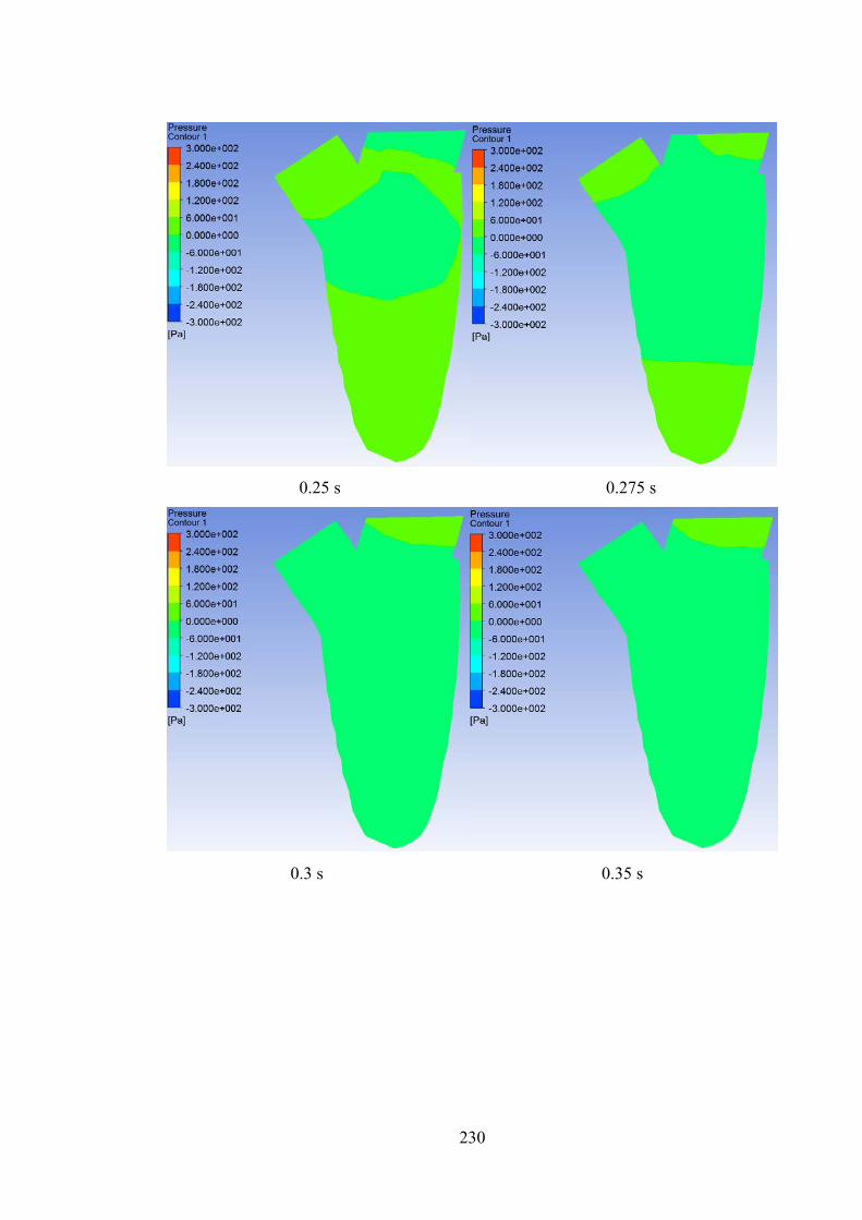
230

0.25 s 0.275 s

0.3 s 0.35 s

231

0.4 s 0.45 s

0.475 s 0.5 s


50°

232


E-wave At the onset of the filling phase, the jet started to enter through the inlet and during the

time step of t= 0.025 s, the pressure inside the ventricle started to rise in the mitral

orifice. With further rise in the inflow velocity, the Ip pressure elevated in the basal

region of the ventricle and the jet started to move towards the apical region. The

magnitude of the Ip started to elevate in the apical region as well (t= 0.05 s). When the

inlet velocity touched the pinnacle of the E-wave, maximum jet entered through the inlet

(t= 0.075 s). Simultaneously, changes in the Ip in the ventricle apex also increased but

much higher Ip was obtained in the apical region, with a magnitude of approximately

2.4E2 Pa. After reaching the peak of the E-wave, inflow velocity started to decelerate

and hence, the magnitude of the Ip in the basal region began to decrease as well.

However, the magnitude of the Ip in the apical region was increasing with a value of

approximately 3E2 Pa (t= 0.125 s). Subsequently, with further decrease in the E-wave

velocity, the magnitude in the basal and the apical region started to decrease as well (t=

0.15 s and t= 0.2 s).

Diastasis When the transmitral velocity (U) reached the diastasis region, Ip in the apical region

was much higher compared to its basal region (t= 0.25 s). This comparison was noticed

due to the minimal inlet flow velocity. Also, a vortex developed in the centre of the

ventricle. During the time step of t= 0.275 s, the magnitude of the apical and basal

pressure was found to be decreasing but the magnitude of the apical pressure was still

higher compared to the Ip in the ventricle base. A maximum magnitude of the Ip was

obtained as approximately 6E1 Pa in the apical region (t= 0.25 s).

A-wave At the onset of the A-wave, the magnitude of the inflow velocity started to elevate and

simultaneously the Ip in the ventricle base began to increase (t= 0.3 s). However, at the

pinnacle of the A-wave, Ip in the apical region was much higher once again than the

basal pressure. After reaching the peak of the A-wave, the inlet flow velocity started to

decelerate and the Ip in the basal region decreased as well (t= 0.45 s). Although with

further deceleration in the A-wave, Ip in the ventricle base started to elevate slightly but

the magnitude was still much lower compared to the Ip in the ventricle apex. At the end

of the filling phase, a much higher magnitude of Ip was at the tip of the ventricle apex

with a value of approximately 3E2 Pa (t= 0.5 s).

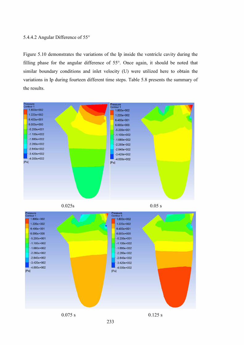
233


Figure 5.10 demonstrates the variations of the Ip inside the ventricle cavity during the

filling phase for the angular difference of 55°. Once again, it should be noted that

similar boundary conditions and inlet velocity (U) were utilized here to obtain the

variations in Ip during fourteen different time steps. Table 5.8 presents the summary of

the results.

0.025s 0.05 s

0.075 s 0.125 s

234

0.15 s 0.2 s

0.25 s 0.275 s

235

0.3 s 0.35 s

0.4 s 0.45 s

236

0.475 s 0.5 s


55°


E-wave At the initiation of the E-wave, minimal inflow velocity entered through the mitral

orifice and during that time step (t= 0.025 s) the magnitude of Ip in the basal region

started to rise and was much higher compared to the apical region. Unlike the angular

difference of 50°, a maximum magnitude of approximately 1.8E2 Pa was found to be in

the ventricle base with the time step of t= 0.025 s. Once more, with the advancement in

the E-wave, apical pressure inside the LV started to elevate and when the inlet velocity

reached the pinnacle of the E-wave (t= 0.075 s), Ip in the apical region was still found to

be increasing compared to its basal section. However, during this exact time step, the

magnitude of the Ip in the basal region was very low. This could be attributed to the fact

that, due to the variation in the ventricle geometry, the transmitral wave could not

directly enter through the mitral orifice and also it may be hindered with the wall of the

inlet region. Consequently, after reaching the pinnacle of the E-wave, inlet velocity

started to decelerate but the Ip in the ventricle apex increased and maximum magnitude

of Ip was approximately 1.8E2 Pa (t= 0.125 s and 0.15 s). At the end of the E-wave,

apical pressure was found to be much higher than the basal pressure (t= 0.2 s).

Diastasis During the diastasis phase, minimal inflow velocity entered through the mitral orifice.

237

During this phase, the magnitude of the Ip in the ventricle apex was decreasing but the Ip

in the basal region elevated slightly. The maximum magnitude of Ip was approximately

6.4E1 Pa in the apical region with the time step t= 0.25 s.

A-wave When the transmitral velocity (U) entered into the A-wave, inflow velocity started to rise

once again and the magnitude of the basal pressure started to elevate simultaneously (t=

0.3 s, t= 0.35 s and t= 0.4 s). At these exact time steps, the magnitude of the Ip in the

basal region was comparatively higher than the Ip in the ventricle apex. After reaching

the pinnacle of the A-wave, inflow velocity once again started to decrease (t= 0.45 s and

t= 0.475 s). During that time, Ip in the ventricle apex was much higher again compared

to the magnitude of Ip in the ventricle base. Also, the magnitude of the Ip in the apical

region of the chamber tended to increase with the deceleration in the A-wave. At the end

of the filling phase (t= 0.5 s) maximum Ip was at the tip of the LV apex with a

magnitude of around 1.8E2 Pa.


All the images in Figure 5.11 illustrate the changes in the magnitudes of Ip inside the

LV chamber during the diastolic wave for the angular difference of 60°, in fourteen

different time steps. The boundary conditions and inlet velocity waveform (U) were

similar to those employed for the angular differences of 50° and 55°. Table 5.9 provides

the summary of the results.

238

0.025s 0.05 s

0.075 s 0.125 s

239

0.15 s 0.2 s

0.25 s 0.275 s

240

0.3 s 0.35 s

0.4 s 0.45 s

241

0.475 s 0.5 s


60°


E-wave At the beginning of the E-wave, the inflow jet started to enter through the mitral orifice

(t= 0.025 s). During that time step, basal pressure was comparatively higher than the

apical pressure. Once again, with a further rise in the inlet velocity waveform, basal

pressure somewhat increased and, during the peak of the E-wave, the maximum inflow

wave entered through the inlet region (t= 0.075 s). At that time, the magnitude of the Ip

in the apical region was elevated compared to its basal counterparts. Once more, after

reaching the peak of the E-wave, the inlet velocity started to decrease and the Ip in the

apical region was still much higher than its basal region (t= 0.125 s, t= 0.15 s and t= 0.2

s). Maximum Ip was in the apical region with a magnitude of 2.5E2 Pa.

Diastasis After the deceleration in the E-wave, the inlet velocity entered into its diastasis phase

where the minimal inflow velocity jet entered through the mitral orifice. The magnitude

of the apical pressure was still somewhat higher than its basal pressure (t= 0.25 s).

During that time, a small vortex developed at the centre of the cavity. With the time step

of t= 0.275 s, the magnitude of Ip, both in the apical and basal region, decreased but the

magnitude of Ip in the ventricle apex was still moderately higher than the basal region.

Moreover, the primary vortex was elongated at the centre of the cavity. Also, the

242

maximum magnitude of Ip during the diastasis stage was approximately 7E1 Pa in the

apical region of the ventricle (t= 0.25 s).

A-wave With the initiation of the A-wave, inflow velocity started to elevate once again through

the mitral orifice. The basal pressure tended to increase with the elevation in the A-wave

and simultaneously the apical pressure was also rising (t= 0.3 s, t= 0.35 s and t= 0.4 s).

After reaching the peak of the A-wave, the inflow velocity started to decrease and during

the time steps of t= 0.45 s and t= 0.475 s, the magnitude of Ip in the ventricle apex

started to elevate once again compared to its basal pressure. At the end of the filling

phase (t= 0.5 s), a much higher magnitude of Ip was in the ventricle apex with a value of

approximately 2.05E2 Pa.

5.4.5 Structure Simulations using Total Mesh Displacement (TMD)


The images in Figure 5.12 demonstrate the variations obtained in the ventricle

displacement during the diastolic wave propagation for thirteen different time steps.

Once again, boundary conditions and inlet velocity wavform (U) were similar to those

previously utilized for the velocity mapping, WSS and pressure distributions. Also, an

XY cross-sectional plane was taken inside the LV cavity to obtain the variations in the

mesh dispalcement of the structure. Moreover, the inlet was considerd fully opened and

the outlet was considered completely closed during the filling phase. Table 5.10

presents the summary of the results.

243

0.05 s

0.075 s 0.125 s

244

0.15 s 0.2 s

0.25 s 0.325 s

245

0.35 s 0.4 s

0.425 s 0.45 s

246

0.475 s 0.5 s


of 50°


E-wave The volume inside the LV chamber started to increase with the flow propagation of the

filling wave. For example, at the beginning of the filling wave, the LV cavity was empty

and with the rise in the inlet velocity waveform, the volume of this chamber started to

elevate. When the inflow velocity touched the pinnacle of the E-wave (t= 0.075 s), a

comparatively higher magnitude of displacement was observed at the apical region of

the ventricle than its basal region. Once again, after touching the peak of the E-wave, the

inlet velocity decreased and hence the magnitude of the displacement increased at the

posterior side of the LV in the apical region, with a value of approximately 3.8E-5 m (t=

0.125 s). Moreover, with further deceleration in the E-wave, the magnitude of the TMD

in the apical region was decreasing.

Diastasis Once the inlet waveform reached its diastasis phase, the magnitude of the displacement

decreased but was still somewhat higher in the apical region than the basal region. The

maximum magnitude of the displacement was approximately 6.7E-6 m in the apical

region with the time step of t= 0.25 s.

A-wave After the minimal inflow velocity in the diastasis phase, the rate increased and entered

247

into the A-wave. With the rise in the A-wave velocity through the mitral orifice, the

magnitude of the displacement started to increase in the ventricle apex and this

magnitude increased even more with a further rise in the A-wave (t= 0.35 s, t= 0.4 s and

t= 0.425 s). After reaching the pinnacle of the A-wave, the inflow velocity once again

started to decrease and the magnitude in the apical region was still rising (t= 0.45 s and

t= 0.5 s). At the end of the filling phase (t= 0.5 s), the maximum magnitude in the

structure displacement was approximately 3.04E-5 m in the posterior LV wall in the

apical region.


All the images in Figure 5.13 show the changes in the structure displacement of the LV

during the filling phase, in thirteen various time steps. Again, similar boundary

conditions and the inlet velocity waveform (U) were implementd during the

simulations. Table 5.11 represents the summary of the results.

0.05 s

248

0.075 s 0.125 s

0.15 s 0.2 s

249

0.25 s 0.325 s

0.35 s 0.4 s

250

0.425 s 0.45 s

0.475 s 0.5 s


of 55°

251


E-wave At the initiation of the filling phase, the inlet jet started to enter the LV chamber and

with the rise in the inlet velocity, the magnitude of the displacement in the apical region

of the LV increased (t= 0.05 s). When the inlet velocity reached the peak of the E-wave

(t= 0.075 s), the magnitude of the displacement elevated even further in the ventricle

apex. After reaching the peak of the E-wave, the inflow velocity started to decline but

the maximum magnitude of displacement was in the ventricle apex with a value of

approximately 2.5E-5 m. Moreover, with further deceleration in the E-wave, TMD was

decreasing in the ventricle apex.

Diastasis When the inflow velocity entered into its diastasis phase, a minimal inflow jet entered

through the inlet region. However, the magnitude of the displacement was slightly

higher in the apical region compared to its basal region. The maximum magnitude of

displacement was still obtained at the posterior side of the LV wall in the apical region

with a value of around 7.5E-6 m (t= 0.25 s).

A-wave The inlet flow velocity entered into the atrial contraction wave (A-wave) and with the

rise in the A-wave, once again accelerated the magnitude of the displacement in the

apical region of the ventricle. After touching the pinnacle of the A-wave, it started to

decline again but the magnitude of the displacement in the apical region was increasing

(t= 0.45 s and t= 0.475 s). At the end of the filling phase (t= 0.5 s) the maximum

displacement was in the anterior side of the LV in the ventricle apex with a magnitude of

approximately 2E-5 m.


Figure 5.14 demonstrates the variations in the displacement of the left ventricle during

the diastolic flow propagation. The inlet waveform (U) and the boundary conditons are

considered to be similar to those noted previosuly. Thirteen different time steps were

chosen to demonstare the variations in the displacement of the structure. Table 5.12

presents the summary of the results.

252

0.05 s

0.075 s 0.125 s

253

0.15 s 0.2 s

0.25 s 0.325 s

254

0.35 s 0.4 s

0.425 s 0.45 s

255

0.475 s 0.5 s


of 60°


E-wave The rate of flow started to increase at the onset of the E-wave through the mitral orifice

into the LV chamber. With a further rise in the inlet velocity, the magnitude of the

displacement in the ventricle apex started to elevate (t= 0.05 s). After reaching the peak

of the E-wave (t= 0.075 s), the inflow velocity started to decrease and the maximum

magnitude of displacement was at the posterior side of the LV wall in the apical region,

with a value of approximately 3.5E-5 m (t= 0.125 s). Subsequently, with further

deceleration in the E-wave, the magnitude of the displacement in the apical region

decreased but it is still higher compared to the basal region.

Diastasis Once the inflow velocity entered into the diastasis phase, a minimal inlet velocity

entered through the inlet region. Although the magnitude of the displacement in the

ventricle apex decreased it was still higher compared to the basal region. Maximum

displacement was in the apical region of the ventricle with a magnitude of 7E-6 m (t=

0.25 s).

A-wave When the inlet velocity entered into the atrial contraction phase (A-wave), the inflow

velocity started to rise once again and with the rise in the A-wave, the magnitude of the

256

displacement in the apical region of the ventricle elevated once again (t= 0.35 s, t= 0.4 s

and t= 0.425 s). After touching the pinnacle of the A-wave, the inlet velocity started to

decrease but the TMD in the posterior side of the ventricle was higher in the ventricle

apex during the time step t= 0.45 s. At the end of the filling phase (t= 0.5 s), a higher

displacement was in the anterior region of the LV in the apex with a magnitude around

2.45E-5 m.

257

5.5 Discussion

5.5.1 Influence of flow dynamics for 50°, 55° and 60° between the mitral and aortic

orifice using velocity mapping

The variations in the flow distributions during the filling phase inside the LV, with

angular differences of:

• 50°

• 55°

• 60°

between the inlet and outlet regions were determined using velocity vectors. From the

simualtions it was evident that, at the onset of the filling wave, a minimal jet entered

through the inlet region. Consequently, with the elevation in the inlet velocity, the

magnitude of the velocity in the basal region of the LV was found to be much higher

compared to the apical region.

When the inlet velocity reached its pinnacle of the E-wave (approximately t= 0.075 s),

the LV geometry, with angular variations of 55° and 60°, developed a weaker vortex

close to the outlet region. This vortex, in both cases, was ring shaped and clockwise

(CW). The development of these vortices primarily depended on the angular variations

of the structure. However, the locations of these vortices were in similar places inside

the chamber. Subsequently, after touching the pinnacle of the E-wave, the inflow jet

started to decelerate and the magnitudes in the basal region of the ventricle began to

decrease. With the time step t= 0.125 s, the ring shaped and CW vortex was in the

vicinty of the inlet and outlet orifices for the 50° case but, for the 55° and 60° cases, the

vortices tended to elongate and shfit towards the core of the chamber. With further

deceleration in the E-wave (t= 0.175 s and t= 0.2 s) a similar kind of behaviour of the

vortices inside the cavity was observed for 50°, 55° and 60°. During these time periods,

the vortices were enlarging and heading into the central region of the LV cavity.

258

Once the inflow velocity entered into the diastasis period, the magnitude of the inflow

velocity decreased and the magnitudes in the ventricle base reduced. During this phase,

the adherence vortices for 50°, 55° and 60° were elongating and moved slightly towards

the core of the cavity. This was attributed to the fact that the primary vortex changed its

location towards the core of the cavity, where the posterior section of the vortex moved

marginally forward and the anterior/frontal section moved in opposite direction to the

posterior section, which in turn generated the adherence vortex. However, for the 55°

case, the location of the vortex was slightly upwards from the core of the LV, compared

to its counterparts (50° and 60°).

When the transmitral velocity entered into the A-wave, the inflow velocity started to

rise once again, as seen earlier. During this period, the adherence vortex in the ventricle

cavity began to merge with the rise in the inflow jet. This incident was apparent for the

50°and 60° cases, but in the 55° case, the the adherence vortex almost amalgamated

with the inflow jet and after touching the pinnacle of the A-wave (approximately t= 0.45

s), a clear, second ring-shaped and CW vortex originated near the outflow tract.

However, for 50° and 60° cases, this second vortex was obscure. This was ascribed to

the fact that, with the rise in the inflow velocity (peak A-wave), a vortex tended to

develop in the vicinity of the outlet tract due to variations of the anguar differences in

the LV geometry. Apparently, at the end of the filling phase, a ring shaped vortex

developed once again at the centre of the cavity.

Once again, the general trends of the flow behaviour, generation, development, shifting

and amalgamation of vortices were in line with the investigations from previously

published research (Arefin and Morsi, 2014, Vierendeels et al., 1999, Nakamura et al.,

2002, Watanabe et al., 2004, Cheng et al., 2005, Lassila et al., 2012).

5.5.2 Influence of intra-ventricular wall shear stress (WSS) for 50°, 55° and 60°

between the mitral and aortic orifice using WSS distributions

259

At the onset of the diastolic wave flow, the influence of the WSS was seen on the inlet

tract. With the elevation in the inlet velocity waveform, the magnitude of the WSS

increased on the inlet region and was also seen on the basal region of the LV wall.

During the pinnacle of the E-wave (t= 0.075 s), the maximum effect of the WSS was

observed on the anterior side of the basal region of the LV. However, a much higher

effect was seen on the basal region for the angular difference of 55° compared to 50°

and 60°. Moreover, for the 55° case, the influecne of WSS was higher close to the

anterior side of the apical region. For 50° and 60° cases, this effect was only observed

close to the anterior section of the ventricle core. With the deceleration of the E-wave,

the effect of the WSS on the inlet tract reduced simultaneously for 50°, 55° and 60°.

Also, during this period of time, the WSS effect minimized and remained on the basal

region for the 50° and 60° cases, but its effect was still evident on the core of the cavity

for 55°.

When the inlet waveform reached into the diastasis phase, the influence of the WSS

significantly reduced for the 50° and 60° cases. Precisely, the effect was minimal only

on the basal region of the LV. However, for the 55° case, this effect was still apparent

around the anterior section of the LV core but the effect was almost negligible on the

inlet tract.

Once again, at the onset of the A-wave, the effect of the WSS started to rise again, both

on the inlet tract and on the anterior position of the basal region for 50°, 55° and 60°.

Additionally, for the 55° case, this effect once again almost reached on the anterior

position of the apical region. With the rise in the A-wave, it accelerated the magnitude

of the WSS but with the deceleration in the A-wave, the WSS on the inlet tract began to

reduce once more for all cases. It also reduces on the basal region (for 50°and 60° cases)

and in the apical region and around the core of the LV (for 55°).

At the end of the filling phase, the WSS effect became negligible for the LV, especially

for the 50° and 60° cases, but was somewhat observed for the 55°. It should be noted

that, during the A-wave, the WSS effect was found to be sightly sideways/just beside

the basal region and on the centre of the LV compared to the effects originating during

the A-wave and the diastasis. This was attributed to the fact that, during the A-wave, the

260

elevation in the flow velocity did not rise much compared to the E-wave and hence, the

WSS effect could move slightly sideways on the LV wall.

5.5.3 Influence of intra-ventricular pressure (Ip) for 50°, 55° and 60° between the

mitral and aortic orifice using pressure distributions

At the begining of the filling wave, the magnitude of the Ip started to rise more in the

ventricle base than its apical region. Also, a negetive pressure gradient was observed at

the ventricle apex, as the propagation of the inflow jet was yet to reach in the apical

region of the cavity. So, the Ip in the basal region was found to be much higher than its

apical region. The magnitude of Ip in the basal region started to increase with the rise in

the early filling wave (E-wave) and the magnitude of Ip also increased in the apical

region of the ventricle. When the inlet velocity waveform reached the pinnacle of the

early filling wave (t= 0.075 s), a maximum inflow velocity entered through the mitral

orifice, which in turn also elevated the magnitude of the Ip in the apical region than the

basal pressure. During this exact time step, the maximum Ip was approximately 2.4E2

Pa for the 50° case, compared with a magnitude of 1.6E2 Pa for 60° and 1.22E2 Pa for

55°.

After reaching the pinnacle of the early filling wave, the inlet velcoity began to dip

down and the propagation of the jet reached to the end of the cavity (apical region) at

that time. Once it reached the apical region of the ventricle, the LV wall produced a

positive reflection back to the propagation of the inflow jet. This

superposition/amalgamation of the propagation of the flow with the reflected-wave from

the ventricle apex was responsible for elevating the magnitude of the Ip in the apical

region, which was generally termed as an "F-wave" (Cheng et al., 2005, Arefin and

Morsi, 2014). From the simulation results, it can be noted that a much higher magnitude

of Ip was found for the 50° and 60° cases compared to 55° for the ventricle apex. At the

end of the E-wave (t= 0.2 s), Ip in the apical region was still found to be moderately

higher for the 50° and 60° compared with 55°.

261

At the onset of the slow filling wave, a minimal inlet velocity entered through the mitral

region and the basal pressure tended to decrease. During this diastasis phase, a

maximum magnitude of Ip was in the apical region of the ventricle for all cases (50°,

55° and 60°). However, the discrepancies in the generation of vortex were found to be

somehwat different during the diastasis phase for the three cases. For the 60° case,

initally a very small vortex originated and then the vortex elongated. For the 50° case, a

much larger vortex (size and shape) was found compared to the 55° case during the time

step of t= 0.25 s. At a time step t= 0.275 s, a much larger vortex was observed for the

55° case compared to the 50° and 60° cases. It should be noted that, for the 50° case, the

primary vortex somewhat merged with fluid inside the chamber (t= 0.275 s).

Subsequently, the inlet velocity started to increase once again and with the rise in the

inlet velocity, the primary vortex started to merge with the propagation of the flow.

During the onset of the atrial contraction wave (A-wave), the magnitude of the Ip in the

ventricle base started to elevate once again compared to its basal pressure. After

reaching the peak of the A-wave, the inflow velocity dipped down once again and

during that time, the magnitude of Ip in the ventricle apex was much higher compared

to its basal pressure. At the end of the filling phase, the maximum magnitude of Ip is

found to be at the tip of the ventricle (apical region) for the 50° case with a magnitude

of approximately 3E2 Pa.

Consequently, the general phenomena of differences in the Ip, inside the ventricle

during the filling phase, were in line with previously published research (Vierendeels et

al., 1999, Nakamura et al., 2002, Cheng et al., 2005, Arefin and Morsi, 2014).

5.5.4 Influence of structure simulation for 50°, 55° and 60° between the mitral and

aortic orifice using total mesh displacement (TMD)

At the intiation of the filling wave, the inlet velocity jet started to enter the chamber,

which also increased the volume inside the cavity. With the rise in the inlet velocity, the

volume rose and, after touching the peak of the early filling wave, the inlet velocity

262

starts to decline. The superposiiton of the F-wave inside the LV; the increase in volume

inside the ventricle, and the intraventricular pressure changes meant that maximum

displacement was found in the apical region (t= 0.125 s) for all three cases. However,

for the 50° and 60° maximum TMD was observed in the posterior side of the LV wall in

the apical region compared to the 55°, where maximum TMD was at the ventricle apex.

With further deceleration in the E-wave, the magnitude of the displacement inside the

ventricle apex was found to be decreasing.

Once the inflow velocity entered into the diastasis phase, the rate of the inflow velocity

was minimal and the magnitude of the displacement in the apical region was decreasing.

However, the magnitude in the ventricle apex was still slightly higher compared to its

basal region for all three cases. This was attributed to the fact that, with minimal inlet

jet volume inside the chamber the variations in the displacement of the structure were

observed to be minimal during the diastasis phase.

When the inlet velocity entered into the A-wave, the flow rate through the inlet region

increased and the magnitude of the displacement started to rise once again. With further

rise in the inlet velocity, volume inside the chamber started to increase again which, in

turn, elevated the magnitude of the dispalcement in the apical region of the ventricle.

After touching the pinancle of the A-wave, the inlet velocity again started to dip down

and with the volume increased inside the cavity, the magnitude of the displacement in

the apical region started to elevate once more. At the end of the filling phase, because of

this increased volume inside the LV chamber, for all three cases, the magnitude of the

displacement in the apical region increased. Specifically, for the 50° case, the maximum

displacement was in the posterior side of the LV wall in the apical region but, for the

55° and 60° cases, it was found to be somewhat in the anterior side of the LV wall in the

ventricle apex.

263

5.6 Summary

From the above discussions and the simulated results, in general, it was evident that the

LV structure with an angular difference of 55° demonstrated different outcomes to the

50° and 60° geometry cases in terms of

• Velocity mapping


• Intraventricular Pressure distributions

• The structure simulations

during the filling phase.

For the velocity mapping, the flow dynamics including the:

• Generation

• Development

• Amalgamation

• Shifting

of vortices inside the LV chamber, for all three geometry cases were investigated and

determined. It was discovered that for the 55° case, the location of the vortex inside the

cavity was moderately upwards relative to the 50° and 60° cases, during the slow filling

phase. Also, during the atrial contraction phase, a second ring-shaped and CW vortex

was observed close to the outlet region for the 55° case, but for 50° and 60° cases, the

second vortex was somewhat obscured. However, after touching the pinnacle of the E-

wave for 50°, a ring shaped and CW vortex was seen developed in the vicinity of the

mitral and aortic orifice but for the 55° and 60° cases, this vortex was found to be

moderately elongating and changed its location towards the centre of the cavity.

The variations in the WSS of the LV wall were observed and it was determined that,

during the peak of the E-wave, the maximum WSS was seen on the anterior position of

the ventricle apex for all three cases. Specifically, a much higher magnitude of WSS

264

was found to be developed on the basal region of the LV for the 55° case than for 50°

and 60° cases. Also, a higher effect of WSS was seen developed near the anterior

position of the ventricle apex for the 55° case compared to 50° and 60° cases, where the

effect was only found near the anterior position of the centre of the LV. Moreover,

during the diastasis phase, the effect of WSS was still evident close to the anterior

position of the ventricle core for the 55° case, whereas for the 50° and 60° cases, very

little effect could be identified at the basal region. With the rise in the A-wave, the

effect of the WSS was increasing for all cases but, at the end of the diastolic wave, the

influence of the WSS became minimal for the 50° and 60° cases, but moderately

observed for the 55° case. Therefore, in general, with the rise in the inlet velocity, the

effect of the WSS increased (E-wave and A-wave) but for minimal inflow velocity this

effect decreased (slow filling phase) (Arefin and Morsi, 2014).

Subsequently, the magnitude of the Ip was also observed for all three cases during the

filling phase and it was noted that, at the end of the E-wave, the magnitude of Ip in the

ventricle apex was still slightly higher for the 50° and 60° cases than for the 55°. Also,

during the slow filling phase, dissimilarities in the generation and merging of the

primary vortex inside the cavity was observed for all cases. Specifically, for the angular

difference of 50°, the principle vortex was observed moderately amalgated with the

fluid inside the cavity (t= 0.275 s). Moreover, at the end of the filling wave, the

maximum magnitude of Ip was found to be at the tip of the ventricle apex for the 50°

case compared to 55° and 60° cases.

Finally, variations in the structural displacement were also observed during the filling

phase for all three cases. After touching the pinnacle of the E-wave, inflow velocity

decreased and at that time, the maximum magnitude of displacement was seen in the

posterior position of the LV wall in the ventricle apex for both the 50° and 60° cases

but, for the 55° cases, it was found to be in the apical region of the ventricle. During the

diastasis phase, for all three cases, the magnitude in the apical region of the LV was still

somewhat higher than its basal region. Consequently, at the end of the filling phase, the

maximum magnitude of displacement was observed in the posterior position of the

ventricle wall in the apical region for the 50° case, but it was observed slightly in the

anterior section of the ventricle wall in the apical region for the 55° and 60° cases.

265

Chapter 6

Numerical Analysis of the Left Ventricle during

Diastole Phase: The Influence of Friction Co-

efficient and Elastic Modulus

266

6.1 Overview

This chapter documents the research that highlighted the hemodynamic characteristics

and structural displacements of the LV during the diastolic phase by implementing the

effects of the:

• Friction co-efficient (Cf)

• Elastic modulus

Similar to the research documented in previous chapters, the Fluid Structure Interaction

(FSI) scheme was utilized for computing the simulations. The Cf and elastic modulus

were determined and implemented during the simulations to observe the influence in

terms of:

• Flow dynamics



• Structural variations

Once again, as reported in Chapter 4 the geometry of a 3D physiologically correct LV

model and required boundary conditions were used during the simulations. Once more,

similar to Chapter 3, Chapter 4 and Chapter 5, the Navier-Stokes equations and the

Arbitrary Lagrangian Eulerian (ALE) methods were employed to couple the solid and

fluid regions of the ventricle model. Subsequently, the results were compared, discussed

and analyzed with previously published research work.

Importantly, the implementation Cf and elastic modulus provided substantial insights

specifically into dilated cardiomyopathy (DCM) disease conditions, which were also

examined.

Finally, this chapter summarizes the findings from the above named simulations which,

as with previous analyses, would be useful for the development of a next generation

VAD system.

267

6.2 Introduction

Diastolic features of the LV are affected by the influence of the friction co-efficient (Cf)

and the elastic modulus, which primarily sway the hemodynamic and physiological

characteristics of the ventricle model. In order to determine and understand the

influence of the Cf and elastic modulus, the FSI method was implemented.

Using the FSI approach, many earlier investigations had been conducted based on the

variations of the flow pattern and the physiological features of the LV, but the

utilization of the Cf was neglected (Taylor et al., 1994, Jones and Metaxas, 1998,

Keldermann et al., 2010). Although in an experimental investigation Cope, 1963,

observed the frictional resistance of the septum but this was based on the insertion of

the transeptal catheter inside the LV (Cope, 1963). However, precise physiological

features were still required in order to simulate the complete functionalities of the

ventricle model (Lee et al., 2009, Nordsletten et al., 2011, Khalafvand et al., 2011).

The literature in Chapter 2 suggested that the FSI scheme was useful in determining the

physiological and hemodynamical characteristics for both the general and diseased

conditions. Hence, the research documented in this chapter once again utilized the FSI

method to determine and understand the structural and hemodynamic properties of the

LV model by implementing the effects of the friction co-efficient (Cf) and elastic

modulus during the filling phase. Moreover, the correlation of these effects with the

DCM was also determined during the diastolic flow conditions. Results are presented

in terms of the:




• Structural variations of the LV model

268


6.3.1 Geometry Extraction

This section provides the details of the LV model and the boundary conditions,

including the effects of Cf and elastic modulus. Similar to the previous approaches,

documented in Chapter 4 and Chapter 5, after selecting the LV model, the transmitral

flow velocity (U) was implemented through the inlet/mitral orifice. Moreover, the

computed Cf and the elastic modulus were varied and implemented during the filling

phase.

For the simulations, the geometry of the LV was considered similar to the model used in

Chapter 4. Therefore, the detailed description of the LV model is not presented here.

For modelling the geometry, SolidWorks 2012 were utilized.

6.3.2 Meshing Statistics and Mesh Independency Trials

Similar to the previous approaches stated in Chapter 4 and Chapter 5, the LV model was

introduced once again into ANSYS 14.5 after being modelled using SolidWorks 2012.

Subsequently, the required meshing was performed and the mandatory boundary

conditions, which also included the varied Cf and the elastic modulus, were

implemented. For this simulation, “Mapped Face Meshing” was executed for the solid

and fluid region independently. Once again, similar to Chapter 3, Chapter 4 and Chapter

5, line control properties were implemented to study the discrepancies in the flow

velocity during the filling phase (Kouhi, 2011, Arefin and Morsi, 2014).

A mesh independency trial was carried out by using this line control properties and the

changes in the velocity of the fluid was computed for consecutive nodes and elements,

both for the solid region and fluid region till the velocity converged. Figure 6.1

illustrates the mesh independency trials by utilizing the fluid velocity. Once more,

269

during this test, three different meshing groups are chosen (coarse, medium and fine).

After utilizing these, it was confirmed that:

• 4507 nodes

• 2362 elements

acceptable for the solid region and:

• 34881 nodes

• 190377 elements

were considered to be accurate for the fluid region respectively. These elements and

nodes were selected for the medium mesh type. Furthermore, similar to the previous

simulations, the convergence criterion for the fluid was considered to be 10-4, and for

the coupling data transfer it is taken to be 10-2, as documented in Chapter 4 and Chapter

5 (Arefin and Morsi, 2014).

Figure 6.1 Mesh independency trial by using fluid velocity

0

0.2

0.4

0.6

0.8

1

1.2

1.4

0 0.02 0.04 0.06 0.08

Velo

city

[m/s

]

Y [m]

Mesh Type-MediumMesh Type-CoarseMesh Type-Fine

270

6.3.3 Boundary Conditions

Once again, similar to Chapter 4, the transmitral flow waveform (U in m/s) was

implemented through the inlet/mitral region and the primary boundary conditions were

also considered to be similar (Arefin and Morsi, 2014).

Subsequently, from the velocity waveform (U), it was recognized that three different

conditions existed, as explained in Chapter 4 and Chapter 5. In brief, the waveform

included:

• Two peaks termed the early filling wave (E-wave) and the atrial contraction

wave (A-wave) with the flow velocity of 0.8 m/s and 0.4 m/s in that order.

• Between these two peaks, the middle phase was recognized as the diastasis/slow

filling phase (0.22<t<0.3s) (Arefin and Morsi, 2014, Vierendeels et al., 1999,

Cheng et al., 2005).

Once more, similar to the Chapter 4 and Chapter 5, the ventricle wall was assumed to be

isotropic and homogeneous, which encompassed:

• The density of the ventricle wall with the value of 1.2 g/cm3

• Elastic modulus of 0.7 MPa

• Poisson’s ratio of 0.4

Consequently, Newtonian fluid flow was assumed for the entire simulation, including

the fluid density with a value of 1050 kg/m3 and a viscosity of 0.0035 Pa.s, which also

included no-slip boundary conditions. The flow property was considered to be laminar

(Cheng et al., 2005, Lassila et al., 2012, Vierendeels et al., 1999, Arefin and Morsi,

2014, Saber et al., 2003).

Moreover, the effect of the friction co-efficient (Cf) was determined by using the

following formula (Online, 2011, Young, 1939, Nash, 1966, Monaghan, 1953):

271

Cf= 2τmax / (ρU2peak) (6.1)

where:

• τmax denotes the maximum wall shear stress

• ρ is the density of the fluid

• U2 peak represents the peak velocity (diastole)

As mentioned above, there are two different peaks and one slow filling phase in the

diastolic phase. The computed Cf for each phase is provided in the following table

(Table 6.1):

Table 6.1 Computations of Cf

Conditions Time (t) Upeak (m/s) Cf

Peak E-wave 0.075s 0.75 0.125

Diastasis/ Slow

Filling Phase 0.275s 0.04 16.679

Peak A-wave 0.425s 0.4 0.193

Initially, the simulations were carried out without implementing the effects of the

friction co-efficient during the entire diastolic wave phase. From the simulations, the

magnitudes of τmax were determined. Subsequently, elastic modulus have been varied

considered as (Lassila et al., 2012):

• 0.35 MPa

• 0.7MPa

• 1.4 MPa

272

The entire simulation was executed for all three values of elastic modulus and the Cf.

Firstly, the magnitudes of the computed Cf for peak E-wave was considered fixed and

the magnitudes of the elastic modulus were then changed throughout the diastolic phase.

Subsequently, this step was employed again for the remaining magnitudes of the elastic

modulus and Cf. Finally, the findings were compared and the results offered substantial

insights in the physiological and hemodynamic influences including the disease factors

for DCM of the LV (Dellimore et al., 2013).

273

6.4 Simulation Results

6.4.1 Overview

The estimation of the Cf was mainly emphasized on the three imperative phases of the

diastolic wave, hence the results for varying the Cf and elastic modulus for the peak E-

wave, diastasis and peak A-wave were presented in terms of:




• Structure simulations using TMD

6.4.2 The influence of friction coefficient and elastic modulus of the LV using wall

shear stress (WSS) distributions

The wall shear stress (WSS) of the LV during the filling phase was demonstrated for

three different time steps in the following figures. Once again, WSS was determined to

examine the influence of the Cf and elastic modulus, implemented on the ventricle wall

motion. Subsequently, the influence of the WSS was observed on the outer surface of

the LV wall. Similar to Chapter 4 and Chapter 5, the outlet region is considered

completely closed and the inlet region was considered fully open during the diastolic

wave conditions. Moreover, the required boundary conditions and the inlet velocity

waveform (U) were employed for this simulation (through the mitral region).

6.4.2.1 Elastic modulus of 0.35 MPa

The images in Figure 6.2 demonstrate the changes in the WSS of the ventricle wall in

three imperative phases in the filling phase. The influences of the Cf and the elastic

274

modulus (0.35 MPa) were added during the simulation for three different time steps. All

the required boundary conditions, including the velocity waveform (U) of the filling

phase, were implemented through the inlet orifice.

0.075 s

0.275 s

275

0.425 s

Figure 6.2 WSS distributions for 0.35 MPa

For this simulation (with a value of 0.35 MPa), initially the elastic modulus was

considered fixed and the Cf was varied during the filling phase. This simulation

therefore provided a better understanding on the effect of the Cf and Wt on LV wall

shear. Table 6.2 provides the summary of the results.


E-wave In general, at the onset of the filling phase, inlet velocity started to enter the LV chamber

and the magnitude of the WSS on the inlet wall and ventricle base started to increase.

However, with the added friction co-efficient (0.125) for the peak E-wave (t= 0.075 s),

the maximum magnitude of WSS of 3.68E1 Pa was observed almost on the whole

ventricle wall. During the peak E-wave, a maximum flow rate of around 0.75 m/s

entered through the inlet orifice. Also, just beside the centre of the ventricle chamber, the

magnitude of the WSS started to decrease up to the apical region. A similar effect could

be found in the inlet and outlet region. This could be attributed to the maximum flow

velocity WSS on the ventricle wall being much higher, thereby providing the added

magnitudes of Cf.

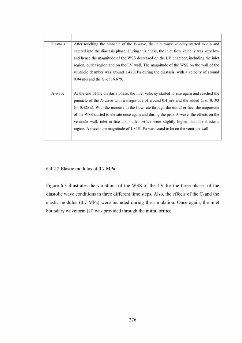
276

Diastasis After touching the pinnacle of the E-wave, the inlet wave velocity started to dip and

entered into the diastasis phase. During this phase, the inlet flow velocity was very low

and hence the magnitude of the WSS decreased on the LV chamber, including the inlet

region, outlet region and on the LV wall. The magnitude of the WSS on the wall of the

ventricle chamber was around 1.47E1Pa during the diastasis, with a velocity of around

0.04 m/s and the Cf of 16.679.

A-wave At the end of the diastasis phase, the inlet velocity started to rise again and reached the

pinnacle of the A-wave with a magnitude of around 0.4 m/s and the added Cf of 0.193

(t= 0.425 s). With the increase in the flow rate through the mitral orifice, the magnitude

of the WSS started to elevate once again and during the peak A-wave, the effects on the

ventricle wall, inlet orifice and outlet orifice were slightly higher than the diastasis

region. A maximum magnitude of 1.84E1 Pa was found to be on the ventricle wall.


Figure 6.3 illustrates the variations of the WSS of the LV for the three phases of the

diastolic wave conditions in three different time steps. Also, the effects of the Cf and the

elastic modulus (0.7 MPa) were included during the simulation. Once again, the inlet

boundary waveform (U) was provided through the mitral orifice.

277

0.075 s

0.275 s

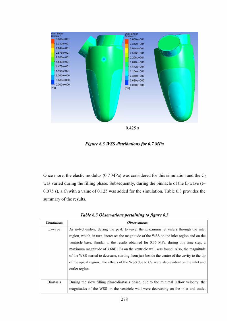
278

0.425 s


Once more, the elastic modulus (0.7 MPa) was considered for this simulation and the Cf

was varied during the filling phase. Subsequently, during the pinnacle of the E-wave (t=

0.075 s), a Cf with a value of 0.125 was added for the simulation. Table 6.3 provides the



E-wave As noted earlier, during the peak E-wave, the maximum jet enters through the inlet

region, which, in turn, increases the magnitude of the WSS on the inlet region and on the

ventricle base. Similar to the results obtained for 0.35 MPa, during this time step, a

maximum magnitude of 3.68E1 Pa on the ventricle wall was found. Also, the magnitude

of the WSS started to decrease, starting from just beside the centre of the cavity to the tip

of the apical region. The effects of the WSS due to Cf were also evident on the inlet and

outlet region.

Diastasis During the slow filling phase/diastasis phase, due to the minimal inflow velocity, the

magnitudes of the WSS on the ventricle wall were decreasing on the inlet and outlet

279

tract. Once more, a maximum magnitude of around 1.47E1 Pa was found to be on the

LV wall. Simultaneously, the magnitudes of the WSS near the centre of the LV wall and

on the ventricle apex were found to be decreasing.

A-wave After the end of the diastasis period, the magnitude of the inlet velocity started to rise

and reached the pinnacle of the A-wave. Once again, due to the added Cf of 0.193 and

with the rise in the inlet velocity, the magnitude of the WSS was slightly higher

compared to the diastasis phase, but much lower than that of its peak E-wave. A

maximum magnitude of the WSS was approximately 1.84E1 Pa was found on the

ventricle wall.


From the images in Figure 6.4, the variations of the WSS on the LV wall of three phases

of the filling phase were investigated. Once more, the effects of the Cf and the elastic

modulus (1.4 MPa) were combined for this simulation. Similar to the previous

simulations, boundary conditions were kept identical. This simulation is presented for

three different time steps. Table 6.4 provides the summary of the results.

0.075 s

280

0.275 s

0.425 s


281


E-wave During the peak of the E-wave, the maximum inflow jet starts to enter through the mitral

orifice and, for the included Cf with a value of 0.125, the maximum magnitude of WSS

was observed - similar to the findings for the 0.35 MPa and 0.7 MPa of elastic modules.

Once again, the influence of the WSS was mostly observed on the ventricle wall with a

magnitude of around 3.68E1 Pa. Higher magnitudes of WSS were also found on the inlet

orifice and outlet orifice. Furthermore, a similar phenomenon was observed with the

magnitude of the WSS - found to be decreasing, just beside the centre to the cavity to the

ventricle apex.

Diastasis After the end of the E-wave, the inlet velocity enters the diastasis phase where the inflow

velocity was minimal. Again, similar effects were observed on the variations of the WSS

for the discrepancies on the elastic modulus (0.35 MPa and 0.7 MPa). During the time

step of t= 0.275 s, in the slow filling phase, the magnitudes of the WSS were declining

and the maximum WSS was observed to be approximately 1.47E1 Pa on the ventricle

wall. Concurrently, magnitudes of the WSS (just beside the core of the ventricle wall to

the ventricle apex) were found to be decreasing as well.

A-wave As the inlet velocity entered into the A-wave, the inflow velocity started to increase and

then reached the peak A-wave. Due to the incline in the inlet velocity jet, the WSS on

the ventricle wall increased and the maximum magnitude of the WSS was approximately

1.84E1 Pa on the ventricle wall. It was noted that similar magnitudes and variations in

the WSS were observed (of 1.4 MPa) for the elastic modulus of 0.35 MPa and 0.7 MPa.

6.4.3 The influence of friction coefficient and elastic modulus using intraventricular

pressure (Ip) distributions


The variations in the Ip pressure distributions during the diastolic wave conditions were

determined for three different time steps, as illustrated in the following figures. Also,

the effects of the Cf and elastic modulus were employed in order to determine the

variations in the Ip. By using similar boundary conditions as stated in Section 6.4.2,

282

discrepancies in the Ip distributions were demonstrated and are presented below. Ip

distributions during three phases are demonstrated using an XY cross-sectional plane

and the outer surface of the LV.

All the images in Figure 6.5 demonstrate the variations in the Ip distributions in three

different time steps during the filling cycle. Also, the effects of the Cf and elastic

modulus (0.35 MPa) are included in determining the changes in the Ip. Table 6.5

provides the summary of the results.

0.075 s

0.275 s

283

0.425 s

Figure 6.5 Ip distributions for the elastic modulus of 0.35MPa


E-wave During the simulation presented in Figure 6.5, the magnitude of the elastic modulus was

considered fixed and the Cf was varied in three different time steps. As noted earlier,

during the pinnacle of the E-wave, the maximum jet entered through the mitral orifice.

As seen in Chapter 4 and Chapter 5, the magnitudes of the intraventricular pressure

started to rise in the apical region during this time period. However, with the added Cf

the maximum magnitude of the WSS was approximately 7.46E2 Pa close to the tip of

the ventricle apex. Also, the Ip in the basal region, inlet and outlet tract was much lower

compared to the apical pressure. Moreover, a ring shaped vortex developed close to the

outlet region.

Diastasis Once again, after reaching the peak of the E-wave, the rate of flow declined and entered

into the diastasis phase. With the increased Cf during this phase, a much higher

magnitude of the Ip was found in the apical region of the LV with a value of around

1.23E2 Pa compared to its basal region. Also, just beside the tip of the ventricle apex, a

higher magnitude of Ip was found with a value of around 3.72E2 Pa. However, the value

of the Ip in the ventricle apex was still much lower compared to the magnitude of the

peak E-wave. As the inlet velocity was minimal during this phase, a lower magnitude of

the Ip in the centre of the ventricle was also observed. Additionally, the previously

284

formed ring shaped vortex changed its position towards the centre of the ventricle and

enlarged slightly.

A-wave At the beginning of the A-wave, the inlet velocity started to elevate once again and when

it reached the peak of the A-wave, a higher velocity of inlet jet entered through the

mitral region. Due to the added Cf of 0.193 the magnitude of the Ip in the apical region

(close to the tip of the LV apex) with a value of around 3.72E2 Pa, was still much higher

compared to its basal region. However, this magnitude was still lower than the peak E-

wave but higher than the diastasis phase. Once again, the vortex was enlarging during

this time step.


The images in Figure 6.6 illustrate the changes in the Ip distributions for three important

phases of the diastolic flow conditions. Once again, the effects of the Cf and elastic

modulus (0.7 MPa) were added during the simulation. Table 6.6 provides the summary

of the results.

0.075 s

285

0.275 s

0.425 s


286


E-wave Similar to the elastic modulus of 0.7 MPa; during the peak E-wave, the maximum flow

velocity entered through the inlet region. Once again, a higher magnitude of Ip was

obtained in the ventricle apex compared to its basal pressure. Precisely, the maximum

magnitude was found to be near the tip of the LV in the apical region with a value of

approximately 7.46E2 Pa. Once more, the magnitudes of the Ip in the inlet and outlet

region were much lower than that of its apical region. Also, a ring shaped vortex

developed near the outlet region.

Diastasis After the end of the E-wave, the inlet velocity entered into the diastasis phase, where the

flow velocity was minimal. During this time step (t= 0.275 s) the magnitude of the Ip in

the ventricle apex was still much higher compared to its basal region. A maximum

magnitude of around 1.23E2 Pa is found to be in the ventricle apex. Moreover, just

beside the tip of the apical region, a much higher magnitude was found with a value of

approximately 3.72E2 Pa. Once again, it was seen that, with the increased Cf during this

phase, the magnitude of the Ip reduced when compared with the peak E-wave. Also at

the core of the LV chamber and in the basal region, the magnitude of Ip was found to be

much lower. Again, the previously formed vortex changed its position towards the core

of the cavity.

A-wave During the peak of the A-wave, the rate of the inlet velocity elevated once again. Once

more, with the reduced magnitude of the Cf (0.193) compared to the diastasis phase, the

magnitude of the Ip in the ventricle apex (near the tip of the apex) was somewhat higher

with a value of approximately 3.72E2 Pa. Simultaneously, at the core of the ventricle,

the inlet and outlet regions, the magnitude of the Ip was much lower when compared

with its apical region. Once more, the previously formed ring shaped vortex was seen

elongated during this time step, at the core of the ventricle.


Ip distributions of the LV, using the effects of the Cf and elastic modulus (1.4 MPa) are

demonstrated in Figure 6.7 during the three phases of the filling wave. Table 6.7


287

0.075 s

0.275 s

288

0.425 s



E-wave In general, similar results were obtained during the peak E-wave, diastasis and peak A-

wave. Specifically, during the peak E-wave, the magnitude of the Ip in the ventricle apex

was much higher compared to its basal region. A maximum magnitude of approximately

7.46E2 Pa was found to be in the ventricle apex close to the tip of the apex. Once again,

the magnitude of the basal pressure was much lower compared to its apical region. At

the same time, a ring shaped vortex, similar to the previous elastic modulus (0.35 MPa

and 0.7 MPa) developed near the outlet region.

Diastasis Once again, after the end of the E-wave, the inlet velocity entered into the diastasis

phase and, during this phase, the flow velocity decreased and the primary vortex was

seen changing its position towards the core of the cavity. Even with the decelerated inlet

velocity, the magnitude of the Ip in the mitral region was still much higher compared to

its apical region. A maximum magnitude of 1.23E2 Pa was found in the apical region of

the ventricle during this phase. Also, a maximum magnitude of approximately 3.72E2 Pa

was in the ventricle apex near the tip of the LV. However, with the increased Cf during

this phase, the magnitude of the Ip in the apical region was found to be comparatively

lower than the peak E-wave.

289

A-wave After the diastasis phase, the inlet velocity wave came to the peak of the A-wave and the

magnitude of the inlet velocity rose once more. During this phase, similar effects were

found with the elastic modulus of 0.35 MPa and 0.7 MPa. Consequently, the magnitude

of the Ip in the apical region (close to the tip of the LV apex) was higher again with a

value of approximately 3.72E2 Pa compared to the ventricle base. Also, the vortex was

enlarged during this time step.

6.4.4 The influence of friction coefficient and elastic modulus using velocity mapping


The changes in the velocity pattern during the peak E-wave, slow filling phase and the

peak A-wave are demonstrated in the following sections. Additionally, the effects of the

Cf and the elastic modulus were incorporated to observe and determine the influence on

the velocity distributions, including the formation, shifting and merging of vortices

during these three phases. In so doing, the required boundary conditions and transmitral

velocity wave (U) were implemented, as reported in Section 6.4.2. Also, an XY cross-

sectional plane was selected to observe the changes in the velocity pattern.

The images in Figure 6.8 demonstrate the discrepancies in the velocity distributions

during the three phases, including the effects of the Cf and elastic modulus (0.35 MPa).

Table 6.8 provides the summary of the results.

290

0.075 s

0.275 s

291

0.425 s

Figure 6.8 Velocity distributions for the elastic modulus of 0.35MPa


E-wave As stated earlier, during the peak E-wave, the inlet velocity was maximum entering

through the mitral orifice and propagated towards the ventricle apex. During the time

step, the elastic modulus was considered fixed (0.35 MPa) and the magnitude of the Cf

was varied. Because of the added Cf a ring shaped, clockwise (CW) vortex developed

close to the outlet region. Also, at the apical region of the ventricle, the flow pattern

appeared to be twisting and moving upwards. During this period, a maximum flow

velocity is obtained as approximately 1.25 m/s in the ventricle base.

Diastasis During the slow filling phase, the magnitude of the inlet flow velocity minimized and the

primary vortex was somewhat elongated and changed its positions towards the centre of

the cavity. Simultaneously, a weak vortex, which was also ring shaped and clockwise,

started to develop near the outlet tract. At the same time, because of the increased Cf a

twisting of the flow pattern was evident in apical region of the ventricle. Moreover, the

maximum velocity of approximately 6.25E-1 m/s was found to be in the basal region.

A-wave When the inlet waveform reached the pinnacle of the A-wave, the inlet velocity

increased and because of that, the primary vortex slowly began to merge with the

propagation of the inlet jet. Also, the weaker vortex amalgamated with the inflow wave,

292

but was still evident close to dead-end of the outlet tract. Additionally, a maximum

magnitude of the velocity of approximately 6.25E-1m/s existed close to the inlet region.

6.4.4.2 Elastic modulus of 0.7MPa

Once again, the velocity pattern for the elastic modulus was varied (0.7 MPa), and the

flow pattern was determined. This is illustrated in the images in Figure 6.9. Table 6.9


0.075 s

293

0.275 s

0.425 s


294


E-wave Similar to the elastic modulus of 0.35 MPa, the flow pattern was also determined for the

elastic modulus of 0.7 MPa by including the effects of the Cf (0.125) in three different

phases. During the peak of the E-wave, the flow rate elevated and a twisting in the flow

appeared at the ventricle apex. At the same time, a ring shaped, CW vortex formed near

the outlet region. During this time period, a maximum flow velocity of approximately

1.25m/s was in the ventricle base.

Diastasis When the inlet velocity entered into the slow filling phase, the inlet velocity became

minimal and the effect of the Cf (16.679) increased. During this time period, the primary

adherence vortex enlarged and shifted its position towards the centre of the cavity. At the

same time, a weak ring shaped CW vortex formed close to the aortic orifice of the

ventricle. Simultaneously, the twisting in the flow pattern in the ventricle apex was

observed, which was found to be moving towards the core of the chamber. During this

time period in the ventricle base, a maximum flow velocity of 6.25E-1 m/s was found.

A-wave During the pinnacle of the A-wave, the rate of flow increased once again, and the flow

dynamics were observed, including the effect of the Cf (0.193), which slightly decreased

compared to the diastasis. Subsequently, with the elevation in the flow rate, the primary

vortex slowly began to merge with the incoming jet from the inlet region and also the

secondary weak vortex started to amalgamate. However, the weaker vortex was still

evident close to the dead-end of the aortic orifice. Simultaneously, the twisting in the

flow dynamics in the apical region was seen amalgamated with the propagation of the

inlet jet. During this time period, the maximum magnitude of the velocity was found to

be approximately 6.25E-1 m/s close to the inlet region.


Similar to the previous elastic modules, the flow dynamics, including the development,

shifting and merging of vortices are shown in Figure 6.10. Table 6.10 provides the


295

0.075 s

0.275 s

296

0.425 s



E-wave Once again, similar effects were found for the flow pattern during the peak of the E-

wave, diastasis and peak of the A-wave, including the added effect of Cf. With higher

flow velocity during the peak E-wave, a wake vortex developed close to the outlet

region. Simultaneously, twisting of the flow was evident in the apical region of the

ventricle. Also, a maximum magnitude of flow velocity was approximately 1.25 m/s in

the basal region of the ventricle.

Diastasis When the inflow velocity entered into the diastasis phase, the rate of flow was minimal

and during this time period, the magnitude of the Cf increased. Hence, the primary

vortex, which was ring shaped and CW, elongated and changed its location to the core of

the chamber. Once again a weak second vortex, which was ring shaped and CW,

developed near the outlet tract. Concurrently, the twisting in the flow pattern in the

ventricle apex was also noticeable and was found to be moving upwards to the centre of

the ventricle. During this time period, a maximum magnitude of the velocity was

obtained to be approximately 6.25E-1 m/s in the basal region of the ventricle.

A-wave During the pinnacle of the A-wave, with the added effect of the Cf and with the rise in

the inflow jet, the primary vortex started to merge with the inflow wave inside the

297

ventricle. Also, the second weak vortex, which was ring shaped and CW was seen

merging but it was still visible near the cul-de-sac of the outlet tract. Moreover, the

twisting was also amalgamated with the propagation of the inlet jet. Subsequently, the

maximum magnitude of the flow velocity was acquired at approximately 6.25E-1 m/s,

close to the inlet tract.

6.4.5 The influence of friction coefficient and elastic modulus structure simulation

using total mesh displacement (TMD)


Structure simulation of the LV during the above mentioned phases was performed and

is illustrated in the following sections. Once again, the variations in the elastic modulus

and the effect of Cf were considered and varied. Similar to the previous boundary

conditions, reported in Section 6.4.2, all the required boundary details were included.

Also, an XY cross-sectional plane was taken to determine the variations in the mesh

displacement of the structure.

Total mesh displacement for the elastic modulus of 0.35 MPa is displayed in Figure

6.11. Table 6.11 provides the summary of the results.

298

0.075 s 0.275 s

0.425 s

Figure 6.11 TMD distributions for the elastic modulus of 0.35MPa

299


E-wave Similar to the previous simulations, initially the elastic modulus was fixed (0.35 MPa)

and the Cf was varied for the three different phases. During the peak of the E-wave,

when the flow velocity was maximum through the inlet region, a much higher

displacement was in the apical region compared to its basal region. A maximum

magnitude of 7.5E-6 m was in the ventricle apex.

Diastasis During the diastasis phase, the flow velocity minimized and the magnitude of the Cf

increased. During this time period, the maximum displacement is still found to be in the

apical region of the ventricle with a value of around 7.5E-6 m. Simultaneously, a much

lower magnitude of displacement was observed in the basal region and in the core of the

cavity.

A-wave Later, during the peak A-wave, the maximum magnitude was still found to be in the

apical region of the ventricle with a value of 7.5E-6 m compared to its basal region. At

the same time, the magnitude of the displacement in the basal region and at the centre of

the ventricle was elevated compared with its diastasis phase, but the magnitude was still

lower than that of its apex.


Once again, the elastic modulus was considered fixed and the magnitudes of the Cf were

varied to determine the variations in the displacement during three different phases.

Table 6.12 provides the summary of the results.

300

0.075 s 0.275 s

0.425 s


301


E-wave During the pinnacle of the E-wave, the maximum flow velocity enters through the inlet

region and at the same time, the elastic modulus was fixed to 0.7 MPa. During this time

period, the maximum magnitude of displacement with a value of 7.5E-6 m was in the

ventricle apex and the magnitude was slightly higher compared to its basal region.

Diastasis When the inlet waveform reached its diastasis phase, the inflow velocity became

minimal and the magnitude of the Cf increased. During this period, the maximum

magnitude of the displacement was still in the apical region but the magnitude with the

value of around 6.75E-6 m decreased compared to its peak E-wave. Also, a lower

magnitude of displacement was in the ventricle base and in the centre of the chamber.

A-wave During the peak of the A-wave, the inlet velocity rose once again and the magnitude of

the Cf decreased relative to the diastasis phase. During this time step, a higher magnitude

of the displacement was still evident in the apical region with a magnitude of around 6E-

6 m, but in the tip of the ventricle apex the magnitude was approximately 6.75E-6 m. At

the same time, the magnitude of the displacement in the basal region increased slightly

when compared with its diastasis region but it was still lower compared with its peak E-

wave.


Images in Figure 6.13 show the variations in the displacement of the LV during three

different phases including the effects of the Cf and elastic modulus (1.4 MPa). Table

6.13 provides the summary of the results.

302

0.075 s 0.275 s

0.425 s


303


E-wave During the peak E-wave, the flow rate increased through the mitral region and, during

this time step, the effects of elastic modulus and Cf were incorporated. With the time step

of 0.075 s, a much higher magnitude of 7.5E-6 was obtained in the apical region

compared to its basal region.

Diastasis During the slow filling phase, a maximum magnitude of the displacement with a value of

approximately 3E-6 m was obtained in the apical region of the LV. It should be noted

that, once again at the tip of the ventricle apex, a slightly higher magnitude of the

displacement with a value of around 3.75E-6 m was observed. Moreover the magnitude

of the Cf increased during this phase. Also, the magnitude of the displacement in the

basal region was much lower compared to its apical region.

A-wave During the peak A-wave, inflow velocity rose once again and with the added effect of

the Cf , the maximum magnitude was in the ventricle apex with a value of approximately

2.25E-6 m. Moreover, in the tip of the LV, a maximum value of around 3.75E-6 m was

found. Once again, a lower magnitude of displacement was in the basal region of the

ventricle but it was slightly higher when compared with its diastasis phase.

6.5 Discussion

6.5.1 The influence of Cf and elastic modulus on the LV using WSS distributions

From the simulations of the LV, including the effects of the Cf, it was evident that

almost identical results were obtained in three phases, after varying the magnitudes of

the elastic modulus. Subsequently, at the peak of the E-wave, a maximum magnitude of

WSS was obtained for all elastic modules. During this time step, the maximum

magnitude of the inflow jet entered through the inlet region and hence the influence of

the WSS was observed mostly on the ventricle wall incorporating the effects of the Cf

for all cases of elastic modulus. This could be attributed to the fact that the variations of

the wall shear depended on the discrepancies of the Cf. Because of minimal Cf (for

example, 0.125) on the LV wall, WSS was much higher, mostly during the peak of the

E-wave, for all elastic modulus.

304

As the inlet jet entered into the diastasis phase, the rate of inlet velocity jet was minimal

and entered through the mitral orifice. During this time (for example, t= 0.275 s) the

magnitude of the Cf increased and this added magnitude results in lower wall shear on

the ventricle wall. This could be ascribed to the fact that, due to the rise in the Cf on the

ventricle wall, resistance increased (Dellimore et al., 2013) which, in due course,

impeded the natural motion of the LV wall and hemodynamic system of the ventricle.

Once again, at the onset of the A-wave, the flow velocity started to accelerate and when

it reached the pinnacle of the A-wave, the inlet velocity rose and the jet entered through

the inlet region with increased velocity. During the peak A-wave, the magnitude of the

Cf was found to be much lower compared to the diastsasis phase but slightly higher than

the peak E-wave. Subsequently, from the simulations it was evident that with the

decrease in the magnitude of the Cf, wall shear elevated compared to the diastasis phase.

Hence, it can be stated, from the simulations that with a rise in the Cf the magnitude of

the wall shear decreased. Also, almost identical WSS distributions were found after

varying the magnitudes of the elastic modulus (Figure 6.2, Figure 6.3 and Figure 6.4).

Moreover, the deceleration in the ventricle wall motion also implied the functional

deficiencies for Dilated Cardiomyopathy (DCM) which severely influenced the natural

hemodynamics of the LV (B. T. Chan et al., 2012). Furthermore, the physiological

property of the ventricle changed due to the inadequacy of the required WSS, which

successively indicated the primary feature of the DCM disease conditions.

From the experimental investigations of (W et al., 1974, Hayashida et al., 1990),

moderately higher WSS was found for the DCM conditions compared to the natural LV.

However, using FSI simulations, Chan et al. 2012 (B. T. Chan et al., 2012) illustrated

that higher WSS could be found in the general LV compared to the dilated ventricle, but

they noted that similar wall thicknesses/elastic modulus had been utilized during the

simulations. On the other hand, the influence of the friction co-efficient was not

included in their investigations.

Varying the elastic modulus generated negligible influences on the WSS distributions

but changing the Cf during the simulations, meant that a clear idea for detecting and

305

determining the DCM condition could be achieved. Also, the findings from the

simulations using these parameters coincided well with the previously published

research.

Subsequently, it was well documented that cardiomyopathies are accountable for the

cardiac muscle dysfunction, which often develops the Congestive Heart Failure (CHF)

(Maisch et al., 2002). Therefore, from this viewpoint, it can be noted that the effects of

friction co-efficient and elastic modulus could also play a noteworthy role in identifying

CHF.

6.5.2 The influence of Cf and elastic modulus on the LV using Ip distributions

Once again, similar effects were found during the investigations of Ip distributions for

three phases of the diastolic flow cycle. During the pinnacle of the E-wave, for all three

elastic modulus, a maximum magnitude was found to be in the apical region of the LV,

close to the tip of the LV apex. During this E-wave, the maximum flow velocity entered

through the mitral region and propagated from the basal region to the apical region

inside the LV cavity. Hence, the maximum magnitude of Ip was found to be in the

ventricle apex compared to its basal region. Moreover, a ring shaped vortex was formed

for all cases, near the outlet tract during this time step. This could be attributed to the

fact that, because the Cf developed higher flow resistance (Dellimore et al., 2013),

hence a vortex formed during this time step.

When the flow velocity came to the diastasis phase, the magnitude of the Ip was still

found to be slightly higher in the apical region of the ventricle compared to its basal

region for all three phases. During this time step, the magnitude of the Cf increased and

because of that, the value of the overall Ip decelerated, even though the magnitude was

still higher in the ventricle apex. Once again, the primary vortex which was formed

earlier changed its location towards the core of the chamber and was moderately

elongated.

306

During the pinnacle of the A-wave, the flow rate increased and entered through the inlet

region. During this time, the magnitude of the Ip in the ventricle apex was

comparatively higher than the basal region. With the incoming jet through the mitral

region, the jet mixed and propagated with the fluid inside the cavity and because of this,

the apical pressure was higher compared to its basal region. It should be noted that,

during this time, the magnitude of the Cf reduced, which also resulted in a slightly

higher magnitude of the Ip in the ventricle apex. Also, the previously formed primary

vortex was seen enlarged in the centre of the cavity.

From the above discussions, it is evident that, a higher magnitude of Cf resulted in a

comparatively lower magnitude of Ip and vice-versa. Also, the variations in the Wt of

the LV had negligible effects on the Ip distributions. Moreover, the general trend in the

variations of the Ip, between the apical and basal region of the LV, during the peak E-

wave, diastasis and peak A-wave were in line with previously published investigations

(Arefin and Morsi, 2014, Cheng et al., 2005, Vierendeels et al., 1999). However it was

discovered that, during the peak E-wave, diastasis and peak A-wave, a vortex originated

and this could be attributed to the implied Cf where higher flow resistance was

generated and hence the vortex became evident during these time periods.

6.5.3 The influence of Cf and elastic modulus on the LV using velocity mapping

During the peak E-wave for all three phases, the maximum inlet velocity started to enter

through the inlet region. Also, the added effects of the Cf variations in the flow pattern

were determined. For all three elastic modulus during the pinnacle of the E-wave, a ring

shaped CW vortex developed near the outlet region. Simultaneously, twisting in the

flow pattern was observed in the ventricle apex. These phenomena could be attributed to

the added Cf , which developed higher flow resistance (Dellimore et al., 2013) and

helped generate the twisting in the flow pattern and concurrently develop an adherence

vortex close to the outlet region.

307

When the inlet velocity entered into the diastasis phase, the magnitude of the inlet

velocity minimized and during this phase, the magnitude of the Cf increased. Because of

these, a twisting of the flow pattern inside the ventricle was evident and it started to

move towards the core of the ventricle. With the deceleration in the inlet velocity

waveform the primary adherence vortex somewhat elongated and travelled towards the

centre of the ventricle. Simultaneously, a second weak vortex developed close to the

aortic orifice.

During the pinnacle of the A-wave, the inlet velocity elevated once again and with the

added effect of the Cf, changes in the flow dynamics were observed. During this time

period, the primary vortex started to merge with the propagation of the inlet jet. Also,

the secondary vortex was also seen somewhat merging with the fluid inside the

ventricle. However, it was still evident as it shifted its position close to the cul-de-sac of

the outlet region. It should be noted that this vortex was ring shaped and CW.

Moreover, no twisting in the flow pattern in the apical region was found and it could be

ascribed to the fact that the fluid inside the cavity (during the E-wave and diastasis),

along with the incoming fluid from the inlet region, mixed and merged together and

hence the fluid circulated normally during this time step.

Once again, from the simulation results it was determined that the Cf influenced the

flow pattern during these three phases. A much higher magnitude of velocity could be

found during the peak of the E-wave but, during the diastasis and the peak A-wave, the

magnitude of the velocity tended to be similar in the basal region. Also, the elastic

modulus did not directly alter the flow pattern during these three phases.

The general trends of the flow pattern, including the development, shifting and merging

of vortices were in line with previously published research (Arefin and Morsi, 2014,

Nakamura et al., 2002, Cheng et al., 2005). However, it should be noted that, with the

added effect of the Cf, variations in the flow pattern, including the generation of vortices

and twisting in the flow pattern were observed.

308

6.5.4 The influence of Cf and elastic modulus on the LV structure simulation using

total mesh displacement (TMD)

During the peak of the E-wave, maximum flow velocity entered through the inlet tract

and with the added effect of the elastic modulus and Cf, the variations in the

displacement of the structure were determined. From the simulation results, during the

peak E-wave, the maximum magnitude of the displacement was found in the apical

region for all thickness. However, with the rise in the elastic modules, the magnitude of

the displacement in the basal region started to decelerate. This could be attributed to the

fact that a higher elastic modulus provided stiffness to the ventricle wall and with the

added effect of Cf, a lower magnitude of displacement was found in the basal region.

Also, due to the maximum flow rate, during the E-wave, the jet started to propagate

from the inlet to the apical region and hence the magnitude of the displacement in the

apical region tended to be higher than the basal region.

During the diastasis phase, similar incidents were noted from the simulations. With a

rise in the elastic modules and the added effect of the Cf, the magnitudes of the

displacement in the ventricle apex started to decelerate. Precisely, higher elastic

modulus resulted in lower magnitude of the displacement. This could be ascribed to the

fact that, with the added effect of the Cf and minimal inlet velocity, due to diastasis, the

volume of the fluid inside the chamber tended to affect the displacement of the

structure. Specially, if the ventricle became stiffer, a lower magnitude of displacement

was found. Also, from the simulation results, a higher magnitude of displacement could

be found in the ventricle apex compared to its basal region for all elastic modulus

during this phase.

Later, during the peak A-wave, the inlet velocity started to rise once again and with the

added effect of the Cf, a much higher magnitude of the displacement was found to be in

the ventricle apex. Once more, with the rise in the elastic modules, the magnitudes of

the displacement in the ventricle apex decreased. Similarly, the magnitudes of the

displacement in the basal region decreased with the elevation in the elastic modules.

309

Therefore, from the results, it was evident that with the rise in the magnitude of the

elastic modulus and its added Cf the magnitudes of the displacement decreased. It is to

be noted that, because of the added friction co-efficient and elastic modulus of the LV

(DCM condition), total displacement of the LV was expected and found to be minimal.

310

6.6 Summary

From the above discussion and the simulation results, it was evident that the effect of

the elastic modulus and Cf certainly influenced the WSS distributions, Ip distributions,

velocity mapping and the structure simulations during the three phases of the diastolic

cycle. Specifically:

(i) WSS Distributions - It was determined that, with the increase in the Cf, the

magnitude of the wall shear decreased. Also, similar WSSs were found by

varying the magnitudes of the elastic modulus. Moreover, the effects of the Cf

provided a better basis for determining DCM disease conditions.

(ii) Ip Distributions - The effect of the Cf was also evident during the three phases.

Results suggested that, with the rise in the magnitude of the Cf, a lower Ip could

be found and vice-versa. However, changing the magnitudes of the elastic

modulus provided negligible effect on the Ip distributions. Moreover, for all

elastic modulus, maximum magnitudes of the Ip were found to be in the

ventricle apex.

(iii) Velocity Distributions - It was noted that the effect of the Cf changed the flow

pattern during these three phases. Precisely, during the peak E-wave, a much

higher magnitude of velocity was found in the basal region, but the velocity was

almost identical during the diastasis and the peak A-wave in the LV base. Once

again, the variations in the elastic modulus were found to have negligible effect

on the flow pattern during the peak E-wave, slow filling phase and the peak A-

wave. Also, the generation, shifting and merging of vortices were evident for all

elastic modulus during these three phases. Additionally, twisting in the flow

pattern was also noticeable during the peak E-wave and diastasis.

(iv) Structural Displacement - The results indicated that the magnitudes of the

displacement depended on both the Cf and elastic modulus. Specifically, the

increase in the elastic modulus and its added Cf resulted in a decrease in the

magnitudes of the displacement. Also, for all elastic modules, higher magnitudes

311

of the displacement were found in the apical region of the ventricle compared to

its basal region during these three phases. Moreover, due to the friction co-

efficient and co-efficient and elastic modulus of the LV (DCM) total magnitude

of the LV deformation was obtained to be minimal.

312

Chapter 7

Conclusions and Future Directions

313

7.1 Overall Conclusions of the Dissertation

The primary purpose of this Doctoral research program was to investigate engineering

issues associated with the development of a "next generation" Ventricular Assist Device

(VAD) system driven by a wireless controller. In order to determine the required

hemodynamic and physiological variations of the LV, FSI simulations were utilized for

different cardiac conditions during the filling phase.

As stated previously, the human heart is a complex 3D structure which functions as a

pump that circulates blood throughout the body. Cardiovascular diseases (CVD) arise

whenever natural blood circulation is hindered for any reason. These diseases greatly

affect morbidity and mortality (Vadakkumpadan et al., 2010) and thus, are a major area

of research at many levels. In this Doctoral research, the focus has been on the

engineering analysis elements that relate to CVD.

One of the critical and leading causes of death from CVD relates to heart failure (HF).

A particular problem of interest relates to Dilated Cardiomyopathy (DCM) or, more

specifically, a weakened heart muscle. Those who are afflicted with a weakened heart

muscle and/or hearts which are otherwise functioning efficiently - generally due to age

and a range of other causative factors - usually require a special device to assist the

functioning of their cardiac muscles effectively. To this end, ventricular assist devices

(VADs) are commonly utilized to aid cardiac structures to circulate blood throughout

the body.

VADs are frequently utilized to support various hemodynamic conditions inside the

human body but these devices have various limitations. One of the most frequent

complications relates to driveline infections which can actually lead to deterioration of

physical and hemodynamic conditions in the human body in the long run. Moreover:

• The size of the device

• Thromboembolism

• Requirements for special maintenance

314

and other issues also hinder the normal process of blood circulation (Pamboukian, 2011,

Friedman et al., 2011, Goldstein et al., 1998). Considering the particular complications

of driveline infections, along with other conditions of VAD systems, this Doctoral

research sought to provide critical, underlying engineering analysis that could be used in

order to develop a next generation VAD system using wireless technology.

In doing so, both experimental and computational approaches were deployed in order to

form the basis of a next generation VAD system. For the computational approaches, it

was challenging to simulate the hemodynamic conditions of the whole heart. Therefore,

the left ventricle (LV) of the heart was considered for the purpose of simulating the

hemodynamic and physiological conditions in different circumstances, namely:

• Examination of general flow dynamics

• Angular variations of the mitral and aortic orifice of the LV

• By varying the elastic modulus and friction co-efficient

The data generated from the simulations could then be used to make a VAD more

effective and efficient. Prior to the execution of a fully-coupled Fluid Structure

Interaction (FSI) scheme in the left ventricle of the heart, a realistic 3D model of the

• Coronary artery bypass graft (CABG)

• Abdominal aortic aneurysm (AAA)

were simulated. The execution of FSI on the CABG and aneurysm model provided

significant knowledge and insights both for both hemodynamics and physiological

properties. Subsequently, and in a similar way, simulations were conducted for the LV

of the heart where changes in both physiological and hemodynamic characteristics were

emphasized.

In Chapter 1, the details of CVDs were described along with various treatments. VADs

were also introduced and the usefulness and the inadequacies of these devices were

highlighted. The needs for enhanced (next generation) VADs were highlighted,

particularly where the existing VADs provided some serious clinical complications.

315

However, a detailed literature review was required to fully understand the problem at

hand and to find a suitable way to develop such a next generation VAD.

For these reasons, Chapter 2 described the physiological and hemodynamic

characteristics of the cardiac structure and its related components - specifically, heart

valves and the arterial system, as well as diseases and suitable treatments. Additionally,

this chapter also contained a discussion of earlier published research based on the

physiological and hemodynamic characteristics of the left ventricle, in terms of

experimental and computational approaches. Earlier investigations and analysis were

also reviewed in relation to dilated cardiomyopathy (DCM), both for experimental and

numerical approaches. This information was beneficial in gaining insights into the

limitations of existing systems and to utilize this data as a basis for constructing the next

generation VAD system.

In Chapter 3, FSI was initiated and utilized to investigate the flow dynamics and the

physiological characteristics of an anatomically correct CABG as well as aortic

aneurysm models. This numerical approach provided a basic understanding of the

hemodynamic and anatomical characteristics of the cardiovascular components. The

outcomes of these numerical simulations helped to facilitate the overall Doctoral

research work, as the primary objective was to simulate the physiological and

hemodynamic characteristics of the LV.

Chapter 4 described the detailed analysis of the hemodynamics and anatomical features

of the LV during the filling phase using FSI. The results were demonstrated in terms of:

• The intraventricular pressure (Ip) distributions

• Velocity profiles

• Wall shear stress (WSS)

• Maximum displacement of the structure

Even though the results were in line with earlier published investigations, these

computational approaches could define the complications related to the hemodynamics

and physiological physiognomies at any particular point of interest.

316

Subsequently, using FSI, variations in the hemodynamic and anatomical features were

computed by changing the angles between the mitral and aortic orifice during the

diastolic phase of the LV in the next chapter. Three different angles:

• 50°

• 55°

• 60°

were chosen between the mitral and aortic orifice to investigate the significance of the

flow dynamics and the structural variations of the LV. The results were also in

agreement with the previous findings. To the best of our knowledge, the variations in

the hemodynamic and physiological conditions of the LV by changing the aortic and

mitral orifices have not been presented till now. Moreover, this data would be very

effective in developing the wireless VAD even if there are angular differences.

In chapter 6, FSI was employed once again to perform simulations of the LV by

effectively varying the changes in the friction co-efficient and elastic modulus during

the filling phase. The results were investigated in terms of

• Wall Shear Stress WSS distributions

• Structural variations



This investigation also provided the knowledge of DCM related to the LV in order to

determine the variations in the hemodynamic and anatomical features. Simulation

results stated that it is possible to identify the conditions of DCM by varying the elastic

modulus and friction co-efficient of the LV. Once more, to the best of our knowledge,

these significant findings have not been documented to date and this information, in

identifying DCM would be very effective as well in developing wireless VAD for the

DCM patients.

317

Moreover, it is to be noted that even though the computational fluid dynamics (CFD)

were extensively utilized by many researchers and engineers for a long time, but

different phenomena such as, turbulence, combustion and multi-phase flow were either

cannot be solved entirely using CFD or unable to characterize the real-time situations.

All these problems ultimately produce many errors and limitations in using different

numerical analysis (Do, 2012). These errors could be related to software, numerical

techniques, and generation of mesh/meshing, user and application errors. Though it is

possible to lessen these errors by many different ways, but substantial amount of time

and cost would be required to obtain the desired solution. In general, engineers and

researchers should equalize/balance between the time and cost and satisfactory

numerical simulation errors. Also, experiment validations were frequently conducted to

boost the confidence of the numerical results (Do, 2012, Do et al., 2011, Owida et al.,

2010, Owida et al., 2012).

318

7.2 Clinical Implications

7.2.1 Overview

In this section, clinical implications are presented for the effects of experimental devices

and the effects of flow dynamics and physiological features. Also, the significance of

the CABG graft and the aneurysm model are described clinically.

7.2.2 Significance of the next generation VAD system

As part of this overall Doctoral research program, and following on from the analytical

research documented herein, four different experimental designs of a new VAD system

were developed. Two experimental designs were developed individually and another

two experimental designs were developed by two undergraduate student groups from

Swinburne University of Technology using wireless technology. These VAD prototypes

were modelled using:

• A DC motor (self)

• Linear actuators and switching circuitry (self)

• Motor driver (Wajid Baryalai, Yining Wang, Abdul Aziz AlMalki and Majid Bin

Masoud) [Please see Appendix Figure A-4]

• Steel wings (Ahmed Salem Alrashdi, Abdulhakim Saud Almutarrid, Ahmed

Awad Aldhahri and Khaled Abdulhadi Alenezi) [Please see Appendix Figure A-

5]

These four approaches offered ideas and substantial insights into new VAD models.

Brief description is provided in Table A-1.

It was well known that the driveline infections from existing VADs posed major threats

to users in the long run and hence the application of wireless technology could provide

both flexibility and risk-reduced operating conditions to the users. From a clinical point

319

of consideration, this next generation wireless VAD device could assist patients affected

by heart failure and/or weakened heart muscle.

7.2.3 Significance of the CABG and aortic aneurysm models

Hemodynamic and structural displacement were investigated in the CABG graft model

and the results were optimized for the bypass graft artery model which was varied with

the degree of stenosis (0%, 30%, 50% and 75%) in the LAD (Left Anterior Descending)

region. More precisely, a correlation was established with the LAD-stenosis and the

WSS distribution including the spatial WSS, velocity mapping and the structural

displacement. Results indicated that a separation of the flow pattern could be identified

near the anatomosis region of the graft. With an increase in the degree of LAD-stenosis

(0%, 30%, 50% and 75%), variations in the hemodynamic features could also be

observed. Reverse-flow conditions were also found near the anatomosis angle and with

an increase in the LAD-stenosis, this flow condition receded accordingly.

Moreover, the findings from the WSS, incorporating the spatial distribution, indicated

that a much higher WSS was found in the anatomosis angle of the graft artery and the

WSS rose with the elevation in the inlet flow velocity. Maximum WSS was near the toe

of the artery, with a magnitude of 12.6 Pa for the 75% LAD-stenosis. Generally, the

effects of the WSS and the flow dynamics could alter considerably with a change in the

inlet flow velocity (Do, 2012). All these findings, including the flow dynamics and the

WSS, were in line with earlier published results (Do, 2012, Ding et al., 2012, Kouhi,

2011). Also, the maximum magnitude of the structural displacement was found to be

2.6 E-06 m which is close to the anatomosis angle for the 75% stenosis.

From a clinical point of view, the findings provided substantial insights for both

structural and hemodynamic features. Moreover, these qualitative and quantitative

findings were effective and could enable different degrees of LAD-stenosis to be re-

vascularized.

320

Similarly, from the aortic aneurysm model, the numerical approach provided substantial

insights and required data, based on physiological and hemodynamic features.

Clinically, this information could be useful in enabling an aneurysm to be re-

vascularized.

7.2.4 Significance of the LV model

A realistic, 3D model of the LV model was simulated in terms of general physiological

and hemodynamic features, by varying the inlet (mitral) and outlet (aortic) angles of the

LV and for the diseased condition, DCM, by changing the friction co-efficient and

elastic modulus of the LV. For all three cases, hemodynamics and the structural

displacement were investigated during the filling phase. Hemodynamics, which

included:

• The flow pattern including the development, merging and shifting of vortices

• Distribution of Ip

• WSS distribution

were computed numerically during the diastolic flow condition.

For the general condition of the LV, results demonstrated that variation in the pressure

inside the ventricle occurred due to the ventricle wall, during the filling flow condition.

The maximum magnitude of the Ip was 5.4E2 Pa. Also, the magnitude of the WSS was

increasing with the rise in the early filling wave (E-wave) and atrial filling wave (A-

wave) but the magnitude of the WSS was decreasing during the diastasis phase. The

maximum magnitude of WSS was 5.7 Pa. Moreover, generation, merging and shifting

of vortices were observed during the transmitral flow propagation but it was determined

that the flow dynamics could change during the late-diastolic phase. The maximum

magnitude of the velocity was 1.55 m/s. These results were in line with earlier

published results (Cheng et al., 2005, Watanabe et al., 2004, Nakamura et al., 2002).

321

The maximum magnitude of the structural displacement is found to be 3.7E-5 m in the

LV apex during the peak E-wave.

A similar approach was undertaken, using the angles of 50°, 55° and 60° respectively

between the mitral and aortic orifices of the LV, during the diastolic phase. To the best

of our knowledge, previous studies did not investigate the variations in the flow pattern

by changing the angles between the mitral and aortic orifices. Hence, the changes in the

Ip, flow propagation and the structural displacement were investigated for the first time.

Results demonstrated that, for the angular difference of 55°, the flow propagation and

shifting of vortices were somewhat different to the 50° and 60° cases. Also, for the

intraventricular pressure, after reaching the peak E-wave, when the flow propagation

was directing towards the diastais phase, a higher Ip was found in the apical region of

the LV for the 50° angular difference. The findings from the simulations matched and

agree well with the previous research (Vierendeels et al., 1999, Lassila et al., 2012).

Subsequently, WSS, Ip and the flow velocity of the LV were determined by varying the

friction co-efficient and the elastic modulus of the LV during the filling wave. Once

again, to the best of our knowledge no one incorporated the friction co-efficient and

elastic modulus to determine the DCM and therefore, for the first time these properties

were coupled together in determining the conditions of DCM. The findings proved that

with the rise in the friction co-efficient, the viscosity of the fluid increased which, in

turn, decreased the magnitude of the WSS, Ip and the velocity. Due to the decrease in

the WSS, Ip and the velocity, LV-wall motion subsided as well. This stipulation led to

the physiological inequity of the LV which suggested the primary condition of the DCM

and chronic heart failure (CHF). The changes in elastic modulus had minimal influence

on the friction co-efficient. However, varying the friction co-efficient and corresponding

elastic modulus effects helped identifying the functional behaviour of the LV

hemodynamics, DCM and CHF conditions.

Table 7.1 generalizes the primary features of the modelling performed in the doctoral

research.

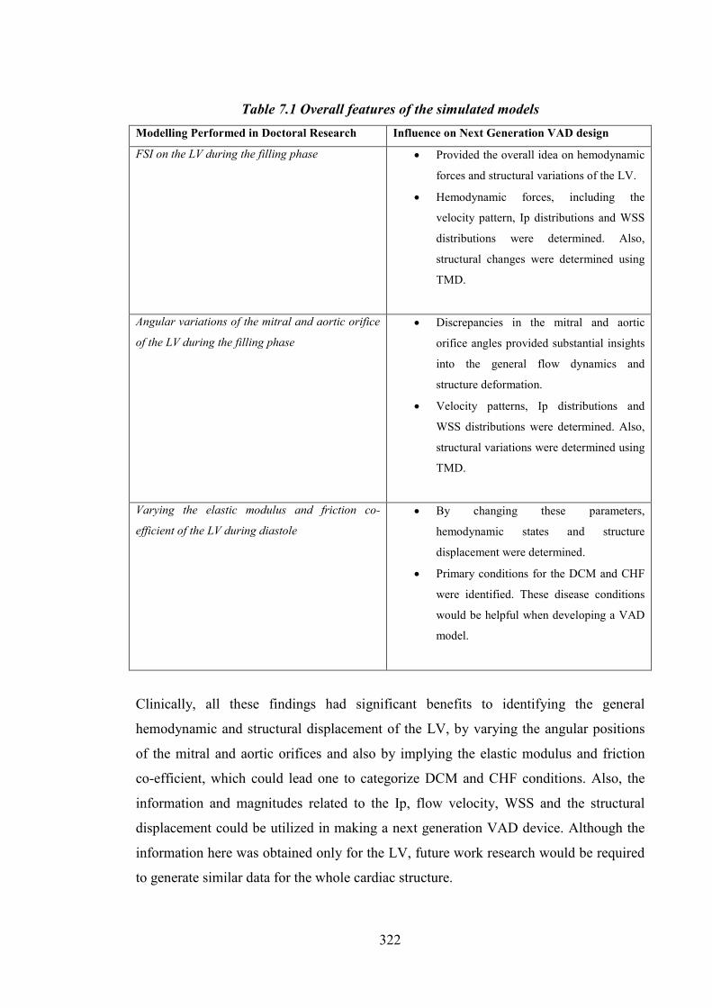
322

Table 7.1 Overall features of the simulated models Modelling Performed in Doctoral Research Influence on Next Generation VAD design

FSI on the LV during the filling phase • Provided the overall idea on hemodynamic

forces and structural variations of the LV.

• Hemodynamic forces, including the

velocity pattern, Ip distributions and WSS

distributions were determined. Also,

structural changes were determined using

TMD.

Angular variations of the mitral and aortic orifice

of the LV during the filling phase

• Discrepancies in the mitral and aortic

orifice angles provided substantial insights

into the general flow dynamics and

structure deformation.

• Velocity patterns, Ip distributions and

WSS distributions were determined. Also,

structural variations were determined using

TMD.

Varying the elastic modulus and friction co-

efficient of the LV during diastole

• By changing these parameters,

hemodynamic states and structure

displacement were determined.

• Primary conditions for the DCM and CHF

were identified. These disease conditions

would be helpful when developing a VAD

model.

Clinically, all these findings had significant benefits to identifying the general

hemodynamic and structural displacement of the LV, by varying the angular positions

of the mitral and aortic orifices and also by implying the elastic modulus and friction

co-efficient, which could lead one to categorize DCM and CHF conditions. Also, the

information and magnitudes related to the Ip, flow velocity, WSS and the structural

displacement could be utilized in making a next generation VAD device. Although the

information here was obtained only for the LV, future work research would be required

to generate similar data for the whole cardiac structure.

323

7.3 Future Directions and Recommendations

7.3.1 Overview

From the analysis documented in this dissertation, it is self-evident that further

investigations are required, involving both experimental and computational approaches.

The remaining future research needs are described here.

7.3.2 Experimental Requirements for VAD Prototype [including the works from two

undergraduate groups]

In general, to improve the next generation VAD model a range of investigations are

required. Specifically:

• It is necessary to determine the pressure exerted by the device on the cardiac

surface. This pressure can be calculated by determining the pressure exerted

from the connecting motors.

• An enclosure, made from polymers, needs to be wrapped around the device

to help expanding and contracting the whole cardiac structure precisely with

the heart beat (HB). Also, once the enclosure is attached, the required

pressure for the expansion and contraction of the cardiac structure needs to

be calculated and matched with the synchronization of the natural HB.

• Biocompatibility for the polymer and the VAD device needs to be assured.

• The power supply needs still needs a special attention. A wireless battery

charger may be an option for preventing surgery required for changing

existing power supplies.

• The total weight of the device needs to be reduced.

324

• Primarily, the VAD prototype was designed without considering any

attachment with the heart but, in the long run, this VAD prototype needs to

be connected effectively with the whole heart.

• This device needs to be tested in both in vitro and in vivo conditions to

ensure its dependability. Animal trials are required for the experiment

initially and this also will require FDA (Food and Drug Administration)

approval before installing the devices into human body.

• Alternatively, a neural classifier of the HB motion could be designed, which

could provide a fuzzy logic controller with precise information of the heart

rate. The fuzzy logic controller could be designed incorporating the HB

motion as an input which could then adaptively control the VAD prototype.

Moreover, an algorithm could be developed for diagnosing the critical

warning signals of the CHF and if this state is found, the necessary HB

motion pattern could be fed into the controller via the neural classifier.

7.3.3 Experimental Requirements of the LV Model

The following elements would be required in order to create the LV model:

• An exact shape of the LV would need to be obtained from MRI (Magnetic

Resonance Imaging) imaging.

• After getting the required values, an LV mould would need to be developed

in the conventional way and the Silicon (Si) rubber would be poured in the

mould to get a transparent Si-rubber LV model. This LV model would be

utilized for different testing using LDA (Laser Doppler Anemometers) and

PIV (Particle Image Velocimetry) measurements.

325

• Once the rubber model of LV was developed, colour liquid would be

decanted into the LV model. It should be noted that, the LV model would be

placed inside a bioreactor or suitable experimental setup where the liquid

would be given into the LV during the systole. Consequently, the LV would

be pushed by a piston, which is placed inside the bioreactor during the

diastolic phase where liquid would come back from the LV sac.

• Two mechanical valves, mitral and aortic, would be used for this

experiment. Therefore, the changes in the hemodynamic structure, including

the merging and shifting of vortices, Ip and the WSS would be defined along

with the structural displacement of the LV model. Moreover, tissue valves

could be implanted instead of mechanical valves and the flow pattern and

anatomical features for the LV could also be compared and determined.

• This result would then be matched with the simulated data to determine the

proper hemodynamic and anatomical data for the LV, which would be very

useful for developing the VAD prototype.

7.3.4 Computational and Experimental Requirements of the CABG and Aortic

Aneurysm Model

The following requirements need to be considered:

• In this research, only the general boundary conditions were applied in order to

investigate the flow dynamics and the anatomical features of these models.

Therefore, in vitro and in vivo boundary conditions need to be applied and

simulated. These would provide a better idea on the hemodynamic behaviour

and structural displacement by applying these boundary conditions. Also,

computational simulation codes could be very useful in order to improve the

accuracy of the whole simulations. These would assist in removing the

326

assumptions made during the simulations (Do, 2012). Moreover, in vivo

pulsatile flow analysis was required to determine the influence of the WSS.

• Although the validation of the numerical investigations here were shown to be

largely in line with other published computational research, but the results still

possessed a few discrepancies (Do, 2012) related to the study. Also, the findings

need to be matched with various experimental studies. Moreover, detailed

analysis on the WSS, flow dynamics and other parameters for the Newtonian

and non-Newtonian models and turbulent and laminar flows would be

determined at the location of the stenosis.

• The geometry utilized in the simulations is drawn using CAD (Computer Aided

Design) software. Therefore, CT-scan (Computed Tomography) or MRI images

can be segmented and utilized for further simulations. In doing so, geometric

complications could be minimized and the results can be made more accurate.

• Only a few selected degrees of LAD-stenosis (Ding et al., 2012) were applied

for the CABG model. Hence, research still needs to be carried out for various

degrees of stenosis and also the anastomosis angle should be varied.

• Moreover, the influence of the bypass graft, using different biomaterials, needs

to be carried out. Additionally, both the flow pattern and the structural

displacement need to be determined as well.

• Similarly, various investigations need to be carried out while changing the

bifurcations angle (β), neck angle (α) and by implying different asymmetry (Li,

2005) in the aneurysm main-body (AAA). Both the structural and hemodynamic

behaviour need to be investigated and determined.

• For both models, experimental studies are required. Moulds can be produced

similar to the LV model and by using the PIV and LDA techniques, the flow

pattern and physiological characteristics of the graft model could be determined.

Bioreactors could also be used for design and experimental purposes. Moreover,

327

an aneurysm model could be developed using the mould and similar

experimental approaches could be utilized for various investigations.

7.3.5 Computational Requirements of the LV Model

The following requirements need to be considered:

• Similar to the previous simulation approaches, in vitro and in vivo boundary

conditions, computational simulation codes and MRI images for the simulations

should be utilized.

• During the simulations, described herein, no valvular effects (mitral and aortic)

were considered. Therefore, both the aortic and mitral valves should be placed

and the related parameters should be determined. Also, systolic flow waveform

needs to be included during the simulations. Moreover, valvular diseases for the

mitral and aortic would be considered.

• More precisely, the myocardial contractility, including the structure-based strain

energy function and the stress tensor of the LV need to be evaluated. For

suitable mathematical formulas and details (Wang et al., 2013). Structure-based

strain energy function (Wang et al., 2013):

𝑊𝐼1, 𝐼4𝑓 , 𝐼4𝑠, 𝐼8𝑓𝑠 = 𝑎2𝑏

exp[𝑏(𝐼1 − 3)] + ∑ 𝑎𝑖2𝑏𝑖𝑖=𝑓,𝑠 exp[𝑏𝑖(𝐼4𝑖 − 1)2] − 1 +

𝑎𝑓𝑠2𝑏𝑓𝑠

exp 𝑏𝑓𝑠𝐼8𝑓𝑠2 − 1 𝑣𝑠 (7.1)

Where, a, b, ai, bi (i= f, s, fs) are eight positive-value material parameters. The

first term is denoted as the Fung-type expression, which resembles to the strain

energy of an isotropic matrix material. The other terms relates to the families of

collagen fibres entrenched inside the tissue. Also, it is presumed that the

328

collagen fibres maintain only lengthening but not the compression and hence the

terms involving 𝐼4𝑓 for i=f, s are denoted in the total energy only if 𝐼4𝑖 > 1.

Also, the stress tensor function (Wang et al., 2013):

𝜎 = 𝑭 𝜕𝑊𝜕𝐼𝑖𝑖=1,4𝑓,4𝑠,8𝑓𝑠

𝜕𝐼𝑖𝜕𝑭

– 𝑝𝑰

= −𝑝𝑰+ 𝑎𝑒𝑥𝑝 [𝑏(𝐼1 − 3)]𝑩

+2𝑎𝑓𝐼4𝑓 − 1 exp 𝑏𝑓𝐼4𝑓 − 12 𝒇⊗ 𝒇 + 2𝑎𝑠(𝐼4𝑠 − 1) exp[𝑏𝑠(𝐼4𝑠 − 1)2]𝒔⊗ 𝒔 +

𝑎𝑓𝑠𝐼8𝑓𝑠 exp 𝑏𝑓𝑠𝐼8𝑓𝑠2 (𝒇⊗ 𝒔+ 𝒔 ⊗ 𝒇) (7.2)

Where, p denotes the Lagrange multiplier initiated to implement the

incompressibility constraint; I denotes the identity tensor; 𝐁=𝐅𝐅𝑻 denotes the

left Cauchy-Green deformation tensor, and 𝐟=𝐅𝐟0 and 𝐬=𝐅𝐬0 denotes the fibre

and sheet axes in the current (i.e., deformed) configuration correspondingly.

• Similar approaches should be conducted in determining other cardiac chambers

(left atrium, right ventricle and right atrium). Also, the simulations of the VAD

enclosure need to be performed.

Once all these computational necessities are completed, all the data accumulated can be

applied to create a VAD prototype. This data will provide the precise hemodynamic and

structural pressure required for the whole cardiac structure to be expanded and

contracted properly by a VAD device. Initially all the computational and experimental

investigations ought to be performed for the natural heart but, in future, these

approaches could be performed for different cardiac disease-conditions.

329

Appendix

1. Variations in the velocity distributions of AAA

0.7 s 0.9 s

1 s

Figure A-1: Velocity distributions of the AAA in different time steps

330

2. Variations in the WSS of AAA

0.5 s 0.7 s

0.9 s 1 s

Figure A-2: WSS distributions of the AAA in different time steps

331

3. Variations in the structural displacement using TMD of AAA

0.7 s 0.9 s

1 s

Figure A-3: Structural displacement using total mesh displacement (TMD)

distributions

332

4. Experimental VAD prototype design – using DC motor and wireless technology

(a)

(b)

Figure A-4: VAD prototype using motor driver and wireless technology (a) External

controller (b) Internal controller

333

5. Experimental VAD prototype design – using steel wings and wireless technology

Figure A-5: VAD prototype using steel wings and wireless technology

334

Table A-1: Comparison between for approaches based on its overall characteristics

Appro

ach

no.

References VAD,

utilizing

Operatio

nal

Voltage(

V)

Uses of

Microcont

roller

Wireless Merits Demerits

1. Self DC

motor

24 No No Only for

demonstration

Too heavy and

requires higher

voltage

2. Self Linear

Actuator

s

12 Yes,

Arduino

Uno

No Only for

demonstration

Displacement/def

ormation is

minimum,

biocompatibility

and need to

fabricate it with

different values

3. Wajid

Baryalai,

Yining

Wang, Abdul

Aziz AlMalki

and Majid

Bin Masoud

Motor

Driver

7.4 Yes,

Arduino

Uno

Yes, XBee Observed

change in the

flow rate

Device size need

to be reduced,

biocompatibility

and modifications

are essential for

input signal

4. Ahmed

Salem

Alrashdi,

Abdulhakim

Saud

Almutarrid,

Ahmed

Awad

Aldhahri

and Khaled

Abdulhadi

Alenezi

Steel

Wings

3.7 Yes,

Arduino

Pro Mini

Yes,

Bluetooth

Reduced

weight, lower

power, easy to

carry

An enclosure

need to be

wrapped, made

from polymers

and

biocompatibility

335

List of Publications

Journal Papers:

1. M. S. Arefin and Y. Morsi, Fluid structure interaction (FSI) simulation of the left

ventricle (LV) during the early filling wave (E-wave), diastasis and atrial contraction

wave (A-wave), Australas Phys Eng Sci Med, 37(2), 2014. DOI: 10.1007/s13246-014-

0250-4

2. M. S. Arefin, Analyses of Hemodynamic and Structural Effects on Bypass Graft for

Different Levels of Stenosis Using Fluid Structure Interaction (FSI), Australas Phys Eng

Sci Med [To be Submitted]

3. M. S. Arefin, Fluid Structure Interaction (FSI) simulation of the left ventricle (LV)

during diastole: Hemodynamic effect by implementing and varying the friction

coefficient and wall thickness, Computer Methods in Biomechanics and Biomedical

Engineering [Submitted]

4. M. S. Arefin, Fluid Structure Interaction simulation of the Left Ventricle during the

diastolic period: The effect of the angles between the mitral and aortic orifice, Journal

of Computational Physics [To be Submitted]

5. M. S. Arefin, A review on the evolution of left ventricle (LV) experimental and

computational approaches: General and Dilated Cardiomyopathy (DCM) conditions,

European Journal of Mechanics – B/Fluids [To be Submitted]

Conference Paper:

1. Md. Shamsul Arefin and Yos S. Morsi, The effects of the angles between the mitral

and aortic orifices in the left ventricle (LV) using fluid structure interaction (FSI)

during filling phase, ICMMB, 2014.

336

Book Chapter:

1. Yos S. Morsi, Amal Ahmed Owida, Hung Do, Md. Shamsul Arefin, Xungai Wang,

Graft–Artery Junctions: Design Optimization and CAD Development, Computer-Aided

Tissue Engineering, Methods in Molecular Biology, Volume 868, 2012, pp 269-287.

DOI: 10.1007/978-1-61779-764-4_16

337

References

ADIB, M. A. H. M., HUI, K. Y., HASNI, N. H. M. & YASSIN, M. Y. M. 2012. Review: Development of Blood Flow through the Heart Valve Leaflet in Experimental Model International Journal of Engineering & Technology, 12, 93-97.

ADIB, M. A. H. M., NAIM, F., HASNI, N. H. M. & OSMAN, K. 2013. Prediction on Behaviour of Blood Velocity and Mitral Leaflet Displacement in the Different Shapes of Heart Valve during Cardiac Cycle. Journal of Biomimetics, Biomaterials & Tissue Engineering, 17, 79-85.

AGARWAL, S. & HIGH, K. M. 2012. Newer-generation ventricular assist devices. Best Practice & Research Clinical Anaesthesiology, 26, 117-130.

AREFIN, M. S. & MORSI, Y. 2014. Fluid structure interaction (FSI) simulation of the left ventricle (LV) during the early filling wave (E-wave), diastasis and atrial contraction wave (A-wave). Australasian Physical & Engineering Sciences in Medicine, 37, 413-423.

AWAD, H., DAYEM, M. A. E., HEARD, J., DIMITROVA, G., YU, L. & SUN, B. C. 2010. Initial experience with off-pump left ventricular assist device implantation in single center: retrospective analysis. J Cardiothorac Surg. , 5.

B. T. CHAN, C. W. ONG, E. LIM, N. A. ABU OSMAN, A. AL ABED, N. H. LOVELL & DOKOS, S. 2012. Simulation of Left Ventricle Flow Dynamics with Dilated Cardiomyopathy during the Filling Phase. 34th Annual International Conference of the IEEE EMBS, 6289 - 6292

BACCANI, B., DOMENICHINI, F. & PEDRIZZETTI, G. 2003. Model and influence of mitral valve opening during the left ventricular filling. Journal of Biomechanics, 36, 355-361.

BACCANI, B., DOMENICHINI, F., PEDRIZZETTI, G. & TONTI, G. 2002. Fluid dynamics of the left ventricular filling in dilated cardiomyopathy. Journal of Biomechanics, 35, 665-671.

BADII, C. 2012. Hypertensive Heart Disease [Online]. Available: http://www.healthline.com/health/hypertensive-heart-disease#Overview [Accessed 26th May 2014].

BAILEY, R. 2011. Cardiac Cycle [Online]. Available: http://biology.about.com/od/anatomy/ss/cardiac_cycle.htm.

BALOA, L. A., BOSTON, J. R. & ANTAKI, J. F. 2001. Elastance-Based Control of a Mock Circulatory System. Annals of Biomedical Engineering, 29, 244-251.

BARBOUR, D. J. & ROBERTS, W. C. 1986. Valve excision only versus valve excision plus replacement for active infective endocarditis involving the tricuspid valve. American Journal of Cardiology, 57, 475-478.

BARYALAI, W., WANG, Y., ALMALKI, A. A. & MASOUD, M. B. 2011. The Electro-Mechanical stimulation of Cardiac Processes. Swinburne University of Technology.

BASÇIFTÇI, F. & INCEKARA, H. 2011. Web based medical decision support system application of Coronary Heart Disease diagnosis with Boolean functions minimization method. Expert Systems with Applications, 38, 14037-14043.

BELLHOUSE, B. J. 1972. Fluid mechanics of a model mitral valve and left ventricle. Cardiovascular Research, 6, 199-210.

BENDER, J. R. 1992. Heart Valve Disease [Online]. Available: http://www.scribd.com/doc/39785094/HEART-VALVE-DISEASE [Accessed 12th November 2012].

BERGER, A., MACCARTHY, P. A., SIEBERT, U., CARLIER, S., WIJNS, W., HEYNDRICKX, G., BARTUNEK, J., VANERMEN, H. & DE BRUYNE, B. 2004. Long-Term Patency of Internal Mammary Artery Bypass Grafts: Relationship With Preoperative Severity of the Native Coronary Artery Stenosis. Circulation, 110, II-36-II-40.

http://www.healthline.com/health/hypertensive-heart-disease#Overview

http://biology.about.com/od/anatomy/ss/cardiac_cycle.htm

http://www.scribd.com/doc/39785094/HEART-VALVE-DISEASE

338

BERTOLOTTI, C. & DEPLANO, V. 2000. Three-dimensional numerical simulations of flow through a stenosed coronary bypass. Journal of Biomechanics, 33, 1011-1022.

BERTOLOTTI, C., DEPLANO, V., FUSERI, J. & DUPOUY, P. 2001. Numerical and experimental models of post-operative realistic flows in stenosed coronary bypasses. Journal of Biomechanics, 34, 1049-1064.

BIANCO, C. 2000. How Your Heart Works [Online]. Available: http://health.howstuffworks.com/human-body/systems/circulatory/heart.htm [Accessed 15th July 2014].

BIJLANI, R. L. & MANJUNATHA, S. 2011. Understanding Medical Physiology. 4th ed.: Jaypee Brothers Medical Publishers.

BOUCEK, M. M., MASHBURN, C., DUNN, S. M., FRIZELL, R., EDWARDS, L., PIETRA, B. & CAMPBELL, D. 2008. Pediatric Heart Transplantation after Declaration of Cardiocirculatory Death. New England Journal of Medicine, 359, 709-714.

BOUTHILLET, T. 2011. Dick Cheney on his LVAD [Online]. Available: http://ems12lead.com/tag/left-ventricular-assist-device/ [Accessed 19th January 2014].

BRONZINO , J. D. 1999. The Biomedical Engineering Handbook, CRC Press. BRONZINO, J. D. 2006. Biomedical Engineering Fundamentals, CRC Press. BRÜCKER, C. 1997. Dual-camera DPIV for flow studies past artificial heart valves. Experiments

in Fluids, 22, 496-506. BRUCKER, C., STEINSEIFER, U., SCHRODER, W. & REUL, H. 2002. Unsteady flow through a new

mechanical heart valve prosthesis analysed by digital particle image velocimetry. Meas. Sci. Technol., 13, 1043–1049.

BURKE, D. J., BURKE, E., PARSAIE, F., POIRIER, V., BUTLER, K., THOMAS, D., TAYLOR, L. & MAHER, T. 2001. The HeartMate II: Design and Development of a Fully Sealed Axial Flow Left Ventricular Assist System. Artificial Organs, 25, 380-385.

CARDIO, L. 2014. The Need [Online]. Available: http://trendlines.com/portfolio/leviticus-cardio/ [Accessed 29th May 2014].

CENEDESE, A., DEL PRETE, Z., MIOZZI, M. & QUERZOLI, G. 2005. A laboratory investigation of the flow in the left ventricle of a human heart with prosthetic, tilting-disk valves. Experiments in Fluids, 39, 322-335.

CENTER, U. O. C. S. F. M. 2014. Heart Failure Treatment [Online]. Available: http://www.ucsfhealth.org/conditions/heart_failure/treatment.html [Accessed 28th May 2014].

CHAN, B. T., ABU OSMAN, N. A., LIM, E., CHEE, K. H., ABDUL AZIZ, Y. F., ABED, A. A., LOVELL, N. H. & DOKOS, S. 2013a. Sensitivity analysis of left ventricle with dilated cardiomyopathy in fluid structure simulation. PLoS One., 8.

CHAN, B. T., LIM, E., CHEE, K. H. & ABU OSMAN, N. A. 2013b. Review on CFD simulation in heart with dilated cardiomyopathy and myocardial infarction. Computers in Biology and Medicine, 43, 377-385.

CHANNEL, B. H. 2014. Heart disease - risk factors explained [Online]. Available: http://www.betterhealth.vic.gov.au/bhcv2/bhcarticles.nsf/pages/Heart_disease_your_risk-factors_explained [Accessed 28th May 2014].

CHENG, Y., OERTEL, H. & SCHENKEL, T. 2005. Fluid-Structure Coupled CFD Simulation of the Left Ventricular Flow During Filling Phase. Annals of Biomedical Engineering, 33.

CIOFFI, G., TARANTINI, L., DE FEO, S., PULIGNANO, G., DEL SINDACO, D., STEFENELLI, C., DI LENARDA, A. & OPASICH, C. 2005. Functional mitral regurgitation predicts 1-year mortality in elderly patients with systolic chronic heart failure. European Journal of Heart Failure, 7, 1112-1117.

COLACINO, F. M., MOSCATO, F., PIEDIMONTE, F., DANIELI, G., NICOSIA, S. & ARABIA, M. 2008. A Modified Elastance Model to Control Mock Ventricles in Real-Time: Numerical and

http://health.howstuffworks.com/human-body/systems/circulatory/heart.htm

http://ems12lead.com/tag/left-ventricular-assist-device/

http://trendlines.com/portfolio/leviticus-cardio/

http://trendlines.com/portfolio/leviticus-cardio/

http://www.ucsfhealth.org/conditions/heart_failure/treatment.html

http://www.betterhealth.vic.gov.au/bhcv2/bhcarticles.nsf/pages/Heart_disease_your_risk-factors_explained

http://www.betterhealth.vic.gov.au/bhcv2/bhcarticles.nsf/pages/Heart_disease_your_risk-factors_explained

339

Experimental Validation. ASAIO Journal, 54, 563-573 10.1097/MAT.0b013e31818a5c93.

COLE, J. S., WATTERSON, J. K. & O’REILLY, M. J. G. 2002. Numerical investigation of the haemodynamics at a patched arterial bypass anastomosis. Medical Engineering & Physics, 24, 393-401.

COPE, C. 1963. Newer Techniques of Transseptal Left-Heart Catheterization. Circulation, 27, 758-761.

COUNCIL, N. H. A. M. R. 2014. Cardiovascular Disease (NHPA) [Online]. Available: http://www.nhmrc.gov.au/grants/research-funding-statistics-and-data/cardiovascular-disease [Accessed 18th July 2014].

COURTOIS, M., KOVÁCS JR, S. J. & LUDBROOK, P. A. 1988. Transmitral pressure-flow velocity relation. Importance of regional pressure gradients in the left ventricle during diastole. Circulation, 78, 661-671.

DE VECCHI, A., GOMEZ, A., PUSHPARAJAH, K., SCHAEFFTER, T., NORDSLETTEN, D. A., SIMPSON, J. M., PENNEY, G. P. & SMITH, N. P. 2014. Towards a fast and efficient approach for modelling the patient-specific ventricular haemodynamics. Progress in Biophysics and Molecular Biology, 116, 3-10.

DELLIMORE, K., KEMP, I., SCHEFFER, C., WEICH, H. & DOUBELL, A. 2013. The influence of leaflet skin friction and stiffness on the performance of bioprosthetic aortic valves. Australasian Physical & Engineering Sciences in Medicine, 36, 473–486.

DEPLANO, V. & SIOUFFI, M. 1999. Experimental and numerical study of pulsatile flows through stenosis:: Wall shear stress analysis. Journal of Biomechanics, 32, 1081-1090.

DI MARTINO, E. S., GUADAGNI, G., FUMERO, A., BALLERINI, G., SPIRITO, R., BIGLIOLI, P. & REDAELLI, A. 2001. Fluid–structure interaction within realistic three-dimensional models of the aneurysmatic aorta as a guidance to assess the risk of rupture of the aneurysm. Medical Engineering & Physics, 23, 647-655.

DING, J., LIU, Y., WANG, F. & BAI, F. 2012. Impact of Competitive Flow on Hemodynamics in Coronary Surgery: Numerical Study of ITA-LAD Model. Computational and Mathematical Methods in Medicine, 2012, 7.

DISEASE, T. H. G. I. F. H. V. About Valvular Heart Disease [Online]. Available: http://www.gilmanheartvalve.us/about_vhd_diseases.html [Accessed 2013 11th February].

DO, H., OWIDA, A. A., YANG, W. & MORSI, Y. S. 2011. Numerical simulation of the haemodynamics in end-to-side anastomoses. International Journal for Numerical Methods in Fluids, 67, 638-650.

DO, H. V. 2012. Design And Optimization Of Coronary Arteries Bypass Graft Using Numerical Method. Doctor of Philosophy, Swinburne University of Technology.

DOMENICHINI, F., PEDRIZZETTI, G. & BACCANI, B. 2005. Three-dimensional filling flow into a model left ventricle. J. Fluid Mech., 539, 179-198.

DOMENICHINI, F., QUERZOLI, G., CENEDESE, A. & PEDRIZZETTI, G. 2007. Combined experimental and numerical analysis of the flow structure into the left ventricle. Journal of Biomechanics, 40, 1988-1994.

DONEA, J., HUERTA, A., PONTHOT, J.-P. & RODR´ıGUEZ-FERRAN, A. 2004. Arbitrary Lagrangian–Eulerian Methods, John Wiley & Sons, Ltd.

DREAMSTIME. 2013. Royalty Free Stock Photo: Heart illustration cross section [Online]. Available: http://www.dreamstime.com/royalty-free-stock-photo-heart-illustration-cross-section-image1021695 [Accessed 8th February 2013].

DRUGS. 2012. Aortic Regurgitation [Online]. Available: http://www.drugs.com/cg/aortic-regurgitation.html [Accessed 12th February 2013].

http://www.nhmrc.gov.au/grants/research-funding-statistics-and-data/cardiovascular-disease

http://www.nhmrc.gov.au/grants/research-funding-statistics-and-data/cardiovascular-disease

http://www.gilmanheartvalve.us/about_vhd_diseases.html

http://www.dreamstime.com/royalty-free-stock-photo-heart-illustration-cross-section-image1021695

http://www.dreamstime.com/royalty-free-stock-photo-heart-illustration-cross-section-image1021695

http://www.drugs.com/cg/aortic-regurgitation.html

http://www.drugs.com/cg/aortic-regurgitation.html

340

EBBERS, T., BOLGER, A. F., WRANNE, B., KARLSSON, M. & WIGSTRÖM, L. 2002. Noninvasive Measurement of Time-Varying Three-Dimensional Relative Pressure Fields Within the Human Heart. Journal of Biomechanical Engineering, 124, 288-293.

ELGER, D. F., JOHANSEN, K. H., BLACKKETTER, D. M. & BUDWIG, R. S. 1996. The Influence of Shape on the Stresses in Model Abdominal Aortic Aneurysms. Journal of Biomechanical Engineering, 118, 326-332.

ELLIOTT, P., ANDERSSON, B., ARBUSTINI, E., BILINSKA, Z., CECCHI, F., CHARRON, P., DUBOURG, O., KÜHL, U., MAISCH, B., MCKENNA, W. J., MONSERRAT, L., PANKUWEIT, S., RAPEZZI, C., SEFEROVIC, P., TAVAZZI, L. & KEREN, A. 2007. Classification of the cardiomyopathies: a position statement from the european society of cardiology working group on myocardial and pericardial diseases. European Heart Journal.

EMETO, T. I., MOXON, J. V., RUSH, C., WOODWARD, L. & GOLLEDGE, J. 2011. Relevance of urocortins to cardiovascular disease. Journal of Molecular and Cellular Cardiology, 51, 299-307.

ESPA, S., BADAS, M. G., FORTINI, S., QUERZOLI, G. & CENEDESE, A. 2012. A Lagrangian investigation of the flow inside the left ventricle. European Journal of Mechanics - B/Fluids, 35, 9-19.

ESPA, S., FORTINI, S., QUERZOLI, G. & CENEDESE, A. 2013. Flow field evolution in a laboratory model of the left ventricle. Journal of Visualization, 16, 323-330.

ETHIER, R. C., STEINMAN, D. A., ZHANG, X., KARPIK, S. R. & OJHA, M. 1998. Flow waveform effects on end-to-side anastomotic flow patterns. Journal of Biomechanics, 31, 609-617.

FARRAR, D. J., BOURQUE, K., DAGUE, C. P., COTTER, C. J. & POIRIER, V. L. 2007. Design Features, Developmental Status, and Experimental Results With the Heartmate III Centrifugal Left Ventricular Assist System With a Magnetically Levitated Rotor. ASAIO Journal, 53, 310-315 10.1097/MAT.0b013e3180536694.

FERRARI, G., DE LAZZARI, C., MIMMO, R., TOSTI, G., AMBROSI, D. & GORCZYNSKA, K. 1998. A computer controlled mock circulatory system for mono- and biventricular assist device testing. Int J Artif Organs, 21, 26-36.

FILLINGER, M. F., MARRA, S. P., RAGHAVAN, M. L. & KENNEDY, F. E. 2003. Prediction of rupture risk in abdominal aortic aneurysm during observation: Wall stress versus diameter. Journal of Vascular Surgery, 37, 724-732.

FILLINGER, M. F., RAGHAVAN, M. L., MARRA, S. P., CRONENWETT, J. L. & KENNEDY, F. E. 2002. In vivo analysis of mechanical wall stress and abdominal aortic aneurysm rupture risk. Journal of Vascular Surgery, 36, 589-597.

FIRSTENBERG, M. S., VANDERVOORT, P. M., GREENBERG, N. L., SMEDIRA, N. G., MCCARTHY, P. M., GARCIA, M. J. & THOMAS, J. D. 2000. Noninvasive estimation of transmitral pressure drop across the normal mitral valve in humans: importance of convective and inertial forces during left ventricular filling. Journal of the American College of Cardiology, 36, 1942-1949.

FLUENT, A. 2013. Fluid–Structure Interaction [Online]. Available: http://www.ansys.com/Products/Simulation+Technology/Fluid+Dynamics/Fluid+Dynamics+Products/ANSYS+Fluent/Features/Fluid%E2%80%93Structure+Interaction [Accessed 25th October 2013].

FOGOROS, R. N. 2014a. Heart Failure - The Basics [Online]. Available: http://heartdisease.about.com/od/livingwithheartfailure/a/heart_failure.htm [Accessed 28th May 2014].

FOGOROS, R. N. 2014b. What Is Diastolic Dysfunction and Diastolic Heart Failure? [Online]. Available: http://heartdisease.about.com/od/livingwithheartfailure/a/diastolic_HF.htm [Accessed 28th May 2014].

http://www.ansys.com/Products/Simulation+Technology/Fluid+Dynamics/Fluid+Dynamics+Products/ANSYS+Fluent/Features/Fluid%E2%80%93Structure+Interaction

http://www.ansys.com/Products/Simulation+Technology/Fluid+Dynamics/Fluid+Dynamics+Products/ANSYS+Fluent/Features/Fluid%E2%80%93Structure+Interaction

http://heartdisease.about.com/od/livingwithheartfailure/a/heart_failure.htm

http://heartdisease.about.com/od/livingwithheartfailure/a/diastolic_HF.htm

341

FORMAGGIA, L., LAMPONI, D., TUVERI, M. & VENEZIANI, A. 2006. Numerical modeling of 1D arterial networks coupled with a lumped parameters description of the heart. Computer Methods in Biomechanics and Biomedical Engineering, 9, 273–288.

FORTINI, S., QUERZOLI, G., CENEDESE, A. & ESPA, S. 2010. 3D reconstruction of the flow inside the left ventricle model. 15th Int Symp on Applications of Laser Techniques to Fluid Mechanics. Lisbon, Portugal.

FORTINI, S., QUERZOLI, G., CENEDESE, A. & MARCHETTI, M. 2008. The Effect of Mitral Valve on Left Ventricular Flow. 14th Int Symp on Applications of Laser Techniques to Fluid Mechanics. Lisbon, Portugal.

FOUNDATION, H. Data and statistics [Online]. Available: http://www.heartfoundation.org.au/information-for-professionals/data-and-statistics/Pages/default.aspx [Accessed 28th May 2014].

FRAUENFELDER, T., BOUTSIANIS, E., SCHERTLER, T., HUSMANN, L., LESCHKA, S., POULIKAKOS, D., MARINCEK, B. & ALKADHI, H. 2007. Flow and wall shear stress in end-to-side and side-to-side anastomosis of venous coronary artery bypass grafts. BioMedical Engineering OnLine, 6, 1-13.

FRAZIER, O. H., MYERS, T. J. & RADOVANCEVIĆ, B. 1998. The HeartMate left ventricular assist system. Overview and 12-year experience. Tex Heart Inst J. , 25, 265–271.

FRESHWATER IJ, M. Y., LAI T 2006. The effect of angle on wall shear stresses in a LIMA to LAD anastomosis: numerical modelling of pulsatile flow. Proc Inst Mech Eng H. , 220, 743-57.

FRIEDMAN, P. A., KUSHWAHA, S. S., BRUCE, C. J., PARK, S. J., LADEWIG, D. J., MIKELL, S. B., JOHNSON, S. B., SUDDENDORF, S. H., DANIELSEN, A. J. & ASIRVATHAM, S. J. 2011. Use of the Aortoatrial Continuity as Means of Providing Left Ventricular Assist Support Without Entering the Ventricle: A Feasibility Study. Journal of Cardiac Failure, 17, 511-518.

FURUSATO, M., SHIMA, T., KOKUZAWA, Y., ITO, K., TANAKA, T., IWASAKI, K., QIAN, Y., UMEZU, M., YAN, Z. & ZHU, L. 2007. A Reproduction of Inflow Restriction in the Mock Circulatory System to Evaluate a Hydrodynamic Performance of a Ventricular Assist Device in Practical Conditions. In: LI, K., LI, X., IRWIN, G. & HE, G. (eds.) Life System Modeling and Simulation. Springer Berlin Heidelberg.

GARBADE, J., BITTNER, H. B., BARTEN, M. J. & MOHR, F.-W. 2011. Current Trends in Implantable Left Ventricular Assist Devices. Cardiology Research and Practice, 2011.

GEORGAKARAKOS, E., IOANNOU, C. V., GEORGIADIS, G. S., KAPOULAS, K., SCHORETSANITIS, N. & LAZARIDES, M. 2011. Expanding Current EVAR Indications to Include Small Abdominal Aortic Aneurysms: A Glimpse of the Future. Angiology, 62, 500-503.

GIUMA, S. K. B., OSMAN, K. & KADIR, M. R. A. 2013. Fluid Structure Interaction Analysis in Abdominal Aortic Aneurysms: Influence of Diameter, Length, and Distal Neck. Journal of Medical Imaging and Health Informatics, 3, 514-522.

GLASS, N. & PONSFORD, M. 2014. Wireless electricity? It's here [Online]. Available: http://edition.cnn.com/2014/03/14/tech/innovation/wireless-electricity/ [Accessed 29th May 2014].

GOLDSTEIN, D. J., OZ, M. C. & ROSE, E. A. 1998. Implantable Left Ventricular Assist Devices. New England Journal of Medicine, 339, 1522-1533.

GOUBERGRITS, L., AFFELD, K., WELLNHOFER, E., ZURBRÜGG , R. & HOLMER, T. 2001. Estimation of wall shear stress in bypass grafts with computational fluid dynamics method. Int J Artif Organs. , 24, 145-51.

GREGORY, S., TIMMS, D., PEARCY, M. J. & TANSLEY, G. 2009. A naturally shaped silicone ventricle evaluated in a mock circulation loop: A preliminary study. Journal of Medical Engineering & Technology, 33, 185-191.

http://www.heartfoundation.org.au/information-for-professionals/data-and-statistics/Pages/default.aspx

http://www.heartfoundation.org.au/information-for-professionals/data-and-statistics/Pages/default.aspx

http://edition.cnn.com/2014/03/14/tech/innovation/wireless-electricity/

342

GROSSMAN, W., MCLAURIN, L. P. & ROLETT, E. 1979. Alterations in left ventricular relaxation and diastolic compliance in congestive cardiomyopathy. Cardiovascular Research, 13, 514-522.

GUNJA-SMITH, Z., MORALES, A. R., ROMANELLI, R. & WOESSNER, J. J. F. 1996. Remodeling of human myocardial collagen in idiopathic dilated cardiomyopathy. Role of metalloproteinases and pyridinoline cross-links. Am J Pathol. , 148, 1639–1648.

GUREV, V., LEE, T., CONSTANTINO, J., AREVALO, H. & TRAYANOVA, N. 2011. Models of cardiac electromechanics based on individual hearts imaging data: image-based electromechanical models of the heart. Biomech Model Mechanobiol. , 10, 295-306.

HARTFORD, J. 2013. Wireless Power For Medical Devices [Online]. Available: http://www.mddionline.com/article/wireless-power-medical-devices [Accessed 29th May 2014].

HAYASHIDA, W., KUMADA, T., NOHARA, R., TANIO, H., KAMBAYASHI, M., ISHIKAWA, N., NAKAMURA, Y., HIMURA, Y. & KAWAI, C. 1990. Left ventricular regional wall stress in dilated cardiomyopathy. Circulation, 82, 2075-83.

HEALTH, F. 2012. What Is Coronary Heart Disease? [Online]. Available: http://familyhealth-center.blogspot.com.au/2012/05/what-is-coronary-heart-disease.html [Accessed 28th May 2014].

HEALTHCENTRAL. 2010. Tricuspid regurgitation [Online]. Available: http://www.healthcentral.com/ency/408/000169.html?ic=506019 [Accessed 15th February 2013].

HEALTHCENTRAL. 2013a. Mitral Valve Stenosis [Online]. Available: http://www.healthcentral.com/encyclopedia/408/714.html [Accessed 12th February 2013].

HEALTHCENTRAL. 2013b. Tricuspid Valve Disease [Online]. Available: http://www.healthcentral.com/encyclopedia/408/93.html?ic=506048 [Accessed 12th February 2013].

HEALTHCENTRAL. 2014. Aortic Valve Stenosis [Online]. Available: http://www.healthcentral.com/encyclopedia/408/531.html?ic=506048 [Accessed 27th May 2014].

HEARTVALVESURGERY. 2012. Tricuspid Valve Stenosis [Online]. Available: http://www.heart-valve-surgery.com/tricuspid-stenosis.php [Accessed 12th February 2013].

HERSHBERGER, R. E. & MORALES, A. 2013. Dilated Cardiomyopathy Overview [Online]. Available: http://www.ncbi.nlm.nih.gov/books/NBK1309/ [Accessed 25th November 2013].

HETZER, R., MÜLLER, J., WENG, Y., WALLUKAT, G., SPIEGELSBERGER, S. & LOEBE, M. 1999. Cardiac recovery in dilated cardiomyopathy by unloading with a left ventricular assist device. The Annals of thoracic surgery, 68, 742-749.

HO, J. S., KIM, S. & POON, A. S. Y. 2013. Midfield wireless powering for implantable systems. Proceedings of the IEEE, 101, 1369-1378.

HOSHI, H., SHINSHI, T. & TAKATANI, S. 2006. Third-generation Blood Pumps With Mechanical Noncontact Magnetic Bearings. Artificial Organs, 30, 324-338.

HOSPIMEDICA. 2012. Cardiac Implants Could Potentially Be Powered Wirelessly [Online]. Available: http://www.hospimedica.com/critical_care/articles/294742895/cardiac_implants_could_potentially_be_powered_wirelessly.html [Accessed 29th May 2014].

HOSPITAL, L. P. C. S. 2013. Pulmonary Stenosis [Online]. Available: http://www.lpch.org/DiseaseHealthInfo/HealthLibrary/cardiac/ps.html [Accessed 12th February 2013].

HUA, J. & MOWER, W. R. 2001. Simple geometric characteristics fail to reliably predict abdominal aortic aneurysm wall stresses. Journal of Vascular Surgery, 34, 308-315.

http://www.mddionline.com/article/wireless-power-medical-devices

http://familyhealth-center.blogspot.com.au/2012/05/what-is-coronary-heart-disease.html

http://familyhealth-center.blogspot.com.au/2012/05/what-is-coronary-heart-disease.html

http://www.healthcentral.com/ency/408/000169.html?ic=506019

http://www.healthcentral.com/encyclopedia/408/714.html

http://www.healthcentral.com/encyclopedia/408/93.html?ic=506048

http://www.healthcentral.com/encyclopedia/408/531.html?ic=506048

http://www.heart-valve-surgery.com/tricuspid-stenosis.php

http://www.heart-valve-surgery.com/tricuspid-stenosis.php

http://www.ncbi.nlm.nih.gov/books/NBK1309/

http://www.hospimedica.com/critical_care/articles/294742895/cardiac_implants_could_potentially_be_powered_wirelessly.html

http://www.hospimedica.com/critical_care/articles/294742895/cardiac_implants_could_potentially_be_powered_wirelessly.html

http://www.lpch.org/DiseaseHealthInfo/HealthLibrary/cardiac/ps.html

343

HUERTA, A. & LIU, W. K. 1998. VISCOUS FLOW WITH LARGE FREE SURFACE MOTION. COMPUTER METHODS IN APPLIED MECHANICS AND ENGINEERING, 69, 277-324.

HUNG, T. K., BALASUBRAMANIAN, S. R., SIMON, M. A., SUFFOLETTO, M. S., BOROVETZ, H. S. & GORCSAN, J. 2008. Hemodynamic information and analysis of cardiac pumping Journal of Mechanics in Medicine and Biology, 08, 87-95.

HUNT, S. A., ABRAHAM, W. T., CHIN, M. H., FELDMAN, A. M., FRANCIS, G. S., GANIATS, T. G., JESSUP, M., KONSTAM, M. A., MANCINI, D. M., MICHL, K., OATES, J. A., RAHKO, P. S., SILVER, M. A., STEVENSON, L. W. & YANCY, C. W. 2009. 2009 Focused Update Incorporated Into the ACC/AHA 2005 Guidelines for the Diagnosis and Management of Heart Failure in Adults. Circulation, 119, e391-e479.

HUNTER, W. C., JANIKCI, J. S., WEBER, K. T. & NOORDERGRAAF, A. 1979. Flow-pulse response: a new method for the characterization of ventricular mechanics. Am. J. Physiol., 237.

INSTITUTE, N. H. L. A. B. 2012. What Is a Ventricular Assist Device? [Online]. Available: http://www.nhlbi.nih.gov/health/health-topics/topics/vad/ [Accessed 28th May 2014].

JACOBS, L. E., KOTLER, M. N. & PARRY, W. R. 1990. Flow patterns in dilated cardiomyopathy: a pulsed-wave and color flow Doppler study. J Am Soc Echocardiogr. , 3, 294-302.

JEFFERIES, J. L. & TOWBIN, J. A. 2010. Dilated cardiomyopathy. The Lancet, 375, 752-762. JONES, T. & METAXAS, D. 1998. Patient-specific analysis of left ventricular blood flow. In:

WELLS, W., COLCHESTER, A. & DELP, S. (eds.) Medical Image Computing and Computer-Assisted Interventation — MICCAI’98. Springer Berlin Heidelberg.

KABINEJADIAN, F. & GHISTA, D. N. 2012. Compliant model of a coupled sequential coronary arterial bypass graft: Effects of vessel wall elasticity and non-Newtonian rheology on blood flow regime and hemodynamic parameters distribution. Medical Engineering & Physics, 34, 860-872.

KELDERMANN, R. H., NASH, M. P., GELDERBLOM, H., WANG, V. Y. & PANFILOV, A. V. 2010. Electromechanical wavebreak in a model of the human left ventricle. American Journal of Physiology - Heart and Circulatory Physiology, 299, H134-H143.

KERCKHOFFS, R. C. P., FARIS, O. P., BOVENDEERD, P. H. M., PRINZEN, F. W., SMITS, K., MCVEIGH, E. R. & ARTS, T. 2003. Timing of Depolarization and Contraction in the Paced Canine Left Ventricle. Journal of Cardiovascular Electrophysiology, 14, S188-S195.

KHALAFVAND, S. S. 2013. Combined CFD/MRI analysis of blood flow in human left ventricle. Doctor of Philosophy, Nanyang Technological University.

KHALAFVAND, S. S., NG, E. Y. K. & ZHONG, L. 2011. CFD simulation of flow through heart: a perspective review. Computer Methods in Biomechanics and Biomedical Engineering, 14, 113–132.

KILNER, P. J., YANG, G.-Z., WILKES, A. J., MOHIADDIN, R. H., FIRMIN, D. N. & YACOUB, M. H. 2000. Asymmetric redirection of flow through the heart. Nature, 404, 759-761.

KIM, S., HO, J. S., CHEN, L. Y. & POON, A. S. Y. 2012. Wireless power transfer to a cardiac implant. Applied Physics Letters, 101, -.

KIM, W. Y., BISGAARD, T., NIELSEN, S. L., POULSEN, J. K., PEDERSEN, E. M., HASENKAM, J. M. & YOGANATHAN, A. P. 1994. Two-dimensional mitral flow velocity profiles in pig models using epicardial doppler echocardiography. Journal of the American College of Cardiology, 24, 532-545.

KIM, W. Y., WALKER, P. G., PEDERSEN, E. M., POULSEN, J. K., OYRE, S., HOULIND, K. & YOGANATHAN, A. P. 1995. Left ventricular blood flow patterns in normal subjects: A quantitative analysis by three-dimensional magnetic resonance velocity mapping. Journal of the American College of Cardiology, 26, 224-238.

KLABUNDE, R. E. 2011. Cardiovascular Physiology Concepts, Lippincott Williams & Wilkins. KLEINSTREUER, C., CHILDRESS, E. & FARBER, M. 2013. Assessment of aortic aneurysm rupture

risk and surgical repair.

http://www.nhlbi.nih.gov/health/health-topics/topics/vad/

344

KOENIG, S. C., PANTALOS, G. M., GILLARS, K. J., EWERT, D. L., LITWAK, K. N. & ETOCH, S. W. 2004. Hemodynamic and Pressure–Volume Responses to Continuous and Pulsatile Ventricular Assist in an Adult Mock Circulation. ASAIO Journal, 50, 15-24.

KOUHI, E. 2011. An Advanced Fluid Structure Interaction Study of Tri-leaflet Aortic Heart Valve. Doctor of Philosophy, Swinburne University of Technology.

KOUHI, E., MORSI, Y. S. & MASOOD, S. H. 2008. Haemodynamic analysis of coronary artery bypass grafting in a non-linear deformable artery and Newtonian pulsatile blood flow. Proc Inst Mech Eng H. , 222, 1273-87.

KRITTIAN, S., JANOSKE, U., OERTEL, H. & BÖHLKE, T. 2010. Partitioned Fluid–Solid Coupling for Cardiovascular Blood Flow. Annals of Biomedical Engineering, 38, 1426-1441.

KŬTOVA, T., CHICHOVSKI, K., KHEKIMIAN, A. & SAVOVA, A. 1981. Echocardiographic diagnosis of congestive cardiomyopathy associated with mitral regurgitation. Vutr Boles. , 20, 81-6.

LAIZZO, P. A. 2009. Handbook of Cardiac Anatomy, Physiology, and Devices, Springer. LANZA, R. P., LANGER, R. S. & VACANTI, J. 2007. Principles of tissue engineering, Burlington, MA

: Elsevier Academic Press, 2007. LASSILA, T., MALOSSI, A. C. I., STEVANELLA, M., VOTTA, E., REDAELLI, A. & DEPARIS, S. 2012.

Multiscale fluid-structure interaction simulation of patient-specific left ventricle fluid dynamics with fictitious elastic structure regularization. Int. J. Numer. Meth. Biomed. Engng., 00, 1-23.

LASSILA, T., MANZONI, A., QUARTERONI, A. & ROZZA, G. 2013. A reduced computational and geometrical framework for inverse problems in hemodynamics. International Journal for Numerical Methods in Biomedical Engineering, 29, 741-776.

LAVU, M., GUNDEWAR, S. & LEFER, D. J. 2011. Gene therapy for ischemic heart disease. Journal of Molecular and Cellular Cardiology, 50, 742-750.

LE, T. B. & SOTIROPOULOS, F. 2013. Fluid–structure interaction of an aortic heart valve prosthesis driven by an animated anatomic left ventricle. Journal of Computational Physics, 244, 41-62.

LEE, J., NIEDERER, S., NORDSLETTEN, D., GRICE, I. L., SMAIL, B., KAY, D. & SMITH, N. 2009. Coupling contraction, excitation, ventricular and coronary blood flow across scale and physics in the heart. Phil. Trans. R. Soc. A, 367, 2311-2331.

LEMMON, J. D. & YOGANATHAN, A. P. 2000. Computational modeling of left heart diastolic function: examination of ventricular dysfunction. J. Biomech. Eng., 122, 297-303.

LEVIN, H. R., OZ, M. C., CATANESE, K. A., ROSE, E. A. & BURKHOFF, D. 1996. Transient normalization of systolic and diastolic function after support with a left ventricular assist device in a patient with dilated cardiomyopathy. J Heart Lung Transplant. , 15, 840-2.

LEVISMAN, J. A. 1977 Echocardiographic diagnosis of mitral regurgitation in congestive cardiomyopathy. Am Heart J. , 93, 33-9.

LI, B. 2011. Hardware Accelerated Non-Rigid Registration for the Evaluation of Cardiac Function. Doctor of Philosophy, University of Auckland.

LI, Z. 2005. Computational Analyses and Simulations of Fluid-Structure Interactions Applied to Stented Abdominal Aortic Aneurysms. Doctor of Philosophy, North Carolina State University.

LI, Z. & KLEINSTREUER, C. 2005. A New Wall Stress Equation for Aneurysm-Rupture Prediction. Annals of Biomedical Engineering, 33, 209-213.

LI, Z. & KLEINSTREUER, C. 2006. Effects of blood flow and vessel geometry on wall stress and rupture risk of abdominal aortic aneurysms. Journal of Medical Engineering & Technology, 30, 283-297.

345

LIDEN, H., KARASON, K., BERGH, C.-H., NILSSON, F., KOUL, B. & WIKLUND, L. 2007. The feasibility of left ventricular mechanical support as a bridge to cardiac recovery. European Journal of Heart Failure, 9, 525-530.

LOEBE, M., WENG, Y., MÜLLER, J., DANDEL, M., HALFMANN, R., SPIEGELSBERGER, S. & HETZER, R. 1997. Successful mechanical circulatory support for more than two years with a left ventricular assist device in a patient with dilated cardiomyopathy. J Heart Lung Transplant., 16, 1176-9.

LOERAKKER, S., COX, L. G. E., VAN HEIJST, G. J. F., DE MOL, B. A. J. M. & VAN DE VOSSE, F. N. 2008. Influence of dilated cardiomyopathy and a left ventricular assist device on vortex dynamics in the left ventricle. Computer Methods in Biomechanics and Biomedical Engineering, 11, 649-660.

LONG, Q., MERRIFIELD, R., YANG, G., KILNER, P., FIRMIN, D. & XU, X. 2003. The influence of inflow boundary conditions on intra left ventricle flow predictions. J Biomech Eng., 125, 922-7.

MAISCH, B., RISTIĆ, A. D., HUFNAGEL, G., FUNCK, R., ALTER, P., TONTSCH, D. & PANKUWEIT, S. 2002. Dilated Cardiomyopathies as a Cause of Congestive Heart Failure. Herz, 27, 113-134.

MAKSYMOWICZ, K., KOBIELARZ, M. & CZOGAŁA, J. 2011. Potential indicators of the degree of abdominal aortic aneurysm development in rupture risk estimation. Advances in Clinical and Experimental Medicine, 20, 221-225.

MANGUAL, J. O., KRAIGHER-KRAINER, E., DE LUCA, A., TONCELLI, L., SHAH, A., SOLOMON, S., GALANTI, G., DOMENICHINI, F. & PEDRIZZETTI, G. 2013. Comparative numerical study on left ventricular fluid dynamics after dilated cardiomyopathy. Journal of Biomechanics, 46, 1611-1617.

MARKL, M., KILNER, P. J. & EBBERS, T. 2011. Comprehensive 4D velocity mapping of the heart and great vessels by cardiovascular magnetic resonance. Journal of Cardiovascular Magnetic Resonance, 13.

MARON, B. J., TOWBIN, J. A., THIENE, G., ANTZELEVITCH, C., CORRADO, D., ARNETT, D., MOSS, A. J., SEIDMAN, C. E. & YOUNG, J. B. 2006. Contemporary Definitions and Classification of the Cardiomyopathies: An American Heart Association Scientific Statement From the Council on Clinical Cardiology, Heart Failure and Transplantation Committee; Quality of Care and Outcomes Research and Functional Genomics and Translational Biology Interdisciplinary Working Groups; and Council on Epidemiology and Prevention. Circulation, 113, 1807-1816.

MARTUFI, G. & GASSER, T. C. 2013. Review: The Role of Biomechanical Modeling in the Rupture Risk Assessment for Abdominal Aortic Aneurysms. Journal of Biomechanical Engineering, 135, 021010-021010.

MATTOX, M. 2013. Managing heart failure with mHealth [Online]. Available: http://axialexchange.com/blog/article/managing-heart-failure-with-mhealth [Accessed 28th May 2014].

MAUGHAN, W. L., SUNAGAWA, K., BURKHOFF, D., GRAVES, W. L., HUNTER, W. C. & SAGAWA, K. 1985. Effect of heart rate on the canine end-systolic pressure-volume relationship. Circulation, 72, 654-9.

MCCULLOCH, A. 2004. Functionally and structurally integrated computational modeling of ventricular physiology. Jpn J Physiol., 54, 531-9.

MCQUEEN, D. M. & PESKIN, C. S. 2000. A three-dimensional computer model of the human heart for studying cardiac fluid dynamics. ACM SIGGRAPH Computer Graphics, 34, 56-60.

MEDIC, L. A. A. 2011. The amazing human heart [Online]. Available: http://accesstomedicine.wordpress.com/2011/11/28/the-amazing-human-heart/ [Accessed 26th May 2014].

http://axialexchange.com/blog/article/managing-heart-failure-with-mhealth

http://accesstomedicine.wordpress.com/2011/11/28/the-amazing-human-heart/

346

MEDINDIA. 2014. Mitral Valve Regurgitation | Mitral Valve Replacement | Mitral Valve Stenosis [Online]. Available: http://www.medindia.net/patients/patientinfo/mitral-valve-regurgitation-replacement.htm [Accessed 27th May 2014].

MIHALEF, V., IONASEC, R. I., SHARMA, P., GEORGESCU, B., VOIGT, I., SUEHLING, M. & COMANICIU, D. 2011. Patient-specific modelling of whole heart anatomy, dynamics and haemodynamics from four-dimensional cardiac CT images. Interface Focus, 1, 286-296.

MILLER, R. 2012. 'Tetherless' Power-Transmission Technology Could Radically Change LVAD Therapy [Online]. Medscape. Available: http://www.medscape.com/viewarticle/758065#1 [Accessed 28th January 2014].

MOAZAMI, N., SUN, B., FELDMAN, D. 2011. Stable patients on left ventricular assist device support have a disproportionate advantage: Time to re-evaluate the current UNOS policy. Journal of Heart and Lung Transplantation 30, 971-974.

MOHR, R. & KRAMER, A. 2006. Left-Sided Myocardial Revascularization with Bilateral Skeletonized Internal Thoracic Artery. In: HE, G.-W. (ed.) Arterial Grafting for Coronary Artery Bypass Surgery.

MOLINA, E. J. & BOYCE, S. W. 2013. Current Status of Left Ventricular Assist Device Technology. Seminars in Thoracic and Cardiovascular Surgery, 25, 56-63.

MONAGHAN, R. J. 1953. A Review and Assessment of Various Formulae for Turbulent Skin Friction in Compressible Flow Aeronautical Research Council, Ministry of Supply.

MORSI, Y., OWIDA, A., DO, H., AREFIN, M. S. & WANG, X. 2012. Graft–Artery Junctions: Design Optimization and CAD Development. In: LIEBSCHNER, M. A. K. (ed.) Computer-Aided Tissue Engineering. Humana Press.

MORSI, Y. S. 2011. Tissue Engineering of Aortic Heart Valve: Fundamentals and Developments, Nova Science Publishers.

MOURET, F., GARITEY, V., GANDELHEID, T., FUSERI, J. & RIEU, R. 2000. A new dual activation simulator of the left heart that reproduces physiological and pathological conditions. Med Biol Eng Comput. , 38, 558-61.

MOZES, A. 2011. Stem Cell Therapy Shrinks Enlarged Hearts [Online]. Available: http://consumer.healthday.com/cardiovascular-and-health-information-20/heart-attack-news-357/stem-cell-therapy-shrinks-enlarged-hearts-650937.html [Accessed 29th May 2014].

NAGUEH, S. F., APPLETON, C. P., GILLEBERT, T. C., MARINO, P. N., OH, J. K., SMISETH, O. A., WAGGONER, A. D., FLACHSKAMPF, F. A., PELLIKKA, P. A. & EVANGELISA, A. 2009. Recommendations for the Evaluation of Left Ventricular Diastolic Function by Echocardiography. European Journal of Echocardiography, 10, 165-193.

NAKAMURA, M., WADA, S., MIKAMI, T., KITABATAKE, A. & KARINO, T. 2002. A Computational Fluid Mechanical Study on the Effects of Opening and Closing of the Mitral Orifice on a Transmitral Flow Velocity Profile and an Early Diastolic Intraventricular Flow. JSME International Journal Series C Mechanical Systems, Machine Elements and Manufacturing, 45, 913-922.

NAKAMURA, M., WADA, S., MIKAMI, T., KITABATAKE, A. & KARINO, T. 2003. Computational study on the evolution of an intraventricular vortical flow during early diastole for the interpretation of color M-mode Doppler echocardiograms. Biomechanics and Modeling in Mechanobiology, 2, 59-72.

NASH, J. F. 1966. A Note on Skin-Friction Laws for the Incompressible Turbulent Boundary Layer Aeronautical Research Council, Ministry of Aviation.

NATIONAL HEART, L. A. B. I. 2012. Who Needs a Heart Transplant? [Online]. Available: http://www.nhlbi.nih.gov/health/health-topics/topics/ht/ [Accessed 28th May 2014].

http://www.medindia.net/patients/patientinfo/mitral-valve-regurgitation-replacement.htm

http://www.medindia.net/patients/patientinfo/mitral-valve-regurgitation-replacement.htm

http://www.medscape.com/viewarticle/758065#1

http://consumer.healthday.com/cardiovascular-and-health-information-20/heart-attack-news-357/stem-cell-therapy-shrinks-enlarged-hearts-650937.html

http://consumer.healthday.com/cardiovascular-and-health-information-20/heart-attack-news-357/stem-cell-therapy-shrinks-enlarged-hearts-650937.html

http://www.nhlbi.nih.gov/health/health-topics/topics/ht/

347

NGUYEN, D. Q. & THOURANI, V. H. 2010. Third-Generation Continuous Flow Left Ventricular Assist Devices. Innovations:Technology and Techniques in Cardiothoracic and Vascular Surgery, 5, 250-258 10.1097/IMI.0b013e3181ee77a1.

NIKOLIC, S., YELLIN, E. L., TAMURA, K., TAMURA, T. & FRATER, R. W. 1990. Effect of early diastolic loading on myocardial relaxation in the intact canine left ventricle. Circulation Research, 66, 1217-26.

NORDGAARD, H., SWILLENS, A., NORDHAUG, D., KIRKEBY-GARSTAD, I., VAN LOO, D., VITALE, N., SEGERS, P., HAAVERSTAD, R. & LOVSTAKKEN, L. 2010. Impact of competitive flow on wall shear stress in coronary surgery: computational fluid dynamics of a LIMA–LAD model. Cardiovascular Research, 88, 512-519.

NORDSLETTEN, D. A., NIEDERER, S. A., NASH, M. P., HUNTER, P. J. & SMITH, N. P. 2011. Coupling multi-physics models to cardiac mechanics. Progress in Biophysics and Molecular Biology, 104, 77-88.

OCHI, M. 2006. Flow Capacity of Arterial Grafts: Internal Thoracic Artery, Gastroepiploic Artery and Other Grafts. In: HE, G.-W. (ed.) Arterial Grafting for Coronary Artery Bypass Surgery.

OLUFSEN, M. S. 1999. Structured tree outflow condition for blood flow in larger systemic arteries. American Journal of Physiology - Heart and Circulatory Physiology, 276, H257-H268.

ONLINE, C. 2011. Skin friction coefficient [Online]. Available: http://www.cfd-online.com/Wiki/Skin_friction_coefficient [Accessed 2nd November 2013].

OSTROVSKY, G. 2006. The MYO-VAD™ [Online]. Available: http://www.medgadget.com/2006/07/the_myovad.html [Accessed 19th January 2014].

OTAKI, M., LUST, R. M., SUN, Y. S., NORTON, T. O., SPENCE, P. A., ZERI, R. S., HOPSON, S. B. & CHITWOOD, J. W. R. 1994. Bilateral vs Single Internal Thoracic Artery Grafting for Left Main Coronary Artery Occlusion. CHEST Journal, 106, 1260-1263.

OWEN, A. 1993. A numerical model of early diastolic filling: importance of intraventricular pressure wave propagation. Cardiovascular Research, 27, 255-261.

OWIDA, A., DO, H., YANG, W. & MORSI, Y. S. 2010. PIV measurements and numerical validation of end-to-side anastomosis. Journal of Mechanics in Medicine and Biology, 10, 123-138.

OWIDA, A. A., DO, H. & MORSI, Y. S. 2012. Numerical analysis of coronary artery bypass grafts: An over view. Computer Methods and Programs in Biomedicine, 108, 689-705.

PAMBOUKIAN, S. V. 2011. Mechanical Circulatory Support: We Are Halfway There. Journal of the American College of Cardiology, 57, 1383-1385.

PANTALOS, G. M., KOENIG, S. C., GILLARS, K. J., GIRIDHARAN, G. A. & EWERT, D. L. 2004. Characterization of an Adult Mock Circulation for Testing Cardiac Support Devices. ASAIO Journal, 50, 37-46.

PARTYKA, C. & TAYLOR, B. 2014. Review article: Ventricular assist devices in the emergency department. Emergency Medicine Australasia, 26, 104-112.

PATANKAR, S. V. & SPALDING, D. B. 1972. A calculation procedure for heat, mass and momentum transfer in 3-D parabolic flows. Int. J. Heat Mass Transfer, 15, 1787-1806.

PEATTIE, R. A., SCHRADER, T., BLUTH, E. I. & COMSTOCK, C. E. 1994. Development of turbulence in steady flow through models of abdominal aortic aneurysms. Journal of Ultrasound in Medicine, 13, 467-72.

PEDRIZZETTI, G. & DOMENICHINI, F. 2005. Nature Optimizes the Swirling Flow in the Human Left Ventricle. Phys Rev Lett., 95.

PELERIN, J. L., KULIK, C., GOKSU, C., COATRIEUX, J. L. & ROCHETTE, M. Fluid/Structure Interaction applied to the simulation of Abdominal Aortic Aneurysms. Engineering in

http://www.cfd-online.com/Wiki/Skin_friction_coefficient

http://www.cfd-online.com/Wiki/Skin_friction_coefficient

http://www.medgadget.com/2006/07/the_myovad.html

348

Medicine and Biology Society, 2006. EMBS '06. 28th Annual International Conference of the IEEE, Aug. 30 2006-Sept. 3 2006 2006. 1754-1757.

PERKTOLD, K. & RAPPITSCH, G. 1995. Computer simulation of local blood flow and vessel mechanics in a compliant carotid artery bifurcation model. Journal of Biomechanics, 28, 845-856.

PESCHAR, M., VERNOOY, K., CORNELUSSEN, R. N., VERBEEK, X. A. A. M., RENEMAN, R. S., VOS, M. A. & PRINZEN, F. W. 2004. Structural, electrical and mechanical remodeling of the canine heart in AV-block and LBBB. European Heart Journal Supplements, 6, D61-D65.

PETROVI, D., OBRENOVI, R., TRBOJEVI-STANKOVI, J., MAJKI-SINGH, N. & STOJIMIROVI, B. 2011. Cardiovascular Mortality in Hemodialysis Patients: Clinical and Epidemiological Analysis. Journal of Medical Biochemistry 30, 302–308.

PHYSIOLOGY, C. A. A. 2013. Cardiac Cycle [Online]. Available: http://cnx.org/content/m46661/latest/ [Accessed 18th July 2014].

PICK, A. 2007. Tricuspid Regurgitation – Symtpoms, Surgery & More [Online]. Available: http://www.heart-valve-surgery.com/heart-surgery-blog/2007/10/31/tricuspid-regurgitation/ [Accessed 2013 11th February].

PICK, A. 2012a. Aortic Stenosis - Symptoms, Diagnosis & Treatment [Online]. Available: http://www.heart-valve-surgery.com/aortic-stenosis-valve-heart-narrowing.php [Accessed 12th February 2013].

PICK, A. 2012b. Mitral Regurgitation - Symptoms, Diagnosis & Treatment [Online]. Available: http://www.heart-valve-surgery.com/mitral-valve-regurgitation-symptoms-leaking.php [Accessed 15th February 2013].

PIERRAKOS, O. & VLACHOS, P. P. 2006. The Effect of Vortex Formation on Left Ventricular Filling and Mitral Valve Efficiency. J Biomech Eng., 128, 527-539

PIERRAKOS, O., VLACHOS, P. P. & TELIONIS, D. P. 2005. Time-Resolved DPIV Analysis of Vortex Dynamics in a Left Ventricular Model Through Bileaflet Mechanical and Porcine Heart Valve Prostheses. Journal of Biomechanical Engineering, 126, 714-726.

PITIGALAARACHCHI, P. 2011. How Does The Heart Beat? [Online]. Available: http://thepansilu.blogspot.com/ [Accessed 26th May 2014].

POLITIS, A. K., STAVROPOULOS, G. P., CHRISTOLIS, M. N., PANAGOPOULOS, P. G., VLACHOS, N. S. & MARKATOS, N. C. 2008. Numerical modelling of simulated blood flow in idealized composite arterial coronary grafts: Transient flow. Journal of Biomechanics, 41, 25-39.

PSC, C. S. H. S. 2008. Pulmonary Regurgitation (pulmonary insufficiency) [Online]. Available: http://mykentuckyheart.com/information/PulmonaryRegurgitation.htm [Accessed 12th February 2013].

QUERZOLI, G., FORTINI, S. & CENEDESE, A. 2010. Effect of the prosthetic mitral valve on vortex dynamics and turbulence of the left ventricular flow. Physics of Fluids (1994-present), 22, -.

RAGHAVAN, M. L. & VORP, D. A. 2000. Toward a biomechanical tool to evaluate rupture potential of abdominal aortic aneurysm: Identification of a finite strain constitutive model and evaluation of its applicability. Journal of Biomechanics, 33, 475-482.

RAGHAVAN, M. L., VORP, D. A., FEDERLE, M. P., MAKAROUN, M. S. & WEBSTER, M. W. 2000. Wall stress distribution on three-dimensionally reconstructed models of human abdominal aortic aneurysm. Journal of Vascular Surgery, 31, 760-769.

REUL, H., TALUKDER, N. & MU¨LLER, E. W. 1981. Fluid mechanics of the natural mitral valve. Journal of Biomechanics, 14, 361-372.

ROBERTS, W. C. & BUCHBINDER, N. A. 1972. Right-sided valvular infective endocarditis. A clinicopathologic study of twelve necropsy patients. The American Journal of Medicine, 53, 7-19.

ROBERTS, W. C. & SJOERDSMA, A. 1964. The cardiac disease associated with the carcinoid syndrome (carcinoid heart disease). The American Journal of Medicine, 36, 5-34.

http://cnx.org/content/m46661/latest/

http://www.heart-valve-surgery.com/heart-surgery-blog/2007/10/31/tricuspid-regurgitation/

http://www.heart-valve-surgery.com/heart-surgery-blog/2007/10/31/tricuspid-regurgitation/

http://www.heart-valve-surgery.com/aortic-stenosis-valve-heart-narrowing.php

http://www.heart-valve-surgery.com/mitral-valve-regurgitation-symptoms-leaking.php

http://www.heart-valve-surgery.com/mitral-valve-regurgitation-symptoms-leaking.php

http://thepansilu.blogspot.com/

http://mykentuckyheart.com/information/PulmonaryRegurgitation.htm

349

RODRIGUEZ, L. E., SUAREZ, E. E., LOEBE, M. & BRUCKNER, B. A. 2013. Ventricular Assist Devices (VAD) Therapy: New Technology, New Hope? Methodist Debakey Cardiovasc J. , 9, 32-37.

ROSE, E. A., GELIJNS, A. C., MOSKOWITZ, A. J., HEITJAN, D. F., STEVENSON, L. W., DEMBITSKY, W., LONG, J. W., ASCHEIM, D. D., TIERNEY, A. R., LEVITAN, R. G., WATSON, J. T., RONAN, N. S., SHAPIRO, P. A., LAZAR, R. M., MILLER, L. W., GUPTA, L., FRAZIER, O. H., DESVIGNE-NICKENS, P., OZ, M. C., POIRIER, V. L. & MEIER, P. 2001. Long-Term Use of a Left Ventricular Assist Device for End-Stage Heart Failure. New England Journal of Medicine, 345, 1435-1443.

SABER, N., GOSMAN, A. D., WOOD, N., KILNER, P., CHARRIER, C. & FIRMIN, D. 2001. Computational Flow Modeling of the Left Ventricle Based on In Vivo MRI Data: Initial Experience. Annals of Biomedical Engineering, 29, 275-283.

SABER, N., WOOD, N., GOSMAN, A. D., MERRIFIELD, R., YANG, G.-Z., CHARRIER, C., GATEHOUSE, P. & FIRMIN, D. 2003. Progress Towards Patient-Specific Computational Flow Modeling of the Left Heart via Combination of Magnetic Resonance Imaging with Computational Fluid Dynamics. Annals of Biomedical Engineering, 31, 42-52.

SABIK, J. F., RAZA, S., BLACKSTONE, E. H., HOUGHTALING, P. L. & LYTLE, B. W. 2013. Value of Internal Thoracic Artery Grafting to the Left Anterior Descending Coronary Artery at Coronary Reoperation. Journal of the American College of Cardiology, 61, 302-310.

SAHOTA, D. 2013. Wireless charging tech with 30ft range showcased [Online]. Available: http://www.telecoms.com/177722/wireless-charging-tech-with-30ft-range-showcased/?utm_source=rss&utm_medium=rss&utm_campaign=wireless-charging-tech-with-30ft-range-showcased [Accessed 29th May 2014].

SANKARAN, S., ESMAILY, M. M., KAHN, A. M., TSENG, E. E., GUCCIONE, J. M. & MARSDEN, A. L. 2012. Patient-Specific Multiscale Modeling of Blood Flow for Coronary Artery Bypass Graft Surgery. Annals of Biomedical Engineering, 40, 2228-2242.

SANKARANARAYANAN, M., GHISTA, D. N., POH, C. L., SENG, T. Y. & KASSAB, G. S. 2006. Analysis of blood flow in an out-of-plane CABG model. American Journal of Physiology - Heart and Circulatory Physiology, 291, H283-H295.

SCOTTI, C., SHKOLNIK, A., MULUK, S. & FINOL, E. 2005. Fluid-structure interaction in abdominal aortic aneurysms: effects of asymmetry and wall thickness. BioMedical Engineering OnLine, 4, 1-22.

SCOTTI, C. M., JIMENEZ, J., MULUK, S. C. & FINOL, E. A. 2008. Wall stress and flow dynamics in abdominal aortic aneurysms: finite element analysis vs. fluid–structure interaction. Computer Methods in Biomechanics and Biomedical Engineering, 11, 301-322.

SENTARA. 2014. Heart Valve Disease [Online]. Available: http://www.sentara.com/HospitalsFacilities/Hospitals/HeartHospital/SentaraHeartValveandStructuralDiseaseCenter/Pages/About-Heart-Valve-Disease.aspx [Accessed 2014 27th May].

SERMESANT, M., MOIREAU, P., CAMARA, O., SAINTE-MARIE, J., ANDRIANTSIMIAVONA, R., CIMRMAN, R., HILL, D. L. G., CHAPELLE, D. & RAZAVI, R. 2005. Cardiac Function Estimation from MRI Using a Heart Model and Data Assimilation: Advances and Difficulties. In: FRANGI, A., RADEVA, P., SANTOS, A. & HERNANDEZ, M. (eds.) Functional Imaging and Modeling of the Heart. Springer Berlin Heidelberg.

SHIPTON, B. & WAHBA, H. 2001. Valvular heart disease: review and update. Am Fam Physician., 63, 2201-8.

SHMOOKLER, B., MARSH, H. & ROBERTS, W. 1977. Primary sarcoma of the pulmonary trunk and/or right or left main pulmonary artery--a rare cause of obstruction to right ventricular outflow. Report on two patients and analysis of 35 previously described patients. Am J Med. , 63, 263-72.

http://www.telecoms.com/177722/wireless-charging-tech-with-30ft-range-showcased/?utm_source=rss&utm_medium=rss&utm_campaign=wireless-charging-tech-with-30ft-range-showcased



http://www.sentara.com/HospitalsFacilities/Hospitals/HeartHospital/SentaraHeartValveandStructuralDiseaseCenter/Pages/About-Heart-Valve-Disease.aspx

http://www.sentara.com/HospitalsFacilities/Hospitals/HeartHospital/SentaraHeartValveandStructuralDiseaseCenter/Pages/About-Heart-Valve-Disease.aspx

350

SHTEINBERG, D., HALAK, M., SHAPIRO, S., KINARTY, A., SOBOL, E., LAHAT, N. & KARMELI, R. 2000. Abdominal aortic anuerysm and aortic occlusive disease: A comparison of risk factors and inflammatory response. European Journal of Vascular and Endovascular Surgery, 20, 462-465.

SIDDIQUI, S. U., VERMA, N. K., MISHRA, S. & GUPTA, R. S. 2009. Mathematical modelling of pulsatile flow of Casson’s fluid in arterial stenosis. Applied Mathematics and Computation, 210, 1-10.

SLAUGHTER, M. S. 2010. Long-Term Continuous Flow Left Ventricular Assist Device Support and End-Organ Function: Prospects for Destination Therapy. Journal of Cardiac Surgery, 25, 490-494.

SONESSON, B., HANSEN, F. & LÄNNE, T. 1997. Abdominal aortic aneurysm: A general defect in the vasculature with focal manifestations in the abdominal aorta? Journal of Vascular Surgery, 26, 247-254.

SOUDAH, E., NG, E. Y. K., LOONG, T. H., BORDONE, M., PUA, U. & NARAYANAN, S. 2013. CFD Modelling of Abdominal Aortic Aneurysm on Hemodynamic Loads Using a Realistic Geometry with CT. Comput Math Methods Med. , 2013.

SOULI, M., OUAHSINE, A. & LEWIN, L. 2000. ALE formulation for fluid–structure interaction problems. COMPUTER METHODS IN APPLIED MECHANICS AND ENGINEERING, 190, 659-675.

STAFF, H. 2012. Heart Transplant [Online]. Available: http://www.webmd.com/heart-disease/heart-failure/heart-transplant [Accessed 29th May 2014].

STEEN, T. & STEEN, S. 1994. Filling of a model left ventricle studied by colour M mode Doppler. Cardiovascular Research, 28, 1821-1827.

STERN, D. Abdominal Aortic Aneurysm Definition [Online]. eHow. Available: http://www.ehow.com/about_5078915_abdominal-aortic-aneurysm-definition.html [Accessed 28th April 2014].

SUGA, H., KITABATAKE, A. & SAGAWA, K. 1979. End-systolic pressure determines stroke volume from fixed end-diastolic volume in the isolated canine left ventricle under a constant contractile state. Circulation Research, 44, 238-49.

SUGA, H., SAGAWA, K. & DEMER, L. 1980. Determinants of instantaneous pressure in canine left ventricle. Time and volume specification. Circulation Research, 46, 256-63.

SUGIURA, S., WASHIO, T., HATANO, A., OKADA, J., WATANABE, H. & HISADA, T. 2012. Multi-scale simulations of cardiac electrophysiology and mechanics using the University of Tokyo heart simulator. Progress in Biophysics and Molecular Biology, 110, 380-389.

SUNAGAWA, K., LIM, K., BURKHOFF, D. & SAGAWA, K. 1982a. Microprocessor control of a ventricular volume servo-pump. Annals of Biomedical Engineering, 10, 145-159.

SUNAGAWA, K., MAUGHAN, W. L., BURKHOFF, D. & SAGAWA, K. 1983. Left ventricular interaction with arterial load studied in isolated canine ventricle. American Journal of Physiology - Heart and Circulatory Physiology, 245, H773-H780.

SUNAGAWA, K., MAUGHAN, W. L., FRIESINGER, G., GUZMAN, P., CHANG, M. S. & SAGAWA, K. 1982b. Effects of coronary arterial pressure on left ventricular end-systolic pressure-volume relation of isolated canine heart. Circulation Research, 50, 727-34.

SVENSJÖ, S., BJÖRCK, M. & WANHAINEN, A. 2014. Editor's Choice: Five-year Outcomes in Men Screened for Abdominal Aortic Aneurysm at 65 Years of Age: A Population-based Cohort Study. European Journal of Vascular and Endovascular Surgery, 47, 37-44.

SWILLENS, A., WITTE, M., NORDGAARD, H., LØVSTAKKEN, L., LOO, D., TRACHET, B., VIERENDEELS, J. & SEGERS, P. 2012. Effect of the degree of LAD stenosis on “competitive flow” and flow field characteristics in LIMA-to-LAD bypass surgery. Medical & Biological Engineering & Computing, 50, 839-849.

http://www.webmd.com/heart-disease/heart-failure/heart-transplant

http://www.webmd.com/heart-disease/heart-failure/heart-transplant

http://www.ehow.com/about_5078915_abdominal-aortic-aneurysm-definition.html

351

TAKENAKA, K., DABESTANI, A., GARDIN, J. M., RUSSELL, D., CLARK, S., ALLFIE, A. & HENRY, W. L. 1986. Pulsed Doppler echocardiographic study of left ventricular filling in dilated cardiomyopathy. The American Journal of Cardiology, 58, 143-147.

TANNÉ, D., BERTRAND, E., KADEM, L., PIBAROT, P. & RIEU, R. 2010. Assessment of left heart and pulmonary circulation flow dynamics by a new pulsed mock circulatory system. Experiments in Fluids, 48, 837-850.

TAY, W.-B., TSENG, Y.-H., LIN, L.-Y. & TSENG, W.-Y. 2011. Towards patient-specific cardiovascular modeling system using the immersed boundary technique. BioMedical Engineering OnLine, 10.

TAYLOR, C., HUGHES, T. R. & ZARINS, C. 1998. Finite Element Modeling of Three-Dimensional Pulsatile Flow in the Abdominal Aorta: Relevance to Atherosclerosis. Annals of Biomedical Engineering, 26, 975-987.

TAYLOR, T. W., OKINO, H. & YAMAGUCHI, T. 1994. Three-Dimensional Analysis of Left Ventricular Ejection Using Computational Fluid Dynamics. Journal of Biomechanical Engineering, 116, 127-130.

TAYLOR, T. W. & YAMAGUCHI, T. 1995. Realistic three-dimensional left ventricular ejection determined from computational fluid dynamics. Med. Eng. Phys., 17, 602-608.

TEMAM, R. 2001. Navier-Stokes Equations: Theory And Numerical Analysis, AMS Chelsea Publishing.

THOMAS, D. E., WHEELER, R., YOUSEF, Z. R. & MASANI, N. D. 2009. The role of echocardiography in guiding management in dilated cardiomyopathy. European Journal of Echocardiography, 10, iii15-iii21.

THUBRIKAR, M. J., AL-SOUDI, J. & ROBICSEK, F. 2001a. Wall Stress Studies of Abdominal Aortic Aneurysm in a Clinical Model. Annals of Vascular Surgery, 15, 355-366.

THUBRIKAR, M. J., LABROSSE, M., ROBICSEK, F., AL-SOUDI, J. & FOWLER, B. 2001b. Mechanical properties of abdominal aortic aneurysm wall. Journal of Medical Engineering & Technology, 25, 133.

TIMMS, D. 2011. A review of clinical ventricular assist devices. Medical Engineering & Physics, 33, 1041-1047.

TONTI, G., PEDRIZZETTI, G., TRAMBAIOLO, P. & SALUSTRI, A. 2001. Space and time dependency of inertial and convective contribution to the transmitral pressure drop during ventricular filling. Journal of the American College of Cardiology, 38, 290-291.

USYK, T. P. & MCCULLOCH, A. D. 2003. Relationship Between Regional Shortening and Asynchronous Electrical Activation in a Three-Dimensional Model of Ventricular Electromechanics. Journal of Cardiovascular Electrophysiology, 14, S196-S202.

VAARTJES, S. R. & BOOM, H. B. 1987. Left ventricular internal resistance and unloaded ejection flow assessed from pressure-flow relations: a flow-clamp study on isolated rabbit hearts. Circulation Research, 60, 727-37.

VADAKKUMPADAN, F., AREVALO, H., PRASSL, A. J., CHEN, J., KICKINGER, F., KOHL, P., PLANK, G. & TRAYANOVA, N. 2010. Image-based models of cardiac structure in health and disease. Wiley Interdisciplinary Reviews: Systems Biology and Medicine, 2, 489-506.

VANOVERSCHELDE, J.-L. J., RAPHAEL, D. A., ROBERT, A. R. & COSYNS, J. R. 1990. Left ventricular filling in dilated cardiomyopathy: Relation to functional class and memodynamics. Journal of the American College of Cardiology, 15, 1288-1295.

VERDONCK, P. & VIERENDEELS, J. 2002. Fluid-Structure Interaction Modelling of Left Ventricular Filling. In: SLOOT, P. A., HOEKSTRA, A., TAN, C. J. K. & DONGARRA, J. (eds.) Computational Science — ICCS 2002. Springer Berlin Heidelberg.

VERHEY, J. F. & NATHAN, N. S. 2004. Feasibility of rapid and automated importation of 3D echocardiographic left ventricular (LV) geometry into a finite element (FEM) analysis model. BioMedical Engineering OnLine, 3.

352

VIERENDEELS, J., RIEMSLAGH, K., DICK, E. & VERDONCK, P. 2000. Computer simulation of intraventricular flow and pressure gradients during diastole. J Biomech Eng., 122, 667-74.

VIERENDEELS, J. A., RIEMSLAGH, K., DICK, E. & VERDONCK, P. Computer simulation of left ventricular filling flow: impact study on echocardiograms. Computers in Cardiology, 1999, 1999 1999. 177-180.

VIMMR, J. & JONÁŠOVÁ, A. 2010. Non-Newtonian effects of blood flow in complete coronary and femoral bypasses. Mathematics and Computers in Simulation, 80, 1324-1336.

VIRGINIA, U. O. 2013. Pulmonary Regurgitation [Online]. Available: http://uvahealth.com/services/cardiac-valve-center/valve-conditions/pulmonary-regurgitation/pulmonary-regurgitation [Accessed 12th February 2013].

VUKIĆEVIĆ, M., FORTINI, S., QUERZOLI, G., ESPA, S. & PEDRIZZETTI, G. 2012. Experimental study of an asymmetric heart valve prototype. European Journal of Mechanics - B/Fluids, 35, 54-60.

W, G., LP, M., SP, M., M, S. & DT, Y. 1974. Wall thickness and diastolic properties of the left ventricle. Circulation, 49, 129-35.

WAITE, L., SCHULZ, S., SZABO, G. & VAHL, C. F. 2000. A lumped parameter model of left ventricular filling-pressure waveforms. Biomed Sci Instrum., 36, 75-80.

WANG, A. & BASHORE, T. M. 2009. Valvular Heart Disease, Humana Press. WANG, H. M., GAO, H., LUO, X. Y., BERRY, C., GRIFFITH, B. E., OGDEN, R. W. & WANG, T. J.

2013. Structure-based finite strain modelling of the human left ventricle in diastole. Int j numer method biomed eng. , 29, 83-103.

WATANABE, H., HISADA, T., SUGIURA, S., OKADA, J.-I. & FUKUNARI, H. 2002. Computer Simulation of Blood Flow, Left Ventricular Wall Motion and Their Interrelationship by Fluid-Structure Interaction Finite Element Method. JSME International Journal Series C, 45, 1003-1012

WATANABE, H., SUGIURA, S., KAFUKU, H. & HISADA, T. 2004. Multiphysics simulation of left ventricular filling dynamics using fluid-structure interaction finite element method. Biophys J. , 87, 2074-85.

WATERS, B., REED, J., KAGI, K., SAMPLE, A., BONDE, P. & SMITH, J. 2013. A Portable Transmitter for Wirelessly Powering a Ventricular Assist Device Using the Free-Range Resonant Electrical Energy Delivery (FREE-D) System. In: SMITH, J. R. (ed.) Wirelessly Powered Sensor Networks and Computational RFID. Springer New York.

WATERS, B. H., SAMPLE, A. P., BONDE, P. & SMITH, J. R. 2012. Powering a ventricular assist device (VAD) with the free-range resonant electrical energy delivery (FREE-D) system. Proceedings of the IEEE, 100, 138-149.

WIJKSTRA, H. & BOOM, H. B. K. 1989. Deactivation in the Rabbit Left Ventricle Induced by Constant Ejection Flow. IEEE TRANSACTIONS ON BIOMEDICAL ENGINEERING, 36.

XENOS, M. Y. D. S. J. N. A. D. 2010. The effect of angulation in abdominal aortic aneurysms: fluid-structure interaction simulations of idealized geometries. Medical & Biological Engineering & Computing, 48, 1175-1190.

XU, Y., LIANG, G., HU, G., YANG, Y., GENG, J. & SAHA, P. K. 2011. Quantification of coronary arterial stenoses in CTA using fuzzy distance transform. Computerized Medical Imaging and Graphics Article in Press.

YAMADA, H., TANAKA, E. & MURAKAMI, S. 1994. Mechanical evaluation of growth and rupture of aneurysm in abdominal aorta. JSME International Journal, Series A: Mechanics and Material Engineering, 37, 181-187.

YOKOYAMA, Y., KAWAGUCHI, O., SHINSHI, T., STEINSEIFER, U. & TAKATANI, S. 2010. A new pulse duplicator with a passive fill ventricle for analysis of cardiac dynamics. Journal of Artificial Organs, 13, 189-196.

http://uvahealth.com/services/cardiac-valve-center/valve-conditions/pulmonary-regurgitation/pulmonary-regurgitation

http://uvahealth.com/services/cardiac-valve-center/valve-conditions/pulmonary-regurgitation/pulmonary-regurgitation

353

YOTTI, R., BERMEJO, J., ANTORANZ, J. C., DESCO, M. M., CORTINA, C., ROJO-ÁLVAREZ, J. L., ALLUÉ, C., MARTÍN, L., MORENO, M., SERRANO, J. A., MUÑOZ, R. & GARCÍA-FERNÁNDEZ, M. A. 2005. A Noninvasive Method for Assessing Impaired Diastolic Suction in Patients With Dilated Cardiomyopathy. Circulation, 112, 2921-2929.

YOUNG, A. D. 1939. The Calculation of the Total and Skin Friction Drags of Bodies of Revolution at Zero Incidence.

ZARINS, C. K., GIDDENS, D. P., BHARADVAJ, B. K., SOTTIURAI, V. S., MABON, R. F. & GLAGOV, S. 1983. Carotid bifurcation atherosclerosis. Quantitative correlation of plaque localization with flow velocity profiles and wall shear stress. Circulation Research, 53, 502-14.

ZHANG, H., LIU, L., CHEN, L., MA, N., ZHOU, L., LIU, Y., LI, Z., LIU, C., HOU, R. & ZHU, S. 2013. The Evolution of Intraventricular Vortex during Ejection Studied by Using Vector Flow Mapping. Echocardiography, 30, 27-36.

ZHANG, J.-M., CHUA, L. P., GHISTA, D. N., ZHOU, T.-M. & TAN, Y. S. 2008. Validation of numerical simulation with PIV measurements for two anastomosis models. Medical Engineering & Physics, 30, 226-247.

ZHENG, X., SEO, J. H., VEDULA, V., ABRAHAM, T. & MITTAL, R. 2012. Computational modeling and analysis of intracardiac flows in simple models of the left ventricle. European Journal of Mechanics - B/Fluids, 35, 31-39.

Fluid structure interaction (FSI) of the left ventricle (LV) in ...

Documents

Transcript of Fluid structure interaction (FSI) of the left ventricle (LV) in ...