Capacity Release in LV Distribution Networks with Power ...
174
Capacity Release in LV Distribution Networks with Power Electronics by Thomas Frost (CID: 782574) Control and Power Research Group Department of Electrical and Electronic Engineering Imperial College London London SW7 2AZ United Kingdom April, 2017 Thesis submitted as part of the requirements for the award of Doctor of Philosophy in Electrical Engineering, Imperial College London
-
Upload
khangminh22 -
Category
Documents
-
view
0 -
download
0
Transcript of Capacity Release in LV Distribution Networks with Power ...

Capacity Release in LV Distribution Networks
with Power Electronics
by
Thomas Frost (CID: 782574)
Control and Power Research Group
Department of Electrical and Electronic Engineering
Imperial College London
London SW7 2AZ
United Kingdom
April, 2017
Thesis submitted as part of the requirements for the award of
Doctor of Philosophy in Electrical Engineering, Imperial College London

i

Abstract
Connection of low carbon technology to the LV distribution network stresses the network voltage
limits. In certain cases this is such that further low carbon technologies such as, distributed
generation sources, heat pumps, and electric vehicles, cannot be accommodated without costly
network reinforcement. One solution is use power electronics to regulate the voltage and so remove
these network voltage constraints. This can defer or even remove the need for network reinforcement
and so reduce investment costs for distribution network operators. This thesis examines how these
power electronics can be installed into distribution network for the purposes of voltage control and
capacity release in constrained networks. The efficacy of five power electronics solutions relative to
both reinforcement and de-regulation (or relaxing) of voltage limits is compared in technical and
economic aspects.
As de-regulation requires knowledge of how the network loads function in response to supply
voltage fluctuation an analysis of how de-regulation effects the loads connected to the grid was
undertaken. This revealed there is more reliable operation of these loads with voltages well below
the present UK limits, however their tolerance of over voltages is shown to be very limited. Fol-
lowing on from this, it was shown that, when coupled to changes to the nominal system voltages,
reinforcement could be deferred by de-regulation. Testing and simulation of both motor loads
and the magnetics in common power supply units was performed, were a method was outlined for
consideration of the losses in a flyback transformer and a boost inductor when subject to supply
voltages outside of their tolerance bands.
Detailed models of distribution networks are needed to accurately quantify the befits of de-
regulation and PEDs, so three detailed test networks where assessed in terms of their hosting
capacity for low carbon technologies. A load model was presented for load flow studies that enables
the model to be used in scenarios where the supply voltages are subject to wide voltage fluctuations.
Additionally, the effect of thermally controlled goods was also considered by implementing either
constant energy or dynamic thermal model into these goods. Finally to aid in assessment of the
huge variance in LV network topology, metrics were developed to indicate the relative constraints
a given network will likely face. These where seen in the cases test to be in good agreement with
the results of the substantially more time consuming load flow methods.
ii

Overall analysis revealed, all of the power electronic solutions which primarily control voltage
were effective in significantly reducing the occurrence of voltage violations, furthermore the control
they offer allows the distribution network operators significantly more flexibility in regards to no
load system voltages which are normally very close to the upper end of the tolerance band. This
flexibility afforded by PEDs enables a greatly increased percentage of distributed generation if this
practice is stopped, indeed this is the cause of over voltages that where seen with only amounts of
distributed generation connected to the LV networks.
iii

Acknowledgements
Firstly, many thanks go to my two supervisors Professor Paul Mitcheson and Professor Tim Green
for their guidance and advice thorough the 4 years of this work. Secondly, I thank all of my
friends and family, those in London, Imperial College, and further afield, for marking these years
so enjoyable, regardless of any ups and downs with study. In particular, Nelly, for putting up with
me during these last 2 years, in spite of my sometimes peculiar work schedules. Finally, and with
deepest gratitude, I thank my parents, Denise and Gerry, for supporting me throughout my (now
many) years of study, both at university and school.
iv

Declaration of Originality
I, Thomas Frost, confirm that all work presented in this thesis is my own and all work undertaken
by other authors is appropriately referenced within the text. All of my work is original and has
not been published before by a different author. All work that has been published by myself is
clearly indicated within the introduction of the relevant chapter.
v

Copyright Declaration
The copyright of this thesis rests with the author and is made available under a Creative Commons
Attribution Non-Commercial No Derivatives licence. Researchers are free to copy, distribute or
transmit the thesis on the condition that they attribute it, that they do not use it for commercial
purposes and that they do not alter, transform or build upon it. For any reuse or redistribution,
researchers must make clear to others the licence terms of this work.
vi

Contents
1 Introduction 1
1.1 GHG Emission Progress Thus Far . . . . . . . . . . . . . . . . . . . . . . . . . . . 2
1.2 Future Predictions . . . . . . . . . . . . . . . . . . . . . . . . . . . . . . . . . . . . 6
1.3 Effects of Increased Load & Generation . . . . . . . . . . . . . . . . . . . . . . . . 8
1.4 Solutions to Networks Constraints . . . . . . . . . . . . . . . . . . . . . . . . . . . 15
1.4.1 Power Electronics . . . . . . . . . . . . . . . . . . . . . . . . . . . . . . . . 15
1.4.2 Other Approaches . . . . . . . . . . . . . . . . . . . . . . . . . . . . . . . . 16
1.5 Problem Statement and Thesis Outline . . . . . . . . . . . . . . . . . . . . . . . . . 22
2 Background 24
2.1 Distribution Networks . . . . . . . . . . . . . . . . . . . . . . . . . . . . . . . . . . 25
2.1.1 Network Structure . . . . . . . . . . . . . . . . . . . . . . . . . . . . . . . . 25
2.1.2 Operation & Protection . . . . . . . . . . . . . . . . . . . . . . . . . . . . . 27
2.1.3 Distribution Network Components and Plant . . . . . . . . . . . . . . . . . 29
2.2 Power Electronic Devices . . . . . . . . . . . . . . . . . . . . . . . . . . . . . . . . 36
2.2.1 Active Power Filter . . . . . . . . . . . . . . . . . . . . . . . . . . . . . . . 37
2.2.2 Soft Open Point . . . . . . . . . . . . . . . . . . . . . . . . . . . . . . . . . 43
2.2.3 Mid Feeder Compensator . . . . . . . . . . . . . . . . . . . . . . . . . . . . 47
2.2.4 On-load Tap Changers . . . . . . . . . . . . . . . . . . . . . . . . . . . . . . 52
2.2.5 Solid State Transformers . . . . . . . . . . . . . . . . . . . . . . . . . . . . . 52
2.2.6 Overview of Power Electronic Devices . . . . . . . . . . . . . . . . . . . . . 53
2.3 Loads Profiles and Models . . . . . . . . . . . . . . . . . . . . . . . . . . . . . . . . 54
2.3.1 Loads without Thermal Control . . . . . . . . . . . . . . . . . . . . . . . . . 54
2.3.2 Loads with Thermal Control . . . . . . . . . . . . . . . . . . . . . . . . . . 57
2.3.3 Final Load Profiles . . . . . . . . . . . . . . . . . . . . . . . . . . . . . . . . 61
3 Effect of Wider Voltage Tolerance on Domestic Loads 63
3.1 Domestic Energy Use . . . . . . . . . . . . . . . . . . . . . . . . . . . . . . . . . . . 64
vii

3.2 Socialised Cost & Device Numbers . . . . . . . . . . . . . . . . . . . . . . . . . . . 67
3.3 Voltage Tolerance - Experimental and Simulation . . . . . . . . . . . . . . . . . . . 70
3.3.1 Motors . . . . . . . . . . . . . . . . . . . . . . . . . . . . . . . . . . . . . . . 70
3.3.2 Magnetics in Power Supplies . . . . . . . . . . . . . . . . . . . . . . . . . . 73
3.4 Voltage Tolerance - Literature . . . . . . . . . . . . . . . . . . . . . . . . . . . . . . 82
3.5 Summary of Voltage Tolerates of Domestic Loads . . . . . . . . . . . . . . . . . . . 90
4 Methods of Analysis in LV Networks 92
4.1 Load Flow . . . . . . . . . . . . . . . . . . . . . . . . . . . . . . . . . . . . . . . . . 92
4.2 Test Networks & Metrics . . . . . . . . . . . . . . . . . . . . . . . . . . . . . . . . . 96
4.3 Monte Carlo Simulation . . . . . . . . . . . . . . . . . . . . . . . . . . . . . . . . . 101
4.4 Economic Assessment . . . . . . . . . . . . . . . . . . . . . . . . . . . . . . . . . . 102
5 Analysis of LV Networks with Wider Voltage Tolerances 105
5.1 Feeder Relief Strategies . . . . . . . . . . . . . . . . . . . . . . . . . . . . . . . . . 106
5.2 Considered Voltage Tolerance Bands . . . . . . . . . . . . . . . . . . . . . . . . . . 106
5.3 Feeder Relief with Voltage Deregulation . . . . . . . . . . . . . . . . . . . . . . . . 109
5.3.1 Generic LV Network . . . . . . . . . . . . . . . . . . . . . . . . . . . . . . . 109
5.3.2 Real Network . . . . . . . . . . . . . . . . . . . . . . . . . . . . . . . . . . . 113
5.3.3 Validation of the Real Network Model . . . . . . . . . . . . . . . . . . . . . 116
5.4 The Benefits of De-regulation in LV Networks . . . . . . . . . . . . . . . . . . . . . 119
6 Analysis of LV Networks with Power Electronic Devices 121
6.1 PED Device Operation . . . . . . . . . . . . . . . . . . . . . . . . . . . . . . . . . . 122
6.2 Feeder Relief with PEDs . . . . . . . . . . . . . . . . . . . . . . . . . . . . . . . . . 123
6.2.1 Generic LV Network . . . . . . . . . . . . . . . . . . . . . . . . . . . . . . . 123
6.3 Analysis of Active Power Filters . . . . . . . . . . . . . . . . . . . . . . . . . . . . 127
6.4 Comparison of PED Regulation Approaches . . . . . . . . . . . . . . . . . . . . . . 129
6.5 The Benefits of PEDs in LV Networks . . . . . . . . . . . . . . . . . . . . . . . . . 130
7 Conclusions and Future Work 131
7.1 Conclusions . . . . . . . . . . . . . . . . . . . . . . . . . . . . . . . . . . . . . . . . 131
7.2 Authors Contribution . . . . . . . . . . . . . . . . . . . . . . . . . . . . . . . . . . 134
7.3 Future Work . . . . . . . . . . . . . . . . . . . . . . . . . . . . . . . . . . . . . . . 136
7.4 Published Works . . . . . . . . . . . . . . . . . . . . . . . . . . . . . . . . . . . . . 137
Appendices 150
A Load Goods Table 151
viii

B HV & LV Feeder Impedances 152
B.1 LV Cable . . . . . . . . . . . . . . . . . . . . . . . . . . . . . . . . . . . . . . . . . 153
C Direct Load Flow Code 155
ix

List of Figures
1.1 GHG Emission in Million Tones of CO2 equivalent (MtCO2e) . . . . . . . . . . . . 2
1.2 Installed Electrical DG Capacity . . . . . . . . . . . . . . . . . . . . . . . . . . . . 3
1.3 GHG Emissions from the Domestic Sector . . . . . . . . . . . . . . . . . . . . . . . 4
1.4 GHG Emissions from the Transport Sector . . . . . . . . . . . . . . . . . . . . . . 5
1.5 Electrical Energy Demand by the Domestic Sector without EV . . . . . . . . . . . 6
1.6 Electrical Energy Demand in the whole domestic sector . . . . . . . . . . . . . . . 7
1.7 Installed Solar Generation . . . . . . . . . . . . . . . . . . . . . . . . . . . . . . . . 7
1.8 Four network capacity constraints . . . . . . . . . . . . . . . . . . . . . . . . . . . 8
1.9 Two Node Network . . . . . . . . . . . . . . . . . . . . . . . . . . . . . . . . . . . . 9
1.10 Voltage Over the Network Line . . . . . . . . . . . . . . . . . . . . . . . . . . . . . 9
1.11 Cable Life Expectancy Due to Thermal Ageing . . . . . . . . . . . . . . . . . . . . 11
1.12 Three Phase to Ground Fault . . . . . . . . . . . . . . . . . . . . . . . . . . . . . . 12
1.13 Temperature Rise of Motor Due to Voltage Unbalance . . . . . . . . . . . . . . . . 14
1.14 Effect of Supply Voltage on Common Domestic Goods . . . . . . . . . . . . . . . . 17
1.15 Rating of Transformer Using Static and Dynamic Ratings . . . . . . . . . . . . . . 18
1.16 DSM and its effect on demand profiles . . . . . . . . . . . . . . . . . . . . . . . . . 19
1.17 Prospective fault current (red) and fault current with an FCL (green) . . . . . . . 21
2.1 Layout of Existing HV Distribution Network . . . . . . . . . . . . . . . . . . . . . 25
2.2 Structure of the HV Distribution Network . . . . . . . . . . . . . . . . . . . . . . . 26
2.3 Secondary Substation Equipment . . . . . . . . . . . . . . . . . . . . . . . . . . . . 27
2.4 Underground equipment used along LV feeder ways . . . . . . . . . . . . . . . . . . 27
2.5 Allocation of voltage drop among network components . . . . . . . . . . . . . . . . 28
2.6 Interconnected ring configuration of an 11kV network . . . . . . . . . . . . . . . . 28
2.7 Primary Substation with Two 15MVA 33/11kV transformers . . . . . . . . . . . . 29
2.8 Secondary Substation and LV Transformer . . . . . . . . . . . . . . . . . . . . . . . 31
2.9 Typical 3 Wire Overhead Distribution Lines . . . . . . . . . . . . . . . . . . . . . . 31
x

2.10 11kV Underground Triplex Cable Current Density with 1A in conductor A and
induced eddy currents in shields . . . . . . . . . . . . . . . . . . . . . . . . . . . . . 32
2.11 Earthing Systems . . . . . . . . . . . . . . . . . . . . . . . . . . . . . . . . . . . . . 33
2.12 ABC Conductors . . . . . . . . . . . . . . . . . . . . . . . . . . . . . . . . . . . . . 35
2.13 Distribution Network with Power Electronics . . . . . . . . . . . . . . . . . . . . . 36
2.14 Configuration of a APF Control Scheme . . . . . . . . . . . . . . . . . . . . . . . . 37
2.15 Comparisons of APF Control Schemes . . . . . . . . . . . . . . . . . . . . . . . . . 41
2.16 Configuration of a APF Control Scheme . . . . . . . . . . . . . . . . . . . . . . . . 41
2.17 Configuration of a APF Control Scheme . . . . . . . . . . . . . . . . . . . . . . . . 43
2.18 Iterations of a SOP Regulating Phase Voltages . . . . . . . . . . . . . . . . . . . . 46
2.19 A SOP connected between two feeders facilitating power flow between them . . . . 46
2.20 Configuration of a UPQC . . . . . . . . . . . . . . . . . . . . . . . . . . . . . . . . 47
2.21 MFC Power Load and Source Flows . . . . . . . . . . . . . . . . . . . . . . . . . . 49
2.22 Performance of an MFC . . . . . . . . . . . . . . . . . . . . . . . . . . . . . . . . . 50
2.23 Automatic Voltage Control (AVC) of an OLTC Transformer . . . . . . . . . . . . . 52
2.24 Possible Configuration of a SST . . . . . . . . . . . . . . . . . . . . . . . . . . . . . 52
2.25 An example of “ZIP Profile” Data . . . . . . . . . . . . . . . . . . . . . . . . . . . 57
2.26 Temperature of House air, mass of building, fridge (electrical load) . . . . . . . . . 59
2.27 Preprocessing Data . . . . . . . . . . . . . . . . . . . . . . . . . . . . . . . . . . . . 60
2.28 During Load Flow . . . . . . . . . . . . . . . . . . . . . . . . . . . . . . . . . . . . 60
2.29 Nominal CWSH Demand Data . . . . . . . . . . . . . . . . . . . . . . . . . . . . . 61
2.30 CWSH Demand with differing supply Voltages . . . . . . . . . . . . . . . . . . . . 62
2.31 Average Domestic 24 hour demand profile, the load is comprised of: Thermally
Controlled (White Goods & Restive Based), Static, EV and HP loads . . . . . . . 62
3.1 Domestic Energy Use by Fuel Type . . . . . . . . . . . . . . . . . . . . . . . . . . . 64
3.2 Detailed domestic Electrical Energy Use by Sector . . . . . . . . . . . . . . . . . . 65
3.3 Ownership of Lighting Products by Type in the UK domestic Sector . . . . . . . . 68
3.4 Ownership of Class A rated cold goods . . . . . . . . . . . . . . . . . . . . . . . . . 69
3.5 Ownership of ICT Products by Type in the UK domestic Sector . . . . . . . . . . 69
3.6 Ownership of Consumer Electronic Products by Type in the UK domestic Sector . 69
3.7 Speed of SPIM in a fridge with different Supply Voltages . . . . . . . . . . . . . . . 71
3.8 Fridge Temperature with Differing Supply Voltages . . . . . . . . . . . . . . . . . . 71
3.9 PQ Demand for Fridge Simulated . . . . . . . . . . . . . . . . . . . . . . . . . . . . 72
3.10 PQ Demand for Fridge Measured . . . . . . . . . . . . . . . . . . . . . . . . . . . . 72
3.11 PQ Demand for Fridge Measured with Stalled & Normal Operation . . . . . . . . 73
3.12 Topology of Flyback Converter . . . . . . . . . . . . . . . . . . . . . . . . . . . . . 73
xi

3.13 Losses in Flyback Transformer . . . . . . . . . . . . . . . . . . . . . . . . . . . . . 79
3.14 Peak Flux Density of Flyback Transformer . . . . . . . . . . . . . . . . . . . . . . . 80
3.15 Topology of Boost Converter . . . . . . . . . . . . . . . . . . . . . . . . . . . . . . 80
3.16 Copper Losses & Peak Flux Density in the Inductor of a Boost Converter for PFC
with varied supply voltage . . . . . . . . . . . . . . . . . . . . . . . . . . . . . . . . 81
3.17 Heating Element Power in Response to Step Voltage Change . . . . . . . . . . . . 83
3.18 Voltage Sag Results . . . . . . . . . . . . . . . . . . . . . . . . . . . . . . . . . . . 87
3.19 Voltage Sag Results for specific types of Load . . . . . . . . . . . . . . . . . . . . . 88
4.1 Full Schematic of Original UK Generic Network . . . . . . . . . . . . . . . . . . . . 94
4.2 A typical Single Phase Nodal Voltage from a 24 load flow . . . . . . . . . . . . . . 95
4.3 Ratings per customer severed for branches in the Generic UK Network . . . . . . . 97
4.4 Layout of the original UK Generic Network . . . . . . . . . . . . . . . . . . . . . . 98
4.5 Layout of the detailed UK Generic Network . . . . . . . . . . . . . . . . . . . . . . 98
4.6 Layout of the real UK Network with street map overlay . . . . . . . . . . . . . . . 99
4.7 Ratings per customer severed for main branches in the Real UK Network . . . . . 99
4.8 Layout of the IEEE European Network . . . . . . . . . . . . . . . . . . . . . . . . . 100
4.9 Ratings per customer severed for main branches in the IEEE Network . . . . . . . 100
4.10 Histogram of Substation Voltages . . . . . . . . . . . . . . . . . . . . . . . . . . . . 101
4.11 EAC of Network Investment Options with uncertain project lifetimes. . . . . . . . 104
5.1 Methods to Increase Capacity for Voltage constrained Networks . . . . . . . . . . . 106
5.2 Application of PoL to Regulate Systems Voltages . . . . . . . . . . . . . . . . . . . 108
5.3 Generic Network Voltages with 60% PV . . . . . . . . . . . . . . . . . . . . . . . . 110
5.4 Generic Network Feeder Losses with 60% PV . . . . . . . . . . . . . . . . . . . . . 110
5.5 Generic Network Service Losses with 60% PV . . . . . . . . . . . . . . . . . . . . . 110
5.6 Generic Network Voltages with 80% HP . . . . . . . . . . . . . . . . . . . . . . . . 111
5.7 Generic Network Branch Thermal Limits with 80% HP . . . . . . . . . . . . . . . 111
5.8 Generic Network Voltages with 71% EV . . . . . . . . . . . . . . . . . . . . . . . . 112
5.9 Generic Network Branch Thermal Limits with 71% EV . . . . . . . . . . . . . . . 112
5.10 Real Network Voltages with 60% PV and -2.5% tap . . . . . . . . . . . . . . . . . 113
5.11 Real Network Voltages with 60% PV and -5% tap . . . . . . . . . . . . . . . . . . 113
5.12 Real Network VUF with 60% PV . . . . . . . . . . . . . . . . . . . . . . . . . . . . 114
5.13 Real Network VUF with 80% HP . . . . . . . . . . . . . . . . . . . . . . . . . . . . 114
5.14 Real Network Branch Thermal Limits with 80% HP . . . . . . . . . . . . . . . . . 115
5.15 Real Network VUF with 80% HP . . . . . . . . . . . . . . . . . . . . . . . . . . . . 115
5.16 Real Network VUF with 71% EV . . . . . . . . . . . . . . . . . . . . . . . . . . . . 115
xii

5.17 Real Network Branch Thermal Limits with 71% EV . . . . . . . . . . . . . . . . . 116
5.18 Efficiency and Annual Power Consumed of UK DNOs from 2000-2010 . . . . . . . 116
5.19 Expected LV Network Losses . . . . . . . . . . . . . . . . . . . . . . . . . . . . . . 117
5.20 Simulated and Expected Network Losses . . . . . . . . . . . . . . . . . . . . . . . . 118
6.1 Distribution Network with Power Electronics . . . . . . . . . . . . . . . . . . . . . 123
6.2 Outlying Results with no LCTs Considered . . . . . . . . . . . . . . . . . . . . . . 124
6.3 Network with 30% proliferation of PV Installations . . . . . . . . . . . . . . . . . . 124
6.4 Network with 60% proliferation of PV Installations . . . . . . . . . . . . . . . . . . 125
6.5 Network with 30% proliferation of Heat Pumps . . . . . . . . . . . . . . . . . . . . 126
6.6 Network with 80% proliferation of Heat Pumps . . . . . . . . . . . . . . . . . . . . 126
6.7 Network with 33% proliferation of Electric Vehicles . . . . . . . . . . . . . . . . . . 127
6.8 Network with 71% proliferation of Electric Vehicles . . . . . . . . . . . . . . . . . . 128
6.9 Network with 60% proliferation of PV Installations . . . . . . . . . . . . . . . . . . 128
B.1 11kV Pole . . . . . . . . . . . . . . . . . . . . . . . . . . . . . . . . . . . . . . . . . 152
B.2 11kV Triplex Single laid direct in ground . . . . . . . . . . . . . . . . . . . . . . . 154
B.3 Current Density in 185mm2 Waveform Cable at 50Hz (top) and 5kHz (bottom) . . 154
xiii

List of Tables
1.1 Renewable Generation and Load Factor in 2015 . . . . . . . . . . . . . . . . . . . . 3
1.2 GHG Emissions From Buildings in 2015 . . . . . . . . . . . . . . . . . . . . . . . . 4
1.3 Surface transport Emissions . . . . . . . . . . . . . . . . . . . . . . . . . . . . . . . 5
1.4 Summary of Power Quality Statutory Limits . . . . . . . . . . . . . . . . . . . . . 13
1.5 Limits on Specific Harmonic Voltages (n � 25) as Percentage of Fundamental . . . 14
1.6 PED Solutions to Limitations in Network Capacity . . . . . . . . . . . . . . . . . . 16
1.7 DG Curtailment with additional DG installed at Nodes 5010 and 5018 . . . . . . . 19
1.8 Comparison of ESS Types . . . . . . . . . . . . . . . . . . . . . . . . . . . . . . . . 20
1.9 Other Solutions to Limitations in Network Capacity . . . . . . . . . . . . . . . . . 21
2.1 11kV/LV Transformer Impedances [1] . . . . . . . . . . . . . . . . . . . . . . . . . 30
2.2 New 11kV Conductor . . . . . . . . . . . . . . . . . . . . . . . . . . . . . . . . . . 32
2.3 New LV Conductors . . . . . . . . . . . . . . . . . . . . . . . . . . . . . . . . . . . 35
2.4 Performance Characterisation of Power Electronic Devices . . . . . . . . . . . . . . 53
2.5 PQ ZIP Parameters . . . . . . . . . . . . . . . . . . . . . . . . . . . . . . . . . . . 56
3.1 Overall UK Domestic Energy Use (ktoe=11.6 G Wh) . . . . . . . . . . . . . . . . . 64
3.2 Domestic Lighting Energy . . . . . . . . . . . . . . . . . . . . . . . . . . . . . . . . 65
3.3 Domestic Cooling Goods Energy . . . . . . . . . . . . . . . . . . . . . . . . . . . . 65
3.4 Domestic Washing Goods Energy . . . . . . . . . . . . . . . . . . . . . . . . . . . . 65
3.5 Domestic Electrical Goods Energy . . . . . . . . . . . . . . . . . . . . . . . . . . . 65
3.6 Domestic ICT Goods Energy . . . . . . . . . . . . . . . . . . . . . . . . . . . . . . 65
3.7 Domestic Cooking Goods Energy . . . . . . . . . . . . . . . . . . . . . . . . . . . . 65
3.8 Grouping of Loads IN CREST Profiler . . . . . . . . . . . . . . . . . . . . . . . . . 66
3.9 Domestic Ownership - Lighting . . . . . . . . . . . . . . . . . . . . . . . . . . . . . 67
3.10 Domestic Ownership - Cooling . . . . . . . . . . . . . . . . . . . . . . . . . . . . . 67
3.11 Domestic Ownership - Washing . . . . . . . . . . . . . . . . . . . . . . . . . . . . . 68
3.12 Domestic Ownership - Electrical . . . . . . . . . . . . . . . . . . . . . . . . . . . . 68
3.13 Domestic Ownership - ICT . . . . . . . . . . . . . . . . . . . . . . . . . . . . . . . 68
xiv

3.14 Domestic Ownership - Cooking . . . . . . . . . . . . . . . . . . . . . . . . . . . . . 68
3.15 Load Torque Speed Relationships . . . . . . . . . . . . . . . . . . . . . . . . . . . . 70
3.16 Flyback Converter Specification . . . . . . . . . . . . . . . . . . . . . . . . . . . . . 74
3.17 Basic Values for Flyback . . . . . . . . . . . . . . . . . . . . . . . . . . . . . . . . . 74
3.18 Values for Magnetic Components in the Flyback . . . . . . . . . . . . . . . . . . . 75
3.19 Parameters of an EDF-25 core with 3C85 Material . . . . . . . . . . . . . . . . . . 75
3.20 Data for AWG #26 Copper Wires . . . . . . . . . . . . . . . . . . . . . . . . . . . 76
3.21 Parameters and Design Choices for Magnetic Components of a Flyback . . . . . . 77
3.22 Losses Incurred in the Magnetic Components of a Flyback . . . . . . . . . . . . . . 78
3.23 Values of Flyback Operating with Reduced Supply Voltage . . . . . . . . . . . . . 79
3.24 Sensitivity Results . . . . . . . . . . . . . . . . . . . . . . . . . . . . . . . . . . . . 82
3.25 Sensitivity Results . . . . . . . . . . . . . . . . . . . . . . . . . . . . . . . . . . . . 83
3.26 Sensitivity Results . . . . . . . . . . . . . . . . . . . . . . . . . . . . . . . . . . . . 84
3.27 Sensitivity Results . . . . . . . . . . . . . . . . . . . . . . . . . . . . . . . . . . . . 84
3.28 Sensitivity Results . . . . . . . . . . . . . . . . . . . . . . . . . . . . . . . . . . . . 84
3.29 Sensitivity Results . . . . . . . . . . . . . . . . . . . . . . . . . . . . . . . . . . . . 86
3.30 Sensitivity Results . . . . . . . . . . . . . . . . . . . . . . . . . . . . . . . . . . . . 87
3.31 Collected Results from Voltage Sag Results . . . . . . . . . . . . . . . . . . . . . . 89
3.32 Averaged PQ Sensitivity Results for Domestic Loads . . . . . . . . . . . . . . . . . 90
4.1 Generic UK Network Topology Metrics . . . . . . . . . . . . . . . . . . . . . . . . . 98
4.2 Real LV Network Topology Metrics . . . . . . . . . . . . . . . . . . . . . . . . . . . 99
4.3 IEEE European Network Topology Metrics . . . . . . . . . . . . . . . . . . . . . . 100
4.4 Cost of UG Cable . . . . . . . . . . . . . . . . . . . . . . . . . . . . . . . . . . . . . 102
4.5 Cost of OH lines . . . . . . . . . . . . . . . . . . . . . . . . . . . . . . . . . . . . . 102
4.6 Cost of Full Substations . . . . . . . . . . . . . . . . . . . . . . . . . . . . . . . . . 103
5.1 De-regulation LCT Proliferation Scenarios (%) . . . . . . . . . . . . . . . . . . . . 105
5.2 Network Loss Allocation . . . . . . . . . . . . . . . . . . . . . . . . . . . . . . . . . 117
5.3 Substation Energy (kWh/day) and Network Efficiency . . . . . . . . . . . . . . . . 118
6.1 LCT Proliferation Scenarios (%) . . . . . . . . . . . . . . . . . . . . . . . . . . . . 121
6.2 Cable Losses . . . . . . . . . . . . . . . . . . . . . . . . . . . . . . . . . . . . . . . 129
6.3 APF Size . . . . . . . . . . . . . . . . . . . . . . . . . . . . . . . . . . . . . . . . . 129
6.4 Scenarios considered without Constraints . . . . . . . . . . . . . . . . . . . . . . . 130
A.1 Classification of Loads in CREST Simulator Worksheet . . . . . . . . . . . . . . . 151
xv

Glossary
APF Active Power Filter
CBA Cost Benefit analysis
CNE Combined Neutral Earth
CPL Customer Path Length
CPZ Customer Path Impedance
CT Constant Torque
CVR Conservative Voltage Reduction
CWSH Cooking, water heating, and space heating (Small)
DG Distributed Generation
D-LCRS Diversified Line rating per customer served
DNO Distribution network operator
DR Demand Response
EHP (Electric) Heat Pump
FCL Fault Current Limiter
FES Future Energy Scenarios
GHG Greenhouse gas
HV High Voltage
LCT Low carbon technologies
LRCS Line rating per customer served
LV Low Voltage
MFC Mid-feeder Compensator
OLTC On-load tap changer
PCC Point of Common Coupling
PED Power Electronic Device
PES Power Electronic Transformer
xvi

PEV (Plug-in) electric vehicle
PME Protective Multi Earth
PoL Point of Load
PQ Power quality
PSU Power Supply Unit
PV Photo voltaic
SH Space Heating (Large)
SOP Soft Open Point
SST Solid State Substation
TSO Transmission system operator
ZIP Coefficients of Impedance, Current, and Power
xvii

Chapter 1
Introduction
In order to provide a framework for the UK to reduce its greenhouse gas (GHG) emissions, the
UK parliament passed the climate change act of 2008 [2]. This act sets out goals and legislation
to facilitate an “economically credible emission reduction path”. The headline target is to reduce
CO2 (and other GHG) emissions by 80% come 2050, relative to levels in 1990. In order to achieve
this there must be a transmission from fossil fuels to low carbon equivalents across a range of
sectors, not just the power sector. Within the power sector there has already been a significant
shift from coal and gas to renewable sources such as large offshore wind farm projects [3] and
smaller distributed generation (DG). However, for upcoming carbon budgets, and the eventual
2050 target to be reached, the committee on climate change (CCC) state progress in other sectors
is required, in particular the domestic (residential) and transport sectors are key priorities [4].
Reducing GHG emissions in a cost effective way in the domestic sector can be achieved by
changes such as improvements to the thermal efficiency of buildings, and take up of electric heat
pumps (EHP) or district heating schemes. Whilst for transport, improved vehicle efficiency, real-
istic and independent vehicle testing, and an increasing share of plug-in electric vehicles (PEV),
are needed for the UK to meet climate change targets [4].
The take up of PEV and EHP represent increasing electrification of the transport and domestic
heating sectors respectively. Electrification, which is the process of moving from other energy
sources to electrical sources, when combined with use of renewable generation, nuclear power,
carbon capture and storage (CCS), and bioenergy, are the low carbon technologies (LCTs), that
along with more general energy efficiency schemes will enable the UK to meet 2050 targets.
However, the issue for the distribution networks operators (DNOs) is how they accommodate
these LCTs efficiently and economically, whilst still providing the quality of service (QoS) required
[5]. In particular it is know that the power quality (PQ), which measures the quality of the supply
voltage [6], is degraded by connection of LCTs [7]. The usual method to alleviate these issues is
reinforcement, but this is very costly and disruptive [8].
1

1.1. GHG Emission Progress Thus Far 2
1.1 GHG Emission Progress Thus Far
Since the climate change act [2] was passed, progress in reducing GHG emissions has been largely
the result of a transition from fossil fuel based generation to low carbon alternatives. GHG emission
figures from the department of Department of Energy & Climate Change (DECC) [9] are shown
in Figure 1.1, were the vertical red line indicates the year the climate change act was brought into
effect (2008). From the nine sectors of GHG sources which DECC uses, the transport sector is the
second largest source of GHG emissions with the domestic sector fourth.
1990 1995 2000 2005 2010 2015
Year
0
100
200
300
MtC
O2e
Energy supply
Business
Transport
Public
Residential
Figure 1.1: GHG Emission in Million Tones of CO2 equivalent (MtCO2e)
GHG emission reduction in the energy supply sector coupled with electrification of transport
and domestic heating can be effective in reducing three of the four biggest GHG emission sectors,
a necessary step in achieving later carbon budgets and the 2050 target [4].
Internationally the Paris Agreement was drafted in December 2015 and if ratified by at least
55 countries which produce over 55% of the world GHG gasses will come into force [10]. The
aims of the agreement are to limit the global rise in temperature to well below 2 �C pre-industrial
levels, and to pursue efforts to actually limit the temperature rise to 1.5 �C. Another aim of the
agreement is to reach zero net emission by 2060-2080.
Three of the sectors DECC uses in grouping GHG emission are particularly relevant when
considering their coupling to LV electrical distribution network, namely:
� Energy Supply
� Domestic
� Transport

1.1. GHG Emission Progress Thus Far 3
Energy Supply
The amount of electricity generated from, and the installed capacity of, renewable sources in the
UK has risen rapidly in recent years, this can be seen in Figure 1.2 were in 2015 the total electrical
generation capacity of renewables was over 30GW a significant portion (36%) of the UK’s total
generation capacity of 82GW [11].
1996 1998 2000 2002 2004 2006 2008 2010 2012 2014
Year
0
2
4
6
8
10
GW
Onshore Wind
Offshore Wind
Wave & Tidal
Solar photovoltaics
Hydro
Bioenergy
Figure 1.2: Installed Electrical DG Capacity
Particularly obvious is the recent growth in solar photovoltaics (PV) since 2010 which has been
supported by feed-in tariffs (FiT), resulting in over 24% of the PV generation capacity being small
scale installations (�4kW) connected to the LV distribution network [12].
Due to the intermittent nature of some renewables sources, the installed capacity needs to
be considered alongside the actual energy generated. In terms of electricity generated by these
sources, renewables accounted for 24.6% of all the electricity generated in the UK [11]. The load
factor relates capacity to annual generation, and is:
Load Factor � 100�Generation
Capacity � 365� 24(1.1)
The load factor of nuclear power stations is typically very high and was over 75% in 2015,
and for other fossil fuel power plants, typically ranges from 30% to 50%. In contrast renewables
typically feature much lower load factors as shown, along with the capacity, in Table 1.1.
Table 1.1: Renewable Generation and Load Factor in 2015
Tecnholgy Generation (GWh) Load Factors (%)
Onshore Wind 22887 28
Offshore Wind 17423 39
Wave & Tidal 2 3
Solar photovoltaics 7561 9
Hydro 6289 41
Bioenergy 29388 64
Total 83550 31

1.1. GHG Emission Progress Thus Far 4
Domestic
Emissions from all buildings, whereby all buildings encompasses, commercial, residential and public
buildings, are shown in Figure 1.3. As heating is a major component of building energy demand
Figure 1.3 also shows a temperature adjusted value of GHG emissions.
2004 2006 2008 2010 2012 2014
Year
80
90
100
110
120
MtC
O2e
Historic
Actual
Temp Adjusted
Figure 1.3: GHG Emissions from the Domestic Sector
Most clearly indicated in the temperature adjusted values, it is seen that GHG emissions
from buildings are generally reducing, this is in spite of small increases to the overall number of
buildings. The reasons for this are due to increases to building thermal efficiency, resulting for
better insulation, and improved device efficiency. Table 1.2 presents GHG emissions figures for the
domestic sector. In Table 1.2 the “electricity” emission come as a result of the generation required
for the loads used within the buildings.
Table 1.2: GHG Emissions From Buildings in 2015
Building TypeDirect Electricity Combined
Share MtCO2e Share MtCO2e Share MtCO2e
Residential 13 64.7 8 39.7 21 104.5
Public 2 10.0 1 29.8 3 39.9
Commercial 2 13.1 6 5.1 8 18.2
Total 17.6 87.9 15 74.6 32.6 162.5
In de-carbonising the power generation sector, the GHG emissions related to buildings elec-
tricity demand will also reduce, as the actual GHG emissions appointed to electrical energy use
within households are the GHG emissions from the part of power sector which supplies this energy
demand. This effect can be amplified if there is a transition from direct emissions within these
buildings to electricity emissions (ie. the process of electrification).

1.1. GHG Emission Progress Thus Far 5
Transport
Emission from the transport sector are now the largest single source of temperature adjusted GHG,
emissions accounting for 24% (118 MtCO2e) of overall GHG emissions [4]. Whilst demand for
travel has increased, the improvements to vehicle efficiency have offset this, resulting in somewhat
steady GHG emissions figures over recent year as is shown in Figure 1.4.
2004 2006 2008 2010 2012 2014
Year
80
100
120
140
MtC
O2e
Transport
Figure 1.4: GHG Emissions from the Transport Sector
Surface transport accounts for 95% of the overall transport emissions, with the remainder due to
sea and air travel. In surface transport, the use of cars remains the main source of GHG emissions
as shown in Table 1.3 which presents GHG contributions by surface transport vehicle type.
Table 1.3: Surface transport Emissions
Vehicle GHG (MtCO2e)
Cars 68
HGVs 19
Vans 17
Buses 3
Rail 2
Other 1
The CCC suggest that the main driver for reduced emissions will be improvement to the
efficiency of conventional internal combustion engine (ICE) based vehicles, whist beyond 2020 take
up of PEV and other ultra low emission vehicles (ULEV) will become increasingly important [4].
Uptake of PEV will require investment in development of a new charging infrastructure system,
reinforcement of the distribution network, and generation capacity to handle the increased load
from PEV charging demand. Indeed, the present lack of distributed vehicle charging infrastructure
is already cited as a key barrier to the uptake of PEVs [13].

1.2. Future Predictions 6
1.2 Future Predictions
The National Grid’s Future Energy Scenarios (FES) document [14], outlines how demand placed
upon the gas and electric transmission networks (which are both owned and operated by the
National Grid) will change up to the year 2050, under 4 possible scenarios:
� Gone Green
� Slow Progression
� No Progression
� Consumer Power
In the gone green scenario, within the residential sector, there is a large increase in electrical
energy consumption driven by uptake of EHP (also to a lesser extent air conditioning) and PEV
charging. Similar uptake of these LCTs is seen in the consumer power scenario but with less
emphasis placed on reducing GHG emissions. Both the slow, and no progression scenarios have
much lower LCT uptake, in large part due to the limited financial backing for LCT growth these
scenarios envision.
Electrical energy demand predictions is shown in Figure 1.6, where by 2040 annual electric
demand is up to 384 TWh/year a 15% increase from present levels in the gone green scenario.
This rise in demand increases to 62% when only the electrical demand from domestic and transport
sectors are considered; it is these two sectors that are severed primarily by the low voltage networks
(for transport when considering electric vehicles).
2005 2010 2015 2020 2025 2030 2035 2040Year
300
320
340
360
380
400
TW
h/Year
HistoricGone GreenSlow ProgressionNo ProgressionConsumer Power
Figure 1.5: Electrical Energy Demand by the Domestic Sector without EV
At the same time as these significant increases to potential loading, the increasing amount of
PV installed is predicted to continue growing for the foreseeable future as shown in Figure 1.7.
Worth noting is that the growth in PV capacity by 2040 is over 440% compared to the present

1.2. Future Predictions 7
2005 2010 2015 2020 2025 2030 2035 2040Year
300
320
340
360
380
400TW
h/Year
HistoricGone GreenSlow ProgressionNo ProgressionConsumer Power
Figure 1.6: Electrical Energy Demand in the whole domestic sector
installed capacity in the consumer power scenario, and significant in all but the no progression
scenario. Additionally, PV generation patterns do no coincide with the peaks in domestic demand
which would thus require large amounts of distributed energy storage where the PV generation
sources to reduce the peak demand in the LV network.
2015 2020 2025 2030 2035 2040
Year
0
10
20
30
40
50
GW
Gone Green
Slow Progression
No Progression
Consumer Power
Figure 1.7: Installed Solar Generation
The overall theme from the FES report when specifically considering the effect on the LV
distribution networks is, that for all but the no progression scenarios there are substantial increases
to low carbon generation (particularly solar PV), and substantially increased electrification of
transport and heating. In effect this means that the loading (demand) will increase, alongside the
generation within the LV network. Thus, the traditional peaks and troughs seen in the demand
profile of a substation be exacerbated by both, with sufficient generation at LV causing reverse
power flow upstream in the network, which is seen as negative troughs in the demand profile.

1.3. Effects of Increased Load & Generation 8
1.3 Effects of Increased Load & Generation
Given we can expect the loading and generation within LV distribution networks to increase due
to LCTs, variations in voltage profile across network would also be expected to widen [15]. Dur-
ing times of peak demand the network voltages are suppressed relative to the no-load condition,
particularly at points in the network most distant from the supply, that is at remote feeder ends.
DG, even with modest proliferations, is known to cause reverse power flows in the main feeder
and even the secondary substation thus increasing the voltage profile [16] such that the voltage at
the LV consumer point of common connection (PCC) can increase above the regulatory maximum
(+10%, -6% of nominal voltage [17]). Beyond a wider voltage profile, LCTs also cause a reduction
in other power quality measures [18, 19], potential increases to fault current levels [20], and ulti-
mately network thermal limits being breached in localised parts of the network [21]. These four
network issues will all ultimately limit the amount of LCTs that a given network can accommodate
without preventative measures being taken. These LCT hosting constraints are shown in Figure
1.8.
Voltage Thermal FaultCurrent
PowerQuality
NetworkConstraint
Figure 1.8: Four network capacity constraints
As indicated in Figure 1.8, it is ultimately the thermal limits of the network that represent the
final barrier to increasing LCT hosting capacity and so, eventually reinforcement will be required
to accommodate further LCT growth. However, by removing other network constraints if they
are encountered prior to thermal limits, or alternately, extending the thermal limits when they are
reached, increased network capacity can be released without costly and disruptive reinforcement
measures. Each of these four hosting constrains is next presented in further detail.
Voltage Regulation Limits
The cause of voltage change across any feeder can be seen by first considering of the simple two node
network shown in Figure 1.9 where the feeder is represented by a single phase lumped impedance,
which connects the sending and receiving ends of the network.
The phasor digram of the line is shown in Figure 1.10 where the voltage at the sending (Vs) and

1.3. Effects of Increased Load & Generation 9
R + jX
Vs Vr
I
Figure 1.9: Two Node Network
receiving (Vr) ends of the line are shown. From these two voltages, the voltage difference (ΔV )
between the two phasors is simply the phasor that connects both the sending and receiving end
voltages (as in Figure 1.10), which is the product of the current (I) and line impedance (Z).
Vq
VpI
Vr
IR
IX
Vs
Figure 1.10: Voltage Over the Network Line
The key difference between transmission and distribution networks when considering ΔV , is
the system X/R ratio. For transmission systems the X/R ratio might typically be around ten [22],
whilst in distribution networks the value is much lower, and often well below unity [16,23,24].
ΔVp � IR cos�θ� � IX sin�θ� (1.2)
ΔVq � IX cos�θ� � IR sin�θ� (1.3)
Given that P � V I cos�θ� and Q � V I sin�θ� we rewrite (1.2) and (1.3) as:
ΔVp �RPs �XQs
Vs(1.4)
ΔVq �XPs �RQs
Vs(1.5)
We then note that for all practical networks (both distribution and transmission), and even under
heavy loading, the direct axis voltage (ΔVp) will have a larger effect on the magnitude of the
received voltage (�Vr�) due to the load angle (δ) being small:
ΔVq � Vr �ΔVp (1.6)

1.3. Effects of Increased Load & Generation 10
Thus,
ΔV �RPs �XQs
Vs(1.7)
The sensitivity of ΔV is found by taking the partial derivatives of (1.7) w.r.t P and Q:
dΔV
dP�R (1.8)
dΔV
dQ�X (1.9)
What (1.8) and (1.9) show is that it is the active power flow (P ), not the reactive power (Q),
which has the greater effect upon voltage magnitude when the network feeders X�R ratio is low,
as is true in distribution networks. Equally, the converse is true in transmission systems or EHV
distribution networks where the X�R ratio is much greater [22]. Hence, it is due to the lower X�R
ratio of LV networks as compared to transmission systems, that the voltage drop along a LV feeder
is dominated by the resistive (R) rather than reactive (X) element of the feeder cable.
Thermal Limits
As the use of overhead cables in urban areas is not a preferable solution to the DNOs due visual
and social objections, thus the great majority of urban networks use predominantly underground
cable [25]. Compared to overhead lines, the thermal time constants in underground insulated
cables are very long and influenced not only by the ampere heating effect in the cable, but also
the proximity to other heat sources (cables), the ground temperature, and the heat stored in the
cable insulation layers. As such there are IEC and IEEE standards for calculation of the steady
state operation of underground cables [26] and for cyclic and emergency ratings of underground
cables [27], the latter of which are more appropriate for LV networks due to their cyclic loading
and high diversity factors.
Once a suitable rating has been deduced, either static, seasonal, or dynamic, the DNO will aim
to operate cables to within these limits, taking measures necessary to avoid frequently breaching
these limits. This is because as the cable is operated at higher loading the temperature increases
and the life expectancy of the cable is degraded [28]. This can be seen in Figure 1.11 where data
is for an XLPE insulated cable and lifetime is calculated based on the Arrhenius model (AM) [29],
which couples thermal and electrical stresses to expected cable lifetime.
The economic balance between cable outlay and power losses (I2R) along with cable ageing
from thermal and electrical stresses is addressed in part 3 of the IEC 60287 standard [26]. In
order to remove thermal constraints power flows can be routed to less utilised routes, voltage
optimisation can be employed, unbalance in the phases can be compensated, loads / generators

1.3. Effects of Increased Load & Generation 11
70 80 90 100 110 120Temp (°C)
0
20
40
60
80
100Lifetim
e(years)
Figure 1.11: Cable Life Expectancy Due to Thermal Ageing
can be disconnected, or a certain reduction in plant lifetime can be accepted. Ultimately if these
are not possible or ineffective then network reinforcement is required.

1.3. Effects of Increased Load & Generation 12
Fault Current Limits
When a short-circuit happens in the distribution network, the upstream network and electrical
machines, from rotating motors with inertia and distributed generators can all act to feed a large
current into the fault. As the assets in the distribution network can handle only a certain amount
of fault current, protection devices have to be chosen to ensure these limits are not breached.
Should the fault current contribution increase, due to network reinforcement or additional fault
contribution from new DG, either fault current limiting equipment such as reactors will be need
or the system will need to be designed with higher short circuit levels in mind [30].
The prospective short circuit current (Isc) is greatest during three phase symmetrical faults, and
although these faults are less common than unsymmetrical faults [31] the ratings of the protection
systems are specified for worst case scenarios and as such three phase fault calculations are used
when rating protection equipment. A symmetrical solid three phase to ground fault (LLL-G) is
shown in Figure 1.12.
A
B
C
F
Figure 1.12: Three Phase to Ground Fault
The fault current for the above illustrated fault is:
Isc �U0�3Zsc
(1.10)
where U0 is the open circuit secondary voltage of the upstream transformer, and Zsc is the
impedance from the source to the fault.
Clearly if the impedance is lowered the prospective short circuit current will increase and from
Figure 1.12 if we assume DG is present downstream (right of fault) then fault current may be feed
from both sizes of the fault, further increasing the fault current. In meshed networks the fault
levels are also increased due to the existence of parallel feeds to the fault, for example, in radial
LV networks in London the maximum design fault current is 25kA whist for the meshed networks
of central London it rises to 46kA [32].

1.3. Effects of Increased Load & Generation 13
Power Quality Limits
Power quality (PQ) is a measure of the voltage waveform quality supplied to customers on the
electrical network, and is as defined in standards such as EN50160 [6]. Voltage magnitude, as
mentioned in section 1.3, is also PQ measure but for the purposes of this thesis it has been
considered separately throughout.
Table 1.4 lists some of the PQ limits defined in the EN50160 standard, along with other
standards relevant to the UK.
Table 1.4: Summary of Power Quality Statutory Limits
Voltage Issue DefinitionPeriod of
AcceptanceMeasurement Monitoring
Frequency�0.5 Hz 10 sec 1 Week 95%
+2,-3 Hz 10 sec 1 Week 100%
Over 110% 10 min 1 Week 100%
Under 94% 10 min 1 Week 95%
Sag / Dip 85% 10 ms 1 Year �1000
THDv 8% 10 min 1 Week 95%
Unbalance1.3% NA 30 min �5 min
2.0% 10 min 1 Week 100%
The power system frequency must be tightly maintained (within 1%), but provision is made
for small islanded systems where frequency excursion are more pronounced due to smaller system
inertia.
Voltage unbalance factor (VUF) has multiple definitions from various institutions [33], but
throughout the following definition is used:
V UF �V�V�
(1.11)
where the sequence voltage components are:
�����
V�
V�
V0
����� �
�����
1 α α2
1 α2 α
1 1 1
�����
�����
Va
Vb
Vc
����� (1.12)
the complex α rotational 120� operator is:
α � e2iπ3 . (1.13)
It is worth noting that voltage balance is a 3 phase (or poly phase) system measurer and is
not measurable at single phase branches of an electricity network. The salient concern regarding

1.3. Effects of Increased Load & Generation 14
voltage unbalance is due to the heating effect it has on three phase motors. This is shown in Figure
1.13 where it can be seen that with 7% VUF the heating effects on motor are doubled relative to
the case with a balanced supply voltage [34].
0 1 2 3 4 5 6 7VUF (%)
0
20
40
60
80
100
Add
iona
l Tem
p R
ise
(%)
Figure 1.13: Temperature Rise of Motor Due to Voltage Unbalance
Total harmonic voltage distortion (THDv) is a measure of the overall potential heating effect
of the harmonic content in the supply voltage waveform [6]. It is calculated as:
THDv �
�40�
n�2V 2n
V1(1.14)
where Vn is the amplitude of particular harmonic voltage component. Further to a THDv limit,
limits for specific harmonics are presented in EN50160, these are given in Table 1.5 for all harmonics
up to the 25th.
Table 1.5: Limits on Specific Harmonic Voltages (n � 25) as Percentage of Fundamental
OddEven
Not Multiples of 3 Multiples of 3
Order (n) Magnitude (%) Order (n) Magnitude (%) Order (n) Magnitude (%)
5 6 3 5 2 2
7 5 9 1.5 4 1
11 3.5 15 0.5 6–24 0.5
13 3 21 0.5 - -
17 2 - - - -
19, 23, 25 1.5 - - - -

1.4. Solutions to Networks Constraints 15
1.4 Solutions to Networks Constraints
To remove any of the network constraints mentioned in section 1.3, a range of options are available
to the DNO. These approaches are grouped into power electronics based options, and other ap-
proaches, which encompass network operation schemes, novel grid technologies (potentially power
electronic based), and the traditional methods of reinforcement.
1.4.1 Power Electronics
Power electronics has been used for improvement of both the stability and capacity of the transmis-
sion network since the 1990’s with the flexible AC transmission systems (FACTS) family of power
electronic based devices [35]. Additionally large high voltage direct current (HVDC) transmission
links [36] utilising naturally commutated thyristors or forced commutation converters using GTOs
or IGBTs have been used since the 1970’s.
Within the distribution network however there is little power electronics used for the distribu-
tion of energy [37]. This is in-spite of the fact that the UK DNOs are aware traditional methods of
reinforcement cannot deliver increased network capacity in the short term and that large scale re-
inforcement, whist effective, is often initially under utilised and thus scope for smaller incremental
upgrades exists. This is the main premise of power electronics for investment “deferral”, that is to
release capacity in the short term allowing larger networks upgrades at a later time when power
electronics can no longer be used or is no longer able to remove increased capacity constraints.
Within this thesis 5 main power electronic based devices will be considered:
� Power Electronic Substation (PES) / Solid State Transformer (SST)
� Mid Feeder Compensator (MFC)
� Active Power Filter (APF)
� On-load Tap Changers (OLTC) for LV Transformers
� Soft Open Point (SOP)
Additionally, a power electronic point of load (PoL) regulator is considered in Chapter 5 for
removal of voltage limitations, thus allowing a fully de-regulated electrical network where the PoL
device is used to regulate the voltage for the end user’s connected loads and thus ensure operation
at rated voltage.
Each of the power electronic devices (PEDs) relative ability to remove the network constraints
mentioned in section 1.3 are listed in Table 1.6, were an “x” indicates the PED is able to remove the
particular network constraints whilst a “-” indicates that the PED not able to, or is very limited
in its ability, to remove the given network constraint.

1.4. Solutions to Networks Constraints 16
Table 1.6: PED Solutions to Limitations in Network Capacity
SolutionNetwork Constraint
Voltage Thermal Fault PQ
SST x - x x
MFC x - x x
SOP x x x x
APF - x - x
OLTC x - - -
Only the SOP is able to improve all of the networks constraints whilst, only the APF is unable
to significantly improve voltage regulation in the LV network, which is in urban arena networks is
the most frequently encountered hosting constraint stemming for LCT uptake [15].
1.4.2 Other Approaches
Beyond the use of PEDs there is considerable research and investment into a range of technologies
and network operation schemes that aim to defer network reinforcement. These include:
� De-regulation
� Dynamic asset rating
� Active network management
� Demand response
� Energy storage systems
� Fault current limiters
� Network Reinforcement
De-regulation
De-regulation involves relaxation of the tolerances on voltage magnitude [38] (and other PQ)
limits, thus allowing for greater proliferation of LCTs where voltage constrains exist, whist not
adversely effecting the loads connected to the network. As the existing voltage limits in the UK
are -6%/+10% from nominal voltage (230V) [39], if the supply voltage at the point of common
coupling (PCC) to the consumer is outside of these limits for more than 5% of the time (see Table
1.4) then the LV network voltage regulation need to be improved. However, if the only network
constraint is that of voltage magnitude by removing (or relaxing) the voltage tolerance, capacity
is released without need of any network upgrades or reinforcement.

1.4. Solutions to Networks Constraints 17
The key requirement of de-regulation is that connected loads must not be adversely effected by
any of these new voltage limits. This can be achieved by limiting the amount of de-regulation to
levels which do not adversely effect most goods [38] or by providing a “firewall” between the LV
networks and the loads, in the form of a PoL regulation device. Figure 1.14 shows how the supply
voltage magnitude effects common domestic loads along with existing and proposed regulatory
limits. In the figure the goods are sorted from left to right monotonically increasing with maxium
and minium supply voltages for the goods mentioned being indicated.
Figure 1.14: Effect of Supply Voltage on Common Domestic Goods from [40]
Deregulation can be considered “passive” solution to voltage regulation, were various levels of
de-regulation can be considered, such as:
� EU limits (�%10)
� Load operation limits [38] (+%10,-15%)
� No regulation
These levels of de-regulation are compared in Chapter 5 of this thesis, whilst the “load operation
limits” de-regulation scenario is justified in Chapter 3.
Dynamic asset rating
Dynamic asset rating (DAR) seeks to adjust the thermal limits placed on network equipment in
response to both environmental and operational conditions. It has been shown that DAR can
effectively increase the loading capacity of network assets, particularly during winter months [41].
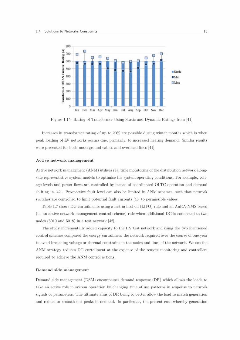
When DAR is used across a network it is termed dynamic network rating (DNR). Figure 1.15
shows the monthly rating of a oil natural air natural (ONAN) cooled transformer over the course
of a year using both static and dynamic ratings.
1.4. Solutions to Networks Constraints 18
Figure 1.15: Rating of Transformer Using Static and Dynamic Ratings from [41]
Increases in transformer rating of up to 20% are possible during winter months which is when
peak loading of LV networks occurs due, primarily, to increased heating demand. Similar results
were presented for both underground cables and overhead lines [41].
Active network management
Active network management (ANM) utilises real time monitoring of the distribution network along-
side representative system models to optimise the system operating conditions. For example, volt-
age levels and power flows are controlled by means of coordinated OLTC operation and demand
shifting in [42]. Prospective fault level can also be limited in ANM schemes, such that network
switches are controlled to limit potential fault currents [43] to permissible values.
Table 1.7 shows DG curtailments using a last in first off (LIFO) rule and an AuRA-NMS based
(i.e an active network management control scheme) rule when additional DG is connected to two
nodes (5010 and 5018) in a test network [42].
The study incrementally added capacity to the HV test network and using the two mentioned
control schemes compared the energy curtailment the network required over the course of one year
to avoid breaching voltage or thermal constrains in the nodes and lines of the network. We see the
ANM strategy reduces DG curtailment at the expense of the remote monitoring and controllers
required to achieve the ANM control actions.
Demand side management
Demand side management (DSM) encompasses demand response (DR) which allows the loads to
take an active role in system operation by changing time of use patterns in response to network
signals or parameters. The ultimate aims of DR being to better allow the load to match generation
and reduce or smooth out peaks in demand. In particular, the present case whereby generation

1.4. Solutions to Networks Constraints 19
Table 1.7: DG Curtailment with additional DG installed at Nodes 5010 and 5018
New DGCapacity (MW)
LIFO rule (MWh) Proposed rule (MWh) Difference(MWh)# 5010 # 5018 # 5010 # 5018
20 0 0 0 0 0
22 21 0 1 0 20
24 128 0 6 0 122
26 756 0 32 0 726
28 2107 0 132 0 1975
30 3142 2 306 0.05 2838
40 6944 2438 1726 184 7472
changes in response to the demand becomes increasingly unsuitable (requiring backup generation
capacity) as the proliferation of intermittent DG sources grows [44].
The principle of DR is shown in Figure 1.16 along with an energy efficiency (marked EE) plot
showing how energy consumption can also be reduced by improving the efficiency of electrical loads
(e.g with low energy lighting). The two DR plots (with and without rebound) also show how DR
may or may not effect the total energy consumption indicated by the area under the respective
curve. In either case, both of the DR plots are seen to reduce the peak seen in the middle of the
graph.
Figure 1.16: DSM and its effect on demand profiles [45]
Energy storage systems
Energy storage systems (ESS), like DR, reduce the need for backup generation capacity by stor-
ing energy using a combination of flywheels, hydrogen fuel cells (FC), compressed air (CAES),
capacitors (EDLC), batteries and pumped hydro to help match generation to demand. For this
reason they are sometimes included as DSM technologies [45]. ESS increase the system demand
during periods of excess generation whist generating or supplying energy during periods of excess
demand. Furthermore, distributed energy storage systems (DESS) can have very rapid response

1.4. Solutions to Networks Constraints 20
times thus improving networks stability and frequency regulation [46] and being distributed reduce
transmission losses.
There are many forms of ESS each with certain advantages and disadvantages, some of the key
technologies uses are presented in Table 1.8.
Table 1.8: Comparison of ESS Types [47]
TypeEfficiency
(%)Energy Density
(Wh/kg)Power Density
(W/kg)Cycle Life
(cycles)Self
Discharge
Pb-acid* 70-80 20-35 25 200-2000 Low
Ni-Cd* 60-90 40-60 140-180 500-2000 Low
Ni-MH* 50-80 60-80 220 �3000 High
Li-ion* 70-85 100-200 360 500-2000 Mid
Li-polymer* 70 200 250-1000 �1200 Mid
NaS* 70 120 120 2000 -
VRB** 80 25 80-150 �16000 Negligible
EDLC 95 �50 4000 �50000 Very High
Hydro 65-80 0.3 - �20 years Negligible
CAES 40-50 10-130 - �20 years -
Flywheel 95 5-30 1000 �20000 Very High
* Denotes Type of Battery or ** Flow Battery
Fault current limiters
Fault current limiters (FCL), limit the fault current levels in the network, thus reducing the
fault ratings of the network protection equipment. As the planning requirements and costs of
circuit breakers are particularly high, FCL offer economic advantages compared to reinforcement
or replacement of the protection systems. In particular, increased fault levels stemming from DG
(where it contributes to faults levels) or network reinforcement can be controlled with FCL. The
ideal FCL features [48]:
� Instantaneous Fault Detection
� Rapid Reduction in Fault Current
� An ability to handle many types of faults
� Automatic Resets capacity without human maintenance
� A Compact and Lightweight package
An example of a FCL, limiting fault current is shown in Figure 1.17, where the FCL fault current
can be controlled so protection systems operate as expected, but are not subject to excessive fault
current.

1.4. Solutions to Networks Constraints 21
Figure 1.17: Prospective fault current (red) and fault current with an FCL (green)
Summary of the Other Solutions
To briefly summarise these technologies, Table 1.9 lists their relative ability to influence network
hosting constraints mentioned in section 1.3.
Table 1.9: Other Solutions to Limitations in Network Capacity
SolutionNetwork Constraint
Voltage Thermal Fault PQ
Reinforcement x x x x
De-regulation x - - x
DAR / DNR - x - -
Active Network Man. x x x x
Energy Storage x x - -
Demand Response x x - -
Fault Current Limiters - - x -
Only active network management, and network reinforcement are able to alleviate at of the
hosting constraints. Nonetheless a mixture of all the above technologies would be expected whereby
the application of a given technology is based on cost befit analysis (CBA) performed by the DNO.

1.5. Problem Statement and Thesis Outline 22
1.5 Problem Statement and Thesis Outline
Problem Statement
Distribution networks are presently subject to increased loading from electrification of transport
and heating, whilst at the same time distributed generation (typically PV) and use of co-generators
(μCHP) supply energy back to the networks and, in sufficient quantity, cause reverse power flow
(or back-feeding). The result is that PQ measures are often breached prior to thermal limitations,
and in particular the supply voltage magnitude can become a severe limitation to suitably hosting
further increases to the loading of, and generation present on, the network. The usual solution,
that is reinforcement, whilst effective, is very costly and time consuming, thus alternative measures
to reinforcement are sought.
Thesis Outline
This thesis explores two of these alternatives to network reinforcement, that is, de-regulation
of voltage tolerances, and the use of PEDs to improve voltage regulation. To asses how these
compare to network reinforcement, a review of distribution networks themselves is first presented.
Following this the specific PEDs considered in this work are presented, where an overview of
their topology, control, and performance is given. In the case of wider voltage tolerances, the
load models themselves become increasingly important as if the loads exhibit any form of voltage
dependency this needs to be captured within the model. Therefore load models are considered in
detail, alongside the commonly used methods to represent single phase LV domestic loads, and
how PQ voltage sensitivity can be implemented in these.
The issue of voltage de-regulation is presented in Chapters 2, 3 and 5. Background informa-
tion presented in Chapter 2 on load modelling is then used to asses how de-regulation will effect
connected loads subject to this de-regulation where the focus is entirely on domestic loads, as
in Chapter 3. From this a relationship between the supply voltage and correct load operation
is formed and by setting various permissible limits on the amount of loads for which their mal-
operation can be accepted we have corresponding ranges (or levels) of de-regulation. These levels
of de-regulation are then used to asses how LCT hosting capacity could be increased as a result of
their application to LV networks in Chapter 5.
The PEDs considered in this work are presented in Chapters 2 and 5. The control structure
and layout of each of the PEDs is presented (Chapter 2) and each device is then implemented
into LV test networks, then analysed, where the benefits brought about by this are presented in
Chapter 6.
This thesis is divided into 6 subsequent chapters, each organised as follows:

1.5. Problem Statement and Thesis Outline 23
� Chapter 2 presents the background material on the topics of: distribution networks, power
electronic devices, and loads modelling. The operation and control schemes of distribution
networks are discussed along with a presentation of the equipment that is used within the
network. The PEDs are discussed in terms of their control objectives, and how these are
applicable to removing hosting constraints in these networks. Load models used in the
literature are presented along with benefits and disadvantages of these models, particular
attention is given to how the load models are effected by changes in the supply voltage (i.e
their voltage sensitivity).
� Chapter 3 presents an assessment of the impact that changes to supply voltage tolerance will
have on domestic loads. In particular, the energy demanded by, and amount of, common
domestic loads are presented first. After grouping loads into classes based on their electrical
characteristics, experimental and simulation based work on: motor loads (found in white
good) and, power supply unit (PSU) magnetics (found in modern consumer electronics), are
presented. A review of the literature relating to experimental testing of domestic loads in
terms of their sensitivity to supply voltage magnitude is presented. Results from this are then
combined to give an indication of what voltage tolerances could potentially be implemented
without large scale malfunction of consumer loads.
� Chapter 4 presented the methodology used in assessing how either voltage regulation or PEDs
can be fairly compared to network reinforcement. Individual steps involved in this process
are then given in detail. Implementation of LV network load flow are first explored. Test
LV networks are then presented along with developed metrics to compare these networks.
The Monte Carlo simulation method is then presented and its use justified. Finally the
economic measures to asses the cost benefits of de-regulation and PEDs relative to network
reinforcement are given.
� Chapter 5 presents results regarding voltage de-regulation of the supply voltage. Varying
“levels” of de-regulation are consider and the benefits associated with each tolerance band,
in terms of their ability to realise additional hosting capacity for LCTs are compared.
� Chapter 6 presents results regarding the use of PEDs in LV distribution networks. The 5
different PEDs are compared initially to each other and then to network reinforcement. Eco-
nomic comparisons whereby the PEDs are used for asset replacement or investment deferral
are then presented.
� Chapter 7 gives conclusions from this work, with particular attention given to the results of
Chapters 5, and 6. Also given are the authors contributions and then recommendations for
further work.

Chapter 2
Background
The aim of this chapter is to provide the relevant technical background on areas that are built
upon in subsequent parts of the thesis. Namely, the specialised areas of:
� Distribution Networks
� Power Electronics for Electricity Distribution
� Domestic Load Profiling
are covered within.
The section on distribution networks is specific to UK networks, although these are largely
typical of European networks. The layout and operations schemes of the distribution networks are
first presented, then an overview of the individual plant (eg. underground cables) that together
form the distribution network is given. Relevant electrical parameters and modelling techniques
for this equipment are also presented.
The section on power electronics focuses upon power electronic topologies that are suited to
applications in low voltage networks rather than providing a general overview of power electronics
itself. For each of the devices the relevant literature is reviewed and, control schemas, physical
implementation, and performance characteristics are presented.
The section on load modelling focuses upon generation of high resolution single phase domestic
load profiles that are suitable for study with a wide supply voltage range. This builds upon the
CREST load profile generation tool [49]. As Chapter 5 considers how voltage tolerances effect LV
network hosting capacity, the ability of the load models to suitably respond to wide changes in
supply voltage is particularity important. Load profiles for new LCTs are also synthesised from
available data in the literature and this procedure is also outlined here.
24

2.1. Distribution Networks 25
2.1 Distribution Networks
In this section the typical plant operated by DNOs will be presented, the representative costs
and operating principles of this equipment is also given. The aim is to give a review of literature
specialised to distribution network plant in the UK along with an understanding of the network
itself and the problems it faces due to LCT uptake. In particular the network from the primary
substation downstream (that is 11kV and below) is presented. Information is taken largely from
available literature produced by the DNOs (long term development strategies) in mainland Britain
[25, 30,50], EON’s network design manual [1], and the distribution code [51].
2.1.1 Network Structure
The transmission system operators (TSO) in the UK own and operate their transmission networks
(400kV or 275kV) which transmit bulk quantities of power over long distances, and connect to
major generating facilities. The DNOs connect their distribution networks to this transmission
network at grid supply points (GSP) and then operate their own sub-transmission systems (132kV).
The sub-transmission system supplies bulk supply points (BSP) where the voltage is further stepped
down (typically to 33kV). The primary distribution network (33kV lines) then supplies the primary
substations (typically 33/11kV). Occasionally GSPs are connected directly to primary substations
(132/11kV) thus by-passing both the primary network, and the BSP stations.
NOP
LV Link Box
Primary Substation
Secondary Substation
Distribution Cabinet
11kV Ring Main Unit
Figure 2.1: Layout of Existing HV Distribution Network
The single line structure of a generic secondary (termed HV network herein) distribution net-
work is shown in Figure 2.1. The primary substation supplies the HV network which as mentioned

2.1. Distribution Networks 26
typically operates at 11kV. Also shown is how the HV network supplies numerous secondary sub-
stations which in turn reduce the voltage to LV levels, and ultimately connect to the loads via
LV feeders. As seen in Figure 2.1, on load tap changers are operated at the primary substa-
tions, whilst for each primary substation transformer in reality there may be up to 60 connected
secondary transformers [25] connected across all the outgoing 11kV feeders.
At each secondary substation the connection to the HV network is made typically via a ring
main unit (RMU) which enables the substation to be connected to a HV ring circuit, improving
security of supply in the case of HV network faults [30]. For this, the RMU has 2 ring switches
and a circuit breaker that connects to the primary side of the transformer. The ring circuit
itself may be connected between two 11kV bus bars at separate different primary substations
(interconnected) or two sections of a busbar within one primary substation (looped). In low
density areas occasionally the substation will be connected to radial HV networks. These three
possible HV network structures are shown in Figure 2.2.
N.O.N.C.
N.C.
N.O. N.C.
N.C.
Radial Interconnected Looped
Figure 2.2: Structure of the HV Distribution Network
From the secondary of the LV transformer, the individual feeders are connected to a LV distri-
bution cabinet that contains of an incoming isolation link, a LV busbar and finally fuses for each
of the feeders. A typical secondary substation RMU and distribution cabinet are shown in Figure
2.3. When coupled with the transformer, the RMU, distribution cabinet, and transformer itself,
form the main components of the secondary substation.
The LV feeders in urban and suburban areas are almost exclusively underground where each
of the main (3 phase) feeders is terminated at a link box or pot end. A link box (see Figure 2.4b)
serves a termination point for multiple feeders and via street level access manual changes to the
links which connect 2 feeder, can be made, so they offer some decree of reconfigurability in the case
of a long term fault. A pot end is simply a insulated termination for a feeder so that any bare end
conductors are suitably protected from the environment. Along the feeder single phase service (or
3 phase) cables branch off and connect to the individual customers. The branch from the main 3φ
feeder to the service cable is made at a cable joint (shown in Figure 2.4a) which much like a pot

2.1. Distribution Networks 27
(a) Ring Main Unit (RMU) (b) Four way LV Distribution Cabinet
Figure 2.3: Secondary Substation Equipment
end, protects any exposed conductors from the environment. The service cable terminates at the
customers breakout board which also serves as the end of the DNOs ownership of the network and
thus the PCC where PQ and QoS requirements must be meet by the DNO.
(a) Branch joint (b) Two way Link Box
Figure 2.4: Underground equipment used along LV feeder ways
2.1.2 Operation & Protection
The causes of and appointment of voltage drop from the primary substation to the LV consumers
PCC assumed by DNOs are given in Figure 2.5.
The OLTC at the primary substation has a resolution around 1.5% of the nominal voltage, this
is shown as the 2% band at the top of Figure 2.5. The HV feeders should be designed to stay
within 6% of the nominal voltage [30] and up to 6% provision is made for voltage drop on the
HV system. The remaining voltage drop under normal operation (i.e when no are faults present,
or maintenance needing special routeing is taking place) is shown across the transformer (2%) and
the LV feeder (4-6%) where the amount permissible in the LV system depends upon the length of
the 11KV feeder serving the secondary substation, where a figure of 15km is given as the break
point between “long” and “standard” feeders.
The 6% contingency for back-feeding (reverse power flow) is required for security of supply and
re-routing, which would potentially result in excessively high or low voltages if this 6% contingency

2.1. Distribution Networks 28
Figure 2.5: Allocation of voltage drop among network components [1]
margin is not used.
The network is operated in a radial or more commonly open ring structure with interconnection
used to provide reliability of service following network faults. Consider an example of the single
line system shown in Figure 2.6.
A
C
B
Fault
Figure 2.6: Interconnected ring configuration of an 11kV network
As seen the two feeders are can be normally operated as distinct radial networks from the two
primary substations by virtue of opening any one of the three sectionaliser switches indicated at
locations A, B or C. For example, if we assume prior to the long term fault indicated, that switch
A was open whilst B and C were closed, for restoration of the supply to all of the substations
switch A would close whilst B and C both open. Worth noting is that the switches at A, B and C
would typically not have fault current breaking capacity (i.e the RMU uses switch disconnecters)
and in such a case would only operate after a circuit breaker has temporarily disconnected the
faulted lines.

2.1. Distribution Networks 29
2.1.3 Distribution Network Components and Plant
This section will present the network owned plant that is most critical to the accuracy of flow
studies, these are the:
� Primary Transformers
� Secondary Transformers
� HV Feeders
� LV Feeders
Primary Transformers
Primary Substations are typically the last point at which voltage control is installed in the dis-
tribution network. The primary substation will have on load tap changer (OLTC) transformers
installed, where the primary voltage is typically 33kV although other voltages are used, and the sec-
ondary voltage is 11kV or 6.6kV. The most common vector group of transformers used at primary
substations is Dyn11.
Figure 2.7: Primary Substation with Two 15MVA 33/11kVtransformers (from [52])
Transformers are usually installed in pairs rated at 15/30MVA (corresponding to ONAN/OFAF-
CER ratings respectively), but scope exists for transformers from 3/6MVA up to 20/40MVA and
single transformers can be used if the load served is below 12MVA [30]. In high density load
areas provision is also made for up to four parallel transformers, with dual winding secondary
transformers also occasionally used [50]. The 11kV star point of the transformer is earthed via
solid or resistive grounding. If the secondary winding is delta connected (as in the case of some
132/11kV transformers) then earth is made via an earthing transformer.

2.1. Distribution Networks 30
Voltage control here is achieved via OTLC with a 1.25% to 1.5% bandwidth and a tap range of
-5% to +10% [30]. As with much of the distribution system, voltage control is designed assuming
power flow is uni-directional; hence voltage control settings are such that voltage drop along
standard 11kV feeders can use the full permissible voltage range (�6% at HV [30]). This means
the voltage at the secondary side busbars is kept towards upper limits at times of peak demand
with typical reference figures of 1.05pu at full load and 0.985pu at no load [25].
Secondary Transformers
Secondary substations connect to the HV distribution networks (11kV or 6.6kV) and step down
the voltage to LV (400V 3φ / 230V 1φ) for distribution to, predominately, single phase customers.
In some rural setting single phase pole mounted transformers (25kVA to 50kVA) are used to supply
distant and widely dispersed customers [1]. For urban and semi-urban distribution, transformers
ratings for those supplying multiple domestic or commercial customers are limited to 1000kVA so
as to limit the disruption caused by faults at the substation. This is because a 1000kVA can supply
only a limited number of individual customers (708 customers assuming an after diversity maximum
demand (ADMD) of 2kW [1]). Where a larger single customer connects to a secondary substation
the permissible rating will be increased, for example, with Northern Power Grid the maximum LV
transformer rating for a transformer supplying single customer is 1600kVA. The smallest ground
mounted transformers used are 200kVA [1] due to the deceasing efficiency of smaller transformer,
and the lower cost of alternative padmount, unit, and pole-mounted transformers.
New use size transformers and their typical impedances (referred to the secondary LV side)and
losses are shown in table 2.1.
Table 2.1: 11kV/LV Transformer Impedances [1]
Size (kVA) LocationImpedance (Ω) Losses (W )
R X Iron Copper
50 Pole 0.0266 0.0496 110 800
100 Pad 0.0271 0.0401 200 1500
200 Ground 0.0158 0.0406 275 3000
500 Ground 0.0051 0.0171 600 7000
Voltage control at secondary substations is limited to no load taps at the transformer. The taps
are located at the primary windings and allow a voltage range, from nominal, of �5% with a 2.5%
resolution. The nominal voltage ratio of many LV transformers is actually 11kV/0.433kV [1, 30].
This is due in part to the previous voltage regulations (prior to 1998) where the voltage tolerance
was 240V �6% and to allow for voltage drop along the feeder [25].
The secondary winding star point is grounded within the substation along with all perimeter
metalwork. If the connected LV network is operated with protective multi-earth (PME) earthing,

2.1. Distribution Networks 31
Figure 2.8: Secondary Substation and LV Transformer (from [53])
the grounding impedance of the substation earth electrode of should not exceed 40Ω [25].
HV Feeders
The 11kV network uses a mix of underground and overhead lines, both in 3 wire arrangements.
In urban areas the vast majority of the 11kV networks is underground whilst in rural areas there
is a greater percentage of overhead liens. The length of the HV network will dictate it general
operation regarding interconnection and voltage profile, with long HV feeders defined as extending
over 15 km [1] from the primary substation.
Overhead Lines The conductors used for overhead lines are, stranded aluminium, uncovered,
and either ACSR (steel reinforced) or AAAC (all aluminium). The conductors are supported on
wooden poles with a specified conductor height of greater than 5.2m [54].
Figure 2.9: Typical 3 Wire Overhead Distribution Lines (from [55])

2.1. Distribution Networks 32
Conductor impedance matrix are developed for the conductors in Table 2.2 using the MATLAB
function power lineparam. The ground resistivity is assumed as 100Ω.m which is a very typical
value [23], and the standard geometry on the conductors are shown in the Appendix B.
Regarding construction of the lines, the DNOs prefer the use all aluminium alloy conductors
(AAAC) or aluminium core steel reinforced (ACSR), with occasional use of general purpose jacked
cables (BXL/PAS). All of these conductors will be used in various sizes deemed appropriate by
the network engineer [1].
The preferred conductors used for underground cable are 11kV rated, solid aluminium core,
XLPE insulated triplex cable. In the E.ON design manual [1] the standard cables are listed as
triplex laid (see B.2) cables, of the sizing shown in Table 2.2.
Table 2.2: New 11kV Conductors [1]
Location Cable Type CSA (mm2)
OH AAAC 50, 100, 200
OH ACSR 50, 100, 150
OH HDA* 300
UG Al-XLPE 70, 95, 185, 300
UG Cu-XLPE* 300, 400
* Special Application
Figure 2.10: 11kV Underground Triplex Cable Current Density with 1A inconductor A and induced eddy currents in shields
For 11kV cable the MATLAB function power cableparam was used rather than finite element
analysis software (as in Figure 2.10), which was restricted in use for parametrisation of LV cables,
shown in section 2.1.3.
Taking the example of underground 185mm2 aluminium triplex cables buried 1 meter below
ground and spaced as can seen in Appendix B, where further details on HV cable impedances can

2.1. Distribution Networks 33
be found, we have the following phase impedance matrix:
Z �
�����
0.095+0.050i 0.002+0.000i 0.002+0.000i
0.002+0.000i 0.095+0.050i 0.002+0.000i
0.002+0.000i 0.002+0.000i 0.095+0.050i
������km (2.1)
C �
�����
211 0 0
0 211 0
0 0 211
�����nF �km (2.2)
All of the calculated phase impedance matrices are used in the load flow studies of chapters 5
and 6, where the cable section length and construction type are both know thus by calculating the
product of the cable length (in km) and the phase impedance matrices (in Ω/km) we have detailed
the branch impedances.
The standard range of cables and lines used in replacement or upgrade work, and for new 11kV
feeders are listed in Table 2.2 (some special application cables are omitted). All use either copper
or aluminium conductors and the CSA ranges from 50mm2 to 400mm2, where by the choice of
cable is dictated by, feeder length, loading, faults levels, and potential for new or increased loading.
LV Feeders
In urban areas the LV network is almost exclusively of underground construction, whilst in rural
areas a mix of overhead and underground cables are used. In both cases the final LV customer is
connected to the LV feeder via a service cable which is owned by the DNO. It is at this point that
the consumer should be supplies with a supply voltage that meets the requirements of EN50160,
and is also the PCC for all connected loads in the customers premises.
The grounding schemes used dictate the cable used, but 3 main schemes are employed for LV
grounding are used, these being TN-CS, TN-S and TT. In all, the final customers has a ground to
create the local equipotential zone. The preferred grounding practice is TN-CS, also called PME,
which use cables with combined neutral and earth conductors (CNE). The TN-CS grounding
scheme is shown in Figure 2.11a.
A
CB
PNE
Load(a) TN-CS (PME)
A
CB
NPE
Load(b) TN-S
Figure 2.11: Earthing Systems

2.1. Distribution Networks 34
An alternative to PME is to isolate the neutral of the LV feeder from the protective earth, with
the customers protective earth coming from a fifth conductor on the feeder, this practice is called
TC-S and is shown in Figure 2.11b. A third method of grounding (TT) uses only a local earth at
the customers site via their own earthing electrode, this is more common in mainland Europe than
the UK.
In urban areas where most of the LV network is underground the preferred conductor amongst
all of the DNOs in the UK is XLPE insulated “wavecon” cable. This has 3 or 4 solid aluminium
phase conductors and a stranded concentric copper, neutral conductors around the phase conduc-
tors.
With PME, as can be seen in Figure 2.11a the neutral conductor is earthed at multiple points
along the feeder length. As PME permits ground currents to flow, even without faults present,
due to the parallel return path formed by the earth and neutral, for accurate representation of
the cable impedance matrices, Carsons equations should be used [56]. Further details regarding
application of Carsons equations to distribution networks are found in [23,57]. The series “circuit”
impedance of a neutral grounded network with 185mm2 wavecon cable is given in (2.3), with the
capacitive suceptance given in (2.4).
Z �
��������
0.239+0.739i 0.047+0.674i 0.047+0.674i 0.048+0.664i
0.047+0.674i 0.239+0.738i 0.047+0.674i 0.048+0.664i
0.047+0.674i 0.047+0.674i 0.239+0.738i 0.048+0.664i
0.048+0.664i 0.048+0.664i 0.048+0.664i 0.220+0.663i
���������km (2.3)
C �
��������
250 �53 �53 �143
�53 250 �53 �143
�53 �53 250 �143
�143 �143 �143 129
��������nF �km (2.4)
The cable shows differing impedance depending on system frequency (due to proximity and
skin effects) for this reason 2d FE analysis is carried out in FEMM [58], where the results given in
(2.3) and (2.4) are from this work. This effect is shown in Appendix B.
For the reduction to an “abc” phase impedance matrix (3x3), via the Kron reduction [23], we
must first assume the neutral conductor is tied solidly to ground at both ends of the line, hence the
voltage to ground of the neutral at either end is zero. This allows the matrix size to be reduced,
but in the case of a resistive non-ideal ground impedance, or missing ground nodes, the accuracy
of this technique has been questioned [59].
Ciric [57] proposes use of a 5x5 impedance matrix (in the case of a 3 phase 4 wire system with
grounded neutral) as a means to “split up” the circuit equations and then accurately model both
the neutral and ground paths, whilst incorporating grounding impedances at specific locations,

2.1. Distribution Networks 35
Figure 2.12: ABC Conductors
Table 2.3: New LV Conductors [1]
Location Cable Type CSA (mm2)
OH-Service Al-ABC 2�25, 2�35
OH-Service* Al-ABC 4�25
OH-Feeder Al-ABC 4�95
UG-Service Al/Cu-CNE 25, 35
UG-Service* Cu-CE 35
UG-Feeder Al-CNE 95, 185, 300
* 3φ Service Cables
but again doubts are cast upon the validity of such a method [59], due to discrepancies between
the above method and that proposed by Anderson [60]. Herein, 4x4 circuit impedance matrices
will be used which are reduced to 3x3 phase impedance matrices if the ground is assumed solidly
tied to ground or the earthing scheme is TN-S.
Outside of urban areas parts of the LV network utilise overhead lines, especially in rural areas.
The preferred standard of these lines is to use insulated aerial bundled conductor (ABC), this is in
part because ABC is considered a less of an eyesore, and due to their improved reliability compared
to bare wire conductors.
ABC conductors with 4 distinct cores where the neutral conductor is regularly grounded (ie.
PME) are the preferred configuration of overhead LV feeders the UK DNOs. The construction of
an ABC conductors is illustrated in Figure 2.12.
All of the various LV cables and lines used for, new LV networks, and asset replacement are
listed in Table 2.3.
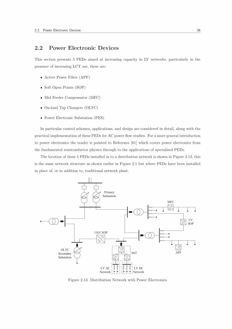
2.2. Power Electronic Devices 36
2.2 Power Electronic Devices
This section presents 5 PEDs aimed at increasing capacity in LV networks, particularly in the
presence of increasing LCT use, these are:
� Active Power Filter (APF)
� Soft Open Points (SOP)
� Mid Feeder Compensator (MFC)
� On-load Tap Changers (OLTC)
� Power Electronic Substation (PES)
In particular control schemes, applications, and design are considered in detail, along with the
practical implementation of these PEDs for AC power flow studies. For a more general introduction
to power electronics the reader is pointed to Reference [61] which covers power electronics from
the fundamental semiconductor physics through to the applications of specialised PEDs.
The location of these 5 PEDs installed in to a distribution network is shown in Figure 2.13, this
is the same network structure as shown earlier in Figure 2.1 but where PEDs have been installed
in place of, or in addition to, traditional network plant.
LVSOP
Primary Substation
OLTCSecondary Substation
LV DCNetwork
11kV SOP
MFC
LV AC Network
SST APF
Figure 2.13: Distribution Network with Power Electronics

2.2. Power Electronic Devices 37
2.2.1 Active Power Filter
Active power filters (APF), and in particular shunt active power filters which will be referred to
simply as APFs are particularity suited to use in distribution systems where single phase, non-
linear loads create both fundamental negative and zero sequence currents components (unbalance)
and harmonic current flows in the network [62]. Although power factor is typically high in LV
networks [1], the APF can also be used to increase power factor and improve other PQ issues such
as flicker. Furthermore it can act to improve the voltage quality by virtue of compensating the
current components that cause the harmonic, zero, and negative voltage components [63]. In [62]
the PQ issues that the APF should aim to address are given as:
� Harmonic distortion
� Fundamental reactive power
� Negative sequence components
� Zero sequence components
� Flicker
The basic topology of an APF comprises an inverter, energy storage element (DC link capacitor)
and coupling to the network (shown as an inductor). The inverter is then controlled in such a way
as to produce the compensation currents (Ic) such that the control objectives are reached. The
connection of such an APF to the network is shown in Figure 2.14.
DC
AC
Vs VlIc
Is Il
Figure 2.14: Configuration of a APF Control Scheme
As LV networks are comprised of single phase loads, feeder unbalance is inevitable, so the APF
must be able to compensate for zero sequence components (i.e eliminate neutral ground current).
This can be achieved in via two main topologies reported in the literature, the split capacitor 3 leg
inverter, the 4 leg inverter, or a combination thereof [64].
There exists a wide range of control strategies for the APF as summarised in [62] which mentions
the use of both time and frequency domain filtering methods along with more recently developed
pattern learning methods. A comparison between APF objectives with time domain filtering

2.2. Power Electronic Devices 38
methods was presented in [65]. This work considered APF operation in 4 wire systems and how
each control scheme performed in the most general case, that is in the presence of both distortion
and unbalance on both the supply voltages and the load currents. The control strategies compared
where:
� UPF
� p-q
� id-iq
� PHC
The conclusion was that the PHC strategy was the most resistant in terms of adhering to the
IEEE Standard 1459 [66] in the presence of distorted or unbalanced voltages at the APF PCC.
The PHC control strategy is so named as the control objective regardless of supply voltage is to
achieve balanced sinusoidal currents in phase with the fundamental positive sequence voltage.
These control strategies are herein formulated in αβ0 coordinates as it gives a more clear insight
to the control objectives than when it is presented in phase coordinates, as noted in [65].
The first step is thus transforming the phase voltage and current into the stationary αβ0
reference frame:
uαβ0 � C� uabc (2.5)
where the power invariant αβ0 transform (C) is:
C �
�2
3
�����
1 �12 �
12
0�32
�32
1�2
1�2
1�2
����� (2.6)
and the reverse transform (CT ) is:
CT� C�1 (2.7)
which allows the transformation from αβ0 coordinates back to phase coordinates:
uabc � CT� uαβ0 (2.8)

2.2. Power Electronic Devices 39
The instantaneous active load power (p) is comprised of three component powers (pα, pβ , p0),
which are:
p � Vαβ0 � Iαβ0 (2.9)
� VαIα � VβIβ � V0I0
� pα � pβ � p0
the instantaneous reactive load power (q) is comprised of three components powers (qα, qβ , q0):
q � Vαβ0 � Iαβ0 (2.10)
� VβI0 � V0Iβ � V0Iα � VαI0 � VαIβ � VβIα
� qα � qβ � q0
and both the load instantaneous real (p) and reactive (q) powers, in the general case, are comprised
of dc and ac components:
p � p� p (2.11)
q � q � q (2.12)
thus, the average load power that must be supplied from the source is the dc component of the
instantaneous active power (p):
p � pα � pβ � p0 (2.13)
From 2.13 the compensation schemes reference αβ0 source currents (I�αβ0) for the PHC control
strategy (Is in Figure 2.14) are in [65], given as:
�����
i�α,phc
i�β,phc
i�0,phc
����� �
pα � pβ � p0
v�2α1 � v�2
β1
�����
v�α1
v�β1
0
����� (2.14)
and for the UPF control strategy [65]:
�����
i�α,upf
i�β,upf
i�0,upf
����� �
pα � pβ � p0�v2α � v2β � v20�dc
�����
vα
vβ
v0
����� (2.15)

2.2. Power Electronic Devices 40
where the dc subscript term represents an average over the fundamental frequency period. For the
modified p-q control strategy [67]:
�����
i�α,pq
i�β,pq
i�0,pq
����� �
pα � pβ � p0v2α � v
2β
�����
vα
vβ
0
����� (2.16)
A comparison of the three control strategies given by (2.14)-(2.16) is shown in Figure 2.15,
where it is seen that the UPF current waveforms match those of the supply voltage waveform
thus the control scheme achieves its goal of unity power factor (UPF). The PHC control scheme
draws balanced and sinusoidal currents that are in phase with the fundamental positive sequence
voltage waveforms (v�1 ). The modified pq strategy draws a constant active power (p) with no zero
sequence current (i�0 ), however as seen from Figure 2.15 and the “p-q current spectrum” subplot this
introduces current harmonics not originally present in the current or voltage waveforms. In Figure
2.15, all of the frequency domain plots are for the blue (phase a) current or voltage waveforms. It
should be noted that as the source is treated as an infinite source and the APF is shunt connected
neither the source voltage nor load currents can be changed, and the APF controls only the source
side current.
As indicated in Figure 2.15, for rejection of voltage distortion and adherence to the IEEE Stan-
dard 1459 the PHC scheme is the most suitable particularly for 4 wire LV distribution networks.
For the purpose of modelling an APF in a fundamental frequency AC load flow study the
compensation currents with the PHC compensation scheme (I�phc) are found by first calculating
the required conductance factor (kg):
kg �P
V �seq � V�seq
(2.17)
where V �seq are the positive sequence voltage vectors at the PCC, additionally V �seq is its conjugate
transpose, and P is the calculated power (a dc term for AC load flow). Given kg, we then multiply
by the positive sequence voltages to find the reference currents (I�s,phc):
I�s,phc � kgV�
seq (2.18)
As before these currents will be balanced and in phase with the positive sequence voltage
vectors. The implementation in signal flow diagrams are shown in Figure 2.16.
As only the fundamental component is considered in AC load flow studies, and the method
used to calculate reference currents is PHC, the APF can be considered as a phase balancer. Once

2.2. Power Electronic Devices 41
-400
0
400
Voltage(V
)
Source Voltage Waveform
0
200
400
Amplitude(V
) Source Voltage Spectrum
-20
0
20
Current(A
)
Load Current Waveform
0
5
10
15
Amplitude(A
) Current Spectrum
-20
0
20
Current(A
)
UPF Current Waveform
0
5
10
15
Amplitude(A
) UPF Current Spectrum
-20
0
20
Current(A
)
p-q Current Waveform
0
5
10
15
Amplitude(A
) p-q Current Spectrum
0 0.02 0.04 0.06 0.08 0.1Time (s)
-20
0
20
Current(A
)
PHC Current Waveform PHC Current Spectrum
0 50 100 150 200 250 300 350 400Frequency (Hz)
0
5
10
15
Amplitude(A
)
Figure 2.15: Comparison of APF control schemes, where the top two rows show the sourcevoltage and load current, whilst the lower 3 row show the source current with three different APF
control methods
Vseq
÷
PcalcVabc
I abc
x'x I *
Figure 2.16: Configuration of a APF Control Scheme
the reference currents are known the compensation current (Ic) is:
Ic � Il � I�
s,phc (2.19)

2.2. Power Electronic Devices 42
where Il is the load side current.
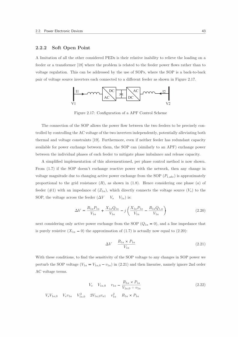
2.2. Power Electronic Devices 43
2.2.2 Soft Open Point
A limitation of all the other considered PEDs is their relative inability to relieve the loading on a
feeder or a transformer [18] where the problem is related to the feeder power flows rather than to
voltage regulation. This can be addressed by the use of SOPs, where the SOP is a back-to-back
pair of voltage source inverters each connected to a different feeder as shown in Figure 2.17.
DC
AC
AC
DCV1
I2I1
V2
Figure 2.17: Configuration of a APF Control Scheme
The connection of the SOP allows the power flow between the two feeders to be precisely con-
trolled by controlling the AC voltage of the two inverters independently, potentially alleviating both
thermal and voltage constraints [19]. Furthermore, even if neither feeder has redundant capacity
available for power exchange between them, the SOP can (similarly to an APF) exchange power
between the individual phases of each feeder to mitigate phase imbalance and release capacity.
A simplified implementation of this aforementioned, per phase control method is now shown.
From (1.7) if the SOP doesn’t exchange reactive power with the network, then any change in
voltage magnitude due to changing active power exchange from the SOP (P1,abc) is approximately
proportional to the grid resistance (R), as shown in (1.8). Hence considering one phase (a) of
feeder (#1) with an impedance of (Z1a), which directly connects the voltage source (Vs) to the
SOP, the voltage across the feeder (ΔV � Vs � V1a) is:
ΔV �R1aP1a
V1a�X1aQ1a
V1a� j
�X1aP1a
V1a�R1aQ1,a
V1a
�(2.20)
next considering only active power exchange from the SOP (Q1a � 0), and a line impedance that
is purely resistive (X1a � 0) the approximation of (1.7) is actually now equal to (2.20):
ΔV �R1a � P1a
V1a(2.21)
With these conditions, to find the sensitivity of the SOP voltage to any changes in SOP power we
perturb the SOP voltage (V1a � V1a,0 � v1a) in (2.21) and then linearise, namely ignore 2nd order
AC voltage terms.
Vs � V1a,0 � v1a �R1a � P1a
V1a,0 � v1a(2.22)
VsV1a,0 � Vsv1a � V21a,0 � 2V1a,0va1 � v
21a � R1a � P1a

2.2. Power Electronic Devices 44
equating the, constant voltage terms (V1a,0) and AC voltage terms (va1) after linearisation, to the
SOP power, which is itself comprised of the SOP operating point power (P1a,0) and SOP AC power
terms (p1a) results in:
P1a,0 �VsV1a,0 � V
21a,0
R1a(2.23)
p1a �Vsv1a � 2V1a,0v1a
R1a(2.24)
So the voltage sensitivity, defined as the incremental change in voltage, in response to a incremental
change in SOP power is:
dV1adP1a
�v1ap1a
�R1a
Vs � 2V1a,0(2.25)
Writing the voltage change at the SOP in terms of SOP power linearised around an operating
point V1a,0:
�dV1adP1a
dP1a � V1a � V1a,0 (2.26)
�v1a � V1a � V1a,0
where V �
1a is the new voltage at the SOP. If the three phase voltages of a connected feeder (here
feeder #1) are decoupled from each other the above expression in matrix from is:
�
���������
dV1adP1a
0 0
0dV1bdP1b
0
0 0dV1cdP1c
���������
���������
dP1a
dP1b
dP1c
����������
���������
V1a
V1b
V1c
����������
���������
V1a,0
V1b,0
V1c,0
���������
(2.27)
the above equation has n (� 3) control variables (dP1a, dP1b, dP1c) with n linearised equations.
We can remove one of these control variables by stating that:
P1a � P1b � P1c � PSOP (2.28)
dP1a � dP1b � dP1c � 0 (2.29)
we next introduce the unknown (V �
1x), and note that if the control scheme is to balance voltage
magnitudes at the SOP as effectively as possible (hence minimising losses [68]), where V �
x is the

2.2. Power Electronic Devices 45
voltage magnitude at the SOP we can write:
���������
�dV1adP1a
0 0
0 �dV1bdP1b
0
0 0 �dV1cdP1c
���������
���������
dP1a
dP1b
�dP1ab
����������
���������
V �
1x
V �
1x
V �
1x
����������
���������
V1a,0
V1b,0
V1c,0
���������
(2.30)
where dP1ab is equal to the sum of dP1a and dP1b. We see now that there exists 3 linear equations
with 3 unknowns (dP1a, dP1b, V�
1x), this equation can be rewritten as:
��������������
�dV1adP1a
0 0 1
0 �dV1bdP1b
0 1
0 0 �dV1cdP1c
1
1 1 1 0
��������������
��������������
dP1a
dP1b
dP1c
V �
1x
��������������
�
��������������
V1a,0
V1b,0
V1c,0
0
��������������
(2.31)
which has the form of:
Ax � B (2.32)
where x is comprised of the per phase changes in power flow in the SOP (dPa, dPb, dPc), and the
magnitude of the reference voltage (V �
x ), which form the unknown variables. Solving for x:
x � A�1B (2.33)
In B, PSOP is the power that the SOP passes from one connected feeder to the other feeder. The
expression above is valid for the other connected feeder (#2) whereby the subscripts are suitably
replaced and the sign of PSOP in (2.28) is switched (i.e �PSOP ).
This principle of SOP phase voltage regulation is demonstrated in Figure 2.18 where the net
SOP power (PSOP ) is specified as zero and an unbalanced load is connected to a feeder that also
connects to the SOP (as in Figure 2.19). Initially the voltages at the SOP are unbalanced (as
can be seen by the voltages at iteration #1 in the top graph of Figure 2.18). The SOP maintains
the requirement of zero net power flow but via adjustment of the per phase powers controls phase
power flows such that it results in balanced voltages at the SOP terminals after the solution is
found by iteration like in usual load flow studies. It is seen that after the first iteration changes to
the SOP power flows are small thus indicating the good convergence characteristics of the above
method.

2.2. Power Electronic Devices 46
1 2 3 4 5Itteration
0.8
0.85
0.9
0.95
1Phase Voltage at SOP (Vpu)
Va
Vb
Vc
-4
-2
0
2×10⁴ SOP Phase Power (W)
Psop,a
Psop,b
Psop,c
Figure 2.18: Iterations of a SOP Regulating Phase Voltages
In the case where the line impedance (Z) has reactance (Z � R� jX) and / or mutual effects
between the SOP phases are considered the number of equations that need to be solved doubles,
as do the number of unknowns, the control objective then becomes to create a balanced voltage
set at the SOP, this necessitates that the SOP also control reactive power flow at its terminals for
independent angular control.
Regarding control of the main SOP power flow parameter, namely PSOP (see (2.28)), which is
the transfer of power from 1 connected feeder to another, a range of schemes are used [68] that
often have a control objective of minimising losses and regulating voltage when if falls outside of
permissible limits.
AC
AC
Feeder #1
Feeder #2SOP
Figure 2.19: A SOP connected between two feeders facilitating power flow between them
The 2 port SOP will be used herein to control voltage at each of its terminal to regulatory levels,
this is only achieved if capacity is available on the other feeder (ie. it does not suffer simultaneous
voltage constraints)

2.2. Power Electronic Devices 47
2.2.3 Mid Feeder Compensator
The MFC in topology is similar to that of a UPFC (or UPQC). It comprises shunt and series
inverters tied to a common DC link. A high level diagram of a MFC inserted between two network
buses is shown in Figure 2.20. The two converters are seen connected to one DC link but if we
were instead to consider two separate DC links (one for each converter), the MFC would actually
resemble a combination of both a shunt APF and series APF; something that can be taken into
account when considering control schemes for the MFC.
DC
AC
AC
DC
Vs VlIc
VcIs Il
Figure 2.20: Configuration of a UPQC
For optimal location of a single MFC it should maintain voltage profile as tightly as possible,
this will be achieved if it is located where the voltage across the feeder is half of total voltage across
the feeder. Conciser a single phase line of length L and impedance Z, with uniformly distributed
load and a total line current It, then at position x on the feeder the line current (ix) is:
ix � It �1� x� (2.34)
The gradient of the voltage at position x is:
dV
dx� Zix (2.35)
the voltage drop (ΔVx) at x is:
ΔVx �� x
0
dV
dx.dx (2.36)
�� x
0
Zix .dx
�� x
0
ZIt �1� x� .dx
The voltage drop is then half that of the remote feeder end voltage drop (ΔVL) when:
x � L2��2
2� ΔVx � ΔVL
2

2.2. Power Electronic Devices 48
The solution indicates the voltage drop is half the maximum value when x equals 0.29L, or 29%
of the total feeder length, which is where the MFC would, ideally, be located along the feeder.
Regarding control of the MFC, we initially consider both converters separately. Thus for the
shunt inverter it can be controlled exactly as the shunt APF shown previously in section 2.2.1 was.
Hence, the source side reference currents (Iαβ0,mfc) assuming PHC operation of the MFC’s shunt
converter are:
�����
i�α,mfc
i�β,mfc
i�0,mfc
����� �
pα � pβ � p0
v�2α1 � v�2
β1
�����
v�α1
v�β1
0
����� (2.37)
For the series connected converter, as a result of duality [69], equations (2.14)-(2.16) can be
applied for a series APF (or DVR) which injects a compensating voltage (Vcomp) to the source
voltage (Vs) such that the load voltage (Vl) is equal to the reference voltage (V �) and any control
objectives are meet. For example, the PHC control objective (2.14) applied to the series MFC
converter results in the MFC load side reference voltages (V�
αβ0,mfc) of:
�����
v�α,mfc
v�β,mfc
v�0,mfc
����� �
pα � pβ � p0
i�2α1 � i�2
β1
�����
i�α1
i�β1
0
����� (2.38)
we then note (2.38) is of the general form:
V�
αβ0,mfc � kr
��i�
αβ,1
0
�� (2.39)
we see the reference voltage components are proportional to the balanced positive sequence source
currents (i�αβ,1) via a resistive factor kr. Hence, by adjustment of kr we can control the load side
reference voltages (V�
αβ0,mfc).
Suppose now that we instead wish to control these load side reference voltages to some prede-
fined magnitude (�Vmfc�), then (2.39) can be reformed as:
V�
αβ0,mfc �
�32 � �Vmfc��i�2α1 � i�2
β1
��i�
αβ,1
0
�� (2.40)
Notice the factor of�
32 which is needed as the αβ0 transform (C) we defined previously (2.6) was
the power invariant transform.
Unlike with the voltages in (2.38) using the voltages of (2.40), the average load side power (Pl),

2.2. Power Electronic Devices 49
i.e the power at the load side of the MFC, which is the dc component of:
Pl � V�
αβ0,mfc � Iαβ0 (2.41)
is not necessarily equal to the average source side power (Ps), i.e the power on the source side of
MFC, which is the dc component of:
Ps � Vαβ0 � I�αβ0,mfc0 (2.42)
Thus there is need for an additional source of energy for the compensator to operate with energy
balance. The power demand of the compensator (Pmfc) is:
Pmfc � Ps � Pl (2.43)
The series compensator power (Pmfc) could be supplied by local energy storage (eg. from
batteries), from another circuit, or by the shunt connected converter. With the latter case it is
helpful to imagine the ideal MFC, as shown in Figure 2.21, connected between two network buses.
MFCImfc
Vmfc
Il
Vs
Pin Pout
Figure 2.21: MFC Power Load and Source Flows
The ideal MFC has no power losses such that the input (Ps) and output powers (Pl) are equal.
Furthermore the MFC controls the source side currents (I�mfc) and load side voltages (V �
mfc) to
the desired values. For the MFC shunt converter to supply the power of the series converter we
have that Ps � Pl, so the MFC reference currents (I�αβ0,mfc) will be such that:
I�αβ0,mfc �
�V�
αβ0,mfc � Iαβ0,l
�dc
V�
αβ0,s
(2.44)
this is due to the use PHC control such that:
P s � V�
αβ0,s � I�αβ0,mfc (2.45)
hence:
I�αβ0,mfc �
�V�
αβ0,mfc � Iαβ0,l
�dc
V�
αβ0,s
(2.46)

2.2. Power Electronic Devices 50
which, when put in the same general form of (2.37), becomes:
�����
i�α,mfc
i�β,mfc
i�0,mfc
����� �
�V�
αβ0,mfc � Iαβ0,l
�dc
v�2α1 � v
�2β1
�����
v�α1
v�β1
0
����� (2.47)
Equation (2.47) is actually identical to (2.37) but for the fact we had assumed (by virtue of
treating both the shunt and series MFC converters entirely separately) the numerator of (2.37)
was the load power without (or prior to) voltage regulation.
The effect of this change to the reference currents (I�αβ0,mfc) is that the shunt compensator
will now draw or supply the power drawn or supplied by the series compensator. Thus only small
energy storage components (i.e. a DC link capacitor) are needed for the MFC, which compared to
battery storage options, significantly reduces both costs and size at the expense of a higher rated
shunt MFC converter.
To demonstrate the operation of the MFC, Figure 2.22 shows the effect of an MFC when it
is used to connect a load comprised of a constant current source (same load current waveform as
in Figure 2.15) to a distorted and unbalanced infinite voltage source supply (same supply voltage
waveform in Figure 2.15). The MFC is set to regulate the peak load side phase voltage to the
maximum permissible UK voltage, namely 357.8V.
-400
0
400
Voltage(V
)
Source Voltage Waveform
-400
0
400
Voltage(V
)
Load Voltage
-20
0
20
Current(A
)
Source Current
-20
0
20
Current(A
)
Load Current
0 0.02 0.04 0.06 0.08 0.1Time (s)
0
2500
5000
7500
10000
Power
(W)
Source Power Load Power
0 0.02 0.04 0.06 0.08 0.1Time (s)
0
2500
5000
7500
10000
Power
(W)
Figure 2.22: Performance of an MFC
We also see that the mean source and load powers (as indicated by the red lines in the lowest
two plots) are equal, although a difference is seen in the instantaneous values, hence the need for
the DC link capacitor or some other form of local energy storage. These oscillations in the source

2.2. Power Electronic Devices 51
and load power are caused by the unbalance and distortion in the source voltage and load current,
respectively.
For the purposes of AC load flow studies operation of the PHC controlled MFC can be calculated
by first calculating the reference voltages (V �
mfc) via:
V �
mfc ��3 � �Vmfc��I�seq � I�seq
� I�seq (2.48)
the new load side apparent power (Sl) is then:
Sl � 0.5� V �mfc � i (2.49)
where the active load power (Pl) is the real component of Sl. The source side reference currents
(I�mfc) are then:
I�mfc �2� Pl
I�seq � I�seq� V �seq (2.50)
Due to the non linearity of load flow studies, ie. the dependencies of the load power flows upon
the supplied voltage itself, the load flow program would proceed iteratively find the actual solution
as usual.

2.2. Power Electronic Devices 52
2.2.4 On-load Tap Changers
The secondary substations in the UK are already fitted with no load taps on the primary winding,
these transformers have a nominal ratio of 11/0.433 kV [1,30], aligned with taps set at the nominal
value. This results in high substation voltages [70], limiting DG hosting capacity [71].
PT
CT
TimeDelay
TapSelection
LDC
AVC
Figure 2.23: Automatic Voltage Control (AVC) of an OLTC Transformer
Herein, we suppose, OLTC functionality is added to 11/0.433kV transformers, where tap selec-
tion is controlled as in Figure 2.23. As with the PES, LDC is used for generation of the reference
voltage. Taps are considered to have a range of �5% and a resolution of 2.5%; this corresponds to
the ratios of the no-load taps presently [30].
2.2.5 Solid State Transformers
Solid state transformers form the main part of power electronic substations for use in LV networks,
that are receiving greater attention [72]. A particular advantage offered is their ability to produce
a continually variable output voltage across each feeder. From Figure 2.24, a modular output con-
verter can be used to enable per feeder control and the possibility of LVDC distribution networks.
For the purposes of this work the SST will be used to offer a continually adjustable set of balanced
voltages on each connected LV feeder.
DC
AC
AC
DC
DC
AC
AC
DC
EnergyStorage
High FrequencyIsolation
DC
AC
AC
DC
ModularOutput
Figure 2.24: Possible Configuration of a SST
The SST control scheme can utilise LDC employed individually for each feeder to control

2.2. Power Electronic Devices 53
the magnitude of the PES voltage. Individual control of each feeder has clear advantages if the
substation had both commercial and residential feeders, which have different load and generation
profiles.
For both the OLTC and SST the voltage at the secondary side or head of the connected feeders
is controlled via line drop compensation, the reference voltage (Vref ) is:
Vref � Vnom � Vcomp �Smeas
Snom(2.51)
where Vnom is the no load reference voltage Vcomp is the compensation voltage that dictates the
change in reference voltage as the power flow though the transformer changes, finally Snom and
Smeas are the nominal and measured substation power, respectively. The difference between the
SST and OLTC comes from the fact that the FES is able to regulate individual feeders rather
than the secondary voltage and hence all the connected feeders, along with the fact the voltage
range is continuously adjustable rather than in discrete steps. Additionally, to avoid hunting and
mechanical wear tap changers have a slow response which will ignore transients in order to improve
the lifespan of the OLTC and improve stability, these requirements are not so with the SST and
so it can very quickly compensate for short transient events.
2.2.6 Overview of Power Electronic Devices
Despite the fact these devices have been proposed to mitigate a specific problems (power flow,
current imbalance, voltage), many of them share multiple features. Distribution networks across
the UK present different characteristics and are faced with different challenges due to a range
of factors including, historic network design choices, climate, population density, and regional
economic development. Therefore, the extent to which the constraints discussed earlier are a
concern to any DNOs will vary, and thus, so will the case for the devices presented. A table to
summarize the characteristics of the devices is presented (Table 2.4).
Table 2.4: Performance Characterisation of Power Electronic Devices
PEDControllability Offered
Voltage Power Balance Harmonics
SST x - limited x
MFC x - x x
SOP x x x x
APF - - x x
OLTC x - - -

2.3. Loads Profiles and Models 54
2.3 Loads Profiles and Models
Domestic loads for power systems studies including those related DSM, voltage optimisation, and
high resolution LV network analysis, should not be simply represented as a constant grouped PQ
demand, instead they should exhibit a representative voltage sensitivity. This sensitivity is the
relationship between the load apparent power and the magnitude of local supply voltage [73] and
its ability to function across a range of voltages. To achieve this models herein build upon work
from [49], an open access, Excel based load profile generator, that produces 24 hour domestic load
profiles with a 1 minute resolution using a bottom up (i.e device by device) approach. This tool
when coupled with previous work [38] which explored the voltage sensitivity (and limits) of all the
loads in the load profile generator, can be used to assign voltage sensitivity figures to each load,
after which a dwelling voltage sensitivity profile is output in the same way as the original load
profile (see Fig 2.25).
An extra complexity is introduced, as for much of the loads in domestic settings thermal
controls are present such that the energy consumed over a sufficient time period will be almost
constant regardless of the instantaneous power drawn. If the load has constant PQ characteristics
this is not an issue as the instantaneous power is independent of supply voltage, but for loads
with non constant PQ characteristics the instantaneous power will change and thus for constant
energy consumption the load duty (or on time) must change. For these loads thermal models are
developed which can be used in networks analysis so they consume constant energy over a sufficient
time period and will therefore more accurately follow temperature (energy) set-points.
2.3.1 Loads without Thermal Control
Many voltage sensitivity studies often characteristics the load as a function of a sum of constant:
� Impedance (Z)
� Current (I)
� Power (P)
type loads. For this reason these terms are called load ZIP parameters. The standard from of
these (ZIP) equations is:
Pm � Pnom �
�Zp
�VmVnom
�2
� IpVmVnom
� Pp
�(2.52)
Qm � Qnom �
�Zq
�VmVnom
�2
� IqVmVnom
� Pq
�(2.53)

2.3. Loads Profiles and Models 55
where, Pnom is the loads nominal power consumption which is specified at nominal voltage (Vnom)
magnitude. Pm is the actual power consumption at the actual supply voltage. Pp, Ip, and Pp are
the coefficients of the polynomial that relate Pm to Pnom. Equivalent expressions for the reactive
power demand are used in (2.53). Additionally, as Pm at nominal voltage must equal Pnom we
have that:
Zp � Ip � Pp � 1 (2.54)
Zq � Iq � Pq � 1 (2.55)
The ZIP model is the commonly used form to describe static load PQ characteristics found in
the literature. Alternatively PQ voltage sensitivity characteristics can be stated in the so called
“exponential” form:
Pm � Pnom �
�VmVnom
�np
(2.56)
Qm � Qnom �
�VmVnom
�nq
(2.57)
Where the np and nq values can be found [73] from the ZIP parameters using :
nx � 2Zx � Ix x � �p, q� (2.58)
The choice of (2.52) & (2.53) or (2.56) & (2.57) is not critical, providing the load PQ charac-
teristics are accurately described by these parameters. Table 2.5 following lists the sensitivity of
common domestic loads.
The loads that are not thermally controlled can be summed (with weighting) to give the overall
voltage sensitivity of the household loads. This will be dependent on the composition of the devices
being used at a given time in the load profile simulator, so will also be a function of time much
like the traditional demand profile.
To find the overall sensitivity of the loads used at a given time (t) we have the total power
consumed at nominal voltage (Pt), which is composted of n loads or devices each with a power
consumption at nominal voltages (Pnom) given as:
Pt,nom �n�
d�1
Pd,nom (2.59)

2.3. Loads Profiles and Models 56
Table 2.5: PQ ZIP Parameters [38]
Device Vmin�pu�
Active Reactive
Zp Ip Pp Zq Iq Pq
Incandescent - 0.53 0.51 -0.05 0.00 0.00 0.00
Halogen - 0.63 0.37 0.00 0.00 0.00 0.00
CFL 0.29 -0.11 1.1 0.00 -0.67 1.58 0.09
FL 0.39 -0.35 1.86 -0.51 1.86 -1.88 1.02
Heating - 1.00 0.00 0.00 0.00 0.00 0.00
Motor (CT) 0.59 0.58 -0.20 0.62 1.70 -1.19 0.49
Motor (FAN) 0.60 0.96 -0.89 0.94 1.20 -0.58 0.38
Motor (ASD) 0.77 1.81 -1.62 0.80 -0.06 1.65 -0.59
E Supply (PFC) 0.54 0.00 0.00 1.00 0.00 0.00 0.00
E Supply 0.54 -0.07 0.27 0.80 1.30 -1.85 1.54
For clarity power (p) and reactive power (q) subscripts are omitted in ZIP parameters giving a
voltage sensitivity of each device (ZIPd) defined as:
ZIPd �
�����
Zd
Id
Pd
����� (2.60)
Where:
d � �1, 2...n�
the total sensitivity (ZIPt) is then:
ZIPt �
�����
Zt
It
Pt
����� �
n�d�1
Pd,nom
Pt,nomZIPd (2.61)
Equation 2.61 is a weighted sum of the individual voltage sensitivities; where the weighting
factor is the device power consumption (Pd,nom) as a faction of the total domestic load (Pt,nom).
The same approach the can be repeated for the reactive power voltage sensitivities.
Extending the above approach for the duration of the load profiler will result in a time vary-
ing ZIP sensitivity profile ZIPt�t� comprised of Zt�t�, It�t� and Pt�t� which will show a strong
correlation to the related demand (Pt�t� and Qt�t�) .
In Figure 2.25 the total active power ZIP demand (ZIPp,t�t�) of a single domestic customer,
onwards from 6am and for 16 hours, is shown. We can notice that generally the curve stays
constant but, for example at 16:00, we see a large change in the voltage ZIP parameters, whereby
Pp,t falls and Zp,t rises. In reality this is likely due to a large resistive load being connected but

2.3. Loads Profiles and Models 57
could also be attributed to a large disconnection of a constant power type load, or a number of
other permutations. Regardless of the root cause, we can notice the coupling between each of the
ZIP parameters in the figure due to the constraint of (2.54).
Demand
0
500
1000
1500
2000
2500
Power
(W,Var) Active
Reactive
Voltage Senstivity
0 4 8 12 16 20 24Time (hours)
0
0.5
1
1.5
2
np,n
q
Active
Reactive
Figure 2.25: Example of “ZIP Profile” Data Synthesised from the CREST profiler and Table 2.5
The lower plot in Figure 2.25 is created by assigning (2.60) to each device modelled in the
CREST simulator, after which (2.61) is applied. This takes advantage of the bottom up modelling
approach taken in the CREST simulator, where the load profile (shown in the top plot of Figure
2.25) is actually comprised of the sum of all the active devices in one dwelling. Where the load
profile simply a total power demand of a dwelling the approach outlined above would not be
possible as the active loads would not be known. By comparing the top profile plot of Figure 2.25
with the top left plot of Figure 2.31 we can see how as the individual load profiles are aggregated
they tend to form the smooth load profiles often used to represent domestic loads in high voltage
power flows where domestic loads are grouped.
With reference to Figure 2.25 it can be seen above that when the reactive power demand is
high the nq tends towards 2 and for the active power the np value fluctuates between 1 and 2.
This is the basis for the often used assumptions of constant current type active power demand and
constant impedance type reactive power demand [74].
2.3.2 Loads with Thermal Control
To model the thermal properties of the loads two distinct approaches can be used, namely:
� Thermal Models
� Constant Energy Models

2.3. Loads Profiles and Models 58
The full thermal model may be more appropriate for domestic space heating, namely heat
pumps and storage heaters, and DR studies, whilst the constant energy consumption model is
sufficient for smaller goods, such as ovens or refrigerators or where decisions such as shifting of
thermal loads (DR) are not important. The effect of using the constant energy model is to decouple
these small loads from the ambient or house temperatures. If we assume the temperature inside a
house is fairly consistent or the range of these temperatures in small this is a valid simplification.
Thermal Model
From heat flow laws and the HVAC thermal system model presented in [75] we have the following
state model of a dwelling. The building heat flow equations, with ambient temperature (T0) set as
the reference is given as:
dTmdt
�Ta � TmRamCm
�Qa
Cm(2.62)
dTadt
�Tm � TaRamCa
�T0 � TaRaCa
�Qh
Ca(2.63)
where: Qh is the heat flow into the house, Ca is the heat capacity out of the house, Cm is the heat
capacity of the house mass, Ta is the temperature the house, Tm is the temperature of the house
mass, T0 is the ambient temperature, Ra is the thermal resistance of the house to the outside, and
Ram is the thermal resistance between the building mass and the house.
����dTadt
dTmdt
���� �
�����1
RaCa+
�1
RamCa
1
RmCa
1
RmCm
�1
RmCm
�������Ta
Tm
����
����
1
RiCa
1
Ca0
0 01
Cm
����
�����T0
Qa
Qm
����� (2.64)
For a coupled thermal model of loads inside a domestic building, consider a fridge which is
referenced to the ambient temperature (T0 � Ta), leading to:
dTfdt
�Qf
Cf�Ta � TfRfCf
(2.65)
The state equation for this first order system is:
dTfdt
��TfRfCf
�
�1
RfCf
1
Cf
���TaQf
�� (2.66)

2.3. Loads Profiles and Models 59
Combing the model of the dwelling and that of the fridge we have:
���������
dTadt
dTmdt
dTfdt
����������
���������
�1
Ca
�1
Ri+
1
Rm+
1
Rf
�1
RmCa
1
RfCa
1
RmCm
�1
RmCm0
1
RfCf0
�1
RfCf
���������
��������
Ta
Tm
Tf
���������
���������
1
RiCa
1
Ca0 0
0 01
Cm0
0 0 01
Cf
���������
��������
T0
Qa
Qm
Qf
��������
(2.67)
The above method could be applied to any internal loads that exchange heat within the building,
for example a cooker or hot water storage system. Figure 2.26 shows an example of a fridge with
initial conditions of 27�C, 20�C, 4�C for the house, mass and fridge, respectively, the ambient
temperature is 15�C. The long time constant of the house mass is evident, as is the coupling
between the house and the fridge, where the fridge temperature is dependant upon its heat flow
(Qf ).
0 0.5 1 1.5 2 2.5 3 3.5 4Time (hours)
0
5
10
15
20
25
30
Tem
prature
(◦C)
House
Mass
Fridge
Figure 2.26: Temperature of House air, mass of building, fridge (electrical load)
Constant Energy Consumption
Considering equation (2.67) if the load (eg. a fridge) is well insulated, the coupling between the air
temperature and load temperature will be low, meaning the fast temperature dynamics of the load
will be mostly sensitive to the heat flow (i.e. the first RHS term in (2.65)). Given an electrical use
profile for this and assuming: the COP (or efficiency) of the load does not change significantly, the
temperature of the house is constant, then the mean load temperature will be proportional to the
electrical energy use (i.e heat flow of load). Then as the voltage sensitivity of the load is known
(Table 2.5) the power consumption and hence instantaneous heat flow is also know. Being that
the load has a thermal controller which keeps the load temperature within a set tolerance the load
can be modelled as a constant energy load over a time scale longer than the loads thermal time
constant.
To calculate the energy needed the load profiles are first preprocessed as shown in Figure 2.27.

2.3. Loads Profiles and Models 60
Find SwitchOn/Off Events
Energy atswitch off
events (Eoff(t))
Times ofSwitch on
Event (Ton(t))
Energy Demand(Ed(t))
Create ZOHtimeseries withEoff(t) at Ton(t)
Load ProfileDemand(Pd(t))
Energy DemandEd(t) = Pd(t) / s
Figure 2.27: Preprocessing Data
Then during the load flow the models acts as shown in Figure 2.28, the model acts to maintain
constant energy use, where possible, given higher or lower supply voltages than nominal and
without incorrect or unrealistic switching of the device at supply voltages other than nominal. It
is noted this process takes advantages of the on/off nature of hysteresis type controllers and is not
suited to loads with ASD for example.
MeasuredConsumption
(Em(t-1))
MeasuredVoltage
(Vm(t-1))
EnergyDemand(Ed(t))
Load ProfileDemand (Pd(t))
Estimated Power (Pest(t))
Pest(t) = Pd(t) * ZIP * Vm(t-1)
Estimated Demand (Eest(t))
Eest(t) = Pest(t) + Em(t-1)
Ps=PdPs=Ps(t-1)
Ps=0
Power(Ps)
Figure 2.28: During Load Flow
An example of the above process is given in Figure 2.29 and Figure 2.30. In Figure 2.29 we
see the initial power demand at nominal voltage in the top plot with the energy consumed by
this load in the the middle. The pre-process operation shown in Figure 2.27 results in the energy
demand used for the load flow, where we can see the energy demand here is in discrete steps which
correspond to the energy when the load turns off (see middle plot) at the times when the load
turns on (see top plot).
In Figure 2.30 the results of a load flow using the load profile data for cooking, water heating
and small heating (CWSH) appliances, which are plotted in Figure 2.29, are shown for 3 different
supply voltages. In these results the load is assumed to be entirely resistive (i.e. ZIPd � �1 0 0�T)
in nature and thermally controlled, (eg. a kettle). Here Vnom is the the nominal supply voltages,
Vlow is a voltage 85% of Vnom, whist Vhigh is 110% of Vnom. The effect of the process described

2.3. Loads Profiles and Models 61
Nominal Power Demand
0
100
200
Power
(W)
Nominal Energy Consumption
0
0.5
1
1.5
Energy(kW
h)
Turn off Energy Consumed at Turn On Events
0 4 8 12 16 20 24Time (hours)
0
0.5
1
1.5
Energy(kW
h)
Figure 2.29: Nominal CWSH Demand Data
visually in Figure 2.28 can be seen in the top graph, whereby at the low supply voltage the device
demand (red plot) remains on after the original load profile (blue plot) has gone to zero until such
a time that the energy consumption (red plot, lower graph) is equal to that of the of the nominal
energy demand (blue plot, lower graph). A similar pattern is noticed for the high supply voltage
whereby the device turns off (yellow plot, upper graph) prior to the turn off times at nominal
voltage (blue plot, upper graph). It is important to notice that the load flow does not simply
compare the measured energy consumption to the energy consumption at nominal voltage, as if
this were to occur at higher than nominal voltages the device would actually just switch on and
off repeatedly, which is not what would occur in practice.
2.3.3 Final Load Profiles
Using the voltage sensitivity figures for the domestic loads given in Table 2.5, the amount of
capacity released from widened voltage levels can now be more accurately assessed. Using the
load profile generation worksheet [49] each device is given parameters to describe its operation
and voltage sensitivity. The thermally controlled loads are also specified and for each node are
separated from the non-thermally controlled loads in the load demand profile.
The advantage of the above scheme is that now a domestic load model, with a demand profile
built up from the distinct loads in a domestic setting, each of which with its own voltage sensitivity

2.3. Loads Profiles and Models 62
Nominal Power Demand
0
100
200
Power
(W) Vnom
Vlow
Vhigh
Nominal Energy Consumption
0 4 8 12 16 20 24Time (hours)
0
0.5
1
1.5
Energy(kW
h) Vnom
Vlow
Vhigh
Figure 2.30: Resultant Demand Profiles of CWSH goods with high, nominal, and low supplyvoltages, the effect of the supply voltage upon the load demand can be seen as shifting of both
the instantaneous power and time out use patters
figures has been produced.
Figure 2.31 shows the average profile from 1000 random individual domestic profiles, where the
load is split up into thermal load and non thermal load. It is noted that any single domestic load
is unlikely to resemble this profile, typically more resembling a square type wave as the customers
individual loads are turned on and off.

2.3. Loads Profiles and Models 63
0 4 8 12 16 20 240
200
400
600
800
1000Present Domestic Load
Powe
r
0 4 8 12 16 20 240
50
100
150
200
250
300Present Thermal Load
Powe
r
0 4 8 12 16 20 240
500
1000
1500
New Load from LCT
Powe
r
0 4 8 12 16 20 240
500
1000
1500
2000
2500Effect of LCT
Powe
rNon ThermalThermalTotal
White GoodsCWSH
EVHP
Domestic & LCTDomestic
Figure 2.31: Average Domestic 24 hour demand profile, the load is comprised of: ThermallyControlled (White Goods & Restive Based), Static, EV and HP loads. Non LCT profiles
from [49].

Chapter 3
Effect of Wider Voltage Tolerance
on Domestic Loads
Widened voltage tolerance is one way voltage constraints can be eased / removed from LV networks
where excess loading or DG has caused voltage profiles to stay outside or regulator standards, prior
to thermal or other network constraints being reached.
Prior to considering the benefits of de-regulation on the network, an assessment of the social
and technological effects a wider voltage band has upon the loads subject to these changes is
presented in this chapter. To aid in this goal, a list of consumer and domestic electrical devices is
first grouped so that the effect of voltage variations on each of these groups can be analysed, these
groups are:
� Lighting
� Heating
� Motors (e.g. motors, white goods)
� Electronic Equipment (e.g. TVs, PCs)
Within each of the above groups there is clearly much variation in the technologies used and
hence the effect wider voltage tolerances will have within each group. As such, the following
analysis aims only to give a broad overview of each groups characteristics.
Results from this chapter where published in the Top and Tail report “Impact of Wider Voltage
Tolerances on Consumer Electronics and Wider Socialised Costs” [38]. This report further served as
a foundation for The UK Energy Research Centre (UKERC) report “Consumer attitudes to changes
in electricity supply voltage” [40] which via customer surveys, addressed customers attitudes to
power quality, with the aim to inform policy development. Further reference to the effects of
de-regulation presented here was made in [76].
64
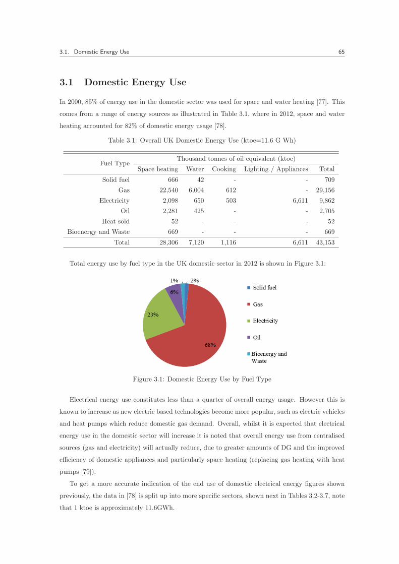
3.1. Domestic Energy Use 65
3.1 Domestic Energy Use
In 2000, 85% of energy use in the domestic sector was used for space and water heating [77]. This
comes from a range of energy sources as illustrated in Table 3.1, where in 2012, space and water
heating accounted for 82% of domestic energy usage [78].
Table 3.1: Overall UK Domestic Energy Use (ktoe=11.6 G Wh)
Fuel TypeThousand tonnes of oil equivalent (ktoe)
Space heating Water Cooking Lighting / Appliances Total
Solid fuel 666 42 - - 709
Gas 22,540 6,004 612 - 29,156
Electricity 2,098 650 503 6,611 9,862
Oil 2,281 425 - - 2,705
Heat sold 52 - - - 52
Bioenergy and Waste 669 - - - 669
Total 28,306 7,120 1,116 6,611 43,153
Total energy use by fuel type in the UK domestic sector in 2012 is shown in Figure 3.1:
Figure 3.1: Domestic Energy Use by Fuel Type
Electrical energy use constitutes less than a quarter of overall energy usage. However this is
known to increase as new electric based technologies become more popular, such as electric vehicles
and heat pumps which reduce domestic gas demand. Overall, whilst it is expected that electrical
energy use in the domestic sector will increase it is noted that overall energy use from centralised
sources (gas and electricity) will actually reduce, due to greater amounts of DG and the improved
efficiency of domestic appliances and particularly space heating (replacing gas heating with heat
pumps [79]).
To get a more accurate indication of the end use of domestic electrical energy figures shown
previously, the data in [78] is split up into more specific sectors, shown next in Tables 3.2-3.7, note
that 1 ktoe is approximately 11.6GWh.

3.1. Domestic Energy Use 66
Table 3.2: Domestic Lighting Energy
Device Energy Use (ktoe)
Standard Bulb 142
Halogen 594
Fluorescent Strip 105
Energy Saving 332
LED 9
Table 3.3: Domestic Cooling Goods Energy
Device Energy Use (ktoe)
Chest Freezer 108
Fridge-freezer 681
Refrigerator 166
Upright Freezer 214
Table 3.4: Domestic Washing Goods Energy
Device Energy Use (ktoe)
Washing Machine 394
Washer-dryer 209
Dishwasher 287
Tumble Dryer 406
Table 3.5: Domestic Electrical Goods Energy
Device Energy Use (ktoe)
TV 746
Set Top Box 364
DVD/VCR 155
Games Consoles 81
Power Supply Units 522
Table 3.6: Domestic ICT Goods Energy
Device Energy Use (ktoe)
Desktops 273
Laptops 128
Monitors 152
Printers 10
Multi-Function Device 24
Table 3.7: Domestic Cooking Goods Energy
Device Energy Use (ktoe)
Electric Oven 268
Electric Hob 270
Microwave 217
Kettle 386
From the data in Tables 3.2-3.7 we have the following split (see Figure 3.2) of electrical energy
consumption by usage sector.
Figure 3.2: Detailed domestic Electrical Energy Use by Sector [78]
The Centre for Renewable Energy Systems Technology (CREST) have used a list of common
domestic devices for generation of daily demand load profiles [49]. A report by Intertek [80] lists all

3.1. Domestic Energy Use 67
the electrical loads found in a monitoring scheme carried out across 251 houses, with an overview
of this report in [81]. Due to the great number distinct devices (115) in the Intertek report,
assessment of the effect of widened voltage tolerances will be limited to the groupings of the 31
devices in [49]. These is shown in Table 3.8 along with the grouping.
Table 3.8: Grouping of Loads IN CREST Profiler
Device Group Device Group
Standard Light Bulb L Set Top Box E
Halogen L DVD/VCR E
Fluorescent Strip Light L Games Consoles E
Energy Saving Bulb L Power Supply Units E
LED E HI-FI E
Chest Freezer* M, E Iron H
Fridge-Freezer* M, E Vacuum M
Refrigerator* M, E Telephone Cordless E
Upright Freezer* M, E Electric Oven** H
Washing Machine H/M, H/E Electric Hob** H
Washer-dryer ** H/M, H/E Microwave E
Dishwasher** H/M, H/E Kettle* H
Tumble Dryer H/M, H/E Water storage Heater* H
Desktops E Electric Water Heater H
Laptops E Electric Shower H
Monitors E Storage Heaters* H
Printers E Other Electric Heating* H
Multi-Function Devices E Heat Pumps* M, E
TV E
* Denotes thermal cycle loads
** Denotes possible thermal cycle loads
As stated, from an electrical perspective, working with devices by sector is not helpful; it is
of more use to class all of the loads in the home by their respective electrical characteristics. For
example, the electrical heating sector is comprised of either electrical storage heating devices, using
an electric element to heat up a large mass that maintains temperature thought out the day or
heat pumps that are like the cold products and comprise of a compressor and motor system.
With reference to the 4 electrical categories mentioned in the introduction, Appendix A groups
each product considered into one or more of these electrical categories of: Heating (H), Lighting
(L), Electronics (E), or Motors (M). In some cases classification is obvious, but for others it is
not so, for example, a washing machine could be listed as heating, motor, or an electronic supply
class of load. The actual classification in this case will ultimately depend upon how the motor is
connected to the supply. In older machines, and still many modern machines, the motor is a single
phase induction motor that is capacitor run. The speed control here is achieved by adjustment

3.2. Socialised Cost & Device Numbers 68
of pole number or mechanically. Alternatively, the machine may use a DC motor or AC motor
and a power electronic drive. Improved control and efficiency are advantages of this latter scheme
but they are costly and a relatively new development in this application. Still, both types should
be considered, especially as the average washing machine has a life expectancy of 16 years [77].
Continuing with the example of the washing machine, the water for the machine is usually heated
within the machine by an element so it can control water beyond limitations of the main hot water
supply. Hence, a washing machine can be electrically grouped as a heater and motor, heater and
electronic, or an electronic type load.
It is apparent that most of the devices listed in Appendix A, will have low voltage circuits
(control circuits). These, for reasons of practically, and use in LV simulations (ie. is their demand
relative to the whole good is small) will not be considered in detail.
3.2 Socialised Cost & Device Numbers
In 2012 there were 27.1 million houses in the UK and a population of 64.1 million; this means the
average house size is 2.36. To find out what types, and how many electrical products, are used in
the UK, figures from DECC [78] were assessed and are presented in this section.
This allows effects of de-regulation to be weighted with trends in the use of specific electrical
products. This is important for predicting the socialised costs of voltage deregulation, where simply
looking at device electrical characteristic does not give a wider picture of the social costs (i.e. if
certain classes of device would need replacement). Tables 3.9-3.14 presents the number of devices
owned in the domestic sector in the UK in 2012 [82].
Table 3.9: Domestic Ownership - Lighting
Device Amount (x1000)
Standard Bulb 78074
Halogen 262801
Fluorescent Strip 15603
Energy Saving 351786
LED 4574
Table 3.10: Domestic Ownership - Cooling
Device Amount (x1000)
Chest Freezer 4183
Fridge-freezer 18585
Refrigerator 10112
Upright Freezer 8382
Beyond the number of devices owned presently, future ownership trends must be taken into
account. As an example, filament lighting luminous output is known to be very sensitive to voltage
changes [83], so much so, that it could be considered a major barrier to voltage deregulation.
However the trend to change away from filament lighting (especially since 2008) to more efficient
fluorescent and LED alleviates this problem. The trend in ownership of lighting technologies since
1990 is illustrated in Figure 3.3.
If wider voltage tolerances were suddenly applied, given the effect on the luminosity of filament

3.2. Socialised Cost & Device Numbers 69
Table 3.11: Domestic Ownership - Washing
Device Amount (x1000)
Washing Machine 21577
Washer-dryer 4179
Dishwasher 10112
Tumble Dryer 12278
Table 3.12: Domestic Ownership - Electrical
Device Amount (x1000)
TV 63042
Set Top Box 34620
DVD/VCR 38070
Games Consoles 20963
Power Supply Units 199382
Table 3.13: Domestic Ownership - ICT
Device Amount (x1000)
Desktops 10547
Laptops 267224
Monitors 20414
Printers 8192
Multi-Function Device 17667
Table 3.14: Domestic Ownership - Cooking
Device Amount (x1000)
Electric Oven 17466
Electric Hob 12124
Microwave 23231
Kettle 26095
1990 1995 2000 2005 2010 2015Year
0
100
200
300
400
500
Number
Owned
(Millions)
Standard Light BulbHalogenFluorescent Strip LightingEnergy Saving Light BulbLED
Figure 3.3: Ownership of Lighting Products by Type in the UK domestic Sector
lighting is large, this would force an uptake of more efficient technologies that are less sensitive to
voltage change. However this obviously has a large social impact (i.e. effectively forcing people to
change lighting fixtures).
From Figure 3.4 we see there is a large trend towards more efficient (class A rated) cold devices
since 2004. In such devices, higher efficiency ratings are achieved by increasing the performance
of the insulation and /or replacing of single phase induction motors with adjustable speed drives
(ASD) and other types of AC or DC motors.
Sectors of recent growth in the domestic sector are those of ICT and consumer electronics.
These ownership patterns are shown in Figures 3.5 & 3.6 respectively.
Separate PSUs used for a variety of electronic devices now represent the most common electrical
load outside of lighting products in the house. Other electronic equipment and ICT products will
use a dedicated PSU. The advantage of separate PSU from a de-regulation point of view is that

3.2. Socialised Cost & Device Numbers 70
2004 2006 2008 2010 2012 2014Year
0
20
40
60
80
PercentageofGoods
RatedClass
AorHigher
Chest FreezerFridge freezerRefrigeratorUpright freezer
Figure 3.4: Ownership of Class A rated cold goods
1990 1995 2000 2005 2010 2015Year
0
10
20
30
Number
Owned
(Millions)
DesktopsLaptopsMonitorsPrintersMulti-Function Devices
Figure 3.5: Ownership of ICT Products by Type in the UK domestic Sector
1990 1995 2000 2005 2010 2015Year
0
50
100
150
200
250
Number
Owned
(Millions)
TVSet Top BoxDVD/VCRGames ConsolesPower Supply Units
Figure 3.6: Ownership of Consumer Electronic Products by Type in the UK domestic Sector
if performance were deemed unsatisfactory following voltage deregulation, it is cheap and easily
replaced by the end user. This is obviously not so true for the integrated PSUs common to the
majority of other products in the ICT and consumer electronics sectors.

3.3. Voltage Tolerance - Experimental and Simulation 71
3.3 Voltage Tolerance - Experimental and Simulation
To see how loads change with the supply voltage, and at what point malfunction or other key
changes to the device operation occur with wider supply voltages, simulation and lab testing were
carried out for some domestic loads.
� Motors
� PSU Magnetics
Although not exhaustive, these two load classes have somewhat more complex voltage sensitivity
characteristics than the two other load group class of heating and lighting.
3.3.1 Motors
The performance of any motor is tied to the load that it is driving. Broadly these mechanical
load types will have a torque - speed characteristic of either: constant power, constant torque, or
variable torque. These are presented for specific loads in Table 3.15.
Table 3.15: Load Torque Speed Relationships
Device Torque - Speed Loading
Conveyor Constant
Centrifugal pump Increases with speed squared
Fans Increases with speed squared
Screw Compressor Constant
Scroll Compressor Constant
Piston Compressor Constant
Winders Constant or decrease with speed
Mixers Increases with speed
Hoist Constant
Centrifuge Increases with speed squared
Relevant to the domestic environment are: mixers, centrifuges, hoists, fans, compressors. These
loads can be found when used in: food processors, washer dryers, lifts or stair lifts, air fans for
cooling/circulation, and fridge freezers / air conditioning, respectively.
Simulation of Motors
A single phase induction motor (SPIM) was simulated under steady state (SS) operation and
coupled to a model of a fridge that uses a constant torque type compressor and a temperature
control system using a hysteresis controller. This is shown in greater detail in Appendix D.

3.3. Voltage Tolerance - Experimental and Simulation 72
The speed of the motor when driving a constant torque load (here a fridge) with a varying
supply voltage is shown in Figure 3.7. Speed (and therefore power) is seen to remain almost
constant until the supply voltage falls to around 0.75 of nominal.
Start/Run Capcitor SPIM & Constant Toruqe Load
0.7 0.8 0.9 1 1.1 1.2 1.3 1.4 1.5Voltage (pu)
0
50
100
150
200
Speed(rad/s)
Figure 3.7: Speed of SPIM in a fridge with different Supply Voltages
The thermal control system for the fridge can be of varying complexity, in this model the control
system is a hysteresis controller. This control scheme turns the motor compressor on when a certain
air temperature is reached and turns it off once a new lower temperature has been reached.
0 0.2 0.4 0.6 0.8 1Time (hours)
0
2
4
6
8
10
Tem
p(◦C)
0.6pu
0.7pu
0.8pu
0.9pu
1.0pu
Figure 3.8: Fridge Temperature with Differing Supply Voltages
Figure 3.8 shows the temperature of the fridge when the supply voltage is reduced from 1.0pu to
0.6pu in steps of 0.1pu. At 0.6pu voltage (Figure 3.8) the motor is unable to produce the required
torque to start the compressor and the fridge will not work. At 0.7pu voltage the starting capacitor
remains permanently engaged as the motor never reaches cross over speed, here the cooling output
is insufficient to cool the fridge to desired temperatures.

3.3. Voltage Tolerance - Experimental and Simulation 73
Testing of Compressor Motor Systems
Single or quasi-dual phase motors are common in white goods (e.g. refrigeration and washing); the
load torque presented to the motor is the main difference between these goods from an electrical
perspective.
To verify simulation results (as in Figure 3.9 for a SPIM) and those in shown previously, lab
measurements on a fridge were taken.
0.4 0.5 0.6 0.7 0.8 0.9 1 1.1 1.2Voltage (pu)
0
100
200
300
Power
(W,VAr,Tω) Active
Reactive
Mechanical
Figure 3.9: PQ Demand for Fridge Simulated
The fridge was tested with a VARIAC supply and an AMTEK power quality meter. Voltage
range from the VARIAC was adjustable from 260V-0V. The motor was tested at various supply
voltages and given time to reach steady state. Over the voltage range of the VARIAC the power
and reactive power of the fridge was recorded and is shown in Figures 3.10 & 3.11:
0.4 0.5 0.6 0.7 0.8 0.9 1 1.1Voltage (pu)
0
50
100
150
200
Power
(W/Var)
Active
Reavtive
Figure 3.10: PQ Demand for Fridge Measured
Below 0.6 of nominal voltage the motor stalls, and the power drawn increases. However over
a wide voltage range (0.6-1.1) the motor operates largely as a constant power load. Once stalled,
if the voltage is restored (�0.6), the motor has a restart delay time where the power consumption

3.3. Voltage Tolerance - Experimental and Simulation 74
0.4 0.5 0.6 0.7 0.8 0.9 1 1.1Voltage (pu)
0
200
400
600
800
1000
Power
(W)
Active
Active (Stalled)
Figure 3.11: PQ Demand for Fridge Measured with Stalled & Normal Operation
rapidly increases. This is due to the back pressure in the compressor and time must pass before
the motor is able start again. This effect is shown in Figure 3.11 where the power drawn when the
motor has stalled and still unable to restart is clearly seen.
This type of effect is also seen with air conditioners that usually have a voltage stalling point
higher than the fridge tested. The effect can be that voltage recovery after a short voltage sag can
be delayed by these loads [84]. Wherever this type of stalled behaviour is possible, thermal relays
are included that trip if the current is too high following a stall condition for a given period, as
indeed was the case with the fridge tested.
3.3.2 Magnetics in Power Supplies
Design of a Flyback Transformer
Another class of common domestic appliances is electronics such as set top boxes and CD players,
which tend to use a flyback SMPS on the input following the rectification stage.
Figure 3.12: Topology of Flyback Converter
The flyback converter is an isolated dc-dc converter commonly used in domestic goods upto

3.3. Voltage Tolerance - Experimental and Simulation 75
100W the output can be higher or lower than the input and is:
VoutVin
� n�D
1�D(3.1)
where D is the duty ratio.
Here, a flyback converter is designed to produce a constant output voltage when supplied from
a 230V (-6, +10%) rectified AC source with negligible voltage ripple across the output capacitor in
the rectifier. Ideally this is equivalent to a 194.6V DC supply at the input of the flyback when the
supply voltage is at its minimum specified value. The flyback should produce 48V and operate at
the discontinuous current boundary (DCB) when supplying its rated power of 100W at its minimum
supply voltage 194.6V . The switching frequency of the flyback is set by the controller’s oscillator
to 100 kHz. A duty cycle of 50% at DCB is also specified and here the flyback is assumed 90%
efficient. These specification are summarised in 3.16 and enable design of the flyback’s transformer.
Table 3.16: Flyback Converter Specification
Parameter Value Parameter Value
�Vin 194.6 Vo 48 V
�Vin 205 Po 100W
fsw 100 kHz Io 2.083 A
η 90% Dmax 0.5
Results of the initial design stage of the flyback are shown in Table 3.17.
Table 3.17: Basic Values for Flyback
Parameter Value Parameter Value
�Iin 0.571 A Ip,rms 0.93 A
Pin 111.1 W L1 426H
Rin 340.81 L2 27 H
Ip 2.28 A N1:N2 (n) 3.97
Vdiode 1V
From the initial specification the magnetic design can now proceed; the design is based upon
the design principles laid out in Magnetics Design Handbook [85]. The energy storage (E) in the
primary inductor is:
E �I2pL1
2(3.2)
The electric constant (Ke) is given at a peak saturation flux density (Bm), which in the case

3.3. Voltage Tolerance - Experimental and Simulation 76
of ferrite cores is set to be 0.25T. Giving:
Ke � 0.145�10�4PoB2m (3.3)
Now the core geometry constant (Kg) is found with:
Kg �E2
Keα(3.4)
A window utilisation factor (Ku) of just 0.29 is appropriate for high frequency SMPS flyback
transformers as shown in the literature [85]. The magnetic core is defined with:
Ap �WaAc (3.5)
Where Ap is the area product which is defined as the product of the winding window area (Wa)
and the cross section area of the core (Ac). The magnetic design parameters are shown in Table
3.18.
Table 3.18: Values for Magnetic Components in the Flyback
Parameter Value
E 1.11 mJ
Ke 1.3� 10�4
Kg 1.27� 10�2
From this an EDF-25 type core with 3C85 grade ferrite is selected using the required value of
Kg calculated previously. This is the point in design where the magnetics would be chosen to be
overrated or not. In this example the core is chosen to be the smallest available standard size EDF
type core with a Kg greater than required. EDF type cores have a low profile that is popular
where space savings are given a high priority and where space saving is facilitated by using a core
with a low profile.
Table 3.19: Parameters of an EDF-25 core with 3C85 Material
Parameter Value Parameter Value
MLP 5.7 cm Area Product �Ap� 0.394 cm4
Core Weight �Wtfe� 16 g Core Geometry �Kg� 0.019 cm5
Copper Weight �Wtcu� 11.5 g Surface Area �At� 21.6 cm2
MLT 4.8 cm Core Permeability 2500
Iron Area �Ac� 0.58 cm2 Winding Length �Lw� 1.86 cm
Window Area �Wa� 0.679 cm2
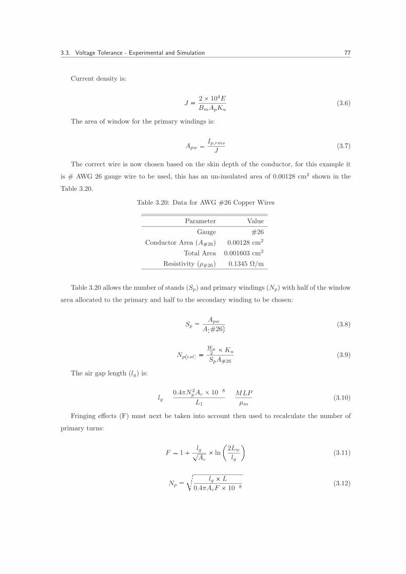
3.3. Voltage Tolerance - Experimental and Simulation 77
Current density is:
J � 2� 104E
BmApKu(3.6)
The area of window for the primary windings is:
Apw � Ip,rms
J(3.7)
The correct wire is now chosen based on the skin depth of the conductor, for this example it
is # AWG 26 gauge wire to be used, this has an un-insulated area of 0.00128 cm2 shown in the
Table 3.20.
Table 3.20: Data for AWG #26 Copper Wires
Parameter Value
Gauge #26
Conductor Area (A#26) 0.00128 cm2
Total Area 0.001603 cm2
Resistivity (ρ#26) 0.1345 Ω/m
Table 3.20 allows the number of stands (Sp) and primary windings (Np) with half of the window
area allocated to the primary and half to the secondary winding to be chosen:
Sp � Apw
A�#26� (3.8)
Np�est� �Wa
2 �Ku
SpA#26(3.9)
The air gap length (lg) is:
lg �0.4πN2
pAc � 10�8
L1� MLP
μm(3.10)
Fringing effects (F) must next be taken into account then used to recalculate the number of
primary turns:
F � 1� lg�Ac
� ln
�2Lw
lg
�(3.11)
Np ��
lg � L
0.4πAcF � 10�8(3.12)

3.3. Voltage Tolerance - Experimental and Simulation 78
The peak flux (Bpk) density and AC flux (Bac) is:
Bpk �0.4πNpFIp � 10�4
lg �MPLm(3.13)
Bac �Bpk
2(3.14)
The secondary turns are calculated assuming DCB operation:
Ns �Np�Vo � Vd�Doff
VpD(3.15)
Choice of secondary winding values and window utilisation (Ku) are shown in Table 3.21.
Using the above design process the final design parameters are shown in Table 3.21.
Table 3.21: Parameters and Design Choices for Magnetic Components of a Flyback
Parameter Value Parameter Value
J 648.6 A/cm2 Bac 0.142
Apw 0.0014 cm2 Ns 15.9(16)
SP 1.123 (1) Is 8.332 A
Np�est� 76.9 (77) Is�rms� 3.402 A
lg 0.078 cm Asw 0.0052 cm2
F 1.5 Ss 4.1(4)
Np 62.7(63) Ku 0.239
Bpk 0.262
Winding losses (Pcu) and regulation (α) then calculated as given in Table 3.22. The core losses
(Pcore) and total losses (Pt) for 3C85 material, using 3 given constants are calculated:
Pcore�kg� � 4.85� f1.63sw �B2.62ac (3.16)
Pcore �Pcore�kg�Wtfe
1000(3.17)
Pt � Pcu � Pcore (3.18)
Finally, the loss density (φ) and resultant core temperature rise (Tr) are found:
ψ �Pt
At(3.19)

3.3. Voltage Tolerance - Experimental and Simulation 79
Tr � 450 ψ0.826 (3.20)
Table 3.22: Losses Incurred in the Magnetic Components of a Flyback
Parameter Value Parameter Value
ρp 0.135 Ω/m α 0.68%
ρs 0.034 Ω/m Pcore�kg� 33.5 W/kg
Rp 0.407 Ω Pcore 0.536 W
Rs 0.026 Ω Pt 1.214 W
Pp 0.379 W ψ 0.056 W/cm2
Ps 0.299 W Tr 41.7 �C
Pcu 0.678 W
To see the effect of wider voltage tolerances, the magnetic design is kept the same but the
regulatory minimum voltage is reduced from 0.94pu of the nominal voltage to 0.85pu of the nominal
voltage; or 176V DC at the input to the flyback. The duty ratio must also be adjusted to regulate
the output voltage that is proportional to the input voltage in continuous current mode (CCM),
here needing a new duty of 52.5%, the flyback will also have entered CCM.
The energy storage in the inductor that is released to the load must be kept constant as the
output voltage is regulated and the load had been represented by a resistance. Meaning the power
and consequently energy that is released by the inductor must remain the same each cycle. As the
voltage has fallen by 9.57% and the duty cycle has been raised by 5.02% the current build up in
the inductor during the on period is now 95% of its previous value. From:
E �1
2LI2 (3.21)
For the energy to remain constant the peak current (I) must increase to a higher value which
means the minimum current (I) must become greater than zero i.e. the flyback enters CCM.
E �1
2L�I2 � I2� (3.22)
The new value of ΔI (defined as: I � I )is found using the duty, and supply voltage. The
energy (E) must stay constant, so the new value of I is found by:
I2DCB�E (3.23)
I2 � I2 � I2DCB (3.24)

3.3. Voltage Tolerance - Experimental and Simulation 80
I � I � ΔI (3.25)
I2 � 2I I � I2 � ΔI2 (3.26)
With simultaneous equations:
I �ΔI2 � I2DCB
�2ΔI(3.27)
This allows the minimum current to be found analytically. For operation of the flyback at
reduced supply voltage (-15% of nominal) the operation parameters are shown in Table 3.23 fol-
lowing.
Table 3.23: Values of Flyback Operating with Reduced Supply Voltage
Parameter Value Parameter Value
�Vin 175.95 V ΔI 1.953 A
Dmax 0.525 I 2.056 A
Ton 5.25 s I 0.106 A
E 0.1 mJ Ip,rms 0.884 A
The winding losses have now increased, as has the peak flux and consequently peak energy
storage in the inductor (which is indicative of inductor size) but the AC losses in the core are
reduced (�ΔI).The overall losses in the transformer of this particular design with reduced voltage
are decreased; these losses are shown in Figure 3.13.
0.45 0.5 0.55 0.6 0.65 0.7 0.75 0.8 0.85 0.9Voltage (pu)
0
0.5
1
1.5
Losses
(W)
Core
Copper
Total
Figure 3.13: Losses in Flyback Transformer
From Figure 3.13, when the flyback is in CCM (i.e. below 0.94 pu), as the core losses are a
function of the AC flux component, at lower supply voltages this AC flux reduces, accordingly
the core losses also reduce. The winding losses increase as the RMS current flowing though each

3.3. Voltage Tolerance - Experimental and Simulation 81
winding increases. The peak energy storage and the peak flux density increase as the supply
voltage is lowered. If the specific flyback in section this had to be rated for worldwide operation
(110-240V) then the magnetic design would need to be changed.
0.45 0.5 0.55 0.6 0.65 0.7 0.75 0.8 0.85 0.9Voltage (pu)
0.23
0.24
0.25
0.26
0.27
0.28
PeakFluxDensity
(T)
Figure 3.14: Peak Flux Density of Flyback Transformer
The peak flux is shown in Figure 3.14 above. From comparison of Figures 3.13 & 3.14 it is seen
that the core in this particular design will be limited by saturation (peak flux above 0.25T) when
the supply voltage falls below 0.67pu of nominal. It will not be limited by temperature rise from
losses that are seen to remain reasonably constant over a wide input voltage range.
The previous magnetic design is valid for CCM (or DCB) flyback converters. Initially, this was
the case (0.94pu), after the magnetic design is completed; the design can then be applied to DCM
operation (higher voltage or lower load).
Design of Filter Inductor for PFC Boost Converter
A similar magnetic design approach to that outlined in previously is followed for a PFC boost
converter and relevant inductor. The PFC boost converter was originally specified to operate with
a voltage supply down to 0.94 of nominal.
Figure 3.15: Topology of Boost Converter
Unlike the flyback convert the output voltage is not isolated from the input and as the name
implies the boost converter is not able to step down the output voltage. The output voltage (Vout)

3.3. Voltage Tolerance - Experimental and Simulation 82
is:
VoutVin
� �
1
1�D(3.28)
where D is the duty ratio.
Losses in the inductor when the boost converter operates with a supply voltage of 0.94pu and
with an output ripple current of 20% of the peak current are dominated by the copper losses. This
is due to the AC flux swing being small and consequently the core losses are negligible compared to
the copper loss. The copper losses are shown against the supply voltage in Figure 3.16. As voltage
is reduced the peak flux again increases and the flux ripple consequently decreases yet further,
meaning the core losses reduce from what was already a negligible value compared to the copper
losses. As the peak flux has increased the peak current and therefore copper losses have increased.
This is visible in Figure 3.16 where only the copper losses are shown due to their dominance in the
total losses on the inductor.
0.45 0.5 0.55 0.6 0.65 0.7 0.75 0.8 0.85 0.9Voltage (pu)
0
2.5
5
7.5
10
Losses
(W)
0
0.2
0.4
0.6
0.8
FluxDensity
(T)Losses
Flux
Figure 3.16: Copper Losses & Peak Flux Density in the Inductor of a Boost Converter for PFCwith varied supply voltage
The peak flux in the core is shown in Figure 3.16 where, due to the design procedure followed
here, a standard sized core almost exactly suited for operation at 0.94pu supply voltage was
available, and chosen, hence flux rises above the saturation value (0.25T) with only slightly reduced
supply voltages. This is indicative of a core that was very tightly designed to a specific voltage
supply band and with the core as small as possible, so to reduce manufacturing costs.
Losses from the windings and saturation of the magnetic core will be limiting factors in this
boost PFC inductor. There will be reduced losses and peak flux in the filter inductor when operated
with higher supply voltages.

3.4. Voltage Tolerance - Literature 83
3.4 Voltage Tolerance - Literature
As the results presented in section are based on the equations that are commonly used to describe
the voltage sensitivity of a load, namely the ZIP parameter based equations ((2.52) & (2.53)), and
the exponential form equations ((2.56) & (2.57)), are repeated here for clarity:
Pm � Pnom �
�Zp
�VmVnom
�2
� IpVmVnom
� Pp
�
Qm � Qnom �
�Zq
�VmVnom
�2
� IqVmVnom
� Pq
�
Pm � Pnom �
�VmVnom
�np
Qm � Qnom �
�VmVnom
�nq
The work literature review herein presents values for the ZIP parameters (Zp, Ip, Pp, Zq, Iq, Iq)
and the powers (np, nq) found in the literature, then curve fitted representative results for all the
works are given.
Static Voltage Sensitivity Studies
Reference [86] presented a general model for power system stability studies, as well as sensitivity
ratings for frequency dependence of loads. Exponential form values of voltage dependence are
shown in Table 3.24.
Table 3.24: Sensitivity Results from [86]
Device np nq
Incandescent lamp 1.6 0
Fluorescent lamp 1.2 3
Heating 2 0
Induction motor, half load 0.2 1.5
Induction motor, full load 0.1 2.8
Electric heating systems behave as a constant impedance, as would be expected, and the in-
duction motor is mostly sensitive in reactive power to voltage changes. The difference between
traditional filament lighting and florescent lighting is also shown, where florescent lighting has
considerable reactive power sensitivity.
Reference [87] was also a complete look at lighting, heating and motor systems. Results from lab

3.4. Voltage Tolerance - Literature 84
tests on different lighting technologies and on-site tests of street lighting were compared. Response
of thermally controlled heating systems to voltage change was investigated as were refrigerators.
Lighting results from this report are presented in Table 3.25 below. The turn off voltage of the
different lighting technologies was also recorded, and is shown.
Table 3.25: Sensitivity Results from [87]
Device Voff Poff np nq
Incandescent Light - - 1.5-1.6 -
Fluorescent lamp (72 W) 160 30 2.0-2.2 4.56.5
Mercury lamp (250 W) 180 165 2.2-2.4 4.0-6.0
High pressure sodium lamp (250 W) 180 180 2.1-2.5 -
Low pressure sodium lamp (91 W) 80 60 0.3-0.5 -
Low-energy lamp (11 W) 60 2.6 0.8-1.2 1.0-1.5
The lighting most applicable to domestic setting are: incandescent, florescent, and low energy
(CFL). Of these, the fluorescent light was the first to turn off when voltage was reduced below
0.7pu of the nominal supply voltage.
In Table 3.25, results are seen to differ for the two fluorescent lights, as the low energy light
used an electronic ballast whist the florescent light an inductive ballast.
In the temperature controlled heating system, the power after a 20% reduction in supply voltage
was recorded. The plots in Figure 3.17 show the load power after this supply voltage reduction
for both electronic, and bi-metallic thermostats, with the mean power recorded over a period
appropriate to the thermal cycle time for a house.
(a) Electronic Thermostat (b) Bi-metallic thermostat
Figure 3.17: Heating Element Power in Response to Step Voltage Change [87]
The bi-metallic switch thermostat system actually consumes more power after the reduction in
supply voltage. In both cases the peak measured power will be lower after the voltage reduction

3.4. Voltage Tolerance - Literature 85
as Table 3.24 had shown heating to have constant impedance voltage sensitivity; it is instead the
increased duty cycle that increased the longer term power drawn.
Tests were carried out on some common domestic loads, two fridges in [87] were tested for their
voltage sensitivity, with these results as shown in Table 3.26.
Table 3.26: Sensitivity Results from [87]
Device np nq
Refrigerator A 1.3-1.6 3.1-3.3
Refrigerator B 1.3-1.8 2.8-3.2
Both fridges were seen to stall at 0.6pu supply voltage, whereupon the current increased sub-
stantially. Like the induction motors measured in [86] from Table 3.26, it is seen there is a greater
voltage sensitivity of the reactive power than that of the active power. However, unlike before
there is substantial active power sensitivity; this may be due to the type of compressors used in
the fridges in these tests or the range of voltages used in the authors curve fitting process.
A report in 2010 [84] presents voltage sensitivity results for typical loads in domestic and
residential settings. Tests on electronic ballast florescent lighting (Lights A & B), and CFLs (now
the most common form of lighting in the UK [78]) and two PCs were conducted.
Power and minimum supply voltage results are shown in Table 3.27, as are voltage sensitivity
figures for the two lights in Table 3.28.
Table 3.27: Sensitivity Results from [84]
Device Power (W) Reactive (VAr) Power Factor Voff (pu) Von (pu)
Light A 56.3 -33 0.86 0.1 0.14
Light B 61.3 -23.8 0.93 0.1 0.39
CFL A 22.2 -12.4 0.87 0.2 0.25
CFL B 26.1 -13.7 0.88 0.2 0.25
PC w/ LCD 152 -14.4 0.99 04-0.5 0.53-0.65
PC w/ CRT 225 -17.4 0.99 0.4-0.5 0.54-0.67
Table 3.28: Sensitivity Results from [84]
S0 Vmin Power (P) Reactive Power (Q)
Device (VA) (pu) Z I P Z I P
Light A 56.3 0.1 0.27 0.79 -0.05 -0.37 1.37 0
Light B 61.3 0.1 -0.13 1.2 -0.07 -0.73 1.72 0
The lights are able to operate down to low voltages without extinguishing, and for the two
fluorescent lights tested present a load that is mostly constant current type (see Table 3.28), with
a greater voltage sensitivity in reactive power.

3.4. Voltage Tolerance - Literature 86
For the PCs both devices behaved as constant power loads until the minimum voltage, which
was at or below half of the nominal value. Turn on following these occurrences was notably higher,
with the CRT PC seen not to turn back on until voltage returned to 0.67 of nominal.
In [3] domestic loads were analysed for their static voltage sensitivity parameters, which were
then used in distribution networks models chosen to represent networks across the US; as was also
done in [88]. Results showed conservative voltage reduction (CVR) an effective method to reduce
the energy consumption and reduce peak demand in all but 2 of the 25 feeders tested.
A comprehensive report [89] on air conditioning units (ACU) was carried out in 2006 by South-
ern California Edison. Performance of the air conditioners was measured and the performance of
the motor in response to voltage change tested. Continuing this work [90] presented methods for
load modelling where large amounts of ACU are present, and its importance in system stability
studies. Delayed voltage recovery (DVR) was the finding from these works, and methods to accu-
rately model this issue were presented. The main cause of this delayed voltage recovery is stalled
single phase induction motors with constant torque loads that are prone to stalling (due to low
inertia). In [89] the final recommendation is that contactors be set to remove these motor systems
(i.e. ACUs) from the network when the voltage falls below the maximum stalling voltage of the
motors tested. A value of 0.78pu voltage is given in the paper. Though it might be thought this
work is of limited relevance to LV systems in the UK, if in the future more HP were installed in the
UK, due to the similarities of HP and ACU (high power constant torque compressor systems with
low inertias) this type of study would need to be considered, especially if wider voltage tolerances
were also introduced.
Reference [91] tested 13 types of load with a total of 55 distinct devices tested. For smaller
lighting loads multiples of the same device were connected to make a 15A load at nominal voltage.
Results were gathered for voltage sensitivity and using equations (2.52) and (2.53). The minimum
supply voltage prior to device failure was also recorded. These results are shown in Table 3.29.
The magnetic ballast fluorescent lighting and microwave are the two domestic products found
to be most sensitive to voltage (with regards to their correct functioning), with both failing at
0.83 of nominal voltage. All other devices tested continued to work down to, or below, 0.8 of the
nominal voltage.
Voltage sensitivity of common loads was also investigated in [92]. This testing was performed
with slow voltage magnitude ramps and with separate tests using voltage magnitude oscillation
and step changes. Results were not initially constrained with (2.54) and (2.55). Results from this
work are shown in Table 3.30.

3.4. Voltage Tolerance - Literature 87
Table 3.29: Sensitivity Results from [91]
Device Snom VminActive Reactive
Z I P Z I P
Dryer Heater 5400 0.5 0.96 0.05 -0.01 0 0 0
Dryer Motor 515 0.5 1.91 -2.23 1.32 2.51 -2.34 0.83
Washing Machine 654 0.5 0.05 0.31 0.64 -0.56 2.2 -0.64
AFD 1 1800 0.75 0.43 0.61 -0.04 -1.21 3.47 -1.26
AFD 2 1780 0.75 3.19 -3.84 1.65 1.09 -0.18 0.09
Heatpump 1 (capacitor) 1160 0.75 0.72 -0.98 1.26 14.78 -23.72 9.94
Heatpump 2 (blower) 575 0.87 5.46 -14.21 9.75 -14.85 31.59 -15.74
Heatpump 2 (compressor) 5700 0.87 0.84 -1.4 1.56 22.92 -40.39 18.47
Fridge Freezer 1030 0.76 1.19 -0.26 0.07 0.59 0.65 -0.24
Battery Charger 6430 0.61 3.51 -3.94 1.43 5.8 -7.26 2.46
CFL 1 (electronic) 60 0.5 0.14 0.77 0.09 -0.06 -0.34 -0.6
CFL 2 (electronic) 53 0.5 0.16 0.79 0.05 0.18 -0.83 -0.35
CFL (magnetic) 151 0.83 0.34 1.31 -0.65 3.03 -2.89 0.86
FL 1 (electronic) 1335 0.65 -2.48 5.46 -1.98 0 0 0
FL 2 (electronic) 1172 0.54 -1.6 3.58 -0.98 0.79 -0.16 0.37
Electronic Dimmer 62 0.63 -0.16 1.77 -0.61 0 0 0
FL Dimmer 157 0.78 -0.48 1.89 -0.41 12.21 -18.38 7.17
High Pressure Na Light 341 0.73 0.98 -0.03 0.05 29.84 -45.26 16.42
Office Equipment 1 1020 0.67 0.34 -0.32 0.98 0 0 0
Office Equipment 2 800 0.67 0.08 0.07 0.85 0 0 0
Microwave Oven 1361 0.83 -2.78 6.06 -2.28 0 0 0
Blower / Heater 1350 0.5 0.98 0.02 0 0.69 0.25 0.06
Baseboard Heater 1200 0 1 0 0 0 0 0
Voltage Sag Studies
Voltage sag is a short term dip in voltage, often caused by transient events such as the starting of
large motors. There is a large body of work that has investigated how domestic loads are affected
by these events. Although it is clearly different from permanent voltage tests, insight can still be
gained from these tests.
Work in the literature looking at the sensitivity of ASDs or variable frequency drives (VFDs)
to voltage sags was performed in [93]. Programmable three phase supplies were used to supply
an induction machine driving a constant torque type load at rated machine power. Results from
balanced 3 phase voltage sag tests are presented in Figure 3.18a.
Unlike the static voltage tests, voltage sag tests take account of both the duration of the applied
sag and the depth of sag. The above Figure (3.18a) shows the normal operational area, shown
above and to the left of the curves. There is a wide variation among the 5 ASDs tested with
a drop-out voltage range from 0.73 to 0.9 of the nominal voltage. For equating these to static

3.4. Voltage Tolerance - Literature 88
Table 3.30: Sensitivity Results from [92]
DeviceS0 Vmin Active Power (P) Reactive Power (Q)
(VA) (pu) Z I P Z I P
Dishwasher 600 0 0.99 0 0 0 0 0
Dryer 4900 0.56 1.02 0 0 0.1 0 0
Oven 3050 0 0.99 0 0 0 0 0
Range Cooker 4100 0 0.97 0 0 0 0 0
FAN 187 0 0.45 0.57 -0.04 -0.03 0.34 -0.02
Halogen 100 0 0.66 0.39 0 0 0 0
Incandescent 100 0 0.64 0.4 0 0 0 0
CFL 19 19 0.14 -0.42 1.5 -0.06 0.66 -1.16 0.06
CFL 23 23 0.23 -0.28 1.35 -0.05 0.58 -1.11 0.05
CFL 20 18 0.17 -0.3 1.36 -0.05 0.6 -1.08 0.04
Fluorescent 32W 56 0.12 0.35 0.72 -0.04 0.28 -0.9 0.03
Fluorescent 40W 50 0.1 0.34 0.71 -0.03 0.2 -0.76 0.02
CRT 120 0.6 0 0 1 0 0 0.15
LCD 120 0.6 0 0 1 0 0 0.15
Clothes Washer 120N.A
Refrigerator 120
(a) Sensitivity of ASD [93] (b) Sensitivity of PC’s [94]
Figure 3.18: Voltage Sag Results from [93] & [94]
performance characteristics in 5.1, the maximum length of time recorded should be considered the
most accurate, which in the above case is 500ms.
In [94] the effect of voltage sag upon personal computers was tested, where the PCs were also
monitored for hard disk read / write lock-up or OS lock-up as well as monitoring that the device
was still powered. None of the PC failed this testing with a supply voltage greater than 65% of
the nominal voltage, for sag durations up to 500ms.
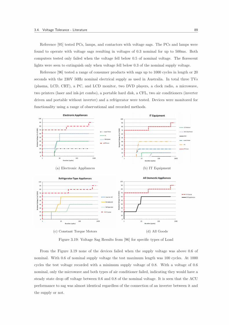
3.4. Voltage Tolerance - Literature 89
Reference [95] tested PCs, lamps, and contactors with voltage sags. The PCs and lamps were
found to operate with voltage sags resulting in voltages of 0.3 nominal for up to 500ms. Both
computers tested only failed when the voltage fell below 0.5 of nominal voltage. The florescent
lights were seen to extinguish only when voltage fell below 0.3 of the nominal supply voltage.
Reference [96] tested a range of consumer products with sags up to 1000 cycles in length or 20
seconds with the 230V 50Hz nominal electrical supply as used in Australia. In total three TVs
(plasma, LCD, CRT), a PC, and LCD monitor, two DVD players, a clock radio, a microwave,
two printers (laser and ink-jet combo), a portable hard disk, a CFL, two air conditioners (inverter
driven and portable without inverter) and a refrigerator were tested. Devices were monitored for
functionality using a range of observational and recorded methods.
(a) Electronic Appliances (b) IT Equipment
(c) Constant Torque Motors (d) All Goods
Figure 3.19: Voltage Sag Results from [96] for specific types of Load
From the Figure 3.19 none of the devices failed when the supply voltage was above 0.6 of
nominal. With 0.6 of nominal supply voltage the test maximum length was 100 cycles. At 1000
cycles the test voltage recorded with a minimum supply voltage of 0.8. With a voltage of 0.6
nominal, only the microwave and both types of air conditioner failed, indicating they would have a
steady state drop off voltage between 0.6 and 0.8 of the nominal voltage. It is seen that the ACU
performance to sag was almost identical regardless of the connection of an inverter between it and
the supply or not.

3.4. Voltage Tolerance - Literature 90
Results from the minimum working voltage of the loads in these studies [93–96] and shown in
Table 3.31:
Table 3.31: Collected Results from Voltage Sag Results
Device Vmin (pu) Time (s) Device Vmin (pu) Time (s)
ASD 1 0.73 0.5 PC 6 0.58 0.5
ASD 2 0.78 0.5 Laser Printer 0.2 20
ASD 3 0.77 0.5 PC 0.4 20
ASD 4 0.9 0.5 Microwave � 0.80 20
ASD 5 0.91 0.5 All in one (MFD) 0.1 20
PC 1 0.47 0.5 External HDD � 0.1 20
PC 2 0.63 0.5 Inverter ACU � 0.80 20
PC 3 0.62 0.5 Portable ACU � 0.80 20
PC 4 0.59 0.5 Refrigerator 0.4 20
PC 5 0.6 0.5
The high drop out voltage Vmin of the ASD 4 & 5 is due to its industrial design and three
phase protection circuitry where contactors open, these devices are however not common (nor are
three phase supplies) in domestic use.
Overview of Findings from the Literature
Regarding the operational voltage range of devices, the literature [86–91] suggests there are few
devices that will malfunction with a voltage down to 80% of nominal (exceptions are two of the
3 phase ADS tested in [93] that tripped with 90% of nominal supply voltage, a microwave and a
magnetically ballasted CFL at tripped with 83% of the nominal supply voltage). All of the other
devices continued to function at 80% of the nominal supply voltage, with many operating down to
much lower than rated voltage. At the recommended minimum voltage (0.85pu) [38], 2 out of the 5
three-phase ASDs failed. However these loads are not common in domestic settings so the impact
on domestic customers of this proposed lower voltage band (0.85pu) can be concluded small.
Regarding the voltage sensitivity of devices, from the literature it has been show how the load
responds to a change in voltage; that is how its P and Q characteristics are described following
changes to the nominal supply voltage. Different methods for presenting these characteristics are
used, and as these results inevitably use a form of curve fitting, the processes of curve fitting
applied to the measured results will also affect the curve fitted results.
The IEEE documents on this subject are found in [97–99] from the IEEE transactions on power
systems released between 1993-1995. In [97] a bibliography referencing an additional 118 academic
papers with results and findings similar to those mentioned previously, are presented. Suggested
methods for representing different areas load composition in simulation studies for load flow and

3.5. Summary of Voltage Tolerates of Domestic Loads 91
stability studies are presented in [98]. Reference [99] lists the IEEE standards that should be used
when modelling loads in power systems simulations. These standards state that IM should usually
be modelled so to include transients; though a static representation can be used depending on
the type of network analysis being carried out. Results will be unsatisfactory if using a static
representation of the IM in transient network studies.
3.5 Summary of Voltage Tolerates of Domestic Loads
Using all of the relevant simulation, experimental and literature review based results, a list was
produced so it can be applied to the CREST load model simulator [49], as is further described in
2.3. The averaged results for the ZIP parameters is presented below in Table 3.32, using a least
squared fits for a range of equipment, in total 55 devices, are given in Table 3.32.
Table 3.32: Averaged PQ Sensitivity Results for Domestic Loads
DeviceVmin Power Reactive Power
(pu) Z I P Z I P
Incandescent - 0.53 0.51 -0.05 0 0 0
Halogen - 0.63 0.37 0 0 0 0
CFL 0.29 -0.11 1.1 0 -0.67 1.58 0.09
FL 0.39 -0.35 1.86 -0.51 1.86 -1.88 1.02
Heating - 1 0 0 0 0 0
Motor (CT) 0.59 0.58 -0.2 0.62 1.7 -1.19 0.49
Motor (FAN) 0.6 0.96 -0.89 0.94 1.2 -0.58 0.38
Motor (ASD) 0.77 1.81 -1.62 0.8 -0.06 1.65 -0.59
E Supply (PFC) 0.54 0 0 1 0 0 0
E Supply 0.54 -0.07 0.27 0.8 1.3 -1.85 1.54
Minimum voltages are taken as an average of all collected results. The surprising results come
from the ASD motors, where the voltage sensitivity was found to be a constant impedance type
load and with a relativity high minimum supply voltage (0.77pu). A constant volts per hertz (V/f)
ASD control scheme will lower the speed of a motor (ω) in order to maintain rated toque (T ) if
the DC bus voltage falls, hence without an active front end the supply voltage will be directly
proportional to the mechanical output power (Pmech � Tω). However even this does not fully
explain the PQ sensitivity, this may be due to undervotlage protections schemes implemented
within the controller itself.
Overall, assessing results from [86–95, 100, 101] shows of the 63 domestic devices tested, and
where the minimum operating voltage was recorded (neglecting the ASDs). Only three loads
(microwave, magnetic ballast CFL, and heat pump) failed to operate with a supply voltage of 0.8
nominal. With 0.85 nominal supply voltages only one heat pump didn’t operate. This gives a

3.5. Summary of Voltage Tolerates of Domestic Loads 92
good indication the vast majority (above 98%) of domestic loads in the UK will operate with the
recommended minimum voltage of 0.85pu nominal voltage.
As LV networks are often voltage constrained by voltage regulatory levels by simply to removing
or relaxing these tolerances capacity can be increased.
This voltage tolerance, and its ability to provide increased capacity to the LV network, is
also crucially dependant of the voltage at the secondary of the LV transformer. As such, this
voltage band needs be applied in conjunction with voltage settings on the secondary side of the
LV transformer. This still allows flexibility to the DNOs, given the range of these new voltage
tolerances is sufficiently wide to allow for a range of voltages on the transformer secondary. As
the maximum voltage is unchanged from current levels the existing practice commonly employed
by DNOs of boosting the secondary side to near its regulatory maximum should not be continued,
as this will limit the amount of DG that can be incorporated. The lowering of the minimum
permissible voltage on the system has in effect removed the need for the DNOs to do this anyhow.
The primary barrier to increased voltage tolerances is how the loads connected to the LV
network will respond to these new voltage levels. Looking at domestic loads it is shown in this
chapter, by using results from the literature and results presented within, that domestic products
exhibit a greater operational sensitivity to elevated voltage levels than they do with reduced voltage
levels. Within the voltage bounds recommended, the loads are shown to function without failure
or malfunction across this new voltage band in over 98% of the cases shown. The power demand
characteristics of each load type are also assessed and aggregated from a range of sources in the
literature. This allows load flow studies to genuinely show how much new load can be added to a
deregulated LV network.
Given all the above, it can be stated that widening of voltage tolerances along with careful
selection of secondary substation transformer tap setting has the ability to increase the capacity
for loading and generation within the LV network. The network capacity limitations now being
tied to thermal limits of the networks components (e.g. UG cables, transformers). If yet further
network capacity was required, then elevated AC distribution schemes might be considered. How-
ever, results presented show that even slightly elevated AC would be problematic and potentially
damaging to consumer products.Hence widespread proliferation of point of load regulation devices
would be needed to ensure the loads operate as normal.
Thus the final suggested voltage range, whereby the upper limit is maintained at 1.1 pu to avoid
damage to loads, and the lower voltage limit of 0.85 pu has been chosen to maintain the correct op-
eration of the great majority of domestic loads, has been justified via experimentation, simulation,
and a literature review. Crucially, these changed could be implemented without disruption to the
distribution network or significant expenditure, whist still increasing hosting capacity of LCTs.

Chapter 4
Methods of Analysis in LV
Networks
In this chapter the methods used for the analysis of LV networks are presented. The methodology
outlined is subsequently used in achieving the results presented in Chapters 5 and 6.
Initially, in section 4.1, types of load flow that are suited to LV simulation are presented and
briefly reviewed. Then in section 4.2, an overview of all the test networks for which results are
later presented is given, along with network topology metrics that are useful in aiding to predict
network performance characteristics, for example indicating most likely network constraints. Next
in section 4.3, a Monte Carlo procedure for statically assessing a given network topology under a
range of conditions is presented. The Monte Carlo based approach to analysis of LV networks is
popular in the literature [102–105] as the operating conditions of a LV network (eg. loading) at a
particular time are not deterministic. Finally some of the values and assumptions used in assessing
the financial benefits of increasing hosting capacity are presented.
4.1 Load Flow
The load flow studies are preformed in Matlab Simulink using the SimPowerSystems library, and
with load flow functions written with MATLAB. This software is built upon easily handling matrix
maths operations and is high level interpreted language which allows rapid deployment of code
without requiring extensive programming experience as is the case with other lower level languages.
This is not without drawbacks however as compared to well written code in an interpreted language,
MATLAB can be slower. Nonetheless, weighing up these and considering that it includes powerful
graphical and data analysis functionality in one software suite it was deemed most appropriate for
this work.
93

4.1. Load Flow 94
SimPowerSystems analysis for Distribution Networks
For small networks (�1000 nodes), networks can be readily constructed in Simulink software from
network topology data, be this in .csv, .xls, or another file format. Although a time domain envi-
ronment, AC steady state load flow can be performed within Simulink using the phasor simulation
method available. The advantage of the GUI based software is that the visual representation of
the network, is the block based, and this modelling environment facilitates rapid testing or modi-
fication of the network, PEDs, and controllers via simple reconfiguration of the model blocks and
parameters, added the large range of already available library blocks. Additionally, with only mi-
nor modification system fault, or stability analysis can be performed. The obvious disadvantages
are the compilation time involved in producing an executable file that describes the system and
the additional computational burden of the GUI itself, these becoming increasingly important as
the network size grows.
Load Flow Specialised for Distribution Networks
For large networks (�1000 nodes) the load flow approach outlined in [106] (termed the direct
approach) is used as it has robust convergence characteristics, is fast, and takes advances of the
radial structure of the LV networks. Compared to the Gauss Z-matrix method [107] the direct
approach is notably faster [106]. Traditional transmission based power flow solutions such as the
Newton-Raphson or Gauss-Seidel approaches are not suited for distribution networks due to the
largely radial structure, low X/R ratio of the system, and its unbalanced operation, which all result
in slow or non convergence of these algorithms [108].
In the “direct approach” the first step in the direct load flow process is to solve the nodal
current injections:
Iik �Pk � jQk
V ik
(4.1)
Then 2 matrices are required to solve the load flow problem, the bus injection, branch current
matrix (BIBC) and the branch current, bus voltage matrix (BCBV). The BIBC matrix relates the
nodal currents (I) to the branch currents (J):
�J��
�BIBC
� �I�
(4.2)
and is formed exclusively of ones and zeros, whereby a one at position �n, k� in the matrix means
that current in branch n is dependant upon the current injection at node k.
The BCBV matrix relates the change in nodal voltage relative to the source (ΔV ), to the

4.1. Load Flow 95
branch currents (J):
�ΔV
��
�BCBV
� �J�
(4.3)
The BCBV matrix is formed of the product of branch impedances (Z) in the network and a
connectivity matrix which contains ones and zeros, whereby a one is placed at position �k, n� if
node k is connected downstream of branch n.
By combining both the BCBI and BCBV matrices into the DLF matrix we can directly relate
the nodal current injections (I) to the change in voltage at a node (ΔV ) :
�ΔV
��
�BCBV
� �BCBI
� �I�
(4.4)
��DLF
� �I�
Thus to solve the load flow, the iterative process involved involves 3 steps:
� Find all nodal current injections Iik, using (4.1) and initial or calculated voltages V ik
� Find the change in voltage ΔV ik , using the current injections Iik and (4.4)
� Update the nodal voltages with, V ik�1 � V 0 �ΔV i
k�1
where k is the node number, i is the iteration count, V 0 is the swing bus voltage. The solution
has converged if:
�V i�1k � V i
k � � ε, �k
where ε is the acceptable tolerance value. Example code is included in Appendix C, where the load
flow algorithm is implemented in under 30 lines of MATLAB code. A simple example to illustrate
the direct load flow method is presented for the following network:
V1
V2
V3 V4
J1
J2
J3
I2
I2 I4
Figure 4.1: Full Schematic of Original UK Generic Network
The BCBI, BCBV and DLF matrices for this network are:

4.1. Load Flow 96
�BCBV
��
�����
1 0 0
0 1 1
0 0 1
����� ,
�BCBV
��
�����
z1 0 0
0 z2 0
0 z2 z3
����� ,
�DLF
��
�����
z1 0 0
0 z2 z2
0 z2 z2+z3
�����
As these matrices do not change, once formed, the iterative scheme outline above can be directly
implemented for any network operating point that does not change the layout of the network.
An example of the voltage on one phase and at one node in the network, is shown in Figure 4.2
over a 24 hour period. Following a load flow we typically generate many thousands of these plots
for the three phase line currents and nodal voltages typically generating many Gb of results when
combined with Monte Carlo methods.
To process the data into compact and presentable results each of the voltage and current plots
are analyses for breaches of relevant regulations, for example the voltage unbalance at each three
phase node is computed. Then results from the many Monte Carlo trails are presented typically in
the form of box plots (as shown frequently in chapters 5 and 6). Thus each of the box plots shown
is actually a snapshot into many thousands of the plots shown in 4.2.
The networks themselves are constructed from detailed net-list type information that at a min-
imum provides: the construction of the lines, that is the type of cable or transformer parameters,
the position of the nodes which is used to infer the length of line sections and the type of each
node, that being whether for example it is a load, junction, or other component of a network. Each
of these databases is thus analysed suitably with missing data inferred, then process and sorted
before then being used to construct either a Simulink model (programatically using MATLAB
commands) or construct the connectively matrices mentioned previously in this section.
4 8 12 16 20 240.99
1
1.01
1.02
1.03
1.04
1.05
1.06
Vol
tage
(pu)
Time
Transfromer Primary Votlage
Figure 4.2: A typical Single Phase Nodal Voltage from a 24 load flow

4.2. Test Networks & Metrics 97
4.2 Test Networks & Metrics
In this section new network metrics are developed that aim to give a compact indication of network
properties, then the topological information regarding the test networks that are used in subsequent
chapters are presented. For the plots and figures within this section that show the test network
metrics the x-axis which is termed branch number is a monotonously increasing tag for each branch
resulting from sorting the branches themselves by their metric.
Network Metrics
The metrics used to characterise the LV networks are:
� Total Feeder Length (service and main)
� Customer Path Length (CPL)
� Customer Path Impedance (CPZ)
� Diversified Line Ratings Per Customer Served (D-LRCS)
The total feeder length is simply a summation of the length of each of the n network branch
lengths (lk):
Length �n�
k�1
lk, N � �1, ..., n� (4.5)
where N is the set of all branches in the network.
The customer path length (CPL) is defined as the length of the m network branches that
connect the supply point to the customers PCC:
CPL ��
lk�M
lk, M � N (4.6)
Similarly for the customer path impedance (CPZ), each branch in the network has a know
impedance (zk), thus the CPZ is given by:
CPZ ��
zk�M
zk, M � N (4.7)
The non-diversified line rating per customer served (LRCS) is given by :
LRCS �1
Rk
�
xi�C
f�xi, Dk�, �k : Dk � C, C � �1, ..., c� (4.8)
where C is the set of all the customers (there being c customers in total) connected to the network,
and Dk is the set of customers connected downstream of branch k, where the rating of this branch

4.2. Test Networks & Metrics 98
is given by Rk. The second term (�
xi�Cf�xi, Dk�) in (4.8) is a simply the number of customers
connected downstream of branch k (ie. the cardinality of set Dk), where the function f�xi, Dk� is
described by:
f�xi, Dk� �
�����1, if xi � Dk
0, otherwise.
(4.9)
If we term the number of customers connected down stream of branch k as kc,k, the diversified
line rating per customer served (D-LRCS) is:
D-LRCS � DF�kc,k� �kc,kRk
(4.10)
Where DF�kc,k� is the diversity factor (DF) associated with kc,k individual customers. DF values
are presented in the literature [23] where the DF ranged from 1 to 3.2 as the amount of customers
increased from 1 to 70.
Given that we have a total of n branches and c customers, there exists one CPL/CPR for each
of the customers and one D-LRCS value for each network branch. The lowest D-LRCS values imply
the highest loading relative to the branch rating thus the D-LRCS typically increases further from
the substation but, the absolute minimum D-LRCS value need not necessarily occur at the start of
a feeder if the line is tapered. The D-LRCS is shown in Figure 4.3 for the main LV feeder segments
of the generic UK network [109].
0 5 10 15 20 25 30Branch Number
0
10
20
30
40
LRCS(A
)
DiversifiedNon-diversifed
Figure 4.3: Ratings per customer severed for branches in the Generic UK Network
As the D-LRCS is essentially a branch parameter much like its resistance or length, customer
path type metrics as previously shown for CPZ and CPL can also be calculated for the D-LRCS.
Generic UK Network
The generic UK test network was first presented in 2003 [109], since then it has been utilised in
numerous studies within the literature [110], this makes it a valuable network to include for com-

4.2. Test Networks & Metrics 99
parative purposes. Furthermore the network was approved by DNOs in the UK as representative
of a “typical” network.
The original network layout is shown in Figure 4.4, where the primary substation is comprised
of two parallel 7.5/15MVA transformers with a PU impedance of 18% on a 15MVA base, an X/R
ratio of 15, and taps with 1.67% resolution, which have range of � 20%.
Figure 4.4: Layout of the original UK Generic Network
As the focus of this work is on LV networks, the generic UK networks is modified as in [111],
such that each feeders supplies 96 single phase customers, each connected by 30m of service cable.
The loads are distributed in groups of 3 evenly along the length of the main 300m feeder (ie. 9.4m
intervals). Thus, there are 32 main feeder sections and, as in the original network, the first 150m
of the network is constructed of 150mm2 CSA cable which then tappers to 95mm2 CSA for the
final 150m. The layout of this modified section of the UK generic network is shown in Figure 4.5
26 Segments
Figure 4.5: Layout of the detailed UK Generic Network
The network topology metrics for the detailed LV section of this network are given in Table 4.1
Table 4.1: Generic UK Network Topology Metrics
Parameter Value Parameter Value
Total Length 3180 m Max CPL 330 m
Service Length 2880 m Mean CPL 185 m
Feeder Length 300 m Max CPR 141 mΩ
No. of Loads 96 Mean CPR 83 mΩ
This network is characterised by a very large proportion of single phase service cables, relatively
high mean CPL, and CPR, and a minimum D-LRCS of 10A.
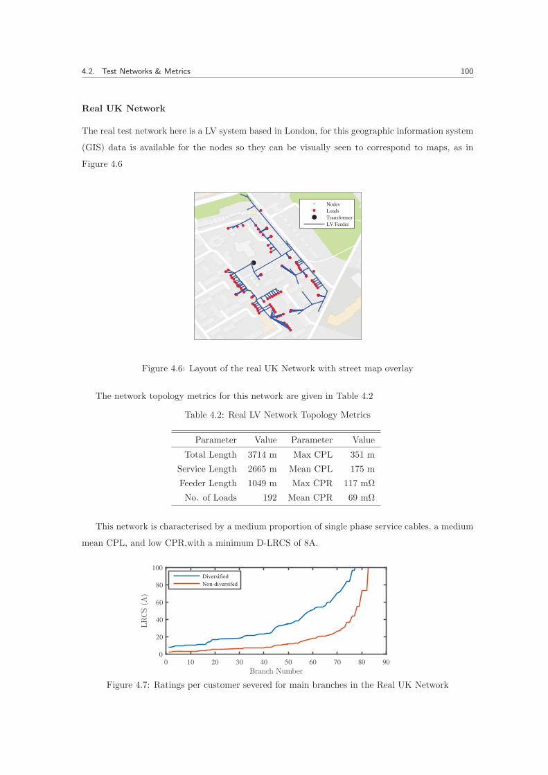
4.2. Test Networks & Metrics 100
Real UK Network
The real test network here is a LV system based in London, for this geographic information system
(GIS) data is available for the nodes so they can be visually seen to correspond to maps, as in
Figure 4.6
NodesLoadsTransformerLV Feeder
Figure 4.6: Layout of the real UK Network with street map overlay
The network topology metrics for this network are given in Table 4.2
Table 4.2: Real LV Network Topology Metrics
Parameter Value Parameter Value
Total Length 3714 m Max CPL 351 m
Service Length 2665 m Mean CPL 175 m
Feeder Length 1049 m Max CPR 117 mΩ
No. of Loads 192 Mean CPR 69 mΩ
This network is characterised by a medium proportion of single phase service cables, a medium
mean CPL, and low CPR,with a minimum D-LRCS of 8A.
0 10 20 30 40 50 60 70 80 90Branch Number
0
20
40
60
80
100
LRCS(A
)
DiversifiedNon-diversifed
Figure 4.7: Ratings per customer severed for main branches in the Real UK Network

4.2. Test Networks & Metrics 101
IEEE European Network
The IEEE power and energy society (PES) recently published data for a “European Low Voltage
Test Feeder.” The other networks published by the IEEE PES such as the 13, 34 and 123 bus feeders
have become a de-facto standard for comparison of load flow methods [112], network integration of
novel grid technologies [113], state-estimation [114], optimal power flow [115] problems and many
more [116,117]. The European LV Network is shown in Figure 4.8.
NodesLoadsTransformerLV Feeder
Figure 4.8: Layout of the IEEE European Network
The network topology metrics for this network are given in Table 4.3
Table 4.3: IEEE European Network Topology Metrics
Parameter Value Parameter Value
Total Length 1431 m Max CPL 293.8 m
Service Length 224 m Mean CPL 171.3 m
Feeder Length 1208 m Max CPR 127 mΩ
No. of Loads 55 Mean CPR 77.1 mΩ
This network is characterised by a small proportion of service cables, normal mean CPL, and
CPR values with a minimum D-LRCS of 8A.
0 100 200 300 400 500 600Branch Number
0
50
100
150
LRCS(A
)
DiversifiedNon-diversifed
Figure 4.9: Ratings per customer severed for main branches in the IEEE Network

4.3. Monte Carlo Simulation 102
4.3 Monte Carlo Simulation
Within the LV distribution network the load profile cannot be given deterministically for any time
period. However at higher voltages, loads are aggregated and the network loading tends to more
closely follow a set of know load profile patterns. The same cannot be said when the aggregation
of loads remains low and large peaks in demand from single customers can be clearly seen at the
secondary substation. Further-more as the uptake of LCTs at particular nodes in the network is
not known in advance, but can be probabilistic determined for a given node from the known (or
herein considered) LCT penetration levels.
The secondary substation primary side voltage was measured in [70] for a range of substation
sites and timestamps. By fitting these results to a Weibull distribution with a scale value of 1.06
and a shape value of 61.3 we have the histogram for 10,000 samples as shown in Figure 4.10
Figure 4.10: Histogram of Substation Voltages
Additionally the phasing information of the particular customers, that is what phase the single
phase service cable branch connects to on the main feeder, is not always known by the DNOs [118].
Hence there cannot be any certainty for some data in the LV networks, specifically:
� Instantaneous demand
� Substation voltage
� Customer phasing
� Location of LCTs
To account for this Monte Carlo simulation methods are employed, such that a statistical
insight can be gained into network variables such as nodal voltages, branch currents and network
losses [119]. This is implemented by assigning, randomly, or with a defined probability, values
to the above variables. In the case of the instantaneous power demand, a random profile from a
database of 7,500 is assigned to each node. The secondary substation voltage is then defined along
with the phasing of each load and the associated LCT uses a Bernoulli distribution where the p
value is defined for various scenarios of LCT uptake.
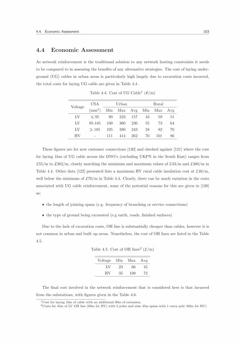
4.4. Economic Assessment 103
4.4 Economic Assessment
As network reinforcement is the traditional solution to any network hosting constraints it needs
to be compared to in assessing the benefits of any alternative strategies. The cost of laying under-
ground (UG) cables in urban areas is particularly high largely due to excavation costs incurred,
the total costs for laying UG cable are given in Table 4.4 .
Table 4.4: Cost of UG Cable1 (�/m)
VoltageCSA Urban Rural
(mm2) Min Max Avg Min Max Avg
LV � 95 90 223 157 43 59 51
LV 95-185 100 360 230 55 73 64
LV � 185 105 380 243 58 82 70
HV - 111 414 262 70 101 86
These figures are for new customer connections [120] and checked against [121] where the cost
for laying 1km of UG cable across the DNO’s (excluding UKPN in the South East) ranges from
�55/m to �382/m, closely matching the minimum and maximum values of �43/m and �380/m in
Table 4.4. Other data [122] presented lists a maximum HV rural cable insulation cost at �48/m,
well below the minimum of �70/m in Table 4.4. Clearly, there can be much variation in the costs
associated with UG cable reinforcement, some of the potential reasons for this are given in [120]
as:
� the length of jointing spans (e.g. frequency of branching or service connections)
� the type of ground being excavated (e.g earth, roads, finished surfaces)
Due to the lack of excavation costs, OH line is substantially cheaper than cables, however it is
not common in urban and built up areas. Nonetheless, the cost of OH lines are listed in the Table
4.5.
Table 4.5: Cost of OH lines2 (�/m)
Voltage Min Max Avg
LV 23 66 45
HV 35 109 72
The final cost involved in the network reinforcement that is considered here is that incurred
from the substations, with figures given in the Table 4.6.
1Cost for laying 10m of cable with an additional 90m of extension.2Costs for 45m of LV OH line (60m for HV) with 2 poles and nine 45m spans with 1 extra pole (60m for HV)

4.4. Economic Assessment 104
Table 4.6: Cost of Full Substations (�1000s)
Voltage Type Rating (kVA) Min Max Avg
HV/LV Pole �100 8 20 14
HV/LV Pole 100-200 11 22 17
HV/LV Pad �200 21 34 27
HV/LV Ground 200-315 20 44 32
HV/LV Ground 315-500 23 50 36
HV/LV Ground 500-800 26 55 40
HV/LV Ground 800-1000 30 57 44
HV/LV Ground �1000 37 119 78
EHV/HV Indoor (x1) - 1208 1575 1391
EHV/HV Indoor (x2) - 1827 2730 2279
EHV/HV Outdoor (x1) - 1155 1470 1313
EHV/HV Outdoor (x2) - 1785 2415 2100
It must be noted the above table is for new substations and not upgrades to existing ones.
Thus the costs listed include the switch gear, fuses, RMU, breakers, and all other substation
equipment. Relative to installation of feeders and particularly UG cables the variance in the costs
for substations ae much reduced. This comes as a result of most DNOs in the UK purchasing a
limited range of distinct transformers in higher quantities
The uptake of power electronic devices by DNOs will only progress if a clear business case
for their use can be made. Typically this will involve a comparison of power electronics and the
alternative solutions relevant to the specific problem faced by the DNO (e.g. network reinforcement
with higher capacity cables or transformers or with additional substations). To facilitate this
comparison, particularly when the power electronics is considered for investment deferral or the
operational lifetime of power electronics and alternative solutions differ greatly, the Equivalent
Annual Costs (EAC) of a distribution asset is a useful measure in that it allows a direct comparison
of two investments with different life cycles:
CEA �Kf
ATl,r� �EeKe �Km� (4.11)
where:
CEA is the equivalent annual cost
Kf is the initial investment cost
Km is the cost of maintenance
Ke is the electrical losses
Ee is the cost of electrical losses
ATl,r is the annuity factor

4.4. Economic Assessment 105
the annuity factor, ATl,r, is a function of the device lifetime, Tl, and the cost of capital, r, given
by:
ATl,r �
1� 1�1�r�Tl
r(4.12)
As an example, suppose it is required to alleviate voltage problems resulting from DG. Given two
solutions, namely PEDs for voltage regulation which will defer network investment for a period
between 8 and 12 years, where the deferral period is assumed to be uniformly distributed, and
network reinforcement which consists of upgrading 200m of the line, which will have an operational
life between 40 and 50 years during which time further upgrades are not envisaged. If the rate of
capital is 5.6%, with initial project costs of �25,000 and �10,000 [120] for the reinforcement and
PED respectively, where the PED incurs further annual costs of �350, the EACs are as shown in
Figure 4.11.
Power Electronics Netwrok ReinfocementEqui
vale
nt A
nual
Cos
ts [£
]
1400
1500
1600
1700
1800
Figure 4.11: EAC of Network Investment Options with uncertain project lifetimes.
Despite similar median costs for both projects, the uncertainty over the deferral period (or
PED lifetime if considered as reinforcement avoidance) of the power electronics is evident when
compared to the network reinforcement solution, which is a low risk solution as is evident from
Figure 4.11. The challenge for PEDs in the distribution network are hence economically motivated
and are driven by: the operating (or deferral) time which will be directly related to its efficacy,
PED costs (both initially and during the assets operation), efficiency, and power density which is
indicative of PED size and thus related to installation costs. All of these can be directly related
to the factors included in equation (4.11).

Chapter 5
Analysis of LV Networks with
Wider Voltage Tolerances
Whilst the use power electronic devices, and other technologies or schemes such DSM, can im-
prove voltage regulation at LV, deregulation can also be considered a “passive” solution to voltage
constraints, varying levels of de-regulation are compared herein, namely:
� EU limits (�%10)
� Load operation limits [38] (+%10,-15%)
� No regulation
The first level of de-regulation “EU limits” represents the voltage tolerance across much of
Europe and is defined in [6]. The second limit was that which was justified in Chapter 3 of this
work, where-by voltage tolerance are increased to the maximum permissible range, prior to frequent
load malfunctions. The final level of deregulation, that is no regulation will clearly need some form
of local regulation to ensure the loads operate correctly. Therefore this will be considered in
conjunction with 100% proliferation of point of load regulation (PoL) devices.
The distinct LCT scenarios for which the befits of de-regulation upon network hosting con-
straints are considered are presented in Table 6.1.
Table 5.1: De-regulation LCT Proliferation Scenarios (%)
PV EV HP
Low - 13 -
Mid 30 33 30
High 60 71 80
106

5.1. Feeder Relief Strategies 107
Results from this chapter were published in the Top and Tail report “Assessment of Feeder
relief versus tolerance band” [123].
5.1 Feeder Relief Strategies
Figure 5.1 presents a tree diagram of the approaches taken to increase capacity within this chapter
along-side other solutions such as network reinforcement. Many further relief strategies can be
found in the literature covering, but not limited to, areas such as: power electronics [72, 124, 125],
reactive power control [126, 127], demand response [44], improved network operation [128, 129],
hybrid reinforcement [130] and dynamic rating methods [41]. All of these works offer alternatives
feeder relief strategies.
Increase NetworkCapacity
Relax Voltage Tolerances
Upgrade the Network
Regulation perDevice
Control Voltage Drop
Regualtion per Household
Reactive Power Control
Assess impact and range of voltage tolerance available
without extra regulation
Install more cables or no. of LV transformers
Control Power Flow
Figure 5.1: Methods to Increase Capacity for Voltage constrained Networks
5.2 Considered Voltage Tolerance Bands
It is known uptake of LCTs stresses voltage limits [130–132] and from [38] a hard limit on domestic
LV voltage tolerances is given as 230V +10,-15%, based on the requirement to maintaining the load
operation. As such voltage tolerances up to +10,-15% could be considered to alleviate network
voltage problems without any need of PoL regulation.
EU Regulations limit
Due to different nominal operating voltages across Europe before harmonisation to a nominal
operating voltage of 230V, where the UK used 240V and much of continental Europe used 220V
[133], the UK enforces a -6% lower bound and a +10% upper bound on voltage levels [39, 134].
It has been considered, but as yet not implemented, to change the voltage band to �10% [133].

5.2. Considered Voltage Tolerance Bands 108
This change would harmonise not only the nominal voltage but also the voltage tolerance band in
Europe, in-line with standard EN50160 [6].
As such the first considered (and smallest) change to the tolerance bands is a reduction in the
lower permissible voltage from -6% to -10%. As the upper limit remains unchanged at +10% the
range of voltage tolerance (VΔ) defined as Vmax - Vmin has been increased from 16% to 20%.
Load operation limit
In Chapter 3 an investigation into the effect of wider voltage tolerances on domestic goods was
presented. Salient results regarding voltage limits for load operation were:
� Domestic good are most sensitive to high voltages, with much equipment functional at very
low voltages (�0.7pu)
� A lower voltage range of -15% allows over 98% of goods to function correctly
� A higher voltage range (�10%) is not appropriate
For these reasons a voltage range of +10,-15% was recommend as the maximum un-disruptive
limit, so this limit will also be considered (VΔ=25%). This limit will be refereed to as “TT” herein.
Point of Load Regulation
It is feasible to remove the requirements upon voltage levels in LV networks if suitable point of
load regulation (PoL) is added (and with 100% proliferation). Two distinct locations within the
final consumers premises are possible:
� Bulk regulation at the PCC
� Regulation of each device
The difference between the two schemes will be the size of the converter required and the voltage
profile on the internal wiring. That is, with a deregulated supply and device by device regulation,
the internal wiring will also be subject to the deregulated network voltages. In the same scenario
but considering bulk regulation, the internal wiring will be subject to only the regulated output
voltage from the bulk PoL converter.
For the purpose of this work no distinction will be made between the two schemes. In modelling
PoL solutions (at either bulk or device locations) the load profiles will be considered to be entirely
constant power loads. This assumption is valid if the converter is able to regulate the output voltage
to the nominal system voltage. Thus the bracketed RHS terms in (2.52) and (2.53) become one and
the device consumes the nominal power as specified by the original load profile. Additionally, this
means thermally controlled loads will draw their specified power, regardless of their PQ voltage

5.2. Considered Voltage Tolerance Bands 109
ACAC
ACAC
ACAC
ACAC
ACAC
ACAC
Bulk Regulation at PCC
Regulation at Device
Figure 5.2: Application of PoL to Regulate Systems Voltages
sensitivity, at all times so the time of use for these device will not change, as it did with the
unregulated voltage.
A key point to note regarding PoL regulation, is that LV cables are rated for 0.6/1kV operation,
this means substantially higher voltages can, potentially, be used without the need to replace
existing cables. Additionally, PoL regulation will be a feasible solution to provide a flexible network
if coupled with LV OLTC or Power Electronic Substations (PES). In the latter case the possibility
of LVDC distribution also raised [135].
The preceding chapters within this report have outlined the problems caused by connection of
various LCTs for LV networks (chapter ??), then detailed how the results presented in this chapter
have been achieved. Namely, how the customers and LCTs are modelled (chapter ??) and well
as the network topology and standard plant and ratings from the UK DNOs (chapter 2.1). Here
we give first details of the LCT scenarios considered, and then metrics used to assess network
performance, before presenting results.

5.3. Feeder Relief with Voltage Deregulation 110
5.3 Feeder Relief with Voltage Deregulation
In this section the benefits of deregulation are explored, with results for the generic network given
first, after which results for the real UK network are given. It must be noted this chapter does not
explore the possibility of using elevated AC voltage alongside PoL or even hybrid DC distribution
networks alongside PoL as the cost of large scale PoL installation is prohibitive and its inclusion
is primarily to severe as a comparison to the de-regulation scenarios.
5.3.1 Generic LV Network
Zero LCT Scenario
Without consideration of any LCTs the network operates within all limits considered. This simply
serves to show without LCT connection to the network it operates without any of the problems or
constraints mentioned in section 1.3.
PV Generation Scenarios
In the case of PV installations it is over voltage and/or thermal problems we would expect to
encounter [131]. Hence, results presented in this section are shown for occurrences of over voltages
and breached thermal limits. Looking at Figure 5.3 it is seen that the introduction of PoL to the
network increases the occurrence of over voltage problems. This can be explained by the fact that
the PoL regulation device is modelled as a constant voltage source for all of the connected domestic
goods, hence they now act of constant power loads. Devices such as resistive based elements used
for space heating, hot water and cooking will no longer consume increased power as the voltage
rises. At the times of peak generation the load with PoL draws a reduced current from the source,
and the voltage rise from DG is consequently higher.
Its must be noted however that with full use of PoL regulation the voltage limits on the feeder
need only be such that insulation breakdown (typically 1kV line to line) and the permissible range
of input voltages for the PoL device itself are satisfied. Assuming the PoL regulation functions
with an input voltage within 25% of nominal no voltage breaches are encountered. This is true for
all of the following figures related to voltage magnitude.
In Figure 5.3 and similar PV scenarios only PoL and the no regulation scenarios are show as
non of the other regulation levels (UK, EU, T&T) propose any change to the upper voltage limit
thus with PV and considering only over voltage issues the results for these 3 would be the same.
The effect of PoL regulation upon networks cable losses is less pronounced, with PoL regulation
acting to reduce current demand at high voltages and increase demand at low voltages (both relative
to nominal). The effect of this can be seen in Figures 5.4 and 5.5 below, which display the cable

5.3. Feeder Relief with Voltage Deregulation 111
30
40
50
No Regulation PoLReg
ulat
ory
Bre
ache
s High PV Nodal Voltage Issues
Figure 5.3: Generic Network Voltages with 60% PV
losses in the main three phase feeder (Lfeed) and the single phase service connections (Lserv)
respectively.
3040506070
No Regulation PoL
Loss
es (k
Wh/
day)
High PV Feeder Losses
Figure 5.4: Generic Network Feeder Losses with 60% PV
5
5.5
6
No Regulation PoL
Loss
es (k
Wh/
day)
High PV Service Losses
Figure 5.5: Generic Network Service Losses with 60% PV
The network hosting capacity for PV (and other DG sources) with de-regulation is unchanged
due to the proposed limits on voltage tolerances all having the same upper limit (+10%). To
increase the hosting capacity of DG the network is instead operated with a lower nominal voltage.
This is easily achieved by reducing the tap position of the off-line tap to its lowest value (-5%).
This tap setting results in substation voltages below those typically measured in the UK [70], but
is requited to accommodate DG, as such, this setting will be maintained when considering the
increased loading with HP and EV that follows.

5.3. Feeder Relief with Voltage Deregulation 112
Heat Pump Scenarios
As the loading due to HP increases, and the business as usual case whereupon the DNOs operate
high system voltages has been changed to increase hosting capacity of DG (section 5.3.1), network
under voltages are encountered with existing voltage tolerance bands as can be seen in Figure 5.6.
In this case the alternative limits on voltage regulation are shown individually in the figure as the
lower regulatory limit and thus occurrence of under voltages, has been changed. Both the EU
limits and load operation (TT) limits remove all occurrences of nodal under voltage breaches. The
same is true when PoL regulation is considered with these two de-regulation strategies.
05
10
15
UK EU TT UK/PoL EU/PoL TT/PoLReg
ulat
ory
Bre
ache
s High HP Nodal Voltages
Figure 5.6: Generic Network Voltages with 80% HP
The effect of PoL regulation upon feeder losses is shown in Figure 5.7. It is noticed that there
is a small increase in network losses where PoL is implemented. The effect is the same in both the
feeder and service cables. As before, the reason for this is that at times of low network voltages, a
portion of the domestic load is resistive in nature and thus the power demanded by this load will
decrease when PoL regulation is not considered, leading to reduced network loading, losses, and
efficiency.
0
10
20
No Regulation PoL
Bra
nch
Ove
rcur
rent
High HP Feeder Thermal Limits
Figure 5.7: Generic Network Branch Thermal Limits with 80% HP
The settings used for the PoL in all of this work are such to regulate the voltage to its nominal
value (230V).
Electric Vehicle Scenarios
As the loading due to EVs increases and lower system voltages are once again used to accommodate
DG, network under voltages with EV use become problematic as can be seen in Figure 5.8.

5.3. Feeder Relief with Voltage Deregulation 113
In this case the alternative limits on voltage regulation are shown. As the lower voltage limit
and thus occurrence of under voltages, is seen to change. Both the EU limits and TT limits reduce
the occurrences of nodal under voltage breaches to permissible levels. From this we can say that
for the generic network, voltage limits are effectively reduced by de-regulation. Furthermore since
voltage limits are encountered prior to thermal limits the network hosting capacity is increased by
de-regulation. The cost of network reinforcer required to remove voltage and current limits for the
case of high EV usage is over �64000 per feeder, with de-regulation able to defer 15% of this cost.
0
10
20
UK EU TT UK/PoL EU/PoL TT/PoLReg
ulat
ory
Bre
ache
s High EV Nodal Voltages
Figure 5.8: Generic Network Voltages with 71% EV
In all high penetration scenarios thermal limits are breached, and like in the case of a high
penetration of heat pumps, the costly network upgrades mentioned above would need to be made
for this scenario to be a viable.
0
10
20
No Regulation PoL
High EV Feeder Thermal Limits
Bra
nch
Ove
rcur
rent
Figure 5.9: Generic Network Branch Thermal Limits with 71% EV

5.3. Feeder Relief with Voltage Deregulation 114
5.3.2 Real Network
Zero LCT Scenario
Without consideration of any LCTs the network operates without any limits being breached. Some
voltages outside tolerance are seen but the frequency of these is very low. This simply serves to
show that without LCT connection to the network it operates without any of the problems and
issues mentioned in section ??.
PV Generation Scenarios
0
20
40
No Regulation PoLReg
ulat
ory
Bre
ache
s High PV Nodal Voltages
Figure 5.10: Real Network Voltages with 60% PV and -2.5% tap
There are no voltage contained limitations with HP or EV but a large number due to PV, for
this reason the tap setting on the LV substation is reduced to its lowest value of -5%. Given a
nominal supply voltage this results in a no load substation voltage of 1.03pu (237V). In this case
results show (Figure 5.11) the network is no longer voltage constrained and no over voltage issues
are seen on the feeder for a high penetration of PV.
−2
0
2x 10⁻¹⁶
No Regulation PoL
High PV Nodal Voltages
Reg
ulat
ory
Bre
ache
s
Figure 5.11: Real Network Voltages with 60% PV and -5% tap
Severe problems are encountered here in regards to voltage unbalance factor (VUF). As shown
(Table ??) there are two distinct limits on the VUF. It is the limit of 1.3% VUF for no more than
5 minutes in any 30 minute period that is the more frequently breached than the absolute limit
of 2%. Indeed there are no breaches of the 2% limit anywhere in the network for all the scenarios
considered. However Figure 5.12 shows that in some cases, from 101 VUF measurement over the
course of the 24 hour period of study all of the readings breach VUF limits; inclusive of even the LV

5.3. Feeder Relief with Voltage Deregulation 115
branches closest to the transformer. This is a result of the source voltage unbalance (ie unbalance
at the star connected transformer secondary).
0
50
100
No Regulation PoL
High PV Voltage Unbalance
Reg
ulat
ory
Bre
ache
s
Figure 5.12: Real Network VUF with 60% PV
Load balancing and voltage compensation can be used to mitigate against high VUF. Regulation
strategies do not help reduce VUF nor does individual voltage regulation (PoL) as can be seen
from Figure 5.12. However if PoL regulation is assumed with full de-regulation of the voltage
magnitude and VUF limits, then this is not a problem.
Heat Pump Scenarios
Considering high penetration of HP, it is noted the network is not voltage constrained even with the
lower tap settings used to accommodate PV installation. Figure 5.13 shows none of the considered
scenarios have voltage issues so voltage de-regulation doesn’t offer any increase to hosting capacity.
−2
0
2x 10⁻¹⁶
UK EU T&T UK/PoL EU/PoLT&T/PoL
High HP Nodal Voltages
Reg
ulat
ory
Bre
ache
s
Figure 5.13: Real Network VUF with 80% HP
For this network it is actually thermally constrained with a high penetration of HP, as can
be seen if Figure 5.14. Thermal limits are slightly exacerbated by the use of PoL regulation as
during times of low system voltage (i.e. with high loading brought on by HP installations) the PoL
regulation acts to increase the load compared to without, this in turn increases the conduction
losses in the feeder.
As was the case with PV there are severe VUF problems as shown in Figure 5.15. For example
considering a high penetration of HP and PoL regulation we see that in all of the simulations
almost all of the feeder branches breach VUF limits.

5.3. Feeder Relief with Voltage Deregulation 116
0
5
10
15
No Regulation PoL
High HP Feeder Thermal Limits
Bra
nch
Ove
rcur
rent
Figure 5.14: Real Network Branch Thermal Limits with 80% HP
0
50
100
No Regulation PoL
High HP Voltage Unbalance
Reg
ulat
ory
Bre
ache
s
Figure 5.15: Real Network VUF with 80% HP
Electric Vehicle Scenarios
Finally with high levels of EV uptake, UK voltage limits are seen to breached as shown in Figure
5.16. This network compared to the generic network is clearly more thermally constrained and
network planning has meant voltage constraints are not a limitation upon network capacity, hence
in this regard there is no benefit to de-regulation of voltage. Although as shown either EU or TT
limits on regulation reduce the occurrence of regulatory breaches to permissible values.
0
5
10
UK EU T&T UK/PoL EU/PoLT&T/PoL
High EV Nodal Voltages
Reg
ulat
ory
Bre
ache
s
Figure 5.16: Real Network VUF with 71% EV
Significant parts of the network are thermally constrained as shown in Figure 5.17. As with all
cases of high LCT penetration in this particular network VUF is a severe limitation too. For this
network high levels of LCT usage leads to breaches of VUF, thermal limits, and voltage magnitude
limits in that order. As the VUF was show to be problematic over the whole network considered,
replacement of the transformer for a lower loss type is the most effective solution, albeit expensive.
Network feeder upgrades to remove thermal limitations in the feeder will cost �82000.

5.3. Feeder Relief with Voltage Deregulation 117
0
10
20
No Regulation PoL
High EV Feeder Thermal Limits
Bra
nch
Ove
rcur
rent
Figure 5.17: Real Network Branch Thermal Limits with 71% EV
5.3.3 Validation of the Real Network Model
Network efficiency for the UK DNOs in the 10 year period up to 2010 are shown in Figure 5.18.
The figure includes losses across all of the distribution network, including EHV and HV which
where not included in our LV modelling, hence losses in this plot should be approximately double
those in the simulation results.
From this we see significant changes in efficiency whilst the consumed power remains fairly
constant for any given DNOs. Looking across the DNOs (less SSE Hydro) we see that they also
achieve similar overall efficiencies (95% � 1.5%) despite large variations in network size, which
comes as a result of similar network planning methodology and imposed regulators limits.
0.5 1 1.5 2 2.5 3 3.5 4x 10⁴
91
92
93
94
95
96
97
98Consumed Power vs. Network Efficiency
Anual Consumed Power (GWh)
Effic
ienc
y (%
)
CN WestCN EastENWCE NEDLCE YEDLWPD S WalesWPD S WestEDFE LPNEDFE SPNEDFE EPNSP DistrbutionSP ManwebSSE HydroSSE Southern
Figure 5.18: Efficiency and Annual Power Consumed of UK DNOs from 2000-2010
Results for the real network without LCT give losses of 4% (i.e. efficiency of 96%) and with
the most increased loading scenarios the LV network has losses around 6.5%. From the UKPN
allocation of losses (see Table 5.2) our model has accounted for 48% of the total system losses.
This means total network losses would be 8% at nominal loading increasing to 13% for high LCT
scenarios, if the full network was to be considered.
This puts losses in the modelled system at the upper range of losses (for no LCT case) compared

5.3. Feeder Relief with Voltage Deregulation 118
Table 5.2: Network Loss Allocation
Fixed Losses (30%)
Location Amount
Grid/EHV 25%
EHV/HV 20%
HV/LV 55%
Variable Losses (70%)
Location Amount
EHV 30%
HV 25%
LV 45%
to the published losses incurred in the measured distribution networks, where losses are seen to
range from 3.3% to 8.3% depending upon the DNO. The high predicted percentage of network
losses are a results of the high load density, medium feeder length, use of 185mm2 legacy cable,
and LCT use, which leads to increased losses and higher neutral current.
Using a 7:3 ratio of variable to fixed losses at nominal load, and assuming 96% efficiency at
nominal loading, where the variable losses change proportional to the square of the load, and the
fixed losses remain constant, results in the expected losses as shown in Figure 5.19. It is noted
peak efficiency is below nominal loading at 0.65 of the nominal load at which point efficiency is
marginally higher at 96.32%.
0.5 1 1.5 293
94
95
96
97Network Loading vs. Predicted Efficiency
Load Factor
Effic
ency
(%)
Figure 5.19: Expected LV Network Losses
As the maximum increased loading cases have more than doubled the total energy consumption
in these network studies, the efficiency also changes as shown in Table 5.3 and Figure 5.20, which
has normalised network efficiency and power flow to the values with no LCT. The absolute value
of power flow though the substation ��Pt��, that is the input power at the primary side, is then
used to find the overall network efficiency �η� with:
η ��Pt�
�Pt� � Ploss(5.1)
Where the total losses �Ploss� are comprised of:
Ploss � Pfeed � Pserv � Ptran (5.2)

5.3. Feeder Relief with Voltage Deregulation 119
For cases with DG, the network efficiency figure is not directly comparable to the other scenar-
ios, where local consumption must be measured at all the nodes to find accurate efficiency figures.
It is noted however that due to large generation and low load the total system losses increase com-
pared to the scenario without LCT, this is unlike the situation for lower DG penetration, where the
generation supplies load locally, even during times of peak generation, and thus reduces network
losses. This can be confirmed by looking at the substitution columns of the PV scenario where
the absolute value of energy though the substation has increased implying that the load has been
supplied by DG and the reverse power (from DG) is greater than the normal demand without DG,
thus increasing the energy flow via the substation. This is confirmed by comparison of the high PV
substation energy values (2230kWh/day & 2232kWh/day) compared to the same no LCT values
(1922kWh/day & 1897kWh/day) in Table 5.3.
Table 5.3: Substation Energy (kWh/day) and Network Efficiency
ScenarioNo Regulation PoL Regulation
Substation Efficiency Substation Efficiency
No LCT 1922 95.58% 1897 95.55%
High PV 2230 94.03% 2232 93.91%
High HP 3994 93.70% 4003 93.65%
High EV 3786 93.41% 3709 93.58%
Load Factor0.5 1 1.5 2
Effic
ency
(%)
92
93
94
95
96
97
****
No LCTDGHPEV
Network Loading vs. Predicted Efficiency
Figure 5.20: Simulated and Expected Network Losses

5.4. The Benefits of De-regulation in LV Networks 120
5.4 The Benefits of De-regulation in LV Networks
The high cost and disruptive nature of network reinforcement drive alternative solutions to power
quality (PQ) issues brought about by low carbon technologies. This chapter has explored the effect
of changing the voltage tolerance bands. To quantify the benefits of this, 3 new voltage tolerance
bands were suggested, given with their reasoning (section 5.2). Requirements of modelling the
distribution network were (see Chapter 4) implemented, now with particular focus on the load
models required when considering a wider range of supply voltages (section 2.3).
The benefits of de-regulation upon the generic network is that it facilitates medium levels of LCT
uptake. At higher LCT penetrations thermal limits and VUF are encountered meaning network
reinforcement is required for these scenarios. Thus de-regulation is effective in deferring network
investment form the time between, the first voltage constraints encountered prior to medium LCT
uptake and, the first thermal constraints encountered prior to high LCT uptake.
Considering the real network, even with medium levels of LCT the networks is already limited
by: thermal bottlenecks close to the substation (as would be expected from comparison of the
minimum D-LRCS values in the real network relative to the generic network) and high VUF across
much of the network. As a result the benefits of de-regulation to the real network are small.
De-regulation can allow a lower operating voltage and consequently a small reduction in energy
consumption and losses but for future cases of LCT proliferation and deferring investment there
was little advantage.
The contrast seen by de-regulation in these two networks is testament to the highly network
topology dependant nature of the various hosting constraints. Overall de-regulation offers in-
creased LCT hosting capacity to voltage contained networks and as such can help smooth out the
transition to LCT that DNOs need accommodate, generally via network upgrades, expansion and
reinforcement. Growing levels of DG mean this deregulation allows the DNOs greater scope to
lower system voltages, which was also shown to slightly reduce total demand. Ultimately, with
higher levels of LCT voltage problems are however unlikely to be the limiting factors or sole limit-
ing factors, instead VUF and thermal ratings will be problematic. In the case of thermal limits this
can only then be addressed with traditional reinforcement measures or re-routeing of the power
flows.
In reducing the permissible lower voltage limit the benefit to the DNO in terms of hosting
capacity can be very rapidly been seen when PV and DG are considered, this is already know
to be a common voltage quality issue [7]. As mentioned the reason for this is that the DNOs in
choosing to run substation voltage at the upper end of the voltage range [70] limit the capacity for
DG to increase the hosting capacity for additional loads. In reducing the lower band the option
for the DNO to operate lower substation voltages becomes available which in turn increases the

5.4. The Benefits of De-regulation in LV Networks 121
hosting capacity for DG, thus despite not changing the upper band the occurrence of network over
voltage constraints can be reduced by new voltage regulator settings, achieved via automatic tap
changers at primary substation of the off-line taps used on secondary substations.
Point of load regulation has been compared throughout this chapter and in this case the only
relevant limits are the thermal and insulation limits of the network (i.e disregard all voltage based
PQ regulations). With PoL, the networks can be used to thermal limits at all times and DNOs
can consider higher voltages to improve system efficiency and capacity.

Chapter 6
Analysis of LV Networks with
Power Electronic Devices
In this chapter results are presented which show the benefits associated with the PEDs installed
in the generic UK network. Following the method presented in [136], losses for the converters are
not initially considered so that break even or required efficiency ratings can be made for each of
the devices to become economically viable. The PEDs considered are:
� Power Electronic Substation (PES)
� Mid Feeder Compensator (MFC)
� Active Power Filter (APF)
� On-load Tap Changers (OLTC)
A brief review of the aforementioned PEDs is given along with the implementation of the Monte
Carlo analysis methods used for comparing these PEDs is first given before results are presented.
Follwing this the effect of power filtering on network losses is given before the PEDs are compared.
As in Chapter 5, the proliferation scenarios shown in Table 6.1 are used in allocating LCTs to
individual customers.
Table 6.1: LCT Proliferation Scenarios (%)
PV EV HP
Low - 13 -
Mid 30 33 30
High 60 71 80
Much of the work from this chapter was published in the PEDG conference paper “Power
electronic voltage regulation in LV distribution networks.”
122

6.1. PED Device Operation 123
6.1 PED Device Operation
A 24 hour load flow is initially performed with a resolution of 1 minute. After the load flow
completes and the voltage and current (VI) measurements are stored and the process is repeated for
a given number of Monte Carlo trails (runs) or for the next scenario. All of the VI measurements
are then compared with relevant standards or equipment limits, with outlying results flagged.
Network losses, utilisation factor, efficiency, and voltage quality measures are calculated. This
process is then repeated for each of the technologies mentioned in section 2.2. Briefly, these are
given again for reference:
� Base : This represents the case “as is” and indicates the effect of LCT use without any
network changes.
� De-Reg : Deregulation scenarios are easily considered by adjustment of the limits defining
outlying results. The voltage range considered for deregulation is �10% as in the EU. From
Chapter 3 a limit on supply voltages which do not adversely effect domestic loads was given as
+10,-15%, the EU voltage limits fall with in this band.
� PES : The PES is configured so that each feeder is individually regulated. The voltage at
the head of each feeder is continually adjusted between 1.08pu and 0.96pu by the LDC, with the
no load reference voltage as 1.02pu.
� OLTC : The OLTC uses LDC using the same settings as the PES. As the tap changers have a
bandwidth of 2.5% with a maximum tap range of �5%, the limits of the supply voltage (assuming
nominal HV) are 0.96pu to 1.06pu. Unlike with the PES, the secondary winding is connected to a
substation busbar so all 4 feeders are regulated simultaneously.
� APF : The APF is considered to provide reactive compensation and load rebalancing. As
the system is 4 wire, the neutral current is also eliminated, this in practice requires use of a 4-leg
(or split capacitor) inverter. No limit is put on the APF rating. The control strategy used it that
termed perfect harmonic cancellation (PHC), which was also shown to be the most suitable APF
control strategy when non ideal supply voltages were considered [65].
� MFC : The MFC here is operated as a power balancing device. The role of the shunt
converter is solely to supply the active power demand by the series converter. In practice the
shunt converter can also be utilised in the same manner as the APF. The MFC is rated to inject
up to 10% of the nominal voltage; which when considered with the MFC location and the cables
thermal limit give a required rating for each converter of 12kVA.

6.2. Feeder Relief with PEDs 124
6.2 Feeder Relief with PEDs
In this section the benefits of the PEDs are explored, with results given for the detailed generic
UK network. Figure 2.13 is repeated for clarity here and shows the location in the distribution
network that the aforementioned power electronics are installed.
LVSOP
Primary Substation
OLTCSecondary Substation
LV DCNetwork
11kV SOP
MFC
LV AC Network
SST APF
Figure 6.1: Distribution Network with Power Electronics
6.2.1 Generic LV Network
In this chapter results are presented in where the number of instantaneous breaches of voltage
regulation and power quality issues are breached along with thermal ratings, this offers a finer
granularity compared to showing weather a node has, over the low flow time period breached
regulator limits. This measurement is termed occurrence in the following figures and is expressed
as a percentage of the measurements that breach limits. For example is all half of the nodes in the
considered network breeched regulator limits half of the time the occurrence percentage would be
25%.
Zero LCT Scenario
Without consideration of any LCTs the network operates without existing limits being breached as
shown in Fig. 6.2. Some voltages outside tolerance are seen without any PEDs but the frequency
of these is very low.

6.2. Feeder Relief with PEDs 125
0
10
20x 10 3
Base OLTC PES APF MFCO
ccur
ance
(%)
Under Voltage Base
2
0
2x 10 16
Base OLTC PES APF MFC
Occ
uran
ce (%
)
Thermal Limitations Base
Figure 6.2: Outlying Results with no LCTs Considered
PV Generation Scenarios
In the case of PV installations it is over voltage and/or thermal problems we would expect to
encounter [131]. Hence, results presented in this section are for occurrences of over voltages and
breached thermal limits.
0
0.05
0.1
0.15
Base OLTC PES APF MFC
Occ
uran
ce (%
)
Over Voltage Mid PV
2
0
2x 10 16
Base OLTC PES APF MFC
Occ
uran
ce (%
)
Thermal Limitations Mid PV
Figure 6.3: Network with 30% proliferation of PV Installations
With a medium penetration of PV (Fig. 6.3) over voltages are seen when no PED based voltage
regulation is present. Compared to medium penetration of HP (see Fig. 6.5) voltage problems are
encountered more frequently. This is a direct result of the high substation voltages chosen by the
DNOs [70]. In this scenario all regulation devices are able to reduce network over voltages, and
again like the medium HP penetration scenario, the APF is effective in reducing the occurrence of
voltage outside regulator limits. In all cases the thermal limits of the network equipment are not

6.2. Feeder Relief with PEDs 126
exceeded.
As the PV penetration level reaches 60%, over voltages become more common as expected
(Fig. 6.4). In this case the APF is not able to effectively reduce the occurrence of over voltages to
an effective level. The other regulation devices are however all effective in reducing the occurrence
of over voltages.
00.5
11.5
Base OLTC PES APF MFC
Occ
uran
ce (%
)
Over Voltage High PV
2
0
2x 10 16
Base OLTC PES APF MFC
Occ
uran
ce (%
)
Thermal Limitations High PV
Figure 6.4: Network with 60% proliferation of PV Installations
As with the medium penetration of PV scenario in no cases are the thermal limits of the
network equipment breached. The difference in occurrence of thermal limits and voltage limits
(over or under) being breached between the PV scenarios and the HP/EV scenarios is a direct
result of network operation voltages. It is clear as the amount of LV connected PV grows and over
voltage becomes more frequent (already encountered more than under voltages [70]) the DNOs
must act to either upgrade network infrastructure, reduce substation voltages, or improve voltage
regulation.
Heat Pump Scenarios
As the amount of HP used increases under voltage measurements are seen at remote feeder ends.
From Fig. 6.5, which show 30% installation of HP, the voltage limits are breached whist the
networks thermal limits are not exceeded. This clearly indicates the network is voltage constrained
in this scenario.
The PES and MFC are both able to improve voltage regulation such that the network is not
voltage constrained. In the case of the OLTC the cause of the voltages which lye outside regulator
limits is due to the delay time used in the tap selection process. The APF is also seen to reduce
the frequency of under voltage measurements.
As the amount of HP installed is increased to 60% network thermal limits are encountered.

6.2. Feeder Relief with PEDs 127
0
0.05
0.1
Base OLTC PES APF MFCO
ccur
ance
(%)
Under Voltage Mid HP
2
0
2x 10 16
Base OLTC PES APF MFC
Occ
uran
ce (%
)
Thermal Limitations Mid HP
Figure 6.5: Network with 30% proliferation of Heat Pumps
Here the PES and MFC compensate for under voltages such that the network can be said to be
thermally limited. This scenario would therefore need further network reinforcement to be a viable
operating scenario for a UK based DNO. The under voltages with the OLTC are again due ot the
tap selection time but also the limit placed on the tap ratio (�5%) which is not the case for the
PES.
0
2
4
Base OLTC PES APF MFC
Occ
uran
ce (%
)
Under Voltage High HP
00.10.20.3
Base OLTC PES APF MFC
Occ
uran
ce (%
)
Thermal Limitations High HP
Figure 6.6: Network with 80% proliferation of Heat Pumps
Thermal limits are reached more frequently with the MFC as compared to the OLTC and PES
as the power required of the voltage injected by the series converter but be balanced by that of
the shunt converter. As the HP is treated as a constant power load operation with high supply
voltages acts to reduce the current drawn.

6.3. Analysis of Active Power Filters 128
Electric Vehicle Scenarios
For brevity results for low penetration of EV are not shown, however in this scenario all regulation
devices except the APF reduce under voltage occurrences to almost zero and in non of the cases
is the network seen to be thermally limited.
Medium penetration of EVs are given in Fig. 6.7, again the PES and MFC are able to remove
any voltage limitations. Thermal limitations in this scenario occur all with very limited frequency
(similar to the frequency of recorded under voltage in the base scenario without voltage regulation).
0
0.2
0.4
Base OLTC PES APF MFC
Occ
uran
ce (%
)
Under Voltage Mid EV
0
0.01
0.02
0.03
Base OLTC PES APF MFC
Occ
uran
ce (%
)
Thermal Limitations Mid EV
Figure 6.7: Network with 33% proliferation of Electric Vehicles
When the amount of EVs increases to 71% results (Fig. 6.8) again show only the PES and MFC
reduce voltage constraints to a level below their thermal limits. The OLTC is effective in reducing
the occurrence of under voltage, where in this case, the remaining under voltages are due to the
limit of �5% on the tap ratios.
In all cases thermal limits are breached and like in the case of a high penetration of heat pumps
network upgrades would need to be made for this scenario to be a viable in the UK. All regulation
devices are shown to reduce the occurrence of thermal limits
6.3 Analysis of Active Power Filters
The active power filter is used for phase rebalancing which in turn reduces network losses; its ability
to regulate voltage coming as a result of this (by virtue of neutral voltage reduction and balanced
voltage drop across each phase). Namely, the APF is not first and foremost a voltage regulator,
this should be clear from Figures 6.5-6.4. It reduces voltage issues only when the occurrence (hence
magnitude) is low.
The impact of the APF upon network operation and losses is shown for an average of 10

6.3. Analysis of Active Power Filters 129
0123
Base OLTC PES APF MFCO
ccur
ance
(%)
Under Voltage High EV
0
0.2
0.4
0.6
Base OLTC PES APF MFC
Occ
uran
ce (%
)
Thermal Limitations High EV
Figure 6.8: Network with 71% proliferation of Electric Vehicles
simulations with high penetration of HP. At node 13 where the APF is located neutral current is
eliminated and the losses in the phase conductors at this node are also equalised. This can be in
Fig. 6.9 which shows the cable losses over the period of simulation (24 hours) for one trail with a
high proliferation of HP.
5 10 15 20 25 300
0.5
1
1.5
Node
Loss
es (k
Wh/
day)
Cable losses with APF at Node 13
A : 16.9B : 15.8C : 16.6N : 2.34
Figure 6.9: Network with 60% proliferation of PV Installations
For the three high penetration scenarios and the base case the average cable losses (phase and
neutral) are given in Table 6.2. It can be seen the reduction in losses is between 7-10%. In absolute
terms if we take the the cost of network losses as �0.06 /kWh [130] the annual cost in reduction
of losses will be �127.
The greater benefit of the APF lies in its ability to reduce the occurrence of thermal limitations
in network equipment as is evident in Figs. 6.2-6.4, and mitigation of power quality issues should
they become limiting factors.

6.4. Comparison of PED Regulation Approaches 130
Table 6.2: Cable Losses
ScenarioLoss (kWh/day)
ReductionNo APF APF
No LCTs 16.10 14.47 1.63 (10%)
High DG 13.21 12.19 1.02 (7.7%)
High EV 60.93 55.14 5.79 (9.5%)
High HP 60.82 56.45 4.37 (7.1%)
As the network voltage drop is small relative to the level of current imbalance present across
the phases, the shunt connected APF is larger than the series connected MFC, which was able
to regulate system voltage with a 12kVA rating. The rating of the APF was not limited in the
simulation and the rating was calculated using the maximum power for one phase, which was then
used to find the total converter rating. The rating of the converter required varied between 42kVA
and 55kVA dependant upon the LCT scenario considered.
Table 6.3: APF Size
Scenrio Rating (kVA)
No LCTs 42.4
High DG 44.4
High EV 55.1
High HP 47.7
6.4 Comparison of PED Regulation Approaches
For the 8 LCT scenarios and all voltage regulation scenarios the 75th percentile is checked for
values above 0.07%, this corresponds to 1 minute of outlying results a day. Table 6.4 lists the
number of LCT scenarios without these outliers, with the final column listing the percentage of
the 16 considered voltage or thermal limits which were not exceeded. This metric was used instead
of individual application of EN50160 to the consumers so to give an indication of the wider network
performance, but results are very similar with either method.
The reason for the OLTC’s poorer voltage regulation (compared to PES) are: the delay time
implemented in the tap selection process (so voltage changes can go un-regulated for a time), the
smaller range of voltages the OLTC can achieve, and the simultaneous regulation of all 4 feeders.
Non of the regulation scenarios are able to remove thermal limits to passable levels, but from
Figs. 6.2-6.4 it is noted they can be reduced. As the LCTs considered are all assumed to be
inverter connected (constant power loads) operation at higher voltage levels can reduce current
drawn by these loads and in the case of the APF current limits are reduced via load balancing.

6.5. The Benefits of PEDs in LV Networks 131
Table 6.4: Scenarios considered without Constraints
RegulationVoltage
Thermal Overall %Under Over
Base 1 0 6 44
De-Reg 3 0 6 56
OLTC 3 2 6 69
PES 6 2 6 88
APF 2 1 6 56
MFC 5 2 6 81
6.5 The Benefits of PEDs in LV Networks
Here we have presented 4 power electronic based voltage regulation to improve voltage regulation
in LV networks and have compared them to the case at present (base) and a de-regulation scenario.
De-regulation was considered as a lowering of the lower permissible supply voltage with the upper
voltage limit unchanged. For this reason the hosing capacity of DG was not increased by de-
regulation. For increased loading scenario the lower voltage limit allowed further network loading
allowing medium penetration of HP or EV without voltage constrains. De-regulation when utilised
in conjunction with changes to the HV operating voltage or the LV substation taps could allows
greater hosing capacity for all the considered LCTs.
In the cases of the MFC, OLTC, and PES, all were able to improve voltage regulation to
accommodate medium levels of LCTs. For DG (i.e PV) hosting capacity was increased by all of
the regulation devices. Voltage control at either the substation or mid-feeder allows for greatly
improved LCT hosting capacity. In practice the advantages of the PES over the OLTC could be
reduced by increasing the range (or number) of the taps, along with faster tap selection. This later
point due to reliability and operating life of new tap changer technologies [137] not be a cause for
reduced OLTC life. The prominent advantages of he MFC compared to the PES (or APF) is the
reduced size needed along with voltage regulation comparable to the PES.

Chapter 7
Conclusions and Future Work
7.1 Conclusions
This thesis has outlined and compared 2 broad solutions to LV network hosting constraints. First,
voltage de-regulation has been considered to reduce the frequency of network voltage constraints
by simply relaxing the voltage tolerance levels. Secondly, a range of power electronic devices has
been implemented in the network models to assess the efficacy of each of the PEDs. Additionally,
we have assessed the voltage sensitivity of domestic loads and drawing together results from the
literature, along with experimentation and simulation. Building on this work load models were
developed that account not only for the load PQ voltage sensitivity but for the thermal control
requirements of these devices which use thermal controllers, this without necessarily resorting to
dynamic heat flow equitations.
Load & Network Modelling
In Chapter 3 the effect of a changing the supply voltage to common domestic loads was studied.
Firstly, regarding the lighting sector the change from incandescent to CFL, halogen and LED
lighting was outlined, as these latter technologies (less halogen) are less sensitive to supply voltage
than incandescent lighting the greatest visual effect to the consumer of supply voltage, that is
domestic lighting luminosity is reduced. Thus regarding lighting as more and more incandescent
bulbs are phased out the visual disturbance resulting from this is also also diminished. Amongst
all the lighting technologies presented PQ voltage sensitivity figures show that for this transition
of technologies the overall load presented to the network becomes less dependant upon the supply
voltage, this in turn reduces the efficacy of voltage optimisation as a means to reduce demand.
Additionally as the loads tends towards a constant power load (CPL) type characteristics network
stability is reduced. However due to the increased efficiency of new lighting technologies the load
132

7.1. Conclusions 133
presented decreases thus offsetting this effect.
Regarding electric heating systems, which are used mostly for space and water heating, the
PQ sensitivity of loads that are resistive where shown, as would be expected, to have a constant
impedance PQ voltage sensitivity. This affords considerable room for voltage optimisation. For
heating loads that use a thermal controller to adjust the load duty cycle, to meet temperature set
points, dynamic thermal models and constant energy models were developed from load profiles
that indicate only the PQ demand at nominal voltage. These additional controls where shown
to have a large effect on network power flow where the proportion of customers having thermally
controlled loads and where the np and nq values (see (2.54) & (2.55)) are high, ie. networks with
economy 7 heating and electric water heaters.
Motors where shown to represent a significant portion of the LV load (�30%) where they are
used in cold appliances (eg. fridges) and loads where the converted kinetic energy is directly
utilised (eg. vacuums, washers). These motors when not interfaced to the network via a power
electronic converter are normally single phase inductions motors, which where shown to have a
constant current type power demand (np=1) and a constant impedance type reactive power demand
(nq=2). When these motors are used in thermally controlled loads they are again required to meet
temperature set points thus need either thermal models or the developed constant energy models
to be include in for accurate load flow studies, especially when the supply voltage is considered
to fluctuate widely. When an adjustable speed drive (ASD) or variable frequency drive (VFD) is
used with the motor the results from the literature indicated that the power demand falls with an
approximately constant impedance power sensitivity (np=2).
In the vast majority of cases, loads were seen to be able to operate as normal with voltages
reduced by as much as 15% from normal and frequently further still. The same was not true of
higher voltages levels where loads where seen to be damaged or malfunction with only 2% higher
voltages than the present regulatory maximum. As such the voltage band that would minimise
disruption to loads whist maximising the hosting capacity of LCTs was given as -15%,+10%.
In section 4.2 metrics were developed to asses the sensitivity of a distribution network to thermal
and voltage problems. These are used to predict the likelihood of network hosting constraints
without having to complete load flow analysis and are based solely upon the topology of the
network which is known, the amount of, and location of the connected customers, which are also
known. As the load profile of each customer at any one time is a stochastic function, diversity
factors (DF) were utilised so the metrics can account for this uncertainty.
Voltage Deregulation
In Chapter 5 the benefits of voltage de-regulation on a network level were explored. In particular
the ability of de-regulation to off set the need for network reinforcement driven by uptake of LCTs

7.1. Conclusions 134
was studied.
De-regulation was compared in two networks and the efficacy of de-regulation was shown to
vary significantly. Initially PV was considered which was seen to cause rapid overvotlage issues
across all the networks, thus tap settings where then modified to accommodate this. Following this,
in the generic UK network de-regulation facilitated increased loading of the network from below
medium LCT levels up to high LCT levels, without voltage constraints. At high LCT levels the
generic network was thermally constrained. In removing the voltage constraints between these two
loading scenarios �10,000 of network upgrades required for 96 customers was deferred / avoided.
If the network reinforcement costs were deferred the effective period of deferral is the time the
network loading takes to grow from the first encountered voltage constraints without de-regulation
to the time at which the first thermal constraints encountered (with or without de-regulation as
thermal limits are unaffected by de-regulation).
For the case of the real network, with medium LCT penetration levels of HP and EV, the
thermal limits of the network were already encountered, thus network reinforcement is needed. As
such de-regulation cannot initially increase the hosting capacity of this network. De-regulation is
however beneficial after targeted network reinforcement has been performed. The target lines can
be identified by inspection of the D-LRCS plot (Figure 4.7) and the box plots of Figure 5.14 where
the “whiskers” extend to a maximum of 16 (branches) which is also a point at which the sorted
D-LRCS values thereafter increase. Once the feeder thermal constraints have been removed the
additional reinforcement required to further remove supply voltage constraints has been avoided.
Power Electronics
In Chapter 6 PEDs for the purpose of increasing network hosting capacity for LCTs were compared
and assessed in their efficacy.
The APF was the least effective of the devices studied when assessed in terms of removing
voltage constraints, this is unsurprising as it is the only PED considered that does not directly
aim to regulate the voltage and any provision for reactive compensation to control the network
voltage was shown to be infective due to the low X/R ratio of the network. For reducing losses
in the network the APF was effective, and seen to reduce cable losses by up to 10%, however in
terms of direct finical incentives to do so, the annual saving in the case of the generic network
would be around 130 in high loading scenarios and 36 with present levels, thus the case for PEDs
to justify their expense based solely on their ability to reduce system losses in difficult to envisage.
The RIIO-ED1 price control framework by Ofgen does however offer funding incentives to DNOs
which are able to reduce system losses.
All of the other considered power electronic solutions were effective in reducing the over voltage
constraints brought about by DG and the lower voltage limits brought about by electrification (ie.

7.2. Authors Contribution 135
HPs and EVs) up to the medium penetration scenarios considered. The PES was further able to
remove all cases of voltage constraints. In doing so, the PEDs afford considerable scope for deferral
of network reinforcement in voltage constraints networks.
The advantage of the MFC is that it controls the voltage effectively whist only processing a
small faction of the the power at its PCC. This “thin” power electronic solution thus drastically
reduces the device rating and capital costs and operational costs as losses in the absolute terms
from the device are reduced. Thus it is the MFC that is the most viable PED for economically
deferring reinforcement costs.
Comparison of Voltage Deregulation and Power Electronics
Both de-regulation and PEDs where able to increase hosting capacity when constrained by voltage
limits (less the APF). This is true only for under voltage when considering de-regulation without
the previously suggested changes to network regulator settings, whilst for the PEDs the voltage
control is suited for both DG and increased demand. Thermal limits in periods of high demand with
de-regulation where seen to be slightly worsened with de-regulation as a result of large constant
power loads, whilst with PEDs the opposite is true.
In regards to absolute efficacy for high loading scenarios both the T&T and EU regulation
limits are seen via relative comparison of Figures 5.6, 5.8, 6.4, and 6.6 to be just as effective as
the most effective of the PEDs, namely the SST, OLTC and MFC. However as shown in chapter 5
by looking at the thermal breaches caused when using PoL, de-regulation can increase the thermal
stress on the network, particularly being that electrification of heating and transport include power
electronic front ends which appear as constant power loads. Conversely PEDs by operating the
network at higher voltage levels reduce the thermal stress on the network. It is work mentioning
that in the case of simple resistive loads the situation would be reversed, hence the need for the
detailed load models and voltage sensitivity profiles that where presented in chapter 2.
7.2 Authors Contribution
The thesis posed the question of how can LV network hosting constraints be removed by integration
of PEDs and voltage de-regulation. Chapter 3 first answered what voltage tolerance levels are
actually needed by the LV connected loads. Chapter 4 then presented a methodology for simulation
of LV networks where voltages fluctuate widely, along with methods to account for the probabilistic
nature of loading at any one instant. Also developed was the new R-LRCS metric that indicates
the likelihood of thermal limit breaches in parts of the network. In Chapter 5 the benefits of
voltage de-regulation on the network hosting capacity was shown. Finally Chapter 6 answered
how specific PED can be used to remove network hosting constraints.
7.2. Authors Contribution 136
In achieving these goals a detailed load flow model for LV networks has been developed that
uses load models which expand upon the bottom up load modelling approach used in the CREST
simulator tool, such that the voltage sensitivity of the network is profiled much in the same way as
the actual demand is over a 24 hour period. This extension of load profiling becomes increasingly
important as the permissible voltage range is increased. A wide range of tools in MATLAB
to perform the load flow where developed with the option to use either Simulink or MATLAB
environment, these tools encompass:
� Building of the network model / equations
� Performing Monte Carlo low flow analysis with accurate load models
� Analysing large quantities of voltage and current datasets
The network build tools are able to interpret network topology datasets in multiple format
and estimate missing data (which is common with typical DNO data which is very large in scale).
Further more optimisation of the network topology is performed so that load flow can utilise fast
“sweep” or “ladder” based methods to solve the load flow by breaking loops in the network or
re-ordering branch to and from nodes to improve solution speed when using the direct approach.
Having generated the results for numerous networks, with differing levels of LCT penetration and
with enough Monte Carlo trails to gain statistical confidence, the data is analyses to check with
relevant regulations. This process typically involves smoothing high resolution data to the required
averaging time period and then checking converting the results (voltage and current measurements)
into a format that can be checked against regulations or plant limits.
Suggestions where also made regarding relaxation of voltage limits in distribution networks
for domestic customers such that in the short term the hosting capacity of LCTs can increased
without the significant expenditure or indeed delays incurred from network reinforcement. These
limits where suggested such that the impact upon customers would would be minimised whilst
still relaxing voltage tolerances by a significant margin such that noteworthy increases to hosting
capacity can be achieved, albeit with the caveat that DNO practices in regards to voltage levels
would need to be adjusted in order to gain maximum benefits for this de-regulation in particular
where large capacities of DG make high voltages particularly problematic.
There is much work regarding development and / or control of power electronics for use in
distribution networks along with individual assessment of certain technologies but little work that
compare the benefits of a wide range of various PEDs specifically within the distribution network,
where many FACTS devices are not applicable.
The work also detailed the implementation of thermally controlled loads into steady state AC
load flow studies. The method proposed needs only the nominal power demand of the load which

7.3. Future Work 137
is available when load profiles are generated from “bottom-up” modelling techniques. This offers
a fast alternative to integrated electro-thermal modelling of these loads.
7.3 Future Work
Further correlation analysis of the suggested network metrics proposed in section ?? would be
needed to fully validate the efficacy of the metrics in assessing network performance
Experimental validation of the voltage sensitivity derived from the CREST load profile simu-
lator would also enable predictions about the time varying efficacy of voltage optimisation.
A further comparison of the schemes mentioned but not further explored in section 1.4.2 would
quantify the befits of PEDs relative to these other approached, not just other PEDs and voltage
de-regulation as was the case within this work.
Voltage optimisation via setting of the PoL regulated voltage is an interesting possibility but
was not further presented. Further to this, with PoLs, it would also be interesting to asses network
hosting capacity by changing the supply voltages to fully utilise cable insulation limits, or even
transitioning the network to LVDC as in [138].

7.4. Published Works 138
7.4 Published Works
A list of works which the author has written or contributed to, and is related to the material in
this thesis, is listed below:
� T. Frost and P. D. Mitcheson, Impact of Wider Voltage Tolerance on Consumer Electronics
and Wider Socialised Costs, Top and Tail Project Report, 2013
� T. Frost and P. D. Mitcheson, Analysis of Feeder Relief Versus Tolerance Band, Top and Tail
Project Report, 2014
� T. Frost, P. D. Mitcheson, and T. C. Green, Power electronic voltage regulation in lv dis-
tribution networks, in Power Electronics for Distributed Generation Systems (PEDG), 2015
IEEE 6th International Symposium on, June 2015.
� T. C. Green, T. Frost, A. Junyent-Ferre, and P. D. Mitcheson, Power electronics for flexible
distribution networks, Smart Grid Handbook, 3 Volume Set, Book Chapter, 2016
� T. Frost and P. D. Mitcheson, Comparison of Power Electronics for Capacity Release in LV
Networks, Top and Tail Project Report 2016

Bibliography
[1] T. Haggis, EON Network Design Manual, 7th ed., E.ON Central Netwroks, December 2006.
[2] “Climate Change Act 2008,” 2008, c.27. London: The Stationary Office.
[3] DONG Energy Power, “RACE BANK Offshore Wind Farm,” Online, Race Bank Wind Farm
Booklet,, 2015.
[4] Commite on Climate Change, “Meeting Carbon Budgets - 2016 Progress Report to Parlia-
ment,” 2016.
[5] Ofgen, “RIIO-ED1 regulatory instructions and guidance: Annex F Interruptions,” Ofgem,
v1.0 2015.
[6] Voltage characteristics of electricity supplied by public electricity networks, British-Standard-
Institution Std. EN 50 160:2010+A1:2015:, January 2015.
[7] N. Bottrell, E. Ortega, M. Bilton, T. Green, and G. Strbac, “Impact of low voltage con-
nected low carbon technologies on power quality,” Imperial College London, Tech. Rep.,
2014, Report B3 for the Low Carbon London LCNF project:.
[8] Z. Hu and F. Li, “Distribution network reinforcement utilizing active management means,”
in IEEE PES General Meeting, July 2010, pp. 1–3.
[9] Department of Energy & Climate Change, “2015 Provisional GHG emissions estimates: data
tables,” Online, March 2016.
[10] United Nations, “Framework Convention on Climate Change,” 2015, Adoption of the Paris
Agreement, 21st Conference of the Parties.
[11] Department for Business, Energy & Industrial Strategy, “Capacity of, and electricity gener-
ated from, renewable sources (DUKES 6.4),” Digest of UK Energy Statistics (DUKES), July
2016.
[12] ——. (2016, July) Solar photovoltaics deployment. Online. National Statistics. [Online].
Available: https://www.gov.uk/government/statistics/solar-photovoltaics-deployment
139

Bibliography 140
[13] C. Cluzel, E. Standen, B. Lane, and J. Anable, “Pathways to high penetration of electric
vehicles,” Element Energy and Ecolane Consultancy and University of Aberdeen, Tech. Rep.,
December 2013, Report for The Committee on Climate Change.
[14] National Grid, “Future Energy Scenarios,” Online, July 2016,
http://fes.nationalgrid.com/fes-document/,.
[15] G. Strbac, C. Gan, M. Aunedi, V. Stanojevic, P. Djapic, J. Dejvises, P. Mancarella,
A. Hawkes, D. Pudjianto, S. L. Vine, J. Polak, D. Openshaw, S. Burns, P. West, D. Brogden,
A. Creighton, and A. Ciaxton, “Benefits of advanced smart metering for demand response
based control of distribution networks,” Imperial College, Tech. Rep., April 2010, energy
Networks Association.
[16] P. Trichakis, P. Taylor, P. Lyons, and R. Hair, “Predicting the technical impacts of high
levels of small-scale embedded generators on low-voltage networks,” IET Renewable Power
Generation, vol. 2, no. 4, pp. 249–262, Dec. 2008.
[17] H. Markiewicz and A. Klajn, “Voltage distrubances: Standard EN 50160,” 2004.
[18] J. Gomez and M. Morcos, “Impact of ev battery chargers on the power quality of distribution
systems,” Power Delivery, IEEE Transactions on, vol. 18, no. 3, pp. 975–981, July 2003.
[19] J. Enslin and P. J. Heskes, “Harmonic interaction between a large number of distributed
power inverters and the distribution network,” Power Electronics, IEEE Transactions on,
vol. 19, no. 6, pp. 1586–1593, Nov 2004.
[20] P. Barker and R. de Mello, “Determining the impact of distributed generation on power
systems. i. radial distribution systems,” in Power Engineering Society Summer Meeting,
2000. IEEE, vol. 3, 2000, pp. 1645–1656 vol. 3.
[21] P. Richardson, D. Flynn, and A. Keane, “Optimal charging of electric vehicles in low-voltage
distribution systems,” Power Systems, IEEE Transactions on, vol. 27, no. 1, pp. 268–279,
Feb 2012.
[22] D. Reimert, Protective Relaying for Power Generation Systems, ser. Power Engineering
(Willis). Taylor & Francis, 2005. [Online]. Available: http://books.google.co.uk/books?
id=i9hXq4QUhmYC
[23] W. Kersting, Distribution System Modeling and Analysis, 3rd ed., ser. Electric Power Engi-
neering. US: CRC Press, 2012.
[24] S. Papathanassiou, N. Hatziargyriou, and K. Strunz, “A benchmark low voltage micrgrid
netwrok,” Power Systems with Dispersed Generation, 2005.

Bibliography 141
[25] Long Term Devlopment Statement for Southern Electric Power Distrbution plc’s Electric
Distrbution System, Scotish and Southern Energy, May 2014, avaivble on Request from
Scottish and Southern Energy (www.SSEPD.co.uk).
[26] Electric cables - Calculation of the current rating, IEC Std.
[27] Calculation of the cyclic and emergency current rating of cables, IEC Std., 1985.
[28] G. C. Montanari and M. Cacciari, “A probabilistic life model for insulating materials showing
electrical thresholds,” IEEE Transactions on Electrical Insulation, vol. 24, no. 1, pp. 127–134,
Feb 1989.
[29] D. A. Zarchi and B. Vahidi, “Optimal placement of underground cables to maximise total
ampacity considering cable lifetime,” IET Generation, Transmission Distribution, vol. 10,
no. 1, pp. 263–269, 2016.
[30] Long Term Devlopment Statement (Northeast), Nothern Powergrid, November 2013, available
on Rerquest from Nothern Powergrid (www.nothernpowergrid.com).
[31] R. Mehta and V. Mehta, Principles of Power System. S. Chand, 2005, 2005.
[32] UK Power Networks, “LV NETWORK DESIGN,” April 2015, ENGINEERING DESIGN
STANDARD - EDS 08-0136.
[33] IEEE, “Definitions of voltage unbalance,” IEEE Power Engineering Review, vol. 21, no. 5,
pp. 49–51, May 2001.
[34] Pacific Gas and Elelctric Company, “Voltage Unbalance and Motors,” Online, October 2008.
[35] N. G. Hingorani and L. Gyugyi, Understanding FACTS: Concepts and Technology of Flexible
AC Transmission Systems. Wiley, 2000.
[36] R. Rudervall, J. Charpentier, and R. Sharma, “High voltage direct current
(hvdc)transmission systems technology review paper,” in Energy Week 2000, Washington,
D.C, USA, March 2000.
[37] T. Green and R. S. T. Lth, “Power electronics in distribution system management,” HubNet
Position Paper Series, Tech. Rep., 2015.
[38] T. Frost and P. Mitcheson, “Impact of Wider Voltage Tolerance on Consumer Electronics
and Wider Socialised Costs,” Imperial College London, Tech. Rep., 2013, Report for the Top
and Tail Project.
[39] D. J. Start, “A review of the new cenelec standard en 50160,” in Issues in Power Quality,
IEE Colloquium on, Nov 1995, pp. 4/1–4/7.

Bibliography 142
[40] M. Bilton and R. Carmichael, “Consumer attitudes to changes in electricity supply voltage,”
UK Energy Reserch Center, Tech. Rep., 2015.
[41] J. Yang, X. Bai, D. Strickland, L. Jenkins, and A. M. Cross, “Dynamic network rating for
low carbon distribution network operation a u.k. application,” IEEE Transactions on Smart
Grid, vol. 6, no. 2, pp. 988–998, March 2015.
[42] Z. Hu and F. Li, “Cost-benefit analyses of active distribution network management, part i:
Annual benefit analysis,” Smart Grid, IEEE Transactions on, vol. 3, no. 3, pp. 1067–1074,
Sept 2012.
[43] S. Grenard, D. Pudjianto, and G. Strbac, “Benefits of active management of distribution
network in the uk,” in Electricity Distribution, 2005. CIRED 2005. 18th International Con-
ference and Exhibition on, June 2005, pp. 1–5.
[44] G. Strbac, “Demand side management: Benefits and challenges,” Energy Policy, vol. 36,
no. 12, pp. 4419 – 4426, 2008, foresight Sustainable Energy Management and the Built
Environment Project. [Online]. Available: http://www.sciencedirect.com/science/article/
pii/S0301421508004606
[45] P. Palensky and D. Dietrich, “Demand side management: Demand response, intelligent
energy systems, and smart loads,” IEEE Transactions on Industrial Informatics, vol. 7,
no. 3, pp. 381–388, Aug 2011.
[46] C. A. Hill, M. C. Such, D. Chen, J. Gonzalez, and W. M. Grady, “Battery energy storage
for enabling integration of distributed solar power generation,” IEEE Transactions on Smart
Grid, vol. 3, no. 2, pp. 850–857, June 2012.
[47] S. Vazquez, S. M. Lukic, E. Galvan, L. G. Franquelo, and J. M. Carrasco, “Energy storage
systems for transport and grid applications,” IEEE Transactions on Industrial Electronics,
vol. 57, no. 12, pp. 3881–3895, Dec 2010.
[48] E. M. Leung, “Superconducting fault current limiters,” IEEE Power Engineering Review,
vol. 20, no. 8, pp. 15–18, 30, Aug 2000.
[49] I. Richardson, M. Thompson, D. Infield, and C. Cifford, “Domestic electricity
use: A high-resolution energy demand model,” 2010. [Online]. Available: https:
//dspace.lboro.ac.uk/dspace-jspui/handle/2134/5786
[50] Long Term Development Statement (LTDS), UK Power Networks, May 2014, available on
Rerquest from UK Power Networks (www.ukpowernetworks.com).

Bibliography 143
[51] THE DISTRIBUTION CODE - OF LICENSED DISTRIBUTION NETWORK OPERA-
TORS OF GREAT BRITAIN, dcode Std., January 2016.
[52] P. Facey, “Fordingbridge electricity substation, puddleslosh lane,” image Copyright Peter
Facey. This work is licensed under the Creative Commons Attribution-Share Alike 2.0 Generic
Licence. To view a copy of this licence, visit http://creativecommons.org/licenses/by-sa/2.0.
[53] K. Williamson, “Substation,” this work is licensed under the Creative Commons
Attribution-Share Alike 2.0 Generic Licence. To view a copy of this licence, visit
http://creativecommons.org/licenses/by-sa/2.0.
[54] Avoiding Danger from Overhead Power Lines, Health and Safty Excutive, March 2013.
[55] P. Facey, “11kv electricity line, south of harbridge,” this work is licensed under the Creative
Commons Attribution-Share Alike 2.0 Generic Licence. To view a copy of this licence, visit
http://creativecommons.org/licenses/by-sa/2.0.
[56] J. R. Carson, “Wave propagation in overhead wires with ground return,” Bell System Tech-
nical Journal, The, vol. 5, no. 4, pp. 539–554, Oct. 1926.
[57] R. Ciric, A. Padilha Feltrin, and L. Ochoa, “Power flow in four-wire distribution networks-
general approach,” IEEE Transactions on Power Systems, vol. 18, no. 4, pp. 1283–1290, Nov.
2003.
[58] D. Meeker. (2012, April) Finite element magnetics (femm).
[59] A. Urquhart and M. Thomson, “Assumptions and approximations typically applied in mod-
elling lv networks with high penetrations of low carbon technologies,” Solar Integration Work-
shop 2013, Oct 2013.
[60] P. Anderson, Analysis of faulted power systems, ser. IEEE Press power system engineering
series. IEEE Press, 1995.
[61] N. Mohan, T. M. Undeland, and W. P. Robbins, Power Electronics. Converters, Applications
and Design, 3rd ed. John Wiley and Sons, Inc, 2003.
[62] T. C. Green and J. H. Marks, “Control techniques for active power filters,” IEE Proceedings
- Electric Power Applications, vol. 152, no. 2, pp. 369–381, March 2005.
[63] C. Hochgraf and R. Lasseter, “Statcom controls for operation with unbalanced voltages,”
Power Delivery, IEEE Transactions on, vol. 13, no. 2, pp. 538–544, Apr 1998.
[64] Q. C. Zhong, L. Hobson, and M. Jayne, “Generating a neutral point for 3-phase 4-wire dc-ac
converters,” in IEEE Compatibility in Power Electronics, 2005., June 2005, pp. 126–133.

Bibliography 144
[65] M. Montero, E. Cadaval, and F. Gonzalez, “Comparison of control strategies for shunt active
power filters in three-phase four-wire systems,” Power Electronics, IEEE Transactions on,
vol. 22, no. 1, pp. 229–236, Jan 2007.
[66] “Ieee standard definitions for the measurement of electric power quantities under sinusoidal,
nonsinusoidal, balanced, or unbalanced conditions,” IEEE Std 1459-2010 (Revision of IEEE
Std 1459-2000), pp. 1–50, March 2010.
[67] H. Akagi, S. Ogasawara, and H. Kim, “The theory of instantaneous power in three-phase
four-wire systems: a comprehensive approach,” in Industry Applications Conference, 1999.
Thirty-Fourth IAS Annual Meeting. Conference Record of the 1999 IEEE, vol. 1, 1999, pp.
431–439 vol.1.
[68] J. M. Bloemink and T. C. Green, “Increasing distributed generation penetration using soft
normally-open points,” in IEEE PES General Meeting, July 2010, pp. 1–8.
[69] F. Z. Peng, “Harmonic sources and filtering approaches,” IEEE Industry Applications Mag-
azine, vol. 7, no. 4, pp. 18–25, Jul 2001.
[70] F. Li and G. Shaddick, “LV network templates for a low carbon future- stresses on the LV
network caused by low carbon technologies,” 2013.
[71] L. Ochoa and P. Mancarella, “Low-carbon lv networks: Challenges for planning and opera-
tion,” in Power and Energy Society General Meeting, 2012 IEEE, July 2012, pp. 1–2.
[72] S. Bala, D. Das, E. Aeloiza, A. Maitra, and S. Rajagopalan, “Hybrid distribution trans-
former: Concept development and field demonstration,” in Energy Conversion Congress and
Exposition (ECCE), 2012 IEEE, Sept 2012, pp. 4061–4068.
[73] A. J. Collin, G. Tsagarakis, A. E. Kiprakis, and S. McLaughlin, “Development of low-voltage
load models for the residential load sector,” IEEE Transactions on Power Systems, vol. 29,
no. 5, pp. 2180–2188, Sept 2014.
[74] J. Milanovic, K. Yamashita, S. Martinez Villanueva, S. Djokic, and L. Korunovic, “Interna-
tional industry practice on power system load modeling,” Power Systems, IEEE Transactions
on, vol. 28, no. 3, pp. 3038–3046, Aug 2013.
[75] K. Schneider, F. Tuffner, R. Singh, and J. Fuller, “Evaluation of conservation
voltage reduction (CVR) on a national level,” 2010. [Online]. Available: http:
//www.pnl.gov/main/publications/external/technical reports/PNNL-19596.pdf
[76] I. Staffell, D. Brett, N. Brandon, and A. Hawkes, Domestic Microgeneration: Renewable and
Distributed Energy Technologies, Policies and Economics. Taylor & Francis, 2015. [Online].
Available: https://books.google.co.uk/books?id=sZvwCQAAQBAJ

Bibliography 145
[77] P. Owen, “The rise of the machines- a reviews of energy using products in the home from
the 1970s to today,” Online, June 2006, Energy Saving Trust.
[78] Department of Energy & Climate Change, “Energy consumption in the UK (ECUK) 2016
Data Tables,” Online, July 2016, Numbers accurate in October 2013.
[79] N. Kelly, “Future energy demand in the domestic sector,” University of Strathclyde, Tech.
Rep., 2012.
[80] J. Zimmerman, M. Evans, J. Griggs, N. King, L. Harding, P. Roberts, and C. Evans, “House-
hold electrical study: A study of dometic elctrical product useage,” Intertek, Tech. Rep.
R66141, 2012.
[81] P. Owen, “Powering the Nation: Household elelectric-using habits revealed,” Online, June
2012, Energy aving Trust.
[82] Department of Energy & Climate Change, “2015 Provisional GHG emissions estimates: data
tables,” Online, March 2013.
[83] Welch Allyn, “HPX Light Lamps Catalog,” Online, November 2009.
[84] D. Kosterev, S. Yang, and B. Lesieutre, “Load Modeling in WECC,” 2010.
[Online]. Available: http://www.wecc.biz/committees/StandingCommittees/PCC/TSS/
SRWG/11032010/Lists/Presentations/1/2010%20SRWG%20Modeling%20Workshop%20-%
20Load%20Model%20Overview.pdf
[85] C. McLyman, Transformer and Inductor Design Handbook, Third Edition, ser. Electrical
and Computer Engineering Series. Taylor & Francis, 2004. [Online]. Available:
https://books.google.co.uk/books?id=s iMztIS8y4C
[86] G. Berg, “Power-system load representation,” Proceedings of the Institution of Electrical
Engineers, vol. 120, no. 3, pp. 344–348, 1973.
[87] K. Linden, K.n and I. Daut, “Modelling of Load Devices and Studying Load/System Char-
acteristics,” Ph.D. dissertation, Chalmers University of Technology, Sweden, 1992.
[88] K. Schneider, Y. Chen, D. Chassin, R. Pratt, D. Engel, and S. Thompson,
“Modern Grid Initiative Distribution Taxonomy Final Report,” 2008. [Online]. Available:
http://www.gridlabd.org/models/feeders/taxonomy of prototypical feeders.pdf
[89] R. Bravo, D. Martinez, R. Yinger, and L. Gaillac, “Air Conditioner Test Report,” Lawrence
Berkeley National Laboratory, Tech. Rep., 2008.

Bibliography 146
[90] B. Lesieutre, R. Bravo, R. Yinger, D. Chassin, H. Huang, N. Lu, I. Hiskens, and G. Venkatara-
manan, “Final Project Report - Loads Modeling Transmission Research,” Lawrence Berkeley
National Laboratory , Tech. Rep., March 2010.
[91] L. Hajagos and B. Danai, “Laboratory measurements and models of modern loads and their
effect on voltage stability studies,” IEEE Transactions on Power Systems, vol. 13, no. 2, pp.
584–592, 1998.
[92] N. Lu, Y. Xie, Z. Huang, F. Puyleart, and S. Yang, “Load component database of household
appliances and small office equipment,” in 2008 IEEE Power and Energy Society General
Meeting - Conversion and Delivery of Electrical Energy in the 21st Century, 2008, pp. 1–5.
[93] S. Djokic, K. Stockman, J. Milanovic, J. J. M. Desmet, and R. Belmans, “Sensitivity of
AC adjustable speed drives to voltage sags and short interruptions,” IEEE Transactions on
Power Delivery, vol. 20, no. 1, pp. 494–505, 2005.
[94] S. Z. Djokic, J. Desmet, G. Vanalme, J. V. Milanovic, and K. Stockman, “Sensitivity of
personal computers to voltage sags and short interruptions,” IEEE Transactions on Power
Delivery, vol. 20, no. 1, pp. 375–383, Jan 2005.
[95] S. Hardi and I. Daut, “Sensitivity of low voltage consumer equipment to voltage sags,” in
Power Engineering and Optimization Conference (PEOCO), 2010 4th International, June
2010, pp. 396–401.
[96] S. Elphick and V. Smith, “The 230 V CBEMA curve 2014; Preliminary studies,” in Univer-
sities Power Engineering Conference (AUPEC), 2010 20th Australasian, 2010, pp. 1–6.
[97] IEEE, “Bibliography on load models for power flow and dynamic performance simulation,”
IEEE Transactions on Power Systems, vol. 10, no. 1, pp. 523–538, Feb 1995.
[98] ——, “Load representation for dynamic performance analysis of power systems,” IEEE
Transactions on Power Systems, vol. 8, no. 2, pp. 472–482, May 1993.
[99] ——, “Standard load models for power flow and dynamic performance simulation,” IEEE
Transactions on Power Systems, vol. 10, no. 3, pp. 1302–1313, 1995.
[100] S. Elphick, P. Ciufo, and S. Perera, “Supply current characteristics of modern domestic
loads,” in Power Engineering Conference, 2009. AUPEC 2009. Australasian Universities,
2009, pp. 1–6.
[101] K. Stockman, J. Desmet, and R. Belmans, “Impact of Harmonic Voltage Distortion on the
Voltage Sag Behavior of Adjustable Speed Drives,” in Presented at the ICEM 2006, 2006.

Bibliography 147
[102] R. Torquato, Q. Shi, W. Xu, and W. Freitas, “A monte carlo simulation platform for studying
low voltage residential networks,” in 2015 IEEE Power Energy Society General Meeting, July
2015, pp. 1–1.
[103] A. Navarro, L. F. Ochoa, and D. Randles, “Monte carlo-based assessment of pv impacts on
real uk low voltage networks,” in 2013 IEEE Power Energy Society General Meeting, July
2013, pp. 1–5.
[104] D. H. O. McQueen, P. R. Hyland, and S. J. Watson, “Application of a monte carlo simulation
method for predicting voltage regulation on low-voltage networks,” IEEE Transactions on
Power Systems, vol. 20, no. 1, pp. 279–285, Feb 2005.
[105] A. Procopiou, J. Quiros-Tortos, and L. Ochoa, “Hpc-based probabilistic analysis of lv net-
works with evs: Impacts and control,” IEEE Transactions on Smart Grid, vol. PP, no. 99,
pp. 1–1, 2016.
[106] J.-H. Teng, “A direct approach for distribution system load flow solutions,” IEEE Transac-
tions on Power Delivery, vol. 18, no. 3, pp. 882–887, July 2003.
[107] T. H. Chen, M. S. Chen, K. J. Hwang, P. Kotas, and E. A. Chebli, “Distribution system
power flow analysis-a rigid approach,” IEEE Transactions on Power Delivery, vol. 6, no. 3,
pp. 1146–1152, Jul 1991.
[108] F. Teng, “Implementation of a Voltage Sweep Power Flow Method and Comparison with
Other Power Flow Techniques,” Ph.D. dissertation, EEH Power Systems Laboratory Swiss
Federal Institute of Technology (ETH) Zurich, 2014.
[109] S. Ingram, R. Probert, and K. Jackson, “The impact of small scale embedded generation on
the operating parameters of distrbution networks,” DTI, Tech. Rep., 2003.
[110] S. Karmacharya, G. Putrus, C. Underwood, and K. Mahkamov, “Evaluation of domestic elec-
trical demand and its effect on low voltage network,” in 2012 47th International Universities
Power Engineering Conference (UPEC), Sept 2012, pp. 1–4.
[111] P. Trichakis, “Multi Agent Systems for the Active Mangement of Electical Distrbution
Netwroks,” Ph.D. dissertation, Durham University, 2009.
[112] C. Guo, B. Jiang, H. Yuan, Z. Yang, L. Wang, and S. Ren, “Performance comparisons
of parallel power flow solvers on gpu system,” in 2012 IEEE International Conference on
Embedded and Real-Time Computing Systems and Applications, Aug 2012, pp. 232–239.
[113] A. Giannitrapani, S. Paoletti, A. Vicino, and D. Zarrilli, “Optimal allocation of energy
storage systems for voltage control in lv distribution networks,” IEEE Transactions on Smart
Grid, vol. PP, no. 99, pp. 1–1, 2016.

Bibliography 148
[114] S. Nanchian, A. Majumdar, and B. C. Pal, “Three-phase state estimation using hybrid
particle swarm optimization,” IEEE Transactions on Smart Grid, vol. PP, no. 99, pp. 1–1,
2015.
[115] E. Dall’Anese, S. V. Dhople, and G. B. Giannakis, “Photovoltaic inverter controllers seeking
ac optimal power flow solutions,” IEEE Transactions on Power Systems, vol. 31, no. 4, pp.
2809–2823, July 2016.
[116] T. Zang, Z. He, L. Fu, Y. Wang, and Q. Qian, “Adaptive method for harmonic contribu-
tion assessment based on hierarchical k-means clustering and bayesian partial least squares
regression,” IET Generation, Transmission Distribution, vol. 10, no. 13, pp. 3220–3227, 2016.
[117] A. Arefi, A. Abeygunawardana, and G. Ledwich, “A new risk-managed planning of electric
distribution network incorporating customer engagement and temporary solutions,” IEEE
Transactions on Sustainable Energy, vol. 7, no. 4, pp. 1646–1661, Oct 2016.
[118] M. H. F. Wen, R. Arghandeh, A. von Meier, K. Poolla, and V. O. K. Li, “Phase identification
in distribution networks with micro-synchrophasors,” in 2015 IEEE Power Energy Society
General Meeting, July 2015, pp. 1–5.
[119] F. J. Soares, J. A. P. Lopes, and P. M. R. Almeida, “A monte carlo method to evaluate electric
vehicles impacts in distribution networks,” in Innovative Technologies for an Efficient and
Reliable Electricity Supply (CITRES), 2010 IEEE Conference on, Sept 2010, pp. 365–372.
[120] SSE, Statement of Methodology and Charges for Connection to Southern Electic Power Dis-
tribtion PLC’s Electricity Distribution System, 1st ed., Southern Electric Power Distribution
plc, May 2013.
[121] J. Stewart, “Review of WPD unit costs,” Parsosn Brinckerhoff, Tech. Rep., 2013.
[122] “Connection Unit Costs,” http://www.esru.strath.ac.uk/EandE/Web sites/01-
02/RE transmission/connection%20unit%20cost.htm, acessed: 3/2/2015.
[123] T. Frost and P. Mitcheson, “Analysis of Feeder Relief Versus Tollerance Band,” Imperial
College London, Tech. Rep., 2014, Report for the Top and Tail Project.
[124] R. Silversides, T. Green, and M. Merlin, “A high density converter for mid feeder voltage
regulation of low voltage distribution feeders,” in Energy Conversion Congress and Exposition
(ECCE), 2014 IEEE, Sept 2014, pp. 1972–1978.
[125] A. Elserougi, A. S. Abdel-Khalik, S. Ahmed, and A. Massoud, “Active and reactive power
management of photovoltaic-based interline dynamic voltage restorer in low voltage distribu-
tion networks,” in 2012 IEEE Energy Conversion Congress and Exposition (ECCE), 2012,
pp. 3098–3104.

Bibliography 149
[126] K. Turitsyn, P. Sulc, S. Backhaus, and M. Chertkov, “Local control of reactive power by
distributed photovoltaic generators,” in Smart Grid Communications (SmartGridComm),
2010 First IEEE International Conference on, Oct 2010, pp. 79–84.
[127] L. Herman, B. Blazic, and I. Papic, “Voltage profile support in LV distribution networks
with distributed generation,” in Universities Power Engineering Conference (UPEC), 2009
Proceedings of the 44th International, 2009, pp. 1–5.
[128] M. Amin, Y. Arafat, S. Lundberg, and S. Mangold, “Low voltage dc distribution system
compared with 230 v ac,” in Electrical Power and Energy Conference (EPEC), 2011 IEEE,
Oct 2011, pp. 340–345.
[129] M. Fila, G. Taylor, J. Hiscock, M. Irving, and P. Lang, “Flexible voltage control to support
distributed generation in distribution networks,” in Universities Power Engineering Confer-
ence, 2008. UPEC 2008. 43rd International, Sept 2008, pp. 1–5.
[130] T. Stetz, F. Marten, and M. Braun, “Improved low voltage grid-integration of photovoltaic
systems in germany,” Sustainable Energy, IEEE Transactions on, vol. 4, no. 2, pp. 534–542,
April 2013.
[131] M. J. E. Alam, K. Muttaqi, and D. Sutanto, “A comprehensive assessment tool for solar PV
impacts on low voltage three phase distribution networks,” in Developments in Renewable
Energy Technology (ICDRET), 2012 2nd International Conference on the, Jan. 2012, pp.
1–5.
[132] P. Mancarella, C. K. Gan, and G. Strbac, “Evaluation of the impact of electric heat pumps
and distributed CHP on LV networks,” in PowerTech, 2011 IEEE Trondheim, 2011, pp. 1–7.
[133] “Energy saving and equipment life prolongation by voltage reduction,”
http://www.claudelyons.co.uk/energy saving.htm, acessed: 3/2/2015.
[134] The Electricity Safety, Quality and Continuity Regulations 2002, UK Statutory Insruments
Legislation 2665, 2002.
[135] D. Antoniou, A. Tzimas, and S. Rowland, “DC utilization of existing LVAC distribution
cables,” in Electrical Insulation Conference (EIC), 2013 IEEE, June 2013, pp. 518–522.
[136] J. M. Bloemink and T. C. Green, “Required vsc efficiency for zero net-loss distribution net-
work active compensation,” in 2016 IEEE 7th International Symposium on Power Electronics
for Distributed Generation Systems (PEDG), June 2016, pp. 1–8.
[137] D. Rogers and T. Green, “An active-shunt diverter for on-load tap changers,” Power Delivery,
IEEE Transactions on, vol. 28, no. 2, pp. 649–657, Apr. 2013.

Bibliography 150
[138] T. Hakala, T. Lhdeaho, and P. Jrventausta, “Low-voltage dc distribution 2014;utilization
potential in a large distribution network company,” IEEE Transactions on Power Delivery,
vol. 30, no. 4, pp. 1694–1701, Aug 2015.

Appendices
151

Appendix A
Load Goods Table
Table A.1: Classification of Loads in CREST Simulator Worksheet
Device Load Class Device Load Class
Standard Light Bulb L Set Top Box E
Halogen L DVD/VCR E
Fluorescent Strip Light L Games Consoles E
Energy Saving Bulb L Power Supply Units E
LED E HI-FI E
Chest Freezer* M, E Iron H
Fridge-Freezer* M, E Vacuum M
Refrigerator* M, E Telephone Cordless E
Upright Freezer* M, E Electric Oven** H
Washing Machine* H/M, H/E, E Electric Hob** H
Washer-dryer */** H/M, H/E, E Microwave** E
Dishwasher** H/M, H/E, E Kettle* H
Tumble Dryer H/M, H/E, E Water storage Heater* H
Desktops E Electric Water Heater H
Laptops E Electric Shower H
Monitors E Storage Heaters* H
Printers E Other Electric Heating* H
Multi-Function Devices E Heat Pumps* M, E
TV E
* Denotes thermal cycle loads
** Denotes possible thermal cycle loads
152
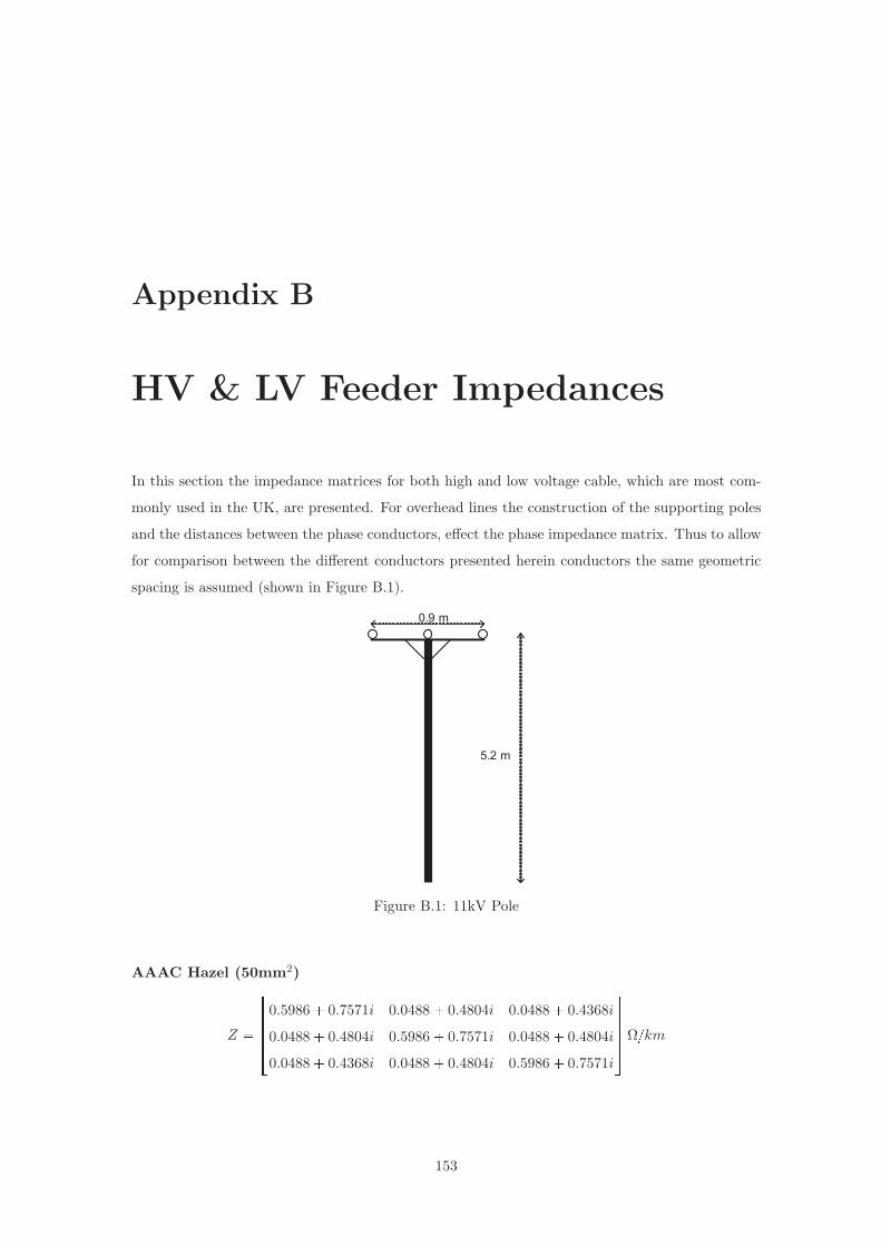
Appendix B
HV & LV Feeder Impedances
In this section the impedance matrices for both high and low voltage cable, which are most com-
monly used in the UK, are presented. For overhead lines the construction of the supporting poles
and the distances between the phase conductors, effect the phase impedance matrix. Thus to allow
for comparison between the different conductors presented herein conductors the same geometric
spacing is assumed (shown in Figure B.1).
5.2 m
0.9 m
Figure B.1: 11kV Pole
AAAC Hazel (50mm2)
Z �
�����
0.5986� 0.7571i 0.0488� 0.4804i 0.0488� 0.4368i
0.0488� 0.4804i 0.5986� 0.7571i 0.0488� 0.4804i
0.0488� 0.4368i 0.0488� 0.4804i 0.5986� 0.7571i
������km
153

C �
�����
9.048 �3.037 �1.652
�3.037 9.766 �3.037
�1.652 �3.037 9.048
�����nF �km
AAAC Oak (100mm2)
Z �
�����
0.3257� 0.8002i 0.0488� 0.4804i 0.0488� 0.4368i
0.0488� 0.4804i 0.3257� 0.8002i 0.0488� 0.4804i
0.0488� 0.4368i 0.0488� 0.4804i 0.3257� 0.8002i
������km
C �
�����
9.58 �3.34 �1.77
�3.34 10.42 �3.34
�1.77 �3.34 9.58
�����nF �km
AAAC Poplar (200mm2)
Z �
�����
0.1873� 0.8438i 0.0488� 0.4804i 0.0488� 0.4368i
0.0488� 0.4804i 0.1873� 0.8438i 0.0488� 0.4804i
0.0488� 0.4368i 0.0488� 0.4804i 0.1873� 0.8438i
������km
C �
�����
10.44 �3.84 �1.95
�3.84 11.49 �3.84
�1.95 �3.84 10.44
�����nF �km
ACSR (150mm2)
Z �
�����
0.2385� 0.8250i 0.0475� 0.4637i 0.0475� 0.4176i
0.0475� 0.4637i 0.2385� 0.8250i 0.0475� 0.4587i
0.0475� 0.4176i 0.0475� 0.4587i 0.2385� 0.8250i
������km
C �
�����
9.41 �3.66 �2.03
�3.66 10.28 �3.49
�2.03 �3.49 9.41
�����nF �km
B.1 LV Cable
To indicate the frequency dependant effect of the cable impedance, the current density (given a
source current of 1A in the top conductor) is shown in figure B.3.
154
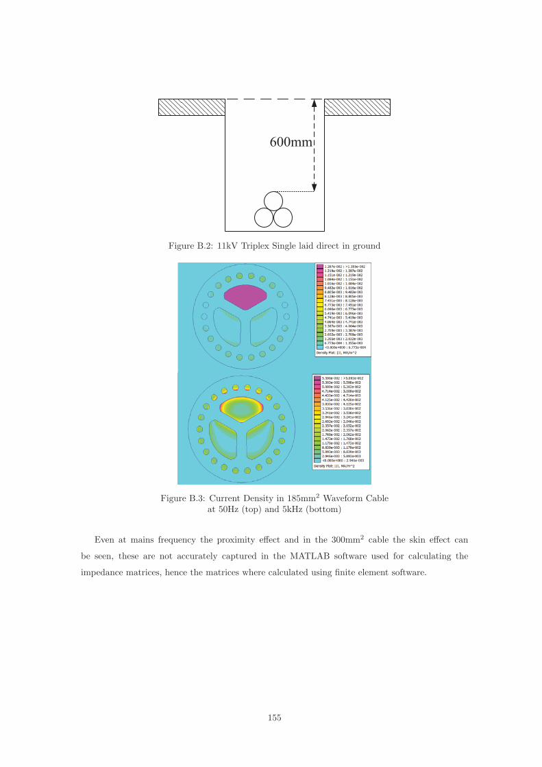
600mm
Figure B.2: 11kV Triplex Single laid direct in ground
Figure B.3: Current Density in 185mm2 Waveform Cableat 50Hz (top) and 5kHz (bottom)
Even at mains frequency the proximity effect and in the 300mm2 cable the skin effect can
be seen, these are not accurately captured in the MATLAB software used for calculating the
impedance matrices, hence the matrices where calculated using finite element software.
155

Appendix C
Direct Load Flow Code
tic; disp('Solving load flow, timestep ...') ; chars=0;
for t = 1 : numel(time)
msg = [num2str(t) ' of ' num2str(numel(time))] ;
fprintf(repmat('\b',1,chars)); fprintf(msg); chars=numel(msg);
k = 0 ;
Pl = Pd(:,t) ;
Ql = Qd(:,t) ;
while 1
W = V ;
Il = conj((Pl + Ql) ./ V );
dV = DLF * Il ;
V = V0 - dV ;
err = max(abs(V-W));
if err <= tol
break
end
k = k + 1 ;
if k >= 20
error([ 'Load flow didnt converge, maxium votlage mismatch %d '...
'greater than tollerance %d at itteration %d, and time %d'],...
err, tol, k, time(t))
end
end
Iline(:,t) = BC * Il ;
Vt(:,t) = V;
It(:,t) = Il;
end
LFt = toc ; fprintf('\nLoad flow took: %d seconds \n',round(LFt));
156