MASTER’S THESIS2006:031 CIV

LINDA LARSSONSAOWANEE SUPHAP

Fluid Structure Interactionin a Rocket Nozzle

MASTER OF SCIENCE PROGRAMME Engineering Physics

Luleå University of TechnologyDepartment of Applied Physics and Mechanical Engineering

Division of Fluid Mechanics and Division of Computer Aided Design

2006:031 CIV • ISSN: 1402 - 1617 • ISRN: LTU - EX - - 06/31 - - SE

Preface This thesis is the final project for the Master of Science in Engineering Physics at Luleå University of Technology. The work has been performed at Volvo Aero Corporation (VAC) in Trollhättan at the department of combustion chambers and nozzles. We would like to thank our supervisors at VAC Dr. Robert Tano and Dr. Lars Ljungkrona for their help and support during the work. We would also like to thank Anders Jansson at Medeso AB in Västerås for his help with the software problems. With the friendly reception from the employees at VAC our work has been a pleasure. Finally we appreciate the time our examiners Professor Staffan Lundström and Dr. Jan-Olov Aidanpää have spent guiding us. Trollhättan, January 2006 Linda Larsson Saowanee Suphap

2

Abstract This thesis is carried out at Volvo Aero in Trollhättan at the Department of combustion chambers and nozzles. The aim is to compare two methods for coupled analysis between structural and fluid calculations and assess if the methods can be applied on a whole nozzle. The softwares used are ANSYS CFX and ANSYS mechanical. The two methods evaluated are unidirectional and bidirectional Fluid Structure Interaction (FSI). The calculations are made on a section of half a coolant channel and the flow of the coolant, heat transfer and the displacements are calculated for the first three seconds of a start-up. In unidirectional FSI the calculations in ANSYS CFX are made first, the convection and pressure at the walls of the channel obtained are then exported to ANSYS mechanical where the displacements are calculated. In bidirectional FSI the calculations are performed simultaneously. The heat flux and total force density are calculated in ANSYS CFX while the temperature and displacement are calculated in ANSYS Mechanical. The conclusion of the thesis is that due to long calculation times neither of the methods is applicable on a whole nozzle even though unidirectional FSI is about ten times faster than bidirectional FSI for the case studied.

3

Contents 1 Introduction................................................................................................................. 4

1.1 Volvo Aero.......................................................................................................... 4 1.2 Nozzles................................................................................................................ 4 1.3 Aim of the thesis ................................................................................................. 4

2 Theory ......................................................................................................................... 6

2.1 Computational Fluid Dynamics .......................................................................... 6 2.1.1 Governing equations ................................................................................... 6 2.1.2 Finite volume method ................................................................................. 7 2.1.3 Turbulence modelling ............................................................................... 11

2.2 Finite Element Method ..................................................................................... 16 2.2.1 Structural static analysis ........................................................................... 16 2.2.2 Thermal analysis ....................................................................................... 21 2.2.3 Errors in FEM ........................................................................................... 25

2.3 Fluid structure interaction ................................................................................. 27 3 Method and results.................................................................................................... 29

3.1 Outline of work ................................................................................................. 30 3.2 Modelling in CFX............................................................................................. 31

3.2.1 Steady state ............................................................................................... 31 3.2.2 Transient ................................................................................................... 37

3.3 Modelling in ANSYS........................................................................................ 40 3.3.1 Building the model.................................................................................... 40 3.3.2 Apply boundary conditions and loads....................................................... 43 3.3.3 Solution controls ....................................................................................... 46

3.4 Unidirectional simulations ................................................................................ 47 3.4.1 Thermal results and analyses .................................................................... 49 3.4.2 Structural results and analyses .................................................................. 50

3.5 Bidirectional simulations .................................................................................. 52 3.5.1 Thermal results and analyses .................................................................... 57 3.5.2 Structural results and analyses .................................................................. 59

4 Discussion and conclusions ...................................................................................... 61

4.1 Unidirectional and bidirectional FSI................................................................. 63 4.2 Limitations and Problems ................................................................................. 64 4.3 Conclusion ........................................................................................................ 65 4.4 Future work....................................................................................................... 66

5 References................................................................................................................. 67

4

1 Introduction

1.1 Volvo Aero Volvo Aero Corporation is part of the Volvo Group and in Sweden it is located in Stockholm, Malmö and Trollhättan (headquarter). The Corporation manufactures and develops components for aircraft engines, gas turbines and rocket parts where nozzles for the European Arianne rockets is one example. This thesis is done at Volvo Aero in Trollhättan at the department of combustion chambers and nozzles.

1.2 Nozzles A nozzle is a subcomponent of the rocket engine and an extension of the combustion chamber. It is where the gas expands and accelerates at the cost of pressure of the fluid. The nozzle and the combustion chamber are both exposed to high temperatures and must therefore be cooled to minimize structural changes. Designing the nozzles is a complicated process since the high temperatures result in large thermal loads. The nozzle needs to be stable enough to manage these loads, and at the same time it needs to be light in order to maximize the lift capacity of the rocket. [1] The four main methods to cool a nozzle are convection, radiation, ablation and film cooling. Radiation cooling means that the flame is allowed to heat the wall which is only cooled by radiation of heat into the surroundings. When the nozzle is covered with a layer which burns off during the usage it is said to be ablation cooled. In film cooling the coolant flows along the inside of the wall in order to create a layer to prevent heat transportation from the flame to the wall. Film cooling is in theory an effective cooling method, but in reality it is very sensitive to outer disturbances which results in inadequate cooling. The most frequently used method is convection cooling where the nozzle has two walls. The coolant flows between these walls and transports the heat away. The coolant is often the same substance used as the fuel for the rocket, for example hydrogen. [1]

1.3 Aim of the thesis For convective cooled rocket nozzles there are strong connections between the structural properties and the flow. Loads obtained from the flow calculations need to be applied as boundary conditions to the structural calculations. Today there is no simple way of doing this. The aim of this thesis is to evaluate two methods for load transfer. This is done by studying the interaction between the flow and the structure, Fluid Structure Interaction (FSI).

5

The rocket nozzle used for calculations in this thesis has about 700 coolant channels, but only a segment of one channel is modelled. The heating of the nozzle causing deformations is studied. Heat transfer coefficient and bulk temperature is applied to the inner wall of the nozzle instead of modelling the entire flame, although in reality the flame is more coupled to the deformation of the nozzle. The only flow modelled is therefore the flow of the coolant. In the structural calculations the dynamical effects such as acceleration are neglected, but the problem is still transient. The methods that are to be evaluated are the transfer of data between the flow calculation software ANSYS CFX and the finite element software ANSYS Mechanical in the following ways: - Unidirectional FSI

Load transfer from ANSYS CFX to ANSYS Mechanical.

- Bidirectional FSI Load transfer from ANSYS CFX to ANSYS Mechanical and from ANSYS Mechanical to ANSYS CFX.

Finally the goal of this thesis is to assess whether the methods are possible to apply to a whole nozzle with the flame.

6

2 Theory To understand the thesis this section describes the theory of Computational Fluid Dynamics (CFD) and Finite Element Method (FEM).

2.1 Computational Fluid Dynamics CFD is a computational tool for calculating different fluid dynamic processes, such as heat, mass and momentum transfer. CFD numerically evaluates partial differential equations, among others the Navier-Stokes equations. Some phenomena are described by different models, for example turbulence models. The numerical method that is frequently used in CFD is the finite volume method. This is the method used in CFX.

2.1.1 Governing equations Newtonian compressible fluid A Newtonian compressible fluid is described by five partial differential equations. The first of these equations describe the conservation of mass which means that rate of mass flow into a volume is equal to the rate of increase of mass in the volume according to

( ) 0=+∂∂ uρρ div

t (2.1.1)

where ρ is density of the fluid and u is the velocity vector in Cartesian coordinates.[1] Newtons second law combined with the fact that for a Newtonian fluid the size of the stress acting on a control volume is proportional to the rate of deformation results in the famous Navier-Stokes equations. The three equations below describe the conservation of momentum in three dimensions. The rate of increase of momentum of a fluid particle is equal to the sum of forces acting on the particle as described by the following equations

( ) ( ) ( ) MxSugraddivxpudiv

tu

++∂∂

−=+∂

∂ µρρ u (2.1.2a)

( ) ( ) ( ) MySvgraddiv

ypvdiv

tv

++∂∂

−=+∂

∂ µρρ u (2.1.2b)

( ) ( ) ( ) MzSwgraddiv

zpwdiv

tw

++∂∂

−=+∂

∂ µρρ u (2.1.2c)

7

Here p is the pressure, µ is the dynamic viscosity and S is the source term. u, v and w are the velocity components of u. [2] The final partial differential equation that governs the flow is the energy equation (2.1.3). This equation is derived from the first law of thermodynamics. The rate of energy increase of a fluid particle is equal to the net rate of heat added to the fluid particle and the net rate of work done to the particle. [2]

( ) ( ) ( ) iSTgraddivdivpidivti

+++−=+∂

∂ Φρρ λuu (2.1.3)

where i is the internal energy, λ is the thermal conductivity, T is the temperature and

( )2222222

322 udiv

yw

zv

xw

zu

xv

yu

zw

yv

xu µµΦ −⎟

⎟

⎠

⎞

⎜⎜

⎝

⎛⎟⎟⎠

⎞⎜⎜⎝

⎛∂∂

+∂∂

+⎟⎠⎞

⎜⎝⎛

∂∂

+∂∂

+⎟⎟⎠

⎞⎜⎜⎝

⎛∂∂

+∂∂

+⎟⎟

⎠

⎞

⎜⎜

⎝

⎛⎟⎠⎞

⎜⎝⎛

∂∂

+⎟⎟⎠

⎞⎜⎜⎝

⎛∂∂

+⎟⎠⎞

⎜⎝⎛

∂∂

= (2.1.4)

These five partial differential equations have seven unknown variables (u, v, w, p, T, ρ and i). In order for this system of equations to be closed one equation for pressure and one for internal energy is introduced. [2]

( )Tpp ,ρ= ; ),( Tii ρ= (2.1.5a, b) Heat transfer in solid domain It is also possible to model the heat transfer in solid domains using CFD. For these domains only a simplified version of the energy equation is solved. [3]

( ) ( ) STgraddivt

TCp +=∂

∂λ

ρ (2.1.6)

where Cp is the specific heat capacity.

2.1.2 Finite volume method The equations in section 2.1.1 are only possible to solve analytically for a few simple cases. In order to solve the equations numerically the flow domain is divided into small volumes. Integration The first step of the finite volume method is to integrate the governing equations over each finite volume. [2] The governing equations can all be said to be of the same form as the general transport equation below.

8

( ) ( ) ( )

termsourcetermdiffusivetermconvective

termchangeofRate

graddivdivt φφρφρφ Su +Γ=+

∂∂

44 344 2143421321

(2.1.7)

where φ is a fluid property and Γ is the diffusion coefficient. [2] Equation (2.1.7) integrated over a control volume, the general transport equation becomes

( ) ( ) ( ) dVdVgraddivdVdivdVt CVCVCVCV

∫∫∫∫ +Γ=+∂

∂φφρφρφ Su (2.1.8)

Gauss divergence theorem gives

( ) ( ) ( ) dVdAgraddAdVt CVAACV

∫∫∫∫ +Γ⋅=⋅+⎟⎟⎠

⎞⎜⎜⎝

⎛

∂∂

φφρφρφ Snun (2.1.9)

For steady state flow the transient term can be ignored, which yields [2]

( ) ( ) dVdAgraddACVAA∫∫∫ +Γ⋅=⋅ φφρφ Snun (2.1.10)

For a transient process the equation (2.1.9) is also integrated over time and the general transport equation becomes [2]

( ) ( ) ( ) dtdVdtdAgraddtdAdtdVt t CVt At At CV

∫ ∫∫∫∫∫∫ ∫∆∆∆∆

+Γ⋅=⋅+⎟⎟⎠

⎞⎜⎜⎝

⎛

∂∂

φφ φρφρφ Snun (2.1.11)

Discretisation The second step of the finite volume method is to express the partial differential equations as algebraic equations.

Figure 2.1 One dimensional grid.

9

The figure above is the one dimensional grid where P, W and E are computational nodes, w and e are the grid faces in the middle between the nodes and ∆x represents one finite volume. [2] A way to discretise the transport equation is to use the upwind differencing scheme. This scheme is of the first order and it accounts for the direction of the flow. Below the process of numerical integration and later the discretisation of the governing equations is described. Example 2.1.1 The problem described is a convection-diffusion problem in one dimension. The second and third term of the general transport equation (2.1.7) is used.

( )⎟⎠⎞

⎜⎝⎛Γ=

dxd

dxd

dxud φφρ (2.1.12)

The one dimensional continuity equation is also used.

( ) 0=dx

ud ρ (2.1.13)

Equation (2.1.12) and (2.1.13) are integrated over ∆x where A is the area of the faces. This gives

( ) ( )we

we dxdA

dxdAuAuA ⎟

⎠⎞

⎜⎝⎛Γ+⎟

⎠⎞

⎜⎝⎛Γ=−

φφφρφρ (2.1.14)

(2.1.15)

The variables F and D are defined as

uF ρ= ; x

DδΓ

= (2.1.16a, b)

The values of F and D at the cell faces then become

ww uF )(ρ= ; ee uF )(ρ= (2.1.17a, b)

WP

ww x

DδΓ

= ; PE

ee x

DδΓ

= (2.1.18a, b)

The next step is to apply the differencing scheme, in this example an upwind scheme. [2]

( ) ( ) 0=− we uAuA ρρ

10

If the direction of the flow is positive which means it flows from west to east. The property φ at the west cell face w is assumed to be equal to φ at the west node W. Also φ at the east cell face is said to be the same as φ at the node P.

Ww φφ = ; Pe φφ = (2.1.19a, b) This inserted to (2.1.14) gives the algebraic equation ( ) ( )[ ] ( ) EeWwWPweeWW DFDFFDFD φφφ ++=−+++ (2.1.20)

The upwind scheme gives a robust solution, but it is sensitive to numerical diffusion. This means that if the flow is not normal to the element faces the results are smeared out over the flow domain. This means that shocks for example are seen as smooth curves. [2][3] To achieve a more accurate solution φ at the grid faces can be approximated with a higher order series.

rgradWw ∆⋅+= φβφφ (2.1.21) and

rgradPe ∆⋅+= φβφφ (2.1.22) where r∆ is the distance and direction from the cell face to the corresponding node. β is a constant between 0 and 1. β=0 results in is an upwind scheme and for β=1 the resulting scheme is of the second order. This second order scheme is less robust and there is a risk of numerical dispersion, which means that there can be oscillations in the solution. This can often happen when there are shockwaves in the solution. [3] As a compromise between the first and second order scheme CFX has two options, the High resolution scheme and Specific blend. For Specific blend the user is asked to set β to a value, and for high resolution CFX automatically sets a value of β as high as possible for each node. [3] Iteration When the governing equations are discretised and consist of algebraic equations CFD uses an iterative numerical method to solve the problem. A simplification of the method used can be described in the following way. The algebraic equations can be written as matrices. [ ][ ] [ ]bA =φ (2.1.23)

11

where [A] is the matrix containing coefficients, [φ ] is the solution vector and [b] is a vector. [3] To obtain a solution a correction 'φ is added to the initial assumption nφ to achieve a more accurate solution of 1+Φ n .

'1 φφφ +=+ nn (2.1.24)

'φ is calculated from

nrA=

∂∂ 'φφ

(2.1.25)

where rn is the residual, which is obtained from

nn Abr φ−= (2.1.26) This process is repeated until the solution is fully converged and the residuals are minimized. [3]

2.1.3 Turbulence modelling For most industrial flows Navier-Stokes equations most be complimented in some way. When the Reynolds number exceeds certain values the flow becomes turbulent on length scales and time scales much smaller than what is practically possible to resolve in any grid. To solve turbulent flow with a direct numerical method takes much more computing power than is possible today, therefore turbulence models are introduced. Reynolds equations Most turbulence models originate from the Reynolds averaged equations. These equations are obtained when the velocity u of the fluid is divided into two components, the mean velocity U and the fluctuating velocity u’.

'uUu += (2.1.27) U yields from

∫∆+

∆=

tt

tdt

tuU 1 (2.1.28)

With the new velocity inserted to the continuity equation (2.1.1) it becomes

12

( ) 0=+∂∂ Uρρ div

t (2.1.29)

and the Navier-Stokes equations transforms into

( ) ( ) ( ) ( ) Mdivgraddivgraddivt

SuuUUUU+⊗−+−=⊗+

∂∂ ''ρµρρ p (2.1.30)

In the same way as with the velocity a general transport property ϕ is divided into the average quantity φ and the fluctuating quantity ϕ’.

'ϕφϕ += (2.1.31) This yields the scalar transport equation.

( ) ( ) ( ) ( )''ϕρφρφρφφ uU divgraddivdiv

t−Γ=+

∂∂ (2.1.32)

In equation (2.1.30) and (2.1.32) two new unknown terms arise, the Reynolds stress '' uu ⊗ρ and the Reynolds flux ''ϕρu . The bars over these terms mean that they are averaged over time. [2] Eddy viscosity models A group of models called the eddy viscosity turbulence models assume that turbulent flow consists of eddies where the Reynolds stress is proportional to the mean velocity gradient in the following way

( )( )Ttt divk UUUuu ∇+∇+−−=⊗− µδµδρρ

32

32'' (2.1.33)

where k is the turbulent kinetic energy and is given by

2'21 u=k (2.1.34)

In the same way the Reynolds fluxes are given by

φϕρ ∇Γ=− t''u (2.1.35) where the eddy diffusivity Γt is given by the turbulent viscosity µt and the turbulent Prandtl number Prt.

13

t

tt Pr

µ=Γ (2.1.36)

All the eddy viscosity models this far are basically the same. It is the method to determine µt that is different between the models. [3] The k-ε model The k-ε model defines µt as

ερµ µ

2kCt = (2.1.37)

where µC is a constant. k and the turbulent eddy dissipation ε are calculated from the following two equations

( ) ( ) ρεσµµρρ

−+⎥⎦

⎤⎢⎣

⎡⎟⎟⎠

⎞⎜⎜⎝

⎛+=+

∂∂

kk

t Pgradkdivkdivtk U (2.1.38)

( ) ( ) ( )ρεεε

σµµερρε

εεε

21 CPCk

graddivdivt k

t −+⎥⎦

⎤⎢⎣

⎡⎟⎟⎠

⎞⎜⎜⎝

⎛+=+

∂∂ U (2.1.39)

where kσ , εσ , 1εC and 2εC are constants and Pk is the turbulence production. [3] The Wilcox k-ω model In the k-ω model µt is defined as

ωρµ k

t = (2.1.40)

Here k and the turbulent frequency ω are derived from the equations below.

( ) ( ) ωρβσµµρρ kPgradkdivkdiv

tk

kk

t '−+⎥⎦

⎤⎢⎣

⎡⎟⎟⎠

⎞⎜⎜⎝

⎛+=+

∂∂ U (2.1.41)

( ) ( ) 2βρωωαω

σµµωρρω

ω

−+⎥⎦

⎤⎢⎣

⎡⎟⎟⎠

⎞⎜⎜⎝

⎛+=+

∂∂

kt P

kgraddivdiv

tU (2.1.42)

kσ , ωσ , α, β’ and β are model constants. [3]

14

The SST model The k-ω and the k-ε models have their advantages and disadvantages. The Shear Stress Transport model (SST) combines the best properties of these two models. The k-ω model handles the flow near no-slip walls much better than the k-ε model, and the grid near the wall does not have to be as fine and the flow is not so grid dependent. On the other hand the handling of free-stream flow in the k-ω model is much more sensitive to inaccurate boundary conditions as compared to the k-ε model. [3] Near wall flow In turbulent flows the flow near the walls also need to be approximated by a model. The flow near a no-slip wall is not affected by the free stream flow. Only the distance to the wall y, the density of the fluid ρ, the viscosity µ and the wall shear stress τw are important. In this case an expression for the velocity near the wall takes the form [2]

( )++ =⎟⎟⎠

⎞⎜⎜⎝

⎛== yf

yuf

uUu

µρ τ

τ

(2.1.43)

u+ and y+ are dimensionless variables of the near wall velocity and distance. uτ is the friction velocity is given by

2/1

⎟⎟⎠

⎞⎜⎜⎝

⎛=

ρτ

τwu (2.1.44)

Linear sub-layer For the fluid closest to the wall, when y+<5, the shear stress is equal to the wall shear stress τw. This yield

µτ y

U w= (2.1.45)

as an expression for the velocity at the wall. This is the same as y+=u+. Even though the velocity U within this layer is not directly coupled to turbulence properties it is indirectly since the velocity in the log-layer is affected. [2] Log-law layer The flow at a distance of approximately 30< y+<500 from the wall exhibits a logarithmic behaviour. Both the viscous and turbulent properties are important in this layer. The relation between the velocity and the wall distance in this region is expressed as

)ln(1ln1 +++ =+= EyByuκκ

(2.1.46)

where κ, B and E are constants dependent of the roughness of the wall. [2]

15

When the first node of the grid has a distance to the wall that is less than y+=5 or even better y+=1, the grid near the wall is said to be resolved and a linear sub-layer can be assumed. For grids with the first node at a distance between y+=30 and 500 the CFD-software should use wall functions, that originate from the log-law, to approximate the behaviour of the flow. In CFX, when the k-ω or SST models are used, there is automatic wall handling. This means that the program automatically chooses the method to solve the near-wall flow, and it also handles the region of 5< y+<30 automatically. [2][3] 2.1.4 Errors in CFD When modelling a flow with CFD it is important to know the limitations. There are several sources of errors and uncertainties in CFD. They can be divided into certain categories. Model uncertainties These are uncertainties due to assumptions and simplifications of the real flow. In many cases these simplifications are necessary in order to be able to solve the problem. One example of this is turbulence models, another example can be the neglecting of chemical reactions and further on. [4] Numerical errors Numerical errors occur from the fact that the governing equations are not solved directly, but are discretised with finite resolution in time and space. The errors can be larger when a first order differencing scheme is used instead of a higher order scheme. [4] Iteration or convergence errors When the residuals have not reached desired levels errors occur. There can be several reasons for this, for example the models and boundary conditions chosen may not allow convergence for the specified flow. In other cases the iteration process takes too long and is aborted before convergence is reached. [4] Round-off errors These are errors caused by the limitations of the computer. There may not be enough space to store values during the solution process, and therefore the values are rounded off. A solution more accurate than machine accuracy is impossible. [4] Application uncertainties Inexact boundary conditions, geometry or unavailable data can also cause inaccurate results. [4] Other errors can naturally occur from user errors and code errors in the software used.

16

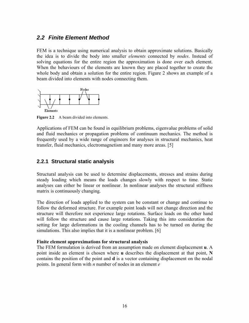
2.2 Finite Element Method FEM is a technique using numerical analysis to obtain approximate solutions. Basically the idea is to divide the body into smaller elements connected by nodes. Instead of solving equations for the entire region the approximation is done over each element. When the behaviours of the elements are known they are placed together to create the whole body and obtain a solution for the entire region. Figure 2 shows an example of a beam divided into elements with nodes connecting them.

Figure 2.2 A beam divided into elements. Applications of FEM can be found in equilibrium problems, eigenvalue problems of solid and fluid mechanics or propagation problems of continuum mechanics. The method is frequently used by a wide range of engineers for analyses in structural mechanics, heat transfer, fluid mechanics, electromagnetism and many more areas. [5]

2.2.1 Structural static analysis Structural analysis can be used to determine displacements, stresses and strains during steady loading which means the loads changes slowly with respect to time. Static analyses can either be linear or nonlinear. In nonlinear analyses the structural stiffness matrix is continuously changing. The direction of loads applied to the system can be constant or change and continue to follow the deformed structure. For example point loads will not change direction and the structure will therefore not experience large rotations. Surface loads on the other hand will follow the structure and cause large rotations. Taking this into consideration the setting for large deformations in the cooling channels has to be turned on during the simulations. This also implies that it is a nonlinear problem. [6] Finite element approximations for structural analysis The FEM formulation is derived from an assumption made on element displacement u. A point inside an element is chosen where u describes the displacement at that point, N contains the position of the point and d is a vector containing displacement on the nodal points. In general form with n number of nodes in an element e

17

[ ] Ndd

d

NNu =⎪⎭

⎪⎬

⎫

⎪⎩

⎪⎨

⎧

== ∑=

M

K β2

β1

β2

β1

kkk dN ,,

n

1

ββ (2.2.1)

where k=1,2,…,n and β =1,2,3 due to three dimensions. [7] The velocity v at the chosen point can easily be described by differentiating the equation above with respect to time

[ ] Nww

w

NNv 2

1

21 =⎪⎭

⎪⎬

⎫

⎪⎩

⎪⎨

⎧

== ∑=

M

K β

β

ββββ ,,wN n

1k

kk (2.2.2)

where w is the nodal velocity. Example 2.2.1 The chosen point inside the element is described by nearby nodes. Contribution from one node represented with number 1 the vectors and matrices look like

⎪⎭

⎪⎬

⎫

⎪⎩

⎪⎨

⎧

=31

21

11

1

dd d

βd ;⎪⎭

⎪⎬

⎫

⎪⎩

⎪⎨

⎧

=3

2

1

uuu

u ;⎪⎭

⎪⎬

⎫

⎪⎩

⎪⎨

⎧

=3

2

1

vvv

v (2.2.3a, b, c)

and the shape function is specified as

IN ββ1N=1 (2.2.4)

where 1=β

1N and I=identity matrix. Finally for displacement and velocity contributed by node number 1 at the point looks like

⎪⎪⎭

⎪⎪⎬

⎫

⎪⎪⎩

⎪⎪⎨

⎧

⎪⎭

⎪⎬

⎫

⎪⎩

⎪⎨

⎧

⎥⎥⎥

⎦

⎤

⎢⎢⎢

⎣

⎡

⎥⎥⎥

⎦

⎤

⎢⎢⎢

⎣

⎡=

⎪⎭

⎪⎬

⎫

⎪⎩

⎪⎨

⎧

M

K31

21

11

3

2

1

,100010001

uuu

ddd

;

⎪⎪⎭

⎪⎪⎬

⎫

⎪⎪⎩

⎪⎪⎨

⎧

⎪⎭

⎪⎬

⎫

⎪⎩

⎪⎨

⎧

⎥⎥⎥

⎦

⎤

⎢⎢⎢

⎣

⎡

⎥⎥⎥

⎦

⎤

⎢⎢⎢

⎣

⎡=

⎪⎭

⎪⎬

⎫

⎪⎩

⎪⎨

⎧

M

K31

21

11

3

2

1

,100010001

vvv

www

(2.2.5a, b)

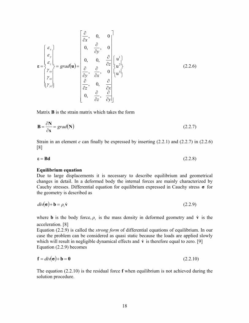
Fundamental mechanics of materials states that the strain ε in the elements is derived from displacement matrix ( )ugrad , see equation (2.2.6). The strain components are divided into normal strain ε and shear strain γ .

18

( )⎪⎭

⎪⎬

⎫

⎪⎩

⎪⎨

⎧

⎥⎥⎥⎥⎥⎥⎥⎥⎥⎥⎥⎥⎥⎥

⎦

⎤

⎢⎢⎢⎢⎢⎢⎢⎢⎢⎢⎢⎢⎢⎢

⎣

⎡

∂∂

∂∂

∂∂

∂∂

∂∂

∂∂

∂∂

∂∂

∂∂

==

⎪⎪⎪⎪

⎭

⎪⎪⎪⎪

⎬

⎫

⎪⎪⎪⎪

⎩

⎪⎪⎪⎪

⎨

⎧

=3

2

1

uuu

,,0

,0,

0,,

,0,0

0,,0

0,0,

yz

xz

xy

z

y

x

grad

yz

xz

xy

z

y

x

uε

γγγεεε

(2.2.6)

Matrix B is the strain matrix which takes the form

( )NxNB grad=

∂∂

= (2.2.7)

Strain in an element e can finally be expressed by inserting (2.2.1) and (2.2.7) in (2.2.6) [8]

Bdε = (2.2.8) Equilibrium equation Due to large displacements it is necessary to describe equilibrium and geometrical changes in detail. In a deformed body the internal forces are mainly characterized by Cauchy stresses. Differential equation for equilibrium expressed in Cauchy stress σ for the geometry is described as

( ) vbσ &tρdiv =+ (2.2.9) where b is the body force, tρ is the mass density in deformed geometry and v& is the acceleration. [8] Equation (2.2.9) is called the strong form of differential equations of equilibrium. In our case the problem can be considered as quasi static because the loads are applied slowly which will result in negligible dynamical effects and v& is therefore equal to zero. [9] Equation (2.2.9) becomes

( ) 0bσf =+= div (2.2.10) The equation (2.2.10) is the residual force f when equilibrium is not achieved during the solution procedure.

19

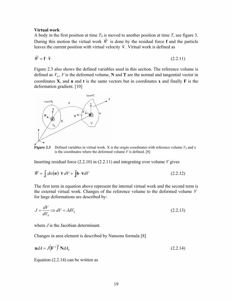
Virtual work A body in the first position at time T0 is moved to another position at time T, see figure 3. During this motion the virtual work W~ is done by the residual force f and the particle leaves the current position with virtual velocity v~ . Virtual work is defined as

vf ~~ ⋅=W (2.2.11) Figure 2.3 also shows the defined variables used in this section. The reference volume is defined as 0V , V is the deformed volume, N and T are the normal and tangential vector in coordinates X, and n and t is the same vectors but in coordinates x and finally F is the deformation gradient. [10]

Figure 2.3 Defined variables in virtual work. X is the origin coordinates with reference volume V0 and x

is the coordinates where the deformed volume V is defined. [8] Inserting residual force (2.2.10) in (2.2.11) and integrating over volume V gives

( ) ∫∫ ⋅+⋅=VV

dVdV divW vbvσ ~~~ (2.2.12)

The first term in equation above represent the internal virtual work and the second term is the external virtual work. Changes of the reference volume to the deformed volume V for large deformations are described by:

00

JdVdVdVdVJ =⇒= (2.2.13)

where J is the Jacobian determinant. Changes in area element is described by Nansons formula [8]

( ) 01- dAJdA NFn T

= (2.2.14) Equation (2.2.14) can be written as

20

00

dAJdAdAdAJ ∗∗ =⇒= (2.2.15)

where

( ) ΝFn TJJ 1−∗ = (2.2.16) Equation (2.2.12) expressed in reference volume is

( ) ∫∫ ⋅+⋅=0V 0

0V 0 JdVJdV divW vbvσ ~~~ (2.2.17)

The first term combined with Gauss theorem, the law for the operator div and the surface stress vector t(n) can be written as

( ) ( )∫∫∫ −⋅=⋅ ∗

0V 000A

0V0 JdV graddAJJdV div vσvtvσ ~~~ : (2.2.18)

which is called the weak form of the differential equations of equilibrium. Inserting (2.2.18) in (2.2.17), the virtual work will take the following form when equilibrium is achieved

( ) 0~~~~

work virtualInternal work virtualExternal

=−⋅+⋅= ∫∫∫ ∗

444 3444 214444 34444 21 0V 00V 00

0AJdV gradJdVdAJW vσv bvt : (2.2.19)

In terms of large deformations Cauchy stress will change due to rigid body rotation which is described in a fixed coordinate system. Cauchy stress is not objective and can not be used in constitutive law. One can express Cauchy stress with an objective rate of stress called Jaumann-Zaremba

ΩσσΩσσ ⋅+⋅−=∇ & (2.2.20) where σ& is the time rate of Cauchy stress and Ω is the spin tensor. [8] After some calculations that can be seen in appendix A the displacement changes is described as

( )444444 3444444 214444 34444 21444 3444 21

ss stiffneLoad

V 00A

ss stiffneStress

V 0

ss stiffneMaterial

0VJdVdAJJdV2JdV W

t 0∫∫∫∫ ∂

⋅∂+

∂⋅∂

+⋅⋅+=∂∂ ∗

000

)~()~()~~

(:~~ :

t

t- v bvtDDLLσDD:C T

(2.2.21)

where C is the isotropic, linear elastic stiffness, D is the rate of deformation and L velocity gradient and L~ correspond the virtual velocity gradient. The last two terms in

21

equation above will only affect the stiffness matrix if it is surface loads. Below is an example of how the stiffness matrix is calculated. The demonstration will only be shown on the material stiffness matrix. Example 2.2.2 The velocity gradient of real and virtual velocity are defined as

wBwx

NxvL k

k ⋅=∂

∂=

∂∂

= ∑=

n

1

k

ββ

; wBwx

NxvL k ~~ ~~ n

1⋅=

∂∂

=∂∂

= ∑=k

kβ

β

(2.2.22a, b)

Hooke’s law describes the stress according to

( ) ( )00 εdBCεεCσ −⋅=−= (2.2.23) Inserting (2.2.2), (2.2.22) and (2.2.23) in the equilibrium equation (2.2.19) gives

( ) ( ) ( ) ( ) ⇒=−−+ ∫∫∫ ∗ 0εΒdCwBbwNtwN000 V 0V 00A

JdVJdVdAJ 0TTT ~~~

( ) ⇒=⎟⎠⎞⎜

⎝⎛ −−+ ∫∫∫ ∗ 0εΒdCBbNtNw

000 V 0V 00AJdVJdVdAJ 0

TTTT~

( )∫∫∫∫ ++=⎟⎠⎞⎜

⎝⎛ ∗

0000 V 0V 00AV 0 JdVJdVdAJdVJ 0CεBbNtNdCΒB TTTT (2.2.24)

This equation in the standard formulation

fKd = (2.2.25) where K is the stiffness matrix, d is the displacement and f represent the force is

∫ ⋅⋅=0V 0dVJΒCBK T (2.2.26)

( )

444 3444 2144344214434421ctorstrain ve Initial

0

vectorLoadvectorBoundary

∫∫∫ ⋅⋅+⋅+⋅= ∗

000 V 0V 00AJdVJdVdAJ εCBbNtNf TTT (2.2.27)

2.2.2 Thermal analysis Thermal analysis is applied to calculate temperature distribution, heat loss or gain, thermal gradients and thermal fluxes. ANSYS can manage heat transfer as conduction, convection and radiation. The program make usage of heat balance equation derived from the principle of conservation of energy. Since ANSYS perform finite element

22

computations it starts with calculating the nodal temperature and can then finding other thermal quantities. There are two types of thermal analyses: steady-state or transient. In the first case the loads do not vary over a period of time which it does in the second case. Thermal equations Convection is when heat transfer is caused by flow of a fluid or gas. At the boundary between the fluid and the coolant channel wall, the velocity of the flow is estimated as stationary therefore the heat is transferred by conduction. The heat transfer will continue until the process has reached equilibrium and there are no temperature differences in the medium. Transmission of heat by convection is a complicated progress because one needs to determine the velocity of the medium and then calculate the temperature. [11] Thermal energy or energy in general can not disappear or be recreated, the energy is said to be conserved. The first law of thermodynamics over a control volume is written as

( ) ( ) qdivTgradtTC p &&&=+⎟

⎠⎞

⎜⎝⎛ ⋅+

∂∂ qvTρ (2.2.28)

where ρ is the density, pC the specific heat, T the temperature, t is the time, q the heat flux vector, v the velocity vector for mass transport of heat and q&&& is the heat generation rate per unit volume. Note that velocity v is the same as u in section 2.1. Equation (2.2.28) might be recognized as the strong form of the heat flow. [6] In thermal analysis ANSYS make use of virtual work and equation (2.2.28) is multiplied with a virtual temperature T~

( ) ( ) TqTdivTTgradtTC p

~~~&&&=⋅+⎟

⎠⎞

⎜⎝⎛ ⋅+

∂∂ qvTρ (2.2.29)

The law for the operator divergence is defined as

( ) ( ) ( )TgradTdivTdiv ~:~~ qqq +⋅=⋅ (2.2.30) and equation (2.2.29) can be written as

( ) ( ) ( )TgradTqTdivTTgradtTCp

~:~~~ qqvT +=⋅+⎟⎠⎞

⎜⎝⎛ ⋅+

∂∂

&&&ρ (2.2.31)

The flux vector q represents the direction of heat flow the body is exposed to. The interesting part of q on the boundary is the normal component since the tangential do not contribute to the flux that passes through the unit. The normal component of the flux q is

nqT ˆ⋅−=nq (2.2.32)

23

Note that the negative sign arises from heat transportation to the body. [12]

Figure 2.4 Heat flux on the surface. Relations between the heat flux q and temperature gradient ( )Tgrad is described by Fourier’s law as

( )Tgrad⋅−= λq (2.2.33) where λ is the conductivity matrix. Inserting this in equation (2.2.31) gives

( ) ( )( ) ( ) ( )TgradTgradTqTTgraddivTTgradtTC T

p~~~~ ⋅⋅−=⋅+⎟

⎠⎞

⎜⎝⎛ ⋅+

∂∂ λλ-v &&&ρ (2.2.34)

Boundary conditions Solving differential equations always requires boundary conditions and this equation for thermal analysis is not an exception. In this problem there are three boundary conditions to be considered. On some surfaces for example surface *T

S known temperatures *T are activated. Let the bulk temperature of the fluid be ∞T and the surface temperature of the body ST . Efficiency of the heat transfer is defined by heat transfer coefficientα . Newton’s convection boundary condition will describe the heat flow nq on the convection surface CS as

( )Sn TTq −= ∞α (2.2.35) The last boundary condition is where the heat flows nq are acting on surface hS . [12] To summarize the boundary conditions in this problem it will be

( )⎪⎩

⎪⎨

⎧

−=

−=

=

∞

hnT

cSn

T

Sqnq

STTq

STT *

surfaceon ˆ

surfaceon

surfaceon *

α (2.2.36a, b, c)

where the total boundary is hcT

SSSS ++= * .

24

Figure 2.5 Thermal boundary conditions including convection. Inserting the boundary conditions in equation (2.2.34), integrating over the volume V and apply Gauss theorem yields the weak form of three dimensional heat flow

( ) ( ) ( ) dSTTTdSqTdVTqdVTgradTgraddVTTgradtTC

ch S SS nVVV p ∫∫∫∫∫ −++=⋅⋅+⎟⎠⎞

⎜⎝⎛ ⋅+

∂∂

∞ )(~~~~~ αρ &&&λv T (2.2.37)

Finite element approximations for thermal analyses The approximations in heat flow are done in the same way as for structural elements. The temperature T on an element with global shape function N and a is the nodal temperatures is written as

[ ] Naa

a

N NT =⎪⎭

⎪⎬

⎫

⎪⎩

⎪⎨

⎧

== ∑=

M

K β2

β1

β2

β1

kkk aN

n

1

ββ (2.2.38)

where k=1,2,…,n and β =1,2,3 due to three dimensions. [7] Temperature gradients will here be

( ) ( ) BaaNT ==

⎥⎥⎥⎥⎥⎥

⎦

⎤

⎢⎢⎢⎢⎢⎢

⎣

⎡

∂∂∂∂∂∂

= grad

zTyTxT

grad (2.2.39)

where

25

( )NB grad

zN

zN

yN

yN

xN

xN

=

⎥⎥⎥⎥⎥⎥

⎦

⎤

⎢⎢⎢⎢⎢⎢

⎣

⎡

∂∂

∂∂

∂∂

∂∂

∂∂

∂∂

=

K

K

K

21

21

21

(2.2.40)

The same approximation is done for virtual temperature

[ ] aNa

a

N NΤ ~~

~

~ ~ n

1=

⎪⎭

⎪⎬

⎫

⎪⎩

⎪⎨

⎧

== ∑=

M

K β2

β1

β2

β1

kkk aN ββ (2.2.41)

and

( ) ( ) aBaNT ~~

~

~

~

~ ==

⎥⎥⎥⎥⎥⎥⎥

⎦

⎤

⎢⎢⎢⎢⎢⎢⎢

⎣

⎡

∂∂∂∂∂∂

= grad

zTyTxT

grad (2.2.42)

2.2.3 Errors in FEM Finite element method approximates a solution, which has been mentioned in earlier. This arises many questions concerning the reliability of the results and existing errors. In FEM there are three errors to be observed. Modelling errors This is related to the transformation from physical model to mathematical model. The physical model is the real structure to be studied, though it might not always be of a simple design. The structure can be built up of different parts with unique shapes that is easier to describe mathematically rather then to explain there physical behaviours. To minimize this error the analyst should carefully decide appropriate numbers of element to be used and suitable types of elements to be applied. For example there are solid elements, shell elements and beam elements. Another factor to be considered is the mesh arrangement. [13] Discretisation errors It is obvious that many more elements generate a better model of the real structure, although it can result in longer simulation time. An error that appears due to the transformation of the partial differential equations to algebraic equations is a

26

discretisation error, which decreases if a finer mesh is used. This kind of error exists because of the miss match of degrees of freedom (d.o.f). In physical model there are infinitely many and the finite element model the d.o.f is limited. Mentioned errors above are mainly made by the analyst who also is capable of controlling and adjusting these types of errors to describe the real structure in an adequate manner. [13] Numerical errors Further on the last error is introduced by the computer. Numerical error can be rounding, truncation and errors that occur when solving the equations. [13]

27

2.3 Fluid structure interaction Fluid structure interaction (FSI) is a method used in coupled field analyses between fluids and solid structures. This method is used when the fluid causes the geometry to deform and the deformed geometry in return causes the flow to change. There are two different types of FSI that are mainly based on how the loads are transferred between the fields. The first one is when loads are transferred in one direction, from one field to the other. This method is called unidirectional FSI. An example of this in when fluid simulations are first done to capture different quantities that later are applied as loads in structural calculations to determine the deformation. The second type called bidirectional FSI is where loads are transferred in both directions. This method is basically similar to unidirectional except that the quantities from the fluid calculations are applied directly on the geometry and that the new deformed structure is updated in the fluid simulation. This procedure is repeated until a converged solution is reached and the simulation will then continue to the next time step. This is illustrated in Figure 2.6.

Figure 2.6 Process scheme on FSI. For the unidirectional FSI the interpolation is done in CFX and in bidirectional in ANSYS. In bidirectional load transferring there are two different interpolation methods available. Global Conservative is a method where the nodes on the sender side are mapped onto the receivers and available options are total force or heat flow. Profile Preserving Interpolation is when data are transferred across the interface and the nodes on the receiver are mapped onto the sender side. Here available options are force density or heat flux. Figure 2.7 illustrates the mapping of the two interpolations.

28

Globally Conservative Interpolation

Profile Preserving Interpolation

Figure 2.7 Interpolation options in bidirectional FSI. When using profile preserving interpolation it is recommended to have a fine mesh on the receiving side and a coarse mesh on the sending side since the receiver can in a more adequately way capture the normal heat flux. On the other hand in the global conservative method the fine mesh should be on the sending side and the coarse mesh on the receiving side. In this case the force will then be better captured on the receiving side. Figure 2.8 is taken from Release 10.0 Documentation for ANSYS and show how the coarse and fine mesh should be divided to achieve the most accurate data when using different mesh arrangements. Profile preserving interpolation Fine mesh on the receiving side

Global conservative interpolation Coarse mesh on the receiving side

Coarse mesh on the receiving side

Fine mesh on the sending side

Figure 2.8 Recommended mesh arrangements on receiver and sender side in the profile preserving interpolation and global conservative interpolation.

29

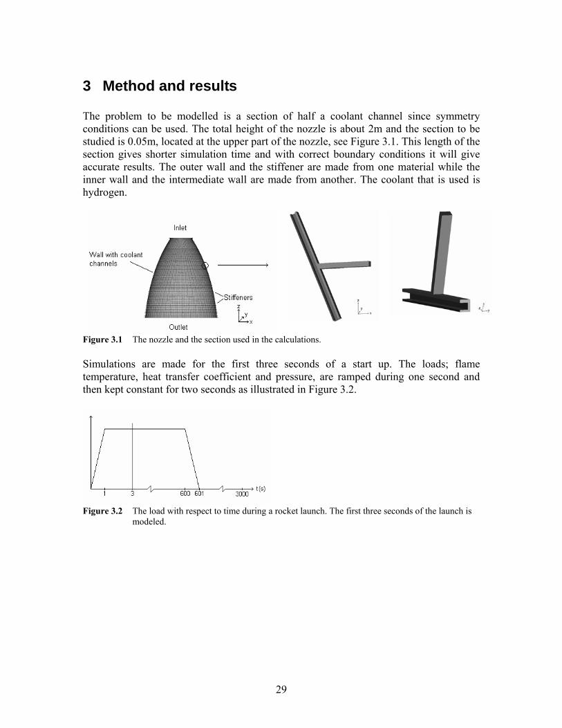
3 Method and results The problem to be modelled is a section of half a coolant channel since symmetry conditions can be used. The total height of the nozzle is about 2m and the section to be studied is 0.05m, located at the upper part of the nozzle, see Figure 3.1. This length of the section gives shorter simulation time and with correct boundary conditions it will give accurate results. The outer wall and the stiffener are made from one material while the inner wall and the intermediate wall are made from another. The coolant that is used is hydrogen.

Figure 3.1 The nozzle and the section used in the calculations. Simulations are made for the first three seconds of a start up. The loads; flame temperature, heat transfer coefficient and pressure, are ramped during one second and then kept constant for two seconds as illustrated in Figure 3.2.

Figure 3.2 The load with respect to time during a rocket launch. The first three seconds of the launch is

modeled.

30

3.1 Outline of work The work in this thesis is outlined in the following way:

- Set-up a model in ANSYS CFX. - Set-up a model in ANSYS Mechanical. - Perform unidirectional FSI. - Perform bidirectional FSI. - Compare the results.

The softwares used in the work are

- ANSYS Mechanical 10.0 for the structural and thermal analyses. - ANSYS CFX 10.0 for the fluid analysis and thermal analysis. - ICEM CFD 10.0 for the grid generation to ANSYS CFX. - ANSA 12.0 for the meshing to ANSYS Mechanical.

Note, below ANSYS CFX is referred to as CFX and ANSYS Mechanical to as ANSYS. The calculations are done in Linux for this case, but it is also possible to run the programs in windows. In unidirectional FSI CFX calculates the flow of the coolant and the heat flow in the solids. The convection and pressure at the channel walls are transferred from CFX to ANSYS and then the displacements are calculated. For bidirectional FSI only the flow of the coolant is modelled in CFX. The temperature and displacement at the walls of the channel are transferred from ANSYS to CFX. From CFX to ANSYS the total force density and heat flux are exported. Bidirectional FSI is only possible to perform in version 10.0 of ANSYS Mechanical and ANSYS CFX.

31

3.2 Modelling in CFX There is a general work order when solving a problem with CFX

- Defining geometry. - Dividing the geometry into a mesh of finite volumes. - Defining the run in CFX-Pre. - Solving the problem with CFX-Solver. - Viewing and analysing the results in CFX-Post.

3.2.1 Steady state Before CFX and ANSYS can be coupled an accurate transient run in CFX is needed. The first step to achieve this is to do a steady state run with full loads, to determine the convergence and accuracy of the conditions and models used. First a CAD-geometry is imported to ICEM CFD and a mesh is generated. This mesh is a structured mesh consisting of hexa blocks, blocks with six sides. The different surfaces and volumes are defined. Before exporting this mesh into CFX the mesh is converted to unstructured since CFX is an unstructured solver. To obtain an as accurate result as possible in the CFX-run, two different meshes are compared. One has a resolved boundary layer and one has a coarser grid for which a wall function is used in the calculations, otherwise they are the same. The meshes at the inlet of the two models are shown in Figure 3.3. In Figure 3.4 the mesh viewed from the side is displayed.

Figure 3.3 The mesh at the inlet. To the left the resolved mesh and to the right the mesh for the wall

function.

32

Figure 3.4 The mesh arrangement viewed from the side. The mesh at the wall is the finest and is then extended by a factor of 1.2 until it is of roughly the same size as the grid in the free stream. In the resolved grid the length of the smallest grid face is about 0.7 µm, and on the less resolved face it is 0.06 mm. The total height of the fluid domain in the channel is about 2 mm. There are certain recommended quantities that can be used to determine the quality of the mesh [3]. These can be seen in Table 3.1. By avoiding high aspect ratios, volume ratios and small angles in the mesh round-off errors may be avoided. These recommendations should be followed when possible, but is in many cases impossible, especially when a resolved boundary layer is used. Resolved mesh Wall function Recommended (*) Minimum face angle

43 36 >10

Maximum edge length ratio

3440 41.83 <100

Maximum element volume ratio

2.04 2.75 <5

Number of elements

135052 68172 X

Number of nodes 146990 77582 X Table 3.1 Mesh statistics. After importing the mesh that is about to be tested into CFX-Pre, boundary conditions are applied.

- As a flame a constant bulk temperature of 3516 K and heat transfer coefficient of

1440 W/m2 K is applied at the whole wall. This is an approximation since the values vary along the wall and also changes due to deformations. In this case with the nozzle only being 5 cm long this approximation is acceptable since the quantities are at a relatively constant level.

33

- At the outside of the nozzle a temperature of 293 K and a heat transfer coefficient of 50 W/m2 K is set.

- At the sides of the geometry symmetry conditions are set. This condition means

that the flow into the boundary is the same as the flow out of the boundary. Symmetry is also set at the inlet- and outlet sides of the solids. This is equivalent to adiabatic conditions.

- At the outlet an average static pressure is chosen. The pressure is then calculated

over the whole outlet area so that the pressure profile is the same as at a bit upstream. In this case the pressure is set to 47.57 bar.

- At the inlet a first approximation to the inlet conditions were made. A plug profile

with mass flow rate and temperature were applied. The mass flow rate in half a channel is about 0.00198 kg/s and the temperature of the coolant at the inlet for this segment is about 395 K.

Figure 3.5 shows the different boundary conditions used on the model.

Figure 3.5 Boundary settings in CFX. The discretisation scheme chosen for this problem was high resolution scheme, and the turbulence model used was the SST model. This model is appropriate in this case since the flow near the wall is important as well as the free stream flow. To see if the solver reaches an acceptable convergence level monitor points were placed at the channel wall. The temperature and pressure at these points were monitored throughout the solution process and one indication of convergence is when these quantities have reached a constant level. Also the residuals were monitored. According to the CFX-manual for most industrial applications the RMS-residuals need to reach a level

34

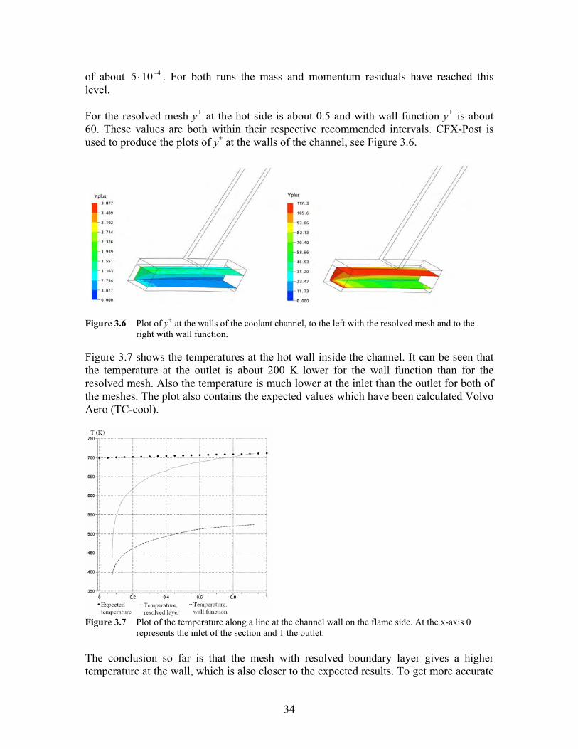
of about 4105 −⋅ . For both runs the mass and momentum residuals have reached this level. For the resolved mesh y+ at the hot side is about 0.5 and with wall function y+ is about 60. These values are both within their respective recommended intervals. CFX-Post is used to produce the plots of y+ at the walls of the channel, see Figure 3.6.

Figure 3.6 Plot of y+ at the walls of the coolant channel, to the left with the resolved mesh and to the

right with wall function. Figure 3.7 shows the temperatures at the hot wall inside the channel. It can be seen that the temperature at the outlet is about 200 K lower for the wall function than for the resolved mesh. Also the temperature is much lower at the inlet than the outlet for both of the meshes. The plot also contains the expected values which have been calculated Volvo Aero (TC-cool).

Figure 3.7 Plot of the temperature along a line at the channel wall on the flame side. At the x-axis 0

represents the inlet of the section and 1 the outlet. The conclusion so far is that the mesh with resolved boundary layer gives a higher temperature at the wall, which is also closer to the expected results. To get more accurate

35

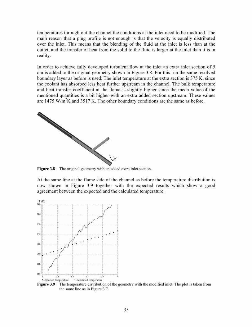
temperatures through out the channel the conditions at the inlet need to be modified. The main reason that a plug profile is not enough is that the velocity is equally distributed over the inlet. This means that the blending of the fluid at the inlet is less than at the outlet, and the transfer of heat from the solid to the fluid is larger at the inlet than it is in reality. In order to achieve fully developed turbulent flow at the inlet an extra inlet section of 5 cm is added to the original geometry shown in Figure 3.8. For this run the same resolved boundary layer as before is used. The inlet temperature at the extra section is 375 K, since the coolant has absorbed less heat further upstream in the channel. The bulk temperature and heat transfer coefficient at the flame is slightly higher since the mean value of the mentioned quantities is a bit higher with an extra added section upstream. These values are 1475 W/m2K and 3517 K. The other boundary conditions are the same as before.

Figure 3.8 The original geometry with an added extra inlet section. At the same line at the flame side of the channel as before the temperature distribution is now shown in Figure 3.9 together with the expected results which show a good agreement between the expected and the calculated temperature.

Figure 3.9 The temperature distribution of the geometry with the modified inlet. The plot is taken from

the same line as in Figure 3.7.

36

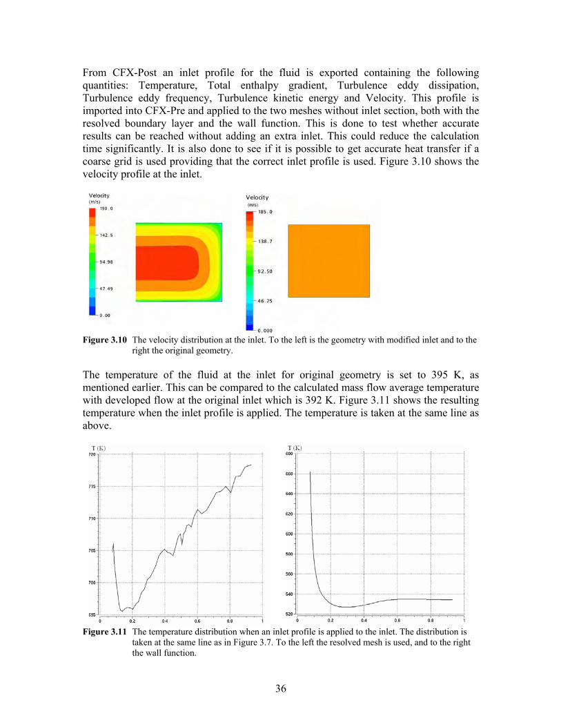
From CFX-Post an inlet profile for the fluid is exported containing the following quantities: Temperature, Total enthalpy gradient, Turbulence eddy dissipation, Turbulence eddy frequency, Turbulence kinetic energy and Velocity. This profile is imported into CFX-Pre and applied to the two meshes without inlet section, both with the resolved boundary layer and the wall function. This is done to test whether accurate results can be reached without adding an extra inlet. This could reduce the calculation time significantly. It is also done to see if it is possible to get accurate heat transfer if a coarse grid is used providing that the correct inlet profile is used. Figure 3.10 shows the velocity profile at the inlet.

Figure 3.10 The velocity distribution at the inlet. To the left is the geometry with modified inlet and to the right the original geometry.

The temperature of the fluid at the inlet for original geometry is set to 395 K, as mentioned earlier. This can be compared to the calculated mass flow average temperature with developed flow at the original inlet which is 392 K. Figure 3.11 shows the resulting temperature when the inlet profile is applied. The temperature is taken at the same line as above.

Figure 3.11 The temperature distribution when an inlet profile is applied to the inlet. The distribution is

taken at the same line as in Figure 3.7. To the left the resolved mesh is used, and to the right the wall function.

37

For the wall function the temperature still is about 200 K too low at the outlet. This means that the correct inlet conditions have no effect to achieve the correct heat transfer for the coarse mesh. For the resolved mesh the temperature at the inlet is about 10 K too high and is then lowered to the expected temperature. The conclusion of the steady state tests is that an extra inlet section is needed, and that a resolved boundary layer gives the best results. Not even when an inlet profile is applied to the original geometry with the resolved mesh yield the expected results. Unfortunately even if the inlet profile applied to the original geometry gives adequate results this method can not be used when setting up the transient run. It is not possible in CFX to set up profiles in both time and space.

3.2.2 Transient The first step of setting up a transient run is to define the loads with respect to time. The loads are applied according to Table 3.2. The values are linearly interpolated between the given time steps. Time (s)

Heat transfer coefficient at flame (W/m2K)

Bulk temperature in flame (K)

Fluid temperature at inlet (K)

Mass flow rate in cooling channel (kg/s)

Outlet pressure (Bar)

0 50 293 100 5105 −⋅ 1 1 1475 3517 375 31098.1 −⋅ 47.54 3 1475 3517 375 31098.1 −⋅ 47.54

Table 3.2 The loads at different times for the transient run. Between each defined time the loads are linearly interpolated.

The quantities chosen at time 0 s are approximate values chosen to represent a nozzle without any heat load and with a small mass flow. The next step is to set the size of the time steps, the times for which the flow is to be evaluated. The steps need to be so small that the transient terms of the flow are resolved, but it can not be so small that the solution takes too long. A way to test if the size of the time step is small enough is to test if the result is different when the time step is doubled and halved. This is done for a few time steps. For the mesh with the resolved boundary layer convergence cannot be reached unless a time step of 5105.1 −⋅ s is used. This is also the size of the physical time step calculated by CFX in the steady state run. In this case this is not possible to use this time step. With about 5 minutes calculation time per time step the total calculation time for the entire transient run will be about 2 years for the computer used. For simulations when the heat

38

transfer is important the mesh needs to be resolved at the wall. There is a connection between the resolution in time and space, the finer grid the smaller time step is needed. As a compromise a mesh whit y+ about 5 is created. In the case of steady state the temperature is approximately 50 K lower than expected. This is an acceptable compromise between accuracy and calculation time. Figure 3.12 illustrates the temperature distribution for the new mesh at the same line as before along with the expected results.

Figure 3.12 The temperature distribution at the same line as in Figure 3.7 for the mesh used in the

transient run. The time step chosen for this mesh is 0.002 s. For the coupled run with ANSYS the maximum time step is set to 0.004 s. The comparison between the results for 0.001, 0.002 and 0.004 s time step can be found in Appendix B. For the time step of 0.008 no convergence could be reached. When solving a steady state problem it takes about 100 iterations to reach convergence. For a transient problem it would take too long if each time step needed 100 loops to converge. Therefore an initial steady state run is used to start the simulation. After that each time step uses the solution from the time step before as initial condition, when doing this about 4 iteration loops are needed for each time step to reach sufficient convergence. The residuals should be reduced by a factor of 2-3 decades during a time step. Figure 3.13 presents the resulting temperature distribution at different times in the model.

39

Time=0.06 s

Time=1.02 s

Time=2 s

Time=3 s

Figure 3.13 The temperature distribution in the geometry for different times in the transient run.

40

3.3 Modelling in ANSYS ANSYS is a FEM software containing pre-processor, solution and post-processor. Simulations in ANSYS are done in the following steps

- Build the model In pre-processor the geometry is built, material properties, element types, real constants and mesh are specified for the model.

- Apply boundary conditions and loads In pre-processor or in solution loads and boundary conditions are applied on nodes, elements or on the solid model. Applicable loads might be displacement, force, temperature, pressure.

- Set solution controls In solution analyse type, equation solver and load step options are specified.

- Solve the analysis Calculations are started.

- Review results

In post-processor results are viewed. [6]

3.3.1 Building the model In pre-processor it is possible to create the actual geometry. Sometimes it is easier to build the geometry in other software and then import the model to ANSYS. When the geometry is finished material properties are specified. Further on appropriate element types are specified. For example in structural analysis beam, pipe, shell or mass elements can be chosen and also if the elements should be in 1-D, 2-D or 3-D. For this project the geometry originates from a Unigraphics format. Geometry clean up and mesh arrangement has been performed in the pre-processing software ANSA. The grouping of elements and nodes were defined as properties in ANSA which makes it easier to apply loads on specific surfaces. For example all the elements that are exposed to the flame, elements on the inlet or elements on the symmetric plane are grouped. In ANSYS these groupings are identified as real constants but it is also possible to define components. During the simulations two different mesh arrangements have been used, see Table 3.3.

Mesh 1 Mesh 2 Total number of surface elements 6298 3734 Total number of volume elements 9951 5574

Table 3.3 Number of elements on models used in ANSYS.

41

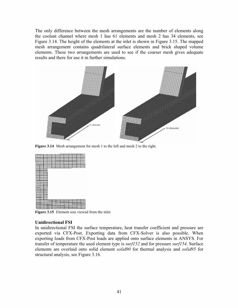
The only difference between the mesh arrangements are the number of elements along the coolant channel where mesh 1 has 61 elements and mesh 2 has 34 elements, see Figure 3.14. The height of the elements at the inlet is shown in Figure 3.15. The mapped mesh arrangement contains quadrilateral surface elements and brick shaped volume elements. These two arrangements are used to see if the coarser mesh gives adequate results and there for use it in further simulations.

Figure 3.14 Mesh arrangement for mesh 1 to the left and mesh 2 to the right.

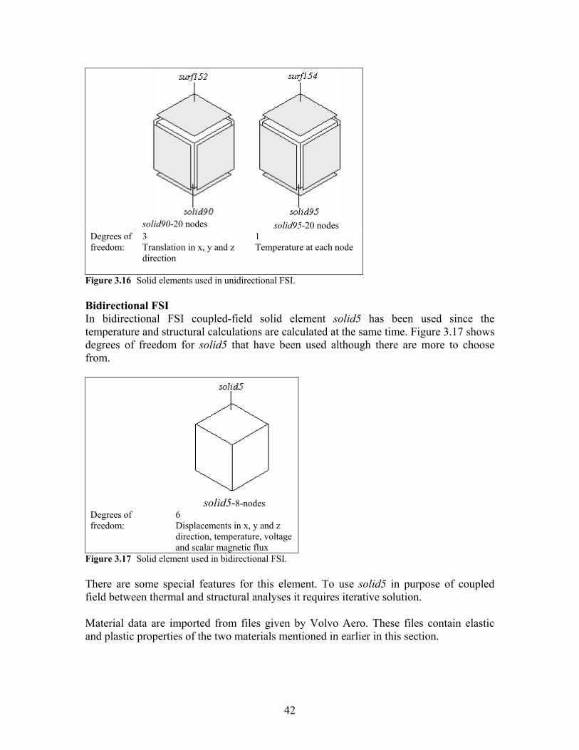
Figure 3.15 Element size viewed from the inlet Unidirectional FSI In unidirectional FSI the surface temperature, heat transfer coefficient and pressure are exported via CFX-Post. Exporting data from CFX-Solver is also possible. When exporting loads from CFX-Post loads are applied onto surface elements in ANSYS. For transfer of temperature the used element type is surf152 and for pressure surf154. Surface elements are overlaid onto solid element solid90 for thermal analysis and solid95 for structural analysis, see Figure 3.16.

42

solid90-20 nodes

solid95-20 nodes

Degrees of freedom:

3 Translation in x, y and z direction

1 Temperature at each node

Figure 3.16 Solid elements used in unidirectional FSI. Bidirectional FSI In bidirectional FSI coupled-field solid element solid5 has been used since the temperature and structural calculations are calculated at the same time. Figure 3.17 shows degrees of freedom for solid5 that have been used although there are more to choose from.

solid5-8-nodes

Degrees of freedom:

6 Displacements in x, y and z direction, temperature, voltage and scalar magnetic flux

Figure 3.17 Solid element used in bidirectional FSI. There are some special features for this element. To use solid5 in purpose of coupled field between thermal and structural analyses it requires iterative solution. Material data are imported from files given by Volvo Aero. These files contain elastic and plastic properties of the two materials mentioned in earlier in this section.

43

3.3.2 Apply boundary conditions and loads To solve the differential equations for thermal and structural analyses boundary conditions are needed. Structural boundary conditions and loads Symmetry is used on areas corresponding to the cut faces, see Figure 3.18. This condition implies that translation outside the plane and rotation inside the plane are zero.

Figure 3.18 Coolant channel viewed from above. To simplify the settings of the boundary conditions local cylindrical coordinates are created. The coordinate systems are placed at a point as shown in Figure 3.19. The distance 1a is calculated as

minmax

min1 rr

dzra

−= (3.3.1)

Point 1P has the following coordinates ),,0( min1max1 zayP += where ,...,, minmaxmin yrr can be found be using the command *get.

Figure 3.19 Creating the local coordinate systems. At the inlet the local coordinate system is given the number 5000 and at the outlet 1000, see Figure 3.20. The nodes at the inlet are locked in '

5000z - direction and at the outlet nodes are coupled in '

1000z - direction which means they all move together.

44

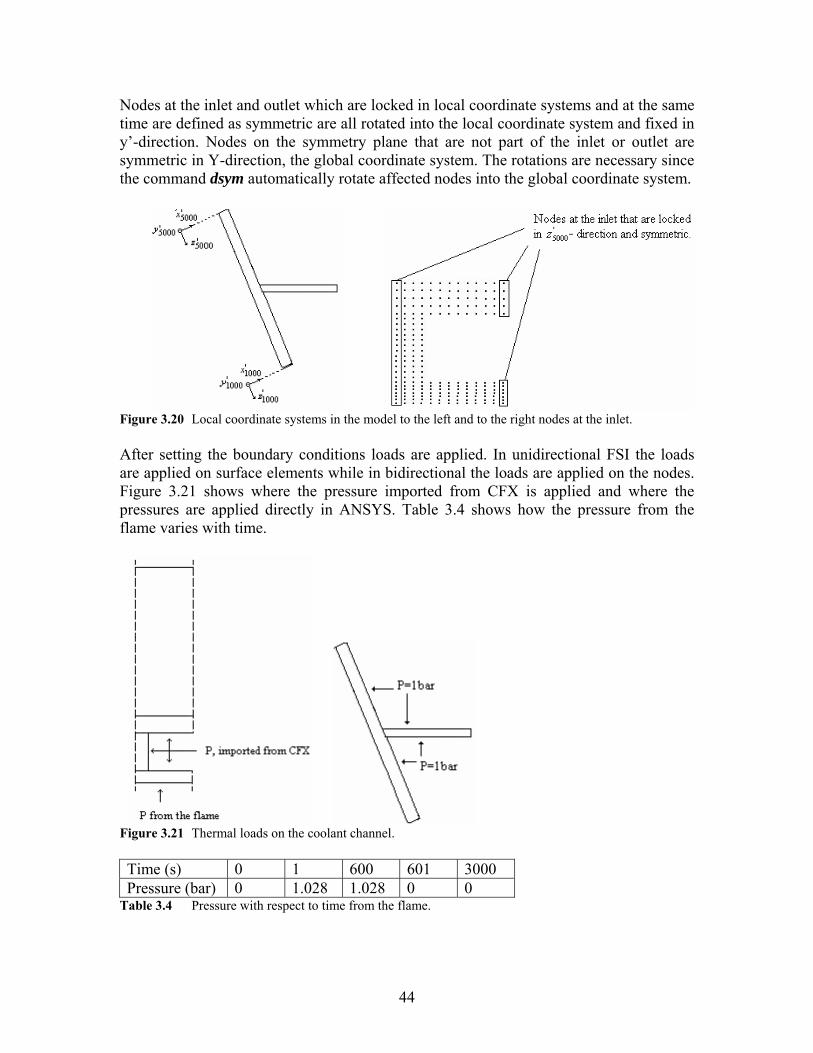
Nodes at the inlet and outlet which are locked in local coordinate systems and at the same time are defined as symmetric are all rotated into the local coordinate system and fixed in y’-direction. Nodes on the symmetry plane that are not part of the inlet or outlet are symmetric in Y-direction, the global coordinate system. The rotations are necessary since the command dsym automatically rotate affected nodes into the global coordinate system.

Figure 3.20 Local coordinate systems in the model to the left and to the right nodes at the inlet. After setting the boundary conditions loads are applied. In unidirectional FSI the loads are applied on surface elements while in bidirectional the loads are applied on the nodes. Figure 3.21 shows where the pressure imported from CFX is applied and where the pressures are applied directly in ANSYS. Table 3.4 shows how the pressure from the flame varies with time.

Figure 3.21 Thermal loads on the coolant channel. Time (s) 0 1 600 601 3000 Pressure (bar) 0 1.028 1.028 0 0

Table 3.4 Pressure with respect to time from the flame.

45

Thermal boundary conditions and loads Boundary conditions and loads applied at the coolant channel for the thermal run in ANSYS are shown in Figure 3.22.

Figure 3.22 Thermal boundary conditions on the coolant channel. Heat transfer coefficient α and bulk temperature ∞T from the flame with respect to time can be seen in Table 3.2. It has been shown in CFX that the initial temperature in the solid is about 120 K. The initial condition in ANSYS is set by uniform temperature of 120 K. Figure 3.23 illustrates the temperature distribution obtained from CFX at time 0 s.

Figure 3.23 Temperature distribution on the coolant channel obtained by a steady state simulation in CFX.

46

3.3.3 Solution controls The first step in ANSYS is to define analysis type; static or transient analysis. The finite element equations in structural analysis can be solved with either direct or iterative methods. The direct method is based on Gaussian elimination approach which means solving for an unknown vector u . The iterative method requires an initial presumption of u and makes iterations to achieve a converged solution. It has been mentioned earlier that the problem is nonlinear. To solve nonlinear problems in thermal analysis there are three solutions to choose between: Quasi option, Linear option or Full option. Quasi option changes the thermal matrix during the solution while linear option on the contrary creates one thermal matrix at the first time step and uses it during the solution. Full option uses the full Newton-Raphson solution option.

47

3.4 Unidirectional simulations The general work order in unidirectional FSI is the following: CFX

- Set up model in CFX and obtain a transient solution. - Load a cdb-file containing the surface elements from ANSYS into CFX-Post. - Export the loads for each time step of interest on these elements as load files.

ANSYS - Import and apply the load files form CFX. - Calculate the displacements.

Figure 3.24 is a scheme of unidirectional FSI.

Figure 3.24 Scheme of unidirectional FSI. CFX For unidirectional FSI the surface elements in the channel are exported from ANSYS to CFX-Post. The convection and pressure is interpolated onto these elements at every 0.06 s and is then exported to ANSYS. ANSYS Loads inside the coolant channels are of two different kinds. The first one contains bulk temperature and heat transfer coefficient for thermal analysis and the second one contains pressure for structural analysis. The files are also separated depending on the material in the coolant channel and the time step, see example below.

48

Example 3.4.1 XXX_data _%times(istep)% XXX indicates the name of the material, data is the name of the transferred load, for example pressure, times is the time vector in ANSYS and istep is the number of the position in the vector times. The array times takes the form

[ ]35.225.118.012.006.0 K=times Imported loads from CFX are applied by the command: /input, Fname, Ext,--, LINE, LOG Fname – Filename of the imported file. Ext – File extension. LINE – Where to begin reading the input file. LOG – Indicates if secondary input is recorded. The input files are read for each time step in the vector times by a loop. The Fname when applying the pressure for material XXX for the first time step is written as XXX_pres _ 0.006. In detail, istep is 1 and the value for times is 0.006. The second time step when istep is 2 and the value for times is 0.012 the input file is then XXX_pres _ 0.012. The code in ANSYS starts with the thermal analysis and then with the command etchg the thermal elements are changed to structural elements and the structural calculations are made. The following settings are used. Thermal run

- Transient thermal analysis. - Full Newton-Raphson solution options. - Maximum number of equilibrium iterations is 15. - Uniform temperature is 120 K in initial step. - Reference temperature 293 K. - Time step = 0.06 s, minimum time step = 0.06/4 s and maximum time step = 0.06

s. Structural run

- Structural static analysis. - Sparse Direct Solver. - Maximum number of equilibrium iterations is 15. - Large deflections included. - The time steps are the same as in the thermal run.

49

3.4.1 Thermal results and analyses Figure 3.25 shows the nodal temperature distribution in the coolant channel where SMN is the minimum temperature and SMX the maximum. The left figure shows the temperature in mesh 1 and the right shows temperature in mesh 2.

Figure 3.25 Temperature distribution in unidirectional FSI. This is the second time the temperatures in the solid are calculated, the first time is in CFX. If these results are reliable or not can only be decided if the temperatures are compared with the ones in CFX. Figure 3.26 shows a plot of the temperature as a function of time. These data are taken from one node close to the inlet of the original geometry with the same coordinates in CFX as in ANSYS. Comparing the temperatures between the softwares they are similar, practically identical. The thermal results in ANSYS are therefore reliable. Note that there are no differences between temperatures in mesh 1 and mesh 2 in ANSYS.

50

Figure 3.26 Temperature with respect to time achieved from simulations in CFX and ANSYS. The data

are taken from a node close to the inlet.

3.4.2 Structural results and analyses Figure 3.27 presents the largest deformation (DMX) at the final time of 3 s for mesh 1 to the left and mesh 2 to the right. The filled body is the deformed shape and the dotted line is the origin structure. One can see that there are no significant differences in the deformation.

Figure 3.27 The final deformation at the time 3s. It is interesting to study the radial displacements which are in X-direction (UX), see figure 3.28. The largest displacements in X-direction (SMX) can be found close to the inlet where the temperature gradient is of its highest order since the coolant is colder there than at the outlet.

51

Figure 3.28 Displacement in X-direction at the time 3s. The largest displacement for mesh 1 is 1.526 mm and for mesh 2 1.524 mm which occurs at the time step 0.06 s. The uniform temperature is 120 K which means that the structure is very cold and therefore shrinks and causes the coolant channel to move towards the centre. The differences in temperature and displacement between mesh 1 and mesh 2 are small therefore mesh 2 is used in bidirectional analysis in order to minimise the simulation time.

52

3.5 Bidirectional simulations The general work order in bidirectional FSI is the following:

- Set up a model in CFX and ANSYS. - Define the surfaces where data are exchanged between the programs. - Define the common settings for the simulation. - Start the solution.

The scheme for bidirectional FSI is illustrated in Figure 3.29.

Figure 3.29 Scheme for bidirectional FSI. All the calculations in bidirectional FSI are made on the same computer. The first software does its calculations, sends the data to the other software which does its calculations and then sends back the data. This solution method is called sequential. It is also possible to do the calculations in ANSYS on one computer and the CFX calculations on another or even several others. CFX For bidirectional FSI only the fluid domain is modelled in CFX since it only allows the fluid domain to be deformed. The same mesh in the channel as in unidirectional FSI is used. First an initial result file needs to be created with only the fluid domain. To do this the convection at the walls from the initial run from earlier is exported and applied as boundary conditions. This gives the same initial conditions for the bidirectional run as for the unidirectional.

53

The settings in CFX for the bidirectional FSI are the following

- The simulation type chosen is transient. The time steps in CFX are overridden by the time steps used in the stagger loops.

- In the settings for the fluid domain the mesh motion is set to “Regions of motion

specified”.

- At the symmetric side the mesh motion is set to “unspecified”. This means that the deformation of this mesh at this surface is defined by the motion of the other surfaces.

- At the walls of the channel the mesh motion is set to “ANSYS MultiField” with

“specified displacement”. This is the setting needed for the displacements from ANSYS to govern the motion of the mesh in CFX.

- The heat transfer settings at the walls are set to “ANSYS MultiField” with “fixed

temperature”. This setting is so that the temperature at the walls of the solid is imported to CFX.

- The boundary conditions at the inlet and outlet are the same as in the

unidirectional run. The mesh motion is set to “stationary”, which is the only option available in CFX-Pre. This is later set to “unspecified” by editing the definition file in CFX-Solver.

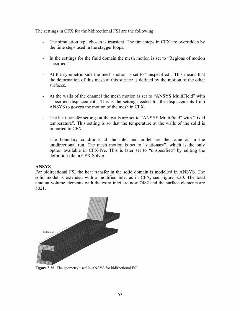
ANSYS For bidirectional FSI the heat transfer in the solid domain is modelled in ANSYS. The solid model is extended with a modified inlet as in CFX, see Figure 3.30. The total amount volume elements with the extra inlet are now 7482 and the surface elements are 5021.

Figure 3.30 The geometry used in ANSYS for bidirectional FSI.

54

There are two different Multi-field Solvers (MFS) available and it is important to know the differences between them. MFS – Single code: All physics fields are in the same product, for example the

whole problem is solved in ANSYS Multiphysics.

MFS – Multiple code: Physics fields are in more than one product like in this thesis. The problem can be solved in ANSYS Multiphysics and ANSYS CFX. This method is often recognized as MFX.

A typical content in Multi-field Solver is following commands: MFAN – Turns on or off the Multi-field Solver analysis. MFCL – Deleting ANSYS Multi-field Solver analysis settings. MFPS – Set up a field solver group. MFSO – Set up the solution order. MFRE – Sets relaxation values on the analysis. MFLC – Define load transfer for code coupling analysis, (see the example below). MFTI – End time for the analysis. MFDT – Time step size for the analysis. MFRS – Restart time for the analysis. MFBU – Turns on or off bucket search. MFTO – Turns on or off normal distance checking for the surface mapping in the

analysis. MFIT – Numbers of stagger iterations. MFCO – Convergence value for the analysis. Inside the coolant channel where CFX and ANSYS exchanges data one has to apply field-surface interface flag. This is done by the command shown below: sf, Nlist, Lab, VALUE, VALUE2 sf – Specifies surface loads on nodes. Nlist – Nodes where the loads should be applied. Lab – Surface load label. Here choose FSIN for fluid-structure interaction analysis. VALUE – Identify surface interface number. VALUE2 – Not used. After the flags are applied it is time to define the load transfer for code coupling. This is illustrated by the command below:

55

MFLC, Type, Fname1, Intname1, Label1, Fname2, Intname2, Label2, Option

option.ion interpolat (NONC) preserving profileor (CONS) veconservati global Choose - . from namesolver for the loads surface Set the -

. from namesolver field for the label load surface Set the - code. receiving for the namesolver filedSet -

. from namesolver field for the label load surface Set the - flag. interface surface-field with definesnumber Interface -

CFX.or ANSYS issolver theif exampleFor name.solver field theSets - transfer.load surfacefor Set to -

coupling. codefor transfer load a Defines -

OptionFname2Label2

Fname2Intname2Fname2

Fname1Label1Intname1Fname1

surfTypeMFLC

Receiver

Sender

⎪⎭

⎪⎬

⎫

⎪⎭

⎪⎬

⎫

Example 3.5.1 a.) MFLC, SURF, ANSYS, 1, TEMP, CFX, XXX, Temperature, NONC b.) MFLC, SURF, CFX, XXX, Wall Heat Flux, ANSYS, 1, HFLU, NONC a.) ANSYS sends temperature from surface interface number 1 to corresponding surface

in CFX called XXX. b.) CFX sends heat flux from surface XXX to corresponding surface in ANSYS labelled

with interface number 1. In the thermal analysis temperature and heat flux will be exchanged inside the coolant channel both for the original channel and the extra inlet. In the structural analysis though displacement and total force density will only be exchanged on the original coolant channel. The extra inlet in ANSYS is only used to satisfy the heat transfer calculations in the flow in CFX. It is not allowed to affect the structural characteristics therefore the coefficient of thermal expansion in all direction is set to zero. Also there will not be any structural boundaries and loads on the extra inlet. Comprehensive setups for the bidirectional analysis in shown below

- solid5 with keyopt(1)=0 which gives the element the degrees of freedom mentioned in section 3.3.1, keyopt(3)=0 include extra shapes (default) and keyopt(5)=0 basic element printout (default).

- Transient thermal analysis. - Full Newton-Raphson Solution options. - Equations solver – Preconditioned Conjugate Gradient. - Uniform temperature is 120 K. - The reference temperature is set to 293 K. - Time step = 0.004 s, minimum time step = 0.002 s and maximum time step =

0.004 s. - Field-surface interface flag. - Solution order is to first solve ANSYS and then CFX.

56

- Define load transfer for code coupling. - Time end is 3 s. - Stagger Iteration Controls is maximum = 10, minimum = 1 and target = 5. - A convergence value for all items is 0.001. - Relaxation factor is 0.75 for all items.

When the settings are done one has to write an input file (.dat). This setting is available in Main menu> Pre-processor or Solution> Multi-field Set Up> Advanced Set up> Write Input. From this point the following files should be available to start the simulation:

- .dat file in ANSYS. - .def file in CFX. - .res file if initial values is needed in CFX.

To run the simulation ANSYS Launcher is needed, see Figure 3.31. The simulation environment is chosen to MFX –ANSYS/CFX since it is a multiple code analysis and license used is ANSYS Mechanical U.

Figure 3.31 ANSYS Launcher for bidirectional simulations. To compare the temperatures calculated in CFX for the unidirectional FSI a bidirectional run with only heat transfer is made. Figure 3.32 shows the simulation scheme the run.

57

Figure 3.32 Scheme for bidirectional FSI where only thermal analysis is performed.

3.5.1 Thermal results and analyses During the work to set up and simulate bidirectional FSI it was found that the simulation time is very long. It takes about one day to calculate 0.1 s of the process and to reach the final time of 3 s would then take about 30 days which is in most cases not acceptable in industrial applications. Unfortunately none of the simulations reached the final time. The most successful attempt was when the run stopped at 1.198 s which took about 8 days to calculate. Following error message was written in the error file in CFX: An error has occurred in cfx5solve: The CFX-5 solver was interrupted by signal SEGV (11) No results file has been created.

This is an error connected to the memory of the computer. Results presented below are at 1.02 s. Figure 3.33 shows the nodal temperature distribution from bidirectional FSI to the left and to the right is from unidirectional.

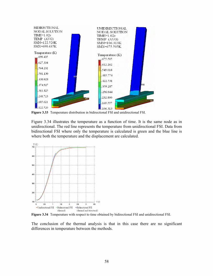
58

Figure 3.33 Temperature distribution in bidirectional FSI and unidirectional FSI. Figure 3.34 illustrates the temperature as a function of time. It is the same node as in unidirectional. The red line represents the temperature from unidirectional FSI. Data from bidirectional FSI where only the temperature is calculated is green and the blue line is where both the temperature and the displacement are calculated.

Figure 3.34 Temperature with respect to time obtained by bidirectional FSI and unidirectional FSI. The conclusion of the thermal analysis is that in this case there are no significant differences in temperature between the methods.

59

3.5.2 Structural results and analyses Result presented in Figure 3.35 illustrates the displacement at the time step 1.02 s. On the left hand side is results in bidirectional FSI and on the right side unidirectional.

Figure 3.35 Deformation at the time 1.02s in bidirectional FSI to the left and unidirectional to right. Figure 3.36 shows radial displacement (UX) in bidirectional FSI to the left and to the right is unidirectional. The maximum deformation (DMX) in bidirectional FSI is 0.216 mm located at the outlet, while in unidirectional the largest displacement is 0.637 mm and can be found at the inlet.

Figure 3.36 The displacement in X-direction in bidirectional FSI and unidirectional FSI.

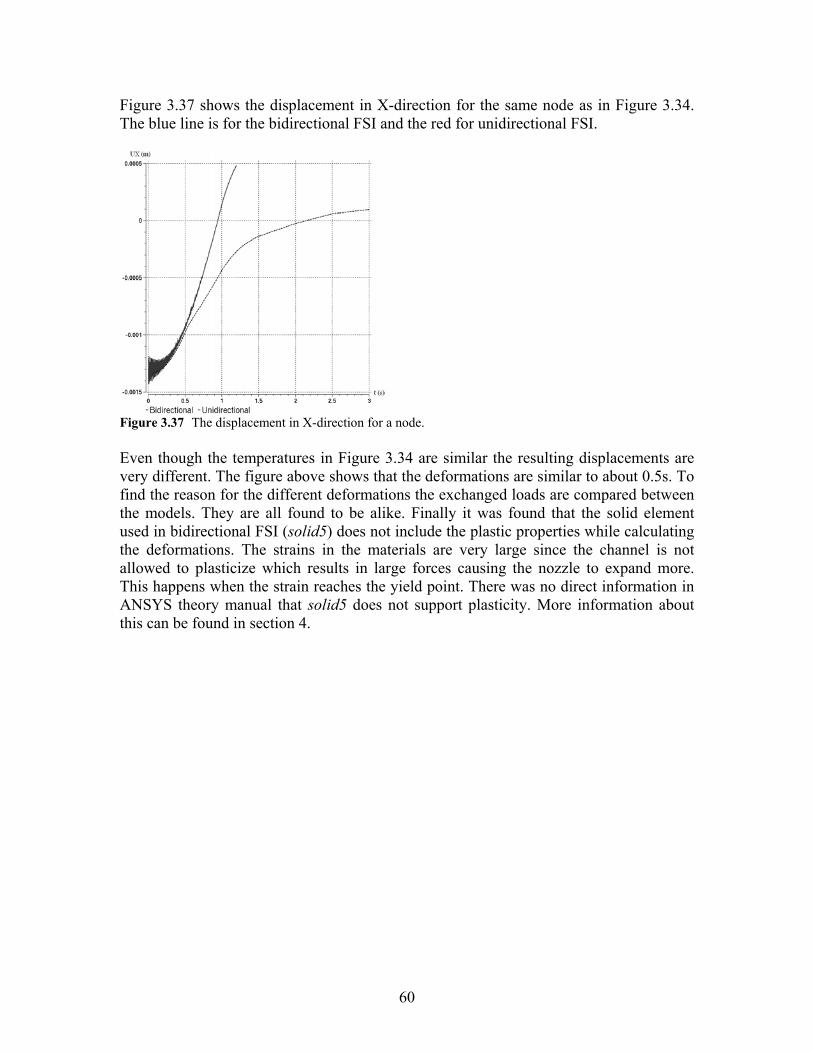
60

Figure 3.37 shows the displacement in X-direction for the same node as in Figure 3.34. The blue line is for the bidirectional FSI and the red for unidirectional FSI.

Figure 3.37 The displacement in X-direction for a node. Even though the temperatures in Figure 3.34 are similar the resulting displacements are very different. The figure above shows that the deformations are similar to about 0.5s. To find the reason for the different deformations the exchanged loads are compared between the models. They are all found to be alike. Finally it was found that the solid element used in bidirectional FSI (solid5) does not include the plastic properties while calculating the deformations. The strains in the materials are very large since the channel is not allowed to plasticize which results in large forces causing the nozzle to expand more. This happens when the strain reaches the yield point. There was no direct information in ANSYS theory manual that solid5 does not support plasticity. More information about this can be found in section 4.

61

4 Discussion and conclusions In both FEM and CFD several approximations are made. In the section below is a description of the approximations made and an attempt to account for the effects. The first approximation in both FEM and CFD is the discretisation of the geometry. Creating a mesh arrangement for a model can sometimes be difficult and demands years of experiences for the analyst to decide whether it is good or not. It might be difficult to achieve a perfect mesh and the analyst will often need to consider mesh arrangement against working hours and simulation time In section 3.3.1 is information of elements used in structural and thermal analyses in ANSYS. For unidirectional analysis selected solid elements have 20 nodes. The solutions obtained in the analyses are only calculated on elements with 8 nodes which mean the midnodes are all ignored. One way to create 20 nodes can be by changing the elements from 1st order to 2nd order in ANSA, which does not work. It is unclear why this problem occurs, it may be an error in the software. Another way is to add midside nodes in ANSYS by using the command emid. This command needs to be used with caution because ANSYS does not pay any attention to whether the structure has regular or irregular surfaces and the effect can be that the midside nodes do not follow the surface smoothly. In our case it would not have been any problem to use an extra node since the solid is regular without any large changes in the curves. The reason for not rerunning the simulations is that the mesh size is acceptable for 8 node elements. When using solid5 large deflections are not possible in coupled field analyses between structural and thermal analyses. One improvement here might be to use the solid element solid226. There are other options to choose from that are more appropriate for the considered problem, for example large deformation can be selected. The most important drawback of coupled field elements is that these elements can not include plasticity in the calculations. Solid226 is only available for the product ANSYS Multiphysics. To get the correct heat transfer in these runs a resolved boundary layer is needed in the CFX-calculations. For the SST turbulence model an y+ of less than one is a resolved layer. In many cases it is adequate to approximate the flow at the wall with a wall function. Tests with different boundary layers have been made and the results show that there is a large grid dependence of the heat transfer. With the correct temperature at the wall the size of the deformations might be different. Concerning the structural boundary conditions one should take into consideration that they are not physically correct. The analyses are done on a very small segment compared to the whole coolant channel and the boundary conditions applied are chosen to compensate for this, but it is not possible to do this entirely. In reality the loads from the flame changes with the deformation of the nozzle. It can cause the nozzle to reach a temperature where it melts. An approximation that has been

62

made is that a constant bulk temperature and heat transfer coefficient represents the flame, so this phenomenon can not be observed in the simulations. The flow of the coolant is not correct at the beginning of the run because the temperature of the coolant and the mass flow rate is just an approximation. It is not possible to set the rate to zero but the lowest possible mass flow rate that still gives convergence is chosen. The temperature of the coolant is an approximation of what the temperature at this position of the nozzle might be provided that the coolant starts as liquid hydrogen, and no heat load is applied. This is done because that in reality the flow of the coolant is turned on just before the flame. A steady state simulation in CFX was done to approximate the initial temperature in the solid that is used in the transient simulation. The temperature in the solid is altering between 120 K in the coolant channel and 244 K at the top of the stiffener. This is included in ANSYS by setting a constant initial temperature, but this approximation is not entirely correct since the temperature is varying. The ultimate solution would have been to create a file containing initial nodal temperatures in the solid by running a simulation in ANSYS with exactly the same boundary conditions as in CFX. The time also needs to be discretised. CFX is an implicit solver, which means that no limitation of the time step size should exist for the simulations. For this case it is not true. As can be seen the more resolved boundary layer the smaller time step is needed. Even if there where no limitations in the solver for the time step size, there are limitations of the physics. The process needs to be resolved by at least the double rate of the frequency in the problem. If the flame is to be modelled the time step needs to be smaller for the effects of the deformations to the flame to be noticed.

63

4.1 Unidirectional and bidirectional FSI A benefit with unidirectional FSI is independent coding where different time steps can be chosen in CFX and ANSYS. The total simulation time for unidirectional analysis is 3 days for the simulation in CFX and about 3 hours in ANSYS. Transferring of data is done manually which is time consuming. Bidirectional FSI has automatic load transferring since the simulations in CFX and ANSYS are running simultaneously. Here ANSYS and CFX have the same time step which is a disadvantage since the CFX simulation requires shorter steps in order to obtain convergence, this result in long calculation times. The main reason for the long computation time is the stagger iterations, where convergence is achieved between the two softwares. For every stagger iteration convergence within each software is also needed. These loops can be repeated up to ten times per time step and gives theoretically a ten time longer calculation time as in unidirectional FSI.

64

4.2 Limitations and Problems There are several limitations of these methods and many problems have occurred during the work. For example in CFX it is not possible to create a profile in both time and space as boundary conditions, which means that the extra inlet section can not be excluded. The largest problem is the long calculation times, especially in two-way FSI. Even if it might be worth the calculation time, there is a big risk that the run is aborted during a calculation. During this thesis a simulation that has been going for several days was aborted due to server problems. In these cases the run has to be restarted from the beginning. Also these runs demand large disk space, because results at every time step are written. The result files are about 20 GB. Another limitation of FSI is that the geometries in both ANSYS and CFX have to fit perfectly together. If they do not the interpolation onto the corresponding surface is done anyway and probably with incorrect loads as a result. There is no time to gain by using a parallel solver in CFX. The communication time between the computers is greater than the calculation time gained by using more than one computer.

65

4.3 Conclusion In the discussion advantages and disadvantages of the evaluated methods are compared. The conclusion is that none of them are applicable on a whole rocket nozzle because the simulation time is beyond acceptable time frames. If the methods are to be used it is recommended to choose unidirectional FSI since the simulation time is much shorter than in bidirectional FSI and also because the element types available (solid90 and solid95) in the simulations can include plastic properties. In CFX the main conclusion is that an extra inlet section and a resolved boundary layer is needed to achieve accurate temperatures at the walls of the channel.

66

4.4 Future work A method to test if the deformation affects the flow is to do unidirectional FSI in the opposite direction, where the deformed geometry is imported into CFX. To make the unidirectional FSI more effective a macro can be created in CFX that automatically writes load files. This saves a lot of time, and removes a tedious part of the work. There are other areas where the calculation time might be shortened for which this method can be tested. An example of this is turbo machinery where the total simulation time can be short enough to use small time steps to allow the heat transfer to be resolved. Other possible applications are where there is no heat transfer, only pressure causing the deformations. Here a coarser grid might be used which allows a larger time step. Another way to perform unidirectional FSI is to transfer loads from CFX-Solver where it is possible to transfer loads on solid elements which in our case means the body temperature. If this is available the thermal analysis in ANSYS is not necessary. This method requires an ANSYS Multiphysics license. In earlier discussions it was mentioned that there are no coupled field elements available to include plasticity in bidirectional FSI. This problem might be possible to avoid by writing a script that changes element types depending on what kind of data that are transferred. In detail, when transferring heat flux and temperature from ANSYS to CFX the solid element solid90 is used and when displacement and total force density are transferred the thermal element solid 95 is selected.

67

5 References [1] – Sutton, George P. (1986). Rocket Propulsion Elements An introduction to engineering of rockets. USA: John Wiley & Sons, Inc [2] –Versteeg, H. K, Malalasekera, W. (1995). An introduction to Computational Fluid Dynamics. Harlow: Pearson Education Limited [3] – Ansys Inc. (2004). ANSYS CFX Release 10.0, SAS IP, Inc. [4] – Quality and trust [5] – Hueber, Kenneth H., Dewhirst, Donald L., Smith, Douglas L., Byrom, Ted G. (2001). THE FINITE ELEMENT METHOD FOR ENGINEERS. USA: John Wiley & Sons, Inc [6] – ANSYS Inc. (2005). Release 10.0 Documentation for ANSYS, SAS IP, Inc. [7] – Zienkiewicz, O.C, Taylor, R.L (2002). The FINITE ELEMENT METHOD, Volume 1: THE BASIS. Bodmin: MPG Books Ltd [8] – Sundström, Bengt (1998). Handbok och formelsamling i hållfasthetslära. Södertälje: Fingraf AB [9] – Dahlberg, Tore (2001). Teknisk hållfasthetslära. Lund: Studentlitteratur [10] – Bonet,J., Wood, R.D (1997). Nonlinear Continuum Mechanics for Finite Element Analysis. Cambridge: Cambridge University Press [11] – Henja, Torvald, Fällström, Karl-Evert, Hermansson, Roger (1996).GRUNDLÄGGANDE VÄRMEÖVERFÖRING. Luleå: Tekniska högskolan i Luleå [12] – Ottosen, Niels Saabye, Petersson Hans (1992). Introduction to the FINITE ELEMENT METHOD. Great Britain: Bookcraft (Bath) Ltd [13] – Cook, Robert D. (1995). FINITE ELEMENT MODELING FOR STRESS ANALYSIS. USA: John Wiley & Sons, Inc.

68

Appendix A Jaumann-Zaremba equation [8]

ΩσσΩσσ ⋅+⋅−=∇ & (A.1) Objective stress rate ∇σ and rate of deformation D has linear relation

DCσ :=∇ (A.2) where C is the isotropic, linear elastic stiffness. Definition of virtual velocity gradient L~ is

( )xX

Xv

xvvL

∂∂

∂∂

=∂∂

==~~~~ grad (A.3)

or

ΩDL ~~~ += (A.4) Rate of virtual deformation D~ is the symmetric part of virtual velocity gradient L~ and virtual spin tensor Ω~ is the asymmetric part. The same conditions are applicable in current coordinates. Components describing the virtual velocity gradient are defined as

( )ΤLLD ~~~ +=21

(A.5)

and

( )ΤLLΩ ~~~ −=21

(A.6)

where ΤL~ is the transpose of L~ . Differentiate the virtual work in equation (2.2.18) and inserting (A.3) and (A.4) gives

( )444 3444 21444444 3444444 21

work virtualInternal work virtualExternal

~~~~~

⎟⎠⎞⎜

⎝⎛ +

∂∂

−⎟⎠⎞⎜

⎝⎛ ⋅

∂∂

+⎟⎠⎞⎜

⎝⎛ ⋅

∂∂

=∂

∂∫∫∫ ∗

0V 0V 00AJdV

tJdV

tdAJ

ttW

00

ΩDσv bvt : (A.7)

A symmetric matrix multiplied with a symmetric matrix results in zero. Evaluation of the internal virtual work of equation (A.7) yields

69

( ) ( ) 0dVJt

Jt0V J

0V 0JdV t

)~:~:~:)~~(∂∂

+∂∂

+∫ (=∫ +∂∂ DσDσDσΩDσ : & (A.8)

The last term in (A.8) is asymmetric and will not contribute significantly to the stiffness matrix. Hence, it can be neglected. Inserting equation (A.1) in (A.8) gives

( ) ( ) ∫∫ ∫∫ ∂∂

+⋅−⋅+=⎟⎠⎞⎜

⎝⎛

∂∂

00 00 VV VV0000 JdV

tJdVJdV JdV

tDσDΩσσΩDD:CDσ~

:~~:~ : : (A.9)

Equation (A.9) is subdivided to make the calculations easier

( ) ( )44344214444 34444 21444 3444 21

c

0V 0

b

0V 0

a

0V 0 JdV t

JdV JdV : ∫∫∫ ∂∂

+⋅−⋅+DσDΩσσΩDD:C~

:~~ : (A.10)

The subparts of equation (A.10) take the form a.)

( ) ( ) ( )∫ ∫=0V 0V 00 JdV JdV grad: DD:CvD:C ~:~ (A.11)

b.)

( ) ( ) ( )∫∫∫ ⋅−⋅=⋅+⋅−⋅−⋅=⋅−⋅0V 0

0V 00V 0 JdV JdV JdV DDLLσDDDLDDDLσDΩσσΩ ΤTΤ ~~:~~~~:~ : (A.12)

c.) Definition of virtual velocity gradient is [8]

( ) ΩDFFxX

Xv

xvvL 1 ~~~~~~~ +==

∂∂

∂∂

=∂∂

== − &grad (A.13)

where F is the deformation gradient. Differential changes in origin coordinate system and changes in time can be described as [8]

⎩⎨⎧

=

=

XFxXFx

dddd&&

(A.14)

The term

Ω:σD:σL:σ += (A.15) can be written as

70

D:σL:σ = (A.16) because a symmetric matrix multiply an asymmetric matrix will be zero. D~ is symmetric therefore TDD ~~ = and in the same way following conditions can be defined as TDD = . If one make use of relationship between F and identity matrix I as shown below

IFF 1 =⋅ − (A.17) the differentiate of relationship above becomes

( ) 111111

FFFFFFFFIFF −−−−−−

⋅⋅−=⇒=⋅+⋅⇒∂∂

=∂⋅∂ &&&& 0

tt (A.18)

Using expressions from (A.8), (A.9) and (A.13) yields

( ) ( ) ( ) ( )TTTΤ-1Τ

LLLLFFFFLLD ~~~~~~~

−−=⎟⎟

⎠

⎞

⎜⎜

⎝

⎛

∂∂

+∂

∂=

∂+∂

=∂∂ −

21

21

21

t&&

ttt (A.19)

Rewriting term c from (A.10) gives

( ) ( )∫∫∫ ⋅−=⋅−⋅−=∂∂

0V 00V 0

0V 0 JdV JdV JdV t

DDσLLLLσDσ TT ~:~~:~

: 21 (A.20)

Adding (A.11), (A.12) and (A.20)

( ) ( ) ( ) ( )∫ ∫∫ ∫∫ ⎟⎟⎠

⎞⎜⎜⎝

⎛⋅−⋅+=⋅−⋅−⋅+

0 00 00 V V 00V V 0V 00 JdV JdVJdVJdV JdV DDDLσ DD:CDDσDDDLσDD:CΤΤ ~2~~:~:~~:~: : (A.21)

The external virtual work from equation (A.3) can be written as

( ) ( ) ( )0A0AV 00A dA

tJdAJJdV

tdAJ

t 0000vtvtv bvt ~

t

~~~ ⋅∂

∂+

∂⋅∂

=⋅∂∂

+⋅∂∂

∫∫∫∫∗

∗∗

( )∫∫ ⋅

∂∂

+∂

⋅∂+

00 V 0V 0 dVtJJdV

tv bv b ~~

(A.22)

The term containing tJ

∂∂ will even here be neglected since it will not contribute of great

deal to the stiffness matrix. Finally with some calculations and adding the external forces the equation to describe the displacement changes takes the form

( ) ( ) ( ) ( )444444 3444444 214444 34444 21444 3444 21

stiffness Load

V 00A

s stiffnes Stress

V 0

stiffness Material

0VJdVdAJJdV2JdV

tW

0∫∫∫∫ ∂

⋅∂+

∂⋅∂

+⋅⋅+=∂∂ ∗

000

~~~~:~~:

t

t- v bvtDDLLσDD:C T

(A.23)

71

Appendix B The temperature at different monitor points for different size of the time step. The first 0.06 seconds are modeled.

Time step=0.001 s

Time step=0.002 s

Time step=0.004 s