Effect of Atmospheric Pressure and Temperature on a Small ...

Air Force Institute of TechnologyAFIT Scholar

Theses and Dissertations Student Graduate Works

3-11-2011

Effect of Atmospheric Pressure and Temperatureon a Small Spark Ignition Internal CombustionEngine's PerformancePeter J. Schmick

Follow this and additional works at: https://scholar.afit.edu/etd

Part of the Aerospace Engineering Commons

This Thesis is brought to you for free and open access by the Student Graduate Works at AFIT Scholar. It has been accepted for inclusion in Theses andDissertations by an authorized administrator of AFIT Scholar. For more information, please contact [email protected].

Recommended CitationSchmick, Peter J., "Effect of Atmospheric Pressure and Temperature on a Small Spark Ignition Internal Combustion Engine'sPerformance" (2011). Theses and Dissertations. 1353.https://scholar.afit.edu/etd/1353

https://scholar.afit.edu?utm_source=scholar.afit.edu%2Fetd%2F1353&utm_medium=PDF&utm_campaign=PDFCoverPages

https://scholar.afit.edu/etd?utm_source=scholar.afit.edu%2Fetd%2F1353&utm_medium=PDF&utm_campaign=PDFCoverPages

https://scholar.afit.edu/graduate_works?utm_source=scholar.afit.edu%2Fetd%2F1353&utm_medium=PDF&utm_campaign=PDFCoverPages

https://scholar.afit.edu/etd?utm_source=scholar.afit.edu%2Fetd%2F1353&utm_medium=PDF&utm_campaign=PDFCoverPages

http://network.bepress.com/hgg/discipline/218?utm_source=scholar.afit.edu%2Fetd%2F1353&utm_medium=PDF&utm_campaign=PDFCoverPages

https://scholar.afit.edu/etd/1353?utm_source=scholar.afit.edu%2Fetd%2F1353&utm_medium=PDF&utm_campaign=PDFCoverPages

mailto:[email protected]

EFFECT OF ATMOSPHERIC PRESSURE AND TEMPERTURE ON A SMALL SPARK IGNITION INTERNAL COMBUSTION ENGINE’S PERFORMANCE

THESIS

Peter J. Schmick, Captain, USAF

AFIT/GAE/ENY/11-M28

DEPARTMENT OF THE AIR FORCE AIR UNIVERSITY

AIR FORCE INSTITUTE OF TECHNOLOGY

Wright-Patterson Air Force Base, Ohio

APPROVED FOR PUBLIC RELEASE; DISTRIBUTION UNLIMITED

The views expressed in this thesis are those of the author and do not

reflect the official policy or position of the United States Air Force, Department

of Defense, or the United States Government. This material is declared a work of

the U.S. Government and is not subject to copyright protection in the United

States.

AFIT/GAE/ENY/11-M28


THESIS

Presented to the Faculty

Department of Aeronautics and Astronautics

Graduate School of Engineering and Management

Air Force Institute of Technology

Air University

Air Education and Training Command

In Partial Fulfillment of the Requirements for the

Degree of Master of Science in Aeronautical Engineering

Peter J. Schmick

Captain, USAF

March 2011

APPROVED FOR PUBLIC RELEASE; DISTRIBUTION UNLIMITED.

AFIT/GAE/ENY/11-M28


Peter Schmick

Captain, USAF

March 2011

Approved:

___________________________________ ________ Dr. Marcus Polanka (Chairman) date _______________________________________ ________ Dr. Paul King (Member) date _____________________________________ ________ Lt Col Frederick Harmon (Member) date

iv

AFIT/GAE/ENY/11-M28

Abstract

The ever increasing use of man portable unmanned aerial vehicles by the US

military in a wide array of environmental conditions calls for the investigation of engine

performance under these conditions. Previous research has focused on individual

changes in pressure or temperature conditions of the air stream entering the engine. The

need was seen for a facility capable of providing an environment representative of

various simulated altitude conditions. A mobile test facility was developed to test small

internal combustion engines with peak powers less than 10 hp. A representative engine

was tested over a range of speeds from 2000 RPM to 9000 RPM at every 1000 RPM.

The throttle was set to 50%, 75%, and 100% open at each of the speeds tested. The test

engine was tested at environmental conditions representing sea level standard day

conditions, 1500 m conditions and 3000 m conditions. The engine torque, fuel flow rate,

and air flow rate were measured at each test point to determine the impact of combined

pressure and temperature variations on engine performance. During the process of

testing the engine and the test stand it was determined that the inlet air pressure had a

significant impact on engine operation. The test engine failed to operate under fuel rich

or fuel lean conditions caused by these pressure oscillations through the carburetor.

v

Acknowledgements I would like to thank my academic advisor, Dr. Marc Polanka, and the research

sponsors, Dr. Fred Schauer and Paul Litke, for allowing me the opportunity to work on

this research with them. Thank you Paul and Dr. Schauer for letting me utilize your

facilities and all of the advice you gave me during the last year and a half. Thank you Dr.

Polanka for the many hours spent discussing this research and listening to all of the

problems encountered and offering suggested solutions.

This research would not have been accomplished if it weren’t for the help and

guidance of several key players that work in D-Bay and 5-Stand. Dr. John Hoke and

Adam Brown of ISSI along with Capt Cary Wilson were instrumental in assisting me

with the experimental setup and I appreciate their patience in helping me solve many of

the issues encountered. I would also like to thank them for helping to further my

understanding of all of the fundamental concepts behind this research. Thanks to Dave

Burris for writing the LabView program. I would like to thank Curtis Rice, Rich

Rymann, and Justin Goffena for all of their always willing lab support, which included

anything from helping me find materials to showing me how to use some of the

machining equipment, to the proper way to install certain components. I would also like

to thank them for helping to fabricate some of the test stand.

Lastly, I would like thank my fiancé for always being understanding and listening

to me talk about how things were going on a daily basis, which was far too often. She

supported my efforts the entire way and encouraged me to do my best.

vi

Table of Contents Page

Abstract .............................................................................................................................. iv

Acknowledgements ............................................................................................................. v

Table of Contents ............................................................................................................... vi

List of Figures .................................................................................................................. viii

List of Tables .................................................................................................................... xii

List of Symbols ................................................................................................................ xiii

List of Abbreviations ........................................................................................................ xv

I. Introduction ..................................................................................................................... 1

I.1 Objectives ............................................................................................................ 4

I.2 Methodology ........................................................................................................ 5

II. Theory and Previous Research ....................................................................................... 7

II.1 Engines ................................................................................................................. 7

II.2 Comparison of Engine Parameters ..................................................................... 12

II.3 Scaling Laws/Issues ........................................................................................... 14

II.4 Pressure Impact .................................................................................................. 21

II.5 Temperature Impact ........................................................................................... 25

II.6 Measurement/Accuracy of Parameters Required ............................................... 29

II.6.1 Pressure .................................................................................................. 29

II.6.2 Temperature ........................................................................................... 33

II.6.3 Flow Meters ........................................................................................... 34

II.6.4 Power, Torque, Speed ............................................................................ 36

II.7 Other Research ................................................................................................... 37

II.7.1 Spark/Valve/Injection Timing ............................................................... 37

II.7.2 Geometry................................................................................................ 39

II.8 Combustion and Fuel Impacts ........................................................................... 46

II.8.1 Impact of Fuel-Air Ratio ........................................................................ 50

II.9 Fuel Impact ........................................................................................................ 53

II.9.1 Categories of Fuels ................................................................................ 53

II.9.2 Impact of Fuel Type ............................................................................... 54

III. Test Setup and Apparatus ........................................................................................... 57

III.1 Engines ............................................................................................................... 61

vii

Page

III.2 Flow Path Design and Components ................................................................... 62

III.2.1 Compressor ............................................................................................ 65

III.2.2 Control Valves ....................................................................................... 70

III.2.3 Heat Exchanger ...................................................................................... 73

III.2.4 Damping Chamber ................................................................................. 77

III.2.5 Flow Meters ........................................................................................... 78

III.2.6 Chamber ................................................................................................. 80

III.2.7 Pressure and Temperature ...................................................................... 83

III.3 Other Important Components ............................................................................ 85

III.3.1 Dynamometer ......................................................................................... 85

III.3.2 Couplings ............................................................................................... 86

III.3.3 Data Acquisition .................................................................................... 90

III.4 Error Uncertainty Analysis ................................................................................ 91

IV. Results......................................................................................................................... 93

IV.1 Initial Test Stand Checkout ................................................................................ 93

IV.2 Testing................................................................................................................ 95

IV.2.1 Altitude Experiments ............................................................................. 95

IV.2.2 Engine Load Tests .................................................................................. 99

IV.2.3 Carburetor Experiments ....................................................................... 107

IV.2.4 Carburetor Tests ................................................................................... 108

V. Conclusions and Recommendations .......................................................................... 109

V.1 Conclusions ...................................................................................................... 109

V.2 Recommendations ............................................................................................ 110

V.3 Future Work ..................................................................................................... 113

Appendix A: Heat Transfer Calculations ........................................................................ 116

Appendix B: Flow Coefficient Calculations ................................................................... 119

Appendix C: Window and Wall Stress Calculation ........................................................ 122

Appendix D: Raw Data ................................................................................................... 125

Appendix E: Chamber Mechanical Drawings ................................................................ 130

Appendix F: Parts List .................................................................................................... 135

Bibliography ................................................................................................................... 145

Vita .................................................................................................................................. 149

viii

List of Figures Page

Figure 1: Current U.S. Unmanned Aerial Systems Programs (2) ....................................... 2

Figure 2: Geometry of cylinder, piston, connecting rod, and crankshaft where B=bore, L=stroke, l=connecting rod length, a=crank radius, θ=crank angle (adapted from 4). ...................................................................................... 9

Figure 3: Common types of scavenging; (a) loop-scavenging, (b) cross-scavenging, (c) uniflow-scavenging configurations (adapted from 5). ............ 11

Figure 4: Power output versus engine size (6) .................................................................. 15

Figure 5: Engine Performance at constant mixture setting and WOT; two different engines and five different tests (8). .................................................................. 18

Figure 6: Delivery ratio as a function of engine speed at WOT for two different mixture settings (8). ......................................................................................... 19

Figure 7: Measured friction losses of the test engine in comparison with those of a typical automotive engine (10). ....................................................................... 21

Figure 8: Maximum engine torque vs. engine speed and ambient pressure (11). ............ 22

Figure 9: Simulation results of BMEP with altitude (10). ................................................ 24

Figure 10: Simulation of engine power with altitude (10). ............................................... 24

Figure 11: Values of λ in Eq. (13), i.e., (12). ............................................. 26

Figure 12: Optimum spark advance (BTDC) for maximum torque and minimum BSFC vs. stock with n-Heptane (15). .............................................................. 39

Figure 13: Variation of brake torque with engine speed for three different intake plenum volumes (21)........................................................................................ 41

Figure 14: Variation of specific fuel consumption with engine speed for three different intake plenum volumes (21). ............................................................. 42

Figure 15: Variation of coefficient of variation of indicated mean effective pressure with engine speed for three different intake plenum volumes (21). .................................................................................................................. 43

Figure 16: Engine power and brake specific fuel consumption as a function of excess air ratio for modified and standard engines at ¾ throttle opening and 2000 RPM (22). ......................................................................................... 45

Figure 17: Spark timing as a function of excess air ratio for modified and standard engines at ¾ throttle opening and 2000 RPM (22). ........................... 46

Figure 18: Pressure-time curves of standard, (a), and modified, (b), engines at full throttle and two different speeds (22). ............................................................. 46

Figure 19: Engine performance for two mixture settings at WOT (8). ........................... 51

ix

Page

Figure 20: HC and CO emissions as a function of excess air ratio for modified and standard engines at ¾ throttle opening and 2000 RPM (22). .................... 52

Figure 21: Variation of brake specific fuel consumption versus engine speed (32). ....... 56

Figure 22: Mobile small engine altitude test system schematic. ...................................... 57

Figure 23: Temperature versus altitude design goal test conditions. ................................ 59

Figure 24: Pressure versus altitude design goal test conditions ........................................ 60

Figure 25: Brison 5.8 in3 test engine (a) off the stand, and (b) mounted on test stand. ................................................................................................................ 62

Figure 26: Mobile altitude test stand air flow paths. ........................................................ 63

Figure 27: Compressor speed versus commanded frequency. .......................................... 69

Figure 28: Compressor map of pressure ratio versus corrected air mass flow rate (adapted from 37). ............................................................................................ 70

Figure 29: Control valve 1 on the engine intake line just downstream of the air mass flowmeter and upstream of damping chamber. ....................................... 71

Figure 30: Cooling air flow path with control valve 2, manual bypass valve, mass air flow sensor, and chamber inlet. .................................................................. 73

Figure 31: Engine inlet flow path heat exchanger installed on test stand. ........................ 76

Figure 32: Fuel system with fuel flow meter installed on test stand. ............................... 79

Figure 33: Test chamber construction (a) and placement (b) on test stand. ..................... 81

Figure 34: Shaft seal damage observed after initial testing and troubleshooting. ............ 82

Figure 35: Upper window gasket damage after several removals of the upper viewing window. .............................................................................................. 83

Figure 36: Magtrol 2WB65 mounted on engine test stand with power supply and programmable controller. ................................................................................. 86

Figure 37: Engine side hub, Lovejoy GS28/38. ................................................................ 89

Figure 38: Engine, coupling one, intermediate shaft, coupling two, and dynamometer installed on test stand. ............................................................... 89

Figure 39: Equipment rack (a) front and (b) back. ........................................................... 91

Figure 40: Control valve position and inlet pressure as a function of time during initial engine start tests. .................................................................................... 94

Figure 41: Engine speed and inlet pressure as a function of time during initial engine start tests. .............................................................................................. 94

Figure 42: Chamber pressure versus time for first test. .................................................... 96

Figure 43: Chamber temperature versus chamber pressure. ............................................. 97

x

Page

Figure 44: BMEP versus engine speed for sea level conditions. .................................... 100

Figure 45: Torque versus engine speed for sea level conditions. ................................... 101

Figure 46: Fuel flow rate and inlet pressure versus elapsed time for test engine at 2000 rpm, WOT, and sea level conditions. .................................................... 102

Figure 47: Sea level Brison 5.8 cubic inch performance map. ....................................... 103

Figure 48: Engine power versus engine speed at sea level conditions. .......................... 104

Figure 49: Engine torque versus engine speed at sea level. ............................................ 105

Figure 50: Engine power and torque versus inlet pressure at 3500 RPM. ...................... 106

Figure 51: Engine power and torque versus inlet pressure at 3000 RPM. ...................... 106

Figure 52: 0.5 inch Triac 30 degree vee port control valve flow coefficient versus percent open. .................................................................................................. 120

Figure 53: 2.5 inch Triac 30 degree vee port control valve flow coefficient versus percent open. .................................................................................................. 121

Figure 54: Inlet pressure and engine speed versus time for 16 February 2011 testing. ............................................................................................................ 125

Figure 55: Inlet pressure and control valve position versus elapsed test time for 16 February 2011 testing. .................................................................................... 125

Figure 56: Chamber pressure versus elapsed time for three separate tests. .................... 126

Figure 57: Inlet air pressure and fuel volumetric flow versus elapsed time. .................. 126

Figure 58: Brake mean effective pressure versus engine speed for test on 15 February 2011. ............................................................................................... 127

Figure 59: Power and Torque versus engine speed for 15 February 2011 test. .............. 127

Figure 60: Power and BMEP versus engine speed for 25 February 2011 test. .............. 128

Figure 61: Throttle position sensor, control valve 2 position and inlet pressure versus elapsed time for 25 February 2011 test. .............................................. 128

Figure 62: Torque, engine speed, and BSFC versus elapsed time for 25 February 2011 test. ........................................................................................................ 129

Figure 63: BMEP and BSFC versus engine speed for 28 February 2011 test. ............... 129

Figure 64: Side view of CAD model showing dynamometer, starter motor, base plate, and exit nozzle. ..................................................................................... 130

Figure 65: Front view of CAD model showing chamber, motor mount, base plate, entrance diffuser, and exit nozzle. .................................................................. 130

xi

Page

Figure 66: Top view of CAD model showing dynamometer, starter motor, base plate, motor mount, motor mount adjustment plate, entrance diffuser, and exit nozzle................................................................................................ 131

Figure 67: Side view of CAD model showing dynamometer, starter motor, base plate, chamber without inlet and exit diffusers, motor mount, and motor mount adjustment plate. ................................................................................. 131

Figure 68: CAD model of motor mount and motor mount adjustment plate. ................. 131

Figure 69: Machine shop drawing of assembled chamber with instructions to create level surface for top and front viewing windows. ............................... 132

Figure 70: Machine shop drawing for creating the chamber rear wall. .......................... 133

Figure 71: Machine shop drawing for fabrication of main base plate. ........................... 134

xii

List of Tables Page

Table 1: Engine Comparison Chart (5) ............................................................................... 8

Table 2: Operating conditions for research and motor octane rating methods (4) ........... 50

Table 3: Typical fuel properties (4, 23, 25, 27, 28) .......................................................... 54

Table 4: Brison 5.8 engine properties ............................................................................... 62

Table 5: Compressor expected operating points. .............................................................. 70

Table 6: Instrument measurement uncertainty values. ..................................................... 92

Table 7: Calculated parameter uncertainty values. ........................................................... 92

Table 8: Altitude test points .............................................................................................. 98

Table 9: Control Valve CV versus on percent of valve opening (39). ............................. 121

Table 10: Material properties for aluminum, steel, and polycarbonate (40, 41). ........... 122

Table 11: Constants for stress equation based on b/a ratio(40). ..................................... 124

Table 12: Solution to stress equations for each region. .................................................. 124

Table 13: Parts List for Mobile Test Stand ..................................................................... 135

xiii

List of Symbols Symbol

∂R/∂xi partial derivative of variable R with respect to variable xi δR change in variable R δxi change in variable xi ηc combustion efficiency ηf fuel conversion efficiency ηmc mechanical efficiency ηth thermal efficiency θ crank angle κ polytropic coefficient λ excess air ratio (Eq. 22) λ delivery ratio (Eq. 8) λ Power (Eq. 13) ρ density ρmix mixture density ρPower power density ρref reference density ф equivalence ratio ψ relative humidity ω air humidity ratio a crank radius (Figure 2) a auto regression coefficient (Eq. 19) a minor dimension in Appendix C A constant (Eq. 9) A constant (Eq. 10) A/F Air to fuel ratio b distance (Eq. 4) b constant (Eq. 9) b major dimension in Appendix C B bore (Figure 2) B constant (Eq. 10) c(θ) compression ratio as a function of crank angle CF correction factor COVimep coefficient of variation of indicated mean effective pressure CO carbon monoxide CO2 carbon dioxide

CP average specific heat at constant pressure

CR compression ratio CV valve flow coefficient E(θ) voltage output as a function of crank angle EI emissions index F force F/A Fuel to air ratio Hc heat of combustion

xiv

Symbol H2O water, dihydrogen oxide KS sensor gain l connecting rod length L stroke � mass flow rate �Air mass air flow rate mengine, x engine mass, (Eq. 9) �f mass fuel flow rate �mix mass flow rate of the mixture MW molecular weight N engine speed, RPM (Eq. 4), (Eq. 6), (Eq. 8) N number of samples (Eq. 20), (Eq. 34), (Eq. 35) Nb, Pb brake power Ne net output power Ni indicated power NOx nitric oxide formations nR number of revolutions per power stroke pD saturated vapor pressure p pressure palt pressure at altitude pin, pinlet inlet pressure pamb ambient pressure P power q volumetric flow Q energy QHV heating value of fuel R specific gas constant Sg specific gravity t time ttot total time T torque (Eq. 4), (Eq. 6) T temperature (Eq. 10), (Eq. 13), (Eq. 22) Talt temperature at altitude TS temperature at reference condition V(θ) volume as a function of crank angle Vc clearance volume Vd displacement volume Vol volume Volpp volume per pulse x number of pulses (Eq. 21) X percent open (Eq. xx)

xv

List of Abbreviations Abbreviation

AFIT Air Force Institute of Technology AFRL Air Force Research Laboratory AGL Above Ground Level ASTM American Society for Testing and Materials ATDC After Top Dead Center BDC Bottom Dead Center BMEP Brake Mean Effective Pressure BSFC Brake Specific Fuel Consumption COTS Commercial Off the Shelf DI Direct Injection DIN Deutsches Institut für Normung, German Institute for Standardization HC Hydrocarbon IC Internal Combustion ICE Internal Combustion Engine KIAS Knots Indicated Air Speed LHV Lower Heating Value MEP Mean Effective Pressure MON Motored Octane Number MSL Mean Sea Level PC Personal Computer PT Pressure Transducer RC Remote Controlled RON Research Octane Number SAE Society of Automotive Engineers SI Spark Ignition TDC Top Dead Center TT Thermocouple TTL Transistor-Transistor Logic U.S. United States UAS Unmanned Aerial System UAV Unmanned Aerial Vehicle UBHC Unburned Hydrocarbons VDC Voltage Direct Current WOT Wide Open Throttle

1

EFFECT OF ATMOSPHERIC PRESSURE AND TEMPERTURE ON A SMALL

SPARK IGNITION INTERNAL COMBUSTION ENGINE’S PERFORMANCE

I. Introduction

The United States military uses many different types of small internal combustion

engines in a wide variety of unmanned aerial system, UAS. These engines run from large

multi-cylinder spark ignition engines like the Rotax 914, to mid-sized rotary Wankle type

UAV Engines Ltd model 801, to single cylinder single digit horsepower engines like the

Fuji B34, down to two stroke spark ignition engines like the OS91. In addition to the

typical spark ignition engines the introduction of diesel engines and small scale turbine

engines is beginning to occur. The size and type of engine chosen for each specific

application is based upon the requirements of the mission. Larger engines are useful for

long duration, large, higher altitude UASs like the Predator or Reaper. The U.S. Army

uses the mid-sized UAV Engines Ltd model 801 in the Shadow UAS and the smaller Fuji

B34 in the Sentinel Hawk (1). The main reasons for engine selection for a particular

aircraft or mission are based on range, endurance, performance, and payload tradeoffs

made during the aircraft design process.

While much research is ongoing in the development of small scale turbines and

larger internal combustion engines the primary focus of this research is on engines in the

small range that are generally commercial off the shelf, COTS, parts that were designed

to run on high octane fuels. There is a requirement for the U.S. armed forces to go to a

single fuel for all classes of UAS (2). This requirement stems from the need to simplify

the fuel logistics train across all services. The fuel of choice for this single logistics train

is JP-8 because of its high energy content and its current use as a fuel for manned aircraft

2

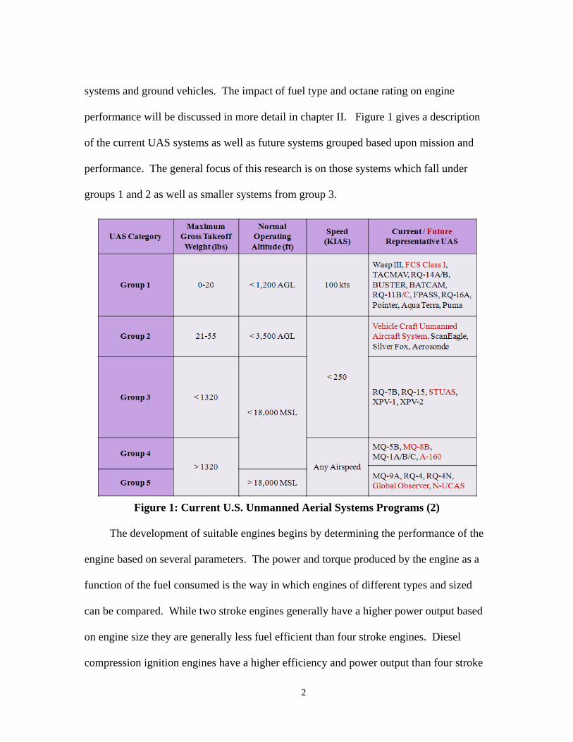
systems and ground vehicles. The impact of fuel type and octane rating on engine

performance will be discussed in more detail in chapter II. Figure 1 gives a description

of the current UAS systems as well as future systems grouped based upon mission and

performance. The general focus of this research is on those systems which fall under

groups 1 and 2 as well as smaller systems from group 3.

Figure 1: Current U.S. Unmanned Aerial Systems Programs (2)

The development of suitable engines begins by determining the performance of the

engine based on several parameters. The power and torque produced by the engine as a

function of the fuel consumed is the way in which engines of different types and sized

can be compared. While two stroke engines generally have a higher power output based

on engine size they are generally less fuel efficient than four stroke engines. Diesel

compression ignition engines have a higher efficiency and power output than four stroke

3

engines but are usually much heavier than similar spark ignition engines. The extra

weight for a diesel engine is due to thicker cylinder walls needed to contain the much

higher cylinder pressures that are created in the compression ignition engine. The higher

energy content of fuels like JP-8 and Jet-A are more suited to the compression ignition

engines where temperatures are allowed to go higher during combustion and knocking or

auto-ignition is desired. The use of low octane fuels in spark ignition engines can lead to

knocking which can damage the engine or cause heavy vibrations which could damage

other parts of the aircraft. The development of new technologies such as direct fuel

injection and variable spark timing have shown promise in reducing engine knock in

engines running on heavy fuels.

One aspect of engine development that has not seen much research is the variation

of engine performance with altitude. Most small COTS engines in use today were

originally developed for the recreational remote controlled, RC, model aircraft enthusiast.

These engines were designed to operate within several hundred feet of sea level. In

general most of these COTS engines run using a carburetor to meter fuel in the intake of

the engine. Most carburetors included on these production engines can be tuned with

some difficulty for operation at higher altitudes by adjusting the needle valve setting by

hand manually. The demand placed on these engines by the military in their employment

of UAS systems has lead to the desire to determine engine performance based on a fixed

engine tuning over a range of pressure and temperature conditions simulated operation

over a range of altitudes.

4

I.1 Objectives

There are several objectives for the current research. This research was aimed at

determining how the engine performance varies as a function of altitude using high

octane fuels as a baseline for future research. A range of engine speed and load

conditions will be run at multiple simulated altitude conditions for the baseline fuel. In

addition the engine performance running on heavy fuels over a range of engine speed,

engine load, and altitude conditions will be run for comparison. The ultimate goal is to

use the information gained in this research to help engine developers and system

designers build systems that are capable of running on low octane fuels over a wide range

of altitudes in a consistent manner.

A secondary goal for this research is to investigate the sensitivity of engine

performance based upon carburetor setting. The carburetor is tuned manually per

manufacturer’s instructions by rotating the needle valve in or out a specific number of

turns. Because the adjustment is made manually the accuracy of the adjustment is quite

crude and as such large variability in the actually setting from flight to flight can occur.

The engines utilized in typical model aircraft applications and currently being used in

small man portable UASs are manufactured without tight tolerances. The lack of

manufacturing precision may lead to significant performance differences from engine to

engine. Designing cost effective platforms with repeatable performance is important to

military utility. A tertiary goal of this research is to attempt to quantify the amount of

variability in engine performance that can be attributed to manufacturing differences

between identical engines.

5

I.2 Methodology

The first step towards completing the research objectives was to design a mobile

test stand capable of generating simulated altitude conditions. Once the design phase was

completed parts were ordered and construction on the mobile test facility was completed.

The next step in the process was to complete a series of system functionality checks.

These checkouts verified that the system could be operated safely, that it was capable of

generating the conditions required, and that it was capable of recording the necessary

measurements to complete the performance analysis.

The capability of the test stand was determined through a series of tests. The first

test was completed by running the main flow path to determine the ability of the stand to

generate low pressures within the chamber. The pressures were achieved by varying the

compressor speed and the control valve positions in increments until the compressor

drive motor reached its power limit. Based upon the ambient temperature pressure tests

the next step was to couple the coolant system with the pressure system. The coolant

flow rate was incrementally increased while the system pressure was incrementally

reduced. The combined pressure and temperature testing set the capability limits of the

mobile test facility.

Once the limits of the test facility were determined a representative test engine was

placed in the chamber. Performance testing of representative engine was completed in

several steps. The first step was to determine sea level performance of the engine. Sea

level performance was determined by incrementally varying engine speed from 2000 to

8500 RPM at set throttle positions. The throttle position was then changed and the

engine speed was again run through the range of speeds. Four throttle positions were

6

used to generate a sea level engine performance map. After the sea level testing was

completed attempts were made to determine engine performance at two additional

altitudes of 5000 ft and 10000 ft. Performance maps at the additional altitudes were not

completed due to limitations of the test facility. The test engine was tested at lower than

sea level pressured to determine how engine inlet pressure impacts engine performance.

The lower pressure load tests were completed by fixing the engine speed and throttle

setting and varying the inlet pressure of the engine. The lower pressure load tests showed

trends in engine performance as the inlet pressure decreases.

The impact of carburetor tuning was observed during the course of performing

engine load tests. Carburetor tuning was critical to completing the full range of sea level

engine performance tests. Future testing of carburetor tuning should involve careful

variation of carburetor needle position in small steps at fixed engine speed and throttle

position to determine the impact to engine torque and power. In order to determine the

full impact of carburetor tuning the needle position test should be repeated for a range of

engine speed and throttle positions.

7

II. Theory and Previous Research

II.1 Engines

Internal combustion engines come in many sizes and types which can make it hard

to apply research done on one test engine to classes of engines. Engine size is usually

based upon the total displacement volume of the engine. Large engines are categorized

as those with a total displacement volume greater than 300 cm3 and small engines are

those with a displacement volume less than about 150 cm3. There are two main engine

designations that differentiate engine operation; the number of strokes and the type of

ignition. The number of strokes that an engine uses determines how many movements of

the piston occur for each power stroke of the engine. A four stroke engine has four

movements for each power stroke that occurs while a two stroke has only two. A four

stroke engine has an intake, compression, expansion, and exhaust stroke which enables

the engine to get rid of most of the burned combustion products before replacing them

with a fresh charge in the cylinder. A two stroke engine has only two strokes, the

compression and expansion. The intake of a fresh charge occurs simultaneously with the

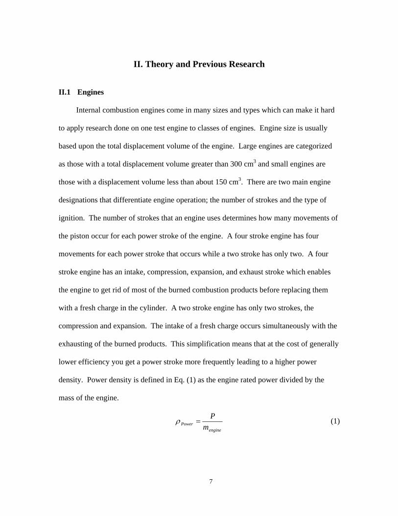
exhausting of the burned products. This simplification means that at the cost of generally

lower efficiency you get a power stroke more frequently leading to a higher power

density. Power density is defined in Eq. (1) as the engine rated power divided by the

mass of the engine.

engine

Power m

P (1)

8

Smith, Boruta, Jerovsek, and Meitner (3) give two metrics for describing engine

loading and engine compactness. Smith et al define engine loading in terms of

horsepower, hp, per volume which allows researchers to compare how much power is

being generated independent of engine type. Smith et al define power density in a

slightly different form than Eq. (1) as horsepower per pound, but this represents a similar

metric for the engine. Table 1 gives a comparison of several state of the art engines and

their related metrics given by Smith et al. Typical spark ignition and diesel engines have

power densities between about 0.3 and 1.0 hp/lb with a power to volume ratios between

1.00 and 2.70 hp/in3.

Table 1: Engine Comparison Chart (5) Engine Type Power

(hp) Displacement

(in3) Volume

(ft3) Weight (lbs.)

hp/lb hp/in3

Yanmar 6L43-EPT Diesel 480 354 32.7 1411 0.3402 1.36 Yanmar 4BY 150 Diesel 150 122 18.3 551 0.2720 1.23

Delta Hawk DH200A4/U4/R4

Diesel 200 202 8.0 327 0.6116 1.00

Rotax 914 UL2 SI 100 74 4.7 166 0.6024 1.35 UAV AR682R SI Rotary 95 36 2.0 124 0.7661 2.64 UAV AR801R SI Rotary 50 18 1.0 65 0.7692 2.70

ZanZottera 498iA SI 39 30 0.75 41 0.9512 1.30

The second designation is the type of ignition used in the engine. Spark ignition

engines use a spark plug or glow plug to provide the additional energy needed for the fuel

air mixture to reach the activation energy level needed to start combustion. Compression

ignition engines compress the fuel air mixture so that the temperature rise caused by

compression exceeds the ignition temperature of the mixture. In compression ignition

engines the compression ratio defined in Eq. (2) is between two and three times higher

than that used in spark ignition engines (4).

9

c

cd

V

VVCR

(2)

where Vd is the displacement or volume swept by the piston from bottom dead center,

BDC, to top dead center, TDC, and Vc is the clearance volume. The clearance volume is

the volume of the cylinder when the piston is at TDC and is the minimum cylinder

volume. Figure 2 shows the relationship between the components that translate power

from the combustion chamber into the output shaft. The crank angle, θ, shown in Figure

2 is a way to relate the change in chamber volume to various engine parameters discussed

in the next section.

Figure 2: Geometry of cylinder, piston, connecting rod, and crankshaft where

B=bore, L=stroke, l=connecting rod length, a=crank radius, θ=crank angle (adapted from 4).

Several other engine descriptions are important in describing the engine being used

in a given research or UAS application. A naturally aspirated engine is one that uses air

from the surrounding environment directly without the aid of a pump. A carbureted

10

engine uses the principles of a venturi or system of venturis to produce the required fuel

flow. The carburetor meters the fuel based on a pressure difference created by the

venturi. This fuel flow mixes with the air stream in the intake of the engine before it

reaches the cylinder. Fuel injection uses a mechanical device to meter pressurized fuel

through an orifice into either the intake or the cylinder. Fuel injected into the intake

stream is generally termed port fuel injection while fuel injection into the cylinder is

generally called direct fuel injection, DI.

The intake process in a two stroke engine is somewhat different than for a four

stroke engine due to the need to increase the intake pressure of the fuel air charge above

the exhaust pressure in order to enhance exchange of gas within the cylinder during

simultaneous intake and exhaust period called scavenging. Scavenging in a two stroke

engine is accomplished in several ways and is based upon the geometry of the ports and

way in which the fresh charge intake pressure is increased. The three main types of

scavenging are cross-scavenged, loop-scavenged, and uniflow-scavenged configurations.

Uniflow scavenged engines bring the fresh charge in one end of the cylinder and exhaust

it at the opposite end of the cylinder using a variety of ports and valves. Cross-scavenged

and loop-scavenged engines use an arrangement of ports in the cylinder wall near BDC

which open and close as the piston moves up and down within the cylinder. The main

difference between cross-scavenged and loop-scavenged engines is the arrangement of

the ports. Cross-scavenged engines have the intake port directly across the cylinder from

the exhaust port and use some upward angle in the intake and exhaust ports to force the

flow up into the cylinder. Loop-scavenged engines use multiple intake ports generally set

perpendicular to the exhaust port. In loop-scavenged engines the intake ports are usually

11

set so that the incoming flow impinges on a wall or on the opposing incoming flow from

the opposite intake port. Figure 3 shows a general diagram of the three types of

scavenging processes. The flow path into and out of cylinder is extremely important in

two stroke engine design and can have a large impact on engine performance and fuel

efficiency (4).

Figure 3: Common types of scavenging; (a) loop-scavenging, (b) cross-scavenging, (c) uniflow-scavenging configurations (adapted from 5).

The compression of the fresh charge in a two stroke engine can be accomplished

using an external pump such as a roots type blower or a centrifugal compressor or it can

be accomplished using the piston and the crankcase to form an internal compressor. For

small single cylinder two stroke engines commonly found in RC airplane applications

and used for small engine applications such as chain saws generally crankcase

compression is used to save space and reduce weight. One major drawback to most two

stroke engines is that the oil used to lubricate the piston and reduce cylinder wear must be

mixed with the fuel and is burned as part of the combustion process. In four stroke

engines the oil is contained within a separate area and is a closed loop system which is

easier for maintenance and logistics.

12

II.2 Comparison of Engine Parameters

In order to compare one engine to another across the wide variety of engine types a

set of performance parameters is needed. The most basic performance parameters are

fuel consumption, power, and torque. Power and torque are based upon engine size and

type. The amount of power required to hold the dynamometer at a fixed speed can be

measured, and is called brake power, Pb. Using a load cell at a fixed distance on the

dynamometer torque can be measured. A shaft encoder on the dynamometer shaft can

measure speed directly. In order to relate engines of different sizes the fuel consumption,

or fuel mass flow rate, fm

, is divided by the engine power as in Eq. (3), and is called the

brake specific fuel consumption, BSFC. BSFC is a measure of the fuel used per amount

of energy produced per unit time and is related to how well the energy can convert the

available chemical energy stored in the fuel into useful shaft work.

b

f

P

mBSFC

(3)

Torque, T, is defined as a force, F, times a distance, b, given by Eq. (4) and is the

measure of an engines ability to do work. Power is the rate at which an engine performs

work and is defined by Eq. (5) as torque times the angular speed of the engine. The

angular speed of the engine is the rotational rate in revolutions per unit time, N, times the

number of radians per revolution, 2π. The engine load required by an ICE is due to the

torque required to move a propeller or other device through some amount of rotation.

This load as well as throttle setting will determine the engine RPM. As engine load and

engine speed increase the total amount of fuel and air running through an engine will

13

increase leading to changes in BSFC and emissions. In a two stroke carbureted engine

changes in engine speed and throttle setting will have an impact on the scavenging of the

engine. Engine load and engine speed can also impact combustion efficiency, but it is

not necessarily a linear dependence and is more likely attributed to the equivalence ratio

driven by the engine speed and throttle setting (4).

bFT * (4)

TNPb **2 (5)

The torque available at the output shaft is the engines ability to do work and can be

related across engine sizes and type by defining the work per cycle of an engine divided

by the cylinder volume. This quantity is termed mean effective pressure, MEP, since it

has units of pressure and is given as Eq. (6). The term nR is the number of crank

revolutions per power stroke per cylinder and is equal to two for a four stroke engine, and

one for a two stroke engine. From Eq. (6) it can be seen that since for a given engine the

only quantity that changes is the torque at the output shaft which leads to maximum

BMEP at the maximum torque value. Maximum power does not occur at the maximum

torque value because it is a function of torque and engine speed. The BMEP value for the

maximum engine power output will be 10% to 15% lower than the maximum BMEP

value (4).

d

R

d

Rb

V

nT

NV

nP **2

*

*BMEP

(6)

Fuel conversion efficiency, ηf, is a measure of how well the engine is able to

convert the chemical energy stored in the fuel and convert it into useful shaft work. Fuel

conversion efficiency is defined as work per cycle divided by the amount of fuel inducted

14

per cycle times the fuel heating value, QHV, and is given by Eq. (7). In four stroke

engines the volumetric efficiency is used to describe the engines ability to induct air into

the cylinder during operation. Two stroke engines do not have a defined induction

process so volumetric efficiency is not applicable and will not be used to compare

engines or past research.

HV

HVf

bf QBSFCQm

P

*

1

*

(7)

In addition to the thermodynamic or fuel conversion efficiency defined in Eq. (7),

two stroke engines use a parameter called the delivery ratio to describe their operating

characteristics. Delivery ratio, λ, from Haywood (4), is defined as the mass of delivered

air or mixture per cycle divided by the reference mass show as Eq. (8). For spark ignition

two stroke engines the mixture mass is used to define the delivery ratio. The reference

mass is the density of the mixture at the inlet conditions times the engine speed and the

displacement volume, and the actual mixture mass delivered is simply the sum of the fuel

mass flow rate and the air mass flow rate. Higher delivery ratios are desired and indicate

that the engine is exhausting a higher percentage of burned products and replacing them

with fresh charge.

dmix

mix

VN

m

**

(8)

II.3 Scaling Laws/Issues

The use of small internal combustion engines for UAS applications requires that

designers understand the implications of scaling the engine size and its impact on engine

15

performance and combustion. Cadou et al have done considerable research on small

scale internal combustion engines (6, 7, 8, and 9) and how the power and efficiency of

the engine can be estimated based upon engine mass. Cadou et al (6) propose a power

scaling law on a log-log scale in the form P=Axb where x is the mass of the engine and A

and b are constants shown as Eq. (9).

7633.03.9901 xP (9)

Figure 4 from Reference 6 shows the relationship between engine mass and output

power. Cadou, Moulton, and Menon attempted to derive a similar log linear relationship

between engine weight and engine efficiency but the data available from engine

manufactures did not support this relationship for engines below 1 kg.

Figure 4: Power output versus engine size (6)

The research by Cadou et al (6) was designed to test small scale internal

combustion engines in order to determine appropriate scaling laws based on actual test

data rather than relying on manufactures reported values. The researchers built a test

system capable of measuring engine speed, engine torque, engine brake power, and fuel

16

consumption. The engine torque was measured using a cradle system connected to a load

cell where the moment arm between the load cell and the cradle can vary in length to

accommodate different engine sizes. The engine brake power was measured using a

Magtrol HB-880 double hysteresis brake where the power absorbed is proportional to the

voltage signal supplied to the brake. The engine speed was measured using an

ElectroSensors system consisting of 16 magnetic poles attached to the power takeoff

shaft and a proximity switch with senses the poles as they pass. The fuel consumption

was measured by taking a series of mass measurements of the fuel tank over fixed

periods of time. The researchers used a least squares fit to the mass measurements to

determine the fuel mass flow rate. Cadou et al used a two stroke spark ignition OS46FX

engine to test first the accuracy of the test system and second to test how running the

engine under fuel rich and fuel lean conditions would impact the engine performance.

The tests performed over a range of engine speeds at wide open throttle showed that

torque and power both increase as the engine is operated in a leaner condition. The

engine efficiency also increases as the engine is run in a leaner condition. The maximum

power output measured for this engine was 0.5 hp which was only about 30% of the

manufacturer’s estimate of 1.65 hp. The researchers also noted that the noise associated

with the fuel mass measurements meant that there was about a 2% error bar around the

engine efficiency calculated.

Menon, Moulton, and Cadou (8) also illustrated one other important aspect related

to small internal combustion engines. The variation in performance between engines of

the same design and variation in the performance of a single engine over multiple tests

was shown to be significant. Using two AP Engines Yellowjacket engines with a

17

displacement of 2.45 cm3 and a mass of 150 g Menon et al (8) showed how two identical

engines from the same manufacturer perform differently. The engines were run with a

constant mixture setting leaned per the manufacturer’s instructions at a wide open

throttle, WOT, over a range of engine speeds from 7000 to 14000 RPM. The fuel mass

flow rate was measured using an FMTD4 nutating microflowmeter manufactured by

DEA Engineering. The air mass flow rate was measured using a TSI model 4021 mass

flowmeter with an operating range of 0-300 L/min and a linear 0-4 VDC output signal.

Power and torque were measured as described above from Reference 7 using the same

dynamometer developed in the previous work. The goal of this work was to determine

power and efficiency values within 10% of the actual value for use in understanding how

engine performance scales with engine size.

Menon et al (8) showed in Figure 5 that a given engine’s performance over repeated

tests was repeatable within the measurement uncertainty. The slight variation in the data

between tests on the same engine was due to torque sensor calibration drift and slight

changes in needle valve setting between runs. Figure 5 also shows the very large

difference in performance between the two engines tested in this research. The reasons

for the variation in performance between identical engines operating at the same

conditions were not identified by the authors. One reason for the differences may be

manufacturing tolerances by the engine builder. A second cause for this variation may be

due to the differences in the carburetors on each engine and how they supply the fuel and

air mixture to the engine.

18

Figure 5: Engine Performance at constant mixture setting and WOT; two

different engines and five different tests (8).

Menon et al (8) also investigated the impact of delivery ratio on engine

performance. They used a slight variation of Eq. (8) where the mass flow and density of

air was used instead of mixture mass flow and mixture density. The slight changes due to

this adjustment would not impact the overall conclusions reached. Menon et al showed

in Figure 6 that the delivery ratio decreases as engine speed increases independent of

mixture setting. Figure 6 shows delivery ratio plotted against engine speed for two

different mixture settings. The authors explain that the decrease in delivery ratio with

increasing engine speed is due to an increase in fuel to air ratio with engine speed. The

increase in fuel to air ratio means that less energy is released per cycle as less air is

available to react with the fuel in the combustion chamber during each cycle. The

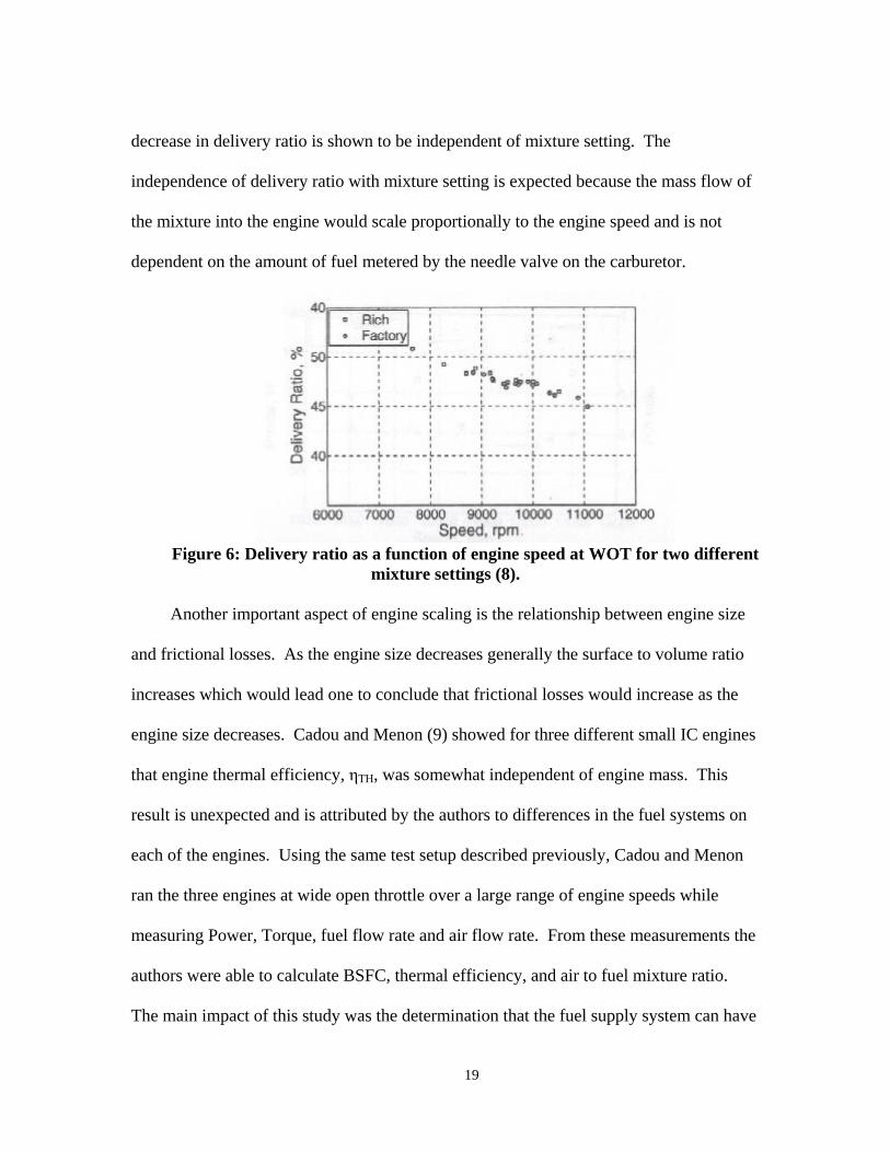
19

decrease in delivery ratio is shown to be independent of mixture setting. The

independence of delivery ratio with mixture setting is expected because the mass flow of

the mixture into the engine would scale proportionally to the engine speed and is not

dependent on the amount of fuel metered by the needle valve on the carburetor.

Figure 6: Delivery ratio as a function of engine speed at WOT for two different

mixture settings (8).

Another important aspect of engine scaling is the relationship between engine size

and frictional losses. As the engine size decreases generally the surface to volume ratio

increases which would lead one to conclude that frictional losses would increase as the

engine size decreases. Cadou and Menon (9) showed for three different small IC engines

that engine thermal efficiency, ηTH, was somewhat independent of engine mass. This

result is unexpected and is attributed by the authors to differences in the fuel systems on

each of the engines. Using the same test setup described previously, Cadou and Menon

ran the three engines at wide open throttle over a large range of engine speeds while

measuring Power, Torque, fuel flow rate and air flow rate. From these measurements the

authors were able to calculate BSFC, thermal efficiency, and air to fuel mixture ratio.

The main impact of this study was the determination that the fuel supply system can have

20

a very large impact on the engine efficiency and performance. The authors also noted

that the measure peak power of each engine were on the low end of the manufactures

reported data but followed the previously noted power law relationship.

Shin, Chang, and Koo (10) studied the effect of altitude variation on engine fuel

efficiency and frictional losses. The main focus of their research was to tune an engine

prediction code. By tuning the code the researchers felt that they would be able to predict

some general guidelines which would help developers design a long endurance miniature

unmanned aerial vehicle, UAV, engine. Tests were conducted on an ENYA Company

Model R155-4c 25.4 cm3 four-stroke glow-plug combustion engine. The researchers

modified the engine to be a four-stroke spark ignition engine run on gasoline with the

addition of a separate lubrication system. The engine frictional losses were measured by

using an electric motor to turn the piston and measure the torque required at different

engine speeds. Figure 7 shows the measured motored mean effective pressure as a

function of engine speed for the test engine. The wide range of data points for engine

speeds below about 5000 RPM is attributed to the large cycle to cycle variations that

occur in small IC engines. The reasons for these large variations will be discussed in

more detail in section II.6.1. The tests showed that there is no one correlation that will

work to predict frictional losses across the engine speed range from 3000 RPM to 10000

RPM. The overall result of these frictional loss tests was to come up with a correlation to

predict power and torque as a function of engine speed. The code developed by the

authors was able to predict the power and torque over a range of engine speeds when

compared to test data. The results from the motoring tests allowed the authors to include

21

frictional losses in an engine prediction code which was used to investigate the impact of

altitude on fuel consumption, power, and torque.

Figure 7: Measured friction losses of the test engine in comparison with those of a

typical automotive engine (10).

II.4 Pressure Impact

The effect of atmospheric pressure on the performance of a two-stroke engine was

presented by Harari and Sher (11). In this study an attempt to build upon the correlations

previously made in other papers was accomplished by including the effect of atmospheric

pressure on the predicted output power. The work by Harari and Sher was done using a

Sachs type SF2-350 Pistion-port engine with 2x350 cm3 opposed-piston crankcase

scavenged, Schnürle type, two-stroke engine. Engine power and torque were measured

using a Hofmann eddy-current dynamometer type 12d. Exhaust gas composition was

measured using a SGA-9000 infrared gas analyzer. The ambient pressure was controlled

by a vacuum pump at the exhaust and by throttling the intake air using a differential

22

pressure gauge between the intake and exhaust. The data collected covered a speed range

from 6000 RPM to 9000 RPM and a pressure range from 44 kPa to 100 kPa. The

pressure range tested equates to a range from sea level up to 7000 km. The maximum

engine power has an approximate linear dependence upon the ambient pressure. Harari

and Sher plotted maximum torque as a function of engine speed for a wide range of inlet

pressure conditions and is shown as Figure 8. The general torque curve increase from

low RPM up to a maximum and then decreases with increasing engine speed. Figure 8

shows that at sea level this engine follows this expected pattern while with decreasing

inlet pressure the maximum torque begins to behave very non-linearly.

Figure 8: Maximum engine torque vs. engine speed and ambient pressure (11).

Harari and Sher replotted the data in Figure 8 as maximum torque versus ambient

pressure and showed that as the inlet pressure decreases the maximum torque for all

engine speeds also decreases. The authors were attempting to determine a correction

factor, CF, which could be used to determine engine power as a function of ambient

23

temperature, T, and pressure, p. The general form of the correction factor is listed as Eq.

(10) and can be used to predict engine power, Pb, as Eq. (11).

B

S

A

SS

B

S

A

SV

V

T

T

p

p

T

T

pp

ppCF

1

1 (10)

where pV is the water vapor partial pressure, ω is the air humidity ratio, and the subscript

S denotes reference sea level static conditions. A and B in Eq. (10) are constants that are

correlated from experimental data.

CFPP Sbb * (11)

When plotted on a log scale the peak power was shown to have a linear dependence

on ambient pressure while the correction factor depends significantly on engine speed.

These results lead the authors to conclude that the correction factor should be a function

of ambient pressure raised to a power proportional to engine speed. The constant A in

Eq. (10) is determined by the authors to be near 1.0 for low engine speeds while for

maximum engine speed A should be 2.0 (11). From the experimental data the author

suggests that the engine torque or BMEP falls 50% when the ambient pressure decreases

from 100 kPa to 50 kPa. One of the conclusions reached by Harari and Sher is that the

scavenging efficiency and the delivery ratio decrease with decreases in ambient pressure

and is one of the main reasons that power and torque decrease while BSFC increases.

Shin, Chang, and Koo (10) established that their computer code could predict the

power and torque of the test engine over a range of engine speeds. The authors then used

the code to simulate engine performance at three altitudes, sea level, 3 km, and 5 km.

Using the code they predicted the effect of altitude on brake mean effective pressure and

engine brake power. Figure 9 and Figure 10 show these predictions and as expected the

24

engine power and BMEP decrease as altitude increases. Shin et al used the code to

predict brake specific fuel consumption, BSFC, of the engine at the same altitudes. Test

data collected from the experiment described previously at sea level conditions when

compared to code predictions of BSFC was not as good as the power and pressure

predictions. The authors give several reasons for the differences including errors in the

measurements made with the air-fuel sensor and possible leakage in the exhaust manifold

which may have allowed fresh air into the system.

Figure 9: Simulation results of BMEP with altitude (10).

Figure 10: Simulation of engine power with altitude (10).

25

II.5 Temperature Impact

Watanabe and Kuroda (12) studied the effect of inlet air temperature on the power

output from a two-stroke crankcase compression gasoline engine. Their effort was

focused on determining a correlation for the power output of the engine as a function of

the absolute inlet temperature in a range of 4.5 °C to 40 °C. The test engine was a 60 cm3

Schnuerle scavenging type engine and was run over a speed range from 1000 RPM to

4000 RPM. The authors used six electric heaters with a total capacity of 900 W to heat

the inlet air allowing a maximum carburetor inlet air temperature of 50 °C. Air flow rate

was measured upstream of a surge tank with a round nozzle. The surge tank was 690

times the size of the engine volume and had a gummy diaphragm attached to reduce

pressure and flow pulsations to allow for more accurate air flow measurements. Engine

power was measured using a 2 hp electric dynamometer and was corrected back to

standard conditions using Eq. (12).

Sb bS

pN N

p (12)

where Nb is break power, p is the atmospheric pressure, and the subscript s denotes

reference conditions. The authors derived a relationship between the power output and

the scavenging pressure to show that as the temperature decreases the power will

decrease due to a decrease in scavenging pressure with increasing ambient temperature.

This result also compares well with compressor theory where an increase inlet

temperature for a fixed inlet temperature will result in a lower outlet pressure. Watanabe

and Kuroda based upon established theory of how four stroke engine power scales with

temperature assumed a form show as Eq. (13).

26

TPb

1 (13)

where brake power, Pb, is proportional to the inlet temperature to a power, λ. From the

test data for engine output power the exponent λ falls between 0.5 and 0.9, where λ=0.5

represents the four stroke engine theory. The exponent in the equation given was

dependent upon the temperature of the inlet air flow and engine speed. The author’s

correlation was compared with the established DIN 6270 correlation which has the form

given by Eqs. (14) thru (16).

*0ee NN (14)

1

117.0

mc (15)

0

4/3

0

0

*D

D

i

i

pp

pp

T

T

N

N

(16)

where Ne is the net power output, Ni is the indicated power output or brake power, ηmc is

mechanical efficiency, p is atmospheric pressure, pD is saturated vapor pressure, ψ is the

relative humidity, and the subscript 0 indicates reference conditions. These equations

along with the authors’ correlations and the experimental data are shown in Figure 11.

Figure 11: Values of λ in Eq. (13), i.e., (12).

27

Watanabe and Kuroda (12) assert that the use of a constant temperature cooling

airflow around the engine may have impacted the data. They state that a cooling airflow

heated to the same temperature as that of the inlet airflow would cause the power drop

due to the temperature increase to be more significant and possibly fall closer to the DIN

6270 lines in Figure 11.

Temperature has also been shown to have a large impact on the formation of several

important combustion products or emissions. Combustion products such as Nitric

Oxides, NOX, unburned hydrocarbons, UBHC, and Carbon Oxides, CO2 and CO, are all

important in relation to combustion efficiency and the ever increasing pressure to reduce

greenhouse gases produced by internal combustion engines. Nitric Oxide compounds,

NOX, emissions have been shown to vary proportionally to the temperature at which the

reaction occurs (13-14). This relation has been show to be independent of engine or fuel

type. Flynn et al (13) showed that there is an approximate minimum temperature under

which conditions are such that a chemical combustion reaction will not occur thus NOX

will not be produced. Flynn also showed the impact of temperature on the production of

UBHCs, where reduced combustion temperatures will increase the amount of UBHC in

the emissions.

The reduction of NOX emissions has been approached from a variety of angles.

Most approaches attempt to reduce the combustion event temperature in order to reduce

the production of NOX. This attempt in the past has come at the price of increasing

carbon monoxide, CO, emissions. CO is an incomplete combustion product and

increased combustion temperatures increase the rate at which CO can be converted to

carbon dioxide, CO2. This is a well know trade off that has been documented for

28

different types of engines. Chen (14) was able to show that by injecting an aqueous

mixture of ethanol and water in addition to the standard fuel injection one could reduce

NOX emissions without significantly impacting CO or unburned hydrocarbon, UBHC,

emissions.

Wilson (15) ran several experiments in an effort to determine the effects of fuel

heating and ultimately mixture temperature on the torque and BSFC of a small internal

combustion engine. The tests utilized a Fuji B-34 single cylinder four stroke spark

ignition engine with stock timing as the test engine. Power and torque were measured

using a Magtrol model 1WB65 eddy current dynamometer. The fuel flow rate was

measured using a Max Machinery model 213 mass flow meter. Wilson built a fuel heater

constructed from a copper block that utilized two 750 W Watlow strip heaters and a

Watlow temperature controller to heat the fuel to the desired temperature. Fuel

temperature was measured with a thermocouple downstream of the heating element to get

an accurate measurement of fuel temperature into the carburetor. Wilson (15) ran three

independent tests in order to determine fuel temperature on engine torque and BSFC.

The first test was run by simply heating the fuel to the desired temperature while

measuring BSFC and torque. The second test compared the heated fuel data from test

one with data obtained by adjusting the carburetor high speed needle with fuel at ambient

temperature. The last test consisted of heating the fuel to a specific temperature and

adjusting the high speed needle on the carburetor. The conclusion from these tests

presented by Wilson is that heating the fuel alone has little impact on the overall engine

performance. Wilson also concluded that the impact of equivalence ratio on engine

performance is significant and can be greatly impacted by carburetor setting and fuel

29

temperature. Based on the results from Wilson (15) for heated fuel tests no conclusions

can be made about how much the air temperature will impact the engine performance.

Equivalence ratio in the engine will be impacted by the air and fuel densities which are

directly related to the temperature of the mixture, so it is expected that inlet air

temperature will have a direct impact on engine performance.

II.6 Measurement/Accuracy of Parameters Required

II.6.1 Pressure

The accuracy of pressure measurements can be crucial to calculating important

engine parameters such as heat release, combustion event timing, and combustion

stability. Pressure measurements along with temperature measurements can be used to

determine the state of the air entering the carburetor and exiting in the exhaust gas flow.

The accuracy of these measurements is important in determining the impact that changes

in intake pressure have on the performance of the engine. Cylinder pressure can vary

widely from cycle to cycle and are impacted by changes to inlet pressure and

temperature, composition of the charge stemming, and changes in the fuel to air ratio.

Turbulent flow in the cylinder would cause changes to the flow pattern causing

differences in the amount of charge being short circuited and altering the percent of

residual charge. Knocking conditions would also cause variations in cylinder pressure

based on the location of the knock center and the severity of the knock.

Intake and exhaust gas pressures can be used to help reference or peg the pressure

signal being transmitted by the pressure transducer for in cylinder measurements. The

signal measured by the in cylinder pressure transducers can change due to the high heat

30

flux associated with combustion in the area of the pressure transducer. In order to

accurately translate the transducer voltage signal into an absolute pressure one or more

points in the signal versus time curve must be related to an independent pressure

measurement. Several methods for pegging the cylinder pressure measurement are

discussed by Lee, Yoon, and Sunwoo (16) who proposed a new method based upon a

modified least squares method which utilizes a variable polytropic coefficient. Lee et al

propose that the reference should be based upon the assumption of polytropic

compression where Eq. (17) allows the calculation of the pressure at an arbitrary crank

angle based upon a reference condition.

cV

V

p

p ref

ref

(17)

where θ is the crank angle degree and the subscript ref represents an arbitrary reference

condition. The modified method proposes the calculation of the polytropic coefficient on

a cycle-by-cycle basis and considering it a fixed value for each independent cycle.

Solving Eq. (17) for κ gives the estimation of the polytropic coefficient of each cycle as

Eq. (18).

]/ln[

]/ln[~

VV

ppi

ref

ref (18)

The use of Eq. (18) allows for the solution of the measurement bias and the

reference pressure for each cycle based on applying a linear least-squares method from

the solution of Eq. (20). The work by Lee et al (16) also uses a first order auto-regressive

filter to help improve the robustness of the resulting polytropic coefficient of the form of

31

Eq. (19). The variable a in Eq. (19) represents the auto-regressive coefficient and was set

at 0.2 for the study completed by Lee et al.

101~

1

~~

aaai ii (19)

yXXXw TT 1 (20)

where the variables in Eq. (19) are

NN

refs

bias

c

c

c

X

E

E

E

ypK

Ew

1

1

1

2

1

2

1

and E(θ) is the voltage at a specific crank angle, Ks is the sensor gain, and c(θ) is equal to

the right hand side of Eq. (17) and N is the total number of sample points used in the

calculation for a single pressure cycle. Lee et al showed based on simulated engine

pressure data and experimental measurements from a four cylinder 2.0 L direct injection

diesel engine that the modified least squares method had better noise rejection capability

and higher accuracy through the calculation of the two norms of the sensor offset

calculation error. The two norm, also referred to as the Euclidean norm, is the length or

size of a vector and is defined as the square root of the sum of the squares of every value

in the vector. The sensor offset calculation error two norm is equivalent to saying the

error bounds of the calculated sensor offset. The calculation error two norm for the

modified lease squares method was 0.96. The three point pegging method discussed by

Lee et al had a two norm of 1.68 while the two point method and the regular least squares

methods were both above 2.33. In addition to the two norm calculated from simulated

engine data, experimental pressure measurements were taken and each of the methods

32

was used to calculate peg drift and the influence on the center of gravity of difference

pressure. Difference pressure is the difference in pressure between the measured

combustion pressure and the measured motored pressure. Lee et al showed that the

modified least squares method had a 4% smaller standard deviation in peg drift and a

60% lower standard deviation in the difference pressure center of gravity.

Wilson (15) did not reference his cylinder pressure data and instead relied only on

normalizing the data based upon the maximum pressure per cycle. Uncalibrated and

normalized data allowed Wilson to investigate the impacts of spark timing on the location

of peak cylinder pressure but did not allow him to directly compare the impact of fuel

type on peak pressure. In addition the in cylinder pressure measurements were able to

show signs of knocking combustion even though the measurements were not referenced.

The use of spark plug measuring sensors such as the one used by Wilson (15) is discussed

further by Bertola et al (17) and Walter et al (18). Bertola et al (17) investigated the

effect of transducer placement and type on measurement values. The experiment was

conducted on a modern four cylinder spark ignition engine with homogeneous charge

operation. The test engine was 0.5 liters with four valves per cylinder. Bertola et al used

both face sealing and shoulder sealing piezoelectric pressure sensors located in five

separate positions within the cylinder head. The data collected during the test was

filtered by selecting representative cycles instead of averaging the data over many cycles.

The reason given for this was averaging the data would make the data less meaningful by

smoothing out the peaks. Bertola et al showed the effect of locating the pressure sensor

very near the cylinder wall which tends to increase the initial pressure rise due to the

shock interactions with the wall. The authors also showed that locating the pressure

33

sensor in the squish gap area of the cylinder tends to increase the initial pressure rise.

The authors (17) propose that the best position for measuring knocking conditions in the

cylinder is in the center of the cylinder. This location provides for the ability to measure

knocking occurring in any location throughout the cylinder with the least interference or

magnification from the cylinder walls or the squish gap. Bertola et al also investigated

the impact that an indicating bore has on the measured pressure signal. Using different

sensors mounted in the same location within the cylinder head the authors were able to

show that sensors using an indicating bore showed signs of signal amplification due to

oscillations within the indicating bore. The amplitude of the enhanced signal was

dependent on the dimension of the indicating bore. The authors recommend a flush

mounted pressure sensor in order to reduce this induced error associated with the

indicating bore.

II.6.2 Temperature

Temperature measurements are important in order to determine the entrance and

exit conditions of the air, fuel, and exhaust gas mixtures. Temperature measurements

along with pressure measurements can be used to determine the state of the mixture,

including the heating value of the mixture which can then be used to determine thermal

efficiency. In addition to thermal efficiency the temperature measurements are needed in

order to determine the correlation between altitude atmospheric conditions and engine

performance. Thermocouples are utilized to measure the temperature of the important

quantities. Thermocouples are available in several different types including washer type,

grounded, ungrounded, and exposed. Washer type thermocouples can be used to measure

34

surface temperatures like engine head temperatures. Grounded thermocouples have a

quicker response time than ungrounded thermocouples but are susceptible to electrical

noise and ground loops. Exposed junction thermocouples are best for use when

measuring gas temperatures by allowing the junction to be in direct contact with the test

gas. Wilson (15) used Omega K-type thermocouples for all temperature measurements.

K-type thermocouples have a temperature range of -200 °C to 1250 °C with standard

limits of error of either 2.2 °C or 0.75% of the scale above 0 °C and 2.2 °C or 2.0% of the

scale below 0 °C (19).

II.6.3 Flow Meters

Flow meters are an important part of any combustion test experiment. The rate of

both fuel and air mass flows can be used to determine the fuel to air ratio in the engine.

The accurate measurement of these two flow rates is important because these values are

used to calculate several secondary parameters such as thermal efficiency, and brake

specific fuel consumption. Errors in the measurement of fuel flow rate can have a

significant impact on the reported BSFC value. BSFC is used to compare engines of

various sizes and types and is an important value that should be calculated accurately.

Typical liquid flow meters use the liquid to turn a shaft based on a specific volume of

fluid. As the shaft rotates a transmitter sends a signal which can be used along with the

density of the fluid to calculate an accurate mass flow. For small internal combustion

engines the required mass flow rate of fuel is low and so care must be taken to size the

liquid flow meter. If the volume of fluid required to turn the meter is high then fewer

pulses are sent to the data acquisition system per unit time. With few pulses the time

35

between pulses can vary significantly leading to errors in the actual mass flow rate of the

fuel. Menon et al (8) gave a table of typical fuel flow rates for small internal combustion

engines which ranged from 0.5 g/s up to about 4 g/s. These small flow rates are

sometimes hard to measure with standard off the shelf liquid flow meters. Menon et al

(8) choose to use a FMTD4 nutating microflowmeter by DEA Engineering which is

capable of measuring 0.02 cm3 of fluid per 5 V pulse. The fuel flow rate can be

calculated directly, Eq. (21), from the number of pulses, x, times the volume per pulse,

Volpp, divided by the total time, ttot. Menon et al used a scale as a backup device to

measure mass flow by taking readings at specific time intervals.

ppf

tot

xVolm

t

(21)

Air mass flow measurements can be done in several ways including thermal mass

flow meters, orifice meters, venturi meters, or a variety of other methods. The basic

principle behind many types of mass flow meters is based upon measuring a pressure

drop between two points with fixed areas and fixed fluid temperature. Using Bernoulli’s

equation the pressure drop and the area difference can be used to compute a volumetric

flow rate which multiplied by the density of the fluid calculated from the pressure and

temperature can be converted into a mass flow rate. Thermal flow meters use the

principles of heat transfer to measure the mass flow rate of the fluid moving past a heater

element. The temperature change sensed by the meter is directly correlated to the mass

flow rate of the gas or liquid. Menon et al (8) used a TSI model 4021 mass flowmeter

that was capable of measuring 0-300 standard liters per minute with a linear 0-4 VDC

36

output signal. Thermal flow meters operate accurately only under steady conditions so

care must be taken to damp out any flow perturbations caused by the engine.

II.6.4 Power, Torque, Speed

From Eq. (4) and Eq. (5) the relationship between power, torque, and speed is

established. The accuracy of any one of these measurements can impact the overall

performance calculations of an engine. Brake mean effective pressure is based upon

measured power, and engine speed. Power can be calculated based upon measured

torque and engine speed. Brake specific fuel consumption is proportional to engine

output power and fuel flow rate. Thermal efficiency of the engine is also based upon

measure power, fuel flow rate, and fuel heating value. Cadou et al (6-9) utilized a

Sensotek model 31 load cell to directly measure engine torque based upon a fixed

measure location. Engine load was applied using a Magtrol model HB-880 double

hysteresis brake affixed to the engine through a gearing system. Cadou et al (8) asserts

that utilizing this setup allows for a more accurate measurement of the torque because

there are no losses associated with a power train. The setup also offers the ability to

adjust the sensitivity of the torque measurement based upon the length of the moment

arm to which the load cell is affixed. The largest uncertainty in power and thermal

efficiency values comes from the torque measurement error and care should be taken to

reduce this error (8).

Wilson utilized a Magtrol 1WB65 eddy current dynamometer which outputs both

engine power and engine torque. The Magtrol has a 0.5% error at full load (15) and

contributed a very large error to reported BSFC values at low torque settings. Wilson

37

also reported that the data acquisition system was not fully utilizing the available torque

values. The original setup only ran at 1 Hz but the Magtrol was outputting the torque

signal at 120 Hz. An upgrade to the acquisition software was made that read the torque

signal at 120 Hz and reported an average value at 1 Hz which gave a more accurate

representation of the average torque.

II.7 Other Research

II.7.1 Spark/Valve/Injection Timing

Engine performance in internal combustion engines can be affected by a wide

variety of parameters. Some of the most important parameters involving the combustion

event include spark timing, and valve timing or injection timing. Spark timing directly

impacts when the combustion event will begin during normal operating conditions in

spark ignited engines. If the spark event occurs early or late relative to TDC then the

peak pressure will not occur at the optimum value of 16° ATDC (4) and maximum brake

torque will not be generated. Valve or injection timing is important because it directly

impacts the mixing process. The combustion process will occur along the boundary

between the fuel and air. If the fuel is not mixed uniformly with the air before the

combustion process is started then incomplete combustion may result. If the fuel or

fuel/air mixture is introduced into the cylinder late in the compression stroke then less

energy will be imparted into the gas. If the fuel or fuel/air mixture is introduced to early

into the cylinder then autoignition may occur causing damage to the engine. For two-

stroke crankcase scavenged engines similar to the test engine utilizing carburetors there

are no valves or direct injection. Crankcase scavenged engines rely on mixing of the fuel

38

and air in the crankcase prior to introduction into the cylinder and allow for a relatively

long mixing time. Spark timing for this type of engine will have the greatest impact on

engine performance.

Wilson (15) investigated the impact of spark timing on BSFC and torque by varying

the spark advance from the stock timing at fixed engine load conditions. With the engine

running at a fixed throttle setting and engine speed the spark advance was varied between

60° BTDC and 10° ATDC. The spark timing was corrected from a given input timing to

the actual spark timing based upon an average error value for each engine speed. Wilson

showed that as expected the fuel flow rate at a given engine speed was approximately

constant and was independent of spark timing advance. The data also showed that the

timing advance which gave the maximum torque also corresponded to a minimum in the

engine BSFC. Figure 12 shows the relationship between engine speed and spark timing

for both minimum BSFC and maximum torque. From the results of the tests Wilson

calculated an average decrease in BSFC of 9.36% across the range of engine speeds and

an average increase in torque of 4.45% with optimized spark timing over the stock

timing. Wilson recommended addition work to determine that actual impact on BSFC

and torque by carefully optimizing spark timing with fixed equivalence ratio and mixture

temperature to isolate the effects of spark timing on engine performance.

39

Figure 12: Optimum spark advance (BTDC) for maximum torque and minimum

BSFC vs. stock with n-Heptane (15).

II.7.2 Geometry

Cylinder geometry will have a large impact on engine performance and can include

engine compression ratio, engine port arrangements, engine clearance volume size and

shape, spark plug location, piston diameter, piston head shape, and piston stroke among

other things. Engine intake and exhaust design can also have an impact on engine

performance based on how area changes and cyclical pressure changes can be amplified

as pipe oscillations. Heywood (4) states that variations in mixture motion within the

cylinder at the time of spark, variations in the amount of fuel and air fed into the cylinder,

and variations in the mixing of fresh mixture and residual gases within the cylinder are

the causes for cycle to cycle differences in engine performance. All of the reasons listed

by Heywood for cyclic variations are directly related to engine geometry.

Beshai, Deniz, Chomiak, and Gupta (20) studied the impact of chamber geometry

on cycle by cycle variations in an optically accessible square piston spark ignition test

40

engine. The single cylinder test engine runs on propane and can be modified to change

the compression ratio and piston head shape with the use of caps placed on top of the

standard flat top piston. The researchers collected data over a minimum of 100 cycles in

order to obtain a representative sample for statistical analysis. Beshai et al (20) used the

maximum heat release rate to compare how the modified piston cap would compare to a

flat top piston. The flat top piston consistently had a maximum heat release rate over the

modified piston. In addition the coefficient of variation was calculated for the heat

release rates for the flat top piston and the modified piston. The coefficient of variation

for the flat top piston heat release rate was between 0.175 and 0.306 while the coefficient

of variation for the modified piston was between 0.516 and 0.792. This result shows that

chamber geometry can have a large impact on the local flow on a cycle by cycle basis

and that care should be taken to minimize this flow variation in order to increase heat

release rates and maximize engine performance.

Ceviz (21) studied the effect that intake plenum volume has on engine performance

over a range of engine speeds. The study was conducted using an engine with a

maximum power of 62 kW at 5800 RPM and a compression ratio of 9.2. The standard

engine was run at five specific speeds of 1250, 1500, 2000, 2500, and 3000 RPMs with

three different intake plenum volumes. The first experiment was run with the original

intake manifold, the second had a 90 cm3 addition, and the third with a 180 cm3 addition

over the original size. In cylinder pressure was measured with a Kistler 6117BFD17

spark plug piezoelectric pressure transducer and was sampled at 100 kHz. Intake

manifold pressure was measured using a Delco Electronics 1 bar manifold absolute

pressure sensor which has a 6.0 ms response time and was positioned 6.5 cm upstream of

41

the intake valve. Both in cylinder pressure and manifold pressure were averaged over 50

consecutive cycles to eliminate the effects of cyclic variations. Cylinder pressure data

was pegged by assuming that the pressure in the cylinder at bottom dead center after the

intake stroke equals the mean intake manifold pressure. During the tests, engine speed

was controlled by changing throttle position with a fixed engine load. No data was given

for experiments with volume additions greater than 180 cm3 because those tests resulted

in a decrease in engine performance according to the author. Ceviz (21) showed that the

increase in intake plenum volume resulted in an increase in brake torque, Figure 13, over

the range of engine speeds tested.

Figure 13: Variation of brake torque with engine speed for three different intake

plenum volumes (21).

Figure 14 shows that a 90 cm3 increase in plenum volume resulted in a decrease in

BSFC for engine speeds below 2500 RPM and was consistent with the BSFC produced

when running the engine above 2500 RPM with the original intake plenum. The 180 cm3

addition resulted in a decrease in BSFC over both the 90 cm3 addition and the original

42

volume for engine speeds below 2300 RPM. For engine speeds above about 2500 RPM

the large volume addition resulted in higher specific fuel consumption. The author (21)

attributes this increase in BSFC at higher engine speeds to an increase in intake manifold

pressure with increased plenum volume and engine speed.

Figure 14: Variation of specific fuel consumption with engine speed for three

different intake plenum volumes (21).

Ceviz (21) also showed the impact of plenum volume on the coefficient of variation

of indicated mean effective pressure, COVimep. COVimep directly impacts engine design

and is an indication of the amount of cyclic variation in the engine. Lowering the

COVimep is desirable because it allows the engine to run closer to its limits without

encountering abnormal combustion events like knock. Figure 15 documents that the

COVimep was about 14% to 39% lower across the range of engine speeds tested for the

engine run with increased plenum volumes. These results lead to the conclusion that the

decrease in coefficient of variation in indicated mean effective pressure can be attributed

to an increase in mixture homogeneities. The decrease in COVimep leads to an increase in

43

power output since the losses attributed to cyclic variations within the engine are

decreased.

Figure 15: Variation of coefficient of variation of indicated mean effective pressure

with engine speed for three different intake plenum volumes (21).

Celik (22) studied the effect of compression ratio, ignition energy, and spark timing

on engine performance and emissions. The tests used a Lombardini LA 250 four stroke

single cylinder carbureted engine which was first tested in an unmodified condition. The

engine was then modified to increase the compression ratio from 5:1 to 10:1, variable

spark timing was added, and the magneto ignition system was replaced with a higher

energy transistorized coil system. The modified engine also had a water cooling system

instead of the standard air cooled design which maintained a cylinder head and block

temperature of 90 °C where the air cooled engine had an engine temperature of 120 °C.

Celik (22) tested the two engines over a range of excess air ratio values, λ, with a fixed

engine speed of 2000 RPM and a fixed engine load of ¾ throttle to determine the lean

burn limits of each engine. Excess air ratio is the ratio between the measured air to fuel

44

ratio and the stoichiometric air to fuel ratio, Eq. (22). Excess air ratio is related to the

equivalence ratio, Eq. (23), ф, by the use of the fuel to air ratio instead of the air to fuel

ratio. The excess air ratio that produced the lowest amount HC emissions was used to set

a fixed excess air ratio while the engine speed was varied at wide open throttle (full load).

Maximum brake torque timing was used for all testing of the modified engine but the

standard engine used a fixed timing.

StFA

FA

/

/ (22)

StAF

AF

/

/ (23)

In Figure 16 Celik (22) showed that the power of the modified engine was on

average ~35% higher than the standard engine. This result shows that as excess air ratio

increases power output decreases and specific fuel consumption increases. Figure 16

shows the well known result that minimum specific fuel consumption occurs at excess air

ratios slightly greater than stoichiometric conditions (4, 22, 23). BSFC was on average

39% lower for the modified engine over the range of excess air ratios tested. Reduction

in BSFC for the modified engine was higher at excess air ratio values greater than 1.3 due

to fewer misfires and partial burns in the modified engine as compared to the standard

engine. The decrease in misfires and partial burns is attributed to the variable spark

timing on the modified engine which allowed leaner operations of the engine without

abnormal combustion events. The engine timing can be seen in Figure 17 for the

modified and standard engines over the range of λ values. The impact of variable spark

timing can be seen in Figure 18 which shows cylinder pressure versus crank angle

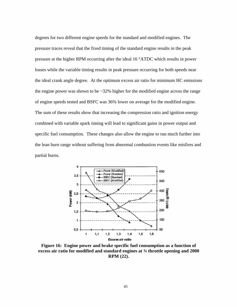
45

degrees for two different engine speeds for the standard and modified engines. The

pressure traces reveal that the fixed timing of the standard engine results in the peak

pressure at the higher RPM occurring after the ideal 16 °ATDC which results in power

losses while the variable timing results in peak pressure occurring for both speeds near

the ideal crank angle degree. At the optimum excess air ratio for minimum HC emissions

the engine power was shown to be ~32% higher for the modified engine across the range

of engine speeds tested and BSFC was 36% lower on average for the modified engine.

The sum of these results show that increasing the compression ratio and ignition energy

combined with variable spark timing will lead to significant gains in power output and

specific fuel consumption. These changes also allow the engine to run much further into

the lean burn range without suffering from abnormal combustion events like misfires and

partial burns.

Figure 16: Engine power and brake specific fuel consumption as a function of

excess air ratio for modified and standard engines at ¾ throttle opening and 2000 RPM (22).

46

Figure 17: Spark timing as a function of excess air ratio for modified and standard

engines at ¾ throttle opening and 2000 RPM (22).

Figure 18: Pressure-time curves of standard, (a), and modified, (b), engines at full

throttle and two different speeds (22).

II.8 Combustion and Fuel Impacts

The chemical reaction that occurs in an engine can be impacted by many things

including fuel to air ratio, temperature, pressure, turbulence, and other molecules not

required for the reaction. The general chemical reaction is given as Eq. (24)

47

2 2 2 2

1 2 2 2 3 2 4 2 5

6 7 2 8 9 2

m n p q r

x y

C H O N S X R O S N T CO h H O

P CO P N P O P H O P CO

P C H P NO P NO P SO

(24)

where the coefficients in Eq. (24) can be determined in several ways. The recommended

practice was originally discussed by Kilpatrick (24) and was further refined as SAE

Aerospace Recommended Practice 1533 (25). While Eq. (24) is the general form of a

hydrocarbon reaction with air, there are many intermediate reactions that occur. These

intermediate reactions are the main reason behind the generation and destruction of

product species. There can be hundreds of intermediate reactions and for each

intermediate reaction there is an associated reaction rate. The reaction rates for many

reactions are not well understood and can be dominated by a variety of variables during

the reaction process, such as residence time, temperature, pressure, turbulence, and

diluents. Previous research has attempted to correlate the production of different

products as a function of equivalence ratio, temperature, and engine loading.

The combustion characteristics of different engine types can make it hard to relate

the results of different research. One way in which to relate the overall effects of a given

engine on the chemical reaction is to calculate combustion efficiency for the engine.

Combustion efficiency, ηC, is defined as the heat of combustion based upon the measured

product concentrations, HC, divided by the stoichiometric heat of combustion, (HC)St, for

a particular set of reactants, Eq. (25).

StC

CC H

H (25)

48

Another way to compare combustion characteristics is to calculate an emissions

index, EI, Eq. (26), for each of the product species. The EI is the ratio of the mass of a

product species Z to 1000 mass units of fuel consumed (25).

1000ZZ

fuel

MWmoles of ZEI

moles of fuel MW

(26)

The EI of a species can be compared for different engines because it is simply a ratio of

the emission per amount of fuel used. Some researchers choose to report product species

emissions levels directly in parts per million or by percent volume. Reduction of several

important product species such as unburned hydrocarbons, UBHC, and carbon monoxide,

CO, lead to increases in combustion efficiency.

In addition to directly comparing how efficient an engine is at converting the fuel

and air mixture into product species, the quality of the combustion event must be

considered. Qualitatively combustion events can be described as normal or abnormal.

Normal combustion occurs as a deflagration where the reaction is controlled by an

ignition source and the flame front propagates through the combustion chamber at a fixed

rate converting the fuel and air mixture into burned gas products. Abnormal combustion

events occur when the fuel and air mixture is ignited in a manner that is uncontrolled and

includes knocking, surface ignition, run on, misfires, and partial burns (4). Misfires

occur when the fuel and air mixture fails to ignite during a particular cycle and results in

the fuel air mixture being exhausted without reacting. Partial burns occur when the fuel

and air mixture does not have enough time to completely burn the fuel and air mixture

due to slow combustion or late ignition timing. Surface ignition is the result of the fuel

air mixture being ignited by a hot surface within the engine and can occur either before or

49

after the spark ignites the rest of the mixture. Surface ignition may result in a related

phenomenon known as run on where the engine continues to run even after the spark

stops firing as the surface ignition event occurs earlier and earlier in the cycle.

By far the most important abnormal combustion event is engine knock. Engine

knock is the result of a detonation of a small part of the fuel air mixture which sends

shock waves through the chamber causing an audible “pinging”. Engine knock is

important because it can cause severe damage to engine components. Engine knock is

avoided by the correct design of an engine which includes choosing the right fuel,

compression ratio, and fuel air mixture ratio. Each fuel has an octane number rating

which is a measure of its anti-knock characteristics in relation to a specific blend of

research fuels under given conditions. The higher the compression ratio the more likely

the engine is to knock all other things being equal as discussed in the previous section.

The impact of the fuel to air ratio, or its related quantities such as λ and ф, on knock and

engine performance will be discussed in more detail below.

The octane rating system is designed to compare a fuels anti knock characteristics

to a blend of reference fuels normal heptanes, n-C7H16, with a rating of zero and

isooctane, C8H18 or 2,2,4-trimethylpentane, with a rating of 100. The octane rating is the

percent of isooctane in the blend of research fuels which corresponds to the same knock

performance characteristics as the test fuel (26). There are two current methods for

testing octane rating, the research octane number, RON, covered under ASTM D-2699,

and the motor octane number, MON, covered under ASTM D-2700. In the U.S. the

octane rating is taken as the average of the RON and MON where the test conditions for

RON and MON are summarized in Table 2. The conditions for the motor octane number

50

test are more severe and usually result in a lower octane number than the research

method.

Table 2: Operating conditions for research and motor octane rating methods (4) Research method Motor method

Inlet temperature 52 °C (125 °F) 149 °C (300 °F) Inlet pressure Atmospheric

Humidity 0.0036-0.0072 kg/kg dry air

Coolant temperature 100 °C (212 °F) Engine speed 600 RPM 900 RPM Spark advance 13° BTC (constant) 19-26° BTC (varies with

compression ratio) Air/fuel ratio Adjusted for maximum knock

II.8.1 Impact of Fuel-Air Ratio

The impact of equivalence ratio, , on the generation of combustion products has

been studied for a variety of engine and fuel types. There has been an effort in recent

years to improve fuel consumption by making the combustion process happen in an

increasingly leaner environment. The effect that this lean combustion has on emissions

and combustion efficiency is an important way to determine the overall impact to the

system. Menon et al (8) studied the impact of using the carburetor to adjust the fuel air

mixture from the factory setting to a richer mixture on the engine performance. The test

was conducted by opening the needle valve to about 1.5 turns for the factory setting and

2.0 turns for the rich setting. The authors note that due to factory setting instructions it

was hard to compare results from this set of tests to other runs completed to compare

engine to engine performance differences. The rich setting resulted in higher fuel to air

ratios across all engine speeds as expected but resulted in lower power and torque across

51

the range of engine speeds. Figure 19 shows the range of fuel air ratios recorded over the

range of engine speeds and the corresponding power and torque of the engine.

Figure 19: Engine performance for two mixture settings at WOT (8).

Celik (22) investigated the impact of the excess air ratio on engine performance

and emissions. Celik showed that as the excess air ratio increases, meaning a leaning of

the mixture, a minimum of fuel consumption and a maximum power, Figure 16, is

achieved at a value slightly greater than stoichiometric. In the case of the test engine the

excess air ratio that produced the lowest emissions of unburned hydrocarbons, UBHC,

was 1.2. Figure 20 shows the exhaust emissions for the standard and test engines as a

function of excess air ratio for carbon monoxide, CO, and UBHC. CO drops to a nearly

52

constant value at excess air ratios above 1.1 while UBHC reaches a minimum and then

begins to increase. The increase in UBHC above an excess air ratio of 1.2 is due to

misfires and partial burn cycles.

Figure 20: HC and CO emissions as a function of excess air ratio for modified and

standard engines at ¾ throttle opening and 2000 RPM (22).

Equivalence ratio will also have an impact on UBHC. As goes from values below

one to values greater than one it creates a peak in the flame temperature. Equivalence

ratios less than one indicate that there is excess air available in the reaction. Equivalence

ratios greater than one indicate that there is excess fuel available in the reaction. Both

conditions lead to heat losses in the reaction. These heat losses lead to an incomplete

reaction of the fuel with the air such that some of the hydrocarbons do not dissociate into

individual hydrogen and carbon atoms that can be recombined into CO2 and H2O, leaving

some hydrocarbon compounds in the exhaust emissions.

53

II.9 Fuel Impact

II.9.1 Categories of Fuels

Fuels fall into several categories including synthetic, petroleum based, and bio-

fuels. Table 3 lists properties for a variety of commonly used fuels. Petroleum based

fuels include things like JP-8, Jet-A, etc which are used extensively by both the military

and civilian aviation communities. Bio-fuels include things like recycled waste oil,

methyl ester compounds from plants, and animal-matter based fuels. Bio-fuels are

beginning to be used more and more by researchers hoping to find an alternative to

petroleum based products that offer similar performance with benefits like lower

emission or cheaper production costs. Synthetic fuels are those refined from coal or other

minerals like Fischer-Tropsch blends. Synthetic fuels have been around since the 1940’s

but have begun to find favor due to a cleaner combustion reaction and lower dependence

on foreign petroleum based fuels (29). One of the main thrusts in the Department of

Defense in recent years is to move towards a single fuel (30) source in order to streamline

the logistics train and save a significant amount of money. The main components that are

important in the chemical makeup of a fuel include the range of carbon numbers found in

the fuel, the arrangement of carbon and hydrogen bonds in each hydrocarbon compound,

and the amount of other additives found in the fuel such as sulfur, oxygen, and nitrogen.

54

Table 3: Typical fuel properties (4, 23, 25, 27, 28) Fuel Formula Molecular

Weight, kg/kmole

LHV, MJ/kg

Octane rating (RON/MON)

JP-8 C10.9H20.9 152.0 43.37 Jet-A C11.6H22 161.5 43.08

Isooctane C8H18 114.23 44.3 100/100 n-heptane C7H16 100.2 48.17 0/0

Avgas C7.68H16.8 112.0 43.50 100 Heavy Diesel CnH1.7n ~200 42.8

Gasoline CnH1.87n ~110 44.0 91-99/82-89

II.9.2 Impact of Fuel Type

The type of fuel used in an engine can have a large impact on the performance of an

engine under test. Using a suitable reference fuel is important so that the test accurately

represents expected performance in the field. Antonovski et al (31) studied the effect of

fuel properties in synthetic fuels and provides a listing of other research that has been

conducted in this area. Antonovski et al focused on learning more about the chemical

kinetics of synthetic fuels through the ignition delay time and determining appropriate

surrogate fuels such as isooctane, n-decane, and n-heptane in representing the different

hydrocarbon compounds found in synthetic fuels. The studies were carried out using

shock-tube kinetics using gas phase mixtures, shock-tube spray using liquid phase fuel in

the test region, and using a high recirculation combustion rig at the University of Florida.

The tests resulted in an initial value for the activation energy 43.3 kcal/mol and a curve of

ignition times versus temperature. The ignition times across the range of temperatures

for the syntroleum fuel was about 50% longer than the reference fuel of kerosene.

Arpa and Yumrutas (32) studied the effect of a fuel derived from waste lubrication

oil on engine performance and emissions in a spark ignition ICE. The basic chemical

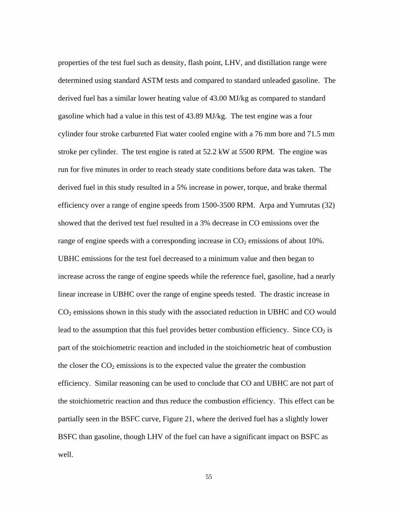
55

properties of the test fuel such as density, flash point, LHV, and distillation range were

determined using standard ASTM tests and compared to standard unleaded gasoline. The

derived fuel has a similar lower heating value of 43.00 MJ/kg as compared to standard

gasoline which had a value in this test of 43.89 MJ/kg. The test engine was a four

cylinder four stroke carbureted Fiat water cooled engine with a 76 mm bore and 71.5 mm

stroke per cylinder. The test engine is rated at 52.2 kW at 5500 RPM. The engine was

run for five minutes in order to reach steady state conditions before data was taken. The

derived fuel in this study resulted in a 5% increase in power, torque, and brake thermal

efficiency over a range of engine speeds from 1500-3500 RPM. Arpa and Yumrutas (32)

showed that the derived test fuel resulted in a 3% decrease in CO emissions over the

range of engine speeds with a corresponding increase in CO2 emissions of about 10%.

UBHC emissions for the test fuel decreased to a minimum value and then began to

increase across the range of engine speeds while the reference fuel, gasoline, had a nearly

linear increase in UBHC over the range of engine speeds tested. The drastic increase in

CO2 emissions shown in this study with the associated reduction in UBHC and CO would

lead to the assumption that this fuel provides better combustion efficiency. Since CO2 is

part of the stoichiometric reaction and included in the stoichiometric heat of combustion

the closer the CO2 emissions is to the expected value the greater the combustion

efficiency. Similar reasoning can be used to conclude that CO and UBHC are not part of

the stoichiometric reaction and thus reduce the combustion efficiency. This effect can be

partially seen in the BSFC curve, Figure 21, where the derived fuel has a slightly lower

BSFC than gasoline, though LHV of the fuel can have a significant impact on BSFC as

well.

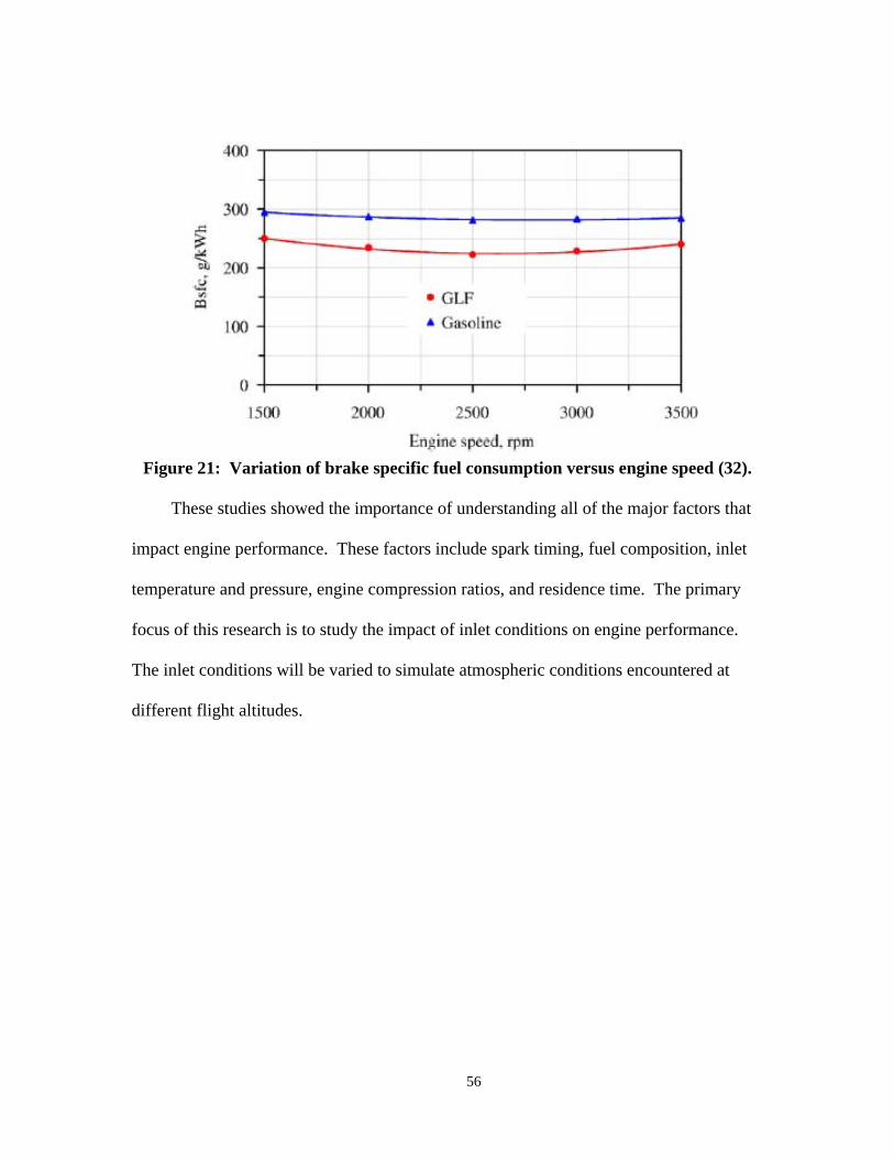
56

Figure 21: Variation of brake specific fuel consumption versus engine speed (32).

These studies showed the importance of understanding all of the major factors that

impact engine performance. These factors include spark timing, fuel composition, inlet

temperature and pressure, engine compression ratios, and residence time. The primary

focus of this research is to study the impact of inlet conditions on engine performance.

The inlet conditions will be varied to simulate atmospheric conditions encountered at

different flight altitudes.

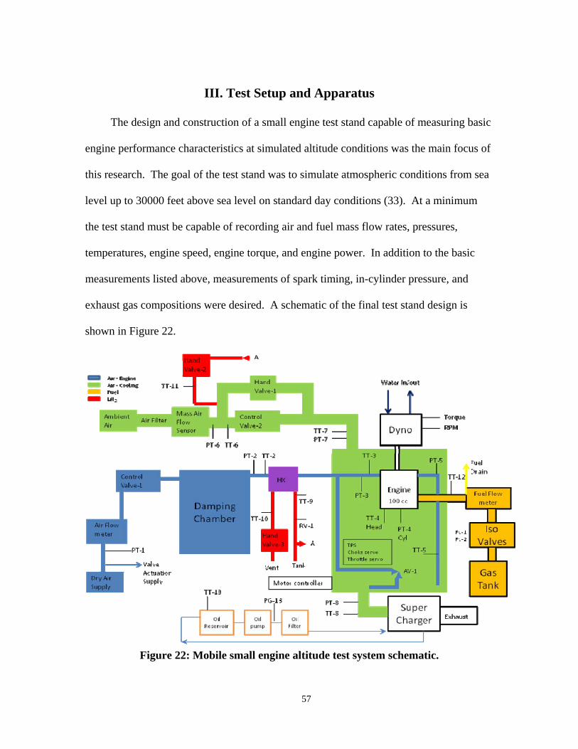
57

III. Test Setup and Apparatus

The design and construction of a small engine test stand capable of measuring basic

engine performance characteristics at simulated altitude conditions was the main focus of

this research. The goal of the test stand was to simulate atmospheric conditions from sea

level up to 30000 feet above sea level on standard day conditions (33). At a minimum

the test stand must be capable of recording air and fuel mass flow rates, pressures,

temperatures, engine speed, engine torque, and engine power. In addition to the basic

measurements listed above, measurements of spark timing, in-cylinder pressure, and

exhaust gas compositions were desired. A schematic of the final test stand design is

shown in Figure 22.

Figure 22: Mobile small engine altitude test system schematic.

58

The design of the mobile test capability began by understanding how the basic

components of the stand would interact with each other. Several preliminary layouts

were considered and were variations of the final design shown in Figure 22. One layout

included a single air flow path which would cool the engine and provide combustion air.

One advantage for this single path layout was the reduction in the number of components.

This layout was discarded due to the complexity of measuring the portion of air being

used for combustion by the engine. A second major drawback for this design layout was

the need for a large heat exchanger capable of cooling a much larger mass flow. Another

layout that was considered was a design where the dynamometer was fully enclosed

inside the altitude chamber. This design’s main advantage was that it would not require a

pressure seal around the rotating shaft connecting the engine to the dynamometer. In

addition only one coupling between the engine and the dynamometer would be needed.

This design was not chosen because of the cooling requirements of the dynamometer and

the sensitivity of the measurement equipment within the dynamometer. The cooling

water would face temperatures below freezing which may have led to the dynamometer

overheating. Furthermore, the electronics used to measure torque and speed and control

the dynamometer were sensitive to extreme temperatures. The final design was chosen

based on the ability to directly measure air flow into the engine for combustion, protect

the sensitive electronics of the dynamometer, and limit the coolant flow rates.

The desired temperature range for the test stand was determined to be from 216.5 K

to 320 K and was based upon the 1976 standard atmosphere model (33). The pressure

range for the test stand was also determined from the standard atmosphere conditions and

ranged from 101325 Pa at sea level to 24014.1 Pa at 30000 ft above sea level.

59

Temperature versus altitude is plotted in Figure 23 and pressure versus altitude is plotted

in Figure 24. In order to attain an inlet pressure equal to that encountered from sea level

up to 30000 ft above sea level, the driving device must be capable of pressure ratios in

the range of 1.0 to 4.2. Based upon the temperature design goals coupled with the

cooling requirements of the engine and the air used for combustion a maximum air mass

flow rate for both paths of 0.3 kg/s would be needed. With this air mass flow rate and the

assumed temperature differences for each test point approximately 5 to 40 g/s of coolant

would be needed to reach the desired operating points.

Figure 23: Temperature versus altitude design goal test conditions.

60

Figure 24: Pressure versus altitude design goal test conditions

Having chosen the flow path layout, the test engine, and the range of desired

pressures and temperatures, component selection was completed for the remaining

systems. A dynamometer was selected to measure engine performance data based on test

engine size and speed. The dynamometer cooling system was designed to remove the

heat absorbed during testing based upon maximum expected engine load. The test engine

required a fuel and air supply system with a means of measuring flow rates and

controlling the flow. The fuel system flow was controlled through a system of supply

isolation valves and was measured with a rotary piston flowmeter. In order to accurately

control the air pressure into the engine intake and around the engine the air flow system

required a driving device, a throttle mechanism, and a supply source. The air system was

coupled with a coolant method to match the desired temperature condition with the

61

desired pressure condition. The coolant system was designed to provide the correct flow

rate of coolant without changing the thermo-physical properties or content of the air

stream entering the engine intake. An additional requirement on the coolant system

design was that it closely matches the thermodynamic properties of air at altitude for the

flow stream passing over the engine cooling fins. The test stand was designed to control

engine speed, and engine throttle position. A data acquisition system was selected in

order to collect all required data during testing. These requirements established the

design criteria for the test stand and served as the parameters to evaluate component

choices against.

III.1 Engines

The Brison 5.8 cubic inch, 95 cc, single cylinder internal combustion engine was

chosen for this project for several reasons. The primary reason was interest by the

sponsoring agency, AFRL/RZTC to test a near 10 horsepower single cylinder engine.

The Brison 5.8 has been in use in giant scale (generally 80 inch wingspan or greater)

remote controlled aircraft models for many years and has potential applications as a small

UAV propulsion system. In the giant scale model application the Brison 5.8 is capable of

providing thrust to models weighing in excess of 178 N. The Brison 5.8, Figure 25, is a

two stroke crank-case scavenged spark ignited engine with a bore of 54.98 mm and a

stroke of 40.64 mm. The inlet and exhaust ports are controlled by the motion of the

piston. The Brison 5.8 has two inlet ports arranged at 180° from each other with a single

exhaust port at 90° from the two inlet ports. The intake ports open and close at 59.7°

before and after BDC while the exhaust port open and close at 81.3° before and after

62

BDC. The test engine utilizes a Walbro SDC80 pump style carburetor with high and low

speed needle valves for tuning the fuel air mixture. Test engine properties are

summarized in Table 4.

Table 4: Brison 5.8 engine properties Property Value

Displacement* 95 cm3

Swept Volume Displacement+ 96.5 cm3

Bore+ 5.498 cm Stroke++ 4.064 cm

Connecting Rod Length+ 7.112 cm Crank Radius+ 2.032 cm

Compression Ratio++ 19.4:1

Type 2-stroke, crankcase scavenged Intake Port Area+ 2.00 cm2 / port

Intake Port Arrangement 2 ports 180° offset Exhaust Port Area+ 4.04 cm2

*Manufacturer advertised value +Measured Value

++Calculated Value

Figure 25: Brison 5.8 in3 test engine (a) off the stand, and (b) mounted on test stand.

III.2 Flow Path Design and Components

The air flow path to and from the engine was designed based upon the required

measurements to calculate engine performance as well as the need to simulate the desired

63

altitude settings. The initial design stage included a discussion of how to measure the air

mass flow rate into the engine, how to cool the engine and reject the heat added to the air

flow, and where to place some of the major measurement devices. The decision was

made to split the flow path into two separate streams. This split made it possible to

accurately measure the mass air flow into the engine directly without having to

differentiate between the air flow cooling the engine and that being used for combustion.

Splitting the air flow into two streams has the drawback of adding system complexity in

the form of additional valves, pressure transducers, and thermocouples. However, the

split has the benefit that it allowed the test stand to independently control the cooling of

the two air streams so that both are matched to the desired altitude condition. Figure 26

shows how the all of the major components were connected in the two separate air flow

paths, while Figure 22 shows how the two flow paths interacted with each other along

with all of the other major subsystems on the test stand.

Figure 26: Mobile altitude test stand air flow paths.

64

The flow paths were designed by first determining how to drive the air flows. The

second step was to determine how to control the air pressure in the two flow paths. The

last step was to determine how to control the air temperature in the two flow paths. Other

design considerations included how to damp the pressure pulsations in the flow path so

that accurate flow rate measurements can be made. Lastly coolant flow rates were

considered in the design in order to minimize the size of the coolant tank needed in order

to run tests of sufficient duration to gather quality data. The LN2 tank has a capacity of

180 L. The minimum desired run time was 60 minutes which lead to a maximum flow

rate of approximately 40 g/s of coolant. The expected flow rates were at or below this

maximum flow rate. Testing that required a coolant flow rate higher than 40 g/s would

lower the run time available.

The heat exchanger shown in Figure 26 was placed as close to the engine as

possible. This was done to reduce increases in air temperature between the heat

exchanger and the engine inlet. The engine air flow gained heat from the surrounding

atmosphere through the metal walls of the tubing as well as through the walls of the flow

path but there were additional heat loads for this flow due to the engine. By separating

the two flow paths the test stand was able to simulate very closely the temperature and

pressure of the air being used for combustion by the engine. The cooling air flow path

around the outside of the engine was not as crucial to the overall test measurements but

still had an impact on the performance of the engine.

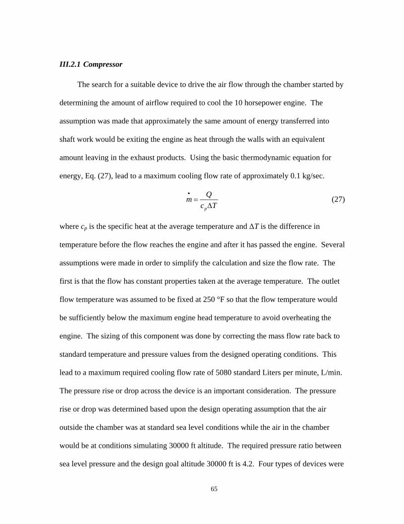
65

III.2.1 Compressor

The search for a suitable device to drive the air flow through the chamber started by

determining the amount of airflow required to cool the 10 horsepower engine. The

assumption was made that approximately the same amount of energy transferred into

shaft work would be exiting the engine as heat through the walls with an equivalent

amount leaving in the exhaust products. Using the basic thermodynamic equation for

energy, Eq. (27), lead to a maximum cooling flow rate of approximately 0.1 kg/sec.

p

Qm

c T

(27)

where cp is the specific heat at the average temperature and ΔT is the difference in

temperature before the flow reaches the engine and after it has passed the engine. Several

assumptions were made in order to simplify the calculation and size the flow rate. The

first is that the flow has constant properties taken at the average temperature. The outlet

flow temperature was assumed to be fixed at 250 °F so that the flow temperature would

be sufficiently below the maximum engine head temperature to avoid overheating the

engine. The sizing of this component was done by correcting the mass flow rate back to

standard temperature and pressure values from the designed operating conditions. This

lead to a maximum required cooling flow rate of 5080 standard Liters per minute, L/min.

The pressure rise or drop across the device is an important consideration. The pressure

rise or drop was determined based upon the design operating assumption that the air

outside the chamber was at standard sea level conditions while the air in the chamber

would be at conditions simulating 30000 ft altitude. The required pressure ratio between

sea level pressure and the design goal altitude 30000 ft is 4.2. Four types of devices were

66

considered for this task and the advantages and disadvantages of each are described

below.

The first type of device considered was the only one capable of providing the flow

rate and pressure ratio needed for the proposed design goals. The steam ejector was

capable of producing a pressure ratio in excess of 4.2 while still being able to provide a

mass flow rate of 0.1 kg/s or greater. The steam ejector considered for this design was a

4 inch diameter steam ejector from Fox Valve Development Corporation. Steam ejectors

are used to drive a wide range of altitude test facilities around the world and are well

suited to the task. The drawback to this device is the need to provide a sufficient supply

of quality steam to the ejector and then remove the steam to a safe exhaust point. The

mobility of the design would be somewhat compromised by the use of a steam ejector as

permanent lines would be required from the main steam supply header to the test

location. The advantage of the steam ejector was that it is capable of providing a

pressure ratio up to and exceeding the original 4.2 design value. Discussion with the

AFRL/RZTC representatives lead to the determination that a steam ejector may be used

in the future to provide simulated altitude conditions above 15000 ft but would not be

used on the current design. A new design goal of a maximum altitude of 15000 ft above

sea level was chosen as a reasonable goal and resulted in a new design pressure ratio of

2.0.

Two other types of devices were considered in order to provide the desired flow

rate and pressure for the chamber but were discarded for a variety of reasons. The first

device that was considered and rejected was a vacuum pump. Vacuum pumps were

determined unfeasible for one of two reasons. The first reason was that most of the off

67

the shelf vacuum pumps were simply not capable of providing the required mass flow

rate needed to keep the engine below the maximum temperature. The second reason that

vacuum pumps were rejected was for size. Several vacuum pumps capable of providing

the required flow rate were found during the search but were considered too large for the

mobile test stand being constructed. Some of the vacuum pumps were capable of flow

rates in the range from 50 to greater than 5000 L/min, however the pressure ratio for

these devices were generally below 1.2.

The second type of device that was considered and rejected was an industrial air

blower or shop air compressor. While the industrial air blowers were able to easily

handle the required air flow rate they were not capable of the required pressure ratio.

Most of the air blowers encountered during the search were only able to provide a

pressure rise of one to two pounds per square inch absolute, psia, at best and most were

only able to provide a pressure rise below one psia. The industrial blowers considered

were also quite large for the proposed application. Shop air compressors are commonly

used to provide higher pressure air for pneumatic tools and other equipment and were

considered as an alternative to the industrial blower. Shop air compressor suffered from

the same problems as the vacuum pump in that they were either incapable of providing

the required air flow rate or were far too large to be used in the small mobile design.

The radial compressor was the final device considered and was ultimately selected

due to its compact size and ability to meet the pressure ratio and flow rate requirements.

The search for a radial compressor began by looking at aftermarket automobile

supercharger compressors. It was calculated, using Eq. (28) that a 20 horsepower motor

would be required to run the compressor.

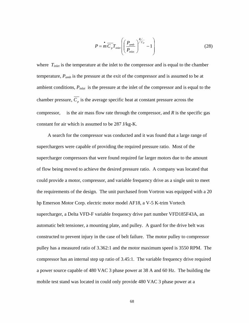
68

1PC

R

inlet

ambinletp P

PTCmP (28)

where Tinlet is the temperature at the inlet to the compressor and is equal to the chamber

temperature, Pamb is the pressure at the exit of the compressor and is assumed to be at

ambient conditions, Pinlet is the pressure at the inlet of the compressor and is equal to the

chamber pressure, pC is the average specific heat at constant pressure across the

compressor, � is the air mass flow rate through the compressor, and R is the specific gas

constant for air which is assumed to be 287 J/kg-K.

A search for the compressor was conducted and it was found that a large range of

superchargers were capable of providing the required pressure ratio. Most of the

supercharger compressors that were found required far larger motors due to the amount

of flow being moved to achieve the desired pressure ratio. A company was located that

could provide a motor, compressor, and variable frequency drive as a single unit to meet

the requirements of the design. The unit purchased from Vortron was equipped with a 20

hp Emerson Motor Corp. electric motor model AF18, a V-5 K-trim Vortech

supercharger, a Delta VFD-F variable frequency drive part number VFD185F43A, an

automatic belt tensioner, a mounting plate, and pulley. A guard for the drive belt was

constructed to prevent injury in the case of belt failure. The motor pulley to compressor

pulley has a measured ratio of 3.362:1 and the motor maximum speed is 3550 RPM. The

compressor has an internal step up ratio of 3.45:1. The variable frequency drive required

a power source capable of 480 VAC 3 phase power at 38 A and 60 Hz. The building the

mobile test stand was located in could only provide 480 VAC 3 phase power at a

69

maximum of 30 A. A temporary line was run in the facility which was capable of 480

VAC at a maximum of 50 A. The VFD is connected to the DAQ and is controlled with a

0-10 VDC analog input signal that sets the motor frequency between 0 Hz and 60Hz.

The compressor speed versus motor input frequency curve was calculated with a simple

linear relationship between the commanded frequency input, the total step up ratio, and

the actual motor speed, Figure 27. The compressor map for the V-5 K trim Vortech

radial compressor, adapted from the manufacturer’s data (37), is shown in Figure 28.

The expected operating points are noted on the compressor map with values listed in

Table 5.

Figure 27: Compressor speed versus commanded frequency.

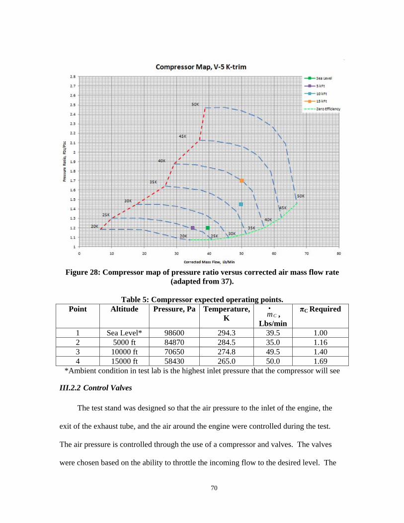
70

Figure 28: Compressor map of pressure ratio versus corrected air mass flow rate

(adapted from 37).

Table 5: Compressor expected operating points. Point Altitude Pressure, Pa Temperature,

K Cm

, Lbs/min

πC Required

1 Sea Level* 98600 294.3 39.5 1.00 2 5000 ft 84870 284.5 35.0 1.16 3 10000 ft 70650 274.8 49.5 1.40 4 15000 ft 58430 265.0 50.0 1.69

*Ambient condition in test lab is the highest inlet pressure that the compressor will see

III.2.2 Control Valves

The test stand was designed so that the air pressure to the inlet of the engine, the

exit of the exhaust tube, and the air around the engine were controlled during the test.

The air pressure is controlled through the use of a compressor and valves. The valves

were chosen based on the ability to throttle the incoming flow to the desired level. The

71

main flow path into the engine cylinder uses a TRIAC ½ inch 30 degree vee port control

valve with a WEM-500 electric actuator and positioned as shown in Figure 29. One

major reason for selecting this valve combination was the fully electric actuator that did

not require a separate air supply. The TRIAC ½ vee port control valve is sized to handle

a maximum flow coefficient of 2.6 at 100% open. The flow coefficient is a function of

the percent opening of the valve and closely approximates Eq. (29), as shown in

Appendix B, where X is in percent open.

XEXEXECV *40.7*40..1*61 23 (29)

Figure 29: Control valve 1 on the engine intake line just downstream of the air mass

flowmeter and upstream of damping chamber.

This valve was chosen based on the inlet pressure and the desired flow rate to the

engine. The flow rate was calculated based upon engine speed, an assumed cylinder

volume of 100 cubic centimeters, and an assumed volumetric efficiency of 85%.

72

Volumetric efficiency does not really apply to two stroke engines and a more appropriate

value would have been to assume a delivery ratio in order to calculate the flow rate. The

inlet pressure to the valve was assumed to be 65 psig and is based upon the available

shop air supply. This flow rate was then corrected back to standard day conditions to

determine the range of flow rates that the control valve must accurately meter. The flow

rate for the small control valve ranged from 85 to 396.5 SLPM, which were translated

into flow coefficient values using Eq. (30) where q is the flow rate in scfm, Sg is the

specific gravity of air, Talt is the temperature of the simulated altitude, Pin is the inlet

pressure in psia, and Palt is the desired simulated altitude pressure in psia. The flow

coefficient required for this smaller control valve ranges from 0.1 to 0.5.

1/2

1/2

460

1360

altv

in alt alt

q Sg TC

P P P

(30)

For the larger engine cooling flow path it was determined that two valves were

needed to cover the range of design pressures. The large flow path must be fed by

ambient air due to the volume of air required. The desire was to use high pressure air to

feed this cooling loop but it was determined that the shop air compressor did not have the

capability to supply the required volumetric flow rate. The next step was to determine

the flow coefficient for a single valve over the entire range of flow conditions. The result

was that at conditions near ambient pressures the flow coefficient was excessively large.

A simple full port manual ball valve was chosen to provide the required flow at these

near sea level pressure conditions. As the pressure drops below the ambient air pressure

the flow coefficient drops dramatically so that the use of a vee port control valve is

acceptable. The large control valve is a 2.5 inch vee port TRIAC ball valve with a

73

WEM-690 electric actuator and positioner. The bypass valve is a 3 inch full port manual

ball valve from TRIAC. The manual actuation of the bypass valve allows the main

control valve to operate farther from its full open position so that the pressure can be

controlled with finer resolution. Figure 30 shows the large control valve and the cooling

flow bypass valve mounted on the test stand.

Figure 30: Cooling air flow path with control valve 2, manual bypass valve, mass air

flow sensor, and chamber inlet.

III.2.3 Heat Exchanger

The temperature control for both flow paths was originally going to be

accomplished through heat exchangers. The search for heat exchangers capable of

producing the required temperatures at the simulated altitude conditions proved

74

somewhat difficult. The first challenge in locating appropriate heat exchangers was the

choice of coolant for the devices. Liquid nitrogen was chosen because of the extreme

temperature range that was required for the higher altitude test points as well as its

readily available supply. For the main engine flow a simple tube in tube counter flow

heat exchanger was chosen due to the much lower volumetric flow rates needed to supply

the engine. The sizing of the small heat exchanger is documented in Appendix A and

began by assuming an approximate volumetric air flow rate required by the engine.

Assuming the engine operates at 8000 RPM with a volumetric efficiency of 85% the

maximum amount of air used for combustion was calculated by multiplying the

volumetric air flow rate times the air density at altitude divided by the reference density

to correct the value back to standard conditions to get the volumetric air flow rate in scfm

using Eq. (31).

ref

C VolRPM

V ***

2

(31)

where RPM is the engine speed, η is the volumetric efficiency, Vol is the volume of the

cylinder, and ρ is the density. Substituting the values assumed above into Eq. (31) and

using 100 cm3 as the cylinder volume leads to a maximum volumetric air flow rate of

14.167 scfm. The uncorrected mass flow rate can be calculated at each altitude using the

standard atmosphere density at altitude times the maximum volumetric flow rate given by

Eq. (32).

*CVm

(32)

The heat that must be removed from the air stream can be calculated from the energy

equation, Eq. (33), using the assumption of an ideal gas with the specific heat at constant

75

pressure, Cp, a function only of temperature. The value used for the specific heat was

calculated at an average temperature where the inlet temperature was assumed to be 300

K.

inaltp TTCmQ

** (33)

Using Eq. (33) the maximum amount of heat that the small heat exchanger must

remove from the flow was calculated as 458 W. In addition to heat removal from the

inlet air stream if hot day conditions at sea level are to be reached then a heater capable of

adding 121 W to the air stream would be needed. Based on the chosen coolant it was

desired to find a heat exchanger which would have a small enough flow rate to allow the

stand to operate for a given amount of time. The assumption was made that one hour of

run time was adequate to collect relevant data before refilling the LN2 supply tank.

Based on the need to sue the coolant for both the engine inlet flow and the engine cooling

flow paths it was determined that 6 g/s of LN2 would be used as the coolant mass flow

rate for determining heat exchanger size. Researching several possible small heat

exchangers lead to the selection of an Exergy LLC tube-in-tube counter flow heat

exchanger model 670. The number of loops needed in the Exergy model 670 was

calculated in Appendix A. The calculations in Appendix A showed that in order to

provide addition cooling capacity in the heat exchanger that a seven loop coil, part

number 00670-3, would be purchased and is shown in Figure 31 installed on the test

stand.

76

Figure 31: Engine inlet flow path heat exchanger installed on test stand.

A commercially available heat exchanger that would work for the engine cooling

flow path was harder to locate. After contacting several companies a design by Super

Radiator CoilsTM was chosen to meet the requirements. This heat exchanger design was

not ordered as it was decided that simply injecting the coolant into the flow stream would

reduce the amount of coolant usage and allow the test stand to run for longer periods of

time. It was understood that direct injection of LN2 into the cooling stream would lead to

slight variations in pressure and mass flow rate. In addition, it was known that exactly

matching the temperature of the cooling flow path stream to the engine inlet stream

would be very difficult. Controlling these variations in the engine cooling flow path were

not deemed critical and no attempt was made to reduce their magnitude. The direct

injection of liquid nitrogen, LN2, into the flow stream will not impact the engine

performance as this stream was not being used in the combustion process and nitrogen

will closely replicate the thermo-physical properties of air. The Super Radiator CoilsTM

77

design was a tube and fin design utilizing aluminum fins and copper tubes listed as coil

model 8x8-4R-38/60. No attempt was made to review the manufacturers calculated heat

removal capacity, however the manufactured did give enough data on the proposed

design in order to perform an analysis in the future.

One additional item of interest for the heat transfer in the engine cooling path was

the need to provide a velocity across the engine in order to generate a high enough local

convective heat transfer coefficient from the engine cooling fins to keep the engine below

the maximum engine head temperature. The calculations done to determine the required

mass flow rate to meet the engine cooling requirement did not take into account the local

velocity or local heat transfer coefficient. There was some concern that there would not

be sufficient air flow velocity across the engine cooling fins to keep the engine from

overheating. In the event that additional flow velocity was required provisions for

installing a fan inside the box were made though not completed. Initial tests of the

engine running with the compressor on showed that a fan was not required. During initial

testing the engine head temperature did not exceed 200 °C and the melting temperature of

aluminum is approximately 660 °C leaving a wide margin of safety.

III.2.4 Damping Chamber

In order to accurately measure the mass air flow into the engine for combustion

calculations a damping chamber was needed in the engine supply air flow path. The

purpose of this damping chamber was to provide sufficient volume to damp out pressure

pulsations from the engine so that they do not impact the mass air flow sensor

measurements. The cyclic nature of internal combustion engines generate pressure pulses

78

in the intake system as the intake ports or valves open and close during each cycle. The

removal of pressure pulses also allows the control valve on the engine supply stream to

operate more smoothly without having to react to constant pressure fluctuations in the

system. The control valve is set based upon downstream pressure measurements and

constant pressure changes in the line would cause the valve to continually modulate

which could cause even larger pressure fluctuations in the intake system preventing the

test from reaching the desired pressure set point.

The size of the damping chamber was determined by examining relevant research

and looking for guidelines to follow. The study conducted by Watanabe and Kuroda (12)

used a damping chamber 690 times, equal to 0.04 m3, the size of the test engine cylinder

volume. Cadou et al (8) used a damping chamber 3000 times, equal to 0.007 m3, the size

of the test engine cylinder volume. These volume ratios were used as an upper and lower

limit on the size of the damping chamber. The size of the chamber was limited by the

space available on the test stand and so a damping chamber that was a little over 1200

times the size of the test engine cylinder volume. The chamber was ordered from Plastic-

Mart.com with part number B273 and has an internal capacity of 0.1154 m3. The

physical volume was much larger than those used by previous researchers but the ratio of

the damping volume to cylinder volume falls towards the lower end of the scale.

III.2.5 Flow Meters

In order to calculate useful engine performance parameters for comparison to other

similar engines accurate measurements of the air mass flow and fuel mass flow rates must

be taken. Based upon the calculated air mass flow rate from the earlier control valve

79

selection it was determined that the air flow meter required a range of 0 to 500 standard

liters per minute, SLPM. The air flow meter selected for the test stand was a Sierra

Instruments Smart-Track series 100 thermal mass flow sensor, with part number M100H-

NR-15-O1/1-PV2-V1-C3. The M100H has a ± 1.0% of full scale accuracy with a ± 0.2%

of full scale repeatability and shown mounted to the test stand in Figure 29.

The fuel flow rate range was determined from the engine owner’s manual given

flow rate. The owner’s manual states that the fuel flow rate will be between 1-2 ounces

per minute which is equivalent to 30-60 cm3/min. The fuel flow meter was ordered from

Max Machinery and is a model 213 piston flow meter with a Max 294 transmitter and is

shown in Figure 32. The model 213 has a range of 0-1800 cc/min with and accuracy of ±

0.2% of reading. The Max Machinery flow meter and transmitter were chosen mainly

due to the familiarity and commonality between it and other fuel flow meters used in

other AFRL/RZTC small engine stands.

Figure 32: Fuel system with fuel flow meter installed on test stand.

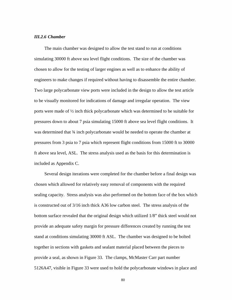
80

III.2.6 Chamber

The main chamber was designed to allow the test stand to run at conditions

simulating 30000 ft above sea level flight conditions. The size of the chamber was

chosen to allow for the testing of larger engines as well as to enhance the ability of

engineers to make changes if required without having to disassemble the entire chamber.

Two large polycarbonate view ports were included in the design to allow the test article

to be visually monitored for indications of damage and irregular operation. The view

ports were made of ½ inch thick polycarbonate which was determined to be suitable for

pressures down to about 7 psia simulating 15000 ft above sea level flight conditions. It

was determined that ¾ inch polycarbonate would be needed to operate the chamber at

pressures from 3 psia to 7 psia which represent flight conditions from 15000 ft to 30000

ft above sea level, ASL. The stress analysis used as the basis for this determination is

included as Appendix C.

Several design iterations were completed for the chamber before a final design was

chosen which allowed for relatively easy removal of components with the required

sealing capacity. Stress analysis was also performed on the bottom face of the box which

is constructed out of 3/16 inch thick A36 low carbon steel. The stress analysis of the

bottom surface revealed that the original design which utilized 1/8” thick steel would not

provide an adequate safety margin for pressure differences created by running the test

stand at conditions simulating 30000 ft ASL. The chamber was designed to be bolted

together in sections with gaskets and sealant material placed between the pieces to

provide a seal, as shown in Figure 33. The clamps, McMaster Carr part number

5126A47, visible in Figure 33 were used to hold the polycarbonate windows in place and

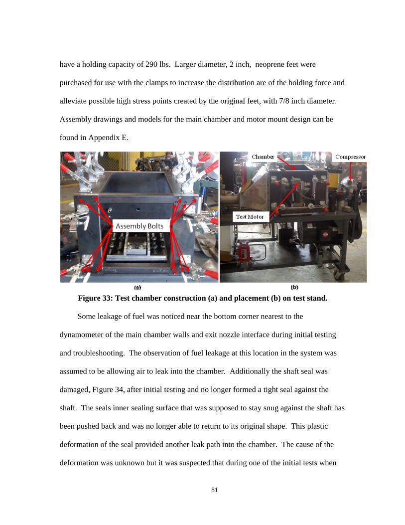
81

have a holding capacity of 290 lbs. Larger diameter, 2 inch, neoprene feet were

purchased for use with the clamps to increase the distribution are of the holding force and

alleviate possible high stress points created by the original feet, with 7/8 inch diameter.

Assembly drawings and models for the main chamber and motor mount design can be

found in Appendix E.

Figure 33: Test chamber construction (a) and placement (b) on test stand.

Some leakage of fuel was noticed near the bottom corner nearest to the

dynamometer of the main chamber walls and exit nozzle interface during initial testing

and troubleshooting. The observation of fuel leakage at this location in the system was

assumed to be allowing air to leak into the chamber. Additionally the shaft seal was

damaged, Figure 34, after initial testing and no longer formed a tight seal against the

shaft. The seals inner sealing surface that was supposed to stay snug against the shaft has

been pushed back and was no longer able to return to its original shape. This plastic

deformation of the seal provided another leak path into the chamber. The cause of the

deformation was unknown but it was suspected that during one of the initial tests when

82

the motor and shaft visibly wobbled the seal was pushed past the manufactures limits of

motion. Lastly, the gasket material used for the upper window tore in several places,

Figure 35, during the repeated openings of the chamber to troubleshoot problems during

activation of the test stand. This seal while torn was used as a partial seal though it was

known that air would leak through at each tear location. From these observations it was

assumed that some additional air was leaking into the box during low pressure runs due

to the pressure differential. This leakage was not addressed as initial test runs of the

compressor were able to create sustained chamber pressures around 10.0 psia. This

pressure differential was not 100% of the design goal of around 7 psia but it was

sufficient to begin altitude testing up to conditions simulating approximately 10000 ft

above sea level.

Figure 34: Shaft seal damage observed after initial testing and troubleshooting.

83

Figure 35: Upper window gasket damage after several removals of the upper

viewing window.

III.2.7 Pressure and Temperature

Pressure measurements for the engine intake and cooling flow paths were made

using Omega piezoresistive absolute pressure transducers with part number PX409-

030A5V. The Omega model PX409 has a compensated temperature range of -29 to 85 °C

with a pressure measurement error of +/-0.5% of span within the temperature range.

Omega type K model KMQSS thermocouples were used throughout the system to obtain

temperature measurements. Omega type K thermocouples have a range of -200 °C to

1250 °C with an error above 0 °C of 2.2 °C or 0.75% of full scale whichever is greater

and an error of 2.2 °C or 2.0% of full scale whichever is greater. Exposed junction

thermocouples were used where immersion in a gas phase flow was needed. Exposed

junction thermocouples were utilized in the gas flow paths because they have a faster

84

response time to changes in the gas temperature than shielded junctions. Ungrounded

shielded thermocouples were used in the fuel system and liquid nitrogen cooling system

lines to ensure that the junction was not damaged by the liquid flows. The choice of

thermocouples and absolute pressure transducers was influenced by common usage

within the engine tests stands of AFRL/RZTC.

In cylinder pressure was measured with a Kistler 6118BFD16Q02A41 measuring

spark plug piezoelectric sensor. The model 6118 has an interference suppression resistor

a BOSCH 6 heat rating which closely matches the original OEM spark plug. The OEM

spark plug has a M14x1.25 mm thread with a depth of 9.5 mm. The Kistler model

6118B was chosen after discussion with Capt. Cary Wilson (15), Adam Brown of ISSI,

and Dr. John Hoke of ISSI on previous experiences with a range of other piezoelectric

spark plug type sensors. Several other models from other companies had been used in the

past but suffered from poor performance and or damage in the knocking combustion

region. The piezoelectric sensor was connected to a Kistler 5064B11 dual channel charge

amplifier module mounted in a Kistler 2852A12 Slim Signal Conditioning Platform,

SCP, with the use of low resistance insulated cables. The charge amplifier 0 to 10 VDC

output was connected to the data acquisition system. The Kistler 6118 measuring spark

plug sensor has a range from 0 to 200 bar with a natural frequency of about 65 kHz and a

sensitivity at 200 °C of about -10 pC/bar. The model 6118 has a linearity of less than or

equal to ± 0.5% of full scale. The accuracy of the cylinder pressure measurement will

depend on the pegging method used as discussed in the previous chapter.

85

III.3 Other Important Components

III.3.1 Dynamometer

One of the main goals of the test stand is to provide accurate measurements of

power, speed, and torque that can be used to create engine performance maps. The

dynamometer must be capable of withstanding large torque variations produced by a

single cylinder internal combustion engine while providing accurate measurements. The

dynamometer chosen for the test stand was the Magtrol Inc. model 2WB65/S006 eddy

current dynamometer with part number 312-201-S006. This particular part number has

more robust bearings for the internal combustion engine test application than the standard

2WB65 model. The 2WB65 is capable of testing engines up to 12 kW or 16.1 hp of

power and can provide a loading torque, TL, of up to 20 N-m with a maximum speed of

30000 RPM. The loading torque is equivalent to the aerodynamic load placed on the

engine by the propeller of a UAV and can vary based on engine speed, propeller size, and

flight operating conditions.

The eddy current dynamometer is controlled by a Magtrol DSP6001 high speed

programmable controller with part number 004604. The system includes a dynamometer

excitation power supply, part number 234-311-123, a torque and speed conditioner, part

number 234-401-122, and the associated interface cables. The Magtrol dynamometer and

controller were chosen primarily due to commonality between other small dynamometers

used with the AFRL/RZTC small engine researchers (15) and due to its cost as compared

to other options that were investigated. Figure 36 shows the dynamometer installed on

the test stand main base plate which is mounted on vibration dampers. The vibration

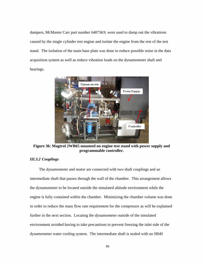
86

dampers, McMaster Carr part number 64875K9, were used to damp out the vibrations

caused by the single cylinder test engine and isolate the engine from the rest of the test

stand. The isolation of the main base plate was done to reduce possible noise in the data

acquisition system as well as reduce vibration loads on the dynamometer shaft and

bearings.

Figure 36: Magtrol 2WB65 mounted on engine test stand with power supply and

programmable controller.

III.3.2 Couplings

The dynamometer and motor are connected with two shaft couplings and an

intermediate shaft that passes through the wall of the chamber. This arrangement allows

the dynamometer to be located outside the simulated altitude environment while the

engine is fully contained within the chamber. Minimizing the chamber volume was done

in order to reduce the mass flow rate requirement for the compressor as will be explained

further in the next section. Locating the dynamometer outside of the simulated

environment avoided having to take precautions to prevent freezing the inlet side of the

dynamometer water cooling system. The intermediate shaft is sealed with an SB40

87

profile rotary seal from American High Performance Seals. This seal was originally

designed to seal high pressure liquid inside an enclosure. After discussion with the

manufacturer it was determined that this seal should easily support the differential gas

pressure created by reducing the pressure inside the chamber. The observation listed

previously of the damaged seal and shown in Figure 34 will be discussed further in

chapter IV.

The intermediate shaft is connected to the dynamometer and engine with Lovejoy

GS28/38 curved jaw couplings with elastomeric spider inserts. Lovejoy curved jaw

couplings were chosen after a considerable search for couplings capable of handling the

torque and speed of the application. Several high torque couplings were researched but

were not capable of the expected maximum speed of the test engine of 10000 RPM.

After considerable discussion with Capt Cary Wilson of AFRL/RZTC on his use of

elastomeric couplings and the issues associated with their use it was determined that the

Lovejoy curved jaw coupling would work the best. The spider inserts used in the

coupling have a shore hardness rating of 92A. Each coupling was made up of two hubs

and the spider insert. The hub connected to the engine was machined to replace the

propeller mount that comes with the test engine and fits on the tapered drive shaft. The

engine side hub, shown in Figure 37, had to fit inside a collar that holds a magnetic

proximity sensor that is used by the engine to sense engine speed and set ignition timing

based upon the speed. The engine side hub has a magnet set at 45° before top dead

center, BTDC, and the ignition box sets the delay time based upon speed and this signal.

The dynamometer side hub is a standard Lovejoy GS28/38 with two keyways that

fits directly onto the dynamometer shaft. The couplings on the intermediate shaft are

88

Lovejoy GS28/38 couplings with a ¾ in diameter shaft and a locking device to clamp the

hub to the shaft. The hubs and spiders that form the two shaft couplings are designed to

withstand 95.00 N-m of torque in normal operation with a maximum peak torque load of

198.93 N-m. The locking device hubs are rated for a maximum speed of 11700 RPM

while the double keyway hub on the dynamometer and the machined hub on the engine

are not given a rating. Tests will be maintained at speeds below 10000 RPM to reduce

concerns of hub failure. The 92A shore spider is made from urethane and is rated for

temperatures down to -50 °F. The minimum temperature expected within the chamber is

down to -70 °F which is lower than the rating of the spider but heat from the load

imparted into the coupling along with heat release from the engine should keep the

coupling above the minimum temperature rating. Tests performed at or below the

minimum temperature rating will be monitored closely for indications of spider failure.

Curved jaw couplings are designed so that failure of the elastomeric spider does not result

in immediate failure of the coupling which is part of the reason they were chosen to

connect the dynamometer to the engine. Figure 38 shows the two couplings installed on

the test table connecting the dynamometer to the test engine.

89

Figure 37: Engine side hub, Lovejoy GS28/38.

Figure 38: Engine, coupling one, intermediate shaft, coupling two, and

dynamometer installed on test stand.

Coupling alignment was very important in reducing loads imparted to the

intermediate shaft and dynamometer as well as the elastomeric spider insert. Coupling

alignment was done by measuring spacing between the two hubs of each coupling at four

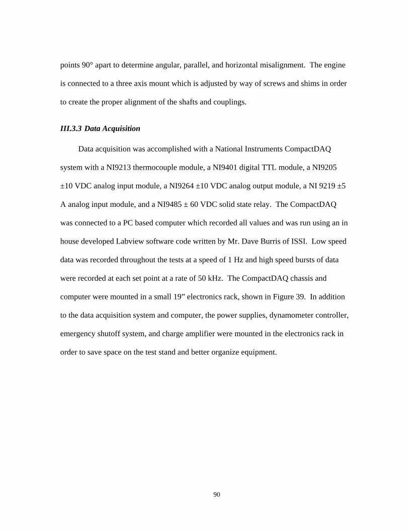
90

points 90° apart to determine angular, parallel, and horizontal misalignment. The engine

is connected to a three axis mount which is adjusted by way of screws and shims in order

to create the proper alignment of the shafts and couplings.

III.3.3 Data Acquisition

Data acquisition was accomplished with a National Instruments CompactDAQ

system with a NI9213 thermocouple module, a NI9401 digital TTL module, a NI9205

±10 VDC analog input module, a NI9264 ±10 VDC analog output module, a NI 9219 ±5

A analog input module, and a NI9485 ± 60 VDC solid state relay. The CompactDAQ

was connected to a PC based computer which recorded all values and was run using an in

house developed Labview software code written by Mr. Dave Burris of ISSI. Low speed

data was recorded throughout the tests at a speed of 1 Hz and high speed bursts of data

were recorded at each set point at a rate of 50 kHz. The CompactDAQ chassis and

computer were mounted in a small 19” electronics rack, shown in Figure 39. In addition

to the data acquisition system and computer, the power supplies, dynamometer controller,

emergency shutoff system, and charge amplifier were mounted in the electronics rack in

order to save space on the test stand and better organize equipment.

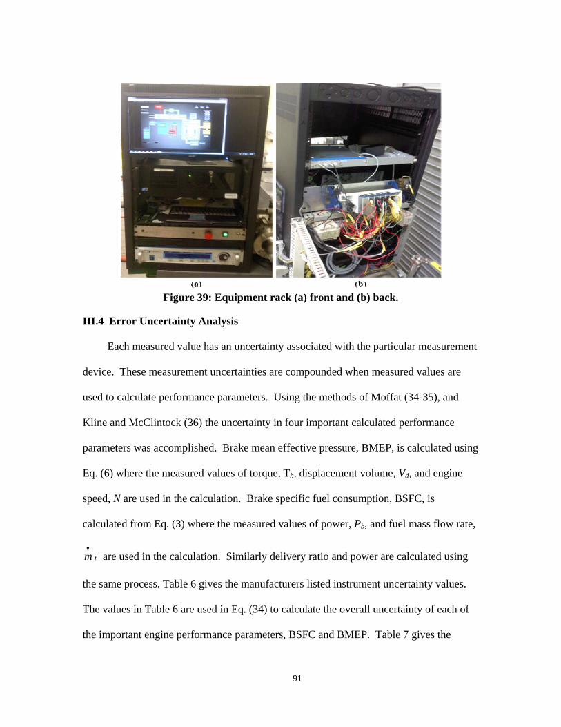
91

Figure 39: Equipment rack (a) front and (b) back.

III.4 Error Uncertainty Analysis

Each measured value has an uncertainty associated with the particular measurement

device. These measurement uncertainties are compounded when measured values are

used to calculate performance parameters. Using the methods of Moffat (34-35), and

Kline and McClintock (36) the uncertainty in four important calculated performance

parameters was accomplished. Brake mean effective pressure, BMEP, is calculated using

Eq. (6) where the measured values of torque, Tb, displacement volume, Vd, and engine

speed, N are used in the calculation. Brake specific fuel consumption, BSFC, is

calculated from Eq. (3) where the measured values of power, Pb, and fuel mass flow rate,

fm

are used in the calculation. Similarly delivery ratio and power are calculated using

the same process. Table 6 gives the manufacturers listed instrument uncertainty values.

The values in Table 6 are used in Eq. (34) to calculate the overall uncertainty of each of

the important engine performance parameters, BSFC and BMEP. Table 7 gives the

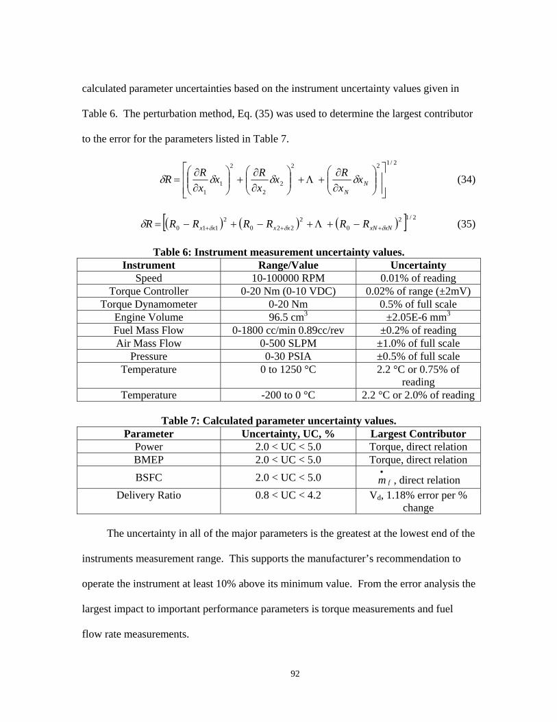
92

calculated parameter uncertainties based on the instrument uncertainty values given in

Table 6. The perturbation method, Eq. (35) was used to determine the largest contributor

to the error for the parameters listed in Table 7.

2/122

22

2

11

NN

xx

Rx

x

Rx

x

RR (34)

2/120

2220

2110 xNxNxxxx RRRRRRR (35)

Table 6: Instrument measurement uncertainty values. Instrument Range/Value Uncertainty

Speed 10-100000 RPM 0.01% of reading Torque Controller 0-20 Nm (0-10 VDC) 0.02% of range (±2mV)

Torque Dynamometer 0-20 Nm 0.5% of full scale Engine Volume 96.5 cm3 ±2.05E-6 mm3

Fuel Mass Flow 0-1800 cc/min 0.89cc/rev ±0.2% of reading Air Mass Flow 0-500 SLPM ±1.0% of full scale

Pressure 0-30 PSIA ±0.5% of full scale Temperature 0 to 1250 °C 2.2 °C or 0.75% of

reading Temperature -200 to 0 °C 2.2 °C or 2.0% of reading

Table 7: Calculated parameter uncertainty values.

Parameter Uncertainty, UC, % Largest Contributor Power 2.0 < UC < 5.0 Torque, direct relation BMEP 2.0 < UC < 5.0 Torque, direct relation

BSFC 2.0 < UC < 5.0 fm

, direct relation Delivery Ratio 0.8 < UC < 4.2 Vd, 1.18% error per %

change The uncertainty in all of the major parameters is the greatest at the lowest end of the

instruments measurement range. This supports the manufacturer’s recommendation to

operate the instrument at least 10% above its minimum value. From the error analysis the

largest impact to important performance parameters is torque measurements and fuel

flow rate measurements.

93

IV. Results

IV.1 Initial Test Stand Checkout

During the initial troubleshooting and checkout phase of activating the altitude test

stand several problems were encountered. Most of the problems encountered were fixed

with minor adjustments to or in some cases replacements of components. An example of

this was the need to change out an actuator on one of the fuel valves due to an incorrect

stop setting which allowed the valve to turn 180° instead of only 90°. During this stage

of testing several changes and enhancements were made to the Labview test program to

allow the stand operator finer control of the throttle, choke, and main valve position

settings. The need for finer valve position control was determined during the second day

of engine testing when it was discovered that after the engine started it would

immediately being to reduce the intake line pressure. If the small control valve was not

opened fast enough to offset this pressure reduction then the engine would flood with fuel

and cease to operate. This effect can be seen in Figure 40 where the control valve

position must be continually adjusted to keep up with the engine demand. In addition the

sharp drop in inlet pressure at 45 seconds and 371 seconds correlate to the engine start

times. The sharp drop in control valve position at 207 seconds and 500 seconds correlate

to engine stop times and the valve closure is to avoid over pressurizing the inlet lines.

The first engine run in Figure 40 started at 45 seconds and engine operation stopped at

187 seconds. In the 10 seconds it took to send the closure command signal the inlet

pressure increased from 15.64 psia to 17.31 psia. This test was done with extremely lean

carburetor needle settings which is why the engine speed did not exceed 2000 RPM

94

during this time frame. The same test is shown in Figure 41 with inlet pressure and

dynamometer speed versus elapsed time. Figure 41 shows how dynamometer and thus

engine speed varied as the inlet pressure oscillated during each engine run. Each spike in

the dynamometer speed data correlates to an attempt to start the engine by turning on the

starter motor briefly. Engine run time can be determined by looking at the dynamometer

speed data and finding time periods where the speed does not return back to zero after the

initial spike.

Figure 40: Control valve position and inlet pressure as a function of time during

initial engine start tests.

Figure 41: Engine speed and inlet pressure as a function of time during initial

engine start tests.

95

It was noted during initial testing with the compressor running that the oil

temperature began increasing over time. The maximum lubrication oil temperature

recommended by the manufacturer is 200 °F. The tests were terminated when the oil

temperature reached 200 °F and the oil pump was left on to circulate the oil through the

system. Once the oil temperature returned to around 90 °F compressor operation was

resumed. The outside door to the test facility was opened slightly after the initial tests to

help cool the oil. The oil tank was located about one foot from the open door and the

outside air temperature was approximately 30 °F. This additional cold air helped cool the

bulk oil temperature with 30 minutes.

IV.2 Testing

IV.2.1 Altitude Experiments

The main experiment was to determine the impact of altitude on engine power, fuel

consumption, and mean effective pressure. The first priority was to determine the range

of conditions that the test stand was capable of achieving. The test stand was designed to

simulate conditions up to 15000 ft above sea level. The test stand should be capable of

achieving temperatures below 270.3 K and pressures below 58521 Pa. In order to

determine the limits of the test stands abilities several check outs were performed. The

first test was to determine the minimum pressure that the compressor was capable of

achieving inside the chamber. This test was completed by varying the main control

valves with the compressor operating. A combination of bypass valve position, main

control valve position, and compressor speeds were used in order to determine the

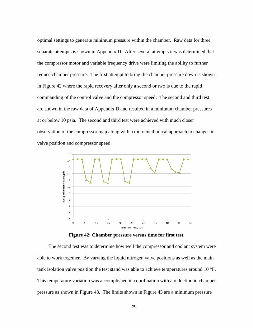
96

optimal settings to generate minimum pressure within the chamber. Raw data for three

separate attempts is shown in Appendix D. After several attempts it was determined that

the compressor motor and variable frequency drive were limiting the ability to further

reduce chamber pressure. The first attempt to bring the chamber pressure down is shown

in Figure 42 where the rapid recovery after only a second or two is due to the rapid

commanding of the control valve and the compressor speed. The second and third test

are shown in the raw data of Appendix D and resulted in a minimum chamber pressures

at or below 10 psia. The second and third test were achieved with much closer

observation of the compressor map along with a more methodical approach to changes in

valve position and compressor speed.

Figure 42: Chamber pressure versus time for first test.

The second test was to determine how well the compressor and coolant system were

able to work together. By varying the liquid nitrogen valve positions as well as the main

tank isolation valve position the test stand was able to achieve temperatures around 10 °F.

This temperature variation was accomplished in coordination with a reduction in chamber

pressure as shown in Figure 43. The limits shown in Figure 43 are a minimum pressure

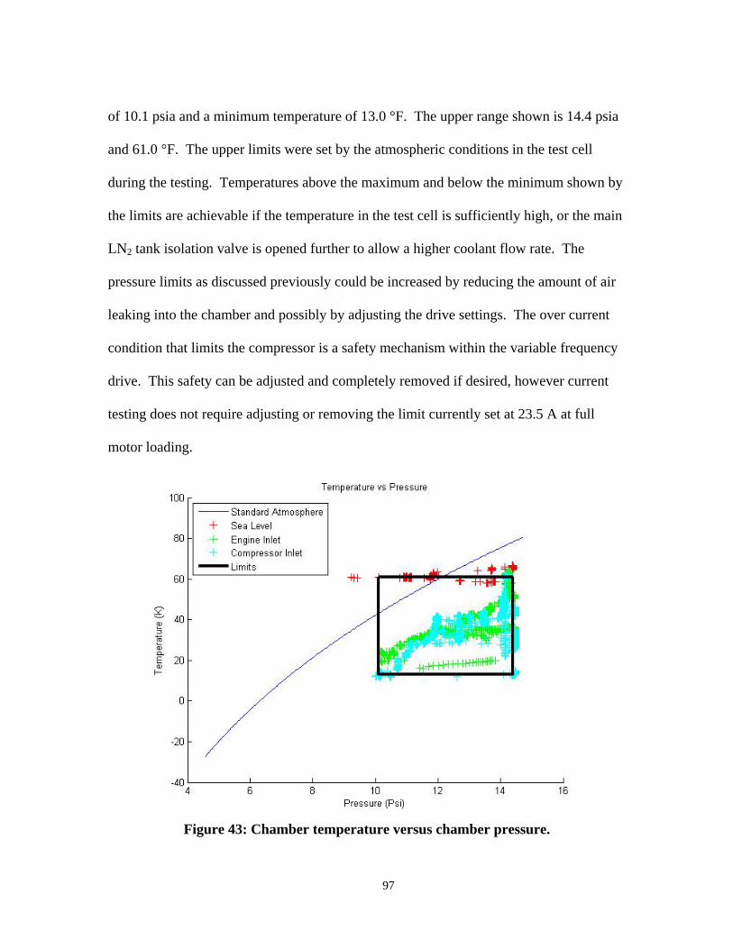
97

of 10.1 psia and a minimum temperature of 13.0 °F. The upper range shown is 14.4 psia

and 61.0 °F. The upper limits were set by the atmospheric conditions in the test cell

during the testing. Temperatures above the maximum and below the minimum shown by

the limits are achievable if the temperature in the test cell is sufficiently high, or the main

LN2 tank isolation valve is opened further to allow a higher coolant flow rate. The

pressure limits as discussed previously could be increased by reducing the amount of air

leaking into the chamber and possibly by adjusting the drive settings. The over current

condition that limits the compressor is a safety mechanism within the variable frequency

drive. This safety can be adjusted and completely removed if desired, however current

testing does not require adjusting or removing the limit currently set at 23.5 A at full

motor loading.

Figure 43: Chamber temperature versus chamber pressure.

98

Attempts were made to complete engine performance maps at 1500 m and 3000 m

conditions, however sufficient data was not collected at these conditions. The series of

test points needed to determine the impact of altitude on engine performance parameters

was generated by varying engine speed over the range of 2000 RPM to 8500 RPM in

increments of 1000 RPM and varying throttle position from wide open throttle, WOT,

down to 25% throttle in increments of 25% at a given altitude condition. At each test

point corresponding to a throttle setting and engine speed, volumetric fuel flow,

temperature, pressure, speed, and torque values would be recorded at a rate of 1 Hz for 10

seconds. High speed data of in cylinder pressure, and spark timing should be taken in

bursts at a rate of 50 kHz to record representative cycles for each test point. The set of

test engine speeds and throttle settings would then be repeated for at each altitude

condition. The pressure and temperature for the three altitude settings are shown in Table

8 and correspond to sea level, 1500 m, and 3000 m above sea level.

Table 8: Altitude test points Altitude, m Pressure, Pa Temperature, K Pressure Ratio Sea Level 101325 300 1.00

1500 85000 285 1.16 3000 70650 275 1.40

Each test point should be averaged over a minimum of 10 seconds and any sample

that was greater than 2 standard deviations away from the mean should be discarded. In

addition samples with negative values or zero values were discarded. Engine

performance maps could be created by putting the averaged data into a matrix form in

order to create plots of BMEP versus engine speed with contours of constant BSFC.

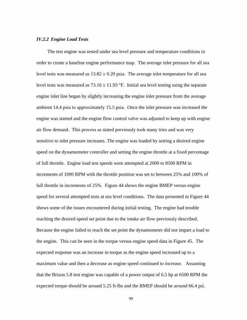
99

IV.2.2 Engine Load Tests

The test engine was tested under sea level pressure and temperature conditions in

order to create a baseline engine performance map. The average inlet pressure for all sea

level tests was measured as 13.82 ± 0.20 psia. The average inlet temperature for all sea

level tests was measured as 73.16 ± 11.93 °F. Initial sea level testing using the separate

engine inlet line began by slightly increasing the engine inlet pressure from the average

ambient 14.4 psia to approximately 15.5 psia. Once the inlet pressure was increased the

engine was started and the engine flow control valve was adjusted to keep up with engine

air flow demand. This process as stated previously took many tries and was very

sensitive to inlet pressure increases. The engine was loaded by setting a desired engine

speed on the dynamometer controller and setting the engine throttle at a fixed percentage

of full throttle. Engine load test speeds were attempted at 2000 to 8500 RPM in

increments of 1000 RPM with the throttle position was set to between 25% and 100% of

full throttle in increments of 25%. Figure 44 shows the engine BMEP versus engine

speed for several attempted tests at sea level conditions. The data presented in Figure 44

shows some of the issues encountered during initial testing. The engine had trouble

reaching the desired speed set point due to the intake air flow previously described.

Because the engine failed to reach the set point the dynamometer did not impart a load to

the engine. This can be seen in the torque versus engine speed data in Figure 45. The

expected response was an increase in torque as the engine speed increased up to a

maximum value and then a decrease as engine speed continued to increase. Assuming

that the Brison 5.8 test engine was capable of a power output of 6.5 hp at 6500 RPM the

expected torque should be around 5.25 ft-lbs and the BMEP should be around 66.4 psi.

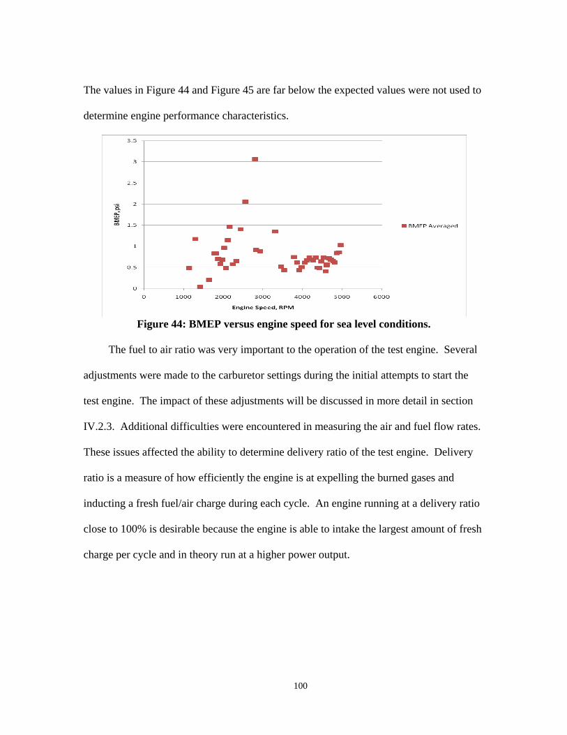
100

The values in Figure 44 and Figure 45 are far below the expected values were not used to

determine engine performance characteristics.

Figure 44: BMEP versus engine speed for sea level conditions.

The fuel to air ratio was very important to the operation of the test engine. Several

adjustments were made to the carburetor settings during the initial attempts to start the

test engine. The impact of these adjustments will be discussed in more detail in section

IV.2.3. Additional difficulties were encountered in measuring the air and fuel flow rates.

These issues affected the ability to determine delivery ratio of the test engine. Delivery

ratio is a measure of how efficiently the engine is at expelling the burned gases and

inducting a fresh fuel/air charge during each cycle. An engine running at a delivery ratio

close to 100% is desirable because the engine is able to intake the largest amount of fresh

charge per cycle and in theory run at a higher power output.

101

Figure 45: Torque versus engine speed for sea level conditions.

In order to correctly calculate the delivery ratio an accurate measurement of fuel

and air mass flows, pressures, and temperatures is required. Fuel pressure was assumed

to be at ambient conditions and fuel temperature was measured with a thermocouple

located outside of the altitude chamber. Fuel flow rates were measured with a Max

Machinery rotary piston flow meter and several issues were encountered. The first issue

was that during testing the data acquisition system would occasionally record flow rates

greater than 340000 cc/sec and was assumed to be a faulty value. All other recorded fuel

flow rates were suspected to be faulty as well and the over estimation was caused by the

method that the data acquisition system originally used to calculate fuel flow rate. The

system was using instantaneous frequency generated by the pulses from the flow meter at

the time of recording the value. A sample of raw data collected with the original

programming is shown in Appendix C. The data was used only for preliminary analysis

by removing obvious outliers from the sample set and using a ten consecutive sample

average. Figure 46 shows how the fuel flow rate varied during two engine test runs at

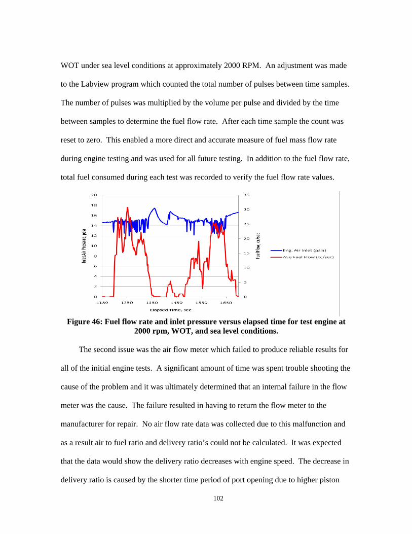
102

WOT under sea level conditions at approximately 2000 RPM. An adjustment was made

to the Labview program which counted the total number of pulses between time samples.

The number of pulses was multiplied by the volume per pulse and divided by the time

between samples to determine the fuel flow rate. After each time sample the count was

reset to zero. This enabled a more direct and accurate measure of fuel mass flow rate

during engine testing and was used for all future testing. In addition to the fuel flow rate,

total fuel consumed during each test was recorded to verify the fuel flow rate values.

Figure 46: Fuel flow rate and inlet pressure versus elapsed time for test engine at

2000 rpm, WOT, and sea level conditions.

The second issue was the air flow meter which failed to produce reliable results for

all of the initial engine tests. A significant amount of time was spent trouble shooting the

cause of the problem and it was ultimately determined that an internal failure in the flow

meter was the cause. The failure resulted in having to return the flow meter to the

manufacturer for repair. No air flow rate data was collected due to this malfunction and

as a result air to fuel ratio and delivery ratio’s could not be calculated. It was expected

that the data would show the delivery ratio decreases with engine speed. The decrease in

delivery ratio is caused by the shorter time period of port opening due to higher piston

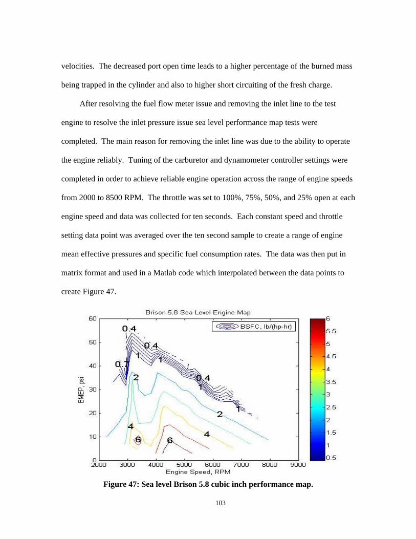
103

velocities. The decreased port open time leads to a higher percentage of the burned mass

being trapped in the cylinder and also to higher short circuiting of the fresh charge.

After resolving the fuel flow meter issue and removing the inlet line to the test

engine to resolve the inlet pressure issue sea level performance map tests were

completed. The main reason for removing the inlet line was due to the ability to operate

the engine reliably. Tuning of the carburetor and dynamometer controller settings were

completed in order to achieve reliable engine operation across the range of engine speeds

from 2000 to 8500 RPM. The throttle was set to 100%, 75%, 50%, and 25% open at each

engine speed and data was collected for ten seconds. Each constant speed and throttle

setting data point was averaged over the ten second sample to create a range of engine

mean effective pressures and specific fuel consumption rates. The data was then put in

matrix format and used in a Matlab code which interpolated between the data points to

create Figure 47.

Figure 47: Sea level Brison 5.8 cubic inch performance map.

104

Engine power and torque for sea level conditions follow the expected trends.

Figure 49 shows engine torque versus engine speed for sea level conditions. The peak

torque for the Brison 5.8 occurs at 4000 RPM while peak power, shown in Figure 48,

occurs at 6500 RPM. Additional testing is needed at smaller engine speed increments to

determine the exact speeds for which peak power and peak torque occur. The large drop

in power output seen in Figure 48 for 25% throttle conditions is due to equivalence ratio.

The Brison 5.8 carburetor was seen to work well at medium to high throttle conditions

but did not perform well under low throttle settings. The carburetor was not able to meter

the correct amount of fuel for the lower air demand causing the engine to operate poorly.

Figure 48: Engine power versus engine speed at sea level conditions.

105

Figure 49: Engine torque versus engine speed at sea level.

Engine performance testing under lower pressure conditions was accomplished to

determine the impact that inlet pressure has on engine performance. The lower pressure

tests were performed with the inlet line disconnected from the engine for the reasons

stated previously. The test was performed by running the test engine at a fixed throttle

position and speed while reducing the inlet pressure. This test was repeated at for two

speeds and three throttle positions. The first test was run at 3500 RPM and is shown in

Figure 50 where the throttle position was set at WOT and 75% throttle. The inlet

pressure was varied from 13.982 psia to 13.865 psia for the WOT setting and 13.865 psia

to 13.455 psia for the 75% throttle setting. Figure 50 shows that for a 0.84% decrease in

inlet pressure at WOT the result is a 14.2% decrease in both power and torque. Figure 50

also shows that at 75% throttle a 2.96% decrease in inlet pressure results in a ~54%

decrease in power and torque. Similar results are seen in Figure 51 with the engine set at

3000 RPM where the throttle positions were set at WOT and 25%. At 3000 RPM and

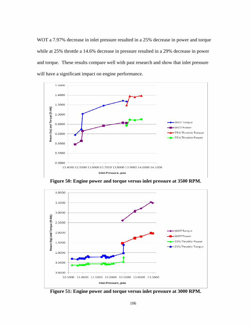
106

WOT a 7.97% decrease in inlet pressure resulted in a 25% decrease in power and torque

while at 25% throttle a 14.6% decrease in pressure resulted in a 29% decrease in power

and torque. These results compare well with past research and show that inlet pressure

will have a significant impact on engine performance.

Figure 50: Engine power and torque versus inlet pressure at 3500 RPM.

Figure 51: Engine power and torque versus inlet pressure at 3000 RPM.

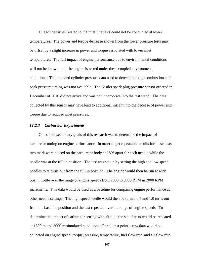
107

Due to the issues related to the inlet line tests could not be conducted at lower

temperatures. The power and torque decrease shown from the lower pressure tests may

be offset by a slight increase in power and torque associated with lower inlet

temperatures. The full impact of engine performance due to environmental conditions

will not be known until the engine is tested under these coupled environmental

conditions. The intended cylinder pressure data used to detect knocking combustion and

peak pressure timing was not available. The Kistler spark plug pressure sensor ordered in

December of 2010 did not arrive and was not incorporate into the test stand. The data

collected by this sensor may have lead to additional insight into the decease of power and

torque due to reduced inlet pressures.

IV.2.3 Carburetor Experiments

One of the secondary goals of this research was to determine the impact of

carburetor tuning on engine performance. In order to get repeatable results for these tests

two mark were placed on the carburetor body at 180° apart for each needle while the

needle was at the full in position. The test was set up by setting the high and low speed

needles to ¾ turns out from the full in position. The engine would then be run at wide

open throttle over the range of engine speeds from 2000 to 8000 RPM in 2000 RPM

increments. This data would be used as a baseline for comparing engine performance at

other needle settings. The high speed needle would then be turned 0.5 and 1.0 turns out

from the baseline position and the test repeated over the range of engine speeds. To

determine the impact of carburetor setting with altitude the set of tests would be repeated

at 1500 m and 3000 m simulated conditions. For all test point’s raw data would be

collected on engine speed, torque, pressure, temperature, fuel flow rate, and air flow rate.

108

The stock timing box should be used for all tests and timing signals recorded. Data

should be averaged at each test point for 10 time samples. Plotting of power versus

engine speed at the baseline, 0.5 turns, and 1.0 turns can be used to compare how

increasing the richness of the mixture impacts engine performance. Similar plots for

BSFC versus engine speed, torque versus engine speed, and BMEPmax versus engine

speed for the different mixture settings and altitudes are also useful in determining the

impact on engine performance and how incorrect engine tuning can change performance

as the engine increases in altitude.

IV.2.4 Carburetor Tests

Specific tests were not accomplished to understand how the carburetor setting

impacts engine performance as the inlet altitude condition changed. Some observations

of carburetor settings can be made based upon the engine load testing that was

performed. The test engine was very sensitive to the air to fuel ratio in the cylinder and

slight changes caused by increasing or decreasing the inlet air pressure caused poor

engine performance. In most cases if the inlet air mass flow was restricted the engine

would flood with fuel and cease to operate. During conditions where the inlet pressure

was allowed to rise quickly the carburetor was unable to keep up and the engine would

end up in a condition where almost no fuel was entering the cylinder. This fuel lean

condition caused the engine to stop running. It was observed that the engine would

continue to operate under fuel lean conditions much more readily than under fuel rich

conditions. Fuel rich conditions caused by low inlet pressures lead to almost

instantaneous engine operational failure, while fuel lean conditions would slowly lead to

misfires and ultimately engine failure.

109

V. Conclusions and Recommendations

V.1 Conclusions

The goal of the research was to design and build a mobile test facility capable of

test small internal combustion engines under 10 hp in size. The facility was tested and

proved capable of reaching pressure and temperature conditions representative of

atmospheric conditions seen at 10000 ft. A representative test engine was tested in the

mobile test stand and performance data was collected under sea level conditions. Initial

data showed the impact of inlet pressure on the power, torque, and fuel flow rates of a

two stroke spark ignition crank case scavenged engine. The primary goal of designing,

building, and testing a mobile test facility for small internal combustion engine

performance testing was partially accomplished. The primary limitation of the test stand

is the ability to operate the engine under low temperature conditions resulting from poor

inlet line design

The secondary goal of testing a representative IC engine to gather performance

information was also partial completed. A seal level performance map was created and

will give a baseline for future testing. The testing process resulted in a better

understanding of the issues involved in operating the altitude test stand. The solution to

many of the issues encountered during the testing process were presented. Additionally

test methodologies were presented for completing engine performance maps at simulated

altitude conditions. Methodologies for investigating carburetor impacts on engine

performance as a function of engine speed and altitude were also presented.

110

The tertiary goal of testing engine to engine performance variations was not

completed during this research. Engine to engine performance variations may play a key

role in system operation along with carburetor tuning. Results from several identical

engines over a range of speed, throttle, and altitude conditions should be compared in

order to determine acceptable correlations of engine performance as a function of

altitude.

V.2 Recommendations

There are many recommendations that could be made regarding the mobile test

capability developed as the major goal for this research. The mobile test stand was only

partially successful in attaining the design goals set forth by AFRL/RZTC. In order to

make the most use of the developed capability some additional functionality should be

added to the test stand. The first step would be to use the facility to take performance

data at simulated altitude conditions on the Brison 5.8 test engine as originally intended.

The creation of performance maps at 1500 m and 3000 m would allow AFRL to better

understand the impact that environmental changes have on the performance of a stock

engine. In order to make it easier to operate the test stand the following steps should be

taken:

1. Resolve the shaft seal, top window gasket, and exit nozzle interface seal

leakage in order to reach and sustain pressure conditions more easily.

2. Methodically test manual bypass, and main control valve position settings as

a function of compressor speed to determine where the over current limit is

and plot it on the compressor map.

111

3. Add an actuated isolation valve to LN2 system in order to quickly shut off

the coolant supply in the event of an emergency or when the compressor

abruptly stops.

4. Design and fabricate a coupling alignment system to quickly and accurately

measure coupling parallel, axial, and angular misalignments.

5. Resolve the inlet line pressure oscillation issue to allow the engine to

operate at lower pressure and temperature conditions.

By undertaking these tasks the mobile test stand would have the ability to quickly

set up tests and the operator would have a better idea of how to achieve desired

conditions quickly and safely. In order to test future engine design modifications that

allow small IC engines to operate above 3000 m the test stands capability limits need to

be expanded upon. The lower temperature limit is easily reduced with the addition of

higher coolant flow rates. The lower pressure limit may be reduced by addressing items

number one and two above. By carefully avoiding the current limit and reducing the

amount of air leaking into the chamber lower pressures should be possible. In order to

test higher temperatures than those shown in Figure 43 the addition of electric heaters on

the main coolant flow path would be needed. The engine flow path should utilize the

current counter flow heat exchanger by flowing warm fluid through the current LN2 side.

This has two benefits, it removes the need to add additional heaters to the line and it

requires no additional wiring or plumbing.

After the baseline and altitude performance maps are complete there are several

additional areas of research that would lead to a better understanding of small internal

combustion engines. The use of carburetors has been common in internal combustion

112

engines of all sizes for many years. In recent year’s advancements in manufacturing and

digital electronics has lead to smaller fuel injectors and engine control systems.

Investigating the impact of carburetor settings at a variety of flight conditions would

enable future researchers to determine what if any performance improvements are made

with the addition of new technologies. The impact manufacturing tolerances on the stock

carburetor and engine performance should be researched. The variability of engine

performance for identical engines from a single manufacturer is an important figure of

merit for the acquisitions and design communities. If there is a large variability in engine

performance than the designers of future systems must account for the lowest common

denominator. This leads to many systems having significant inefficiencies due simply to

the fact that they have more capability than they were designed for.

Research specifically tailored to two stroke engines includes determining an

appropriate pegging method for the in cylinder pressure measurements, determining

trapping efficiencies, and investigating the impact of intake and exhaust geometry on

engine performance. Many of the pegging methods described in chapter II focused on

four stroke engines without any type of scavenging. For the test engine presented in this

research the fresh fuel and air charge is pre-compressed in the crankcase prior to entering

the cylinder. This pre-compression is done in order to increase the inlet pressure helping

to force the burned gases out of the cylinder prior to port closing. Pre-compression also

increases the enthalpy of the fuel air mixture just prior to injection into the cylinder

making it easier to ignite the mixture. The increase pressure and temperature caused by

the pre-compression may aid in mixing. The impact of this type of scavenging on engine

performance at increasing altitude conditions is of interest. If scavenging efficiencies

113

increase with altitude then two stroke engines may be a better option even though their

fuel consumption is greater than similar four stroke engines.

Two stroke engines use a mixture of fuel and oil and the ratio and type of oil may

have an impact on engine performance. The heating value and thus the available energy

in the fuel and oil mixture are a function of the fuel and oil types as well as the

volumetric or mass ratio of the mix. Tests designed to measure the impact of fuel and oil

mixture ratio would be useful in determining the best mixture ratio for specific fuel and

oil combinations. It would of interest to test if the fuel to oil mixture ratio is specific to

each engine design.

With the mandate for a single fuel supply chain within the DoD it is of great

importance to test the impact of using heavy fuels in two stroke engines. Heavy fuels

have very different qualities than the standard high octane fuels used in most small two

stroke IC engines. Additionally the impact of heavy fuels on engine performance at

different altitudes is also crucial for the development of small IC engines capable of

running on heavy low octane fuels over a wide range of environmental conditions. These

engines will power new man portable UAS’s and it is vital to understand how they will

perform.

V.3 Future Work

The mobile altitude chamber functioned well during the current test program. In

the future automation of the test stand is desired in order to remotely operate the stand

from the control room. In order to operate the stand remotely, actuators must be added to

all of the manual valves including the two coolant valves, and the main engine cooling

flow bypass valve. The addition of PID control loops for the control valve actuators

114

would be useful in preventing compressor surge or over current conditions. PID control

loops would also prevent engine cutout due to inappropriate fuel to air ratio conditions

caused by restricting the air flow once the engine starts running. Upgrades to the

chamber seals are necessary in order to reach higher pressure ratios as well as making it

easier to open and close the chamber without worrying about the lid seals. A more robust

and accurate system for aligning the engine and dynamometer couplings is also desired.

The addition of an oil cooling system is needed to allow the compressor to operate for

sustained periods of time. The last improvement to the test stand would be to allow

connection of the fuel system to the test bay fuel distribution system. This upgrade

would allow for the testing of multiple fuels without having to empty the fuel tank.

Connecting to the facility fuel system would require the addition of a separate oiling

system for the mixing of fuel and oil in the proper ratio for two stroke engine operation.

The fuel and oil mixing control should be capable of adjustable mixture settings from

zero mixing up to about 30:1 mixing ratios in order to operate a wide range of small

internal combustion engines. The impact of oil addition to the fuel should be studied in

order to quantify the effect that the fuel oil mixture has on engine performance.

Other future work includes continuing to take a larger number of data points to

enhance the resolution of the engine performance maps for the Brison 5.8. The stock

timing box should be investigated in more detail to determine if an upgrade is needed to

reach maximum cylinder pressure at the desired crank angle degree. An investigation of

the intake and exhaust system should be conducted to see if tuning the intake and exhaust

legs would lead to increases in power and torque and decreases in BSFC. Work by other

115

researchers has indicated that fuel injection technologies may lead to decreases in BSFC

without significantly impacting engine power or engine torque.

Testing of carburetor tuning impacts is an important step that is needed to baseline

engine performance. This baseline can then be used to determine the impact of using a

fuel injector in the test engine. Implementing fuel injectors into the Brison 5.8 will be a

challenge due to the two stroke crankcase scavenged operation of the engine but may lead

to a more consistent fuel and air mixture on a cycle to cycle basis. Carburetor tuning

impacts should be investigated to determine how slight adjustments in the needle valve

settings impact performance at a constant altitude. The impact of carburetor tuning on

engine performance based on a fixed needle valve setting over a range of altitude

conditions should also be determined. The variability of engine performance based on

carburetor tuning is an important design consideration for UAS systems that must be

operated in austere conditions with limited tools and limited time.

The Brison 5.8 should be tested to determine how much variability occurs between

identical engines by testing multiple Brison 5.8 engines under the same throttle and speed

conditions. Engine to engine performance variation is an important design consideration

for the DoD as a large number of engines would be needed to power a single type of

UAS. UAS system and mission design must account for the lowest average performance

of an engine.

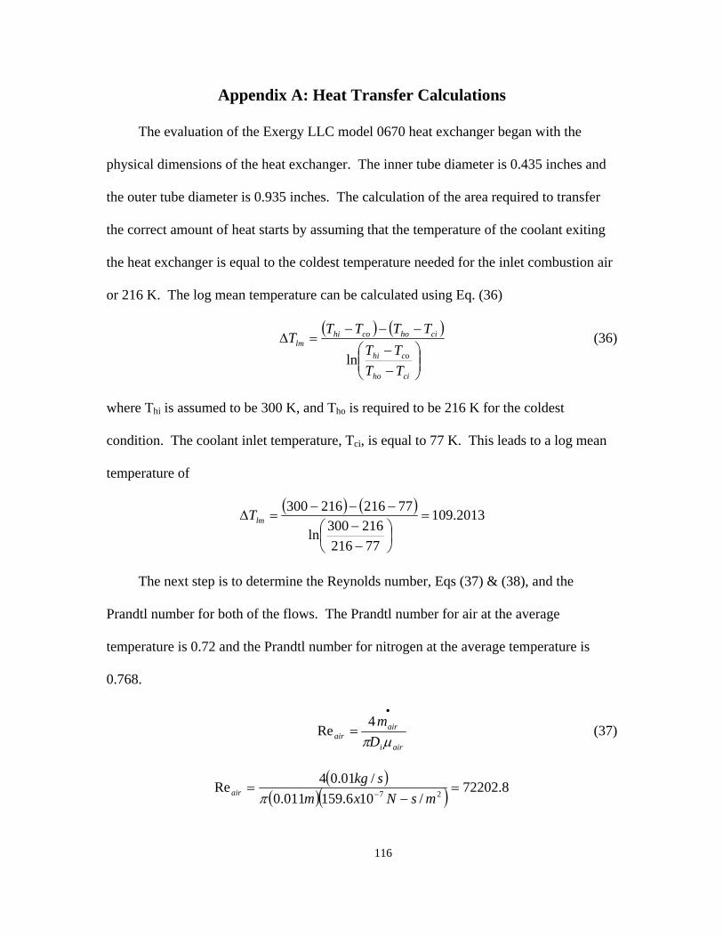
116

Appendix A: Heat Transfer Calculations

The evaluation of the Exergy LLC model 0670 heat exchanger began with the

physical dimensions of the heat exchanger. The inner tube diameter is 0.435 inches and

the outer tube diameter is 0.935 inches. The calculation of the area required to transfer

the correct amount of heat starts by assuming that the temperature of the coolant exiting

the heat exchanger is equal to the coldest temperature needed for the inlet combustion air

or 216 K. The log mean temperature can be calculated using Eq. (36)

ciho

cohi

cihocohilm

TT

TT

TTTTT

ln

(36)

where Thi is assumed to be 300 K, and Tho is required to be 216 K for the coldest

condition. The coolant inlet temperature, Tci, is equal to 77 K. This leads to a log mean

temperature of

2013.109

77216

216300ln

77216216300

lmT

The next step is to determine the Reynolds number, Eqs (37) & (38), and the

Prandtl number for both of the flows. The Prandtl number for air at the average

temperature is 0.72 and the Prandtl number for nitrogen at the average temperature is

0.768.

airi

airair D

m

4

Re (37)

8.72202

/106.159011.0

/01.04Re

27

msNxm

skgair

117

2

22

4Re

Nio

NN DD

m

(38)

31909.4

/108.68011.002375.0

/006.04Re

27

msNxmm

skgair

Since both of the Reynolds numbers are well above the transition point for flow

thru a duct it is assumed that the flow is fully turbulent and the correlation from

Reference 39 can be used to calculate the Nusselt number as Eq. (39)

CoolingnHeatingnNu nD 3.0,4.0PrRe023.0 5/4 (39)

82.99768.04.31909023.0

61.16072.08.72202023.04.05/4

2

3.05/4

DN

Dair

Nu

Nu

Using the standard relation for the convective heat transfer coefficient given by Eq. (40)

the overall heat transfer coefficient, U, can be calculated by Eq. (41). The area required

can be calculated by using Eq. (42).

h

D D

kNuh (40)

KmWm

KmWh

KmWm

KmWh

c

h

2

2

/60.620127.0

/00958.099.82

/155.324011.0

/0223.061.160

ch hh

U11

1

(41)

KmWU

2/47.52

60.621

155.3241

1

lmTU

QA

(42)

2087.02.109*47.52

500mA

118

Based on the above area and to provide some factor of additional capacity due to

the fact that several somewhat questionable assumptions had to be made the 7 coil heat

exchanger with an area of 0.19m2 allows for an area of slightly more than twice what is

required. No attempt was made to account for the phase change that will occur in the

nitrogen which will aid in the exchange of heat.

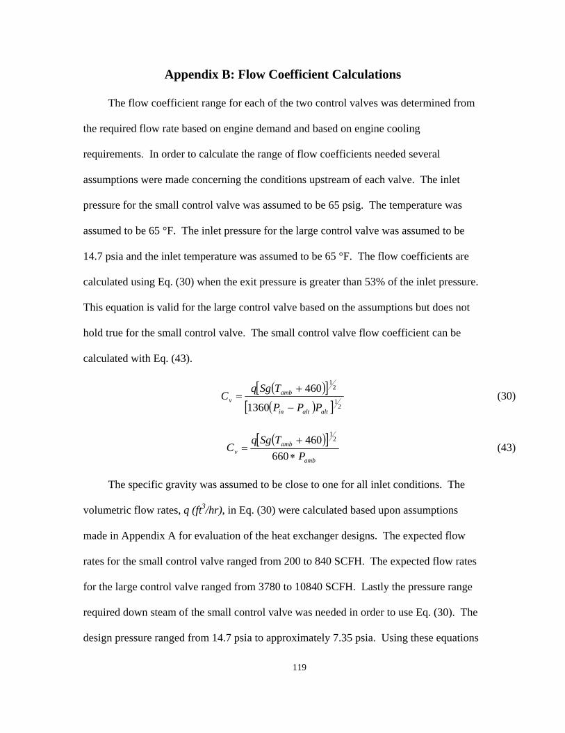
119

Appendix B: Flow Coefficient Calculations

The flow coefficient range for each of the two control valves was determined from

the required flow rate based on engine demand and based on engine cooling

requirements. In order to calculate the range of flow coefficients needed several

assumptions were made concerning the conditions upstream of each valve. The inlet

pressure for the small control valve was assumed to be 65 psig. The temperature was

assumed to be 65 °F. The inlet pressure for the large control valve was assumed to be

14.7 psia and the inlet temperature was assumed to be 65 °F. The flow coefficients are

calculated using Eq. (30) when the exit pressure is greater than 53% of the inlet pressure.

This equation is valid for the large control valve based on the assumptions but does not

hold true for the small control valve. The small control valve flow coefficient can be

calculated with Eq. (43).

2

1

21

1360

460

altaltin

ambv

PPP

TSgqC

(30)

amb

ambv P

TSgqC

660

460 21

(43)

The specific gravity was assumed to be close to one for all inlet conditions. The

volumetric flow rates, q (ft3/hr), in Eq. (30) were calculated based upon assumptions

made in Appendix A for evaluation of the heat exchanger designs. The expected flow

rates for the small control valve ranged from 200 to 840 SCFH. The expected flow rates

for the large control valve ranged from 3780 to 10840 SCFH. Lastly the pressure range

required down steam of the small control valve was needed in order to use Eq. (30). The

design pressure ranged from 14.7 psia to approximately 7.35 psia. Using these equations

120

lead to a calculated flow coefficient range for the small control valve of 0.10 to 0.53

while the large control valve required a flow coefficient range of 0.5 to 54.0. Figure 52

shows that the small control valve should be operating between 15% open and 50% open

for the flow rates expected during engine testing. Figure 53 shows that the large control

valve should be operating between 15% open and 70% open based on the expected flow

rates. In actual testing the large control valve operates between 50% open and 100%

open in order to meet the mass flow demands of the compressor.

Figure 52: 0.5 inch Triac 30 degree vee port control valve flow coefficient versus

percent open.

121

Figure 53: 2.5 inch Triac 30 degree vee port control valve flow coefficient versus

percent open.

Table 9: Control Valve CV versus on percent of valve opening (39). 0% 15% 20% 30% 40% 50% 60% 70% 80% 90% 100%

0.5” Valve CV

0 0.1 0.1 0.2 0.3 0.5 0.8 1.1 1.6 2.2 2.6

2.5” Valve CV

0 0.4 1 4 8 12 18 28 37 62 75

122

Appendix C: Window and Wall Stress Calculation

Stress calculations were performed during the design phase in order to determine

the required thickness of the chamber windows, the inlet and exit nozzles, and the

chamber bottom surface. The stress calculations were based upon standard material

properties for structural steel, 6061 aluminum, and polycarbonate (40, 41). The material

properties used for the stress calculations are shown in Table 10. Each surface was

considered to be in a held but not fixed configuration according to the definition in

Reference 40.

Table 10: Material properties for aluminum, steel, and polycarbonate (40, 41).

Yield

Strength, MPa

Tensile Strength,

MPa

Elastic Modulus, E, GPa

Allowable Design Stress*,

MPa Aluminum 270.00 310.00 70.00 67.50 A36 Steel 360.00 580.00 210.00 90.00 Polycarbonate40 55.16 65.50 2.24 13.79

*Based on a safety factor of 4 from the yield strength.

The first step in calculating the stress in the material is to determine the

unsupported area that will be subjected to a differential pressure force. The upper poly

carbonate window opening is 13.5 inches by 19 inches. The front polycarbonate view

port has an opening 13.5 inches by 15 inches. The base of the box has two small

unsupported areas that are 7 inches by 18 inches. Lastly the largest panel wall area for

both the inlet and exit nozzles is approximated as 15 inches by 9 inches. This

approximation was made to simplify the calculations for the inlet and exit which was

constructed from trapezoid shaped pieces of differing sizes.

The next step in the process is to determine the maximum pressure differential, Δp,

that will be generated across the unsupported regions. Based upon the design

123

assumptions a maximum pressure differential of 745 kPa is assumed to be the maximum

for 15000 ft above sea level test runs. For conditions approximating 30000 ft the

maximum pressure differential would be approximately 1114.5 kPa. Equation (44) was

used to determine the displacement to thickness ratio. This ratio is then used to

determine the stress in the center of the unsupported region, Eq. (45). The solution must

be solved iteratively by varying the displacement to thickness ratio, Eq. (46) until the left

hand side of Eq. (44) matches the right hand side of Eq. (44).

3

214

4

t

wK

t

wK

Et

ap (44)

2

43

2

t

wK

t

wK

a

tEScenter (45)

1

2

2

4

43

21

13 K

t

wK

Et

ap

t

wK

t

wK

t

w

t

w

n

nn

nn

(46)

The solution to the set of equations depends on the choice of material thickness, t.

If the converged stress at the center, Scenter, exceeds the design stress the material

thickness must be increased and the process repeated. The constants, K1 through K4, are

given in Table 11 for thin plate theory and are a function of the maximum dimension of

the unsupported region, b, divided by the minimum dimension of the unsupported region,

a. The subscript n in Eq. (46) denotes the current iteration and the variable E represents

the elastic modulus of the material given in Table 10. The equation set given above was

given in English units of psi and inches so all further calculations will be done in inches

and pounds per square inch for consistency.

124

Table 11: Constants for stress equation based on b/a ratio(40). b/a K1 K2 K3 K4

1 22.5 30.5 6.5 2.7

1.1 18.9 27.6 6.3 2.7 1.2 16.2 25.7 6.1 2.7

1.3 14.3 24.6 5.9 2.7 1.4 13 23.7 5.9 2.7 1.5 11.9 23.1 5.8 2.7 1.6 11 22.7 5.7 2.7 1.8 9.8 22.2 5.6 2.7 2 9 22 5.5 2.7

3 7.5 21.4 5.3 2.7 ∞ 7 21.4 5.3 2.7

The solution to Eqs. (44), (45), and (46) for each of the given materials and

dimensions is given in Table 12. While some of the materials have maximum stresses

higher than the design stress at the higher differential pressure they are all well below the

yield stress of the material. The only part that is still above the design stress at a

differential pressure of 8 psi is the upper viewing window. This was accepted as a risk

for two reasons. The first reason was that the window stress is only 1.4% above the

design stress limit so the risk of breaking is very low. The second reason for accepting

the risk was due to the cost of the material. The cost of ¾” thick polycarbonate was

approximately $800 more than the cost of the ½” thick material for the same length and

width.

Table 12: Solution to stress equations for each region.

Name Material Dimension,

b x a, in Thickness,

in

Max Displacement

@ 11psi, in

Max Stress @ 11psi, psi

Max Stress @ 8psi, psi

Upper Viewing Window Polycarbonate 15 x 13.5 0.5000 0.307 2498.6 2028.6

Front Viewing Window Polycarbonate 19 x 13.5 0.5000 0.358 2177.8 1723.6 Chamber

Bottom A36 Structural

Steel 18 x 7 0.1875 0.015 9587.7 6952.3 Chamber Inlet

and Exit 6061

Aluminum 15 x 9 0.2500 0.040 7548.9 5514.3

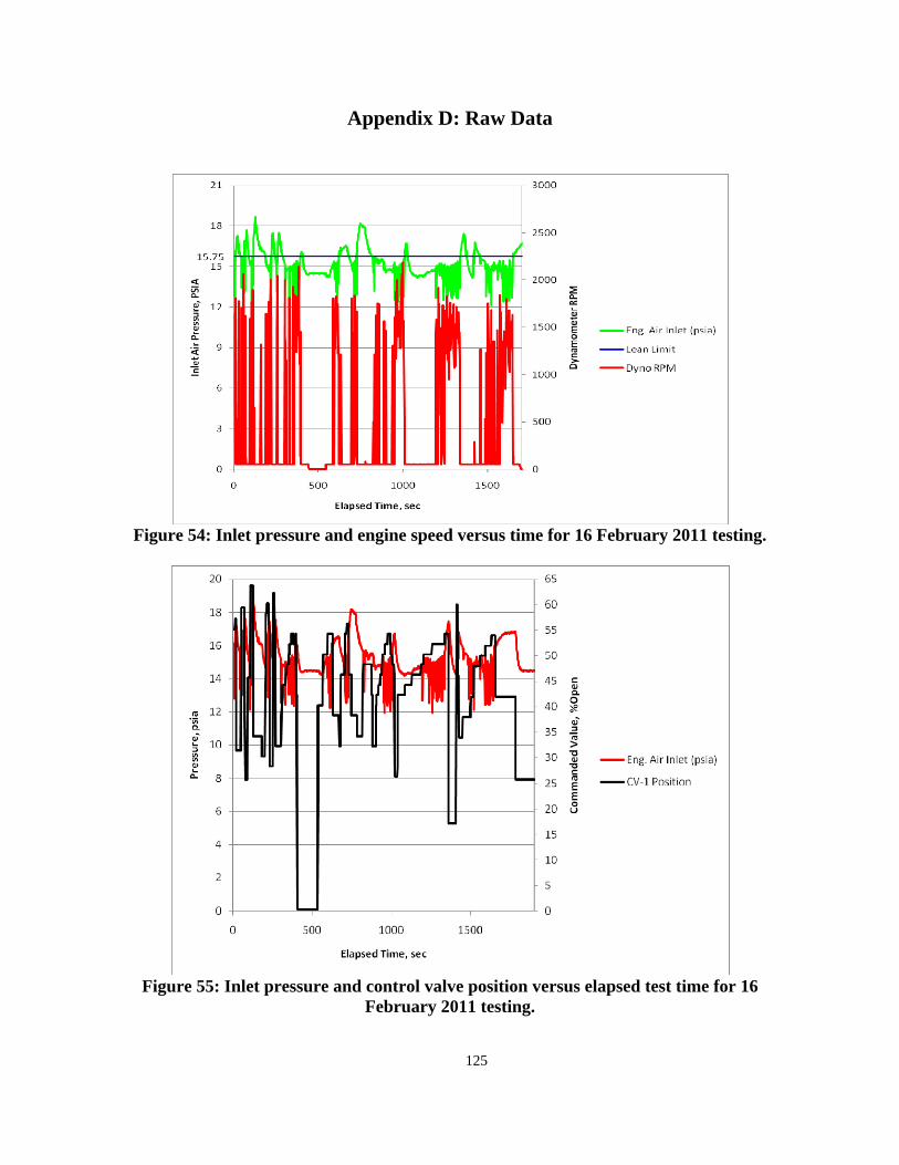
125

Appendix D: Raw Data

Figure 54: Inlet pressure and engine speed versus time for 16 February 2011 testing.

Figure 55: Inlet pressure and control valve position versus elapsed test time for 16

February 2011 testing.

126

Figure 56: Chamber pressure versus elapsed time for three separate tests.

Figure 57: Inlet air pressure and fuel volumetric flow versus elapsed time.

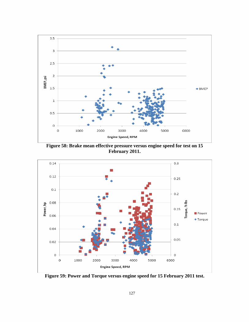
127

Figure 58: Brake mean effective pressure versus engine speed for test on 15

February 2011.

Figure 59: Power and Torque versus engine speed for 15 February 2011 test.

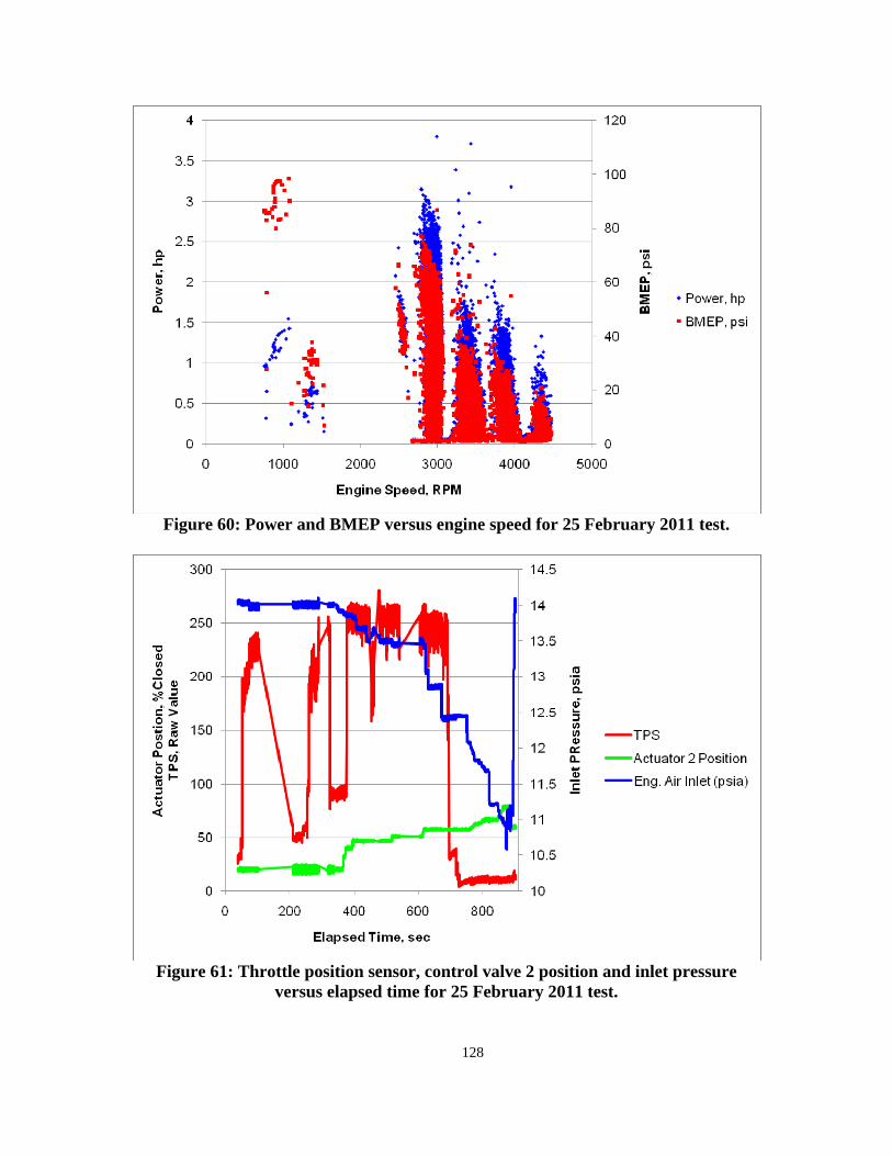
128

Figure 60: Power and BMEP versus engine speed for 25 February 2011 test.

Figure 61: Throttle position sensor, control valve 2 position and inlet pressure

versus elapsed time for 25 February 2011 test.

129

Figure 62: Torque, engine speed, and BSFC versus elapsed time for 25 February

2011 test.

Figure 63: BMEP and BSFC versus engine speed for 28 February 2011 test.

130

Appendix E: Chamber Mechanical Drawings

The chamber was designed using the NX 7 CAD package from Siemens. The

following are some of the drawings and models used to develop the overall chamber

design and layout.

Figure 64: Side view of CAD model showing dynamometer, starter motor, base

plate, and exit nozzle.

Figure 65: Front view of CAD model showing chamber, motor mount, base plate,

entrance diffuser, and exit nozzle.

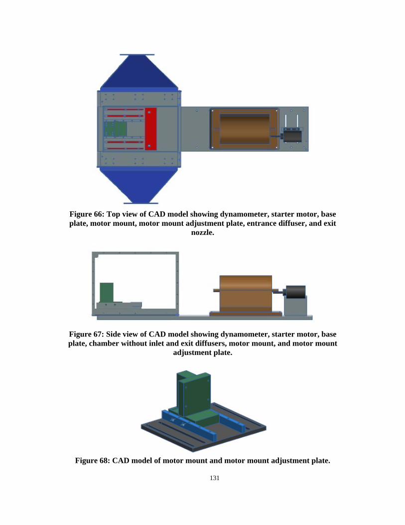
131

Figure 66: Top view of CAD model showing dynamometer, starter motor, base plate, motor mount, motor mount adjustment plate, entrance diffuser, and exit

nozzle.

Figure 67: Side view of CAD model showing dynamometer, starter motor, base plate, chamber without inlet and exit diffusers, motor mount, and motor mount

adjustment plate.

Figure 68: CAD model of motor mount and motor mount adjustment plate.

132

Figure 69: Machine shop drawing of assembled chamber with instructions to create

level surface for top and front viewing windows.

133

Figure 70: Machine shop drawing for creating the chamber rear wall.

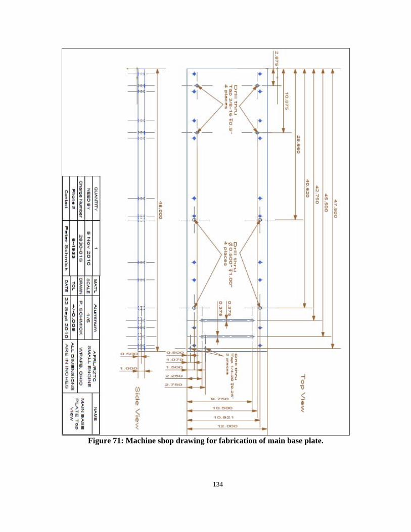
134

Figure 71: Machine shop drawing for fabrication of main base plate.

135

Appendix F: Parts List

Table 13: Parts List for Mobile Test Stand Ref #

Item Qty Status Contact Part

Number S/N Price Notes

1 Engine Starter Motor 1

Installed Quick Start Automotive Electric

Kohler 5761N (2-2129-UT)

N/A $99.99 starter motor run off 12v car battery

2 Starter Gear

1 Installed Motion Systems

Inc. N/A N/A $160.00 3.5" diameter gear with 33 teeth and

pitch of 10 with 14.5 deg pitch angle

3 Starter Relay 1 Installed Unknown N/A N/A $0.00 Found in Bldg 21.

4

Dynamometer and controller equipment 1

Installed Paul Abbott 716-668-5555 ext. 161 [email protected]

2WB-65, DSP-6001, TSC 401, DES Power Supply

Dyno: 3000054 Power: 01153 Torque: 3000054 Controller: OH601155

$28,780.00 includes eddy current dyno sized for 12kW with max 30000rpm, excitation supply, torque/speed conditioner, programmable controller, and cords

5

Fuel Flow Meter

1

Installed Max Machinery T707-433-2662 F707-433-1818 33A Healdsburg Ave, Healdsburg, CA 95448

213-311-000 flow meter, 294 transmitter, 181-294-060 cable assembly

Flow Meter: Transmitter:

$2,570.00 Flow Meter(213), tranmitter(294), calibration, chords

6

Test Engines

2

One installed, one in storage

Cimmaster Arthur Lueng 905-564-3099

Brison 5.8 engine

N/A $1,540.00

7

Thermocouples

12

Installed Omega KQSS-14U-6, KQSS-14E-6, KMQSS-062G-6

N/A $359.00 Omega

136

Ref #



8

Charge Amplifier and Chassis 1

Installed Simon Johnson, Kistler T248 489 1090 x 6030 F248 489 1280

5064B11 Amp, 2852A12 Chassis

Amp: 1910377 Chassis: 1931559

$3,910.00 Kistler charge amplifier with analog direct current voltage output of in cylinder PT signal and 19" rack mount chassis

9

Low Noise Cable and Pass Through 1

Installed Simon Johnson, Kistler T248 489 1090 x 6030 F248 489 1280, Mouser

1601BSP2M, 523-21-3220

N/A $76.16 Kistler low noise cable to connect in cylinder transducer through the chamber wall and into the charge amplifier

10

In cylinder PT

2

Waiting for Part

Simon Johnson, Kistler T248 489 1090 x 6030 F248 489 1280

6118BFD16Q02A41

N/A $7,770.00 Kistler spark plug sensor

11

Pressure Transducers

7

Installed Omega PX409-030A5V 403607, 403809, 413900, 418686, 403595, 403599, 403598

$3,675.00 Omega 0-30 PSIA transducers

12 Pressure Transducer

1 Installed Honeywell 060-3883-

09TJA 1305129 $0.00 Honeywell 0-100 PSIA transducer

13 Throttle and Choke Servo 2

Installed Polulu 6001HB N/A $25.90

14

Servo Motor Controller

1

Installed Polulu mini-Maestro 12 channel USB servo controller

N/A $32.44 Ability to control up to 12 servo motors, currently only using two channels for throttle and choke positioning

15

Throttle Position Sensor

1

Installed Sensor Product Manager, CTS Automotive Products, T574-389-2890, F574-295-3580, [email protected]

CTS P/N: 521-99-015 Advanced P/N: EC3026

N/A $26.09 CTS Corp provided samples but actual TPS was purchased from Advanced Auto

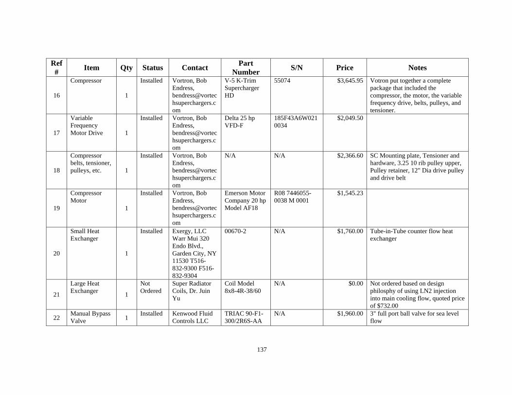
137

Ref #



16

Compressor

1

Installed Vortron, Bob Endress, [email protected]

V-5 K-Trim Supercharger HD

55074 $3,645.95 Votron put together a complete package that included the compressor, the motor, the variable frequency drive, belts, pulleys, and tensioner.

17

Variable Frequency Motor Drive 1


Delta 25 hp VFD-F

185F43A6W0210034

$2,049.50

18

Compressor belts, tensioner, pulleys, etc. 1


N/A N/A $2,366.60 SC Mounting plate, Tensioner and hardware, 3.25 10 rib pulley upper, Pulley retainer, 12" Dia drive pulley and drive belt

19

Compressor Motor

1


Emerson Motor Company 20 hp Model AF18

R08 7446055-0038 M 0001

$1,545.23

20

Small Heat Exchanger

1

Installed Exergy, LLC Warr Mui 320 Endo Blvd., Garden City, NY 11530 T516-832-9300 F516-832-9304

00670-2 N/A $1,760.00 Tube-in-Tube counter flow heat exchanger

21

Large Heat Exchanger

1

Not Ordered

Super Radiator Coils, Dr. Juin Yu

Coil Model 8x8-4R-38/60

N/A $0.00 Not ordered based on design philosphy of using LN2 injection into main cooling flow, quoted price of $732.00

22 Manual Bypass Valve 1

Installed Kenwood Fluid Controls LLC

TRIAC 90-F1-300/2R6S-AA

N/A $1,960.00 3" full port ball valve for sea level flow

138

Ref #



23 0.5" Control Valve 1


TRIAC V9-FS-050/WEA2-XX-30

0105550-3-1-1 $2,369.00

24 2.5" Control Valve 1


TRIAC V9-FS-250/WEB2-XX-30

0105550-16-1-1 $3,891.00

25 Damping Chamber

1 Installed Plastic Mart B273 N/A $189.00 Ordered with 1/2" FNPT fittings

26 Test Table 1 Installed McMaster Carr $0.00 Used Existing Equipment

27 Fuel Tank 1 Installed Unknown N/A N/A $0.00 Used Existing Equipment

28 Fuel Filter

1 Installed Earl's

Performance Plumbing

230206ERL N/A $0.00 Used Existing Equipment

29

Shaft Seal

2

Installed American High Performance Seals

SB-40 Profile Rotary Seal - Perchachem 6235

N/A $75.00 Seal originally designed to seal higher pressure liquids not gases

30 Electrical Pass Throughs 3

Installed Conax Technologies

TG-24T(CU)-A12-G, TG-24(K)-A12-G

N/A $1,410.00 Wire pas throughs have 12 wires each, Thermocouple pass through has 6 wire pairs

31

Air Flow Meter

1

Installed Sierra Instruments, Glen Coblentz, 303-215-9160

Flow Meter: M100H-NR-15-O1/1-PV2-VI-C3 Power Supply: 100-T8F

137040 $2,609.00 Model M100H-NR-15-OV1-PV2-VI-C3, flow meter with 0-500slpm, 1/2"FNPT fitting, no digital readout, 24VDC power, analog output, 3' cable.

139

Ref #



32

Dynamometer Coupling

1

Installed Applied Industrial Technologies, Rusty Auxier, P: (937) 276-5340 F : (937) 276-5419 Email: [email protected]

Lovejoy GS28/38 B hub 78204, Lovejoy GS28/38 B hub 79718, Lovejoy GS28SOX92YELLOW Spider

N/A $268.56 Dyno side is Lovejoy GS28/38 B hub with 18mm Keyway and Clamping device, with Lovejoy GS28 spider 92 yellow, Shaft side is Lovejoy GS28/38 B hub with 3/4" keyway and Clamping device

33

Engine Coupling

1

Installed Applied Industrial Technologies, Rusty Auxier, P: (937) 276-5340 F : (937) 276-5419 Email: [email protected]

Lovejoy GS28/38 B hub 79718, Lovejoy CJ28 A hub 90102, Lovejoy GS28SOX92YELLOW Spider

N/A $293.60 Engine side is Lovejoy CJ28 A hub solid, with Lovejoy GS28 spider 92 yellow, Shaft side is Lovejoy GS28/38 B hub with 3/4" keyway and Clamping device, plus two extra spiders.

34 Shaft 1 Installed McMaster Carr 8377T17 N/A $54.76 3/4" diameter keyed shaft 24" long

35 Control Computer

1 Installed Super Logics SL-4U-CL-

G41MX-HA 414000064 $1102.00 Ordered by Dave Burris of ISSI

36 Dynamometer Cooling System N/A

Installed N/A N/A N/A $0.00 Water system fabricated from existing components

37 LN2 RV 2 Installed McMaster Carr 49315K732 N/A $117.12 75 psi set pressure.

38

LN2 Flex Lines

2

One installed, one in storage

Grainger 6MP53 N/A $332.00 Tank to stand supply line.

39 LN2 Tank Dolly

N/A Installed Grainger 5WXG2 N/A $1,151.00

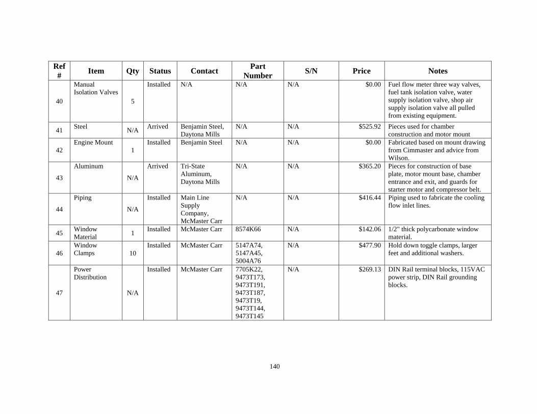
140

Ref #



40

Manual Isolation Valves

5

Installed N/A N/A N/A $0.00 Fuel flow meter three way valves, fuel tank isolation valve, water supply isolation valve, shop air supply isolation valve all pulled from existing equipment.

41 Steel

N/A Arrived Benjamin Steel,

Daytona Mills N/A N/A $525.92 Pieces used for chamber

construction and motor mount

42 Engine Mount

1 Installed Benjamin Steel N/A N/A $0.00 Fabricated based on mount drawing

from Cimmaster and advice from Wilson.

43

Aluminum

N/A

Arrived Tri-State Aluminum, Daytona Mills

N/A N/A $365.20 Pieces for construction of base plate, motor mount base, chamber entrance and exit, and guards for starter motor and compressor belt.

44

Piping

N/A

Installed Main Line Supply Company, McMaster Carr

N/A N/A $416.44 Piping used to fabricate the cooling flow inlet lines.

45 Window Material

1 Installed McMaster Carr 8574K66 N/A $142.06 1/2" thick polycarbonate window

material.

46 Window Clamps 10

Installed McMaster Carr 5147A74, 5147A45, 5004A76

N/A $477.90 Hold down toggle clamps, larger feet and additional washers.

47

Power Distribution

N/A

Installed McMaster Carr 7705K22, 9473T173, 9473T191, 9473T187, 9473T19, 9473T144, 9473T145

N/A $269.13 DIN Rail terminal blocks, 115VAC power strip, DIN Rail grounding blocks.

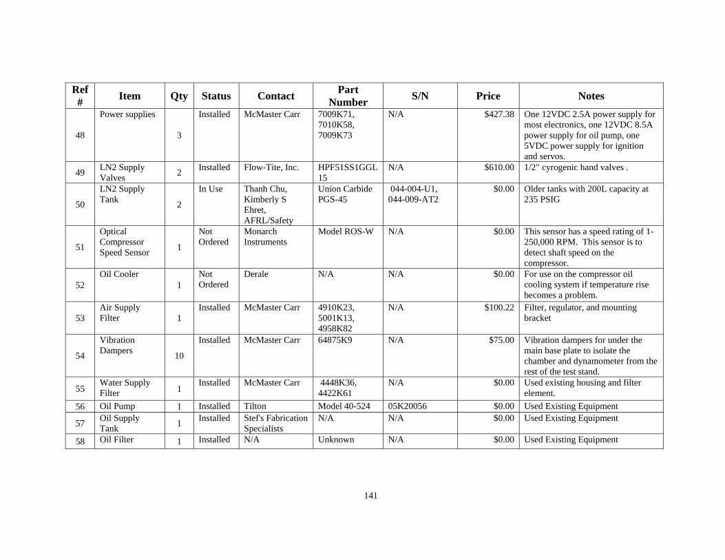
141

Ref #



48

Power supplies

3

Installed McMaster Carr 7009K71, 7010K58, 7009K73

N/A $427.38 One 12VDC 2.5A power supply for most electronics, one 12VDC 8.5A power supply for oil pump, one 5VDC power supply for ignition and servos.

49 LN2 Supply Valves

2 Installed Flow-Tite, Inc. HPF51SS1GGL

15 N/A $610.00 1/2" cyrogenic hand valves .

50

LN2 Supply Tank

2

In Use Thanh Chu, Kimberly S Ehret, AFRL/Safety

Union Carbide PGS-45

044-004-U1, 044-009-AT2

$0.00 Older tanks with 200L capacity at 235 PSIG

51

Optical Compressor Speed Sensor

1

Not Ordered

Monarch Instruments

Model ROS-W N/A $0.00 This sensor has a speed rating of 1-250,000 RPM. This sensor is to detect shaft speed on the compressor.

52 Oil Cooler

1 Not Ordered

Derale N/A N/A $0.00 For use on the compressor oil cooling system if temperature rise becomes a problem.

53 Air Supply Filter 1

Installed McMaster Carr 4910K23, 5001K13, 4958K82

N/A $100.22 Filter, regulator, and mounting bracket

54

Vibration Dampers

10

Installed McMaster Carr 64875K9 N/A $75.00 Vibration dampers for under the main base plate to isolate the chamber and dynamometer from the rest of the test stand.

55 Water Supply Filter 1

Installed McMaster Carr 4448K36, 4422K61

N/A $0.00 Used existing housing and filter element.

56 Oil Pump 1 Installed Tilton Model 40-524 05K20056 $0.00 Used Existing Equipment

57 Oil Supply Tank

1 Installed Stef's Fabrication

Specialists N/A N/A $0.00 Used Existing Equipment

58 Oil Filter 1 Installed N/A Unknown N/A $0.00 Used Existing Equipment

142

Ref #



59

Pressure and Temperature Transducer Fittings

N/A

Installed Swagelok, Cincinnati Valve and Fitting

Various N/A $1,068.40 Used existing components when possible

60 Fuel Valve Actuator Solenoids

2 Installed Ingersoll Rand A0059, 12VDC

with 1/4" NPT fittings

N/A $0.00 Used Existing Equipment

61 Fuel Valves and Actuators 2

Installed Hoke 3-way hand valve with 1/4" NPT fittings


62 Air Solenoid Valve 1

Installed Ingersoll Rand A0059, 12VDC with 1/4" NPT fittings


63

Data Acquisition Chassis 1

Installed National Instruments, Alex Stoermer, [email protected]

Compact DAQ 150881A $1099.00 8 slot chassis

64

Analog Input Module

1


NI 9205 N/A $799.00 32 channel +/-10VDC analog input module

65

Analog Output Module

1


NI 9264 N/A $900.00 16 channel +/- 10VDC analog output module

66

Thermocouple Module

1


NI 9213 N/A $999.00 NI9213 16-channel thermocouple module

143

Ref #



67

Digital TTL Signal Module

1


NI 9401 N/A $269.00 8 channel TTL Digital input/output module for flow meter signal

68

Solid State Relay Module

1


NI 9485 N/A $319.00 High voltage +/- 60 VDC relay module

69

Analog Input Module

1


NI 9227 N/A $ 999.00

NI9227, 4 channel universal analog input module for +/- 5 A rms

70

Battery

1

Installed Advanced Auto Autocraft Silver Battery, Group Size 58, 550 CCA, P/N 58-2

N/A $86.99

71 Compressor Cooling Oil 3

Installed Auto Zone Maxlife DEX-MERC ATF, VV322

N/A $59.97 1 gal size, similar performance to fluid recommended by Vortron for compressor oil.

72 Window Gasket Material

2 Installed McMaster Carr 95715K71,

95715K72 N/A $164.42 Graphite sheet gasket material for

windows and chamber ends.

73

Monitor and Keyboard

1 ea

Installed Tiger Direct Monitor: A179-2268 Keyboard: A68-1200

N/A $169.98 Acer 22" LCD flat panel monitor with Adesso SlimTouch keyboard and touchpad combination

74 Mass Air Flow Sensor and Filter

1 Installed Pro-M Racing

LLC Model 92 03A2794 $44.99 Used existing MAF but ordered a

new filter

75 Electronics Rack 1

Installed Rack Mount Solutions

ERK-2125 21U N/A $448.00

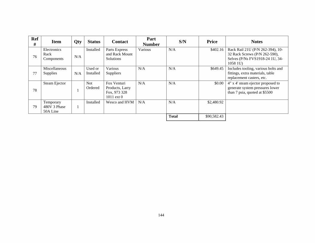
144

Ref #



76

Electronics Rack Components N/A

Installed Parts Express and Rack Mount Solutions

Various N/A $402.16 Rack Rail 21U (P/N 262-394), 10-32 Rack Screws (P/N 262-590), Selves (P/Ns FVS1918-24 1U, 34-1058 1U)

77 Miscellaneous Supplies N/A

Used or Installed

Various Suppliers

N/A N/A $649.45 Includes tooling, various bolts and fittings, extra materials, table replacement casters, etc.

78

Steam Ejector

1

Not Ordered

Fox Venturi Products, Larry Fox, 973 328 1011 ext 0

N/A N/A $0.00 4" x 4' steam ejector proposed to generate system pressures lower than 7 psia, quoted at $5500

79 Temporary 480V 3 Phase 50A Line

1 Installed Wesco and HVM N/A N/A $2,480.92

Total $90,582.43

145

Bibliography

1) United States Air Force Unmanned Aircraft Systems Flight Plan 2009-2047, Headquarters, United States Air Force, Washington DC, 18 May 2009.

2) Weatherington, Dyke, Unmanned Aircraft Systems Roadmap, 2005-2030, Deputy, UAV Planning Task Force, OUSD(AT&L) 2005.

3) Smith, G., Boruta, M., Jerovsek, J., Meitner, P., Meyer Nutating Disk Engine, a New Concept in Internal Combustion Engine Technology, AIAA 2007-5122, 43rd AIAA/ASME/SAE/ASEE Joint Propulsion Conference & Exhibit, Cincinnati, OH, 8-11 July 2007.

4) Haywood, John B., Internal Combustion Engine Fundamentals; McGraw-Hill, Inc., 1988.

5) http://www.marineengineeringonline.com/scavenging_in_diesel_engines.htm [cited 5 Dec 2010].

6) Cadou, C., Moulton, N., Menon, S., Performance Measurement and Scaling in Small Internal-Combustion Engines, AIAA 2003-0671, 41st Aerospace Sciences Meeting and Exhibit, Reno, NV, 6-9 January 2003.

7) Cadou, C., Sookdeo, T., Moulton, N., Leach, T., Performance Scaling and Measurement for Hydrocarbon-Fueled Engines with Mass Less than 1 Kg, AIAA 2002-3448, AIAA’s 1st Technical Conference and Workshop on Unmanned Aerospace Vehicles, S, Portsmouth, VA, 20-23 May 2002.

8) Menon, S., Moulton, N., Cadou, C., Development of a Dynamometer for Measuring Small Internal-Combustion Engine Performance, Journal of Propulsion and Power, Vol. 23, No. 1, January-February 2007. DOI: 10.2514/1.19825

9) Cadou, C., Menon, S., Scaling of Losses in Small IC Aero Engines with Engine Size, AIAA 2004-690, 42nd AIAA Aerospace Sciences Meeting and Exhibit, Reno, NV, 5-8 January 2004.

10) Shin, Y., Chang, S.H., Koo, S.O., Performance Test and Simulation of a Reciprocating Engine for Long Endurance Miniature Unmanned Aerial Vehicles, Proceedings of Institution of Mechanical Engineers Vol. 219, Part D: Journal of Automobile Engineering, Pg 573-581, 6 Oct 2004.

11) Harari, R., Sher, E., The Effect of Ambient Pressure on the Performance Map of a Two-Stroke SI Engine, 930503, SAE International Congress & Exposition, Detroit, MI, Pg 115-123, 01 March 1993.

146

12) Watanabe, I., Kuroda, H., Effect of Atmospheric Temperature on the Power Output of a Two-Stroke Cycle Crankcase Compression Gasoline Engine, 810295, SAE International Congress and Exposition, Detroit, MI, 23-27 February 1981.

13) Flynn, P.F., Hunter, G.L., Farrell L.A., Durrett, R.P., Akinyemi, O.C., Westbrook, C.K., Pitz, W.J., The Inevitability of Engine-Out NOx Emissions from Spark-Ignition and Diesel Engines, 28th International Symposium on Combustion, Edinburgh, Scotland, 11 Jan 2000. US DOE Lawrence Livermore National Laboratory.

14) Chen, Rong-Horng, Chiang, Li-Bin, Wu, Ming-Hsun, Lin, Ta-Hui, Gasoline displacement and NOx reduction in an SI engine by aqueous alcohol injection; Fuel 89 (2010) pg 604-610.

15) Wilson, C., Performance of a Small Internal Combustion Engine Using N-Heptane and Iso-Octane, AFIT Thesis, AFIT/GAE/ENY/10-M28, Air Force Institute of Technology, Wright Patterson AFB, OH, March 2010.

16) Lee, K., Yoon, M., and Sunwoo, M., A Study on Pegging Methods for Noisy Cylinder Pressure Signal, Control Engineering Practice 16, pg 922 to 929, Elsevier Ltd., 28 Nov 2007.

17) Bertola, A., Stadler, J., Walter, T., Wolfer, P., Gossweiler, C., Rothe, M., Spicher, U., Pressure Indication During Knocking Conditions, Pressure Sensor, Kistler Instrumente AG, special print 920-349e-11.06, 2006.

18) Walter, T., Brechbühl, S., Gossweiler, C., Schnepf, M., Wolfer, P., Pressure Indicating with Measurement Spark Plugs on a DI-Gasoline Engine – State of Technology, Combustion Engines, Kistler Intrumente AG, special print 920-333e-09.04, 2004.

19) Revised Thermocouple Reference Tables, Reference Tables N.I.S.T. Monograph 175 Revised to ITS-90, pgs Z-204 to Z-205, http://www.omega.com/temperature/Z/pdf/z204-206.pdf cited [2 Jan 2011].

20) Beshia,S., Deniz, O., Chomiak, J., Gupta, A., An Experimental Study of the Variations in Cyclic Energy Release Rate in a Spark Ignition Engine, AIAA 89-2890, AIAA/ASME/SAE/ASEE 25th Joint Propulsion Conference, Monterey, CA, July 10-12, 1989.

21) Ceviz, M. A., Intake Plenum Volume and its Influence on the Engine Performance, Cyclic Variability and Emissions, Energy Conversion and Management 48 (2007) pgs 961-966.

22) Celik, M. B., Performance Improvement and Emission Reduction in Small Engine with Low Efficiency, Journal of the Energy Institute, Vol 80, No 3, pgs 175-180, 2007.

147

23) Turns, S. R. An Introduction to Combustion (2nd

Ed.). New York: McGraw-Hill, Inc., 1996.

24) Kilpatrick, D.A., Calculation methodology for basic engine exhaust gaseous emissions parameters, “National Gas Turbine Establishment Memorandum M81002” Feb 1981, Controller HMSO London.

25) Procedure for the Analysis and Evaluation of Gaseous Emissions from Aircraft Engines, SAE Aerospace Recommended Practice ARP1533 Revision A; Issued 1996-01, Revised 2004-07.

26) Totten, G. E., Westbrook, S. R., and Shah, R. J., Fuels and Lubricants Handbook: Technology, Properties, Performance, and Testing, ASTM International, Glen Burnie, 2003.

27) NIST Chemistry Webbook. http://webbook.nist.gov [cited 22 Jan 2011].

28) Handbook of Aviation Fuel Properties(Second Printing). Prepared by the Coordinating Research Council, Inc., Society of Automotive Engineers, Inc., May 1984

29) National Energy Technology Lab, Office of Fossil Energy, U.S. Department of Energy, R & D Facts, Fischer-Tropsch Fuels April 2008 http://www.netl.doe.gov/publications/factsheets/rd/R&D089.pdf [cited 22 Jan 2011].

30) Korres, D.M. and Karonis, E. Lois. Use of Alternative Fuels on a Diesel Engine, AIAA 1st International Energy Conversion Engineering Conference, Portsmouth, VA, 2003.

31) Antonovski, Viktorio, Rotavera, Brandon M., Petersen, Eric L., Combustion Measurements of Synthetic Fuels at Gas Turbine Conditions, 43rd AIAA/ASME/SAE/ASEE Joint Propulsion Conference, AIAA-2007-5667, 8-11 July 2007, Cincinnati, OH.

32) Arpa, Orhan, Yumutas, Recep, Experimental investigation of Gasoline-Like Fuel obtained from waste lubrication oil on engine performance and exhaust emission, Fuel Processing Technology 91 (2010) pg 197-204.

33) National Oceanic and Atmospheric Administration, National Aeronautics and Space Administration, United States Air Force, U.S. Standard Atmosphere, 1976, Washington D.C., October 1976.

34) Moffat, R.J., Using Uncertainty Analysis in the Planning of an Experiment, Journal of Fluids Engineering, June 1985, Vol 107, pg 173-178.

148

35) Moffat, R.J., Describing the Uncertainties in Experimental Results, Experimental Thermal and Fluid Science, 1988; 1:3-17. Elsevier Science Publishing Co. Inc.

36) Kline, S.J., McClintock, F.A., Describing Uncertainties in Single-Sample Experiments, Mechanical Engineering, pg 3-8, Jan 1953.

37) Vortech Engineering, Inc., Compressor Performance Map, Model V5 K-trim, Test 1213F, 16 July 2010.

38) A-T Controls, Inc., Triac Division, “V” Series Control Port Ball Valves, 0308-V, http://download.a-tcontrols.com/pdf/Series-V.pdf [cited 21 February 2011].

39) Incropera, F.P., DeWitt, D.P., Bergman, T.L., Lavine, A.S., Fundamentals of Heat and Mass Transfer (6th Ed.), New York: John Wiley and Sons, Inc., 2007.

40) ASME, Guide for Glass and Plastic Window Design for Pressure Vessels, 2.0/17606e011.doc, November 2008.

41) Riley, W.F., Sturges, L.D., Morris, D.H., Mechanics of Materials (5th Ed.), New York: John Wiley and Sons, Inc., 1999.

149

Vita

Captain Peter John Schmick was born in St. Paul, Minnesota and graduated from

Champlin Park High School in June 2000. He enrolled in undergraduate studies at Iowa

State University in Ames, Iowa in the Fall of 2000. He majored in aerospace engineering

with a minor in military studies. Capt Schmick was a graduate of the four year Air Force

Reserve Officer Training Corps program at Detachment 250. He graduated with a B.S. in

aerospace engineering and was commissioned in the United States Air Force in

December 2004.

Peter’s first assignment was at the Air Force Research Lab Propulsion Directorate

Detachment 7 at Edwards AFB, CA. He served as a test stand engineer in the

Experimental Demonstrations Branch on Test Stand 2A from 2005 until June 2007.

After a short period working as the Predictive Avoidance engineer for the Airborne Laser

Flight Test Squadron, he took over as the BMC4I integrated product team lead for the

417 FLTS. Following this assignment, he enrolled in the Graduate School of

Engineering and Management at the Air Force Institute of Technology in August 2009,

seeking a degree in Aeronautical Engineering. Upon graduating, he will be assigned to

the AFRL Air Vehicles Directorate at Wright Patterson AFB.

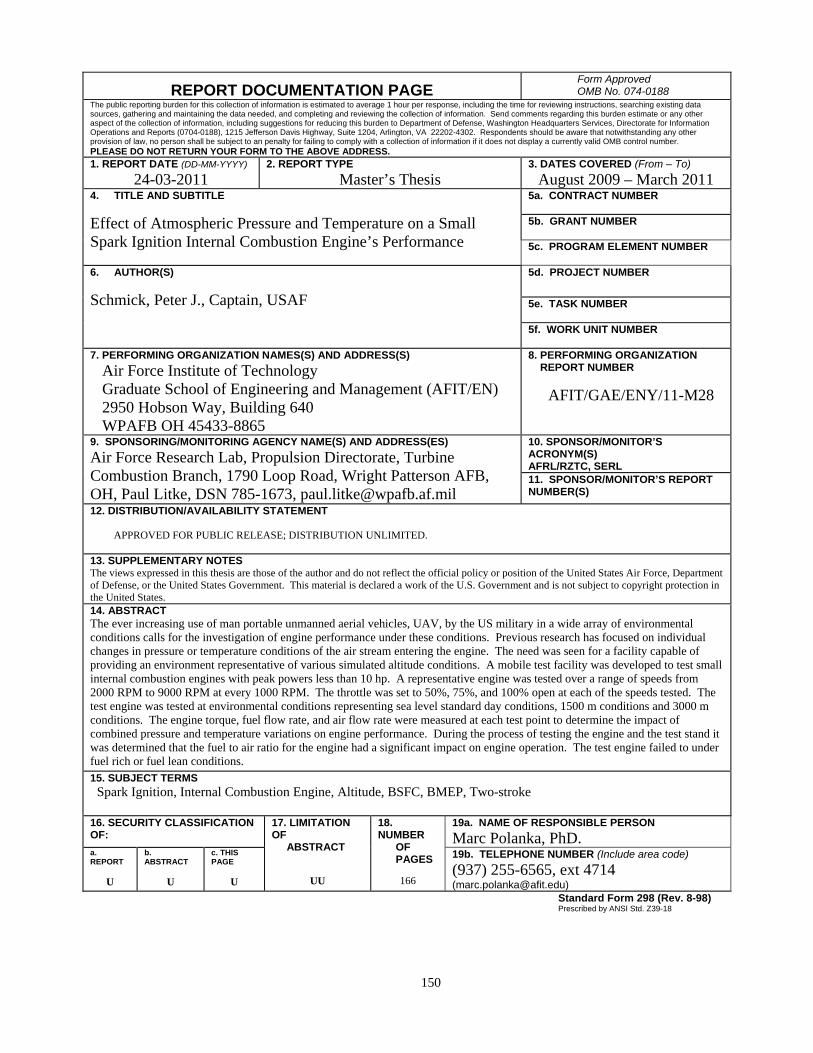
150

REPORT DOCUMENTATION PAGE Form Approved OMB No. 074-0188

The public reporting burden for this collection of information is estimated to average 1 hour per response, including the time for reviewing instructions, searching existing data sources, gathering and maintaining the data needed, and completing and reviewing the collection of information. Send comments regarding this burden estimate or any other aspect of the collection of information, including suggestions for reducing this burden to Department of Defense, Washington Headquarters Services, Directorate for Information Operations and Reports (0704-0188), 1215 Jefferson Davis Highway, Suite 1204, Arlington, VA 22202-4302. Respondents should be aware that notwithstanding any other provision of law, no person shall be subject to an penalty for failing to comply with a collection of information if it does not display a currently valid OMB control number. PLEASE DO NOT RETURN YOUR FORM TO THE ABOVE ADDRESS. 1. REPORT DATE (DD-MM-YYYY)

24-03-2011 2. REPORT TYPE

Master’s Thesis

3. DATES COVERED (From – To)

August 2009 – March 2011 4. TITLE AND SUBTITLE

Effect of Atmospheric Pressure and Temperature on a Small Spark Ignition Internal Combustion Engine’s Performance

5a. CONTRACT NUMBER

5b. GRANT NUMBER 5c. PROGRAM ELEMENT NUMBER

6. AUTHOR(S)

Schmick, Peter J., Captain, USAF

5d. PROJECT NUMBER

5e. TASK NUMBER

5f. WORK UNIT NUMBER

7. PERFORMING ORGANIZATION NAMES(S) AND ADDRESS(S)

Air Force Institute of Technology Graduate School of Engineering and Management (AFIT/EN) 2950 Hobson Way, Building 640 WPAFB OH 45433-8865

8. PERFORMING ORGANIZATION REPORT NUMBER

AFIT/GAE/ENY/11-M28

9. SPONSORING/MONITORING AGENCY NAME(S) AND ADDRESS(ES)

Air Force Research Lab, Propulsion Directorate, Turbine Combustion Branch, 1790 Loop Road, Wright Patterson AFB, OH, Paul Litke, DSN 785-1673, [email protected]

10. SPONSOR/MONITOR’S ACRONYM(S) AFRL/RZTC, SERL 11. SPONSOR/MONITOR’S REPORT NUMBER(S)

12. DISTRIBUTION/AVAILABILITY STATEMENT APPROVED FOR PUBLIC RELEASE; DISTRIBUTION UNLIMITED.

13. SUPPLEMENTARY NOTES The views expressed in this thesis are those of the author and do not reflect the official policy or position of the United States Air Force, Department of Defense, or the United States Government. This material is declared a work of the U.S. Government and is not subject to copyright protection in the United States. 14. ABSTRACT The ever increasing use of man portable unmanned aerial vehicles, UAV, by the US military in a wide array of environmental conditions calls for the investigation of engine performance under these conditions. Previous research has focused on individual changes in pressure or temperature conditions of the air stream entering the engine. The need was seen for a facility capable of providing an environment representative of various simulated altitude conditions. A mobile test facility was developed to test small internal combustion engines with peak powers less than 10 hp. A representative engine was tested over a range of speeds from 2000 RPM to 9000 RPM at every 1000 RPM. The throttle was set to 50%, 75%, and 100% open at each of the speeds tested. The test engine was tested at environmental conditions representing sea level standard day conditions, 1500 m conditions and 3000 m conditions. The engine torque, fuel flow rate, and air flow rate were measured at each test point to determine the impact of combined pressure and temperature variations on engine performance. During the process of testing the engine and the test stand it was determined that the fuel to air ratio for the engine had a significant impact on engine operation. The test engine failed to under fuel rich or fuel lean conditions. 15. SUBJECT TERMS Spark Ignition, Internal Combustion Engine, Altitude, BSFC, BMEP, Two-stroke

16. SECURITY CLASSIFICATION OF:

17. LIMITATION OF ABSTRACT

UU

18. NUMBER OF PAGES

166

19a. NAME OF RESPONSIBLE PERSON

Marc Polanka, PhD. a. REPORT

U

b. ABSTRACT

U

c. THIS PAGE

U

19b. TELEPHONE NUMBER (Include area code)

(937) 255-6565, ext 4714 ([email protected])

Standard Form 298 (Rev. 8-98) Prescribed by ANSI Std. Z39-18

Effect of Atmospheric Pressure and Temperature on a Small ...

Documents

Transcript of Effect of Atmospheric Pressure and Temperature on a Small ...