http://doc.rero.ch

CANADIAN PRESSURE OBSERVATIONS AND CIRCULATIONVARIABILITY: LINKS TO AIR TEMPERATURE

VICTORIA C. SLONOSKY† and EDWARD GRAHAM*Climate Monitoring and Data Interpretation Division, Climate Research Branch, Meteorological Service of Canada, Environment

Canada, 4905 Dufferin St, Downsview, Ontario M3H 5T4, Canada

Received 14 May 2004Revised 23 December 2004

Accepted 1 March 2005

ABSTRACT

A set of 71 station series of surface pressure from Canada and Greenland have been examined for quality control andhomogeneity. These records range in length from 50 to 130 years. The object of this exercise was to investigate station-based surface pressure series and atmospheric circulation on a decadal time scale, and to examine the effects of theatmospheric circulation on climate. The data considered here are monthly means.

Several major inhomogeneities were discovered during the course of this exercise, the most serious of which relates toa Canadian-wide change in reporting practice which took place in 1977. This type of inhomogeneity is almost impossibleto uncover using conventional homogenization techniques based upon reference series. The final homogenized series showappreciable differences in regional trends of atmospheric pressure compared with the unhomogenized series, particularlyin southern Canada.

Empirical orthogonal function (EOF) analyses on the station series revealed three main modes of circulation overCanada and Greenland; these patterns were compared with results from the UK Hadley Centre’s gridded pressure dataset.There are appreciable differences between the leading EOF modes of the two datasets, which may be due to an artificiallyenhanced number of degrees of freedom in the gridded dataset. Trends in atmospheric pressure were also calculated;these suggest an intensification of zonal flow during winter over the period 1950–98, but these variations appear to bemuch less pronounced and not statistically significant when considered over the whole of the 20th century.

The new station database was also compared with a gridded surface temperature dataset. There are strong correlationsbetween the various circulation indices and temperature anomalies. Some of the trends of temperature in Canada duringthe period 1950–98 can be attributed to these changes of atmospheric circulation. The regional atmospheric circulationindices described here are shown to have considerable influence on the surface temperature variability and trends for allseasons of the year.

KEY WORDS: Canada; Greenland; station pressure; observations; atmospheric pressure; homogenization; atmospheric circulation;empirical orthogonal functions; temperature

1. INTRODUCTION

Climate change is one of the most important issues of our times, with anthropogenic climate change havingpotentially high socio-economic impacts. The atmospheric circulation plays a fundamental role in redistributingheat and moisture and, as such, is critical to our understanding of climate variability and climatic change.

The atmospheric circulation is described through changes in atmospheric pressure. Atmospheric pressureat the Earth’s surface has been measured since the invention of the barometer by Evangelista Torricelli(1608–47) in 1644 (Middleton, 1964). In the past 50 years, upper air observations have led to a morecomplete understanding of the atmospheric circulation dynamics in the free troposphere and stratosphere.

* Correspondence to: Edward Graham, Department of Geosciences, University of Fribourg, Chemin de Musee 4, Perolles, Fribourg,CH-1700 Switzerland; e-mail: edward.graham@unifr.ch† Present address: Ouranos Consortium for Regional Climate Change and Adaptation, Department of Atmospheric and Oceanic Sciences,McGill University, 550 Sherbrooke St W, Montreal, Quebec H3A 1B9, Canada.

Published in which should be cited to reference this work.

"International Journal of Climatology 25(11): 1473 - 1492, 2005"

1

http://doc.rero.ch

However, for the study of decadal- to century-scale atmospheric circulation dynamics, the only data availableare those of surface pressure. Many observations of surface pressure exist, but most are still in paper form,and need to be collected, digitized, quality controlled and homogenized before they can be effectively usedfor analysis of decadal-scale circulation variability. The homogenization procedure is especially important, asnon-climatic changes, such as site relocations, instrument replacement, or changes in the observation practice(including changes in the time of observation or calculation procedure), can introduce biases of the samemagnitude as the long-term climatic variability of pressure into the series, leading to spurious trends andvariability (Young, 1993; Peterson et al., 1998; Slonosky et al., 1999; Vincent et al., 2002).

Considerable international interest in the collection and analysis of surface pressure data has led to theproduction of new national and international pressure datasets (e.g. Basnett and Parker, 1997; Jones et al.,1999b; Kaplan et al., 2000), individual pressure series (Barring et al., 1999; Allan et al., 2002; Moberg et al.,2002), as well as atmospheric circulation indicators (Allan et al., 1991; Jones et al., 1997, 1999a) extendingback into the 18th century.

This paper describes the quality control and homogenization of 71 long-term monthly surface pressure seriesfrom stations in Canada and Greenland. This data set was constructed with the aim of analysing decadal-scalevariability in atmospheric circulation over Canada. With this intention in mind, the series selected for qualitycontrol and homogenization were those with a duration of at least 50 years, and were chosen so as to giveas complete a spatial coverage as possible, given the limited number of long series in northern Canada.The original data series are described in Section 2. In Section 3, the quality control and homogenizationprocedures used on these data are described. A comparison with the gridded sea-level atmospheric pressuredataset produced by the Hadley Centre (HadSLP; R. Allan and T. Ansell, personal communication, 2001)using empirical orthogonal functions (EOFs) is presented in Section 4. Section 5 presents circulation indicesbased on the EOF patterns and examines their trends in time. Section 6 investigates correlations between thevarious circulation indices and a gridded temperature dataset (New et al., 2000). Discussion and conclusionsare presented in Section 7.

2. DATA PROVENANCE AND MANIPULATION

The stations selected are shown in Figure 1; as can be seen, the longest series are those in southern andnorthwestern Canada. Long series from Greenland were also included in order to provide more completespatial coverage relevant for northeastern Canada. The primary sources of monthly data were the WorldWeather Records of the Smithsonian Miscellaneous Collections, the Monthly Climatic Data for the WorldBulletins, and, more recently, the electronic meteorological report archives of Environment Canada (for theCanadian stations). These data (excluding the Greenland stations) were all recorded at official observingstations of the Meteorological Service of Canada observational network, which started in 1841 for Torontoand in 1873 for other stations across Canada. Although some fragmentary observations exist at stations otherthan Toronto prior to 1873, taken in part by amateur meteorologists (Slonosky, 2003), and in part by themilitary regiment of the British Royal Engineers, these data are not included in the present analysis and willbe studied separately.

The Environment Canada electronic archives contain data for most Canadian reporting stations from 1953onwards, but in hourly synoptic format. Therefore, it was necessary to calculate monthly means of air pressurefor each station from this data. In the interests of data quality, months with fewer than 21 reporting daysof data were discarded, as were days with fewer than three different synoptic reports. In total, over 66 000individual mean monthly pressure values were obtained, with a missing value rate of 5.9%.

Despite the different data sources, there were no significant differences in the standard deviation of dataoriginating from different sources for each station; typical standard deviations of mean monthly pressureranged from about 2.0 hPa over the Canadian Prairies to greater than 5.0 hPa at some Greenland stations(this difference is due to the greater natural variability in Arctic regions). Data published by the WorldWeather Records was also corrected for rounding errors, because prior to 1971 the mean monthly pressurewas rounded to the nearest millibar (hPa). It was calculated, however, that these rounding errors had no effecton the standard deviation or standard error of mean monthly pressure.

2

http://doc.rero.ch Figure 1. Location of station series

Station-level observations were selected in preference to sea-level values, as it was considered that station-level observing was more reliable and, as fewer calculations were involved in obtaining the station-levelseries, there were fewer opportunities for calculation-related inhomogeneities to occur. This choice did nothave an effect on our final results, as all analyses were carried out on monthly anomaly data. In several casesonly sea- or station-level observations were available for certain portions of the record; in these cases, eitherthe station information or, if the station information was unavailable, adjustment factors based on monthlymean differences between the different segments of the records were used to relate the segments and producea uniform station- or sea-level series. Figure 2(a) shows an example for Charlottetown, Prince Edward Island.

At Charlottetown, station-level pressure data was available from 1874 to 1940. Station data resumed again in1951, but with a mean long-term value of about 6 hPa lower than before, most likely due to a station relocation.Fortunately, a sea-level pressure record overlaps the broken period, and by calculating monthly adjustmentfactors (subtracting one series from the other), a complete station-level pressure record was obtained.

Several observation series that started relatively early (in the late 19th or early 20th centuries) endedabruptly; in these cases, when possible, nearby stations were used to complete the series and produce acomposite series of longer duration. Monthly mean adjustments were again calculated using the overlappingportions of both series to produce the composite series; the earlier segments were reduced to conform with thelater, most modern segment. The example of Point-au-Pere, Quebec, is shown in Figure 2(b). Station-leveldata are available from 1874 to 1940, with a sea-level pressure record from 1921 to 1950, after which recordscease. However, the nearby station of Bagotville started recording data in 1942; so, using the overlappingperiod between 1942 and 1950, all three segments of atmospheric pressure were reduced to one continuousrecord through to the present.

3. QUALITY CONTROL AND HOMOGENIZATION

3.1. Quality control

Quality control of the newly digitized data was undertaken in a first step by a visual inspection of the pressuretime series and by comparing station- and sea-level time series for each location, when available. When bothwere available, difference series between the two were plotted in order to perform a quality control. Severalinhomogeneities were discovered using this technique, including a nationwide inhomogeneity between 1976

3

http://doc.rero.ch

Figure 2. Mean annual atmospheric pressure (hPa) records. (a) Charlottetown, Prince Edward Island, 1874–1990. Station pressure isavailable from 1874 to 1940 and from 1951 to 1990. An overlapping sea-level record allows computation of a complete station-levelrecord. (b) The nearby sites of Point-au-Pere and Bagotville, 1874–2000. Overlapping of the sea- and station-level records allowsconstruction of one complete station record. (c) Aklavik (Inuvik) mean annual sea-level atmospheric pressure minus station-level

atmospheric pressure. Note the discontinuity in 1977 when surface pressure reporting was adapted to WMO guidelines (see text)

and 1977 which otherwise may have gone undetected. Note that some conventional homogeneity techniques,relying on reference series (e.g. Caussinus and Mestre, 1996; Alexandersson and Moberg, 1997; Vincentet al., 2002) are unable to detect this kind of widespread inhomogeneity.

In November 1976, computer-generated pressure reduction tables were used for the first time by theMeteorological Service of Canada (formerly the Atmospheric Environment Service), replacing the previouscalculations which were made either manually or by using primitive desk calculators. The algorithms used tocalculate the station pressure correction and the station to sea pressure reductions were also adapted to WorldMeteorological Organization (WMO) guidelines at this time, including the addition of plateau correction(Savdie, 1982). The result was a discontinuity in both sea-level and station-level pressure records across allparts of Canada (see Figure 2(c)). The discontinuity between the station-level and sea-level pressure serieswas detected at almost 80% of Canadian stations, with an average discontinuity on the order of 0.9 hPa;in some cases it was of the order of several hectopascals, especially in colder and higher Arctic regions,where the adjustments from station-level to sea-level pressure were greatest (the largest correction factor was5.5 hPa at Dawson in northwestern Canada; see also Jones (1987)). If undetected, this discontinuity wouldhave led to spurious trends of atmospheric pressure across large parts of Canada.

An added complication was caused by what was termed the established elevation of a site. This termwas used to describe ‘the vertical distance above sea level, adopted as the datum level to which barometric

4

http://doc.rero.ch

reports at the station refer’ (McMaster, 1975). However, if the established elevation of an office whose cisternwas less than 50 ft (∼15 m) in elevation, then the established elevation was arbitrarily assigned as sea level(Upton, 1972; it appears this rule was put in place some time in the 1930s). Furthermore, site relocation of lessthan 50 ft in height resulted in no new established elevation – a correction factor was assumed to have beenadded. All this changed on 1 January 1977, when ‘established elevation’ was replaced by ‘station elevation’in accordance with WMO guidelines (Environment Canada, 1976). ‘Station elevation’ was defined as the‘vertical distance above mean sea level of the datum level to which barometric pressure reports at the stationrefer’. Mean sea-level (MSL) pressures should not have been affected, but station pressures (for those stationspreviously at an altitude between sea level and 50 ft) will have experienced a slight drop (McMaster, 1975).

Several other inhomogeneities due to changes in observing practice were brought to light during the courseof this exercise. On 1 January 1935, a new table for reduction to sea level (using the Bigelow method) wasfirst used. Uniformity was not achieved until January 1941, however, when all Canadian stations receivednew reduction cards during the changeover from reporting of pressures in inches of mercury to hectopascals.These inhomogeneities led Potter (1955) to make a decision to exclude all MSL pressure data prior to 1940when constructing monthly mean sea-level pressure maps. Potter (1955) also notes that, prior to 1940s,barometers were not inspected regularly, and ‘periods of 20 years or more passed without reports on theindex’. Godson (1955) notes that MSL pressure during the period 1938–54 had been about 0.4 to 0.5 hPa toohigh. Another relatively minor inhomogeneity occurred on 30 June 1955, when a new value of 9.80655 m s−2

was introduced for the acceleration due to gravity (the old value was 9.80616 m s−2). However, it is importantto note that our study uses station-level pressure, wherever possible, and inhomogeneities have been correctedusing standard homogenization techniques.

3.2. Homogenization

The homogenization technique used was that described in detail by Slonosky et al. (1999). This is asemi-objective iterative technique based upon graphical inspection of difference series between neighbouringstations. For each candidate station, four neighbouring stations were chosen for comparison, one in eachcardinal direction. Four difference series were calculated, and the graphical results plotted together. If adiscontinuity occurred in more than two difference plots, then the jump was attributed to the candidatestation. All stations were inspected, all adjustments deemed necessary were applied, and the process repeated toensure that the discontinuities were correctly attributed. Adjustment factors were calculated to adjust identifiedinhomogeneous periods to the modern portion of the series. An evaluation of this method, compared withthe standard normal homogeneity test (SNHT; Alexandersson and Moberg, 1997) and the Bayesian methoddeveloped by Caussinus and Mestre (1996) is given in Slonosky et al. (1999). The results presented inSlonosky et al. (1999) indicate that the iterative graphical method performed as well as the other two methods,and in the case of data-sparse regions it outperformed the other methods as it eliminated the propagationof errors. Furthermore, the iterative graphical method does not require the existence of a homogeneoussurrounding series a priori to adjust an inhomogeneous series. It was not possible to apply the SNHT methodto the Canadian and Greenland pressures series as the SNHT method relies on the existence of homogeneousreferences series for comparison purposes, which do not exist for this region prior to the advent of reanalysisproducts in the 1950s. The Bayesian method developed by Caussinus and Mestre (1996) does not rely onhomogeneous reference series, but calculates adjustment factors based on surrounding stations. Although thismethod of obtaining adjustment factors is usually the preferred one, we were concerned by the possiblepropagation of errors in the data-sparse regions, as was seen in Slonosky et al. (1999). A concern of theSlonosky et al. (1999) method was the reduction of variability within a series, as the adjustment factors werederived from different portions of the same series, under the assumption that pressure is a conserved variablein the long term. However, as was demonstrated in Slonosky et al. (1999) with much longer series, there wereno differences in the variance of the series which were adjusted using the three different techniques. As thepressure characteristics of the high and middle latitudes are similar between the European region studied inSlonosky et al. (1999) and the Canadian region considered in this paper, we assumed that the results obtainedconcerning the biases and shortcomings of the various homogenization techniques in Slonosky et al. (1999)

5

http://doc.rero.ch

would apply in this study. A final quality control check was carried out by plotting the monthly mean mapsfor each month and each year, and visually inspecting the plots for outliers.

3.3. Comparison of regional trends

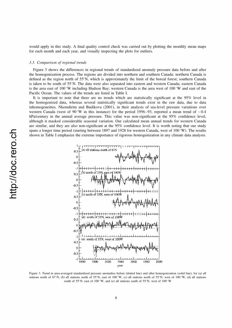
Figure 3 shows the differences in regional trends of standardized anomaly pressure data before and afterthe homogenization process. The regions are divided into northern and southern Canada: northern Canada isdefined as the region north of 55°N, which is approximately the limit of the boreal forest; southern Canadais taken to be south of 55°N. The data were also separated into eastern and western Canada; eastern Canadais the area east of 100 °W including Hudson Bay; western Canada is the area west of 100 °W and east of thePacific Ocean. The values of the trends are listed in Table I.

It is important to note that there are no trends which are statistically significant at the 95% level inthe homogenized data, whereas several statistically significant trends exist in the raw data, due to datainhomogeneities. Nkemdirim and Budikova (2001), in their analysis of sea-level pressure variations overwestern Canada (west of 90 °W in this instance) for the period 1956–93, reported a mean trend of −0.4hPa/century in the annual average pressure. This value was non-significant at the 95% confidence level,although it masked considerable seasonal variation. Our calculated mean annual trends for western Canadaare similar, and they are also non-significant at the 95% confidence level. It is worth noting that our studyspans a longer time period (starting between 1897 and 1928 for western Canada, west of 100 °W). The resultsshown in Table I emphasize the extreme importance of rigorous homogenization in any climate data analysis.

Figure 3. Trend in area-averaged standardized pressure anomalies before (dotted line) and after homogenization (solid line), for (a) allstations north of 67°N, (b) all stations north of 55°N, east of 100 °W, (c) all stations north of 55°N, west of 100 °W, (d) all stations

south of 55°N, east of 100 °W, and (e) all stations south of 55°N, west of 100 °W

6

http://doc.rero.ch

Table I. Trends in original and homogenized dataa

Stations Original data (standardizedunits per century)

Homogenized data (standardizedunits per century)

North of 67 °N −2.85 −1.23North of 55 °N, east of 100 °W +0.53 −0.78North of 55 °N, west of 100 °W −1.30 −1.28South of 55 °N, east of 100 °W −1.17 +0.30South of 55 °N, west of 100 °W +3.24 −1.30

a Values in bold/italic are statistically significant at the 95% confidence level.

The statistically significant trends in the area-averaged unhomogenized series for southern Canada could leadto false conclusions about the nature of atmospheric variability, trends and climate change.

4. EOF ANALYSES OF STATION AND GRIDDED DATASETS

4.1. Station-based EOFs

EOF analyses were carried out on the station data. The results are shown in Figure 4; we used the set ofstations available from 1948 onwards in order to give the greatest possible spatial representation over northernCanada, where very few stations existed prior to World War II. The data from 65 surface stations in Canadaand Greenland were used to create the EOFs. The results from 1941 to 1998 (using 52 stations) and 1932 to1998 (using 41 stations) are similar; the correlation coefficients between the first two EOFs of the 1948–98analysis and those of the longer periods range from 0.94 to 0.99, and the correlation coefficients for EOF 3range from 0.86 to 0.94.

All analyses were carried on the correlation matrix to provide equal weighting to all points. The analysiswas carried out on monthly anomaly data. Analyses were carried out (not shown) which compare the resultsobtained using all the calendar months together against results using a seasonal decomposition. The correlationsfor the leading three EOFs between the monthly analysis and the seasonally decomposed analysis range from0.99 in winter to 0.90 in summer; given that virtually the same information was recovered in the two instances,it was felt to be more consistent to use the monthly analysis rather than the seasonally decomposed analyses.

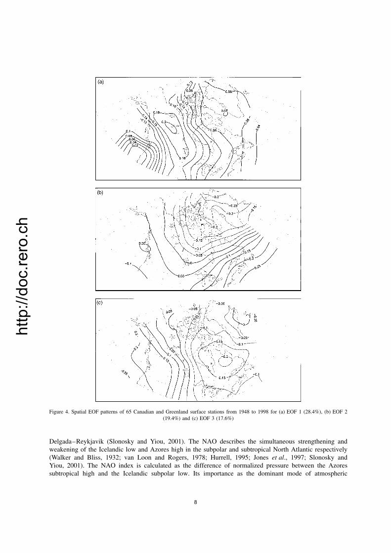
The first EOF of the station analysis (Figure 4(a)) is of the same sign over the entire domain, showing alocal maximum over northwestern Canada, over the MacKenzie River basin and the Rockies to the north,and in the lee of the Rockies and over the Prairie region further south. When the temporal loadings are high,the positive pressure anomalies are strong. This pressure pattern has been identified by Potter (1955) as thedominant circulation type at monthly scales for the months of November to June.

The configuration of pressure anomalies depicted by EOF 1 of the station data analysis is associated withcold air outbreaks from the Arctic spreading over central and eastern Canada (see Section 6 also; Bonsalet al., 2001). This pattern is somewhat similar, although displaced to the east, to the western North Americancentre of action of the Pacific–North American (PNA) pattern described by Wallace and Gutzler (1981), ateleconnection pattern based on a rotated EOF analysis of hemispheric-scale gridded pressure data. However,there is no significant correlation in the monthly time series between the first EOF time series coefficients ofthe station data and the time series of the PNA (r = 0.19).

EOF 2 of the station analysis shows a zonal bipole, with negative pressure anomalies in the northeast andover northern Greenland, and positive anomalies in the southeast. There is a clear spatial separation betweenthe first two EOF patterns, suggesting that the western and eastern circulation modes are unconnected. Thesecond EOF has most weight over the western Atlantic region. There is a significant correlation (r = 0.54;r = 0.63 for November–March) between the monthly EOF time series associated with this pattern andthe time series of the North Atlantic oscillation (NAO), based on the station series of Gilbraltar/Ponta

7

http://doc.rero.ch

Figure 4. Spatial EOF patterns of 65 Canadian and Greenland surface stations from 1948 to 1998 for (a) EOF 1 (28.4%), (b) EOF 2(19.4%) and (c) EOF 3 (17.6%)

Delgada–Reykjavik (Slonosky and Yiou, 2001). The NAO describes the simultaneous strengthening andweakening of the Icelandic low and Azores high in the subpolar and subtropical North Atlantic respectively(Walker and Bliss, 1932; van Loon and Rogers, 1978; Hurrell, 1995; Jones et al., 1997; Slonosky andYiou, 2001). The NAO index is calculated as the difference of normalized pressure between the Azoressubtropical high and the Icelandic subpolar low. Its importance as the dominant mode of atmospheric

8

http://doc.rero.ch

variability in the Northern Hemisphere has been shown by Barnston and Livezey (1987). The NAO isoften considered as a measure of the westerly wind, or zonal flow, over the eastern Atlantic basin, althoughthis is a simplification of the complex North Atlantic circulation dynamics. The correlation between EOF2 of the station EOF analysis and the NAO teleconnection pattern based on 700 hPa heights originallydefined by Barnston and Livezey (1987) is 0.72. The Arctic oscillation (AO; Thompson and Wallace, 1998)is defined as the first principal component of the gridded surface pressure field over the Northern Hemisphereand is also, conceptually, an indicator of Northern Hemisphere zonal flow, although there is considerablecontroversy as to the dynamic interpretation, or lack thereof, of the AO (Deser, 2000; Ambaum et al.,2001; Itoh, 2002; Rogers and McHugh, 2002). The correlation between EOF 2 of the station analysisand the AO is 0.70. There is also a high negative correlation (r = −0.77) between the time series ofstation EOF 2 and the Baffin Island–west Atlantic (BWA) upper air atmospheric circulation index (Shabbaret al., 1997).

The third EOF pattern shows a meridional or cyclonic pattern, centred over central Quebec and Labrador,but with anomalies of opposite sign over western Canada, suggesting an anomalous meridional flow. Thispressure pattern has also been identified by Potter (1955) as the dominant pattern for the months of July,August and September, and may reflect the Hudson Bay’s low-pressure centre. The EOF of this pattern alsohas a significant correlation with the monthly time series of the tropical–North American teleconnectionpattern described by Mo and Livezey (1986) (r = 0.61).

4.2. Gridded data EOFs (using HadSLP)

We also calculated EOFs for a gridded surface air pressure data set produced by the UK Hadley Centre(HadSLP; R. Allan, personal communication, 2001). The Hadley Centre pressure dataset was chosen as itstarts in 1873, has been recently updated to 2001, and the data have recently undergone rigorous qualitycontrol checks, particularly in the Northern Hemisphere (Basnett and Parker, 1997). The spatial EOF patternsof the HadSLP analysis from 1930 to 1998 are shown in Figure 5. The results from 1901–98 and 1950–98are virtually identical; the correlation coefficients between the first two EOFs of the 1901–98 and 1950–98analyses are 0.99, and for EOF 3 the correlation is 0.98.

There are considerable differences between the leading EOFs of the HadSLP dataset and those fromour station-based analyses (Section 4.1). In contrast to the station analyses, the first EOF of HadSLPrepresents zonal-type flow (Figure 5(a)), somewhat reminiscent of the NAO teleconnection pattern (Barnstonand Livezey, 1987) and the AO (Thompson and Wallace, 1997) pattern, although the AO does not haveany spatial loadings over southern Canada. The correlation between EOF 2 of HadSLP and the NAO timeseries is 0.69; between EOF 2 of HadSLP and the AO the correlation is 0.79, and it is −0.82 for the BWA.Correlation coefficients were calculated between the first three EOFs of our station pressure series and theHadSLP grid, and are shown in Table II.

EOF 2 of HadSLP (Figure 5(b)) is quite similar in concept to EOF 1 of the station data (Figure 4(a));although in EOF 2 of HadSLP there is a clear east–west dipole, there are again negative loadings overnortheastern Canada and Greenland, as there were also in EOF 1 of HadSLP, and there does not appear to

Table II. Correlation coefficients between the EOFs of station pressure seriesand HadSLPa

EOFs stations 1930–98 monthly EOFs HadSLP

1 2 3

1 −0.61 0.59 0.112 0.80 0.43 0.123 0.28 0.19 0.61

a Values in bold/italic are statistically significant at the 95% confidence level.

9

http://doc.rero.ch

(a)

(b)

(c)

Figure 5. Spatial patterns of an EOF analysis of the HadSLP dataset restricted to 40–90°N and 20–180 °W, for the period 1930–98:(a) EOF 1 (40.5%); (b) EOF 2 (15.3%); (c) EOF 3 (9.3%)

be as clear a spatial separation between eastern and western circulation modes as there was in the stationEOFs. The western centre is further west and does not extend to the same extent over the Prairie region. Thecorrelation between EOF 2 of HadSLP and the PNA is −0.48. EOF 3 of HadSLP (Figure 5(c)) is similar toEOF 3 of the station data, with an east–west dipole and a cyclonic centre over central Quebec and Labrador,

10

http://doc.rero.ch

although the cyclonic centre extends farther east than in EOF 3 of station data, and does not extend as farnorth. The correlation between EOF 3 of HadSLP and the time series of the tropical Northern Hemisphere(TNH) pattern is −0.51.

It should be noted that some of the differences in the loading patterns between the HadSLP analysis andthe station analysis are undoubtedly due to differences in spatial coverage; fewer of the northern stations wereavailable when the HadSLP dataset was constructed, and they have only been properly investigated, qualitycontrolled and homogenized in this present exercise. HadSLP also contains data from the USA.

These differences, notwithstanding some of the causes described in the above paragraph, raise the questionof to what degree the concept of gridded data in itself influences EOF and other variance-based analyses. Thereis an inherent degree of spatial memory in pressure data; this is higher than for most other meteorologicalvariables and is due to the large-scale nature of the atmospheric circulation. Because synoptic weather systemsand the pressure patterns associated with them extend over many hundreds of kilometres, the surface pressurefield is smooth and has a much higher degree of spatial autocorrelation than do temperature or precipitation,especially on a monthly scale. This degree of spatial memory is artificially enhanced in the construction ofgridded datasets, particularly over data-sparse regions, as there are usually more grid points than there arestation data to inform the grid construction processes. An EOF analysis, however, does not ‘know’ a priorithe degree of dependence between grid points in a gridded dataset, and will treat all points as independentobservations. This could lead to artificially high EOF spatial loadings over data-sparse regions, leading topatterns that may not be realistic.

The correlations between the time series of the station-based EOFs and the HadSLP EOFs (Table II) werecalculated on all months since 1930; results for the periods 1901–98 and 1951–98 are very similar. Becauseof the large number of observations and the relatively low temporal autocorrelation of pressure, the p-valuefor a correlation to be considered not equal to zero at the 95% confidence level is 0.08, a value so low asto be meaningless (Nicholls, 2001). The correlation between station EOF 2 (Figure 6(b)) and HadSLP EOF1 (Figure 6(c)) is high (0.8) and there is also some correlation between EOF 1 of the stations and EOF 2 ofHadSLP (r = 0.59; Figure 6(a)). The correlation between the third EOFs of both analyses (Figure 6(d)) isalso high (r = 0.61).

5. CANADIAN CIRCULATION INDICES

5.1. Introduction to the circulation indices

In order to provide long series of atmospheric circulation indices for long-term studies, atmosphericcirculation indices were constructed from selected stations with the longest records available to date. Theseseries were based on stations located near the ‘centres of action’ identified by the EOF analysis describedin Section 4. A northwest index (‘NW’) was constructed based on the average of the standardized pressureanomaly series of Dawson, Fort Simpson, Prince Albert and Hay River (Figures 1 and 6(a)); this index(NW) starts in 1911. A zonal index for eastern Canada (‘East’) was constructed by subtracting the averageof the standardized pressure anomaly of Godthaab and Jacobshaven from the average of the standardizedpressure anomaly series of Sydney and Halifax (Figures 1 and 6(b)); this index starts in 1875. A meridionalindex (‘Meridional’) was constructed by subtracting the mean of the standardized pressure anomaly series ofEdmonton and Port Hardy from the mean of the standardized pressure anomaly of Sept-Iles and Point-au-Pere(Figures 1 and 6(d)); this index starts in 1898. The station-based NAO (Wanner et al., 2001) is also includedas a station-based index; the data used here are those from Slonosky and Yiou (2001) and are shown inFigure 6(b).

Table III shows the correlations between these station-based atmospheric circulation series and the leadingEOFs of the analyses described in the previous section for the months of November to March. The AO, whichis based on a hemispheric-scale EOF analysis of gridded pressure data, is also included (Figure 6(c)).

There are high correlations between the NW index and EOF 1 of the station analysis and EOF 2 HadSLP.The Eastern zonal index is well correlated with EOF 2 of the station analysis, EOF 1 of HadSLP and the AO(the AO itself is also well correlated with EOF 2 of the station analysis and EOF 1 of the HadSLP analysis).

11

http://doc.rero.ch

Figure 6. Temporal variations of surface atmospheric circulation indices, averaged over November to March, for (a) northwest typecirculation indices (Northwest, EOF 1 stations and EOF 2 HadSLP), (b) eastern zonal-type circulation indices (EOF 2 stations, East andthe NAO), (c) central zonal-type circulation indices (EOF 1 HadSLP, AO) and (d) meridional-type circulation indices (EOF 3 stations,

Meridional, EOF 3 HadSLP)

Table III. Correlation coefficients between the EOFs and station-based circulation indicesa

1950–98 EOF stations EOFs HadSLP NAO AONovember–March

1 2 3 1 2 3

Northwest 0.80 −0.00 0.38 −0.32 0.75 0.16 −0.16 −0.11East −0.27 0.95 0.18 0.79 0.41 0.08 0.62 0.71Meridional 0.35 −0.50 +0.60 −0.37 0.07 0.40 −0.34 −0.34NAO −0.32 0.63 0.08 0.68 0.15 0.06AO −0.42 0.75 0.23 0.82 0.29 0.04

a Values in bold/italic are statistically significant at the 95% confidence level.

12

http://doc.rero.ch

Table IV. Trends in winter-season (November–March) atmosphericcirculation indicatorsa

Trend (standardized units per century)

1951–98 1901–98

Northwest (since 1911) −0.38 −0.14East +1.85 −0.44Meridional −0.08 −0.02Stations EOF 1 −2.0 −0.37Stations EOF 2 +2.7 −0.00Stations EOF 3 +1.3 −0.12HadSLP EOF 1 +1.73 −0.28HadSLP EOF 2 −0.37 −0.34HadSLP EOF 3 −0.11 +0.42NAO +1.71 −0.32AO +2.44

a Values in bold are statistically significant at the 90% confidence level. Valuesin italic are statistically significant at the 95% confidence level.

There is also a high negative correlation with the BWA (−0.79; not shown). The Meridional index does notcorrelate particularly well with any of the other indices, although the highest correlation is with EOF 3 of thestation analysis. It may be noted that the NAO, based much further east over the eastern Atlantic and westernEurope, does not correlate especially well with any of the circulation indices based over Canada; the highestcorrelations are with EOF 2 of the station analysis and EOF 1 of the HadSLP analysis.

5.2. Variability and trends in circulation indices

Table IV shows the trends for 1901–98 and 1951–98 of the time series shown in Figure 6. Although manyof the circulation indices and EOFs, especially the zonal-type circulation indices (such as East, EOF 2 of thestation analysis, EOF 1 HadSLP, and the AO), show statistically significant positive trends at the 95% level(z-values >1.96) over the period 1951–98, only EOF 3 of HadSLP shows a statistically significant trendat the 90% confidence level over the course of the entire 20th century. An examination of Figure 6(b) and(c) shows that the period from 1950 to roughly 1970 marks a notably negative phase of the zonal circulationindicators, and the period 1980–95 marks an extreme positive phase; there is, of course, a marked positivetrend between these two phases. However, these positive and negative phases, when considered on a centuryscale in Figure 6(b), do not appear to be hugely out of the ordinary.

The statistically significant increasing trend in EOF 2 of the station series from 1951 to 1998 during wintercould partially explain some of the cooling over northeastern Canada during the second half of the 20thcentury (see Section 6; Zhang et al., 2000). EOF 3 of the station series also shows an increasing trend (non-significant) – this might indicate a strengthening of the low-pressure centre over Quebec, Labrador and theLabrador Sea, and increased cyclonic circulation over this area.

6. CIRCULATION LINKS WITH TEMPERATURE AND IMPLICATIONS FOR CLIMATE CHANGE

Correlation maps were calculated between the circulation indices described above and a gridded temperaturedataset, taken from New et al. (2000), over the Canada–Greenland domain. These correlation maps, calculatedover the period 1931–98, show areas of highly significant correlation between the circulation indices andtemperature on the monthly and seasonal time scales (Figure 7). The relationship between temperature andthe circulation pattern defined by EOF 1 (Figure 4(a)) of the station series (Figure 7(a)–(d)) is consistent

13

http://doc.rero.ch

(a)0.60.50.40.30.2−0.2−0.3−0.4−0.5−0.6

(b)

(c) 0.60.50.40.30.2−0.2−0.3−0.4−0.5−0.6

(d)

(e)0.60.50.40.30.2−0.2−0.3−0.4−0.5−0.6

(f)

(g) 0.60.50.40.30.2−0.2−0.3−0.4−0.5−0.6

(h)

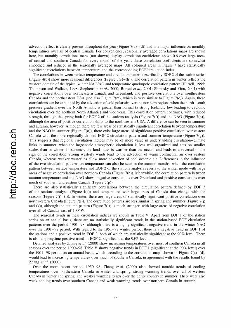
Figure 7. Correlation maps (1932–98) between temperature and: (a) EOF 1 stations winter; (b) EOF 1 stations spring; (c) EOF 1stations summer; (d) EOF 1 stations autumn; (e) EOF 2 stations winter; (f) EOF 2 stations spring; (g) EOF 2 stations summer; (h) EOF2 stations autumn; (i) EOF 3 stations winter; (j) EOF 3 stations spring; (k) EOF 3 stations summer; (l) EOF 3 stations autumn; (m) NAOwinter; (n) NAO spring; (o) NAO summer; (p) NAO autumn; (q) EOF 1 annual; (r) EOF 2 annual; (s) EOF 3 annual; (t) NAO annual.

All coloured areas are statistically significant at the 95% confidence level

throughout the year, with high negative correlations over most of central and southern Canada. When thepressure is higher than normal over the Canadian northwest and Mackenzie basin (positive EOF 1 of thestations analysis), the anticyclonic pressure patterns lead to cold air advection from the Arctic regions oversouthern Canada and much of central North America. Conversely, when the high-pressure system over thisregion is weaker than normal (negative EOF 1 of the stations analysis), cold air advection from the northis reduced and warmer air advection from the south is encouraged by the anomalous cyclonic flow. This

14

http://doc.rero.ch

advection effect is clearly present throughout the year (Figure 7(a)–(d)) and is a major influence on monthlytemperatures over all of central Canada. For convenience, seasonally averaged correlations maps are shownhere, but monthly correlations maps (not shown) display correlation coefficients above 0.6 over large areasof central and southern Canada for every month of the year; these correlation coefficients are somewhatsmoothed and reduced in the seasonally averaged maps. All coloured areas in Figure 7 have statisticallysignificant correlations between temperature and the corresponding EOF/circulation index.

The correlations between surface temperature and circulation pattern described by EOF 2 of the station series(Figure 4(b)) show more seasonal differences (Figure 7(e)–(h)). The correlation pattern in winter reflects thewestern domain of the typical winter NAO/AO and temperature quadrupole correlation pattern (Hurrell, 1995;Thompson and Wallace, 1998; Stephenson et al., 2000; Bonsal et al., 2001; Slonosky and Yiou, 2001) withnegative correlations over northeastern Canada and Greenland, and positive correlations over southeasternCanada and the northeastern USA (see also Figure 7(m), which is very similar to Figure 7(e)). Again, thesecorrelations can be explained by the advection of cold polar air over the northern regions when the north–southpressure gradient over the North Atlantic is greater than normal (a strong Icelandic low leading to cycloniccirculation over the northern North Atlantic) and vice versa. This correlation pattern continues, with reducedstrength, through the spring both for EOF 2 of the stations analysis (Figure 7(f)) and the NAO (Figure 7(n)),although the area of positive correlation shifts to the northwestern USA. A difference can be seen in summerand autumn, however. Although there are few areas of statistically significant correlation between temperatureand the NAO in summer (Figure 7(o)), there exist large areas of significant positive correlation over easternCanada with the more regionally defined EOF 2 circulation pattern and summer temperature (Figure 7(g)).This suggests that regional circulation indices may be of more value in understanding circulation–climatelinks in summer, when the large-scale atmospheric circulation is less well-organized and acts on smallerscales than in winter. In summer, the land mass is warmer than the ocean, and leads to a reversal of thesign of the correlation; strong westerly winds lead to the advection of warm continental air over easternCanada, whereas weaker westerlies allow more advection of cool oceanic air. Differences in the influenceof the two circulation patterns on temperature can also be seen in the autumn months, when the correlationpattern between surface temperature and EOF 2 of the stations analysis reverts to the winter mode with largeareas of negative correlation over northern Canada (Figure 7(h)). Meanwhile, the correlation pattern betweenautumn temperature and the NAO shows negative correlations over Greenland and positive correlations overmuch of southern and eastern Canada (Figure 7(p)).

There are also statistically significant correlations between the circulation pattern defined by EOF 3of the stations analysis (Figure 4(c)) and temperature over large areas of Canada that change with theseasons (Figure 7(i)–(l)). In winter, there are large areas of statistically significant positive correlation overnorthwestern Canada (Figure 7(i)). The correlation patterns are less similar in spring and summer (Figure 7(j)and (k)), although the autumn pattern (Figure 7(l)) is much stronger, with large areas of negative correlationover all of Canada east of 100 °W.

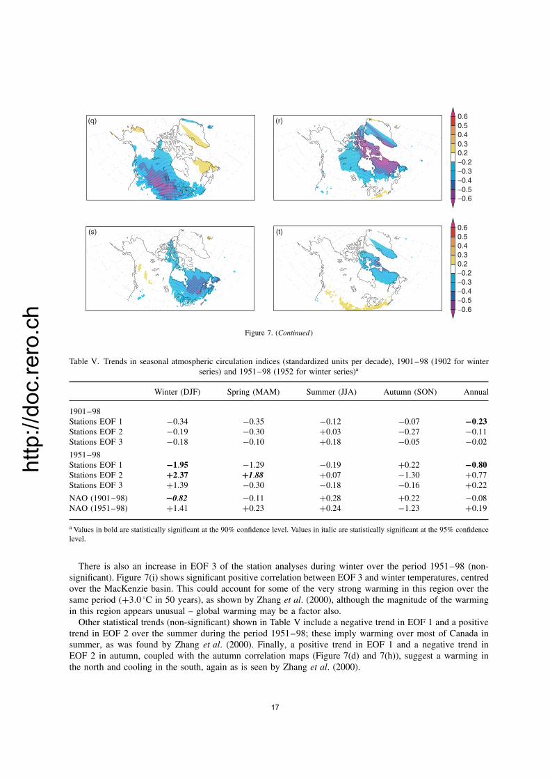
The seasonal trends in these circulation indices are shown in Table V. Apart from EOF 1 of the stationseries on an annual basis, there are no statistically significant trends in the station-based EOF circulationpatterns over the period 1901–98, although there is a highly significant negative trend in the winter NAOover the 1901–98 period. With regard to the 1951–98 winter period, there is a negative trend in EOF 1 ofthe stations and a positive trend in EOF 2, both of which are statistically significant at the 90% level. Thereis also a springtime positive trend in EOF 2, significant at the 95% level.

Detailed analyses by Zhang et al. (2000) show increasing temperatures over most of southern Canada in allseasons over the period 1900–98. Table V shows negative trends in EOF 1 (significant at the 90% level) overthe 1901–98 period on an annual basis, which according to the correlation maps shown in Figure 7(a)–(d),would lead to increasing temperatures over much of southern Canada, in agreement with the results found byZhang et al. (2000).

Over the more recent period, 1950–98, Zhang et al. (2000) also showed notable trends of coolingtemperatures over northeastern Canada in winter and spring, strong warming trends over all of westernCanada in winter and spring, and weaker warming trends over the entire country in summer. There were alsoweak cooling trends over southern Canada and weak warming trends over northern Canada in autumn.

15

http://doc.rero.ch

(i) (j) 0.60.50.40.30.2−0.2−0.3−0.4−0.5−0.6

(k) 0.60.50.40.30.2−0.2−0.3−0.4−0.5−0.6

(l)

(m)0.60.50.40.30.2−0.2−0.3−0.4−0.5−0.6

(n)

(o)0.60.50.40.30.2−0.2−0.3−0.4−0.5−0.6

(p)

Figure 7. (Continued)

The statistically significant positive trends in the winter and spring values of EOF 2 of the station analysisover the 1951–98 period (Table V), together with the increasing trend of the NAO over this period (non-significant), the decreasing trend of EOF 1 (significant at the 90% level) and the correlation maps between thesecirculation indices and temperature (Figure 7), support the hypothesis that some of the trends in temperature,as described by Zhang et al. (2000), are related to trends in the circulation indices. For example, significantdecreasing trends in EOF 1 in winter (Table V) suggest warming over southern Canada and the Prairies(Figure 7(a)), somewhat similar to what was found by Zhang et al. (2000). In addition, the statisticallysignificant positive trends of EOF 2 in winter and spring may be linked to the significant cooling overnortheast Canada and Labrador (Figure 7(e) and (f)), as identified by Zhang et al. (2000).

16

http://doc.rero.ch

(q)0.60.50.40.30.2−0.2−0.3−0.4−0.5−0.6

(r)

(s)0.60.50.40.30.2−0.2−0.3−0.4−0.5−0.6

(t)

Figure 7. (Continued)

Table V. Trends in seasonal atmospheric circulation indices (standardized units per decade), 1901–98 (1902 for winterseries) and 1951–98 (1952 for winter series)a

Winter (DJF) Spring (MAM) Summer (JJA) Autumn (SON) Annual

1901–98Stations EOF 1 −0.34 −0.35 −0.12 −0.07 −0.23Stations EOF 2 −0.19 −0.30 +0.03 −0.27 −0.11Stations EOF 3 −0.18 −0.10 +0.18 −0.05 −0.02

1951–98Stations EOF 1 −1.95 −1.29 −0.19 +0.22 −0.80Stations EOF 2 +2.37 +1.88 +0.07 −1.30 +0.77Stations EOF 3 +1.39 −0.30 −0.18 −0.16 +0.22

NAO (1901–98) −0.82 −0.11 +0.28 +0.22 −0.08NAO (1951–98) +1.41 +0.23 +0.24 −1.23 +0.19

a Values in bold are statistically significant at the 90% confidence level. Values in italic are statistically significant at the 95% confidencelevel.

There is also an increase in EOF 3 of the station analyses during winter over the period 1951–98 (non-significant). Figure 7(i) shows significant positive correlation between EOF 3 and winter temperatures, centredover the MacKenzie basin. This could account for some of the very strong warming in this region over thesame period (+3.0 °C in 50 years), as shown by Zhang et al. (2000), although the magnitude of the warmingin this region appears unusual – global warming may be a factor also.

Other statistical trends (non-significant) shown in Table V include a negative trend in EOF 1 and a positivetrend in EOF 2 over the summer during the period 1951–98; these imply warming over most of Canada insummer, as was found by Zhang et al. (2000). Finally, a positive trend in EOF 1 and a negative trend inEOF 2 in autumn, coupled with the autumn correlation maps (Figure 7(d) and 7(h)), suggest a warming inthe north and cooling in the south, again as is seen by Zhang et al. (2000).

17

http://doc.rero.ch

6. DISCUSSION AND CONCLUSIONS

The importance of the tedious, but fundamentally necessary work of carefully scrutinizing station meteorolog-ical data for errors and inhomogeneities before applying these data to climatic analyses is demonstrated in thispaper. Several large-scale inhomogeneities were discovered in the 71 monthly mean surface-level pressureseries analysed here, including a widespread inhomogeneity due to a change in observing practice between1976 and 1977. These inhomogeneities introduced spurious trends in the regional pressure tendencies whichcould affect climate analyses that rely upon surface pressure, particularly of atmospheric circulation.

EOF analyses of our station series were undertaken and these were compared with a gridded dataset fromthe UK Hadley Centre. The results showed considerable differences in the dominant EOF pressure patterns forCanada and Greenland. It is suggested that these differences may be related to extrapolation of gridded dataover data-sparse regions. There are few observing stations in the high Arctic and over ocean areas, althoughthe situation is improving with the considerable efforts of the international data community to incorporatemarine data, non-standard meteorological data and to digitize and quality control the realms of paper recordsin the meteorological and other archives of the world. However, all these efforts will never be able to recoverdata and observations that simply do not exist. Reanalysis projects do go some way to estimating whatmay have been happening in data-sparse regions, and they generate plausible estimates. Nevertheless, thescientific community should not lose sight of the fact that these are estimates, and that we will not knowfrom instrumental records what the true multi-decadal to century-scale variability is over, e.g. the Arctic, untilanother 30 to 50 years of observations have been recorded. Even gridded observational data products (suchas the temperature data used to calculate the correlation maps in Section 5.2) should be treated with caution,as the number of independent observing stations informing the grid construction procedure is often muchless, sometimes by several orders of magnitude, than the number of grid points contained in the grid overdata-sparse regions. The number of degrees of freedom in a grid is thus artificially enhanced in a grid overdata-sparse regions. Note that this is a problem independent of the equal-area weighting problem faced bygridded data in high latitudes. This is an effect that increases as one goes further back in time, with fewer andfewer observing stations operating in the first half of the 20th century. It is a problem that may become worseif governments continue to cut back observing stations as they have done, particularly in Canada, through the1990s.

The first three modes of variability recovered from the station-based EOF analysis do, in fact, make sensephysically as well as mathematically and have dynamical interpretations. They also have simple patternloadings. The first circulation pattern relates to the ridge of high pressure over northwestern Canada to the leeof the Rockies, centred over the MacKenzie basin. In its positive phase this is a synoptic pattern associatedwith cold air outbreaks over most of central Canada and the USA in winter, and is the dominant patternin the monthly mean pressure field for the months of November to June. The second circulation patternrelates clearly to the mean zonal flow over the western Atlantic basin, with isolines concentrated along the StLawrence Valley–Newfoundland/Labrador storm track. The third atmospheric circulation pattern is a cyclonicmeridional flow centred on Hudson Bay.

Station-based atmospheric circulation indices were constructed based on the areas of maximum variabilityseen in the EOF analyses. These station-based indices have longer records and are more easily updated thanthe EOFs of the EOF analysis. Trends in the station-based indices, the EOFs of the station analysis and thegridded HadSLP analysis, as well as the AO and the NAO, were examined both over the past 50 years andthe past 100 years. Statistically significant trends were identified over the winter period (November–March)from 1951 to 1998 in the following circulation indices: Eastern zonal index, stations EOF 1, stations EOF2, NAO, AO, HadSLP EOF 1 and HadSLP EOF 2. However, no trends were statistically significant duringwinter over the longer time period of 1901–98, except for EOF 3 of HadSLP.

Correlation maps show that these three patterns of circulation are significantly related to temperaturevariability over Canada. The first pressure pattern is highly correlated with temperature over southern Canadaand central North America in all seasons. The second pattern is associated with temperature variabilityin eastern Canada and the northwestern Atlantic, with negative correlations over northeastern Canada andpositive correlation over southern Canada in winter; this pattern also shows positive correlations over much

18

http://doc.rero.ch

of eastern Canada in summer. The third atmospheric circulation pattern is related to temperature variability innorthern and central Canada, particularly in autumn and winter. The implied direction of the temperature trendssuggested by the trends in the atmospheric circulation and the correlations maps confirms the independentanalysis on temperature trends over Canada (Zhang et al., 2000), although the magnitude of the warming insome cases can probably not be explained solely by changes in circulation.

It is clear that in order to understand the cause of the temperature trends over Canada, which differ byregion and season, it is necessary to understand the variability of the atmospheric circulation. Regionalcirculation indices, based on analyses over specific regions, provide better diagnostic results in explaining thevariability of temperature on a regional scale in non-winter months than do larger scale indices based on thecirculation over the entire hemisphere. This is to be expected, as the circulation in non-winter months is lesswell-organized than in winter, and more prone to regional variations.

ACKNOWLEDGEMENTS

We would like to thank Francis Zwiers and Val Swail for their support of this work, Roberta McCarthy andMalcolm Geast for help in tracking down sources, and Rob Allan and Tara Ansell of the Hadley Centrefor providing the HadSLP data. The last 5 years of the NAO series were obtained from Tim Osborn’sWebsite at CRU (http://www.cru.uea.ac.uk/timo/projpages/nao update.htm), the AO series was obtained fromthe annular modes Website (http://horizon.atmos.colostate.edu/ao/) and the teleconnection time series fromthe NOAA Climate Prediction Center Website (http://www.cpc.noaa.gov/data/teledoc/telecontents.html). Thefigures were produced using GrADS and XMGrace freewares. This paper is dedicated to Ignacio Lozano.

REFERENCES

Alexandersson H, Moberg A. 1997. Homogenization of Swedish temperature data. Part I: a homogeneity test for linear trends.International Journal of Climatology 17: 25–34.

Allan RJ, Nicholls N, Jones PD, Butterworth IJ. 1991. A further extension of the Tahiti–Darwin SOI, early SOI results and Darwinpressure. Journal of Climate 4: 743–749.

Allan RJ, Reason CJC, Carroll P, Jones PD. 2002. A reconstruction of Madras (Chennai) mean sea-level pressure using instrumentalrecords from the late 18th and early 19th centuries. International Journal of Climatology 22: 1119–1142.

Ambaum MH, Hoskins PBJ, Stephenson DB. 2001. Arctic oscillation or North Atlantic oscillation? Journal of Climate 14: 3495–3507.Barnston AG, Livezey RE. 1987. Classification, seasonality and persistence of low-frequency atmospheric circulation patterns. Monthly

Weather Review 115: 1083–1126.Barring LP, Jonsson C, Acheberger M, Ekstrom H, Alexandersson H. 1999. The Lund instrumental record of meteorological

observations: reconstruction of monthly sea-level pressure 1780–1997. International Journal of Climatology 19: 1427–1443.Basnett TA, Parker DE. 1997. Development of the global mean sea level pressure data set GMSLP2. Hadley Centre of the UK

Meteorological Office for Climate Research, Technical Note 79. Hadley Centre for Climate Prediction and Research, MeteorologicalOffice, Bracknell, UK.

Bonsal BR, Shabbar A, Higuichi K. 2001. Impacts of low frequency variability modes on Canadian winter temperature. InternationalJournal of Climatology 21: 95–108.

Caussinus H, Mestre O. 1996. Towards new tools and methodologies for relative homogeneity testing. In First Seminar forHomogenization of Surface Climatological data, Budapest, Hungary. Hungarian Meteorological Service: 62–82.

Deser C. 2000. On the teleconnectivity of the “Arctic Oscillation”. Geophysical Research Letters 27: 779–782.Environment Canada. 1976. Internal memorandum no. OBS 2-76, Atmospheric Environment Service, Downsview, Ontario, Canada,

November.Godson WL. 1955. Report on Canadian standard barometry, Atmospheric Environment Service, Toronto, Ontario, Canada.Hurrell JW. 1995. Decadal trends in the North Atlantic oscillation: regional temperatures and precipitation. Science 269: 676–679.Itoh H. 2002. True versus apparent Arctic oscillation. Geophysical Research Letters 29: 1268. DOI: 10.1029/2001GL013978Jones PD. 1987. The early twentieth century Arctic high – fact or fiction? Climate Dynamics 1: 63–75.Jones PD, Jonsson T, Wheeler D. 1997. Extension to the North Atlantic oscillation using early instrumental pressure observations from

Gibraltar and south-west Iceland. International Journal of Climatology 17: 1433–1450.Jones PD, Davies TD, Lister DH, Slonosky V, Jonsson T, Barring L, Jonsson P, Maheras P, Kolyva-Machera F, Barriendos M, Martin-

Vide J, Alcoforado MJ, Wanner H, Pfister C, Schuepbach E, Kaas E, Schmith T, Jacobeit J, Beck C. 1999a. Monthly mean pressurereconstructions for Europe. International Journal of Climatology 19: 347–364.

Jones PD, Salinger MJ, Mullan AB. 1999b. Extratropical circulation indices in the Southern Hemisphere based on station data.International Journal of Climatology 19: 1301–1317.

Kaplan A, Kushnir Y, Cane MA. 2000. Reduced space optimal interpolation of historical marine sea level pressure: 1854–1992. Journalof Climate 13: 2987–3002.

McMaster RS. 1975. Memorandum No. 8437-1 from ACNS to ACNC. Data Standards Division, Government of Canada, Toronto,Canada, 22 September.

Middleton WEK. 1964. The History of the Barometer. Johns Hopkins University Press: Baltimore.

19

http://doc.rero.ch

Mo KC, Livezey RE. 1986. Tropical–extratropical geopotential height teleconnections during the Northern Hemisphere winter. MonthlyWeather Review 114: 2488–2515.

Moberg A, Bergstrom H, Ruiz Krigsman J, Svanered O. 2002. Daily air temperature and pressure series for Stockholm (1756–1998).Climatic Change 53: 171–212.

New M, Hulme M, Jones PD. 2000. Representing twentieth century space–time climate variability. Part 2: development of 1901–96monthly grids of terrestrial surface climate. Journal of Climate 13: 2217–2238.

Nicholls N. 2001. The insignificance of significance testing. Bulletin of the American Meteorological Society 81: 981–986.Nkemdirim LC, Budikova D. 2001. Trends in sea level pressure across western Canada. Journal of Geophysical Research D 106I:

11 801–11 812.Peterson TC, Easterling DR, Karl TR, Groisman P, Nicholls N, Plummer N, Torok S, Auer I, Boehm R, Gullett D, Vincent LA,

Heino R, Tuomenvirta H, Mestre O, Szentimrey T, Salinger J, Førland E, Hanssen-Bauer I, Alexandersson H, Jones PD, Parker DE.1998. Homogeneity adjustments of in situ atmospheric climate data: a review. International Journal of Climatology 18: 1493–1517.

Potter JG. 1955. Monthly mean sea level pressure maps for Canada. CIR-2710, Tec-224, Meteorological Division, Department ofTransport: Toronto, Canada, 18 October. 1955.

Rogers JC, McHugh MJ. 2002. On the separability of the North Atlantic oscillation and Arctic oscillation. Climate Dynamics 19:599–608.

Savdie I. 1982. AES barometry program, Technical Record No. 9. Network Planning and Standards Division, Data Acquisition ServicesBranch, Environment Canada, Downsview, Ontario, Canada, August.

Shabbar A, Higuichi K, Skinner W, Knox JL. 1997. The association between the BWA index and winter surface temperature variabilityover eastern Canada and west Greenland. International Journal of Climatology 17: 1195–1210.

Slonosky VC. 2003. The meteorological observations of Jean-Francois Gaultier, Quebec, Canada 1742–56. Journal of Climate 16:2232–2247.

Slonosky VC, Yiou P. 2001. The North Atlantic oscillation and its relationship with near surface temperature. Geophysical ResearchLetters 28: 807–810.

Slonosky VC, Jones PD, Davies TD. 1999. Homogenization techniques for European monthly surface pressure series. Journal of Climate12: 2658–2672.

Stephenson DB, Pavan V, Bojariu R. 2000. Is the North Atlantic oscillation a random walk? International Journal of Climatology 20:1–18.

Thompson DWJ, Wallace JM. 1998. The Arctic oscillation signature in the wintertime geopotential height and temperature fields.Geophysical Research Letters 25: 1297–1300.

Upton FT. 1972. Headquarters standards and procedures for barometry in Canada. Atmospheric Environment Service, Toronto, Canada.Van Loon H, Rogers JC. 1978. The seesaw in winter temperatures between Greenland and northern Europe. Part 1: general description.

Monthly Weather Review 106: 296–310.Vincent LA, Zhang X, Bonsal BR, Hogg WD. 2002. Homogenization of daily temperatures over Canada. Journal of Climate 15:

1322–1334.Walker GT, Bliss EW. 1932. World weather V. Memoirs of the Royal Meteorological Society 4: 53–84.Wallace JM, Gutzler DS. 1981. Teleconnections in the geopotential height field during the Northern Hemisphere winter. Monthly Weather

Review 109: 784–812.Wanner H, Bronnimann S, Casty C, Gyalistras D, Luterbacher J, Schmutz C, Stephenson DB, Xoplaki E. 2001. North Atlantic

oscillation – concept and studies. Surveys in Geophysics 22: 321–382.Young KC. 1993. Detecting and removing inhomogeneities from long-term sea level pressure time series. Journal of Climate 6:

1205–1220.Zhang X, Vincent LA, Hogg WD, Niitsoo A. 2000. Temperature and precipitation trends in Canada during the 20th century.

Atmosphere–Ocean 38: 395–429.

20