INTERNATIONAL JOURNAL OF CLIMATOLOGYInt. J. Climatol. 29: 1642–1660 (2009)Published online 10 December 2008 in Wiley InterScience(www.interscience.wiley.com) DOI: 10.1002/joc.1807

Observed and modelled influence of atmospheric circulationon central England temperature extremes

S. Blenkinsop,a* P. D. Jones,b S. R. Dorlingc and T. J. Osbornb

a Water Resource Systems Research Laboratory, School of Civil Engineering and Geosciences, Newcastle University, Newcastle upon Tyne, UKb Climatic Research Unit, School of Environmental Sciences, University of East Anglia, Norwich, Norfolk, UK

c School of Environmental Sciences, University of East Anglia, Norwich, UK

ABSTRACT: The regional atmospheric circulation is a major driver of climate for western Europe and so the ability ofclimate models to accurately simulate its characteristics forms an important part of the rigorous testing of their performance.In this paper we examine the skills of seven regional climate models (RCMs) to reproduce mean daily temperatures forthe central England region. Their ability to reproduce observed characteristics of the circulation is then tested using threeairflow indices. This is achieved by comparing: (1) the frequency distribution of each index, (2) the relationships betweenthe daily airflow indices and temperature, including daily extremes and (3) the ability of models to reproduce the observedpersistence of specific flow regimes and the temperature response to this persistence.

It is demonstrated that RCM selection introduces uncertainty into temperature simulations and that there is no singlemodel which outperforms the others. Although the models qualitatively reproduce the observed distributions of the airflowindices reasonably well, most models produce distributions that are statistically significantly different from the observations.In particular, all models overestimate the frequency of winter westerly flow, and biases in the relationships betweencirculation and temperature are also noted for extreme values of the airflow indices. The persistence of flow regimes isshown to have a significant effect on the observed temperature, though models have difficulty in reproducing the magnitudeof the response to this persistence for some flow types.

The results presented here not only form a useful model validation exercise but also further highlight the need for theuse of multi-model ensembles in the generation of future climate scenarios. Furthermore, they suggest that the use ofatmospheric circulation in statistical downscaling methods might be enhanced by the inclusion of persistence, particularlywhen producing scenarios of temperature extremes. Copyright 2008 Royal Meteorological Society

KEY WORDS temperature; RCMs; atmospheric circulation; CET; validation; persistence

Received 7 November 2007; Revised 8 October 2008; Accepted 11 October 2008

1. Introduction

Climate models are important tools in our ability toassess the likely trajectory of future climate changeand to form the basis of impact assessments whichdetermine adaptation and mitigation strategies. However,limitations in our knowledge of atmospheric processesand the parameterization of small-scale physics meanthat uncertainties are inherent in simulations producedby climate models. Therefore, rigorous validation of allaspects of climate model output forms an importantfeature of work in the climate community.

One of the key determinants of climate for the westernEurope region is the large-scale atmospheric circulation.Its observed variability has been extensively studied (e.g.Jones et al., 1993; Esteban et al., 2006; James, 2007) ashas its influence on temperature (e.g. Osborn et al., 1999;Brabson and Palutikof, 2002) and precipitation (e.g.

* Correspondence to: S. Blenkinsop, Water Resource Systems ResearchLaboratory, School of Civil Engineering and Geosciences, CassieBuilding, University of Newcastle, Newcastle upon Tyne, NE1 7RU,UK. E-mail: s.blenkinsop@ncl.ac.uk

Goodess and Jones, 2002; McGregor and Phillips, 2004).The atmospheric circulation has also been identified asa key determinant of extreme events such as heat waves(Della-Marta et al., 2007), droughts (Fowler and Kilsby,2002) and floods (Bardossy and Filiz, 2005). The roleof circulation in influencing temperature trends duringthe 20th century has been examined (Osborn and Jones,2000; van Oldenborgh and van Ulden, 2003) and maybe useful for the attribution of observed climate change.The ability of individual models to reproduce observedcharacteristics of regional circulation and its relationshipwith surface climate has also been examined (e.g. Osbornet al., 1999; James, 2006).

However, more recently, increased emphasis has beenplaced on appreciating uncertainties in climate modelsimulations, and examining atmospheric circulation is animportant part of understanding the ability of models toreproduce physical atmospheric processes. Jacob et al.(2007) have investigated biases of variables includingmean sea level pressure (MSLP) fields in an ensembleof regional climate model (RCM) simulations from thePRUDENCE project (Christensen et al., 2007). Biases in

Copyright 2008 Royal Meteorological Society

OBSERVED AND MODELLED CIRCULATION–TEMPERATURE RELATIONSHIPS 1643

RCM simulations of wintertime MSLP were shown tobe largely dependent on the driving general circulationmodel (GCM) boundary conditions, but in summertimesmaller scale processes make differences between GCMand RCM biases more important. van Ulden and van Old-enborgh (2006) examined simulations of two geostrophicflow indices which correspond to westerly and southerlyflow components, and a third representing geostrophicvorticity for 23 global coupled climate models. Manyshowed serious biases at mid-latitudes, particularly in thesimulation of spatial variance which produced a poorsimulation of circulation indices over central Europe.van Ulden et al. (2007) also compared the simulation ofthe same indices over central Europe for three GCMsand nine PRUDENCE RCMs. Furthermore, relationshipsbetween monthly temperature and rainfall statistics andwesterly flow were compared for two of the regionalmodels noting HadRM3H to be poor in reproducing theobserved relationship between summer temperature andwesterly flow.

Here, we use daily MSLP data to derive daily cir-culation indices for central England, which are used toexamine the relationship between the atmospheric circu-lation and daily temperature means and extremes. Thisapproach has been used to assess the output from anindividual GCM (Osborn et al., 1999) and RCM (Turn-penny et al., 2002). However, both studies as well asonly considering single model simulations only examinedthe relationships with mean daily temperature. We com-pare the ability of seven RCMs in simulating observeddaily mean temperature and six of those in simulatingdaily extreme temperatures for central England as wellas comparing their simulations of daily airflow indices.These models are described briefly in Section 2. Wethen outline the scheme used to represent the regionalatmospheric circulation over the UK in Section 3. InSection 4, the ability of models to reproduce observedmean temperatures for central England is assessed. Their

skill in reproducing observed frequencies of circulationregimes is examined along with the relationships betweenthose regimes and near-surface temperature. The abilityof models to reproduce observed characteristics of thepersistence of different circulation regimes is also testedand will enable a more rigorous evaluation of RCM per-formance, offering a greater insight as to the nature ofmodel biases in temperature simulations while the useof multiple climate models provides an indication of theuncertainty range in RCM simulations.

2. Data and models

2.1. Data

Two ‘observed’ temperature data sets are used here.Firstly, the Climatic Research Unit (CRU) TS 2.0 dataset (Mitchell et al., 2004) is used to enable a directcomparison between models and observations using iden-tical spatial domains. This is a gridded global series ofmonthly climate means for the land surface for the period1901–2000 and was constructed by the interpolation ofstation data onto a 0.5° grid and is an updated versionof earlier datasets (New et al., 1999a,b). This series willbe referred to hereafter as CRU. Secondly, the CentralEngland Temperature (CET) series is used. This was firstpublished as a series of monthly mean temperatures from1698 (Manley, 1953) and later extended back to 1659(Manley, 1974), and subsequently a daily temperatureseries has been constructed back to 1772 (Parker et al.,1992) from various combinations of stations throughoutthe period of record due to station closures and miss-ing data. These stations represent Manley’s concept ofcentral England and try to combine stations with long,unbroken records and those which avoid urban influences.This daily series is used to derive observed relationshipsbetween circulation and temperature and the RCM gridcells used to represent the CET region are shown inFigure 1.

Figure 1. Grid points used to construct the airflow indices for the British Isles. The solid circles represent the grid points used in this study; thehollow circles represent those traditionally used when all grid points are available. The shaded boxes are the grid cells used to define the central

England region on the CRU and RCM grids.

Copyright 2008 Royal Meteorological Society Int. J. Climatol. 29: 1642–1660 (2009)DOI: 10.1002/joc

1644 S. BLENKINSOP ET AL.

Finally, to calculate the airflow indices, a gridded2.5° × 2.5° daily MSLP re-analysis series is used from theNational Centers for Environmental Prediction (NCEP)re-analysis project described by Kalnay et al. (1996). Anobserved daily series of MSLP from the UK Meteorolog-ical Office (UKMO) data set (Jones, 1987) was consid-ered; however, a coarser resolution of 5° latitude × 10°

longitude resulted in one of the gridpoints used to calcu-late the airflow indices outside the domain of the RCMs.Potential inhomogeneities in the NCEP series have beenidentified over Greenland and the high altitude regionsof southern Europe. Also, prior to the mid-1960s, NCEPannual MSLP is lower than the UKMO data at many gridpoints due to a data input error. The former problem isoutside the area of interest of this study, while the lattershould not affect the calculation of airflow indices as theyare not dependent on absolute values, but the relative dif-ference between selected grid points. Reid et al. (2001)indicate an excellent agreement between monthly meanMSLP obtained from NCEP and UKMO over northwestEurope while Blenkinsop (2005) indicated a good agree-ment in the derived airflow indices from the two datasetsfor the UK region.

Daily temperature and pressure data for the period1961–1990 were extracted from each dataset to corre-spond with the control period used in the RCM simula-tions which are described in the following section.

2.2. Regional climate models

RCM output from the European Union Fifth Frame-work Programme (FP5) PRUDENCE project (Chris-tensen et al., 2007) provides a series of high-resolutionsimulations of European climate for the control period1961–1990 for a large range of climatic variables, usingRCMs driven by boundary conditions from differentGCMs. These ‘time-slice’ simulations are representativeof a stationary climate over a 30-year period and may becompared with observations as part of model verification(Raisanen, 2007). Here the model selection was madeto examine the uncertainty in RCM output due to thebounding GCM and that due to the choice of RCM. Thecontribution of these two sources to RCM uncertainty is

tested by using a selection of models which investigatethe role of:

• same bounding GCM in combination with differentRCMs (e.g. HIRHAM H v RCAO H; Table I);

• same RCM in combination with different boundingGCMs (e.g. HIRHAM H v HIRHAM E; Table I)

A list of models and their acronyms used in this studyis provided in Table I. The HIRHAM model is a ver-sion of HIRHAM4 (Christensen et al., 1996, 1998)updated to incorporate high-resolution physiographicaldata of surface topography and land use classification(Christensen et al., 2001; Hagemann et al., 2001). TheRCAO model is composed of an atmospheric part RCA2(Jones et al., 2004a) and an ocean model RCO (Meieret al., 2003) while HadRM3P (Jones et al., 2004b) is anupdated version of HadRM3H (Hudson and Jones, 2002).Finally, ARPEGE-IFS is a global operational forecastmodel which may be run at a variable horizontal res-olution and is nested directly within HadCM3. This isan updated version of that described by Deque et al.(1998) to reflect changes in the radiation and cloud-precipitation-turbulence schemes. Model simulations ofdaily minimum, mean and maximum temperature anddaily MSLP are available for control integrations forthe period 1961–1990, though daily minima and max-ima are not available for HIRHAM E. Therefore, anadditional simulation of HIRHAM using boundary condi-tions derived from the ECHAM5 GCM is also examined.The main changes in ECHAM5 include an updated long-wave radiation scheme, to that used in ECHAM4, newcloud microphysics and changes in the representation ofland surface processes (Roeckner et al., 2003). Temper-ature and MSLP data for each of these simulations werere-gridded onto the CRU 0.5° grid to allow direct com-parison with the CET and NCEP series respectively.

3. Circulation classification

Daily atmospheric circulation characteristics are repre-sented here by the circulation indices described by Jenk-inson and Collison (1977) and were demonstrated to be

Table I. Selection of PRUDENCE RCMs used for this study. Different acronyms are adopted here to provide an easierunderstanding of the format of each model run. The first part of each acronym refers to the RCM and the second to theGCM data used to provide the boundary conditions. Models are run for a 30-year control period (1961–90) except for HadRM3P

which is run for a total of 31 years (1960–90).

RCM Driving GCM PRUDENCEacronym

Modified acronym

Danish Meteorological Institute(DMI)

HIRHAM HadAM3HECHAM4/OPYCECHAM5

HC1EcctrlECC

HIRHAM HHIRHAM EHIRHAM E5

Swedish Meteorological andHydrological Institute (SMHI)

RCAO HadAM3HECHAM4/OPYC

HCCTLMPICTL

RCAO HRCAO E

Hadley Centre–UK Met Office HadRM3P HadAM3P Adeha HAD H 3PMeteo-France, France ARPEGE-IFS HadCM3 DA9 ARPEGE H

Copyright 2008 Royal Meteorological Society Int. J. Climatol. 29: 1642–1660 (2009)DOI: 10.1002/joc

OBSERVED AND MODELLED CIRCULATION–TEMPERATURE RELATIONSHIPS 1645

a useful means of objectively classifying daily circula-tion types affecting the UK (Jones et al., 1993), produc-ing strong correlations with the subjective Lamb (1972)scheme in terms of circulation type frequencies and theirrelationship with seasonal temperature and precipitation.Three indices; flow direction (DIR), flow strength (STR)and vorticity (VORT) may be derived from the grid-ded MSLP at the points shown in Figure 1 using theequations shown in the appendix. For STR, each unit isequivalent to approximately 0.6 ms−1, while for VORT,which reflects the rotation of an air mass, 100 unitsare equivalent to 0.46 times the Coriolis parameter at55 °N. Negative (positive) VORT values are indicativeof anti-cyclonic (cyclonic) rotation of an air mass. TheDIR index is simply expressed in degrees from north(0–360°).

This automated typing scheme has also been appliedto studies in Scandinavia (Chen, 2000; Linderson, 2001)and the Iberian Peninsula (Goodess and Jones, 2002). Asin Osborn et al. (1999) each index is divided into 20-equal sized bins with each day subsequently classifiedaccording to the bin into which the index value for thatday falls. The resultant distribution is used to describethe frequency of occurrence of different flow regimesand the climate characteristics on a given day. Theseindices have been used to assess the ability of the singleGCM (Osborn et al., 1999) and RCM (Turnpenny et al.,2002) simulations to reproduce the observed relationshipsbetween daily circulation and surface climate. Here, weextend the analysis to examine multiple RCM simulationsin order to obtain an estimate of the uncertainties inreproducing regional atmospheric circulation. Using thesame indices to compare RCM simulations with thosederived from the NCEP re-analysis data provides a directcomparison of model performance.

4. Results

4.1. RCM simulations of central England temperature

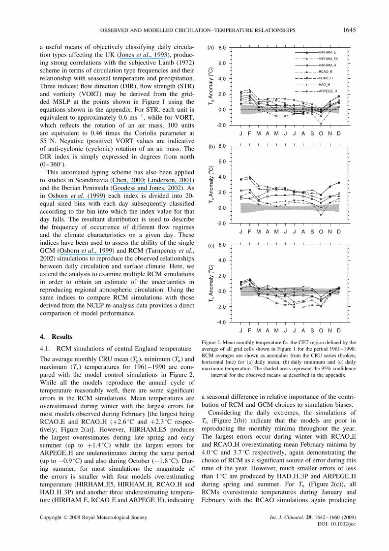
The average monthly CRU mean (Tg), minimum (Tn) andmaximum (Tx) temperatures for 1961–1990 are com-pared with the model control simulations in Figure 2.While all the models reproduce the annual cycle oftemperature reasonably well, there are some significanterrors in the RCM simulations. Mean temperatures areoverestimated during winter with the largest errors formost models observed during February [the largest beingRCAO E and RCAO H (+2.6 °C and +2.3 °C respec-tively; Figure 2(a)]. However, HIRHAM E5 producesthe largest overestimates during late spring and earlysummer (up to +1.4 °C) while the largest errors forARPEGE H are underestimates during the same period(up to −0.9 °C) and also during October (−1.8 °C). Dur-ing summer, for most simulations the magnitude ofthe errors is smaller with four models overestimatingtemperature (HIRHAM E5, HIRHAM H, RCAO H andHAD H 3P) and another three underestimating tempera-ture (HIRHAM E, RCAO E and ARPEGE H), indicating

Figure 2. Mean monthly temperature for the CET region defined by theaverage of all grid cells shown in Figure 1 for the period 1961–1990.RCM averages are shown as anomalies from the CRU series (broken,horizontal line) for (a) daily mean, (b) daily minimum and (c) dailymaximum temperature. The shaded areas represent the 95% confidence

interval for the observed means as described in the appendix.

a seasonal difference in relative importance of the contri-bution of RCM and GCM choices to simulation biases.

Considering the daily extremes, the simulations ofTn (Figure 2(b)) indicate that the models are poor inreproducing the monthly minima throughout the year.The largest errors occur during winter with RCAO Eand RCAO H overestimating mean February minima by4.0 °C and 3.7 °C respectively, again demonstrating thechoice of RCM as a significant source of error during thistime of the year. However, much smaller errors of lessthan 1 °C are produced by HAD H 3P and ARPEGE Hduring spring and summer. For Tx (Figure 2(c)), allRCMs overestimate temperatures during January andFebruary with the RCAO simulations again producing

Copyright 2008 Royal Meteorological Society Int. J. Climatol. 29: 1642–1660 (2009)DOI: 10.1002/joc

1646 S. BLENKINSOP ET AL.

the largest errors, but in all cases the magnitude of theerrors is smaller than for Tn. Throughout the rest of theyear there is a general underestimation of Tx resulting ina smaller than observed amplitude of the annual cycle.Consequently, most models fail to accurately reflectthe daily temperature range (not shown), especially thetwo RCAO simulations which underestimate the meantemperature range by up to 4.2 °C during late summerdue to the simulation of minima that are too warmand maxima that are too cool. In contrast, HAD H 3Pproduces the smallest errors in temperature range, lessthan 1 °C for 9 months of the year.

The root mean square error (RMSE) statistic was cal-culated to quantify these model biases based on the

differences between simulated and CRU seasonal meantemperatures for each grid cell over the central Englandregion. Figure 3 indicates that for Tg the largest errorsduring autumn and winter are produced by the RCAOsimulations with the smallest produced by HAD H 3Pand ARPEGE H respectively. In contrast, during sum-mer, the RCAO simulations produce the lowest RMSEstatistic. For temperature extremes, some differences areobserved. For Tn, HAD H 3P and ARPEGE H producethe smallest errors throughout the year while the largestRMSE statistics are generally produced by the RCAOsimulations, particularly during autumn and winter. ForTx, ARPEGE H is relatively poor in all seasons exceptwinter when it produces relatively small errors, although

Figure 3. RMSE statistics for all grid cells in the CET region relative to CRU. Results are presented seasonally and separately for Tn (left), Tg

(centre) and Tx (right). The first row is winter (DJF) with subsequent rows spring (MAM), summer (JJA) and autumn (SON).

Copyright 2008 Royal Meteorological Society Int. J. Climatol. 29: 1642–1660 (2009)DOI: 10.1002/joc

OBSERVED AND MODELLED CIRCULATION–TEMPERATURE RELATIONSHIPS 1647

there is little difference between the models in this sea-son. The RCAO and ARPEGE H simulations produce thelargest errors during summer when the range of modelresults is largest; this range suggesting model parameter-ization has the greatest effect on warm extremes dur-ing summer months. Considering the RMSE statisticsin conjunction with Figure 2 indicates that in generalterms, RCAO has the greatest problems in the simulationof extremes with minima that are too high throughoutthe year and maxima that are too low during summer.These models would thus provide a poor representationof events such as summer heat waves and cold spellsthroughout the year. In contrast, HAD H 3P performsreasonably well in minimizing errors in winter Tn andsummer Tx.

4.2. RCM simulations of regional atmosphericcirculation

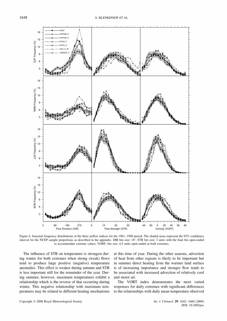
Figure 4 compares model simulations of the frequen-cies of the airflow indices with those derived fromthe NCEP data. Chi-squared goodness-of-fit tests wereapplied to test each of the modelled seasonal distribu-tions shown against observations (NCEP) and indicatedthat the seasonal RCM distributions for each airflowindex are significantly different from the correspondingNCEP distributions at the 95% level with the exceptionof the ARPEGE H autumn STR distribution. For DIR,all models overestimate the frequency of westerly flowduring winter at the expense of easterly and southerlyregimes, while during spring HAD H 3P, RCAO H andHIRHAM H capture the frequency of flow regimes rea-sonably well whereas HIRHAM E, RCAO E and partic-ularly ARPEGE H again overestimate the westerly flow.This is consistent with results obtained by van Uldenet al. (2007) who noted that ARPEGE produced a strongpositive bias in a zonal flow index during winter overcentral Europe. The overestimation of westerly flows byGCMs and their inability to produce sufficient blockingtypes in the Northern Hemisphere has been noted previ-ously (D’Andrea et al., 1998; Pelly and Hoskins, 2003;James, 2006; van Ulden and van Oldenborgh, 2006).Nonetheless, the comparison of a common circulationindex for a selection of PRUDENCE models is usefulas it is indicative of the range of errors in simulations.Qualitatively, observed summer and autumn flow regimesare captured much better, though the two ECHAM-drivensimulations both have a significant westerly bias, whereasHAD H 3P has an easterly bias. In all cases, the impor-tance of GCM boundary conditions is noted with thepaired simulations driven by ECHAM and HadAM3Hboth producing similar distributions. This conditioning ofRCM projections by the behaviour of the driving GCMshas been demonstrated to be important when model out-puts are used to generate scenarios of climate changeimpacts (e.g. Wilby and Harris, 2006; Fronzek and Carter,2007).

For STR, most models simulate the observed winterdistribution reasonably well, though most underestimatethe frequency of low STR days to the preference of

moderate strength flow days. However, ARPEGE Hagain produces poor results, along with HAD H 3Psignificantly overestimating the frequency of strong flowdays during winter, consistent with their simulation of toofrequent westerly flow days. Throughout the rest of theyear, most models tend to underestimate the frequencyof high STR days, producing more frequent days withmoderate STR values.

For VORT the greatest spread of results is againobtained for winter, but throughout the year most sim-ulations underestimate the number of anti-cyclonic days(VORT <0) with too many moderately cyclonic days,particularly for the two ECHAM-driven simulations dur-ing summer and autumn. During spring and autumn, mostmodels also tend to underestimate the frequencies of bothextreme cyclonic and anti-cyclonic days.

4.3. Model simulations of the relationships betweencirculation and temperature

To examine the relationship between circulation andtemperature, the daily temperature values were convertedinto anomalies. These were obtained by first calculatingthe annual cycle over the baseline period of 1961–90by averaging the 30 values for each calendar date. An11-term binomial filter was next applied to the resultingannual averages to produce a temperature cycle lessstrongly influenced by random variations while stillmaintaining genuine features of annual temperature. Theannual cycle obtained from the observations and fromeach model was then subtracted from the correspondingdaily temperature series to derive the anomalies.

Interdependencies in the relationship between temper-ature and airflow indices have previously been identifiedby considering a bivariate analysis of combinations ofindices (Osborn et al., 1999). However, one of the dis-advantages associated with the use of these indices is theloss of information when considering marginal distribu-tions of bivariate pairs relative to those of the zonal andmeridional flow components. Here, this problem is appar-ent due to the small sample sizes for some combinationsof regimes, e.g. strong easterly flow, for the 30-year timeslices and prohibits such an analysis here. Therefore, hererelationships between daily temperature anomalies andthe three airflow indices are determined and comparedindependently. Previous analysis of these relationships(Osborn et al., 1999; Turnpenny et al., 2002) indicatedthat mean daily temperature anomalies are most stronglydependent upon DIR, but also upon STR and vorticityduring winter when stronger flow and cyclonic condi-tions are associated with milder temperatures. Some dif-ferences in relationships are observed when consideringobserved minimum and maximum temperatures. Figure 5shows that DIR exerts a strong influence on minimum,mean and maximum daily temperature throughout theyear but that this influence is greatest on maximum tem-perature and least on minima. This is most clearly demon-strated in summer when for maximum temperatures theamplitude of the influence of DIR is approximately 5 °Cbut for minima it is less than 2 °C.

Copyright 2008 Royal Meteorological Society Int. J. Climatol. 29: 1642–1660 (2009)DOI: 10.1002/joc

1648 S. BLENKINSOP ET AL.

Figure 4. Seasonal frequency distributions of the three airflow indices for the 1961–1990 period. The shaded areas represent the 95% confidenceinterval for the NCEP sample proportions as described in the appendix. DIR bin size: 18°; STR bin size: 2 units with the final bin open-ended

to accommodate extreme values; VORT: bin size: 6.5 units open-ended at both extremes.

The influence of STR on temperature is strongest dur-ing winter for both extremes when strong (weak) flowstend to produce large positive (negative) temperatureanomalies. This effect is weaker during autumn and STRis less important still for the remainder of the year. Dur-ing summer, however, maximum temperatures exhibit arelationship which is the reverse of that occurring duringwinter. This negative relationship with maximum tem-peratures may be related to different heating mechanisms

at this time of year. During the other seasons, advectionof heat from other regions is likely to be important butin summer direct heating from the warmer land surfaceis of increasing importance and stronger flow tends tobe associated with increased advection of relatively cooland moist air.

The VORT index demonstrates the most variedresponses for daily extremes with significant differencesto the relationships with daily mean temperature observed

Copyright 2008 Royal Meteorological Society Int. J. Climatol. 29: 1642–1660 (2009)DOI: 10.1002/joc

OBSERVED AND MODELLED CIRCULATION–TEMPERATURE RELATIONSHIPS 1649

Figure 5. Mean daily temperature anomaly for Tn, Tg and Tx on days falling into each index bin over the period 1961–1990. Calculations weremade using CET temperature data and airflow indices calculated using the NCEP data. The bin sizes are as defined in Figure 4 and shading as

in Figure 2. Means are only calculated for bins with a sample of at least 20 days throughout the period to ensure representativeness.

by Osborn et al. (1999). Whereas they found thatvorticity only exerts a strong, positive influence overmean temperatures in winter, minimum temperatureanomalies display a consistent, positive relationship withvorticity throughout most of the year, anti-cyclonicconditions producing cool/cold nights while cyclonicconditions result in warmer temperatures, as would beexpected. However, the relationship is strongest whenVORT <0, whereas for VORT >0 the curves flatten

indicating that the influence on temperature anomaliesis not as strong under cyclonic conditions. In contrast,for maxima the relationship with VORT reverses insign during the year. In spring and summer VORThas a negative relationship with maximum temperatures(anti-cyclonic: warm, cyclonic: cool) but this changesto a weak relationship during autumn and a positiveone (anti-cyclonic: cool, cyclonic: warm) during winter.These relationships with VORT reflect seasonal surface

Copyright 2008 Royal Meteorological Society Int. J. Climatol. 29: 1642–1660 (2009)DOI: 10.1002/joc

1650 S. BLENKINSOP ET AL.

radiation budgets, with summer daytime temperaturesmore strongly influenced by inward short-wave radiationthan is the case in winter. These relationships maybe related to cloud cover, as generally maximumtemperatures decrease when cloud cover is above averageand minimum temperatures increase. Relationshipsbetween cloudiness and temperature extremes have beenidentified (Plantico et al., 1990; Karl et al., 1993) andwould be expected to affect extremes more than means(Campbell and Vonder Haar, 1997). The effect of cloudcover on maximum temperatures has been observed tobe greater than on minima (Campbell and Vonder Haar,1997; Dai et al., 1999), particularly for low-based cloud(Dai et al., 1999), which may be a mechanism for theincreased response of maximum temperatures to certaincirculation conditions. However, the role of clouds is notfully understood, with other factors such as particle sizeand cloud type also being important (Arking, 1991).

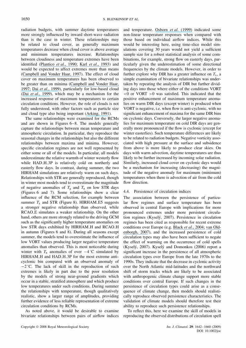
The same relationships were examined for the RCMsand are shown in Figures 6–8. The models generallycapture the relationships between mean temperature andatmospheric circulation. In particular, they reproduce theseasonal changes in the relationships but also the differentrelationships between maxima and minima. However,specific circulation regimes are not well represented byeither some or all of the models. In particular, all modelsunderestimate the relative warmth of winter westerly flowwhile HAD H 3P is relatively cold on northerly andeasterly flow days. In contrast, during summer, the twoHIRHAM simulations are relatively warm on such days.Relationships with STR are generally reproduced, thoughin winter most models tend to overestimate the magnitudeof negative anomalies of Tg and Tn on low STR days(Figures 6 and 7). Some relationships show a clearinfluence of the RCM selection, for example betweensummer Tx and STR (Figure 8). HIRHAM E5 suggestsa stronger negative relationship than observed, whileRCAO E simulates a weaker relationship. On the otherhand, others are more strongly related to the driving GCMsuch as the significantly higher temperature anomalies onlow STR days exhibited by HIRHAM H and RCAO Hin autumn (Figures 6 and 8). During all seasons exceptsummer, the models tend to overestimate the influence oflow VORT values producing larger negative temperatureanomalies than observed. This is most noticeable duringwinter with Tn anomalies of over −4 °C simulated byHIRHAM H and HAD H 3P for the most extreme anti-cyclonic bin compared with an observed anomaly of−2 °C. The lack of skill in the reproduction of suchextremes is likely in part due to the poor resolutionby the models of strong near-ground gradients whichoccur in a stable, stratified atmosphere and which producelow temperatures under such conditions. During summerthe relationships with temperature, though qualitativelyrealistic, show a larger range of amplitudes, providingfurther evidence of less reliable representation of extremecirculation conditions by RCMs.

As noted above, it would be desirable to examinebivariate relationships between pairs of airflow indices

and temperature. Osborn et al. (1999) indicated somenon-linear temperature responses when compared withthose based on individual airflow indices. While thiswould be interesting here, using time-slice model sim-ulations covering 30 years would not yield a sufficientsample size for a robust statistical analysis of some com-binations, for example, strong flow on easterly days, par-ticularly given the underestimation of some directionalfrequencies by the climate models. However, in order tofurther explore why DIR has a greater influence on Tx, asimple examination of bivariate relationships was under-taken by repeating the analysis of DIR but further divid-ing days into those where either of the conditions VORT<0 or VORT >0 was satisfied. This indicated that thepositive enhancement of maximum temperature anoma-lies on warm DIR days (except winter) is produced whenVORT is negative, i.e. when flow is anti-cyclonic, with nosignificant enhancement of maxima for the same DIR binson cyclonic days. Conversely, the larger negative anoma-lies for maximum temperature on cold DIR days are gen-erally more pronounced if the flow is cyclonic (except forwinter easterlies). Such temperature differences are likelyto be related to radiation budgets. Negative vorticity asso-ciated with high pressure at the surface and subsidencefrom above is more likely to produce clear skies. Ondays with warm advection, daytime temperatures are thuslikely to be further increased by incoming solar radiation.Similarly, increased cloud cover on cyclonic days wouldbe a mechanism for increasing (decreasing) the magni-tude of the negative anomaly for maximum (minimum)temperatures when there is advection of air from the coldflow direction.

4.4. Persistence of circulation indices

The association between the persistence of particu-lar flow regimes and surface temperature has beenobserved in central Europe with implications for morepronounced extremes under more persistent circula-tion regimes (Kysely, 2007). Persistence in circulationregimes has been cited as responsible for recent extremeconditions over Europe (e.g. Black et al., 2004; van Old-enborgh, 2007), and the increased persistence of coldcirculation types may also have been sufficient to negatethe effect of warming on the occurrence of cold spells(Kysely, 2007). Kysely and Domonkos (2006) report asignificant increase in the persistence of all atmosphericcirculation types over Europe from the late 1970s to the1990s. They indicate that the decrease in cyclonic activityover the North Atlantic mid-latitudes and the northwardshift of storm tracks which are likely to be associatedwith anthropogenic climate change support more stableconditions over central Europe. If such changes in thepersistence of circulation types could arise as a conse-quence of climate change, then models should realisti-cally reproduce observed persistence characteristics. Thevalidation of climate models should therefore test theirability to reproduce such persistence relationships.

To reflect this, here we examine the skill of models inreproducing the observed distributions of circulation spell

Copyright 2008 Royal Meteorological Society Int. J. Climatol. 29: 1642–1660 (2009)DOI: 10.1002/joc

OBSERVED AND MODELLED CIRCULATION–TEMPERATURE RELATIONSHIPS 1651

Figure 6. Mean daily temperature anomaly for Tg on days falling into each airflow index bin over the period 1961–1990 for observed dataand RCM simulations. The shading represents the uncertainty of the sample mean for the observed data as defined in Figure 2. Means are only

calculated for bins with a sample of at least 20 days.

frequencies and the influence of these on temperature.Two types of spells are examined, firstly those of specificdirectional types based solely on DIR. Because flowfrom some directions occurs relatively infrequently, thedaily DIR values were grouped into classes of severalcombined DIR bins in order to ensure a sufficient samplesize for statistical analysis. Thus, for example, easterlyflow days are less frequent than westerly days and so agreater range of bins is used to represent these days. The

bin groupings used to define four directional types aredescribed in the caption for Figure 9. Secondly, spellsof anti-cyclonic and cyclonic regimes are also studied.These regimes are defined by the pure anti-cyclonic andcyclonic types of Jenkinson and Collison (1977). Thesetypes occur on days where |VORT| > 2STR. Pure anti-cyclonic (cyclonic) types are thus days where the abovecondition is satisfied and VORT is negative (positive).The position of each day within a sequence of each

Copyright 2008 Royal Meteorological Society Int. J. Climatol. 29: 1642–1660 (2009)DOI: 10.1002/joc

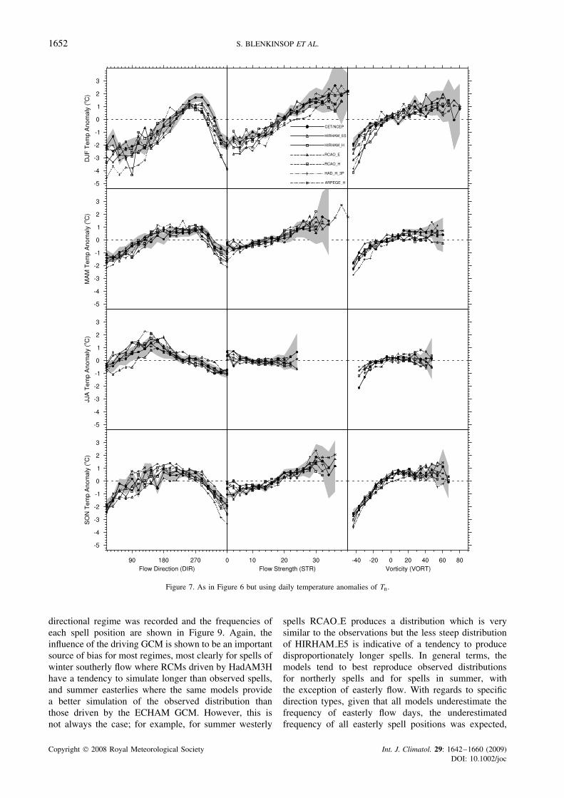
1652 S. BLENKINSOP ET AL.

Figure 7. As in Figure 6 but using daily temperature anomalies of Tn.

directional regime was recorded and the frequencies ofeach spell position are shown in Figure 9. Again, theinfluence of the driving GCM is shown to be an importantsource of bias for most regimes, most clearly for spells ofwinter southerly flow where RCMs driven by HadAM3Hhave a tendency to simulate longer than observed spells,and summer easterlies where the same models providea better simulation of the observed distribution thanthose driven by the ECHAM GCM. However, this isnot always the case; for example, for summer westerly

spells RCAO E produces a distribution which is verysimilar to the observations but the less steep distributionof HIRHAM E5 is indicative of a tendency to producedisproportionately longer spells. In general terms, themodels tend to best reproduce observed distributionsfor northerly spells and for spells in summer, withthe exception of easterly flow. With regards to specificdirection types, given that all models underestimate thefrequency of easterly flow days, the underestimatedfrequency of all easterly spell positions was expected,

Copyright 2008 Royal Meteorological Society Int. J. Climatol. 29: 1642–1660 (2009)DOI: 10.1002/joc

OBSERVED AND MODELLED CIRCULATION–TEMPERATURE RELATIONSHIPS 1653

Figure 8. As in Figure 6 but using daily temperature anomalies of Tx.

though the steeper curves do indicate a tendency for themto be disproportionately short. Broadly, reasonably resultsare observed for spells of meridional flow with all modelsnot only reproducing the absolute frequencies of northerlyand southerly spells reasonably well but in most cases,also reproducing the distribution of spell frequencies. Itis also worth noting that the overestimation of winterwesterlies by the models is manifested in terms of muchmore frequent, short to moderate spell lengths but withfewer long spells by all models except HAD H 3P. Given

the large overestimation of these days, particularly byARPEGE H, it is somewhat surprising that this does notresult in more frequent long spells and indicates thatthe model is not only poorly representing the frequencyof zonal flow but also failing to capture some of itsimportant characteristics.

The observed temperature effect of persistent circu-lation regimes is shown in Figure 10 with a significanteffect demonstrated for some spell types. Longer spells ofnortherly flow, for example, produce lower temperatures

Copyright 2008 Royal Meteorological Society Int. J. Climatol. 29: 1642–1660 (2009)DOI: 10.1002/joc

1654 S. BLENKINSOP ET AL.

Figure 9. Frequency of occurrence of spells for different direction types during winter (left) and summer (right). Northerly (N) days are definedwhen DIR is in the range 307–54° (6 bins), easterly (E) 37–144° (6 bins), southerly (S) 145–216° (4 bins) and westerly (W) 217–288° (4 bins).

in all seasons but there are seasonal differences in boththe magnitude of the temperature response and the num-ber of days required to produce the greatest response. Inwinter, by the third day of northerly flow, temperatureanomalies have reached their minimum, but in summerthe effect is smaller and is on an average reached after asequence of four days. In contrast, spells of winter east-erlies have a greater effect on temperature than northerlyflows, but longer spells are required to produce theseeffects while the warming effect of summer easterlies is

not significantly enhanced by persistent flows. Persistentsoutherly flow produces warmer temperatures through-out the year but the effect is again strongest duringwinter when temperature anomalies increase through-out the duration of a sequence of such days. Spells ofwesterlies also produce warmer temperatures through-out most of the year, particularly winter, except sum-mer when the temperature is not sensitive to the persis-tence of this type of flow. The models have limited skillin capturing these persistence–temperature relationships,

Copyright 2008 Royal Meteorological Society Int. J. Climatol. 29: 1642–1660 (2009)DOI: 10.1002/joc

OBSERVED AND MODELLED CIRCULATION–TEMPERATURE RELATIONSHIPS 1655

Figure 10. Mean daily temperature anomalies (Tg) for spell direction types. The anomaly for each type is calculated according to its position ina sequence of days of the same type. Results are presented for winter (left) and summer (right). The shaded areas are as described in Figure 2;

direction classes are as defined in Figure 9.

generally reproducing the form but not always the mag-nitude of the observations. For example, the effects of thepersistence of winter northerly flow are overestimated bymost models, while the effects of winter westerly spellsare underestimated. Other relationships are poorly rep-resented by most models, particularly that of persistentwinter southerly flow.

Persistent anti-cyclonic conditions are shown to havea negative effect on temperatures during winter and a

positive effect in summer (Figure 11) while persistentcyclonic conditions have a negative effect in winter (notshown). The models generally capture the form of theserelationships but fail to reflect the magnitude. All modelssimulate too strong a temperature response to persistentwinter anti-cyclonic regimes, with temperatures decreas-ing at over 3 times the observed rate in most cases.In summer, RCAO H, HAD H 3P and ARPEGE H doreasonably well in simulating the observed temperature

Copyright 2008 Royal Meteorological Society Int. J. Climatol. 29: 1642–1660 (2009)DOI: 10.1002/joc

1656 S. BLENKINSOP ET AL.

Figure 11. Temperature anomaly on anti-cyclonic (AC) flow days for winter (left) and summer (right). Relationships are shown for Tg but forsummer the upper and lower CET/NCEP relationships represent those for Tx and Tn respectively. The shaded areas are as described in Figure 2.

increase but the other models produce a stronger tem-perature response. During summer the observed responseof maximum temperatures is greater than that of mini-mum temperatures (Figure 11, right). This may be dueto feedbacks between soil moisture and the atmosphere.Brabson et al. (2005) demonstrated that an increase inhot spells may be partly due to extended periods of lowsoil moisture. Soil moisture is likely to decrease as dryanti-cyclonic conditions persist, especially in summer,resulting in the use of less heat for surface evaporation.Though not shown here, the models do generally repro-duce this temperature response – though the magnitudeagain varies depending upon RCM selection.

5. Discussion and conclusions

This study used seven RCMs from the PRUDENCE suiteof model simulations for the 1961–1990 control periodand demonstrated that although they are able to repro-duce the form and magnitude of the annual cycle oftemperature for the central England region, significantbiases in monthly means are apparent. All of the modelsexamined here overestimate temperatures during winterwhile the RCAO and ARPEGE H simulations are alsounable to reproduce the magnitude of summer maxima.Only HAD H 3P reasonably captures the mean temper-ature range. RCM selection thus introduces considerableuncertainties into regional temperature simulations. TheRMSE statistics calculated for all grid cells in the regionindicate that the relative size of model errors varies notonly between models but also internally for each modelthroughout the year and between daily extremes. Thereis thus no model which fully reproduces all aspects ofregional temperatures and could be described as ‘best’.Similar conclusions have been derived for mean UK pre-cipitation. Blenkinsop and Fowler (2007) noted that therelative skill of six of the same RCMs varies throughoutthe year and also spatially across the UK. Furthermore,

the models display different relative skills in captur-ing precipitation occurrence and intensity. Fowler et al.(2007a) have also noted that HAD H which has a drybias in mean precipitation has the greatest relative skillfor extremes.

Model simulations of the frequencies of three airflowindices representing the atmospheric circulation producedistributions which qualitatively reflect those obtainedfrom re-analysis data, including the changing seasonaldistributions of flow regimes, but which are statisticallysignificantly different. Of most concern are winter simu-lations, with all models overestimating the frequency ofdays with westerly/cyclonic flow characteristics. Apply-ing the same indices to a suite of models has indicated therelative extent of this problem with ARPEGE H notice-ably worse than the other models. The model biases inwinter temperature simulations are likely to be in partattributable to these errors in regional atmospheric circu-lation. However, errors in the simulation of DIR do nottranslate directly into errors in the simulation of surfacetemperature; despite the large overestimation of westerlyflow days by ARPEGE H, it has relatively small errorsin the simulation of mean temperature compared to othermodels.

Examining the modelled relationships between theairflow indices and temperature indicates that furthertemperature biases arise from the RCM simulations.Although the models reproduce the general relationshipsbetween the atmospheric circulation and near-surfacetemperature, they have the most difficulty in reproduc-ing the relationships at extreme values of the STR andVORT indices and the relationships with the DIR indexduring winter and summer. This could have a signifi-cant effect when considering the relationship between theatmospheric circulation and extreme temperature events.To demonstrate this, extreme cold events, as defined bythose days where the temperature anomaly relative tothe 30-year mean is less than the 10th percentile daily

Copyright 2008 Royal Meteorological Society Int. J. Climatol. 29: 1642–1660 (2009)DOI: 10.1002/joc

OBSERVED AND MODELLED CIRCULATION–TEMPERATURE RELATIONSHIPS 1657

temperature anomaly, were identified using the daily min-imum series for both the observed data and HAD H 3Psimulation. This model was selected because it has largeerrors in the temperature relationships with DIR andVORT at the part of the distribution producing the lowesttemperature anomalies. For this purpose, percentiles werecalculated using the method described by Horton et al.(2001). Figure 12 indicates significant differences in therelationships between the DIR and VORT indices andthe probability of an extreme cold event. The probabilityof such an event may be twice as likely on a northerlyflow day with HAD H 3P while the relationship on anti-cyclonic days is also poorly reproduced. This poorlyrepresented relationship not only indicates deficienciesin model dynamics but could also limit the application ofdynamically downscaled RCM output to studies of someclimate change impacts. For example, given the more per-sistent nature of some anti-cyclonic systems, the greaterprobability of simulated extremes on these days may leadto biases in the simulation of cold spell characteristics.

The boundary conditions provided by adopting differ-ent driving GCMs are a major source of uncertainty inthe simulation of the occurrence of circulation regimes.Biases in simulated monthly means, however, are morestrongly influenced by RCM selection than by GCM-induced biases in circulation frequencies. The same isalso true of the circulation–temperature relationship; forexample, during summer there are large differences inthe DIR- and STR-temperature relationships simulatedby HIRHAM E and RCAO E.

This study has highlighted a number of implications forthe application of statistical downscaling techniques inthis region where such methods apply functions betweenthe large-scale circulation and local-scale climate vari-ables. In addition to biases in the frequencies of simulatedflow regimes, the observed persistence of some circu-lation regimes has been demonstrated to exert a stronginfluence on the relationship between some directionaltypes and temperature, particularly in winter. This may be

due to the advection of cold/warm air which consequentlyleads to an increase in the magnitude of the temperatureanomaly as those conditions persist. Failing to considerthe effects of persistence could lead to an underesti-mation of the frequency and magnitude of temperatureextremes and in turn to an underestimation of spells ofsuch events, particularly if a change in the persistenceof certain regimes is considered a potential symptom ofclimate change (Kysely and Domonkos, 2006). Most ofthe RCM simulations examined here capture the formof these persistence relationships, though the magnitudeof the relationship is not always accurately reproduced.This suggests the failure of climate models to representimportant atmospheric processes which could be associ-ated with significant future impacts such as heat waves.

Given the uncertainties in model simulation of thesefeatures, and of the other climatic properties examinedhere, the use of multi-model ensembles is consideredessential in generating future scenarios of events suchas heat waves. Any exercise that is based on only oneclimate model is constrained by its ability to reproduceobserved circulation frequency and persistence. It is nowwidely appreciated that the production of climate changescenarios should not be restricted to only one model(e.g. Raisanen, 1997; Raisanen and Palmer, 2001; Fowleret al., 2007b; Tebaldi and Knutti, 2007) and multi-modelensembles are now being applied for use in climatechange impacts studies (e.g. Fronzek and Carter, 2007).Such approaches enable the uncertainties inherent inthe use of RCM output for generating climate changeimpacts scenarios to be highlighted. For example, Pryoret al. (2005) indicate that the differences between near-surface wind fields for the Baltic region derived in climatechange projections are of a magnitude similar to thedifferences between RCAO fields and re-analysis datafor the control period. Blenkinsop and Fowler (2007) usethe same PRUDENCE simulations as this study to deriveprojections of future characteristics of meteorologicaldrought occurrence across the UK, finding that for most

Figure 12. Observed and modelled probabilities for HAD H 3P of extreme cold events defined by 10th percentile minimum temperature anomalies.Relationships are shown with DIR (left) and VORT (right) for winter. The shaded areas represent the 95% confidence intervals as calculated in

Figure 4.

Copyright 2008 Royal Meteorological Society Int. J. Climatol. 29: 1642–1660 (2009)DOI: 10.1002/joc

1658 S. BLENKINSOP ET AL.

areas the uncertainty in the frequency of long durationdroughts encompasses the direction of change. Fowleret al. (2007a) undertook a comparable study of regionalUK precipitation extremes but additionally producedmulti-model ensemble projections of change to indicatethe uncertainties in RCM simulations.

Raisanen (2007), in reviewing assessments of modelreliability, raises the questions of how well a modelshould mimic reality to be believed in and which aspectsare most important. He indicates that the lack of a gener-ally accepted figure of merit for measuring model per-formance makes the ranking of models difficult. Thisis almost certainly the case but any ranking of mod-els should not only be based on reproducing climaticcharacteristics important for the application but shouldalso be used with care and not for the selection of onemodel. Rather, such metrics would be best employed astools for the weighting of climate models in the gener-ation of probabilistic future scenarios. It may be arguedthat for climate variables that are strongly coupled to theregional atmospheric circulation, any skill in reproducingobserved statistics that is not supported by skill in repro-ducing the observed circulation regime is achieved with-out adequately capturing the physical mechanisms thatdetermine the climate. Thus, simulations of future climatecould not be viewed with a great degree of confidence. Ingenerating climate change scenarios for the Netherlands,van den Hurk et al. (2007) eliminated GCMs which dis-played systematic biases in surface pressure and circu-lation patterns (van Ulden and van Oldenborgh, 2006).However, Raisanen (2007) also highlights the lack ofevidence that models that simulate present-day climatepoorly produce outliers in terms of future temperaturechange. The exclusion of models on the basis of theirsimulation of current climate is therefore likely to leadto an underestimation of uncertainty in future scenar-ios. This is particularly important if using some repre-sentation of the atmospheric circulation given that therelationship between large-scale circulation patterns andregional climates are characterized by substantial non-stationarity (Slonosky et al., 2001; Beck et al., 2007).Nonetheless, consideration of how well models reproduceatmospheric circulation regimes and their relationshipswith surface climate offers potential in not only under-standing the source of errors in those models but alsoprovides insights into the appropriate choice of predictorsfor statistical downscaling, most notably, the inclusionof persistence when considering impacts associated withextreme events.

Acknowledgements

Some of this work was part of a PhD studentship fundedby the School of Environmental Sciences, Universityof East Anglia (UEA), Norwich. Thanks for supervi-sion are extended to Phil Jones, Tim Osborn and SteveDorling of the UEA, and to Hayley Fowler of New-castle University for useful comments and the develop-ment of ideas within the AquaTerra project. The NCEP

re-analysis data are available to download from theNOAA-CIRES Climate Diagnostics Center website athttp://www.cdc.noaa.gov/cdc/reanalysis/reanalysis.shtml.PRUDENCE models data may be obtained from http://prudence.dmi.dk/. CRU dataset TS 2.0 was made avail-able by the Climatic Research Unit, University ofEast Anglia. Further details may be obtained fromhttp://www.cru.uea.ac.uk/∼timm/grid/CRU TS 2 0.html.

A1. Appendix

A1.1. Airflow indices

Each of the indices is calculated using a network of 16grid points as shown in Figure 1.

• The westerly flow (w) is the westerly (zonal) compo-nent of the geostrophic surface wind calculated as thepressure gradient between 50 °N and 60 °N.

w = 1

2(12 + 13) − 1

2(4 + 5) (A1)

• The southerly flow (s) is the southerly (meridional)component of the geostrophic surface wind and is thepressure gradient between 10 °W and 0°.

s = 1.74[

1

4(5 + 2 × 9 + 13) − 1

4(4 + 2 × 8 + 12)

]

(A2)

• The resultant flow (f ) strength is the total resultantwesterly and southerly flow.

f = (s2 + w2)12 (A3)

• The westerly shear vorticity (zw ) is the difference ofthe westerly flow between 45 °N and 55 °N minus thatbetween 55 °N and 65 °N and represents the meridionalgradient of w.

zw = 1.07[

1

2(15 + 16) − 1

2(8 + 9)

]

− 0.95[

1

2(8 + 9) − 1

2(1 + 2)

](A4)

• The southerly shear vorticity (zs) is the difference ofthe southerly flow between 10 °E and 0° minus thatbetween 10 °W and 20 °W and is the zonal gradientof s.

zs = 1.52[

1

4(6 + 2 × 10 + 14) − 1

4(5 + 2 × 9 + 13)

−1

4(4 + 2 × 8 + 12) + 1

4(3 + 2 × 7 + 11)

](A5)

• The total shear vorticity (z) is the sum of the westerlyand southerly vorticity.

z = zw + zs (A6)

Copyright 2008 Royal Meteorological Society Int. J. Climatol. 29: 1642–1660 (2009)DOI: 10.1002/joc

OBSERVED AND MODELLED CIRCULATION–TEMPERATURE RELATIONSHIPS 1659

The constants used in these equations reflect thediffering sizes of the grid cells at each latitude. The STRand VORT indices referred to in the paper are calculatedfrom Equations (A3) and (A6) respectively. The directionof flow (DIR) is calculated as tan−1(w/s) with 180°

added if w is positive.

A1.2. Confidence intervals

Confidence intervals (CI) of observed mean statisticsare calculated using the method described by Osbornet al. (1999). As sample means of daily temperaturesare approximately normally distributed, the Student’s t

distribution may be used to calculate CI for each flowbin using the following equation:

CI = x ± tα/2,df × s√n

(A7)

where x is the sample mean, and tα/2,df is the t valueassociated with the required confidence level and binsample size (von Storch and Zwiers, 1999). The samplestandard deviation is denoted by s, and the bin samplesize by n.

CI for proportions are calculated using the Gaussianapproximation to the binomial distribution. The CI iscalculated as described by Wilks (1995):

CI = p ± zα/2 ×√

p(1 − p)

n(A8)

where p is the sample proportion which is the bestestimate of the binomial event probability π , za/2 is thez value associated with the desired confidence level, andn is the sample size.

References

Arking A. 1991. The radiative effects of clouds and their impacton climate. Bulletin of the American Meteorological Society 71:795–813.

Bardossy A, Filiz F. 2005. Identification of flood producingatmospheric circulation patterns. Journal of Hydrology 313: 48–57.

Beck C, Jacobeit J, Jones PD. 2007. Frequency and within-typevariations of large-scale circulation types and their effects onlow-frequency climate variability in Central Europe since 1780.International Journal of Climatology 27: 473–491.

Black E, Blackburn M, Harrison G, Hoskins B, Methven J. 2004.Factors contributing to the summer 2003 European heatwave.Weather 59: 217–223.

Blenkinsop S. 2005. Extreme daily temperature and precipitationevents in north western Europe and the role of atmosphericcirculation, Unpublished PhD thesis, University of East Anglia.

Blenkinsop S, Fowler HJ. 2007. Changes in drought frequency andseverity over the British Isles projected by the PRUDENCE regionalclimate models. Journal of Hydrology 342: 50–71.

Brabson BB, Lister DH, Jones PD, Palutikof JP. 2005. Soil moistureand predicted spells of extreme temperatures in Britain.Journal of Geophysical Research 110: 1–9, D05104, doi10.1029/2004JD005156.

Brabson BB, Palutikof J. 2002. The evolution of extreme temperaturesin the Central England temperature record. Geophysical ResearchLetters 29: 2163.

Campbell GG, Vonder Haar TH. 1997. Comparison of surfacetemperature minimum and maximum and satellite measuredcloudiness and radiation budget. Journal of Geophysical Research102: 16639–16645.

Chen D. 2000. A monthly circulation climatology for Sweden and itsapplication to a winter temperature case study. International Journalof Climatology 20: 1067–1076.

Christensen JH, Carter TR, Rummukainen M, Amanatidis G. 2007.Evaluating the performance and utility of regional climate models:the PRUDENCE project. Climatic Change 81(Supplement 1): 1–6.

Christensen JH, Christensen OB, Lopez P, van Meijgaard E, Botzet M.1996. The HIRHAM4 Regional Atmospheric Climate Model,Scientific Report 96-4, 51, Available from DMI, Lyngbyvej 100,Copenhagen Ø.

Christensen OB, Christensen JH, Machenhauer B, Botzet M. 1998.Very high-resolution regional climate simulations over Scandinavia:present climate. Journal of Climate 11: 3204–3229.

Christensen JH, Christensen OB, Schultz JP. 2001. High resolutionphysiographic data set for HIRHAM4: An application to a 50 kmhorizontal resolution domain covering Europe, DMI Technical Report01–15, Available from DMI, Lyngbyvej 100, Copenhagen Ø.

D’Andrea F, Tibaldi S, Blackburn M, Boer G, Deque M, Dix MR,Dugas B, Ferranti L, Iwasaki T, Kitoh A, Pope V, Randall D,Roeckner E, Strauss D, Stern W, Van den Dool H, Williamson D.1998. Northern Hemisphere atmospheric blocking as simulated by15 atmospheric general circulation models in the period 1979–1988.Climate Dynamics 14: 385–407.

Dai A, Trenberth KE, Karl TR. 1999. Effects of clouds, soil moisture,precipitation, and water vapour on diurnal temperature range.Journal of Climate 12: 2451–2473.

Della-Marta PM, Luterbacher J, Weissenfluh H, Xoplaki E, Brunet M,Wanner H. 2007. Summer heat waves over western Europe1990–2003, their relationship to large-scale forcings and predictabil-ity. Climate Dynamics 29: 251–275.

Deque M, Marquet P, Jones RG. 1998. Simulation of climate changeover Europe using a global variable resolution general circulationmodel. Climate Dynamics 14: 173–189.

Esteban P, Martin-Vide J, Mases M. 2006. Daily atmosphericcirculation catalogue for western Europe using multivariatetechniques. International Journal of Climatology 26: 1501–1515.

Fowler HJ, Blenkinsop S, Tebaldi C. 2007b. Linking climate changemodelling to impacts studies: recent advances in downscalingtechniques for hydrological modelling. International Journal ofClimatology 27: 1547–1578.

Fowler HJ, Ekstrom M, Blenkinsop S, Smith AP. 2007a. Estimatingchange in extreme European precipitation using a multi-modelensemble. Journal of Geophysical Research-Atmospheres 112:D18104, DOI:10.1029/2007JD008619.

Fowler HJ, Kilsby CG. 2002. A weather-type approach to analysingwater resource drought in the Yorkshire region from 1881 to 1998.Journal of Hydrology 262: 177–192.

Fronzek S, Carter TR. 2007. Assessing uncertainties in climate changeimpacts on resource potential for Europe based on projections fromRCMs and GCMs. Climatic Change 81: 357–371.

Goodess CM, Jones PD. 2002. Links between circulation and changesin the characteristics of Iberian rainfall. International Journal ofClimatology 22: 1593–1615.

Hagemann S, Botzet M, Machenhauer B. 2001. The summer dryingproblem over south-eastern Europe: sensitivity of the limited areamodel HIRHAM4 to improvements in physical parametrization andresolution. Physics and Chemistry of the Earth Part B 26: 391–396.

Horton EB, Folland CK, Parker DE. 2001. The changing incidence ofextremes in worldwide and Central England Temperatures to the endof the twentieth century. Climatic Change 50: 267–295.

Hudson DA, Jones RG. 2002. Regional climate model simulations ofpresent-day and future climates of southern Africa, Hadley CentreTechnical Note No 39, Met. Office, Exeter.

Jacob D, Barring L, Christensen OB, Christensen JH, de Castro M,Deque M, Giorgi F, Hagemann S, Hirschi M, Jones R, Kjell-strom E, Lenderink G, Rockel B, Sanchez E, Schar C, Senevi-ratne SI, Somot S, van Ulden A, van den Hurk B. 2007. An inter-comparison of regional climate models for Europe: model perfor-mance in present-day climate. Climatic Change 81: 31–52.

James PM. 2006. An assessment of European synoptic variability inHadley Centre Global Environmental models based on an objectiveclassification of weather regimes. Climate Dynamics 27: 215–231.

James PM. 2007. An objective classification method for Hess andBrezowsky Grosswetterlagen over Europe. Theoretical and AppliedClimatology 88: 17–42.

Jenkinson AF, Collison FP. 1977. An initial climatology of gales overthe North Sea, Synoptic Climatology Branch Memorandum No. 62,Meteorological Office, Bracknell.

Copyright 2008 Royal Meteorological Society Int. J. Climatol. 29: 1642–1660 (2009)DOI: 10.1002/joc

1660 S. BLENKINSOP ET AL.

Jones PD. 1987. The early twentieth century Arctic high – fact orfiction? Climate Dynamics 1: 63–75.

Jones PD, Hulme M, Briffa KR. 1993. A comparison of Lamb circu-lation types with an objective classification scheme. InternationalJournal of Climatology 13: 655–663.

Jones RG, Noguer M, Hassell DC, Hudson D, Wilson SS, Jenkins GJ,Mitchell JFB. 2004b. Generating high resolution climate changescenarios using PRECIS, 35, Tech. report available from Met. Office,Hadley Centre, Exeter.

Jones CG, Ullerstig A, Willen U, Hansson U. 2004a. The RossbyCentre regional atmospheric climate model (RCA). Part I: Modelclimatology and performance characteristics for present climate overEurope. Ambio 33: 199–210.

Kalnay E, Kanamitsu M, Kistler R, Collins W, Deavan D,Iredell M, Saha S, White G, Woolen J, Zhu Y, Leetmaa A,Reynolds R, Chelliah M, Ebisuzaki W, Higgins W, Janowiak H,Mo KC, Ropelewski C, Wang J, Jenne R, Joseph D. 1996. TheNCEP/NCAR 40-year reanalysis project. Bulletin of the AmericanMeteorological Society 77: 437–471.

Karl TR, Jones PD, Knight RW, Kukla G, Plummer N, Razuvayev V,Gallo KP, Lindseay J, Charlson R, Peterson TC. 1993. Asymmetrictrends of daily maximum and minimum temperature. Bulletin of theAmerican Meteorological Society 74: 1007–1023.

Kysely J. 2007. Implications of enhanced persistence of atmosphericcirculation for the occurrence and severity of temperature extremes.International Journal of Climatology 27: 689–695.

Kysely J, Domonkos P. 2006. Recent increase in persistence ofatmospheric circulation over Europe: Comparison with long-termvariations since 1881. International Journal of Climatology 26:461–483.

Lamb HH. 1972. British Isles weather types and a register of thedaily sequence of circulation patterns 1861–1971, Geophys. Memoir.No.116, 85, HMSO for Met. Office.

Linderson M. 2001. Objective classification of atmospheric circulationover southern Scandinavia. International Journal of Climatology 21:155–169.

McGregor GR, Phillips ID. 2004. Specification and prediction ofmonthly and seasonal rainfall over the south-west peninsula ofEngland. Quarterly Journal of the Royal Meteorological Society 130:193–210.

Manley G. 1953. The mean temperature of central England, 1698 to1952. Quarterly Journal of the Royal Meteorological Society 79:242–261.

Manley G. 1974. Central England temperatures: Monthly means 1659to 1973. Quarterly Journal of the Royal Meteorological Society 100:389–405.

Meier HEM, Doscher R, Faxen T. 2003. A multiprocessor coupled ice-ocean model for the Baltic Sea. application to the salt inflow. Journalof Geophysical Research 108: 3273, DOI:10.1029/2000JC000521.

Mitchell TD, Carter TR, Jones PD, Hulme M, New M. 2004. Acomprehensive set of high-resolution grids of monthly climatefor Europe and the globe: the observed record (1901–2000) and16 scenarios, Tyndall Working Paper 55, Tyndall Centre, UEA,Norwich.

New M, Hulme M, Jones PD. 1999a. Representing twentieth-centuryspace-time climate variability. Part I: Development of a 1961-90 mean monthly terrestrial climatology. Journal of Climate 12:829–856.

New M, Hulme M, Jones PD. 1999b. Representing twentieth-centuryspace-time climate variability. Part II: Development of 1901–1996monthly grids of terrestrial surface climate. Journal of Climate 13:2217–2238.

Osborn TJ, Conway D, Hulme M, Gregory JM, Jones PD. 1999. Airflow influences on local climate: observed and simulated meanrelationships for the United Kingdom. Climate Research 13:173–191.

Osborn TJ, Jones PD. 2000. Air flow influences on local climate:observed United Kingdom climate variations. Atmospheric ScienceLetters 1: 62–74, DOI:10.1006/asle.2000.0017.

Parker DE, Legg TP, Folland CK. 1992. A new daily centralEngland temperature series. International Journal of Climatology 12:317–342.

Pelly JL, Hoskins BJ. 2003. A new perspective on blocking. Journalof the Atmospheric Sciences 60: 743–755.

Plantico MS, Karl TR, Kukla G, Gavin J. 1990. Is recent climatechange across the United States related to rising levels ofanthropogenic greenhouse gases? Journal of Geophysical Research95: 16617–16637.

Pryor SC, Barthelmie RJ, Kjellstrom E. 2005. Potential climate changeimpact on wind energy resources in northern Europe: analyses usinga regional climate model. Climate Dynamics 25: 815–835.

Raisanen J. 1997. Objective comparison of patterns of CO2 inducedclimate change in coupled GCM experiments. Climate Dynamics13: 197–211.

Raisanen J. 2007. How reliable are climate models? Tellus 59A: 2–29.Raisanen J, Palmer TN. 2001. A probability and decision-model

analysis of a multimodel ensemble of climate change simulations.Journal of Climate 14: 3212–3226.

Reid PA, Jones PD, Brown O, Goodess CM, Davies TD. 2001.Assessments of the reliability of NCEP circulation data and relationships with surface climate by direct comparison with station baseddata. Climate Research 17: 247–261.

Roeckner E, Bauml G, Bonaventura L, Brokopf R, Esch M,Giorgetta M, Hagemann S, Kirchner I, Kornblueh L, Manzini E,Rhodin A, Schlese U, Schulzweida U, Tompkins A. 2003. Theatmospheric general circulation model ECHAM5. Report No. 349.Part I: model description. Max Planck-Institute for Meteorology:Hamberg.

Slonosky VC, Jones PD, Davies TD. 2001. Atmospheric circulationand surface temperature in Europe from the 18th century to 1995.International Journal of Climatology 21: 63–75.

Tebaldi C, Knutti R. 2007. The use of the multi-model ensemble inprobabilistic climate projections. Philosophical Transactions of theRoyal Society A 365: 2053–2075.

Turnpenny JR, Crossley JF, Hulme M, Osborn TJ. 2002. Air flowinfluences on local climate: comparison of a regional climate modelwith observations over the United Kingdom. Climate Research 20:189–202.

van den Hurk BJJM, van den Klein Tank AMG, Lenderink G, vanUlden AP, van Oldenborgh GJ, Katsman CA, van den Brink HW,Keller F, Bessembinder JJF, Burgers G, Komen GJ, Hazeleger W,Drijfhout SS. 2007. New climate change scenarios for theNetherlands. Water Science and Technology 56: 27–33.

van Oldenborgh GJ. 2007. How unusual was autumn 2006 in Europe?Climate of the Past Discussions 3: 811–837.

van Oldenborgh GJ, van Ulden A. 2003. On the relationship betweenglobal warming, local warming in the netherlands and changes in the20th century. International Journal of Climatology 23: 1711–1725.

von Storch H, Zwiers FW. 1999. Statistical Analysis in ClimateResearch. Cambridge University Press: Cambridge.

van Ulden AP, van Oldenborgh GJ. 2006. Large-scale atmosphericcirculation biases and changes in global climate model simulationsand their importance for climate change in Central Europe.Atmospheric Chemistry and Physics 6: 863–881.

van Ulden A, Leberink G, van den Hurk B, van Meijgaard E. 2007.Circulation statistics and climate change in Central Europe:PRUDENCE simulations and observations. Climatic Change 81:179–192.

Wilby RL, Harris I. 2006. A framework for assessing uncertaintiesin climate change impacts: low flow scenarios for theRiver Thames, UK. Water Resources Research 42: W02419,DOI:10.1029/2005WR004065.

Wilks DS. 1995. Statistical Methods in the Atmospheric Sciences.Academic Press: San Diego.

Copyright 2008 Royal Meteorological Society Int. J. Climatol. 29: 1642–1660 (2009)DOI: 10.1002/joc