Divergences test statistics for discretely observed diffusion processes
27
Divergences Test Statistics for Discretely Observed Diffusion Processes Alessandro De Gregorio a , Stefano M. Iacus b,* a Department of Statistics, Probability and Applied Statistics P.le Aldo Moro 5, 00185 Rome-Italy, Email: [email protected] b Department of Economics, Business and Statistics Via Conservatorio 7, 20124 Mlan-Italy, Email: [email protected] Abstract In this paper we propose the use of φ-divergences as test statistics to ver- ify simple hypotheses about a one-dimensional parametric diffusion process dX t = b(X t ,θ)dt+σ(X t ,θ)dW t , from discrete observations {X t i ,i =0,...,n} with t i = iΔ n , i =0, 1,...,n, under the asymptotic scheme Δ n → 0, nΔ n →∞ and nΔ 2 n → 0. The class of φ-divergences is wide and in- cludes several special members like Kullback-Leibler, R´ enyi, power and α- divergences. We derive the asymptotic distribution of the test statistics based on φ-divergences. The limiting law takes different forms depending on the regularity of φ. These convergence differ from the classical results for inde- pendent and identically distributed random variables. Numerical analysis is used to show the small sample properties of the test statistics in terms of estimated level and power of the test. Key words: diffusion processes, empirical level, hypotheses testing, φ-divergences, α-divergences 1. Introduction We consider the problem of parametric testing using φ-divergences. Let X be a r.v. and f (X, θ) and g(X, θ), θ ∈ Θ two families of probability densities on the same measurable space. The φ-divergences are defined as D φ (f,g)= E θ φ (f (X )/g(X )), where E θ is the expected value with respect to * Corresponding author Preprint submitted to Elsevier August 12, 2008
Transcript of Divergences test statistics for discretely observed diffusion processes

Divergences Test Statistics for Discretely Observed
Diffusion Processes
Alessandro De Gregorioa, Stefano M. Iacusb,∗
aDepartment of Statistics, Probability and Applied StatisticsP.le Aldo Moro 5, 00185 Rome-Italy, Email: [email protected]
bDepartment of Economics, Business and StatisticsVia Conservatorio 7, 20124 Mlan-Italy, Email: [email protected]
Abstract
In this paper we propose the use of φ-divergences as test statistics to ver-ify simple hypotheses about a one-dimensional parametric diffusion processdXt = b(Xt, θ)dt+σ(Xt, θ)dWt, from discrete observations {Xti , i = 0, . . . , n}with ti = i∆n, i = 0, 1, . . . , n, under the asymptotic scheme ∆n → 0,n∆n → ∞ and n∆2
n → 0. The class of φ-divergences is wide and in-cludes several special members like Kullback-Leibler, Renyi, power and α-divergences. We derive the asymptotic distribution of the test statistics basedon φ-divergences. The limiting law takes different forms depending on theregularity of φ. These convergence differ from the classical results for inde-pendent and identically distributed random variables. Numerical analysis isused to show the small sample properties of the test statistics in terms ofestimated level and power of the test.
Key words: diffusion processes, empirical level, hypotheses testing,φ-divergences, α-divergences
1. Introduction
We consider the problem of parametric testing using φ-divergences. LetX be a r.v. and f(X, θ) and g(X, θ), θ ∈ Θ two families of probabilitydensities on the same measurable space. The φ-divergences are defined asDφ(f, g) = Eθφ (f(X)/g(X)), where Eθ is the expected value with respect to
∗Corresponding author
Preprint submitted to Elsevier August 12, 2008

Pθ, the true law of the observations. Because we focus the attention on theuse of divergences for hypotheses testing, we will use a simplified notation:let θ and θ0 two points in the interior of Θ and define the divergence as
Dφ(θ, θ0) = Eθ0φ
(p(X, θ)
p(X, θ0)
)(1.1)
In equation (1.1) the density {p(X, θ), θ ∈ Θ} is a same family of probabil-ity densities and φ(·) is a function with the minimal property that φ(1) =0. Examples of divergences of the form Dα(θ, θ0) = Dφα(θ, θ0) are the α-divergences, defined by means of the following function
φα(x) =4(1− x 1+α
2 )
1− α2, −1 < α < 1
Note that Dα(θ0, θ) = D−α(θ, θ0). The class of α-divergences has been widelystudied in statistics (see, e.g., Csiszar, 1967 and Amari, 1985) and it is afamily of divergences which includes several members of particular interest.For example, in the limit as α → −1, D−1(θ, θ0) reduces to the well-knownKullback-Leibler measure
D−1(θ, θ0) = −Eθ0 log
(p(X, θ)
p(X, θ0)
)while as α→ 0, the Hellinger distance (see, e.g., Beran, 1977, Simpson, 1989)emerges
D0(θ, θ0) =1
2E(√
p(X, θ)−√p(X, θ0)
)2
As noticed in Chandra and Taniguchi (2006), the α-divergence is also equiv-alent to the Renyi’s divergence (Renyi, 1961) defined, for α ∈ (0, 1), as
Rα(θ, θ0) =1
1− αlogEθ0
(p(X, θ)
p(X, θ0)
)αfrom which is easy to see that in the limit as α → 1, Rα reduces to theKullback-Leibler divergence. The transformation ψ(Rα) = (exp{(α−1)Rα−1}/(1−α) returns the power-divergence studied in Cressie and Read (1984).Liese and Vajda (1987) provide extensive study of a modified version ofRα and Morales et al. (1997) consider divergences with convex φ(·) for in-dependent and identically distributed (i.i.d) observations; for example the
2

power-divergences Dφλ(θ, θ0) with
φλ(x) =xλ − λ(x− 1)− 1
λ(λ− 1), λ ∈ R− {0, 1} (1.2)
In this paper we focus our attention on the φ-divergences Dφ(θ, θ0), de-fined as in (1.1), for one-dimensional ergodic diffusion process {Xt, t ∈ [0, T ]},solution of the following stochastic differential equation
dXt = b(α,Xt)dt+ σ(β,Xt)dWt, X0 = x0, (1.3)
with θ = (α, β) ∈ Θα × Θβ = Θ, Θα ⊂ Rp and Θβ ⊂ Rq. We in-dicate the discrete time observations from X as Xn = {Xti}06i6n, ti =i∆n, i = 0, 1, 2, ..., n, where ∆n is the length of the steps. The asymptoticsis ∆n → 0, n∆n →∞ and n∆2
n → 0 as n→∞. We study the properties ofthe estimated φ-divergence Dφ(θn(Xn), θ0), for discretely observed diffusion
processes, defined as Dφ(θn(Xn), θ0) = φ(fn(Xn,θn(Xn))fn(Xn,θ0)
)where fn(·, ·) is the
approximated likelihood proposed by Dacunha-Castelle and Florens-Zmirou(1986) and θn(Xn) is any consistent, asymptotically normal and efficient esti-mator of θ. We prove that, for φ(·) functions which satisfying three differentregularity conditions, the statistic Dφ converge weakly to three different func-tions of the χ2
p+q random variable. This result differs from the case of i.i.d.setting.
Up to our knowledge the only result concerning the use of divergencesfor discretely observed diffusion process is due to Rivas et al. (2005) wherethey consider the model of Brownian motion with drift dXt = adt + bdWt
where a and b are two scalars. In that case, the exact likelihood of the ob-servations is available in explicit form and is the gaussian law. Conversely,in the general setup of this paper, the likelihood of the process in (1.3)is known only for three particular stochastic differential equations, namelythe Ornstein-Uhlembeck diffusion, the geometric Brownian motion and theCox-Ingersoll-Ross model. In all other cases, the likelihood has to be approx-imated. We choose the approximation due to Dacunha-Castelle and Florens-Zmirou (1986) and, to derive a proper estimator, we use the local gaussianapproximation proposed by Yoshida (1992) although our result holds for anyconsistent and asymptotically Gaussian estimator. This approach has beensuggested by the work on Akaike Information Criteria by Uchida and Yoshida(2005).
3

For continuous time observations from diffusion processes, Vajda (1990)considered the model dX(t) = −b(t)Xtdt + σ(t)dWt; Kuchler and Sørensen(1997) and Morales et al. (2004) contain several results on the likelihoodratio test statistics and Renyi statistics for exponential family of diffusions.Explicit derivations of the Renyi information on the invariant law of ergodicdiffusion processes have been presented in De Gregorio and Iacus (2007).For small diffusion processes, with continuous time observations, informationcriteria have been derived in Uchida and Yoshida (2004) using Malliavincalculus.
The problem of testing statistical hypotheses from general diffusion pro-cesses is still a developing stream of research. Kutoyants (2004) and Dachianand Kutoyants (2008) consider the problem of testing statistical hypothesesfor ergodic diffusion models in continuous time; Kutoyants (1984) and Iacusand Kutoyants (2001) consider parametric and semiparametric hypothesestesting for small diffusion processes; Negri and Nishiyama (2007a, b) proposea non parametric test based on score marked empirical process for both con-tinuous and discrete time observation from small diffusion processes furtherextended to the ergodic case in Masuda et al. (2008). Lee and Wee (2008)considered the parametric version of the same test statistics for a simpli-fied model. Aıt-Sahalia (1996, 2008), Giet and Lubrano (2008) and Chenet al. (2008) proposed tests based on the several distances between para-metric and nonparametric estimation of the invariant density of discretelyobserved ergodic diffusion processes. The present paper complements theabove references.
The paper is organized as follows. Section 2 introduces notation and reg-ularity assumptions. Section 3 states the main result. Section 4 containsnumerical experiments to study the small sample performance of the pro-posed test statistics in terms of empirical level and empirical power undersome alternatives. The proofs are contained in Section 5.
2. Assumptions on diffusion model
We consider the family of one-dimensional diffusion processes {Xt, t ∈[0, T ]}, solution to
dXt = b(α,Xt)dt+ σ(β,Xt)dWt, X0 = x0, (2.1)
where Wt is a Brownian motion. Let θ = (α, β) ∈ Θα × Θβ = Θ, where Θα
and Θβ are respectively compact convex subset of Rp and Rq. Furthermore
4

we assume that the drift function b : R×Θα → R and the diffusion coefficientσ : R×Θβ → R are known apart from the parameters α and β. We assumethat the process Xt is ergodic for every θ with invariant law µθ. The processXt is observed at discrete times ti = i∆n, i = 0, 1, 2, ..., n, where ∆n is thelength of the steps. We indicate the observations with Xn = {Xti}06i6n. Theasymptotic is ∆n → 0, n∆n →∞ and n∆2
n → 0 as n→∞.In the definition of the φ-divergence (1.1) the likelihood of the process is
need, but as noted in the Introduction, this is usually not know. There areseveral ways to approximate the likelihood of a discretely observed diffusionprocess (for a review see, e.g., Chap. 3, Iacus, 2008). In this paper, we usethe approximation proposed by Dacunha-Castelle and Florens-Zmirou (1986)although our result hold true (with some adaptations of the proofs) for otherapproximations, like, e.g. the one based on Hermite polynomial expansionby Aıt-Sahalia (2002). To write it in explicit way, we use the same setup asin Uchida and Yoshida (2005). We introduce the following functions
s(x, β) =
∫ x
0
du
σ(β, u), B(x, θ) =
b(α, x)
σ(β, x)− σ′(β, x)
2
B(x, θ) = B(s−1(β, x), θ), h(x, θ) = B2(x, θ) + B′(x, θ)
The following set of assumptions ensure the good behaviour of the approxi-mated likelihood and the existence of a weak solution of (2.1)
Assumption 2.1. [Regularity on the process]
i) There exists a constant C such that
|b(α0, x)− b(α0, y)|+ |σ(β0, x)− σ(β0, y)| ≤ C|x− y|.
ii) infβ,x σ2(β, x) > 0.
iii) The process X is ergodic for every θ with invariant probability measureµθ. All polynomial moments of µθ are finite.
iv) For all m ≥ 0 and for all θ, suptE|Xt|m <∞.
v) For every θ, the coefficients b(α, x) and σ(β, x) are twice differentiablewith respect to x and the derivatives are polynomial growth in x, uni-formly in θ.
5

vi) The coefficients b(α, x) and σ(β, x) and all their partial derivatives re-spect to x up to order 2 are three times differentiable respect to θ for allx in the state space. All derivatives respect to θ are polynomial growthin x, uniformly in θ.
Assumption 2.2. [Regularity for the approximation]
i) h(x, θ) = O(|x|2) as x→∞.
ii) infx h(x, θ) > −∞ for all θ.
iii) supθ supx |h3(x, θ)| ≤M <∞.
iv) There exists γ > 0 such that for every θ and j = 1, 2, |Bj(x, θ)| =
O(|B(x, θ)|γ) as |x| → ∞.
Assumption 2.3. [Identifiability] The coefficients b(α, x) = b(α0, x) andσ(β, x) = σ(β0, x) for µθ0 a.s. all x then α = α0 and β = β0.
Under Assumptions 2.1 and 2.2 Dacunha-Castelle and Florens-Zmirou(1986) introduced the following approximation of transition density f of theprocess X from y to x at lag t
f(x, y, t, θ) =1√
2πtσ(y, β)exp
{−S
2(x, y, β)
2t+H(x, y, θ) + tg(x, y, θ)
}(2.2)
and its logarithm
l(x, y, t, θ) = −1
2log(2πt)− log σ(y, β)− S2(x, y, β)
2t+H(x, y, θ) + tg(x, y, θ)
where
S(x, y, β) =
∫ y
x
du
σ(u, β), H(x, y, θ) =
∫ y
x
{b(α, u)
σ2(β, u)− 1
2
σ′(β, u)
σ(β, u)
}du
g(x, y, θ) = −1
2
{C(x, θ) + C(y, θ) +
1
3B(x, θ)B(y, θ)
}C(x, θ) =
1
3B2(x, θ) +
1
2B′(x, θ)σ(x, β)
The approximated likelihood and log-likelihood functions of the observationsXn become respectively
fn(Xn, θ) =n∏i=1
f(∆n, Xti−1, Xti , θ) and ln(Xn, θ) =
n∑i=1
l(∆n, Xti−1, Xti , θ)
6

3. Construction of the test statistics and results
Consider the divergence defined in (1.1) and let φ(·) be such that φ(1) = 0and, when they exist, define Cφ = φ′(1) and Kφ = φ′′(1). We consider threedifferent setup
Assumption 3.1. Cφ 6= 0 is a finite constant depending only on φ andindependent of θ;
Assumption 3.2. Cφ = 0 and Kφ 6= 0 is a finite constant depending onlyon φ and independent of θ;
Assumption 3.3. Cφ 6= 0 and Kφ 6= 0 are finite constants depending onlyon φ and independent of θ;
Remark 3.1. The above Assumptions are not so strong. In fact, for examplethe α-divergences Dφα(θ, θ0) satisfy the Assumptions 3.1 and 3.3, while forthe power-divergences Dφλ(θ, θ0) it’s easy to verify that Cφ = φ′(1) = 0.
Clearly, the quantity Dφ(θ, θ0) measures the discrepancy between θ andthe true value of the parameter θ0 and is an ideal candidate to construct atest statistics. Let θn(Xn) be any consistent estimator of θ0 and such that
Γ−1/2(θn(Xn)− θ0)d→ N(0, I(θ0)−1) (3.1)
where I(θ0) is the positive definite and invertible Fisher information matrixat θ0 equal to
I(θ0) =
((Ikjb (θ0))k,j=1,...,p 0
0 (Ikjσ (θ0))k,j=1,...,q
)where
Ikjb (θ0) =
∫1
σ2(β0, x)
∂b(α0, x)
∂αk
∂b(α0, x)
∂αjµθ0(dx)
Ikjσ (θ0) = 2
∫1
σ2(β0, x)
∂σ(β0, x)
∂βk
∂σ(β0, x)
∂βjµθ0(dx)
We indicate with Γ the (p+ q)× (p+ q) matrix
Γ =
(1
n∆nIp 0
0 1nIq
)7

and Ip is the p × p identity matrix. Using the approximated likelihoodfn(Xn, θ) and fn(Xn, θ0), the φ-divergence in (1.1) becomes
Dφ(θ, θ0) = Eθ0φ
(fn(Xn, θ)
fn(Xn, θ0)
)(3.2)
To construct a test statistics we replace θ by the estimator θn(Xn) and,having only one single observation of Xn, i.e. only one observed trajectory,we estimate (3.2) with
Dφ(θn(Xn), θ0) = φ
(fn(Xn, θn(Xn))
fn(Xn, θ0)
)(3.3)
Please notice that, conversely to the i.i.d. case, there is no integral in thedefinition of (3.3). We will discuss this point after the presentation of theTheorem 3.1. The proposed test for testing H0 : θ = θ0 versus H1 : θ 6= θ0 isrealized as Dφ(θn(Xn), θ0) = 0 versus Dφ(θn(Xn), θ0) 6= 0.
Theorem 3.1. Under H0 : θ = θ0, Assumptions 2.1-2.3, convergence (3.1),we have that
i) if function φ(·) satisfies Assumption 3.1, then
Dφ(θn(Xn), θ0)d→ Cφχ
2p+q (3.4)
ii) if function φ(·) satisfies Assumption 3.2, then
Dφ(θn(Xn), θ0)d→ Kφ
2Zp+q (3.5)
where√Zp+q = χ2
p+q.
iii) if function φ(·) satisfies Assumption 3.3, then
Dφ(θn(Xn), θ0)d→ 1
2(Cφχ
2p+q + (Cφ +Kφ)Zp+q) (3.6)
Remark 3.2. It’s clear that for Cφ = 0 from (3.6) we immediately reobtainthe convergence result (3.5).
8

Remark 3.3. If we consider the limits as α → −1 for φα(x) of the α-divergences, i.e. we consider the Kullback-Leibler divergence, we have
φ(x) = limα→−1
φα(x) = − log(x)
for which Cφ = −1 and Kφ = 1. In that case, (3.6) reduces to the standardresult for the likelihood ratio test statistics.
The convergence in Theorem 3.1 may appear somewhat strange if onethinks about the usual results on φ-divergences for i.i.d. observations. Themain difference in diffusion models, is that our estimate of the divergencehas not the usual form of an expected value, i.e. it estimates the expectedvalue with one observation only. This is why, in the i.i.d case, the first termin the Taylor expansion of Dφ vanishes being the expected value of the scorefunction, while in our case it remains only the score function which, as usual,converges to a Gaussian random variable. For the same reason, in the secondterm of the Taylor expansion, in the i.i.d. case appears the expected value ofthe second order derivative which converges to the Fisher information and,in our case, we have not the expected value, hence the convergence to thesquare of the χ2 emerges.
If one wants to emulate the standard results for the i.i.d. case, it is stillpossible to work on the invariant density of the diffusion process. In thatcase, the φ-divergence takes the usual form of the i.i.d. case because theinvariant density have the explicit form. Indeed, let
s(x, θ) = exp
{−2
∫ x
x
b(y, θ)
σ2(y, θ)dy
}, m(x, θ) =
1
σ2(x, θ)s(x, θ)
be the scale and speed functions of the diffusion, with x some value in thestate space of the diffusion process. Let M =
∫m(x, θ)dx, then π(x, θ) =
m(x, θ)/M is the invariant density of the diffusion process. In this case, it ispossible to define the φ-divergence as
Dφ(θn, θ0) =
∫φ
(π(x, θn)
π(x, θ0)
)π(x, θ0)dx
and the standard results follows.
Remark 3.4. In our application, to derive and estimator, we consider fur-ther the local gaussian approximation of the same transition density (see,
9

Yoshida, 1992)
gn(Xn, θ) =n∑i=1
gn(∆n, Xti−1, Xti , θ) (3.7)
where
g(t, x, y, θ) = −1
2log(2πt)− log σ(β, x)− [y − x− tb(α, x)]2
2tσ2(β, x)
The approximate maximum likelihood estimator θn(Xn) based on (3.7) is thendefined as
θn(Xn) = arg supθgn(Xn, θ) (3.8)
Under the condition n∆2n → 0 (see Theorem 1 in Kessler, 1997) the estimator
θn(Xn) in (3.8) satisfies (3.1). Hence, the result of Theorem 3.1 applies forθn(Xn) = θn(Xn).
Remark 3.5. In Theorem 3.1 there is no need to impose Cφ = 0 and Kφ = 1as, e.g. in Morales et al. (1997). Of course, in our case the constants Cφand Kφ enter in the asymptotic distribution of the test statistics. The con-vergence result is also interesting because, contrary to the i.i.d case, the rateof convergence of the estimators of θ for the drift and diffusion coefficientsare different and are respectively equal to
√n∆n and
√n.
Remark 3.6. As remarked in Uchida and Yoshida (2001), it is always bet-ter to derive approximate ML estimators and the test statistics on differentapproximations of the true likelihood to avoid circularities.
4. Numerical analysis
Although asymptotic properties have been obtained, what really mattersin application is the behaviour of the test statistics under fine sample setup.We study the empirical performance of the test for small samples in termsof level of the test and power under some alternatives. In the analysis weconsider the estimator (3.8) and the following quantities
• estimated α-divergences
Dα(θn(Xn), θ0) = φα
(fn(Xn, θn(Xn))
fn(Xn, θ0)
)
10

with φα(x) = 4(1 − x 1+α2 )/(1 − α2), with Cα = 2
α−1and Kφ = 1. We
consider α ∈ {−0.99,−0.90,−0.75,−0.50,−0.25,−0.10};
• estimated power-divergences
Dλ(θn(Xn), θ0) = φλ
(fn(Xn, θn(Xn))
fn(Xn, θ0)
)
with φλ(x) = (xλ+1 − x− λ(x− 1))/(λ(λ + 1)), with Cλ = 0, Kλ = 1.We consider λ ∈ {−0.99,−1.20,−1.50,−1.75,−2.00,−2.50};
• likelihood ratio statistic
Dlog(θn(Xn), θ0) = − log
(fn(Xn, θn(Xn))
fn(Xn, θ0)
)
For Dα and Dλ, the threshold of the rejection region of the test are calculatedusing formula (3.6) as the empirical quantiles of (3.6) of 100000 simulationsof the random variable χ2
p+q. For Dlog is again used formula (3.6) but exactquantiles of the random variable χ2
p+q are used. Because the interest is in
testing Dφ = 0 against Dφ 6= 0, whenever fn(Xn, θn(Xn)) > fn(Xn, θ0) weexchange the numerator and the denominator to avoid negative signs in thetest statistics. Usually, this is not going to happen if φ is convex and φ′(1) = 0(see, e.g. Morales et al., 1997).
We evaluate the empirical level of the test calculated as the number oftimes the test rejects the null hypothesis under the true model, i.e.
αn =1
M
M∑i=1
1{Dφ>cα}
where 1A is the indicator function of set A, M = 10000 is the numberof simulations and cα is the (1 − α)% quantile of the proper distribution.Similarly we calculate the power of the test under alternative models as
βn =1
M
M∑i=1
1{Dφ>cα}
In our experiments we consider the two families of stochastic processes bor-rowed from finance
11
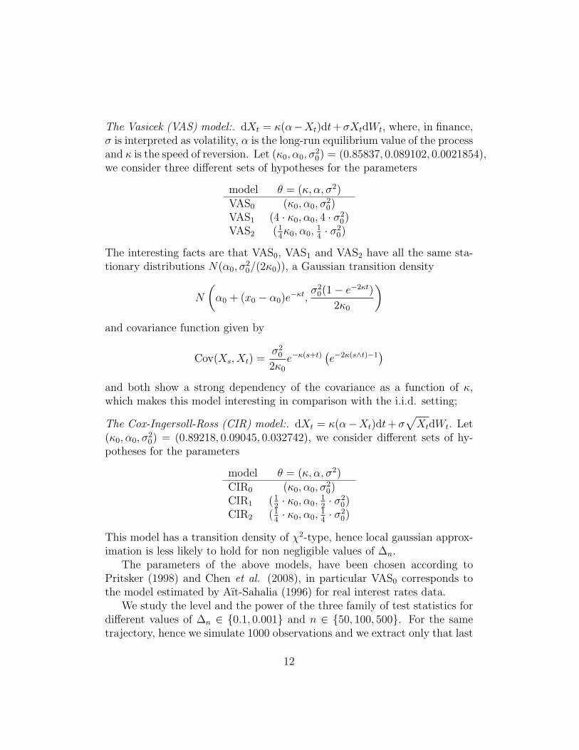
The Vasicek (VAS) model:. dXt = κ(α−Xt)dt+σXtdWt, where, in finance,σ is interpreted as volatility, α is the long-run equilibrium value of the processand κ is the speed of reversion. Let (κ0, α0, σ
20) = (0.85837, 0.089102, 0.0021854),
we consider three different sets of hypotheses for the parameters
model θ = (κ, α, σ2)VAS0 (κ0, α0, σ
20)
VAS1 (4 · κ0, α0, 4 · σ20)
VAS2 (14κ0, α0,
14· σ2
0)
The interesting facts are that VAS0, VAS1 and VAS2 have all the same sta-tionary distributions N(α0, σ
20/(2κ0)), a Gaussian transition density
N
(α0 + (x0 − α0)e−κt,
σ20(1− e−2κt)
2κ0
)and covariance function given by
Cov(Xs, Xt) =σ2
0
2κ0
e−κ(s+t)(e−2κ(s∧t)−1
)and both show a strong dependency of the covariance as a function of κ,which makes this model interesting in comparison with the i.i.d. setting;
The Cox-Ingersoll-Ross (CIR) model:. dXt = κ(α−Xt)dt+σ√XtdWt. Let
(κ0, α0, σ20) = (0.89218, 0.09045, 0.032742), we consider different sets of hy-
potheses for the parameters
model θ = (κ, α, σ2)CIR0 (κ0, α0, σ
20)
CIR1 (12· κ0, α0,
12· σ2
0)CIR2 (1
4· κ0, α0,
14· σ2
0)
This model has a transition density of χ2-type, hence local gaussian approx-imation is less likely to hold for non negligible values of ∆n.
The parameters of the above models, have been chosen according toPritsker (1998) and Chen et al. (2008), in particular VAS0 corresponds tothe model estimated by Aıt-Sahalia (1996) for real interest rates data.
We study the level and the power of the three family of test statistics fordifferent values of ∆n ∈ {0.1, 0.001} and n ∈ {50, 100, 500}. For the sametrajectory, hence we simulate 1000 observations and we extract only that last
12

n observations. Disregarding the first part of the trajectory ensures that theprocess is in the stationary state.
The results of these simulations are reported in the Tables 1-9. We pointout that in the Tables 3, 5, 7 and 9, in the column “model (α, n)” the αcorresponds to the true level of the test used to calculate cα. The other α’sin the first row of the tables correspond to the α in φα-divergences.
Summary of the analysis for the Vasicek model. It turns out that α-divergencesare not very good in terms of estimated level of the test, but their powerfunction behaves as expected. It also emerges that for λ = −0.99, the powerdivergence cannot identify as wrong model VAS1 for small sample size n = 50and ∆n = 0.001 (Table 4, row 2), although this is not the case for the power-divergences and the likelihood ratio test (Tables 3 and 1, row 2).
In general power divergences for λ in {−0.99,−1.20,−1.50,−1.75,−2.00}have always very small estimated level and high power under the selectedalternatives. The α-divergences, do not behave very good and, the way theyare defined, only approximate the likelihood ratio for α = −0.99.
The power divergences are, on average, better than the likelihood ra-tio test in terms of both empirical level α and power β under the selectedalternatives.
Summary of the analysis for the CIR model. The same average considerationsapply to the case of CIR model. The difference is that, for small sample size,all test statistics have low power under the alternative CIR1 while CIR2
doesn’t present particular problems.
5. Proofs
The following important Lemmas are useful to prove the Theorem 3.1.
Lemma 5.1 (Kessler, 1997). Under the assumptions 2.1-2.3, as n∆2n → 0
the following hold true
Γ12∇θgn(Xn, θ0)
p→ N(0, I(θ0)) (5.1)
Lemma 5.2 (Uchida and Yoshida, 2005). Under the assumptions 2.1-2.3,as n∆2
n → 0 the following hold true
Γ12∇θln(Xn, θ0) = Γ
12∇θgn(Xn, θ0) + op(1) (5.2)
13

Lemma 5.3 (Uchida and Yoshida, 2005). Under the assumptions 2.1-2.3,as n∆2
n → 0 the following hold true
Γ12∇2
θln(Xn, θ0)Γ12
p→ −I(θ0) (5.3)
Proof of Theorem 3.1. We start by applying delta method. We denote thegradient vector by ∇θ = [∂/∂θi], i = 1, . . . , p + q and similarly the Hessianmatrix by ∇2
θ = [∂2/∂θi∂θj], i, j = 1, . . . , p+ q.i) We can write that
Dφ(θn(Xn), θ0) = Dφ(θ0, θ0) + [∇θDφ(θ0, θ0)]T (θn(Xn)− θ0) + op(1)
= [∇θDφ(θ0, θ0)]T (θn(Xn)− θ0) + op(1)
because Dφ(θ0, θ0) = 0. Noting that for k = 1, ..., p+ q
∂
∂θk
[φ
(fn(·, θ)fn(·, θ0)
)]=
1
fn(·, θ0)φ′(fn(·, θ)fn(·, θ0)
)∂fn(·, θ)∂θk
by Assumption 3.1 follows that
∇θDφ(θ0, θ0) = Cφ ∇θln(Xn, θ)|θ=θ0 = Cφ∇θln(Xn, θ0)
and therefore
Dφ(θn(Xn), θ0) = Cφ
[Γ
12∇θln(Xn, θ0)
]TΓ−
12 (θn(Xn)− θ0) + op(1) (5.4)
From (5.4) by means of Lemma 5.2-5.1 and Slutsky’s Theorem immediatelyfollows
Dφ(θn(Xn), θ0)d→ Cφχ
2p+q
ii) Since for k, j = 1, ..., p+ q
∂2
∂θk∂θj
[φ
(fn(·, θ)fn(·, θ0)
)]=
1
f 2n(·, θ0)
φ′′(fn(·, θ)fn(·, θ0)
)∂fn(·, θ)∂θk
∂fn(·, θ)∂θj
+1
fn(·, θ0)φ′(fn(·, θ)fn(·, θ0)
)∂2fn(·, θ)∂θk∂θj
follows that
Dφ(θn(Xn), θ0) =1
2[Γ−1/2(θn(Xn)− θ0)]TΓ1/2∇2
θDφ(θ0, θ0)Γ1/2
×Γ−1/2(θn(Xn)− θ0) + op(1)
=Kφ
2[Γ−1/2(θn(Xn)− θ0)]TΓ1/2∇θln(Xn, θ0)[Γ1/2∇θln(Xn, θ0)]T
×Γ−1/2(θn(Xn)− θ0) + op(1)
14

From (5.4) by means of Lemma 5.2-5.1 and Slutsky’s Theorem immediatelyfollows
Dφ(θn(Xn), θ0)d→ Kφ
2Zp+q
It’s easy to verify that the density function of the r.v. Zp+q is equal to
fZp+q(z) =(1/2)
p+q2
Γ(p+q
2
) √z p+q2−1e−√z/2 1
2√z, z > 0 (5.5)
iii) By previous considerations we have that
Dφ(θn(Xn), θ0) = [∇θDφ(θ0, θ0)]T (θn(Xn)− θ0)
+1
2[Γ−1/2(θn(Xn)− θ0)]TΓ1/2∇2
θDφ(θ0, θ0)Γ1/2
×Γ−1/2(θn(Xn)− θ0) + op(1) (5.6)
where
∇2θDφ(θ0, θ0)
= Kφ∇θln(Xn, θ0)[∇θln(Xn, θ0)]T + Cφ1
f(Xn, θ0)∇2θf(Xn, θ0)
= (Kφ + Cφ)∇θln(Xn, θ0)[∇θln(Xn, θ0)]T + Cφ∇2θln(Xn, θ0) (5.7)
Plugging in (5.6) the quantity (5.7) we derive, applying again Lemma 5.1-5.3,the following result
Dφ(θn(Xn), θ0)d→ 1
2
[Cφχ
2p+q + (Cφ +Kφ)Zp+q
]
Conclusions
It seems that, as in the i.i.d. case, also for discretely observed diffusionprocesses the φ-divergences may compete or improve the performance of thestandard likelihood ratio statistics. In particular, the power divergences arein general quite good in terms of estimated level and power of the test evenfor moderate sample sizes (e.g. n ≥ 100 in our simulations).
The package sde for the R statistical environment (R Development CoreTeam, 2008) and freely available at http://cran.R-Project.org containsthe function sdeDiv which implements the φ-divergence test statistics.
15

References
Aıt-Sahalia, Y. (1996) Testing continuous-time models of the spot interestrate, Rev. Financial Stud., 70(2), 385-426.
Aıt-Sahalia, Y. (2002) Maximum-likelihood estimation for discretely-sampleddiffusions: a closed-form approximation apporach, Econometrica, 70, 223-262.
Aıt-Sahalia, Y., Fan, J., Peng, H. (2006) Nonparametric transition basedtests for jump diffusions. Working paper. Available at http://www.
princeton.edu/yacine/research.htm
Amari, S.(1985) Differential-Geometrical Methods in Statistics, LectureNotes in Statist., Vol. 28, New York, Springer.
Beran, R.J. (1977) Minimum Hellinger estimates for parametric models, An-nals of Statistics, 5, 445-463.
Burbea, J. (1984) The convexity with respect to gaussian distribution ofdivergences of order α, Utilitas Math., 26, 171-192.
Chandra, S.A., Taniguchi, M. (2006) Minimum α-divergence estimation forarch models, Journal of Time Series Analysis, 27(1), 19-39.
Chen, S.X., Gao, J., Cheng, Y.T. (2008) A test for model specification ofdiffusion processes, Ann. Stat., 36(1), 167-198.
Cressie, N., Read, T.R.C. (1984) Multinomial goodness of fit tests, J. Roy.Statist. Soc. Ser B, 46, 440-464.
Csiszar, I. (1967) On topological properties of f -divergences, Studia ScientificMathematicae Hungarian, 2, 329-339.
Dachian, S., Kutoyants, Yu. A. (2008) On the goodness-of-t tests for somecontinuous time processes, in Statistical Models and Methods for Biomed-ical and Technical Systems, 395-413. Vonta, F., Nikulin, M., Limnios, N.and Huber-Carol C. (Eds), Birkhuser, Boston.
Dacunha-Castelle, D., Florens-Zmirou, D. (1986) Estimation of the coeffi-cients of a diffusion from discrete observations, Stochastics, 19, 263-284.
16

De Gregorio, A., Iacus, S.M. (2007) Renyi information for ergodic diffusionprocesses. Available at http://arxiv.org/abs/0711.1789
Giet, L., Lubrano, M. (2008) A minimum Hellinger distance estimator forstochastic differential equations: An application to statistical inference forcontinuous time interest rate models, Computational Statistics and DataAnalysis, 52, 2945-2965.
Iacus, S.M. (2008) Simulation and Inference for Stochastic Differential Equa-tions, Springer, New York.
Iacus, S.M., Kutoyants, Y. (2001) Semiparametric hypotheses testing fordynamical systems with small noise, Mathematical Methods of Statistics,10(1), 105-120.
Kessler, M. (1997) Estimation of an ergodic diffusion from discrete observa-tions, Scand. J. Statist., 24, 211-229.
Kutoyants, Y. (1994) Identification of Dynamical Systems with Small Noise,Kluwer, Dordrecht.
Kutoyants, Y. (2004) Statistical Inference for Ergodic Diffusion Processes,Springer-Verlag, London.
Kuchler, U., Sørensen, M. (1997) Exponential Families of Stochastic Pro-cesses, Springer, New York.
Lee, S., Wee, I.-S. (2008) Residual emprical process for diffusion processes,Journal of Korean Mathematical Society, 45(3), 2008.
Liese, F., Vajda, I. (1987) Convex Statistical Distances, Tuebner, Leipzig.
Morales, D., Pardo, L., Vajda, I. (1997) Some New Statistics for TestingHypotheses in Parametric Models, Journal of Multivariate Analysis, 67,137-168.
Morales, D., Pardo, L., Pardo,, M.C., Vajda, I. (2004) Renyi statistics indirected families of exponential experiments, Statistics, 38(2), 133-147.
Negri, I., Nishiyama, Y. (2007a) Goodness of fit test for ergodic diffusionprocesses, to appear in Ann. Inst. Statist. Math.. Available at http://
arxiv.org/abs/math/0701022v1
17

Negri, I. and Nishiyama, Y. (2007b). Goodness of t test for small diffu-sions based on discrete observationsm, Research Memorandum 1054, Inst.Statist. Math., Tokyo.
Masuda, H., Negri, I., Nishiyama, Y. (2008) Goodness of fit test for er-godic diffusions by discrete time observations: an innovation martingaleapproach, Research Memorandum 1069, Inst. Statist. Math., Tokyo.
Pritsker, M. (1998) Nonparametric density estimation and tests of continuoustime interest rate models, Rev. financial Studies, 11, 449-487.
R Development Core Team (2008) R: A language and environment for statis-tical computing, R Foundation for Statistical Computing, Vienna, Austria.ISBN 3-900051-07-0, URL http://www.R-project.org
Renyi, A. (1961) On measures of entropy and information, Proceedings of theFourth Berkeley Symposium on Probability and Mathematical Statistics,Vol 1, University of California, Berkeley, 547-461.
Rivas, M.J., Santos, M.T., Morales, D. (2005) Renyi test statistics for par-tially observed diffusion processes, Journal of Statistical Planning and In-ference, 127, 91-102.
Simpson, D.G. (1989) Hellinger deviance tests: Efficinecy, breakdown points,and examples, J. Amer. Statist. Assoc., 84, 107-113.
Uchida, M., Yoshida, N. (2004) Information Criteria for Small Diffusionsvia the Theory of Malliavin-Watanabe, Statistical Inference for StochasticProcesses, 7, 35-67.
Uchida, M., Yoshida, N. (2005) AIC for ergodic diffusion processes from dis-crete observations, preprint MHF 2005-12, march 2005, Faculty of Mathe-matics, Kyushu University, Fukuoka, Japan.
Yoshida, N. (1992) Estimation for diffusion processes from discrete observa-tion, J. Multivar. Anal., 41(2), 220–242.
18

model (n) α = 0.01 α = 0.05VAS0 (50) 0.01 0.04VAS1 (50) 1.00 1.00VAS2 (50) 1.00 1.00
VAS0 (100) 0.01 0.04VAS1 (100) 1.00 1.00VAS2 (100) 1.00 1.00
VAS0 (500) 0.01 0.07VAS1 (500) 1.00 1.00VAS2 (500) 1.00 1.00
model (n) α = 0.01 α = 0.05VAS0 (50) 0.01 0.04VAS1 (50) 1.00 1.00VAS2 (50) 1.00 1.00
VAS0 (100) 0.01 0.04VAS1 (100) 1.00 1.00VAS2 (100) 1.00 1.00
VAS0 (500) 0.00 0.02VAS1 (500) 1.00 1.00VAS2 (500) 1.00 1.00
Table 1: Numbers represent probability of rejection under the true generating model, withcα calculated under H0. Therefore, the values are α under model “0” and β otherwise.Estimates calculated on 10000 experiments. Likelihood ratio, for ∆n = 0.001 (left) and∆n = 0.1 (right).
model (n) α = 0.01 α = 0.05CIR0 (50) 0.02 0.11CIR1 (50) 0.59 0.84CIR2 (50) 1.00 1.00
CIR0 (100) 0.03 0.11CIR1 (100) 0.96 0.99CIR2 (100) 1.00 1.00
CIR0 (500) 0.02 0.09CIR1 (500) 1.00 1.00CIR2 (500) 1.00 1.00
model (n) α = 0.01 α = 0.05CIR0 (50) 0.01 0.04CIR1 (50) 0.78 0.93CIR2 (50) 1.00 1.00
CIR0 (100) 0.01 0.04CIR1 (100) 0.99 1.00CIR2 (100) 1.00 1.00
CIR0 (500) 0.00 0.02CIR1 (500) 1.00 1.00CIR2 (500) 1.00 1.00
Table 2: Numbers represent probability of rejection under the true model, with rejectionregion calculated under H0. Therefore, the values are α under model “0” and β otherwise.Estimates calculated on 10000 experiments. Likelihood ratio, for ∆n = 0.001 (left) and∆n = 0.1 (right).
19

mod
el(α
,n
)α
=−
0.99
α=−
0.90
α=−
0.75
α=−
0.50
α=−
0.25
α=−
0.10
VA
S 0(0
.01,
50)
0.01
0.10
0.39
0.62
0.73
0.77
VA
S 1(0
.01,
50)
1.00
1.00
1.00
1.00
1.00
1.00
VA
S 2(0
.01,
50)
1.00
1.00
1.00
1.00
1.00
1.00
VA
S 0(0
.05,
50)
0.04
0.12
0.39
0.62
0.73
0.77
VA
S 1(0
.05,
50)
1.00
1.00
1.00
1.00
1.00
1.00
VA
S 2(0
.05,
50)
1.00
1.00
1.00
1.00
1.00
1.00
VA
S 0(0
.01,
100)
0.01
0.10
0.39
0.63
0.74
0.78
VA
S 1(0
.01,
100)
1.00
1.00
1.00
1.00
1.00
1.00
VA
S 2(0
.01,
100)
1.00
1.00
1.00
1.00
1.00
1.00
VA
S 0(0
.05,
100)
0.04
0.11
0.40
0.63
0.74
0.78
VA
S 1(0
.05,
100)
1.00
1.00
1.00
1.00
1.00
1.00
VA
S 2(0
.05,
100)
1.00
1.00
1.00
1.00
1.00
1.00
VA
S 0(0
.01,
500)
0.02
0.18
0.61
0.83
0.90
0.92
VA
S 1(0
.01,
500)
1.00
1.00
1.00
1.00
1.00
1.00
VA
S 2(0
.01,
500)
1.00
1.00
1.00
1.00
1.00
1.00
VA
S 0(0
.05,
500)
0.07
0.20
0.61
0.83
0.90
0.92
VA
S 1(0
.05,
500)
1.00
1.00
1.00
1.00
1.00
1.00
VA
S 2(0
.05,
500)
1.00
1.00
1.00
1.00
1.00
1.00
Tab
le3:
Num
bers
repr
esen
tpr
obab
ility
ofre
ject
ion
unde
rth
etr
uege
nera
ting
mod
el,w
ithc α
calc
ulat
edun
derH
0.
The
refo
re,
the
valu
esar
eα
unde
rm
odel
“0”
andβ
othe
rwis
e.E
stim
ates
calc
ulat
edon
1000
0ex
peri
men
ts.
Est
imat
edα
-div
erge
nces
,fo
r∆n
=0.
001.
20

mod
el(α
,n
)λ
=−
0.99
λ=−
1.20
λ=−
1.50
λ=−
1.75
λ=−
2.00
λ=−
2.50
VA
S 0(0
.01,
50)
0.00
0.00
0.00
0.01
0.02
0.04
VA
S 1(0
.01,
50)
0.00
0.99
1.00
1.00
1.00
1.00
VA
S 2(0
.01,
50)
0.40
1.00
1.00
1.00
1.00
1.00
VA
S 0(0
.05,
50)
0.00
0.00
0.00
0.01
0.03
0.06
VA
S 1(0
.05,
50)
0.67
1.00
1.00
1.00
1.00
1.00
VA
S 2(0
.05,
50)
0.99
1.00
1.00
1.00
1.00
1.00
VA
S 0(0
.01,
100)
0.00
0.00
0.00
0.01
0.02
0.04
VA
S 1(0
.01,
100)
0.23
1.00
1.00
1.00
1.00
1.00
VA
S 2(0
.01,
100)
0.88
1.00
1.00
1.00
1.00
1.00
VA
S 0(0
.05,
100)
0.00
0.00
0.00
0.01
0.03
0.06
VA
S 1(0
.05,
100)
1.00
1.00
1.00
1.00
1.00
1.00
VA
S 2(0
.05,
100)
1.00
1.00
1.00
1.00
1.00
1.00
VA
S 0(0
.01,
500)
0.00
0.00
0.00
0.01
0.03
0.08
VA
S 1(0
.01,
500)
1.00
1.00
1.00
1.00
1.00
1.00
VA
S 2(0
.01,
500)
1.00
1.00
1.00
1.00
1.00
1.00
VA
S 0(0
.05,
500)
0.00
0.00
0.01
0.03
0.06
0.12
VA
S 1(0
.05,
500)
1.00
1.00
1.00
1.00
1.00
1.00
VA
S 2(0
.05,
500)
1.00
1.00
1.00
1.00
1.00
1.00
Tab
le4:
Num
bers
repr
esen
tpr
obab
ility
ofre
ject
ion
unde
rth
etr
uege
nera
ting
mod
el,w
ithc α
calc
ulat
edun
derH
0.
The
refo
re,
the
valu
esar
eα
unde
rm
odel
“0”
andβ
othe
rwis
e.E
stim
ates
calc
ulat
edon
1000
0ex
peri
men
ts.
Est
imat
edpo
wer
-div
erge
nces
for
∆n
=0.
001
21

mod
el(α
,n
)α
=−
0.99
α=−
0.90
α=−
0.75
α=−
0.50
α=−
0.25
α=−
0.10
VA
S 0(0
.01,
50)
0.01
0.15
0.55
0.78
0.86
0.88
VA
S 1(0
.01,
50)
1.00
1.00
1.00
1.00
1.00
1.00
VA
S 2(0
.01,
50)
1.00
1.00
1.00
1.00
1.00
1.00
VA
S 0(0
.05,
50)
0.05
0.17
0.55
0.78
0.86
0.88
VA
S 1(0
.05,
50)
1.00
1.00
1.00
1.00
1.00
1.00
VA
S 2(0
.05,
50)
1.00
1.00
1.00
1.00
1.00
1.00
VA
S 0(0
.01,
100)
0.01
0.13
0.48
0.71
0.80
0.83
VA
S 1(0
.01,
100)
1.00
1.00
1.00
1.00
1.00
1.00
VA
S 2(0
.01,
100)
1.00
1.00
1.00
1.00
1.00
1.00
VA
S 0(0
.05,
100)
0.04
0.15
0.48
0.71
0.80
0.83
VA
S 1(0
.05,
100)
1.00
1.00
1.00
1.00
1.00
1.00
VA
S 2(0
.05,
100)
1.00
1.00
1.00
1.00
1.00
1.00
VA
S 0(0
.01,
500)
0.00
0.06
0.25
0.54
0.69
0.74
VA
S 1(0
.01,
500)
1.00
1.00
1.00
1.00
1.00
1.00
VA
S 2(0
.01,
500)
1.00
1.00
1.00
1.00
1.00
1.00
VA
S 0(0
.05,
500)
0.02
0.07
0.25
0.54
0.69
0.74
VA
S 1(0
.05,
500)
1.00
1.00
1.00
1.00
1.00
1.00
VA
S 2(0
.05,
500)
1.00
1.00
1.00
1.00
1.00
1.00
Tab
le5:
Num
bers
repr
esen
tpr
obab
ility
ofre
ject
ion
unde
rth
etr
uege
nera
ting
mod
el,w
ithc α
calc
ulat
edun
derH
0.
The
refo
re,
the
valu
esar
eα
unde
rm
odel
“0”
andβ
othe
rwis
e.E
stim
ates
calc
ulat
edon
1000
0ex
peri
men
ts.
Est
imat
edα
-div
erge
nces
,fo
r∆n
=0.
1
22

mod
el(α
,n
)λ
=−
0.99
λ=−
1.20
λ=−
1.50
λ=−
1.75
λ=−
2.00
λ=−
2.50
VA
S 0(0
.01,
50)
0.00
0.00
0.00
0.01
0.02
0.05
VA
S 1(0
.01,
50)
1.00
1.00
1.00
1.00
1.00
1.00
VA
S 2(0
.01,
50)
1.00
1.00
1.00
1.00
1.00
1.00
VA
S 0(0
.05,
50)
0.00
0.00
0.00
0.02
0.03
0.09
VA
S 1(0
.05,
50)
1.00
1.00
1.00
1.00
1.00
1.00
VA
S 2(0
.05,
50)
1.00
1.00
1.00
1.00
1.00
1.00
VA
S 0(0
.01,
100)
0.00
0.00
0.00
0.00
0.01
0.05
VA
S 1(0
.01,
100)
1.00
1.00
1.00
1.00
1.00
1.00
VA
S 2(0
.01,
100)
1.00
1.00
1.00
1.00
1.00
1.00
VA
S 0(0
.05,
100)
0.00
0.00
0.00
0.01
0.03
0.08
VA
S 1(0
.05,
100)
1.00
1.00
1.00
1.00
1.00
1.00
VA
S 2(0
.05,
100)
1.00
1.00
1.00
1.00
1.00
1.00
VA
S 0(0
.01,
500)
0.00
0.00
0.00
0.00
0.01
0.02
VA
S 1(0
.01,
500)
1.00
1.00
1.00
1.00
1.00
1.00
VA
S 2(0
.01,
500)
1.00
1.00
1.00
1.00
1.00
1.00
VA
S 0(0
.05,
500)
0.00
0.00
0.00
0.01
0.01
0.04
VA
S 1(0
.05,
500)
1.00
1.00
1.00
1.00
1.00
1.00
VA
S 2(0
.05,
500)
1.00
1.00
1.00
1.00
1.00
1.00
Tab
le6:
Num
bers
repr
esen
tpr
obab
ility
ofre
ject
ion
unde
rth
etr
uege
nera
ting
mod
el,w
ithc α
calc
ulat
edun
derH
0.
The
refo
re,
the
valu
esar
eα
unde
rm
odel
“0”
andβ
othe
rwis
e.E
stim
ates
calc
ulat
edon
1000
0ex
peri
men
ts.
Est
imat
edpo
wer
-div
erge
nces
for
∆n
=0.
1
23

mod
el(α
,n
)α
=−
0.99
α=−
0.90
α=−
0.75
α=−
0.50
α=−
0.25
α=−
0.10
CIR
0(0
.01,
50)
0.03
0.28
0.69
0.83
0.89
0.90
CIR
1(0
.01,
50)
0.63
0.95
1.00
1.00
1.00
1.00
CIR
2(0
.01,
50)
1.00
1.00
1.00
1.00
1.00
1.00
CIR
0(0
.05,
50)
0.12
0.31
0.69
0.83
0.89
0.90
CIR
1(0
.05,
50)
0.86
0.96
1.00
1.00
1.00
1.00
CIR
2(0
.05,
50)
1.00
1.00
1.00
1.00
1.00
1.00
CIR
0(0
.01,
100)
0.03
0.28
0.69
0.85
0.89
0.91
CIR
1(0
.01,
100)
0.97
1.00
1.00
1.00
1.00
1.00
CIR
2(0
.01,
100)
1.00
1.00
1.00
1.00
1.00
1.00
CIR
0(0
.05,
100)
0.12
0.31
0.69
0.85
0.89
0.91
CIR
1(0
.05,
100)
0.99
1.00
1.00
1.00
1.00
1.00
CIR
2(0
.05,
100)
1.00
1.00
1.00
1.00
1.00
1.00
CIR
0(0
.01,
500)
0.03
0.22
0.59
0.79
0.86
0.88
CIR
1(0
.01,
500)
1.00
1.00
1.00
1.00
1.00
1.00
CIR
2(0
.01,
500)
1.00
1.00
1.00
1.00
1.00
1.00
CIR
0(0
.05,
500)
0.09
0.24
0.59
0.79
0.86
0.89
CIR
1(0
.05,
500)
1.00
1.00
1.00
1.00
1.00
1.00
CIR
2(0
.05,
500)
1.00
1.00
1.00
1.00
1.00
1.00
Tab
le7:
Num
bers
repr
esen
tpr
obab
ility
ofre
ject
ion
unde
rth
etr
uem
odel
,wit
hre
ject
ion
regi
onca
lcul
ated
unde
rH
0.
The
refo
re,
the
valu
esar
eα
unde
rm
odel
“0”
andβ
othe
rwis
e.E
stim
ates
calc
ulat
edon
1000
0ex
peri
men
ts.
Est
imat
edα
-div
erge
nces
,fo
r∆n
=0.
001
24

mod
el(α
,n
)λ
=−
0.99
λ=−
1.20
λ=−
1.50
λ=−
1.75
λ=−
2.00
λ=−
2.50
CIR
0(0
.01,
50)
0.00
0.00
0.00
0.02
0.05
0.13
CIR
1(0
.01,
50)
0.00
0.01
0.28
0.55
0.71
0.87
CIR
2(0
.01,
50)
0.00
0.81
1.00
1.00
1.00
1.00
CIR
0(0
.05,
50)
0.00
0.00
0.01
0.04
0.09
0.19
CIR
1(0
.05,
50)
0.00
0.09
0.48
0.70
0.81
0.92
CIR
2(0
.05,
50)
0.00
0.97
1.00
1.00
1.00
1.00
CIR
0(0
.01,
100)
0.00
0.00
0.00
0.02
0.05
0.14
CIR
1(0
.01,
100)
0.00
0.21
0.83
0.95
0.98
0.99
CIR
2(0
.01,
100)
0.00
1.00
1.00
1.00
1.00
1.00
CIR
0(0
.05,
100)
0.00
0.00
0.01
0.05
0.09
0.20
CIR
1(0
.05,
100)
0.00
0.53
0.93
0.98
0.99
1.00
CIR
2(0
.05,
100)
0.24
1.00
1.00
1.00
1.00
1.00
CIR
0(0
.01,
500)
0.00
0.00
0.00
0.02
0.04
0.10
CIR
1(0
.01,
500)
0.00
1.00
1.00
1.00
1.00
1.00
CIR
2(0
.01,
500)
1.00
1.00
1.00
1.00
1.00
1.00
CIR
0(0
.05,
500)
0.00
0.00
0.01
0.04
0.07
0.15
CIR
1(0
.05,
500)
0.95
1.00
1.00
1.00
1.00
1.00
CIR
2(0
.05,
500)
1.00
1.00
1.00
1.00
1.00
1.00
Tab
le8:
Num
bers
repr
esen
tpr
obab
ility
ofre
ject
ion
unde
rth
etr
uem
odel
,wit
hre
ject
ion
regi
onca
lcul
ated
unde
rH
0.
The
refo
re,
the
valu
esar
eα
unde
rm
odel
“0”
andβ
othe
rwis
e.E
stim
ates
calc
ulat
edon
1000
0ex
peri
men
ts.
Est
imat
edpo
wer
-div
erge
nces
for
∆n
=0.
001
25

mod
el(α
,n
)α
=−
0.99
α=−
0.90
α=−
0.75
α=−
0.50
α=−
0.25
α=−
0.10
CIR
0(0
.01,
50)
0.01
0.14
0.54
0.77
0.85
0.87
CIR
1(0
.01,
50)
0.80
0.98
1.00
1.00
1.00
1.00
CIR
2(0
.01,
50)
1.00
1.00
1.00
1.00
1.00
1.00
CIR
0(0
.05,
50)
0.05
0.16
0.54
0.77
0.85
0.87
CIR
1(0
.05,
50)
0.94
0.98
1.00
1.00
1.00
1.00
CIR
2(0
.05,
50)
1.00
1.00
1.00
1.00
1.00
1.00
CIR
0(0
.01,
100)
0.01
0.13
0.49
0.71
0.79
0.82
CIR
1(0
.01,
100)
0.99
1.00
1.00
1.00
1.00
1.00
CIR
2(0
.01,
100)
1.00
1.00
1.00
1.00
1.00
1.00
CIR
0(0
.05,
100)
0.04
0.15
0.49
0.71
0.79
0.82
CIR
1(0
.05,
100)
1.00
1.00
1.00
1.00
1.00
1.00
CIR
2(0
.05,
100)
1.00
1.00
1.00
1.00
1.00
1.00
CIR
0(0
.01,
500)
0.00
0.06
0.28
0.54
0.69
0.74
CIR
1(0
.01,
500)
1.00
1.00
1.00
1.00
1.00
1.00
CIR
2(0
.01,
500)
1.00
1.00
1.00
1.00
1.00
1.00
CIR
0(0
.05,
500)
0.02
0.08
0.28
0.54
0.69
0.74
CIR
1(0
.05,
500)
1.00
1.00
1.00
1.00
1.00
1.00
CIR
2(0
.05,
500)
1.00
1.00
1.00
1.00
1.00
1.00
Tab
le9:
Num
bers
repr
esen
tpr
obab
ility
ofre
ject
ion
unde
rth
etr
uem
odel
,wit
hre
ject
ion
regi
onca
lcul
ated
unde
rH
0.
The
refo
re,
the
valu
esar
eα
unde
rm
odel
“0”
andβ
othe
rwis
e.E
stim
ates
calc
ulat
edon
1000
0ex
peri
men
ts.
Est
imat
edα
-div
erge
nces
,fo
r∆n
=0.
1
26

mod
el(α
,n
)λ
=−
0.99
λ=−
1.20
λ=−
1.50
λ=−
1.75
λ=−
2.00
λ=−
2.50
CIR
0(0
.01,
50)
0.00
0.00
0.00
0.01
0.02
0.06
CIR
1(0
.01,
50)
0.00
0.06
0.52
0.75
0.86
0.94
CIR
2(0
.01,
50)
0.00
0.99
1.00
1.00
1.00
1.00
CIR
0(0
.05,
50)
0.00
0.00
0.00
0.02
0.04
0.09
CIR
1(0
.05,
50)
0.00
0.23
0.70
0.85
0.92
0.96
CIR
2(0
.05,
50)
0.06
1.00
1.00
1.00
1.00
1.00
CIR
0(0
.01,
100)
0.00
0.00
0.00
0.01
0.02
0.05
CIR
1(0
.01,
100)
0.00
0.56
0.96
0.99
1.00
1.00
CIR
2(0
.01,
100)
0.00
1.00
1.00
1.00
1.00
1.00
CIR
0(0
.05,
100)
0.00
0.00
0.00
0.02
0.03
0.08
CIR
1(0
.05,
100)
0.00
0.83
0.99
1.00
1.00
1.00
CIR
2(0
.05,
100)
0.97
1.00
1.00
1.00
1.00
1.00
CIR
0(0
.01,
500)
0.00
0.00
0.00
0.00
0.01
0.02
CIR
1(0
.01,
500)
0.00
1.00
1.00
1.00
1.00
1.00
CIR
2(0
.01,
500)
1.00
1.00
1.00
1.00
1.00
1.00
CIR
0(0
.05,
500)
0.00
0.00
0.00
0.01
0.02
0.04
CIR
1(0
.05,
500)
1.00
1.00
1.00
1.00
1.00
1.00
CIR
2(0
.05,
500)
1.00
1.00
1.00
1.00
1.00
1.00
Tab
le10
:N
umbe
rsre
pres
ent
prob
abili
tyof
reje
ctio
nun
der
the
true
mod
el,w
ith
reje
ctio
nre
gion
calc
ulat
edun
derH
0.
The
re-
fore
,th
eva
lues
areα
unde
rm
odel
“0”
andβ
othe
rwis
e.E
stim
ates
calc
ulat
edon
1000
0ex
peri
men
ts.
Est
imat
edpo
wer
-di
verg
ence
sfo
r∆n
=0.
1
27