Vertical crustal motion observed in the BIFROST project

www.elsevier.com/locate/jog

Vertical crustal motion observed in the BIFROST project

Hans-Georg Schernecka,*, Jan M. Johanssona, Hannu Koivulab,Tonie van Damc, James L. Davisd

aChalmers University of Technology, Onsala Space Observatory, SE-439 92 Onsala, SwedenbFinnish Geodetic Institute, PL 15, FI-02431 Masala, Finland

cEuropean Centre for Geodynamics amd Seismology, 19, rue Josy Welter, LU-7256 Walferdange,Grand Duchy of Luxembourg

dHarvard-Smithsonian Center for Astrophysics, 60 Garden Street, Cambridge, MA 02138, USA

Abstract

This paper reports from investigations on the robustness of estimated rates of intraplate motion from thecontinuous GPS project BIFROST (Baseline Inferences from Fennoscandian Rebound Observations,Sealevel and Tectonics). We study loading effects due to ocean, atmosphere and hydrology and theirimpact on estimated rate parameters. We regularly find the admittance of a modelled perturbation at lessthan fifty percent of the full effect. We think that the finding relates to a difficult noise situation at allperiods, and that a satisfying model for the dominating noise source has not been found yet. An additionalreason for low admittance is found in the mapping process of the no-fiducial network solution into aconventional reference frame.# 2003 Elsevier Science Ltd. All rights reserved.

1. Introduction

The BIFROST project was created in 1993 to measure postglacial isostatic adjustment in Fen-noscandia with continuous GPS in all three spatial dimensions. The project aims at inference ofabsolute sea level change by combination of the vertical rates with tide gauge derived relative sealevel rates. The project also expects to reveal horizontal motion, maybe at first order due topostglacial rebound, but also possibly due to other sources of stress generally covered under theterm of neotectonics or intraplate tectonics. Several publications are available, BIFROST project(1996), Scherneck et al. (1998, 2001, 2002), Milne et al. (2000) and Johansson et al. (2002), thatcentre on the measurement and its interpretation in terms of models for deglaciation history,

0264-3707/03/$ - see front matter # 2003 Elsevier Science Ltd. All rights reserved.

doi:10.1016/S0264-3707(03)00005-X

Journal of Geodynamics 35 (2003) 425–441

* Corresponding author. Tel.: +46-31-772-5556; fax: +46-31-772-5590.

E-mail address: [email protected] (H.-G. Scherneck).

http://www.elsevier.com/locate/jog/a4.3d

mailto:[email protected]

earth isostatic adjustment response, and the sea level problem. In this context it appears impor-tant to assess the robustness of the rates estimated in the regression analysis. For instance we willhave to test their dependence on the presence of time series of modelled or measured perturba-tions. This will be the main subject of the present paper.

Since the beginning the BIFROST data base contains position estimates from 2500 daily solu-tions. A typical vertical precision is 7 mm (east 3 mm, north 2 mm). For each of the stations inthe data base, time series of position estimates are formed, from which components of motion canbe estimated. The question arises what components can be attributed to the physical motion ofthe tectonic unit, whether components are present due to the monument or the local rock unit,and further what are the components contributing to this motion. Remaining variations of posi-tion might then be viewed as measurement errors, and also they are considered as being com-posed of signals from different origins, e.g. variable antenna phase centre offsets.

1.1. Time series of positions

Daily position estimates have been derived on the basis of a mixed reference system; we haveadopted the International Terrestrial Reference Frame ITRF97 for positions and JPL2000 forvelocities (see Scherneck et al., 2002, for more detail.) The movement of a rigid frame was sub-sequently subtracted from the daily positions in order to reduce the motion to an average Eur-asian motion. Thus, the relative motion, e.g. due to intraplate deformation, is emphasized whileall information relevant for deformation is preserved.

In the following we will concentrate on the vertical. An example for the data series is shown inFig. 1 for the case of Sundsvall. The question arises as to whether the introduction of bias para-meters in the time series for the reduction of antenna phase centre offsets does not interact withessentially unbounded noise so as to make the time series falsely stationary. The only answer wepresently can give in this regard is, that our time series are not disturbed by antenna reconfi-gurations after autumn 1996, when the last bias parameter was introduced. If power-law noisewould be present, the three years of data since then should be expected to exhibit the feature inthe form of an upward sloping low-frequency asymptote.

Antenna related problems in the BIFROST project were first studied in Elosegui et al. (1995)and Jaldehag et al. (1996a). The findings suggest that non hemispherical covers above theantenna (radomes), mounted for the purpose of protection against environmental perturbations,have a significant impact on the antenna diagram. This leads to changes of the antenna phasecentre that depend on satellite elevation, and therefore a dependence of the estimated positionon the visible satellite geometry, the horizon mask and/or the elevation cutoff angle (a proces-sing parameter). Further, a snow cover on a radome was found to have a strong influence onthe estimated vertical position (Jaldehag et al., 1996b). Some antennas were protected againstthe incidence of indirect satellite signal, e.g. scattered off from surfaces near the antenna, usingradar wave absorbing material (‘‘eccosorb’’). An exact position of the eccosorb slab that wouldlead to perturbation-free antenna diagram is difficult to find, as it again depends on satelliteelevation. The task to find neutral receiving conditions involves a large amount of trade-offsand compromises; the changes that occurred in the SWEPOS and FinnRef networks aredetailed in Johansson et al. (2002). At every change of the configuration we have to be preparedthat the estimated position changes. One of the lessons learnt in the process suggests that a low

426 H.-G. Scherneck et al. / Journal of Geodynamics 35 (2003) 425–441

(5�) elevation cutoff angle leads to a more balanced sampling of the antenna sensitivity pattern,given its variations typical in our networks. In lieu of the reprocessing of the GPS data cur-rently carried out at Onsala Space Observatory with the lower elevation cutoff, bias parametersmust be introduced in the data analysis when average positions are estimated from the dailysolutions.

Fig. 1. Top frame: time series of vertical position at Sundsvall (black curve with a gray background that shows thestandard deviation of each daily estimate). Fitted simple motion model, consisting of adjusted constant rate and biasparameters is shown as a gray line. The biases are seen as jumps permitted to occur at times when we might expect thatchanges in antenna configuration could have reverberations on the estimated position, e.g. covering radomes, where

changed. Bottom frames: Cutoff test, showing estimated parameters for bias and rate as chunks of 30-day length arechopped off the beginning (lower left) and the end (lower right) of the time series. The antenna radome events aredenoted with four-letter codes, see text.

H.-G. Scherneck et al. / Journal of Geodynamics 35 (2003) 425–441 427

The introduction of biases interacts with the estimation of a constant rate. By cutting batcheswith increasing length from the time series, from both the heading and the trailing end, the sta-bility of the rate and bias estimates can be evaluated. Changes of rate estimates can be monitoredwhen a bias time is cut away. The result, again for Sundsvall, is shown in Fig. 1. At this stationthe following antenna radome reconfigurations were carried out (codes used in the figure in par-enthesis). The Delft type radome was changed against a pointed fibreglass ‘‘white’’ type (DEWH).Later, the white radome was removed and operation continued for a short time without radome(WOFF). Finally, a hemispherical Plexiglas radome was installed (PLON) leading to muchreduced elevation dependence of the measured satellite range (the previous models were conical).In the southern part of the network this change occurred several months earlier, thereforeallowance is given for a side-effect jump (SIDA).

The test results indicate that data from before autumn 1996 could be sacrificed, trading off onlya little of the resolution. The cut-off test at the end shows that there is still some drift of the rateduring the last twelve-month period, and the present estimate of 10�0.2 mm/year might changeby more than one standard deviation. There are stations in the network the trends of which aremore difficult to determine in the presence of more antenna jumps and greater long-period noise.

1.2. Concepts to separate motion and measurement error

The standard BIFROST model for motion of a station consists of a constant rate and of biasesthat are introduced when antenna configuration or receiving conditions have been changed; thesesignals are conceived of as being embedded in Gauss-Markov noise. The important notion withthis kind of noise, in contrast to random walk, is that it possesses a stable mean. If the time spanis long enough during which a station is observed, a meaningful mean and lower polynomialorders of a motion model can be estimated. This notion corresponds to the notion of stable,almost rigid tectonic plates. In sediment-covered areas such stability conditions might be difficultto establish (Langbein and Johnson, 1997).

From power spectrum estimation we know that the noise character of our time series to dateshows a slope that is far from the 1=f2 of random walk. However, we do not know the spectrumat periods that are as long as or longer than the duration of the experiment. Linear motion gen-erated by a random walk process that fits the noise power at the lowest frequency could be mis-interpreted as deterministic. As an exercise for BIFROST, a typical noise power figure at one yearperiod is 500 mm2 day, which is about 10 dB above the noise power at the Nyquist frequency.The case is illustrated in Fig. 2 for the case of the vertical position estimates at Sundsvall. Arandom walk spectrum taking off at the Nyquist with 50 mm2 day would reach 20�10

log(365)=51 dB at a 1 year period. However, the 500 mm2 day figure could be indicative ofrandom walk with a process noise parameter of

ffiffiffiffiffiffiffiffi

500p

=365 ¼ 0:06 mm=ffiffiffi

dp

. This noise would bescreened by other processes more white in character. In 2500 days, the random walk componentcould build up an offset of 150 mm, which would be misinterpreted as an average rate of 20 mmper year.

Power-law noise with a less steep character than the 1=f2 slope of random walk is frequentlyencountered (Williams et al., 2001; Calais, 1999). Although these types of noise are less severe interms of the long-period drift of the station position, they have in common that they are deficientof a stable mean.


2. Inferred motion

The article by Johansson et al. (2002) describes the three approaches that have been taken in thepost-processing of the GPS analysis, inferring three-dimensional crustal motion in Fennoscandia.These results show a high degree of correspondence with predicted motion on the basis of glacialisostatic rebound models (Milne et al., 2001) and contemporary vertical rates of motion relativeto the conventional sea level (Ekman, 1996). The new implications in the BIFROST GPS mea-surements are that the observed motion is truly three-dimensional, and that it aims to relate themotion to the geocentric origin that is maintained by the International Terrestrial ReferenceSystem (ITRS) rather than a conventional mean sea level.

In the standard BIFROST solution, we reduce the time series for loading effects due to airpressure and fit sinusoidal harmonics with annual and sub-annual signatures up to four cycles peryear, as these effects are both straight-forward to model and visually discernable in the resultingtime series. At various degrees of sophistication several stations have obtained extended sitemotion models. For instance, near the Baltic Sea coast, loading due to the varying water level ofthe sea is considered. Using an Empirical Orthogonal Function (EOF) approach, we also con-sider a stochastic portion of motion to be more or less in common at all stations in an area. In

Fig. 2. Power spectrum and auto-covariance at Sundsvall, vertical component. The times series of daily estimates is

analysed after reduction of the simple motion model (one constant rate of motion and bias parameters introduced attimes of antenna reconfiguration). This motion residual has then been normalised with the standard deviation at everyestimate (mean value 7 mm). Thus, zero decibel corresponds to a power spectrum density of 50 mm2 day. The power

spectrum noise colour indicates a Gauss-Markov noise process, as the spectrum appears to saturate at a finite levelwhen the frequency decreases. The Bartlett estimate is denoted by circles. The spectrum has also been estimated using aMaximum Entropy method (MEM). This is shown as a band of vertical bars. The bar length indicates the 95% con-

fidence interval of the Bartlett spectrum. Thus, outliers of the Bartlett spectrum outside this band are significant at the95% level. We find 15 small outliers out of 720 samples. Only the spectral lines at 0.2 and 0.4 cycles per day, that havebeen picked up by the MEM, might bear any significance. The auto-covariance series (right frame) indicates a Gauss-

Markov parameter of 0.6.


Fig. 3 we show a map produced from the three-dimensional rates of motion determined with theEOF-method where possible (all stations in Sweden and Metsahovi). Elsewhere a solution withautomated outlier editing using a criterion of five standard deviations is used.

2.1. Vertical motions compared with tide gauges and leveling

We show two variants of comparison of the GPS results with vertical rates determined fromtide gauges and precise levelling, first with the EOF-solution, second with the standard solution(Fig. 4). We use the tide gauge and levelling results of Ekman (1996) and add the geoid motiondue to the rebound model of Mitrovica et al. (1994). In both cases, GPS and tide gauge/levelling,we obtain the geometric rate of motion of the earth surface. In the case of GPS the motion isrelative to the centre of the satellite frame, which is constrained to the earth’s gravity centre (howwell remains to be determined). In the case of tide gauge/levelling the reference is the regional sea

Fig. 3. Three-dimensional rates, vertical rates plotted as colours, horizontal rates as arrows with error ellipses for one

standard deviation. The vertical standard deviation is typically 0.25–0.35 mm/year in Sweden; the somewhat shorterobservation time span in Finland causes error limits near 0.5 mm/year.


surface. The difference between the two data sets interpolated to the point where GPS motion, i.e.inferred land surface motion is zero determines the regional change of sea level with respect to theearth’s gravity centre.

Where no tide gauge/levelling data is available from Ekman (1996), which is the case at manyIGS stations, we resort to ITRF97 motions. In the case of Ny Alesund (NYAL) a careful eval-uation of mareograph data was presented by Breuer and Wolf (1995), who estimated a relativeuplift velocity of 2.6�0.7 mm/yr. The ITRF97 motions have been excepted from computing theregression line shown in Fig. 4. More discussion on this subject follows in Section 4.

3. Loading effects

Recently, global hydrological data was used by van Dam et al. (2001) to predict loadinginduced displacements of the earth surface. We apply the method to predict displacements at theset of BIFROST GPS stations.

Storage of water in snow cover, soil, and groundwater was calculated using a global model ofland water and energy balance (Milly and Shmakin, 2002a). Summation of model water storageoutputs (snow, soil water and groundwater) provides our estimate of terrestrial water storageloading on a monthly time scale at 1� by 1� global spacing.

Fig. 4. Regression of GPS derived vertical motion with respect to motion inferred from tide gauges and precise level-ling (Ekman, 1996). Tide gauge readings and levelling are reckoned relative to a changing sea level, while GPS refers tothe mass centre of the Earth. Thus, the intercept of both curves indicates the rate of the relative vertical motion of the

land surface reduced for postglacial rebound as a regional average. The negative of this figure hints at the regionalchange of sea level reduced for the postglacial land motion. A perfect fit to a straight line with unity slope wouldindicate that the sea level rise is uniform. In the left frame only the GPS results from the stations with the longestrecords have been used, and the empirical orthogonal function method has been used to remove common modes of

noise. In the right frame the BIFROST standard solution has been used, where station motion is modelled as one rateand biases as required. The motion solutions are described in Johansson et al. (2002).


The atmospheric pressure data set consists of 6-h estimates of surface pressure determined bythe European Centre for Medium Range Weather Forecast (ECMWF). The data are retrievedfrom spherical harmonic developments up to degree and order 213 and represented globally on a1� by 1� grid.

For both the atmospheric pressure and continental water storage loading estimates, the masswas convolved with Farrell’s elastic Green’s functions (Farrell, 1972). The procedure has beendescribed in detail in van Dam and Wahr (1987).

Time series for the case of Ostersund are shown in Fig. 5. This station is a good example for theimpact of severe snow winters. The hydrological loading predictions are available for a timeperiod between January 1994 and December 1998. We have also acquired soil moisture and snowcoverage data observed in a network of climate monitoring stations operated by the SwedishMeteorological and Hydrological Institute (SMHI). This data covers the period from January1996 to date. Although these measurements of soil moisture and snow height are local, corre-lation between the stations in the network is generally high over distances of several hundredkilometres. For this reason we think that they are representative of the hydrological budget in theground. In contrast to the Milly and Shmakin (2002a) model, which makes detailed assumptionsof vegetation related parameters (Milly and Shmakin, 2002b), the SMHI data does not includethe water bound in vegetation over ground.

To convert the local observations into predicted loading effects we have used a coefficient of�0.03 m per metre of water column. This coefficient has been obtained by convolving typicalmass distributions with an elastic Greens function (Farrell, 1972), see Fig. 6. The SMHIhydrology time series are for snow and soil are added to form a loading-efficient time series. Theseries with the snow alone is included in the regression with the GPS observations, since othereffects of snow, e.g. average effects on the wave propagation, might be reduced in this way. Acomparison of both time series during the 3 years overlap shows that the typical summer waterstorage peak appears generally low in the local soil measurements compared to the soil andvegetation model.

With respect to the daily GPS solutions the loading effects can be regarded as quasi-static.Therefore we consider only one in-phase admittance coefficient for each of the perturbing effects.Unfortunately, the atmospheric load and the hydrological load compete at annual frequencies,while the atmospheric load—quite uniquely—has substantial variations also on a weekly scale. Inthis short period range we think that, besides the barometrically and tidally incurred displace-ments, only atmospheric perturbations of signal propagation and multipath would affect the GPSderived positions.

A typical result for atmospheric loading that we have found before hydrological loading wasconsidered ranges between 0.2 and 0.35 for the ratio between the observed and the predictedeffect. The admittance does not change significantly when the Gauss-Markov noise parameter isvaried over a wide range of values.

When we use the hydrological loading predictions from the global convolution we find admit-tance coefficients below unity (cf. Table 1). As an alternative we have used the soil moisture datafrom the SMHI Climate Stations operated by the Swedish Meteorological and HydrologicalInstitute (SMHI). For these time series typically a very low admittance is found. In each case weexplain the deficiency as follows in the discussion. The estimated admittance coefficients forhydrological loading at stations in northern Sweden are shown in Fig. 7.


Fig. 5. Time series at Ostersund, vertical component. The observed variation of position is dominated by postglacialrebound. Observations are shown in the bottom curve together with standard deviations. The the series labeled hydro-loading is computed from Milly and Shmakin (2002a) using global convolution; the soil (-moisture) and snow curves

are predicted using local observations and a coefficient of �0.03. The conditions are typical also for the other stationsespecially in northern Sweden.


4. Discussion

We start the discussion with a look at the comparison of the motion inferred from tide gaugeobservations and precise levelling to the GPS observations (see Fig. 4). The graph indicates aregional mean sea level change. How- ever, we obtain different results depending on the post-processing analysis strategy, the simple standard analysis versus the empirical orthogonal func-tion analysis (described in Johansson et al., 2002). Clearly the sea level rate that might be inferreddepends upon data quality or data processing related features. Although the error bars in thisfigure have been derived from the a posteriori residuals and adjusted for noise colour, the differ-ence between the solutions is significant at almost three standard deviations. The analysis to datesuggests so far that a sea level rate based on BIFROST GPS is not sufficiently robust, hencepremature, and that the confidence limit of 0.15 mm/year is over-optimistic. Tentatively, themethods that treat the data more homogeneously and that have an enhanced capability to sepa-

Fig. 6. Loading effects due to a uniform slab of 1 m water separately covering the land part (left frame) and the seapart (right frame) of the Fennoscandian shield.

Table 1

GPS vertical position variations, admittance coefficients for predicted hydrological loading effects according to vanDam et al. (2001)

Site
Coeff. S.D. Comment
ARJE
0.974 0.098 JONK 0.408 0.133 KIRU 0.005 0.092 LOW
MART
0.304 0.120 OSKA �0.234 0.215 CONTRA VANE 0.577 0.157
OVER
0.664 0.107 SUND 0.565 0.114 SVEG 0.723 0.089
UMEA
1.016 0.101 VILH 0.909 0.088

rate signal from noise, that is the EOF method, could be interpreted as more reliable, and sowould be their result, a sea level rate slightly in excess of 1 mm/year. Removing observationsunder snow conditions from the post-processing, Scherneck et al. (2002) arrived at a sea level ratecloser to 1.5 mm/year. Thus, there is a continuing interest to understand the systematic effectsthat perturb the measurement and that so far have been treated as noise.

Interesting candidates in this context are the loading effects. The associated signals in our timeseries can be considered as being spatially coherent over large distances. This spatial coherencecould be seen as an effect of the elastic stiffness of the mantle. However, the extent of the coherencealso happens to be on the order of the diameter of the load distribution, typically involving scalesof 200–1000 km (ocean basins, weather systems, the continental landmass of Fennoscandia).

The GPS network solution uses a seven-parameter transform in order to map the daily positionsolutions into a conventional, International Terrestrial Reference Frame (ITRF). At the stage ofmapping the loading model has not been applied (except for global tide and ocean tide loading).The mapping is a time-consuming task and results in a space-consuming product, leaving littleroom to experiment. The mapping attenuates the local displacements at the controlling sitesbecause the associated equation system is over-determined. Thus, the time-series that is obtainedat these stations may look ‘‘better than true’’. This might explain the very low barometric loadingadmittance (less than 10% of the theoretical value) found at these sites (cf. Fig. 8, especiallyMETS, Metsahovi).

Hydrological loading and atmospheric pressure loading occur simultaneously. Now, if botheffects are realistically modelled and the data is affected by both of these effects, their admittancecoefficients ought to become larger. However, our findings seem to suggest that long-periodloading due to hydrology is admitted by trading off the more wide-band barometric loading. This

Fig. 7. Estimated admittance coefficients for observed versus predicted hydrological loading effects (leftmost nineframes) and the vertical rate parameters solved for a number of processing variants (rightmost nine frames). The pro-

cessing variants are explained in Tables 2 and 3.


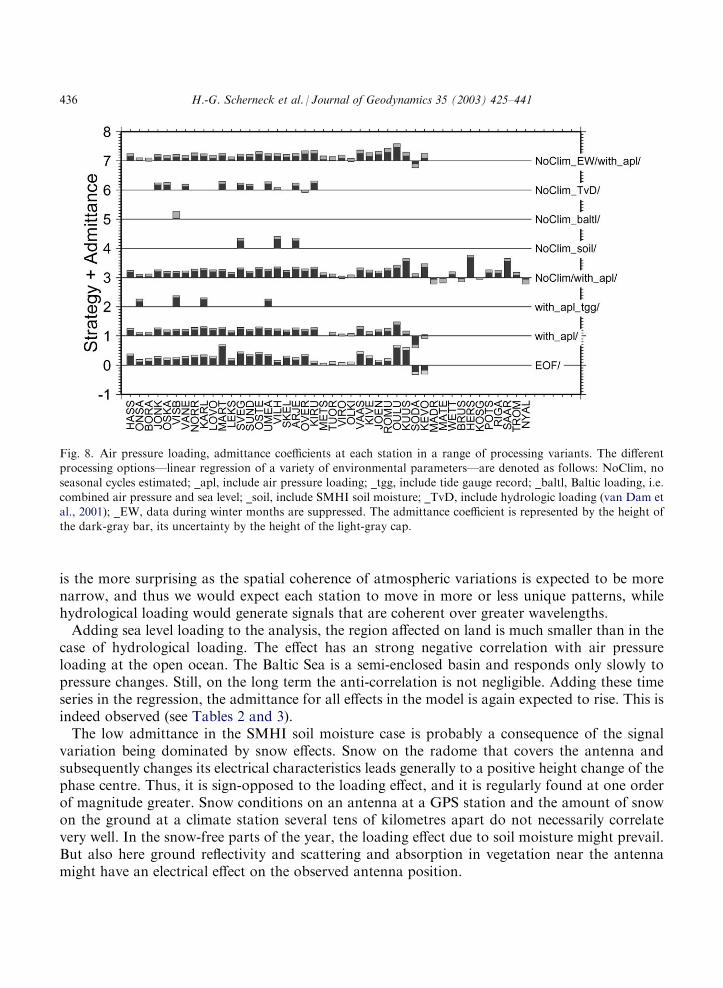
is the more surprising as the spatial coherence of atmospheric variations is expected to be morenarrow, and thus we would expect each station to move in more or less unique patterns, whilehydrological loading would generate signals that are coherent over greater wavelengths.

Adding sea level loading to the analysis, the region affected on land is much smaller than in thecase of hydrological loading. The effect has an strong negative correlation with air pressureloading at the open ocean. The Baltic Sea is a semi-enclosed basin and responds only slowly topressure changes. Still, on the long term the anti-correlation is not negligible. Adding these timeseries in the regression, the admittance for all effects in the model is again expected to rise. This isindeed observed (see Tables 2 and 3).

The low admittance in the SMHI soil moisture case is probably a consequence of the signalvariation being dominated by snow effects. Snow on the radome that covers the antenna andsubsequently changes its electrical characteristics leads generally to a positive height change of thephase centre. Thus, it is sign-opposed to the loading effect, and it is regularly found at one orderof magnitude greater. Snow conditions on an antenna at a GPS station and the amount of snowon the ground at a climate station several tens of kilometres apart do not necessarily correlatevery well. In the snow-free parts of the year, the loading effect due to soil moisture might prevail.But also here ground reflectivity and scattering and absorption in vegetation near the antennamight have an electrical effect on the observed antenna position.

Fig. 8. Air pressure loading, admittance coefficients at each station in a range of processing variants. The differentprocessing options—linear regression of a variety of environmental parameters—are denoted as follows: NoClim, noseasonal cycles estimated; _apl, include air pressure loading; _tgg, include tide gauge record; _baltl, Baltic loading, i.e.

combined air pressure and sea level; _soil, include SMHI soil moisture; _TvD, include hydrologic loading (van Dam etal., 2001); _EW, data during winter months are suppressed. The admittance coefficient is represented by the height ofthe dark-gray bar, its uncertainty by the height of the light-gray cap.


Visby (VISB) on the island of Gotland presents an interesting case in Fig. 8. When the loadingfrom air pressure and sea level are combined, giving approximately a sea bottom pressure, theremaining air pressure loading effect has an insignificant amplitude. The effect to be admitted issupposed to consist of the pressure acting on the island only, which is expected to cause only littleadditional deformation.

First attempts to discriminate loading effects due to variations in the Gulf of Bothnia and BalticSea level reveals low admittance again by a factor of three to four. Table 4 shows admittancecoefficients of vertical position versus water level at the closest tide gauge. These values are typi-cally close to �0.004, whereas Fig. 6 suggests coefficients between �0.01 and �0.02. In particular,the Gulf of Bothnia has some unique features that are not expected to correlate with perturba-tions at IGS stations (even not Metsahovi, the closest station). The basin is small, is subject to achanging supply in the freshwater catchment area, and on the short time scale, large excursionsfrom equilibrium (typically at 0.3 m range) can occur because of its dynamic response to the windfield. The low sensitivity of the GPS station vertical to sea level loading contradicts our favourite

Table 2Processing options for hydrological loading used in Fig. 7

1
global convolution, S=no 2 like 2, S=yes 3 local soil moisture observations, S=no
4
like 3, S=yes 5 like 3, S=yes, EOF-method
‘‘S’’ denotes simultaneous estimation of seasonal sinusoids. Simultaneous air pressure loading is always considered. Inthe fit to the GPS observations, simple regression is used unless EOF denotes when the Empirical Orthogonal Function

method has been used. Global convolution uses the predictions from van Dam et al., 2001, local soil moisture uses theobservations from SMHI.

Table 3Processing variants for rate estimation

1
standard analysis, AP=no, S=yes 2 like 1, with AP 3 like 2, with tide gauge
4
like 1, but S=no 5 like 4, with AP 6 Summer-only solution (Scherneck et al., 2002) with AP
7
like 2, H=LO, S=yes 8 like 2, H=LO, S=no 9 like 5, H=GC, S=yes
10
like 5, H=GC, S=no 11 EOF, S=yes 12 like 11, with AP 13 like 11, H=LO
14
like 11, with AP, H=LO
Here, different loading scenarios are played through, e.g. air pressure loading (AP) with and without simultaneoushydrology (H), and hydrology represented by global convolution (H=GC) or local observation (H=LO). Estimationof seasonal cycles is denoted by ‘‘S’’.


explanation for low admittance for air pressure loading, namely the long-wavelength correlationof these parameters and the neglected influence of the effect at the IGS stations (in orbit compu-tation as well as during mapping of regional results into the reference frame).

Our investigation on the dependence of the rate parameter on different processing optionsseems to indicate that (1) data from before autumn 1996 do not contribute significantly to therobustness of the estimates. Thus the early years of the project could soon be ignored in theestimation of motion; during this period most of the changes of the antenna assemblies hadoccurred, necessitating the estimation of many bias parameters. (2) The loading effects that wehave studied are not vital for the robustness of rate estimates. Most of the variations shown inFig. 7 are within one standard deviation.

The largest changes can be seen in the variants 9 and 10. They include the hydrological loadingfrom the global convolution of the Milly and Shmakin (2002a) data set (van Dam et al., 2001).The change in the rate, however, is possibly a consequence of the truncation of the time seriesanalysis at the end of the year 1998. This notion is supported by the end-cutoff test shown inFig. 1. From Fig. 8 we find that the admittance of hydrological loading trades off with theadmittance of atmospheric pressure loading. This could be interpreted as a competitive processabout mostly the annual period in the observations. An annual period in GPS data, however,may collect many more effects than those considered in this study.

Fig. 5 includes the EOF common mode. Like in the example shown, we regularly find that thissignal contains roughly 50% of the of the observation residual as measured by the RMS. TheEOF common mode shown has been derived in an extended solution with all perturbing pro-cesses included in the signal model (hydrology from SMHI observations). This finding is inter-preted as a large degree of the perturbations at one station being correlated in a wide region, andthe loading effects due to atmosphere and hydrology (eventually including sea level) do notreduce the residual more than marginally.

The hydrological loading time series, global convolution (van Dam et al., 2001) versus SMHIlocal observation, are found to differ in their signal content. The SMHI data shows generally lessvariation. The reason may be that the soil is not the only storage volume for meteoric water. Thevan Dam et al. (2001) data shows a loading effect at the level of centimetres. If this signal range is

Table 4GPS vertical position variations, admittance coefficients for regional sea level

Site
Coeff. S.D. Tide gauge Pressure loading
w/o
with tide gauge
ONSA
�0.0041 0.0012 Ringhals 0.17 0.25 KARL �0.0056 0.0009 Lake Vanern 0.29 0.29 VISB �0.0109 0.0011 0.20 0.33
OSKA
�0.0036 0.0011 0.17 0.23 SUND �0.0059 0.0009 Spikarna 0.21 0.20 UMEA �0.0020 0.0008 Ratan 0.24 0.29
SKEL
�0.0034 0.0008 Furuogrund 0.17 0.25
Theoretical coefficient is between �0.01 and �0.03. Pressure loading coefficients represent admittance of predictedeffect. Their typical standard deviation is 0.03.


realistic the parameter has the potential to impact the estimated rates, especially if the non-annualcomponents undergo changes, or if secular terms exist. However, extended modeling and testingis needed in order to draw more definitive conclusions.

5. Conclusions

Loading effects of different kinds, air pressure, sea level and hydrology, appear to be resolvablein BIFROST GPS data. In all cases the admittance coefficients found are small on average,smaller than the modelled deformation. The situation for hydrology is especially complicatedsince the effect of snow on the GPS antennas is twofold, depression due to loading of the crust,and a virtual uplift due to electrical effects.

Our estimated velocities come from a network solution which implies a mapping into the velo-city field of a global terrestrial reference system. The connection between these systems is main-tained by a few, reliable IGS stations in the larger region. Biases due to correlated long-term noiseperturbation can be attenuated with the reduction of a common mode. The common mode can beobtained with an Empirical Orthogonal function method using the longest records.

We certainly can conclude that many perturbing effects are visible in the data. Hydrologicalloading appears to have a mid but nevertheless significant impact, and it appears necessary toinclude this signal in the estimation of vertical motion. The present BIFROST solutions used forinference of crustal motion and regional sea level rise have ignored some of the perturbing effectssince data availability would lead to truncation of the GPS data. The relatively low admittancecoefficients found seem to indicate that the system fends off the perturbations. We can presenttwo explanations. First, large scale effects that affect the region correlate with the motions at theconstraining stations; the network solution of a station is the difference of the motion with respectto an effective mean motion of the constraining stations. Second, the reduction of noise in thetime series in terms of attenuation is not overwhelming. We think that a combination of effects onthe signal side that are difficult to model, higher-order atmospheric propagation perturbations,multipath and scattering are the reason. Thus, explicit and improved modelling in the first phasesof the analysis process is the general route to lower noise. All this appears as a process of manysmall steps rather than expecting a major breakthrough. Improvements that are feasible include:computation of orbits and site positions in a consistent way, taking full advantage of the stationdensity in the area; and elevation masks as low as possible.

Acknowledgements

We thank Sten Bergstrom and Nils Gustavsson at SMHI for their help with ECMWF pressureand SMHI climate data. Knut and Alice Wallenberg’s Foundation and the Swedish Council forPlanning and Coordination of Research (FRN) have supported us with equipment. We alsothank the National Land Survey of Sweden, especially the staff engaged in the establishment,maintenance, and operation of SWEPOS. Some stations in Finland were created with the supportof Posiva OY. In campaigns we used equipment made available by the University Navstar Con-sortium (UNAVCO). We also acknowledge the support given be the Swedish Research and


Testing Institute (SP). Research projects have been funded by the Swedish Natural ScienceResearch Council (NFR) under project accounts G-AA/GU04770, continued by The SwedishResearch Council (SRC) under R 504-15/2001, the Swedish National Space Board (SNSB) underDnr 171/98, and the Swedish Research Council for Engineering Sciences (TFR). Some figureswere generated with the Generic Mapping Tools (Wessel and Smith, 1998). Finally our sincerethanks to the ones that reviewed this work and helped improve the manuscript.

References

BIFROST Project 1996 (R.A. Bennett, T.R. Carlsson, T.M. Carlsson, R. Chen, J.L. Davis, M. Ekman, G. El-gered, P.Elosegui, G. Hedling, R.T.K. Jaldehag, P.O.J. Jarlemark, J.M. Johansson, B. Jonsson, J. Kakkuri, H. Koivula, G.A.Milne, J.X. Mitrovica, B.I. Nilsson, M. Ollikainen, M. Paunonen, M. Poutanen, R.N. Pyskly-wec, B.O. Ronnang,H.-G. Scherneck, I.I. Shapiro, and M. Vermeer), 1996. GPS Measurements to Constrain Geo-dynamic Processes in

Fennoscandia. EOS, Trans. AGU 77, 337–341.Breuer, D., Wolf, D., 1995. Deglacial land emergence and lateral upper-mantle heterogeneity in the Svalbard archipe-

lago—I. First results for simple load models. Geophys. J. Int. 121, 775–788.

Calais, E., 1999. Continuous GPS measurements across the Western Alps, 1996-1998. Geophys. J. Int. 138, 221–230.Ekman, M., 1996. A consistent map of the post glacial uplift of Fennoscandia. Terra Nova 8, 158–165.Elosegui, P., Davis, J.L., Jaldehag, R.T.K., Johansson, J.M., Niell, A.E., Shapiro, I.I., 1995. Geodesy using the Global

Positioning System: the effects of signal scattering on estimates of site position. J. Geophys. Res. 100, 9921–9934.Farrell, W.E., 1972. Deformation of the Earth by surface loads. Rev. of Geophys. 10, 761–797.Jaldehag, R.T.K., Johansson, J.M., Elosegui, P., Davis, J.L., Niell, A.E., Rnnng, B.O., Shapiro, I.I., 1996a. Geodesy

using the Swedish permanent GPS network: effects of signal scattering on estimates of relative site positions. J.

Geophys. Res. 101, 17–841-17,860.Jaldehag, R.T.K., Johansson, J.M., Davis, J.L., Elsegui, P., 1996b. Geodesy using the Swedish permanent GPS net-

work: effects of snow accumulation on estimates of site positions. Geophys. Res. Letters 23, 1601–1604.

Johansson, J.M., Davis, J.L., Scherneck, H.-G., Milne, G.A., Vermeer, M., Mitrovica, J.X., Bennett, R.A., El-gered,G., Elosegui, P., Koivula, H., Poutanen, M., Ronnang, B.O., Shapiro, I.I., 2002. Continuous GPS measurements ofpostglacial adjustment in Fennoscandia, 1. Geodetic results. J. Geophys. Res. 107, 28. (DOI 10.1029/2001JB000400).

Langbein, J., Johnson, H., 1997. Correlated errors in geodetic time series; implications for time-dependent deforma-tion. J. Geophys. Res. 102, 591–604.

Milly, P.C.D., Shmakin, A.B., 2002a. Global modelling of land water and energy balances: I. The land dynamics (LaD)

model. J. Hydrometeorology 3, 283–299.Milly, P.C.D., Shmakin, A.B., 2002b. Global modelling of land water and energy balances: II. Land-characteristic

contributions to spatial variability. J. Hydrometeorology 3, 301–310.Milne, G.A., Davis, J.L., Mitrovica, J.X., Scherneck, H.-G., Johansson, J.M., Vermeer, M., Koivula, H., 2001. A map

of 3-D crustal deformation in Fennoscandia emerges from a network of GPS measurements. Science 291, 2382–2385.Mitrovica, J.X., Davis, J.L., Shapiro, I.I., 1994. A spectral formalism for computing three-dimensional defor-mations

due to surface loads, 2. Present-day glacial isostatic adjustment. J. Geophys. Res. 99, 7075–7101.

Scherneck, H.-G., Johansson, J.M., Elgered, G., Davis, J.L., Jonsson, B., Hedling, G., Koivula, H., Ollikainen, M.,Poutanen, M., Vermeer, M., Mitrovica, J.X., Milne, G.A., 2002. BIFROST: observing the three-dimensional defor-mation of Fennoscandia. In: Mitro-vica, J.X., Vermeersen, B.L.A. (Eds.), Glacial Isostatic Adjustment and the Earth

System. Geodynamics Series, Vol. 29, American Geophysical Union, Washington, DC, pp. 69–93.Scherneck, H.-G., Johansson, J.M., Mitrovica, J.X., Davis, J.L., 1998. The BIFROST project: GPS determined 3-D

displacement rates in Fennoscandia from 800 days of continuous observations in the SWEPOS network. Tectono-physics 294, 305–321.

Scherneck, H.-G., Johansson, J.M., Vermeer, M., Davis, J.L., Milne, G.A., Mitrovica, J.X., 2001. BIFROST Project:3-D crustal deformation rates derived from GPS confirm postglacial rebound in Fennoscandia. Earth Planets Space53, 703–708.


van Dam, T.M., Wahr, J., 1987. Displacements of the Earth’s surface due to atmospheric loading: effects on gravity

and baseline measurements. J. Geophys. Res. 92, 1281–1286.van Dam, T.M., Wahr, J., Milly, P.C.D., Shmakin, A.B., Blewitt, G., Lavallee, D., Larson, K.M., 2001. Crustal dis-

placements due to continental water loading. Geophys. Res. Letters 28, 651–654.

Wessel, P., Smith, W.H.F., 1998. New, improved version of the Generic Mapping Tools released. EOS Trans. AGU 79,579.

Williams, S.D.P., Baker, T.F., Jeffreys, G. 2001. Coloured noise and annually repeating signals in GPS and gravity

time. Geophys. Res. Abstr. CD-ROM, 3, Session G3.02, p. 1628. European Geophysical Society, CopernicusGesellschaft, Katlenburg-Lindau, Germany.


Vertical crustal motion observed in the BIFROST project

Documents

Transcript of Vertical crustal motion observed in the BIFROST project