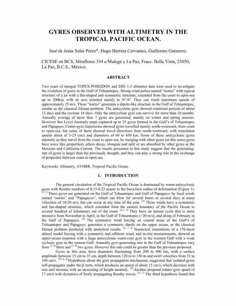
GYRES OBSERVED WITH ALTIMETRY IN THE TROPICAL PACIFIC OCEAN.

José de Jesús Salas Pérez*, Hugo Herrera Cervantes, Guillermo Gutierrez.

CICESE en BCS, Miraflores 334 e/Mulegé y La Paz, Fracc. Bella Vista, 23050, La Paz, B.C.S., México.

ABSTRACT Two years of merged TOPEX-POSEIDON and ERS 1-2 altimeter data were used to investigate the evolution of gyres in the Gulf of Tehuantepec. Strong wind pulses named “nortes” with typical structure of a jet with a fan-shaped and symmetric structure, extended from the coast to open-sea up to 200km, with its axis oriented mainly to Nº-Sº. They can reach maximum speeds of approximately 25 m/s. These “nortes” generates a dipole-like structure in the Gulf of Tehuantepec, similar as the classical Ekman problem. The anticyclone gyre showed rotational periods of about 12 days and the cyclone 18 days. Only the anticyclone gyre can survive for more than 10 months. Annually average of more than 7 gyres are generated, mainly on winter and spring seasons. However Sea Level Anomaly maps captured up to 25 gyres formed in the Gulf’s of Tehuantepec and Papagayo. Center-gyre trajectories showed gyres travelled mainly south-westward, from coast to open-sea, but some of them showed travel directions from north-westward, with translation speeds about of 3-25 cm/s and diameters of 60 to 450 km. Some of these anticyclonic gyres intensify as they travel from the coast to open sea, by merging with other gyres (in this sense gyres have wave like properties), others decay, elongate and split or are absorbed by other gyres or the Mexican and California Current. The results presented in this study suggest that the generating-rate of gyres is larger than the previously thought, and they can play a strong role in the exchange of properties between coast to open sea. Keywords: Altimetry, AVHRR, Tropical Pacific Ocean.

1. INTRODUCTION

The general circulation of the Tropical Pacific Ocean is dominated by warm-anticyclonic

gyres with Rossby numbers of 0.15-0.22 nearer to the baroclinic radius of deformation (Figure 1). [1, 2] These gyres are generated on the Gulf of Tehuantepec and Gulf of Papagayo, by local winds named “nortes” and “Papagayos”, which can blow for several hours or several days at mean velocities of 10-20 m/s, but can occur at any time of the year. [3] These winds have a symmetric and fan-shaped structure, which extended from the eastern boundary of the Pacific Ocean to several hundred of kilometers out of the coast. [4,1, 3] They have an annual cycle that is more intensive from November to April, in the Gulf of Tehuantepec (>20 m/s), and along of February in the Gulf of Papagayo. [5] The symmetric wind forcing on coastal areas of the Gulf’s of Tehuantepec and Papagayo, generates a symmetric dipole on the upper ocean, as the classical Ekman problem predicted with analytical results. [6, 1, 3] Numerical simulations of a 1½-layer alineal model forcing with a symmetric and offshore wind, and in-situ measurements, showed an upper-ocean response with a large anticyclonic warm-core gyre in the western Gulf with a weak cyclonic gyre in the eastern Gulf. Annually gyre-generating rate in the Gulf of Tehuantepec vary from [7, 8] three and [1, 9] two gyres. However this rate could be greater than the previous proposed.

Gyres in this area, have diameters fluctuating from 200 to 400 km, with a surface amplitude between 15 cm to 35 cm, depth between 120 m to 150 m and swirl velocities from 53 to 100 cm/s. [10, 6, 4] Hypothesis about the gyre propagation mechanism, suggested that isolated-gyres self-propagates under the β term, which produces an speed of about 15 cm/s, which decrease with size and increase with an increasing of height anomaly. [9] Another proposal relates gyre speed of 17 cm/s with dynamics of freely propagating Rossby waves. [11, 1] The third hypothesis found that

a speed of about 12-13 cm/s, gyres could propagate with the group velocity of non-dispersive baroclinic Rossby waves.

Figure 1. Seasonal variability in the Tropical Pacific Ocean, from surface sea level anomalies,

derived from the merged TOPEX-POSEIDON and ERS 1-2 altimeters. Indicated are the 0-cm, 10-cm, 20-cm, 30-cm, 40-cm, 50-cm isoheights above the mean sea level.

[1,4, 8] From computed values of Available Potential Energy (APE) of 1-4.1 PJ and Kinetic Energy (KE) 1.3-2.9 PJ and ratios (APE/KE) of 0.8-1.4, the resulted life time estimated of gyres in the Tropical Pacific Ocean is about 6 months. [4, 6] Dissipation of gyres in this area, are by collision with and probably by the reforming of the NECC (North Equatorial Counter Current).

The long-term significance of the gyres on the circulation depends upon how frequently they occur, in this sense is important to increase our acknowledge on the gyre generating rate, propagation, interactions and last fate of the gyres in this area, and its role on the exchange of momentum (kinetic and potential energy), and heat-salt transport from coast to open-sea.

The relationship between winds and gyre evolution in this area, made of the satellite altimetric radars (TOPEX-POSEIDON, ERS 1-2, ERS-1 scatterometer) the appropriate tool to study synoptically this phenomena at large scales and analyse our results on the frame of previous hypothesis. The TOPEX-POSEIDON and ERS 1-2 altimeters offered better accuracy than previous studies made with another altimeter mission (GEOSAT radar), even with those experiments performed with discrete sampling as the carried out with in-situ CTD and ADCP data, or with [12] buoy trajectories which sometimes releasing from the gyres at large periods.

2. DATA SET AND METHODOLOGIES

Satellite altimetry is now a recognized method by which time variable mesoscale ocean

dynamics can be studied. The data set used in this study is composed of altimetric data (TOPEX-POSEIDON and ERS 1-2), wind stress field maps from ERS-1 scatterometer and Sea Surface

Temperature images (SST). These observations covered the period of November of 1995 to January of 1997, to capture the period of maxima occurrence of the northerly winds.

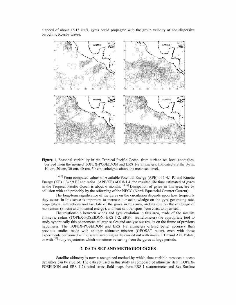
Gyre evolution of the Tropical Pacific Ocean is study with Corrected Sea Surface Height Products (CSSH), computed from merging TOPEX/POSEIDON (T/P) and ERS 1-2 altimeter data. [13, 14] They are provided by Archiving Validation and Integration of Satellite Oceanographic data AVISO/Altimetry. The raw altimeter data are corrected of instrumental errors, ocean wave influences (sea state bias), tide influence and inverse barometer effect, more details concerned on the applied corrections are well explained in the manual. [15] The sea level accuracy measured with the (T/P) orbit is 2-cm rms while ERS 1-2 orbit is determined with the same accuracy of T/P.

Figure 2. TOPEX-POSEIDON and ERS 1-2 ground tracks

CSSH from T/P and ERS 1-2 missions were merged at temporal periods of 10 days to fill gaps on individual files of T/P and ERS 1-2 data, and to increase the spatial resolution of the gyres tracking on the area enclosed between 120º-80º W and from 0º-25ºN (Figure 2). Then Sea Level Anomaly (SLA=η’) was computed removing the annual mean sea level signal estimated for the year of 1996. This technique remove the mean marine geoid also eliminates the mean surface current of the Tropical Pacific Ocean. In this area of the Tropical Pacific Ocean, the little variations in the topography (unmarked variations in the geoid) not obscured the surface gyre signature in altimeter data. [16] Using an objective interpolation analysis, maps of SLA were constructed on a regular grid 0.2ºx0.2º, using a Gaussian correlation function with an e-folding radius of interpolation of 0.2 degrees. Because 15% of the surface height anomaly is reduced when we made the interpolation analysis, smoothed individual profiles were plotted as time series to observe their decay, avoiding the less of resolution involving with the interpolating process. [17]

CERSAT and IFREMEMER provided the weekly wind stress field computed from ERS-1 scatterometer. They were used to identify the shape of the forcing (“nortes” and “Papagayos”) in the Gulf’s of Tehuantepec and Papagayo, and their relationship with gyres generation, observed on maps of altimetry and sea surface temperature. Wind fields are limited to predict the lasts of nortes and Papagayos events, on time-scales of hours. [17] The procedure to compute wind stress fields interpolated in boxes of 1ºx1º are well explained in the manual. Errors in the wind-stress fields are smaller than 0.20 dyn/cm^2.

By the large variability of the phenomena in both time and space, altimeter-data must be analysed together with AVHRR images (Advanced Very High Resolution Radiometer). The AVHRR images are 8-day averaged images from version 4.1 of SST analysis, carrying out by NOAA/NASA AVHRR Oceans Pathfinder Project. The images have only the highest quality declouded pixels. Coastal gyre evolution was well observed on SST images, but on open-sea its signal was masked by cloud coverage.

3. RESULTS AND DISCUSSION

In this section we present the main features of the gyre evolution captured with altimetric

and SST maps and their relationship with wind fields. The main aspects of gyre evolution are generation, propagation, interaction, decay and exchange of momentum and heat. In general, a complete life history of several anticyclonic gyres is clearly observed in this area during our period of study, however to avoid repeated information along the article, the observations are focusing in two gyre life-history (G1 and G2), observed in the Gulf of Tehuantepec from

November of 1995 to December of 1996. Only in such cases that we consider necessary to explain more details of others gyres, we will introduce them along of the article. 3.1 Wind forcing

During the period of measurement, 29 weak and strong northerly winds took place on the Gulf of Tehuantepec. Wind events are more frequently in November than other months. Not all of these 29 wind events were associated with a gyre generation. The typical structure of one norte, is a jet, which extend from the head of the Gulf of Tehuantepec to open-sea by about 150-210 km (Figure 3). The strongest events, with fluctuating magnitudes of about 12-25 m/s, showed approximately a symmetric and fan-shaped structure with its axis oriented mainly to Nº-Sº, but spontaneously its axis direction changed to NWº-NEº and NEº-NWº directions. The maximum velocities of the jet are in its own center, about 25 m/s. The most intense event of this season occurred between 13-20 November of 1995 (Figure 3b).

3.1 Rate-generating gyre and gyre generation

A total of 25 warm gyres were identified in the SLA maps, between November of 1995

to December of 1996. Of these gyres, 7 were clearly identified as gyres formed in the Gulf of Tehuantepec by wind events named “nortes”, while 7 gyres more originated in the Gulf of Papagayo by wind events named Papagayos. The upper-ocean response to wind events in the Gulf of Tehuantepec is well captured on the composite images of SLA, plus SST and wind fields.

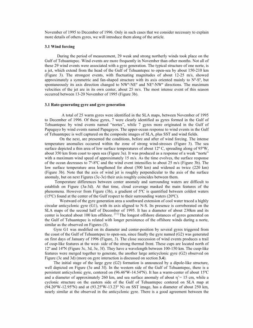
On the next, are presented the conditions, before and after of wind forcing. The intense temperature anomalies occurred within the zone of strong wind-stresses (Figure 3). The sea surface depicted a thin area of low surface temperatures of about 12º C, spreading along of 95ºW, about 350 km from coast to open sea (Figure 3a). It was produced as a response of a weak “norte” with a maximum wind speed of approximately 15 m/s. As the time evolves, the surface response of the ocean decreases to 7º-8ºC and the wind event intensifies to about 25 m/s (Figure 3b). The low surface temperature area lengthened for about (500 km) and widened as twice (220 km) (Figure 3b). Note that the axis of wind jet is roughly perpendicular to the axis of the surface anomaly, but on next Figures (3c-3e) their axis roughly coincides between them.

Temperature differences between center anomaly and surrounding waters are difficult to establish on Figure (3a-3d). At that time, cloud coverage masked the main features of the phenomena. However from Figure (3h), a gradient of 5ºC is quantified between coldest waters (15ºC) found at the center of the Gulf respect to their surrounding waters (20ºC).

Westward of the gyre generation area a southward extension of cool water traced a highly circular anticyclonic gyre (G1), with its axis aligned to N-S. Its presence is corroborated on the SLA maps of the second half of December of 1995. It has a diameter of about 230km and its center is located about 100 km offshore. [11] The longest offshore distances of gyres generated on the Gulf of Tehuantepec is related with longer persistence of the offshore winds during a norte, similar as the observed on Figures (3).

Gyre G1 was modified on its diameter and center-position by several gyres triggered from the coast of the Gulf of Tehuantepec to open-sea, since finally the gyre named (G2) was generated on first days of January of 1996 (Figure, 3). The close succession of wind events produces a trail of cusp-like features at the west- side of the strong thermal front. These cups are located north of 12º and 14ºN (Figure 3c, 3d, 3e, 3f). They have a wavelength between 100-150 km. The cusp-like features were merged together to generate, the another large anticyclonic gyre (G2) observed on Figure (3c and 3d) (more on gyre interaction is discussed on section 3.4).

The initial stage of the large gyre (G2) formation is announced by a dipole-like structure, well depicted on Figure (3e and 3f). In the western side of the Gulf of Tehuantepec, there is a persistent anticyclonic gyre, centered on (96.46ºW-14.54ºN). It has a warm-center of about 15ºC and a diameter of approximately 260 km, and sea surface anomaly of about η’= 15 cm, while a cyclonic structure on the eastern side of the Gulf of Tehuantepec centered on SLA map at (94.20ºW-12.95ºN) and at (93.25ºW-13.23º N) on SST image, has a diameter of about 250 km, nearly similar at the observed in the anticyclonic gyre. There is a good agreement between the

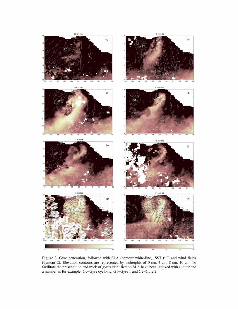
Figure 3. Gyre generation, followed with SLA (contour white-line), SST (ºC) and wind fields (dyn/cm^2). Elevation contours are represented by isoheights of 0-cm, 4-cm, 8-cm, 10-cm. To facilitate the presentation and track of gyres identified on SLA have been indexed with a letter and a number as for example: Gc=Gyre cyclonic, G1=Gyre 1 and G2=Gyre 2.

placing and size of gyre G2 on SST and SLA maps. Its surface signature η’= 22 cm is larger than the anticyclonic one. The signal of this cyclonic gyre is persistent, about 20 days. This result not agrees with previous studies, where the cyclonic structure of the dipole, is not well depicted on the SST image [[1] Figure 3].

Moreover the cyclonic gyre decays rapidly by an “entrainment” processes in the base of the termocline (McCreary et al, 1989; Barton et al, 1993; Trasviña et al, 1995). On Figure (3g and 3h) the geostrophic velocity of the dipole was superposed on the SST image. A strong offshore flow occurred at the center of the dipole, which turn to the west to describe the anticyclonic gyre, which flowed at maximum speeds of about 80 cm/s. While in the eastern side, the flow describes a cyclonic gyre with maximum speeds of about 40 cm/s, weaker than the observed on the anticyclonic flow. At that time a warm surface streamer of warm waters is seen to advance from the head of the Gulf to both gyres (Figure 3g and 3h). On this stage of its generation the newly generated gyres typically maintain temperatures over 17ºC at its core.

The relative vorticity on the dipole well agrees with the flow depicted by geostrophic currents. The highest values of relative vorticity occur at gyre centers. The maximum of relative vorticity in the anticyclone is about ζ=–1.2x10^-5 1/s, while in the cyclone is of approximately ζ=8x10^-6 1/s. The estimated local Rossby numbers Ro=(ζ/f) are 0.36 (anticyclone) and 0.24 (cyclone). It means that the Coriolis parameter f is about 36% and 24%. These values suggested that gyre cores are less non-linear than their surrounding waters. For a radius of about 125km the gyres are in solid body rotation, which means that the Rossby numbers inside the core of the gyres needs to be constant. Rotational periods, estimated from the vorticity, were about 12 days (anticyclone) and 18 days (cyclone).

Something unusual in comparison with previous studies of this area is a gyre emanating from the head of the Gulf of Tehuantepec on summer (11-31 July) (Figure 1c). This gyre shows height amplitude of 15 cm and a diameter of about 100 km. It translates its center of mass not so far from its source area. Then of about 1 month, it not depicted a clear signal on the SLA and SST maps. The generation of this gyre is not well correlated with a wind event. So, the gyre could be formed by another forcing mechanism, which we cannot explain for lacking of strong “trails” that help to put forward a hypothesis about of its generation. [4] In other study proposed that drifting westward gyres could be generated by the onset of the NECC (North Equatorial Counter Current) in July. However on (Figure 1c) is clear that this gyre was triggered from the Gulf of Tehuantepec to open-sea. This requires verification trough closer and more systematic investigation. 3.2 Kinematic properties of gyres

Quantitative analyses of the size, eccentricity, and orientation of the gyres (G1 and G2)

from the SLA maps are presented as time-series. The kinematic properties of both gyres were computed as much as gyres G1 and G2 were drifted as isolated gyres. As consequence they have different time-length on Figure 3. The formed gyres (G1 and G2) clearly grow in diameter as they propagate westward. Gyre G1 approximately doubling in size, from 200 km to 400 km on its diameter, for about 60 days, while the maximum increase of gyre G2 was on day 70, with approximately 300 km. On their propagation the gyres diameter is modified both in latitude and longitude, and the eccentricity mainly showed an elliptical shape, with a 2:1 ratio of long-to-short axes. On merged and decay processes gyres tended to acquire a circular shape with eccentricity values close 1. The diameter of both gyres at long-times tend to fall (not showed on figure 3a). This behaviour is an indicative of the gyre decaying. The major axis was directed on the north-south direction (Figure 3). From altimeter data we estimated the Rossby number (Ro=V/fL). Here V is the maximum geostrophic velocity found within the gyre (the velocity at L). [4, 8] We found Ro=0.3, comparable to the values estimated previously and in other studies.

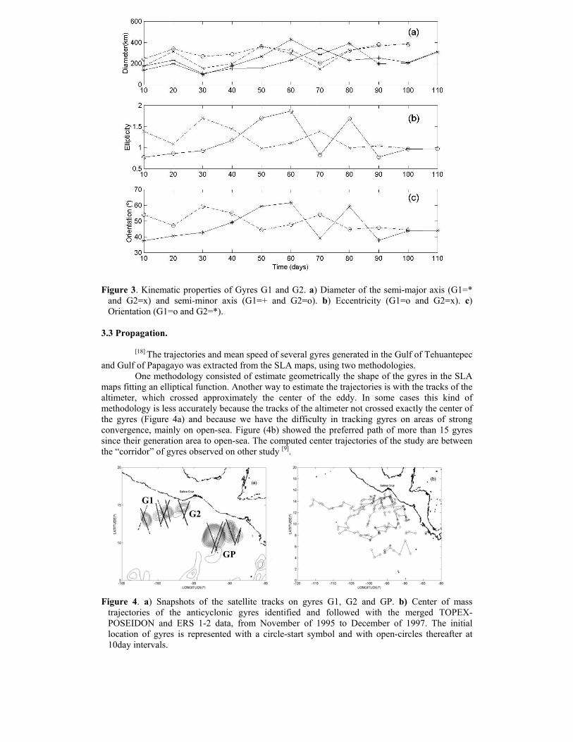
Figure 3. Kinematic properties of Gyres G1 and G2. a) Diameter of the semi-major axis (G1=* and G2=x) and semi-minor axis (G1=+ and G2=o). b) Eccentricity (G1=o and G2=x). c) Orientation (G1=o and G2=*).

3.3 Propagation.

[18] The trajectories and mean speed of several gyres generated in the Gulf of Tehuantepec

and Gulf of Papagayo was extracted from the SLA maps, using two methodologies. One methodology consisted of estimate geometrically the shape of the gyres in the SLA

maps fitting an elliptical function. Another way to estimate the trajectories is with the tracks of the altimeter, which crossed approximately the center of the eddy. In some cases this kind of methodology is less accurately because the tracks of the altimeter not crossed exactly the center of the gyres (Figure 4a) and because we have the difficulty in tracking gyres on areas of strong convergence, mainly on open-sea. Figure (4b) showed the preferred path of more than 15 gyres since their generation area to open-sea. The computed center trajectories of the study are between the “corridor” of gyres observed on other study [9].

Figure 4. a) Snapshots of the satellite tracks on gyres G1, G2 and GP. b) Center of mass trajectories of the anticyclonic gyres identified and followed with the merged TOPEX-POSEIDON and ERS 1-2 data, from November of 1995 to December of 1997. The initial location of gyres is represented with a circle-start symbol and with open-circles thereafter at 10day intervals.

GP

G2 G1

The largest trajectories, comes from gyres formed in the Gulf of Tehuantepec, while the shortest from gyres generated on Gulf of Papagayo. Gyres drift directions is confined at a “corridor” between 6º-14ºN and 90º-120ºW. With a few exceptions, most of the gyres moved in a more or less south-westerly direction. Their average speed between the start and end date, fluctuated between 3 to 26 cm/s, where the interval of 12 to 17 cm/s approximately falls within the range of speeds reported in previous studies [1, 4, 8,9].

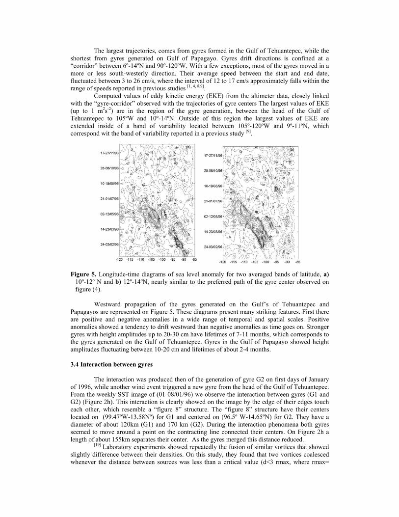
Computed values of eddy kinetic energy (EKE) from the altimeter data, closely linked with the “gyre-corridor” observed with the trajectories of gyre centers The largest values of EKE (up to 1 m2s-2) are in the region of the gyre generation, between the head of the Gulf of Tehuantepec to 105ºW and 10º-14ºN. Outside of this region the largest values of EKE are extended inside of a band of variability located between 105º-120ºW and 9º-11ºN, which correspond wit the band of variability reported in a previous study [9].

Figure 5. Longitude-time diagrams of sea level anomaly for two averaged bands of latitude, a) 10º-12º N and b) 12º-14ºN, nearly similar to the preferred path of the gyre center observed on figure (4).

Westward propagation of the gyres generated on the Gulf’s of Tehuantepec and

Papagayos are represented on Figure 5. These diagrams present many striking features. First there are positive and negative anomalies in a wide range of temporal and spatial scales. Positive anomalies showed a tendency to drift westward than negative anomalies as time goes on. Stronger gyres with height amplitudes up to 20-30 cm have lifetimes of 7-11 months, which corresponds to the gyres generated on the Gulf of Tehuantepec. Gyres in the Gulf of Papagayo showed height amplitudes fluctuating between 10-20 cm and lifetimes of about 2-4 months. 3.4 Interaction between gyres

The interaction was produced then of the generation of gyre G2 on first days of January of 1996, while another wind event triggered a new gyre from the head of the Gulf of Tehuantepec. From the weekly SST image of (01-08/01/96) we observe the interaction between gyres (G1 and G2) (Figure 2h). This interaction is clearly showed on the image by the edge of their edges touch each other, which resemble a “figure 8” structure. The “figure 8” structure have their centers located on (99.47ºW-13.58Nº) for G1 and centered on (96.5º W-14.65ºN) for G2. They have a diameter of about 120km (G1) and 170 km (G2). During the interaction phenomena both gyres seemed to move around a point on the contracting line connected their centers. On Figure 2h a length of about 155km separates their center. As the gyres merged this distance reduced.

[19] Laboratory experiments showed repeatedly the fusion of similar vortices that showed slightly difference between their densities. On this study, they found that two vortices coalesced whenever the distance between sources was less than a critical value (d<3 rmax, where rmax=

radius of the smaller vortice). Applying this to the observed gyres (G1 and G2), rmax of the smaller gyre was 60 km and the distance between G1 and G2 155 km, or less than the critical distance (d) for coalescence. These anticyclonic gyres merged at a time scale of about 40 days into one stronger gyre (Figure 6e). Something important is to note that not always the formation of cusp-like features herald coalescing [19]. In these cases gyres can interact and exchange some properties of their water (not probe with our observations), but then move apart and become more circular again [19]. On open-sea, gyres repeatedly coalesced to and separated again by the change of the wind field fluctuations and by collision by self without any forcing.

3.5 Gyre Decay

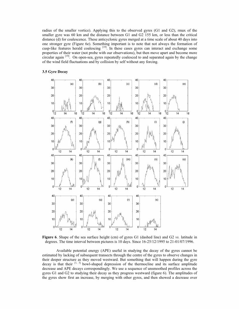
Figure 6. Shape of the sea surface height (cm) of gyres G1 (dashed line) and G2 vs. latitude in degrees. The time interval between pictures is 10 days. Since 16-25/12/1995 to 21-01/07/1996.

Available potential energy (APE) useful in studying the decay of the gyres cannot be

estimated by lacking of subsequent transects through the centre of the gyres to observe changes in their deeper structure as they moved westward. But something that will happen during the gyre decay is that their [1, 3] bowl-shaped depression of the thermocline and its surface amplitude decrease and APE decays correspondingly. We use a sequence of unsmoothed profiles across the gyres G1 and G2 to studying their decay as they progress westward (figure 6). The amplitudes of the gyres show first an increase, by merging with other gyres, and then showed a decrease over

time and with distance from its source area. Apart of its natural decay, the height amplitude of the gyres captured with SLA maps, will have been attenuated by several factors as for example: The maximum amplitude for the gyres depends on the position of the gyre relative to the satellite ground tracks as is seen in figure 4a, and by interaction between gyres.

To estimate the decay rate, we used gyres G1 and G2 that were crossed approximately at its center by the satellite tracks. Gyre G1 merged with gyre G2 up of about 1 month (figure, 6e), while gyre 2 decayed then of about 8 months (figure 6s). The individual rate of decrease of gyre G2 was about 1.8cm month-1, it gives an estimation of the lifetime of the gyre.

4. SUMMARY

Remote sensing observations give relevant information on the evolution of gyres in the

Tropical Pacific Ocean, providing continuos coverage. This allows a long enough time series to efficiently track the gyres surface signature evolution, since its generation to its final destiny.

In some aspects of this research the remote sensing observations are limited to explain some observed gyres features with SLA and SST maps, as for example: the generation of one gyre in summer; the vertical structure of the gyres as they moved westward and their related heat and salt properties to compute fluxes. In such cases is strongly recommended to use information obtained from in-situ observations.

Future studies will be focusing on the track of one gyre, since its generation to its final destiny, combining altimeter data and in-situ observations. Moreover the estimation of transfer fluxes between gyres and its environment, could be a good subject of study to elucidate the role which gyres plays on the surface circulation of the Tropical Pacific Ocean.

ACKNOWLEDGEMENTS

We are gratefully with CONACYT (Consejo Nacional de Ciencia y Tecnologia) for providing funds through the project “Circulación Tridimensional de Mesoescala en el Pacifico Tropical Mexicano” (Ref. I32963-T). The CSSH were provided by AVISO, from CLS of France. The AVHRR images were obtained via FTP from the public PO.DAAC user services. B. Bentamy from CERSAT and IFREMER kindly provide me, the wind fields used in this study. I’m thankfully with the people of my Institution who contributed to complete this research.

5. REFERENCES

1. E.D. Barton, M.L. Argote, J. Brown., P. Michel Kosro, M.F. Lavín, J.M. Robles, R.L. Smith,

A. Trasviña and H.S. Veléz, Supersquirt: Dynamics of the Gulf of Tehuantepec, Mexico. Oceanography, 6,1: 23-30,1993.

2. R.V. Legeckis, Upwelling off the Gulfs of the Panama and Papagayo in the Tropical Pacific During March 1985. J. Geophys. Res., 95, No. C12, 15,485-15489, 1988.

3. A. Trasviña., E.D. Barton, J. Brown, H.S. Velez, P.M. Kosro and R.L. Smith, Offshore wind forcing in the Gulf of Tehuantepec, México: The asymmetric circulation. J.Geophys. Res.,100: 20,649-20,663, 1995.

4. D.V Hansen and G.A. Maul, Anticyclonic Current Rings in the Eastern Tropical Pacific Ocean. J. Geophys. Res., 96: 6965-6979, 1991.

5. M. Crepon and C. Richez, Transient upwelling generated by two-dimensional atmospheric forcing and variability in the coastline. J. Phys. Oceanogr, 1012-1033, 1982.

6. J.P. McCreary, H.S. Lee and D.B. Enfield, The response of the coastal ocean to strong offshore winds: with application to circulation in the Gulf’s of Tehuantepec and Papagayo. J. Mar. Res.,47,81-109, 1989.

7. Leben, R.R., J.D. Hawkins, H.E. Hulburt and J.D. Thompson, Wind Driven Anticyclonic Eddies in the Eastern Pacific, EOS, 71, No. 43, 1364, 1990.

8. Whillet, C.S. and L. Kantha, A simple dynamical model of anticyclonic eddies in the eastern tropical Pacific Ocean, J. Geophys. Res., 2-50, 1997.

9. B. Giese, J.A. Carton, and L.J. Holl, Sea Level variability in the eastern tropical Pacific as observed by TOPEX and Tropical Ocean-Global Atmosphere-Ocean Experiment, 9, C12, 24739-24,749, 1994.

10. T. Matsuura and T. Yamagata, On the evolution of nonlinear planetary eddies larger than the radius of deformation, J. Phys. Oceanogr., 12, 5, 449-456, 1982.

11. Stumpf, G.H. and R.V. Legeckis, Satellite Observations of Mesoscale Eddy Dynamics in the Eastern Tropical Pacific Ocean. J. Phys. Oceanogr., 7: 648-658, 1977.

12. Shapiro, G.I., E.D. Barton and S.L. Meschanov, Capture and release of Lagrangian floats by eddies in shear flow. J. Geophys. Res.,102: 27,887-27,092, 1995.

13. AVISO User handbook for Corrected Sea Surface Heights altimeter products, AVI-NT-011-311-CN, edition 2.0, 1996.

14. Le Traon, P.Y., Gaspar, P., Bouyssel, F. and Makhmara, H., Using Topex Poseidon data to enhance ERS1 data. J. Atmos. Oceanic Technol., 12, 161-170, 1995.

15. Le Traon, P.Y., F. Nadal, and N. Ducet, An improved mapping method of multisatellite altimeter data. J. Atmos .Oceanic Technol., 15: 522-534, 1998.

16. Bretherton, F.P., R.E. Davis and C.B. Fandry, A technique for objective analysis design of oceanographic experiments applied to Mode 73, Deep. Sea. Res., 23, 559-582, 1976.

17. C2-MUT-W-02-IF, Scatterometer mean wind field products, user manual, CERSAT, Version 1, 1-57, 1996.

18. H.E., Willoughby, and M.B. Chelmow, Objective determination of hurricane tracks from aircraft observations. Mon. Wea. Rev., 110, 1298-1305, 1982.

19. R.W. Griffths and E.J. Hopfinger, Coalescing of geostrophic vortices, J. Fluid. Mech., 178, 73-97, 1987.

_______________________________________________________________________________ * Correspondence: E-mail: joses@pv1.udg.mx