Sea Level and Eddy Kinetic Energy variability using Satelite altimetry
45
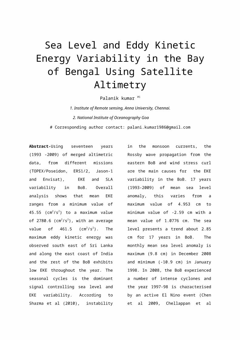
Sea Level and Eddy Kinetic Energy Variability in the Bay of Bengal Using Satellite Altimetry Palanik kumar #1 1. Institute of Remote sensing, Anna University, Chennai. 2. National Institute of Oceanography Goa # Corresponding author contact: [email protected] Abstract-Using seventeen years (1993 -2009) of merged altimetric data, from different missions (TOPEX/Poseidon, ERS1/2, Jason-1 and Envisat), EKE and SLA variability in BoB. Overall analysis shows that mean EKE ranges from a minimum value of 45.55 (cm 2 /s 2 ) to a maximum value of 2780.6 (cm 2 /s 2 ), with an average value of 461.5 (cm 2 /s 2 ). The maximum eddy kinetic energy was observed south east of Sri Lanka and along the east coast of India and the rest of the BoB exhibits low EKE throughout the year. The seasonal cycles is the dominant signal controlling sea level and EKE variability. According to Sharma et al (2010), instability in the monsoon currents, the Rossby wave propagation from the eastern BoB and wind stress curl are the main causes for the EKE variability in the BoB. 17 years (1993-2009) of mean sea level anomaly, this varies from a maximum value of 4.953 cm to minimum value of -2.59 cm with a mean value of 1.0776 cm. The sea level presents a trend about 2.85 cm for 17 years in BoB. The monthly mean sea level anomaly is maximum (9.8 cm) in December 2008 and minimum (-10.9 cm) in January 1998. In 2008, the BoB experienced a number of intense cyclones and the year 1997-98 is characterised by an active El Nino event (Chen et al 2009, Chellappan et al
Transcript of Sea Level and Eddy Kinetic Energy variability using Satelite altimetry
Sea Level and Eddy KineticEnergy Variability in the Bay
of Bengal Using SatelliteAltimetry
Palanik kumar #1
1. Institute of Remote sensing, Anna University, Chennai.
2. National Institute of Oceanography Goa
# Corresponding author contact: [email protected]
Abstract-Using seventeen years
(1993 -2009) of merged altimetric
data, from different missions
(TOPEX/Poseidon, ERS1/2, Jason-1
and Envisat), EKE and SLA
variability in BoB. Overall
analysis shows that mean EKE
ranges from a minimum value of
45.55 (cm2/s2) to a maximum value
of 2780.6 (cm2/s2), with an average
value of 461.5 (cm2/s2). The
maximum eddy kinetic energy was
observed south east of Sri Lanka
and along the east coast of India
and the rest of the BoB exhibits
low EKE throughout the year. The
seasonal cycles is the dominant
signal controlling sea level and
EKE variability. According to
Sharma et al (2010), instability
in the monsoon currents, the
Rossby wave propagation from the
eastern BoB and wind stress curl
are the main causes for the EKE
variability in the BoB. 17 years
(1993-2009) of mean sea level
anomaly, this varies from a
maximum value of 4.953 cm to
minimum value of -2.59 cm with a
mean value of 1.0776 cm. The sea
level presents a trend about 2.85
cm for 17 years in BoB. The
monthly mean sea level anomaly is
maximum (9.8 cm) in December 2008
and minimum (-10.9 cm) in January
1998. In 2008, the BoB experienced
a number of intense cyclones and
the year 1997-98 is characterised
by an active El Nino event (Chen
et al 2009, Chellappan et al
2009). SLAs (both positive and
negative) during December of all
the years (1993-2009) show high
fluctuations associated with warm
and cold core eddies. The minimum
SLA was observed in March/April.
This annual cycle variation in sea
level is due to the steric-effect
- increase in the volume of ocean
without change in the mass
(Caballero et al., 2007). The
intense variability in sea level
along the east coast of India and
around Sri-Lankan coast is due to
the existence of western boundary
currents (WBC). Since the ocean
and the atmosphere are a coupled
system, variability of sea level
reflects changes in climate. One
of the most important aspects of
the climate in the bay is the
Indian monsoon, which possesses
large inter-annual variability.
This variability may cause marked
sea level change due to uctuationfl
of monsoon wind, precipitation
minus evaporation (P - E), heat
uxes, and river runoff into thefl
bay.
Keywords- sea level anomaly, eddy kinetic energy, El-Nino, Rossby waves, Bay of Bengal.
I. INTRODUCTION
Monitoring ocean eddies is vital
for a number of reasons; ocean
eddies affect climate,
transportation, recreation and the
food supply. Sensor technology has
made it easier to probe the ocean
and monitor its eddies, currents,
temperature, salinity, colour and
sea surface height. This
introduction part discusses remote
sensing of oceans by satellite
altimeter, its principle and
applications. Before satellite
altimeter missions, most knowledge
of the global ocean circulation
has been pieced together from
spatially and temporally scattered
observations, which are not
adequate
for a quantitative description of
either the mean or the time-
varying components of the global
ocean circulation. The only
viable approach to observe the
surface circulation of the global
ocean with sufficient resolution
and consistent sampling is the use
of a satellite radar altimeter to
measure the height of the sea
surface [Wunsch and Gaposchkin,
1980; Stewart, 1985; Wunsch,
1992]. Use of satellite radar

altimeters to measure global sea
surface height (SSH) has come a
long way since the brief Seasat
mission of 1978. Early missions
measured SSH with an accuracy of
tens of meters. Satellite
altimeter missions such as
TOPEX/Poseidon (launched August
1992) and Jason-1 (launched
December 2001) measure SSH to an
accuracy of a few centimetres.
These satellites were specifically
designed to measure SSH to the
highest possible accuracy.
1.1 Measuring the ocean from space
A moment of reflection will
remind us of the many
oceanographic insights which first
came from satellite images such as
ubiquity of mesoscale eddies in
the ocean, the existence of
phytoplankton blooms in global
oceans. The rapid development of
remote sensing techniques has
provided more and more multi-
source and large area ocean remote
sensing data. How to retrieve the
ocean eddy information from those
remote sensing products and
utilize them effectively in
scientific applications has became
an urgent priority. An examination
of global picture of satellite sea
level anomaly shows that along the
western boundaries of the ocean,
SLA tends to be heterogeneous,
consisting of positive as well as
negative anomaly indicating strong
eddy activity.
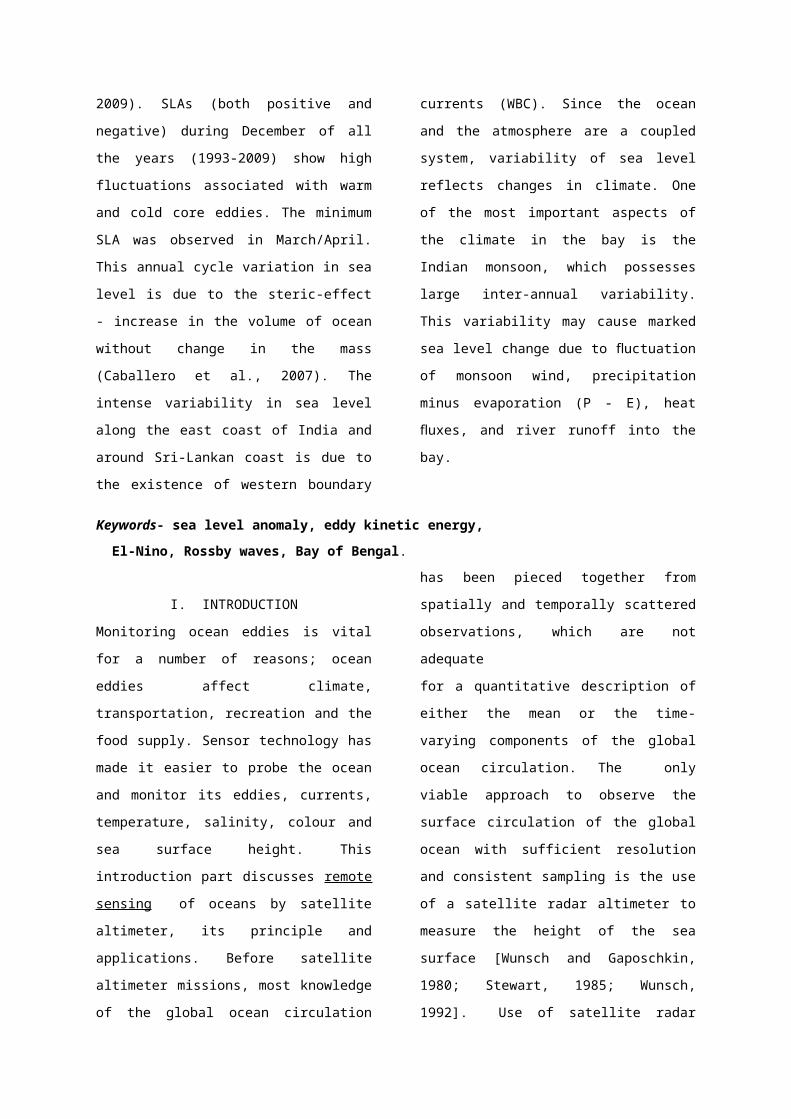
Fig. 1.1. Principle of Satellite Altimeter
(www.jason.noaa.gov.org)
1.1.1 Satellite altimeter and
principle of altimetry
Altimetry satellites determine the
height of the ocean surface with
respect to a reference such as
average global sea level (known as
the Earth’s “geoid”). Orbiting
altimeters make very precise
measurements of the ocean’s
surface topography to derive the
speed and direction of ocean
currents and eddies and to observe
tides and other features.
The primary function of satellite
altimeter is the determination of
satellite's height above the sea
surface. On the simplest level the
altimeter consists of a
transmitter that sends out the
sharp pulses towards the earth, a
receiver to record the pulse after
it is reflected from the surface
and a clock to measure the round
trip travel time of the pulse.
Because the velocity of radar
pulse is known these times can be
used to calculate the satellite’s
height above the surface (Stewart,
1985). As depicted in Fig. 1. 1 to
calculate SSH, several
measurements and calculations are
required along with altimetry
data, including precise
determination of the orbit and
highly accurate tide models. In
addition, because satellite
altimeters measure SSH relative to
the geoid (the sea surface at
resting state), accurate knowledge
of the geoid is required. Besides
surface height, by looking at the
return signal’s amplitude and
waveform, we can also measure wave
height and wind speed over the
oceans, and more generally,
backscatter coefficient and
surface roughness. If the
altimeter emits in two
frequencies, the comparison
between the signals, with respect
to the frequencies used can also
generate interesting results (rain
rate over the oceans, detection of
crevasses over ice shelves, etc).
1.1.2. Components of satellite
altimetry: The main components of
satellite altimetry systems are:
The radar altimeter and antenna,
which measure the sea surface
height , the radiometer, which
measures atmospheric disturbances,
the systems for determining the
satellite precise location in
orbit.
1.1.3 Sources of error in
satellite altimetry: The errors
which occur while measuring SSH
are described below. The
uncertainties of the sea-state
bias have become the leading
sources of error in satellite
altimetry. This error can be
reduced by using BM3 model and
non-parametric model [Gaspar,
1994, Labroue, 2004]. Instrumental
error, atmospheric refraction, and
the interaction between the radar
pulse and the air-sea interface
are the other errors. Instrumental
error consist of random and
systematic component (long-
wavelength). The random error
referred to as instrumental
precision. Uncertainty in SSH
introduced by atmospheric
refraction results from decrease
in the speed of light mainly due
to dry gases, water vapour, and
atmospheric free electrons (Lee et
al.,1988). The range error due to
refraction by dry gases is large,
but can be corrected with the
knowledge of sea level atmospheric
pressure obtained from the
meteorological models. Ionospheric
model (Bentmodel[ERS-1/2]),
(DORIS&TOPEX) dual-frequency[T/P]
by AVISO,1996 is used to correct
the ionospheric range error. ECMWF
model is used to reduce the error
by dry troposphere (Cabellero et
al., 2005)
1.2 Multi-mission mapping
In many ways, the orbit
design of an altimetry satellite
is a compromise. But one point
that deserves special attention is
to get the right balance between
spatial and temporal resolution. A
satellite that revisits the same
spot frequently covers fewer
points than a satellite with a
longer orbital cycle. One solution
to achieve high resolution
coverage is to operate several
satellites together. Merging
multisatellite data sets open a
door to resolve the main space
scales and time scales of the
ocean circulation, in particular,
the meso-scale. Combining
different altimetric missions is a
delicate task: since each mission
has different error budgets and
orbit differences, leading to
large-scale biases and requiring
trends to be corrected. It has
been shown that homogenous and
inter calibrated SSH data sets can
be obtained by using the most
precise mission (T/P and, later
on, Jason-l) as a reference for
the less precise missions (Le
Traon et al., 1995; Le Traon and
Ogor, 1998). Ducet and Le Traon
(2000) gave the first results of
the global mapping. Increasing the
spatial and temporal resolution
was only an idea until the launch
of T/P and ERS-1, which in fact
provided the first opportunity to
merge observations from two
altimeters. Most meso-scale
studies are now taking advantage
of the improved resolution derived
from the SSALTO/DUACS merged,
gridded data sets distributed by
AVISO (Le Traon et al., 1998).
Ducet et al. (2000) presented the
first global high- resolution maps
of mesoscale variability.
Comparing the SSH wavenumber
spectrum from the merged data to
that from the along-track data,
which was considered to represent
the intrinsic resolution of the
altimeter data, they estimated
the resolution of the merged data
to be about 150 km in wavelength.
A similar resolution of about
2° longitude by 2° latitude has
recently been inferred from
wavenumber spectral analysis of
the gridded SSH fields (Chelton
et al., 2009). For Gaussian-
shaped eddies, this wavelength
resolution is able to detect meso-
scale features with e-folding
scales of about 0.4°.
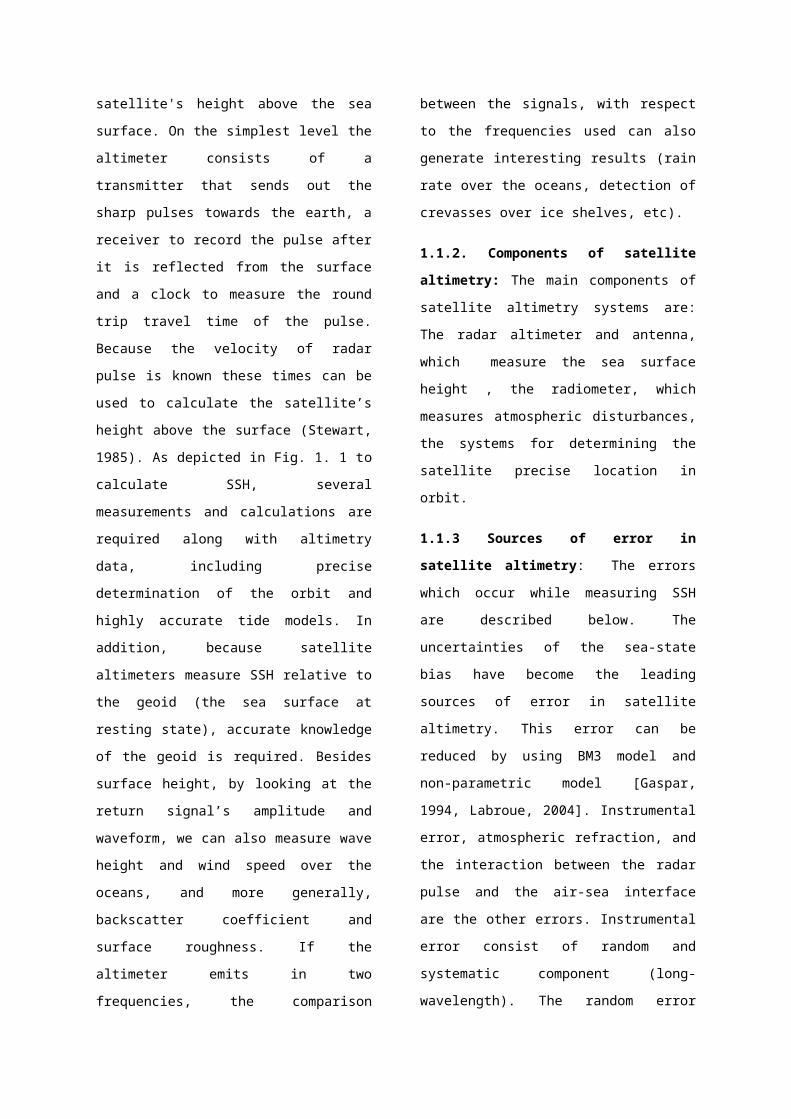
1.3. Ocean dynamic topography:
Ocean currents are mapped by
studying the peaks and trough in
maps of the height of the sea
surface relative to the geoid. The
height is called “dynamic
topography. The altimetric
observation of dynamic topography
η is described in Fig.1.2. Present
geoids are not generally accurate
enough to estimate globally the
absolute dynamic topography η
except at very long wavelengths.
The variable part of dynamic
topography η′ = η -< η>or sea
level anomaly (SLA) is, however,
easily extracted since the geoid
is stationary on the time scale of
an altimetric mission. The most
commonly used method is the
repeat-track method (collinear
analysis). This method is suitable
for satellites whose orbits repeat
their ground tracks (to within ± 1
km) at regular intervals. For a
given track, the variable part of
the signal is obtained by removing
a mean profile (e.g., over the
mission duration), which contains
the geoid and the quasi-permanent
dynamic topography from each
profile.
Fig.1.2. Schematic diagram of dynamics inOcean. (Deborah Klatt 1987)
1.3.1. Sea level change and
variability
The measurement of long-term
changes in global mean sea level
can provide an important
corroboration of predictions by
Ho -- Height of thesatellite’s orbit
Hg -- Geoid height
Ha-- Height of thealtimeter above thesea surface
Hs-- Height of sea
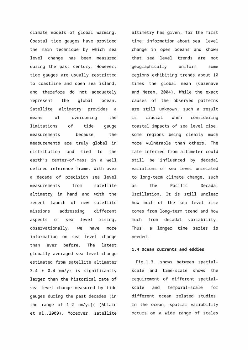
climate models of global warming.
Coastal tide gauges have provided
the main technique by which sea
level change has been measured
during the past century. However,
tide gauges are usually restricted
to coastline and open sea island,
and therefore do not adequately
represent the global ocean.
Satellite altimetry provides a
means of overcoming the
limitations of tide gauge
measurements because the
measurements are truly global in
distribution and tied to the
earth’s center-of-mass in a well
defined reference frame. With over
a decade of precision sea level
measurements from satellite
altimetry in hand and with the
recent launch of new satellite
missions addressing different
aspects of sea level rising,
observationally, we have more
information on sea level change
than ever before. The latest
globally averaged sea level change
estimated from satellite altimeter
3.4 ± 0.4 mm/yr is significantly
larger than the historical rate of
sea level change measured by tide
gauges during the past decades (in
the range of 1–2 mm/yr)( (Ablain
et al.,2009). Moreover, satellite
altimetry has given, for the first
time, information about sea level
change in open oceans and shown
that sea level trends are not
geographically uniform some
regions exhibiting trends about 10
times the global mean (Cazenave
and Nerem, 2004). While the exact
causes of the observed patterns
are still unknown, such a result
is crucial when considering
coastal impacts of sea level rise,
some regions being clearly much
more vulnerable than others. The
rate inferred from altimeter could
still be influenced by decadal
variations of sea level unrelated
to long-term climate change, such
as the Pacific Decadal
Oscillation. It is still unclear
how much of the sea level rise
comes from long-term trend and how
much from decadal variability.
Thus, a longer time series is
needed.
1.4 Ocean currents and eddies
Fig.1.3. shows between spatial-
scale and time-scale shows the
requirement of different spatial-
scale and temporal-scale for
different ocean related studies.
In the ocean, spatial variability
occurs on a wide range of scales
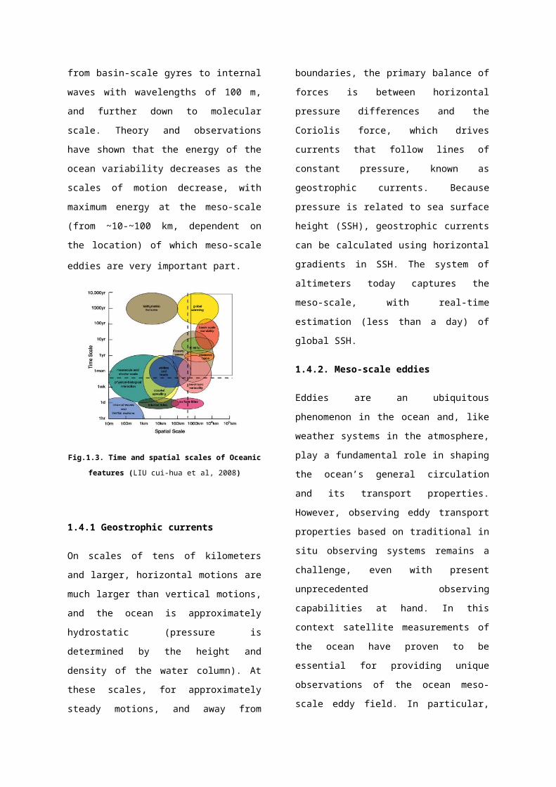
from basin-scale gyres to internal
waves with wavelengths of 100 m,
and further down to molecular
scale. Theory and observations
have shown that the energy of the
ocean variability decreases as the
scales of motion decrease, with
maximum energy at the meso-scale
(from ~10-~100 km, dependent on
the location) of which meso-scale
eddies are very important part.
Fig.1.3. Time and spatial scales of Oceanic
features (LIU cui-hua et al, 2008)
1.4.1 Geostrophic currents
On scales of tens of kilometers
and larger, horizontal motions are
much larger than vertical motions,
and the ocean is approximately
hydrostatic (pressure is
determined by the height and
density of the water column). At
these scales, for approximately
steady motions, and away from
boundaries, the primary balance of
forces is between horizontal
pressure differences and the
Coriolis force, which drives
currents that follow lines of
constant pressure, known as
geostrophic currents. Because
pressure is related to sea surface
height (SSH), geostrophic currents
can be calculated using horizontal
gradients in SSH. The system of
altimeters today captures the
meso-scale, with real-time
estimation (less than a day) of
global SSH.
1.4.2. Meso-scale eddies
Eddies are an ubiquitous
phenomenon in the ocean and, like
weather systems in the atmosphere,
play a fundamental role in shaping
the ocean’s general circulation
and its transport properties.
However, observing eddy transport
properties based on traditional in
situ observing systems remains a
challenge, even with present
unprecedented observing
capabilities at hand. In this
context satellite measurements of
the ocean have proven to be
essential for providing unique
observations of the ocean meso-
scale eddy field. In particular,

altimetry is instrumental for
observing properties of the ocean
eddy field and more generally for
improving our understanding of
eddy dynamics. A detailed summary
of what has been learned from
altimetric sea surface height
(SSH) observations in terms of
large-scale and eddy dynamics is
summarized by Le Traon and Morrow
(2001). Ferrari and Wunsch (2009)
provide a more recent summary of
altimeter-based studies of the
energetics of the ocean
circulation.
Mesoscale eddies occur when there
is a balance of two major forces,
one is a horizontal pressure
gradient force arising from
differences in water density and
the other is an "apparent" force
associated with the Earth’s
rotation, called the Coriolis
force. The Coriolis effect causes
cold-core eddies in the southern
hemisphere to rotate clockwise
(cyclonic) and warm-core eddies
rotate counter clockwise (anti-
cyclonic).
Satellite altimetry has made a
unique contribution to observing
and understanding mesoscale
eddies. We now have more than 20
years of good mesoscale
variability measurements from
Geosat (1986-1989), ERS-1 and ERS-
2 (1991-2008), T/P (1992-2005),
and Jason-1 (2001-2008) to learn
more about the
seasonal/interannual variations in
meso-scale variability. Analyses
of altimeter data have produced
global, quantitative estimates of
eddy kinetic energy (EKE) with
high spatial resolution, revealing
details such as correlation of EKE
with the mean currents and the
role of topography and winds.
Energy of meso-scale eddies
generally exceeds the energy of
mean flow by an order of magnitude
or more (e.g, Wyrtki et al.,
1976; Richardson, 1983; Schmitz
and Luyten, 1991). Merged datasets
from multiple altimeters greatly
improved ability of resolving
mesoscale eddies (Chelton and
Schlax, 2003; Fu et al., 2003;
Pascual et al., 2006). The ability
to monitor them from space has
applications in navigation,
offshore operations, fisheries,
hurricane and climate forecasting.
1.4.3 .Eddy Kinetic Energy
The energy associated with the
turbulent part of the flow of a
fluid or kinetic energy of that
component of fluid flow represents
a departure from the average
kinetic energy of fluid, the mode
of averaging depends on the
particular problem. Also known as
turbulence energy. There are
several studies taken up by
various researchers on EKE of the
global oceans as well as regional
oceans. The satellite altimetry is
a powerful tool to observe the EKE
variability in oceans. The main
sources of EKE is major current
systems exist in the oceans.
Stammer (1997) showed that there
is a good correspondence between
EKE and mean kinetic energy (MKE),
which confirms that the currents
are the main sources of eddies. Xu
et al (2008) showed that Agulhas
region, Kuroshio, Gulf Stream and
ACC are having maximum EKE. They
also found that, ACC meso-scale
variability is found in regions of
abrupt changes of bottom
topography and do not appear to be
associated with strong mean
currents. This may simply imply
that in these areas, baroclinic
instability is unlikely to occur
and that other mechanisms are to
be sought (e.g., barotropic
instability, mean current/bottom
topography interaction). Sources
and sinks of eddy kinetic energy
are Wind-driven sources/sink of
kinetic energy, Sink of KE via
bottom friction,conversion of
potential energy into KE and
dissipation. The baroclinic
instability process depends on the
presence of vertical shear in the
mean flow, implying sloping
density gradients, and an
available store of potential
energy. Under certain conditions,
instabilities form, releasing this
potential energy and converting it
to eddy potential and kinetic
energies. If the mean flow has
significant horizontal shear as in
strong narrow jets, barotropic
instabilities can also occur. In
the real ocean, the mean flow has
both vertical and horizontal
shear, so potentially both
baroclinic and barotropic (mixed)
instabilities can coexist. Through
these instability-forcing
mechanisms, eddy activity is
maximum in regions of major
oceanic currents.

1.4.4. Application of eddy kinetic
energy (EKE)
These oceanic feature having main
applications such as
• Acoustic propagation,
• Optimum ship route planning
• Fishery
• Delineation of good/badmonsoon years
• Heat transport mechanisms.
1.4.5. Wind and its role on EKE
Wind stress is the vertical
transfer of horizontal momentum,
and this momentum is transferred
from the atmosphere to the ocean
by wind stress. Wind fluctuating
in the oceans may generate the EKE
[Stammer 2001]. Seasonal changes
in eddy energy imply that relative
importance of wind –generated eddy
energy is maximum at depth where
baroclinic variability level is
low. There significant correlation
between the seasonal cycle in the
variance of wind stress and the
seasonal cycle in eddy energy over
a substantially wider area than
near the surface. There is a close
correlation between sea level
anomaly and wind stress. Quilfen,
(2000) analysed El-Nino event
during 1997-1998, and showed that
correlation between SLA and wind
stress is 0.94 in the Pacific
region.
1.5. Challenges and perspectives
Better knowledge of ocean
circulation enable us to
understand and predict climate
variability. Altimetry is one of
the most important tools for
monitoring ocean dynamics, and as
such is a source of vital data to
include in forecasting models of
ocean-atmosphere coupled events
such as El Niño, monsoons, the
North Atlantic Oscillation or
decadal oscillations (Xu et al
2008).
However, challenges still exist in
monitoring the ocean variability
from satellite altimetry.
Satellite altimeters are not able
to measure the time-mean
geostrophic currents due to large
uncertainty in geoid. This poses
challenges for deriving the
absolute geostrophic flow in
regions where bottom velocities
are non-zero since hydrographic
estimates of absolute dynamic
topography are unable to capture
the effects of the bottom. The
uncertainties of satellite
altimetry measurements have a high
geographic variability. The
existence of high frequency
energetic barotropic motions in
the ocean can lead to a large
aliasing error in satellite
altimetric observations. New
evidences show that the combined
aliasing from several neighbouring
and crossing tracks could produce
unreal meso-scale signals in
altimeter mapped product. Although
satellite altimetry has improved
our understanding of the climate
system dramatically, it is
important to keep in mind the
problems and new challenges.
1.6. Need for study
A key weakness of nearly all
global climate models is the
absence of an explicit
representation of ocean eddies,
thereby relying on
parameterization. The overall
effect of eddy structure is
important for climate; the
understanding of ocean circulation
is very important for diagnosing
and predicting climate changes and
their effects.Meso-scale eddy are
a critical element in the
establishment of ocean tracer
properties; Eddy provide an avenue
for affecting the ventilation of
heat, Carbon, and other tracers,
and they support rich levels of
biological activity.
A better understanding of large-
scale ocean circulation and long-
term climate variability requires
the knowledge of ocean eddy
kinetic energy.
1.7. Objectives of this study
to estimate the Eddy Kinetic
Energy using geostrophic velocity
components from 17 years of Merged
Sea Level Anomaly altimetry data.
To study the sea level and EKE
variability in the Bay of Bengal
at different temporal and spatial
scales. To infer the eddies,
seasonal currents and other
factors that affect the
variabilities.
2.1. Satellite altimetry and its applications for ocean studies:
The instrument precision of the
Skylab altimeter was inadequate to
detect unambiguously even the sea
level variability associated with
the Gulf Stream (Fu et al 1983).
The first oceanographically useful

altimeter measurements were made
by the Geos-3 Mission (April 1975-
December 1978), which gave
continuous coverage only in the
western North Atlantic. In spite
of crude precision and accuracy,
the Geos-3 data have been used
to produce a map of Gulf Stream
meso-scale variability that
compares well with historical
ship observations (Douglas et
al., 1983). Fu et al. (1987)
demonstrated that a seasonal
signal in the surface current of
the Gulf Stream could be detected
from the Geos-3 data.
The Seasat altimeter (July-October
1978) was the first designed for
oceanographic applications. An
on-board microwave radiometer was
used to estimate the water vapour
range correction. Precision
orbit determination has resulted
in a Seasat orbit accuracy of
better than 50cm (Marsh et
al., 1988). Seasat altimeter sea
level measurements have been shown
to agree with dynamic heights
computed from aircraft
expendable bathythermographs to
an accuracy of 10cm at scales
up to order 1000kin (Bemstein
et al., 1982). With the Seasat
data, oceanographers began to
develop confidence in the quality
and utility of altimeter
measurements. An important aspect
of the Seasat mission is the
availability of a nearly
continuous global data set for the
3.5-month mission, providing
the first global perspective of
sea surface topography and its
variability.
Using only data from the last
month, when Seasat was flown in a
3-day repeat orbit, Cheney et al.
(1983) produced a map showing the
global distribution of mesoscale
sea level variability. Mazzega
(1985) and Woodworth and
Cartwright (1986) pro- duced
altimetrically-determined global
charts of the M2 tide. Using a
mean sea surface computed from
the Seasat data, Tai and Wunsch
(1984) derived the first global
absolute dynamic topography,
showing many qualitatively
plausible patterns of the long
wavelength components of the
mean circulation of the world
ocean. Fu and Chelton (1985)
used Seasat altimeter data to
study the large-scale temporal
variability of the Antarctic
Circumpolar Current for the
period July-October 1978.
After launching of TOPEX/Poseidon
in 1992 there was great
improvement in ocean studies
especially in sea level and meso-
scale studies. There were many
studies taken up by various
researchers using single mission
data understand the dynamics of
ocean. A detailed analysis taken
by Leo Troan (1996, 1998, 2002,
2004) shows main contribution
about merging and analysig methods
of altimetry data to study
mesoscale variability and
estimation of EKE. The T/P+ERS
merged data provide a very good
representation of the meso-scale
variability, the remaining error
can be quite important especially
for correctly determining the
velocity field in coastal and
meso-scale situations (Greenslade
et al., 1997; Tai, 1998). Le Traon
and Dibarboure (2002) provided a
summary of the mapping
capabilities of the T/P + ERS
(Jason-1 + Envisat) configuration,
using simulations from a high-
resolution ocean general
circulation model. With two
altimeters in the T/P-ERS
configuration, they found that sea
level could be mapped with an
accuracy of better than 10% of
signal variance, while velocity
can be mapped with an accuracy of
20–40% of signal variance
(depending on latitude). The
mapping of the ocean signal was
done globally through an improved
objective analysis method that
takes long wavelength residual
errors into account and uses
realistic correlation scales of
the ocean circulation with a
global high-resolution of ¼ degree
every 10 days. To reduce
measurement noise, sea level
anomaly (SLA) is filtered and sub-
sampled. SSALTO/DUACS project
applied the sub-optimal
interpolation technique to
construct gridded data sets from
multi-mission altimeter data (Le
Traon and Dibarboure, 2002).
Before mapping, a crossover
analysis is applied to minimize
the errors between ground tracks,
including a correction for the
large-scale orbit errors. All of
the available altimetric data is
then mapped onto a regular 1/3°
grid every 7-10 days.
2.2 Eddy kinetic energy studies using altimetry
Holloway et al., (1986) provided
the first demonstration of using
satellite altimetry to estimate
the spatial pattern of eddy heat
transport. He applied geostrophic
turbulence theory to the standard
deviation of global SSH obtained
from Seasat altimeter data for
estimating eddy diffusivity, which
was then multiplied by the depth-
averaged climatological gradient
of temperature to compute eddy
heat transport in the North
Pacific Ocean. His results
revealed a great deal of
variability associated with the
Kuroshio Current. Shum et al.
(1990) carried out detailed
analysis of global distribution of
eddy kinetic energy synoptically
from the analysis of GEOSAT Exact
Repeat Mission altimeter data
collected from a 2-year period
from November 1986 November 1988.
The result shows that the maximum
eddy kinetic energy per unit mass
exceeds for most of western
boundary currents. More than 60%
of World Ocean has relatively low
variability with an eddy kinetic
energy less than 300 cm2/s2.
Karen J. Heywood et al. (1997) used
Sea level anomalies from ERS-1
altimetry data to calculate eddy
kinetic energy (EKE) in the South
Indian Ocean and they concluded
that the clearest annual signal is
in the Leeuwin Current, which
displays markedly higher eddy
energy in austral winter than in
austral summer. The South
Equatorial Current shows high
energy at 10-20° S, strongest in
winter. To the east of Madagascar,
low EKE is seen to the west of the
point at which the South
Equatorial Current branches: the
northern branch passing around the
northern tip of Madagascar, while
the southern branch becomes the
eddy rich east Madagascar Current,
which is markedly more variable in
winter. Stammer et al. (1997)
analyzed the correlation between
the T/P derived EKE (assuming
isotropy) and mean kinetic energy
(MKE) (0/1000 dbar geostrophic
current) as derived from Levitus
historical data. As expected,
there is a good correlation
between T/P EKE and MKE maxima, as
the currents are the main sources
of eddies. Qiu et al. (1999) has
made a detailed analysis of the
North Pacific Subtropical Counter
current (STCC) using more than 5
years of T/P data. They showed
that the seasonal modulation of
the STCC eddy field is related to
seasonal variations in the
intensity of baroclinic
instability. The seasonal
cooling/heating of the upper
thermocline modifies the vertical
velocity shear of the STCC/NEC and
the density difference between the
STCC and NEC layers. As a result,
the spring time condition is
considerably more favourable for
baroclinc instability than the
fall-time condition. The
theoretically predicted time scale
of the instability is 60 days and
matches the time lag between the
EKE maximum and the maximum shear
of STCC/NEC. Ducet et al. (2000)
provide a more recent estimation
of the EKE based on the
combination of 5 years of T/P and
values upto 4500 cm2/s2 has been
observed in the western boundary
currents.
Sharma et al. (1999) explained
that Eddy kinetic energy
variations in the Indian Ocean
using four years, 1993-1996 TOPEX
altimeter data. They showed that
along 5±N, EKE is high (>1,000
cm2/s2) toward the eastern side up
to 73±E due to the strong north
equatorial current also observed
in the current atlas. Lowest EKE
is present in the north-eastern
parts of the Arabian Sea and Bay
of Bengal. Almost the entire
Arabian Sea has EKE less than 300
cm2/s2, with a sharp gradient near
the Somali region. Along 50N, east-
to-west strong zonal currents are
observed in the current atlas in
January up to 650E, and is
strongest between 700 and 750E due
to the north equatorial current.
EKE is also more than 1,000
cm2 /s2at this location. The NEC is
more organized and extends beyond
650E toward the west in February
(Cutler and Swallow, 1984). They
noticed During January 1993, the
highest EKE of more than 1,000 cm2
/s2 is above the Sri Lanka coast
in the Bay of Bengal, which is not
present in the other years. They
found that in all the years, the
Arabian Sea experiences low EKE
compared to the Bay of Bengal,
which is in accordance with the
climatological current magnitudes.
Several studies have shown that
Eddy Kinetic Energy approximation
is largely underestimated when
only one satellite is used (Ducet
et al., 2000; Pascual et al.,

2005). Ducet et al.(2000) showed
that the merging of data from two
satellites (T/P and ERS 1/2)
yields EKE levels 30% higher than
EKE from one satellite. A study
by Pasual et al.( 2005) showed
that the EKE can be improved
considerably in areas with intense
vaiability by merging data from
four satellites rather than two.
Pujol et al. (2005) analysed the
eddy kinetic energy (EKE)
variability of the Mediterranean
Sea over eleven years (1993–2003)
was studied using merged (T/P,
Jason, ERS and Envisat) altimetric
data. They showed that the mean
EKE structure is the consequence
of the superposition of different
variability components and meso-
scale, seasonal and inter-annual
components play a key role in this
variability, but the contribution
of long-term decadal signals, as
well as sporadic events, are also
important.
2.3. Methods of estimating EKE
The first estimation of EKE is
provided by Wyrtki et al (1976 )
estimated the mean flow kinetic
energy and from that deviation
energy (EKE ) was calculated using
velocity components derived from
surface drift currents. They are
computed kinetic energy per unit
mass, Emean = ½(u2+v2), of the mean
velocity field on square averages.
Then they computed EKE using
velocity deviations ,
and the quantities
u'u', u'v', We consider these
quantities as estimates of the
horizontal components of the
Reynolds stress tensor of the
large-scale oceanic turbulence
with time scales larger than 1
day and length scales
2.4. Role of different components for generation of EKE
Gill et al. (1974) studied the
conditions for the baroclinic
instability of the oceanic
interior circulation, and showed
that regions such as the Atlantic
North Equatorial Current are
potentially unstable, and, in
principle, would provide eddy
source terms in the interior
oceans. A field study (Fu et al.,
1982), however, failed to confirm
the hypothesis. Later observations
also failed to produce unequivocal
evidence for any simple baroclinic
instability hypothesis in the open
sea (e.g., Mercier and Colin de
Verdiere, 1985). Wyrtki et al
(1976) studied the eddy energy in
the ocean. They observed the
surface currents using merchant
ships to calculate the MKE as well
EKE. Stammer et al. (1999)
investigated relationship between
temporal changes of the eddy field
and local wind stress forcing, no
simple conclusions was arrived and
negatively correlated. The eddy
source terms are associated with
the ocean flow field (baroclinic
and barotropic instability) and
most of the seasonal and secular
changes of the eddy energy
variability are associated with
similar fluctuations in the
strength and stability properties
of these currents, and in the
strength of the interactions with
local bottom topography.
Exceptions are a few places with
high wind energy, notably in the
North Pacific and in the northern
North Atlantic, where a
significant correlation of
altimetric eddy kinetic energy
with the NCEP wind stress fields
can be found both on annual and
inter-annual time scale. Carsten
et al. (2002) analysed the sources
of Eddy Kinetic Energy in the
Labrador Sea. They concluded that
main source of EKE in the Labrador
Sea is an energy transfer due to
Reynolds interaction work
(barotropic instability) in a
con ned region. Brandt et al.fi
(2004) investigated the seasonal
to interannual variability of the
eddy field in the Labrador Sea.
The mean EKE shows strong
seasonality, and the inter-annual
variability shows distinct
regional differences. Pujol et al
(2005) showed a strong positive
EKE trend, coupled with an
increase in the seasonal cycle
amplitude. They found that high
correlation of wind stress
variations and high-frequency EKE
in the Ionian Sea, from this they
conclude that seasonal variations
are partly due to wind-induced
meso-scale activity. Wu et al.
(1999) and Wang, Y. et al. (2006)
suggested that the anomalous wind
stress curl is responsible for the
inter-annual variability of the
SCS circulation. The wind stress
curl over the SCS is closely
correlated with ENSO at inter-
annual scale (Wang, B. et al.,
2000; Fang et al., 2006; Wang, Y.
et al., 2006). The wind stress in

boreal winter exhibits an anti
cyclonic (cyclonic) anomaly during
El Niño (La Niña) events and a
negative (positive) wind stress
curl anomaly occupies the central
basin during El Niño (La Niña)
events. By contrast, the coastal
area has a positive (negative)
wind stress curl anomaly in boreal
winter during El Niño (La Niña)
events. As the climatologically
mean current field in boreal
winter is cyclonic, a weakened
(strengthened) boreal winter
monsoon during El Niño (La Niña)
events is associated with a spin
down (spin up) of the SCS upper-
layer circulation (Liu et al.,
2004; Wang, Y. et al.,
2006).Caballero et al. (2007) used
twelve years (1993–2005) of
altimetric data, combining
different missions (ERS-1/2,
TOPEX/Poseidon, Jason-1 and
Envisat), to analyse sea level and
Eddy Kinetic Energy variability in
the Bay of Biscay at different
time-scales. They showed that the
seasonal cycle is the main time-
scale affecting the sea level and
Eddy Kinetic Energy variability.
Some areas of the ocean basin are
also characterised by intense
variability, due to the presence
of eddies.
Xiaoming et al. (2008) analysed the
seasonal variability in Gulf
Stream region. They found that
eddy kinetic energy (EKE) peaks in
summer while, as measured by the
baroclinic eddy growth time scale,
the ocean is most baroclinically
unstable in late winter. They
argued that the seasonally-varying
Ekman pumping is unlikely to be
responsible for the seasonal
variation in growth time, and that
the summer peak in EKE results
from a reduction in dissipation in
summer compared to winter. They
also note that the ocean surface
velocity dependence of the wind
stress leads to a direct
mechanical damping of eddies
( Duhaut and Straub, 2006; Zhai
and Greatbatch, 2007). The damping
depends on wind speed and implies
stronger damping in winter than in
summer. Fifteen years of merged
altimetric data to analyze the
seasonal to inter-annual
variations of eddy kinetic energy
in South China Sea (SCS). Their
results show the maximum eddy
kinetic energy in the SCS occurs
in August-February, while it peaks

in September-December. Besides,
the seasonal variation, the EKE
also shows strong inter-annual
variation, which has a negative
anomaly in boreal winter during
El-Nino events. The inter-annual
variation of local wind stress
curl associated with El-Nino
Southern Oscillation events may be
cause of inter-annual variation of
eddy kinetic energy in the SCS
(Xuhua et al. 2009).
2.6. Sea level anomaly and EKE
Sea-surface height anomalies
(SSHA) from TOPEX/Poseidon
altimeter from January1993 to
December 1997 were analysed
seasonal, intra-seasonal and
inter-annual variability of
surface circulation in the Bay of
Bengal by Somayajulu et al.
(2002). The western bay between
121 and 161N exhibited large
variability on all time scales. A
strong cyclonic gyre prevailed in
this region from autumn through
winter season and was replaced by
an anti-cyclonic gyre in spring.
In 1993 and 1997, the intense
winter cyclonic gyre was embedded
as cyclonic eddy between two anti-
cyclonic cells in the following
spring. During summer (southwest
monsoon period), alternate
cyclonic and anti-cyclonic
circulation cells prevailed in the
western bay. On inter-annual time
scales, the surface circulation of
the bay was closely linked to the
El Nino Southern Oscillation
(ENSO) and the bay circulation
responded to all the phases of
ENSO events. The SSHA and the sea-
surface temperature anomaly (SSTA)
off Sumatra and in the bay were
negatively correlated to the SSTA
in the Western Equatorial Paci cfi
both during El Ni * no and La Ni *
na. The coastal trapped Kelvin
waves and radiated Rossby waves
provide the oceanic link between
the equatorial region and the bay
for the observed variability in
SSHA. Eigenheer et al. (2000)
analysed the circulation in the
interior of the Bay of Bengal
and of its western boundary
current, the East Indian
Coastal Current, is inferred
from historical ship drift data
and from TOPEX/Poseidon
altimeter data. The boundary
current shows a strong seasonal
variability with reversals twice
per year that lead the
reversal of the local monsoon
wind field by several months.
They concluded that some unusual
behaviour of BoB can be because of
influence of remotely forced
planetary waves.
2.7 Forcing Mechanisms in BoB:
Vinayachandran et al.1997 studied
the monsoon response of sea around
Sri-Lanka. The study provides
further insight into the structure
of the SMC. As in MKM, part of the
SMC turns north-eastward east of
Sri Lanka and ows into the Bay offl
Bengal. This turning, the shallow
nature of the SMC, and its
termination in the east are
attributed to Rossby wave
propagation. The Rossby wave
associated with the spring Wyrtki
(1973) jet has dominant velocity
toward the northeast. A second
Rossby wave, generated by
weakening of the spring Wyrtki jet
and wind stress curl in the
eastern Bay of Bengal, has
dominant velocity toward the
southwest. We note that, while
both Rossby waves can cause the
migration of the SMC toward the
coast of Sri Lanka and maintain
the northeastward branch that owsfl
into the Bay of Bengal (Schott et
al. 1994). Vinayachandran et al,
1998 studies suggest that there
are two important mechanisms that
drive the summer monsoon
circulation in the interior of the
BoB. The first one is due to the
Ekman pumping by the winds over
the BoB. The winds over the BoB
are south-westerly’s during
summer and they possess
positive (cyclonic) curl in the
western part of the Bay of
Bengal and negative
(anticyclonic) curl in the
eastern part. In particular,
the curl of the wind stress
has large positive value
around Sri Lanka. This large
cyclonic curl drives a cyclonic
circulation east of Sri Lanka
leading to the formation of the
Sri-Lanka Dome(SLD). The second
mechanism is due to the Rossby
wave radiated from the eastern
boundary, primarily by the
reflection of the eastward
spring Wyrtki jet in the
equatorial Indian Ocean. During
the transition between monsoons
(i.e., during April- May and
October-November) the westerly
winds along the equatorial
Indian Ocean drive intense
eastward jets (Wyrtki, 1973). The
Kelvin wave associated with these
equatorial jets propagates

eastward, and on meeting the
eastern boundary, one part of
the energy reflects as a Rossby
wave and the other propagates
poleward as a coastal Kelvin
wave (Moore and Philander,
1977). The presence of these
waves in climatological
hydrographic data and numerical
models has been confirmed
(e.g., Yamagata et al., 1996),
and their implications to the
circulation in the BoB has been
studied in detail (Po- temra et
al., 1991; Yu et al., 1991;
McCreary et al., 1993, 1996;
Kumar and Unnikrishnan, 1995;
Shankar et al., 1996;
Vinayachandran et al., 1996)
3. MATERIALS AND METHODS
3.1 Study region:
Figure 3.1 Bay of Bengal
The Bay of Bengal located (50
N to 250 N, 75 0 E to 100 0 N) in
north-eastern part of Indian
Ocean. The Bay of Bengal (BOB) is
one of the least studied basins of
the world ocean. On an average BOB
is warmer and less saline than
Arabian Sea. It is the largest bay
in the world. This region is land
locked on three sides undergoing
intense air-sea interaction
processes. It is also dominated by
upwelling-derived plumes, wedges
of cold waters, and oceanic
eddies. The Bay of Bengal is
forced locally by seasonally
reversing monsoon winds and
remotely by the winds in the
equatorial Indian Ocean [McCreary
et al., 1993]. In addition, the
Bay receives a large quantity of
freshwater from both rainfall and
river runoff from the bordering
countries. The circulation along
the western boundary of the Bay of
Bengal consists of the East India
Coastal Current (EICC) that
reverses its direction with
seasons. The Bay of Bengal is
characteristically different from
the other tropical basins of the
world. This is partly due to its
limited northern extent and the
monsoonal wind forcing which
reverses semi- annually. Although
the geographical setting of the
Bay of Bengal is very similar to
the Arabian Sea, the Bay appears
to be vastly different from the
Arabian Sea in physical, chemical
and biological features. The prime
reason for this is the immense
quantities of fresh water runoff
(~1.5 x 10¹² m3 per year) and the
associated sediment load (billions
of tonnes) it brings in to the
basin. There are two monsoons,
northeast and southwest monsoon
well dominate in the bay and
highly modulated in EKE because
this monsoon. During monsoon
seasons the bay receives more rain
particularly in northeast monsoon,
the areas, Sri-Lanka and Tamil-
Nadu Andhra coast.
3.2 Data and Methodology
In order to understand the
characteristics of the Sea Level
and EKE and their variability in
the BOB and address their origin
and evolution, a suite of data
sets of remote sensing were
utilized. The spatial structure
and the variability of eddies
were examined by analyzing using
weekly merged sea level anomalies
data and geostrophic velocity
components of Topex-
Posiedon,ERS1/2 ,Envisat,Jason-
1,and Ocean Surface Topography
Mission (OSTM)/Jason-2 satellites
obtained from AVISO ftp
ftp.aviso.oceanobs.com . 17 years
of merged altimetry data were
selected for this study extending
from October- 1992 March-2010 with
weekly interval on 1/3 degree
Mercator grid.
Merged product were obtained:
From October 1992 to August
2002 : Topex/Poseidon + ERS-
1 or ERS-2.
From August 2002 to June
2003 : jason-1 + ERS-2.
Topex/Poseidon was replaced
by Jason – 1 in August 2003
after it orbit change.
From June 2003 to January
2004 : Jason – 1 + Envisat.
ERS – 2 is no longer used
since the loss of its Low
Bit Recorder (LBR) in June
2003.
From January 2009 :
OSTM/Jason – 2 + Envisat. Jason –
2 was replaced by OSTM/Jason – 2
in January 2009 after its orbit
change (ground track interlaced
with Jason-1’s and with a time lag
of approximately 5 days between
both) Several studies have shown
that Eddy Kinetic Energy
approximation is largely
underestimated when only one
satellite is used (Ducet et al.,
2000; Pascual et al., 2005). Ducet
et al.(2000) showed that the
merging of data from two
satellites (T/P and ERS 1/2)
yields EKE levels 30% higher than
EKE from one satellite. A study
by Pasual et al.( 2005) showed
that the EKE can be improved
considerably in areas with intense
vaiability by merging data from
four satellites rather than two.
However very, few studies have
been carried out to understand the
impact of different altimeter
configuration on the Eddy Kinetic
Energy level in the BoB. The data
continues to be used to map the
sea surface height, geostrophic
velocity and significant wave
height over the global ocean. In
combination with other data
streams such as ocean colour,
winds, sea surface temperature,
gravity and ocean profiling
floats, scientific researchers are
discovering a new ways to view the
ocean processes and are
increasingly able to discern more
mesoscale structures. The data has
proved to be a key to understand
the Earth’s delicate climate
balance, and is a critical
component of global climate
studies, research on El Nino and
La Nino, and longer term climate
events, and studies of Sea Level
Rise
3.2.1 MSLA delayed Time Products:
The Delayed Time component of
SSALTO/DUACS system is responsible
for the production of processed
Jason-1, Jason-2, T/P, ENVISAT,
GFO, ERS1/2 and even Geosat data
in order to provide a
homogeneous, inter-calibrated and
highly accurate long time series
of SLA and MSLA altimeter data.
DT products are more precise than
NRT products. Two reasons explain
this quality difference. The first
one is the better intrinsic
quality of the POE orbit used in
the GDR processing. The second
reason is that in the DT DUACS
processing, both SLA and MSLA
products can be computed optimally
with a centred computation time
window for OER, LWE and mapping
processes (6 weeks before and
after the date). The nomenclature
used for the along-track delayed
time Maps of Sea level Anomaly
data product is:

delay_range_zone_mission_product_variable_d
atebegin_date end_dateprod.nc
Eg:dt_upd_global_merged_msla_h_199
30414_19930414_20100503.nc
3.3 Computation of Sea level anomaly and EKE
The energy can be calculated
from sea level anomaly and
geostrophic velocity components.
The energy associated with
turbulent part of the fluid in
oceanic motion. This parameter is
very important to study the
circulation pattern and
variability in oceans. The
satellite altimeter will give the
sea level anomaly computed as
mentioned below. From the sea
level anomaly using geostrophic
balance equations the zonal and
meridional velocities are
computed. If Ho, the height of
satellite orbit above a standard
reference ellipsoid is also
accurately known, the height of
the sea surface referenced to the
same ellipsoid given by
Hs(x,t )= Ho(x,t) - Ha(x,t)
Where Ha(x,t) is the altimeter
measurement of its height above
the sea surface. If the ocean were
at rest, the sea surface would
vary only because of variations in
gravity due to irregular
distribution of the earth’s mass.
This surface of constant
geopotential, which varies
worldwide by approximately 100 m
(Born et al.,1982) is called geoid
Because the ocean is not at rest,
however ,there is a displacement η
of the surface relative to geoid
called dynamic topography.
According to Stewart (1985) causes
of this departure includes tides,
winds, atmospheric pressure and
current systems with associated
mesoscale feature. Combining the
definition of η
η(x,t )= Hs(x,t )- Hg(x)
the η(x,t ) is called sea level
anomaly. and from there the zonal
and meridonial components of the
geostrophic velocity anomalies are
derived
Ug = -g/f* η /y
Vg = -g/f* η /x
Where f and g are the Coriolis
parameter and gravity,
respectively. The variance of
these velocity anomalies is
considered as EKE, which is

representative of mesoscale
vaiablity,
EKE=1/2(Ug2+Vg
2)
This is a proven tool in studying
the mesoscale features as well as
seasonal variation of the ocean.
3.4 Software used:
3.4.1 Basic Radar Altimetry
Toolbox (BRAT):
It is a collection of tools
to use the radar altimetry data
from all altimeter-satellite. Such
a tool is an integrated approach
and view is vital not only for
assessing the current status of
what altimeter products but also
show a systematic and consistency
with past. It is able to read most
distributed radar altimetry data,
from ERS-1/2, Topex/Poseidon,
Geosat Follow-on,
Jason-1/2/Envisat, and Cryosat
missions, and also perform data
processing, editing and providing
results statistics and
visualization the results. As a
part of the toolbox, a Radar
Altimetry Tutorial gives general
information about altimetry, the
technique involved and its
applications, as well as an
overview of past, present and
future missions, including
information on how to access data
and additional software and
documentation. It also presents a
series of data use cases, covering
all uses of altimetry over ocean,
cryosphere and land, showing the
basic methods for some of the most
frequent manners of using
altimetry data. BRAT is being
developed under contract with ESA
and CNES.
Figure3.2: Snapshot of GUI in BRAT
3.5 Ferret: Ferret is an
interactive computer visualization
and analysis environment designed
to meet the needs of
oceanographers and meteorologists
analyzing large and complex
gridded data sets. Ferret’s
gridded variables can be one to
four dimensions-usually longitude,
latitude, depth, and time. The
coordinates along each axis may be
regularly or irregularly spaced.

Ferret offers the ability to
define new variables interactively
as mathematical expressions
involving dataset variables and
abstract coordinates.
3.6 Flow chart explaining the work flow:
Figure 3.3 Methodology
RESULTS AND DISCUSSIONS:
4.1 Climatological mean EKE distribution
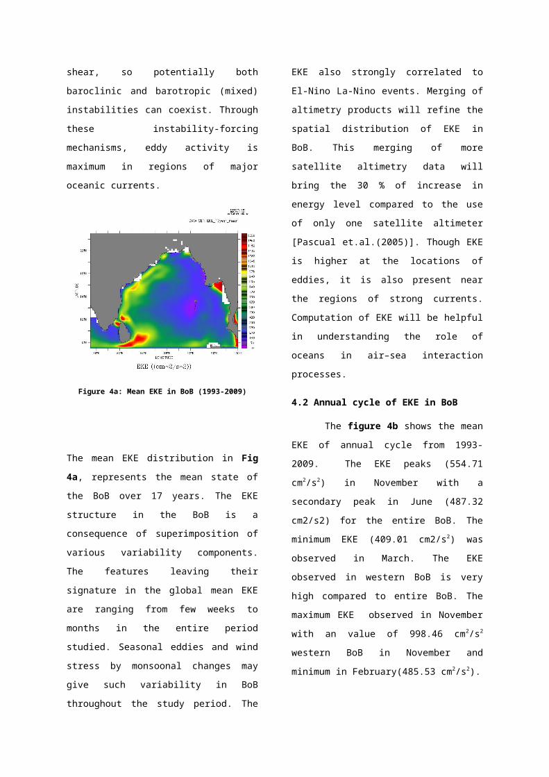
Figure 4a shows the
climatologically mean EKE
distribution derived from merged
data during 1993-2009. For the
first time, a 17-year series of
altimetric data has made it
possible to produce a relatively
realistic view of the main
characteristics of the mean EKE in
the BoB (75°–100°E, 5°–25°N).
Overall analysis of BoB shows that
mean EKE ranges from a minimum
value of 45.55 (cm2/s2) to a
altimetry data products
geostrophic velocity (u,v)
computation of eddy kinetic energy, sla
basic radar altimetry tool box, ferret
analyzing the eke and sea level in spatial and time series in bob
monthly variability
seasonal variabilit
y
interannual variability
sea level anomaly (h)
maximum value of 2780.6 (cm2/s2),
with an average value of 461.5
(cm2/s2). The maximum eddy kinetic
energy was observed south east of
Sri Lanka, along the east coast of
India and the rest of the BoB
exhibits low EKE throughout the
year. The spatial distribution of
EKE is found to be higher when
compared to previous estimation
made by Sharma et al., (1999)
using four years of TOPEX/Poseidon
altimeter data(1993-1996). This
region is modified by seasonally
reversing current pattern during
northeast as well as southwest
monsoons, Shankar et.al (2002).
The main sources of EKE is the
East Indian Coastal Current (EICC)
instability which changes its
direction twice a year. During
southwest monsoon it flows
poleward and flows towards equator
during winter monsoon. Average EKE
of BoB was high compared to
Arabian sea and whole Indian
Ocean. BoB is prone to intense
tropical cyclones throughout the
year. It is also remotely forced
by equatorial process such as IOD
Vinayachandran et al., (1997) and
El-Nino and La-Nino. 1984). During
November1998, the highest mean EKE
of more than 700 cm2/s2 is noticed
above the Sri Lanka coast in the
Bay of Bengal, which is not
present in the other years except
the June same year and December
2005. The dominant influence of
warm El-Nino event, particularly
off east coast of India, off
Sumatra and equatorial region,
south of Sri-Lanka has been
reported by Somayajulu et.al,
(2003). The monsoonal wind
develops wind stress curl near
Sri-Lanka. This negative and
positive wind stress curl may
cause the high EKE. In the east
coast the currents produce
instability
(barotrophic/baroclinic) which
causes the high EKE. The baroclinc
instability process depends on the
presence of vertical shear in the
mean flow, implying sloping
density gradients, and an
available store of potential
energy. Under certain conditions,
instabilities form, releasing this
potential energy and converting it
to eddy potential and kinetic
energies. If the mean flow has
significant horizontal shear as in
strong narrow jets, barotropic
instabilities can also occur. In
the real ocean, the mean flow has
both vertical and horizontal
shear, so potentially both
baroclinic and barotropic (mixed)
instabilities can coexist. Through
these instability-forcing
mechanisms, eddy activity is
maximum in regions of major
oceanic currents.
Figure 4a: Mean EKE in BoB (1993-2009)
The mean EKE distribution in Fig
4a, represents the mean state of
the BoB over 17 years. The EKE
structure in the BoB is a
consequence of superimposition of
various variability components.
The features leaving their
signature in the global mean EKE
are ranging from few weeks to
months in the entire period
studied. Seasonal eddies and wind
stress by monsoonal changes may
give such variability in BoB
throughout the study period. The
EKE also strongly correlated to
El-Nino La-Nino events. Merging of
altimetry products will refine the
spatial distribution of EKE in
BoB. This merging of more
satellite altimetry data will
bring the 30 % of increase in
energy level compared to the use
of only one satellite altimeter
[Pascual et.al.(2005)]. Though EKE
is higher at the locations of
eddies, it is also present near
the regions of strong currents.
Computation of EKE will be helpful
in understanding the role of
oceans in air–sea interaction
processes.
4.2 Annual cycle of EKE in BoB
The figure 4b shows the mean
EKE of annual cycle from 1993-
2009. The EKE peaks (554.71
cm2/s2) in November with a
secondary peak in June (487.32
cm2/s2) for the entire BoB. The
minimum EKE (409.01 cm2/s2) was
observed in March. The EKE
observed in western BoB is very
high compared to entire BoB. The
maximum EKE observed in November
with an value of 998.46 cm2/s2
western BoB in November and
minimum in February(485.53 cm2/s2).
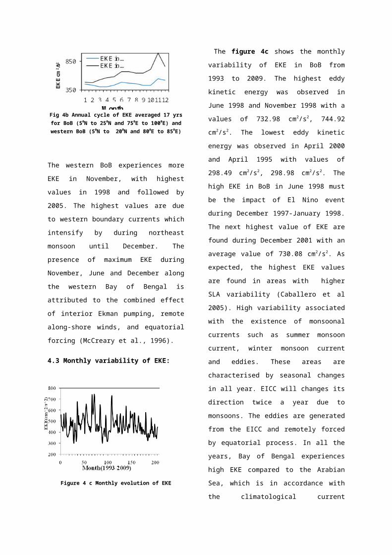
Fig 4b Annual cycle of EKE averaged 17 yrsfor BoB (50N to 250N and 750E to 1000E) andwestern BoB (50N to 200N and 800E to 850E)
The western BoB experiences more
EKE in November, with highest
values in 1998 and followed by
2005. The highest values are due
to western boundary currents which
intensify by during northeast
monsoon until December. The
presence of maximum EKE during
November, June and December along
the western Bay of Bengal is
attributed to the combined effect
of interior Ekman pumping, remote
along-shore winds, and equatorial
forcing (McCreary et al., 1996).
4.3 Monthly variability of EKE:
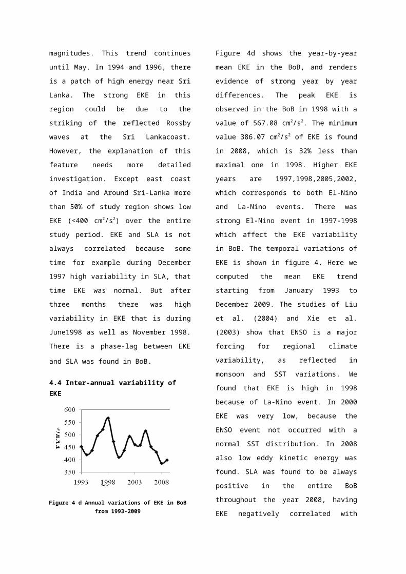
Figure 4 c Monthly evolution of EKE
The figure 4c shows the monthly
variability of EKE in BoB from
1993 to 2009. The highest eddy
kinetic energy was observed in
June 1998 and November 1998 with a
values of 732.98 cm2/s2, 744.92
cm2/s2. The lowest eddy kinetic
energy was observed in April 2000
and April 1995 with values of
298.49 cm2/s2, 298.98 cm2/s2. The
high EKE in BoB in June 1998 must
be the impact of El Nino event
during December 1997-January 1998.
The next highest value of EKE are
found during December 2001 with an
average value of 730.08 cm2/s2. As
expected, the highest EKE values
are found in areas with higher
SLA variability (Caballero et al
2005). High variability associated
with the existence of monsoonal
currents such as summer monsoon
current, winter monsoon current
and eddies. These areas are
characterised by seasonal changes
in all year. EICC will changes its
direction twice a year due to
monsoons. The eddies are generated
from the EICC and remotely forced
by equatorial process. In all the
years, Bay of Bengal experiences
high EKE compared to the Arabian
Sea, which is in accordance with
the climatological current
magnitudes. This trend continues
until May. In 1994 and 1996, there
is a patch of high energy near Sri
Lanka. The strong EKE in this
region could be due to the
striking of the reflected Rossby
waves at the Sri Lankacoast.
However, the explanation of this
feature needs more detailed
investigation. Except east coast
of India and Around Sri-Lanka more
than 50% of study region shows low
EKE (<400 cm2/s2) over the entire
study period. EKE and SLA is not
always correlated because some
time for example during December
1997 high variability in SLA, that
time EKE was normal. But after
three months there was high
variability in EKE that is during
June1998 as well as November 1998.
There is a phase-lag between EKE
and SLA was found in BoB.
4.4 Inter-annual variability of EKE
Figure 4 d Annual variations of EKE in BoBfrom 1993-2009
Figure 4d shows the year-by-year
mean EKE in the BoB, and renders
evidence of strong year by year
differences. The peak EKE is
observed in the BoB in 1998 with a
value of 567.08 cm2/s2. The minimum
value 386.07 cm2/s2 of EKE is found
in 2008, which is 32% less than
maximal one in 1998. Higher EKE
years are 1997,1998,2005,2002,
which corresponds to both El-Nino
and La-Nino events. There was
strong El-Nino event in 1997-1998
which affect the EKE variability
in BoB. The temporal variations of
EKE is shown in figure 4. Here we
computed the mean EKE trend
starting from January 1993 to
December 2009. The studies of Liu
et al. (2004) and Xie et al.
(2003) show that ENSO is a major
forcing for regional climate
variability, as reflected in
monsoon and SST variations. We
found that EKE is high in 1998
because of La-Nino event. In 2000
EKE was very low, because the
ENSO event not occurred with a
normal SST distribution. In 2008
also low eddy kinetic energy was
found. SLA was found to be always
positive in the entire BoB
throughout the year 2008, having
EKE negatively correlated with

SLA. Figure 4e shows the spatial
distribution of EKE from 1993 to
2009. Off southeast of Sri-Lanka,
EKE remains high in all year. This
is be because of the monsoonal
winds, westward propagation of
Rossby waves (vinayachandran et al
2005) and bottom topography of
Sri-Lanka. Pujol et al. (2005)
also showed that recurrent
structures contribute
significantly to EKE annual
variations. Second, Beckmann et
al. (1994) and Stammer (1998)
found that the eddy kinetic energy
distributions we closely
associated with the (local) mean
baroclinic flow. Detlef et al.
(1999) pointed out that mean flow
instabilities were the major
source of eddy energy over most
areas of the mid-latitude oceans.
However, the strong western
boundary current also exists in
winter (Li et al., 2000) when the
EKE is relatively weak, indicating
that mean flow baroclinic
instabilities are not the major
source of the EKE seasonal
variability in this area. Fang et
al. (2002) and Wu et al. (1998)
noticed wind stress curl was the
major factor in generating gyres
in the BoB. Detlef et al. (1999)
found a strong correlation with
time-varying altimetric eddy
kinetic energy (in the
northeastern Pacific, etc.) over
annual or longer periods where
wind stress forcing was found. The
figure 4e shows spatial
distribution of EKE from 1993-2009
in BoB. The figure shows that EKE
varies with annually particularly
in 1996,1997,1998 shows strong
variations in EKE compare to rest
of the years. Every year high EKE
is found in southeast of Sri-
Lanka. The EKE was also seasonally
modulated in the east coast of
India particularly in the Tamil
Nadu and Andhra coastal regions.
These are coastal upwelling
regions which causes the formation
of eddies.
Figure 4e Spatial distribution of Inter-
annual EKE in BoB.
Intra-annual variability:
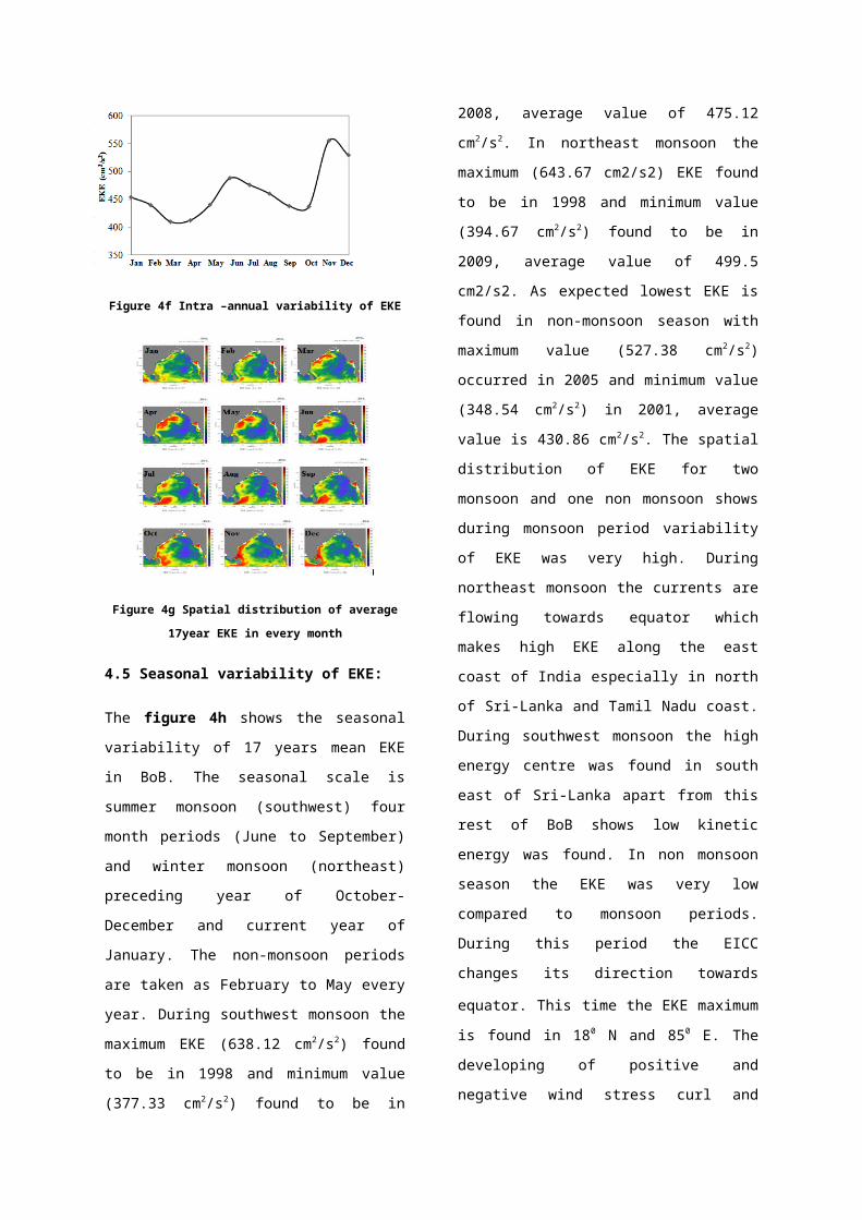
Figure 4f Intra –annual variability of EKE
Figure 4g Spatial distribution of average
17year EKE in every month
4.5 Seasonal variability of EKE:
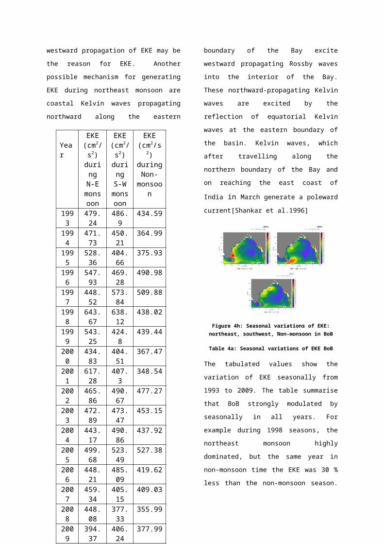
The figure 4h shows the seasonal
variability of 17 years mean EKE
in BoB. The seasonal scale is
summer monsoon (southwest) four
month periods (June to September)
and winter monsoon (northeast)
preceding year of October-
December and current year of
January. The non-monsoon periods
are taken as February to May every
year. During southwest monsoon the
maximum EKE (638.12 cm2/s2) found
to be in 1998 and minimum value
(377.33 cm2/s2) found to be in
2008, average value of 475.12
cm2/s2. In northeast monsoon the
maximum (643.67 cm2/s2) EKE found
to be in 1998 and minimum value
(394.67 cm2/s2) found to be in
2009, average value of 499.5
cm2/s2. As expected lowest EKE is
found in non-monsoon season with
maximum value (527.38 cm2/s2)
occurred in 2005 and minimum value
(348.54 cm2/s2) in 2001, average
value is 430.86 cm2/s2. The spatial
distribution of EKE for two
monsoon and one non monsoon shows
during monsoon period variability
of EKE was very high. During
northeast monsoon the currents are
flowing towards equator which
makes high EKE along the east
coast of India especially in north
of Sri-Lanka and Tamil Nadu coast.
During southwest monsoon the high
energy centre was found in south
east of Sri-Lanka apart from this
rest of BoB shows low kinetic
energy was found. In non monsoon
season the EKE was very low
compared to monsoon periods.
During this period the EICC
changes its direction towards
equator. This time the EKE maximumis found in 180 N and 850 E. The
developing of positive and
negative wind stress curl and
westward propagation of EKE may be
the reason for EKE. Another
possible mechanism for generating
EKE during northeast monsoon are
coastal Kelvin waves propagating
northward along the eastern
boundary of the Bay excite
westward propagating Rossby waves
into the interior of the Bay.
These northward-propagating Kelvin
waves are excited by the
reflection of equatorial Kelvin
waves at the eastern boundary of
the basin. Kelvin waves, which
after travelling along the
northern boundary of the Bay and
on reaching the east coast of
India in March generate a polewardcurrent[Shankar et al.1996]
Figure 4h: Seasonal variations of EKE:northeast, southwest, Non-monsoon in BoB
Table 4a: Seasonal variations of EKE BoB
The tabulated values show the
variation of EKE seasonally from
1993 to 2009. The table summarise
that BoB strongly modulated by
seasonally in all years. For
example during 1998 seasons, the
northeast monsoon highly
dominated, but the same year in
non-monsoon time the EKE was 30 %
less than the non-monsoon season.
Year
EKE(cm2/s2)duringN-Emonsoon
EKE(cm2/s2)duringS-Wmonsoon
EKE(cm2/s
2)duringNon-
monsoon
1993
479.24
486.9
434.59
1994
471.73
450.21
364.99
1995
528.36
404.66
375.93
1996
547.93
469.28
490.98
1997
448.52
573.84
509.88
1998
643.67
638.12
438.02
1999
543.25
424.8
439.44
2000
434.83
404.51
367.47
2001
617.28
407.3
348.54
2002
465.86
490.67
477.27
2003
472.89
473.47
453.15
2004
443.17
490.86
437.92
2005
499.68
523.49
527.38
2006
448.21
485.09
419.62
2007
459.34
405.15
409.03
2008
448.08
377.33
355.99
2009
394.37
406.24
377.99

But some reverse trend observed in
2005 seasons. During non-monsoon
was high compare to the other two
seasons. Except 2005 rest of the
year non-monsoon seasons show low
value of EKE than other two
monsoon. Strong El-Nino event
observed in December of 1997 and
January of 1998 in Pacific region,
in BoB during 1997 northeast
monsoon EKE was very low which
consists of November ,December
periods of El-Nino event. This El-
Nino event may causes the low EKE
in northeast monsoon during 1997.
But 1998 is a La-Nino year, during
that time high monsoonal EKE was
observed in two seasons. The
regionally averaged picture
confirms that EKE is higher in
northeast monsoon, especially in
east coast of India (100N to 180
N). During summer the EKE also
relatively high, especially in
south east of Sri-Lanka (800 E to
860 E). During non-monsoon the EICC
changes its direction towards
equator. During that time high EKE
found in 180 N.
Figure 4i: EKE variations during monsoonperiods top 54 seasons from 1993 southwestmonsoon to non-monsoon, below shows thetemporal evolution of EKE every year all
monsoon and non-monsoon
The temporal evolution of EKE
during season time for entire BoB
figured out. The EKE was very low
during non-monsoon periods on
because of currents are stable and
not fluctuated by wind, but during
seasons time the wind highly
fluctuating the currents speed and
its direction. Xiaoming Zhai et
al, 2008 reported that Subtropical
Countercurrent is subject to
strong baroclinic instability in
spring, but is only weakly
unstable in fall, due to seasonal
variation of the background
stratification. The dissipation of
EKE might also vary seasonally.
Alexander and Deser [1995] have
discussed how sea surface
temperature anomalies can
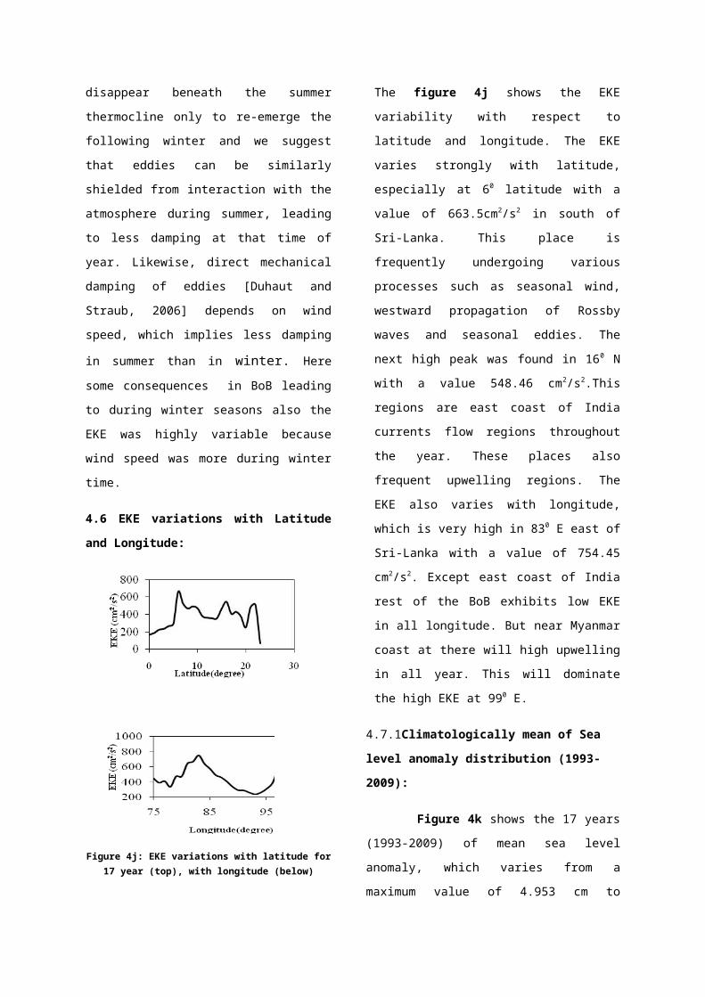
disappear beneath the summer
thermocline only to re-emerge the
following winter and we suggest
that eddies can be similarly
shielded from interaction with the
atmosphere during summer, leading
to less damping at that time of
year. Likewise, direct mechanical
damping of eddies [Duhaut and
Straub, 2006] depends on wind
speed, which implies less damping
in summer than in winter. Heresome consequences in BoB leading
to during winter seasons also the
EKE was highly variable because
wind speed was more during winter
time.
4.6 EKE variations with Latitude
and Longitude:
Figure 4j: EKE variations with latitude for17 year (top), with longitude (below)
The figure 4j shows the EKE
variability with respect to
latitude and longitude. The EKE
varies strongly with latitude,
especially at 60 latitude with a
value of 663.5cm2/s2 in south of
Sri-Lanka. This place is
frequently undergoing various
processes such as seasonal wind,
westward propagation of Rossby
waves and seasonal eddies. The
next high peak was found in 160 N
with a value 548.46 cm2/s2.This
regions are east coast of India
currents flow regions throughout
the year. These places also
frequent upwelling regions. The
EKE also varies with longitude,
which is very high in 830 E east of
Sri-Lanka with a value of 754.45
cm2/s2. Except east coast of India
rest of the BoB exhibits low EKE
in all longitude. But near Myanmar
coast at there will high upwelling
in all year. This will dominate
the high EKE at 990 E.
4.7.1Climatologically mean of Sea
level anomaly distribution (1993-
2009):
Figure 4k shows the 17 years
(1993-2009) of mean sea level
anomaly, which varies from a
maximum value of 4.953 cm to
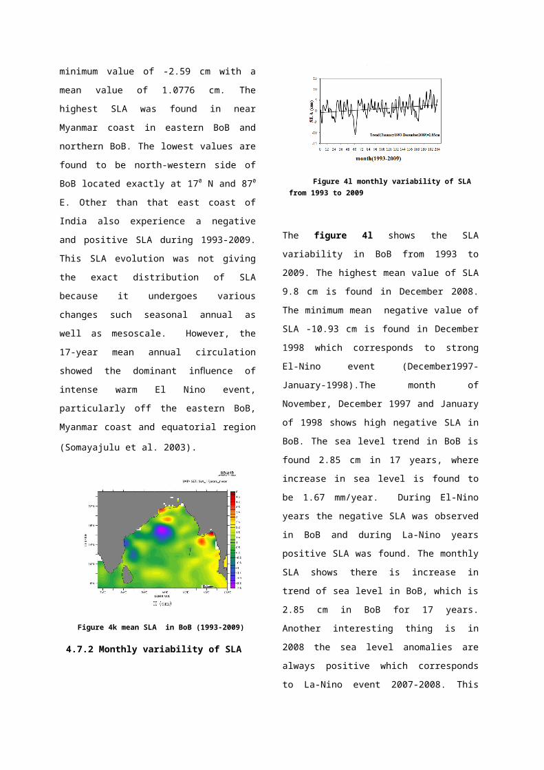
minimum value of -2.59 cm with a
mean value of 1.0776 cm. The
highest SLA was found in near
Myanmar coast in eastern BoB and
northern BoB. The lowest values are
found to be north-western side of
BoB located exactly at 170 N and 870
E. Other than that east coast of
India also experience a negative
and positive SLA during 1993-2009.
This SLA evolution was not giving
the exact distribution of SLA
because it undergoes various
changes such seasonal annual as
well as mesoscale. However, the
17-year mean annual circulation
showed the dominant in uence offl
intense warm El Nino event,
particularly off the eastern BoB,
Myanmar coast and equatorial region
(Somayajulu et al. 2003).
Figure 4k mean SLA in BoB (1993-2009)
4.7.2 Monthly variability of SLA
Figure 4l monthly variability of SLA from 1993 to 2009
The figure 4l shows the SLA
variability in BoB from 1993 to
2009. The highest mean value of SLA
9.8 cm is found in December 2008.
The minimum mean negative value of
SLA -10.93 cm is found in December
1998 which corresponds to strong
El-Nino event (December1997-
January-1998).The month of
November, December 1997 and January
of 1998 shows high negative SLA in
BoB. The sea level trend in BoB is
found 2.85 cm in 17 years, where
increase in sea level is found to
be 1.67 mm/year. During El-Nino
years the negative SLA was observed
in BoB and during La-Nino years
positive SLA was found. The monthly
SLA shows there is increase in
trend of sea level in BoB, which is
2.85 cm in BoB for 17 years.
Another interesting thing is in
2008 the sea level anomalies are
always positive which corresponds
to La-Nino event 2007-2008. This

year BoB experiences more cyclones
(ref:IMD). The sea level is a good
indicator for changes that occur in
the upper ocean water properties as
well as in the oceanic circulation;
thus, it is particularly important
in the sea level variation studies.
In recent decades, considerable
efforts have been devoted to
estimate long-term sea level trends
(e.g. Douglas, 1991; Cabanes et
al.,2001; Church et al., 2001;
White et al., 2005). It is commonly
accepted that global sea level has
been rising at a rate of 1.5±0.5
mm/yr during the last century
(Church et al., 2001) and
satellite-based estimation suggest
that sea level rise has increased
to a even faster rate of 2.8±0.4
mm/yr during the last decade
(Cazenave and Nerem, 2004).
However, mean rise in sea level is
only part of the story. Many
studies have indicated that the
spatial distribution of sea level
rise presents regional differences
and sea level instead fell in some
regions (e.g. Douglas, 2001;
Cazenave et al., 2002; Cazenave and
Nerem, 2004; Carton et al., 2005).
There are larger sea level
variations in the western tropical
Pacific, eastern Indian and
Southern Ocean during the past
decade (Carton et al., 2005). Some
studies on marginal sea level
variations suggested an even faster
changing rate in those areas during
the last decade (Cazenave et al.,
2002; Li et al., 2002). There are
two reasons to be consider increase
in sea level, the first process
involved an increase in mass of
water in the ocean (eustatic
component ) derived largely from
the melting of ice on land and an
increase of the volume of ocean
without change in mass (steric
effect) largely caused by thermal
expansion of ocean water.
4.7.3 Inter-Annual Variability of
Sea level anomaly in BoB:
Figure 4m Inter-Annual variations of SLA in
BoB from 1993-2009
The figure 4m shows the inter-
annual variability of SLA from 1993
to 2009.The lowest mean value of
SLA (-2.345 cm) was observed in
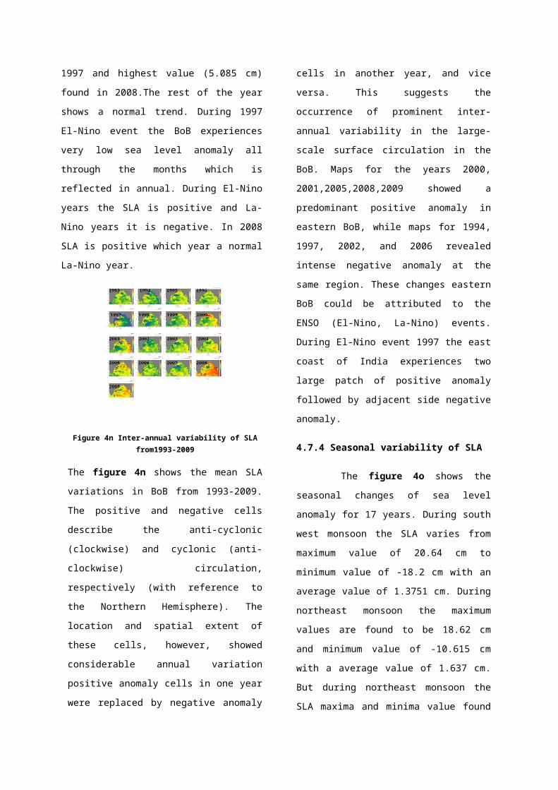
1997 and highest value (5.085 cm)
found in 2008.The rest of the year
shows a normal trend. During 1997
El-Nino event the BoB experiences
very low sea level anomaly all
through the months which is
reflected in annual. During El-Nino
years the SLA is positive and La-
Nino years it is negative. In 2008
SLA is positive which year a normal
La-Nino year.
Figure 4n Inter-annual variability of SLAfrom1993-2009
The figure 4n shows the mean SLA
variations in BoB from 1993-2009.
The positive and negative cells
describe the anti-cyclonic
(clockwise) and cyclonic (anti-
clockwise) circulation,
respectively (with reference to
the Northern Hemisphere). The
location and spatial extent of
these cells, however, showed
considerable annual variation
positive anomaly cells in one year
were replaced by negative anomaly
cells in another year, and vice
versa. This suggests the
occurrence of prominent inter-
annual variability in the large-
scale surface circulation in the
BoB. Maps for the years 2000,
2001,2005,2008,2009 showed a
predominant positive anomaly in
eastern BoB, while maps for 1994,
1997, 2002, and 2006 revealed
intense negative anomaly at the
same region. These changes eastern
BoB could be attributed to the
ENSO (El-Nino, La-Nino) events.
During El-Nino event 1997 the east
coast of India experiences two
large patch of positive anomaly
followed by adjacent side negative
anomaly.
4.7.4 Seasonal variability of SLA
The figure 4o shows the
seasonal changes of sea level
anomaly for 17 years. During south
west monsoon the SLA varies from
maximum value of 20.64 cm to
minimum value of -18.2 cm with an
average value of 1.3751 cm. During
northeast monsoon the maximum
values are found to be 18.62 cm
and minimum value of -10.615 cm
with a average value of 1.637 cm.
But during northeast monsoon the
SLA maxima and minima value found
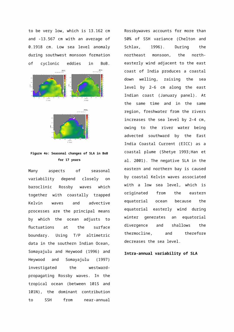
to be very low, which is 13.162 cm
and -13.567 cm with an average of
0.1918 cm. Low sea level anomaly
during southwest monsoon formation
of cyclonic eddies in BoB.
Figure 4o: Seasonal changes of SLA in BoB
for 17 years
Many aspects of seasonal
variability depend closely on
baroclinic Rossby waves which
together with coastally trapped
Kelvin waves and advective
processes are the principal means
by which the ocean adjusts to
uctuations at the surfacefl
boundary. Using T/P altimetric
data in the southern Indian Ocean,
Somayajulu and Heywood (1996) and
Heywood and Somayajulu (1997)
investigated the westward-
propagating Rossby waves. In the
tropical ocean (between 101S and
101N), the dominant contribution
to SSH from near-annual
Rossbywaves accounts for more than
50% of SSH variance (Chelton and
Schlax, 1996). During the
northeast monsoon, the north-
easterly wind adjacent to the east
coast of India produces a coastal
down welling, raising the sea
level by 2–6 cm along the east
Indian coast (January panel). At
the same time and in the same
region, freshwater from the rivers
increases the sea level by 2–4 cm,
owing to the river water being
advected southward by the East
India Coastal Current (EICC) as a
coastal plume (Shetye 1993;Han et
al. 2001). The negative SLA in theeastern and northern bay is caused
by coastal Kelvin waves associated
with a low sea level, which is
originated from the eastern
equatorial ocean because the
equatorial easterly wind during
winter generates an equatorial
divergence and shallows the
thermocline, and therefore
decreases the sea level.
Intra-annual variability of SLA

Figure 4p Spatial Distribution of EKE in
all months(average 17 year)
From February to May, negative
wind curl in the central and
western bay produces a high sea
level, especially in the
southwestern bay The negative SLA
in the eastern and northern bay
strengthens and extends farther
along the coast and to the bay
interior due to coastal Kelvin
waves and westward propagating
Rossby waves. In May, a high sea
level pattern presents in the
eastern equatorial ocean due to
the eastward propagation of
equatorial Kelvin waves associated
with a high sea level. The strong
equatorial westerly winds during
April and May cause equatorial
convergence, deepen the
thermocline, and increase the sea
level. In addition, the spring
Wyrtki jet acts to pile up water
in the eastern basin, contributing
to the sea level increase. This
high sea level signal with an
amplitude of 2–4 cm propagates
into the eastern and northern bay
as coastal Kelvin waves, and it
also radiates westward from the
eastern boundary into the bay
interior as Rossby waves, raising
the sea level in the eastern,
northern, and central bay from May
to July. During the same period
the bay rivers have signi cantfi
discharges, increasing the sea
level by 2–4 cm in some regions of
the bay. From July to September,
the southwest monsoon wind
generates coastal upwelling,
causing a low sea level along the
east Indian coast. At the same
time, sea level in the eastern
equatorial ocean decreases, due to
the relaxation of equatorial
westerly wind. As in during
November is caused by coastal
Kelvin waves originated from the
eastern equatorial ocean, where
the strong equatorial westerly
wind during fall and the fall
Wyrtki jet produce a high sea
level.(Han et al., 2000)
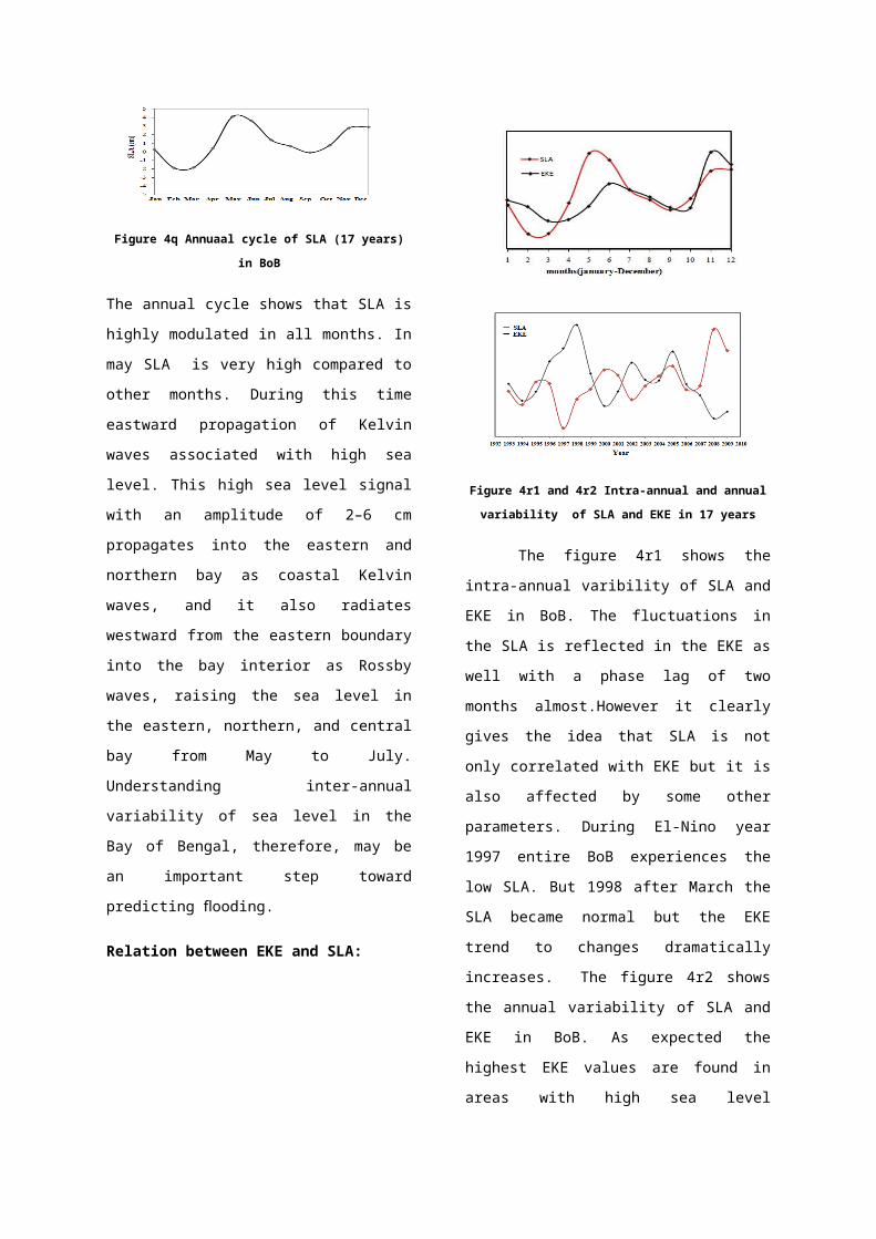
Figure 4q Annuaal cycle of SLA (17 years)
in BoB
The annual cycle shows that SLA is
highly modulated in all months. In
may SLA is very high compared to
other months. During this time
eastward propagation of Kelvin
waves associated with high sea
level. This high sea level signal
with an amplitude of 2–6 cm
propagates into the eastern and
northern bay as coastal Kelvin
waves, and it also radiates
westward from the eastern boundary
into the bay interior as Rossby
waves, raising the sea level in
the eastern, northern, and central
bay from May to July.
Understanding inter-annual
variability of sea level in the
Bay of Bengal, therefore, may be
an important step toward
predicting ooding.fl
Relation between EKE and SLA:
Figure 4r1 and 4r2 Intra-annual and annual
variability of SLA and EKE in 17 years
The figure 4r1 shows the
intra-annual varibility of SLA and
EKE in BoB. The fluctuations in
the SLA is reflected in the EKE as
well with a phase lag of two
months almost.However it clearly
gives the idea that SLA is not
only correlated with EKE but it is
also affected by some other
parameters. During El-Nino year
1997 entire BoB experiences the
low SLA. But 1998 after March the
SLA became normal but the EKE
trend to changes dramatically
increases. The figure 4r2 shows
the annual variability of SLA and
EKE in BoB. As expected the
highest EKE values are found in
areas with high sea level
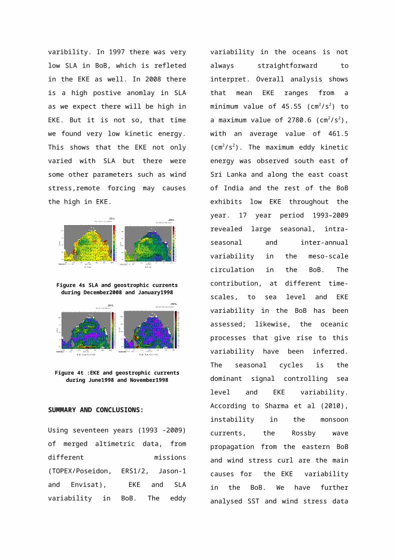
varibility. In 1997 there was very
low SLA in BoB, which is refleted
in the EKE as well. In 2008 there
is a high postive anomlay in SLA
as we expect there will be high in
EKE. But it is not so, that time
we found very low kinetic energy.
This shows that the EKE not only
varied with SLA but there were
some other parameters such as wind
stress,remote forcing may causes
the high in EKE.
Figure 4s SLA and geostrophic currentsduring December2008 and January1998
Figure 4t :EKE and geostrophic currentsduring June1998 and November1998
SUMMARY AND CONCLUSIONS:
Using seventeen years (1993 -2009)
of merged altimetric data, from
different missions
(TOPEX/Poseidon, ERS1/2, Jason-1
and Envisat), EKE and SLA
variability in BoB. The eddy
variability in the oceans is not
always straightforward to
interpret. Overall analysis shows
that mean EKE ranges from a
minimum value of 45.55 (cm2/s2) to
a maximum value of 2780.6 (cm2/s2),
with an average value of 461.5
(cm2/s2). The maximum eddy kinetic
energy was observed south east of
Sri Lanka and along the east coast
of India and the rest of the BoB
exhibits low EKE throughout the
year. 17 year period 1993–2009
revealed large seasonal, intra-
seasonal and inter-annual
variability in the meso-scale
circulation in the BoB. The
contribution, at different time-
scales, to sea level and EKE
variability in the BoB has been
assessed; likewise, the oceanic
processes that give rise to this
variability have been inferred.
The seasonal cycles is the
dominant signal controlling sea
level and EKE variability.
According to Sharma et al (2010),
instability in the monsoon
currents, the Rossby wave
propagation from the eastern BoB
and wind stress curl are the main
causes for the EKE variability
in the BoB. We have further
analysed SST and wind stress data
to substantiate our study on the
sea level and EKE variability in
BoB. 17 years (1993-2009) of mean
sea level anomaly, this varies
from a maximum value of 4.953 cm
to minimum value of -2.59 cm with
a mean value of 1.0776 cm. The
highest SLA was found in near
Myanmar coast in eastern BoB and
northern BoB. The sea level
presents a trend about 2.85 cm for
17 years in BoB. We find that the
sea level rise in BoB is about
1.67 mm/year, which is within the
averaged values of sea level
rise for the global ocean (Xuhua
et al, 2007, Ablain et al, 2009).
The monthly mean sea level anomaly
is maximum (9.8 cm) in December
2008 and minimum (-10.9 cm) in
January 1998. In 2008, the BoB
experienced a number of intense
cyclones and the year 1997-98 is
characterised by an active El Nino
event (Chen et al 2009, Chellappan
et al 2009). SLAs (both positive
and negative) during December of
all the years (1993-2009) show
high fluctuations associated with
warm and cold core eddies. The
minimum SLA was observed in
March/April. This annual cycle
variation in sea level is due to
the steric-effect - increase in
the volume of ocean without change
in the mass (Caballero et al.,
2007). The intense variability in
sea level along the east coast of
India and around Sri-Lankan coast
is due to the existence of western
boundary currents (WBC). Since the
ocean and the atmosphere are a
coupled system, variability of sea
level reflects changes in climate.
One of the most important aspects
of the climate in the bay is the
Indian monsoon, which possesses
large inter-annual variability.
This variability may cause marked
sea level change due to uctuationfl
of monsoon wind, precipitation
minus evaporation (P - E), heat
uxes, and river runoff into thefl
bay. There are also potential
remote in uences. Sea levelfl
signals driven by the equatorial
wind can propagate into the bay as
coastal Kelvin waves and westward
radiating Rossby waves, each of
which has a sea level signature
that may impact the sea level in
the BoB.
Acknowledgement:
Authors express gratitude to the
NIO for giving such opportunity
for dissertation work. Thanks to
AVISO for providing data and other
valuable information. Finally
authors thanks to P.vethamony for
giving valuable guidance.
References:
Ali, M. M. and Sharma, R. (1998). StudyingIndian Ocean typical phenomena using TOPEXobservations, Mar. Geod., 21, 193-201.
AVISO/Altimetry 1996, “AVISO User Handbookfor Merged TOPEX/POSEIDON products”, AVI-NT-02-101, Edition 3.0.
Cheng, X. and Qi, Y. (2010). Variations ofEddy Kinetic Energy in the South China Sea,Journal of Oceanography, 66, 85-94.
Ducet, N., Le Traon, P. Y., and Reverdin,G. (2000). Global high-resolution mappingof ocean circulation from TOPEX/Poseidonand ERS-1 and-2, J. Geophys. Res., 105(C8),19477-19498
Eden, C., and Boning, C. (2002). Sources ofEddy Kinetic Energy in the Labrador Sea, J.Phys. Oceanogr., 32, 3346-3363.
Fu, L. L., and Zlotnicki. V. (1989).Observing oceanic mesoscale eddies fromGeosat altimetry, Preliminary results,Geophys. Res. Lett., 16(5), 457-460.
Gille, S.T., and Kelly, K.A. (1996). Scalesof spatial and temporal variability in theSouthern Ocean. J. Geophys. Res. 101, 8759-8773.
Glazman, R. E., Fabrikant, A., andGreysukh, A. (1996). Statistics of spatial-temporal variations of sea surface heightbased on Topex altimeter measurements. Int.J. Remote Sensing 17, 2647-2666.
Le Traon, P. Y.(1992). Time scales ofmesoscale variability and theirrelationship with spatial scales in theNorth Atlantic. J. Mar. Res. 49, 467-492.‐ 60 ‐
Le Traon, P. Y. and Dibarboure, G.(1999). Mesoscale mapping capabilities ofmultiple-satellite altimeter missions. J.Atmos. Oceanic. Technol., 16, 1208-1223.
Le Traon, P. Y., Nadal, F. and Ducet, N.(1998). An improved mapping method ofmultisatellite altimeter data. J. Atmos.Oceanic Technil., 15, 522-534.
Le Traon, P. Y. and Diabarboure, G.(2004). An illustration of the contributionof the
TOPEX/Poseidon-Jason-1 Tandem Mission tomesoscale variability studies, MarineGeodesy, 27,3-13.
Le Traon, P. Y. and R. A. Morrow, (2001).Ocean currents and mesoscale eddies,Satellit
Altimetery and Earth Sciences. A Handbookof Techniques and Applicaions, AcademicPress ed.
L. L. Fu and A. Cazenave, Eds., Academicpress, 171-215.
Le Traon, P. Y. and Dibarboure, G. (2002).Velocity mapping capabilities of presentand future altimeter missions: the role ofhigh frequency signals. J. Atm. OceanTech., 19, 2077-2088.
Pascual, A., Faugere, Y., Larnicol, G. andLe Traon, P. Y. (2006). Improveddescription of the
ocean mesoscale variability by combiningfour satellite altimeters, GeoohysicalResearch Letters,33, L02611.
Pujol, M. I. and Larnicol, G. (2005),Mediterranean sea eddy kinetic energyvariability from 11 years of altimetricdata, J. Marine Sys., 58, 121-142.
Robinson, A. R. (Ed), Eddies in MarineScience, 609 pp., Springer-Verlag, NewYork, 1983.
Rosmorduc, V., J. Benveniste, O. Lauret, C.Maheu, M. Millagro, N. Picot, RadarAltimetry
Tutorial, J. Benveniste and N. PicotEd.,http://www.altimetry.info.2009.
Shenoi, S., Saji, P., Almeida, A. (1999).Near-surface circulation and kineticenergy in the tropical Indian Ocean derivedfrom Lagrangian drifters, J. Marine Res.,57(6), 885-907.
Shum, C. K., Werner, R. A., Sanwell, D.T.,Zhang, B. H., Nerem, R.S. and Tapley, D.(1990). Variations of global mesoscale eddyenergy observed from Geosat,J.Geophys. Res., 95, 17865-17876