Design of an Innovative Car Braking System using Eddy ...

Design of an Innovative Car Braking System using Eddy Currents

David Jose Torres Cruz Bachelor in Aeroespace Engineering, Instituto Superior Tecnico (IST), 2002

A Thesis Submitted in Partial Fulfillment of the Requirements for the Degree of

MASTER OF APPLIED SCIENCE in the

Department of Mechanical Engineering.

University of Victoria

All rights reserved. This thesis may not be reproduced in whole or in part, by photocopy or other means, without the permission of the author.

Supervisors: Dr. Afzal Suleman, Dr. Edward Park

Abstract

The development of an innovative car brake actuator is the purpose of this project.

The motivation lies in improving the performance provided by current hydraulic and

electro-hydraulic brake systems, as well as providing an electro-mechanical solution

which is also more environmentally friendly. A study of existing braking solutions is

presented, as well as the testing of a conventional disk brake system in the laboratory.

A survey of automotive brake systems currently under development is also provided.

Our search for a new brake is initiated by analysing various types of actuators, which

consequently led to the selection of an eddy current system. When a rotating non-

ferromagnetic disc is exposed to a magnetic flux, eddy currents are induced in the

surface of the conductive disc. A braking torque is generated by the interaction be-

tween the eddy currents and the magnetic flux. In principle, such a braking system is

simple, consisting of a conductive rotating disk and an electromagnet to provide the

braking field. Then, the braking torque can be expressed as a function of the angular

speed of the disk and the applied current to the electromagnet. A detailed description

of the working principle as well as its mathematical modelling are provided. Finite

element modelling of the system provided computational results that allowed an en-

suing parametric study of the behaviour of the system. Analysis of the system for

a low velocity regime as well as high velocity was required since the system has dif-

ferent responses according to the velocity at which it operates. However, there was

a much heavier emphasis placed in the behaviour of the system for the high velocity

region. The ensuing development was consequently focused towards the high velocity

regime. After a parametric optimization process of the various design variables, an

experimental setup was built and laboratory results were obtained for comparison

with the ones originated from computational simulations. The results from the ex-

perimental tests were quite close to the ones predicted by the computational model,

thus validating the concept presented.

Table of Contents

Abstract

List of Tables

List of Figures

Nomenclature

1 Introduction . . . . . . . . . . . . . . . . . . . . . . . . . . . . . . . . . 1.1 Motivation

. . . . . . . . . . . . . . 1.2 Background on Automotive Braking Systems . . . . . . . . . . . . . . . . . . . . . . . 1.2.1 Existing Technology

. . . . . . . . . . . . . . . . . . . . 1.2.2 Electro-Mechanical Brakes 1.2.3 Braking Dynamics . . . . . . . . . . . . . . . . . . . . . . . .

. . . . . . . . . . . . . . . . . . . . . . . . . . 1.3 Structure of the Thesis

2 Design Solution Search . . . . . . . . . . . . . . . . . . . . . . . . . . . . 2.1 Actuation Materials

2.1.1 Shape Memory Alloys . . . . . . . . . . . . . . . . . . . . . . 2.2 Piezoelectric Materials . . . . . . . . . . . . . . . . . . . . . . . . . .

. . . . . . . . . . . . . . . . . . 2.2.1 Piezoelectric Based Concepts 2.3 Electromagnets . . . . . . . . . . . . . . . . . . . . . . . . . . . . . . 2.4 Voice Coils . . . . . . . . . . . . . . . . . . . . . . . . . . . . . . . . .

. . . . . . . . . . . . . . . . . . . . 2.5 High performance electric motors . . . . . . . . . . . . . . . . . . . . . . . . . . . . . . . . . . 2.6 Synopsis

3 Eddy Current Brake System 3.0.1 High Velocity . . . . . . . . . . . . . . . . . . . . . . . . . . .

. . . . . . . . . . . . . . . . . . . . . . . . . . . 3.0.2 Low Velocity . . . . . . . . . . . . . . . . . . . . . . . . . . . . . . . . . . . 3.1 Theory

. . . . . . . . . . . . . . . . . . . . . . . . . 3.2 Modeling and Simulation

vii

TABLE OF CONTENTS v

3.2.1 Finite Element Modelling . . . . . . . . . . . . . . . . . . . . 43 3.2.2 Braking Torque Analysis . . . . . . . . . . . . . . . . . . . . . 49

3.3 Parametric Study . . . . . . . . . . . . . . . . . . . . . . . . . . . . . 53 3.4 Proposed Brake System . . . . . . . . . . . . . . . . . . . . . . . . . 66

. . . . . . . . . . . . . . . . . . . . . . . . . 3.4.1 Enhanced Design 66 . . . . . . . . . . . . . . . . . . . . . . . . . . . . . . . . . . 3.5 Synopsis 70

4 Experimental Setup and Validation 71 . . . . . . . . . . . . . . . . . . . . . . . . . 4.1 The Experimental Setup 71

. . . . . . . . . . . . . . . . . . . . . . . . . . . . . . . 4.1.1 Motor 71 4.1.2 Gear Reducer . . . . . . . . . . . . . . . . . . . . . . . . . . . 73 4.1.3 Coupling . . . . . . . . . . . . . . . . . . . . . . . . . . . . . . 74 4.1.4 Clutch . . . . . . . . . . . . . . . . . . . . . . . . . . . . . . . 75

. . . . . . . . . . . . . . . . . . . . . . . . . . 4.1.5 Electromagnets 77 . . . . . . . . . . . . . . . . . . . . . . . . . . . . 4.1.6 Disk Brake 78

. . . . . . . . . . . . . . . . . . . . . . . . . . . 4.1.7 Power Supply 78 4.1.8 Encoder . . . . . . . . . . . . . . . . . . . . . . . . . . . . . . 79

. . . . . . . . . . . . . . . . . . . . . . . . . . . . . . 4.1.9 Supports 81 . . . . . . . . . . . . . . . . . . . . . . . . . . . 4.2 ExperimentalResults 84 . . . . . . . . . . . . . . . . . . . . . . . . . . . 4.2.1 Experiment 1 85 . . . . . . . . . . . . . . . . . . . . . . . . . . . 4.2.2 Experiment 2 86

4.2.3 Experimental Results and Discussion . . . . . . . . . . . . . . 86 . . . . . . . . . . . . . . . . . . . . . . . . . . . . . . . . . . 4.3 Synopsis 96

5 Conclusions and Recommendat ions 9 7 5.1 Conclusions . . . . . . . . . . . . . . . . . . . . . . . . . . . . . . . . 97 5.2 Advantages and Limitations . . . . . . . . . . . . . . . . . . . . . . . 98 5.3 Recommendations for Future Work . . . . . . . . . . . . . . . . . . . 99

List of Tables

. . . . . . . . . . . . . . . 1.1 Physical parameters for the car modelling 13

. . . . . . . . . . . . . . . . . . . . . . . . 2.1 Values for Midi's actuator 20 . . . . . . . . . . . . . . . . . . . 2.2 Values for Cedrat's linear actuator 20

. . . . . . . . . . . . . . . . . . 2.3 Values for Cedrat's rotating actuator 21 . . . . . . . . . . . . . . . . . . . . . . . . . 2.4 Values for rotating speed 23

. . . . . . . . . . . . . . . . . . . . . . . . 2.5 Values for rotating torque 23 . . . . . . . . . . . . . . . . . . . . 2.6 Values for voice coils from Kimco 28

. . . . . . . . . . . . . . . 3.1 Input variables in the different subdomains 49 . . . . . . . . . 3.2 Effect of varying the shape of the pole projection area 54

. . . . . . . . . . 3.3 Effect of varying the size of the pole projection area 58 . . . . . . . 3.4 Effect of varying the position of the pole projection area 59

3.5 Effect of varying the relative position of the pole projection areas . . 62 . . . . . . . . . . . . . . . 3.6 Effect of varying the magnetic flux density 65 . . . . . . . . . . . . . . . 3.7 Physical parameters for the car modelling 66

. . . . . . . 4.1 Time response for different magnetic fields and velocities 87 . . . . . 4.2 Comparison between experimental and computational times 92

vii

List of Figures

1.1 Disk brake . . . . . . . . . . . . . . . . . . . . . . . . . . . . . . . . . 1.2 Drum brake . . . . . . . . . . . . . . . . . . . . . . . . . . . . . . . . 1.3 Electric drum brake . . . . . . . . . . . . . . . . . . . . . . . . . . . .

. . . . . . . . . . . . . . . . . . . . . . . 1.4 Telma eddy current retarder 1.5. Anti-lock brake pump and valves . . . . . . . . . . . . . . . . . . . .

. . . . . . . . . . . . . . . . . . . . . . . 1.6 Electric caliper from Delphi . . . . . . . . . . . . . . . . . . . . . . . . . 1.7 Car with EMB by Delphi

2.1 Piezoelectric Actuator . . . . . . . . . . . . . . . . . . . . . . . . . . . . . . . . . . . . . . . . . . . . . . . . 2.2 Rotary Piezoelectric Actuator

. . . . . . . . . . . . . . . . . 2.3 Schematic of a Conventional Voice Coil

. . . . . . . . . . . . . . . . . . 3.1 Magnetic forces actuating in the disk 3.2 Eddy Current Model . . . . . . . . . . . . . . . . . . . . . . . . . . .

. . . . . . . . . . . . . . . 3.3 Schematic of Eddy Current Brake System 3.4 Finite Element Drawing . . . . . . . . . . . . . . . . . . . . . . . . . 3.5 Coarse Finite Element Mesh . . . . . . . . . . . . . . . . . . . . . . . 3.6 Refined Finite Element Mesh . . . . . . . . . . . . . . . . . . . . . . 3.7 Fine Finite Element Mesh . . . . . . . . . . . . . . . . . . . . . . . . 3.8 Finite Element Solution . . . . . . . . . . . . . . . . . . . . . . . . . 3.9 Simulink system for the real car model . . . . . . . . . . . . . . . . . 3.10 Torque vs . Time . . . . . . . . . . . . . . . . . . . . . . . . . . . . . 3.11 Velocity vs . Time . . . . . . . . . . . . . . . . . . . . . . . . . . . . . 3.12 Rectangle shaped pole projection area . . . . . . . . . . . . . . . . . 3.13 Square shaped pole projection area . . . . . . . . . . . . . . . . . . . 3.14 Circle shaped pole projection area . . . . . . . . . . . . . . . . . . . . 3.15 Best pole projection area placement . . . . . . . . . . . . . . . . . . . 3.16 Pole projection area placement too close to outside . . . . . . . . . .

. . . . . . . . . . . . . . . . 3.17 Best angle between pole projection areas 3.18 Pole projection areas too close . . . . . . . . . . . . . . . . . . . . . .

... LIST OF FIGURES VIU

. . . . . . . . . . . . 3.19 Schematic of geared eddy current brake system 67 . . . . . . . . . . . 3.20 Velocity evolution of the car model during braking 69

. . . . . . . 4.1 Electric motor used to power the experimental assembly 72 . . . . . . . . 4.2 Amplifier and Capacitor that power the electric motor 73

. . . . . . . . . . . . 4.3 Gear system used in the experimental assembly 74 . . . . . . . . . . . 4.4 Coupling system used to maintain shaft alignment 75 . . . . . . . . . . . 4.5 Clutch system used in the experimental assembly 76 . . . . . . . . . . . 4.6 Electromagnets used in the experimental assembly 77

. . . . . . . . . . . . . . . . . . . . . . . 4.7 Direct current power supply 79 . . . . . . . . . . . . . . . . . . . . . 4.8 Alternate current power supply 79

. . . . . . . . . . . . . . . . . . . 4.9 Encoder to record velocity evolution 80 . . . . . 4.10 Support that couples the electric motor and the gear system 81

. . . . . . . . . . . . . . . . . 4.11 Support that maintains shaft alignment 82 . . . . . . . . . . . . . . 4.12 Stand that holds the electromagnets in place 83

. . . . . . . . . . . . . . . . . . . . . . 4.13 Complete experimental setup 84 . . . . . . . . . . . . . . . . . . . . . . . . . . . 4.14 Experiment a1 results 88

. . . . . . . . . . . . 4.15 Computational simulation of experimental setup 89 . . . . . . . . . . . . . . . . . . . . . . . . . . . . . . 4.16 Simulink Model 90

. . . . . . . . . . . . . . . . . . . . . . . . . . 4.17 Computational results 91 4.18 Detailed comparison of experimental and computational results . . . 93

. . . . . . . . . . . . . . . . . 4.19 DC power supply experimental results 94

. . . . . . . . . . . . . . . . . 4.20 AC power supply experimental results 95

Nomenclature

Acceleration [m/s2] Area [m2] Magnetic flux density [TI Applied magnetic flux density [TI Magnetic flux density in air gap [TI Electric displacement [C/m2] Force [N] Average force [N] Friction force [N] Rolling resistance force [N] Electric field [N/C] Acceleration of gravity [m/s2] Air gap [m] Height of center of gravity [m] Magnetic field [Aim] Electric current [A] Total moment of inertia of wheel and engine [Kg.m2] Average electric current [A] Electric current density [A/m2] Wheel base, [m] Vehicle mass [Kg] Wheel mass [Kg] Mass [Kg] Number of turns Pressure [N/m2] Radius [m] Wheel radius [m]

NOMENCLATURE

Stroke [m] Average stroke [m] Time [s] Torque [N.m] Braking torque [N.m] Velocity [mls] Volume [m3] Average volume [m3] Linear velocity [m/s] Linear acceleration [m/s2]

Greek Symbols

p Braking force coefficient p Magnetic permeability

po Magnetic permeability of free space [N/A2] p Charge density [C/m3] a Electric conductivity [S.m] w Frequency [Hz] w Angular velocity [radls]

Acronynms

ABS AC DC EBD EC ECB ECU EMB ER MR MRI PPA OEM RPM SMA TCS

Anti-lock Brake System Alternate Current Direct Current Electronic Brake Distribution Eddy Current Eddy Current Brake Electronic Control Unit Electro Mechanical Brake Electro-Rheological Magneto-Rheological Magnetic Ressonance Imaging Pole Projection Area Organized External Manufacturer Rotations Per Minute Shape Memory Alloys Traction Control System

Acknowledgements

I would like to thank Dr. Afzal Suleman for giving me the opportunity to work on

this project and consequently for making me grow as a person and an enginneer. The

faith put in me by accepting me as a graduate student will not be forgotten.

I would also like to thank Dr. Edward Park for the support he provided during

the course of the project.

Special appreciation to Rodney Katz for the help in setting up the experiment.

His effort, availability and teachings were very valuable. Thanks also to Ken Bergley

for the help on machining of the parts.

Also to be thanked is Dillian Stoikov for his help in the electronic part of the

experimental component. I am also grateful to Steve Ferguson for his insight in real

systems and for helping me get started with the stand for the disk brake system.

Thanks to Shahab for his work in the preliminary stage of the experimental setup.

I would also like to thank Sandra for all the help in everyday affairs and for the

occasional treats.

Personal feelings of gratitude are in order to Goncalo and Kirstie, for their help in

adjusting to this change and for always having been there since I began this endeavour.

They made me feel at home and I can't thank them enough. Another couple worth of

a word of praise is Marc and Tabitha. Thanks for their friendship. Thanks to Scott

for all his good disposition and easy laughs. He contributed significantly to make the

office a pleasant place to work. I would also like to thank Luis for accompanying me

in this journey. Thanks to Diogo for always carrying happiness whith you.

A final word of gratitude has to go to my parents for their continuous support and

undying faith in me. I would also like to thank Magda for always being there for me,

cheering me on and giving me strength whenever I needed it. Their love was always

felt and truly appreciated.

xii

T o my parents and my beloved

Chapter 1

Introduction

The braking mechanism is an important component in automobiles as the ability to

slow down or stop a moving vehicle in the least amount of time and in a controlled

fashion is an important safety feature. Braking systems have maintained essentially

the same basic design principle over the years. Notable upgrades include the addition

of electronic controllers and sensors to decrease the braking distance by preventing

skidding (e.g., anti-lock brake systems). There also has been the inclusion of addi-

tional driver assist devices to increase the braking torque while demanding less of the

driver's physical input.

Currently, in order to dissipate a vehicle's kinetic energy, thus bringing it to a

stop, requires applying friction to a rotating disk connected to the wheel using brake

pads. The friction generates heat, which in turn dissipates the car's kinetic energy.

The conventional method to provide the force necessary to produce sufficient friction

is by using a hydraulic actuation system. These systems have many performance and

environmental shortcomings that can be improved upon and, as we progress towards

more electric cars, an electro-mechanical brake seems to be the natural solution.

Several major companies (e.g., Delphi, Continental, etc.) have already stated their

CHAPTER 1. INTRODUCTION 2

interest in the development of Electro-Mechanical Brakes (EMB). These developments

are still at the development stage and there is a technological race in progress to bring

an EMB system to the market.

This thesis proposes an eddy current electric brake (ECB) actuator. It is a con-

tactless and electrically powered system and applies the same principle as the one

behind the high speed magnetic levitation trains [I]. The search for a design solution

consists of a preliminary study of the existing braking mechanisms and its auxiliary

devices, followed by an analysis of several possible EMB technologies. The search

revealed that the eddy current system may provide the most feasible solution. The

thesis presents analytical and numerical studies using the finite element method, and

simulated performance results are presented. A parametric study was performed in

order to optimize ECB design parameters. Finally, the proposed concept was vali-

dated using an experimental proof-of-concept laboratory setup.

Next, the motivation for this work is described followed by a review of current

braking systems. A general overview of the developments and applications of EMB

technologies are presented in Section 1.2.2. In Section 1.2.3 some basic calculations

for a typical brake system are included to provide a qualitative and quantitative

understanding of the physical phenomenon involved in the braking process. Finally,

a general overview of subsequent chapters is provided in Section 1.3.

1.1 Motivation

Everyday there are new and improved automotive parts, components and integrated

systems to make driving a car easier, safer and more environmentally friendly. In

other words, there is a focus on improving automotive system performance while

reducing pollution. The motivation for this thesis is to develop an innovative EMB


actuator for automobiles. The goal is to develop a working, commercially viable and

innovative ECB system.

In order to achieve this goal, it was necessary to carry out a review on the existing

designs. Current systems require periodic maintenance to ensure proper response and

replacement of worn-out or damaged parts. Because friction is the mechanism behind

braking, wear of the brake pads is inevitable, as is the loss of properties of brake fluid

due to heat exposure. Because of the forces involved in the braking process, occasional

warping or rupture of other parts is also to be expected.

Another major disadvantage in existing systems is the fact that their performance

deteriorates with continuous use. Since friction leads to heat build up, and heat

build up leads to a decrease in the friction coefficient, the performance of the brakes

diminishes when applied for a prolonged time. This can be clearly seen on a truck

when dealing with a long downhill at constant braking. The truck uses engine braking

to aid the wheel braking, in order to prevent the heat build up on the pads that can

pot tentially lead to catastrophic accidents.

Response time is another parameter where an EMB usually gains a natural ad-

vantage over the conventional hydraulic systems. While the response time of an EMB

is approximately the time the electric current takes to go through the circuit, in a

hydraulic system, that time delay is far greater. This delay (200 ms or more) is due

mainly to pressure build-up within the brake system. Minimizing the time delay leads

to a significant decrease in braking distance, especially at higher velocities.

From an environmental perspective, brake fluids are classified as water hazardous

and cannot be completely recovered during the recycling process.

CHAPTER 1. INTROD UCTION 4

1.2 Background on Automotive Braking Systems

1.2.1 Existing Technology

Most of current automotive vehicles employ two types of brakes. Disk brakes are used

for the front wheels, while the rear wheel braking power is provided by drum brakes.

Both of these systems rely on hydraulic power to exert a frictional force that converts

the car's kinetic energy into thermal energy, thus dissipating it.

The driver presses the brake pedal and the force applied is amplified through a

mechanical lever. Then an hydraulic amplification occurs when the brake fluid is

compressed in the master cylinder and then pushed out through the brake lines into

each wheel. There, fluid pressure is converted back to mechanical force as the liquid

pushes the piston connected to the brake pads. The force presses the brake pads

against the rotating surface associated with the shaft. This friction generates braking

torque that is transmitted to the wheel and the reaction between the wheel and the

road ultimately stops the car.

The major difference between drum brakes and disk brakes lies in the way the

brake pads are applied. Disk brakes are considered more effective and are already

being used in both the front and rear wheels in some cars. In others, they are only

used in the front brakes because these are the ones that provide most of force to stop

the car. More than two-thirds of the braking power is provided by the front brakes

because of the weight transfer that takes place during braking. Pictures of disk and

drum brakes [2] are presented in Fig. 1.1 and Fig. 1.2, respectively.

There are other automotive braking systems available, although they are mostly

not used in cars, but rather in trailers and trucks. In a trailer, it is not convenient

to have a hydraulic braking system. An electrical solution is much more advisable


Figure 1.1: Disk brake

because it makes the whole process of connecting the trailer faster and more reliable.

Usually, drum brakes are used but the actuator power comes from an electromagnet

installed inside the drum. The current required to activate the electromagnet is

provided directly from the car battery and this type of drum brake usually has less

strict performance requirements than the ordinary car brakes. They are meant to act

only as an aid in stopping the additional mass attached to the car. A picture of such

a brake [3] is presented in Fig. 1.3.

As for trucks, due to their large dimensions, greater number of wheels and also

the need to attach and de-attach trailers, they use mostly pneumatic brakes. This

system relies on air pressure rather than fluid pressure, but the principle of operation

is similar. They use this kind of brakes because it is easier to connect and to pressurize

than using fluid. Due to the great amount of weight inherent to trucks, the braking

torque is more demanding than standard brakes are designed to provide. To assist

CHAPTER 1. INTRODUCTION

Figure 1.2: Drum brake

the braking process, several auxiliary systems were also developed.

6

One of them is

referred to as the Jake brake [4], which utilizes the power of the internal combustion

engine as an air compressor to provide more braking power. Basically, after the

air in the combustion chamber is compressed by the piston and then injected with

fuel to cause the explosion that moves the piston, the air is exhausted through the

valves. However, the compressed air can be released in an explosive manner while still

compressed. If properly directed, it is a valuable auxiliary in providing compressing

power. That is how the engine is used as an air compressor in Jake brakes. The

drawbacks of such a system include additional fuel consumption and very high noise

while in use. This particular disadvantage has led them to be banned from some

populated areas but they are still being used in open roads.

CHAPTER 1. INTRODUCTION

Figure 1.3: Electric drum brake

There is another type of brake that addresses brake wear and brake fade (loss

of friction due to heating). This particular device is named a retarder. The use

of a retarder used in conjunction with friction brakes, takes about 80% of the load

from the friction brakes. This is quite useful in vehicles that usually place very high

demands on their brake systems (trucks, emergency vehicles, etc.) and vehicles that

make frequent stops like garbage collectors and buses. These retarders are contactless

and use an electromagnetic phenomenon called eddy currents to provide the braking

power [ 5 ] . Since friction brakes are used less, the wear is substantially decreased and

problems such as brake fade are avoided since the temperatures never reach critical

levels. This system is usually mounted in the drive shaft or just after the gearbox.

However, the weight and power consumption of this system has caused it not to be

more widely used. However, this is a system that appears to be quite promising and


should see significant developments in the future. The picture presented in Fig. 1.4

is a schematic of an eddy current retarder from one of the two main manufacturers

of such systems(Telma, Frenelsa) [6, 71.

Figure 1.4: Telma eddy current retarder

In addition to the various types of brakes there are other auxiliary components

that aid in increasing brake performance. These are Anti-lock Brake Systems (ABS),

Electronic Brake Distribution (EBD), etc. These systems control the amount of

braking torque applied to the wheels in order to prevent them from "locking-up" or

skidding. Therefore they allow for a decrease in braking distance, as well as still

enabling steering.

The state-of-the-art brake systems operating in cars today are a hybrid solution

between electric and hydraulic mechanisms. They include a sensor that reads the

amount of force the driver applies and then an Electronic Control Unit (ECU) tells

the actuators how much force to apply. This feature conjugated with ABS control


Figure 1.5: Anti-lock brake pump and valves

provides the best braking response available. However, these features require a set of

valves and pumps to accurately apply the desired torque, thus adding to the weight

and complexity of the system. A picture illustrating the brake pump and valves of

an anti-lock brake system [8] can be seen in Fig. 1.5.

1.2.2 Electro-Mechanical Brakes

In the previous section, state-of-the-art brake systems currently available in the mar-

ket were described. Now, let us take a look at what lies ahead in terms of next

generation brake systems.

Research into the development of a new Electro Mechanical Brake (EMB) has

been quite competitive for many years, involving a number of automotive part man-

ufacturers. There are two designs that stand out as the most promising. One design

is by Delphi and the other is the Continental Teves solution. Both manufacturers


have proposed a caliper powered by high performance electric motors. In Fig. 1.6, a

picture of the fully electric calliper from Delphi [9] is shown.

Figure 1.6: Electric caliper from Delphi

Using a high performance electric motor and a planetary gear system they have

developed an effective replacement for the conventional system. This model can then

be applied to their concept of an EMB system [9] as depicted in Fig. 1.7. While

Delphi is probably struggling with the lifespan and cost-effectiveness of their electric

motor, Continental Teves is also pursuing the same goal, although they have disclosed

less details than Delphi. They do however mention a brake system that is referred to

as an Electric and Active Parking Brake.

This device provides braking power when the car is stopped, to prevent it from

rolling down when parked on a slope and also to act as a theft countermeasure.

However, a main system would be required to provide the major braking force when


rake Pedal Feel Emulator ith Integral Sensors

Park Brake Swltch (optional)

Park Brake

Eisctricat Lines Front Electric Vehicle Powor

Signal Lines Generator

Figure 1.7: Car with EMB by Delphi

in motion, especially at high speeds. In their website [lo], Continental Teves dis-

plays their ideas about the differences existing between conventional and Electro-

Mechanical brake systems. A glimpse of their brake system using high performance

electric motors is also available in their online documentation.

Another aspect worth mentioning as far as future developments are concerned is

the evolution of car batteries Ill]. As mentioned earlier, in the automotive industry

there is a clear trend pointing towards more electric vehicles. In order to respond

to the increasing electric power demands, the industry is considering adopting a 42

V battery system (current car batteries provide 12 V to satisfy the needs of all the

electric components). The increase in the battery voltage has already been attempted

in the past, but at the time it simply did not justify (cost wise) a replacement of all the

subsystems and components to operate at a higher voltage. However, the increased


need for more power makes this change imperative and there are already vehicles

that accommodate two batteries. A 12 V battery for the standard components and

a 42 V battery for the already upgraded ones. It is believed that in the future, all

components will operate using the 42 V battery.

1.2.3 Braking Dynamics

The previous section provided a generic description of how actual brakes work. Here, a

quantitative analysis is presented to convey an understanding on the brake dynamics.

In order to decelerate a given mass, a force has to be applied to it. Using Newton's

equation (Eq. (1. I)) :

The forces that come into play in stopping a car are all applied through the

interaction between the tires and the road. The various forces are: rolling resistance

Fr, friction force Ff and the force resulting from the applied braking torque.

The rolling resistance is defined in Eq. (1.2), where the constant K, is a conversion

factor from meters per second (m/s) to miles per hour (mph), x is the vehicle's linear

velocity and f o and f, are curve fit parameters [12].

The friction force is highly dependent on the normal load of the vehicle. In this

case, only a quarter of the mass is considered as we are considering one of the wheels.

In Eq. (1.3), F, is the load force and p is the braking force coefficient, which depends

on the conditions of the road.


The normal load is defined by mt as quarter of the car mass plus the tire mass; g

as the acceleration of gravity; m, as the car mass; hcG as the height of the center of

gravity; I as the wheel base and x as the acceleration of the car.

The braking torque Tb that must be applied to the wheel can then be calculated

using Eq. (1.5), where I refers to the total moment of inertia of the wheel and engine

and 8 is the angular velocity of the wheel.

The values for most of the physical parameters are presented in Table 1.1 [13].

Table 1.1: Physical parameters for the car modelling

Wheel radius, R, 0.326[m] Wheel base, 1 2.5[m] Height of center of gravity, hcG 0.5[m] Wheel mass, m, 40LKgl 114 of vehicle's mass, 114 m, 415[Kgl Total moment of inertia of wheel and engine, I 1.75[Kg.m2] basic coefficient, fo 1 x speed effect coefficient, f, 5 x lo-3 Scaling constant, K, 2.237

Another approach to the braking dynamics is to look at the forces along the


hydraulic line in the braking system. Based on the amount of force the driver exerts

on the brake pedal, it is possible to calculate how much force is actually applied in

terms of braking torque [14].

The following approximations are a first-order estimation of the forces involved in

the braking process. Assuming that the driver applies a force of 200 N and that the

brake pedal has a lever effect with a 4:l ratio, we effectively apply a force of 800 N

at the end of the rod attached to the brake pedal. Other brake pedal ratios could be

used to further maximize this value but one must bear in mind that the increase in

force will also be accompanied by an increase in travel distance of the driver's foot.

The 800 N force at the end of a rod goes into the master cylinder, where the

majority of the brake fluid is stored. Because of the incompressibility of the brake

fluid, when the rod goes into the master cylinder the pressure increases. The amount

of pressure P generated is the force F exerted divided by the cross section area A of

the rod.

For the same force, smaller areas will translate into bigger pressure. This is the

basis of the hydraulic principle. However, since mass must also be conserved and due

to the incompressibility of the fluid, the travel distance of the fluid exiting through

the smaller openings must be bigger than the travel distance of the rod going in. If

we assume a master cylinder diameter of approximately 23 mm, there is an area of

4.1 x ~ O - ~ r n ~ , which translates to a pressure of 1.95 MPa from Eq. (1.6).

This is the pressure at which the brake fluid is pushed within the brake lines that

lead it to the calipers placed at the wheels. As can be seen, it is quite a high pressure

for a force of around 20 kg in the brake pedal. With such pressures involved it is


normal that occasionally leaks occur when the material is not properly mantained.

The diameter of the master cylinder has a crucial impact on the pressure of the

system. Although reducing that diameter would further increase the pressure, it

must be insured that it is large enough to house the excess fluid necessary to fill

the extra volume generated due to compliance. Compliance is the expansion of the

various components of the system due to the increase in pressure. There are some

flexible components that will deform until all gaps are full. Only then can the system

be fully pressurized. If there is a leak, the fluid will escape since that would be the

path of least resistance and would originate a pressure drop.

The component that follows does the opposite of the master cylinder and is called

caliper. The caliper transforms the fluid pressure back into a directed mechanical

force. Reformulating Eq.(1.6) we obtain

From the above calculations, we have a 1.95 MPa pressure in the fluid and if

we assume that the caliper has one piston, with a diameter of 75 mm, then the force

exerted would be approximately 8615 N. This is the compression force that the caliper

applies on the disk rotor through the brake pads.

Knowing the load applied on the brake pads, we need to know their friction

coefficient to know exactly how much force is being made upon the disk and how

does that translate into braking torque. Assuming a friction value of 0.5, the braking

force goes down to 4307.5 N due to a single fixed piston from Eq.(1.7). Solutions have

been found to increase this value such as floating calipers that effectively double the

force by using the reaction force as well. So, if we have a floating caliper applying

8615 N worth of friction force on the disk, the torque can be calculated based on the


radius of the point where the force is being applied. If the radius is of 0.16 m, then

the torque generated amounts to nearly 1400 N.m transmitted to the wheel. If the

wheel has a radius of 0.30 m, then the force applied to the ground is 4667 N. This

force, when acting in conjunction with the rolling resistance and the friction force,

actually brings the car to a stop. Computing all three components and adding the

contributions of all four wheels, it is possible to obtain the total force applied. Care

must be taken when computing this as the front wheels usually are responsible for

70% of the braking. With all this in mind, it is possible to calculate the deceleration

and braking distances for different brake configurations.

These calculations, although based on possible values for the various aspects, are

to be taken only as an example. Its purpose is to provide a feel for the magnitude

of forces generated during the braking process and to demonstrate more thoroughly

how a current system operates and provided us with some base values to work with

in the development of our innovative actuator.

Structure of the Thesis

Chapter 1 has provided a brief glimpse on the state-of-the-art in brake actuators.

Chapter 2 presents several viable alternatives that were considered to replace hy-

draulic actuators. The advantages and disadvantages of each are explained. Many

factors were considered in this process of elimination, such as force capability, power

consumption, competitiveness, dimensions, etc. A choice was ultimately made for a

system that uses eddy currents. Chapter 3 presents the description of the magnetic

phenomenon, the associated mathematical equations, its limitations, the finite ele-

ment modelling and design considerations. Next, in Chapter 4, a description of the

experimental setup is given, with a11 the major difficulties encountered in testing the


model. Experimental results are compared with predicted computational results and

the reasons for possible differences are analyzed. The built model is a proof-of-concept

working brake actuator. Finally, Chapter 5 provides the main conclusions, limitations

of the current design as well as suggestions for a continuation of the research in this

field.

Chapter 2

Design Solution Search

The conceptual design phase includes a search for a feasible design solution to replace

the hydraulic brake actuator. The goal is to find an acceptable electric brake system

that replaces all the brake lines, master cylinders and bulky ABS with its pumps

and valves. Several possibilities were considered. The first step was to explore the

possibility of using multifunctional materials. To this end, shape memory alloys and

piezoelectric materials have been considered. Electromagnets and voice coils are also

contemplated.

2.1 Actuation Materials

2.1.1 Shape Memory Alloys

Shape memory alloys (SMA) are materials that change dimensions between two dif-

ferent values depending on their temperature, as if they have some kind of memory.

At one temperature they have a predefined shape, and when they are heated or cooled

to another specific temperature, they assume another shape, returning to the original

CHAPTER 2. DESIGN SOLUTION SEARCH 19

configuration as soon as the temperature returns to its original state. The property

of changing shape under the action of a temperature change can be utilized to gen-

erate mechanical energy. These materials can exert great forces when undergoing

the deformation. However, shape memory alloys present a disadvantage in terms of

speed of actuation, i.e, the frequency at which the deformation can occur. Usually

the heating part poses no problem. However, the cooling phase is more challenging

since it requires the wire to return to its original dimensions at room temperature by

dissipating the heat generated. This solution was set aside because of the long period

of time required between periods of activation, which are unacceptable in a car brake

system.

Piezoelectric Materials

Piezoelectric materials, when subjected to a voltage, undergo a deformation, and

conversely when deformed, they provide a voltage signal. This capability allows them

to be used both as sensors and actuators.

Table 2.1 presents some of the characteristics of some piezoelectric devices suitable

for application in a brake actuation system that were found in the literature. This

actuator has been developed by Mid6 Technology Corporation [15]. There are 3 series

for the same model.

The properties of relevance to a brake actuator in a piezoelectric device are the

displacement produced and the force it can exert. Dimensions and power consumption

are also important design parameters for the intended application. There are two

possible solutions for application in a brake actuator: the linear actuation device and

the rotating mechanism. For the linear actuation device, it can be observed that it is

possible to achieve a maximum stroke of 4.5 mm and a force of 16N. Unfortunately,

CHAPTER 2. DESIGN SOLUTION SEARCH

Table 2.1: Values for Midi's actuator

ACS-2 ACS-4 ACS-6 Max.Tkavel(mm) 1.5 3 4.5 Force (N) 16 16 16 Weight (g) 11.4 11.4 11.4 Length (mm) 50 100 150

these two performance parameters cannot be obtained simultaneously. In other words,

maximum force implies zero displacement and vice- versa. The best solution is a

compromise between the two values. The values for the force were found to be not

suitable for the brake applications.

Cedrat Technologies [16] has also developed piezoelectric stacks. Table 2.2 presents

the main specifications for some of their Super Amplified Linear Actuators.

Table 2.2: Values for Cedrat's linear actuator

APAlOOM APA150M APA200M APA400M Travel (,urn) 110 169 200 400 Blocked Force (N) 110 75 49 38 Weight (g) 19.5 17.4 15.7 19.0 Length (mm) 55.1 55.1 55.1 55.1

This actuator device can produce larger forces, but the displacement it produces

is quite low. These piezo devices can also be used in groups, to enhance the force and

displacement actuation capabilities.

The values for the rotating actuator are presented in Table 2.3. The rotating

actuator is able to provide a torque of 0.5 N.m however the short lifetime (1000h)

makes this an infeasible option


Table 2.3: Values for Cedrat 's rotating actuator

Rated Torque (N.m) 0.5 Maximum Torque (N.m) 1 Holding Torque (N.m) 1 Rated Rotating Speed (rpm) 100 Lifetime (h) 1000

Additionally, there are two families of actuators from Ref.[l7] that exhibit high

values of force capability. The displacements however are quite small. A difference

between these actuators is the voltage that they require to operate at full poten-

tial. While one of them has a voltage of 1000 V, the other one requires ten times

less. However, that difference is proportionally compensated in the force output ca-

pability. The actuation frequency requirements for piezoelectrics is very good for the

intended application. Summarizing, piezoelectric actuators present an unacceptable

compromise between actuation force and displacement capability.

2.2.1 Piezoelectric Based Concepts

In this section we shall explore two different configurations for actuator braking sys-

tems using piezoelectric materials. The first concept proposes using a lever effect

to enhance the small displacements produced by piezoelectric actuators. Fig. 2.1

presents an illustration of the proposed concept. The two cylinders represent the

piezoelectric components and the darker, leftmost component represents the brake

pad. Applying a force vertically upon a base which is connected to the flexure hinge

transmits a force horizontally to the brake pads. There is a loss of exerted force

proportional to the gain in displacement. Considering two actuators from Ref.[l7], a

combined force of 30,000 N can be achieved with a displacement of 0.12 mm. This

CHAPTER 2. DESIGN SOLUTION SEARCH 2 2

presents a simple solution but unfortunately does not provide the required perfor-

mance required for the intended application.

Figure 2.1: Piezoelectric Actuator

The concept of a rotating actuator can be very appealing when combined with a

very simple screw system. If rotation with enough torque is achieved, that motion can

be transformed into a clamping of the brake pads against the disk rotor. The concept

of the rotary actuator consists of three conjugated systems: a rotating, a clamping

and a clutching one [18]. A mechanical amplifier enhances the displacement of a

piezoelectric stack in a rotational form. The shaft follows the rotation because two

other mechanically amplified piezoelectric stacks ensure it. By the end of the rotation,

two other stacks would clamp the shaft thus preventing it to rotate backwards while

the rest of the system would return to the original position and so it could restart

another time step. At high frequencies, this means a continuous motion provided


that all the components respond as expected. By replacing the clamping system that

prevents the shaft from accompanying the rotating part in the recovery process by a

similar rotating mechanism it enables the shaft to rotate at twice the speed. When

one part of the actuator is rotating, its counterpart is recuperating, and this means

that the shaft always has a forward rotating component and thus reduced dead times.

The Tables 2.4 and 2.5 show the results from the rotating actuator as far as torque

and rotation speed is concerned.

Table 2.4: Values for rotating speed

Frequency (Hz) Speed (rpm) 20 0.8 42 2.1 > 50 0

Table 2.5: Values for rotating torque

Speed (rpm) Torque (N.m) 0.2 13 1 6 2 1.1

A representation of the suggested concept is presented in Fig. 2.2, based on

Gursan's actuator, but modified to produce improved performance. The rotating

actuator concept presents some serious limitations. The rotating speed is very low,

due to the low frequencies at which the actuator is forced to operate because the

mechanical amplifiers cannot respond quickly enough. Although the piezoelectric

stacks could operate at much higher frequencies, as soon as the frequency goes over

50 Hz, the mechanical parts just do not respond and the whole system ends up


Figure 2.2: Rotary Piezoelectric Actuator

stalling. The best result was at 42 Hz and it managed only 2 rotations per minute.

Furthermore, the torque is extremely low and the the maximum value can only be

obtained at a rotation speed of 0.2 rotations per minute.

Summarizing, piezoelectric materials are not suitable for brake actuators. The

need to increase the displacement leads invariably to the need for mechanical ampli-

fiers thus reducing the force capability and operating frcqucncy.

2.3 Electromagnets

This solution consists of an electromagnet to attract an iron plate using a lever effect

to exert the force on the brake pads of the car. The lever is used to amplify the force

exerted by the electromagnet although it decreases the travel distance of the pads.

The size of the air gap between the face of the electromagnet and the iron plate is

related to the force that can be exerted. The closer they are, the stronger the force,


because there is less resistance to be overcome. However, a smaller air gap also leads

to smaller displacement. From Section 1.2.3, a 8kN force is required to be exerted on

the disks. The force is given by the Eq. (2.1) as seen in Ref. [19], where Bg is the

magnetic flux density in the air gap, A is the area of contact between the iron plate

and the electromagnet and po is the magnetic resistivity of the air:

Furthermore, due to saturation problems, most electromagnets can not have a

magnetic flux density above 2 Tesla. Knowing that the resistivity of air is 47r x

and assuming a square area of side 0.05 m, it is possible to attain values of the desired

order of magnitude. The problem arises when we calculate the actual magnetic flux

density given by:

In fact, to obtain the highest possible value for the magnetic flux density it is

required a small air gap (g) and a high number of turns (N) of the electromagnet and

a high current (I). This relation can be clearly seen if we combine both equations and

simplify them. We then have the following equation where a is the side of the square

area of contact.

In order to build an electromagnet with a large enough air gap to produce a

displacement, it would require many turns of copper wire around the core of the

electromagnet with a large cross section. This leads to a heavy and large device and


would consume unacceptable levels of electric current, making it infeasible.

Voice Coils

Voice coils were originally used in speakers. They are the component responsible

for producing the vibrations that move the membrane of the speaker generating the

sound wave. Since the movement of the device is dependent on the amount of electric

current that goes through its coil, they translate the electrical signals to sound signals

that we can hear.

Electromagnets relied on generating movement by means of the attraction forces

exerted by an electromagnet on a magnetic component. Here, this concept is refined a

little further. Instead of an electromagnet and a ferromagnetic material, the voice coils

rely on two coils, or one coil and a permanent magnet. In its most basic configuration,

there is a cylindrical coil that is inserted in the air gap of a cylindrical magnet. This

magnet is placed in such a way that the side facing the coils always has the same

polarity. The iron core that encircles the cylinder also has an inside pole so as to

provide some guidance for the coil as well as completing the magnetic circuit. This

design is illustrated in Fig. 2.3.

Voice coils rely on the Lorentz force principle that states that a force will be

applied on a current-carrying conductor under the influence of a magnetic field. So,

by having a permanent magnet and creating a magnetic circuit with the help of an

iron core, we have an air gap traversed by a magnetic flux density. By inserting a coil

in the air gap and having current run through it, it generates a force.

The magnitude of the force applied depends on the amount of current running

through the coil and the direction of the force depends on the direction of the cur-

rent flow. It is the same phenomenon that originates the motion of electric motors,


Figure 2.3: Schematic of a Conventional Voice Coil

although this application is less complex.

Unfortunately, these actuators also have some limitations. An evaluation of the

whole range of voice coil actuators available from Bei Kimco [20] showed the limi-

tations. In order to assert the applicability of voice coils, an objective function was

established. This function took into account the stroke of the actuator S, the output

force F, the volume V and the current I necessary to power it. The weight of each

of these parameters was assumed to be equal and they were all non dimensionalized

using its average value in order to provide a meaningful comparison. The goal is

to maximize the stroke and force and minimize volume and current. The objective

function was then established as can be seen in Eq. (2.4)

S F V I ObjectiveFunction = - + - - - - -

Sawg Favg Vavg Iavg (2.4)

The higher the value of the objective function, the better suited the voice coil

would be. The negative values occur when the volume and current components dom-

inate. This means that the gain from stroke and force does not make up for the loss


due to volume and current. In Table 2.6, the several properties as well as the results

from the ranking and the objective function can be observed.

Table 2.6: Values for voice coils from Kimco

Voice Stroke Force Volume Current Rank Objective Coil (mm) (N) (m3> (A) Funtion

0.51 0.52 4.22 x 1.09 9 -0.112238

Analyzing the results from the table, we see that the voice coils that supposedly

would better suit our needs are the fourth, the tenth and the thirteenth. However,

the amount of force and displacement these can provide is not high enough. It would

require a large number of voice coils to actually meet the amount of force necessary.

Since voice coils of these dimensions are quite expensive, the cost would become

prohibitive. An additional factor would be the weight of the system. Mechanical


amplifiers would still be required and the whole system would not be a competitive

solution.

2.5 High performance electric motors

The electric motor consists of electromagnets interacting with other electromagnets or

permanent magnets. There are many kinds of electric motors but the basic principle

remains the same. An electric current goes through a copper wire wound around a

core creating a magnetic field. This field interacts with another generating motion

because of the repulsion of opposite magnetic poles and the attraction of like poles.

The more conventional motors have brushes that keep the current flowing through

the wires as they are turning, but these motors have short life spans because of the

wear of the brushes.

Another kind of motors are brushless. Most electric motors generate rotational

motion, but this motion can be transformed into linear motion using a gear system.

These gears operate in the same manner as a vise or a wrench, where rotational

motion is transformed into linear motion with a worm gear. This same concept can

be applied for a braking system. With enough torque and a vise like system, it could

be made to apply the force to the brake pads in the same way the hydraulic fluid

pushes them against the disk. The torque generated by the electric motor would

have to be big enough to be converted into the amount of force required. The forces

however are usually well below the level required for our system, but the rotation

speed could be made to make up for that shortcoming. In fact, most motors have

already a system of planetary gears whose purpose is to convert the high rotation

velocity into bigger torques. The rotation velocity decreases through the gears, but

the torque increases in the same proportion.


This idea was discarded mainly because of the high complexity in developing such

a high performance electric motor. Commercially available motors of this kind are

quite expensive, especially in small dimensions. These facts, along with Delphi's

electric caliper having the same concept behind it made us look for an alternative

solution that could prove to be more easily accomplished and more innovative.

2.6 Synopsis

This chapter presents the process for the search of a feasible solution to be applied

on an electric brake actuator system. The multifunctional materials are not suitable

due to the limitations on force, displacement and frequency capabilities. The electro-

magnets were found to be very bulky and heavy for the intended application while

the voice coils and electric motors were discarded due to their complexity and cost.

In the next chapter, a solution based on eddy currents is proposed and the compu-

tational simulations are presented to assert their suitability as electric brake actuators.

Chapter 3

Eddy Current Brake System

Eddy currents are swirl-like electric currents generated on the surface of materials

by means of a varying magnetic field. They are exhibited in every material but

with a greater degree on conductive materials. Eddy currents vary inversely with

the material's electrical resistance [21]. Thus, eddy currents are much stronger in

conductors, which have a low resistance and they induce an opposing magnetic field to

the applied one. The forces resulting from this magnetic interaction can be harnessed

to generate work.

The eddy current principle is currently used in a number of applications. It is

used to make high speed trains levitate [I], to set the different levels of resistance in

an exercising bicycle, in dynamometers for automotive testing [22] and in industrial

braking systems. More recently, Lee et al. [23, 24, 25, 261 have developed math-

ematical models for the design and control of electric brake actuators using eddy

currents.

A system composed of a conductive, non-ferromagnetic disk associated with a

rotating shaft and an electromagnet placed in such a way that the disk crosses its

CHAPTER 3. EDDY CURRENT BRAKE SYSTEM 32

air gap, induces eddy currents on the disk surface. These currents induce a magnetic

field that opposes the applied field, and the magnetic interaction generates a retarding

force that slows down the disk.

In order to better explain the concept, let us consider the polarity of the magnetic

fields involved, as illustrated in Fig. 3.1. The pole of the electromagnet directly

influences an area of the disk. This area will be referred to as the pole projection area

(PPA). Despite the fact that the magnetic influence of the electromagnet affects more

than the pole projection area, this area corresponds to where most of the magnetic

field lines pass through the disk. As the disk rotates, there is always a specific part of

the disk entering the pole projection area as there is always a part leaving it. The area

of the disk leaving the pole projection area has an opposing polarity to the applied

field. Conversely, the area entering the PPA has the same polarity. Since like poles

repel and opposing poles attract, we have repulsion from the area approaching the

area of influence and attraction from the area leaving the area of influence. The sum

of the vectors of the forces exerted by the attraction and the repulsion generate a

force directed in the opposite direction of the movement of the disk. The disposition

of the magnetic forces can be seen schematically in Fig. 3.1 [27] and the brake system

can be seen in schematic form in Fig. 3.3.

In practice, the poles of the electromagnet will have to be as close as possible

to the disk without touching it. The minimal distance between the poles and the

disk must ensure that there is no contact between them so as not to damage the

poles. However, it must also prevent too much dispersion of the magnetic field. The

distance between the two poles greatly influences the intensity of the magnetic field.

A larger gap means that more power is required by the electromagnet to provide the

same intensity of magnetic field. Consequently, an increase in the gap also means a

substantial increase in weight and bulkiness of the system.

CHAPTER 3. EDDY CURRENT BRAKE SYSTEM

s s S S S s S S S

IqNNWNNN S S S S S S S -=-- Motion o f Sum o f Rotating

Disk Magnetic Forces

I s s s s s s s s s l

Repulsive Force

Attractive Force

Figure 3.1: Magnetic forces actuating in the disk

The proposed ECB is a completely contactless system. This approach provides

a solution that does not require the use of brake pads to stop the car through fric-

tion. In the case of ECB, magnetic forces cause the car to slow down. Some of the

kinetic energy is still dissipated in the form of heat, with the rest being converted

into magnetic energy. More importantly, most of the kinetic energy actually aids in

stopping the vehicle. Since this braking mechanism depends greatly in the rotational

motion of the disk, the actual movement of the car is providing the energy to power

the brakes. In fact, as it will be explained later, the faster the car moves, the more

braking force will be available.


Figure 3.2: Eddy Current Model

The absence of moving parts, aside from the rotating disk, also makes this system

less prone to malfunction. It is very simple and easy to implement. It greatly reduces

the maintenance costs, as well as the costs for parts due to the absence of components

that wear out. It is an all electrical solution with a very fast response time. Basically,

such a system addresses and eliminates most if not all of the faults existing in current

brake systems mentioned earlier.

On the other hand, there is a significant disadvantage associated with such a

system. The braking torque depends essentially on two factors. The magnitude of

the magnetic field and the velocity of the motion. The magnetic field can be controlled

through the amount of electric current that is sent to the electromagnets. The other

factor is related to the velocity at which the wheels are turning. The higher the

velocity, the more braking power will be available. In conventional systems, higher


Figure 3.3: Schematic of Eddy Current Brake System

velocities eventually lead to a decrease in performance because of the reduction of the

friction coefficient resulting from heating. With the proposed concept, performance is

actually enhanced at higher velocities. However, in the low velocity region there is a

problem. If the velocity is not high enough, then there is not enough available power

to actually stop the car. If the car is to stand still on a slope or just inching away

while commuting, the wheels barely move. As such, the braking power is virtually

non-existent .

Next, the modelling of the system is presented with both modes of operation in

mind. The integration of both the high and the low velocity modes is a complicated

issue that must be addressed while developing the control system for the system. The


aim here is just to provide a design that can successfully operate in both modes. This

way, the system will be capable of handling the whole range of operation of a regular

car brake.

3.0.1 High Velocity

As was mentioned previously, the high velocity mode of operation of the ECB system

is where it offers the greatest advantages. With a constant magnetic field applied, the

rotation velocity of the disk dictates the amount of braking torque applied. The faster

the disk rotates, the higher the torque obtained. This allows harnessing of the kinetic

energy of the car to provide the power required to slow it down. The power input

does not have to be very large since energy is being derived from the kinetic energy

of the car. Additionally, such a system also adjusts the amount of braking torque

according to the velocity. When engaging the brake, the initial deceleration will be

stronger. This factor can lead to more comfort for the passengers when braking. On

the other hand, one may want a constant deceleration, but that is an issue to be dealt

with when programming the control unit.

3.0.2 Low Velocity

The performance of the system at low velocities is quite poor. An alternative solution

must be found to compensate for the lack of braking power provided by the eddy

currents.

The velocity controls the amount of braking torque applied. This is due to the

fact that the rotation induces the necessary eddy currents in the disk. The strength

of the field generated by the eddy currents is proportional to the value of the induced

current density. Since at low velocities the induced currents do not generate enough


power, another approach needs to be considered. Instead of relying solely in the

relative motion between the disk and the electromagnet, it is proposed to enhance

the generation of eddy currents by alternating the magnetic field. By having an AC

powered electromagnet working at a certain frequency, continuous eddy currents are

created, regardless of the velocity of the car.

It is hypothesized that the high frequency variation of the magnetic flux density

may generate enough power to supplement the needs required. Unfortunately, this

was not observed in practice. The performance under the influence of the alternate

current was below desirable values. Although the concept is theoretically feasible, the

value of the force generated is not enough to meet the requirements for braking.

3.1 Theory

Since eddy currents are essentially a magnetic phenomenon, we start this section by

stating Maxwell's equations. These are the basic equations describing the general

electromagnetic physics. In this work, the equations are presented in the differential

form.

The physical meaning of each of these equations is as follows. Maxwell-Amp2re1s


law is described by Eq. (3.la). It relates the magnetic field H with the electric

current density J and the variation in time of the electric displacement D. More

simply, in a static electric field, it defines the magnetic field based on the flow of

electric current. It is quite useful when determining the magnetic field distribition

for simple geometries.

The next equation is the one that more directly relates with the eddy current

phenomenon. In Eq. (3.lb), Faraday's law or law of induction as it is also known is

stated. The meaning of the equation is that a variation in the magnetic flux density B

will have an impact in the electric field E. Basically, if there is a changing magnetic

flux applied to a conductive material, a voltage will be induced that gives rise to

a current in the conductor. This is also the basic principle for electric generators,

inductors and transformers.

The third equation, Eq. (3.lc), also known as Gauss' law for electricity, quite

simply specifies that the variation in electric displacement D is proportional to the

charges p that generate it. When determining the electric field around charged ob-

jects, the integral form of this equation is very useful.

The last of Maxwell's equations is known as Gauss' law for magnetism. Its mean-

ing can be defined quite simply by stating that there are no magnetic monopoles.

Since it has not been possible to create a magnetic monopole, the variation of mag-

netic flux density is zero, because for every line that leaves one pole, there is another

coming into the opposing pole.

To complement these four equations, we also need the equation of continuity. It

states that the variation of current density is related to the time variation of the

charge density:


Eddy currents are swirl-like electric currents that occur in conductive materials

when subjected to a varying magnetic field. This effect is directly explained by Eq.

(3.lb), also known as Faraday7s law, as stated earlier. The induced electric currents

will in turn generate a magnetic field. Since Lenz's law says that the induced magnetic

field has a flux contrary in direction to the field that originated it 1281, there is a

magnetic interaction that generates a force. Through Lorentz's force equation, as

presented below in Eq.(3.3), it is possible to calculate the components of the force

density F based on the magnetic flux density B and the current density J.

The magnetic flux density will depend on the electromagnet that generates it. The

main variables in determining the value of the magnetic flux density are the size of

the air gap, the current going through the coil windings and the number of wire turns

you have around the core. Usually a basic calculation for the value of the magnetic

flux density in the air gap of an electromagnet can be obtained using Eq.(3.4).

The above equation means that the gap of the electromagnet plays an important

part, as will the relation between the number of turns and the current going through

them. The product of the number of turns and the current going through those

turns is of vital importance. It conditions the weight and power consumption of the

electromagnet. More current going through the wire means less turns, but it also

means thicker wire. Thicker wire amounts to more volume and weight. However,

the compromise between these factors is a problem to be addressed by electromagnet

manufacturers. They are more suitably equipped to manufacture an electromagnet


with the least amount of losses and therefore with the smallest dimension to suit the

desired requirements.

We have discussed how a varying magnetic field affects a conductive material.

There are two ways to achieve this effect. One is to have an alternate current (AC)

powered electromagnet with a plate of conductive material in its air gap. The current

density for the case where there are no motion of the plates can be calculated using

Eq.(3.5).

To calculate the components of the electric field, we must make use of Eq.(S.lb).

Knowing that the applied flux density only has a component perpendicular to the in-

plane currents that are generated, an expanded form can be obtained. In this form, it

is assumed that eddy currents are generated in the X-Y plane and that the magnetic

flux density only has a Z-axis component. Also, since it is assumed that the magnetic

field is generated by an AC current, the variation can be defined by a sinusoidal

representation. The sine wave changes based on the frequency of the current being

provided. The form for the magnetic fieId density for an AC electromagnet is given

by Eq. (3.6).

In order to obtain the necessary components to be fed to Eq.(3.5), we must first

solve Eq. (3.7), that comes from expanding Eq. (3. lb).


The expanded form of Faraday's law however, only provides one equation for two

unknowns. So, as can be seen from Eqs. (3.8a) and (3.8b), to obtain one of the

components the other equation is required.

dEy + Bowcos (wt) J(z dEx + Bowcos(wt) E~ = J (-,

It is possible to come up with a value for the components of the electric field. That

approach assumes that the variation of the electric field is negligible. The values for

the electric current density are obtained from Eq.(3.5). The resulting equation is

presented in Eq. (3.9).

The other way to generate eddy currents is to have a constant magnetic Aux

density but relative motion between the electromagnet and the conductive material.

In this second case, the current density is calculated using the Eq.(3.10). A component

is added for the velocity. This component will in fact dominate the value of the current

density. This happens because there is no time variation of the imposed magnetic

flux density. As such, all the components on the right side of Eq.(3.7) will be zero.

The value of the electric field is then solely determined by the motion.


With either Eq.(3.5) or Eq.(3.10) in mind it is possible to obtain a value for

the braking torque. The first step consists of determining the amount of the forces

generated. For that we use Eq.(3.3), which is presented in Eq.(3.11) in an expanded

form.

The results from Eq.(3.11) allows the determination of the braking torque by

multiplying the force by the arm. By integrating all the contributions for the torque

over the surface of the disk we obtain Eq.(3.12).

The integrand of the previous equation is determined by solving the cross product.

The expanded form of the result is presented in Eq. (3.13)

Many of the variables in the above formulation have a zero value. That is the

case of any component of the magnetic flux density other than Z or any one that

does not has an in-plane component of the torque. After simplifying the expression


to the maximum we obtain Eq.(3.14) for the determination of the braking torque.

The components of the current density are determined accordingly to the situation,

from either Eq. (3.5) or Eq. (3.10).

The results from the above equation can not be obtained using an analytical

approach. A numerical finite element method needs to be used to provide an accurate

estimate for the values. The description of the finite element process is presented next.

3.2 Modeling and Simulation

3.2.1 Finite Element Modelling

Before proceeding with experimental testing, the performance of the brake system

has been modelled using a finite element program. The program used is called FEM-

LAB [29] and it runs in a MATLAB environment [30]. FEMLAB's Electromagnetic

Module models magnetic and electric phenomena. This program was chosen for its

ability to deal with eddy currents. Some of its examples feature applications where

eddy currents are well studied. Additionally, the fact that this program is already

integrated in MATLAB makes it much easier to use in the future when addressing

control design issues.

Furthermore, the capability to export the results from the FEMLAB program to

MATLAB also enables the use of other features such as SIMULINK. This module is

quite useful when defining control models. It is also useful in our representation of

the model of a car. By combining the finite element program with this module makes


it possible to simulate the performance of the car. The simulation uses FEMLAB

for the results from the magnetic analysis and feeds the program the input resulting

from the model.

The analysis for the constant magnetic field and disk motion is quite similar to the

one concerning the alternate magnetic field. As such, the following description will

cover the steps for both cases. Only when there are significant differences between

both models will those be explained separately.

Initially, the idea was to develop a complete 3D model of the system. Eddy

currents, however, are a skin effect [31]. This meins that there is not a significant

component on the axis perpendicular to the plane where the currents are induced.

With this in mind, it is sufficient to have a 2D model to represent the behaviour of

the system.

A planar representation of the surface of the disk with the respective pole pro-

jection areas defined are sufficient to capture the physical phenomena . There is

nevertheless some impact on the outcome. The more significant contribution to take

this factor into account is the thickness of the disk. Naturally, the eddy currents

will have some depth, albeit being almost exclusively planar. So, if the disk is not

thick enough, the intensity of the current density can be affected. This factor will be

taken into account when defining the conductive properties of the disk, namely the

resistivity. A thicker disk provides more power but it also means more weight, and

furthermore, a bigger air gap. It is therefore recommended a relatively thin disk.

Since the analysis for low velocities takes into account an alternate current powered

electromagnet, it was deemed wise to perform a time harmonic analysis. However, for

the high velocity mode, there was no such requirement and a linear analysis is enough.

However, both the analysis were based on the assumptions that govern quasi-static

fields. The quasi-static approximation assumes that electric currents are constant at


every instant. This has to be taken into account because in reality a variation in time

of the currents is not exactly synchronized with the change in the electromagnetic

field. The delay is due to the finite speed of propagation of the electromagnetic waves

[32]. Besides the quasi-static field assumption, it was also specified that the currents

would be in-plane in both cases. This way, a better description of the model was

accomplished and a better approximation to reality is possible. However, as was

mentioned earlier, the next step in defining the type of analysis is different for the

two cases. While the low velocity mode was performed with a time harmonic analysis,

the high velocity used a linear static model.

After defining the kind of analysis to be performed, it is necessary to establish a

geometry. For this effect, the graphical user interface of FEMLAB is quite helpful.

The drawing features resemble those of most computer aided drawing programs. It

was then fairly easy to create our disk with the pole projection areas represented

on its surface. A representation of the geometry for the disk and six square pole

projection areas is illustrated in Fig. 3.4.

Some material properties were inserted as input. First, the resistivity of the

material of the disk was input as either 6 x lo7 for copper or 2.459 x lo7 for aluminium

[33]. The reason to use these materials is that they are the most suitable and common

materials to act as non-ferromagnetic and conductive. Although copper clearly has

better conductive properties it also has a higher density. While it conducts 33% better

it is also nearly 70% heavier and more expensive.

For reasons of cost, the analysis assumes that the disk is made of aluminium. The

thickness of the disk is also one of the values to be input. The thickness of the disk,

together with the resistivity of the material provides the actual resistivity of the disk

on the surface. Another important input variable is the magnitude of the magnetic

flux density to be applied. In the case of the high velocity mode, the velocity of


-0.2 -0.15 -0.1 -0.05 0 0.05 0.1 0.15 0.2

Figure 3.4: Finite Element Drawing

rotation of the disk is also a factor to be predetermined. In the low velocity analysis

the frequency of operation is a factor to be taken into account.

Next, the boundary conditions were applied to the defined geometrical represen-

tation. There are two main borders to be taken into account. One is the border that

defines the edges of the disk. The other border is the one defining the pole projec-

tion areas. Both the outer and inner borders of the disk are defined as electrically

insulated. This prevents the generated eddy currents to escape the disk. Thus, they

are confined to its surface and are forced to flow within its limits. It also prevents

interference from any electrical source outside the system. The other boundary con-

dition that is applied is the magnetic insulation in the areas defined as pole projection

areas. By setting such a condition guarantees the continuity of the magnetic field.

This avoids discontinuities in magnetic field in the surface of the disk. It should be


noted that the poles drawn are a part of the disk. They are there only to represent

the area of influence of the electromagnet.

The program generates the mesh automatically. In Fig. 3.5 it is possible to see a

visualization of the coarser mesh for the finite element model defined . The poles are

included, although they are barely visible.

Figure 3.5: Coarse Finite Element Mesh

In Figs. 3.6 and 3.7 are presented representations of the other two mesh definitions

tried.

Figure 3.6: Refined Finite Element Mesh


Figure 3.7: Fine Finite Element Mesh

The coarser mesh was deemed accurate enough for the desired results. The varia-

tion in values was not significant with an increase in refinement of the mesh, although

the computational time did increase significantly.

Before obtaining a solution, it was necessary to assign some values to the several

subdomains. In this case, the subdomains correspond to the pole projection areas

in the disk and the remaining surface area. One of the values that must be defined

for all and is equal in all cases is the resistivity of the disk. This assumes the value

defined earlier when constants were defined. Then, we have differences between the

two modes in question.

For the low velocity mode, all that is defined is the X and Y components of the

electric current density as obtained from Eq.(3.9). This variable has to be multiplied

by the respective coordinate so that an individual value is obtained for every point

in the subdomain. These values only apply to the subdomains representing pole

projection areas, though. As for the high velocity mode of operation, the same rule

applies. This time however, the values for the current density are obtained from

Eq.(3.10). Additionally, for this case, all the subdomains must take into account the

rotational motion of the disk. This is obtained by multiplying the rotational velocity


by the cartesian coordinate, thus obtaining the cartesian components for the rotation.

For a better understanding of the variables involved in the determination of the values

for the pole projection areas, these are summarized in Table 3.1.

Table 3.1: Input variables in the different subdomains

Low Velocity High Velocity Jex a - B o . w . c o s ( w t ) - x a - B o - w . x Je, a . B o . w . c o s ( w t ) . y a . B o . w - y "Jx - - W e x

"JY - -w . y

After defining the variables associated with each subdomain, it is then possible to

solve the problem. With the aid of the post-processing tool provided by the program

it is possible to visualise the results in contour form, flow lines or even to animate

the solution for the time-harmonic analysis.

Fig. 3.8 shows a plot of the results obtained for a test case. The contour plot

defines the magnetic flux density generated by the induced eddy currents. The flow

lines represent the eddy currents resulting from the time variation of the applied

magnetic flux density.

3.2.2 Braking Torque Analysis

To complete the computational simulation of the physical system, the finite element

model is exported to SIMULINK. This allows for a more complete analysis in predict-

ing the behaviour of a vehicle during the braking process. This step is not required

in the time harmonic analysis because we assume that there is no motion of the disk.

The torque is evaluated at a stopped position but its influence is measured over the


Surface: magnetic flux density (Bzi Flow: [total current density (Jx).total current density (JvN !?:D0363

Figure 3.8: Finite Element Solution

frequency evolution. As such, it is possible to evaluate the evolution over time. For

the high velocity analysis, however, a time evolution is required. So, the results from

the finite element model are exported to SIMULINK.

Since FEMLAB does not provide the value for the torque, that variable has to be

calculated with a user defined function. By implementing Eq. (3. Id), the value of the

torque for the variables are obtained and returned to the finite element program.

The input variables of the exported model are the magnetic flux density and the

rotation velocity. The output value is then the braking torque. It is then necessary

to establish a loop to continuously feed the velocity to the finite element model.

From the value of the torque generated in the disk we determine the amount of

force applied on the wheel. This force is then computed together with the friction force

and the rolling resistance to provide the total force applied on the car during braking.

It is then possible to calculate the decceleration suffered by the car. Integrating that


- U soop.4

Stopping d h n n

Figure 3.9: Simulink system for the real car model

value we can determine the velocity. Taking into account the slip of the wheel we

obtain the velocity of the vehicle as well as the rotational velocity of the wheel. This

new velocity is then transferred to the finite element model which performs another

analysis with this new input and returns the updated value for the torque. With

this setup, it becomes possible to have a time evolution of the torque with several

quasi-static analysis.

The SIMULINK model is presented in Fig. 4.16 with all the boxes for the calcula-

tions and for monitoring of standard results such as torque, deceleration and velocity.

In Fig. 3.10 we can see a plot of the evolution of the torque over time. This plot

is a result of the SIMULINK time step process and it comes from the solving of Eq.

(3.12). The time progress is obtained by feeding the model new values for the velocity


Figure 3.10: Torque vs. Time

resultant from the obtained value of the torque. As can be seen, the torque decays

quite steeply in the beginning and then it acquires a less steep slope as its value

approaches zero.

The plot from Fig. 3.11 refers to the integration of the values for the acceleration

and is the value that will be transferred to the system for the following iteration.

As mentioned earlier, it is observed the significant decrease in velocity while in the

high velocity range, and a reduction of the slope as the values for velocity become

increasingly smaller.


Time (s)

Figure 3.11: Velocity vs. Time

3.3 Parametric Study

A parametric study consists of "freezing" all the design variables except one. This

one is changed and the impact that the design variable has on the final outcome is

studied. The same is then done for the other design variables. This way, it is possible

to determine what are the most significant and favorable factors for the final result.

The purpose of the parametric study is to achieve a compromise between all

the factors that affect the final result in order to achieve the best possible solution.

Knowing the performance of the system and its sensibility to certain factors, a weight

can then be assigned to each one and a minimization of an objective function can

lead to a better configuration.

The design variables studied for this case were the shape of the pole projection

area of the electromagnet, its size, placement on the disk, placement with regards


to other pole projection area and the magnetic flux density acting on the disk. The

solution values are presented in the following tables. Each parametric study will

inevitably have a solution that is better than the others. This solution will be used

as the reference point for the next parametric evaluation. This way, a parametric

optimization can be obtained. As we progress with the evaluation of the impact of

each parameter we are also using the best solution from the previous step.

The following results were obtained for a copper disk with a 14 cm outer radius and

a 5 cm inner radius. The disk's thickness is 8mm and there are two pole projection

areas. The velocity of rotation of the disk is the equivalent to the one of a wheel of a

car travelling at 100 Km/h. For the purpose of the parametric study and optimization,

two electromagnets have been used. The final design will most probably require more

electromagnets.

The first parameter to be evaluated was the shape of the pole projection area.

Three possibilities were considered: a rectangular shape with the longer side facing

the inside of the disk, a square shape and a circular one. An effort was made to

ensure that all shapes were placed with its center in the same position and had the

same area. The dimensions used were a circle with a radius of 0.02 m; a square with

0.03545 m of side; a rectangle with 0.02 m x 0.06283 m. The results are presented in

Table 3.2.

Table 3.2: Effect of varying the shape of the pole projection area

A = 1.2566 x 10-3m2 r=O.ll m 90" between poles B=0.75 T Shape of P.P.A. Braking Torque T (N.m)

rectangle 156.5582 square 292.3374 circle 291.9562

CHAPTER 3. EDDY CURRENT BRAKE SYSTEM 5 5

Figure 3.12: Rectangle shaped pole projection area

Analysis of the results seems to suggest that a square shape is the most adequate.

It must be said that the difference to the values regarding the circular shape is barely

significant. This difference can also be explained due to the slight difference in area of

both shapes. The square does indeed have a superior pole projection area. However,

since the results are so similar, we choose to maintain a square shape because it is

also more easily manufactured. There is however a substantial difference for the result

obtained with the rectangular shape. This is probably due to the fact that most of the

influence of the eddy currents occurs immediately before and after the pole projection

area. In the case of the rectangle, the area of influence is smaller than in the other

cases and the majority of the area of the pole is within the two zones. As such, the

creation of eddy currents in the extremities of the pole is inferior. Having a smaller

area under the influence of eddy currents directly translates to smaller magnetic forces


Surface: magnetic flux density (62) Flow: [total current density (Jx).total current density (Jy)] Max. 0.0378

Mln: -0.0372

Figure 3.13: Square shaped pole projection area

and consequently less torque.

The next factor to be studied was the size of the pole projection area. All the

values from the previous analysis were maintained, except the side of the square shape

was varied. Additionally we have a smaller area in the first test. The third and fourth

tests have a bigger area than the previous ones. The side of the square shape was,

in the same order as the tests are presented in Table 3.3, 0.035m, 0.03545m, 0.036m

and 0.04m.

The values obtained in this set of simulations indicate that a bigger area implies

more torque. This is in accordance to what was expected and to what was said earlier

when discussing the shapes. A bigger pole projection area will affect a larger area of

the disk before and after the pole of the electromagnet. The bigger the area affected

by the magnetic field, the bigger the induced currents will be. With a bigger current


Surface rnagnet~c flux densty (Bz) Flow [total current density (Jx).total current densty (Jy)] Mm 03''

0 03

Figure 3.14: Circle shaped pole projection area


Table 3.3: Effect of varying the size of the pole projection area

square shape r=O.ll m 90' between poles B=0.75 T Area of P.P.A. (m2) Braking Torque T (N.m)

1.2250 x low3 285.8571

density comes higher values for the magnetic flux density and consequently, torque.

However, this increase is not linear. Doubling the area of the pole projection area

will not double the value of the torque. It will however seriously add to the bulk and

weight of the electromagnet. It was decided to have an area that produces significant

torque but as small as possible to enable the placement of more electromagnets along

the disk. In this case, a square of 0.04m sides was selected, corresponding to the last

test of this set.

Now that the shape and size of the electromagnet are defined, it becomes necessary

to determine where to place it. Since the velocity is an important factor in the

generation of eddy currents, it seems advisable to place the poles as far away from

the center of the disk as possible. Although the angular velocity remains the same for

the whole disk, the linear component of the velocity as it crosses the area of influence

of the pole will be bigger on the outside. So, in Table 3.4, the values of the torque

for different placements are presented. Bearing in mind that the square shape has a

side of 0.04m and that the outer radius of the disk is 0.14m, the initial placement of

the center of the pole was at 0.105m from the center of the disk. This distance is a

reduction from the distance of the best test performed in the previous set. The third

and fourth tests featured a distance to the center greater than the one from previous

results. The last simulation nearly had parts of the pole projection area outside of


the disk and that was not desirable because it would mean there would be magnetic

flux not being used.

Table 3.4: Effect of varying the position of the pole projection area

square shape A = 1.6 x 10-3m2 90" between poles B=0.75 T Radius to center (m) Braking Torque T (N.m)

0.105 341.5018

The results are presented in Table 3.4. The torque does increase as the center of

the pole moves further away from the center of the disk, but the furthest position does

not provide the best result. The reason for this becomes apparent after analyzing the

surface distribution of the magnetic field density and the flow lines defined by the

eddy currents. When the pole is too close to the outer edge of the conductive surface

of the disk, there is not enough room for the currents to flow freely. That lack of

space translates to less currents and therefore less torque. So, in order to maximize

the torque, the pole projection area should be as far away as possible from the center

of the disk, but leave enough surface area of the disk for the eddy currents to flow.

With this in mind, the third test of this set is the best solution. It has the center

of the pole projection area at a distance of 0.115m from the center. Since the pole

has a square shape of 0.04m of side and the outer radius of the disk is 0.14m there

is still 0.015m free space at the wider part. The results from this parametric study

show that there is indeed room for further optimization as the curve describing the

evolution of torque shows a maximum.

The next set of tests is the only one where the parametric analysis is concerned

with the interaction between pole projection areas. In all the other parametric studies,


Surface: magnetic flux density (Bz) Flow: ltotal cunent density (Jx),total current density (Jy)]

Figure 3.15: Best pole projection area placement

Max: 0.0406

Mln: -0.04


Sutface: magnetic flux density (Bz) Flow: [total current density (Jx),total current density (Jy)]

Figure 3.16: Pole projection area placement too close to outside


the existence of one or more electromagnets in the disk did not directly affect the

result. Of course that more poles imply more torque. In this case we evaluate how

the relative position of two electromagnets affects the value of the torque. For that

effect, the angle at which they are placed with regards to each other will be varied

from 90•‹ to 25O. It is not possible to have a smaller angle because otherwise the areas

will overlap. The results obtained are presented in Table 3.5.

Table 3.5: Effect of varying the relative position of the pole projection areas

square shape A = 1.6 x l ~ - ~ ~ ~ r=0.115 m B=0.75 T Relative position (degrees) Braking Torque T (N.m)

90 361.1674

The results from this set of simulations indicate that the torque increases as the

angle decreases from 90" to 50•‹, then it suffers a big drop and starts increasing again.

This was counter-intuitive. The explanation for this result comes from a compromise

between the amount of area affected and the interaction of the eddy currents generated

by both the electromagnets.

The polarity of the magnetic field for adjacent electromagnets is deliberately set

in opposing phases so that the induced currents in the area between them will have

the same direction. This way, it is possible to have a constructive interaction instead

of a destructive one. Such interaction not also augments the area affected by the eddy

currents (increasing the electric current density) but also increases the magnitude of


Surface: magnetic flux density (Bz) Flow: [total current density (Jx),total current density (Jy)] 0.15-

Max: 0.0439

0.04

0.03

0.02

0.01

0

-0.01

-0.02

-0.03

Mln: -0.0393

Figure 3.17: Best angle between pole projection areas

the induced magnetic flux density. All this factors contribute to a bigger torque.

Thus, the closer the poles become to one another, the higher the value of torque will

be. However, as the results illustrate, once they cross a certain threshold, the value

of the torque suffers a sharp decrease. This probably results from a disturbance of

the compromise between affected area and strength of the induced magnetic field.

As the distance decreases, the affected area also decreases but the magnetic field is

reinforced. Once it gets too close, the balance is disrupted and the dominating factor

becomes the magnetic field. This explains why after the decrease it then proceeds

to increase again, although still at lower values. This threshold was established to

be at around a 50" angle. This was verified not only in this set of experiments, but

it had been noticed before. As such, it is recommended that the relative distance

between two adjacent electromagnets remains above the 50" angle, but as close to


Surface rnagnetlc flux dens~ty (Bz) Flow [total current dens@ (Jx),total current density (Jy)] 015, r I I I

-0151 ' I I 1 I 1 I I I I 1 I

-0 2 -0 15 -0 1 -0 05 0 O W 5 0011500115 02

Figure 3.18: Pole projection areas too close

Max: 0.0454

Mln: -0.039

that value as possible. Once again, it would be beneficial to further subject this to a

more complex optimization procedure in order to attain the best possible results.

The last series of simulations is concerned with the most dominant factor of them

all. The magnetic flux density crossing the disk. These simulations serve only to

demonstrate the impact that the magnitude of this variable has on the performance

of the system. The importance of this parameter has already been explained earlier,

but it was felt it was important to verify it computationally. Table 3.6 presents the

values for the torque for a magnetic flux density between 0.60 T and 0.90 T.

As expected, the higher the magnetic flux density, the bigger the torque will be.

This happens because a bigger flux density will induce bigger voltages in the disk

and consequently stronger currents. However, this increase is based on a quadratic

relation. If the magnetic flux density is doubled, the torque will increase by a factor


Table 3.6: Effect of varying the magnetic flux density

square shape A = 1.6 x l ~ - ~ r n ~ r=0.115 m 50' between poles Applied Flux B(T) Braking Torque T (N.m)

0.60 237.3694 0.70 323.0862 0.75 370.8897 0.80 421.9901 0.90 534.0812

of four. Although this seems to provide the answer to our problems, a series of factors

imposes limits on this parameter. The fact that usually the material used for the core

of electromagnets reaches saturation at about 2 T implies that the flux in an air gap

of the same size has naturally to be lower than that. Besides, and more importantly,

higher values will require an electromagnet much heavier and bulky. This can lead to

an impractical solution for a car brake. It will also increase the power consumption

of the electromagnet. However, a solution that provides a magnetic flux density

of 0.8, 0.9 or even 1 T should be attainable within reasonable dimensions for the

electromagnet.

Summarizing, the best solution for the pole projection area features a square

shape with a side of 0.04 m, whose center is placed at a distance of 0.115 m from the

center of the disk. The angle between adjacent electromagnets should be of 50" or

higher. The magnetic flux density should be as high as possible, keeping in mind the

dimensioning of the electromagnet and its power consumption.


3.4 Proposed Brake System

The ultimate aim of this work is to develop a fully functional and competitive braking

system for a car. Modifications were made to the SIMULINK model to better simulate

the performance of an ECB system in a car. The values for the physical parameters

concerning the car such as weight and wheel radius were obtained from [13] and can

be seen in Table 3.7.

Table 3.7: Physical parameters for the car modelling Wheel radius, R, 0.326[m] Wheel base, 1 2.5[m] Height of center of gravity, hcG 0.5[m] Wheel mass, m, 40 [Kg] 114 of vehicle's mass, 114 m , W K 9 1 Total moment of inertia of wheel and engine, I 1.75[Kg.m2] basic coefficient, fo 1 x speed effect coefficient, f, 5 lo-3 Scaling constant, Kv 2.237

3.4.1 Enhanced Design

The moving car needs a braking torque above 1000 N.m during most of the range of

operation. However, the physical limitations of the system does not allow for such

torque. It is possible to obtain it using around six electromagnets placed along the

disk and each disk generating 0.75 T of magnetic flux density. But this setup only

provides the required braking power at velocities exceeding 70 km/h. This is not an

acceptable design configuration. Besides having a very limited range of operations,

such a number of electromagnets would amount to unacceptable weight. Aside from

the weight and bulkiness inherent to six different electromagnets, there is another


restriction. The power consumption for such a system would exceed the capabilities

a car could support. Because of the high intensity of magnetic flux density required,

each of these electromagnets would consume between 5 and 10 A while operating.

Considering that there would be 6 on each wheel, we are looking at a minimum

consumption of 120 A for the whole car. That is quite unacceptable.

Figure 3.19: Schematic of geared eddy current brake system

An alternative solution was then required to employ the eddy current concept.

Since the direct approach simply does not provide the desired response for the amount

of power input, a mechanical advantage device is required.

The inclusion of a gear system between the wheel and the actual rotating disk was

then considered. There are several advantages to this solution. Usually, a mechanical


advantage device such as a lever, a pulley or a gear requires a compromise in order

to multiply the desired output. For instance, in order to conserve energy, one has to

trade distance for force or rotational velocity for torque.

In the present case, the trade-off actually presents benefits. If the gear system

increases the rotation velocity of the wheel, then the disk will rotate faster. This

increase in rotation velocity means additional braking torque from the eddy current

system. As it was shown earlier, the velocity has a proportional effect on the torque

the system outputs. As such, by increasing the rotation velocity through the gear,

the braking torque is increased.

In addition to this increase proportional to the gear ratio, for the gear in the oppo-

site direction, the torque suffers another increase. This increase is also proportional

to the gear ratio. As such, by adding a gear to the braking system, it is possible

to increase the braking torque by the square of the ratio of the gears. With such

a solution it is possible to conceive a eddy current brake system that only uses two

electromagnets. Each of these electromagnets requires a substantial smaller amount

of power because the magnitude of the magnetic flux density they need to generate is

not as high. This results in a less bulky system and much less power consuming. Also,

it extends the range of operation up to the 20 Km/h range. This solution considered

a 10:l or even a 9:l ratio in the gear.

Although the gear will add to the weight and bulkiness of the complete system,

it is an increase that is more than compensated by the decrease in the number of

electromagnets. The overall system will be lighter, less bulky and much more efficient

performance-wise. Additionally, by removing the braking system from the immediate

vicinity of the wheel, we are also decreasing the unsprung weight of the car. The only

component to be unsprung would be the wheel itself. The shock absorbers can be

closer to the wheel and thus provide a smoother ride, as the braking system would fit


better on the outside. Although with this system it seems that we have an impossible

win-win situation involving a mechanical advantage device, there.is a good reason for

that. In this type of gears, you trade rotation velocity for torque in one direction and

vice versa in the other. In this particular case, the increase in velocity that occurs

benefits the braking system and that is the main difference. As mentioned earlier,

the eddy current braking system harnesses the kinetic energy of the car to provide

braking power. The gear here simply converts that kinetic energy so that it can be

better used by the system. In the other direction, we simply trade the velocity for

the torque, which is the desired goal. This solution requires however that the disk

is not mounted on the main driving shaft of the car. That would require that the

engine produced much more power than it does now to generate the same performance

values. However, if the disk is installed on a parallel shaft, connected through the

gear, this inconvenience can be overcome.

Figure 3.20: Velocity evolution of the car model during braking


3.5 Synopsis

The current study has provided a computational model for an electric brake actuator

based on eddy currents. The design provides several advantages over hydraulic sys-

tems. However, the limitation appears in the low velocity region and this needs to be

overcome using a secondary brake system for low velocities.

The proposed configuration features two square shaped electromagnets, placed

around an aluminium disk. The poles can have 0.04m of dimensions regarding face

size. The disk needs to have a radius of at least 14 cm, and the center of the pole

projection area should be placed at a distance of 0.115 m from the center of the disk.

Such a configuration, associated with a gear system of at least 9:1, requires an applied

magnetic flux density of 0.5 T. This translates to more than enough braking power up

until the 20 Km/h velocity. The power consumption should be very limited because

the magnetic flux density is relatively low. The two poles are also relatively small.

Design improvements or alternative systems are needed to provide a braking

torque at low velocities, as well as to keep the car stopped when parked. Basically,

to provide the function of the hand brake as well as to provide the additional braking

while commuting, for instance. Such a system would not have to be as robust as the

eddy current system, which would provide the majority of the braking power.

Chapter 4

Experimental Setup and Validation

This chapter describes the experimental work done during the process of designing,

manufacturing and testing the proposed brake system prototype to validate the com-

putational results and findings presented in Chapter 3.

4.1 The Experimental Setup

4.1.1 Motor

An electric motor was required to provide rotational power to the disk. A high per-

formance brushless servo motor was selected from "Torque Systems" 1341. This BMR

4067 DC Brushless Servo Motor is made by "Cleveland Motion Control". It provides

a fast response, allows for accurate control and supplies a high torque-to-inertia ra-

tio. It can reach velocities up to 6600 r.p.m. and has a peak torque of 33.9 N.m. Its

maximum stall torque is 7.6 N.m and its windings stand up to 20 V/Krpm. It can

accommodate DC bus voltages up to 130 V and uses high performance Neodymium

permanent magnet technology. The motor is presented in Fig. 4.1.

CHAPTER 4. EXPERIMENTAL SETUP AND VALIDATION 72

Figure 4.1: Electric motor used to power the experimental assembly

The motor has an encoder imbedded that allows for sensing and monitoring the

performance of the motor at all times. The power to run the motor is obtained

using a standard electrical plug. This plug is connected to a capacitor that in turn is

connected to a PWM Servo Amplifier.

The BDC40A20 PWM servo amplifier is used to drive the brushless DC motor at

a high switching frequency. It is fully protected against over-voltage, over-current,

over-heating and short-circuits. It interfaces with dSPACE controllers with digital

PWM output. PWM IN determines the output current. DIR determines the direction

of rotation. A single redlgreen LED indicates operating status.

The capacitor that limits the amount of current fed to the motor only handles

about 20 A, which means that due to this physical constraint the motor can only be

run up to around 5000 rpm. In Fig. 4.2 it is possible to see the capacitor and the

amplifier and their connection to the motor.

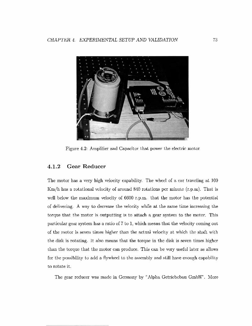
CHAPTER 4. EXPERIMENTAL SETUP AND VALIDATION

Figure 4.2: Amplifier and Capacitor that power the electric motor

4.1.2 Gear Reducer

The motor has a very high velocity capability. The wheel of a car traveling at 100

Km/h has a rotational velocity of around 840 rotations per minute (r.p.m). That is

well below the maximum velocity of 6600 r.p.m. that the motor has the potential

of delivering. A way to decrease the velocity while at the same time increasing the

torque that the motor is outputting is to attach a gear system to the motor. This

particular gear system has a ratio of 7 to I, which means that the velocity coming out

of the motor is seven times higher than the actual velocity at which the shaft with

the disk is rotating. It also means that the torque in the disk is seven times higher

than the torque that the motor can produce. This can be very useful later as allows

for the possibility to add a flywheel to the assembly and still have enough capability

to rotate it.

The gear reducer was made in Germany by "Alpha Getriebebau GmbH". More


information concerning the company or the specifications of the part can be found in

[35] . The main advantages of this gear system are its high power density and smooth

running with a significant lifespan. With a weight below 4 Kg, it presents a very

compact size, and it does not need lubrication during its lifetime. This component

can be seen in Fig. 4.3 as it is connected to the motor through the support.

Figure 4.3: Gear system used in the experimental assembly

4.1.3 Coupling

When dealing with such high rotation velocities and loads, it is necessary to maintain a

correct alignment of the shafts. This helps to maintain the system balanced and avoids

undesirable and damaging vibrations. To minimize such a problem, this coupling was

added to the setup. It allows to connect two shafts compensating for any misalignment

that may exist between them. This coupling was positioned between the gear reducer

and the clutch.


The manufacturer of this part was "Zero-Max, Inc." and additional information

regarding the characteristics of this component can be found through [36]. An image

of the coupling connecting the gear and the clutch shafts is shown in Fig. 4.4

Figure 4.4: Coupling system used to maintain shaft alignment

4.1.4 Clutch

The electromagnetic clutch allows the decoupling of the disk motion from the electric

motor as soon as it reaches the desired velocity. It also isolates the motor from the

braking process. This allows for more accurate measurements as well as preserving

the longevity of the motor. Due to the existence of permanent magnets in the motor,

and if the clutch was not present, once power to the motor was turned off, the

magnets would induce current in the windings of the motor and consequently generate

a braking torque, very much in analogy to the brake under development. With the

clutch, all the braking torque comes from the electromagnets.

CHAPTER 4. EXPENMENTAL SETUP AND VALIDATION 76

A part of the clutch is connected to the shaft coming from the motor and the

other part is connected to another shaft leading to the disk. These two parts, when

the unit is energized are magnetically attracted to each other. Hence, the two shafts

rotate at the same speed as if they were connected. Once the power to the clutch

is switched off, the two components decouple, making the motion of the respective

shafts independent from each other. The disk rotates freely at the desired velocity

with no additional forces being applied to it other than friction in the supports. This

makes it possible to evaluate the effects of braking torque produced by the eddy

current system.

The clutch is manufactured by "Inertia Dynamics, Inc", Model SO42 with a power

supply of 24 V.D.C. Additional information regarding this product is available in [37].

An image of the clutch connecting the two shafts is shown in Fig. 4.5.

Figure 4.5: Clutch system used in the experimental assembly


4.1.5 Electromagnets

The electromagnets are the primary components of the brake system proposed. AC

electromagnets were selected because they can handle both AC and DC current in

order allow for testing in the low velocity regime. Two AC electromagnets were

purchased and placed opopsite of each other and operating in phase opposition to

generate the desired magnetic flux between them. A picture of the electromagnets

used in the setup is made available in Fig. 4.6.

Figure 4.6: Electromagnets used in the experimental assembly

The electromagnets were purchased from "Magnetech Corp." and additional in-

formation can be found in [38]. Due to its laminated steel core there is minimal eddy

current formation in the core and consequently fewer losses. Because of this feature

this electromagnet is adequate for vibratory and quick on-off applications. The mag-

netic flux generator made from these electromagnets can generate 0.5 T of magnetic

flux density over a 10 mm air gap. In AC mode, it requires 125 V.D.C. and consumes

10.5 A of current at 80% duty cycle. In DC mode it only requires a voltage of 6.5

V.D.C and 10 A of current. Since the direct current mode will be the preferential


one, the power requirements are deemed suitable to be used in a car using current

power capabilities. It should be noted that these electromagnets have a rectangular

shape and opposing poles placed side by side. These factors amount to less desirable

properties than the ones that could possibly be obtained from a more tailored electro-

magnet specific to the design needs. However, for preliminary and proof-of-concept

purposes, they were considered acceptable.

4.1.6 Disk Brake

The disk brake is the other component necessary to make the eddy current brake

work. This component was built in the machine shop. It was necessary to purchase a

component that would connect the disk to the shaft. That piece, called a QD Bushing

was acquired from "Western Technologies". The details for this component can be

found in [39].

The central part of the disk was then designed to connect to the bushing, while

the outer portion of the disk was manufactured to meet the requirements of the

experiment. The disk has a radius of 0.15 m and a thickness of 8 mm. The material

used was aluminum due to its non-magnetic and electric and conductive properties.

The aluminum used was of grade 6061-T6, which means that it is a wrought aluminum

alloy with 0.6% Si and 1.0% Mg. The material has a density of 2700 ~ g / m ~ , a

conductivity of 2.459 x lo7 [33] and a magnetic permeability of 1.

4.1.7 Power Supply

Power supplies to run the electromagnets and the electromagnetic clutch were re-

quired. This equipment was kindly loaned by the Electrical Engineering Department

of the University of Victoria for this purpose. It consisted of DC power supplies for


the experiments requiring a continuous current and so a steady state magnetic field,

and variacs so that the current could be controlled for the experiments when alternate

current was needed. Figs. 4.7 and 4.8 show this equipment.

Figure 4.7: Direct current power supply

Figure 4.8: Alternate current power supply

4.1.8 Encoder

In order to measure the angular velocity of the disk while performing the experiments,

an encoder was installed. This encoder was connected to the shaft immediately after


the disk using a belt. The electronic measurements were acquired by connecting the

encoder to the DSPACE DAQ that also controls the motor. this allowed to record

the measurements for later data processing. Fig. 4.9 shows the encoder connected to

the shaft with the disk in the immediate background.

Figure 4.9: Encoder to record velocity evolution


4.1.9 Supports

The support structures for the experimental assembly were designed and manufac-

tured in-house. Three kinds of support structures were designed and manufactured.

Besides supporting the motor and the gear reducer, one of the supports also main-

tained the axial alignment between the two components, thus avoiding the need of an

additional coupling. It is extremely important to have these two components perfectly

aligned to avoid additional vibration. The component can be visualized in Fig.4.10.

Figure 4.10: Support that couples the electric motor and the gear system

The other type of support served to place the roller bearings of the pillow blocks

in the right position. This way the shaft is supported between components thus

distributing the weight and avoiding areas of high vertical loading that might deform

it. The pillow block supports were placed on either side of the disk and between the


clutch and the coupling that connects the clutch and the gear reducer. An image of

such supports is displayed in Fig.4.11 [40].

Figure 4.11: Support that maintains shaft alignment

The other support is the one that also serves to place the electromagnets in the

correct position. This support consists of three plates, for structural reinforcement

reasons. Since the electromagnets that are in opposite sides of the disk are being

fed so that one of them acts as the north pole and the other as the south pole, the


magnets are naturally attracted to one another. It was then necessary to create a

structure that could keep them fixed. These structures also place the magnets in

the desired position with regards to the rotating disk. The vertical plate holds the

magnet and the horizontal one connects the structure to the table while the gusset

provides structural support between these two plates. The support structure for the

electromagnets so that they become magnetic flux generators can be seen in Fig. 4.12.

Figure 4.12: Stand that holds the electromagnets in place

Finally, in Fig. 4.13, the complete experimental setup can be seen fully assembled.

The picture shows the motor with the capacitor and amplifier behind it; the support

that also connects to the gear reducer; the coupling attached to the gear; a shaft

support; the magnets in their stands with the disk in between and the power supplies.


Figure 4.13: Complete experimental setup

4.2 Experimental Results

Since the objective is to demonstrate the proof-of-concept, a flywheel was not added to

the setup as further safety issues would have to be incorporated. For the preliminary

experimental results, the only inertia considered comes from the aluminum disk. At

a later stage, additional experiments can be performed including a flywheel with all

the safety measures taken into account.


4.2.1 Experiment 1

This experiment is quite basic in its nature. Its purpose is to provide us with data

regarding the velocity variation suffered by the disk once the brakes are activated.

This data can then be compared with similar data obtained from the computational

simulations.

The first step is to get the motor running. The disk should start rotating as

well as we assume the clutch is engaged. At this point there are two alternatives.

It is possible to deactivate the clutch and simultaneously activate the brakes or we

can simply activate the brakes and subsequently decouple the disk from the motor.

In this later mode of operation, it is necessary to wait until the disk reaches the

desired rotation velocity once again. This method is the one most similar to the

computational simulations and it also decreases the error in measurements that might

be originated by the human delay in activating the brake once the clutch is switched

off. So, the standard procedure is to allow the disk to reach the prescribed velocity and

then turn on the eddy current brake system. The disk will slow down substantially,

but then the motor will increase its torque to maintain the prescribed value for the

velocity.

The braking system is, as expected unable to stall the motor, due to the torque

requirements stated when we purchased the motor but also because the torque is

being increased seven times through the gear reducer. On the other hand, the braking

torque generated by the electromagnets is decreased seven times before it reaches the

motor. Once the disk has once again reached the desired velocity due to the additional

effort from the motor, we can then turn off power from the clutch. The disk will then

only be subject to the braking torque generated by the eddy currents and so it stops.

This procedure is then repeated several times for different values of disk velocity as

well as for different values of the applied magnetic flux density. The data recorded


concerning the evolution of angular velocity of the disk was ten processed in order to

compare with results from the computational simulations.

4.2.2 Experiment 2

The other experiment to be performed at this stage has as an only objective to

prove that the alternate current idea in fact does not generate the additional torque

required at the low velocities. Using the same procedure as the one described in

the previous experiment, measurements of the evolution of angular velocity of the

disk when subjected to a time varying magnetic field were recorded These results

were then compared to measurements performed in the same conditions but with a

continuous magnetic flux density.

4.2.3 Experimental Results and Discussion

Five different values for the angular velocity of the disk were considered. For the

magnetic flux density, we defined the current to be fed to the electromagnets that

originated the desired magnetic field. The values of the magnetic flux density varied

from 0.1 to 0.4 T in increments of O.1T. The angular velocity of the disk varied between

14 and 71 radians per second with approximately 14 rad/s of increment. The data

in Table 4.1 shows the total time (in seconds) it took for the disk to completely stop

after the clutch was disengaged.

The first line of the table simply illustrates the time it takes for the free spin-

ning disk to stop rotating due essentially to the friction existing between the shaft

and the supports that hold it. The electromagnets were kept switched off while the

measurements were taken. It is seen that the stopping time is clearly superior to


Table 4.1: Time response for different magnetic fields and velocities

any of the other situations. The measurement presented here was the one that most

approximated the average times of stopping for this situation.

The other observation is that the values decrease as the intensity of the magnetic

flux density increases. The stopping time also increases when the initial rotation

velocity increases. All of these results are in accordance with the computational sim-

ulations. A more intense magnetic flux density generates more intense eddy currents,

thus resulting in higher braking torque. Consequently, the stopping time will be in-

ferior. A more careful analysis of the results however shows that the time difference

between contiguous values decreases as the velocity increases. This is also explained

by the fact that the higher the velocity, the bigger braking torque and so at higher

velocities there is a more accentuated deceleration of the disk.

The plots represents the time evolution of the disk velocity when subjected to

the different magnetic flux densities. The starting velocity is the same and it was

chosen to be the highest as it is the one that allows for a more clear image of all

the data points. It can be seen in Fig. 4.14 that except for the line that represents

absence of braking torque, the curves are nonlinear. In the absence of braking torque

from the electromagnets the velocity decreases somewhat linearly because the fric-

tion is constant and causes a constant deceleration. When the electromagnets are


powered up, that is not the case. Because braking torque changes according to the

rotational velocity, as this decreases, so does the torque and consequently there is less

deceleration. That accounts for the rounding of the curves as they approach zero.

Experimental results

80 1 I

70 1,

60 -

? 50 - P - 2

h %

2 40 I L - I g 30

I -

I

20 i

I

10 I - I

0 i

0 0.5 1 1.5 2 2.5 3 3.5 4 4.5 5 5.5 6 6.5 7 7.5 8 8.5 9 time (s)

Figure 4.14: Experimental results

Although the results from the experimental tests match our expectations quali-

tatively speaking, it is also necessary to take into account the quantitative aspect.

To that end, a computational analysis was performed duplicating the experimental

testing. The pole projection areas were redefined accordingly to the dimensions of

the poles in the electromagnets that were purchased. A plot of the new simulation

model can be seen in Fig. 4.15.


Surface: magnetic flux density (Bz) Flow. [total current density (Jx),total current density (Jy)]

_I

89

Max: 0.551

0.5

0.4

0.3

0.2

0.1

0

-0.1

-0.2

-0.3

-0.4

-0.5

Min: -0.56

Figure 4.15: Computational simulation of experimental setup

The Simulink model was also updated to take into account the inertia of the disk.

The inertia of the shaft and the component of the clutch also attached to it was not

considered as it was difficult to calculate and nearly negligible in comparison. The

results from the computational simulation runs are presented in Fig. 4.17. It should

be noted that the line regarding absence of magnetic field was not included in this

graphic. The scale of the time axis is also different in this figure. The colors and

shapes of the points that define the curves were kept the same for easy comparison.

These results are overall superior to the ones obtained in the experimental tests.

They predict a stronger braking torque, as indicated by the steeper initial slope of


n+-- acceleration of the di*

T o q u e u Ilinertla

FEMLRB Subsystem

Figure 4.16: Simulink Model

Products

the curves. Near the zero region they round up in a more noticeable fashion than

in the experimental plot. The major difference is noticeable in the case with smaller

intensity of magnetic field. In Table 4.2 is a comparison of the results from both the

experimental and the computational runs.

Examining the Table 4.2, we notice that there is ,an interesting evolution of the

differences between the two. The experimental time is always superior to the compu-

tational values but the difference never exceeds 0.15 s except in the case of the less


Computational Results

1

time (s)

Figure 4.17: Computational results

intense magnetic field. The computational prediction for a magnetic flux density of

0.1 T expected a much faster response time than the one that was actually obtained.

This can be explained by a number of factors.

The most significant reason was that probably, the magnitude of the magnetic flux

lines going into the magnet was inferior to what was expected. The prediction for

the magnetic field was performed based on information provided by the manufacturer

but that information did not contemplate this case. It is then possible that for the


Table 4.2: Comparison between experimental and computational times

Magnetic Flux Density (T) 0.1 0.2 0.3 0.4 Experimental time (s) 4.025 1.31 0.755 0.41 Computational time (s) 1.5 1.2022 0.607 0.2867 Time difference (s) 2.525 0.1078 0.148 0.1233

current that was fed to the electromagnets did not generated an intense enough field.

The computational model assumes that the whole area under the influence of the

magnet pole is subjected to a constant field directed perpendicularly to the disk. In

reality, the weaker the magnetic field, the more the lines will curve and dissipate

in air. Additionally, because the flux generator was made from two independent

electromagnets, it would be easier for those lines to go from one pole to the other

than to cross the air gap to reach the opposing pole in the other side. This effect

would account for a much more "diluted" magnetic field than predicted, thus affecting

adversely the performance of the system.

As for the other cases, they behaved very closely to what was expected. Addition-

ally, because the braking power was activated through a manual switch, it was not

always clear exactly at what point in time the braking actually began. This problem

can be addressed by installing relays and controlling the power fed to the electromag-

nets through the computer. These modifications along with a more precise encoder

should enable more precise readings.

It should be noted that there was also a contribution for the braking torque from

the friction of the shaft in the bearings. This was not taken into account in the

simulations and would probably cause a greater difference between the sets of results.

However, for a first approximation of the electric brake system, these results appear

to be highly encouraging. An additional plot illustrates more clearly the differences


between the evolution in two of the cases, as can be seen in Fig. 4.18

- Experimental 0.4 - Computational 0.4

Experimental 0.2

Figure 4.18: Detailed comparison of experimental and computational results

The experiment as described in subsection 4.2.2 had the objective to demonstrate

the performance of the system when powered by alternate current. This test was

performed because in the low velocity region, the direct current does not provide

enough braking torque to satisfy the needs of a car braking system. It was then

hypothesized that eddy currents could be generated using a time varying magnetic

field to make up for that shortcoming of the original concept. The Figs.4.19 and

4.20 illustrate, rewspectively, the results obtained using a continuous current that

generates a 0.2 T of magnetic flux density and an alternate current to make the

magnetic field density oscillate between 0.2 and -0.2 T. These measurements were

performed for three different initial velocities.


DC power supply

0 0.2 0.4 0.6 0.8 1 1.2 1.4 1.6

time (s)

Figure 4.19: DC power supply experimental results

Although the graphics have very similar curves, the difference that exists between

them is quite noticeable as far as the time scales are concerned. The AC powered

electromagnets produced a result only slightly superior to the ones from when there

was no magnetic field applied. However, it was worse than when there was a 0.1 T

flux density applied. Because the intensity of the eddy currents varies with the square

of the applied magnetic field, every time that the flux is reversed there is a period of

time when it is well below the value that is being provided by the continuous field.

Although the frequency of change is high, the maximum value of the flux density

is only reached twice in every cycle, which translates to 1/30 of a second in every

second. With this in mind, it is easy to see that the intensity of the field is overall far


AC power supply

time (s)

Figure 4.20: AC power supply experimental results

inferior to the one obtained when using direct current. There are more eddy currents

being generated, because there is not only the motion of the disk, but also the time

changing field. These eddy currents however do not produce the same amount of

braking torque than the ones from a stationary field.

It should be pointed out also that the temperature of the aluminum disk increased

significantly when subjected to the time varying magnetic field. This was due to the

Joule effect losses from the eddy currents. While the magnets were working at a

frequency of 60 Hz, eddy currents were also being generated in the disk at that rate.

These electric currents, like any others, dissipate power in the form of heat. That

accounts for the heating of the disk. When the magnetic field is continuous the eddy


currents only form due to the motion of the disk. Hence, although they have a greater

intensity, there is less power being dissipated because they are not being generated

at such high rates.

Synopsis

The experimental study presented here had the objective of validating the computa-

tional results obtained in Chapter 3. The proof-of-concept prototype clearly demon-

strated that eddy currents are a viable solution in the design of electric brake actu-

ators. The experimental results further confirmed that alternative designs need to

be considered in the low velocity regime. The results obtained in the high velocity

regime confirmed the computational simulations.

Further improvements are required on the experimental setup in order to represent

more realistically the dynamics of a car. The incorporation of a flywheel and re-design

of the magnets needs to be carried out. Overall, this simple experimental setup

provided the necessary answers on the proposed electric brake actuators in order to

carry out the required improvements in the future.

Chapter 5

Conclusions and Recommendat ions

5.1 Conclusions

The multifunctional materials are not yet at a point in their development where they

can be used for such high demand applications as a car brake actuator. Shape memory

alloys have a long time delay and are temperature dependent. This is a limiting factor

in friction based systems. Piezoelectric materials appear as a possibility that may have

potential should significant improvements in material properties develop. Presently,

their force-displacement curve is not capable of responding to the requirements of a

brake actuator. Furthermore, their fragility and the fact that with continued use they

heat up rapidly are also constraining factors. Electromagnetic based solutions require

a large power input in terms of electric energy, are invariably bulky and heavy to be

suitably fitted on a car wheel.

A system was designed and manufactured using eddy currents. The eddy current

solution appeared to be a feasible solution at high velocities. Computational sim-

ulations using finite element models provided acceptable performance solutions. A

CHAPTER 5. CONCLUSIONS AND RECOMMENDATIONS 98

parametric optimization process provided the best combination of design parameters.

The introduction of a gear system to enhance performance proportional was pro-

posed. This translated in huge savings in power consumption and in the dimension

of the system making it a viable solution. An experimental setup was assembled to

validate the performance of the actuator. The comparison of the performance values

obtained from the experimental testing and the computational simulation are in good

agreement.

5.2 Advantages and Limitations

The main advantages inherent in the proposed concept encompass environmental,

performance and control issues. Because the system is purely electrical, there is no

longer a need for hydraulic components, making it more environmentally acceptable.

Furthermore, there are other components that can be discarded, such as brake pads,

calipers, brake lines and master cylinder. The absence of contact, given that this sys-

tem operates purely on magnetic interaction, eliminates the need for friction. Without

friction, problems such as squealing, brake fade and brake wear also vanish. Aside

from the reduced parts and maintenance costs, the sheer simplicity of the system

decreases the possibilities of malfunction. Given that the amount of braking torque is

controlled by the intensity of the applied magnetic field, the only parameter required

to control it is the electric current that is transmitted to the electromagnets. This

makes the controllability of the braking torque much easier, since there is only one

parameter to control with the rest of the work being done by an electronic control

unit.

However, there is a serious limitation to the proposed system. As mentioned

earlier, the magnitude of the braking torque is directly related to the rotation velocity


of the disk. While at higher velocities this translates to additional braking power,

causing the deceleration to be limited solely by the tires and the traction of the road,

there is the other side of the equation. The implication of the velocity dependency is

that in the low velocity region the system is incapable of producing sufficient torque

to meet the requirements.

To take this limitation to the extreme, it suffices to say that while stopped, there

is no braking power being applied. This translates into the inability to hold the

car still in a slope. It also disables the capability of stopping in a slow moving

situation such as a traffic jam. An alternative was contemplated to compensate for

this effect. It was thought that the application of a time varying magnetic field would

generate additional eddy currents thus compensating for the drop in torque. It was

seen that although more eddy currents were indeed generated they did not increase

braking power. The intensity of the currents was not big enough and it exacerbated

the problem. The generation of so many electric currents led to an increased rise

in the disk temperature. The increase in temperature led to greater resistivity and

consequently decreased braking power.

5.3 Recommendations for Future Work

There are a few recommendations to be made that can lead to a significant improve-

ment of this work. Some of them fall entirely out of the scope of this work while

others were not performed due to time constraints.

It is advisable to perform a study regarding thermal issues concerning this system.

The temperature in the disk due to the eddy currents will not be a factor that can

significantly affect the feasibility of the concept. While disk conductivity will be

affected by the temperature at which it operates, the fact that it will be in a forced


air environment should provide sufficient cooling. The thermal problems that may

arise can be further mitigated by accelerating the flow of air around the disk or

installing a fan as it is done in current retarder brakes.

Although our preliminary study revealed that AC current does not provide the

braking power we need in the low velocity, further study into the performance of

the system is recommended. This work focused in the high velocity region and as a

consequent suggests that an alternative braking system be placed on the rear wheels

to handle the low velocity performance as well as the parking situation. The high

velocity system should therefore be implemented on the front wheels so that it takes

full advantage of its capabilities while driving at higher velocities as most of the work

is done by the front wheels.

Further experimental validation is required. Additional testing with more accurate

measuring equipment is recommended as well as the inclusion of the braking mecha-

nism in a completely electronically controlled system. The addition of a flywheel is

mandatory, but safety concerns should be addressed.

The electromagnets used in the experimental setup were adapted for the purpose

of validating computational results. They are in no way the most suitable design to

be employed in such a system. A horseshoe shaped electromagnet placed in the outer

edge of the disk may improve the design.

Finally, another additional possibility inherent to this concept is called regener-

ative braking. Instead of dissipating all the energy every time that the brakes are

applied, this system allows for some of that energy to be captured and re-utilized.

Since there are electric currents flowing in the surface of the disk and these currents

generate magnetic energy, much of that energy can be used to generate current in

a coil. This is the same principle that is behind the operation of generators. The

regenerated electric current can then be used to power the brake system or any other

CHAPTER 5. CONCLUSIONS AND RECOMMENDATIONS

additional electrical system in the car.

References

[I] Richard D. Thornton. Magnetic levitation and propulsion. IEEE Transactions

on Magnetics, July 1975.

[2] Drum brakes. http://www.masterhitch.com/hitchAcc.asp?prodID=32.

[3] Electric drum brakes. www.marksrv.com/ idl2dexbrake.htm.

[4] Jacobs vehicle systems. http://www.jakebrake.com.

[5] Qian Ming. Sliding mode controller design for a.b.s. system. Master's thesis,

Virginia Polytechnic Institute and State University, 1997.

[6] Telma - frictionless braking systems. http://www.telmausa.com/telma~htm/ de-

fault.htm.

[7] Frenelsa - frenos electricos unidos. http://www . frenelsa.com.

[8] Karim Nice. How anti-lock brakes work. Technical report, HowStufFWorks, Inc.,

2002. Available: http://www~howstuffworks.com.

[9] Delphi brake modules - electric caliper. Technical report, Delphi,Co., Troy,MI,

2002. Available: ht tp://www.delphi.com.

[lo] Electro-mechanical brake.

online.com/generator/www/start/index~uv.html.

REFERENCES 103

[ll] T.K. Keim. 42volts - the view from today. In Proceedings of 2004 International

Congress on transportation Electronics, 2004.

[12] T. Gillespie. Fundamentals of Vehicle Dynamics. Society of Automotive Engi-

neers, 1992.

[13] A.B. Will, S. Hui, and S.H. Zak. Sliding mode wheel slip controller for an antilock

braking sytem. International Journal of Vehicle Design, 19:523-539, 1998.

[14] James Walker Jr. Pulp friction - a plain-talk primer on your

car's braking system. Grassroots Motorsports, February 1991. Avail-

able:http://www.scirocco.org/faq/brakes/pulpfriction/pfpagel.html.

[15] midi - acsmart actuator. Technical report, Midi Technology Corporation, Med-

ford,MA. Available: http://www.mide.com.

[16] Piezo products catalogue. Technical report, Cedrat Technologies, France,

September 2003. Available: http://www.cedrat.com.

[17] Piezo actuators and assemblies. Technical report, Physik Instrumente (PI)

GmbH and Co., Germany. Available: http://www.pi.ws.

[18] Selcuk Gursan. Development of a continuous-motion piezoelectric rotary actua-

tor for mechatronics and micropositioning applications. Master's thesis, Univer-

sity of Victoria, 1996.

[19] Sen P.C. Principles of Electric Machines and Power Electronics. John Wiley &

Sons, second edition, 1997.

[20] Voice coil actuators. Technical report, BE1 Technologies, Inc., San MArcos, CA.

Available: http://www.beikimco.com.

REFERENCES 104

[21] I. J. Busch-Vushniac. Electromechanical Sensor and Actuator. Springer-Verlag,

1999.

[22] Small engine eddy current dynamometers. http://www.land-and-sea.com/kart-

dyno/kart-eddy-current-dyno.htm.

[23] K.J. Lee and K.H. Park. Analysis of an eddy current brake considering the finite

radius and induced magnetic flux. Journal of Applied Physics, 92:5532-5538,

2002.

[24] K. J. Lee and K.H. Park. Modeling of eddy currents with boundary conditions by

using coulomb's law and the method of image. IEEE Transactions on Magnetics,

38: 1333-1340, 2002.

[25] K.J. Lee and K.H. Park. Optimal robust control of a contactless brake system

using an eddy current. Journal of Mechatronics, 9:615-631, 1999.

[26] K.J. Lee, J.N. Kang, S.M. Wang, and K.H. Park. Torque analysis and optimiza-

tion of an eddy current brake system. In Proceedings of 28th Annual Symposium

of Incremental Motion Control System and Devices, 1999.

[27] Rick Hoadley. Magnet man - cool experiments with magnets.

http: //my.execpc.com/~hoadley/magindex.htm.

[28] W.F. Archenhold. Electromagnetism and Electrostatics using SI Units. Oliver

and Boyd, 1969.

[29] Comsol. FEMLAB 2.3, June 2002.

[30] The Mathworks, Inc. MATLAB 6.1 Help, May 2001.

REFERENCES 105

[31] Depth of penetration & current density. http://www.ndt-

ed.org/EducationResources/CommunityCollege/EddyCurrents/Physics/

depthcurrentdensity.htm.

[32] D. K. Cheng. Field and Wave Electromagnetics. Addison-Wesley, 2nd edition,

1991.

[33] Eddy Current Technology Inc. Electrical conductivity & resistivity for aluminum

& aluminum alloys. ND T Magazine, Sept/Oct 1955. Available:http://www.ndt-

ed.org/GeneralResources/MaterialProperties/ET/et~matlpropindex.htm.

[34] Brushless servo motors, bmr 4000 series. Technical report, Torque

Systems, 6 Enterprise Road, Billerica, MA 01821-3954 USA. Avail-

able:http://www. torquesystems.com/bmr4000. html.

[35] Sp+ the new generation, low backlash palanetary gearhead. Technical report,

alpha getriebebau GmbH, Walter-Wittenstein-Stra8e 1, 97999 Igersheim, Ger-

many, 2004. Available: http://alphagetriebe.de/en/170-287.001.htm.

[36] Zero-max, servoclass couplings. Technical report, Zero-Max, Inc., 13200 Sixth

Avenue North, Plymouth, MN 55441, 2003. Available: http://www.zero-

max.com/products/servo/servo~main.asp.

[37] Shaft mounted clutch couplings - type so. Technical report, Inertia Dynam-

ics, Inc, 100 Franklin Drive, P.O. Box 1277, Torrington, CT 06790. Available:

http://www.idicb.com/elecmgcb/SO.

[38] True ac electromagnets. Technical report, Magnetech Corp.,

22809 Heslip Drive, Novi, MI 48375 U.S.A., 2004. Available:

http://www.magnetechcorp.com/True~ac~electromagnet .htm.

REFERENCES 106

[39] Qd bushings. Technical report, Martin Sprocket & Gear Inc.,

3100 Sprocket Drive, Arlington, TX 76015 USA. Available:

http://www.martinsprocket.com/Bushings.htm.

[40] Rhp bearings, self-lube. Technical report, NSK Canada Inc., 3353 Way-

burne Drive, Burnaby, British Columbia V5G 4L4, Canada. Available:

http://www.eu.nsk.com/products/article.asp?LID=l & ProductID=298.

Design of an Innovative Car Braking System using Eddy ...

Documents

Transcript of Design of an Innovative Car Braking System using Eddy ...