Extremes on river networks - arXiv

arX

iv:1

501.

0266

3v2

[st

at.M

E]

4 F

eb 2

016

The Annals of Applied Statistics

2015, Vol. 9, No. 4, 2023–2050DOI: 10.1214/15-AOAS863c© Institute of Mathematical Statistics, 2015

EXTREMES ON RIVER NETWORKS1

By Peiman Asadi∗, Anthony C. Davison† and

Sebastian Engelke∗,†

Universite de Lausanne∗ and Ecole Polytechnique Federale de Lausanne†

Max-stable processes are the natural extension of the classicalextreme-value distributions to the functional setting, and they are in-creasingly widely used to estimate probabilities of complex extremeevents. In this paper we broaden them from the usual situation inwhich dependence varies according to functions of Euclidean distanceto situations in which extreme river discharges at two locations ona river network may be dependent because the locations are flow-connected or because of common meteorological events. In the for-mer case dependence depends on river distance, and in the second itdepends on the hydrological distance between the locations, either ofwhich may be very different from their Euclidean distance. Inferencefor the model parameters is performed using a multivariate thresholdlikelihood, which is shown by simulation to work well. The ideas areillustrated with data from the upper Danube basin.

1. Introduction. Modeling extreme events has recently become of greatinterest. The financial crisis, heat waves, storms and heavy precipitationunderline the importance of assessing rare phenomena when few relevantdata are available.

There is a vast literature on modeling the univariate upper tail of thedistribution of environmental quantities such as precipitation or river dis-charges at a fixed location t. If Xi(t) (i = 1, . . . , n) are n ∈ N independentmeasurements of a random spatial process X at location t, then the prob-ability law of the maximum of the n observations can be approximated bythe generalized extreme value distribution (GEVD)

P

{

maxi=1,...,n

Xi(t)− bnan

≤ x

}

≈G(x) = exp{−(1 + ξx)−1/ξ+ }, x ∈R,(1)

Received February 2015; revised July 2015.1Supported by the Swiss National Science Foundation and the EU-FP7 project Im-

pact2C.Key words and phrases. Extremal coefficient, hydrological distance, max-stable pro-

cess, network dependence, threshold-based inference, upper Danube basin.

This is an electronic reprint of the original article published by theInstitute of Mathematical Statistics in The Annals of Applied Statistics,2015, Vol. 9, No. 4, 2023–2050. This reprint differs from the original in paginationand typographic detail.

1

http://arxiv.org/abs/1501.02663v2

http://www.imstat.org/aoas/

http://dx.doi.org/10.1214/15-AOAS863

http://www.imstat.org

http://www.imstat.org

http://www.imstat.org/aoas/

http://dx.doi.org/10.1214/15-AOAS863

2 P. ASADI, A. C. DAVISON AND S. ENGELKE

where z+ =max(z,0) and bn ∈ R, an > 0 and ξ ∈ R are the location, scaleand shape parameters, respectively. For ξ = 0, G(x) is read as the limitexp{− exp(−x)}. In fact, (1) represents the only possible nondegeneratelimit for maxima of independent and identically distributed sequences ofrandom variables [see, e.g., Coles (2001), Chapter 3]. This justifies the ex-trapolation to high quantiles using the parametric tail approximation (1) foru close to the upper endpoint of the distribution of X(t) by

P{X(t)>u} ≈ 1

n

(

1 + ξu− bnan

)−1/ξ

+

.(2)

Often, however, univariate considerations are insufficient, because near-simultaneous extreme events may cause the most severe damage. In con-sidering flooding of a river basin, for example, it is crucial to understandthe extremal dependence between flows at different gauging stations. Manyauthors have analyzed this using multivariate copulas or multivariate ex-treme value distributions [e.g., Salvadori and De Michele (2010), Renardand Lang (2007)], but the explosion of the number of parameters in highdimensions limits the applicability of such models, and information on thegeographical location of the stations cannot be readily incorporated. Mete-orological considerations suggest that extremal dependence can be modeledas a function of the distance between two locations. Indeed, for precipita-tion, temperature or wind data, the use of Euclidean distance has becomestandard in spatial extremes [e.g., Davison and Gholamrezaee (2012), Huserand Davison (2014), Engelke et al. (2015)]. An important class of proba-bility models for extreme spatial dependence on the Euclidean space R

2 isthe class of max-stable processes, giving several flexible models whose depen-dence is parameterized in terms of covariance functions [Schlather (2002),Opitz (2013)] or of negative definite kernels [Brown and Resnick (1977),Kabluchko, Schlather and de Haan (2009), Kabluchko (2011)]. Almost allsuch models have hitherto presupposed that extremal dependence dependsonly on the Euclidean distance between two locations, but this may be toorestrictive when more is known about the physical processes underlying thedata: locations on a river network may interact because of the flow of waterdownstream between them.

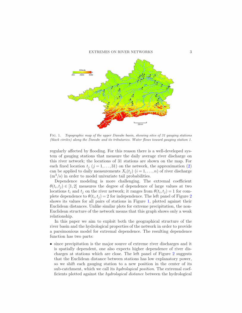
In this paper we focus on assessment of the risk of extreme discharges onriver networks in order to understand and prevent flooding. There is long-standing interest in the application of extreme value statistics in hydrology[e.g., Katz, Parlange and Naveau (2002), Keef, Svensson and Tawn (2009),Keef, Tawn and Svensson (2009)]. In Europe, floods are major natural haz-ards that can end human lives and cause huge material damage. Figure 1shows the upper Danube basin, which covers most of the German state ofBavaria and parts of Baden-Wurtemberg, Austria and Switzerland, and is

EXTREMES ON RIVER NETWORKS 3

Fig. 1. Topographic map of the upper Danube basin, showing sites of 31 gauging stations(black circles) along the Danube and its tributaries. Water flows toward gauging station 1.

regularly affected by flooding. For this reason there is a well-developed sys-tem of gauging stations that measure the daily average river discharge onthis river network; the locations of 31 stations are shown on the map. Foreach fixed location tj (j = 1, . . . ,31) on the network, the approximation (2)can be applied to daily measurements Xi(tj) (i= 1, . . . , n) of river discharge(m3/s) in order to model univariate tail probabilities.

Dependence modeling is more challenging. The extremal coefficientθ(ti, tj) ∈ [1,2] measures the degree of dependence of large values at twolocations ti and tj on the river network; it ranges from θ(ti, tj) = 1 for com-plete dependence to θ(ti, tj) = 2 for independence. The left panel of Figure 2shows its values for all pairs of stations in Figure 1, plotted against theirEuclidean distances. Unlike similar plots for extreme precipitation, the non-Euclidean structure of the network means that this graph shows only a weakrelationship.

In this paper we aim to exploit both the geographical structure of theriver basin and the hydrological properties of the network in order to providea parsimonious model for extremal dependence. The resulting dependencefunction has two parts:

• since precipitation is the major source of extreme river discharges and itis spatially dependent, one also expects higher dependence of river dis-charges at stations which are close. The left panel of Figure 2 suggeststhat the Euclidean distance between stations has low explanatory power,so we shift each gauging station to a new position in the center of itssub-catchment, which we call its hydrological position. The extremal coef-ficients plotted against the hydrological distance between the hydrological


Fig. 2. Extremal coefficients (estimated using the madogram) of all pairs of gaugingstations plotted against Euclidean distance (left) and hydrological distance (right); thosefor flow-connected pairs are blue crosses, and those for flow-unconnected pairs are blackcircles.

positions exhibit a strong functional relationship, shown in the right panelof Figure 2, which is exploited in the dependence model described in Sec-tion 3.3;

• the crosses in Figure 2 represent the extremal coefficients of pairs of flow-connected stations, which have one station located upstream of the other.Such pairs are generally more dependent than flow-unconnected pairs,not only because the catchments are close but also owing to the flow ofwater along the river. In Section 3.2 we explain how knowledge about thenetwork structure and river sizes can be included in the dependence modelfor flooding using ideas of Ver Hoef and Peterson (2010), who definedcovariance functions on river networks.

As one application of such a model, we would like to be able to computethe multivariate counterpart of (2), that is, the probability of a rare eventsuch as

P{X(s1)> u1, . . . ,X(sk)> uk}for large u1, . . . , uk > 0, where s1, . . . , sk ∈ T can be any stations on the rivernetwork, even without measurements there. More complicated quantities,such as the sum of discharges at several stations, may also be of interest.

2. Preliminaries.

2.1. Extreme value theory. The only nontrivial limiting distribution forthe normalized maxima of an independent and identically distributed se-quence of scalar random variables is the max-stable GEVD, expression (1).


In the multivariate case, we can transform each margin such that the max-limit has a standard Frechet cumulative distribution function exp(−1/x)(x > 0). In this way, without loss of generality, we can concentrate on themultivariate dependence between the components [Resnick (1987), Proposi-tion 5.8].

Let Xi = (X1,i, . . . ,Xm,i) (i = 1, . . . , n) be independent copies of an m-variate random vector X and assume that for each j = 1, . . . ,m the maximummaxiXj,i converges to a GEVD Gj , as in (1), with norming constants bj,n ∈R, aj,n > 0 and shape parameter ξj . Define the transformations

Uj(x) =−1/ logGj(x) = (1 + ξjx)1/ξj+ ,(3)

and note that

limn→∞

P

{

maxi=1,...,n

Uj

(

Xj,i − bj,naj,n

)

≤ x

}

= exp(−1/x), j = 1, . . . ,m.

We say that X is in the multivariate maximum domain of attraction(MDA) of a random vector Z= (Z1, . . . ,Zm), if for any z= (z1, . . . , zm),

limn→∞

P

{

maxi=1,...,n

U1

(

X1,i − b1,na1,n

)

≤ z1, . . . , maxi=1,...,n

Um

(

Xm,i − bm,n

am,n

)

≤ zm

}

(4)= P(Z≤ z);

call this joint distribution FZ(z). In this case, Z is max-stable with standardFrechet marginal distributions; see before (9). Moreover, by Resnick (1987),Proposition 5.8, we may write

FZ(z) = exp{−V (z)}, z ∈Rm,(5)

where the exponent measure V is a measure defined on the cone E =[0,∞)m \ {0} and V (z) is shorthand for V ([0,z]C). The object V incorpo-rates the extremal dependence structure of Z, where V (z) = 1/min(z1, . . . ,zm) and V (z) = 1/z1 + · · ·+1/zm represent complete dependence and inde-pendence, respectively. The measure V is homogeneous of order −1, that is,V (λz) = λ−1V (z), for λ > 0, and it satisfies V (z,∞, . . . ,∞) = 1/z for z > 0and any permutation of its arguments. There are many parametric modelsfor the exponent measure V and thus for multivariate extreme value distri-butions or copulas. The explosion of parameters in most such models makesfitting them feasible only in low dimensions.

By Proposition 5.17 of Resnick (1987) the convergence in (4) is equivalentto

limn→∞

nP

[{

U1

(

X1 − b1,na1,n

)

, . . . ,Um

(

Xm − bm,n

am,n

)}

∈A

]

= V (A)(6)


for any Borel subset A ⊂ E which is bounded away from 0 and satisfiesV (∂A) = 0, where ∂A is the boundary of A. This important observationallows us to approximate the probability that X falls into a rare region. Forinstance, if A = (u1,∞) × · · · × (um,∞) (u1, . . . , um ∈ R), then for large n(6) implies that

P(X1 > u1, . . . ,Xm > um)≈ 1

nV

{

m∏

j=1

(

Uj

(

uj − bj,naj,n

)

,∞)

}

,(7)

where∏

denotes the Cartesian product. More complicated events such asA= {x ∈R

m :∑m

i=1 xi >u} for some u ∈R can also be considered. Equation(6) implies that as n→∞ the empirical point process

{(

U1

(

X1,i − b1,na1,n

)

, . . . ,Um

(

Xm,i − bm,n

am,n

))

: i= 1, . . . , n

}

converges vaguely to a Poisson point process on E with intensity measureV [Resnick (1987), Proposition 3.21]. In Section 4 this result will be usedto derive the asymptotic distribution of exceedances and to fit parametricmodels for V .

In the bivariate case m= 2, a common summary statistic for the depen-dence among components of FZ is the extremal coefficient θ ∈ [1,2] [see, e.g.,Schlather and Tawn (2003)], which is defined through the expression

P(Z1 ≤ u,Z2 ≤ u) = P(Z1 ≤ u)θ, u > 0,(8)

or, equivalently, θ = V (1,1). Consequently, the cases θ = 1 and θ = 2 corre-spond to complete dependence and independence. Model-free estimation ofthe extremal coefficient is possible through the madogram [Cooley, Naveauand Poncet (2006)], and these estimates of θ can be used for model-checking.

2.2. Max-stable processes. Max-stable processes can be defined on anyindex set T , though this is usually taken to be a subset of an Euclideanspace Rd. A random process {Z(t) : t ∈ T} is called max-stable if there existsa sequence (Xi)i∈N of independent copies of a process {X(t) : t ∈ T} andfunctions an(t)> 0, bn(t) ∈R, such that the convergence

Z(t) = limn→∞

{

maxi=1,...,n

Xi(t)− bn(t)}

/an(t), t ∈ T,(9)

holds in the sense of finite dimensional distributions. In this case, the processX is said to lie in the max-domain of attraction of Z.

The class of max-stable processes is generally too large for statisticalmodeling, so one typically considers parametric subclasses of models. Ex-amples include mixed moving maxima processes [Wang and Stoev (2010)],Schlather processes [Schlather (2002)] and Brown–Resnick processes [Brown


and Resnick (1977), Kabluchko, Schlather and de Haan (2009)]. In this pa-per we rely on the construction principle for a large class of max-stable pro-cesses given in Kabluchko (2011); see also Kabluchko, Schlather and de Haan(2009). A negative definite kernel Γ on an arbitrary nonempty set T is amapping Γ : T ×T → [0,∞) such that for any n ∈N and a1, . . . , an ∈R with∑n

i=1 ai = 0, we have

n∑

i=1

n∑

j=1

aiajΓ(ti, tj)≤ 0, t1, . . . , tn ∈ T.

The following result states that there corresponds a max-stable process toany negative definite kernel on T .

Theorem 2.1 [Kabluchko (2011), Theorem 1]. Suppose that Wi (i ∈N)are independent copies of the zero-mean Gaussian process {W (t) : t ∈ T}whose incremental variance E{W (s)−W (t)}2 equals Γ(s, t) for all s, t ∈ T .Let σ2(t) = E{W (t)2} denote the variance function of W and let {Ui : i ∈N}denote a Poisson process on (0,∞) with intensity u−2 du. Then the process

ηΓ(t) = maxi∈N

Ui exp{Wi(t)− σ2(t)/2}, t ∈ T,(10)

is max-stable, has standard Frechet margins, and its distribution dependsonly on Γ.

If T =Rd and W is an intrinsically stationary Gaussian process, then ηΓ

is called a Brown–Resnick process [Brown and Resnick (1977), Kabluchko,Schlather and de Haan (2009)]. This is a popular model for complex ex-treme events. The generation of random samples from Brown–Resnick typeprocesses is challenging [cf. Engelke, Kabluchko and Schlather (2011), Oest-ing, Kabluchko and Schlather (2012)], but recent advances provide exactand efficient algorithms [Dieker and Mikosch (2015), Dombry, Engelke andOesting (2016)].

Remark 2.2. (a) For any negative definite kernel Γ there are many dif-ferent Gaussian processes with incremental variance Γ [Kabluchko (2011),Remark 1]. In particular, for u ∈ T , we can choose a unique Gaussian pro-cess W (u) with incremental variance Γ and W (u)(u) = 0 almost surely. Thecovariance function of this process is

E{W (u)(t)W (u)(s)}= {Γ(s,u) + Γ(t, u)− Γ(s, t)}/2.(11)

Thus, there is a one-to-one correspondence between negative definite kernelsΓ and the class of max-stable processes ηΓ.

(b) If {X(t) : t ∈ T} is a zero-mean Gaussian process with covariancefunction C : T ×T →R, then Γ(s, t) =C(s, s)+C(t, t)−2C(s, t) is a negativedefinite kernel on T .


The bivariate distribution function of (ηΓ(s), ηΓ(t)) (s, t ∈ T ) is

P{ηΓ(s)≤ x, ηΓ(t)≤ y}

= exp

{

−1

xΦ

[

√

Γ(s, t)

2+

log(y/x)√

Γ(s, t)

]

− 1

yΦ

[

√

Γ(s, t)

2+

log(x/y)√

Γ(s, t)

]}

,(12)

x, y > 0,

where Φ is the standard normal distribution function. Analogously to theextremal coefficient in (8), one considers the extremal coefficient functionθ(s, t) (s, t ∈ T ), defined as the extremal coefficient of the bivariate vector(ηΓ(s), ηΓ(t)), as a measure of the functional extremal dependence of themax-stable process ηΓ. By (12), we conclude that

θ(s, t) = 2Φ

{

√

Γ(s, t)

2

}

,(13)

so the negative definite kernel Γ parameterizes the extremal dependencebetween observations at positions s and t; small and large values of Γ(s, t)correspond to strong and weak dependence, respectively. By Remark 2.2(a),any kernel Γ yields a max-stable process ηΓ, so in Section 3 we can and willfocus on finding a parametric model for Γ suitable for our application.

The higher dimensional distributions of ηΓ are more complicated. Forinstance, for t= (t1, . . . , tm) ∈ Tm, the random vector (ηΓ(t1), . . . , ηΓ(tm)) ismax-stable and its exponent measure VΓ,t defined in (5) is characterized by[Kabluchko (2011)]

VΓ,t(x1, . . . , xm) = E

[

maxi=1,...,m

{

W (ti)− σ2(ti)/2

xi

}]

.(14)

This multivariate max-stable distribution is called the Husler–Reiss distri-bution [Husler and Reiss (1989)]. Computation of the expected value in (14)involves high-dimensional integrals and thus is awkward in general.

3. Model.

3.1. River network. In the previous section we showed how to definemax-stable processes on an arbitrary index set T . From here on, T willrepresent a river network and we will construct a kernel Γ flexible enoughto explain the extremal dependence observed in data.

Let us first fix some notation for river networks [Ver Hoef and Peterson(2010)]. We embed our network T in the Euclidean space R

2 representingthe geographical river basin. To this end, let T ⊂ R

2 denote the collectionof piecewise differentiable curves, called river segments, that are connectedat the junctions of the river and whose union constitutes the river network.


Fig. 3. River network with three locations t1, t2, t3 ∈ T ; t1 is flow-connected with both t2and t3, but t2 and t3 are flow-unconnected.

There is a finite number M ∈ N of such segments and we index them byi ∈ S = {1, . . . ,M}. The network is dendritic, in the sense that there is onemost downstream segment, which splits up into other segments when goingupstream; see Figure 3. For a location ti ∈ T on the ith segment, we letDi ⊆ S denote the index set of river segments downstream of ti, includingthe ith segment. Moreover, for another location tj ∈ T on the jth segment wesay that ti and tj are flow-connected, written ti ↔ tj , if and only if Di ⊆Dj

or Dj ⊆Di. If ti and tj are not flow-connected, we say that they are flow-unconnected and write ti = tj . If tj is upstream of ti, that is, Di ⊂Dj , thenwe denote the set of segments between tj and ti, inclusive of the jth butexclusive of the ith segment, by Bi,j =Dj \Di. If tj is downstream of ti,then Bi,j =Di \Dj . In the case that ti and tj are on the same segment, thatis, Di =Dj , we put Bi,j =∅.

We define the river distance d(t1, t2) between two arbitrary points t1, t2on the network T as the shortest distance along T , that is, we sum thearc-lengths of the segment curves lying between t1 and t2; see Figure 3.The embedding of the river network T in the Euclidean space R

2 has theadvantage that we can exploit the geographical structure of the river basin.To this end, associate to each location t= (x, y) ∈ T ⊂ R

2 the set St ⊂ R2

of all points on the geographical map such that water from this point willeventually flow through point t on the river. The set St is called the sub-catchment of location t; see Figure 4.

As explained in Section 2.2, we need to construct a negative definite ker-nel Γ on the space T ×T that captures the dependence structure of extremevalues on the river network T . Figure 2 suggests that this should be basedon two components: one, ΓRiv, for the flow-connected dependence along theriver, taking into account the hydrological properties of the river network;and another, ΓEuc, for the dependence resulting from the geographical struc-ture of the river basin and spatially distributed meteorological variables.

3.2. Dependence measure ΓRiv. There are many models for Gaussianrandom fields where the covariance between two locations depends only onthe Euclidean distance between two points. Such covariances are not validwith metrics such as the river distance d on our network because they may


Fig. 4. Gauging stations 5 and 23 (black circles), their sub-catchments in light green andblue, respectively, and their hydrological locations (black triangles) as defined in (17).

not be positive definite. Recent work [Ver Hoef, Peterson and Theobald(2006), Cressie et al. (2006), Ver Hoef and Peterson (2010)] has developedcovariances that are positive definite as functions of river distance. A re-lated approach, the top-kriging of Skøien, Merz and Bloschl (2006), usesvariograms integrated over catchments, but does not provide closed-formformulae, so we focus on river distance methods.

Following the “upstream construction” in Ver Hoef, Peterson and Theobald(2006), we can define a covariance function based on river distance forti, tj ∈ T by

CRiv(ti, tj) =

∏

k∈Bi,j

√πkC1{d(ti, tj)}, ti ↔ tj,

0, ti = tj,

(15)

where the covariance function C1 arises from a moving average constructionon R. If Bi,j = ∅ in (15), then

∏

k∈Bi,j

√πk is set to 1. The corresponding

weights πk (k ∈Bi,j) are chosen such that the variance is constant, that is,CRiv(ti, ti) =CRiv(tj , tj) =C1(0) for all ti, tj ∈ T . For a fuller treatment, seeVer Hoef, Peterson and Theobald (2006) and Ver Hoef and Peterson (2010),who also provide different parametric classes for the covariance function C1,including the linear with sill model

C1(h) = (1− h/τ)+, τ > 0,

which we use below. Intuitively, the covariance function (15) can be under-stood as follows: an event at a downstream location, for example, t1 in Fig-ure 3, can be caused by an event on one of the two branches of an upstream


bifurcation. The weights πk quantify the proportions of events coming fromthe branches. If several bifurcations lie between two flow-connected loca-tions, then the weights along the connection must be multiplied. The choiceof the weights in the covariance function CRiv in (15) is crucial and dependson the application. As we consider extreme discharges on river networks,the weights at a bifurcation should reflect the proportion of large dischargevalues at the downstream river that are caused by a large discharge of oneof the upstream rivers. In Figure 3, for example, a natural choice for theweights π2, π3 on the river segments of t2, t3 is to take the proportion ofmean water volumes, that is, πi = Eti/(Et2 + Et3), where Eti is the aver-age discharge at location ti (i= 2,3). This, however, requires measurementsat all bifurcations. Since we would like to use our model for extrapolationto parts of the network without measurements, we must approximate Et1

and Et2 . A digital elevation model can be used to extract the geographicalcoordinates of the sub-catchment St corresponding to each location t ∈ Ton the river network, including the altitude h(x, y) at all (x, y) ∈ St. Ex-ploratory analysis shows that altitude is an excellent covariate for averageprecipitation, so we define E∗

t as the integrated altitude over St, that is,

E∗t =

∫

St

h(x, y)dxdy,

which is thus approximately proportional to the average runoff accumulatedin the sub-catchment St. We then define the weights in the above exampleto be

πi =E∗ti/(E

∗t2 +E∗

t3), i= 2,3.(16)

By the second part of Remark 2.2 and the construction of the positive def-inite covariance function in (15), we obtain a negative definite kernel ΓRiv

on the river network T by setting

ΓRiv(ti, tj) =

1−∏

k∈Bi,j

√πk(1− d(ti, tj)/τ)+, ti ↔ tj,

1, ti = tj.

3.3. Dependence measure ΓEuc. Two flow-unconnected locations on theriver network can have dependent extreme discharges, since precipitationis spatially dependent. As shown in Figure 2, the usual Euclidean distancebetween two points cannot fully explain this dependence, because the to-tal amount of water at location t ∈ T on the river network comes not onlyfrom precipitation there, but also from the accumulated runoff from its sub-catchment St. Thus, instead of the Euclidean distance between two pointss, t ∈ T , we should consider a hydrological distance that appropriately de-scribes the distance between runoff in sub-catchments Ss and St due to


precipitation. For this purpose we first shift each location t ∈ T to a hydro-logical location by a function H : T → R

2. In our case, the center of massof mean annual precipitation on the sub-catchment St gives a good choice[Merz and Bloschl (2005)]. As noted in Section 3.2, precipitation data ona dense grid is often difficult to obtain, so we use the altitude h(x, y) atlocation (x, y) ∈ St instead.

The hydrological location H(t), or “altitude weighted centroid,” of a pointon the river network is

H(t) =

(

1

E∗t

∫

St

xh(x, y)dxdy,1

E∗t

∫

St

yh(x, y)dxdy

)T

, t ∈ T,(17)

and the hydrological distance between s, t ∈ T is ‖H(s)−H(t)‖, where ‖ · ‖denotes Euclidean distance. Figure 4 shows two stations on the river net-work that are close in terms of Euclidean distance but whose hydrologicallocations are far apart. The right-hand panel of Figure 2 reveals strong func-tional dependence of the extremal coefficients on hydrological distance.

A variogram that is valid on the Euclidean space R2 can be applied

to the hydrological positions H(t) (t ∈ T ). The fractal variogram familyΓα(x, y) = ‖x− y‖α (x, y ∈R

2), where α ∈ (0,2] is called the shape param-eter, is commonly used, but it is isotropic: the dependence decreases atthe same rate in each direction. Extremal meteorological data often exhibitanisotropies that can be captured by including a rotation and dilation matrix[Blanchet and Davison (2011), Engelke et al. (2015)]

R≡R(β, c) =

(

cosβ − sinβ

c sinβ c cosβ

)

, β ∈ [π/4,3π/4], c > 0,(18)

where the restriction of β to one quadrant ensures the identifiability of theparameters (β, c). Applying the kernel Γα and transformation R to the po-sitions H(t), we obtain a negative definite kernel on the river network T ,that is,

ΓEuc(ti, tj) = ‖R ·H(ti)−R ·H(tj)‖α, ti, tj ∈ T,

where R · v denotes matrix multiplication of R and the vector v ∈R2.

3.4. Max-stable process on T . In Sections 3.2 and 3.3 we defined twonegative definite kernels on the river network T : ΓRiv models the extremaldependence of flow-connected stations due to the specific hydrological prop-erties of the river network, and ΓEuc describes additional dependence be-tween all stations due to the geographical structure of the river basin andspatially distributed precipitation. We combine these to obtain our finaldependence model: given weights λRiv, λEuc ≥ 0, we put

Γ(ti, tj) = λRivΓRiv(ti, tj) + λEucΓEuc(ti, tj)


(19)

=

λRiv

{

1−∏

k∈Bi,j

√πk(1 + d(ti, tj)/τ)+

}

+ λEuc‖R ·H(ti)−R ·H(tj)‖α, ti ↔ tj,

λRiv + λEuc‖R ·H(ti)−R ·H(tj)‖α, ti = tj,

for any ti, tj ∈ T . By Remark 2.2 we can define a Gaussian random field Won T with variogram Γ, and by Theorem 2.1 we obtain a max-stable processηΓ on T , defined in (10), with dependence function Γ. The process ηΓ isnonstationary: indeed, since it is not defined on a Euclidean space, even thenotion of stationarity is unclear.

The process ηΓ has standard Frechet margins. However, even after nor-malization of the data with scale and location parameters at each locationt ∈ T as in (1), the univariate tail distributions will have different shapes. Wemust therefore transform the standard Frechet margins in (10) to GEVD.We set

ηΓ(t) =ηΓ(t)

ξ(t) − 1

ξ(t), t ∈ T,(20)

where ξ(t) ∈R is the shape parameter at point t ∈ T . It is then easily verifiedthat the margins of ηΓ follow a GEVD, that is,

P{ηΓ(t)≤ x}= exp[−{1 + ξ(t)x}−1/ξ(t)+ ], x ∈R.

4. Inference.

4.1. General. Inference for the extremes of univariate data is well devel-oped [Coles (2001), de Haan and Ferreira (2006), Embrechts, Kluppelbergand Mikosch (1997)], so we merely sketch it in Section 4.2. Statistical infer-ence for multivariate or spatial models is more difficult, as their distributionsare rarely known in closed form or involve high-dimensional integration.Composite likelihood methods based on bivariate densities have thereforebeen widely applied [Padoan, Ribatet and Sisson (2010), Davison and Gho-lamrezaee (2012), Huser and Davison (2014)]. Recent research has focusedon methods that exploit full likelihoods of multivariate extreme observationsthrough peaks-over-threshold approaches [Wadsworth and Tawn (2014), En-gelke et al. (2015), Thibaud and Opitz (2015), Bienvenue and Robert (2014)]and on M -estimators for spatial extremes [Einmahl et al. (2015)]. However,different definitions of an extreme event yield different inferences. One mightcall a multivariate observation extreme if at least one component is large,leading to multivariate generalized Pareto distributions [Rootzen and Taj-vidi (2006)], whereas choosing data where a single fixed component exceeds ahigh threshold gives a conditional extreme value model [Heffernan and Tawn


(2004)], and spectral estimation is based on observations where a suitablenorm of the components is large [cf. Coles and Tawn (1991)]. For finitesamples each choice has advantages and disadvantages [Huser, Davison andGenton (2014)].

We consider two estimation procedures tailor-made for a max-stable pro-cess ηΓ whose finite-dimensional margins follow the Husler–Reiss distribu-tion (14). Engelke et al. (2015) compute the spectral density of the exponentmeasure (14) and introduce an estimator for the parameters of a Brown–Resnick process [Kabluchko, Schlather and de Haan (2009)]. Wadsworthand Tawn (2014) use events for which at least one component exceeds ahigh threshold, and censor any components that stay below it.

In Section 4.3 we review these two methods, show how they can beadapted to our framework, and derive a new representation of the condi-tional densities, simpler than that in Wadsworth and Tawn (2014). Asadi,Davison and Engelke (2015) describe a small simulation study that aids inthe choice of estimator for our application.

4.2. Univariate margins. We must estimate the univariate extreme valueparameters, that is, the norming constants aj,n, bj,n, and the shape param-eter ξj (j = 1, . . . ,m) in (1). This allows the calculation of univariate returnlevels at each location and is needed for the transformations Uj,n in (3) thatappear in the multivariate exceedance probabilities (7). We use the Poissonpoint process approach [Coles (2001), Section 7.3] to fit these models for theunivariate exceedances.

Recall that Xi = (X1,i, . . . ,Xm,i) (i= 1, . . . , n) are independent copies ofan m-variate random vector X as in Section 2.1. For each location j =1, . . . ,m, let qj,p be the empirical p-quantile, with p≈ 1, of the data Xj,1, . . . ,Xj,n, and write Ij = {i ∈ {1, . . . , n} : Xj,i > qj,p}. Then the Poisson pointprocess likelihood for the exceedances at station tj , assumed independent,can be written as [Coles (2001), (7.9)]

L(ξj, aj,n, bj,n)∝ exp

{

−nj

[

1 + ξj

(

qj,p − bj,naj,n

)]−1/ξj}

(21)

×∏

i∈Ij

a−1j,n

[

1 + ξj

(

Xj,i − bj,naj,n

)]−1/ξj−1

,

where nj is the number of years of observations at location tj . Owing to theinclusion of nj, the parameters aj,n, bj,n and ξj equal those in the GEVD(1) for yearly maxima. A joint model for the parameters at different loca-tions, such as a linear model with environmental covariates, can be fitted bymaximizing a so-called independence likelihood [Chandler and Bate (2007)]based on the product of (21) over all stations.


4.3. Estimation of ηΓ. In order to fit the max-stable process ηΓ intro-duced in Section 3 with dependence kernel (19), we must estimate the sixparameters

λRiv ≥ 0, λEuc ≥ 0, τ > 0,(22)

α ∈ (0,2], β ∈ [π/4,3π/4], c > 0,

that characterize the river and Euclidean dependence functions ΓRiv andΓEuc and their weights. Below we write ϑ= (λRiv, λEuc, τ,α,β, c), and denotethe corresponding parameter space by Θ. When stressing that Γ depends onthe parameter ϑ, we write Γ = Γϑ.

We do not observe data from the asymptotic limit model ηΓ itself, so letus specify the assumptions for our observations. As in Section 3, let T denotethe river network and assume that we have n observations X1, . . . ,Xn ∈R

m

at m locations t= (t1, . . . , tm) ∈ Tm. Further, suppose that the data are nor-malized to standard Pareto margins with cumulative distribution function1−1/x (x≥ 1) and that the vectors Xk (k = 1, . . . , n) are independent copiesof a random vector X in the max-domain of attraction of the max-stableprocess ηΓ(t) = (ηΓ(t1), . . . , ηΓ(tm)). This means that

limn→∞

nP(X/n ∈A) = VΓ,t(A),(23)

for any Borel subset A⊂ E which is bounded away from 0 and which haszero VΓ,t measure on its boundary; recall the definition of the exponentmeasure in Section 2.1.

4.3.1. Spectral estimation of Γϑ. The random vector ηΓ(t) follows a mul-tivariate Husler–Reiss distribution. Even though its multivariate densitiesare not available, the densities of its exponent measure VΓ,t have closedforms for any dimensions and we can apply the spectral estimator proposedby Engelke et al. (2015). Indeed, for large thresholds u > 0 the convergencein (23) justifies the approximation

P(X ∈ dx,‖X‖1 > u)≈− ∂m

∂x1 · · ·∂xmVΓ,t(x1, . . . , xm)dx,(24)

where ‖x‖1 =∑m

j=1 xj (x ∈ E) denotes the L1-norm, and VΓ,t({x ∈ E :

‖x‖1 > 1}) = m. Owing to the homogeneity of the exponent measure VΓ,t

in Section 2.1, it suffices to specify the angular part of (24), namely, itsspectral density on the positive L1-sphere Sm−1 = {x ≥ 0 : ‖x‖1 = 1} ⊂ R

m

[Coles and Tawn (1991)]. Engelke et al. (2015) showed that the spectraldensity of the Husler–Reiss exponent measure is

gϑ(ω1, . . . , ωm) =1

ω21ω2 · · ·ωm(2π)(m−1)/2 |detΣϑ|1/2

exp

(

−1

2ω

TΣ−1ϑ ω

)

,

ω ∈ Sm−1,


where ω = (log(ωj/ω1)+Γϑ(tj , t1)/2 : j = 2, . . . ,m)T and Σϑ ⊂R(m−1)×(m−1)

is the covariance matrix from Remark 2.2(a) for u= t1, that is,

Σϑ =12{Γϑ(ti, t1) + Γϑ(tj , t1)− Γϑ(ti, tj)}2≤i,j≤m.(25)

Thus, denoting the index set of extremal observations by I = {k = 1, . . . , n :

‖Xk‖1 > u}, the spectral estimator ϑSPEC of ϑ is defined by

ϑSPEC = argmaxϑ∈Θ

∑

k∈I

log gϑ(Xk/‖Xk‖1).(26)

The advantage of this estimator over composite likelihood counterparts isthat it uses a full likelihood and thus is fully efficient, thus giving improvedestimation of Brown–Resnick processes; see the simulation study in Engelkeet al. (2015). Owing to the explicit form of the spectral densities, this ap-proach is feasible even for a large number m of locations.

4.3.2. Censored estimation of Γϑ. Conditioning on the norm of obser-vations being large, as in (24), might introduce bias, since the limit distri-bution may provide a poor density approximation to any of the Xk thathave small individual components. To overcome this, Wadsworth and Tawn(2014) apply censoring to those components that do not exceed a fixed highthreshold. We adopt their approach, giving a new, simpler expression forthe censored likelihood, valid for any process with Husler–Reiss margins,not just for stationary Brown–Resnick processes.

Similarly to the spectral estimation based on (24), for large thresholdsu > 0 we have the approximation

P

(

X ∈ dx, maxj=1,...,m

Xj >u)

≈− ∂m

∂x1 · · ·∂xmVΓ,t(x1, . . . , xm)dx.(27)

Here, a multivariate observation is said to be extreme if at least one compo-nent exceeds the threshold. For the likelihood contribution from an obser-vation X= (X1, . . . ,Xm) we distinguish two cases:

• if at least one component exceeds the threshold, that is, Xj > u for allj ∈ K and Xj ≤ u for all j ∈ KC = {1, . . . ,m} \ K for a nonempty sub-set K ⊂ {1, . . . ,m}, we compute the likelihood fϑ,K(X) by censoring allKC -components of the full likelihood fϑ,1:m(X). We thus only use theinformation that those components are below the threshold u, but nottheir exact values. Without loss of generality, let K= {1, . . . , b}, for someb ∈ {1, . . . ,m}. Then the censored likelihood is

fϑ,K(x) =− ∂b

∂x1 · · ·∂xbVΓ,t(x1, . . . , xb, u, . . . , u)

(28)

=1

x21x2 · · ·xbφb−1(x2:b;Σ2:b,2:b)Φm−b(µC ;ΣC),


where Σ = Σϑ is the covariance matrix in (25), x = (logxj − logx1 +Γϑ(tj , t1)/2 : j = 1, . . . ,m)T ∈ R

m, and φp(·,Ψ) and Φp(·,Ψ) denote thedensity and the cumulative distribution function of a p-dimensional, zero-mean normal distribution with covariance matrix Ψ. We set φ0 to 1 ifb = 1, and Φ0 to 1 if b = m. The conditional mean µC and covariancematrix ΣC are

µC = (logu− logx1 +Γϑ(tj, t1)/2)j=b+1,...,m −Σ(b+1):m,2:bΣ−12:b,2:bx2:b,(29)

ΣC =Σ(b+1):m,(b+1):m −Σ(b+1):m,2:bΣ−12:b,2:bΣ2:b,(b+1):m.(30)

In the case b= 1, µC and ΣC are unconditional, that is, the last summandsin the formulas above vanish. The derivation of this new representationof fϑ,K can be found in Asadi, Davison and Engelke (2015).

• if none of the components exceeds u, that is, K =∅, then the likelihoodcontribution is just the probability fϑ,K(x) = 1− VΓ,t(u) that X lies en-tirely below the threshold.

Let J = {i = 1, . . . , n : maxk=1,...,mXi,k > u} denote the index set of ob-servations extreme in the sense of (27) and, for each i ∈ J , let Ki be theindex set of those components of Xi that exceed u. Then, the censored es-timator ϑCENS is obtained by maximizing the log-likelihood [Thibaud andOpitz (2015), Section 3]

ϑCENS = argmaxϑ∈Θ

[

(n− |J |) log{1− VΓ,t(u)}+∑

i∈J

log fϑ,Ki(Xi)

]

.(31)

This estimator has the advantage of using full likelihoods and reducing po-tential bias by censoring components that might not yet have converged,but the disadvantage of being slow when m is large, since the censored like-lihood fϑ,K then involves the burdensome evaluation of high-dimensionalnormal distribution functions.

4.3.3. Simulation study. The two estimators ϑSPEC and ϑCENS use dif-ferent data and will have different behavior for finite sample sizes. We con-ducted a small simulation study to assess their performance in a settingsimilar to our application. Details can be found in Asadi, Davison and En-gelke (2015). Both estimation procedures work for the simulated data, evenwith a low number of observations; only the extreme events contribute tothe likelihoods. In simulated data, the advantage of censoring cannot beseen, but it will reduce any bias for real data. As also noted by Engelkeet al. (2015) and Einmahl et al. (2015), the estimates of λEuc have largervariation than the others. In fact, owing to a near-functional relationshipbetween the scale λEuc and the shape α of the fractal variogram, these twoparameters are strongly related in the range considered here, and this nearlack of identifiability gives highly variable estimators of λEuc.


5. Extreme river discharges in the upper Danube basin.

5.1. Data. We used data for average daily discharges recorded at m= 31German gauging stations on 20 rivers in the upper Danube basin, made avail-able by the Bavarian Environmental Agency (http://www.gkd.bayern.de).The average discharges at these stations range from around 20 m3/s at highaltitudes to around 1400m3/s at the most downstream station. The majorpart of the runoff in the basin arises from the Alps, situated south of theDanube; see Figure 1. The series at individual stations have lengths from 50to 130 years, with 50 years of data for all stations from 1960–2009. Origi-nally, data were provided for 47 stations, but we excluded 16 stations whichhave very small discharges or whose largest discharges are affected by hy-droelectric installations or dampened by big lakes; it might be possible toinclude these data by applying special preprocessing techniques, but we havenot explored this.

Exploratory analysis shows that around one-half of the annual maximain the basin occur in June, July and August. This agrees with the study offloods in the Danube tributaries Lech and Isar by Bohm and Wetzel (2006),which shows that nearly all major floods in recent decades have occurredin these three months; floods in this area are typically caused by heavysummer rain. In order to eliminate temporal nonstationarities and the effectof snow melt, we restrict our analysis to these months. For k = 1, . . . ,N , welet Yk = (Y1,k, . . . , Ym,k) denote the daily mean discharge at the m stationson day k. The number of common measurements at all stations is thusN = 50× 92 = 4600, that is, 50 years of 92 daily observations in the summermonths.

Seasonality and overall trend are the main sources of nonstationarity inriver flow data, but as we use only the summer month discharges, the sea-sonality becomes negligible. National studies have concluded that there areno significant trends in the extremes of stream flows in our area of interest[Katz, Parlange and Naveau (2002), Kundzewicz et al. (2005)], in agreementwith our exploratory analysis, so henceforth we treat our data as temporallystationary.

In addition to the time series of daily average discharges, we use a digitalelevation model to obtain the following geographical covariates at each sta-tion: the latitude and longitude of both the station itself and the weightedcentroid of its sub-catchment, and catchment attributes including its size,mean altitude and mean slope.

5.2. Declustering. Extreme discharges at a given station occur in clustersdue to temporal dependence, which must be removed for spatial modeling.Moreover, a large value at an upstream station may cause a peak furtherdownstream a day or two later. These slightly shifted maximum values on

http://www.gkd.bayern.de


Fig. 5. Declustered flood events at four gauging stations. The grey hatched areas are thep-day time windows around flood events. Only events for which at least one river exceedsits 90% quantile (dotted horizontal lines) are shown. The black circles show maxima foreach river in each window.

different rivers stem from the same event and should be treated as depen-dent. In the framework of meteorology, multivariate declustering is used byTawn (1988), Coles and Tawn (1991) and Palutikof et al. (1999) to extractindependent “storm events.” We apply a similar technique to obtain a setof independent flood events X1, . . . , Xn ∈R

m on the river network from thefull time series Yk (k = 1, . . . ,N ).

In order to extract the flood events, we first identify nonoverlapping win-dows of length p days in each of the 50 summer periods. We replace eachobservation by its rank within its series, and then consider the day withthe highest rank across all series, choosing this day randomly if it is notunique. We then take a window of p days centered upon the chosen day,and form an event by taking the largest observation for each series withinthis window. We delete the data in this window and then repeat the processof forming events, stopping when no windows of p consecutive days remain.Figure 5 illustrates this declustering procedure. In agreement with Kallacheet al. (2010), our data suggest that flood events last no longer than 9 days,so we put p= 9; a sensitivity analysis showed that our results are robust tothis choice. For the ith time window, the corresponding flood event Xi is them-dimensional vector whose jth entry is the maximum discharge value at lo-cation tj within this window. This procedure yields a declustered time series

of n = 428 supposedly independent events Xi from the N = 4600 summermeasurements common to the 31 series.

5.3. Marginal fitting. Before using the techniques from Section 4.3 to fitthe multivariate dependence model, we assess the univariate tail behaviorat individual gauging stations, obtaining the constants aj,n, bj,n and shape


parameters ξj that allow us to normalize the margins to lie in the standardFrechet max-domain of attraction, using (3). The model ηΓ in (20) is amax-stable stochastic process on the whole river network T , so in order tomake predictions throughout T , we must allow the norming constants andshape parameters to vary with covariates that are easily obtainable evenat locations without gauging stations or find some other way to extend themodel to the entire network, such as kriging.

We fitted a generalized extreme value distribution (2) to the tail of thedeclustered daily discharges at each gauging station location tj , estimatingthe extreme value parameters aj,n, bj,n and ξj . At each location we testedwhether the extremal behavior from any available earlier data changed rel-ative to the 50 common years. In almost all cases there was no such change,and we could use the longer series of independent events, declustered usingthe procedure of Section 5.2, for each station. For the marginal fitting weuse the independent events at gauging stations and estimate the GEV pa-rameters by maximizing the joint Poisson process likelihood given in (21) inan independence likelihood [Chandler and Bate (2007)].

We fitted and compared a variety of different models using this technique,finally settling on a version of regional analysis, as widely used in hydro-logical applications. The idea is similar to the regionalization method ofMerz and Bloschl (2005), who predict high quantiles of river flows using thecatchment attributes of stations that are “hydrologically” close. Exploratoryanalysis suggests that for our purposes the upper Danube basin can be splitinto four disjoint regions: R1 contains eight stations in the southwest of theupper Danube basin and has mid-altitude sub-catchments; R2 comprises fivestations in the Inn basin that are fed by precipitation in high-altitude alpineregions; R3 contains 13 stations in the center of the Danube basin that arefed by precipitation from regions with both high and low altitudes; andR4 contains five stations with sources north of the Danube. With J1, . . . , J4denoting the index sets of stations in regions R1, . . . ,R4, we let for j ∈ Ji(i= 1, . . . ,4)

log(aj,n) =4

∑

k=1

α(i)k log(Pj,k),

(32)

log(bj,n) =4

∑

k=1

β(i)k log(Pj,k), ξj = ξ(i),

where Pj,1, . . . , Pj,4 are the latitude of the centroid, the size, the mean alti-tude and the mean slope of the sub-catchment of gauging station j. Likeli-hood ratio statistics were used to further simplify the model, finally yieldinga model with 28 parameters, compared to 93 = 3 × 31 parameters in thefull model. Diagnostic plots indicate a very satisfactory fit of the simpler


Fig. 6. 100-year return levels for river flow (m3/s), extrapolated to the entire networkT ; the colors of the points indicate the return levels at the 31 numbered gauging stations.

model, which is also strongly favored by the AIC. The estimated shape pa-rameters and their standard errors for the four regions are 0.030 (0.025),0.145 (0.034), 0.028 (0.022) and 0.294 (0.045), suggesting that catchmentsinfluenced by mountain regions tend to have heavier-tailed responses.

This model allows the extrapolation of the marginal fit to ungauged lo-cations on the network T , thereby enabling computation of return levelsthroughout T ; see Figure 6. More details are given in Asadi, Davison andEngelke (2015).

5.4. Joint fitting. The generalized extreme value distributions constituteall possible limits for univariate maxima, but the dependence structure ofmultivariate extremes is infinite-dimensional, so we must first check that theextreme discharges at different stations on the river network are asymptoti-cally dependent; if not, max-stable processes would not be suitable models.Keef, Svensson and Tawn (2009) note that the spatial dependence of ex-treme river flows is much stronger than that of precipitation data, since theformer averages the latter and thus is less vulnerable to small-scale vari-ation, and standard diagnostics [Coles, Heffernan and Tawn (1999)] showstrong extremal dependence between all 31 stations in our data. Moreover,Figure 7 shows bivariate scatter plots of two flow-connected and two flow-unconnected stations. In both cases, the assumption of asymptotic depen-dence seems appropriate and, moreover, a symmetric model for the tail de-pendence can be justified.

The choice of a parametric subclass within the asymptotic dependencemodels must be a good approximation to the infinite-dimensional struc-ture of multivariate max-stable distributions. Theorem 17 in Kabluchko,


Fig. 7. Scatter plots of declustered discharges (normalized to the unit Frechet scale) oftwo flow-connected stations (left) and two flow-unconnected stations (right).

Schlather and de Haan (2009) gives some justification for the fitting ofHusler–Reiss distributions and Brown–Resnick type processes, which areessentially the only possible limits of pointwise maxima of suitably rescaledand normalized, independent, stationary Gaussian processes.

In order to assess whether the Husler–Reiss distribution approximates theextremal dependence of our data well, we estimate the extremal coefficient θas in (8) for each pair of locations using the madogram [Cooley, Naveau andPoncet (2006)] based on summer maxima. We then fit the bivariate Husler–Reiss distribution (12) to these data by a censored peaks-over-thresholdapproach and use (13) to compute a model-based extremal coefficient esti-

mate θHR. The left panel of Figure 8 suggests that the Husler–Reiss model

Fig. 8. Comparison of empirical estimates of extremal coefficients found nonparametri-cally using the madogram and those implied by different models, for all pairs of gaugingstations. Left: madogram-based estimates and extremal coefficients θHR of the Husler–Reissmodel, estimated by fitting to independent events. Center: estimates using Γ3 plottedagainst hydrological distance. Right: madogram-based estimates and those from fitted jointmodel Γ3. Those for flow-connected pairs are blue crosses, and those for flow-unconnectedpairs are black circles.


provides an excellent overall approximation to the bivariate extremal depen-dence structure of the discharge data, albeit with slight overestimation ofdependence at longer distances for flow-unconnected pairs.

We compare four overall models for the dependence kernel Γ:

• the stationary variogram based on Euclidean distances with anisotropymatrix R as in (18),

Γ1(s, t) = λ‖R · (s− t)‖α, λ > 0, α ∈ (0,2], β ∈ [π/4,3π/4], c > 0;

• a variogram using the transformation H to hydrological locations,

Γ2(s, t) = λ‖R · {H(s)−H(t)}‖α,λ > 0, α ∈ (0,2], β ∈ [π/4,3π/4], c > 0;

• a variogram that includes the hydrological properties of the river networkfor flow-connected locations, corresponding to (19),

Γ3(s, t) = λRivΓRiv(s, t) + λEuc‖R · {H(t)−H(s)}‖α,whose six parameters are given in (22); finally,

• we also consider the previous model without anisotropy,

Γ4(s, t) = λRivΓRiv(s, t) + λEuc‖H(t)−H(s)‖α,λRiv, λEuc > 0, τ > 0, α ∈ (0,2].

The weights in ΓRiv are computed according to (16) using a digital elevationmodel.

In Section 5.2 we extracted n= 428 independent multivariate flood eventsX1, . . . , Xn, whose univariate extremal behavior was analyzed in Section 5.3.In order to fit the multivariate dependence structure, we use the marginalempirical distribution functions to transform the distribution at each gaug-ing station to standard Pareto, and denote the resulting data by X1, . . . ,Xn.We fit the functions Γ1, . . . ,Γ4 for the negative definite kernel in ηΓ to thesedata using the inference procedures described in Section 4.3, first obtainingthe spectral estimate ϑSPEC in (26) by grid search on the parameter spaceΘ, and then using this as an initial value for the more demanding computa-tion of the censored estimate ϑCENS in (31). It would be preferable to fit theunivariate margins and the dependence structure simultaneously, but herethis is infeasible since the optimization for the dependence structure is verytime intensive.

The maximized log-likelihoods corresponding to Γ1, . . . ,Γ4 are −6629.17,−6161.86, −5907.49 and −5915.97; Γ3 has six parameters, and the others allhave four parameters. The use of hydrological distances for Γ2,Γ3,Γ4 givesa huge improvement over the use of Euclidean distances in Γ1, and addingthe component ΓRiv for flow-connected dependence means that Γ3 is much


better than Γ2. The drop from Γ3 to Γ4 shows that the anisotropy matrixR also contributes to the good fit of the model based on Γ3.

The center and right panels of Figure 8 (recall also the right panel ofFigure 2) compare the extremal coefficients obtained with the madogramand those implied by the fitted model Γ3. The center panel shows thatthe latter do not lie on a smooth curve; flow-connected pairs at the samedistance can have different extremal coefficients, depending on where thetwo stations lie on the network, because the river dependence kernel ΓRiv isnonstationary, unlike those based on simple meteorology. Overall there is afairly good fit, though the model tends to slightly understate dependence atshort hydrological distances and to overstate it at long ones.

The parameter estimates ϑCENS are λRiv = 0.73 (0.07), λEuc = 1.93 ×10−4(0.75 × 10−4), τ = 839 (280) km, α = 1.75 (0.08), β = 1.10 (0.11) andc= 0.64 (0.08), with standard errors in parentheses obtained from 100 non-

parametric bootstrap simulations. The high uncertainty for λEuc was men-tioned when discussing the simulation study; it does not translate into highvariation of the fitted model.

The fitted weights λRiv and λEuc cannot be compared directly, becausethe variogram ΓEuc is unbounded and thus does not have a natural normal-ization. The influences of the river and the Euclidean dependence kernel onthe overall extremal dependence between two flow-connected points s, t ∈ Tcan be measured by ΓRiv(s, t)/Γ3(s, t) and ΓEuc(s, t)/Γ3(s, t), respectively.In fact, for certain pairs of stations the river dependence kernel is dominant,whereas for others the Euclidean kernel has a stronger influence on the ex-tremal dependence. The parameter τ is the scale for dependence along theriver; as expected, this dependence is very strong, decreasing to zero onlyafter τ = 839 km. The shape parameter α describes how local the influ-ence of spatial meteorological events on river flows is; note that α= 1.75 ismuch larger than in applications on extreme precipitation, confirming theobservation of Keef, Svensson and Tawn (2009) that extreme river flowsexhibit stronger spatial dependence due to an averaging effect. The parame-ters β and c describe the anisotropy of meteorological dependence, since thetransformation R(β, c) dilates the space in direction (sin β, cos β) by c. Asc < 1, extremal dependence is increased in this direction, which correspondsapproximately to the planar vector (2,1). Thus, in terms of hydrologicaldistance, two stations that are 64 km apart in a direction roughly parallel tothe Alps have the same dependence as two stations that are 100 km apartperpendicular to the Alps. In view of the orientations of the catchments andthe blocking effect that the Alps have on weather systems, this seems quiteplausible.

5.5. Higher-order properties. Figure 8 shows how the max-stable modelηΓ3 fits the bivariate extremal features of the data. In practice, higher-order


Fig. 9. QQ-plots (Gumbel scale) of observed groupwise yearly maxima and theoreticalvalues from the fitted model, for groups of 3 (top left), 5 (top right), 15 (bottom left) and all31 (bottom right) stations. Dashed lines and dotted lines correspond to values for completeindependence and complete dependence, respectively, and the solid line corresponds to thefitted model.

properties such as multivariate exceedance probabilities are also of interest,and to check these we randomly choose groups of 3, 10, 15 and 31 sta-tions and compute the quantiles of their observed group maxima, suitablyrescaled [cf. Davison and Gholamrezaee (2012)]. Figure 9, which comparesthese quantiles with the theoretical values derived from the fitted model,shows that the model captures even high order structures of the data verywell. Moreover, the comparison of observed quantiles to those correspondingto complete independence and complete dependence underlines the impor-tance of proper dependence modeling.

A joint extremal model allows the estimation of the risk of simultane-ous exceedances of high thresholds at multiple locations. More precisely,we can use equation (7) to approximate these probabilities as a function ofthe univariate extreme value parameters and the exponent measure V ofthe dependence model. For three stations t= (t1, t2, t3) ∈ T 3, the exponentmeasure for our model is VΓ,t as in (14). Let qj,p be the p-quantile of thedistribution of daily discharges at station tj . The probability of a flood thatexceeds the respective p-quantiles at all three stations in the same summer


can be approximated by

KP(X(tj)> qj,p; j = 1,2,3)(33)

≈ VΓ3,t

{

3∏

j=1

((

1 + ξjqj,p − bj,n

aj,n

)1/ξj

+

,∞)

}

,

where K is the mean number of multivariate events per year. The estimatesfor the shape and scale parameters are taken from the fitted covariate modelin (32), so this multivariate exceedance probability, and others for morecomplex events, can be computed for any locations, even ungauged, on theriver network. To compare the model with empirical data, we randomlychoose 500 out of the

(

313

)

possible triplets of gauging stations and evaluate(33) for different values of p close to 1. The mean relative absolute differencesof these model probabilities and their empirical counterparts are 15% forp = 0.95, 14% for p = 0.97, 19% for p = 0.99, and 31% for p = 0.995; theempirical counterparts are highly variable, since they are based on very fewevents.

6. Discussion. The approach described above was used to fit other max-stable processes, such as the extremal-t or Schlather models, but we foundthat the Brown–Resnick model was the best of those fitted; perhaps this isnot surprising, since this model is flexible and allows independent extremesat long distances, unlike the Schlather model, for example.

Keef, Svensson and Tawn (2009), Keef, Tawn and Svensson (2009), Keef,Tawn and Lamb (2013) describe an alternative approach to modeling jointflooding that allows the possibility of asymptotically independent extremesthrough the fitting of the Heffernan and Tawn (2004) model. This can han-dle large-scale problems, but has the drawback of not treating the variablessymmetrically, and it is not clear whether it corresponds to a well-definedjoint model. In those papers, it is important to allow for asymptotic inde-pendence because the data arise from rivers that may be quite unrelated,whereas stronger dependence might be anticipated in a single river network,as in the present paper. Moreover, our approach uses the known structureof the river networks, which should provide better dependence modeling.

Finally, the ideas suggested here might be extended to similar problems forwhich Euclidean geometry does not seem natural, such as the transmissionof earthquake shocks along fault lines, or communication networks, thoughit would then be important to allow for flows in different directions. In someapplications it might be useful to include the relative timings of extremes atdifferent nodes of the network.

Acknowledgments. We thank Jonathan Tawn, Hansjoerg Albrecher, Mar-ianne Milano and the editorial team for helpful remarks.


SUPPLEMENTARY MATERIAL

Supplement to “Extremes on river networks”

(DOI: 10.1214/15-AOAS863SUPP; .pdf). The supplementary material con-tains the following: a PDF document containing the derivation of the newlikelihood representation mentioned in Section 4.3.2, results of the simula-tion study mentioned in Section 4.3.3, and additional details germane toSection 5.3; and R code and data files to reproduce the data analysis andfigures.

REFERENCES

Asadi, P., Davison, A. C. and Engelke, S. (2015). Supplement to “Extremes on rivernetworks.” DOI:10.1214/15-AOAS863SUPP.

Bienvenue, A. and Robert, C. (2014). Likelihood based inference for high-dimensionalextreme value distributions. Available at http://arxiv.org/abs/1403.0065.

Blanchet, J. and Davison, A. C. (2011). Spatial modeling of extreme snow depth. Ann.Appl. Stat. 5 1699–1725. MR2884920

Bohm, O. and Wetzel, K.-F. (2006). Flood history of the Danube tributaries Lech andIsar in the Alpine foreland of Germany. Hydrological Sciences Journal 51 784–798.

Brown, B. M. and Resnick, S. I. (1977). Extreme values of independent stochasticprocesses. J. Appl. Probab. 14 732–739. MR0517438

Chandler, R. E. and Bate, S. (2007). Inference for clustered data using the indepen-dence loglikelihood. Biometrika 94 167–183. MR2367830

Coles, S. (2001). An Introduction to Statistical Modeling of Extreme Values. Springer,London. MR1932132

Coles, S., Heffernan, J. and Tawn, J. (1999). Dependence measures for extreme valueanalyses. Extremes 2 339–365.

Coles, S. G. and Tawn, J. A. (1991). Modelling extreme multivariate events. J. R. Stat.Soc. Ser. B. Stat. Methodol. 53 377–392. MR1108334

Cooley, D., Naveau, P. and Poncet, P. (2006). Variograms for spatial max-stablerandom fields. In Dependence in Probability and Statistics (P. Bertail, P. Soulier

and P. Doukhan, eds.). Lecture Notes in Statist. 187 373–390. Springer, New York.MR2283264

Cressie, N., Frey, J., Harch, B. and Smith, M. (2006). Spatial prediction on a rivernetwork. J. Agric. Biol. Environ. Stat. 11 127–150.

Davison, A. C. and Gholamrezaee, M. M. (2012). Geostatistics of extremes. Proc. R.Soc. Lond. Ser. A Math. Phys. Eng. Sci. 468 581–608. MR2874052

de Haan, L. and Ferreira, A. (2006). Extreme Value Theory: An Introduction. Springer,New York. MR2234156

Dieker, A. B. and Mikosch, T. (2015). Exact simulation of Brown–Resnick randomfields at a finite number of locations. Extremes 18 301–314. MR3351818

Dombry, C., Engelke, S. and Oesting, M. (2016). Exact simulation of max-stableprocesses. Biometrika 103. To appear.

Einmahl, J., Kiriliouk, A., Krajina, A. and Segers, J. (2015). An M-estimator ofspatial tail dependence. J. R. Stat. Soc. Ser. B. Stat. Methodol. 77. To appear.

Embrechts, P., Kluppelberg, C. and Mikosch, T. (1997). Modelling Extremal Events:For Insurance and Finance. Applications of Mathematics (New York) 33. Springer,Berlin. MR1458613

http://dx.doi.org/10.1214/15-AOAS863SUPP

http://dx.doi.org/10.1214/15-AOAS863SUPP

http://arxiv.org/abs/1403.0065

http://www.ams.org/mathscinet-getitem?mr=2884920











Engelke, S., Kabluchko, Z. and Schlather, M. (2011). An equivalent representationof the Brown–Resnick process. Statist. Probab. Lett. 81 1150–1154. MR2803757

Engelke, S., Malinowski, A., Kabluchko, Z. and Schlather, M. (2015). Estimationof Husler–Reiss distributions and Brown–Resnick processes. J. R. Stat. Soc. Ser. B.Stat. Methodol. 77 239–265. MR3299407

Heffernan, J. E. and Tawn, J. A. (2004). A conditional approach for multivariateextreme values. J. R. Stat. Soc. Ser. B. Stat. Methodol. 66 497–546. MR2088289

Huser, R. and Davison, A. C. (2014). Space–time modelling of extreme events. J. R.Stat. Soc. Ser. B. Stat. Methodol. 76 439–461. MR3164873

Huser, R., Davison, A. C. and Genton, M. G. (2014). A comparative study of para-

metric estimators for multivariate extremes. Extremes. Under review.Husler, J. and Reiss, R.-D. (1989). Maxima of normal random vectors: Between inde-

pendence and complete dependence. Statist. Probab. Lett. 7 283–286. MR0980699Kabluchko, Z. (2011). Extremes of independent Gaussian processes. Extremes 14 285–

310. MR2824498

Kabluchko, Z., Schlather, M. and de Haan, L. (2009). Stationary max-stable fieldsassociated to negative definite functions. Ann. Probab. 37 2042–2065. MR2561440

Kallache, M., Rust, H. W., Lange, H. and Kropp, J. P. (2010). Extreme valueanalysis considering trends: Application to discharge data of the Danube river basin.In Extremis: Disruptive Events and Trends in Climate and Hydrology (J. Kropp and

H. Schellnhuber, eds.) 167–184. Springer, Berlin.Katz, R. W., Parlange, M. B. and Naveau, P. (2002). Statistics of extremes in hy-

drology. Advances in Water Resources 25 1287–1304.Keef, C., Svensson, C. and Tawn, J. A. (2009). Spatial dependence in extreme river

flows and precipitation for Great Britain. Journal of Hydrology 378 240–252.

Keef, C., Tawn, J. A. and Lamb, R. (2013). Estimating the probability of widespreadflood events. Environmetrics 24 13–21. MR3042270

Keef, C., Tawn, J. and Svensson, C. (2009). Spatial risk assessment for extreme riverflows. J. R. Stat. Soc. Ser. C. Appl. Stat. 58 601–618. MR2750258

Kundzewicz, Z. W., Ulbrich, U., Brucher, T., Graczyk, D., Kruger, A., Lecke-

busch, G. C., Menzel, L., Pinskwar, I., Radziejewski, M. and Szwed, M. (2005).Summer floods in central Europe–Climate change track? Natural Hazards 36 165–189.

Merz, R. and Bloschl, G. (2005). Flood frequency regionalisation—Spatial proximityvs. catchment attributes. Journal of Hydrology 302 283–306.

Oesting, M., Kabluchko, Z. and Schlather, M. (2012). Simulation of Brown–Resnick

processes. Extremes 15 89–107. MR2891311Opitz, T. (2013). Extremal t processes: Elliptical domain of attraction and a spectral

representation. J. Multivariate Anal. 122 409–413. MR3189331Padoan, S. A., Ribatet, M. and Sisson, S. A. (2010). Likelihood-based inference for

max-stable processes. J. Amer. Statist. Assoc. 105 263–277. MR2757202

Palutikof, J. P., Brabson, B. B., Lister, D. H. and Adcock, S. T. (1999). A reviewof methods to calculate extreme wind speeds. Meteorol. Appl. 6 119–132.

Renard, B. and Lang, M. (2007). Use of a Gaussian copula for multivariate extremevalue analysis: Some case studies in hydrology. Advances in Water Resources 30 897–912.

Resnick, S. I. (1987). Extreme Values, Regular Variation, and Point Processes. AppliedProbability. A Series of the Applied Probability Trust 4. Springer, New York. MR0900810

Rootzen, H. and Tajvidi, N. (2006). Multivariate generalized Pareto distributions.Bernoulli 12 917–930. MR2265668
















Salvadori, G. and De Michele, C. (2010). Multivariate multiparameter extreme valuemodels and return periods: A copula approach. Water Resources Research 46 W10501.

Schlather, M. (2002). Models for stationary max-stable random fields. Extremes 5 33–44.MR1947786

Schlather, M. and Tawn, J. A. (2003). A dependence measure for multivariate andspatial extreme values: Properties and inference. Biometrika 90 139–156. MR1966556

Skøien, J., Merz, R. and Bloschl, G. (2006). Top-kriging-geostatistics on stream net-works. Hydrol. Earth Syst. Sci. 10 277–287.

Tawn, J. A. (1988). An extreme-value theory model for dependent observations. Journalof Hydrology 101 227–250.

Thibaud, E. and Opitz, T. (2015). Efficient inference and simulation for elliptical Paretoprocesses. Biometrika 102 855–870.

Ver Hoef, J. M. and Peterson, E. E. (2010). A moving average approach for spatialstatistical models of stream networks. J. Amer. Statist. Assoc. 105 6–18. MR2757185

Ver Hoef, J. M., Peterson, E. and Theobald, D. (2006). Spatial statistical modelsthat use flow and stream distance. Environ. Ecol. Stat. 13 449–464. MR2297373

Wadsworth, J. L. and Tawn, J. A. (2014). Efficient inference for spatial extremevalue processes associated to log-Gaussian random functions. Biometrika 101 1–15.MR3180654

Wang, Y. and Stoev, S. A. (2010). On the structure and representations of max-stableprocesses. Adv. in Appl. Probab. 42 855–877. MR2779562

P. Asadi

Faculte des Hautes Etudes Commerciales

Universite de Lausanne

Extranef, UNIL-Dorigny

1015 Lausanne

Switzerland

E-mail: [email protected]

A. C. Davison

S. Engelke

Ecole Polytechnique Federale de Lausanne

EPFL-FSB-MATHAA-STAT

Station 8

1015 Lausanne

Switzerland

E-mail: [email protected]@epfl.ch







mailto:[email protected]



Extremes on river networks - arXiv

Documents

Transcript of Extremes on river networks - arXiv