TEACHERS’USE OF TRANSNUMERATION IN SOLVING STATISTICAL TASKS WITH DYNAMIC STATISTICAL SOFTWARE5
Upload
khangminh22Category
view
0download
0
Statistical Modelling of Extremes inSpace and Time Using Max-Stable
Processes
Christina Katharina Steinkohl
DissertationTECHNISCHE UNIVERSITAT MUNCHEN
Lehrstuhl fur Mathmatische Statistik


TECHNISCHE UNIVERSITAT MUNCHENLehrstuhl fur Mathmatische Statistik
Statistical Modelling of Extremes in Space andTime Using Max-Stable Processes
Christina Katharina Steinkohl
Vollstandiger Abdruck der von der Fakultat fur Mathematik der Technischen UniversitatMunchen zur Erlangung des akademischen Grades eines
Doktors der Naturwissenschaften (Dr. rer. nat.)
genehmigten Dissertation.
Vorsitzender: Univ.-Prof. Dr. Folkmar BornemannPrufer der Dissertation: 1. Univ.-Prof. Dr. Claudia Kluppelberg
2. Prof. Richard A. Davis , Ph.D.Columbia University, New York City, USA
3. Prof. Dr. Thomas MikoschUniversity of Copenhagen, Copenhagen, Denmark
Die Dissertation wurde am 20.11.2012 bei der Technischen Universitat Munchen eingereichtund durch die Fakultat fur Mathematik am 30.01.2013 angenommen.


Zusammenfassung
Diese Dissertation befasst sich mit der statistischen Modellierung von Extremwerten in Raumund Zeit. Dabei werden Daten durch einen stochastischen Prozess beschrieben, der auf derstetigen Raum-Zeit Menge Rd × [0,∞) definiert wird.
Fur die Modellierung von raumliche Extrema haben sich max-stabile Zufallsfelder alsbesonders geeignet erwiesen. In dieser Arbeit werden stationare, max-stabile Prozessevorgestellt, die zur Modellierung von Raum-Zeit Extrema verwendet werden konnen. Zu-nachst wird ein solcher Prozess als Grenzwert von reskalierten, punktweisen Maxima un-abhangiger Gauss Prozesse konstruiert. Die so entstehenden Prozesse sind mit einer Klassevon Kovarianzfunktionen der zugrundeliegenden Gauss-Felder assoziiert. Das Analogonzur Kovarianzfunktion fur extreme Abhangigkeiten ist gegeben durch das so genannte Ex-tremogramm. Der Zusammenhang zwischen der Kovarianzfunktion, die dem Gauss Prozesszugrunde liegt, und dem Extremogramm wird detailliert herausgearbeitet, und verschiedeneKonstruktionsprinzipien fur Raum-Zeit Kovarianzfunktionen werden analysiert. Unter an-derem wird Gneitings Klasse von Kovarianzfunktionen in diesen Kontext eingearbeitet. DesWeiteren wird Smiths Sturmprofilmodell in den Raum-Zeit Kontext ubertragen und eine ex-plizite Darstellung der bivariaten Verteilungsfunktionen bereitgestellt.
Nach Einfuhrung von Raum-Zeit Parametern wird die paarweise Likelihood Schatzungvorgestellt, bei der die bivariate Dichte des max-stabilen Prozesses verwendet wird. StarkeKonsistenz und asymptotische Normalitat der Schatzer wird gezeigt unter der Annahme, dassdie Beobachtungsorte auf einem regularen Grid liegen. Es werden außerdem Erweiterungenauf irregular verteilte Beobachtungsorte diskutiert.
Des Weiteren wird eine alternative, semiparametrische Schatzmethode vorgestellt. Basie-rend auf dem empirischen Extremogramm in Raum und Zeit werden die Parameter mit Hilfevon gewichteter Regressionsverfahren geschatzt. Wir zeigen asymptotische Normalitat derSchatzer und verwenden Bootstrap Methoden zur Konstruktion von punktweisen Konfidenz-intervallen.
Eine Simulationsstudie untersucht das Verhalten auf kleinen Stichproben und vergleichtdie vorgeschlagenen Schatzmethoden.
Abschließend wird das Raum-Zeit Modell und die Schatzmethoden auf Radar Regendatenangewandt, um die extremen Eigenschaften der Daten zu quantifizieren.


Abstract
This thesis deals with the statistical modelling of extreme and rare events in space and time.Max-stable processes have proved to be useful for the statistical modelling of spatial ex-tremes. We introduce families of max-stable processes on the continuous space-time domainRd × [0,∞).
In a first step, we construct max-stable random fields as limits of rescaled pointwise max-ima of independent Gaussian processes. Specific space-time covariance models, which sat-isfy weak regularity assumptions are employed for the underlying Gaussian process. Theanalogon of the covariance function for extremal dependence is called the extremogram. Weshow how the spatio-temporal covariance function underlying the Gaussian process can beinterpreted in terms of the extremogram. Within this context, we examine different conceptsfor constructing covariance functions in space and time, and analyse several specific exam-ples, including Gneiting’s class of nonseparable stationary covariance functions. In additionto the above construction, Smith’s storm profile model is defined for space-time domains, andexplicit expressions for the bivariate distribution functions are provided.
After introducing parameters for the max-stable space-time process, we establish pair-wise likelihood estimation, where the pairwise density of the process is used to estimate themodel parameters. For regular grid observations we prove strong consistency and asymptoticnormality of the estimates as the joint number of spatial locations and time points tends toinfinity. Furthermore, we discuss extensions to irregularly spaced locations.
As an alternative to pairwise likelihood estimation we propose a semiparametric estima-tion procedure based on a closed form expression of the extremogram. In particular, theextremogram is estimated nonparametrically and constrained weighted linear regression isapplied to obtain the parameters of interest. We show asymptotic normality of the result-ing estimates and discuss bootstrap methods to obtain pointwise confidence intervals for theparameter estimates.
A simulation study illustrates the small sample behaviour of the procedures, and comparesthe two different approaches for estimating the space-time parameters.
Finally, the introduced model and methods are applied to radar rainfall measurements inorder to quantify the extremal properties of the space-time observations.


Acknowledgements
First of all, I would like to thank Claudia Kluppelberg and Richard Davis for being such greatsupervisors. Their support, confidence in me and their remarkable knowledge always pointedme in the right direction and it was such an honour to work with these excellent professors.
My special thanks go to Claudia Kluppelberg for making this thesis, including all the un-forgettable experiences, possible. I am grateful for her encouragement, her helpful adviceconcerning all theoretical and practical matters, the excellent working conditions, and forgiving me the possibility to travel to several conferences, where I was able to present ourwork and meet famous researchers from all over the world.In addition, I would like to thank Richard Davis for his excellent ideas, his experience and hisgreat support throughout this thesis. Further, I am particularly grateful to Patti and Richardfor their time, the helpful advices during my stay in New York and for welcoming me to theirhome. I really enjoyed spending time with them in New York and of course also here inMunich.Further, I want to express my gratefulness to Thomas Mikosch for the enlightening discus-sion in Denmark and for being a reviewer of my thesis.In addition, I would like to thank Chin Man Bill Mok and Daniel Straub for their help infinding the data and their discussions regarding the results.I owe my gratitude to the TUM-Institute of Advanced Study (TUM-IAS) in cooperation withthe International Graduate School for Science and Engineering (IGSSE) for their financialsupport. They made it possible for me to spend several months abroad, including 4 monthsat Columbia University (New York, USA) and 4 weeks at the Risø National Laboratory forSustainable Energy (Roskilde, Denmark). Special thanks go to the director of the TUM-IAS,Patrick Dewilde, for his interest in my work, the fruitful discussions, and for giving me theopportunity to be part of the TUM-IAS building opening ceremony. I will never forget thisremarkable event!Furthermore, I would like to thank my colleagues and friends at the department of statisticsfor their company and many helpful discussions. Especially, I want to thank Florian for shar-ing the office with me and helping me out several times.Last, but not least I want to express my sincere gratitude to the most important people inmy life: my parents and my sister, Stephanie, for their love and unconditional support at anytime, my girls Susie and Babsi for being the best friends one can have, and my boyfriendSchorsch for his love and his patience during my stays abroad.


CONTENTS
1 Introduction 11.1 General introduction and motivation . . . . . . . . . . . . . . . . . . . . . . 11.2 Outline and main objective of this thesis . . . . . . . . . . . . . . . . . . . . 41.3 Open problems for future research . . . . . . . . . . . . . . . . . . . . . . . 10
2 Preliminaries on extreme value theory and space-time modelling 132.1 Extreme value theory . . . . . . . . . . . . . . . . . . . . . . . . . . . . . . 13
2.1.1 Univariate extreme value theory . . . . . . . . . . . . . . . . . . . . 132.1.2 Point processes and regular variation . . . . . . . . . . . . . . . . . . 182.1.3 Multivariate extreme value distributions . . . . . . . . . . . . . . . . 212.1.4 Definition and families of max-stable processes . . . . . . . . . . . . 26
2.2 Space-time models . . . . . . . . . . . . . . . . . . . . . . . . . . . . . . . 302.2.1 Fundamentals for space-time processes . . . . . . . . . . . . . . . . 302.2.2 Simulation of Gaussian space-time processes . . . . . . . . . . . . . 31
3 Max-stable processes for extremes observed in space and time 353.1 Extension of extreme spatial fields to the space-time setting . . . . . . . . . . 36
3.1.1 Max-stable random fields based on spatio-temporal correlation func-tions . . . . . . . . . . . . . . . . . . . . . . . . . . . . . . . . . . . 36
3.1.2 Extension of the storm profile model . . . . . . . . . . . . . . . . . . 413.2 Pickands dependence function and tail dependence coefficient . . . . . . . . 433.3 Possible correlation functions for the underlying Gaussian space-time process 44
3.3.1 Gneiting’s class of correlation functions . . . . . . . . . . . . . . . . 483.3.2 Modelling spatial anisotropy . . . . . . . . . . . . . . . . . . . . . . 57
3.4 Proofs . . . . . . . . . . . . . . . . . . . . . . . . . . . . . . . . . . . . . . 613.4.1 Proof of tightness in Theorem 3.1 . . . . . . . . . . . . . . . . . . . 61
XI

3.4.2 Derivation of the bivariate distribution function for the space-timeSmith model . . . . . . . . . . . . . . . . . . . . . . . . . . . . . . 68
4 Composite likelihood methods for max-stable space-time processes 714.1 Reminder: Description of model parameters . . . . . . . . . . . . . . . . . . 724.2 Pairwise likelihood estimation . . . . . . . . . . . . . . . . . . . . . . . . . 74
4.2.1 Composite likelihood estimation for the space-time setting . . . . . . 744.2.2 Pairwise likelihood estimation for regular grid observations . . . . . 76
4.3 Strong consistency of the pairwise likelihood estimates for regular grid ob-servations . . . . . . . . . . . . . . . . . . . . . . . . . . . . . . . . . . . . 784.3.1 Ergodic properties for max-stable processes . . . . . . . . . . . . . . 784.3.2 Consistency for large m and T . . . . . . . . . . . . . . . . . . . . . 81
4.4 Asymptotic normality of the pairwise likelihood estimates for regular gridobservations . . . . . . . . . . . . . . . . . . . . . . . . . . . . . . . . . . . 854.4.1 Asymptotic normality and α-mixing . . . . . . . . . . . . . . . . . . 87
4.5 Extension to irregularly spaced locations . . . . . . . . . . . . . . . . . . . . 914.5.1 Deterministic irregularly spaced lattice . . . . . . . . . . . . . . . . 914.5.2 Random locations generated by a Poisson process . . . . . . . . . . . 93
4.6 Proof of Lemma 4.2 . . . . . . . . . . . . . . . . . . . . . . . . . . . . . . . 99
5 A semiparametric estimation procedure 1035.1 Derivation of the semiparametric estimation procedure . . . . . . . . . . . . 1045.2 Estimation for the space-time Brown-Resnick process . . . . . . . . . . . . . 107
5.2.1 Asymptotics of the spatial extremogram . . . . . . . . . . . . . . . . 1075.2.2 Spatial parameter estimates and their properties . . . . . . . . . . . . 1145.2.3 Temporal parameter estimates and their properties . . . . . . . . . . 118
5.3 Bootstrapping parameter estimates for the Brown-Resnick process . . . . . . 1225.3.1 Spatial parameters: the unconstrained case . . . . . . . . . . . . . . 1235.3.2 Spatial parameters: the constrained case . . . . . . . . . . . . . . . . 1255.3.3 Temporal parameters . . . . . . . . . . . . . . . . . . . . . . . . . . 126
5.4 Some general theory for the spatial extremogram . . . . . . . . . . . . . . . 128
6 Simulation study 1336.1 Setup for simulation study . . . . . . . . . . . . . . . . . . . . . . . . . . . 1336.2 Results for pairwise likelihood estimation . . . . . . . . . . . . . . . . . . . 1346.3 Results for the semiparametric estimation procedure using the extremogram . 1406.4 Comparison of pairwise likelihood and semiparametric estimation . . . . . . 144
7 Analysis of radar rainfall measurements in Florida 1497.1 Description of data set . . . . . . . . . . . . . . . . . . . . . . . . . . . . . 1497.2 Daily maxima of rainfall measurements . . . . . . . . . . . . . . . . . . . . 1507.3 Hourly rainfall measurements June 2002-September 2002 . . . . . . . . . . . 159

CHAPTER 1
INTRODUCTION
1.1 General introduction and motivation
In statistics, extreme value theory concentrates on the analysis and quantification of rare andextreme events characterized by exceptionally large (or small) magnitudes compared to themajority of the population. By nature, natural disasters like hurricanes, earthquakes, anddroughts leave destruction and chaos behind while passing over certain areas. As an exam-ple, consider a tropical storm passing over some region at high wind speeds and with unusualamount of rainfall. Extreme wind or rainfall observations exhibit a spatial dependence struc-ture, meaning that neighbouring locations within some distance show similar patterns, as wellas temporal dependence, which can be seen from similar high values for two consecutive timepoints (e.g. within hours). This thesis aims to develop models and methods which allow for adetailed analysis of extreme events and the extremal space-time dependence structure. Beforestating the main results of this thesis, we start with a motivating example concerning rainfallmeasurements introducing the main problems solved in this thesis.
Motivating example: Rainfall measurements
Heavy rainfall is one of the most important weather risks: Rainfall of extreme magnitudecan result in flooding or landslides which in turn threatens human life, disrupt transport andcommunication, and damage buildings and infrastructure. Flood protection structures like
1

1 Introduction
damns and sea walls are built such that they can withstand extreme hydrological events,which might occur on average only every 100 years.
Figure 1.1.1 shows spatial block maxima of radar rainfall measurements observed on a12 × 12 grid of size 10 km in a region in Florida, where each square corresponds to thehourly accumulated spatial maxima of rainfall in inches. In particular, the spatial maximais calculated for a squared region containing 25 locations and the corresponding time seriesfor each maxima is used for further analysis. The plots show spatial maximal rainfall fieldsfor four consecutive hours (clockwise from the top left to the bottom left). For illustration,the fields in Figure 1.1.1 were chosen such that they represent values of high magnitudewith respect to the majority of the data, which can be seen from the time series in Figure1.1.2, where the highest values are close to 2. From the figures particular patterns for rainfallprocesses can be detected. We see that neighbouring locations show similar magnitudes,indicating that there is extremal spatial dependence in the data. On the other hand, the rainfallfields for consecutive time points show that temporal dependence is present. Figure 1.1.2shows the corresponding time series for one fixed grid location (7,7). We see that it is likelythat a high value is followed by a value with similar magnitude. In the following, we denoteby Z(s, t), s ∈ Rd, t ∈ [0,∞) the rainfall process, where Z(s, t) denotes the hourly rainfall atlocation s ∈ Rd (consisting for example of latitude and longitude) and time point t ∈ [0,∞).Typical questions arising for the rainfall data are the following:
• What is the probability P that the rainfall process at location s1 and time point t1 ex-ceeds a high threshold z1, given that the process exceeds a high level z2 at anotherlocation s2 and time point t2? In particular, how can we predict
P(Z(s1, t1) > z1 | Z(s2, t2) > z2)?
• What is the conditional return level zc with return period 1/pc of the rainfall process atlocation s1 and time point t1, given that the process exceeds some threshold z at anotherspace-time location (s2, t2), i.e. what is the predicted level zc for which
P(Z(s1, t1) > zc | Z(s2, t2) > z) = pc?
• How can we simulate from the extremal rainfall space-time process?
In this thesis, we develop a statistical model together with inference procedures which aim
2

1.1 General introduction and motivation
to answer these questions.
0.0
0.5
1.0
1.5
2.0
0.2
0.2
0.2
0.2
0.2
0.2
0.2
0.4
0.4
0.4
0.4
0.4
0.6
0.6
0.6
0.8
0.8
0.8
1
1
1
1.2
1.4 0.0
0.5
1.0
1.5
2.0
0.2
0.2
0.2
0.2
0.4
0.4
0.4
0.4
0.4
0.6
0.6
0.6
0.8
0.8
0.8
0.8
0.8
1 1
1
1
1.2
1.2
1.4
1.4
1.4
1.6
1.6
1.6
0.0
0.5
1.0
1.5
2.0
0.2
0.4
0.4
0.4 0.6
0.6
0.8
1
0.0
0.5
1.0
1.5
2.0
0.2
0.2
0.2
0.2
0.4
0.4
0.4
0.6
0.6
0.8
0.8
1
1
1
1.2
1.2
1.4
1.6
1.6
Figure 1.1.1: Spatial maxima of rainfall measurements in inches for four consecutive hours in the wetseason 2002 (clockwise from the top left to the bottom left). In particular, the maximumin space is taken over a squared 5 × 5 region with size 2 km.
3

1 Introduction
0.0
0.5
1.0
1.5
2.0
June July August September
Figure 1.1.2: Hourly accumulated rainfall measurements in inches for one fixed location (grid loca-tion (7,7)) in the wet season 2002 (June to September).
1.2 Outline and main objective of this thesis
The main goal of this thesis is the development of a statistical model, which is able to captureextremal dependence in space and time. In addition, procedures for statistical inference aredeveloped, analysed theoretically, tested for simulated data and applied to rainfall observa-tions.
In the following, we denote by η = η(s, t), s ∈ Rd, t ∈ [0,∞) the stochastic process,which is introduced to model extremes on the continuous space-time domain Rd × [0,∞). Fora specific location s ∈ Rd and some time point t ∈ [0,∞), η(s, t) denotes the value of interest.The technical basis for modelling extremes as continuous space-time processes is given bymax-stable processes as natural extension of the generalized extreme value distributions toinfinite dimensions. The general definition is as follows. A stationary continuous space-timeprocess process η(s, t), s ∈ Rd, t ∈ [0,∞) is called max-stable if there exist sequences ofconstants an(s, t) > 0 and bn(s, t) ∈ R for n ∈N, such thatan(s, t)−1
( n∨j=1
η j(s, t) − bn(s, t)), s ∈ Rd, t ∈ [0,∞)
,
where∨n
j=1 x j = maxx j, j = 1, . . . , n, is identical in distribution to η(s, t), s ∈ Rd, t ∈
[0,∞), and η1, . . . , ηn are n independent replications of η. From the general definition, we
4

1.2 Outline and main objective of this thesis
derive special families of max-stable processes, which allow for the introduction of parame-ters and further properties concerning the extremal space-time dependence structure. In thefollowing, we summarize the main results of this thesis.
Max-stable processes for extremes observed in space and time
Chapter 3 is based on the publication Davis, Kluppelberg and Steinkohl [26] and introducesthe space-time process used later on for modelling extremes in space and time.
So far, max-stable processes have mostly been used for the statistical modelling of spatialdata. Several examples can be found in the literature, see for example Coles [16] and Colesand Tawn [18], who model extremal rainfall fields using max-stable processes. Anotherapplication to rainfall data can be found in Padoan, Ribatet and Sisson [66], who also describea practicable pairwise likelihood estimation procedure. An interesting application to windgusts is shown in Coles and Walshaw [19], who use max-stable processes to model the angulardependence for wind speed directions.
In the literature first approaches concerning the analysis and quantification of the extremalbehaviour of processes observed both in space and time, where a temporal dependence struc-ture is taken into account, can be found. One idea can be found in Davis and Mikosch [22],who study the extremal properties of a moving average process, where the coefficients and thewhite-noise process depend on the location and the time point. Sang and Gelfand [74] pro-pose a hierarchical modelling procedure, where on a latent stage spatio-temporal dependenceis included via the parameters of the generalized extreme value distribution. Extremes ofspace-time Gaussian processes have been studied in Kabluchko [49]. He analyses processesof the form supt′∈[0,tn] Z(sns, t′) for some suitable chosen space-time Gaussian process andshows that the finite dimensional distributions of a properly scaled version converge to thoseof a max-stable process. An application of combined methods from univariate and bivariateextreme value theory to high frequency wind speed data measured at three masts is shown inSteinkohl, Davis and Kluppelberg [80].
The idea of constructing max-stable random fields as limits of normalized and rescaledpointwise maxima of Gaussian random fields was introduced in Kabluchko, Schlather andde Haan [50], who construct max-stable random fields associated with a class of covariance
5

1 Introduction
functions. In particular, we consider the space-time process, defined by
ηn(s, t) =n∨
j=1
−1
log(Φ(Z j(sns, tnt))), s ∈ Rd, t ∈ [0,∞), (1.1)
where the positive scaling sequences (sn)n∈N and (tn)n∈N tend to zero as n → ∞, and Φ(·)
is the standard normal distribution function. In (1.1) Z j(s, t), s ∈ Rd, t ∈ [0,∞) denoteindependent replications of a Gaussian space-time process Z(s, t), s ∈ Rd, t ∈ [0,∞) withcorrelation function γ satisfying
(log n)(1 − γ(sns, tnt))→ δ(s, t) > 0, n→ ∞. (1.2)
This regularity condition of the correlation function at 0 is taken from a fundamental resultin Husler and Reiss [47]. Under Condition (1.2), the sequence ηn converges weakly to themax-stable process, defined by
η(s, t) =∞∨
j=1
ξ j expW j(s, t) − δ(s, t), s ∈ Rd, t ∈ [0,∞), (1.3)
where ξ j denote points of a Poisson random measure, W j are independent replications of aGaussian process W with stationary increments and correlation function δ(s1, t1)+ δ(s2, t2)−
δ(s1 − s2, t1 − t2), and the function δ arises from (1.2). The max-stable process in (1.3) iscalled Brown-Resnick process (see Brown and Resnick [14] and Kabluchko et al. [50]). Themain advantage of this approach is the fact, that we can easily simulate from the model bytaking pointwise maxima of independent realizations from a Gaussian space-time processand rescaling properly.
In an earlier paper Smith [79] introduced another family of max-stable processes, whichbecame known as the storm profile model. The process is based on points of a Poissonrandom measure
(ξ j, z j, x j), j ∈N
together with a kernel function f , which in particular
can be a centred Gaussian density. The max-stable process is then given by
η(s, t) =∞∨
j=1
ξ j f (z j, x j; s, t), s ∈ Rd, t ∈ [0,∞).
For the construction in (1.1) we establish an explicit connection between the limit func-tion δ(h, u), which arises from the correlation function underlying the Gaussian space-time
6

1.2 Outline and main objective of this thesis
process Z(s, t), s ∈ Rd, t ∈ [0,∞), and the tail dependence coefficient of the max-stablespace-time process. Recently, the development of covariance models in space and time hasreceived much attention and there is now a large literature available for the construction of awide-range of spatio-temporal covariance functions. Examples can be found in Cressie andHuang [21], Gneiting [43], Ma [63, 61], and Schlather [76]. Within this context, we introducea condition on correlation functions, generalized from the analysis of extremes for stationaryGaussian processes (see for instance Leadbetter et al. [57], Chapter 12). The condition issufficient for (1.2), introduces parameters to the model and allows for an explicit expressionof the δ function,
δ(s, t) = θ1‖s‖α1 + θ2|t|α2 , s ∈ Rd, t ∈ [0,∞), (1.4)
where θ1, θ2 > 0 and α1,α2 ∈ (0, 2] denotes the parameters of interest, and ‖ · ‖ is an arbitrarynorm on Rd. This limit function occurs as large class of covariance functions. We showhow Gneiting’s class of nonseparable and isotropic covariance functions [43] fits into thisframework.
In addition, we examine spatial anisotropic correlation functions, which allow for direc-tional dependence in the spatial components. Perhaps the easiest way to introduce anisotropyin a model is to use geometric anisotropy. For a detailed introduction, we refer to Wack-ernagel [88], Chapter 9. Using this concept in the underlying correlation function, we canmodel anisotropy in the corresponding max-stable random field. Furthermore, we revisit amore elaborate way of constructing anisotropic correlation models based on Bernstein func-tions introduced in Porcu, Gregori and Mateu [70], called the Bernstein class.
Pairwise likelihood estimation for max-stable space-time processes
The main difficulty in deriving parameter estimates in max-stable processes is the fact thatthe finite-dimensional distribution functions and, thus, the densities are intractable, whichprecludes the use of standard maximum likelihood procedures. On the other hand, pairwiselikelihood methods, where only the pairwise density is needed, can be implemented. Thesemethods go back to Besag [8] and Godambe [44], and there is an extensive literature availabledealing with applications and properties of the estimates, see for example Cox and Reid [20],Lindsay [60], Varin[86], or Varin and Vidoni [87]. Recent work concerning the application ofpairwise likelihood methods to max-stable random fields can be found in Huser and Davison[46] and Padoan, Ribatet and Sisson [66].
In Chapter 4 results are presented concerning statistical inference using pairwise likelihood
7

1 Introduction
methods, taken from Davis, Kluppelberg and Steinkohl [27]. In particular, we study pairwiselikelihood methods for the Brown-Resnick process defined in (1.3) with δ given in (1.4).The pairwise likelihood function for a general setting with M locations and T time points isdefined as a function of the parameter vector ψ = (θ1,α1, θ2,α2) by
PL(M,T )(ψ) =M−1∑i=1
M∑j=i+1
T−1∑k=1
T∑l=k+1
w(M)i, j w(T )
k,l log fψ(η(si, tk), η(s j, tl)),
where w(M)i, j ≥ 0 and w(T )
k,l ≥ 0 denote spatial and temporal weights, respectively, and fψ isthe bivariate density of the max-stable space-time process containing the parameter vectorψ = (θ1,α1, θ2,α2). The estimates are obtained by maximizing PL(M,T )(ψ) with respect toψ:
ψ = arg maxψ
PL(M,T )(ψ).
We start by showing asymptotic properties of the estimates for an increasing number ofspace-time observations if locations lie on a regular grid, i.e. the set of locations is givenby (i1, . . . , id), i1, . . . , id ∈ 1, . . . , m, and for equidistant time points. In particular, weshow strong consistency
ψa.s.→ ψ∗, M, T → ∞,
wherea.s.→ denotes almost sure convergence and ψ∗ is the true parameter vector, and asymp-
totic normality of the estimates,
(MT )1/2(ψ − ψ∗)d→ N(0, F−1ΣF−1ᵀ), M, T → ∞,
whered→ is convergence in distribution, and F−1ΣF−1ᵀ is some covariance matrix. In con-
trast to previous studies we assume a spatial and temporal dependence structure and show theasymptotic properties for a jointly increasing number of spatial locations and time points. Inaddition, theorems in the literature addressing asymptotic properties for pairwise likelihoodestimates often have restrictive assumptions, such as finite moment conditions of high order,which might not be reasonable in practical applications. For the setting considered in thisthesis very weak assumptions are sufficient. In addition to the results described above, wediscuss extensions to settings, where locations are irregularly spaced. For example, we con-sider a deterministic irregularly spaced grid, and randomly spaced locations generated by aPoisson process.
8

1.2 Outline and main objective of this thesis
A semiparametric estimation procedure for the estimation of the parameters in a
max-stable space-time process
As we will see in the simulation study, pairwise likelihood estimation is a reliable way ofestimating the parameters of a max-stable process. Some disadvantages should be mentionedhere. First, the computation time for evaluating the pairwise likelihood function is ratherhigh and the maximization of the pairwise likelihood function requires optimization routinesfor which accurate starting values are needed. In addition, the asymptotic variance of theparameter estimates is analytically intractable which leads to the use of resampling methodslike the bootstrap. These methods sample from the data, and parameters are estimated basedon the resampled data. The computation time for the usage of such methods is extensive.
The structure of the Brown-Resnick process in (1.3) allows us to introduce a new semi-parametric estimation procedure for the parameters, which provides a fast method to estimatethe parameters. The semiparametric estimates could be used as starting values for the op-timization algorithm used to maximize the pairwise log-likelihood function. The followingresults are taken from Davis, Kluppelberg and Steinkohl [28]. The method is based on theextremogram, which is the natural extreme analogue of the correlation function of a station-ary process. It was introduced in Davis and Mikosch [23] and extended to a spatial settingin Cho, Davis and Ghosh [15]. A special case was also considered in Fasen, Kluppelbergand Schlather [37]. The extremogram for a stationary space-time process X(s, t), (s, t) ∈
Rd × [0,∞) is defined by
ρAB(r, u) = limz→∞
P(z−1X(s, t) ∈ A, z−1X(s + h, t + u) ∈ B
)P (z−1X(s, t) ∈ A)
, minr = ‖h‖, u ≥ 0,
where A and B are Borel sets bounded away from 0. The special case A = B = (1,∞) isknown as the tail dependence coefficient and can be calculated for the Brown-Resnick processin (1.3) as
ρ(1,∞)(1,∞)(r, u) = 2(1 −Φ(√θ1rα1 + θ2uα2)),
with parameters θ1,α1, θ2 and α2, where r = ‖h‖ is the spatial lag and u is the time lag.Setting, for example, the temporal lag u equal to zero and transforming the equation leads to
2 log(Φ−1
(1 −
12χ(r, 0)
))= log(θ1) + α1 log(r),
9

1 Introduction
which is a linear function in log(r). Given a nonparametric estimate for ρ(1,∞)(1,∞)(r, 0),the parameters can be estimated by the method of least squares. The same approach worksfor the temporal parameters θ2 and α2. As for the pairwise likelihood method we show thatthe estimates are asymptotically normal. Since the resulting asymptotic covariance matricesfor the parameter estimates are intractable we apply bootstrap procedures as done for theextremogram in Davis, Mikosch and Cribben [25] to obtain pointwise confidence intervalsfor the parameters.
Outline of the thesis
After stating some preliminaries on univariate and multivariate extreme value theory togetherwith fundamentals for space-time processes in Chapter 2, we develop the max-stable space-time process, which is used throughout this thesis in Chapter 3. Statistical inference proce-dures are described and analysed in Chapters 4 and 5. In Chapter 4 we introduce pairwiselikelihood estimation and show strong consistency and asymptotic normality of the param-eter estimates. Chapter 5 introduces a semiparametric estimation procedure based on theextremogram. A simulation study in Chapter 6 illustrates the small sample behaviour of theestimation methods developed in Chapters 4 and 5. In Chapter 7 we return to the radar rain-fall measurements described in the motivating example and quantify the extremal behaviourusing the process and methods introduced in this thesis.
1.3 Open problems for future research
To conclude the introduction, we would like to mention some problems which are subject tofuture research.
Nonseparability of parameters in the extremes
In this thesis, we assume that the correlation function of the Gaussian process in the con-struction of the max-stable space-time process (cf. (1.1)) has an expansion around zero, suchthat the δ function describing the extremal space-time dependence is given by δ(h, u) =
θ1‖h‖α1 + θ2|u|α2 . This assumption is satisfied by a large class of correlation functions. InChapter 3 we see that even for nonseparable correlation models like Gneiting’s class, the spa-tial parameters θ1 and α1 separate from the temporal parameters θ2 and α2 in the describedway. This property allows us to estimate the spatial and temporal parameters separately by
10
1.3 Open problems for future research
setting either the spatial or the temporal lag equal to zero. A possible extension of our modelis to assume that some of the spatial parameters depend on the temporal lag u and that thetemporal parameters are modelled as a function of the spatial lag ‖h‖. For example, we couldmodel the δ function by
δ(h, u) = θ1(u)‖h‖α1 + θ2(‖h‖)|u|α2 ,
for suitable relationships for the parameters and the space-time lags.
Introducing anisoptropy
In Chapter 3 we show how spatial anisotropy can be introduced to the max-stable space-timeprocess in (1.3). In particular, using anisotropic correlation functions in the underlying Gaus-sian process in the construction of the max-stable process (see (1.1)) relate to an anisotropicstructure in the extremogram of the limit process. For given data, it might be important tocheck whether the extremes in space and time have directional dependence. One possibil-ity is as follows. First, parameters have to be introduced to the model, which describe theanisotropic behaviour. Pairwise likelihood estimation is a possible method to estimate theseparameters, but one has to be careful with the identifiability of the pairwise densities, whichmight cast problems if more parameters are introduced. Once, the parameters are estimated,one could test whether they have a significant influence for the given data.
Nonstationary max-stable space-time processes
Throughout the thesis we assume that the considered process is stationary in space and time.This is needed as usual in all proofs concerning properties of the estimates from pairwiselikelihood and the semiparametric estimation procedure. The analysis of high frequencywind speed (cf. Steinkohl et al. [80]) shows for example, that wind speed time series arenonstationary, which is clearly the case for many environmental data. A topic for futureresearch is, therefore, the extension of the max-stable space-time process developed to thenonstationary case. One possibility is to assume a nonstationary correlation function C, whichsatisfies
(log n)(1 −C(sns1, tnt1; sns2, tnt2))→ δ(s1, t1; s2, t2), n→ ∞,
and δ does not only depend on the space-time lag (s1 − s2, t1 − t2). One has to check whetherthe theoretical results still hold for this setting.
11


CHAPTER 2
PRELIMINARIES ON EXTREME VALUETHEORY AND SPACE-TIME
MODELLING
This chapter introduces theoretical fundamentals, which will be used in the following Chap-ters. After reviewing well-known results in univariate and multivariate extreme value theory,max-stable processes are defined, which build the technical basis for models developed inthis thesis. In addition, we state some general definitions for space-time processes, whichwill be frequently used. Furthermore, we describe how Gaussian space-time processes canbe simulated using circular embedding.
2.1 Extreme value theory
2.1.1 Univariate extreme value theory
Classical results in extreme value theory
Univariate extreme value theory is well established and detailed introductions can be foundin textbooks and lecture notes. Well-known representatives are for example Beirlant et al.[7], Coles [17], Embrechts, Kluppelberg and Mikosch [36], de Haan and Ferreira [30] and
13

2 Preliminaries on extreme value theory and space-time modelling
Leadbetter, Lindgren and Rootzen [57]. We start with the fundamental theorem, which intro-duces the generalized extreme value distribution (GEV) as appropriate limit distribution forrescaled maxima of independent and identical distributed (iid) random variables.
Theorem 2.1 (Fisher Tippett [39], Gnedenko[42]). Let X1, . . . , Xn be iid random variables
with distribution function F. Assume there exist sequences of constants (an)n∈N > 0 and
(bn)n∈N ∈ R, and a non-degenerate distribution function G such that for all x ∈ R, for
which the limit is continuous,
P
n∨
i=1Xi − bn
an≤ x
→ G(x), as n→ ∞, (2.1)
where∨n
i=1 xi = maxxi, i = 1, . . . , n. Then, G has the representation:
G(x) =
exp
−
(1 + ξ
x−µσ
)−1/ξ
, ξ , 0,
exp−e−
x−µσ
, ξ = 0,
(2.2)
provided that 1 + ξx−µσ > 0, σ > 0 and µ, ξ ∈ R. We say that F is in the maximum domain of
attraction of G.
The variables σ > 0 and µ ∈ R denote scale and location parameters, respectively. Theshape parameter ξ ∈ R determines the tail behaviour of the distribution. Accordingly, itdivides the GEV in the following three standardized families of distributions.
Type I (Gumbel, ξ = 0) : G(x) = exp−e−x
, x ∈ R,
Type II (Frechet, ξ = α−1 > 0) : G(x) =
0, x < 0,
exp−x−α
, x ≥ 0,
Type III (Weibull, ξ = −α−1 < 0) : G(x) =
exp−(−x)α
, x ≤ 0,
1, x ≥ 0.
Figure 2.1.1 visualizes the densities of the three families.An important characterization of extreme value distributions is max-stability.
Definition 2.1 (Max-stability). A distribution function G is called max-stable if for all inte-
14

2.1 Extreme value theory
−10 −5 0 5 10
0.0
0.2
0.4
0.6
0.8 ξ > 0 (Type II)
ξ = 0 (Type I)ξ < 0 (Type III)
Figure 2.1.1: Densities of the GEV distributions
gers k ∈N there exist sequences of constants (αk)k∈N > 0 and (βk)k∈N ∈ R, such that
Gk(αkx + βk) = G(x), k ∈N.
Equivalently, if X1, . . . , Xk are iid random variables with distribution function G, then G is
max-stable if there exist (αk)k∈N > 0 and (βk)k∈N ∈ R such that (∨k
i=1 Xi − βk)/αk is
identical in distribution to X1.
The following theorem is fundamental for the generalization of univariate extreme valuedistributions to multivariate and infinite dimensions. A proof can be found for example inEmbrechts et al. [36].
Theorem 2.2. A distribution function G is max-stable if and only if it is a generalized extreme
value distribution.
Example 2.1. For later purposes we present results for the standard normal distribution. Inparticular, defining the sequences (an)n∈N and (bn)n∈N by
bn = (2 log n − log log n − 4 log(4π))1/2,
an = 1/bn,
15

2 Preliminaries on extreme value theory and space-time modelling
for n ∈N, it follows that
limn→∞
n(1 −Φ(anx + bn)) = e−x, x ∈ R,
where Φ is the standard normal distribution function. This implies that the normal distributionis in the Gumbel (Type I) domain of attraction. A proof of this result can be found in de Haanand Ferreira [30].
For modelling purposes we state the following important result, which relates the asymp-totic distribution of maxima to the distribution of threshold exceedances.
Theorem 2.3. The distribution function F is in the domain of attraction of the extreme value
distribution G with shape parameter ξ, if and only if there exists a positive function f such
that
limu→x∗
1 − F(u + x f (u))1 − F(u)
=
(1 + ξx)−1/ξ, ξ , 0,
e−x, ξ = 0,
where x∗ = supx : F(x) < 1 is the upper right endpoint of F.
Remark 2.1. The excess distribution equals
P(X > x) = P(X > u)P(X > x − u | X > u) = P(X > u)1 − F(u + x)
1 − F(u)
= P(X > u)1 − F(u + x f (u)/ f (u))
1 − F(u).
By using Theorem 2.3 and interpreting 1/ f (u) as scale parameter σ > 0, the conditionaldistribution P(X ≤ x − u | X > u) can be approximated by
GPD(x) =
1 −(1 + ξx
σ
)−1/ξ, ξ > 0, x ∈ (0,∞) or ξ < 0, x ∈ (0,−x/ξ),
1 − e−x/σ, ξ = 0, x ∈ (0,∞).
This distribution function is called generalized Pareto distribution (GPD). Note, that the pa-rameters of the corresponding GEV distribution µ, ξ and σ are linked to the GPD parameterσ through σ = σ+ ξ(u − µ). The shape parameter ξ is the same in both distributions.
16

2.1 Extreme value theory
Statistical modelling of univariate extremes
We describe two methods for modelling univariate extreme values, which will be applied tothe rain data in Chapter 7. First, we describe the estimation based on block maxima. LetZ1, . . . , Zk/n denote sample maxima with block length k based on observations X1, . . . , Xn,i.e. Z j =
∨k jl=k( j−1)+1
Xl for j = 1, . . . , k/n. The parameters of the GEV can be estimatedusing maximum-likelihood estimation, where the log-likelihood function, given by
l(µ,σ, ξ) = −kn
log(σ) + (1/ξ+ 1)k/n∑j=1
log(1 + ξ
Z j − µ
σ
)−
k/n∑j=1
(1 + ξ
Z j − µ
σ
)−1/ξ
,
provided that 1 + ξ(Z j − µ)/σ > 0 for j = 1, . . . , k/n, is maximized.
An important application of extreme value theory is the prediction of extreme return levels,which are defined as the level zp for which the probability that the underlying random variableexceeds zp is equal to a prespecified value p ∈ (0, 1), i.e. P(X > zp) = p. The value 1/p iscalled return period. Return levels with long return period, i.e. for very low values of p canbe predicted by using the quantiles resulting from the fitted GEV. In particular, the predicted1/p-return level is given by
zp = µ −σ
ξ(1 − (− log(1 − p)))−ξ.
Note, that the description above holds for ξ , 0. For shape parameter estimates close to zeroone should check whether the GEV with ξ = 0 is more appropriate. We refer to Coles [17]for more information.
Another way to quantify the extremal behavior of data is to model threshold exceedancesinstead of block maxima. Let X1, . . . , Xn be independent random variables with distributionfunction F ∈ MDA(G) and define
Nu = #i ∈ 1, . . . , n : Xi > u
as the number of exceedances Y1, . . . , YNu , where Y j = X j − u, if X j > u, j = 1, . . . , Nu.From Theorem 2.3 and Remark 2.1 the conditional excess distribution P(X − u > x | X > u)
can be approximated by a GPD. Using threshold exceedances, the parameters σ and ξ are
17

2 Preliminaries on extreme value theory and space-time modelling
estimated by maximizing the log-likelihood function
l(σ, ξ) = −Nu log(σ) − (1/ξ+ 1)Nu∑j=1
log(1 + ξ
Y j
σ
),
with respect to σ > 0 and ξ ∈ R. An estimate for the excess distribution P(X > x) is thengiven by
P(X > x) =Nu
n
(1 + ξ
x − uˆσ
)−1/ξ,
where Nu/n approximates the probability P(X > u). Return levels are predicted by
zp =ˆσξ
(( nNu
(1 − p))−ξ− 1
)+ u.
2.1.2 Point processes and regular variation
For the definition of max-stable processes and further properties of extreme value distribu-tions we introduce point processes and the relation to extreme value distributions. If not stateddifferently, the following definitions and results are taken from Resnick [71, 72, 73]. Suppose(Ω,F , P) is a probability space and S is a subspace of the Euclidean space with Borel σ-algebra S. Let further Mp(S ) denote the set of all measures µ on (Ω,F , P) with µ(A) ∈ N
for all A ∈ F , and letMp(S ) be the Borel σ-algebra of subsets of Mp(S ) generated by opensets. Formally, a point process N with state space S is a measurable mapping from (Ω,F )to (Mp(S ),Mp(S )). A more intuitive representation of point processes is given as follows.Let Xn, n ≥ 0 denote random points in the space S . For Xn, n ≥ 0, we define the discretemeasure εXn : S → 0, 1 by
εXn(A) =
1, Xn ∈ A,
0, Xn < A,
called Dirac measure. A point process on (S ,S) is defined as the counting measure N with
N(·) =∑n≥0
εXn(·),
and N(A) < ∞ for A ∈ S compact, i.e. N is a Radon measure. For A ∈ F , N(A) is therandom number of points Xn falling into the set A.
18

2.1 Extreme value theory
Definition 2.2 (Poisson Point process). A point process N on (S ,S) is called Poisson processor Poisson random measure with mean measure µ, denoted by PRM(µ), if
1. For A ∈ S
P(N(A) = x) =
1x!e−µ(A)(µ(A))x, µ(A) < ∞,
0, µ(A) = ∞.
2. The random variables N(A1), . . . , N(Am) are independent for disjoint A1, . . . , Am ∈ S,
m ∈N.
A Poisson random measure is called homogeneous if the mean measure is a multiple of theLebesgue measure.
In order to connect point processes to extreme value theory, we define point process con-vergence. The definition is taken from Embrechts et al. [36], Chapter 5.
Definition 2.3 (Weak convergence of point processes). Let N, N1, N2, . . . denote point pro-
cesses on (S ,S). The sequence of point processes (Nn) converges weakly to N in Mp(S ),
denoted by Nn ⇒ N, if
P(Nn(A1) = x1, . . . , Nn(Am) = xm)→ P(N(A1) = x1, . . . , N(Am) = xm), n→ ∞,
for all possible choices of sets A j ∈ S for which P(N(∂A j) = 0) = 1, j = 1, . . . , m,
m ∈ N and ∂A j denotes the boundary of A j, i.e. for weak convergence of point processes it
is sufficient to show convergence of the finite-dimensional distributions.
We connect weak convergence of Poisson random measures with the convergence of theirmean measure. To do so, we introduce vague convergence for random measures.
Definition 2.4 (Vague convergence). Let µn, µ be non-negative Radon measures on (S ,S),i.e. µn(K) < ∞, µ(K) < ∞ for bounded Borel sets K ∈ S. µn converges vaguely to µ,
µnν→ µ, if ∫
S
f (x)µn(dx)→∫S
f (x)dµ(dx), n→ ∞,
for all continuous non-negative functions f : S → R+ with compact support, i.e. there exists
K ⊂ S such that f (x) = 0 for all x ∈ S \K.
Useful characterizations of vague convergence can be found in Resnick [71], Chapter 3.4.For Poisson random measures the following theorem summarizes some basic convergencefacts.
19

2 Preliminaries on extreme value theory and space-time modelling
Theorem 2.4. The following statements hold
1. Let N, N1, N2, . . . denote a sequence of Poisson random measures with mean measures
µ, µ1, µ2, ..., i.e. N j = PRM(µ j). Then,
Nn ⇒ N if and only if µnν→ µ, n→ ∞.
2. Let Xn, j be iid random variables on (S ,S) and N = PRM(µ) on (S ,S). Define
Nn =n∑
j=1εXn, j . Then,
Nn ⇒ N if and only if nP(Xn,1 ∈ ·)ν→ µ(·), n→ ∞.
3. Let Xn, j be iid random variables on (S ,S) and let ξ be a PRM on [0,∞)× S with mean
measure dt × dµ, i.e. for t > s and µ(A) < ∞
P(ξ((s, t] × A) = x) = (t − s)e−µ(A)µ(A)x/x!.
Define further ξn =∞∑
j=1ε( j/n,Xn, j). Then,
ξn ⇒ ξ if and only if nP(Xn,1 ∈ ·)ν→ µ(·), n→ ∞.
As a last step we define regularly varying functions and explain the relationship betweenpoint processes, regular variation and extreme values.
Definition 2.5 (Regular variation). A function f : R+ → R+ is called regularly varying with
index α > 0 iff (tx)f (x)
→ x−α, t → ∞.
The following theorem shows the connection of the Frechet domain of attraction, regularvariation and point process convergence.
Theorem 2.5. Let X1, X2, . . . denote non-negative iid random variables with distribution
function F. Then, the following statements are equivalent:
20

2.1 Extreme value theory
1. F is in the maximum domain of attraction of a Type II (Frechet) extreme value distri-
bution, i.e. there exists an > 0 such that
Fn(anx)→ exp(−x−α), n→ ∞.
2. The tail distribution 1 − F is regularly varying with index −α.
3. There exists a sequence an > 0 such that
ξn =∞∑
j=1
ε( j/n,X j/an) ⇒ ξ = PRM(dt × dνα), n→ ∞,
where να(x,∞) = x−α, x > 0.
2.1.3 Multivariate extreme value distributions
So far, we introduced the generalized extreme value distribution as the limit distribution ofmaxima of univariate random variables. To extend the theory to multivariate random vectorswe introduce the following notation. Let Xi = (Xi,1, . . . , Xi,d), i = 1, . . . , n denote iid d-variate random vectors with common distribution function F. The vector of componentwisemaxima is defined as
Mn =n∨
i=1
Xi =
( n∨i=1
Xi,1, . . . ,n∨
i=1
Xi,d
),
where X ≤ x, if Xi ≤ xi, i = 1, . . . , n, componentwise. The main objective is to characterizethe limit distribution G, for which
Fn(anx + bn)→ G(x), n→ ∞, (2.3)
where an > 0 and bn ∈ Rd are sequences of normalizing constants. The distribution functionG in (2.3) is called multivariate extreme value distribution. A first observation from (2.3) isthe fact that the marginal distributions of G have to be univariate extreme value distributions,i.e.
Fnj (a j,nx j + b j,n)→ G(∞, . . . ,∞, x j,∞, . . . ,∞) = G j(x j), n→ ∞.
Using the probability integral transform one can always achieve standardized marginal dis-tributions. Assume that G is a multivariate distribution function with continuous marginal
21

2 Preliminaries on extreme value theory and space-time modelling
distributions G j, j = 1, . . . , d. Then, the transformations
T (I)j (y) = − log(− log(G j(y))),
T (II)j (y) = −
1log G j(y)
,
T (III)j (y) = log(G j(y)),
induce multivariate distributions
G(I)(y1, . . . , yd) = G(T (I)1 (y1), T (I)
2 (y2), . . . , T (I)d (yd))
G(II)(y1, . . . , yd) = G(T (II)1 (y1), T (II)
2 (y2), . . . , T (II)d (yd))
G(III)(y1, . . . , yd) = G(T (III)1 (y1), T (III)
2 (y2), . . . , T (III)d (yd))
with standard Gumbel, Frechet and Weibull marginal distributions, respectively. In addition,G(I), G(II) and G(III) are multivariate extreme value distributions if and only if G is one.
As in the univariate case, max-stable distributions are defined as distributions for whichthere exist sequences of constants αk > 0 and βk ∈ Rd such that
Gk(αkx + βk) = G(x)
for all k ∈N.
Theorem 2.6. The class of multivariate extreme value distributions satisfying (2.3) coincides
with the class of max-stable distribution functions.
A proof of this result can be found in Resnick [71], Chapter 5. We give one characterizationof multivariate extreme value distributions with standardized marginal distributions, which isdue to Pickands [67] and de Haan and Resnick [32].
Theorem 2.7. The distribution function G is a multivariate extreme value distribution with
standard Frechet marginals, i.e. G j(x j) = e−1/x, x > 0, if and only if there exists a finite
measure H on the unit sphere BH = x ∈ [0,∞)\0 : ‖x‖ = 1 for an arbitrary norm
‖ · ‖ ∈ Rd such that
G(x) = exp−V(x) = exp−
∫BH
d∨j=1
ω j
x jH(dω)
, (2.4)
22

2.1 Extreme value theory
where the measure H satisfies ∫BH
ω jH(dω) = 1.
The measure resulting from the representation in (2.4), given by
ν((0, x]c) = V(x) =∫BH
d∨j=1
ω j
x jH(dω), (2.5)
is called exponent measure. We introduce two well-known extremal dependence measuresresulting from the representation in (2.4). For more information we refer to Beirlant et al.[7]. The stable tail dependence function is defined by
L(x1, . . . , xd) = V(1/x1, . . . , 1/xd).
We list some properties of the stable tail dependence function.
• L is continuous and convex.
•d∨
j=1x j ≤ L(x1, . . . , xd) ≤
d∑j=1
x j. The boundaries correspond to complete dependence
on the left and independence on the right.
• L(0, . . . , 0, 1, 0, . . . , 0) = 1.
• L(sx) = sL(x), s > 0.
• L determines the copula of an extreme value distribution, i.e. the distribution of(G1(x1), . . . , Gd(xd)),
C(u) = exp−L(− log(u1), . . . ,− log(ud))
Another measure of dependence is Pickands dependence function, which is defined on the
unit simplex (u1, . . . , ud−1) ∈ [0, 1]d−1 :d−1∑j=1
u j ≤ 1 by
A(u1, . . . , ud−1) =
∫BH
maxω1u1, . . . ,ωd−1ud−1,ωd
(1 −
d−1∑j=1
u j
)H(dω).
23

2 Preliminaries on extreme value theory and space-time modelling
Using the representation of G in (2.4) Pickands dependence function determines G by thefollowing relation.
G(x) = exp−
( d∑j=1
1x j
)A
(1/x1∑d
k=1 1/xk, . . . ,
1/xd∑dk=1 1/xk
)
Pickands dependence function satisfies some important properties listed below.
• A is continuous and convex.
• 1/d ≤ maxu1, . . . , ud−1, 1 −∑d−1
j=1 u j ≤ A(u1, . . . , ud−1) ≤ 1. The lower bound againcorresponds to complete dependence and the upper bound to independence.
• A(0, . . . , 0, 1, 0, . . . , 0) = 1 and A(0) = 1.
For the estimation of extremal dependence functions several nonparametric and parametricprocedures have been developed, see Beirlant et al. [7], Chapter 8, for an overview of existingmodels and methods. We just mention two parametric models in the example below.
Example 2.2. The first example is the multivariate symmetric logistic model, defined throughthe stable tail dependence function by
L(x1, . . . , xd) = (x1/α1 + · · ·+ x1/α
d )α
with parameter 0 < α ≤ 1. Originally, the logistic model was defined in Gumbel [45].An extension of the logistic model, which is able to allow for the exchangeability of theparameters in two dimensions is given in Tawn [84]. The so-called asymmetric logistic model
is defined by
L(x1, x2) = (1 − θ1)x1 + (1 − θ2)x2 + ((θ1x1)1/α + (θ2x2)
1/α)α
with parameters 0 < θ1, θ2,α ≤ 1. A multivariate extension of the asymmetric logistic modelcan be found in Tawn [85]. Figure 2.1.2 shows Pickands dependence function for the logistic(left) and the asymmetric logistic (right) model in the two dimensional case.
To complete the theory of multivariate extreme values we introduce the notion of multi-variate regular variation and make the connection to point processes. In Resnick [73] mul-tivariate regular variation is defined for distributions on cones. We restrict ourselves to thecone [0,∞)\0, since this is the corresponding domain for extreme value distributions.
24

2.1 Extreme value theory
0.0 0.2 0.4 0.6 0.8 1.0
0.5
0.6
0.7
0.8
0.9
1.0
logistic
u
A(u
)
α = 0.4α = 0.6α = 0.8
0.0 0.2 0.4 0.6 0.8 1.0
0.5
0.6
0.7
0.8
0.9
1.0
asymmetric logistic
u
A(u
)
α = 0.1, θ1 = 0.4, θ2 = 0.9α = 0.2, θ1 = 0.8, θ2 = 0.3α = 0.2, θ1 = 0.5, θ2 = 0.5
Figure 2.1.2: Pickands dependence function for the logistic (left) and the asymmetric logistic model(right) and different sets of parameters.
Definition 2.6 (Multivariate regular variation). The random vector X = (X1, . . . , Xd) is
called multivariate regularly varying if there exists a sequence an → ∞, an > 0 and a nonzero
Radon measure ν on B([0,∞)\0), called the limit measure, such that
nP(a−1n X ∈ ·)
ν→ ν(·), n→ ∞
onB([0,∞)\0). Equivalently, X is regularly varying if there exists a(t)→ ∞ and a nonzero
Radon measure ν such that
tP(a(t)−1X ∈ ·)ν→ ν(·), t → ∞.
The sequence (an)n∈N can be defined by
an = infz ≥ 0 : P(‖X‖ > an) ∼ n−1,
where ∼ denotes asymptotic equivalence. Assume, the marginal distributions are standardFrechet, that the maximum norm is used, and that c > 0 is some constant. Then,
nP(‖X‖ > an) = nP( maxj=1,...,d
X j > an) = nP(∃ j : X j > an)
25

2 Preliminaries on extreme value theory and space-time modelling
≤ nd∑
j=1
P(X1 > an) = nd(1 − e−1/an) ∼ndan→ c, n→ ∞,
if and only if an ∼ n.In order to make statements about the domain of attraction of some distribution function
F, we need to standardize the marginal distributions of F as well. For the Frechet domain ofattraction consider the transformation U j = 1/(1 − F j), j = 1, . . . , d. Then,
F∗(x) = F(U←1 (x1), . . . , U←d (xd)) (2.6)
is in the domain of attraction of some extreme value distribution G with Frechet marginals, ifand only if F∗ is in the domain of attraction of G. The following proposition describes the re-lations between multivariate regular variation and the multivariate extreme value distribution.It is taken from Resnick [71], Proposition 5.17.
Proposition 2.1. Assume that G is a multivariate extreme value distribution with standard
Frechet marginal distributions. Further let X∗ denote a random vector with distribution
function F∗ as defined in (2.6). The following statements are equivalent.
1. F∗ is in the maximum domain of attraction of G.
2. X∗ is multivariate regularly varying on [0,∞)\0 with limit distribution ν, i.e.
nP(n−1X∗ ∈ ·)ν→ ν(·), where ν is the exponent measure in (2.5).
3. nP((n−1‖X∗‖, ‖X∗‖−1X∗) ∈ ·)ν→ r−2dr × H on (0,∞] × BH , where H is the measure
in (2.4).
2.1.4 Definition and families of max-stable processes
Max-stable processes form the natural extension of the multivariate extreme value distributionto infinite dimensions. Detailed introductions and different families of stationary max-stableprocesses have been developed for example in Brown and Resnick [14], Deheuvels [33], deHaan [29], de Haan and Pickands [31], Kabluchko, Schlather and de Haan [50] and Schlather[75]. We start with the definition of max-stable processes.
Definition 2.7 (Max-stable process). In the following, let Xt, t ∈ T denote a continuous
stationary stochastic process, where T is an arbitrary index set. The process is called max-stable if there exist sequences of constants an,t > 0 and bn,t ∈ R for n ≥ 1 and t ∈ T, such
26

2.1 Extreme value theory
that ∨n
j=1 X j,t − bn,t
an,t, t ∈ T
,
is identical in distribution to Xt, t ∈ T , where X1,t, . . . , Xn,t are n independent replications
of the process Xt, t ∈ T .
Remark 2.2. From the definition it immediately follows, that all finite-dimensional distribu-tions must be multivariate extreme value distributions. In particular, the marginal distribu-tions are GEVs. In the following we will assume that the marginal distributions are standardFrechet, i.e.
P(Xt ≤ x) = exp−1/x, x > 0, t ∈ T .
The definition of max-stable processes simplifies to the following condition:The process Xt, t ∈ T with standard Frechet marginals is max-stable if
∨nj=1 X j,t/n, t ∈
T is identical in distribution to Xt, t ∈ T . To show that a process with standard Frechetmarginals is max-stable, it suffices to verify that
(P(Xt1 ≤ kx1, . . . , Xtn ≤ kxn))k = P(Xt1 ≤ x1, . . . , Xtn ≤ xn). (2.7)
for all 0 ≤ t1 < · · · < tn, k, n ∈N and x1, . . . , xn > 0.
We describe three families of max-stable processes which have been suggested in the liter-ature.
Smith’s storm profile model
The first model was originally introduced in de Haan [29] and further analysed in Smith [79].Let
(ξ j, x j), j ≥ 1
denote points of a Poisson random measure on (0,∞) × X with intensity
measure ξ−2dξ × λ(dx), where X is a measurable set and λ denotes Lebesgue measure on X.Further assume that ft, t ∈ T is a non-negative function on X for which∫
X
ft(x)dx = 1, t ∈ T .
Then, the process defined by
ηt =∞∨
j=1
ξ j ft(x j), t ∈ T , (2.8)
27

2 Preliminaries on extreme value theory and space-time modelling
is max-stable. To see this, one shows (2.7) by using properties of the Poisson process (seeSection 2.1.2). For t1, . . . , tn ∈ T and y1, . . . , yn > 0 it holds
(P(ηt1 ≤ ky1, . . . , ηtn ≤ kyn))k
=
P(ξ j ≤
n∧l=1
kyl
ftl(x j), j = 1, 2, . . .
)k
=
P(no points of the Poisson process above the function g(x) =
n∧l=1
kyl/ ftl(x))k
=
exp
−∫X
∞∫0
1ξ>∧n
l=1 ky j/ ft(x)ξ−2dξdx
= exp
−∫X
n∨l=1
ftl(x)yl
dx
= P(ηt1 ≤ y1, . . . , ηtn ≤ yn).
The above derivation also shows how the finite-dimensional distribution function can becalculated. The most popular choice for the function ft is the density of a normal distribution,i.e.
ft(x) = f0(x − t) =1√
2πσexp
−(x − t)2
2σ2
,
leading to a Gaussian extreme value process. Other choices are possible, for examples werefer to Smith [79]. The model is often called Smith’s storm profile model resulting from theinterpretation of the components in terms of rainfall storms. In particular, the points x j canbe seen as center of storm j, ξ j is the corresponding intensity, the function ft describes theshape of the storm, and the product ξ j ft(x j) is the rainfall or wind speed at time t from stormj. Smith’s storm profile model will be put into the space-time context in Section 3.1.2.
Brown-Resnick process
Another family of max-stable process was introduced in Brown and Resnick [14] and latergeneralized in Kabluchko et al. [50]. Let
ξ j, j ≥ 1
denote points of a Poisson random
measure on [0,∞) with intensity measure ξ−2dξ. Further let W j be independent replicatesof a Gaussian process with stationary increments and covariance function γ. The processdefined by
ηt =∞∨
j=1
ξ j expW j(t) − δ(t), t ∈ T , (2.9)
28

2.1 Extreme value theory
where δ(t) = γ(0)−γ(t) is the variogram of the Gaussian process W, is a max-stable processwith Frechet marginals known as the Brown-Resnick process. In contrast to Smith’s stormprofile model, there is no storm center (in Smith’s model denoted by x j). But since thedeterministic function ft is replaced by a stochastic process, it allows for random shapes inthe storm.
Schlather model
A generalization of the Brown-Resnick process is described in Schlather [75], where theprocess expW j(t) − δ(t) in (2.9) is replaced by some stationary process. Let ξ j, j ≥ 1be an enumeration of points of a Poisson process on (0,∞) with intensity measure ξ−2dξ.Further assume that Yt, t ∈ T is a stationary process such that E [max0, Yt] = 1, t ∈ T .Let Y j,t, j ≥ 1 be independent replications of Yt, t ∈ T and independent of ξ j, j ≥ 1. Theprocess, defined by
ηt =∞∨
j=1
ξ j max0, Y j,t, t ∈ T ,
is max-stable with unit Frechet marginal distributions.
29

2 Preliminaries on extreme value theory and space-time modelling
2.2 Space-time models
In this section, we introduce some basic concepts for Gaussian space-time processes, whichwill be used throughout this thesis. In addition, we explain how Gaussian space-time pro-cesses can be simulated.
2.2.1 Fundamentals for space-time processes
We denote by Z(s, t), s ∈ Rd, t ∈ [0,∞) a space-time process, where s ∈ Rd denote d-dimensional locations and t ∈ [0,∞) is the time. The correlation function of a space-timeprocess is defined by
C(s1, t1; s2, t2) =Cov(Z(s1, t1), Z(s2, t2))√
Var(Z(s1, t1))Var(Z(s2, t2)).
For simplicity, we assume that the variance equals one, i.e. Var(Z(s, t)) = 1 for all s ∈ Rd
and t ∈ [0,∞). In subsequent chapters we will make use of the following basic concepts forspace-time processes.
Definition 2.8 (Basic concepts for space-time correlation functions). We call the correlation
function C
• stationary, if C only depends on the spatial and the temporal lag. In particular, for all
h ∈ Rd and u ∈ [0,∞),
C(s1, t1) = C(s1 + h, t1 + u) C γ(h, u).
• isotropic, if the stationary correlation function only depends on the absolute spatial
and temporal lag, i.e. there exists a correlation function γ such that
γ(h, u) C γ(‖h‖, |u|).
• separable, if C can be separated into a spatial correlation function C1 and a temporal
correlation function C2,
C(s1, t1; s2, t2) = C1(s1, s2)C2(t1, t2) or
30

2.2 Space-time models
C(s1, t1; s2, t2) = C1(s1, s2) +C2(t1, t2).
A space-time process Z(s, t), s ∈ Rd, t ∈ [0,∞) is Gaussian, if all finite-dimensionaldistributions are multivariate Gaussian, i.e. for all k ∈ N, s1, . . . , sk ∈ Rd and t1, . . . , tk ∈
[0,∞), the vector(Z(s1, t1), . . . , Z(sk, tk))
is multivariate normally distributed.
2.2.2 Simulation of Gaussian space-time processes
Assume, we want to obtain realizations from a stationary Gaussian space-time processZ(s, t), s ∈ Rd, t ∈ [0,∞) with mean µ and stationary correlation function γ (assume thatthe variance equals 1). To simulate from Gaussian processes with M locations s1, . . . , sM andT time points t1, . . . , tT we need to draw values from a multivariate normal distribution withmean vector µ ∈ RMT and positive-definite covariance matrix Σ ∈ RMT ×RMT , given by
Σ[(i − 1)T + (1 + k), ( j − 1)T + (1 + l)] = γ(si − s j, tk − tl)
for i, j = 1, . . . , M, k, l = 1, . . . , T . In general, one starts by simulating a vector of standardnormal distributed random variables Z(0) = (Z(0)
1 , . . . , Z(0)MT ) with independent components.
This can be done by using the Box-Muller transform (see Box and Muller [12]). In a secondstep the covariance matrix is decomposed such that Σ = LL
ᵀ, where L is a lower triangular
matrix, by using for instance the Cholesky decomposition. By transforming Z(0) to Z =
µ+ LZ(0) we obtain the desired simulated random vector.
Even for a relatively small number of locations and time points, the correlation matrixcan be huge and the Cholseky decomposition invisible. Therefore, approximation methodsincorporating the structure of correlation matrices are used to simulate such processes. Ifspace-time locations lie on a regular grid, one can use circulant embedding, introduced inWood and Chan [92]. We shorty describe the procedure in the simplest case for the simulationof a stationary Gaussian random field Z(s) with one-dimensional locations s = 1, . . . , m. The
31
2 Preliminaries on extreme value theory and space-time modelling
correlation matrix in this case is given byγ(0) γ(1) · · · γ(m − 1)
...... · · ·
...γ(m − 1) γ(m − 2) · · · γ(0)
.
The idea is to embed the correlation matrix into a larger circulant matrix, i.e. there exists afunction g such that the entries in the circulant matrix G satisfy G[i, j] = g( j − i). The newmatrix is of size m × m, where m = 2 f > 2(m − 1) for some integer f , and is defined by
G =
g(0) g(1) · · · g(m − 1)
g(m − 1) g(0) · · · g(m − 2)...
... · · ·...
g(1) g(2) · · · g(0)
,
where
g( j) =
γ(k) 0 ≤ k ≤ m/2,
γ(m − k) m/2 < k ≤ m − 1.
As pointed out in Brockwell and Davis [13], Section 4.5, the circulant matrix G can be diag-onalized using the relation
QGQᵀ= diagλ0, . . . , λm−1,
where Q is the matrix of eigenvectors and λ0, . . . , λm−1 are the eigenvalues of M. Using thisresult, it follows that
Z = Q(diagλ1/20 , . . . , λ1/2
m−1)QᵀZ(0) ∼ Nm(0, G), (2.10)
where Z(0) is a standard normally distributed random vector. The first m entries of the re-sulting vector have the desired distribution. Special properties of circulant matrices, seeBrockwell and Davis [13], allow for the use of the discrete Fourier transform in the algorithmto calculate the eigenvalues of G and to evaluate the first equation in (2.10). The procedurecan be extended to random fields and space-time processes. For details see Kozintsev [52].Figure 2.2.1 shows realizations of Gaussian space-time processes for four consecutive timepoints (clockwise from the top left to the bottom left). The fields were simulated using theR-package RandomFields, where the circulant embedding method is implemented.
32

2.2 Space-time models
Figure 2.2.1: Simulated Gaussian space-time processes for four consecutive time points (clockwisefrom the top left to the bottom left) using the circulant embedding method.
33


CHAPTER 3
MAX-STABLE PROCESSES FOREXTREMES OBSERVED IN SPACE AND
TIME
This chapter is based on Davis, Kluppelberg and Steinkohl [26]. In Section 2.1.4, max-stableprocesses were introduced as natural extension of the generalized extreme value distributionto infinite dimensions. This chapter deals with the construction of max-stable processes de-fined on the continuous space-time domain Rd × [0,∞). We follow the approach introducedin Kabluchko et al. [50], who construct max-stable processes as infinite maximum of rescaledand transformed replications of Gaussian processes. We extend this concept to a space-timedomain and relate the process to an extended version of Smith’s storm profile model (seeSection 2.1.4). Basic properties regarding extremal dependence and possible choices for theunderlying correlation function of the Gaussian process are discussed.
The chapter is organized as follows. Max-stable space-time processes are developed inSection 3.1. In Section 3.2, we show how Pickands dependence function and the tail de-pendence coefficient relate to the correlation model used in the underlying Gaussian process.Further correlation models are discussed in Section 3.3 and simulations based on a set ofdifferent parameters are visualized. Section 3.3.2 analyses anisotropic correlation functions,where one can see directional movements in the storm profile model, which are not possiblein the isotropic case.
35

3 Max-stable processes for extremes observed in space and time
3.1 Extension of extreme spatial fields to the space-time
setting
Max-stable processes form the natural extension of multivariate extreme value distributionsto infinite dimensions. In the literature, different families of max-stable processes have beenconsidered. In Section 3.1.1 we describe the construction introduced in Kabluchko, Schlatherand de Haan [50], which is based on the limit of pointwise maxima from an array of inde-pendent Gaussian random fields. Furthermore, we extend the approach introduced in deHaan [29] and interpreted by Smith [79] as the storm profile model to a space-time setting inSection 3.1.2.
3.1.1 Max-stable random fields based on spatio-temporal
correlation functions
Before presenting the construction of a max-stable Gaussian random field in space and time,we recall the definition of the Brown-Resnick space-time process with Frechet marginals(see Section 2.1.4). Let ξ j, j ≥ 1 denote points of a Poisson random measure on [0,∞) withintensity measure ξ−2dξ and let Y j(s, t), j = 1, 2, . . ., be independent replications of somespace-time process Y(s, t), (s, t) ∈ Rd × [0,∞) with E(Y(s, t)) < ∞, and Y(s, t) ≥ 0 a.s.,which are also independent of ξ j. The space-time process, defined by
η(s, t) =∞∨
j=1
ξ jY j(s, t), (s, t) ∈ Rd × [0,∞), (3.1)
is a max-stable process with Frechet marginals and often referred to as the Brown-Resnickprocess (see Kabluchko et al. [50]). The finite-dimensional distributions can be calculatedusing a point process argument as done in de Haan [29]. For example, if (s1, t1), . . . , (sK , tK)
are distinct space-time locations (duplicates in the space or the time components are allowed),then
P(η(s1, t1) ≤ y1, . . . , η(sK , tK) ≤ yK) = P
ξ j
K∨k=1
Y j(sk, tk)yk
≤ 1,∀ j = 1, 2, . . .
= P (N(A) = 0) = exp
−E
K∨k=1
Y(sk, tk)yk
, (3.2)
36

3.1 Extension of extreme spatial fields to the space-time setting
where A =(u, v); uv > 1
and N is the Poisson random measure with points at
ξ j,K∨
k=1
Y j(sk, tk)yk
.
As we will see below, the Brown-Resnick process appears as limit of a sequence of pointwisemaxima of independent Gaussian space-time processes. In the following, let Z(s, t), s ∈Rd, t ∈ [0,∞) denote a space-time Gaussian process with covariance function given by
C(s1, t1; s2, t2) = Cov (Z(s1, t1), Z(s2, t2)) ,
for two locations s1, s2 ∈ Rd and time points t1, t2 ∈ [0,∞). We assume stationarity in spaceand time, so that we can write
C(s1, t1; s2, t2) = C(s1 − s2, t1 − t2) = C(h, u),
where h = s1 − s2 and u = t1 − t2. Furthermore, let γ(h, u) = C(h, u)/C(0, 0) denotethe corresponding correlation function. We will assume smoothness conditions on γ(·, ·)near (0, 0). This assumption is natural in the context of spatio-temporal processes, since itbasically relates to the smoothness of the underlying process.
Assumption 3.1. There exist two nonnegative sequences of constants sn → 0, tn → 0 as
n→ ∞ and a nonnegative function δ such that
(log n)(1 − γ(sn(s1 − s2), tn(t1 − t2)))→ δ(s1 − s2, t1 − t2) ∈ (0,∞), n→ ∞,
for all (s1, t1) , (s2, t2), s1, s2 ∈ Rd, t1, t2 ∈ [0,∞).
Examples of such correlation functions are given in Section 3.3. If (s1, t1) = (s2, t2), itfollows that the correlation function equals one, γ(0, 0) = 1, which implies δ(0, 0) = 0. Thefollowing theorem regarding limits of finite-dimensional distributions stems from Theorem1 in Husler and Reiss [47] and Theorem 17 in Kabluchko et al. [50]. In the following letC(Rd × [0,∞)) denote the space of continuous functions on Rd × [0,∞), where convergenceis defined as uniform convergence on compact subsets K of Rd × [0,∞).
Theorem 3.1. Let Z j(s, t), j = 1, 2, . . . be independent replications from a stationary Gaus-
sian space-time process with mean 0, variance 1 and correlation model γ satisfying Assump-
37

3 Max-stable processes for extremes observed in space and time
tion 3.1 with limit function δ. Assume there exists a metric D on Rd × [0,∞) such that
δ(s1 − s2, t1 − t2) ≤ (D((s1, t1), (s2, t2)))2, s1, s2 ∈ Rd, t1, t2 ∈ [0,∞), (3.3)
and set
ηn(s, t) =1n
n∨j=1
−1
log (Φ(Z j(sns, tnt))), s ∈ Rd, t ∈ [0,∞). (3.4)
Then,
ηn(s, t)⇒ η(s, t), n→ ∞, (3.5)
where ⇒ denotes weak convergence in C(Rd × [0,∞)) andη(s, t), (s, t) ∈ Rd × [0,∞)
is
a max-stable space-time process. The bivariate distribution functions for η(s, t) have an
explicit form given by
F(y1, y2) = exp
− 1y1
Φ
log y2y1
2√δ(h, u)
+√δ(h, u)
− 1y2
Φ
log y1y2
2√δ(h, u)
+√δ(h, u)
.
(3.6)
Remark 3.1. Condition (3.1) is sufficient to prove tightness of the sequence (ηn)n∈N inC(Rd × [0,∞)). As shown in the proof of Theorem 17 in Kabluchko et al. [50] the limitprocess η turns out to be a Brown-Resnick process with Y in (3.1) given by
expW(s, t) − δ(s, t)
, s ∈ Rd, t ∈ [0,∞),
where W(s, t), s ∈ Rd, t ∈ [0,∞) is a Gaussian process with mean 0 and covariancefunction
Cov(W(s1, t1), W(s2, t2)) = δ(s1, t1) + δ(s2, t2) − δ(s1 − s2, t1 − t2). (3.7)
In particular, δ is a variogram leading to a valid covariance function in (3.7).
Proof. Although this proof is similar to the one given in Kabluchko et al. [50], we providea sketch of the arguments for completeness. We start with the bivariate distributions. Fromclassical extreme value theory (see Example 2.1 in Chapter 2), we have for
bn =√
2 log n −log log n + log(4π)
2√
2 log n, n ∈N, (3.8)
38

3.1 Extension of extreme spatial fields to the space-time setting
that
limn→∞
Φn(bn +
log(y)bn
)= e−1/y, y > 0.
By using the standard arguments as in Embrechts et al. [36], it follows that
Φ−1(e−1/ny
)∼
log ybn
+ bn,
where ∼ denotes asymptotic equivalence. By applying this relation and Theorem 1 in Huslerand Reiss [47] to the random variables ηn(s1, t1) and ηn(s2, t2) for fixed s1, s2 ∈ Rd, t1, t2 ∈
[0,∞), we obtain for y1, y2 > 0
P(ηn(s1, t1) ≤ y1, ηn(s2, t2) ≤ y2)
= P
n∨j=1
−1
log(Φ(Z j(sns1, tnt1)))≤ ny1,
n∨j=1
−1
log(Φ(Z j(sns2, tnt2)))≤ ny2
= P
n∨j=1
Z j(sns1, tnt1) ≤ Φ−1(e−1/(ny1)
),
n∨j=1
Z j(sns2, tnt2) ≤ Φ−1(e−1/(ny2)
)∼ Pn
(Z1(sns1, tnt1) ≤
log(y1)
bn+ bn, Z1(sns2, tnt2) ≤
log(y2)
bn+ bn
)∼ exp
−
1y1−
1y2
+ nP(Z1(sns1, tnt1) >
log(y1)
bn+ bn, Z1(sns2, tnt2) >
log(y2)
bn+ bn
)
for n → ∞. The vector (Z1(sns1, tnt1), Z2(sns2, tnt2)) is bivariate normally distributed withmean 0 and covariance matrix given by γ(sn(s1 − s2), tn(t1 − t2)). Using the properties of theconditional normal distribution and Assumption 3.1, it can be shown that the last expressionconverges to (3.6). Similarly to the procedure above, the finite-dimensional limit distributionsof beyond second order can be calculated by using Theorem 2 in Husler and Reiss [47].
It remains to show that the sequence (ηn) is tight in C(Rd × [0,∞)). Following Kabluchkoet al. [50], the main step of the proof is to show that the conditional family of processesYωn (s, t), (s, t) ∈ Rd × [0,∞)
, defined by
Yωn (s, t) = (bn(Z(sns, tnt) − bn) −ω) | (bn(Z(0, 0) − bn) = ω), ω ∈ [−c, c], n ∈N,
is tight in C(K), where K is any compact subset of Rd × [0,∞) and bn is defined in (3.8).
39

3 Max-stable processes for extremes observed in space and time
This is achieved by calculating an upper bound for the variance of the distance between theprocess at two spatio-temporal locations, which in our case is given by Assumption (3.3).That is, for large n,
Var(Yωn (s1, t1) − Yωn (s2, t2)) ≤ 2b2n(1 − γ(sn(s1 − s2), tn(t1 − t2)))
≤ 2Bδ(s1 − s2, t1 − t2) ≤ 2B(D((s1, t1), (s1, t2)))2,
where B > 0 is some constant. The rest of the proof follows analogously to the proof in [50]and is shown in full detail in Section 3.4.1.
Remark 3.2. Kabluchko [49] studies the limit behaviour of rescaled space-time processes ofthe form
supt′∈[0,tn]
Z(sns, t′),
and shows that a rescaled version converges in the sense of finite-dimensional distributionsto a space-time Brown-Resnick process. The assumptions on the covariance function in theunderlying Gaussian space-time random field are similar to those we use in Section 3.3. Theapproach differs from ours in the sense that we analyse the pointwise maxima of independentreplications of space-time random fields, rather than the supremum over time of a singlerandom field.
Remark 3.3. In applications, the marginal distributions are often fitted by a generalized ex-treme value distribution and are then transformed to standard Frechet. Sometimes it may beuseful to think about other marginal distributions, such as the Gumbel or Weibull. In order touse Gumbel marginals, we need
ηn(s, t) =n∨
j=1
− log (− log (Φ (Z j(sns, tnt)))) − log(n), (3.9)
and obtain the bivariate distribution function in (3.6) with 1/y1 and 1/y2 replaced by e−y1
and e−y2 . If Weibull marginals should be used, we define
ηn(s, t) = nn∨
j=1
log (Φ (Z j(sns, tnt))) , (3.10)
leading to the same bivariate distribution function as in (3.6), but with 1/y1 and 1/y2 replacedby y1 and y2, respectively.
40

3.1 Extension of extreme spatial fields to the space-time setting
3.1.2 Extension of the storm profile model
In this section, we extend the max-stable process introduced in Section 2.1.4, see Equation(2.8), to the space-time setting. The process was interpreted by Smith [79] as a model forstorms, where each component can be interpreted as elements of a storm, like intensity orcentre. In later papers, including for instance Schlather and Tawn [77] this process is calledthe storm profile model. We extend the concept to a space-time setting, where extremes areobserved at certain locations through time. For simplicity of presentation we assume withoutloss of generality that R2 is the space domain. Assume, that we have a domain for pointprocesses of storm centres Z ⊂ R2 and a time domain X ⊂ [0,∞), for which the stormis strongest at its centres. Further, let
(ξ j, z j, x j), j ≥ 1
denote points of a Poisson random
measure on (0,∞)×Z ×X with intensity measure ξ−2dξ×λ2(dz)×λ1(dx), where λd denotesLebesgue measure on Rd for d = 1, 2. Each ξ j represents the intensity of storm j. Moreover,let f (z, x; s, t) for (z, x) ∈ Z × X and (s, t) ∈ Rd × [0,∞) be a non-negative function with∫
Z×X
f (z, x; s, t)λ2(dz)λ1(dx) = 1, (s, t) ∈ R2 × [0,∞).
The function f represents the shape of the storm. Define
η(s, t) =∞∨
j=1
ξ j f (z j, x j; s, t)
, (s, t) ∈ R2 × [0,∞). (3.11)
The product ξ j f (z j, x j; s, t) can be interpreted as the wind speed at location s and timepoint t from storm j with intensity ξ j, spatial location of the center z j and maximum windspeed at time x j at the centre. The distribution function of (η(s1, t1), . . . , η(sK , tK)) for fixeds1 . . . , sK ∈ Rd, t1, . . . , tK ∈ [0,∞) and y1, . . . , yK > 0, is given through the spectral represen-tation calculated in de Haan [29] by
F(y1, . . . , yK) = exp
−∫
Z×X
K∨k=1
f (z, x; sk, tk)yk
λ2(dz)λ1(dx)
. (3.12)
To connect the storm model with the Brown-Resnick process that arises in Theorem 3.1,we assume a trivariate Gaussian density for the function f with mean (z, x) and covariance
41

3 Max-stable processes for extremes observed in space and time
matrix Σ, i.e.f (z, x; s, t) = f0(z − s, x − t),
where f0 is a Gaussian density with mean 0 and covariance matrix Σ. We assume that thespatial dependence is modelled through the matrix Σ and the temporal dependence is giventhrough σ2
3, leading to the covariance matrix
Σ =
Σ 00 σ2
3
=σ2
1 σ12 0σ12 σ2
2 00 0 σ2
3
. (3.13)
In the following theorem, we calculate a closed form of the bivariate distribution functionresulting from the setting defined above. The derivation of the bivariate distribution functionin a purely spatial setting can be found in Padoan, Ribatet and Sisson [66] and we stickclosely to their notation. The idea of the proof is widely known and for completeness, detailsare given in Section 3.4.
Theorem 3.2. With the setting defined above, the max-stable space-time process
η(s, t) =∞∨
j=1
ξ j f0(z j − s; x j − t)
, s ∈ R2, t ∈ [0,∞), (3.14)
has the bivariate distribution function given by
F(y1, y2) = P(η(s1, t1) ≤ y1, η(s2, t2) ≤ y2)
= exp
−1y1
Φ
2σ2
3 log(
y2y1
)+ σ2
3a(h)2 + u2
2σ3
√σ2
3a(h)2 + u2
− 1y2
Φ
2σ2
3 log(
y1y2
)+ σ2
3a(h)2 + u2
2σ3
√σ2
3a(h)2 + u2
,
(3.15)
where h = s1 − s2 is the space lag, u = t1 − t2 is the time lag and a(h) = (hT Σ−1h)1/2.
Note, that if the time lag u equals zero, the formula reduces to
F(y1, y2) = exp
−1y1
Φ
a(h)2
+log
(y2y1
)a(h)
− 1y2
Φ
a(h)2
+log
(y1y2
)a(h)
,
42

3.2 Pickands dependence function and tail dependence coefficient
which is the bivariate distribution of a Gaussian max-stable random field as calculated inPadoan, Ribatet and Sisson [66]. If the space lag h is zero, the bivariate distribution functionis given by
F(y1, y2) = exp
− 1y1
Φ
1u
log(y2
y1
)+
u2
2σ23
− 1y2
Φ
1u
log(y1
y2
)+
u2
2σ23
.
By comparing the bivariate distributions from the Smith model with those of the approachdiscussed in (3.6) in Section 3.1.1, we recognize that the functions are the same, if
δ(h, u) =14
a(h)2 +1σ2
3
u2. (3.16)
In Section 3.3, where we study a more detailed representation of the function δ, we return tothis point.
3.2 Pickands dependence function and tail dependence
coefficient
The Pickands dependence function (Pickands [67]) was introduced in Section 2.1.3 as a mea-sure of extremal dependence and is related to the exponent measure. In particular, the jointdistribution of the max-stable space-time process can be expressed by the exponent measureV ,
P(η(s1, t1) ≤ y1, η(s2, t2) ≤ y2) = exp−V(y1, y2; δ(s1 − s2, t1 − t2))
,
where V is given through the bivariate distribution function (3.5) by
V(y1, y2; δ(h, u)) =1y1
Φ
log y2y1
2√δ(h, u)
+√δ(h, u)
+ 1y2
Φ
log y1y2
2√δ(h, u)
+√δ(h, u)
and depends on the space and time lags h and u. In the bivariate case, the Pickands depen-dence function is defined through
exp−V(y1, y2, δ(h, u))
= exp
−
(1y1
+1y2
)A
(y1
y1 + y2
).
43

3 Max-stable processes for extremes observed in space and time
Setting λ = y1/(y1 + y2), hence 1 − λ = y2/(y1 + y2), we obtain
A(λ; δ(h, u)) = λ(1 − λ)V(λ, 1 − λ; δ(h, u))
= λΦ
log λ1−λ
2√δ(h, u)
+√δ(h, u)
+ (1 − λ)Φ
log 1−λλ
2√δ(h, u)
+√δ(h, u)
.
A useful summary measure for extremal dependence is the tail-dependence coefficient, whichgoes back to Geffroy [40, 41] and Sibuya [78]. It is defined by
χ = limx→∞
P(η(s1, t1) > F←
η(s1,t1)(x) | η(s2, t2) > F←
η(s2,t2)(x)
),
where F←η(s,t) is the generalized inverse of the marginal distribution for fixed location s ∈ Rd
and time point t ∈ [0,∞). For the stationary isotropic limit process in Theorem 3.1 χ is givenas a function of the spatial lag r = ‖h‖ and the (positive) time lag u by
χ(r, u) = 2(1 −Φ
(√δ(h, u)
)). (3.17)
The tail dependence coefficient is a special case of the extremogram introduced in Davis andMikosch [23] (Section 1.4), with A and B defined by (1,∞). The two cases χ(r, u) = 0and χ(r, u) = 1 correspond to the boundary cases of asymptotic independence and completedependence. Thus, if δ(h, u) → 0, the marginal components in the bivariate case are com-pletely dependent and if δ(h, u)→ ∞, the components become independent. In the followingsection, we examine the relationship between the underlying correlation function and the taildependence coefficient.
3.3 Possible correlation functions for the underlying
Gaussian space-time process
Provided the correlation function of the underlying Gaussian process is sufficiently smoothnear (0, 0), then Assumption 3.1 holds for some sequences sn and tn. One such condition isgiven below. Throughout this section let h = s1 − s2 denote the space lag and u = t1 − t2 thetime lag.
44

3.3 Possible correlation functions for the underlying Gaussian space-time process
Assumption 3.2. Assume that the correlation function allows for the following expansion
γ(h, u) = 1 − θ1‖h‖α1 − θ2|u|α2 + O(‖h‖α1 + |u|α2)
around (0, 0), where α1,α2 ∈ (0, 2] and θ1, θ2 ≥ 0 are constants independent of h and u.
Remark 3.4. The parameters α1 and α2 relate to the smoothness of the sample paths in theunderlying Gaussian space-time process. The special case α1 = α2 = 2 corresponds to amean-square differentiable process. (For further reference see for example Adler [1], Chapter2). The characterizing condition is given in terms of the correlation function, i.e. a process ismean-square differentiable if and only if all second-order partial derivatives of the correlationfunction exist in 0, i.e. for a spatial dimension d = 2,
∂2γ(h1, h2, u)∂hm1
1 ∂hm22 ∂um3
∣∣∣∣∣∣(0,0,0)
,
where m = (m1, m2, m3) ∈N30 and m1 +m2 +m3 = 2, exist and are finite. It is obvious, that
the special case α1 = α2 = 2 in Assumption 3.2 corresponds to a mean-square differentiableprocess. For α1 < 2 or α2 < 2, one of the partial derivatives of the correlation function doesnot exist in 0, and thus the process is not mean-square differentiable. The condition for a.s.differentiability in the Gaussian case is given through the second derivative of the correlationfunction. In the univariate case, a Gaussian process is a.s. differentiable, if for some constantsK1, K2 > 0
−γ′′(u) = K1 − K2|u|β + o(|u|β), β ∈ (0, 2].
With the expansion in Assumption 3.2 this is not possible, since β = α2 − 2 ∈ (−2, 0](set the spatial lag equal to zero). Furthermore, a Gaussian process is a.s. continuous, ifα1,α2 ∈ (0, 2], which is the case in Assumption 3.2.
Under Assumption 3.2, the scaling sequences in Assumption 3.1 can be chosen as sn =
(log n)−1/α1 and tn = (log n)−1/α2 . It follows that
(log n)(1 − γ(snh, tnu))→ θ1‖h‖α1 + θ2|u|α2 = δ(h, u), as n→ ∞. (3.18)
The condition for the tightness in (3.3) can be obtained by setting
D((s1, t1), (s2, t2)) = max‖s1 − s2‖
α1/2, |t1 − t2|α2/2
,
45

3 Max-stable processes for extremes observed in space and time
which is a metric in Rd × [0,∞), since α1,α2 ∈ (0, 2].
Smith’s storm profile model can recover a subset of the class of correlation functions spec-ified in Assumption 3.2. Choosing α1 = α2 = 2 and
σ12 = 0, σ21 = σ2
2 =1
4θ1, and σ2
3 =1
4θ2
in the Smith model, we find that δ(h, u) is of the form given in Assumption 3.2,
δ(h, u) =1
4(σ21σ
22 −σ
212)
(σ22h2
1 − 2σ12h1h2 + σ21h2
2) +1
4σ23
u2,
and, hence, has the same finite-dimensional distributions as the limit process in Theorem 3.1.
In the following, we analyse several correlation models used in the literature for modellingGaussian space-time processes. In recent years, the interest in spatio-temporal correlationmodels has been growing significantly; especially in the construction of valid covariancefunctions in space and time. A simple way to construct such a model is to take the product ofa spatial correlation function γ1(h) and a temporal correlation function γ2(u), i.e. γ(h, u) =
γ1(h)γ2(u) (see for example Cressie and Huang [21]). Such a model is called separableand Assumption 3.2 is satisfied if the spatial and the temporal correlation functions haveexpansions around zero of the form
γ1(h) = 1 − θ1‖h‖α1 + O(‖h‖α1), γ2(u) = 1 − θ2|u|α2 + O(|u|α2),
respectively.
Example 3.1. A more sophisticated method to obtain covariance models is given on a process-based level. An interesting example in this context is presented in Baxevani, Podgorski andRychlik [6] and Baxevani, Caires and Rychlik [5], who construct Gaussian space-time pro-cesses in a continuous setup using moving averages of spatial random fields over time, givenby
X(s, t) =
∞∫−∞
f (t − u)Φ(s, du),
where Φ(·, du) is a Gaussian random field valued measure (see Appendix 5.1 in [5] for adefinition) which is uniquely determined by the stationary correlation function γ1(h) and f
is a deterministic kernel function. Note, that the process stated here is the special case of the
46

3.3 Possible correlation functions for the underlying Gaussian space-time process
process introduced in [6].
Consider the kernel function f (t) = e−λt1t≥0 and the stationary spatial covariance modelγ1(h) = exp
−‖h‖2/C
. Using equation (5) in [6], the covariance function for the spatial
lag h and the temporal lag u > 0 can be calculated as
γ(h, u) = γ1(h)∞∫−∞
e−λ(u−y)1u−y≥0eλy1y≤0dy = γ1(h)0∫
−∞
e−λu+2λydy
= γ1(h)1
2λe−λu =
12λ
exp−‖h‖2
C− λu
,
where the temporal dependence is of Ornstein-Uhlenbeck type (see Example 2 in [6]). Thecorresponding correlation function satisfies
γ(h, u) = 1 −1C‖h‖2 − λ|u|+ O(‖h‖2 + |u|).
Separable space-time models do not allow for any interaction between space and time.Disadvantages of this assumption are pointed out for example in Cressie and Huang [21].Therefore, nonseparable model constructions have been developed. One approach for com-bining purely spatial and temporal covariance functions leading to nonseparable covariancemodels is introduced in Ma [61, 62], given in terms of correlation functions by
γ(h, u) =
∞∫0
∞∫0
γ1(hv1)γ2(uv2)dG(v1, v2),
where G is a bivariate distribution function on [0,∞) × [0,∞). Using the expansions above,it follows that
γ(h, u) = 1 − θ1
∞∫0
vα11 dG1(v1)‖h‖α1 − θ2
∞∫0
vα22 dG2(v2)|u|α2 + O(‖h‖α1 + |u|α2),
where G1 and G2 denote the marginal distributions of G, respectively. From this representa-tion, the components in Assumption 3.2 can be defined.
47

3 Max-stable processes for extremes observed in space and time
3.3.1 Gneiting’s class of correlation functions
A more elaborate class of nonseparable, stationary correlation functions is given by Gneit-ing’s class [43]. This family of covariance functions is based on completely monotonefunctions, which are defined as functions ϕ on (0,∞) with existing derivatives of all ordersϕ(n), n = 0, 1, . . . and
(−1)nϕ(n)(t) ≥ 0, t > 0, n = 0, 1, . . . .
For our purpose we use a slightly different definition of Gneiting’s class.
Definition 3.1 (Gneiting’s class of correlation functions [43]). Let ϕ : R+ → R be com-
pletely monotone and let ψ : R+ → R be a positive function with completely monotone
derivative. Further assume that ψ(0)−d/2ϕ(0) = 1, where d is the spatial dimension, and
β1, β2 ∈ (0, 1]. The function
γ(h, u) =1
ψ(|u|2β2
)d/2ϕ
‖h‖2β1
ψ(|u|2β2
) , (h, u) ∈ Rd ×R+,
defines a non-separable, isotropic space-time correlation function with γ(0, 0) = 1.
Compared to the original definition in [43], we included the parameters β1 and β2, whichis not a restriction since we can simply change the norms by defining ‖ · ‖∗ and | · |∗ in termsof the old ones through
‖h‖∗ = ‖h‖β1 , and |u|∗ = |u|β2 .
These new quantities are still norms since β1, β2 ∈ (0, 1]. In the next step, we provide anexpansion of the correlation function around zero to obtain Assumption 3.2. The followingproposition generalizes a result by Xue and Xiao [93] (Proposition 6.1).
Proposition 3.1. Assume that ψ′(0) , 0. The correlation function taken from the Gneiting
class satisfies Assumption 3.2 with α1 = 2β1, α2 = 2β2 and
θ1 = ψ(0)−1
∞∫
0
zdFϕ(z)/ ∞∫
0
dFϕ(z)
, θ2 =d2ψ(0)−1ψ′(0), (3.19)
where Fϕ is a non-decreasing bounded function with Fϕ(0) , 0 and∫ ∞
0 zdFϕ(z) < ∞.
48

3.3 Possible correlation functions for the underlying Gaussian space-time process
Proof. Since the function ϕ is completely monotone, Bernstein’s theorem (see for exampleFeller [38], Chapter 13) gives
ϕ(x) =
∞∫0
e−xzdFϕ(z), x ≥ 0.
From the properties of the correlation function ψ(0)−d/2ϕ(0) = 1, it follows that ψ(0) , 0and ϕ(0) , 0. We apply a Taylor expansion to the functions ψ(·)−d/2 and the exponential inthe representation of ϕ:
ψ(u)−d/2 = ψ(0)−d/2 −d2ψ(0)−d/2−1ψ′(0)u + o(u), u→ 0,
ϕ(x) =
∞∫0
(1 − xz + o(x))dFϕ(z) =
∞∫0
dFϕ(z) − x
∞∫0
zdFϕ(z) + o(x), x→ 0.
Using the expansions in the correlation function and replacing u by |u|2β2 and x by‖h‖2β1/ψ(|u|2β2), we obtain
γ(h, u) =(ψ(0)−d/2 −
d2ψ(0)−d/2−1ψ′(0)|u|2β2 + o(|u|2β2)
)
×
( ∞∫0
dFϕ(z) −
∞∫0
zdFϕ(z)‖h‖2β1[ψ(0)−1 − ψ(0)−2ψ′(0)|u|2β2
+o(|u|2β2)]+ o(‖h‖2β1)
)
= ψ(0)−d/2ϕ(0) −d2ψ(0)−d/2−1ϕ(0)ψ′(0)|u|2β2 − ψ(0)−d/2−1
∞∫0
zdFϕ(z)‖h‖2β1
+ O(‖h‖2β1 + |u|2β2)
= 1 −d2ψ(0)−1ψ′(0)|u|2β2 − ψ(0)−1
∞∫
0
zdFϕ(z)/ ∞∫
0
dFϕ(z)
‖h‖2β1
+ O(‖h‖2β1 + |u|2β2)
= 1 − θ1‖h‖2β1 − θ2|u|2β2 + O(‖h‖2β1 + |u|2β2),
where θ1 and θ2 are defined as in (3.19). Note that we used O(‖h‖2β1 |u|2β2) + o(‖h‖2β1) +
49

3 Max-stable processes for extremes observed in space and time
o(|u|2β2) = O(‖h‖2β1 + |u|2β2), which follows immediately from
‖h‖2β1 |u|2β2 + ‖h‖2β1 + |u|2β2
‖h‖2β1 + |u|2β2=
11
‖h‖2β1+ 1|u|2β2
+ 1 < C, ‖h‖, |u| → 0.
Remark 3.5. For various choices of β1, β2 ∈ (0, 1], the correlation functions in the Gneitingclass have the flexibility to model different levels of smoothness of the underlying Gaussianprocess.
Example 3.2. We illustrate with a specific example, where the functions φ and ψ are takenfrom [43]; namely
ϕ(x) = (1 + bx)−ν1 , ψ(x) = (1 + ax)ν2 ,
where a, b, ν1 > 0 and 0 < ν2 ≤ 1. The function ϕ is the Laplace transform of a gammaprobability density function with shape ν1 > 0 and scale b > 0, which has mean bν. Thefirst-order derivative of ψ at zero is given by ψ′(0) = aν2. We choose β1 = β2 = 1 leadingto α1 = α2 = 2 and, thus, a mean-square differentiable Gaussian random field. The constantsθ1 and θ2 are given by
θ1 = bν1, and θ2 =d2
aν2.
Figure 3.3.1 shows contour plots of the correlation function and the resulting tail dependencecoefficient as in (3.17) based on different values for a and b with ν1 = 3/2 and ν2 = 1fixed as a function of the space-lag ‖h‖ and time lag |u|. We see that the tail dependencefunction exhibits virtually the identical pattern of the underlying correlation function undera compression of the space-time scale. In particular, the extremal dependence dies out morequickly for large space and time lags than for the correlation function.
In a second step, we simulate processes in space and time using the above defined corre-lation model with a = b = 0.03, ν1 = 3/2 and ν2 = 1. We start the simulation procedurewith n = 100 replications of a Gaussian random field with correlation function γ(sns, tnu)
using the simulation routine in the R-package RandomFields by Schlather [75], where thecirculant embedding method introduced in Section 2.2.2 is implemented. The fields are thentransformed to standard Frechet and the pointwise maximum is taken over the 100 repli-cations. Figure 3.3.3 shows image and perspective plots (using the R-package fields for
50

3.3 Possible correlation functions for the underlying Gaussian space-time process
visualization) of the simulated random fields for four consecutive time points. Figures 3.3.4and 3.3.5 show the resulting random fields, if the margins are transformed to standard Gum-bel and Weibull instead of Frechet distributions. Clearly, in both cases the peaks are not ashigh as in the Frechet case, leading to a smoother appearance of the resulting random field.One still sees the isolation of the peaks in the Frechet case, which are well-known from thestorm model of Smith using a centered Gaussian density for the function f . However, in theother two cases, they are not as pronounced.
51

3 Max-stable processes for extremes observed in space and time
0 5 10 15 20
05
1015
20
Underlying correlation function, a=0.03, b=0.03
||h||
|u|
0.2
0.4
0.6
0.8
1.0
0.1
0.2
0.3 0.4
0.5
0.6
0.8
0 5 10 15 20
05
1015
20
Tail dependence coefficient, a=0.03, b=0.03
||h||
|u|
0.2
0.4
0.6
0.8
1.0
0.1
0.2 0.3
0.4 0.6
0 5 10 15 20
05
1015
20
Underlying correlation function, a=0.01, b=0.05
||h||
|u|
0.2
0.4
0.6
0.8
1.0
0.1
0.2
0.3
0.4 0.5
0.6 0.7
0.8
0 5 10 15 20
05
1015
20
Tail dependence coefficient, a=0.01, b=0.05
||h||
|u|
0.0
0.2
0.4
0.6
0.8
1.0
0.1
0.2
0.3 0.4
0.5 0.6
0.7
0 5 10 15 20
05
1015
20
Underlying correlation function, a=0.05, b=0.01
||h||
|u|
0.2
0.4
0.6
0.8
1.0
0.1
0.2
0.3 0.4
0.5 0.6
0.7 0.9
0 5 10 15 20
05
1015
20
Tail dependence coefficient, a=0.05, b=0.01
||h||
|u|
0.2
0.4
0.6
0.8
1.0
0.1
0.2 0.3
0.4 0.5
0.6 0.8
Figure 3.3.1: Contour plots for the underlying correlation function (left) and the resulting tail depen-dence coefficient (right) depending on the absolute space lag ‖h‖ and time lag |u| fordifferent values of the scaling parameters a (time) and b (space), ν1 = 3/2 and ν2 = 1.
52

3.3 Possible correlation functions for the underlying Gaussian space-time process
10 20 30 40
1020
3040
s1
s2
0
20
40
60
80
100
120
140
20
20
20
40
40
40
40
60
60
60
60
80
0 20 40 60 80 100 120 140
10 20 30 40
1020
3040
s1
s2
−1
0
1
2
3
4
5
−1
−1
−1
0
0
0
0 0
1
1
1
1
1
1
1
2
2
2
2
2
2
3 3
3
4
4
4
4
s1s2
−1 0 1 2 3 4 5
10 20 30 40
1020
3040
s1
s2
−5
−4
−3
−2
−1
0
1
−3
−3
−3
−2
−2
−2
−2
−2
−2
−2
−1
−1
−1
−1
−1
−5 −4 −3 −2 −1 0 1
Figure 3.3.2: Simulated max-stable random fields (for fixed time point) with Frechet (top), Gumbel(middle) and Weibull (bottom) marginal distributions.
53

3 Max-stable processes for extremes observed in space and time
10 20 30 40 50 60
1020
3040
5060
s1
s2
0
20
40
60
80
100
10
10
20
20
30
30
40
40
50
60
70 80
90 s1
s2
0 20 40 60 80 100
10 20 30 40 50 60
1020
3040
5060
s1
s2
0
20
40
60
80
100
10
20
20
20
30
30 40
50
60
70
s1
s2
0 20 40 60 80 100
10 20 30 40 50 60
1020
3040
5060
s1
s2
0
20
40
60
80
100
5
5
10
15
15
20
20
25
25
30
30
35
35
40
40
40
45
45 45
50
50
50
55
s1
s2
0 20 40 60 80 100
10 20 30 40 50 60
1020
3040
5060
s1
s2
0
20
40
60
80
100
10
10
20
20
30
30
40
40
50
60
70 80
90 s1
s2
0 20 40 60 80 100
Figure 3.3.3: Simulated max-stable random fields with Type II (Frechet) marginals for four consecu-tive time points (from the top to the bottom).
54

3.3 Possible correlation functions for the underlying Gaussian space-time process
10 20 30 40 50 60
1020
3040
5060
s1
s2
−2
−1
0
1
2
3
4
−1.
5
−1
−1
−0.5
−0.5
−0.5
−0.5
−0.
5
0
0
0 0.5
0.5
0.5
0.5
0.5 1
1
1
1
1.5
1.5
1.5
1.5
1.5
2
2
2
2
2
2
2.5
2.5
2.5
3
3
3
3.5
s1
s2
−2 −1 0 1 2 3 4
10 20 30 40 50 60
1020
3040
5060
s1
s2
−2
−1
0
1
2
3
4
−1.5
−1
−1
−1
−1 −0.5
−0.5
−0.5 0 0
0
0
0
0.5
0.5
0.5
0.5
0.5
1
1
1
1
1
1.5
1.5
1.5
2
2
2.5
3 3
3
3.5 3.5
4
s1
s2
−2 −1 0 1 2 3 4
10 20 30 40 50 60
1020
3040
5060
s1
s2
−2
−1
0
1
2
3
4
−1.5
−1
−0.5
−0.5
−0.
5
0
0
0
0.5
0.5
0.5
0.5
0.5
0.5
1
1
1
1
1
1.5
1.5
1.5
2
2 2.5
3
3
3.5
3.5
4
s1
s2
−2 −1 0 1 2 3 4
10 20 30 40 50 60
1020
3040
5060
s1
s2
−2
−1
0
1
2
3
4
−1.5
−1
−0.5
−0.5
−0.5
−0.5
0
0
0
0
0
0
0.5 0.5
0.5
0.5
0.5
0.5
1
1
1
1
1
1.5
1.5
2
2.5
2.5
3
3
3.5
3.5
4
4.5 s1
s2
−2 −1 0 1 2 3 4
Figure 3.3.4: Simulated max-stable random fields with Type I (Gumbel) marginals for four consecu-tive time points (from the top to the bottom).
55

3 Max-stable processes for extremes observed in space and time
10 20 30 40 50 60
1020
3040
5060
s1
s2
−7
−6
−5
−4
−3
−2
−1
0
−5
−4
−4
−3.5
−3
−3
−2.5
−2.5
−2
−2
−2 −2
−1.5
−1.5
−1.5
−1.
5 −1
−1
−1 −0.5
−0.5 −0.5
−0.5
s1
s2
−7 −6 −5 −4 −3 −2 −1 0
10 20 30 40 50 60
1020
3040
5060
s1
s2
−7
−6
−5
−4
−3
−2
−1
0
−5.
5
−4.
5
−4
−3.5
−3
−3
−2.5
−2.5
−2.5 −
2
−2
−2
−2
−2
−1.5
−1.5
−1.5
−1 −1
−1
−1
−1
−0.5
−0.5
−0.5
−0.5
−0.5
s1
s2
−7 −6 −5 −4 −3 −2 −1 0
10 20 30 40 50 60
1020
3040
5060
s1
s2
−7
−6
−5
−4
−3
−2
−1
0
−5.
5
−5 −4.5
−4
−3.5
−3
−2.5
−2
−2
−2
−2
−1.5
−1.5
−1.5
−1.
5
−1.5
−1
−1
−1
−0.5
−0.5
−0.5
−0.5
−0.5
−0.5
−0.5 s1
s2
−7 −6 −5 −4 −3 −2 −1 0
10 20 30 40 50 60
1020
3040
5060
s1
s2
−7
−6
−5
−4
−3
−2
−1
0
−6 −5
−5
−4 −3
−2
−2
−1
−1
−1
−1
−1
−1
s1
s2
−7 −6 −5 −4 −3 −2 −1 0
Figure 3.3.5: Simulated max-stable random fields with Type III (Weibull) marginals for four consec-utive time points (from the top to the bottom).
56

3.3 Possible correlation functions for the underlying Gaussian space-time process
3.3.2 Modelling spatial anisotropy
The correlation functions of the underlying Gaussian random fields in the previous sectionswere assumed to be spatially isotropic, meaning that the correlation function only dependson the absolute space and time lags ‖h‖ and |u|. An easy way to introduce spatial anisotropyto a model is given by geometric anisotropy, i.e.,
γ(h, u) = γ(‖Ah‖ , |u|),
where A is a transformation matrix.In the two dimensional case geometric anisotropy in space can be modelled by the transfor-mation matrix A = TR, with rotation and distance matrix where
R =
cosα sinα− sinα cosα
, T =
1/amax 00 1/amin
.
Geometric anisotropy directly relates to the tail dependence coefficient
χ(h, u) = 2(1 −Φ(√δ(Ah, u))).
Figure 3.3.6 compares isotropic and anisotropic correlation functions and the correspondingtail dependence coefficients as function of the space lag components h = (h1, h2)
ᵀ, where the
isotropic correlation is the same as in Example 3.2 with ν1 = 3/2, ν2 = 1 and a = b = 0.03.For the anisotropic parameters we choose amin = 1, amax = 3 and α = 45. It can beseen, that the structure in the correlation function translates to the tail dependence coefficient.Corresponding max-stable random fields with Frechet margins are shown for four consecutivetime points in Figure 3.3.7. From the image plots, one clearly sees that the dependence isstronger in one direction. The perspective plots show that the isolated peaks are now stretchedin one direction. In reality, this could correspond to wind speed peaks coming for examplefrom a storm shaped particular in this wind direction.
A more complex way of introducing anisotropy in space is given by the Bernstein class,which is introduced in Porcu et al. [70] and revisited in Mateu et al. [64]. The covariancemodel is defined by
57

3 Max-stable processes for extremes observed in space and time
C(h, u) =
∞∫0
∞∫0
exp
− d∑i=1
ψi(|hi|)v1 − ψt(|u|)v2
dF(v1, v2),
where F is a bivariate distribution function and ψi, i = 1, . . . , d and ψt are positive functionson [0,∞) with completely monotone derivatives, also called Bernstein functions. We assumethat ψi, i = 1, . . . , d and ψt are standardized, such that ψi(0) = ψt(0) = 1, i = 1, . . . , d.Assumption 3.1 can directly be derived for the corresponding correlation function.
γ(h, u) = C(h, u)/C(0, 0)
=
(1 −
d∑i=1
ψi(|hi|)
∞∫0
∞∫0
v1dF(v1, v2) − ψt(|u|)
∞∫0
∞∫0
v2dF(v1, v2)
)/(1 − d
∞∫0
∞∫0
v1dF(v1, v2) −
∞∫0
∞∫0
v2dF(v1, v2)
)
=
(1 −
d∑i=1
(1 − θ1|hi|α1 + o(|hi|
α1))
∞∫0
v1dFv1(v1) − (1 − θ2|u|α2 + O(|u|α2))
×
∞∫0
v2dFv2(v2)
)/(1 − d
∞∫0
v1dFv1(v1) −
∞∫0
v2dFv2(v2)
)
= 1 − θ1
∞∫0
v1dFv1(v1)d∑
i=1
|hi|α1 − θ2
∞∫0
v2dFv2(v2)|u|α2 + O(d∑
i=1
|hi|α1) + O(|u|α2).
58

3.3 Possible correlation functions for the underlying Gaussian space-time process
0 2 4 6 8 10 12 14
02
46
810
1214
Underlying covariance function (isotropic)
h1
h2
0.1
0.2
0.3 0.4
0.5 0.6
0.7 0.8
0 2 4 6 8 10 12 14
02
46
810
1214
Tail dependence coefficient (isotropic)
h1
h2
0.1
0.2
0.3 0.4
0.5
0.6
0.7
0 2 4 6 8 10 12 14
02
46
810
1214
Underlying covariance function (anisotropic)
h1
h2
0.2
0.2
0.3
0.3
0.3
0.4
0.5
0.6
0.7
0.8
0.9
0 2 4 6 8 10 12 14
02
46
810
1214
Tail dependence coefficient (anisotropic)
h1
h2
0.1
0.1
0.2
0.3
0.4
0.5
0.6
0.7
0.8
0.9
Figure 3.3.6: Contour plots for covariance functions and tail dependence coefficients depending on thespatial lag components h1 and h2 in the isotropic case (top) and for included geometricanisotropy (bottom) for a = b = 0.03, amin = 1, amax = 3 and α = 45.
59

3 Max-stable processes for extremes observed in space and time
5 10 15 20 25 30
510
1520
2530
s1
s2
0
500
1000
1500
2000
500
500
500
500
500
1000
1000
150
0
s1
s2
0 500 1000 1500 2000
5 10 15 20 25 30
510
1520
2530
s1
s2
0
500
1000
1500
2000
200
200
200
200
400
400
400
600
600
600
600
600
800
800
1000
1000
1200
120
0
s1
s2
0 500 1000 1500 2000
5 10 15 20 25 30
510
1520
2530
s1
s2
0
500
1000
1500
2000 200
200
200
400
400
600
600 600
600
600
800
800
800
s1
s2
0 500 1000 1500 2000
5 10 15 20 25 30
510
1520
2530
s1
s2
0
500
1000
1500
2000
100
100
100
100 100
100
100
200
200
200
300
300
400
400
400
500
500
500
500
600
600
700
s1
s2
0 500 1000 1500 2000
Figure 3.3.7: Simulated anisotropic max-stable random fields with Frechet margins from Example3.2 (a = 0.03, b = 0.03, ν1 = 3/2, ν2 = 1) with anisotropic parameters amin = 1,amax = 3 and α = 45.
60

3.4 Proofs
3.4 Proofs
3.4.1 Proof of tightness in Theorem 3.1 (see Kabluchko et al. [50])
The objective is to show that the sequence ηn, n ∈N, defined by
ηn(s, t) =n∨
j=1
−1
log Φ(Z j(sns, tnt)), s ∈ Rd, t ∈ [0,∞),
is tight in C(K), where K ⊂ Rd × [0,∞) is a compact set and C(K) is the space of continuousfunctions on K. The proof is taken from Kabluchko et al. [50] and extended to the space-timesetting here. First, note that
P(ηn(s, t) ≤ x) = Pn(Z(sns, tnt) ≤ Φ−1
(e−1/nx
))∼ Pn
(Z(sns, tnt) ≤
log(x)bn
+ bn
)= P
n∨j=1
bn(Z j(sns, tnt) − bn) ≤ log(x)
,
where
bn =√
2 log n −log log n + log(4π)
2√
log n.
Define for n ∈N
Yn(s, t) = bn(Z(sns, tnt) − bn), s ∈ Rd, t ∈ [0,∞).
The key point in the proof is the following lemma:
Lemma 3.1. For ω ∈ R, let Yωn denote the conditional process Yn − ω given Yn(0, 0) = ω.
Then,
1. The family of processes Yωn − µωn , ω ∈ R, n ∈N, is tight in C(K), where
µωn (s, t) = E [Yωn (s, t)] = E [Yn(s, t) −ω | Yn(0, 0) = ω] .
2. For every c > 0, the family of processes Yωn , ω ∈ [−c, c], n ∈N, is tight in C(K).
61

3 Max-stable processes for extremes observed in space and time
Proof of Lemma 3.1. Since
Yn(s, t) −ω = bnZ(sns, tnt) − b2n −ω
d∼ N(−b2
n −ω, b2n),
Yn(0, 0) = bnZ(0, 0) − b2n
d∼ N(−b2
n, b2n),
where d∼ denotes asymptotic equivalence in distribution, it follows for all (s, t) ∈ K that
µωn (s, t)
= E [Yn(s, t) −ω] + Cor(Yn(s, t) −ω, Yn(0, 0))√
Var(Yn(s, t) −ω)ω −E [Yn(0, 0)]√
Var(Yn(0, 0))
= −b2n −ω+ b2
nγ(sns, tnt)ω+ b2
n
b2n
= −(b2n +ω)(1 − γ(sns, tnt))
∼ − log nδ(s, t)log n
−ωδ(s, t)
log n→ −δ(s, t), n→ ∞,
where we used (log n)(1− γ(sns, tnt))→ δ(s, t), n→ ∞. Furthermore, for (s1, t1), (s2, t2) ∈
K,
Cov(Yωn (s1, t1), Yωn (s2, t2)) = b2n(γ(sn(s1 − s2), tn(t1 − t2)) − γ(sns1, tnt1)γ(sns2, tnt2))
∼ (log n)(−(1 − γ(sn(s1 − s2))) + 1 − γ(sns1, tnt1)γ(sns2, tnt2))
∼ −δ(s1 − s2, t1 − t2) + log n(δ(s1, t1)
log n+δ(s2, t2)
log n−δ(s1, t1)δ(s2, t2)
(log n)2
)→ −δ(s1 − s2, t1 − t2) + δ(s1, t1) + δ(s2, t2), n→ ∞.
We derive an upper bound for the variance of the difference of Yωn (s1, t1) and Yωn (s2, t2) for(s1, t1), (s2, t2) ∈ K,
Var(Yωn (s1, t1) − Yωn (s2, t2)) = b2n(1 − γ(sns1, tnt1)2) + b2
n(1 − γ(sns2, tnt2)2)
− 2b2n(γ(sn(s1 − s2), tn(t1 − t2)) − γ(sns1, tnt1)γ(sns2, tnt2))
= b2n(2 − 2γ(sn(s1 − s2), tn(t1 − t2)) − (γ(sns1, tnt1) − γ(sns2, tnt2))2)
≤ 2b2n(1 − γ(sn(s1 − s2), tn(t1 − t2))) ≤ K1δ(s1 − s2, t1 − t2)
≤ K1(D((s1, t1), (s2, t2)))2, (3.20)
62

3.4 Proofs
where K1 > 0 is some constant and the last inequality follows from (3.3). The followingcorollary is taken from Ledoux and Talagrand [58], Corollary 11.7, and will be used to showLemma 3.1.
Corollary 3.1 (Ledoux and Talagrand [58]). Let (T , d) be compact and let ψ be a Young
function (convex, increasing, limt→∞ ψ(t) = ∞, ψ(0) = 0). Assume, that d is a pseudo-
metric (d(x, y) ≥ 0, d(x, y) = d(y, x), d(x, z) ≤ d(x, y) + d(y, z) and d(x, x) = 0, not
necessarily: d(x, y) = 0⇒ x = y). Furthermore,
D∫0
ψ−1(N(T , d, ε))dε < ∞,
where D = supd(x, y), x, y ∈ T
and N(T , d; ε) denotes the smallest number of open balls
of radius ε in the metric d which form a covering of T . LetX be a family of separable random
processes X = (X(t))t∈T in L1(Ω,A, P), such that for all t1, t2 ∈ T and A ∈ A measurable∫A
∣∣∣X(t1) − X(t2)∣∣∣ dP ≤ d(t1, t2)P(A)ψ−1(1/P(A)).
Then, each element of X defines a tight probability distribution on C(T ) and X is weakly
relatively compact if and only if, for some t ∈ T,X(t); X ∈ X
is weakly relatively compact.
Now it follows with (3.20) that
E[∣∣∣Yωn (s1, t1) − µωn (s1, t1) − Yωn (s2, t2) + µωn (s2, t2)
∣∣∣]2
≤ E
[∣∣∣Yωn (s1, t1) − µωn (s1, t1) − Yωn (s2, t2) + µωn (s2, t2)∣∣∣2]
= Var(Yωn (s1, t1) − Yn(s2, t2)) ≤ K1(D((s1, t1), (s2, t2)))2.
Set ψ(x) = x2 in Corollary 3.1. It follows that the family of processes Yωn − µωn , ω ∈ R,
n ∈ N is tight in C(K). Since µωn (s, t) → −δ(s, t), n → ∞ uniformly in (s, t) ∈ K andω ∈ [−c, c] it follows, that the family µωn is tight in C(K). Together with part (a), the secondstatement of the lemma follows.
Together with Lemma 3.1 the tightness of the sequence ηn is shown by using Theorem 8.3in Billingsley [10]. In particular, the following two statements are verified.
63

3 Max-stable processes for extremes observed in space and time
(I) The sequence ηn(0, 0), n ∈N is tight in R.
(II) For all ε > 0, a > 0, there exist δ > 0 and N ∈N, such that
P(
sup(s1,t1),(s2,t2)∈K‖(s1,t1),(s2,t2)‖≤δ
‖ηn(s1, t1) − ηn(s2, t1)‖ > a)< ε, for all n > N.
The first assertion (I) is obvious, since ηn(0, 0) converges weakly to a Frechet distribution forn→ ∞, and is therefore tight in R. Now, define for n ∈N
ωδ(ηn) = sup(s1,t1),(s2,t2)∈K‖(s1,t1),(s2,t2)‖≤δ
‖ηn(s1, t1) − ηn(s2, t1)‖ and Kn =ωδ(ηn) > a
.
To prove (II) the following statements are shown.
1. a) Kn ⊂ Gn ∪ Hn, where
Gn B
∃(s, t) ∈ K :
n∨j=1
Y j,n(s, t) , supj=1,...,n
|Y j,n(0,0)|<c2
Y j,n(s, t)
,
Hn Bn⋃
j=1
C j,n
Bn⋃
j=1
Y j,n(0, 0) ∈ [−c2, c2], sup
(s1,t1),(s2,t2)∈K‖(s1,t1),(s2,t2)‖≤δ
|Y j,n(s1, t1) − Y j,n(s2, t2)| > a
.
b) Gn ⊂ En ∪ Fn ∪n⋃
j=1B j,n with
En B
inf
(s,t)∈K
n∨j=1
Y j,n(s, t) < −c1
,
Fn Bn⋃
j=1
Y j,n(0, 0) > c2
⇒ P(Fn) = P(ηn(0, 0) > c2) < ε, n > N,
B j,n B
Y j,n(0, 0) < −c2, sup(s,t)∈K
Y j,n(s, t) > −c1.
64

3.4 Proofs
c) En ⊂n⋂
j=1Ac
j,n, where
Acj,n B
n⋂j=1
Y j,n(0, 0) ∈ [−c0, c0], inf
(s,t)∈KY j,n(s, t) − Y j,n(0, 0) ≥ c0 − c1
.
2. In a second step the positive constants c0, c1 and c2 are chosen such that the probabili-ties P(A j,n), P(Fn), P(B j,n) and P(C j,n) are bounded by ε.
We show 1.a) (i.e. Kn ⊂ Gn ∪ Hn). Assume there exists ω ∈ Ω such that ω < Gn ∪ Hn. Then,
n∨j=1
Y j,n(s, t)(ω) = supj=1,...,n
|Y j,n(0,0)(ω)|<c2
Y j,n(s, t)(ω), for all (s, t) ∈ K,
and for all j = 1, . . . , n
Y j,n(0, 0)(ω) < [−c2, c2]
sup(s1,t1),(s2,t2)∈K‖(s1,t1),(s2,t2)‖≤δ
|Y j,n(s1, t1)(ω) − Y j,n(s2, t2)(ω)| ≤ a.
It follows that
sup(s1,t1),(s2,t2)∈K‖(s1,t1),(s2,t2)‖≤δ
‖ηn(s1, t1)(ω) − ηn(s2, t2)(ω)‖
= sup(s1,t1),(s2,t2)∈K‖(s1,t1),(s2,t2)‖≤δ
∣∣∣∣∣∣ supj=1,...,n
|Y j,n(0,0)(ω)|<c2
Y j,n(s1, t1)(ω) − supj=1,...,n
|Y j,n(0,0)(ω)|<c2
Y j,n(s2, t2)(ω)
∣∣∣∣∣∣≤ sup
(s1,t1),(s2,t2)∈K‖(s1,t1),(s2,t2)‖≤δ
supj=1,...,n
|Y j,n(0,0)(ω)|<c2
∣∣∣Y j,n(s1, t1)(ω) − Y j,n(s2, t2)(ω)∣∣∣ ≤ a,
which implies ω < Kn.
We show 1.b) (i.e. Gn ⊂ En ∪ Fn ∪n⋃
j=1B j,n). Since Gn ⊂ En ∪ Fn ∪Gn\(En ∪ Fn), it is
sufficient to verify that
Gn\(En ∪ Fn) ⊂n⋃
j=1
B j,n.
65
3 Max-stable processes for extremes observed in space and time
Let ω ∈ Gn\(En ∪ Fn). Then, it follows that there exists (s, t) ∈ K such that
n∨j=1
Y j,n(s, t)(ω) , supj=1,...,n
|Y j,n(0,0)(ω)|<c2
Y j,n(s, t)(ω).
In addition,
(a) ∀ j = 1, . . . , n : Y j,n(0, 0)(ω) ≤ c2 and
(b) inf(s,t)∈K
n∨j=1
Y j,n(s, t)(ω) ≥ −c1.
From (a) it follows that Y j,n(0, 0)(ω) < −c2, since otherwisen∨
j=1Y j,n(s, t)(ω) = sup
j=1,...,n|Y j,n(0,0)(ω)|<c2
Y j,n(s, t)(ω) for all (s, t) ∈ K. From (b) there exists j =
1, . . . , n such thatsup
(s,t)∈KY j,n(s, t)(ω) > −c1.
Therefore, ω ∈n⋃
j=1B j,n.
To show 1.c) assume that ω <n⋂
j=1Ac
j,n. Then, there exists j ∈ 1, . . . , n such that
Y j,n(0, 0)(ω) ∈ [−c0, c0] and inf(s,t)∈K
Y j,n(s, t)(ω) − Y j,n(0, 0)(ω) ≥ c0 − c1.
Therefore,inf
(s,t)∈KY j,n(s, t)(ω) ≥ −c1,
which implies
inf(s,t)∈K
n∨j=1
Y j,n(s, t)(ω) ≥ −c1,
and, thus, ω < En.By using the tightness of the conditional family of processes Yωn ,ω ∈ [−c0, c0], n ∈N, the
constants c0, c1 and c2 can be chosen, such that the probabilities P(A j,n), P(Fn), P(B j,n) andP(C j,n) are bounded by ε. First,
P(A j,n) = P(Y j,n(0, 0) ∈ [−c0, c0], inf(s,t)∈K
Y j,n(s, t) − Y j,n(0, 0) ≥ c0 − c1)
66

3.4 Proofs
=
c0∫−c0
P(
inf(s,t)∈K
Y j,n(s, t) −ω ≥ c0 − c1 | Y j,n(0, 0) = ω
)fY j,n(0,0)(ω)dω
=
c0∫−c0
1√
2πbne−(ω−bn)2
(2bn)2 P(
inf(s,t)∈K
Yωj,n(s, t) ≥ c0 − c1
)dω
=1
√2πbn
e−b2n/2
c0∫−c0
e−ω−ω2/(2b2
n)P(
inf(s,t)∈K
Yωj,n(s, t) ≥ c0 − c1
)dω
The constant c0 is chosen large enough such that 2e−c0 < ε. Since Yωn ,ω ∈ [−c0, c0], n ∈ N,is tight, it follows that c1 > 0 can be chosen, such that
P ( inf(s,t)∈K
Yωn (s, t) < c0 − c1) < 1/2.
Therefore,
P(A j,n) ≥1
4n
c0∫−c0
e−ω−ω2/(2b2
n)dω ≥c0
n, n > N,
which implies
P(En) ≤ P
n⋂j=1
Acj,n
≤ (1 −
c0
n
)n≤ 2e−c0 < ε.
We analyse the probability P(B j,n). Note that for large n there exist constants c4, κ > 0 suchthat
µn(s, t) ≤ c4 −ω
2, and Var(Yωn (s, t)) ≤ κ2, (s, t) ∈ K.
Further, there exists c3 > 0 such that
P
sup(s,t)∈K
(Yωn (s, t) − µωn (s, t)) > c3
< 12
, ω ∈ R, n ∈N.
Using Borell’s inequality (Theorem D.1 in [58]), it follows
P
sup(s,t)∈K
Yωn (s, t) > −c1 −ω
< 2Φ(−−c1 −ω/2 − c3 − c4
κ
).
Now, with ω < −4(c1 + c3 + c4) and ψ(x) ≤ e−t2/2,
67

3 Max-stable processes for extremes observed in space and time
P ( sup(s,t)∈K
Yωn (s, t) > −c1 −ω) < 2e−ω2/(32κ2), n > N, and, thus,
P(B j,n) = P(Y j,n(0, 0) < −c2, sup(s,t)∈K
Y j,n(s, t) > −c1)
=1
√2πbn
e−b2n/2
−c2∫−∞
e−ω−ω2/(2b2
n)P( sup(s,t)∈K
Yωn (s, t) > −c1 −ω)dω
≤4n
−c2∫−∞
e−ωe−ω2/(32κ2)dω.
The constant c2 is chosen large enough, such that nP(B j,n) < ε, n > N. For the probabilityP(C j,n) it finally follows
P(C j,n) = P(Yn(0, 0) ∈ [−c2, c2],ωδ(Y j,n) > a)
=1
√2πbn
e−b2n/2
−c2∫−c2
e−ω−ω2/(2b2
n)P(ωδ(Yωn ) > a)dω,
and δ can be chosen sufficiently small such that
P(C j,n) <ε
n.
3.4.2 Derivation of the bivariate distribution function for the
space-time Smith model
Proof of Theorem 3.2. Since space and time are independent, we can write
f0(z, x) = f1(z) f2(x), z ∈ R2, x ∈ R
where f1 is the density of a bivariate normal distribution with mean 0 and covariance matrixΣ, and f2 is the density of a normal distribution with mean 0 and variance σ2
3. Starting from
68

3.4 Proofs
equation (3.12) with K = 2, we obtain
F(y1, y2) = exp
−∞∫−∞
∞∫−∞
∞∫−∞
(f0(z, x)
y1
)∨
(f0(z − h, x − u)
y2
)dzdx
= exp
−∞∫−∞
∞∫−∞
∞∫−∞
f0(z, x)y1
1
f0(z, x)
y1≥
f0(z − h, x − u)y2
dzdx
−
∞∫−∞
∞∫−∞
∞∫−∞
f0(z − h, x − u)y2
1
f0(z − h, x − u)
y2≥
f0(z, x)y1
dzdx
= exp −(I) − (II)
(I) =
∞∫−∞
f2(x)
∞∫−∞
∞∫−∞
f1(z)y1
1
f1(z) f2(x)
y1≥
f1(z − h) f2(x − u)y2
dzdx
=
∞∫−∞
f2(x)1y1
E
[1
f1(Z) f2(x)
y1≥
f1(Z − h) f2(x − u)y2
]dx,
where Z has a normal density with mean 0 and variance Σ. Now note that
f1(Z) f2(x)y1
≥f1(Z − h) f2(x − u)
y2⇔ f1(Z) ≥ f1(Z − h)
y1
y2
f2(x − u)f2(x)
⇔ (2π)−d/2 |Σ|−1 exp−
12
ZT Σ−1Z
≥ (2π)−d/2 |Σ|−1 exp−
12(Z − h)T Σ−1(Z − h)
y1
y2
f2(x − u)f2(x)
⇔ ZT Σ−1Z
< ZT Σ−1Z − 2ZT Σ−1h + hT Σ−1h − 2 log(y1
y2
)− 2 log
(f2(x − u)
f2(x)
)⇔ ZT Σ−1h ≤
12
hT Σ−1h − log(y1
y2
)− log
(f2(x − u)
f2(x)
).
The random variable ZT Σ−1h =: ZT B is normally distributed with mean 0 and variance
BT ΣB = hT Σ−1ΣΣ−1h = hT Σ−1h.
69

3 Max-stable processes for extremes observed in space and time
Since f2 is the density of a zero mean normal distribution with variance σ23, we obtain
log(
f2(x − u)f2(x)
)= −
12σ2
3
(u2 − 2ux).
With a(h) = (hT Σ−1h)1/2 and ZT Σ−1h/a(h) ∼ N(0, 1) it follows
P(ZT Σ−1h ≤
12
hT Σ−1hT − log(y1
y2
)− log
(f2(x − u)
f2(x)
))= P
ZT Σ−1ha(h)
≤a(h)
2−
log(y1/y2)
a(h)+
12σ2
3a(h)(u2 − 2ux)
= Φ
a(h)2
+log(y2/y1)
a(h)+
u2 − 2ux2σ2
3a(h)
.
Altogether, for independent random variables N and X with N standard normally distributedand X normally distributed with mean 0 and variance σ2
3, it holds
(I) =1y1
∞∫−∞
f2(x)Φ
a(h)2
+log(y2/y1)
a(h)+
u2
2σ23a(h)
−u
σ23a(h)
x
dx
=1y1
P
N +u
σ3a(h)Xσ3≤
a(h)2
+log(y2/y1)
a(h)+
u2
2σ23a(h)
=
1y1
Φ
a(h)
2 +log(y2/y1)
a(h) + u2
2σ23a(h)√
1 + u2
σ23a(h)2
=1y1
Φ
2σ23 log(y2/y1) + σ2
3a(h)2 + u2
2σ3
√σ2
3a(h)2 + u2
,
since N + u/(σ3a(h))(X/σ3) is normally distributed with mean 0 and variance1 + u2/(σ2
3a(h)2).Analogously to (I), using the substitution Z → Z + h, we obtain the second term (II) in(3.15).
70

CHAPTER 4
COMPOSITE LIKELIHOOD METHODSFOR MAX-STABLE SPACE-TIME
PROCESSES
The results in this chapter are based on the findings in Davis, Kluppelberg and Steinkohl [27].We follow the approach described in Chapter 3, where the max-stable process introduced inKabluchko et al. [50] is extended to a space-time setting.
As it is well-known for max-stable processes, the full likelihood function is computation-ally intractable and other methods have to be used to derive parameter estimates. Standardprocedures for such cases are composite likelihood including pairwise likelihood estimation.
Since the observations in a space-time setting are correlated, we use special properties ofmax-stable processes to show strong consistency and asymptotic normality of the estimates.First, it is assumed that the locations lie on a regular lattice and that the time points areequidistant. The spatial and the temporal dimension, i.e., the number of spatial locations andtime points, increases to infinity. The main step in the proof of strong consistency is thederivation of a strong law of large numbers for the pairwise likelihood function. Stoev [81]analysed ergodic properties for max-stable processes in time resulting from extremal integralrepresentations for max-stable processes that were introduced in Stoev and Taqqu [82]. Theextension to a spatial setting and the resulting strong law of large numbers was shown byWang, Roy and Stoev [91]. By combining these two results we obtain a strong law of large
71
4 Composite likelihood methods for max-stable space-time processes
numbers for a jointly increasing space-time domain.In addition to strong consistency, we prove asymptotic normality for the pairwise likeli-
hood estimates. A first result concerning asymptotic normality of pairwise likelihood esti-mates for max-stable space-time processes can be found Huser and Davison [46], who fixthe number of locations and let the number of time points tend to infinity. We formulateasymptotic normality for the space-time setting and use Bolthausen’s theorem [11] togetherwith strong mixing properties, shown by Dombry and Eyi-Minko [34], to prove asymptoticnormality for a jointly increasing number of space-time locations.
The chapter is organized as follows. In Section 4.1 we recall the definition of the max-stable space-time process for which inference properties will be considered in subsequentsections. Section 4.2 describes pairwise likelihood estimation and the particular setting forour model. In Sections 4.3 and 4.4 we prove strong consistency and asymptotic normality,when locations lie on a regular grid and for equidistant time points. In Section 4.5 we discusstwo possible ways of redefining the set of spatial locations, which can be irregularly spaced,for which consistency and asymptotic normality of the pairwise likelihood estimates stillhold.
4.1 Reminder: Description of model parameters
We shortly recall the definition of the model which was fully devolped in Section 3.1. Wecalculate the bivariate density needed for the definition of the pairwise likelihood function.Let
Z j(s, t), s ∈ Rd, t ∈ [0,∞)
, j = 1, . . . , n, be independent replications of a space-time
Gaussian process with correlation function γ satisfying the following condition.
Condition 4.1. The correlation function γ satisfies
(log n)(1 − γ(snh, tnu))→ δ(h, u) = θ1‖h‖α1 + θ2|u|α2 > 0, as n→ ∞,
where sn = (log n)−1/α1 , tn = (log n)−1/α2 , α1,α2 ∈ (0, 2] and θ1, θ2 > 0.
Let furtherξ j, j ∈N
denote points of a Poisson random measure on [0,∞) with intensity
measure ξ−2dξ. By Theorem 3.1 the random fieldsηn(s, t)), s ∈ Rd, t ∈ [0,∞)
, defined for
n ∈N by
ηn(s, t) =n∨
j=1
−1
log(Φ(Z j(sns, tnt))), s ∈ Rd, t ∈ [0,∞), (4.1)
72

4.1 Reminder: Description of model parameters
converge weakly on the space of continuous functions on Rd × [0,∞) to the stationary Brown-Resnick process
η(s, t) =∞∨
j=1
ξ j expW j(s, t) − δ(s, t)
, (4.2)
where the deterministic function δ is defined in Condition 4.1 andW j(s, t), s ∈ Rd, t ∈ [0,∞)
,
j ∈N are independent replications of a Gaussian process with stationary increments,W(0, 0) = 0, E(W(s, t)) = 0 and covariance function for s1, s2 ∈ Rd, t1, t2 ∈ [0,∞)
Cov (W(s1, t1), W(s2, t2)) = δ(s1, t1) + δ(s2, t2) − δ(s1 − s2, t1 − t2).
The bivariate distribution function of η can be expressed in closed form and is based on afundamental result by Husler and Reiss [47];
F(x1, x2) = exp
− 1x1
Φ
log x2x1
2√δ(h, u)
+√δ(h, u)
− 1x2
Φ
log x1x2
2√δ(h, u)
+√δ(h, u)
,
where Φ denotes the standard normal distribution function.From the bivariate distribution function we calculate the bivariate density. For later pur-
poses we state the closed form expression in the following lemma. For simplicity we suppressthe argument (x1, x2).
Lemma 4.1. Set δ B δ(h, u) and define for x1, x2 > 0
q1 Blog(x2/x1)
2√δ
+√δ q2 B
log(x1/x2)
2√δ
+√δ, (4.3)
V B1x1
Φ(q(1)ψ ) +1x2
Φ(q(2)ψ ). (4.4)
The partial derivatives of q1 and q2 are given by
∂q1
∂x1= −
1
2√δx1
,∂q1
∂x2=
1
2√δx2
,∂q2
∂x2= −
1
2√δx2
,∂q2
∂x1=
1
2√δx1
.
73

4 Composite likelihood methods for max-stable space-time processes
The first and second order partial derivatives of V are given by
V1 =∂V∂x1
= −1x2
1
Φ(q1) −1
2√δx2
1
ϕ(q1) +1
2√δx1x2
ϕ(q2),
V2 =∂V∂x2
= −1x2
2
Φ(q2) −1
2√δx2
2
ϕ(q2) +1
2√δx1x2
ϕ(q(1)ψ ),
V12 =∂2V∂x1∂x2
= −2√δ − q1
4δx21x2
ϕ(q1) −2√δ − q2
4δx1x22
ϕ(q2).
Finally, the bivariate log-density is
log f (x1, x2) = −V + log(V1V2 − V12). (4.5)
4.2 Pairwise likelihood estimation
In this section, we describe the pairwise likelihood procedure for estimating the parametersof the Brown-Resnick process (4.2), when the underlying correlation function satisfies Con-dition 4.1. Composite likelihood methods have been used, whenever the full likelihood is notavailable or intractable. We present the general definition of composite and pairwise likeli-hood functions for a space-time setting in Section 4.2.1. Afterwards, we rewrite the pairwiselikelihood for regular grid observations.
4.2.1 Composite likelihood estimation for the space-time setting
Composite likelihood methods go back to Besag [8] and Lindsay [60] and there is vast litera-ture available, from a theoretical and an applied point of view. For more information we referto Varin [86], who presents an overview of existing models and inference including an exten-sive number of references. In the most general setting the composite log-likelihood functionis given by
lc(ψ, x) =q∑
i=1
wi log fψ(x ∈ Ai),
where for i = 1, . . . , p the sets Ai describe measurable events and the wi are non-negativeweights associated to the events. From this general form special composite likelihood func-
74

4.2 Pairwise likelihood estimation
tions can be derived. We define the (weighted) pairwise log-likelihood function by
PL(ψ; x) =n∑
i=1
n∑j=1
wi, j log fψ(xi, x j), (4.6)
where x = (x1, . . . , xn) is the data vector, fψ(xi, x j) is the density of the bivariate observa-tions (xi, x j), and the wi, j are weights which can be used for example to reduce the number ofpairs included in the estimation. The parameter estimates are obtained by maximizing (4.6).
As noted in Cox and Reid [20], for dependent observations, estimates based on the compos-ite likelihood need not be consistent or asymptotically normal. This is important for space-time applications, since all components may be highly dependent across space and time. Wedescribe the pairwise likelihood estimation for observations from the Brown-Resnick process(4.2), where the underlying correlation function satisfies Condition 4.1. The resulting param-eter vector is given by ψ = (θ1,α1, θ2,α2). The pairwise likelihood for a general setting withM locations s1, . . . , sM and T time points 0 ≤ t1 < · · · < tT < ∞ is given by
PL(M,T )(ψ) =M−1∑i=1
M∑j=i+1
T−1∑k=1
T∑l=k+1
w(M)i, j w(T )
k,l log fψ(η(si, tk), η(s j, tl)), (4.7)
where w(M)i, j ≥ 0 and w(T )
k,l ≥ 0 denote spatial and temporal weights, respectively, and fψ isthe bivariate density in (4.5). Since it is expected that space-time pairs, which are far apartin space or in time, have only little influence on the dependence parameters to be estimated,we define the weights, such that in the estimation only pairs with a maximal spatio-temporaldistance of (r, p) are included, i.e.,
w(M)i, j = 1‖si−s j‖≤r, w(T )
k,l = 1|tk−tl|≤p, (4.8)
where ‖ · ‖ denotes any arbitrary norm on Rd. The pairwise likelihood estimates are given by
(θ1, α1, θ2, α2) = arg max(θ1,α1,θ2,α2)
PL(M,T )(θ1,α1, θ2,α2). (4.9)
Using the definition of the weights in (4.8), the log-likelihood function in (4.7) can be rewrit-
75

4 Composite likelihood methods for max-stable space-time processes
ten as
PL(M,T )(ψ) =M−1∑i=1
M∑j=i+1
‖si−s j‖≤r
T−p∑k=1
mink+p,T ∑l=k+1
log fψ(η(si, tk), η(s j, tl)). (4.10)
4.2.2 Pairwise likelihood estimation for regular grid observations
The proof of strong consistency and asymptotic normality in Sections 4.3 and 4.4 is based onthe assumption that locations lie on a regular grid and that time points are equidistant. Thefollowing condition summarizes the sampling scheme.
Condition 4.2. We assume that the locations lie on a regular d-dimensional lattice,
S m =(i1, . . . , id), i1, . . . , id ∈ 1, . . . , m
.
Further assume that the time points are equidistant and given by the set 1, . . . , T .
For later purposes, we rewrite the pairwise log-likelihood function under Condition 4.2in the following way. Define Hr as the set of all vectors with non-negative integer-valuedcomponents h without the 0-vector, which point to other sites in the set of locations withindistance r, i.e.,
Hr = Nd ∩ B(0, r)\0,
where B(0, r) = s : ‖s‖ < r. Nott and Ryden [65] call this the design mask. We denote by|Hr| the cardinality of the set Hr. In our application, we will use design masks according tothe Euclidean distance; for example with d = 2 (cf. Figure 4.2.1),
H3 =(1, 0), (0, 1), (1, 1), (0, 2), (2, 0), (1, 2), (2, 1), (2, 2), (0, 3), (3, 0)
.
Using Condition 4.2 and the design mask, the pairwise log-likelihood function in (4.9) canbe rewritten as
PL(m,T )(ψ) =∑s∈S m
T∑t=1
∑h∈Hr
s+h∈S m
p∑u=1
t+u≤T
log fψ(η(s, t), η(s + h, t + u))
=∑s∈S m
T∑t=1
gψ (s, t; r, p) −R(m,T )(ψ), (4.11)
76

4.2 Pairwise likelihood estimation
where
gψ(s, t; r, p) =∑
h∈Hr
p∑u=1
log fψ(η(s, t), η(s + h, t + u)), (4.12)
and R(m,T )(ψ) is a boundary term, given by
R(m,T )(ψ) =∑s∈S m
T∑t=1
∑h∈Hr
s+h<S m
p∑u=1
t+u>T
log fψ(η(s, t), η(s + h, t + u)). (4.13)
Figure 4.2.1: Visualization of the boundary term R(m,T ) for d = 2, m = 6, r = 2, and any fixed timepoint; the set S m of locations is the inner square and the outer polygon represents theendpoints of pairs in the boundary.
Figure 4.2.1 depicts a spatial grid with side length m = 6, where the inner square is the setof observed locations S m and the points in the outer polygon are endpoints of pairs which arein the boundary term R(m,T ). The figure visualizes the case H2, which is represented by thequarter circles.
77

4 Composite likelihood methods for max-stable space-time processes
4.3 Strong consistency of the pairwise likelihood
estimates for regular grid observations
In this section we establish strong consistency for the pairwise likelihood estimates based onregular grid observations introduced in Section 4.2.2. For univariate time series models Davisand Yau [24] proved strong consistency of the composite likelihood estimates in full detail.For max-stable random fields with replicates, which are independent in time, Padoan et al.[66] showed consistency and asymptotic normality of the pairwise likelihood estimates. Incontrast to previous studies, where either the spatial or the time domain increases, we showstrong consistency as the space-time domain increases jointly.
4.3.1 Ergodic properties for max-stable processes
Stoev and Taqqu [82] introduced extremal integrals as an analogy to sum-stable integrals. Webriefly explain the notion of an extremal integral. The basis for the definition are α-Frechetsup-measures. Given a measure space (E,E, µ) with σ−finite, positive measure µ, the set-indexed random process
Mα(A), A ∈ E
is called an independently scattered α−Frechet sup-
measure with control measure µ, if
1. for disjoint A1, . . . , An ∈ E, the random variables Mα(A1), . . . , Mα(An) are indepen-dent,
2. for A ∈ E
P(Mα(A) ≤ x) = exp−µ(A)x−α
1x>0,
i.e. Mα(A) is α−Frechet distributed with scale parameter µ(A)1/α,
3. for disjoint A j ∈ E, j ∈N, with⋃
j∈N A j ∈ E,
Mα
( ⋃j∈N
A j
)=
∨j∈N
Mα(A j).
78

4.3 Strong consistency of the pairwise likelihood estimates for regular grid observations
For a non-negative simple function f : E → R, f (x) =∑n
j=1 a j1A j(x), where A1, . . . , An ∈
E are disjoint, the extremal integrale∫
is defined by
e∫E
f (x)Mα(dx) Bn∨
j=1
a jMα(A j),
and the integral is independent of the representation of f . This definition can be extendedstepwise from simple functions to nondecreasing sequences of simple functions and finallyto any non-negative function f : E → R satisfying
∫E( f (x))αµ(dx) < ∞. Based on the
extremal integral representation of max-stable processes Stoev [81] establishes conditionsunder which a max-stable process is ergodic. Wang et al. [91] extend these results to aspatial setting. In the following, let τ(h1,...,hd ,u) denote the multiparameter shift-operator. Inaccordance with the definitions and results in Wang et al. [91], we define ergodic and mixingspace-time processes.
Definition 4.1. Letη(s, t), s ∈ Rd, t ∈ [0,∞)
be a strictly stationary space-time process.
The process is called
1. ergodic, if for all A, B ∈ ση(s, t), s ∈ Rd, t ∈ [0,∞)
lim
m1,...,md ,T→∞
1m1 · · ·mdT
m1∑h1=1
· · ·
md∑hd=1
T∑u=1
P(A∩ τ(h1,...,hd ,u)(B)
)= P(A)P(B), (4.14)
where m1, . . . , md, T → ∞ means that each individual component of (m1, . . . , mk, T )
tends to infinity.
2. mixing, if
limn→∞
P(A∩ τ(s1,n,...,sd,n,tn)(B)
)= P(A)P(B), (4.15)
for all sequences(s1,n, . . . , sd,n, tn), n ∈N
with max
|s1,n|, . . . , |sd,n|, |tn|
→ ∞.
Note in (4.14) that in contrast to the ergodic theorem in Wang et al. [91], the number ofterms in each sum is not equal, since we have an additional sum for the time component. Us-ing Theorem 6.1.2 in Krengel [53], we can relate the conventional definition of ergodicity to
79
4 Composite likelihood methods for max-stable space-time processes
the one given above. We focus on max-stable processes with extremal integral representation
η(s1, . . . , sd, t) =
e∫E
U(s1,...,sd ,t)( f )dM1, (4.16)
where U(s1,...,sd ,t) : L1(µ) → L1(µ) given by U(s1,...,sd ,t)( f ) = f τ(s1,...,sd ,t) is a groupof max-linear automorphisms with U(0,...,0,0)( f ) = f , M1 is an independently scattered 1−Frechet random sup-measure with control measure µ, where (E, µ) can be chosen as the stan-dard Lebesgue space (R, λ). The following result is a direct extension of the uniparametertheorem established in Stoev [81], Theorem 3.4, and its multiparameter counterpart:
Proposition 4.1 (Wang et al. [91], Theorem 5.3). The max-stable process defined in (4.16) is
mixing, if and only if∫E
U(s1,n,...,sd,n,tn)( f ) ∧U(0,...,0,0)( f )dµ =
∫E
U(s1,n,...,sd,n,tn)( f ) ∧ f dµ→ 0, (4.17)
for all sequences(s1,n, . . . , sd,n, tn)
with max
|s1,n|, . . . , |sd,n|, |tn|
→ ∞ as n→ ∞.
Wang et al. [91] showed that the ergodic theorem stated above holds for mixing max-stableprocesses with extremal integral representation (4.16) in the case of T = m. The extensionto the multiparameter case where T , m is a simple generalization using Theorem 6.1.2 inKrengel [53], which is a multiparameter extension of the Ackoglu’s ergodic theorem. Ergodicproperties of Brown-Resnick processes have been studied for the uniparameter case in Stoevand Taqqu [82] and Wang and Stoev [90]. The Brown-Resnick process (4.2) has a stochasticrepresentation
e∫E
expW(s, t) − δ(s, t)
dM1, s ∈ Rd, t ∈ [0,∞)
, (4.18)
where M1 is a random 1-Frechet sup-measure on the probability space (Ω,E, P) on whichthe Gaussian process W is defined. The intensity is P, the probability measure which definesthe Gaussian process W. We summarize the results in the following proposition.
Proposition 4.2. If δ satisfies Condition 4.1, the Brown-Resnick process given above in (4.18)is mixing in space and time. The strong law of large numbers holds: for every measurable
80

4.3 Strong consistency of the pairwise likelihood estimates for regular grid observations
function g : R→ R such that E [|g(η(s1, 1))|] < ∞;
1mdT
m∑i1=1
· · ·
m∑id=1
T∑t=1
g(η((i1, . . . , id), t)) =∑s∈S m
T∑t=1
g(η(s, t))
a.s.→ E [g(η((1, . . . , 1), 1))] = E [η(s1, 1)] m, T → ∞.
4.3.2 Consistency for large m and T
In the following we show that the pairwise likelihood estimate resulting from maximizing(4.11) for the Brown-Resnick process (4.2) is strongly consistent.
Theorem 4.1. Assume that the correlation function γ satisfies Condition 4.1 with param-
eter vector ψ = (θ1,α1, θ2,α2). Suppose further that the true parameter vector ψ∗ =
(θ∗1,α∗1, θ∗2,α∗2) lies in a compact set Ψ, which does not contain 0 and which satisfies for
some c > 0Ψ ⊆
min θ1, θ2 > c,α1,α2 ∈ (0, 2]
. (4.19)
Assume also that the identifiability condition
ψ = ψ ⇔ fψ(η(s1, t1), η(s2, t2)) = fψ(η(s1, t1), η(s2, t2)), (4.20)
is satisfied for all (s1, t1), (s2, t2). It then follows that the pairwise likelihood estimate
ψ = arg maxψ∈Ψ
PL(m,T )(ψ) (4.21)
for observations from the Brown-Resnick process (4.2) is strongly consistent, i.e. ψa.s.→ ψ∗ as
m, T → ∞.
Remark 4.1. For the identifiability condition (4.20) we consider different cases accordingto the maximal space-time lag (r, p) included in the composite likelihood. The pairwisedensity depends on the spatial distance h and the time lag u only through the functionδ(h, u) = θ1‖h‖α1 + θ2|u|α2 . For specific combinations of (r, p) not all parameters are identi-fiable. Strong consistency still holds for the remaining parameters. Table 4.1 lists the variousscenarios.
Proof of Theorem 4.1. To show strong consistency of the estimates (4.21) we follow the
81
4 Composite likelihood methods for max-stable space-time processes
Maximal spatial lag r Maximal temporal lag p Identifiable parameters0 1 θ20 > 1 θ2, α21 0 θ1> 1 0 θ1, α11 1 θ1, θ21 > 1 θ1, θ2, α2> 1 1 θ1, α1, θ2> 1 > 1 θ1, α1, θ2, α2
Table 4.1: Identifiable parameters corresponding to different maximal space-time lags (r, p) includedin the pairwise likelihood function.
method of Wald [89]. From (4.11) we show
1mdT
PL(m,T )(ψ) =1
mdT
( ∑s∈S m
T∑t=1
gψ (s, t; r, p) −R(m,T )(ψ))
a.s.→ PL(ψ),
as m, T → ∞, where PL(ψ) B E [gψ(s1, 1; r, p)] and gψ and R(m,T )(ψ) are defined in (4.12)and (4.13), respectively.
We use the following three steps.
(C1) Strong law of large numbers: Uniformly on the compact parameter space Ψ,
1mdT
∑s∈S m
T∑t=1
gψ (s, t; r, p)a.s.−→ PL(ψ) = E [gψ(s1, 1; r, p)] , m, T → ∞,
(C2) 1mdTR
(m,T )(ψ)a.s.→ 0, m, T → ∞.
(C3) and the limit function PL(ψ) in (C1) is uniquely maximized at the true parameter vectorψ∗ ∈ Ψ.
We first prove (C1). For fixed ψ ∈ Ψ the convergence in (C1) follows immediately fromProposition 4.2 together with the fact that gψ in (4.12) is a measurable function of laggedversions of η(s, t). To prove uniform convergence we have from (3.6) for x1, x2 > 0
log fψ(x1, x2) = −V(x1, x2) + log(V1(x1, x2)V2(x1, x2) − V12(x1, x2)),
V(x1, x2) = Φ(q1)/x1 + Φ(q2)/x2,
82

4.3 Strong consistency of the pairwise likelihood estimates for regular grid observations
V1(x1, x2) =∂V(x1, x2)
∂x1, V2(x1, x2) =
∂V(x1, x2)
∂x2, V12(x1, x2) =
∂2V(x1, x2)
∂x1∂x2,
and
q1 = q1(x1, x2) =log(x2/x1)
2√δ(h, u)
+√δ(h, u) and
q2 = q2(x1, x2) =log(x1/x2)
2√δ(h, u)
+√δ(h, u).
For x1, x2 > 0 the log-density log fψ(x1, x2) can be bounded as follows.∣∣∣log fψ(x1, x2)∣∣∣ = ∣∣∣−V(x1, x2) + log(V1(x1, x2)V2(x1, x2) − V12(x1, x2)
∣∣∣≤
∣∣∣Φ(q1)/x1∣∣∣+ ∣∣∣Φ(q2)/x2
∣∣∣+ ∣∣∣V1(x1, x2)V2(x1, x2) − V12(x1, x2)∣∣∣
≤1x1
+1x2
+1
x21x2
2
+1
2√δ(h, u)
1x2
1x22
+1
x31x2
+1
x21x2
2
+1
x1x32
+1
x21x2
+1
x1x22
+
14δ(h, u)
1x2
1x22
+1
x31x2
+1
x1x32
+1
x21x2
2
+
∣∣∣∣∣∣∣ q1
x21x2
+q2
x1x22
∣∣∣∣∣∣∣ ,
where Φ(·) ≤ 1 was used. Finally note that
q1
4δ(h, u)x21x2
=log(x2/x1) + 2δ(h, u)
8(δ(h, u))3/2x21x2
≤1
8(δ(h, u))3/2x31
+1
4√δ(h, u)x1x2
2
.
Since the marginal distributions of the Brown-Resnick process (4.2) are assumed to be stan-dard Frechet, it follows that for every fixed location s ∈ S m and fixed time point t ∈ 1, . . . , T
the random variable 1/η(s, t) is standard exponentially distributed with all moments finite.Using Holder’s inequality, it follows that
E[∣∣∣log fψ(η(s1, t1), η(s2, t2))
∣∣∣] ≤ K1 +K2
2√δ(h, u)
+K3
4δ(h, u)+
K4
8(δ(h, u))3/2,
where K1, K2, K3, K4 > 0 are finite constants. Since the parameter space Ψ is assumed to becompact and together with assumption (4.19), δ can be bounded away from zero, i.e.
δ(h, u) ≥ min θ1, θ2 (‖h‖α1 + |u|α2) > c(‖h‖α1 + |u|α2) > c > 0, (4.22)
83

4 Composite likelihood methods for max-stable space-time processes
where c > 0 is independent of the parameters. Therefore,
E[∣∣∣log fψ(η(s1, t1), η(s2, t2))
∣∣∣] < K1 +K2
2√
c+
K3
4c+
K4
8c3/2C K5 < ∞, (4.23)
where K5 > 0. From (4.22) and (4.23) it follows that
E
supψ∈Ψ
∣∣∣log fψ(η(s1, 1), η(s1 + h, 1 + u))∣∣∣ < ∞,
which implies E[supψ∈Ψ
∣∣∣gψ(s1, 1, r, p)∣∣∣] < ∞. By Theorem 2.7 in Straumann [83] uniform
convergence in (C1) follows.
Turning to (C2), note from (4.13) that by similar arguments as above
E
[∣∣∣∣∣ 1mdT
R(m,T )(ψ)
∣∣∣∣∣]≤
1mdT
∑s∈S m
∑h∈Hr
s+h<S m
T∑t=1
p∑u=1
t+u>T
E[∣∣∣log fψ(η(s, t), η(s + h, t + u))
∣∣∣]
≤1
mdT
∑s∈S m
∑h∈Hr
s+h<S m
T∑t=1
p∑u=1
t+u>T
K5 ≤K5K6
mT→ 0, m, T → ∞,
where we used the bound derived in (4.23) and the fact that the number of space-time points inthe boundary is of order md−1 (independent of T ) and, therefore, can be bounded by K6md−1
with K6 > 0 a constant independent of m and T .
We denote by Bm,T the set of “boundary” points, i.e.
Bm,T = s ∈ S m : s + h < Hr × t ∈ 1, . . . , T : t + u > T .
Then,
R(m,T )(ψ) =∑
h∈Hr
p∑u=1
∑(s,t)∈Bm,T
log fψ(η(s, t), η(s + h, t + u)).
By Proposition 4.2 and (4.23) it follows uniformly on Ψ, that
∑h∈Hr
p∑u=1
1|Bm,T |
∑(s,t)∈Bm,T
log fψ(η(s, t), η(s + h, t + u))
84

4.4 Asymptotic normality of the pairwise likelihood estimates for regular grid observations
→ E
∑h∈Hr
p∑u=1
log fψ(η(s1, 1), η(s1 + h, 1 + u)
, m, T → ∞.
Therefore,
1mdT
R(m,T )(ψ) ≤K6
mT
∑h∈Hr
p∑u=1
1|Bm,T |
∑(s,t)∈Bm,T
log fψ(η(s, t), η(s + h, t + u))a.s.−→ 0,
since E [| log fψ(η(s, t), η(s + h, t + u))|] < ∞. This proves (C2).
To prove (C3), note that by Jensen’s inequality
E
[log
(fψ(x1, x2)
fψ∗(x1, x2)
)]≤ log
(E
[fψ(x1, x2)
fψ∗(x1, x2)
])= 0
and, hence,PL(ψ) ≤ PL(ψ∗)
for all ψ ∈ Ψ. So, ψ∗ maximizes PL(ψ) and is the unique optimum if and only if there isequality in Jensen’s inequality. However, this is precluded by (4.20).
4.4 Asymptotic normality of the pairwise likelihood
estimates for regular grid observations
In order to prove asymptotic normality of the pairwise likelihood estimates resulting frommaximizing (4.11) we need the following results for the pairwise log-density. The proofs canbe found in Section 4.6.
Lemma 4.2. Consider the Brown-Resnick process in (4.2), where the underlying correlation
function satisfies Condition 4.1. Further assume that all conditions from Theorem 4.1 hold.
(1) The gradient of the bivariate log-density satisfies
E
[∣∣∣∇ψ log fψ(η(s1, t1), η(s2, t2))∣∣∣3] < ∞
85

4 Composite likelihood methods for max-stable space-time processes
(2) The Hessian of the pairwise log-density satisfies
E
supψ∈Ψ
∣∣∣∣∇2ψ log fψ(η(s1, t1), η(s2, t2))
∣∣∣∣ < ∞.
The absolute values of the vector in (1) and the matrix in (2) are perceived componentwise.
Assuming asymptotic normality of the pairwise score function ∇ψPL(m,T )(ψ) it is rela-tively routine to show that the pairwise likelihood estimates are asymptotically normal. Weformulate the first result.
Theorem 4.2. Assume that the conditions of Theorem 4.1 hold. In addition, assume that a
central limit theorem holds for the gradient of gψ defined in (4.12) in the following sense
1
md/2√
T
∑s∈S m
T∑t=1
∇ψgψ∗(s, t; r, p)d−→ N(0, Σ), m, T → ∞, (4.24)
where ψ∗ is the true parameter vector and Σ is some covariance matrix. Then it follows that
the pairwise likelihood estimate in (4.21) satisfies
md/2√
T (ψ − ψ∗)d−→ N(0, F−1Σ(F−1)T ), m, T → ∞,
where
F = E[−∇2
ψgψ∗(s1, 1; r, p)]
.
Proof. We use a standard Taylor expansion of the pairwise score function around the trueparameter vector and obtain
md/2√
T (ψ − ψ∗) = −(
1mdT
∇2ψPL(m,T )(ψ)
)−1 (1
md/2√
T∇ψPL(m,T )(ψ∗)
)
= −
1mdT
∑s∈S m
T∑t=1
∇2ψgψ(s, t; r, p) −
1mdT
∇2ψR
(m,T )(ψ)
−1
×
1
md/2√
T
∑s∈S m
T∑t=1
∇ψgψ∗(s, t; r, p) −1
md/2√
T∇ψR
(m,T )(ψ∗)
= −(I1 − I2)
−1(J1 − J2),
86

4.4 Asymptotic normality of the pairwise likelihood estimates for regular grid observations
where ψ ∈ [ψ,ψ∗]. By (4.24) J1 converges weakly to a normal distribution with mean 0 andcovariance matrix Σ. By using the same arguments as in the proof of Theorem 4.1 togetherwith (4.24) we have that J2
P→ 0. Since the underlying space-time process in the likelihood
function is mixing, it follows that the process∇2ψgψ(s, t; r, p), s ∈ Zd, t ∈N
is mixing as a
measurable function of mixing and lagged processes. To prove the uniform convergence weverify that
E
supψ∈Ψ
∣∣∣∣∇2ψgψ(s1, 1; r, p)
∣∣∣∣ < ∞.
This follows immediately from Lemma 4.2. Putting this together with the fact that ψ ∈[ψ,ψ∗], and because of the strong consistency of ψ, it follows that
I1a.s.−→ E
[∇2ψgψ∗(s1, 1; r, p)
]C −F.
Using the strong law of large numbers for∇2ψ log fψ(η(s, t), η(s + h, t + u)
it follows in the
same way as in the proof of Theorem 4.1 that I2a.s.→ 0 as m, T → ∞. Combining these results,
we obtain by Slutzky’s lemma
md/2√
T (ψ − ψ∗)d−→ N(0, F−1Σ(F−1)T ), m, T → ∞.
In the next section we provide a sufficient condition for (4.24).
4.4.1 Asymptotic normality and α-mixing
In this section we consider asymptotic normality of the parameters estimates for the Brown-Resnick process in (4.2). Under the assumption of α-mixing of the random field the key isto show asymptotic normality for the pairwise score function. For an increasing time domainand fixed number of locations asymptotic normality of the pairwise likelihood estimates wasshown in Huser and Davison [46]. The main difference between a temporal setting and aspace-time setting is the definition of the α-mixing coefficients and the resulting assumptionsto obtain a central limit theorem for the score function.
We apply the central limit theorem for random fields established in Bolthausen [11] to thepairwise score function of the pairwise likelihood in our model. In a second step we verify theα-mixing conditions for the Brown-Resnick process (4.2), where the underlying correlation
87

4 Composite likelihood methods for max-stable space-time processes
function satisfies Condition 4.1. First, we define the α-mixing coefficients in a space-timesetting as follows. Define the distances
d((s1, t1), (s2, t2)) = max
max1≤i≤d
|s1(i) − s2(i)|, |t1 − t2|
, s1, s2 ∈ Zd, t1, t2 ∈N,
d(Λ1, Λ2) = infd((s1, t1), (s2, t2)), (s1, t1) ∈ Λ1, (s2, t2) ∈ Λ2
,
where Λ1, Λ2 ⊂ Zd ×N, and sk = (sk(1), . . . , sk(d)), k = 1, 2. Let further FΛi =
ση(s, t), (s, t) ∈ Λi
for i = 1, 2. The mixing coefficients are defined for k, l ∈ N and
n ∈N∪ ∞ by
αk,l(n) = sup∣∣∣P(A1 ∩ A2) − P(A1)P(A2)
∣∣∣ : Ai ∈ FΛi , |Λ1| ≤ k, |Λ2| ≤ l, d(Λ1, Λ2) ≥ n
(4.25)and depend on the sizes and the distance of the sets Λ1 and Λ2.
A space-time process is called α-mixing, if αk,l(n) → 0 as n → ∞ for all k, l > 0. Weassume that the process
η(s, t), s ∈ Zd, t ∈N
is α-mixing with mixing coefficients defined
in (4.25), from which it follows that the space-time process∇ψgψ(s, t; r, p), s ∈ Zd, t ∈N
(4.26)
is α-mixing for all ψ ∈ Ψ. We apply Bolthausen’s central limit theorem this process. Byadjusting the assumptions on the α-mixing coefficients we obtain the following proposition.
Proposition 4.3. We consider the Brown-Resnick process (4.2) with δ(h, u) = θ1‖h‖α1 +
θ2|u|α2 . Assume, that the following conditions hold:
(1) The process(η(s, t), s ∈ Zd, t ∈N
is α-mixing.
(2) The α-mixing coefficients in (4.25) satisfy∞∑
n=1ndαk,l(n) < ∞ for k+ l ≤ 4(|Hr|+ 1)(p+ 1) and α(|Hr |+1)(p+1),∞(n) = o(n−(d+1)).
(3) There exists some β > 0 such that
E
[∣∣∣∇ψgψ∗(s, t; r, p)∣∣∣2+β] < ∞ and
∞∑n=1
ndα(|Hr |+1)(p+1),(|Hr |+1)(p+1)(n)β/(2+β) < ∞.
88

4.4 Asymptotic normality of the pairwise likelihood estimates for regular grid observations
Then,1
md/2√
T
∑s∈S m
T∑t=1
∇ψgψ∗(s, t; r, p)d→ N(0, Σ), m, T → ∞,
where Σ =∑
s∈Zd
∑t∈N
Cov(∇ψgψ∗(s1, 1; r, p),∇ψgψ∗(s, t; r, p)
).
Recent work by Dombry and Eyi-Minko [34] deals with strong mixing properties for max-stable random fields. By using a point process representation of max-stable processes to-gether with coupling techniques, they show that the α-mixing coefficients can be boundedby a function of the tail dependence coefficient. A direct extension to the space-time settinggives the following lemma.
Lemma 4.3 (Dombry and Eyi-Minko [34], Corollary 2.2). Consider a stationary max-stable
space-time processη(s, t), s ∈ Zd, t ∈N
with arbitrary tail dependence coefficient χ(h, u). The α-mixing co-
efficients (4.25) satisfy
αk,l(n) ≤ kl supmax‖h‖,|u|≥n
χ(h, u) and αk,∞(n) ≤ k∑
max‖h‖,|u|≥n
χ(h, u).
In the following we show that Proposition 4.3 applies for the Brown-Resnick process (4.2)with tail dependence coefficient χ given by
χ(h, u) = 2(1 −Φ(√θ1‖h‖α1 + θ2|u|α2)).
By using the inequality for the normal tail probability 1 −Φ(x) = Φ(x) ≤ e−x2/2 for x > 0it follows that
αk,l(n) ≤ 4kl supmax‖h‖,|u|≥n
(1 −Φ(√δ(h, u))) ≤ 4kl sup
max‖h‖,|u|≥nexp
−δ(h, u)
2
= 4kl sup
max‖h‖,|u|≥nexp
−
12(θ1‖h‖α1 + θ2|u|α2)
≤ 4kl sup
max‖h‖,|u|≥nexp
−
12
min θ1, θ2 (max ‖h‖, |u|)minα1,α2
.
For n → ∞, the right hand side tends to zero for all k, l ≥ 0. Thus,η(s, t), s ∈ Zd, t ∈N
is
89

4 Composite likelihood methods for max-stable space-time processes
α-mixing. Furthermore, for k + l ≤ 4(|Hr|+ 1)(p + 1) the coefficients satisfy
∞∑n=1
ndαk,l(n) ≤ 4kl∞∑
n=1
nd supmax‖h‖,|u|≥n
exp−
12(θ1‖h‖α1 + θ2|u|α2)
≤ 4kl∞∑
n=1
nd exp−
12
min θ1, θ2 nminα1,α2
< ∞.
In addition,
nd+1α(|Hr |+1)(p+1),∞(n) ≤ nd+1(|Hr|+ 1)(p + 1)∑x≥n
exp−
12
min θ1, θ2 xminα1,α2
,
where the right hand side converges to zero as n → ∞, which finally proves (2). As for (3),from Lemma 4.2 and using β = 1 we know that
E
[∣∣∣∇ψgψ∗(s, t; r, p)∣∣∣(2+β)] < ∞.
By the same arguments as in the proof of (2) above the second condition in (3) holds.
By combining the above results with Theorem 4.2 we obtain asymptotic normality for theparameter estimates ψ for an increasing number of space-time locations. We summarize thisresult as follows.
Theorem 4.3. Assume that the conditions of Theorem 4.1 hold. Then,
(mdT )1/2(ψ − ψ∗)d→ N(0, F−1Σ(F−1)
ᵀ), m, T → ∞,
where
F = E[−∇2
ψgψ∗(s1, 1; r, p)]
,
and
Σ =∑s∈Zd
∑t∈N
Cov(∇ψgψ∗(s1, 1; r, p),∇ψgψ∗(s, t; r, p)
).
Remark 4.2. Unfortunately, we cannot provide a closed form expression for the asymptoticcovariance matrix. The matrix F is the expected Hessian matrix of the pairwise log-likelihood
90

4.5 Extension to irregularly spaced locations
function and an estimate is given by its empirical version
F = −∑s∈S m
T∑t=1
∑h∈Hr
s+h∈S m
p∑u=1
t+u≤T
∇2ψ log fψ(η(s, t), η(s + h, t + u)),
which can be obtained numerically from the optimization routine used to maximize the pair-wise likelihood function. The calculation of Σ or estimates for Σ seems to be a difficult task.We therefore rely on resampling methods like bootstrap or jackknife for obtaining estimatesof the variance and confidence regions. For example a block bootstrap procedure could beapplied which approximates the distribution of ψ − ψ. The situation here is similar to theestimation of the extremogram, where bootstrap methods have been suggested to constructasymptotically correct confidence bands (see Davis and Mikosch [23] and Davis et al. [25]).The justification of resampling methods is the subject of another study.
4.5 Extension to irregularly spaced locations
So far we have assumed that the spatial sampling is a regular grid. In the following we discusstwo settings, where the locations are irregularly spaced.
4.5.1 Deterministic irregularly spaced lattice
One way to extend our results to irregularly spaced locations is to invoke the ideas in Bai etal. [4] as adapted from Jenish and Prucha [48]. Let
D ⊂ Rd × [0,∞) ×Rd × [0,∞)
denote an infinitely countable lattice such that all elements of D have distances of at leastd0 > 0:
‖(s1, t1, s2, t2) − (s3, t3, s4, t4)‖ > d0
for any (s1, t1, s2, t2), (s3, t3, s4, t4) ∈ D, where ‖ · ‖ is an arbitrary norm. Note that D de-scribes pairs of space-time locations. Further let Dn : n ∈ N be a sequence of arbitraryfinite subsets of D satisfying |Dn| → ∞ as n → ∞, where | · | denotes the cardinality. Inaddition the sets Dn contain only pairs of space-time locations for which ‖s1 − s2‖ ≤ r,|t1 − t2| ≤ p and at least one of the lags ‖s1 − s2‖ and |t1 − t2| is larger than zero. The pairwise
91

4 Composite likelihood methods for max-stable space-time processes
log-likelihood function (see general definition in (4.10)) is now given by
PL(n)(ψ) =∑
(s1,t1,s2,t2)∈Dn
log fψ(η(s1, t1), η(s2, t2)).
Denote by S × T the sampling region with cardinality |S × T | = n. To prove consistencyof the pairwise likelihood estimates Theorems 2 and 3 in Jenish and Prucha [48] are usedto show that the pairwise log-likelihood function satisfies a law of large numbers. Usingthe same arguments as in Theorem 4.1 in Section 4.3.2 we can show that the estimates areconsistent, i.e.
ψP→ ψ∗, n→ ∞.
Compared to the conditions needed to prove Theorem 4.1 the stronger assumption that thepairwise log-density is uniformly L1+δ integrable (for a definition see Section 3.1 in Bai et al.[4]) has to be shown. For the Brown-Resnick process (4.2) and the assumptions in Theorem4.1 this can be verified in a similar fashion as in the derivation of the upper bound for the log-density in the proof of Theorem 4.1, (C1). To show asymptotic normality of the estimates,Bai et al. [4] use Theorem 1 in Jenish and Prucha [48] assuming eight conditions, where thefirst two define the setting for the space-time locations. For the Brown-Resnick process withδ(h, u) = θ1‖h‖α1 + θ2|u|α2 and together with the assumptions in Theorem 4.1 all conditionsexcept their Assumptions (7) and (8) can be shown. For our setting, Assumptions (7) and (8)in [4] are equivalent to
nVar(∇ψPLn(ψ))→ Σ and E[∇2ψPLn(ψ)
]→ F, n→ ∞, (4.27)
where F and Σ are positive definite matrices. Note that by using Theorem 2 and 3 in Jenishand Prucha [48] together with the arguments in the proof of Theorem 4.2 we can show thefirst part of Assumption 8 in Bai et al. [4]:
supψ∈Ψ
∣∣∣∣∇2ψPL(n)(ψ) −E
[∇2ψPL(n)(ψ)
]∣∣∣∣→ 0, n→ ∞.
Altogether, in contrast to the regular grid case we have two additional assumptions (4.27),which seem difficult to show.
92

4.5 Extension to irregularly spaced locations
4.5.2 Random locations generated by a Poisson process
In the following we assume that observations are taken at random locations. For simplicitywe consider a spatial random field and no time component. We use the ideas and results inKarr [51] and Li et al. [59] to redefine the pairwise likelihood function and to show that theresulting estimates are asymptotically normal. Let η(s), s ∈ Rd be the max-stable randomfield defined analogously to (4.2), where δ is now given by δ(h) = θ1‖h‖α1 , and let N denotea Poisson random measure with mean measure νλ(·), where λ is Lebesgue measure, i.e. N isa stationary homogeneous Poisson process with intensity parameter ν which is assumed to beknown. As before, we denote by S m the set of possible spatial locations where the process isobserved. Suppose that the set S m is convex and compact. Following Karr [51] we define
N(2)(ds1, ds2) = N(ds1)N(ds2)1s1,s2, s1, s2 ∈ S m.
The pairwise log-likelihood function is now given by
PL(m)(ψ) =
∫S m
∫S m
w(s1 − s2) log fψ(η(s1), η(s2))N(2)(ds1, ds2), (4.28)
where w is some positive weight function. We adapt Lemma A.2 from Li et al. [59] to showthat the pairwise score function satisfies a central limit theorem. The variance calculation isdifferent from Li et al. [59] in the sense that we investigate the pairwise score function insteadof a kernel smoothed estimator of a covariance function, which requires different arguments.
Lemma 4.4. Assume that locations are generated by a stationary homogeneous Poisson pro-
cess N with intensity ν. Suppose further that the following conditions hold.
1. The sets S m satisfy
λ(S m) = O(md), and λ(∂S m) = O(md−1),
where λ denotes the Lebesgue measure and ∂S m is the boundary of S m.
2. The random field η(s), s ∈ Rd is α-mixing with mixing coefficients as in (4.25) for
which hold
supk∈N
1k2αk,k(r) = O(r−ε), for some ε > 0.
93

4 Composite likelihood methods for max-stable space-time processes
3. Let w be a positive weight function satisfying∫Rd
w(u)du < ∞ and∫Rd
w(u)2du < ∞.
4. The gradient of the bivariate log-density satisfies
E[|∇ψ log fψ∗(η(s1), η(s2))|
]< ∞ and E
[|∇ψ log fψ∗(η(s1), η(s2))|
2]< ∞.
5. Define S m − S m as the the set of all pairwise differences in S m. Denote further
Aψ∗(s1, s2) = ∇ψ log fψ∗(η(s1), η(s2)).
$(S m−S m)3
w(v1)w(v3 − v2)E[Aψ∗(v1, 0)Aψ∗(v2, v3)
]
×λ(S m ∩ (S m + v1) ∩ (S m + v2) ∩ (S m + v3))
λ(S m)dv1dv2dv3
→
$Rd×Rd×Rd
w(v1)w(v3 − v2)E[Aψ∗(v1, 0)Aψ∗(v2, v3)
]dv1dv2dv3, m→ ∞.
6. There exists β > 0, such that
supm>0
E
[|
√λ(S m)∇ψPL(m)(ψ∗)|2+β
]< Cβ
for some constant Cβ > 0.
Then,1√λ(S m)
∇ψPL(m)(ψ∗)d→ N(0, Σ), m→ ∞,
where
Σ =2ν2
∫Rd
w2(v)E[A2ψ∗(v, 0)
]dv +
4ν
Var
∫Rd
w(u)Aψ∗(u, 0)du
94

4.5 Extension to irregularly spaced locations
+
$Rd×Rd×Rd
w(v1)w(v3 − v2)Cov[Aψ∗(v1, 0), Aψ∗(v2, v3)
]dv1dv2dv3. (4.29)
Proof. We calculate the expectation and the variance of the pairwise score function∇ψPL(m)(ψ∗). By using standard properties of the Poisson process it follows that
E[∇ψPL(m)(ψ∗)
]= E
"
S m×S m
w(s1 − s2)Aψ∗(s1, s2)N(2)(ds1, ds2)
= ν2
"S m×S m
w(s1 − s2)E[Aψ∗(s1, s2)
]ds1ds2 = 0,
To calculate the variance note that
λ(S m)−1Var(ν−2∇ψPL(m)(ψ∗))
= λ(S m)−1ν−4
&S 4
m
w(s1 − s2)w(s3 − s4)E[Aψ∗(s1, s2)Aψ∗(s3, s4)
]×E
[N(2)(ds1, ds2)N(2)(ds3, ds4)
].
The expectation E[N(2)(ds1, ds2)N(2)(ds3, ds4)
]can be calculated by using standard prop-
erties of the Poisson process leading to seven terms as stated in Karr [51] or Li et al. [59]. Inthe limit, some of these terms are equal. We calculate the three representative different parts.We denote by εs(·) the Dirac measure.
λ(S m)−1ν−4
&S 4
m
w(s1 − s2)w(s3 − s4)E[Aψ∗(s1, s2)Aψ∗(s3, s4)
]× ν2ds1ds2εs1(ds3)εs2(ds4)
= λ(S m)−1ν−2
"S 2
m
w2(s1 − s2)E[A2ψ∗(s1 − s2, 0)
]ds1ds2
= ν−2∫
S m−S m
w2(u)E[A2ψ∗(u, 0)
] λ(S m ∩ (S m + u))λ(S m)
du = (1)
Since λ(S m ∩ (S m + u))/λ(S m) → 1 as m → ∞ for every fixed u ∈ Rd (see Lemma 3.2 in
95

4 Composite likelihood methods for max-stable space-time processes
Karr [51]), and due to the fact that∫S m−S m
w2(u)E[A2ψ∗(u, 0)
] λ(S m ∩ (S m + u))λ(S m)
du ≤∫
S m−S m
w2(u)E[A2ψ∗(u, 0)
]du
→
∫Rd
w2(u)E[A2ψ∗(u, 0)
]du < ∞
it follows by dominated convergence that (1) converges to
ν−2∫Rd
Var(w(u)Aψ∗(u, 0)
)du.
Using similar arguments,
λ(S m)−1ν−4
&S 4
m
w(s1 − s2)w(s3 − s4)E[Aψ∗(s1, s2)Aψ∗(s3, s4)
]ν3ds1ds2εs1(ds3)ds4
= λ(S m)−1ν−1
$S 3
m
w(s1 − s2)w(s1 − s4)E[Aψ∗(0, s2 − s1)Aψ∗(0, s4 − s1)
]ds1ds2ds4
= ν−1"
(S m−S m)2
w(v1)w(v2)E[Aψ∗(v1, 0)Aψ∗(v2, 0)
] λ(S m ∩ (S m + v1) ∩ (S m + v2))
λ(S m)dv1dv2
→ ν−1Var
∫Rd
w(u)Aψ∗(u, 0)du
.
For the last term we obtain
λ(S m)−1ν−4
&S 4
m
w(s1 − s2)w(s3 − s4)E[Aψ∗(s1, s2)Aψ∗(s3, s4)
]ν4ds1ds2ds3ds4
=
$(S m−S m)3
w(v1)w(v3 − v2)E[Aψ∗(v1, 0)Aψ∗(v2, v3)
]
×λ(S m ∩ (S m + v1) ∩ (S m + v2) ∩ (S m + v3))
λ(S m)dv1dv2dv3.
96

4.5 Extension to irregularly spaced locations
Altogether, as m→ ∞,
Var((λ(S m))−1/2∇ψPL(m)(ψ∗))→ Σ
= 2ν−2∫Rd
Var(w(v)Aψ∗(v, 0))dv + 4ν−1Var
∫Rd
w(u)Aψ∗(u, 0)du
+
$Rd×Rd×Rd
Cov[w(v1)Aψ∗(v1, 0), w(v3 − v2)Aψ∗(v2, v3)
]dv1dv2dv3.
The central limit theorem for ∇ψPL(m)(ψ∗) follows in exactly the same way as in LemmaA.2. together with Lemma A.4. in Li et al. [59].
In a second step we show that the estimates resulting by maximizing the pairwise log-likelihood function in (4.28) are asymptotically normal.
Theorem 4.4. In addition to the conditions in Lemma 4.4 assume that
8. E[|∇2ψ log fψ∗(η(s1), η(s2))|
]< ∞ and E
[|∇2ψ log fψ∗(η(s1), η(s2))|2
]< ∞, and
9. supψ∈Ψ
∫Rd
w(u)E[∇2ψ log fψ(η(u), η(0))
]du < ∞, and
10. further, as m→ ∞ and for fixed ψ ∈ Ψ,$(S m−S m)3
w(v1)w(v3 − v2)E [∇ψAψ(v1, 0)∇ψAψ(v2, v3)]
×λ(S m ∩ (S m + v1) ∩ (S m + v2) ∩ (S m + v3))
λ(S m)dv1dv2dv3
→
$Rd×Rd×Rd
w(v1)w(v3 − v2)E [∇ψAψ(v1, 0)∇ψAψ(v2, v3)] dv1dv2dv3.
Then, the pairwise likelihood estimate ψ is asymptotically normal:√λ(S m)(ψ − ψ
∗)d→ N(0, F−1Σ(F−1)
ᵀ), m→ ∞,
97

4 Composite likelihood methods for max-stable space-time processes
where Σ is defined in (4.29) and
F =
∫Rd
w(u)E[∇2ψ log fψ∗(η(u), η(0))
]du.
Proof. For the second derivative of the pairwise log-likelihood function (4.28) we obtain forfixed ψ ∈ Ψ
E[λ(S m)
−1ν−2∇2PL(m)(ψ)]= λ(S m)
−1"
S m×S m
w(s1 − s2)E [∇ψAψ(s1, s2)] ds1ds2
=
∫(S m−S m)
w(u)E [∇ψAψ(s1 − s2, 0)]λ(S m ∩ (S m + u))
λ(S m)du
→
∫Rd
w(u)E [∇ψAψ(u, 0)] du, m→ ∞.
Using the same argument as for the pairwise score function it follows thatVar(λ(S m)−1ν−2∇2
ψPL(m)(ψ))→ 0. This shows pointwise convergence of ∇2ψPL(m)(ψ) to∫
Rd
w(u)E[∇2ψ log fψ(η(u), η(0))
]du. The uniform convergence is implied by Assumption (i).
Therefore,λ(S m)
−1ν−2∇2ψPL(m)(ψ)→ F.
Using a Taylor expansion
0 = ∇ψPL(m)(ψ) =1
λ(S m)ν2∇ψPL(m)(ψ∗) +
(1
λ(S m)ν2∇2ψPL(m)(ψ)
)(ψ − ψ∗),
we obtain√λ(S m)(ψ − ψ
∗) = −
(1
λ(S m)ν2∇2ψPL(m)(ψ)
)−1 1√λ(S m)ν2
∇ψPL(m)(ψ∗)
.
Together with the central limit theorem for the pairwise score function (Lemma 4.4) it followsthat √
λ(S m)(ψ − ψ∗)
d→ N(0, Σ), m→ ∞.
98

4.6 Proof of Lemma 4.2
Remark 4.3. First note that the rate of convergence here is√λ(S m) = O(md/2) (see As-
sumption (a)) which is the same as for regular grids. For the max-stable random field in (4.2)satisfying Condition 4.1, Assumption (d) was shown in Lemma 4.2. Assumptions (f) and (h)can be shown in the same way as Lemma 4.2. The condition (b) on the α-mixing coefficientsis easily verified using Lemma 4.3, from which follows that
1k2αk,k(r) ≤ exp−θ1rα1 /2 ≤ Cr−α1 ,
where C > 0 is some constant.
4.6 Proof of Lemma 4.2
In the following, we use the same abbreviations as in the proof of Theorem 4.1. The gradientof the bivariate log-density with respect to the parameter vector ψ is given by
∇ψ log f (x1, x2) =∂ log f (x1, x2)
∂δ∇ψδ.
Assume in the following that all parameters θ1,α1, θ2 and α2 are identifiable. Since all partialderivatives
∂δ
∂θ1= ‖h‖α1 ,
∂δ
∂θ2= |u|α2 ,
∂δ
∂α1θ1α1‖h‖α1−1,
∂δ
∂α2= θ2α2|u|α2−1,
as well as all second order partial derivatives can be bounded from below and above for0 < min ‖h‖, |u| , max ‖h‖, |u| < ∞ using assumption (4.19) and, independently of theparameters θ1, θ2, α1 and α2, it suffices to show that
Eψ∗
∣∣∣∣∣∣∂ log fψ(η(s1, t1), η(s2, t2))∂δ
∣∣∣∣∣∣3 < ∞
and
Eψ∗
supψ∈Ψ
∣∣∣∣∣∣∂2 log fψ(η(s1, t1), η(s2, t2))∂δ
∣∣∣∣∣∣ < ∞.
99

4 Composite likelihood methods for max-stable space-time processes
Since δ can be bounded away from zero using assumption (4.19), we can treat δ as a constant.For simplification we drop the argument in the following equalities. Define
V1 =∂V∂x1
, V2 =∂V∂x2
, and V12 =∂2V∂x1x2
.
The partial derivative of the bivariate log-density with respect to δ has the following form
∂ log fψ∂δ
= −∂V∂δ
+ (V1V2 − V12)−1
(∂V1
∂δV2 + V1
∂V2
∂δ−∂V12
∂δ
).
We identify stepwise the “critical” terms, where “critical” means higher order terms of func-tions of x1 and x2. To give an idea on how to handle the components in the derivatives, wedescribe one such step. Note that (V1V2 − V12)−1 can be written as
(V1V2 − V12)−1 =
x1x2
g1
(1x1
, 1x2
, 1x1x2
, 1x2
1, 1
x22
) ,
where g1 describes the sum of the components together with additional multiplicative factors.By using
∂Φ(q(1)ψ )
∂δ=
q(1)ψ
2δϕ(q(1)ψ ) and
∂ϕ(q(1)ψ )
∂δ= −
(q(1)ψ )2
2δϕ(q(1)ψ ),
where q(1)ψ = log(x2/x1)/(2√δ) +
√δ, we have
∂V1
∂δV2 = g2
1x2
1, x22
,q1
x21x2
2
,q2
1
x21x2
2
,1
x31x2
,q1
x31x2
,q2
1
x31x2
,1
x1x32
,q1)2
x1x32
,
where g2 is a linear function of the components. By combining the two representations above,we obtain that all terms in(V1V2 − V12)−1(∂V1/∂δ)V2 are of the form
| log x1|k1 | log x2|
k2
xk31 xk4
2
, k1, k2, k3, k4 ≥ 0. (4.30)
100

4.6 Proof of Lemma 4.2
The second derivative of the bivariate log-density with respect to δ is given by
∂2 log fψ(∂δ)2 = −
∂2V(∂δ)2 − (V1V2 − V12)
−2(∂V1
∂δV2 + V1
∂V2
∂δ−∂V12
∂δ
)2
+ (V1V2 − V12)−1
(∂2V1
(∂δ)2 V2 + 2∂V1
∂δ
∂V2
∂δ+ V1
∂2V2
(∂δ)2 −∂2V12
(∂δ)2
)Stepwise calculation of the single components shows that all terms are also of form (4.30).This implies that for both statements it suffices to show that for all k1, k2, k3, k4 ≥ 0
E
[(log η(s, t))k1(log η(s, t))k2
|η(s, t)|k3 |η(s, t)|k4
]< ∞.
Since η(s, t) is standard Frechet log(η(s, t)) is standard Gumbel and 1/η(s, t) is standardexponential. Using Holder’s inequality, we obtain
E
[| log(η(s, t))|k1 | log(η(s, t))|k2
|η(s, t)|k3 |η(s, t)|k4
]
<(E
[| log(η(s, t))|4k1
]E
[| log(η(s, t))|4k2
])1/2E ∣∣∣∣∣∣ 1
η(s, t)
∣∣∣∣∣∣4k3 E
∣∣∣∣∣∣ 1η(s, t)
∣∣∣∣∣∣4k41/2
< ∞,
since all moments of the exponential and the Gumbel distributions are finite.
101


CHAPTER 5
A SEMIPARAMETRIC ESTIMATIONPROCEDURE FOR THE PARAMETERS
IN A MAX-STABLE SPACE-TIMEPROCESS
In this chapter, we introduce a new semiparametric estimation procedure as an alternative tothe proposed pairwise likelihood estimation in Chapter 4. The results are based on Davis,Kluppelberg and Steinkohl [28]. The extremogram is the natural extreme analogue of thecorrelation function for stationary processes. It was introduced in Davis and Mikosch [23]and extended to a spatial setting in Cho, Davis and Ghosh [15]. A special case of the ex-tremogram was also considered in Fasen et al. [37]. Based on a closed form expression of theextremogram containing the parameters of interest, we estimate the extremogram empiricallyand apply constrained weighted linear regression to estimate the parameters.
The chapter is organized as follows. Section 5.1 describes the semiparametric estimationprocedure in full detail. Asymptotic normality of the parameter estimates is established inSection 5.2. In Section 5.3 bootstrap methods for the construction of pointwise confidenceintervals are introduced and analysed theoretically.
103

5 A semiparametric estimation procedure
5.1 Derivation of the semiparametric estimation
procedure
As before, we consider the Brown-Resnick process in (4.2) with δ given by
δ(h, u) = θ1‖h‖α1 + θ2|u|α2 ,
where ψ = (θ1,α1, θ2,α2) denotes the parameter vector. As described in Chapter 4 com-posite likelihood methods can be used to estimate the parameters. Unfortunately, parameterestimation using composite likelihood methods can be laborious since the computation andsubsequent optimization of the objective function is time-consuming. The choice of goodinitial values for the optimization of the composite likelihood is essential.
In the following, we introduce an alternative estimation approach, which is based on theclosed form expression for the tail dependence coefficient given by
χ = limx→∞
P (η(s1, t1) > x | η(s2, t2) > x) .
This can be viewed as a special case of the space-time extremogram, which is an adaption ofthe temporal extremogram introduced in Davis and Mikosch [23].
Definition 5.1 (The extremogram). For strictly stationary space-time processes X(s, t), (s, t) ∈
Rd × [0,∞) the space-time extremogram is defined for two Borel-sets A and B bounded away
from 0 by
ρAB(r, u) = limz→∞
P(z−1X(s, t) ∈ A, z−1X(s + h, t + u) ∈ B
)P (z−1X(s, t) ∈ A)
, minr = ‖h‖, u ≥ 0, (5.1)
provided the limit exists.
In the following, we denote by χ(r, u) the tail dependence coefficient as special case ofthe extremogram with A = B = (1,∞), i.e. χ(r, u) = ρ(1,∞)(1,∞)(r, u). For the Brown-Resnick process in (4.2) we obtain a closed form expression for χ which builds the basis forour estimation procedure.
Proposition 5.1. The extremogram for A = B = (1,∞) (tail dependence coefficient) of the
104

5.1 Derivation of the semiparametric estimation procedure
space-time Brown-Resnick process in (4.2), and δ(h, u) = θ1‖h‖α1 + θ2|u|α2 , is given by
χ(r, u) = 2(1−Φ(
√δ(h, u))
)= 2
(1−Φ(
√θ1rα1 + θ2uα2)
), minr = ‖h‖, u ≥ 0. (5.2)
We describe the idea behind the new estimation procedure. Solving equation (5.2) forδ(h, u) leads to
δ(h, u) =(Φ−1
(1 −
12χ(r, u)
))2
. (5.3)
Using a temporal lag equal to zero and taking the logarithm on both sides gives
2 log(Φ−1
(1 −
12χ(r, 0)
))= log(θ1) + α1 log(r).
In the same way, we obtain
2 log(Φ−1
(1 −
12χ(0, u)
))= log(θ2) + α2 log(u).
These equations are the basis for estimating the parameters. We replace the extremogram onthe left hand side in both of these equations with a nonparametric estimate at several lags.Then we use constrained weighted least squares in a regression framework to yiels estimatesof the parameters. The parameter estimation is based on the following observation schemefor the space-time data.
Condition 5.1. We assume that the locations lie on a regular d-dimensional lattice,
S m =s j, j = 1, . . . , M = md
=
(i1, . . . , id), i1, . . . , id ∈ 1, . . . , m
.
Further assume that the time points are equidistant, given by the set t1, . . . , tT = 1, . . . , T .
In the following scheme we illustrate the two step procedure to estimate the parameters.LetH andU denote sets of spatial and temporal lags, respectively, which are included in theestimation.
(1) Nonparametric estimates for the extremogram:
105

5 A semiparametric estimation procedure
(1a) For all t ∈ t1, . . . , tT calculate
χ(t)(r, 0) =
M∑i=1
M∑j=1
‖si−s j‖=r
1η(si,t)>q,η(s j,t)>q
M∑i=1
1η(si,t)>q
, r ∈ H , (5.4)
where q is a high empirical quantile of η(si, t), i = 1, . . . , M.
(1b) For all s ∈ S m estimate the extremogram by
χ(s)(0, u) =
T−u∑k=1
1η(s,tk)>q,η(s,tk+u)>q
T∑k=1
1η(s,tk)>q
, u ∈ U, (5.5)
where q is a high empirical quantile of η(s, tk), k = 1, . . . , T .
(2) The respective “spatial” and “temporal” extremograms are defined by computing aver-ages over the temporal and spatial locations, i.e.,
(2a) χ(r, 0) = 1T
T∑k=1
χ(tk)(r, 0), r ∈ H .
(2b) χ(0, u) = 1M
M∑i=1
χ(si)(0, u), u ∈ U.
(3) Solve the following optimization problems to obtain estimates for θ1,α1, θ2 and α2.
(3a)
minθ1,α1
α1∈(0,2]
∑r∈H
wr
(2 log
(Φ−1(1 −
12χ(r, 0))
)− (log(θ1) + α1 log(r))
)2
, (5.6)
(3b)
minθ2,α2
α2∈(0,2]
∑u∈U
wu
(2 log
(Φ−1(1 −
12χ(0, u))
)− (log(θ2) + α2 log(u))
)2
, (5.7)
where wu > 0 and wr > 0 are certain weights which control the emphasis of spatial or tempo-ral lags included in the estimation. In the following sections we show asymptotic properties
106

5.2 Estimation for the space-time Brown-Resnick process
of the estimates.
5.2 Estimation for the space-time Brown-Resnick
process
In this section we analyse asymptotic properties for estimation in the context of the Brown-Resnick process in (4.2) and d = 2. The proof is done in three steps. We first show α-mixingfor the model, which is needed to show asymptotic normality of the spatial extremogram. Us-ing the results we show asymptotic normality of the semiparametric estimates. Some generaltheory for the spatial extremogram is discussed in Section 5.4.
5.2.1 Asymptotics of the spatial extremogram
For a strictly stationary max-stable random field recent work in Dombry and Eyi-Minko [34]shows that the α-mixing coefficient can be related to the tail dependence coefficient of themax-stable process. The following proposition is a direct application of Corollary 2.2 inDombry and Eyi-Minko [34].
Proposition 5.2. For all fixed time points t ∈ N the random fieldη(s, t), s ∈ Zd
defined in
(4.2) is α-mixing with mixing coefficients satisfying
αk,l( j) ≤ 2kl supr≥ j
χ(r, 0) ≤ 4kl exp−θ1 jα1
2
, k, l, j ≥ 0. (5.8)
For all fixed locations s ∈ Zd the time seriesη(s, t), t ∈N
in (4.2) is α-mixing with mixing
coefficients
α( j) ≤ 4∞∑
u= j
χ(0, u) ≤ 8∞∑
u= j
exp−θ2uα2
2
, j ≥ 0. (5.9)
In the following sections we will make use of the following simple result.
Lemma 5.1. Let z denote an arbitrary integer and x > 0. For (θ,α) = (θ1,α1), (θ2,α2) the
function
gz(x) =∞∑
u=xuz exp
−θuα/2
107

5 A semiparametric estimation procedure
satisfies
gz(x) ≤ ce−θxα/2xz+1,
for some constant c > 0.
Proof. It holds
gz(x) =∞∑
u=xuz exp
−θuα/2
≤
∞∫x
uze−θuα/2du
=
(2θ
)z/α+1/α−1 2θα
∞∫θxα/2
tα−1(z+1)−1e−tdt ≤ c1Γ
(⌈α−1(z + 1)
⌉, θxα/2
)
= c1(⌈α−1(z + 1)
⌉− 1
)! e−θxα/2
dα−1(z+1)e−1∑k=0
θkxαk
2kk!≤ ce−θxα/2xα(dα
−1(z+1)e−1)
≤ ce−θxα/2xz+1,
where Γ(s, x) =∫ ∞
x ts−1e−tdt is the incomplete Gamma function and c1, c > 0 are someconstants.
In Section 5.4 we explain and extend fundamental theory for the spatial extremogram. Byshowing Conditions (1) - (4) in Proposition 5.4 we prove a central limit theorem for the em-pirical spatial extremogram of the Brown-Resnick process (4.2) centred by the preasymptoticextremogram, which is defined for A = B = (1,∞) and u = 0 by
χm(r, 0) =P(η(0, 0) > anm , η(h, 0) > anm)
P(η(0, 0) > anm), r ∈ H[1, p], (5.10)
where the sequence (anm) is chosen such that P(‖ vecη(h), h ∈ B(0, p)‖ > anm) ∼ n−1m ,
which implies that anm = nm since the marginal distributions are standard Frechet. Thesequence (nm) will be specified in Theorem 5.1. For the estimation of the parameters we useall spatial lags smaller or equals to p > 1, i.e.
H = H[1, p] = r = ‖s1 − s2‖ ∈ [1, p] : s1, s2 ∈ S m.
The preasymptotic extremogram in the central limit theorem can be replaced by the theo-retical one, if it converges to the theoretical extremogram with the same convergence rate as
108

5.2 Estimation for the space-time Brown-Resnick process
the empirical extremogram to the preasymptotic extremogram (see Remark 5.2). We showthat for the spatial setting the preasymptotic extremogram cannot be directly replaced by thetheoretical one. Instead we propose a bias correction, which gives us the desired central limittheorem. The maximum norm is used throughout.
Theorem 5.1. Consider the random fieldη(s, t), s ∈ Rd
defined in (4.2) for fixed time point
t ∈ t1, . . . , tT . Let further nm = mβ with 0 < β < 2/3. The empirical spatial extremogram
χ(t)(r, 0) defined in (5.4) satisfies
(m2
nm
)1/2 (χ(t)(r, 0) − χm(r, 0)
)r∈H[1,p]
d→ N(0, Π(space)
1 ), m→ ∞,
where Π(space)1 is the covariance matrix given explicitely in (5.29), and χm is the preasymp-
totic extremogram in (5.10).
Proof. We use the following notation in the proof.
H[a, b) = r = ‖s1 − s2‖ ∈ [a, b) : s1, s2 ∈ S m
p(r) = #(s, s j) : ‖s − s j‖ = r, j = 1, . . . , m2
c(p) =
∑r∈H[1,p]
p(r) = |H[1, p]|
B(h, p) = s ∈ S m : ‖s − h‖ ≤ p
For fixed time point t ∈ t1, . . . , tT the random fieldη(s, t), s ∈ Rd
is stationary and all
finite-dimensional distributions are multivariate extreme value distributions with Frechet marginalsand, thus, are multivariate regularly varying. In addition, these distribution functions only de-pend on the absolute spatial lag between two locations, which implies that the random fieldis isotropic. We apply Proposition 5.4, and show that the assumptions are satisfied for theBrown-Resnick process (4.2). By Proposition 5.2 it directly follows that the random field isα-mixing. In addition to the sequence (nm) we define
rm =(2 log(m5)/θ1
)1/α1→ ∞, m→ ∞.
The sequences satisfy the basic assumptions nm/m → 0, rm/nm → 0 and r3m/n2
m → 0 asm → ∞. We verify Assumption (3a) by using (5.8), Lemma 5.1 and the fact that the number
109

5 A semiparametric estimation procedure
of pairs p(r) with distance r can be bounded by 8r.
nm
∑r∈H(rm,∞)
p(r)αc(p),c(p)(r) ≤ nm
∑r∈H(rm,∞)
8r4c(p)2e−θ1rα1 /2
≤ 32c(p)2nm
∞∫rm
re−θ1rα1 /2dr = 32c(p)2nmg1(rm)
≤ 32c(p)2c2e−θ1rα1m /2r2
m ≤ 32c(p)2c2nm
m5
(2θ1
log(m5)
)2/α1
→ 0, m→ ∞.
Furthermore,
nm
∑r∈H(k,rm)
p(r)P(
maxs1∈B(0,p)
η(s1, t) >εanm
c(p), max
s2∈B(h,p)η(s2, t) >
εanm
c(p)
)
≤ nm
∑r∈H(k,∞)
∑s1∈B(0,p)
∑s2∈B(h,p)
8rP(η(s1, t) >
εanm
c(p), η(s2, t) >
εanm
c(p)
)
≤2nmc(p)εanm
∑r∈H(k,∞)
∑s1∈B(0,p)
∑s2∈B(h,p)
exp−θ1‖s1 − s2‖
α1
2
=2nmc(p)εanm
∑r∈H(k,∞)
∑s1∈B(0,p)
∑s2∈B(0,p)
exp−θ1‖h + s1 − s2‖
α1
2
< ∞.
Since the marginal distributions are standard Frechet, we have anm ∼ nm (see Section 2.1.3for a proof) and, thus, Condition (3b) holds. In addition, it holds that
(m/nm)2∑l=1
4α(nm−rm)2,ln2m(rm) ≤ 4
(m/nm)2∑l=1
(nm − rm)2ln2
m1
m5
= 2(nm − rm)2 n2
m
m5m2
n2m
(m2
n2m+ 1
)=
2(nm − rm)2(
m2
n2m+ 1
)m3 → 0, m→ ∞,
which implies (3c). We consider Condition (4b). As before, we obtain
n7m
m2
∑r∈H[rm,∞)
p(r)α1,1(r) ≤ 8c2n7
m
m7
(2θ1
log(m5)
)2/α1
→ 0 m→ ∞,
110

5.2 Estimation for the space-time Brown-Resnick process
since β < 1. In addition, n3mr2
m/m2 → 0 if β < 2/3. By Proposition 5.4 it follows that theempirical extremogram centred by the preasymptotic extremogram is asymptotically normal.As a last step we analyse Assumption (5) in Remark 5.2.
(m2
nm
)1/2 P(a−1nmη(s, t) ∈ A, a−1
nmη(s + h, t) ∈ B)
P(a−1nmη(s, t) ∈ A)
− χ(‖h‖, 0)
=
(m2
nm
)1/2 (P(η(s, t) > anm , η(s + h, t) > anm)
P(η(s, t) > anm)− 2(1 −Φ(
√θ1‖h‖α1))
)∼
(m2
nm
)1/2 1anm
(Φ(√θ1‖h‖α1)2 − 1) ∼
(m2
m3β
)1/2
(Φ(√θ1‖h‖α1)2 − 1)
→ 0 m→ ∞, if β > 2/3.
The last condition is in contrary to (4b) and prevents us from directly replacing the preasymp-totic extremogram by the theoretical one.
Bias correction for the spatial empirical extremogram
Since it is not possible to find a sequence (nm) such that Condition (5) in Remark 5.2 issatisfied, we apply a bias correction to obtain a central limit theorem for the empiricalextremogram centred by the theoretical extremogram. We calculate the preasymptotic ex-tremogram in the case A = B = (1,∞).
χnm(r, 0) =P(η(s, t) > anm , η(s + h, t) > anm)
P(η(s, t) > anm)
∼ anm
(1 − 2
(1 −
1anm
+1
2a2nm
)+
(1 −
2anm
Φ(√θ1rα1) +
1a2
nm
Φ(√θ1rα1)2
))∼ 2 −
1nm− 2Φ(
√θ1rα1) +
1nm
Φ(√θ1rα1)2
= χ(r, 0) −1
nm(1 −Φ(
√θ1rα1)(1 + Φ(
√θ1rα1)
= χ(r, 0) +1
nm
12χ(r, 0)(1 −Φ(
√θ1rα1) − 2)
= χ(r, 0) +1
4nm(χ(r, 0)2 − χ(r, 0)) = χ(r, 0) +
14nm
ν(r, 0),
111

5 A semiparametric estimation procedure
where ν(r, 0) B χ(r, 0)2 − χ(r, 0). We propose to use the bias corrected estimate
ˆχ(r, 0) = χ(r, 0) −1
4nm(χ(r, 0)2 − χ(r, 0)). (5.11)
Theorem 5.2. For fixed time point t ∈ t1, . . . , tT consider the random fieldη(s, t), s ∈ R2
defined in (4.2). Then, the bias corrected empirical spatial extremogram in (5.11) satisfies
(m2
nm
)1/2 (ˆχ(t)(r, 0) − χ(r, 0)
)r∈H[1,p]
d→ N(0, Π(space)
1 ), m→ ∞,
where Π(space)1 is the covariance matrix in (5.29) and nm = mβ with 2
5 < β <23 . Furthermore,
(m2
nm
)1/2 ( 1T
T∑k=1
ˆχ(tk)(r, 0) − χ(r, 0))r∈H[1,p]
d→ N(0, Π(space)
2 ), m→ ∞,
with covariance matrix Π(space)2 in (5.32), Corollary 5.4.
Proof. For simplicity we leave out the time point t in the notation. Since
m√
nm( ˆχ(r, 0) − χ(r, 0)) =
m√
nm(χ(r, 0) − χm(r, 0)) +
m4nm√
nm(ν(r, 0) − ν(r, 0))
it suffices to show that (m/4nm√
nm)(ν(r, 0) − ν(r, 0))P→ 0, m→ ∞.
m4nm√
nm(ν(r, 0) − ν(r, 0))
=m
4nm√
nm(ν(r) − νm(r, 0)) +
m4nm√
nm(νm(r, 0) − ν(r, 0))
C A1 + A2.
Using the continuous mapping theorem (delta method) together with the fact that χm(r, 0)P→
χ(r, 0) it holds for fixed r ∈ H[1, p] that
m√
nm(2χ(r, 0) − 1)
(ν(r, 0) − νm(r, 0)
)=
m√
nm(2χ(r, 0) − 1)
(χ(r, 0)2 − χ(r, 0) − (χm(r, 0)2 − χm(r, 0))
)
112

5.2 Estimation for the space-time Brown-Resnick process
converges weakly to a normal distribution. Since
2χ(r, 0) − 14nm
→ 0, m→ ∞,
it follows that A1P→ 0. Further note that
νm(r, 0) = χm(r, 0)2 − χm(r, 0)
∼
(χ(r, 0) +
14nm
(χ(r, 0)2 − χ(r, 0)))2− χ(r, 0) −
14nm
(χ(r, 0)2 − χ(r, 0))
= χ(r, 0)2 +1
2nmχ(r, 0)(χ(r, 0)2 − χ(r, 0)) +
116n2
m(χ(r, 0)2 − χ(r, 0))2
− χ(r, 0) −1
4nm(χ(r, 0)2 − χ(r, 0))
= ν(r, 0) +ν(r, 0)
nm
(14−
12χ(r, 0) +
116nm
ν(r, 0)).
1.0 1.5 2.0 2.5 3.0 3.5 4.0
0.5
0.6
0.7
0.8
0.9
Empirical Extremogram
||h||
1.0 1.5 2.0 2.5 3.0 3.5 4.0
0.5
0.6
0.7
0.8
0.9
Bias Corrected Empirical Extremogram
||h||
Figure 5.2.1: Empirical extremgogram (left) and bias corrected version (right) for one hundred sim-ulated max-stable random fields. The middle black line represents the theoretical ex-tremogram and the middle blue or red line is the mean over all estimates.
This implies
A2 =m
4nm√
nm
ν(r, 0)nm
(14−χ(r, 0)
2−ν(r, 0)16nm
)P→ 0,
113

5 A semiparametric estimation procedure
ifm
n2m√
nm→ 0, m→ ∞.
With nm = mβ, it follows that β > 25 . Finally, with 2
5 < β < 23 the statement follows together
with Theorem 5.1.
To get an intuition on how the bias corrected empirical extremogram behaves, we simulateone hundred max-stable random fields, estimate the extremogram and compare the estimatesχ and ˆχ. Figure 5.2.1 shows the empirical extremogram on the left hand side compared to thebias corrected one on the right hand side. We clearly see, that the bias corrected extremogramis closer to the true value. In the following, we replace the nonparametric estimate for theextremogram in (5.4) by the bias corrected extremogram.
5.2.2 Spatial parameter estimates and their properties
In this section we prove asymptotic normality for the semiparametric estimates introduced inSection 5.1. We use the following notation. Set
yr = 2 log(Φ−1
(1 −
12
ˆχ(r, 0)))
, xr = log(r), r ∈ H[1, p],
where ˆχ(r, 0) = 1T
T∑k=1
ˆχ(tk)(r, 0). To show asymptotic normality of the constrained weighted
least-squares (WLS) estimates, the design matrix X and weight matrix W are defined by
X = [1, vec(xr, r ∈ H[1, p])ᵀ] and W = diagwr, r ∈ H[1, p],
respectively. Let ψ1 = (log(θ1),α1) be the parameter vector with parameter space Ψ =
R × (0, 2]. Denote the WLS estimator
ψ1 = (XᵀWX)−1X
ᵀW vec(yr, r ∈ H[1, p]).
Without any constraints ψ1 may produce estimates of α1 outside the parameter space. Insuch cases the parameter estimate is set equal to 2 and we denote the resulting estimate byψ
c1 = ( log(θ1)c, αc
1)ᵀ.
114
5.2 Estimation for the space-time Brown-Resnick process
Theorem 5.3. Let ψc1 = ( log(θ1)c, αc
1) denote the constrained WLS estimate resulting from
the minimization problem in (5.6) and let ψ∗1 ∈ Ψ denote the true parameter vector. Fur-
ther, let ϕµ,Σ(β1, β2) denote the density of a bivariate normal distribution with mean µ and
covariance matrix Σ. The following asymptotic properties hold.
(m2
nm
)1/2 (ψ
c1 − ψ
∗1
)d→
Z1, α∗1 < 2,
Z2, α∗1 = 2,m→ ∞, (5.12)
where Z1 ∼ N(0, Π(space)3 ) and
P (Z2 ∈ B) =∫
B∩(b1,b2)∈R2,b2<0
ϕ0,Π(space)
3(β1, β2)dβ1dβ2
+
∞∫0
∫b1∈R:(b1,0)∈B
ϕ0,Π(space)
3(β1 −
( ∑r∈H[1,p]
wrxr
)/( ∑r∈H[1,p]
wr
)β2, β2)dβ1dβ2
(5.13)
with
Π(space)3 = Q(w)
x GΠ(space)2 G
ᵀQ(w)
xᵀ, (5.14)
where Π(space)2 is the covariance matrix in (5.31), nm = mβ, 2/5 < β < 2/3,
Q(w)x = (X
ᵀWX)−1X
ᵀW and (5.15)
G = diag(−√
2π expθ∗1rα
∗1/2
√θ∗1uα
∗1
), r ∈ H[1, p]
. (5.16)
Proof. For r ∈ H[1, p] it holds
yr = g( ˆχ(r, 0)), with g(x) = 2 log(Φ−1(1 − x/2)).
The derivative of g is given by
g′(x) = −(Φ−1(1 −12
x)ϕ(Φ−1(1 −12
x)))−1
115

5 A semiparametric estimation procedure
and, thus,
g′(χ(r, 0)) = −(√
θ∗1rα∗1ϕ(
√θ∗1rα
∗1)
)−1=−√
2π expθ∗1rα
∗1/2
√θ∗1rα
∗1
.
Using the multivariate delta method together with Theorem 5.2 it follows that
(m2
nm
)1/2 (yr − g(χ(r, 0))
)r∈H[1,p]
d→ N(0, GΠ(space)
2 Gᵀ), m→ ∞,
where G is defined in (5.16). Since
Q(w)x (g(χ(r, 0)))r∈H[1,p] = (log(θ∗1),α
∗1) = ψ∗1
ᵀ,
it follows by Cramer Wold’s device that
(m2
nm
)1/2 (ψ1 − ψ
∗1
)d→ N
(0, Q(w)
x GΠ(space)2 G
ᵀQ(w)
xᵀ)
, m→ ∞.
We now turn to the constraints on α1. Since the objective function is quadratic, it followsby standard arguments from optimization theory, that if the unconstrained estimate exceedstwo, the constraints α2 ∈ (0, 2] result in an estimate equal to two. We consider the two casesα∗1 < 2 and α∗1 = 2, i.e. the parameter lies either in the interior of the parameter space oron the boundary of the parameter space. The constrained estimator, denoted by ψc
1, can bewritten in the following way.
ψc1 = ψ11α1≤2 + (θ1, 2)
ᵀ1α1>2.
We calculate the asymptotic probabilities for α1 ≤ 2 and α1 > 2,
P(α1 ≤ 2) = P
(m2
nm
)1/2
(α1 − α∗1) ≤
(m2
nm
)1/2
(2 − α∗1)
.
Since (m2/nm)1/2(α1 − α∗1)
d→ N(0, Π(space)
3 [2, 2]), m → ∞ and (m2/nm)1/2(2 − α∗1) →
116

5.2 Estimation for the space-time Brown-Resnick process
∞, m→ ∞ (α∗1 < 2), it follows that
P(α1 ≤ 2)→ 1, and P(α1 > 2)→ 0, m→ ∞.
Therefore, for α∗1 < 2
(m2
nm
)1/2 (ψ
c1 − ψ
∗1
) d→ N(0, Π(space)
3 ), m→ ∞.
We now consider the case α∗1 = 2 and α1 > 2 (the unconstrained estimate exceeds 2). Inthis case the optimization problem
minψ1
(W1/2(y − Xψ1))ᵀ(W1/2(y − Xψ1)), s.t. (0, 1)ψ1 = 2,
has to be solved. To obtain asymptotic results for the optimal solution, the vector ψ1 − ψ∗1 is
projected onto the line Λ = ψ ∈ R2, (0, 1)ψ = 0, i.e. the projection matrix is given byPΛ = I2 − (X
ᵀWX)−1(0, 1)
ᵀ((0, 1)(X
ᵀWX)−1(0, 1)
ᵀ)−1(0, 1). For simplicity we use the
abbreviation pwx =∑
r∈H[1,p] wrxr/∑
r∈H[1,p] wr. It follows,
(ψc1 − ψ
∗1)1α1>2 = PΛ(ψ1 − ψ
∗1)1α1>2
= (ψ1 − ψ∗1)1α1>2 − (X
ᵀWX)−1(0, 1)
ᵀ ((0, 1)(X
ᵀWX)−1(0, 1)
ᵀ)−1(α1 − 2)1α1>2
= ψ11α1>2 +
−pwx
1
(α1 − 2)1α1>2.
For the joint constrained estimator we obtain
ψc1 − ψ
∗1 = (ψ
c1 − ψ
∗1)1α1≤2 + (ψ
c1 − ψ
∗1)1α1>2
= (ψ1 − ψ∗1)1α1≤2 + (ψ1 − ψ
∗1)1α1>2 +
pwx
−1
(α1 − 2)1α1>2
This implies
(m2
nm
)1/2
(ψc1 − ψ
∗1) =
(m2
nm
)1/2 ( log(θ1) − log(θ∗1)) + pwx(α1 − 2)1α1>2
(α1 − α∗1) − (α1 − 2)1α1>2
.
For the joint asymptotic distribution of the constrained estimator it follows with
117

5 A semiparametric estimation procedure
f (x1, x2) = (x1 + pwxx21x2>0, x2 − x21x2>0)ᵀ, that
P
(m2
nm
)1/2
(ψc1 − ψ
∗1) ∈ B
= P( f (ψ1 − ψ∗1) ∈ B)
= P(ψ1 − ψ∗1 ∈ f −1(B∩ (b1, b2) ∈ R2 : b2 < 0) ∪ f −1(B∩ (b1, 0), b1 ∈ R))
= P(ψ1 − ψ∗1 ∈ (B∩ (b1, b2) ∈ R2 : b2 < 0) ∪ ((b1 − cb2, b2), b2 ≥ 0, b1 ∈ B))
→
∫B∩(b1,b2)∈R2,b2<0
ϕ0,Π(space)
3(β1, β2)dβ1dβ2
+
∞∫0
∫b1∈R:(b1,0)∈B
ϕ0,Π(space)
3(β1 − pwxβ2, β2)dβ1dβ2, m→ ∞.
Remark 5.1. The derivation of the asymptotic properties for the constrained estimate is infact a special case of Corollary 1 in Andrews [2], who shows asymptotic properties of pa-rameter estimates in a very general setting when the true parameter is on the boundary of theparameter space. The asymptotic distribution of the estimates in the case α∗1 = 2 is drivenby the fact that approximately half of the estimates lie above the true value and are there-fore equal to two, which is reflected by the second term in the asymptotic distribution of theestimates.
5.2.3 Temporal parameter estimates and their properties
The estimation of the temporal parameters θ2 and α2 is analogous to the estimation of thespatial parameters as described in Sections 5.2.1 an 5.2.2 with one exception. Since theempirical temporal extremogram centered by the theoretical one is asymptotically normal, abias correction is not needed. The set of temporal lags used in the estimation is given by
U = 1, . . . , p.
Theorem 5.4. For fixed location s ∈ S m consider the Brown-Resnick processη(s, t), t ∈ [0,∞)
defined in (4.2). The empirical extremogram in (5.5) for A = B = (1,∞) satisfies
(TnT
)1/2 (χ(s)(0, u) − χ(0, u)
)u∈1,...,p
d→ N(0, Π(time)
1 ), T → ∞,
118

5.2 Estimation for the space-time Brown-Resnick process
where nT = T β with 1/3 < β < 1/2, and Π(time)1 is the covariance matrix defined in a similar
fashion to Π(space)1 in Proposition (5.4). For the exact definition see Davis and Mikosch [23].
Furthermore,(TnT
)1/2 ( 1M
M∑i=1
χ(si)(0, u) − χ(0, u))u∈1,...,p
d→ N(0, Π(time)
2 ), T → ∞, (5.17)
with covariance matrix Π(time)2 in (5.18).
Proof. We verify the assumptions for the central limit theorem of the temporal extremogramin Davis and Mikosch [23], Corollary 3.4. Define the sequences nT = T β → ∞, β < 1and rT = (2 log T /θ2)1/α2 → ∞ as T → ∞. The sequences satisfy the basic assumptionsnT /T → 0 and rT /nT → 0. As for the spatial setting, all finite-dimensional distributions aremultivariate extreme value distributions and, thus, are regularly varying. Since the marginaldistributions are standard Frechet, we choose aT ∼ T . From Lemma 5.2 the time seriesη(s, t), t ∈ [0,∞) is α-mixing. By Lemma 5.1 it holds that
nT
∞∑u=rT
α(u) ≤ 8c1nT g1(rT ) ≤ 8cT β−1(2 log T /θ2)2/α2 → 0, T → ∞.
In addition,
nT
rT∑u=k
P (‖(η(s, t1+u), . . . , η(s, t1+u+p))‖ > εanT , ‖(η(s, t1), . . . , η(s, t1+p))‖ > εanT )
≤ nT
∞∑u=k
u+p∑i=u
p∑j=0
P (η(s, ti+1) > εanT , η(s, t j+1) > εanT )
= nT
∞∑u=k
u+p∑i=u
p∑j=0
(2
εanT
−
2Φ(√
δ(0, ti+1 − t j+1))
εanT
+ O( 1ε2a2
nT
)
+ O(4Φ(
√δ(0, ti+1 − t j+1))2
ε2a2nT
))
∼ nT
∞∑u=k
u+p∑i=u
p∑j=0
2εanT
Φ(√
δ(0, ti+1 − t j+1))
119

5 A semiparametric estimation procedure
≤ nT
∞∑u=k
u+p∑i=u
p∑j=0
2εanT
exp−δ(0, ti+1 − t j+1)
2
≤2nT
anT
∞∑u=k
p∑i=0
p∑j=0
exp−θ2|u + ti+1 − t j+1|
α2
2
< ∞.
Since anT ∼ nT this shows Condition (M) in Davis and Mikosch [23]. As before, we have
n4T
T
nT∑u=rT
α(u) ≤ 8c1
T 4β−2
(2θ2
log T)2/α2
→ 0, T → ∞,
which is satisfied for β < 1/2. Furthermore, nT r3T /T → 0, T → ∞. As a last step we verify
the convergence rate of the preasymptotic to the theoretical extremogram.(TnT
)1/2 P(a−1nTη(s, t1) ∈ A, a−1
nTη(s, t1+u) ∈ B)
P(a−1nT η(s, t1) ∈ A)
− χ(0, u)
=
(TnT
)1/21 − 2 exp
−1/anT
+ exp
− 2
anTΦ
(√θ2|u|α2
)1 − exp
−1/anT
− 2(1 −Φ
( √θ2|u|α2
))∼
(TnT
)1/2 (−
1anT
+1
anT
Φ( √
θ2|u|α2)2
)=
(TnT
)1/2 1anT
(Φ
( √θ2|u|α2
)2− 1
)∼
T 1/2
T 3β/2
(Φ
( √θ2|u|α2
)2− 1
)=
1T 3β/2−1/2
(Φ
( √θ2|u|α2
)2− 1
)→ 0, T → ∞,
if β > 1/3. Altogether, we require nT = T β with 1/3 < β < 1/2. By Corollary 3.4 in Davisand Mikosch [23] it follows that(
TnT
)1/2(χ(s)(0, u) − χ(0, u)
)u∈1,...,p
d→ N(0, Π(time)
1 ), T → ∞,
for each fixed location s ∈ S m. The extension of the statement to spatial means of ex-tremograms follows in the same way as in Corollary 5.4 by using the vectorized process
(Yt) = vec(η(s, t), . . . , η(s, t + p)), s ∈ S m
and defining the sets Du,k and Ck for u = 1, . . . , p and k = 1, . . . , M = m2 properly to extend
120

5.2 Estimation for the space-time Brown-Resnick process
the covariance matrix. This leads to the statement in (5.17), where
Π(time)2 =
1M2
1 · · · 1 0 · · · 0 · · · 0 · · · 00 · · · 0 1 · · · 1 · · · 0 · · · 0
. . .
0 · · · 0 · · · · · · 1 · · · 1
FΣF
ᵀ
1 · · · 1 0 · · · 0 · · · 0 · · · 00 · · · 0 1 · · · 1 · · · 0 · · · 0
. . .
0 · · · 0 · · · · · · 1 · · · 1
ᵀ
(5.18)
and F and Σ are defined in a similar fashion as the matrices in Corollary 5.4.
The asymptotic properties of the semiparametric estimates θ2 and α2 can be derived inexactly the same way as for the spatial parameters θ1 and α1. Accordingly, we define foru ∈ 1, . . . , p,
yu = 2 log(Φ−1
(1 −
12χ(0, u)
)), xu = log(u),
andX = [1, vec(xu, u ∈ 1, . . . , p)], W = diagwu, u ∈ 1, . . . , p.
We state the theorem for asymptotic normality.
Theorem 5.5. Let ψc2 = ( log(θ2)c, αc
2) be the constrained weighted estimate resulting from
the minimization problem in (5.7) and let ψ∗2 ∈ Ψ be the true parameter vector. The following
asymptotic properties hold.
(TnT
)1/2 (ψ
c2 − ψ
∗2
)d→
Z1, α∗2 < 2,
Z2, α∗2 = 2,T → ∞, (5.19)
where Z1 ∼ N(0, Π(time)3 ) and
P (Z2 ∈ B) =∫
B∩(b1,b2)∈R2,b2<0
ϕ0,Π(time)
3(β1, β2)dβ1dβ2
+
∞∫0
∫b1∈R:(b1,0)∈B
ϕ0,Π(time)
3(β1 −
( p∑u=1
wuxu
)/( p∑u=1
wu
)β2, β2)dβ1dβ2 (5.20)
with
Π(time)3 = Q(w)
x GΠ(time)2 G
ᵀQ(w)
xᵀ, (5.21)
121

5 A semiparametric estimation procedure
where Π(time)2 is the covariance matrix in (5.18), nT = T β, 1/3 < β < 1/2,
Q(w)x = (X
ᵀWX)−1X
ᵀW and (5.22)
G = diag(−√
2π expθ∗2uα
∗2/2
√θ∗2uα
∗2
), u ∈ 1, . . . , p
. (5.23)
5.3 Bootstrapping parameter estimates for the
Brown-Resnick process
Since the variance of the estimates is computationally intractable, we use bootstrap methodsto construct pointwise confidence intervals for the estimates. The circular bootstrap, intro-duced in Politis and Romano [68], for the spatial empirical extremogram and observations ona 2-dimensional regular grid is described in Cho et al. [15]. As before, the set of locations isgiven by
(i1, i2), i1, i2 ∈ 1, . . . , m
. The data is first wrapped to obtain observations outside
the actual set of locations. In particular, for some l > 0 large enough, such that all blocks fallwithin the new set of observations,
X((i, j)) =
X((i, j −m)), i = 1, . . . , m, j = m + 1, . . . , m + l − 1,
X((i −m, j)), i = m + 1, . . . , m + l − 1, j = 1, . . . , m,
X((i −m, j −m)), i = m + 1, . . . , m + l − 1, j = m + 1, . . . , m + l − 1.
The blocks with side length L = Lm and random starting point (I1, I2) are defined by
B(I1,I2),L =X((I1, I2)), . . . , X((I1 + L, I2 + L))
.
Now, let (I(1)1 , I(1)2 ), (I(2)1 , I(2)2 ), . . . be an iid sequence of uniform random variables on1, . . . , m2. The bootstrap sample X∗((1, 1)), . . . X∗((m, m)) is then constructed from theblocks
B(I(1)1 ,I(1)2 ),L
, B(I(2)1 ,I(2)2 ),L
, . . .
Figure 5.3.1 visualizes the procedure. On the left hand side the coloured squares show theblocks for two random starting points with block length L = 2, which build the first twoblocks in the bootstrap sample on the right hand side.
122

5.3 Bootstrapping parameter estimates for the Brown-Resnick process
XI1
XI1 + (L,L)XI2
XI2 + (L,L)
X1,1* X1,3
* X1,4* X1,6
*
X3,1* X6,3
*
Figure 5.3.1: Visualization of the circular bootstrap with block length L = 2 for a two-dimensionalgrid. The red squared grid on the left hand side builds the first block for the bootstrapsample on the right hand side.
5.3.1 Spatial parameters: the unconstrained case
For the unconstrained estimates, theoretical results can be obtained using the same tech-niques and calculations as in previous sections. The following proposition is an extensionof the results in Davis, Mikosch and Cribben [25] and states a central limit theorem for thebootstrapped spatial extremogram.
Proposition 5.3 (Cho et al. [15]). Assume that the conditions of Proposition 5.4 are satisfied
for the random fieldX(s), s ∈ R2
. In addition, suppose that
(1) n2m
∑r∈H[Lm,∞)
p(r)α2p(r),2p(r)(r)→ 0, m→ ∞ and
(2) L2m/nm → 0, m→ ∞.
Then, conditionally on (X(s)) the bootstrapped spatial empirical extremogram ρ(BS)AB satisfies
(m2
nm
)1/2
(ρ(BS)AB (r) − ρAB(r))r∈H[1,p]
d→ N(0, Π(space)
1 ), m→ ∞, (5.24)
123

5 A semiparametric estimation procedure
where Π(space)1 is the covariance matrix defined in Proposition 5.4. The same result holds for
the bias corrected extremogram defined in (5.11) for the case A = B = (1,∞).
For the space-time Brown-Resnick process in (4.2), we extend the procedure as follows.For each fixed time point t ∈ t1, . . . , tT we construct a sample η∗(s1, t), . . . , η∗(sM, t) byusing the steps described above and estimate the parameters as described in Section 4.1.Note, that we use the same sequence (Ii) for all time points t1, . . . , tT to keep the dependencestructure in time. The result in Proposition 5.3 can also be extended to the temporal mean ofspatial extremograms as done in the Corollary 5.4. In particular,
(m2
nm
)1/2 ( 1T
T∑k=1
ρ(BS ),(tk)AB (r, 0) −
1T
T∑k=1
ρ(tk)AB (r, 0)
)d→ N(0, Π(space)
2 ), m→ ∞,
conditional on η(s, t), where ρ(BS ),(t)AB (r, 0) denotes the bootstrapped spatial extremogram
for fixed time point t ∈ t1, . . . , tT . We obtain bootstrap estimates θ(BS)1 and α(BS)
1 . Showingasymptotic normality of the unconstrained estimates is straight forward using Proposition 5.3together with the steps in the proofs of Theorem 5.1, 5.2 and 5.3.
Theorem 5.6. Assume that the block size Lm is given by Lm =(
2θ1
log(Cm2))1/α1 for some
constant C > 0. Then, conditionally on (η(s, t)) the bootstrapped unconstrained semipara-
metric estimates satisfy
(m2
nm
)1/2 (ψ(BS)1 − ψ1
)d→ N
(0, Π(space)
3
), m→ ∞, (5.25)
where Π(space)3 is the covariance matrix in (5.14).
Proof. Using equation (5.8) it holds
n2m
∑r∈H[Lm,∞)
p(r)α2p(r),2p(r)(r) ≤ 32n2m
∞∫Lm
r3e−θ1rα1 /2dr
= 32n2mg3(Lm) ≤ 32c2n2
me−θ1Lα1m /2L4
m = 32c2n2
m
m2 L4m → 0, m→ ∞.
Obviously, L2m/nm → 0 as m → ∞. This shows Assumptions (1) and (2) in Proposition
5.3.
124

5.3 Bootstrapping parameter estimates for the Brown-Resnick process
5.3.2 Spatial parameters: the constrained case
In the literature many examples can be found in which the bootstrap fails to be consistent, seeBickel, Gotze and Zwet [9]. In particular, Andrews [3] shows that bootstrap estimates can beinconsistent when parameters are on the boundary of the parameter space which is the casein our procedure. Since P(α1 ≥ 2) 9 0, m → ∞, if the true value α∗1 < 2 (take for exampleα∗1 = 2 − (nm/m2)1/2) we cannot apply the same arguments as in the proof of Theorem 5.3to show that the asymptotic distribution of (m2/nm)1/2(ψ1 − ψ
∗1) can be approximated by
the conditional asymptotic distribution of (m2/nm)1/2(ψ(BS)1 − ψ1). As suggested by several
authors, including for example Andrews [3], a possible solution to this problem is to use asmaller sample size Um < m for the bootstrap such that Umnm/m2nUm → 0. Let ˆχ(BS)
Umdenote
the temporal mean of the bootstrapped bias corrected empirical extremograms based on aspatial subsample with side length Um, and let ˆχ denote the empirical extremogram based onthe whole set of locations S m. In particular,
ˆχ(BS )Um
(r, 0) =1T
T∑k=1
ˆχ(BS ),(tk)Um
(r, 0), ˆχ(r, 0) =1T
T∑k=1
ˆχ(tk)(r, 0),
where ˆχ(tk)(r, 0) is defined in (5.11). Then,
(U2
m
nUm
)1/2
( ˆχ(BS)Um
(r, 0) − ˆχ(r, 0))r∈H[1,p]
=
(U2
m
nUm
)1/2
( ˆχ(BS)Um
(r, 0) − χ(r, 0))r∈H[1,p] −
(U2
mnm
m2nUm
)1/2 (m2
nm
)1/2
( ˆχ(r, 0) − χ(r, 0))r∈H[1,p]
= A1 − A2.
Since the bias corrected empirical extremogram is asymptotically normal it holds that A2P→ 0
as m→ ∞. Using the same arguments as in the proof of Theorem 2.1 in Davis et al. [25] onecan show that conditionally on (η(s, t)),
A1 =
(m2
nm
)1/2
( ˆχ(BS)Um
(r, 0) − χ(r, 0))r∈H[1,p]d→ N(0, Π(space)
2 ), m→ ∞.
Since ˆχ does not appear in the first sum, we can now use the same steps as in the proof ofTheorem 5.3 to prove the asymptotic properties of the bootstrap estimates.
125
5 A semiparametric estimation procedure
Corollary 5.1. Assume the bootstrap sample is based on a subsample grid with side length
Um < m satisfying U2mnm/m2nUm → 0, m→ ∞. Let ψ(BS),c
1,Umdenote the constrained weighted
least-squares estimate resulting from a bootstrap sample based on a grid of side length Um
and let ψc1 be the parameter estimate based on the whole sample grid with side length m.
Then, conditional on (η(s, t)),
(U2
m
nUm
)1/2 (ψ(BS),c1,Um
− ψc1
)d→
Z1 α∗1 < 2,
Z2 α∗1 = 2,m→ ∞,
where Z1 ∼ N(0, Π(space)3 ) with Π(space)
3 defined in (5.14) and the distribution function of Z2
is given in (5.13).
5.3.3 Temporal parameters
As described in Davis, Mikosch and Cribben [25] for the extremogram, we use the station-ary bootstrap method proposed by Politis and Romano [69] and reviewed by Lahiri [54] forthe temporal parameters. The procedure is as follows. In a first step the observations areperiodically extended.
Xi = X j, i = lT + j, 1 ≤ j ≤ T ,
for some l > 0. Let (L j) denote a sequence of block sizes used to construct the bootstrapsample. It is assumed that (L j) is geometrically distributed with mean 1/q. The blocks oflength L j are defined as
BI,L j =XI , . . . , XI+L j−1
, j = 1, 2 . . .
for some start index I. In addition, let I1, I2, . . . be a sequence of iid random variables withuniform distribution on 1, . . . , T . The bootstrap sample X∗1, . . . , X∗T is given by the first T
observations from the blocks BI1,L1 , BI2,L2 , . . . ,
XI1 , . . . , XI1+L1−1, XI2 , . . . , XI2+L2−1, . . .
For the resulting bootstrap sample X∗1, . . . , X∗T , the empirical extremogram is calculated foru = 1, . . . , p, leading to bootstrap estimates ρ(BS )
AB (u), u ∈ 1, . . . , p. As for the spatialparameters we use the following procedure for the space-time model. For each fixed location
126
5.3 Bootstrapping parameter estimates for the Brown-Resnick process
s ∈ s1, . . . , sM construct a sample η∗(s, t1), . . . , η∗(s, tT ) by using the stationary bootstrapand estimate the parameters as described in Section 4.1, i.e. we estimate the extremogram forall u ∈ 1, . . . , p and solve the minimization problem in (5.7). Note, that we use the samesequences (Ii) and (L j) for all locations s1, . . . , sM to keep the dependence structure in space.This results in bootstrap estimates θ(BS)
2 and α(BS)2 .
The asymptotic properties can be obtained in the same way as for the spatial parameters.We only state the result when the constraints on α2 are ignored. It follows directly fromCorollary 3.3 in Davis et al. [25].
Corollary 5.2. Assume that the sequence (qT ) for the generation of the block sizes (Li)
satisfies q = qT → 0 and Tq2T /nT → 0, as T → ∞. Then, the bootstrapped unconstrained
semiparametric estimates (ignoring the constraints) satisfy conditionally on (η(s, t))
(TnT
)1/2 (ψ(BS)2 − ψ2
)d→ N
(0, Π(time)
3
), T → ∞, (5.26)
where Π(time)3 is the covariance matrix in (5.21).
The theoretical result including the constraints in the estimation can be obtained in exactlythe same way as for the spatial parameters. For completeness we state the result for theboostrapped temporal parameter estimates when subsamples of size UT < T are used for theboostrap samples.
Corollary 5.3. Assume the bootstrap sample is based on a subsample of size UT < T satis-
fying UT nT /TnT → 0, T → ∞. Let ψ(BS),c2,UT
denote the constrained weighted least-squares
estimate resulting from a bootstrap sample based on a time series of length UT and let ψc2 be
the parameter estimate based on the whole sample of size T . Then, conditional on the data
η(s, t), s ∈ 1, . . . , m2, t ∈ t1, . . . , tT ,
U2T
nUT
1/2 (ψ(BS),c2,Um
− ψc2
)d→
Z1 α∗2 < 2,
Z2 α∗2 = 2,m→ ∞,
where Z1 ∼ N(0, Π(time)3 ) with Π(time)
3 defined in (5.21) and the distribution function of Z2 is
given in (5.20).
127
5 A semiparametric estimation procedure
5.4 Some general theory for the spatial extremogram
In this section we state results for the spatial extremogram, which are used to show asymptoticproperties of the semiparametric estimates introduced in Section 5.1. First, we introduce α-mixing coefficients for random fields which can be found for instance in Doukhan [35] orBolthausen [11].
Definition 5.2. Consider a strictly stationary random fieldX(s), s ∈ Rd
and define the
distances
d(s1, s2) = max1≤i≤d
|s1(i) − s2(i)|, s1, s2 ∈ Rd,
d(Λ1, Λ2) = infd(s1, s2), s1 ∈ Λ1, s2 ∈ Λ2
, Λ1, Λ2 ⊂ Rd.
Let further FΛi = σX(s), s ∈ Λi
, i = 1, 2 denote the σ-algebra generated by X(s), s ∈ Λi
for i = 1, 2. The α-mixing coefficients are defined by
αk,l( j) = sup∣∣∣P(A1 ∩ A2) − P(A1)P(A2)
∣∣∣ : Ai ∈ FΛi , |Λ1| ≤ k, |Λ2| ≤ l, d(Λ1, Λ2) ≥ j
,(5.27)
where |Λi| is the cardinality of the set Λi, i = 1, 2. The random field is called α-mixing, if
αk,l( j)→ 0 as j→ ∞ for all k, l ≥ 0.
Asymptotic normality of the spatial empirical extremogram is proved in Cho et al. [15],where also extensions to the d-dimensional case can be found. We only summarize the cased = 2. In accordance we use the following notations.
S m = 1, . . . , m2
Dm = r = ‖s1 − s2‖ : s1, s2 ∈ S m
H[a, b) = r ∈ Dm, a ≤ r < b , D∞ = H[0,∞)
p(r) = #(s, s j) : ‖s − s j‖ = r, j = 1, . . . , M
c(p) =
∑r∈H[1,p]
p(r)
B(h, p) = s ∈ S m : ‖s − h‖ ≤ p
X(sr) = one of the p(r) neighbours from a fixed point with distance r.
For simplified notation, we enumerate the distances r ∈ H[1, p] by r1, . . . , rh(p), where
128

5.4 Some general theory for the spatial extremogram
h(p) = |H[1, p]| denotes the cardinality of H[1, p]. Accordingly, we define the setsD1, . . . , Dh(p) by the property,
vecX(s + h), h ∈ B(0, p) ∈ Di = X(s) ∈ A, X(s′) ∈ B; ‖s − s′‖ = ri,
for i = 1, . . . , h(p) We further define the preasymptotic extremogram ρAB,m for m ∈N by
ρAB,m(r) =P
(a−1
nmX(s) ∈ A, a−1
nmX(s + h) ∈ B
)P(a−1
nm X(s) ∈ A). (5.28)
Proposition 5.4 (Cho et al. [15]). Suppose the following conditions are satisfied.
(1) The vectorized random field Y(s), s ∈ R2 = vec(X(s + h), h ∈ B(0, p)), s ∈ R2 is
strictly stationary, isotropic and all finite dimensional distributions are regularly varying.
(2) Y(s), s ∈ R2 is spatially α-mixing with mixing coefficients αk,l( j) defined in (5.27).
(3) There exist sequences nm → ∞ and rm → ∞ with nm/m→ 0, rm/nm → 0 and r3m/n2
m →
0 as m→ ∞, such that
(3a)
nm
∑r∈H(rm,∞)
p(r)αc(p),c(p)(r)→ 0, m→ ∞.
(3b) For all ε > 0 and k → ∞,
lim supm→∞
nm
∑r∈H(k,rm)
p(r)P(
maxs∈B(0,p)
|X(s)| >εanm
c(p), max
s′∈B(h,p)|X(s′)| >
εanm
c(p)
)→ 0.
(3c) and(m/nm)2∑
l=14α(nm−rm)2,ln2
m(rm)→ 0, m→ ∞.
(4) In addition,
(4a) n5m/m2 → 0, m→ ∞ or
(4b) n7m
m2
∑r∈H[rm,∞)
p(r)α1,1(r)→ 0 and n3mr2
m/m2 → 0, m→ ∞.
129

5 A semiparametric estimation procedure
Then, the spatial empirical extremogram centred by the preasymptotic extremogram is asymp-
totically normal, i.e.
(m2
nm
)1/2 (ρAB(r) − ρAB,m(r)
)r∈H[1,p]
d→ N(0, Π(space)
1 ), m→ ∞, (5.29)
where ρAB,m is defined in (5.28), Π(space)1 = µ(A)−4FΣF
ᵀwith
Σ[i, i] = σ(Di) = µB(0,p)(Di) + 2∑
r∈D∞\0
p(r)τB(0,p)×B(sr,p)(Di × Di),
Σ[i, j] = rDi,D j = µB(0,p)(Di ∩ D j) +∑
r∈D∞\0
p(r)τB(0,p)×B(sr,p)(Di × D j),
F1 = µ(A)I|H[1,p]|, F2 = vec(−µB(0,p)(D1), . . . ,−µB(0,p)(Dh(p))),
F = [F1, F2],
and
• µ(A) is the limit distribution resulting from the relation
µ(A) = limz→∞
P(z−1X(s) ∈ A)P(‖Y(s)‖ > z)
.
• µB(0,p) is defined as limit distribution of the vectorized process Y, i.e.
µB(0,p)(Di) = limz→∞
P(z−1Y(s) ∈ Di)
P(‖Y(s)‖ > z).
• τB(0,p)×B(sr,p) is given by
τB(0,p)×B(sr,p)(Di × D j) = limz→∞
P(Y(s) ∈ Di, Y(sr) ∈ D j)
P(‖ vecY(s), s ∈ B(0, r)‖ > z).
Remark 5.2. Consider the following condition.
(5) limm→∞
(m2
nm
)1/2(
P(a−1nm X(s)∈A,a−1
nm X(s+h)∈B)P(a−1
nm X(s)∈A)− ρAB(‖h‖)
)= 0,
for all spatial distances ‖h‖ = r ∈ H[1, p].
130

5.4 Some general theory for the spatial extremogram
If (5) is satisfied in addition to conditions (1)-(4), then the empirical extremogram centred bythe theoretical extremogram is asymptotically normal, i.e.
(m2
nm
)1/2 (ρAB(r) − ρAB(r)
)r∈H[1,p]
d→ N(0, µ(A)−4FΣF
ᵀ), m→ ∞.
We now turn to space-time processes. In the following corollary we show that the tem-poral mean of empirical spatial extremograms satisfies a central limit theorem under certainconditions. The proof is a simple extension of Corollary 3.3 and Corollary 3.4 in Davis andMikosch [23].
Corollary 5.4. Consider the space-time processX(s, t), s ∈ Rd, t ∈ [0,∞)
. Assume we ob-
serve the process at time points t ∈ t1, . . . , tT . If the vectorized process
(Y(s)) = vec(X(s + h, t1), . . . , X(s + h, tT )) , h ∈ B(0, p)
, s ∈ R2 (5.30)
satisfies the assumptions as in Proposition 5.4, then
(m2
nm
)1/2 ( 1T
T∑k=1
ρ(tk)AB (r, 0) − ρAB,m(r, 0)
)r∈H[1,p]
d→ N(0, Π(space)
2 ), m→ ∞, (5.31)
where ρ(tk)AB (r, 0) is the empirical spatial extremogram based onη(si, tk), i = 1, . . . , M
for
fixed time point tk, k = 1, . . . , T and Π(space)2 is the covariance matrix specified in (5.32).
Proof. We redefine the sets Dr for each spatial distance r ∈ H[1, p] by including the timecomponent. In particular, define Dr,k for r = 1, . . . , h(p) and k = 1, . . . , T by
Y(s) ∈ Dr,k = vecX(s, tk) ∈ A, X(s1, tk) ∈ B; ‖s − s1‖ = r,
and Ck = Dh(p)+1,k by
Y(s) ∈ Dh(p)+1,k = X(s, tk) ∈ A, k = 1, . . . , T .
131

5 A semiparametric estimation procedure
Define the matrices Σ ∈ RT (h(p)+1)×T (h(p)+1) by
Σ =
σ2(D1,1) · · · rD1,1,D1,T · · · rD1,1,Dh(p)+1,1 · · · rD1,1,Dh(p)+1,T
... . . . ... . . . ... . . . ...rD1,1,Dh(p)+1,T · · · rD1,T ,Dh(p)+1,T · · · rDh(p)+1,1,Dh(p)+1,T · · · σ2(Dh(p)+1,T )
,
and F ∈ RT (h(p)+1)×T (h(p)+1) by
F =
F1 0 · · · 0 F(1)
2
0 F1 · · · 0 F(2)2
...... . . . ...
...
0 0 · · · F1 F(h(p))2
,
where
F1 =
1µ(C1)
0 · · · 0
0 1µ(C2)
· · · 0...
... . . . ...0 0 · · · 1
µ(CT )
, F(i)
2 =
−µ(Di,1)
µ(C1)2 0 · · · 0
0 −µ(Di,2)
µ(C2)2 · · · 0...
... . . . ...
0 0 · · · −µ(Di,T )µ(CT )2
,
for i = 1, . . . , h(p). The covariance terms rDi, j,Dk,l and the limit distributions µ are defined asin Proposition 5.4 but using the extended vector process Y(s) in (5.30). Using the proof ofCorollary 3.3 in Davis and Mikosch [23], it follows that
(m2
nm
)1/2
ρ(t1)AB (r, 0) − ρAB,m(r, 0)
...
ρ(tT )AB (r, 0) − ρAB,m(r, 0)
r∈H[1,p]
d→ N(0, FΣF
ᵀ) m→ ∞,
and by using the Cramer Wold device the statement in (5.31) follows with
Π(space)2 =
1T 2
1 · · · 1 0 · · · 0 · · · 0 · · · 00 · · · 0 1 · · · 1 · · · 0 · · · 0
. . .
0 · · · 0 · · · · · · 1 · · · 1
FΣF
ᵀ
1 · · · 1 0 · · · 0 · · · 0 · · · 00 · · · 0 1 · · · 1 · · · 0 · · · 0
. . .
0 · · · 0 · · · · · · 1 · · · 1
ᵀ
. (5.32)
132

CHAPTER 6
SIMULATION STUDY
In this chapter we evaluate pairwise likelihood estimation and the semiparametric estimationprocedure for the Brown-Resnick process introduced in Chapter 3. The construction of themax-stable process was introduced in Theorem 3.1, and is based on taking pointwise max-ima of independent replications of Gaussian space-time processes. This allows for an easysimulation setup, provided that we can simulate from the Gaussian processes.
6.1 Setup for simulation study
We illustrate the small sample behaviour of the two proposed estimation methods for spatialdimension d = 2 in a simulation experiment. The setup for this study is:
1. The spatial locations consisted of a 10 × 10 grid
S 10 =s(i1,i2) = (i1, i2), i1, i2 ∈ 1, . . . , 10
.
The time points are chosen equidistantly, 1, . . . , T = 200.
2. One thousand independent Gaussian space-time processes Z j(sns, tnt), j = 1, . . . , n =
1000 were generated using the R-package RandomFields with covariance functionγ(snh, tnu), where the circulant embedding procedure introduced in Section 2.2.2 isimplemented. We use the following correlation function for the underlying Gaussian
133

6 Simulation study
random field.γ(h, u) = (1 + θ1‖h‖α1 + θ2|u|α2)−3/2.
Assumption 4.1 is fulfilled and the limit function δ is given by
limn→∞
(log n)(1 − γ(snh, tnu)) = δ(h, u) =32θ1‖h‖α1 +
32θ2|u|α2 ,
where sn = (log n)−1/α1 and tn = (log n)−1/α2 .
3. The simulated processes were transformed to standard Frechet margins using the trans-formation −1/ log(Φ(Z j(s, t))) for s ∈ S 10 and t ∈ 1, . . . , T .
4. The pointwise maximum of the transformed Gaussian random fields was computed andrescaled by 1/n to obtain an approximation of a max-stable random field, i.e.
η(s, t) =1
1000
1000∨j=1
−1
log (Φ(Z j(sns, tnt))), s ∈ S 10, t ∈ 1, . . . , T .
5. The parameters θ1,α1, θ2 and α2 were estimated by using pairwise likelihood estima-tion and the semiparametric procedure.
6. Steps (a)-(e) were repeated 100 times.
Note first, that we only get an approximation of a Brown-Resnick process since we cannotchoose n = ∞. The true parameter vector for the simulation study equals
ψ∗ = (θ∗1,α∗1, θ∗2,α∗2) = (0.06, 1, 0.04, 1).
6.2 Results for pairwise likelihood estimation
We start by presenting the results for the pairwise likelihood estimation. The computation ofthe pairwise likelihood function is implemented in C and used as function in R. The code isadapted such that it takes care of identifiability issues, when some of the parameters are notidentifiable, cf. Remark 4.1. Figures 6.2.1 and 6.2.2 show the resulting estimates as a functionof (r, p). Figure 6.2.1 shows boxplots of the resulting estimates for the spatial parametersθ1 and α1. The horizontal axis shows the different maximal space-time lags included in the
134

6.2 Results for pairwise likelihood estimation
pairwise likelihood function from (4.11). We also show qq-plots against a normal distributionfor all parameters and different combinations of r and p in Figure 6.2.3. In addition to thegraphical output we calculate the root mean square error (RMSE) and the mean absolute error(MAE) to see how the choice of (r, p) influences the estimation.
We make the following observations. As already pointed out by Davis and Yau [24] andHuser and Davison [46], there might be a loss in efficiency if too many pairs are included inthe estimation. This can be explained by the fact that pairs get more and more independentas the space-time lag increases. Adding more pairs to the pairwise log-likelihood functioncan introduce some noise which decreases the efficiency. This is evident in Figure 6.2.2 forthe temporal parameter α2, where the estimates vary more around the mean as more pairs areincluded in the estimation.
An interesting observation for our model is that using a maximal spatial lag of 0 or amaximal temporal lag 0, respectively, leads to very good results. For the spatial parameters,the space-time lags which lead to the lowest RMSE and MAE are (2, 0) for θ1 and (2, 0)(RMSE) or (3, 0) (MAE) for α2 (see Table 6.1), i.e. we use all pairs within a spatial distanceof 2 or 3 at the same time point. Basically, this suggests that we could also estimate thespatial parameters based on each individual random field for fixed time points and then takethe mean over all estimates in time. The same holds for the time parameters θ2 and α2, wherethe best results in the sense of the lowest RMSE and MAE are obtained for the space-timelags (0, 3), i.e. if we use all pairwise densities corresponding to the space-time pairs (s, t1)
and (s, t2), where |t2 − t1| ≤ 3 (see Table 6.2). The reason for this observation is that theparameters of the underlying space-time correlation function get “separated” in the extremalsetting in the sense that for example a spatial lag equal to zero does not affect the temporalparameters θ1 and α1 and vice versa.
135

6 Simulation study
θ1 (1,0) (1,1) (1,2) (1,3) (1,4) (1,5) (2,0) (2,1) (2,2)
RMSE 0.010 0.012 0.012 0.012 0.012 0.012 0.010 0.010 0.011MAE 0.007 0.009 0.009 0.009 0.009 0.010 0.008 0.008 0.008
(2,3) (2,4) (2,5) (3,0) (3,1) (3,2) (3,3) (3,4) (3,5)
RMSE 0.010 0.010 0.010 0.011 0.011 0.011 0.011 0.011 0.011MAE 0.008 0.008 0.008 0.008 0.008 0.008 0.008 0.008 0.008
α1 (2,0) (2,1) (2,2) (2,3) (2,4) (2,5) (3,0) (3,1) (3,2)
RMSE 0.134 0.140 0.153 0.149 0.154 0.157 0.135 0.141 0.158MAE 0.108 0.112 0.115 0.114 0.123 0.125 0.105 0.111 0.113
(3,3) (3,4) (3,5) (4,0) (4,1) (4,2) (4,3) (4,4) (4,5)
RMSE 0.160 0.164 0.165 0.142 0.148 0.161 0.167 0.174 0.175MAE 0.123 0.129 0.130 0.112 0.118 0.111 0.128 0.137 0.139
Table 6.1: RMSE and MAE based on 100 simulations for the spatial estimates θ1 and α1 for differentcombinations of maximal space-time lags (r, p).
θ2 (0,1) (0,2) (0,3) (0,4) (0,5) (1,1) (1,2) (1,3) (1,4)
RMSE 0.018 0.018 0.018 0.018 0.018 0.018 0.018 0.018 0.018MAE 0.017 0.017 0.017 0.017 0.017 0.017 0.017 0.017 0.017
(1,5) (2,1) (2,2) (2,3) (2,4) (2,5) (3,1) (3,2) (3,3)
RMSE 0.018 0.019 0.019 0.019 0.019 0.019 0.019 0.019 0.019MAE 0.017 0.018 0.017 0.017 0.017 0.017 0.018 0.018 0.017
α2 (0,2) (0,3) (0,4) (0,5) (1,2) (1,3) (1,4) (1,5) (2,2)
RMSE 0.132 0.127 0.128 0.129 0.144 0.140 0.143 0.144 0.147MAE 0.110 0.099 0.102 0.104 0.109 0.108 0.114 0.115 0.118
(2,3) (2,4) (2,5) (3,2) (3,3) (3,4) (3,5) (4,2) (4,3)
RMSE 0.153 0.158 0.162 0.147 0.153 0.159 0.164 0.155 0.161MAE 0.122 0.128 0.129 0.117 0.122 0.127 0.132 0.123 0.128
Table 6.2: RMSE and MAE based on 100 simulations for the spatial estimates θ2 and α2 for differentcombinations of maximal space-time lags (r, p).
136

6.2 Results for pairwise likelihood estimation
0.02
0.04
0.06
0.08
0.10
0.12
Estimates for theta1
maximal space/time lag (r,p)
(1,0) (1,3) (2,0) (2,3) (3,0) (3,3) (4,0) (4,3) (5,0) (5,3)
0.5
1.0
1.5
Estimates for alpha1
maximal space/time lag (r,p)
(2,0) (2,2) (2,4) (3,0) (3,2) (3,4) (4,0) (4,2) (4,4) (5,0) (5,2) (5,4)
Figure 6.2.1: Pairwise likelihood estimates for θ1 and α1 (spatial parameters) as a function of maximalspace-time lags (r, p). Each boxplot represents the estimates for 100 simulations. Thedashed line is the true value.
137

6 Simulation study
0.01
0.02
0.03
0.04
0.05
0.06
0.07
0.08
Estimates for theta2
maximal space/time lag (r,p)
(0,1) (0,4) (1,2) (1,5) (2,3) (3,1) (3,4) (4,2) (4,5) (5,3)
0.5
1.0
1.5
Estimates for alpha2
maximal space/time lag (r,p)
(0,2) (0,4) (1,2) (1,4) (2,2) (2,4) (3,2) (3,4) (4,2) (4,4) (5,2) (5,4)
Figure 6.2.2: Pairwise likelihood estimates for θ2 and α2 (spatial parameters) as a function of maximalspace-time lags (r, p). Each boxplot represents the estimates for 100 simulations. Thedashed line is the true value.
138

6.2 Results for pairwise likelihood estimation
−2 −1 0 1 2
0.04
0.05
0.06
0.07
0.08
0.09
Estimates for theta1, (r,p)=(1,1)
Theoretical Quantiles
Sam
ple
Qua
ntile
s
−2 −1 0 1 2
0.6
0.8
1.0
1.2
1.4
Estimates for alpha1, (r,p)=(2,2)
Theoretical Quantiles
Sam
ple
Qua
ntile
s
−2 −1 0 1 2
0.02
50.
035
0.04
50.
055
Estimates for theta2, (r,p)=(0,2)
Theoretical Quantiles
Sam
ple
Qua
ntile
s
−2 −1 0 1 2
0.7
0.8
0.9
1.0
1.1
1.2
1.3
Estimates for alpha2, (r,p)=(1,4)
Theoretical Quantiles
Sam
ple
Qua
ntile
s
Figure 6.2.3: QQ-plots of the pairwise likelihood estimates against the normal distribution, where foreach parameter we chose a random combination of r and p.
139

6 Simulation study
6.3 Results for the semiparametric estimation procedure
using the extremogram
We present results for the semiparametric estimation procedure introduced and analysed inChapter 5. For the empirical extremogram we choose the 70%-quantile, which allows forenough observations included in the estimation. Since we assume that data arises from amax-stable process, i.e. that we have extreme data, we choose a threshold which is lowerthan in the usual case. The weights in the constrained weighted linear regression problem(see (5.6) and (5.7)) are chosen as wi = exp−i2 for i = u ∈ U or i = r ∈ H . For the spatialand temporal parameters 500 bootstrap samples are constructed separately. In Section 5.3.2we showed theoretical results for a bootstrap procedure which takes care of the constraints onα1 or α2. Here, we ignore the constraints since it is not possible to simulate the max-stablespace-time processes with a reasonable number of observations to use subsamples for thebootstrap samples. Figure 6.3.1 shows the estimates for the spatial parameters θ1 and α1 andFigure 6.3.2 visualizes the temporal estimates for θ2 and α2. Each dot represents one estimatebased on one simulated max-stable space-time process. The dotted lines above and below arepointwise confidence intervals based on the bootstrap sample. They were calculated by usingquantiles, i.e. for ψ = θ1,α1, θ2,α2,
CI =[ψ − q(1 −
β
2), ψ − q(
β
2)]
,
where q is the empirical quantile of the bootstrap sample and β is the level of significance.Table 6.3 shows the mean, RMSE and MAE of the simulations. Altogether, we observethat the estimates are close to the true values, and that the bootstrap method gives accuratepointwise confidence intervals.
MEAN RMSE MAE
θ1 0.0584 0.0106 0.0088α1 1.1016 0.2375 0.1897θ2 0.0423 0.0166 0.0139α2 0.9509 0.1154 0.0876
Table 6.3: Mean, root mean squared error and mean absolute squared error for the semiparametricestimates
140

6.3 Results for the semiparametric estimation procedure using the extremogram
0 20 40 60 80 100
0.00
0.02
0.04
0.06
0.08
0.10
0.12
Estimates for theta1
0 20 40 60 80 100
0.0
0.5
1.0
1.5
2.0
Estimates for alpha1
Figure 6.3.1: Semiparametric estimates for θ1 (top) and α1(bottom) based on 100 simulated max-stable processes together with pointwise 95%- bootstrap confidence intervals (blue).The middle red line is the true value and the middle black line represents the mean overall estimates.
141
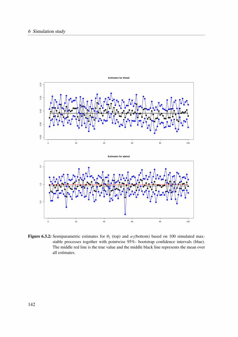
6 Simulation study
0 20 40 60 80 100
−0.
050.
000.
050.
100.
15
Estimates for theta2
0 20 40 60 80 100
0.5
1.0
1.5
Estimates for alpha2
Figure 6.3.2: Semiparametric estimates for θ2 (top) and α2(bottom) based on 100 simulated max-stable processes together with pointwise 95%- bootstrap confidence intervals (blue).The middle red line is the true value and the middle black line represents the mean overall estimates.
142

6.3 Results for the semiparametric estimation procedure using the extremogram
−2 −1 0 1 2
0.04
0.05
0.06
0.07
0.08
Estimates for theta1
Theoretical Quantiles
Sam
ple
Qua
ntile
s
−2 −1 0 1 2
0.6
0.8
1.0
1.2
1.4
1.6
Estimates for alpha1
Theoretical Quantiles
Sam
ple
Qua
ntile
s
−2 −1 0 1 2
0.01
0.02
0.03
0.04
0.05
0.06
0.07
0.08
Estimates for theta2
Theoretical Quantiles
Sam
ple
Qua
ntile
s
−2 −1 0 1 2
0.7
0.8
0.9
1.0
1.1
Estimates for alpha2
Theoretical Quantiles
Sam
ple
Qua
ntile
s
Figure 6.3.3: QQ-plots of the semiparametric estimates against the normal distribution.
143

6 Simulation study
6.4 Comparison of pairwise likelihood and
semiparametric estimation
As a last step in the simulation study, we compare the estimates resulting from the two dif-ferent methods. Figures 6.4.1 and 6.4.2 contrast the pairwise likelihood estimates with thesemiparametric estimates. On the left hand side, the estimates (blue: pairwise likelihood,red: semiparametric) are plotted for each of the 100 simulations together with the true valueas solid line in the middle. On the right hand side, boxplots resulting from the simulationsare shown. We see that the semiparametric estimates differ more from the true value thanthe pairwise likelihood estimates, which can be explained from the bias in the spatial andtemporal empirical extremogram, which cannot be cancelled completely, since the thresholdused in the estimation cannot be set equal to infinity. The variability around the true valuediffers for the different parameters, and no particular pattern can be detected.
The semiparametric estimates rely on the choice of the threshold for the empirical ex-tremogram, where a tradeoff between a high threshold and enough observations has to bemade. We measured the time needed to estimate one set of parameters in the simplest case,i.e. for the pairwise likelihood estimation we use (r, p) = (0, 2) to estimate θ2 and α2 and(r, p) = (2, 0) for θ1 and α1. Table 6.4 compares the computation time in seconds measuredfor the calculation on a Laptop (Windows 7, 64 bit, Intel(R) Core(TM) i5 CPU, 2.53 GHz)using the statistic software R. We see that the semiparametric estimation is much faster thanthe pairwise likelihood estimation.
Pairwise likelihood Semiparametric(r, p) = (2, 0) and (r, p) = (0, 2)
Computation time 34.3 2.2
Table 6.4: Computation time in seconds for the estimation of the parameters θ1, α1, θ2 and α2.
To conclude this section, we make some summarizing comments.Pairwise likelihood estimation:
• The pairwise likelihood estimation serves as reliable method to estimate parameters inmax-stable process.
144

6.4 Comparison of pairwise likelihood and semiparametric estimation
• Accurate starting values are needed for the optimization routine, which maximizes thelog-likelihood function.
• The computation time is rather high compared to the semiparametric estimation.
Semiparametric estimation:
• The semiparametric estimates show a larger bias than the pairwise likelihood estimatesand are sensible to the choice of the threshold used for the extremogram.
• The computation time is around 15 times lower than for the pairwise likelihood esti-mation.
• The implementation of bootstrap confidence intervals is feasible and gives regions ofconfidence in a reasonable amount of time.
• The semiparametric estimates could serve as starting values for the optimization routineused to maximize the pairwise log-likelihood function.
145

6 Simulation study
0 20 40 60 80 100
0.03
0.04
0.05
0.06
0.07
0.08
0.09
PLSemiparametric
0.03
0.04
0.05
0.06
0.07
0.08
0.09
PL Semiparametric
0 20 40 60 80 100
0.5
1.0
1.5
PLSemiparametric
0.5
1.0
1.5
PL Semiparametric
Figure 6.4.1: Comparison of estimates for θ1 (top) and α1 (bottom), where in the left plots each dot(blue: pairwise likelihood, red: semiparametric) corresponds to one of the 100 simula-tions. The plots on the right hand side show the corresponding boxplots resulting fromthe simulations.
146

6.4 Comparison of pairwise likelihood and semiparametric estimation
0 20 40 60 80 100
0.00
0.02
0.04
0.06
0.08
0.10
PLSemiparametric
0.00
0.02
0.04
0.06
0.08
0.10
PL Semiparametric
0 20 40 60 80 100
0.4
0.6
0.8
1.0
1.2
1.4
PLSemiparametric
0.4
0.6
0.8
1.0
1.2
1.4
PL Semiparametric
Figure 6.4.2: Comparison of estimates for θ2 (top) and α2 (bottom), where in the left plots each dot(blue: pairwise likelihood, red: semiparametric) corresponds to one of the 100 simula-tions. The plots on the right hand side show the corresponding boxplots resulting fromthe simulations.
147


CHAPTER 7
ANALYSIS OF RADAR RAINFALLMEASUREMENTS IN FLORIDA
The final step in this thesis is the application of our introduced model and methods to realdata. In particular, we quantify the extremal behaviour of radar rainfall data in a region inFlorida by using spatial block maxima and two different time domains, namely daily maximaand hourly measurements.
7.1 Description of data set
The rainfall data we use in this study was collected by the Southwest Florida Water Man-agement District (SWFWMD) 1. The data base consists of radar values measured on a gridwith size 2 km covering a region in Florida. A map of the area in Florida is shown in Figure7.1.1. Radar rainfall observations are given in inches as 15-minutes increments from 1999 to2004. To present our methods we choose 60 × 60 locations in the middle of the consideredregion (see red square in Figure 7.1.1) resulting in a 120 km × 120 km squared region. Wecalculate the accumulated hourly rainfall measurements and take the maximum over 25 loca-tions lying on a square with side length of 10 km. In that way we obtain 12 × 12 locationswith spatial maxima of rainfall observations. The corresponding time series for each spatial
1http://www.swfwmd.state.fl.us/
149

7 Analysis of radar rainfall measurements in Florida
maxima is used for further analysis. In the following two sections we consider two differentsettings for the time domain taken into account. In both settings we only consider the wetseason in Florida (June to September). For simplified notation we denote the set of locationsby S = (i1, i2), i1, i2 ∈ 1, . . . , 12.
© OpenStreetMap www.openstreetmap.org/copyright
Figure 7.1.1: Map of Florida with region of observations.
7.2 Daily maxima of rainfall measurements
We start by analysing daily maxima of rainfall measurements. Since we take maxima in spaceand time, the assumption of a max-stable space-time process becomes reasonable. As a firststep we remove a seasonal component by using a simple moving average with a period of122 days, which is the number of days in the wet season considered in one particular year.By inspecting autocorrelation plots for the daily maxima with fixed location, we concludethat there is no temporal dependence in the time series. As described in Section 2.1.1 we fitthe generalized extreme value distribution to the block maxima for each fixed location. Sincethe estimates for the shape parameter are close to zero with confidence intervals containing
150

7.2 Daily maxima of rainfall measurements
zero, we directly fit a Gumbel distribution (GEV with ξ = 0) to the data. The observationsare then transformed to standard Frechet margins by using the probability integral transform.Afterwards, we estimate the parameters of the max-stable Brown-Resnick process to obtainthe extremal dependence structure. We explain the procedure in more detail.
1. Marginal modelling: For each fixed location s ∈ S we follow the steps below.
a) The time series η(s, t), t ∈ t1, . . . , t732 is deseasonalized by calculating
η(s, tk+122( j−1)) = η(s, tk+122( j−1)) −16
6∑j=1
η(s, tk+122( j−1)) (7.1)
for k = 1, . . . , 122.
b) The deseasonalized observations are fitted to a Gumbel distribution with distribu-tion function
GEVµ(s),σ(s),0(x) = exp− exp
−
x − µ(s)σ(s)
. (7.2)
c) The data are transformed according to
˜η(s, t) = −1
log(GEVµ(s),σ(s),0(η(s, t))), t ∈ t1, . . . , t732,
where µ(s) and σ(s) are the parameter estimates resulting from fitting the Gum-bel distribution.
2. Estimating the extremal dependence structure: We assume that ˜η(s, t), s ∈ S , t ∈
t1, . . . , t732 are realizations from the Brown-Resnick process (cf. (4.2))
˜η(s, t) =∞∨
j=1
ξ j expW j(s, t) − δ(s, t),
where W j are independent replications of a Gaussian process with stationary incre-ments and correlation function δ(s1, t1) + δ(s2, t2) − δ(s1 − s2, t1 − t2). The δ functionis assumed to equal δ(s, t) = θ1‖s‖α1 + θ2|t|α2 and contains the extremal dependenceparameters θ1, α1, θ2 and α2, which are estimated using the following two procedures.
151

7 Analysis of radar rainfall measurements in Florida
a) We use the semiparametric estimation procedure introduced in Section 5.1 to es-timate the parameters and construct 500 bootstrap samples to obtain pointwiseconfidence intervals for the estimated parameters.
b) In addition, we estimate the parameters using the pairwise likelihood estimationprocedure developed in Section 4.2.
The results are summarized in Figures 7.2.2, 7.2.3, 7.2.4, 7.2.5, 7.2.6, Tables 7.1 and 7.2.Figure 7.2.2 shows time series for the daily maxima of four representative locations, indicatedin Figure 7.2.1. Three of the locations are safely inside the study region and one is on theboundary. The fit of the Gumbel distribution is supported by qq-plots in Figure 7.2.3, whichshow a straight line pattern. In Figure 7.2.4 plots of the original rainfall fields (left) andthe standard Frechet transformations are shown for two arbitrary fixed time points t166 (July14th 2000) and t434 (August 7th 2002). The parameter estimates are given in Tables 7.1 and7.2. The temporal estimates θ2 and α2 indicate that there is little or no temporal extremaldependence. In particular, recall from (5.2) that the extremogram for a spatial lag equal tozero is given by
χ(0, u) = 2(1 −Φ(√θ2|u|α2))
for temporal lags u > 0. If α2 is near zero then χ(0, u) is approximately constant indicatingthat the extremal dependence is the same for all temporal lags u > 0. If, in addition, θ2 islarge χ(0, u) is close to zero indicating asymptotic independence. So, the combination of α2
small and θ2 large implies asymptotic independence. Figure 7.2.5 shows the empirical spatial(left) and temporal (right) extremogram, which are used to estimate the parameters. Note,that the plots show the temporal mean of spatial extremograms (left) and the spatial meanof temporal extremograms (right) as described in (2a) and (2b) in Section 5.1. In addition,we include pointwise 95%-bootstrap confidence intervals (red lines) calculated based on 500bootstrap samples. Recall from (5.32) that the asymptotic variance for the temporal mean ofspatial extremograms includes the factor 1/T 2 which reduces the standard error. Since wehave 732 time points, the confidence intervals for the spatial extremogram are narrow. Tocheck whether the extremal dependence is significant, we permutate the space-time data andcalculate empirical extremograms as before. For the temporal extremogram, we fix the onelocation s and sample from the corresponding time series without replacement. Using thesame indices as for s we sample the other time series accordingly to keep the spatial depen-dence structure, i.e. for all locations s ∈ S the permutated space-time observations are givenby (s, κ(t1)), . . . , (s, κ(t732), where κ describes one permutation. We calculate the empiri-
152

7.2 Daily maxima of rainfall measurements
cal temporal extremogram as before and repeat the procedure 1000 times. 97.5% and 2.5%empirical quantiles are calculated from the resulting temporal extremogram sample whichgives a 95% confidence region for temporal extremal independence. To see how the extremaldependence lasts in space, we do the same for the spatial extremogram. In particular, foreach fixed time point we permutate the spatial locations and estimate the empirical spatialextremogram for the permutated space-time data. Figure 7.2.6 shows the estimates togetherwith the independence confidence intervals. Since the estimate for the temporal extremogramlies within the obtained confidence region, we conclude that there is no temporal extremal de-pendence for the daily maxima of rainfall. We also conclude that there is no spatial extremaldependence for spatial lags larger than 4.
Estimate θ1 0.3496 α1 0.9040Bootstrap-CI [0.3254,0.3640] [0.8183,0.9897]
Estimate θ2 2.2803 α2 0.0951Bootstrap-CI [1.8810,2.6796] [0.000,0.2161]
Table 7.1: Semiparametric estimates for the spatial parameters θ1 and α1 and the temporal parametersθ2 and α2 for the Brown-Resnick process in (4.2) together with 95% bootstrap confidenceintervals.
PL estimates θ1 α1 θ2 α2
0.3485 0.8858 2.419 0.1973
Table 7.2: Pairwise likelihood estimates for the parameters in the Brown-Resnick process in (4.2).
Figure 7.2.1: Reference locations for time series plots in Figure 7.2.2.
153

7 Analysis of radar rainfall measurements in Florida0.
01.
02.
0
Location (1,1)
time
1999 2000 2001 2002 2003 2004 2005
0.0
1.0
2.0
Location (5,6)
time
1999 2000 2001 2002 2003 2004 2005
0.0
1.0
2.0
Location (8,10)
time
1999 2000 2001 2002 2003 2004 2005
0.0
1.0
2.0
Location (10,7)
time
1999 2000 2001 2002 2003 2004 2005
Figure 7.2.2: Plot of daily maximal rainfall (calculated based on the 15 minutes measurements) ininches for four different grid locations with simplified coordinates (1,1), (5,6), (8,10)and (10,7).
154

7.2 Daily maxima of rainfall measurements
−0.5 0.0 0.5 1.0 1.5
−0.
50.
00.
51.
01.
5
Location (1,1)
Model
Em
piric
al
−0.5 0.0 0.5 1.0 1.5
−0.
50.
00.
51.
01.
5
Location (5,6)
Model
Em
piric
al
−0.5 0.0 0.5 1.0 1.5
−0.
50.
00.
51.
01.
52.
0
Location (8,10)
Model
Em
piric
al
−0.5 0.0 0.5 1.0 1.5
−0.
50.
00.
51.
01.
5
Location (10,7)
Model
Em
piric
al
Figure 7.2.3: QQ-Plot of deseasonalized rain series against the fitted Gumbel distribution (GEV withµ(s), σ(s) and 0) based on the time series corresponding to the grid locations shown in7.2.1.
155

7 Analysis of radar rainfall measurements in Florida
0.0
0.2
0.4
0.6
0.8
1.0
1.2
0.1
0.1
0.2
0.2
0.2
0.2
0.2
0.3
0.3
0.3
0.3
0.3
0.3
0.3
0.3
0.4
0.4
0.4
0.4
0.5
0.5 0.5 0.6
0.6
0.6 0.6
0.7
0.8
0.9
1
0
2
4
6
8
10
1
1
1
1
1
1
1
1
1
2
2
2
2
2 3
3
3
3
4
4
4
4
4
5
5
5
6
6
7
7
7
8 9
0.0
0.5
1.0
1.5 0.2
0.4
0.4
0.4
0.4
0.4
0.4
0.6
0.6
0.6
0.6
0.6
0.8
0.8
0.8
1
1
1
1
1.2
1.2
1.4
0
20
40
60
80
10
10
10
20
20
20
20
30
30
30
40
40 50
50
Figure 7.2.4: Plots of spatial maxima of rainfall measurements (left) and to standard Frechet marginstransformed rain fields for fixed time points t166 (July 14th 2000) and t434 (August 7th2002).
156

7.2 Daily maxima of rainfall measurements
0.05
0.10
0.15
0.20
Temporal extremogram
Temporal lag
1 2 3 4 5 6 7 8 9 10
0.1
0.2
0.3
0.4
0.5
0.6
Spatial extremogram
Spatial lag
1 2 2 5 8 3 10 13 4 17
Figure 7.2.5: Temporal (left) and spatial (right) empirical extremogram as introduced (2a) and (2b) ofSection 5.1 together with 95% bootstrap confidence intervals. Note, that the scale of thetemporal extremogram is much smaller than the scale of the spatial extremogram.
0.06
0.08
0.10
0.12
0.14
0.16
Temporal extremogram
Temporal lag
1 2 3 4 5 6 7 8 9 10
0.2
0.3
0.4
0.5
0.6
Spatial extremogram
Spatial lag
1 2 2 5 8 3 10 13 4 17
Figure 7.2.6: Permutation test for extremal independence in time (left) and space (right). The up-per and lower black lines show 97.5% and 2.5% empirical quantiles of empirical ex-tremograms for 1000 temporal (left) and spatial (right) permuations of the space-timeobservations.
157

7 Analysis of radar rainfall measurements in Florida
Conditional probabilities and return level maps
We now return to the fundamental questions raised in the Introduction. Based on the fittedmodel we are interested in the prediction of conditional probabilities as well as conditionalreturn level maps. Given a particular reference space-time location (s∗, t∗) we consider theconditional probability
P(η(s, t) > zc | η(s∗, t∗) > z∗),
where P(η(s∗, t∗) > z∗) = p∗, and η is the deseaonalized process in (7.1). In other words,we predict the conditional probability that the rainfall process exceeds the level zc at anylocation (s, t), given that the process exceeds z∗ at the reference location (s∗, t∗). Assumingthat η(s, t), s ∈ S , t ∈ t1, . . . , t732 are realizations from a Brown-Resnick process (see(4.2)) with generalized extreme value marginal distributions GEVµ(s),σ(s),0 fitted in (7.2), weobtain
P(η(s, t) > zc | η(s∗, t∗) > z∗) =
=1p∗
(1 −GEVµ(s),σ(s),0(zc) − (1 − p∗) + P(η(s, t) ≤ zc, η(s∗, t∗) ≤ z∗)
)= 1 −
1p∗
GEVµ(s),σ(s),0(zc)
+1p∗
P
−1log(GEVµ(s),σ(s),0(η(s, t)))
≤−1
log(GEVµ(s),σ(s),0(zc)),
−1log(GEVµ(s∗),σ(s∗),0(η(s∗, t∗)))
≤−1
log(1 − p∗)
= 1 −
1p∗
GEVµ(s),σ(s),0(zc) +1p∗
F
−1log(GEVµ(s),σ(s),0(zc))
,−1
log(1 − p∗)
,
where F is the bivariate extreme value distribution of the Brown-Resnick process (see (3.6)).As a first step, we plot the predicted conditional probabilities with z∗ = zc = 2.5 for alllocations s and reference locations in Figure 7.2.1, where the marginal estimates µ(s) andσ(s) are used in GEVµ(s),σ(s),0(zc) and the extremal dependence estimates for the Brown-Resnick process θ1, α1, θ2 and α2 are plugged into F. Since there is no temporal extremaldependence (see Figure 7.2.6), we only consider fixed time points. Figure 7.3.1 shows thepredicted conditional probability fields.
158

7.3 Hourly rainfall measurements June 2002-September 2002
The conditional return level is defined as the value zc for which
P(η(s, t) > zc | η(s∗, t∗) > z∗) = pc,
where z∗ is chosen as the (1 − p∗)-quantile, P(η(s∗, t∗) > z∗) = p∗. In particular, theconditional return level with return period 1/pc is the value for which the probability that theprocess exceeds that level given that the process at a reference location exceeds z∗ equals p∗.To estimate zc we plug in the parameter estimates µ(s) and σ(s) for the marginal distributionand θ1, α1, θ2 and α2 for the extremal dependence. First note, that if z∗ equals the minimumof the data, i.e. p∗ = 1, we obtain a field of unconditional quantiles which is the same as ifthe return levels at each location are estimated using the marginal fitted distributions. Figure7.3.2 shows the predicted conditional return levels for p∗ = 0.01 and pc = 0.01 with thesame reference locations. The conditional probability, as well as the conditional return levelfields confirm the findings from estimating the extremogram, where we concluded that spatialextremal dependence is present for lags smaller than
√17.
7.3 Hourly rainfall measurements June 2002-September
2002
Since there is no temporal extremal dependence for the daily maxima we turn to hourlyrainfall measurements. In particular, we analyse the hourly rainfall observations in the rainfallseason 2002 from June to September, leading to 2928 time points and 144 locations, denotedby
Z(s, t), s ∈ S , t ∈ t1, . . . , t2928,
where S = (i1, i2), i1, i2 ∈ 1, . . . , 12. As for the daily maxima, we first remove dailyseasonality by using a simple moving average with block length of one day (24 time points).By inspecting autocorrelation plots we assume that the marginal time series are stationarywith short-range dependence. Leadbetter [55, 56] shows that stationary time series satisfyingadditional mixing conditions have the same extreme value properties than the correspondingiid sequence. Therefore, we fit the generalized Pareto distribution to threshold exceedancesas described in Section 2.1.1 and use the fitted distributions to transform the data to standardFrechet marginal distributions. Afterwards, we estimate the extremal dependence parametersas before. The procedure is explained in full detail below.
159

7 Analysis of radar rainfall measurements in Florida
2 4 6 8 10 12
24
68
1012
0.0
0.2
0.4
0.6
0.8
1.0
0.1
0.1
0.1
0.1
0.1
0.2
0.3
0.4
0.5
0.6
0.7
2 4 6 8 10 12
24
68
1012
0.0
0.2
0.4
0.6
0.8
1.0
0.2
0.2
0.2
0.2
0.2
0.2
0.2
0.3
0.4
0.5
0.6
0.7
0.8
2 4 6 8 10 12
24
68
1012
0.0
0.2
0.4
0.6
0.8
1.0
0.1
0.1
0.2 0.2
0.3
0.3
0.3
0.4
0.4
0.5
0.6
0.7
0.9
2 4 6 8 10 12
24
68
1012
0.0
0.2
0.4
0.6
0.8
1.0
0.1
0.1
0.2
0.3
0.3
0.3
0.3
0.4
0.4
0.4
0.5
0.5
0.6
0.7
0.9
Figure 7.3.1: Predicted conditional probability fields P(Z(s, t) > zc | Z(s∗, t) > z∗) for fixed timepoint t with reference locations (s∗, t∗) = ((1, 1), 1) (upper left) (s∗, t∗) = ((5, 6), 1)(upper right), (s∗, t∗) = ((8, 10), 1) (lower left) and (s∗, t∗) = ((10, 7), 1) (lower right)together with contour lines. The values zc and z∗ equal 2.5.
160

7.3 Hourly rainfall measurements June 2002-September 2002
2 4 6 8 10 12
24
68
1012
1.8
2.0
2.2
2.4
2.6
2.8 1.9 1.9
1.9
1.9
1.9
2
2
2
2 2.1
2.1
2.1
2.1
2.1
2.1
2.2
2.2
2.2
2.2
2.3
2.3 2.3
2.4
2.5
2.6
2 4 6 8 10 12
24
68
1012
1.8
2.0
2.2
2.4
2.6
2.8
1.9
1.9
1.9
1.9
2
2
2
2
2
2.1
2.1
2.1
2.1
2.1
2.1
2.1
2.2
2.2
2.2
2.2
2.2
2.2
2.3
2.3
2.3
2.4 2.4
2.5
2.6
2 4 6 8 10 12
24
68
1012
1.8
2.0
2.2
2.4
2.6
2.8
1.9
1.9
1.9
2
2
2
2
2.1
2.1
2.1
2.1
2.1
2.1
2.1
2.2
2.2
2.2
2.2
2.2
2.2
2.3
2.3
2.3
2.4
2.4
2.4
2.4
2.5
2 4 6 8 10 12
24
68
1012
1.8
2.0
2.2
2.4
2.6
2.8
1.9
1.9
1.9
2
2
2
2
2.1
2.1
2.1
2.1
2.1
2.2
2.2
2.2
2.2
2.2
2.2
2.2
2.3
2.3
2.3
2.3
2.3
2.4
2.4
2.4
2.4
2.4 2.4
2.5
Figure 7.3.2: Conditional 100-day return levels resulting from solving P(Z(s, t) > zc | Z(s∗, t∗) >z∗) − pc = 0 for zc with four different reference locations (s∗, t∗) = ((1, 1), 1) (upperleft) (s∗, t∗) = ((5, 6), 1) (upper right), (s∗, t∗) = ((8, 10), 1) (lower left) and (s∗, t∗) =((10, 7), 1) (lower right), which are shown as white square.
161

7 Analysis of radar rainfall measurements in Florida
1. Marginal modelling: For each fixed location s ∈ S = (i1, i2), i1, i2 ∈ 1, . . . , 12 wefollow the steps below.
a) The time series Z(s, t), t ∈ t1, . . . , t2928 is deseasonalized by calculating
Z(s, tk+24( j−1)) = Z(s, tk+24( j−1)) −1
122
122∑j=1
Z(s, tk+24( j−1))
for k = 1, . . . , 24.
b) Threshold exceedances with a threshold thres = 0.2 are fitted to a GeneralizedPareto distribution with distribution function
GPDσ(s),ξ(s)(x) = 1 −(1 +
ξ(s)xσ(s)
)−1/ξ(s). (7.3)
c) The data are transformed according to
˜Z(s, t) = −1
log(Fs(Z(s, t))), t ∈ t1, . . . , t2928,
where
Fs(x) =
1 − Nthres,s
2928
(1 + ξ(s) x−thres
σ(s)
)−1/ξ(s), x > thres,
12928
2928∑k=1
1Z(s,tk)≤x, x ≤ thres,(7.4)
and Nthres,s denotes the number of threshold exceedances for fixed location s.
2. Estimating the extremal dependence structure: We estimate the parameters θ1, α1, θ2
and α2 of the Brown-Resnick process (cf. (4.2)) by using the semiparametric estimationprocedure in Chapter 5 and the pairwise likelihood estimation in Chapter 4.
The results are shown in Figures 7.3.4, 7.3.5, 7.3.6, 7.3.7, 7.3.8 and Tables 7.3 and 7.4.Figure 7.3.4 visualizes the hourly accumulated rainfall series for the locations shown in 7.3.3.QQ-plots in Figure 7.3.5 of the exceedances against the fitted GPD support the marginalgoodness of fit. Figure 7.3.6 shows rainfall fields for four consecutive hours on the lefthand side together with the marginally transformed fields on the right hand side. Usingthe transformed space-time observations we estimate the parameters of the Brown-Resnickprocess, which are shown in Tables 7.3 and 7.4. We notice that the spatial parameter estimates
162
7.3 Hourly rainfall measurements June 2002-September 2002
θ1 and α1 are close to the estimates for the daily maxima (compare to Tables 7.1 and 7.2).This is not unexpected since the spatial extremal dependence structure remains the same if thetime domain is scaled. To see this, consider the extremogram of the Brown-Resnick processwith scaled time lag u/m where m ∈ N (To get from the daily maxima to the hourly valuesuse m = 24),
χ(h, u/m) = 2(1 −Φ(
√θ1‖h‖α1 + θ2|u/m|α2)
).
For a temporal lag equal to zero, this is the same as for the original time domain.
Figure 7.3.7 shows the spatial and temporal mean of temporal (left) and spatial (right)extremograms as described in (2a) and (2b) of Section 5.1 together with 95% bootstrap con-fidence intervals. When we compare Figure 7.3.7 to Figure 7.2.5 we see that the spatialextremogram on the right hand side is similar to the one for the daily maxima. The tempo-ral extremogram now shows more extremal dependence compared to the daily maxima. Werepeat the permutation test for independence. The results are shown in Figure 7.3.8 and indi-cate that there is no temporal extremal dependence for time lags larger than 6 and no spatialextremal dependence for spatial lags larger than 4.
As for the daily maxima, we return to the fundamental questions raised in the introduction.In particular, we predict the conditional probabilities
P(Z(s, t) > zc | Z(s∗, t∗) > z∗),
where P(Z(s∗, t∗) > z∗) = p∗, by
1 −1p∗
Fs(zc) +1p∗
F(
−1log(Fs(zc))
,−1
log(1 − p∗)
),
where Fs is defined in (7.4) and F is the fitted bivariate distribution function of the Brown-Resnick process (see (3.6)). In addition, we estimate the conditional return levels zc for which
P(Z(s, t) > zc | Z(s∗, t∗) > z∗) = pc.
Figure 7.3.9 shows the predicted conditional probability fields for zc = z∗ = 1 for tworeference locations s∗ = (5, 6) (left) and s∗ = (10, 7) (right) and t∗ = t1. The plots visualizethe prediction for all locations and for t ∈ t1, t2, t3, t4 (from the top to the bottom). Since weassume stationarity only the time lag t − t∗, and not the starting reference time point t∗, is ofinterest. Figures 7.3.10 and 7.3.11 show the predicted conditional return level maps for time
163

7 Analysis of radar rainfall measurements in Florida
lags u = 0, 1, . . . , 7 based on the reference locations s∗ = (1, 1) (left), s∗ = (5, 6) (middle)and s∗ = (10, 7) (right). Both, the conditional probability fields as well as the conditionalreturn level fields show how the dependence in space and time develops. The plots confirmthe findings from the extremogram estimates, where we concluded spatial independence forlags larger than 4 and temporal independence for time lags larger than 6.
As a final step in this chapter we simulate from the fitted space-time process for extremes toobtain realizations for the space-time rainfall process. We start by simulating from the max-stable space-time process as described in Chapter 6 with the parameter estimates obtained forthe rainfall measurements. Afterwards, we transform the marginal distributions according tothe fitted GPD distributions for each location. Figure 7.3.12 shows the resulting realizationsfor four consecutive time points. By comparing the figures with the plots in the introduction(see Figure 1.1.1), we see that the simulations are similar to the rainfall measurements.
Estimate θ1 0.2987 α1 0.9664Bootstrap-CI [0.2469,0.3505] [0.8407,1.0921]
Estimate θ2 0.4763 α2 1.0686Bootstrap-CI [0.2889,0.6637] [0.8514,1.2859]
Table 7.3: Semiparametric estimates for the spatial parameters θ1 and α1 and the temporal parametersθ2 and α2 for the Brown-Resnick process in (4.2) together with 95% bootstrap confidenceintervals.
PL estimates θ1 α1 θ2 α2
0.3353 0.9302 0.4845 1.0648
Table 7.4: Pairwise likelihood estimates for the parameters in the Brown-Resnick process in (4.2).
164

7.3 Hourly rainfall measurements June 2002-September 2002
Figure 7.3.3: Reference locations for time series plots in Figure 7.2.2.
0.0
0.5
1.0
1.5
Location a=(1,1)
time
June July August September
0.0
0.5
1.0
1.5
Location b=(5,6)
time
June July August September
0.0
0.5
1.0
1.5
Location c=(8,10)
time
June July August September
0.0
0.5
1.0
1.5
Location d=(10,7)
time
June July August September
Figure 7.3.4: Accumulated hourly rainfall measurements calculated from the 15-minutes measure-ments (June 2002 - September 2002) in inches for the grid locations in 7.3.3.
165

7 Analysis of radar rainfall measurements in Florida
0.0 0.2 0.4 0.6 0.8 1.0 1.2 1.4
0.0
0.5
1.0
1.5
Location s=(1,1)
Model
Em
piric
al
0.0 0.2 0.4 0.6 0.8 1.0 1.2
0.0
0.2
0.4
0.6
0.8
1.0
Location s=(5,6)
Model
Em
piric
al
0.0 0.5 1.0 1.5
0.0
0.5
1.0
1.5
2.0
Location s=(8,10)
Model
Em
piric
al
0.0 0.5 1.0 1.5
0.0
0.5
1.0
1.5
Location s=(10,7)
Model
Em
piric
al
Figure 7.3.5: QQplot of threshold exceedances against fitted GPD distribution for the grid locationsin 7.3.3 with a threshold equal to 0.2.
166

7.3 Hourly rainfall measurements June 2002-September 2002
0.0
0.2
0.4
0.6
0.8
1.0
1.2
1.4
0.2
0.2
0.4
0.6 0
200
400
600
800
1000
1200
100
100
100
100
100
200
200
0.0
0.2
0.4
0.6
0.8
1.0
1.2
1.4
0.2
0.2
0.4
0.6
0.8 1
1
0
200
400
600
800
1000
1200
100
100
100
100
200
200
300
300
0.0
0.2
0.4
0.6
0.8
1.0
1.2
1.4
0.2
0.2
0.2
0.2
0.4
0.4
0.6
0.6
0.6
0.6
0.8
0.8
1
1
1
1.2
0
200
400
600
800
1000
1200
100
100
100
100
100
100
100
200
200
200
300
400
500
600 700
Figure 7.3.6: Plots of original and transformed (to standard Frechet) rain fields for three subsequenttime points t1016, t1017 and t1018 (July 13th, 2002, 10pm - 12pm).
167

7 Analysis of radar rainfall measurements in Florida
0.1
0.2
0.3
0.4
0.5
0.6
Temporal extremogram
Temporal lag
1 2 3 4 5 6 7 8 9 10
0.1
0.2
0.3
0.4
0.5
0.6
Spatial extremogram
Spatial lag
1 2 2 5 8 3 10 13 4 17
Figure 7.3.7: Temporal (left) and spatial (right) empirical extremogram based on spatial and tempo-ral means for the space-time observations as described in (2a) and (2b) in Section 5.1together with 95% bootstrap confidence intervals.
0.1
0.2
0.3
0.4
0.5
0.6
Temporal extremogram
Temporal lag
1 2 3 4 5 6 7 8 9 10
0.2
0.3
0.4
0.5
0.6
Spatial extremogram
Spatial lag
1 2 2 5 8 3 10 13 4 17
Figure 7.3.8: Permutation test for extremal independence based on 1000 space-time permutations ofthe observations, which destroy the extremal dependence in time (left) and space (right).The black lines show the 97.5% and 2.5% quantiles of the extremogram estimates forthe 1000 permutations.
168

7.3 Hourly rainfall measurements June 2002-September 2002
2 4 6 8 10 12
24
68
1012
time lag 0
0.0
0.1
0.2
0.3
0.4
0.5
0.6
0.7
0.15
0.15
0.15
0.2
0.2
0.2
5
0.3
0.3
0.3
5
0.4
0.45
0.5
0.55
0.6
0.6
5
0.7
2 4 6 8 10 12
24
68
1012
time lag 0
0.0
0.1
0.2
0.3
0.4
0.5
0.6
0.1
0.1
0.1
5
0.15
0.15
0.2
0.25
0.3
0.3
5
0.35
0.4
0.45
0.5
0.55
0.6
2 4 6 8 10 12
24
68
1012
time lag 1
0.0
0.1
0.2
0.3
0.4
0.5
0.6
0.7
0.1
0.1
0.15
0.2
0.2
0
.25
0.3
0.3
5
0.4
0.4
5
2 4 6 8 10 12
24
68
1012
time lag 1
0.0
0.1
0.2
0.3
0.4
0.5
0.6 0.05
0.1
0.1
0.1
0.15
0.15
0.2
0.2
5 0
.25
0.3
0.35
0.4
2 4 6 8 10 12
24
68
1012
time lag 2
0.0
0.1
0.2
0.3
0.4
0.5
0.6
0.7
0.1
0.1
0.1
0.1
0.1
0.1
5
0.1
5
0.2
0.2
5
0.3
2 4 6 8 10 12
24
68
1012
time lag 2
0.0
0.1
0.2
0.3
0.4
0.5
0.6
0.05
0.0
5
0.1
0.15
0.2
0.25
0.3
2 4 6 8 10 12
24
68
1012
time lag 3
0.0
0.1
0.2
0.3
0.4
0.5
0.6
0.7
0.05 0.1
0.1
0.15
0.2
2 4 6 8 10 12
24
68
1012
time lag 3
0.0
0.1
0.2
0.3
0.4
0.5
0.6
0.0
5
0.05 0.05
0.1
0.15
0.2
Figure 7.3.9: Predicted conditional probability fields P(Z(s, t) > zc | Z(s∗, t∗) > z∗) for zc = z∗ = 1,s∗ = (5, 6) (left) and s∗ = (10, 7) (right). From the top to the bottom the fields showthe development in time for lags u = 0, 1, 2, 3.
169

7 Analysis of radar rainfall measurements in Florida
2 4 6 8 10 12
24
68
1012
time lag 0
0.5
1.0
1.5
2.0
2.5
1.4
1.4
1.4
1.4
1.4
1.4
1.6
1.6 1.6
1.6
1.6
1.6
1.8
1.8
1.8
1.8
2
2
2
2
2
2.2
2 4 6 8 10 12
24
68
1012
time lag 0
0.5
1.0
1.5
2.0
2.5
1.4
1.4
1.4
1.4
1.4
1.4 1
.6
1.6
1.6
1.6
1.6
1.6
1.6
1.8
1.8
1.8
1
.8
1.8
1.8
1.8
2
2
2
2
2
2
2
2
2.2
2 4 6 8 10 12
24
68
1012
time lag 0
0.5
1.0
1.5
2.0
2.5
1.4
1.4
1.4
1.4
1.4
1.6
1.6
1.6
1.6
1.6
1.6
1.8
1.8
1.8 1.8
1.8
1.8
1.8
1.8
2
2
2
2
2
2.2
2.2
2.4
2.4
2.6
2 4 6 8 10 12
24
68
1012
time lag 1
0.5
1.0
1.5
2.0
2.5
1.2
1.2
1.4
1.4
1.4 1.4
1.4
1.4
1.4
1.6
1.6
1.6
1.6
1.6
1.6
1.8
1.8
1.8
1.8
2
2
2
2 4 6 8 10 12
24
68
1012
time lag 1
0.5
1.0
1.5
2.0
2.5
1.2
1.2
1.4
1.4
1.4 1.4
1.4
1.4
1.4 1
.6
1.6
1.6
1.6
1.6
1.8
1.8
2
2
2
2 2
2.2
2 4 6 8 10 12
24
68
1012
time lag 1
0.5
1.0
1.5
2.0
2.5
1.2
1.4
1.4
1.4
1.4
1.4
1.6
1.6
1.6
1.6
1.6
1.6
1.6
1.8
1.8 1.8
1.8
1.8
1.8
2 2
2
2
2.2
2.4
2.4
2 4 6 8 10 12
24
68
1012
time lag 2
0.5
1.0
1.5
2.0
2.5
1.2
1.2
1.2
1.2
1.2 1.2
1.4
1.4
1.4
1.4
1.6
1.6
1.6 1.8
1.8
1.8
2
2
2
2 4 6 8 10 12
24
68
1012
time lag 2
0.5
1.0
1.5
2.0
2.5
1.2
1.2
1.2
1.2
1.2
1.4
1.4
1.4 1
.4
1.4 1.6
1.6
1.6
1.8
1.8
1.8
2
2
2
2.2
2 4 6 8 10 12
24
68
1012time lag 2
0.5
1.0
1.5
2.0
2.5
1.2
1.2
1.2
1.2
1.4
1.4
1.4
1.4
1.6
1.6
1.6
1.6
1.6
1.6
1.6
1.8
1.8
1.8
2
2
2
2.2
2.4
2 4 6 8 10 12
24
68
1012
time lag 3
0.5
1.0
1.5
2.0
2.5 1.2
1.2
1.2
1.4
1
.4
1.4
1.6
1.6
1.6
1.6
1.8
1.8
2
2 4 6 8 10 12
24
68
1012
time lag 3
0.5
1.0
1.5
2.0
2.5
1.2
1.2
1.2
1.4
1.4
1.4 1.4
1.6
1.6
1.6
1.6 1.8
1.8 1.8
1.8
1.8
2
2 4 6 8 10 12
24
68
1012
time lag 3
0.5
1.0
1.5
2.0
2.5
1.2
1.2
1.2
1.2
1.2
1.2
1.4
1.4
1.4 1.4
1.6
1.6
1.6
1.8
1.8
2
2.2
2.2
2.2
Figure 7.3.10: Conditional 100-hour return level maps for time lags u = 0, . . . , 3 and reference loca-tions s∗ = (1, 1) (left), s∗ = (5, 6) (middle) and s∗ = (10, 7) (right).
170
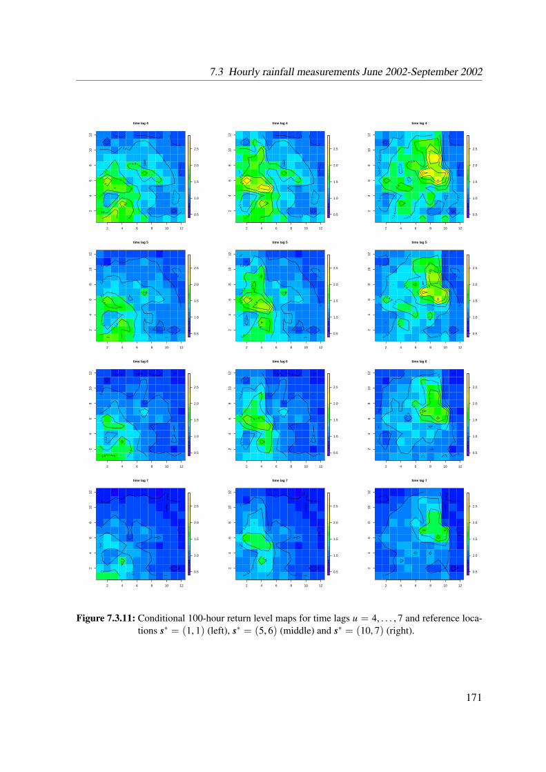
7.3 Hourly rainfall measurements June 2002-September 2002
2 4 6 8 10 12
24
68
1012
time lag 4
0.5
1.0
1.5
2.0
2.5
1
1 1
1
1
1
1.2
1.2
1.2
1.4
1.4
1.4
1.6
1.6
1.8
1.8
2 4 6 8 10 122
46
810
12
time lag 4
0.5
1.0
1.5
2.0
2.5
1
1
1
1
1.2
1.2
1.2
1.2
1.4
1.4
1.6
1.6
1.8
1.8
2
2 4 6 8 10 12
24
68
1012
time lag 4
0.5
1.0
1.5
2.0
2.5
1
1
1
1
1.2
1
.2
1.2
1.2
1.4
1.4
1.4
1.4
1.6
1.6
1.8
2
2
2 4 6 8 10 12
24
68
1012
time lag 5
0.5
1.0
1.5
2.0
2.5 1
1 1
1
1.2
1.4
1.4 1.4
1.6
1.6
2 4 6 8 10 12
24
68
1012
time lag 5
0.5
1.0
1.5
2.0
2.5
1
1 1
1
1.2
1.2
1.4
1.4
1.4
1.6
1.6
1.6
1.8
1.8
2 4 6 8 10 12
24
68
1012
time lag 5
0.5
1.0
1.5
2.0
2.5 1
1
1
1
1.2
1.2
1.2
1.4
1.4
1.4
1.4
1.4
1.6
1.8
1.8
2 4 6 8 10 12
24
68
1012
time lag 6
0.5
1.0
1.5
2.0
2.5
0.8 0.8 0.8
1
1
1.2
1
.2
1.2
1.4
1.4
1.6
2 4 6 8 10 12
24
68
1012
time lag 6
0.5
1.0
1.5
2.0
2.5
0.8 0.8
1
1
1
1.2
1.2
1.2 1.4
1.6
2 4 6 8 10 12
24
68
1012
time lag 6
0.5
1.0
1.5
2.0
2.5
1
1
1
1
1.2
1.2
1.4
1.6
2 4 6 8 10 12
24
68
1012
time lag 7
0.5
1.0
1.5
2.0
2.5
0.8 0.8
0.8
0.8
0.8
1
1
1.2
1.4
1.4
2 4 6 8 10 12
24
68
1012
time lag 7
0.5
1.0
1.5
2.0
2.5
0.8
0.8
0.8
0.8
0.8
1
1
1.2
1.2
1.4
1.4
2 4 6 8 10 12
24
68
1012
time lag 7
0.5
1.0
1.5
2.0
2.5
0.8 0.8
0.8
0.8
0.8
1
1
1
1.2
1.4
Figure 7.3.11: Conditional 100-hour return level maps for time lags u = 4, . . . , 7 and reference loca-tions s∗ = (1, 1) (left), s∗ = (5, 6) (middle) and s∗ = (10, 7) (right).
171
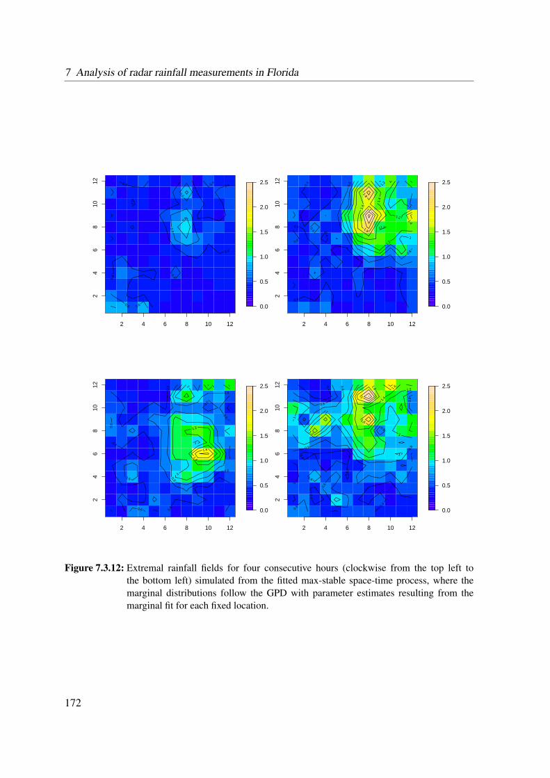
7 Analysis of radar rainfall measurements in Florida
2 4 6 8 10 12
24
68
1012
0.0
0.5
1.0
1.5
2.0
2.5
0.4
0.4
0.4
0.4
0.4
0.4 0.4
0.6 0.6
0.6
0.6
0.8
2 4 6 8 10 12
24
68
1012
0.0
0.5
1.0
1.5
2.0
2.5
0.4
0.4
0.4
0.4
0.4
0.6
0.6
0.8
1
1
1.2
1.2
1.2
1.2
1.4
1.4
1.6
1.8
1.8 2
2 4 6 8 10 12
24
68
1012
0.0
0.5
1.0
1.5
2.0
2.5
0.4
0.4
0
.4
0.6
0.6
0.6
0.6
0.6
0.6
0.8
0.8
1
1
1
1
1.2
1.4
1.6
2 4 6 8 10 12
24
68
1012
0.0
0.5
1.0
1.5
2.0
2.5
0.4
0.4
0.4
0.4
0.4
0.4
0.6
0.6
0.6
0.6
0.6
0.8
0.8
0.8
0.8
1
1
1
1
1.2
1.2
1.4
1.6
1.6
1.6
2
Figure 7.3.12: Extremal rainfall fields for four consecutive hours (clockwise from the top left tothe bottom left) simulated from the fitted max-stable space-time process, where themarginal distributions follow the GPD with parameter estimates resulting from themarginal fit for each fixed location.
172

BIBLIOGRAPHY
[1] R.J. Adler. The Geometry of Random Fields. John Wiley, New York, 1981.
[2] D. W. K. Andrews. Estimation when a parameter is on a boundary. Econometrica, 67(6):1341–1383, 1999.
[3] D. W. K. Andrews. Inconsistency of the boostrap when a parameter is on the boundaryof the parameter space. Econometrica, 68(2):399–405, 2000.
[4] Y. Bai, X.-K. Song, and T.E. Raghunathan. Joint composite estimating functions inspatiotemporal models. Journal of the Royal Statistical Society B, 75(5):799–824, 2012.
[5] A. Baxevani, S. Caires, and I. Rychlik. Spatio-temporal stationary modelling of signif-icant wave height. Environmetics, 20(1):14–31, 2009.
[6] A. Baxevani, K. Podgorski, and I. Rychlik. Dynamically evolving Gaussian spatialrandom fields. Extremes, 14(2):223–251, 2011.
[7] J. Beirlant, Y. Goegebeur, J. Segers, and J. Teugels. Statistics of Extremes, Theory
and Applications. Wiley Series in Probability and Statistics, John Wiley & Sons Ltd,Chichester, 2004.
[8] J.E. Besag. Spatial interaction and the statistical analysis of lattice systems. Journal of
the Royal Statistical Society B, 34(2):192–236, 1974.
173

Bibliography
[9] P.J. Bickel, F. Gotze, and W.R. van Zwet. Resampling fewer than n observations: gains,losses, and remedies for losses. Statistica Sinica, 7:1–31, 1997.
[10] P. Billingsley. Convergence of probability measures. Wiley Series in Probability andStatistics: Probability and Statistics, New York, 1999.
[11] E. Bolthausen. On the central limit theorem for stationary mixing random fields. The
Annals of Probability, 10(4):1047–1050, 1982.
[12] G.E.P. Box and M.E. Muller. A note on the generation of random normal deviates.Annals of Mathematical Statistics, 29(2):610–611, 1958.
[13] P.J. Brockwell and R.A. Davis. Time Series: Theory and Methods. Springer-Verlag,New York, 2nd edition, 1991.
[14] B.M. Brown and S.I. Resnick. Extreme values of independent stochastic processes.Journal of Applied Probability, 14(4):732–739, 1977.
[15] Y. Cho, R.A. Davis, and S. Ghosh. Asymptotic properties of the spatial empirical ex-tremogram. 2012. In preparation.
[16] S.G. Coles. Regional modelling of extreme storms via max-stable processes. Journal
of the Royal Statistical Society B, 55(4):797–816, 1993.
[17] S.G. Coles. An Introduction to Statistical Modeling of Extreme Values. Springer Seriesin Statistics, Springer, New York, 2001.
[18] S.G. Coles and J.A Tawn. Modelling extremes of the areal rainfall process. Journal of
the Royal Statistical Society B, 58(2):329–347, 1996.
[19] S.G. Coles and D. Walshaw. Directional modelling of extreme wind speeds. Journal of
the Royal Statistical Society C, 43:139–157, 1994.
[20] D.R. Cox and N. Reid. Miscellanea: A note on pseudolikelihood constructed frommarginal densities. Biometrika, 91(3):729–737, 2004.
[21] N. Cressie and H.C. Huang. Classes of nonseperable spatio-temporal stationary covari-ance functions. Journal of the American Statistical Association, 94(448):1330–1340,1999.
174

Bibliography
[22] R.A. Davis and T. Mikosch. Extreme value theory for space-time processes with heavy-tailed distributions. Stochastic Processes and their Applications, 118(4):560–584, 2008.
[23] R.A. Davis and T. Mikosch. The extremogram: A correlogram for extreme events.Bernoulli, 15(4):977–1009, 2009.
[24] R.A. Davis and C.Y. Yau. Comments on pairwise likelihood in time series models.Statistica Sinica, 21(1):255–277, 2011.
[25] R.A. Davis, T. Mikosch, and I. Cribben. Towards estimating extremal series dependencevia the bootstrapped extremogram. Journal of Econometrics, 17(1):142–152, 2012.
[26] R.A. Davis, C. Kluppelberg, and C. Steinkohl. Max-stable processes for extremes ofprocesses observed in space and time. Journal of the Korean Statistical Society, 2013.http://dx.doi.org/10.1016/j.jkss.2013.01.002.
[27] R.A. Davis, C. Kluppelberg, and C. Steinkohl. Statistical inference for max-stable pro-cesses in space and time. Journal of the Royal Statistical Society B, 2013. to appear.
[28] R.A. Davis, C. Kluppelberg, and C. Steinkohl. Semiparametric estimation for max-stable space-time processes. 2013. In preparation.
[29] L. de Haan. A spectral representation for max-stable processes. The Annals of Proba-
bility, 12(4):1194–1204, 1984.
[30] L. de Haan and A. Ferreira. Extreme Value Theory: An Introduction. Springer Series inOperations Research and Financial Engineering, New York, 2006.
[31] L. de Haan and J. Pickands. Stationary min-stable stochastic processes. Probability
Theory and Related Fields, 72(4):477–492, 1986.
[32] L. de Haan and S. Resnick. Limit theory for multivariate sample extremes. Zeitschrift
fur Wahrscheinlichkeitstheorie, 40:317–337, 1977.
[33] P. Deheuvels. Point processes and multivariate extreme values. Journal of Multivariate
Analysis, 13(2):257–272, 1983.
[34] C. Dombry and F. Eyi-Minko. Strong mixing properties of max-infinitely divisiblerandom fields. Stochastic Processes and their Applications, 122(11):3790–3811, 2012.
175

Bibliography
[35] P. Doukhan. Mixing: Properties and Examples. Springer, New York, 1994.
[36] P. Embrechts, C. Kluppelberg, and T. Mikosch. Modelling Extremal Events. Springer,Berlin, 1997.
[37] V. Fasen, C. Kluppelberg, and M. Schlather. High-level dependence in time series mod-els. Extremes, 13(1):1–33, 2010.
[38] W. Feller. An introduction to probability theory and its applications, volume 2 of Wiley
series in probability and mathematical statistics: Probability and mathematical statis-
tics. Wiley, 1971.
[39] R.A. Fisher and L.H.C. Tippett. On the estimation of the frequency distributions of thelargest or smallest member of a sample. Proceedings of the Cambridge Philosophical
Society, 24:180–190, 1928.
[40] J. Geffroy. Contributions a la theorie des valeurs extreme. Publ. Inst. Stat. Univ. Paris,7:36–123, 1958.
[41] J. Geffroy. Contributions a la theorie des valeurs extreme. Publ. Inst. Stat. Univ. Paris,8:3–52, 1959.
[42] B.V. Gnedenko. Sur la distribution limite du terme maximum d’une serie aleatoire.Annals of Mathematics, 44(3):423–453, 1943.
[43] T. Gneiting. Nonseparable, stationary covariance functions for space-time data. Journal
of the American Statistical Association, 95(458):590–600, 2002.
[44] V.P. Godambe. An optimum property of regular maximum likelihood estimation. Annals
of Mathematical Statistics, 31:1208–1211, 1960.
[45] E.J. Gumbel. Distributions de valeurs extremes en plusieurs dimensions. Publications
of the Institute of Statistics of the University of Paris, 9:171–173, 1960.
[46] R. Huser and A. Davison. Space-time modelling for extremes. Preprint, 2012.arXiv:1201.3245v1 [stat.ME].
[47] J. Husler and R.-D. Reiss. Maxima of normal random vectors: between independenceand complete dependence. Statistics and Probability Letters, 7(4):283–286, 1989.
176

Bibliography
[48] N. Jenish and I.R. Prucha. Central limit theorems and uniform laws of large numbersfor arrays of random fields. Journal of Econometrics, 150(1):86–98, 2009.
[49] Z. Kabluchko. Extremes of space-time Gaussian processes. Stochastic Processes and
their Applications, 119:3962–3980, 2009.
[50] Z. Kabluchko, M. Schlather, and L. de Haan. Stationary max-stable fields associated tonegative definite functions. The Annals of Probability, 37(5):2042–2065, 2009.
[51] A. F. Karr. Inference for stationary random fields given Poisson samples. Advances in
Applied Probability, 18(2):406–422, 1986.
[52] B. Kozintsev. Computations with Gaussian Random Fields. PhD thesis, Institute forSystems Research, University of Maryland, 1999.
[53] U. Krengel. Ergodic Theorems. de Gruyter, Berlin, 1985.
[54] S. N. Lahiri. Theoretical comparisons of block bootstrap methods. The Annals of
Statistics, 27(1):386–404, 1999.
[55] M.R. Leadbetter. On extreme values in stationary sequences. Zeitschrift fur Wahrschein-
lichkeitstheorie und verwandte Gebiete, 28:289–303, 1974.
[56] M.R. Leadbetter. Extremes and local dependence in stationary sequences. Zeitschrift
fur Wahrscheinlichkeitstheorie und verwandte Gebiete, 65:291–306, 1983.
[57] M.R. Leadbetter, G. Lindgren, and H. Rootzen. Extremes and Related Properties of
Random Sequences and Processes. Springer Verlag, New York, 1983.
[58] M. Ledoux and M. Talagrand. Probability in Banach Spaces: Isoperimetry and Pro-
cesses. Springer Verlag, Berlin, 1991.
[59] B. Li, M.G. Genton, and M. Sherman. On the asymptotic joint distribution of samplespace-time covariance estimators. Bernoulli, 14(1):208–248, 2008.
[60] B.G. Lindsay. Composite likelihood methods. Contemporary Mathematics, 80:221–239, 1988.
[61] C. Ma. Spatio-temporal covariance functions generated by mixtures. Mathematical
geology, 34(8):965–975, 2002.
177
Bibliography
[62] C. Ma. Spatio-temporal stationary covariance functions. Journal of Multivariate Anal-
ysis, 86(1):97–107, 2003.
[63] C. Ma. Linear combinations of space-time covariance functions and variograms. IEEE
Transactions on signal processing, 53(3):857–864, 2005.
[64] J. Mateu, E. Porcu, and P. Gregori. Recent advances to model anisotropic space-timedata. Statistical Methods and Applications, 17(2):209–223, 2007.
[65] D. J. Nott and T. Ryden. Pairwise likelihood methods for inference in image models.Biometrika, 86(3):661–676, 1999.
[66] S.A. Padoan, M. Ribatet, and S.A. Sisson. Likelihood-based inference for max-stableprocesses. Journal of the American Statistical Association, 105(489):263–277, 2009.
[67] J. Pickands. Multivariate extreme value distributions. Proceedings of the 43rd Session
of the Int. Stat. Institute, pages 859–878, 1981.
[68] D.N. Politis and J.P. Romano. A circular block resampling procedure for stationarydata. In R. Lepage and L. Billard, editors, Exploring the Limits of Bootstrap. Wiley,New York, 1992.
[69] D.N. Politis and J.P. Romano. The stationary bootstrap. Journal of the American Sta-
tistical Society, 89(428):1303–1313, 1998.
[70] E. Porcu, P. Gregori, and J. Mateu. La descente et la montee etendues: the spatiallyd-anisotropic and spatio-temporal case. Stochastic Environmental Research and Risk
Assessment, 21(6):683–693, 2007.
[71] S.I. Resnick. Point processes, regular variation and weak convergence. Advances in
Applied Probability, 18(1):66–138, 1986.
[72] S.I. Resnick. Adventures in Stochastic Processes. Birkhauser, Boston, 1992.
[73] S.I. Resnick. Heavy-Tail Phenomena, Probabilistic and Statistical Modeling. SpringerSeries in Operations Research and Financial Engineering, 2007.
[74] H. Sang and A. Gelfand. Hierarchical modeling for extreme values observed over spaceand time. Environmental and Ecological Statistics, 16(3):407–426, 2009.
178

Bibliography
[75] M. Schlather. Models for stationary max-stable random fields. Extremes, 5(1):33–44,2002.
[76] M. Schlather. Some covariance models based on normal scale mixtures. Bernoulli, 16(3):780–797, 2010.
[77] M. Schlather and J.A. Tawn. A dependence measure for multivariate and spatial extremevalues: Properties and inference. Biometrika, 90(1):139–156, 2003.
[78] M. Sibuya. Bivariate extreme statistics. Annals of the Institute of Statistical Mathemat-
ics, 11:195–210, 1960.
[79] R. L. Smith. Max-stable processes and spatial extremes. Unpublished manuscript,University of North California, 1990.
[80] C. Steinkohl, R.A. Davis, and C. Kluppelberg. Extreme value analysis of multivariatehigh frequency wind speed data. Journal of Statistical Theory and Practice, 2013. toappear.
[81] S.A. Stoev. On the ergodicity and mixing of max-stable processes. Stochastic Processes
and their Applications, 18(9):1679–1705, 2008.
[82] S.A. Stoev and M.S. Taqqu. Extremal stochastic integrals: a parallel between max-stable processes and α-stable processes. Extremes, 8:237–266, 2005.
[83] D. Straumann. Estimation in Conditionally Heteroscedastic Time Series Models. Lec-ture Notes in Statistics, Springer, Berlin, 2004.
[84] J.A. Tawn. Bivariate extreme value theory: models and estimation. Biometrika, 75(3):397–415, 1988a.
[85] J.A. Tawn. Modelling multivariate extreme value distributions. Biometrika, 77(2):245–253, 1990.
[86] C. Varin. On composite marginal likelihoods. Advances in Statistical Analysis, 92(1):1–28, 2008.
[87] C. Varin and P. Vidoni. Pairwise likelihood inference and model selection. Biometrika,92(3):519–528, 2005.
179
Bibliography
[88] H. Wackernagel. Multivariate Geostatistics. Springer, Heidelberg, 2003.
[89] A. Wald. Note on the consistency of the maximum likelihood estimate. The Annals of
Mathematical Statistics, 20(4):595–601, 1946.
[90] Y. Wang and S.A. Stoev. On the structure and representations of max-stable processes.Advances in Applied Probability, 42(3):855–877, 2010.
[91] Y. Wang, P. Roy, and S.A. Stoev. Ergodic properties of sum-and max-stable stationaryrandom fields via null and positive group actions. Preprint, 2011. arXiv:0911.0610v2[math.PR].
[92] A.T.A. Wood and G. Chan. Simulation of stationary gaussian processes on [0, 1]d.Journal of Computational and Graphical Statistics, 3(4):409–432, 1994.
[93] Y. Xue and Y. Xiao. Fractal and smoothness properties of space-time gaussian models.Frontiers of Mathematics in China, 6(6):1217–1248, 2011.
180
Copyright © 2022 FDOKUMEN