The statistical analysis of multienvironment data: modelling genotype-by-environment interaction and...

I.6 The statistical analysis of multienvironment data: modelling

genotype-by-environment interaction and its genetic basis

Marcos Malosetti (WUR, The Netherlands), Jean-Marcel Ribaut (GCP, Mexico)and Fred A van Eeuwijk (WUR, The Netherlands)

R O

kono

123

Introduction: phenotype, genotype and environmentThe success of a plant breeding programme is refl ected in its ability to provide farmers with better phenotypes under a range of environmental conditions. A good, or better phenotype can be defi ned in terms of higher production at harvest, or higher quality. The aim of a plant breeder is to develop genotypes with guaranteed good phenotypes. To achieve this aim, it is necessary to have an understanding of the causes behind a good phenotype.

In general, we tend to think of a phenotype from a static rather than a dynamic perspective. Thus, the phenotype is regarded as the state of a trait at a given moment in time. There are good reasons for this since, in general, we are primarily interested in phenotypes such as grain weight at maturity and not grain weight before maturity. However, it is important to consider that the fi nal state of a trait is the cumulative result of a number of causal interactions between the genetic make-up of the plant (the genotype) and the conditions in which that plant developed (the environment). This is shown in Figure 1, with the phenotype building up in time from the close interaction between genotype and environment.

Plants differ in the effi ciency and adequacy with which they capture and convert the environmental inputs and stimuli into the tissues that constitute a product. A plant’s capture and conversion abilities are determined by the particular ensemble of genes present in the plant. Environments differ in the amount and quality of inputs and stimuli that they convey to plants including, eg, the amount of water, nutrients or incoming radiation. A primary objective in plant breeding is to match genotypes and environments in such a way that improved phenotypes are created. For example, a breeder might be interested in selecting genotypes that do well under water stress conditions.

While there can be genotypes that do well across a wide range of conditions (widely adapted genotypes), there are also genotypes that do relatively better than

others exclusively under a restricted set of conditions (specifi cally adapted genotypes). Specifi c adaptation of genotypes is closely related to the phenomenon of genotype-by-environment interaction (GEI). GEI exists whenever the relative phenotypic performance of genotypes depends on the environment, or in other words, when the difference in performance between genotypes varies in dependence on the environment.

To illustrate the phenomenon of GEI, we can consider two different genotypes that differ in the genetic machinery involved in tolerance to water-limited conditions, while being equal for all other characteristics. If these two genotypes are exposed to a poorly watered environment, their performance will differ depending on the genetic properties related to tolerance of water-limited conditions. However, this genotypic difference will disappear in an environment that provides the right amount of water. So, the difference in performance between the two genotypes thus depends on the environment, through the amount of water that it provides.

I.6 The statistical analysis of multienvironment data: modelling genotype-by-environment

interaction and its genetic basisMarcos Malosetti (WUR, The Netherlands), Jean-Marcel Ribaut (GCP, Mexico)

and Fred A van Eeuwijk (WUR, The Netherlands)

Figure 1. The phenotype develops over time as the outcome of cumulative causal interactions between genotype and environment. The arrow originating from the genotype represents genetic information, say gene-expression, while the arrow representing the environmental fl ux refers to resources and hazards (eg, water availability, physical and chemical soil characteristics, incoming radiation, frost, heat, etc).

Genotype Environment

124

Some scenarios that can occur when comparing the performances of pairs of genotypes across environments are presented in Figure 2. The function describing the phenotypic performance of a genotype in relation to an environmental characterisation is called the ‘norm of reaction’ (Griffi ths et al. 1996). The upper left plot in Figure 2 shows the case where there is no GEI, the genotype and the environment behave additively (this will be developed later) and the reaction norms are parallel. The remaining plots show different situations in which GEI occurs: divergence, convergence, and the most critical one, crossover interaction. Crossover interactions are the most important for breeders as they imply that the choice of the best genotype is determined by the environment at which the genotype is targeted.

Above, GEI was discussed in terms of the relative difference between genotypic means. From a different perspective, GEI can be regarded in terms of heterogeneity of genetic variance and covariance, or correlation. As a consequence of GEI, the magnitude of the genetic variance as observed within individual environments can change from one environment to the next. It is frequently observed that in comparatively poorer environments the genetic variance is lower than in better environments. Figure 3 illustrates the phenomenon of heterogeneity of genetic variance across environments, showing box plots for a series of maize trials, as described in greater detail below. In Figure 3, compare the smaller range of variation in the poor environments LN96a and

LN96b with the larger range in the good environments HN96b and NS92a.

GEI has also consequences for the correlations between genotypic performances in different environments.

Figure 2. Genotype-by-environment interaction in terms of changing mean performances across environments.

Figure 3. Boxplot for yields for a maize F2 population across eight environments. The box encloses observations between the 25th and 75th quantiles, with the lines extending to the minimum and maximum of observed values, except when extreme values occur, in which case outliers are indicated by crosses. Environment names are coded as: LN = low nitrogen, HN = high Nitrogen, SS = severe water stress, IS = intermediate water stress, and NS = no water stress. The number indicates the year of the trial, and the letters a and b the cropping season: a = winter, b = summer.

Env 1 Env 2

Env 1 Env 2

Env 1 Env 2

Env 1 Env 2

Phen

otyp

ic pe

rform

ance

Phen

otyp

ic pe

rform

ance

Phen

otyp

ic pe

rform

ance

Phen

otyp

ic pe

rform

ance

No interaction = additivity of G and E Divergence

Convergence Crossover interaction

876543210

876543210

876543210

876543210

10

8

6

4

2

0

Yield

(ton

/ha)

LN96

a

LN96

b

SS92

a

SS94

a

IS92a

IS94a

HN

96b

NS9

2a

Marcos Malosetti et al

125

When GEI is signifi cant, the observed performance of a set of genotypes in one environment may not be very informative for the performance of the same genotypes in another environment. Environments with similar characteristics will induce similar responses which, in turn, results in higher genetic correlations. Figure 4 shows that the correlation between the similar environments IS92a and IS94a is larger than the correlation between the dissimilar environments IS92a and HN96b.

In conclusion, given the complexity of the mechanisms and processes underlying the phenotypic response across diverse and changing environmental conditions – frequently in an unpredictable way – it is necessary to develop analytical tools to help breeders understand GEI. The use of adequate strategies to analyse GEI is a fi rst and important step towards more informed breeding decisions. Good analytical methods are a prerequisite for predicting the performance of genotypes as accurately as possible. This chapter explores several strategies to model GEI, starting with simple methods that have been

Figure 4. Scatter plot matrix for two stress environments (IS92a, and IS94a) and two non-stress environments (HN96b and NS92a). Environment names are coded as in Figure 3.

6543210

6543210

10987654

IS94a

HS9

6aN

S92a

HN96bIS94aIS92a2 3 4 5 6 7 0 1 2 3 4 5 6 0 1 2 3 4 5 6

historically popular within the plant breeding community. It then moves to more elaborated models in which additional information is used in the form of explicit environmental characterisation to model GEI. A fi nal section is devoted to the integration of molecular marker information into GEI models, leading to the detection of quantitative trait loci (QTLs) and more specifi cally, to the modelling of QTL by environment interaction (QEI). The statistical methodology is illustrated using a maize data set obtained from a series of drought and nitrogen stress trials from the maize breeding program at CIMMYT (Centro Internacional de Mejoramiento de Maíz y Trigo; the International Maize and Wheat Improvement Center; Ribaut et al, 1996; 1997). To encourage readers to carry out these statistical analyses themselves, GenStat programs for the Discovery® version of this statistical package (Payne et al, 2003) are presented in Appendix I.

Generating data to study genotype-by-environment interactionAn obvious fi rst step to investigate GEI is to obtain phenotypic observations on a set of genotypes exposed to a range of environmental conditions. The set of genotypes can include advanced lines of a breeding programme, and old and/or new cultivars. It can also consist of the segregating offspring generation of a specifi c cross such as F2, a backcross, or a recombinant inbred line (RIL) population.

Genotypes can be tested under different management regimes that represent increasing levels of a particular stress, or a combination of stresses. This type of experiment is called a ‘managed stress trial’ and is appropriate when the researcher wishes to focus on a particular type of stress. When performing managed

Statistical models for GEI

126

stress trials, it is important to control the system in such a way that all other factors infl uencing the phenotype are as homogenous as possible. Stress type and level can be diffi cult to implement, because the relationship between the phenotype and the stresses is generally complex, with genes and environmental stresses interacting throughout the various developmental phases. A common way for plant breeders to screen for genotypic reactions to environmental factors is by ‘multienvironment trials’ (METs). In an MET, a number of genotypes are evaluated at a number of geographical locations for a number of years in the hope that the pattern of stresses that the genotypes experience is representative of the collection of future growing environments of the genotypes that are eventually selected.

A convenient way to summarise the data, either coming from managed stress trials or from METs, is to construct a two–way table of means, with genotypes in the rows and environments in the columns. Each cell of the table contains the mean of a particular genotype in a specifi c environment. To identify genotypes and environments unequivocally, we use indices, say the letter i for genotypes (i = 1…I), and letter j for environments (j = 1…J). The representation in Figure 5 shows a genotype-by-environment table of expected means, μij, with the dimensions of the maize example that is used in this chapter, with I = 211 genotypes, and J = 8 environments.

The models that will be presented in the following sections will assume as a starting point a genotype-by-environment table of means as described above.

CIMMYT maize drought stress trials: example dataThe models to be presented in this chapter are illustrated using data produced by the maize drought stress breeding programme of CIMMYT. A brief description of the data is given here, with a more detailed description available in the original publications (Ribaut et al, 1996; 1997). A maize F2 population was generated by crossing a drought tolerant parent (P1) with a drought susceptible one (P2).

Seeds harvested from each of 211 F2 plants were reserved as F3 families. The F3 families were evaluated in managed stress trials in 1992, 1994 and 1996. In the winter of 1992, a managed water stress trial was conducted in Mexico, including no stress (NS), intermediate stress (IS), and severe stress (SS). In the winter of 1994, a similar trial was conducted, but only included the IS and SS treatments. In the summer of 1996, the families were tested in a nitrogen stress trial with two levels: low (LN) and high nitrogen (HN). An extra LN trial was conducted in the winter of the same year. In total, the families were evaluated in eight different environments, each environment consisting of year–stress treatment combinations. DNA was extracted from each of the 211 F2 plants to produce a total of 132 restriction fragment length polymorphism (RFLP) markers covering the 10 maize chromosomes.

Models for genotype-by-environment interaction: modelling the meanThe additive model as a benchmarkThe phenomenon of GEI is of primary interest in plant breeding, and has resulted in a large body of literature on models and strategies for analysis of GEI (see, for example, the reviews in Cooper and Hammer, 1996; Kang and Gauch, 1996; van Eeuwijk, et al, 1996; van Eeuwijk, 2006). A dominant feature of strategies used to describe and understand GEI is a heavy reliance on parameters that are statistical rather than biological. This is not by coincidence, since historically, a large part of quantitative genetics has relied on simple statistical models. A notorious example is the well known model: P = G + E, where P stands for phenotype, G for genotype and E for environment (Falconer and Mackay, 1996; Lynch and Walsh, 1998). A statistical formulation of this model for a two–way table of means can be written as:

μij = μ + Gi + Ej + ij [1]

Environments j = 1 … J

LN96a LN96b SS92a SS94a IS92a IS94a HN96b NS92a

G001 μ1,1 μ1,2 μ1,3 μ1,4 μ1,5 μ1,6 μ1,7 μ1,8 G002 μ2,1 μ2,2 … … … … … μ2,8 … … … G211 μ211,1 μ211,2 μ211,3 μ211,4 μ211,5 μ211,6 μ211,7 μ211,8

Figure 5. Schematic layout of a two–way table of means, with the mean corresponding to genotype i in environment j in the cell identifi ed by row i and column j.

Gen

otyp

es i

= 1

… 2

11


127

From here onwards, in the model formulations, random terms are underlined to emphasise the fact that their effects are assumed to follow a normal distribution. Model 1 describes the random mean of genotype i in environment j, μij, as the result of the common fi xed intercept term μ, a fi xed genotypic main effect corresponding to genotype i, Gi, plus a fi xed environmental main effect corresponding to environment j, Ej, and fi nally the random term, ij, representing the error term, typically normally distributed, with a mean of zero and constant variance, 2; ij ~ N(0,2).

One remarkable feature of model 1 is that it predicts that for any genotype the change in phenotypic mean between two environments j and j* will always be equal to Ej-Ej*. As a consequence, the norms of reaction of different genotypes will be parallel (as in the upper left plot of Figure 2). Another important aspect is that, although the parameters in the model suggest that something intrinsically genetic and something intrinsically environmental is determining the trait, the genotypic and environmental effects purely follow from a convenient way of partitioning phenotypic variation from a statistical point of view. In a balanced data set, the genotypic main effects can be estimated simply from the average performance of the genotypes across environments. Rather than being something inherently genotypic, this is entirely dependent on the set of environments that were used in the experiment. If a few environments are dropped, the genotypic effects of a set of genotypes can be completely different. The same argument applies to the main environmental effects, which completely depend on the set of genotypes used in the experiment.

The results of the fi t of an additive model to the maize data set are presented in Table 1. The results show that, according to the F test, there is a signifi cant environmental and genotypic main effect (the F statistic for environments equals 1466.5, and for genotypes 5.3, both of which are highly signifi cant: P < 0.001). As just mentioned, environments are characterised by the average performance of the genotypes in the

particular environment, and the results indicate that the environments differ signifi cantly in their quality. In general, differences between environmental main effects are signifi cant, and from the breeder’s point of view this is not a major concern. Breeders want to concentrate on differences between genotypes. A signifi cant genotypic main effect indicates that genotypes differ in their average performance across environments, something certainly more interesting to breeders. Finally, it should be mentioned that the residual in Table 1 corresponds to the discrepancy between the predicted genotype-by-environment means from an additive model and the observed means.

There are two reasons for the disagreement between the predicted values from an additive model and the observed means for environment-specifi c genotypic performances: (i) a specifi c effect related to the particular combination of genotype and environment; and (ii) experimental error. The obvious way to disentangle one cause from the other is to include an explicit term in the model for the effect of specifi c genotype–environment combinations. This term that is called ‘GEI’ and that is read as ‘genotype-by-environment interaction effect’ is double-indexed:

μij = μ + Gi + Ej + (GEIij + ij ) [2]

We can not separate GEI from error when using a two-way table of means, because for that we would need replicated observations on genotype-by-environment combinations. Therefore, both the terms GEI and the error are written within brackets. When plot data are available, we can fi t a full model, including replicates within trials (environments), to estimate all the parameters in model 2, that is, main effects and GEI interaction effects. Use of model 2 implies estimation of as many parameters as there are genotype-by-environment combinations, something that is not desirable in the interest of parsimony. Another limitation of the model is that it is not possible to estimate the genotypic performance in environments that are not included in the trial. Accordingly, fi tting model 2 could tell us something about the amount of variation due to genotypic main effects in relation to GEI, by comparing sums of squares or mean squares, but it does not bring much progress towards understanding GEI.

The regression on the mean modelA more attractive alternative is to extend the additive model (model 1) by incorporating terms that explain as much as possible of the GEI. A popular strategy in plant breeding is that proposed by Finlay and Wilkinson

Table 1. ANOVA table for the additive model (model 1), as applied to CIMMYT maize stress trials. DF = degrees of freedom, SS = sum of squares, MS = mean squares, F = F statistic, P = cumulative upper probability associated to F.

Term DF SS MS F P

E 7 5679 811.2 1466.5 < 0.001G 210 614 2.9 5.3 < 0.001 1470 813 0.6Total 1687 7106 4.2


128

(1963), which describes GEI as a regression line on the environmental quality. In the absence of explicit environmental information, the biological quality of an environment can be refl ected in the average performance of all genotypes in that environment. Good environments will have a high average genotypic performance, and bad environments will have a low average genotypic performance. The GEI part is then described by genotype-specifi c regression slopes on the environmental quality, and the model can be written in the following equivalent ways:

μij = μ + Gi + Ej + biEj + ij * [3a]

μij = Gi + biEj + ij * [3b]

Models 3a and 3b are equivalent. Model 3b follows from model 3a by taking μ + Gi = Gi and Ej + biEj = (1+bi)Ej = biEj. Model 3b is easier to interpret because it consists of a set of regression lines; each genotype has a linear reaction norm with intercept Gi and slope bi. The explanatory environmental variable in these reaction norms is simply the environmental main effect Ej. Model 3a shows more clearly how GEI is tried to be captured by a regression on the environmental main effect, with the hope that the term biEj will contain as much as possible of the original GEI signal.

In the regression on the mean model, GEI is explained in terms of differential sensitivities to the improvement of the environment, with some genotypes (the ones with larger values of bi) benefi ting more than others from an

increase in environmental quality. Note that in model 3a, bi = 0, so that the average slope value is zero, while in model 3b the average value of b is 1, meaning that b > 1 for genotypes with a higher than average sensitivity, and b < 1 for genotypes that are less sensitive than average.

Table 2 gives the fi t of model 3a to the maize example data. The fi rst two rows of the table, corresponding to the genotypic and environmental main effects, are identical to Table 1. The third row corresponds to the GEI effect in terms of the regression on environmental quality, where quality is represented by the environmental mean. This regression is highly signifi cant, according to the F tests (F = 2.4, P < 0.001). The residual sum of squares in Table 1 (SS = 813) has been divided into a part explained by genotypic sensitivities to environmental quality (SSb = 230), and a residual (SS* = 583).

By way of example, the fi tted reaction norms of fi ve genotypes (out of the full set of 211 genotypes) have been given in Figure 6, together with the parameters estimated according to the parameterisation in model

Table 2. ANOVA table for the regression on the mean model (model 3), as applied to CIMMYT maize stress trials

Term DF SS MS F P

E 7 5679 811.2 1752.3 < 0.001G 210 614 2.9 6.3 < 0.001B 210 230 1.1 2.4 < 0.001* 1260 583 0.5Total 1687 7106 4.2

Figure 6. Response curves of fi ve maize genotypes in relation to environmental quality. The vertical dashed line indicates the average environment. Next to genotype labels, the values for the two curve parameters are given, the intercept (G = the response in the average environment) and the slope (b = the genotypic sensitivity to changes in the environmental quality). Arrows point to the average yield of each environment as deviation from the overall mean.

G bG025 3.8 1.27

G045 4.0 0.99G016 2.3 1.18G012 2.5 1.01

G008 2.1 0.65

8

6

4

2

0

Yield

-3 -2 -1 0 1 2 3 4Environmental quality

LN96aSS92a

IS94a

HN96b IS92a NS92aLN96b SS94a


129

3b (G and b). Figure 6 shows that, in the average environment, genotypes G025 and G045 are better than G008, G012 and G016. The estimates of the parameters G can directly be observed in the plot as the value corresponding to environment quality equal to 0, i.e. the average environment (indicated by the dashed vertical line). Although G045 does slightly better than G025 in the average environment, G025 is superior to G045 in the high-quality environments. This is because G025 has a better ability to exploit improved environmental conditions, which is refl ected in the higher genotypic sensitivity of the former (bG025 = 1.27 > bG045 = 0.99). A similar observation can be made with respect to G008 versus G012 and G016. While G008 does relatively better in low quality environments, it is clearly surpassed by G012 and G016 in the best environments, since it is not capable of profi ting from the better environmental conditions (bG008 = 0.65, which is the lowest sensitivity among the fi ve genotypes).

In summary, the regression on the mean model describes GEI in terms of parameters that can be given some biological meaning. In addition, and in contrast with the full interaction model (model 2), model 3 can be used to predict the performance of genotypes in environments that were not present in the experiment. This is provided that the environment for which predictions are required can reasonably be placed within the range of environments used in the original experiment. Nevertheless, the regression on the mean model suffers from the fact that the environmental characterisation is based on a single dimension. Environmental quality can be hard to summarise within a single explanatory variable. Therefore, a substantial amount of GEI can remain unexplained. In the next section, the regression on the mean model will be extended by including multidimensional environmental characterisations in the statistical model for the genotype-by-environment data.

The additive main effects and multiplicative interaction modelThe limitation of a single dimension in environmental characterisation can be eased by employing a more fl exible model, in which more than one environmental quality variable is allowed. A popular model of this type is the so-called ‘AMMI model’ – the additive main effects and multiplicative interaction model (Gabriel, 1978; Gauch, 1988; Gollob, 1968; Mandel, 1969). To emphasise the parallelism with model 3a, the AMMI model can be written as:

K

μij = μ + Gi + Ej + bikzjk + ij * [4] k = 1

where the GEI is now explained by K multiplicative terms (k = 1…K), each multiplicative term formed by the product of a genotypic sensitivity bik (also known as ‘genotypic score’) with a hypothetical environmental characterisation, zjk (also known as ‘environmental score’). Although genotypic and environmental scores are deemed to represent genetic and environmental qualities, they come from a mathematical procedure that maximises the variation explained by the products of the genotypic and environmental scores. The fi rst product term is the one that explains most of the variation, followed by the second one, and so on. This is refl ected in Table 3, which shows the application of the AMMI model to the maize example data. In the AMMI model, GEI is explained by two axes (principal component 1, PCA1, and principal component 2, PCA2) that are highly signifi cant (F = 2.8 and 2.0 respectively, both with an associated P < 0.001). The fi rst axis (PCA1) explains the largest part (SSPCA1 = 242), the second one explains a little less (SSPCA2 = 173), with a total explained sum of squares for GEI of 242+173 = 415, a clear improvement over the explained sum of squares in the regression on the mean model (SSb = 230).A desirable property of the AMMI model is that the genotypic and environmental scores can be used to construct powerful graphical representations called biplots (Gabriel, 1978) that help to interpret the GEI. Figure 7 present a biplot for the maize data. A fi rst thing to recognise is that both genotypes and environments are present in the same plot; genotypes are represented by open circles and environments by fi lled rectangles. A second important characteristic is the presence of environmental axes that allow approximations of GEI for individual genotypes in a given environment. These environmental axes pass through the origin and point in the direction of the corresponding environment symbol. To avoid a too large number of lines in the plot, environmental axes have been drawn only from the origin to the environmental symbol, but as is shown for environment NS92a, axes can be prolonged. To help

Table 3. ANOVA table corresponding to application of AMMI2 model (model 4) to CIMMYT maize stress trials. PCA1 and PCA2 are the principal component axes 1 and 2, respectively.

Term DF SS MS F P

E 7 5679 811.2 1752.3 < 0.001G 210 614 2.9 6.3 < 0.001PCA1 216 242 1.1 2.8 < 0.001PCA2 214 173 0.8 2.0 < 0.001 * 1040 398 0.4Total 1687 7106 4.2


130

approximating the GEI, a scale can be indicated on the environmental axes, as shown for the axis of NS92a (Graffelman and van Eeuwijk, 2005).

Biplots facilitate the exploration of relationships between genotypes and/or environments. Genotypes that are similar to each other are closer in the plot than genotypes that are different. Similarly, environments that are more alike tend to group together as well. The angle between the environmental axes is related to the correlation between the environments. An acute angle indicates positive correlation (eg, between LN96a and LN96b), a right angle indicates no correlation (eg, between HN96b and NS92a), and an obtuse angle indicates negative correlation (eg NS92a and LN96a). The projection of a genotype onto an environmental axis refl ects the relative performance of the genotype in that particular environment (for GEI). For example the projection of genotype G91 on the NS92a axis gave a value of +2, which is above 0, indicating a positive interaction with that environment (ie, a good adaptation to NS92a). Conversely, genotype G41 (on the left hand side of the plot) gave a negative value (of almost -3) which points to a negative interaction with environment NS92a (ie, not well adapted to this environment). Following a similar procedure it is possible to conclude that while genotype G91 showed a positive adaptation to environment NS92a, it is not well adapted to environments LN96a and LN96b (note that the projection of this genotype on the LN96a and LN96b axes would fall in the range of negative values). Biplots are useful tools to investigate patterns in GEI, because they can help to quickly identify interesting genotypes that are adapted to particular environments, and to classify environments in groups.

Plant breeders are interested in the whole of the genetic variation and not exclusively in the GEI part. For that reason, it is useful to have a modifi cation of model 4 that writes the joint effects of the genotypic main effect and the GEI as a sum of multiplicative terms. Effectively, the two-way table of genotype-by-environment means is exposed to a standard principal components analysis, with genotypes as objects and environments as variables (Yan et al, 2000). For this new model, 5, closely the same estimation and interpretation procedures hold as for model 4. Because genotypic scores now describe genotypic main effects G and GEI together, this type of model is also known as the ‘Genotype main effects and GEI model’, or ‘GGE model’. The biplots are called ‘GGE biplots’ (Yan et al, 2000). The model reads:

K

μij = μ + Ej + bikzjk + ij * [5] k = 1

The results of model 5 fi tted to the maize data are presented in the form of a biplot in Figure 8. In GGE biplots, genotypes are distributed according to the overall performance in each environment. This is in contrast to Figure 7, which concentrated exclusively on GEI. From Figure 8 we see that high yielding genotypes are concentrated on the right hand side of the biplot as their projections on the environmental axes would fall mostly on the positive range of values (see for example genotype G91 that gave a performance of 2.5 above average in NS92a, while genotype G41 gave 3 below average). On the contrary, low yielding genotypes (as genotype G41) are concentrated on the left hand side of the biplot.

Factorial regression modelsThe models discussed so far assumed that we do not have explicit information about the environments. While such models can be useful to explain GEI, the biological interpretation of their results is not always obvious. What do hypothetical environmental variables, as in AMMI, mean in terms of quantifi able environmental characteristics such as temperature, water, nutrients etc? A straightforward approach is to correlate environmental scores with environmental covariables. However, if we do have explicit information about the environment, the information can be used directly in the model by including it in the form of explanatory variables. GEI is then described as differential genotypic sensitivity to explicit environmental factors such as temperature, precipitation, water availability etc. Such models are known as ‘factorial regression models’(Denis, 1988; van Eeuwijk et al, 1996). Two examples of factorial regression models are given here. Model 6a includes a single environmental covariable, while model 6b includes multiple environmental covariables:

μij = μ + Gi + Ej + bi ZjK + ij * [6a]

K

μij = μ + Gi + Ej + bikZjk + ij * [6b] k = 1

Models 6a and 6b look identical to models 3a and 4, but there is a substantial difference between them. In models 6a and 6b, Zj represents an explicit environmental covariable and not a hypothetical environmental covariable as in models 3a and 4 (it is capitalised as Z to highlight this difference). This distinction is critical since the interpretation of the GEI in models 6a and 6b is placed into a more biological context. Instead of describing GEI as differential reactions to hypothetical environmental covariables, factorial regression models help to identify genotypes that are differentially sensitive to changes in identifi ed environmental quality components, for example, in a particular nutrient, or in water availability.


131

Figure 7. Biplot from an AMMI model used to describe GEI in the maize example data. Open circles represent genotypes, fi lled rectangles environments. Vectors represent environment axes, which for simplifi cation have been drawn only between the origin and the corresponding environment symbol. The full axis is given for environment NS92a, for which also a scale is also included (in ton ha–1). By means of example, the projection of two genotypes (G041 and G091) on the NS92a axis is indicated with a dashed line.

2

1

0

-1

-2

(21.25%)

(29.80%)

PCA2

PCA1

-4 -3.5 -3 -2.5 -2 -1.5 -1 -0.5 0 0.5 1 1.5 2 2.5 3

3

-4-3.5

-3-2.5

-2-1.5

-1-0.5

00.5

11.5 2

2.5G041

G091

HN96b

NS92aLN96a

LN96b

SS94a

SS92a

IS94a IS92a

Figure 8. GGE biplot produced from the fi t of a GGE model to the maize example data. See Figure 7 legend for description of symbols and vectors.

1

0.5

0

-0.5

-1

-1.5

-2

(13.65%)

(52.25%)

PCA2

PCA1 -3 -2.5 -2 -1.5 -1 -0.5 0 0.5 1 1.5 2 2.5 3

3

-3

-2

-1

0

1

4

2

5

G041

G091

HN96b

NS92a

LN96a

LN96b

SS94a

SS92a

IS94a

IS92a


132

Table 4 shows the results of a factorial regression model fi tted to the maize example data, in which GEI is explained by differential genotypic sensitivities to the minimum temperature during fl owering (minTF, F = 1.7, P < 0.001) and to the amount of radiation during grain fi lling (radiationGF, F = 1.2, P = 0.038). In many cases, different combinations of explanatory variables could produce closely similar models in terms of the amount of explained GEI. Therefore, to arrive at biologically meaningful models, it is crucial to combine statistical criteria for model selection with physiological knowledge about the trait that is involved.

Mixed models for genotype-by-environment interaction: modelling genetic variances and covariancesIn the introduction, it is mentioned that GEI can be regarded both in terms of differential mean responses across environments and in terms of heterogeneity of genetic variation and covariation between environments. While the models presented in the previous sections focused on modelling the mean response, the models presented in this section focus on the modelling of GEI in terms of heterogeneity of variances and covariances. This section switches to the framework of so-called mixed models. Rather than going into the details of mixed model theory, it concentrates on presenting the main characteristics of a few, relatively simple yet powerful, mixed models that can be used to model GEI in terms of heterogeneity of variance and covariance. A more detailed description of mixed models can be found in the literature elsewhere (Galwey, 2006; Verbeke and Molenberghs, 2000).

The models discussed in the previous sections were all examples of fi xed effects models, because all terms except the residual term were fi xed. Testing of model terms in fi xed models can be interpreted as comparing mean

squares for genotypic and environmental effects against the error term. However, choosing all terms as fi xed for more complicated data – as MET data typically are – leads to suboptimal estimation and testing procedures for genetic effects. More realistic estimation and testing procedures can be obtained by taking genotype–related model terms as random as soon as enough genotypes are involved. As a rule of thumb, genetic model terms can be taken as random as soon as more than 10 genotypes are involved. Models with at least two fi xed and at least two random terms are called mixed models. A review of the use of mixed models to analyse complex data sets in plant breeding can be found in Smith et al (2005). For the maize example data set, there are 211 genotypes. When the genotypic main effects are taken as random, the following mixed model equivalent of the additive model can be defi ned as:

μij = μ + Gi + Ej + + ij [7]

Gi ~ N(0, 2G) ij ~ N(0, 2

)

It should be recalled that the term Gi is underlined to indicate that it is a random term; its distribution needs to be specifi ed, and is taken by default to be normal, with zero mean and a variance specifi c to the term. In model 7, two variance components are needed, one corresponding to the random genotypic main effects, 2

G, and a second one corresponding to the residual (which includes true GEI and error). An important consequence of including genotypes as random is that a genetic variance–covariance structure is automatically imposed on the data (in our case, the genotype-by-environment means). To help visualise such a structure, Figure 9 shows a representation of the variance–covariance matrix between observations on two genotypes in eight environments (to stay close to the maize example). The diagonal of the variance–covariance matrix (dark shaded cells) contains the total variance for an individual genotypic observation in a particular environment, which is equal to the sum of the two sources of variation: 2

G + 2. The off–diagonals of the matrix

contain the covariance between genotypic observations, which depends on the particular pair of genotype-by-environment observations that is considered. It is equal to 2

G when taking observations on the same genotype in different environments (dashed cells), and it is equal to 0 when taking observations on different genotypes (clear cells). This means that, in model 7, similarities (or covariation, and therefore correlation) between observations made on the same genotype in different environments are assumed, but covariation between

Table 4. ANOVA table corresponding to application of a factorial regression model (model 6) to CIMMYT maize stress trials.

Term DF SS MS F P

E 7 5679 811.2 1752.3 < 0.001G 210 614 2.9 6.3 < 0.001G.minTF 210 172 0.8 1.7 < 0.001G.radiationGF 210 124 0.6 1.2 0.038 * 1050 517 0.5 Total 1687 7106 4.2


133

observations from different genotypes (regardless whether the observation is done in the same or in different environments) is assumed to be absent. In terms of correlations, considering the general defi nition of a correlation:

covariance (x; y)r(x; y)=

√var (x) √var (y)

where x and y represent genotypic observations in different environments, model 7 imposes a constant correlation between environments, with the correlation between any pair of environments j and j*, where we write Envj and Envj* when referring to those environments, being equal to:

2G 2

Gr(Envj; Envj*)= =

√2G +

2 √2

G + 2 2

G + 2

Although mixed models can be fi tted by standard least squares procedures in some special situations, a more general way of fi tting mixed models is by the method of residual maximum likelihood, or REML (Patterson and Thompson, 1971). Results of analyses based on REML are presented in another way than the familiar ANOVA tables. As an example Table 5 shows the results obtained by fi tting model 7 to the maize example data.

Table 5 does not contain sums of squares, mean squares nor F statistics. Instead, there is a table with three main sections, one with the results for testing fi xed model

terms, a second with the estimates for the variances of the random terms, and a third with a goodness-of-fi t statistic, the deviance, that can be used to compare mixed models with equal fi xed terms and differing random terms. For the fi xed effects (environments in this case), Table 5 shows a Wald test statistic, the corresponding degrees of freedom (DF), and a P value. The Wald test statistic is used to assess the signifi cance of fi xed effects in the REML mixed model framework, with under the null hypothesis of no fi xed effects, a distribution that is approximately a Chi-square with DF equal to the number of independent effects for the particular fi xed term. In the maize example, the Wald test statistic for environments is 10265.3 and it has 8–1 = 7 degrees of freedom. This Wald statistic has a very low tail probability in the Chi-square distribution under the null hypothesis of no environmental effects (P < 0.001). So, it is concluded that there is a signifi cant difference between environments. Nowadays, some statistical packages can also provide an F-distributed approximation to the Wald statistic.

Figure 9: Representation of the covariance matrix for environment-specifi c means for two genotypes (G001 and G002) across eight environments (j = 1…8). Cells on the diagonal (dark shaded) contain the variance for the genotypic means (equal to: 2

G+2). Means for the same genotype (i) but in different environments (j and j*) have covariance equal to 2

G (cross-hatched cells), and means for different genotypes (i and i*) have covariance equal to 0 (clear cells).

G001 Env1-8

G002 Env1-8

2G + 2

2G

2GGenotype i r(Env j; Env j*) = 2

G + 2

Genotype i and i* r(Env j; Env j*) = 2

G + 2

Table 5. REML output for a compound symmetry model (model 7), as fi tted to CIMMYT maize stress trials.

Fixed terms Wald DF P

E 10265.3 7 < 0.001

Random terms Estimate SE

2G 0.297 0.036

2 0.553 0.020

Deviance (DF) 1077.9 (1678)


134

Table 6. REML output of a mixed model assuming heterogeneity of genetic variance across environments (model 8), as fi tted to CIMMYT maize stress trials.


E 9759.4 7 < 0.001

Random terms Estimate SE

2G

0.125 0.017 2

1 0.135 0.018 2

2 0.152 0.019 2

3 0.551 0.057 2

4 0.704 0.072 2

5 0.692 0.071 2

6 0.672 0.069 2

7 0.761 0.078 2

8 1.399 0.140

Deviance (DF) 838.4 (1671)

The estimates of the two parameters associated to the random terms in the model: 2

G = 0.297 and 2

= 0.553

are seen in the second part of Table 5. The magnitude of the variance components can be compared in order to have an impression of the relative importance of genotypic main effects (2

G) in relation to GEI and error

(2). In addition, the genetic correlation between any

two environments is estimated as:

2G 0.297

r(Envj; Envj*)= = = 0.358

2G +

2 0.297 + 0.533

The last row in Table 5 presents the deviance (equal to -2 times the restricted loglikelihood), which is a measure of how well the model fi tted to the data. The better the model, the lower the deviance. As will be seen later, the deviance can be used to compare different models in order to select the best model for the data, provided that the fi xed part of the model remains unchanged.

Model 7 assumes a constant genetic covariance between environments and a constant genetic variance within environments, thereby determining a constant genetic correlation between environments. In the context of METs, the assumption of constant genetic variance and genetic correlation across environments is, in general, very unrealistic (see, eg, Figure 4). It has already been mentioned that, because of GEI, the genetic variance within environments can change from one environment to the next. If GEI is present, a more realistic model would account for heterogeneity of genetic variance across environments which will, in turn, cause heterogeneous genetic correlations between environments. The model can be written as:

μij = μ + Gi + Ej + ij * [8]

Gi ~ N(0, 2G) ij ~ N(0, 2

j)

In model 8, there is still a single genetic variance component for genotypes, and therefore, a constant genetic covariance between environments. However, the variance for the term ij is assumed to depend on the environment (ie, the variance component 2

j is

indexed by j). Table 6 presents the results of fi tting model 8 to the maize data. Instead of two variance components, there are now nine, one corresponding to the variance component for genotypes (2

G = 0.125), and eight corresponding to a form of GEI for each of the eight environments. The heterogeneity of variance for ij refl ects the fact that in some environments there

is a larger variation (eg, in environment 8, which is the high-yielding NS92a) than in other environments (eg, in environments 1 and 2, which are low-yielding, LN96a and LN96b). In addition, the heterogeneity of variance introduces heterogeneous genetic correlations between environments. For example, the correlation between environment 1 and 2 is:

0.125 r(Env1; Env2)

= = 0.466 √0.125 + 0.135 √0.125 + 0.152

and between environments 1 and 8 is: 0.125 r(Env1; Env8)

= = 0.199 √0.125 + 0.135 √0.125 + 1.399

In conclusion, model 8 accommodates heterogeneity of variance between environments and, with it, allows for heterogeneous correlations between environments, which can be desirable when analysing environments that strongly differ (eg, with strong stress and without stress).

The deviance for model 8 is 838.4 with 1671 DF, which is much lower than the one for model 7 (deviance 1077.9 with 1678 DF). The deviance has dropped, but at the expense of having to estimate more parameters (nine instead of two parameters). Is the decrease in deviance large enough to consider model 8 a signifi cant improvement over model 7? Because model 7 and 8 are nested models (model 7 is a special case of model 8 when the 2

j are all the same), a deviance test can be used to answer this question. Under the null hypothesis


135

of no difference in quality of the fi ts, the difference in deviance between the two models is Chi-square distributed with the number of degrees of freedom equal to the difference in the number of parameters between the models. In the example, the difference in deviance is 1077.9 - 838.4 = 239.5, and the models differ by seven parameters. The P value associated to 239.5 in a Chi-square distribution with 7 DF is very small (P < 0.001), so it is concluded that model 8 provides a signifi cant improvement in model fi t.

In cases where the models are not nested, the comparison can be done by the Akaike Information Criterion (AIC) (Akaike, 1974). The AIC is calculated for each model as AIC = deviance + 2p, where p is the number of parameters in the model. For model 7, AIC = 1077.9 + 2×2 = 1081.9, and for model 8 AIC = 838.4 + 2×9 = 856.4. The model that has the lowest AIC value is the one that is chosen. Model 8 has the lowest AIC value, which confi rms the conclusion based on the deviance test.

Model 8 assumes heterogeneous variances across environments, in combination with a constant covariance between environments. This latter constraint can be relaxed by also allowing the genetic covariance between environments to be heterogeneous. A possibility is to estimate a covariance parameter for each pair of environments, producing a variance-covariance model that is referred to as the ‘unstructured model’. A somewhat simpler, but often equally effective strategy consists of estimating covariances between groups of environments instead of between individual environments, in which the environments are fi rst grouped in a number of clusters and then fi tting the following model:

μi(c)j = μ + Gi(c) + Ej + i(c)j [9]

Gi(c) ~ N(0, c) i(c)j ~ N(0, 2j)

In model 9 a random genetic main effect is fi tted that changes between groups of environments and that has a covariance matrix C, with group specifi c genetic variances on the diagonals and genetic covariances between groups on the off-diagonals. Model 9 retains the residual heterogeneity of model 8, which means that environment specifi c genotypic effects are added to the group (of environments) specifi c effects. To illustrate model 9 using the same example, and based on Figure 8, the environments were clustered in three groups: group 1 = (LN96a, LN96b), group 2 = (SS92a, SS94a, IS92a, IS94a, HN96b), and group 3 = (NS92a). Therefore, the covariance matrix C will contain on the diagonal the genetic variances for groups 1, 2, and 3 (2

c1,

2c2, and 2

c3 respectively), and on the off-diagonals the covariances between the groups (2

c1c2, 2c1c3, and 2

c2c3). The full covariance matrix can be written as:

2c1

C = 2c1c2

2c2

2c1c3 2

c2c3 2c3

The results of fi tting model 9 to the maize data are presented in Table 7, where the estimates of the parameters in the covariance matrix C can be found. Figure 10 shows a representation of how the VCOV matrix is structured according to model 9.

The diagonals of C show that, on average, the genetic variation is lower in group 1 (the group of nitrogen stress environments) than in group 2. It should be noted that because group 3 is composed of a single environment, 2

c3 and 28 are confounded, so 2

c3 can not be estimated and is given the arbitrary value of 1. In other words, for group 3 the genetic variation cannot be partitioned into a component due to the group and a residual and the total variance is estimated as 1.000 + 0.736. The total variance in each of the other environments is equal to the sum of the group’s variance plus the environment-specifi c residual variance. For example, the variance in environment 1 is equal to 0.187, which is the sum of the variance of group 1, ie, 2

c1 = 0.042, and 2

1 = 0.145. Recalling that the covariance

Table 7. REML output of a mixed model assuming heterogeneity of genetic covariance between groups of environments and heterogeneity of genetic variance (model 9), fi tted to CIMMYT maize stress trials.


E 6268.8 7 < 0.001Random terms Estimate SE

2C 0.042 0.013

2C 0.439 0.053

2C 1.000 -

CC 0.109 0.019 CC 0.115 0.032 CC 0.551 0.077 2

0.145 0.018 2

0.138 0.017 2

0.446 0.051 2

0.508 0.057 2

0.445 0.052 2

0.428 0.050 2

0.740 0.080 2

0.736 0.169

Deviance (DF) 619.9 (1667)


136

Table 8. Comparison of the goodness of fi t for three different mixed models (models 7 to 9), as fi tted to CIMMYT maize stress trials. The columns ‘ deviance’ and ‘ DF’ indicate the differences in deviance and number of degrees of freedom between subsequent models. The associated P values correspond to a Chi-square distribution with degrees of freedom.

Model Deviance DF deviance DF P AIC

Model 7 1077.9 1678 1081.9Model 8 838.4 1671 239.5 7 < 0.001 856.4Model 9 619.9 1667 218.5 4 < 0.001 645.9

between environments within the same group is given by 2

c1, 2c2 and 2

c3, and the covariance between environments in different groups by 2

c1c2, 2c1c3 and

2c2c3, the correlation between any pair of environments

can be estimated. For example, the correlation between environments 1 and 2 is:

0.042 r(Env1; Env2)

= = 0.229 √0.042 + 0.145 √0.042 + 0.138

and between environments 1 and 8 is:

0.115 r(Env1; Env8)= = 0.202

√0.042 + 0.145 √1.000 + 0.736

Finally, the deviance can be checked to evaluate whether the allowance for heterogeneity of covariance between environments improved the quality of the model.

The deviance for this model 9 is 669.9 with 1667 DF. The difference in deviance with model 8 is 218.5, with

four extra parameters. The associated P value for 218.5 in a Chi-square distribution with 4 DF is very low (P < 0.001), so it can be concluded that model 9 is a signifi cant improvement over model 8. The AIC for model 9 (AIC = 619.9 + 2×13 = 645.9) is smaller than for model 8 (AIC = 856.4), which confi rms this conclusion. A summary of the comparison of models 7 to 9 is presented in Table 8.

Three different mixed models that can be used to model GEI in terms of heterogeneity of variance and covariance between environments have been formulated. First presented was the compound symmetry model, which is the commonly used default model when fi tting a mixed model to a two–way table of means. Then next two alternative models were presented that accommodated heterogeneity of genetic variances across environments, and heterogeneity of genetic variances as well as covariances across environments. More VCOV models are possible (Boer et al, 2007; Malosetti et al, 2004), but their discussion is outside the scope of this chapter.

Figure 10. The variance–covariance (VCOV) matrices resulting from the estimated parameters from model 9. C is the VCOV between groups and it is extended to the original eight environments (represented by the 8x8 matrix following the arrow). The total VCOV is given by the sum of two matrices: the between group VCOV and the VCOV containing the environment-specifi c variances.

0.042c = 0.109 0.439 0.115 0.551 1.000

0.0420.042 0.0420.109 0.109 0.4390.109 0.109 0.439 0.4390.109 0.109 0.439 0.439 0.4390.109 0.109 0.439 0.439 0.439 0.4390.109 0.109 0.439 0.439 0.439 0.439 0.4390.115 0.115 0.551 0.551 0.551 0.551 0.551 1.000

0.0420.042 0.0420.109 0.109 0.4390.109 0.109 0.439 0.4390.109 0.109 0.439 0.439 0.4390.109 0.109 0.439 0.439 0.439 0.4390.109 0.109 0.439 0.439 0.439 0.439 0.4390.115 0.115 0.551 0.551 0.551 0.551 0.551 1.000

vcov =

0.145 0.138 0.446 0.508 0.445 0.428 0.740 0.736

+


137

The analysis of a data set is an iterative process consisting of fi tting and comparing alternative models to identify a good model for the data under study. That process has been illustrated with a maize data set. The next section goes one step further in the modelling process by including molecular marker information, with the ultimate objective of identifying genomic regions, QTLs, that underlie genetic variation. Within the context of METs, the use of such models is a powerful tool to identify and understand the genetic basis of GEI, that is, QTL by environment interaction (QEI).

QTL mapping in the context of multienvironment trials: modelling main effect QTLs and QTL-by-environment interactionThe initial part of this chapter presented models that use either implicit or explicit environmental characterisations to understand GEI. This section presents models that use explicit genotypic information to describe GEI. Use of such information in statistical models for GEI can help understand the basis of GEI in terms of the action of genome regions, QTLs, in their dependence on the environment, ie, QEI. Nowadays, various molecular marker systems such as RFLP, amplifi ed fragment length polymorphism (AFLP), diversity arrays technology (DArT), microsatellites, single nucleotide polymorphism (SNP), and others, are available, providing information about the DNA composition of an individual at specifi c chromosome locations. That information can be employed in models for GEI. For example, within the framework of factorial regression models, markers can be used as explanatory variables, which underlies regression–based approaches for QTL mapping (Haley and Knott, 1992; Martínez and Curnow, 1992).

Elaborating upon factorial regression ideas, the following section presents mixed models that can accommodate explicit genotypic information to describe GEI in terms of QTL and QEI effects (Malosetti et al, 2004; Boer et al, 2007; van Eeuwijk et al, 2007). The genotypic information stemming from markers is introduced in the statistical models in the form of so-called genetic predictors. How to construct genetic predictors from marker information will be demonstrated. The QTL models developed in this paper are, in the fi rst place,

applicable to standard biparental populations, but can be adapted rather easily to other types of population, such as those occurring in association mapping (Malosetti et al, 2007).

Explanatory variables for differences between genotypes: genetic predictorsMost populations in QTL mapping originate from crosses between pairs of inbred lines. A segregating offspring population can be produced from an F1 hybrid after one generation of selfi ng (F2), after several generations of self-pollination (recombinant inbred lines or RILs), or after crossing the F1 with one of the parental lines (backcross). In addition, by chromosome doubling of F1 gametes, a population of doubled haploid lines can be generated. In all of these cases, two alleles at most will segregate at each locus. Considering a locus referred to as ‘locus M1’, individuals can have the genotypes M1M1, M1m1, or m1m1, where it is assumed that the M1 allele is the allele that comes from the paternal line, and the m1 allele comes from the maternal line. By convention the locus names are given in italics (so for example M1 refers to locus 1, and M1 and m1 refer to the paternal and maternal alleles at locus 1). The relative frequency of the genotypes in the offspring population will depend on the type of population; for example, in an F2 the expected frequencies will be ¼, ½, and ¼, respectively for M1M1, M1m1, and m1m1.

With the help of molecular markers, it can be revealed whether a particular individual is of the M1M1, M1m1, or m1m1 type. To detect QTLs and estimate their effects, it is necessary to translate the marker information into explanatory variables – genetic predictors. A straightforward way of constructing genetic predictors is to create an explanatory variable that contains the number of copies of one of the alleles, for example the M1 allele. The genetic predictor will then take the value 2 whenever an individual is of the M1M1 genotype, ie, when the offspring individual has two alleles like those of the paternal line. The genetic predictor will further take the value 1 when the offspring individual is M1m1, and 0 when is m1m1. Using a simple regression model, the slope for the regression of the genotypic means on a genetic predictor defi ned by the number of M1 alleles corresponds to the effect of a substitution of an m1 allele by an M1 allele at the given locus (Lynch and Walsh 1998; Bernardo 2002). This effect is also known as the additive genetic effect of the QTL allele. By analogy, a dominance genetic predictor can be constructed by creating an explanatory variable with


138

values 0 when the offspring individual is M1M1 or m1m1, and value 1 whenever it is M1m1. Table 9 shows how to convert marker information into genetic predictors.

With complete information on the marker genotypes, ie, codominant markers without missing values, the construction of genetic predictors at marker positions consists of simply counting the number of alleles coming from a particular parent. For genomic positions in between marker loci (putative QTL positions), for dominant markers, and for markers with missing values, the construction of genetic predictors requires more effort. In a general formulation, the value for the additive genetic predictor, Xadd, for an offspring individual can be defi ned as the expected number of alleles coming from the paternal line, the number of M1 alleles:

Xadd = Pr (M1M1|markers) × 2 + Pr (M1m1|markers) × 1 + Pr (m1m1|markers) × 0, [10a]

with Pr (M1M1|markers), Pr (M1m1|markers), and Pr (m1m1|markers) the conditional probabilities of the individual being of the M1M1, M1m1, or m1m1 type, respectively given the observed marker information. In the case of complete information, the individual’s genotype is known, so either Pr (M1M1|markers), Pr (M1m1|markers) or Pr (m1m1|markers) will be equal to 1. For example, if the individual is of type M1M1, Pr (M1M1|markers) = 1, and Pr (M1m1|markers) = Pr (m1m1|markers) = 0, leading to Xadd = 2.

In the case of incomplete information, although the genotype of an individual may not be known with certainty, information can be obtained from nearby markers to estimate the probability of the offspring individual being of a particular genotype. This probability is a function of the observed genotypes at neighbouring markers and the expected recombination occurring between those marker loci and the locus under evaluation (Lynch and Walsh, 1998). Effi cient methods to calculate conditional genetic probabilities for the different types of population commonly used for plants have been proposed in the literature; see Jiang and Zeng (1997) for an exhaustive overview.

The calculation of genotypic probabilities conditional on marker information provides the basis for all QTL mapping strategies; QTL mapping packages calculate these probabilities behind the scenes. In addition, there are packages such as Grafgen1 (Servin et al, 2002) that can be used to explicitly obtain such conditional probabilities. With the estimated conditional probabilities, the genetic predictors at positions where no or partial marker information is available can be calculated by simply inputting the conditional probabilities in expression 10. An analogous reasoning holds for the estimation of dominance genetic predictors:

Xdom = Pr (M1M1|markers) × 0 + Pr (M1m1|markers) × 1 + Pr (m1m1|markers) × 0. [10b]

This section ends with a small example to illustrate the construction of genetic predictors when there is missing or incomplete marker information. Figure 11 presents a hypothetical case in which six loci, M1 to M6 are considered in an F2 population. All loci map to the same chromosome and at the positions indicated in Figure 11. While for loci M1, M3, and M6 there is complete information, the information for loci M2, M4 and M5 is either incomplete because of the marker being dominant (locus M2) because of a missing value (locus M5 individual 2) or because it is was not observed at all (locus M4; say, a putative QTL position).

In principle, conditional genotypic probabilities can be calculated for a few marker loci using a pocket calculator, but with many markers, the work becomes complicated

Table 9. Conversion table of marker genotypes to additive genetic predictors (Xadd) and dominance genetic predictors (Xdom) for the locus M1.

Marker genotype Xadd Xdom

M1M1 2 0M1m1 1 1m1m1 0 0

Figure 11. Example data consisting of six loci, M1 to M6, located on one chromosome, with the genotypes for three F2 individuals. The question mark (?) indicates unobserved alleles at the locus.

0 locus M1

7 locus M2

15 locus M3

30 locus M4

38 locus M5

50 locus M6

Individual 1 Individual 2 Individual 3

locus M1 m1m1 M1m1 M1M1

locus M2 m2m2 M1? M1?locus M3 m3m3 M3m3 M3M3

locus M4 ? ? ? ? ? ?locus M5 m5m5 ? ? M5m5

locus M6 m6m6 M6m6 M6m6

1 Grafgen is freely available at http://fhospital.free.fr/fred/work/programs/grafgen/.


139

and tedious. A more effi cient way is to use computer packages such as Grafgen to perform the calculations.1 Table 10 shows the conditional genotypic probabilities at locus positions on chromosome 1, as calculated by Grafgen; input fi les and required commands are given in Appendix II. At positions where there is complete information, the conditional genotypic probability is equal to 1 for one of the genotypes. For example, locus M1 in individual 1 has Pr (m1m1|markers) = 1, and Pr (M1m1|markers) = Pr (M1M1|markers) = 0, indicating that given the marker information we are certain that individual 1 is of the genotype m1m1 and, according to expression 10, the additive genetic predictor for individual 1 is Xadd = 0. In addition, because Pr(M1m1|markers) = 0, the dominance genetic predictor for individual 1 is equal to Xdom = 0. In the case of individual 2, Pr (M1m1|markers) = 1, and Pr (m1m1|markers) = Pr (M1M1|markers) = 0, which, in turn, gives Xadd = 1, and Xdom = 1.

A similar reasoning can be followed for the other two loci for which complete marker information is available (locus M3 and M6). Conversely, it is not possible to be sure about the genotype for locus M2 in individuals 2 and 3, because they can be either heterozygous, M2m2, or homozygous, M2M2. Intuitively, a higher chance is expected for individual 3 to be homozygous, M2M2, than for individual 2. This is because in individual 3 both neighbouring markers are homozygous for the allele coming from the fi rst parent. The estimated conditional probabilities confi rm this expectation, with Pr(M2M2|markers) = 0.0109 (very low) in individual 2, and Pr(M2M2|markers) = 0.9890 (very high) in individual 3. From the conditional probabilities in Table 10, the additive genetic predictor value for individual 2 at locus 2 can be estimated as: Xadd = 0.0109 × 2+0.9891 × 1 = 1.0109, and the additive genetic predictor value for individual 3 as: Xadd = 0.9890 × 2+0.0110 × 1 = 1.9890. The dominance genetic predictor of individuals 2 and 3 are equal to Xdom = 0.9891 and Xdom = 0.0110, respectively. Following

the same procedure, the additive and dominance genetic predictors can be calculated at every genomic position, including those positions for which no genetic information was available, as is the case for the locus M4. The values of the additive and dominance genetic predictors for this example are presented in Figure 12.

Modelling genotype-by-environment interaction in terms of QTL effectsThe inclusion of genetic predictors in a GEI model allows testing the hypothesis that the DNA at a particular genome position has an effect on a phenotypic trait, and that this effect is environment dependent, ie, that there is QEI. Taking the phenotypic model 7 as a starting point, this model is extended to accommodate two new terms,

Table 10. Conditional genotypic probabilities of three F2 individuals at different chromosome positions on ahypothetical chromosome. Individual 1 Individual 2 Individual 3 Position Marker Pr(MiMi) Pr(Mimi) Pr(mimi) Pr(MiMi) Pr(Mimi) Pr(mimi) Pr(MiMi) Pr(Mimi) Pr(mimi) 0 M1 0 0 1 0 1 0 1 0 0 7 M2 0 0 1 0.0109 0.9891 0 0.9890 0.0110 0 15 M3 0 0 1 0 1 0 1 0 0 30 M4 0.0001 0.0232 0.9767 0.0498 0.9004 0.0498 0.3449 0.6474 0.0077 38 M5 0 0 1 0.0460 0.9080 0.0460 0 1 0 50 M6 0 0 1 0 1 0 0 1 0

Figure 12. Translation of the molecular marker information into additive genetic predictors (Xadd, upper table) and dominance genetic predictors (Xdom, lower table), of six loci (M1 to M6) for three hypothetical F2 individuals with information on fi ve molecular markers.

0 locus M1

7 locus M2

15 locus M3

30 locus M4

38 locus M5

50 locus M6

Xadd

Individual 1 Individual 2 Individual 3locus M1 0 1 2locus M2 0 1.019 1.9890locus M3 0 1 2locus M4 0.0235 1.0000 1.3373locus M5 0 1.0000 1locus M6 0 1 1

Xdom

Individual 1 Individual 2 Individual 3locus M1 0 1 0locus M2 0 0.9891 0.0110locus M3 0 1 0locus M4 0.0232 0.9004 0.6474locus M5 0 0.9080 1locus M6 0 1 1


140

Table 11. Results of the test for fi xed effects in a mixed model including a fi xed environment–specifi c additive (j) and dominance (j) QTL effect. The additive QTL effect is partitioned into a QTL main effect (Q), and a QEI effect (j

QEI).


E 10875.5 7 < 0.001Additive effect (j) 100.9 8 < 0.001 Q 12.8 1 < 0.001 j

QEI 88.0 7 < 0.001Dominance effect (j) 13.5 8 0.097

one for the additive genetic effect of a possible QTL (Xi

addj), and a second for the dominance effect of the same locus (Xi

domj):

μij = μ + Ej + Xiaddj + Xi

domj + Gi + ij * [11],

where Xiadd, and Xi

dom stand for the values of the additive and dominance genetic predictors of individual i at a position at which a QTL is postulated and tested for. The parameters j and j represent the additive and dominance effects of this QTL. In model 11, both types of QTL effects are indexed by j, because environment-specifi c effects are allowed for the additive and dominance QTL effects. Residual genetic main effects (ie, genetic effects not explained by the QTL) contribute to the random genetic effect, Gi

*, and residual GEI (residual QEI) contributes to *

ij. The test for the presence of a QTL at a particular position is based on a Wald test (Verbeke and Molenberghs, 2000) that tests for the environment-specifi c additive and dominance genetic effects being null across all environments: Ho: j = 0, and Ho: j = 0, j = 1…J. By defi nition, dominance effects are deviations from additive effects. Therefore, dominance effects should be tested on the condition that the additive effects are already in the model. In practice, and to assure that the proper test is used, it is important to include the term for additive genetic effects in the model before the term for the dominance effects, and then use the sequential Wald test (eg, in the GenStat output, this test can be found under the heading ‘Sequentially adding terms to fi xed model’).

For the maize example, Table 11 shows an example of the application of model 11 to a particular genomic position. The table indicates that the dominance effect at this genome position was not signifi cant when applying a test level, (to be distinguished from the additive QTL effects), of 0.05 (Wald statistic = 13.5 on 8 DF, P = 0.097), and, therefore, the null hypothesis of no dominance effects can be accepted. However, the Wald statistic for the additive genetic effects was highly signifi cant (Wald = 100.9, on 8 DF, P < 0.001), indicating

the existence of additive QTL effects. It is still necessary to fi nd out whether they are environment specifi c, ie, whether a QEI term is needed, or whether a model with just main effect QTL expression would suffi ce. To this purpose, the environment–specifi c QTL effects (j) are partitioned into an additive main effect (Q) and QEI effects (j

QEI), leading to the following model:

μij = μ + Ej

+ XiaddQ + Xi

addjQEI + Xi

domj + Gi*

+ ij* [12]

If required, a similar partitioning of the QTL effects may be carried out for the dominance effects. As a result of the partitioning of the environment-specifi c QTL effects, there is a Wald test for QTL main effect and a Wald test for QEI (Table 11). The QEI effects should be tested, conditional on the main effect being fi tted into the model, ie, the QTL main effect should always precede the term for QEI. In the example, it is observed that the QEI interaction effect is highly signifi cant (Wald = 88.0 on 7 DF, P < 0.001), so it is concluded that QTL effects are dependent on the environment. Since there is signifi cant QEI, no attempt will be made to interpret the QTL main effect. When QEI is not signifi cant, the model can be simplifi ed by omitting the QEI term, as the QTL main effect will suffi ce to describe the QTL effect.

A QTL mapping strategy for multi-environment trials based on mixed modelsThe preceding section presented a number of models that can be useful in the detection of QTLs for MET data. The present section now presents a strategy for a genome-wide scan for QTLs, ie, QTL mapping. This can be regarded as a model selection process which, essentially, aims to identify a model that describes the phenotypic response in terms of QTL effects. However, it is not known either how many QTLs are actually involved or their effects. Therefore, a strategy is needed to explore effi ciently the vast range of possible models to arrive at a suitable one. There is no unique way of performing this search, because many strategies are eligible. An effective strategy is presented here, consisting of the following steps: (i) fi nd a good model for the phenotypic data; (ii) perform a genome–wide scan for QTLs by simple interval mapping (SIM); (iii) perform one or more rounds of composite interval mapping (CIM) with cofactors selected from the SIM step; and (iv) fi t a fi nal multi–QTL model to estimate QTL effects. Each step is illustrated using the maize example data. In the Appendix, a sketch is provided of the code that performs the different steps in GenStat Discovery® (Payne et al, 2003) which, can serve as a template for user–defi ned programs.


141

Step 1: Identify the best model for thephenotypic dataA number of models can be fi tted (for example models 7 to 9), and compared based on the comparison of the AIC values. The selected mixed model will represent the starting point from which to develop a QTL model. Table 8 gives the AIC for three candidate models for the maize example data. Model 9 had the lowest AIC and was, therefore, chosen as the basic phenotypic model.

Step 2: Genome-wide QTL scan, simple interval mappingAfter choosing the phenotypic model, a genome-wide scan is performed fi tting single QTL models across the genome at marker and in between marker positions, ie, SIM. To perform SIM, we need to estimate genetic predictors that cover the genome. A reasonable predictor coverage for most population types and population sizes is obtained by calculating the genetic predictors at a distance of 5 to 10cM. The genetic predictors are used to extend the phenotypic model and to test for QTL effect at the predictor locations. Model 9 was selected for the maize data set, and the SIM scan can then be done by fi tting the following model at every genetic predictor position:

μij = μ + Ej + Xiaddj + Xi

domj + Gi* + ij * [13]

The results of a genome-wide SIM scan can be visualised as in Figure 13, where the P value of the Wald statistic test is plotted (for convenience expressed as the –log10 of the P value) for the additive and dominance effect along one chromosome. Dominance is tested conditionally on the additive effect being in the model. The horizontal line indicates a threshold value, above which the null hypothesis of no QTL is rejected. In Figure 13 the profi le for the dominance effect does not go beyond the threshold level but the profi le for the additive effect does, having a maximum around 70cM. The conclusion is that there is a QTL with a signifi cant additive effect on yield in this part of the chromosome. Scanning the results across the full set of chromosomes produces a list of putative QTL positions that can be used in the following stage of the QTL mapping.

SIM implies performing multiple tests along the genome, one test at each putative QTL position. For example, for the maize data genetic predictors were calculated at 423 chromosome positions, which means that model 13 was fi tted 423 times (and, therefore, 423 tests were performed). When performing multiple tests, the frequency of false positives (ie, falsely rejecting the null hypothesis) increases dramatically. To avoid

overoptimistic conclusions, it is necessary to use some kind of correction for multiple testing, such as the Bonferroni correction. If n tests are performed, the Bonferroni correction defi nes a comparison-wise type I error rate P* = P / n, which assures an experiment-wise type I error rate P. For example, to accept a maximum of 5% of false rejections in the whole of the experiment (genome–wide), the threshold P* that needs to be used for an individual test at particular position is equal to P* = 0.05 / n (in the maize example P* = 0.05 / 423 = 0.0001). A disadvantage of the Bonferroni correction is that it is too conservative, which means that some QTLs may go undetected. It also assumes that tests are independent, which in the case of QTL mapping is not true because tests at nearby positions are correlated.

Modifi cations to the Bonferroni correction in the context of QTL mapping have been proposed by Cheverud (2001), and further modifi cations proposed by Li and Ji (2005). Both approaches essentially compensate for the fact that, in QTL mapping, tests are correlated by using an estimated effective number of tests (n*) instead of the actual number of tests (n) to calculate P*. For the maize example, the Li and Ji (2005) approach produced a value of n* = 98, which gave the critical P* = 0.05 / 98 = 0.0005, which is fi ve times larger than given by the Bonferroni correction.

Figure 13. SIM chromosome scan for one chromosome. The profi les correspond to the log10 of the P value associated to the null hypothesis of no additive QTL effect (solid line), and to the null hypothesis of no dominance QTL effect (dashed line). The horizontal line indicates a threshold value above which the null hypothesis is rejected.

7

6

5

4

3

2

1

0

-log1

0(p)

0 20 40 60 80 100 120 140Map position (cM)


142

f F

Step 3: Composite interval mappingThe power of QTL detection can be improved by reducing the background noise caused by QTLs outside the region under test. This is the principle of the CIM approach, simultaneously proposed by Jansen and Stam (1994) and by Zeng (1994). What makes the difference between SIM and CIM, is that when performing CIM the model includes a number of cofactors (F) that correct for the effects of the genetic background:

μij = μ + Ej + Xifcfj+ Xi

addj + Xidomj + Gi* + ij * [14]

f F

In model 14 the term Xifcfj accounts for the effects (additive and dominance) of QTLs outside the region that is being tested (Xi

add and Xidom), reducing the

error variation and thereby improving the chances to detect a signifi cant QTL. Various strategies exist for the construction of a set of cofactors to be included in a CIM scan. A pragmatic approach is to use the results from the SIM scan, including the positions indicative of QTLs after SIM as cofactors.

Another issue that needs to be addressed is that when testing in a region close to a cofactor, it is necessary to exclude the particular cofactor from the model to avoid co-linearity problems. A popular solution is to choose a window around an evaluation position and, if a cofactor falls inside that window, then the cofactor is excluded from the model. Window size affects the results of a CIM scan, and there are no clear–cut recommendations about which window size to use. For the present example, all cofactors that are on the chromosome being evaluated were excluded, a strategy known as restricted CIM.

The results of the restricted CIM scan for the maize data are presented in Figure 14. The profi les point to six regions for QTLs (all with additive effects; dominance was not signifi cant in any of the cases). One QTL is on each of chromosomes 1, 2, 6 and 10, and two are on chromosome 3.

Step 4: establishing a fi nal QTL modelIn a subsequent modelling step, the QTLs for all positions that were found signifi cant in the restricted CIM scan are included simultaneously in the mixed model:

μij = μ + Ej + Xiqaddjq+

Xiqdomjq + Gi* + ij* [15]

q Qadd q Qdom

Model 15 is a multi–QTL model constructed by inclusion of the full set of QTLs identifi ed in the previous CIM scan. QTLs with non-signifi cant effects will be removed using Wald tests (conditional on all other QTLs) to arrive

at a fi nal model. The fi nal model for our example data is shown in Table 12. No dominance effect was found signifi cant. Table 12 show that all six QTLs from the CIM scan retained a signifi cant effect in the multi-QTL model. Further, by breaking down the QTL effects into QTL main effects (q

Q) and QEI effects (qQEI), it was possible

Figure 14. Profi les corresponding to the restricted composite interval mapping scan for QTLs in a maize population. The profi les represent log10 of the associated P value of the null hypothesis of no additive QTL (solid line) and dominance QTL (dashed line) effects present at a specifi c position. When the profi le goes beyond the horizontal line (threshold value) there is an indication of a signifi cant QTL. A maximum profi le value beyond the threshold indicates the most plausible location of the QTL (indicated by arrows).

Chromosome 1

Chromosome 3

Chromosome 5

Chromosome 7

Chromosome 9

Chromosome 2

Chromosome 4

Chromosome 6

Chromosome 8

Chromosome 10

15

10

5

0

15

10

5

0

15

10

5

0

15

10

5

0

15

10

5

0

log10(p)

0 80 160 240 0 80 160 240Map position (cM)


143

to investigate whether QTL effects were consistent across environments. All QTLs had signifi cant QEI, so environment–specifi c QTL effects were estimated.

The estimated QTL effects are given in Table 13, with QTL effects declared signifi cant when zero is outside the confi dence interval of the estimated QTL effect (CI = estimate ± 2se, with se the average standard error obtained from the REML analysis). Note that now we refer to the different QTLs as Q1, Q2, Q3, etc, and following the same convention the paternal and maternal alleles at QTL Q1 are indicated by Q1 and q1 respectively. The fi rst QTL, Q1, had a signifi cant effect of 0.551 ton·ha-1 in environment SS92a, which means that for each replacement of q1 by Q1, a yield increase of about half a ton is expected. The effect of the same QTL in environment HN96b had a negative sign (0.263 ton·ha-1), which means that rather than an increase, a decrease in yield is expected for the same substitution of q1 by Q1. It is remarkable that the effects of Q1 (1) were not only inconsistent across environments in terms of the size of the effects, but also in terms of the sign of the effect.

Inconsistency in size and sign of QTL effects underlies crossover interactions, the most important case of GEI (see bottom right panel of Figure 2). From the breeder’s point of view, the crossover QEI means that, while allele q1 has to be selected when breeding for the environment

Table 12. Effects in a multiple QTL mixed model with six QTLs with environment–specifi c effects. For each QTL, a separate test of the QTL main effect and QEI effect is presented. Wald tests for individual QTLs are conditional on the presence of all other QTLs.

Fixed terms Wald DF PE 7265.2 7 < 0.0011 95.8 8 < 0.001 1

Q 0.5 1 0.480 1

QEI 95.3 7 < 0.0012 39.8 8 < 0.001 2

Q 2.3 1 0.129 2

QEI 37.5 7 < 0.0013 31.7 8 < 0.001 3

Q 8.3 1 0.004 3

QEI 23.4 7 0.0014 26.6 8 < 0.001 4

Q 12.0 1 < 0.001 4

QEI 14.6 7 0.0425 31.9 8 < 0.001 5

Q 0.4 1 0.527 5

QEI 31.5 7 < 0.0016 53.3 8 < 0.001 6

Q 4.3 1 0.038 6

QEI 49.1 7 < 0.001

HN96b, allele Q1 will be the choice when selecting for the other environments. The effects of Q2 to Q6 were inconsistent in the size of effects but not in their sign, indicating that the favourable allele came from the second parent for Q2, Q4, and Q5 (2, 4, and 5 with a negative sign), but from the fi rst parent for Q3, and Q6 (3, and 6 with a positive sign). This is interesting information at the moment of selecting complementary lines that combine the good alleles coming from the fi rst parent with the good alleles coming from the second parent.

Modelling QTL effects in relation to environmental informationAn interesting possibility with the QTL models presented here is that they allow the inclusion of environmental information to explain QTL effects in terms of sensitivities to environmental factors. Similarly to GEI models in which environmental information can be integrated to describe GEI effects, QEI models can integrate environmental information to describe QEI effects. Expressing QTL effects in terms of sensitivities to a particular environmental factor allows prediction of the effect of the QTL under any condition within the range of the original experiments. In addition, the inclusion of environmental information can help unravel the physiological mechanisms that are behind the action of a particular QTL.

The fi nal QTL model for the maize example data consisted of six QTLs, contained in the set Qadd, with environment-specifi c additive effects:

μij = μ + Ej + Xiqaddjq + Gi* + ij* [16]

q Qadd

Table 13. QTL effect estimates (ton ha-1) for individual environments (signifi cant effects in bold). A positive sign indicates that the superior allele comes from P1 (drought-susceptible genotype), and a negative sign indicates the superior allele comes from P2 (drought-tolerant genotype). Effects with an absolute value larger than 2 x avg(se) [avg(s.) = average standard error] were declared signifi cant. The average standard error is given in the last row.

Environment 1 2 3 4 5 6LN96a 0.014 -0.019 0.021 -0.202 -0.090 0.064LN96b 0.022 0.139 0.156 -0.062 0.113 0.054SS92a 0.551 -0.153 0.118 -0.019 -0.002 0.098SS94a 0.198 -0.135 0.070 -0.233 0.008 0.394IS92a 0.408 -0.384 0.130 -0.274 0.044 0.369IS94a 0.389 -0.063 0.183 -0.138 0.068 0.291HN96b -0.263 0.129 0.390 -0.040 -0.166 0.616NS92a 0.448 -0.413 -0.036 -0.137 -0.286 0.310Avg(se) 0.087 0.101 0.086 0.095 0.081 0.086


144

It can now be investigated as to whether the variation in effects of those QTLs is related to changes in one or more external environmental variable (note the analogy with the factorial regression models discussed for GEI, models 6a and 6b). Figure 15 presents a scatter plot of the Q1 effects across environments versus the minimum temperature during fl owering time. The plot shows a negative relationship between the QTL effect and temperature.

Assuming a simple linear relationship between the effect of a QTL and a given environmental covariable, it is possible to test for that relationship using the following model:

add addμij = μ + Ej + Xiq

jq + Xi (q* + q*Zj + ajq*)

+ Gi* + ij* [17] q Q, q=q*

Note that for the sake of simplicity, in model 17, the regression of environment-specifi c QTL effects on environmental covariables is developed for a single QTL only, Qq*. However, the procedure can be applied equally to other QTLs with environment–specifi c effects. In model 17, the effect of Qq* is expressed in relation to an environmental covariable (Z), where the effect of the QTL is equal to: jq* = q* + q*Zj + ajq*. Zj represents the value of the covariable Z for environment j. When Zj is centred around zero, the parameters of the QTL effects can be interpreted as follows: q* corresponds to the effect of Qq* in the average environment (that is, when Z = 0); q* corresponds to the change of the QTL effect per unit of change of the covariable’s value; and the random term ajq* corresponds to the residual (unexplained) QTL effect, with aj~N(0,2

aq*). Applying model 17 and choosing Q1 to represent Qq*, while taking minimum temperature during fl owering time as covariable, leads to Table 14. Q1 reacts signifi cantly to changes in the minimum temperature during fl owering (the Wald test for is highly signifi cant).

The estimate for the parameter , when the covariable is the minimum temperature during fl owering equals 0.045 ton ha-1 °C-1. Replacing the allele Q1 by allele q1, will cause an increase of 0.045 ton ha-1 for each degree Celsius of increase in the minimum temperature during fl owering.

The example assumed a simple linear relationship between the QTL effect and a single environmental covariable, but more complex explanatory models can be constructed. For example, it is possible to include higher order terms to model the response curve (eg, a quadratic term), to use spline formulations, or to include more than one environmental covariable in the model. A close interaction with physiologists is crucial to explore and select biologically sound models.

ConclusionsThis chapter has presented an inventory of statistical models that can be useful to plant breeding practitioners who are dealing with GEI. For each application, the specifi c breeding context determines whether such models are appropriate or inappropriate. No procedure provides a gold standard for data analysis. On the contrary, data analysis is an iterative process that requires a critical attitude towards the models that are being used. The process involves the task of choosing the most appropriate model to answer the questions that the researcher has posed. The models presented here are not intended as the ultimate set of models from which a researcher should choose. Following the editors in the introduction to the contents of the book, the purpose of this chapter is to present a set of commonly used models not as a cookbook for data analysis, but as a background that can assist each cook (= researcher) in developing his/her own recipe (= data analysis).

Figure 15. Q1 effects (ton ha-1) in eight environments versus the minimum temperature (ºC) during fl owering in those environments.

Table 14. Wald test statistic and parameter estimates of environment–specifi c QTL effects (Q1 of the maize example) expressed in terms of the QTL sensitivity to the minimum temperature during fl owering time. The QTL sensitivity to the temperature is given by the slope parameter (), and the intercept term () can be interpreted as the QTL effect in the average environment.

Fixed term Wald DF P 5.5 1 0.019 18.1 1 < 0.001

Estimate SE Units 0.220 0.071 ton·ha-1

-0.045 0.011 ton·ha-1·°C

0.6

0.4

0.2

0.0

-0.2

QTL

effe

ct (t

on h

a-1)

10 12 14 16 18 20 22Min temp fl owering (ºC)


145

ReferencesAkaike H (1974). A new look at the statistical

model identifi cation. IEEE Transactions on Automatic Control, AC-19:716-723.

Bernardo R (2002). Breeding for quantitative traits in plants. Stemma Press, Woodbury, Minnesota, USA. 369 pp.

Boer MP, Wright D, Feng L, Podlich DW, Luo L, Cooper M and van Eeuwijk FA (2007). A mixed-model quantitative trait loci (QTL) analysis for multiple-environment trial data using environmental covariables for QTL-by-environment interactions, with an example in maize. Genetics 177:1801–1813.

Cheverud JM (2001). A simple correction for multiple comparisons in interval mapping genome scans. Heredity 87:52–58.

Cooper M and Hammer GL, eds (1996). Plant adaptation and crop improvement. CAB International, Wallingford, UK. 636 pp.

Denis JB (1988). Two-way analysis using covariables. Statistics 19:123–132.

Falconer DS and Mackay TFC (1996). Introduction to quantitative genetics (4th edition). Longman, Harlow, UK, 464 pp.

Finlay KW, and Wilkinson GN (1963). The analysis of adaptation in a plant-breeding programme. Australian Journal of Agricultural Research 14:742–754.

Gabriel K (1978). Least squares approximation of matrices by additive and multiplicative models. Journal of the Royal Statistical Society: Series B 40:186–196.

Galwey NW (2006). Introduction to mixed modelling: beyond regression and analysis of variance. John Wiley & Sons Ltd, Chichester, West Sussex, UK, 366 pp.

Gauch HG (1988). Model selection and validation for yield trials with interaction. Biometrics 44:705–715.

Gollob H (1968). A statistical model which combines features of factor analysis and analysis of variance techniques. Psychometrika 33:73–115.

Graffelman J and van Eeuwijk FA (2005) Calibration of multivariate scatter plots for exploratory analysis of relations within and between sets of variables in genomic research. Biometrical Journal 47:863-879

Griffi ths AJF, Miller JH, Suzuki DT, Lewontin RC and Gelbart WM (1996). An introduction to Genetic Analysis. WH Freeman and Company, New York, USA, 916 pp.

Haley CS and Knott SA (1992). A simple regression method for mapping quantitative trait loci in line crosses using fl anking markers. Heredity 69:315–324.

Jansen RC and Stam P (1994). High resolution of quantitative traits into multiple loci via interval mapping. Genetics 136:1447–1455.

Jiang CJ and Zeng ZB (1997). Mapping quantitative trait loci with dominant and missing markers in various crosses from two inbred lines. Genetica 101:47–58.

Kang MS and Gauch HG eds (1996). Genotype-by-environment interaction. CRC Press Inc, Boca Raton, Florida, USA, 416 pp.

Li J and Ji L (2005). Adjusting multiple testing in multilocus analyses using the eigenvalues of a correlation matrix. Heredity 95:221–227.

Lynch M and Walsh B (1998). Genetics and analysis of quantitative traits. Sinauer Associates Inc, Sunderland, MA, USA, 980 pp.

Malosetti M, van der Linden CG, Vosman B, van Eeuwijk FA (2007). A mixed-model approach to association mapping using pedigree information with an illustration of resistance to Phytophthora infestans in potato. Genetics 175:879–889.

Malosetti M, Voltas J, Romagosa I, Ullrich SE and van Eeuwijk FA (2004). Mixed models including environmental covariables for studying QTL by environment interaction. Euphytica 137:139–145.

Mandel J (1969). The partitioning of interaction in analysis of variance. Journal of Research of the National Bureau of Standards, Mathematical Sciences 73B:309–328.

Martínez O and Curnow RN (1992). Estimating the locations and the sizes of the effects of quantitative trait loci using fl anking markers. Theoretical and Applied Genetics 85:480–488.

Patterson HD and Thompson R (1971). Recovery of inter-block information when block sizes are unequal. Biometrika 58:545–554.

Payne RW, Murray DA, Harding SA, Baird DB, Soutar DM and Lane P (2003). Introduction. In: GenStat for Windows (7th Edition). VSN International, Oxford, UK.

Ribaut J-M, Hoisington DA, Deutsch JA, Jiang C and Gonzalez de Leon D (1996). Identifi cation of quantitative trait loci under drought conditions in tropical maize. 1. Flowering parameters and the anthesis-silking interval. Theoretical and Applied Genetics 92:905–914.

Ribaut J-M, Jiang C, Gonzalez de Leon D, Edmeades GO and Hoisington DA (1997). Identifi cation of quantitative trait loci under drought conditions in tropical maize. 2. Yield components and marker-assisted selection strategies. Theoretical and Applied Genetics 94:887–896.

Servin B, Dillmann C, Decoux G and Hospital F (2002). MDM: A program to compute fully informative genotype frequencies in complex breeding schemes. Journal of Heredity 93:227–228.

Smith AB, Cullis BR and Thompson R (2005). The analysis of crop cultivar breeding and evaluation trials: an overview of current mixed model approaches. Journal of Agricultural Science 143:449–462.

van Eeuwijk FA (2006). Genotype by environment interaction: basics and beyond. In: Plant Breeding: The Arnell Hallauer International Symposium. (Lamkey K and Lee M, eds). Blackwell Publishing, Oxford, UK, pp 155–170.

van Eeuwijk FA, Denis JB and Kang MS (1996). Incorporating additional information on genotypes and environments in models for two-way genotype by environment tables. In: Genotype-by-environment interaction (Kang MS and Gauch HG, eds). CRC Press Inc, Boca Raton, Florida, USA, pp 15–50

van Eeuwijk FA, Malosetti M and Boer MP (2007). Modelling the genetic basis of response curves underlying genotype x environment interaction. In: Scale and complexity in plant systems research. Gene-plant-crop relations. (Spiertz JHJ, Struik PC and van Laar HH, eds). Springer, Dordrecht, The Netherlands, pp 115–126.

Verbeke G and Molenberghs G (2000). Linear mixed models for longitudinal data. Springer-Verlag, New York, 568 pp.

Yan W, Hunt LA, Sheng Q and Szlavnics Z (2000). Cultivar evaluation and mega-environment investigation based on the GGE biplot. Crop Science 40:597–605.

Zeng ZB (1994). Precision mapping of quantitative trait loci. Genetics 136:1457–1468.


146

Appendix I

Genstat® Code To Fit Models 1 To 9

\ Open the fi le: MET maize.gsh\*******************************************************\ Model 1 (Fixed additive model)\*******************************************************model Y=yieldfi t [print=model,summary,accumulated; fprobability=yes] E+G

\*******************************************************\ Model 2 (Full interaction model)\ note that because the data set do not contain information from replicates we cannot fi t this model\*******************************************************model Y=yieldfi t [print=model,summary,accumulated; fprobability=yes] E+G+G.E

\*******************************************************\ Model 3 (Finlay-Wilkinson model)\*******************************************************

\ To produce the ANOVA table in TABLE 2 (model 3b)model Y=yieldfi t [print=model,summary,accumulated; fprobability=yes] E+G+G.E_index

\ To produce parameters G and b (model 3c)model Y=yieldfi t [print=model,summary,accumulated,estimates; fprobability=yes; constant=omit] G+G.E_index

\*******************************************************\ Model 4 (AMMI model)\*******************************************************

ammi [print=aovtable; nroots=2] data=yield; genotypes=G; environments=E

\*******************************************************\ Model 5 (GGE model)\*******************************************************

pointer [values=LN96a,LN96b,SS92a,SS94a,IS92a,IS94a,HN96b,NS92a] ENVunstack [dataset=env] stackedvector=8(yield); datasetindex=1...8; unstackedvector=ENV[1...8]biplot [print=singular,scores; standardize=centre; method=principal] ENV


147

\*******************************************************\ Model 6 (Factorial regression model)\*******************************************************

\ First center the environmental covariables around zerocalculate minTF=MINTF-mean(MINTF)calculate radiationGF=RADG-mean(RADG)

model Y=yieldfi t [print=model,summary,accumulated; fprobability=yes] E+G+G.minTF+G.radiationGF

\*******************************************************\ Model 7 (Mixed additive model)\*******************************************************

vcomponents [fi xed=E] random=Greml [print=model,components,wald,deviance,covariancemodels] Y=yield

\*******************************************************\ Model 8 (Mixed additive model with environment specifi c genetic variance)\*******************************************************

vcomponents [fi xed=E; experiments=E] random=Greml [print=model,components,wald,deviance,covariancemodels] Y=yield

\*******************************************************\ Model 9 (Mixed additive model with grouped environments)\*******************************************************

vcomponents [fi xed=E; experiments=E] random=G.groupvstructure [terms=G.group] model=unstructured; factor=group; initial=!(0.04,0.11,0.44,0.12,0.55,1)reml [print=model,components,wald,deviance,covariancemodels] Y=yield


148

Appendix II

Diploid species

Example Grafgen input fi les and commands to calculate conditional genetic probabilitiesTo calculate conditional genotypic probabilities, Grafgen requires two input fi les: (1) the genotyping coding system fi le ‘codsys.ex’, and (2) the infi le (*.inf) (see layout below). Assuming the codsys.ex fi le is in the working directory of Grafgen and an input fi le called ‘inputfi le.inf’ in the root of the D drive, the following command can be typed in to calculate genotypic probabilities every 1cM:

grafgen –x 1 –T0 d:\outputfi le d:\inputfi le.inf

Note: the input fi le ‘inputfi le.inf’ is in the D:\ directory and an output fi le called ‘outputfi le.dat’ will be produced and placed in the D:\ directory.

1) codsys.ex fi le:

0 = aa1 = Aa or aA (phase unknown)2 = AA3 = not AA (a allele dominant)4 = not aa (A allele dominant)5 = unknown6 = Aa7 = aA


149

2) *.inf fi le:


150

Appendix III

Genstat® code for performing QTL mapping in four steps

\ Open the fi le: MET maize.gsh\ Open the fi le: X_additive.gsh\ Open the fi le: X_dominance.gsh\ Open the fi le: info.gsh

\******************************************************\ STEP 1: Fitting different mixed models\******************************************************

\ model 7vcomponents [fi xed=E] random=Greml [print=model,components,wald,deviance,covariancemodels] Y=yield

\ model 8vcomponents [fi xed=E; experiments=E] random=Greml [print=model,components,wald,deviance,covariancemodels] Y=yield

\ model 9vcomponents [fi xed=E; experiments=E] random=G.groupvstructure [terms=G.group] model=unstructured; factor=group; initial=!(0.04,0.11,0.44,0.12,0.55,1)reml [print=model,components,wald,deviance,covariancemodels] Y=yield

\******************************************************\ STEP 2: Simple interval mapping\******************************************************

calculate nloc=nvalues(Xadd)

for i=1...nloc print !t(position),i; decimals=0 calculate add=newlevels(G; Xadd[i]) calculate dom=newlevels(G; Xdom[i]) vcomponents [fi xed=E+add.E+dom.E; experiments=E] random=G.group vstructure [terms=G.group] model=unstructured; factor=group; initial=!(0.04,0.11,0.44,0.12,0.55,1) reml [print=wald] Y=yieldendfor


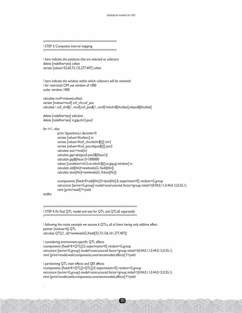
151

\******************************************************\ STEP 3: Composite interval mapping\******************************************************

\ here indicate the positions that are selected as cofactorsdelete [redefi ne=yes] cofsetvariate [values=32,60,73,123,277,407] cofset

\ here indicate the window within which cofactors will be removed\ for restricted CIM use window of 1000scalar window; 1000

calculate ncof=nvalues(cofset)variate [nvalues=ncof] cof_chr,cof_poscalculate \ cof_chr$[1...ncof],cof_pos$[1...ncof]=mkchr$[#cofset],mkpos$[#cofset]

delete [redefi ne=yes] add,domdelete [redefi ne=yes] in,gap,chr2,pos2

for i=1...nloc print !t(position),i; decimals=0 variate [values=#cofset,i] in variate [values=#cof_chr,mkchr$[i]] chr2 variate [values=#cof_pos,mkpos$[i]] pos2 calculate aux1=nval(in) calculate gap=abs(pos2-pos2$[#aux1]) calculate gap$[#aux1]=1000000 subset [condition=chr2.ne.mkchr$[i].or.gap.gt.window] in calculate add[#in]=newlevels(G; Xadd[#in]) calculate dom[#in]=newlevels(G; Xdom[#in]) vcomponents [fi xed=E+add[#in].E+dom[#in].E; experiment=E] random=G.group vstructure [terms=G.group] model=unstructured; factor=group; initial=!(0.04,0.11,0.44,0.12,0.55,1) reml [print=wald] Y=yieldendfor

\*********************************************************************\ STEP 4: Fit fi nal QTL model and test for QTL and QTLxE separatelly\*********************************************************************

\ following the maize example we assume 6 QTLs, all of them having only additive effectpointer [nvalues=6] QTLcalculate QTL[1...6]=newlevels(G;Xadd[32,73,126,161,277,407])

\ considering environment-specifi c QTL effectsvcomponents [fi xed=E+QTL[].E; experiments=E] random=G.groupvstructure [terms=G.group] model=unstructured; factor=group; initial=!(0.04,0.11,0.44,0.12,0.55,1)reml [print=model,wald,components,covariancemodels,effects] Y=yield

\ partitioning QTL main effects and QEI effectsvcomponents [fi xed=E+QTL[]+QTL[].E; experiments=E] random=G.groupvstructure [terms=G.group] model=unstructured; factor=group; initial=!(0.04,0.11,0.44,0.12,0.55,1)reml [print=model,wald,components,covariancemodels,effects] Y=yield

.


The statistical analysis of multienvironment data: modelling genotype-by-environment interaction and...

Documents

Transcript of The statistical analysis of multienvironment data: modelling genotype-by-environment interaction and...