METHODS ARTICLEpublished: 12 March 2013

doi: 10.3389/fphys.2013.00044

The statistical analysis of multi-environment data:modeling genotype-by-environment interactionand its genetic basisMarcos Malosetti 1*, Jean-Marcel Ribaut2 and Fred A. van Eeuwijk1

1 Biometris - Applied Statistics, Department of Plant Science, Wageningen University, Wageningen, Netherlands2 Consultative Group on International Agricultural Research Generation Challenge Programme, México DF, Mexico

Edited by:

Philippe Monneveux, InternationalPotato Center, Peru

Reviewed by:

Jin Chen, Michigan State University,USAPawel Krajewski, Institute of PlantGenetics, PolandJohn Doonan, AberystwythUniversity, UK

*Correspondence:

Marcos Malosetti, Biometris -Applied Statistics, Department ofPlant Science, WageningenUniversity, PO Box 100, 6700 AA,Wageningen, Netherlands.e-mail: marcos.malosetti@wur.nl

Genotype-by-environment interaction (GEI) is an important phenomenon in plant breeding.This paper presents a series of models for describing, exploring, understanding, andpredicting GEI. All models depart from a two-way table of genotype by environmentmeans. First, a series of descriptive and explorative models/approaches are presented:Finlay–Wilkinson model, AMMI model, GGE biplot. All of these approaches have incommon that they merely try to group genotypes and environments and do not use otherinformation than the two-way table of means. Next, factorial regression is introduced asan approach to explicitly introduce genotypic and environmental covariates for describingand explaining GEI. Finally, QTL modeling is presented as a natural extension of factorialregression, where marker information is translated into genetic predictors. Tests forregression coefficients corresponding to these genetic predictors are tests for main effectQTL expression and QTL by environment interaction (QEI). QTL models for which QEIdepends on environmental covariables form an interesting model class for predicting GEIfor new genotypes and new environments. For realistic modeling of genotypic differencesacross multiple environments, sophisticated mixed models are necessary to allow forheterogeneity of genetic variances and correlations across environments. The use andinterpretation of all models is illustrated by an example data set from the CIMMYT maizebreeding program, containing environments differing in drought and nitrogen stress. Tohelp readers to carry out the statistical analyses, GenStat® programs, 15th Edition andDiscovery® version, are presented as “Appendix.”

Keywords: adaptation, genotype by environment interaction, multi-environment trials, QTL by environment

interaction, QTL mapping methodology, REML

INTRODUCTION: PHENOTYPE, GENOTYPE, ANDENVIRONMENTThe success of a plant breeding program depends on its abilityto provide farmers with genotypes with guaranteed superior per-formance (phenotype) in terms of yield and/or quality across arange of environmental conditions. To achieve this aim, it is nec-essary to have an understanding of the factors leading to a goodphenotype.

Usually the phenotype is the value for a trait at the end of thegrowing season. The reason is that we are primarily interested inphenotypes like yield or grain weight at maturity and not, or less,in yield or grain weight at earlier stages. The final state of a trait isthe cumulative result of a number of causal interactions betweenthe genetic make-up of the plant (the genotype) and the condi-tions in which that plant developed (the environment). Plantsdiffer in the efficiency and adequacy with which they capture andconvert environmental inputs and stimuli into the biomass andorgans that constitute a final product. The capture and conver-sion abilities of a plant are determined by its particular ensembleof genes. Environments differ in the amount and quality of inputsand stimuli that they convey to plants including, e.g., the amount

of water, nutrients or incoming radiation. A primary objective inplant breeding is to match genotypes and environments in sucha way that improved phenotypes are obtained. For example, abreeder might be interested in selecting genotypes that do wellunder water stress conditions.

While there can be genotypes that do well across a widerange of conditions (widely adapted genotypes), there are alsogenotypes that do relatively better than others exclusively undera restricted set of conditions (specifically adapted genotypes).Specific adaptation of genotypes is closely related to the phe-nomenon of genotype-by-environment interaction (GEI). GEIexists whenever the relative phenotypic performance of genotypesdepends on the environment, or in other words, when the dif-ference in reactions of genotypes varies in dependence on theenvironment.

To illustrate the phenomenon of GEI, we can consider two dif-ferent genotypes that differ in the genetic machinery involvedin tolerance to water-limited conditions, while being equal forall other characteristics. If these two genotypes are exposedto a poorly watered environment, their performance will dif-fer depending on the genetic properties related to tolerance for

www.frontiersin.org March 2013 | Volume 4 | Article 44 | 1

Malosetti et al. Statistical models for genotype and QTL-by-environment interaction

water-limited conditions. However, this genotypic difference willdisappear in an environment that provides the right amount ofwater. So, the difference in performance between the two geno-types depends on the environment, through the amount of waterthat it provides.

Some scenarios that can occur when comparing the perfor-mances of pairs of genotypes across environments are presentedin Figure 1. The function describing the phenotypic performanceof a genotype in relation to an environmental characterization iscalled the “norm of reaction” (Griffiths et al., 1996). Figure 1Ashows the case where there is no GEI, the genotype and the envi-ronment behave additively (this will be developed later) and thereaction norms are parallel. The remaining plots show differentsituations in which GEI occurs: divergence (Figure 1B), conver-gence (Figure 1C), and the most critical one, crossover interac-tion (Figure 1D). Crossover interactions are the most important

FIGURE 1 | Genotype-by-environment interaction in terms of changing

mean performances across environments: (A) additive model, (B)

divergence, (C) convergence, (D) cross-over interaction.

for breeders as they imply that the choice of the best genotype isdetermined by the environment.

GEI was introduced in terms of the relative difference betweengenotypic means. GEI can also be regarded in terms of hetero-geneity of genetic variance and covariance, or correlation. As aconsequence of GEI, the magnitude of the genetic variance asobserved within individual environments will change from oneenvironment to the next. Often, the genetic variance tends tobe larger in better environments than in poorer environments,although the opposite can be observed as well (Przystalski et al.,2008). Figure 2A illustrates the phenomenon of heterogeneity ofgenetic variance across environments, showing box plots for aseries of maize trials, where the range of variation in the poorenvironments LN96a and LN96b is smaller than that in the goodenvironments HN96b and NS92a.

GEI has also consequences for the correlations between geno-typic performances in different environments. When GEI is large,the observed performance of a set of genotypes in one environ-ment may not be very informative for the performance of thesame genotypes in another environment. Environments with sim-ilar characteristics will induce corresponding responses in plantsand will lead to strong genetic correlations. Figure 2B shows thatthe correlation between the similar environments IS92a and IS94ais larger than the correlation between the dissimilar environmentsNS92a and HN96b.

In conclusion, given the complexity of the mechanisms andprocesses underlying the phenotypic response across diverse andchanging environmental conditions—frequently in an unpre-dictable way—it is necessary to develop analytical tools to helpbreeders understand GEI. The use of adequate strategies to ana-lyze GEI is a first and important step toward more informedbreeding decisions. Good analytical methods are a prerequisitefor predicting the performance of genotypes as accurately as

FIGURE 2 | (A) Boxplot for yield of a maize F2 population in eightenvironments displaying total range, interquartile range (box) and median(line). Environment names are coded as: LN, low nitrogen; HN, high Nitrogen;SS, severe water stress; IS, intermediate water stress; NS, no water stress.

The two digits indicate the year of the trial, and the letters a and b thecropping season: a, winter; b, summer. (B) Scatter plot matrix for twostress environments (IS92a, and IS94a) and two non-stress environments(HN96b and NS92a).

Frontiers in Physiology | Plant Physiology March 2013 | Volume 4 | Article 44 | 2

Malosetti et al. Statistical models for genotype and QTL-by-environment interaction

possible. This paper explores several strategies to model GEI,starting with simple methods that have been historically popu-lar within the plant breeding community. It then moves to moreelaborate models in which additional information is used in theform of explicit environmental characterization to model GEI. Afinal section is devoted to the integration of molecular markerinformation into GEI models, leading to the detection of quanti-tative trait loci (QTLs) and more specifically, to the modeling ofQTL by environment interaction (QEI). The statistical methodol-ogy is illustrated using a maize data set obtained from a series ofdrought and nitrogen stress trials from the maize breeding pro-gram at Centro Internacional de Mejoramiento de Maíz y Trigo(CIMMYT; the International Maize and Wheat ImprovementCenter; Ribaut et al., 1996, 1997). To encourage readers to carryout these statistical analyses themselves, GenStat® programs forthe 15th Edition (VSN International, 2012) and the Discovery®version of this statistical package (Payne et al., 2007) are presentedas “Appendix.”

GENERATING DATA TO STUDYGENOTYPE-BY-ENVIRONMENT INTERACTIONAn obvious first step to investigate GEI is to obtain phenotypicobservations on a set of genotypes exposed to a range of envi-ronmental conditions. The set of genotypes can include advancedlines of a breeding program, cultivars, and segregating offspringfrom a specific cross such as F2, a backcross, or a recombinantinbred line (RIL) population.

Genotypes can be tested under different management regimesthat represent increasing levels of a particular stress, or a com-bination of stresses. This type of experiment is called a “managedstress trial” and is appropriate when the researcher wishes to focuson a particular type of stress. When performing managed stresstrials, it is important to control the system in such a way thatall other factors influencing the phenotype are as homogenousas possible.

Managed stress trials are not a default option in plant breed-ing, because stress type and level can be difficult to implementand because the relationship between phenotype and stress iscomplex, with genes and environmental stress(es) interactingthroughout the various developmental phases. In those situations,a common way for plant breeders to screen for genotypic reac-tions to environmental factors is by “multi-environment trials”(METs). In a MET, a number of genotypes are evaluated at anumber of geographical locations for a number of years in thehope that the pattern of stresses that the genotypes experience isrepresentative of future growing environments.

A convenient way to summarize data from managed stress tri-als and METs is in the form of two-way tables of means, withgenotypes in the rows and environments in the columns. Eachcell of such a table contains an estimate of the performance(adjusted mean) of a particular genotype in a specific environ-ment. To identify genotypes and environments unequivocally, weuse indices, the letter i for genotypes (i = 1 . . . I), and the letter jfor environments (j = 1 . . . J).

The models in the following sections will assume as a start-ing point a genotype-by-environment table of means. Thesemodels are used in a so-called two-stage strategy for analyzing

MET data. In the first stage, individual trials are analyzed withmodels including terms for design features and spatial varia-tion. From these individual trial analyses, adjusted means andweights, usually reciprocals of the variances of the means, arecarried forward to the second stage, where a model is fitted tothe genotype by environment means, using either no weights orweights estimated in the first stage. Various choices can be madefor the weights in a two stage analysis (Mohring and Piepho,2009; Welham et al., 2010), and a good choice of weights willlead to a two-stage analysis with results very close to those ofa so-called single stage analysis, in which plot data are analyzedinstead of means. Single stage analyses have certain theoreti-cal advantages over two-stage analyses, but two-stage analysesare logistically and computationally easier to handle. This paperfocuses on two-stage analyses, because of the small differenceswith single stage analyses and the aforementioned larger handlingease. Still, good descriptions of single stage analyses are offeredby Cullis et al. (1996a,b), Gilmour et al. (1997), and Smith et al.(2005). In principle, the QTL mapping approach outlined laterin this paper could also be embedded in a single stage analysisstrategy.

CIMMYT MAIZE DROUGHT STRESS TRIALS: EXAMPLE DATAThe models to be presented here are illustrated using data pro-duced by the maize drought stress breeding program of CIMMYT.A brief description of the data is given here, a more detaileddescription is available in the original publications (Ribaut et al.,1996, 1997). A maize F2 population was generated by crossinga drought tolerant parent (P1) with a drought susceptible one(P2). Seeds harvested from each of 211 F2 plants formed F3 fam-ilies, which were stored for further evaluation. The F3 familieswere evaluated in managed stress trials in 1992, 1994, and 1996.In the winter of 1992, a managed water stress trial was con-ducted in Mexico, including no stress (NS), intermediate stress(IS), and severe stress (SS). In the winter of 1994, a similar trialwas conducted, but it only included the IS and SS treatments.In the summer of 1996, the families were tested in a nitrogenstress trial with two levels: low (LN) and high nitrogen (HN). Anextra LN trial was conducted in the winter of the same year. Intotal, the families were evaluated in eight different environments,each environment characterized by year, stress type and inten-sity, and management factors. DNA was extracted from each ofthe 211 F2 plants to produce a total of 132 restriction fragmentlength polymorphism (RFLP) markers covering the 10 maizechromosomes.

MODELS FOR GENOTYPE-BY-ENVIRONMENT INTERACTION:MODELING THE MEANTHE ADDITIVE MODEL AS A BENCHMARKThe phenomenon of GEI is of primary interest in plant breed-ing, and has resulted in a large body of literature on modelsand strategies for analysis of GEI [see, for example, the reviewsin Cooper and Hammer (1996), Kang and Gauch (1996), vanEeuwijk et al. (1996), van Eeuwijk (2006)]. A dominant feature ofstrategies used to describe and understand GEI is a heavy relianceon parameters that are statistical rather than biological. This isno coincidence, since historically, a large part of quantitative

www.frontiersin.org March 2013 | Volume 4 | Article 44 | 3

Malosetti et al. Statistical models for genotype and QTL-by-environment interaction

genetics has relied on simple, yet very useful, statistical models. Anotorious example is the well-known model: P = G + E, whereP stands for phenotype, G for genotype and E for environment(Falconer and Mackay, 1996; Lynch and Walsh, 1998). A statisti-cal formulation of this model for a two-way table of means can bewritten as:

μij

= μ + Gi + Ej + εij. (1)

From here onwards, in the model formulations, random terms areunderlined to emphasize the fact that their effects are assumed tofollow a normal distribution. Model 1 describes the response vari-able, that is, the mean of genotype i in environment j, μ

ij, as the

result of the common fixed intercept term μ, a fixed genotypicmain effect corresponding to genotype i, Gi, plus a fixed envi-ronmental main effect corresponding to environment j, Ej, andfinally the random term, εij, representing the error term, typicallyassumed normally distributed, with a mean of zero and constantvariance, σ2; εij ∼ N(0, σ2).

Model 1 predicts that for any genotype the difference meansbetween any two environments j and j∗ will be equal to the dif-ference in the environmental main effects: Ej–Ej∗ . Consequently,the norms of reaction of genotypes will be parallel (Figure 1A).Another important aspect is that, although the parameters in themodel suggest that something intrinsically genetic and somethingintrinsically environmental is determining the trait, the genotypicand environmental effects purely follow from a convenient way ofpartitioning phenotypic variation from a statistical point of view.In a balanced data set, the genotypic main effects can be estimatedfrom the average performance of the genotypes across environ-ments. Rather than being something inherently genotypic, thisis dependent on the set of environments used in the experi-ment. If a few environments are dropped, the genotypic effectswill change. The same argument applies to the environmentalmain effects, which depend on the set of genotypes used in theexperiment.

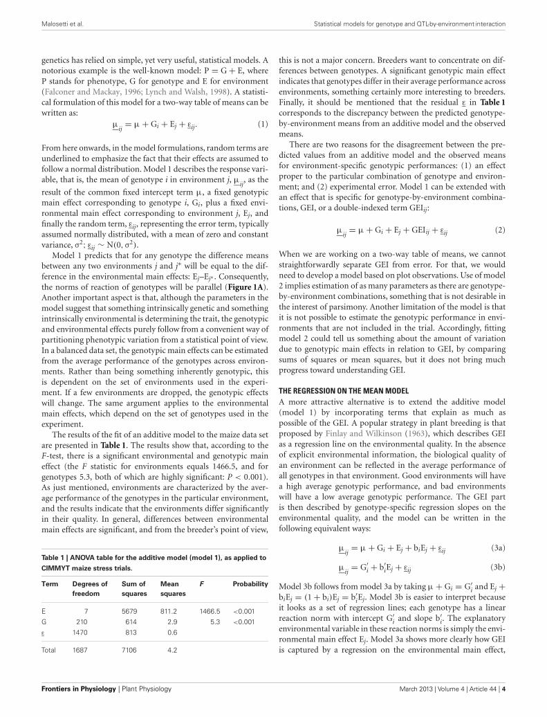
The results of the fit of an additive model to the maize data setare presented in Table 1. The results show that, according to theF-test, there is a significant environmental and genotypic maineffect (the F statistic for environments equals 1466.5, and forgenotypes 5.3, both of which are highly significant: P < 0.001).As just mentioned, environments are characterized by the aver-age performance of the genotypes in the particular environment,and the results indicate that the environments differ significantlyin their quality. In general, differences between environmentalmain effects are significant, and from the breeder’s point of view,

Table 1 | ANOVA table for the additive model (model 1), as applied to

CIMMYT maize stress trials.

Term Degrees of

freedom

Sum of

squares

Mean

squares

F Probability

E 7 5679 811.2 1466.5 <0.001

G 210 614 2.9 5.3 <0.001

ε 1470 813 0.6

Total 1687 7106 4.2

this is not a major concern. Breeders want to concentrate on dif-ferences between genotypes. A significant genotypic main effectindicates that genotypes differ in their average performance acrossenvironments, something certainly more interesting to breeders.Finally, it should be mentioned that the residual ε in Table 1corresponds to the discrepancy between the predicted genotype-by-environment means from an additive model and the observedmeans.

There are two reasons for the disagreement between the pre-dicted values from an additive model and the observed meansfor environment-specific genotypic performances: (1) an effectproper to the particular combination of genotype and environ-ment; and (2) experimental error. Model 1 can be extended withan effect that is specific for genotype-by-environment combina-tions, GEI, or a double-indexed term GEIij:

μij

= μ + Gi + Ej + GEIij + εij (2)

When we are working on a two-way table of means, we cannotstraightforwardly separate GEI from error. For that, we wouldneed to develop a model based on plot observations. Use of model2 implies estimation of as many parameters as there are genotype-by-environment combinations, something that is not desirable inthe interest of parsimony. Another limitation of the model is thatit is not possible to estimate the genotypic performance in envi-ronments that are not included in the trial. Accordingly, fittingmodel 2 could tell us something about the amount of variationdue to genotypic main effects in relation to GEI, by comparingsums of squares or mean squares, but it does not bring muchprogress toward understanding GEI.

THE REGRESSION ON THE MEAN MODELA more attractive alternative is to extend the additive model(model 1) by incorporating terms that explain as much aspossible of the GEI. A popular strategy in plant breeding is thatproposed by Finlay and Wilkinson (1963), which describes GEIas a regression line on the environmental quality. In the absenceof explicit environmental information, the biological quality ofan environment can be reflected in the average performance ofall genotypes in that environment. Good environments will havea high average genotypic performance, and bad environmentswill have a low average genotypic performance. The GEI partis then described by genotype-specific regression slopes on theenvironmental quality, and the model can be written in thefollowing equivalent ways:

μij

= μ + Gi + Ej + biEj + εij (3a)

μij

= G′i + b′

iEj + εij (3b)

Model 3b follows from model 3a by taking μ + Gi = G′i and Ej +

biEj = (1 + bi)Ej = b′iEj. Model 3b is easier to interpret because

it looks as a set of regression lines; each genotype has a linearreaction norm with intercept G′

i and slope b′i. The explanatory

environmental variable in these reaction norms is simply the envi-ronmental main effect Ej. Model 3a shows more clearly how GEIis captured by a regression on the environmental main effect,

Frontiers in Physiology | Plant Physiology March 2013 | Volume 4 | Article 44 | 4

Malosetti et al. Statistical models for genotype and QTL-by-environment interaction

with the hope that as much as possible of the GEI signal will beretained by the term biEj.

In the regression on the mean model, GEI is explained in termsof differential sensitivities to the improvement of the environ-ment, with some genotypes (the ones with larger values of bi)benefiting more than others from an increase in environmen-tal quality. Note that in model 3a, �bi = 0, so that the averageslope value is zero, while in model 3b the average value of b′ is1, meaning that b′ > 1 for genotypes with a higher than averagesensitivity, and b′ < 1 for genotypes that are less sensitive thanaverage.

Table 2 gives the fit of model 3a to the maize example data.The first two rows of the table, corresponding to the genotypicand environmental main effects, are identical to Table 1. The thirdrow corresponds to the GEI effect in terms of the regression onenvironmental quality, where quality is represented by the envi-ronmental mean. This regression is highly significant, accordingto the F-tests (F = 2.4, P < 0.001). The residual sum of squaresin Table 1 (SSε = 813) has been divided into a part explained bygenotypic sensitivities to environmental quality (SSb = 230), anda residual (SSε = 583).

By way of example, the fitted reaction norms of five geno-types (out of the full set of 211 genotypes) are given in Figure 3,together with the parameters estimated according to the param-eterization in model 3b (G′ and b′). Figure 3 shows that, in theaverage environment, genotypes G025 and G045 are better thanG008, G012, and G016. The estimates for the parameters G′ canbe read-off from the plot as the fitted values at the null value ofthe x-axis, i.e., the average environment indicated by the dashedvertical line. Although G045 does slightly better than G025 inthe average environment, G025 is superior to G045 in the high-quality environments. This is because G025 has a better ability toexploit improved environmental conditions, which is reflected inits higher genotypic sensitivity (b′

G025 = 1.27 > b′G045 = 0.99). A

similar observation can be made for G008 vs. G012 and G016.While G008 does relatively better in low quality environments, itis clearly surpassed by G012 and G016 in the best environments,since it is not capable of profiting from the better environmentalconditions (b′

G008 = 0.65, which is the lowest sensitivity amongthe five genotypes).

In summary, the regression on the mean model describes GEIin terms of parameters that can be given some biological mean-ing. In addition, and in contrast with the full interaction model

Table 2 | ANOVA table for the regression on the mean model

(model 3), as applied to CIMMYT maize stress trials.

Term Degrees of

freedom

Sum of

squares

Mean

squares

F Probability

E 7 5679 811.2 1752.3 <0.001

G 210 614 2.9 6.3 <0.001

Heterogeneityof slopes

210 230 1.1 2.4 <0.001

ε 1260 583 0.5

Total 1687 7106 4.2

(model 2), model 3 can be used to predict the performance ofgenotypes in environments that were not present in the MET, aslong as the environment for which predictions are required canreasonably be placed within the range of environments used inthe original MET. Nevertheless, the regression on the mean modelsuffers from the fact that the environmental characterization isbased on a single dimension. Environmental quality can be hardto summarize within a single explanatory variable. Therefore, asubstantial amount of GEI can remain unexplained. In the nextsection, the regression on the mean model will be extended byincluding multidimensional environmental characterizations inthe statistical model for the genotype-by-environment data.

THE ADDITIVE MAIN EFFECTS AND MULTIPLICATIVE INTERACTIONSMODELThe limitation of a single dimension in environmental character-ization can be removed by employing a more flexible model, inwhich more than one environmental quality variable is allowed.A popular model of this type is the additive main effectsand multiplicative interaction (AMMI) model (Gollob, 1968;Mandel, 1969; Gabriel, 1978; Gauch, 1988; van Eeuwijk, 1995).To emphasize the similarities with model 3a, we write the AMMImodel as:

μij

= μ + Gi + Ej +K∑

k = 1

bikzjk + εij (4)

where the GEI is now explained by K multiplicative terms (k =1 . . . K), each multiplicative term formed by the product ofa genotypic sensitivity bik (genotypic score) and a hypothet-ical environmental characterization zjk (environmental score).Although genotypic and environmental scores are deemed to rep-resent genetic and environmental qualities, they come from a

FIGURE 3 | Finlay–Wilkinson regression curves of five maize

genotypes. The vertical line indicates the average environment. Next togenotype labels, the corresponding Finlay-Wilkinson regression equation isgiven.

www.frontiersin.org March 2013 | Volume 4 | Article 44 | 5

Malosetti et al. Statistical models for genotype and QTL-by-environment interaction

mathematical procedure, a principal components analysis on theGEI (Gabriel, 1978; Gauch, 1988) that maximizes the variationexplained by the products of the genotypic and environmentalscores. The first product term is the one that explains most ofthe variation, followed by the second one, and so on. This isreflected in Table 3, which shows the results from the AMMImodel to the maize example data. In the AMMI model, GEI isexplained by two axes (principal component 1, PCA1, and princi-pal component 2, PCA2) that are highly significant (F = 2.8 and2.0 respectively, both with an associated P < 0.001). The first axis(PCA1) explains the largest part (SSPCA1 = 242), the second oneexplains a little less (SSPCA2 = 173), with a total explained sumof squares for GEI of 242 + 173 = 415, an improvement over theexplained sum of squares in the regression on the mean model(SSb = 230).

Table 3 | ANOVA table corresponding to application of AMMI2 model

(model 4) to CIMMYT maize stress trials.

Term Degrees of

freedom

Sum of

squares

Mean

squares

F Probability

E 7 5679 811.2 1752.3 <0.001

G 210 614 2.9 6.3 <0.001

PCA1 216 242 1.1 2.8 <0.001

PCA2 214 173 0.8 2.0 <0.001

ε 1040 398 0.4

Total 1687 7106 4.2

PCA1 and PCA2 are the principal component axes 1 and 2, respectively.

A desirable property of the AMMI model is that the geno-typic and environmental scores can be used to construct powerfulgraphical representations called biplots (Gabriel, 1978) that helpto interpret the GEI. Figure 4A presents a biplot for the maizedata. A first thing to recognize is that both genotypes and envi-ronments are present in the same plot; genotypes are representedby gray circles and environments by filled triangles (red, blue,and black). The environments are typically represented as axesintersecting at their origins. The origins represent the averagesfor the trait in the corresponding environments. The trianglespoint in the direction of increasing trait values. By projectinggenotypes on environmental axes, GEI for individual genotypesis approximated. To help interpretation, environmental axes canbe enriched by including a scale (Graffelman and van Eeuwijk,2005).

Biplots facilitate the exploration of relationships betweengenotypes and/or environments. Genotypes that are more similarto each other are closer to each other in the plot than geno-types that are less similar. The same is true for environments.Genotypes/environments that are alike tend to cluster together.The angle between environmental axes is related to the correlationbetween the environments. An acute angle indicates positive cor-relation (e.g., between LN96a and LN96b), a right angle indicatesno correlation (e.g., between HN96b and NS92a), and an obtuseangle indicates negative correlation (e.g., NS92a and LN96a). Theprojection of a genotype onto an environmental axis reflects theperformance of that genotype in that environment (for GEI). Forexample, genotype G091 projects on the NS92a axis above the ori-gin, indicating a positive interaction with that environment i.e.,the relative performance (GEI part) of G091 in NS92a is above the

FIGURE 4 | (A) Biplot from the AMMI model used to describe GEI in themaize example data. Gray circles represent genotypes, and filled trianglesenvironments, with triangles pointing in the direction of increasing GEI(at origin GEI = 0). The projection of two genotypes (G041 and G091) onthe NS92a axis is shown by a dashed line. (B) GGE biplot for the maize

data set, with same characteristics as of the AMMI biplot, except thattriangles point in the direction of increasing overall performance (G + GEI),so the origin corresponds to the average performance of all genotypes inthe particular environment. Projections for genotypes G041 and G091 aregiven.

Frontiers in Physiology | Plant Physiology March 2013 | Volume 4 | Article 44 | 6

Malosetti et al. Statistical models for genotype and QTL-by-environment interaction

average of all genotypes in NS92a. Conversely, genotype G041 (onthe right hand side of the plot) projects below the origin on thesame axis, which points to a negative interaction with environ-ment NS92a (i.e., G041 performs worse than average). Followinga similar procedure it is possible to conclude that while geno-type G091 showed positive adaptation to environment NS92a, itis not well adapted to environments LN96a and LN96b (the pro-jection of G091 on the LN96a and LN96b axes falls below theorigin). Biplots are useful tools to investigate patterns in GEI,because they can help to identify interesting genotypes that areadapted to particular environments, and to classify environmentsin groups.

Plant breeders are interested in the total genetic variation andnot exclusively in the GEI part. For that reason, it is useful tohave a modification of model 4 that considers the joint effects ofthe genotypic main effect and the GEI as a sum of multiplicativeterms. Effectively, the two-way table of genotype-by-environmentmeans is exposed to a standard principal components analysis,with genotypes as objects and environments as variables (Yanet al., 2000). For this model, closely the same estimation andinterpretation procedures hold as for model 4. Because genotypicscores now describe genotypic main effects G and GEI together,this type of model is also known as the “Genotype main effectsand GEI model,” or “GGE model” and the biplots are called “GGEbiplots” (Yan et al., 2000). The model reads:

μij

= μ + Ej +K∑

k = 1

bikzjk + εij (5)

The results of model 5 fitted to the maize data are presented inthe form of a biplot in Figure 4B. GGE biplots approximate over-all performance (G + GEI). This is in contrast to AMMI biplots,Figure 4A, that approximate only the GEI part of the phenotype.Figure 4B shows the high yielding genotypes concentrated on theright hand side of the biplot, with their projections on environ-mental axes covering the above average range (for example, G091projects above the origin in NS92a, whereas G041 is found belowthe origin). In contrast, low yielding genotypes (as G041) are con-centrated on the left hand side of the biplot (projects below originin most of the environments).

FACTORIAL REGRESSION MODELSThe models discussed so far assumed that we do not have explicitinformation about the environments. While such models can beuseful to explain GEI, the biological interpretation of their resultsis not always obvious. What do hypothetical environmentalvariables, as in AMMI, mean in terms of quantifiable environ-mental characteristics such as temperature, water, nutrientsetc? A straightforward approach is to correlate environmentalscores with environmental covariables. However, if we do haveexplicit information about the environment, the informationcan be used directly in the model by including it in the formof explanatory variables. GEI is then described as differentialgenotypic sensitivity to explicit environmental factors such astemperature, precipitation, water availability etc. Such models areknown as factorial regression models (Denis, 1988; van Eeuwijket al., 1996). Two examples of factorial regression models are

given here. Model 6a includes a single environmental covariable,while model 6b includes multiple environmental covariables:

μij

= μ + Gi + Ej + biZj + εij (6a)

μij

= μ + Gi + Ej +K∑

k = 1

bikZjk + εij (6b)

Models 6a and 6b look very similar to models 3a and 4, but thereis a substantial difference between them. In models 6a and 6b, Zj

represents an explicit environmental covariable and not a hypo-thetical environmental covariable as in models 3a and 4 (note thatZ is capitalized to highlight this difference). This distinction iscritical since the interpretation of the GEI in models 6a and 6b isautomatically placed into a biological context. Instead of describ-ing GEI as differential reactions to hypothetical environmentalcovariables, factorial regression models help to identify genotypesthat are differentially sensitive to changes in identified environ-mental quality components, for example, in a particular nutrient,or in water availability.

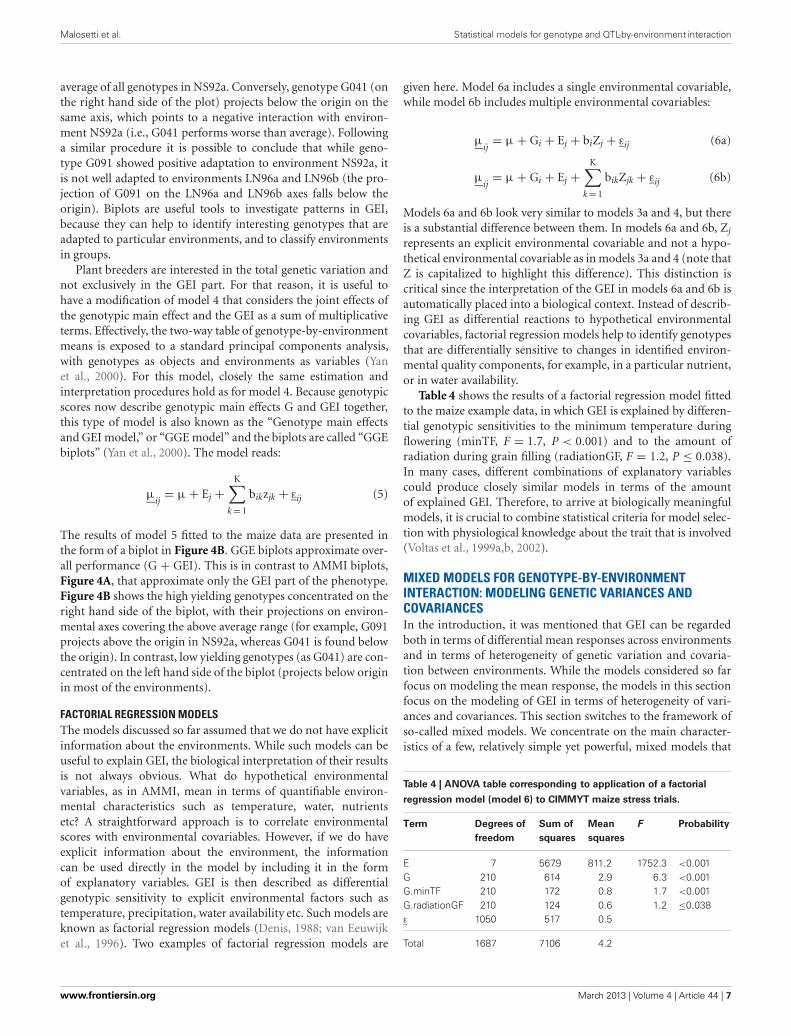
Table 4 shows the results of a factorial regression model fittedto the maize example data, in which GEI is explained by differen-tial genotypic sensitivities to the minimum temperature duringflowering (minTF, F = 1.7, P < 0.001) and to the amount ofradiation during grain filling (radiationGF, F = 1.2, P ≤ 0.038).In many cases, different combinations of explanatory variablescould produce closely similar models in terms of the amountof explained GEI. Therefore, to arrive at biologically meaningfulmodels, it is crucial to combine statistical criteria for model selec-tion with physiological knowledge about the trait that is involved(Voltas et al., 1999a,b, 2002).

MIXED MODELS FOR GENOTYPE-BY-ENVIRONMENTINTERACTION: MODELING GENETIC VARIANCES ANDCOVARIANCESIn the introduction, it was mentioned that GEI can be regardedboth in terms of differential mean responses across environmentsand in terms of heterogeneity of genetic variation and covaria-tion between environments. While the models considered so farfocus on modeling the mean response, the models in this sectionfocus on the modeling of GEI in terms of heterogeneity of vari-ances and covariances. This section switches to the framework ofso-called mixed models. We concentrate on the main character-istics of a few, relatively simple yet powerful, mixed models that

Table 4 | ANOVA table corresponding to application of a factorial

regression model (model 6) to CIMMYT maize stress trials.

Term Degrees of

freedom

Sum of

squares

Mean

squares

F Probability

E 7 5679 811.2 1752.3 <0.001G 210 614 2.9 6.3 <0.001G.minTF 210 172 0.8 1.7 <0.001G.radiationGF 210 124 0.6 1.2 ≤0.038ε 1050 517 0.5

Total 1687 7106 4.2

www.frontiersin.org March 2013 | Volume 4 | Article 44 | 7

Malosetti et al. Statistical models for genotype and QTL-by-environment interaction

can be used to model GEI in terms of heterogeneity of varianceand covariance. A more detailed description of mixed models canbe found in the literature elsewhere (Verbeke and Molenberghs,2000; Galwey, 2006).

The models discussed in the previous sections were all exam-ples of fixed effects models, with all terms except the residual termfixed. However, genotypes can be regarded as a random samplefrom a larger population (especially easy when the number ofgenotypes is large, say more than 10), in which case genotypesare an extra source of random variation. This situation calls fora mixed model, with genotypes taken as random term. A reviewof the use of mixed models to analyse complex data sets in plantbreeding can be found in Smith et al. (2005). For the maize exam-ple data set, there are 211 genotypes. When the genotypic maineffects are taken as random, the following mixed model equivalentof the additive model can be defined as:

μij

= μ + Gi + Ej + εij (7)

Gi ∼ N(0, σ2G) εij ∼ N(0, σ2

ε )

The term Gi is underlined to indicate that it is a random term;its distribution needs to be specified, and usually is taken tobe normal, with zero mean and a variance specific to the term.Model 7 contains two variance components, one correspondsto the random genotypic main effects, σ2

G, and a second one,σ2

ε , corresponds to the residual (which includes true GEI anderror). An important consequence of including genotypes as ran-dom is that automatically genetic covariances and correlationsbetween performances in different environments are imposed.The total variance for individual genotypic observations in a par-ticular environment j, σ2

j , is the sum of two sources of variation:

σ2j = σ2

G + σ2ε . The covariance between observations for a par-

ticular genotype in environments j and j∗, σjj∗ , following from

model 7 is: σjj∗ = σ2G. For observations on different genotypes

σjj∗ = 0. In model 7, similarities (or covariation, and thereforecorrelation) between observations made on the same genotypein different environments are assumed to be positive, but covari-ation between observations on different genotypes (regardlesswhether the observation is done in the same or in different envi-ronments) is assumed to be zero. Model 7 is referred as thecompound symmetry model (Verbeke and Molenberghs, 2000).

The general definition for a correlation between two traits, ortwo environments, x and y is:

r(x; y) = covariance(x; y)√var(x)

√var(y)

Model 7 imposes a constant correlation between environments,with the correlation between any pair of environments j and j∗(for clarity, we write Envj and Envj∗ when referring to thoseenvironments), being equal to:

r(Envj; Envj∗ ) = σjj∗√σ2

j

√σ2

j∗= σ2

G√σ2

G + σ2ε

√σ2

G + σ2ε

= σ2G

σ2G + σ2

ε

Although mixed models can be fitted by standard least squaresprocedures in the case of balanced data, a more general method of

inference to fit mixed models is by residual maximum likelihood,or REML (Patterson and Thompson, 1971). Results of analysesbased on REML are presented in another way than the famil-iar ANOVA tables. Table 5 shows the results obtained by fittingmixed models to the maize example data.

Table 5 does not contain sums of squares, nor mean squares.Instead, there is a table with three main sections. For model 7, thecompound symmetry model, one section contains the results fortesting fixed model terms (header Fixed terms). A second sectionshows the estimates for the variances of the random terms (headerRandom terms), and a third section a goodness-of-fit statistic, thedeviance, that can be used to compare mixed models with equalfixed terms and differing random terms (header Deviance). Forthe fixed effects (environments in this case), Table 5 shows a Waldtest statistic, the corresponding degrees of freedom (DF), and aP value. The Wald test statistic is used to assess the significanceof fixed effects in the REML mixed model framework. Under thenull hypothesis of no fixed effects, the Wald test has a distributionthat is approximately a Chi-square with DF equal to the num-ber of independent effects for the particular fixed term. In themaize example, the Wald test statistic for environments is 10,265.3and it has 8 − 1 = 7 degrees of freedom. This Wald statistic has avery low tail probability in the Chi-square distribution under thenull hypothesis of no environmental effects (P < 0.001). So, it isconcluded that there is a significant difference between environ-ments. Some statistical packages, including GenStat®, can providean F-distributed approximation to the Wald statistic.

The estimates of the two parameters associated to the ran-dom terms in the model: σ2

G = 0.297 and σ2ε = 0.553 are given in

the second part of Table 5. The magnitude of the variance com-ponents can be compared to have an impression of the relativeimportance of genotypic main effects (σ2

G) in relation to the sumof GEI and error (σ2

ε ). The genetic correlation between any twoenvironments is estimated as:

r(Envj; Envj∗ ) = 0.297

0.297 + 0.553= 0.349

The last row in Table 5 presents the deviance (equal to −2 timesthe restricted loglikelihood), which is a measure of how well themodel fitted to the data. The better the model, the lower thedeviance is. As will be seen later, the deviance can be used tocompare different models to select the best model for the data,provided that the fixed part of the model remains unchanged.

Model 7 assumes a constant genetic variance and correlationbetween pairs of environments. For METs, the assumption ofconstant genetic variance and genetic correlation across environ-ments is unrealistic (Figure 2A). In the presence of GEI, a morerealistic model would allow the total genetic variance to changefrom environment to environment, which will in turn, causeheterogeneous genetic correlations between environments:

μij

= μ + Gi + Ej + εij (8)

Gi ∼ N(0, σ2G) εij ∼ N(0, σ2

εj)

In model 8, there is still a single genetic variance component forgenotypes, and therefore, a constant genetic covariance between

Frontiers in Physiology | Plant Physiology March 2013 | Volume 4 | Article 44 | 8

Malosetti et al. Statistical models for genotype and QTL-by-environment interaction

Table 5 | REML output of the fit of different mixed models to the CIMMYT maize stress trials.

Model 7 Model 8 Model 9

Fixed Wald (DF ) P Fixed Wald (DF ) P Fixed Wald (DF ) P

E 10265.3 (7) <0.001 E 9759.4 (7) <0.001 E 6268.8 (7) <0.001

Random Estimate SE Random Estimate SE Random Estimate SE

σ2G 0.297 0.036 σ2

G 0.125 0.017 σ2C1 0.439 0.053

σ2ε 0.553 0.020 σ2

ε1 0.551 0.057 σ2C2 1 –

σ2ε2 0.692 0.071 σ2

C3 0.042 0.013

σ2ε3 1.399 0.140 σC1C2 0.551 0.077

σ2ε4 0.672 0.069 σC1C3 0.109 0.019

σ2ε5 0.704 0.072 σC2C3 0.115 0.032

σ2ε6 0.135 0.018 σ2

ε1 0.446 0.051

σ2ε7 0.152 0.019 σ2

ε2 0.445 0.052

σ2ε8 0.761 0.078 σ2

ε3 0.736 0.169

σ2ε4 0.428 0.050

σ2ε5 0.508 0.057

σ2ε6 0.145 0.018

σ2ε7 0.138 0.017

σ2ε8 0.740 0.080

Deviance (DF ) 1077.9 (1678) Deviance (DF ) 838.4 (1671) Deviance (DF ) 619.9 (1667)

Model 7 assumes compound symmetry, model 8: assumes heterogeneity of genetic variance across environments, and model 9 assumes heterogeneity of genetic

covariance between groups of environments and heterogeneity of genetic variance across individual environments. Environments are indexed as: 1 = SS92a, 2 =IS92a, 3 = NS92a, 4 = IS94a, 5 = SS94a, 6 = LN96a, 7 = LN96b, 8 = HN96b. Groups of environments are indexed as: C1 = SS92a, IS92a, IS94a, SS94a, HN96b;

C2 = NS92a; C3 = LN96a, LN96b.

environments. However, the variance for the term εij that includesGEI and error, is assumed to depend on the environment (i.e.,the variance component σ2

εj is indexed by j). Table 5 presents the

results of fitting model 8 to the maize data. Instead of two vari-ance components, there are now nine, one corresponding to thevariance component for genotypes (σ2

G = 0.125), and eight cor-responding to a form of GEI for each of the eight environments(for convenience, we assume constant errors). The heterogene-ity of variance for εij reflects that in some environments there is alarger variation (e.g., in environment 3, which is the high-yieldingNS92a) than in other environments (e.g., in environments 6and 7, which are low-yielding, LN96a and LN96b). The hetero-geneity of variance leads to heterogeneous genetic correlationsbetween environments. For example, the correlation betweenenvironments 6 and 7 is:

r(Env6; Env7) = 0.125√0.125 + 0.135

√0.125 + 0.152

= 0.466

and between environments 3 and 6 is:

r(Env3; Env6) = 0.125√0.125 + 1.399

√0.125 + 0.135

= 0.199

In conclusion, model 8 accommodates heterogeneity of variancebetween environments and, with it, allows for heterogeneouscorrelations between environments, which can be desirable when

analyzing environments that strongly differ (e.g., with strongstress and without stress).

The deviance for model 8 is 838.4 with 1671 DF, whichis much lower than the one for model 7 (deviance 1077.9with 1678 DF). The deviance has dropped, but at the expenseof having to estimate more parameters (nine instead of twoparameters). Is the decrease in deviance large enough to con-sider model 8 a significant improvement over model 7? Becausemodel 7 and 8 are nested models (model 7 is a special caseof model 8 when the σ2

εj are equal for all j), a deviance test

can be used to answer this question. Under the null hypoth-esis of no difference in quality of the fits, the difference indeviance between the two models is Chi-square distributed withthe number of DF equal to the difference in the number ofparameters between the models. In the example, the differencein deviance is 1077.9 − 838.4 = 239.5, and the models differ byseven parameters. The P value associated to 239.5 in a Chi-squaredistribution with 7 DF is very small (P < 0.001), so it is con-cluded that model 8 provides a significant improvement overmodel 7.

In cases where the models are not nested, the comparisoncan be done by the Akaike Information Criterion (AIC) (Akaike,1974). For model 7, AIC = 4170, and for model 8 AIC = 3944.The model that has the lowest AIC value is the one that is cho-sen. Model 8 has the lowest AIC value, which agrees with theconclusion based on the deviance test.

www.frontiersin.org March 2013 | Volume 4 | Article 44 | 9

Malosetti et al. Statistical models for genotype and QTL-by-environment interaction

Model 8 assumes heterogeneous variances across environ-ments, in combination with a constant covariance between envi-ronments. This latter assumption can be relaxed by also allowingthe genetic covariance between environments to be heteroge-neous. A possibility is to estimate a covariance parameter for eachpair of environments, producing a variance-covariance modelthat is referred to as the “unstructured model” (Verbeke andMolenberghs, 2000). A somewhat simpler strategy consists of esti-mating covariances between groups of environments instead ofbetween individual environments, in which the environments arefirst grouped in a number of clusters and then fitting the followingmodel:

μi(c)j

= μ + Gi(c) + Ej + εi(c)j (9)

Gi(c) ∼ N(0,�c) εi(c)j ∼ N(0, σ2εj)

In model 9 a random genetic main effect is fitted that changesbetween groups of environments and that has a covariance matrix�c that consists of group specific genetic variances, with σ2

cj for

group j, on the diagonals, and pairwise-specific genetic covari-ances, with σcjj∗between groups j and j∗, on the off-diagonals.Model 9 retains the residual heterogeneity of model 8, whichmeans that environment specific genotypic effects are added togroup specific genotypic effects. To illustrate model 9, using themaize example, and based on Figure 4, the environments wereclustered in three groups: group 1 = (SS92a, SS94a, IS92a, IS94a,HN96b), group 2 = (NS92a), and group 3 = (LN96a, LN96b).Therefore, the covariance matrix �C will contain on the diago-nal the genetic variances for groups 1, 2, and 3 (σ2

c1, σ2c2, and σ2

c3respectively), and on the off-diagonals the covariances betweenthe groups (σc12, σc13, and σc23). The full covariance matrix canbe written as:

�C =⎛⎝

σ2c1

σc12 σ2c2

σc13 σc23 σ2c3

⎞⎠

The results of fitting model 9 to the maize data are presented inTable 5, where the estimates of the parameters in the covariancematrix �C can be found.

The diagonals of �C show that, on average, the genetic vari-ation is lower in group 1 (the group of nitrogen stress environ-ments) than in group 2. It should be noted that because group 3is composed of a single environment, the genetic variation can-not be partitioned into a component due to the group and aresidual, so σ2

c3 is not estimated but arbitrarily fixed to 1. Thetotal variance in each of the environments is equal to the sumof the group’s variance plus the environment-specific variance.For example, the variance in environment 1 is equal to 0.885,which is the sum of the variance of group 1, i.e., σ2

c1 = 0.439, andσ2

ε1 = 0.446. Recalling that the covariance between environmentswithin the same group is given by σ2

c1, σ2c2 and σ2

c3, and the covari-ance between environments in different groups by σc1c2, σc1c3,and σc2c3, the correlation between any pair of environments canbe estimated. For example, the correlation between environments1 and 2 is:

r(Env1; Env2) = 0.439√0.439 + 0.446

√0.439 + 0.445

= 0.496

and between environments 1 and 7 is:

r(Env1; Env7) = 0.109√0.439 + 0.446

√0.042 + 0.138

= 0.273

Finally, the deviance can be used to evaluate whether theallowance for heterogeneity of covariance between environmentsimproved the quality of the model or not.

The deviance for model 9 is 619.9 with 1667 DF, and thedifference in deviance with model 8 is 218.5, with four extraparameters. The associated P value for 218.5 in a Chi-squaredistribution with 4 DF is very low (P < 0.001), so it can be con-cluded that model 9 is a significant improvement over model 8.For model 9 AIC = 3736, which is smaller than for model 8(AIC = 3944), and confirms this conclusion.

We have presented different mixed model formulations tomodel GEI in terms of heterogeneity of variance and covariancebetween environments. The compound symmetry model, whichis the commonly used default model when fitting a mixed modelto a two–way table of means, forces variances and covariances tobe constant across environments. Two alternative models accom-modated either heterogeneity of genetic variances across envi-ronments, or heterogeneity of genetic variances and covariancesacross environments. There are other useful variance-covariancemodels such as the factor analytic (Malosetti et al., 2004; Boeret al., 2007) that combines flexibility with parsimony (reducednumber of parameters), but their discussion is outside the scopeof this paper.

The analysis of a data set is an iterative process consistingof fitting and comparing alternative models to identify a goodmodel for the data under study. That process has been illustratedwith a maize data set. The next section goes one step further inthe modeling process by including molecular marker informa-tion, with the ultimate objective of identifying genomic regions,QTLs, that underlie genetic variation of quantitative traits. Withinthe context of METs, the use of such models is a powerfultool to identify and understand the genetic basis of GEI, thatis, QEI.

QTL MAPPING IN THE CONTEXT OF MULTI-ENVIRONMENTTRIALS: MODELING MAIN EFFECT QTLs ANDQTL-BY-ENVIRONMENT INTERACTIONSo far, we discussed models that use either implicit or explicitenvironmental characterizations to understand GEI. We switchin this section to the use of explicit genotypic information inthe models describing GEI. Use of such information in sta-tistical models for GEI can help understand the basis of GEIin terms of the action of genome regions, QTLs, in theirdependence on the environment, i.e., QEI. Molecular markersystems (RFLP, AFLP, DArT, SSR, SNP) provide informationabout variation at the DNA level that can be employed instatistical models. For example, within the framework of fac-torial regression models, markers can serve as explanatoryvariables, which is at the core of regression–based approaches for

Frontiers in Physiology | Plant Physiology March 2013 | Volume 4 | Article 44 | 10

Malosetti et al. Statistical models for genotype and QTL-by-environment interaction

QTL mapping (Haley and Knott, 1992; Martínez and Curnow,1992).

Elaborating upon factorial regression ideas, the following sec-tion presents mixed models that can accommodate explicit geno-typic information to describe GEI in terms of QTL and QEIeffects (Malosetti et al., 2004; Boer et al., 2007; van Eeuwijk et al.,2007, 2010). The genotypic information stemming from mark-ers is introduced in the statistical models in the form of so-calledgenetic predictors. Applications of mixed model QTL by envi-ronment detection as the one described here, can be found inwheat (Mathews et al., 2008), sugar cane (Pastina et al., 2012),and sorghum (Sabadin et al., 2012). We should emphasize, thatalthough we focus on QTL models applied to standard biparentalpopulations, these models can be adapted rather easily to multi-parental populations (van Eeuwijk et al., 2010; Huang et al.,2011), or association mapping panels (Malosetti et al., 2007; vanEeuwijk et al., 2010).

While here we focus in this paper on mixed model QTL detec-tion, this is certainly not the only method for multi-environmentQTL mapping. A well known and common alternative is to usemixture model approaches (Jiang and Zeng, 1995), for whichvarious user-friendly QTL software packages exist (e.g., QTLCartographer, Basten et al., 2002). However, such QTL softwarepackages typically provide little or no opportunity to intervenewith the statistical model, nor do they allow for applying differ-ent model building strategies. For example, in the mixture modelcontext, it is hard to switch between different models for repre-senting the dependencies between environments or add explicitinformation on the environments, something that is relativelyeasy in the mixed model context.

EXPLANATORY VARIABLES FOR DIFFERENCES BETWEENGENOTYPES: GENETIC PREDICTORSMost populations in QTL mapping originate from crossesbetween pairs of inbred lines. A segregating offspring popula-tion can be produced from an F1 hybrid after one generation ofselfing (F2), after several generations of self-pollination (recom-binant inbred lines or RIL), or after crossing the F1 with one ofthe parental lines (backcross). In addition, by chromosome dou-bling of F1 gametes, a population of doubled haploid lines can begenerated. In all of these cases, two alleles at most will segregateat each locus. For a locus M1, individuals can have the genotypesM1M1, M1m1, or m1m1, with M1 the allele that comes from thepaternal line, and m1 the allele that comes from the maternal line.By convention the locus names are given in italics (so for exam-ple M1 refers to locus 1, and M1 and m1 refer to the paternal andmaternal alleles at locus 1, respectively). The relative frequency ofthe genotypes in the offspring population depend on the type ofpopulation; for example, in an F2 the expected frequencies are ¼,½, and ¼ for M1M1, M1m1, and m1m1, respectively.

With the help of molecular markers, it can be revealed whethera particular individual is of the M1M1, M1m1, or m1m1 type. Todetect QTLs and estimate their effects, it is necessary to translatethe marker information into explanatory variables or genetic pre-dictors. A straightforward way of constructing genetic predictorsis to create an explanatory variable that contains the number ofcopies of one of the alleles, for example, the M1 allele. The genetic

predictor will then take the value 2 whenever an individual hastwo paternal alleles (M1M1), the value 1 when the offspring indi-vidual is M1m1, and 0 when it is m1m1. Using a simple regressionmodel, the slope for the regression of the genotypic means on agenetic predictor defined by the number of M1 alleles correspondsto the effect of a substitution of an m1 allele by an M1 allele at thegiven locus (Lynch and Walsh, 1998; Bernardo, 2002). This effectis also known as the additive genetic substitution effect of theQTL allele. By analogy, a dominance genetic predictor can be con-structed by creating an explanatory variable with values 0, whenthe offspring individual is M1M1 or m1m1, and value 1 wheneverit is M1m1.

With complete information on the marker genotypes, i.e.,codominant markers without missing values, the constructionof genetic predictors at marker positions consists of simplycounting the number of alleles coming from a particular parent.For genomic positions in between marker loci (putative QTLpositions), for dominant markers, and for markers with missingvalues, the construction of genetic predictors requires moreeffort. In a general formulation, the value for the additive geneticpredictor, Xadd, for an offspring individual can be defined as theexpected number of alleles coming from the paternal line, thenumber of M1 alleles:

Xadd = Pr(M1M1|all markers) × 2 + Pr(M1m1|all markers)

× 1 + Pr(m1m1|all markers) × 0, (10a)

with Pr(M1M1|all markers), Pr(M1m1|all markers), andPr(m1m1|all markers) the conditional probabilities of theindividual being of the M1M1, M1m1, or m1m1 type, respec-tively given the observed marker information. Note that inthe case of complete information, the individual’s genotype isknown, so one of Pr(M1M1|markers), Pr(M1m1|markers) andPr(m1m1|markers) will be equal to 1, while the others will be 0.

In the case of incomplete information, although the genotypefor a locus of an individual may not be known with certainty,information can be obtained from nearby markers to estimatethe probability of the offspring individual being of a partic-ular genotype. This probability is a function of the observedgenotypes at neighboring markers and the expected recombina-tion occurring between those marker loci and the locus underevaluation (Lynch and Walsh, 1998). Efficient methods to cal-culate conditional genetic probabilities for the different typesof population commonly used for plants have been proposedin the literature; see Jiang and Zeng (1997) for an exhaustiveoverview. The calculation of genotypic probabilities conditionalon marker information provides the basis for all QTL mappingstrategies; QTL mapping packages calculate these probabilitiesbehind the scenes. In GenStat® (see “Appendix”), a very generalHidden Markov Model algorithm has been programmed to calcu-late those condtional probabilities. Other packages that calculatethose probabilities and that are free are Grafgen (Servin et al.,2002) and r/qtl (Broman et al., 2003).

With the estimated conditional probabilities, the geneticpredictors at positions where no or partial marker information isavailable can be calculated by using the conditional probabilities

www.frontiersin.org March 2013 | Volume 4 | Article 44 | 11

Malosetti et al. Statistical models for genotype and QTL-by-environment interaction

in expression 10a. An analogous reasoning holds for the estima-tion of dominance genetic predictors:

Xdom = Pr(M1M1|all markers) × 0 + Pr(M1m1|all markers)

× 1 + Pr(m1m1|all markers) × 0. (10b)

MODELING GENOTYPE-BY-ENVIRONMENT INTERACTION INTERMS OF QTL EFFECTSThe inclusion of genetic predictors in a GEI model allows testingthe hypothesis that the DNA at a particular genome position hasan effect on a phenotypic trait, and whether that effect is envi-ronment dependent or not. A basic GEI phenotypic model, as theone discussed in the previous sections, can be extended to accom-modate two new terms, one for the additive genetic effect of apossible QTL (Xadd

i αj), and a second for the dominance effect of

the same locus (Xdomi δj):

μij

= μ + Ej + Xaddi αj + Xdom

i δj + Gi + εij, (11)

where Xaddi , and Xdom

i stand for the values of the additive anddominance genetic predictors of individual i at the positionat which a QTL is postulated and tested for. The parametersαj and δj represent the additive and dominance effects of thisQTL. In model 11, both types of QTL effects are indexed by j,because environment-specific effects are allowed. Residual geneticmain effects (i.e., genetic effects not explained by the QTL)contribute to the random genetic effect, Gi, and residual GEI(residual QEI) contributes to εij. The conclusion about the pres-ence of a QTL at a particular position is based on a Wald test(Verbeke and Molenberghs, 2000) that assess the null hypothe-sis of the environment-specific additive and dominance geneticeffects being zero across all environments: Ho: αj = 0, and Ho:δj = 0, j = 1 . . . J. Note that as by definition, dominance effectsare deviations from additivity, so dominance effects should betested conditional on the additive effects present in the model. Inpractice, and to assure that the proper test is used, it is advicedto include the term for additive genetic effects in the modelbefore the term for the dominance effects, and use the sequen-tial Wald test (e.g., in GenStat® output, the test under the heading“Sequentially adding terms to fixed model”).

For the maize data, Table 6 shows an example of the appli-cation of model 11 to a particular genomic position. The tableindicates that the dominance effect at this genome position wasnot significant (Wald statistic = 13.5 on 8 DF, P ≤ 0.097), and,therefore, the null hypothesis of no dominance effects is notrejected. However, the Wald statistic for the additive geneticeffects was highly significant (Wald = 100.9, on 8 DF, P < 0.001),indicating the existence of additive QTL effects. It is still necessaryto find out whether they are environment specific, i.e., whethera QEI term is needed, or whether a model with just main effectQTL expression would suffice. To this purpose, the environment–specific QTL effects (αj) are partitioned into an additive main

effect (αQ) and QEI effects (αQEIj ), leading to the following model:

μij

= μ + Ej + Xaddi αQ + Xadd

i αQEIj + Xdom

i δj + Gi + εij (12)

Table 6 | Results of the test for fixed effects in a mixed model

including a fixed environment–specific additive (αj ) and dominance

(δj ) QTL effect.

Fixed terms Wald DF P

E 10875.5 7 <0.001

Additive effect (αj ) 100.9 8 <0.001

αQ 12.8 1 <0.001

αQEIj 88 7 <0.001

Dominance effect (δj ) 13.5 8 ≤0.097

The additive QTL effect is partitioned into a QTL main effect (αQ), and a QEI

effect (αQEIj ).

If required, a similar partitioning of the QTL effects may becarried out for the dominance effects. As a result of the parti-tioning of the environment-specific QTL effects, there is a Waldtest for QTL main effect and a Wald test for QEI (Table 6). TheQEI effects should be tested, conditional on the main effect beingfitted into the model, i.e., the QTL main effect should always pre-cede the term for QEI. In the example, it is observed that theQEI interaction effect is highly significant (Wald = 88.0 on 7 DF,P < 0.001), so it is concluded that QTL effects are dependent onthe environment. Since there is significant QEI, no attempt willbe made to interpret the QTL main effect. When QEI is not sig-nificant, the model can be simplified by omitting the QEI term, asthe QTL main effect will suffice to describe the QTL effect.

A QTL MAPPING STRATEGY FOR MULTI-ENVIRONMENTTRIALS BASED ON MIXED MODELSThe preceding section presented a number of models that canbe useful in the detection of QTLs for MET data. The presentsection discusses a strategy for a genome-wide scan for QTLs.QTL mapping can be regarded as a model selection process aim-ing to identify a model that describes the phenotypic responsein terms of QTL effects. Since a priori neither the number ofQTLs nor their effects are known, we need a strategy that allowsto explore the vast range of possible models. There is no uniqueway of performing this search, but an effective strategy is pre-sented here consisting of the following steps: (1) find a goodmodel for the phenotypic data; (2) perform a genome–wide scanfor QTLs by simple interval mapping (SIM); (3) perform one ormore rounds of composite interval mapping (CIM) starting withcofactors selected from the SIM step; and (4) fit a final multi–QTLmodel to estimate QTL effects. Each step is illustrated using themaize example data. An example code that performs the differ-ent steps in GenStat® (VSN International, 2012) and in GenStatDiscovery® (Payne et al., 2007) is given in the “Appendix.”

STEP 1: IDENTIFY THE BEST VARIANCE-COVARIANCE MODEL FOR THEPHENOTYPIC DATAA number of models can be fitted (for example models 7 to 9plus the unstructured model), and compared based on the AICvalues. The selected mixed model will be the starting point fromwhich to develop a QTL model. Table 7 gives the AIC for fourcandidate models for the maize example data, and shows that

Frontiers in Physiology | Plant Physiology March 2013 | Volume 4 | Article 44 | 12

Malosetti et al. Statistical models for genotype and QTL-by-environment interaction

Table 7 | Comparison of the goodness of fit for four different mixed

models (models 7 to 9 and the unstructured model), as fitted to

CIMMYT maize stress trials.

Model Deviance DF � Deviance � DF P AIC

Model 7 1077.9 1678 – – – 4170

Model 8 838.4 1671 239.5 7 <0.001 3944

Model 9 619.9 1667 218.5 4 <0.001 3736

Unstructured 548.7 1644 71.2 23 <0.001 3708

The columns “� deviance” and “� DF” indicate the differences in deviance and

number of degrees of freedom between the current and the preceding model

in the list. The associated P values correspond to a Chi-square distribution with

� DF degrees of freedom.

the unstructured model is the best (lowest AIC) and is, therefore,chosen as the basic phenotypic model.

STEP 2: GENOME-WIDE QTL SCAN, SIMPLE INTERVAL MAPPINGAfter choosing the phenotypic model, a genome-wide scan is per-formed by fitting single QTL models across the genome at markerand in between marker positions, i.e., SIM. To perform SIM, weneed to estimate genetic predictors that cover the genome. Formost population types and population sizes of a few hundredindividuals, calculating the genetic predictors every 5–10 cM issufficient. The genetic predictors are used to test for QTL effectat the predictor location. The unstructured model was selectedfor the maize data set, so the SIM scan can be done by fitting thefollowing model at every genetic predictor position (only additiveeffects are tested as a previous analysis showed little dominance):

μij

= μ + Ej + Xaddi αj + Gi + εij (13)

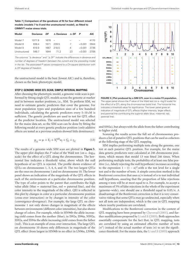
The results of a genome-wide SIM scan are plotted in Figure 5.The upper plot displays the P value of the Wald test (on a –log10

scale) for the effect of a QTL along the chromosomes. The hor-izontal line indicates a threshold value, above which the nullhypothesis of no QTL is rejected. The profile shows evidence ofQTLs on chromosomes 1, 3, 4, 6, and 10. The two largest QTLsare the ones on chromosome 1 and on chromosome 10. The lowerpanel shows an indication of the magnitude of the QTL effects ineach of the environments at a particular chromosome position.The type of color points to the parent that contributes the highvalue allele (blue = maternal line, red = paternal line), and thecolor intensity to the magnitude of the effect. QEI is reflected inthis plot by changes in color at a particular chromosome position(cross-over interaction) or by changes in intensity of the color(convergence-divergence). For example, the large QTL on chro-mosome 1 not only shows changes in magnitude of the effectsbetween environments (different color intensities), but also showschange of colors. For example, while in HN96b the allele increas-ing yield comes from the mother (blue), in IS92a, IS94a, NS92a,SS92a, and SS94a the allele increasing yield comes from the father(red). This is an example of cross-over interaction. The large QTLon chromosome 10 shows only differences in magnitude of theQTL effect (from largest in HN96b to no effect in LN96a, LN96b,

FIGURE 5 | Plot produced by a SIM QTL scan in a maize F2 population.

The upper panel shows the P value of the Wald test (on a –log10 scale) forthe effect of a QTL along the chromosomes (solid line). The horizontal lineindicates a threshold value for significance. The lower panel gives anindication of magnitude of QTL effects (higher intensity, larger effect),and parental line contributing the superior allele (blue, maternal; red,parental line).

and SS92a), but always with the allele from the father contributingto higher yield.

Scanning the results across the full set of chromosomes pro-duces a list of putative QTL positions that can be used as cofactorsat the following stage of the QTL mapping.

SIM implies performing multiple tests along the genome, onetest at each putative QTL position. For example, for the maizedata genetic predictors were calculated at 246 chromosome posi-tions, which means that model 13 was fitted 246 times. Whenperforming multiple tests, the probability of at least one false pos-itive (i.e., falsely rejecting the null hypothesis) increases accordingto the expression 1 − (1 − α)n,with α the test level for a singletest and n the number of tests. A simple correction method is theBonferroni correction that uses α/n instead of α to test individualnull hypotheses, assuring that the proportion of false rejectionsamong n tests will be at most equal to α. For example, to accept amaximum of 5% of false rejections in the whole of the experiment(genome–wide), one should use a threshold equal to 0.05/n. Adisadvantage of the Bonferroni correction is that it is very conser-vative risking that some QTLs may go undetected, especially whennot all tests are independent, which is the case in QTL mappingwhere nearby positions are correlated.

Modifications to the Bonferroni correction in the context ofQTL mapping have been proposed by Cheverud (2001), and fur-ther modifications proposed by Li and Ji (2005). Both approachesessentially compensate for the fact that, in QTL mapping, testsare correlated by using an estimated effective number of tests(n∗) instead of the actual number of tests (n) to set the signifi-cance threshold. For the maize data, the Li and Ji (2005) approach

www.frontiersin.org March 2013 | Volume 4 | Article 44 | 13

Malosetti et al. Statistical models for genotype and QTL-by-environment interaction

produced a value of n∗ = 81, which gives a larger thresholdP value than the Bonferroni correction (divide 0.05 by 81, insteadof dividing by 246). By default, GenStat estimates n∗ and uses itto set the corresponding significance threshold.

STEP 3: COMPOSITE INTERVAL MAPPINGThe power of QTL detection can be improved by reducing thebackground noise caused by QTLs outside the region under test.This is the principle of the CIM approach, simultaneously pro-posed by Jansen and Stam (1994) and Zeng (1994). What makesthe difference between SIM and CIM, is that when performingCIM the model includes a number of cofactors that corrects forthe effects of the genetic background:

μij

= μ + Ej +∑

Xif cjf + Xaddi αj + Gi + εij (14)

In model 14 the term∑

Xif cjf accounts for the effects of QTLs

outside the region that is being tested (Xaddi ), reducing the error

variation and thereby improving the power for QTL detection.Various strategies exist for the selection of a set of cofactors, buta pragmatic approach is to use the results from the SIM scan,including the positions indicative of QTLs by SIM as cofactors.

Another issue that needs to be addressed is that when testingin a region close to a cofactor, it is necessary to exclude the partic-ular cofactor from the model to avoid colinearity with the testedposition. A popular solution is to choose a window around anevaluation position such that if a cofactor falls inside that window,then the cofactor is excluded from the model. Window size affectsthe results of a CIM scan, and there are no clear–cut recommen-dations about which window size to use. For the present example,all cofactors that are on the chromosome being evaluated areexcluded, a strategy known as restricted CIM.

The results of the restricted CIM scan for the maize data arepresented in Figure 6. The profiles point to QTLs on chromo-somes 1, 2, 3, 4, 6, 9, and 10. In comparison with the resultsfrom SIM, the CIM profile reveals the same QTLs (the two majorQTLs on chromosome 1 and 10, and the ones on chromosome3, 4, and 6), but in addition it shows indications of QTLs onchromosomes 2 and 9.

STEP 4: ESTABLISHING A FINAL QTL MODELIn a subsequent modeling step, the QTLs for all positions thatwere found significant in the restricted CIM scan are includedsimultaneously in the mixed model:

μij

= μ + Ej +∑

Xaddiq αjq + Gi + εij (15)

Model 15 is a multi–QTL model constructed by inclusion of thefull set of QTLs identified in the previous CIM scan. QTLs withnon-significant effects will be removed using Wald tests (condi-tional on all other QTLs) to arrive at a final model. The finalmodel for our example data showed that nine out of the ten QTLsfrom the CIM scan were significant in the multi-QTL model.Further, by breaking down the QTL effects into QTL main effects

(αQq ) and QEI effects (αQEI

q ), it was possible to investigate whetherQTL effects were consistent across environments or not. All QTLs

FIGURE 6 | Plot produced by a CIM QTL scan in a maize F2 population.

The upper panel shows the P value of the Wald test (on a –log10 scale) forthe effect of a QTL along the chromosomes (solid line). The horizontal lineindicates a threshold value for significance. The lower panel gives anindication of magnitude of QTL effects (higher intensity, larger effect), andparental line contributing the superior allele (blue, maternal; red,parental line).

but the one at the end of chromosome 3, had significant QEI(P < 0.01).

The estimated QTL effects are given in Table 8. The effect ofa QTL in a particular environment is declared significant whenzero is outside the confidence interval of the estimated effect(CI = estimate ± 2∗s.e., with s.e. the average standard errorobtained from the REML analysis). Results for the large QTL onchromosome 1 (QTL1,141) showed that the QTL had a significanteffect of 0.469 ton·ha−1 in environment SS92a, which means thatfor each replacement of the maternal allele by a paternal allele,a yield increase of about half a ton is expected. The effect of thesame QTL in environment HN96b had a negative sign (−0.232ton·ha−1), which means that rather than an increase, a decreasein yield is expected for the same allele substitution. The effects ofQTL1,141 are inconsistent across environments not only in termsof the size of the effects, but also in terms of the sign of the effect.Inconsistency in size and sign of QTL effects underlies crossoverinteractions, the most important case of GEI (recall Figure 1D).From the breeder’s point of view, the crossover QEI means that,while the maternal allele has to be selected when breeding forenvironment HN96b, the paternal allele will be the choice whenselecting for all the other environments. The other large QTL,which is on chromosome 10 (QTL10,67) showed changes of thesizes of the effects but not of their signs, indicating that the favor-able allele came always from the paternal line. The size of theQTL effect was largest in HN96b (0.564 ton·ha−1), around 0.300ton·ha−1 in IS92a, IS94a, NS92a, and SS94a, and not significantin LN96a, LN96b, and SS92a. Despite changes in effect sizes,

Frontiers in Physiology | Plant Physiology March 2013 | Volume 4 | Article 44 | 14

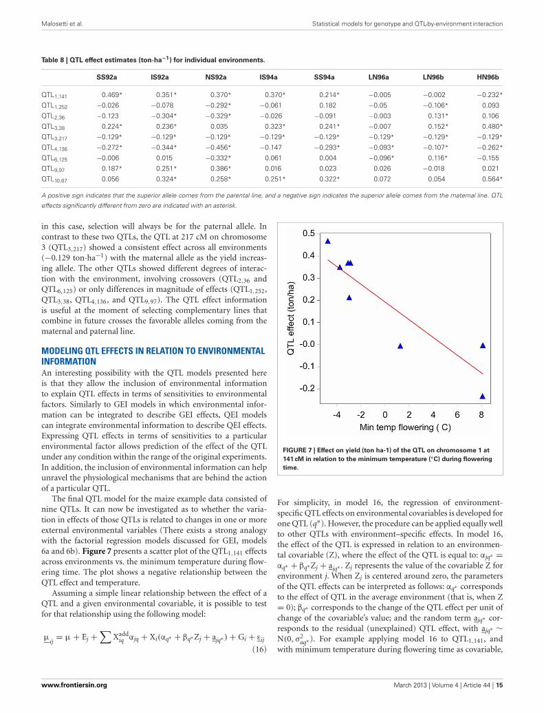
Malosetti et al. Statistical models for genotype and QTL-by-environment interaction

Table 8 | QTL effect estimates (ton·ha−1) for individual environments.

SS92a IS92a NS92a IS94a SS94a LN96a LN96b HN96b

QTL1,141 0.469* 0.351* 0.370* 0.370* 0.214* −0.005 −0.002 −0.232*

QTL1,252 −0.026 −0.078 −0.292* −0.061 0.182 −0.05 −0.106* 0.093

QTL2,36 −0.123 −0.304* −0.329* −0.026 −0.091 −0.003 0.131* 0.106

QTL3,38 0.224* 0.236* 0.035 0.323* 0.241* −0.007 0.152* 0.480*

QTL3,217 −0.129* −0.129* −0.129* −0.129* −0.129* −0.129* −0.129* −0.129*

QTL4,136 −0.272* −0.344* −0.456* −0.147 −0.293* −0.093* −0.107* −0.262*

QTL6,125 −0.006 0.015 −0.332* 0.061 0.004 −0.096* 0.116* −0.155

QTL9,97 0.187* 0.251* 0.386* 0.016 0.023 0.026 −0.018 0.021

QTL10,67 0.056 0.324* 0.258* 0.251* 0.322* 0.072 0.054 0.564*

A positive sign indicates that the superior allele comes from the parental line, and a negative sign indicates the superior allele comes from the maternal line. QTL

effects significantly different from zero are indicated with an asterisk.

in this case, selection will always be for the paternal allele. Incontrast to these two QTLs, the QTL at 217 cM on chromosome3 (QTL3,217) showed a consistent effect across all environments(−0.129 ton·ha−1) with the maternal allele as the yield increas-ing allele. The other QTLs showed different degrees of interac-tion with the environment, involving crossovers (QTL2,36 andQTL6,125) or only differences in magnitude of effects (QTL1,252,QTL3,38, QTL4,136, and QTL9,97). The QTL effect informationis useful at the moment of selecting complementary lines thatcombine in future crosses the favorable alleles coming from thematernal and paternal line.

MODELING QTL EFFECTS IN RELATION TO ENVIRONMENTALINFORMATIONAn interesting possibility with the QTL models presented hereis that they allow the inclusion of environmental informationto explain QTL effects in terms of sensitivities to environmentalfactors. Similarly to GEI models in which environmental infor-mation can be integrated to describe GEI effects, QEI modelscan integrate environmental information to describe QEI effects.Expressing QTL effects in terms of sensitivities to a particularenvironmental factor allows prediction of the effect of the QTLunder any condition within the range of the original experiments.In addition, the inclusion of environmental information can helpunravel the physiological mechanisms that are behind the actionof a particular QTL.

The final QTL model for the maize example data consisted ofnine QTLs. It can now be investigated as to whether the varia-tion in effects of those QTLs is related to changes in one or moreexternal environmental variables (There exists a strong analogywith the factorial regression models discussed for GEI, models6a and 6b). Figure 7 presents a scatter plot of the QTL1,141 effectsacross environments vs. the minimum temperature during flow-ering time. The plot shows a negative relationship between theQTL effect and temperature.

Assuming a simple linear relationship between the effect of aQTL and a given environmental covariable, it is possible to testfor that relationship using the following model:

μij

= μ + Ej +∑

Xaddiq αjq + Xi(αq∗ + βq∗Zj + ajq∗) + Gi + εij

(16)

FIGURE 7 | Effect on yield (ton ha-1) of the QTL on chromosome 1 at

141 cM in relation to the minimum temperature (◦C) during flowering

time.

For simplicity, in model 16, the regression of environment-specific QTL effects on environmental covariables is developed forone QTL (q∗). However, the procedure can be applied equally wellto other QTLs with environment–specific effects. In model 16,the effect of the QTL is expressed in relation to an environmen-tal covariable (Z), where the effect of the QTL is equal to: αjq∗ =αq∗ + βq∗Zj + ajq∗ . Zj represents the value of the covariable Z forenvironment j. When Zj is centered around zero, the parametersof the QTL effects can be interpreted as follows: αq∗ correspondsto the effect of QTL in the average environment (that is, when Z= 0); βq∗ corresponds to the change of the QTL effect per unit ofchange of the covariable’s value; and the random term ajq∗ cor-responds to the residual (unexplained) QTL effect, with ajq∗ ∼N(0, σ2

aq∗ ). For example applying model 16 to QTL1,141, andwith minimum temperature during flowering time as covariable,

www.frontiersin.org March 2013 | Volume 4 | Article 44 | 15

Malosetti et al. Statistical models for genotype and QTL-by-environment interaction

showed a significant reaction of QTL1,141 to changes in the min-imum temperature during flowering, with β estimate equal to−0.040 ton ha−1 ◦C−1. We can interpret this result saying thatwhen the maternal allele is replaced by the paternal allele, weexpect a yield decrease of 0.040 ton ha−1 for each degree Celsiusof increase in the minimum temperature during flowering.

The example assumed a simple linear relationship betweenthe QTL effect and a single environmental covariable, but morecomplex explanatory models can be constructed. For example, itis possible to include higher order terms to model the responsecurve (e.g., a quadratic term), to use spline formulations, or toinclude more than one environmental covariable in the model. Itis important to mention that a close interaction with physiologistsis crucial to explore and select biologically sound models.

CONCLUSIONWe have discussed a suite of statistical models that are usefulto plant breeding practitioners who are dealing with GEI. Whatall models have in common is that they make an attempt toreplace the ANOVA GEIij term by product terms of genotypic

parameters/covariates and environmental parameters/covariates,with as examples bizj (FW, AMMI, and GGE), biZj (factorialregression), and Xiαj (QTL mapping). For some models no otherinformation than the two-way table of means is required (FW,AMMI, and GGE), others require explicit environmental (facto-rial regression) and/or genotypic information (QTL models). Forexploring patterns of GEI, FW, AMMI, and GGE are very useful.For prediction and understanding, factorial regression and QTLmodels are more appropriate.

ACKNOWLEDGMENTSWe acknowledge the support of the Generation ChallengeProgram—Integrated Breeding Platform projects 2.2.1 and 3.2.4for supporting the work presented here. We also thank threeanonymous reviewers for helping us to improve the manuscript.

SUPPLEMENTARY MATERIALThe Supplementary Material for this article can be found onlineat: http://www.frontiersin.org/Plant_Physiology/10.3389/fphys.2013.00044/abstract

REFERENCESAkaike, H. (1974). A new look at the

statistical model identification. IEEETrans. Automat. Contr. 19, 716–723.

Basten, C. J., Weir, B. S., and Zeng, Z.-B.(2002). QTL Cartographer, Version1.16. Department of Statistics,North Carolina State University,Raleigh, NC.

Bernardo, R. (2002). Breeding forQuantitative Traits in Plants.Woodbury, MN: Stemma Press.

Boer, M. P., Wright, D., Feng, L.,Podlich, D. W., Luo, L., Cooper,M., et al. (2007). A mixed-modelquantitative trait loci (QTL) analysisfor multiple-environment trial datausing environmental covariables forQTL-by-environment interactions,with an example in maize. Genetics177, 1801–1813.

Broman, K. W., Wu, H., Sen, S., andChurchill, G. A. (2003). R/qtl: QTLmapping in experimental crosses.Bioinformatics 19, 889–890.

Cheverud, J. M. (2001). A simple cor-rection for multiple comparisonsin interval mapping genome scans.Heredity 87, 52–58.

Cooper, M., and Hammer, G. L.(eds.). (1996). Plant Adaptationand Crop Improvement. Wallingford,UK: CAB International.

Cullis, B. R., Thomson, F. M., Fisher, J.A., Gilmour, A. R., and Thompson,R. (1996a) The analysis of the NSWwheat variety database. I. Modellingtrial error variance. Theor. Appl.Genet. 92, 21–27.

Cullis, B. R., Thomson, F. M., Fisher, J.A., Gilmour, A. R., and Thompson,R. (1996b) The analysis of the NSW

wheat variety database. II. Variancecomponent estimation. Theor. Appl.Genet. 92, 28–39.

Denis, J. B. (1988). Two-way analy-sis using covariables. Statistics 19,123–132.

Falconer, D. S., and Mackay, T.F. C. (1996). Introduction toQuantitative Genetics. 4th Edn.Harlow: Longman.

Finlay, K. W., and Wilkinson, G.N. (1963). The analysis of adap-tation in a plant-breeding pro-gramme. Aust. J. Agric. Res. 14,742–754.

Gabriel, K. (1978). Least squaresapproximation of matrices by addi-tive and multiplicative models. J. R.Stat. Soc. B 40, 186–196.

Galwey, N. W. (2006). Introduction toMixed Modeling: Beyond Regressionand Analysis of Variance. Chichester:John Wiley and Sons Ltd.

Gauch, H. G. (1988). Model selec-tion and validation for yield tri-als with interaction. Biometrics 44,705–715.

Gilmour, A. R., Cullis, B. R., andVerbyla, A. P. (1997). Accountingfor natural and extraneous varia-tion in the analysis of field experi-ments. J. Agric. Biol. Environ. Stat. 2,269–293.

Gollob, H. (1968). A statistical modelwhich combines features of fac-tor analysis and analysis of vari-ance techniques. Psychometrika 33,73–115.

Graffelman, J., and van Eeuwijk, F. A.(2005). Calibration of multivariatescatter plots for exploratory analysisof relations within and between sets

of variables in genomic research.Biom. J. 47, 863–879.

Griffiths, A. J. F., Miller, J. H., Suzuki,D. T., Lewontin, R. C., and Gelbart,W. M. (1996). An Introduction toGenetic Analysis. New York, NY: WHFreeman and Company.

Haley, C. S., and Knott, S. A. (1992).A simple regression method formapping quantitative trait loci inline crosses using flanking markers.Heredity 69, 315–324.

Huang, X., Paulo, M. J., Boer, M.,Effgen, S., Keizer, P., Koornneef, M.,et al. (2011). Analysis of naturalallelic variation in Arabidopsis usinga multiparent recombinant inbredline population. Proc. Natl. Acad.Sci. U.S.A. 108, 4488–4493.

Jansen, R. C., and Stam, P. (1994). Highresolution of quantitative traits intomultiple loci via interval mapping.Genetics 136, 1447–1455.

Jiang, C., and Zeng, Z.-B. (1995).Multiple trait analysis of geneticmapping for quantitative trait loci.Genetics 140, 1111–1127.

Jiang, C. J., and Zeng, Z. B. (1997).Mapping quantitative trait loci withdominant and missing markers invarious crosses from two inbredlines. Genetica 101, 47–58.

Kang, M. S., and Gauch, H. G. (eds.).(1996). Genotype-by-EnvironmentInteraction. Boca Raton, FL: CRCPress Inc.

Li, J., and Ji, L. (2005). Adjusting mul-tiple testing in multilocus analysesusing the eigenvalues of a correla-tion matrix. Heredity 95, 221–227.

Lynch, M., and Walsh, B. (1998).Genetics and Analysis of Quantitative

Traits. Sunderland, MA: SinauerAssociates Inc.

Malosetti, M., van der Linden, C. G.,Vosman, B., and van Eeuwijk, F.A. (2007). A mixed-model approachto association mapping using pedi-gree information with an illustra-tion of resistance to Phytophthorainfestans in potato. Genetics 175,879–889.

Malosetti, M., Voltas, J., Romagosa, I.,Ullrich, S. E., and van Eeuwijk, F.A. (2004). Mixed models includ-ing environmental covariablesfor studying QTL by environ-ment interaction. Euphytica 137,139–145.

Mandel, J. (1969). The partitioning ofinteraction in analysis of variance.J. Res. Natl. Bur. Stand. Math. Sci.73B, 309–328.

Martínez, O., and Curnow, R. N.(1992). Estimating the locations andthe sizes of the effects of quan-titative trait loci using flankingmarkers. Theor. Appl. Genet. 85,480–488.

Mathews, K., Malosetti, M., Chapman,S., McIntyre, L., Reynolds, M.,Shorter, R., et al. (2008). Multi-environment QTL mixed modelsfor drought stress adaptation inwheat. Theor. Appl. Genet. 117,1077–1091.

Mohring, J., and Piepho, H. P. (2009).Comparison of weighting in two-stage analysis of plant breeding tri-als. Crop Sci. 49, 1977–1988.

Pastina, M. M., Malosetti, M., Gazaffi,R., Mollinari, M., Margarido, G.R., Oliveira, K. M., et al. (2012).A mixed model QTL analysis

Frontiers in Physiology | Plant Physiology March 2013 | Volume 4 | Article 44 | 16

Malosetti et al. Statistical models for genotype and QTL-by-environment interaction

for sugarcane multiple-harvest-location trial data. Theor. Appl.Genet. 124, 835–849.

Patterson, H. D., and Thompson,R. (1971). Recovery of inter-block information when blocksizes are unequal. Biometrika 58,545–554.

Payne, R. W., Murray, D. A., Harding,S. A., Baird, D. B., Soutar,D. M., and Lane, P. (2007).GenStat for Windows, 10th EditionIntroduction. Hertfordshire, UK:VSN International, 355.

Przystalski, M., Osman, A., Thiemt, E.M., Rolland, B., Ericson, L., Østerga,H., et al. (2008). Comparing theperformance of cereal varietiesin organic and non-organiccropping systems in differentEuropean countries. Euphytica 163,417–433.

Ribaut, J.-M., Hoisington, D. A.,Deutsch, J. A., Jiang, C., andGonzalez de Leon, D. (1996).Identification of quantitative traitloci under drought conditionsin tropical maize. 1. Floweringparameters and the anthesis-silkinginterval. Theor. Appl. Genet. 92,905–914.

Ribaut, J.-M., Jiang, C., Gonzalezde Leon, D., Edmeades, G. O.,and Hoisington, D. A. (1997).Identification of quantitative traitloci under drought conditions intropical maize. 2. Yield compo-nents and marker-assisted selectionstrategies. Theor. Appl. Genet. 94,887–896.

Sabadin, P., Malosetti, M., Boer, M.,Tardin, F., Santos, F., Guimarães,C., et al. (2012). Studying thegenetic basis of drought tolerancein sorghum by managed stress trialsand adjustments for phenological

and plant height differences. Theor.Appl. Genet. 124, 1389–1402.

Servin, B., Dillmann, C., Decoux, G.,and Hospital, F. (2002). MDM: aprogram to compute fully informa-tive genotype frequencies in com-plex breeding schemes. J. Hered. 93,227–228.

Smith, A. B., Cullis, B. R., andThompson, R. (2005). The analysisof crop cultivar breeding and evalu-ation trials: an overview of currentmixed model approaches. J. Agric.Sci. 143, 449–462.

van Eeuwijk, F. A. (1995). Linear andbilinear models for the analysisof multi-environment trials: I. Aninventory of models. Euphytica 84,1–7.

van Eeuwijk, F. A. (2006). “Genotypeby environment interaction: basicsand beyond,” in Plant Breeding:The Arnell Hallauer InternationalSymposium, eds K. Lamkey andM. Lee (Oxford, UK: BlackwellPublishing), 155–170.

van Eeuwijk, F. A., Bink, M. C. A.M., Chenu, K., and Chapman, S. C.(2010). Detection and use of QTLfor complex traits in multiple envi-ronments. Curr. Opin. Plant Biol. 13,193–205.

van Eeuwijk, F. A., Denis, J. B., andKang, M. S. (1996). “Incorporatingadditional information ongenotypes and environments inmodels for two-way genotype byenvironment tables,” in Genotype-by-Environment Interaction, edsM. S. Kang and H. G. Gauch(Boca Raton, FL: CRC Press Inc.),15–50.

van Eeuwijk, F. A., Malosetti, M., andBoer, M. P. (2007). “Modelingthe genetic basis of responsecurves underlying genotype x

environment interaction,” inScale and Complexity in PlantSystems Research. Gene-Plant-Crop Relations, eds J. H. J.Spiertz, P. C. Struik, and H. H.van Laar (Dordrecht: Springer),115–126.

Verbeke, G., and Molenberghs, G.(2000). Linear Mixed Models forLongitudinal Data. New York, NY:Springer-Verlag.

Voltas, J., van Eeuwijk, F. A., Araus,J. L., and Romagosa, I. (1999a)Integrating statistical and ecophys-iological analysis of genotype byenvironment interaction for grainfilling of barley in Mediterraneanareas. II. Grain growth. Field CropsRes. 62, 75–84.

Voltas, J., van Eeuwijk, F. A., Sombrero,A., Lafarga, A., Igartua, E., andRomagosa, I. (1999b) Integratingstatistical and ecophysiologicalanalysis of genotype by environ-ment interaction for grain filling ofbarley in Mediterranean areas. I.Individual grain weight. Field CropsRes. 62, 63–74.

Voltas, J., van Eeuwijk, F., Igartua, E.,del Moral, L. G., Molina-Cano,J. L., and Romagosa, I. (2002).“Genotype by environment inter-action and adaptation in barleybreeding: basic concepts and meth-ods of analysis,” in Barley Science:Recent Advances from MolecularBiology to Agronomy of Yield andQuality, ed G. Slafer (Binghampton,NY: Food Products Press),205–241.

VSN International. (2012). GenStatfor Windows, 15th Edn. HemelHempstead: VSN International.Web page: GenStat.co.uk

Welham, S. J., Beverley, J. G., Smith,A. B., Thompson, R., and Cullis, B.

R. (2010). A Comparison of analysismethods for late-stage variety eval-uation trials. Aust. N.Z. J. Stat. 52,125–149.

Yan, W., Hunt, L. A., Sheng,Q., and Szlavnics, Z. (2000).Cultivar evaluation and mega-environment investigation basedon the GGE biplot. Crop Sci. 40,597–605.

Zeng, Z. B. (1994). Precision mappingof quantitative trait loci. Genetics136, 1457–1468.

Conflict of Interest Statement: Theauthors declare that the researchwas conducted in the absence of anycommercial or financial relationshipsthat could be construed as a potentialconflict of interest.

Received: 28 September 2012; accepted:25 February 2013; published online: 12March 2013.Citation: Malosetti M, Ribaut J-M andvan Eeuwijk FA (2013) The statisticalanalysis of multi-environment data:modeling genotype-by-environmentinteraction and its genetic basis. Front.Physiol. 4:44. doi: 10.3389/fphys.2013.00044This article was submitted to Frontiers inPlant Physiology, a specialty of Frontiersin Physiology.Copyright © 2013 Malosetti,Ribaut and van Eeuwijk. This is anopen-access article distributed underthe terms of the Creative CommonsAttribution License, which permitsuse, distribution and reproduc-tion in other forums, provided theoriginal authors and source are cred-ited and subject to any copyrightnotices concerning any third-partygraphics etc.

www.frontiersin.org March 2013 | Volume 4 | Article 44 | 17