ClickHere

for

FullArticle

Changing climate in the Bolivian Altiplano: CMIP3projections for temperature and precipitationextremes

J. M. Thibeault,1 A. Seth,1 and M. Garcia2

Received 23 June 2009; revised 25 November 2009; accepted 7 December 2009; published 22 April 2010.

[1] Rural agriculture in the Bolivian Altiplano is vulnerable to climate related shocksincluding drought, frost, and flooding. We examine multimodel, multiscenario projectionsof eight precipitation and temperature extreme indices for the Altiplano and computetemperature indices for La Paz/Alto, covering 1973–2007. Significant increasing trends inobserved warm nights and warm spells are consistent with increasing temperatures in thetropical Andes. The increase in observed frost days is not simulated by the models inthe 20th century, and projections of warm nights, frost days, and heat waves are consistentwith projected annual cycle temperature increases; PDFs are outside their 20th centuryranges by 2070–2099. Projected increases in precipitation extremes share the same sign asobserved trends at Patacamaya and are consistent with annual cycle projections indicatinga later rainy season characterized by less frequent, more intense precipitation. Patacamayaprecipitation indices show shifts in observed distributions not seen in the models until2020–2049, implying that precipitation changes may occur earlier than projected. Theobserved increase in frost days can be understood within the context of precipitationchanges and an increase in radiative cooling. Model warm/wet biases suggest that adecrease in frost days may not occur as early or be as large as projected. Nevertheless,consistencies between simulated and observed extremes, other than frost days, suggest thedirections of projected changes are reliable. These results are a first step toward providingthe critical information necessary to reduce threats to food security and water resourcesin the Altiplano from changing climate.

Citation: Thibeault, J. M., A. Seth, and M. Garcia (2010), Changing climate in the Bolivian Altiplano: CMIP3 projections fortemperature and precipitation extremes, J. Geophys. Res., 115, D08103, doi:10.1029/2009JD012718.

1. Introduction

[2] The Altiplano is a high plateau located in the centralAndes of South America. Traditional methods of rainfedagriculture are practiced by approximately fifty percent ofthe rural population [Garcia et al., 2007]. More than 60% ofannual precipitation occurs during the months of Decemberthrough February and is associated with the southwestmargin of the South American Monsoon (SAM) [Garreaudet al., 2003; Garreaud and Aceituno, 2001]. Crop produc-tion in the Altiplano is particularly vulnerable to climaterelated shocks including drought, flooding, frost and pests[Gilles and Valdivia, 2009]. Information about futurechanges in extreme precipitation and temperature is beingsought by government and NGOs in the Altiplano for thepurpose of developing strategies to reduce future climate‐related risks to agriculture. This research examines climate

projections for the Altiplano region with a focus on theevolution of precipitation and temperature related extremes,and discusses their consistency with the projected changesin the annual cycle.[3] Analyses of 21st century climate projections for the

Altiplano indicate that changes in mean temperature andprecipitation are likely [Urrutia and Vuille, 2009; Seth et al.,2010; Bradley et al., 2006]. Mean temperature changes athigh elevations in the Andes are expected to be greater thanthose in lower elevations [Bradley et al., 2006] and researchefforts are ongoing to understand the effects of increasingtemperatures on tropical Andean glaciers [e.g., Vuille et al.,2008; Juen et al., 2007; Bradley et al., 2006; Francou et al.,2003; Thompson et al., 2003; Vuille et al., 2003]. Whileprojected changes in annual mean precipitation appear to besmall, Seth et al. [2010] have noted a shift in the annualcycle of precipitation in the Altiplano toward reduced earlyseason rains (October–December) and increased peak seasonrains (January–March). This shift is apparently related tosimilar changes documented in the larger‐scale SAM [Sethet al., 2009].[4] Temperature increases are likely to have a substantial

impact on agriculture in tropical regions. Battisti and Naylor

1Department of Geography, University of Connecticut, Storrs,Connecticut, USA.

2Instituto de Investigaciones Agropecuarias y de Recursos Naturales,Universidad Mayor de San Andres, La Paz, Bolivia.

Copyright 2010 by the American Geophysical Union.0148‐0227/10/2009JD012718

JOURNAL OF GEOPHYSICAL RESEARCH, VOL. 115, D08103, doi:10.1029/2009JD012718, 2010

D08103 1 of 18

[2009] point out that projected mean growing season tem-peratures through much of the tropics will likely be outsidethe range of extremes experienced in the 20th century.While the need for climate projection information in theAltiplano is clear, and such information is essential to thedevelopment of local and national climate change adaptationpolicies [Giorgi et al., 2008], two challenges in this regioninclude a lack of observations and climate model resolution.[5] Analyses of observed changes in temperature and

precipitation related extremes require daily data sets ofsufficient quality and length [e.g., Easterling et al., 1999;Alexander et al., 2006]. Observed changes in the frequencyand intensity of extreme temperature [Vincent et al., 2005]and precipitation [Haylock et al., 2006] events have beendocumented for South America; only one station in theAltiplano (Patacamaya, Bolivia) had daily data that met thequality and length criteria to be included in these studies.While analyses of global observations show trends inextreme temperatures consistent with warming [Frich et al.,2002; Alexander et al., 2006], no significant trends intemperature extremes were identified at Patacamaya byVincent et al. [2005]. Consistent with increasing precipita-tion intensity observed in many regions [e.g., Frich et al.,2002; Groisman et al., 2005; Alexander et al., 2006], sig-nificant increasing trends were identified in several extremeprecipitation indices at Patacamaya by Haylock et al.[2006]. This study examines daily data for La Paz/Alto,Bolivia (located in El Alto at the airport, hereafter La Paz),covering 1973–2007, providing a new set of extreme tem-perature indices (as defined byAlexander et al. [2006]) for theAltiplano. In the present analysis, precipitation indices fromPatacamaya and temperature indices computed for La Pazare compared with model simulations for the 20th century.[6] At current horizontal resolutions, coupled global cli-

mate models are not capable of representing complex event‐driven climatic extremes which occur rarely, but researchsuggests that such models can simulate the more simple andfrequently occurring statistics related to high and low dailytemperature and precipitation [Easterling et al., 2000;Meehlet al., 2000, 2005]. Simulated temperature and precipitationextremes have been analyzed by Tebaldi et al. [2006] for20th century historical simulations and 21st century pro-jections using output from the World Climate ResearchProgram (WCRP) Coupled Model Intercomparison Projectversion 3 (CMIP3) [Meehl et al., 2007b]. Simulated his-torical trends in temperature extremes are qualitativelyconsistent with observed global trends and are considered tobe reliable [Tebaldi et al., 2006]. Projected temperatureextremes are consistent with what would be expected in awarmer world (e.g., fewer frost days, more warm nights,increasing heat waves). Projected precipitation extremessuggest greater precipitation intensity, but the CMIP3models disagree about regional patterns of change. Previousstudies have shown that models have less skill at simulatingprecipitation extremes regionally [Kiktev et al., 2003, 2007;Kharin et al., 2007] and identification of trends can besomewhat dependent on the index being examined [Meehl etal., 2007a; Sillmann and Roeckner, 2008; Alexander andArblaster, 2009].[7] Frost days, which are a threat to agriculture in the

Altiplano, were not analyzed for tropical regions by Tebaldiet al. [2006]. In the Altiplano, increases in consecutive dry

days, warm nights, heat waves, and the extreme temperaturerange are expected by 2080–2099. However, climate changeprojections for the next two or three decades are more rel-evant to decision makers and planners who are developingadaptation strategies now.[8] The analysis performed here specifically for the Alti-

plano involves the added challenge of a relatively small,high‐elevation region (∼3800–4000 m). The CMIP3 modelstend to produce excess precipitation near the Andes [Vera etal., 2006; Seth et al., 2010], but most are able to realisticallysimulate the phase of the annual cycle in the core region ofthe SAM [Bombardi and Carvalho, 2009]. Being relativelyflat, the Altiplano is coarsely represented in the medium‐and higher‐resolution global models employed here. Inaddition, consistencies between the large‐scale projectionsfor the SAM [Seth et al., 2009] and Altiplano [Seth et al.,2010] projections suggest that the current models may beable to provide qualitative information about the direction offuture changes in climate extremes for the Altiplano, whilethe tools needed to assess regional‐scale climate changecontinue to improve.[9] This research explores the evolution of extreme tem-

perature and precipitation indices for the Bolivian Altiplanoin the 20th century and Special Report on Emissions Sce-narios (SRES) B1, A1B, and A2 scenarios (B1, A1B, andA2, hereafter) using nine CMIP3 models. Ten extreme cli-mate indices (defined by Frich et al. [2002]) based onsimulated daily temperature and precipitation are availablefor the CMIP3 models. This study examines eight of theseten indices that are relevant for the Altiplano, focusing ontime evolution of the indices and changes in probabilitydensity functions (PDFs) for the middle of the 21st century(2020–2049), an appropriate time frame for adaptation, aswell as the end of the century (2070–2099). To betterunderstand the model projections, this study makes quali-tative comparisons between simulated Altiplano extremesand observed precipitation extremes at Patacamaya andobserved temperature extremes that we calculate for La Paz,Bolivia. Though climate models cannot simulate extremesas they occur in nature, if there are consistencies betweensimulated and observed extremes (e.g., the directions oftrends), greater confidence can be placed in the projections.The Altiplano spans an area from 13°S–25°S and 65°W–70°W; however, the southern region is arid and it is thenorthern Lake Titicaca region which lies on the southernmargin of the SAM, where conditions are more favorablefor agriculture [Garcia et al., 2007].[10] The remainder of the paper is structured as follows.

Section 2 describes the data sets and methods used in thestudy. The results follow in section 3. We begin withobserved extremes indices for comparison with the modeledindices: (1) temperature indices for La Paz and (2) PDFs ofprecipitation indices from Patacamaya. Our analysis of thesimulated extremes indices follows, including comparisonwith projected changes in the annual cycle. The results arefollowed by a discussion in section 4, which is followed byour conclusions.

2. Data and Methods

[11] Eight simulated annual indices are analyzed (definedin Table 1); four indices derived from daily minimum and/or

THIBEAULT ET AL.: ALTIPLANO CLIMATE EXTREMES D08103D08103

2 of 18

maximum temperature: extreme temperature range, frostdays, heat wave duration index, and warm nights, and fourfrom daily precipitation: consecutive dry days, 5 day pre-cipitation, precipitation >95th percentile, and precipitationintensity. Hereafter, all discussion of the simulated indiceswill use the names listed in Table 1.[12] Simulations from nine CMIP3 global coupled climate

models are analyzed. Extreme indices are not available forall models in all scenarios (see Table 2). 20th century his-torical simulations and 21st century B1, A1B, and A2emissions scenarios are examined using a single realizationfrom each model. Intermodel variability is larger by an orderof magnitude than the internal variability of the models. Byusing only one realization from each model, we are sam-pling the larger uncertainty. Pierce et al. [2009] havedemonstrated that incorporating more models into the mul-timodel average actually improves model skill more quicklythan including a larger number of realizations of the samemodel in the multimodel average. In cases where more thanone realization was available, we chose the run at random.[13] This research focuses on the northern Altiplano

(Figure 1). All calculations for the models are averaged forthe area 16°S–19°S by 67°W–70°W. Model selection was

based on resolution and the availability of extremes indices.Eight models are used for the B1 scenario, nine for A1B,and seven for A2. Medium‐ and high‐resolution modelswere carefully examined to determine how well they repre-sent the northern Altiplano. The area defined by 16°S–19°S/67°W–70°W is above 2000 m for all grid points in allmodels selected with one exception: one grid point in theCCSM3 model has an elevation of 1828 m. Because thesensitivity of the area averaged surface temperature annualcycle to the inclusion of this grid point was very smallcompared with the warm bias, it was retained in the analysis.Being relatively flat, the models do represent the northernAltiplano, but several are lower than observed and nonerepresent the highest peaks in the region. Extending theregion to 15°S–20°S by 65°W–70°W includes more gridpoints from elevations below 2000 m, especially in thehigher‐resolution models, increasing warm and wet biases.Sensitivity of the results to area definition will be exploredin the discussion.[14] Observed extreme indices from La Paz (16.50°S/

68.18°W, 4061 m) and Patacamaya (17.20°S/67.92°W,3789 m) are used to validate model simulations of theindices and identify consistencies in the directions of trends.

Table 1. Modeled Extreme Indices Used in This Study and Their Definitionsa

Index Name Definition Unit

Extreme temperature range xtemp range Difference between the highest and lowest temperatureobservations within a given year

K

Frost days frost days Total number of days with minimum temperature <0°C daysHeat wave duration index heat waves Max. period of at least 5 d when Tmax >5°C above the

1961–1990 daily Tmax averagedays

Warm nights warm nights Percent of time in a year when Tmin >90th percentileof minimum temperature for a particular calendar date

%

Consecutive dry days dry days Maximum number of consecutive dry days (Rday <1 mm) days5 day precipitation 5 day precip Maximum 5 day precipitation total mmPrecipitation >95th percentile precip >95th Fraction of total annual precipitation from events >the

1961–1990 95th percentile%

Precipitation intensity precip intensity Annual total precipitation divided by the number of dayswith precip. ≥1 mm d−1

mm d−1

aFrom Frich et al. [2002] and Tebaldi et al. [2006].

Table 2. CMIP3 Coupled Ocean‐Atmosphere Models Used in This Study

Modeling Center Model NameAtmosphereResolutiona

OceanResolutionb

National Center for Atmospheric Research CCSM3c 1.4 × 1.4 320 × 395Meteo‐France, Centre National de Recherches Meteorologiques CNRM‐CM3 2.8 × 2.8 180 × 170U.S. Department of Commerce/NOAA/Geophysical Fluid

Dynamics LaboratoryGFDL‐CM2.0 2.5 × 2 360 × 200

U.S. Department of Commerce/NOAA/Geophysical FluidDynamics Laboratory

GFDL‐CM2.1 2.5 × 2 360 × 200

Center for Climate System Research (University of Tokyo),National Institute for Environmental Studies, and FrontierResearch Center for Global Change (JAMSTEC)

MIROC3.2‐MedRes 2.8 × 2.8 256 × 192

Center for Climate System Research (University of Tokyo),National Institute for Environmental Studies, and FrontierResearch Center for Global Change (JAMSTEC)

MIROC3.2‐HiResc 1.1 × 1.1 320 × 320

National Center for Atmospheric Research PCM 2.8 × 2.8 360 × 180Institut Pierre Simon Laplace IPSL‐CM4 3.75 × 2.5 180 × 170Meteorological Research Institute MRI‐CGCM2.3.2d 2.8 × 2.8 144 × 111

aLongitude by latitude in degrees.bNumber of grids in longitude and latitude.cAnnual extreme indices not provided for A2 scenario.dAnnual extreme indices not provided for B1 scenario.

THIBEAULT ET AL.: ALTIPLANO CLIMATE EXTREMES D08103D08103

3 of 18

The comparison of areally averaged data from the modelswith station (point) data can be problematic [Chen andKnutson, 2008], but our main intention is to make qualita-tive comparisons regarding the signs of observed and sim-ulated trends.[15] Temperature extreme indices are calculated for La

Paz using the U.S. National Climatic Data Center’s (NCDC)Global Surface Summary of the Day (GSOD), and coverthe period 1973–2007. The definitions of observed warmnights and warm spells differ from the model definitions(see Table 3). After the modeling centers submitted extremeindices to the CMIP3 archive, several statistical problemswere discovered in indices calculated using the originaldefinitions of Frich et al. [2002] [Alexander et al., 2006].Modeled indices could not be recalculated using the newdefinitions because the original daily model output is notavailable. Percentiles for observed warm nights and warmspells now use the bootstrapping method of Zhang et al.[2005] to address problems related to inhomogeneities thatexist at base period boundaries [Alexander et al., 2006]. InAustralia, trends in warm nights and heat waves calculatedusing the definition of Frich et al. [2002] were about twiceas large as trends in warm nights and warm spells calculatedusing the definition of Alexander et al. [2006] [Alexanderand Arblaster, 2009]. Many temperature data for La Pazhave a precision of 1°C, especially in the earlier portion ofthe record. Low precision in the temperature data, as is the

case for La Paz, is known to produce a bias in the calcu-lation of percentile‐based temperature indices [Zhang et al.,2009]. Therefore it was necessary to artificially restore thedata precision, as described by Zhang et al. [2009], beforecalculating warm spells and warm nights for La Paz. Theseissues make quantitative comparisons between the observedand modeled indices impossible, and our discussion willemphasize the qualitative aspects of indicated changes.Hereafter, all discussion of La Paz temperature indices willuse the names listed in Table 3.[16] Precipitation extreme indices for Patacamaya (1951–

1999) were provided by the CCl/CLIVAR/JCOMM ExpertTeam on Climate Change Detection and Indices (ETCCDI)Climate Extreme Indices data set available at their Web site:http://cccma.seos.uvic.ca/ETCCDI/data.shtml. The defini-tions for observed 5 day precip, precip >95th, and precipintensity are the same as those for the models. The definitionfor observed dry days is the same as for the models exceptthat a spell can continue across calendar years [Alexanderand Arblaster, 2009]. Because the calendar year changesduring the Altiplano wet season, the difference in definitionis not likely to present a problem in analysis of dry days inthe Altiplano.[17] The time evolution of changes in simulated annual

extreme indices is evaluated by calculating multimodelaverage time series for each scenario covering the period1901–2099. Time series for 1901–2099 were produced byappending data from 21st century scenarios to data from the20th century experiments for each model. The time series ofeach index for each model were standardized, adjusting forany absolute differences in the models and anomalies werecalculated with respect to the base period of 1961–2099.Anomalies were standardized by the standard deviation ofthe detrended base period and the time series for each modelin each scenario were then centered by removing the 1980–1999 average before calculating the multimodel averages.Each multimodel average time series is smoothed by a10 year running average, indicating the direction of change.The significance of trends in the multimodel averages areevaluated at the 90% confidence level using the nonpara-metric Mann‐Kendall trend test, which has been used ex-tensively to evaluate trends in environmental time series[Mann, 1945; Hipel and McLeod, 1994]. As a measure ofintermodel variability, the width of one standard deviationof the ensemble mean is shown with each time series. PDFsof multimodel averages of the eight selected extreme indicesare plotted for two periods in the 20th century (1940–1969and 1970–1999) and two periods in the 21st century (2020–

Figure 1. The northern Altiplano: 16°S–19°S and 67°W–70°W (shaded).

Table 3. Trends in Annual Temperature Extreme Indices at La Paz, Bolivia, for 1973–2007a

Index Name Definition t p Value

Xtemp range same as models 0.138 0.270Frost days same as models 0.194 0.120Warm nights Tmin >90th percentile, but percentile calculation uses

bootstrapping method of [Zhang et al., 2005] (see text)0.457 0.000

Warm spells maximum period >5 consecutive days with Tmax >90thpercentile of daily Tmax for base period. Percentilesare calculated using bootstrapping method of[Zhang et al., 2005] and spells continue acrosscalendar years

0.357 0.008

aBoldface indicates significance at the 90% confidence level based on the Mann Kendall trend test. Indices were derivedfrom NCDC GSOD data.

THIBEAULT ET AL.: ALTIPLANO CLIMATE EXTREMES D08103D08103

4 of 18

2049 and 2070–2099) to identify shifts in the distributionsfor each scenario. Kolmogorov‐Smirnov tests were per-formed on the modeled indices to determine whether themiddle and late 21st century samples are significantly dif-ferent from 1970–1999.[18] Trends in La Paz temperature indices were identified

and tested for statistical significance at the 90% confidencelevel using the Mann‐Kendall trend test. Relative frequencyhistograms and PDFs of xtemp range, frost days, warmspells, and warm nights were produced for comparison withsimulated indices. Precipitation indices at La Paz could notbe calculated for most years because many precipitation dataare missing. To explore the precipitation indices for Pata-camaya beyond what was presented by Haylock et al.[2006], we plot PDFs of dry days, 5 day precip, precip>95th, and precip intensity for 1951–1975 and 1976–1999.Kolmogorov‐Smirnov tests were used to determine whetherthese samples are significantly different from each other.[19] Examination of simulated extreme indices appears to

provide insight into the projected shift in the annual cycle ofprecipitation identified by Seth et al. [2010]. However, theirselection of models was not constrained by the availabilityof extremes data. For consistency, this study recalculateschanges in the annual cycles of temperature and precipita-tion using the same models employed in the extremesanalysis. The changes in each scenario are analyzed bycalculating the differences between the middle (2020–2049)or late 21st century (2070–2099) and late 20th century(1970–1999) climate and then standardizing by each model’slate 20th century standard deviation. The multimodel sta-tistics for present day and future climate are represented bybox plots, which provide information on variability amongthe models. Differences in 21st century minus 1970–1999multimodel mean monthly, seasonal (SON and JFMA), andannual precipitation were tested for their significance. Eachsample was first tested for normality using the Shapiro‐Wilktest. F tests were then used to compare the variances betweennormally distributed 21st and 20th century samples. Two‐sample t tests (Wilcoxon tests) were performed for normally(not normally) distributed samples to identify significantdifferences in multimodel mean precipitation at the 90%confidence level.

3. Results

[20] First, we present our results for the Altiplano observedextreme indices: temperature indices that we calculate for LaPaz, and PDFs for Patacamaya precipitation indices. Wethen present results for the multimodel simulated extremes,including comparison with observed extremes. The simu-lated extreme indices are then compared to projections forthe annual cycle.

3.1. Observed Extreme Indices

[21] We begin with La Paz temperature indices, whichprovided annual indices for 94% of the period 1973–2007.Trends are shown in Table 3 along with index definitions.Positive trends exist in all four indices: xtemp range, frostdays, warm nights, and warm spells. Trends in warm nightsand warm spells are significant. Zhang et al. [2009] havedemonstrated that after artificially restoring low‐precisiontemperature data, exceedance rates have long‐term means

and trends similar to those from data that are originally ofthe same precision as the artificially restored data. Thisprovides a measure of confidence in our results for La Pazwarm nights and warm spells, which were calculated withprecision‐adjusted data.[22] PDFs of precipitation extreme indices at Patacamaya

are shown for two periods (1951–1975 and 1976–1999) inFigure 2. The PDFs of dry days (Figure 2a) and precip>95th (Figure 2c) suggest positive shifts in 1976–1999, butthey are not significantly different from the 1951–1975samples according to Kolmogorov‐Smirnov tests. The dis-tributions of 5 day precip (Figure 2b) show no clear differ-ences between 1951–1975 and 1976–1999. The 1976–1999distribution of precip intensity (Figure 2d) is more variablecompared to 1951–1975; it has longer tails at both ends,with a larger increase at the high end. The time periodsselected for comparison coincide with a cold and warmphase of the Pacific Decadal Oscillation (PDO), whichentered a warm phase in the late 1970s [Mantua et al.,1997]. Decadal variability may also be an important factorin explaining the differences in rainfall extremes at Pataca-maya for the two periods.[23] To summarize, increasing trends were found in all

four temperature indices at La Paz. Increases in warm nightsand warm spells are significant. Frost days and warm nights,both based on daily minimum temperatures, exhibit simul-taneously increasing trends. This result is somewhat unex-pected, but can be understood within the context ofprecipitation changes. Trends in extreme precipitation indicesat Patacamaya suggest that rainfall events may be occurringless frequently in the Altiplano. If this is the case in La Paz,there may be an increase in the number of clear nightsand radiation frosts, offering a possible explanation for theincrease in frost days. PDFs of the precipitation indicessuggest shifts in 1976–1999 distributions: positive shifts indry days and precip >95th, higher variability in precipintensity with larger changes at the high end of the distri-bution. Kolmogorov‐Smirnov tests did not reveal any sta-tistically significant differences in the distributions ofprecipitation indices in 1976–1999 relative to 1951–1975.

3.2. Simulated Temperature Related Extreme Indices

[24] This section presents the multimodel results fortemperature related extreme indices. The results are dis-cussed by index and include analysis of the time evolutionof the indices over 1901–2099, and examination of PDFsfor 1940–1969, 1970–1999, 2020–2049, and 2070–2099.Observed temperature extremes from La Paz are comparedto 20th century simulated extremes to identify qualitativeconsistencies. Time series of multimodel average tempera-ture indices are shown in Figure 3, relative frequency his-tograms and PDFs of temperature extremes at La Paz areshown in Figure 4, and PDFs of multimodel temperatureextremes are shown in Figure 5. Standardized changes in theannual cycle of temperature are shown in Figure 6.[25] Xtemp range is projected to increase by the end of the

21st century in all three scenarios, sharing the same sign as thetrend observed at La Paz (Figure 3a). The largest increaseshown by the 10 year running average is approximately 1.0standard deviation (hereafter, SD) in the A2 scenario; theincrease is about 0.7 SD in the B1 and A1B scenarios. Therange of observed xtemp range at La Paz (about 10°C) is

THIBEAULT ET AL.: ALTIPLANO CLIMATE EXTREMES D08103D08103

5 of 18

more than twice as large as the simulated 20th centuryxtemp range (about 4–5°C for each group of models)(Figures 4a, 5a, 5b, and 5c). PDFs of multimodel averagextemp range exhibit shifts toward higher values by themiddle and late 21st century in each scenario (Figures 5a, 5b,and 5c). However, in the B1 scenario, low values of xtemprange are still close to low values for the 20th century. Thelowest values of xtemp range in the A1B and A2 scenarios areapproximately 1–2°C higher than the lowest 20th centuryvalues.[26] Preliminary analysis revealed that the IPSL‐CM4

model is not simulating frost days for the Altiplano inmost years. It also overestimates Altiplano temperature byapproximately 8°C throughout the year, which is approxi-mately 4°C greater than the next warmest models. IPSL‐CM4 was excluded from the frost days analysis because itwould not provide any useful information about changes infrost days for the Altiplano. Despite its poor simulation offrost days in the Altiplano, the IPSL‐CM4model is employedin the multimodel averages of the remaining seven indices inorder to include the maximum number of models possible.[27] Frost days decrease over 1901–2099 in all three

scenarios (Figure 3b). From approximately 1901–1999, eachscenario shows a decrease in frost days of about 1.0–1.5 SD.

This is in contrast to the increase in frost days observed atLa Paz, and is discussed below. From 2000 to 2099, eachscenario shows a decrease in frost days of approximately2.0 SD. Multimodel averages of frost days are low comparedto the number of frost days that occur annually in La Paz,consistent with warm biases in several models (Figures 4b,5d, 5e, and 5f). In each scenario, distributions of frost days(Figures 5d, 5e, and 5f) show a steady shift toward lowervalues from the middle 20th century to the late 21st century,with the largest reduction in frost days occurring in the A2scenario. By the late century, the distributions of frost days donot share any values with those from the 20th century in theA1B and A2 scenarios, suggesting that the highest numberof annual frost days in the late 21st century will be less thanthe lowest number of annual frost days in the 20th century.[28] Heat waves (Figure 3c) increase sharply after

approximately 2040 in all three scenarios, but appear toincrease more slowly in the B1 scenario after 2070. By2099, heat waves increase by about 3.0 SD in the A2 andA1B scenarios and by about 2.0 SD in the B1 scenario. ThePDFs of multimodel averages of heat waves (Figures 5g, 5h,and 5i) show increases in range and variability from the 20thcentury to the middle century (2020–2049). By the latecentury (2070–2099), all three scenarios show dramatic

Figure 2. PDFs of precipitation extreme indices for Patacamaya, Bolivia. Two periods are shown for the20th century: 1951–1975 (solid line) and 1976–1999 (dashed line). Data are from the ETCCDI ClimateExtreme Indices data set available at http://cccma.seos.uvic.ca/ETCCDMI/data.shtml.

THIBEAULT ET AL.: ALTIPLANO CLIMATE EXTREMES D08103D08103

6 of 18

changes in heat waves relative to the middle century withlarge shifts toward higher values and greater variability. Itshould be noted that heat waves, as defined by Frich et al.[2002], is not a statistically robust index because it uses afixed threshold of 5°C above the 1961–1990 daily Tmax

average in its definition. This is problematic in some regions(e.g., the tropics) where there is little variability in dailytemperatures [Kiktev et al., 2003; Alexander et al., 2006].Warm spell duration at La Paz is calculated from a per-centile‐based threshold and is not directly comparable tomodeled heat waves (Figures 4c, 5g, 5h, and 5i).[29] Warm nights increase in all three scenarios by about

1.0 SD from 1901–1999 (Figure 3d). Though they are notdirectly comparable, trends in modeled warm nights andobserved warm nights at La Paz share the same sign. From2000 to 2099, warm nights increase dramatically in eachscenario: an additional 5.0 SD in the A2 and A1B scenarios,and 4.0 SD in the B1 scenario. The multimodel averages ofwarm nights in the 20th century are consistent with thoseobserved at La Paz (Figures 4d, 5j, 5k, and 5l). The verticalline in Figure 4d indicates the base period average, which isclose to 10%. PDFs of the multimodel averages for the 20thcentury indicate a shift toward more warm nights and highervariability in 1970–1999 relative to 1940–1969 (Figures 5j,5k, and 5l). By the middle century (2020–2049), there is ashift toward more warm nights with increased variability inall three scenarios. By the late century (2070–2049), the

PDFs show larger shifts toward more warm nights, notsharing any values with the 20th century distributions in allthree scenarios.[30] Seth et al. [2010] have previously shown that Alti-

plano temperature is expected to increase throughout theannual cycle by the end of the century. For consistency, wehave recalculated the changes using the models and areadefinition employed in the extremes analysis. Our resultsaffirm earlier results for the late century and also showresults for the middle century (2020–2049).[31] The multimodel medians and means increase by

approximately 2.0 SD across all scenarios by 2020–2049(Figures 6a, 6c, and 6e). By 2070–2099, multimodel statis-tics show that there is less agreement among the models inthe magnitude of the temperature increase, but multimodelmeans and medians suggest an increase of 3.0–6.0 SDthroughout the year across all scenarios (Figures 6b, 6d,and 6f).[32] In summary, projections of frost days, heat waves,

and warm nights are consistent with the projected warming.With the exception of xtemp range, intermodel variability issmaller than the projected changes. Mann‐Kendall trendtests reveal that increasing trends in warm nights, heatwaves, and xtemp range are significant (all p values<0.000). Trends in simulated warm nights and xtemp rangeshare the same sign as those observed at La Paz. Thenegative trends in frost days are also significant (all p values

Figure 3. Simulated time series of temperature extreme indices for 1901–2099 for the Altiplano. The21st century simulations were appended to 20th century simulations. The resulting time series have beenstandardized for each model, then averaged to provide a multimodel time series for each scenario. Thicklines show 10 year running averages. Shading represents the width of 1 standard deviation of the ensemblemean. The 21st century scenarios are shown for the B1 (blue, eight models), A1B (green, nine models),and A2 (red, seven models) scenarios. Note that each scenario uses a different subset of models, resultingin differences in the 20th century portions of the time series.

THIBEAULT ET AL.: ALTIPLANO CLIMATE EXTREMES D08103D08103

7 of 18

<0.000). The decrease in simulated frost days is inconsistentwith the increasing trend at La Paz. However, the increase atLa Paz can be understood within the context of observedand projected precipitation changes: in the early stages ofwarming, an increase in clear nights may lead to an increasein radiation frosts. The models at present are not able tosimulate this observed increase in frost days. The differencein projected and observed trends in frost days will need to beevaluated with high‐resolution models. One possible expla-nation for the increase in xtemp range, which is based ononly two temperatures out of the year, is that very lowminimum temperatures will still occur while maximumtemperatures increase. The PDFs of frost days and warmnights show 2070–2099 values that are completely outsidethe range of 20th century values. Kolmogorov‐Smirnov

tests revealed that the distributions of frost days, heat waves,and warm nights for the middle and late century are sig-nificantly different from 1970–1999 distributions in allscenarios (all p values <0.000). The distribution of xtemprange is significantly different from 1970–1999 in all sce-narios by the late century (all p values <0.05). The result forheat waves should be taken with caution because the modeldefinition is not statistically robust, especially in regions likethe tropics where there is little variability in daily maximumtemperatures. The term “heat waves,” as defined here for themodel simulations, is usually more applicable in warmregions and cities where larger populations are vulnerable tothe effects of extremely high temperatures. In this sense, anincrease in heat waves may be less of a health concern for

Figure 4. Extreme temperature indices for La Paz, Bolivia (1973–2007). The base period is 1973–2002.Relative frequency histograms (shaded) and PDFs (black lines) are shown. Vertical line in Figure 4dindicates base period average of warm nights.

THIBEAULT ET AL.: ALTIPLANO CLIMATE EXTREMES D08103D08103

8 of 18

Figure 5. PDFs of multimodel average extreme temperature indices for the Altiplano; 20th centurysimulations (1940–1969 and 1970–1999) and 21st century projections (2020–2049 and 2070–2099).(a, d, g, j) B1 models (blue), (b, e, h, k) A1B models (green), and (c, f, i, l) A2 models (red). Forconsistency, 1940–1969 and 1970–1999 PDFs use the same models as 21st century PDFs.

THIBEAULT ET AL.: ALTIPLANO CLIMATE EXTREMES D08103D08103

9 of 18

society in the Altiplano, but rather a concern for the effectsof such temperatures on water availability and agriculture.

3.3. Simulated Precipitation Related Extreme Indices

[33] This section presents the multimodel results for pre-cipitation related extreme indices. 20th century simulationsare compared to observed precipitation extremes fromPatacamaya. Time series of multimodel average precipitationindices are shown in Figure 7, PDFs of precipitation extremesat Patacamaya are shown in Figure 2, and PDFs of multi-model temperature extremes are shown in Figure 8. Stan-dardized changes in the annual cycle of precipitation areshown in Figure 9.

[34] Dry days increase in each scenario from the firstdecade of the 21st century to about 2040, sharing the samesign as the trend at Patacamaya (Figure 7a). From 2040, drydays in the B1 scenario remain steady throughout the rest ofthe century with a total increase of about 0.5 SD. Dry daysin the A1B scenario increase until reaching a peak atapproximately 2060, and then change little from 2070onward, reaching a total increase of about 0.5 SD. The A2scenario shows a steady increase throughout the century,increasing by approximately 1.0 SD by 2100. Maximumvalues of the 20th century multimodel averages of dry daysare low compared to the maximum values of dry days atPatacamaya, which can be greater than 100–110 days

Figure 6. Standardized monthly temperature differences (21st century minus 1970–1999) for the middle(2020–2049) and late 21st century (2070–2099): (a) B1midcentury, (b) B1 late century, (c) A1Bmidcentury,(d) A1B late century, (e) A2 midcentury, and (f) A2 late century. Box plots show multimodel statistics:the interquartile range (IQR, shaded) and multimodel median values (horizontal black lines); whiskersrepresent the furthest model value within 1.5 times the IQR, and outliers are shown as open circles.Circled cross symbols indicate the multimodel average.

THIBEAULT ET AL.: ALTIPLANO CLIMATE EXTREMES D08103D08103

10 of 18

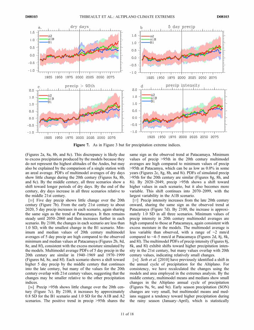
(Figures 2a, 8a, 8b, and 8c). This discrepancy is likely dueto excess precipitation produced by the models because theydo not represent the highest altitudes of the Andes, but mayalso be explained by the comparison of a single station withan areal average. PDFs of multimodel averages of dry daysshow little change during the 20th century (Figures 8a, 8b,and 8c). By the middle century, all three scenarios show ashift toward longer periods of dry days. By the end of thecentury, dry days increase in all three scenarios relative tothe middle 21st century.[35] Five day precip shows little change over the 20th

century (Figure 7b). From the early 21st century to about2020, 5 day precip increases in each scenario, again sharingthe same sign as the trend at Patacamaya. It then remainssteady until 2050–2060 and then increases further in eachscenario. By 2100, the changes in each scenario are less than1.0 SD, with the smallest change in the B1 scenario. Min-imum and median values of 20th century multimodelaverages of 5 day precip are high compared to the observedminimum and median values at Patacamaya (Figures 2b, 8d,8e, and 8f), consistent with the excess moisture simulated bythe models. Multimodel average PDFs of 5 day precip in the20th century are similar in 1940–1969 and 1970–1999(Figures 8d, 8e, and 8f). Each scenario shows a shift towardhigher 5 day precip by the middle century that continuesinto the late century, but many of the values for the 20thcentury overlap with 21st century values, suggesting that thechanges may be smaller relative to the other precipitationindices.[36] Precip >95th shows little change over the 20th cen-

tury (Figure 7c). By 2100, it increases by approximately0.8 SD for the B1 scenario and 1.0 SD for the A1B and A2scenarios. The positive trend in precip >95th shares the

same sign as the observed trend at Patacamaya. Minimumvalues of precip >95th in the 20th century multimodelaverages are high compared to minimum values of precip>95th at Patacamya, which can be as low as 0.0% in someyears (Figures 2c, 8g, 8h, and 8i). PDFs of simulated precip>95th for the 20th century are similar (Figures 8g, 8h, and8i). By 2020–2049, precip >95th shows a shift towardhigher values in each scenario, but it also becomes morevariable. This shift continues into 2070–2099, with thelargest variability in the A1B scenario.[37] Precip intensity increases from the late 20th century

onward, sharing the same sign as the observed trend atPatacamaya (Figure 7d). By 2100, the increase is approxi-mately 1.0 SD in all three scenarios. Minimum values ofprecip intensity in 20th century multimodel averages arehigh compared to those at Patacamaya, again consistent withexcess moisture in the models. The multimodel average isless variable than observed, with a range of ∼2 mm/dcompared to ∼4–5 mm/d at Patacamaya (Figures 2d, 8j, 8k,and 8l). The multimodel PDFs of precip intensity (Figures 8j,8k, and 8l) exhibit shifts toward higher precipitation inten-sity in the 21st century, but many values overlap with 20thcentury values, indicating relatively small changes.[38] Seth et al. [2010] have previously identified a shift in

the annual cycle of precipitation for the Altiplano. Forconsistency, we have recalculated the changes using themodels and area employed in the extremes analysis. By themiddle century, multimodel means and medians show smallchanges in the Altiplano annual cycle of precipitation(Figures 9a, 9c, and 9e). Early season precipitation (SON)changes are very small, but multimodel means and med-ians suggest a tendency toward higher precipitation duringthe rainy season (January–April), which is statistically

Figure 7. As in Figure 3 but for precipitation extreme indices.

THIBEAULT ET AL.: ALTIPLANO CLIMATE EXTREMES D08103D08103

11 of 18

Figure 8. As in Figure 5 but for precipitation extreme indices.

THIBEAULT ET AL.: ALTIPLANO CLIMATE EXTREMES D08103D08103

12 of 18

significant at the 90% level (+4.2%) in the B1 scenario(Table 4). By the late century, the rainy season changes inthe multimodel means and medians are larger in the B1 andA1B scenarios (Figures 9b, 9d, and 9f). In the A2 scenario,rainy season multimodel mean and median values for 2070–2099 are similar to middle century values. Variabilityamong the models increases in all three scenarios by latecentury. Early rainy season multimodel means suggest adecrease in precipitation, but multimodel medians showsmall changes in all scenarios. Late century changes in themultimodel seasonal means are statistically significant in allthree scenarios: increased precipitation during the rainyseason (+3–6%) and decreased in the early season (−3.5 to−7%). These results suggest that by the late century, the rainyseason may be shorter and more intense and the dry seasonmay extend longer into what is now the early rainy season.[39] Note that precipitation decreases during the dry season

(May–August) are not very meaningful for the Altiplano

because precipitation is already very low during thesemonths, less than 0.5 mm/d. Projected changes in totalannual precipitation are generally small and not significant.[40] Mann‐Kendall tests confirm that increasing trends in

dry days, 5 day precip, precip >95th, and precip intensity inthe modeled precipitation indices are significant (all p values<0.000). The positive trends in modeled precipitation indi-ces share the same sign as trends calculated for Patacamayaby Haylock et al. [2006], but intermodel variability is rela-tively large compared to the projected changes. Modeledprecipitation indices have values that are consistent withexcess moisture in the models; dry days are too low and theother indices have minimum and median values that are toohigh. PDFs of simulated precipitation indices suggest thatincreases will be small; many 21st century values overlapwith 20th century values. Kolmogorov−Smirnov tests showthat middle and late century distributions of dry days, precip>95th, and precip intensity are significantly different from

Figure 9. As in Figure 6 but for standardized precipitation differences, including annual and seasonal(SON, JFMA) multimodel averages.

THIBEAULT ET AL.: ALTIPLANO CLIMATE EXTREMES D08103D08103

13 of 18

1970–1999 distributions (all p values <0.05). Distributionsof 5 day precip are significantly different from 1970–1999distributions in all scenarios by the late century (all p values<0.000). The expected increases in dry days, 5 day precip,precip >95th, and precip intensity are consistent with annualcycle projections for a drier or weaker early rainy seasonand shorter more intense peak rainy season.

4. Discussion

[41] Our results indicate positive trends in observedtemperature indices at La Paz: xtemp range, frost days,warm nights, and warm spells, of which warm nights andwarm spells are significant. Haylock et al. [2006] identifiedincreasing trends in precipitation indices at Patacamaya: drydays, 5 day precip, precip >95th, precip intensity, of whichprecip >95th was significant. With the exception of frostdays, the observed trends agree in direction with the projectedtrends. In this section we will discuss the observed versusprojected trends, and begin with a sensitivity analysis.[42] Because the resolution of the CMIP3 models presents

a challenge in our analysis for the Altiplano, we examine thesensitivity of our results to area definition. Individual modelgrid points do represent the northern Altiplano with ele-vations between approximately 2000 m and 4000 m within16°S–19°S and 67°W–70°W (defined as the northern Alti-plano, hereafter, “study region”). Because this region is small,we reexamine frost days for a larger region encompassing15°S–20°S by 65°W–70°W (hereafter, “extended region”).[43] PDFs of frost days illustrate the sensitivity of our

results to area definition (Figure 10). The extended regionincludes more grid points from lower elevations, increasingthe warm and wet biases in the results. Simulated frost daysare sensitive to the area selected, but the direction of changeis not. The results continue to indicate that the number offrost days is expected to decrease through the 21st centurywith late century values largely outside the range of 20thcentury frost days. Standardized time series show that thedecrease in frost days in the extended region (not shown) isapproximately 3.0 SD (covering 1901–2099) compared toapproximately 4.0 SD in the study region. Standardized time

series of dry days and precip intensity in the extended regionshow similar changes to those for the study region. TheirPDFs (not shown) indicate a larger wet bias in comparisonwith the study region. Frost days seem to be the most sen-sitive index to area selection. Similarities in the standardizedtime series of dry days and precip intensity in the extendedregion and study region provide added confidence that theextremes projections presented above are reliable, indicatingthe direction of future changes.[44] The observed temperature indices at La Paz

(section 3.1), were shown to have increasing trends in warmnights and warm spells, which are consistent with increasingtemperature trends identified in the tropical Andes by anumber of studies [see Vuille et al., 2008]. However, unex-pectedly, frost days and warm nights both exhibit increasingtrends. An additional index calculation for cold nights,defined as the number of days within a year in which Tmin

<10th percentile also shows an increasing trend at La Paz.Though this trend is not statistically significant, it providesfurther evidence that the frequencies of both cold and warmnights are increasing at La Paz. Vincent et al. [2005] alsoidentified positive trends in cold nights and warm nights atPatacamaya covering 1960–2000 that were not statisticallysignificant. The increasing trends in cold nights and warmnights at Patacamaya provide evidence that the simultaneousincreases and decreases in minimum temperatures found atLa Paz may not be an isolated occurrence.[45] We found that these observed increasing trends in

frost days and cold nights at La Paz are not simulated by themodels in the 20th century. In the early stages of warming,there may be more frequent radiation frosts resulting fromclear nights due to precipitation changes. However, frostsare likely to decrease as warming continues. Because the20th century simulated frost days are fewer than thoseobserved at La Paz, the reduction in frost days may not be aslarge or occur as soon as the models project. A reduction infrost days may be beneficial to agriculture in the Altiplano ifwater supplies are adequate. However, the expected highertemperatures may limit the potential benefits from a reduc-tion in frost days unless there is an increase in precipitationlarge enough to offset increased evaporation. The projected

Table 4. Multimodel Projected Precipitation Changes for the B1, A1B, and A2 Scenarios for the Middle (2020–2049) and Late (2070–2099) 21st Century for the Altiplanoa

B1 A1B A2

Midcentury Late Century Midcentury Late Century Midcentury Late Century

Jan 4.05 4.33 1.31 3.29 3.60 0.90Feb 3.06 5.41 0.09 5.91 −0.40 3.76Mar 4.59 7.72 3.35 10.42 2.75 3.04Apr 6.08 8.55 3.78 4.86 2.89 8.06May −19.20 −9.04 −14.65 −16.43 −12.61 −28.72Jun 2.78 −13.71 −3.63 −17.00 −0.66 −17.16Jul −20.35 −22.44 −17.91 −16.59 −12.35 −39.96Aug 0.45 −15.66 −6.54 −18.60 −5.31 −16.42Sep −3.77 −7.93 −4.31 −11.08 −2.70 −24.95Oct 0.30 −7.73 −0.02 −5.36 3.16 −5.44Nov 1.10 0.55 2.90 1.14 1.55 −3.02Dec −0.19 1.61 −0.24 1.82 1.08 0.65

JFMA 4.19 6.11 1.77 6.09 2.07 3.33SON −0.16 −4.05 0.46 −3.54 1.39 −7.31Annual 1.35 1.31 0.25 1.33 1.11 3.31

aDifferences are shown in percent change. Boldface indicates statistical significance at the 90% confidence level.

THIBEAULT ET AL.: ALTIPLANO CLIMATE EXTREMES D08103D08103

14 of 18

Figure 10. PDFs of frost days. Results for (a, c, e) 16°S–19°S by 67°W–70°W and (b, d, f) 15°S–20°Sby 65°W–70°W. Blue, green, and red indicate the B1, A1B, and A2 models, respectively. For consistency,1940–1969 and 1970–1999 PDFs use the same models as 21st century PDFs.

THIBEAULT ET AL.: ALTIPLANO CLIMATE EXTREMES D08103D08103

15 of 18

increases in heat waves and warm nights are qualitativelyconsistent with the increasing trends in warm spells andwarm nights observed at La Paz, but an increase in heatwaves, as calculated by the models, is not likely to increasethe threats to human health in the Altiplano from extremelyhigh temperatures. On the other hand, extended periods ofrelatively high temperatures may affect the surface waterbalance, impacting water supplies and agriculture. Theprojected increase in xtemp range is consistent with the ideathat some very low minimum temperatures will still occur inthe Altiplano while daytimemaximum temperatures increase.The lowest temperatures of the year in the Altiplano occurduring the dry season. This will likely continue to be true inthe future, not seriously impacting agriculture in the region.[46] Results from Haylock et al. [2006] showed increasing

trends in precipitation extreme indices at Patacamaya (pos-itive shifts in dry days and precip >95th, higher variability inprecip intensity), which combined with no significantchange in total annual precipitation, suggests that rainfall isoccurring in less frequent, more intense events. The increasein dry days is likely to be during the dry season, and extendinginto the early rainy season in September. If precipitation atLa Paz is changing in a similar manner, the increasing trendsin frost days and cold nights may be related to changes inprecipitation extremes. Fewer rainfall events would lead toan increase in clear nights with very low temperatures. Thus,the projected increases in 5 day precip, precip >95th, precipintensity, and dry days are all consistent with annual cycleprojections for a shorter rainy season characterized by lessfrequent, yet more intense rainfall events. The increases inmodeled precipitation indices share the same signs as trendsin observed precipitation indices at Patacamaya, suggestingthat despite the uncertainty in precipitation projections, themodels are able to provide reliable qualitative informationabout the direction of future trends. However, additionalfactors, such as decadal variability associated with the PDOare likely to be important in both the observed and futuretrends.

5. Conclusions

[47] This study has examined projected changes inextremes of temperature and precipitation for the BolivianAltiplano using the CMIP3 database and observations fromtwo stations. Our purpose has been to make qualitativecomparisons between the observed and simulated extremesto gain insight into the projections.[48] Analysis of observations shows significant increasing

trends in warm nights and warm spell duration, which areconsistent with increasing temperatures in the tropical Andes.However, observed frost days also show increasing trends,while model simulated temperature indices (frost days andwarm nights) are both consistent with temperature increases.The models are overpredicting a decrease in frost days in theobserved record due to the warm/wet biases in the models.Thus, improved representation of topography is essential inthe projection of frost days in this region. The observedincreases in frost days and cold nights can be understoodwithin the context of observed precipitation indices; reduc-tions in precipitation frequency may lead to an increase inthe frequency of clear nights with very low temperatures.Positive shifts in the observed distributions of dry days,

precip >95th, and precip intensity at Patacamaya suggestshifts that are not seen in the models until 2020–2049,implying that a lengthening of the dry season or weakeningof the early rainy season may already be occurring in theAltiplano. This shift may also be influenced by natural cli-mate variability associated with the recent warm phase ofthe PDO, which began in the late 1970s.[49] Projections of Altiplano precipitation extremes pro-

vide insight into and are consistent with the projected shiftin the annual cycle, but intermodel variability is large rela-tive to the projected increases. A delayed or weaker earlyrainy season could delay the sowing date of late varieties ofquinoa, which is an important staple crop in the Altiplano[Aguilar and Jacobsen, 2003]. Positive trends in precipita-tion indices are consistent with annual cycle projectionsindicating a shorter rainy season characterized by less fre-quent, but more intense rainfall events. More intense pre-cipitation may increase the risk of flooding in the Altiplanoand may also impact agriculture; e.g., heavy precipitationand saturated soils lower quinoa yields [Aguilar andJacobsen, 2003]. The simulated precipitation extremeshave values consistent with excess moisture produced by themodels, but the projected increases share the same signs astrends in precipitation indices at Patacamaya, providingconfidence in our results.[50] Projected increases in warm nights and decreases in

frost days may prove to be beneficial to Altiplano agricul-ture if water supplies are adequate. However, in mostsemiarid regions, the expected large temperature increasesare likely to increase rates of evapotranspiration, reducingsoil moisture even with small increases in precipitation[Wang, 2005]. Our results suggest that any increase in totalprecipitation is likely to be small, and may not be sufficientto offset the effects of higher temperatures on evapotrans-piration. Battisti and Naylor [2009] suggest that in the tro-pics, decreased soil moisture will cause large crop losses inaddition to those that might be expected from highertemperatures alone. In the Altiplano, crop losses due todecreased soil moisture may be particularly severe becauseevapotranspiration rates are already high and soils have alow moisture retention capacity [Garcia et al., 2007]. Heatstress and drought can also make plants more vulnerable todisease and insect pests [Garrett et al., 2006]. In the future,even with an increase in warm nights and higher maximumtemperatures, frost is likely to be a continued, though lessfrequent, threat to agriculture in the Altiplano. The projectedincrease in xtemp range suggests that relatively cool nightswill continue, but the coldest nights will likely occur duringthe dry season (austral winter).[51] Consistencies between projected and observed extreme

indices in the Altiplano (with the exception of frost days)suggest that the global models may be reliable tools forindicating the direction of future changes. The direction ofchange is not sensitive to area definition, which providesfurther confidence in the results. Annual cycle projectionsfor precipitation and temperature, as well as projections fortemperature indices (except xtemp range) show betteragreement among the models in 2020–2049 than in 2070–2099, a time frame that is appropriate for developingadaptation strategies. Cox and Stephenson [2007] explainthat climate predictions have the lowest uncertainty whenforecast lead times range from 30 to 50 years, hence, the

THIBEAULT ET AL.: ALTIPLANO CLIMATE EXTREMES D08103D08103

16 of 18

results presented for the middle century may be useful forinitial planning that seeks to limit future climate‐relatedrisks to agriculture in the Altiplano.[52] We note two primary caveats associated with these

results. First, the lack of available daily station data makes itdifficult to accurately assess observed trends in Altiplanoextreme indices. Data mining exercises are in progress in theregion (personal communication, SENAMHI Bolivia), andin the meantime, the results from Patacamaya and La Pazprovide insight into the model projections. Second, climatemodels do not simulate extreme weather and climate in thesame way that they occur in nature and comparisons ofstation (point) data with areally averaged data from themodels cannot be made directly. Climate model projectionsfor regions with complex topography must be taken withcaution. The results presented here will need to be furthertested in improved, higher resolution climate models.Nevertheless, the Altiplano is relatively flat, and the medium‐and higher‐resolution global models do represent this region(though lower than observed elevations). Further, sensitivityanalysis supported the use of a 3° by 3° region to representthe Altiplano in this analysis. Comparisons between theprojections and observed extreme indices have been usefulin interpreting the projections, and suggest that the modelsmay be able to provide reliable qualitative information aboutthe direction of future changes in extreme temperature andprecipitation for the Altiplano.[53] Because the warming in the tropical Andes may be

larger and occur at a faster rate than what the CMIP3 modelsproject [Bradley et al., 2006; Vuille et al., 2008], thechanges in extremes may also be larger and felt sooner thanour results indicate. Battisti and Naylor [2009] point out thatprojected mean growing season temperatures through muchof the tropics will likely be outside the range of extremesexperienced in the 20th century. Our results suggest thatextreme indices also show substantial shifts in distribution,which will have serious impacts on agriculture and waterresources in the Altiplano. Adaptation strategies are beingdeveloped to mitigate the potential effects of changing cli-mate. Results presented here, including likely higher tem-peratures and less frequent but more intense precipitation, area first step toward the critical information needed to reducethreats to food security and water resources in the Altiplano.

[54] Acknowledgments. The authors thank Xuebin Zhang and FengYang from ETCCDI for their assistance with the La Paz temperature dataand Claudia Tebaldi for helpful comments and suggestions. The thoroughand constructive comments from three anonymous reviewers haveimproved the quality of this manuscript substantively. The authors thankthe international modeling groups for providing their data for analysis,the Program for Climate Model Diagnosis and Intercomparison (PCMDI)for collecting and archiving the model data, the JSC/CLIVAR WorkingGroup on Coupled Modelling (WGCM) and their Coupled Model Inter-comparison Project (CMIP3) and Climate Simulation Panel for organizingthe model data analysis activity, and the IPCC WG1 TSU for technical sup-port. The IPCC Data Archive at Lawrence Livermore National Laboratoryis supported by the Office of Science, U.S. Department of Energy. Thisresearch was supported by a Long‐Term Research award (LTR‐4) in theSustainable Agriculture and Natural Resource Management (SANREM)Collaborative Research Program (CRSP) with funding from USAID.

ReferencesAguilar, P. C., and S. E. Jacobsen (2003), Cultivation of quinoa on the PeruvianAltiplano, Food Rev. Int., 19(1–2), 31–41, doi:10.1081/FRI-120018866.

Alexander, L. V., and J. M. Arblaster (2009), Assessing trends in observedand modelled climate extremes over Australia in relation to future projec-tions, Int. J. Climatol., 29(3), 417–435, doi:10.1002/joc.1730.

Alexander, L. V., et al. (2006), Global observed changes in daily climateextremes of temperature and precipitation, J. Geophys. Res., 111,D05109, doi:10.1029/2005JD006290.

Battisti, D. S., and R. L. Naylor (2009), Historical warnings of future foodinsecurity with unprecedented seasonal heat, Science, 323(5911), 240–244, doi:10.1126/science.1164363.

Bombardi, R., and L. Carvalho (2009), IPCC global coupled model simu-lations of the South America monsoon system, Clim. Dyn., 33, 893–916,doi:10.1007/s00382-008-0488-1.

Bradley, R. S., M. Vuille, H. F. Diaz, and W. Vergara (2006), Threats towater supplies in the tropical Andes, Science, 312(5781), 1755–1756,doi:10.1126/science.1128087.

Chen, C.‐T., and T. Knutson (2008), On the verification and comparison ofextreme rainfall indices from climate models, J. Clim., 21(7), 1605–1621,doi:10.1175/2007JCLI1494.1.

Cox, P., and D. Stephenson (2007), Climate change—A changing climatefor prediction, Science, 317(5835), 207–208, doi:10.1126/science.1145956.

Easterling, D. R., H. F. Diaz, A. V. Douglas, W. D. Hogg, K. E. Kunkel,J. C. Rogers, and J. F. Wilkinson (1999), Long‐term observations formonitoring extremes in the Americas, Clim. Change, 42(1), 285–308.

Easterling, D. R., G. A. Meehl, C. Parmesan, S. A. Changnon, T. R. Karl,and L. O. Mearns (2000), Climate extremes: Observations, modeling, andimpacts, Science, 289(5487), 2068–2074, doi:10.1126/science.289.5487.2068.

Francou, B., M. Vuille, P. Wagnon, J. Mendoza, and J. E. Sicart (2003),Tropical climate change recorded by a glacier in the central Andes duringthe last decades of the twentieth century: Chacaltaya, Bolivia, 16°S,J. Geophys. Res., 108(D5), 4154, doi:10.1029/2002JD002959.

Frich, P., L. V. Alexander, P. Della‐Marta, B. Gleason, M. Haylock, A. M.G. K. Tank, and T. Peterson (2002), Observed coherent changes in climaticextremes during the second half of the twentieth century, Clim. Res., 19,193–212.

Garcia, M., D. Raes, S. E. Jacobsen, and T. Michel (2007), Agroclimaticconstraints for rainfed agriculture in the Bolivian Altiplano, J. AridEnviron., 71(1), 109–121, doi:10.1016/j.jaridenv.2007.02.005.

Garreaud, R. D., and P. Aceituno (2001), Interannual rainfall variabilityover the South American Altiplano, J. Clim., 14(12), 2779–2789.

Garreaud, R., M. Vuille, and A. C. Clement (2003), The climate of theAltiplano: Observed current conditions and mechanisms of past changes,Palaeogeogr. Palaeoclimatol . Palaeoecol. , 194(1–3), 5–22,doi:10.1016/S0031-0182(03)00269-4.

Garrett, K. A., S. P. Dendy, E. E. Frank, M. N. Rouse, and S. E. Travers(2006), Climate change effects on plant disease: Genomes to ecosystems,Annu. Rev. Phytopathol., 44, 489–509, doi:10.1146annurev.phyto.44.070505.143420.

Gilles, J. L., and C. Valdivia (2009), Local forecast communication in theAltiplano, Bull. Am. Meteorol. Soc., 90(1), 85–91, doi:10.1175/2008BAMS2183.1.

Giorgi, F., et al. (2008), The regional climate change hyper‐matrix frame-work, Eos Trans. AGU, 89(45), 445–446, doi:10.1029/2008EO450001.

Groisman, P. Y., R. W. Knight, D. R. Easterling, T. R. Karl, G. C. Hegerl,and V. A. N. Razuvaev (2005), Trends in intense precipitation in the cli-mate record, J. Clim., 18(9), 1326–1350.

Haylock, M. R., et al. (2006), Trends in total and extreme South Americanrainfall in 1960–2000 and links with sea surface temperature, J. Clim.,19(8), 1490–1512, doi:10.1175/JCLI3695.1.

Hipel, K. W., and A. I. McLeod (1994), Time Series Modelling of WaterResources and Environmental Systems, Elsevier, Amsterdam.

Juen, I., G. Kaser, and C. Georges (2007), Modelling observed and futurerunoff from a glacierized tropical catchment (Cordillera Blanca, Peru),Global Planet. Change, 59(1–4), 37–48, doi:10.1016/j.gloplacha.2006.11.038.

Kharin, V. V., F. W. Zwiers, X. B. Zhang, and G. C. Hegerl (2007),Changes in temperature and precipitation extremes in the IPCC ensembleof global coupled model simulations, J. Clim., 20(8), 1419–1444.

Kiktev, D., D. M. H. Sexton, L. Alexander, and C. K. Folland (2003),Comparison of modeled and observed trends in indices of daily climateextremes, J. Clim., 16(22), 3560–3571, doi:10.1175/1520-0442(2003)016.

Kiktev, D., J. Caesar, L. V. Alexander, H. Shiogama, and M. Collier(2007), Comparison of observed and multimodeled trends in annualextremes of temperature and precipitation, Geophys. Res. Lett., 34,L10702, doi:10.1029/2007GL029539.

Mann, H. B. (1945), Nonparametric tests against trend, Econometrica, 13,245–259.

THIBEAULT ET AL.: ALTIPLANO CLIMATE EXTREMES D08103D08103

17 of 18

Mantua, N. J., S. R. Hare, Y. Zhang, J. M. Wallace, and R. C. Francis(1997), A Pacific interdecadal climate oscillation with impacts on salmonproduction, Bull. Am. Meteorol. Soc., 78(6), 1069–1079.

Meehl, G. A., et al. (2000), An introduction to trends in extreme weatherand climate events: Observations, socioeconomic impacts, terrestrial eco-logical impacts, and model projections, Bull. Am. Meteorol. Soc., 81(3),413–416.

Meehl, G. A., J. M. Arblaster, and C. Tebaldi (2005), Understanding futurepatterns of increased precipitation intensity in climate model simulations,Geophys. Res. Lett., 32, L18719, doi:10.1029/2005GL023680.

Meehl, G. A., J. M. Arblaster, and C. Tebaldi (2007a), Contributions ofnatural and anthropogenic forcing to changes in temperature extremesover the United States, Geophys. Res. Lett., 34, L19709, doi:10.1029/2007GL030948.

Meehl, G. A., C. Covey, T. Delworth, M. Latif, B. McAvaney, J. F. B.Mitchell, R. J. Stouffer, and K. E. Taylor (2007b), The WCRP CMIP3multimodel dataset–A new era in climate change research, Bull. Am.Meteorol. Soc., 88(9), 1383–1394, doi:10.1175/BAMS-88-9-1383.

Pierce, D. W., T. P. Barnett, B. D. Santer, and P. J. Gleckler (2009), Select-ing global climate models for regional climate change studies, Proc Natl.Acad. Sci. U. S. A., 106(21), 8441–8446, doi:10.1073/pnas.0900094106.

Seth, A., M. Rojas, and S. Rauscher (2009), CMIP3 projected changes inthe annual cycle of the South American monsoon, Clim. Change, 98(3),331–357, doi:10.1007/s10584-009-9736-6.

Seth, A., J. Thibeault, M. Garcia, and C. Valdivia (2010), Making sense of21st century climate change in the Altiplano: Observed trends andCMIP3 projections, Ann. Assoc. Am. Geogr., in press.

Sillmann, J., and E. Roeckner (2008), Indices for extreme events in projec-tions of anthropogenic climate change, Clim. Change, 86(1), 83–104.

Tebaldi, C., K. Hayhoe, J. M. Arblaster, and G. A. Meehl (2006), Going tothe extremes: An intercomparison of model‐simulated historical andfuture changes in extreme events, Clim. Change, 79(3–4), 185–211,doi:10.1007/S10584-006-9051-4.

Thompson, L. G., E. Mosley‐Thompson, M. E. Davis, P. N. Lin,K. Henderson, and T. A. Mashiotta (2003), Tropical glacier and ice core

evidence of climate change on annual to millennial time scales, Clim.Change, 59(1–2), 137–155.

Urrutia, R., andM. Vuille (2009), Climate change projections for the tropicalAndes using a regional climate model: Temperature and precipitationsimulations for the end of the 21st century, J. Geophys. Res., 114,D02108, doi:10.1029/2008JD011021.

Vera, C., G. Silvestri, B. Liebmann, and P. González (2006), Climatechange scenarios for seasonal precipitation in South America fromIPCC‐AR4 models, Geophys. Res. Lett., 33, L13707, doi:10.1029/2006GL025759.

Vincent, L. A., et al. (2005), Observed trends in indices of daily tempera-ture extremes in South America 1960–2000, J. Clim., 18(23), 5011–5023, doi:10.1175/JCLI3589.1.

Vuille, M., R. S. Bradley, M. Werner, and F. Keimig (2003), 20th centuryclimate change in the tropical Andes: Observations and model results,Clim. Change, 59(1–2), 75–99.

Vuille, M., B. Francou, P. Wagnon, I. Juen, G. Kaser, B. G. Mark, andR. S. Bradley (2008), Climate change and tropical Andean glaciers:Past, present and future, Earth Sci. Rev., 89(3–4), 79–96, doi:10.1016/j.earscirev.2008.04.002.

Wang, G. L. (2005), Agricultural drought in a future climate: Results from15 global climate models participating in the IPCC 4th assessment, Clim.Dyn., 25, 739–753, doi:10.1007/s00382-005-0057-9.

Zhang, X., G. Hegerl, F. Zwiers, and J. Kenyon (2005), Avoiding inhomo-geneity in percentile‐based indices of temperature extremes, J. Clim.,18(11), 1641–1651, doi:10.1175/JCLI3366.1.

Zhang, X., F. W. Zwiers, and G. Hegerl (2009), The influences of dataprecision on the calculation of temperature percentile indices, Int. J.Climatol., 29(3), 321–327, doi:10.1002/joc.1738.

M. Garcia, Instituto de Investigaciones Agropecuarias y de RecursosNaturales, Universidad Mayor de San Andres, La Paz, Bolivia.A. Seth and J. M. Thibeault, Department of Geography, University of

Connecticut, CLAS Bldg., 215 Glenbrook Rd., U‐4148, Storrs, CT06269‐4148, USA. (jeanne.thibeault@uconn.edu)

THIBEAULT ET AL.: ALTIPLANO CLIMATE EXTREMES D08103D08103

18 of 18