Progress in the Study of Climatic Extremes in Northern and Central Europe
Upload
khangminh22Category
view
0download
0
Pacific-Australia Climate Change Science and Adaptation Planning Program
Climate Variability, Extremes and Change in the Western Tropical Pacific: New Science and Updated Country Reports
2014

Climate Variability, Extremes and Change in the Western Tropical Pacific: New Science and Updated Country Reports
© Australian Bureau of Meteorology and Commonwealth Scientific and Industrial Research Organisation (CSIRO) 2014
National Library of Australia Cataloguing-in-Publication entry
978-1-4863-0288-8 Climate Variability, Extremes and Change in the Western Tropical Pacific: New Science and Updated Country Reports. Australian Bureau of Meteorology and CSIRO – PRINT
978-1-4863-0289-5 Climate Variability, Extremes and Change in the Western Tropical Pacific: New Science and Updated Country Reports. Australian Bureau of Meteorology and CSIRO – ONLINE
Includes index.
Climatic changes--Pacific Region. Climate change mitigation--Pacific Region.
This publication should be cited as:
Australian Bureau of Meteorology and CSIRO (2014). Climate Variability, Extremes and Change in the Western Tropical Pacific: New Science and Updated Country Reports. Pacific-Australia Climate Change Science and Adaptation Planning Program Technical Report, Australian Bureau of Meteorology and Commonwealth Scientific and Industrial Research Organisation, Melbourne, Australia.
Cover: Manono Island, Samoa, Stuart Chape

Pacific-Australia Climate Change Science and Adaptation Planning Program
Climate Variability, Extremes and Change in the Western Tropical Pacific: New Science and Updated Country Reports
2014
Australian Bureau of Meteorology and Commonwealth Scientific and Industrial Research Organisation (CSIRO)

Climate Variability, Extremes and Change in the Western Tropical Pacific: New Science and Updated Country Reports

Foreword
Foreword
On a global basis, small island developing states are known to be highly vulnerable to climate-related impacts. People living in the Pacific Islands and East Timor are already experiencing higher temperatures, shifts in rainfall patterns, rising sea levels and changes in frequency and intensity of extreme climatic events. Further changes are expected long into the future as a result of climate change associated with human activity. On top of an existing, naturally variable climate, these longer-term changes are now affecting the sustainability of important infrastructure, industries and environmental assets in the western tropical Pacific region. As a consequence, changes of this magnitude are having a profound impact directly on the livelihoods of Pacific islanders, particularly in terms of cultural heritage, socio-economic wellbeing and personal health and safety.
Despite widespread international awareness of climate impacts in this region, to date there has been limited scientific information available to inform climate adaptation planning and disaster risk management for Pacific Island countries and East Timor. Indeed, better scientific knowledge is urgently needed to provide evidence that is based on reliable data and analyses to enable these countries to more effectively and efficiently plan and adapt for a sustainable future.
The science component of the Pacific-Australia Climate Change Science and Adaptation Planning (PACCSAP) program works in 14 island countries and East Timor. The program is a collaborative partnership between Australian scientists and Partner Countries and regional and non-government organisations in the western tropical Pacific over the period 2011–14. This program has helped fill the climate information and knowledge gap in the region by:
• Collating and digitising climate data records for Pacific Island countries and East Timor.
• Examining past climate observations and trends, large-scale climate processes and natural variability.
• Providing national-scale climate projections for the 21st century for four different greenhouse gas and aerosol emissions scenarios based on global climate model outputs.
• Developing a suite of digital tools to improve management, access, modelling and analysis of climate data, including enhanced seasonal forecasting capability at national-scale; and
• Communicating key climate science findings and developing in-country climate science capacity.
This report is a key output of the program and provides policy developers, planners and other stakeholders with the latest peer-reviewed and most relevant, science-based evidence to inform decision-making for climate adaptation planning and disaster risk management purposes. In the longer term, such evidence-based decisions are expected to facilitate more sustainable, resilient development outcomes for Partner Countries and communities across the region.
Dr Andrew Johnson
Executive Director Environment CSIRO
Dr Rob Vertessy
Director of Meteorology and CEO Bureau of Meteorology

Climate Variability, Extremes and Change in the Western Tropical Pacific: New Science and Updated Country Reports

iContents
Contents
Abbreviations .................................................................................................................................................... iv
Acknowledgements ........................................................................................................................................... v
Executive Summary ...........................................................................................................................................1
About this Report .............................................................................................................................................................. 2
Climate Modelling and Performance .................................................................................................................................. 3
About the Projections ........................................................................................................................................................ 3
Regional Climate Observations and Trends ....................................................................................................................... 4
Regional Climate Projections ............................................................................................................................................. 5
Chapter 1 Introduction to the Country Reports .................................................................................................7
1.1 Climate Summary ....................................................................................................................................................... 8
1.2 Data Availability ........................................................................................................................................................... 8
1.3 Seasonal Cycles ......................................................................................................................................................... 8
1.4 Observed Trends ......................................................................................................................................................... 9
1.5 Projections ................................................................................................................................................................ 10
Chapter 2 Cook Islands ...................................................................................................................................21
2.1 Climate Summary ..................................................................................................................................................... 22
2.2 Data Availability ......................................................................................................................................................... 23
2.3 Seasonal Cycles ....................................................................................................................................................... 23
2.4 Observed Trends ....................................................................................................................................................... 26
2.5 Climate Projections ................................................................................................................................................... 31
Chapter 3 East Timor (Timor-Leste) .................................................................................................................49
3.1 Climate Summary ..................................................................................................................................................... 50
3.2 Data Availability ......................................................................................................................................................... 50
3.3 Seasonal Cycles ....................................................................................................................................................... 51
3.4 Observed Trends ....................................................................................................................................................... 52
3.5 Climate Projections ................................................................................................................................................... 53
Chapter 4 Federated States of Micronesia ......................................................................................................65
4.1 Climate Summary ..................................................................................................................................................... 66
4.2 Data Availability ......................................................................................................................................................... 67
4.3 Seasonal Cycles ....................................................................................................................................................... 67
4.4 Observed Trends ....................................................................................................................................................... 70
4.5 Climate Projections ................................................................................................................................................... 76
Chapter 5 Fiji Islands .......................................................................................................................................93
5.1 Climate Summary ..................................................................................................................................................... 94
5.2 Data Availability ......................................................................................................................................................... 94
5.3 Seasonal Cycles ....................................................................................................................................................... 95
5.4 Observed Trends ....................................................................................................................................................... 97
5.5 Climate Projections ................................................................................................................................................. 102

ii Climate Variability, Extremes and Change in the Western Tropical Pacific: New Science and Updated Country Reports
Chapter 6 Kiribati ...........................................................................................................................................113
6.1 Climate Summary ................................................................................................................................................... 114
6.2 Data Availability ....................................................................................................................................................... 115
6.3 Seasonal Cycles ..................................................................................................................................................... 115
6.4 Observed Trends ..................................................................................................................................................... 118
6.5 Climate Projections ................................................................................................................................................. 122
Chapter 7 Marshall Islands ............................................................................................................................141
7.1 Climate Summary ................................................................................................................................................... 142
7.2 Data Availability ....................................................................................................................................................... 143
7.3 Seasonal Cycles ..................................................................................................................................................... 143
7.4 Observed Trends ..................................................................................................................................................... 145
7.5 Climate Projections ................................................................................................................................................. 150
Chapter 8 Nauru ............................................................................................................................................167
8.1 Climate Summary ................................................................................................................................................... 168
8.2 Data Availability ....................................................................................................................................................... 168
8.3 Seasonal Cycles ..................................................................................................................................................... 169
8.4 Observed Trends ..................................................................................................................................................... 170
8.5 Climate Projections ................................................................................................................................................. 172
Chapter 9 Niue ...............................................................................................................................................183
9.1 Climate Summary ................................................................................................................................................... 184
9.2 Data Availability ....................................................................................................................................................... 185
9.3 Seasonal Cycles ..................................................................................................................................................... 185
9.4 Observed Trends ..................................................................................................................................................... 187
9.5 Climate Projections ................................................................................................................................................. 190
Chapter 10 Palau ...........................................................................................................................................201
10.1 Climate Summary ................................................................................................................................................. 202
10.2 Data Availability ..................................................................................................................................................... 203
10.3 Seasonal Cycles ................................................................................................................................................... 203
10.4 Observed Trends ................................................................................................................................................... 205
10.5 Climate Projections ............................................................................................................................................... 208
Chapter 11 Papua New Guinea .....................................................................................................................219
11.1 Climate Summary ................................................................................................................................................. 220
11.2 Data Availability ..................................................................................................................................................... 220
11.3 Seasonal Cycles ................................................................................................................................................... 221
11.4 Observed Trends ................................................................................................................................................... 222
11.5 Climate Projections ............................................................................................................................................... 227

iiiContents
Chapter 12 Samoa .........................................................................................................................................241
12.1 Climate Summary ................................................................................................................................................. 242
12.2 Data Availability ..................................................................................................................................................... 242
12.3 Seasonal Cycles .................................................................................................................................................. 243
12.4 Observed Trends ................................................................................................................................................... 244
12.5 Climate Projections ............................................................................................................................................... 248
Chapter 13 Solomon Islands .........................................................................................................................259
13.1 Climate Summary ................................................................................................................................................. 260
13.2 Data Availability ..................................................................................................................................................... 261
13.3 Seasonal Cycles ................................................................................................................................................... 261
13.4 Observed Trends ................................................................................................................................................... 264
13.5 Climate Projections ............................................................................................................................................... 268
Chapter 14 Tonga ..........................................................................................................................................281
14.1 Climate Summary ................................................................................................................................................. 282
14.2 Data Availability ..................................................................................................................................................... 282
14.3 Seasonal Cycles ................................................................................................................................................... 283
14.4 Observed Trends ................................................................................................................................................... 285
14.5 Climate Projections ............................................................................................................................................... 289
Chapter 15 Tuvalu ..........................................................................................................................................301
15.1 Climate Summary ................................................................................................................................................. 302
15.2 Data Availability ..................................................................................................................................................... 302
15.3 Seasonal Cycles ................................................................................................................................................... 303
15.4 Observed Trends ................................................................................................................................................... 305
15.5 Climate Projections ............................................................................................................................................... 308
Chapter 16 Vanuatu .......................................................................................................................................319
16.1 Climate Summary ................................................................................................................................................. 320
16.2 Data Availability ..................................................................................................................................................... 321
16.3 Seasonal Cycles ................................................................................................................................................... 321
16.4 Observed Trends ................................................................................................................................................... 324
16.5 Climate Projections ............................................................................................................................................... 329
References ....................................................................................................................................................341
Glossary ........................................................................................................................................................345
Appendix A Models included for each analysis for each scenario ...................................................................353

iv Climate Variability, Extremes and Change in the Western Tropical Pacific: New Science and Updated Country Reports
Abbreviations
CCAM Conformal Cubic Atmospheric Model
CMIP5 Coupled Model Intercomparison Project (Phase 5)
CSIRO Commonwealth Scientific and Industrial Research Organisation
EEZ Exclusive Economic Zone
ENSO El Niño-Southern Oscillation
GCM global climate model
GPCP Global Precipitation Climatology Project
IPCC Intergovernmental Panel on Climate Change
ITCZ Intertropical Convergence Zone
PACCSAP Pacific-Australia Climate Change Science and Adaptation Planning Program
PCCSP Pacific Climate Change Science Program
RCP Representative Concentration Pathway
SAM Southern Annular Mode
SPCZ South Pacific Convergence Zone
SST sea-surface temperature
WPM West Pacific Monsoon

vAcknowledgements
Acknowledgements
This report has benefited from the high degree of cooperation and collaboration that exists between the implementing agencies for the science component of the Pacific-Australia Climate Change Science and Adaptation Planning Program, specifically the Australian Bureau of Meteorology and the Commonwealth Scientific and Industrial Research Organisation, together with the valuable, ongoing support from the National Meteorological and Weather Services in Partner Countries, regional organisations and other stakeholders across the western tropical Pacific.
Lead AuthorsDeborah Abbs, Michael Grose, Mark Hemer, Andrew Lenton, Simon McGree, Claire Trenham and Xuebin Zhang.
Josephine Brown, Tom Durrant, Chris Evenhuis, Diana Greenslade, Kevin Hennessy, Agata Imileska, Jack Katzfey, Yuri Kuleshov, Clothilde Langlais, Sugata Narsey, Kevin Tory, Kirien Whan and Louise Wilson.
External Peer ReviewDavid Wratt, National Institute of Water and Atmospheric Research (NIWA), New Zealand.
Scientific EditorBryson Bates.
Scientific ReviewersKevin Hennessy, Kathleen McInnes, Brad Murphy, Scott Power and Blair Trewin.
Editorial CommitteeJodie Kane, Mandy Hopkins, Jillian Rischbieth, Jessica Ciccotelli and Geoff Gooley.
Editorial SupportStephanie Baldwin and Kathy Pullman.
Design and LayoutSiobhan Duffy.

vi Climate Variability, Extremes and Change in the Western Tropical Pacific: New Science and Updated Country Reports

1
Executive Summary
Solomon Islands

2 Climate Variability, Extremes and Change in the Western Tropical Pacific: New Science and Updated Country Reports
About this Report
This report documents the key findings of the science component of the Pacific-Australia Climate Change Science and Adaptation Planning (PACCSAP) Program (2011–2014). It describes new understanding of large-scale climate processes, variability and extremes in the western tropical Pacific (Figure 1.1), together with new projections for the 21st century based on Coupled Model Intercomparison Project (Phase 5) (CMIP5)-based global climate model (GCM) projections for individual countries. The projections are aligned with greenhouse gas and aerosol concentration scenarios and terminology adopted by the Intergovernmental Panel on Climate Change (IPCC) 2013 report; Climate Change 2013: The Physical Science Basis. Contribution of Working Group I to the Fifth Assessment Report of the Intergovernmental Panel on Climate Change.
This new report supplements information from a previous report published jointly by the Australian Bureau of Meteorology and the Commonwealth Scientific and
Industrial Research Organisation (CSIRO) in 2011 as part of the Pacific Climate Change Science Program (PCCSP), entitled:
Climate change in the Pacific: Scientific assessment and new research – Volume 1: Regional Overview and Volume 2: Country reports
The previous PCCSP report (Australian Bureau of Meteorology and CSIRO, 2011) provides a general, regional-scale description of large-scale climate processes, variability and extremes and projections based on Coupled Model Intercomparison Project CMIP Phase 3 (CMIP3)-GCMs. This provides context for the latest national-scale climate science findings provided in this new PACCSAP report.
The first chapter provides a general introduction to the content, structure and methods used for each Partner Country report in subsequent chapters, including specific reference to:
• Data availability;
• Seasonal cycles, including wind-driven waves;
• Observed trends over the past 30-60 years, including air temperature, rainfall and tropical cyclones; and
• Climate projections, including how to understand new CMIP5 GCM outputs and emission scenarios, multiple possible futures, natural variability, confidence statements, presentation of projections, and detailed projection methods for relevant climate variables.
Each subsequent Partner Country chapter has five key sections that provide: (1) a current and future climate summary, (2) historical data records, (3) seasonal cycles, (4) observed trends, and (5) projections for atmospheric and oceanic variables. Projections are provided for temperature, rainfall, extreme events (including tropical cyclones, extreme hot days, and heavy rainfall days), sea-surface temperature, ocean acidification and sea-level rise for four future 20-year periods centred on 2030, 2050, 2070 and 2090.
Map showing the western tropical Pacific Partner Countries in this report: Cook Islands, Federated States of Micronesia, Fiji, Kiribati, Marshall Islands, Nauru, Niue, Palau, Papua New Guinea, Samoa, Solomon Islands, Tonga, Tuvalu, Vanuatu and East Timor.

3Executive Summary
Climate Modelling and Performance
While global climate models (GCMs) are presently the best available tool for making climate projections out to 2100, it is not possible to identify a single ‘best’ scenario or GCM that will accurately forecast the future evolution of greenhouse gas concentrations and our climate.
GCMs produce large-scale projections for computational grid cells that have a horizontal spacing of 70–280 km. This means some results may not incorporate finer-scale but otherwise locally-influential features such as the spatial characteristics of island topography and land cover, inshore bathymetry and local-scale meteorological effects.
Even though all GCMs are based on the same physical laws, they are not perfect representations of the real world because they cannot take into account the things we do not know, e.g. how society will develop and adapt, and what natural climate variability will be experienced in the future. GCMs also differ in how they represent physical processes that occur at spatial scales smaller than that of the grid cells.
Confidence in GCM projections (see About the Projections) is higher for some variables (e.g. temperature) than for others (e.g. rainfall), and it is higher for larger spatial scales and longer averaging periods. On the other
hand, confidence is lower for smaller spatial scales, which represents a particular challenge for Partner Country projections in the Pacific, particularly for some of the smaller, low lying atoll nations.
When interpreting projected climate changes throughout this report, it is also important to keep in mind that natural climate variability, such as the state of El Niño–Southern Oscillation (ENSO), strongly affects the climate from one year to the next. The Interdecadal Pacific Oscillation (IPO) can also affect the Pacific climate from one decade to the next.
About the Projections
The science component of the PACCSAP Program has produced climate projections for the western tropical Pacific using up to 26 new GCMs that have been assessed to perform acceptably well over the region. This means there is a range of possible futures generated from these models for each Partner Country. These futures are expressed as a multi-model average change, with a range of uncertainty due to differences between models.
Consistent with the IPCC (2013), the projections use four new greenhouse gas and aerosol concentration emission scenarios, called Representative Concentration Pathways (RCPs): RCP2.6 (very low emissions), RCP4.5 (low emissions), RCP6 (medium emissions) and RCP8.5 (very high emissions). The lowest scenario shows the likely outcome of reducing emissions (mitigation), and the highest scenario shows the impact of a pathway with no climate policy and high emissions. These pathways cover a broader range of possibilities compared with the emission scenarios (B1-low, A1B-
medium, and A2-high) used for the previous CMIP3-based projections presented in the 2011 PCCSP report (Australian Bureau of Meteorology and CSIRO, 2011). New analyses included in this latest PACCSAP report, and not previously in the Australian Bureau of Meteorology and CSIRO (2011) report, include trends in extreme air temperature, rainfall and ocean waves.
In practice, results from the CMIP5 projections in this report are very similar to the previous CMIP3 results (Australian Bureau of Meteorology and CSIRO, 2011) when the differences in emission scenarios are taken into account. Another important change between the previous PCCSP work and the new PACCSAP work in this report is the way more advanced and appropriate methods for calculating changes to extremes and drought are used and documented, e.g. using box plots of drought in different categories. Once again, after accounting for the effect of different pathways, the main differences between the previous and new results are mainly reflected in changes to country rainfall projections.
A confidence rating (very high, high, medium, and low) for the direction and magnitude of change is provided with each projection, consistent with the IPCC guidance on confidence assessment. Confidence in the magnitude of change indicates how well the model represents the expected change for a particular scenario. The confidence in the magnitude of change is often lower than the confidence in the direction of change. Confidence is reduced when there are model biases in relevant climate features and where there is a wide range of projections from the models.
Some confidence ratings have changed from those described previously by PCCSP (Australian Bureau of Meteorology and CSIRO, 2011). This is due to new PACCSAP research showing greater uncertainty in the projection of large-scale climate features and processes. It is also due to a greater range of projections that are produced using CMIP5 compared with CMIP3 models. In particular, some rainfall confidence ratings have been reduced from ‘high’ to ‘medium’ or from ‘medium’ to ‘low.’

4 Climate Variability, Extremes and Change in the Western Tropical Pacific: New Science and Updated Country Reports
Regional Climate Observations and Trends
Large-scale Regional Climate ProcessesMost of the GCM projections described in this report show increases in Western Pacific Monsoon (WPM) rainfall in a warmer climate, mostly over the wet season, leading to a stronger seasonal rainfall cycle.
They project increases in rainfall within the Inter-Tropical Convergence Zone (ITCZ), particularly in the June to August season, which will amplify the seasonal cycle. This area is projected to expand, in line with these increases, towards the equator.
The average position of the South Pacific Convergence Zone (SPCZ) is not expected to change significantly, although the years when it moves north and merges with the ITCZ will become more frequent. Changes in SPCZ rainfall are uncertain but they are sensitive to sea-surface temperatures not well simulated by many models.
El Niño and La Niña events will continue to occur in the future, but there is little agreement between the climate models on whether these events will change in intensity or frequency.
In general, climate observations and trends across the region for Partner Countries indicate:
Temperature• On a regional scale, station-based
observations show a persistent mean annual warming trend of 0.18°C since 1961, with most of the warmest years on record in the last two decades. There have been significantly more warm days and nights, and fewer cool days and nights.
• Since 1951, the frequency of warm days and nights has increased more than three-fold across the region. Once rare extremes, that used to occur approximately 20 days in a year, are now occurring much more frequently, between 45–80 days in a year.
Rainfall• Rainfall is highly variable, and over
the past 30 years, the southwest and northwest Pacific has become wetter and the central Pacific drier.
• In general, there has been no consistent trend across the region in the long-term for mean and daily extremes of rainfall over the past half century.
Oceans• Sea surface temperatures have
increased, and year-to-year variability is largely due to ENSO.
• Ocean acidification continues to increase in response to human activities.
• As the ocean warms, the risk of coral bleaching (recurrence and severity) increases.
• Sea levels have risen, and vary across the Pacific with large-scale climate processes.
• Extreme sea levels are caused by a combination of long-term sea-level rise from climate change and short-term climate variability factors, such as combined effects of king tides, storm surge and associated wind-wave setup.
• Wind-driven waves that have influence on coastal regions exhibit strong seasonality, and year-to-year variability is largely due to ENSO. The relationship of annual wind-wave properties to ENSO varies regionally.
Tropical cyclones• An updated analysis of cyclone
track data for the South Pacific through to the 2010–11 season shows a slight decrease in the total number of cyclones, with little change in the number of the most intense. As complete records of estimated tropical cyclone intensity are only available from 1981, studies of tropical cyclone trends are limited to this time. Using three different tropical cyclone archives, researchers found contrary trends in the proportion of intense tropical cyclones in the western North Pacific over the past few decades.

5Executive Summary
Regional Climate Projections
At a regional scale, climate projections that are consistent for Partner Countries across the region in general indicate:
TemperatureCompared to the base period 1986–2005:
• Average temperatures will increase, bringing more extremely hot days and warm nights (by 2030, the projected warming is likely to be around +0.5–1.0°C, regardless of the emissions scenario, and by 2090 a very high emissions scenario could increase temperatures by +2.0–4.0°C).
• Extreme temperatures that occur once every 20 years on average are projected to increase in line with average temperatures by up to +2.0–4.0°C by 2090 under the very high emissions scenario.
Rainfall• Average annual rainfall will increase
with fewer droughts in most areas.
• Extreme rainfall events that occur once every 20 years on average during 1986–2005 are projected to occur once every seven to ten years by 2090 under a very low emissions scenario, and every four to six years by 2090 under a very high emissions scenario.
Other• Rising sea levels.
• Increasing sea surface temperature.
• Increasing ocean acidification.
• More frequent and longer lasting coral bleaching.
• Changes to wind-driven waves.
• Less frequent but more severe tropical cyclones.
The details of specific projections for rainfall, temperature, drought, waves and other variables vary to some extent between the Partner Countries. All observed climate trends and projections are explained in detail for each Partner Country in Chapters 2-16.

6 Climate Variability, Extremes and Change in the Western Tropical Pacific: New Science and Updated Country Reports

7
Chapter 1 Introduction to the Country Reports
Tuvalu, PACC, SPREP

8 Climate Variability, Extremes and Change in the Western Tropical Pacific: New Science and Updated Country Reports
1.1 Climate SummaryA climate summary is presented at the beginning of each country chapter which gives an overview of the observations and projections for the relevant country.
1.2 Data AvailabilityThis section provides updated information on the meteorological observation networks and data records available in each country. The length, completeness and quality of historical data records differ from country to country. For many observation sites there have been changes in station position, instrumentation and local environment that have produced inhomogeneities which are artificial changes in the data over time. For rainfall, only records or parts of records that have passed homogeneity tests are used in this report. For temperature, where possible, inhomogeneities have been identified and corrected using statistical techniques. Details on the quality control and homogenisation procedures are available in Whan et al. (2013), and McGree et al. (2013) for temperature and rainfall respectively.
1.3 Seasonal CyclesInformation on temperature and rainfall seasonal cycles can be found in Australian Bureau of Meteorology and CSIRO (2011).
1.3.1 Wind-driven Waves
This section provides new information on wind-driven waves. Observational wave data in the Pacific are sparse, with few wave rider buoy records in the region. Continuous satellite altimeter coverage from 1993 exists, but the temporal and spatial characteristics of these data present a number of challenges on longer time scales, with insufficient data resolution or duration for long-term wave climate studies. To supplement observational data, so-called hindcasts are used. A hindcast is an estimate of past observational data from numerical
models run for past years using historical forcing data. Hindcasts provide a homogenous dataset in both space and time for studying wave climate. A reanalysis is an assimilation of historical observational data, which may be used to drive a hindcast.
Historically, the ability to produce a hindcast has been limited by the lack of global high-resolution reanalysis wind data to force the wave model. The recently completed Climate Forecast System Reanalysis (CFSR; Saha et al., 2010), performed at the National Center for Environmental Prediction, provides hourly surface winds on a 0.3 degree spatial grid. These winds were used to force the WaveWatch III model (Tolman 1991, 2009) for the period 1979–2009. This hindcast comprised a global grid at a spatial resolution of 0.4 degrees, providing boundary data to high-resolution nested sub-grids of 10 and 4 arcminutes (18 and 7 km respectively) around Australia and Pacific Island Partner Countries
(Figure 1.1). All output data were archived at hourly intervals. Data were taken from the nearest model grid point to locations of interest (e.g. capital cities) from the 4 arcminute grid.
1.3.2 Data Presented
The wave model outputs give information on ocean wave climate in terms of three main variables: Significant Wave Height (m), Mean Wave Period (s) and Mean Wave Direction (degrees clockwise from north, indicating the direction from which the wave is travelling) (see Table X.1 in each country report). A mean annual cycle for each variable was generated by finding the average of all values in each month.
For brevity, only wave height and direction are plotted, while values and confidence ranges are given for all three variables. These wave height values are for off-shore waves only and do not apply to any lagoonal waves in atolls, which are not modelled.
Figure 1.1: Region of validated high-resolution 30-year wave hindcast (an estimate of past observational data derived from models), showing a global 10 degree grid, with a series of nested grids of 10 and 4 arcminutes (~18 and 7 km respectively) in the western tropical Pacific. Data in ‘Seasonal Cycles’ sections for each country were taken from the nearest model grid point to locations of interest (e.g. capital cities) from the 4 arcminute (7km) grid.

9Chapter 1: Introduction to the Country Reports
Uncertainties are shown as a box drawn at 1 standard deviation from the mean, determined from all data in that month. Bars show the 5th and 95th percentiles, representing interannual variability.
1.4 Observed TrendsThis section provides revised and updated analyses of observed trends for annual and seasonal air temperature and rainfall. Where only monthly records are available, these have been used to extend and fill gaps in the monthly average/total time series derived from daily values (subject to passing quality control and homogeneity checks). This product supersedes the Pacific Climate Change Science Programme (PCCSP), (Australian Bureau of Meteorology and CSIRO, 2011) high quality monthly rainfall and temperature datasets and related analyses. New analyses include trends in extreme air temperature, rainfall and ocean waves.
1.4.1 Annual, Half-year and Extreme (Daily) Air Temperature and Rainfall
Each chapter provides information on mean annual and half-year air temperature and total rainfall trends for one or two sites in each country, depending on data availability. Information is also provided on annual extreme (daily) air temperature and rainfall trends.
Linear trends for station records are calculated using a Kendall’s tau-based slope estimator (Sen, 1968). This method has been widely used to compute trends in hydro-meteorological series (Wang and Swail, 2001; Zhang et al., 2005; Caesar et al., 2011). The significance of the trend and confidence intervals is modified to account for the presence of lag-1 autocorrelation in the residuals (Wang and Swail, 2001). Seventy percent of data are required (once processing has taken place) before a trend can be computed using the Kendall’s slope estimator. Trends are deemed significant at the 5%
level when results lie beyond ±1.96 standard deviations of the median trend. In most cases, differences between the linear trends from this method and the ordinary least squares method (used in the mean and extreme plot in the Pacific Climate Change Data Portal www.bom.gov.au/climate/pccsp/) are small. Further information on methodology and additional results can be found in McGree et al. (2013) and Whan et al. (2013).
The eight rainfall and air temperature extreme indices (Table 1.1) used in the country chapters are based on the recommendations of the Expert Team on Climate Change Detection and Indices (ETCCDI, http://cccma.seos.univ.ca/ETCCDMI). Of the 27 core ETCCDI indices, 25 indices (excluding indices relating to freezing conditions) and several user-defined indices are available in the Pacific Climate Change Data Portal. Where the four air temperature extreme indices in Table 1.1 cannot be computed due to data limitations, four alternative but equally relevant indices (Table 1.2) have been presented.
Table 1.1: Selected rainfall and air temperature extreme indices.
Indices Index ID Definition Units
Cool Nights TN10p Number of days with minimum temperature less than the 10th percentile for the base period 1971–2000
days/decade
Cool Days TX10p Number of days with maximum temperature less than the 10th percentile for the base period 1971–2000
days/decade
Warm Nights TN90p Number of days with minimum temperature greater than the 90th percentile for the base period 1971–2000
days/decade
Warm Days TX90p Number of days with maximum temperature greater than the 90th percentile for the base period 1971–2000
days/decade
Rain Days ≥ 1 mm R1 Annual count of days where rainfall is greater or equal to 1 mm (0.039 inches) days/decade
Very Wet Day Rainfall R95p Amount of rain where daily rainfall is greater than the 95th percentile for the reference period 1971–2000
mm/decade
Consecutive Dry Days CDD Maximum number of consecutive days with rainfall less than 1 mm (0.039 inches) days/decade
Max 1-day Rainfall Rx1day Annual maximum 1-day rainfall mm/decade
Table 1.2: Alternative air temperature extreme indices.
Indices Index ID Definition Units
Max Tmax TXx Annual maximum value of daily maximum temperature °C or F/decade
Max Tmin TNx Annual maximum value of daily minimum temperature °C or F/decade
Min Tmax TXn Annual minimum value of daily maximum temperature °C or F/decade
Min Tmin TNn Annual minimum value of daily minimum temperature °C or F/decade

10 Climate Variability, Extremes and Change in the Western Tropical Pacific: New Science and Updated Country Reports
Colour-coding is used in data plots to show the influence of the El Niño–Southern Oscillation (ENSO): light-blue columns indicate El Niño years, dark blue columns La Niña years and grey columns neutral years. El Niño and La Niña years are defined using the June–December Southern Oscillation Index (SOI) calculated according to the standard Bureau of Meteorology method (www.bom.gov.au): a La Niña year is when the June–December SOI is greater than 5; an El Niño year is when June–December SOI is less than -5 (Power and Smith, 2007; Callaghan and Power, 2011). The influence of ENSO on the climate of the partner countries is not always clear. This is because: (1) these events often start in the middle of one year and continue into the next; (2) the impact of the ENSO on local rainfall and air temperature is not always simultaneous, i.e. there can be a lag of a few months between the ENSO development and impact at some locations; and (3) in some countries the ENSO does not have a major influence.
1.4.2 Tropical Cyclones
In each chapter, Section X.4.3, new information is presented on the number of tropical cyclones that have developed within or crossed Partner Country Exclusive Economic Zones (EEZs) between 1969/70–2010/11 seasons in the Southern Hemisphere, and 1977–2011 seasons in the Northern Hemisphere. Year to year changes in tropical cyclone occurrence are characterised by ENSO phases if the differences in average occurrence of tropical cyclones in El Niño and La Niña years, El Niño and neutral years and La Niña and neutral years are deemed statistically significant at the 5% level (using the method employed by Chand et al., 2013). Numbers of tropical cyclones crossing Southern Hemisphere Partner Country EEZs are obtained from the Pacific Tropical Cyclone Data Portal www.bom.gov.au/cyclone/history/tracks/. A ‘preliminary’ version of the equivalent for the Northern Hemisphere is available at http://reg.bom.gov.au/cyclone/
history/tracks/beta/?region=nw_pacific (Kuleshov et al., 2013).
Data for the Australian region (90°E–160°E) have been provided by the Australian Tropical Cyclone Warning Centres (Brisbane, Darwin and Perth), and for the eastern South Pacific Ocean (east of 160°E) by the meteorological services of Fiji and New Zealand. Tropical cyclone tracks from these archives were merged into one archive, ensuring consistency of track data when tropical cyclones cross regional borders. For the north-west Pacific, data have been obtained from the Regional Specialised Meteorological Centre, Tokyo. A graph with annual occurrences and an eleven-year running mean shows the interannual behaviour of tropical cyclones.
For most countries, the interannual variability in the number of tropical cyclones is large. For others, especially those close to the equator, only a small number of tropical cyclones occur within the EEZ boundary. One or other condition makes reliable detection of long-term trends in frequency difficult, and they are not calculated in this report. Intensity analysis is presented for the period 1981–2011 when tropical cyclone intensity estimates are most complete.
Some analysed tropical cyclone tracks include the tropical depression stage (sustained winds less than and equal to 34 knots) before and/or after tropical cyclone formation. This means that some ‘tropical cyclones’ may actually be tropical depressions when they developed within or passed through the Partner Country EEZ.
In addition, the area of cyclone genesis and tracks analysed for each Partner Country in this report (Australian Bureau of Meteorology and CSIRO, 2014), is different from the area analysed in Australian Bureau of Meteorology and CSIRO (2011). In the 2011 report, the area of analysis was restricted to tropical cyclones developing or crossing within a 400 km radius of a specific city within a Partner Country. In contrast, in this
report, the area of tropical cyclone genesis and tracks analysed is much larger, covering the entire EEZ of each Partner Country, and as a result the numbers of tropical cyclones given have increased for some countries.
1.5 Projections
1.5.1 Understanding climate model projections
New climate models
The country reports use global climate model (GCM) simulations taken from the international Coupled Model Intercomparison Project Phase 5 (CMIP5) (Taylor et al., 2012). These projections are an update of those produced using the Coupled Model Intercomparison Project Phase 3 (CMIP3) models presented in Australian Bureau of Meteorology and CSIRO (2011). Many CMIP5 models include components that were not in the CMIP3 models, including biogeochemistry and interactive aerosol. The core components of the models have also undergone some development. This means that some models can be used for new purposes, such as examining ocean chemistry reactions.
CMIP3 projections are still relevant and useful for impact and adaptation analyses. Many results from CMIP5 are similar to those from CMIP3, including high confidence in warming of the climate system, sea-level rise and an increase in rainfall along the equator (Australian Bureau of Meteorology and CSIRO, 2011). An important change to keep in mind is that the new projections are made using a new set of emissions scenarios (see New Emissions Scenarios). All model outputs should be used as a guide to what is plausible for a particular emissions scenario, not as a firm single ‘prediction’ of the future. In other words, projected changes (especially for the late 21st century) tend to vary strongly depending on what emissions scenario is used.

11Chapter 1: Introduction to the Country Reports
The CMIP5 dataset is still in development and will eventually contain outputs from more than 50 models. The performance of 27 CMIP5 models over the Pacific-Australia Climate Change Science and Adaptation Planning Program region was evaluated (Grose et al., 2014), leading to projections based on a maximum of 24 models for the South Pacific Convergence Zone (SPCZ) region, and 26 models in other regions. Models used in each analysis are listed in Appendix A (models not used for SPCZ countries are also listed).
Insights from the downscaling of previous CMIP3 models using the Conformal Cubic Atmospheric Model (CCAM) (McGregor, 2005) done for the Australian Bureau of Meteorology and CSIRO (2011) report are included throughout the country reports where relevant.
New Emissions Scenarios
Since it is uncertain how society and technology will evolve over the next century, it is impossible to know exactly how emissions of greenhouse gases and aerosols resulting from human activities will change in the future. Results in the country reports are presented for four new scenarios of greenhouse gases and aerosol emissions, called Representative Concentration Pathways (RCPs): RCP2.6 (very low emissions), RCP4.5 (low emissions), RCP6 (medium emissions) and RCP8.5 (very high emissions) used by the IPCC (2013). These cover a broader range of possibilities relative to the three previous emissions scenarios (B1-low, A1B-medium and A2-high) presented by Australian Bureau of Meteorology and CSIRO (2011) (Figure 1.2). The higher Special Report on Emission Scenarios (SRES) scenario (A1FI) not used by the Australian Bureau of Meteorology and CSIRO (2011) is also shown on the plot. All scenarios are plausible future pathways relevant to climate adaptation policymakers and planners. The lowest scenario shows the likely outcome of reducing
emissions (mitigation), and the highest scenario shows the impact of ‘a pathway with no climate policy and high emissions’. Recent carbon dioxide (CO2) emissions have been tracking the highest scenario (Peters et al., 2013).
Multiple Possible Futures
As it is not possible to identify a single ‘best’ GCM, nor a single scenario that will best approximate future emissions, it is not prudent to rely on a single projected ‘future climate’. The Pacific Climate Futures web-tool www.pacificclimatefutures.net/ provides guidance on the range of different future climates for different countries, years and emissions scenarios. Climate futures beyond the range of RCP scenarios and those simulated by the 26 climate models analysed in this report are also possible. While, climate
futures beyond 2100 are not considered here, warming will continue beyond 2100 under all RCP scenarios except RCP2.6. It is virtually certain that global mean sea level will continue beyond 2100, with sea-level rise due to thermal expansion to continue for many centuries.
Natural Variability
When interpreting projected changes in the mean climate in the Pacific, it is important to keep in mind that natural climate variability, such as the state of the ENSO, strongly affects the climate from one year to the next, and the Interdecadal Pacific Oscillation (IPO) can affect the climate from one decade to the next. For example, within a warming trend it is still possible in some locations to experience years with mild temperatures, although these would become less frequent over time.
Figure 1.2: Comparison of CO2 concentrations in parts per million by volume (ppmv) for CMIP3 (SRES, dotted lines) and CMIP5 (RCP, solid lines) emissions scenarios.

12 Climate Variability, Extremes and Change in the Western Tropical Pacific: New Science and Updated Country Reports
Confidence statements
Confidence statements are a characterisation of uncertainty and an estimation of the level of confidence in the projections based on expert judgment. They are generated in the same way as for the report by Australian Bureau of Meteorology and CSIRO (2011). Greater confidence is placed in a result if the driving mechanism is understood, when models have low biases in their simulation of the processes involved, and there is high model agreement on the projected change (Australian Bureau of Meteorology and CSIRO, 2011, Volume 2, Chapter 1.7).
A confidence rating for the direction of change is given in some sections of the country chapters, and confidence ratings for the magnitude of change are given in the summary table. Confidence in the magnitude of change is how well the multi-model mean is judged to represent the expected change for a particular scenario. Confidence in the magnitude
of change is often lower than for direction of change, and is reduced when there are model biases in relevant climate features and where there is a wide range of projections from the models.
Some confidence statements have changed from Australian Bureau of Meteorology and CSIRO (2011), including some rainfall confidence ratings reduced from high to medium or from medium to low. This is primarily due to new research showing greater uncertainty in the projection of large-scale climate features and processes in the western tropical Pacific (updated findings on climate features are summarised in Box 1) and also a greater range of projections in CMIP5 compared to CMIP3 models. Some of the patterns of change previously thought to predominate have now been found to be less important. We have developed further understanding of the various processes driving change in the western tropical Pacific, and revised some previously simple viewpoints. In some cases this more
sophisticated understanding leads to a reduction in confidence ratings. For example, we now know that the simple ‘wet get wetter and the dry get drier’ pattern of change does not predominate over the western tropical Pacific, but there are other important drivers of change such as increases of sea-surface temperature gradients near the equator leading to increased rainfall (Chadwick et al., 2013).
Many CMIP5 models retain the ‘cold-tongue bias’ that was present in most CMIP3 models (Grose et al., 2014). This means that models have a region along the equatorial Pacific where the sea-surface temperatures are colder than the observations, and rainfall is less than in observations. This is reflected in an incorrect shape of the edge to the West Pacific Warm Pool, and is linked to biases in the large-scale climate features in the western tropical Pacific, such as the SPCZ (Figure 1.3 and Box 1). This bias is the largest factor reducing the confidence rating for projections in many Partner Countries.
Figure 1.3: Map showing the average positions of the major climate features of the western tropical Pacific region in November to April. The yellow arrows show near surface winds, the blue shading represents the bands of rainfall (convergence zones with relatively low pressure), and the red dashed oval indicates the West Pacific Warm Pool. H represents the typical positions of moving high pressure systems.

13Chapter 1: Introduction to the Country Reports
Box 1: Projected changes in large-scale climate features in the western tropical PacificThere are two main processes that determine changes in the West Pacific Monsoon, Inter-Tropical Convergence Zone and South Pacific Convergence Zone : (i) in a warmer climate, atmospheric moisture is increased, leading to increased rainfall (‘thermodynamic’ processes), and (ii) changes in atmospheric circulation, such as weaker surface wind convergence, lead to decreased rainfall in some regions (‘dynamic’ processes). The balance between these two processes is different for each location and in each climate model, leading to a wide range of projections for rainfall in some cases.
El Niño–Southern Oscillation (ENSO): As for the previous CMIP3 models reported in Australian Bureau of Meteorology and CSIRO (2011), there is no consensus from the new CMIP5 models on whether El Niño and La Niña events will become more or less frequent, or whether El Niño-driven sea-surface temperature variability will become stronger or weaker in a future warmer climate. However, recent research shows the frequency of extreme El Niños is expected to double due to climate change, with the average frequency increasing from once every 20 years to once per decade (Cai et al., 2014). All models indicate that El Niño and La Niña events will continue to occur and have a significant impact on interannual variability in the region. Some of the impacts of ENSO on rainfall (e.g. floods) may intensify in a warmer climate due to increased atmospheric moisture (e.g. Seager et al., 2012). Global warming is also expected to enhance average rainfall along the equator, and new research suggests it will also enhance El Niño-driven drying in the western tropical Pacific and El Niño-driven increases in rainfall over the central and eastern tropical Pacific (Power et al., 2013).
South Pacific Convergence Zone (SPCZ): The average December–February position of the SPCZ is not expected to change significantly (Brown et al., 2013a), although years when the SPCZ moves north and merges with the ITCZ (zonal SPCZ events) are projected to become more frequent (Cai et el., 2012). Changes in SPCZ rainfall are uncertain due to the balance between thermodynamic and dynamic processes (Widlansky et al., 2013; Brown et al., 2013a). Changes are also sensitive to sea-surface temperature gradients, which are not well simulated by many models (Widlansky et al., 2013).
Inter-Tropical Convergence Zone (ITCZ): Climate models indicate that rainfall in the ITCZ will increase, particularly in the June–August period, amplifying the seasonal cycle. The area of the ITCZ is projected to expand as rainfall increases on the equatorward side of the ITCZ. CMIP3 models show a small southward shift (less than 1° latitude) in the average position of the ITCZ in March–August (Australian Bureau of Meteorology and CSIRO, 2011, Volume 1 Chapter 6.4.3). The results from CMIP5 models (this report) are similar.
West Pacific Monsoon (WPM): CMIP3 models show evidence of a slight weakening of westerly winds in the equatorial WPM region in a warmer climate (Smith et al., 2012). Despite this, most models show increases in monsoon rainfall in a future warmer climate, with much of the increase occurring during the wet season, leading to an amplification of the seasonal cycle (Australian Bureau of Meteorology and CSIRO, 2011, Volume 1 Chapter 6.4.4). The results from CMIP5 models are similar (Brown et al., 2013b); see also this report.
1.5.2 Presentation of Projections
The country reports provide a summary of GCM results, including a detailed description of the projections and an explanation of the important model biases. Projections are given for average surface air temperature and rainfall, and extremes (daily minimum and maximum air temperatures, daily rainfalls,12-month drought and tropical cyclones) for each of the four RCPs (2.6, 4.5, 6 and 8.5) and four 20-year time periods centred on 2030, 2050, 2070 and 2090. Projections for ocean acidification, coral bleaching, sea-level rise and wind-driven waves are provided, followed by a table summarising the projections, including ranges of change in selected climate variables.
Surface air temperatures in the Pacific are closely related to sea-surface temperatures (SST), so the projected changes to air temperature given in the projections summary tables can be used as a guide to the expected changes to SST. The availability of data for each RCP depends on the climate variable in question (Appendix A).
CMIP5 GCMs have relatively coarse spatial resolution (around 100–300 km between data-points), meaning there may be considerable deviation from these large-scale projections at smaller scales due to island topography and other local features. A technique known as dynamical downscaling has been used to enhance the representation of these influences. This requires high resolution atmospheric model simulations, driven by changes in SSTs simulated by a subset of CMIP3 GCMs. Dynamical downscaling results are only discussed in the presentation of projections for each Partner Country when they highlight small-scale details not present in the GCM projections. Dynamical downscaling provides more detail at the local level, but this does not guarantee increased reliability in representing the future climate. Since downscaling is computationally demanding, a subset of GCMs is

14 Climate Variability, Extremes and Change in the Western Tropical Pacific: New Science and Updated Country Reports
usually downscaled, so the range of downscaled projections does not cover the full range of uncertainty from GCMs. It is not good practice therefore to assume that projections based on a small number of downscaled models are necessarily more reliable than projections from a larger number of (coarser) models. In general, the projections provided for each Partner Country are not specific to any town or city. Instead, they refer to an average change over the broad geographic region encompassing the country of interest and the surrounding ocean, with four countries being divided into nominal sub-regions (Cook Islands, Federated States of Micronesia, Kiribati and Marshall Islands) due to the differing influences of large-scale climate features across those countries (Figure 1.3).
Figures displaying projections show an observed dataset up to the year 2006, and projections from 2005 onwards. For simplicity, data from a single observational dataset are shown over the observational period of each projection figure; the GISS-TEMP (Goddard Institute for Space Studies surface temperature analysis) dataset for air temperature (Hansen et al., 2010), the HadISST dataset for sea-surface temperature (Rayner et al., 2003) and the Global Precipitation Climatology Project (GPCP) dataset for rainfall (Adler et al., 2003). Each of the gridded datasets uses its own specific method for converting sparse, irregularly spaced and temporally incomplete observations into a gridded product. Some differences may therefore be evident in the year to year values, and long-term trends from these products compared to station records or other gridded datasets. There are also some inevitable differences between measurements at a single station and the areal average from gridded datasets. We therefore use the average over the country
and surrounding ocean from gridded datasets to ensure comparability with model outputs.
Approach to Presenting the Projections
The following approach for the direction and magnitude of change has been used for projections of surface air temperature, sea-surface temperature (SST), rainfall, extreme weather events, ocean acidification and sea level throughout the report.
Projected Direction of Change
Each climate variable has a statement for the likely direction of change over the course of the 21st century. This likely direction of change is estimated from various lines of evidence, including physical theory and principles, process-based studies of the relevant large-scale climate features (Box 1) and the range of model projections for all scenarios. The statement is followed by a confidence level, which is assigned through assessing the range of evidence and the agreement between these lines of evidence.
Projected Magnitude of Change
For each climate variable, a statement is provided for the level of confidence in the simulated magnitude of change (quantified in the Summary Table(s) at the end of each chapter). For example, for RCP8.5 the models may simulate a change in (multi-model mean) annual rainfall of +4% (range: -4–+9%) by 2030, +12% (-14–+24%) by 2090 and +12% (-14–+24%) by 2090 (compared with the observed rainfall for the period 1986–2005). The confidence in the magnitude of change defines how well we think the multi-model mean value represents the most likely projection. The confidence level is supported by one or more statements based on expert judgement about the ability of the models to capture the full range
of possible futures. A very large range between model results also reduces the confidence in the multi-model mean magnitude of change. The confidence associated with the magnitude of change need not be the same as that for the projected direction of change. For example, if expert judgement of theory, relevant processes and models suggests that a projected increase in rainfall is most likely, confidence in the direction of change might be high. However, if the models are known to systematically underestimate rainfall in the country of interest, then confidence in the magnitude of change might be low.
1.5.3 Detailed Projection Methods
The methods used to generate projections are the same as for Australian Bureau of Meteorology and CSIRO (2011), except where otherwise further described for each variable.
Mean Temperature and Rainfall
In the figures and summary table for each country report, the range between CMIP5 models is presented as the lowest 5% and the highest 95% value across models. With around 25 models used, this means in most cases the highest and lowest model values are not included in the plotted lines or calculated values, and the range shows the second highest and second lowest values. This is consistent with the IPCC (2013) method, but slightly different to the use of two standard deviations from the mean in Australian Bureau of Meteorology and CSIRO (2011). Also, the 5% and 95% range of models are shown as values in the table rather than as a single value of two standard deviations (with the ± symbol) used by the Australian Bureau of Meteorology and CSIRO (2011).

15Chapter 1: Introduction to the Country Reports
Extreme Daily Temperature and Rainfall
Projected changes in days of extreme temperature and rainfall were made relative to the event that occurred, on average, once every 20 years, calculated for the period 1986–2005. This 1-in-20-year event was calculated using the method of L-moments to fit the Generalised Extreme Value distribution to annual maxima series. A boot-strapped Kolmogorov-Smirnov goodness-of-fit test was applied to test the suitability of the fitting method, similar to that performed by Kharin and Zwiers, (2000). In general, two types of projection are given:
• Change in the magnitude of the 1-in-20-year event obtained by comparing fitted distributions of the future periods with the present. For example, in a warming climate the temperature experienced on the 1-in-20-year hot day may increase by 2.0°C by 2090 (i.e. 2080–2099) relative to 1995 (i.e. 1986–2005).
• Change in the frequency of the present day 1-in-20-year event obtained by inverting the distribution for the future period for the present day return value. For example, in a climate of increasing rainfall, the current (i.e. 1986–2005) 1-in-20-year daily rainfall total may become on average a 1-in 12-year event by 2090 (i.e. 2080–2099).
Drought
Projected changes in the frequency and duration of mild, moderate, severe and extreme meteorological droughts were made using the Standardized Precipitation Index (SPI) (Australian Bureau of Meteorology and CSIRO, 2011, Volume 1, Chapter 6.2.7.3; Lloyd-Hughes and Saunders, 2002). This index is based solely on rainfall (i.e. periods of low rainfall are classified as drought). It does not take into account factors such as evapotranspiration or soil moisture content. The SPI is commonly used in many regions including the Pacific due to the relative simplicity with which it is calculated, as well as its relevance across temporal and spatial scales.
To calculate the SPI, the monthly time series of rainfall must be accumulated using a moving window, according to the type of drought of interest. The 12 month SPI is calculated in this report.
For each month of the year, an assumed distribution is fitted to a representative sample of the accumulated (or ’smoothed’) time series of rainfall. A two-parameter gamma distribution is assumed, with the period of fitting applied for each model from 1900 to 2005. Every month in the accumulated series is then assigned a percentile score according to the appropriate fitted gamma-distribution for that particular month. This percentile score can then be transformed into a standardised z-score (i.e. SPI score) by applying a simple transformation from the cumulative distribution (gamma) to a normal distribution (Lloyd-Hughes and Saunders, 2002).
The drought categories (McKee et al., 1993) according to the SPI score are as follows:
SPI value Drought category
0–-0.99 Mild drought
-1–-1.49 Moderate drought
-1.5–-1.99 Severe drought
-2 or less Extreme drought
A drought event is defined as a period where the SPI is continuously negative and reaches a value of -1.0 or less
(McKee et al., 1993). The drought duration is defined by the zero-crossings bounding a drought event, i.e. it begins when the SPI falls below zero and ends where the SPI becomes positive, following an SPI value of -1.0 or less (Figure 1.4).
The method of defining drought conditions differs slightly from the Australian Bureau of Meteorology and CSIRO, 2011, Volume 1, Section 6.2.7.3. A drought event was previously defined as a peak bounded by a particular threshold. For example, an extreme drought length was counted as only the months with an SPI of below -2, and not including the preceding and following months that were still in drought.
The overall change in the incidence of drought is described by the ‘percent of time in drought’. This is calculated by aggregating the durations for drought events in the moderate, severe and extreme categories during the time period of interest. Projections of drought in each category for drought duration and frequency were estimated according to the median of model projections for each scenario for each period. Confidence in drought projections is informed by the model projection spread, as well as the confidence in rainfall projections.
Figure 1.4: A schematic diagram showing how a drought event is defined using the Standardized Precipitation Index.

16 Climate Variability, Extremes and Change in the Western Tropical Pacific: New Science and Updated Country Reports
Tropical Cyclones
The current generation of GCMs is able to simulate the broad-scale atmospheric conditions associated with tropical cyclone activity, but they have insufficient temporal and spatial resolution to capture the high wind speeds and other small-scale features associated with observed tropical cyclones. Despite this limitation, GCMs do produce atmospheric circulations that resemble tropical cyclones with global distributions that generally match the observed tropical cyclone climatology.
The projected changes of tropical cyclone frequency and location were derived using the following methods:
Three ‘empirical methods’ that infer tropical cyclone activity from the large-scale climatological environmental conditions were applied to the outputs of 17 CMIP5 GCMs. These schemes are known as the Genesis Potential Index (Emanuel and Nolan, 2004), the Murakami modification of the Genesis PotentiaI Index (Murakami and Wang, 2010) and the Tippett Index (Tippett) (Tippett et al., 2011).
Two ’direct detection’ schemes were applied to the outputs from a subset of CMIP5 GCM model outputs: the CSIRO Direct Detection (CDD) scheme (Nguyen and Walsh, 2001; Hart, 2003) and the Okubo-Weiss-Zeta Parameter (OWZP) (Tory et al., 2013 a,b,c).
The CDD identifies features that have the characteristics of a tropical cyclone, i.e. a closed low pressure system accompanied by strong winds and a warm core through the depth of the atmosphere. The CDD uses a wind speed threshold set at 70% of the value recommended by Walsh et al. (2007) and was applied to outputs from a subset of 17 CMIP5 GCMs for which suitable sub-daily, multi-level model outputs were available. Of the 17 CMIP5 models examined, the tropical cyclone detections in 11 models reproduced a current-climate tropical cyclone climatology with annual tropical cyclone numbers
within ±50% of observed. The OWZP identifies larger-scale weather features that are present while tropical cyclones form, e.g. a persistent region of circular flow and high humidity. The OWZP has been applied to 14 CMIP5 GCMs for which suitable daily, multi-level model outputs were available. Of these models, the tropical cyclone detections in nine models reproduced a current-climate tropical cyclone climatology with annual tropical cyclone numbers within ±50% of observed.
The results were compared with the findings documented in Australian Bureau of Meteorology and CSIRO (2011) and provide new projected changes in the frequency of tropical cyclones at the end of the 21st century under RCP8.5. The cyclonic wind hazard for both the current and future climate was also assessed using Geoscience Australia’s Tropical Cyclone Risk Model (TCRM).
Tropical Cyclone Wind Hazard
The current climate wind hazard associated with tropical cyclone activity in the western tropical Pacific was estimated by applying the TCRM to the historical track record. The TCRM is a statistical-parametric model of tropical cyclone behaviour which enables users to generate synthetic records of tropical cyclones representing many thousands of years of activity. The model was applied to tracks of tropical cyclone-like vortices detected in the CMIP5 GCM outputs (using the CDD scheme) to determine how the cyclonic wind hazard may change in the future. The TCRM uses an auto-regressive model, similar to the model developed by Hall and Jewson (2007), to create synthetic tracks of tropical cyclone events based on the characteristics (speed, intensity, bearing, size and genesis location) of a record of tropical cyclone events. Once a set of synthetic tropical cyclone events has been created, a parametric wind field (Powell et al., 2005) and boundary layer model (Kepert, 2001) is applied to each track, and the maximum wind speed over the life of
each event is captured. A generalised extreme value distribution is then fitted to the maximum wind speed values for each location (Hosking, 1990).
Ocean Acidification
The figures in each country report show how distributions of aragonite saturation change between the year 2000 and 2099. Aragonite is a metastable form of calcium carbonate used by hard reef building corals to build skeletons. As the oceans acidify in response to increasing ocean carbon uptake, the carbonate ion concentration of seawater decreases making it harder for corals to build these skeletons. Saturation states above 4 are optimal, 3.5-4 adequate, and between 3-3.5 marginal, with no corals historically found below 3 (Guinotte et al., 2003). The transition from adequate to marginal conditions (aragonite saturation state of 3.5) is labelled in the projection figures provided in each country report. By aggregating the data, the plotted distribution includes the interannual variability within each model and the variation between models. The graphs show the median value, the interquartile range, and the 5th and 95th percentiles.
This method differs from that described previously by the Australian Bureau of Meteorology and CSIRO (2011), in which climate models without a carbon cycle were used. Projections from coupled climate-carbon models that include an active carbon cycle under three of the RCPs (2.6, 4.5 and 8.5) are used in the new simulations, which allow the changes in the ocean carbon cycle to be projected, and their impact on ocean acidification quantified. Coupled climate-carbon models presently simulate a larger range of values compared to the observed aragonite saturation state in the western tropical Pacific. These biases were removed by scaling the mean value of aragonite in the year 2000 to match the observed values reported in Kuchinke et al. (2014).

17Chapter 1: Introduction to the Country Reports
As coupled carbon-climate models do not explicitly simulate coral reefs and the key ecosystem services they provide, the changes in aragonite saturation can only be quantified for the open ocean. While increasing ocean acidification is a significant stressor in the western tropical Pacific, it remains only one of a number of stressors facing coral reefs in the future, e.g. coral bleaching, storm damage, fishing pressure and other human impacts.
Coral Bleaching Risk
Coral bleaching risk is increased by elevated water temperatures. When ocean temperatures exceed summertime maximums by 1.0–2.0°C for a prolonged period (1–3 weeks), the corals become stressed, raising the risk of coral bleaching Berkelmans et al., 2004; Hoegh-Guldberg, 1999). The longer the temperature is elevated above this limit, the greater the coral bleaching risk. The risk therefore depends on the duration and magnitude of elevated temperature. Degree Heating Weeks (DHW), defined as the sum of weekly sea-surface temperature (SST) anomalies above the thermal stress threshold accumulated over 12 weeks (Donner, 2009), is a measure of this accumulation of stress. DHW values above 8 means that the risk of bleaching is considered severe, e.g. eight weeks at 1.0°C above the thermal limit. Despite the severe risk, this does not mean that coral bleaching will occur, only that it is likely. When bleaching occurs, recovery is dependent on the severity and extent of the bleaching event.
One impact of long-term ocean warming will be a decrease of the time between two risk events, defined as the frequency (or recurrence) and duration of severe bleaching risk events. Once the frequency of severe bleaching events occurs more often than once every five years, the long-term viability of coral reef ecosystems becomes threatened (Donner, 2009).
Ocean warming will increase the duration and recurrence of severe bleaching risk. As projected changes in SST show a large range across RCPs and climate models, changes in the recurrence and duration of severe bleaching risk are presented for different projected SST changes. The occurrence of elevated SSTs (above the thermal threshold) is also dependent on ENSO frequency and amplitude. As there is little consensus on how ENSO frequency and amplitude may change in the future (See Box 1, Section 1.5.1 in this report), the observed SST variability (1982–2012) is used for the calculation of the projected coral bleaching risk, assuming no change in ENSO behaviour.
Analysis in the country reports only represents coral bleaching due to projected changes of open ocean SST, and does not take into account other factors that could influence coral bleaching, such as:
• Temperature changes at the reef scale, which can play a role in modulating large-scale changes;
• Stressors like ocean acidification, storm damage, fishing pressure and
other human impacts, which may limit the ability of coral reefs to cope with elevated temperature, resulting in lower thermal thresholds above which corals become stressed and prone to bleaching; and
• The risk of coral bleaching decreasing due to coral adaptation to higher temperature (acclimatization or shift in communities).
Sea level
Projections of global meal sea-level rise require consideration of ocean thermal expansion, the melting of glaciers and ice caps, the surface mass balance (SMB) and dynamic response of the ice sheets of Antarctica and Greenland, and any changes in land water storage. The IPCC (2013) includes projections of global mean sea-level rise and various contributions under four different RCPs (Table 1.3 and Figure 1.5). The projected likely ranges between the periods 1986–2005 and 2081–2100 are from 26 to 55 cm for the RCP2.6 emissions scenario and from 45 to 82 cm for the RCP8.5 emissions scenario.
Table 1.3: Median values and likely ranges (5th to 95th percentiles) in metres for projections of global average sea-level rise and its components in 2081–2100 relative to 1986–2005 under four emission scenarios (modified from Table 13.5 of the IPCC (2013).
RCP2.6 RCP4.5 RCP6.0 RCP8.5
Thermal expansion 0.14[0.10–0.18]
0.19[0.14–0.23]
0.19[0.15–0.24]
0.27[0.21–0.33]
Glaciers 0.10[0.04–0.16]
0.12[0.06–0.19]
0.12[0.06–0.19]
0.16[0.09–0.23]
Greenland Ice Sheet SMB
0.03[0.01–0.07]
0.04[0.01–0.09]
0.04[0.01–0.09]
0.07[0.03–0.16]
Antarctic Ice Sheet SMB
-0.02[-0.04–-0.00]
-0.02[-0.05–-0.01]
-0.02[-0.05–-0.01]
-0.04[-0.07–-0.01]
Greenland Ice Sheet Rapid Dynamics
0.04[0.01–0.06]
0.04[0.01–0.06]
0.04[0.01–0.06]
0.05[0.02–0.07]
Antarctic Ice Sheet Rapid Dynamics
0.07[-0.01–0.16]
0.07[-0.01–0.16]
0.07[-0.01–0.16]
0.07[-0.01–0.16]
Land Water Storage 0.04[-0.01–0.09]
0.04[-0.01–0.09]
0.04[-0.01–0.09]
0.04[-0.01–0.09]
Sea Level Rise in 2081–2100
0.40[0.26–0.55]
0.47[0.32–0.63]
0.48[0.33–0.63]
0.63[0.45–0.82]

18 Climate Variability, Extremes and Change in the Western Tropical Pacific: New Science and Updated Country Reports
Figure 1.5: (a): Projections of global mean sea-level rise (GMSL) for four emission scenarios relative to 1986–2005. Bars on the right indicate likely ranges (5–95%) and the median values of global sea-level rise in 2100.
(b) Projections of (total) global mean sea-level rise and its components (from 1995) to 2100 for the RCP4.5 emissions scenario. Refer to Table 1.3 for list of components.
To estimate regional sea-level changes in the western tropical Pacific, the approach of Church et al. (2011) and Slangen et al. (2012) was used to combine global average sea-level projection and regional distributions associated with ocean density and circulation changes, and redistributions of mass due to changes in ice sheets, glaciers and ice caps. Each of the terms associated with a change in mass to the ocean implies changes in the Earth’s gravitational field and vertical movement of the crust (sea-level fingerprints). The analysis for the country reports used the fingerprints calculated by Mitrovica et al. (2011). Additionally, an estimate was included of land motions associated with an ongoing glacial isostatic adjustment associated with changes in surface loading over the last glacial cycle (Mitrovica et al., 2011). The glacial isostatic motions are relatively small for the western tropical Pacific.
There are regional variations in projected sea-level changes for 2081–2100 relative to 1986–2005 for each emissions scenario. An example for the RCP4.5 scenario is shown in Figure 1.6. The amount of regional sea-level rise is largest for the RCP8.5 and smallest for the RCP2.6 emissions scenario, with RCP4.5 and RCP6.0 being similar (not shown). Compared with the Australian Bureau of Meteorology and CSIRO (2011) and based on Meehl et al. (2007) and CMIP3 models, the updated country reports give larger central projections of sea-level rise for comparable emissions scenarios, but with (1.0–4.0 cm) smaller uncertainty ranges.

19Chapter 1: Introduction to the Country Reports
Figure 1.6: The regional distribution of projected sea-level rise for the period 2081–2100 relative to 1986–2005 from emissions scenario RCP4.5. The uncertainty is indicated by the contours (in centimetres).
The increase of projected sea-level rise is mainly due to larger contributions from glacier and ice caps, and combined Greenland and Antarctica ice sheets (both SMB and dynamics). Another contributing factor which is not mentioned in Australian Bureau of Meteorology and CSIRO (2011) is a positive contribution from ground water depletion and reservoir storage. The slightly smaller uncertainty ranges in the updated country reports can be partially explained by better agreement of regional sea level simulation among CMIP5 models than for CMIP3 models.
Wind-driven Waves
Projections of future wave climates were made in a similar manner to the hindcast, using 3-hourly surface wind data from four selected CMIP5 GCMs to drive the WAVEWATCH III wave model (Tolman, 1991, 2009) on a 1 degree grid between -80˚S and 80˚N. All models had substantial bias in wave parameters compared to reanalysis data. The four models were chosen on the basis of relatively high spatial resolution and early availability of high temporal resolution (3-hourly) data. The models’ monthly surface winds were compared to the full distribution of CMIP5 GCM winds,
and it was found that all four fall in the middle 50% of projected winds. These models are therefore considered to be typical of other CMIP5 models, and it is assumed in the analysis for the updated country reports that they represent the distribution of the full model ensemble. In practice they do not, so uncertainty estimates provided are likely to underestimate the model uncertainty in the full CMIP5 ensemble.
Projections were made for RCP4.5 and RCP8.5 over two 20-year periods (2026–2045 and 2081–2100), relative to a 1986–2005 historical period.

20 Climate Variability, Extremes and Change in the Western Tropical Pacific: New Science and Updated Country Reports
Figure 1.7: Schematic showing the methods used to develop historical and projected wave climates. Historical wave climate is provided by hindcasts made by forcing a wave model with reanalysis winds (left column). Projected changes are made by forcing the wave model with CMIP5 model winds (middle column). Changes in wave properties are found by the difference between the historical and future time slices (right column).
The projected changes in wind-wave climate are the ensemble average of changes between each model’s future scenario and its historical values. Thus the hindcast was used to describe the historical wave climate, but the historical model ensemble was used as the benchmark for projections (Figure 1.7). Both sets of historical values are provided (Seasonal Cycles) for comparison of model bias from the more accurate hindcast values.
The bias in wave properties between the models and the reference dataset is typically much larger than the changes between the historical and projection runs, which combined with the uncertainty of ENSO index projections means that all wave projections have low confidence ratings (Hemer et al., 2013).
Due to the coarser spatial resolution of the CMIP5 models, a set of values over a grid covering the area of most countries was extracted and averaged at each time step to make
regional projections, rather than using the values from the nearest model grid point to the locations of interest used in the hindcast. This is done for consistency with other projection variables.
Data Presented
To provide future projections, the difference between all four models’ historical and future cases was calculated for each month of the year and averaged across the four models. Projected change in wave height was calculated for each month and plotted, similar to the observations section, while seasonal projected change values and confidence ranges are given for all three variables (height, period and mean direction).
The ensemble mean projected change in wave height is plotted, with a box showing the standard deviation between the four models’ means in each month. This is a very small sample so is likely to be an
underestimate of the full range of CMIP5 model means. The 5–95% whisker range was estimated by calculating 1.64 times the standard deviation of the model means assuming a normal distribution. The same method was used in the projection tables to generate 5–95% confidence ranges, but taking the differences over four months (December–March and June–September) for the four models, and calculating the standard deviation of these 16 values rather than four in any one month.
Projection Summaries
A summary table of projections is included at the end of each chapter. In some cases there are two or three tables for different country regions that span a wide geographical area, and imperial units are included for the Federated States of Micronesia, the Marshall Islands and Palau.

21
Chapter 2 Cook Islands

22 Climate Variability, Extremes and Change in the Western Tropical Pacific: New Science and Updated Country Reports
2.1 Climate Summary
2.1.1 Current Climate• Warming trends are evident in
annual and half-year maximum and minimum air temperatures at Rarotonga (Southern Cook Islands) for the period 1934–2011. For the period 1941–1991 there was no trend in annual mean temperature at Penrhyn (Northern Cook Islands).
• The annual number of Warm Days and Warm Nights from 1935 increased at Rarotonga, while the number of Cold Nights has decreased.
• Annual and half-year rainfall trends show little change at Rarotonga since 1899 and Penrhyn since 1937. There has also been little change in extreme daily rainfall at both sites since the mid 1930s.
• Tropical cyclones affect the Cook Islands mainly between November and April. An average of 18 cyclones per decade developed within or crossed the Cook Islands Exclusive Economic Zone (EEZ) between the 1969/70 and 2010/11 seasons. Tropical cyclones were most frequent in El Niño years (28 cyclones per decade) and least frequent in La Niña years (6 cyclones per decade). Seventeen of the 53 tropical cyclones (32%) between the 1981/82 and 2010/11 seasons became severe events (Category 3 or higher) within the Cook Islands EEZ. Available data are not suitable for assessing long-term trends.
• Wind-waves in the Cook Islands are dominated by trade winds and the South Pacific Convergence Zone (SPCZ) seasonally, and the El Niño–Southern Oscillation (ENSO) and Southern Annular Mode (SAM) interannually. Larger storm waves are seen in the Southern Cook Islands than in the Northern Cook Islands. Available data are not suitable for assessing long-term trends (see Section 1.3).
2.1.2 Climate ProjectionsFor the period to 2100, the latest global climate model (GCM) projections and climate science findings indicate:
• El Niño and La Niña events will continue to occur in the future (very high confidence), but there is little consensus on whether these events will change in intensity or frequency;
• Annual mean temperatures and extremely high daily temperatures will continue to rise (very high confidence);
• Average annual rainfall is projected to stay similar to the current climate, except for a small decrease in May–October in the Northern Cook Islands under the high emission scenario (medium confidence), with more extreme rain events (high confidence);
• Drought frequency is projected to remain similar to the current climate in the Southern Cook Islands, but increase slightly in the Northern Cook Islands under the high emission scenario (medium confidence);
• Ocean acidification is expected to continue (very high confidence);
• The risk of coral bleaching is expected to increase (very high confidence);
• Sea level will continue to rise (very high confidence); and
• Wave climate is not projected to change significantly (low confidence).

23Chapter 2: Cook Islands
2.2 Data Availability
The Cook Islands Meteorological Service is responsible for monitoring weather and climate in the Cook Islands. It currently operates six automatic weather stations on three of the Southern Cook Islands (Mangaia, Mauke, Aitutaki) and three of the Northern Cook Islands (Pukapuka, Penrhyn, Manihiki). Good quality historical manually observed meteorological data exist for six stations until the mid-1990s. Observations are sporadic after this period, with the exception of Rarotonga the main observation station where manual multiple 24-hr observations continue to present day. The Rarotonga climate station is located at Nikao, near the western end of the Rarotonga International
Airport runway, on the north-western side of the island. Data are available here from 1899 to present for rainfall and from 1907 to present for air temperature. For Penrhyn, rainfall data are available from 1937 to present, and air temperature data from 1941 to 1995. The Penrhyn rainfall record from October 1996 has been constructed from Cook Islands Meteorological Service AWS data and manual observations from two other sites on the island. Temperature data from the AWS have not been used due to quality issues.
Rarotonga rainfall from 1899 (daily values from 1937) and air temperature data from 1934, as well as Penrhyn
rainfall from 1937 and air temperature data from 1941 to 1991, have been used in this report. Both records are homogeneous. Additional information on historical climate trends in the Cook Islands region can be found in the Pacific Climate Change Data Portal www.bom.gov.au/climate/pccsp/.
Wind-wave data from buoys are particularly sparse in the Pacific region, with very short records. Model and reanalysis data are therefore required to detail the wind-wave climate of the region. Reanalysis surface wind data have been used to drive a wave model over the period 1979–2009 to generate a hindcast of the historical wind-wave climate.
2.3 Seasonal Cycles
Information on temperature and rainfall seasonal cycles can be found in Australian Bureau of Meteorology and CSIRO (2011).
2.3.1 Wind-driven WavesThe wind-wave climate of the Cook Islands shows differences between the Northern Cook Islands and the Southern Cook Islands.
In the Southern Cook Islands (e.g. on the north coast of Rarotonga), waves are predominantly driven by trade winds, showing strong seasonal variability of direction with a rotation from the southeast in June–September to the northeast during December–March (Figure 2.1). There is no significant variation in wave height or period throughout the year (Table 2.1), though monthly mean periods are slightly longer during December–March (mean around 9.8 s) than during June–September (mean around 9.0 s).
The wave climate is characterised by trade wind generated waves from the east, and a small component of swell propagated from storm events in the Southern Ocean throughout the year and also from the north during December–March due to Northern Hemisphere storms and tropical depressions. Waves larger than 3.4 m (99th percentile) at Rarotonga occur predominantly during December–March. They are usually directed from the north, associated with cyclones and North Pacific storm swell, with some large south-easterly and westerly waves observed during June–September, associated with Southern Ocean storms. The height of a 1-in-50 year wave event on the north coast of Rarotonga is calculated to be 11.1 m.
In the Northern Cook Islands (e.g. on the west coast of Penrhyn), waves are characterised by variability of trade winds and location of the South Pacific Convergence Zone (SPCZ). Trade winds generate local waves from the northeast, though south-easterly
waves may be blocked at this location by the island (Figure 2.2). Wave height and period remain fairly constant throughout the year (Table 2.1). In December–March waves are on average north-westerly; comprising some locally generated north-easterly waves, with north-westerly swell waves from cyclones and North Pacific storms, and some south-westerly swell. In June–September, waves are predominantly from the south-southwest, propagating as swell from southern mid-latitude storm events, with a smaller proportion of the wave field being locally generated north-easterly waves. Waves larger than 2.8 m (99th percentile) occur predominantly during December–March from the west-northwest due to tropical cyclones, with some large southerly waves during June–September from extra-tropical storms. The height of a 1-in-50 year wave event on the west coast of Penrhyn is calculated to be 6.8 m.

24 Climate Variability, Extremes and Change in the Western Tropical Pacific: New Science and Updated Country Reports
No suitable dataset is available to assess long-term historical trends in the Cook Islands wave climate. However, interannual variability may be assessed in the hindcast record. The wind-wave climate displays strong interannual variability in the Cook Islands, varying with the El Niño–Southern Oscillation (ENSO) and the Southern Annular Mode (SAM). During La Niña years, wave power on the west coast of Penrhyn is less than
during El Niño years, and waves are less strongly directed from the west, associated with increased trade wind speeds. At Rarotonga, in December–March waves have slightly more power in El Niño years though less than at Penrhyn, while in June–September waves have approximately 30% more power in La Niña years and are more strongly directed from the east, associated with a strengthening of southern trade winds and movement
of the SPCZ. When the SAM index is negative, waves at Rarotonga are directed less strongly from the east, while waves at Penrhyn are directed slightly more strongly from the west, associated with increased westerly swell due to enhanced mid-latitude storms in the Southern Ocean.
Table 2.1: Mean wave height, period and direction from which the waves are travelling around the Cook Islands in December–March (wet season) and June–September (dry season). Observation (hindcast) and climate model simulation mean values are given for the Northern and Southern Cook Islands with the 5–95th percentile range (in brackets). Historical model simulation values are given for comparison with projections (see Section 2.5.6 and Tables 2.9 and 2.10). A compass relating number of degrees to cardinal points (direction) is shown.
Hindcast Reference Data
(1979–2009)north Rarotonga
(SouthernCook Islands)
Climate Model Simulations (1986–2005)(Southern
Cook Islands)
Hindcast Reference Data
(1979–2009)west Penrhyn
(NorthernCook Islands)
Climate Model Simulations (1986–2005)
(NorthernCook Islands)
Wave Height (metres)
December–March
1.8(1.2–2.7m)
2.0(1.6–2.4m)
1.7(1.2–2.4m)
1.9(1.5–2.3m)
June–September
1.7(1.1–2.6)
2.2(1.8–2.7)
1.6(1.1–2.2)
1.9(1.6–2.2)
Wave Period (seconds)
December–March
9.8(7.5–12.7)
9.4(7.8–11.0)
11.1(8.6–13.9)
10.1(8.3–11.9)
June–September
9.0(6.9–11.8)
9.0(8.0–10.1)
10.5(7.9–13.5)
8.5(7.3–9.8)
Wave Direction(degrees
clockwise from North)
December– March
30(280–130°)
90(10–160°)
340(200–70°)
20(330–70°)
June–September
150(70–240°)
160(140–200°)
170(110–210°)
140(120–150°)

25Chapter 2: Cook Islands
Figure 2.1: Mean annual cycle of wave height (grey) and mean wave direction (blue) at Rarotonga (Southern Cook Islands) in hindcast data (1979–2009). To give an indication of interannual variability of the monthly means of the hindcast data, shaded boxes show 1 standard deviation around the monthly means, and error bars show the 5–95% range. The direction from which the waves are travelling is shown (not the direction towards which they are travelling).
Figure 2.2: Mean annual cycle of wave height (grey) and mean wave direction (blue) at Penrhyn (Northern Cook Islands) in hindcast data (1979–2009). To give an indication of interannual variability of the monthly means of the hindcast data, shaded boxes show 1 standard deviation around the monthly means, and error bars show the 5–95% range. The direction from which the waves are travelling is shown (not the direction towards which they are travelling).

26 Climate Variability, Extremes and Change in the Western Tropical Pacific: New Science and Updated Country Reports
2.4 Observed Trends
2.4.1 Air Temperature
Annual and Half-year Mean Air Temperature
Warming trends (Figure 2.3 and Table 2.2) of similar magnitude have been identified in annual, May–October, and November–April mean air temperatures at Rarotonga for the 1934–2011 period. Annual and half-year minimum air temperature trends
are greater than those observed for maximum air temperatures at Rarotonga (Table 2.2). Over the period 1941–1991, the annual, winter and summer Rarotonga trends are slightly larger and more significant compared to Penrhyn (Figure 2.4) over the same period. This suggests that the warming at Penrhyn is slightly less than we see at Rarotonga.
Extreme Daily Air Temperature
Warming trends are also evident in the extreme indices (Table 2.3). The annual number of Warm Day and Warm Nights has increased at Rarotonga, while the number of Cold Nights has decreased (Figure 2.5). These trends are statistically significant at the 5% level and consistent with global warming trends. Trends in extreme temperatures at Penrhyn could not be calculated due to insufficient data.
Figure 2.3: Observed time series of annual average values of mean air temperature (red dots and line) and total rainfall (bars) at Rarotonga. Light blue, dark blue and grey bars denote El Niño, La Niña and neutral years respectively. Solid black trend lines indicate a least squares fit.

27Chapter 2: Cook Islands
Figure 2.4: Observed time series of annual average values of mean air temperature (red dots and line) and total rainfall (bars) at Penrhyn. Light blue, dark blue and grey bars denote El Niño, La Niña and neutral years respectively. Solid black trend lines indicate a least squares fit.
Table 2.2: Annual, wet season (Nov-Apr) and dry season (May-Oct) trends in air temperature (Tmax, Tmin, Tmean) and rainfall at Rarotonga (top) and Penrhyn (bottom). The 95% confidence intervals are shown in brackets. Values for trends that are significant at the 5% level are shown in boldface.
Rarotonga(Southern
Cook Islands)
Tmax(°C/10yrs)
Tmin(°C/10yrs)
Tmean(°C/10yrs)
Total Rainfall(mm/10yrs)
1934–2011 1899–2011
Annual +0.09(+0.02, +0.17)
+0.19(+0.13, +0.25)
+0.14(+0.07, +0.20)
-4.9(-30.1, +17.4)
Nov–Apr(wet season)
+0.09(+0.01, +0.17)
+0.18(+0.12, +0.24)
+0.12(+0.06, +0.18)
-25.5(0, -7.3)
May–Oct(dry season)
+0.12(+0.05, +0.22)
+0.20(+0.13, +0.27)
+0.18(+0.11, +0.24)
+0.9(-11.9, +13.1)
Penrhyn(Northern
Cook Islands)
Tmax(°C /10yrs)
Tmin(°C/10yrs)
Tmean(°C/10yrs)
Total Rainfall(mm/10yrs)
1941–1991 1937–2011
Annual 0.09(-0.15, 0.31)
+0.04(-0.19, +0.25)
+0.05(-0.20, +0.24)
+131.8(-87.3, +371.0)
Nov–Apr +0.14(-0.15, 0.41)
+0.15(-0.15, +0.43)
+0.11(-0.15, +0.35)
+80.8(-24.4, +196.6)
May–Oct +0.04(-0.16, -0.23)
+0.05(-0.10, +0.15)
+0.04(-0.13, +0.19)
+20.1(-59.4, +102.0)

28 Climate Variability, Extremes and Change in the Western Tropical Pacific: New Science and Updated Country Reports
Table 2.3: Annual trends in air temperature and rainfall extremes at Rarotonga (left) and Penrhyn (right). The 95% confidence intervals are shown in brackets. Values for trends that are significant at the 5% level are shown in boldface. Dash (‘-‘) indicates trend not calculated due to insufficient data.
Rarotonga(Southern Cook Islands)
Penrhyn(Northern Cook Islands)
TEMPERATURE (1935–2011)
Warm Days (days/decade) +7.55 (+2.98, +11.35) -
Warm Nights (days/decade) +6.66 (+4.44, +8.55) -
Cool Days (days/decade) -5.83 (-8.53, -3.31) -
Cool Nights (days/decade) -9.02 (-12.41, -5.30) -
RAINFALL (1934–2011) (1937–2011)
Rain Days ≥ 1 mm (days/decade) -1.83 (-4.14, +0.14) +8.60 (-1.12, +16.82)
Very Wet Days (mm/decade) -3.69 (-29.75, +21.87) +74.85 (-29.49, +212.01)
Consecutive Dry Days (days/decade) +0.21 (0, +0.59) -0.19 (-0.94, +0.36)
Max 1-day rainfall (mm/decade) +1.76 (-2.56, +5.52) +3.62 (-7.44, +15.70)
Warm Days: Number of days with maximum temperature greater than the 90th percentile for the base period 1971–2000Warm Nights: Number of days with minimum temperature greater than the 90th percentile for the base period 1971–2000Cool Days: Number of days with maximum temperature less than the 10th percentile for the base period 1971–2000Cool Nights: Number of days with minimum temperature less than the 10th percentile for the base period 1971–2000Rain Days ≥ 1 mm: Annual count of days where rainfall is greater or equal to 1 mm (0.039 inches)Very Wet Day rainfall: Amount of rain in a year where daily rainfall is greater than the 95th percentile for the reference period 1971–2000Consecutive Dry Days: Maximum number of consecutive days in a year with rainfall less than 1 mm (0.039 inches)Max 1-day rainfall: Annual maximum 1-day rainfall
Figure 2.5: Observed time series of annual total number of Warm Nights (left) and Cool Nights (right) at Rarotonga. Solid black trend lines indicate a least squares fit.

29Chapter 2: Cook Islands
2.4.2 Rainfall
Annual and Half-year Total Rainfall
Notable interannual variability associated with ENSO is evident in the observed rainfall records for Rarotonga since 1899 (Figure 2.3) and Penrhyn since 1937 (Figure 2.4). Trends in annual and seasonal rainfall shown in Table 2.2 and Figures 2.3 and 2.4 are not statistically significant at the 5% level. In other words, annual and half-year rainfall trends show little change at Rarotonga and Penrhyn.
Daily Rainfall
Daily rainfall trends for Rarotonga and Penrhyn are also presented in Table 2.3. Due to large year-to-year variability, there are no significant trends in the daily rainfall indices. Figure 2.6 shows statistically insignificant trends in annual Very Wet Days and Rain Days ≥ 1 mm at Rarotonga and Penrhyn.
Figure 2.6: Observed time series of annual total values of Very Wet Day rainfall at Rarotonga (top left panel) and Penrhyn (bottom left panel), and annual Rain Days ≥ 1 mm at Rarotonga (top right panel) and Penrhyn (bottom right panel). Solid black line indicates least squares fit.

30 Climate Variability, Extremes and Change in the Western Tropical Pacific: New Science and Updated Country Reports
2.4.3 Tropical CyclonesWhen tropical cyclones affect the Cook Islands they tend to do so between November and April. Occurrences outside this period are rare. The tropical cyclone archive for the Southern Hemisphere indicates that between the 1969/70 and 2010/11 seasons, 74 tropical cyclones developed within or crossed the Cook Islands EEZ. This represents an average of 18 cyclones per decade. Refer to Chapter 1, Section 1.4.2 (Tropical Cyclones) for an explanation of the difference in the number of tropical cyclones occurring in the Cook
Islands in this report (Australian Bureau of Meteorology and CSIRO, 2014) compared to Australian Bureau of Meteorology and CSIRO (2011).
Interannual variability in the number of tropical cyclones in the Cook Islands EEZ is large, ranging from zero in some seasons to six in the 1980/81, 1997/98 and 2005/06 seasons (Figure 2.7). Tropical cyclones were most frequent in El Niño years (28 cyclones per decade) and least frequent in La Niña years (6 cyclones per decade). The neutral season average is 13 cyclones per decade. Seventeen of the 53 tropical cyclones (32%) between the 1981/82 and 2010/11 seasons
became severe events (Category 3 or higher) within the Cook Islands EEZ.
Long-term trends in frequency and intensity have not been presented as country-scale assessment is not recommended. Some tropical cyclone tracks analysed in this subsection include the tropical depression stage (sustained winds less than or equal to 34 knots) before and/or after tropical cyclone formation.
Additional information on historical tropical cyclones in the Cook Islands region can be found at www.bom.gov.au/cyclone/history/tracks/index.shtml
Figure 2.7: Time series of the observed number of tropical cyclones developing within and crossing the Cook Islands EEZ per season. The 11-year moving average is in blue.

31Chapter 2: Cook Islands
2.5 Climate Projections
The performance of the available CMIP5 climate models over the Pacific has been rigorously assessed (Brown et al., 2013a, b; Grose et al., 2014; Widlansky et al., 2013). The simulation of the key processes and features for the Cook Islands region is similar to the previous generation of CMIP3 models, with all the same strengths and many of the same weaknesses. However, the best-performing CMIP5 models used here have lower biases (differences between the simulated and observed climate data) than the best CMIP3 models, and there are fewer poorly-performing models. For the Cook Islands, the most important model bias is that the rainfall maximum of the SPCZ is too zonally (east-west) oriented and therefore the Northern Cook Islands are too wet and the Southern Cook Islands are too dry in models. This lowers confidence in the model projections. Out of 27 models assessed, three models were rejected for use in these projections due to biases in the mean climate and in the simulation of the SPCZ. Climate projections have been derived from up to 24 GCMs in the CMIP5 database (the exact number is different for each scenario, Appendix A), compared with up to 18 models in the CMIP3 database reported in Australian Bureau of Meteorology and CSIRO (2011).
It is important to realise that the models used give different projections under the same scenario. This means there is not a single projected future for the Cook Islands, but rather a range of possible futures for each emission scenario. This range is described below.
2.5.1 TemperatureFurther warming is expected over the Cook Islands (Figure 2.8, Tables 2.7 and 2.8). Under all Representative Concentration Pathways (RCPs), the warming is up to 1.0°C by 2030, relative to 1995, but after 2030 there is a growing difference in warming between each RCP. For example, in the Northern Cook Islands by 2090, a warming of 2.0 to 3.8°C is projected for RCP8.5 (very high emissions) while a warming of 0.5 to 1.2°C is projected for RCP2.6 (very low emissions). The total range of projected temperatures is broader than that presented in Australian Bureau of Meteorology and CSIRO (2011) because a wider range of emissions scenarios is considered. While relatively warm and cool years and decades will still occur due to natural variability, there is projected to be more warm years and decades on average in a warmer climate.
There is very high confidence that temperatures will rise because:
• It is known from theory and observations that an increase in greenhouse gases will lead to a warming of the atmosphere; and
• Climate models agree that the long-term average temperature will rise.
There is medium confidence in the model average temperature change shown in Tables 2.7 and 2.8 because:
• The new models simulate the rate of temperature change of the recent past with reasonable accuracy; and
• There are biases in the simulation of sea-surface temperatures in the region of the Cook Islands, and associated biases in the simulation of the SPCZ, which affect projections of both temperature and rainfall.

32 Climate Variability, Extremes and Change in the Western Tropical Pacific: New Science and Updated Country Reports
Figure 2.8: Historical and simulated surface air temperature time series for the region surrounding the Northern Cook Islands (top) and the Southern Cook Islands (bottom).The graph shows the anomaly (from the base period 1986–2005) in surface air temperature from observations (the GISS dataset, in purple), and for the CMIP5 models under the very high (RCP8.5, in red) and very low (RCP2.6, in blue) emissions scenarios. The solid red and blue lines show the smoothed (20-year running average) multi-model mean anomaly in surface air temperature, while shading represents the spread of model values (5–95th percentile). The dashed lines show the 5–95th percentile of the observed interannual variability for the observed period (in black) and added to the projections as a visual guide (in red and blue). This indicates that future surface air temperature could be above or below the projected long-term averages due to interannual variability. The ranges of projections for a 20-year period centred on 2090 are shown by the bars on the right for RCP8.5, 6.0, 4.5 and 2.6.

33Chapter 2: Cook Islands
2.5.2 RainfallThe long-term average rainfall is projected by most models to stay approximately the same as the current records for the Northern Cook Islands and the Southern Cook Islands. The multi-model average shows no marked change under each emission scenario, but with a greater range of uncertainty for the higher emission scenario by the end of the century (Figure 2.9, Tables 2.7 and 2.8). There are some differences in the Northern Cook Islands compared to the Southern Cook Islands. The Northern Cook Islands are projected to get drier in the May–October season under the high emission scenario. These results are different to the results from Australian Bureau of Meteorology and CSIRO (2011), which found that annual and seasonal mean rainfall is projected to increase in the Northern Cook Islands and the Southern Cook Islands.
Mean rainfall increased in the Southern Cook Islands between 1979 and 2006 (Figure 2.9, bottom panel), but the models do not project this will continue into the future. This indicates that the recent increase may be caused by natural variability and not caused by global warming. It is also possible that the models do not simulate a key process driving the recent change. However, the recent change is not particularly large (<10%) and the observed record shown is not particularly long (28 years), so it is difficult to determine the significance
of this difference, and its cause. The year-to-year rainfall variability over the Cook Islands is much larger than the projected change, even in the highest emission scenario by 2090. There will still be wet and dry years and decades due to natural variability. There may be different changes across the Northern Cook Islands and the Southern Cook Islands through the local climate influence of topography.
There is general agreement between models that average rainfall will not change significantly from the present day. However, there is a greater range of change under the high emission scenario, and biases in model rainfall in the region of SPCZ. This lowers the confidence of the projected changes, and makes the amount difficult to determine.
There is medium confidence that the long-term rainfall over the Cook Islands will remain approximately the same, with the exception of May–October rainfall in the Northern Cook Islands which decreases, because:
• The model average shows little change, and there is a reasonable agreement between models except for the highest emission scenario. The models consistently place the Cook Islands between regions of increasing and decreasing rainfall; and
• Changes in the SPCZ rainfall are uncertain. The majority of CMIP5 models simulate increased
rainfall in the western part of the SPCZ (Brown et al., 2013a) and decreased rainfall in the eastern part of the SPCZ, however rainfall changes are sensitive to sea-surface temperature gradients, which are not well simulated in many models (Widlansky et al., 2013). See Box in Chapter 1 for more details.
There is low confidence in the multi-model average rainfall change shown in Tables 2.7 and 2.8 because:
• The complex set of processes involved in tropical rainfall is challenging to simulate in models. This means that the confidence in the projection of rainfall is generally lower than for other variables such as temperature;
• There is a different magnitude of change in the SPCZ rainfall projected by models that have reduced sea-surface temperature biases (Australian Bureau of Meteorology and CSIRO, 2011, Chapter 7 (downscaling); Widlanksy et al., 2012) compared to the CMIP5 models; and
• The future behaviour of the ENSO is unclear, and the ENSO strongly influences year-to-year rainfall variability.

34 Climate Variability, Extremes and Change in the Western Tropical Pacific: New Science and Updated Country Reports
Figure 2.9: Historical and simulated annual average rainfall time series for the region surrounding the Northern Cook Islands (top) and the Southern Cook Islands (bottom).The graph shows the anomaly (from the base period 1986–2005) in rainfall from observations (the GPCP dataset, in purple), and for the CMIP5 models under the very high (RCP8.5, in red) and very low (RCP2.6, in blue) emissions scenarios. The solid red and blue lines show the smoothed (20-year running average) multi-model mean anomaly in rainfall, while shading represents the spread of model values (5–95th percentile). The dashed lines show the 5–95th percentile of the observed interannual variability for the observed period (in black) and added to the projections as a visual guide (in red and blue). This indicates that future rainfall could be above or below the projected long-term averages due to interannual variability. The ranges of projections for a 20-year period centred on 2090 are shown by the bars on the right for RCP8.5, 6.0, 4.5 and 2.6.

35Chapter 2: Cook Islands
2.5.3 Extremes
Extreme Temperature
The temperature on extremely hot days is projected to increase by about the same amount as average temperature. This conclusion is based on analysis of daily temperature data from a subset of CMIP5 models (Chapter 1). The frequency of extremely hot days is also expected to increase.
For the Northern Cook Islands, the temperature of the 1-in-20-year hot day is projected to increase by approximately 0.6°C by 2030 under the RCP2.6 (very low emissions) scenario and by 0.8°C under the RCP8.5 (very high emissions) scenario. By 2090 the projected increase is 0.8°C for RCP2.6 and 2.8°C for RCP8.5.
For the Southern Cook Islands, the temperature of the 1-in-20-year hot day is projected to increase by approximately 0.5°C by 2030 under RCP2.6 scenario and by 0.7°C under RCP8.5 scenario. By 2090 the projected increase is 0.6°C for RCP2.6 and 2.7°C for RCP8.5.
There is very high confidence that the temperature of extremely hot days and extremely cool days will increase (Tables 2.7 and 2.8), because:
• A change in the range of temperatures, including the extremes, is physically consistent with rising greenhouse gas concentrations;
• This is consistent with observed increases in extreme temperatures around the world over recent decades; and
• All the CMIP5 models agree on an increase in the frequency and intensity of extremely hot days and a decrease in the frequency and intensity of cool days.
There is medium confidence in the magnitude of projected change in extreme temperature because models generally underestimate the current intensity and frequency of extreme events. Changes to the particular driver of extreme temperatures affect whether the change to extremes is more or less than the change in the average temperature, and the changes to the drivers of extreme temperatures in the Cook Islands are currently unclear.
Extreme Rainfall
The frequency and intensity of extreme rainfall events are projected to increase. This conclusion is based on analysis of daily rainfall data from a subset of CMIP5 models using a similar method to that in Australian Bureau of Meteorology and CSIRO (2011) with some improvements (Chapter 1), so the results are slightly different to those in Australian Bureau of Meteorology and CSIRO (2011).
For the Northern Cook Islands, the current 1-in-20-year daily rainfall amount is projected to increase by approximately 3 mm by 2030 for RCP2.6 (very low emissions) and by 7 mm by 2030 for RCP8.5 (very high emissions). By 2090, it is projected to increase by approximately 6 mm for RCP2.6 and by 32 mm for RCP8.5. The majority of models project the current 1-in-20-year daily rainfall event will become, on average, a 1-in-9-year event for RCP2.6 and a 1-in-5-year event for RCP8.5 by 2090.
For the Southern Cook Islands, the current 1-in-20-year daily rainfall amount is projected to increase by approximately 7 mm by 2030 for RCP2.6 and by 9 mm by 2030 for RCP8.5. By 2090, it is projected to increase by approximately 5 mm for RCP2.6 and by 36 mm for RCP8.5. The majority of models project the current 1-in-20-year daily rainfall event will become, on average, a 1-in-9-year event for RCP2.6 and a 1-in-5-year event for RCP8.5 by 2090.
These results are different to those found in Australian Bureau of Meteorology and CSIRO (2011) because of different methods used (Chapter 1).
There is high confidence that the frequency and intensity of extreme rainfall events will increase because:
• A warmer atmosphere can hold more moisture, so there is greater potential for extreme rainfall (IPCC, 2012);
• Increases in extreme rainfall in the Pacific are projected in all available climate models; and
• An increase in extreme rainfall events within the South Pacific Convergence Zone (SPCZ) region was found by an in-depth study of extreme rainfall events in the SPCZ (Cai et al., 2012).

36 Climate Variability, Extremes and Change in the Western Tropical Pacific: New Science and Updated Country Reports
There is low confidence in the magnitude of projected change in extreme rainfall because:
• Models generally underestimate the current intensity of local extreme events. The simulation of extreme events in the Cook Islands is influenced by the SPCZ biases;
• Changes in extreme rainfall projected by models may be underestimated because models seem to underestimate the observed increase in heavy rainfall with warming (Min et al., 2011);
• GCMs have a coarse spatial resolution, so they do not adequately capture some of the processes involved in extreme rainfall events; and
• The Conformal Cubic Atmospheric Model (CCAM) downscaling model has finer spatial resolution and the CCAM results presented in Australian Bureau of Meteorology and CSIRO (2011) indicates a smaller increase in the number of extreme rainfall days, and there is no clear reason to accept one set of models over another.
Drought
Meteorological drought projections (defined in Chapter 1) are described in terms of changes in proportion of time in drought, frequency and duration by 2090 for RCP2.6 and 8.5.
For the Northern Cook Islands the overall proportion of time spent in drought is expected to increase slightly under RCP8.5 and stay approximately the same under all other scenarios (Figure 2.10). Under RCP8.5 the frequency of extreme droughts is projected to increase while the frequency of events in other categories is projected to decrease slightly. The duration of events is projected to stay approximately the same in all categories under RCP8.5. Under RCP2.6 the frequency and duration of events in all drought categories is projected to stay approximately the same from the present to 2090.
For the Southern Cook Islands the overall proportion of time spent in drought is expected to decrease slightly under RCP8.5 and stay approximately the same under all other scenarios (Figure 2.10). Under RCP8.5 the frequency of mild droughts is projected to decrease while the frequency of events in other categories is projected to remain the same.
The duration of events is projected to stay approximately the same in all categories under RCP8.5. Under RCP2.6 the frequency and duration of events in all drought categories is projected to stay approximately the same from the present to 2090.
These results are different from those found in Australian Bureau of Meteorology and CSIRO (2011), which reported that the incidence of drought is projected to decrease in the Northern and Southern Cook Islands.
There is medium confidence in this direction of change because:
• There is only medium confidence in the direction of mean rainfall change;
• These drought projections are based upon a subset of models; and
• Like the CMIP3 models, the majority of the CMIP5 models agree on this direction of change.
There is low confidence in the projections of drought frequency and duration because there is low confidence in the magnitude of rainfall projections, and no consensus about projected changes in the El Niño–Southern Oscillation, which directly influence the projection of drought.

37Chapter 2: Cook Islands
Figure 2.10: Box-plots showing percent of time in moderate, severe or extreme drought (left hand side), and average drought duration and frequency for the different categories of drought (mild, moderate, severe and extreme) for the Northern Cook Islands (top) and Southern Cook Islands (bottom). These are shown for 20-year periods centred on 1995, 2030, 2050, 2070 and 2090 for the RCP8.5 (very high emissions) scenario. The thick dark lines show the median of all models, the box shows the interquartile (25–75%) range, the dashed lines show 1.5 times the interquartile range and circles show outlier results.

38 Climate Variability, Extremes and Change in the Western Tropical Pacific: New Science and Updated Country Reports
Tropical Cyclones
Global Picture
There is a growing level of consistency between models that on a global basis the frequency of tropical cyclones is likely to decrease by the end of the 21st century. The magnitude of the decrease varies from 6%–35% depending on the modelling study. There is also a general agreement between models that there will be an increase in the mean maximum wind speed of cyclones by between 2% and 11% globally, and an increase in rainfall rates of the order of 20% within 100 km of the cyclone centre (Knutson et al., 2010). Thus, the scientific community has a medium level of confidence in these global projections.
Cook Islands
In the Cook Islands, the projection is for a decrease in cyclone genesis (formation) frequency for the South-east basin (see Figure 2.11 and Table 2.4). The confidence level for this projection is high. The GCMs show consistent results across models for changes in cyclone frequency for the South-east basin, using the direct detection methodologies described in Chapter 1. Approximately 80% of the projected changes, based on these methods, vary between a 5% decrease to a 50% decrease in genesis frequency with half projecting a decrease between 20 and 40%. Projections based upon empirical techniques suggest the conditions for cyclone formation will become less favourable in this region with about half of projected changes indicating decreases between 10 and 40% in genesis frequency. These projections are consistent with those of Australian Bureau of Meteorology and CSIRO (2011).
Table 2.4: Projected percentage change in cyclone frequency in the south-east basin (0–40°S; 170°E–130°W), for 2080–2099 relative to 1980–1999 for RCP8.5 (very high emissions) and based on five methods. 22 CMIP5 climate models were selected based upon the availability of data or on their ability to reproduce a current-climate tropical cyclone climatology (See Section 1.5.3 – Detailed Projection Methods, Tropical Cyclones). Blue numbers indicate projected decreases in tropical cyclone frequency, red numbers an increase. MMM is the multi-model mean change. N increase is the proportion of models (for the individual projection method) projecting an increase in cyclone formation.
Model GPI change GPI-M change Tippett CDD OWZ
access10 5 -22 -54 -23
access13 -26 -26 -36 -10
bcccsm11 -3 -1 -28 -5
canesm2 -7 -13 -49 -6
ccsm4 -78 -5
cnrm_cm5 -4 -5 -26 8 7
csiro_mk36 -16 -13 -33 -26 -27
fgoals_g2 6 -8 -40
fgoals_s2 -15 -20 -48
gfdl_esm2m -48 -36
gfdl_cm3 -1 -5 -25 -11
gfdl_esm2g -18 -36
gisse2r 17 16 -6
hadgem2_es -8 -11 -51
inm -3 -3 -30
ipslcm5alr -13 -19 -43
ipslcm5blr 7
miroc5 -43 -22
mirocesm -40 -38 46
mpim -26 -19 -41
mricgcm3 -8 -10 -28
noresm1m -36 -40 -59 -80
MMM -11 -14 -32 -29 -17
N increase 0.2 0.1 0.1 0.2 0.125

39Chapter 2: Cook Islands
Figure 2.11: Projected percentage change in cyclone frequency in the south-east basin (data from Table 2.4).
2.5.4 Coral Reefs and Ocean AcidificationAs atmospheric CO2 concentrations continue to rise, oceans will warm and continue to acidify. These changes will affect the health and viability of marine ecosystems, including coral reefs that provide many key ecosystem services, such as food, resources for livelihoods (e.g. tourism) and coastal protection (high confidence). These impacts are also likely to be compounded by other stressors such as storm damage, fishing pressure and other human impacts.
The projections for future ocean acidification and coral bleaching use three RCPs (2.6, 4.5, and 8.5).
Ocean acidification
Ocean acidification is expressed in terms of aragonite saturation state (Chapter 1). In the Northern Cook Islands and the Southern Cook Islands, the aragonite saturation state has declined from about 4.5 in the late 18th century to an observed value of about 4.1±0.2 in 2000 (Kuchinke et al., 2014). All models show that the aragonite saturation state, a proxy for coral reef growth rate, will continue to decrease as atmospheric CO2 concentrations increase (very high confidence). Projections from CMIP5 models indicate that under RCP8.5 and RCP4.5 the median aragonite saturation state will transition to marginal conditions (3.5) around 2030. In RCP8.5 the aragonite saturation state continues to strongly decline thereafter to values where coral reefs
have not historically been found (< 3.0). Under RCP4.5 (low emissions) the aragonite saturation plateaus around 3.2, i.e. marginal conditions for healthy coral reefs. Under RCP2.6, the median aragonite saturation state never falls below 3.5, and increases slightly toward the end of the century (Figure 2.12), suggesting that the conditions remain adequate for healthy corals reefs. There is medium confidence in this range and distribution of possible futures because the projections are based on climate models that do not resolve the reef scale that can play a role in modulating large-scale changes. The impacts of ocean acidification are also likely to affect the entire marine ecosystem, affecting the key ecosystem services provided by reefs.

40 Climate Variability, Extremes and Change in the Western Tropical Pacific: New Science and Updated Country Reports
Figure 2.12: Projected decreases in aragonite saturation state in the Northern (top) and Southern (bottom) Cook Islands from CMIP5 models under RCP2.6, 4.5 and 8.5. Shown are the median values (solid lines), the interquartile range (dashed lines), and 5% and 95% percentiles (light shading). The horizontal line represents the transition to marginal conditions for coral reef health (from Guinotte et al., 2003).

41Chapter 2: Cook Islands
Coral Bleaching Risk
As the ocean warms, the risk of coral bleaching increases (very high confidence). There is medium confidence in the projected increase in coral bleaching risk for the Cook Islands because there is medium confidence in the rate of increase of sea-surface temperature (SST), and the changes at the reef scale (which can play a role in modulating large-scale changes) are not adequately simulated. Importantly, the coral bleaching risk calculation does not account the impact of other potential stressors (Chapter 1).
The changes in the frequency (or recurrence) and duration of severe bleaching risk are quantified for different projected SST changes (Table 2.5 – Northern Cook Islands and Table 2.6 – Southern Cook Islands). Overall there is a decrease in the time between two periods of elevated risk and an increase in the duration of the elevated risk. For example, under a long-term mean increase of 1°C (relative to 1982–1999 period), the average period of severe bleaching risk (referred to as a risk event) will last 10.6 weeks (with a minimum duration of 2.5 weeks and a maximum duration of 3.8 months) and the average time between two periods of elevated risk will be 2.7 years (with the minimum recurrence of 5.2 months and a maximum recurrence of 7.5 years). If severe bleaching events occur more often than once every five years, the long-term viability of coral reef ecosystems becomes threatened.
Table 2.5: Projected changes in severe coral bleaching risk for the Northern Cook Islands EEZ for increases in SST relative to 1982–1999.
Temperature change 1 Recurrence interval 2 Duration of the risk event 3
Change in observed mean 0 0
+0.25°C 30 years 4 weeks
+0.5°C 28.2 years(27.4 years – 29.9 years)
4.7 weeks(4.5 weeks – 4.9 months)
+0.75°C 6.6 years(1.6 years – 14.4 years)
6.7 weeks(3.3 weeks – 9.8 months)
+1°C 2.7 years(5.2 months – 7.5 years)
10.6 weeks(2.5 weeks – 3.8 months)
+1.5°C 10.9 months(2.1 months – 2.7 years)
3.6 months(2.9 weeks – 6.3 months)
+2°C 6.5 months(1.8 months – 1.4 years)
6.0 months(6.1 weeks – 8.2 months)
1 This refers to projected SST anomalies above the mean for 1982–1999. 2 Recurrence is the mean time between severe coral bleaching risk events. Range (min – max) shown in brackets.3 Duration refers to the period of time where coral are exposed to the risk of severe bleaching. Range (min – max) shown in brackets.
Table 2.6: Projected changes in severe coral bleaching risk for the Southern Cook Islands EEZ for increases in SST relative to 1982–1999.
Temperature change 1 Recurrence interval 2 Duration of the risk event 3
Change in observed mean 0 0
+0.25°C 30 years 2 weeks
+0.5°C 28.2 years(27.9 years – 28.6 years)
6.0 weeks(5.8 weeks – 1.4 months)
+0.75°C 10.7 years(7.0 years – 14.4 years)
6.9 weeks(4.6 weeks – 2.1 months)
+1°C 3.4 years(11.8 months – 7.0 years)
8.8 weeks(3.5 weeks – 2.8 months)
+1.5°C 1.1 years(5.5 months – 2.4 years)
3.0 months(4.3 weeks – 5.0 months)
+2°C 8.5 months(5.5 months – 1.6 years)
4.4 months(6.6 weeks – 6.7 months)
1 This refers to projected SST anomalies above the mean for 1982–1999. 2 Recurrence is the mean time between severe coral bleaching risk events. Range (min – max) is shown in brackets.3 Duration refers to the period of time where coral are exposed to the risk of severe bleaching. Range (min – max) is shown in brackets.

42 Climate Variability, Extremes and Change in the Western Tropical Pacific: New Science and Updated Country Reports
2.5.5 Sea Level Mean sea level is projected to continue to rise over the course of the 21st century. There is very high confidence in the direction of change. The CMIP5 models simulate a rise of between approximately 7–17 cm by 2030 (very similar values for different RCPs), with increases of 39–86 cm by 2090 under the RCP8.5 (Figure 2.13 and Table 2.7). There is medium confidence in the range mainly because there is still uncertainty associated with projections of the Antarctic ice sheet contribution. Interannual variability of sea level will lead to periods of lower and higher regional sea levels. In the past, this interannual variability has been about 19 cm (5–95% range, after removal of the seasonal signal, see dashed lines in Figure 2.13 (a) and it is likely that a similar range will continue through the 21st century.
Figure 2.13 (a): The observed tide-gauge records of relative sea-level (since the late 1970s) are indicated in purple, and the satellite record (since 1993) in green. The gridded (reconstructed) sea level data at the Cook Islands (since 1950) is shown in black. Multi-model mean projections from 1995–2100 are given for the RCP8.5 (red solid line) and RCP2.6 emissions scenarios (blue solid line), with the 5–95% uncertainty range shown by the red and blue shaded regions. The ranges of projections for four emission scenarios (RCPs 2.6, 4.5, 6.0 and 8.5) by 2100 are also shown by the bars on the right. The dashed lines are an estimate of interannual variability in sea level (5–95% uncertainty range about the projections) and indicate that individual monthly averages of sea level can be above or below longer-term averages.
(b) The regional distribution of projected sea level rise under the RCP4.5 emissions scenario for 2081–2100 relative to 1986–2005. Mean projected changes are indicated by the shading, and the estimated uncertainty in the projections is indicated by the contours (in cm).

43Chapter 2: Cook Islands
2.5.6 Wind-driven WavesThe projected changes in wave climate vary across the Cook Islands.
In the Northern Cook Islands, projected changes in wave properties include a small and largely non-significant decrease in wave height in November to March (Figure 2.14) with no change in wave period or direction during December–March (low confidence) (Table 2.9). During June–September, wave height is projected to increase in September, otherwise no significant changes are projected to occur in wave climate
(low confidence), with less variable wave directions. An increase in the height of storm waves is indicated in December–March (low confidence).
In the Southern Cook Islands, there is a projected small decrease in December–March wave height and period (significant in January under RCP8.5 (very high emissions) by 2090 (Figure 2.15) with no change in direction (low confidence) (Table 2.10). In June–September, there is no projected change in wave height or period but a small anticlockwise rotation toward the east is simulated (low confidence). No change is projected in storm waves (low confidence).
There is low confidence in projected changes in the Cook Islands wind-wave climate because:
• Projected changes in wave climate are dependent on confidence in projected changes in the El Niño–Southern Oscillation, which is low.
• The differences between simulated and observed (hindcast) wave data are larger than the projected wave changes, which further reduces our confidence in projections.
Figure 2.14: Mean annual cycle of change in wave height (m) between projection scenarios and historical models in the Northern Cook Islands. Shaded boxes show 1 standard deviation of models’ means around the ensemble means, and error bars show the 5–95% range inferred from the standard deviation. Colours represent RCP scenarios and time periods: blue 2035 RCP4.5 (low emissions), red 2035 RCP8.5 (very high emissions), green 2090 RCP4.5 (low emissions), purple 2090 RCP8.5 (very high emissions).

44 Climate Variability, Extremes and Change in the Western Tropical Pacific: New Science and Updated Country Reports
Figure 2.15: Mean annual cycle of change in wave height (m) between projection scenarios and historical models in the Southern Cook Islands. Shaded boxes show 1 standard deviation of models’ means around the ensemble means, and error bars show the 5–95% range inferred from the standard deviation. Colours represent RCP scenarios and time periods: blue 2035 RCP4.5 (low emissions), red 2035 RCP8.5 (very high emissions), green 2090 RCP4.5 (low emissions), purple 2090 RCP8.5 (very high emissions).
2.5.7 Projections SummaryThere is very high confidence in the direction of long-term change in a number of key climate variables, namely an increase in mean and extremely high temperatures, sea level and ocean acidification. There is high confidence that the frequency and intensity of extreme rainfall will increase. There is medium confidence that mean rainfall and drought frequency will stay approximately the
same, except for the Northern Cook Islands in the May–October season which is projected to get drier.
Tables 2.7–2.10 quantify the mean changes and ranges of uncertainty for a number of variables, years and emissions scenarios. A number of factors are considered in assessing confidence, i.e. the type, amount, quality and consistency of evidence (e.g. mechanistic understanding, theory, data, models, expert judgment) and the degree of model agreement, following the IPCC Guidelines
(Mastrandrea et al., 2010). Confidence ratings in the projected magnitude of mean change are generally lower those for the direction of change (see paragraph above) because magnitude of change is more difficult to assess. For example, there is very high confidence that temperature will increase, but medium confidence in the magnitude of mean change.

45Chapter 2: Cook Islands
Table 2.7: Projected changes in the annual and seasonal mean climate for the Northern Cook Islands under four emissions scenarios; RCP2.6 (very low emissions, in dark blue), RCP4.5 (low emissions, in light blue), RCP6 (medium emissions, in orange) and RCP8.5 (very high emissions, in red). Projected changes are given for four 20-year periods centred on 2030, 2050, 2070 and 2090, relative to a 20-year period centred on 1995. Values represent the multi-model mean change, with the 5–95% range of uncertainty in brackets. Confidence in the magnitude of change is expressed as high, medium or low. Surface air temperatures in the Pacific are closely related to sea-surface temperatures (SST), so the projected changes to air temperature given in this table can be used as a guide to the expected changes to SST. (See also Section 1.5.2). ‘NA’ indicates where data are not available.
Variable Season 2030 2050 2070 2090Confidence
(magnitude of change)
Surface air temperature (°C)
Annual 0.6 (0.4–0.9) 0.7 (0.5–1.2) 0.8 (0.4–1.2) 0.8 (0.5–1.2) High
0.7 (0.4–1) 1 (0.6–1.3) 1.2 (0.8–1.8) 1.3 (0.9–2.1)
0.6 (0.4–0.9) 0.9 (0.6–1.4) 1.2 (0.8–1.8) 1.6 (1–2.4)
0.8 (0.5–1) 1.3 (0.9–1.8) 2 (1.5–2.9) 2.7 (2–3.8)
Maximum temperature (°C)
1-in-20 year event
0.6 (0.1–0.8) 0.8 (0.1–1.2) 0.8 (0–1.4) 0.8 (0.2–1.1) Medium
0.6 (0.2–0.8) 0.9 (0.4–1.2) 1.1 (0.1–1.7) 1.3 (0.6–1.9)
NA (NA–NA) NA (NA–NA) NA (NA–NA) NA (NA–NA)
0.7 (0.2–1.1) 1.4 (0.5–2.1) 2.2 (0.8–3.1) 2.8 (1.3–4.2)
Minimum temperature (°C)
1-in-20 year event
0.6 (0.3–1) 0.7 (0–1.1) 0.8 (0.2–1.2) 0.8 (0.2–1.1) Medium
0.6 (0.2–0.9) 0.9 (0.5–1.3) 1.1 (0.7–1.7) 1.3 (0.6–2)
NA (NA–NA) NA (NA–NA) NA (NA–NA) NA (NA–NA)
0.8 (0.4–1.1) 1.4 (0.9–2) 2.1 (1.5–2.9) 2.8 (1.9–4)
Total rainfall (%) Annual -1 (-7–5) 0 (-7–7) -1 (-10–7) 1 (-5–9) Low
1 (-6–9) 1 (-7–9) 0 (-8–9) -1 (-10–7)
-1 (-8–6) -3 (-7–1) -5 (-15–4) -8 (-22–6)
1 (-4–6) -1 (-14–14) -2 (-13–13) -3 (-21–16)
Total rainfall (%) Nov-Apr 1 (-4–8) 2 (-5–10) 2 (-7–9) 3 (-3–16) Low
3 (-5–9) 2 (-7–13) 3 (-8–10) 2 (-5–9)
0 (-7–10) -2 (-7–3) -3 (-15–7) -3 (-21–9)
3 (-5–7) 2 (-11–12) 3 (-10–14) 3 (-20–22)
Total rainfall (%) May-Oct -4 (-12–4) -3 (-16–5) -5 (-16–6) -3 (-10–6) Low
-1 (-9–9) -2 (-14–12) -4 (-16–9) -5 (-20–4)
-3 (-12–5) -6 (-13–0) -9 (-22–4) -15 (-30–0)
-2 (-11–7) -5 (-21–16) -9 (-27–12) -11 (-35–13)
Aragonite saturation state (Ωar)
Annual -0.3 (-0.6–0.0) -0.4 (-0.7–-0.1) -0.4 (-0.6–-0.1) -0.3 (-0.6–0.0) Medium
-0.3 (-0.6–0.0) -0.5 (-0.8–-0.2) -0.7 (-0.9–-0.4) -0.7 (-1.0–-0.4)
NA (NA–NA) NA (NA–NA) NA (NA–NA) NA (NA–NA)
-0.4 (-0.7–-0.1) -0.7 (-1.0–-0.4) -1.1 (-1.4–-0.8) -1.5 (-1.7–-1.2)
Mean sea level (cm) Annual 12 (7–17) 21 (13–29) 30 (18–43) 39 (22–57) Medium
12 (7–17) 22 (14–30) 33 (21–47) 46 (28–65)
11 (7–16) 21 (13–29) 33 (20–46) 46 (28–66)
12 (8–17) 24 (16–33) 40 (26–56) 61 (39–86)

46 Climate Variability, Extremes and Change in the Western Tropical Pacific: New Science and Updated Country Reports
Table 2.8: Projected changes in the annual and seasonal mean climate for the Southern Cook Islands under four emissions scenarios; RCP2.6 (very low emissions, in dark blue), RCP4.5 (low emissions, in light blue), RCP6 (medium emissions, in orange) and RCP8.5 (very high emissions, in red). Projected changes are given for four 20-year periods centred on 2030, 2050, 2070 and 2090, relative to a 20-year period centred on 1995. Values represent the multi-model mean change, with the 5–95% range of uncertainty in brackets. Confidence in the magnitude of change is expressed as high, medium or low. Surface air temperatures in the Pacific are closely related to sea-surface temperatures (SST), so the projected changes to air temperature given in this table can be used as a guide to the expected changes to SST. (See also Section 1.5.2). ‘NA’ indicates where data are not available.
Variable Season 2030 2050 2070 2090Confidence
(magnitude of change)
Surface air temperature (°C)
Annual 0.5 (0.3–0.9) 0.6 (0.3–1) 0.6 (0.3–1.1) 0.6 (0.2–1.1) High
0.6 (0.3–0.9) 0.9 (0.6–1.5) 1.1 (0.7–1.8) 1.2 (0.7–2.1)
0.5 (0.3–0.9) 0.8 (0.5–1.4) 1.1 (0.8–1.9) 1.5 (1.1–2.4)
0.6 (0.4–1) 1.2 (0.8–2) 1.8 (1.3–3) 2.5 (1.7–4.2)
Maximum temperature (°C)
1-in-20 year event
0.5 (0.2–0.8) 0.5 (0–0.9) 0.6 (0.1–1.1) 0.6 (0.1–1.1) Medium
0.5 (0.2–0.8) 0.8 (0.3–1.2) 1.1 (0.5–1.6) 1.2 (0.7–1.8)
NA (NA–NA) NA (NA–NA) NA (NA–NA) NA (NA–NA)
0.7 (0.2–1.1) 1.3 (0.9–1.8) 2 (1.1–2.8) 2.7 (1.6–3.9)
Minimum temperature (°C)
1-in-20 year event
0.5 (0.1–0.7) 0.6 (-0.1–1) 0.6 (-0.1–0.9) 0.6 (-0.1–1) Medium
0.4 (0–0.8) 0.8 (0.4–1.4) 1.1 (0.5–1.9) 1.1 (0.6–1.8)
NA (NA–NA) NA (NA–NA) NA (NA–NA) NA (NA–NA)
0.7 (0.3–1) 1.3 (0.6–1.9) 2 (1.6–3) 2.8 (2–4.5)
Total rainfall (%) Annual 1 (-6–6) 0 (-6–5) 1 (-3–6) 0 (-8–5) Low
1 (-10–9) 2 (-8–11) 4 (-7–15) 0 (-12–10)
1 (-5–8) 1 (-8–10) 3 (-9–17) 1 (-12–16)
0 (-10–10) 1 (-10–9) 2 (-11–20) 3 (-14–24)
Total rainfall (%) Nov-Apr 0 (-9–7) 0 (-9–10) 1 (-7–9) -1 (-9–7) Low
1 (-8–8) 2 (-10–17) 3 (-7–17) 1 (-15–18)
1 (-7–10) -1 (-13–11) 1 (-13–19) 0 (-16–20)
1 (-10–14) 1 (-9–13) 2 (-13–26) 3 (-18–26)
Total rainfall (%) May-Oct 3 (-4–9) 1 (-8–12) 1 (-7–7) 4 (-4–10) Low
1 (-8–9) 1 (-8–10) 4 (-8–17) 0 (-8–12)
1 (-7–8) 5 (-3–12) 7 (-6–21) 3 (-12–19)
1 (-4–8) 2 (-12–15) 3 (-7–11) 3 (-15–26)
Aragonite saturation state (Ωar)
Annual -0.3 (-0.6–-0.1) -0.4 (-0.7–-0.1) -0.4 (-0.7–-0.1) -0.3 (-0.6–0.0) Medium
-0.4 (-0.6–-0.1) -0.6 (-0.8–-0.3) -0.7 (-1.0–-0.4) -0.8 (-1.0–-0.5)
NA (NA–NA) NA (NA–NA) NA (NA–NA) NA (NA–NA)
-0.4 (-0.7–-0.1) -0.8 (-1.0–-0.5) -1.1 (-1.4–-0.9) -1.5 (-1.8–-1.3)
Mean sea level (cm) Annual 12 (7–17) 21 (13–29) 30 (18–43) 39 (22–57) Medium
12 (7–17) 22 (14–30) 33 (21–47) 46 (28–65)
11 (7–16) 21 (13–29) 33 (20–46) 46 (28–66)
12 (8–17) 24 (16–33) 40 (26–56) 61 (39–86)

47Chapter 2: Cook Islands
Waves Projections Summary
Table 2.9: Projected average changes in wave height, period and direction in the Northern Cook Islands for December–March and June–September for RCP4.5 (low emissions, in blue) and RCP8.5 (very high emissions, in red), for two 20-year periods (2026–2045 and 2081–2100), relative to a 1986–2005 historical period. The values in brackets represent the 5th to 95th percentile range of uncertainty.
Variable Season 2035 2090 Confidence (range)
Wave height change (m) December–March -0.0 (-0.3–0.2)-0.0 (-0.3–0.2)
-0.1 (-0.3–0.2)-0.1 (-0.3–0.2)
Low
June–September 0.0 (-0.2–0.2)+0.0 (-0.1–0.2)
0.0 (-0.1–0.2)+0.0 (-0.2–0.3)
Low
Wave period change (s) December–March +0.0 (-1.7–1.8)-0.0 (-1.7–1.6)
-0.1 (-2.0–1.9)-0.1 (-2.2–2.0)
Low
June–September +0.0 (-1.1–1.2)+0.0 (-1.1 to1.1)
-0.0 (-1.3–1.2)-0.0 (-1.4–1.3)
Low
Wave direction change (° clockwise) December–March +0 (-30–40)0 (-30–30)
0 (-30–30)0 (-40–40)
Low
June–September 0 (-10–10)0 (-10–10)
-0 (-20–10)-0 (-20–10)
Low
Table 2.10: Projected average changes in wave height, period and direction in the Southern Cook Islands for December–March and June–September for RCP4.5 (low emissions, in blue) and RCP8.5 (very high emissions, in red), for two 20-year periods (2026–2045 and 2081–2100), relative to a 1986–2005 historical period. The values in brackets represent the 5th to 95th percentile range of uncertainty.
Variable Season 2035 2090 Confidence (range)
Wave height change (m) December–March 0.0 (-0.3–0.2)-0.0 (-0.3–0.2)
-0.0 (-0.3–0.2)-0.1 (-0.3–0.2)
Low
June–September +0.0 (-0.3–0.4)0.0 (-0.3–0.3)
0.0 (-0.4–0.4)0.0 (-0.4–0.4)
Low
Wave period change (s) December–March -0.0 (-1.5–1.4)-0.0 (-1.4––1.3)
-0.1 (-1.7–1.5)-0.1 (-1.9–1.6)
Low
June–September 0.0 (-0.9–0.9)0.0 (-0.9–0.9)
0.0 (-1.1–1.1)-0.0 (-1.2–1.1)
Low
Wave direction change (° clockwise) December–March 0 (-70–70)0 (-60–60)
-0 (-60–60)-10 (-70–60)
Low
June–September -0 (-20–10)-0 (-20–10)
-0 (-20–10)-10 (-20–5)
Low
Wind-wave variables parameters are calculated for a 20-year period centred on 2035.

48 Climate Variability, Extremes and Change in the Western Tropical Pacific: New Science and Updated Country Reports

49
Chapter 3 East Timor (Timor-Leste)

50 Climate Variability, Extremes and Change in the Western Tropical Pacific: New Science and Updated Country Reports
3.1 Climate Summary
3.1.1 Current Climate• Despite missing temperature
records for Dili Airport, it is probable that over the past half century there has been a warming air temperature trend at Dili Airport in line with regional and global trends, partly due to the warming ocean temperatures around East Timor.
• Annual and seasonal rainfall trends show little change at Dili Airport since 1952.
• Seven tropical cyclones developed within or crossed the East Timor Exclusive Economic Zone (EEZ) between the 1969/70 and 2010/11 seasons. None of these cyclones became severe events (Category 3 or higher) within the Zone.
• Wind-waves around East Timor are quite small (typically less than 1 m high), and characterised by trade winds in June–September and westerly monsoon winds in December–March. Available data are not suitable for assessing long-term trends.
3.1.2 Climate ProjectionsFor the period to 2100, the latest global climate model (GCM) projections and climate science findings indicate:
• El Niño and La Niña events will continue to occur in the future (very high confidence), but there is little consensus on whether these events will change in intensity or frequency;
• Annual mean temperatures and extremely high daily temperatures will continue to rise (very high confidence);
• There is a range of projections of average annual rainfall, from a decrease to increase (therefore low confidence in the model average projection), but with more extreme rain events (high confidence);
• Drought frequency is projected to remain similar to the current climate (medium confidence);
• Ocean acidification is expected to continue (very high confidence);
• The risk of coral bleaching will increase in the future (very high confidence);
• Sea level will continue to rise (very high confidence); and
• A reduction of wave period in January is projected, with no other projected changes in the wave climate at East Timor (low confidence).
3.2 Data Availability
There are currently five operational stations in the East Timor national meteorological network. The primary climate station is located at Dili Airport, near the nation’s capital, on the northern side of the island of Timor. Monthly rainfall and air temperature data are available for Dili Airport from 1917 and 2003 to present respectively. More data will become available in the next few years as historical data are recovered from colonial archives and digitised. At the time of writing this chapter, sub-daily and daily rainfall and temperature data for 1980s and 1990s
were being digitised at the Bureau of Meteorology in Melbourne.
Homogeneous monthly rainfall data for Dili Airport for 1952 to 2010 have been used in this report. There are insufficient data available at the current time for extreme daily rainfall and mean and extreme daily air temperature trend calculations. Additional information on historical climate trends in the East Timor region can be found in the Pacific Climate Change Data Portal www.bom.gov.au/climate/pccsp/.
Wind-wave data from buoys are particularly sparse in the Pacific region, with very short records. Model and reanalysis data are therefore required to detail the wind-wave climate of the region. Reanalysis surface wind data have been used to drive a wave model over the period 1979–2009 to generate a hindcast of the historical wind-wave climate.

51Chapter 3: East Timor (Timor-Leste)
3.3 Seasonal Cycles
Information on temperature and rainfall seasonal cycles can be found in Australian Bureau of Meteorology and CSIRO (2011).
3.3.1 Wind-driven WavesSurface wind-wave driven processes can impact on many aspects of Pacific Island coastal environments, including: coastal flooding during storm wave events; coastal erosion, both during episodic storm events and due to long-term changes in integrated wave climate; characterisation of reef morphology and marine habitat/species distribution; flushing and circulation of lagoons; and potential shipping and renewable wave energy solutions. The surface offshore wind-wave climate can be described
by characteristic wave heights, wave lengths or wave periods, and directions.
The wind-wave climate of East Timor is strongly characterised by the West Pacific Monsoon (WPM) winds in December–March and south-easterly trade winds in June–September. At Dili on the north coast, waves are directed from the east-northeast during June–September, associated with trade winds, and are slightly larger (mean height around 0.3 m) (Table 3.1) than in other months. Waves are directed from the north-west and west during December–March, due to monsoon systems, with typically smaller than average heights (mean around 0.2 m) (Figure 3.1). Wave period does not vary significantly (Table 3.1). Waves larger than 0.6 m (99th percentile) occur predominantly during December–
March, generated locally by monsoon storms from the west, and occur less often during the dry months from the east. The height of a 1-in-50 year wave event near Dili is calculated to be 1.8 m.
No suitable dataset is available to assess long-term historical trends in the East Timor wave climate. However, interannual variability may be assessed in the hindcast record. The wind-wave climate displays weak interannual variability near East Timor, varying slightly with the El Niño–Southern Oscillation (ENSO). During La Niña years, wave power is approximately 50% greater than during El Niño years during December–March and slightly more westerly, associated with an increase in monsoon winds. No relationship with the ENSO is apparent during June–September.
Table 3.1: Mean wave height, period and direction from which the waves are travelling in East Timor in December–March (wet season) and June–September (dry season). Observation (hindcast) and climate model simulation mean values are given with the 5–95th percentile range (in brackets). Historical model simulation values are given for comparison with projections (see Section 3.5.6 and Table 3.5). A compass relating number of degrees to cardinal points (direction) is shown.
Hindcast Reference Data(1979–2000)
Dili
Climate Model Simulations(1986–2005)
Wave Height(metres)
December–March 0.2(0.0–0.5)
0.4(0.2–0.7)
June–September 0.3(0.1–0.5)
0.9(0.5–1.4)
Wave Period(seconds)
December–March 4.6(2.6–8.2)
5.6(4.2–7.0)
June–September 4.1(2.9–5.5)
5.7(5.0–6.3)
Wave direction(degrees clockwise
from North)
December–March 310(260–20)
240(180–300)
June–September 60(0–80)
120(100–140)

Figure 3.1: Mean annual cycle of wave height (grey) and mean wave direction (blue) at Dili, East Timor in hindcast data (1979–2009). To give an indication of interannual variability of the monthly means of the hindcast data, shaded boxes show 1 standard deviation around the monthly means, and error bars show the 5–95% range. The direction from which the waves are travelling is shown (not the direction towards which they are travelling).
52 Climate Variability, Extremes and Change in the Western Tropical Pacific: New Science and Updated Country Reports
3.4 Observed Trends
3.4.1 Air Temperature
Annual, Half-year and Extreme Mean Air Temperature
There is insufficient data available to provide mean and extreme air temperature trends. Over the past half century it is likely that there has been a warming air temperature trend at Dili in line with regional and global trends, partly due to the warming ocean temperatures around East Timor.
3.4.2 Rainfall
Annual and Half-year Total Rainfall
Notable interannual variability associated with the ENSO is evident in the observed rainfall record for Dili Airport since 1952 (Figure 3.2). Trends in annual and half-year rainfall shown in Figure 3.2 and Table 3.2 are not statistically significant at the 5% level. In other words, annual and half-year rainfall trends show little change at Dili Airport.
Figure 3.2: Observed annual average values of total rainfall (bars) at Dili Airport. Light blue, dark blue and grey bars denote El Niño, La Niña and neutral years respectively. Solid black trend line indicates a least squares fit.

53Chapter 3: East Timor (Timor-Leste)
Table 3.2: Annual and half-year trends in rainfall at Dili Airport for the period 1952–2010. The 95% confidence intervals are shown in brackets. None of the trends are significant at the 5% level.
Dili AirportTotal Rain
(mm/10yrs)(1952–2010)
Annual -29.3 (-77.9, +15.7)
Nov–Apr -2.5 (-41.1, +45.4)
May–Oct -20.2 (-45.2, +5.3)
Daily Rainfall
Due to insufficient historical daily rainfall records, observed extreme rainfall trends have not been calculated.
3.4.3 Tropical CyclonesThe tropical cyclone archive for the Southern Hemisphere indicates that between the 1969/70 and 2010/11 seasons, seven tropical cyclones developed within or crossed the East Timor EEZ between the months of November and April. None of these tropical cyclones became severe events (Category 3 or higher) within the East Timor EEZ. The low numbers and intensities are due to East Timor’s proximity to the equator and small EEZ. Refer to Chapter 1, Section 1.4.2 (Tropical Cyclones) for an explanation of the difference in the number of tropical cyclones occurring
in East Timor in this report (Australian Bureau of Meteorology and CSIRO, 2014) compared to Australian Bureau of Meteorology and CSIRO (2011). Available data are not suitable for assessing long-term trends.
Some tropical cyclone tracks analysed in this subsection include the tropical depression stage (sustained winds less than or equal to 34 knots) before and/or after tropical cyclone formation.
Additional information on historical tropical cyclones in the East Timor region can be found at www.bom.gov.au/cyclone/history/tracks/index.shtml
3.5 Climate Projections
The performance of the available Coupled Model Intercomparison Project (Phase 5) (CMIP5) climate models over the Pacific has been rigorously assessed (Brown et al., 2013a, b; Grose et al., 2014; Widlansky et al., 2013). The simulation of the key processes and features for the East Timor region is similar to the previous generation of CMIP3 models, with all the same strengths and many of the same weaknesses. The best-performing CMIP5 models used here have lower biases (differences between the simulated and observed climate data) than the best CMIP3 models, and there are fewer poorly-performing models. For East Timor, the most important model bias is in the simulated wind and rainfall in the WPM. Rainfall is too strong in the present climate, especially in the November–April season, but the size of this bias depends on which observed dataset
is used. This affects the confidence in the model projections. Out of 27 models assessed, one model was rejected for use in these projections due to biases in the mean climate. Climate projections have been derived from up to 26 new GCMs in the CMIP5 database (the exact number is different for each scenario, Appendix A), compared with up to 18 models in the CMIP3 database reported in Australian Bureau of Meteorology and CSIRO (2011).
It is important to realise that the models used give different projections under the same scenario. This means there is not a single projected future for East Timor, but rather a range of possible futures for each emission scenario. This range is described below.
3.5.1 TemperatureFurther warming is expected over East Timor (Figure 3.3 and Table 3.4). Under all RCPs, the warming is up to 1.1°C by 2030, relative to 1995, but after 2030 there is a growing difference in warming between each RCP. For example, in East Timor by 2090 a warming of 2.4 to 4.2°C is projected for RCP8.5 (very high emissions) while a warming of 0.5 to 1.2°C is projected for RCP2.6 (very low emissions) gives a warming of 0.4 to 1.2°C. This range is broader than that presented in Australian Bureau of Meteorology and CSIRO (2011) because a wider range of emissions scenarios is considered. While relatively warm and cool years and decades will still occur due to natural variability, there is projected to be more warm years and decades on average in a warmer climate. Dynamical downscaling of climate models (Australian Bureau of Meteorology and CSIRO, 2011, Volume 1, Chapter 7) suggests that temperature rises may be about 0.4°C greater over land than over ocean in this area.
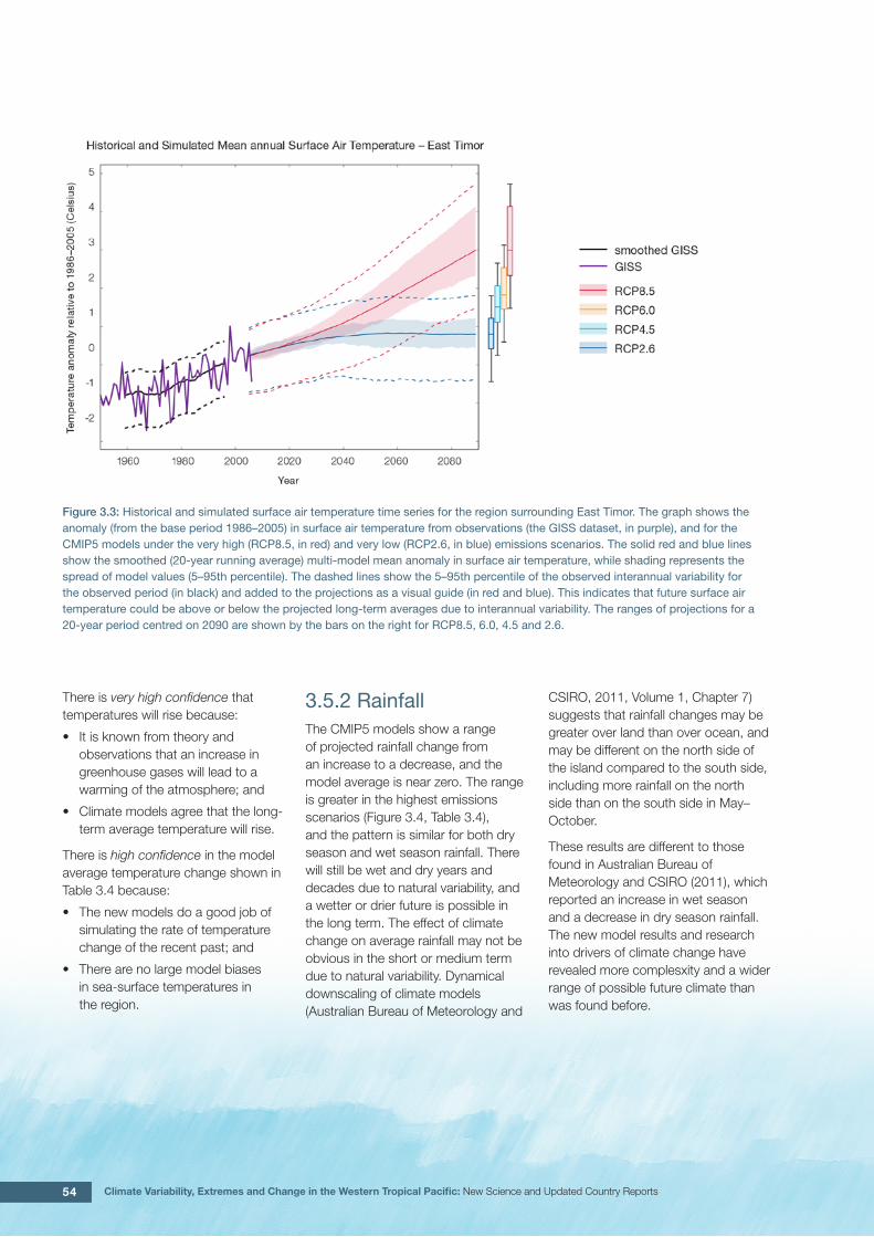
54 Climate Variability, Extremes and Change in the Western Tropical Pacific: New Science and Updated Country Reports
Figure 3.3: Historical and simulated surface air temperature time series for the region surrounding East Timor. The graph shows the anomaly (from the base period 1986–2005) in surface air temperature from observations (the GISS dataset, in purple), and for the CMIP5 models under the very high (RCP8.5, in red) and very low (RCP2.6, in blue) emissions scenarios. The solid red and blue lines show the smoothed (20-year running average) multi-model mean anomaly in surface air temperature, while shading represents the spread of model values (5–95th percentile). The dashed lines show the 5–95th percentile of the observed interannual variability for the observed period (in black) and added to the projections as a visual guide (in red and blue). This indicates that future surface air temperature could be above or below the projected long-term averages due to interannual variability. The ranges of projections for a 20-year period centred on 2090 are shown by the bars on the right for RCP8.5, 6.0, 4.5 and 2.6.
There is very high confidence that temperatures will rise because:
• It is known from theory and observations that an increase in greenhouse gases will lead to a warming of the atmosphere; and
• Climate models agree that the long-term average temperature will rise.
There is high confidence in the model average temperature change shown in Table 3.4 because:
• The new models do a good job of simulating the rate of temperature change of the recent past; and
• There are no large model biases in sea-surface temperatures in the region.
3.5.2 RainfallThe CMIP5 models show a range of projected rainfall change from an increase to a decrease, and the model average is near zero. The range is greater in the highest emissions scenarios (Figure 3.4, Table 3.4), and the pattern is similar for both dry season and wet season rainfall. There will still be wet and dry years and decades due to natural variability, and a wetter or drier future is possible in the long term. The effect of climate change on average rainfall may not be obvious in the short or medium term due to natural variability. Dynamical downscaling of climate models (Australian Bureau of Meteorology and
CSIRO, 2011, Volume 1, Chapter 7) suggests that rainfall changes may be greater over land than over ocean, and may be different on the north side of the island compared to the south side, including more rainfall on the north side than on the south side in May–October.
These results are different to those found in Australian Bureau of Meteorology and CSIRO (2011), which reported an increase in wet season and a decrease in dry season rainfall. The new model results and research into drivers of climate change have revealed more complesxity and a wider range of possible future climate than was found before.

55Chapter 3: East Timor (Timor-Leste)
Figure 3.4: Historical and simulated annual average rainfall time series for the region surrounding East Timor. The graph shows the anomaly (from the base period 1986–2005) in rainfall from observations (the GPCP dataset, in purple), and for the CMIP5 models under the very high (RCP8.5, in red) and very low (RCP2.6, in blue) emissions scenarios. The solid red and blue lines show the smoothed (20-year running average) multi-model mean anomaly in rainfall, while shading represents the spread of model values (5–95th percentile). The dashed lines show the 5–95th percentile of the observed interannual variability for the observed period (in black) and added to the projections as a visual guide (in red and blue). This indicates that future rainfall could be above or below the projected long-term averages due to interannual variability. The ranges of projections for a 20-year period centred on 2090 are shown by the bars on the right for RCP8.5, 6.0, 4.5 and 2.6.
There is no agreement in the direction of rainfall change in the models, and many models project little change in annual rainfall. This lowers the confidence that we can determine the most likely direction of change in annual rainfall, and makes the amount difficult to determine. The 5–95th percentile range of projected values from CMIP5 climate models is large, e.g. for RCP8.5 (very high emissions) the range is -8 to +8% by 2030 and -30 to +28% by 2090.
There is medium confidence that the long-term rainfall over East Timor will remain similar to the current climate because:
• The finding of little change is the average of a large number of models whose results range from a projected rainfall increase to a
rainfall decrease, including many models that project little change; and
• Rainfall associated with the WPM is projected to generally increase, but the regional detail of change is uncertain. See Box in Chapter 1 for more details.
There is low confidence in the model average rainfall change for East Timor shown in Table 3.4 because:
• There is a large spread in model rainfall projections, which range from a projected rainfall increase to a rainfall decrease;
• The complex set of processes involved in tropical rainfall is challenging to simulate in models. This means that the confidence in the projection of rainfall is generally
lower than for other variables such as temperature;
• The new CMIP5 models broadly simulate the influence from the key features such as the WPM, but nevertheless have some uncertainty and biases, similar to the old CMIP3 models; and
• The future behaviour of the ENSO is unclear, and the ENSO strongly influences year-to-year rainfall variability.

56 Climate Variability, Extremes and Change in the Western Tropical Pacific: New Science and Updated Country Reports
3.5.3 Extremes
Extreme Temperature
The temperature of extremely hot days is projected to increase by about the same amount as average temperature. This conclusion is based on analysis of daily temperature data from a subset of CMIP5 models (Chapter 1). The frequency of extremely hot days is also expected to increase.
The temperature of the 1-in-20-year hot day is projected to increase by approximately 0.7°C by 2030 under the RCP2.6 (very low) scenario and by 0.9°C under the RCP8.5 (very high emissions) scenario. By 2090 the projected increase is 0.9°C for RCP2.6 (very low) and 3°C for RCP8.5 (very high emissions).
There is very high confidence that the temperature of extremely hot days and the temperature of extremely cool days will increase, because:
• A change in the range of temperatures, including the extremes, is physically consistent with rising greenhouse gas concentrations;
• This is consistent with observed changes in extreme temperatures around the world over recent decades; and
• All the CMIP5 models agree on an increase in the frequency and intensity of extremely hot days and a decrease in the frequency and intensity of cool days.
There is medium confidence in the magnitude of projected change in extreme temperature because models generally underestimate the current intensity and frequency of extreme events. Changes to the particular driver of extreme temperatures affect whether the change to extremes is more or less than the change in the average temperature, and the changes to the drivers of extreme temperatures in East Timor are currently unclear. Also, while all models project the same direction of change there is a range in the projected magnitude of change among the models.
Extreme Rainfall
The frequency and intensity of extreme rainfall events are projected to increase. This conclusion is based on analysis of daily rainfall data from a subset of CMIP5 models using a similar method to that in Australian Bureau of Meteorology and CSIRO (2011) with some improvements (Chapter 1), so the results are slightly different to those in Australian Bureau of Meteorology and CSIRO (2011). The current 1-in-20-year daily rainfall amount is projected to increase by approximately 11 mm by 2030 for RCP2.6 and by 15 mm by 2030 for RCP8.5 (very high emissions). By 2090, it is projected to increase by approximately 18 mm for RCP2.6 and by 45 mm for RCP8.5 (very high emissions).The majority of models project the current 1-in-20-year daily rainfall event will become, on average, a 1-in-7-year event for RCP2.6 and a 1-in-5-year event for RCP8.5 (very high emissions) by 2090. These results are different to those found in Australian Bureau of Meteorology and CSIRO (2011) because of different methods used (Chapter 1).
There is high confidence that the frequency and intensity of extreme rainfall events will increase because:
• A warmer atmosphere can hold more moisture, so there is greater potential for extreme rainfall (IPCC, 2012); and
• Increases in extreme rainfall in the Pacific are projected in all available climate models.
There is low confidence in the magnitude of projected change in extreme rainfall because:
• Models generally underestimate the current intensity of local extreme events. The results in this region are influenced by the biases in the PM;
• Changes in extreme rainfall projected by models may be underestimated because models seem to underestimate the observed increase in heavy rainfall with warming (Min et al., 2011);
• GCMs have a coarse spatial resolution, so they do not adequately capture some of the processes involved in extreme rainfall events; and
• The Conformal Cubic Atmospheric Model (CCAM) downscaling model has finer spatial resolution and the CCAM results presented in Australian Bureau of Meteorology and CSIRO (2011) indicates a smaller increase in the number of extreme rainfall days, and there is no clear reason to accept one set of models over another.

57Chapter 3: East Timor (Timor-Leste)
Drought
Drought projections (defined in Chapter 1) are described in terms of changes in proportion of time in drought, frequency and duration by 2090 for very low and very high emissions (RCP2.6 and 8.5).
For East Timor the overall proportion of time spent in drought is expected to decrease slightly under RCP8.5 and stay approximately the same under all other scenarios (Figure 3.5). Under RCP8.5 the frequency of moderate and severe drought is projected to decrease slightly while the frequency of events in other categories is projected to stay the same. The duration of events is
projected to stay approximately the same in all categories under RCP8.5. Under RCP2.6 (very low emissions) the frequency and duration of events in all drought categories is projected to stay approximately the same from the present to 2090.
There is low confidence in this direction of change because:
• There is only low confidence in the direction of mean rainfall change;
• These drought projections are based upon a subset of models; and
• Like the CMIP3 models, the majority of the CMIP5 models agree on this direction of change.
There is low confidence in the projections of drought frequency and duration because there is low confidence in the magnitude of rainfall projections, and no consensus about projected changes in the ENSO, which directly influence the projection of drought.
Figure 3.5: Box-plots showing percent of time in moderate, severe or extreme drought (left hand side), and average drought duration and frequency for the different categories of drought (mild, moderate, severe and extreme) for East Timor. These are shown for 20-year periods centred on 1995, 2030, 2050, 2070 and 2090 for the RCP8.5 (very high emissions) scenario. The thick dark lines show the median of all models, the box shows the interquartile (25–75%) range, the dashed lines show 1.5 times the interquartile range and circles show outlier results.
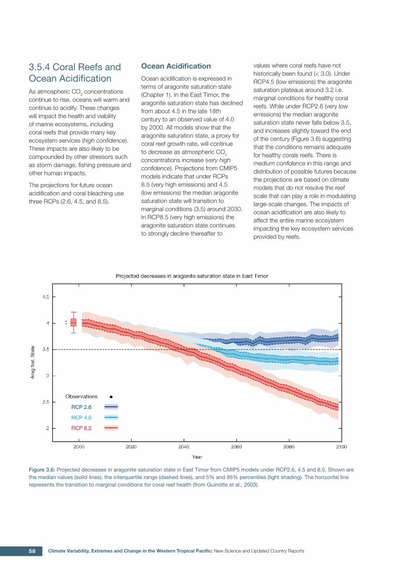
58 Climate Variability, Extremes and Change in the Western Tropical Pacific: New Science and Updated Country Reports
3.5.4 Coral Reefs and Ocean AcidificationAs atmospheric CO2 concentrations continue to rise, oceans will warm and continue to acidify. These changes will impact the health and viability of marine ecosystems, including coral reefs that provide many key ecosystem services (high confidence). These impacts are also likely to be compounded by other stressors such as storm damage, fishing pressure and other human impacts.
The projections for future ocean acidification and coral bleaching use three RCPs (2.6, 4.5, and 8.5).
Ocean Acidification
Ocean acidification is expressed in terms of aragonite saturation state (Chapter 1). In the East Timor, the aragonite saturation state has declined from about 4.5 in the late 18th century to an observed value of 4.0 by 2000. All models show that the aragonite saturation state, a proxy for coral reef growth rate, will continue to decrease as atmospheric CO2 concentrations increase (very high confidence). Projections from CMIP5 models indicate that under RCPs 8.5 (very high emissions) and 4.5 (low emissions) the median aragonite saturation state will transition to marginal conditions (3.5) around 2030. In RCP8.5 (very high emissions) the aragonite saturation state continues to strongly decline thereafter to
values where coral reefs have not historically been found (< 3.0). Under RCP4.5 (low emissions) the aragonite saturation plateaus around 3.2 i.e. marginal conditions for healthy coral reefs. While under RCP2.6 (very low emissions) the median aragonite saturation state never falls below 3.5, and increases slightly toward the end of the century (Figure 3.6) suggesting that the conditions remains adequate for healthy corals reefs. There is medium confidence in this range and distribution of possible futures because the projections are based on climate models that do not resolve the reef scale that can play a role in modulating large-scale changes. The impacts of ocean acidification are also likely to affect the entire marine ecosystem impacting the key ecosystem services provided by reefs.
Figure 3.6: Projected decreases in aragonite saturation state in East Timor from CMIP5 models under RCP2.6, 4.5 and 8.5. Shown are the median values (solid lines), the interquartile range (dashed lines), and 5% and 95% percentiles (light shading). The horizontal line represents the transition to marginal conditions for coral reef health (from Guinotte et al., 2003).

59Chapter 3: East Timor (Timor-Leste)
Coral Bleaching Risk
As the oceans warm, the risk of coral bleaching increases (very high confidence). There is medium confidence in the projected rate of change for East Timor because there is medium confidence in the rate of change of sea-surface temperature (SST), and the changes at the reef scale (which can play a role in modulating large-scale changes) are not adequately resolved. Importantly, the coral bleaching risk calculation does not account the impact of other potential stressors (Chapter 1).
The changes in the frequency (or recurrence) and duration of severe bleaching risk are quantified for different projected SST changes (Table 3.3). Overall there is a decrease in the time between two periods of elevated risk and an increase in the duration of the elevated risk.
For example, under a long-term mean increase of 1°C (relative to 1982–1999 period), the average period of severe bleaching risk (referred to as a risk event) will last 8.4 weeks (with a minimum duration of 3.0 weeks and a maximum duration of 3.1 months) and the average time between two risks will be 3.8 years (with the minimum recurrence of 7.8 months and a maximum recurrence of 10.7 years). If severe bleaching events occur more often than once every five years, the long-term viability of coral reef ecosystems becomes threatened.
We quantify the changes in the frequency (or recurrence) and duration of severe bleaching risk (Figure 3.6) for different projected SST changes (Table 3.3). For example, under a long-term mean increase of 1°C (relative to 1982–1999 period), the average severe bleaching risk event.
The impact of long-term ocean warming is a decrease of the time between two risk events and an increase in the period of the risk (Figure 3.6). If severe bleaching event occurs more often than once every five years, the long-term viability of coral reef ecosystems becomes threatened.
3.5.5 Sea Level Mean sea level is projected to continue to rise over the course of the 21st century. There is very high confidence in the direction of change. The CMIP5 models simulate a rise of between approximately 8–18 cm by 2030 (very similar values for different RCPs), with increases of 43–88 cm by 2090 under the RCP8.5 (Figure 3.7 and Table 3.4). There is medium confidence in the range mainly because there is still uncertainty associated with projections of the Antarctic ice sheet contribution. Interannual variability of sea level will lead to periods of lower and higher regional sea levels. In the past, this interannual variability has been about 24 cm (5–95% range, after removal of the seasonal signal, see dashed lines in Fig. 3.7a) and it is likely that a similar range will continue through the 21st century.
Table 3.3: Projected changes in severe coral bleaching risk for the East Timor EEZ for increases in SST relative to 1982–1999.
Temperature change 1 Recurrence interval 2 Duration of the risk event 3
Change in observed mean 0 0
+0.25°C 0 0
+0.5°C 27.3 years(26.1 years – 28.5 years)
4.6 weeks(4.4 weeks – 4.8 weeks)
+0.75°C 13.6 years(8.2 years – 20.3 years)
6.3 weeks(4.6 weeks – 8.1 weeks)
+1°C 3.8 years(7.8 months – 10.7 years)
8.4 weeks(3.0 weeks – 3.1months)
+1.5°C 10.1 months(2.0 months – 2.3 years)
2.7 months(1.8 weeks – 5.3 months)
+2°C 6.1 months(1.2 months – 9.6 months)
4.7 months (2.4 weeks – 7.5 months)
1 This refers to projected SST anomalies above the mean for 1982–1999. 2 Recurrence is the mean time between severe coral bleaching risk events. Range (min – max) shown in brackets.3 Duration refers to the period of time where coral are exposed to the risk of severe bleaching. Range (min – max) shown in brackets

60 Climate Variability, Extremes and Change in the Western Tropical Pacific: New Science and Updated Country Reports
Figure 3.7 (a): The observed tide-gauge records of relative sea-level (since the late 1970s) are indicated in purple, and the satellite record (since 1993) in green. The gridded (reconstructed) sea level data at East Timor (since 1950) is shown in black. Multi-model mean projections from 1995–2100 are given for the RCP8.5 (red solid line) and RCP2.6 emissions scenarios (blue solid line), with the 5–95% uncertainty range shown by the red and blue shaded regions. The ranges of projections for four emission scenarios (RCPs 2.6, 4.5, 6.0 and 8.5) by 2100 are also shown by the bars on the right. The dashed lines are an estimate of interannual variability in sea level (5–95% uncertainty range about the projections) and indicate that individual monthly averages of sea level can be above or below longer-term averages.
(b) The regional distribution of projected sea level rise under the RCP4.5 emissions scenario for 2081–2100 relative to 1986–2005. Mean projected changes are indicated by the shading, and the estimated uncertainty in the projections is indicated by the contours (in cm).
3.5.6 Wind-driven WavesDuring December–March, the wet season in East Timor, there are no projected changes in wave properties (Figure 3.8, Table 3.5), except for a decrease in wave period in January, which is significant in 2035 under RCP4.5 and RCP8.5 (very high emissions), and in 2090 under RCP4.5 (low confidence). This decrease is characteristic of an increase in the locally generated wind sea, or reduced swell. Wave direction is projected to be more variable in December–March (wet months) than June–September (dry months). There is a suggested decrease in the height of the larger waves (low confidence).
In the dry season (represented here by June–September), there are no significant projected changes in wave properties (low confidence) (Table 3.5).
There is low confidence in projected changes in the East Timor wind-wave climate because:
• Projected changes in wave climate are dependent on confidence in projected changes in the ENSO, which is low; and
• The differences between simulated and observed (hindcast) wave data are larger than the projected wave changes, which further reduces our confidence in projections.

61Chapter 3: East Timor (Timor-Leste)
Figure 3.8: Mean annual cycle of change in wave height (m) between projection scenarios and historical models at East Timor. This plot shows no significant change in wave heights throughout the year. Shaded boxes show 1 standard deviation of models’ means around the ensemble means, and error bars show the 5–95% range inferred from the standard deviation. Colours represent RCP scenarios and time periods: blue 2035 RCP4.5 (low emissions), red 2035 RCP8.5 (very high emissions), green 2090 RCP4.5 (low emissions), purple 2090 RCP8.5 (very high emissions).
3.5.7 Projections SummaryThere is very high confidence in the direction of long-term change in a number of key climate variables, namely an increase in mean and extremely high temperatures, sea level and ocean acidification. There is high confidence that the frequency and intensity of extreme rainfall will increase. There is medium confidence that mean rainfall and drought frequency will remain similar to the current climate.
Tables 3.4 and 3.5 quantify the mean changes and ranges of uncertainty for a number of variables, years and emissions scenarios. A number of factors are considered in assessing confidence, i.e. the type, amount, quality and consistency of evidence (e.g. mechanistic understanding, theory, data, models, expert judgment) and the degree of agreement, following the IPCC guidelines (Mastrandrea et al., 2010). Confidence ratings in the projected magnitude of mean
change are generally lower than those for the direction of change (see paragraph above) because magnitude of change is more difficult to assess. For example, there is very high confidence that temperature will increase, but medium confidence in the magnitude of mean change.

62 Climate Variability, Extremes and Change in the Western Tropical Pacific: New Science and Updated Country Reports
Table 3.4: Projected changes in the annual and seasonal mean climate for East Timor under four emissions scenarios; RCP2.6 (very low emissions, in dark blue), RCP4.5 (low emissions, in light blue), RCP6 (medium emissions, in orange) and RCP8.5 (very high emissions, in red). Projected changes are given for four 20-year periods centred on 2030, 2050, 2070 and 2090, relative to a 20-year period centred on 1995. Values represent the multi-model mean change, with the 5–95% range of uncertainty in brackets. Confidence in the magnitude of change is expressed as high, medium or low. Surface air temperatures in the Pacific are closely related to sea-surface temperatures (SST), so the projected changes to air temperature given in this table can be used as a guide to the expected changes to SST. (See also Section 1.5.2). ‘NA’ indicates where data are not available.
Variable Season 2030 2050 2070 2090Confidence
(magnitude of change)
Surface air temperature (°C)
Annual 0.6 (0.4–0.8) 0.8 (0.5–1.1) 0.8 (0.4–1.1) 0.8 (0.4–1.2) High
0.7 (0.4–1) 1.1 (0.8–1.5) 1.4 (0.9–1.9) 1.5 (1.1–2.1)
0.6 (0.4–1) 1 (0.7–1.5) 1.4 (1.1–1.9) 1.8 (1.5–2.6)
0.8 (0.5–1.1) 1.4 (1–2) 2.2 (1.7–3.1) 3 (2.4–4.2)
Maximum temperature (°C)
1-in-20 year event
0.7 (0.4–1.1) 0.9 (0.4–1.1) 0.9 (0.4–1.2) 0.9 (0.4–1.4) Medium
0.7 (0–1.1) 1 (0.1–1.4) 1.3 (0.6–1.8) 1.5 (0.9–2)
NA (NA–NA) NA (NA–NA) NA (NA–NA) NA (NA–NA)
0.9 (0.3–1.2) 1.5 (0.4–2.2) 2.4 (1.2–3.3) 3.3 (1.9–4.3)
Minimum temperature (°C)
1-in-20 year event
0.6 (0.2–0.9) 0.8 (0.3–1.2) 0.7 (0.3–1) 0.7 (0.1–1) Medium
0.6 (-0.2–0.9) 1 (0.4–1.3) 1.3 (0.4–1.6) 1.5 (0.6–2)
NA (NA–NA) NA (NA–NA) NA (NA–NA) NA (NA–NA)
0.8 (0.2–1.4) 1.6 (1–2.2) 2.4 (1.4–3.2) 3.2 (2.1–4.3)
Total rainfall (%) Annual -1 (-15–6) 0 (-11–9) -1 (-13–8) -1 (-12–8) Low
0 (-15–11) 0 (-16–10) -2 (-22–9) -1 (-20–16)
1 (-11–8) 2 (-11–16) 1 (-9–11) 2 (-17–19)
0 (-8–8) 1 (-13–16) 1 (-25–21) 2 (-30–28)
Total rainfall (%) Nov-Apr 0 (-12–10) 1 (-7–8) 0 (-10–13) 1 (-8–12) Low
0 (-12–10) 1 (-16–9) -1 (-16–9) 1 (-14–15)
2 (-5–10) 4 (-7–13) 3 (-7–13) 4 (-11–20)
1 (-12–10) 2 (-12–19) 2 (-19–20) 1 (-29–25)
Total rainfall (%) May-Oct -4 (-24–14) -3 (-28–11) -4 (-22–19) -5 (-25–14) Low
-1 (-23–32) -1 (-27–24) -5 (-34–20) -4 (-31–24)
1 (-22–24) 1 (-23–26) -2 (-18–17) 1 (-39–33)
0 (-19–29) 0 (-16–28) -3 (-39–29) 2 (-60–54)
Aragonite saturation state (Ωar)
Annual -0.3 (-0.6–-0.1) -0.4 (-0.6–-0.1) -0.4 (-0.6–-0.1) -0.3 (-0.6–-0.1) Medium
-0.3 (-0.5–-0.1 -0.5 (-0.7–-0.3) -0.7 (-0.9–-0.5) -0.7 (-0.9–-0.5)
NA (NA–NA) NA (NA–NA) NA (NA–NA) NA (NA–NA)
-0.4 (-0.6–-0.2) -0.7 (-0.9–-0.5) -1.1 (-1.2–-0.9) -1.4 (-1.6–-1.3)
Mean sea level (cm) Annual 13 (8–17) 22 (15–30) 32 (21–45) 42 (26–59) Medium
13 (9–17) 23 (16–31) 36 (24–48) 49 (32–67)
12 (8–17) 23 (15–30) 35 (23–47) 50 (33–68)
13 (9–18) 26 (18–34) 43 (30–58) 64 (43–88)

63Chapter 3: East Timor (Timor-Leste)
Waves Projections Summary
Table 3.5: Projected average changes in wave height, period and direction in East Timor for December–March and June–September for RCP4.5 (low emissions, in blue) and RCP8.5 (very high emissions, in red), over two 20-year periods (2026–2045 and 2081–2100), relative to a 1986–2005 historical period. The values in brackets represent the 5th to 95th percentile range of uncertainty.
Variable Season 2035 2090 Confidence (range)
Wave height change (m) December–March 0.0 (-0.2–0.2)0.0 (-0.2–0.2)
0.0 (-0.2–0.2)-0.0 (-0.2–0.2)
Low
June–September 0.0 (-0.4–0.5)0.0 (-0.4–0.4)
0.0 (-0.4–0.5)0.0 (-0.4–0.6)
Low
Wave period change (s) December–March -0.1(-1.0–0.9)-0.0 (-1.1–1.0)
-0.0 (-0.9–0.9)-0.0 (-1.1–1.0)
Low
June–September 0.0 (-0.5–0.5)0.0 (-0.5–0.5)
+0.0 (-0.5–0.7)+0.0 (-0.5–0.6)
Low
Wave direction change (° clockwise) December–March +0 (-40–50)0 (-50–50)
0 (-40–40)-0 (-50–40)
Low
June–September 0 (-10–10)0 (-20–10)
0 (-20–20)-0 (-20–10)
Low
Wind-wave variables parameters are calculated for a 20-year period centred on 2035.

64 Climate Variability, Extremes and Change in the Western Tropical Pacific: New Science and Updated Country Reports

65
Chapter 4 Federated States of Micronesia
Bill Jaynes, FSM

66 Climate Variability, Extremes and Change in the Western Tropical Pacific: New Science and Updated Country Reports
4.1 Climate Summary
4.1.1 Current Climate• Warming trends are evident
in annual and half-year mean air temperatures for Pohnpei since 1951. The Yap mean air temperature trend shows little change for the same period.
• Extreme temperatures such as Warm Days and Warm Nights have been increasing at Pohnpei consistent with global warming trends. Trends in minimum temperatures at Yap are not consistent with Pohnpei or global warming trends and may be due to unresolved inhomogeneities in the record.
• At Pohnpei, there has been a decreasing trend in May–October rainfall since 1950. This implies either a shift in the mean location of the Inter-Tropical Convergence Zone (ITCZ) away from Pohnpei and/or a change in the intensity of rainfall associated with the ITCZ.
• There has also been a decreasing trend in Very Wet Day rainfall at Pohnpei and Consecutive Dry Days at Yap since 1952. The remaining annual, half-year and extreme daily rainfall trends show little change at both sites.
• Tropical cyclones (typhoons) affect the Federated States of Micronesia mainly between June and November. An average of 71 cyclones per decade developed within or crossed the Federated States of Micronesia’s Exclusive Economic Zone (EEZ) between the 1977 and 2011 seasons. Tropical cyclones were most frequent in El Niño years (88 cyclones per decade) and least frequent in La Niña years (38 cyclones per decade). The neutral season average is 84 cyclones per decade. Thirty-seven of the 212 tropical cyclones (17%) between the 1981 and 2011 seasons became severe events (Category 3 or stronger) in the Federated States of Micronesia’s EEZ. Available data are not suitable for assessing long-term trends.
• Wind-waves in the Federated States of Micronesia are dominated by north-easterly trade winds and westerly monsoon winds seasonally, and the El Niño–Southern Oscillation (ENSO) interannually. There is little variation in wave climate between the eastern and western parts of the country; however Yap, in the west, has a more marked dependence on the El Niño–Southern Oscillation in June–September than Pohnpei, in the east. Available data are not suitable for assessing long-term trends (see Section 1.3).
4.1.2 Climate ProjectionsFor the period to 2100, the latest global climate model (GCM) projections and climate science findings indicate:
• El Niño and La Niña events will continue to occur in the future (very high confidence), but there is little consensus on whether these events will change in intensity or frequency;
• Annual mean temperatures and extremely high daily temperatures will continue to rise (very high confidence);
• Average annual rainfall is projected to increase (medium confidence), with more extreme rain events (high confidence);
• Drought frequency is projected to decrease (medium confidence);
• Ocean acidification is expected to continue (very high confidence);
• The risk of coral bleaching will increase in the future (very high confidence);
• Sea level will continue to rise (very high confidence); and
• Wave height is projected to decrease in December–March (low confidence), and waves may be more directed from the south in the June–September (low confidence).

67Chapter 4: Federated States of Micronesia
4.2 Data Availability
There are 23 operational meteorological stations in the Federated States of Micronesia. Multiple observations within a 24-hour period are taken at five stations in Chuuk State, six in Pohnpei State (including Kosrae State) and three in Yap State. In addition, there are two single-observation-a-day climate stations in Pohnpei and seven single-observation-a-day rainfall stations in Yap. Rainfall data for Pohnpei are available from 1949 and Yap from 1951. Air temperature data are available from 1950 for Pohnpei and 1951 for Yap.
The complete historical rainfall and air temperature records for Pohnpei and Yap have been used in this report. These records are considered homogeneous given the available metadata, however low confidence is given to Yap’s minimum air temperature data that remain inconsistent with temperature records in the region, likely due to remaining inhomogeneities in the record. Additional information on historical climate trends in the Federated States of Micronesia region can be found in the Pacific Climate Change Data Portal www.bom.gov.au/climate/pccsp/.
Wind-wave data from buoys are particularly sparse in the Pacific region, with very short records. Model and reanalysis data are therefore required to detail the wind-wave climate of the region. Reanalysis surface wind data have been used to drive a wave model over the period 1979–2009 to generate a hindcast of the historical wind-wave climate.
4.3 Seasonal Cycles
Information on temperature and rainfall seasonal cycles can be found in Australian Bureau of Meteorology and CSIRO (2011).
4.3.1 Wind-driven WavesSurface wind-wave driven processes can impact on many aspects of Pacific Island coastal environments, including: coastal flooding during storm wave events; coastal erosion, both during episodic storm events and due to long-term changes in integrated wave climate; characterisation of reef morphology and marine habitat/species distribution; flushing and circulation of lagoons; and potential shipping and renewable wave energy solutions. The surface offshore wind
wave climate can be described by characteristic wave heights, lengths (wave period) and directions.
In the eastern Federated States of Micronesia (e.g. on the north coast of Pohnpei), waves are predominantly directed from the north-east throughout the year, but display strong seasonal variability of direction with increased variability in direction during June–September (Figure 4.1). Wave heights and periods also vary seasonally, reaching a maximum in December–March (mean wave height 7’1” (2.2 m) and period 8.7 s), with minima around the start of the wetter season (June–September) (seasonal mean wave height 3’9” (1.1 m) and period 7.8 s) (Table 4.1). The wave climate is characterised by trade wind generated waves from the north-east
and east. During December–March swell is propagated from storm events in the north-west from monsoons and North Pacific extra-tropical storms. In June–September swell waves are generated from Southern Hemisphere storms and occasionally from the south-east from trade winds. Waves larger than 10’2” (3.1 m) (99th percentile) to the north of Pohnpei occur predominantly between November and April and have longer than average periods, usually directed from the north-east to north-west, associated with typhoons and extra-tropical storms. The height of a 1-in-50 year wave event on the north coast of Pohnpei is calculated to be 19’2” (5.8 m).

68 Climate Variability, Extremes and Change in the Western Tropical Pacific: New Science and Updated Country Reports
In the western Federated States of Micronesia (e.g. on the south coast of Yap), waves are characterised by variability of the Northern Hemisphere trade winds and westerly monsoon winds. During the northern trade wind season, December–March, waves at Yap are east-northeasterly and have a larger height and slightly longer period than in other months (mean height around 5’1” (1.5 m) and period around 7.5 s), with some north-westerly swell from extra-tropical storms (Figure 4.2). In the wetter months of June–September, waves have a slightly shorter period (mean around 7.2 s) and lower height (mean around 3’6” (1.1 m) than December–March (Table 4.1). These waves consist of locally generated trade wind waves
from the east and north-east, as well as locally generated westerly monsoon waves and easterly trade wind swell. Waves larger than 9’6” (2.9 m) (99th percentile) occur from the south-west in the wetter months due to monsoon systems and typhoons, and from the west, east, and varying directions in November–March from extra-tropical storms. The height of a 1-in-50 year wave event on the south coast of Yap is calculated to be 31’3” (9.5 m).
No suitable dataset is available to assess long-term historical trends in wave climate for the Federated States of Micronesia. However, interannual variability may be assessed in the hindcast record. The wind-wave climate displays strong interannual variability at both
Pohnpei and Yap, varying with the El Niño–Southern Oscillation (ENSO) in June–September. During La Niña years, mean wave power at Pohnpei is greater than during El Niño years in June–September, and waves are more strongly directed from the east, associated with increased trade wind speeds. At Yap, wave power does not vary substantially between in El Niño and La Niña years in December–March, but in June–September much weaker waves are directed from the east in La Niña years but stronger and from the west in El Niño years, associated with movement of the Inter-Tropical Convergence Zone (ITCZ) influencing changes in the trade winds and monsoon systems.
Table 4.1: Mean wave height, period and direction from which the waves are travelling around the Federated States of Micronesia in December–March and June–September. Observation (hindcast) and climate model simulation mean values are given with the 5–95th percentile range (in brackets). Projections are made for eastern and western area averages of the Federated States of Micronesia, so historical model simulation values are given for these areas for comparison (see Section 4.5.6 – Wind driven waves, and Tables 4.8 and 4.9). A compass relating number of degrees to cardinal points (direction) is shown.
Hindcast Reference Data (1979–2009),
north Pohnpei
Climate Model Simulations
(1986–2005) – Eastern Federated
States of Micronesia
Hindcast Reference Data (1979–2009),
south Yap
Climate Model Simulations
(1986–2005) – Western Federated
States of Micronesia
Wave Height(metres)
December–March 2.2 (1.5–2.9)
2.0 (1.7–2.4)
1.5 (1.0–2.2)
1.8 (1.5–2.2)
June–September 1.1 (0.7–1.6)
1.1 (0.9–1.4)
1.1 (0.6–2.1)
1.0 (0.8–1.3)
Mean wave height(feet)
December–March 7.1 (5.0–9.5)
6.7 (5.5–7.8)
5.1 (3.1–7.4)
6.0 (4.8–7.2)
June–September 3.7 (2.4–5.4)
3.7 (3.1–4.4)
3.5 (1.9–7.0)
3.2 (2.5–4.4)
Wave Period(seconds)
December–March 8.7 (7.3–10.7)
8.0 (7.4–8.8)
7.5 (6.3–9.3)
7.6 (7.0–8.2)
June–September 7.8 (6.3–9.7)
7.2 (6.5–7.9)
7.2 (5.7–8.8)
6.6 (6.0–7.1)
Wave direction(degrees clockwise
from North)
December–March 40 (10–60)
50 (40–60)
70 (60–90)
50 (40–60)
June–September 40 (310–80)
110 (80–160)
130 (70–270)
100 (50–150)

69Chapter 4: Federated States of Micronesia
Figure 4.1: Mean annual cycle of wave height (grey) and mean wave direction (blue) at Pohnpei (eastern Federated States of Micronesia) in hindcast data (1979–2009). To give an indication of interannual variability of the monthly means of the hindcast data, shaded boxes show 1 standard deviation around the monthly means, and error bars show the 5–95% range. The direction from which the waves are travelling is shown (not the direction towards which they are travelling).
Figure 4.2: Mean annual cycle of wave height (grey) and mean wave direction (blue) at Yap (western Federated States of Micronesia) in hindcast data (1979–2009). To give an indication of interannual variability of the monthly means of the hindcast data, shaded boxes show 1 standard deviation around the monthly means, and error bars show the 5–95% range. The direction from which the waves are travelling is shown (not the direction towards which they are travelling).

70 Climate Variability, Extremes and Change in the Western Tropical Pacific: New Science and Updated Country Reports
4.4 Observed Trends
4.4.1 Air Temperature
Annual and Half-year Mean Air Temperature
Trends for annual and half-year mean temperatures are positive at Pohnpei with little change observed at Yap (Figure 4.3, Figure 4.4 and Table 4.2). At Pohnpei and Yap the warming trends in maximum annual and half-year air temperatures are
statistically significant at the 5% level and consistent with regional and global warming trends. Minimum temperatures show significant positive trends at Pohnpei over November–April and May–October. Also at Pohnpei, annual and half-year trends in maximum air temperature are greater than those observed in minimum air temperature. The cooling trends in Yap annual and half-year minimum temperatures are
inconsistent with regional and global trends. This could potentially be due to remaining inhomogeneities in record which cannot be resolved due to lack of metadata. Strong cooling trends in the minimum air temperature are responsible for no significant trends in the mean air temperatures at Yap.
Figure 4.3: Observed time series of annual average values of mean air temperature (red dots and line) and total rainfall (bars) at Pohnpei. Light blue, dark blue and grey bars denote El Niño, La Niña and neutral years respectively. Solid black trend lines indicate a least squares fit.

71Chapter 4: Federated States of Micronesia
Figure 4.4: Observed time series of annual average values of mean air temperature (red dots and line) and total rainfall (bars) at Yap. Light blue, dark blue and grey bars denote El Niño, La Niña and neutral years respectively. Solid black trend lines indicate a least squares fit.

72 Climate Variability, Extremes and Change in the Western Tropical Pacific: New Science and Updated Country Reports
Table 4.2: Annual and half-year trends in air temperature (Tmax, Tmin, Tmean) and rainfall at Pohnpei (top) and Yap (bottom). The 95% confidence intervals are shown in parentheses. Values for trends significant at the 5% level are shown in boldface.
Pohnpei
Tmax°F/10yrs
[°C/10yrs]
Tmin°F/10yrs
[°C/10yrs]
Tmean°F/10yrs
[°C/10yrs]
Total Raininches/10yrs[mm/10yrs]
1951–2011 1950–2011
Annual +0.32 (+0.19, +0.46)
[+0.18 (+0.10, +0.26)]
+0.16(-0.02, +0.35)
[+0.09 (-0.01, +0.20)]
+0.27(+0.12, +0.38)
[+0.15 (+0.07, +0.21)]
-2.26 (-5.32, +0.61)
[-57.3 (-135.1, +15.5)]
Nov–Apr +0.31(+0.17, +0.48)
[+0.17 (+0.09,+0.27)]
+0.25(+0.03, +0.42)
[+0.14 (+0.02, +0.23)]
+0.29(+0.11, +0.44)
[+0.16 (+0.06, +0.25)]
-1.80 (-4.60, +1.64)
[-45.8 (-116.7, +41.8)]
May–Oct +0.32(+0.16, +0.46)
[+0.18 (+0.09, +0.26)]
+0.19(+0.03, +0.37)
[+0.11 (+0.02, +0.21)]
+0.27(+0.13, +0.39)
[+0.15 (+0.07, +0.22)]
-2.23 (-4.52, -0.12)
[-56.6 (-114.9, -3.1)]
Yap
Tmax°F/10yrs
(°C/10yrs)
Tmin°F/10yrs
(°C/10yrs)
Tmean°F/10yrs
(°C/10yrs)
Total Raininches/10yrs(mm/10yrs)
1951–2011 1952–2011
Annual +0.41(+0.36, +0.48)
[+0.23 (+0.20, +0.26)]
-0.36(-0.43, -0.27)
[-0.20 (-0.24, -0.15)]
+0.03(-0.02, +0.07)
[+0.01 (-0.01, +0.04)]
0.00 (-2.85, +3.22)
[-0.1 (-72.5, +81.8)]
Nov–Apr +0.39(+0.34, +0.44)
[+0.22 (+0.19, +0.25)
-0.27(-0.37, -0.18)
[-0.15 (-0.21, -0.10)]
+0.04(-0.02, +0.11)
[+0.02 (-0.01, +0.06)]
+0.86 (-2.87, +1.44)
[-21.9 (-72.8, +36.6)]
May–Oct +0.44(+0.37, +0.51)
[+0.24 (+0.20, +0.28)]
-0.40(-0.48, -0.33)
[-0.22 (-0.27, +0.18)]
+0.01(-0.04, +0.05)
[0.00 (-0.02, +0.03)]
+0.93 (-1.27, +3.10)
[ +23.6 (-32.1,+78.8)]

73Chapter 4: Federated States of Micronesia
Extreme Daily Air Temperature
Warming trends are present in the extreme indices (Table 4.3 and Figure 4.5) at Pohnpei. The annual number of Warm Days and Warm Nights has increased with Cool Days decreasing. These trends were found to be statistically significant. At Yap, Warm Days are increasing with Cool Days decreasing consistent
with day-time temperature trends at Pohnpei. However, extreme minimum temperature trends show opposite trends; Cool Nights are increasing and Warm Nights decreasing – a trend that is inconsistent with mean and extreme global warming trends. This is likely due to remaining inhomogeneities in the record which could not be resolved given the metadata available at Yap.
Table 4.3: Annual trends in air temperature and rainfall extremes at Pohnpei (top) and Yap (bottom). The 95% confidence intervals are shown in parentheses. Values for trends significant at the 5% level are shown in boldface.
Pohnpei Yap
TEMPERATURE 1952–2011 1952–2011
Warm Days (days/decade) 7.86 (+3.65, 11.70) 12.23 (+4.60, +19.80)
Warm Nights (days/decade) 5.12 (+1.22, +9.05) -16.68 (-21.57, -10.24)
Cool Days (days/decade) -3.98 (-5.53, -2.52) -8.50 (-13.66, -2.67)
Cool Nights (days/decade) -2.73 (-8.21, +3.68) +8.70 (+3.71, +14.90)
RAINFALL
Rain Days ≥ 1 mm (days/decade) -0.21 (-2.79, +2.48) -1.01 (-4.20, +1.82)
Very Wet Day rainfall (inches/decade) -2.63 (-5.15, -0.12) +0.22 (-1.39, +1.97)
(mm/decade) -66.88 (-130.81, -3.05) +5.55 (-35.30, +49.95)
Consecutive Dry Days (days/decade) 0.00 (-0.43, +0.20) -0.37 (-0.77, 0.00)
Max 1-day rainfall (inches/decade) -0.015 (-0.29, 0.27) -0.04 (-0.30, +0.21)
(mm/decade) -0.38 (-7.29, +6.84) -0.88 (-7.62, +5.41)
Warm Days: Number of days with maximum temperature greater than the 90th percentile for the base period 1971–2000Warm Nights: Number of days with minimum temperature greater than the 90th percentile for the base period 1971–2000Cool Days: Number of days with maximum temperature less than the 10th percentile for the base period 1971–2000Cool Nights: Number of days with minimum temperature less than the 10th percentile for the base period 1971–2000Rain Days ≥ 1mm: Annual count of days where rainfall is greater or equal to 1mm (0.039 inches)Very Wet Day rainfall: Amount of rain in a year where daily rainfall is greater than the 95th percentile for the reference period 1971–2000Consecutive Dry Days: Maximum number of consecutive days in a year with rainfall less than 1mm (0.039 inches)Max 1-day rainfall: Annual maximum 1-day rainfall

74 Climate Variability, Extremes and Change in the Western Tropical Pacific: New Science and Updated Country Reports
Figure 4.5: Observed time series of annual total number of Warm Days at Pohnpei (top left panel) and Yap (bottom left panel). Annual total number of Cool Nights at Pohnpei (top right panel) and Yap (bottom right panel). Solid black line indicates least squares fit.
4.4.2 Rainfall
Annual and Half-year Total Rainfall
Notable interannual variability associated with the ENSO is evident in the observed rainfall records for Pohnpei since 1950 (Figure 4.3) and Yap since 1952 (Figure 4.4). The negative trend in Pohnpei rainfall from May–October is statistically significant at the 5% level (Table 4.2). This implies either a shift in the mean location of the ITCZ away from Pohnpei and/or a change in the intensity of rainfall associated with the ITCZ. The ITCZ is closest to the equator in March–May, and furthest north during September–November, when it becomes broader, expanding both to the north and south.
The other total rainfall trends presented in Table 4.2, Figure 4.3 and Figure 4.4 are not statistically significant. In other words, excluding Pohnpei May–October rainfall, there has been little change in rainfall at Pohnpei and Yap.
Daily Rainfall
Daily rainfall trends for Pohnpei and Yap are presented in Table 4.3. Figure 4.6 shows trends in annual Very Wet Days and Consecutive Dry Days at Pohnpei and Yap. The negative trends in annual Very Wet Day rainfall at Pohnpei and annual Consecutive Dry Days at Yap are statistically significant. The decrease in annual Consecutive Dry Days at Yap does not coincide with an increase in the number of rain days. The other extreme rainfall trends in Table 4.3 are not statistically significant.
4.4.3 Tropical CyclonesWhen tropical cyclones (typhoons) affect the Federated States of Micronesia they tend to do so between June and November. The tropical cyclone archive of the Northern Hemisphere indicates that between the 1977 and 2011 seasons, 248 tropical cyclones developed within or crossed the Federated States of Micronesia’s EEZ. This represents an average of 71 cyclones per decade. Refer to Chapter 1, Section 1.4.2 (Tropical Cyclones) for an explanation of the difference in the number of tropical cyclones occurring in the Federated States of Micronesia in this report (Australian Bureau of Meteorology and CSIRO, 2014) compared to Australian Bureau of Meteorology and CSIRO (2011).

75Chapter 4: Federated States of Micronesia
Figure 4.6: Observed time series of annual Consecutive Dry Days at Pohnpei (top left panel) and Yap (bottom left panel), and annual Very Wet Days at Pohnpei (top right panel) and Yap (bottom right panel). Solid black line indicates least squares fit.
Interannual variability in the number of tropical cyclones in the Federated States of Micronesia’s EEZ is large, ranging from zero in 1999 to 12 in 1979 and 1987 (Figure 4.7). Tropical cyclones were most frequent in El Niño and neutral years, and least frequent in La Niña years. The neutral season average is 84 cyclones per decade. Thirty-seven of the 212 tropical cyclones (17%) between the 1981 and 2011 seasons became severe events (Category 3 or higher) within the Federated States of Micronesia’s EEZ.
Long term trends in frequency and intensity have not been presented as country scale assessment is not recommended. Some tropical cyclone tracks analysed in this subsection include the tropical depression stage (sustained winds less than or equal to 34 knots) before and/or after tropical cyclone formation.
Figure 4.7: Time series of the observed number of tropical cyclones developing within and crossing the Federated States of Micronesia EEZ per season. The 11-year moving average is in blue.

76 Climate Variability, Extremes and Change in the Western Tropical Pacific: New Science and Updated Country Reports
4.5 Climate Projections
The performance of the available Coupled Model Intercomparison Project (Phase 5) (CMIP5) climate models over the Pacific has been rigorously assessed (Brown et al., 2013a, b; Grose et al., 2014; Widlansky et al., 2013). The simulation of the key processes and features for the Federated States of Micronesia region is similar to the previous generation of CMIP3 models, with all the same strengths and many of the same weaknesses. The best-performing CMIP5 models used here have lower biases (differences between the simulated and observed climate data) than the best CMIP3 models, and there are fewer poorly-performing models. For the Federated States of Micronesia, the most important model bias is that the simulated rainfall in the ITCZ and the West Pacific Monsoon (WPM) is too wet in November–April in the present climate, but March–October rainfall is within observed uncertainty. This affects the confidence in the model projections. Out of 27 models assessed, one model was rejected for use in these projections due to biases in the mean climate. Climate projections have been derived from up to 26 new GCMs in the CMIP5 database (the exact number is different for each scenario, Appendix A), compared with up to 18 models in the CMIP3 database reported in Australian Bureau of Meteorology and CSIRO (2011).
It is important to realise that the models used give different projections under the same scenario. This means there is not a single projected future for the Federated States of Micronesia, but rather a range of possible futures for each emission scenario. This range is described below.
4.5.1 TemperatureFurther warming is expected over the Federated States of Micronesia (Figure 4.8, Tables 4.6 and 4.7). Under all RCPs, the warming is up to 1.1°C by 2030, relative to 1995, but after 2030 there is a growing difference between each RCP. For example, in the eastern Federated States of Micronesia by 2090, a warming of 2.1 to 4.1°C is projected for RCP8.5 (very high emissions) while a warming of 0.5 to 1.2°C is projected for RCP2.6 (very low emissions), with a very similar change in Western Federated States of Micronesia. The total range of projected temperatures is broader than that presented in Australian Bureau of Meteorology and CSIRO (2011) because a wider range of emissions scenarios is considered. While relatively warm and cool years and decades will still occur due to natural variability, there is projected to be more warm years and decades on average in a warmer climate.
There is very high confidence that temperatures will rise because:
• It is known from theory and observations that an increase in greenhouse gases will lead to a warming of the atmosphere; and
• Climate models agree that the long-term average temperature will rise.
There is high confidence in the model average temperature change shown in Tables 4.6 and 4.7 because:
• The new models do a good job of simulating the rate of temperature change of the recent past; and
• There are no large model biases in sea-surface temperatures in the region.
4.5.2 RainfallThe long-term average rainfall over the Federated States of Micronesia is projected by almost all models to increase (Figure 4.9, Table 4.6 and 4.7). Models consistently project a greater increase in rainfall in May–October rainfall than in November–April rainfall. However, the year-to-year rainfall variability over the Federated States of Micronesia is still the same or larger than the projected change, even in the highest emission scenario by 2090. Mean rainfall increased markedly in the western Federated States of Micronesia between 1979 and 2006 (Figure 4.8, bottom panel), but the models do not project this will continue at this rate into the future. This indicates that the recent increase may be caused partly by natural variability and not caused by global warming. It is also possible that the models do not simulate a key process driving the recent change. However, the recent change is not particularly large (<10%) and the observed record shown is not particularly long (28 years), so it is difficult to determine the importance of this difference, and its cause. There will still be wet and dry years and decades due to natural variability, but models show that the long-term average may be wetter in the Federated States of Micronesia by the end of the century. The effect of climate change on average rainfall may not be obvious in the short or medium term due to natural variability.
These results are similar to those from Australian Bureau of Meteorology and CSIRO (2011), however the confidence rating has been reduced from high confidence to medium confidence. The new model results and new research into drivers of climate change have there is revealed greater complexity than was found previously.

77Chapter 4: Federated States of Micronesia
Figure 4.8: Historical and simulated surface air temperature time series for the region surrounding the eastern (top) and western (bottom) Federated States of Micronesia. The graph shows the anomaly (from the base period 1986–2005) in surface air temperature from observations (the GISS dataset, in purple), and for the CMIP5 models under the very high (RCP8.5, in red) and very low (RCP2.6, in blue) emissions scenarios. The solid red and blue lines show the smoothed (20-year running average) multi-model mean anomaly in surface air temperature, while shading represents the spread of model values (5–95th percentile). The dashed lines show the 5–95th percentile of the observed interannual variability for the observed period (in black) and added to the projections as a visual guide (in red and blue). This indicates that future surface air temperature could be above or below the projected long-term averages due to interannual variability. The ranges of projections for a 20-year period centred on 2090 are shown by the bars on the right for RCP8.5, 6.0, 4.5 and 2.6.

78 Climate Variability, Extremes and Change in the Western Tropical Pacific: New Science and Updated Country Reports
Figure 4.9: Historical and simulated annual average rainfall time series for the region surrounding the eastern (top) and western (bottom) Federated States of Micronesia. The graph shows the anomaly (from the base period 1986–2005) in rainfall from observations (the GPCP dataset, in purple), and for the CMIP5 models under the very high (RCP8.5, in red) and very low (RCP2.6, in blue) emissions scenarios. The solid red and blue lines show the smoothed (20-year running average) multi-model mean anomaly in rainfall, while shading represents the spread of model values (5–95th percentile). The dashed lines show the 5–95th percentile of the observed interannual variability for the observed period (in black) and added to the projections as a visual guide (in red and blue). This indicates that future rainfall could be above or below the projected long-term averages due to interannual variability. The ranges of projections for a 20-year period centred on 2090 are shown by the bars on the right for RCP8.5, 6.0, 4.5 and 2.6.

79Chapter 4: Federated States of Micronesia
There is general agreement between models that rainfall will increase, and this increase is larger later in the century and for the higher emissions scenarios. There are some biases in the models in the region that lower the confidence in the amount of projected change. The 5–95th percentile range of projected values from CMIP5 climate models is moderate, e.g. for the eastern Federated States of Micronesia RCP8.5 (very high emissions) the range is 1 to +9% by 2030 and 3 to +23% by 2090.
There is medium confidence that the long-term rainfall over the Federated States of Micronesia will increase because:
• The majority of CMIP3 and CMIP5 models agree that the rainfall in the ITCZ and WPM will increase under a warmer climate (only two of the 27 models used showed a rainfall decrease); and
• There are well understood physical reasons why a warmer climate will lead to increased rainfall in the ITCZ region.
There is medium confidence in the model average rainfall change shown in Tables 4.6 and 4.7 because:
• The complex set of processes involved in tropical rainfall is challenging to simulate in models. This means that the confidence in the projection of rainfall is generally lower than for other variables such as temperature;
• Many models have a bias in November–April rainfall in the current climate; and
• The future behaviour of the El Niño–Southern Oscillation is unclear, and the El Niño–Southern Oscillation strongly influences year-to-year rainfall variability.
4.5.3 Extremes
Extreme Temperature
The temperature on extremely hot days is projected to increase by about the same amount as average temperature. This conclusion is based on analysis of daily temperature data from a subset of CMIP5 models (Chapter 1). The frequency of extremely hot days is also expected to increase.
For the eastern Federated States of Micronesia the temperature of the 1-in-20-year hot day is projected to increase by approximately 1.1°F (0.6°C) by 2030 under the RCP2.6 (very low) scenario and by 1.4°F (0.8°C) under the RCP8.5 (very high) scenario. By 2090 the projected increase is 1.4°F (0.8°C) for RCP2.6 (very low) and 5.4°F (3°C) for RCP8.5 (very high).
For the western Federated States of Micronesia the temperature of the 1-in-20-year hot day is projected to increase by approximately 1.1°F (0.6°C) by 2030 under the RCP2.6 (very low) scenario and by 1.4°F (0.8°C) under the RCP8.5 (very high) scenario. By 2090 the projected increase is 1.4°F (0.8°C) for RCP2.6 (very low) and 5.8°F (3.2°C) for RCP8.5 (very high).
There is very high confidence that the temperature of extremely hot days and extremely cool days will increase, because:
• A change in the range of temperatures, including the extremes, is physically consistent with rising greenhouse gas concentrations;
• This is consistent with observed changes in extreme temperatures around the world over recent decades; and
• All the CMIP5 models agree on an increase in the frequency and intensity of extremely hot days and a decrease in the frequency and intensity of cool days.
There is low confidence in the magnitude of projected change in extreme temperature because models generally underestimate the current intensity and frequency of extreme events. Changes to the particular driver of extreme temperatures affect whether the change to extremes is more or less than the change in the average temperature, and the changes to the drivers of extreme temperatures in the Federated States of Micronesia are currently unclear.
Extreme Rainfall
The frequency and intensity of extreme rainfall events are projected to increase. This conclusion is based on analysis of daily rainfall data from a subset of CMIP5 models using a similar method to that in Australian Bureau of Meteorology and CSIRO (2011) with some improvements (Chapter 1), so the results are slightly different to those in Australian Bureau of Meteorology and CSIRO (2011).
For the eastern Federated States of Micronesia the current 1-in-20-year daily rainfall amount is projected to increase by approximately 0.4 in (11 mm) by 2030 for RCP2.6 and by 0.6 in (15 mm) by 2030 for RCP8.5 (very high emissions). By 2090, it is projected to increase by approximately 0.8 in (20 mm) for RCP2.6 and by 1.5 in (38 mm) for RCP8.5 (very high emissions).The majority of models project the current 1-in-20-year daily rainfall event will become, on average, a 1-in-7-year event for RCP2.6 and a 1-in-6-year event for RCP8.5 (very high emissions) by 2090.

80 Climate Variability, Extremes and Change in the Western Tropical Pacific: New Science and Updated Country Reports
For the western Federated States of Micronesia the current 1-in-20-year daily rainfall amount is projected to increase by approximately 0.6 in (14 mm) by 2030 for RCP2.6 and by 0.7 in (18 mm) by 2030 for RCP8.5 (very high emissions). By 2090, it is projected to increase by approximately 0.75 in (19 mm) for RCP2.6 and by 1.9 in (47 mm) for RCP8.5 (very high emissions).The majority of models project the current 1-in-20-year daily rainfall event will become, on average, a 1-in-8-year event for RCP2.6 and a 1-in-4-year event for RCP8.5 (very high emissions) by 2090. These results are different to those found in Australian Bureau of Meteorology and CSIRO (2011) because of different methods used (Chapter 1).
There is high confidence that the frequency and intensity of extreme rainfall events will increase because:
• A warmer atmosphere can hold more moisture, so there is greater potential for extreme rainfall (IPCC, 2012); and
• Increases in extreme rainfall in the Pacific are projected in all available climate models.
There is low confidence in the magnitude of projected change in extreme rainfall because:
• Models generally underestimate the current intensity of local extreme events, especially in this area due to the ‘cold-tongue bias’ (Chapter 1);
• Changes in extreme rainfall projected by models may be underestimated because models seem to underestimate the observed increase in heavy rainfall with warming (Min et al., 2011);
• GCMs have a coarse spatial resolution, so they do not adequately capture some of the processes involved in extreme rainfall events; and
• The Conformal Cubic Atmospheric Model (CCAM) downscaling model has finer spatial resolution and the CCAM results presented in Australian Bureau of Meteorology and CSIRO (2011) indicates a smaller increase in the number of extreme rainfall days, and there is no clear reason to accept one set of models over another.
Drought
Drought projections (defined in Chapter 1) are described in terms of changes in proportion of time in drought, frequency and duration by 2090 for very low and very high emissions (RCP2.6 and 8.5).
For both the eastern and western Federated States of Micronesia the overall proportion of time spent in drought is expected to decrease under all scenarios. Under RCP8.5 the frequency of drought in all categories is projected to decrease slightly while the duration of events is projected to stay approximately the same (Figure 4.10). Under RCP2.6 (very low emissions) the frequency of severe drought is projected to decrease slightly while the frequency of drought in all other categories is projected to remain the same. The duration of events in all drought categories is projected to stay approximately the same under RCP2.6 (very low emissions).
There is medium confidence in this direction of change because:
• There is high confidence in the direction of mean rainfall change;
• These drought projections are based upon a subset of models; and
• Like the CMIP3 models, the majority of the CMIP5 models agree on this direction of change.
There is medium confidence in the projections of drought frequency and duration because there is medium confidence in the magnitude of rainfall projections, and no consensus about projected changes in the ENSO, which directly influence the projection of drought.
Tropical Cyclones
Global Picture
There is a growing level of agreement among models that on a global basis the frequency of tropical cyclones is likely to decrease by the end of the 21st century. The magnitude of the decrease varies from 6%–35% depending on the modelling study. There is also a general agreement between models that there will be an increase in the mean maximum wind speed of cyclones by between 2% and 11% globally, and an increase in rainfall rates of the order of 20% within 100 km of the cyclone centre (Knutson et al., 2010). Thus, the scientific community has a medium level of confidence in these global projections.
Federated States of Micronesia
The projection is for a decrease in tropical cyclone genesis (formation) frequency for the northern basin (Figure 4.11 and Table 4.4). However the confidence level for this projection is low.
The GCMs show inconsistent results across models for changes in tropical cyclone frequency for the northern basin, using either the direct detection methodologies (CVP or CDD) or the empirical methods described in Chapter 1. The direct detection methodologies tend to indicate a decrease in formation with almost half of results suggesting decreases of between 20 and 50%. The empirical techniques assess changes in the main atmospheric ingredients known to be necessary for tropical cyclone formation. About four-fifths of results suggest the conditions for tropical cyclone formation will become more favourable in this region. However, when only the models for which direct detection and empirical methods are available are considered, the assessment is for a decrease in tropical cyclone formation. These projections are consistent with those of Australian Bureau of Meteorology and CSIRO (2011).

81Chapter 4: Federated States of Micronesia
Figure 4.10: Box-plots showing percent of time in moderate, severe or extreme drought (left hand side), and average drought duration and frequency for the different categories of drought (mild, moderate, severe and extreme) for the eastern (top) and western (bottom) Federated States of Micronesia. These are shown for 20-year periods centred on 1995, 2030, 2050, 2070 and 2090 for the RCP8.5 (very high emissions) scenario. The thick dark lines show the median of all models, the box shows the interquartile (25–75%) range, the dashed lines show 1.5 times the interquartile range and circles show outlier results.

82 Climate Variability, Extremes and Change in the Western Tropical Pacific: New Science and Updated Country Reports
Table 4.4: Projected percentage change in cyclone frequency in the northern basin (0–15°N; 130–180°E) for 22 CMIP5 climate models, based on five methods, for 2080–2099 relative to 1980–1999 for RCP8.5 (very high emissions). The 22 CMIP5 climate models were selected based upon the availability of data or on their ability to reproduce a current-climate tropical cyclone climatology (See Section 1.5.3 – Detailed Projection Methods, Tropical Cyclones). Blue numbers indicate projected decreases in tropical cyclone frequency, red numbers an increase. MMM is the multi-model mean change. N increase is the proportion of models (for the individual projection method) projecting an increase in cyclone formation.
Model GPI change GPI-M change Tippett CDD OWZ
access10 71 22 -54 71
access13 55 48 -33 107
bcccsm11 13 11 -22 2
canesm2 34 22 -47 24
ccsm4 -81 -12
cnrm_cm5 0 -2 -25 -1 -23
csiro_mk36 7 -1 -30 8 15
fgoals_g2 -5 -15 -10
fgoals_s2 -3 -3 -35
gfdl-esm2m -2 -8
gfdl_cm3 15 5 -17 -40
gfdl-esm2g -33 -37
gisse2r 14 9 -17
hadgem2_es 13 1 -57
inm 25 26 -5
ipslcm5alr 19 9 -17
ipslcm5blr -49
miroc5 -52 -50
mirocesm 17 2 26
mpim 19 17 -45
mricgcm3 1 -3 -34
noresm1m -11 -17 -19 -42
MMM 17 8 -26 -5 -19
N increase 0.8 0.7 0.1 0.4 0.3
4.5.4 Coral Reefs and Ocean AcidificationAs atmospheric CO2 concentrations continue to rise, oceans will warm and continue to acidify. These changes will impact the health and viability of marine ecosystems, including coral reefs that provide many key ecosystem services (high confidence). These impacts are also likely to be compounded by other stressors such as storm damage, fishing pressure and other human impacts.
The projections for future ocean acidification and coral bleaching use three RCPs (2.6, 4.5, and 8.5).
Ocean acidification
In the Federated States of Micronesia, the aragonite saturation state has declined from about 4.5 in the late 18th century to an observed value of about 3.9±0.1 by 2000 (Kuchinke et al., 2014). All models show that the aragonite saturation state, a proxy for coral reef growth rate, will continue to decrease as atmospheric CO2 concentrations increase (very high confidence). Projections from CMIP5 models indicate that under RCPs 8.5 (very high emissions) and 4.5 (low emissions) the median aragonite saturation state will transition to marginal conditions (3.5) around 2030.

83Chapter 4: Federated States of Micronesia
Figure 4.11: Projected percentage change in cyclone frequency in the northern basin (data from Table 4.4).
In RCP8.5 (very high emissions) the aragonite saturation state continues to strongly decline thereafter to values where coral reefs have not historically been found (< 3.0). Under RCP4.5 (low emissions) the aragonite saturation plateaus around 3.2 i.e. marginal conditions for healthy coral reefs. While under RCP2.6 (very low emissions) the median aragonite saturation state never falls below 3.5, and increases slightly toward the end of the century (Figure 4.12) suggesting that the conditions remains adequate
for healthy corals reefs. There is medium confidence in this range and distribution of possible futures because the projections are based on climate models that do not resolve the reef scale that can play a role in modulating large-scale changes. The impacts of ocean acidification are also likely to affect the entire marine ecosystem impacting the key ecosystem services provided by reefs.

84 Climate Variability, Extremes and Change in the Western Tropical Pacific: New Science and Updated Country Reports
Figure 4.12: Projected decreases in aragonite saturation state in western (upper) and eastern (lower) Federated States of Micronesia from CMIP5 under RCPs 2.6, 4.5 and 8.5. Shown on this plots are the median values, the interquartile range (the dashed line), and 5% and 95% percentiles. The horizontal line represents the transition to marginal conditions for coral reef health (from Guinotte et al., 2003).

85Chapter 4: Federated States of Micronesia
Coral Bleaching Risk
As the ocean warms, the risk of coral bleaching increases (very high confidence). There is medium confidence in the projected rate of change for the Federated States of Micronesia because there is medium confidence in the rate of change of SST, and the changes at the reef scale (which can play a role in modulating large-scale changes) are not adequately resolved. Importantly, the coral bleaching risk calculation does not account the impact of other potential stressors (Chapter 1).
The changes in the frequency (or recurrence) and duration of severe bleaching risk are quantified for different projected SST changes (Table 4.5). Overall there is a decrease in the time between two periods of
elevated risk and an increase in the duration of the elevated risk. For example, under a long-term mean increase of 1°C (relative to 1982–1999 period), the average period of severe bleaching risk (referred to as a risk event) will last 9.4 weeks (with a minimum duration of 1.7 weeks and a maximum duration of 6.3 months) and the average time between two risks will be 1.9 years (with the minimum recurrence of 3.2 months and a maximum recurrence of 6.0 years). If severe bleaching events occur more often than once every five years, the long-term viability of coral reef ecosystems becomes threatened.
4.5.5 Sea LevelMean sea level is projected to continue to rise over the course of the 21st century. There is very high confidence in the direction of change. The CMIP5 models simulate a rise of between approximately 7–18 cm by 2030 (very similar values for different RCPs), with increases of 41–90 cm by 2090 under the RCP8.5 (Figure 4.13 and Table 4.6). There is medium confidence in the range mainly because there is still uncertainty associated with projections of the Antarctic ice sheet contribution. Interannual variability of sea level will lead to periods of lower and higher regional sea levels. In the past, this interannual variability has been about 26 cm (5–95% range, after removal of the seasonal signal, see dashed lines in Figure 4.13 (a) and it is likely that a similar range will continue through the 21st century.
Table 4.5: Projected changes in severe coral bleaching risk for the Federated States of Micronesia EEZ for increases in SST relative to 1982–1999.
Temperature change 1 Recurrence interval 2 Duration of the risk event 3
Change in observed mean 30 years 5.7 weeks
+0.25°C 26.9 years (25.4 years – 29.1 years) 5.2 weeks (4.9 weeks – 5.7 weeks)
+0.5°C 20.6 years (18.3 years – 23.3 years) 6.2 weeks (4.8 weeks – 8.8 weeks)
+0.75°C 7.4 years (2.9 years – 14.0 years) 7.2 weeks (2.7 weeks – 3.6 months)
+1°C 1.9 years (3.2 months – 6.0 years) 9.4 weeks (1.7 weeks – 6.3 months)
+1.5°C 5.4 months (1.1 months – 1.4 years) 4.6 months (1.8 weeks – 1.5 years)
+2°C 3.2 months (1.1 months – 5.4 months) 1.1 years (3.0 months – 5.1 years)
1 This refers to projected SST anomalies above the mean for 1982–1999. 2 Recurrence is the mean time between severe coral bleaching risk events. Range (min – max) shown in brackets.3 Duration refers to the period of time where coral are exposed to the risk of severe bleaching. Range (min – max) shown in brackets.

86 Climate Variability, Extremes and Change in the Western Tropical Pacific: New Science and Updated Country Reports
Figure 4.13: (a) The observed tide-gauge records of relative sea-level (since the late 1970s) are indicated in purple, and the satellite record (since 1993) in green. The gridded (reconstructed) sea level data at the Federated States of Micronesia (since 1950) is shown in black. Multi-model mean projections from 1995–2100 are given for the RCP8.5 (red solid line) and RCP2.6 emissions scenarios (blue solid line), with the 5–95% uncertainty range shown by the red and blue shaded regions. The ranges of projections for four emission scenarios (RCPs 2.6, 4.5, 6.0 and 8.5) by 2100 are also shown by the bars on the right. The dashed lines are an estimate of interannual variability in sea level (5–95% uncertainty range about the projections) and indicate that individual monthly averages of sea level can be above or below longer-term averages.
(b) The regional distribution of projected sea level rise under the RCP4.5 emissions scenario for 2081–2100 relative to 1986–2005. Mean projected changes are indicated by the shading, and the estimated uncertainty in the projections is indicated by the contours (in cm).
4.5.6 Wind-driven WavesThe projected changes in wave climate are spatially consistent across the Federated States of Micronesia.
In the western region, there is a projected decrease in December–March wave height and period (significant under RCP8.5, very high emissions in 2090) (Figure 4.14) with no change in direction (low confidence) (Table 4.8). In June–September there is no projected change in wave height, a small decrease in period is suggested, with a clockwise rotation toward the south implied, particularly under RCP8.5 (very high emissions) in 2090 (low confidence). A decrease in the height of storm waves is suggested in December–March (low confidence).
In the eastern region, projected changes in wave properties include a small decrease in wave height (significant under RCP8.5 very high emissions, by 2090) (Figure 4.15), with no change in wave period or direction during December–March (low confidence) (Table 4.9). During June–September, otherwise no significant changes are projected to occur in wave climate (low confidence), with a suggestion of less variable wave directions. An increase in the height of storm waves is suggested in June–September (low confidence).
There is low confidence in projected changes in the Federated States of Micronesia wind-wave climate because:
• Projected changes in wave climate are dependent on confidence in projected changes in the ENSO, which is low. and
• The differences between simulated and observed (hindcast ) wave data can be larger than the projected wave changes, which further reduces our confidence in projections.

87Chapter 4: Federated States of Micronesia
Figure 4.14: Mean annual cycle of change in wave height between projection scenarios and historical models in the western Federated States of Micronesia. This plot shows a decrease in wave heights in the dry season months (significant under RCP8.5, very high emissions by 2090), and no change in the wet season months. Shaded boxes show 1 standard deviation of models’ means around the ensemble means, and error bars show the 5–95% range inferred from the standard deviation. Colours represent RCP scenarios and time periods: blue 2035 RCP4.5 (low emissions), red 2035 RCP8.5 (very high emissions), green 2090 RCP4.5 (low emissions), purple 2090 RCP8.5 (very high emissions).

88 Climate Variability, Extremes and Change in the Western Tropical Pacific: New Science and Updated Country Reports
Figure 4.15: Mean annual cycle of change in wave height between projection scenarios and historical models in the eastern Federated States of Micronesia. This plot shows a decrease in wave heights in December–March (significant under RCP8.5, very high emissions, in 2090, as well as RCP4.5 2090 and RCP8.5, very high emissions, 2035 in March), and no significant change in June–September. Shaded boxes show 1 standard deviation of models’ means around the ensemble means, and error bars show the 5–95% range inferred from the standard deviation. Colours represent RCP scenarios and time periods: blue 2035 RCP4.5 (low emissions), red 2035 RCP8.5 (very high emissions), green 2090 RCP4.5 (low emissions), purple 2090 RCP8.5 (very high emissions).
4.5.7 Projections SummaryThere is very high confidence in the direction of long-term change in a number of key climate variables, namely an increase in mean and extremely high temperatures, sea level and ocean acidification. There is high confidence that mean annual rainfall and the frequency and intensity of extreme rainfall will increase. There is medium confidence that mean rainfall
will increase and drought frequency will decrease.
Tables 4.6–4.9 quantify the mean changes and ranges of uncertainty for a number of variables, years and emissions scenarios. A number of factors are considered in assessing confidence, i.e. the type, amount, quality and consistency of evidence (e.g. mechanistic understanding, theory, data, models, expert judgment) and the degree of agreement, following the IPCC guidelines (Mastrandrea et
al., 2010). Confidence ratings in the projected magnitude of mean change are generally lower than those for the direction of change (see paragraph above) because magnitude of change is more difficult to assess. For example, there is very high confidence that temperature will increase, but medium confidence in the magnitude of mean change.

89Chapter 4: Federated States of Micronesia
Table 4.6: Projected changes in the annual and seasonal mean climate for the eastern Federated States of Micronesia under four emissions scenarios; RCP2.6 (very low emissions, in dark blue), RCP4.5 (low emissions, in light blue), RCP6 (medium emissions, in orange) and RCP8.5 (very high emissions, in red). Projected changes are given for four 20-year periods centred on 2030, 2050, 2070 and 2090, relative to a 20-year period centred on 1995. Values represent the multi-model mean change, with the 5–95% range of uncertainty in brackets. Confidence in the magnitude of change is expressed as high, medium or low. Surface air temperatures in the Pacific are closely related to sea-surface temperatures (SST), so the projected changes to air temperature given in this table can be used as a guide to the expected changes to SST. (See also Section 1.5.2). ‘NA’ indicates where data are not available.
Variable Season 2030 2050 2070 2090Confidence
(magnitude of change)
Surface air temperature (°C)
Annual 0.7 (0.4–0.9) 0.8 (0.6–1.2) 0.8 (0.5–1.2) 0.8 (0.5–1.2) High
0.7 (0.5–1) 1.1 (0.8–1.4) 1.4 (1–1.9) 1.5 (1–2.1)
0.6 (0.4–0.9) 1 (0.7–1.4) 1.4 (1–2) 1.8 (1.3–2.6)
0.8 (0.6–1.1) 1.4 (1–1.9) 2.2 (1.6–3.1) 3 (2.1–4.1)
Maximum temperature (°C)
1-in-20 year event
0.6 (0.1–1.1) 0.7 (0.3–1.2) 0.7 (0.3–1.1) 0.8 (0.3–1.1) Medium
0.6 (0.2–0.9) 0.9 (0.5–1.4) 1.2 (0.7–1.6) 1.3 (0.9–2.1)
NA (NA–NA) NA (NA–NA) NA (NA–NA) NA (NA–NA)
0.8 (0.3–1.1) 1.4 (0.8–2.2) 2.3 (1.4–3.4) 3.1 (2–4.3)
Minimum temperature (°C)
1-in-20 year event
0.6 (0.4–0.9) 0.8 (0.5–1.3) 0.8 (0.4–1) 0.8 (0.3–1.1) Medium
0.7 (0.4–0.9) 1 (0.7–1.3) 1.3 (0.9–1.8) 1.4 (1–1.8)
NA (NA–NA) NA (NA–NA) NA (NA–NA) NA (NA–NA)
0.8 (0.5–1.1) 1.5 (1–2.1) 2.3 (1.7–3.2) 3.2 (2.3–4.3)
Total rainfall (%) Annual 3 (-3–9) 4 (-5–13) 6 (2–14) 6 (0–11) Medium
3 (-5–12) 5 (-1–12) 7 (1–20) 6 (-2–13)
3 (-3–9) 4 (-2–9) 5 (-5–12) 7 (-3–17)
3 (1–9) 6 (1–14) 8 (3–18) 12 (3–23)
Total rainfall (%) Nov-Apr 2 (-7–10) 3 (-7–10) 4 (-3–16) 6 (-2–15) Medium
1 (-12–15) 3 (-4–13) 5 (-5–16) 2 (-8–12)
2 (-6–10) 2 (-7–7) 4 (-8–18) 5 (-10–16)
1 (-5–6) 3 (-7–15) 4 (-8–13) 7 (-10–21)
Total rainfall (%) May-Oct 4 (-1–10) 5 (-3–15) 7 (1–13) 7 (1–14) Medium
4 (-3–10) 7 (1–14) 9 (-1–18) 9 (2–17)
3 (-3–12) 6 (-2–16) 7 (-1–13) 10 (-2–21)
5 (-1–12) 9 (2–16) 12 (-1–23) 18 (2–29)
Aragonite saturation state (Ωar)
Annual -0.3 (-0.6–0.0) -0.4 (-0.7–-0.1) -0.4 (-0.6–-0.1) -0.3 (-0.6–-0.1 Medium
-0.3 (-0.6–-0.1) -0.5 (-0.8–-0.3) -0.7 (-0.9–-0.5) -0.8 (-1.0–-0.5)
NA (NA–NA) NA (NA–NA) NA (NA–NA) NA (NA–NA)
-0.4 (-0.6–-0.1) -0.7 (-1.0–-0.5) -1.1 (-1.4–-0.9) -1.5 (-1.7–-1.3)
Mean sea level (cm) Annual 13 (8–18) 22 (14–30) 32 (20–45) 42 (24–60) Medium
12 (8–17) 22 (14–31) 35 (22–49) 48 (30–68)
12 (7–17) 22 (14–30) 34 (22–48) 49 (31–69)
13 (8–18) 26 (17–35) 43 (28–59) 64 (41–90)

90 Climate Variability, Extremes and Change in the Western Tropical Pacific: New Science and Updated Country Reports
Table 4.7: Projected changes in the annual and seasonal mean climate for the western Federated States of Micronesia under four emissions scenarios; RCP2.6 (very low emissions, in dark blue), RCP4.5 (low emissions, in light blue), RCP6 (medium emissions, in orange) and RCP8.5 (very high emissions, in red). Projected changes are given for four 20-year periods centred on 2030, 2050, 2070 and 2090, relative to a 20-year period centred on 1995. Values represent the multi-model mean change, with the 5–95% range of uncertainty in brackets. Confidence in the magnitude of change is expressed as high, medium or low. Surface air temperatures in the Pacific are closely related to sea-surface temperatures (SST), so the projected changes to air temperature given in this table can be used as a guide to the expected changes to SST. (See also Section 1.5.2). ‘NA’ indicates where data are not available.
Variable Season 2030 2050 2070 2090Confidence
(magnitude of change)
Surface air temperature (°C)
Annual 0.7 (0.5–0.9) 0.8 (0.6–1.1) 0.8 (0.5–1.2) 0.8 (0.4–1.2) High
0.7 (0.5–1) 1 (0.8–1.4) 1.3 (1–1.8) 1.5 (1–2.1)
0.6 (0.4–0.9) 1 (0.7–1.4) 1.4 (1.1–1.9) 1.8 (1.4–2.6)
0.8 (0.6–1.1) 1.4 (1.1–1.9) 2.2 (1.6–3.1) 3 (2.1–4)
Maximum temperature (°C)
1-in-20 year event
0.6 (0.4–1) 0.8 (0.4–1.1) 0.7 (0.3–1.1) 0.8 (0.2–1.1) Medium
0.7 (0.3–0.9) 1 (0.5–1.3) 1.3 (0.8–1.6) 1.3 (0.8–2)
NA (NA–NA) NA (NA–NA) NA (NA–NA) NA (NA–NA)
0.8 (0.4–1.1) 1.5 (0.9–2.1) 2.3 (1.5–3.2) 3.2 (2–4.3)
Minimum temperature (°C)
1-in-20 year event
0.7 (0.4–0.8) 0.8 (0.5–1.1) 0.8 (0.4–1) 0.8 (0.4–1) Medium
0.7 (0.3–0.8) 1 (0.7–1.2) 1.2 (0.8–1.7) 1.4 (1–1.7)
NA (NA–NA) NA (NA–NA) NA (NA–NA) NA (NA–NA)
0.8 (0.5–1.1) 1.5 (1–2) 2.3 (1.7–3.2) 3.2 (2.2–4.1)
Total rainfall (%) Annual 3 (-3–8) 3 (-4–8) 3 (-1–8) 3 (-1–8) Medium
3 (-4–8) 4 (-3–12) 6 (-3–13) 4 (-4–10)
0 (-6–5) 3 (-1–8) 3 (-6–10) 5 (-4–15)
2 (-1–7) 5 (-1–15) 7 (0–12) 10 (0–27)
Total rainfall (%) Nov-Apr 3 (-4–10) 2 (-6–12) 2 (-6–9) 2 (-5–11) Medium
2 (-7–11) 3 (-9–12) 5 (-7–27) 3 (-8–13)
1 (-5–7) 2 (-4–6) 3 (-10–12) 4 (-11–17)
2 (-4–8) 4 (-6–20) 4 (-11–15) 7 (-10–28)
Total rainfall (%) May-Oct 3 (-2–7) 5 (-1–14) 5 (-3–13) 4 (0–10) Medium
3 (0–9) 5 (-2–13) 7 (-1–14) 6 (-1–13)
1 (-5–5) 5 (-2–17) 4 (-3–12) 7 (-3–17)
3 (0–6) 7 (-2–18) 10 (-3–22) 14 (-2–31)
Aragonite saturation state (Ωar)
Annual -0.3 (-0.6–0.0) -0.4 (-0.7–-0.1) -0.4 (-0.7–-0.1) -0.3 (-0.6–-0.1) Medium
-0.3 (-0.6–0.0) -0.5 (-0.8–-0.3) -0.7 (-0.9–-0.4) -0.7 (-1.0–-0.5)
NA (NA–NA) NA (NA–NA) NA (NA–NA) NA (NA–NA)
-0.4 (-0.6–-0.1) -0.7 (-1.0–-0.4) -1.1 (-1.3–-0.8) -1.4 (-1.7–-1.2)
Mean sea level (cm) Annual 13 (8–18) 22 (14–30) 32 (20–45) 42 (24–60) Medium
12 (8–17) 22 (14–31) 35 (22–49) 48 (30–68)
12 (7–17) 22 (14–30) 34 (22–48) 49 (31–69)
13 (8–18) 26 (17–35) 43 (28–59) 64 (41–90)

91Chapter 4: Federated States of Micronesia
Waves Projections Summary
Table 4.8: Projected average changes in wave height, period and direction in the eastern Federated States of Micronesia for December–March and June–September for RCP4.5 (low emissions, in blue) and RCP8.5 (very high emissions, in red), for two 20-year periods (2026–2045 and 2081–2100), relative to a 1986–2005 historical period. The values in brackets represent the 5th to 95th percentile range of uncertainty.
Variable Season 2035 2090 Confidence (range)
Wave height change (m) December–March -0.0 (-0.2–0.2)-0.1 (-0.3–0.2)
-0.1 (-0.3–0.1)-0.2 (-0.4–-0.0)
Low
June–September +0.0 (-0.2–0.2)+0.0 (-0.1–0.2)
0.0 (-0.2–0.2)+0.0 (-0.1–0.2)
Low
Wave height change (ft) December–March -0.1 (-0.8–0.7)-0.2 (-1.0–0.7)
-0.3 (-1.0–0.4)-0.7 (-1.2–-0.1)
Low
June–September +0.0 (-0.7–0.7)+0.0 (-0.4 to 0.6)
0.0 (-0.6 to 0.6)+0.0 (-0.5 to 0.8)
Low
Wave period change (s) December–March -0.1 (-0.6–0.4)-0.1 (-0.6–0.5)
-0.1 (-0.7–0.5)-0.2 (-0.9–0.4)
Low
June–September 0.0 (-0.6–0.6)-0.0 (-0.6–0.5)
-0.0 (-0.7–0.6)-0.1 (-0.7–0.5)
Low
Wave direction change (° clockwise) December–March 0 (-10–10)0 (-10–10)
0 (-10–10)0 (-10–10)
Low
June–September +0 (-20–40)0 (-20–40)
+0 (-20–30)+10 (-20–60)
Low
Table 4.9: Projected average changes in wave height, period and direction in the western Federated States of Micronesia for December–March and June–September for RCP4.5 (low emissions, in blue) and RCP8.5 (very high emissions, in red), for two 20-year periods (2026–2045 and 2081–2100), relative to a 1986–2005 historical period. The values in brackets represent the 5th to 95th percentile range of uncertainty.
Variable Season 2035 2090 Confidence (range)
Wave height change (m) December–March -0.0 (-0.3–0.2)-0.0 (-0.3–0.2)
-0.1 (-0.3–0.1)-0.2 (-0.4–0.0)
Low
June–September 0.0 (-0.2–0.2)0.0 (-0.2 to0.2)
0.0 (-0.2–0.2)0.0 (-0.2–0.2)
Low
Wave height change (ft) December–March -0.1 (-0.8–0.7)-0.1 (-0.9–0.7)
-0.3 (-1.0–0.5)-0.7 (-1.3–0.0)
Low
June–September 0.0 (-0.6–0.6)0.0 (-0.4–0.7)
0.0 (-0.4–0.7)0.0 (-0.3–0.8)
Low
Wave period change (s) December–March -0.1 (-0.4–0.3)-0.1 (-0.5–0.3)
-0.1 (-0.5–0.3)-0.3 (-0.7–0.2)
Low
June–September 0.0 (-0.4–0.4)0.0 (-0.4–0.4)
-0.0 (-0.5–0.4)-0.1 (-0.6–0.4)
Low
Wave direction change (° clockwise) December–March 0 (-5–5)0 (-5–5)
0 (-10–5)-0 (-10–5)
Low
June–September +0 (-40–40)0 (-40–40)
+0 (-30–40)+10 (-30–50)
Low
Wind-wave variables parameters are calculated for a 20-year period centred on 2035.

92 Climate Variability, Extremes and Change in the Western Tropical Pacific: New Science and Updated Country Reports

93
Chapter 5 Fiji Islands
SPREP

94 Climate Variability, Extremes and Change in the Western Tropical Pacific: New Science and Updated Country Reports
5.1 Climate Summary
5.1.1 Current Climate• Annual and half-year maximum
and minimum temperatures have been increasing at both Suva and Nadi Airport since 1942 with trends significant at the 5% level in all cases except Nadi Airport November–April maximum temperature. Minimum air temperature trends are greater than maximum air temperature trends.
• The annual numbers of Cool Days and Cool Nights have decreased and Warm Nights have increased at both sites. Warm Days have increased at Suva. These temperature trends are consistent with global warming.
• Annual, half-year and extreme daily rainfall trends show little change at Suva and Nadi Airport since 1942.
• Tropical cyclones affect Fiji mainly between November and April, and occasionally in October and May during El Niño years. An average of 28 cyclones per decade developed within or crossed Fiji’s Exclusive Economic Zone (EEZ) between the 1969/70 and 2010/11 seasons. Twenty-five out of 78 (32%) tropical cyclones between the 1981/82 and 2010/11 seasons
became severe events (Category 3 or stronger) in Fiji’s EEZ. Available data are not suitable for assessing long-term trends.
• Wind-waves around Fiji are typically not large, with wave heights around 1.3 m year-round. Seasonally, waves are influenced by the trade winds, location of the South Pacific Convergence Zone (SPCZ), southern storms, and cyclones, and display little variability on interannual time scales with the El Niño–Southern Oscillation (ENSO) and Southern Annular Mode (SAM) (see Box 1). Available data are not suitable for assessing long-term trends.
5.1.2 Climate ProjectionsFor the period to 2100, the latest global climate model (GCM) projections and climate science findings indicate:
• El Niño and La Niña events will continue to occur in the future (very high confidence), but there is little consensus on whether these events will change in intensity or frequency;
• Annual mean temperatures and extremely high daily temperatures will continue to rise (very high confidence);
• There is a range in model projections in mean rainfall, with the model average indicating little change in annual rainfall but an increase in the November–April season (low confidence), with more extreme rain events (high confidence);
• The proportion of time in drought is projected to decrease slightly (low confidence);
• Ocean acidification is expected to continue (very high confidence);
• The risk of coral bleaching will increase in the future (very high confidence);
• Sea level will continue to rise (very high confidence); and
• Wave height is projected to decrease across the Fiji area in the wet season, with a possible small increase in dry season wave heights (low confidence).
5.2 Data Availability
There are currently 21 climate stations (single observation at 9 am), 14 synoptic stations (multiple daily observations) and 40 rainfall-only stations (excluding the National Hydrology Network) operational in Fiji’s meteorological network. There are at least six stations or multi-station composites with records available before 1900.
The complete historical rainfall and air temperature records for Laucala Bay (Suva) and Nadi Airport from 1942 have been used in this report. Suva and Nadi Airport are located on the south-eastern and western sides of Viti Levu respectively. Both records are homogeneous and more than 95% complete. Additional information on historical climate trends in the Fiji region can be found in the Pacific Climate Change Data Portal www.bom.gov.au/climate/pccsp/.
Wind-wave data from buoys are particularly sparse in the Pacific region, with very short records. Model and reanalysis data are therefore required to detail the wind-wave climate of the region. Reanalysis surface wind data have been used to drive a wave model over the period 1979–2009 to generate a hindcast of the historical wind-wave climate.

95Chapter 5: Fiji Islands
5.3 Seasonal Cycles
Information on temperature and rainfall seasonal cycles can be found in Australian Bureau of Meteorology and CSIRO (2011).
5.3.1 Wind-driven WavesSurface wind-wave driven processes can impact on many aspects of Pacific Island coastal environments, including: coastal flooding during storm wave events; coastal erosion, both during episodic storm events and due to long-term changes in integrated wave climate; characterisation of reef morphology and marine habitat/species distribution; flushing and circulation of lagoons; and potential shipping and renewable wave energy solutions. The surface offshore wind wave climate can be described by characteristic wave heights, lengths (wave period) and directions.
The wind-wave climate of Fiji shows significant spatial variability along the coast due to the size of the main island and the prevailing winds.
At Suva, on the south-east coast of Viti Levu, waves are predominantly directed from the south-southeast throughout the year, with only small variation in wave heights. During June–September mean waves are largest (seasonal mean height around
1.7 m), consisting of trade wind generated waves from the south-east, and southerly and south-westerly swell propagated from storm events in the Southern Ocean (Figure 5.1). During December–March mean waves reach a minimum (seasonal mean height around 1.3 m), directed from the south-east, with increasing wave period as the season progresses (Table 5.1). Waves larger than 2.9 m (99th percentile) at Suva are predominantly directed from the south-east, with some large waves from other directions observed, particularly in March, likely associated with cyclones. The height of a 1-in-50 year wave event at Suva is calculated to be 7.8 m.
Near Nadi on the west coast of Viti Levu, waves are generally small and directed from the west due to being sheltered from the prevailing trade winds. Wave height does not vary significantly throughout the year (Figure 5.2), while period is slightly longer in the shoulder seasons between the wet and dry seasons. During December–March, waves at Nadi are more north-westerly. These waves consist predominantly of small magnitude swell waves with some influence from cyclones. During June–September, the observed waves are small and directed from the west with long periods (Table 5.1). There is a
small fraction of locally generated wind waves usually from the south-east resulting from the trade winds, or the north during the wet season. Waves larger than 1.0 m (99th percentile) occur mostly in December–March from the north-west, and are due to tropical cyclones, e.g. Cyclone Gavin on 8 March 1997. The height of a 1-in-50 year wave event at Nadi is calculated to be 4.3 m.
No suitable dataset is available to assess long-term historical trends in the Fiji wave climate. However, interannual variability may be assessed in the hindcast record. The wind-wave climate displays some interannual variability at Nadi and Suva, varying somewhat with the El Niño–Southern Oscillation (ENSO) and the Southern Annular Mode (SAM). During El Niño years at Nadi, there is an anticlockwise rotation of the direction from which the waves are travelling with respect to La Niña years. At Suva, wave power is greater and direction slightly more easterly during December–March in El Niño years, associated with suppression of trade winds due to the South Pacific Convergence Zone (SPCZ) in La Niña years. When the SAM index is negative, a slight southerly rotation in waves in June–September at Suva is due to enhanced mid-latitude storms in the Southern Ocean.
Table 5.1: Mean wave height, period and direction from which the waves are travelling around Fiji in December–March and June–September. Observation (hindcast) and climate model simulation mean values are given for Fiji with the 5–95th percentile range (in brackets). Historical model simulation values are given for comparison with projections (see Section 5.5.6 and Table 5.7). A compass relating number of degrees to cardinal points (direction) is shown.
Hindcast Reference Data (1979–2009),
Suva
Hindcast Reference Data (1979–2009),
Nadi
Climate Model Simulations
(1986–2005) – Fiji
Wave Height (metres)
December–March 1.3 (0.8–2.1) 0.4 (0.2–0.8) 1.6 (1.2–1.9)
June–September 1.7 (1.0–2.5) 0.5 (0.2–0.7) 1.8 (1.4–2.2)
Wave Period (seconds)
December–March 9.1 (6.8–11.8) 10.2 (5.9–13.4) 8.3 (7.3–9.3)
June–September 9.6 (7.2–12.4) 10.4 (5.7–14.2) 8.2 (7.2–9.3)
Wave Direction (degrees clockwise
from North)
December–March 140 (90–190) 290 (260–340) 120 (80–150)
June–September 160 (120–210) 270 (190–330) 140 (120–160)

96 Climate Variability, Extremes and Change in the Western Tropical Pacific: New Science and Updated Country Reports
Figure 5.1: Mean annual cycle of wave height (grey) and mean wave direction (blue) at Suva in hindcast data (1979–2009). To give an indication of interannual variability of the monthly means of the hindcast data, shaded boxes show 1 standard deviation around the monthly means, and error bars show the 5–95% range. The direction from which the waves are travelling is shown (not the direction towards which they are travelling).
Figure 5.2: Mean annual cycle of wave height (grey) and mean wave direction (blue) at Nadi in hindcast data (1979–2009). To give an indication of interannual variability of the monthly means of the hindcast data, shaded boxes show 1 standard deviation around the monthly means, and error bars show the 5–95% range. The direction from which the waves are travelling is shown (not the direction towards which they are travelling).

97Chapter 5: Fiji Islands
5.4 Observed Trends
5.4.1 Air Temperature
Annual and Half-year Mean Air Temperature
Maximum and minimum temperatures have been increasing at both Suva and Nadi Airport since 1942 (Figure 5.3, Figure 5.4 and Table 5.2). All of these temperature trends are statistically significant at the 5% level, with the exception of the Nadi Airport maximum temperature trends in November–April. Minimum temperature trends are stronger than maximum temperature trends.
Extreme Daily Air Temperature
Trends in night-time extreme daily temperatures were found to be stronger than day-time extreme temperatures (Table 5.3; Figure 5.5). At both Suva and Nadi Airport there have been statistically significant decreases in annual Cool Days and Cool Nights and significant increases in the annual Warm Nights. Warm Days have increased at Suva but not at Nadi Airport where the trend is not significant.
The positive trends in air temperatures at Laucala Bay, Suva are larger than expected for this part of the Pacific. This appears to be due to gradual changes in the environment around the observation site since 1942. Large trees and buildings surround the observation site which previously appeared (from photographs) to be more exposed to the cool south-easterly trade-winds. A large area of mangrove to the west has also been filled in and built on in recent years.
Figure 5.3: Observed time series of annual average values of mean air temperature (red dots and line) and total rainfall (bars) at Suva. Light blue, dark blue and grey bars denote El Niño, La Niña and neutral years respectively. Solid black trend lines indicate a least squares fit.

98 Climate Variability, Extremes and Change in the Western Tropical Pacific: New Science and Updated Country Reports
Figure 5.4: Observed time series of annual average values of mean air temperature (red dots and line) and total rainfall (bars) at Nadi Airport. Light blue, dark blue and grey bars denote El Niño, La Niña and neutral years respectively. Solid black trend lines indicate a least squares fit.
Table 5.2: Annual and half-year trends in air temperature (Tmax, Tmin, Tmean) and rainfall at Suva (top) and Nadi Airport (bottom) for the period 1942–2011. The 95% confidence intervals are shown in parentheses. Values for trends significant at the 5% level are shown in boldface.
SuvaTmax
(°C/10yrs)Tmin
(°C/10yrs)Tmean
(°C/10yrs)Total Rain
(mm/10yrs)
Annual +0.15 (+0.10, +0.20)
+0.26(+0.22, +0.30)
+0.21 (+0.17, +0.25)
-9.4 (-81.5, +55.7)
Nov-Apr +0.17 (+0.09, +0.25)
+0.28 (+0.21, +0.34)
+0.22 (+0.16, +0.28)
-38.7 (-93.0, +15.8)
May-Oct +0.16 (+0.12, +0.20)
+0.28 (+0.10, +0.46)
+0.24(+0.08, +0.36)
+15.2 (-28.7, +60.6)
Nadi AirportTmax
(°C /10yrs)Tmin
(°C/10yrs)Tmean
(°C/10yrs)Total Rain
(mm/10yrs)
Annual +0.04 (+0.01, +0.08)
+0.13(+0.09, +0.18)
+0.08(+0.04, +0.12)
-3.3 (-79.5, +76.8)
Nov–Apr +0.01(-0.04, +0.06)
+0.13(+0.08, +0.17)
+0.08(+0.04, +0.11)
+14.0 (-50.8, +76.3)
May–Oct +0.06 (+0.01, +0.12)
+0.14(+0.06, +0.21)
+0.10(+0.03, +0.16)
-6.2 (-25.1, +17.2)

99Chapter 5: Fiji Islands
Table 5.3: Annual trends in air temperature and rainfall extremes at Suva (left) and Nadi Airport (right) for the period 1942–2011. The 95% confidence intervals are shown in parentheses. Values for trends significant at the 5% level are shown in boldface.
Suva Nadi Airport
TEMPERATURE 1942–2011
Warm Days (days/decade) 4.19 (+1.32, +7.58) 1.46 (-0.30, +3.15)
Warm Nights (days/decade) 7.87 (+5.83, +10.62) 5.97 ( +2.88, +9.30)
Cool Days (days/decade) -4.18 (-6.76, -1.60) -3.10 (-5.01, -1.37)
Cool Nights (days/decade) -11.81 (-13.51, -10.08) -6.01 (-9.43, -3.14)
RAINFALL
Rain Days ≥ 1 mm (days/decade) 1.1 (-2.05, +3.82) -1.45 (-5.13, +2.36)
Very Wet Day rainfall (mm/decade) -16.02 (-65.20, +31.87) 7.17 (-25.63, +40.12)
Consecutive Dry Days (days/decade) -0.36 (-0.78, +0.05) 0.31 (-1.58, +2.24)
Max 1-day rainfall (mm/decade) 2.33 (-3.23, +7.36) -2.91 (-10.19, +3.83)
Warm Days: Number of days with maximum temperature greater than the 90th percentile for the base period 1971–2000Warm Nights: Number of days with minimum temperature greater than the 90th percentile for the base period 1971–2000Cool Days: Number of days with maximum temperature less than the 10th percentile for the base period 1971–2000Cool Nights: Number of days with minimum temperature less than the 10th percentile for the base period 1971–2000Rain Days ≥ 1 mm: Annual count of days where rainfall is greater or equal to 1 mm (0.039 inches)Very Wet Day rainfall: Amount of rain in a year where daily rainfall is greater than the 95th percentile for the reference period 1971–2000Consecutive Dry Days: Maximum number of consecutive days in a year with rainfall less than 1 mm (0.039 inches)Max 1-day rainfall: Annual maximum 1-day rainfall

100 Climate Variability, Extremes and Change in the Western Tropical Pacific: New Science and Updated Country Reports
Figure 5.5: Observed time series of annual total number of Warm Days at Suva (top left panel) and Nadi Airport (bottom left panel), and annual Warm Nights at Suva (top right panel) and Nadi Airport (bottom right panel). Solid black line indicates least squares fit.
5.4.2 Rainfall
Annual and Half-year Total Rainfall
Notable interannual variability associated with the ENSO is evident in the observed rainfall records for Nadi Airport (Figure 5.3) and Suva (Figure 5.4) since 1942. Trends in annual and half-year rainfall presented in Table 5.2, Figure 5.3 and Figure 5.4 are not statistically significant at the 5% level. In other words, annual and half-yearly rainfall trends show little change at Suva and Nadi Airport.
Daily Rainfall
Daily rainfall trends for Suva and Nadi Airport are presented in Table 5.3. Due to large year-to-year variability, none of these trends are statistically significant. Figure 5.6 shows insignificant trends in the annual number of Rain Days ≥ 1 mm and Consecutive Dry Days at Suva and Nadi Airport.
5.4.3 Tropical CyclonesWhen tropical cyclones affect Fiji they tend to do so between November and April. Tropical cyclones also occasionally occur in October and May in El Niño years. The tropical cyclone archive of the Southern Hemisphere indicates that between the 1969/70 and 2010/11 seasons,
117 tropical cyclones crossed the Fiji Exclusive Economic Zone (EEZ), usually approaching Fiji from the north-west. This represents an average of 28 cyclones per decade. Refer to Chapter 1, Section 1.4.2 (Tropical Cyclones) for an explanation of the difference in the number of tropical cyclones occurring in Fiji in this report (Australian Bureau of Meteorology and CSIRO, 2014) compared to Australian Bureau of Meteorology and CSIRO (2011).
Interannual variability in the number of tropical cyclones in the Fiji EEZ is large, ranging from zero in 1994/95 to six in 1979/80 and 1992/93 (Figure 5.7). The differences between tropical cyclone average occurrence in El Niño, La Niña and neutral years are not statistically significant.

101Chapter 5: Fiji Islands
Figure 5.6: Observed time series of annual total number of Consecutive Dry Days at Suva (top left panel) and Nadi Airport (bottom right panel), and annual Rain Days ≥ 1 mm at Suva (top right panel) and Nadi Airport (bottom right panel). Solid black line indicates least squares fit.
Twenty-five of the 78 tropical cyclones (32%) between the 1981/82 and 2010/11 seasons became severe events (Category 3 or stronger) in the Fiji EEZ.
Long term trends in frequency and intensity have not been presented as country scale assessment is not recommended. Some tropical cyclone tracks analysed in this subsection include the tropical depression stage (sustained winds less than or equal to 34 knots) before and/or after tropical cyclone formation.
Additional information on historical tropical cyclones in the Fiji region can be found at www.bom.gov.au/cyclone/history/tracks/index.shtml
Figure 5.7: Time series of the observed number of tropical cyclones developing within and crossing the Fiji EEZ per season. The 11-year moving average is in blue.

102 Climate Variability, Extremes and Change in the Western Tropical Pacific: New Science and Updated Country Reports
The performance of the available Coupled Model Intercomparison Project (Phase 5) (CMIP5) climate models over the Pacific has been rigorously assessed (Brown et al., 2013a, b; Grose et al., 2014; Widlansky et al., 2013). The simulation of the key processes and features for the Fiji region is similar to the previous generation of CMIP3 models, with all the same strengths and many of the same weaknesses. The best-performing CMIP5 models used here have lower biases (differences between the simulated and observed climate data) than the best CMIP3 models, and there are fewer poorly-performing models. For Fiji, the most important model bias is that the rainfall maximum of the SPCZ is too zonally (east-west) oriented. This lowers confidence in the model projections. Out of 27 models assessed, three models were rejected for use in these projections due to biases in the mean climate and in
the simulation of the SPCZ. Climate projections have been derived from up to 24 new GCMs in the CMIP5 database (the exact number is different for each scenario, Appendix A), compared with up to 18 models in the CMIP3 database reported in Australian Bureau of Meteorology and CSIRO (2011).
It is important to realise that the models used give different projections under the same scenario. This means there is not a single projected future for Fiji, but rather a range of possible futures for each emission scenario. This range is described below.
5.5.1 TemperatureFurther warming is expected over Fiji (Figure 5.8, Table 5.6). Under all RCPs, the warming is up to 1.0°C by 2030, relative to 1995, but after 2030 there is a growing difference
in warming between each RCP. For example, in Fiji by 2090, a warming of 1.9 to 4.0°C is projected for RCP8.5 (very high emissions) while a warming of 0.3 to 1.1°C is projected for RCP2.6 (very low emissions). This range is broader than that presented in Australian Bureau of Meteorology and CSIRO (2011) because a wider range of emissions scenarios is considered. While relatively warm and cool years and decades will still occur due to natural variability, there is projected to be more warm years and decades on average in a warmer climate. Dynamical downscaling of climate models (Australian Bureau of Meteorology and CSIRO, 2011, Volume 1, Chapter 7) suggests that temperature rises may be about 0.4°C greater over land than over ocean in this area.
5.5 Climate Projections
Figure 5.8: Historical and simulated surface air temperature time series for the region surrounding Fiji. The graph shows the anomaly (from the base period 1986–2005) in surface air temperature from observations (the GISS dataset, in purple), and for the CMIP5 models under the very high (RCP8.5, in red) and very low (RCP2.6, in blue) emissions scenarios. The solid red and blue lines show the smoothed (20-year running average) multi-model mean anomaly in surface air temperature, while shading represents the spread of model values (5–95th percentile). The dashed lines show the 5–95th percentile of the observed interannual variability for the observed period (in black) and added to the projections as a visual guide (in red and blue). This indicates that future surface air temperature could be above or below the projected long-term averages due to interannual variability. The ranges of projections for a 20-year period centred on 2090 are shown by the bars on the right for RCP8.5, 6.0, 4.5 and 2.6.

103Chapter 5: Fiji Islands
There is very high confidence that temperatures will rise because:
• It is known from theory and observations that an increase in greenhouse gases will lead to a warming of the atmosphere; and
• Climate models agree that the long-term average temperature will rise.
There is medium confidence in the model average temperature change shown in Table 5.6 because:
• The new models do not simulate the temperature change of the recent past in Fiji as well as in other places; and
• There are biases in the simulation of sea-surface temperatures in the region of Fiji, and associated biases in the simulation of the South Pacific Convergence Zone, which affect projections of both temperature and rainfall.
5.5.2 RainfallThe CMIP5 models show a range of projected annual rainfall change from an increase to a decrease, and the model average indicates little change. The range is greater in the highest emissions scenarios (Figure 5.9, Table 5.6). Similar to the CMIP3 results, there is greater model agreement for a slight increase in November–April rainfall in the Fiji region. There is a range of projections for May–October rainfall with the model average indicating little change. This is different from Australian Bureau of Meteorology and CSIRO (2011), which reported a slight decrease projected in May–October rainfall.
The year-to-year rainfall variability over Fiji is generally larger than the projected change, except for the models with the largest projected
change in the highest emission scenario by 2090. The effect of climate change on average rainfall may not be obvious in the short or medium term due to natural variability. Dynamical downscaling of climate models suggests that rainfall changes may be different in the east (windward) side of the island compared to the west (leeward) side of the island. In the November–April season CCAM indicates for a group of three models that project a mean rainfall increase over the entire region, rainfall may increase more than the regional average on the west, but increase less or even decrease in the eastern half of the two main Fijian islands. CCAM indicates any east-west pattern to be weak in the May–October season.
Figure 5.9: Historical and simulated annual average rainfall time series for the region surrounding Fiji. The graph shows the anomaly (from the base period 1986–2005) in rainfall from observations (the GPCP dataset, in purple), and for the CMIP5 models under the very high (RCP8.5, in red) and very low (RCP2.6, in blue) emissions scenarios. The solid red and blue lines show the smoothed (20-year running average) multi-model mean anomaly in rainfall, while shading represents the spread of model values (5–95th percentile). The dashed lines show the 5–95th percentile of the observed interannual variability for the observed period (in black) and added to the projections as a visual guide (in red and blue). This indicates that future rainfall could be above or below the projected long-term averages due to interannual variability. The ranges of projections for a 20-year period centred on 2090 are shown by the bars on the right for RCP8.5, 6.0, 4.5 and 2.6.

104 Climate Variability, Extremes and Change in the Western Tropical Pacific: New Science and Updated Country Reports
There is no agreement on the direction of annual average rainfall change in the models, and many models project little change in annual rainfall. This lowers the confidence that we can determine the most likely direction of change in annual rainfall. The 5–95th percentile range of projected values from CMIP5 climate models for RCP8.5 (very high emissions) is -5 to +9% by 2030 and -15 to +25% by 2090.
There is low confidence that the average annual rainfall will not change, because:
• The finding of little change to average annual rainfall is the average of a large model spread from a projected rainfall increase to a rainfall decrease, including many models that project little change;
• Changes in SPCZ rainfall are uncertain. The majority of CMIP5 models simulate increased rainfall in the western part of the SPCZ (Brown et al., 2013a) and decreased rainfall in the eastern part of the SPCZ, however rainfall changes are sensitive to sea-surface temperature gradients, which are not well simulated in many models (Widlansky et al., 2013). See Box 1 in Chapter 1 for more details; and
• Dynamical downscaling also does not indicate a consistent direction of change (some simulations show increased rainfall, others show decreased rainfall).
There is low confidence in the model average rainfall change shown in Table 5.6 because:
• There is a spread in model rainfall projections, which range from a projected rainfall increase to a rainfall decrease;
• The complex set of processes involved in tropical rainfall is challenging to simulate in models. This means that the confidence in the projection of rainfall is generally lower than for other variables such as temperature;
• There is a different magnitude of change in SPCZ rainfall projected by models that have reduced sea-surface temperature biases (Australian Bureau of Meteorology and CSIRO, 2011, Chapter 7 (downscaling); Widlanksy et al., 2012) compared to the CMIP5 models; and
• The future behaviour of the El Niño–Southern Oscillation is unclear, and the El Niño–Southern Oscillation strongly influences year-to-year rainfall variability.
5.5.3 Extremes
Extreme Temperature
The temperature on extremely hot days is projected to increase by about the same amount as average temperature. This conclusion is based on analysis of daily temperature data from a subset of CMIP5 models (Chapter 1). The frequency of extremely hot days is also expected to increase.
The temperature of the 1-in-20-year hot day is projected to increase by approximately 0.6°C by 2030 under the RCP2.6 (very low) scenario and by 0.8°C under the RCP8.5 (very high) scenario. By 2090 the projected increase is 0.7°C for RCP2.6 (very low) and 3°C for RCP8.5 (very high).
There is very high confidence that the temperature of extremely hot days and the temperature of extremely cool days will increase, because:
• A change in the range of temperatures, including the extremes, is physically consistent with rising greenhouse gas concentrations;
• This is consistent with observed changes in extreme temperatures around the world over recent decades; and
• All the CMIP5 models agree on an increase in the frequency and intensity of extremely hot days and a decrease in the frequency and intensity of cool days.
There is low confidence in the magnitude of projected change in extreme temperature because models generally underestimate the current intensity and frequency of extreme events, especially in this area, due to the ‘cold-tongue bias’ (Chapter 1). Changes to the particular driver of extreme temperatures affect whether the change to extremes is more or less than the change in the average temperature, and the changes to the drivers of extreme temperatures in Fiji are currently unclear. Also, while all models project the same direction of change there is a wide range in the projected magnitude of change among the models.
Extreme Rainfall
The frequency and intensity of extreme rainfall events are projected to increase. This conclusion is based on analysis of daily rainfall data from a subset of CMIP5 models using a similar method to that in Australian Bureau of Meteorology and CSIRO (2011) with some improvements (Chapter 1), so the results are slightly different to those in Australian Bureau of Meteorology and CSIRO (2011). The current 1-in-20-year daily rainfall amount is projected to increase by approximately 5 mm by 2030 for RCP2.6 and by 7 mm by 2030 for RCP8.5 (very high emissions). By 2090, it is projected to increase by approximately 6 mm for RCP2.6 and by 36 mm for RCP8.5 (very high emissions).The majority of models project the current 1-in-20-year daily rainfall event will become, on average, a 1-in-9-year event for RCP2.6 and a 1-in-4-year event for RCP8.5 (very high emissions) by 2090. These results are different to those found in Australian Bureau of Meteorology and CSIRO (2011) because of different methods used (Chapter 1).

105Chapter 5: Fiji Islands
There is high confidence that the frequency and intensity of extreme rainfall events will increase because:
• A warmer atmosphere can hold more moisture, so there is greater potential for extreme rainfall (IPCC, 2012);
• Increases in extreme rainfall in the Pacific are projected in all available climate models; and
• An increase in extreme rainfall events within the SPCZ region was found by an in-depth study of extreme rainfall events in the SPCZ (Cai et al., 2012).
There is low confidence in the magnitude of projected change in extreme rainfall because:
• Models generally underestimate the current intensity of local extreme events, especially in this area due to the ‘cold-tongue bias’ (Chapter 1);
• Changes in extreme rainfall projected by models may be underestimated because models seem to underestimate the observed increase in heavy rainfall with warming (Min et al., 2011);
• GCMs have a coarse spatial resolution, so they do not adequately capture some of the
processes involved in extreme rainfall events; and
• The Conformal Cubic Atmospheric Model (CCAM) downscaling model has finer spatial resolution and the CCAM results presented in Australian Bureau of Meteorology and CSIRO (2011) indicates a smaller increase in the number of extreme rainfall days, and there is no clear reason to accept one set of models over another.
Drought
Drought projections (defined in Chapter 1) are described in terms of changes in proportion of time in drought, frequency and duration by 2090 for very low and very high emissions (RCP2.6 and 8.5).
For Fiji the overall proportion of time spent in drought is expected to decrease slightly under all scenarios. Under RCP8.5 the frequency of drought in all categories is projected to decrease and the duration of events is projected to stay approximately the same (Figure 5.10). Under RCP2.6 (very low emissions) the frequency of mild and moderate drought events is expected to decrease slightly
while the frequency of severe and extreme events is projected to stay approximately the same. The duration of events in all drought categories is projected to stay approximately the same under RCP2.6 (very low emissions). These results are different to those found in Australian Bureau of Meteorology and CSIRO (2011), which reported little change in drought was likely for Fiji.
There is low confidence in this direction of change because:
• There is only low confidence in the direction of mean rainfall change;
• These drought projections are based upon a subset of models; and
• Like the CMIP3 models, the majority of the CMIP5 models agree on this direction of change.
There is low confidence in the projections of drought frequency and duration because there is low confidence in the magnitude of rainfall projections, and no consensus about projected changes in the ENSO, which directly influence the projection of drought.
Figure 5.10: Box-plots showing percent of time in moderate, severe or extreme drought (left hand side), and average drought duration and frequency for the different categories of drought (mild, moderate, severe and extreme) for Fiji. These are shown for 20-year periods centred on 1995, 2030, 2050, 2070 and 2090 for the RCP8.5 (very high emissions) scenario. The thick dark lines show the median of all models, the box shows the interquartile (25–75%) range, the dashed lines show 1.5 times the interquartile range and circles show outlier results.

106 Climate Variability, Extremes and Change in the Western Tropical Pacific: New Science and Updated Country Reports
Tropical Cyclones
Global Picture
There is a growing level of consistency between models that on a global basis the frequency of tropical cyclones is likely to decrease by the end of the 21st century. The magnitude of the decrease varies from 6%–35% depending on the modelling study. There is also a general agreement between models that there will be an increase in the mean maximum wind speed of cyclones by between 2% and 11% globally, and an increase in rainfall rates of the order of 20% within 100 km of the cyclone centre (Knutson et al., 2010). Thus, the scientific community has a medium level of confidence in these global projections.
Fiji
In Fiji, the projection is for a decrease in cyclone genesis (formation) frequency for the south-east basin (see Figure 5.11 and Table 5.4). The confidence level for this projection is high. The GCMs show consistent results across models for changes in cyclone frequency for the south-east basin, using the direct detection methodologies (OWZ or CDD) described in Chapter 1. Approximately 80% of the projected changes, based on these methods, vary between a 5% decrease to a 50% decrease in genesis frequency with half projecting a decrease between 20 and 40%. The empirical techniques assess changes in the main atmospheric ingredients known to be necessary for cyclone formation. Projections based upon these techniques suggest the conditions for cyclone formation will become less favourable in this region with about half of projected changes indicating decreases between 10 and 40% in genesis frequency. These projections are consistent with those of Australian Bureau of Meteorology and CSIRO (2011).
Table 5.4: Projected percentage change in cyclone frequency in the south-east basin (0–40°S; 170°E–130°W) for 22 CMIP5 climate models, based on five methods, for 2080–2099 relative to 1980–1999 for RCP8.5 (very high emissions). The 22 CMIP5 climate models were selected based upon the availability of data or on their ability to reproduce a current-climate tropical cyclone climatology (See Section 1.5.3 – Detailed Projection Methods, Tropical Cyclones). Blue numbers indicate projected decreases in tropical cyclone frequency, red numbers an increase. MMM is the multi-model mean change. N increase is the proportion of models (for the individual projection method) projecting an increase in cyclone formation.
Model GPI change GPI-M change Tippett CDD OWZ
access10 5 -22 -54 -23
access13 -26 -26 -36 -10
bcccsm11 -3 -1 -28 -5
canesm2 -7 -13 -49 -6
ccsm4 -78 -5
cnrm_cm5 -4 -5 -26 8 7
csiro_mk36 -16 -13 -33 -26 -27
fgoals_g2 6 -8 -40
fgoals_s2 -15 -20 -48
gfdl_esm2m -48 -36
gfdl_cm3 -1 -5 -25 -11
gfdl_esm2g -18 -36
gisse2r 17 16 -6
hadgem2_es -8 -11 -51
inm -3 -3 -30
ipslcm5alr -13 -19 -43
ipslcm5blr 7
miroc5 -43 -22
mirocesm -40 -38 46
mpim -26 -19 -41
mricgcm3 -8 -10 -28
noresm1m -36 -40 -59 -80
MMM -11 -14 -32 -29 -17
N increase 0.2 0.1 0.1 0.2 0.125

107Chapter 5: Fiji Islands
5.5.4 Coral Reefs and Ocean AcidificationAs atmospheric CO2 concentrations continue to rise, oceans will warm and continue to acidify. These changes will impact the health and viability of marine ecosystems, including coral reefs that provide many key ecosystem services (high confidence). These impacts are also likely to be compounded by other stressors such as storm damage, fishing pressure and other human impacts.
The projections for future ocean acidification and coral bleaching use three RCPs (2.6, 4.5, and 8.5).
Ocean Acidification
Ocean acidification is expressed in terms of aragonite saturation state (Chapter 1). In the Fiji region, the aragonite saturation state has declined from about 4.5 in the late 18th century to an observed value of about 3.9±0.1 by 2000 (Kuchinke et al., 2014). All models show that the aragonite saturation state, a proxy for coral reef growth rate, will continue to decrease as atmospheric CO2 concentrations increase (very high confidence). Projections from CMIP5 models indicate that under RCPs 8.5 (very high emissions) and 4.5 (low emissions) the median aragonite saturation state will transition to marginal conditions (3.5) around 2030. In RCP8.5 (very high emissions) the aragonite saturation state continues to strongly decline thereafter to
values where coral reefs have not historically been found (< 3.0). Under RCP4.5 (low emissions) the aragonite saturation plateaus around 3.2 i.e. marginal conditions for healthy coral reefs. While under RCP2.6 (very low emissions) the median aragonite saturation state never falls below 3.5, and increases slightly toward the end of the century (Figure 5.12) suggesting that the conditions remains adequate for healthy corals reefs. There is medium confidence in this range and distribution of possible futures because the projections are based on climate models that do not resolve the reef scale that can play a role in modulating large-scale changes. The impacts of ocean acidification are also likely to affect the entire marine ecosystem impacting the key ecosystem services provided by reefs.
Figure 5.11: Projected percentage change in cyclone frequency in the south-east basin (data from Table 5.4).

108 Climate Variability, Extremes and Change in the Western Tropical Pacific: New Science and Updated Country Reports
Coral Bleaching Risk
As the ocean warms, the risk of coral bleaching increases (very high confidence). There is medium confidence in the projected rate of change for Fiji because there is medium confidence in the rate of change of sea-surface temperature (SST), and the changes at the reef scale (which can play a role in modulating large-scale changes) are not adequately resolved. Importantly, the coral bleaching risk calculation does not account the impact of other potential stressors (Chapter 1).
The changes in the frequency (or recurrence) and duration of severe bleaching risk are quantified for different projected SST changes (Table 5.5). Overall there is a decrease in the time between two periods of elevated risk and an increase in the duration of the elevated risk. For example, under a long-term mean increase of 1°C (relative to 1982–1999 period), the average period of severe
bleaching risk (referred to as a risk event) will last 7.9 weeks (with a minimum duration of 2.6 weeks and a maximum duration of 3.3 months) and the average time between two risks will be 3.5 years (with the minimum
recurrence of 8.3 months and a maximum recurrence of 10.2 years). If severe bleaching events occur more often than once every five years, the long-term viability of coral reef ecosystems becomes threatened.
Figure 5.12: Projected decreases in aragonite saturation state for Fiji from CMIP5 models under RCP2.6, 4.5 and 8.5. Shown are the median values (solid lines), the interquartile range (dashed lines), and 5% and 95% percentiles (light shading). The horizontal line represents the transition to marginal conditions for coral reef health (from Guinotte et al., 2003).
Table 5.5: Projected changes in severe coral bleaching risk for the Fiji EEZ for increases in SST relative to 1982–1999.
Temperature change 1 Recurrence interval 2 Duration of the risk event 3
Change in observed mean 0 0
+0.25°C29.3 years (29.2 years – 29.3 years)
4.3 weeks (4.2 weeks – 4.3 weeks)
+0.5°C 23.6 years (22.7 years – 24.5 years)
5.3 weeks (4.9 weeks – 5.8 weeks)
+0.75°C13.1 years (7.9 years – 18.7 years)
6.4 weeks (4.0 weeks – 8.7 weeks)
+1°C 3.5 years (8.3 months – 10.2 years)
7.9 weeks (2.6 weeks – 3.3 months)
+1.5°C 11.7 months (6.4 months – 2.0 years)
2.9 months (3.5 weeks – 5.0 months)
+2°C 8.1 months (5.7 months – 1.4 years)
4.6 months (1.7 months – 6.4 months)
1 This refers to projected SST anomalies above the mean for 1982–1999. 2 Recurrence is the mean time between severe coral bleaching risk events. Range (min – max) shown in brackets.3 Duration refers to the period of time where coral are exposed to the risk of severe bleaching. Range (min – max) shown in brackets.

109Chapter 5: Fiji Islands
5.5.5 Sea LevelMean sea level is projected to continue to rise over the course of the 21st century. There is very high confidence in the direction of change. The CMIP5 models simulate a rise of between approximately 8–18 cm by 2030 (very similar values for different RCPs), with increases of 41–88 cm by 2090 under the RCP8.5 (Figure 5.13 and Table 5.6). There is medium confidence in the range mainly because there is still uncertainty associated with projections of the Antarctic ice sheet contribution. Interannual variability of sea level will lead to periods of lower and higher regional sea levels. In the past, this interannual variability has been about 18 cm (5–95% range, after removal of the seasonal signal, see dashed lines in Figure 5.13 (a) and it is likely that a similar range will continue through the 21st century.
Figure 5.13: (a) The observed tide-gauge records of relative sea-level (since the late 1970s) are indicated in purple, and the satellite record (since 1993) in green. The gridded (reconstructed) sea level data at Fiji (since 1950) is shown in black. Multi-model mean projections from 1995–2100 are given for the RCP8.5 (red solid line) and RCP2.6 emissions scenarios (blue solid line), with the 5–95% uncertainty range shown by the red and blue shaded regions. The ranges of projections for four emission scenarios (RCPs 2.6, 4.5, 6.0 and 8.5) by 2100 are also shown by the bars on the right. The dashed lines are an estimate of interannual variability in sea level (5–95% uncertainty range about the projections) and indicate that individual monthly averages of sea level can be above or below longer-term averages.
(b) The regional distribution of projected sea level rise under the RCP4.5 emissions scenario for 2081–2100 relative to 1986–2005. Mean projected changes are indicated by the shading, and the estimated uncertainty in the projections is indicated by the contours (in cm).
5.5.6 Wind-driven WavesDuring December–March in Fiji, projected changes in wave properties include a decrease in mean wave height of approximately 8 cm (significant only under the high emission RCP8.5, very high emissions, scenario in 2090), accompanied by a small decrease in wave period and a possible clockwise rotation in February (more waves from the south-west) (low confidence) (Table 5.7). These features are characteristic of a decrease in strength of the south-easterly trade winds.
In June–September, there are no statistically significant projected changes in wave properties (low confidence) (Table 5.7). Non-significant changes include a suggested increase in wave height (Figure 5.14), with a possible increase in period in September. A projected decrease in the larger waves is suggested (low confidence).

110 Climate Variability, Extremes and Change in the Western Tropical Pacific: New Science and Updated Country Reports
There is low confidence in projected changes in the Fiji wind-wave climate because:
• Projected changes in wave climate are dependent on confidence of projected changes in the El Niño–Southern Oscillation, which is low; and
• The difference between simulated and observed (hindcast) waves can be larger than the projected wave changes, which further reduces our confidence in projections.
Figure 5.14: Mean annual cycle of change in wave height between projection scenarios and mean of historical models in Fiji. This plot shows a small decrease in wave heights in the wet season months (statistically significant in 2090 RCP8.5, very high emissions), and no change in the drier months. Shaded boxes show 1 standard deviation of models’ means around the ensemble means, and error bars show the 5–95% range inferred from the standard deviation. Colours represent RCP scenarios and time periods: blue 2035 RCP4.5 (low emissions), red 2035 RCP8.5 (very high emissions), green 2090 RCP4.5 (low emissions), purple 2090 RCP8.5 (very high emissions).
5.5.7 Projections SummaryThere is very high confidence in the direction of long-term change in a number of key climate variables, namely an increase in mean and extremely high temperatures, sea level and ocean acidification. There is high confidence that the frequency and intensity of extreme rainfall will increase. However, it is unclear whether average annual rainfall and drought frequency will increase, decrease or stay similar to the current climate.
Tables 5.6 and 5.7 quantify the mean changes and ranges of uncertainty
for a number of variables, years and emissions scenarios. A number of factors are considered in assessing confidence, i.e. the type, amount, quality and consistency of evidence (e.g. mechanistic understanding, theory, data, models, expert judgment) and the degree of agreement, following the IPCC guidelines (Mastrandrea et al., 2010). Confidence ratings in the projected magnitude of mean change are generally lower than those for the direction of change (see paragraph above) because magnitude of change is more difficult to assess. For example, there is very high confidence that temperature will increase, but medium confidence in the magnitude of mean change.

111Chapter 5: Fiji Islands
Table 5.6: Projected changes in the annual and seasonal mean climate for Fiji under four emissions scenarios; RCP2.6 (very low emissions, in dark blue), RCP4.5 (low emissions, in light blue), RCP6 (medium emissions, in orange) and RCP8.5 (very high emissions, in red). Projected changes are given for four 20-year periods centred on 2030, 2050, 2070 and 2090, relative to a 20-year period centred on 1995. Values represent the multi-model mean change, with the 5–95% range of uncertainty in brackets. Confidence in the magnitude of change is expressed as high, medium or low. Surface air temperatures in the Pacific are closely related to sea-surface temperatures (SST), so the projected changes to air temperature given in this table can be used as a guide to the expected changes to SST. (See also Section 1.5.2). ‘NA’ indicates where data are not available.
Variable Season 2030 2050 2070 2090Confidence
(magnitude of change)
Surface air temperature (°C)
Annual 0.5 (0.4–0.8) 0.7 (0.5–1) 0.7 (0.4–1.1) 0.6 (0.3–1.1) Medium
0.6 (0.3–1) 0.9 (0.6–1.4) 1.1 (0.7–1.8) 1.3 (0.8–2)
0.6 (0.4–0.9) 0.9 (0.6–1.3) 1.2 (0.9–1.8) 1.6 (1.2–2.5)
0.7 (0.5–1) 1.3 (0.8–2) 1.9 (1.4–2.9) 2.7 (1.9–4)
Maximum temperature (°C)
1-in-20 year event
0.6 (0.1–0.8) 0.7 (0.2–1.1) 0.7 (0–1) 0.7 (-0.1–1.2) Medium
0.6 (0.1–0.9) 0.8 (0.3–1.2) 1.2 (0.5–1.7) 1.3 (0.7–1.9)
NA (NA–NA) NA (NA–NA) NA (NA–NA) NA (NA–NA)
0.8 (0.1–1.3) 1.4 (0.6–2) 2.2 (1.4–3.1) 2.9 (1.7–4.1)
Minimum temperature (°C)
1-in-20 year event
0.5 (0.2–0.9) 0.7 (0.2–1.1) 0.7 (0.4–1) 0.6 (0.1–0.8) Medium
0.6 (0.3–0.8) 0.9 (0.4–1.3) 1.1 (0.8–1.5) 1.3 (0.9–1.9)
NA (NA–NA) NA (NA–NA) NA (NA–NA) NA (NA–NA)
0.7 (0.3–1) 1.3 (0.9–1.9) 2.1 (1.6–2.7) 2.9 (2–4.1)
Total rainfall (%) Annual 2 (-4–8) 2 (-3–8) 0 (-9–9) 1 (-6–6) Low
0 (-7–8) -1 (-11–7) 2 (-9–14) 1 (-14–10)
3 (-3–11) 2 (-8–10) 3 (-7–14) 5 (-6–19)
1 (-5–9) 1 (-10–11) 1 (-15–15) 4 (-15–25)
Total rainfall (%) Nov-Apr 2 (-3–11) 3 (-4–10) 1 (-7–12) 1 (-5–11) Low
1 (-7–10) 0 (-7–10) 4 (-7–20) 2 (-11–13)
4 (-4–13) 2 (-9–11) 4 (-8–16) 6 (-7–22)
1 (-4–13) 2 (-6–13) 4 (-14–21) 8 (-10–32)
Total rainfall (%) May-Oct 2 (-6–9) 2 (-8–11) 0 (-12–9) 1 (-9–11) Low
1 (-9–11) -2 (-12–8) -1 (-13–11) 0 (-20–10)
3 (-9–11) 3 (-6–10) 3 (-11–14) 3 (-7–15)
0 (-10–10) -1 (-14–10) -2 (-18–12) -1 (-21–18)
Aragonite saturation state (Ωar)
Annual -0.3 (-0.7–0.0) -0.4 (-0.7–-0.1) -0.4 (-0.7–0.0) -0.3 (-0.7–0.0) Medium
-0.4 (-0.7–0.0) -0.6 (-0.9–-0.3) -0.7 (-1.0–-0.4) -0.8 (-1.1–-0.5)
NA (NA–NA) NA (NA–NA) NA (NA–NA) NA (NA–NA)
-0.4 (-0.7–-0.1) -0.7 (-1.1–-0.4) -1.1 (-1.4–-0.9) -1.5 (-1.8–-1.2)
Mean sea level (cm) Annual 13 (8–18) 22 (14–31) 31 (19–44) 41 (24–58) Medium
13 (8–18) 23 (14–31) 35 (22–48) 47 (29–67)
13 (8–17) 22 (14–31) 34 (22–47) 49 (30–68)
13 (8–18) 25 (17–35) 42 (28–58) 64 (41–88)

112 Climate Variability, Extremes and Change in the Western Tropical Pacific: New Science and Updated Country Reports
Waves Projections Summary
Table 5.7: Projected average changes in wave height, period and direction in Fiji for December–March and June–September for RCP4.5 (low emissions, in blue) and RCP8.5 (very high emissions, in red), for two 20-year periods (2026–2045 and 2081–2100), relative to a 1986–2005 historical period. The values in brackets represent the 5th to 95th percentile range of uncertainty.
Variable Season 2035 2090 Confidence (range)
Wave height change (m) December–March 0.0 (-0.2–0.2)-0.0 (-0.2–0.2)
-0.0 (-0.3–0.2)-0 1 (-0.3–0.1)
Low
June–September +0.0 (-0.3–0.4)+0.0 (-0.3–0.3)
+0.0 (-0.3–0.4)+0.0 (-0.3–0.4)
Low
Wave period change (s) December–March -0.1 (-0.9–0.7)-0.0 (-0.9–0.8)
-0.1 (-1.0–0.8)-0.1 (-1.1–0.9)
Low
June–September +0.0 (-0.9–0.9)+0.0 (-0.8–0.9)
+0.1 (-1.0–1.2)+0.1 (-1.1–1.2)
Low
Wave direction change (° clockwise) December–March 0 (-20–20)0 (-20–20)
0 (-20–20)10 (-20–30)
Low
June–September 0 (-10–10)0 (-10–10)
0 (-10–10)-0 (-10–10)
Low
Wind-wave variables parameters are calculated for a 20-year period centred on 2035.

113
Chapter 6 Kiribati
Jill Key

114 Climate Variability, Extremes and Change in the Western Tropical Pacific: New Science and Updated Country Reports
6.1.1 Current Climate• Warming trends are evident in
both annual and half-year mean air temperatures at Tarawa from 1950.
• At Kiritmati, in eastern Kiribati, there has been an increase in November–April rainfall since 1946. This implies either a shift in the mean location of the Inter-Tropical Convergence Zone (ITCZ) towards Kiritimati and/or a change in the intensity of rainfall associated with the ITCZ. The remaining annual and seasonal rainfall trends for Kiritimati and Tarawa and the extreme rainfall trends for Tarawa show little change.
• At Kiritmati, in eastern Kiribati, there has been an increase in November–April rainfall since 1946. This implies either a shift in the mean location of the ITCZ towards Kiritimati and/or a change in the intensity of rainfall associated with the ITCZ. The remaining annual and seasonal rainfall trends for Kiritimati and Tarawa and the extreme rainfall trends for Tarawa show little change.
• Wind-waves in Kiribati are strongly influenced by both north-easterly and south-easterly trade winds seasonally, and the location of the South Pacific Convergence Zone (SPCZ), with some effect of the El Niño–Southern Oscillation (ENSO) interannually. There is little variation in wave climate across the country. Available data are not suitable for assessing long-term trends (see Section 1.3).
6.1.2 Climate ProjectionsFor the period to 2100, the latest global climate model (GCM) projections and climate science findings indicate:
• El Niño and La Niña events will continue to occur in the future (very high confidence), but there is little consensus on whether these events will change in intensity or frequency;
• Annual mean temperatures and extremely high daily temperatures will continue to rise (very high confidence);
• Average rainfall is projected to increase (high confidence), along with more extreme rain events (high confidence);
• Droughts are projected to decline in frequency (medium confidence);
• Ocean acidification is expected to continue (very high confidence);
• The risk of coral bleaching will increase in the future (very high confidence);
• Sea level will continue to rise (very high confidence); and
• Wave height is projected to decrease in December–March (low confidence), waves may be more directed from the south in October (low confidence).
6.1 Climate Summary

115Chapter 6: Kiribati
Information on temperature and rainfall seasonal cycles can be found in Australian Bureau of Meteorology and CSIRO (2011).
6.3.1 Wind-driven WavesSurface wind-wave driven processes can impact on many aspects of Pacific Island coastal environments, including: coastal flooding during storm wave events; coastal erosion, both during episodic storm events and due to long-term changes in integrated wave climate; characterisation of reef morphology and marine habitat/species distribution; flushing and circulation of lagoons; and potential shipping and renewable wave energy solutions. The surface offshore wind-wave climate can be described by characteristic wave heights, lengths or periods, and directions.
The wind-wave climate of Kiribati shows only a little spatial variability across the region despite its large extent.
Waves in the Gilbert Islands are strongly characterised by trade winds, with waves coming from the north-east to east in December–March and the east and south-east during June–September.
Phoenix Islands similarly experience waves characterised by trade winds, but with northerly swell in December–March from north Pacific-generated storm waves, and south-east swell in June–September.
Waves in the Line Islands are similar, being from the north-east to east in December–March and slightly south of east in June–September due to trade winds, with swell from the north-west to north-east in December–March resulting from north Pacific storms, and south to south-easterly swell in June–September.
In the west, e.g. off the south-east coast of Tarawa, waves are characterised by variability of the trade winds, both north and south, with some swell from extra-tropical storms. During the northern trade wind
season, December–March, waves at Tarawa have a slightly larger height and longer period than in other months (mean height around 1.8 m and period around 8.7 s) (Figure 6.1 and Table 6.1). In the southern trade wind season, June–September, waves have a slightly shorter period (mean around 8.3 s) and lower height (mean around 1.4 m) than December–March (Table 6.1). These waves consist of locally generated trade wind waves from the east and north-east in December–March and from the east and south-east during June–September, as well as trade wind induced swell, and some swell propagating from extra-tropical storms in the North Pacific and Southern Ocean. Waves larger than 2.5 m (99th percentile) occur usually from the east-northeast, in any month, with some large west and north-westerly waves due to extra-tropical storms in the north Pacific in northern winter months. The height of a 1-in-50 year wave event at the south-east coast of Tarawa is calculated to be 3.6 m.
6.2 Data Availability
There are currently five operational meteorological stations in Kiribati. Tarawa, the primary station, is located on the southern side of Tarawa Atoll at Betio in the Gilbert Islands. Kiritimati, the primary station in the Line Islands, is situated on the north-west side of the Kiritimati Atoll. All five operational stations, including Banaba and Tabuaeran, have rainfall records which begin between 1909 and 1945. Banaba has the earliest temperature record which began in
1909 but closed in 1993. Tarawa, Beru and Kanton (also known as Canton) have temperature records from 1947. Some temperature data are available for Kiritimati but these records are insufficient for analysis.
Tarawa rainfall from 1947, air temperature from 1950, and Kiritimati monthly rainfall from 1946, have been used in this report. These records are homogeneous. Additional information on historical climate trends in the Kiribati region can be found in the
Pacific Climate Change Data Portal www.bom.gov.au/climate/pccsp/.
Wind-wave data from buoys are particularly sparse in the Pacific region, with very short records. Model and reanalysis data are therefore required to detail the wind-wave climate of the region. Reanalysis surface wind data have been used to drive a wave model over the period 1979–2009 to generate a hindcast of the historical wind-wave climate.
6.3 Seasonal Cycles

116 Climate Variability, Extremes and Change in the Western Tropical Pacific: New Science and Updated Country Reports
Table 6.1: Mean wave height, period and direction from which the waves are travelling around Kiribati in December–March and June–September. Observation (hindcast) and climate model simulation mean values are given for Kiribati with the 5–95th percentile range (in brackets). Historical model simulation values are given for comparison with projections (see Section 6.5.6 – Wind-driven waves, and Tables 6.8, 6.9 and 6.10). A compass relating number of degrees to cardinal points (direction) is shown.
HindcastReferenceData (1979
2009),Tarawa
Climate Model Simulations
(1986–2005) – Gilbert Islands
Climate Model Simulations
(1986–2005) – Phoenix Islands
Hindcast Reference Data
(1979–2009), Kiritimati
Climate Model Simulations
(1986–2005) – Line Islands
Wave Height (metres)
December–March
1.8 (1.3–2.4) 1.9 (1.6–2.2) 2.0 (1.7–2.3) 1.8 (1.3–2.4) 2.0 (1.6–2.4)
June–September
1.4 (1.0–1.9) 1.3 (1.2–1.5) 1.6 (1.4–1.8) 1.4 (1.0–1.9) 1.7 (1.5–2.0)
Wave Period (seconds)
December–March
8.7 (7.4–10.3) 8.8 (7.8–10.2) 9.7 (8.4–11.7) 10.6 (8.5–13.5) 9.8 (8.5–11.8)
June–September
8.3 (7.0–9.8) 7.8 (7.1–8.7) 8.3 (7.3–9.3) 10.0 (7.5–13.1) 8.3 (7.4–9.4)
Wave direction (degrees
clockwise from North)
December–March
60 (40–80) 50 (30–60) 30 (0–50) 10 (330–60) 30 (350–60)
June–September
100 (80–120) 110 (90–120) 120 (110–130) 150 (60–210) 120 (110–140)
In the east, e.g. off the north-west coast of Kiritimati, waves are characterised by trade winds seasonally. Waves come from the north-east during the northern trade wind season, December–March, with some small south-easterly waves, and both north-east and north-west swell from trade winds and extra-tropical storms. Most south-east trade wind waves in June–September are blocked by the island, with some small locally generated trade wind waves, and southerly swell from Southern Ocean storms observed (Figure 6.2). Wave heights also vary seasonally, reaching a maximum height in December–March (mean wave height 1.8 m), with smaller average waves in June–September (seasonal mean wave height 1.4 m) (Table 6.1).
There is no significant variation in wave period. Waves larger than 2.6 m (99th percentile) at Kiritimati occur predominantly during December–March and have periods of between 9 and 17s, usually directed from the north due to North Pacific storms, with some large waves directed from the south observed during other months (February, April-June) and from the west in February and October. The height of a 1-in-50 year wave event is calculated to be 3.9 m.
No suitable dataset is available to assess long-term historical trends in the Kiribati wave climate. However, interannual variability may be assessed in the hindcast data. The wind-wave climate displays interannual variability at both Tarawa and Kiritimati, varying with the El Niño–Southern Oscillation (ENSO). During La Niña years, wave
power at Tarawa is around 35% greater than during El Niño years in June–September but slightly less in December–March, with waves more strongly directed from the east, associated with increased trade wind speeds. To the north-west of Kiritimati, wave power is slightly greater during La Niña years in June–September than in El Niño years, but is ~20% less in December–March than in El Niño years. Due to increased trade winds, waves are directed more from the east in La Niña years. Location of the SPCZ over a region may suppress locally generated waves. When the Southern Annular Mode (SAM) index is negative, waves at Kiritimati are directed more from the west in December–March due to propagation of swell from increased mid-latitude storms in the Southern Ocean.

117Chapter 6: Kiribati
Figure 6.1: Mean annual cycle of wave height (grey) and mean wave direction (blue) at the south-east of Tarawa in hindcast data (1979–2009). To give an indication of interannual variability of the monthly means of the hindcast data, shaded boxes show 1 standard deviation around the monthly means, and error bars show the 5–95% range. The direction from which the waves are travelling is shown (not the direction towards which they are travelling).
Figure 6.2: Mean annual cycle of wave height (grey) and mean wave direction (blue) off the north-west coast of Kiritimati in hindcast data (1979–2009). To give an indication of interannual variability of the monthly means of the hindcast data, shaded boxes show 1 standard deviation around the monthly means, and error bars show the 5–95% range. The direction from which the waves are travelling is shown (not the direction towards which they are travelling).

118 Climate Variability, Extremes and Change in the Western Tropical Pacific: New Science and Updated Country Reports
6.4 Observed Trends
6.4.1 Air Temperature
Annual and Half-year Mean Air Temperature
Warming trends of similar magnitude are evident in both annual and half-year mean air temperature at Tarawa for the period 1950–2011. Annual and November–April trends in maximum temperature are stronger than annual and November–April trends in minimum air temperatures (Figure 6.3 and Table 6.2).
Figure 6.3: Observed time series of annual average values of mean air temperature (red dots and line) and total rainfall (bars) at Tarawa. Light blue, dark blue and grey bars denote El Niño, La Niña and neutral years respectively. Solid black trend lines indicate a least squares fit.
Extreme Daily Air Temperature
Trends in extreme daily temperatures were all found to be positive but not statistically significant at the 5% level at Tarawa. Low temperature variability across the tropics means that trends in the absolute extreme temperature indices (i.e. Max Tmax, Max Tmin, Min Tmax, Min Tmin) are generally less than 0.1°C per decade, however, trends at Tarawa are particularly small. This is partly due to missing data in daily temperature record.
The strongest trends identified were in Max Tmin and Min Tmax. This shows that the warmest night-time temperature each year (Max Tmin) and the coolest day-time temperature each year (Min Tmax) have warmed. Mean annual maximum temperature shows a stronger warming compared to Max Tmax, with the warming in Min Tmax being of similar magnitude. This may be due to missing data but could also reflect that mean and cool extremes at Tarawa are warming more than the warm extremes.

119Chapter 6: Kiribati
Table 6.2: Annual and half-year trends in air temperature (Tmax, Tmin, Tmean) and rainfall at Tarawa and Kiritimati. The 95% confidence intervals are shown in brackets. Values for trends significant at the 5% level are shown in boldface.
Tarawa Tmax
(°C/10yrs)
Tarawa Tmin
(°C/10yrs)
Tarawa Tmean
(°C/10yrs)
Tarawa Total Rain
(mm/10yrs)
Kiritimati Total Rain
(mm/10yrs)
1950–2011 1947–2011 1946–2011
Annual +0.13(+0.06, +0.21)
+0.04(-0.07, +0.14)
+0.08(+0.01, +0.14)
-6.7(-154.7, +156.9)
+84.2(-4.4, +195.6)
Nov–Apr +0.16(+0.06,+0.23)
+0.07(-0.03, +0.17)
+0.10(+0.02, +0.18)
-17.4(-133.3, +77.2)
+58.0(+2.2, +112.3)
May–Oct +0.07(-0.03, +0.17)
+0.05(-0.03, +0.13)
+0.07(+0.01, +0.12)
+37.2(-24.9, +97.0)
+10.3(-15.2, +33.6)
Figure 6.4: Observed time series of annual total rainfall (bars) at Kiritimati. Light blue, dark blue and grey bars denote El Niño, La Niña and neutral years respectively. Solid black trend lines indicate a least squares fit.

120 Climate Variability, Extremes and Change in the Western Tropical Pacific: New Science and Updated Country Reports
Table 6.3: Annual trends in air temperature and rainfall extremes at Tarawa. The 95% confidence intervals are shown in brackets. None of the trends are significant at the 5% level.
Tarawa
TEMPERATURE (1950–2011)
Max Tmax (˚C/decade) 0.05 (-0.10, +0.17)
Max Tmin (˚C /decade) 0.14 (-0.02, +0.31)
Min Tmax (˚C /decade) 0.12 (-0.01, 0.33)
Min Tmin (˚C /decade) 0.08 (0, +0.12)
RAINFALL (1947–2011)
Rain Days ≥ 1 mm (days/decade) +3.54 (-3.05, +10.73)
Very Wet Day rainfall (mm/decade) -20.78 (-74.19, +24.65)
Consecutive Dry Days (days/decade) -1.01 (-3.03, +0.66)
Max 1-day rainfall (mm/decade) -0.63 (-7.10, +5.24)
Minimum Tmin: Annual minimum value of minimum temperature Maximum Tmin: Annual maximum value of maximum temperature Minimum Tmax: Annual minimum value of maximum temperature Maximum Tmax: Annual maximum value of maximum temperatureRain Days ≥ 1 mm: Annual count of days where rainfall is greater or equal to 1 mm (0.039 inches)Very Wet Day rainfall: Amount of rain in a year where daily rainfall is greater than the 95th percentile for the reference period 1971–2000Consecutive Dry Days: Maximum number of consecutive days in a year with rainfall less than 1 mm (0.039 inches)Max 1-day rainfall: Annual maximum 1-day rainfall
Figure 6.5: Observed time series of annual highest daily maximum temperature (Max Tmax - left) and Annual lowest daily minimum temperature (Min Tmin - right) at Tarawa. Solid black trend lines indicate a least squares fit.

121Chapter 6: Kiribati
6.4.2 Rainfall
Annual and Half-year Total Rainfall
Notable interannual variability associated with the ENSO is evident in the observed rainfall records for Tarawa since 1947 (Figure 6.3) and Kiritimati since 1946 (Figure 6.4). The positive trend in Kiritimati November—April rainfall (Table 6.2) is statistically significant at the 5% level. This implies either a shift in the mean location of the ITCZ or a change in the intensity of rainfall associated with the Inter-Tropical Convergence Zone. A daily rainfall record for the station is needed before changes in the intensity can be assessed. The ITCZ is closest to the equator in March–May, and furthest north during September–November, when it becomes broader, expanding both to the north and south.
The other total rainfall trends in Table 6.2, Figure 6.3 and Figure 6.4 are not statistically significant. In other words, excluding Kiritimati November–April rainfall, there has been little change in rainfall at Tarawa and Kiritimati.
Daily Rainfall
Daily rainfall trends for Tarawa are presented in Table 6.3. None of these trends are statistically significant. Figure 6.6 shows insignificant trends in the annual Consecutive Dry Days and Rain Days ≥ 1 mm.
Figure 6.6: Observed time series of annual Rain Days ≥ 1 mm (left), and annual Consecutive Dry Days (right) at Tarawa. Solid black trend lines indicate a least squares fit.
recorded events are Cyclone Alice (1978/79) in the North Pacific (records from 1977–2011) and Cyclone Anne (1987/88) in the South Pacific (based on records from 1969/70 and 2010/11). Refer to Chapter 1, Section 1.4.2 (Tropical Cyclones) for an explanation of the difference in the number of tropical cyclones occurring in Kiribati in this report (Australian Bureau of Meteorology and CSIRO, 2014) compared to Australian Bureau of Meteorology and CSIRO (2011).
Additional information on historical tropical cyclones in the Kiribati region (Southern Hemisphere) can be found at www.bom.gov.au/cyclone/history/tracks/index.shtml6.4.3 Tropical Cyclones
As the Kiribati Islands are located within a few degrees of the equator, tropical cyclones rarely develop within or cross the Kiribati Exclusive Economic Zone (EEZ). The only

122 Climate Variability, Extremes and Change in the Western Tropical Pacific: New Science and Updated Country Reports
The performance of the available Coupled Model Intercomparison Project (Phase 5) (CMIP5) climate models over the Pacific has been rigorously assessed (Brown et al., 2013a, b; Grose et al., 2014; Widlansky et al., 2013). The simulation of the key processes and features for the Kiribati region is similar to the previous generation of CMIP3 models, with all the same strengths and many of the same weaknesses. The best-performing CMIP5 models used here have lower biases (differences between the simulated and observed climate data) than the best CMIP3 models, and there are fewer poorly-performing models. For Kiribati, the most important model bias is that islands are either along the equator where models have an ocean that is too cold with too little rainfall (the ‘cold-tongue bias’, also see Chapter 1), or within the SPCZ or ITCZ, where models overestimate rainfall. These issues mean that models have a bias in the temperature and rainfall in the present day and this affects the confidence in the model projections. Out of 27 models assessed, three models were rejected for use in these projections due to biases in the mean climate and in the simulation of the SPCZ. Climate projections have been derived from up to 24 new GCMs in the CMIP5 database (the exact number is different for each scenario, Appendix A), compared with up to 18 models in the CMIP3 database reported in Australian Bureau of Meteorology and CSIRO (2011).
It is important to realise that the models used give different projections under the same scenario. This means there is not a single projected future for Kiribati, but rather a range of possible futures for each emission scenario. This range is described below.
6.5.1 TemperatureFurther warming is expected over Kiribati (Figure 6.7, Tables 6.5–6.7). Under all RCPs, the warming is up to 1.2°C by 2030, relative to 1995, but after 2030 there is a growing difference in warming between each RCP. For example, in the Gilbert Islands by 2090, a warming of 2.1–4.5°C is projected for RCP8.5 (very high emissions) while a warming of 0.6 to 1.5°C is projected for RCP2.6 (very low emissions), and there is a similar range in the Phoenix and Line Islands. This range is broader than that presented in Australian Bureau of Meteorology and CSIRO (2011) because a wider range of emissions scenarios is considered. While relatively warm and cool years and decades will still occur due to natural variability, there is projected to be more warm years and decades on average in a warmer climate.
6.5.2 RainfallThe long-term average rainfall over much of Kiribati is projected by almost all models to increase. The increase is greater for the higher emissions scenarios, especially towards the end of the century (Figure 6.8, Tables 6.5-6.7). There is an increase projected for both the dry and wet season rainfall for all three island groups. The projected rainfall increase is greater in the Gilbert group and lower in the Line group. Mean rainfall decreased in the Line Islands and Phoenix Islands between 1979 and 2006 (Figure 6.8, middle and bottom panels), but the models do not project this will continue into the future. This indicates that the recent decrease may be caused by natural variability and not caused by global warming. It is also possible that the models do not simulate a key process driving the recent change. However, the recent change is not particularly large (<10%) and the observed record shown is not particularly long (28 years), so it is difficult to determine the significance of this difference, and its cause. There will still be wet and dry years and decades due to natural variability, but most models show that the long-term average is expected to be wetter. The effect of climate change on average rainfall may not be obvious in the short or medium term due to natural variability. These projections are similar to those in Australian Bureau of Meteorology and CSIRO (2011).
6.5 Climate Projections
There is very high confidence that temperatures will rise because:
• It is known from theory and observations that an increase in greenhouse gases will lead to a warming of the atmosphere; and
• Climate models agree that the long-term average temperature will rise.
There is medium confidence in the model average temperature change shown in Tables 6.5–6.7 because:
• The new models simulate the rate of temperature change of the recent past with reasonable accuracy;
• Sea-surface temperatures over the equator are too cold in most CMIP5 climate models in the current climate, including over some regions of the Line, Phoenix and Gilbert Groups, and this affects the projection into the future; and
• There is a bias in the simulation of the SPCZ and the ITCZ, affecting the uncertainty the projections of rainfall but also temperature. This is relevant to islands further from the equator.

123Chapter 6: Kiribati
Figure 6.7: Historical and simulated surface air temperature time series for the region surrounding the Kiribati Gilbert Group (top), Line Group (middle) and Phoenix Group (bottom). The graph shows the anomaly (from the base period 1986–2005) in surface air temperature from observations (the GISS dataset, in purple), and for the CMIP5 models under the very high (RCP8.5, in red) and very low (RCP2.6, in blue) emissions scenarios. The solid red and blue lines show the smoothed (20-year running average) multi-model mean anomaly in surface air temperature, while shading represents the spread of model values (5–95th percentile). The dashed lines show the 5–95th percentile of the observed interannual variability for the observed period (in black) and added to the projections as a visual guide (in red and blue). This indicates that future surface air temperature could be above or below the projected long-term averages due to interannual variability. The ranges of projections for a 20-year period centred on 2090 are shown by the bars on the right for RCP8.5, 6.0, 4.5 and 2.6.

124 Climate Variability, Extremes and Change in the Western Tropical Pacific: New Science and Updated Country Reports
Figure 6.8: Historical and simulated annual average rainfall time series for the region surrounding the Kiribati Gilbert Group (top), Line Group (middle) and Phoenix Group (bottom). The graph shows the anomaly (from the base period 1986–2005) in rainfall from observations (the GPCP dataset, in purple), and for the CMIP5 models under the very high (RCP8.5, in red) and very low (RCP2.6, in blue) emissions scenarios. The solid red and blue lines show the smoothed (20-year running average) multi-model mean anomaly in rainfall, while shading represents the spread of model values (5–95th percentile). The dashed lines show the 5–95th percentile of the observed interannual variability for the observed period (in black) and added to the projections as a visual guide (in red and blue). This indicates that future rainfall could be above or below the projected long-term averages due to interannual variability. The ranges of projections for a 20-year period centred on 2090 are shown by the bars on the right for RCP8.5, 6.0, 4.5 and 2.6.

125Chapter 6: Kiribati
There is general agreement between models that rainfall will increase. However there are important biases in the models in the region, which lowers the confidence of the projected changes and makes the amount difficult to determine. The 5–95th percentile range of projected values from CMIP5 climate models is large, for example in the Phoenix Group for RCP8.5 the range is 1–34% by 2030 and 3 to +102% by 2090.
There is high confidence that the long-term rainfall over Kiribati will increase because:
• The majority of CMIP3 and CMIP5 models indicate that rainfall will increase along the equator, however confidence in the magnitude of this change is influenced by the ‘cold-tongue bias’ in the current climate (Chapter 1);
• The majority of models agree that the rainfall in the ITCZ will increase under a warmer climate; and
• Changes in the SPCZ rainfall are uncertain. The majority of CMIP5 models simulate increased rainfall in the western part of the SPCZ (Brown et al., 2013a) and decreased rainfall in the eastern part of the SPCZ, however rainfall changes are sensitive to sea-surface temperature gradients, which are not well simulated in many models (Widlansky et al., 2013). See Box in Chapter 1 for more details.
There is low confidence in the model average rainfall change shown in Tables 6.5–6.7 because:
• The complex set of processes involved in tropical rainfall is challenging to simulate in models. This means that the confidence in the projection of rainfall is generally lower than for other variables such as temperature;
• The CMIP5 models (similar to the previous CMIP3 models) have a bias in the present day average rainfall of Kiribati due to the ‘cold-tongue bias’ (Chapter 1), and biases in the ITCZ and the SPCZ;
• There is a different magnitude of rainfall change in the SPCZ projected by models that have reduced sea-surface temperature biases (Australian Bureau of Meteorology and CSIRO, 2011, Chapter 7 (downscaling); Widlanksy et al., 2012) compared to the CMIP5 models; and
• The future behaviour of the ENSO is unclear, and the ENSO strongly influences year-to-year rainfall variability.
6.5.3 Extremes
Extreme Temperature
The temperature on extremely hot days is projected to increase by about the same amount as average temperature. This conclusion is based on analysis of daily temperature data from a subset of CMIP5 models (Chapter 1). The frequency of extremely hot days is also expected to increase.
For the Gilbert Islands the temperature of the 1-in-20-year hot day is projected to increase by approximately 0.6°C by 2030 under the RCP2.6 (very low) scenario and by 0.9°C under the RCP8.5 (very high) scenario. By 2090 the projected increase is 0.8°C for RCP2.6 (very low) and 3°C for RCP8.5 (very high).
For the Phoenix Islands the temperature of the 1-in-20-year hot day is projected to increase by approximately 0.6°C by 2030 under the RCP2.6 (very low) scenario and by 0.8°C under the RCP8.5 (very high) scenario. By 2090 the projected increase is 0.8°C for RCP2.6 (very low) and 3°C for RCP8.5 (very high).
For the Line Islands the temperature of the 1-in-20-year hot day is projected to increase by approximately 0.7°C by 2030 under the RCP2.6 (very low) scenario and by 0.9°C under the RCP8.5 (very high) scenario. By 2090 the projected increase is 0.8°C for RCP2.6 (very low) and 3°C for RCP8.5 (very high).
There is very high confidence that the temperature of extremely hot days and the temperature of extremely cool days will increase, because:
• A change in the range of temperatures, including the extremes, is physically consistent with rising greenhouse gas concentrations;
• This is consistent with observed changes in extreme temperatures around the world over recent decades; and
• All the CMIP5 models agree on an increase in the frequency and intensity of extremely hot days and a decrease in the frequency and intensity of cool days.
There is low confidence in the magnitude of projected change in extreme temperature because models generally underestimate the current intensity and frequency of extreme events, especially in this area, due to the ‘cold-tongue bias’ (Chapter 1). Changes to the particular driver of extreme temperatures affect whether the change to extremes is more or less than the change in the average temperature, and the changes to the drivers of extreme temperatures in Kiribati are currently unclear. Also, while all models project the same direction of change there is a wide range in the projected magnitude of change among the models.

126 Climate Variability, Extremes and Change in the Western Tropical Pacific: New Science and Updated Country Reports
Extreme Rainfall
The frequency and intensity of extreme rainfall events are projected to increase. This conclusion is based on analysis of daily rainfall data from a subset of CMIP5 models using a similar method to that in Australian Bureau of Meteorology and CSIRO (2011) with some improvements (Chapter 1), so the results are slightly different to those in Australian Bureau of Meteorology and CSIRO (2011).
For the Gilbert Islands the current 1-in-20-year daily rainfall amount is projected to increase by approximately 6 mm by 2030 for RCP2.6 and by 8 mm by 2030 for RCP8.5 (very high emissions). By 2090, it is projected to increase by approximately 13 mm for RCP2.6 and by 30 mm for RCP8.5 (very high emissions).The majority of models project the current 1-in-20-year daily rainfall event will become, on average, a 1-in-7-year event for RCP2.6 and a 1-in-5-year event for RCP8.5 (very high emissions) by 2090.
For the Phoenix Islands the current 1-in-20-year daily rainfall amount is projected to increase by approximately 9 mm by 2030 for RCP2.6 and by 6 mm by 2030 for RCP8.5 (very high emissions). By 2090, it is projected to increase by approximately 12 mm for RCP2.6 and by 36 mm for RCP8.5 (very high emissions).The majority of models project the current 1-in-20-year daily rainfall event will become, on average, a 1-in-7-year event for RCP2.6 and a 1-in-5-year event for RCP8.5 (very high emissions) by 2090.
For the Line Islands the current 1-in-20-year daily rainfall amount is projected to increase by approximately 7 mm by 2030 for RCP2.6 and by 8 mm by 2030 for RCP8.5 (very high emissions). By 2090, it is projected to increase by approximately 8 mm for RCP2.6 and by 42 mm for RCP8.5 (very high emissions).The majority of models project the current 1-in-20-year daily rainfall event will become, on average, a 1-in-8-year event for RCP2.6 and a 1-in-4-year event for RCP8.5 (very high emissions) by 2090. These results are different to those found in Australian Bureau of Meteorology and CSIRO (2011) because of different methods used (Chapter 1).
There is high confidence that the frequency and intensity of extreme rainfall events will increase because:
• A warmer atmosphere can hold more moisture, so there is greater potential for extreme rainfall (IPCC, 2012); and
• Increases in extreme rainfall in the Pacific are projected in all available climate models.
There is low confidence in the magnitude of projected change in extreme rainfall because:
• Models generally underestimate the current intensity of local extreme events, especially in this area due to the ‘cold-tongue bias’ (Chapter 1);
• Changes in extreme rainfall projected by models may be underestimated because models seem to underestimate the observed increase in heavy rainfall with warming (Min et al., 2011);
• GCMs have a coarse spatial resolution, so they do not adequately capture some of the processes involved in extreme rainfall events; and
• The Conformal Cubic Atmospheric Model (CCAM) downscaling model has finer spatial resolution and the CCAM results presented in Australian Bureau of Meteorology and CSIRO (2011) indicates a smaller increase in the number of extreme rainfall days, and there is no clear reason to accept one set of models over another.

127Chapter 6: Kiribati
Drought
Drought projections (defined in Chapter 1) are described in terms of changes in proportion of time in drought, frequency and duration by 2090 for very low and very high emissions (RCP2.6 and 8.5).
For the Gilbert Islands the overall proportion of time spent in drought is expected to decrease under all scenarios. Under RCP8.5 the frequency of mild, moderate and severe drought is projected to decrease while the frequency of extreme drought is projected to remain stable. The duration of events in all drought categories is projected to stay approximately the same under RCP8.5 (Figure 6.9). Under RCP2.6 (very low emissions) the frequency of mild, moderate and severe drought is projected to decrease while the frequency of extreme drought is projected to remain stable. The duration of events in all categories is projected to stay approximately the same under RCP2.6 (very low emissions).
For the Phoenix Islands the overall proportion of time spent in drought is expected to decrease under all scenarios. Under RCP8.5 the frequency of mild, moderate and severe drought is projected to
decrease while the frequency of extreme drought is projected to remain stable. The duration of events in all drought categories is projected to stay approximately the same under RCP8.5. Under RCP2.6 (very low emissions) the frequency of mild, moderate and severe drought is projected to decrease while the frequency of extreme drought is projected to remain stable. The duration of events in all categories is projected to stay approximately the same under RCP2.6 (very low emissions).
For the Line Islands the overall proportion of time spent in drought is expected to decrease under all scenarios. Under RCP8.5 the frequency of mild, moderate and severe drought is projected to decrease while the frequency of extreme drought is projected to remain stable. The duration of extreme drought events is projected to increase slightly while in all other drought categories is projected to stay approximately the same under RCP8.5. Under RCP2.6 (very low emissions) the frequency of mild, moderate and severe drought is projected to decrease while the frequency of extreme drought is projected to remain stable. The duration of events in all categories is projected to stay approximately the same under RCP2.6 (very low emissions).
There is medium confidence in this direction of change because:
• There is only medium confidence in the direction of mean rainfall change;
• These drought projections are based upon a subset of models; and
• Like the CMIP3 models, the majority of the CMIP5 models agree on this direction of change.
There is low confidence in the projections of drought frequency and duration because there is low confidence in the magnitude of rainfall projections, and no consensus about projected changes in the ENSO, which directly influence the projection of drought.

128 Climate Variability, Extremes and Change in the Western Tropical Pacific: New Science and Updated Country Reports
Figure 6.9: Box-plots showing percent of time in moderate, severe or extreme drought (left hand side), and average drought duration and frequency for the different categories of drought (mild, moderate, severe and extreme) for the Kiribati Gilbert Group (top), Line group (middle) and Phoenix group (bottom). These are shown for 20-year periods centred on 1995, 2030, 2050, 2070 and 2090 for the RCP8.5 (very high emissions) scenario. The thick dark lines show the median of all models, the box shows the interquartile (25–75%) range, the dashed lines show 1.5 times the interquartile range and circles show outlier results.

129Chapter 6: Kiribati
6.5.4 Coral Reefs and Ocean AcidificationAs atmospheric CO2 concentrations continue to rise, oceans will warm and continue to acidify. These changes will impact the health and viability of marine ecosystems, including coral reefs that provide many key ecosystem services (high confidence). These impacts are also likely to be compounded by other stressors such as storm damage, fishing pressure and other human impacts.
The projections for future ocean acidification and coral bleaching use three RCPs (2.6, 4.5, and 8.5).
Ocean Acidification
Ocean acidification is expressed in terms of aragonite saturation state (Chapter 1). In Kiribati, the aragonite saturation state has declined from about 4.5 in the late 18th century to an observed value of about 3.9±0.1 by 2000 (Kuchinke et al., 2014). All models show that the aragonite saturation state, a proxy for coral reef growth rate, will continue to decrease as atmospheric CO2 concentrations increase (very high confidence).
Projections from CMIP5 models indicate that under RCPs 8.5 (very high emissions) and 4.5 (low emissions) the median aragonite saturation state will transition to marginal conditions (3.5) around 2030. In RCP8.5 (very high emissions) the aragonite saturation state continues to strongly decline thereafter to values where coral reefs have not historically been found (< 3.0). Under RCP4.5 (low emissions) the aragonite saturation plateaus around 3.2 i.e. marginal conditions for healthy coral reefs.
While under RCP2.6 (very low emissions) the median aragonite saturation state never falls below 3.5 in the Gilbert and Phoenix Islands, and increases slightly toward the end of the century (Figure 6.10) suggesting that the conditions remains adequate for healthy corals reefs. However in the Line Islands the median aragonite saturation state falls below 3.5 and settles at a value of ~3.4 by the end of this century. There is medium confidence in this range and distribution of possible futures because the projections are based on climate models that do not resolve the reef scale that can play a role in modulating large-scale changes. The impacts of ocean acidification are also likely to affect the entire marine ecosystem impacting the key ecosystem services provided by reefs.
Coral Bleaching Risk
As the ocean warms, the risk of coral bleaching increases (very high confidence). There is medium confidence in the projected rate of change for Kiribati because there is medium confidence in the rate of change of sea-surface temperature (SST), and the changes at the reef scale (which can play a role in modulating large-scale changes) are not adequately resolved. Importantly, the coral bleaching risk calculation does not account the impact of other potential stressors (Chapter 1).
The changes in the frequency (or recurrence) and duration of severe bleaching risk are quantified for different projected SST changes (Table 6.4). Overall there is a decrease in the time between two periods of elevated risk and an increase in the duration of the elevated risk. For example, under a long-term mean increase of 1°C (relative to 1982–1999 period), the average period of severe bleaching risk (referred to as a risk event) will last 4.7 months (with a minimum duration of 2.3 weeks and a maximum duration of 12.0 months) and the average time between two risks will be 1.2 years (with the minimum recurrence of 1.2 months and a maximum recurrence of 4.2 years). If severe bleaching events occur more often than once every five years, the long-term viability of coral reef ecosystems becomes threatened.

130 Climate Variability, Extremes and Change in the Western Tropical Pacific: New Science and Updated Country Reports
Figure 6.10: Projected decreases in aragonite saturation state in the three island groups of Kiribati, Gilbert Group (upper), the Line Group (middle) and the Phoenix Group (lower) from CMIP5 under RCPs 2.6, 4.5 and 8.5. Shown are the median values (solid line), the interquartile range (dashed lines), and 5% and 95% percentiles (light shading). The horizontal line represents the transition to marginal conditions for coral reef health (from Guinotte et al., 2003).

131Chapter 6: Kiribati
6.5.5 Sea LevelMean sea level is projected to continue to rise over the course of the 21st century. There is very high confidence in the direction of change. The CMIP5 models simulate a rise of between approximately 7–17 cm by 2030 (very similar values for different RCPs), with increases of 38–87 cm by 2090 under the RCP8.5 (Figure 6.11 and Tables 6.5-6.7). There is medium confidence in the range mainly because there is still uncertainty associated with projections of the Antarctic ice sheet contribution. Interannual variability of sea level will lead to periods of lower and higher regional sea levels. In the past, this interannual variability has been about 23 cm (5–95% range, after removal of the seasonal signal, see dashed lines in Figure 6.11 (a) and it is likely that a similar range will continue through the 21st century.
Table 6.4: Projected changes in severe coral bleaching risk for the Kirabati EEZ for increases in SST relative to 1982–1999.
Temperature change 1 Recurrence interval 2 Duration of the risk event 3
Change in observed mean 11.8 years (8.0 years – 16.5 years) 10.5 weeks (4.9 weeks – 17.9 weeks)
+0.25°C 9.6 years (5.9 years – 14.3 years) 12.0 weeks (4.5 weeks – 5.1 months)
+0.5°C 7.5 years (4.4 years – 12.1 years) 12.4 weeks (3.3 weeks – 6.2 months)
+0.75°C 2.5 years (3.7 months – 6.7 years) 3.4 months (2.3 weeks – 8.5 months)
+1°C 1.2 years (1.2 months – 4.2 years) 4.7 months (2.3 weeks –12.0 months)
+1.5°C 8.4 months (0.9 months – 2.3 years) 8.1 months (2.9 weeks – 2.5 years)
+2°C 4.7 months (1.0 months – 11.8 months) 9.7 months (4.4 weeks – 5.5 years)
1 This refers to projected SST anomalies above the mean for 1982–1999. 2 Recurrence is the mean time between severe coral bleaching risk events. Range (min – max) shown in brackets.3 Duration refers to the period of time where coral are exposed to the risk of severe bleaching Range (min – max) shown in brackets.
6.5.6 Wind-driven WavesThe projected changes in wave climate vary across Kiribati.
In the Gilbert Islands, there is a projected decrease in November–April wave height (significant in February and March in 2035 under RCP8.5 (very high emissions) and in 2090 under both RCP4.5 and RCP8.5, and significant in February only in 2035 under RCP4.5) (Figure 6.12) accompanied by a suggested decrease in wave period (significant in some months by 2090), with no change in direction (low confidence) (Table 6.8). In May–October there is no projected change in wave height or period, but a clockwise rotation is projected toward the South (significant in October in 2035 under RCP4.5 and in 2090 under both RCP4.5 and
RCP8.5 (very high emissions) (low confidence). A decrease of about 20 cm in the height of storm waves is suggested in December–March (low confidence).
In the Phoenix Islands, there is a projected decrease in November–March wave height (significant in February in 2035 and 2090 under RCP8.5) (Figure 6.13) with no significant change in wave period or direction (low confidence) (Table 6.9). In June–September there is no projected change in wave height or period, with a clockwise rotation toward the South suggested (significant in October in 2090 under RCP8.5, very high confidence) (low confidence). No change in storm wave properties is projected (low confidence).

132 Climate Variability, Extremes and Change in the Western Tropical Pacific: New Science and Updated Country Reports
In the Line Islands, projected changes in wave properties include a small decrease in wave height (significant in February under RCP8.5, very high emissions, in 2035) (Figure 6.14), with a possible small decrease in wave period and no change in direction during December–March (low confidence) (Table 6.10), though there is a suggestion of less north-easterly waves with more waves from the north and the east. During June–September, wave height is projected to increase slightly in September (significant in 2090 under both RCP4.5 and RCP8.5, very high emissions), with no projected change in wave period or direction (low confidence). No change in storm wave properties is projected (low confidence).
There is low confidence in projected changes in the Kiribati wind-wave climate because:
• Projected changes in wave climate are dependent on confidence in projected changes in the ENSO, which is low; and
• The differences between simulated and observed (hindcast) wave data are larger than the projected wave changes, which further reduces our confidence in projections.
Figure 6.11: (a) The observed tide-gauge records of relative sea-level (since the late 1970s) are indicated in purple, and the satellite record (since 1993) in green. The gridded (reconstructed) sea level data at Kiribati (since 1950) is shown in black. Multi-model mean projections from 1995–2100 are given for the RCP8.5 (red solid line) and RCP2.6 emissions scenarios (blue solid line), with the 5–95% uncertainty range shown by the red and blue shaded regions. The ranges of projections for four emission scenarios (RCPs 2.6, 4.5, 6.0 and 8.5) by 2100 are also shown by the bars on the right. The dashed lines are an estimate of interannual variability in sea level (5–95% uncertainty range about the projections) and indicate that individual monthly averages of sea level can be above or below longer-term averages.
(b) The regional distribution of projected sea level rise under the RCP4.5 emissions scenario for 2081–2100 relative to 1986–2005. Mean projected changes are indicated by the shading, and the estimated uncertainty in the projections is indicated by the contours (in cm).

133Chapter 6: Kiribati
Figure 6.12: Mean annual cycle of change in wave height between projection scenarios and historical models in the Gilbert Islands, Kiribati. This plot shows a decrease in wave heights in the northern trade winds season (December–March) (significant in February in all projections), and no change in the southern trade winds months of June–September. Shaded boxes show 1 standard deviation of models’ means around the ensemble means, and error bars show the 5–95% range inferred from the standard deviation. Colours represent RCP scenarios and time periods: blue 2035 RCP4.5 (low emissions), red 2035 RCP8.5 (very high emissions), green 2090 RCP4.5 (low emissions), purple 2090 RCP8.5 (very high emissions).

134 Climate Variability, Extremes and Change in the Western Tropical Pacific: New Science and Updated Country Reports
Figure 6.13: Mean annual cycle of change in wave height between projection scenarios and historical models in the Phoenix Islands, Kiribati. This plot shows a decrease in wave heights in the northern trade wind season (December–March) (significant in February under RCP4.5 and RCP8.5, very high emissions, in 2090, as well as RCP8.5, very high emissions, in 2035), and no significant change in June–September (though a significant increase in wave height is projected under RCP8.5, very high emissions, in 2090). Shaded boxes show 1 standard deviation of models’ means around the ensemble means, and error bars show the 5–95% range inferred from the standard deviation. Colours represent RCP scenarios and time periods: blue 2035 RCP4.5 (low emissions), red 2035 RCP8.5 (very high emissions), green 2090 RCP4.5 (low emissions), purple 2090 RCP8.5 (very high emissions).

135Chapter 6: Kiribati
Figure 6.14: Mean annual cycle of change in wave height between projection scenarios and historical models in the Line Islands, Kiribati. This plot shows a decrease in wave heights in November–March (significant under RCP8.5 (very high emissions) in 2090 in November and February, as well as RCP4.5 2090 in November and RCP8.5, very high emissions, 2035 in February), and no significant change in June-August, with an increase in height significant in September in 2090. Shaded boxes show 1 standard deviation of models’ means around the ensemble means, and error bars show the 5–95% range inferred from the standard deviation. Colours represent RCP scenarios and time periods: blue 2035 RCP4.5 (low emissions), red 2035 RCP8.5 (very high emissions), green 2090 RCP4.5 (low emissions), purple 2090 RCP8.5 (very high emissions).

136 Climate Variability, Extremes and Change in the Western Tropical Pacific: New Science and Updated Country Reports
6.5.7 Projections SummaryThere is very high confidence in the direction of long-term change in a number of key climate variables, namely an increase in mean and extremely high temperatures, sea level and ocean acidification. There is high confidence that the frequency and intensity of extreme rainfall will increase. There is medium confidence that mean rainfall will increase, and
medium confidence in a decrease in drought frequency.
Tables 6.5–6.10 quantify the mean changes and ranges of uncertainty for a number of variables, years and emissions scenarios. A number of factors are considered in assessing confidence, i.e. the type, amount, quality and consistency of evidence (e.g. mechanistic understanding, theory, data, models, expert judgment) and the degree of agreement, following the IPCC guidelines (Mastrandrea et
al., 2010). Confidence ratings in the projected magnitude of mean change are generally lower than those for the direction of change (see paragraph above) because magnitude of change is more difficult to assess. For example, there is very high confidence that temperature will increase, but medium confidence in the magnitude of mean change.
Table 6.5: Projected changes in the annual and seasonal mean climate for Kiribati Gilbert Group under four emissions scenarios; RCP2.6 (very low emissions, in dark blue), RCP4.5 (low emissions, in light blue), RCP6 (medium emissions, in orange) and RCP8.5 (very high emissions, in red). Projected changes are given for four 20-year periods centred on 2030, 2050, 2070 and 2090, relative to a 20-year period centred on 1995. Values represent the multi-model mean change, with the 5–95% range of uncertainty in brackets. Confidence in the magnitude of change is expressed as high, medium or low. Surface air temperatures in the Pacific are closely related to sea-surface temperatures (SST), so the projected changes to air temperature given in this table can be used as a guide to the expected changes to SST. (See also Section 1.5.2). ‘NA’ indicates where data are not available.
Variable Season 2030 2050 2070 2090Confidence
(magnitude of change)
Surface air temperature (°C)
Annual 0.7 (0.4–1) 0.9 (0.6–1.5) 0.9 (0.5–1.4) 0.9 (0.6–1.5) Medium
0.8 (0.4–1.2) 1.1 (0.6–1.7) 1.4 (0.8–2.1) 1.6 (1.1–2.5)
0.7 (0.4–1) 1 (0.7–1.6) 1.5 (0.9–2.3) 1.9 (1.1–2.9)
0.9 (0.6–1.2) 1.5 (1–2.2) 2.3 (1.5–3.5) 3.1 (2.1–4.5)
Maximum temperature (°C)
1-in-20 year event
0.6 (0.2–1.1) 0.7 (0.3–1.2) 0.8 (0.3–1.4) 0.8 (0.4–1.3) Medium
0.7 (0.2–0.9) 0.9 (0.5–1.2) 1.2 (0.6–1.9) 1.3 (0.9–2.2)
NA (NA–NA) NA (NA–NA) NA (NA–NA) NA (NA–NA)
0.9 (0.2–1.4) 1.5 (0.8–2.3) 2.3 (1.2–3.4) 2.9 (1.8–4.4)
Minimum temperature (°C)
1-in-20 year event
0.7 (0.3–0.9) 0.8 (0.4–1.5) 0.9 (0.2–1.5) 0.9 (0.4–1.2) Medium
0.6 (0.3–1) 1 (0.6–1.4) 1.2 (0.7–2) 1.4 (1–2)
NA (NA–NA) NA (NA–NA) NA (NA–NA) NA (NA–NA)
0.9 (0.3–1.3) 1.6 (0.9–2.6) 2.5 (1.6–3.9) 3.1 (2.1–4.4)
Total rainfall (%) Annual 10 (-9–27) 16 (-3–44) 21 (-1–59) 24 (1–55) Low
16 (0–37) 21 (1–72) 29 (-1–74) 34 (1–87)
16 (1–37) 22 (1–43) 25 (4–60) 37 (10–81)
18 (2–43) 30 (-2–70) 48 (-4–124) 59 (-3–141)
Total rainfall (%) Nov-Apr 5 (-21–21) 13 (-12–37) 17 (-5–52) 21 (-8–49) Low
13 (-8–36) 17 (-8–61) 23 (-5–69) 23 (-11–77)
16 (-1–34) 21 (-2–45) 20 (-4–53) 29 (-4–84)
12 (-7–27) 25 (-7–73) 34 (-8–107) 42 (-8–128)
Total rainfall (%) May-Oct 15 (1–37) 20 (2–50) 25 (-8–69) 25 (5–58) Low
18 (-2–44) 26 (-1–71) 36 (3–101) 44 (11–110)
14 (-3–40) 23 (-7–51) 30 (-1–69) 46 (11–83)
24 (5–58) 36 (7–87) 64 (10–155) 78 (7–169)
Aragonite saturation state (Ωar)
Annual -0.3 (-0.6–-0.1) -0.4 (-0.7–-0.1) -0.4 (-0.6–-0.1) -0.3 (-0.6–-0.1) Medium
-0.3 (-0.6–0.0) -0.5 (-0.7–-0.2) -0.6 (-0.9–-0.4) -0.7 (-0.9–-0.4)
NA (NA–NA) NA (NA–NA) NA (NA–NA) NA (NA–NA)
-0.3 (-0.6–-0.1) -0.6 (-0.9–-0.4) -1.0 (-1.2–-0.7) -1.3 (-1.6–-1.1)
Mean sea level (cm) Annual 12 (7–17) 21 (13–29) 31 (18–44) 40 (23–59) Medium
12 (7–16) 22 (13–30) 33 (20–47) 46 (27–66)
11 (7–16) 21 (13–29) 33 (19–46) 47 (28–67)
12 (7–17) 24 (16–33) 40 (26–56) 61 (38–87)

137Chapter 6: Kiribati
Table 6.6: Projected changes in the annual and seasonal mean climate for Kiribati Phoenix Group under four emissions scenarios; RCP2.6 (very low emissions, in dark blue), RCP4.5 (low emissions, in light blue), RCP6 (medium emissions, in orange) and RCP8.5 (very high emissions, in red). Projected changes are given for four 20-year periods centred on 2030, 2050, 2070 and 2090, relative to a 20-year period centred on 1995. Values represent the multi-model mean change, with the 5–95% range of uncertainty in brackets. Confidence in the magnitude of change is expressed as high, medium or low. Surface air temperatures in the Pacific are closely related to sea-surface temperatures (SST), so the projected changes to air temperature given in this table can be used as a guide to the expected changes to SST. (See also Section 1.5.2). ‘NA’ indicates where data are not available.
Variable Season 2030 2050 2070 2090Confidence
(magnitude of change)
Surface air temperature (°C)
Annual 0.7 (0.5–1) 0.9 (0.6–1.4) 0.9 (0.5–1.4) 0.9 (0.6–1.4) Medium
0.7 (0.4–1.1) 1.1 (0.7–1.7) 1.4 (0.8–2.1) 1.6 (1–2.4)
0.7 (0.4–1) 1 (0.6–1.5) 1.4 (0.9–2.1) 1.8 (1.1–2.8)
0.9 (0.5–1.2) 1.5 (0.9–2.2) 2.3 (1.6–3.4) 3 (2.1–4.3)
Maximum temperature (°C)
1-in-20 year event
0.6 (-0.2–1) 0.9 (0.4–1.4) 0.7 (-0.3–1.4) 0.8 (-0.1–1.4) Medium
0.7 (0–1.1) 0.9 (0.2–1.4) 1.2 (0.2–1.9) 1.4 (0.7–2.3)
NA (NA–NA) NA (NA–NA) NA (NA–NA) NA (NA–NA)
0.8 (-0.1–1.3) 1.4 (0.5–2.1) 2.3 (0.7–3.4) 3 (1.3–4.4)
Minimum temperature (°C)
1-in-20 year event
0.6 (0.1–0.9) 0.8 (0.4–1.1) 0.8 (0.3–1.4) 0.8 (0.2–1.4) Medium
0.6 (0.2–0.9) 1 (0.6–1.3) 1.2 (0.7–1.8) 1.4 (0.7–1.9)
NA (NA–NA) NA (NA–NA) NA (NA–NA) NA (NA–NA)
0.8 (0.4–1.4) 1.5 (0.9–2.3) 2.4 (1.6–3.5) 3.1 (2–4.2)
Total rainfall (%) Annual 8 (-4–22) 15 (1–36) 15 (-8–40) 14 (0–30) Low
12 (-4–33) 15 (-3–49) 21 (1–61) 27 (5–59)
12 (-1–33) 14 (-4–31) 16 (-8–48) 22 (-8–61)
13 (1–34) 23 (-1–60) 34 (1–92) 40 (3–102)
Total rainfall (%) Nov-Apr 10 (-8–29) 21 (-1–52) 20 (-9–60) 20 (1–41) Low
18 (-11–52) 22 (-5–82) 29 (0–88) 35 (9–74)
17 (2–41) 22 (3–50) 22 (-9–58) 34 (-8–91)
18 (-2–56) 34 (-1–116) 49 (5–147) 54 (3–148)
Total rainfall (%) May-Oct 6 (-6–17) 11 (1–22) 10 (-7–29) 9 (-5–25) Low
9 (-6–25) 9 (-5–27) 15 (-4–39) 20 (2–44)
7 (-6–26) 8 (-8–20) 11 (-8–34) 14 (-8–38)
9 (-2–23) 16 (-2–40) 23 (-1–59) 29 (2–68)
Aragonite saturation state (Ωar)
Annual -0.3 (-0.6–-0.1) -0.4 (-0.6–-0.1) -0.4 (-0.6–-0.1) -0.3 (-0.6–-0.1) Medium
-0.3 (-0.6–0.0) -0.5 (-0.7–-0.2) -0.6 (-0.9–-0.4) -0.7 (-0.9–-0.4)
NA (NA–NA) NA (NA–NA) NA (NA–NA) NA (NA–NA)
-0.3 (-0.6–-0.1) -0.6 (-0.9–-0.4) -1.0 (-1.2–-0.7) -1.3 (-1.6–-1.1)
Mean sea level (cm) Annual 12 (7–17) 21 (13–29) 31 (18–44) 40 (23–59) Medium
12 (7–16) 22 (13–30) 33 (20–47) 46 (27–66)
11 (7–16) 21 (13–29) 33 (19–46) 47 (28–67)
12 (7–17) 24 (16–33) 40 (26–56) 61 (38–87)

138 Climate Variability, Extremes and Change in the Western Tropical Pacific: New Science and Updated Country Reports
Table 6.7: Projected changes in the annual and seasonal mean climate for Kiribati Line Group under four emissions scenarios; RCP2.6 (very low emissions, in dark blue), RCP4.5 (low emissions, in light blue), RCP6 (medium emissions, in orange) and RCP8.5 (very high emissions, in red). Projected changes are given for four 20-year periods centred on 2030, 2050, 2070 and 2090, relative to a 20-year period centred on 1995. Values represent the multi-model mean change, with the 5–95% range of uncertainty in brackets. Confidence in the magnitude of change is expressed as high, medium or low. Surface air temperatures in the Pacific are closely related to sea-surface temperatures (SST), so the projected changes to air temperature given in this table can be used as a guide to the expected changes to SST. (See also Section 1.5.2). ‘NA’ indicates where data are not available.
Variable Season 2030 2050 2070 2090Confidence
(magnitude of change)
Surface air temperature (°C)
Annual 0.7 (0.5–0.9) 0.8 (0.6–1.3) 0.8 (0.5–1.3) 0.8 (0.5–1.3) Medium
0.7 (0.5–1.1) 1.1 (0.7–1.6) 1.3 (0.9–1.9) 1.5 (1–2.3)
0.6 (0.4–0.9) 1 (0.6–1.4) 1.3 (0.9–1.9) 1.7 (1.1–2.5)
0.8 (0.6–1.1) 1.4 (1–2) 2.2 (1.5–3.2) 2.9 (2–4)
Maximum temperature (°C)
1-in-20 year event
0.7 (0.2–1) 0.8 (0.3–1.4) 0.8 (0.1–1.6) 0.8 (0.3–1.3) Medium
0.6 (-0.1–1) 0.9 (0.3–1.5) 1.1 (0.1–1.8) 1.4 (0.8–2.2)
NA (NA–NA) NA (NA–NA) NA (NA–NA) NA (NA–NA)
0.9 (0.3–1.4) 1.5 (0.8–2.3) 2.3 (1–3.7) 3 (1.7–4.4)
Minimum temperature (°C)
1-in-20 year event
0.6 (0.2–0.7) 0.8 (0.4–1.1) 0.8 (0.3–1.3) 0.8 (0.4–1.2) Medium
0.6 (0.1–0.9) 0.9 (0.6–1.3) 1.2 (0.4–1.6) 1.4 (0.7–2)
NA (NA–NA) NA (NA–NA) NA (NA–NA) NA (NA–NA)
0.8 (0.4–1.3) 1.4 (0.8–2) 2.3 (1.5–3.3) 3 (2–3.9)
Total rainfall (%) Annual 2 (-5–7) 5 (-4–14) 6 (-2–14) 6 (-3–14) Low
5 (-5–16) 6 (-2–15) 7 (-8–15) 11 (1–20)
4 (-5–10) 5 (-3–12) 5 (-4–15) 7 (-2–18)
5 (-1–11) 9 (-2–19) 13 (0–26) 16 (2–30)
Total rainfall (%) Nov-Apr 3 (-5–8) 7 (-5–15) 8 (2–17) 8 (-5–18) Low
6 (-8–15) 9 (-2–19) 9 (-13–21) 12 (2–22)
5 (-5–13) 7 (-2–16) 7 (-6–19) 8 (-3–23)
7 (-1–17) 11 (-1–26) 16 (2–31) 18 (5–35)
Total rainfall (%) May-Oct 0 (-8–6) 2 (-9–12) 4 (-8–14) 3 (-8–11) Low
3 (-7–13) 3 (-7–12) 4 (-5–14) 8 (-4–18)
1 (-10–8) 0 (-9–9) 2 (-11–13) 4 (-10–15)
2 (-6–9) 5 (-4–14) 9 (-7–20) 14 (-3–29)
Aragonite saturation state (Ωar)
Annual -0.3 (-0.5–-0.1) -0.4 (-0.6–-0.2) -0.4 (-0.6–-0.2) -0.3 (-0.5–-0.1) Medium
-0.3 (-0.5–-0.1) -0.5 (-0.7–-0.3) -0.6 (-0.8–-0.4) -0.7 (-0.9–-0.4)
NA (NA–NA) NA (NA–NA) NA (NA–NA) NA (NA–NA)
-0.3 (-0.6–-0.1) -0.6 (-0.8–-0.4) -1.0 (-1.2–-0.8) -1.3 (-1.5–-1.1)
Mean sea level (cm) Annual 12 (7–17) 21 (13–29) 31 (18–44) 40 (23–59) Medium
12 (7–16) 22 (13–30) 33 (20–47) 46 (27–66)
11 (7–16) 21 (13–29) 33 (19–46) 47 (28–67)
12 (7–17) 24 (16–33) 40 (26–56) 61 (38–87)

139Chapter 6: Kiribati
Waves Projections Summary
Table 6.8: Projected average changes in wave height, period and direction in the Gilbert Islands, Kiribati for December–March and June–September for RCP4.5 (low emissions, in blue) and RCP8.5 (very high emissions, in red), for two 20-year periods (2026–2045 and 2081–2100), relative to a 1986–2005 historical period. The values in brackets represent the 5th to 95th percentile range of uncertainty.
Variable Season 2035 2090 Confidence (range)
Wave height change (m) December–March -0.0 (-0.2–0.1)-0.1 (-0.2–0.1)
-0.1 (-0.2–0.1)-0.2 (-0.3–0.1)
Low
June–September 0.0 (-0.1–0.1)0.0 (-0.1–0.1)
0.0 (-0.1–0.1)0.0 (-0.1–0.1)
Low
Wave period change (s) December–March -0.0 (-1.0–1.5)-0.1 (-1.3–1.1)
-0.1 (-1.2–1.6)-0.2 (-1.3–1.5)
Low
June–September +0.1 (-0.5–0.7)0.0 (-0.6–0.6)
+0.0 (-0.7–0.7)-0.0 (-0.7–0.7)
Low
Wave direction change (°clockwise) December–March 0 (-10–10)0 (-10–10)
0 (-10–10)0 (-10–10)
Low
June–September +0 (-10–10)0 (-10–10)
+0 (-10–20)+0 (-10–20)
Low
Table 6.9: Projected average changes in wave height, period and direction in the Phoenix Islands, Kiribati for December–March and June–September for RCP4.5 (low emissions, in blue) and RCP8.5 (very high emissions, in red), for two 20-year periods (2026–2045 and 2081–2100), relative to a 1986–2005 historical period. The values in brackets represent the 5th to 95th percentile range of uncertainty.
Variable Season 2035 2090 Confidence (range)
Wave height change (m) December–March -0.0 (-0.3–0.2)-0.0 (-0.3–0.2)
-0.1 (-0.3–0.2)-0.1 (-0.4–0.2)
Low
June–September 0.0 (-0.1–0.2)0.0 (-0.1–0.1)
0.0 (-0.1–0.2)+0.0 (-0.2–0.2)
Low
Wave period change (s) December–March 0.0 (-1.5–1.8)-0.1 (-1.4–1.6)
-0.1 (-1.8–2.0)-0.1 (-1.9–1.9)
Low
June–September +0.1 (-0.8–0.9)+0.0 (-0.8–0.9)
0.0 (-1.0–1.0)-0.0 (-1.0–0.9)
Low
Wave direction change (°clockwise) December–March 0 (-20–20)0 (-20–20)
-0 (-20–20)-0 (-20–20)
Low
June–September +0 (-10–10)0 (-10–10)
0 (-10–10)+0 (-10–10)
Low
Table 6.10: Projected average changes in wave height, period and direction in the Line Islands, Kiribati for December–March and June–September for RCP4.5 (low emissions, in blue) and RCP8.5 (very high emissions, in red), for two 20-year periods (2026–2045 and 2081–2100), relative to a 1986–2005 historical period. The values in brackets represent the 5th to 95th percentile range of uncertainty.
Variable Season 2035 2090 Confidence (range)
Wave height change (m) December–March -0.0 (-0.3–0.3)-0.0 (-0.3–0.2)
-0.1 (-0.4–0.2)-0.1 (-0.4–0.2)
Low
June–September 0.0 (-0.2–0.2)+0.0 (-0.1–0.2)
0.0 (-0.2–0.2)+0.0 (-0.2–0.3)
Low
Wave period change (s) December–March 0.0 (-1.5–1.8)-0.1 (-1.4–1.7)
-0.1 (-1.7–1.9)-0.1 (-1.8–2.0)
Low
June–September +0.0 (-0.9–1.0)0.0 (-0.9–0.9)
0.0 (-1.0–1.0)+0.0 (-1.2–1.0)
Low
Wave direction change (° clockwise) December–March 0 (-30–30)0 (-20–20)
0 (-30–20)0 (-30–30)
Low
June–September 0 (-10–10)0 (-10–10)
0 (-10–10)+0 (-10–10)
Low
Wind-wave variables parameters are calculated for a 20-year period centred on 2035.

140 Climate Variability, Extremes and Change in the Western Tropical Pacific: New Science and Updated Country Reports

141
Chapter 7 Marshall Islands
Lee Jacklick, RMI

142 Climate Variability, Extremes and Change in the Western Tropical Pacific: New Science and Updated Country Reports
7.1.1 Current Climate• Warming trends are evident in
both annual and half-year mean air temperatures at Majuro (southern Marshall Islands) since 1955 and at Kwajalein (northern Marshall Islands) since 1952.
• The frequency of Warm Days has increased while the number of Cool Nights has decreased at both Majuro and Kwajalein. These temperature trends are consistent with global warming.
• At Majuro, a decreasing trend in annual rainfall is evident since 1954. This implies either a shift in the mean location of the Inter-Tropical Convergence Zone (ITCZ) away from Majuro and/or a change in the intensity of rainfall associated with the ITCZ. There has also been a decrease in the number of Very Wet Days since 1953. The remaining annual, seasonal and extreme rainfall trends at Majuro and Kwajalein show little change.
7.1 Climate Summary
• Tropical cyclones (typhoons) affect the Marshall Islands mainly between June and November. An average of 22 cyclones per decade developed within or crossed the Marshall Islands Exclusive Economic Zone (EEZ) between the 1977 and 2011 seasons. Tropical cyclones were most frequent in El Niño years (50 cyclones per decade) and least frequent in La Niña years (3 cyclones per decade). Thirteen of the 71 tropical cyclones (18%) between the 1981/82 and 2010/11 seasons became severe events (Category 3 or stronger) in the Marshall Islands EEZ. Available data are not suitable for assessing long-term trends.
• Wind-waves in the Marshall Islands are influenced by trade winds seasonally, and the El Niño–Southern Oscillation (ENSO) interannually. Wave heights are greater in December–March than June–September. Available data are not suitable for assessing long-term trends (see Section 1.3).
7.1.2 Climate ProjectionsFor the period to 2100, the latest global climate model (GCM) projections and climate science findings indicate:
• El Niño and La Niña events will continue to occur in the future (very high confidence), but there is little consensus on whether these events will change in intensity or frequency;
• Annual mean temperatures and extremely high daily temperatures will continue to rise (very high confidence);
• Average rainfall is projected to increase (high confidence), along with more extreme rain events (high confidence);
• Droughts are projected to decline in frequency (medium confidence);
• Ocean acidification is expected to continue (very high confidence);
• The risk of coral bleaching will increase in the future (very high confidence);
• Sea level will continue to rise (very high confidence); and
• Wave height is projected to decrease in the dry season (low confidence) and wave direction may become more variable in the wet season (low confidence).

143Chapter 7: Marshall Islands
Information on temperature and rainfall seasonal cycles can be found in Australian Bureau of Meteorology and CSIRO (2011).
7.3.1 Wind-driven WavesSurface wind-wave driven processes can impact on many aspects of Pacific Island coastal environments, including: coastal flooding during storm wave events; coastal erosion, both during episodic storm events and due to long-term changes in integrated wave climate; characterisation of reef morphology and marine habitat/species distribution; flushing and circulation of lagoons; and potential shipping and renewable wave energy solutions. The surface offshore wind-wave climate can be described by characteristic wave heights, lengths or periods, and directions.
The wind-wave climate of the Marshall Islands shows spatial variability between the northern and southern Islands.
In the south (e.g. on the south-east coast of Majuro), the wave climate is characterised by trade wind generated waves from the north-east and
south-east. A northerly component of swell propagated from storm events in the north Pacific is observed in December–March, with swell from Southern Ocean storms in June–September. Some southerly waves which may be associated with cyclones are also observed. Waves are directed from the north-east during the northern trade months of December–March, have greater wave heights than the annual mean (mean around 4’8” (1.4 m), and slightly shorter periods (mean 7.8 s) (Figure 7.1). During the wetter months June–September, waves are directed mostly from the east and south-east, have smaller heights (mean 3’8” (1.1 m)) and slightly longer periods than the annual mean (mean 8.5 s) (Table 7.1). Waves larger than 6’9” (2.1 m) (99th percentile) at Majuro occur predominantly during December–March directed from north-east to south, with some large long-period northerly and north-easterly waves observed, associated with extra-tropical storms. The height of a 1-in-50 year wave event to the southeast of Majuro is calculated to be 12’0” (3.7 m).
In the north (e.g. on the sheltered east coast of Kwajalein), waves are characterised by variability of the
Northern Hemisphere trade winds. During June–September waves at Kwajalein are locally generated in the east and have increasing period through the season (mean around 7.6 s) and lower than average wave heights (mean 2’10” (0.9 m)), with southerly swell waves associated with Southern Ocean storms (Figure 7.2). In December–March waves are north-easterly and have a fairly stable monthly mean period (mean around 7.5 s) and greater than average heights (mean around 4’3” (1.3 m) (Table 7.1). These waves consist of local trade wind generated waves, and some swell generated by northern extra-tropical storms and cyclones to the south. Waves larger than 6’6” (2.0 m) (99th percentile) occur mostly during the dry months (December–March) from around the east due to trade winds, with large easterly and south-westerly waves in other months. Large waves are seen from all directions in November caused by tropical cyclones and extra-tropical storms, with some long period waves greater than 10 s. The height of a 1-in-50 year wave event at the east coast of Kwajalein is calculated to be 16’6” (5.0 m).
7.2 Data Availability
There are currently nine operational observation stations in the Marshall Islands. Multiple observations within a 24-hour period are taken at Majuro, Utirik, Ailinglaplap, Jaluit, Wotje, Mili, Amata Kabua International Airport and Kwajalein, and single daily observations at Laura and Arno. The primary meteorological stations are located at Majuro (the capital) on the southern end of the Ratak chain and at Kwajalein near the centre of the Ralik chain. Observations began at Majuro in 1951 and at Kwajalein in 1945.
Majuro rainfall from 1954 and air temperature from 1955, and Kwajalein rainfall from 1945 and air temperature from 1949 (daily values from 1953), have been used in this report. Both records are homogeneous. Additional information on historical climate trends in the Marshall Islands region can be found in the Pacific Climate Change Data Portal www.bom.gov.au/climate/pccsp/.
Wind-wave data from buoys are particularly sparse in the Pacific region, with very short records. Model and reanalysis data are therefore required to detail the wind-wave climate of the region. Reanalysis surface wind data have been used to drive a wave model over the period 1979–2009 to generate a hindcast of the historical wind-wave climate.
7.3 Seasonal Cycles

144 Climate Variability, Extremes and Change in the Western Tropical Pacific: New Science and Updated Country Reports
No suitable dataset is available to assess long-term historical trends in the Marshall Islands wave climate. However, interannual variability may be assessed in the hindcast data. The wind-wave climate displays strong interannual variability at both Majuro and Kwajalein, varying with the El
Figure 7.1: Mean annual cycle of wave height (grey) and mean wave direction (blue) on the south-east coast of Majuro in hindcast data (1979–2009). To give an indication of interannual variability of the monthly means of the hindcast data, shaded boxes show 1 standard deviation around the monthly means, and error bars show the 5–95% range. The direction from which the waves are travelling is shown (not the direction towards which they are travelling).
Niño–Southern Oscillation (ENSO). During La Niña years, wave power is greater than during El Niño years in June–September at both locations. Waves are directed more strongly from the east year round near Majuro in La Niña years, and from the east rather than south-east in June–September at
Table 7.1: Mean wave height, period and direction from which the waves are travelling around the Marshall Islands in December–March and June–September. Observation (hindcast) and climate model simulation mean values are given with the 5–95th percentile range (in brackets). Historical model simulation values are given for comparison with projections (see Section 7.5.6 – Wind-driven waves, and Tables 7.8 and 7.9). A compass relating number of degrees to cardinal points (direction) is shown.
Hindcast Reference Data (1979–2009),
Kwajalein(northern Marshall
Islands)
Climate Model Simulations (1986–2005)
(northern Marshall Islands)
Hindcast Reference Data (1979–2009),
Majuro,(southern Marshall
Islands)
Climate Model Simulations (1986–2005)
(southern Marshall Islands)
Mean wave height (feet)
December–March 4.3 (2.8–5.9) 8.0 (6.8–9.2) 4.7 (3.3–6.3) 6.9 (5.6–8.3)
June–September 2.8 (1.8–4.1) 4.0 (3.3–4.9) 3.7 (2.6–4.9) 3.8 (3.2–4.7)
Wave Period (seconds)
December–March 7.5 (6.3–9.4) 8.2 (7.6–9.0) 7.8 (6.4–10.3) 8.0 (7.3–8.9)
June–September 7.6 (6.0–9.8) 7.1 (6.2–8.0) 8.5 (6.6–10.6) 7.4 (6.5–8.2)
Wave direction (degrees clockwise
from North)
December–March 60 (40–80) 50 (40–70) 60 (30–100) 50 (40–60)
June–September 110 (70–200) 90 (70–120) 130 (90–180) 100 (80–140)
Kwajalein with no change in direction in December–March in La Niña years. The location of the Inter-Tropical Convergence Zone (ITCZ) can also have an impact in this area, reducing locally generated wind waves.

145Chapter 7: Marshall Islands
Figure 7.2: Mean annual cycle of wave height (grey) and mean wave direction (blue) on the sheltered east coast of Kwajalein in hindcast data (1979–2009). To give an indication of interannual variability of the monthly means of the hindcast data, shaded boxes show 1 standard deviation around the monthly means, and error bars show the 5–95% range. The direction from which the waves are travelling is shown (not the direction towards which they are travelling).
7.4.1 Air Temperature
Annual and Half-year Mean Air Temperature
Warming trends in annual and half-year mean temperatures at Majuro since 1955 and Kwajalein since 1949 are statistically significant at the 5% level (Figure 7.3, Figure 7.4 and Table 7.2). Maximum and minimum temperature trends at Kwajalein are much stronger compared to Majuro. The warming temperature trends at both sites are consistent with global warming trends.
7.4 Observed Trends
Extreme Daily Air Temperature
Warming trends are also evident in extreme daily temperatures with the number of Warm Days increasing and Cool Nights decreasing at both Majuro and Kwajalein (Figure 7.5, Table 7.3). Warm Nights have also increased at Majuro. All of these trends are statistically significant. The remainder of the extreme daily temperature trends presented in Table 7.3 are not statistically significant.

146 Climate Variability, Extremes and Change in the Western Tropical Pacific: New Science and Updated Country Reports
Figure 7.3: Observed time series of annual average values of mean air temperature (red dots and line) and total rainfall (bars) at Majuro. Light blue, dark blue and grey bars denote El Niño, La Niña and neutral years respectively. Solid black trend lines indicate a least squares fit.
Figure 7.4: Observed time series of annual average values of mean air temperature (red dots and line) and total rainfall (bars) at Kwajalein. Light blue, dark blue and grey bars denote El Niño, La Niña and neutral years respectively. Solid black trend lines indicate a least squares fit.

147Chapter 7: Marshall Islands
Table 7.2: Annual and half-year trends in air temperature (Tmax, Tmin, Tmean) and rainfall at Majuro (top) and Kwajalein (bottom). The 95% confidence intervals are shown in brackets. Values for trends significant at the 5% level are shown in boldface.
Majuro
Tmax°F/10yrs
[°C/10yrs]
Tmin°F/10yrs
[°C/10yrs]
Tmean°F/10yrs
[°C/10yrs]
Raininches/10yrs[mm/10yrs]
1955–2011 1954–2011
Annual +0.18(+0.02, +0.31)
[+0.10(+0.01, +0.17)]
+0.23(+0.15, +0.31)
[+0.13(+0.08, +0.17)]
+0.21(+0.11, +0.29)
[+0.12(+0.06, +0.16)]
-3.05 (-6.33, -0.02)
[-77.4 (-160.7, -0.5)]
Nov–Apr +0.06(-0.23, +0.40)
[+0.03 (-0.13, +0.22)]
+0.21(+0.14, +0.30)
[+0.12 (+0.08, +0.17)]
+0.16(+0.02, +0.32)
[+0.09(+0.01, +0.18)]
-0.97 (-3.80, +1.52)
(-24.6 (-96.4, +38.6)]
May–Oct +0.21(+0.08, +0.32)
[+0.12 (+0.05, +0.18)]
+0.23(+0.09, +0.38)
[+0.13 (+0.05, +0.21)]
+0.22(+0.14, +0.30)
[+0.12 (+0.08, +0.17)]
-1.78 (-3.77, +0.32)
(-45.1 (-95.7, +8.1)]
Kwajalein
Tmax°F/10yrs
[°C/10yrs]
Tmin°F/10yrs
[°C/10yrs]
Tmean°F/10yrs
[°C/10yrs]
Raininches/10yrs[mm/10yrs]
1949–2011 1945–2011
Annual +0.49(+0.35, +0.65)
[+0.27(+0.19, +0.36)]
+0.48(+0.38, +0.58)
[+0.27 (+0.21, +0.32)]
+0.53(+0.44, +0.60)
[+0.30(+0.24, +0.33)]
-1.19 (-3.80, +1.36)
[-30.4 (-96.5, +34.6)]
Nov–Apr +0.46(+0.26, +0.67)
[+0.26(+0.15, +0.37)]
+0.45(+0.31, +0.56)
[+0.25(+0.17, +0.31)]
+0.44(+0.31, +0.59)
[+0.24(+0.17, +0.33)]
-0.22 (-1.73, +1.11)
[-5.5 (-44.0, +28.3)]
May–Oct +0.65(+0.48, +0.78)
[+0.36(+0.27, +0.43)]
+0.51(+0.43, +0.58)
[+0.28 (+0.24, +0.32)]
+0.58(+0.49, +0.66)
[+0.32+0.27, +0.37)]
-1.03 (-2.56, +0.51)
[-26.1 (-65.0, +12.9)]

148 Climate Variability, Extremes and Change in the Western Tropical Pacific: New Science and Updated Country Reports
Table 7.3: Annual trends in air temperature and rainfall extremes at Majuro and Kwajalein. The 95% confidence intervals are shown in parentheses. Values for trends significant at the 5% level are shown in boldface.
Majuro Kwajalein
TEMPERATURE 1956–2011 1953–2011
Warm Days (days/decade) +3.94 (+2.02, +5.61) +6.21 (-8.79, +23.89)
Warm Nights (days/decade) +9.61 (+5.12, +16.06) +8.24 (-1.19, +17.58)
Cool Days (days/decade) -3.31 (-6.88, +0.75) -18.50 (-44.97, +0.39)
Cool Nights (days/decade) -6.77 (-11.21, -3.36) -12.08 (-18.44, -7.78)
RAINFALL 1955–2011 1953–2011
Rain Days ≥ 1 mm (days/decade) -1.11 (-4.29, +1.84) -1.71 (-4.85, +1.67)
Very Wet Day rainfall (inches/decade) -2.30 (-4.52, -0.16) -0.74 (-2.54, +1.22)
(mm/decade) -58.44 (-114.75, -4.00) -18.70 (-64.57, +31.00)
Consecutive Dry Days (days/decade) -0.36 (-0.94, 0.00) 0.00 (-0.91, +0.43)
Max 1-day rainfall (inches/decade) -0.04 (-0.29, +0.19) -0.02 (-0.22, +0.16)
(mm/decade) -0.98 (-7.45, +4.73) -0.56 (-5.63, +4.04)
Warm Days: Number of days with maximum temperature greater than the 90th percentile for the base period 1971–2000Warm Nights: Number of days with minimum temperature greater than the 90th percentile for the base period 1971–2000Cool Days: Number of days with maximum temperature less than the 10th percentile for the base period 1971–2000Cool Nights: Number of days with minimum temperature less than the 10th percentile for the base period 1971–2000Rain Days ≥ 1 mm: Annual count of days where rainfall is greater or equal to 1 mm (0.039 inches)Very Wet Day rainfall: Amount of rain in a year where daily rainfall is greater than the 95th percentile for the reference period 1971–2000Consecutive Dry Days: Maximum number of consecutive days in a year with rainfall less than 1 mm (0.039 inches)Max 1-day rainfall: Annual maximum 1-day rainfall
Figure 7.5: Observed time series of annual total number of Warm Days at Majuro (top left panel) and Kwajalein (bottom left panel), and annual Cool Nights at Majuro (top right panel) and Kwajalein (bottom right panel). Solid black trend lines indicate a least squares fit.

149Chapter 7: Marshall Islands
7.4.2 Rainfall
Annual and Half-year Total Rainfall
Notable interannual variability associated with the ENSO is evident in the observed rainfall records for Majuro since 1954 (Figure 7.3) and Kwajalein since 1945 (Figure 7.4). The negative trend in Majuro annual rainfall (Table 7.2) is statistically significant at the 5% level. This implies either a shift in the mean location of the Inter-Tropical Convergence Zone or a change in the intensity of rainfall associated with the ITCZ. The ITCZ is closest to the equator in March–May, and furthest north during September–November, when it becomes broader, expanding both to the north and south.
The other total rainfall trends presented in Table 7.2 and Figure 7.4 are not statistically significant. In other words, excluding Majuro annual rainfall, the other trends show little change at Majuro and Kwajalein.
Daily Rainfall
Daily rainfall trends for Majuro and Kwajalein are presented in Table 7.3. Figure 7.6 shows trends in annual Very Wet Days and Rain Days ≥ 1 mm (days with rainfall) at Majuro and Kwajalein. The negative trend in Majuro annual Very Wet Day rainfall is statistically significant. The other daily rainfall trends in Table 7.3 are not significant.
The tropical cyclone archive of the Northern Hemisphere indicates that between the 1977 and 2011 seasons, 78 tropical cyclones developed within or crossed the Marshall Islands EEZ. This represents an average of 22 cyclones per decade. Refer to Chapter 1, Section 1.4.2 (Tropical Cyclones) for an explanation of the difference in the number of tropical cyclones occurring in the Marshall Islands in this report (Australian Bureau of Meteorology and CSIRO, 2014) compared to Australian Bureau of Meteorology and CSIRO (2011). The interannual variability in the number of tropical cyclones in the Marshall Islands EEZ is large, ranging from zero in some seasons to 11 in 1997 (Figure 7.7).
Figure 7.6: Observed time series of annual total values of Very Wet Days at Majuro (top left panel) and Kwajalein (bottom right panel), and annual Rain Days ≥ 1 mm at Majuro (top right panel) and Kwajalein (bottom right panel). Solid black trend lines indicate a least squares fit.
7.4.3 Tropical CyclonesWhen tropical cyclones (typhoons) affect the Marshall Islands they tend to do so between June and November.

150 Climate Variability, Extremes and Change in the Western Tropical Pacific: New Science and Updated Country Reports
Tropical cyclones were most frequent in El Niño years (50 cyclones per decade) and least frequent in La Niña years (3 cyclone per decade). The neutral season average is 18 cyclones per decade. Thirteen of the 71 tropical cyclones (18%) between the 1981/82 and 2010/11 seasons became severe events (Category 3 or stronger) in the Marshall Islands EEZ.
Long term trends in frequency and intensity have not been presented as country scale assessment is not recommended. Some tropical cyclone tracks analysed in this subsection include the tropical depression stage (sustained winds less than or equal to 34 knots) before and/or after tropical cyclone formation.
Figure 7.7: Time series of the observed number of tropical cyclones developing within and crossing the Marshall Islands EEZ per season. The 11-year moving average is in blue.
7.5 Climate Projections
The performance of the available Coupled Model Intercomparison Project (Phase 5) (CMIP5) climate models over the Pacific has been rigorously assessed (Brown et al., 2013a, b; Grose et al., 2014; Widlansky et al., 2013). The simulation of the key processes and features for the Marshall Islands region is similar to the previous generation of CMIP3 models, with all the same strengths and many of the same weaknesses. The best-performing CMIP5 models used here have lower biases (differences between the simulated and observed climate data) than the best CMIP3 models, and there are fewer poorly-performing models. For the Marshall Islands, the most important model bias is that the simulated rainfall in the ITCZ in the present day is too strong, particularly in the northern part of the Marshall Islands. This affects the confidence in the model projections. Out of 27 models assessed, one model was rejected for use in these
projections due to biases in the mean climate. Climate projections have been derived from up to 26 new GCMs in the CMIP5 database (the exact number is different for each scenario, Appendix A), compared with up to 18 models in the CMIP3 database reported in Australian Bureau of Meteorology and CSIRO (2011).
It is important to realise that the models used give different projections under the same scenario. This means there is not a single projected future for the Marshall Islands, but rather a range of possible futures for each emission scenario. This range is described below.
7.5.1 TemperatureFurther warming is expected over the northern and southern Marshall Islands (Figure 7.8, Tables 7.6 and 7.7). Under all RCPs, the warming is up to 1.1°C by 2030, relative to 1995, but after
2030 there is a growing difference in warming between each RCP. For example, in the northern Marshall Islands by 2090, a warming of 2.2 to 4.2°C is projected for RCP8.5 (very high emissions) while a warming of 0.5 to 1.2°C is projected for RCP2.6 (very low emissions), with a similar range in the southern Marshall Islands. This range is broader than that presented in Australian Bureau of Meteorology and CSIRO (2011) because a wider range of emissions scenarios is considered. While relatively warm and cool years and decades will still occur due to natural variability, there is projected to be more warm years and decades on average in a warmer climate.

151Chapter 7: Marshall Islands
Figure 7.8: Historical and simulated surface air temperature time series for the region surrounding the northern (top) and southern (bottom) Marshall Islands. The graph shows the anomaly (from the base period 1986–2005) in surface air temperature from observations (the GISS dataset, in purple), and for the CMIP5 models under the very high (RCP8.5, in red) and very low (RCP2.6, in blue) emissions scenarios. The solid red and blue lines show the smoothed (20-year running average) multi-model mean anomaly in surface air temperature, while shading represents the spread of model values (5–95th percentile). The dashed lines show the 5–95th percentile of the observed interannual variability for the observed period (in black) and added to the projections as a visual guide (in red and blue). This indicates that future surface air temperature could be above or below the projected long-term averages due to interannual variability. The ranges of projections for a 20-year period centred on 2090 are shown by the bars on the right for RCP8.5, 6.0, 4.5 and 2.6.

152 Climate Variability, Extremes and Change in the Western Tropical Pacific: New Science and Updated Country Reports
There is very high confidence that temperatures will rise because:
• It is known from theory and observations that an increase in greenhouse gases will lead to a warming of the atmosphere; and
• Climate models agree that the long-term average temperature will rise.
There is medium confidence in the model average temperature change shown in Tables 7.6 and 7.7 because:
• The new models do not match temperature changes in the recent past in the Marshall Islands as well as in other places, possibly due to problems with the observed records or with the models; and
• There is a bias in the simulation of sea-surface temperatures and the ITCZ in this region, affecting the uncertainty the projections of rainfall but also temperature.
7.5.2 RainfallThe long-term average rainfall in the northern and southern Marshall Islands is projected by almost all models to increase. The increase is greater for the higher emissions scenarios, especially towards the end of the century (Figure 7.9, Tables 7.6 and 7.7). Most models project an increase in rainfall in both the wet and dry seasons. The year-to-year rainfall variability over Marshall Islands is much larger than the projected change, except in the upper range of models in the highest emission scenario by 2090 (Figure 7.9). There will still be wet and dry years and decades due to natural variability, but most models show that the long-term average is expected to be wetter. The effect of climate change on average rainfall may not be obvious in the short or medium term due to natural variability. These projections are similar to those in Australian Bureau of Meteorology and CSIRO (2011).
There is general agreement between models that rainfall will increase. However the bias in the ITCZ intensity in the models lowers the confidence of the magnitude of the projected changes. The 5–95th percentile range of projected values from CMIP5 climate models is large, e.g. for example in the northern Marshall Islands in RCP8.5 (very high emissions) the range is -5 to +7% by 2030 and -2 to 46% by 2090.
There is high confidence that the long-term rainfall over Marshall Islands will increase because:
• The majority of CMIP3 and CMIP5 models agree that the rainfall in the ITCZ will increase under a warmer climate; and
• There are well-understood physical reasons why a warmer climate will lead to increased rainfall in the ITCZ region.
There is medium confidence in the model average rainfall change shown in Tables 7.6 and 7.7 because:
• The complex set of processes involved in tropical rainfall is challenging to simulate in models. This means that the confidence in the projection of rainfall is generally lower than for other variables such as temperature;
• The new CMIP5 models broadly simulate the influence from the key features such as the Inter-Tropical Convergence Zone, but have some uncertainty and biases, similar to the old CMIP3 models;
• The future behaviour of the ENSO is unclear, and the ENSO strongly influences year-to-year rainfall variability; and
• The CMIP5 models are similar to the previous CMIP3 models in overestimating the present average rainfall of Marshall Islands.
7.5.3 Extremes
Extreme Temperature
The temperature on extremely hot days is projected to increase by about the same amount as average temperature. This conclusion is based on analysis of daily temperature data from a subset of CMIP5 models (Chapter 1). The frequency of extremely hot days is also expected to increase.
For the northern Marshall Islands the temperature of the 1-in-20-year hot day is projected to increase by approximately 0.7°C by 2030 under the RCP2.6 (very low) scenario and by 0.8°C under the RCP8.5 (very high) scenario. By 2090 the projected increase is 0.8°C for RCP2.6 (very low) and 3.3°C for RCP8.5 (very high).
For the southern Marshall Islands the temperature of the 1-in-20-year hot day is projected to increase by approximately 0.7°C by 2030 under the RCP2.6 (very low) scenario and by 0.8°C under the RCP8.5 (very high) scenario. By 2090 the projected increase is 0.8°C for RCP2.6 (very low) and 3.1°C for RCP8.5 (very high).
There is very high confidence that the temperature of extremely hot days and the temperature of extremely cool days will increase, because:
• A change in the range of temperatures, including the extremes, is physically consistent with rising greenhouse gas concentrations;
• This is consistent with observed changes in extreme temperatures around the world over recent decades; and
• All the CMIP5 models agree on an increase in the frequency and intensity of extremely hot days and a decrease in the frequency and intensity of cool days.

153Chapter 7: Marshall Islands
Figure 7.9: Historical and simulated annual average rainfall time series for the region surrounding the northern (top) and southern (bottom) Marshall Islands. The graph shows the anomaly (from the base period 1986–2005) in rainfall from observations (the GPCP dataset, in purple), and for the CMIP5 models under the very high (RCP8.5, in red) and very low (RCP2.6, in blue) emissions scenarios. The solid red and blue lines show the smoothed (20-year running average) multi-model mean anomaly in rainfall, while shading represents the spread of model values (5–95th percentile). The dashed lines show the 5–95th percentile of the observed interannual variability for the observed period (in black) and added to the projections as a visual guide (in red and blue). This indicates that future rainfall could be above or below the projected long-term averages due to interannual variability. The ranges of projections for a 20-year period centred on 2090 are shown by the bars on the right for RCP8.5, 6.0, 4.5 and 2.6.

154 Climate Variability, Extremes and Change in the Western Tropical Pacific: New Science and Updated Country Reports
There is low confidence in the magnitude of projected change in extreme temperature because models generally underestimate the current intensity and frequency of extreme events, especially in this area, due to the ‘cold-tongue bias’ (Chapter 1). Changes to the particular driver of extreme temperatures affect whether the change to extremes is more or less than the change in the average temperature, and the changes to the drivers of extreme temperatures in Marshall Islands are currently unclear. Also, while all models project the same direction of change there is a wide range in the projected magnitude of change among the models.
Extreme Rainfall
The frequency and intensity of extreme rainfall events are projected to increase. This conclusion is based on analysis of daily rainfall data from a subset of CMIP5 models using a similar method to that in Australian Bureau of Meteorology and CSIRO (2011) with some improvements (Chapter 1), so the results are slightly different to those in Australian Bureau of Meteorology and CSIRO (2011).
For the northern Marshall Islands current 1-in-20-year daily rainfall amount is projected to increase by approximately 1 mm by 2030 for RCP2.6 and by 7 mm by 2030 for RCP8.5 (very high emissions). By 2090, it is projected to increase by approximately 6 mm for RCP2.6 and by 32 mm for RCP8.5 (very high emissions).The majority of models project the current 1-in-20-year daily rainfall event will become, on average, a 1-in-8-year event for RCP2.6 and a 1-in-5-year event for RCP8.5 (very high emissions) by 2090.
For the southern Marshall Islands the current 1-in-20-year daily rainfall amount is projected to increase by approximately 4 mm by 2030 for RCP2.6 and by 11 mm by 2030 for RCP8.5 (very high emissions).
By 2090, it is projected to increase by approximately 9 mm for RCP2.6 and by 30 mm for RCP8.5 (very high emissions).The majority of models project the current 1-in-20-year daily rainfall event will become, on average, a 1-in-9-year event for RCP2.6 and a 1-in-6-year event for RCP8.5 (very high emissions) by 2090. These results are different to those found in Australian Bureau of Meteorology and CSIRO (2011) because of different methods used (Chapter 1).
There is high confidence that the frequency and intensity of extreme rainfall events will increase because:
• A warmer atmosphere can hold more moisture, so there is greater potential for extreme rainfall (IPCC, 2012); and
• Increases in extreme rainfall in the Pacific are projected in all available climate models.
There is low confidence in the magnitude of projected change in extreme rainfall because:
• Models generally underestimate the current intensity of local extreme events, especially in this area due to the ‘cold-tongue bias’ (Chapter 1);
• Changes in extreme rainfall projected by models may be underestimated because models seem to underestimate the observed increase in heavy rainfall with warming (Min et al., 2011);
• Global climate models have a coarse spatial resolution, so they do not adequately capture some of the processes involved in extreme rainfall events; and
• The Conformal Cubic Atmospheric Model (CCAM) downscaling model has finer spatial resolution and the CCAM results presented in Australian Bureau of Meteorology and CSIRO (2011) indicates a smaller increase in the number of extreme rainfall days, and there is no clear reason to accept one set of models over another.
Drought
Drought projections (defined in Chapter 1) are described in terms of changes in proportion of time in drought, frequency and duration by 2090 for very low and very high emissions (RCP2.6 and 8.5).
For both the northern and southern Marshall Islands the overall proportion of time spent in drought is expected to decrease under all scenarios. Under RCP8.5 the frequency of drought in all categories is projected to decrease and the duration of events in all drought categories is projected to stay approximately the same (Figure 7.10). Under RCP2.6 (very low emissions) the frequency of moderate, severe and extreme drought is projected to decrease while the frequency of mild drought is projected to remain stable. The duration of events in all categories is projected to stay approximately the same under RCP2.6 (very low emissions).
There is medium confidence in this direction of change because:
• There is high confidence in the direction of mean rainfall change;
• These drought projections are based upon a subset of models; and
• Like the CMIP3 models, the majority of the CMIP5 models agree on this direction of change.
There is low confidence in the projections of drought frequency and duration because there is medium confidence in the magnitude of rainfall projections, and no consensus about projected changes in the ENSO, which directly influence the projection of drought.

155Chapter 7: Marshall Islands
Figure 7.10: Box-plots showing percent of time in moderate, severe or extreme drought (left hand side), and average drought duration and frequency for the different categories of drought (mild, moderate, severe and extreme) for the northern (top) and southern (bottom) Marshall Islands. These are shown for 20-year periods centred on 1995, 2030, 2050, 2070 and 2090 for the RCP8.5 (very high emissions) scenario. The thick dark lines show the median of all models, the box shows the interquartile (25–75%) range, the dashed lines show 1.5 times the interquartile range and circles show outlier results.

156 Climate Variability, Extremes and Change in the Western Tropical Pacific: New Science and Updated Country Reports
Tropical Cyclones
Global Picture
There is a growing level of agreement among models that on a global basis the frequency of tropical cyclones is likely to decrease by the end of the 21st century. The magnitude of the decrease varies from 6%–35% depending on the modelling study. There is also a general agreement between models that there will be an increase in the mean maximum wind speed of cyclones by between 2% and 11% globally, and an increase in rainfall rates of the order of 20% within 100 km of the cyclone centre (Knutson et al., 2010). Thus, the scientific community has a medium level of confidence in these global projections.
Marshall Islands
The projection is for a decrease in tropical cyclone genesis (formation) frequency for the northern basin (see Figure 7.11 and Table 7.4). However the confidence level for this projection is low.
The GCMs show inconsistent results across models for changes in tropical cyclone frequency for the northern basin, using either the direct detection methodologies (CVP or CDD) or the empirical methods described in Chapter 1. The direct detection methodologies tend to indicate a decrease in formation with almost half of results suggesting decreases of between 20 and 50%. The empirical techniques assess changes in the main atmospheric ingredients known to be necessary for tropical cyclone formation. About four-fifths of results suggest the conditions for tropical cyclone formation will become more favourable in this region. However, when only the models for which direct detection and empirical methods are available are considered, the assessment is for a decrease in tropical cyclone formation. These projections are consistent with those of Australian Bureau of Meteorology and CSIRO (2011).
Table 7.4: Projected percentage change in cyclone frequency in the northern basin (0–15°N; 130–180°E) for 22 CMIP5 climate models, based on five methods, for 2080–2099 relative to 1980–1999 for RCP8.5 (very high emissions). The 22 CMIP5 climate models were selected based upon the availability of data or on their ability to reproduce a current-climate tropical cyclone climatology (See Section 1.5.3 – Detailed Projection Methods, Tropical Cyclones). Blue numbers indicate projected decreases in tropical cyclone frequency, red numbers an increase. MMM is the multi-model mean change. N increase is the proportion of models (for the individual projection method) projecting an increase in cyclone formation.
Model GPI change GPI-M change Tippett CDD OWZ
access10 71 22 -54 71
access13 55 48 -33 107
bcccsm11 13 11 -22 2
canesm2 34 22 -47 24
ccsm4 -81 -12
cnrm_cm5 0 -2 -25 -1 -23
csiro_mk36 7 -1 -30 8 15
fgoals_g2 -5 -15 -10
fgoals_s2 -3 -3 -35
gfdl-esm2m -2 -8
gfdl_cm3 15 5 -17 -40
gfdl-esm2g -33 -37
gisse2r 14 9 -17
hadgem2_es 13 1 -57
Inm 25 26 -5
ipslcm5alr 19 9 -17
ipslcm5blr -49
miroc5 -52 -50
mirocesm 17 2 26
mpim 19 17 -45
mricgcm3 1 -3 -34
noresm1m -11 -17 -19 -42
MMM 17 8 -26 -5 -19
N increase 0.8 0.7 0.1 0.4 0.3

157Chapter 7: Marshall Islands
7.5.4 Coral Reefs and Ocean AcidificationAs atmospheric CO2 concentrations continue to rise, oceans will warm and continue to acidify. These changes will impact the health and viability of marine ecosystems, including coral reefs that provide many key ecosystem services (high confidence). These impacts are also likely to be compounded by other stressors such as storm damage, fishing pressure and other human impacts.
The projections for future ocean acidification and coral bleaching use three RCPs (2.6, 4.5, and 8.5).
Ocean Acidification
In the Marshall Islands the aragonite saturation state has declined from about 4.5 in the late 18th century to an observed value of about 3.9±0.1 by 2000 (Kuchinke et al., 2014). All models show that the aragonite saturation state, a proxy for coral reef growth rate, will continue to decrease as atmospheric CO2 concentrations increase (very high confidence). Projections from CMIP5 models indicate that under RCPs 8.5 (very high emissions) and 4.5 (low emissions) the median aragonite saturation state will transition to marginal conditions (3.5) around 2030. In RCP8.5 (very high emissions) the aragonite saturation state continues to strongly decline thereafter to values where coral reefs have not
historically been found (< 3.0). Under RCP4.5 (low emissions) the aragonite saturation plateaus around 3.2 i.e. marginal conditions for healthy coral reefs. While under RCP2.6 (very low emissions) the median aragonite saturation state never falls below 3.5, and increases slightly toward the end of the century (Figure 7.12) suggesting that the conditions remains adequate for healthy corals reefs. There is medium confidence in this range and distribution of possible futures because the projections are based on climate models that do not resolve the reef scale that can play a role in modulating large-scale changes. The impacts of ocean acidification are also likely to affect the entire marine ecosystem impacting the key ecosystem services provided by reefs.
Figure 7.11: Projected percentage change in cyclone frequency in the northern basin (data from Table 7.4).

158 Climate Variability, Extremes and Change in the Western Tropical Pacific: New Science and Updated Country Reports
Figure 7.12: Projected decreases in aragonite saturation state in the northern (upper panel) and southern Marshall Islands (lower panel) from CMIP5 models under RCP2.6, 4.5 and 8.5. Shown are the median values (solid lines), the interquartile range (dashed lines), and 5% and 95% percentiles (light shading). The horizontal line represents the transition to marginal conditions for coral reef health (from Guinotte et al., 2003).

159Chapter 7: Marshall Islands
Coral Bleaching Risk
As the ocean warms, the risk of coral bleaching increases (very high confidence). There is medium confidence in the projected rate of change for the Marshall Islands because there is medium confidence in the rate of change of sea-surface temperature (SST), and the changes at the reef scale (which can play a role in modulating large-scale changes) are not adequately resolved. Importantly, the coral bleaching risk calculation does not account the impact of other potential stressors (Chapter 1).
The changes in the frequency (or recurrence) and duration of severe bleaching risk are quantified for different projected SST changes (Table 7.5). Overall there is a decrease in the time between two periods of
Table 7.5: Projected changes in severe coral bleaching risk for the Marshall Islands EEZ for increases in SST relative to 1982–1999.
Temperature change 1 Recurrence interval 2 Duration of the risk event 3
Change in observed mean 0 0
+0.25°C 30 years 3.5 weeks
+0.5°C 28.0 years (27.3 years – 28.7 years) 5.4 weeks (5.2 weeks – 5.6 weeks)
+0.75°C 13.8 years (9.0 years – 19.5 years) 6.4 weeks (4.2 weeks – 8.8 weeks)
+1°C 3.3 years (8.3 months – 10.0 years) 8.9 weeks (2.5 weeks – 3.5 months)
+1.5°C 9.6 months (3.4 months – 2.5 years) 4.1 months (3.0 weeks – 7.4 months)
+2°C 5.1 months (2.3 months – 8.3 months) 7.3 months (8.5 weeks – 1.6 years)
1 This refers to projected SST anomalies above the mean for 1982–1999. 2 Recurrence is the mean time between severe coral bleaching risk events. Range (min – max) shown in brackets.3 Duration refers to the period of time where coral are exposed to the risk of severe bleaching. Range (min – max) shown in brackets.
elevated risk and an increase in the duration of the elevated risk. For example, under a long-term mean increase of 1°C (relative to 1982–1999 period), the average period of severe bleaching risk (referred to as a risk event) will last 8.9 weeks (with a minimum duration of 2.5 weeks and a maximum duration of 3.5 months) and the average time between two risks will be 3.3 years (with the minimum recurrence of 8.3 months and a maximum recurrence of 10.0 years). If severe bleaching events occur more often than once every five years, the long-term viability of coral reef ecosystems becomes threatened.
7.5.5 Sea LevelMean sea level is projected to continue to rise over the course of the 21st century. There is very high confidence in the direction of change. The CMIP5 models simulate a rise of between approximately 7–19 cm by 2030 (very similar values for different RCPs), with increases of 41–92 cm by 2090 under the RCP8.5 (Figure 7.13 and Tables 7.6 and 7.7). There is medium confidence in the range mainly because there is still uncertainty associated with projections of the Antarctic ice sheet contribution. Interannual variability of sea level will lead to periods of lower and higher regional sea levels. In the past, this interannual variability has been about 20 cm (5–95% range, after removal of the seasonal signal, see dashed lines in Figure 7.13 (a) and it is likely that a similar range will continue through the 21st century.

160 Climate Variability, Extremes and Change in the Western Tropical Pacific: New Science and Updated Country Reports
Figure 7.13: (a) The observed tide-gauge records of relative sea-level (since the late 1970s) are indicated in purple, and the satellite record (since 1993) in green. The gridded (reconstructed) sea level data at the Marshall Islands (since 1950) is shown in black. Multi-model mean projections from 1995–2100 are given for the RCP8.5 (red solid line) and RCP2.6 emissions scenarios (blue solid line), with the 5–95% uncertainty range shown by the red and blue shaded regions. The ranges of projections for four emission scenarios (RCPs 2.6, 4.5, 6.0 and 8.5) by 2100 are also shown by the bars on the right. The dashed lines are an estimate of interannual variability in sea level (5–95% uncertainty range about the projections) and indicate that individual monthly averages of sea level can be above or below longer-term averages.
(b) The regional distribution of projected sea level rise under the RCP4.5 emissions scenario for 2081–2100 relative to 1986–2005. Mean projected changes are indicated by the shading, and the estimated uncertainty in the projections is indicated by the contours (in cm).
7.5.6 Wind-driven WavesThe projected changes in wave climate vary across the Marshall Islands.
In the northern Marshall Islands, there is a projected decrease in December–March wave height (significant under RCP8.5, very high emissions, by 2090 across the season, and also in February under RCP4.5 in 2035 and 2090, and March under RCP8.5, very high emissions, in 2035 and RCP4.5 in 2090) (Figure 7.14) consistent with a decrease in northern trade winds, with a suggested decrease in wave period, and no change in direction (low confidence) (Table 7.8). In the wet season (June–September) there is no projected change in wave height or period but a strong clockwise rotation toward the south is suggested under RCP8.5, very high emissions, in 2090 and in all scenarios in September, possibly as a result of increased projected numbers of westerly and south-westerly waves from monsoons or typhoons, or southern storm swell (low confidence). Storm wave heights are projected to decrease by around 1’ (30 cm) by the end of the 21st century in December–March (low confidence).

161Chapter 7: Marshall Islands
In the southern Marshall Islands, projected changes in wave properties include a decrease in wave height (significant in January-March under RCP8.5, very high emissions, by 2090, in February under RCP4.5 in 2090 and in March in all scenarios except RCP4.5 in 2035) (Figure 7.15) consistent with a decrease in northern trade winds, with an associated decrease in wave period and no change in direction during the December–March dry season (low confidence) (Table 7.9). During
Figure 7.14: Mean annual cycle of change in wave height between projection scenarios and historical models in the northern Marshall Islands. This plot shows a decrease in wave heights in November–March, and no change in June–September. Shaded boxes show 1 standard deviation of models’ means around the ensemble means, and error bars show the 5–95% range inferred from the standard deviation. Colours represent RCP scenarios and time periods: blue 2035 RCP4.5 (low emissions), red 2035 RCP8.5 (very high emissions), green 2090 RCP4.5 (low emissions), purple 2090 RCP8.5 (very high emissions).
June–September, no significant changes are projected to occur in wave height or period (low confidence), while a large but non-significant clockwise rotation of direction is projected by 2090, due to more southerly and south-westerly waves resulting from monsoons or typhoons, or perhaps swell from southern storms (very low confidence). A decrease in the height of storm waves by around 8” (20 cm) is suggested in the dry season (low confidence).
There is low confidence in projected changes in the Marshall Islands wind-wave climate because:
• Projected changes in wave climate are dependent on confidence in projected changes in the ENSO, which is low; and
• The differences between simulated and observed (hindcast) wave data can be larger than the projected wave changes, which further reduces our confidence in projections.

162 Climate Variability, Extremes and Change in the Western Tropical Pacific: New Science and Updated Country Reports
Figure 7.15: Mean annual cycle of change in wave height between projection scenarios and historical models in the southern Marshall Islands. This figure shows a decrease in wave heights in November–March (significant in January-March in some scenarios), and no significant change in June–September. Shaded boxes show 1 standard deviation of models’ means around the ensemble means, and error bars show the 5–95% range inferred from the standard deviation. Colours represent RCP scenarios and time periods: blue 2035 RCP4.5 (low emissions), red 2035 RCP8.5 (very high emissions), green 2090 RCP4.5 (low emissions), purple 2090 RCP8.5 (very high emissions).
7.5.7 Projections SummaryThere is very high confidence in the direction of long-term change in a number of key climate variables, namely an increase in mean and extremely high temperatures, sea level and ocean acidification. There is high confidence that the frequency and intensity of extreme rainfall will increase. There is high confidence that mean rainfall will increase, and
medium confidence in a decrease in drought frequency.
Tables 7.6–7.9 quantify the mean changes and ranges of uncertainty for a number of variables, years and emissions scenarios. A number of factors are considered in assessing confidence, i.e. the type, amount, quality and consistency of evidence (e.g. mechanistic understanding, theory, data, models, expert judgment) and the degree of agreement, following
the IPCC guidelines (Mastrandrea et al., 2010). Confidence ratings in the projected magnitude of mean change are generally lower than those for the direction of change (see paragraph above) because magnitude of change is more difficult to assess. For example, there is very high confidence that temperature will increase, but medium confidence in the magnitude of mean change.

163Chapter 7: Marshall Islands
Table 7.6: Projected changes in the annual and seasonal mean climate for the northern Marshall Islands under four emissions scenarios; RCP2.6 (very low emissions, in dark blue), RCP4.5 (low emissions, in light blue), RCP6 (medium emissions, in orange) and RCP8.5 (very high emissions, in red). Projected changes are given for four 20-year periods centred on 2030, 2050, 2070 and 2090, relative to a 20-year period centred on 1995. Values represent the multi-model mean change, with the 5–95% range of uncertainty in brackets. Confidence in the magnitude of change is expressed as high, medium or low. Surface air temperatures in the Pacific are closely related to sea-surface temperatures (SST), so the projected changes to air temperature given in this table can be used as a guide to the expected changes to SST. (See also Section 1.5.2). ‘NA’ indicates where data are not available.
Variable Season 2030 2050 2070 2090Confidence
(magnitude of change)
Surface air temperature (°C)
Annual 0.7 (0.5 to 1) 0.8 (0.6 to 1.2) 0.8 (0.5 to 1.2) 0.8 (0.5 to 1.2) Medium
0.7 (0.4 to 1) 1.1 (0.7 to 1.4) 1.4 (0.9 to 1.9) 1.5 (1 to 2.1)
0.6 (0.4 to 0.9) 1 (0.7 to 1.4) 1.4 (1.1 to 2) 1.9 (1.4 to 2.6)
0.8 (0.5 to 1.1) 1.5 (1 to 1.9) 2.2 (1.6 to 3.2) 3.1 (2.2 to 4.2)
Maximum temperature (°C)
1-in-20 year event
0.7 (0.4 to 1.1) 0.8 (0.4 to 1.3) 0.8 (0.2 to 1) 0.8 (0.4 to 1.2) Medium
0.7 (0.3 to 1) 1 (0.6 to 1.4) 1.3 (0.6 to 2) 1.4 (0.8 to 2)
NA (NA to NA) NA (NA to NA) NA (NA to NA) NA (NA to NA)
0.8 (0.4 to 1.2) 1.6 (0.9 to 2.2) 2.4 (1.4 to 3.5) 3.3 (1.9 to 4.4)
Minimum temperature (°C)
1-in-20 year event
0.7 (0.4 to 1) 0.9 (0.5 to 1.3) 0.9 (0.4 to 1.2) 0.9 (0.2 to 1.3) Medium
0.7 (0.1 to 1.1) 1.1 (0.7 to 1.4) 1.4 (0.9 to 1.9) 1.5 (0.8 to 2)
NA (NA to NA) NA (NA to NA) NA (NA to NA) NA (NA to NA)
0.9 (0.3 to 1.2) 1.7 (0.9 to 2.3) 2.4 (1.5 to 3.3) 3.4 (1.9 to 4.7)
Total rainfall (%) Annual 3 (-2 to 11) 3 (-2 to 8) 1 (-4 to 4) 3 (-2 to 7) Medium
2 (-6 to 7) 4 (-7 to 15) 7 (-2 to 10) 5 (-3 to 21)
1 (-6 to 8) 4 (0 to 7) 6 (-1 to 13) 5 (-3 to 13)
3 (-5 to 7) 8 (-2 to 26) 8 (-4 to 16) 14 (-2 to 46)
Total rainfall (%) Nov-Apr 6 (-6 to 18) 8 (-4 to 18) 7 (-7 to 18) 4 (-9 to 13) Medium
2 (-8 to 16) 6 (-7 to 24) 11 (-2 to 29) 8 (-5 to 26)
0 (-9 to 14) 7 (-5 to 18) 11 (0 to 23) 12 (-1 to 27)
5 (-8 to 15) 10 (-4 to 29) 11 (-5 to 26) 18 (-4 to 52)
Total rainfall (%) May-Oct 2 (-5 to 11) 2 (-3 to 6) -1 (-7 to 3) 3 (-2 to 7) Medium
2 (-5 to 8) 4 (-6 to 19) 5 (-2 to 10) 4 (-6 to 21)
1 (-6 to 8) 3 (-1 to 7) 4 (-5 to 12) 3 (-7 to 12)
2 (-3 to 10) 7 (-3 to 26) 8 (-7 to 13) 13 (-6 to 44)
Aragonite saturation state (Ωar)
Annual -0.3 (-0.6 to -0.1) -0.4 (-0.7 to -0.1) -0.4 (-0.6 to -0.1) -0.3 (-0.6 to -0.1) Medium
-0.3 (-0.6 to -0.1) -0.5 (-0.8 to -0.3) -0.7 (-0.9 to -0.5) -0.7 (-1.0 to -0.5)
NA (NA to NA) NA (NA to NA) NA (NA to NA) NA (NA to NA)
-0.4 (-0.6 to -0.1) -0.7 (-0.9 to -0.5) -1.1 (-1.3 to -0.9) -1.5 (-1.7 to -1.3)
Mean sea level (cm) Annual 13 (7 to 18) 22 (13 to 30) 31 (19 to 45) 41 (23 to 60) Medium
12 (7 to 18) 23 (14 to 32) 35 (21 to 49) 48 (28 to 69)
12 (7 to 17) 22 (14 to 31) 35 (21 to 49) 49 (30 to 70)
13 (8 to 19) 26 (16 to 35) 43 (27 to 60) 65 (41 to 92)
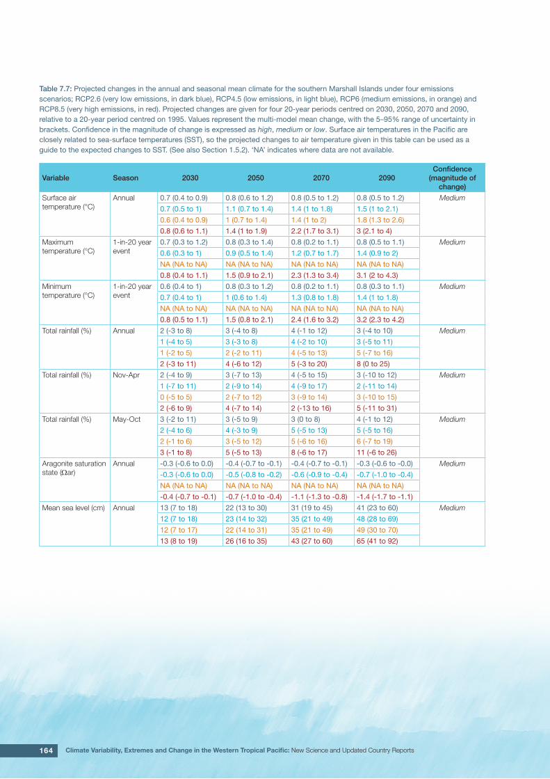
164 Climate Variability, Extremes and Change in the Western Tropical Pacific: New Science and Updated Country Reports
Table 7.7: Projected changes in the annual and seasonal mean climate for the southern Marshall Islands under four emissions scenarios; RCP2.6 (very low emissions, in dark blue), RCP4.5 (low emissions, in light blue), RCP6 (medium emissions, in orange) and RCP8.5 (very high emissions, in red). Projected changes are given for four 20-year periods centred on 2030, 2050, 2070 and 2090, relative to a 20-year period centred on 1995. Values represent the multi-model mean change, with the 5–95% range of uncertainty in brackets. Confidence in the magnitude of change is expressed as high, medium or low. Surface air temperatures in the Pacific are closely related to sea-surface temperatures (SST), so the projected changes to air temperature given in this table can be used as a guide to the expected changes to SST. (See also Section 1.5.2). ‘NA’ indicates where data are not available.
Variable Season 2030 2050 2070 2090Confidence
(magnitude of change)
Surface air temperature (°C)
Annual 0.7 (0.4 to 0.9) 0.8 (0.6 to 1.2) 0.8 (0.5 to 1.2) 0.8 (0.5 to 1.2) Medium
0.7 (0.5 to 1) 1.1 (0.7 to 1.4) 1.4 (1 to 1.8) 1.5 (1 to 2.1)
0.6 (0.4 to 0.9) 1 (0.7 to 1.4) 1.4 (1 to 2) 1.8 (1.3 to 2.6)
0.8 (0.6 to 1.1) 1.4 (1 to 1.9) 2.2 (1.7 to 3.1) 3 (2.1 to 4)
Maximum temperature (°C)
1-in-20 year event
0.7 (0.3 to 1.2) 0.8 (0.3 to 1.4) 0.8 (0.2 to 1.1) 0.8 (0.5 to 1.1) Medium
0.6 (0.3 to 1) 0.9 (0.5 to 1.4) 1.2 (0.7 to 1.7) 1.4 (0.9 to 2)
NA (NA to NA) NA (NA to NA) NA (NA to NA) NA (NA to NA)
0.8 (0.4 to 1.1) 1.5 (0.9 to 2.1) 2.3 (1.3 to 3.4) 3.1 (2 to 4.3)
Minimum temperature (°C)
1-in-20 year event
0.6 (0.4 to 1) 0.8 (0.3 to 1.2) 0.8 (0.2 to 1.1) 0.8 (0.3 to 1.1) Medium
0.7 (0.4 to 1) 1 (0.6 to 1.4) 1.3 (0.8 to 1.8) 1.4 (1 to 1.8)
NA (NA to NA) NA (NA to NA) NA (NA to NA) NA (NA to NA)
0.8 (0.5 to 1.1) 1.5 (0.8 to 2.1) 2.4 (1.6 to 3.2) 3.2 (2.3 to 4.2)
Total rainfall (%) Annual 2 (-3 to 8) 3 (-4 to 8) 4 (-1 to 12) 3 (-4 to 10) Medium
1 (-4 to 5) 3 (-3 to 8) 4 (-2 to 10) 3 (-5 to 11)
1 (-2 to 5) 2 (-2 to 11) 4 (-5 to 13) 5 (-7 to 16)
2 (-3 to 11) 4 (-6 to 12) 5 (-3 to 20) 8 (0 to 25)
Total rainfall (%) Nov-Apr 2 (-4 to 9) 3 (-7 to 13) 4 (-5 to 15) 3 (-10 to 12) Medium
1 (-7 to 11) 2 (-9 to 14) 4 (-9 to 17) 2 (-11 to 14)
0 (-5 to 5) 2 (-7 to 12) 3 (-9 to 14) 3 (-10 to 15)
2 (-6 to 9) 4 (-7 to 14) 2 (-13 to 16) 5 (-11 to 31)
Total rainfall (%) May-Oct 3 (-2 to 11) 3 (-5 to 9) 3 (0 to 8) 4 (-1 to 12) Medium
2 (-4 to 6) 4 (-3 to 9) 5 (-5 to 13) 5 (-5 to 16)
2 (-1 to 6) 3 (-5 to 12) 5 (-6 to 16) 6 (-7 to 19)
3 (-1 to 8) 5 (-5 to 13) 8 (-6 to 17) 11 (-6 to 26)
Aragonite saturation state (Ωar)
Annual -0.3 (-0.6 to 0.0) -0.4 (-0.7 to -0.1) -0.4 (-0.7 to -0.1) -0.3 (-0.6 to -0.0) Medium
-0.3 (-0.6 to 0.0) -0.5 (-0.8 to -0.2) -0.6 (-0.9 to -0.4) -0.7 (-1.0 to -0.4)
NA (NA to NA) NA (NA to NA) NA (NA to NA) NA (NA to NA)
-0.4 (-0.7 to -0.1) -0.7 (-1.0 to -0.4) -1.1 (-1.3 to -0.8) -1.4 (-1.7 to -1.1)
Mean sea level (cm) Annual 13 (7 to 18) 22 (13 to 30) 31 (19 to 45) 41 (23 to 60) Medium
12 (7 to 18) 23 (14 to 32) 35 (21 to 49) 48 (28 to 69)
12 (7 to 17) 22 (14 to 31) 35 (21 to 49) 49 (30 to 70)
13 (8 to 19) 26 (16 to 35) 43 (27 to 60) 65 (41 to 92)

165Chapter 7: Marshall Islands
Waves Projections Summary
Table 7.8: Projected average changes in wave height, period and direction in the northern Marshall Islands for December–March and June–September for RCP4.5 (low emissions, in blue) and RCP8.5 (very high emissions, in red), for two 20-year periods (2026–2045 and 2081–2100), relative to a 1986–2005 historical period. The values in brackets represent the 5th to 95th percentile range of uncertainty.
Variable Season 2035 2090 Confidence (range)
Wave height change (m) December–March -0.0 (-0.2 to 0.2)-0.1 (-0.3 to 0.1)
-0.1 (-0.3 to 0.1)-0.2 (-0.5 to 0.0)
Low
June–September +0.0 (-0.2 to 0.2)+0.0 (-0.2 to 0.2)
0.0 (-0.2 to 0.2)0.0 (-0.2 to 0.2)
Low
Wave height change (ft) December–March -0.1 (-0.8 to 0.7)-0.2 (-1.0 to 0.5)
-0.3 (-1.1 to 0.4)-0.8 (-1.5 to 0.1)
Low
June–September +0.0 (-0.6 to 0.6)+0.0 (-0.6 to 0.6)
0.0 (-0.6 to 0.7)0.0 (-0.6 to 0.8)
Low
Wave period change (s) December–March -0.1 (-0.6 to 0.5)-0.1 (-0.6 to 0.5)
-0.1 (-0.8 to 0.5)-0.2 (-1.0 to 0.5)
Low
JuneSeptember -0.0 (-0.9 to 0.8)-0.1 (-0.9 to 0.7)
-0.0 (-0.9 to 0.9)-0.0 (-0.9 to 0.8)
Low
Wave direction change (° clockwise) December–March 0 (-10 to 10)0 (-10 to 10)
0 (-10 to 10)-0 (-10 to 10)
Low
June–September 0 (-10 to 10)+0 (-10 to 20)
+0 (-10 to 20)+10 (-10 to 30)
Low
Table 7.9: Projected average changes in wave height, period and direction in the southern Marshall islands for December–March and June–September for RCP4.5 (low emissions, in blue) and RCP8.5 (very high emissions, in red), for two 20-year periods (2026–2045 and 2081–2100), relative to a 1986–2005 historical period. The values in brackets represent the 5th to 95th percentile range of uncertainty.
Variable Season 2035 2090 Confidence (range)
Wave height change (m) December–March -0.0 (-0.3 to 0.2)-0.1 (-0.3 to 0.2)
-0.1 (-0.3 to 0.1)-0.2 (-0.4 to 0.0)
Low
June–September 0.0 (-0.2 to 0.2)+0.0 (-0.2 to 0.2)
0.0 (-0.2 to 0.2)0.0 (-0.1 to 0.1)
Low
Wave height change (ft) December–March -0.1 (-0.9 to 0.7)-0.2 (-1.0 to 0.7)
-0.3 (-1.1 to 0.4)-0.7 (-1.4 to 0.1)
Low
June–September +0.0 (-0.5 to 0.7)+0.1 (-0.5 to 0.7)
0.0 (-0.6 to 0.6)0.0 (-0.3 to 0.5)
Low
Wave period change (s) December–March -0.1 (-0.7 to 0.7)-0.1 (-0.7 to 0.8)
-0.1 (-0.8 to 0.8)-0.2 (-1.0 to 0.8)
Low
June–September 0.0 (-0.9 to 0.9)-0.1 (-0.9 to 0.8)
0.0 (-0.9 to 0.9)-0.0 (-0.8 to 0.8)
Low
Wave direction change (° clockwise) December–March 0 (-10 to 10)0 (-10 to 10)
0 (-10 to 10)-0 (-10 to 10)
Low
June–September 0 (-20 to 20)0 (-20 to 20)
+0 (-20 to 30)+10 (-20 to 40)
Low
Wind-wave variables parameters are calculated for a 20-year period centred on 2035.

166 Climate Variability, Extremes and Change in the Western Tropical Pacific: New Science and Updated Country Reports

167
Chapter 8 Nauru

168 Climate Variability, Extremes and Change in the Western Tropical Pacific: New Science and Updated Country Reports
8.1.1 Current Climate• Over the past half century it is likely
that there has been a warming air temperature trend at Nauru which is partly associated with warming ocean temperatures.
• Annual and half-year rainfall trends from 1927 show little change at Nauru.
• Variability of wind-waves at Nauru is characterised by trade winds seasonally, and the El Niño–Southern Oscillation (ENSO) interannually. Available data are not suitable for assessing long-term trends (see Section 1.3).
8.1.2 Climate Projections• For the period to 2100, the latest
global climate model (GCM) projections and climate science findings indicate:
• El Niño and La Niña events will continue to occur in the future (very high confidence), but there is little consensus on whether these events will change in intensity or frequency;
• Annual mean temperatures and extremely high daily temperatures will continue to rise (very high confidence);
• Mean rainfall is projected to increase (medium confidence), along with more extreme rain events (high confidence);
• Droughts are projected to decline in frequency (medium confidence);
• Ocean acidification is expected to continue (very high confidence);
• The risk of coral bleaching will increase in the future (very high confidence);
• Sea level will continue to rise (very high confidence); and
• Wave height and period are projected to decrease in December–March (low confidence). No significant changes are projected in June–September (low confidence).
8.1 Climate Summary
8.2 Data Availability
Currently, meteorological observations are taken by two automatic weather stations (AWS; data from the Bureau of Meteorology ‘ARC-2’ AWS are available from July 2003) and a manual rain gauge near Yaren. There is also a sub-daily rain gauge near the centre of the island which has been operational since October 2009. Nauru data are available from 1893 to present for rainfall and 1951 to present
for air temperature; however there are significant gaps in both records. Monthly rainfall data, homogeneous from 1927 has been used in this report. There are insufficient air temperature data for trend analyses. The search for historical hard copy and digitised climate data for Nauru is ongoing.
Wind-wave data from buoys are particularly sparse in the Pacific region, with very short records. Model and reanalysis data are therefore required to detail the wind-wave climate of the region. Reanalysis surface wind data have been used to drive a wave model over the period 1979–2009 to generate a hindcast of the historical wind-wave climate.

169Chapter 8: Nauru
Information on temperature and rainfall seasonal cycles can be found in Australian Bureau of Meteorology and CSIRO (2011).
8.3.1 Wind-driven WavesSurface wind-wave driven processes can impact on many aspects of Pacific Island coastal environments, including: coastal flooding during storm wave events; coastal erosion, both during episodic storm events and due to long-term changes in integrated wave climate; characterisation of reef morphology and marine habitat/species distribution; flushing and circulation of lagoons; and potential shipping and renewable wave energy solutions. The surface offshore wind-wave climate can be described by characteristic wave heights, lengths or periods, and directions.
8.3 Seasonal Cycles
The wind-wave climate of Nauru is strongly characterised by the seasonal trade winds. On the west coast of Nauru, waves are directed from the south-east during June–September, and are directed from the north-east, and are slightly larger and longer than in the dry months, during December–March (Table 8.1, Figure 8.1). In June–September, swell waves are incident from the south resulting from extra-tropical storms, while in December–March waves are also observed from the west due to monsoon systems and from the north due to North Pacific extra-tropical storms. Waves larger than 2.3 m (99th percentile) occur predominantly during the wet season, generated by North Pacific extra-tropical storms and are observed as long, northerly and north-westerly swell. Some large westerly waves, thought to be generated by Philippine typhoons based on their wavelength
and direction, have been observed in other months (August and November). The height of a 1-in-50 year wave event on the west coast is calculated to be 5.0 m.
No suitable dataset is available to assess long-term historical trends in the Nauru wave climate. However, interannual variability may be assessed in the hindcast record. The wind-wave climate displays strong interannual variability at Nauru, varying strongly with the El Niño–Southern Oscillation (ENSO). During La Niña years, wave power is approximately 30% greater than during El Niño years in June–September, and waves are more strongly directed from the east year round, associated with increased trade wind speeds.
Table 8.1: Mean wave height, period and direction from which the waves are travelling near Nauru in December–March and June–September. Observation (hindcast) and climate model simulation mean values are given with the 5–95th percentile range (in brackets). Historical model simulation values are given for comparison with projections (see Section 8.5.6 – Wind-driven waves, and Tables 8.5). A compass relating number of degrees to cardinal points (direction) is shown.
Hindcast Reference Data (1979–2009)
Climate Model Simulations (1986–2005)
Wave Height(metres)
December–March 1.5 (1.1–2.0) 1.7 (1.4–2.0)
June–September 1.2 (0.9–1.7) 1.2 (1.1–1.4)
Wave Period(seconds)
December–March 9.3 (7.5–11.6) 8.4 (7.5–9.7)
June–September 8.6 (7.0–10.3) 7.9 (7.1–8.6)
Wave Direction(degrees clockwise from North)
December–March 30 (320–70) 40 (20–60)
June–September 130 (100–180) 120 (100–140)

170 Climate Variability, Extremes and Change in the Western Tropical Pacific: New Science and Updated Country Reports
8.4.1 Air Temperature
Annual, Half-year and Extreme Air Temperature
Due to incomplete historical air temperature records, observed mean and extreme air temperature trends for Nauru have not been calculated. Over the past half century it is likely that there has been a warming air temperature trend at Nauru partly due to the warming ocean temperatures (See Section 8.5.4 in the Nauru Country Report).
8.4.2 Rainfall
Annual and Half-year Total Rainfall
Notable interannual variability associated with the ENSO is evident in the Nauru observed rainfall record since 1927 (Figure 8.2). Trends in annual and half-year rainfall presented in Figure 8.2 and Table 8.2 are not statistically significant at the 5% level. In other words, annual and half-yearly rainfall trends show little change for Nauru.
Daily Rainfall
Due to incomplete historical daily rainfall records, observed extreme rainfall trends have not been calculated.
8.4.3 Tropical CyclonesTropical cyclone formation within the Nauru Exclusive Economic Zone (EEZ) is highly unlikely due to the islands proximity to the equator. There are no events on record, based on tropical cyclone data available from 1969/70 for the Southern Hemisphere and from 1977 for the Northern Hemisphere.
Figure 8.1: Mean annual cycle of wave height (grey) and mean wave direction (blue) at Nauru in hindcast data (1979–2009). To give an indication of interannual variability of the monthly means of the hindcast data, shaded boxes show 1 standard deviation around the monthly means, and error bars show the 5–95% range. The direction from which the waves are travelling is shown (not the direction towards which they are travelling).
8.4 Observed Trends

171Chapter 8: Nauru
Figure 8.2: Observed time series of annual total rainfall for Nauru. Light blue, dark blue and grey bars denote El Niño, La Niña and neutral years respectively. Solid black trend lines indicate least squares fit.
Table 8.2: Annual and half-year trends in rainfall at Nauru for the period 1927–2011. The 95% confidence intervals are shown in parentheses. None of the trends are significant at the 5% level.
Nauru Total Rain
(mm/10yrs)
Annual -15.1 (-136.9, +115.1)
Nov–Apr -40.8 (-130.2, +45.6)
May–Oct +6.6 (-34.1, +59.9)

172 Climate Variability, Extremes and Change in the Western Tropical Pacific: New Science and Updated Country Reports
The performance of the available Coupled Model Intercomparison Project (Phase 5) (CMIP5) climate models over the Pacific has been rigorously assessed (Brown et al., 2013a, b; Grose et al., 2014; Widlansky et al., 2013). The simulation of the key processes and features for the Nauru region is similar to the previous generation of CMIP3 models, with all the same strengths and many of the same weaknesses. The best-performing CMIP5 models used here have lower biases (differences between the simulated and observed climate data) than the best CMIP3 models, and there are fewer poorly-performing models. For Nauru, the most important model bias is that the models have an ocean that is too cold along the equator of the Pacific, known as the ‘cold-tongue bias’ (Chapter 1). This issue means
that the models underestimate the temperature and rainfall in the present day and this affects the confidence in the model projections. Out of 27 models assessed, three models were rejected for use in these projections due to biases in the mean climate and in the simulation of the SPCZ. Climate projections have been derived from up to 24 new global climate models (GCMs) in the CMIP5 database (the exact number is different for each scenario, Appendix A), compared with up to 18 models in the CMIP3 database reported in Australian Bureau of Meteorology and CSIRO (2011).
It is important to realise that the models used give different projections under the same scenario. This means there is not a single projected future for Nauru, but rather a range of possible futures for each emission scenario. This range is described below.
8.5.1 TemperatureFurther warming is expected over Nauru (Figure 8.3, Table 8.4). Under all RCPs, the warming is up to 1.2°C by 2030, relative to 1995, but after 2030 there is a growing difference in warming between each RCP. For example, in Nauru by 2090, a warming of 2.0 to 4.5°C is projected for RCP8.5 (very high emissions) while a warming of 0.6 to 1.5°C is projected for RCP2.6 (very low emissions). This range is broader than that presented in Australian Bureau of Meteorology and CSIRO (2011) because a wider range of emissions scenarios is considered. While relatively warm and cool years and decades will still occur due to natural variability, there is projected to be more warm years and decades on average in a warmer climate.
8.5 Climate Projections
Figure 8.3: Historical and simulated surface air temperature time series for the region surrounding Nauru. The graph shows the anomaly (from the base period 1986–2005) in surface air temperature from observations (the GISS dataset, in purple), and for the CMIP5 models under the very high (RCP8.5, in red) and very low (RCP2.6, in blue) emissions scenarios. The solid red and blue lines show the smoothed (20-year running average) multi-model mean anomaly in surface air temperature, while shading represents the spread of model values (5–95th percentile). The dashed lines show the 5–95th percentile of the observed interannual variability for the observed period (in black) and added to the projections as a visual guide (in red and blue). This indicates that future surface air temperature could be above or below the projected long-term averages due to interannual variability. The ranges of projections for a 20-year period centred on 2090 are shown by the bars on the right for RCP8.5, 6.0, 4.5 and 2.6.

173Chapter 8: Nauru
There is very high confidence that temperatures will rise because:
• It is known from theory and observations that an increase in greenhouse gases will lead to a warming of the atmosphere; and
• Climate models agree that the long-term average temperature will rise.
There is medium confidence in the model average temperature change shown in Table 8.4 because:
• The new models simulate the rate of temperature change of the recent past with reasonable accuracy; and
• Sea-surface temperatures near Nauru are too cold in most CMIP5 climate models in the current climate, and this affects the confidence in the projection into the future.
8.5.2 RainfallAn increase in long-term average rainfall is projected by almost all models for Nauru. The increase is greater for the higher emissions scenarios, especially towards the end of the century (Figure 8.4, Table 8.4). More than two thirds of models project an increase in both dry season and wet season rainfall. The year-to-year rainfall variability over Nauru is much larger than the projected change, except in the upper range of model in the highest emission scenario by 2090. There will still be wet and dry years and decades due to natural variability, but most models show that the long-term average is expected to be wetter. The effect of climate change on average rainfall may not be obvious in the short or medium term due to
natural variability. These projections are similar to those in Australian Bureau of Meteorology and CSIRO (2011), except the confidence rating on direction of change in mean rainfall has been changed from high confidence to medium confidence. The effect of the ‘cold-tongue bias’ in models (Chapter 1) is particularly strong in this region and the confidence in projections is strongly affected.
Figure 8.4: Historical and simulated annual average rainfall time series for the region surrounding Nauru. The graph shows the anomaly (from the base period 1986–2005) in rainfall from observations (the GPCP dataset, in purple), and for the CMIP5 models under the very high (RCP8.5, in red) and very low (RCP2.6, in blue) emissions scenarios. The solid red and blue lines show the smoothed (20-year running average) multi-model mean anomaly in rainfall, while shading represents the spread of model values (5–95th percentile). The dashed lines show the 5–95th percentile of the observed interannual variability for the observed period (in black) and added to the projections as a visual guide (in red and blue). This indicates that future rainfall could be above or below the projected long-term averages due to interannual variability. The ranges of projections for a 20-year period centred on 2090 are shown by the bars on the right for RCP8.5, 6.0, 4.5 and 2.6.
There is general agreement between models that rainfall will increase. However, biases in the models in the current climate lower the confidence of the projected changes, and makes the amount difficult to determine. The 5–95th percentile range of projected values from CMIP5 climate models is large, e.g. for RCP8.5 (very high emissions) the range is 1 to 52% by 2030 and 6 to 168% by 2090.

174 Climate Variability, Extremes and Change in the Western Tropical Pacific: New Science and Updated Country Reports
There is medium confidence that the long-term rainfall over Nauru will increase because:
• The majority of CMIP3 and CMIP5 models agree that the rainfall along the equator and in the ITCZ will increase under a warmer climate; and
• Changes in SPCZ rainfall are uncertain. The majority of CMIP5 models simulate increased rainfall in the western part of the SPCZ (Brown et al., 2013a), however rainfall changes are sensitive to sea-surface temperature gradients, which are not well simulated in many models (Widlansky et al., 2013). See Box in Chapter 1 for more details.
There is low confidence in the model average rainfall change shown in Table 8.4 because:
• The complex set of processes involved in tropical rainfall is challenging to simulate in models. This means that the confidence in the projection of rainfall is generally lower than for other variables such as temperature;
• The CMIP5 models are underestimate the present average rainfall of Nauru due to the ’cold-tongue bias’ (Chapter 1), similar to the previous CMIP3 models; and
• The future behaviour of the ENSO is unclear, and the ENSO strongly influences year-to-year rainfall variability.
8.5.3 Extremes
Extreme Temperature
The temperature on extremely hot days is projected to increase by about the same amount as average temperature. This conclusion is based on analysis of daily temperature data from a subset of CMIP5 models (Chapter 1). The frequency of extremely hot days is also expected to increase.
The temperature of the 1-in-20-year hot day is projected to increase by approximately 0.6°C by 2030 under the RCP2.6 (very low) scenario and by 0.9°C under the RCP8.5 (very high) scenario. By 2090 the projected increase is 0.8°C for RCP2.6 (very low) and 3°C for RCP8.5 (very high).
There is very high confidence that the temperature of extremely hot days and the temperature of extremely cool days will increase, because:
• A change in the range of temperatures, including the extremes, is physically consistent with rising greenhouse gas concentrations;
• This is consistent with observed changes in extreme temperatures around the world over recent decades; and
• All the CMIP5 models agree on an increase in the frequency and intensity of extremely hot days and a decrease in the frequency and intensity of cool days.
There is low confidence in the magnitude of projected change in extreme temperature because models generally underestimate the current intensity and frequency of extreme events, especially in this area, due to the ‘cold-tongue bias’ (Chapter 1). Changes to the particular driver of extreme temperatures affect whether the change to extremes is more or less than the change in the average temperature, and the changes to the drivers of extreme temperatures in Nauru are currently unclear. Also, while all models project the same direction of change there is a wide range in the projected magnitude of change among the models.
Extreme Rainfall
The frequency and intensity of extreme rainfall events are projected to increase. This conclusion is based on analysis of daily rainfall data from a subset of CMIP5 models using a similar method to that in Australian Bureau of Meteorology and CSIRO (2011) with some improvements (Chapter 1), so the results are slightly different to those in Australian Bureau of Meteorology and CSIRO (2011). The current 1-in-20-year daily rainfall amount is projected to increase by approximately 4 mm by 2030 for RCP2.6 and by 10 mm by 2030 for RCP8.5 (very high emissions). By 2090, it is projected to increase by approximately 16 mm for RCP2.6 and by 29 mm for RCP8.5 (very high emissions).The majority of models project the current 1-in-20-year daily rainfall event will become, on average, a 1-in-10-year event for RCP2.6 and a 1-in-5-year event for RCP8.5 (very high emissions) by 2090. These results are different to those found in Australian Bureau of Meteorology and CSIRO (2011) because of different methods used (Chapter 1).

175Chapter 8: Nauru
There is high confidence that the frequency and intensity of extreme rainfall events will increase because:
• A warmer atmosphere can hold more moisture, so there is greater potential for extreme rainfall (IPCC, 2012); and
• Increases in extreme rainfall in the Pacific are projected in all available climate models.
There is low confidence in the magnitude of projected change in extreme rainfall because:
• Models generally underestimate the current intensity of local extreme events, especially in this area due to the ‘cold-tongue bias’ (Chapter 1);
• Changes in extreme rainfall projected by models may be underestimated because models seem to underestimate the observed increase in heavy rainfall with warming (Min et al., 2011);
• GCMs have a coarse spatial resolution, so they do not adequately capture some of the processes involved in extreme rainfall events; and
• The Conformal Cubic Atmospheric Model (CCAM) downscaling model has finer spatial resolution and the CCAM results presented in Australian Bureau of Meteorology and CSIRO (2011) indicates a smaller increase in the number of extreme rainfall days, and there is no clear reason to accept one set of models over another.
Drought
Drought projections (defined in Chapter 1) are described in terms of changes in proportion of time in drought, frequency and duration by 2090 for very low and very high emissions (RCP2.6 and 8.5).
For Nauru the overall proportion of time spent in drought is expected to decrease under all scenarios. Under RCP8.5 the frequency of drought in all categories is projected to decrease and the duration of events in all drought categories is projected to stay approximately the same (Figure 8.5). Under RCP2.6 (very low emissions) the frequency of mild drought is projected
to increase slightly while the frequency of moderate, severe and extreme drought is projected to remain stable. The duration of events in all categories is projected to decrease slightly under RCP2.6 (very low emissions).
There is medium confidence in this direction of change because:
• There is only medium confidence in the direction of mean rainfall change;
• These drought projections are based upon a subset of models; and
• Like the CMIP3 models, the majority of the CMIP5 models agree on this direction of change.
There is low confidence in the projections of drought frequency and duration because there is low confidence in the magnitude of rainfall projections, and no consensus about projected changes in the ENSO, which directly influence the projection of drought.
Figure 8.5: Box-plots showing percent of time in moderate, severe or extreme drought (left hand side), and average drought duration and frequency for the different categories of drought (mild, moderate, severe and extreme) for Nauru. These are shown for 20-year periods centred on 1995, 2030, 2050, 2070 and 2090 for the RCP8.5 (very high emissions) scenario. The thick dark lines show the median of all models, the box shows the interquartile (25–75%) range, the dashed lines show 1.5 times the interquartile range and circles show outlier results.

176 Climate Variability, Extremes and Change in the Western Tropical Pacific: New Science and Updated Country Reports
8.5.4 Coral Reefs and Ocean AcidificationAs atmospheric CO2 concentrations continue to rise, oceans will warm and continue to acidify. These changes will impact the health and viability of marine ecosystems, including coral reefs that provide many key ecosystem services (high confidence). These impacts are also likely to be compounded by other stressors such as storm damage, fishing pressure and other human impacts.
The projections for future ocean acidification and coral bleaching use three RCPs (2.6, 4.5, and 8.5).
Ocean Acidification
In Nauru the aragonite saturation state has declined from about 4.5 in the late 18th century to an observed value of about 3.9±0.1 by 2000 (Kuchinke et al., 2014). All models show that the aragonite saturation state, a proxy for coral reef growth rate, will continue to decrease as atmospheric CO2 concentrations increase (very high confidence). Projections from CMIP5 models indicate that under RCPs 8.5 (very high emissions) and 4.5 (low emissions) the median aragonite saturation state will transition to marginal conditions (3.5) around 2030. In RCP8.5 (very high emissions) the aragonite saturation state continues to strongly decline thereafter to values where coral reefs have not historically been found (< 3.0). Under RCP4.5
(low emissions) the aragonite saturation plateaus around 3.2 i.e. marginal conditions for healthy coral reefs. While under RCP2.6 (very low emissions) the median aragonite saturation state never falls below 3.5, and increases slightly toward the end of the century (Figure 8.6) suggesting that the conditions remains adequate for healthy corals reefs. There is medium confidence in this range and distribution of possible futures because the projections are based on climate models that do not resolve the reef scale that can play a role in modulating large-scale changes. The impacts of ocean acidification are also likely to affect the entire marine ecosystem impacting the key ecosystem services provided by reefs.
Figure 8.6: Projected decreases in aragonite saturation state in Nauru from CMIP5 models under RCP2.6, 4.5 and 8.5. Shown are the median values (solid lines), the interquartile range (dashed lines), and 5% and 95% percentiles (light shading). The horizontal line represents the transition to marginal conditions for coral reef health (from Guinotte et al., 2003).

177Chapter 8: Nauru
Coral Bleaching Risk
As the ocean warms, the risk of coral bleaching increases (very high confidence). There is medium confidence in the projected rate of change for Nauru because there is medium confidence in the rate of change of sea-surface temperature (SST), and the changes at the reef scale (which can play a role in modulating large-scale changes) are not adequately resolved. Importantly, the coral bleaching risk calculation does not account the impact of other potential stressors (Chapter 1).
Corals can bleach when they are exposed to elevated temperatures over extended periods.
The changes in the frequency (or recurrence) and duration of severe bleaching risk are quantified for different projected SST changes (Table 8.3). Overall there is a decrease in the time between two periods of elevated risk and an increase in the duration of the elevated risk. For example, under a long-term mean increase of 1°C (relative to 1982–1999 period), the average period of severe bleaching risk (referred to as a risk event) will last 10.2 weeks (with a minimum duration of 1.4 weeks and a maximum duration of 6.6 months) and the average time between two risks will be 2.4 years (with the minimum recurrence of 2.9 months and a maximum recurrence of 8.1 years). If severe bleaching events occur more often than once every five years, the long-term viability of coral reef ecosystems becomes threatened.
8.5.5 Sea LevelMean sea level is projected to continue to rise over the course of the 21st century. There is very high confidence in the direction of change. The CMIP5 models simulate a rise of between approximately 7–18 cm by 2030 (very similar values for different RCPs), with increases of 41–89 cm by 2090 under the RCP8.5 (Figure 8.7 and Table 8.4). There is medium confidence in the range mainly because there is still uncertainty associated with projections of the Antarctic ice sheet contribution. Interannual variability of sea level will lead to periods of lower and higher regional sea levels. In the past, this interannual variability has been about 23 cm (5–95% range, after removal of the seasonal signal, see dashed lines in Figure 8.7a) and it is likely that a similar range will continue through the 21st century.
Table 8.3: Projected changes in severe coral bleaching risk for the Nauru Exclusive Economic Zone (EEZ) for increases in SST relative to 1982–1999.
Temperature change 1 Recurrence interval 2 Duration of the risk event 3
Change in observed mean 30 years 3.0 weeks
+0.25°C 6.2 years (3.7 months – 13.8 years) 6.7 weeks (2.8 weeks – 3 months)
+0.5°C 2.4 years (2.9 months – 8.1 years) 10.2 weeks (1.4 weeks – 6.6 months)
+0.75°C 1.1 years (0.8 months – 4.5 years) 12.8 weeks (1.3 weeks – 12.5 months)
+1°C 9.9 months (0.8 months – 3.9 years) 4.1 months (1.5 weeks – 2.8 years)
+1.5°C 6.4 months (0.8 months – 2.5 years) 6.9 months (5.2 weeks – 4.7 years)
+2°C 4.7 months (1.1 months – 9.9 months) 13.6 months (5.8 weeks – 6.8 years)
1 This refers to projected SST anomalies above the mean for 1982–1999. 2 Recurrence is the mean time between severe coral bleaching risk events. Range (min – max) shown in brackets.3 Duration refers to the period of time where coral are exposed to the risk of severe bleaching. Range (min – max) shown in brackets.

178 Climate Variability, Extremes and Change in the Western Tropical Pacific: New Science and Updated Country Reports
8.5.6 Wind-driven WavesDuring December–March at Nauru (in the wet season), projected changes in wave properties include a decrease in wave height (Figure 8.8), accompanied by a decrease in wave period and a possible small anticlockwise rotation (more northerly waves) (low confidence) (Table 8.5). These features are characteristic of a decrease in strength of the north-easterly trade winds. This change is only statistically significant by the end of the century in a high emission scenario and only in March, with a projected decrease in wave height of approximately 15 cm.
In June–September (the dry season), there are no statistically significant projected changes in wave properties (low confidence) (Table 8.5). Non-significant changes include a possible increase in wave height, a small decrease in period, and a clockwise rotation of direction (more southerly waves). A projected decrease in the height of larger waves is suggested (low confidence).
There is low confidence in projected changes in the Nauru wind-wave climate because:
• Projected changes in wave climate are dependent on confidence in projected changes in ENSO, which is low; and
• The differences between simulated and observed (hindcast) wave data can be larger than the projected wave changes, which further reduces our confidence in projections.
Figure 8.7: (a) The observed tide-gauge records of relative sea-level (since the late 1970s) are indicated in purple, and the satellite record (since 1993) in green. The gridded (reconstructed) sea level data at Nauru (since 1950) is shown in black. Multi-model mean projections from 1995–2100 are given for the RCP8.5 (red solid line) and RCP2.6 emissions scenarios (blue solid line), with the 5–95% uncertainty range shown by the red and blue shaded regions. The ranges of projections for four emission scenarios (RCPs 2.6, 4.5, 6.0 and 8.5) by 2100 are also shown by the bars on the right. The dashed lines are an estimate of interannual variability in sea level (5–95% uncertainty range about the projections) and indicate that individual monthly averages of sea level can be above or below longer-term averages.
(b) The regional distribution of projected sea level rise under the RCP4.5 emissions scenario for 2081–2100 relative to 1986–2005. Mean projected changes are indicated by the shading, and the estimated uncertainty in the projections is indicated by the contours (in cm).
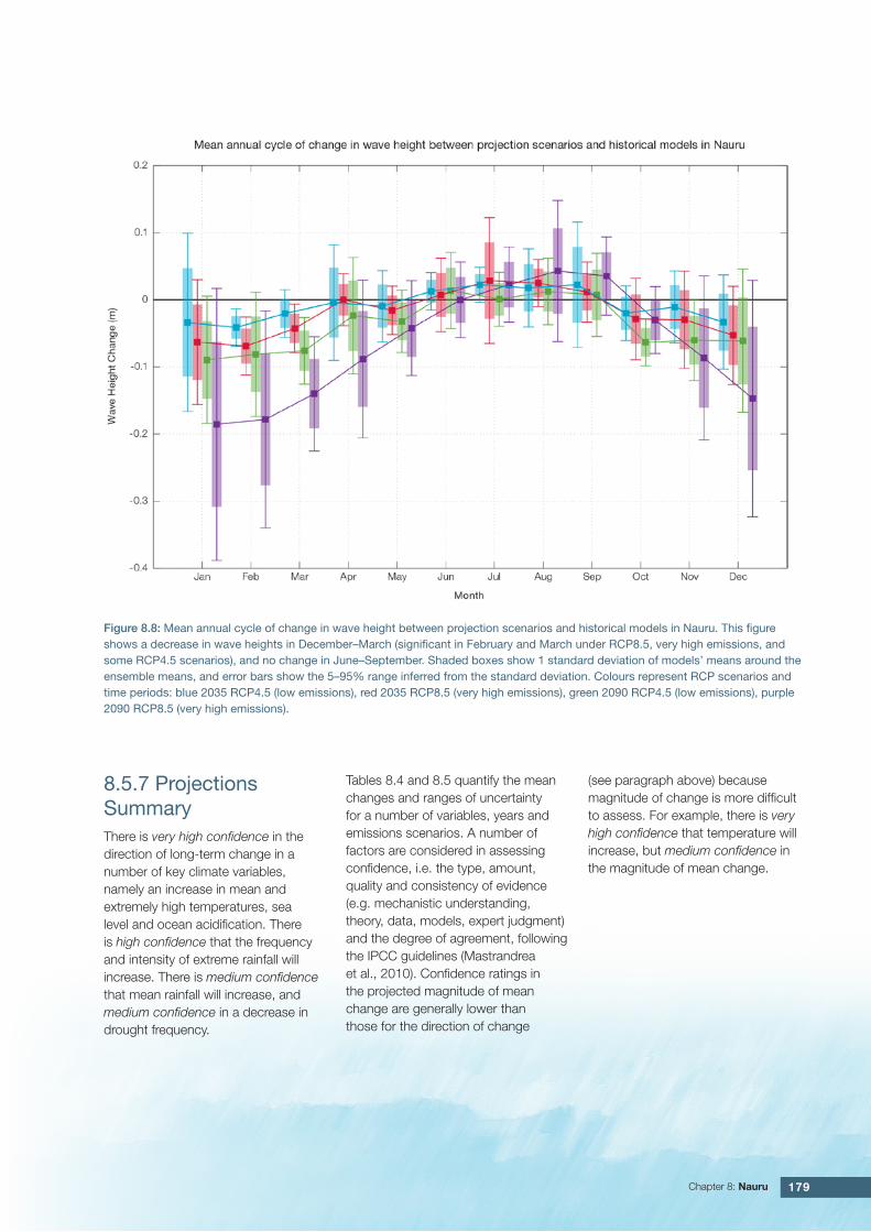
179Chapter 8: Nauru
Figure 8.8: Mean annual cycle of change in wave height between projection scenarios and historical models in Nauru. This figure shows a decrease in wave heights in December–March (significant in February and March under RCP8.5, very high emissions, and some RCP4.5 scenarios), and no change in June–September. Shaded boxes show 1 standard deviation of models’ means around the ensemble means, and error bars show the 5–95% range inferred from the standard deviation. Colours represent RCP scenarios and time periods: blue 2035 RCP4.5 (low emissions), red 2035 RCP8.5 (very high emissions), green 2090 RCP4.5 (low emissions), purple 2090 RCP8.5 (very high emissions).
8.5.7 Projections SummaryThere is very high confidence in the direction of long-term change in a number of key climate variables, namely an increase in mean and extremely high temperatures, sea level and ocean acidification. There is high confidence that the frequency and intensity of extreme rainfall will increase. There is medium confidence that mean rainfall will increase, and medium confidence in a decrease in drought frequency.
Tables 8.4 and 8.5 quantify the mean changes and ranges of uncertainty for a number of variables, years and emissions scenarios. A number of factors are considered in assessing confidence, i.e. the type, amount, quality and consistency of evidence (e.g. mechanistic understanding, theory, data, models, expert judgment) and the degree of agreement, following the IPCC guidelines (Mastrandrea et al., 2010). Confidence ratings in the projected magnitude of mean change are generally lower than those for the direction of change
(see paragraph above) because magnitude of change is more difficult to assess. For example, there is very high confidence that temperature will increase, but medium confidence in the magnitude of mean change.

180 Climate Variability, Extremes and Change in the Western Tropical Pacific: New Science and Updated Country Reports
Table 8.4: Projected changes in the annual and seasonal mean climate for Nauru under four emissions scenarios; RCP2.6 (very low emissions, in dark blue), RCP4.5 (low emissions, in light blue), RCP6 (medium emissions, in orange) and RCP8.5 (very high emissions, in red). Projected changes are given for four 20-year periods centred on 2030, 2050, 2070 and 2090, relative to a 20-year period centred on 1995. Values represent the multi-model mean change, with the 5–95% range of uncertainty in brackets. Confidence in the magnitude of change is expressed as high, medium or low. Surface air temperatures in the Pacific are closely related to sea-surface temperatures (SST), so the projected changes to air temperature given in this table can be used as a guide to the expected changes to SST. (See also Section 1.5.2). ‘NA’ indicates where data are not available.
Variable Season 2030 2050 2070 2090Confidence
(magnitude of change)
Surface air temperature (°C)
Annual 0.7 (0.4 to 1) 0.9 (0.6 to 1.4) 0.9 (0.5 to 1.4) 0.9 (0.6 to 1.5) Medium
0.7 (0.4 to 1.2) 1.1 (0.6 to 1.5) 1.4 (0.8 to 2.1) 1.5 (1.1 to 2.5)
0.7 (0.4 to 1) 1 (0.7 to 1.6) 1.5 (0.9 to 2.3) 1.9 (1.1 to 3)
0.9 (0.5 to 1.2) 1.5 (1 to 2.2) 2.3 (1.5 to 3.5) 3 (2 to 4.5)
Maximum temperature (°C)
1-in-20 year event
0.6 (0.1 to 1.1) 0.7 (0.2 to 1.2) 0.8 (0.4 to 1.4) 0.8 (0.4 to 1.3) Medium
0.6 (0.2 to 0.9) 0.9 (0.5 to 1.3) 1.2 (0.6 to 1.8) 1.4 (0.8 to 2.2)
NA (NA to NA) NA (NA to NA) NA (NA to NA) NA (NA to NA)
0.9 (0.4 to 1.2) 1.5 (0.8 to 2.4) 2.3 (1.4 to 3.5) 3 (1.9 to 4.4)
Minimum temperature (°C)
1-in-20 year event
0.7 (0.3 to 1) 0.8 (0 to 1.6) 0.8 (0.2 to 1.6) 0.8 (0.4 to 1.2) Medium
0.6 (0.2 to 0.9) 1 (0.6 to 1.3) 1.2 (0.6 to 1.6) 1.4 (0.8 to 2.1)
NA (NA to NA) NA (NA to NA) NA (NA to NA) NA (NA to NA)
0.8 (0.4 to 1.3) 1.5 (0.8 to 2.8) 2.4 (1.5 to 3.6) 3 (2 to 4.3)
Total rainfall (%) Annual 11 (-7 to 27) 19 (-9 to 56) 25 (5 to 72) 30 (-4 to 60) Low
18 (2 to 40) 24 (1 to 61) 33 (0 to 84) 37 (-1 to 105)
18 (-1 to 38) 26 (2 to 49) 29 (4 to 65) 40 (6 to 79)
21 (1 to 52) 32 (-3 to 69) 52 (-2 to 142) 63 (6 to 168)
Total rainfall (%) Nov-Apr 7 (-16 to 27) 16 (-17 to 47) 21 (-8 to 59) 28 (-9 to 60) Low
15 (-4 to 41) 19 (-7 to 50) 26 (-3 to 65) 27 (-7 to 90)
18 (-3 to 46) 24 (-11 to 50) 25 (-11 to 57) 34 (-12 to 83)
13 (-4 to 32) 26 (-12 to 74) 35 (-12 to 105) 45 (-7 to 139)
Total rainfall (%) May-Oct 16 (-1 to 51) 24 (-4 to 63) 31 (-3 to 93) 31 (-2 to 76) Low
22 (-1 to 50) 32 (3 to 108) 43 (0 to 128) 48 (10 to 143)
17 (-8 to 43) 28 (-7 to 73) 33 (-4 to 80) 48 (8 to 100)
32 (5 to 90) 41 (7 to 107) 73 (2 to 212) 86 (3 to 202)
Aragonite saturation state (Ωar)
Annual -0.3 (-0.6 to -0.1) -0.4 (-0.7 to -0.1) -0.4 (-0.6 to -0.1) -0.3 (-0.6 to -0.1) Medium
-0.3 (-0.6 to 0.0) -0.5 (-0.8 to -0.2) -0.6 (-0.9 to -0.4) -0.7 (-1.0 to -0.4)
NA (NA to NA) NA (NA to NA) NA (NA to NA) NA (NA to NA)
-0.3 (-0.6 to -0.1) -0.6 (-0.9 to -0.4) -1.0 (-1.3 to -0.7) -1.4 (-1.6 to -1.1)
Mean sea level (cm) Annual 12 (8–17) 22 (14–30) 32 (19–45) 42 (24–60) Medium
12 (7–17) 22 (14–31) 35 (22–48) 48 (29–68)
12 (7–16) 22 (14–30) 34 (21–48) 49 (30–69)
13 (8–18) 25 (17–34) 42 (28–58) 63 (41–89)

181Chapter 8: Nauru
Waves Projections Summary
Table 8.5: Projected average changes in wave height, period and direction at Nauru for December–March and June–September for RCP4.5 (low emissions, in blue) and RCP8.5 (very high emissions, in red), for two 20-year periods (2026–2045 and 2081–2100), relative to a 1986–2005 historical period. The values in brackets represent the 5th to 95th percentile range of uncertainty.
Variable Season 2035 2090 Confidence (range)
Wave height change (m) December–March -0.0 (-0.2 to 0.2)-0.1 (-0.3 to 0.1)
-0.1 (-0.2 to 0.1)-0.2 (-0.3 to -0.1)
Low
June–September +0.0 (-0.1 to 0.1)+0.0 (-0.1 to 0.1)
0.0 (-0.1 to 0.1)+0.0 (-0.1 to 0.1)
Low
Wave period change (s) December–March -0.0(-1.1 to 1.0)-0.1 (-1.1 to 1.0)
-0.1 (-1.2 to 1.1)-0.2 (-1.3 to 1.0)
Low
June–September +0.0 (-0.6 to 0.7)0.0 (-0.6 to 0.6)
0.0 (-0.7 to 0.7)-0.1 (-0.8 to 0.6)
Low
Wave direction change (° clockwise) December–March 0 (-10 to 10)0 (-10 to 10)
0 (-10 to 10)0 (-10 to 10)
Low
June–September +0 (-10 to 20)+0 (-10 to 20)
+0 (-10 to 20)+10 (-10 to 30)
Low
Wind-wave variables parameters are calculated for a 20-year period centred on 2035.

182 Climate Variability, Extremes and Change in the Western Tropical Pacific: New Science and Updated Country Reports

183
Chapter 9 Niue

184 Climate Variability, Extremes and Change in the Western Tropical Pacific: New Science and Updated Country Reports
9.1.1 Current Climate• Annual and half-year mean
temperatures have warmed at Alofi-Hanan Airport since 1940.
• The frequency of Warm Days and Warm Nights has significantly increased while Cool Days have decreased at Alofi-Hanan Airport.
• Annual and half-year rainfall trends show little change at Alofi-Hanan Airport since 1905. There has also been little change in extreme rainfall since 1915.
• Tropical cyclones affect Niue mainly between November and April. An average of 10 cyclones per decade developed within or crossed the Niue Exclusive Economic Zone (EEZ) between the 1969/70 and 2010/11 seasons. Six of the 24 tropical cyclones (25%) between the 1981/82 and 2010/11 seasons became severe events (Category 3 or stronger) in the Niue EEZ. Available data are not suitable for assessing long-term trends.
• Wind-waves at Niue have a nearly constant height period and direction throughout the year, with a slight seasonal increase in wave height and period with southern trade winds. Waves are characterised by trade winds seasonally and the El Niño–Southern Oscillation (ENSO) and Southern Annular Mode (SAM) interannually. Available data are not suitable for assessing long-term trends (see Section 1.3).
9.1.2 Climate ProjectionsFor the period to 2100, the latest global climate model (GCM) projections and climate science findings indicate:
• El Niño and La Niña events will continue to occur in the future (very high confidence), but there is little consensus on whether these events will change in intensity or frequency;
• Annual mean temperatures and extremely high daily temperatures will continue to rise (very high confidence);
9.1 Climate Summary
• Mean annual rainfall could increase or decrease with the model average indicating little change (low confidence in this model average), with more extreme rain events (high confidence);
• The proportion of time in drought is projected to increase or decrease in line with average rainfall (low confidence);
• Ocean acidification is expected to continue (very high confidence);
• The risk of coral bleaching will increase in the future (very high confidence);
• Sea level will continue to rise (very high confidence); and
• Wave heights may decrease in December–March (low confidence), with no significant changes projected in June–September waves (low confidence).

185Chapter 9: Niue
Information on temperature and rainfall seasonal cycles can be found in Australian Bureau of Meteorology and CSIRO (2011).
9.3.1 Wind-driven WavesThe wind-wave climate of Niue is strongly characterised by the Southern Hemisphere trade winds. On the west coast, where easterly waves may be blocked by the island, waves are directed from the south year round, with more directional variability during December–March. Swell is observed from the south to south-west year round due to Southern Ocean storms. Wave heights and period are slightly smaller in December–March, when mean height is around 1.8 m and mean period
around 9.9 s, than June–September, when mean height is around 2.1 m and period around 10.3 s (Table 9.1, Figure 9.1). Waves larger than 3.6 m (99th percentile) occur year round, usually from the south and south-west, due to Southern Ocean swell waves. Large northerly and westerly waves, associated with cyclones, are seen in December–March. The height of a 1-in-50 year wave event on the west coast of Niue is calculated to be 10.2 m.
No suitable dataset is available to assess long-term historical trends in the Niue wave climate. However, interannual variability may be assessed in the hindcast record. The wind-wave climate displays strong interannual variability at Niue, varying strongly with ENSO in December–March and SAM in both December–March
and June–September. During El Niño years, southerly wave power is greater than during La Niña years in December–March due to movement of the South Pacific Convergence Zone (SPCZ) away from Niue. Wave power is similar during June–September in both phases of ENSO, slightly weaker during La Niña, with waves directed more from the east in these months in La Niña years associated with increased trade winds. When the Southern Annular Mode (SAM) index is negative there is a strong rotation of waves toward the south-west due to enhanced extra-tropical storms in the Southern Ocean, with a 50% increase in wave power in December–March and a slight reduction in June–September.
9.2 Data Availability
There are currently two operational meteorological observation stations on Niue. The primary station, where multiple observations are conducted on a daily basis, is located at Hanan Airport, south of Alofi on the western side of the island. A single daily observation rainfall station is located at Liku on the eastern side of the island. Observations began at Liku in 1990. The complete historical record for Hanan Airport, Alofi and Kaimiti has been used to create a Hanan Airport composite. Observations were taken close to the Alofi wharf from 1905 to
1971 and adjacent to the current Alofi Police Station from 1977 to 1996. Between 1971 and 1976 observations were taken at Kaimiti, 2.4 km south of Alofi. Hanan Airport monthly rainfall from 1905 (daily values from 1915) and air temperature from 1940 have been used in this report. The Hanan Airport composite record is homogeneous. Additional information on historical climate trends in the Niue region can be found in the Pacific Climate Change Data Portal www.bom.gov.au/climate/pccsp/.
Wind-wave data from buoys are particularly sparse in the Pacific region, with very short records. Model and reanalysis data are therefore required to detail the wind-wave climate of the region. Reanalysis surface wind data have been used to drive a wave model over the period 1979–2009 to generate a hindcast of the historical wind-wave climate.
9.3 Seasonal Cycles

186 Climate Variability, Extremes and Change in the Western Tropical Pacific: New Science and Updated Country Reports
Table 9.1: Mean wave height, period and direction from which the waves are travelling near Niue in December–March and June–September. Observation (hindcast) and climate model simulation mean values are given with the 5–95th percentile range (in brackets). Historical model simulation values are given for comparison with projections (see Section 9.5.6 – Wind-driven waves, and Table 9.7). A compass relating number of degrees to cardinal points (direction) is shown.
Hindcast Reference Data (1979–2009)
Climate Model Simulations (1986–2005)
Wave Height(metres)
December–March 1.8 (1.2–2.8) 2.0 (1.6–2.3)
June–September 2.1 (1.4–3.1) 2.2 (1.7–2.6)
Wave Period(seconds)
December–March 9.9 (7.9–12.2) 8.9 (7.9–10.2)
June–September 10.3 (8.0–12.9) 8.9 (7.7–9.8)
Wave Direction (degrees clockwise from North)
December–March 180 (40–320) 90 (60–130)
June–September 180 (140–220) 150 (130–170)
Figure 9.1: Mean annual cycle of wave height (grey) and mean wave direction (blue) at Niue in hindcast data (1979–2009). To give an indication of interannual variability of the monthly means of the hindcast data, shaded boxes show 1 standard deviation around the monthly means, and error bars show the 5–95% range. The direction from which the waves are travelling is shown (not the direction towards which they are travelling).

187Chapter 9: Niue
9.4 Observed Trends
9.4.1 Air Temperature
Annual and Half-year Mean Air Temperature
Warming trends are evident in November–April maximum and minimum temperatures at Alofi-Hanan Airport for the period 1940–2011 (Figure 9.2 and Table 9.2). The strongest trend is in minimum temperatures for November to April. All the temperature trends are consistent with regional and global warming trends.
Figure 9.2: Observed time series of annual average values of mean air temperature (red dots and line) and total rainfall (bars) at Alofi-Hanan Airport. Light blue, dark blue and grey bars denote El Niño, La Niña and neutral years respectively. Solid black trend lines indicate a least squares fit.
Table 9.2: Annual and half-year trends in air temperature (Tmax, Tmin, Tmean) and rainfall at Alofi-Hanan Airport. The 95% confidence intervals are shown in brackets. Values for trends significant at the 5% level are shown in boldface.
Alofi-Hanan Airport
Tmax(°C/10yrs)
Airport Tmin
(°C/10yrs)
Tmean(°C/10yrs)
Total Rain(mm/10yrs)
1940–2011 1905–2011
Annual - - - +2.20 (-25.6, +29.7)
Nov–Apr +0.06(0.00, +0.10)
+0.12(+0.05, +0.19)
- +12.20 (-9.8, +29.6)
May–Oct +0.02(-0.01, +0.08)
+0.07(-0.01, +0.13)
+0.05(-0.01, +0.1)
0.00 (-0.30, +0.30)

188 Climate Variability, Extremes and Change in the Western Tropical Pacific: New Science and Updated Country Reports
Extreme Daily Air Temperature
Extreme daily temperatures have warmed at Alofi-Hanan Airport (Figure 9.3 and Table 9.3). The number of Warm Days and Warm Nights have significantly increased while Cool Days have decreased. These trends are statistically significant at the 5% level and consistent with regional and global warming trends.
Table 9.3: Annual trends in air temperature and rainfall extremes at Alofi-Hanan Airport. The 95% confidence intervals are shown in parentheses. Values for trends significant at the 5% level are shown in boldface.
Alofi-Hanan Airport
TEMPERATURE (1940–2011)
Warm Days (days/decade) +3.90 (+0.46, +7.20)
Warm Nights (days/decade) +3.97 (+1.22, +7.12)
Cool Days (days/decade) -5.77 (-7.85, -3.95)
Cool Nights (days/decade) -1.80 (-4.81, +1.28)
RAINFALL (1915–2011)
Rain Days ≥ 1 mm (days/decade) +1.48 (-0.35, +3.22)
Very Wet day rainfall (mm/decade) -7.93 (-36.64, +22.25)
Consecutive Dry Days (days/decade) 0.00 (-0.34, +0.32)
Max 1-day rainfall (mm/decade) -1.17 (-4.66, +2.26)
Warm Days: Number of days with maximum temperature greater than the 90th percentile for the base period 1971–2000Warm Nights: Number of days with minimum temperature greater than the 90th percentile for the base period 1971–2000Cool Days: Number of days with maximum temperature less than the 10th percentile for the base period 1971–2000Cool Nights: Number of days with minimum temperature less than the 10th percentile for the base period 1971–2000Rain Days ≥ 1 mm: Annual count of days where rainfall is greater or equal to 1 mm (0.039 inches)Very Wet Day rainfall: Amount of rain in a year where daily rainfall is greater than the 95th percentile for the reference period 1971–2000Consecutive Dry Days: Maximum number of consecutive days in a year with rainfall less than 1mm (0.039 inches)Max 1-day rainfall: Annual maximum 1-day rainfall
Figure 9.3: Observed time series of annual total number of Warm Days (left) and Cool Nights (right) at Alofi-Hanan Airport. Solid black trend lines indicate a least squares fit.
9.4.2 Rainfall
Annual and Half-year Total Rainfall
Notable interannual variability associated with the ENSO is evident in the observed rainfall record for Alofi-Hanan Airport since 1905 (Figure 9.2). Trends in annual and half-year rainfall shown in Table 9.2 and Figure 9.2 are not statistically significant at the 5% level. In other words, annual and half-
year rainfall trends show little change at Alofi-Hanan Airport.
Daily Rainfall
Daily rainfall trends for Alofi-Hanan Airport are presented in Table 9.3. Due to large year-to-year variability, there are no significant trends in the daily rainfall indices. Figure 9.4 shows insignificant trends in annual Max 1-day rainfall and Rain Days ≥ 1 mm (days with rainfall).

189Chapter 9: Niue
9.4.3 Tropical CyclonesTropical cyclones affect Niue between November and April. Occurrences outside this period are rare. The tropical cyclone archive for the Southern Hemisphere indicates that between the 1969/70 and 2010/11 seasons, 41 tropical cyclones developed within or crossed the Niue EEZ. This represents an average of 10 cyclones per decade. Refer to Chapter 1, Section 1.4.2 (Tropical Cyclones) for an explanation of the difference in the number of tropical cyclones occurring in Niue in this report (Australian Bureau of Meteorology and CSIRO, 2014) compared to Australian Bureau of Meteorology and CSIRO (2011).
The interannual variability in the number of tropical cyclones in the Niue EEZ is large ranging from zero in some seasons to four in the 1979/80 season (Figure 9.5). The differences between tropical cyclone average occurrence in El Niño, La Niña and neutral years are not statistically significant. Six of the 24 tropical cyclones (25%) between the 1981/82 and 2010/11 seasons became severe events (Category 3 or stronger) in the Niue EEZ.
Long term trends in frequency and intensity have not been presented as country scale assessment is not recommended. Some tropical cyclone tracks analysed in this subsection include the tropical depression stage (sustained winds less than or equal to
Figure 9.5: Time series of the observed number of tropical cyclones developing within and crossing the Niue EEZ per season. The 11-year moving average is in blue.
Figure 9.4: Observed time series of annual Max 1-day rainfall (left) and Rain Days ≥ 1 mm at Alofi-Hanan Airport (right). Solid black trend lines indicate a least squares fit.
34 knots) before and/or after tropical cyclone formation.
Additional information on historical tropical cyclones in the Niue region can be found at www.bom.gov.au/cyclone/history/tracks/index.shtml

190 Climate Variability, Extremes and Change in the Western Tropical Pacific: New Science and Updated Country Reports
The performance of the available Coupled Model Intercomparison Project (Phase 5) (CMIP5) climate models over the Pacific has been rigorously assessed (Brown et al., 2013a, b; Grose et al., 2014; Widlansky et al., 2013). The simulation of the key processes and features for the Niue region is similar to the previous generation of CMIP3 models, with all the same strengths and many of the same weaknesses. The best-performing CMIP5 models used here have lower biases (differences between the simulated and observed climate data) than the best CMIP3 models, and there are fewer poorly-performing models. For Niue, the most important model bias is that the rainfall maximum of the SPCZ is too zonally (east-west) oriented and does not extend in a diagonal band to the southeast of
Niue. This lowers confidence in the model projections. Out of 27 models assessed, three models were rejected for use in these projections due to biases in the mean climate and in the simulation of the SPCZ. Climate projections have been derived from up to 24 new global climate models (GCMs) in the CMIP5 database (the exact number is different for each scenario, Appendix A), compared with up to 18 models in the CMIP3 database reported in Australian Bureau of Meteorology and CSIRO (2011).
It is important to realise that the models used give different projections under the same scenario. This means there is not a single projected future for Niue, but rather a range of possible futures for each emission scenario. This range is described below.
9.5.1 TemperatureFurther warming is expected over Niue (Figure 9.6, Table 9.6). Under all RCPs, the warming is up to 1.1°C by 2030, relative to 1995, but after 2030 there is a growing difference in warming between each RCP. For example, in Niue by 2090, a warming of 1.7 to 4.2°C is projected for RCP8.5 (very high emissions) while a warming of 0.2 to 1.1°C is projected for RCP2.6 (very low emissions). This range is broader than that presented in Australian Bureau of Meteorology and CSIRO (2011) because a wider range of emissions scenarios is considered. While relatively warm and cool years and decades will still occur due to natural variability, there is projected to be more warm years and decades on average in a warmer climate.
9.5 Climate Projections
Figure 9.6: Historical and simulated surface air temperature time series for the region surrounding Niue. The graph shows the anomaly (from the base period 1986–2005) in surface air temperature from observations (the GISS dataset, in purple), and for the CMIP5 models under the very high (RCP8.5, in red) and very low (RCP2.6, in blue) emissions scenarios. The solid red and blue lines show the smoothed (20-year running average) multi-model mean anomaly in surface air temperature, while shading represents the spread of model values (5–95th percentile). The dashed lines show the 5–95th percentile of the observed interannual variability for the observed period (in black) and added to the projections as a visual guide (in red and blue). This indicates that future surface air temperature could be above or below the projected long-term averages due to interannual variability. The ranges of projections for a 20-year period centred on 2090 are shown by the bars on the right for RCP8.5, 6.0, 4.5 and 2.6.

191Chapter 9: Niue
There is very high confidence that temperatures will rise because:
• It is known from theory and observations that an increase in greenhouse gases will lead to a warming of the atmosphere; and
• Climate models agree that the long-term average temperature will rise.
There is medium confidence in the model average temperature change shown in Table 9.6 because:
• The new models do not simulate the temperature change of the recent past in Niue as well as in other places; and
• There is a bias in the simulation of the current SPCZ near Niue, and uncertainty in the projection of the SPCZ, which not only affects the current bias and uncertainty in projections of rainfall but also temperature.
9.5.2 RainfallThe CMIP5 models show a range of projected annual mean rainfall change from an increase to a decrease, and the model average is for a slight increase for the high emission scenario by the end of the century. The range is greater in the highest emissions scenarios (Figure 9.7, Table 9.6). Similar to the CMIP3 results, there is greater model agreement for a slight increase in November–April rainfall (more than two thirds of models), and little change in May–October rainfall. There was greater confidence in the projected change in November–April rainfall in the previous report, however new research has raised more uncertainty about the future of the SPCZ (see Box in Chapter 1 for more details). Mean rainfall increased in Niue between 1979 and 2006 (Figure 9.7),
but the models do not project this will continue at the same rate into the future. This indicates that the recent increase may be caused by natural variability and not caused by global warming. It is also possible that the models do not simulate a key process driving the recent change. However, the recent change is not particularly large (<10%) and the observed record shown is not particularly long (28 years), so it is difficult to determine the significance of this difference, and its cause. The year-to-year rainfall variability over Niue is generally larger than the projected change, except for the models with the largest projected change in the highest emission scenario by 2090. The effect of climate change on average rainfall may not be obvious in the short or medium term due to natural variability.
Figure 9.7: Historical and simulated annual average rainfall time series for the region Niue. The graph shows the anomaly (from the base period 1986–2005) in rainfall from observations (the GPCP dataset, in purple), and for the CMIP5 models under the very high (RCP8.5, in red) and very low (RCP2.6, in blue) emissions scenarios. The solid red and blue lines show the smoothed (20-year running average) multi-model mean anomaly in rainfall, while shading represents the spread of model values (5–95th percentile). The dashed lines show the 5–95th percentile of the observed interannual variability for the observed period (in black) and added to the projections as a visual guide (in red and blue). This indicates that future rainfall could be above or below the projected long-term averages due to interannual variability. The ranges of projections for a 20-year period centred on 2090 are shown by the bars on the right for RCP8.5, 6.0, 4.5 and 2.6.

192 Climate Variability, Extremes and Change in the Western Tropical Pacific: New Science and Updated Country Reports
The model mean shows an increase in rainfall, but not all models agree. This lowers the confidence that we can determine the most likely direction of change in annual rainfall, and makes the amount difficult to determine. The 5–95th percentile range of projected values from CMIP5 climate models is large, e.g. for RCP8.5 (very high emissions) the range is -12 to +18% by 2030 and -12 to +46% by 2090.
There is low confidence in the model average result of slight increase in annual rainfall for Niue because:
• This average finding of no change is the average of a model spread from a projected rainfall increase to a rainfall decrease, and also many models project little change; and
• The future of the SPCZ is not clear due to model biases in the current climate, and likewise the future behaviour of the ENSO is unclear (see Box in Chapter 1).
There is low confidence in the model average rainfall change shown in Table 9.6 because:
• There is a spread in model rainfall projections, which range from a projected rainfall increase to a rainfall decrease;
• The complex set of processes involved in tropical rainfall is challenging to simulate in models. This means that the confidence in the projection of rainfall is generally lower than for other variables such as temperature;
• There is a different magnitude of change in SPCZ rainfall projected by models that have reduced sea-surface temperature biases (Australian Bureau of Meteorology and CSIRO, 2011, Chapter 7 (downscaling); Widlanksy et al., 2012) compared to the CMIP5 models; and
• The future behaviour of the ENSO is unclear, and the ENSO strongly influences year-to-year rainfall variability.
9.5.3 Extremes
Extreme Temperature
The temperature on extremely hot days is projected to increase by about the same amount as average temperature. This conclusion is based on analysis of daily temperature data from a subset of CMIP5 models (Chapter 1). The frequency of extremely hot days is also expected to increase.
The temperature of the 1-in-20-year hot day is projected to increase by approximately 0.5°C by 2030 under the RCP2.6 (very low) scenario and by 0.7°C under the RCP8.5 (very high) scenario. By 2090 the projected increase is 0.7°C for RCP2.6 (very low) and 2.8°C for RCP8.5 (very high).
There is very high confidence that the temperature of extremely hot days and the temperature of extremely cool days will increase, because:
• A change in the range of temperatures, including the extremes, is physically consistent with rising greenhouse gas concentrations;
• This is consistent with observed changes in extreme temperatures around the world over recent decades; and
• All the CMIP5 models agree on an increase in the frequency and intensity of extremely hot days and a decrease in the frequency and intensity of cool days.
There is low confidence in the magnitude of projected change in extreme temperature because models generally underestimate the current intensity and frequency of extreme events. Changes to the particular driver of extreme temperatures affect whether the change to extremes is more or less than the change in the average temperature, and the changes to the drivers of extreme temperatures in Niue are currently unclear. Also, while all models project the same direction of change there is a wide range in the projected magnitude of change among the models.
Extreme Rainfall
The frequency and intensity of extreme rainfall events are projected to increase. This conclusion is based on analysis of daily rainfall data from a subset of CMIP5 models using a similar method to that in Australian Bureau of Meteorology and CSIRO (2011) with some improvements (Chapter 1), so the results are slightly different to those in Australian Bureau of Meteorology and CSIRO (2011). The current 1-in-20-year daily rainfall amount is projected to increase by approximately 12 mm by 2030 for RCP2.6 and by 13 mm by 2030 for RCP8.5 (very high emissions). By 2090, it is projected to increase by approximately 7 mm for RCP2.6 and by 39 mm for RCP8.5 (very high emissions).The majority of models project the current 1-in-20-year daily rainfall event will become, on average, a 1-in-9-year event for RCP2.6 and a 1-in-4-year event for RCP8.5 (very high emissions) by 2090. These results are different to those found in Australian Bureau of Meteorology and CSIRO (2011) because of different methods used (Chapter 1).
There is high confidence that the frequency and intensity of extreme rainfall events will increase because:
• A warmer atmosphere can hold more moisture, so there is greater potential for extreme rainfall (IPCC, 2012);
• Increases in extreme rainfall in the Pacific are projected in all available climate models; and
• An increase in extreme rainfall events within the SPCZ region was found by an in-depth study of extreme rainfall events in the SPCZ (Cai et al., 2012).

193Chapter 9: Niue
There is low confidence in the magnitude of projected change in extreme rainfall because:
• Models generally underestimate the current intensity of local extreme events, especially in this area due to the ‘cold-tongue bias’ (Chapter 1);
• Changes in extreme rainfall projected by models may be underestimated because models seem to underestimate the observed increase in heavy rainfall with warming (Min et al., 2011);
• GCMs have a coarse spatial resolution, so they do not adequately capture some of the processes involved in extreme rainfall events; and
• The Conformal Cubic Atmospheric Model (CCAM) downscaling model has finer spatial resolution and the CCAM results presented in Australian Bureau of Meteorology and CSIRO (2011) indicates a smaller increase in the number of extreme rainfall days, and there is no clear reason to accept one set of models over another.
Drought
Drought projections (defined in Chapter 1) are described in terms of changes in proportion of time in drought, frequency and duration by 2090 for very low and very high emissions (RCP2.6 and 8.5).
For Niue the overall proportion of time spent in drought is expected to decrease under RCP8.5 and stay approximately the same under other scenarios (Figure 9.8). Under RCP8.5 the frequency of moderate and severe drought is projected to decrease while the frequencuy of drought in other categories is projected to remain stable. The duration of events in all drought categories is projected to decrease slightly under RCP8.5. Under RCP2.6 (very low emissions) the frequency and duration of drought in all cateogires is projected to remain stable. These results are different from those found in Australian Bureau of Meteorology and CSIRO (2011), which reported a projection of little change in all scenarios.
There is low confidence in this direction of change because:
• There is only low confidence in the direction of mean rainfall change;
• These drought projections are based upon a subset of models; and
• Like the CMIP3 models, the majority of the CMIP5 models agree on this direction of change.
There is low confidence in the projections of drought duration and frequency because there is low confidence in the magnitude of rainfall projections, and no consensus about projected changes in the ENSO, which directly influence the projection of drought.
Figure 9.8: Box-plots showing percent of time in moderate, severe or extreme drought (left hand side), and average drought duration and frequency for the different categories of drought (mild, moderate, severe and extreme) for Niue. These are shown for 20-year periods centred on 1995, 2030, 2050, 2070 and 2090 for the RCP8.5 (very high emissions) scenario. The thick dark lines show the median of all models, the box shows the interquartile (25–75%) range, the dashed lines show 1.5 times the interquartile range and circles show outlier results.

194 Climate Variability, Extremes and Change in the Western Tropical Pacific: New Science and Updated Country Reports
Tropical Cyclones
Global Picture
There is a growing level of consistency between models that on a global basis the frequency of tropical cyclones is likely to decrease by the end of the 21st century. The magnitude of the decrease varies from 6%–35% depending on the modelling study. There is also a general agreement between models that there will be an increase in the mean maximum wind speed of cyclones by between 2% and 11% globally, and an increase in rainfall rates of the order of 20% within 100 km of the cyclone centre (Knutson et al., 2010). Thus, the scientific community has a medium level of confidence in these global projections.
Niue
In Niue, the projection is for a decrease in cyclone genesis (formation) frequency for the south-east basin (see Figure 9.9 and Table 9.4). The confidence level for this projection is high. The GCMs show consistent results across models for changes in cyclone frequency for the south-east basin, using the direct detection methodologies (OWZ or CDD) described in Chapter 1. Approximately 80% of the projected changes, based on these methods, vary between a 5% decrease to a 50% decrease in genesis frequency with half projecting a decrease between 20 and 40%. The empirical techniques assess changes in the main atmospheric ingredients known to be necessary for cyclone formation. Projections based upon these techniques suggest the conditions for cyclone formation will become less favourable in this region with about half of projected changes indicating decreases between 10 and 40% in genesis frequency. These projections are consistent with those of Australian Bureau of Meteorology and CSIRO (2011).
Table 9.4: Projected percentage change in cyclone frequency in the south-east basin (0–40°S; 170°E–130°W) for 22 CMIP5 climate models, based on five methods, for 2080–2099 relative to 1980–1999 for RCP8.5 (very high emissions). The 22 CMIP5 climate models were selected based upon the availability of data or on their ability to reproduce a current-climate tropical cyclone climatology (See Section 1.5.3 – Detailed Projection Methods, Tropical Cyclones). Blue numbers indicate projected decreases in tropical cyclone frequency, red numbers an increase. MMM is the multi-model mean change. N increase is the proportion of models (for the individual projection method) projecting an increase in cyclone formation.
Model GPI change GPI-M change Tippett CDD OWZ
access10 5 -22 -54 -23
access13 -26 -26 -36 -10
bcccsm11 -3 -1 -28 -5
canesm2 -7 -13 -49 -6
ccsm4 -78 -5
cnrm_cm5 -4 -5 -26 8 7
csiro_mk36 -16 -13 -33 -26 -27
fgoals_g2 6 -8 -40
fgoals_s2 -15 -20 -48
gfdl_esm2m -48 -36
gfdl_cm3 -1 -5 -25 -11
gfdl_esm2g -18 -36
gisse2r 17 16 -6
hadgem2_es -8 -11 -51
inm -3 -3 -30
ipslcm5alr -13 -19 -43
ipslcm5blr 7
miroc5 -43 -22
mirocesm -40 -38 46
mpim -26 -19 -41
mricgcm3 -8 -10 -28
noresm1m -36 -40 -59 -80
MMM -11 -14 -32 -29 -17
N increase 0.2 0.1 0.1 0.2 0.125

195Chapter 9: Niue
9.5.4 Coral Reefs and Ocean AcidificationAs atmospheric CO2 concentrations continue to rise, oceans will warm and continue to acidify. These changes will impact the health and viability of marine ecosystems, including coral reefs that provide many key ecosystem services (high confidence). These impacts are also likely to be compounded by other stressors such as storm damage, fishing pressure and other human impacts.
The projections for future ocean acidification and coral bleaching use three RCPs (2.6, 4.5, and 8.5).
Ocean Acidification
Ocean acidification is expressed in terms of aragonite saturation state (Chapter 1). In Niue the aragonite saturation state has declined from about 4.5 in the late 18th century to an observed value of about 4.0±0.1 by 2000 (Kuchinke et al., 2014). All models show that the aragonite saturation state, a proxy for coral reef growth rate, will continue to decrease as atmospheric CO2 concentrations increase (very high confidence). Projections from CMIP5 models indicate that under RCPs 8.5 (very high emissions) and 4.5 (low emissions) the median aragonite saturation state will transition to marginal conditions (3.5) around 2030. In RCP8.5 (very high emissions) the aragonite saturation state continues to strongly decline thereafter to
values where coral reefs have not historically been found (< 3.0). Under RCP4.5 (low emissions) the aragonite saturation plateaus around 3.2 i.e. marginal conditions for healthy coral reefs. While under RCP2.6 (very low emissions) the median aragonite saturation state never falls below 3.5, and increases slightly toward the end of the century (Figure 9.10) suggesting that the conditions remains adequate for healthy corals reefs. There is medium confidence in this range and distribution of possible futures because the projections are based on climate models that do not resolve the reef scale that can play a role in modulating large-scale changes. The impacts of ocean acidification are also likely to affect the entire marine ecosystem impacting the key ecosystem services provided by reefs.
Figure 9.9: Projected percentage change in cyclone frequency in the south-east basin (data from Table 9.4).

196 Climate Variability, Extremes and Change in the Western Tropical Pacific: New Science and Updated Country Reports
9.5.5 Sea LevelMean sea level is projected to continue to rise over the course of the 21st century. There is very high confidence in the direction of change. The CMIP5 models simulate a rise of between approximately 7–18 cm by 2030 (very similar values for different RCPs), with increases of 41–87 cm by 2090 under the RCP8.5 (Figure 9.11 and Table 9.6). There is medium confidence in the range mainly because there is still uncertainty associated with projections of the Antarctic ice sheet contribution. Interannual variability of sea level will lead to periods of lower and higher regional sea levels. In the past, this interannual variability has been about 17 cm (5–95% range, after removal of the seasonal signal, see dashed lines in Figure 9.11 (a) and it is likely that a similar range will continue through the 21st century.
Figure 9.10: Projected decreases in aragonite saturation state in Niue from CMIP5 models under RCP2.6, 4.5 and 8.5. Shown are the median values (solid lines), the interquartile range (dashed lines), and 5% and 95% percentiles (light shading). The horizontal line represents the transition to marginal conditions for coral reef health (from Guinotte et al., 2003).
Coral Bleaching Risk
As the ocean warms, the risk of coral bleaching increases (very high confidence). There is medium confidence in the projected rate of change for Niue because there is medium confidence in the rate of change of sea-surface temperature (SST), and the changes at the reef scale (which can play a role in modulating large-scale changes) are not adequately resolved. Importantly, the coral bleaching risk calculation does not account the impact of other potential stressors (Chapter 1).
The changes in the frequency (or recurrence) and duration of severe bleaching risk are quantified for different projected SST changes (Table 9.5). Overall there is a decrease in the time between two periods of
elevated risk and an increase in the duration of the elevated risk. For example, under a long-term mean increase of 1°C (relative to 1982–1999 period), the average period of severe bleaching risk (referred to as a risk event will last 8.1 weeks (with a minimum duration of 2.9 weeks and a maximum duration of 3.0 months) and the average time between two risks will be 3.0 years (with the minimum recurrence of 10.3 months and a maximum recurrence of 6.7 years). If severe bleaching events occur more often than once every five years, the long-term viability of coral reef ecosystems becomes threatened.

197Chapter 9: Niue
Figure 9.11: (a) The observed tide-gauge records of relative sea-level (since the late 1970s) are indicated in purple, and the satellite record (since 1993) in green. The gridded (reconstructed) sea level data at Niue (since 1950) is shown in black. Multi-model mean projections from 1995–2100 are given for the RCP8.5 (red solid line) and RCP2.6 emissions scenarios (blue solid line), with the 5–95% uncertainty range shown by the red and blue shaded regions. The ranges of projections for four emission scenarios (RCPs 2.6, 4.5, 6.0 and 8.5) by 2100 are also shown by the bars on the right. The dashed lines are an estimate of interannual variability in sea level (5–95% uncertainty range about the projections) and indicate that individual monthly averages of sea level can be above or below longer-term averages.
(b) The regional distribution of projected sea level rise under the RCP4.5 emissions scenario for 2081–2100 relative to 1986–2005. Mean projected changes are indicated by the shading, and the estimated uncertainty in the projections is indicated by the contours (in cm).
Table 9.5: Projected changes in severe coral bleaching risk for the Niue EEZ for increases in SST relative to 1982–1999.
Temperature change 1 Recurrence interval 2 Duration of the risk event 3
Change in observed mean 0 0
+0.25°C 0 0
+0.5°C 30 years 5.0 weeks
+0.75°C 16.0 years (9.7 years – 23.2 years) 6.9 weeks (5.5 weeks – 8.6 weeks)
+1°C 3.0 years (10.3 months – 6.7 years) 8.1 weeks (2.9 weeks – 3.0 months)
+1.5°C 1.0 years (4.0 months – 2.7 years) 3.0 months (2.4 weeks –5.1 months)
+2°C 8.4 months (6.0 months – 1.5 years) 4.4 months (1.5 months – 6.8 months)
1 This refers to projected SST anomalies above the mean for 1982–1999. 2 Recurrence is the mean time between severe coral bleaching risk events. Range (min – max) shown in brackets.3 Duration refers to the period of time where coral are exposed to the risk of severe bleaching. Range (min – max) shown in brackets.

198 Climate Variability, Extremes and Change in the Western Tropical Pacific: New Science and Updated Country Reports
9.5.6 Wind-driven WavesDuring December–March at Niue, projected changes in wave properties include a decrease in wave height (Figure 9.12), accompanied by a slight decrease in wave period and no significant rotation (low confidence) (Table 9.7). These features are characteristic of a decrease in strength of the south-easterly trade winds. This change is only statistically
Figure 9.12: Mean annual cycle of change in wave height between projection scenarios and historical models in Niue. This plot shows a non-significant decrease in wave heights in the wet season months (apart from RCP8.5, very high emissions, December, January and March 2090 which are significant), and no change in the dry season months. Shaded boxes show 1 standard deviation of models’ means around the ensemble means, and error bars show the 5–95% range inferred from the standard deviation. Colours represent RCP scenarios and time periods: blue 2035 RCP4.5 (low emissions), red 2035 RCP8.5 (very high emissions), green 2090 RCP4.5 (low emissions), purple 2090 RCP8.5 (very high emissions).
significant by the end of the century in a high emission scenario and only in December, January and March, with a projected decrease in wave height of approximately 8 cm.
In June–September, projected changes include a small anticlockwise rotation toward the east, with no change in wave height or period (low confidence) (Table 9.7). No change is projected in larger waves (low confidence).
There is low confidence in projected changes in the Niue wind-wave climate because:
• Projected changes in wave climate are dependent on confidence in projected changes in the ENSO, which is low; and
• The differences between simulated and observed (hindcast) wave data can be larger than the projected wave changes, which further reduces our confidence in projections.

199Chapter 9: Niue
9.5.7 Projections SummaryThere is very high confidence in the direction of long-term change in a number of key climate variables, namely an increase in mean and extremely high temperatures, sea level and ocean acidification. There is high confidence that the frequency and intensity of extreme rainfall will increase. There is low confidence that annual rainfall will increase
slightly and drought incidence will decrease slightly.
Tables 9.6 and 9.7 quantify the mean changes and ranges of uncertainty for a number of variables, years and emissions scenarios. A number of factors are considered in assessing confidence, i.e. the type, amount, quality and consistency of evidence (e.g. mechanistic understanding, theory, data, models, expert judgment) and the degree of agreement, following the IPCC guidelines (Mastrandrea et
al., 2010). Confidence ratings in the projected magnitude of mean change are generally lower than those for the direction of change (see paragraph above) because magnitude of change is more difficult to assess. For example, there is very high confidence that temperature will increase, but medium confidence in the magnitude of mean change.
Table 9.6: Projected changes in the annual and seasonal mean climate for Niue under four emissions scenarios; RCP2.6 (very low emissions, in dark blue), RCP4.5 (low emissions, in light blue), RCP6 (medium emissions, in orange) and RCP8.5 (very high emissions, in red). Projected changes are given for four 20-year periods centred on 2030, 2050, 2070 and 2090, relative to a 20-year period centred on 1995. Values represent the multi-model mean change, with the 5–95% range of uncertainty in brackets. Confidence in the magnitude of change is expressed as high, medium or low. Surface air temperatures in the Pacific are closely related to sea-surface temperatures (SST), so the projected changes to air temperature given in this table can be used as a guide to the expected changes to SST. (See also Section 1.5.2). ‘NA’ indicates where data are not available.
Variable Season 2030 2050 2070 2090Confidence
(magnitude of change)
Surface air temperature (°C)
Annual 0.5 (0.3 to 0.9) 0.6 (0.3 to 1) 0.6 (0.3 to 1) 0.6 (0.2 to 1.1) Medium
0.5 (0.3 to 0.9) 0.8 (0.6 to 1.5) 1.1 (0.7 to 1.8) 1.2 (0.7 to 2.1)
0.5 (0.3 to 0.9) 0.8 (0.5 to 1.4) 1.2 (0.8 to 1.9) 1.6 (1.1 to 2.5)
0.6 (0.4 to 1.1) 1.2 (0.8 to 2) 1.9 (1.3 to 3) 2.6 (1.7 to 4.2)
Maximum temperature (°C)
1-in-20 year event
0.5 (0.2 to 0.8) 0.6 (0.2 to 0.9) 0.7 (0.1 to 1.1) 0.7 (0.1 to 1.2) Medium
0.5 (0.2 to 1) 0.9 (0.5 to 1.3) 1.1 (0.6 to 1.5) 1.2 (0.6 to 1.8)
NA (NA to NA) NA (NA to NA) NA (NA to NA) NA (NA to NA)
0.7 (0.2 to 1.3) 1.4 (0.7 to 1.9) 2.1 (1.3 to 2.9) 2.8 (1.9 to 3.9)
Minimum temperature (°C)
1-in-20 year event
0.5 (-0.1 to 0.9) 0.6 (0.1 to 1) 0.7 (0.4 to 1) 0.7 (-0.1 to 1.1) Medium
0.5 (-0.2 to 0.9) 0.9 (0.3 to 1.4) 1.2 (0.6 to 1.8) 1.2 (0.6 to 1.9)
NA (NA to NA) NA (NA to NA) NA (NA to NA) NA (NA to NA)
0.8 (0.3 to 1.2) 1.4 (0.7 to 2.2) 2.1 (1.4 to 3) 2.9 (2.1 to 4.6)
Total rainfall (%) Annual 2 (-9 to 11) 1 (-13 to 12) 1 (-8 to 12) 1 (-12 to 11) Low
0 (-11 to 12) 0 (-17 to 16) 3 (-18 to 16) 2 (-12 to 22)
1 (-10 to 12) 3 (-6 to 15) 6 (-9 to 27) 6 (-12 to 27)
1 (-12 to 18) 1 (-14 to 13) 4 (-16 to 32) 7 (-12 to 46)
Total rainfall (%) Nov-Apr 3 (-13 to 15) 2 (-13 to 18) 1 (-10 to 11) 0 (-17 to 12) Low
1 (-13 to 16) 1 (-18 to 21) 4 (-16 to 24) 3 (-14 to 31)
3 (-10 to 19) 3 (-10 to 16) 6 (-11 to 33) 7 (-14 to 33)
1 (-18 to 21) 2 (-16 to 17) 6 (-19 to 45) 10 (-14 to 67)
Total rainfall (%) May-Oct 1 (-8 to 9) 1 (-11 to 13) 1 (-9 to 11) 2 (-5 to 11) Low
0 (-9 to 12) 0 (-15 to 12) 3 (-16 to 19) 2 (-13 to 14)
-2 (-13 to 7) 4 (-5 to 14) 5 (-6 to 16) 5 (-6 to 25)
1 (-11 to 13) 1 (-11 to 13) 1 (-15 to 16) 4 (-15 to 31)
Aragonite saturation state (Ωar)
Annual -0.3 (-0.6 to 0.0) -0.4 (-0.7 to -0.1) -0.4 (-0.7 to -0.1) -0.3 (-0.7 to 0.0) Medium
-0.4 (-0.6 to -0.1) -0.6 (-0.8 to -0.3) -0.7 (-1.0 to -0.4) -0.8 (-1.0 to -0.5)
NA (NA to NA) NA (NA to NA) NA (NA to NA) NA (NA to NA)
-0.4 (-0.7 to -0.1) -0.7 (-1.0 to -0.5) -1.1 (-1.4 to -0.9) -1.5 (-1.8 to -1.3)
Mean sea level (cm) Annual 12 (7 to 17) 21 (13 to 30) 30 (18 to 43) 40 (23 to 57) Medium
12 (8 to 17) 22 (14 to 31) 34 (22 to 47) 47 (29 to 66)
12 (7 to 17) 22 (13 to 30) 34 (21 to 47) 47 (29 to 67)
13 (8 to 18) 25 (16 to 34) 42 (27 to 57) 62 (41 to 87)

200 Climate Variability, Extremes and Change in the Western Tropical Pacific: New Science and Updated Country Reports
Waves Projections Summary
Table 9.7: Projected average changes in wave height, period and direction at Niue for December–March and June–September for RCP4.5 (low emissions, in blue) and RCP8.5 (very high emissions, in red), for two 20-year periods (2026–2045 and 2081–2100), relative to a 1986–2005 historical period. The values in brackets represent the 5th to 95th percentile range of uncertainty.
Variable Season 2035 2090 Confidence (range)
Wave height change (m) December–March 0.0 (-0.2 to 0.2)-0.0 (-0.2 to 0.2)
-0.0 (-0.3 to 0.2)-0.1 (-0.3 to 0.1)
Low
June–September +0.0 (-0.3 to 0.4)+0.0 (-0.3 to 0.4)
0.0 (-0.4 to 0.4)0.0 (-0.4 to 0.4)
Low
Wave period change (s) December–March -0.1 (-1.1 to 1.0)-0.1 (-1.1 to 0.9)
-0.1 (-1.2 to 1.1)-0.2 (-1.4 to 1.2)
Low
June–September 0.0 (-0.9 to 0.9)0.0 (-0.9 to 0.9)
0.0 (-1.0 to 1.0)-0.0 (-1.1 to 1.1)
Low
Wave direction change (° clockwise) December–March 0 (-30 to 30)0 (-30 to 30)
-0 (-30 to 30)-0 (-40 to 30)
Low
June–September -0 (-10 to 10)-0 (-10 to 10)
-0 (-10 to 10)-5 (-10 to 5)
Low
Wind-wave variables parameters are calculated for a 20-year period centred on 2035.

201
Chapter 10 Palau

202 Climate Variability, Extremes and Change in the Western Tropical Pacific: New Science and Updated Country Reports
10.1.1 Current Climate• Warming trends are evident in
both annual and half-year mean air temperatures at Koror from 1951. The annual numbers of Warm Days and Warm Nights have increased and the annual number of Cool Days has decreased. These temperature trends are consistent with global warming.
• Annual, half-year and extreme daily rainfall trends show little change at Koror since 1948.
• Tropical cyclones (typhoons) affect Palau mainly between June and November. An average of 28 cyclones per decade developed within or crossed the Palau Exclusive Economic Zone (EEZ) between the 1977 and 2011 seasons. Seventy-three of the 85 tropical cyclones (86%) between the 1981/82 and 2010/11 seasons were weak to moderate events (below Category 3) in the Palau EEZ. Available data are not suitable for assessing long-term trends.
• Variability of wind-waves at Palau is characterised by trade winds and monsoons seasonally, and the El Niño–Southern Oscillation (ENSO) and Inter-Tropical Convergence Zone (ITCZ) location interannually. Available data are not suitable for assessing long-term trends (see Section 1.3).
10.1.2 Climate ProjectionsFor the period to 2100, the latest global climate model (GCM) projections and climate science findings indicate:
• El Niño and La Niña events will continue to occur in the future (very high confidence), but there is little consensus on whether these events will change in intensity or frequency;
• Annual mean temperatures and extremely high daily temperatures will continue to rise (very high confidence);
• Average rainfall is projected to increase, especially in the wet season (medium confidence), along with more extreme rain events (high confidence);
• Droughts are projected to decline in frequency (medium confidence);
• Ocean acidification is expected to continue (very high confidence);
• The risk of coral bleaching will increase in the future (very high confidence);
• Sea level will continue to rise (very high confidence); and
• A reduction of wave height in December–March is projected in 2090 but not 2035, with a slight decrease in wave period (low confidence). In June–September a small decrease in period is projected, with a clockwise rotation toward the south (low confidence).
10.1 Climate Summary

203Chapter 10: Palau
Palau has five operational meteorological observation stations. Multiple observations within a 24-hour period are taken at Koror and at the Palau International Airport. Climate observations are taken once a day at Kayangel, Nekken and Peleliu. Data are available for Koror from 1924 for rainfall and from 1953 for air temperature. Rainfall data for
the pre World War 2 period have not been used in this report due to uncertainty surrounding the quality of the Japanese era data and the large gap in the record between 1938 and 1948. Koror data from 1948 are homogeneous. Additional information on historical climate trends in the Palau region can be found in the Pacific Climate Change Data Portal www.bom.gov.au/climate/pccsp/.
Wind-wave data from buoys are particularly sparse in the Pacific region, with very short records. Model and reanalysis data are therefore required to detail the wind-wave climate of the region. Reanalysis surface wind data have been used to drive a wave model over the period 1979–2009 to generate a hindcast of the historical wind-wave climate.
10.2 Data Availability
10.3 Seasonal Cycles
Information on temperature and rainfall seasonal cycles can be found in Australian Bureau of Meteorology and CSIRO (2011).
10.3.1 Wind-driven WavesSurface wind-wave driven processes can impact on many aspects of Pacific Island coastal environments, including: coastal flooding during storm wave events; coastal erosion, both during episodic storm events and due to long-term changes in integrated wave climate; characterisation of reef morphology and marine habitat/species distribution; flushing and circulation of lagoons; and potential shipping and renewable wave energy solutions. The surface offshore wind-wave climate can be described by characteristic wave heights, lengths or periods, and directions.
The wind-wave climate of Palau is strongly characterised by the West Pacific Monsoon (WPM) winds and north-easterly trade winds. On the north-west coast near Koror, south-easterly waves are blocked by the island. Waves on the north-west coast are directed from the north-east due to trade winds during December–March with larger wave heights (mean around 3’10” (1.2 m) and longer periods (mean around 7.7 s) than the annual mean (Figure 10.1). Waves are directed from the west and north-east during June–September due to monsoon systems and prevailing trade winds. These waves have smaller heights (mean around 2’3” (0.7 m)) and shorter periods (mean around 6.4 s) than the annual mean (Table 10.1). Waves larger than 8’6” (2.6 m) (99th percentile) occur year round, locally generated in the west by monsoon winds during June–September, and
appearing as long, typically north-westerly swell in December–March due to extra-tropical Northern Hemisphere storms. The height of a 1-in-50 year wave event near Koror is calculated to be 19’9” (6.0 m).
No suitable dataset is available to assess long-term historical trends in the Palau wave climate. However, interannual variability may be assessed in the hindcast record. The wind-wave climate displays strong interannual variability near Koror, varying strongly with the El Niño–Southern Oscillation (ENSO). During La Niña years, wave power is slightly greater than during El Niño years in December–March. Low energy waves are directed from the north-east under La Niña compared to the higher energy waves from the west in June–September under El Niño due to changes in the WPM.

204 Climate Variability, Extremes and Change in the Western Tropical Pacific: New Science and Updated Country Reports
Table 10.1: Mean wave height, period and direction from which the waves are travelling at Palau in December–March and June–September. Observation (hindcast) and climate model simulation mean values are given with the 5–95th percentile range (in brackets). Historical model simulation values are given for comparison with projections (see Section 10.5.6 – Wind-driven waves, and Table 10.7). A compass relating number of degrees to cardinal points (direction) is shown.
Hindcast Reference Data (1979–2009)
north-west Palau
Climate Model Simulations (1986–2005)
Wave Height(metres)
December–March 1.2 (0.7–1.9) 1.8 (1.4–2.2)
June–September 0.7 (0.2–1.7) 0.8 (0.6–1.2)
Mean Wave Height(feet)
December–March 3.8 (2.2–6.3) 5.8 (4.7–7.1)
June–September 2.3 (0.6–5.7) 2.7 (2.0–3.8)
Wave Period(seconds)
December–March 7.7 (5.5–10.2) 7.2 (6.6–7.8)
June–September 6.4 (4.0–9.6) 6.4 (5.7–7.1)
Wave Direction(degrees clockwise from North)
December–March 10 (350–30) 60 (50–70)
June–September 320 (250–40) 110 (70–200)
Figure 10.1: Mean annual cycle of wave height (grey) and mean wave direction (blue) at Palau in hindcast data (1979–2009). To give an indication of interannual variability of the monthly means of the hindcast data, shaded boxes show 1 standard deviation around the monthly means, and error bars show the 5–95% range. The direction from which the waves are travelling is shown (not the direction towards which they are travelling).

205Chapter 10: Palau
10.4.1 Air Temperature
Annual and Half-year Mean Air Temperature
Mean temperature has increased at Koror since 1951 (Figure 10.2 and Table 10.2). This is largely due to increases in maximum temperature. Only the November–April trend in minimum temperature is statistically significant at the 5% level.
Figure 10.2: Observed time series of annual average values of mean air temperature (red dots and line) and total rainfall (bars) at Koror. Light blue, dark blue and grey bars denote El Niño, La Niña and neutral years respectively. Solid black trend lines indicate a least squares fit.
10.4 Observed Trends
Table 10.2: Annual and half-year trends in air temperature (Tmax, Tmin, Tmean) and rainfall at Koror. The 95% confidence intervals are shown in parentheses. Values for trends significant at the 5% level are shown in boldface.
Koror
Tmax°F/10yrs
[°C/10yrs]
Tmin°F/10yrs
[°C/10yrs]
Tmean°F/10yrs
[°C/10yrs]
Raininches/10yrs[mm/10yrs]
1951–2011 1948–2011
Annual +0.36(+0.26, +0.47)
[+0.20 (+0.15, +0.26)]
+0.01(-0.07, +0.08)
[+0.01(-0.04, +0.04)]
+0.18(+0.13, +0.24)
[+0.10(+0.07, +0.14)]
+0.52 (-2.74, +3.21)
[+13.2 (-69.2, +81.5)]
Nov–Apr +0.33(+0.23, +0.44)
[+0.18 (+0.13, +0.24)]
+0.07(0.00, +0.13)
[+0.04(0.00, +0.07)]
+0.20(+0.15, +0.25)
[+0.11 (+0.09, +0.14)]
+0.83 (-1.49, +2.92)
[+21.1 (-37.9, +74.1)]
May–Oct +0.36(+0.27, +0.46)
[+0.20(+0.15, +0.26)]
-0.02(-0.09, +0.05)
[-0.01(-0.05, +0.03)]
+0.16(+0.11, +0.23)
[+0.09(+0.06, +0.13)]
-0.13 (-0.49, +0.22)
[-3.2 (-12.4, +5.7)]

206 Climate Variability, Extremes and Change in the Western Tropical Pacific: New Science and Updated Country Reports
Extreme Daily Air Temperature
At Koror there have been statistically significant increases in the annual number of Warm Days and Warm Nights and decreases in annual number of Cool Days. Small increases in mean temperatures can have significant impact on temperature extremes, such as the strong trend in Warm Days at Koror. Although this is likely the case, it may also be associated with undiagnosed inhomogeneities in the record. The trend in the annual number of Cool Nights is not significant (Table 10.3 and Figure 10.3).
Table 10.3: Annual trends in air temperature and rainfall extremes at Koror. The 95% confidence intervals are shown in brackets. Values for trends significant at the 5% level are shown in boldface.
Koror
TEMPERATURE 1952–2011
Warm Days (days/decade) +21.03 (+9.03, +37.22)
Warm Nights (days/decade) +3.53 (+0.80, +5.97)
Cool Days (days/decade) -6.31 (-9.62, -3.48)
Cool Nights (days/decade) -0.26 (-4.22, +3.53)
RAINFALL 1948–2011
Rain Days ≥ 1 mm (days/decade) -0.43 (-4.41, +3.58)
Very Wet Day rainfall (inches/decade) -0.04 (-2.46, +2.02)
(mm/decade) -1.02 (-62.48, +51.34)
Consecutive Dry Days (days/decade) +0.36 (-0.16, +0.96)
Max 1-day rainfall (inches/decade) -0.07 (-0.37, +0.25)
(mm/decade) -1.84 (-9.31, +6.36)
Warm Days: Number of days with maximum temperature greater than the 90th percentile for the base period 1971–2000Warm Nights: Number of days with minimum temperature greater than the 90th percentile for the base period 1971–2000Cool Days: Number of days with maximum temperature less than the 10th percentile for the base period 1971–2000Cool Nights: Number of days with minimum temperature less than the 10th percentile for the base period 1971–2000Rain Days ≥ 1 mm: Annual count of days where rainfall is greater or equal to 1 mm (0.039 inches)Very Wet Day rainfall: Amount of rain in a year where daily rainfall is greater than the 95th percentile for the reference period 1971–2000Consecutive Dry Days: Maximum number of consecutive days in a year with rainfall less than 1 mm (0.039 inches)Max 1-day rainfall: Annual maximum 1-day rainfall
since 1948 (Figure 10.2). Trends in annual and half-year rainfall presented in Table 10.2 and Figure 10.2 are not statistically significant at the 5% level. In other words, annual and half-year rainfall trends show little change at Koror.
Daily Rainfall
Daily rainfall trends for Koror are presented in Table 10.3. Due to large year-to-year variability, there are no significant trends in the daily rainfall indices. Figure 10.4 shows insignificant trends in annual Consecutive Dry Days and Max 1-day rainfall.
1977 and 2011 seasons, 97 tropical cyclones developed within or crossed the Palau EEZ. This represents an average of 28 cyclones per decade. Refer to Chapter 1, Section 1.4.2 (Tropical Cyclones) for an explanation of the difference in the number of tropical cyclones occurring in Palau in this report (Australian Bureau of Meteorology and CSIRO, 2014) compared to Australian Bureau of Meteorology and CSIRO (2011).
The interannual variability in the number of tropical cyclones in the Palau EEZ is large ranging from zero in some seasons to seven in 1986 (Figure 10.5). The differences between tropical cyclone average occurrence in El Niño, La Niña and neutral years are not statistically significant. Seventy-three of the 85 tropical cyclones (86%) between the 1981/82 and 2010/11 seasons were weak to moderate events (below Category 3) in the Palau EEZ.
10.4.2 Rainfall
Annual and Half-year Total Rainfall
Notable interannual variability associated with the ENSO is evident in the observed rainfall record for Koror
10.4.3 Tropical CyclonesWhen tropical cyclones (typhoons) affect Palau they tend to do so between June and November. The tropical cyclone archive of the Northern Hemisphere indicates that between the

207Chapter 10: Palau
Figure 10.3: Observed time series of annual total number of annual Warm Days (left) and annual Cool Nights (right) at Koror. Solid trend lines indicate a least squares fit.
Figure 10.4: Observed time series of annual Consecutive Dry Days (left) and Max 1-day rainfall (right) at Koror. Solid trend lines indicate a least squares fit.
Long term trends in frequency and intensity have not been presented as country scale assessment is not recommended. Some tropical cyclone tracks analysed in this subsection include the tropical depression stage (sustained winds less than or equal to 34 knots) before and/or after tropical cyclone formation.
Figure 10.5: Time series of the observed number of tropical cyclones developing within and crossing the Palau EEZ per season. The 11-year moving average is in blue.

208 Climate Variability, Extremes and Change in the Western Tropical Pacific: New Science and Updated Country Reports
The performance of the available Coupled Model Intercomparison Project (Phase 5) (CMIP5) climate models over the Pacific has been rigorously assessed (Brown et al., 2013a, b; Grose et al., 2014; Widlansky et al., 2013). The simulation of the key processes and features for the Palau region is similar to the previous generation of CMIP3 models, with all the same strengths and many of the same weaknesses. The best-performing CMIP5 models used here have lower biases (differences between the simulated and observed climate data) than the best CMIP3 models, and there are fewer poorly-performing models. For Palau, the most important model bias is that the westerly winds of the monsoon do not extend far enough east in many models, and the position of the monsoon region and the Inter-Tropical Convergence Zone (ITCZ) are not correct, producing overly
wet conditions in November–April and dry conditions in May–October. This affects the confidence in the model projections. Out of 27 models assessed, one model was rejected for use in these projections due to biases in the mean climate. Climate projections have been derived from up to 26 new GCMs in the CMIP5 database (the exact number is different for each scenario, Appendix A), compared with up to 18 models in the CMIP3 database reported in Australian Bureau of Meteorology and CSIRO (2011).
It is important to realise that the models used give different projections under the same scenario. This means there is not a single projected future for Palau, but rather a range of possible futures for each emission scenario. This range is described below.
10.5.1 TemperatureFurther warming is expected over Palau (Figure 10.6, Table 10.6). Under all RCPs, the warming is up to 1.0°C by 2030, relative to 1995, but after 2030 there is a growing difference in warming between each RCP. For example, in Palau by 2090 a warming of 2.1 to 4.0°C is projected for RCP8.5 while a warming of 0.4–1.2°C is projected for RCP2.6. This range is broader than that presented in Australian Bureau of Meteorology and CSIRO (2011) because a wider range of emissions scenarios is considered. While relatively warm and cool years and decades will still occur due to natural variability, there is projected to be more warm years and decades on average in a warmer climate.
10.5 Climate Projections
Figure 10.6: Historical and simulated surface air temperature time series for the region surrounding Palau. The graph shows the anomaly (from the base period 1986–2005) in surface air temperature from observations (the GISS dataset, in purple), and for the CMIP5 models under the very high (RCP8.5, in red) and very low (RCP2.6, in blue) emissions scenarios. The solid red and blue lines show the smoothed (20-year running average) multi-model mean anomaly in surface air temperature, while shading represents the spread of model values (5–95th percentile). The dashed lines show the 5–95th percentile of the observed interannual variability for the observed period (in black) and added to the projections as a visual guide (in red and blue). This indicates that future surface air temperature could be above or below the projected long-term averages due to interannual variability. The ranges of projections for a 20-year period centred on 2090 are shown by the bars on the right for RCP8.5, 6.0, 4.5 and 2.6.

209Chapter 10: Palau
There is very high confidence that temperatures will rise because:
• It is known from theory and observations that an increase in greenhouse gases will lead to a warming of the atmosphere; and
• Climate models agree that the long-term average temperature will rise.
There is medium confidence in the model average temperature change shown in Table 10.6 because:
• The new models do not match temperature changes in the recent past in the Palau as well as in other places, possibly due to problems with the observed records or with the models; and
• There is a bias in the simulation of the ITCZ, affecting the uncertainty the projections of rainfall but also temperature.
10.5.2 RainfallThe long-term average rainfall is projected by almost all models to increase. The increase is greater for the higher emissions scenarios, especially towards the end of the century (Figure 10.7, Table 10.6). Similar to the CMIP3 results, more than 80% of models project an increase in May–October rainfall. The models show little change for November–April rainfall. The year-to-year rainfall variability over Palau is much larger than the projected change, even in the upper range of models in the highest emission scenario by 2090. There will still be wet and dry years and decades due to natural variability, but most models show that the long-term average is
expected to be wetter. The effect of climate change on average rainfall may not be obvious in the short or medium term due to natural variability. These results are similar to those reported in Australian Bureau of Meteorology and CSIRO (2011).
Figure 10.7: Historical and simulated annual average rainfall time series for the region surrounding Palau. The graph shows the anomaly (from the base period 1986–2005) in rainfall from observations (the GPCP dataset, in purple), and for the CMIP5 models under the very high (RCP8.5, in red) and very low (RCP2.6, in blue) emissions scenarios. The solid red and blue lines show the smoothed (20-year running average) multi-model mean anomaly in rainfall, while shading represents the spread of model values (5–95th percentile). The dashed lines show the 5–95th percentile of the observed interannual variability for the observed period (in black) and added to the projections as a visual guide (in red and blue). This indicates that future rainfall could be above or below the projected long-term averages due to interannual variability. The ranges of projections for a 20-year period centred on 2090 are shown by the bars on the right for RCP8.5, 6.0, 4.5 and 2.6.
There is general agreement between models that rainfall will increase. However there is a significant bias in the position of the WPM in the models and this lowers the confidence in the magnitude of the projected changes. The 5–95th percentile range of projected values from CMIP5 climate models is large, e.g. for example in Palau North in RCP8.5 the range is -5 to +8% by 2030 and -4–25% by 2090.

210 Climate Variability, Extremes and Change in the Western Tropical Pacific: New Science and Updated Country Reports
There is medium confidence that the long-term rainfall over Palau will increase because:
• The majority of CMIP3 and CMIP5 models agree that the rainfall in the WPM and ITCZ will increase under a warmer climate; and
• There are well-understood physical reasons why a warmer climate will lead to increased rainfall in the ITCZ region.
There is medium confidence in the model average rainfall change shown in Table 10.6 because:
• The complex set of processes involved in tropical rainfall is challenging to simulate in models. This means that the confidence in the projection of rainfall is generally lower than for other variables such as temperature;
• The new CMIP5 models broadly simulate the influence from the key features such as the WPM and the ITCZ, but have some uncertainty and biases, similar to the old CMIP3 models; and
• The future behaviour of teh ENSO is unclear, and the ENSO strongly influences year-to-year rainfall variability.
10.5.3 Extremes
Extreme Temperature
The temperature on extremely hot days is projected to increase by about the same amount as average temperature. This conclusion is based on analysis of daily temperature data from a subset of CMIP5 models (Chapter 1). The frequency of extremely hot days is also expected to increase.
The temperature of the 1-in-20-year hot day is projected to increase by approximately 0.7°C by 2030 under the RCP2.6 scenario and by 0.8°C under the RCP8.5 scenario. By 2090 the projected increase is 0.8°C for RCP2.6 and 3.2°C for RCP8.5.
There is very high confidence that the temperature of extremely hot days and the temperature of extremely cool days will increase, because:
• A change in the range of temperatures, including the extremes, is physically consistent with rising greenhouse gas concentrations;
• This is consistent with observed changes in extreme temperatures around the world over recent decades (IPCC, 2012); and
• All the CMIP5 models agree on an increase in the frequency and intensity of extremely hot days and a decrease in the frequency and intensity of cool days.
There is low confidence in the magnitude of projected change in extreme temperature because models generally underestimate the current intensity and frequency of extreme events. Changes to the particular driver of extreme temperatures affect whether the change to extremes is more or less than the change in the average temperature, and the changes to the drivers of extreme temperatures in Palau are currently unclear. Also, while all models project the same direction of change there is a wide range in the projected magnitude of change among the models.
Extreme Rainfall
The frequency and intensity of extreme rainfall events are projected to increase. This conclusion is based on analysis of daily rainfall data from a subset of CMIP5 models using a similar method to that in Australian Bureau of Meteorology and CSIRO (2011) with some improvements (Chapter 1), so the results are slightly different to those in Australian Bureau of Meteorology and CSIRO (2011). The current 1-in-20-year daily rainfall amount is projected to increase by approximately 18 mm by 2030 for RCP2.6 and by 13 mm by 2030 for RCP8.5. By 2090, it is projected to increase by approximately 19 mm for RCP2.6 and by 50 mm for RCP8.5.The majority of models project the current 1-in-20-year daily rainfall event will become, on average, a 1-in-8-year event for RCP2.6 and a 1-in-4-year event for RCP8.5 by 2090. These results are different to those found in Australian Bureau of Meteorology and CSIRO (2011) because of different methods used (Chapter 1).
There is high confidence that the frequency and intensity of extreme rainfall events will increase because:
• A warmer atmosphere can hold more moisture, so there is greater potential for extreme rainfall (IPCC, 2012); and
• Increases in extreme rainfall in the Pacific are projected in all available climate models.

211Chapter 10: Palau
There is low confidence in the magnitude of projected change in extreme rainfall because:
• Models generally underestimate the current intensity of local extreme events, especially in this area due to the ‘cold-tongue bias’ (Chapter 1);
• Changes in extreme rainfall projected by models may be underestimated because models seem to underestimate the observed increase in heavy rainfall with warming (Min et al., 2011);
• GCMs have a coarse spatial resolution, so they do not adequately capture some of the processes involved in extreme rainfall events; and
• The Conformal Cubic Atmospheric Model (CCAM) downscaling model has finer spatial resolution and the CCAM results presented in Australian Bureau of Meteorology and CSIRO (2011) indicates a smaller increase in the number of extreme rainfall days, and there is no clear reason to accept one set of models over another.
Drought
Drought projections (defined in Chapter 1) are described in terms of changes in proportion of time in drought, frequency and duration by 2090 for very low and very high emissions (RCP 2.6 and 8.5).
For Palau the overall proportion of time spent in drought is expected to decrease under all scenarios. Under RCP8.5 the frequency of drought in all categories is projected to decrease (Figure 10.8). The duration of moderate, severe and extreme drought events is projected to decrease while the duration of mild drought events is projected to remain stable under RCP8.5. Under RCP2.6 the frequency of mild and moderate drought is projected to decrease while the frequency of severe and extreme drought is projected to remain stable. The duration of events in all categories is projected to remain stable under RCP2.6. These results are similar to those reported in Australian Bureau of Meteorology and CSIRO (2011).
There is medium confidence in this direction of change because:
• There is only medium confidence in the direction of mean rainfall change;
• These drought projections are based upon a subset of models; and
• Like the CMIP3 models, the majority of the CMIP5 models agree on this direction of change.
There is medium confidence in the projections of drought frequency and duration because there is medium confidence in the magnitude of rainfall projections, and no consensus about projected changes in the ENSO, which directly influence the projection of drought.
Figure 10.8: Box-plots showing percent of time in moderate, severe or extreme drought (left hand side), and average drought duration and frequency for the different categories of drought (mild, moderate, severe and extreme) for Palau. These are shown for 20-year periods centred on 1995, 2030, 2050, 2070 and 2090 for the RCP8.5 (very high emissions) scenario. The thick dark lines show the median of all models, the box shows the interquartile (25–75%) range, the dashed lines show 1.5 times the interquartile range and circles show outlier results.

212 Climate Variability, Extremes and Change in the Western Tropical Pacific: New Science and Updated Country Reports
Tropical Cyclones
Global Picture
There is a growing level of agreement among models that on a global basis the frequency of tropical cyclones is likely to decrease by the end of the 21st century. The magnitude of the decrease varies from 6–35% depending on the modelling study. There is also a general agreement between models that there will be an increase in the mean maximum wind speed of cyclones by between 2% and 11% globally, and an increase in rainfall rates of the order of 20% within 100 km of the cyclone centre (Knutson et al., 2010). Thus, the scientific community has a medium level of confidence in these global projections.
Palau
The projection is for a decrease in tropical cyclone genesis (formation) frequency for the northern basin (see Figure 10.9 and Table 10.4). However the confidence level for this projection is low.
The GCMs show inconsistent results across models for changes in tropical cyclone frequency for the northern basin, using either the direct detection methodologies (CVP or CDD) or the empirical methods described in Chapter 1. The direct detection methodologies tend to indicate a decrease in formation with almost half of results suggesting decreases of between 20–50%. The empirical techniques assess changes in the main atmospheric ingredients known to be necessary for tropical cyclone formation. About four-fifths of results suggest the conditions for tropical cyclone formation will become more favourable in this region. However, when only the models for which direct detection and empirical methods are available are considered, the assessment is for a decrease in tropical cyclone formation. These projections are consistent with those of Australian Bureau of Meteorology and CSIRO (2011).
Table 10.4: Projected percentage change in cyclone frequency in the northern basin (0–15°N; 130–180°E) for 22 CMIP5 climate models, based on five methods, for 2080–2099 relative to 1980–1999 for RCP8.5 (very high emissions). 22 CMIP5 climate models were selected based upon the availability of data or on their ability to reproduce a current-climate tropical cyclone climatology (See Section 1.5.3 – Detailed Projection Methods, Tropical Cyclones). Blue numbers indicate projected decreases in tropical cyclone frequency, red numbers an increase. MMM is the multi-model mean change. N increase is the proportion of models (for the individual projection method) projecting an increase in cyclone formation.
Model GPI change GPI-M change Tippett CDD OWZ
access10 71 22 -54 71
access13 55 48 -33 107
bcccsm11 13 11 -22 2
canesm2 34 22 -47 24
ccsm4 -81 -12
cnrm_cm5 0 -2 -25 -1 -23
csiro_mk36 7 -1 -30 8 15
fgoals_g2 -5 -15 -10
fgoals_s2 -3 -3 -35
gfdl-esm2m -2 -8
gfdl_cm3 15 5 -17 -40
gfdl-esm2g -33 -37
gisse2r 14 9 -17
hadgem2_es 13 1 -57
inm 25 26 -5
ipslcm5alr 19 9 -17
ipslcm5blr -49
miroc5 -52 -50
mirocesm 17 2 26
mpim 19 17 -45
mricgcm3 1 -3 -34
noresm1m -11 -17 -19 -42
MMM 17 8 -26 -5 -19
N increase 0.8 0.7 0.1 0.4 0.3

213Chapter 10: Palau
10.5.4 Coral Reefs and Ocean AcidificationAs atmospheric CO2 concentrations continue to rise, oceans will warm and continue to acidify. These changes will impact the health and viability of marine ecosystems, including coral reefs that provide many key ecosystem services (high confidence). These impacts are also likely to be compounded by other stressors such as storm damage, fishing pressure and other human impacts.
The projections for future ocean acidification and coral bleaching use three RCPs (2.6, 4.5, and 8.5).
Ocean Acidification
Ocean acidification is expressed in terms of aragonite saturation state (Chapter 1). In Palau the aragonite saturation state has declined from about 4.5 in the late 18th century to an observed value of about 3.9±0.1 by 2000 (Kuchinke et al., 2014). All models show that the aragonite saturation state, a proxy for coral reef growth rate, will continue to decrease as atmospheric CO2 concentrations increase (very high confidence). Projections from CMIP5 models indicate that under RCPs 8.5 and 4.5 the median aragonite saturation state will transition to marginal conditions (3.5) around 2030. In RCP8.5 the aragonite saturation state continues to strongly decline thereafter to values where coral reefs have not historically
been found (< 3.0). Under RCP4.5 the aragonite saturation plateaus around 3.2 i.e. marginal conditions for healthy coral reefs. While under RCP2.6 the median aragonite saturation state never falls below 3.5, and increases slightly toward the end of the century (Figure 10.10) suggesting that the conditions remains adequate for healthy corals reefs. There is medium confidence in this range and distribution of possible futures because the projections are based on climate models that do not resolve the reef scale that can play a role in modulating large-scale changes. The impacts of ocean acidification are also likely to affect the entire marine ecosystem impacting the key ecosystem services provided by reefs.
Figure 10.9: Projected percentage change in cyclone frequency in the northern basin (data from Table 10.4).

214 Climate Variability, Extremes and Change in the Western Tropical Pacific: New Science and Updated Country Reports
Coral Bleaching Risk
As the ocean warms, the risk of coral bleaching increases (very high confidence). There is medium confidence in the projected rate of change for Palau because there is medium confidence in the rate of change of sea-surface temperature (SST), and the changes at the reef scale (which can play a role in modulating large-scale changes) are not adequately resolved. Importantly, the coral bleaching risk calculation does not account the impact of other potential stressors (Chapter 1).
The changes in the frequency (or recurrence) and duration of severe bleaching risk are quantified for different projected SST changes (Table 10.5). Overall there is a
decrease in the time between two periods of elevated risk and an increase in the duration of the elevated risk. For example, under a long-term mean increase of 1°C (relative to 1982–1999 period), the average period of severe bleaching risk (referred to as a risk event will last 8.9 weeks (with a minimum duration of 1.7 weeks and a maximum duration of 6.4 months) and the average time between two risks will be 2.0 years (with the minimum recurrence of 1.9 months and a maximum recurrence of 8.2 years). If severe bleaching events occur more often than once every five years, the long-term viability of coral reef ecosystems becomes threatened.
Figure 10.10: Projected decreases in aragonite saturation state in Palau from CMIP5 models under RCP2.6, 4.5 and 8.5. Shown are the median values (solid lines), the interquartile range (dashed lines), and 5% and 95% percentiles (light shading). The horizontal line represents the transition to marginal conditions for coral reef health (from Guinotte et al., 2003).
10.5.5 Sea LevelMean sea level is projected to continue to rise over the course of the 21st century. There is very high confidence in the direction of change. The CMIP5 models simulate a rise of between approximately 8–18 cm by 2030 (very similar values for different RCPs), with increases of 41–88 cm by 2090 under the RCP8.5 (Figure 10.11 and Table 10.6). There is medium confidence in the range mainly because there is still uncertainty associated with projections of the Antarctic ice sheet contribution. Interannual variability of sea level will lead to periods of lower and higher regional sea levels. In the past, this interannual variability has been about 36 cm (5–95% range, after removal of the seasonal signal, see dashed lines in Figure 10.11 (a) and it is likely that a similar range will continue through the 21st century.

215Chapter 10: Palau
Table 10.5: The impacts of increasing SST on severe coral bleaching risk for the Palau EEZ.
Temperature change 1 Recurrence interval 2 Duration of the risk event 3
Change in observed mean 30 years 4.9 weeks
+0.25°C 29.1 years (28.4 years – 29.8 years) 9.3 weeks (4.9 weeks – 5.7 weeks)
+0.5°C 28.8 years (28.4 years – 29.1 years) 3.7 months (3.6 months – 3.8 months)
+0.75°C 7.3 years (2.6 years – 13.6 years) 7.4 weeks (3.1 weeks – 5.1 months)
+1°C 2.0 years (1.9 months – 8.2 years) 8.9 weeks (1.7 weeks – 6.4 months)
+1.5°C 4.5 months (0.8 months – 1.1 years) 3.0 months (1.8 weeks – 9.8 months)
+2°C 2.7 months (0.8 months – 4.7 months) 8.8 months ( 9.7 months – 2.7 years)
1 This refers to projected SST anomalies above the mean for 1982–1999. 2 Recurrence is the mean time between severe coral bleaching risk events. Range (min – max) shown in brackets.3 Duration refers to the period of time where coral are exposed to the risk of severe bleaching. Range (min – max) shown in brackets.
Figure 10.11: (a) The observed tide-gauge records of relative sea-level (since the late 1970s) are indicated in purple, and the satellite record (since 1993) in green. The gridded (reconstructed) sea level data at Palau (since 1950) is shown in black. Multi-model mean projections from 1995–2100 are given for the RCP8.5 (red solid line) and RCP2.6 emissions scenarios (blue solid line), with the 5–95% uncertainty range shown by the red and blue shaded regions. The ranges of projections for four emission scenarios (RCPs 2.6, 4.5, 6.0 and 8.5) by 2100 are also shown by the bars on the right. The dashed lines are an estimate of interannual variability in sea level (5–95% uncertainty range about the projections) and indicate that individual monthly averages of sea level can be above or below longer-term averages.
(b) The regional distribution of projected sea level rise under the RCP4.5 emissions scenario for 2081–2100 relative to 1986–2005. Mean projected changes are indicated by the shading, and the estimated uncertainty in the projections is indicated by the contours (in cm).

216 Climate Variability, Extremes and Change in the Western Tropical Pacific: New Science and Updated Country Reports
10.5.6 Wind-driven WavesDuring December–March in Palau, there is a projected decrease in wave heights in 2090 (Figure 10.12) which is significant in January and February under RCP8.5, but no change is projected in 2035 (low confidence) (Table 10.7). Wave period is projected to decrease slightly, particularly in February and March (significant in March under RCP4.5 and RCP8.5, in 2090 and in 2035 under RCP8.5) (low confidence). No significant change is projected in wave direction (low confidence). These changes are characteristic of a decrease in the prevailing north-easterly trade winds.
There is a suggested small decrease in the height of the larger waves in 2090 under RCP8.5 (low confidence).
In June–September (the monsoon season), there is no change in projected in wave height, but a small decrease is projected in wave period, significant in September in 2090 under both emissions scenarios (low confidence) (Table 10.7). A clockwise rotation (toward the south) is suggested in 2090 and in 2035 under RCP4.5, significant in September by 2090 under RCP8.5, and direction is projected to be more variable than in the dry season, similar to the present climate (low confidence).
There is low confidence in projected changes in the Palau wind-wave climate because:
• Projected changes in wave climate are dependent on confidence in projected changes in the ENSO, which is low; and
• The differences between simulated and observed (hindcast) wave data are larger than the projected wave changes, which further reduces our confidence in projections.
Figure 10.12: Mean annual cycle of change in wave height between projection scenarios and historical models in Palau. This panel shows a projected decrease in wave height in December–March in 2090, with no change in June–September. Shaded boxes show 1 standard deviation of models’ means around the ensemble means, and error bars show the 5–95% range inferred from the standard deviation. Colours represent RCP scenarios and time periods: blue 2035 RCP4.5 (low emissions), red 2035 RCP8.5 (very high emissions), green 2090 RCP4.5 (low emissions), purple 2090 RCP8.5 (very high emissions).

217Chapter 10: Palau
10.5.7 Projections SummaryThere is very high confidence in the direction of long-term change in a number of key climate variables, namely an increase in mean and extremely high temperatures, sea level and ocean acidification. There is high confidence that the frequency and intensity of extreme rainfall will increase. There is high confidence that mean annual rainfall will increase, and
medium confidence in a decrease in drought frequency.
Tables 10.6 and 10.7 quantify the mean changes and ranges of uncertainty for a number of variables, years and emissions scenarios. A number of factors are considered in assessing confidence, i.e. the type, amount, quality and consistency of evidence (e.g. mechanistic understanding, theory, data, models, expert judgment) and the degree
of agreement, following the IPCC guidelines (Mastrandrea et al., 2010). Confidence ratings in the projected magnitude of mean change are generally lower than those for the direction of change (see paragraph above) because magnitude of change is more difficult to assess. For example, there is very high confidence that temperature will increase, but medium confidence in the magnitude of mean change.
Table 10.6: Projected changes in the annual and seasonal mean climate for Palau under four emissions scenarios; RCP2.6 (very low emissions, in dark blue), RCP4.5 (low emissions, in light blue), RCP6 (medium emissions, in orange) and RCP8.5 (very high emissions, in red). Projected changes are given for four 20-year periods centred on 2030, 2050, 2070 and 2090, relative to a 20-year period centred on 1995. Values represent the multi-model mean change, with the 5–95% range of uncertainty in brackets. Confidence in the magnitude of change is expressed as high, medium or low. Surface air temperatures in the Pacific are closely related to sea-surface temperatures (SST), so the projected changes to air temperature given in this table can be used as a guide to the expected changes to SST. (See also Section 1.5.2). ‘NA’ indicates where data are not available.
Variable Season 2030 2050 2070 2090Confidence
(magnitude of change)
Surface air temperature (°C)
Annual 0.6 (0.5–0.9) 0.8 (0.6–1.1) 0.8 (0.5–1.2) 0.8 (0.4–1.2) Medium
0.7 (0.5–1) 1 (0.7–1.4) 1.3 (0.9–1.8) 1.4 (1–2.1)
0.6 (0.4–0.9) 0.9 (0.7–1.4) 1.4 (1.1–1.9) 1.8 (1.4–2.5)
0.8 (0.6–1) 1.4 (1–1.9) 2.2 (1.6–3.1) 3 (2.1–4)
Maximum temperature (°C)
1-in-20 year event
0.7 (0.2–1) 0.8 (0.3–1.1) 0.8 (0.2–1.1) 0.8 (0.1–1.1) Medium
0.7 (0.4–1.1) 1 (0.5–1.4) 1.3 (0.7–1.6) 1.4 (0.9–2)
NA (NA–NA) NA (NA–NA) NA (NA–NA) NA (NA–NA)
0.8 (0.4–1.2) 1.5 (0.9–2.2) 2.3 (1.6–3.3) 3.2 (2–4.4)
Minimum temperature (°C)
1-in-20 year event
0.7 (0.4–1.1) 0.7 (0.3–1) 0.7 (0.2–0.9) 0.7 (0.3–1) Medium
0.6 (0.4–0.8) 0.9 (0.6–1.2) 1.2 (0.6–1.6) 1.3 (0.9–1.7)
NA (NA–NA) NA (NA–NA) NA (NA–NA) NA (NA–NA)
0.8 (0.4–1) 1.5 (1.1–2) 2.3 (1.5–3.2) 3.2 (2.3–4.1)
Total rainfall (%) Annual 2 (.-4–10) 3 (-4–10) 2 (-5–9) 3 (-3–14) Medium
3 (-8–9) 3 (-5–11) 5 (-6–14) 5 (-2–15)
1 (-7–8) 3 (-4–11) 3 (-6–14) 5 (-5–19)
2 (-5–8) 4 (-7–13) 6 (-2–16) 8 (-4–25)
Total rainfall (%) Nov-Apr 1 (-7–12) 1 (-8–11) 0 (-10–8) 3 (-7–13) Low
2 (-6–10) 1 (-13–12) 4 (-12–16) 3 (-10–10)
1 (-7–11) 2 (-7–10) 2 (-10–17) 3 (-10–20)
1 (-5–10) 3 (-11–14) 2 (-12–14) 3 (-15–19)
Total rainfall (%) May-Oct 3 (-2–9) 6 (-1–13) 5 (-1–12) 5 (-1–14) Medium
4 (-5–15) 5 (-2–11) 8 (-2–19) 8 (-1–17)
1 (-6–6) 4 (-2–18) 5 (-2–13) 8 (0–20)
3 (-3–9) 7 (-1–15) 10 (3–20) 14 (1–38)
Aragonite saturation state (Ωar)
Annual -0.3 (-0.6–-0.1) -0.4 (-0.7–-0.1) -0.4 (-0.6–-0.2) -0.3 (-0.6–-0.1) Medium
-0.3 (-0.6–-0.1) -0.6 (-0.8–-0.3) -0.7 (-0.9–-0.5) -0.8 (-1.0–-0.5)
NA (NA–NA) NA (NA–NA) NA (NA–NA) NA (NA–NA)
-0.4 (-0.6–-0.2) -0.7 (-1.0–-0.5) -1.1 (-1.4–-0.9) -1.5 (-1.7–-1.2)
Mean sea level (cm) Annual 13 (8–17) 22 (14–30) 32 (20–44) 42 (25–59) Medium
12 (8–17) 23 (15–31) 35 (23–48) 48 (30–67)
12 (8–17) 22 (14–30) 34 (22–47) 49 (31–68)
13 (8–18) 26 (17–35) 43 (28–58) 64 (41–88)

218 Climate Variability, Extremes and Change in the Western Tropical Pacific: New Science and Updated Country Reports
Waves Projections Summary
Table 10.7: Projected average changes in wave height, period and direction in Palau for December–March and June–September for RCP4.5 (low emissions, in blue) and RCP8.5 (very high emissions, in red), for two 20-year periods (2026–2045 and 2081–2100), relative to a 1986–2005 historical period. The values in brackets represent the 5th to 95th percentile range of uncertainty.
Variable Season 2035 2090 Confidence (range)
Wave height change (m) December–March -0.0 (-0.3–0.3)-0.0 (-0.4–0.3)
-0.1 (-0.4–0.2)-0.2 (-0.4–0.1)
Low
June–September 0.0 (-0.2–0.2)0.0 (-0.2–0.2)
0.0 (-0.2–0.2)0.0 (-0.2–0.2)
Low
Wave height change (ft) December–March -0.1 (-1.0–0.9)-0.1 (-1.2–1.0)
-0.3 (-1.3–0.7)-0.6 (-1.4–0.6)
Low
June–September 0.0 (-0.5–0.8)-0.0 (-0.5–0.8)
0.0 (-0.5–0.7)0.0 (-0.5–0.8)
Low
Wave period change (s) December–March -0.1(-0.4–0.3)-0.1 (-0.6–0.6)
-0.1 (-0.6–0.4)-0.2 (-0.8–0.4)
Low
June–September -0.0 (-0.6–0.5)-0.0 (-0.6–0.6)
-0.1 (-0.7–0.6)-0.1 (-0.8–0.5)
Low
Wave direction change (° clockwise) December–March 0 (-5–5)0 (-10–5)
-0 (-10–5)-5 (-10–5)
Low
June–September +0 (-30 tp 80)0 (-0–60)
+0 (-30–80)+10 (-30–70)
Low
Wind-wave variables parameters are calculated for a 20-year period centred on 2035.

219
Chapter 11 Papua New Guinea
Jill Key

220 Climate Variability, Extremes and Change in the Western Tropical Pacific: New Science and Updated Country Reports
11.1.1 Current Climate• Annual and half-year air
temperatures at Port Moresby and Kavieng have been warming since 1943 and 1962 respectively. Minimum air temperature trends are stronger than maximum air temperature trends.
• Warm temperature extremes have increased and cool temperature extremes have decreased at both sites. All temperature trends are consistent with global warming.
• At Kavieng, there has been a decrease in the number of days with rainfall since 1957. The remaining annual, half-year and extreme rainfall trends show little change at Kavieng and Port Moresby.
• Tropical cyclones affect the Southern Hemisphere portion of Papau New Guinea, mainly between November and April. An average of 15 cyclones per decade developed within or crossed the Papua New Guinea Exclusive Economic Zone (EEZ) between the 1969/70 and 2010/11 seasons. Eleven of the 43 tropical cyclones (26%) between
11.1 Climate Summary
the 1981/82 and 2010/11 seasons were severe events (Category 3 or stronger) in the Papua New Guinea EEZ. Available data are not suitable for assessing long-term trends.
• Wind-waves around Papua New Guinea are typically not large, with markedly different behaviour on the north and south coasts. Waves are seasonally influenced by the trade winds, the West Pacific Monsoon (WPM) and location of the Inter-Tropical Convergence Zone (ITCZ), and display variability on interannual time scales with the El Niño–Southern Oscillation (ENSO). Available data are not suitable for assessing long-term trends.
11.1.2 Climate ProjectionsFor the period to 2100, the latest global climate model (GCM) projections and climate science findings indicate:
• El Niño and La Niña events will continue to occur in the future (very high confidence), but there is little consensus on whether these events will change in intensity or frequency;
• Annual mean temperatures and extremely high daily temperatures will continue to rise (very high confidence);
• Average rainfall is projected to increase in most areas (medium confidence), along with more extreme rain events (high confidence);
• Droughts are projected to decline in frequency (medium confidence);
• Ocean acidification is expected to continue (very high confidence);
• The risk of coral bleaching will increase in the future (very high confidence);
• Sea level will continue to rise (very high confidence); and
• No changes in waves along the Coral Sea coast of Papua New Guinea are projected (low confidence). On the northern coasts, December–March wave heights and periods are projected to decrease (low confidence).
There are currently 39 operational meteorological stations in Papua New Guinea. Multiple observations within a 24-hour period are taken at 18 stations: four synoptic stations in Momase, two in the Highlands, six in the Southern region and six in the New Guinea Islands. In addition, there are three single observation climate stations and 18 single observation rainfall stations. The primary climate station, Port Moresby Weather Office, is located at Jacksons Airport near Port Moresby. Rainfall data for Port Moresby are available from 1890, and are largely complete from 1905.
Air temperature data are available from 1939. Madang, Wewak, Misima, Kavieng and Momote have more than 50 years of rainfall data. Port Moresby rainfall data from 1945 and air temperature data from 1943, and Kavieng (an island to the north-east) rainfall data from 1957 and air temperature from 1962 have been used in this report. Even though recent temperature data are patchy, both temperature and rainfall records are homogeneous. Additional information on historical climate trends in the Papua New Guinea region can be found in the Pacific Climate Change Data Portal www.bom.gov.au/climate/pccsp/.
Wind-wave data from buoys are particularly sparse in the Pacific region, with very short records. Model and reanalysis data are therefore required to detail the wind-wave climate of the region. Reanalysis surface wind data have been used to drive a wave model over the period 1979–2009 to generate a hindcast of the historical wind-wave climate.
11.2 Data Availability

221Chapter 11: Papua New Guinea
11.3 Seasonal Cycles
Information on temperature and rainfall seasonal cycles can be found in Australian Bureau of Meteorology and CSIRO (2011).
11.3.1 Wind-driven WavesSurface wind-wave driven processes can impact on many aspects of Pacific Island coastal environments, including: coastal flooding during storm wave events; coastal erosion, both during episodic storm events and due to long-term changes in integrated wave climate; characterisation of reef morphology and marine habitat/species distribution; flushing and circulation of lagoons; and potential shipping and renewable wave energy solutions. The surface offshore wind-wave climate can be described by characteristic wave heights, lengths or periods, and directions.
The wind-wave climate of Papua New Guinea shows strong spatial variability. On the south coast (e.g. south of Port Moresby), waves are predominantly directed from the south-east throughout the year, but display strong seasonal variability of magnitude with the Southern Hemisphere trade winds and monsoon winds. During June–September, mean waves are largest (seasonal mean height around
1.4 m) (Table 11.1), consisting of trade wind generated waves from the south-east, and a small component of swell propagated from storm events in the Tasman Sea and in the south. During the wetter months of December–March, mean waves reach a minimum (seasonal mean height around 0.8 m) (Figure 11.1) and are directed from the south with some locally generated monsoonal westerly waves. Waves larger than 2.3 m (99th percentile) at Port Moresby occur predominantly during the dry months, usually directed from the south, with some large westerly and south-westerly waves observed during the monsoon season. The height of a 1-in-50 year wave event near Port Moresby is calculated to be 4.1 m.
On the northern coast (e.g. Kavieng), waves are characterised by variability of trade winds and monsoon systems. During December–March, waves near Kavieng have slightly higher magnitude (mean height around 1.4 m) and a longer period (around 9.3 s) than the annual mean (Table 11.1). These waves consist of local monsoon-generated westerly waves, and north-easterly swell generated by trade winds and northern Pacific extra-tropical storms. During June–September, the observed easterly waves are typically generated locally
by trade winds with north-easterly swell, and are smaller (mean height around 0.9 m) and of shorter period (about 7.3 s) than the annual mean (Figure 11.2). Waves larger than 2.0 m (99th percentile) occur in December–March from the north-west to north-east due to tropical storms. Some large easterly and north-easterly waves are seen in the dry months. The height of a 1-in-50 year wave event at Kavieng is calculated to be 3.0 m.
No suitable dataset is available to assess long-term historical trends in the Papua New Guinea wave climate, but interannual variability may be assessed in the hindcast record. The wind-wave climate displays strong interannual variability on the north coast of Papua New Guinea (near Kavieng), varying strongly with the El Niño–Southern Oscillation (ENSO). Wave power is much greater during La Niña years than El Niño years in June–September, with waves more strongly directed from the east in both December–March and June–September, associated with increased trade wind strength and changed monsoonal influence in the wet season. The ENSO variability of wave climate on the south coast (e.g. near Port Moresby) is less prominent.
Table 11.1: Mean wave height, period and direction from which the waves are travelling around Papua New Guinea in December–March and June–September. Observation (hindcast) and climate model simulation mean values are given with the 5–95th percentile range (in brackets). Historical model simulation values are given for comparison with projections (see Section 11.5.6 – Wind-driven waves, and Tables 11.7 and 11.8). A compass relating number of degrees to cardinal points (direction) is shown.
Hindcast Reference Data (1979–2009),
Port Moresby
Climate Model Simulations (1986–2005),
Coral Sea region
Hindcast Reference Data (1979–2009),
Kavieng
Climate Model Simulations (1986–2005),
North coast region
Wave Height(metres)
December–March 0.8 (0.3–1.5) 0.4 (0.3–0.6) 1.4 (1.0–1.9) 1.1 (0.9–1.3)
June–September 1.4 (0.7–2.1) 0.8 (0.5–1.0) 0.9 (0.5–1.4) 0.8 (0.5–1.1)
Wave Period(seconds)
December–March 6.9 (4.7–9.5) 5.9 (4.7–7.1) 9.3 (7.5–11.2) 8.2 (7.2–9.2)
June–September 6.7 (5.2–8.3) 5.7 (5.0–6.4) 7.3 (5.5–9.3) 5.6 (4.8–6.7)
Wave Direction (degrees clockwise
from North)
December–March 180 (140–270) 160 (150–210) 30 (0–50) 30 (10–50)
June–September 160 (150–170) 150 (145–160) 60 (20–90) 110 (60–160)

222 Climate Variability, Extremes and Change in the Western Tropical Pacific: New Science and Updated Country Reports
Figure 11.1: Mean annual cycle of wave height (grey) and mean wave direction (blue) at Port Moresby in hindcast data (1979–2009). To give an indication of interannual variability of the monthly means of the hindcast data, shaded boxes show 1 standard deviation around the monthly means, and error bars show the 5–95% range. The direction from which the waves are travelling is shown (not the direction towards which they are travelling).
Figure 11.2: Mean annual cycle of wave height (grey) and mean wave direction (blue) at Kavieng in hindcast data (1979–2009). To give an indication of interannual variability of the monthly means of the hindcast data, shaded boxes show 1 standard deviation around the monthly means, and error bars show the 5–95% range. The direction from which the waves are travelling is shown (not the direction towards which they are travelling).
11.4 Observed Trends
11.4.1 Air Temperature
Annual and Half-year Mean Air Temperature
Trends in annual and half-year mean air temperatures at Port Moresby and Kavieng from 1943 and 1962 respectively are positive and shown in Figure 11.3, Figure 11.4 and
Table 11.2 (where data are available). Minimum temperature trends are stronger than maximum temperature trends at Port Moresby.
Extreme Air Temperature
Warming trends are also evident in the extreme indices (Table 11.3). The annual number of Warm Days
and Warm Nights has significantly increased (5% level) at Port Moresby and Kavieng (Figure 11.5). There have also been significant decreases in the annual number of Cool Days and Cool Nights at both sites (Figure 11.5). Trends in night-time extreme temperatures are stronger than day-time extremes at Port Moresby.

223Chapter 11: Papua New Guinea
Figure 11.3: Observed time series of annual average values of mean air temperature (red dots and line) and total rainfall (bars) at Port Moresby. Light blue, dark blue and grey bars denote El Niño, La Niña and neutral years respectively. Solid black trend lines indicate a least squares fit.
Figure 11.4: Observed time series of annual average values of mean air temperature (red dots and line) and total rainfall (bars) at Kavieng. Light blue, dark blue and grey bars denote El Niño, La Niña and neutral years respectively. Solid black trend lines indicate a least squares fit. The trend line for mean temperature is not presented as more than 20% of the record is missing.

224 Climate Variability, Extremes and Change in the Western Tropical Pacific: New Science and Updated Country Reports
Table 11.2: Annual and seasonal trends in air temperature and rainfall at Port Moresby (top) and Kavieng (bottom). The 95% confidence intervals are shown in brackets. Values for trends significant at the 5% level are shown in boldface. A dash (-) indicates insufficient data for calculating trends.
Port MoresbyTmax
(°C/10yrs)Tmin
(°C/10yrs)Tmean
(°C/10yrs)Total Rain
(mm/10yrs)
1943–2011 1945–2011
Annual +0.13(+0.07, +0.19)
+0.30(+0.10, +0.46)
+0.22(+0.10, +0.32)
+5.3(-39.3, +45.6
Nov–Apr +0.16 (+0.09, +0.22)
+0.31(+0.27, +0.36)
+0.24(+0.19, +0.28)
+1.8(-31.6, +32.7)
May–Oct +0.11(+0.05, +0.18)
+0.27(+0.10, +0.45)
+0.20(+0.09, +0.30)
+1.1(-14.0, +15.8)
KaviengTmax
(°C/10yrs)Tmin
(°C/10yrs)Tmean
(°C/10yrs)Total Rain
(mm/10yrs)
1962–2011 1957–2011
Annual - +0.43(+0.37, +0.47)
- -56.4(-148.5, +52.2)
Nov–Apr - +0.38(+0.29, +0.47)
- -57.5(-142.8, +8.3)
May–Oct +0.23(+0.14, +0.33)
+0.41(+0.36, +0.47)
- +7.2(-59.4, +66.7)
Table 11.3: Annual trends in air temperature and rainfall extremes at Port Moresby (left) and Kavieng (right). The 95% confidence intervals are shown in brackets. Values for trends significant at the 5% level are shown in boldface.
Port Moresby Kavieng
TEMPERATURE (1943–2011) (1962–2011)
Warm Days (days/decade) +4.02 (+2.21, +6.24) +21.97 (+12.36, +28.63)
Warm Nights (days/decade) +9.69 (+7.74, +12.06) +15.96 (+10.81, +20.88)
Cool Days (days/decade) -7.08 (-11.24, -2.87) -14.45 (-18.80, -8.21)
Cool Nights (days/decade) -19.7 (-28.34, -9.68) -20.93 (-31.34, -11.16)
RAINFALL (1945–2011) (1957–2011)
Rain Days ≥ 1 mm (days/decade) -0.93 (-3.75, +1.86) -6.29 (-11.23, -1.97)
Very Wet Day rainfall (mm/decade) +10.48 (-15.68, +33.57) -4.49 (-58.06, 49.82)
Consecutive Dry Days (days/decade) +1.11 (-1.25, +3.53) +0.36 (0.00, +1.04)
Max 1-day rainfall (mm/decade) +1.31 (-3.78, +6.86) -1.71 (-8.56, +2.87)
Warm Days: Number of days with maximum temperature greater than the 90th percentile for the base period 1971–2000Warm Nights: Number of days with minimum temperature greater than the 90th percentile for the base period 1971–2000Cool Days: Number of days with maximum temperature less than the 10th percentile for the base period 1971–2000Cool Nights: Number of days with minimum temperature less than the 10th percentile for the base period 1971–2000Rain Days ≥ 1 mm: Annual count of days where rainfall is greater or equal to 1 mm (0.039 inches)Very Wet Day rainfall: Amount of rain in a year where daily rainfall is greater than the 95th percentile for the reference period 1971–2000Consecutive Dry Days: Maximum number of consecutive days in a year with rainfall less than 1 mm (0.039 inches)Max 1-day rainfall: Annual maximum 1-day rainfall

225Chapter 11: Papua New Guinea
11.4.2 Rainfall
Total Rainfall
Notable interannual variability associated with the ENSO is evident in the observed rainfall records for Port Moresby since 1945 (Figure 11.3) and Kavieng since 1947 (Figure 11.4). Trends in annual and seasonal rainfall presented in Table 11.2, Figures 11.3 and 11.4 are not statistically significant at the 5% level, and show little change at Port Moresby and Kavieng.
Daily Rainfall
Daily rainfall trends for Port Moresby and Kavieng are presented in Table 11.3. Figure 11.6 shows trends in annual Consecutive Dry Days and Rain Days ≥ 1 mm (days with rainfall) at both sites. At Kavieng the annual Rain Days ≥ 1 mm has decreased (trend is statistically significant), however no significant trend is present in the other rainfall indices.
Figure 11.5: Observed time series of annual total number of Warm Nights and Cool Nights at Port Moresby (top) and Kavieng (bottom). Light blue, dark blue and grey columns denote El Niño, La Niña and ENSO neutral years respectively Solid line indicates least squares fit.

226 Climate Variability, Extremes and Change in the Western Tropical Pacific: New Science and Updated Country Reports
Figure 11.6: Observed time series of annual Consecutive Dry Days and Rain Days ≥ 1 mm at Port Moresby (top) and Kavieng (bottom). Annual and Kavieng (bottom right panel). Light blue, dark blue and grey columns denote El Niño, La Niña and ENSO neutral years respectively. Solid line indicates least squares fit.
11.4.3 Tropical CyclonesWhen tropical cyclones affect Papua New Guinea they tend to do so between November and April. Occurrences outside this period are rare. The tropical cyclone archive for the Southern Hemisphere indicates that between the 1969/70 and 2010/11 seasons, 64 tropical cyclones developed within or crossed the Papua New Guinea EEZ (Figure 11.7). This represents an average of 15 cyclones per decade. Refer to Chapter 1, Section 1.4.2 (Tropical Cyclones) for
an explanation of the difference in the number of tropical cyclones occurring in Papua New Guinea in this report (Australian Bureau of Meteorology and CSIRO, 2014) compared to Australian Bureau of Meteorology and CSIRO (2011).
The differences between tropical cyclone average occurrence in El Niño, La Niña and neutral years are not statistically significant. Eleven of the 43 tropical cyclones (26%) between the 1981/82 and 2010/11 seasons were severe events (Category 3 or stronger) in the Papua New Guinea EEZ.
Long term trends in frequency and intensity have not been presented as country scale assessment is not recommended. Some tropical cyclone tracks analysed in this subsection include the tropical depression stage (sustained winds less than and equal to 34 knots) before and/or after tropical cyclone formation.
Additional information on historical tropical cyclones in the Papua New Guinea region can be found at www.bom.gov.au/cyclone/history/tracks/index.shtml

227Chapter 11: Papua New Guinea
The performance of the available CMIP5 GCMs over the Pacific has been rigorously assessed (Brown et al., 2013a, b; Grose et al., 2014; Widlansky et al., 2013). The simulation of the key processes and features for the Papua New Guinea region is similar to the previous generation of CMIP3 models, with all the same strengths and many of the same weaknesses. The best-performing CMIP5 models used here simulate climate more accurately than the best CMIP3 models, and there are fewer poorly-performing models used here than there were in the CMIP3 models used in Australian Bureau of Meteorology and CSIRO 2011. For Papua New Guinea, the two most serious model errors are (1) that the simulated rainfall in the present day is too high over land, perhaps due to biases in the WPM; and (2) the simulated relationship between the ENSO and Papua New Guinea rainfall does not
fully match observations. These errors affect the confidence we have in the model projections. Out of 27 models assessed, three models were rejected for use in these projections due to biases in the mean climate and in the simulation of the SPCZ. Climate projections have been derived from up to 24 new GCMs in the CMIP5 database (the exact number is different for each scenario, Appendix A), compared with up to 18 models in the CMIP3 database reported in Australian Bureau of Meteorology and CSIRO (2011).
It is important to realise that the models used give different projections under the same scenario. This means there is not a single projected future for Papua New Guinea, but rather a range of possible futures for each emissions scenario. This range is described below.
11.5.1 TemperatureFurther warming is expected over Papua New Guinea (Figure 11.8, Table 11.6). Under all RCPs, the warming is up to 1.1°C by 2030, relative to 1995, but after 2030 there is a growing difference in warming between each RCP. For example, in Papua New Guinea by 2090, a warming of 2.1– 4.2°C is projected for RCP8.5 while a warming of 0.4–1.3°C is projected for RCP2.6. This range is broader than that presented in Australian Bureau of Meteorology and CSIRO (2011) because a wider range of emissions scenarios is considered. While relatively warm and cool years and decades will still occur due to natural variability, there is projected to be more warm years and decades on average in a warmer climate. Dynamical downscaling of climate models (Australian Bureau of Meteorology and CSIRO, 2011, Volume 1, Chapter 7) suggests that temperature rises may be about 0.4°C greater over land than over ocean in this area.
Figure 11.7: Time series of the observed number of tropical cyclones developing within and crossing the Papua New Guinea EEZ per season. The 11-year moving average is in blue.
11.5 Climate Projections

228 Climate Variability, Extremes and Change in the Western Tropical Pacific: New Science and Updated Country Reports
There is very high confidence that temperatures will rise because:
• It is known from theory and observations that an increase in greenhouse gases will lead to a warming of the atmosphere; and
• Climate models agree that the long-term average temperature will rise.
There is medium confidence in the magnitude of the model average temperature change shown in Table 11.6 because:
• The new models do not match temperature changes in the recent past in Papua New Guinea as well as in other places, possibly due to problems with the observed records or biases with the models noted below;
• There is a large bias in sea-surface temperature in the nearby western equatorial Pacific; and
• There is a bias in the simulation of the WPM, affecting the uncertainty the projections of rainfall but also temperature.
11.5.2 RainfallThe long-term average rainfall is projected to increase in most areas of Papua New Guinea in almost all models. The increase is greater for the higher emissions scenarios, especially towards the end of the century (Figure 11.9, Table 11.6). Almost all models project an increase in rainfall in both the May–October and November–April seasons. The year-to-year rainfall variability over Papua New Guinea is much larger than the projected change, except in the upper range of models in the highest emissions scenario by 2090. There will still be wet and dry years and decades due to natural variability, but most models show that
the long-term average is expected to be wetter. The effect of climate change on average rainfall may not be obvious in the short or medium term due to natural variability. Dynamical downscaling of CMIP3 climate models (Australian Bureau of Meteorology and CSIRO, 2011, Volume 1, Chapter 7) suggests that there may be large spatial variation in rainfall changes across Papua New Guinea that is not resolved by coarse GCMs. Specifically, CCAM indicates that increases greater than the regional average are possible on northern-facing slopes in both May–October and November–April seasons. Conversely, CCAM indicates that increases less than the regional average or even decreases are possible in some highlands and southern-facing slope regions. These spatial patterns relate to the effects of mountains and the position within the monsoon flow.
Figure 11.8: Historical and simulated surface air temperature time series for the region surrounding Papua New Guinea. The graph shows the anomaly (from the base period 1986–2005) in surface air temperature from observations (the GISS dataset, in purple), and for the CMIP5 models under the very high (RCP8.5, in red) and very low (RCP2.6, in blue) emissions scenarios. The solid red and blue lines show the smoothed (20-year running average) multi-model mean anomaly in surface air temperature, while shading represents the spread of model values (5–95th percentile). The dashed lines show the 5–95th percentile of the observed interannual variability for the observed period (in black) and added to the projections as a visual guide (in red and blue). This indicates that future surface air temperature could be above or below the projected long-term averages due to interannual variability. The ranges of projections for a 20-year period centred on 2090 are shown by the bars on the right for RCP8.5, 6.0, 4.5 and 2.6.

229Chapter 11: Papua New Guinea
Figure 11.9: Historical and simulated annual average rainfall time series for the region surrounding Papua New Guinea. The graph shows the anomaly (from the base period 1986–2005) in rainfall from observations (the GPCP dataset, in purple), and for the CMIP5 models under the very high (RCP8.5, in red) and very low (RCP2.6, in blue) emissions scenarios. The solid red and blue lines show the smoothed (20-year running average) multi-model mean anomaly in rainfall, while shading represents the spread of model values (5–95th percentile). The dashed lines show the 5–95th percentile of the observed interannual variability for the observed period (in black) and added to the projections as a visual guide (in red and blue). This indicates that future rainfall could be above or below the projected long-term averages due to interannual variability. The ranges of projections for a 20-year period centred on 2090 are shown by the bars on the right for RCP8.5, 6.0, 4.5 and 2.6.
There is general agreement between models that rainfall will increase in most areas. However, biases in the nearby sea-surface temperatures of the western equatorial Pacific, in the WPM and in the adjacent SPCZ and ITCZ regions, lowers the confidence in the models of the magnitude of the projected changes. The 5–95th percentile range of projected values from CMIP5 climate models is large, for example in Papua New Guinea North, under RCP8.5 the range is -2– +12% by 2030 and 5–48% by 2090.
There is medium confidence that the long-term rainfall will increase in many locations within Papua New Guinea because:
• The majority of CMIP3 and CMIP5 models agree that the rainfall in the WPM and the ITCZ will increase under a warmer climate;
• There are well-understood physical reasons why a warmer climate will lead to increased rainfall in the ITCZ region; and
• The majority of models project that rainfall in the adjacent SPCZ region will increase.
There is medium confidence in the model average rainfall change shown in Table 11.6 because:
• The complex set of processes involved in tropical rainfall is challenging to simulate in models.
This means that the confidence in the projection of rainfall is generally lower than for other variables such as temperature;
• The new CMIP5 models broadly simulate the influence from the key features such as the ITCZ, but have some uncertainty and biases, similar to the old CMIP3 models;
• The CMIP5 models are similar to the previous CMIP3 models in overestimating the present average rainfall of Papua New Guinea; and
• The future behaviour of the ENSO is unclear, and the ENSO strongly influences year-to-year rainfall variability.

230 Climate Variability, Extremes and Change in the Western Tropical Pacific: New Science and Updated Country Reports
11.5.3 Extremes
Extreme Temperature
The temperature on extremely hot days is projected to increase by about the same amount as average temperature. This conclusion is based on analysis of daily temperature data from a subset of CMIP5 models (Chapter 1). The frequency of extremely hot days is also expected to increase.
The temperature of the 1-in-20-year hot day is projected to increase by approximately 0.6°C by 2030 under RCP2.6 and by 0.8°C under RCP8.5. By 2090, the projected temperature of the 1-in-20-year hot day is expected to decrease by 0.8°C for RCP2.6 and increase by 3°C for RCP8.5.
There is very high confidence that the temperature of extremely hot days and the temperature of extremely cool days will increase, because:
• A change in the range of temperatures, including the extremes, is physically consistent with rising greenhouse gas concentrations;
• This is consistent with observed changes in extreme temperatures around the world over recent decades (IPCC, 2012); and
• All the CMIP5 models agree on an increase in the frequency and intensity of extremely hot days and a decrease in the frequency and intensity of cool days.
There is low confidence in the magnitude of projected change in extreme temperature because models generally underestimate the current intensity and frequency of extreme events. Changes to the particular driver of extreme temperatures affect whether the change to extremes is more or less than the change in the average temperature, and the changes to the drivers of extreme temperatures in Papua New Guinea are currently unclear. Also, while all models project the same direction of change, there is a wide range in the projected magnitude of change among the models.
Extreme Rainfall
The frequency and intensity of extreme rainfall events are projected to increase. This conclusion is based on analysis of daily rainfall data from a subset of CMIP5 models using a similar method to that described in Australian Bureau of Meteorology and CSIRO (2011). Some improvements have been applied for this report (Chapter 1), so the results are slightly different to those in Australian Bureau of Meteorology and CSIRO (2011). By 2030, the current 1-in-20-year daily rainfall amount is projected to increase by approximately 14 mm under RCP2.6 and 12 mm under RCP8.5. By 2090, it is projected to increase by approximately 21 mm for RCP2.6 and by 55 mm for RCP8.5. By 2090, the majority of models project the current 1-in-20-year daily rainfall event will become, on average, a 1-in-7 year event for RCP2.6 and a 1-in-4 year event for RCP8.5.
There is high confidence that the frequency and intensity of extreme rainfall events will increase because:
• A warmer atmosphere can hold more moisture, so there is greater potential for extreme rainfall (IPCC, 2012); and
• Increases in extreme rainfall in the Pacific are projected in all available climate models.
There is low confidence in the magnitude of projected change in extreme rainfall because:
• Models generally underestimate the current intensity of local extreme events, especially in this area due to the ‘cold-tongue bias’ (Chapter 1);
• Changes in extreme rainfall projected by models may be underestimated because models seem to underestimate the observed increase in heavy rainfall with warming (Min et al., 2011);
• GCMs have a coarse spatial resolution, so they do not adequately capture some of the processes involved in extreme rainfall events; and
• The CCAM downscaling results presented in Australian Bureau of Meteorology and CSIRO (2011) indicates a smaller increase in the number of extreme rainfall days, and there is no clear reason to accept one set of models over another.
Drought
Drought projections (Chapter 1) are described in terms of changes in proportion of time in drought, frequency and duration by 2090 for RCP2.6 and RCP 8.5 emissions scenarios.
For Papua New Guinea, the overall proportion of time spent in drought is expected to decrease in most locations under all scenarios (Figure 11.10). Under RCP8.5, the frequency and duration of drought in all categories is projected to decrease. Under RCP2.6 the frequency of mild drought is projected to increase slightly, while the frequency of severe and extreme drought is projected to decrease slightly. The duration of mild drought events is projected to remain stable, while the duration of events in all categories is projected to decrease slightly under RCP2.6.
There is medium confidence in this direction of change because:
• There is high confidence in the direction of mean rainfall change;
• These drought projections are based upon a subset of models; and
• Like the CMIP3 models, the majority of the CMIP5 models agree on this direction of change.
There is medium confidence in the projections of drought duration and frequency because there is medium confidence in the magnitude of rainfall projections, and no consensus about projected changes in the ENSO, which directly influence the projection of drought.

231Chapter 11: Papua New Guinea
Tropical Cyclones
Global Picture
The level of consistency between studies projecting a decrease in the frequency of tropical cyclones by the end of the 21st century has increased since (2011). The magnitude of the decrease varies from 6% to 35% depending on the modelling study. There is also a general agreement between models that there will be an increase in the mean maximum wind speed of cyclones by between 2% and 11% globally, and an increase in rainfall rates of the order of 20% within 100 km of the cyclone centre (Knutson et al., 2010). Thus, the scientific community has a medium level of confidence in these global projections.
Papua New Guinea
The projection is for a decrease in cyclone genesis (formation) frequency for the south-west basin (Figure 11.11 and Table 11.4). However the confidence level for this projection is medium. The GCMs show inconsistent results across 22 models for changes in cyclone frequency for the south-west basin. These models were selected based upon the availability of data (GPI, GPI-M, Tippett) or on the ability of those models to reproduce a current-climate tropical cyclone climatology with annual tropical cyclone numbers within ±50% of observed (CDD and OWZ) (Chapter 1). A little over a half of projected changes indicate a decrease
in genesis frequency. About half of the projected changes, based on these methods, vary between a 15%–35% decrease in genesis frequency. The three empirical techniques assess changes in the main atmospheric ingredients known to be necessary for cyclone formation. About two-thirds of models suggest the conditions for cyclone formation will become less favourable in this region, with about one third of projected changes being for a decrease in genesis frequency of between 5–30%. These projections are consistent with those of Australian Bureau of Meteorology and CSIRO (2011).
Figure 11.10: Box-plots showing percent of time in moderate, severe or extreme drought (left hand side), and average drought duration and frequency for the different categories of drought (mild, moderate, severe and extreme) for Papua New Guinea. These are shown for 20-year periods centred on 1995, 2030, 2050, 2070 and 2090 for the RCP8.5 (very high emissions) scenario. The thick dark lines show the median of all models, the box shows the interquartile (25–75%) range, the dashed lines show 1.5 times the interquartile range and circles show outlier results.

232 Climate Variability, Extremes and Change in the Western Tropical Pacific: New Science and Updated Country Reports
Table 11.4: Projected percentage change in cyclone frequency in the south-west basin (0–40°S; 130°E–170°E). The 22 CMIP5 climate models were selected based upon the availability of data or on their ability to reproduce a current-climate tropical cyclone climatology (See Section 1.5.3 – Detailed Projection Methods, Tropical Cyclones). Blue numbers indicate projected decreases in tropical cyclone frequency, red numbers an increase. MMM is the multi-model mean change. N increase is the proportion of models (for the individual projection method) projecting an increase in cyclone formation.
Model GPI change GPI-M change Tippett CDD OWZ
access10 -11 -11 -62 -17
access13 11 2 -36 24
bcccsm11 1 -2 -28 -21
canesm2 24 13 -51 28
ccsm4 -86 4
cnrm_cm5 -3 -5 -26 -4 -26
csiro_mk36 0 -9 -29 -21 12
fgoals_g2 13 8 -5
fgoals_s2 3 -3 -40
gfdl-esm2m 17 26
gfdl_cm3 24 17 -4 -19
gfdl_esm2g -21 3
gisse2r 4 -2 -30
hadgem2_es 2 -4 -63
inm 3 3 -16
ipslcm5alr 4 -1 -29
ipslcm5blr -35
miroc5 -27 -24
mirocesm -44 -50 -30
mpim -4 -7 -47
mricgcm3 -5 -9 -38
noresm1m 0 -6 -30 -39
MMM 1 -4 -33 -16 -6
N increase 0.7 0.3 0.0 0.3 0.5
11.5.4 Coral Reefs and Ocean AcidificationAs atmospheric CO2 concentrations continue to rise, oceans will warm and continue to acidify (high confidence). These changes will impact the health and viability of marine ecosystems, including coral reefs that provide many key ecosystem services. These impacts are also likely to be compounded by other stressors such as storm damage, fishing pressure and other human impacts.
The projections for future ocean acidification and coral bleaching use three RCPs (2.6, 4.5, and 8.5).
Ocean Acidification
Ocean acidification is expressed in terms of aragonite saturation state (Chapter 1). In Papua New Guinea the aragonite saturation state has declined from about 4.5 in the late 18th century to an observed value of about 3.9±0.1 by 2000 (Kuchinke et al., in press). All models show that the aragonite saturation state, a proxy for coral reef growth rate, will continue to decrease as atmospheric CO2 concentrations increase (very high confidence). Projections from CMIP5 models
Figure 11.11: Projected percentage change in cyclone frequency in the south-west basin (data from Table 11.4).

233Chapter 11: Papua New Guinea
indicate that under RCPs 8.5 and 4.5, the median aragonite saturation state will transition to marginal conditions (3.5) around 2030. In RCP8.5 the aragonite saturation state continues to strongly decline thereafter to values where coral reefs have not historically been found (< 3.0). Under RCP4.5 the aragonite saturation plateaus around 3.2 i.e. marginal conditions for healthy coral reefs. While under RCP2.6 the median aragonite saturation state never falls below 3.5, and increases slightly toward the end of the century (Figure 11.12), suggesting that conditions remain adequate for healthy coral reefs. There is medium confidence in this range and distribution of possible futures because the projections are based on climate models that do not resolve the reef scale that can play a role in modulating large-scale changes. The impacts of ocean acidification are also likely to
Coral Bleaching Risk
As the ocean warms, the risk of coral bleaching increases (very high confidence). There is medium confidence in the projected rate of change for Papua New Guinea because there is medium confidence in the rate of change of SST, and the changes at the reef scale (which can play a role in modulating large-scale changes) are not adequately resolved. Importantly, the coral bleaching risk calculation does not account for the impact of other potential stressors (Chapter 1).
The changes in the frequency (or recurrence) and duration of severe bleaching risk are quantified for
different projected SST changes (Table 11.5). Overall there is a decrease in the time between two periods of elevated risk and an increase in the duration of the elevated risk. For example, under a long-term mean increase of 1°C (relative to 1982–1999 period), the average period of severe bleaching risk (referred to as a risk event) will last 8.4 weeks (with a minimum duration of 1.6 weeks and a maximum duration of 5.3 months) and the average time between two risks will be 1.8 years (with the minimum recurrence of 2.8 months and a maximum recurrence of 6.5 years). If severe bleaching events occur more often than once every five years, the long-term viability of coral reef ecosystems becomes threatened.
Figure 11.12: Projected decreases in aragonite saturation state in Papua New Guinea from CMIP5 models under RCP2.6, 4.5 and 8.5. Shown are the median values (solid lines), the interquartile range (dashed lines), and 5% and 95% percentiles (light shading). The horizontal line represents the transition to marginal conditions for coral reef health (from Guinotte et al., 2003).
affect the entire marine ecosystem, impacting the key ecosystem services provided by reefs.

234 Climate Variability, Extremes and Change in the Western Tropical Pacific: New Science and Updated Country Reports
Table 11.5: Projected changes in severe coral bleaching risk for the Papua New Guinea EEZ for increases in SST relative to 1982–1999.
Temperature change 1 Recurrence interval 2 Duration of the risk event 3
Change in observed mean 30 years 6.6 weeks
+0.25°C 29.1 years (29.0 years – 29.2 years) 6.8 weeks (6.7 weeks – 6.8 weeks)
+0.5°C 22.3 years (19 years – 25.6 years) 6.1 weeks (5.0 weeks – 7.3 weeks)
+0.75°C 6.7 years (1.7 years – 13.9 years) 7.0 weeks (2.9 weeks – 2.8 months)
+1.0°C 1.8 years (2.8 months – 6.5 years) 8.4 weeks (1.6 weeks – 5.3 months)
+1.5°C 6.6 months (1.5 months – 1.9 years) 3.7 months (1.8 weeks –1.4 years)
+2.0°C 4.2 months (1.6 months – 9.2 months) 11.4 months (1.5 months – 4.0 years)
1 This refers to projected SST anomalies above the mean for 1982–1999. 2 Recurrence is the mean time between severe coral bleaching risk events. Range (min – max) shown in brackets.3 Duration refers to the period of time where coral are exposed to the risk of severe bleaching. Range (min – max) shown in brackets.
11.5.5 Sea LevelMean sea level is projected to continue to rise over the course of the 21st century under all RCP emissions scenarios. There is very high confidence in the direction of change. The CMIP5 models simulate a rise of between approximately 7–17 cm by 2030 (very similar values for different RCPs), with increases of 41–87 cm by 2090 under the RCP8.5 (Figure 11.13 and Table 11.6). There is medium confidence in the range mainly because there is still uncertainty associated with projections of the Antarctic ice sheet contribution. Interannual variability of sea level will lead to periods of lower and higher regional sea levels. In the past, this interannual variability has been about 23 cm (5–95% range, after removal of the seasonal signal; see dashed lines in Figure 11.13a) and it is likely that a similar range will continue through the 21st century.
The projected changes in wave climate are spatially variable along the Papua New Guinea coast.
On Papua New Guinea’s Coral Sea coast, there is no statistically significant projected future change in wave properties (low confidence) (Table 11.7). Suggested changes include a slight decrease in wave height (Figure 11.14) and period in December–March with variable direction, while during June–September there may be less variability in period and direction, with a slight clockwise rotation.
On Papua New Guinea’s north coast, projected changes in wave properties include a decrease in wave height (significant under RCP8.5 by 2090) (Figure 11.15), accompanied by a slight decrease in wave period and possible anticlockwise rotation (more northerly waves) during December–March consistent with a weakening trade wind contribution
(low confidence) (Table 11.8). During June–September, projected changes in wave climate are small and not significant (low confidence), including a clockwise rotation toward the south. These features are characteristic of a decrease in strength of the north-easterly trade winds. A decrease in larger waves is suggested (low confidence).
There is low confidence in projected changes in the Papua New Guinea wind-wave climate because:
• Projected changes in wave climate are dependent on confidence of projected changes in the ENSO, which is low; and
• The difference between simulated and observed (hindcast) wave data are larger than the projected wave changes, which further reduces confidence in projections.

235Chapter 11: Papua New Guinea
Figure 11.13: (a) The observed tide-gauge records of relative sea-level (since the late 1970s) are indicated in purple, and the satellite record (since 1993) in green. The gridded (reconstructed) sea level data at Papua New Guinea (since 1950) is shown in black. Multi-model mean projections from 1995–2100 are given for the RCP8.5 (red solid line) and RCP2.6 emissions scenarios (blue solid line), with the 5–95% uncertainty range shown by the red and blue shaded regions. The ranges of projections for four emission scenarios (RCPs 2.6, 4.5, 6.0 and 8.5) by 2100 are also shown by the bars on the right. The dashed lines are an estimate of interannual variability in sea level (5–95% uncertainty range about the projections) and indicate that individual monthly averages of sea level can be above or below longer-term averages.
(b) The regional distribution of projected sea level rise under the RCP4.5 emissions scenario for 2081–2100 relative to 1986–2005. Mean projected changes are indicated by the shading, and the estimated uncertainty in the projections is indicated by the contours (in cm).

236 Climate Variability, Extremes and Change in the Western Tropical Pacific: New Science and Updated Country Reports
Figure 11.14: Projected mean annual cycle of change in wave height for 2035 and 2090 under RCP4.5 and 8.5 emissions scenarios and mean of historical models on Papua New Guinea’s Coral Sea coast. Shaded boxes show 1 standard deviation of models’ means around the ensemble means, and error bars show the 5–95% range inferred from the standard deviation. Colours represent RCP scenarios and time periods: blue 2035 RCP4.5 (low emissions), red 2035 RCP8.5 (very high emissions), green 2090 RCP4.5 (low emissions), purple 2090 RCP8.5 (very high emissions).

237Chapter 11: Papua New Guinea
Figure 11.15: Projected mean annual cycle of change in wave height for 2035 and 2090 under RCP4.5 and 8.5 emissions scenarios and mean of historical models on Papua New Guinea’s North coast. Shaded boxes show 1 standard deviation of models’ means around the ensemble means, and error bars show the 5–95% range inferred from the standard deviation. Colours represent RCP scenarios and time periods: blue 2035 RCP4.5 (low emissions), red 2035 RCP8.5 (very high emissions), green 2090 RCP4.5 (low emissions), purple 2090 RCP8.5 (very high emissions).

238 Climate Variability, Extremes and Change in the Western Tropical Pacific: New Science and Updated Country Reports
11.5.7 Projections SummaryThere is very high confidence in the direction of long-term change in a number of key climate variables, namely an increase in mean and extremely high temperatures, sea level and ocean acidification. There is high confidence that the frequency and intensity of extreme rainfall will increase. There is medium confidence that mean rainfall will increase, and
medium confidence in a decrease in drought frequency.
Tables 11.6, 11.7 and 11.8 summarise the quantified mean changes and ranges of uncertainty for a number of variables, years and emissions scenarios. A number of factors are considered in assessing confidence, i.e. the type, amount, quality and consistency of evidence (e.g. mechanistic understanding, theory, data, models, expert judgment) and
the degree of agreement, following the IPCC guidelines (Mastrandrea et al., 2010). Confidence ratings in the projected magnitude of mean change are generally lower than those for the direction of change because magnitude of change is more difficult to assess. For example, there is very high confidence that temperature will increase, but medium confidence in the magnitude of mean change.
Table 11.6: Projected changes in the annual and seasonal mean climate for Papua New Guinea under four emissions scenarios; RCP2.6 (very low emissions, in dark blue), RCP4.5 (low emissions, in light blue), RCP6 (medium emissions, in orange) and RCP8.5 (very high emissions, in red). Projected changes are given for four 20-year periods centred on 2030, 2050, 2070 and 2090, relative to a 20-year period centred on 1995. Values represent the multi-model mean change, with the 5–95% range of uncertainty in brackets. Confidence in the magnitude of change is expressed as high, medium or low. Surface air temperatures in the Pacific are closely related to sea-surface temperatures (SST), so the projected changes to air temperature given in this table can be used as a guide to the expected changes to SST. (See also Section 1.5.2). ‘NA’ indicates where data are not available.
Variable Season 2030 2050 2070 2090Confidence
(magnitude of change)
Surface air temperature (°C)
Annual 0.6 (0.5–0.9) 0.8 (0.6–1.2) 0.8 (0.5–1.3) 0.8 (0.4–1.3) Medium
0.7 (0.4–1) 1 (0.8–1.5) 1.3 (0.9–1.9) 1.4 (1–2.2)
0.6 (0.5–0.9) 1 (0.7–1.4) 1.4 (1.1–2) 1.8 (1.4–2.7)
0.8 (0.5–1.1) 1.4 (1–2) 2.2 (1.6–3.2) 2.9 (2.1–4.2)
Maximum temperature (°C)
1-in-20 year event
0.6 (0.3–0.8) 0.7 (0.4–1.1) 0.7 (0.4–1.1) 0.8 (0.4–1) Medium
0.6 (0.2–0.9) 0.9 (0.5–1.3) 1.2 (0.7–1.7) 1.4 (0.9–2)
NA (NA–NA) NA (NA–NA) NA (NA–NA) NA (NA–NA)
0.8 (0.5–1.1) 1.5 (0.9–2) 2.3 (1.5–3.3) 3 (2–4.3)
Minimum temperature (°C)
1-in-20 year event
0.6 (0.3–0.9) 0.7 (0.2–1.1) 0.8 (0.4–1.1) 0.8 (0.2–1.1) Medium
0.6 (0.2–0.9) 1 (0.6–1.3) 1.2 (0.7–1.6) 1.4 (0.9–1.8)
NA (NA–NA) NA (NA–NA) NA (NA–NA) NA (NA–NA)
0.8 (0.4–1.3) 1.5 (1–2.1) 2.3 (1.6–3.4) 3.2 (2.2–4.3)
Total rainfall (%) Annual 4 (-5–13) 6 (-1–15) 7 (0–18) 8 (0–16) Medium
5 (-4–13) 6 (0–14) 8 (0–21) 9 (0–24)
5 (-2–11) 7 (0–14) 10 (0–24) 13 (-1–28)
4 (-2–12) 8 (2–18) 12 (2–28) 16 (5–48)
Total rainfall (%) Nov-Apr 4 (-9–16) 6 (-3–14) 6 (-1–15) 8 (-2–16) Medium
4 (-6–13) 5 (-3–13) 8 (-3–20) 8 (-2–18)
5 (-3–14) 7 (-2–15) 9 (-2–22) 11 (-4–23)
3 (-2–9) 7 (-2–18) 11 (-2–25) 14 (-1–35)
Total rainfall (%) May-Oct 4 (-4–11) 5 (-2–14) 8 (1–20) 8 (1–18) Medium
5 (-5–14) 7 (-4–19) 9 (1–27) 9 (-1–31)
4 (-2–9) 8 (-1–18) 10 (-1–27) 14 (-2–35)
5 (-1–14) 8 (-1–22) 13 (2–36) 18 (-2–51)
Aragonite saturation state (Ωar)
Annual -0.3 (-0.6–0.0) -0.4 (-0.7–-0.1) -0.4 (-0.7–-0.1) -0.3 (-0.6–0.0) Medium
-0.3 (-0.6–-0.1) -0.5 (-0.8–-0.3) -0.7 (-0.9–-0.4) -0.7 (-1.0–-0.4)
NA (NA–NA) NA (NA–NA) NA (NA–NA) NA (NA–NA)
-0.4 (-0.7–-0.1) -0.7 (-1.0–-0.4) -1.1 (-1.4–-0.8) -1.5 (-1.8–-1.2)
Mean sea level (cm) Annual 12 (8–17) 22 (14–30) 31 (19–44) 41 (24–58) Medium
12 (7–17) 22 (14–31) 34 (22–47) 47 (29–66)
12 (7–16) 22 (14–29) 34 (21–46) 48 (30–67)
13 (8–17) 25 (17–34) 42 (28–57) 63 (41–87)

239Chapter 11: Papua New Guinea
Table 11.7: Projected average changes in wave height, period and direction for Papua New Guinea Coral Sea coast for December–March and June–September for RCP4.5 (low emissions, in blue) and RCP8.5 (very high emissions, in red), for two 20-year periods (2026–2045 and 2081–2100), relative to a 1986–2005 historical period. The values in brackets represent the 5th to 95th percentile range of uncertainty.
Variable Season 2035 2090 Confidence (range)
Wave height change (m) December–March -0.0 (-0.1–0.1)0.0 (-0.1–0.1)
-0.0 (-0.2–0.1)-0.0 (-0.2–0.1)
Low
June–September 0.0 (-0.2–0.2)0.0 (-0.2–0.2)
0.0 (-0.2–0.1)0.0 (-0.2 –0.2)
Low
Wave period change (s) December–March -0.1(-1.0–0.8)-0.1 (-1.0–0.9)
-0.2 (-0.9–0.6)-0.2 (-1,0–0.7)
Low
June–September -0.1 (-0.4–0.3)-0.0 (-0.4–0.3)
-0.1 (-0.4–0.3)-0.0 (-0.4–0.3)
Low
Wave direction change (° clockwise) December–March +0 (-30–30)0 (-30–30)
0 (-30–30)0 (-30–30)
Low
June–September 0 (-10–10)0 (-5–10)
0 (-5–5)0 (-5–10)
Low
Table 11.8: Projected average changes in wave height, period and direction for Papua New Guinea North Coast for December–March and June–September for RCP4.5 (low emissions, in blue) and RCP8.5 (very high emissions, in red), for two 20-year periods (2026–2045 and 2081–2100), relative to a 1986–2005 historical period. The values in brackets represent the 5th to 95th percentile range of uncertainty.
Variable Season 2035 2090 Confidence (range)
Wave height change (m) December–March -0.0 (-0.2–0.1)-0.0 (-0.2–0.1)
-0.1 (-0.2–0.1)-0.1 (-0.2–0.0)
Low
June–September 0.0 (-0.3–0.3)+0.0 (-0.3–0.3)
+0.0 (-0.2–0.3)+0.0 (-0.2 –0.3)
Low
Wave period change (s) December–March -0.0(-0.9–0.8)-0.1 (-1.0–0.8)
-0.1 (-1.0–0.8)-0.2 (-1.2–0.7)
Low
June–September -0.0 (-0.8–0.7)-0.1 (-0.9–0.8)
-0.1 (-0.9–0.7)-0.2 (-1.1–0.7)
Low
Wave direction change (° clockwise) December–March 0 (-10–10)0 (-10–10)
-0 (-10–10)-0 (-10–10)
Low
June–September +0 (-40–70)0 (-40–70)
+0 (-30–60)+10 (-50–70)
Low
Wind-wave variables parameters are calculated for a 20-year period centred on 2035.

240 Climate Variability, Extremes and Change in the Western Tropical Pacific: New Science and Updated Country Reports

241
Chapter 12 Samoa

242 Climate Variability, Extremes and Change in the Western Tropical Pacific: New Science and Updated Country Reports
12.1.1 Current Climate• Mean air temperature trends show
little change at Apia since 1957 and the annual number of Cool Days has decreased.
• Annual and May–October rainfall has increased at Apia since 1890. This is most likely due to a shift in the mean location of the South Pacific Convergence Zone (SPCZ) towards Samoa and/or there being a change in the intensity of rainfall associated with the SPCZ over the 122 year period. There has been little change in November–April rainfall since 1890 and extreme daily rainfall since 1961.
• Tropical cyclones affect Samoa mainly between the months of November and April. An average of six cyclones per decade developed within or crossed the Samoa Exclusive Economic Zone (EEZ) between the 1969/70 to 2010/11 seasons. Five of the 21 tropical cyclones (24%) between the 1981/82 and 2010/11 seasons were severe events (Category 3 or stronger) in the Samoa EEZ.
Available data are not suitable for assessing long-term trends.
• Variability of wind-waves at Samoa is characterised by trade winds and location of the SPCZ seasonally, and the El Niño–Southern Oscillation (ENSO) and the Southern Annular Mode (SAM) interannually with little variation in wave height throughout the year. Available data are not suitable for assessing long-term trends (see Section 1.3).
12.1.2 Climate ProjectionsFor the period to 2100, the latest global climate model (GCM) projections and climate science findings indicate:
• El Niño and La Niña events will continue to occur in the future (very high confidence), but there is little consensus on whether these events will change in intensity or frequency;
• Annual mean temperatures and extremely high daily temperatures will continue to rise (very high confidence);
• The CMIP5 models project little change in mean annual rainfall (low confidence), with more extreme rain events (high confidence);
• Incidence of drought is projected to decline or stay approximately the same (low confidence);
• Ocean acidification is expected to continue (very high confidence);
• The risk of coral bleaching will increase in the future (very high confidence);
• Sea level will continue to rise (very high confidence); and
• A reduction of wave period in December–March is projected with no change in wave height (low confidence). No change is projected in June–September (low confidence).
12.1 Climate Summary
12.2 Data Availability
There are eight operational meteorological stations in Samoa. The primary meteorological station is located in Apia where rainfall and air temperature data are available from 1890. Apia, Faleolo and Maota stations take multiple observations within a 24-hour period. The other stations (Afiamalu, Nafanua, Alafua, Togitogiga on Upolu and Asau on Savaii) record rainfall once a day only. The complete monthly rainfall record for Apia from 1890 and the daily record from 1961 have been used in this report.
The monthly temperature records from 1957 and daily temperature records from 1959 for Apia have also been used. Additional daily data exist but are yet to be recovered from colonial archives. The Apia records are homogeneous. Additional information on historical climate trends in the Samoa region can be found in the Pacific Climate Change Data Portal www.bom.gov.au/climate/pccsp/.
Wind-wave data from buoys are particularly sparse in the Pacific region, with very short records. Model and reanalysis data are therefore required to detail the wind-wave climate of the region. Reanalysis surface wind data have been used to drive a wave model over the period 1979–2009 to generate a hindcast of the historical wind-wave climate.

243Chapter 12: Samoa
Information on temperature and rainfall seasonal cycles can be found in Australian Bureau of Meteorology and CSIRO (2011).
12.3.1 Wind-driven WavesSurface wind-wave driven processes can impact on many aspects of Pacific Island coastal environments, including: coastal flooding during storm wave events; coastal erosion, both during episodic storm events and due to long-term changes in integrated wave climate; characterisation of reef morphology and marine habitat/species distribution; flushing and circulation of lagoons; and potential shipping and renewable wave energy solutions. The surface offshore wind-wave climate can be described by characteristic wave heights, lengths or periods, and directions.
The wind-wave climate of Samoa is strongly characterised by variation in
the southern trade winds. Waves from southerly directions due to south-easterly trade winds or Southern Ocean storm swell are blocked on the north coast near Apia. Waves at this location are directed predominantly from the east to north-east during June–September with smaller heights (mean around 1.3 m) and shorter periods (mean around 7.1 s) than December–March (Table 12.1). During December–March, waves are directed mostly from the north-east and north, and have the longest mean periods (around 9.8 s) and greatest mean heights (around 1.5 m) in the year (Figure 12.1). Waves larger than 2.5 m (99th percentile) occur predominantly during the wet season generated by tropical cyclones and extra-tropical North Pacific storms, with directions from north-west to east, with some large waves in the dry season propagating from the east and north-west. The height of a 1-in-50 year wave event near Apia is calculated to be 11.3 m.
No suitable dataset is available to assess long-term historical trends in the Samoa wave climate. However, interannual variability may be assessed in the hindcast record. The wind-wave climate displays strong interannual variability near Apia, varying strongly with the El Niño–Southern Oscillation (ENSO) and somewhat with the Southern Annualar Mode (SAM). During La Niña years, wave power is approximately 30% greater than during El Niño years in June–September, but around 25% less in December–March. Waves are stronger from the east in December–March due to increased trade winds in La Niña years. When the SAM index is negative, westerly winds blow further north in the higher latitudes, with some westerly swell reaching Samoa, causing a slight anticlockwise rotation in waves and reduction in easterly wave power.
12.3 Seasonal Cycles
Table 12.1: Mean wave height, period and direction from which the waves are travelling around Samoa in December–March and June–September. Observation (hindcast) and climate model simulation mean values are given with the 5–95th percentile range (in brackets). Historical model simulation values are given for comparison with projections (see Section 12.5.6 – Wind-driven waves, and Tables 12.7). A compass relating number of degrees to cardinal points (direction) is shown.
Hindcast Reference Data (1979–2009)
Climate Model Simulations (1986–2005)
Wave Height(metres)
December–March 1.5 (1.0–2.2) 1.7 (1.4–2.0)
June–September 1.3 (0.8–1.9) 1.9 (1.6–2.3)
Wave Period(seconds)
December–March 9.8 (7.5–12.8) 9.3 (8.3–10.8)
June–September 7.1 (5.9–8.5) 8.3 (7.2–9.4)
Wave Direction(degrees clockwise from North)
December–March 20 (350–60) 60 (360–100)
June–September 70 (50–90) 130 (120–150)

244 Climate Variability, Extremes and Change in the Western Tropical Pacific: New Science and Updated Country Reports
12.4.1 Air Temperature
Annual and Half-year Mean Air Temperature
Mean air temperature trends for Apia from 1957 are only available for November–April with only minimum temperature trends available for May–October. None of the temperature trends presented are statistically significant at the 5% level
Figure 12.1: Mean annual cycle of wave height (grey) and mean wave direction (blue) near Apia in hindcast data (1979–2009). To give an indication of interannual variability of the monthly means of the hindcast data, shaded boxes show 1 standard deviation around the monthly means, and error bars show the 5–95% range. The direction from which the waves are travelling is shown (not the direction towards which they are travelling).
12.4 Observed Trends
Extreme Daily Air Temperature• While there are no significant mean
warming trends in Apia (Table 12.3), the annual number of Cool Days has decreased significantly (Table 12.3 and Figure 12.3). Trends in Warm Days, Warm Nights and Cool Nights are not significant.
(Figure 12.2 and Table 12.2) over the last 54 years. This may be related to missing data in the latter part of the record (Figure 12.2) or could be associated with surrounding water temperatures cooling from the 1950s to about 1980, followed by a period of warming to 2011 (See Section 12.6.4). Overall, the water temperature trend over the 1950–2011 period is marginally positive.

245Chapter 12: Samoa
Table 12.2: Annual and half-year trends in air temperature (Tmax, Tmin, Tmean) and rainfall at Apia. The 95% confidence intervals are shown in brackets. Values for trends significant at the 5% level are shown in boldface.
ApiaTmax(°C/10yrs)
Tmin(°C/10yrs)
Tmean(°C/10yrs)
Total Rain(mm/10yrs)
1957–2011 1890–2011
Annual - - - +33.7 (+0.8, +67.3)
Nov–Apr +0.08(-0.01, +0.17)
+0.02(-0.04, +0.08)
+0.04(-0.03, +0.13)
+4.0 (-19.5, +26.8)
May–Oct - +0.02(-0.03, +0.06)
- +29.2 (+12.2, +46.7)
Figure 12.2: Observed time series of annual average values of mean air temperature (red line) and annual total rainfall (bars) at Apia. Light blue, dark blue and grey bars denote El Niño, La Niña and neutral years respectively. Solid trend lines indicate a least squares fit.

246 Climate Variability, Extremes and Change in the Western Tropical Pacific: New Science and Updated Country Reports
12.4.2 Rainfall
Annual and Half-year Total Rainfall
Notable interannual variability associated with the ENSO is evident in the observed rainfall record for Apia (Figure 12.2). The positive trends in Apia annual and May–October rainfall (Table 12.2) are statistically significant at the 5% level. This implies that either the mean location of the South
Pacific Convergence Zone (SPCZ) has either shifted towards Samoa and/or there has been a change in the intensity of rainfall associated with the SPCZ. Samoa’s rainfall is influenced by position and strength of the SPCZ which lies between Samoa and Fiji between November–April (wet season). From May–October the SPCZ is normally to the north-east of Samoa, often weak, inactive and sometimes non-existent. The November–April rainfall trend presented in Table 12.2
is not statistically significant. In other words, there has been little change in Apia wet season rainfall.
Daily Rainfall
Daily rainfall trends for Apia are presented in Table 12.3. Due to large year-to-year variability, there are no significant trends in the daily rainfall indices. Figure 12.4 shows insignificant trends in annual Very Wet Days and Rain Days ≥ 1 mm (days with rainfall).
Table 12.3: Annual trends in air temperature and rainfall extremes at Apia. The 95% confidence intervals are shown in brackets. Values for trends significant at the 5% level are shown in boldface.
Apia
TEMPERATURE (1959–2011)
Warm Days (days/decade) +9.17 (-1.31, +20.37)
Warm Nights (days/decade) +2.31 (-1.64, +6.11)
Cool Days (days/decade) -5.19 (-9.01, -1.08)
Cool Nights (days/decade) -0.84 (-5.17, +2.58)
RAINFALL (1961–2011)
Rain Days ≥ 1 mm (days/decade) -2.67 (-7.33, +1.79)
Very Wet Day rainfall (mm/decade) +46.40 (-22.43, +101.38)
Consecutive Dry Days (days/decade) +0.32 (-0.67, +1.25)
Max 1-day rainfall (mm/decade) +5.50 (-6.59, +17.97)
Warm Days: Number of days with maximum temperature greater than the 90th percentile for the base period 1971–2000Warm Nights: Number of days with minimum temperature greater than the 90th percentile for the base period 1971–2000Cool Days: Number of days with maximum temperature less than the 10th percentile for the base period 1971–2000Cool Nights: Number of days with minimum temperature less than the 10th percentile for the base period 1971–2000Rain Days ≥ 1 mm: Annual count of days where rainfall is greater or equal to 1 mm (0.039 inches)Very Wet Day rainfall: Amount of rain in a year where daily rainfall is greater than the 95th percentile for the reference period 1971–2000Consecutive Dry Days: Maximum number of consecutive days in a year with rainfall less than 1 mm (0.039 inches)Max 1-day rainfall: Annual maximum 1-day rainfall
Figure 12.3: Observed time series of annual total number of Warm Days (left) and Annual Cool Nights (right) at Apia. Solid black trend lines indicate a least squares fit.

247Chapter 12: Samoa
12.4.3 Tropical CyclonesWhen tropical cyclones affect Samoa they tend to do so between November and April. Between 1969/70 and 2009/10 only Cyclone Keli occurred outside these months in June 1997. The tropical cyclone archive for the Southern Hemisphere indicates that between the 1969/70 and 2010/11 seasons, 26 tropical cyclones developed within or crossed the Samoa EEZ (Figure 12.5). This represents an average of 6 cyclones per decade. Refer to Chapter 1, Section 1.4.2 (Tropical Cyclones) for an explanation of the difference in the number of tropical cyclones occurring in Samoa in this report (Australian Bureau of Meteorology and CSIRO, 2014) compared to Australian Bureau of Meteorology and CSIRO (2011). The differences between tropical cyclone average occurrence in El Niño, La Niña and neutral years are not statistically significant. Five of the 21 tropical cyclones (24%) between the 1981/82 and 2010/11 seasons were severe events (Category 3 or stronger) in the Samoa EEZ.
Figure 12.5: Time series of the observed number of tropical cyclones developing within and crossing the Samoa EEZ per season. The 11-year moving average is in blue.
Figure 12.4: Observed time series of annual total values of Very Wet Days (left) and Rain Days ≥ 1 mm (right) at Apia. Solid black trend lines indicate a least squares fit.
Long term trends in frequency and intensity have not been presented as country scale assessment is not recommended. Some tropical cyclone tracks analysed in this subsection include the tropical depression stage (sustained winds less than or equal to
34 knots) before and/or after tropical cyclone formation.
Additional information on historical tropical cyclones in the Samoa region can be found at www.bom.gov.au/cyclone/history/tracks/index.shtml

248 Climate Variability, Extremes and Change in the Western Tropical Pacific: New Science and Updated Country Reports
The performance of the available Coupled Model Intercomparison Project (Phase 5) (CMIP5) climate models over the Pacific has been rigorously assessed (Brown et al., 2013a, b; Grose et al., 2014; Widlansky et al., 2013). The simulation of the key processes and features for the Samoa region is similar to the previous generation of CMIP3 models, with all the same strengths and many of the same weaknesses. The best-performing CMIP5 models used here have lower biases (differences between the simulated and observed climate data) than the best CMIP3 models, and there are fewer poorly-performing models. For Samoa, the most important model bias is that the rainfall maximum of the SPCZ is too zonally (east-west) oriented. This lowers confidence in the model projections. Out of 27 models assessed, three models were rejected for use in these projections due to biases in the mean
climate and in the simulation of the SPCZ. Climate projections have been derived from up to 24 new GCMs in the CMIP5 database (the exact number is different for each scenario, Appendix A), compared with up to 18 models in the CMIP3 database reported in Australian Bureau of Meteorology and CSIRO (2011).
It is important to realise that the models used give different projections under the same scenario. This means there is not a single projected future for Samoa, but rather a range of possible futures for each emission scenario. This range is described below.
12.5.1 TemperatureFurther warming is expected over Samoa (Figure 12.6, Table 12.6). Under all RCPs, the warming is up to 1.1°C by 2030, relative to 1995, but after 2030 there is a growing difference in warming between each RCP.
For example, in Samoa by 2090, a warming of 2.0–4.0°C is projected for RCP8.5 while a warming of 0.3–1.2°C is projected for RCP2.6. This range is broader than that presented in Australian Bureau of Meteorology and CSIRO (2011) because a wider range of emissions scenarios is considered. While relatively warm and cool years and decades will still occur due to natural variability, there is projected to be more warm years and decades on average in a warmer climate. Dynamical downscaling of climate models (Australian Bureau of Meteorology and CSIRO, 2011, Volume 1, Chapter 7) suggests that temperature rises may be about 0.2°C greater over land than over ocean in this area.
12.5 Climate Projections
Figure 12.6: Historical and simulated surface air temperature time series for the region surrounding Samoa. The graph shows the anomaly (from the base period 1986–2005) in surface air temperature from observations (the GISS dataset, in purple), and for the CMIP5 models under the very high (RCP8.5, in red) and very low (RCP2.6, in blue) emissions scenarios. The solid red and blue lines show the smoothed (20-year running average) multi-model mean anomaly in surface air temperature, while shading represents the spread of model values (5–95th percentile). The dashed lines show the 5–95th percentile of the observed interannual variability for the observed period (in black) and added to the projections as a visual guide (in red and blue). This indicates that future surface air temperature could be above or below the projected long-term averages due to interannual variability. The ranges of projections for a 20-year period centred on 2090 are shown by the bars on the right for RCP8.5, 6.0, 4.5 and 2.6.

249Chapter 12: Samoa
There is very high confidence that temperatures will rise because:
• It is known from theory and observations that an increase in greenhouse gases will lead to a warming of the atmosphere
• Climate models agree that the long-term average temperature will rise.
There is medium confidence in the model average temperature change shown in Table 12.6 because:
• The new models do not simulate the temperature change of the recent past in Samoa as well as in other places; and
• There are biases in the simulation of sea-surface temperatures in the region Samoa, and associated biases in the simulation of the SPCZ, which affect projections of both temperature and rainfall.
12.5.2 RainfallThe CMIP5 models show a range of projected annual average rainfall change from an increase to a decrease, and the model average is near zero. The range is greater in the highest emissions scenarios
(Figure 12.7, Table 12.6). For both the November–April and May–October seasons there is a spread of results from a decrease to an increase, and the model average projects little change. These results are different from those found in Australian Bureau of Meteorology and CSIRO (2011), which reported a projected increase in rainfall in the wet season and anual rainfall and little change in dry season rainfall. The range of new model results and new research into the drivers of change suggest that there is less certainty in the direction of projected change than found previously.
Mean rainfall increased in Samoa between 1979 and 2006 (Figure 12.7), but the models do not project this will
continue into the future. This indicates that the recent increase may be caused by natural variability and not caused by global warming. It is also possible that the models do not simulate a key process driving the recent change. However, the recent change is not particularly large (<10%) and the observed record shown is not particularly long (28 years), so it is difficult to determine the significance of this difference, and its cause. The year-to-year rainfall variability over Samoa is generally larger than the projected change, except for the models with the largest projected decrease in rainfall after 2030. The effect of climate change on average rainfall may not be obvious in the short or medium term due to natural variability. Dynamical downscaling of climate models (Australian Bureau of Meteorology and CSIRO, 2011, Volume 1, Chapter 7) suggests that for a set of models where rainfall is projected to increase, the rainfall increase may be enhanced over the west side of islands and less over the eastern side in the May–October season.
Figure 12.7: Historical and simulated annual average rainfall time series for the region surrounding Samoa. The graph shows the anomaly (from the base period 1986–2005) in rainfall from observations (the GPCP dataset, in purple), and for the CMIP5 models under the very high (RCP8.5, in red) and very low (RCP2.6, in blue) emissions scenarios. The solid red and blue lines show the smoothed (20-year running average) multi-model mean anomaly in rainfall, while shading represents the spread of model values (5–95th percentile). The dashed lines show the 5–95th percentile of the observed interannual variability for the observed period (in black) and added to the projections as a visual guide (in red and blue). This indicates that future rainfall could be above or below the projected long-term averages due to interannual variability. The ranges of projections for a 20-year period centred on 2090 are shown by the bars on the right for RCP8.5, 6.0, 4.5 and 2.6.

250 Climate Variability, Extremes and Change in the Western Tropical Pacific: New Science and Updated Country Reports
There is no agreement as to the direction of change in the models and many models project little change. This lowers the confidence that we can determine the most likely direction of change in annual rainfall, and makes the amount difficult to determine. The 5–95th percentile range of projected values from CMIP5 climate models is large, e.g. for RCP8.5 (very high emissions) the range is -6 to +9% by 2030 and -18 to +14% by 2090.
There is low confidence that rainfall will remain the same for Samoa because:
• This average finding of little change is the average of a model spread from a projected rainfall increase to a large decrease, and also many models project little change; and
• The future of the SPCZ is not clear due to model biases in the current climate, and likewise the future behaviour of the ENSO is unclear (see Box in Chapter 1).
There is low confidence in the model average rainfall change shown in Table 12.6 because:
• There is a spread in model rainfall projections, which range from a projected rainfall increase to a rainfall decrease;
• The complex set of processes involved in tropical rainfall is challenging to simulate in models. This means that the confidence in the projection of rainfall is generally lower than for other variables such as temperature;
• There is a different magnitude of change in the SPCZ rainfall projected by models that have reduced sea-surface temperature biases (Australian Bureau of Meteorology and CSIRO, 2011, Chapter 7 (downscaling); Widlanksy et al., 2012) compared to the CMIP5 models; and
• The future behaviour of the ENSO is unclear, and the ENSO strongly influences year-to-year rainfall variability.
12.5.3 Extremes
Extreme Temperature
The temperature on extremely hot days is projected to increase by about the same amount as average temperature. This conclusion is based on analysis of daily temperature data from a subset of CMIP5 models (Chapter 1). The frequency of extremely hot days is also expected to increase.
The temperature of the 1-in-20-year hot day is projected to increase by approximately 0.5°C by 2030 under the RCP2.6 scenario and by 0.7°C under the RCP8.5 scenario. By 2090 the projected increase is 0.7°C for RCP2.6 and 2.9°C for RCP8.5.
There is very high confidence that the temperature of extremely hot days and the temperature of extremely cool days will increase, because:
• A change in the range of temperatures, including the extremes, is physically consistent with rising greenhouse gas concentrations;
• This is consistent with observed changes in extreme temperatures around the world over recent decades (IPCC, 2012); and
• All the CMIP5 models agree on an increase in the frequency and intensity of extremely hot days and a decrease in the frequency and intensity of cool days.
There is low confidence in the magnitude of projected change in extreme temperature because models generally underestimate the current intensity and frequency of extreme events. Changes to the particular driver of extreme temperatures affect whether the change to extremes is more or less than the change in the average temperature, and the changes to the drivers of extreme temperatures in Samoa are currently unclear. Also, while all models project the same direction of change there is a wide range in the projected magnitude of change among the models.
Extreme Rainfall
The frequency and intensity of extreme rainfall events are projected to increase. This conclusion is based on analysis of daily rainfall data from a subset of CMIP5 models using a similar method to that in Australian Bureau of Meteorology and CSIRO (2011) with some improvements (Chapter 1), so the results are slightly different to those in Australian Bureau of Meteorology and CSIRO (2011). The current 1-in-20-year daily rainfall amount is projected to increase by approximately 10 mm by 2030 for RCP2.6 and by 8 mm by 2030 for RCP8.5. By 2090, it is projected to increase by approximately 11 mm for RCP2.6 and by 32 mm for RCP8.5.The majority of models project the current 1-in-20-year daily rainfall event will become, on average, a 1-in-9-year event for RCP2.6 and a 1-in-6-year event for RCP8.5 (very high emissions) by 2090. These results are different to those found in Australian Bureau of Meteorology and CSIRO (2011) because of different methods used (Chapter 1).
There is high confidence that the frequency and intensity of extreme rainfall events will increase because:
• A warmer atmosphere can hold more moisture, so there is greater potential for extreme rainfall (IPCC, 2012);
• Consistent with the mixed changes in mean and extreme rainfall indices, the pattern of change in the extreme rainfalls shows considerable variation from station to station. For the lower recurrence intervals (2 and 5 years) there is little systematic change in rainfall intensity. In some contrast the very most extreme rainfall being that occurring with an average recurrence interval of 20 years shows a mean increase of 3.5%, (significant at the 10% level);
• Increases in extreme rainfall in the Pacific are projected in all available climate models; and

251Chapter 12: Samoa
• An increase in extreme rainfall events within the SPCZ region was found by an in-depth study of extreme rainfall events in the South Pacific Convergence Zone (Cai et al., 2012).
There is low confidence in the magnitude of projected change in extreme rainfall because:
• Models generally underestimate the current intensity of local extreme events, especially in this area due to the ‘cold-tongue bias’ (Chapter 1);
• Changes in extreme rainfall projected by models may be underestimated because models seem to underestimate the observed increase in heavy rainfall with warming (Min et al., 2011);
• GCMs have a coarse spatial resolution, so they do not adequately capture some of the processes involved in extreme rainfall events; and
• The Conformal Cubic Atmospheric Model (CCAM) downscaling model has finer spatial resolution and the CCAM results presented in Australian Bureau of Meteorology
and CSIRO (2011) indicates a smaller increase in the number of extreme rainfall days, and there is no clear reason to accept one set of models over another.
Drought
Drought projections (defined in Chapter 1) are described in terms of changes in proportion of time in drought, frequency and duration by 2090 for very low and very high emissions (RCP2.6 and 8.5).
For Samoa the overall proportion of time spent in drought is expected to decrease slightly under RCP2.6 (very low emissions) and remain approximately the same under all other scenarios. Under RCP8.5 the frequency of mild, moderate and severe drought events is projected to decrease slightly while the frequency of extreme drought is projected to remain stable (Figure 12.8). The duration of drought events in all categories is projected to remain approximately the same under RCP8.5. Under RCP2.6 the frequency of mild and moderate drought is projected to decrease
slightly, while the frequency of severe and extreme drought is projected to remain stable. The duration of drought events in all categories is projected to remain approximately the same under RCP2.6.
There is low confidence in this direction of change because:
• There is only low confidence in the direction of mean rainfall change;
• These drought projections are based upon a subset of models; and
• Like the CMIP3 models, the majority of the CMIP5 models agree on this direction of change.
There is low confidence in the projections of drought duration and frequency because there is low confidence in the magnitude of rainfall projections, and no consensus about projected changes in the ENSO, which directly influence the projection of drought.
Figure 12.8: Box-plots showing percent of time in moderate, severe or extreme drought (left hand side), and average drought duration and frequency for the different categories of drought (mild, moderate, severe and extreme) for Samoa. These are shown for 20-year periods centred on 1995, 2030, 2050, 2070 and 2090 for the RCP8.5 (very high emissions) scenario. The thick dark lines show the median of all models, the box shows the interquartile (25–75%) range, the dashed lines show 1.5 times the interquartile range and circles show outlier results.

252 Climate Variability, Extremes and Change in the Western Tropical Pacific: New Science and Updated Country Reports
Tropical Cyclones
Global Picture
There is a growing level of consistency between models that on a global basis the frequency of tropical cyclones is likely to decrease by the end of the 21st century. The magnitude of the decrease varies from 6–35% depending on the modelling study. There is also a general agreement between models that there will be an increase in the mean maximum wind speed of cyclones by between 2% and 11% globally, and an increase in rainfall rates of the order of 20% within 100 km of the cyclone centre (Knutson et al., 2010). Thus, the scientific community has a medium level of confidence in these global projections.
Samoa
In Samoa, the projection is for a decrease in cyclone genesis (formation) frequency for the south-east basin (see Figure 12.9 and Table 12.4). The confidence level for this projection is high. The GCMs show consistent results across models for changes in cyclone frequency for the south-east basin, using the direct detection methodologies (OWZ or CDD) described in Chapter 1. Approximately 80% of the projected changes, based on these methods, vary between a 5% decrease to a 50% decrease in genesis frequency with half projecting a decrease between 20 and 40%. The empirical techniques assess changes in the main atmospheric ingredients known to be necessary for cyclone formation. Projections based upon these techniques suggest the conditions for cyclone formation will become less favourable in this region with about half of projected changes indicating decreases between 10 and 40% in genesis frequency. These projections are consistent with those of Australian Bureau of Meteorology and CSIRO (2011).
Table 12.4: Projected percentage change in cyclone frequency in the south-east basin (0–40°S; 170°E–130°W) for 22 CMIP5 climate models, based on five methods, for 2080–2099 relative to 1980–1999 for RCP8.5 (very high emissions). The 22 CMIP5 climate models were selected based upon the availability of data or on their ability to reproduce a current-climate tropical cyclone climatology (See Section 1.5.3 – Detailed Projection Methods, Tropical Cyclones). Blue numbers indicate projected decreases in tropical cyclone frequency, red numbers an increase. MMM is the multi-model mean change. N increase is the proportion of models (for the individual projection method) projecting an increase in cyclone formation.
Model GPI change GPI-M change Tippett CDD OWZ
access10 5 -22 -54 -23
access13 -26 -26 -36 -10
bcccsm11 -3 -1 -28 -5
canesm2 -7 -13 -49 -6
ccsm4 -78 -5
cnrm_cm5 -4 -5 -26 8 7
csiro_mk36 -16 -13 -33 -26 -27
fgoals_g2 6 -8 -40
fgoals_s2 -15 -20 -48
gfdl_esm2m -48 -36
gfdl_cm3 -1 -5 -25 -11
gfdl_esm2g -18 -36
gisse2r 17 16 -6
hadgem2_es -8 -11 -51
inm -3 -3 -30
ipslcm5alr -13 -19 -43
ipslcm5blr 7
miroc5 -43 -22
mirocesm -40 -38 46
mpim -26 -19 -41
mricgcm3 -8 -10 -28
noresm1m -36 -40 -59 -80
MMM -11 -14 -32 -29 -17
N increase 0.2 0.1 0.1 0.2 0.125

253Chapter 12: Samoa
12.5.4 Coral Reefs and Ocean AcidificationAs atmospheric CO2 concentrations continue to rise, oceans will warm and continue to acidify. These changes will impact the health and viability of marine ecosystems, including coral reefs that provide many key ecosystem services (high confidence). These impacts are also likely to be compounded by other stressors such as storm damage, fishing pressure and other human impacts.
The projections for future ocean acidification and coral bleaching use three RCPs (2.6, 4.5, and 8.5).
Ocean Acidification
Ocean acidification is expressed in terms of aragonite saturation state (Chapter 1). In Samoa the aragonite saturation state has declined from about 4.5 in the late 18th century to an observed value of about 4.1±0.1 by 2000 (Kuchinke et al., 2014). All models show that the aragonite saturation state, a proxy for coral reef growth rate, will continue to decrease as atmospheric CO2 concentrations increase (very high confidence). Projections from CMIP5 models indicate that under RCPs 8.5 and 4.5 the median aragonite saturation state will transition to marginal conditions (3.5) around 2030. In RCP8.5 (very high emissions) the aragonite
saturation state continues to strongly decline thereafter to values where coral reefs have not historically been found (< 3.0). Under RCP4.5 the aragonite saturation plateaus around 3.2 i.e. marginal conditions for healthy coral reefs. While under RCP2.6 the median aragonite saturation state never falls below 3.5, and increases slightly toward the end of the century (Figure 12.10) suggesting that the conditions remains adequate for healthy corals reefs. There is medium confidence in this range and distribution of possible futures because the projections are based on climate models that do not resolve the reef scale that can play a role in modulating large-scale changes. The impacts of ocean acidification are also likely to affect the entire marine ecosystem impacting the key ecosystem services provided by reefs.
Figure 12.9: Projected percentage change in cyclone frequency in the south-east basin (data from Table 12.4).

254 Climate Variability, Extremes and Change in the Western Tropical Pacific: New Science and Updated Country Reports
Coral Bleaching Risk
As the ocean warms, the risk of coral bleaching increases (very high confidence). There is medium confidence in the projected rate of change for Samoa because there is medium confidence in the rate of change of SST, and the changes at the reef scale (which can play a role in modulating large-scale changes) are not adequately resolved. Importantly, the coral bleaching risk calculation does not account the impact of other potential stressors (Chapter 1).
The changes in the frequency (or recurrence) and duration of severe bleaching risk are quantified for different projected sea-surface temperature (SST) changes (Table 12.5). Overall there is a
decrease in the time between two periods of elevated risk and an increase in the duration of the elevated risk. For example, under a long-term mean increase of 1°C (relative to 1982–1999 period), the average period of severe bleaching risk (referred to as a risk event will last 9.3 weeks (with a minimum duration of 1.5 weeks and a maximum duration of 3.8 months) and the average time between two risks will be 2.1 years (with the minimum recurrence of 4.1 months and a maximum recurrence of 7.4 years). If severe bleaching events occur more often than once every five years, the long-term viability of coral reef ecosystems becomes threatened.
Figure 12.10: Projected decreases in aragonite saturation state in Samoa from CMIP5 models under RCP2.6, 4.5 and 8.5. Shown are the median values (solid lines), the interquartile range (dashed lines), and 5% and 95% percentiles (light shading). The horizontal line represents the transition to marginal conditions for coral reef health (from Guinotte et al., 2003).
12.5.5 Sea LevelMean sea level is projected to continue to rise over the course of the 21st century. There is very high confidence in the direction of change. The CMIP5 models simulate a rise of between approximately 7–17 cm by 2030 (very similar values for different RCPs), with increases of 40–87 cm by 2090 under the RCP8.5 (Figure 12.11 and Table 12.6). There is medium confidence in the range mainly because there is still uncertainty associated with projections of the Antarctic ice sheet contribution. Interannual variability of sea level will lead to periods of lower and higher regional sea levels. In the past, this interannual variability has been about 20 cm (5–95% range, after removal of the seasonal signal, see dashed lines in Figure 12.11 (a) and it is likely that a similar range will continue through the 21st century.

255Chapter 12: Samoa
Table 12.5: Projected changes in severe coral bleaching risk for the Samoa EEZ for increases in SST relative to 1982–1999.
Temperature change 1 Recurrence interval 2 Duration of the risk event 3
Change in observed mean 0 0
+0.25°C 0 0
+0.5°C 26.1 years (24.0 years – 28.3 years) 2.6 weeks (2.5 weeks – 2.9 weeks)
+0.75°C 7.9 years (3.3 years – 13.1 years) 5.1 weeks (2.2 weeks – 2.1 months)
+1°C 2.1 years (4.1 months – 7.4 years) 9.3 weeks (1.5 weeks – 3.8 months)
+1.5°C 9.2 months (1.1 months – 2.7 years) 4.6 months (2.5 weeks – 7.1 months)
+2°C 4.4 months (0.9 months – 8.1 months) 7.0 months (5.1 weeks – 11.0 months)
1 This refers to projected SST anomalies above the mean for 1982–1999. 2 Recurrence is the mean time between severe coral bleaching risk events. Range (min – max) shown in brackets.3 Duration refers to the period of time where coral are exposed to the risk of severe bleaching. Range (min – max) shown in brackets.
Figure 12.11: (a) The observed tide-gauge records of relative sea-level (since the late 1970s) are indicated in purple, and the satellite record (since 1993) in green. The gridded (reconstructed) sea level data at Samoa (since 1950) is shown in black. Multi-model mean projections from 1995–2100 are given for the RCP8.5 (red solid line) and RCP2.6 emissions scenarios (blue solid line), with the 5–95% uncertainty range shown by the red and blue shaded regions. The ranges of projections for four emission scenarios (RCPs 2.6, 4.5, 6.0 and 8.5) by 2100 are also shown by the bars on the right. The dashed lines are an estimate of interannual variability in sea level (5–95% uncertainty range about the projections) and indicate that individual monthly averages of sea level can be above or below longer-term averages.
(b) The regional distribution of projected sea level rise under the RCP4.5 emissions scenario for 2081–2100 relative to 1986–2005. Mean projected changes are indicated by the shading, and the estimated uncertainty in the projections is indicated by the contours (in cm).

256 Climate Variability, Extremes and Change in the Western Tropical Pacific: New Science and Updated Country Reports
12.5.6 Wind-driven WavesDuring December–March, there is a projected decrease in wave period, significant in January-March in 2090 under RCP8.5, and also in March in 2090 under RCP4.5 and 2035 under RCP8.5 (low confidence) (Table 12.7). No statistically significant changes are projected in wave height (Figure 12.12) and no change is projected in wave direction, though direction is projected to be highly variable particularly in March, with a slight rotation of waves from northeast toward the east, but an increase in waves from the northwest and possibly other directions. This may be associated with cyclones or changes in the location of the SPCZ (low confidence).
In June–September, no change is projected in wave period or direction (Table 12.7), though a small increase in wave height is suggested (low confidence). No change is projected in the larger waves (low confidence).
There is low confidence in projected changes in the Samoa wind-wave climate because:
• Projected changes in wave climate are dependent on confidence in projected changes in the ENSO, which is low; and
• The differences between simulated and observed (hindcast) wave data are larger than the projected wave changes, which further reduces our confidence in projections.
12.5.7 Projections SummaryThere is very high confidence in the direction of long-term change in a number of key climate variables, namely an increase in mean and extremely high temperatures, sea level and ocean acidification. There is high confidence that the frequency and intensity of extreme rainfall will increase. However, it is unclear whether average annual rainfall and drought frequency will increase, decrease or stay similar to the current climate.
Figure 12.12: Mean annual cycle of change in wave height between projection scenarios and historical models in Samoa. This panel shows no projected change in wave height throughout the year. Shaded boxes show 1 standard deviation of models’ means around the ensemble means, and error bars show the 5–95% range inferred from the standard deviation. Colours represent RCP scenarios and time periods: blue 2035 RCP4.5 (low emissions), red 2035 RCP8.5 (very high emissions), green 2090 RCP4.5 (low emissions), purple 2090 RCP8.5 (very high emissions).

257Chapter 12: Samoa
Tables 12.6 and 12.7 quantify the mean changes and ranges of uncertainty for a number of variables, years and emissions scenarios. A number of factors are considered in assessing confidence, i.e. the type, amount, quality and consistency of evidence (e.g. mechanistic understanding, theory, data, models, expert judgment) and the degree of agreement, following
the IPCC guidelines (Mastrandrea et al., 2010). Confidence ratings in the projected magnitude of mean change are generally lower than those for the direction of change (see paragraph above) because magnitude of change is more difficult to assess. For example, there is very high confidence that temperature will increase, but medium confidence in the magnitude of mean change.
Table 12.6: Projected changes in the annual and seasonal mean climate for Samoa under four emissions scenarios; RCP2.6 (very low emissions, in dark blue), RCP4.5 (low emissions, in light blue), RCP6 (medium emissions, in orange) and RCP8.5 (very high emissions, in red). Projected changes are given for four 20-year periods centred on 2030, 2050, 2070 and 2090, relative to a 20-year period centred on 1995. Values represent the multi-model mean change, with the 5–95% range of uncertainty in brackets. Confidence in the magnitude of change is expressed as high, medium or low. Surface air temperatures in the Pacific are closely related to sea-surface temperatures (SST), so the projected changes to air temperature given in this table can be used as a guide to the expected changes to SST. (See also Section 1.5.2). ‘NA’ indicates where data are not available.
Variable Season 2030 2050 2070 2090Confidence
(magnitude of change)
Surface air temperature (°C)
Annual 0.6 (0.4–0.9) 0.7 (0.5–1.1) 0.7 (0.4–1.1) 0.7 (0.3–1.2) Medium
0.6 (0.4–1) 1 (0.7–1.4) 1.2 (0.9–1.8) 1.3 (0.9–2.1)
0.6 (0.4–0.9) 0.9 (0.6–1.4) 1.2 (0.9–1.9) 1.6 (1.1–2.5)
0.7 (0.5–1.1) 1.3 (1–1.9) 2 (1.5–2.9) 2.7 (2–4)
Maximum temperature (°C)
1-in-20 year event
0.5 (0.2–0.6) 0.6 (0–0.9) 0.7 (0.2–1.1) 0.8 (0.3–1.1) Medium
0.6 (0.2–0.9) 0.9 (0.3–1.3) 1.1 (0.5–1.7) 1.3 (0.6–2)
NA (NA–NA) NA (NA–NA) NA (NA–NA) NA (NA–NA)
0.7 (0.3–1.2) 1.4 (0.9–2.1) 2.2 (1.2–3) 2.9 (1.5–4.1)
Minimum temperature (°C)
1-in-20 year event
0.6 (0.3–1) 0.6 (0–0.9) 0.7 (0.4–1) 0.7 (0.3–0.9) Medium
0.5 (0.2–0.8) 0.9 (0.5–1.3) 1.1 (0.6–1.6) 1.2 (0.7–2)
NA (NA–NA) NA (NA–NA) NA (NA–NA) NA (NA–NA)
0.7 (0.3–1) 1.4 (0.8–2.1) 2.1 (1.5–2.9) 2.9 (2.1–4.2)
Total rainfall (%) Annual 1 (-7–8) 1 (-7–8) -1 (-8–5) 2 (-8–11) Low
2 (-7–9) 1 (-9–7) 2 (-6–10) 0 (-11–5)
1 (-7–6) 0 (-7–7) 0 (-14–8) -3 (-17–6)
2 (-6–9) 0 (-9–6) 0 (-16–12) -1 (-18–14)
Total rainfall (%) Nov-Apr 2 (-4–6) 2 (-6–9) 1 (-9–9) 2 (-10–11) Low
3 (-3–10) 1 (-8–7) 3 (-7–15) 1 (-11–9)
1 (-6–6) 1 (-5–6) 1 (-15–11) -1 (-17–12)
3 (-5–10) 2 (-11–9) 2 (-15–14) 2 (-18–20)
Total rainfall (%) May-Oct 1 (-11–14) -1 (-11–10) -3 (-13–9) 2 (-9–16) Low
0 (-11–11) 0 (-11–15) 0 (-11–10) -2 (-15–9)
1 (-9–15) 0 (-13–13) -1 (-13–11) -6 (-16–8)
0 (-11–14) -2 (-13–10) -2 (-18–16) -5 (-23–13)
Aragonite saturation state (Ωar)
Annual -0.3 (-0.7–0.0) -0.4 (-0.8–-0.0) -0.4 (-0.7–-0.0) -0.3 (-0.7–0.0) Medium
-0.3 (-0.7–0.0) -0.5 (-0.9–-0.2) -0.7 (-1.0–-0.4) -0.7 (-1.1–-0.4)
NA (NA–NA) NA (NA–NA) NA (NA–NA) NA (NA–NA)
-0.4 (-0.7–-0.1) -0.7 (-1.1–-0.4) -1.1 (-1.5–-0.8) -1.5 (-1.8–-1.2)
Mean sea level (cm) Annual 12 (8–17) 21 (13–30) 31 (18–44) 41 (23–59) Medium
12 (7–17) 22 (13–30) 34 (21–47) 46 (28–66)
12 (7–17) 21 (13–29) 33 (21–46) 48 (29–67)
12 (7–17) 24 (16–33) 41 (27–56) 62 (40–87)

258 Climate Variability, Extremes and Change in the Western Tropical Pacific: New Science and Updated Country Reports
Waves Projections Summary
Table 12.7: Projected average changes in wave height, period and direction in Samoa for December–March and June–September for RCP4.5 (low emissions, in blue) and RCP8.5 (very high emissions, in red), for two 20-year periods (2026–2045 and 2081–2100), relative to a 1986–2005 historical period. The values in brackets represent the 5th to 95th percentile range of uncertainty.
Variable Season 2035 2090 Confidence (range)
Wave height change (m) December–March -0.0 (-0.2–0.2)-0.0 (-0.2–0.1)
-0.0 (-0.2–0.1)-0.1 (-0.2–0.2)
Low
June–September +0.0 (-0.2–0.3)+0.0 (-0.2–0.2)
0.0 (-0.2–0.2)+0.0 (-0.2–0.3)
Low
Wave period change (s) December–March -0.1(-1.3–1.2)-0.1 (-1.2–1.2)
-0.1 (-1.3–1.5)-0.2 (-1.6–1.6)
Low
June–September 0.0 (-0.9–1.0)+0.0 (-1.0–1.0)
+0.0 (-1.1–1.2)0.0 (-1.3–1.3)
Low
Wave direction change (° clockwise) December–March 0 (-40–40)0 (-40–30)
0 (-40–40)0 (-50–50)
Low
June–September 0 (-10–10)0 (-10–10)
0 (-10–10)0 (-10–10)
Low
Wind-wave variables parameters are calculated for a 20-year period centred on 2035.

259
Chapter 13 Solomon Islands

260 Climate Variability, Extremes and Change in the Western Tropical Pacific: New Science and Updated Country Reports
13.1.1 Current Climate• Annual and half-year minimum
temperatures have been increasing at Honiara since 1953 and Munda since 1962. Minimum temperature trends are generally stronger than maximum temperature trends.
• There have been significant increases in Warm Nights and decreases in Cool Nights at Honiara and Munda. Cool Days have decreased at Munda. These temperature trends are consistent with global warming.
• Annual and half-year rainfall trends show little change at Honiara since 1950 and Munda since 1962. At Honiara, there is a decreasing trend in the number of rain days since 1955 and at Munda there is an increasing trend in annual maximum 1-day rainfall since 1962.
• Tropical cyclones affect Solomon Islands mainly between November and April. An average of 29 cyclones per decade developed within or crossed the Solomon Islands Exclusive Economic Zone
(EEZ) between the 1969/70 to 2010/11 seasons. Tropical cyclones were most frequent in El Niño years (39 cyclones per decade) and least frequent in La Niña and neutral years (21 cyclones per decade). Twenty-two of the 82 tropical cyclones (27%) between the 1981/82 and 2010/11 seasons were severe events (Category 3 or stronger) in the Solomon Islands EEZ. Fifteen of the 22 intense events occurred in seasons when an El Niño was present. Available data are not suitable for assessing long-term trends.
• Wind-waves around the Solomon Islands vary across the country, being small at Honiara, while at the outlying islands such as Santa Cruz waves are much larger. Seasonally, waves are influenced by the trade winds and the West Pacific Monsoon (WPM), and display variability on interannual time scales with the El Niño–Southern Oscillation (ENSO). Available data are not suitable for assessing long-term trends.
13.1.2 Climate ProjectionsFor the period to 2100, the latest global climate model (GCM) projections and climate science findings indicate:
• El Niño and La Niña events will continue to occur in the future (very high confidence), but there is little consensus on whether these events will change in intensity or frequency;
• Annual mean temperatures and extremely high daily temperatures will continue to rise (very high confidence);
• Annual rainfall is projected to increase slightly (low confidence), with more extreme rain events (high confidence);
• Incidence of drought is projected to decrease slightly (low confidence);
• Ocean acidification is expected to continue (very high confidence);
• The risk of coral bleaching will increase in the future (very high confidence);
• Sea level will continue to rise (very high confidence); and
• December–March wave heights are projected to decrease (low confidence), while there are no significant changes projected in June–September waves (low confidence).
13.1 Climate Summary

261Chapter 13: Solomon Islands
There are currently six operational meteorological stations in the Solomon Islands. Multiple observations over a 24-hour period are taken at Taro, Munda, Auki, Honiara, Henderson and Santa Cruz (also known as Lata). A single rainfall observation per day is taken at Kirakira (previously multiple observations). More than 60 volunteer single observation rainfall-only stations have closed in recent years. The primary climate station is located in Honiara on the northern side of Guadalcanal Island. Several stations, including Auki and Kirakira, have
rainfall data from the late 1910s. Honiara has air temperature data from the early 1950s.
Honiara monthly rainfall from 1950 (Honiara-Henderson composite; daily values from 1955) and monthly air temperature data from 1953, and Munda rainfall and air temperature data from 1962 have been used in this report. The Honiara and Munda records are homogeneous. Additional information on historical climate trends in the Solomon Islands region can be found in the Pacific
Climate Change Data Portal www.bom.gov.au/climate/pccsp/.
Wind-wave data from buoys are particularly sparse in the Pacific region, with very short records. Model and reanalysis data are therefore required to detail the wind-wave climate of the region. Reanalysis surface wind data have been used to drive a wave model over the period 1979–2009 to generate a hindcast of the historical wind-wave climate.
13.2 Data Availability
13.3 Seasonal Cycles
Information on temperature and rainfall seasonal cycles can be found in Australian Bureau of Meteorology and CSIRO (2011).
13.3.1 Wind-driven WavesSurface wind-wave driven processes can impact on many aspects of Pacific Island coastal environments, including: coastal flooding during storm wave events; coastal erosion, both during episodic storm events and due to long-term changes in integrated wave climate; characterisation of reef morphology and marine habitat/species distribution; flushing and circulation of lagoons; and potential shipping and renewable wave energy
solutions. The surface offshore wind-wave climate can be described by characteristic wave heights, lengths or periods, and directions.
The wind-wave climate of the Solomon Islands shows strong spatial variability across the region. At the capital Honiara, which is sheltered from easterly trade winds by the island chain, waves are small (mean height around 0.15 m). They vary little in height throughout the year, but display strong seasonal variability of direction characterised by trade winds, monsoons and cyclones (Figure 13.1). During June–September, waves are directed from the east, generated locally by prevailing trade winds, and have shorter periods (seasonal mean around 4.6 s)
than in December–March, with a small component of south-easterly trade wind swell. During December–March, mean waves reach an annual maximum period (seasonal mean period around 8.1 s) (Table 13.1) and are directed from the north-west as locally generated monsoon waves and from the north as swell from extra-tropical storms in the North Pacific. Waves larger than 0.8 m (99th percentile) at Honiara occur predominantly during December–March, directed from the north-west through to north-east as the wet season progresses, and are associated with monsoons and cyclones. The height of a 1-in-50 year wave event is calculated to be 3.0 m.

262 Climate Variability, Extremes and Change in the Western Tropical Pacific: New Science and Updated Country Reports
Table 13.1: Mean wave height, period and direction from which the waves are travelling around the Solomon Islands in December–March and June–September. Observation (hindcast) and climate model simulation mean values are given with the 5–95th percentile range (in brackets). Historical model simulation values are given for comparison with projections (see Section 13.5.6 – Wind-driven waves, and Table 13.7). A compass relating number of degrees to cardinal points (direction) is shown.
Hindcast Reference Data (1979–2009) – Honiara
Hindcast Reference Data (1979–2009) – Santa Cruz
Climate Model Simulations (1986–2005) – Solomon
Islands
Wave Height(metres)
December–March 0.2 (0.1–0.6) 1.2 (0.8–2.1) 1.3 (1.1–1.6)
June–September 0.1 (0.0–0.3) 1.2 (0.8–1.9) 1.4 (1.1–1.7)
Wave Period(seconds)
December–March 8.1 (3.5–12.9) 9.2 (6.8–11.6) 8.2 (7.4–9.0)
June–September 4.6 (2.6–8.5) 7.1 (5.9–8.8) 6.8 (6.2–7.7)
Wave direction(degrees clockwise
from North)
December–March 350 (300–30) 10 (310–60) 50 (0–80)
June–September 80 (20–110) 100 (80–120) 120 (110–130)
On the outlying easterly islands (e.g. to the north of Santa Cruz), waves are characterised by variability of the Southern Hemisphere trade winds and westerly monsoon winds. During the southern trade wind season, June–September, waves at Santa Cruz are easterly and have a shorter than annual average period (around 7.1 s) (Table 13.1). These waves consist primarily of local trade wind generated waves, with some south-westerly swell from extra-tropical storms. During December–March, waves are mostly north-easterly swell from the northern trade winds with a longer than annual average period (mean around 9.2s) (Figure 13.2), with some locally generated easterly trade wind waves
and north-westerly monsoon waves, and a northerly component of swell propagating from extra-tropical storms in the Northern Hemisphere. Waves larger than 2.5 m (99th percentile) occur during December–March from the north-west through to north-east associated with tropical cyclones and extra-tropical storms, with some large easterly waves in July-October. The height of a 1-in-50 year wave event on the north coast of Santa Cruz is calculated to be 8.0 m, much greater than at Honiara.
No suitable dataset is available to assess long-term historical trends in the Solomon Islands wave climate. However, interannual variability may be assessed in the hindcast record.
The wind-wave climate displays strong interannual variability at Honiara and Santa Cruz, varying with the El Niño–Southern Oscillation (ENSO). During La Niña years, a rotation of north-westerly waves toward the east during December–March is observed at Honiara, with June–September waves more strongly directed from the east. At Santa Cruz, there is a reversal from north-westerly to north-easterly waves during La Niña years in December–March, while in June–September wave power increases slightly with waves more strongly directed from the east, both associated with a strengthening in trade winds.

263Chapter 13: Solomon Islands
Figure 13.1: Mean annual cycle of wave height (grey) and mean wave direction (blue) at Honiara in hindcast data (1979–2009). To give an indication of interannual variability of the monthly means of the hindcast data, shaded boxes show 1 standard deviation around the monthly means, and error bars show the 5–95% range. The direction from which the waves are travelling is shown (not the direction towards which they are travelling).
Figure 13.2: Mean annual cycle of wave height (grey) and mean wave direction (blue) near Santa Cruz in hindcast data (1979–2009). To give an indication of interannual variability of the monthly means of the hindcast data, shaded boxes show 1 standard deviation around the monthly means, and error bars show the 5–95% range. The direction from which the waves are travelling is shown (not the direction towards which they are travelling).

264 Climate Variability, Extremes and Change in the Western Tropical Pacific: New Science and Updated Country Reports
13.4.1 Air Temperature
Annual and Half-year Mean Air Temperature
Annual and half-year minimum temperatures increased at Honiara and Munda from 1953 and 1962 respectively (Figure 13.3, Figure 13.4 and Table 13.2). These trends and the positive annual and November–April maximum temperature trends at Munda are statistically significant at the 5% level. Minimum temperature trends are generally stronger than maximum temperature trends.
13.4 Observed Trends
Figure 13.3: Observed time series of annual average values of mean air temperature (red dots and line) and total rainfall (bars) at Honiara. Light blue, dark blue and grey bars denote El Niño, La Niña and neutral years respectively. Solid black trend lines indicate a least squares fit.
Extreme Daily Air Temperature• Trends in night-time extreme
daily temperatures were were stronger than day-time extreme temperatures (Table 13.3 and Figure 13.5). At both Honiara and Munda there have been significant increases in annual Warm Nights and decreases in Cool Nights. Cool Days have decreased at Munda.

265Chapter 13: Solomon Islands
Table 13.2: Annual and half-year trends in air temperature (Tmax, Tmin, Tmean) and rainfall at Honiara (top) and Munda (bottom). The 95% confidence intervals are shown in brackets. Values for trends significant at the 5% level are shown in boldface.
HoniaraTmax
(°C/10yrs)Tmin
(°C/10yrs)Tmean
(°C/10yrs)Total Rain
(mm/10yrs)
1953–2011 1950–2011
Annual +0.05 (-0.03, +0.12)
+0.17(+0.12, +0.21)
+0.12(+0.04, +0.21)
-32.4 (-103.9, +46.5)
Nov–Apr +0.04(-0.02, +0.09)
+0.17 (+0.12, +0.22)
+0.10(+0.05, +0.16)
-27.9 (-85.4, +28.9)
May–Oct +0.06(-0.03, +0.14)
+0.15(+0.04, +0.28)
+0.12(+0.03, +0.20)
-9.4 (-35.4, +21.6)
MundaTmax
(°C /10yrs)Tmin
(°C/10yrs)Tmean
(°C/10yrs)Total Rain
(mm/10yrs)
1962–2008
Annual +0.09(+0.03, +0.17)
+0.18(+0.08, +0.27)
+0.14(+0.03, +0.25)
+13.3 (-91.8, +112.5)
Nov–Apr +0.16(+0.08, +0.24)
+0.18(+0.06, +0.28)
+0.18(+0.12, +0.22)
-0.3 (-82.6, +91.9)
May–Oct +0.07(0.00, +0.16)
+0.16(+0.08, +0.24)
+0.13(+0.02, +0.23)
+35.9 (-53.2, +95.3)
Figure 13.4: Observed time series of annual average values of mean air temperature (red dots and line) and total rainfall (bars) at Munda. Light blue, dark blue and grey bars denote El Niño, La Niña and neutral years respectively. Solid black trend lines indicate a least squares fit.

266 Climate Variability, Extremes and Change in the Western Tropical Pacific: New Science and Updated Country Reports
Table 13.3: Annual trends in air temperature and rainfall extremes at Honiara (left) and Munda (right). The 95% confidence intervals are shown in brackets. Values for trends significant at the 5% level are shown in boldface.
Honiara Munda
TEMPERATURE (1953–2011) (1962–2011)
Warm Days (days/decade) +5.11 (-1.19, +11.25) +3.91 (-2.53, +10.92)
Warm Nights (days/decade) +11.70 (+8.44, +16.16) +10.37 (+4.58, +17.26)
Cool Days (days/decade) -1.54 (-3.65, +0.50) -3.80 (-6.71, -1.40)
Cool Nights (days/decade) -12.44 (-16.04, -7.89) -11.95 (-19.19, -4.12)
RAINFALL (1955–2011) (1962–2011)
Rain Days ≥ 1 mm (days/decade) -3.75 (-8.06, -0.27) +0.49 (-2.92, +3.33)
Very Wet Day rainfall (mm/decade) +2.19 (-44.53, +53.81) +55.40 (-43.00, +119.55)
Consecutive Dry Days (days/decade) +0.51 (-0.69, +1.69) +0.03 (-0.71, +0.85)
Max 1-day rainfall (mm/decade) +1.42 (-5.68, +9.22) +9.82 (+2.75, +18.12)
Warm Days: Number of days with maximum temperature greater than the 90th percentile for the base period 1971–2000Warm Nights: Number of days with minimum temperature greater than the 90th percentile for the base period 1971–2000Cool Days: Number of days with maximum temperature less than the 10th percentile for the base period 1971–2000Cool Nights: Number of days with minimum temperature less than the 10th percentile for the base period 1971–2000Rain Days ≥ 1 mm: Annual count of days where rainfall is greater or equal to 1 mm (0.039 inches)Very Wet Day rainfall: Amount of rain in a year where daily rainfall is greater than the 95th percentile for the reference period 1971–2000Consecutive Dry Days: Maximum number of consecutive days in a year with rainfall less than 1 mm (0.039 inches)Max 1-day rainfall: Annual maximum 1-day rainfall
Figure 13.5: Observed time series of annual total number of Warm Days at Honiara (top left) and Munda (bottom left), and annual Cool Nights at Honiara (top right) and Munda (right bottom). Solid black trend lines indicate a least squares fit.

267Chapter 13: Solomon Islands
13.4.2 Rainfall
Annual and Half-year Total Rainfall
Notable interannual variability associated with the ENSO is evident in the observed rainfall records for Honiara since 1950 (Figure 13.6) and Munda since 1962 (Figure 13.6). Trends in annual and seasonal rainfall presented in Table 13.2 and Figure 13.6 are not statistically significant at the 5% level. In other words, annual and half-year rainfall trends show little change at Honiara and Munda.
Daily Rainfall
Daily rainfall trends for Honiara and Munda are presented in Table 13.3. Figure 13.6 shows trends in annual Max 1-day rainfall and Rain Days ≥ 1 mm (days with rainfall) at both
sites. The Honiara negative annual Rain Days ≥ 1 mm trend and Munda positive Max 1-day rainfall trend are statistically significant (regardless of the large positive outlier in Munda 1-day rainfall). Both these trends occur even though there is no significant trend in annual or seasonal rainfall. The remaining daily rainfall trends are not statistically significant.
per decade. Refer to Chapter 1, Section 1.4.2 (Tropical Cyclones) for an explanation of the difference in the number of tropical cyclones occurring in the Solomon Islands in this report (Australian Bureau of Meteorology and CSIRO, 2014) compared to Australian Bureau of Meteorology and CSIRO (2011).
The interannual variability in the number of tropical cyclones in the Solomon Islands EEZ is large, ranging from zero in some seasons to eight in 1997/98 (Figure 13.7). Tropical cyclones were most frequent in El Niño years (39 cyclones per decade). The La Niña and neutral year averages are 21 cyclones per decade. Twenty-two of the 82 tropical cyclones (27%) between the 1981/82 and 2010/11 seasons were severe events (Category 3 or stronger) in the Solomon Islands EEZ.
Figure 13.6: Observed time series of annual Max 1-day rainfall at Honiara (top left panel) and Munda (bottom left panel). Annual Rain Days ≥ 1 mm at Honiara (top right panel) and Munda (bottom right panel). Solid black trend lines indicate a least squares fit.
13.4.3 Tropical CyclonesWhen tropical cyclones affect the Solomon Islands they tend to do so between November and April. Occurrences outside this period are rare. The tropical cyclone archive for the Southern Hemisphere indicates that between the 1969/70 and 2010/11 cyclone seasons, 120 tropical cyclones developed within or crossed the Solomon Islands EEZ. This represents an average of 29 cyclones

268 Climate Variability, Extremes and Change in the Western Tropical Pacific: New Science and Updated Country Reports
Long-term trends in frequency and intensity have not been presented as country scale assessment is not recommended. Some tropical cyclone tracks analysed in this subsection include the tropical depression stage (sustained winds less than or equal to 34 knots) before and/or after tropical cyclone formation.
Additional information on historical tropical cyclones in the Solomon Islands region can be found at www.bom.gov.au/cyclone/history/tracks/index.shtml
The performance of the available Coupled Model Intercomparison Project (Phase 5) (CMIP5) climate models over the Pacific has been rigorously assessed (Brown et al., 2013a, b; Grose et al., 2014; Widlansky et al., 2013). The simulation of the key processes and features for the Solomon Islands region is similar to the previous generation of CMIP3 models, with all the same strengths and many of the same weaknesses. The best-performing CMIP5 models used here have lower biases (differences between the simulated and observed climate data) than the best CMIP3 models, and there are fewer poorly-performing models. For the Solomon Islands the most important model bias is that the rainfall maximum of the the South Pacific Convergence Zone (SPCZ) is too zonally (east-west) oriented. The region directly to the north is too dry due to overly cold sea-surface temperatures near the equator. Also, the WPM westerly
winds do not extend far enough east in many models. This lowers confidence in the model projections. Out of 27 models assessed, three models were rejected for use in these projections due to biases in the mean climate and in the simulation of SPCZ. Climate projections have been derived from up to 24 new GCMs in the CMIP5 database (the exact number is different for each scenario, Appendix A), compared with up to 18 models in the CMIP3 database reported in Australian Bureau of Meteorology and CSIRO (2011).
It is important to realise that the models used give different projections under the same scenario. This means there is not a single projected future for the Solomon Islands, but rather a range of possible futures for each emission scenario. This range is described below.
Figure 13.7: Time series of the observed number of tropical cyclones developing within and crossing the Solomon Islands EEZ per season. The 11-year moving average is in blue.
13.5 Climate Projections
13.5.1 TemperatureFurther warming is expected over the Solomon Islands (Figure 13.8, Table 13.6). Under all RCPs, the warming is up to 1.0°C by 2030, relative to 1995, but after 2030 there is a growing difference in warming between each RCP. For example, in the Solomon Islands by 2090, a warming of 2.0–4.0°C is projected for RCP8.5 while a warming of 0.4–1.2°C is projected for RCP2.6. This range is broader than that presented in Australian Bureau of Meteorology and CSIRO (2011) because a wider range of emissions scenarios is considered. While relatively warm and cool years and decades will still occur due to natural variability, there is projected to be more warm years and decades on average in a warmer climate. Dynamical downscaling of climate models (Australian Bureau of Meteorology and CSIRO, 2011, Volume 1, Chapter 7) suggests that temperature rises may be about 0.2°C greater over land than over ocean in this area.

269Chapter 13: Solomon Islands
There is very high confidence that temperatures will rise because:
• It is known from theory and observations that an increase in greenhouse gases will lead to a warming of the atmosphere; and
• Climate models agree that the long-term average temperature will rise.
There is medium confidence in the model average temperature change shown in Table 13.6 because:
• The new models do a good job of simulating the temperature change of the recent past in the Solomon Islands.
13.5.2 RainfallThe CMIP5 models show a range of projected annual rainfall change from an increase to a decrease, and the model average is for a slight increase. The range is greater in the highest emissions scenarios (Figure 13.9, Table 13.6). There is a similar range of results in both November–April and May–October rainfall, with a slight increase in the model average in both seasons. These results are different to those found in Australian Bureau of Meteorology and CSIRO (2011), which reported an increase in mean rainfall in all seasons with high confidence. The range of new model results and new research into the drivers of change suggest that there is less certainty in the direction of projected change than found previously.
The year-to-year rainfall variability over the Solomon Islands is generally larger than the projected change, except for the models with the largest projected change in rainfall later in the century. The effect of climate change on average rainfall may not be obvious in the short or medium term due to natural variability. Dynamical downscaling of climate models (Australian Bureau of Meteorology and CSIRO, 2011, Volume 1, Chapter 7) suggests that there may be some difference in the rainfall change over land compared to over ocean and on the western side of each island compared to the east side of the island.
Figure 13.8: Historical and simulated surface air temperature time series for the region surrounding the Solomon Islands. The graph shows the anomaly (from the base period 1986–2005) in surface air temperature from observations (the GISS dataset, in purple), and for the CMIP5 models under the very high (RCP8.5, in red) and very low (RCP2.6, in blue) emissions scenarios. The solid red and blue lines show the smoothed (20-year running average) multi-model mean anomaly in surface air temperature, while shading represents the spread of model values (5–95th percentile). The dashed lines show the 5–95th percentile of the observed interannual variability for the observed period (in black) and added to the projections as a visual guide (in red and blue). This indicates that future surface air temperature could be above or below the projected long-term averages due to interannual variability. The ranges of projections for a 20-year period centred on 2090 are shown by the bars on the right for RCP8.5, 6.0, 4.5 and 2.6.

270 Climate Variability, Extremes and Change in the Western Tropical Pacific: New Science and Updated Country Reports
Although the average of models shows a slight increase in rainfall, there is no strong agreement as to the direction of change in the models. This lowers the confidence that we can determine the most likely direction of change in annual rainfall, and makes the amount difficult to determine. The 5–95th percentile range of projected values from CMIP5 climate models is large, e.g. for RCP8.5 (very high emissions) the range is -1 to +7% by 2030 and -7 to +20% by 2090.
There is low confidence that rainfall will slightly increase for the Solomon Islands because:
• There is a model spread from a projected rainfall increase to a decrease; and
• The future of the SPCZ is not clear due to model biases in the current climate, and likewise the future of the ENSO is unclear (see Box in Chapter 1).
There is low confidence in the model average rainfall change shown in Table 13.6 because:
• There is a large spread in rainfall projections, which range from a projected rainfall increase to a decrease;
• The complex set of processes involved in tropical rainfall is challenging to simulate in models. This means that the confidence in the projection of rainfall is generally lower than for other variables such as temperature;
• There is a different magnitude of change in the SPCZ rainfall projected by models that have reduced sea-surface temperature biases (Australian Bureau of Meteorology and CSIRO, 2011, Chapter 7 (downscaling); Widlanksy et al.,2012) compared to the CMIP5 models; and
• The future behaviour of the ENSO is unclear, and the ENSO strongly influences year-to-year rainfall variability.
13.5.3 Extremes
Extreme Temperature
The temperature on extremely hot days is projected to increase by about the same amount as average temperature. This conclusion is based on analysis of daily temperature data from a subset of CMIP5 models (Chapter 1). The frequency of extremely hot days is also expected to increase.
The temperature of the 1-in-20-year hot day is projected to increase by approximately 0.6°C by 2030 under the RCP2.6 scenario and by 0.8°C under the RCP8.5 scenario. By 2090 the projected increase is 0.8°C for RCP2.6 and 2.9°C for RCP8.5.
Figure 13.9: Historical and simulated annual average rainfall time series for the region surrounding the Solomon Islands. The graph shows the anomaly (from the base period 1986–2005) in rainfall from observations (the GPCP dataset, in purple), and for the CMIP5 models under the very high (RCP8.5, in red) and very low (RCP2.6, in blue) emissions scenarios. The solid red and blue lines show the smoothed (20-year running average) multi-model mean anomaly in rainfall, while shading represents the spread of model values (5–95th percentile). The dashed lines show the 5–95th percentile of the observed interannual variability for the observed period (in black) and added to the projections as a visual guide (in red and blue). This indicates that future rainfall could be above or below the projected long-term averages due to interannual variability. The ranges of projections for a 20-year period centred on 2090 are shown by the bars on the right for RCP8.5, 6.0, 4.5 and 2.6.

271Chapter 13: Solomon Islands
There is very high confidence that the temperature of extremely hot days and the temperature of extremely cool days will increase, because:
• A change in the range of temperatures, including the extremes, is physically consistent with rising greenhouse gas concentrations;
• This is consistent with observed changes in extreme temperatures around the world over recent decades (IPCC, 2012); and
• All the CMIP5 models agree on an increase in the frequency and intensity of extremely hot days and a decrease in the frequency and intensity of cool days.
There is low confidence in the magnitude of projected change in extreme temperature because models generally underestimate the current intensity and frequency of extreme events. Changes to the particular driver of extreme temperatures affect whether the change to extremes is more or less than the change in the average temperature, and the changes to the drivers of extreme temperatures in the Solomon Islands are currently unclear. Also, while all models project the same direction of change there is a wide range in the projected magnitude of change among the models.
Extreme Rainfall
The frequency and intensity of extreme rainfall events are projected to increase. This conclusion is based on analysis of daily rainfall data from a subset of CMIP5 models using a similar method to that in Australian Bureau of Meteorology and CSIRO (2011) with some improvements (Chapter 1), so the results are slightly different to those in Australian Bureau of Meteorology and CSIRO (2011). The current 1-in-20-year daily rainfall amount is projected to increase by approximately 9 mm by 2030 for RCP2.6 and by 9 mm by 2030 for RCP8.5. By 2090, it is projected to increase by approximately 6 mm for RCP2.6 and by 43 mm for RCP8.5.The majority of models project the current 1-in-20-year daily rainfall event will become, on average, a 1-in-9-year event for RCP2.6 and a 1-in-4-year event for RCP8.5 by 2090. These results are different to those found in Australian Bureau of Meteorology and CSIRO (2011) because of different methods used (Chapter 1).
There is high confidence that the frequency and intensity of extreme rainfall events will increase because:
• A warmer atmosphere can hold more moisture, so there is greater potential for extreme rainfall (IPCC, 2012);
• Consistent with the mixed changes in mean and extreme rainfall indices, the pattern of change in the extreme rainfalls shows considerable variation from station to station. For the lower recurrence intervals (2 and 5 years) there is little systematic change in rainfall intensity. In some contrast the
very most extreme rainfall being that occurring with an average recurrence interval of 20 years shows a mean increase of 3.5%, (significant at the 10% level);
• Increases in extreme rainfall in the Pacific are projected in all available climate models; and
• An increase in extreme rainfall events within the SPCZ region was found by an in-depth study of extreme rainfall events in the SPCZ (Cai et al., 2012).
There is low confidence in the magnitude of projected change in extreme rainfall because:
• Models generally underestimate the current intensity of local extreme events, especially in this area due to the ‘cold-tongue bias’ (Chapter 1);
• Changes in extreme rainfall projected by models may be underestimated because models seem to underestimate the observed increase in heavy rainfall with warming (Min et al., 2011);
• GCMs have a coarse spatial resolution, so they do not adequately capture some of the processes involved in extreme rainfall events; and
• The Conformal Cubic Atmospheric Model (CCAM) downscaling model has finer spatial resolution and the CCAM results presented in Australian Bureau of Meteorology and CSIRO (2011) indicates a smaller increase in the number of extreme rainfall days, and there is no clear reason to accept one set of models over another.

272 Climate Variability, Extremes and Change in the Western Tropical Pacific: New Science and Updated Country Reports
Drought
Drought projections (defined in Chapter 1) are described in terms of changes in proportion of time in drought, frequency and duration by 2090 for very low and very high emissions (RCP2.6 and 8.5).
For the Solomon Islands the overall proportion of time spent in drought is expected to decrease under all scenarios. Under RCP8.5 the frequency of mild, moderate and severe drought events is expected to decrease while the frequency of extreme drought events is expected to remain stable (Figure 13.10). The duration of mild, moderate and severe drought events is expected to decrease while the duration of extreme drought events is expected to remain stable under RCP8.5. Under RCP2.6 the frequency of moderate, severe and extreme drought events are expected to decrease slightly while the frequency
of mild drought events is expected to remain stable. The duration of events in all categories is projected to remain stable under RCP2.6 (very low emissions).
There is low confidence in this direction of change because:
• There is low confidence in the direction of mean rainfall change;
• These drought projections are based upon a subset of models; and
• Like the CMIP3 models, the majority of the CMIP5 models agree on this direction of change.
There is low confidence in the projections of drought duration and frequency because there is low confidence in the magnitude of rainfall projections, and no consensus about projected changes in the ENSO, which directly influence the projection of drought.
Tropical Cyclones
Global Picture
There is a growing level of consistency between models that on a global basis the frequency of tropical cyclones is likely to decrease by the end of the 21st century. The magnitude of the decrease varies from 6%–35% depending on the modelling study. There is also a general agreement between models that there will be an increase in the mean maximum wind speed of cyclones by between 2% and 11% globally, and an increase in rainfall rates of the order of 20% within 100 km of the cyclone centre (Knutson et al., 2010). Thus, the scientific community has a medium level of confidence in these global projections.
Figure 13.10: Box-plots showing percent of time in moderate, severe or extreme drought (left hand side), and average drought duration and frequency for the different categories of drought (mild, moderate, severe and extreme) for the Solomon Islands. These are shown for 20-year periods centred on 1995, 2030, 2050, 2070 and 2090 for the RCP8.5 (very high emissions) scenario. The thick dark lines show the median of all models, the box shows the interquartile (25–75%) range, the dashed lines show 1.5 times the interquartile range and circles show outlier results.

273Chapter 13: Solomon Islands
Solomon Islands
The projection is for a decrease in cyclone genesis (formation) frequency for the south-west basin (see Figure 13.11 and Table 13.4). However the confidence level for this projection is medium. The GCMs show inconsistent results across models for changes in cyclone frequency for the south-west basin, using the direct detection methodologies (OWZ or CDD) described in Chapter 1 with a little over a half of projected changes being for a decrease in genesis frequency. About half of the projected changes, based on these methods, vary between a 15–35% decrease in genesis frequency. The three empirical techniques assess changes in the main atmospheric ingredients known to be necessary for cyclone formation. About two-thirds of models suggest the conditions for cyclone formation will become less favourable in this region with about one third of projected changes being for a decrease in genesis frequency of between 5 and 30%. These projections are consistent with those of Australian Bureau of Meteorology and CSIRO (2011).
Table 13.4: Projected percentage change in cyclone frequency in the south-west basin (0–40°S; 130°E–170°E) for 22 CMIP5 climate models, based on five methods, for 2080–2099 relative to 1980–1999 for RCP8.5 (very high emissions). The 22 CMIP5 climate models were selected based upon the availability of data or on their ability to reproduce a current-climate tropical cyclone climatology (See Section 1.5.3 – Detailed Projection Methods, Tropical Cyclones). Blue numbers indicate projected decreases in tropical cyclone frequency, red numbers an increase. MMM is the multi-model mean change. N increase is the proportion of models (for the individual projection method) projecting an increase in cyclone formation.
Model GPI change GPI-M change Tippett CDD OWZ
access10 -11 -11 -62 -17
access13 11 2 -36 24
bcccsm11 1 -2 -28 -21
canesm2 24 13 -51 28
ccsm4 -86 4
cnrm_cm5 -3 -5 -26 -4 -26
csiro_mk36 0 -9 -29 -21 12
fgoals_g2 13 8 -5
fgoals_s2 3 -3 -40
gfdl-esm2m 17 26
gfdl_cm3 24 17 -4 -19
gfdl_esm2g -21 3
gisse2r 4 -2 -30
hadgem2_es 2 -4 -63
inm 3 3 -16
ipslcm5alr 4 -1 -29
ipslcm5blr -35
miroc5 -27 -24
mirocesm -44 -50 -30
mpim -4 -7 -47
mricgcm3 -5 -9 -38
noresm1m 0 -6 -30 -39
MMM 1 -4 -33 -16 -6
N increase 0.7 0.3 0.0 0.3 0.5
Figure 13.11: Projected percentage change in cyclone frequency in the south-west basin (data from Table 13.4).

274 Climate Variability, Extremes and Change in the Western Tropical Pacific: New Science and Updated Country Reports
13.5.4 Coral Reefs and Ocean AcidificationAs atmospheric CO2 concentrations continue to rise, oceans will warm and continue to acidify. These changes will impact the health and viability of marine ecosystems, including coral reefs that provide many key ecosystem services (high confidence). These impacts are also likely to be compounded by other stressors such as storm damage, fishing pressure and other human impacts.
The projections for future ocean acidification and coral bleaching use three RCPs (2.6, 4.5, and 8.5).
Ocean Acidification
Ocean acidification is expressed in terms of aragonite saturation state (Chapter 1). In the Solomon Islands the aragonite saturation state has declined from about 4.5 in the late 18th century to an observed value of about 3.9±0.1 by 2000 (Kuchinke et al., 2014). All models show that the aragonite saturation state, a proxy for coral reef growth rate, will continue to decrease as atmospheric CO2 concentrations increase (very high confidence). Projections from CMIP5 models indicate that under RCPs 8.5 (very high emissions) and 4.5 (low emissions) the median aragonite saturation state will transition to marginal conditions (3.5) around 2030. In RCP8.5 (very high emissions) the aragonite saturation state continues to strongly decline thereafter to values
where coral reefs have not historically been found (< 3.0). Under RCP4.5 (low emissions) the aragonite saturation plateaus around 3.2 i.e. marginal conditions for healthy coral reefs. While under RCP2.6 (very low emissions) the median aragonite saturation state never falls below 3.5, and increases slightly toward the end of the century (Figure 13.12) suggesting that the conditions remains adequate for healthy corals reefs. There is medium confidence in this range and distribution of possible futures because the projections are based on climate models that do not resolve the reef scale that can play a role in modulating large-scale changes. The impacts of ocean acidification are also likely to affect the entire marine ecosystem impacting the key ecosystem services provided by reefs.
Figure 13.12: Projected decreases in aragonite saturation state in the Solomon Islands from CMIP5 models under RCP2.6, 4.5 and 8.5. Shown are the median values (solid lines), the interquartile range (dashed lines), and 5% and 95% percentiles (light shading). The horizontal line represents the transition to marginal conditions for coral reef health (from Guinotte et al., 2003).

275Chapter 13: Solomon Islands
(Table 13.5). Overall there is a decrease in the time between two periods of elevated risk and an increase in the duration of the elevated risk. For example, under a long-term mean increase of 1°C (relative to 1982–1999 period), the average period of severe bleaching risk (referred to as a risk event) will last 8.2 weeks (with a minimum duration of 1.8 weeks and a maximum duration of 4.5 months) and the average time between two risks will be 2.6 years (with the minimum recurrence of 4.3 months and a maximum recurrence of 7.4 years). If severe bleaching events occur more often than once every five years, the long-term viability of coral reef ecosystems becomes threatened.
Table 13.5: Projected changes in severe coral bleaching risk for the Solomon Islands EEZ for increases in SST relative to 1982–1999.
Temperature change 1 Recurrence interval 2 Duration of the risk event 3
Change in observed mean 30 years 5.4 weeks
+0.25°C 30 years 6.5 weeks
+0.5°C 26.7 years (24.2 years – 29.1 years) 6.8 weeks (6.4 weeks – 7.2 weeks)
+0.75°C 9.7 years (3.5 years – 17.4 years) 6.9 weeks (3.6 weeks – 2.6 months)
+1°C 2.6 years (4.3 months – 7.4 years) 8.2 weeks (1.8 weeks – 4.5 months)
+1.5°C 7.5 months (1.4 months – 2.2 years) 3.8 months (1.6 weeks –10.3 months)
+2°C 4.4 months (1.6 months – 8.7 months) 10.2 months (5.1 weeks – 3.3 years)
1 This refers to projected SST anomalies above the mean for 1982–1999. 2 Recurrence is the mean time between severe coral bleaching risk events. Range (min – max) shown in brackets.3 Duration refers to the period of time where coral are exposed to the risk of severe bleaching. Range (min – max) shown in brackets.
13.5.5 Sea LevelMean sea level is projected to continue to rise over the course of the 21st century. There is very high confidence in the direction of change. The CMIP5 models simulate a rise of between approximately 7–18cm by 2030 (very similar values for different RCPs), with increases of 40–89 cm by 2090 under the RCP8.5 (Figure 13.13 and Table 13.6). There is medium confidence in the range mainly because there is still uncertainty associated with projections of the Antarctic ice sheet contribution. Interannual variability of sea level will lead to periods of lower and higher regional sea levels. In the past, this interannual variability has been about 31 cm (5–95% range, after removal of the seasonal signal, see dashed lines in Figure 13.13 (a) and it is likely that a similar range will continue through the 21st century.
Coral Bleaching Risk
As the ocean warms, the risk of coral bleaching increases (very high confidence). There is medium confidence in the projected rate of change for the Solomon Islands because there is medium confidence in the rate of change of sea-surface temperature (SST), and the changes at the reef scale (which can play a role in modulating large-scale changes) are not adequately resolved. Importantly, the coral bleaching risk calculation does not account the impact of other potential stressors (Chapter 1).
The changes in the frequency (or recurrence) and duration of severe bleaching risk are quantified for different projected SST changes

276 Climate Variability, Extremes and Change in the Western Tropical Pacific: New Science and Updated Country Reports
Figure 13.13: (a) The observed tide-gauge records of relative sea-level (since the late 1970s) are indicated in purple, and the satellite record (since 1993) in green. The gridded (reconstructed) sea level data at the Solomon Islands (since 1950) is shown in black. Multi-model mean projections from 1995–2100 are given for the RCP8.5 (red solid line) and RCP2.6 emissions scenarios (blue solid line), with the 5–95% uncertainty range shown by the red and blue shaded regions. The ranges of projections for four emission scenarios (RCPs 2.6, 4.5, 6.0 and 8.5) by 2100 are also shown by the bars on the right. The dashed lines are an estimate of interannual variability in sea level (5–95% uncertainty range about the projections) and indicate that individual monthly averages of sea level can be above or below longer-term averages.
(b) The regional distribution of projected sea level rise under the RCP4.5 emissions scenario for 2081–2100 relative to 1986–2005. Mean projected changes are indicated by the shading, and the estimated uncertainty in the projections is indicated by the contours (in cm).
13.5.6 Wind-driven WavesDuring December–March, projected changes in Solomon Islands wave properties include a decrease in mean wave height (significant under the very high emission RCP8.5 scenario in 2090) (Figure 13.14), accompanied by a decrease in wave period, with no significant change in direction, which is variable in the wet season (low confidence) (Table 13.7). These features are characteristic of a decrease in the strength of prevailing winds. No change is projected in the height of larger storm waves (low confidence).
In June–September, there are no statistically significant projected changes in wave properties (low confidence) (Table 13.7). Non-significant changes include a suggested increase in wave height and a possible decrease in period. A slight increase in the heights of larger waves is suggested (low confidence).
There is low confidence in projected changes in the Solomon Islands wind-wave climate because:
• Projected changes in wave climate are dependent on confidence of projected changes in the ENSO, which is low; and
• The difference between simulated and observed (hindcast) wave data are larger than the projected wave changes, which further reduces our confidence in projections.

277Chapter 13: Solomon Islands
13.5.7 Projections SummaryThere is very high confidence in the direction of long-term change in a number of key climate variables, namely an increase in mean and extremely high temperatures, sea level and ocean acidification. There is high confidence that the frequency and intensity of extreme rainfall will increase. There is low confidence that annual rainfall will increase slightly and the incidence of drought will decrease slightly.
Tables 13.6 and 13.7 quantify the mean changes and ranges of uncertainty for a number of variables, years and emissions scenarios. A number of factors are considered in assessing confidence, i.e. the type, amount, quality and consistency of evidence (e.g. mechanistic understanding, theory, data, models, expert judgment) and the degree of agreement, following the IPCC guidelines (Mastrandrea et al., 2010).
Confidence ratings in the projected magnitude of mean change are generally lower than those for the direction of change (see paragraph above) because magnitude of change is more difficult to assess. For example, there is very high confidence that temperature will increase, but medium confidence in the magnitude of mean change.
Figure 13.14: Mean annual cycle of change in wave height between projection scenarios and mean of historical models in the Solomon Islands. This panel shows a small decrease in wave heights in the wet season months (which is statistically significant in 2090 RCP8.5, very high emissions, and in February and March in 2035 RCP8.5 and in March in 2090 RCP4.5), with no significant change in the dry season months. Shaded boxes show 1 standard deviation of models’ means around the ensemble means, and error bars show the 5–95% range inferred from the standard deviation. Colours represent RCP scenarios and time periods: blue 2035 RCP4.5 (low emissions), red 2035 RCP8.5 (very high emissions), green 2090 RCP4.5 (low emissions), purple 2090 RCP8.5 (very high emissions).

278 Climate Variability, Extremes and Change in the Western Tropical Pacific: New Science and Updated Country Reports
Table 13.6: Projected changes in the annual and seasonal mean climate for the Solomon Islands under four emissions scenarios; RCP2.6 (very low emissions, in dark blue), RCP4.5 (low emissions, in light blue), RCP6 (medium emissions, in orange) and RCP8.5 (very high emissions, in red). Projected changes are given for four 20-year periods centred on 2030, 2050, 2070 and 2090, relative to a 20-year period centred on 1995. Values represent the multi-model mean change, with the 5–95% range of uncertainty in brackets. Confidence in the magnitude of change is expressed as high, medium or low. Surface air temperatures in the Pacific are closely related to sea-surface temperatures (SST), so the projected changes to air temperature given in this table can be used as a guide to the expected changes to SST. (See also Section 1.5.2). ‘NA’ indicates where data are not available.
Variable Season 2030 2050 2070 2090Confidence
(magnitude of change)
Surface air temperature (°C)
Annual 0.6 (0.4–0.9) 0.8 (0.6–1.2) 0.8 (0.4–1.2) 0.7 (0.4–1.2) Medium
0.7 (0.4–1) 1 (0.7–1.4) 1.2 (0.9–1.8) 1.4 (1–2.1)
0.6 (0.5–0.9) 0.9 (0.7–1.4) 1.3 (1–2) 1.7 (1.3–2.6)
0.7 (0.5–1) 1.3 (1–1.9) 2.1 (1.5–3) 2.8 (2–4)
Maximum temperature (°C)
1-in-20 year event
0.6 (0.2–0.8) 0.7 (0.4–1) 0.7 (0.3–1) 0.8 (0.4–1.1) Medium
0.6 (0.3–0.8) 0.9 (0.4–1.3) 1.2 (0.7–1.8) 1.3 (0.9–2)
NA (NA–NA) NA (NA–NA) NA (NA–NA) NA (NA–NA)
0.8 (0.4–1.2) 1.4 (0.9–2.1) 2.2 (1.5–3.2) 2.9 (2–4.1)
Minimum temperature (°C)
1-in-20 year event
0.6 (0.2–0.9) 0.7 (0.4–1) 0.7 (0.3–1) 0.7 (0.1–0.9) Medium
0.6 (0.3–0.9) 0.9 (0.5–1.3) 1.1 (0.6–1.5) 1.3 (0.8–1.9)
NA (NA–NA) NA (NA–NA) NA (NA–NA) NA (NA–NA)
0.7 (0.5–1.2) 1.5 (1–2.1) 2.2 (1.5–3.3) 3 (2.2–4.4)
Total rainfall (%) Annual 3 (-1–8) 3 (-1–7) 3 (-3–8) 4 (-1–12) Low
3 (-2–9) 3 (-4–9) 4 (-2–12) 3 (-4–10)
4 (-1–9) 3 (-3–8) 5 (-3–14) 4 (-6–15)
3 (-1–7) 3 (-3–9) 5 (-3–14) 6 (-7–20)
Total rainfall (%) Nov-Apr 3 (-2–9) 3 (-1–9) 3 (-3–9) 4 (0–10) Low
2 (-2–9) 2 (-4–7) 4 (-2–13) 4 (-1–10)
3 (-2–9) 2 (-4–9) 4 (-3–11) 4 (-5–14)
3 (-2–9) 3 (-5–10) 5 (-4–13) 6 (-6–20)
Total rainfall (%) May-Oct 3 (-4–8) 3 (-4–12) 3 (-5–11) 4 (-4–15) Low
3 (-4–11) 4 (-3–11) 4 (-3–11) 3 (-8–12)
4 (-3–13) 5 (-4–13) 5 (-8–16) 4 (-8–16)
3 (-2–8) 3 (-6–9) 5 (-7–15) 5 (-11–22)
Aragonite saturation state (Ωar)
Annual -0.3 (-0.6–0.0) -0.4 (-0.7–0.0) -0.4 (-0.7–0.0) -0.3 (-0.7–0.0) Medium
-0.3 (-0.7–0.0) -0.5 (-0.9–-0.2) -0.7 (-1.0–-0.4) -0.7 (-1.1–-0.4)
NA (NA–NA) NA (NA–NA) NA (NA–NA) NA (NA–NA)
-0.4 (-0.7–-0.1) -0.7 (-1.0–-0.4) -1.1 (-1.4–-0.8) -1.5 (-1.8–-1.2)
Mean sea level (cm) Annual 13 (8–18) 22 (14–31) 32 (19–45) 42 (24–60) Medium
12 (7–17) 22 (14–31) 35 (21–48) 47 (29–67)
12 (7–17) 22 (14–30) 34 (21–47) 49 (30–69)
13 (8–18) 25 (16–35) 42 (28–58) 63 (40–89)

279Chapter 13: Solomon Islands
Waves Projections Summary
Table 13.7: Projected average changes in wave height, period and direction in the Solomon Islands for December–March and June–September for RCP4.5 (low emissions, in blue) and RCP8.5 (very high emissions, in red), for two 20-year periods (2026–2045 and 2081–2100), relative to a 1986–2005 historical period. The values in brackets represent the 5th to 95th percentile range of uncertainty.
Variable Season 2035 2090 Confidence (range)
Wave height change (m) December–March -0.0 (-0.2–0.1)-0.0 (-0.2–0.1)
-0.1 (-0.2–0.1)-0 1 (-0.2–0.0)
Low
June–September +0.0 (-0.3–0.3)+0.0 (-0.3–0.3)
+0.0 (-0.3–0.3)+0.0 (-0.3–0.3)
Low
Wave period change (s) December–March -0.0 (-0.7–0.7)-0.0 (-0.7–0.7)
-0.1 (-1.0–0.7)-0.2 (-1.1–0.8)
Low
June–September -0.0 (-0.6–0.5)-0.0 (-0.6–0.5)
-0.1 (-0.7–0.6)-0.1 (-0.7–0.7)
Low
Wave direction change (° clockwise) December–March +0 (-30–30)+0 (-30–30)
0 (-30–30)-0 (-30–30)
Low
June–September 0 (-5–5)0 (-5–5)
0 (-5–10)0 (-5–10)
Low
Wind-wave variables parameters are calculated for a 20-year period centred on 2035.

280 Climate Variability, Extremes and Change in the Western Tropical Pacific: New Science and Updated Country Reports

281
Chapter 14 Tonga

282 Climate Variability, Extremes and Change in the Western Tropical Pacific: New Science and Updated Country Reports
14.1.1 Current Climate• Annual and November–April mean
temperatures have increased at Nuku’alofa since 1949. Trends in Nuku’alofa annual maximum temperature and November–April maximum and minimum temperature are also positive. This is consistent with global warming.
• Annual and half-year rainfall trends show little change at Nuku’alofa and Lupepau’u with the exception of Lupepau’u May–October rainfall which has increased since 1947. Extreme daily rainfall trends show little change at Nuku’alofa since 1971 and Lupepau’u since 1947.
• Tropical cyclones affect Tonga mainly between November and April. An average of 20 cyclones per decade developed within or crossed the Tonga Exclusive Economic Zone (EEZ) between the 1969/70 to 2010/11 seasons. Nineteen of the 55 tropical cyclones (35%) between the 1981/82 and 2010/11 seasons were severe
14.1 Climate Summary
events (Category 3 or stronger) in the Tonga EEZ. Available data are not suitable for assessing long-term trends.
• Wind-waves around Tonga do not vary substantially in height throughout the year. Seasonally, waves are influenced by the trade winds and tropical storms, and display variability on interannual time scales with the El Niño–Southern Oscillation (ENSO) and Southern Annular Mode (SAM). Available data are not suitable for assessing long-term trends.
14.1.2 Climate ProjectionsFor the period to 2100, the latest global climate model (GCM) projections and climate science findings indicate:
• El Niño and La Niña events will continue to occur in the future (very high confidence), but there is little consensus on whether these events will change in intensity or frequency;
There are currently seven operational meteorological stations in Tonga. Multiple observations within a 24-hour period are taken at Fua’amotu, Lupepau’u, Niuatoputapu (formerly known as Keppel), Ha’apai and Niuafo’ou. A single daily observation is taken at Nuku’alofa and Kaufana. Nuku’alofa and Fua’amotu, the primary stations, are located on the northern and southern side of Tongatapu Island, respectively. Nuku’alofa has rainfall data from 1938 and air temperature data from 1945. Lupepau’u, Ha’apai
and Niuatoputapu have temperature data from 1950 and rainfall data from 1940 to 1947.
Nuku’alofa monthly rainfall from 1938 (daily values from 1971) and monthly air temperature data from 1949, and Lupepau’u rainfall from 1947 and air temperature data from 1956 have been used in this report. Both records are homogeneous. Additional information on historical climate trends in the Tongan region can be found in the Pacific Climate Change Data Portal www.bom.gov.au/climate/pccsp/.
Wind-wave data from buoys are particularly sparse in the Pacific region, with very short records. Model and reanalysis data are therefore required to detail the wind-wave climate of the region. Reanalysis surface wind data have been used to drive a wave model over the period 1979–2009 to generate a hindcast of the historical wind-wave climate.
14.2 Data Availability
• It is not clear whether mean annual rainfall will increase or decrease and the model average indicates little change (low confidence in this model average), with more extreme rain events (high confidence);
• Drought frequency is projected to decrease slightly (low confidence);
• Ocean acidification is expected to continue (very high confidence);
• The risk of coral bleaching will increase in the future (very high confidence);
• Sea level will continue to rise (very high confidence); and
• December–March wave heights and periods are projected to decrease slightly (low confidence).

283Chapter 14: Tonga
14.3 Seasonal Cycles
Information on temperature and rainfall seasonal cycles can be found in Australian Bureau of Meteorology and CSIRO (2011).
14.3.1 Wind-driven WavesSurface wind-wave driven processes can impact on many aspects of Pacific Island coastal environments, including: coastal flooding during storm wave events; coastal erosion, both during episodic storm events and due to long-term changes in integrated wave climate; characterisation of reef morphology and marine habitat/species distribution; flushing and circulation of lagoons; and potential shipping and renewable wave energy solutions. The surface offshore wind-wave climate can be described by characteristic wave heights, lengths or periods, and directions.
The wind-wave climate of Tonga shows small spatial variability across the region.
Near the capital, Nuku’alofa, southerly waves are blocked by the island. Throughout the year, waves are predominantly directed from the east and display little variability in height (Figure 14.1). The wave climate at Nuku’alofa is characterised by the trade winds, with swell from extra-tropical storms. During June–September, mean waves are slightly shorter than the
annual mean (seasonal mean period around 7.4 s), consisting of trade wind generated waves from the east, and a south-westerly component of swell propagated from storm events in the Southern Ocean. During December–March, mean waves are slightly longer than the annual mean (seasonal mean period around 8.6s) (Table 14.1) and are directed mostly from the north-east due to locally and remotely generated trade wind waves, with some northerly swell due to North Pacific storms and cyclones. Waves larger than 2.9 m (99th percentile) at Nuku’alofa occur predominantly during December–March, directed from the north-west through to east, with large waves incident from the north-west and east in other months. The height of a 1-in-50 year wave event to the north of Nuku’alofa is calculated to be 10.6 m.
On the outlying northern islands (e.g. to the north of Lupepau’u airport), waves are characterised by variability of the Southern Hemisphere trade winds, though wave height remains fairly consistent year round (Figure 14.2). During June–September, waves near Lupepau’u are easterly and of slightly shorter than annual mean period (seasonal mean around 8.0 s). These waves consist of local trade wind generated waves, and south-east and south-west swell from Southern Ocean extra-tropical storms. During December–March, the mostly easterly waves are generated locally
by trade winds, with swell waves from the south-east, north-east and north-northwest, giving a slightly longer average seasonal period (mean period around 9.1 s) (Table 14.1). Waves larger than 3.2 m (99th percentile) occur in December–March from the north-west through to the east due to tropical cyclones and extra-tropical storms, with some large easterly waves seen in the dry season, likely associated with Southern Ocean storms. The height of a 1-in-50 year wave event north of Lupepau’u is calculated to be 9.3 m.
No suitable dataset is available to assess long-term historical trends in the Tonga wave climate. However, interannual variability may be assessed in the hindcast record. The wind-wave climate displays strong interannual variability near both Nuku’alofa and Lupepau’u, varying with the El Niño–Southern Oscillation (ENSO) and slightly with the Southern Annular Mode (SAM). During El Niño years, wave power is approximately 25% greater during December–March due to movement of the South Pacific Convergence Zone (SPCZ) away from Tonga, while in June–September wave power is substantially greater during La Niña years with waves more strongly directed from the east associated with increased trade winds. When the SAM index is negative, easterly wave power is reduced due to enhanced westerly components during June–September.
Table 14.1: Mean wave height, period and direction from which the waves are travelling around Tonga in December–March and June–September. Observation (hindcast) and climate model simulation mean values are given with the 5–95th percentile range (in brackets). Historical model simulation values are given for comparison with projections (see Section 14.5.6 – Wind-driven waves, and Table 14.7). A compass relating number of degrees to cardinal points (direction) is shown.
Hindcast Reference Data (1979–2009) –
Nuku’alofa
Hindcast Reference Data (1979–2009) –
Lupepau’u
Climate Model Simulations (1986–2005) –
Tonga
Wave Height(metres)
December–March 1.4 (0.8–2.3) 1.7 (1.1–2.6) 1.8 (1.7–2.0)
June–September 1.3 (0.7–2.2) 1.6 (1.0–2.5) 2.1 (1.7–2.4)
Wave Period(seconds)
December–March 8.6 (6.5–11.4) 9.1 (7.2–11.8) 8.7 (7.8–9.6)
June–September 7.4 (5.7–9.8) 8.0 (6.5–10.3) 8.8 (7.9–9.7)
Wave Direction(degrees clockwise
from North)
December–March 50 (330–90) 50 (330–100) 110 (80–130)
June–September 100 (30–240) 110 (70–200) 150 (140–160)

284 Climate Variability, Extremes and Change in the Western Tropical Pacific: New Science and Updated Country Reports
Figure 14.1: Mean annual cycle of wave height (grey) and mean wave direction (blue) at Nuku’alofa in hindcast data (1979–2009). To give an indication of interannual variability of the monthly means of the hindcast data, shaded boxes show 1 standard deviation around the monthly means, and error bars show the 5–95% range. The direction from which the waves are travelling is shown (not the direction towards which they are travelling).
Figure 14.2: Mean annual cycle of wave height (grey) and mean wave direction (blue) at Lupepau’u in hindcast data (1979–2009). To give an indication of interannual variability of the monthly means of the hindcast data, shaded boxes show 1 standard deviation around the monthly means, and error bars show the 5–95% range. The direction from which the waves are travelling is shown (not the direction towards which they are travelling).

285Chapter 14: Tonga
14.4.1 Air Temperature
Annual and Half-year Mean Air Temperature
Annual and November–April mean and minimum temperatures have increased at Nuku’alofa since 1949 (Figure 14.3 and Table 14.2). Maximum, minimum and mean temperatures have increased in the November–April period. Minimum temperatures have increased in the May–October period.
14.4 Observed Trends
Figure 14.3: Observed time series of annual average values of mean air temperature (red dots and line) and total rainfall (bars) at Nuku’alofa. Light blue, dark blue and grey bars denote El Niño, La Niña and neutral years respectively. Solid black trend lines indicate a least squares fit.
Annual temperature trends are not available for Lupepau’u due to insufficient data. May–October trends are presented with maximum temperature trends for November–April. These trends are mostly positive. A statistically significant (5% level) cooling trend is present in minimum temperature data during May–October at Lupepau’u. This is likely due to underlying data issues including missing data throughout the record,
particularly in the last decade, and/or the extension of the Lupepau’u record with data from the Vava’u observation site which is on the opposite side of the island (Figure 14.4).

286 Climate Variability, Extremes and Change in the Western Tropical Pacific: New Science and Updated Country Reports
Figure 14.4: Observed time series of annual average values of mean air temperature (red dots and line) and total rainfall (bars) at Lupepau’u. Light blue, dark blue and grey bars denote El Niño, La Niña and neutral years respectively. Solid black trend lines indicate a least squares fit.
Table 14.2: Annual and half-year trends in air temperature and rainfall at Nuku’alofa (top) and Lupepau’u (bottom). The 95% confidence intervals are shown in brackets. Values for trends significant at the 5% level are shown in boldface.
Nuku’alofaTmax
(°C/10yrs)Tmin
(°C/10yrs)Tmean
(°C/10yrs)Total Rain
(mm/10yrs)
1949–2011 1938–2011
Annual +0.08(0.00, +0.17)
+0.20(+0.08, +0.30)
+0.14(+0.04, +0.23)
-20.1 (-103.9, +67.0)
Nov-Apr +0.15(+0.06, +0.22)
+0.29(+0.16, +0.4)
+0.22 (+0.1, +0.23)
-14.3 (-74.8, +50.2)
May-Oct +0.03(-0.017 +0.13)
+0.13 (+0.01, +0.25)
+0.07(-0.03, +0.19)
-5.3 (-30.0, +24.0)
Lupepau’uTmax
(°C /10yrs)Tmin
(°C/10yrs)Tmean
(°C/10yrs)Total Rain
(mm/10yrs)
1956–2011 1947–2011
Annual - - - +11.7 (-73.4, +91.1)
Nov–Apr +0.40(+0.14, +0.66)
- - -23.1 (-82.8, +38.0)
May–Oct +0.35(+0.17, +0.53)
-0.16(-0.31, -0.03)
+0.11(-0.04, +0.26)
+38.7 (+0.4, +74.5)
Extreme Daily Air Temperature
There is insufficient daily temperature data to produce trends in temperature extremes for Nuku’alofa. The positive trend in the number of Cool Days at Lupepau’u from 1947 is statistically significant (Table 14.3 and Figure 14.5) but inconsistent with regional and global trends. This is likely due to underlying data issues including missing data in the last decade, but may be related to the extension of the Lupepau’u record with data from the Vava’u observation site which is on the opposite side of the island.

287Chapter 14: Tonga
Table 14.3: Annual trends in air temperature and rainfall extremes at Nuku’alofa (left) and Lupepau’u (right). The 95% confidence intervals are shown in brackets. Values for trends significant at the 5% level are shown in boldface. A dash (-) indicates insufficient data for calculating trends.
Nuku’alofa Lupepau’u
TEMPERATURE 1957–2011
Warm Days (days/decade) - +8.27 (0.00, +16.17)
Warm Nights (days/decade) - -
Cool Days (days/decade) - -14.26 (-20.83, -7.64)
Cool Nights (days/decade) - -
RAINFALL 1971–2011 1947–2011
Rain Days ≥ 1 mm (days/decade) -0.47 (-9.85, +11.16) +0.02 (-4.36, +4.13)
Very Wet Day rainfall (mm/decade) +79.18 (-38.45, +182.61) +41.66 (-30.68, +92.23)
Consecutive Dry Days (days/decade) -1.5 (-4.28, +1.30) -0.09 (-1.17, +0.91)
Max 1-day rainfall (mm/decade) +6.89 (-13.11, +24.88) +0.96 (-6.87, +9.57)
Warm Days: Number of days with maximum temperature greater than the 90th percentile for the base period 1971–2000Warm Nights: Number of days with minimum temperature greater than the 90th percentile for the base period 1971–2000Cool Days: Number of days with maximum temperature less than the 10th percentile for the base period 1971–2000Cool Nights: Number of days with minimum temperature less than the 10th percentile for the base period 1971–2000Rain Days ≥ 1 mm: Annual count of days where rainfall is greater or equal to 1 mm (0.039 inches)Very Wet Day rainfall: Amount of rain in a year where daily rainfall is greater than the 95th percentile for the reference period 1971–2000Consecutive Dry Days: Maximum number of consecutive days in a year with rainfall less than 1 mm (0.039 inches)Max 1-day rainfall: Annual maximum 1-day rainfall
Figure 14.5: Observed time series of annual total number of Warm Days (left) and annual Cool Nights (right) at Lupepau’u. Solid black trend line indicates a least squares fit.

288 Climate Variability, Extremes and Change in the Western Tropical Pacific: New Science and Updated Country Reports
14.4.2 Rainfall
Annual and Half-year Total Rainfall
Notable interannual variability associated with the ENSO is evident in the observed rainfall record for Nuku’alofa (Figure 14.3) and Lupepau’u (Figure 14.4). The positive trend in Lupepau’u May–October rainfall (dry season; Table 14.2) is statistically significant at the 5% level. This trend may be associated with the mean location of the SPCZ either being displaced towards Tonga and/or there being a change in the intensity of rainfall associated with the SPCZ. Tonga’s rainfall is influenced by the position and strength of the SPCZ which lies between Samoa and Tonga between November and April (wet season). From May–October, the SPCZ is normally to the north-east
of Samoa, often weak, inactive and sometimes non-existent. Another possibility may be an increase in the amount of rainfall that is associated with the southerly trade winds. Tonga is usually within the trade wind zone between May and October. The other total rainfall trends presented in Table 14.2, Figure 14.3 and 14.4 are not statistically significant. In other words, excluding Lupepau’u dry season rainfall, the other trends show little change at Nuku’alofa and Lupepau’u.
Daily Rainfall
Daily rainfall trends for Nuku’alofa and Lupepau’u are presented in Table 14.3. Due to large year-to-year variability, there are no significant trends in the daily rainfall indices. Figure 14.6 shows insignificant trends in the annual Very Wet Days and Max 1-day rainfall at both sites.
Figure 14.6: Observed time series of annual total values of Very Wet Days at Lupepau’u (top left panel) and Nuku’alofa (bottom left panel). Annual Max 1-day rainfall at Lupepau’u (top right panel) and Nuku’alofa (bottom right panel). Solid black trend lines indicate a least squares fit.
14.4.3 Tropical CyclonesWhen tropical cyclones affect Tonga they tend to do so between November and April. Occurrences outside this period are rare. The tropical cyclone archive for the Southern Hemisphere indicates that between the 1969/70 and 2010/11 seasons 85 tropical cyclones developed within or crossed the Tonga EEZ. This represents an average of 20 cyclones per decade. Refer to Chapter 1, Section 1.4.2 (Tropical Cyclones) for an explanation of the difference in the number of tropical cyclones occurring in Tonga in this report (Australian Bureau of Meteorology and CSIRO, 2014) compared to Australian Bureau of Meteorology and CSIRO (2011).
The interannual variability in the number of tropical cyclones in Tonga EEZ is large, ranging from zero in some seasons to five in 1979/80, 1992/93

289Chapter 14: Tonga
and 2002/03 (Figure 14.7). The differences between tropical cyclone average occurrence in El Niño, La Niña and neutral years are not statistically significant. Nineteen of the 55 tropical cyclones (35%) between the 1981/82 and 2010/11 seasons were severe events (Category 3 or stronger) in the Tonga EEZ.
Long term trends in frequency and intensity have not been presented as country scale assessment is not recommended. Some tropical cyclone tracks analysed in this subsection include the tropical depressions stage (sustained winds less than or equal to 34 knots) before and/or after tropical cyclone formation.
Additional information on historical tropical cyclones in the Tonga region can be found at www.bom.gov.au/cyclone/history/tracks/index.shtml
The performance of the available Coupled Model Intercomparison Project (Phase 5) (CMIP5) climate models over the Pacific has been rigorously assessed (Brown et al., 2013a, b; Grose et al., 2014; Widlansky et al., 2013). The simulation of the key processes and features for Tonga region is similar to the previous generation of CMIP3 models, with all the same strengths and many of the same weaknesses. The best-performing CMIP5 models used here have lower biases (differences between the simulated and observed climate data) than the best CMIP3 models, and there are fewer poorly-performing models. For Tonga, the most important model bias is that the rainfall maximum of the SPCZ is too zonally (east-west) oriented and the rainfall region to the south of Tonga, especially in Southern
Hemisphere winter, is not simulated by most models. This lowers confidence in the model projections. Out of 27 models assessed, three models were rejected for use in these projections due to biases in the mean climate and in the simulation of the SPCZ. Climate projections have been derived from up to 24 new GCMs in the CMIP5 database (the exact number is different for each scenario, Appendix A), compared with up to 18 models in the CMIP3 database reported in Australian Bureau of Meteorology and CSIRO (2011).
It is important to realise that the models used give different projections under the same scenario. This means there is not a single projected future for Tonga, but rather a range of possible futures for each emission scenario.
Figure 14.7: Time series of the observed number of tropical cyclones developing within and crossing the Tonga EEZ per season. The 11-year moving average is in blue.
14.5 Climate Projections
This range is described below. 14.5.1 Temperature
Further warming is expected over Tonga (Figure 14.8, Table 14.6). Under all RCPs, the warming is up to 1.0°C by 2030, relative to 1995, but after 2030 there is a growing difference in warming between each RCP. In Tonga by 2090, RCP8.5 results in a warming of 1.8–4.1°C while RCP2.6 gives a warming of 0.2–1.1°C. The total range of projected temperatures is broader than that presented in Australian Bureau of Meteorology and CSIRO (2011) because a wider range of emissions scenarios is considered. While relatively warm and cool years and decades will still occur due to natural variability, there is projected to be more warm years and decades on average in a warmer climate.

290 Climate Variability, Extremes and Change in the Western Tropical Pacific: New Science and Updated Country Reports
Figure 14.8: Historical and simulated surface air temperature time series for the region surrounding Tonga. The graph shows the anomaly (from the base period 1986–2005) in surface air temperature from observations (the GISS dataset, in purple), and for the CMIP5 models under the very high (RCP8.5, in red) and very low (RCP2.6, in blue) emissions scenarios. The solid red and blue lines show the smoothed (20-year running average) multi-model mean anomaly in surface air temperature, while shading represents the spread of model values (5–95th percentile). The dashed lines show the 5–95th percentile of the observed interannual variability for the observed period (in black) and added to the projections as a visual guide (in red and blue). This indicates that future surface air temperature could be above or below the projected long-term averages due to interannual variability. The ranges of projections for a 20-year period centred on 2090 are shown by the bars on the right for RCP8.5, 6.0, 4.5 and 2.6.
There is very high confidence that temperatures will rise because:
• It is known from theory and observations that an increase in greenhouse gases will lead to a warming of the atmosphere; and
• Climate models agree that the long-term average temperature will rise.
There is medium confidence in the model average temperature change shown in Table 14.6 because the new models do a good job of simulating the rate of temperature change of the recent past.
14.5.2 RainfallThe CMIP5 models show a range of projected annual rainfall change from an increase to a decrease, and the model average is for a slight increase. There is a range of results from the different models under each scenario, with the largest range of uncertainty for the higher emission scenario by the end of the century (Figure 14.9, Table 14.6). Similar to the CMIP3 results, around two-thirds of models simulate increased rainfall in November–April, but there is less agreement on the direction of changes in May–October rainfall. Mean rainfall increased in Tonga between 1979 and 2006 (Figure 14.9), but the models do not project this will continue at
the same rate into the future. This indicates that the recent increase may be partly caused by natural variability, not entirely by global warming. It is also possible that the models do not simulate a key process driving the recent change. However, the recent change is not particularly large (<10%) and the observed record shown is not particularly long (28 years), so it is difficult to determine the significance of this difference, and its cause. The year-to-year rainfall variability over Tonga is much larger than the projected change, except in the highest emission scenario by 2090. There will still be wet and dry years and decades due to natural variability, but models show that the long-term average may be wetter or drier by the end of the century under the high scenario.

291Chapter 14: Tonga
Although the average of models shows a slight increase in rainfall, there is no strong agreement as to the direction of change in the models. This lowers the confidence of the projected changes, and makes the amount difficult to determine. The 5–95th percentile range of projected values from CMIP5 climate models is large for RCP8.5 (very high emissions): -11 to +10% by 2030 and -15 to +35% by 2090.
There is low confidence that annual rainfall over Tonga will increase slightly in the long-term, because:
• There are a range of different results from the models from an increase to a decrease, especially for the high emission scenario, and many models project little change; and
• Changes in the SPCZ rainfall are uncertain. The majority of CMIP5 models simulate increased rainfall in the western part of the SPCZ (Brown et al., 2013a) and decreased rainfall in the eastern part of the SPCZ, however rainfall changes are sensitive to sea-surface temperature gradients, which are not well simulated in many models (Widlansky et al., 2013). See Box in Chapter 1 for more details.
There is low confidence in the model average rainfall change shown in Table 14.6 because:
• The complex set of processes involved in tropical rainfall is challenging to simulate in models.
This means that the confidence in the projection of rainfall is generally lower than for other variables such as temperature;
• There is a different magnitude of change in the SPCZ rainfall projected by models that have reduced sea-surface temperature biases (Australian Bureau of Meteorology and CSIRO, 2011, Chapter 7 (downscaling); Widlanksy et al., 2012) compared to the CMIP5 models; and
• The future behaviour of the ENSO is unclear, and the ENSO strongly influences year-to-year rainfall variability.
Figure 14.9: Historical and simulated annual average rainfall time series for the region surrounding Tonga. The graph shows the anomaly (from the base period 1986–2005) in rainfall from observations (the GPCP dataset, in purple), and for the CMIP5 models under the very high (RCP8.5, in red) and very low (RCP2.6, in blue) emissions scenarios. The solid red and blue lines show the smoothed (20-year running average) multi-model mean anomaly in rainfall, while shading represents the spread of model values (5–95th percentile). The dashed lines show the 5–95th percentile of the observed interannual variability for the observed period (in black) and added to the projections as a visual guide (in red and blue). This indicates that future rainfall could be above or below the projected long-term averages due to interannual variability. The ranges of projections for a 20-year period centred on 2090 are shown by the bars on the right for RCP8.5, 6.0, 4.5 and 2.6.

292 Climate Variability, Extremes and Change in the Western Tropical Pacific: New Science and Updated Country Reports
14.5.3 Extremes
Extreme Temperature
The temperature on extremely hot days is projected to increase by about the same amount as average temperature. This conclusion is based on analysis of daily temperature data from a subset of CMIP5 models (Chapter 1). The frequency of extremely hot days is also expected to increase.
The temperature of the 1-in-20-year hot day is projected to increase by approximately 0.6°C by 2030 under the RCP2.6 scenario and by 7°C under the RCP8.5 scenario. By 2090 the projected increase is 0.7°C for RCP2.6 and 3°C for RCP8.5.
There is very high confidence that the temperature of extremely hot days and the temperature of extremely cool days will increase, because:
• A change in the range of temperatures, including the extremes, is physically consistent with rising greenhouse gas concentrations;
• This is consistent with observed changes in extreme temperatures around the world over recent decades (IPCC, 2012); and
• All the CMIP5 models agree on an increase in the frequency and intensity of extremely hot days and a decrease in the frequency and intensity of cool days;
There is medium confidence in the magnitude of projected change in extreme temperature because models generally underestimate the current intensity and frequency of extreme events. Changes to the particular driver of extreme temperatures affect whether the change to extremes is more or less than the change in the average temperature, and the changes to the drivers of extreme temperatures in Tonga are currently unclear.
Extreme Rainfall
The frequency and intensity of extreme rainfall events are projected to increase. This conclusion is based on analysis of daily rainfall data from a subset of CMIP5 models using a similar method to that in Australian Bureau of Meteorology and CSIRO (2011) with some improvements (Chapter 1), so the results are slightly different to those in Australian Bureau of Meteorology and CSIRO (2011). The current 1-in-20-year daily rainfall amount is projected to increase by approximately 7 mm by 2030 for RCP2.6 and by 4 mm by 2030 for RCP8.5. By 2090, it is projected to increase by approximately 5 mm for RCP2.6 and by 36 mm for RCP8.5.The majority of models project the current 1-in-20-year daily rainfall event will become, on average, a 1-in-9-year event for RCP2.6 and a 1-in-5-year event for RCP8.5 by 2090. These results are different to those found in Australian Bureau of Meteorology and CSIRO (2011) because of different methods used (Chapter 1).
There is high confidence that the frequency and intensity of extreme rainfall events will increase because:
• A warmer atmosphere can hold more moisture, so there is greater potential for extreme rainfall (IPCC, 2012);
• Consistent with the mixed changes in mean and extreme rainfall indices, the pattern of change in the extreme rainfalls shows considerable variation from station to station. For the lower recurrence intervals (2 and 5 years) there is little systematic change in rainfall intensity. In some contrast the very most extreme rainfall being that occurring with an average recurrence interval of 20 years shows a mean increase of 3.5%, (significant at the 10% level);
• Increases in extreme rainfall in the Pacific are projected in all available climate models; and
• An increase in extreme rainfall events within the SPCZ region was found by an in-depth study of extreme rainfall events in the SPCZ (Cai et al., 2012).
There is low confidence in the magnitude of projected change in extreme rainfall because:
• Models generally underestimate the current intensity of local extreme events;
• The simulation of extreme events in Tonga is influenced by the SPCZ biases;
• Changes in extreme rainfall projected by models may be underestimated because models seem to underestimate the observed increase in heavy rainfall with warming (Min et al., 2011);
• GCMs have a coarse spatial resolution, so they do not adequately capture some of the processes involved in extreme rainfall events; and
• The Conformal Cubic Atmospheric Model (CCAM) downscaling model has finer spatial resolution and the CCAM results presented in Australian Bureau of Meteorology and CSIRO (2011) indicates a smaller increase in the number of extreme rainfall days, and there is no clear reason to accept one set of models over another.

293Chapter 14: Tonga
Drought
Drought projections (defined in Chapter 1) are described in terms of changes in proportion of time in drought, frequency and duration by 2090 for very low and very high emissions (RCP2.6 and 8.5).
For Tonga the overall proportion of time spent in drought is expected to decrease slightly under all scenarios. These results are different to those in Australian Bureau of Meteorology and CSIRO (2011), which reported little change in drought. Under RCP8.5 the frequency and duration of drought in all categories is projected to decrease slightly (Figure 14.10). Under RCP2.6 the frequency and duration of severe and extreme drought events is expected to decrease slightly while the frequency and duration of mild and moderate drought events is projected to stay approximately the same.
There is low confidence in this direction of change because:
• There is only low confidence in the direction of mean rainfall change;
• These drought projections are based upon a subset of models; and
• Like the CMIP3 models, the majority of the CMIP5 models agree on this direction of change.
There is low confidence in the projections of drought duration and frequency because there is low confidence in the magnitude of rainfall projections, and no consensus about projected changes in the ENSO, which directly influence the projection of drought.
Tropical Cyclones
Global Picture
There is a growing level of consistency between models that on a global basis the frequency of tropical cyclones is likely to decrease by the end of the 21st century. The magnitude of the decrease varies from 6% to35 % depending on the modelling study. There is also a general agreement between models that there will be an increase in the mean maximum wind speed of cyclones by between 2% and 11% globally, and an increase in rainfall rates of the order of 20% within 100 km of the cyclone centre (Knutson et al., 2010). Thus, the scientific community has a medium level of confidence in these global projections.
Figure 14.10: Box-plots showing percent of time in moderate, severe or extreme drought (left hand side), and average drought duration and frequency for the different categories of drought (mild, moderate, severe and extreme) for Tonga. These are shown for 20-year periods centred on 1995, 2030, 2050, 2070 and 2090 for the RCP8.5 (very high emissions) scenario. The thick dark lines show the median of all models, the box shows the interquartile (25–75%) range, the dashed lines show 1.5 times the interquartile range and circles show outlier results.

294 Climate Variability, Extremes and Change in the Western Tropical Pacific: New Science and Updated Country Reports
Tonga
In Tonga, the projection is for a decrease in cyclone genesis (formation) frequency for the south-east basin (see Figure 14.11 and Table 14.4). The confidence level for this projection is high. The GCMs show consistent results across models for changes in cyclone frequency for the south-east basin, using the direct detection methodologies (OWZ or CDD) described in Chapter 1. Approximately 80% of the projected changes, based on these methods, vary between a 5% decrease to a 50% decrease in genesis frequency with half projecting a decrease between 20 and 40%. The empirical techniques assess changes in the main atmospheric ingredients known to be necessary for cyclone formation. Projections based upon these techniques suggest the conditions for cyclone formation will become less favourable in this region with about half of projected changes indicating decreases between 10 and 40% in genesis frequency. These projections are consistent with those of Australian Bureau of Meteorology and CSIRO (2011).
Table 14.4: Projected percentage change in cyclone frequency in the south-east basin (0–40°S; 170°E–130°W) for 22 CMIP5 climate models, based on five methods, for 2080–2099 relative to 1980–1999 for RCP8.5 (very high emissions). The 22 CMIP5 climate models were selected based upon the availability of data or on their ability to reproduce a current-climate tropical cyclone climatology (See Section 1.5.3 – Detailed Projection Methods, Tropical Cyclones). Blue numbers indicate projected decreases in tropical cyclone frequency, red numbers an increase. MMM is the multi-model mean change. N increase is the proportion of models (for the individual projection method) projecting an increase in cyclone formation.
Model GPI change GPI-M change Tippett CDD OWZ
access10 5 -22 -54 -23
access13 -26 -26 -36 -10
bcccsm11 -3 -1 -28 -5
canesm2 -7 -13 -49 -6
ccsm4 -78 -5
cnrm_cm5 -4 -5 -26 8 7
csiro_mk36 -16 -13 -33 -26 -27
fgoals_g2 6 -8 -40
fgoals_s2 -15 -20 -48
gfdl_esm2m -48 -36
gfdl_cm3 -1 -5 -25 -11
gfdl_esm2g -18 -36
gisse2r 17 16 -6
hadgem2_es -8 -11 -51
Inm -3 -3 -30
ipslcm5alr -13 -19 -43
ipslcm5blr 7
miroc5 -43 -22
mirocesm -40 -38 46
mpim -26 -19 -41
mricgcm3 -8 -10 -28
noresm1m -36 -40 -59 -80
MMM -11 -14 -32 -29 -17
N increase 0.2 0.1 0.1 0.2 0.125
Figure 14.11: Projected percentage change in cyclone frequency in the south-east basin (data from Table 14.4).

295Chapter 14: Tonga
14.5.4 Coral Reefs and Ocean AcidificationAs atmospheric CO2 concentrations continue to rise, oceans will warm and continue to acidify. These changes will impact the health and viability of marine ecosystems, including coral reefs that provide many key ecosystem services (high confidence). These impacts are also likely to be compounded by other stressors such as storm damage, fishing pressure and other human impacts.
The projections for future ocean acidification and coral bleaching use three RCPs (2.6, 4.5, and 8.5).
Ocean Acidification
Ocean acidification is expressed in terms of aragonite saturation state (Chapter 1). In Tonga the aragonite saturation state has declined from about 4.5 in the late 18th century to an observed value of about 4.0±0.1 by 2000 (Kuchinke et al., 2014). All models show that the aragonite saturation state, a proxy for coral reef growth rate, will continue to decrease as atmospheric CO2 concentrations increase (very high confidence). Projections from CMIP5 models indicate that under RCPs 8.5 and 4.5 the median aragonite saturation state will transition to marginal conditions (3.5) around 2030. In RCP8.5 the aragonite saturation state continues to strongly decline thereafter to values
where coral reefs have not historically been found (< 3.0). Under RCP4.5 the aragonite saturation plateaus around 3.2 i.e. marginal conditions for healthy coral reefs. While under RCP2.6 the median aragonite saturation state never falls below 3.5, and increases slightly toward the end of the century (Figure 14.12) suggesting that the conditions remains adequate for healthy corals reefs. There is medium confidence in this range and distribution of possible futures because the projections are based on climate models that do not resolve the reef scale that can play a role in modulating large-scale changes. The impacts of ocean acidification are also likely to affect the entire marine ecosystem impacting the key ecosystem services provided by reefs.
Figure 14.12: Projected decreases in aragonite saturation state in Tonga from CMIP5 models under RCP2.6, 4.5 and 8.5. Shown are the median values (solid lines), the interquartile range (dashed lines), and 5% and 95% percentiles (light shading). The horizontal line represents the transition to marginal conditions for coral reef health (from Guinotte et al., 2003

296 Climate Variability, Extremes and Change in the Western Tropical Pacific: New Science and Updated Country Reports
Coral Bleaching Risk
As the ocean warms, the risk of coral bleaching increases (very high confidence). There is medium confidence in the projected rate of change for Tonga because there is medium confidence in the rate of change of SST, and the changes at the reef scale (which can play a role in modulating large-scale changes) are not adequately resolved. Importantly, the coral bleaching risk calculation does not account the impact of other potential stressors (Chapter 1).
The changes in the frequency (or recurrence) and duration of severe bleaching risk are quantified for different projected SST changes (Table 14.5). Overall there is a
decrease in the time between two periods of elevated risk and an increase in the duration of the elevated risk. For example, under a long-term mean increase of 1°C (relative to 1982–1999 period), the average period of severe bleaching risk (referred to as a risk event) will last 8.2 weeks (with a minimum duration of 1.8 weeks and a maximum duration of 4.5 months) and the average time between two risks will be 2.6 years (with the minimum recurrence of 4.3 months and a maximum recurrence of 7.4 years). If severe bleaching events occur more often than once every five years, the long-term viability of coral reef ecosystems becomes threatened.
14.5.5 Sea LevelMean sea level is projected to continue to rise over the course of the 21st century. There is very high confidence in the direction of change. The CMIP5 models simulate a rise of between approximately 7–18 cm by 2030 (very similar values for different RCPs), with increases of 41–88 cm by 2090 under the RCP8.5 (Figure 14.13 and Table 14.6). There is medium confidence in the range mainly because there is still uncertainty associated with projections of the Antarctic ice sheet contribution. Interannual variability of sea level will lead to periods of lower and higher regional sea levels. In the past, this interannual variability has been about 18 cm (5–95% range, after removal of the seasonal signal, see dashed lines in Figure 14.13 (a) and it is likely that a similar range will continue through the 21st century.
Table 14.5: Projected changes in severe coral bleaching risk for the Tonga EEZ for increases in SST relative to 1982–1999.
Temperature change 1 Recurrence interval 2 Duration of the risk event 3
Change in observed mean 30 years 6.4 weeks
+0.25°C 24.8 years (23.2 years – 26.3 years) 5.9 weeks (5.3 weeks – 6.6 weeks)
+0.5°C 15.1 years (10.0 years – 19.9 years) 6.5 weeks (4.5 weeks – 8.1 weeks)
+0.75°C 6.3 years (1.5 years – 12.8 years) 8.6 weeks (3.6 weeks – 2.8 months)
+1°C 2.9 years (7.9 months – 7.7 years) 9.0 weeks (2.6 weeks – 3.8 months)
+1.5°C 1.0 years (4.7 months – 2.4 years) 2.8 months (3.3 weeks – 5.1 months)
+2°C 8.8 months (6.0 months – 1.6 years) 4.1 months (6.3 weeks – 6.1 months)
1 This refers to projected SST anomalies above the mean for 1982–1999. 2 Recurrence is the mean time between severe coral bleaching risk events. Range (min – max) shown in brackets.3 Duration refers to the period of time where coral are exposed to the risk of severe bleaching. Range (min – max) shown in brackets.

297Chapter 14: Tonga
Figure 14.13: (a) The observed tide-gauge records of relative sea-level (since the late 1970s) are indicated in purple, and the satellite record (since 1993) in green. The gridded (reconstructed) sea level data at Tonga (since 1950) is shown in black. Multi-model mean projections from 1995–2100 are given for the RCP8.5 (red solid line) and RCP2.6 emissions scenarios (blue solid line), with the 5–95% uncertainty range shown by the red and blue shaded regions. The ranges of projections for four emission scenarios (RCPs 2.6, 4.5, 6.0 and 8.5) by 2100 are also shown by the bars on the right. The dashed lines are an estimate of interannual variability in sea level (5–95% uncertainty range about the projections) and indicate that individual monthly averages of sea level can be above or below longer-term averages.
(b) The regional distribution of projected sea level rise under the RCP4.5 emissions scenario for 2081–2100 relative to 1986–2005. Mean projected changes are indicated by the shading, and the estimated uncertainty in the projections is indicated by the contours (in cm).
14.5.6 Wind-driven WavesDuring December–March, there are no significant projected changes in wave properties (low confidence) (Table 14.7). Suggested changes include a slight decrease in wave height (Figure 14.14) and period. These features are characteristic of a decrease in the strength of prevailing trade winds. No change is projected in the height of larger storm waves though they may be increasingly directed from the north and west, associated with cyclonic activity (low confidence).
In June–September, there are no statistically significant projected changes in wave height or period, but a very small anticlockwise rotation (toward the southeast) is suggested (low confidence) (Table 14.7) possibly associated with a shift in trade winds. Non-significant changes include a slight increase in wave height and period. No change is projected in the larger waves (low confidence).
There is low confidence in projected changes in the Tongan wind-wave because:
• Projected changes in wave climate are dependent on confidence of projected changes in the ENSO, which is low; and
• The difference between simulated and observed (hindcast) wave data can be larger than the projected wave changes , which further reduces our confidence in projections.

298 Climate Variability, Extremes and Change in the Western Tropical Pacific: New Science and Updated Country Reports
Figure 14.14: Mean annual cycle of change in wave height between projection scenarios and mean of historical models in Tonga. This panel shows a possible small decrease in wave heights in the wet season months (statistically significant in 2090 RCP8.5, very high emissions, in December, January and March), with no change in the dry season months but a suggested increase in wave heights. Shaded boxes show 1 standard deviation of models’ means around the ensemble means, and error bars show the 5–95% range inferred from the standard deviation. Colours represent RCP scenarios and time periods: blue 2035 RCP4.5 (low emissions), red 2035 RCP8.5 (very high emissions), green 2090 RCP4.5 (low emissions), purple 2090 RCP8.5 (very high emissions).
14.5.7 Projections SummaryThere is very high confidence in the direction of long-term change in a number of key climate variables, namely an increase in mean and extremely high temperatures, sea level and ocean acidification. There is high confidence that the frequency and intensity of extreme rainfall will increase. There is low confidence that mean annual rainfall will increase slightly and the incidence of drought will decrease slightly.
Tables 14.6 and 14.7 quantify the mean changes and ranges of uncertainty for a number of variables, years and emissions scenarios. A number of factors are considered in assessing confidence, i.e. the type, amount, quality and consistency of evidence (e.g. mechanistic understanding, theory, data, models, expert judgment) and the degree of agreement, following the IPCC guidelines (Mastrandrea et al., 2010). Confidence ratings in
the projected magnitude of mean change are generally lower than those for the direction of change (see paragraph above) because magnitude of change is more difficult to assess. For example, there is very high confidence that temperature will increase, but medium confidence in the magnitude of mean change.

299Chapter 14: Tonga
Table 14.6: Projected changes in the annual and seasonal mean climate for Tonga under four emissions scenarios; RCP2.6 (very low emissions, in dark blue), RCP4.5 (low emissions, in light blue), RCP6 (medium emissions, in orange) and RCP8.5 (very high emissions, in red). Projected changes are given for four 20-year periods centred on 2030, 2050, 2070 and 2090, relative to a 20-year period centred on 1995. Values represent the multi-model mean change, with the 5–95% range of uncertainty in brackets. Confidence in the magnitude of change is expressed as high, medium or low. Surface air temperatures in the Pacific are closely related to sea-surface temperatures (SST), so the projected changes to air temperature given in this table can be used as a guide to the expected changes to SST. (See also Section 1.5.2). ‘NA’ indicates where data are not available.
Variable Season 2030 2050 2070 2090Confidence
(magnitude of change)
Surface air temperature (°C)
Annual 0.5 (0.3–0.9) 0.6 (0.4–1) 0.6 (0.3–1) 0.6 (0.2–1.1) High
0.6 (0.3–1) 0.9 (0.6–1.4) 1.1 (0.7–1.8) 1.2 (0.8–2.1)
0.5 (0.3–0.8) 0.8 (0.6–1.3) 1.2 (0.8–1.8) 1.6 (1.2–2.4)
0.7 (0.4–1) 1.2 (0.8–2) 1.9 (1.4–2.9) 2.6 (1.8–4.1)
Maximum temperature (°C)
1-in-20 year event
0.6 (0.2–0.9) 0.7 (0.1–1) 0.7 (0–1) 0.7 (-0.1–1.1) Medium
0.6 (0.2–0.9) 0.9 (0.2–1.2) 1.1 (0.4–1.7) 1.3 (0.6–1.8)
NA (NA–NA) NA (NA–NA) NA (NA–NA) NA (NA–NA)
0.7 (0.2–1.2) 1.4 (0.7–2) 2.2 (1.3–3) 2.9 (1.7–4.2)
Minimum temperature (°C)
1-in-20 year event
0.5 (0.1–0.8) 0.6 (0–0.9) 0.7 (0.4–1) 0.6 (0.1–0.9) Medium
0.6 (0–0.9) 0.9 (0.5–1.3) 1.1 (0.7–1.5) 1.3 (0.7–1.9)
NA (NA–NA) NA (NA–NA) NA (NA–NA) NA (NA–NA)
0.7 (0.3–1.1) 1.3 (0.7–1.9) 2.1 (1.6–2.7) 2.9 (2.1–4.2)
Total rainfall (%) Annual 2 (-7–7) 3 (-5–12) 0 (-11–10) 1 (-7–8) Low
1 (-12–10) -1 (-12–10) 2 (-11–18) 3 (-10–16)
1 (-8–8) 3 (-8–14) 5 (-8–19) 6 (-7–25)
1 (-11–10) 2 (-10–15) 3 (-16–24) 6 (-15–35)
Total rainfall (%) Nov-Apr 3 (-9–12) 5 (-6–16) 1 (-11–13) 1 (-11–12) Low
2 (-14–14) 1 (-13–16) 4 (-10–21) 4 (-9–22)
4 (-6–13) 4 (-9–16) 6 (-7–23) 8 (-8–30)
2 (-10–12) 3 (-9–18) 6 (-13–35) 11 (-10–53)
Total rainfall (%) May-Oct 1 (-8–7) 3 (-5–12) -1 (-14–8) 1 (-6–10) Low
0 (-9–9) -2 (-11–9) 0 (-15–12) 1 (-11–13)
-1 (-11–5) 3 (-7–12) 3 (-9–14) 4 (-5–17)
0 (-11–12) 0 (-12–11) -1 (-17–13) 1 (-22–23)
Aragonite saturation state (Ωar)
Annual -0.3 (-0.6–0.0) -0.4 (-0.7–-0.1) -0.4 (-0.7–-0.1) -0.3 (-0.7–0.0) Medium
-0.3 (-0.6–-0.1) -0.6 (-0.8–-0.3) -0.7 (-1.0–-0.4) -0.8 (-1.0–-0.5)
NA (NA–NA) NA (NA–NA) NA (NA–NA) NA (NA–NA)
-0.4 (-0.7–-0.1) -0.7 (-1.0–-0.5) -1.1 (-1.4–-0.9) -1.5 (-1.8–-1.2)
Mean sea level (cm) Annual 13 (8–18) 22 (14–30) 31 (19–43) 40 (23–58) Medium
13 (8–18) 23 (15–31) 35 (22–48) 47 (29–66)
12 (7–17) 22 (14–31) 34 (21–47) 48 (30–67)
13 (8–18) 25 (17–35) 42 (28–58) 63 (41–88)

300 Climate Variability, Extremes and Change in the Western Tropical Pacific: New Science and Updated Country Reports
Waves Projections Summary
Table 14.7: Projected average changes in wave height, period and direction in Tonga for December–March and June–September for RCP4.5 (low emissions, in blue) and RCP8.5 (very high emissions, in red), for two 20-year periods (2026–2045 and 2081–2100), relative to a 1986–2005 historical period. The values in brackets represent the 5th to 95th percentile range of uncertainty.
Variable Season 2035 2090 Confidence (range)
Wave height change (m) December–March 0.0 (-0.2–0.2)-0.0 (-0.2–0.2)
-0.0 (-0.3–0.2)-0 1 (-0.3–0.1)
Low
June–September +0.0 (-0.3–0.4)+0.0 (-0.3–0.4)
0.0 (-0.4–0.4)+0.0 (-0.4–0.4)
Low
Wave period change (s) December–March -0.1 (-1.0–0.9)-0.1 (-1.0–0.8)
-0.1 (-1.2–0.9)-0.1 (-1.3–1.1)
Low
June–September +0.0 (-0.9–1.0)+0.0 (-0.8–0.9)
+0.0 (-1.1–1.1)0.0 (-1.2–1.1)
Low
Wave direction change (° clockwise) December–March -0 (-30–20)0 (-30–20)
-0 (-30–30)0 (-30–30)
Low
June–September 0 (-10–10)-0 (-10–10)
0 (-10–10)-5 (-10–5)
Low
Wind-wave variables parameters are calculated for a 20-year period centred on 2035.

301
Chapter 15 Tuvalu

302 Climate Variability, Extremes and Change in the Western Tropical Pacific: New Science and Updated Country Reports
15.1.1 Current Climate• Annual and May–October mean
and maximum air temperatures at Funafuti have increased since 1933. The frequency of night-time cool temperature extremes have decreased and warm temperature extremes have increased. These temperature trends are consistent with global warming.
• Annual and half-year rainfall trends show little change at Funafuti since 1927. There has also been little change in extreme daily rainfall since 1961.
• Tropical cyclones affect Tuvalu mainly between November and April. An average of 8 cyclones per decade developed within or crossed the Tuvalu Exclusive Economic Zone (EEZ) between the 1969/70 to 2010/11 seasons. Tropical cyclones were most frequent in El Niño years (12 cyclones per decade) and least frequent in La Niña years (3 cyclones per decade). Only three of the 24 tropical cyclones (13%) between the 1981/82 and 2010/11 seasons were severe
events (Category 3 or stronger) in the Tuvalu EEZ. Available data are not suitable for assessing long-term trends.
• Wind-waves around Tuvalu do not vary significantly in height during the year. Seasonally, waves are influenced by the trade winds, extra-tropical storms and cyclones, and display variability on interannual time-scales with the El Niño–Southern Oscillation (ENSO) and the strength and location of the South Pacific Convergence Zone (SPCZ). Available data are not suitable for assessing long-term trends.
15.1.2 Climate ProjectionsFor the period to 2100, the latest global climate model (GCM) projections and climate science findings indicate:
• El Niño and La Niña events will continue to occur in the future (very high confidence), but there is little consensus on whether these events will change in intensity or frequency;
• Annual mean temperatures and extremely high daily temperatures will continue to rise (very high confidence);
• It is not clear whether mean annual rainfall will increase or decrease, the model average indicating little change (low confidence), with more extreme rain events (high confidence);
• Incidence of drought is projected to decrease slightly (low confidence);
• Ocean acidification is expected to continue (very high confidence);
• The risk of coral bleaching will increase in the future (very high confidence);
• Sea level will continue to rise (very high confidence); and
• December–March wave heights and periods are projected to decrease slightly (low confidence).
There are currently nine operational meteorological stations in Tuvalu. Multiple observations within a 24-hour period are taken at Nanumea, Nui, Funafuti and Niulakita. There are five single observation rainfall stations at Nanumaga, Niutao, Nukufetau, Vaitupu and Nukulaelae. The Funafuti station has the longest record, with monthly rainfall data available from 1927 and air temperature data from 1933. The Funafuti climate station is located on the Fongafale islet on the eastern side of the Funafuti Atoll in southern Tuvalu.
Funafuti monthly rainfall from 1927 (daily values from 1961) and air temperature from 1961 have been used in this report. The Funafuti record is considered homogeneous (given the available metadata). Additional information on historical climate trends in the Tuvalu region can be found in the Pacific Climate Change Data Portal www.bom.gov.au/climate/pccsp/.
Wind-wave data from buoys are particularly sparse in the Pacific region, with very short records. Model and reanalysis data are therefore required to detail the wind-wave climate of the region. Reanalysis surface wind data have been used to drive a wave model over the period 1979–2009 to generate a hindcast of the historical wind-wave climate.
15.1 Climate Summary
15.2 Data Availability

303Chapter 15: Tuvalu
15.3 Seasonal Cycles
Information on temperature and rainfall seasonal cycles can be found in Australian Bureau of Meteorology and CSIRO (2011).
15.3.1 Wind-driven WavesSurface wind-wave driven processes can impact on many aspects of Pacific Island coastal environments, including: coastal flooding during storm wave events; coastal erosion, both during episodic storm events and due to long-term changes in integrated wave climate; characterisation of reef morphology and marine habitat/species distribution; flushing and circulation of lagoons; and potential shipping and renewable wave energy solutions. The surface offshore wind-wave climate can be described by characteristic wave heights, lengths or periods, and directions.
The wind-wave climate of Tuvalu shows little spatial variability across its region.
On the east coast of the capital Funafuti, waves display strong seasonal variability with the trade winds. During June–September, mean wave period reaches its minimum (seasonal mean period around 8.6 s) with slightly larger than average waves (mean height around 1.8 m) consisting of trade wind generated waves from
the east and south-east, and a small component of south-southwesterly swell propagated from storm events in the Southern Ocean (Figure 15.1). During December–March, mean waves reach a maximum period (seasonal mean around 9.6 s) with slightly smaller height (mean around 1.6 m) than in June–September (Table 15.1). These waves are directed from the north-east due to trade winds, with storm waves coming from the north. Waves larger than 2.6 m (99th percentile) at Funafuti occur predominantly during the dry season from the south-east, with some large north-westerly, northerly and north-easterly waves from cyclones in the wet season. The height of a 1-in-50 year wave event on the east coast near Funafuti is calculated to be 5.0 m.
To the north-west at Nanumea, waves are characterised by variability of trade winds and strength of the South Pacific Convergence Zone (SPCZ). Mean wave height and period do not vary significantly throughout the year on the south coast of Nanumea (Table 15.1), though waves are slightly smaller than average before the start of the wet season. During December–March, waves at Nanumea are on average north-easterly (Figure 15.2), associated with northern trade winds, with westerly and north-westerly waves from the WPM and tropical storms. During June–September, the
observed south-easterly waves are generated by southern trade winds with some south to south-westerly swell from extra-tropical storms to the south. Waves larger than 2.7 m (99th percentile) occur predominantly in the wet season from highly variable directions around the north-west due largely to tropical cyclones and storms, with some large south-easterly waves observed in other months. The height of a 1-in-50 year wave event to the south of Nanumea is calculated to be 6.5 m.
No suitable dataset is available to assess long-term historical trends in the Tuvalu wave climate. However, interannual variability may be assessed in the hindcast record. The wind-wave climate displays strong interannual variability at both Funafuti and Nanumea, varying strongly with the El Niño–Southern Oscillation (ENSO). During La Niña years, waves are more strongly directed from the east in June–September at both locations, and also in December–March at Nanumea. Wave power is greater during La Niña years due to increased trade winds, and reduced winds during El Niño years due to the SPCZ being located over Tuvalu. When the Southern Annular Mode index is negative, there is a slight reduction in wave power at both Funafuti and Nanumea.
Table 15.1: Mean wave height, period and direction from which the waves are travelling around Tuvalu in December–March and June–September. Observation (hindcast) and climate model simulation mean values are given with the 5–95th percentile range (in brackets). Historical model simulation values are given for comparison with projections (see Section 15.5.6 – Wind-driven waves, and Table 15.7). A compass relating number of degrees to cardinal points (direction) is shown.
Hindcast Reference Data (1979–2009), east Funafuti
Hindcast Reference Data (1979–2009), Nanumea
Climate Model Simulations (1986–2005)
– Tuvalu
Wave Height(metres)
December–March 1.6 (1.2–2.2) 1.7 (1.2–2.3) 1.7 (1.4–2.0)
June–September 1.8 (1.3–2.5) 1.7 (1.3–2.3) 1.6 (1.4–1.9)
Wave Period(seconds)
December–March 9.6 (7.8–11.7) 9.3 (7.6–11.3) 9.2 (8.1–10.5)
June–September 8.6 (7.1–10.8) 8.8 (7.2–11.2) 8.0 (7.0–9.4)
Wave Direction(degrees clockwise
from North)
December–March 50 (10–100) 50 (300–120) 40 (0–60)
June–September 120 (90–160) 130 (100–170) 120 (110–140)

304 Climate Variability, Extremes and Change in the Western Tropical Pacific: New Science and Updated Country Reports
Figure 15.1: Mean annual cycle of wave height (grey) and mean wave direction (blue) at Funafuti in hindcast data (1979–2009). To give an indication of interannual variability of the monthly means of the hindcast data, shaded boxes show 1 standard deviation around the monthly means, and error bars show the 5–95% range. The direction from which the waves are travelling is shown (not the direction towards which they are travelling).
Figure 15.2: Mean annual cycle of wave height (grey) and mean wave direction (blue) at Nanumea in hindcast data (1979–2009). To give an indication of interannual variability of the monthly means of the hindcast data, shaded boxes show 1 standard deviation around the monthly means, and error bars show the 5–95% range. The direction from which the waves are travelling is shown (not the direction towards which they are travelling).

305Chapter 15: Tuvalu
15.4 Observed Trends
15.4.1 Air Temperature
Annual and Half-year Mean Air Temperature
Annual and May–October mean and maximum temperatures increased at Funafuti over the period 1933–2011 (Figure 15.3, Table 15.2). These increasing trends are statistically significant at the 5% level. Minimum temperature and November–April trends show little change.
Table 15.2: Annual and half-year trends in air temperature (Tmax, Tmin, Tmean) and rainfall at Funafuti. The 95% confidence intervals are shown in brackets. Values for trends significant at the 5% level are shown in boldface.
FunafutiTmax
(°C/10yrs)Tmin
(°C/10yrs)Tmean
(°C/10yrs)Total Rain
(mm/10yrs)
1933–2011 1927–2011
Annual +0.09(+0.02, +0.15)
+0.09(-0.01, +0.19)
+0.10(+0.02, +0.16)
-57.6 (-140.9, +25.6)
Nov–Apr +0.03(-0.03, +0.10)
+0.10(-0.03, +0.23)
+0.06(-0.02, +0.13)
-8.3 (-44.0, +25.9)
May–Oct +0.11(+0.05, +0.18)
+0.09(0.00, +0.18)
+0.10(+0.03, +0.16)
-10.8 (-53.6, +33.4)
Figure 15.3: Observed time series of annual average values of mean air temperature (red dots and line) and total rainfall (bars) at Funafuti. Light blue, dark blue and grey bars denote El Niño, La Niña and neutral years respectively. Solid black trend lines indicate a least squares fit.

306 Climate Variability, Extremes and Change in the Western Tropical Pacific: New Science and Updated Country Reports
Extreme Daily Air Temperature
Trends in night-time extreme daily temperatures were found to be stronger than day-time extreme temperatures (Table 15.3, Figure 15.4). At Funafuti, there have been significant increases in Warm Nights and significant decreases in Cool Nights. Trends in Warm and Cool Days are not significant, suggesting there has been little change in day-time extreme daily temperatures since 1961, which is in line with the little change found in mean maximum air temperatures (Table 15.3).
Table 15.3: Annual trends in air temperature and rainfall extremes at Funafuti. The 95% confidence intervals are shown in brackets. Values for trends significant at the 5% level are shown in boldface.
Funafuti
TEMPERATURE (1961–2011)
Warm Days (days/decade) +5.99 (-6.47, +23.83)
Warm Nights (days/decade) +11.73 (+6.21, +17.59)
Cool Days (days/decade) -1.36 (-5.18, +3.25)
Cool Nights (days/decade) -8.00 (-18.59, -0.22)
RAINFALL
Rain Days ≥ 1 mm (days/decade) -0.67 (-4.59, +3.33)
Very Wet Day rainfall (mm/decade) -39.78 (-134.21, +42.99)
Consecutive Dry Days (days/decade) 0.00 (-0.24, +0.67)
Max 1-day rainfall (mm/decade) -1.23 (-8.63, +5.76)
Warm Days: Number of days with maximum temperature greater than the 90th percentile for the base period 1971–2000Warm Nights: Number of days with minimum temperature greater than the 90th percentile for the base period 1971–2000Cool Days: Number of days with maximum temperature less than the 10th percentile for the base period 1971–2000Cool Nights: Number of days with minimum temperature less than the 10th percentile for the base period 1971–2000Rain Days ≥ 1 mm: Annual count of days where rainfall is greater or equal to 1 mm (0.039 inches)Very Wet Day rainfall: Amount of rain in a year where daily rainfall is greater than the 95th percentile for the reference period 1971–2000Consecutive Dry Days: Maximum number of consecutive days in a year with rainfall less than 1 mm (0.039 inches)Max 1-day rainfall: Annual maximum 1-day rainfall
15.4.2 Rainfall
Annual and Half-year Total Rainfall
Notable interannual variability associated with the ENSO is evident in the observed rainfall record for Funafuti since 1927 (Figure 15.3). Trends in annual and half-year rainfall presented in Table 15.3 and Figure 15.2 are not statistically significant at the 5% level. In other words, annual and half-year rainfall trends show little change at Funafuti.
Daily Rainfall
Daily rainfall trends for Funafuti are presented in Table 15.3. Due to large year-to-year variability, there are no significant trends in the daily rainfall indices. Figure 15.5 shows insignificant trends in annual Very Wet Days and Consecutive Dry Days.
Figure 15.4: Observed time series of annual total number of Warm Nights (left) and Cool Nights (right) at Funafuti. Solid black trend lines indicate least squares fit.

307Chapter 15: Tuvalu
Figure 15.5: Observed time series of annual total values of Very Wet Days (left) and Consecutive Dry Days (right) at Funafuti. Solid black trend lines indicate least squares fit.
15.4.3 Tropical CyclonesWhen tropical cyclones affect Tuvalu they tend to do so between November and April. Occurrences outside this period are rare. The tropical cyclone archive for the Southern Hemisphere indicates that between the 1969/70 and 2010/11 cyclone seasons 35 tropical cyclones developed within or crossed the Tuvalu EEZ (Figure 15.6) This represents an average of 8 cyclones per decade. Refer to Chapter 1, Section 1.4.2 (Tropical Cyclones) for an explanation of the difference in the number of tropical cyclones occurring in Tuvalu in this report (Australian Bureau of Meteorology and CSIRO, 2014) compared to Australian Bureau of Meteorology and CSIRO (2011). Tropical cyclones were most frequent in El Niño years (12 cyclones per decade) and least frequent in La Niña years (3 cyclones per decade). The neutral year average is 7 cyclones per decade. Only three of the 24 tropical cyclones (13%) between the 1981/82 and 2010/11 seasons were severe events (Category 3 or stronger) in the Tuvalu EEZ.
Long term trends in frequency and intensity have not been presented as country scale assessment is not recommended. Some tropical cyclone tracks analysed in this subsection include the tropical depression stage (sustained winds less than or equal to
34 knots) before and/or after tropical cyclone formation.
Additional information on historical tropical cyclones in the Tuvalu region can be found at www.bom.gov.au/cyclone/history/tracks/index.shtml
Figure 15.6: Time series of the observed number of tropical cyclones developing within and crossing the Tuvalu EEZ per season. The 11-year moving average is in blue.

308 Climate Variability, Extremes and Change in the Western Tropical Pacific: New Science and Updated Country Reports
The performance of the available Coupled Model Intercomparison Project (Phase 5) (CMIP5) climate models over the Pacific has been rigorously assessed (Brown et al., 2013a, b; Grose et al., 2014; Widlansky et al., 2013). The simulation of the key processes and features for the Tuvalu region is similar to the previous generation of CMIP3 models, with all the same strengths and many of the same weaknesses. The best-performing CMIP5 models used here have lower biases (differences between the simulated and observed climate data) than the best CMIP3 models, and there are fewer poorly-performing models. For Tuvalu, there are two main issues that affect the confidence in climate projections. The simulated temperatures near the equator to the north are too cold compared too observations (the ‘cold-tongue bias’, also see Chapter 1) and therefore the region is too dry, and simulated rainfall in the SPCZ is too zonally (east-west) oriented and too
wet in May–October due to the SPCZ extending too far east in this season. Also, the West Pacific Monsoon does not reach Tuvalu in the majority of CMIP5 models. These issues create biases in the mean annual rainfall and seasonal cycle of rainfall. This means there is not a single projected future for Tuvalu, but rather a range of possible futures for each emission scenario. Changes in large–scale climate features provide important contextual information for the regional climate projections (Chapter 1). Out of 27 models assessed, three models were rejected for use in these projections due to biases in the mean climate and in the simulation of the SPCZ. Climate projections have been derived from up to 24 new GCMs in the CMIP5 database (the exact number is different for each scenario, Appendix A), compared with up to 18 models in the CMIP3 database reported in Australian Bureau of Meteorology and CSIRO (2011).
15.5.1 TemperatureFurther warming is expected over Tuvalu (Figure 15.7, Table 15.6). Under all RCPs, the warming is up to 1.0°C by 2030, relative to 1995, but after 2030 there is a growing difference in warming between each RCP. For example, in Tuvalu by 2090, a warming of 2.0–4.0°C is projected for RCP8.5 while a warming of 0.4–1.3°C is projected for RCP2.6. This range is broader than that presented in Australian Bureau of Meteorology and CSIRO (2011) because a wider range of emissions scenarios is considered. While relatively warm and cool years and decades will still occur due to natural variability, there is projected to be more warm years and decades on average in a warmer climate.
15.5 Climate Projections
Figure 15.7: Historical and simulated surface air temperature time series for the region surrounding Tuvalu. The graph shows the anomaly (from the base period 1986–2005) in surface air temperature from observations (the GISS dataset, in purple), and for the CMIP5 models under the very high (RCP8.5, in red) and very low (RCP2.6, in blue) emissions scenarios. The solid red and blue lines show the smoothed (20-year running average) multi-model mean anomaly in surface air temperature, while shading represents the spread of model values (5–95th percentile). The dashed lines show the 5–95th percentile of the observed interannual variability for the observed period (in black) and added to the projections as a visual guide (in red and blue). This indicates that future surface air temperature could be above or below the projected long-term averages due to interannual variability. The ranges of projections for a 20-year period centred on 2090 are shown by the bars on the right for RCP8.5, 6.0, 4.5 and 2.6.

309Chapter 15: Tuvalu
There is very high confidence that temperatures will rise because:
• It is known from theory and observations that an increase in greenhouse gases will lead to a warming of the atmosphere; and
• Climate models agree that the long-term average temperature will rise.
There is medium confidence in the model average temperature change shown in Table 15.6 because:
• The new models simulate the temperature change of the recent past in Tuvalu with reasonable accuracy; and
• Sea-surface temperatures north of Tuvalu are too cold in most CMIP5 climate models in the current climate, and this affects the projection into the future.
15.5.2 RainfallThe CMIP5 models show a range of projected average annual rainfall change from an increase to a decrease, and the model average is near zero. The range is greater in the highest emissions scenarios (Figure 15.8, Table 15.6). Tuvalu sits between a region where rainfall is projected to increase to the north, and a region of little change or slight decrease to the south. In the November–April season and in the May–October season there is a wide spread in model projections. These results are very different from those found in Australian Bureau of Meteorology and CSIRO (2011), which reported an increase in rainfall in all seasons with high confidence. The range of new model results and new research into the drivers of change suggest that there is less certainty in the direction of projected change and the location of Tuvalu in relation to the
regionos of increasing and decreasing rainfall than found previously.
The year-to-year rainfall variability over Tuvalu is generally larger than the projected change, except for the models with the largest projected changes in rainfall towards the end of the century. The effect of climate change on average rainfall may not be obvious in the short or medium term due to natural variability.
Figure 15.8: Historical and simulated annual average rainfall time series for the region surrounding Tuvalu. The graph shows the anomaly (from the base period 1986–2005) in rainfall from observations (the GPCP dataset, in purple), and for the CMIP5 models under the very high (RCP8.5, in red) and very low (RCP2.6, in blue) emissions scenarios. The solid red and blue lines show the smoothed (20-year running average) multi-model mean anomaly in rainfall, while shading represents the spread of model values (5–95th percentile). The dashed lines show the 5–95th percentile of the observed interannual variability for the observed period (in black) and added to the projections as a visual guide (in red and blue). This indicates that future rainfall could be above or below the projected long-term averages due to interannual variability. The ranges of projections for a 20-year period centred on 2090 are shown by the bars on the right for RCP8.5, 6.0, 4.5 and 2.6.
There is no strong agreement as to the direction of change in the models and some models project little change. This lowers the confidence that we can determine the most likely direction of change in annual rainfall, and makes the amount difficult to determine. The 5–95th percentile range of projected values from CMIP5 climate models is large, e.g. for RCP8.5 (very high emissions) the range is -1 to +9% by 2030 and -26 to +31% by 2090.

310 Climate Variability, Extremes and Change in the Western Tropical Pacific: New Science and Updated Country Reports
There is low confidence that there will be little change in average annual rainfall for Tuvalu because:
• This average finding of little change is the average of a large model spread from a projected rainfall increase to a large decrease, and also many models project little change; and
• The future of the SPCZ is not clear due to model biases in the current climate, and likewise the future behaviour of the ENSO is unclear (see Box in Chapter 1).
There is low confidence in the model average rainfall change shown in Table 15.6 because:
• There is a large spread in model rainfall projections, which range from a projected rainfall increase to a rainfall decrease;
• Simulated ocean temperatures are generally too cold to the north of Tuvalu, rainfall is too strong in the SPCZ to the south and the seasonal cycle of rainfall does not fully match observations for the current climate, lowering the confidence in the projections;
• The complex set of processes involved in tropical rainfall is challenging to simulate in models. This means that the confidence in the projection of rainfall is generally lower than for other variables such as temperature; and
• The future behaviour of the ENSO is unclear, and the ENSO strongly influences year-to-year rainfall variability.
15.5.3 Extremes
Extreme Temperature
The temperature on extremely hot days is projected to increase by about the same amount as average temperature. This conclusion is based on analysis of daily temperature data from a subset of CMIP5 models (Chapter 1). The frequency of extremely hot days is also expected to increase.
The temperature of the 1-in-20-year hot day is projected to increase by approximately 0.5°C by 2030 under the RCP2.6 scenario and by 0.7°C under the RCP8.5 scenario. By 2090 the projected increase is 0.7°C for RCP2.6 and 3°C for RCP8.5.
There is very high confidence that the temperature of extremely hot days and the temperature of extremely cool days will increase, because:
• A change in the range of temperatures, including the extremes, is physically consistent with rising greenhouse gas concentrations;
• This is consistent with observed changes in extreme temperatures around the world over recent decades (IPCC, 2012); and
• All the CMIP5 models agree on an increase in the frequency and intensity of extremely hot days and a decrease in the frequency and intensity of cool days.
There is low confidence in the magnitude of projected change in extreme temperature because models generally underestimate the current intensity and frequency of extreme events, especially in this area, due to the ‘cold-tongue bias’ (Chapter 1). Changes to the particular driver of extreme temperatures affect whether the change to extremes is more or less than the change in the average temperature, and the changes to the drivers of extreme temperatures in Tuvalu are currently unclear. Also, while all models project the same direction of change there is a wide range in the projected magnitude of change among the models.
Extreme Rainfall
The frequency and intensity of extreme rainfall events are projected to increase. This conclusion is based on analysis of daily rainfall data from a subset of CMIP5 models using a similar method to that in Australian Bureau of Meteorology and CSIRO (2011) with some improvements
(Chapter 1), so the results are slightly different to those in Australian Bureau of Meteorology and CSIRO (2011). The current 1-in-20-year daily rainfall amount is projected to increase by approximately 0 mm by 2030 for RCP2.6 and by 5 mm by 2030 for RCP8.5. By 2090, it is projected to increase by approximately 7 mm for RCP2.6 and by 28 mm for RCP8.5.The majority of models project the current 1-in-20-year daily rainfall event will become, on average, a 1-in-10-year event for RCP2.6 and a 1-in-6-year event for RCP8.5 by 2090. These results are different to those found in Australian Bureau of Meteorology and CSIRO (2011) because of different methods used (Chapter 1).
There is high confidence that the frequency and intensity of extreme rainfall events will increase because:
• A warmer atmosphere can hold more moisture, so there is greater potential for extreme rainfall (IPCC, 2012);
• Consistent with the mixed changes in mean and extreme rainfall indices, the pattern of change in the extreme rainfalls shows considerable variation from station to station. For the lower recurrence intervals (2 and 5 years) there is little systematic change in rainfall intensity. In some contrast the very most extreme rainfall being that occurring with an average recurrence interval of 20 years shows a mean increase of 3.5%, (significant at the 10% level);
• Increases in extreme rainfall in the Pacific are projected in all available climate models; and
• An increase in extreme rainfall events within the SPCZ region was found by an in-depth study of extreme rainfall events in the SPCZ (Cai et al., 2012).

311Chapter 15: Tuvalu
There is low confidence in the magnitude of projected change in extreme rainfall because:
• Models generally underestimate the current intensity of local extreme events, especially in this area due to the ‘cold-tongue bias’ (Chapter 1);
• Changes in extreme rainfall projected by models may be underestimated because models seem to underestimate the observed increase in heavy rainfall with warming (Min et al., 2011);
• GCMs have a coarse spatial resolution, so they do not adequately capture some of the processes involved in extreme rainfall events; and
• The Conformal Cubic Atmospheric Model (CCAM) downscaling model has finer spatial resolution and the CCAM results presented in Australian Bureau of Meteorology and CSIRO (2011) indicates a smaller increase in the number of extreme rainfall days, and there is no clear reason to accept one set of models over another.
Drought
Drought projections (defined in Chapter 1) are described in terms of changes in proportion of time in drought, frequency and duration by 2090 for very low and very high emissions (RCP2.6 and 8.5).
For Tuvalu the overall proportion of time spent in drought is expected to decrease under all scenarios. Under RCP8.5 the frequency of mild, moderate and severe drought events is expected to decrease while the frequency of extreme drought events is expected to remain stable (Figure 15.9). The duration of drought events in all categories is expected to remain stable under RCP8.5. Under RCP2.6 the frequency and duration of drought events in all categories is projected to decrease slightly. These results are similar to those found in Australian Bureau of Meteorology and CSIRO (2011), except the uncertainty related to projected rainfall change means that these drought projections have been given the rating of low confidence.
There is low confidence in this direction of change because:
• There is low confidence in the direction of mean rainfall change;
• These drought projections are based upon a subset of models; and
• Like the CMIP3 models, the majority of the CMIP5 models agree on this direction of change.
There is low confidence in the projections of drought duration and frequency because there is low confidence in the magnitude of rainfall projections, and no consensus about projected changes in the ENSO, which directly influence the projection of drought.
Figure 15.9: Box-plots showing percent of time in moderate, severe or extreme drought (left hand side), and average drought duration and frequency for the different categories of drought (mild, moderate, severe and extreme) for Tuvalu. These are shown for 20-year periods centred on 1995, 2030, 2050, 2070 and 2090 for the RCP8.5 (very high emissions) scenario. The thick dark lines show the median of all models, the box shows the interquartile (25–75%) range, the dashed lines show 1.5 times the interquartile range and circles show outlier results.

312 Climate Variability, Extremes and Change in the Western Tropical Pacific: New Science and Updated Country Reports
Tropical Cyclones
Global Picture
There is a growing level of consistency between models that on a global basis the frequency of tropical cyclones is likely to decrease by the end of the 21st century. The magnitude of the decrease varies from 6%–35% depending on the modelling study. There is also a general agreement between models that there will be an increase in the mean maximum wind speed of cyclones by between 2% and 11% globally, and an increase in rainfall rates of the order of 20% within 100 km of the cyclone centre (Knutson et al., 2010). Thus, the scientific community has a medium level of confidence in these global projections.
Tuvalu
In Tuvalu, the projection is for a decrease in cyclone genesis (formation) frequency for the south-east basin (see Figure 15.10 and Table 15.4). The confidence level for this projection is high. The GCMs show consistent results across models for changes in cyclone frequency for the south-east basin, using the direct detection methodologies (OWZ or CDD) described in Chapter 1. Approximately 80% of the projected changes, based on these methods, vary between a 5% decrease to a 50% decrease in genesis frequency with half projecting a decrease between 20 and 40%. The empirical techniques assess changes in the main atmospheric ingredients known to be necessary for cyclone formation. Projections based upon these techniques suggest the conditions for cyclone formation will become less favourable in this region with about half of projected changes indicating decreases between 10 and 40% in genesis frequency. These projections are consistent with those of Australian Bureau of Meteorology and CSIRO (2011).
Table 15.4 Projected percentage change in cyclone frequency in the south-east basin (0–40ºS; 170 ºE–130ºW) for 22 CMIP5 climate models, based on five methods, for 2080–2099 relative to 1980–1999 for RCP8.5 (very high emissions). The 22 CMIP5 climate models were selected based upon the availability of data or on their ability to reproduce a current-climate tropical cyclone climatology (See Section 1.5.3 – Detailed Projection Methods, Tropical Cyclones). Blue numbers indicate projected decreases in tropical cyclone frequency, red numbers an increase. MMM is the multi-model mean change. N increase is the proportion of models (for the individual projection method) projecting an increase in cyclone formation.
Model GPI change GPI-M change Tippett CDD OWZ
access10 5 -22 -54 -23
access13 -26 -26 -36 -10
bcccsm11 -3 -1 -28 -5
canesm2 -7 -13 -49 -6
ccsm4 -78 -5
cnrm_cm5 -4 -5 -26 8 7
csiro_mk36 -16 -13 -33 -26 -27
fgoals_g2 6 -8 -40
fgoals_s2 -15 -20 -48
gfdl_esm2m -48 -36
gfdl_cm3 -1 -5 -25 -11
gfdl_esm2g -18 -36
gisse2r 17 16 -6
hadgem2_es -8 -11 -51
Inm -3 -3 -30
ipslcm5alr -13 -19 -43
ipslcm5blr 7
miroc5 -43 -22
mirocesm -40 -38 46
mpim -26 -19 -41
mricgcm3 -8 -10 -28
noresm1m -36 -40 -59 -80
MMM -11 -14 -32 -29 -17
N increase 0.2 0.1 0.1 0.2 0.125

313Chapter 15: Tuvalu
15.5.4 Coral Reefs and Ocean AcidificationAs atmospheric CO2 concentrations continue to rise, oceans will warm and continue to acidify. These changes will impact the health and viability of marine ecosystems, including coral reefs that provide many key ecosystem services (high confidence). These impacts are also likely to be compounded by other stressors such as storm damage, fishing pressure and other human impacts.
The projections for future ocean acidification and coral bleaching use three RCPs (2.6, 4.5, and 8.5).
Ocean Acidification
In Tuvalu the aragonite saturation state has declined from about 4.5 in the late 18th century to an observed value of about 4.0±0.1 by 2000 (Kuchinke et al., 2014). All models show that the aragonite saturation state, a proxy for coral reef growth rate, will continue to decrease as atmospheric CO2 concentrations increase (very high confidence). Projections from CMIP5 models indicate that under RCPs 8.5 and 4.5 the median aragonite saturation state will transition to marginal conditions (3.5) around 2030. In RCP8.5 the aragonite saturation state continues to strongly decline thereafter to values where coral reefs have not historically been found
(< 3.0). Under RCP4.5 the aragonite saturation plateaus around 3.2 i.e. marginal conditions for healthy coral reefs. While under RCP2.6 the median aragonite saturation state never falls below 3.5, and increases slightly toward the end of the century (Figure 15.11) suggesting that the conditions remains adequate for healthy corals reefs. There is medium confidence in this range and distribution of possible futures because the projections are based on climate models that do not resolve the reef scale that can play a role in modulating large-scale changes. The impacts of ocean acidification are also likely to affect the entire marine ecosystem impacting the key ecosystem services provided by reefs.
Figure 15.10: Projected percentage change in cyclone frequency in the south-east basin (data from Table 15.4).

314 Climate Variability, Extremes and Change in the Western Tropical Pacific: New Science and Updated Country Reports
Coral Bleaching Risk
As the ocean warms, the risk of coral bleaching increases (very high confidence). There is medium confidence in the projected rate of change for Tuvalu because there is medium confidence in the rate of change of SST, and the changes at the reef scale (which can play a role in modulating large-scale changes) are not resolved. Importantly, the coral bleaching risk calculation does not account the impact of other potential stressors (Chapter 1).
The changes in the frequency (or recurrence) and duration of severe bleaching risk are quantified for different projected sea-surface
temperature (SST) changes (Table 15.5). Overall there is a decrease in the time between two periods of elevated risk and an increase in the duration of the elevated risk. For example, under a long-term mean increase of 1°C (relative to 1982–1999 period), the average severe bleaching risk event will last 10.5 weeks (with a minimum duration of 1.4 weeks and a maximum duration of 7.7 months) and the average time between two risks will be 1.3 years (with the minimum recurrence of 0.9 months and a maximum recurrence of 4.6 years). If severe bleaching events occur more often than once every five years, the long-term viability of coral reef ecosystems becomes threatened.
Figure 15.11: Projected decreases in aragonite saturation state in Tuvalu from CMIP5 models under RCP2.6, 4.5 and 8.5. Shown are the median values (solid lines), the interquartile range (dashed lines), and 5% and 95% percentiles (light shading). The horizontal line represents the transition to marginal conditions for coral reef health (from Guinotte et al., 2003).
15.5.5 Sea LevelMean sea level is projected to continue to rise over the course of the 21st century. There is very high confidence in the direction of change. The CMIP5 models simulate a rise of between approximately 7–18 cm by 2030 (very similar values for different RCPs), with increases of 39–87 cm by 2090 under the RCP8.5 (Figure 15.12 and Table 15.6). There is medium confidence in the range mainly because there is still uncertainty associated with projections of the Antarctic ice sheet contribution. Interannual variability of sea level will lead to periods of lower and higher regional sea levels. In the past, this interannual variability has been about 26 cm (5–95% range, after removal of the seasonal signal, see dashed lines in Figure 15.12 (a) and it is likely that a similar range will continue through the 21st century.

315Chapter 15: Tuvalu
Table 15.5: The impacts of increasing SST on severe coral bleaching risk for the Tuvalu EEZ.
Temperature change 1 Recurrence interval 2 Duration of the risk event 3
Change in observed mean 0 0
+0.25°C 30 years 4.2 weeks
+0.5°C 19.1 years (14.6 years – 24.6 years) 7.0 weeks (5.2weeks – 9.0 weeks)
+0.75°C 4.3 years (6.7 months – 10.3 years) 8.7 weeks (2.4 weeks – 4.3 months)
+1°C 1.3 years (0.9 months – 4.6 years) 10.5 weeks (1.4 weeks – 7.7months)
+1.5°C 6.8 months (0.8 months – 2.3 years) 5.8 months (1.7 weeks – 2.1 years)
+2°C 2.9 months (0.8 months – 6.6 months) 8.4 months ( 3.3 weeks – 6.6 years)
1 This refers to projected SST anomalies above the mean for 1982–1999. 2 Recurrence is the mean time between severe coral bleaching risk events. Range (min – max) shown in brackets.3 Duration refers to the period of time where coral are exposed to the risk of severe bleaching. Range (min – max) shown in brackets.
Figure 15.12: (a) The observed tide-gauge records of relative sea-level (since the late 1970s) are indicated in purple, and the satellite record (since 1993) in green. The gridded (reconstructed) sea level data at Tuvalu (since 1950) is shown in black. Multi-model mean projections from 1995–2100 are given for the RCP8.5 (red solid line) and RCP2.6 emissions scenarios (blue solid line), with the 5–95% uncertainty range shown by the red and blue shaded regions. The ranges of projections for four emission scenarios (RCPs 2.6, 4.5, 6.0 and 8.5) by 2100 are also shown by the bars on the right. The dashed lines are an estimate of interannual variability in sea level (5–95% uncertainty range about the projections) and indicate that individual monthly averages of sea level can be above or below longer-term averages.
(b) The regional distribution of projected sea level rise under the RCP4.5 emissions scenario for 2081–2100 relative to 1986–2005. Mean projected changes are indicated by the shading, and the estimated uncertainty in the projections is indicated by the contours (in cm).

316 Climate Variability, Extremes and Change in the Western Tropical Pacific: New Science and Updated Country Reports
15.5.6 Wind-driven WavesDuring December–March, a small decrease in wave height is projected (significant in December, February and March in 2090 under RCP8.5, January in 2090 under RCP4.5 and February in 2035 under RCP8.5) (Figure 15.13), with a possible but non-significant decrease in wave period, and a small clockwise rotation in mean wave direction toward the east, with a suggested increase in waves from the
north also, associated with cyclones, in 2090 under the RCP8.5 scenario (low confidence) (Table 15.7). No change is projected in the larger storm waves (low confidence).
In June–September, there are no statistically significant projected changes in wave properties (low confidence) (Table 15.7). Non-significant changes include an increase in wave height. An increase in the height of larger waves is suggested (low confidence).
Figure 15.13: Mean annual cycle of change in wave height between projection scenarios and mean of historical models in Tuvalu. This panel shows a small decrease in wave heights in the wet season months (statistically significant in 2090 RCP8.5 (very high emissions) in December, February and March, in January in 2090 under RCP4.5 and February in 2035 under RCP8.5, very high emissions), with no statistically significant change in the dry season months but a suggested increase in wave heights. Shaded boxes show 1 standard deviation of models’ means around the ensemble means, and error bars show the 5–95% range inferred from the standard deviation. Colours represent RCP scenarios and time periods: blue 2035 RCP4.5 (low emissions), red 2035 RCP8.5 (very high emissions), green 2090 RCP4.5 (low emissions), purple 2090 RCP8.5 (very high emissions).
There is low confidence in projected changes in the Tuvalu wind-wave climate because:
• Projected changes in wave climate are dependent on confidence of projected changes in the ENSO, which is low; and
• The difference between simulated and observed (hindcast) wave data can be larger than the projected wave changes, which further reduces our confidence in projections.

317Chapter 15: Tuvalu
15.5.7 Projections SummaryThere is very high confidence in the direction of long-term change in a number of key climate variables, namely an increase in mean and extremely high temperatures, sea level and ocean acidification. There is high confidence that the frequency and intensity of extreme rainfall will increase. However, it is unclear whether average annual rainfall
and drought frequency will increase, decrease or stay similar to the current climate.
Tables 15.6 and 15.7 quantify the mean changes and ranges of uncertainty for a number of variables, years and emissions scenarios. A number of factors are considered in assessing confidence, i.e. the type, amount, quality and consistency of evidence (e.g. mechanistic understanding, theory, data, models, expert judgment) and the degree
of agreement, following the IPCC guidelines (Mastrandrea et al., 2010). Confidence ratings in the projected magnitude of mean change are generally lower than those for the direction of change (see paragraph above) because magnitude of change is more difficult to assess. For example, there is very high confidence that temperature will increase, but medium confidence in the magnitude of mean change.
Table 15.6: Projected changes in the annual and seasonal mean climate for Tuvalu under four emissions scenarios; RCP2.6 (very low emissions, in dark blue), RCP4.5 (low emissions, in light blue), RCP6 (medium emissions, in orange) and RCP8.5 (very high emissions, in red). Projected changes are given for four 20-year periods centred on 2030, 2050, 2070 and 2090, relative to a 20-year period centred on 1995. Values represent the multi-model mean change, with the 5–95% range of uncertainty in brackets. Confidence in the magnitude of change is expressed as high, medium or low. Surface air temperatures in the Pacific are closely related to sea-surface temperatures (SST), so the projected changes to air temperature given in this table can be used as a guide to the expected changes to SST. (See also Section 1.5.2). ‘NA’ indicates where data are not available.
Variable Season 2030 2050 2070 2090Confidence
(magnitude of change)
Surface air temperature (°C)
Annual 0.6 (0.5–0.9) 0.8 (0.5–1.2) 0.8 (0.5–1.2) 0.8 (0.4–1.3) Medium
0.7 (0.5–1) 1 (0.7–1.4) 1.3 (0.9–1.8) 1.4 (1–2.1)
0.6 (0.4–0.9) 0.9 (0.6–1.4) 1.3 (0.9–2) 1.7 (1.1–2.6)
0.8 (0.5–1) 1.4 (1–1.9) 2.1 (1.5–3.1) 2.8 (2–4)
Maximum temperature (°C)
1-in-20 year event
0.5 (-0.1–0.8) 0.7 (0.1–1.1) 0.7 (-0.1–1.1) 0.7 (-0.1–1.1) Medium
0.6 (-0.1–0.9) 0.9 (0.1–1.3) 1.2 (0.4–1.8) 1.3 (0.6–2)
NA (NA–NA) NA (NA–NA) NA (NA–NA) NA (NA–NA)
0.7 (0.1–1.1) 1.4 (0.5–2) 2.2 (0.7–3.1) 2.9 (1.4–4.2)
Minimum temperature (°C)
1-in-20 year event
0.6 (0.3–0.8) 0.7 (0.2–1) 0.8 (0.4–1) 0.8 (0.4–0.9) Medium
0.6 (0.4–0.8) 0.9 (0.5–1.3) 1.1 (0.8–1.5) 1.3 (1–1.9)
NA (NA–NA) NA (NA–NA) NA (NA–NA) NA (NA–NA)
0.8 (0.4–1) 1.5 (1–2.1) 2.2 (1.6–3.3) 3 (2.2–4)
Total rainfall (%) Annual 2 (-2–5) 3 (-6–11) 3 (-10–12) 5 (-4–12) Low
4 (-2–12) 3 (-3–10) 6 (-5–15) 4 (-8–18)
4 (-4–10) 3 (-6–8) 1 (-10–8) -1 (-20–13)
4 (-1–9) 3 (-11–17) 6 (-15–28) 6 (-26–31)
Total rainfall (%) Nov-Apr 2 (-5–7) 3 (-6–10) 4 (-10–13) 6 (-6–15) Low
4 (-3–11) 3 (-7–11) 6 (-4–14) 4 (-10–15)
4 (-4–10) 4 (-8–11) 1 (-13–11) 2 (-21–15)
4 (-4–10) 4 (-16–16) 7 (-18–24) 8 (-25–36)
Total rainfall (%) May-Oct 3 (-2–8) 2 (-5–14) 2 (-8–14) 4 (-2–17) Low
3 (-1–13) 4 (-3–15) 5 (-3–21) 4 (-7–19)
5 (-3–16) 3 (-4–15) 0 (-9–10) -3 (-18–8)
3 (-1–11) 3 (-9–17) 4 (-15–30) 3 (-26–24)
Aragonite saturation state (Ωar)
Annual -0.3 (-0.6–0.0) -0.4 (-0.7–0.0) -0.4 (-0.7–0.0) -0.3 (-0.7–0.0) Medium
-0.3 (-0.7–0.0) -0.5 (-0.9–-0.2) -0.7 (-1.0–-0.4) -0.7 (-1.1–-0.4)
NA (NA–NA) NA (NA–NA) NA (NA–NA) NA (NA–NA)
-0.4 (-0.7–-0.1) -0.7 (-1.0–-0.4) -1.1 (-1.4–-0.8) -1.5 (-1.8–-1.1)
Mean sea level (cm) Annual 12 (7–17) 21 (13–30) 31 (19–44) 41 (23–59) Medium
12 (7–17) 22 (13–31) 34 (20–48) 47 (28–67)
12 (7–16) 21 (13–29) 33 (20–47) 48 (28–67)
12 (7–18) 24 (16–34) 41 (26–57) 62 (39–87)

318 Climate Variability, Extremes and Change in the Western Tropical Pacific: New Science and Updated Country Reports
Waves Projections Summary
Table 15.7: Projected average changes in wave height, period and direction in Tuvalu for December–March and June–September for RCP4.5 (low emissions, in blue) and RCP8.5 (very high emissions, in red), for two 20-year periods (2026–2045 and 2081–2100), relative to a 1986–2005 historical period. The values in brackets represent the 5th to 95th percentile range of uncertainty.
Variable Season 2035 2090 Confidence (range)
Wave height change (m) December–March -0.0 (-0.1–0.1)-0.0 (-0.2–0.1)
-0.1 (-0.2–0.0)-0 1 (-0.2–-0.0)
Low
June–September +0.0 (-0.2–0.2)+0.0 (-0.2–0.2)
+0.0 (-0.2–0.3)+0.1 (-0.2–0.3)
Low
Wave period change (s) December–March -0.0 (-1.1–1.2)-0.1 (-1.2–1.1)
-0.1 (-1.4–1.4)-0.1 (-1.6–1.4)
Low
June–September +0.0 (-1.1–1.1)+0.0 (-1.1–1.4)
+0.0 (-1.3–1.4)0.0 (-1.4–1.4)
Low
Wave direction change (° clockwise) December–March +0 (-20–20)0 (-20–20)
0 (-20–20)+0 (-20–20)
Low
June–September +0 (-10–10)0 (-10–10)
+0 (-10–10)+0 (-10–10)
Low
Wind-wave variables parameters are calculated for a 20-year period centred on 2035.

319
Chapter 16 Vanuatu

320 Climate Variability, Extremes and Change in the Western Tropical Pacific: New Science and Updated Country Reports
16.1.1 Current Climate• Maximum and minimum air
temperatures increased at Bauerfield Airport (Port Vila) from 1948–2011 as did November–April and May–October maximum temperatures at Aneityum. This is consistent with global warming.
• Annual and half-year rainfall trends show little change at Bauerfield Airport since 1907 and Aneityum since 1949. Extreme daily rainfall trends also show little change at Aneityum and Bauerfield Airport since 1945.
• Tropical cyclones affect Vanuatu mainly between November and April. An average of 24 cyclones per decade developed within or crossed the Vanuatu Exclusive Economic Zone (EEZ) between the 1969/70 to 2010/11 seasons. Twenty-nine of the 71 tropical cyclones (41%) between the 1981/82 and 2010/11 seasons were severe events (Category 3 or stronger) in the Vanuatu EEZ. Available data are not suitable for assessing long-term trends (see Section 1.3).
Wind-waves around Vanuatu do not vary significantly throughout the year, having fairly constant wave heights and periods, and being typically directed from the south-east. Waves are influenced by the southern trade winds and movement of the South Pacific Convergence Zone (SPCZ), and display some variability on interannual time scales with the El Niño–Southern Oscillation (ENSO) and Southern Annular Mode (SAM). Available data are not suitable for assessing long-term trends.
16.1.2 Climate Projections• For the period to 2100, the latest
global climate model (GCM) projections and climate science findings indicate:
• El Niño and La Niña events will continue to occur in the future (very high confidence), but there is little consensus on whether these events will change in intensity or frequency;
• Annual mean temperatures and extremely high daily temperatures will continue to rise (very high confidence);
• Mean annual rainfall could increase or decrease with the model average indicating little change (low confidence), with more extreme rain events (high confidence);
• Incidence of drought is projected to decrease slightly under the high emission scenario and stay approximately the same under the other emissions scenarios (low confidence);
• Ocean acidification is expected to continue (very high confidence);
• The risk of coral bleaching will increase in the future (very high confidence);
• Sea level will continue to rise (very high confidence); and
• Wet season wave heights and periods are projected to decrease slightly (low confidence), with no significant changes projected in the dry season (low confidence).
16.1 Climate Summary

321Chapter 16: Vanuatu
Information on temperature and rainfall seasonal cycles can be found in Australian Bureau of Meteorology and CSIRO (2011).
16.3.1 Wind-driven WavesSurface wind-wave driven processes can impact on many aspects of Pacific Island coastal environments, including: coastal flooding during storm wave events; coastal erosion, both during episodic storm events and due to long-term changes in integrated wave climate; characterisation of reef morphology and marine habitat/species distribution; flushing and circulation of lagoons; and potential shipping and renewable wave energy
solutions. The surface offshore wind-wave climate can be described by characteristic wave heights, lengths or periods, and directions.
The wind-wave climate of Vanuatu shows little spatial variability across the region.
Near the capital Port Vila, waves are characterised by the Southern Hemisphere trade winds. At this location, waves from the north and east are blocked by the island. Mean wave properties do not vary significantly through the year (Table 16.1). During June–September, waves come mainly from the southeast, consisting of trade wind generated waves from the south-east, and a component of swell propagated
from storm events in the Southern Ocean. During December–March, mean waves are slightly smaller than in June–September due to reduced local winds under the South Pacific Convergence Zone (SPCZ), with more variable wave direction (Figure 16.1) due to westerly waves associated with storms and tropical cyclones. Waves larger than 2.8 m (99th percentile) at Port Vila are directed from the south-east year-round, and from various directions from south through to north-west during the wet season. During the dry season, large westerly waves are seen occasionally. The height of a 1-in-50 year wave event near Port Vila is calculated to be 7.8 m.
16.2 Data Availability
There are currently 47 operational meteorological stations in Vanuatu. Multiple observations within a 24-hour period are taken at Sola, Pekoa, Saratamata, Lamap, Bauerfield, Whitegrass and Analguahat (Aneityum). At three climate stations (Lambubu, Lamap and Aneityum) and at 39 rainfall stations across the country, a single observation is taken at 9.00 am local time. The primary climate stations are located at Port Vila and Bauerfield Airport on the island of Efate. Several stations, including Iririki
(Port Vila), have rainfall data from the early 1900s. Iririki also has the earliest air temperature observations which began in the late 1940s.
An Iririki-PortVila-Bauerfield composite has been created and named Bauerfield Airport. Bauerfield Airport monthly rainfall from 1907 (daily values from 1949) and air temperature from 1949, and Aneityum rainfall and air temperature from 1948 have been used in this report. The Bauerfield Airport composite and Aneityum records are homogeneous.
Wind-wave data from buoys are particularly sparse in the Pacific region, with very short records. Model and reanalysis data are therefore required to detail the wind-wave climate of the region. Reanalysis surface wind data have been used to drive a wave model over the period 1979–2009 to generate a hindcast of the historical wind-wave climate.
16.3 Seasonal Cycles

322 Climate Variability, Extremes and Change in the Western Tropical Pacific: New Science and Updated Country Reports
Table 16.1: Mean wave height, period and direction from which the waves are travelling around Vanuatu in December–March and June–September. Observation (hindcast) and climate model simulation mean values are given with the 5–95th percentile range (in brackets). Historical model simulation values are given for comparison with projections (see Section 16.5.6 – Wind-driven waves, and Table 16.7). A compass relating number of degrees to cardinal points (direction) is shown.
Hindcast Reference Data (1979–2009) – Port Vila
Hindcast Reference Data (1979–2009) – Aneityum
Climate Model Simulations (1986–2005) –
Vanuatu
Wave Height(metres)
December–March 1.1 (0.5–2.1) 1.9 (1.2–3.0) 1.5 (1.2–1.8)
June–September 1.3 (0.6–2.2) 2.1 (1.3–3.2) 1.6 (1.2–2.0)
Wave Period(second)
December–March 7.4 (5.5–9.8) 9.0 (7.2–11.3) 7.7 (7.0–8.3)
June–September 7.2 (5.5–9.9) 9.6 (7.4–12.4) 7.1 (6.5–7.8)
Wave Direction(degrees clockwise
from North)
December–March 150 (120–280) 150 (110–200) 90 (60–110)
June–September 140 (120–180) 160 (110–200) 120 (110–130)
In the south at Aneityum, waves are also characterised by the Southern Hemisphere trade winds, with swell propagating from the south-southwest from extra-tropical storms in the Southern Ocean. Wave properties do not change significantly throughout the year (Figure 16.2). During June–September, waves to the south of Aneityum are locally generated by south-easterly trade winds with south-westerly swell from Southern Ocean storms, and a slightly greater mean wave height and period (seasonal mean height around 2.1 m and period 9.6 s) in June–September than in December–March (Table 16.1). During December–March, waves
are mostly generated locally in the south-east by trade winds, with some south-easterly and south-westerly swell. Waves larger than 4.0 m (99th percentile) are directed predominantly from the south-east, with some waves from other directions observed in the wet season due to tropical cyclones. The height of a 1-in-50 year wave event at Aneityum is calculated to be 8.7 m.
No suitable dataset is available to assess long-term historical trends in the Vanuatu wave climate. However, interannual variability may be assessed in the hindcast record. The wind-wave climate displays interannual variability
at Port Vila and Aneityum, varying with the El Niño–Southern Oscillation (ENSO), and changing slightly with the Southern Annualar Mode (SAM) at Aneityum. During La Niña years waves are slightly more strongly directed from the east in June–September due to enhanced trade winds, with a reduction in wave power and southerly rotation in December–March due to position and strength of the SPCZ over Vanuatu reducing local winds. When the SAM index is negative, westerlies blow further north in the higher latitudes, resulting in a southerly rotation of waves at Aneityum with more westerly swell.

323Chapter 16: Vanuatu
Figure 16.1: Mean annual cycle of wave height (grey) and mean wave direction (blue) at Port Vila in hindcast data (1979–2009). To give an indication of interannual variability of the monthly means of the hindcast data, shaded boxes show 1 standard deviation around the monthly means, and error bars show the 5–95% range. The direction from which the waves are travelling is shown (not the direction towards which they are travelling).
Figure 16.2: Mean annual cycle of wave height (grey) and mean wave direction (blue) at Aneityum in hindcast data (1979–2009). To give an indication of interannual variability of the monthly means of the hindcast data, shaded boxes show 1 standard deviation around the monthly means, and error bars show the 5–95% range. The direction from which the waves are travelling is shown (not the direction towards which they are travelling).

324 Climate Variability, Extremes and Change in the Western Tropical Pacific: New Science and Updated Country Reports
16.4.1 Air Temperature
Annual and Half-year Mean Air Temperature
Over the period 1948–2011, maximum and minimum temperatures at Bauerfield Airport (Port Vila) increased as did November–April and May–October maximum temperatures at Aneityum (Figure 16.3, Figure 16.4 and Table 16.2). These temperature trends are statistically significant at the 5% level. Half-year Aneityum minimum temperature trends show little change.
16.4 Observed Trends
Figure 16.3: Observed time series of annual average values of mean air temperature (red dots and line) and total rainfall (bars) at Bauerfield Airport (Port Vila). Light blue, dark blue and grey bars denote El Niño, La Niña and neutral years respectively. Solid black trend lines indicate a least squares fit.
Table 16.2: Annual and half-year trends in air temperature (Tmax, Tmin, Tmean) and rainfall at Bauerfield Airport (top) and Aneityum (bottom). The 95% confidence intervals are shown in brackets. Values for trends significant at the 5% level are shown in boldface. A dash (-) indicates insufficient data for calculating trends.
Bauerfield Airport
Tmax(°C/10yrs)
Tmin(°C/10yrs)
Tmean(°C/10yrs)
Total Rain(mm/10yrs)
1948–2011 1907–2011
Annual +0.11(+0.06, +0.16)
+0.16(+0.07, +0.22)
+0.14(+0.08, +0.19)
+25.9 (-24.7, +76.8)
Nov-Apr +0.12(+0.02, +0.19)
+0.15(+0.05, +0.23)
+0.14(+0.07, +0.21)
+17.1 (-15.0, +53.3)
May-Oct +0.11(+0.05, +0.18)
+0.17(+0.08, +0.25)
+0.14(+0.07, +0.20)
+8.2 (-12.5, +30.6)
AneityumTmax
(°C /10yrs)Tmin
(°C/10yrs)Tmean
(°C/10yrs)Total Rain
(mm/10yrs)
1948–2011
Annual - - - -40.9 (-111.9, +45.6)
Nov–Apr +0.14(+0.02, +0.27)
+0.06(-0.06, +0.17)
+0.10(+0.01, +0.18)
+15.6 (-66.0, +82.5)
May–Oct +0.12(+0.06, +0.20)
+0.04(-0.09, +0.17)
+0.09(0.00, +0.16)
-26.6 (-72.0, +13.4)

325Chapter 16: Vanuatu
Figure 16.4: Observed time series of annual average values of mean air temperature (red dots and line) and total rainfall (bars) at Aneityum. Light blue, dark blue and grey bars denote El Niño, La Niña and neutral years respectively. Solid black trend lines indicate a least squares fit.

326 Climate Variability, Extremes and Change in the Western Tropical Pacific: New Science and Updated Country Reports
Extreme Daily Air Temperature• Trends in extreme daily air
temperatures at Bauerfield Airport and Aneityum are not statistically significant (where data are available, Table 16.3; Figure 16.5) suggesting there has been little change in extreme day and night-time temperatures at these sites. The Aneityum trends are inconsistent with those in neighbouring countries and may be the result of unresolved inhomogenities in the temperature records.
Table 16.3: Annual trends in air temperature and rainfall extremes at Bauerfield Airport (left) and Aneityum (right). The 95% confidence intervals are shown in brackets. Values for trends significant at the 5% level are shown in boldface. A dash (-) indicates insufficient data for calculating trends.
Bauerfield Airport Aneityum
TEMPERATURE 1969–2011 1949–2011
Minimum Tmin (°C/decade) - -0.10 (-0.30, +0.08)
Maximum Tmin (°C /decade) - +0.02 (-0.08, +0.14)
Minimum Tmax (°C /decade) - +0.15 (-0.04, +0.39)
Maximum Tmax (°C /decade) +0.14 (-0.10, +0.38) 0.00 (-0.20, +0.17)
RAINFALL 1945–2011 1949–2011
Rain Days ≥ 1 mm (days/decade) -1.37 (-5.78, +3.16) -2.64 (-5.71, +0.74)
Very Wet Day rainfall (mm/decade) +28.17 (-35.18, +81.97) +15.55 (-52.73, +80.31)
Consecutive Dry Days (days/decade) 0.00 (-0.47, +0.83) +0.15 (-0.83, +1.13)
Max 1-day rainfall (mm/decade) +5.54 (-1.56, +14.38) +5.97 (-3.15, +15.09)
Minimum Tmin: Annual minimum value of minimum temperature Maximum Tmin: Annual maximum value of maximum temperature Minimum Tmax: Annual minimum value of maximum temperature Maximum Tmax: Annual maximum value of maximum temperatureRain Days ≥ 1 mm: Annual count of days where rainfall is greater or equal to 1 mm (0.039 inches)Very Wet Day rainfall: Amount of rain in a year where daily rainfall is greater than the 95th percentile for the reference period 1971–2000Consecutive Dry Days: Maximum number of consecutive days in a year with rainfall less than 1 mm (0.039 inches)Max 1-day rainfall: Annual maximum 1-day rainfall
16.4.2 Rainfall
Annual and Half-year Total Rainfall
Notable interannual variability associated with the ENSO is evident in the observed rainfall records for Bauerfield Airport since 1907 (Figure 16.3) and Aneityum since 1949 (Figure 16.4). Trends in annual and half-year rainfall presented in Table 16.2, Figure 16.3 and Figure 16.4 are not statistically significant at the 5% level. In other words, annual and half-year rainfall trends show little change at Bauerfield Airport and Aneityum.
Daily Rainfall
Daily rainfall trends for Bauerfield Airport and Aneityum are presented in Table 16.3. Due to large year-to-year variability, there are no significant trends in the daily rainfall indices. Figure 16.6 shows insignificant trends in the annual Rain Days ≥ 1 mm and Max 1-day rainfall at Bauerfield Airport and Aneityum.

327Chapter 16: Vanuatu
Figure 16.5: Observed time series of annual highest daily maximum temperature (Max Tmax) at Bauerfield Airport (top left) and Aneityum (bottom left), and annual lowest daily minimum temperature (Min Tmin) at Bauerfield Airport (top right) and Aneityum (bottom right). Solid black trend lines indicate a least squares fit.

328 Climate Variability, Extremes and Change in the Western Tropical Pacific: New Science and Updated Country Reports
16.4.3 Tropical CyclonesWhen tropical cyclones affect Vanuatu they tend to do so between November and April. Occurrences outside this period are rare. The tropical cyclone archive for the Southern Hemisphere indicates that between the 1969/70 and 2010/11 seasons, 101 tropical cyclones developed within or crossed the Vanuatu EEZ. This represents an average of 24 cyclones per decade. Refer to Chapter 1, Section 1.4.2 (Tropical Cyclones) for an explanation of the difference in the number of tropical cyclones occurring in Vanuatu
in this report (Australian Bureau of Meteorology and CSIRO, 2014) compared to Australian Bureau of Meteorology and CSIRO (2011).
The interannual variability in the number of tropical cyclones in the Vanuatu EEZ is large, ranging from zero in 2001/02 to six in 1991/92 (Figure 16.7). The difference between tropical cyclone average occurrence in El Niño, La Niña and neutral years are not statistically significant. Twenty-nine of the 71 tropical cyclones (41%) between the 1981/82 and 2010/11 seasons were severe events (Category 3 or stronger) in the Vanuatu EEZ.
Figure 16.6: Observed time series of annual Max 1-day rainfall at Bauerfield Airport (top left panel) and Aneityum (bottom left panel), and annual Rain Days ≥ 1 mm at Bauerfield Airport (top right panel) and Aneityum (bottom right panel). Solid black trend lines indicate a least squares fit.
Long term trends in frequency and intensity have not been presented as country scale assessment is not recommended. Some tropical cyclone tracks analysed in this subsection include the tropical depression stage (sustained winds less than or equal to 34 knots) before and/or after tropical cyclone formation.
Additional information on historical tropical cyclones in the Vanuatu region can be found at www.bom.gov.au/cyclone/history/tracks/index.shtml

329Chapter 16: Vanuatu
Figure 16.7: Time series of the observed number of tropical cyclones developing within and crossing the Vanuatu EEZ per season. The 11-year moving average is in blue.
The performance of the available Coupled Model Intercomparison Project (Phase 5) (CMIP5) climate models over the Pacific has been rigorously assessed (Brown et al., 2013a, b; Grose et al., 2014; Widlansky et al., 2013). The simulation of the key processes and features for the Vanuatu region is similar to the previous generation of CMIP3 models, with all the same strengths and many of the same weaknesses. The best-performing CMIP5 models used here have lower biases (differences between the simulated and observed climate data) than the best CMIP3 models, and there are fewer poorly-performing models. For the Vanuatu, the most important model bias is that the rainfall maximum of the SPCZ is too zonally (east-west) oriented and extends too far east in May–October. This lowers confidence in the model projections.
Out of 27 models assessed, three models were rejected for use in these projections due to biases in the mean climate and in the simulation of the SPCZ. Climate projections have been derived from up to 24 new GCMs in the CMIP5 database (the exact number is different for each scenario, Appendix A), compared with up to 18 models in the CMIP3 database reported in Australian Bureau of Meteorology and CSIRO (2011).
It is important to realise that the models used give different projections under the same scenario. This means there is not a single projected future for Vanuatu, but rather a range of possible futures for each emission scenario. This range is described below.
16.5.1 TemperatureFurther warming is expected over Vanuatu (Figure 16.8, Table 16.6). Under all RCPs, the warming is up to 1.0°C by 2030, relative to 1995, but after 2030 there is a growing difference in warming between each RCP. For example, in Vanuatu by 2090, a warming of 1.9–4.0°C is projected for RCP8.5 while a warming of 0.3–1.2°C is projected for RCP2.6. This range is broader than that presented in Australian Bureau of Meteorology and CSIRO (2011) because a wider range of emissions scenarios is considered. While relatively warm and cool years and decades will still occur due to natural variability, there is projected to be more warm years and decades on average in a warmer climate. Dynamical downscaling of climate models (Australian Bureau of Meteorology and CSIRO, 2011, Volume 1, Chapter 7) suggests that temperature rises may be about 0.3°C greater over land than over ocean in this area.
16.5 Climate Projections

330 Climate Variability, Extremes and Change in the Western Tropical Pacific: New Science and Updated Country Reports
Figure 16.8: Historical and simulated surface air temperature time series for the region surrounding Vanuatu. The graph shows the anomaly (from the base period 1986–2005) in surface air temperature from observations (the GISS dataset, in purple), and for the CMIP5 models under the very high (RCP8.5, in red) and very low (RCP2.6, in blue) emissions scenarios. The solid red and blue lines show the smoothed (20-year running average) multi-model mean anomaly in surface air temperature, while shading represents the spread of model values (5–95th percentile). The dashed lines show the 5–95th percentile of the observed interannual variability for the observed period (in black) and added to the projections as a visual guide (in red and blue). This indicates that future surface air temperature could be above or below the projected long-term averages due to interannual variability. The ranges of projections for a 20-year period centred on 2090 are shown by the bars on the right for RCP8.5, 6.0, 4.5 and 2.6.
There is very high confidence that temperatures will rise because:
• It is known from theory and observations that an increase in greenhouse gases will lead to a warming of the atmosphere; and
• Climate models agree that the long-term average temperature will rise.
There is medium confidence in the model average temperature change shown in Table 16.6 because:
• The new models do not simulate the temperature change of the recent past in Vanuatu as well as in other places; and
• There are biases in the simulation of sea-surface temperatures in the region of Vanuatu, and associated biases in the simulation of the SPCZ, which affect projections of both temperature and rainfall.
16.5.2 RainfallThe CMIP5 models show a range of projected annual average rainfall change from an increase to a decrease, and the model average is near zero. The range is greater in the highest emissions scenarios (Figure 16.9, Table 16.6). There is a range of projections for May–October rainfall from an increase to a decrease, and a slight projected increase in November–April rainfall. The result for mean annual rainfall is similar to that reported in Australian Bureau of Meteorology and CSIRO (2011), however there is less certainty about the seasonal rainfall projections here than in Australian Bureau of Meteorology and CSIRO (2011). The range of new model results and new research into the drivers of change suggest that there is less certainty in
the direction of projected change than found previously.
The year-to-year rainfall variability over Vanuatu is generally larger than the projected change, except for the models with the largest projected change in the highest emission scenario by 2090. The effect of climate change on average rainfall may not be obvious in the short or medium term due to natural variability. Dynamical downscaling of climate models (Australian Bureau of Meteorology and CSIRO, 2011, Volume 1, Chapter 7) suggests that under a wet scenario, the rainfall increase may be enhanced on the southeast side of islands and reduced on the northwest side of islands in the May–October season.

331Chapter 16: Vanuatu
There is no agreement as to the direction of change in the models, and many models project little change in annual rainfall. This lowers the confidence that we can determine the most likely direction of change in annual rainfall, and makes the amount difficult to determine. The 5–95th percentile range of projected values from CMIP5 climate models is large, e.g. for RCP8.5 (very high emissions) the range is -6 to +8% by 2030 and -15 to +34% by 2090.
There is low confidence that there will be little change in annual rainfall for Vanuatu because:
• This finding of little change is the average of a large model spread from a projected rainfall increase to a rainfall decrease; and
• The future of the SPCZ is not clear due to model biases in the current climate, and likewise the future behaviour of the ENSO is unclear (see Box in Chapter 1).
There is low confidence in the model average rainfall change shown in Table 16.6 because:
• There is a large spread in model rainfall projections, which range from a projected rainfall increase to a rainfall decrease;
• The complex set of processes involved in tropical rainfall is challenging to simulate in models. This means that the confidence in the projection of rainfall is generally lower than for other variables such as temperature;
• There is a different magnitude of change in the SPCZ rainfall projected by models that have reduced sea-surface temperature biases (Australian Bureau of Meteorology and CSIRO, 2011, Chapter 7 (downscaling); Widlanksy et al., 2012) compared to the CMIP5 models; and
• The future behaviour of the ENSO is unclear, and the ENSO strongly influences year to year rainfall variability.
16.5.3 Extremes
Extreme Temperature
The temperature on extremely hot days is projected to increase by about the same amount as average temperature. This conclusion is based on analysis of daily temperature data from a subset of CMIP5 models (Chapter 1). The frequency of extremely hot days is also expected to increase.
The temperature of the 1-in-20-year hot day is projected to increase by approximately 0.6°C by 2030 under the RCP2.6 scenario and by 0.7°C under the RCP8.5 scenario. By 2090 the projected increase is 0.7°C for RCP2.6 and 3°C for RCP8.5.
Figure 16.9: Historical and simulated annual average rainfall time series for the region surrounding Vanuatu. The graph shows the anomaly (from the base period 1986–2005) in rainfall from observations (the GPCP dataset, in purple), and for the CMIP5 models under the very high (RCP8.5, in red) and very low (RCP2.6, in blue) emissions scenarios. The solid red and blue lines show the smoothed (20-year running average) multi-model mean anomaly in rainfall, while shading represents the spread of model values (5–95th percentile). The dashed lines show the 5–95th percentile of the observed interannual variability for the observed period (in black) and added to the projections as a visual guide (in red and blue). This indicates that future rainfall could be above or below the projected long-term averages due to interannual variability. The ranges of projections for a 20-year period centred on 2090 are shown by the bars on the right for RCP8.5, 6.0, 4.5 and 2.6.

332 Climate Variability, Extremes and Change in the Western Tropical Pacific: New Science and Updated Country Reports
There is very high confidence that the temperature of extremely hot days and the temperature of extremely cool days will increase, because:
• A change in the range of temperatures, including the extremes, is physically consistent with rising greenhouse gas concentrations;
• This is consistent with observed changes in extreme temperatures around the world over recent decades (IPCC, 2012); and
• All the CMIP5 models agree on an increase in the frequency and intensity of extremely hot days and a decrease in the frequency and intensity of cool days.
There is low confidence in the magnitude of projected change in extreme temperature because models generally underestimate the current intensity and frequency of extreme events. Changes to the particular driver of extreme temperatures affect whether the change to extremes is more or less than the change in the average temperature, and the changes to the drivers of extreme temperatures in Vanuatu are currently unclear. Also, while all models project the same direction of change there is a wide range in the projected magnitude of change among the models.
Extreme Rainfall
The frequency and intensity of extreme rainfall events are projected to increase. This conclusion is based on analysis of daily rainfall data from a subset of CMIP5 models using a similar method to that in Australian Bureau of Meteorology and CSIRO (2011) with some improvements (Chapter 1), so the results are slightly different to those in Australian Bureau of Meteorology and CSIRO (2011). The current 1-in-20-year daily rainfall amount is projected to increase by approximately 9 mm by 2030 for RCP2.6 and by 8 mm by 2030 for RCP8.5. By 2090, it is projected to increase by approximately 1 mm
for RCP2.6 and by 40 mm for RCP8.5.The majority of models project the current 1-in-20-year daily rainfall event will become, on average, a 1-in-13-year event for RCP2.6 and a 1-in-5-year event for RCP8.5 by 2090. These results are different to those found in Australian Bureau of Meteorology and CSIRO (2011) because of different methods used (Chapter 1).
There is high confidence that the frequency and intensity of extreme rainfall events will increase because:
• A warmer atmosphere can hold more moisture, so there is greater potential for extreme rainfall (IPCC, 2012);
• Consistent with the mixed changes in mean and extreme rainfall indices, the pattern of change in the extreme rainfalls shows considerable variation from station to station. For the lower recurrence intervals (2 and 5 years) there is little systematic change in rainfall intensity. In some contrast the very most extreme rainfall being that occurring with an average recurrence interval of 20 years shows a mean increase of 3.5%, (significant at the 10% level);
• Increases in extreme rainfall in the Pacific are projected in all available climate models; and
• An increase in extreme rainfall events within the SPCZ region was found by an in-depth study of extreme rainfall events in the SPCZ (Cai et al., 2012).
There is low confidence in the magnitude of projected change in extreme rainfall because:
• Models generally underestimate the current intensity of local extreme events, especially in this area due to the ‘cold-tongue bias’ (Chapter 1);
• Changes in extreme rainfall projected by models may be underestimated because models seem to underestimate the observed increase in heavy rainfall with warming (Min et al., 2011);
• GCMs have a coarse spatial resolution, so they do not adequately capture some of the processes involved in extreme rainfall events; and
• The Conformal Cubic Atmospheric Model (CCAM) downscaling model has finer spatial resolution and the CCAM results presented in Australian Bureau of Meteorology and CSIRO (2011) indicates a smaller increase in the number of extreme rainfall days, and there is no clear reason to accept one set of models over another.
Drought
Drought projections (defined in Chapter 1) are described in terms of changes in proportion of time in drought, frequency and duration by 2090 for very low and very high emissions (RCP2.6 and 8.5).
For Vanuatu the overall proportion of time spent in drought is expected to decrease slightly under RCP8.5 and stay approximately the same under all other scenarios. Under RCP8.5 the frequency of drought events in all categories is expected to decrease while the duration of drought events in all categories is expected to remain stable (Figure 16.10). Under RCP2.6 the frequency and duration of drought events in all categories is projected to remain stable.
There is low confidence in this direction of change because:
• There is only low confidence in the direction of mean rainfall change;
• These drought projections are based upon a subset of models; and
• Like the CMIP3 models, the majority of the CMIP5 models agree on this direction of change.
There is low confidence in the projections of drought duration and frequency because there is low confidence in the magnitude of rainfall projections, and no consensus about projected changes in the ENSO, which directly influence the projection of drought.

333Chapter 16: Vanuatu
Tropical Cyclones
Global Picture
There is a growing level of consistency between models that on a global basis the frequency of tropical cyclones is likely to decrease by the end of the 21st century. The magnitude of the decrease varies from 6%–35% depending on the modelling study. There is also a general agreement between models that there will be an increase in the mean maximum wind speed of cyclones by between 2% and 11% globally, and an increase in rainfall rates of the order of 20% within 100 km of the cyclone centre (Knutson et al., 2010). Thus, the scientific community has a medium level of confidence in these global projections.
Vanuatu
The projection is for a decrease in cyclone genesis (formation) frequency for the south-west basin (see Figure 16.11 and Table 16.4). However the confidence level for this projection is medium. The GCMs show inconsistent results across models for changes in cyclone frequency for the south-west basin, using the direct detection methodologies (OWZ or CDD) described in Chapter 1 with a little over a half of projected changes being for a decrease in genesis frequency. About half of the projected changes, based on these methods, vary between a 15–35% decrease in genesis frequency.
The three empirical techniques assess changes in the main atmospheric ingredients known to be necessary for cyclone formation. About two-thirds of models suggest the conditions for cyclone formation will become less favourable in this region with about one third of projected changes being for a decrease in genesis frequency of between 5 and 30%. These projections are consistent with those of Australian Bureau of Meteorology and CSIRO (2011).
Figure 16.10: Box-plots showing percent of time in moderate, severe or extreme drought (left hand side), and average drought duration and frequency for the different categories of drought (mild, moderate, severe and extreme) for Vanuatu. These are shown for 20-year periods centred on 1995, 2030, 2050, 2070 and 2090 for the RCP8.5 (very high emissions) scenario. The thick dark lines show the median of all models, the box shows the interquartile (25–75%) range, the dashed lines show 1.5 times the interquartile range and circles show outlier results.

334 Climate Variability, Extremes and Change in the Western Tropical Pacific: New Science and Updated Country Reports
Table 16.4: Projected percentage change in cyclone frequency in the south-west basin (0–40ºS; 130ºE–170ºE) for 22 CMIP5 climate models, based on five methods, for 2080–2099 relative to 1980–1999 for RCP8.5 (very high emissions). The 22 CMIP5 climate models were selected based upon the availability of data or on their ability to reproduce a current-climate tropical cyclone climatology (See Section 1.5.3 – Detailed Projection Methods, Tropical Cyclones). Blue numbers indicate projected decreases in tropical cyclone frequency, red numbers an increase. MMM is the multi-model mean change. N increase is the proportion of models (for the individual projection method) projecting an increase in cyclone formation.
Model GPI change GPI-M change Tippett CDD OWZ
access10 -11 -11 -62 -17
access13 11 2 -36 24
bcccsm11 1 -2 -28 -21
canesm2 24 13 -51 28
ccsm4 -86 4
cnrm_cm5 -3 -5 -26 -4 -26
csiro_mk36 0 -9 -29 -21 12
fgoals_g2 13 8 -5
fgoals_s2 3 -3 -40
gfdl-esm2m 17 26
gfdl_cm3 24 17 -4 -19
gfdl_esm2g -21 3
gisse2r 4 -2 -30
hadgem2_es 2 -4 -63
inm 3 3 -16
ipslcm5alr 4 -1 -29
ipslcm5blr -35
miroc5 -27 -24
mirocesm -44 -50 -30
mpim -4 -7 -47
mricgcm3 -5 -9 -38
noresm1m 0 -6 -30 -39
MMM 1 -4 -33 -16 -6
N increase 0.7 0.3 0.0 0.3 0.5
16.5.4 Coral Reefs and Ocean AcidificationAs atmospheric CO2 concentrations continue to rise, oceans will warm and continue to acidify. These changes will impact the health and viability of marine ecosystems, including coral reefs that provide many key ecosystem services (high confidence). These impacts are also likely to be compounded by other stressors such as storm damage, fishing pressure and other human impacts.
The projections for future ocean acidification and coral bleaching use three RCPs (2.6, 4.5, and 8.5).
Ocean Acidification
In Vanuatu the aragonite saturation state has declined from about 4.5 in the late 18th century to an observed value of about 3.9±0.1 by 2000 (Kuchinke et al., 2014). All models show that the aragonite saturation state, a proxy for coral reef growth rate, will continue to decrease as atmospheric CO2 concentrations increase (very high confidence).
Figure 16.11: Projected percentage change in cyclone frequency in the south-west basin (data from Table 16.4).

335Chapter 16: Vanuatu
Projections from CMIP5 models indicate that under RCPs 8.5 and 4.5 the median aragonite saturation state will transition to marginal conditions (3.5) around 2030. In RCP8.5 the aragonite saturation state continues to strongly decline thereafter to values where coral reefs have not historically been found (< 3.0). Under RCP4.5 the aragonite saturation plateaus around 3.2 i.e. marginal conditions for healthy coral reefs. While under RCP2.6 the median aragonite saturation state never falls below 3.5, and increases slightly toward the end of the century (Figure 16.12) suggesting that the conditions remains adequate for healthy corals reefs. There is medium confidence in this range and distribution of possible futures because the projections are based on climate models that do not resolve the reef scale that can play a role in modulating large-scale changes. The impacts of
Coral Bleaching Risk
As the ocean warms, the risk of coral bleaching increases (very high confidence). There is medium confidence in the projected rate of change for Vanuatu because there is medium confidence in the rate of change of SST, and the changes at the reef scale (which can play a role in modulating large-scale changes) are not adequately resolved. Importantly, the coral bleaching risk calculation does not account the impact of other potential stressors (Chapter 1).
The changes in the frequency (or recurrence) and duration of severe bleaching risk are quantified for
Figure 16.12: Projected decreases in aragonite saturation state in Vanuatu from CMIP5 models under RCP2.6, 4.5 and 8.5. Shown are the median values (solid lines), the interquartile range (dashed lines), and 5% and 95% percentiles (light shading). The horizontal line represents the transition to marginal conditions for coral reef health (from Guinotte et al., 2003).
different projected sea-surface temperature (SST) changes (Table 16.5). Overall there is a decrease in the time between two periods of elevated risk and an increase in the duration of the elevated risk. For example, under a long-term mean increase of 1°C (relative to 1982–1999 period), the average period of severe bleaching risk (referred to as a risk event) will last 8.0 weeks (with a minimum duration of 2.2 weeks and a maximum duration of 3.5 months) and the average time between two risks will be 3.1 years (with the minimum recurrence of 7.4 months and a maximum recurrence of 8.7 years). If severe bleaching events occur more often than once every five years, the long-term viability of coral reef ecosystems becomes threatened.
ocean acidification are also likely to affect the entire marine ecosystem impacting the key ecosystem services provided by reefs.

336 Climate Variability, Extremes and Change in the Western Tropical Pacific: New Science and Updated Country Reports
Table 16.5: Projected changes in severe coral bleaching risk for the Vanuatu EEZ for increases in SST relative to 1982–1999.
Temperature change 1 Recurrence interval 2 Duration of the risk event 3
Change in observed mean 30 years 4.1 weeks
+0.25°C 26.1 years (24.8 years – 27.4 years) 5.6 weeks (5.1 weeks – 6.0 weeks)
+0.5°C 20.3 years (15.8 years – 24.4 years) 5.3 weeks (4.2 weeks – 6.5 weeks)
+0.75°C 9.5 years (3.2 years – 18.0 years) 6.9 weeks (3.3 weeks – 2.3 months)
+1°C 3.1 years (7.4 months – 8.7 years) 8.0 weeks (2.2 weeks – 3.5 months)
+1.5°C 11.8 months (4.9 months – 3.2 years) 3.1 months (2.8 weeks – 5.3 months)
+2°C 8.0 months (5.0 months – 1.6 years) 4.8 months (1.7 months – 6.5 months)
1 This refers to projected SST anomalies above the mean for 1982–1999. 2 Recurrence is the mean time between severe coral bleaching risk events. Range (min – max) shown in brackets.3 Duration refers to the period of time where coral are exposed to the risk of severe bleaching. Range (min – max) shown in brackets.
In June–September, there are no statistically significant projected changes in wave properties (low confidence) (Table 16.7). Non-significant changes include a small increase in wave height in August and September.
There is low confidence in projected changes in the Vanuatu wind-wave climate because:
• Projected changes in wave climate are dependent on confidence of projected changes in the ENSO, which is low; and
• The difference between simulated and observed (hindcast) wave data can be larger than the projected wave, which further reduces our confidence in projections.
16.5.5 Sea LevelMean sea level is projected to continue to rise over the course of the 21st century. There is very high confidence in the direction of change. The CMIP5 models simulate a rise of between approximately 8–19 cm by 2030 (very similar values for different RCPs), with increases of 42–89 cm by 2090 under the RCP8.5 (Figure 16.13 and Table 16.6). There is medium confidence in the range mainly because there is still uncertainty associated with projections of the Antarctic ice sheet contribution. Interannual variability of sea level will lead to periods of lower and higher regional sea levels. In the past, this interannual variability has been about 18 cm (5–95% range, after removal of the seasonal signal, see dashed lines in Figure 16.13 (a) and it is likely that a similar range will continue through the 21st century.
16.5.6 Wind-driven WavesDuring December–March, a small decrease in wave height of up to 10 cm is projected (significant in December and March in 2090 under RCP8.5, and both emissions scenarios in 2035 in December) (Figure 16.14), with a suggested but non-significant decrease in wave period, and no change in mean wave direction (low confidence) (Table 16.7). An anticlockwise rotation is projected in the larger storm waves, indicative of them being directed more frequently from the north than the south, with a suggested decrease in height (low confidence).

337Chapter 16: Vanuatu
Figure 16.13: (a) The observed tide-gauge records of relative sea-level (since the late 1970s) are indicated in purple, and the satellite record (since 1993) in green. The gridded (reconstructed) sea level data at Vanuatu (since 1950) is shown in black. Multi-model mean projections from 1995–2100 are given for the RCP8.5 (red solid line) and RCP2.6 emissions scenarios (blue solid line), with the 5–95% uncertainty range shown by the red and blue shaded regions. The ranges of projections for four emission scenarios (RCPs 2.6, 4.5, 6.0 and 8.5) by 2100 are also shown by the bars on the right. The dashed lines are an estimate of interannual variability in sea level (5–95% uncertainty range about the projections) and indicate that individual monthly averages of sea level can be above or below longer-term averages.
(b) The regional distribution of projected sea level rise under the RCP4.5 emissions scenario for 2081–2100 relative to 1986–2005. Mean projected changes are indicated by the shading, and the estimated uncertainty in the projections is indicated by the contours (in cm).

338 Climate Variability, Extremes and Change in the Western Tropical Pacific: New Science and Updated Country Reports
16.5.7 Projections SummaryThere is very high confidence in the direction of long-term change in a number of key climate variables, namely an increase in mean and extremely high temperatures, sea level and ocean acidification. There is high confidence that the frequency and intensity of extreme rainfall will increase. However, it is unclear whether average annual rainfall and incidence of drought will increase, decrease or stay similar to the current climate.
Tables 16.6 and 16.7 quantify the mean changes and ranges of uncertainty for a number of variables, years and emissions scenarios. A number of factors are considered in assessing confidence, i.e. the type, amount, quality and consistency of evidence (e.g. mechanistic understanding, theory, data, models, expert judgment) and the degree of agreement, following the IPCC guidelines (Mastrandrea et al., 2010).
Figure 16.14: Mean annual cycle of change in wave height between projection scenarios and mean of historical models in Vanuatu. This panel shows a small decrease in wave heights in the wet season months (statistically significant in 2090 RCP8.5, very high emissions, in December and March, and December in 2035 under RCP8.5), with no statistically significant change in the dry season months but a suggested increase in wave heights in August and September. Shaded boxes show 1 standard deviation of models’ means around the ensemble means, and error bars show the 5–95% range inferred from the standard deviation. Colours represent RCP scenarios and time periods: blue 2035 RCP4.5 (low emissions), red 2035 RCP8.5 (very high emissions), green 2090 RCP4.5 (low emissions), purple 2090 RCP8.5 (very high emissions).
Confidence ratings in the projected magnitude of mean change are generally lower than those for the direction of change (see paragraph above) because magnitude of change is more difficult to assess. For example, there is very high confidence that temperature will increase, but medium confidence in the magnitude of mean change.

339Chapter 16: Vanuatu
Table 16.6: Projected changes in the annual and seasonal mean climate for Vanuatu under four emissions scenarios; RCP2.6 (very low emissions, in dark blue), RCP4.5 (low emissions, in light blue), RCP6 (medium emissions, in orange) and RCP8.5 (very high emissions, in red). Projected changes are given for four 20-year periods centred on 2030, 2050, 2070 and 2090, relative to a 20-year period centred on 1995. Values represent the multi-model mean change, with the 5–95% range of uncertainty in brackets. Confidence in the magnitude of change is expressed as high, medium or low. Surface air temperatures in the Pacific are closely related to sea-surface temperatures (SST), so the projected changes to air temperature given in this table can be used as a guide to the expected changes to SST. (See also Section 1.5.2). ‘NA’ indicates where data are not available.
Variable Season 2030 2050 2070 2090Confidence
(magnitude of change)
Surface air temperature (°C)
Annual 0.6 (0.4–0.9) 0.7 (0.5–1.1) 0.7 (0.4–1.1) 0.7 (0.3–1.2) Medium
0.6 (0.3–1) 0.9 (0.6–1.5) 1.2 (0.7–1.8) 1.3 (0.8–2)
0.6 (0.4–1) 0.9 (0.6–1.3) 1.2 (1–1.9) 1.6 (1.2–2.5)
0.7 (0.5–1) 1.3 (0.8–2) 2 (1.5–2.9) 2.7 (1.9–4)
Maximum temperature (°C)
1-in-20 year event
0.6 (0.4–0.9) 0.7 (0.2–0.9) 0.7 (0.3–1) 0.7 (0.3–0.9) Medium
0.6 (0.2–0.9) 0.9 (0.5–1.2) 1.2 (0.6–1.6) 1.3 (0.7–2)
NA (NA–NA) NA (NA–NA) NA (NA–NA) NA (NA–NA)
0.7 (0.3–1.1) 1.4 (0.7–2) 2.1 (1.4–3.1) 2.9 (1.9–4.2)
Minimum temperature (°C)
1-in-20 year event
0.5 (0.2–0.9) 0.6 (0.2–1) 0.7 (0.1–1) 0.6 (0.1–0.9) Medium
0.6 (0.1–0.8) 1 (0.3–1.2) 1.1 (0.5–1.6) 1.3 (0.7–1.8)
NA (NA–NA) NA (NA–NA) NA (NA–NA) NA (NA–NA)
0.8 (0.3–1) 1.4 (0.9–1.8) 2.2 (1.6–2.7) 3 (2.1–3.9)
Total rainfall (%) Annual 1 (-7–9) 1 (-6–9) 0 (-10–9) 0 (-8–7) Low
0 (-9–13) 0 (-9–6) 1 (-9–9) 0 (-14–10)
2 (-4–13) 2 (-8–12) 3 (-6–16) 4 (-11–19)
0 (-6–8) 0 (-12–14) 2 (-16–15) 5 (-15–34)
Total rainfall (%) Nov-Apr 2 (-5–13) 2 (-6–9) 0 (-9–14) 1 (-7–13) Low
0 (-8–15) 1 (-9–9) 2 (-8–18) 1 (-13–13)
3 (-5–15) 2 (-7–11) 3 (-5–16) 3 (-11–22)
1 (-6–12) 1 (-9–13) 3 (-14–17) 5 (-13–30)
Total rainfall (%) May-Oct 0 (-11–12) 1 (-8–13) -1 (-17–9) -2 (-15–10) Low
0 (-12–15) -1 (-13–11) -2 (-14–12) -1 (-25–14)
2 (-6–13) 2 (-11–16) 2 (-11–18) 5 (-9–21)
-2 (-10–8) -1 (-19–16) -1 (-21–17) 3 (-26–34)
Aragonite saturation state (Ωar)
Annual -0.3 (-0.7–0.0) -0.4 (-0.7–-0.1) -0.4 (-0.7–0.0) -0.3 (-0.7–0.0) Medium
-0.4 (-0.7–0.0) -0.6 (-0.9–-0.3) -0.7 (-1.0–-0.4) -0.8 (-1.1–-0.5)
NA (NA–NA) NA (NA–NA) NA (NA–NA) NA (NA–NA)
-0.4 (-0.7–-0.1) -0.8 (-1.1–-0.5) -1.2 (-1.4–-0.9) -1.5 (-1.8–-1.3)
Mean sea level (cm) Annual 13 (8–19) 23 (15–31) 32 (20–45) 42 (25–59) Medium
13 (8–18) 23 (15–32) 36 (23–49) 48 (30–67)
13 (8–18) 23 (15–31) 35 (23–48) 50 (32–69)
13 (8–18) 26 (17–35) 43 (29–59) 64 (42–89)

340 Climate Variability, Extremes and Change in the Western Tropical Pacific: New Science and Updated Country Reports
Waves Projections Summary
Table 16.7: Projected average changes in wave height, period and direction in Vanuatu for December–March and June–September for RCP4.5 (low emissions, in blue) and RCP8.5 (very high emissions, in red), for two 20-year periods (2026–2045 and 2081–2100), relative to a 1986–2005 historical period. The values in brackets represent the 5th to 95th percentile range of uncertainty.
Variable Season 2035 2090 Confidence (range)
Wave height change (m) December–March -0.0 (-0.2–0.1)-0.0 (-0.2–0.1)
-0.1 (-0.2–0.1)-0 1 (-0.3–0.0)
Low
June–September +0.0 (-0.2–0.3)0.0 (-0.2–0.3)
0.0 (-0.2–0.3)+0.0 (-0.2–0.3)
Low
Wave period change (s) December–March -0.1 (-0.6–0.4)-0.1 (-0.6–0.5)
-0.1 (-0.7–0.5)-0.2 (-0.8–0.5)
Low
June–September 0.0 (-0.5–0.5)0.0 (-0.5–0.5)
-0.0 (-0.6–0.6)-0.1 (-0.6–0.5)
Low
Wave direction change (° clockwise) December–March +0 (-10–10)0 (-10–10)
+0 (-10–10)+0 (-10–10)
Low
June–September 0 (-5–5)0 (-5–5)
0 (-5–10)-0 (-10–5)
Low
Wind-wave variables parameters are calculated for a 20-year period centred on 2035.

341
References
Cook Islands

342 Climate Variability, Extremes and Change in the Western Tropical Pacific: New Science and Updated Country Reports
Adler, R. F., Huffman, G. J., Chang, A., Ferraro, R., Xie, P. P., Janowiak, J., Rudolf, B., Schneider, U., Curtis, S., Bolvin, D., Gruber, A., Susskind, J., Arkin, P., and Nelkin, E., (2003). The version-2 global precipitation climatology project (GPCP) monthly precipitation analysis (1979-present): Journal of Hydrometeorology, v. 4, no. 6, p. 1147-1167.
Australian Bureau of Meteorology and CSIRO, (2011). Climate Change in the Pacific: Scientific Assessment and New Research. Volume 1: Regional Overview. Volume 2: Country Reports.
Berkelmans, R., De’ath, G., Kininmonth, S., and Skirving, W. J., (2004). A comparison of the 1998 and 2002 coral bleaching events on the Great Barrier Reef: spatial correlation, patterns, and predictions: Coral Reefs, v. 23, no. 1, p. 74-83.
Brown, J. R., Colman, R. A., Moise, A. F., and Smith, I. N., (2013b). The western Pacific monsoon in CMIP5 models: Model evaluation and projections: Journal of Geophysical Research-Atmospheres, v. 118, no. 22, p. 12458-12475.
Brown, J. R., Moise, A. F., and Colman, R. A., (2013a). The South Pacific Convergence Zone in CMIP5 simulations of historical and future climate: Climate Dynamics, v. 41, no. 7-8, p. 2179-2197.
Caesar, J., Alexander, L. V., Trewin, B., Tse-Ring, K., Sorany, L., Vuniyayawa, V., Keosavang, N., Shimana, A., Htay, M. M., Karmacharya, J., Jayasinghearachchi, D. A., Sakkamart, J., Soares, E., Hung, L. T., Thuong, L. T., Hue, C. T., Dung, N. T. T., Hung, P. V., Cuong, H. D., Cuong, N. M., and Sirabaha, S., (2011). Changes in temperature and precipitation extremes over the Indo-Pacific region from 1971 to 2005: International Journal of Climatology, v. 31, no. 6, p. 791-801.
Cai, W., Borlace, S., Lengaigne, M., van Rensch, P., Collins, M., Vecchi, G., Timmermann, A., Santoso, A., McPhaden, M. J., Wu, L., England, M. H., Wang, G., Guilyardi, E. and Jin, F., (2014). Increasing frequency of extreme El Niño events due to greenhouse warming: Nature Climate Change v. 4, p. 111-116.
Cai, W. J., Lengaigne, M., Borlace, S., Collins, M., Cowan, T., McPhaden, M. J., Timmermann, A., Power, S., Brown, J., Menkes, C., Ngari, A., Vincent, E. M., and Widlansky, M. J., (2012). More extreme swings of the South Pacific convergence zone due to greenhouse warming: Nature, v. 488, no. 7411, p. 365-369.
Callaghan, J., and Power, S. B., (2011). Variability and decline in the number of severe tropical cyclones making land-fall over eastern Australia since the late nineteenth century: Climate Dynamics, v. 37, no. 3-4, p. 647-662.
Chadwick, R., Boutle, I., and Martin, G., (2013). Spatial Patterns of Precipitation Change in CMIP5: Why the Rich Do Not Get Richer in the Tropics: Journal of Climate, v. 26, no. 11, p. 3803-3822.
Chand, S. S., Tory, K. J., McBride, J. L., Wheeler, M. C., Dare, R. A., and Walsh, K. J. E., (2013). The Different Impact of Positive-Neutral and Negative-Neutral ENSO Regimes on Australian Tropical Cyclones: Journal of Climate, v. 26, no. 20, p. 8008-8016.
Church, J. A., Gregory, J. M., White, N. J., Platten, S. M., and Mitrovica, J. X., (2011). Understanding and Projecting Sea Level Change: Oceanography, v. 24, no. 2, p. 130-143.
Donner, S. D., (2009). Coping with Commitment: Projected Thermal Stress on Coral Reefs under Different Future Scenarios: PLOS ONE, v. 4, no. 6.
Emanuel, K. A., and Nolan, D. S., (2004). Tropical cyclone activity and global climate: Bulletin of the American Meteorological Society, v. 85, no. 5, p. 666-667.
Grose, M. R., Brown, J. N., Narsey, S., Brown, J. R., Murphy, B. F., Langlais, C., Sen Gupta, A., Moise, A. F., and Irving, D. B., (2014). Assessment of the CMIP5 global climate model simulations of the western tropical Pacific climate system and comparison to CMIP3. International Journal of Climatology (doi: 10.1002/joc.3916)
Guinotte, J. M., Buddemeier, R. W., and Kleypas, J. A., (2003). Future coral reef habitat marginality: temporal and spatial effects of climate change in the Pacific basin: Coral Reefs, v. 22, no. 4, p. 551-558.
Hall, T. M., and Jewson, S., (2007). Statistical modelling of North Atlantic tropical cyclone tracks: Tellus Series A-Dynamic Meteorology and Oceanography, v. 59, no. 4, p. 486-498.
Hansen, J., Ruedy, R., Sato, M., and Lo, K., (2010). Global Surface Temperature Change: Reviews of Geophysics, v. 48.
Hart, R. E., (2003). A cyclone phase space derived from thermal wind and thermal asymmetry: Monthly Weather Review, v. 131, no. 4, p. 585-616.
Hemer, M. A., Fan, Y. L., Mori, N., Semedo, A., and Wang, X. L. L., (2013). Projected changes in wave climate from a multi-model ensemble: Nature Climate Change, v. 3, no. 5, p. 471-476.
Hoegh-Guldberg, O., (1999). Climate change, coral bleaching and the future of the world’s coral reefs: Marine and Freshwater Research, v. 50, no. 8, p. 839-866.
Hosking, J. R. M., (1990). L-Moment - Analysis and Estimation of Distributions Using Linear-Combinations of Order-Statistics: Journal of the Royal Statistical Society Series B-Methodological, v. 52, no. 1, p. 105-124.

343References
IPCC, (2013). Climate Change 2013: The Physical Science Basis. Contribution of Working Group I to the Fifth Assessment Report of the Intergovernmental Panel on Climate Change. [Stocker, T.F., D. Qin, G.-K. Plattner, M. Tignor, S.K. Allen, J. Boschung, A. Nauels, Y. Xia, V. Bex and P.M. Midgley (eds.)]. Cambridge University Press, Cambridge, United Kingdom and New York, NY, USA, 1535 pp.
IPCC, (2012). Managing the Risks of Extreme Events and Disasters to Advance Climate Change Adaptation. A Special Report of Working Groups I and II of the Intergovernmental Panel on Climate Change [Field, C.B., V. Barros, T.F. Stocker, D. Qin, D.J. Dokken, K.L. Ebi, M.D. Mastrandrea, K.J. Mach, G.-K. Plattner, S.K. Allen, M. Tignor, and P.M. Midgley (eds.)]. Cambridge University Press, Cambridge, UK, and New York, NY, USA, 582 pp.
Kepert, J., (2001). The dynamics of boundary layer jets within the tropical cyclone core. Part I: Linear theory: Journal of the Atmospheric Sciences, v. 58, no. 17, p. 2469-2484.
Kharin, V. V., and Zwiers, F. W., (2000). Changes in the extremes in an ensemble of transient climate simulations with a coupled atmosphere-ocean GCM: Journal of Climate, v. 13, no. 21, p. 3760-3788.
Knutson, T. R., McBride, J. L., Chan, J., Emanuel, K., Holland, G., Landsea, C., Held, I., Kossin, J. P., Srivastava, A. K., and Sugi, M., (2010). Tropical cyclones and climate change: Nature Geoscience, v. 3, no. 3, p. 157-163.
Kuleshov, Y., de Wit, R., Atalifo, T., Prakash, B., Waqaicelua, A., Kunitsugu, M., Caroff, P. and Chane-Ming, F., (2013). Developing an enhanced tropical cyclone data portal for the Southern Hemisphere and the Western Pacific Ocean. European Geosciences Union General Assembly, 7-12 April 2013, Vienna, Austria.
Kuchinke, M., Tilbrook, B., and Lenton, A., (2014). Seasonal variability of aragonite saturation state in the western pacific: Marine Chemistry, v. 161, p. 1-13 (doi: 10.1016/j.marchem.2014.01.001)
Lloyd-Hughes, B., and Saunders, M. A., (2002). A drought climatology for Europe: International Journal of Climatology, v. 22, no. 13, p. 1571-1592.
Mastrandrea, M.D., C.B. Field, T.F. Stocker, O. Edenhofer, K.L. Ebi, D.J. Frame, H. Held, E. Kriegler, K.J. Mach, P.R. Matschoss, G.-K. Plattner, G.W. Yohe, and F.W. Zwiers, (2010): Guidance Note for Lead Authors of the IPCC Fifth Assessment Report on Consistent Treatment of Uncertainties. Intergovernmental Panel on Climate Change (IPCC).
McGree, S., Whan, K., Jones, D., Alexander, L. V., Imielska, A., Diamond, H., Ene, E., Finaulahi, S., Inape, K., Jacklick, L., Kumar, R., Laurent, V., Malala, H., Malsale, P., Moniz, T., Ngemaes, M., Peltier, A., Porteous, A., Pulehetoa-Mitiepo, R., Seuseu, S., Skilling, E., Tahani, L., Teimitsi, F., Toorua, U. and Vaiimene, M., (2013). An updated assessment of trends and variability in total and extreme rainfall in the western Pacific: International Journal of Climatology (doi: 10.1002/joc.3874)
McGregor, J.L, (2005). C-CAM: Geometric aspects and dynamical formulation. CSIRO Atmospheric Research Technical Paper, 70 (http://www.cmar.csiro.au/e-print/open/mcgregor_2005a.pdf)
McKee, T. B., Doesken, N. J., and Kleist, J. (1993). The relationship of drought frequency and duration to time scales. Eighth Conference on Applied Climatology. 17-22 January 1993, Anaheim, California.
Meehl, G.A., T.F. Stocker, W.D. Collins, P. Friedlingstein, A.T. Gaye, J.M. Gregory, A. Kitoh, R. Knutti, J.M. Murphy, A. Noda, S.C.B. Raper, I.G. Watterson, A.J. Weaver and Z.-C. Zhao (2007). Global Climate Projections. In: Climate Change 2007: The Physical Science Basis. Contribution of Working Group I to the Fourth Assessment Report of the Intergovernmental Panel on Climate Change [Solomon, S., D. Qin, M. Manning, Z. Chen, M. Marquis, K.B. Averyt, M. Tignor and H.L. Miller (eds.)]. Cambridge University Press, Cambridge, United Kingdom and New York, NY, USA.
Min, S. K., Zhang, X. B., Zwiers, F. W., and Hegerl, G. C., (2011). Human contribution to more-intense precipitation extremes: Nature, v. 470, no. 7334, p. 378-381.
Mitrovica, J. X., Gomez, N., Morrow, E., Hay, C., Latychev, K., and Tamisiea, M. E., (2011). On the robustness of predictions of sea level fingerprints: Geophysical Journal International, v. 187, no. 2, p. 729-742.
Murakami, H., and Wang, B., (2010). Future Change of North Atlantic Tropical Cyclone Tracks: Projection by a 20-km-Mesh Global Atmospheric Model: Journal of Climate, v. 23, no. 10, p. 2699-2721.
Nguyen, K. C., and Walsh, K. J. E., (2001). Interannual, decadal, and transient greenhouse simulation of tropical cyclone-like vortices in a regional climate model of the South Pacific: Journal of Climate, v. 14, no. 13, p. 3043-3054.
Peters, G. P., Andrew, R. M., Boden, T., Canadell, J. G., Ciais, P., Le Quere, C., Marland, G., Raupach, M. R., and Wilson, C., (2013). Commentary: The challenge to keep global warming below 2°C: Nature Climate Change, v. 3, no. 1, p. 4-6.

344 Climate Variability, Extremes and Change in the Western Tropical Pacific: New Science and Updated Country Reports
Powell, M., Soukup, G., Cocke, S., Gulati, S., Morisseau-Leroy, N., Hamid, S., Dorst, N., and Axe, L., (2005). State of Florida hurricane loss projection model: Atmospheric science component: Journal of Wind Engineering and Industrial Aerodynamics, v. 93, no. 8, p. 651-674.
Power, S. B., and Smith, I. N., (2007). Weakening of the Walker Circulation and apparent dominance of El Niño both reach record levels, but has ENSO really changed?: Geophysical Research Letters, v. 34, no. 18.
Power, S., Delage, F., Chung, C., Kociuba, G. and Keay, K., (2013). Robust twenty-first-century projections of El Niño and related precipitation variability: Nature, v. 502, p. 541–545.
Rayner, N. A., Parker, D. E., Horton, E. B., Folland, C. K., Alexander, L. V., Rowell, D. P., Kent, E. C., and Kaplan, A., (2003). Global analyses of sea surface temperature, sea ice, and night marine air temperature since the late nineteenth century: Journal of Geophysical Research-Atmospheres, v. 108, no. D14.
Saha, S., Moorthi, S., Pan, H. L., Wu, X. R., Wang, J. D., Nadiga, S., Tripp, P., Kistler, R., Woollen, J., Behringer, D., Liu, H. X., Stokes, D., Grumbine, R., Gayno, G., Wang, J., Hou, Y. T., Chuang, H. Y., Juang, H. M. H., Sela, J., Iredell, M., Treadon, R., Kleist, D., Van Delst, P., Keyser, D., Derber, J., Ek, M., Meng, J., Wei, H. L., Yang, R. Q., Lord, S., Van den Dool, H., Kumar, A., Wang, W. Q., Long, C., Chelliah, M., Xue, Y., Huang, B. Y., Schemm, J. K., Ebisuzaki, W., Lin, R., Xie, P. P., Chen, M. Y., Zhou, S. T., Higgins, W., Zou, C. Z., Liu, Q. H., Chen, Y., Han, Y., Cucurull, L., Reynolds, R. W., Rutledge, G., and Goldberg, M., (2010). The NCEP Climate Forecast System Reanalysis: Bulletin of the American Meteorological Society, v. 91, no. 8, p. 1015-1057.
Seager, R., Naik, N., and Vogel, L., (2012). Does Global Warming Cause Intensified Interannual Hydroclimate Variability?: Journal of Climate, v. 25, no. 9, p. 3355-3372.
Sen, P. K., (1968), Estimates of Regression Coefficient Based on Kendall’s Tau: Journal of the American Statistical Association, v. 63, no. 324, p. 1379-1389.
Slangen, A. B. A., Katsman, C. A., van de Wal, R. S. W., Vermeersen, L. L. A., and Riva, R. E. M., (2012). Towards regional projections of twenty-first century sea-level change based on IPCC SRES scenarios: Climate Dynamics, v. 38, no. 5-6, p. 1191-1209.
Smith, I. N., Moise, A. F., and Colman, R. A., (2012). Large-scale circulation features in the tropical western Pacific and their representation in climate models: Journal of Geophysical Research-Atmospheres, v. 117.
Taylor, K. E., Stouffer, R. J., and Meehl, G. A., (2012). An Overview of CMIP5 and the Experiment Design: Bulletin of the American Meteorological Society, v. 93, no. 4, p. 485-498.
Tippett, M. K., Camargo, S. J., and Sobel, A. H., (2011). A Poisson Regression Index for Tropical Cyclone Genesis and the Role of Large-Scale Vorticity in Genesis: Journal of Climate, v. 24, no. 9, p. 2335-2357.
Tolman, H. L., (1991). A 3rd-Generation Model for Wind-Waves on Slowly Varying, Unsteady, and Inhomogeneous Depths and Currents: Journal of Physical Oceanography, v. 21, no. 6, p. 782-797.
Tolman, H. L., (2009). User manual and system documentation of WAEVWATCH III version 3.14: NOAA/NWS/NCEP/MMAB Technical Note 267, 194 pp.
Tory, K. J., Chand, S. S., Dare, R. A., and McBride, J. L., (2013a). An Assessment of a Model-, Grid-, and Basin-Independent Tropical Cyclone Detection Scheme in Selected CMIP3 Global Climate Models: Journal of Climate, v. 26, no. 15, p. 5508-5522.
Tory, K. J., Chand, S. S., Dare, R. A., and McBride, J. L., (2013b). The Development and Assessment of a Model-, Grid-, and Basin-Independent Tropical Cyclone Detection Scheme: Journal of Climate, v. 26, no. 15, p. 5493-5507.
Tory, K. J., Dare, R. A., Davidson, N. E., McBride, J. L., and Chand, S. S., (2013c). The importance of low-deformation vorticity in tropical cyclone formation: Atmospheric Chemistry and Physics, v. 13, no. 4, p. 2115-2132.
Wang, X. L. L., and Swail, V. R., (2001). Changes of extreme wave heights in Northern Hemisphere oceans and related atmospheric circulation regimes: Journal of Climate, v. 14, no. 10, p. 2204-2221.
Whan, K., Alexander, L. V., Imielska, A., McGree, S., Jones, D., Ene, E., Finaulahi, S., Inape, K., Jacklick, L., Kumar, R., Laurent, V., Malala, H., Malsale, P., Pulehetoa-Mitiepo, R., Ngemaes, M., Peltier, A., Porteous, A., Seuseu, S., Skilling, E., Tahani, L., Toorua, U. and Vaiimene, M., (2013). Trends and variability of temperature extremes in the tropical Western Pacific. International Journal of Climatology (doi: 10.1002/joc.3861)
Widlansky, M. J., Timmermann, A., Stein, K., McGregor, S., Schneider, N., England, M. H., Lengaigne, M., and Cai, W. J., (2013). Changes in South Pacific rainfall bands in a warming climate: Nature Climate Change, v. 3, no. 4, p. 417-423.
Zhang, X. B., Aguilar, E., Sensoy, S., Melkonyan, H., Tagiyeva, U., Ahmed, N., Kutaladze, N., Rahimzadeh, F., Taghipour, A., Hantosh, T. H., Albert, P., Semawi, M., Ali, M. K., Al-Shabibi, M. H. S., Al-Oulan, Z., Zatari, T., Khelet, I. A., Hamoud, S., Sagir, R., Demircan, M., Eken, M., Adiguzel, M., Alexander, L., Peterson, T. C., and Wallis, T., (2005). Trends in Middle East climate extreme indices from 1950 to 2003: Journal of Geophysical Research-Atmospheres, v. 110, no. D22.T

345
Glossary
Niue

346 Climate Variability, Extremes and Change in the Western Tropical Pacific: New Science and Updated Country Reports
A
Anthropogenic
Resulting from or produced by human beings.
Anthropogenic emissions
Emissions of greenhouse gases, greenhouse gas precursors, and aerosols associated with human activities, including the burning of fossil fuels, deforestation, land-use changes, livestock, fertilisation, etc.
Anthropogenic forcing – see Forcing
Anomaly
In climate science, a deviation from the normal value of a variable. It is usually the deviation of a variable from the average value at a specific place and time.
Aragonite saturation state – see also Ocean acidification
Aragonite is a form of calcium carbonate that makes up the shells and skeletons of key organisms in reef ecosystems, including reef-building corals. The saturation state of aragonite in seawater (known as Ω) is a measure of the potential for the mineral to form or to dissolve. When the Ω = 1, the seawater is in equilibrium with respect to aragonite, so aragonite does not dissolve or precipitate. When Ω > 1 seawater is supersaturated with respect to aragonite and aragonite will precipitate, and when Ω < 1 aragonite will dissolve. Aragonite saturations states above about 4 are considered optimal conditions for healthy coral reef ecosystems, with values below 3.5 becoming increasingly marginal for supporting healthy coral reef growth.
B
Bias – see also Model bias, Cold-tongue bias
For climate studies, bias is a systematic difference between one set of data and another (e.g. a model and an observation) that may affect the confidence that a conclusion is correct.
C
Climate
Climate in a narrow sense is usually defined as the average weather, or more rigorously, as the statistical description in terms of the mean and variability of relevant quantities over a period of time ranging from months to thousands or millions of years. The classical period for averaging these variables is 30 years, as defined by the World Meteorological Organization. The relevant quantities are most often surface variables such as temperature, precipitation and wind. Climate in a wider sense is the state, including a statistical description, of the climate system. In various parts of this publication different averaging periods, such as a period of 20 years, are also used.
Climate change – see also Climate variability
Climate change refers to a change in the state of the climate that can be identified (e.g. by using statistical tests) by changes in the mean and/or the variability of its properties, and that persists for an extended period, typically decades or longer. Climate change may be due to natural internal processes or external forcings, or to persistent anthropogenic changes in the composition of the atmosphere or in land use.
Climate projection – see also Projection
A projection of the response of the climate system to emission or concentration scenarios of greenhouse gases and aerosols, or radiative forcing scenarios, often based upon simulations by climate models. Climate projections are distinguished from climate predictions in order to emphasise that climate projections depend upon the radiative forcing scenario used, which are based on assumptions concerning, for example, future socioeconomic and technological developments that may or may not be realised and are therefore subject to substantial uncertainty.
Climate variability – see also Climate change, Modes of climate variability
Climate variability refers to variations in the mean state and other statistics (such as standard deviations, the occurrence of extremes, etc.) of the climate on all spatial and temporal scales beyond that of individual weather events. Variability may be due to natural internal processes within the climate system, or to variations in natural or anthropogenic external forcing.
Climatology
a. The description and scientific study of climate.
b. The long-term average state of a particular climate variable or process (e.g. the 30-year average temperature at a location). Climatology is used in this context within this report.

347Glossary
CMIP3 (Coupled Model Intercomparison Project Phase 3) – see also CMIP5
Coupled Model Intercomparison Project (Phase 3) is a set of climate model experiments conducted during 2005-2006 by 17 groups in 12 countries with 24 models simulating the past, present and future climate collected by the Programme for Climate Model Diagnosis and Intercomparison at Lawrence Livermore National Laboratory in the US. The resulting CMIP3 dataset was used to inform the 4th Assessment Report of the Intergovernmental Panel on Climate Change (IPCC) in 2007.
CMIP5 (Coupled Model Intercomparison Project Phase 5) – see also CMIP3
Coupled Model Intercomparison Project (Phase 5) is a new set of coordinated climate model experiments subsequent to the CMIP3 dataset. From 2008 to 2011, 20 climate modelling groups from around the world developed a new set of coordinated climate model experiments which provide a wider range of emissions scenarios, and improved models and simulation. The resulting CMIP5 dataset was used to inform the 5th Assessment Report of the Intergovernmental Panel on Climate Change (IPCC) in 2013. The CMIP5 dataset is also used in this report.
Cold tongue
This is a region of relatively cool surface water in the equatorial eastern Pacific Ocean and along the west coast of South America.
Cold tongue bias – see also Anomaly, Bias, Model bias
The cold tongue bias is an anomaly in climate models in which the equatorial cold tongue is simulated as too cold, extends too far into the west Pacific warm pool and is too confined near the equator. This bias is associated with a rainfall bias at the equator and also in the Inter-Tropical Convergence Zone (ITCZ) and South Pacific Convergence Zone (SPCZ), and is one of the most persistent and problematic model biases that affect confidence in regional climate projections for the Pacific.
Convergence
In meteorology where winds flow from different directions toward each other, thus meeting at one point or along one line. Similarly, in oceanography, where water currents flow toward each other and meet. Horizontal convergence usually forces vertical motion to occur, such as convection.
Coral bleaching
Coral bleaching results from a breakdown of the symbiotic relationship between corals and unicellular algae (zooxanthellae). The symptoms of bleaching include a gradual loss of colour as the algae are expelled from the coral tissue, in severe cases can result in the death of the coral. The stress factor most commonly associated with bleaching is elevated sea temperature, although it also occurs in response to any number of environmental pressures, whether natural or anthropogenic, such as: changes in solar radiation, salinity (freshwater input), disease, sedimentation, nutrients and pollution.
D
Downscaling – see also Dynamical downscaling
Downscaling refers to techniques that derive small-scale (at a single location or region) information from data on larger spatial scales, such as Global Climate Model output. Two main methods are generally applied: dynamical downscaling (using fine-resolution global or regional climate models) and statistical downscaling (using statistical relationships).
Dynamical downscaling
Dynamical downscaling uses a finer resolution atmospheric climate model, driven by large-scale data from a global climate model to derive local or regional scale information. The fine resolution model provides better representation of topography and land/sea boundaries. This method is computationally intensive and the results are strongly dependent on the choice of both the global climate model and the atmospheric model.
Driver (of climate change)
Any natural or human-induced factor that directly or indirectly causes a change.
Dynamic Response (of ice sheets)
Rapid disintegration of ice sheets through dynamic processes.
E
El Niño – see also El Niño-Southern Oscillation (ENSO), La Niña
This is the warm phase of the El Niño-Southern Oscillation (ENSO). El Niño events occur on average once every two to seven years. They are associated with basin-wide warming of the tropical Pacific Ocean east of the dateline and a weakening of the Walker Circulation.

348 Climate Variability, Extremes and Change in the Western Tropical Pacific: New Science and Updated Country Reports
El Niño-Southern Oscillation (ENSO) – see also El Niño, La Niña
The term El Niño was initially used to describe a warm-water current that periodically flows along the coast of Ecuador and Perú, disrupting the local fishery. It has since become identified with a basin-wide warming of the tropical Pacific Ocean east of the dateline. This oceanic event is associated with a fluctuation of a global-scale tropical and subtropical surface pressure pattern called the Southern Oscillation. This naturally occurring coupled atmosphere-ocean phenomenon, with time scales of approximately two to seven years, is known as the El Niño-Southern Oscillation (ENSO). The state of ENSO is often measured by the Southern Oscillation Index (SOI) and sea-surface temperatures in the central and eastern equatorial Pacific.
During an ENSO event, the prevailing trade winds weaken, reducing upwelling and altering ocean currents such that the sea-surface temperatures warm, further weakening the trade winds. This event has a great impact on the wind, sea-surface temperature and precipitation patterns in the tropical Pacific. It has climatic effects throughout the Pacific region and in many other parts of the world. The cold phase of ENSO is called La Niña.
Ensemble
An ensemble refers to a group of model simulations used for climate projections. It may refer either to a group of simulations from different models; or to a group of simulations run on the same model but using slightly different starting conditions.
Evapotranspiration
Evapotranspiration is the sum of evaporation from the land surface (e.g. from the soil and bodies of water such as lakes and rivers) and transpiration from vegetation.
External forcing – see Forcing
Extreme weather event
An event that is rare at a particular place and time of year. An extreme weather event would normally be as rare as or rarer than the 10th or 90th percentile of the observed distribution. For example, warm nights or hot days are those exceeding the 90th percentile of temperature, while cold nights or days are those falling below the 10th percentile.
F
Forcing
An agent that causes a change in the climate system. External forcing refers to agents outside the climate system. Volcanic eruptions, solar variations, anthropogenic changes in the composition of the atmosphere and land use change are external forcings. Anthropogenic forcing is a forcing that is caused by human activities including changes in greenhouse gas and aerosol concentrations and land-use changes. Radiative forcing refers specifically to external forcings that change the net radiation at the tropopause.
G
Global Climate Model (GCM)
This is a numerical representation of the climate system based on the physical, chemical and biological properties of its components, their interactions and feedback processes, and accounting for all or some of its known properties. Coupled Atmosphere-Ocean General Circulation Models provide a representation of the climate system that is near the most comprehensive end of the spectrum currently available. There is an evolution towards more complex models with interactive chemistry and biology.
Gridded Datasets – see also Reanalysis
A set of climate data that are given for the same time or average period on a regular grid in space. Data at each grid point represent the average value over a grid box whose size is determined by the spacing between the grid points (also called the grid resolution). Global climate model and reanalysis data are produced as gridded data.
H
Hindcast – see also Reanalysis
A statistical calculation determining probable past conditions. In this case, reanalysis wind data, (i.e. wind data which has been calculated for a regular global grid based on directly and indirectly measured data on an irregular grid), is applied to a wave model to compute the likely wave structure over an historical time period, in lieu of directly sensed wave data.
Homogenisation – see also Inhomogeneities
Climate data homogenisation aims to adjust data if necessary, so that all variations in the data series are caused by real changes in the climate, and not due to artificial changes in the way or location at which the data have been recorded.
Humidity – see Relative Humidity

349Glossary
I
Index/Indices
A number representing a measure of a particular feature of the climate system at a given time, varying with time and used as some measure of variability.
Inhomogeneities – see also Homogenisation
Inhomogeneities in climate data are caused when artificial changes affect the climate observations through time. These changes may be abrupt or gradual. The main causes of inhomogeneities are changes in instrumentation, station moves, changes in the local environment such as urbanization, or the introduction of different observing practices. These inhomogeneities can interfere with the proper assessment of any climate trends and extremes. To account for these artificial changes, homogenisation methods are applied to the data.
Interannual
From year to year.
Interdecadal Pacific Oscillation (IPO) – see also Pacific Decadal Oscillation (PDO)
The Interdecadal Pacific Oscillation is a natural recurring pattern of variability in tropical Pacific Ocean sea-surface temperatures occurring on periods of about 15 years and longer. While defined differently the IPO and PDO (Pacific Decadal Oscillation) describe essentially the same variability.
Inter-Tropical Convergence Zone (ITCZ) – see also Trade winds
An east-west band of low-level wind convergence near the equator where the Southeast trade winds of the Southern Hemisphere meet the Northeast trade winds of the Northern Hemisphere. It has an associated band of heavy rainfall as the winds converge and moist air is forced upward.
L
La Niña – see also El Niño, El Niño–Southern Oscillation (ENSO)
The most common of several names given to cold phase of the El Niño–Southern Oscillation (ENSO). La Niña is the counterpart to the El Niño warm event, although La Niña events tend to be somewhat less regular in their behaviour and duration. La Niña is associated with large-scale cooling of the surface waters of the eastern tropical Pacific Ocean and a strengthening of the Walker Circulation.
M
Mean Sea Level – see also Relative sea level, Sea-level change/rise
Mean sea level is normally defined as the average relative sea level over a period, such as a month or a year, long enough to average out transients such as waves and tides.
Meridional – see also Zonal
In meteorology, a flow in a direction that is parallel to a line of longitude; along a meridian; northerly or southerly; as opposed to zonal.
Model bias – see also Anomaly, Bias, Cold tongue bias
Model biases are spurious differences between climate model simulations and observations. These may be caused by a number of factors including a lack of model resolution or an insufficiently realistic representation of certain physical processes. Systematic biases are errors that are common to a majority the climate models.
Modes of climate variability – see also Climate variability
Natural variability of the climate system, in particular on seasonal and longer time scales, predominately occurs with preferred spatial patterns and time scales, through the dynamical characteristics of the atmospheric circulation and through interactions with the land and ocean surfaces. Such patterns are often called regimes or modes. Modes of variability often involve a connection between a remote driver and a local effect, termed a teleconnection. Examples are the El Niño-Southern Oscillation (ENSO) and the Southern Annular Mode (SAM).
O
Ocean acidification
Ocean acidification is the name given to the ongoing decrease in the pH and carbonate concentration of the Earth’s oceans, caused by their uptake of anthropogenic carbon dioxide from the atmosphere. Calcium carbonate is used by corals and other organisms (e.g. oysters, clams, crabs, lobsters and starfish) to form reef structures and hard shells. The reduction of carbonate in the ocean means it will be harder for these creatures to make their shells and to build and repair reef structures. The decrease in pH is likely to have impacts on the entire marine ecosystem, impacting reproductive health, growth and physiology, species composition and diversity.

350 Climate Variability, Extremes and Change in the Western Tropical Pacific: New Science and Updated Country Reports
P
Pacific-Australia Climate Change Science Adaptation Planning program (PACCSAP) – see also PCCSP
The 2011–2014 Pacific-Australia Climate Change Science Adaptation Planning program (PACCSAP) is building on the success of the 2009 - 2011 Pacific Climate Change Science Program (PCCSP). With support from AusAID, the Department of the Environment (DOE), the Australian Bureau of Meteorology and the Commonwealth Scientific and Industrial Research Organisation (CSIRO), PACCSAP continues the collaborative partnership between Australian scientists, 14 Pacific island countries and East Timor, and regional and non-government organisations in the western tropical Pacific. Using climate observations, projections and targeted communication, it is helping to fill the climate information and knowledge gap and to generate scientific insight into the state of climate change in the Pacific region now and in the future.
Pacific Climate Change Science Program (PCCSP) – see also PACCSAP
The Pacific Climate Change Science Program (PCCSP) was a collaborative research partnership between the Australian Bureau of Meteorology and the CSIRO, Australian Government agencies (AusAID and the Department for Climate Change and Energy Efficiency), 14 Pacific island countries and East Timor, and regional and international organisations which ran from 2009-2011. It provided critical climate scientific research and was instrumental in building the capacity of Pacific Island countries to manage the effects of climate change.
Projection – see also Climate projection
The term projection is used in two senses in the climate change literature. In general usage, a projection can be regarded as any description of the future and the pathway leading to it. However, a more specific interpretation has been attached to the term climate projection by the IPCC when referring to model-derived estimates of future climate.
R
Radiative Forcing – see also Forcing
Radiative forcing is the change in the net vertical irradiance (expressed in Watts per square metre; Wm–2) at the tropopause due to an internal or external forcing of the climate system, such as a change in the concentration of CO2 or the output of the Sun.
Radiative forcing is a measure of the influence a factor has in altering the balance of incoming and outgoing energy in the Earth-atmosphere system and is an index of the importance of the factor as a potential climate change mechanism.
A positive forcing (more incoming energy) warms the system, while negative forcing (more outgoing energy) cools it.
Radiative forcing scenario
A radiative forcing scenario is a plausible representation of the future development of radiative forcing associated with changes in atmospheric composition or land use change or with external factors such a variation in solar activity. Radiative forcing scenarios can be used as input into climate models to compute climate projections.
Reanalysis – see also Gridded data, Hindcast
An analysis combining many irregular meteorological or oceanographic observations from close to the same time into a physically consistent, complete gridded data set for a given time and usually for the whole globe. A reanalysis may be used to drive a hindcast.
Relative humidity
Relative humidity is defined as the amount of water vapour in the air, relative to the maximum amount of water vapour that the air is able to hold, without it condensing (expressed as a percentage).
Relative sea level – see also Mean sea level
Relative sea level is sea level measured by a tide gauge with respect to the land upon which it is situated.
Relative sea-level change/rise – see also Mean sea level, Sea-level change/rise
Relative sea-level rise occurs where there is a local increase in the level of the ocean relative to the land, which might be due to ocean rise and/or land level subsidence.

351Glossary
Representative Concentration Pathways (RCPs) – see also Scenario
Representative Concentration Pathways (RCPs) are four greenhouse gas and aerosol concentration pathways for modelling experiments and climate projections. Projections for these RCPs are used by the Intergovernmental Panel on Climate Change (IPCC) Fifth Assessment Report in 2013.
The four RCPs span the range of plausible radiative forcing scenarios produced by the end of the 21st century (i.e. future climate scenarios from greenhouse gas emissions due to human activities). Radiative forcing is the extra heat the lower atmosphere will retain as a result of additional greenhouse gases, measured in Watts per square metre (W/m²) by 2100. The RCPs represent radiative forcing of 2.6, 4.5, 6.0 and 8.5 W/m² and are referred to as:
• RCP2.6 (very low emissions)
• RCP4.5 (low emissions)
• RCP6 (medium emissions) and
• RCP8.5 (very high emissions).
These four new pathways cover a broader range of possibilities compared with the emission scenarios (B1-low, A1B-medium, and A2-high) used for the previous projections presented in the Australian Bureau of Meteorology and CSIRO report in 2011.
S
Scenario – see also Representative Concentration Pathways (RCPs)
A scenario is a coherent, internally consistent and plausible description of a possible future state of the world. It is not a forecast; rather, each scenario is one alternative image of how the future can unfold. A set of scenarios is often adopted to reflect the range of uncertainty in projections.
Sea level change/rise – see also Mean sea level, Relative sea-level change/rise
Sea level can change, both globally and locally, due to; (1) changes in the shape of the ocean basins; (2) changes in the total mass of water and, (3) changes in water density.
Factors leading to sea level rise under global warming include both increases in the total mass of water from the melting of land-based snow and ice, and changes in water density from an increase in ocean water temperatures and salinity changes.
Sea-surface temperature (SST)
The temperature of the ocean surface. The term sea-surface temperature is generally representative of the upper few metres of the ocean as opposed to the skin temperature, which is the temperature of the upper few centimetres.
Southern Annular Mode (SAM)
The Southern Annular Mode (SAM) is the most important recurring pattern of natural variability in the Southern Hemisphere outside of the tropics. Oscillations in the SAM are associated with shifts in the position and strength of the mid-latitude westerly winds and changes in heat and precipitation.
Southern Annular Mode Index
Index measuring the difference in surface pressure between latitudes 40°S and 65°S. A positive SAM index corresponds to a southward movement and intensification of the sub-tropical westerly winds.
Southern Oscillation – see also El Niño-Southern Oscillation (ENSO)
Fluctuation of a global-scale tropical and subtropical surface pressure pattern.
Southern Oscillation Index (SOI)
The Southern Oscillation Index (SOI) is calculated from the monthly or seasonal fluctuations in the air pressure difference between Tahiti and Darwin.
South Pacific Convergence Zone (SPCZ)
A persistent and greatly elongated zone of low-level convergence extending from approximately 140°E near the equator to approximately 120°W at 30°S. The zone is not quite linear, but is oriented more west to east near the equator and has a more diagonal orientation (northwest to southeast) at higher latitudes.
Standardized Precipitation Index
The Standardised Precipitation Index (SPI) is an index based on the probability of recording a given amount of precipitation. The probabilities are standardized so that an index of zero indicates the median precipitation amount. The index is negative for drought, and positive for wet conditions.
Storm surge
The temporary increased height of the sea above the level expected from tidal variation alone at that time and place due to extreme meteorological conditions.
Surface Mass Balance (SMB)
The mass balance is the net gain or loss of ice and snow for an ice sheet. It is related to difference between snow accumulation versus melt, runoff and iceberg calving.

352 Climate Variability, Extremes and Change in the Western Tropical Pacific: New Science and Updated Country Reports
T
Thermal Expansion – see also Sea-level change/rise, Mean sea-level
The increase in volume (and decrease in density) that results from warming water.
Time series
The values of a variable generated successively in time. Graphically, a time series is usually plotted with time on the horizontal axis (x-axis), and the values of the variable on the vertical axis (y-axis).
Trade winds – see also Inter-Tropical Convergence Zone (ITCZ)
The wind system, occupying most of the Tropics that blow from the subtropical high pressure areas toward the equator.
Tropical Cyclone
A tropical cyclone is a tropical depression of sufficient intensity to produce sustained gale force winds (at least 63 km per hour). A severe tropical cyclone produces sustained hurricane force winds (at least 118 km per hour). Severe tropical cyclones correspond to the hurricanes or typhoons of other parts of the world.
W
Walker Circulation
The Walker Circulation is the east-west circulation of air, oriented along the Equator, across the Pacific region.
Warm Pool (also known as West Pacific Warm Pool)
An extensive pool of the world’s warmest water, with temperatures exceeding 28-29°C extending from the central Pacific to the far eastern Indian Ocean.
West Pacific Monsoon
A monsoon is a tropical and subtropical seasonal reversal of both surface winds and associated rainfall, caused by differential heating between a continental scale land mass and the adjacent ocean. The West Pacific Monsoon is the eastern edge of the Indonesian or Maritime Continent Monsoon, and the southern extension of the larger Asian-Australian Monsoon system.
Z
Zonal – see also Meridional
In meteorology, latitudinal, that is, easterly or westerly; opposed to meridional.

353
Appendix A Models included for each analysis
for each scenario
FSM

354 Climate Variability, Extremes and Change in the Western Tropical Pacific: New Science and Updated Country Reports
(y = yes included; n = not included; blank = insufficient models available so the results are not presented).
Note: Climate models MIROC-ESM and MIROC-ESM-CHEM were not included for countries adjacent to the South Pacific Convergence Zone.
Variable model
RCP2.6 RCP4.5 RCP6.0 RCP8.5
2030
2050
2070
2090
2030
2050
2070
2090
2030
2050
2070
2090
2030
2050
2070
2090
maximum one-day rainfall (rx1day)
ACCESS1-0 n n n n y y y y y y y y
ACCESS1-3 n n n n n n n n y y y y
bcc-csm1-1 y y y y y y y y n n n n
CanCM4 n n n n n n n n n n n n
CanESM2 y y y y y y y y y y y y
CCSM4 y y y y y y y y n n n n
CNRM-CM5 y y y y y y y y y y y y
GFDL-CM3 y y y y n n n n y y y y
GFDL-ESM2G y y y y y y y y y y y y
GFDL-ESM2M y y y y y y y y y y y y
GISS-E2-H n n n n n n n n n n n n
GISS-E2-R n n n n n n n n n n n n
HadCM3 n n n n n n n n n n n n
HadGEM2-CC n n n n y y y n y y y n
HadGEM2-ES y y y n y y y n y y y n
INMCM4 n n n n n n n n n n n n
IPSL-CM5A-LR y y y y y y y y y y y y
IPSL-CM5A-MR y y y y y y y y y y y y
MIROC4h n n n n n n n n n n n n
MIROC5 y y y y y y y y y y y y
MIROC-ESM y y y y y y y y y y y y
MIROC-ESM-CHEM y y y y y y y y y y y y
MPI-ESM-LR y y y y y y y y y y y y
MRI-CGCM3 y y y y y y y y y y y y
NorESM1-M y y y y y y y y y y y y
NorESM1-ME n n n n n n n n n n n n
maximum temperature (txx)
ACCESS1-0 n n n n y y y y y y y y
ACCESS1-3 n n n n y y y y y y y y
bcc-csm1-1 y y y y y y y y n n n n
CanCM4 n n n n n n n n n n n n
CanESM2 y y y y y y y y y y y y
CCSM4 y y y y y y y y n n n n
CNRM-CM5 y y y y y y y y y y y y
GFDL-CM3 y y y y n n n n y y y y
GFDL-ESM2G y y y y y y y y y y y y
GFDL-ESM2M y y y y y y y y y y y y
GISS-E2-H n n n n n n n n n n n n
GISS-E2-R n n n n n n n n n n n n
HadCM3 n n n n n n n n n n n n
HadGEM2-CC n n n n y y y n y y y n
HadGEM2-ES y y y n y y y n y y y n
INMCM4 n n n n n n n n n n n n
IPSL-CM5A-LR y y y y y y y y y y y y
IPSL-CM5A-MR y y y y y y y y y y y y
MIROC4h n n n n n n n n n n n n
MIROC5 y y y y y y y y y y y y
MIROC-ESM y y y y y y y y y y y y
MIROC-ESM-CHEM y y y y y y y y y y y y
MPI-ESM-LR y y y y y y y y y y y y
MRI-CGCM3 y y y y y y y y y y y y
NorESM1-M y y y y y y y y y y y y
NorESM1-ME n n n n n n n n n n n n

355Appendix A
Variable model
RCP2.6 RCP4.5 RCP6.0 RCP8.5
2030
2050
2070
2090
2030
2050
2070
2090
2030
2050
2070
2090
2030
2050
2070
2090
minimum temperature (tnn)
ACCESS1-0 n n n n y y y y y y y y
ACCESS1-3 n n n n n n n n y y y y
bcc-csm1-1 y y y y y y y y n n n n
CanCM4 n n n n n n n n n n n n
CanESM2 y y y y y y y y y y y y
CCSM4 y y y y y y y y n n n n
CNRM-CM5 y y y y y y y y y y y y
GFDL-CM3 y y y y n n n n y y y y
GFDL-ESM2G y y y y y y y y y y y y
GFDL-ESM2M y y y y y y y y y y y y
GISS-E2-H n n n n n n n n n n n n
GISS-E2-R n n n n n n n n n n n n
HadCM3 n n n n n n n n n n n n
HadGEM2-CC n n n n y y y n y y y n
HadGEM2-ES y y y n y y y n y y y n
INMCM4 n n n n n n n n n n n n
IPSL-CM5A-LR y y y y y y y y y y y y
IPSL-CM5A-MR y y y y y y y y y y y y
MIROC4h n n n n n n n n n n n n
MIROC5 y y y y y y y y y y y y
MIROC-ESM y y y y y y y y y y y y
MIROC-ESM-CHEM y y y y y y y y y y y y
MPI-ESM-LR y y y y y y y y y y y y
MRI-CGCM3 y y y y y y y y y y y y
NorESM1-M y y y y y y y y y y y y
NorESM1-ME n n n n n n n n n n n n
rainfall (pr, both seasons)
ACCESS1-0 n n n n y y y y n n n n y y y y
ACCESS1-3 n n n n y y y y n n n n y y y y
bcc-csm1-1 y y y y y y y y y y y y y y y y
CanCM4 n n n n n n n n n n n n n n n n
CanESM2 y y y y y y y y n n n n y y y y
CCSM4 y y y y y y y y y y y y y y y y
CNRM-CM5 y y y y y y y y n n n n y y y y
GFDL-CM3 y y y y y y y y y y y y y y y y
GFDL-ESM2G y y y y y y y y y y y y y y y y
GFDL-ESM2M y y y y y y y y y y y y y y y y
GISS-E2-H y y y y y y y y y y y y y y y y
GISS-E2-R n n n n y y y y n n n n y y y y
HadCM3 n n n n n n n n n n n n n n n n
HadGEM2-CC n n n n n n n n n n n n n n n n
HadGEM2-ES n n n n n n n n n n n n n n n n
INMCM4 n n n n y y y y n n n n y y y y
IPSL-CM5A-LR y y y y y y y y y y y y y y y y
IPSL-CM5A-MR y y y y y y y y y y y y y y y y
MIROC4h n n n n n n n n n n n n n n n n
MIROC5 y y y y y y y y y y y y y y y y
MIROC-ESM y y y y y y y y y y y y y y y y
MIROC-ESM-CHEM y y y y y y y y y y y y y y y y
MPI-ESM-LR y y y y y y y y n n n n y y y y
MRI-CGCM3 y y y y y y y y y y y y y y y y
NorESM1-M y y y y y y y y y y y y y y y y
NorESM1-ME y y y y y y y y y y y y y y y y

356 Climate Variability, Extremes and Change in the Western Tropical Pacific: New Science and Updated Country Reports
Variable model
RCP2.6 RCP4.5 RCP6.0 RCP8.5
2030
2050
2070
2090
2030
2050
2070
2090
2030
2050
2070
2090
2030
2050
2070
2090
sea surface temperature (tos)
ACCESS1-0 n n n n y y y y n n n n y y y y
ACCESS1-3 n n n n n n n n n n n n n n n n
bcc-csm1-1 n n n n n n n n n n n n n n n n
CanCM4 n n n n n n n n n n n n n n n n
CanESM2 y y y y y y y y n n n n y y y y
CCSM4 y y y y y y y y n n n n y y y y
CNRM-CM5 y y y y y y y y n n n n y y y y
GFDL-CM3 n n n n n n n n n n n n n n n n
GFDL-ESM2G n n n n n n n n n n n n n n n n
GFDL-ESM2M n n n n n n n n n n n n n n n n
GISS-E2-H y y y y y y y y y y y y y y y y
GISS-E2-R y y y y y y y y y y y y y y y y
HadCM3 n n n n n n n n n n n n n n n n
HadGEM2-CC n n n n n n n n n n n n n n n n
HadGEM2-ES y y y y n n n n y y y y y y y y
INMCM4 n n n n n n n n n n n n n n n n
IPSL-CM5A-LR y y y y y y y y y y y y y y y y
IPSL-CM5A-MR y y y y y y y y n n n n y y y y
MIROC4h n n n n n n n n n n n n n n n n
MIROC5 y y y y y y y y y y y y y y y y
MIROC-ESM n n n n n n n n n n n n n n n n
MIROC-ESM-CHEM n n n n n n n n n n n n n n n n
MPI-ESM-LR y y y y y y y y n n n n y y y y
MRI-CGCM3 y y y y y y y y y y y y y y y y
NorESM1-M y y y y y y y y y y y y y y y y
NorESM1-ME y y y y y y y y y y y y y y y y
surface air temperature (tas)
ACCESS1-0 n n n n y y y y n n n n y y y y
ACCESS1-3 n n n n y y y y n n n n y y y y
bcc-csm1-1 y y y y y y y y y y y y y y y y
CanCM4 n n n n n n n n n n n n n n n n
CanESM2 y y y y y y y y n n n n y y y y
CCSM4 y y y y y y y y y y y y y y y y
CNRM-CM5 y y y y y y y y n n n n y y y y
GFDL-CM3 y y y y y y y y y y y y y y y y
GFDL-ESM2G y y y y y y y y y y y y y y y y
GFDL-ESM2M y y y y y y y y y y y y y y y y
GISS-E2-H y y y y y y y y y y y y y y y y
GISS-E2-R y y y y y y y y n n n n y y y y
HadCM3 n n n n n n n n n n n n n n n n
HadGEM2-CC n n n n n n n n n n n n n n n n
HadGEM2-ES n n n n n n n n n n n n n n n n
INMCM4 n n n n y y y y n n n n y y y y
IPSL-CM5A-LR y y y y y y y y y y y y y y y y
IPSL-CM5A-MR y y y y y y y y y y y y y y y y
MIROC4h n n n n n n n n n n n n n n n n
MIROC5 y y y y y y y y y y y y y y y y
MIROC-ESM y y y y y y y y y y y y y y y y
MIROC-ESM-CHEM y y y y y y y y y y y y y y y y
MPI-ESM-LR y y y y y y y y n n n n y y y y
MRI-CGCM3 y y y y y y y y y y y y y y y y
NorESM1-M y y y y y y y y y y y y y y y y
NorESM1-ME y y y y y y y y y y y y y y y y

357Appendix A
Variable model
RCP2.6 RCP4.5 RCP6.0 RCP8.5
2030
2050
2070
2090
2030
2050
2070
2090
2030
2050
2070
2090
2030
2050
2070
2090
mean sea level ACCESS1-0 n n n n y y y y n n n n y y y y
ACCESS1-3 n n n n y y y y n n n n y y y y
bcc-csm1-1 y y y y y y y y y y y y y y y y
CanCM4 n n n n n n n n n n n n n n n n
CanESM2 y y y y y y y y n n n n y y y y
CCSM4 n n n n n n n n n n n n n n n n
CNRM-CM5 y y y y y y y y n n n n y y y y
GFDL-CM3 y y y y y y y y y y y y y y y y
GFDL-ESM2G y y y y n n n n y y y y y y y y
GFDL-ESM2M n n n n n n n n y y y y y y y y
GISS-E2-H n n n n n n n n n n n n n n n n
GISS-E2-R y y y y y y y y y y y y y y y y
HadCM3 n n n n n n n n n n n n n n n n
HadGEM2-CC n n n n y y y y n n n n y y y y
HadGEM2-ES y y y y y y y y y y y y y y y y
INMCM4 n n n n y y y y n n n n y y y y
IPSL-CM5A-LR y y y y n n n n y y y y y y y y
IPSL-CM5A-MR y y y y y y y y n n n n y y y y
MIROC4h n n n n n n n n n n n n n n n n
MIROC5 y y y y y y y y y y y y y y y y
MIROC-ESM y y y y y y y y y y y y y y y y
MIROC-ESM-CHEM y y y y y y y y y y y y y y y y
MPI-ESM-LR y y y y y y y y n n n n y y y y
MRI-CGCM3 y y y y y y y y y y y y y y y y
NorESM1-M y y y y y y y y y y y y y y y y
NorESM1-ME n n n n n n n n n n n n n n n n
aragonite saturation
ACCESS1-0 n n n n n n n n n n n n
ACCESS1-3 n n n n n n n n n n n n
bcc-csm1-1 n n n n n n n n n n n n
CanCM4 n n n n n n n n n n n n
CanESM2 y y y y y y y y y y y y
CCSM4 n n n n n n n n n n n n
CESM1-BGC y y y y y y y y y y y y
CNRM-CM5 y y y y y y y y y y y y
GFDL-CM3 n n n n n n n n n n n n
GFDL-ESM2G n n n n n n n n n n n n
GFDL-ESM2M y y y y y y y y y y y y
GISS-E2-H n n n n n n n n n n n n
GISS-E2-R n n n n n n n n n n n n
HadCM3 n n n n n n n n n n n n
HadGEM2-CC y y y y y y y y y y y y
HadGEM2-ES y y y y y y y y y y y y
INMCM4 n n n n n n n n n n n n
IPSL-CM5A-LR n n n n n n n n n n n n
IPSL-CM5B-LR y y y y y y y y y y y y
IPSL-CM5A-MR y y y y y y y y y y y y
MIROC4h n n n n n n n n n n n n
MIROC5 n n n n n n n n n n n n
MIROC-ESM n n n n n n n n n n n n
MIROC-ESM-CHEM n n n n n n n n n n n n
MPI-ESM-LR y y y y y y y y y y y y
MPI-ESM-MR y y y y y y y y y y y y
MRI-CGCM3 n n n n n n n n n n n n
NorESM1-M n n n n n n n n n n n n
NorESM1-ME n n n n n n n n n n n n

358 Climate Variability, Extremes and Change in the Western Tropical Pacific: New Science and Updated Country Reports
Variable model
RCP2.6 RCP4.5 RCP6.0 RCP8.5
2030
2050
2070
2090
2030
2050
2070
2090
2030
2050
2070
2090
2030
2050
2070
2090
SPI (drought) ACCESS1-0 n n n n y y y y y y y y
ACCESS1-3 n n n n y y y y y y y y
bcc-csm1-1 y y y y y y y y y y y y
CanCM4 n n n n n n n n n n n n
CanESM2 y y y y y y y y y y y y
CCSM4 y y y y y y y y n y y y
CNRM-CM5 n y y y n y y y y y y y
GFDL-CM3 y y y y y y y y y y y y
GFDL-ESM2G y y y y y y y y y y y y
GFDL-ESM2M y y y y y y y y y y y y
GISS-E2-H n n n n y y y y y y y y
GISS-E2-R n n n n n n n n n n n n
HadCM3 n n n n n n n n n n n n
HadGEM2-CC n n n n y y y y y y y y
HadGEM2-ES y y y y y y y y y y y y
INMCM4 n n n n y y y y y y y y
IPSL-CM5A-LR y y y y y y y y y y y y
IPSL-CM5A-MR y y y y y y y y y y y y
MIROC4h n n n n n n n n n n n n
MIROC5 n y y y y y y y y y y y
MIROC-ESM y y y y y y y y y y y y
MIROC-ESM-CHEM y y y y y y y y y y y y
MPI-ESM-LR y y y y y y y y y y y y
MRI-CGCM3 n y y n n y y n n y y n
NorESM1-M y y y y y y y y y y y y
NorESM1-ME y y y y y y y y y y y y


www.pacificclimatechangescience.org
Bureau of Meteorology
Copyright © 2022 FDOKUMEN