Overview and characterization of retrievals of temperature, pressure, and atmospheric constituents...

Overview and characterization of retrievals of temperature, pressure,

and atmospheric constituents from the High Resolution Dynamics

Limb Sounder (HIRDLS) measurements

Rashid Khosravi,1 Alyn Lambert,1,2 Hyunah Lee,1,3 John Gille,1,4 John Barnett,5

Gene Francis,1 David Edwards,1 Chris Halvorson,1 Steve Massie,1 Cheryl Craig,1

Charles Krinsky,4 Joe McInerney,1 Ken Stone,1,6 Thomas Eden,1,7 Bruno Nardi,1

Christopher Hepplewhite,5 William Mankin,1,8 and Michael Coffey1

Received 18 February 2009; revised 22 April 2009; accepted 26 June 2009; published 23 October 2009.

[1] The retrieval algorithm for the High Resolution Dynamics Limb Sounder (HIRDLS)instrument onboard NASA’s Earth Observing System (EOS) Aura satellite is presented. Thealgorithm is based on optimal estimation theory, using a modified Levenberg-Marquardtapproach for the iterative solution. Overview of the retrieval scheme, convergence criteria,and the forward models is given. Treatments of clouds and aerosols as well as line-of-sightgradients in temperature are described. The retrievals are characterized by high verticalresolution of 1 km and negligible a priori contribution for all products in regions ofhigh signal-to-noise ratio (SNR) (most of the retrieval ranges). It is shown that thesecharacteristics hold for all latitudes along a HIRDLS orbit. The weighting functions arenarrow and show good sensitivity to temperature or gas perturbations in regions of highSNR. The retrieval error predicted by the algorithm consists of radiometric noise, pointingjitter error, smoothing error, and forward model error. For temperature, these componentsare shown for a midlatitude profile as well as for a full orbit. The predicted temperatureerror varies from 0.5 K to 0.8 K from the upper troposphere to the stratopause region,consistent with the empirical estimates given by Gille et al. (2008). For O3 and HNO3,the predicted errors and their useful pressure ranges are, respectively, 10–5% from 50 to1 hPa and 5–10% from 100 to 10 hPa. These results are based on version V004 of theretrieved data, released in August 2008 to the Goddard Earth Sciences Data and InformationServices Center (http://daac.gsfc.nasa.gov).

Citation: Khosravi, R., et al. (2009), Overview and characterization of retrievals of temperature, pressure, and atmospheric

constituents from the High Resolution Dynamics Limb Sounder (HIRDLS) measurements, J. Geophys. Res., 114, D20304,

doi:10.1029/2009JD011937.

1. Introduction

[2] The High Resolution Dynamics Limb Sounder(HIRDLS) instrument is an infrared limb-scanning radiom-eter onboard NASA’s Aura satellite, launched on 15 July2004 in a Sun-synchronous polar orbit (705-km averageequator crossing altitude, 98� inclination, and 13:45 ±15 min local equator crossing time [Schoeberl et al.,

2006]). The instrument’s goal is to measure atmosphericlimb emissions from 6.12 to 17.76 mm in 21 spectral channelsto obtain vertical profiles of temperature, pressure, mixingratios of H2O, O3, NO2, CH4, N2O, ClONO2, N2O5, HNO3,CFC-11, CFC-12, and aerosol extinction, as well as cloudtop pressures.[3] HIRDLSwas designed to sound the upper troposphere,

stratosphere, and lower mesosphere with high vertical andhorizontal resolution, obtaining global coverage (includingthe poles) during both day and night [Gille et al., 2008, 2003].The design incorporates a two-axis scan mirror to obtainacross-track (longitudinal) resolution of approximately 5� atthe equator (�500 km) between vertical profiles. The highvertical resolution (�1 km) is achieved by continuouslyscanning a 1.2-km vertical field of view (FOV) and over-sampling the radiance profiles every 0.2 km.[4] These features represented much improved capabilities

over previous limb scanners such as the Limb InfraredMonitor of the Stratosphere (LIMS) [Gille and Russell,1984], and the Improved Stratospheric and MesosphericSounder (ISAMS) [Rodgers et al., 1996]. However, the

JOURNAL OF GEOPHYSICAL RESEARCH, VOL. 114, D20304, doi:10.1029/2009JD011937, 2009

1Atmospheric Chemistry Division, National Center for AtmosphericResearch, Boulder, Colorado, USA.

2Now at Jet Propulsion Laboratory, California Institute of Technology,Pasadena, California, USA.

3Deceased 6 July 2007.4Center for Limb Atmospheric Sounding, University of Colorado at

Boulder, Boulder, Colorado, USA.5Department of Physics, University of Oxford, Oxford, UK.6Now at ERT Corporation, Aurora, Colorado, USA.7Now at Computational Physics, Inc., Boulder, Colorado, USA.8Retired.

Copyright 2009 by the American Geophysical Union.0148-0227/09/2009JD011937

D20304 1 of 13

instrument’s capability to scan across track was lost dur-ing decompression at launch, when (apparently) a piece ofinsulating material detached from inside the instrumenthousing and covered most of the scan mirror [Gille et al.,2008]. Thus, the radiance scans, which have retained theirhigh vertical resolution, are obtained at a fixed azimuth angle,47� from the negative velocity vector, on the side away fromthe Sun. (Note that HIRDLS looks backward relative to thevelocity vector.)[5] The blockage has contaminated the optical beam

received at the detectors with its own signal, to varyingdegree. Depending on a channel’s location on the focal planeand the scan mirror’s elevation angle, the beam is obscuredby �80–98%. However, on the basis of characterizing theemission from the blockage, algorithms have been designedand implemented in the HIRDLS Level-1 software to correctthe measured radiances for the interfering signal. Throughthese correction algorithms, the retrievals of T, O3, HNO3,CFC-11, CFC-12, cloud top pressures, and aerosol extinctionat 12.1 mm have improved to the extent that these productshave been validated, released, and used in scientific studies[Gille et al., 2008; Massie et al., 2007; Nardi et al., 2008;Coffey et al., 2008; Kinnison et al., 2008; Alexander et al.,2008; Olsen et al., 2008]. As of this writing (June 2009), thelatest version of these data is V004 (internally v2.04.19),which is the basis of the results and illustrations in this paperand is available from the Goddard Earth Sciences Data andInformation Services Center (GES DISC) (http://daac.gsfc.nasa.gov).[6] The impact of the blockage on HIRDLS radiances

and the correction scheme to remove its contribution to themeasured signal is described byGille et al. [2008]. The focusof this paper is on the retrieval algorithm, where the maineffects of the obstruction have been on the use of the forwardmodels (section 2.4) and on the approach for correction ofline-of-sight (LOS) gradients in temperature and constituentmixing ratios (section 3.4).[7] The paper is organized as follows. In section 2, the

mathematical description of the algorithm is presented. Anoverview of key retrieval and instrument aspects, such as thesounding channels, retrieval scheme, and treatment of LOSgradients is given in section 3. This is followed by charac-terization of the retrievals in section 4 and error analysis insection 5. A summary is presented in section 6.

2. Retrieval Algorithm

2.1. Mathematical Description and Solution Method

[8] The HIRDLS retrieval algorithm is based on theoptimal estimation solution technique for inverse problems[Rodgers, 1976, 1990, 2000]. The objective of this approachis to obtain vertical profiles of atmospheric constituents, forwhich the algorithm’s (forward) radiative transfer modelcalculates radiances that are consistent with those observed.This is achieved by constructing a scalar cost function, F(x),given by

F xð Þ ¼ x� xað ÞTS�1a x� xað Þ þ y� f xð Þ½ �TS�1y y� f xð Þ½ �; ð1Þ

where x is the state vector of size N that contains the verticalprofiles of all products to be retrieved, xa is the a priori statevector having identical structure as x and representing the

prior knowledge of the atmospheric state, Sa is the N � N apriori error covariance matrix, y is the measurement vector ofsize M that consists of the vertical profiles of the observedradiances in all channels, Sy is the M�M covariance matrixof measurement noise (diagonal for HIRDLS), and f(x) is thevector of radiances calculated by the forwardmodel, based onthe current state of the atmosphere given by x, and havingstructure identical to y.[9] The first term in equation (1), the penalty function,

constrains the solution to the prior knowledge of the atmo-sphere, weighted by the a priori uncertainties. The secondterm, the c2 statistics, evaluates the ‘‘distance’’ between themeasured and calculated radiances and provides the obser-vational constraint on the retrieved state, weighted by themeasurement errors. The maximum a posteriori (MAP)solution is obtained by minimizing equation (1) with respectto x and solving the resulting equation numerically [Rodgers,2000].[10] If the system is weakly or moderately nonlinear and

the initial guess for the state vector is close to the solution, aNewtonian iteration scheme can be used. However, if thesystem is strongly nonlinear or the initial guess is far from thesolution, the method of steepest descent is more appropriate.For HIRDLS retrievals, the Levenberg-Marquardt approach[Lambert et al., 1999; Rodgers, 2000; Bowman et al., 2006],which covers both cases, is adopted. This yields the follow-ing iteration equation, which is the basis of the HIRDLSretrieval algorithm:

xiþ1 ¼ xi þ 1þ gð ÞS�1a þKTi S�1y Ki

h i�1

� KTi S�1y y� f xið Þ½ � � S�1a xi � xað Þ

n o; ð2Þ

where i is the iteration count, g is the step size parameter, andK =

@f xð Þ@x is the weighting function matrix (M � N), which

represents the sensitivity of the forward model to perturba-tions in the state vector (section 4.2). To solve this equationefficiently, it is cast into the form of a set of simultaneousequations that are solved by using the methods of linearalgebra,

M dx ¼ b; ð3Þ

where M � (1 + g)Sa�1 + Ki

TSy�1Ki is an N � N symmet-

ric, positive definite matrix, dx � xi+1 � xi is the solutionincrement vector of size N, and b � Ki

TSy�1[y � f(xi)] �

Sa�1(xi � xa) is a vector of size N.[11] Note that because of the wide range of values of

volume mixing ratios (VMR) of the trace gas products(e.g., H2O, O3), ln(VMR) is used in the state vector toobtain more accurate retrievals [Rodgers, 2000; Deeteret al., 2007].

2.2. Trust Region and Determination of g[12] The general criterion for updating g is to increase it

and reject xi+1 ifF(xi+1) >F(xi), and to decrease it and acceptxi+1 if F(xi+1) < F(xi). A more efficient scheme is imple-mented in the HIRDLS retrieval algorithm, which combinesthe general criterion with a simplified ‘‘trust region’’ ap-proach [Rodgers, 2000]. In this scheme, g is updated on thebasis of the ratio of the change in the actual cost function to

D20304 KHOSRAVI ET AL.: OVERVIEW OF HIRDLS RETRIEVALS

2 of 13

D20304

that calculated using a linear approximation to the forwardmodel,

R ¼ F xið Þ � F xiþ1ð ÞF xið Þ � F _L xiþ1ð Þ ; ð4Þ

where F _L(xi+1) is calculated by using f(xi+1) � f(xi) +K[xi+1 � xi] in equation (1).[13] If the estimate of the state vector at iteration i + 1 is

close to the solution, then F _L(xi+1) � F(xi+1) and R � 1.In contrast, if xi+1 is far away from the solution, then R isclose to 0 (or negative). Therefore, there is a ‘‘trust region,’’within which xi+1 is an acceptable iterate. This region isbounded by Rmin =

14and Rmax =

34[Rodgers, 2000], so that:

(1) if R < Rmin, xi+1 is probably far from the solution, it isrejected, and g! 10g; (2) if R > Rmax, xi+1 is probably closeto the solution, it is accepted, and g! 1

10g; (3) otherwise, xi+1

is in the trust region, it is accepted and g is unchanged.

2.3. Convergence

[14] The general guidelines for stopping the iterationloop are as follows: (1) prevent overrunning the loop, whichwould waste computational resources and degrade perfor-mance; (2) prevent underrunning the loop so as not to stopshort of the optimal solution; and (3) terminate ill-behavedretrievals that do not converge.[15] The first two criteria are implemented by requiring

that the difference between the current and the last iterates,xi+1 � xi, weighted by the calculated covariance, Sx, be lessthan a predefined convergence parameter, e, scaled by thenumber of elements in the state vector (N); i.e.,

xiþ1 � xið ÞTS�1x xiþ1 � xið Þ < eN ; ð5Þ

where Sx is given by equation (7). The last criterion isimplemented by limiting the number of iterations. For V004of HIRDLS data, the values of e and maximum iterationnumber, optimized after many test runs of the algorithm, are0.1 and 20, respectively.

2.4. Forward Models

[16] Two forward models, FM1 and FM2 [Francis et al.,2006], are used in the current version of HIRDLS operationalprocessing (V004). FM1 is based on Curtis-Godson (CG)and emissivity-growth (EG) approximations [Curtis, 1952;Weinreb and Neuendorffer, 1973], and depending on channeland tangent height achieves radiance accuracy of 1–5%relative to line-by-line calculations based on GENLN-3[Edwards, 1992]. FM2 was developed to achieve the highaccuracy and performance requirements imposed by theprelaunch instrument design specifications. It combines theCG and EG framework of FM1 with a physically basedstatistical regression model to yield radiances having accu-racy of 0.5–1.0% relative to GENLN-3.[17] One impact of the obstruction on the retrievals has

been on the use of the HIRDLS forward models. Prior tolaunch, the retrievals were set up to be run in one pass usingFM2. However, because of contamination of the radianceswith the blockage signal, temperature and mixing ratioprofiles obtained during the retrieval iteration are too noisyto take direct advantage of the accuracy of FM2 in one pass.Therefore, the retrievals are performed in two passes. In the

first stage, FM1 is used to obtain inversions that are near theoptimal solution. These retrievals are then passed as initialguess to the second stage, which employs FM2 to obtain thefinal solution. This scheme yields more accurate retrievalsand reduces the number of diverged profiles.

2.5. Algorithm Testing

[18] A series of tests are performed with every build of theHIRDLS Level-2 software (L2) to verify the correctness ofchanges in the results due to any algorithm or softwaremodifications, and to help diagnose and prevent anomalousretrievals. Among these is a consistency test, designed toevaluate the accuracy of the retrievals when the inputradiances are ‘‘perfect,’’ i.e., noise free. The radiances forthese tests are simulated by the forward model based on a‘‘truth’’ climatology consisting of model and/or indepen-dently measured data. In the subsequent retrieval step usingthese radiances, the same sources for temperature/pressureand mixing ratios of channel contaminants are used as in thesimulation. Also, these retrievals are performed using thesame error sources as in the operational processing (section 5);i.e., measurement, a priori, and forward model. The retrievalsin these tests show very close agreement with the ‘‘truth’’climatology. For example, the absolute value of the devia-tions are 0.5 K for temperature, and 2% for the tracegases in most of the retrieval regions.

3. Key Retrieval Aspects

3.1. Sounding Channels

[19] The 21 spectral channels of HIRDLS were selectedon the basis of spectral and radiative transfer modeling[Edwards et al., 1995], with the objectives of maximizingthe signal-to-noise ratio for the target gases, avoiding orminimizing interfering signals from contaminating species,and characterizing contamination with the aid of the otherchannels. Optimizing these criteria has yielded the channelconfiguration given in Table 1. The 50% filter responsevalues were obtained during instrument calibration (T. EdenJr. et al., Spectral characterization of the HIRDLS flightinstrument from pre-launch calibration data, submitted toIEEE Transactions on Geoscience and Remote Sensing,2009), and generally fall within the specified requirements[Lambert et al., 1999]. The radiometric (measurement) noisevalues are higher than the prelaunch specifications by about1.1 to 2.7 times (depending on channel), reflecting theincreased noise level due to the obstruction of the scanmirror.[20] The sounding range given in Table 1 for each channel

represents an estimate of tangent heights over which usefulretrievals could have been obtained without the blockage.However, the presence of the blockage has resulted in lowerlevels for the retrieval top, which in the current (V004)operational processing correspond to tangent heights abovewhich channel radiances are too contaminated with theblockage signal (noise).[21] Channels 4 and 5 (temperature), 11 (O3), and 20 (H2O)

were designed to sound higher altitudes in the atmospherethan their companion channels by situating their spectralresponse curves in the high optical depth regions of the CO2,O3, andH2O spectra, respectively [Edwards et al., 1995]. Thelower retrieval limits for these channels have been extended


3 of 13

D20304

downward to increase the measurement contribution asmuch as possible.[22] Table 2 shows the absorbers that contribute to each

channel’s total radiance. These are distinguished as primaryproducts, jointly retrieved products, and contaminants, whichare gases whose contributions to the total radiance in achannel are significant but are not retrieved. Jointly retrievedproducts are target gases that have relatively strong signal in achannel’s spectral band and are retrieved simultaneously withthe primary product. For example, channels 14, 15, 16, and17, having a combined band pass of 1210–1400 cm�1, weredesigned to retrieve N2O5, N2O, ClONO2, and CH4, respec-tively. However, since the spectra of these gases overlap inthis band pass, these channels cannot be considered as

independent and the four gases are therefore retrievedsimultaneously in one step using all four channels. Similarly,CFC-11, HNO3, and CFC-12 are jointly retrieved in channels7, 8, and 9. Note that channel 9 is also used in a separatestep to retrieve aerosol extinction in the spectral band,910–940 cm�1.

3.2. Retrieval Scheme and Supporting Data

[23] Before launch, various retrieval schemes were inves-tigated to optimize accuracy and processing performance.These schemes included simultaneous retrieval of all prod-ucts in one step, multistep retrievals with feedback of aretrieved gas profile to a subsequent step as a contaminant,and applying line-of-sight gradient correction for both tem-

Table 1. Characteristics of HIRDLS Sounding Channels

Channel Target Speciesa

50% Response(cm�1)

Sounding Range (km) Retrieval Range (km)Radiometric Noise(10�4 W/m2/sr)Lower Upper

1 Aerosol 566.87 584.29 8–70 7–32 20.182 T, P (L) 599.82 615.11 8–60 7–65 6.693 T, P (M) 612.06 636.52 8–60 7–65 6.784 T, P (M) 629.44 652.73 15–60 7–65 7.295 T, P (H) 657.09 680.81 30–105 7–65 4.196 Aerosol 819.89 834.94 8–55 7–32 4.587 CFC11 834.61 850.64 8–50 7–44 4.178 HNO3 861.96 900.82 8–70 7–44 6.169 CFC12 915.59 931.99 8–50 7–44 2.6810 O3 (M) 991.79 1008.49 8–55 7–60 2.7711 O3 (H) 1013.69 1043.96 30–85 7–65 2.6112 O3 (L) 1120.41 1139.69 8–55 7–55 1.7913 Aerosol 1202.61 1221.42 8–55 7–32 1.7414 N2O5 1230.47 1257.60 8–60 7–44 2.2215 N2O 1255.93 1278.48 8–70 7–44 2.5016 ClONO2 1279.19 1299.48 8–70 7–44 1.8517 CH4 1327.04 1366.05 8–80 7–44 2.7218 H2O (M) 1386.95 1432.21 8–40 7–55 2.0219 Aerosol 1401.38 1415.50 8–55 7–32 1.7420 H2O (H) 1428.38 1532.57 15–85 7–55 4.3221 NO2 1585.19 1632.92 8–70 7–52 1.96aL, M, and H next to some target gases denote low-, medium-, and high-altitude sounding ranges for the corresponding channel.

Table 2. Identification of Primary Products and Contaminants in the HIRDLS Sounding Channels

Channel Primary Product Contaminants and Products Retrieved Jointlya

1 Aerosol 17.4 mm CO2, H2O, O3, N2O, N2O5

2 T, P H2O, O3, N2O, N2O5, Aerosol3 T, P H2O, O3, N2O, Aerosol4 T, P H2O, O3, N2O, Aerosol5 T, P H2O, O3, Aerosol6 Aerosol 12.1 mm CO2, H2O, O3, NO2, HNO3, CFC11, ClONO2

7 CFC11 CFC12 (J), HNO3 (J), CO2, H2O, O3, NO2, ClONO2, Aerosol,8 HNO3 CFC11 (J), CFC12 (J), CO2, H2O, O3, NO2, Aerosol9 CFC12 CFC11 (J), HNO3 (J), CO2, H2O, O3, NO2, N2O, Aerosol9 Aerosol 10.8 mm CO2, H2O, O3, NO2, N2O10 O3 CO2, H2O, Aerosol11 O3 CO2, H2O, Aerosol12 O3 CO2, H2O, N2O, CFC12, CH4, Aerosol13 Aerosol 8.3 mm CO2, H2O, O3, N2O, CH4, N2O5

14 N2O5 N2O (J), ClONO2 (J), CH4 (J), HNO3, CO2, H2O, O3, Aerosol15 N2O N2O5 (J), ClONO2 (J), CH4 (J), HNO3, CO2, H2O, Aerosol16 ClONO2 N2O5 (J), N2O (J), CH4 (J), HNO3, CO2, H2O, Aerosol17 CH4 N2O5 (J), N2O (J), ClONO2 (J), HNO3, CO2, H2O, Aerosol18 H2O CO2, CH4, O2, Aerosol19 Aerosol 7.1 mm CO2, H2O, CH4

20 H2O CO2, CH4, O2, Aerosol21 NO2 CO2, H2O, CH4, O2, AerosolaJ denotes gases that are retrieved jointly with the primary gas (see text).


4 of 13

D20304

perature and gas retrievals (see section 3.4). In the currentoperational processing, retrieval of the complete suite ofproducts is performed in sequential steps, beginning withtemperature and pressure (T/P). This is followed by retrievalsof H2O, O3, NO2, the group of N2O, N2O5, ClONO2, andCH4, the group of CFC-11, HNO3, and CFC-12, and aerosolextinction at 17.4, 12.1, 10.8, 8.3, and 7.1 mm (midbandwavelengths of channels 1, 6, 9, 13, and 19). Gas andextinction retrievals are performed using the retrieved T/Pfrom the first step. In version 4 of HIRDLS data, the retrievalsof T/P, H2O, and O3 from the first pass through the iterationloop are used as initial guess in the second pass to obtainmoreaccurate results (section 2.4).[24] Temperature and pressure retrievals are performed

jointly (section 3.3) using Global Modeling and AssimilationOffice (GMAO) Goddard Earth Observing System (GEOS)(see http://gmao.gsfc.nasa.gov) data for initial guess and LOSgradient correction. GEOS-5 version 5.0.1 analyses dataare used for HIRDLS V004 retrievals. T/P a priori profilesare constructed by geolocating to HIRDLS tangent heightsCommittee on Space Research (COSPAR) InternationalReference Atmosphere (CIRA) [Fleming et al., 1990] data.[25] Retrievals of gas mixing ratios are performed using

‘‘climatology’’ data for initial guess, a priori, and contami-nants. This data set is constructed by geolocating to HIRDLStangent heights monthly mean gas mixing ratios from theNCAR 3-D chemical transport model, MOZART (Modelfor Ozone And Related chemical Tracers) [Kinnison et al.,2007]. The climatology data set is also used for the contam-inants in the temperature channels. The a priori covariancematrix is constructed according to Table 3 (see also section 5).

3.3. Pressure Retrieval

[26] Pressure profiles, P(z), are obtained by jointly retriev-ing with temperature, the pressure P0 corresponding to areference altitude z0 (30 km in V004), and then integratingthe hydrostatic equation using the retrieved temperature pro-files, T(z),

ln P zð Þð Þ ¼ ln P0 z0ð Þð Þ þZ z

z0

Mrg f; zð ÞRT zð Þ dz;

where R is the gas constant, Mr is the molecular mass of air,and g(f, z) is the acceleration due to gravity at latitude f andaltitude z.

3.4. Line-of-Sight Gradient Correction

[27] Another impact of the blockage on the retrievalalgorithm has been on the method for correction of LOSgradients in T and gas mixing ratios. Because of the loss ofcapability to scan the atmosphere in longitudinal direction(across track), the prelaunch scheme for LOS gradientcorrection could not be exercised. This method employedtwo passes through the retrieval algorithm. In the first pass,the atmospheric field would be considered as homogeneous(no gradients along LOS). The retrieved fields would then beused in the subsequent pass to compute the gradients, whichwould be applied in the forward model calculations.[28] In the current scheme, LOS gradient correction is

performed only for temperature, using GMAO/GEOS(section 3.2) data collocated to points along the LOS. Tem-perature gradients are calculated and applied in the forwardmodel as before. The retrieved T/P profiles are then used forthe subsequent gas retrievals, where LOS temperature gradientsare again applied to calculate transmittances accurately.

3.5. Treatment of Aerosols and Clouds

[29] Aerosols and clouds absorb atmospheric infraredradiation, and hence affect radiance data measured by satel-lite remote sensing. Aerosol opacity varies gradually withwavelength (in contrast to gaseous opacity), and is a signif-icant component of atmospheric infrared optical depth, par-ticularly after volcanic eruptions. Therefore, inversion ofradiance data must account for aerosol absorption.[30] HIRDLS retrievals incorporate aerosols in two ways.

Background sulfate aerosols are included as contaminatingabsorbers in all channels. Extinction profiles for these aero-sols are calculated by a spectral model [Livingston andRussell, 1989; Carslaw et al., 1995] that uses the radiancedata in the most sensitive aerosol channel (6) as reference.[31] In addition to correcting for their interfering signals

as contaminants, vertical profiles of aerosol extinction areretrieved using radiances measured in channels 1, 6, 9, 13,and 19, with midband wavelengths of 17.4, 12.1, 10.8, 8.3,and 7.1 mm, respectively. These inversions are performedwith the retrieved T/P profiles. Using the spectral modelmentioned above, the initial guess and a priori data areconstructed by mapping the Stratospheric Aerosol and GasExperiment II (SAGE-II) [Russell and McCormick, 1989]retrievals to the midband wavelengths of the aerosol chan-nels. These SAGE-II data reflect the volcanically quiescentperiod well after the eruption ofMount Pinatubo. The mixing

Table 3. Construction of Covariance Matrices for the Error Sources in the HIRDLS Retrieval Algorithm V004a

Error Covariance Diagonal Elements Off-Diagonal Elements

a priori (Sa) (20 K)2 . . . temperatureffiffiffiffiffiffiffiffiffiffiSiiaS

jja

qexp(�jzi � zjj/l)

(0.75)2 . . . pressure(3)2 . . . trace gases(10)2 . . . aerosol extinction

Forward Model (Sf 0) (0.3% * Forward Model Rad)2 0Measurement (Sy) (Radiometric Detector Noise)2 + (Pointing Jitter Noise)2 0

aFor Sa, the diagonal elements represent the variances of the a priori data (square of the standard deviations). For pressure, trace gases, and aerosol extinction,the a priori errors are constructed so as to give the stated standard deviations relative to the a priori data. For example, for an a priori ozone mixing ratio of 6ppmv, the corresponding error is constructed to be 18 ppmv, yielding a standard deviation of 3 (300%). Large values are selected for the diagonal elements toallow the retrieval ample freedom to arrive at a solution dominated by the observed radiances. For the off-diagonal elements, l is the covariance length, taken tobe 5 km for T and trace gases and 1 km for aerosol extinction. Detector noise is based on calibration data (T. Eden Jr. et al., Radiometric calibration of theHIRDLS flight instrument from pre-launch calibration data, submitted to IEEE Transactions on Geoscience and Remote Sensing, 2009), scaled by theunobstructed area of the aperture.


5 of 13

D20304

ratio profiles of the gas contaminants in the aerosol channelsare obtained from the MOZART model data.[32] In the current operational algorithm, the radiances at

and below cloud tops in all channels are excluded from theretrievals to avoid inaccurate solutions. By construct, theoptimal estimation method increases the contribution of apriori data in the retrieved profiles in these regions (progres-sively below cloud tops). The cloud top heights are passed onto the retrieval step by a cloud detection algorithm that isdescribed by Massie et al. [2007]. It is based on detectingradiance perturbations in channels 6 and 12 relative to clear-sky conditions. Note also that to account for a detector’s finiteFOV, it is deconvolved from the observed radiances prior tothe retrieval step, thus correcting for possible cloud contam-ination of the radiances above cloud tops.

4. Retrieval Characterization

4.1. Averaging Kernels

[33] In this section, HIRDLS retrievals, based on observedradiances (V004), are characterized by analyzing the aver-aging kernel matrix, A, calculated using the followingexpression [Rodgers, 2000]:

A ¼ Sx KTS�1y K; ð6Þ

where SX is the solution error covariance matrix given by

Sx ¼ S�1a þKTS�1y K� ��1

; ð7Þ

and the other terms are defined in section 2.1. Matrix Arepresents the response of the retrieved state to perturbationsof the ‘‘true’’ state,

A ¼ @x

@xt;

where xt is the state vector of the true atmosphere. Row i ofA,denoted byAij, represents the variation of a retrieved quantitywith altitude (j) due to a perturbation at level i of the same(or another) quantity in the true atmosphere. For an idealinstrument and retrieval algorithm, A = I, where I is theidentity matrix, so that each row of A is a delta functionwhose peak is at the perturbation level, indicating that theretrieved quantity is affected only at that level. For a nonidealsystem, averaging kernels indicate how the true profiles aresmoothed by the instrument FOVand the retrieval algorithm.For example, full width at half maximum (FWHM) of thekernels gives a measure of the vertical resolution of the sys-tem. Each kernel also has an area that represents approxi-mately the fraction of the contribution to the retrieval by theobserved radiances rather than by the a priori data; that is, thecloser the area is to 1 the less the a priori contribution.[34] Limb viewing instruments with low noise and high

vertical resolution can approach the ideal case, havingsharply peaked kernels. As shown in Figure 1, HIRDLS issuch an instrument. Figure 1 illustrates representative aver-aging kernels for Temperature, H2O, O3, and HNO3 forretrievals based on a northern hemisphere winter, mid latituderadiance scan (see Figure 1 caption). The kernels are sharply

peaked at almost 1 (0.99) and are very narrow, having aFWHMof 1 km at most tangent heights, as shown by the bluecurves. Furthermore, the red curves, which consist of pointsthat are the areas of the kernels placed at the perturbationtangent heights, show that HIRDLS retrievals are indepen-dent of the a priori in most of the retrieval range. The a prioribegins to contribute to the solution at the top most levels,where the signal-to-noise ratio (SNR) weakens, as well as atthe bottom most levels, where either the channels becomesaturated (e.g., temperature channels), the SNR is small (e.g.,HNO3), or clouds are encountered (see sections 3.5 and 4.2).Note also that in regions where the retrievals are independentof the a priori, the averaging kernels peak at the heights wherethe perturbations occur. Combined with the narrow widthsof the kernels in these regions, this indicates that the responseof the retrieval is localized at the perturbation level, withalmost no smoothing by the a priori. In the lower mostregions, however, the retrieval responds at tangent heightshigher than the perturbation levels (because of lack ofsensitivity), causing the averaging kernels to overlap.[35] It is important to note that the retrieval characteristics

described above for a single profile are maintained for alllatitudes along full orbits of HIRDLS observations. This isillustrated in Figures 2 and 3, which show, respectively,curtain plots of the red and blue curves in Figure 1 along afull HIRDLS orbit (for temperature and O3). Clearly, theretrievals are dominated by the observed radiances and havehigh vertical resolution for all latitudes along the orbit trackfor most of the retrieval’s vertical range.

4.2. Weighting Functions

[36] Another retrieval diagnostic tool is provided by

weighting functions, defined by the matrix K =@f xð Þ@x . Each

row ofK represents the response, as a function of altitude, ofthe radiances calculated by the forward model to a perturba-tion in temperature or gas mixing ratio at a given tangentheight (see caption for Figure 4). The weighting functions,i.e., the rows of K, corresponding to the averaging kernelsof Figure 1. are plotted in Figures 4, 5, and 6 for the tempera-ture, H2O, and O3 sounding channels, respectively.[37] As shown in Figure 4, the weighting functions for

channels 2 and 3 show sensitivity down to�11 km, and reachmaximum response at �20 km and 26 km, respectively,achieving the design objectives of these channels for highsensitivity at lower altitudes [Edwards et al., 1995]. It canalso be seen that, consistent with the radiance profiles for thisscan (Figure 7), these channels do not respond to temperatureperturbations below �10 km, i.e., are opaque in that region.As a result, at these lower altitudes in the upper tropospherelower stratosphere (UTLS), the weighting functions peak(and overlap) at altitudes higher than the perturbation tangentheights that are marked by the red dots (see Figure 4 caption).Beginning at about 14 km (channel 2) and 17 km (channel 3),the red dots coincide with the peaks, showing that the max-imum radiance response in these channels occurs at the sametangent height as the perturbation height. Moreover, theweighting functions for altitudes above 17 km become nar-row, indicating that most of the radiance response comes fromthe perturbation level, implying good vertical resolution.[38] Note that for a weighting function whose peak

coincides with its red dot, the value at the tangent height


6 of 13

D20304

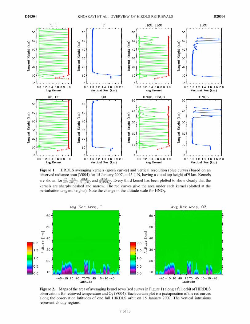
Figure 2. Maps of the area of averaging kernel rows (red curves in Figure 1) along a full orbit of HIRDLSobservations for retrieved temperature and O3 (V004). Each curtain plot is a juxtaposition of the red curvesalong the observation latitudes of one full HIRDLS orbit on 15 January 2007. The vertical intrusionsrepresent cloudy regions.

Figure 1. HIRDLS averaging kernels (green curves) and vertical resolution (blue curves) based on anobserved radiance scan (V004) for 15 January 2007, at 45.4�N, having a cloud top height of 9 km. Kernels

are shown for @T@Tt,@O3

@ O3ð Þt, @H2O@ H2Oð Þt

, and @HNO3

@ HNO3ð Þt. Every third kernel has been plotted to show clearly that the

kernels are sharply peaked and narrow. The red curves give the area under each kernel (plotted at theperturbation tangent heights). Note the change in the altitude scale for HNO3.


7 of 13

D20304

Figure 3. Maps of the vertical resolution (blue curves in Figure 1) along a full orbit of HIRDLSobservations for retrieved temperature and O3 (V004). Each curtain plot is a juxtaposition of the blue curvesalong the observation latitudes of one full HIRDLS orbit on 15 January 2007.

Figure 4. Weighting functions for the HIRDLS temperature sounding channels for the radiance scan usedin Figure 1 (V004, 45.4�N). Each curve for channel n (n = 2, 3, 4, 5) is a plot of row i ofK (section 4.2) and

shows@fnj@Ti

as a function of altitude ( j) due to a perturbation in temperature at tangent height i (f is the forward

model radiance and T is temperature). Each weighting function curve has a corresponding red dot, whichmarks the peak of that curve on the horizontal axis and is placed vertically at the perturbation tangent heightof the curve (i). Coincidence of a red dot with the peak of its corresponding curve indicates that themaximum sensitivity of the channel radiance to a temperature perturbation at tangent height i occurs at thesame height (i). Every third function is plotted for clarity. Note that when the peaks coincide with the reddots, the weighting functions are not zero immediately below their peaks owing to refraction effects (seesection 4.2).


8 of 13

D20304

immediately below the red dot is not zero, although verysmall (e.g., channel 2 between 10 and 20 km). This is becausethe tangent heights of the weighting functions (red dots) areplotted on the geometric (and uniform) grid of the retrievalalgorithm. The true tangent heights, however, are lower thanthe geometric ones owing to atmospheric refraction [Lambertet al., 1999], resulting in a (small) radiance response imme-diately below the plotted perturbation levels (red dots). Theweighting functions are zero below these lowest levels, andare not shown. Furthermore, as the red dots move up inaltitude, the effect of refraction diminishes, resulting in anexceedingly smaller value of the weighting function at thelevel immediately below a peak. These near-zero valuesappear to lie on the vertical axis, but are not exactly zero.[39] For channels 4 and 5, the weighting functions peak at

about 31 km and 34 km, respectively, indicating high channelsensitivity to temperature in the mid to upper stratosphere;these channels are opaque below �15 km and 21 km,respectively (see also Figure 7). The peaks of the radianceresponse for channels 4 and 5 begin to coincide with theperturbation heights at about 26 km and 31 km, respectively.Note that these channels retain good sensitivity in the upperstratosphere and lower mesosphere region. This is particu-larly true of channel 5, which is by design the highest-altitudetemperature sounding channel [Edwards et al., 1995].[40] As mentioned in section 3.5, parts of a radiance scan

that pass through clouds are omitted from the y vector in theretrieval algorithm (equation (2)), resulting in a progressivelylarger contribution by the a priori to the retrievals belowcloud tops. In these cases, the lower portions of the weightingfunctions of channels 2, 3, and 4 that peak above theirperturbations levels (red dots) could lose sensitivity at higheraltitudes than shown in Figure 4, depending on the cloud topheight (9 km for the present radiance scan).[41] The weighting functions for the H2O and O3 sounding

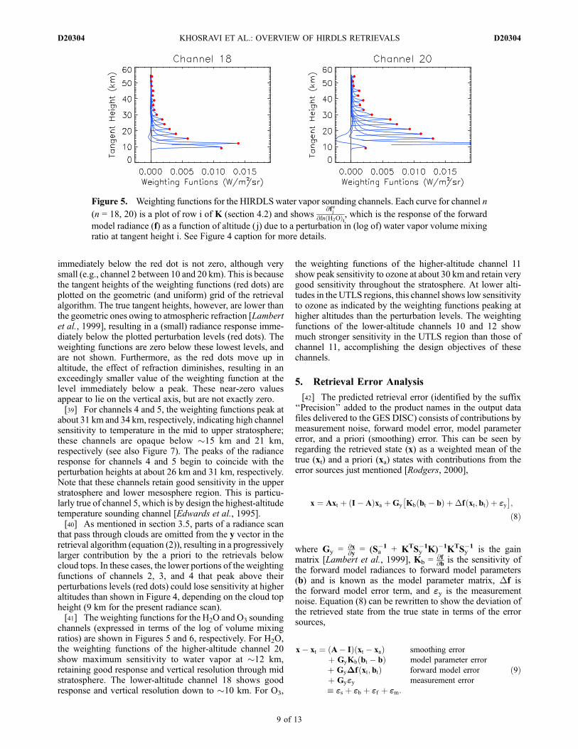
channels (expressed in terms of the log of volume mixingratios) are shown in Figures 5 and 6, respectively. For H2O,the weighting functions of the higher-altitude channel 20show maximum sensitivity to water vapor at �12 km,retaining good response and vertical resolution through midstratosphere. The lower-altitude channel 18 shows goodresponse and vertical resolution down to �10 km. For O3,

the weighting functions of the higher-altitude channel 11show peak sensitivity to ozone at about 30 km and retain verygood sensitivity throughout the stratosphere. At lower alti-tudes in the UTLS regions, this channel shows low sensitivityto ozone as indicated by the weighting functions peaking athigher altitudes than the perturbation levels. The weightingfunctions of the lower-altitude channels 10 and 12 showmuch stronger sensitivity in the UTLS region than those ofchannel 11, accomplishing the design objectives of thesechannels.

5. Retrieval Error Analysis

[42] The predicted retrieval error (identified by the suffix‘‘Precision’’ added to the product names in the output datafiles delivered to the GES DISC) consists of contributions bymeasurement noise, forward model error, model parametererror, and a priori (smoothing) error. This can be seen byregarding the retrieved state (x) as a weighted mean of thetrue (xt) and a priori (xa) states with contributions from theerror sources just mentioned [Rodgers, 2000],

x ¼ Axt þ I� Að Þxa þGy Kb bt � bð Þ þDf xt;btð Þ þ ey� �

;

ð8Þ

where Gy = @x@y = (Sa

�1 + KTSy�1K)�1KTSy

�1 is the gainmatrix [Lambert et al., 1999], Kb = @f

@b is the sensitivity ofthe forward model radiances to forward model parameters(b) and is known as the model parameter matrix, Df isthe forward model error term, and ey is the measurementnoise. Equation (8) can be rewritten to show the deviation ofthe retrieved state from the true state in terms of the errorsources,

x� xt ¼ A� Ið Þ xt � xað Þ smoothing error

þ GyKb bt � bð Þ model parameter error

þ GyDf xt; btð Þ forward model error

þ Gyey measurement error

� es þ eb þ ef þ em:

: ð9Þ

Figure 5. Weighting functions for the HIRDLS water vapor sounding channels. Each curve for channel n

(n = 18, 20) is a plot of row i of K (section 4.2) and shows@fnj

@ln H2Oð Þi, which is the response of the forward

model radiance (f) as a function of altitude (j) due to a perturbation in (log of) water vapor volume mixingratio at tangent height i. See Figure 4 caption for more details.


9 of 13

D20304

The contribution of each error source to the total errorcovariance can now be obtained by deriving its individualcovariance matrix. For smoothing error this is

Ss ¼ E eseTs� �

¼ E A� Ið Þ xt � xað Þ xt � xað ÞT A� Ið ÞTn o

¼ A� Ið ÞE xt � xað Þ xt � xað ÞTn o

A� Ið ÞT

¼ I� Að ÞSa I� Að ÞT¼ GaSaG

Ta

; ð10Þ

where E is the expectation value operator, Sa is the error

covariance matrix of the a priori data, andGa =@x@xa

= I�A=

(Sa�1 + KTSy

�1K)�1Sa�1 represents the sensitivity of the

retrieved state with respect to the a priori state (the apriori gain matrix) [Lambert et al., 1999]. The contribu-tions of the other error sources are similarly derived,

SB ¼ E ebeTb� �

¼ GyKbSbKTbG

Ty ; ð11Þ

where Sb = E{(bt � b)(bt � b)T} is the error covariance ofmodel parameters,

SF ¼ E efeTf� �

¼ GySfGTy ; ð12Þ

where Sf = E{DfDfT} is the forward model error covari-ance, and

Sm ¼ E emeTm� �

¼ GySyGTy ; ð13Þ

where Sy = E{eyeyT} is the covariance of measurement(radiometric) noise. Therefore, the total solution covar-iance can now be obtained,

Sx ¼ Ss þ SB þ SF þ Sm: ð14Þ

In version 4 of HIRDLS retrievals, the input errorcovariance matrices (e.g., Sa, Sy) are constructed as shownin Table 3. Note that in this version, the a priori andforward model errors are independent of altitude, and themeasurement noise is a combination of detector noise andpointing jitter error (radiance uncertainty due to imprecisepointing, smaller than detector noise by 1 to 2 orders ofmagnitude, depending on channel and altitude). Also, themodel parameter and forward model errors are combinedin a single ‘‘forward model’’ covariance matrix, Sf 0, whichreplaces Sf in equation (12) and eliminates SB, so that thetotal error is

Sx ¼ Ss þ SF0 þ Sm; ð15Þ

where SF0 = GySf 0GyT.

Figure 6. Weighting functions for the HIRDLS ozonesounding channels. Each curve for channel n (n = 10, 11, 12)

is a plot of row i ofK (section 4.2) and shows@fnj

@ln O3ð Þi, which is

the response of the forwardmodel radiance (f) as a function ofaltitude ( j) due to a perturbation in log of ozone volumemixing ratio at tangent height i. See Figure 4 caption for moredetails.

Figure 7. Variation of HIRDLS radiances with altitudein the temperature channels for the radiance scan describedin Figure 1.


10 of 13

D20304

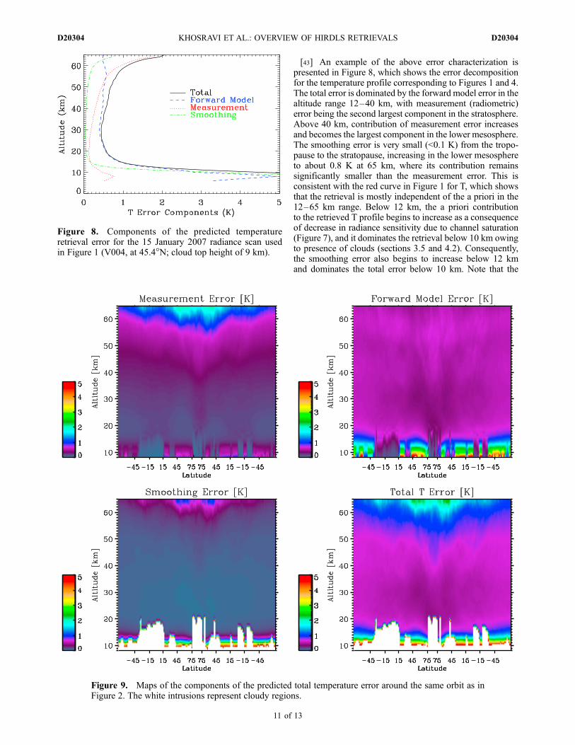
[43] An example of the above error characterization ispresented in Figure 8, which shows the error decompositionfor the temperature profile corresponding to Figures 1 and 4.The total error is dominated by the forward model error in thealtitude range 12–40 km, with measurement (radiometric)error being the second largest component in the stratosphere.Above 40 km, contribution of measurement error increasesand becomes the largest component in the lower mesosphere.The smoothing error is very small (<0.1 K) from the tropo-pause to the stratopause, increasing in the lower mesosphereto about 0.8 K at 65 km, where its contribution remainssignificantly smaller than the measurement error. This isconsistent with the red curve in Figure 1 for T, which showsthat the retrieval is mostly independent of the a priori in the12–65 km range. Below 12 km, the a priori contributionto the retrieved T profile begins to increase as a consequenceof decrease in radiance sensitivity due to channel saturation(Figure 7), and it dominates the retrieval below 10 km owingto presence of clouds (sections 3.5 and 4.2). Consequently,the smoothing error also begins to increase below 12 kmand dominates the total error below 10 km. Note that the

Figure 8. Components of the predicted temperatureretrieval error for the 15 January 2007 radiance scan usedin Figure 1 (V004, at 45.4�N; cloud top height of 9 km).

Figure 9. Maps of the components of the predicted total temperature error around the same orbit as inFigure 2. The white intrusions represent cloudy regions.


11 of 13

D20304

saturation heights as well as cloud top levels vary withlatitude.[44] These error characteristics generally hold for all

latitudes, as illustrated in Figure 9, which shows maps ofthe temperature error components along a full orbit ofHIRDLS retrievals. The total error is dominated by theforward model error in the upper troposphere and almostall of the stratosphere, and by the measurement error in thelower mesosphere. The smoothing error contributions be-come significant below about 12 km for clear sky regions,and are the dominant components in cloudy regions (whiteintrusions).

6. Summary and Data Status

6.1. Summary

[45] We have described the HIRDLS retrieval algorithm,which is based on the Optimal Estimation formalism ofRodgers [2000]. It minimizes a cost function that is con-strained by the prior knowledge of the atmosphere, weightedby its covariance, to obtain vertical profiles of the desiredatmospheric constituents that are consistent with the radi-ances calculated by the algorithm’s radiative transfer model.The technique used to solve the resulting iteration equation isa modified version of the Leveberg-Marquardt approach, inwhich the step size, g, is updated on the basis of the ‘‘trustregion’’ concept (section 2.2).[46] The retrievals are characterized for a northern hemi-

sphere winter, midlatitude profile (V004 data), showing highvertical resolution of about 1–1.1 km (sharply peakedaveraging kernels) and minimal a priori contribution, exceptin cloudy regions and at tangent heights where the channelradiances saturate. The weighting functions are relativelybroad in these regions of low radiance sensitivity, but areotherwise narrow and show good response to temperatureor gas mixing ratio perturbations. Curtain plots show that thecharacteristics of high vertical resolution and negligible apriori contribution are maintained for all latitudes alongHIRDLS orbits.[47] The total temperature error, calculated by the retrieval

algorithm, varies from 0.5 K to 0.8 K from the uppertroposphere to the stratopause region, consistent with theempirical estimates given by Gille et al. [2008]. Contribu-tions to the total error are by measurement (detector andpointing jitter), forward model, and smoothing. In regions ofstrong SNR, forward model error is the largest component ofthe calculated temperature error, followed by measurementand smoothing errors (very small contribution). In the lowerto upper troposphere regions, where clouds are present orwhere radiance sensitivity is low, smoothing error is thelargest component, followed by forward model and measure-ment errors. In the upper stratosphere lower mesosphereregion, the total temperature error is dominated by themeasurement error. These relative weightings of the errorcomponents hold for all latitudes along HIRDLS orbits.[48] Accuracies of the retrieved data are described in detail

in the validation papers [Gille et al., 2008; Massie et al.,2007; Nardi et al., 2008; Coffey et al., 2008; Kinnison et al.,2008]. As a quick reference, temperature accuracy is ±0.5 Kfrom 400 to 10 hPa (compare sondes), and ±1 K from 10 to1 hPa (compare ECMWF). O3 accuracy is 20–5% from250 to 200 hPa, and 10–1% from 200 to 5 hPa.

6.2. Data Status

[49] Correction algorithms for removing the blockagesignal from the measured radiances have made possible thevalidation, release, and scientific applications of HIRDLS T,O3, HNO3, CFC-11, CFC-12, aerosol extinction at 12.1 mm,and cloud top pressure data. The latest version of these data(as of June 2009) is V004, released to the GES DISC (http://daac.gsfc.nasa.gov) in August 2008. Useful range, screeningcriteria, predicted retrieval error, and accuracy of the data aredescribed in the data quality document that is also availablefrom the GES DISC.

[50] Acknowledgments. We thank the following colleagues for theircontributions to the HIRDLS L2 algorithm and/or other aspects of theHIRDLS program: Phil Arter (deceased), Paul Bailey, Charles Cavanaugh,Jim Craft, Alan Darbyshire, Vince Dean, Mike Dials, David Ellis, JimHannigan, Craig Hartsough, Linda Henderson, Brian Johnson, DougKinnison, Aaron Lee, Joanne Loh, Larry Lyjack, Joe Moorhouse, SojiOduleye, Dan Packman, Chris Palmer, Dan Peters, Brent Petersen, LaurieRokke, Leslie Smith, Brendan Torpy, Barbara Tunison, Peter Venters,Jinxue Wang, Bob Watkins, Bob Wells, John Whitney, Doug Woodard(deceased), Helen Worden, Greg Young, and Valery Yudin. In addition,Alyn Lambert would like to thank the following colleagues for theirvaluable comments and suggestions: Anu Dudhia, Clive Rodgers, PaulMorris, Nathaniel Livesey, and Don Grainger. We would also like to thankthe reviewers of this paper for their time and constructive comments andsuggestions. This work was funded by NASA’s Aura satellite programunder HIRDLS contract NAS5–97046. The National Center for Atmo-spheric Research is sponsored by the National Science Foundation. Workat the Jet Propulsion Laboratory, California Institute of Technology, wascarried out under a contract with NASA.

ReferencesAlexander, M. J., et al. (2008), Global estimates of gravity wave momen-tum flux from High Resolution Dynamics Limb Sounder (HIRDLS) ob-servations, J. Geophys. Res., 113, D15S18, doi:10.1029/2007JD008807.

Bowman, K.W., et al. (2006), Tropospheric emission spectrometer: Retrievalmethod and error analysis, IEEE Trans. Geosci. Remote Sens., 44, 1297–1307, doi:10.1109/TGRS.2006.871234.

Carslaw, K. S., B. Luo, and T. Peter (1995), An analytic expression for thecomposition of aqueous HNO3–H2SO4 stratospheric aerosols includinggas phase removal of HNO3, Geophys. Res. Lett., 22(14), 1877–1880,doi:10.1029/95GL01668.

Coffey, M., et al. (2008), Airborne Fourier transform spectrometer observa-tions in support of EOS Aura validation, J. Geophys. Res., 113, D16S42,doi:10.1029/2007JD008833.

Curtis, A. R. (1952), Discussion of ‘A statistical model for water vapourabsorption’ by R. M. Goody, Q. J. R. Meteorol. Soc., 78, 638–640,doi:10.1002/qj.49707833820.

Deeter, M. N., D. P. Edwards, and J. C. Gille (2007), Retrievals of carbonmonoxide profiles from MOPITT observations using lognormal a prioristatistics, J. Geophys. Res., 112, D11311, doi:10.1029/2006JD007999.

Edwards, D. P. (1992), GENLN2: A general line-by-line atmospheric trans-mittance and radiance model, Version 3 description and users guide,NCAR Rep. NCAR/TN-367+STR, Natl. Cent. for Atmos. Res., Boulder,Colo.

Edwards, D. P., J. C. Gille, P. L. Bailey, and J. J. Barnett (1995), Selectionof sounding channels for the High Resolution Dynamics Limb Sounder,Appl. Opt., 34, 7006–7018.

Fleming, E., S. Chandra, J. Barnett, and M. Corney (1990), Zonal meantemperature, pressure, zonal wind and geopotential height as functions oflatitude, Adv. Space Res., 10, 11–53. (Available at http://badc.nerc.ac.uk/data/cira/), doi:10.1016/0273-1177(90)90386-E.

Francis, G. L., D. P. Edwards, A. Lambert, C. M. Halvorson, J. M. Lee-Taylor, and J. C. Gille (2006), Forward modeling and radiative transferfor the NASA EOS-Aura High Resolution Dynamics Limb Sounder(HIRDLS) instrument, J. Geophys. Res., 111, D13301, doi:10.1029/2005JD006270.

Gille, J. C., and J. M. Russell (1984), The Limb Infrared Monitor of theStratosphere: Experiment, description, performance, and results,J. Geophys. Res., 89, 5125–5140, doi:10.1029/JD089iD04p05125.

Gille, J. C., J. J. Barnett, J. C. Whitney, M. A. Dials, D. M. Woodard,W. Rudolf, A. Lambert, and W. Mankin (2003), The High ResolutionDynamics Limb Sounder (HIRDLS) experiment on Aura, Proc. SPIE Int.Soc. Opt. Eng., 5152, 162–171, doi:10.1117/12.507657.


12 of 13

D20304

Gille, J. C., et al. (2008), The High Resolution Dynamics Limb Sounder(HIRDLS): Experiment overview, recovery and validation of initial temper-ature data, J. Geophys. Res., 113, D16S43, doi:10.1029/2007JD008824.

Kinnison, D. E., et al. (2007), Sensitivity of chemical tracers to meteoro-logical parameters in the MOZART-3 chemical transport model,J. Geophys. Res., 112, D20302, doi:10.1029/2006JD007879.

Kinnison, D. E., et al. (2008), Global observations of HNO3 from the HighResolution Dynamics Lim Sounder (HIRDLS): First results, J. Geophys.Res., 113, D16S44, doi:10.1029/2007JD008814.

Lambert, A., P. L. Bailey, D. P. Edwards, J. C. Gille, B. R. Johnson, C. M.Halvorson, S. T. Massie, and K. A. Stone (1999), HIRLDS level-2 algo-rithm theoretical basis document, report, 109 pp., NASA Goddard SpaceFlight Cent., Greenbelt, Md. (Available at http://eospso.gsfc.nasa.gov/eos_homepage/for_scientists/atbd/docs/HIRDLS/ATBD-HIR-02.pdf)

Livingston, J. M., and P. B. Russell (1989), Retrieval of aerosol size distri-bution moments from multi-wavelength particulate extinction measure-ments, J. Geophys. Res., 94, 8425–8433, doi:10.1029/JD094iD06p08425.

Massie, S., et al. (2007), High Resolution Dynamics Limb Sounder obser-vations of polar stratospheric clouds and subvisible cirrus, J. Geophys.Res., 112, D24S31, doi:10.1029/2007JD008788.

Nardi, B., et al. (2008), Initial validation of ozone measurements from theHigh Resolution Dynamics Limb Sounder, J. Geophys. Res., 113,D16S36, doi:10.1029/2007JD008837.

Olsen, M. A., A. R. Douglas, P. A. Newman, J. C. Gille, B. Nardi, V. A.Yudin, D. E. Kinnison, and R. Khosravi (2008), HIRDLS observationand simulation of a lower stratospheric intrusion of tropical air to highlatitudes, Geophys. Res. Lett., 35, L21813, doi:10.1029/2008GL035514.

Rodgers, C. D. (1976), Retrieval of atmospheric temperature and composi-tion from remote measurements of thermal radiation, Rev. Geophys., 14,609–624, doi:10.1029/RG014i004p00609.

Rodgers, C. D. (1990), Characterization and error analysis of profilesretrieved from remote sounding measurements, J. Geophys. Res., 95,5587–5595, doi:10.1029/JD095iD05p05587.

Rodgers, C. D. (2000), Inverse Methods for Atmospheric Sounding: Theoryand Practice, World Sci., Hackensack, N. J.

Rodgers, C. D., R. J. Wells, R. G. Grainger, and F. W. Taylor (1996),Improved stratospheric and mesospheric sounder validation: General ap-proach and in-flight radiometric calibration, J. Geophys. Res., 101,9775–9793, doi:10.1029/95JD02466.

Russell, P. B., and M. P. McCormick (1989), SAGE II aerosol data valida-tion and initial data use: An introduction and overview, J. Geophys. Res.,94, 8335–8338, doi:10.1029/JD094iD06p08335.

Schoeberl, M. R., et al. (2006), Overview of the EOS Aura mission, IEEETrans. Geosci. Remote Sens., 44, 1066–1074, doi:10.1109/TGRS.2005.861950.

Weinreb, M. P., and A. C. Neuendorffer (1973), Method to applyhomogeneous-path transmittance models to inhomogeneous atmospheres,J. Atmos. Sci., 30, 662–666, doi:10.1175/1520-0469(1973)030<0662:MTAHPT>2.0.CO;2.

��J. Barnett and C. Hepplewhite, Department of Physics, University of

Oxford, Oxford OX1 3PU, UK.M. Coffey, C. Craig, D. Edwards, G. Francis, J. Gille, C. Halvorson,

R. Khosravi, S. Massie, J. McInerney, and B. Nardi, Atmospheric ChemistryDivision, National Center for Atmospheric Research, P.O. Box 3000,Boulder, CO 80307, USA. ([email protected])T. Eden, Computational Physics, Inc., Boulder, CO 80301, USA.C. Krinsky, Center for Limb Atmospheric Sounding, University of

Colorado, Boulder, CO 80301, USA.A. Lambert, Jet Propulsion Laboratory, California Institute of Technology,

Pasadena, CA 91109, USA.K. Stone, ERT Corporation, Aurora, CO 80011, USA.


13 of 13

D20304

Overview and characterization of retrievals of temperature, pressure, and atmospheric constituents...

Documents

Transcript of Overview and characterization of retrievals of temperature, pressure, and atmospheric constituents...