Declining Aerosols in CMIP5 Projections: Effects on Atmospheric TemperatureStructure and Midlatitude Jets

LEON D. ROTSTAYN,* EMILY L. PLYMIN,* MARK A. COLLIER,* OLIVIER BOUCHER,1 JEAN-LOUIS

DUFRESNE,1 JING-JIA LUO,# KNUT VON SALZEN,@ STEPHEN J. JEFFREY,& MARIE-ALICE FOUJOLS,** YI

MING, 11AND LARRY W. HOROWITZ

11

* Centre for Australian Weather and Climate Research, CSIRO, Aspendale, Victoria, Australia1Laboratoire de Météorologie Dynamique, Institut Pierre-Simon Laplace, CNRS/UPMC, Paris, France

#Centre for Australian Weather and Climate Research, Bureau of Meteorology, Melbourne, Victoria, Australia@Canadian Centre for Climate Modelling and Analysis, Environment Canada, University of Victoria, Victoria, British Columbia, Canada

&Department of Science, Information Technology, Innovation and the Arts, Dutton Park, Queensland, Australia

** Institut Pierre-Simon Laplace, CNRS/UPMC, Paris, France11NOAA/Geophysical Fluid Dynamics Laboratory, Princeton, New Jersey

(Manuscript received 4 April 2014, in final form 6 June 2014)

ABSTRACT

The effects of declining anthropogenic aerosols in representative concentration pathway 4.5 (RCP4.5) are

assessed in four models from phase 5 the Coupled Model Intercomparison Project (CMIP5), with a focus on

annual, zonal-mean atmospheric temperature structure and zonal winds. For each model, the effect of de-

clining aerosols is diagnosed from the difference between a projection forced by RCP4.5 for 2006–2100 and

another that has identical forcing, except that anthropogenic aerosols are fixed at early twenty-first-century

levels. The response to declining aerosols is interpreted in terms of the meridional structure of aerosol ra-

diative forcing, which peaks near 408N and vanishes at the South Pole.

Increasing greenhouse gases cause amplified warming in the tropical upper troposphere and strengthening

midlatitude jets in both hemispheres. However, for declining aerosols the vertically averaged tropospheric

temperature response peaks near 408N, rather than in the tropics. This implies that for declining aerosols the

tropospheric meridional temperature gradient generally increases in the Southern Hemisphere (SH), but in

the Northern Hemisphere (NH) it decreases in the tropics and subtropics. Consistent with thermal wind

balance, the NH jet then strengthens on its poleward side and weakens on its equatorward side, whereas the

SH jet strengthens more than the NH jet. The asymmetric response of the jets is thus consistent with the

meridional structure of aerosol radiative forcing and the associated tropospheric warming: in the NH

the latitude ofmaximumwarming is roughly collocated with the jet, whereas in the SHwarming is strongest in

the tropics and weakest at high latitudes.

1. Introduction

Climate projections in phase 5 of the Coupled Model

Intercomparison Project (CMIP5) are forced by four

representative concentration pathways (RCPs). De-

clining aerosol emissions are a feature of all the RCPs

during the twenty-first century, because emission con-

trols are assumed to increase as income rises (Smith

et al. 2005). The decline is much larger than assumed in

earlier scenarios (van Vuuren et al. 2011), although it is

unclear how realistic it is. Declining aerosols may have

important implications for projections carried out dur-

ing CMIP5, since their effects are unlikely to be identical

to those of increasing greenhouse gases. However, there

have been few studies of these implications.

Since all the RCPs include sharp declines in aerosols,

the range of plausible aerosol futures is not adequately

sampled by the standard RCPs (Kirtman et al. 2014).

The effects of projected aerosol changes can be identi-

fied by running simulations that are similar to the stan-

dard RCPs, except that emissions or concentrations of

anthropogenic aerosols are held fixed at present-day

levels. A few groups have recently published analyses of

such simulations, which have generally been based on

single models (Levy et al. 2013; Gillett and von Salzen

Corresponding author address: Leon Rotstayn, CSIRO Marine

and Atmospheric Research, Private Bag 1, Aspendale, Victoria,

3195, Australia.

E-mail: leon.rotstayn@csiro.au

6960 JOURNAL OF CL IMATE VOLUME 27

DOI: 10.1175/JCLI-D-14-00258.1

� 2014 American Meteorological Society

2013; Rotstayn et al. 2013). To varying degrees, these

studies show that declining aerosols increase projected

twenty-first-century warming.

A similar conclusion was reached by Meehl et al.

(2013), who analyzed CMIP5 projections carried out

with the Community Earth System Model, version 1

(CESM1). Compared to the previous version of the

model (which only treated direct aerosol effects), they

found that inclusion of indirect aerosol effects in

CESM1 added close to 1Wm22 of positive radiative

forcing during the twenty-first century.

In addition to analysis of a single model, Rotstayn

et al. (2013) considered intermodel correlations be-

tween historical aerosol radiative forcing and projected

changes in temperature and precipitation in RCP4.5

from 13 CMIP5 models; they found that models with

stronger (more negative) historical aerosol forcing tend

to simulate less warming during 1850–2005 and more

warming during 2006–2100. In other words, models

with more aerosol cooling in the historical period

tend to have more projected warming due to declining

aerosols. However, until now there have been no con-

ventional multimodel analyses of the effects of declin-

ing aerosols.

Some insights into the possible effects of declining

aerosols on large-scale circulation can be gained from

analyses of the effects of historically increasing aerosols.

Several studies have focused on the effects of stronger

aerosol forcing in the Northern Hemisphere (NH) than

the Southern Hemisphere (SH). In response to the in-

terhemispheric gradient in forcing, models generally

simulate more cooling in the NH than the SH, and an

associated southward shift of tropical precipitation. This

has been seen in atmospheric global climate models

(GCMs) coupled to slab ocean models (Rotstayn et al.

2000; Williams et al. 2001; Rotstayn and Lohmann 2002;

Kristjánsson et al. 2005; Jones et al. 2007; Yoshimori and

Broccoli 2008; Ming and Ramaswamy 2011), and more

recently in fully coupled ocean–atmosphere GCMs

(Chang et al. 2011; Wilcox et al. 2013; Hwang et al.

2013). Various studies also suggest large regional im-

pacts on circulation and rainfall from historical increases

in aerosols, especially in the Sahel (Rotstayn andLohmann

2002; Kawase et al. 2010; Ackerley et al. 2011), South

Asia (Ramanathan et al. 2005; Meehl et al. 2008;

Bollasina et al. 2011), and East Asia (Cheng et al. 2005;

Liu et al. 2011).

These studies have generally emphasized the effects

of spatially inhomogeneous aerosol forcing. On the

other hand, Xie et al. (2013) analyzed CMIP5 climate

simulations, and concluded that the spatial patterns of

climate response to increasing greenhouse gases and

aerosols are qualitatively similar (but of opposite sign)

over the ocean. They argued that common feedbacks

occur in response to both forcing agents, leading to

similar spatial patterns of sea surface temperature (SST)

and rainfall response, despite different patterns of

forcing.

This raises questions about whether declining aero-

sols have similar effects on climate to those of in-

creasing greenhouse gases, or whether it is necessary to

account for the unique spatial distribution of aerosol

radiative forcing in climate projections. One reason

why this is important is that aerosol effects are highly

uncertain; for example, the global-mean radiative forc-

ing due to anthropogenic aerosols is estimated to have an

uncertainty range from 20.1 to 21.9Wm22 (Boucher

et al. 2014). Also, because all the RCPs have sharply

declining aerosols, CMIP5 projections may show sys-

tematic differences from CMIP3 projections because of

spatially inhomogeneous aerosol changes (Kirtman et al.

2014).

A topic that has recently received some attention is

the effect of aerosol forcing on the jet streams, which are

important features of extratropical climate. The wind

shear associated with the jet streams contributes to

baroclinic instability, so they are associated with mid-

latitude eddy formation; thus, projected changes in the

jets have implications for changes in storm development

and extreme weather (Frederiksen et al. 2011; Francis

and Vavrus 2012). In the SH, future changes in the as-

sociated surface westerlies may weaken the uptake of

CO2 by the Southern Ocean, so reliable projections of

changes in the jets are also important for understanding

the carbon cycle (Lenton et al. 2009).

Ming et al. (2011) considered the effects of increasing

anthropogenic aerosols on winter extratropical circula-

tion in theNH in an atmosphericmodel coupled to a slab

ocean model. The zonal-mean response of their model

included an equatorward shift of the subtropical jet.

Since the aerosol-induced cooling was roughly collo-

cated with the NH jet, it strengthened the meridional

temperature gradient on the equatorward side of the jet,

and weakened it on the poleward side; consistent with

thermal wind balance, the jet strengthened (weakened)

on its equatorward (poleward) side.

Allen and coworkers have studied the effects on at-

mospheric circulation of increases in scattering or ab-

sorbing aerosols, with a primary focus on the width of

the tropics and associated jet displacement in the NH. In

simulations by Allen and Sherwood (2011), the direct

radiative effects of increases in scattering aerosols shif-

ted the NH subtropical jets equatorward, whereas ab-

sorbing aerosols had the opposite effect. Allen et al.

(2012a) showed that recent NH tropical expansion has

been primarily driven by short-lived tropospheric warming

15 SEPTEMBER 2014 ROTS TAYN ET AL . 6961

agents (black carbon and ozone); further, poleward ex-

pansion of the tropics and the NH tropospheric jet was

consistent with an ‘‘expansion index’’ (Allen et al. 2012b),

which compared midlatitude tropospheric warming with

that at other latitudes. Allen et al. (2012a,b) noted that

warming of midlatitudes relative to others displaces the

maximum meridional temperature gradient poleward,

so the jet also shifts poleward [similar to the explana-

tion of Ming et al. (2011)]. Recently, Allen and Ajoku

(2014, manuscript submitted to Geophys. Res. Lett.)

showed that projected declines in anthropogenic aero-

sol amplify simulated twenty-first-century warming in

the NH midlatitudes, and cause a poleward shift of NH

circulation.

Considering the SH, a weakening of annual-mean

surface zonal winds at sub-Antarctic latitudes in re-

sponse to historically increasing aerosols has been noted

in CMIP5models (Xie et al. 2013; Collier et al. 2013); this

suggests that increasing aerosols induce a weakening and/

or equatorward shift of the eddy-driven jet in the SH,

a response that resembles the inverse of the effects of

increasing greenhouse gases (Fyfe et al. 1999; Kushner

et al. 2001). Rotstayn (2013) considered the simulated

effects of projected aerosol declines on SH extratropical

circulation in austral summer and found a poleward shift

of the eddy-driven jet, which is qualitatively consistent

with the results of Xie et al. (2013) and Collier et al.

(2013).

Here we consider projections based on RCP4.5 from

four GCMs that participated in CMIP5. For each of

these models, we compare the standard RCP4.5 pro-

jection with a modified RCP4.5, in which anthropogenic

aerosols are held fixed at present-day values. By com-

paring the standard and modified RCP4.5 projections,

we diagnose the effects of declining aerosols during the

twenty-first century. The focus of this study is on annu-

ally and zonally averaged atmospheric temperature

structure and the midlatitude jets in both hemispheres.

Since aerosol effects are complex and uncertain, we aim

to identify broad, large-scale responses that are common

to the models, but we also identify differences among

the models.

2. Models, experiments, and methods

We use simulations from four CMIP5 models: Can-

ESM2, CSIRO Mk3.6, GFDL CM3, and IPSL-CM5A-

LR (references and expansions of these model names

are given in Table 1). Anthropogenic aerosols treated in

all models are sulfate, organic aerosol, and black carbon.

In IPSL-CM5A-LR, aerosol concentrations are pre-

scribed, based on offline calculations with the atmo-

spheric model (Szopa et al. 2013); in the other models,

anthropogenic aerosol concentrations are calculated

interactively, using prescribed emissions based on

Lamarque et al. (2011). In CSIRO Mk3.6, emissions of

organic aerosol and black carbon are increased by 50%

and 25%, respectively (Rotstayn et al. 2012). All models

treat direct aerosol radiative effects and the first indirect

effect, but there are differences in the inclusion of other

indirect effects; see Table 2 for a summary. Further

details of the forcing agents used in eachmodel are given

in Table 12.1 of Collins et al. (2014).

Our analysis of twenty-first-century projections is

based on the following experiments:

d RCP45 is a projection for 2006–2100 forced by the

medium-low RCP4.5 pathway (Thomson et al. 2011).

Anthropogenic forcing in this experiment is based on

time-varying, prescribed concentrations of ozone and

well-mixed greenhouse gases (WMGHGs) and emis-

sions of anthropogenic aerosols and their precursors

(for CanESM2, CSIRO Mk3.6, and GFDL CM3) or

prescribed concentrations of anthropogenic aerosols

(for IPSL-CM5A-LR). Note that anthropogenic sour-

ces include biomass burning. Land use change is also

included in all models except CSIRO Mk3.6. Ensem-

ble sizes range from 3 (GFDL CM3) to 10 (CSIRO

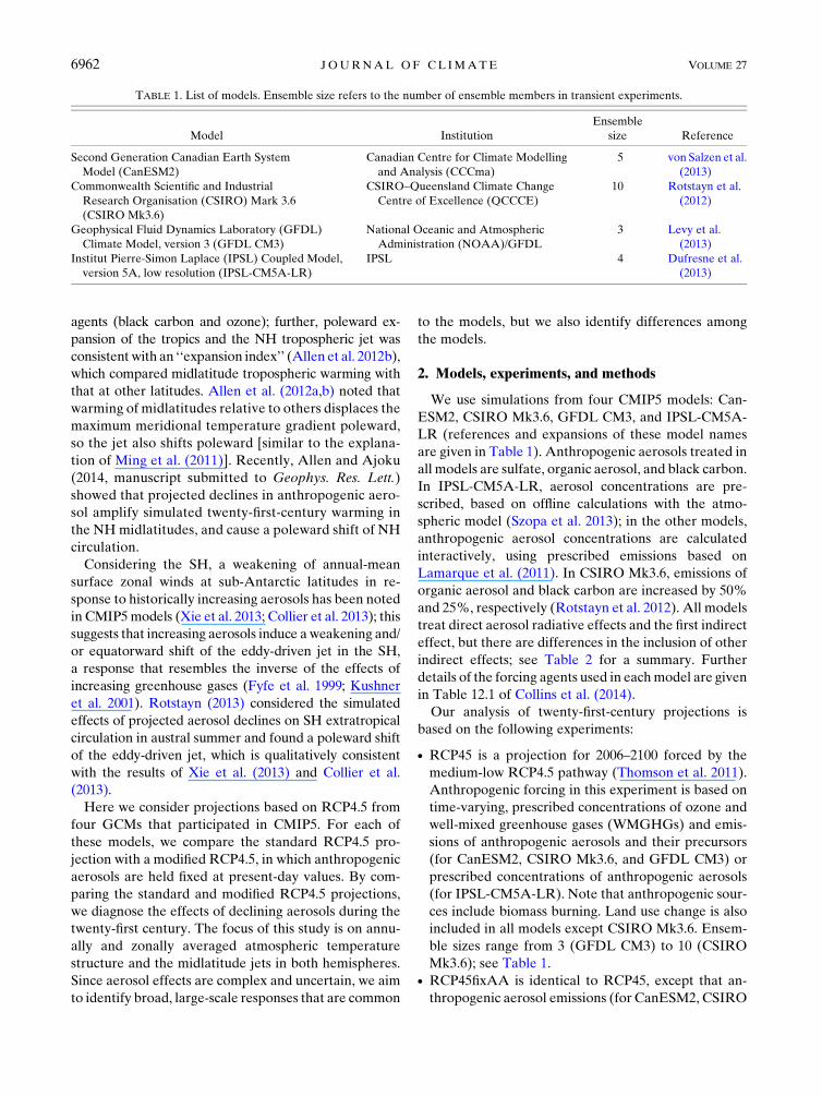
Mk3.6); see Table 1.d RCP45fixAA is identical to RCP45, except that an-

thropogenic aerosol emissions (for CanESM2, CSIRO

TABLE 1. List of models. Ensemble size refers to the number of ensemble members in transient experiments.

Model Institution

Ensemble

size Reference

Second Generation Canadian Earth System

Model (CanESM2)

Canadian Centre for Climate Modelling

and Analysis (CCCma)

5 von Salzen et al.

(2013)

Commonwealth Scientific and Industrial

Research Organisation (CSIRO) Mark 3.6

(CSIRO Mk3.6)

CSIRO–Queensland Climate Change

Centre of Excellence (QCCCE)

10 Rotstayn et al.

(2012)

Geophysical Fluid Dynamics Laboratory (GFDL)

Climate Model, version 3 (GFDL CM3)

National Oceanic and Atmospheric

Administration (NOAA)/GFDL

3 Levy et al.

(2013)

Institut Pierre-Simon Laplace (IPSL) Coupled Model,

version 5A, low resolution (IPSL-CM5A-LR)

IPSL 4 Dufresne et al.

(2013)

6962 JOURNAL OF CL IMATE VOLUME 27

Mk3.6, and GFDL CM3) or concentrations (for

IPSL-CM5A-LR) are held fixed at 2005 levels (or

2000 for CanESM2). Since sulfur dioxide and organic

aerosol emissions are slightly larger in 2005 than 2000

in the CMIP5 inventory (e.g., Takemura 2012), using

2000 as the baseline level in CanESM2 is expected to

slightly reduce the effect of declining aerosols in that

model.

In addition, standard historical simulations are used to

derive climatological fields for 1986–2005, which are

used for reference in some of the figures. For three of the

models, further details of the RCP45fixAA simulations

have been given by Gillett and von Salzen (2013)

(CanESM2), Rotstayn et al. (2013) (CSIROMk3.6), and

Levy et al. (2013) (GFDLCM3).We diagnose the effects

of declining aerosols from RCP45 minus RCP45fixAA,

consistent with the approach used in these studies; we

shall use the term ‘‘declining aerosols’’ to refer to

aerosols from anthropogenic and biomass-burning

sources, noting that natural aerosols (such as dust and

sea salt) may also change, but do not necessarily decline.

The large-scale climate response in RCP45fixAA is ex-

pected to be mostly dominated by the effects of in-

creasingWMGHGs. In some respects this assumption is

not valid; a notable example is circulation in the SH in

austral summer, when the effects of stratospheric ozone

recovery are important (Arblaster et al. 2011; Eyring

et al. 2013).

The CMIP5 protocol also includes runs that enable

calculation of aerosol effective radiative forcing (ERF)

for the year 2000 relative to 1850. Aerosol ERF is an

estimate of total aerosol forcing, which includes direct

and indirect radiative effects as well as rapid adjust-

ments of the atmosphere (such as the semidirect effect).

Aerosol ERF can be calculated from pairs of atmo-

spheric model runs with the same prescribed climato-

logical SSTs. In CMIP5, these are referred to as sstClim

and sstClimAerosol (Taylor et al. 2012). The first

(sstClim) has all forcing agents set to 1850 values, while

the second (sstClimAerosol) differs from sstClim only

with respect to anthropogenic aerosols, which have

emissions or concentrations appropriate for the year

2000. The difference in net radiation at the top of the

atmosphere between the two runs gives aerosol ERF

for 2000 relative to 1850. A further run (sstClimSulfate)

enables calculation of aerosol ERF for 2000 relative to

1850 for sulfate only (Taylor et al. 2012). As noted by

Boucher et al. (2014), the method is not perfect, because

of the nonzero change in land surface temperature be-

tween the two runs; one effect of this is to artificially per-

turb the land–sea temperature gradient, which can induce

changes in circulation in monsoonal regions (Rotstayn

et al. 2013). Some results from these runs are discussed in

section 3a. In addition, we use another pair of analogous

runs from CSIRO Mk3.6 for the years 2005 and 2100

(using emissions from RCP4.5 in 2100); the difference of

these two runs enables calculation of twenty-first-century

aerosol ERF in that model.

Changes in twenty-first-century climate are expressed

as least squares linear trends over the period 2006–2100;

note that the use of linear trends does not imply that

changes are necessarily linear over the time period.

Statistical significance of the ensemble mean from each

model is assessed using a two-sided t test, taking the

individual trend values from each ensemble member as

independent data points. The multimodel ensemble

(MME) mean is calculated as the average of the en-

semble means from the four models. When plotting

zonally averaged trends, model agreement is assessed

following the method of Tebaldi et al. (2011). Specifi-

cally, stippling is used to denote agreement in plots of

the MME-mean trend if both of the following criteria

are satisfied: 1) at least three of the four models have

zonal-mean trends that are significantly different from

zero at the 5% level, and 2) at least three of the models

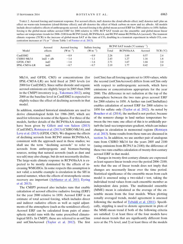
TABLE 2. Aerosol forcing and transient response. For aerosol effects, ind1 denotes the cloud-albedo effect; ind2 denotes ind1 plus an

effect on warm-rain formation (cloud-lifetime effect); and alb denotes the effect of black carbon on snow and ice albedo. All models

include direct radiative effects of anthropogenic aerosol. Aerosol forcing is the global-mean aerosol ERF for 2000 relative to 1850. Sulfate

forcing is the global-mean sulfate aerosol ERF for 2000 relative to 1850. RCP SAT trends are the ensemble- and global-mean linear

surface air temperature trends for 2006–2100 fromRCP45 (total), RCP45fixAA, and RCP45minus RCP45fixAA (aerosol). The transient

climate response (TCR) is the increase of global-mean SAT at the time of CO2 doubling in a transient experiment in which CO2 con-

centration increases at 1%yr21 (from Table 1 of Forster et al. 2013).

Model

Aerosol

effects

Aerosol forcing

(Wm22)

Sulfate forcing

(Wm22)

RCP45 SAT trends (8Ccentury21)

TCR (8C)Total RCP45fixAA Aerosol

CanESM2 ind1 20.9 20.9 2.26 1.69 0.57 2.4

CSIRO Mk3.6 ind2 1 alb 21.4 21.1 2.43 1.27 1.16 1.8

GFDL CM3 ind2 21.6 21.6 2.71 1.67 1.04 2.0

IPSL-CM5A-LR ind1 20.7 20.7 2.19 1.77 0.42 2.0

15 SEPTEMBER 2014 ROTS TAYN ET AL . 6963

with significant trends (i.e., three out of three or three

out of four) agree on the sign of the trend.

3. Results and discussion

a. Aerosol radiative forcing

A useful guide to the magnitude of the effects of

declining aerosols is the aerosol ERF, which can be

calculated from pairs of runs with prescribed SSTs

(section 2). This quantity is not generally available from

models for the twenty-first century, but in RCP4.5 (and

the other RCPs), assumed emissions of sulfur and car-

bonaceous aerosols return to roughly nineteenth-

century levels by 2100 (Lamarque et al. 2011; Smith

and Bond 2014). It follows that global-mean aerosol

ERF almost returns to its preindustrial value by 2100

(Takemura 2012; Shindell et al. 2013; Rotstayn et al.

2013; Smith and Bond 2014). Thus, to first order, pub-

lished CMIP5 aerosol ERF for 2000 relative to 1850 can

be used as a proxy (with sign reversed) for aerosol ERF

during the twenty-first century (Rotstayn et al. 2013).

In other words, the change in aerosol ERF during the

twenty-first century is similar to the historical change in

aerosol ERF, except that it is positive rather than

negative.

Global-mean values of aerosol ERF from published

CMIP5 runs are given in Table 2; note that the two

models that include treatments of the cloud-lifetime

effect (CSIROMk3.6 and GFDL CM3) have markedly

stronger aerosol ERF than CanESM2 and IPSL-

CM5A-LR. The modeled values can be compared

with the best estimate (20.9Wm22) and uncertainty

range (from 20.1 to 21.9Wm22) from the recent In-

tergovernmental Panel on Climate Change (IPCC)

report (Boucher et al. 2014); note that the IPCC values

apply to the period 1750–2010, and exclude the effects of

black carbon on snow and ice albedo. The mean aerosol

ERF from the four models is 21.15Wm22, which is

essentially the same as the mean value from the 13

models considered by Rotstayn et al. (2013).

Table 2 shows an interesting difference between

CSIRO Mk3.6 and the other three models. Assuming

linearity, the difference between aerosol ERF and sulfate

ERF gives an estimate of ERF from carbonaceous

aerosol (organic aerosol and black carbon). InCanESM2,

GFDL CM3, and IPSL-CM5A-LR, carbonaceous aero-

sol ERF is close to zero, but in CSIRO Mk3.6 it is

20.3Wm22. This implies that CSIROMk3.6 has positive

ERF fromdeclining carbonaceous aerosol in the twenty-

first century (because of organic aerosol, since ERF

from black carbon is positive). As discussed by Rotstayn

et al. (2012), negative ERF from carbonaceous aerosol

may be caused by the 50% increase of organic aerosol

emissions in CSIRO Mk3.6, as well as a substantial in-

direct effect (which is parameterization dependent). Note

that CMIP5 models show considerable uncertainty in

carbonaceous aerosol ERF, ranging from roughly zero to

20.6Wm22 (Boucher et al. 2014, their Table 7.5).

The models with stronger aerosol ERF in the histor-

ical period (CSIROMk3.6 andGFDLCM3) have larger

projected trends in global-mean surface air temperature

(SAT) due to declining aerosols than CanESM2 and

IPSL-CM5A-LR (Table 2). The fraction of projected

warming due to declining aerosols is 19% in IPSL-

CM5A-LR, 25% in CanESM2, 38% in GFDL CM3,

and 48% in CSIRO Mk3.6, reflecting the uncertainty

associated with aerosol effects. This range also suggests

that the magnitude of changes in circulation caused by

declining aerosols will vary substantially among the

models. Comparing CSIROMk3.6 andGFDLCM3, it is

initially surprising that the fraction of projected warm-

ing is larger in CSIRO Mk3.6, even though historical

aerosol ERF is stronger in GFDL CM3; this occurs be-

cause future aerosol ERF is not exactly the inverse of

historical aerosol ERF, as discussed below.

Simulated temperature changes depend on climate

sensitivity as well as forcing. Transient climate response

(TCR) is the change in SAT at the time of CO2 doubling

in an experiment forced by CO2 concentrations that

increase at 1%yr21; it depends on equilibrium climate

sensitivity and ocean heat uptake (e.g., Forster et al.

2013). Values of TCR in the four models (last column of

Table 2) range from 1.88 to 2.48C. For comparison,

Forster et al. (2013) found aMME-mean value of 1.828 60.638C from 23 CMIP5models (where the range is a 90%

confidence interval); thus the four models in this study

tend to have larger TCR than the average from CMIP5.

One might expect the models’ different TCR values

to be reflected in their SAT trends in RCP45fixAA, in

which the main forcing agent is increasing WMGHGs.

Consistent with having the lowest TCR, CSIROMk3.6

also has the smallest SAT trend in RCP45fixAA

(1.278C century21). The other models all have sim-

ilar SAT trends in RCP45fixAA (between 1.678 and1.778Ccentury21), and there is no obvious correlation

with their TCR values, which range from 2.08C (GFDL

CM3 and IPSL-CM5A-LR) to 2.48C (CanESM2). It is

unclear why the larger TCR in CanESM2 is not reflected

in its SAT response in RCP45fixAA; it may be that

forcing agents other than CO2 (non-CO2 greenhouse

gases and land use change) cause more warming in that

model.

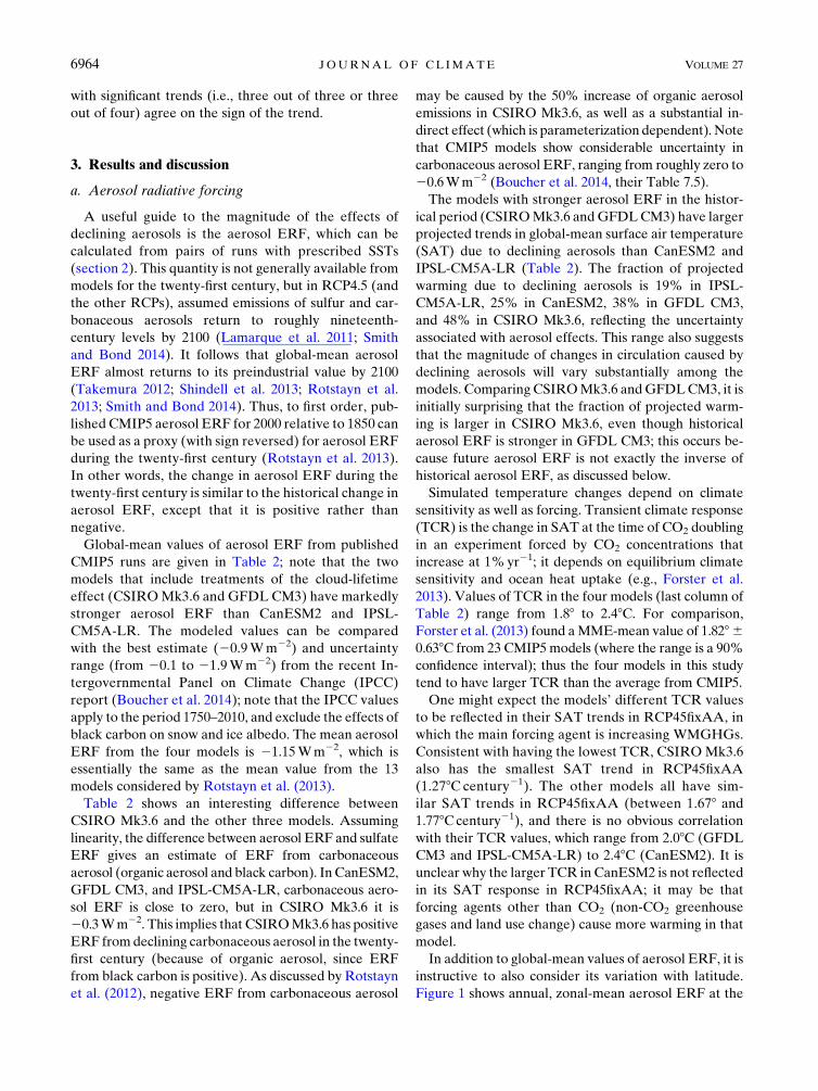
In addition to global-mean values of aerosol ERF, it is

instructive to also consider its variation with latitude.

Figure 1 shows annual, zonal-mean aerosol ERF at the

6964 JOURNAL OF CL IMATE VOLUME 27

top of the atmosphere for 2000 relative to 1850, multi-

plied by21 (as solid curves); the sign is changed so that

the values are generally positive, as would be the case for

twenty-first-century aerosol ERF.

Consistent with the global-mean values given in Table 2,

CSIRO Mk3.6 and GFDL CM3 tend to show stronger

aerosol ERF than IPSL-CM5A-LR and CanESM2. An

exception is in the Arctic region, where inclusion of BC

effects on snow and ice albedo causes aerosol ERF in

CSIRO Mk3.6 to change sign. The curves tend to be

somewhat noisier in CSIRO Mk3.6 and GFDL CM3

than the other models; this may be due to the shorter run

length in thesemodels, as well as the largermagnitude of

aerosol ERF. The individual models and the MME

mean have largest aerosol ERF near 408N, while in the

SH aerosol ERF tends to decrease toward the pole; we

shall return to this important point in section 3b, when

we consider the response of atmospheric temperature to

declining aerosols.

Also shown (as the dashed blue curve) is aerosol ERF

from CSIRO Mk3.6 for 2100 relative to 2005. The me-

ridional variation of future aerosol ERF resembles the

inverse of the historical pattern, with peak magnitude

near 408N.However, there are also some differences; for

example, future aerosol ERF in CSIRO Mk3.6 is

stronger in NH midlatitudes but weaker near the

equator than historical aerosol ERF.

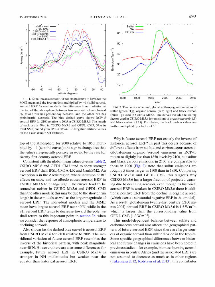
Why is future aerosol ERF not exactly the inverse of

historical aerosol ERF? In part this occurs because of

different effects from sulfate and carbonaceous aerosol.

Global-mean organic aerosol emissions in RCP4.5

return to slightly less than 1850 levels by 2100, but sulfur

and black carbon emissions in 2100 are comparable to

those in 1900 (Fig. 2); note that sulfur emissions are

roughly 5 times larger in 1900 than in 1850. Comparing

CSIRO Mk3.6 and GFDL CM3, this suggests why

CSIRO Mk3.6 has a larger fraction of projected warm-

ing due to declining aerosols, even though its historical

aerosol ERF is weaker: in CSIRO Mk3.6 there is addi-

tional positive ERF from the decline in organic aerosol

(which exerts a substantial negative ERF in that model).

As a result, global-mean twenty-first century (2100 mi-

nus 2005) aerosol ERF in CSIRO Mk3.6 is 1.5Wm22,

which is larger than the corresponding value from

GFDL CM3 (1.3Wm22).

This model-dependent balance between sulfate and

carbonaceous aerosol also affects the geographical pat-

tern of future aerosol ERF, since there are larger sour-

ces of organic aerosol than sulfur dioxide in the tropics.

Some specific geographical differences between histor-

ical and future changes in emissions have been noted in

previous studies—for example, biomass-burning aerosol

emissions in central Africa (and the associated ERF) are

not assumed to decrease as much as in other regions

(Takemura 2012; Rotstayn et al. 2013); this contributes

FIG. 1. Zonal-mean aerosol ERF for 2000 relative to 1850, for the

MME mean and the four models, multiplied by 21 (solid curves).

Aerosol ERF for each model is the difference in net radiation at

the top of the atmosphere between two runs with climatological

SSTs; one run has present-day aerosols, and the other run has

preindustrial aerosols. The blue dashed curve shows RCP4.5

aerosol ERF for 2100 relative to 2005 in CSIROMk3.6. The length

of each run is 30 yr in CSIRO Mk3.6 and GFDL CM3, 50 yr in

CanESM2, and 51 yr in IPSL-CM5A-LR. Negative latitude values

on the x axis denote SH latitudes.

FIG. 2. Time series of annual, global, anthropogenic emissions of

sulfur (green; Tg), organic aerosol (red; TgC) and black carbon

(blue; Tg) used in CSIRO Mk3.6. The curves include the scaling

factors used in CSIROMk3.6 for emissions of organic aerosol (1.5)

and black carbon (1.25). For clarity, the black carbon values are

further multiplied by a factor of 5.

15 SEPTEMBER 2014 ROTS TAYN ET AL . 6965

to the weaker future aerosol ERF in the deep tropics in

CSIRO Mk3.6.

In comparison to aerosol ERF, the radiative forcing

due to increasing WMGHGs is more uniform in space

(not shown). When evaluated as the traditional ‘‘strato-

sphere adjusted’’ forcing (i.e., as the change in radiative

flux at the tropopause, after allowing the stratosphere to

adjust), WMGHG forcing is quasi-uniform in space,

with only a modest enhancement in the subtropics

(Shindell et al. 2013, their Fig. 20).When evaluated as an

ERF (i.e., using an analogous method as used to gen-

erate the aerosol ERF in Fig. 1), rapid adjustments of

the atmosphere and land surface allowmore variation of

the forcing with latitude, although this variation is still

much less than for aerosol ERF (Xie et al. 2013, their

Fig. 1).

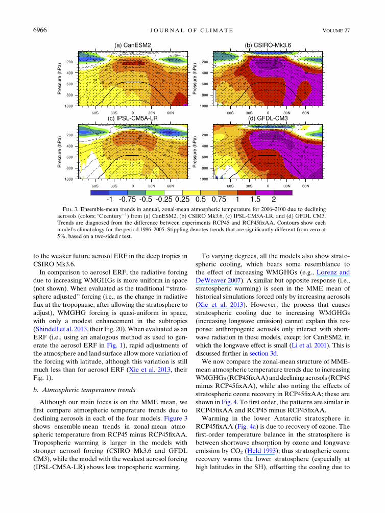
b. Atmospheric temperature trends

Although our main focus is on the MME mean, we

first compare atmospheric temperature trends due to

declining aerosols in each of the four models. Figure 3

shows ensemble-mean trends in zonal-mean atmo-

spheric temperature from RCP45 minus RCP45fixAA.

Tropospheric warming is larger in the models with

stronger aerosol forcing (CSIRO Mk3.6 and GFDL

CM3), while the model with the weakest aerosol forcing

(IPSL-CM5A-LR) shows less tropospheric warming.

To varying degrees, all the models also show strato-

spheric cooling, which bears some resemblance to

the effect of increasing WMGHGs (e.g., Lorenz and

DeWeaver 2007). A similar but opposite response (i.e.,

stratospheric warming) is seen in the MME mean of

historical simulations forced only by increasing aerosols

(Xie et al. 2013). However, the process that causes

stratospheric cooling due to increasing WMGHGs

(increasing longwave emission) cannot explain this res-

ponse: anthropogenic aerosols only interact with short-

wave radiation in these models, except for CanESM2, in

which the longwave effect is small (Li et al. 2001). This is

discussed further in section 3d.

We now compare the zonal-mean structure of MME-

mean atmospheric temperature trends due to increasing

WMGHGs (RCP45fixAA)anddeclining aerosols (RCP45

minus RCP45fixAA), while also noting the effects of

stratospheric ozone recovery in RCP45fixAA; these are

shown in Fig. 4. To first order, the patterns are similar in

RCP45fixAA and RCP45 minus RCP45fixAA.

Warming in the lower Antarctic stratosphere in

RCP45fixAA (Fig. 4a) is due to recovery of ozone. The

first-order temperature balance in the stratosphere is

between shortwave absorption by ozone and longwave

emission by CO2 (Held 1993); thus stratospheric ozone

recovery warms the lower stratosphere (especially at

high latitudes in the SH), offsetting the cooling due to

FIG. 3. Ensemble-mean trends in annual, zonal-mean atmospheric temperature for 2006–2100 due to declining

aerosols (colors; 8Ccentury21) from (a) CanESM2, (b) CSIRO Mk3.6, (c) IPSL-CM5A-LR, and (d) GFDL CM3.

Trends are diagnosed from the difference between experiments RCP45 and RCP45fixAA. Contours show each

model’s climatology for the period 1986–2005. Stippling denotes trends that are significantly different from zero at

5%, based on a two-sided t test.

6966 JOURNAL OF CL IMATE VOLUME 27

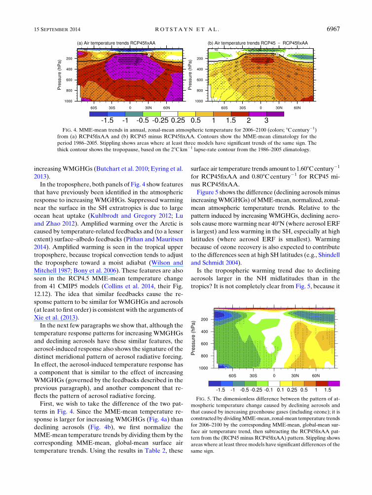
increasingWMGHGs (Butchart et al. 2010; Eyring et al.

2013).

In the troposphere, both panels of Fig. 4 show features

that have previously been identified in the atmospheric

response to increasing WMGHGs. Suppressed warming

near the surface in the SH extratropics is due to large

ocean heat uptake (Kuhlbrodt and Gregory 2012; Lu

and Zhao 2012). Amplified warming over the Arctic is

caused by temperature-related feedbacks and (to a lesser

extent) surface–albedo feedbacks (Pithan and Mauritsen

2014). Amplified warming is seen in the tropical upper

troposphere, because tropical convection tends to adjust

the troposphere toward a moist adiabat (Wilson and

Mitchell 1987; Bony et al. 2006). These features are also

seen in the RCP4.5 MME-mean temperature change

from 41 CMIP5 models (Collins et al. 2014, their Fig.

12.12). The idea that similar feedbacks cause the re-

sponse pattern to be similar for WMGHGs and aerosols

(at least to first order) is consistent with the arguments of

Xie et al. (2013).

In the next few paragraphs we show that, although the

temperature response patterns for increasing WMGHGs

and declining aerosols have these similar features, the

aerosol-induced response also shows the signature of the

distinct meridional pattern of aerosol radiative forcing.

In effect, the aerosol-induced temperature response has

a component that is similar to the effect of increasing

WMGHGs (governed by the feedbacks described in the

previous paragraph), and another component that re-

flects the pattern of aerosol radiative forcing.

First, we wish to take the difference of the two pat-

terns in Fig. 4. Since the MME-mean temperature re-

sponse is larger for increasing WMGHGs (Fig. 4a) than

declining aerosols (Fig. 4b), we first normalize the

MME-mean temperature trends by dividing them by the

corresponding MME-mean, global-mean surface air

temperature trends. Using the results in Table 2, these

surface air temperature trends amount to 1.608Ccentury21

for RCP45fixAA and 0.808Ccentury21 for RCP45 mi-

nus RCP45fixAA.

Figure 5 shows the difference (declining aerosols minus

increasingWMGHGs) ofMME-mean, normalized, zonal-

mean atmospheric temperature trends. Relative to the

pattern induced by increasing WMGHGs, declining aero-

sols cause more warming near 408N (where aerosol ERF

is largest) and less warming in the SH, especially at high

latitudes (where aerosol ERF is smallest). Warming

because of ozone recovery is also expected to contribute

to the differences seen at high SH latitudes (e.g., Shindell

and Schmidt 2004).

Is the tropospheric warming trend due to declining

aerosols larger in the NH midlatitudes than in the

tropics? It is not completely clear from Fig. 5, because it

FIG. 4. MME-mean trends in annual, zonal-mean atmospheric temperature for 2006–2100 (colors; 8Ccentury21)

from (a) RCP45fixAA and (b) RCP45 minus RCP45fixAA. Contours show the MME-mean climatology for the

period 1986–2005. Stippling shows areas where at least three models have significant trends of the same sign. The

thick contour shows the tropopause, based on the 28Ckm21 lapse-rate contour from the 1986–2005 climatology.

FIG. 5. The dimensionless difference between the pattern of at-

mospheric temperature change caused by declining aerosols and

that caused by increasing greenhouse gases (including ozone); it is

constructed by dividingMME-mean, zonal-mean temperature trends

for 2006–2100 by the corresponding MME-mean, global-mean sur-

face air temperature trend, then subtracting the RCP45fixAA pat-

tern from the (RCP45 minus RCP45fixAA) pattern. Stippling shows

areas where at least threemodels have significant differences of the

same sign.

15 SEPTEMBER 2014 ROTS TAYN ET AL . 6967

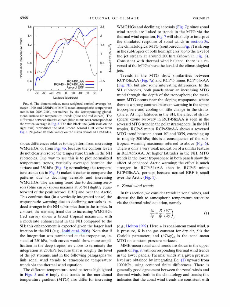
shows differences relative to the pattern from increasing

WMGHGs, or from Fig. 4b, because the contour levels

do not clearly resolve the temperature trends in the NH

subtropics. One way to see this is to plot normalized

temperature trends, vertically averaged between the

surface and 250 hPa (Fig. 6); normalizing the tempera-

ture trends (as in Fig. 5) makes it easier to compare the

patterns due to declining aerosols and increasing

WMGHGs. The warming trend due to declining aero-

sols (blue curve) shows maxima at 358N (slightly equa-

torward of the peak aerosol ERF) and over the Arctic.

This confirms that (in a vertically integrated sense) the

tropospheric warming due to declining aerosols is in-

deed stronger in theNH subtropics than in the tropics. In

contrast, the warming trend due to increasing WMGHGs

(red curve) shows a broad tropical maximum, with

a moderate enhancement in the NH compared to the

SH; this enhancement is expected given the larger land

fraction in the NH (e.g., Joshi et al. 2008). Note that if

the integration was terminated at the tropopause, in-

stead of 250 hPa, both curves would show more ampli-

fication in the deep tropics; we chose to terminate the

integration at 250 hPa because that is roughly the level

of the jet streams, and in the following paragraphs we

link zonal wind trends to atmospheric temperature

trends via the thermal wind equation.

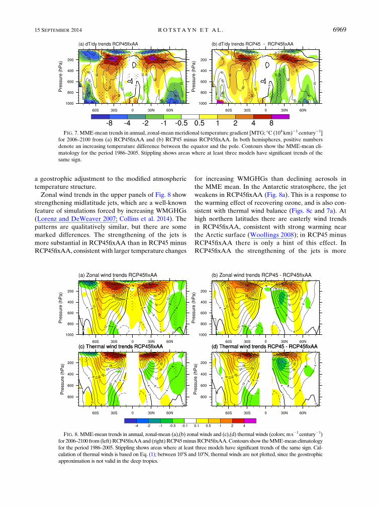
The different temperature trend patterns highlighted

in Figs. 5 and 6 imply that trends in the meridional

temperature gradient (MTG) also differ for increasing

WMGHGs and declining aerosols (Fig. 7); since zonal

wind trends are linked to trends in the MTG via the

thermal wind equation, Fig. 7 will also help to interpret

the simulated response of zonal winds in section 3c.

The climatological MTG (contoured in Fig. 7) is strong

in the subtropics of both hemispheres, up to the level of

the jet stream at around 200 hPa (shown in Fig. 8).

Consistent with thermal wind balance, there is a re-

versal of theMTG above the level of the climatological

jets.

Trends in the MTG show similarities between

RCP45fixAA (Fig. 7a) and RCP45 minus RCP45fixAA

(Fig. 7b), but also some interesting differences. In the

SH subtropics, both panels show an increasing MTG

trend through the depth of the troposphere; the maxi-

mum MTG occurs near the sloping tropopause, where

there is a strong contrast between warming in the upper

troposphere and cooling or little change in the strato-

sphere. At high latitudes in the SH, the effect of strato-

spheric ozone recovery in RCP45fixAA is seen in the

reversedMTG trend in the polar stratosphere. In the NH

tropics, RCP45 minus RCP45fixAA shows a reversed

MTG trend between about 108 and 308N, extending up

to roughly 300 hPa; this is a consequence of the sub-

tropical warming maximum referred to above (Fig. 6).

There is only a very weak indication of a similar feature

in RCP45fixAA. At higher latitudes in the NH, MTG

trends in the lower troposphere in both panels show the

effect of enhanced Arctic warming; the effect is much

stronger in RCP45fixAA than in RCP45 minus

RCP45fixAA, perhaps because aerosol ERF is small

over the Arctic (Fig. 1).

c. Zonal wind trends

In this section, we consider trends in zonal winds, and

discuss the link to atmospheric temperature structure

via the thermal wind equation, namely

›u

›p5

R

fp

�›T

›y

�p

(1)

(e.g., Holton 1992). Here, u is zonal-mean zonal wind, p

is pressure, R is the gas constant for dry air, f is the

Coriolis parameter, and (›T/›y)p is the zonal-mean

MTG on constant pressure surfaces.

MME-mean zonal wind trends are shown in the upper

panels of Fig. 8, with corresponding thermal wind trends

in the lower panels. Thermal winds at a given pressure

level are obtained by integrating Eq. (1) upward from

1000 hPa, using centered finite differences. There is

generally good agreement between the zonal winds and

thermal winds, both in the climatology and trends; this

indicates that the zonal wind trends are consistent with

FIG. 6. The dimensionless, mass-weighted vertical average be-

tween 1000 and 250 hPa of MME-mean atmospheric temperature

trends for 2006–2100, normalized by the corresponding global-

mean surface air temperature trends (blue and red curves). The

difference between the two curves (blue minus red) corresponds to

the vertical average in Fig. 5. The thin black line (with scale on the

right axis) reproduces the MME-mean aerosol ERF curve from

Fig. 1. Negative latitude values on the x axis denote SH latitudes.

6968 JOURNAL OF CL IMATE VOLUME 27

a geostrophic adjustment to the modified atmospheric

temperature structure.

Zonal wind trends in the upper panels of Fig. 8 show

strengthening midlatitude jets, which are a well-known

feature of simulations forced by increasing WMGHGs

(Lorenz and DeWeaver 2007; Collins et al. 2014). The

patterns are qualitatively similar, but there are some

marked differences. The strengthening of the jets is

more substantial in RCP45fixAA than in RCP45 minus

RCP45fixAA, consistent with larger temperature changes

for increasing WMGHGs than declining aerosols in

the MME mean. In the Antarctic stratosphere, the jet

weakens in RCP45fixAA (Fig. 8a). This is a response to

the warming effect of recovering ozone, and is also con-

sistent with thermal wind balance (Figs. 8c and 7a). At

high northern latitudes there are easterly wind trends

in RCP45fixAA, consistent with strong warming near

the Arctic surface (Woollings 2008); in RCP45 minus

RCP45fixAA there is only a hint of this effect. In

RCP45fixAA the strengthening of the jets is more

FIG. 7. MME-mean trends in annual, zonal-meanmeridional temperature gradient [MTG; 8C (104 km)21 century21]

for 2006–2100 from (a) RCP45fixAA and (b) RCP45 minus RCP45fixAA. In both hemispheres, positive numbers

denote an increasing temperature difference between the equator and the pole. Contours show the MME-mean cli-

matology for the period 1986–2005. Stippling shows areas where at least three models have significant trends of the

same sign.

FIG. 8. MME-mean trends in annual, zonal-mean (a),(b) zonal winds and (c),(d) thermal winds (colors; ms21 century21)

for 2006–2100 from(left)RCP45fixAAand (right)RCP45minusRCP45fixAA.Contours show theMME-mean climatology

for the period 1986–2005. Stippling shows areas where at least three models have significant trends of the same sign. Cal-

culation of thermal winds is based on Eq. (1); between 108S and 108N, thermal winds are not plotted, since the geostrophic

approximation is not valid in the deep tropics.

15 SEPTEMBER 2014 ROTS TAYN ET AL . 6969

symmetric between the hemispheres, although there is

a somewhat larger response in the SH than the NH.

In the NH, the jet shows a distinct response in RCP45

minus RCP45fixAA (Fig. 8b); it weakens on its equator-

ward, lower flank and strengthens on its poleward, upper

flank, so it shifts poleward and upward. This is also seen in

the corresponding thermal wind trends (Fig. 8d). The

thermal wind relation does not—in itself—distinguish

between cause and effect, but the above discussion sug-

gests that there is a direct causal link from the peak in

aerosol ERF near 408N, to the corresponding tempera-

ture response and then to the change in zonal wind

structure. A similar (but opposite) response in NH

winter was found by Ming et al. (2011) for increasing

aerosols in an atmospheric model coupled to a slab

ocean model (their Fig. 3b). Our explanation in terms of

thermal wind balance is consistent with theirs.

Another interesting aspect of the zonal wind response

to declining aerosols is that the jet strengthens more in

the SH than the NH. Since aerosol concentrations are

generally lower in the SH than the NH, this may seem

counterintuitive. However, Fig. 7b shows that this result

is consistent with the more widespread increase of the

MTG in the subtropics and midlatitudes of the SH than

in the NH. Thus it is the very fact that aerosol forcing is

stronger in the NH that causes this effect: aerosol ERF

peaks near 408N, and in the MME mean it is relatively

flat between the equator and 408N (Fig. 1). On the other

hand, south of the equator its magnitude falls away

rapidly with increasing latitude.

In the SH, MME mean strengthening westerlies in

RCP45fixAA and RCP45 minus RCP45fixAA extend

down to the surface; this equivalent barotropic struc-

ture is consistent with a strengthening and poleward

shift of the eddy-driven jet (Kushner et al. 2001).

However, there is little stippling below the upper tro-

posphere in Fig. 8, denoting a lack of model agreement.

In RCP45fixAA (figure not shown), different re-

sponses of the SH westerlies reflect different balances

between the effects of increasing WMGHGs, which

shift them poleward, and recovering stratospheric

ozone, which shifts them equatorward (Arblaster et al.

2011; Eyring et al. 2013). Since declining aerosols are

the main focus of this paper, the lack of model agree-

ment in RCP45 minus RCP45fixAA merits a closer

look.

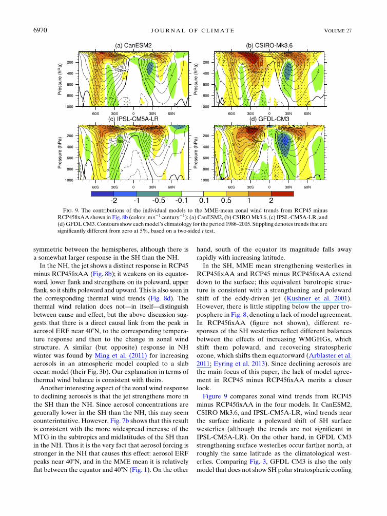
Figure 9 compares zonal wind trends from RCP45

minus RCP45fixAA in the four models. In CanESM2,

CSIRO Mk3.6, and IPSL-CM5A-LR, wind trends near

the surface indicate a poleward shift of SH surface

westerlies (although the trends are not significant in

IPSL-CM5A-LR). On the other hand, in GFDL CM3

strengthening surface westerlies occur farther north, at

roughly the same latitude as the climatological west-

erlies. Comparing Fig. 3, GFDL CM3 is also the only

model that does not show SH polar stratospheric cooling

FIG. 9. The contributions of the individual models to the MME-mean zonal wind trends from RCP45 minus

RCP45fixAA shown in Fig. 8b (colors; m s21 century21): (a) CanESM2, (b) CSIROMk3.6, (c) IPSL-CM5A-LR, and

(d) GFDLCM3. Contours show eachmodel’s climatology for the period 1986–2005. Stippling denotes trends that are

significantly different from zero at 5%, based on a two-sided t test.

6970 JOURNAL OF CL IMATE VOLUME 27

in RCP45 minus RCP45fixAA; this is discussed further

in section 3d.

There are several qualitative features that all models

have in common in Fig. 9. At middle-to-high SH lati-

tudes, the zonal wind response has an equivalent baro-

tropic vertical structure in all models, consistent with

a strengthening eddy-driven jet. In the subtropics of the

SH, there is an indication of a baroclinic response, with

a stronger subtropical jet and easterly wind trends near

the surface. In the NH, the subtropical jet in all models

moves upward and poleward, but only CSIRO Mk3.6

shows significant strengthening of the eddy-driven jet

(i.e., stronger midlatitude westerlies at the surface).

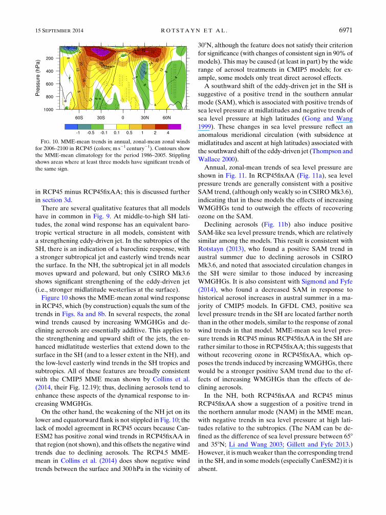
Figure 10 shows the MME-mean zonal wind response

in RCP45, which (by construction) equals the sum of the

trends in Figs. 8a and 8b. In several respects, the zonal

wind trends caused by increasing WMGHGs and de-

clining aerosols are essentially additive. This applies to

the strengthening and upward shift of the jets, the en-

hanced midlatitude westerlies that extend down to the

surface in the SH (and to a lesser extent in the NH), and

the low-level easterly wind trends in the SH tropics and

subtropics. All of these features are broadly consistent

with the CMIP5 MME mean shown by Collins et al.

(2014, their Fig. 12.19); thus, declining aerosols tend to

enhance these aspects of the dynamical response to in-

creasing WMGHGs.

On the other hand, the weakening of the NH jet on its

lower and equatorward flank is not stippled in Fig. 10; the

lack of model agreement in RCP45 occurs because Can-

ESM2 has positive zonal wind trends in RCP45fixAA in

that region (not shown), and this offsets the negativewind

trends due to declining aerosols. The RCP4.5 MME-

mean in Collins et al. (2014) does show negative wind

trends between the surface and 300hPa in the vicinity of

308N, although the feature does not satisfy their criterion

for significance (with changes of consistent sign in 90% of

models). This may be caused (at least in part) by the wide

range of aerosol treatments in CMIP5 models; for ex-

ample, some models only treat direct aerosol effects.

A southward shift of the eddy-driven jet in the SH is

suggestive of a positive trend in the southern annular

mode (SAM), which is associated with positive trends of

sea level pressure at midlatitudes and negative trends of

sea level pressure at high latitudes (Gong and Wang

1999). These changes in sea level pressure reflect an

anomalous meridional circulation (with subsidence at

midlatitudes and ascent at high latitudes) associated with

the southward shift of the eddy-driven jet (Thompson and

Wallace 2000).

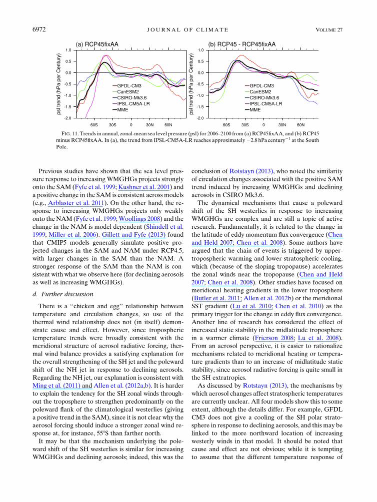
Annual, zonal-mean trends of sea level pressure are

shown in Fig. 11. In RCP45fixAA (Fig. 11a), sea level

pressure trends are generally consistent with a positive

SAM trend, (although only weakly so in CSIROMk3.6),

indicating that in these models the effects of increasing

WMGHGs tend to outweigh the effects of recovering

ozone on the SAM.

Declining aerosols (Fig. 11b) also induce positive

SAM-like sea level pressure trends, which are relatively

similar among the models. This result is consistent with

Rotstayn (2013), who found a positive SAM trend in

austral summer due to declining aerosols in CSIRO

Mk3.6, and noted that associated circulation changes in

the SH were similar to those induced by increasing

WMGHGs. It is also consistent with Sigmond and Fyfe

(2014), who found a decreased SAM in response to

historical aerosol increases in austral summer in a ma-

jority of CMIP5 models. In GFDL CM3, positive sea

level pressure trends in the SH are located farther north

than in the other models, similar to the response of zonal

wind trends in that model. MME-mean sea level pres-

sure trends in RCP45 minus RCP45fixAA in the SH are

rather similar to those inRCP45fixAA; this suggests that

without recovering ozone in RCP45fixAA, which op-

poses the trends induced by increasingWMGHGs, there

would be a stronger positive SAM trend due to the ef-

fects of increasing WMGHGs than the effects of de-

clining aerosols.

In the NH, both RCP45fixAA and RCP45 minus

RCP45fixAA show a suggestion of a positive trend in

the northern annular mode (NAM) in the MME mean,

with negative trends in sea level pressure at high lati-

tudes relative to the subtropics. (The NAM can be de-

fined as the difference of sea level pressure between 658and 358N; Li and Wang 2003; Gillett and Fyfe 2013.)

However, it ismuchweaker than the corresponding trend

in the SH, and in somemodels (especially CanESM2) it is

absent.

FIG. 10. MME-mean trends in annual, zonal-mean zonal winds

for 2006–2100 in RCP45 (colors; m s21 century21). Contours show

the MME-mean climatology for the period 1986–2005. Stippling

shows areas where at least three models have significant trends of

the same sign.

15 SEPTEMBER 2014 ROTS TAYN ET AL . 6971

Previous studies have shown that the sea level pres-

sure response to increasing WMGHGs projects strongly

onto the SAM (Fyfe et al. 1999; Kushner et al. 2001) and

a positive change in the SAM is consistent across models

(e.g., Arblaster et al. 2011). On the other hand, the re-

sponse to increasing WMGHGs projects only weakly

onto theNAM (Fyfe et al. 1999;Woollings 2008) and the

change in the NAM is model dependent (Shindell et al.

1999; Miller et al. 2006). Gillett and Fyfe (2013) found

that CMIP5 models generally simulate positive pro-

jected changes in the SAM and NAM under RCP4.5,

with larger changes in the SAM than the NAM. A

stronger response of the SAM than the NAM is con-

sistent with what we observe here (for declining aerosols

as well as increasing WMGHGs).

d. Further discussion

There is a ‘‘chicken and egg’’ relationship between

temperature and circulation changes, so use of the

thermal wind relationship does not (in itself) demon-

strate cause and effect. However, since tropospheric

temperature trends were broadly consistent with the

meridional structure of aerosol radiative forcing, ther-

mal wind balance provides a satisfying explanation for

the overall strengthening of the SH jet and the poleward

shift of the NH jet in response to declining aerosols.

Regarding the NH jet, our explanation is consistent with

Ming et al. (2011) and Allen et al. (2012a,b). It is harder

to explain the tendency for the SH zonal winds through-

out the troposphere to strengthen predominantly on the

poleward flank of the climatological westerlies (giving

a positive trend in the SAM), since it is not clear why the

aerosol forcing should induce a stronger zonal wind re-

sponse at, for instance, 558S than farther north.

It may be that the mechanism underlying the pole-

ward shift of the SH westerlies is similar for increasing

WMGHGs and declining aerosols; indeed, this was the

conclusion of Rotstayn (2013), who noted the similarity

of circulation changes associated with the positive SAM

trend induced by increasing WMGHGs and declining

aerosols in CSIRO Mk3.6.

The dynamical mechanisms that cause a poleward

shift of the SH westerlies in response to increasing

WMGHGs are complex and are still a topic of active

research. Fundamentally, it is related to the change in

the latitude of eddy momentum flux convergence (Chen

and Held 2007; Chen et al. 2008). Some authors have

argued that the chain of events is triggered by upper-

tropospheric warming and lower-stratospheric cooling,

which (because of the sloping tropopause) accelerates

the zonal winds near the tropopause (Chen and Held

2007; Chen et al. 2008). Other studies have focused on

meridional heating gradients in the lower troposphere

(Butler et al. 2011; Allen et al. 2012b) or the meridional

SST gradient (Lu et al. 2010; Chen et al. 2010) as the

primary trigger for the change in eddy flux convergence.

Another line of research has considered the effect of

increased static stability in the midlatitude troposphere

in a warmer climate (Frierson 2008; Lu et al. 2008).

From an aerosol perspective, it is easier to rationalize

mechanisms related to meridional heating or tempera-

ture gradients than to an increase of midlatitude static

stability, since aerosol radiative forcing is quite small in

the SH extratropics.

As discussed by Rotstayn (2013), the mechanisms by

which aerosol changes affect stratospheric temperatures

are currently unclear. All four models show this to some

extent, although the details differ. For example, GFDL

CM3 does not give a cooling of the SH polar strato-

sphere in response to declining aerosols, and this may be

linked to the more northward location of increasing

westerly winds in that model. It should be noted that

cause and effect are not obvious; while it is tempting

to assume that the different temperature response of

FIG. 11. Trends in annual, zonal-mean sea level pressure (psl) for 2006–2100 from (a)RCP45fixAA, and (b) RCP45

minus RCP45fixAA. In (a), the trend from IPSL-CM5A-LR reaches approximately22.8 hPa century21 at the South

Pole.

6972 JOURNAL OF CL IMATE VOLUME 27

GFDL CM3 causes the dynamical response to differ, it

is also possible that the temperature response is caused

by the different circulation change. For example,

Thompson and Wallace (2000) showed that positive

fluctuations in the SAM on interannual time scales are

associated with lower temperatures in the polar strato-

sphere (their Fig. 7c); they attributed this to adiabatic

cooling associated with anomalous ascent. Considering

direct radiative arguments as an explanation for strato-

spheric cooling due to declining aerosols, it is possibly

caused by decreasing shortwave absorption by black

carbon, although it is also possible that this effect is

overestimated. There are other plausible explanations,

such as changes in stratospheric water vapor (Rotstayn

2013). This is an interesting topic for further research.

A caveat concerning this study is that none of the

models treat nitrate aerosol. Nitrate is expected to offset

declines in other aerosol species, since emissions of

ammonia from agriculture are assumed to be insensitive

to emission controls in the RCPs (van Vuuren et al.

2011; Bellouin et al. 2011; Lamarque et al. 2011).

However, few CMIP5 models treat nitrate; Collins et al.

(2014) (their Table 12.1) list only 6 models out of 47 that

included nitrate. So in this respect our results are

broadly representative of most CMIP5 models.

The models in this study all have substantial negative

aerosol ERF at the top of the atmosphere (from20.7 to

21.6Wm22 for 2000 relative to 1850). We have not

explicitly considered the role of solar absorption by

black carbon, which is generally underestimated by

CMIP5 models (Shindell et al. 2013; Allen et al. 2013).

Allen et al. (2012a) showed that solar absorption by

black carbon and tropospheric ozone causes a north-

ward expansion of the tropics and the NH jet during

1979–99 in CMIP3 models. Also, Allen and Ajoku (2014,

manuscript submitted to Geophys. Res. Lett.) found that

in twenty-first-century projections with the Community

Atmospheric Model, declining sulfate and declining

black carbon exert opposing effects on large-scale NH

circulation. Thus it is possible that stronger black carbon

absorption in the models used here would tend to drive

an equatorward shift of the NH jet in response to de-

clining aerosols (i.e., an opposite response to what we

found).

All four models used in this study include a treatment

of indirect aerosol effects: two include only the cloud-

albedo effect, and two include both the cloud-albedo

and cloud-lifetime effects. Table 12.1 in Collins et al.

(2014) shows that a number of CMIP5 models (15 out

of 47 listed) do not treat indirect aerosol effects. These

models are likely to have weaker aerosol radiative

forcing (and climatic response) than the models con-

sidered here.

There are other aerosol–cloud interactions that may

be climatically important and are not resolved by the

models in this study. For example, cloud-resolving sim-

ulations by Zhang et al. (2007) suggested that pollution

aerosols from Asia have caused an intensification of the

winter storm track over the North Pacific Ocean. The

mechanism involves interactions between aerosols and

deep convection, which are generally not treated in

GCMs. Note that the extent to which aerosols invigorate

(i.e., deepen) convective clouds is very uncertain; see

Altaratz et al. (2014) for a recent review.

4. Summary and conclusions

We compared the projected effects of declining aerosols

in RCP4.5 using four models, with a focus on annual,

zonal-mean atmospheric temperature structure and zonal

winds. We interpreted the response in terms of the me-

ridional structure of aerosol radiative forcing, which peaks

near 408N and vanishes at the South Pole. Our main em-

phasis was on features that were consistent across a ma-

jority of models, although we also considered differences

among the models. Consistent aspects of the response

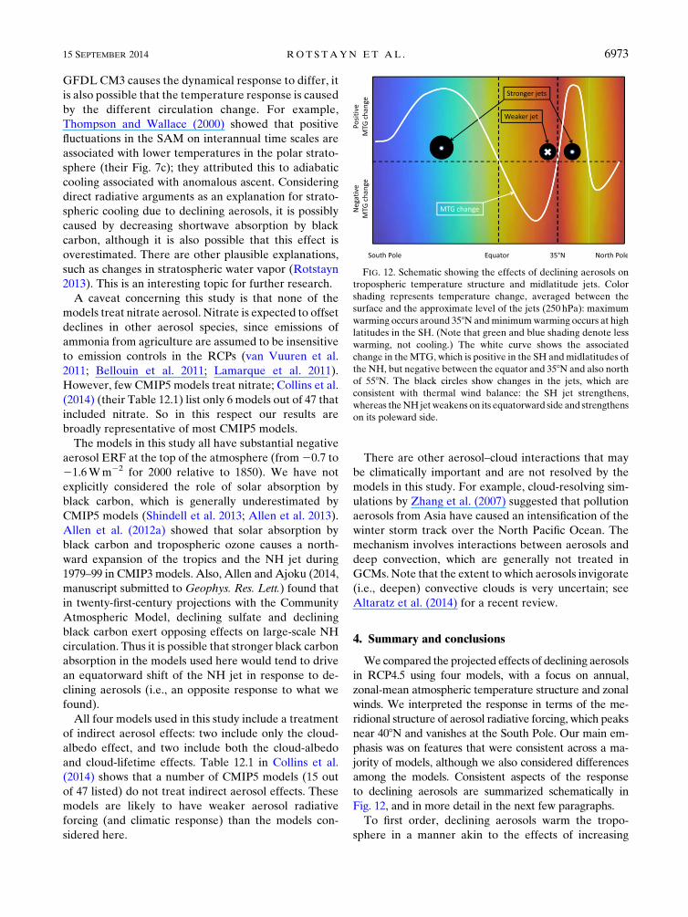
to declining aerosols are summarized schematically in

Fig. 12, and in more detail in the next few paragraphs.

To first order, declining aerosols warm the tropo-

sphere in a manner akin to the effects of increasing

FIG. 12. Schematic showing the effects of declining aerosols on

tropospheric temperature structure and midlatitude jets. Color

shading represents temperature change, averaged between the

surface and the approximate level of the jets (250 hPa): maximum

warming occurs around 358N andminimumwarming occurs at high

latitudes in the SH. (Note that green and blue shading denote less

warming, not cooling.) The white curve shows the associated

change in theMTG, which is positive in the SH andmidlatitudes of

the NH, but negative between the equator and 358N and also north

of 558N. The black circles show changes in the jets, which are

consistent with thermal wind balance: the SH jet strengthens,

whereas theNH jet weakens on its equatorward side and strengthens

on its poleward side.

15 SEPTEMBER 2014 ROTS TAYN ET AL . 6973

WMGHGs: similar features include amplified warming

in the tropical upper troposphere and near the Arctic

surface, and less warming in the extratropical lower

troposphere in the SH. These common features are due

to feedbacks that act similarly in response to both

forcing agents (Xie et al. 2013). It should be noted that

feedbacks are not expected to be identical for changes

in aerosols and WMGHGs; Shindell (2014) recently

showed that the larger weighting of aerosol forcing to-

ward the NH extratropics provokes stronger feedbacks,

and a larger change in surface temperature per unit

forcing for aerosols than WMGHGs.

The effect of the meridional structure of aerosol

forcing is also seen in the tropospheric temperature re-

sponse to declining aerosols, which has a different

structure to that caused by increasing WMGHGs. Rel-

ative to the pattern of warming caused by increasing

WMGHGs, declining aerosols cause more warming in

NHmidlatitudes, and less warming in the SH, especially

at high latitudes. Averaged between the surface and

250 hPa, the maximum warming due to declining aero-

sols is at 358N (whereas the warming due to increasing

WMGHGs shows a broad tropical maximum). As a

consequence, declining aerosols cause the MTG in the

troposphere to generally increase in the SH, whereas in

the NH it decreases in the tropics and subtropics.

Declining aerosols cause the midlatitude jets to

strengthen in both hemispheres, but more substantially in

the SH. In the NH, the jet strengthens on its upper and

poleward flank, but weakens on its lower and equatorward

flank, so it shifts poleward and upward. We showed that

these effects are broadly consistent with thermal wind

balance. Thus the jet strengthens more in the SH than the

NH because aerosol forcing has its largest magnitude in

the NH midlatitudes, and is relatively flat between the

equator and 408N, whereas in the SH aerosol forcing

generally decreases between the equator and the pole. The

meridional structure of aerosol forcing is then reflected in

the response of the MTG and the midlatitude jets.

The response to declining aerosols in the SH shows

increasing sea level pressure at midlatitudes and de-

creasing sea level pressure at high latitudes (i.e., a posi-

tive trend in the southern annular mode). In the NH

there is a suggestion of a positive trend in the northern

annular mode in theMMEmean, but the response is not

consistent among the models. In the SH, the effects of

increasing WMGHGs and declining aerosols on annual-

mean zonal winds and the annular mode are broadly

additive. The picture is more complex in the NH, be-

cause the jet is roughly collocated with the latitude of

maximum aerosol forcing.

Changes in circulation (zonal winds and sea level

pressure) caused by declining aerosols are of comparable

magnitude to those caused by increasing WMGHGs in

the MME mean, even though corresponding tempera-

ture changes are substantially smaller: global-mean

surface air temperature trends are 1.68Ccentury21 in

RCP45fixAA and 0.88Ccentury21 in RCP45 minus

RCP45fixAA, and tropospheric temperature trends are

also smaller in Fig. 4b than Fig. 4a. Based on the above

discussion, the explanation is that trends in theMTG are

of comparable magnitude for declining aerosols and

increasing WMGHGs.

The jets are a source of baroclinic instability, so the

effects of declining aerosols on the jets may be impor-

tant for understanding projected changes in storm tracks

and precipitation. For example, Chang et al. (2012) com-

paredprojected changes in storm tracks (based on filtered

meridional wind variance) from CMIP5 and CMIP3. In

the SH they found similar results in CMIP3 and CMIP5,

namely a poleward and upward shift of the storm track.

However, in the NH the CMIP5 projections differed

substantially from CMIP3. CMIP5 models projected

a modest poleward and upward shift of the storm track,

but mainly a weakening of the storm track on its lower

and equatorward flank (which was much more pro-

nounced in CMIP5 than CMIP3). Although Chang et al.

(2012) did not consider the role of aerosols, the qualita-

tive similarity of their CMIP5 NH storm track changes to

our results for the NH jet suggests that declining aerosols

contribute to the weakening NH storm track in CMIP5

projections.

The sensitivity of the SAM to changing aerosols is

intriguing. Long-term trends in the SAM are thought to

affect precipitation in themiddle-to-high latitudes of the

SH (Fyfe et al. 2012), the Southern Ocean carbon sink

(Lenton et al. 2009), and Antarctic sea ice extent

(Sigmond and Fyfe 2014). Thus, aerosol forcing, which is

principally located in the NH, is likely to be important

for understanding climate change in the most remote

and pristine parts of the SH.

We analyzed the annual- and zonal-mean response to

declining aerosols, and found both similarities to and

differences from the effects of increasing WMGHGs,

which are relatively well known. We did not consider

seasonal effects or zonal variations in circulation; the

latter are especially important in the NH (e.g., Barnes

and Polvani 2013). Studies of the effects of historically

increasing aerosols, such as those reviewed in section 1,

suggest that tropical and regional circulation will also

show a distinct response to declining aerosols in climate

projections. These are interesting topics for further

research.

The magnitude of aerosol forcing varies substantially

among the four models we considered, and so does the

response. Global-mean historical aerosol ERF ranges

6974 JOURNAL OF CL IMATE VOLUME 27

from 20.7Wm22 in IPSL-CM5A-LR to 21.6Wm22 in

GFDL CM3. Although aerosol ERF for the period 2006

to 2100 in RCP4.5 is not available, the global-mean

surface air temperature change due to declining aerosols

is larger in the models with stronger aerosol ERF in the

historical period (CSIRO Mk3.6 and GFDL CM3) than

in IPSL-CM5A-LR or CanESM2. This is consistent with

the argument that historical aerosol ERF (with sign re-

versed) is a reasonable proxy for twenty-first-century

aerosol ERF (Rotstayn et al. 2013). Trends in atmo-

spheric temperature and zonal winds were also generally

stronger in the models with stronger aerosol forcing.

However, the range of aerosol forcing in these models

does not fully capture the uncertainty, even in the global

mean. The uncertainty is even larger when considering

regional effects. In view of this, and the fact that the

RCPs do not adequately sample the phase space of

possible future aerosol emissions, systematic efforts are

needed to investigate the role of declining aerosols in

climate projections.

Acknowledgments. This research is supported by the

Australian Government Department of the Environ-

ment, the Bureau of Meteorology, and CSIRO through

the Australian Climate Change Science Programme. The

contribution by the IPSL-CM5A-LR model was possible

thanks to the high performance computing resources of

CCRT and IDRIS made available by GENCI (Grand

Equipement National de Calcul Intensif), CEA (Com-

missariat à l’Energie Atomique et aux Energies Alter-

natives) and CNRS (Centre National de la Recherche

Scientifique). We appreciate helpful comments on the

manuscript by J. Katzfey at CSIRO and R. Mahmood,

M. Sigmond, and S. Kharin at Environment Canada.

Knut von Salzen thanks staff at CCCma for carrying out

simulations and processing data. We acknowledge the

World Climate Research Programme’s Working Group

on Coupled Modelling and the U.S. Department of

Energy’s Program for Climate Model Diagnosis and

Intercomparison, and we thank the climate modeling

groups (listed in Table 1 of this paper) for producing and

making available their model output. We thank Robert

Allen and two anonymous reviewers for their con-

structive comments, which improved the presentation of

the paper.

REFERENCES

Ackerley, D., B. B. B. Booth, S. H. E. Knight, E. J. Highwood, D. J.

Frame, M. R. Allen, and D. P. Rowell, 2011: Sensitivity of

twentieth-century Sahel rainfall to sulfate aerosol and CO2 forc-

ing. J. Climate, 24, 4999–5014, doi:10.1175/JCLI-D-11-00019.1.

Allen, R. J., and S. C. Sherwood, 2011: The impact of natural versus

anthropogenic aerosols on atmospheric circulation in the

CommunityAtmosphereModel.ClimateDyn., 36, 1959–1978,

doi:10.1007/s00382-010-0898-8.

——, ——, J. R. Norris, and C. Zender, 2012a: Recent Northern

Hemisphere tropical expansion primarily driven by black

carbon and tropospheric ozone. Nature, 485, 350–354,

doi:10.1038/nature11097.

——, ——, ——, and ——, 2012b: The equilibrium response to

idealized thermal forcings in a comprehensive GCM: Impli-

cations for recent tropical expansion.Atmos. Chem. Phys., 12,

4795–4816, doi:10.5194/acp-12-4795-2012.

——, J. R. Norris, and M. Wild, 2013: Evaluation of multidecadal

variability in CMIP5 surface solar radiation and inferred un-

derestimation of aerosol direct effects over Europe, China,

Japan, and India. J. Geophys. Res., 118, 6311–6336,

doi:10.1002/jgrd.50426.

Altaratz, O., I. Koren, L. A. Remer, and E. Hirsch, 2014: Review:

Cloud invigoration by aerosols—Coupling between micro-

physics and dynamics.Atmos. Res., 140–141, 38–60, doi:10.1016/

j.atmosres.2014.01.009.

Arblaster, J. M., G. A. Meehl, and D. J. Karoly, 2011: Future cli-

mate change in the Southern Hemisphere: Competing effects

of ozone and greenhouse gases. Geophys. Res. Lett., 38,

L02701, doi:10.1029/2010GL045384.

Barnes, E. A., and L. Polvani, 2013: Response of the midlatitude

jets, and of their variability, to increased greenhouse gases in

the CMIP5 models. J. Climate, 26, 7117–7135, doi:10.1175/

JCLI-D-12-00536.1.

Bellouin, N., J. Rae, A. Jones, C. Johnson, J. Haywood, and

O. Boucher, 2011: Aerosol forcing in the Climate Model In-

tercomparison Project (CMIP5) simulations by HadGEM2-

ES and the role of ammonium nitrate. J. Geophys. Res., 116,

D20206, doi:10.1029/2011JD016074.

Bollasina, M. A., Y. Ming, and V. Ramaswamy, 2011: Anthropo-

genic aerosols and the weakening of the South Asian summer

monsoon. Science, 334, 502–505, doi:10.1126/science.1204994.

Bony, S., and Coauthors, 2006: How well do we understand and

evaluate climate change feedback processes? J. Climate, 19,

3445–3482, doi:10.1175/JCLI3819.1.

Boucher, O., and Coauthors, 2014: Clouds and aerosols. Climate

Change 2013: The Physical Science Basis, T. F. Stocker et al.,

Eds., Cambridge University Press, 571–657.

Butchart, N., and Coauthors, 2010: Chemistry–climate model

simulations of twenty-first century stratospheric climate and

circulation changes. J. Climate, 23, 5349–5374, doi:10.1175/

2010JCLI3404.1.

Butler, A. H., D. W. J. Thompson, and T. Birner, 2011: Isentropic

slopes, downgradient eddy fluxes, and the extratropical atmo-

spheric circulation response to tropical tropospheric heating.

J. Atmos. Sci., 68, 2292–2305, doi:10.1175/JAS-D-10-05025.1.

Chang, C.-Y., J. C. H. Chiang, M. F. Wehner, A. R. Friedman, and

R. Ruedy, 2011: Sulfate aerosol control of tropical Atlantic

climate over the twentieth century. J. Climate, 24, 2540–2555,

doi:10.1175/2010JCLI4065.1.

Chang, E. K. M., Y. Guo, and X. Xia, 2012: CMIP5 multimodel en-

semble projection of storm track change under global warming.

J. Geophys. Res., 117, D23118, doi:10.1029/2012JD018578.

Chen, G., and I. M. Held, 2007: Phase speed spectra and the recent

poleward shift of Southern Hemisphere surface westerlies.

Geophys. Res. Lett., 34, L21805, doi:10.1029/2007GL031200.

——, J. Lu, and D. M. W. Frierson, 2008: Phase speed spectra and

the latitude of surface westerlies: Interannual variability and

global warming trend. J. Climate, 21, 5942–5959, doi:10.1175/

2008JCLI2306.1.

15 SEPTEMBER 2014 ROTS TAYN ET AL . 6975

——, R. A. Plumb, and J. Lu, 2010: Sensitivities of zonal mean

atmospheric circulation to SST warming in an aqua-planet

model. Geophys. Res. Lett., 37, L12701, doi:10.1029/

2010GL043473.

Cheng, Y., U. Lohmann, J. Zhang, Y. Luo, Z. Liu, and G. Lesins,

2005: Contribution of changes in sea surface temperature and

aerosol loading to the decreasing precipitation trend in

southern China. J. Climate, 18, 1381–1390, doi:10.1175/

JCLI3341.1.

Collier, M. A., L. D. Rotstayn, K.-Y. Kim, A. C. Hirst, and S. J.

Jeffrey, 2013: Ocean circulation response to anthropogenic-

aerosol and greenhouse gas forcing in the CSIRO-Mk3.6

coupled climate model. Aust. Meteor. Ocean J., 63, 27–39.

Collins, M., and Coauthors, 2014: Long-term climate change:

Projections, commitments and irreversibility. Climate Change

2013: The Physical Science Basis, T. F. Stocker et al., Eds.,

Cambridge University Press, 1029–1136.

Dufresne, J.-L., and Coauthors, 2013: Climate change pro-

jections using the IPSL-CM5 Earth System Model: From

CMIP3 to CMIP5.Climate Dyn., 40, 2123–2165, doi:10.1007/

s00382-012-1636-1.

Eyring, V., and Coauthors, 2013: Long-term ozone changes and

associated climate impacts in CMIP5 simulations. J. Geophys.

Res., 118, 5029–5060, doi:10.1002/jgrd.50316.Forster, P. M., T. Andrews, P. Good, J. M. Gregory, L. S. Jackson,

and M. Zelinka, 2013: Evaluating adjusted forcing and model

spread for historical and future scenarios in the CMIP5 gen-

eration of climate models. J. Geophys. Res., 118, 1139–1150,

doi:10.1002/jgrd.50174.

Francis, J. A., and S. J. Vavrus, 2012: Evidence linking Arctic

amplification to extreme weather in mid-latitudes. Geophys.

Res. Lett., 39, L06801, doi:10.1029/2012GL051000.

Frederiksen, C. S., J. S. Frederiksen, J.M. Sisson, andS. L.Osbrough,

2011: Australian winter circulation and rainfall changes and

projections. Int. J. Climate Change Strategies Manage., 3, 170–

188, doi:10.1108/17568691111129002.

Frierson, D. M. W., 2008: Midlatitude static stability in simple and

comprehensive general circulation models. J. Atmos. Sci., 65,

1049–1062, doi:10.1175/2007JAS2373.1.

Fyfe, J. C., G. J. Boer, and G. M. Flato, 1999: The Arctic and

Antarctic oscillations and their projected changes under global

warming. Geophys. Res. Lett., 26, 1601–1604, doi:10.1029/

1999GL900317.

——, N. P. Gillett, and G. J. Marshall, 2012: Human influence on

extratropical Southern Hemisphere summer precipitation.

Geophys. Res. Lett., 39, L23711, doi:10.1029/2012GL054199.

Gillett, N. P., and J. C. Fyfe, 2013: Annular mode changes in the

CMIP5 simulations. Geophys. Res. Lett., 40, 1189–1193,

doi:10.1002/grl.50249.

——, and K. von Salzen, 2013: The role of reduced aerosol pre-

cursor emissions in driving near-term warming. Environ. Res.

Lett., 8, 034008, doi:10.1088/1748-9326/8/3/034008.

Gong, D., and S. Wang, 1999: Definition of Antarctic Oscillation in-

dex.Geophys. Res. Lett., 26, 459–462, doi:10.1029/1999GL900003.

Held, I.M., 1993:Large-scaledynamics andglobalwarming.Bull.Amer.

Meteor. Soc., 74, 228–241, doi:10.1175/1520-0477(1993)074,0228:

LSDAGW.2.0.CO;2.

Holton, J. R., 1992: An Introduction to Dynamic Meteorology. 3rd

ed. Academic Press, 511 pp.

Hwang, Y.-T., D. M. W. Frierson, and S. M. Kang, 2013: Anthro-

pogenic sulfate aerosol and the southward shift of tropical

precipitation in the late 20th century. Geophys. Res. Lett., 40,

2845–2850, doi:10.1002/grl.50502.

Jones, A., J. M. Haywood, and O. Boucher, 2007: Aerosol forcing,

climate response and climate sensitivity in the Hadley Centre

climate model. J. Geophys. Res., 112, D20211, doi:10.1029/

2007JD008688.

Joshi,M.M., J.M.Gregory,M. J.Webb,D.M.H. Sexton, and T. C.

Johns, 2008: Mechanisms for the land/sea warming contrast

exhibited by simulations of climate change. Climate Dyn., 30,

455–465, doi:10.1007/s00382-007-0306-1.

Kawase, H., M. Abe, Y. Yamada, T. Takemura, T. Yokohata, and

T. Nozawa, 2010: Physical mechanism of long-term drying

trend over tropical North Africa. Geophys. Res. Lett., 37,

L09706, doi:10.1029/2010GL043038.

Kirtman, B., and Coauthors, 2014: Near-term climate change:

Projections and predictability. Climate Change 2013: The

Physical Science Basis, T. F. Stocker et al., Eds., Cambridge

University Press, 953–1028.

Kristjánsson, J. E., T. Iversen, A. Kirkevåg, Ø. Seland, and

J. Debernard, 2005: Response of the climate system to

aerosol direct and indirect forcing: Role of cloud feedbacks.

J. Geophys. Res., 110, D24206, doi:10.1029/2005JD006299.

Kuhlbrodt, T., and J. M. Gregory, 2012: Ocean heat uptake and its

consequences for the magnitude of sea level rise and climate

change. Geophys. Res. Lett., 39, L18608, doi:10.1029/

2012GL052952.

Kushner, P. J., I. M. Held, and T. L. Delworth, 2001: Southern

Hemisphere atmospheric circulation response to global

warming. J. Climate, 14, 2238–2249, doi:10.1175/

1520-0442(2001)014,0001:SHACRT.2.0.CO;2.

Lamarque, J.-F., G. P. Kyle, M.Meinshausen, K. Riahi, S. J. Smith,

D. P. van Vuuren, A. J. Conley, and F. Vitt, 2011: Global and

regional evolution of short-lived radiatively-active gases and

aerosols in the representative concentration pathways. Cli-

matic Change, 109, 191–212, doi:10.1007/s10584-011-0155-0.Lenton, A., F. Codron, L. Bopp, N.Metzl, P. Cadule, A. Tagliabue,

and J. Le Sommer, 2009: Stratospheric ozone depletion re-

duces ocean carbon uptake and enhances ocean acidification.

Geophys. Res. Lett., 36, L12606, doi:10.1029/2009GL038227.

Levy, H., II, L. W. Horowitz, M. Daniel Schwarzkopf, Y. Ming,

J.-C. Golaz, V. Naik, and V. Ramaswamy, 2013: The roles of

aerosol direct and indirect effects in past and future climate

change. J.Geophys. Res., 118, 4521–4532, doi:10.1002/jgrd.50192.

Li, J., and J. X. L. Wang, 2003: A modified zonal index and its

physical sense. Geophys. Res. Lett., 30, 1632, doi:10.1029/

2003GL017441.

——, J. G. D. Wong, J. S. Dobbie, and P. Chýlek, 2001: Parame-

terization of the optical properties of sulfate aerosols. J. At-

mos. Sci., 58, 193–209, doi:10.1175/1520-0469(2001)058,0193:

POTOPO.2.0.CO;2.

Liu, X., X. Xie, Z.-Y. Yin, C. Liu, and A. Gettelman, 2011: A

modeling study of the effects of aerosols on clouds and pre-

cipitation over East Asia. Theor. Appl. Climatol., 106, 343–

354, doi:10.1007/s00704-011-0436-6.

Lorenz, D. J., and E. T. DeWeaver, 2007: Tropopause height and

zonal wind response to global warming in the IPCC scenario

integrations. J. Geophys. Res., 112, D10119, doi:10.1029/

2006JD008087.

Lu, J., and B. Zhao, 2012: The role of oceanic feedback in the cli-

mate response to doubling CO2. J. Climate, 25, 7544–7563,

doi:10.1175/JCLI-D-11-00712.1.

——,G. Chen, and D.M.W. Frierson, 2008: Response of the zonal

mean atmospheric circulation to El Niño versus globalwarming. J. Climate, 21, 5835–5851, doi:10.1175/

2008JCLI2200.1.

6976 JOURNAL OF CL IMATE VOLUME 27

——, ——, and ——, 2010: The position of the midlatitude storm

track and eddy-driven westerlies in aquaplanet AGCMs.

J. Atmos. Sci., 67, 3984–4000, doi:10.1175/2010JAS3477.1.

Meehl, G. A., J. M. Arblaster, and W. D. Collins, 2008: Effects of

black carbon aerosols on the Indian monsoon. J. Climate, 21,

2869–2882, doi:10.1175/2007JCLI1777.1.

——, and Coauthors, 2013: Climate change projections in CESM1

(CAM5) compared to CCSM4. J. Climate, 26, 6287–6308,

doi:10.1175/JCLI-D-12-00572.1.

Miller, R. L., G. A. Schmidt, and D. T. Shindell, 2006: Forced an-

nular variations in the 20th century Intergovernmental Panel

on Climate Change Fourth Assessment Report models.

J. Geophys. Res., 111, D18101, doi:10.1029/2005JD006323.

Ming, Y., and V. Ramaswamy, 2011: A model investigation of

aerosol-induced changes in tropical circulation. J. Climate, 24,5125–5133, doi:10.1175/2011JCLI4108.1.

——, ——, and G. Chen, 2011: A model investigation of aerosol-

induced changes in boreal winter extratropical circulation.

J. Climate, 24, 6077–6091, doi:10.1175/2011JCLI4111.1.Pithan, F., and T. Mauritsen, 2014: Arctic amplification dominated

by temperature feedbacks in contemporary climate models.

Nat. Geosci., 7, 181–184, doi:10.1038/ngeo2071.

Ramanathan, V., and Coauthors, 2005: Atmospheric brown clouds:

Impacts on South Asian climate and hydrological cycle.

Proc. Natl. Acad. Sci. USA, 102, 5326–5333, doi:10.1073/

pnas.0500656102.

Rotstayn, L. D., 2013: Projected effects of declining anthropogenic

aerosols on the southern annular mode. Environ. Res. Lett., 8,

044028, doi:10.1088/1748-9326/8/4/044028.

——, and U. Lohmann, 2002: Tropical rainfall trends and the in-

direct aerosol effect. J. Climate, 15, 2103–2116, doi:10.1175/

1520-0442(2002)015,2103:TRTATI.2.0.CO;2.

——, B. F. Ryan, and J. E. Penner, 2000: Precipitation changes in

a GCM resulting from the indirect effects of anthropogenic

aerosols. Geophys. Res. Lett., 27, 3045–3048, doi:10.1029/

2000GL011737.

——, S. J. Jeffrey, M. A. Collier, S. M. Dravitzki, A. C. Hirst, J. I.

Syktus, and K. K. Wong, 2012: Aerosol- and greenhouse gas-

induced changes in summer rainfall and circulation in the

Australasian region: A study using single-forcing climate

simulations. Atmos. Chem. Phys., 12, 6377–6404, doi:10.5194/acp-12-6377-2012.

——, M. A. Collier, A. Chrastansky, S. J. Jeffrey, and J.-J. Luo,

2013: Projected effects of declining aerosols in RCP4.5: Un-

masking global warming? Atmos. Chem. Phys., 13, 10 883–10 905, doi:10.5194/acp-13-10883-2013.

Shindell, D. T., 2014: Inhomogeneous forcing and transient climate

sensitivity. Nat. Climate Change, 4, 274–277, doi:10.1038/

nclimate2136.

——, and G. A. Schmidt, 2004: Southern Hemisphere climate re-

sponse to ozone changes and greenhouse gas increases.Geophys.

Res. Lett., 31, L18209, doi:10.1029/2004GL020724.

——, R. L. Miller, G. A. Schmidt, and L. Pandolfo, 1999: Simula-

tion of recent northern winter climate trends by greenhouse-

gas forcing. Nature, 399, 452–455, doi:10.1038/20905.

——, and Coauthors, 2013: Radiative forcing in the ACCMIP

historical and future climate simulations.Atmos. Chem. Phys.,

13, 2939–2974, doi:10.5194/acp-13-2939-2013.

Sigmond,M., and J. C. Fyfe, 2014: TheAntarctic sea ice response to

the ozone hole in climate models. J. Climate, 27, 1336–1342,doi:10.1175/JCLI-D-13-00590.1.

Smith, S. J., and T. C. Bond, 2014: Two hundred fifty years of

aerosols and climate: The end of the age of aerosols. Atmos.

Chem. Phys., 14, 537–549, doi:10.5194/acp-14-537-2014.

——,H. Pitcher, and T.M. L.Wigley, 2005: Future sulfur dioxide

emissions. Climatic Change, 73, 267–318, doi:10.1007/

s10584-005-6887-y.

Szopa, S., and Coauthors, 2013: Aerosol and ozone changes as

forcing for climate evolution between 1850 and 2100. Climate

Dyn., 40, 2223–2250, doi:10.1007/s00382-012-1408-y.

Takemura, T., 2012: Distributions and climate effects of atmo-

spheric aerosols from the preindustrial era to 2100 along

representative concentration pathways (RCPs) simulated us-

ing the global aerosol model SPRINTARS. Atmos. Chem.

Phys., 12, 11 555–11 572, doi:10.5194/acp-12-11555-2012.

Taylor, K. E., R. J. Stouffer, andG.A.Meehl, 2012: An overview of

CMIP5 and the experiment design. Bull. Amer. Meteor. Soc.,

93, 485–498, doi:10.1175/BAMS-D-11-00094.1.

Tebaldi, C., J. M. Arblaster, and R. Knutti, 2011: Mapping model

agreement on future climate projections. Geophys. Res. Lett.,

38, L23701, doi:10.1029/2011GL049863.

Thompson, D. W. J., and J. M.Wallace, 2000: Annular modes in the

extratropical circulation. Part I: Month-to-month variability.

J. Climate, 13, 1000–1016, doi:10.1175/1520-0442(2000)013,1000:

AMITEC.2.0.CO;2.

Thomson, A. M., and Coauthors, 2011: RCP4.5: A pathway for

stabilization of radiative forcing by 2100. Climatic Change,

109, 77–94, doi:10.1007/s10584-011-0151-4.

van Vuuren, D. P., and Coauthors, 2011: The representative con-

centration pathways: An overview. Climatic Change, 109, 5–

31, doi:10.1007/s10584-011-0148-z.

von Salzen, K., and Coauthors, 2013: The Canadian fourth gener-

ation atmospheric global climate model (CanAM4). Part I:

Representation of physical processes.Atmos.–Ocean, 51, 104–

125, doi:10.1080/07055900.2012.755610.

Wilcox, L. J., E. J. Highwood, and N. J. Dunstone, 2013: The in-

fluence of anthropogenic aerosol on multi-decadal variations

of historical global climate. Environ. Res. Lett., 8, 024033,

doi:10.1088/1748-9326/8/2/024033.

Williams, K. D., A. Jones, D. L. Roberts, C. A. Senior, and M. J.

Woodage, 2001: The response of the climate system to the

indirect effects of anthropogenic sulfate aerosol. Climate

Dyn., 17, 845–856, doi:10.1007/s003820100150.

Wilson, C. A., and J. F. B. Mitchell, 1987: A doubled CO2 climate

sensitivity experiment with a global climate model including

a simple ocean. J. Geophys. Res., 92, 13 315–13 343,

doi:10.1029/JD092iD11p13315.

Woollings, T., 2008: Vertical structure of anthropogenic zonal-

mean atmospheric circulation change.Geophys. Res. Lett., 35,

L19702, doi:10.1029/2008GL034883.

Xie, S.-P., B. Lu, and B. Xiang, 2013: Similar spatial patterns of

climate responses to aerosol and greenhouse gas changes.Nat.

Geosci., 6, 828–832, doi:10.1038/ngeo1931.

Yoshimori, M., and A. J. Broccoli, 2008: Equilibrium response of

an atmosphere–mixed layer oceanmodel to different radiative

forcing agents: Global and zonal mean response. J. Climate,

21, 4399–4423, doi:10.1175/2008JCLI2172.1.

Zhang, R., G. Li, J. Fan, D. L. Wu, and M. J. Molina, 2007: In-

tensification of Pacific storm track linked to Asian pollution.

Proc. Natl. Acad. Sci. USA, 104, 5295–5299, doi:10.1073/

pnas.0700618104.

15 SEPTEMBER 2014 ROTS TAYN ET AL . 6977