How does internal variability influence the ability of CMIP5 models to reproduce the recent trend in...

The Cryosphere, 7, 451–468, 2013www.the-cryosphere.net/7/451/2013/doi:10.5194/tc-7-451-2013© Author(s) 2013. CC Attribution 3.0 License.

EGU Journal Logos (RGB)

Advances in Geosciences

Open A

ccess

Natural Hazards and Earth System

Sciences

Open A

ccess

Annales Geophysicae

Open A

ccess

Nonlinear Processes in Geophysics

Open A

ccess

Atmospheric Chemistry

and Physics

Open A

ccess

Atmospheric Chemistry

and Physics

Open A

ccess

Discussions

Atmospheric Measurement

Techniques

Open A

ccess

Atmospheric Measurement

Techniques

Open A

ccess

Discussions

Biogeosciences

Open A

ccess

Open A

ccess

BiogeosciencesDiscussions

Climate of the Past

Open A

ccess

Open A

ccess

Climate of the Past

Discussions

Earth System Dynamics

Open A

ccess

Open A

ccess

Earth System Dynamics

Discussions

GeoscientificInstrumentation

Methods andData Systems

Open A

ccess

GeoscientificInstrumentation

Methods andData Systems

Open A

ccess

Discussions

GeoscientificModel Development

Open A

ccess

Open A

ccess

GeoscientificModel Development

Discussions

Hydrology and Earth System

Sciences

Open A

ccess

Hydrology and Earth System

SciencesO

pen Access

Discussions

Ocean Science

Open A

ccess

Open A

ccess

Ocean ScienceDiscussions

Solid Earth

Open A

ccess

Open A

ccess

Solid EarthDiscussions

The Cryosphere

Open A

ccess

Open A

ccess

The CryosphereDiscussions

Natural Hazards and Earth System

Sciences

Open A

ccess

Discussions

How does internal variability influence the ability of CMIP5 modelsto reproduce the recent trend in Southern Ocean sea ice extent?

V. Zunz, H. Goosse, and F. Massonnet

Georges Lemaıtre Centre for Earth and Climate Research, Earth and Life Institute, Universite catholique de Louvain,Louvain-la-Neuve, Belgium

Correspondence to:V. Zunz ([email protected])

Received: 24 July 2012 – Published in The Cryosphere Discuss.: 3 September 2012Revised: 1 February 2013 – Accepted: 12 February 2013 – Published: 12 March 2013

Abstract. Observations over the last 30 yr have shown thatthe sea ice extent in the Southern Ocean has slightly in-creased since 1979. Mechanisms responsible for this positivetrend have not been well established yet. In this study wetackle two related issues: is the observed positive trend com-patible with the internal variability of the system, and do themodels agree with what we know about the observed inter-nal variability? For that purpose, we analyse the evolution ofsea ice around the Antarctic simulated by 24 different gen-eral circulation models involved in the 5th Coupled ModelIntercomparison Project (CMIP5), using both historical andhindcast experiments. Our analyses show that CMIP5 modelsrespond to the forcing, including the one induced by strato-spheric ozone depletion, by reducing the sea ice cover in theSouthern Ocean. Some simulations display an increase in seaice extent similar to the observed one. According to models,the observed positive trend is compatible with internal vari-ability. However, models strongly overestimate the varianceof sea ice extent and the initialization methods currently usedin models do not improve systematically the simulated trendsin sea ice extent. On the basis of those results, a critical roleof the internal variability in the observed increase of sea iceextent in the Southern Ocean could not be ruled out, but cur-rent models results appear inadequate to test more preciselythis hypothesis.

1 Introduction

The way climate models reproduce the observed character-istics of sea ice has received a lot of attention (e.g.Flato,2004; Arzel et al., 2006; Parkinson et al., 2006; Lefebvre and

Goosse, 2008a; Sen Gupta et al., 2009). One conclusion ofthose studies is that the models’ skill is higher in the North-ern Hemisphere than in the Southern Hemisphere. In partic-ular, simulations performed for the 3rd Coupled Model Inter-comparison Project (CMIP3) are generally able to reproducerelatively well the timing of the seasonal cycle of SouthernOcean sea ice extent, but fail in simulating the observed am-plitude (Parkinson et al., 2006). Furthermore, the models areusually unable to simulate the observed increase in SouthernOcean sea ice extent (e.g.Arzel et al., 2006; Parkinson et al.,2006), which is estimated to be of 11 200± 2680 km2yr−1

between 1979 and 2006 (Comiso and Nishio, 2008). Atthe regional scale, the 1979–2006 trend in observed sea iceextent is positive in all the sectors of the Southern Ocean,except in the Bellingshausen–Amundsen seas sector, and theRoss Sea sector exhibits the largest positive trend (e.g.Cava-lieri and Parkinson, 2008; Comiso and Nishio, 2008). Lefeb-vre and Goosse(2008a) have studied the trend simulated byseveral CMIP3 models in the different sectors of the South-ern Ocean, and they have shown that these models were notable to reproduce this observed spatial structure.

The observed increase in sea ice extent during the pastdecades is statistically significant at the 95 % significant level(e.g.Cavalieri and Parkinson, 2008). However, its potentialcauses are still debated. We do not know the part of this trendthat can be attributed to external forcing and the one thatis due to natural variability. This issue has already been ad-dressed for the Arctic sea ice extent (e.g.Kay et al., 2011),but remains poorly investigated for the Southern Ocean seaice.

Published by Copernicus Publications on behalf of the European Geosciences Union.

452 V. Zunz et al.: CMIP5 1979–2005 Southern Ocean sea ice

Several studies dealing with the potential role of the forcedresponse have pointed out the relationship between strato-spheric ozone depletion over the past few decades (Solomon,1999) and changes in the atmospheric circulation at high lat-itudes (e.g.Turner et al., 2009; Thompson et al., 2011). In-deed, variations of sea ice extent in the Southern Ocean arestrongly influenced by changes in the atmosphere circulation(e.g.Holland and Raphael, 2006; Goosse et al., 2009b). How-ever, the link between atmospheric circulation and the sea iceextent integrated over the Southern Ocean is not straightfor-ward (e.g.Lefebvre and Goosse, 2008b; Stammerjohn et al.,2008; Landrum et al., 2012) and several recent studies cameto the conclusion that the stratospheric ozone depletion doesnot lead to an increase in the sea ice extent (e.g.Sigmondand Fyfe, 2010; Smith et al., 2012; Bitz and Polvani, 2012).A second potential cause of the observed expansion of sea icecover relies on an enhanced stratification of the ocean whichwould inhibit the heat transfer to the surface. This strength-ened stratification is mainly due to a freshening of the surfacewater, triggered by an increase in the precipitation over theSouthern Ocean, the melting of the ice shelf, and changes inthe production and transport of sea ice (e.g.Bitz et al., 2006;Zhang, 2007; Goosse et al., 2009b; Kirkman and Bitz, 2010).Liu and Curry(2010) pointed out that an enhanced hydrolog-ical cycle may also increase the snowfalls at high latitudes inthe Southern Ocean. In that case, the snow cover on thickersea ice would raise the surface albedo, strengthen the insula-tion between the atmosphere and the ocean, and thus wouldprotect the sea ice from melting. Nevertheless, this mecha-nism mainly impacts thick ice because for thin ice, the highersnow load leads to seawater flooding and to the formation ofsnow ice. This decreases the effect of the initial increase insnow thickness.

Another hypothesis suggests that the positive trend in theSouthern Ocean sea ice extent could arise from the internalvariability of the system that masks the warming signal inthe Southern Ocean that should characterize the response toan increase in greenhouse gases concentration, according toclimate models. In this framework some recent studies havedrawn the attention to the importance of distinguishing thelack of agreement between models from the lack of signifi-cant signal (e.g.Tebaldi et al., 2011; Deser et al., 2012). Atrend can be significant from a statistical point of view, i.e. ifit is above a threshold of significance computed through astatistical test. This does not imply that its value is outside ofthe range that can be reached by the internal variability. Forinstance,Landrum et al.(2012) have pointed out that large in-terannual variability in simulated sea ice concentration leadsto late 20th Century trends in sea ice concentration that arenot always statistically significant for individual membersof an ensemble simulation. The observed positive trend ofSouthern Ocean sea ice extent is statistically significant atthe 95 % level for the last 30 yr (e.g.Cavalieri and Parkin-son, 2008). However, this time period is too short to prop-erly assess the multidecadal variability of the system. Conse-

quently, we cannot estimate if this trend is exceptional or ifsimilar conditions have already occurred many times in therecent past. The period spanning the last 30 yr during whichsea ice cover slightly expanded in the Southern Ocean mightfollow a large melting that may have happened before 1979(e.g.de la Mare, 1997, 2009; Cavalieri et al., 2003; Curranet al., 2003; Cotte and Guinet, 2007; Goosse et al., 2009b).This suggests that multidecadal variability in the SouthernOcean is large, but the available data do not allow a quan-titative estimation of its value. Sparse data from the 1960sare currently being processed (e.g.Meier et al., 2013), mak-ing observations of the sea ice extent available over a longertime period. Further analyses based on these prolonged timeseries might therefore improve our knowledge of the internalvariability of the sea ice extent. Nevertheless, until longercontinuous time series are available, the results from modelsimulations appear to be crucial to balance the lack of obser-vations. Provided that models are compatible with the avail-able observations, they can help addressing the issue whetherthe observed positive trend in the Antarctic sea ice extent isdue to external forcing or to internal variability, or to both ofthem.

The decreasing trend in many model simulations may bedue to a misrepresentation of the response of the circulationand/or of the hydrological cycle to the forcing. Alternatively,the observed changes may belong to the range of the trendsthat can be attributed to the internal variability of the sys-tem. In this hypothesis the positive trend observed over thelast decades is just one particular realization among all thepossible ones. A negative trend in one model’s simulationsdoes not imply necessarily a disagreement between modeland data as another simulation with the same model (anothermember of an ensemble, for instance) would likely display apositive one. Furthermore, if this is valid and if the internalvariability is to some extent predictable, an adequate initial-ization of the system could lead to a better simulation of theevolution of the sea ice cover around the Antarctic.

In this paper we examine outputs from general circulationmodels (GCMs) following the 5th Coupled Model Intercom-parison Project (CMIP5) protocol. To further study the roleof the internal variability in the increasing trend in sea ice ex-tent in the Southern Ocean and in the apparent disagreementsbetween models and observations, we deal with two kinds ofsimulations: historical and hindcast (or decadal) simulations.The first ones are driven by external forcing and are initial-ized without observational constraints. They are used to as-sess how well each model simulates the observed mean state,variability and trends in sea ice concentration and extent. Theobjective is to study the possible links between the internalvariability of the system and the simulated trend in sea iceextent. Our purpose is, on the one hand, to test if the internalvariability of the models agrees with the one of the observa-tions. On the other hand, we check if the observed positivetrend stands in the range of trends provided by models inter-nal variability. Analysing the mean state also appears to be

The Cryosphere, 7, 451–468, 2013 www.the-cryosphere.net/7/451/2013/

V. Zunz et al.: CMIP5 1979–2005 Southern Ocean sea ice 453

important here because of its impact on the simulated vari-ability (e.g.Goosse et al., 2009a). In addition to those pointsrelated to the variability of the system, the way stratosphericozone is taken into account in models is also discussed to es-timate if this has a significant impact on the simulated trends.However, it is out of the scope of this study to discuss specificmechanisms that link the sea ice extent and the stratosphericozone variations.

The second kind of simulations – the hindcasts – are alsodriven by external forcing, but, in contrast to the historicalsimulations, are initialized through data assimilation of ob-servations. Consequently, these simulations allow us to as-sess how the state of the system in the early 80s impacts thevariability of the models and their representation of the trendover the last 30 yr. Idealized model studies have shown highpotential predictability at decadal time scales in the SouthernOcean (e.g.Latif et al., 2010), i.e. models have determinis-tic decadal variability, in particular for surface temperatures(Pohlmann et al., 2004). The predictive skill of the models atdecadal time scales is also discussed here to see if this poten-tial predictability is confirmed in real applications.

An initial investigation of the results of CMIP5 modelshas shown that, in agreement with previous studies relatedto CMIP3 models (e.g.Lefebvre and Goosse, 2008a), cur-rent GCMs do not simulate a spatial structure of the trendin sea ice extent similar to the observed one. This spatialstructure might as well arise from the internal variability. Insuch a case, models would not have to fit the observed patternas discussed above. However, this remains a hypothesis andwe have chosen to focus on the sea ice extent in the wholeSouthern Ocean rather than in the individual sectors to avoidthe additional complexity associated with the spatial struc-ture of the changes. Models and observation data are brieflypresented in Sect.2. The time period we analyse is limitedby the available observations. For the Southern Ocean, val-idation data are quite sparse before 1979. We therefore ex-amine outputs between 1979 and 2005. Results provided bymodels’ historical simulations are presented and discussed inSect.3. The analyses of hindcast simulations are described inSect.4. Finally, Sect.5 summarizes our results and proposesconclusions.

2 Models and observation data

The models’ data were obtained from the CMIP5 (Tayloret al., 2011) multi-model ensemble:http://pcmdi3.llnl.gov/esgcet/home.htm. We have analysed results of historical sim-ulations from 24 models which have the required data avail-able. Among these models, 10 of them provide results forhindcast simulations. Both historical and hindcast simula-tions consist of ensemble simulations of various sizes. His-torical runs finish in 2005 and we have decided not to prolongthem with the RCP (Representative Concentration Pathways)simulations. Given that these latter contain less members,

it would have made the analysis of the internal variabilityless reliable. Models and their respective modelling groupsare listed in Table1, along with the number of members ineach model historical and hindcast simulations. The modelshave different spatial resolution and representation of physi-cal processes. The spatial resolution of models’ componentsis summarized in Table S1 of the Online Supplement Tablesof this paper. A reference is also given for more completedocumentation.

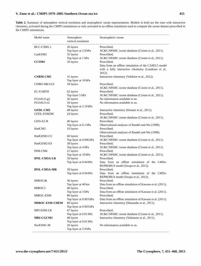
We give specific information on the treatment of ozone inTable2 as a basis for the discussion presented in Sect.3.3.The AC&C/SPARC ozone database (Cionni et al., 2011) isused to prescribe ozone in most of the models without in-teractive chemistry. In this database, stratospheric ozone forthe period 1979–2009 is zonally and monthly averaged. Itdepends on the altitude and it takes solar variability into ac-count. Whether they have interactive chemistry or prescribedstratospheric ozone, the 24 models analysed in this studythus take into account the stratospheric ozone depletion intheir historical simulations. This is an improvement sincethe CMIP3 simulations. Indeed, nearly half of the CMIP3models prescribed a constant ozone climatology (Son et al.,2008). Nevertheless, some of the models have a coarse at-mosphere resolution which sometimes does not encompassthe whole stratosphere. In that case, processes related to theinteraction between radiation and ozone as well as the ex-change between the stratosphere and the troposphere may berepresented rather crudely.

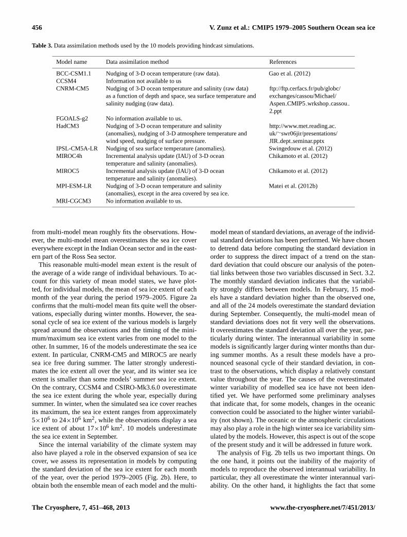
The hindcast simulations were initialized from a state thathas been obtained through a data assimilation procedure,i.e. constrained to be close to some observed fields. Thereis a large panel of data assimilation methods, but most of themodels involved in CMIP5 assimilate observations througha nudging. This method consists of adding to the model equa-tions a term that slightly pulls the solution towards the ob-servations (Kalnay, 2007). MIROC4h and MIROC5 incor-porate observations in their data assimilation experimentsby an incremental analysis update (IAU). Details about thismethod can be found inBloom et al.(1996). Table3 sum-marizes the data assimilation method corresponding to eachmodel as well as the variable it assimilates. The relevant doc-umentation was not available to us for CCSM4, FGOALS-g2 and MRI-CGCM3. All the models for which we havethe adequate information, except BCC-CSM1.1 and CNRM-CM5, assimilate anomalies. Those anomalies are calculatedfor both model and observations by subtracting their respec-tive climatology, computed over the same reference period.Working with anomalies does not prevent model biases, but itavoids the initialization of the model with a state which is toofar from its own climatology and thus limits model drift (e.g.Pierce et al., 2004; Smith et al., 2007; Troccoli and Palmer,2007; Keenlyside et al., 2008; Pohlmann et al., 2009), as dis-cussed in Sect.4.

www.the-cryosphere.net/7/451/2013/ The Cryosphere, 7, 451–468, 2013

http://pcmdi3.llnl.gov/esgcet/home.htm

http://pcmdi3.llnl.gov/esgcet/home.htm


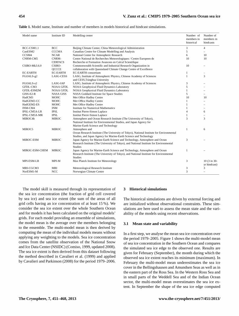
Table 1.Model name, Institute and number of members in models historical and hindcast simulations.

Model name Institute ID Modelling center Number ofmembers inhistorical

Number ofmembers inhindcasts

BCC-CSM1.1 BCC Beijing Climate Center, China Meteorological Administration 3 4CanESM2 CCCMA Canadian Centre for Climate Modelling and Analysis 5 –CCSM4 NCAR National Center for Atmospheric Research 6 10CNRM-CM5 CNRM-

CERFACSCentre National de Recherches Meteorologiques / Centre Europeen deRecherche et Formation Avancees en Calcul Scientifique

10 10

CSIRO-Mk3.6.0 CSIRO-QCCCE

Commonwealth Scientific and Industrial Research Organization incollaboration with Queensland Climate Change Centre of Excellence

10 –

EC-EARTH EC-EARTH EC-EARTH consortium 1 –FGOALS-g2 LASG-CESS LASG, Institute of Atmospheric Physics, Chinese Academy of Sciences

and CESS,Tsinghua University1 3

FGOALS-s2 LASG-IAP LASG, Institute of Atmospheric Physics, Chinese Academy of Sciences 3 –GFDL-CM3 NOAA GFDL NOAA Geophysical Fluid Dynamics Laboratory 5 –GFDL-ESM2M NOAA GFDL NOAA Geophysical Fluid Dynamics Laboratory 1 –GISS-E2-R NASA GISS NASA Goddard Institute for Space Studies 5 –HadCM3 MOHC Met Office Hadley Centre 10 10HadGEM2-CC MOHC Met Office Hadley Centre 1 –HadGEM2-ES MOHC Met Office Hadley Centre 1 –INM-CM4 INM Institute for Numerical Mathematics 1 –IPSL-CM5A-LR IPSL Institut Pierre-Simon Laplace 4 6IPSL-CM5A-MR IPSL Institut Pierre-Simon Laplace 1 –MIROC4h MIROC Atmosphere and Ocean Research Institute (The University of Tokyo),

National Institute for Environmental Studies, and Japan Agency forMarine-Earth Science and Technology

3 3

MIROC5 MIROC Atmosphere andOcean Research Institute (The University of Tokyo), National Institute for EnvironmentalStudies, and Japan Agency for Marine-Earth Science and Technology

1 6

MIROC-ESM MIROC Japan Agency for Marine-Earth Science and Technology, Atmosphere and OceanResearch Institute (The University of Tokyo), and National Institute for EnvironmentalStudies

3 –

MIROC-ESM-CHEM MIROC Japan Agency for Marine-Earth Science and Technology, Atmosphere and OceanResearch Institute (The University of Tokyo), and National Institute for EnvironmentalStudies

1 –

MPI-ESM-LR MPI-M Max Planck Institute for Meteorology 3 10 (3 in 30-yr hindcast)

MRI-CGCM3 MRI Meteorological Research Institute 3 3NorESM1-M NCC Norwegian Climate Centre 3 –

The model skill is measured through its representation ofthe sea ice concentration (the fraction of grid cell coveredby sea ice) and sea ice extent (the sum of the areas of allgrid cells having an ice concentration of at least 15 %). Weconsider the sea ice extent over the whole Southern Oceanand for models it has been calculated on the original models’grids. For each model providing an ensemble of simulations,the model mean is the average over the members belongingto the ensemble. The multi-model mean is then derived bycomputing the mean of the individual models means withoutapplying any weighting to the models. Sea ice concentrationcomes from the satellite observation of the National Snowand Ice Data Center (NSIDC) (Comiso, 1999, updated 2008).The sea ice extent is then derived from this dataset followingthe method described inCavalieri et al.(1999) and appliedby Cavalieri and Parkinson(2008) for the period 1979–2006.

3 Historical simulations

The historical simulations are driven by external forcing andare initialized without observational constraints. These sim-ulations are here used to assess the mean state and the vari-ability of the models using recent observations.

3.1 Mean state and variability

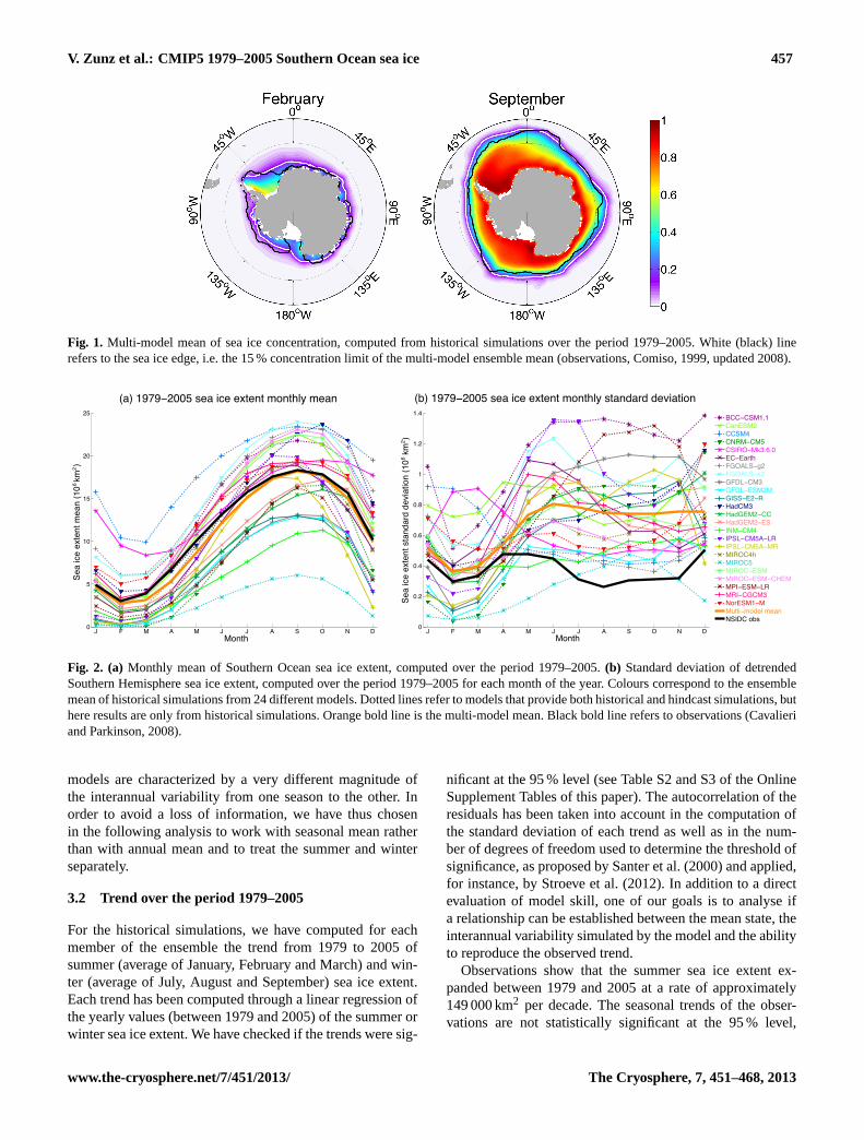
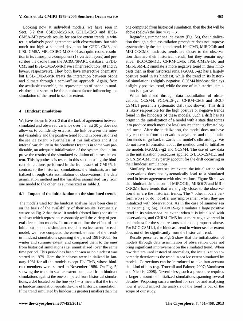
In a first step, we analyse the mean sea ice concentration overthe period 1979–2005. Figure1 shows the multi-model meanof sea ice concentration in the Southern Ocean and comparesthe simulated sea ice edge to the observed one. Results aregiven for February (September), the month during which theobserved sea ice extent reaches its minimum (maximum). InFebruary the multi-model mean underestimates the sea icecover in the Bellingshausen and Amundsen Seas as well as inthe eastern part of the Ross Sea. In the Western Ross Sea andin small parts of the Weddell Sea and of the Indian Oceansector, the multi-model mean overestimates the sea ice ex-tent. In September the shape of the sea ice edge computed



Table 2. Summary of atmosphere vertical resolution and stratospheric ozone representation. Models in bold are the ones with interactivechemistry, activated during the CMIP5 simulations or only activated in an offline simulation used to compute the ozone dataset prescribed inthe CMIP5 simulations.

Model name Atmospherevertical resolution

Stratospheric ozone

BCC-CSM1.1 26 layersTop layer at 2.9 hPa

Prescribed;AC&C/SPARC ozone database (Cionni et al., 2011).

CanESM2 35 layersTop layer at 1 hPa


CCSM4 26 layers Prescribed;Data from an offline simulation of the CAM3.5 modelwith a fully interactive chemistry (Landrum et al.,2012).

CNRM-CM5 31 layersTop layer at 10 hPa

Interactive chemistry (Voldoire et al., 2012).

CSIRO-Mk3.6.0 18 layers Prescribed;AC&C/SPARC ozone database (Cionni et al., 2011).

EC-EARTH 62 layersTop layer 5 hPa


FGOALS-g2 26 layers No information available to us.FGOALS-s2 26 layers

Top layer at 2.19 hPaNo information available to us.

GFDL-CM3 48 layers Interactive chemistry (Donner et al., 2011).GFDL-ESM2M 24 layers Prescribed;

AC&C/SPARC ozone database (Cionni et al., 2011).GISS-E2-R 40 layers

Top layer at 0.1 hPaPrescribed;Observational analyses ofRandel and Wu(1999).

HadCM3 19 layers Prescribed;Observational analyses ofRandel and Wu(1999).

HadGEM2-CC 60 layersTop layer at 0.006 hPa


HadGEM2-ES 38 layersTop layer at 4 hPa


INM-CM4 21 layersTop layer at 10 hPa


IPSL-CM5A-LR 39 layersTop layer at 0.04 hPa

Prescribed;Data from an offline simulation of the LMDz-REPROBUS model (Szopa et al., 2012).

IPSL-CM5A-MR 39 layersTop layer at 0.04 hPa

Prescribed;Data from an offline simulation of the LMDz-REPROBUS model (Szopa et al., 2012).

MIROC4h 56 layersTop layer at 40 km

Prescribed;Data from an offline simulation ofKawase et al.(2011).

MIROC5 40 layersTop layer at 3 hPa


MIROC-ESM 80 layersTop layer at 0.003 hPa


MIROC-ESM-CHEM 80 layersTop layer at 0.003 hPa

Interactive chemistry (Watanabe et al., 2011).

MPI-ESM-LR 47 layersTop layer at 0.01 hPa


MRI-CGCM3 48 layersTop layer at 0.01 hPa

Interactive chemistry (Yukimoto et al., 2011).

NorESM1-M 26 layersTop layer at 2.9 hPa

No information available to us.



Table 3.Data assimilation methods used by the 10 models providing hindcast simulations.

Model name Data assimilation method References

BCC-CSM1.1 Nudging of 3-D ocean temperature (raw data). Gao et al.(2012)CCSM4 Information not available to usCNRM-CM5 Nudging of 3-D ocean temperature and salinity (raw data)

as a function of depth and space, sea surface temperature andsalinity nudging (raw data).

ftp://ftp.cerfacs.fr/pub/globc/exchanges/cassou/Michael/AspenCMIP5 wrkshopcassou2.ppt

FGOALS-g2 No information available to us.HadCM3 Nudging of 3-D ocean temperature and salinity

(anomalies), nudging of 3-D atmosphere temperature andwind speed, nudging of surface pressure.

http://www.met.reading.ac.uk/∼swr06jir/presentations/JIR deptseminar.pptx

IPSL-CM5A-LR Nudging of sea surface temperature (anomalies). Swingedouw et al.(2012)MIROC4h Incremental analysis update (IAU) of 3-D ocean

temperature and salinity (anomalies).Chikamoto et al.(2012)

MIROC5 Incremental analysis update (IAU) of 3-D oceantemperature and salinity (anomalies).

Chikamoto et al.(2012)

MPI-ESM-LR Nudging of 3-D ocean temperature and salinity(anomalies), except in the area covered by sea ice.

Matei et al.(2012b)

MRI-CGCM3 No information available to us.

from multi-model mean roughly fits the observations. How-ever, the multi-model mean overestimates the sea ice covereverywhere except in the Indian Ocean sector and in the east-ern part of the Ross Sea sector.

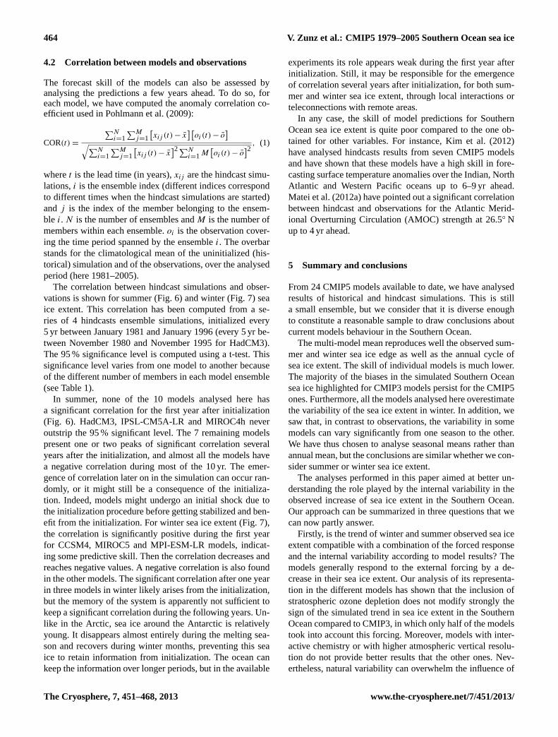
This reasonable multi-model mean extent is the result ofthe average of a wide range of individual behaviours. To ac-count for this variety of mean model states, we have plot-ted, for individual models, the mean of sea ice extent of eachmonth of the year during the period 1979–2005. Figure2aconfirms that the multi-model mean fits quite well the obser-vations, especially during winter months. However, the sea-sonal cycle of sea ice extent of the various models is largelyspread around the observations and the timing of the mini-mum/maximum sea ice extent varies from one model to theother. In summer, 16 of the models underestimate the sea iceextent. In particular, CNRM-CM5 and MIROC5 are nearlysea ice free during summer. The latter strongly underesti-mates the ice extent all over the year, and its winter sea iceextent is smaller than some models’ summer sea ice extent.On the contrary, CCSM4 and CSIRO-Mk3.6.0 overestimatethe sea ice extent during the whole year, especially duringsummer. In winter, when the simulated sea ice cover reachesits maximum, the sea ice extent ranges from approximately5×106 to 24×106 km2, while the observations display a seaice extent of about 17×106 km2. 10 models underestimatethe sea ice extent in September.

Since the internal variability of the climate system mayalso have played a role in the observed expansion of sea icecover, we assess its representation in models by computingthe standard deviation of the sea ice extent for each monthof the year, over the period 1979–2005 (Fig.2b). Here, toobtain both the ensemble mean of each model and the multi-

model mean of standard deviations, an average of the individ-ual standard deviations has been performed. We have chosento detrend data before computing the standard deviation inorder to suppress the direct impact of a trend on the stan-dard deviation that could obscure our analysis of the poten-tial links between those two variables discussed in Sect.3.2.The monthly standard deviation indicates that the variabil-ity strongly differs between models. In February, 15 mod-els have a standard deviation higher than the observed one,and all of the 24 models overestimate the standard deviationduring September. Consequently, the multi-model mean ofstandard deviations does not fit very well the observations.It overestimates the standard deviation all over the year, par-ticularly during winter. The interannual variability in somemodels is significantly larger during winter months than dur-ing summer months. As a result these models have a pro-nounced seasonal cycle of their standard deviation, in con-trast to the observations, which display a relatively constantvalue throughout the year. The causes of the overestimatedwinter variability of modelled sea ice have not been iden-tified yet. We have performed some preliminary analysesthat indicate that, for some models, changes in the oceanicconvection could be associated to the higher winter variabil-ity (not shown). The oceanic or the atmospheric circulationsmay also play a role in the high winter sea ice variability sim-ulated by the models. However, this aspect is out of the scopeof the present study and it will be addressed in future work.

The analysis of Fig.2b tells us two important things. Onthe one hand, it points out the inability of the majority ofmodels to reproduce the observed interannual variability. Inparticular, they all overestimate the winter interannual vari-ability. On the other hand, it highlights the fact that some


ftp://ftp.cerfacs.fr/pub/globc/exchanges/cassou/Michael/Aspen_CMIP5_wrkshop_cassou_2.ppt




http://www.met.reading.ac.uk/~swr06jir/presentations/JIR_dept_seminar.pptx




Fig. 1. Multi-model mean of sea ice concentration, computed from historical simulations over the period 1979–2005. White (black) linerefers to the sea ice edge, i.e. the 15 % concentration limit of the multi-model ensemble mean (observations,Comiso, 1999, updated 2008).

Month

Sea

ice

exte

nt m

ean

(10

6 km

2

(a) 1979−2005 sea ice extent monthly mean

Month

(b) 1979−2005 sea ice extent monthly standard deviationS

ea ic

e ex

tent

sta

ndar

d de

viat

ion

(106 k

m2)

J F M A M J J A S O N D0

5

10

15

20

25

)

J F M A M J J A S O N D0

0.2

0.4

0.6

0.8

1

1.2

1.4

BCC−CSM1.1CanESM2CCSM4CNRM−CM5CSIRO−Mk3.6.0EC−EarthFGOALS−g2FGOALS−s2GFDL−CM3GFDL−ESM2MGISS−E2−RHadCM3HadGEM2−CCHadGEM2−ESINM−CM4IPSL−CM5A−LRIPSL−CM5A−MRMIROC4hMIROC5MIROC−ESMMIROC−ESM−CHEMMPI−ESM−LRMRI−CGCM3NorESM1−MMulti−model meanNSIDC obs

Fig. 2. (a) Monthly mean of Southern Ocean sea ice extent, computed over the period 1979–2005.(b) Standard deviation of detrendedSouthern Hemisphere sea ice extent, computed over the period 1979–2005 for each month of the year. Colours correspond to the ensemblemean of historical simulations from 24 different models. Dotted lines refer to models that provide both historical and hindcast simulations, buthere results are only from historical simulations. Orange bold line is the multi-model mean. Black bold line refers to observations (Cavalieriand Parkinson, 2008).

models are characterized by a very different magnitude ofthe interannual variability from one season to the other. Inorder to avoid a loss of information, we have thus chosenin the following analysis to work with seasonal mean ratherthan with annual mean and to treat the summer and winterseparately.

3.2 Trend over the period 1979–2005

For the historical simulations, we have computed for eachmember of the ensemble the trend from 1979 to 2005 ofsummer (average of January, February and March) and win-ter (average of July, August and September) sea ice extent.Each trend has been computed through a linear regression ofthe yearly values (between 1979 and 2005) of the summer orwinter sea ice extent. We have checked if the trends were sig-

nificant at the 95 % level (see Table S2 and S3 of the OnlineSupplement Tables of this paper). The autocorrelation of theresiduals has been taken into account in the computation ofthe standard deviation of each trend as well as in the num-ber of degrees of freedom used to determine the threshold ofsignificance, as proposed bySanter et al.(2000) and applied,for instance, byStroeve et al.(2012). In addition to a directevaluation of model skill, one of our goals is to analyse ifa relationship can be established between the mean state, theinterannual variability simulated by the model and the abilityto reproduce the observed trend.

Observations show that the summer sea ice extent ex-panded between 1979 and 2005 at a rate of approximately149 000 km2 per decade. The seasonal trends of the obser-vations are not statistically significant at the 95 % level,



(a) 1979−2005 JFM trend VS. mean

(b) 1979−2005 JFM trend VS. standard deviation

(c) 1979−2005 JAS trend VS. mean (d) 1979−2005 JAS trend VS. standard deviation

BCC−CSM1.1(3)CanESM2(5)CCSM4(6)CNRM−CM5(10)CSIRO−Mk3.6.0(10)EC−Earth(1)FGOALS−g2(1)FGOALS−s2(3)GFDL−CM3(5)GFDL−ESM2M(1)GISS−E2−R(5)HadCM3(10)HadGEM2−CC(1)HadGEM2−ES(1)INM−CM4(1)IPSL−CM5A−LR(4)IPSL−CM5A−MR(1)MIROC4h(3)MIROC5(1)MIROC−ESM(3)MIROC−ESM−CHEM(1)MPI−ESM−LR(3)MRI−CGCM3(3)NorESM1−M(3)Multi−model meansNSIDC obsNSIDC obs +/− 2 σ

JFM sea ice extent standard deviation (106 km2)

JFM

sea

ice

exte

nt tr

end

(103 k

m2 /d

ecad

e)

0 0.1 0.2 0.3 0.4 0.5 0.6 0.7 0.8 0.9−1000

−800

−600

−400

−200

0

200

400

JFM sea ice extent mean (106 km2)

JFM

sea

ice

exte

nt tr

end

(103 k

m2 /d

ecad

e)

0 2 4 6 8 10 12 14−1000

−800

−600

−400

−200

0

200

400

JAS sea ice extent standard deviation (106 km2)

JAS

sea

ice

exte

nt tr

end

(103 k

m2 /d

ecad

e)

0.2 0.4 0.6 0.8 1 1.2 1.4 1.6 1.8−3000

−2500

−2000

−1500

−1000

−500

0

500

1000

1500

JAS sea ice extent mean (106 km2)

JAS

sea

ice

exte

nt tr

end

(103 k

m2 /d

ecad

e)

4 6 8 10 12 14 16 18 20 22 24−3000

−2500

−2000

−1500

−1000

−500

0

500

1000

1500

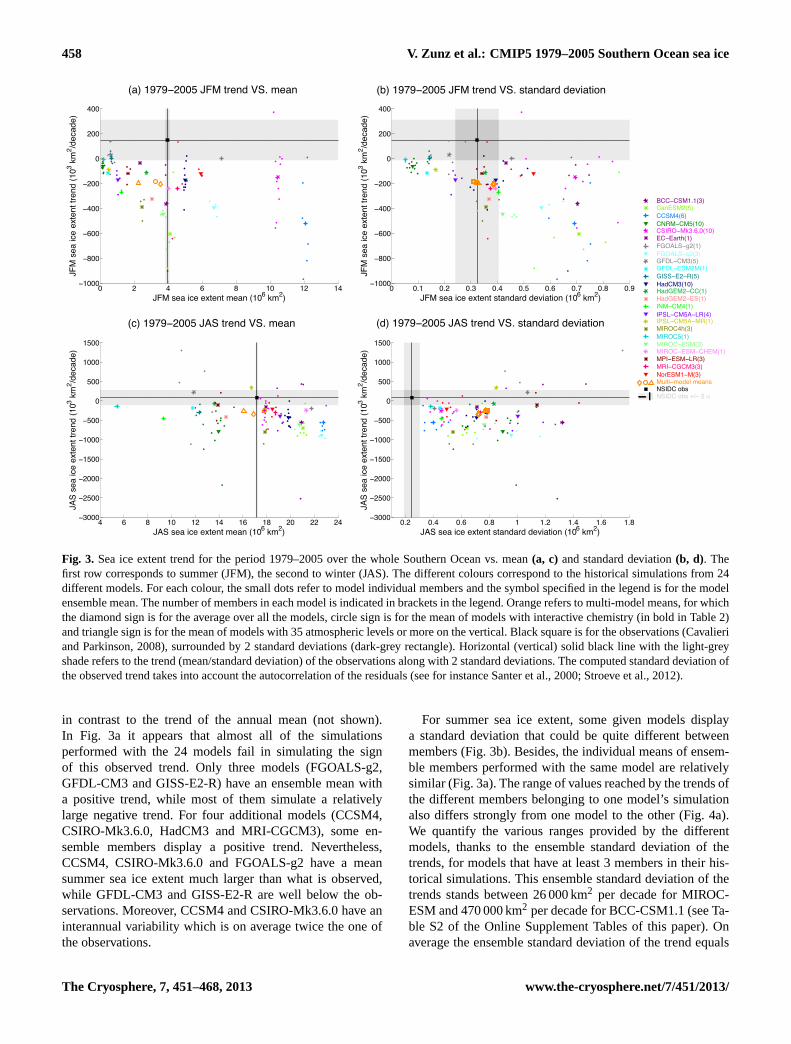
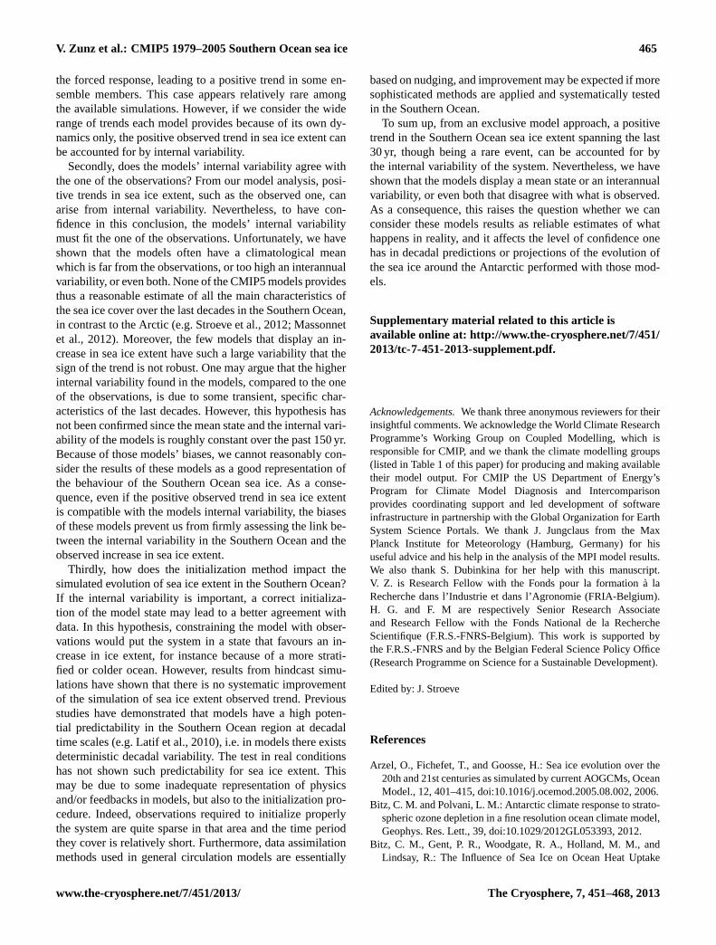
Fig. 3. Sea ice extent trend for the period 1979–2005 over the whole Southern Ocean vs. mean(a, c) and standard deviation(b, d). Thefirst row corresponds to summer (JFM), the second to winter (JAS). The different colours correspond to the historical simulations from 24different models. For each colour, the small dots refer to model individual members and the symbol specified in the legend is for the modelensemble mean. The number of members in each model is indicated in brackets in the legend. Orange refers to multi-model means, for whichthe diamond sign is for the average over all the models, circle sign is for the mean of models with interactive chemistry (in bold in Table2)and triangle sign is for the mean of models with 35 atmospheric levels or more on the vertical. Black square is for the observations (Cavalieriand Parkinson, 2008), surrounded by 2 standard deviations (dark-grey rectangle). Horizontal (vertical) solid black line with the light-greyshade refers to the trend (mean/standard deviation) of the observations along with 2 standard deviations. The computed standard deviation ofthe observed trend takes into account the autocorrelation of the residuals (see for instanceSanter et al., 2000; Stroeve et al., 2012).

in contrast to the trend of the annual mean (not shown).In Fig. 3a it appears that almost all of the simulationsperformed with the 24 models fail in simulating the signof this observed trend. Only three models (FGOALS-g2,GFDL-CM3 and GISS-E2-R) have an ensemble mean witha positive trend, while most of them simulate a relativelylarge negative trend. For four additional models (CCSM4,CSIRO-Mk3.6.0, HadCM3 and MRI-CGCM3), some en-semble members display a positive trend. Nevertheless,CCSM4, CSIRO-Mk3.6.0 and FGOALS-g2 have a meansummer sea ice extent much larger than what is observed,while GFDL-CM3 and GISS-E2-R are well below the ob-servations. Moreover, CCSM4 and CSIRO-Mk3.6.0 have aninterannual variability which is on average twice the one ofthe observations.

For summer sea ice extent, some given models displaya standard deviation that could be quite different betweenmembers (Fig.3b). Besides, the individual means of ensem-ble members performed with the same model are relativelysimilar (Fig.3a). The range of values reached by the trends ofthe different members belonging to one model’s simulationalso differs strongly from one model to the other (Fig.4a).We quantify the various ranges provided by the differentmodels, thanks to the ensemble standard deviation of thetrends, for models that have at least 3 members in their his-torical simulations. This ensemble standard deviation of thetrends stands between 26 000 km2 per decade for MIROC-ESM and 470 000 km2 per decade for BCC-CSM1.1 (see Ta-ble S2 of the Online Supplement Tables of this paper). Onaverage the ensemble standard deviation of the trend equals



BCC−CSM1.1(3)

CanESM2(5)

CCSM4(6)

CNRM−CM5(10)

CSIRO−Mk3.6.0(10)

FGOALS−s2(3)

GFDL−CM3(5)

GISS−E2−R(5)

HadCM3(10)

IPSL−CM5A−LR(4)

MIROC4h(3)

MIROC−ESM(3)

MPI−ESM−LR(3)

MRI−CGCM3(3)

NorESM1−M(3)

Trend of sea ice extent (103 km2/decade)

(a) 1979−2005 JFM sea ice extent trend range

BCC−CSM1.1(3)

CanESM2(5)

CCSM4(6)

CNRM−CM5(10)

CSIRO−Mk3.6.0(10)

FGOALS−s2(3)

GFDL−CM3(5)

GISS−E2−R(5)

HadCM3(10)

IPSL−CM5A−LR(4)

MIROC4h(3)

MIROC−ESM(3)

MPI−ESM−LR(3)

MRI−CGCM3(3)

NorESM1−M(3)

(b) 1979−2005 JAS sea ice extent trend range

Trend of sea ice extent (103 km2/decade)

−1000 −800 −600 −400 −200 0 200 400

−3000 −2500 −2000 −1500 −1000 −500 0 500 1000 1500

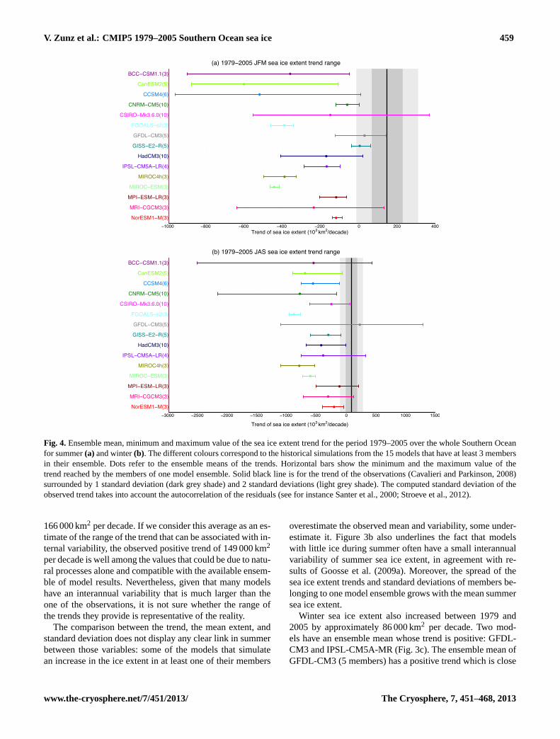
Fig. 4. Ensemble mean, minimum and maximum value of the sea ice extent trend for the period 1979–2005 over the whole Southern Oceanfor summer(a) and winter(b). The different colours correspond to the historical simulations from the 15 models that have at least 3 membersin their ensemble. Dots refer to the ensemble means of the trends. Horizontal bars show the minimum and the maximum value of thetrend reached by the members of one model ensemble. Solid black line is for the trend of the observations (Cavalieri and Parkinson, 2008)surrounded by 1 standard deviation (dark grey shade) and 2 standard deviations (light grey shade). The computed standard deviation of theobserved trend takes into account the autocorrelation of the residuals (see for instanceSanter et al., 2000; Stroeve et al., 2012).

166 000 km2 per decade. If we consider this average as an es-timate of the range of the trend that can be associated with in-ternal variability, the observed positive trend of 149 000 km2

per decade is well among the values that could be due to natu-ral processes alone and compatible with the available ensem-ble of model results. Nevertheless, given that many modelshave an interannual variability that is much larger than theone of the observations, it is not sure whether the range ofthe trends they provide is representative of the reality.

The comparison between the trend, the mean extent, andstandard deviation does not display any clear link in summerbetween those variables: some of the models that simulatean increase in the ice extent in at least one of their members

overestimate the observed mean and variability, some under-estimate it. Figure3b also underlines the fact that modelswith little ice during summer often have a small interannualvariability of summer sea ice extent, in agreement with re-sults ofGoosse et al.(2009a). Moreover, the spread of thesea ice extent trends and standard deviations of members be-longing to one model ensemble grows with the mean summersea ice extent.

Winter sea ice extent also increased between 1979 and2005 by approximately 86 000 km2 per decade. Two mod-els have an ensemble mean whose trend is positive: GFDL-CM3 and IPSL-CM5A-MR (Fig.3c). The ensemble mean ofGFDL-CM3 (5 members) has a positive trend which is close



(a) 1981−2005 JFM hindcast VS. historical trend (b) 1981−2005 JAS hindcast VS. historical trend

−2000 −1000 0 1000 2000 3000 4000 5000 6000

−2000

−1000

0

1000

2000

3000

4000

5000

6000

JAS sea ice extent trend of historical simulation (103 km2/decade)JA

S s

ea ic

e ex

tent

tren

d of

hin

dcas

t sim

ulat

ion

(103 k

m2 /d

ecad

e)

BCC−CSM1.1CCSM4CNRM−CM5FGOALS−g2HadCM3IPSL−CM5A−LRMIROC4hMIROC5MPI−ESM−LRMRI−CGCM3NSIDC obs

−1500 −1000 −500 0 500 1000 1500 2000−1500

−1000

−500

0

500

1000

1500

2000

JFM sea ice extent trend of historical simulation (103 km2/decade)

JFM

sea

ice

exte

nt tr

end

of h

indc

ast s

imul

atio

n (1

03 km

2 /dec

ade)

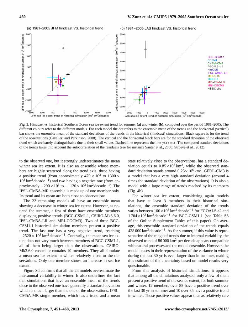
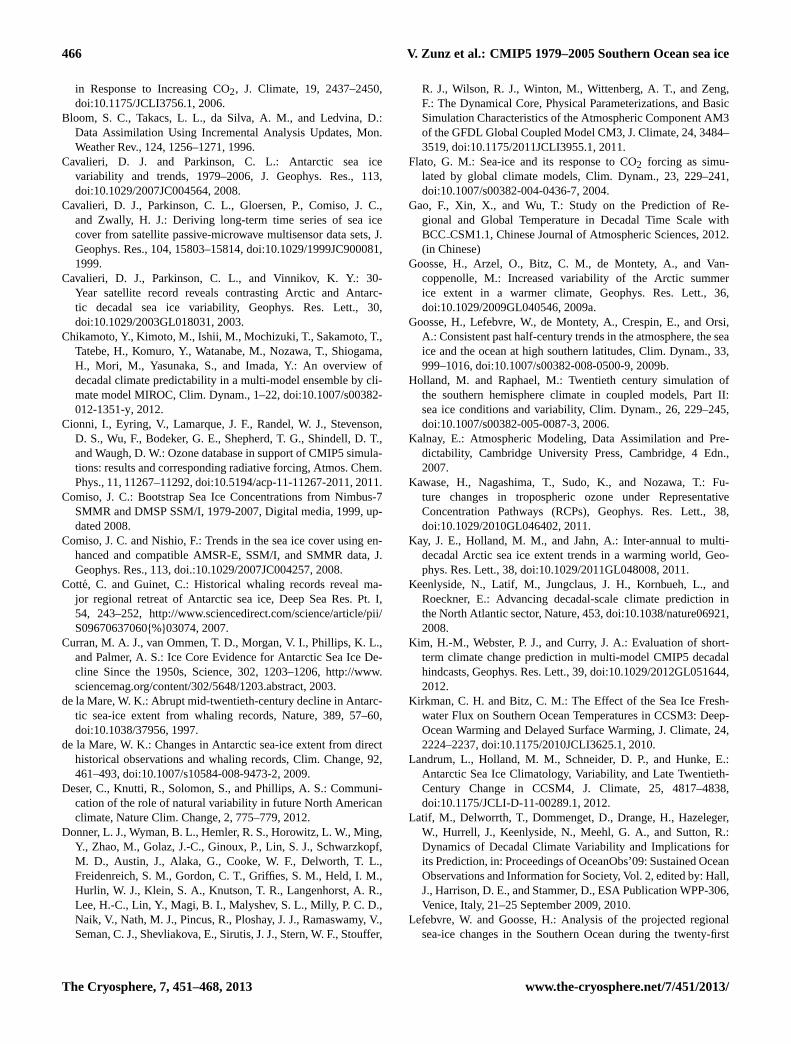
Fig. 5.Hindcast vs. historical Southern Ocean sea ice extent trend for summer(a) and winter(b), computed over the period 1981–2005. Thedifferent colours refer to the different models. For each model the dot refers to the ensemble mean of the trends and the horizontal (vertical)bar shows the ensemble mean of the standard deviations of the trends in the historical (hindcast) simulations. Black square is for the trendof the observations (Cavalieri and Parkinson, 2008). The vertical and the horizontal black bars are for the standard deviation of the observedtrend which are barely distinguishable due to their small values. Dashed line represents the liney(x) = x. The computed standard deviationsof the trends takes into account the autocorrelation of the residuals (see for instanceSanter et al., 2000; Stroeve et al., 2012).

to the observed one, but it strongly underestimates the meanwinter sea ice extent. It is also an ensemble whose mem-bers are highly scattered along the trend axis, three havinga positive trend (from approximately 470× 103 to 1300×103 km2decade−1) and two having a negative one (from ap-proximately−290×103 to −1120×103 km2decade−1). TheIPSL-CM5A-MR ensemble is made up of one member only.Its trend and its mean are both close to observations.

The 22 remaining models all have an ensemble meanshowing a decrease in winter sea ice extent. However, as no-ticed for summer, a few of them have ensemble membersdisplaying positive trends (BCC-CSM1.1, CSIRO-Mk3.6.0,IPSL-CM5A-LR and MRI-CGCM3). Two of three BCC-CSM1.1 historical simulation members present a positivetrend. The last one has a very negative trend, reaching−2520×103 km2decade−1. Contrarily, the mean sea ice ex-tent does not vary much between members of BCC-CSM1.1,all of them being larger than the observations. CSIRO-Mk3.6.0 ensemble contains 10 members. They all simulatea mean sea ice extent in winter relatively close to the ob-servations. Only one member shows an increase in sea iceextent.

Figure3d confirms that all the 24 models overestimate theinterannual variability in winter. It also underlines the factthat simulations that have an ensemble mean of the trendsclose to the observed one have generally a standard deviationwhich is much larger than the one of the observations. IPSL-CM5A-MR single member, which has a trend and a mean

state relatively close to the observations, has a standard de-viation equals to 0.85×106 km2, while the observed stan-dard deviation stands around 0.25×106 km2. GFDL-CM3 isa model that has a very high standard deviation (around 4times the standard deviation of the observations). It is also amodel with a large range of trends reached by its members(Fig. 4b).

For winter sea ice extent, considering again modelsthat have at least 3 members in their historical sim-ulations, the ensemble standard deviation of the trendsvaries between 100×103 km2decade−1 for FGOALS-s2 and1 704×103 km2decade−1 for BCC-CSM1.1 (see Table S3of the Online Supplement Tables of this paper). On aver-age, this ensemble standard deviation of the trends equals428 000 km2decade−1. As for summer, if this value is repre-sentative of the range of trends due to internal variability, theobserved trend of 86 000 km2 per decade appears compatiblewith natural processes and the model ensemble. However, themodel biases in their representation of the variance in winterduring the last 30 yr is even larger than in summer, makingthis estimate of the uncertainty based on model results veryquestionable.

From this analysis of historical simulations, it appearsthat among all the simulations analysed, only a few of thempresent a positive trend of the sea ice extent, for both summerand winter. 12 members over 85 have a positive trend overthe last 30 yr in summer and 10 over 85 have a positive trendin winter. Those positive values appear thus as relatively rare



1 2 3 4 5 6 7 8 9 10−1

−0.5

0

0.5

1

Lead time (years)

JFM

sea

ice

exte

nt c

orre

latio

n

BCC−CSM1.1

1 2 3 4 5 6 7 8 9 10−1

−0.5

0

0.5

1

Lead time (years)

JFM

sea

ice

exte

nt c

orre

latio

n

CCSM4

1 2 3 4 5 6 7 8 9 10−1

−0.5

0

0.5

1

Lead time (years)

JFM

sea

ice

exte

nt c

orre

latio

n

CNRM−CM5

1 2 3 4 5 6 7 8 9 10−1

−0.5

0

0.5

1

Lead time (years)

JFM

sea

ice

exte

nt c

orre

latio

n

HadCM3

1 2 3 4 5 6 7 8 9 10−1

−0.5

0

0.5

1

Lead time (years)

JFM

sea

ice

exte

nt c

orre

latio

n

IPSL−CM5A−LR

1 2 3 4 5 6 7 8 9 10−1

−0.5

0

0.5

1

Lead time (years)

JFM

sea

ice

exte

nt c

orre

latio

n

MIROC4h

1 2 3 4 5 6 7 8 9 10−1

−0.5

0

0.5

1

Lead time (years)

JFM

sea

ice

exte

nt c

orre

latio

n

MIROC5

1 2 3 4 5 6 7 8 9 10−1

−0.5

0

0.5

1

Lead time (years)

JFM

sea

ice

exte

nt c

orre

latio

n

MPI−ESM−LR

1 2 3 4 5 6 7 8 9 10−1

−0.5

0

0.5

1

Lead time (years)

JFM

sea

ice

exte

nt c

orre

latio

n

MRI−CGCM3

1 2 3 4 5 6 7 8 9 10−1

−0.5

0

0.5

1

Lead time (years)

JFM

sea

ice

exte

nt c

orre

latio

n

FGOALS−g2

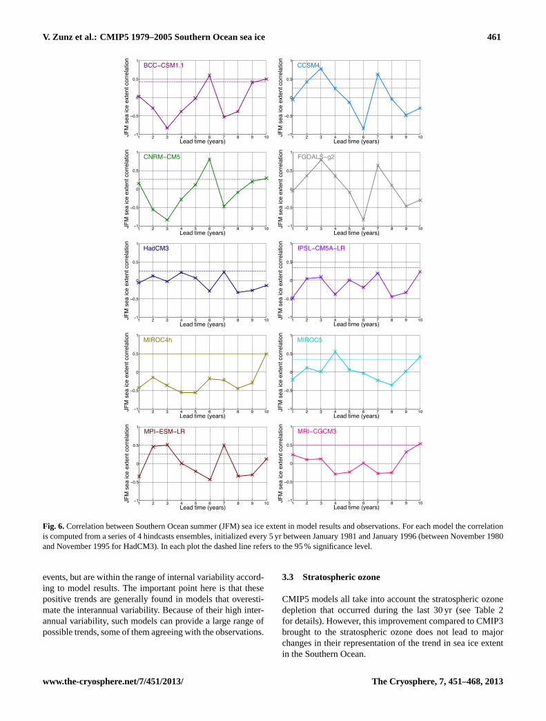
Fig. 6. Correlation between Southern Ocean summer (JFM) sea ice extent in model results and observations. For each model the correlationis computed from a series of 4 hindcasts ensembles, initialized every 5 yr between January 1981 and January 1996 (between November 1980and November 1995 for HadCM3). In each plot the dashed line refers to the 95 % significance level.

events, but are within the range of internal variability accord-ing to model results. The important point here is that thesepositive trends are generally found in models that overesti-mate the interannual variability. Because of their high inter-annual variability, such models can provide a large range ofpossible trends, some of them agreeing with the observations.

3.3 Stratospheric ozone

CMIP5 models all take into account the stratospheric ozonedepletion that occurred during the last 30 yr (see Table2for details). However, this improvement compared to CMIP3brought to the stratospheric ozone does not lead to majorchanges in their representation of the trend in sea ice extentin the Southern Ocean.



1 2 3 4 5 6 7 8 9 10−1

−0.5

0

0.5

1

Lead time (years)

JAS

sea

ice

exte

nt c

orre

latio

n

MIROC5

1 2 3 4 5 6 7 8 9 10−1

−0.5

0

0.5

1

Lead time (years)

JAS

sea

ice

exte

nt c

orre

latio

n

BCC−CSM1.1

1 2 3 4 5 6 7 8 9 10−1

−0.5

0

0.5

1

Lead time (years)

JAS

sea

ice

exte

nt c

orre

latio

n

CNRM−CM5

1 2 3 4 5 6 7 8 9 10−1

−0.5

0

0.5

1

Lead time (years)

JAS

sea

ice

exte

nt c

orre

latio

n

CCSM4

1 2 3 4 5 6 7 8 9 10−1

−0.5

0

0.5

1

Lead time (years)

JAS

sea

ice

exte

nt c

orre

latio

n

HadCM3

1 2 3 4 5 6 7 8 9 10−1

−0.5

0

0.5

1

Lead time (years)

JAS

sea

ice

exte

nt c

orre

latio

n

IPSL−CM5A−LR

1 2 3 4 5 6 7 8 9 10−1

−0.5

0

0.5

1

Lead time (years)

JAS

sea

ice

exte

nt c

orre

latio

n

MIROC4h

1 2 3 4 5 6 7 8 9 10−1

−0.5

0

0.5

1

Lead time (years)

JAS

sea

ice

exte

nt c

orre

latio

n

MRI−CGCM3

1 2 3 4 5 6 7 8 9 10−1

−0.5

0

0.5

1

Lead time (years)

JAS

sea

ice

exte

nt c

orre

latio

n

MPI−ESM−LR

1 2 3 4 5 6 7 8 9 10−1

−0.5

0

0.5

1

Lead time (years)

JAS

sea

ice

exte

nt c

orre

latio

n

FGOALS−g2

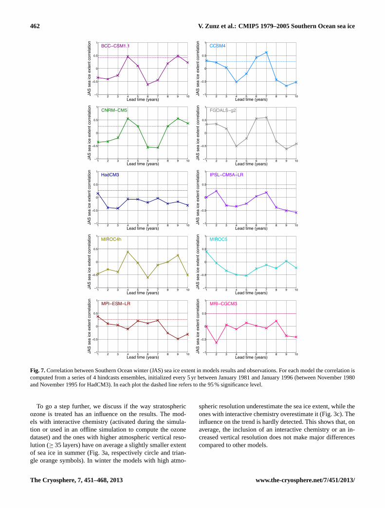
Fig. 7.Correlation between Southern Ocean winter (JAS) sea ice extent in models results and observations. For each model the correlation iscomputed from a series of 4 hindcasts ensembles, initialized every 5 yr between January 1981 and January 1996 (between November 1980and November 1995 for HadCM3). In each plot the dashed line refers to the 95 % significance level.

To go a step further, we discuss if the way stratosphericozone is treated has an influence on the results. The mod-els with interactive chemistry (activated during the simula-tion or used in an offline simulation to compute the ozonedataset) and the ones with higher atmospheric vertical reso-lution (≥ 35 layers) have on average a slightly smaller extentof sea ice in summer (Fig.3a, respectively circle and trian-gle orange symbols). In winter the models with high atmo-

spheric resolution underestimate the sea ice extent, while theones with interactive chemistry overestimate it (Fig.3c). Theinfluence on the trend is hardly detected. This shows that, onaverage, the inclusion of an interactive chemistry or an in-creased vertical resolution does not make major differencescompared to other models.



Looking now at individual models, we have seen inSect. 3.2 that CSIRO-Mk3.6.0, GFDL-CM3 and IPSL-CM5A-MR provide results for sea ice extent trends in win-ter in relatively good agreement with observations, but withmuch too high a standard deviation for GFDL-CM3 andIPSL-CM5A-MR. CSIRO-Mk3.6.0 has a quite coarse resolu-tion in its atmosphere component (18 vertical layers) and pre-scribes the ozone from the AC&C/SPARC database. GFDL-CM3 and IPSL-CM5A-MR have a finer resolution (48 and 39layers, respectively). They both have interactive chemistry,but IPSL-CM5A-MR treats the interaction between ozoneand climate through a semi-offline approach. Again, fromthe available ensemble, the representation of ozone in mod-els does not seem to be the dominant factor influencing thesimulation of the trend in sea ice extent.

4 Hindcast simulations

We have shown in Sect.3 that the lack of agreement betweensimulated and observed variance over the last 30 yr does notallow us to confidently establish the link between the inter-nal variability and the positive trend found in observations ofthe sea ice extent. Nevertheless, if this link exists and if theinternal variability in the Southern Ocean is in some way pre-dictable, an adequate initialization of the system should im-prove the results of the simulated evolution of the sea ice ex-tent. This hypothesis is tested in this section using the hind-cast simulations performed in the framework of CMIP5. Incontrast to the historical simulations, the hindcasts are ini-tialized through data assimilation of observations. The dataassimilation method and the variables assimilated vary fromone model to the other, as summarized in Table3.

4.1 Impact of the initialization on the simulated trends

The models used for the hindcast analysis have been chosenon the basis of the availability of their results. Fortunately,we see on Fig.2 that these 10 models (dotted lines) constitutea subset which represents reasonably well the variety of gen-eral circulation models. In order to outline the effect of theinitialization on the simulated trend in sea ice extent for eachmodel, we have computed the ensemble mean of the trendsin hindcast simulations spanning the period 1981–2005, forwinter and summer extent, and compared them to the onesfrom historical simulations (i.e. uninitialized) over the sametime period. This period has been chosen as no hindcast wasstarted in 1979. Here the hindcasts were initialized in Jan-uary 1981 for all the models except HadCM3, whose hind-cast members were started in November 1980. On Fig.5,showing the trend in sea ice extent computed from hindcastsimulations against the one computed from historical simula-tions, a dot located on the liney(x) = x means that the trendin hindcast simulation equals the one of historical simulation.If the trend simulated by hindcast is greater (smaller) than the

one computed from historical simulation, then the dot will beabove (below) the liney(x) = x.

Regarding summer sea ice extent (Fig.5a), the initializa-tion through a data assimilation procedure does not improvesystematically the simulated trend. HadCM3, MIROC4h andMRI-CGCM3 hindcasts trends are closer to the observa-tion than are their historical trends, but they remain neg-ative. BCC-CSM1.1, CNRM-CM5, IPSL-CM5A-LR andMPI-ESM-LR simulate a more negative trend in their hind-casts than in their historical runs. FGOALS-g2 has a largelypositive trend in its hindcast, while the trend in its histori-cal simulation is slightly negative. CCSM4 hindcast displaysa slightly positive trend, while the one of its historical simu-lation is negative.

When initialized through data assimilation of obser-vations, CCSM4, FGOALS-g2, CNRM-CM5 and BCC-CSM1.1 present a systematic drift (not shown). This driftis likely responsible for the high positive or negative trendsfound in the hindcasts of these models. Such a drift has itsorigin in the initialization of a model with a state that forcesit to produce much more (or less) sea ice than its climatolog-ical mean. After the initialization, the model does not haveany constraint from observations anymore, and the simula-tion tends to go back towards the model’s climatology. Wedo not have information about the method used to initializethe models FGOALS-g2 and CCSM4. The use of raw datain the initialization procedures applied to BCC-CSM1.1 andto CNRM-CM5 may partly account for the drift occurring intheir hindcast simulations.

Similarly, for winter sea ice extent, the initialization withobservations does not systematically lead to a simulatedtrend in better agreement with observations. Figure5b showsthat hindcast simulations of MIROC4h, MIROC5 and MRI-CGCM3 have trends that are slightly closer to the observa-tion than are the historical trends. The 7 other models per-form worse or do not offer any improvement when they areinitialized with observations. As in the case of summer seaice extent (Fig.5a), FGOALS-g2 simulates a large positivetrend in its winter sea ice extent when it is initialized withobservations, and CNRM-CM5 has a more negative trend inits hindcast for the same reasons as the one proposed above.For BCC-CSM1.1, the hindcast trend in winter sea ice extentdoes not differ significantly from the historical trend.

Results presented in Fig.5 show that the initialization ofmodels through data assimilation of observation does notbring significant improvement on the simulated trend. Whenraw data are used instead of anomalies, the initialization ap-parently deteriorates the trend in sea ice extent simulated bymodels. Corrections can be introduced to take into accountthat kind of bias (e.g.Troccoli and Palmer, 2007; Vannitsemand Nicolis, 2008). Nevertheless, such a procedure requiresa larger amount of initialized simulations spanning severaldecades. Proposing such a method for sea ice and analysinghow it would impact the analysis of the trend is out of thescope of our study.



4.2 Correlation between models and observations

The forecast skill of the models can also be assessed byanalysing the predictions a few years ahead. To do so, foreach model, we have computed the anomaly correlation co-efficient used inPohlmann et al.(2009):

COR(t) =

∑Ni=1

∑Mj=1

[xij (t) − x

][oi(t) − o

]√∑Ni=1

∑Mj=1

[xij (t) − x

]2∑Ni=1M

[oi(t) − o

]2, (1)

wheret is the lead time (in years),xij are the hindcast simu-lations,i is the ensemble index (different indices correspondto different times when the hindcast simulations are started)andj is the index of the member belonging to the ensem-ble i. N is the number of ensembles andM is the number ofmembers within each ensemble.oi is the observation cover-ing the time period spanned by the ensemblei. The overbarstands for the climatological mean of the uninitialized (his-torical) simulation and of the observations, over the analysedperiod (here 1981–2005).

The correlation between hindcast simulations and obser-vations is shown for summer (Fig.6) and winter (Fig.7) seaice extent. This correlation has been computed from a se-ries of 4 hindcasts ensemble simulations, initialized every5 yr between January 1981 and January 1996 (every 5 yr be-tween November 1980 and November 1995 for HadCM3).The 95 % significance level is computed using a t-test. Thissignificance level varies from one model to another becauseof the different number of members in each model ensemble(see Table1).

In summer, none of the 10 models analysed here hasa significant correlation for the first year after initialization(Fig. 6). HadCM3, IPSL-CM5A-LR and MIROC4h neveroutstrip the 95 % significant level. The 7 remaining modelspresent one or two peaks of significant correlation severalyears after the initialization, and almost all the models havea negative correlation during most of the 10 yr. The emer-gence of correlation later on in the simulation can occur ran-domly, or it might still be a consequence of the initializa-tion. Indeed, models might undergo an initial shock due tothe initialization procedure before getting stabilized and ben-efit from the initialization. For winter sea ice extent (Fig.7),the correlation is significantly positive during the first yearfor CCSM4, MIROC5 and MPI-ESM-LR models, indicat-ing some predictive skill. Then the correlation decreases andreaches negative values. A negative correlation is also foundin the other models. The significant correlation after one yearin three models in winter likely arises from the initialization,but the memory of the system is apparently not sufficient tokeep a significant correlation during the following years. Un-like in the Arctic, sea ice around the Antarctic is relativelyyoung. It disappears almost entirely during the melting sea-son and recovers during winter months, preventing this seaice to retain information from initialization. The ocean cankeep the information over longer periods, but in the available

experiments its role appears weak during the first year afterinitialization. Still, it may be responsible for the emergenceof correlation several years after initialization, for both sum-mer and winter sea ice extent, through local interactions orteleconnections with remote areas.

In any case, the skill of model predictions for SouthernOcean sea ice extent is quite poor compared to the one ob-tained for other variables. For instance,Kim et al. (2012)have analysed hindcasts results from seven CMIP5 modelsand have shown that these models have a high skill in fore-casting surface temperature anomalies over the Indian, NorthAtlantic and Western Pacific oceans up to 6–9 yr ahead.Matei et al.(2012a) have pointed out a significant correlationbetween hindcast and observations for the Atlantic Merid-ional Overturning Circulation (AMOC) strength at 26.5 Nup to 4 yr ahead.

5 Summary and conclusions

From 24 CMIP5 models available to date, we have analysedresults of historical and hindcast simulations. This is stilla small ensemble, but we consider that it is diverse enoughto constitute a reasonable sample to draw conclusions aboutcurrent models behaviour in the Southern Ocean.

The multi-model mean reproduces well the observed sum-mer and winter sea ice edge as well as the annual cycle ofsea ice extent. The skill of individual models is much lower.The majority of the biases in the simulated Southern Oceansea ice highlighted for CMIP3 models persist for the CMIP5ones. Furthermore, all the models analysed here overestimatethe variability of the sea ice extent in winter. In addition, wesaw that, in contrast to observations, the variability in somemodels can vary significantly from one season to the other.We have thus chosen to analyse seasonal means rather thanannual mean, but the conclusions are similar whether we con-sider summer or winter sea ice extent.

The analyses performed in this paper aimed at better un-derstanding the role played by the internal variability in theobserved increase of sea ice extent in the Southern Ocean.Our approach can be summarized in three questions that wecan now partly answer.

Firstly, is the trend of winter and summer observed sea iceextent compatible with a combination of the forced responseand the internal variability according to model results? Themodels generally respond to the external forcing by a de-crease in their sea ice extent. Our analysis of its representa-tion in the different models has shown that the inclusion ofstratospheric ozone depletion does not modify strongly thesign of the simulated trend in sea ice extent in the SouthernOcean compared to CMIP3, in which only half of the modelstook into account this forcing. Moreover, models with inter-active chemistry or with higher atmospheric vertical resolu-tion do not provide better results that the other ones. Nev-ertheless, natural variability can overwhelm the influence of



the forced response, leading to a positive trend in some en-semble members. This case appears relatively rare amongthe available simulations. However, if we consider the widerange of trends each model provides because of its own dy-namics only, the positive observed trend in sea ice extent canbe accounted for by internal variability.

Secondly, does the models’ internal variability agree withthe one of the observations? From our model analysis, posi-tive trends in sea ice extent, such as the observed one, canarise from internal variability. Nevertheless, to have con-fidence in this conclusion, the models’ internal variabilitymust fit the one of the observations. Unfortunately, we haveshown that the models often have a climatological meanwhich is far from the observations, or too high an interannualvariability, or even both. None of the CMIP5 models providesthus a reasonable estimate of all the main characteristics ofthe sea ice cover over the last decades in the Southern Ocean,in contrast to the Arctic (e.g.Stroeve et al., 2012; Massonnetet al., 2012). Moreover, the few models that display an in-crease in sea ice extent have such a large variability that thesign of the trend is not robust. One may argue that the higherinternal variability found in the models, compared to the oneof the observations, is due to some transient, specific char-acteristics of the last decades. However, this hypothesis hasnot been confirmed since the mean state and the internal vari-ability of the models is roughly constant over the past 150 yr.Because of those models’ biases, we cannot reasonably con-sider the results of these models as a good representation ofthe behaviour of the Southern Ocean sea ice. As a conse-quence, even if the positive observed trend in sea ice extentis compatible with the models internal variability, the biasesof these models prevent us from firmly assessing the link be-tween the internal variability in the Southern Ocean and theobserved increase in sea ice extent.

Thirdly, how does the initialization method impact thesimulated evolution of sea ice extent in the Southern Ocean?If the internal variability is important, a correct initializa-tion of the model state may lead to a better agreement withdata. In this hypothesis, constraining the model with obser-vations would put the system in a state that favours an in-crease in ice extent, for instance because of a more strati-fied or colder ocean. However, results from hindcast simu-lations have shown that there is no systematic improvementof the simulation of sea ice extent observed trend. Previousstudies have demonstrated that models have a high poten-tial predictability in the Southern Ocean region at decadaltime scales (e.g.Latif et al., 2010), i.e. in models there existsdeterministic decadal variability. The test in real conditionshas not shown such predictability for sea ice extent. Thismay be due to some inadequate representation of physicsand/or feedbacks in models, but also to the initialization pro-cedure. Indeed, observations required to initialize properlythe system are quite sparse in that area and the time periodthey cover is relatively short. Furthermore, data assimilationmethods used in general circulation models are essentially

based on nudging, and improvement may be expected if moresophisticated methods are applied and systematically testedin the Southern Ocean.

To sum up, from an exclusive model approach, a positivetrend in the Southern Ocean sea ice extent spanning the last30 yr, though being a rare event, can be accounted for bythe internal variability of the system. Nevertheless, we haveshown that the models display a mean state or an interannualvariability, or even both that disagree with what is observed.As a consequence, this raises the question whether we canconsider these models results as reliable estimates of whathappens in reality, and it affects the level of confidence onehas in decadal predictions or projections of the evolution ofthe sea ice around the Antarctic performed with those mod-els.

Supplementary material related to this article isavailable online at:http://www.the-cryosphere.net/7/451/2013/tc-7-451-2013-supplement.pdf.

Acknowledgements.We thank three anonymous reviewers for theirinsightful comments. We acknowledge the World Climate ResearchProgramme’s Working Group on Coupled Modelling, which isresponsible for CMIP, and we thank the climate modelling groups(listed in Table1 of this paper) for producing and making availabletheir model output. For CMIP the US Department of Energy’sProgram for Climate Model Diagnosis and Intercomparisonprovides coordinating support and led development of softwareinfrastructure in partnership with the Global Organization for EarthSystem Science Portals. We thank J. Jungclaus from the MaxPlanck Institute for Meteorology (Hamburg, Germany) for hisuseful advice and his help in the analysis of the MPI model results.We also thank S. Dubinkina for her help with this manuscript.V. Z. is Research Fellow with the Fonds pour la formationa laRecherche dans l’Industrie et dans l’Agronomie (FRIA-Belgium).H. G. and F. M are respectively Senior Research Associateand Research Fellow with the Fonds National de la RechercheScientifique (F.R.S.-FNRS-Belgium). This work is supported bythe F.R.S.-FNRS and by the Belgian Federal Science Policy Office(Research Programme on Science for a Sustainable Development).

Edited by: J. Stroeve

References

Arzel, O., Fichefet, T., and Goosse, H.: Sea ice evolution over the20th and 21st centuries as simulated by current AOGCMs, OceanModel., 12, 401–415, doi:10.1016/j.ocemod.2005.08.002, 2006.

Bitz, C. M. and Polvani, L. M.: Antarctic climate response to strato-spheric ozone depletion in a fine resolution ocean climate model,Geophys. Res. Lett., 39,doi:10.1029/2012GL053393, 2012.

Bitz, C. M., Gent, P. R., Woodgate, R. A., Holland, M. M., andLindsay, R.: The Influence of Sea Ice on Ocean Heat Uptake


http://www.the-cryosphere.net/7/451/2013/tc-7-451-2013-supplement.pdf

http://www.the-cryosphere.net/7/451/2013/tc-7-451-2013-supplement.pdf

http://dx.doi.org/10.1029/2012GL053393


in Response to Increasing CO2, J. Climate, 19, 2437–2450,doi:10.1175/JCLI3756.1, 2006.

Bloom, S. C., Takacs, L. L., da Silva, A. M., and Ledvina, D.:Data Assimilation Using Incremental Analysis Updates, Mon.Weather Rev., 124, 1256–1271, 1996.

Cavalieri, D. J. and Parkinson, C. L.: Antarctic sea icevariability and trends, 1979–2006, J. Geophys. Res., 113,doi:10.1029/2007JC004564, 2008.

Cavalieri, D. J., Parkinson, C. L., Gloersen, P., Comiso, J. C.,and Zwally, H. J.: Deriving long-term time series of sea icecover from satellite passive-microwave multisensor data sets, J.Geophys. Res., 104, 15803–15814, doi:10.1029/1999JC900081,1999.

Cavalieri, D. J., Parkinson, C. L., and Vinnikov, K. Y.: 30-Year satellite record reveals contrasting Arctic and Antarc-tic decadal sea ice variability, Geophys. Res. Lett., 30,doi:10.1029/2003GL018031, 2003.

Chikamoto, Y., Kimoto, M., Ishii, M., Mochizuki, T., Sakamoto, T.,Tatebe, H., Komuro, Y., Watanabe, M., Nozawa, T., Shiogama,H., Mori, M., Yasunaka, S., and Imada, Y.: An overview ofdecadal climate predictability in a multi-model ensemble by cli-mate model MIROC, Clim. Dynam., 1–22, doi:10.1007/s00382-012-1351-y, 2012.

Cionni, I., Eyring, V., Lamarque, J. F., Randel, W. J., Stevenson,D. S., Wu, F., Bodeker, G. E., Shepherd, T. G., Shindell, D. T.,and Waugh, D. W.: Ozone database in support of CMIP5 simula-tions: results and corresponding radiative forcing, Atmos. Chem.Phys., 11, 11267–11292, doi:10.5194/acp-11-11267-2011, 2011.

Comiso, J. C.: Bootstrap Sea Ice Concentrations from Nimbus-7SMMR and DMSP SSM/I, 1979-2007, Digital media, 1999, up-dated 2008.

Comiso, J. C. and Nishio, F.: Trends in the sea ice cover using en-hanced and compatible AMSR-E, SSM/I, and SMMR data, J.Geophys. Res., 113, doi.:10.1029/2007JC004257, 2008.

Cotte, C. and Guinet, C.: Historical whaling records reveal ma-jor regional retreat of Antarctic sea ice, Deep Sea Res. Pt. I,54, 243–252,http://www.sciencedirect.com/science/article/pii/S09670637060%03074, 2007.

Curran, M. A. J., van Ommen, T. D., Morgan, V. I., Phillips, K. L.,and Palmer, A. S.: Ice Core Evidence for Antarctic Sea Ice De-cline Since the 1950s, Science, 302, 1203–1206,http://www.sciencemag.org/content/302/5648/1203.abstract, 2003.

de la Mare, W. K.: Abrupt mid-twentieth-century decline in Antarc-tic sea-ice extent from whaling records, Nature, 389, 57–60,doi:10.1038/37956, 1997.

de la Mare, W. K.: Changes in Antarctic sea-ice extent from directhistorical observations and whaling records, Clim. Change, 92,461–493,doi:10.1007/s10584-008-9473-2, 2009.

Deser, C., Knutti, R., Solomon, S., and Phillips, A. S.: Communi-cation of the role of natural variability in future North Americanclimate, Nature Clim. Change, 2, 775–779, 2012.

Donner, L. J., Wyman, B. L., Hemler, R. S., Horowitz, L. W., Ming,Y., Zhao, M., Golaz, J.-C., Ginoux, P., Lin, S. J., Schwarzkopf,M. D., Austin, J., Alaka, G., Cooke, W. F., Delworth, T. L.,Freidenreich, S. M., Gordon, C. T., Griffies, S. M., Held, I. M.,Hurlin, W. J., Klein, S. A., Knutson, T. R., Langenhorst, A. R.,Lee, H.-C., Lin, Y., Magi, B. I., Malyshev, S. L., Milly, P. C. D.,Naik, V., Nath, M. J., Pincus, R., Ploshay, J. J., Ramaswamy, V.,Seman, C. J., Shevliakova, E., Sirutis, J. J., Stern, W. F., Stouffer,

R. J., Wilson, R. J., Winton, M., Wittenberg, A. T., and Zeng,F.: The Dynamical Core, Physical Parameterizations, and BasicSimulation Characteristics of the Atmospheric Component AM3of the GFDL Global Coupled Model CM3, J. Climate, 24, 3484–3519, doi:10.1175/2011JCLI3955.1, 2011.

Flato, G. M.: Sea-ice and its response to CO2 forcing as simu-lated by global climate models, Clim. Dynam., 23, 229–241,doi:10.1007/s00382-004-0436-7, 2004.

Gao, F., Xin, X., and Wu, T.: Study on the Prediction of Re-gional and Global Temperature in Decadal Time Scale withBCC CSM1.1, Chinese Journal of Atmospheric Sciences, 2012.(in Chinese)

Goosse, H., Arzel, O., Bitz, C. M., de Montety, A., and Van-coppenolle, M.: Increased variability of the Arctic summerice extent in a warmer climate, Geophys. Res. Lett., 36,doi:10.1029/2009GL040546, 2009a.

Goosse, H., Lefebvre, W., de Montety, A., Crespin, E., and Orsi,A.: Consistent past half-century trends in the atmosphere, the seaice and the ocean at high southern latitudes, Clim. Dynam., 33,999–1016, doi:10.1007/s00382-008-0500-9, 2009b.

Holland, M. and Raphael, M.: Twentieth century simulation ofthe southern hemisphere climate in coupled models, Part II:sea ice conditions and variability, Clim. Dynam., 26, 229–245,doi:10.1007/s00382-005-0087-3, 2006.

Kalnay, E.: Atmospheric Modeling, Data Assimilation and Pre-dictability, Cambridge University Press, Cambridge, 4 Edn.,2007.

Kawase, H., Nagashima, T., Sudo, K., and Nozawa, T.: Fu-ture changes in tropospheric ozone under RepresentativeConcentration Pathways (RCPs), Geophys. Res. Lett., 38,doi:10.1029/2010GL046402, 2011.

Kay, J. E., Holland, M. M., and Jahn, A.: Inter-annual to multi-decadal Arctic sea ice extent trends in a warming world, Geo-phys. Res. Lett., 38, doi:10.1029/2011GL048008, 2011.

Keenlyside, N., Latif, M., Jungclaus, J. H., Kornbueh, L., andRoeckner, E.: Advancing decadal-scale climate prediction inthe North Atlantic sector, Nature, 453, doi:10.1038/nature06921,2008.

Kim, H.-M., Webster, P. J., and Curry, J. A.: Evaluation of short-term climate change prediction in multi-model CMIP5 decadalhindcasts, Geophys. Res. Lett., 39, doi:10.1029/2012GL051644,2012.

Kirkman, C. H. and Bitz, C. M.: The Effect of the Sea Ice Fresh-water Flux on Southern Ocean Temperatures in CCSM3: Deep-Ocean Warming and Delayed Surface Warming, J. Climate, 24,2224–2237, doi:10.1175/2010JCLI3625.1, 2010.

Landrum, L., Holland, M. M., Schneider, D. P., and Hunke, E.:Antarctic Sea Ice Climatology, Variability, and Late Twentieth-Century Change in CCSM4, J. Climate, 25, 4817–4838,doi:10.1175/JCLI-D-11-00289.1, 2012.

Latif, M., Delworrth, T., Dommenget, D., Drange, H., Hazeleger,W., Hurrell, J., Keenlyside, N., Meehl, G. A., and Sutton, R.:Dynamics of Decadal Climate Variability and Implications forits Prediction, in: Proceedings of OceanObs’09: Sustained OceanObservations and Information for Society, Vol. 2, edited by: Hall,J., Harrison, D. E., and Stammer, D., ESA Publication WPP-306,Venice, Italy, 21–25 September 2009, 2010.

Lefebvre, W. and Goosse, H.: Analysis of the projected regionalsea-ice changes in the Southern Ocean during the twenty-first


http://www.sciencedirect.com/science/article/pii/S09670637060%03074

http://www.sciencedirect.com/science/article/pii/S09670637060%03074

http://www.sciencemag.org/content/302/5648/1203.abstract

http://www.sciencemag.org/content/302/5648/1203.abstract

http://dx.doi.org/10.1038/37956

http://dx.doi.org/10.1007/s10584-008-9473-2


century, Clim. Dynam., 30, 59–76–76, doi:10.1007/s00382-007-0273-6, 2008a.

Lefebvre, W. and Goosse, H.: An analysis of the atmo-spheric processes driving the large-scale winter sea icevariability in the Southern Ocean, J. Geophys. Res., 113,doi:10.1029/2006JC004032, 2008b.

Liu, J. and Curry, J. A.: Accelerated warming of the Southern Oceanand its impacts on the hydrological cycle and sea ice, Proceed-ings of the National Academy of Sciences, 107, 14987–14992,http://www.pnas.org/content/107/34/14987.abstract, 2010.

Massonnet, F., Fichefet, T., Goosse, H., Bitz, C. M., Philippon-Berthier, G., Holland, M. M., and Barriat, P.-Y.: Constrainingprojections of summer Arctic sea ice, The Cryosphere, 6, 1383–1394,doi:10.5194/tc-6-1383-2012, 2012.

Matei, D., Baehr, J., Jungclaus, J. H., Haak, H., Muller, W. A.,and Marotzke, J.: Multiyear Prediction of Monthly Mean At-lantic Meridional Overturning Circulation at 26.5N, Science,335, 76–79, doi:10.1126/science.1210299, 2012a.

Matei, D., Pohlmann, H., Jungclaus, J., Muller, W., Haak, H., andMarotzke, J.: Two Tales of Initializing Decadal Climate Predic-tion Experiments with the ECHAM5/MPI-OM Model, J. Cli-mate, 25, 8502–8523, 2012b.

Meier, W. N., Gallaher, D., and Campbell, G. G.: New estimates ofArctic and Antarctic sea ice extent during September 1964 fromrecovered Nimbus I satellite imagery, The Cryosphere Discuss.,7, 35–53,doi:10.5194/tcd-7-35-2013, 2013.

Parkinson, C. L., Vinnikov, K. Y., and Cavalieri, D. J.: Evaluation ofthe simulation of the annual cycle of Arctic and Antarctic sea icecoverages by 11 major global climate models, J. Geophys. Res.,111, doi:10.1029/2005JC003408, 2006.

Pierce, D. W., Barnett, T. P., Tokmakian, R., Semtner,A., Maltrud, M., Lysne, J., and Craig, A.: The ACPIProject, Element 1: Initializing a Coupled Climate Modelfrom Observed Conditions, Clim. Change, 62, 13–28,doi:10.1023/B:CLIM.0000013676.42672.23, 2004.

Pohlmann, H., Botzet, M., Latif, M., Roesch, A., Wild, M., andTschuck, P.: Estimating the Decadal Predictability of a CoupledAOGCM, J. Climate, 17, 4463–4472, doi:10.1175/3209.1, 2004.

Pohlmann, H., Jungclaus, J. H., Kohl, A., Stammer, D., andMarotzke, J.: Initializing Decadal Climate Predictions with theGECCO Oceanic Synthesis: Effects on the North Atlantic, J. Cli-mate, 22, 3926–3938, doi:10.1175/2009JCLI2535.1, 2009.

Randel, W. J. and Wu, F.: A stratospheric ozone trends data set forglobal modeling studies, Geophys. Res. Lett., 26, 3089–3092,doi:10.1029/1999GL900615, 1999.

Santer, B. D., Wigley, T. M. L., Boyle, J. S., Gaffen, D. J., Hnilo,J. J., Nychka, D., Parker, D. E., and Taylor, K. E.: Statistical sig-nificance of trends and trend differences in layer-average atmo-spheric temperature time series, J. Geophys. Res., 105, 7337–7356, 2000.

Sen Gupta, A., Santoso, A., Taschetto, A. S., Ummenhofer,C. C., Trevena, J., and England, M. H.: Projected Changesto the Southern Hemisphere Ocean and Sea Ice in theIPCC AR4 Climate Models, J. Climate, 22, 3047–3078,doi:10.1175/2008JCLI2827.1, 2009.

Sigmond, M. and Fyfe, J. C.: Has the ozone hole contributed toincreased Antarctic sea ice extent?, Geophys. Res. Lett., 37,doi:10.1029/2010GL044301, 2010.

Smith, D. M., Cusack, S., Colman, A. W., Folland, C. K., Harris,G. R., and Murphy, J. M.: Improved Surface Temperature Pre-diction for the Coming Decade from a Global Climate Model,Science, 317, 796–799, doi:10.1126/science.1139540, 2007.

Smith, K. L., Polvani, L. M., and Marsh, D. R.: Mitigation of 21stcentury Antarctic sea ice loss by stratospheric ozone recovery,Geophys. Res. Lett., 39,doi:10.1029/2012GL053325, 2012.

Solomon, S.: Stratospheric ozone depletion: A reviewof concepts and history, Rev. Geophys., 37, 275–316,doi:10.1029/1999RG900008, 1999.

Son, S. W., Polvani, L. M., Waugh, D. W., Akiyoshi, H., Garcia, R.,Kinnison, D., Pawson, S., Rozanov, E., Shepherd, T. G., and Shi-bata, K.: The Impact of Stratospheric Ozone Recovery on theSouthern Hemisphere Westerly Jet, Science, 320, 1486–1489,2008.

Stammerjohn, S. E., Martinson, D. G., Smith, R. C., Yuan, X.,and Rind, D.: Trends in Antarctic annual sea ice retreat andadvance and their relation to El Nino Southern Oscillationand Southern Annular Mode variability, J. Geophys. Res., 113,doi:10.1029/2007JC004269, 2008.

Stroeve, J. C., Kattsov, V., Barrett, A., Serreze, M., Pavlova, T.,Holland, M., and Meier, W. N.: Trends in Arctic sea ice extentfrom CMIP5, CMIP3 and observations, Geophys. Res. Lett., 39,doi:10.1029/2012GL052676, 2012.

Swingedouw, D., Mignot, J., Labtoulle, S., Guilyardi, E., andMadec, G.: Initialisation and predictability of the AMOCover the last 50 years in a climate model, Clim. Dynam.,doi:10.1007/s00382-012-1516-8, 2012.

Szopa, S., Balkanski, Y., Schulz, M., Bekki, S., Cugnet, D.,Fortems-Cheiney, A., Turquety, S., Cozic, A., Deandreis, C.,Hauglustaine, D., Idelkadi, A., Lathiere, J., Lefevre, F., Marc-hand, M., Vuolo, R., Yan, N., and Dufresne, J.-L.: Aerosoland Ozone changes as forcing for Climate Evolution between1850 and 2100, Clim. Dynam.,doi:10.1007/s00382-012-1408-y,2012.

Taylor, K. E., Stouffer, R. J., and Meehl, G. A.: An Overview ofCMIP5 and the Experiment Design, Bull. Am. Meteorol. Soc.,93, 485–498, doi:10.1175/BAMS-D-11-00094.1, 2011.

Tebaldi, C., Arblaster, J. M., and Knutti, R.: Mapping model agree-ment on future climate projections, Geophys. Res. Lett., 38,doi:10.1029/2011GL049863, 2011.

Thompson, D. W. J., Solomon, S., Kushner, P. J., England,M. H., Grise, K. M., and Karoly, D. J.: Signatures of theAntarctic ozone hole in Southern Hemisphere surface climatechange, Nature Geosci, 4, 741–749, doi:10.1038/ngeo1296,doi:10.1038/ngeo1296, 2011.

Troccoli, A. and Palmer, T. N.: Ensemble decadal predictions fromanalysed initial conditions, Philosophical Transactions of theRoyal Society A: Mathematical, Phys. Eng. Sci., 365, 2179–2191, doi:10.1098/rsta.2007.2079, 2007.

Turner, J., Comiso, J. C., Marshall, G. J., Lachlan-Cope, T. A.,Bracegirdle, T., Maksym, T., Meredith, M. P., Wang, Z., andOrr, A.: Non-annular atmospheric circulation change inducedby stratospheric ozone depletion and its role in the recent in-crease of Antarctic sea ice extent, Geophys. Res. Lett., 36,doi:10.1029/2009GL037524, 2009.

Vannitsem, S. and Nicolis, C.: Dynamical Properties of ModelOutput Statistics Forecasts, Mon. Weather Rev., 136, 405–419,doi:10.1175/2007MWR2104.1, 2008.


http://www.pnas.org/content/107/34/14987.abstract

http://dx.doi.org/10.5194/tc-6-1383-2012

http://dx.doi.org/10.5194/tcd-7-35-2013

http://dx.doi.org/10.1023/B:CLIM.0000013676.42672.23

http://dx.doi.org/10.1029/2012GL053325

http://dx.doi.org/10.1029/1999RG900008

http://dx.doi.org/10.1029/2007JC004269

http://dx.doi.org/10.1029/2012GL052676

http://dx.doi.org/10.1007/s00382-012-1516-8

http://dx.doi.org/10.1007/s00382-012-1408-y

http://dx.doi.org/10.1038/ngeo1296

http://dx.doi.org/10.1029/2009GL037524


Voldoire, A., Sanchez-Gomez, E., Salas y Melia, D., Decharme, B.,Cassou, C., Senesi, S., Valcke, S., Beau, I., Alias, A., Cheval-lier, M., Deque, M., Deshayes, J., Douville, H., Fernandez, E.,Madec, G., Maisonnave, E., Moine, M. P., Planton, S., Saint-Martin, D., Szopa, S., Tyteca, S., Alkama, R., Belamari, S.,Braun, A., Coquart, L., and Chauvin, F.: The CNRM-CM5.1global climate model: description and basic evaluation, Clim.Dynam., doi:10.1007/s00382-011-1259-y, 2012.

Watanabe, S., Hajima, T., Sudo, K., Nagashima, T., Takemura, T.,Okajima, H., Nozawa, T., Kawase, H., Abe, M., Yokohata, T., Ise,T., Sato, H., Kato, E., Takata, K., Emori, S., and Kawamiya, M.:MIROC-ESM: model description and basic results of CMIP5-20c3m experiments, Geosci. Model Dev. Discuss., 4, 1063–1128,doi:10.5194/gmdd-4-1063-2011, 2011.

Yukimoto, S., Yoshimura, H., Hosaka, M., Sakami, T., Tsujino, H.,Hirabara, M., Tanaka, T. Y., Deushi, M., Obata, A., Nakano, H.,Adachi, Y., Shindo, E., Yabu, S., Ose, T., and Kitoh, A.: Meteoro-logical Research Institute-Earth System Model Version 1 (MRI-ESM1) – Model Description, Tech. Rep. 64, Meteorological Re-search Institute, Japan, 2011.

Zhang, J.: Increasing Antarctic Sea Ice under Warming Atmo-spheric and Oceanic Conditions, J. Climate, 20, 2515–2529,doi:10.1175/JCLI4136.1, 2007.


http://dx.doi.org/10.1175/JCLI4136.1

How does internal variability influence the ability of CMIP5 models to reproduce the recent trend in...

Documents

Transcript of How does internal variability influence the ability of CMIP5 models to reproduce the recent trend in...