Prepared for Los Angeles County Flood Control District Flood ...
Upload
khangminh22Category
view
2download
0
Ecophysiological studies on the flood tolerance ofcommon ash (Fraxinus excelsior L.) — impact of
root-zone hypoxia on central parameters of Cmetabolism
Thesis submitted in partial fulfilment of the requirements of thedegree Doctor rer. nat. of the
Faculty of Forest and Environmental Sciences,Albert-Ludwigs-Universitat Freiburg im Breisgau, Germany
by
Carsten Jaeger
Freiburg im Breisgau, Germany2008

Dean: Prof. Dr. Heinz Rennenberg
Supervisor: Prof. Dr. Heinz Rennenberg
Second Reviewer: Prof. Dr. Siegfried Fink
Date of thesis’ defence: 11 July 2008

iii
The present study was financially supported by the European Community, ProgrammeInterreg IIIB, NorthWest Europe; Project FOWARA (Problems in the Realization ofForested Water Retention Areas); Project Number B039

iv

Contents
List of Figures xi
List of Tables xiii
List of abbreviations xvi
1 Introduction 1
2 Materials and Methods 11
2.1 Plant material and growth conditions . . . . . . . . . . . . . . . . . . . . . 11
2.1.1 Ash provenances . . . . . . . . . . . . . . . . . . . . . . . . . . . . 11
2.1.2 Seedlings of other species . . . . . . . . . . . . . . . . . . . . . . . . 13
2.2 Design, location and ambient conditions of the experiments . . . . . . . . . 14
2.2.1 Experiment I: Effect of flooding on the C metabolism of commonash provenances “Alb”, “Rhine” and “BFor” . . . . . . . . . . . . . 16
2.2.2 Experiment II: Effect of flooding on the C metabolism of commonash provenances “Alb”, “Ras” as well as F. angustifolia . . . . . . . 17
2.2.3 Experiment III: Effect of flooding on the photosynthetic perfor-mance of common ash and three other tree species of varying floodtolerance . . . . . . . . . . . . . . . . . . . . . . . . . . . . . . . . . 19
2.2.4 Experiment IV: Effect of flooding on phloem transport of leaf-fed13C-glucose . . . . . . . . . . . . . . . . . . . . . . . . . . . . . . . 19
2.2.5 Experiment V: Effect of flooding on stem-internal oxygen concen-trations . . . . . . . . . . . . . . . . . . . . . . . . . . . . . . . . . 20
2.3 Sampling procedures . . . . . . . . . . . . . . . . . . . . . . . . . . . . . . 20
2.3.1 Collection of leaf and root material . . . . . . . . . . . . . . . . . . 20

vi CONTENTS
2.3.2 Collection of xylem sap . . . . . . . . . . . . . . . . . . . . . . . . . 20
2.3.3 Collection of phloem exudates . . . . . . . . . . . . . . . . . . . . . 21
2.4 Physiological and analytical methods . . . . . . . . . . . . . . . . . . . . . 22
2.4.1 Gas exchange measurements . . . . . . . . . . . . . . . . . . . . . . 22
2.4.2 Acetaldehyde exchange . . . . . . . . . . . . . . . . . . . . . . . . . 25
2.4.3 Sapflow rate . . . . . . . . . . . . . . . . . . . . . . . . . . . . . . . 29
2.4.4 Chlorophyll contents . . . . . . . . . . . . . . . . . . . . . . . . . . 29
2.4.5 Soluble carbohydrates . . . . . . . . . . . . . . . . . . . . . . . . . 30
2.4.6 Starch . . . . . . . . . . . . . . . . . . . . . . . . . . . . . . . . . . 32
2.4.7 ADH activity . . . . . . . . . . . . . . . . . . . . . . . . . . . . . . 33
2.4.8 Soluble leaf proteins . . . . . . . . . . . . . . . . . . . . . . . . . . 36
2.4.9 Ethanol . . . . . . . . . . . . . . . . . . . . . . . . . . . . . . . . . 36
2.5 Flap-feeding of U-13C-glucose . . . . . . . . . . . . . . . . . . . . . . . . . 39
2.5.1 Feeding procedure . . . . . . . . . . . . . . . . . . . . . . . . . . . 39
2.5.2 Determination of 13C derived . . . . . . . . . . . . . . . . . . . . . 40
2.5.3 Calculation of the amount of 13C derived . . . . . . . . . . . . . . . 42
2.6 Oxygen measurements within the stem . . . . . . . . . . . . . . . . . . . . 44
2.6.1 Principle . . . . . . . . . . . . . . . . . . . . . . . . . . . . . . . . . 44
2.6.2 Experimental setup . . . . . . . . . . . . . . . . . . . . . . . . . . . 44
2.6.3 Manual calculation of the O2 concentration from raw data . . . . . 46
2.7 Biometry . . . . . . . . . . . . . . . . . . . . . . . . . . . . . . . . . . . . . 48
2.7.1 Stem height and diameter . . . . . . . . . . . . . . . . . . . . . . . 48
2.7.2 Fresh and dry weight . . . . . . . . . . . . . . . . . . . . . . . . . . 48
2.7.3 Leaf area . . . . . . . . . . . . . . . . . . . . . . . . . . . . . . . . 48
2.7.4 Leaf number . . . . . . . . . . . . . . . . . . . . . . . . . . . . . . . 48
2.8 Statistical analysis . . . . . . . . . . . . . . . . . . . . . . . . . . . . . . . 49
2.8.1 General data analysis and statistics . . . . . . . . . . . . . . . . . . 49
2.8.2 Analysis of light and CO2 response curves . . . . . . . . . . . . . . 50

CONTENTS vii
3 Results 53
3.1 Experiment I: Effect of flooding on the C metabolism of ash provenances“Alb”, “Rhine” and “BFor” . . . . . . . . . . . . . . . . . . . . . . . . . . 53
3.1.1 Leaf gas exchange . . . . . . . . . . . . . . . . . . . . . . . . . . . . 53
3.1.2 Soluble carbohydrates . . . . . . . . . . . . . . . . . . . . . . . . . 57
3.1.3 ADH activity, ethanol contents and acetaldehyde exchange . . . . . 64
3.1.4 Water content of leaf, root and stem . . . . . . . . . . . . . . . . . 72
3.1.5 Stem height and diameter . . . . . . . . . . . . . . . . . . . . . . . 73
3.1.6 Flood injuries and morphological adaptations . . . . . . . . . . . . 75
3.2 Experiment II: Effect of flooding on C metabolism of F. excelsior prove-nances “Alb” and “Rhine” as well as F. angustifolia . . . . . . . . . . . . . 79
3.2.1 Leaf gas exchange . . . . . . . . . . . . . . . . . . . . . . . . . . . . 79
3.2.2 Pigment contents . . . . . . . . . . . . . . . . . . . . . . . . . . . . 81
3.2.3 Contents of soluble leaf proteins . . . . . . . . . . . . . . . . . . . . 83
3.2.4 Soluble carbohydrates and starch . . . . . . . . . . . . . . . . . . . 83
3.2.5 ADH activity, ethanol contents and acetaldehyde exchange . . . . . 90
3.3 Experiment III: Effect of flooding on the photosynthetic performance ofcommon ash and three other species of varying flood tolerance . . . . . . . 95
3.3.1 Light response curves . . . . . . . . . . . . . . . . . . . . . . . . . . 95
3.3.2 CO2 response curves . . . . . . . . . . . . . . . . . . . . . . . . . . 96
3.4 Experiment IV: Effect of flooding on phloem transport of leaf-fed 13C-glucose101
3.4.1 Feeding-derived 13C in the application leaf . . . . . . . . . . . . . . 101
3.4.2 Feeding-derived 13C in phloem exudates . . . . . . . . . . . . . . . 101
3.5 Experiment V: Effect of flooding on stem-internal oxygen concentrations . 105
3.5.1 O2 concentrations before flooding . . . . . . . . . . . . . . . . . . . 105
3.5.2 Response to flooding . . . . . . . . . . . . . . . . . . . . . . . . . . 105
3.5.3 Response to reaeration . . . . . . . . . . . . . . . . . . . . . . . . . 107
3.5.4 Determination of sapflow . . . . . . . . . . . . . . . . . . . . . . . . 107
3.5.5 ADH activity in bark tissue . . . . . . . . . . . . . . . . . . . . . . 108

viii CONTENTS
4 Discussion 117
4.1 Anaerobic root metabolism . . . . . . . . . . . . . . . . . . . . . . . . . . . 119
4.2 Photosynthesis . . . . . . . . . . . . . . . . . . . . . . . . . . . . . . . . . 122
4.3 Carbohydrate metabolism . . . . . . . . . . . . . . . . . . . . . . . . . . . 125
4.4 Stem-internal O2 concentrations . . . . . . . . . . . . . . . . . . . . . . . . 135
4.5 Conclusions . . . . . . . . . . . . . . . . . . . . . . . . . . . . . . . . . . . 138
Summary 143
German Summary 147
Bibliography 151
Acknowledgements 167

List of Figures
1.1 Polder Erstein (France) as an example of forested water retention basinsat the Upper Rhine . . . . . . . . . . . . . . . . . . . . . . . . . . . . . . . 2
1.2 Identifying characteristics of common ash . . . . . . . . . . . . . . . . . . . 6
2.1 Studied provenances of common ash (F. excelsior L.) . . . . . . . . . . . . 12
2.2 Provenance area HKG 81107 . . . . . . . . . . . . . . . . . . . . . . . . . . 13
2.3 Sampling scheme for experiments I and II . . . . . . . . . . . . . . . . . . 17
2.4 Ash experiment I - picture showing greenhouse with flooding basin . . . . . 18
2.5 Calibration curve for acetaldehyde . . . . . . . . . . . . . . . . . . . . . . . 28
2.6 Analysis of soluble carbohydrates by HPLC (chromatogram and standardcurves) . . . . . . . . . . . . . . . . . . . . . . . . . . . . . . . . . . . . . . 32
2.7 ADH assay: determination of slopes for blind and main reaction . . . . . . 35
2.8 Calibration curve for Bradford protein assay . . . . . . . . . . . . . . . . . 37
2.9 Illustration of flap-feeding method and chemical structure of U-13C-glucose 40
2.10 Position of feeding leaf and sampled stem segments . . . . . . . . . . . . . 41
2.11 Stem-internal oxygen measurements . . . . . . . . . . . . . . . . . . . . . . 45
2.12 Oxygen measurements with needle-type micro-optode sensors (time of in-sertion marked by arrow). Approx. 30 min were required for the measuredconcentration to settle down to a stable level. Data were recorded every 5min. . . . . . . . . . . . . . . . . . . . . . . . . . . . . . . . . . . . . . . . 46
3.1 Effect of flooding on net assimilation and stomatal conductance of threeF. excelsior provenances (experiment I) . . . . . . . . . . . . . . . . . . . . 54
3.2 Effect of flooding on net assimilation and stomatal conductance of threeF. excelsior provenances, expressed as percent of the controls (experiment I) 55
3.3 Analysis of the relationship between Amax and gs for experiment I . . . . . 57

x LIST OF FIGURES
3.4 Effect of flooding on contents of soluble carbohydrates in leaves of threeprovenances of F. excelsior (experiment I) . . . . . . . . . . . . . . . . . . 59
3.5 Effect of flooding on contents of soluble carbohydrates in leaves of threeprovenances of F. excelsior , expressed as % of the control (experiment I) . 60
3.6 Effect of flooding on contents of soluble carbohydrates in roots of threeprovenances of F. excelsior (experiment I) . . . . . . . . . . . . . . . . . . 62
3.7 Effect of flooding on contents of soluble carbohydrates in roots of threeprovenances of F. excelsior , expressed as % of the control (experiment I) . 63
3.8 Effect of flooding on contents of soluble carbohydrates in phloem exudatesof three provenances of F. excelsior (experiment I) . . . . . . . . . . . . . . 65
3.9 Effect of flooding on contents of soluble carbohydrates in phloem exudatesof three provenances of F. excelsior , expressed as % of the control (exper-iment I) . . . . . . . . . . . . . . . . . . . . . . . . . . . . . . . . . . . . . 66
3.10 Effect of flooding on contents of soluble carbohydrates in xylem sap of threeprovenances of F. excelsior (experiment I) . . . . . . . . . . . . . . . . . . 67
3.11 Effect of flooding on contents of soluble carbohydrates in xylem sap of threeprovenances of F. excelsior , expressed as % of the control (experiment I) . 68
3.12 Effect of flooding on alcohol dehydrogenase (ADH) activity in roots of threeprovenances of F. excelsior (experiment I) . . . . . . . . . . . . . . . . . . 69
3.13 Effect of flooding on leaf and xylem ethanol contents of three provenancesof F. excelsior (experiment I) . . . . . . . . . . . . . . . . . . . . . . . . . 70
3.14 Effect of flooding on leaf acetaldehyde exchange of three provenances ofF. excelsior (experiment I) . . . . . . . . . . . . . . . . . . . . . . . . . . . 72
3.15 Effect of flooding on the water content of leaves, roots and stems of threeprovenances of F. excelsior (experiment I) . . . . . . . . . . . . . . . . . . 73
3.16 Effect of flooding on stem diameter and height of three provenances ofF. excelsior (experiment I) . . . . . . . . . . . . . . . . . . . . . . . . . . . 74
3.17 Effect of flooding on leaf number and on the percentage of trees developingfresh leaves for three provenances of F. excelsior (experiment I) . . . . . . 75
3.18 Leaf loss after flooding and development of fresh leaves (experiment I) . . . 76
3.19 Decay of fine roots in the provenance “Alb” . . . . . . . . . . . . . . . . . 77
3.20 Effect of flooding on the dry weight of roots in three provenances of F. ex-celsior (experiment I) . . . . . . . . . . . . . . . . . . . . . . . . . . . . . . 77
3.21 Formation of hypertrophied lenticels in flooded ash seedlings (experiment I) 78
3.22 Adventitious roots in ash and willow seedlings . . . . . . . . . . . . . . . . 78

LIST OF FIGURES xi
3.23 Effect of flooding on net assimilation and stomatal conductance of “Alb”,“Rhine” and F. angustifolia (experiment II) . . . . . . . . . . . . . . . . . 80
3.24 Effect of flooding on net assimilation (A) and stomatal conductance (B) of“Alb”, “Rhine” and F. angustifolia, expressed as percent of the controls(experiment II) . . . . . . . . . . . . . . . . . . . . . . . . . . . . . . . . . 81
3.25 Effect of flooding on leaf pigment content of “Alb”, “Rhine” and F. angus-tifolia (experiment II) . . . . . . . . . . . . . . . . . . . . . . . . . . . . . 82
3.26 Effect of flooding on soluble leaf protein contents of “Alb”, “Rhine” andF. angustifolia (experiment II) . . . . . . . . . . . . . . . . . . . . . . . . . 83
3.27 Effect of flooding on contents of soluble carbohydrates in leaf and root of“Alb”, “Rhine” and F. angustifolia (experiment II) . . . . . . . . . . . . . 85
3.28 Effect of flooding on contents of soluble carbohydrates in phloem exudatesand xylem sap of “Alb”, “Rhine” and F. angustifolia (experiment II) . . . 88
3.29 Effect of flooding on leaf (A) and root (B) starch contents of two prove-nances of F. excelsior and of F. angustifolia (experiment II) . . . . . . . . 90
3.30 Effect of flooding on leaf (A) and root (B) ADH activity in two provenancesof F. excelsior and in F. angustifolia (experiment II) . . . . . . . . . . . . 91
3.31 Effect of flooding on ethanol contents in leaf, root and xylem sap of twoprovenances of F. excelsior and F. angustifolia (experiment II) . . . . . . . 92
3.32 Effect of flooding on light response curves in ash, lime, oak and willow . . . 97
3.33 Effect of flooding on CO2 response curves in ash, lime, oak and willow . . . 99
3.34 Effect of flooding on the translocation of 13C in the phloem of ash, mapleand poplar seedlings . . . . . . . . . . . . . . . . . . . . . . . . . . . . . . 103
3.35 Response of stem-internal O2 concentrations in ash, oak and poplar seedlingsto flooding . . . . . . . . . . . . . . . . . . . . . . . . . . . . . . . . . . . . 109
3.36 Responses of stem-internal O2 concentrations to flooding and reaeration . . 110
3.37 Stem-internal O2 concentration vs. sensor implantation height . . . . . . . 111
3.38 Change of O2 concentration in response to flooding vs. sensor distance fromwater surface . . . . . . . . . . . . . . . . . . . . . . . . . . . . . . . . . . 112
3.39 Effect of flooding on stem-internal O2 and sapflow in oak . . . . . . . . . . 113
3.40 Effect of flooding on stem-internal O2 and sapflow in poplar . . . . . . . . 114
3.41 Effect of flooding on ADH activity in bark of ash, maple, oak and poplarseedlings . . . . . . . . . . . . . . . . . . . . . . . . . . . . . . . . . . . . . 115
4.1 Alteration of carbohydrate contents by flooding . . . . . . . . . . . . . . . 126


List of Tables
2.1 Stand geographic coordinates and pedoclimatic characteristics of the ashprovenances . . . . . . . . . . . . . . . . . . . . . . . . . . . . . . . . . . . 12
2.2 Provenance, age and size of other seedlings . . . . . . . . . . . . . . . . . . 14
2.3 Ambient conditions at the different locations of the experiments . . . . . . 15
2.4 Device settings used for photosynthesis measurements . . . . . . . . . . . . 24
2.5 Protocol used for sequential recording of light and CO2 response curves . . 25
2.6 Custom GFS-3000 program used for sequential recording of light and CO2
response curves . . . . . . . . . . . . . . . . . . . . . . . . . . . . . . . . . 26
2.7 HPLC gradient used for separation of carbonyl compounds . . . . . . . . . 27
2.8 Natural carbon isotope ratios used for computation of excess 13C derivedfrom feeding . . . . . . . . . . . . . . . . . . . . . . . . . . . . . . . . . . . 43
3.1 Statistical analysis of ADH activity in roots of flooded ash seedlings (ex-periment I) . . . . . . . . . . . . . . . . . . . . . . . . . . . . . . . . . . . 70
3.2 Comparison of leaf gas exchange results between experiments I and II . . . 82
3.3 Statistical analysis of soluble carbohydrate contents in flooded seedlings of“Alb”, “Rhine” and F. angustifolia (experiment II) . . . . . . . . . . . . . 86
3.4 Summary of parameters obtained from light and CO2 curve analysis . . . . 96
3.5 Molar amounts of 13C derived from feeding . . . . . . . . . . . . . . . . . . 102
3.6 Stem-internal O2 concentrations in ash, oak and poplar seedlings in re-sponse to flooding . . . . . . . . . . . . . . . . . . . . . . . . . . . . . . . . 106


List of abbreviations
Amax CO2 CO2-saturated net assimilation rateAmax light-saturated net assimilation rate at ambient CO2
Aqe apparent quantum yielde.g. for exampleε apparent carboxylation efficiencyE transpiration rategs stomatal conductance to water vapour“Alb” F. excelsior provenance “Schwabische Alb” (Swabian Jura)“BFor” F. excelsior provenance “Black Forest”“Rhine” F. excelsior provenance from an alluvial forest of the river Rhinea.s. air saturationa.s.l. above sea levelADH alcohol dehydrogenaseAGS amyloglucosidaseALDH acetaldehyde dehydrogenaseANOVA analysis of varianceANP anaerobic proteinATP adenosine triphosphateBSA bovine serum albuminC carbonCAP chloramphenicolCCP CO2 compensation pointChl chlorophyllCO control (treatment, plant, . . . )ddH2O double-distilled waterDNPH 2,4-dinitrophenylhydrazineDW dry weightEDTA ethylenediaminetetraacetic acidEtOH ethanolfig. figureFL flooded (treatment, plant, . . . )FW fresh weightHKG “Herkunftsgebiet”, (certified) provenance areaHPAE-PAD high pressure anion exchange chromatography with pulsed amperometric
detectionHPLC high performance liquid chromatographyHSD honest significant difference

xvi LIST OF ABBREVIATIONS
IRGA infrared gas analyzerIRMS isotope ratio mass spectrometerLCP light compensation pointMS mass spectrometerna not availableNAD+ nicotinamide adenine dinucleotide, oxidised formNADH nicotinamide adenine dinucleotide, reduced formnd no dataNLME non-linear mixed effects modelPAR photosynthetically active radiationPCR polymerase chain reactionPDB Pee Dee Belemnite (C isotope standard)PDC pyruvate decarboxylasePFA perfluoroalkoxyPPFD photosynthetic photon flux densityPVPP polyvinylpolypyrrolidoneRH relative humidityrpm rotations per minuteRubisco ribulose-1,5-bisphosphate carboxylase/oxygenaseSD standard deviationsec. sectiontab. tableteflon tetrafluorethyleneTSC total soluble carbohydratesU enzyme unitUV ultraviolet lightVIS visible light

Chapter 1
Introduction
Flooding — ecological factor and natural hazard
Inundations of varying temporal and spatial extents occur in almost all regions of the
world. These are in most cases due to natural causes. Heavy precipitation can pro-
duce large water masses that exceed the absorption capacity of soils and cause small or
large-scale waterlogging of land areas. Rivers overflow their banks, drowning surrounding
regions, as a consequence of intense rainfall or rapid snowmelt in springtime. The sea can
deluge large coastal areas in the wake of storm surges or spring tides. Extensive floodings
also occur in urban areas, which, however, is often exacerbated by large-scale soil sealing
and thus influenced by human activities.
Flooding is an ecologically important factor for wetlands, under whose influence manifold
habitats are shaped. Mires, for example, often form in plain tracts or in the neigh-
bourhood of lake banks and are characterised by permanent, stagnant flooding. Bogs,
widespread in cold temperate climes of the northern hemisphere, resemble mires in terms
of hydrological conditions but accumulate acidic peat, arising from dead plant material.
Other wetland systems such as mangrove forests, by contrast, exhibit periodical flooding,
in this particular case as a result of the diurnal turn of the tides. Temporary, but regular
inundation is also representative of alluvial forests which connect aquatic and terrestrial
environments along rivers and streams. In Central Europe, alluvial forests rate among
the most productive and species-rich ecosystems (Schnitzler, 1994), due to the positive
effects of flooding on soil fertility on the one hand, and flood-caused formation of diverse
small-scale habitats on the other hand (e.g. Carbiener and Schnitzler, 1990). Each of
these wetland types harbours a varied flora and fauna, which is often specifically adapted
to the prevailing flooding regimes and not seldomly includes endemic species (Cronk and

2 Introduction
Fennessy, 2001).
Wetlands cover 6 % of the world’s land surface (WWF-International, 2004). Due to human
land use change, however, their continued existence is severely endangered, in fact on a
global scale. In Asia, 50 % of mangrove forests have been lost already, and conversion
into other land use forms, e.g. ponds for shrimp farming, takes place at an increasing pace
(Naylor et al., 1998). In North America, about half of the forested wetlands were, due to
highly fertile soils, converted into cropland as early as by the 1930s (Conner, 2001), leaving
locally only 25 % of the original wetland cover (e.g. in the Mississippi River floodplains;
Battaglia et al., 1995). In Central Europe, wetland loss is similarly serious, affecting most
notably alluvial forests (UNEP, 2000; Halkka and Lappalainen, 2001). These were already
decimated by measures of river regulation in the 19th and 20th centuries (FOWARA, 2006),
and are still converted into agricultural, urban and industrial areas (WWF-International,
2004). European alluvial forests presently span 670 km2, equating to merely 12 % of their
original distribution.
Floodings represent an important ecological factor, however, they also represent a nat-
ural hazard that costs many peoples’ lives and causes huge economic losses in terms of
crop production. In low-lying countries such as Bangladesh, floodings can reach catas-
trophic dimensions, with often two thirds of its land inundated during monsoon season
Figure 1.1: Polder Erstein (France) as an exam-
ple of forested water retention basins at the river
Rhine. At high water, such flood protection facilities
along the Upper Rhine are flooded, mitigating runoff
peaks and thereby reducing downstream hazards of
inundation.
(Brammer, 1990a). The economic impact
of flooding on these and other develop-
ing countries is immense, not least because
technical flood protection measures such
as river embankments are often lacking
(Brammer, 1990b). In developed countries,
by contrast, the most severe consequences
of inundations can often be mitigated, ow-
ing to enormous resources invested in tech-
nical flood protection. However, excep-
tional inundation events in the 1990s and
at the beginning of the 21th century at
the rivers Rhine and Elbe have demon-
strated that these technical solutions may
also meet their limit. This may particu-
larly apply for the future, since Central Eu-
rope will likely face increased winter rain-
fall frequency and intensity (IPCC, 2007),
resulting in increased flooding probabili-
ties in the Rhine basin (Middelkoop et al.,

3
2001; Pfister et al., 2004). Modern flood management efforts at big stream systems such
as the Rhine therefore focus on restoring lost retention space rather than further increas-
ing embankment height (FOWARA, 2006). This has the intended side-effect that former
riparian forests are reconnected to the flood dynamics of the river (Klein et al., 1994),
thereby restoring valuable floodplain habitats. As one of these measures, water retention
basins are built upstream with the purpose of absorbing exuberant water masses at ex-
treme flooding events, thereby reducing downstream risks of inundation. In some of these
basins, which are often forested (fig. 1.1), additional “ecological floodings” are carried out
at regular intervals to favour near-natural vegetation and “train” trees towards higher
flood resistance (Siepe, 1994, 2006; FOWARA, 2006).
Impact of flooding on soil and plant
Soil
Any adverse effect of flooding on non-adapted plants is primarily due to rapid elimination
of oxygen from flooded soils (Armstrong et al., 1994). Air in soil pores is replaced by water,
resulting in 30 times lower oxygen concentrations as compared to aerated soils (Armstrong
et al., 1994). Oxygen diffusion into water-saturated soils is decelerated by a factor of 104.
Residual oxygen pockets are consumed by plant root respiration and aerobic microorgan-
isms within hours or days (Drew, 1992). Thereby, an ideal environment for anaerobic
microorganisms is established, whose metabolic activity results in the accumulation of
carbon dioxide, ammonium and sulfide (Ponnamperuma, 1972, 1984). Micro-nutrients
such as phosphorous, iron and manganese are chemically reduced, thereby decreasing
their availability for plant growth and development. In addition, heavy metals (cadmium,
nickle and zinc) may become soluble and cause contamination of anoxic soils (Kashem
and Singh, 2001).
Plant physiological response
With oxygen increasingly depleted in the soil, plant roots are more and more deprived of
the possibility to continue aerobic energy metabolism. Most organisms, including higher
plants, possess anaerobic pathways (Kennedy et al., 1992) which can in part substitute
ATP and NAD+ regeneration under hypoxia. However, energy efficiency of these path-
ways is drastically lower compared to aerobic respiration. Alcoholic fermentation, for
example, the most important fermentative pathway in hypoxic plant roots (Good and
Muench, 1993), yields only 2 mol ATP per mol glucose consumed, as opposed to 36 mol

4 Introduction
ATP per mol glucose gained by aerobic respiration (Stryer, 1996). As a consequence,
carbohydrate consumption can be strongly increased (“Pasteur effect”), resulting in sub-
strate depletion in hypoxic roots of several tree species (reviewed in Kreuzwieser et al.,
2004). In other species, however, soluble carbohydrate contents increase under flooding
(Albrecht and Biemelt, 1998; Geigenberger, 2003, e.g. ), possibly due to decreased con-
sumption for growth (Albrecht et al., 2004) or decreased carbohydrate partitioning into
structural compounds (Barta, 1987; Kogawara et al., 2006). Moreover, high fermentation
rates may result in self-poisoning with the fermentative end product ethanol (McManmon
and Crawford, 1971), or the more toxic acetaldehyde, which can build up in the roots from
ethanol after reaeration of the soil (Crawford and Braendle, 1996).
One of the earliest symptoms of hypoxia-stressed plants is a marked closure of leaf stom-
ata, measurable within few hours of inundation (Jackson, 2002) even in highly flood-
tolerant tree species such as bald cypress (Nyssa sylvatica; Pezeshki et al., 1996). The
response is associated with hormonal signals originating from the flooded roots (Else et al.,
1995; Jackson, 2002). Stomatal closure can contribute to the preservation of high leaf wa-
ter potentials, which would otherwise decrease due to reduced hydraulic conductivity of
the roots (Else et al., 2001; Tournaire-Roux et al., 2003; Kreuzwieser et al., 2004). On the
other hand, it also causes leaf-internal CO2 to decrease (Farquhar et al., 1980), thereby
reducing carbon fixation rates in most plant species investigated (Kozlowski, 1997). De-
spite reduced assimilation, concentrations of photoassimilates have been found to increase
in leaves of flooded herbaceous and tree species (e.g. Wample and Davis, 1983; Vu and Ye-
lenosky, 1991; Gravatt and Kirby, 1998), as well as in whole shoots of seedlings (Islam and
Macdonald, 2004). This accumulation has been connected to disturbed assimilate translo-
cation to sink tissues (Saglio, 1985; Barta, 1987; Kreuzwieser et al., 2004; Kogawara et al.,
2006).
As a consequence of disturbed physiological functioning, vegetative and reproductive
growth of non-adapted plants are negatively affected by flooding (Kozlowski, 1984; Gibbs
and Greenway, 2003). Overall viability decreases, resulting in increased mortality rates
(Kozlowski, 1997). Bark and roots may suffer structural damage, which increases their
susceptibility to fungal infestations, e.g. by Phytophthora zoospores which are spread
with the flood water (Kozlowski, 1997; Jung and Blaschke, 2004). Seed germination and
seedling development are partially or entirely retarded by hypoxia (e.g. Perata and Alpi,
1993). As a result of these effects, regular floodings alter species frequency and composi-
tion of a given area (Crawford, 1992).

5
Plant adaptations to flooding
Flood-tolerant species possess different adaptations that enable them to withstand peri-
ods of soil anoxia. Morphological and anatomical features like hypertrophied lenticels and
aerenchyma in stem and roots allow for enhanced internal aeration, supplying oxygen to
the flooded roots (Colmer, 2003; Voesenek et al., 2006). Formation of these adaptations is
induced by a hormonal signal (e.g. ethylene) originating from the flooded roots (Jackson,
2002). Oxygen arriving at the roots facilitates aerobic metabolism, but also oxidation of
the surrounding rhizosphere, thereby enabling the uptake of minerals (Kozlowski, 1997).
Adventitious roots are developed within the flooded stem section to increase water as well
as mineral uptake and compensate for loss of original roots (Gomes and Kozlowski, 1980;
Voesenek et al., 2006). Furthermore, accelerated shoot elongation can represent an escape
reaction to avoid complete submergence (Siebel and Bouwma, 1998; Voesenek et al., 2003;
Visser et al., 2003). All these responses have in common that direct consequences of hy-
poxia are mitigated by improved access to oxygen (“tolerance by avoidance”). Metabolic
adaptations, by contrast, comprise those abilities that convey “true” hypoxia tolerance tis-
sues. Features required for sustained anaerobic energy metabolism include (1) the ability
to switch to anaerobic fermentation pathways, involving expression of anaerobic proteins
(ANPs; Sachs et al., 1996); (2) the provision of extensive energy resources and their re-
plenishment by sustained assimilate transport (Greenway and Gibbs, 2003; Kreuzwieser
et al., 2004; Kogawara et al., 2006); (3) the elimination of potential cell toxins which
occur as intermediate or end products of the fermentation processes (Armstrong et al.,
1994); (4) down-regulation of metabolic activities that are not required or essential under
anaerobic conditions (Drew, 1997; Albrecht and Biemelt, 1998; Albrecht et al., 2004).
Common ash
Distribution and ecology
Common ash (F. excelsior), a deciduous tree reaching heights of 40 meters, abundantly
occurs in Northern, Central and parts of Southern Europe. The distribution area is
characterised by mean annual temperatures of 4–12 ◦C and reaches from 60th degree
of latitude in Norway to Northern Spain and Central Italy (Marigo et al., 2000)1. The
climatic limit is due to cold winters in the north and to hot summers in the south (Wardle,
1961). The altitudinal limit amounts to ca. 1650 m a.s.l. in Central Europe (Wardle, 1961).
1A recent distribution map has been made available by the FRAXIGEN project (FRAXIGEN 2005;www.fraxigen.net)

6 Introduction
Figure 1.2: Identifying characteristics of common
ash. Source: “Baume”. Verlag Werner Dausien,
Hanau (1986).
Common ash is a member of the Oleaceae
family of plants, which comprises 25 gen-
era and approx. 600 species (Wallander and
Albert, 2000). The eponymous species of
the Oleaceae, Olea europea (olive tree), is
widespread in in Southern Europe. The
genus Fraxinus includes 65 deciduous tree
and shrub species, distributed in all cli-
mates of the earth (Hane, 2001). Apart
from F. excelsior , three Fraxinus species
are autochthonous in Europe, namely
narrow-leaved ash (F. angustifolia Vahl),
flowering ash (manna ash, F. ornus L.) and
moraine ash (F. holotricha Koehne). The
present thesis was focused on F. excelsior ,
but also included studies on the flood tol-
erance of F. angustifolia.
F. excelsior occurs on alluvial stands with
fresh to wet soils, but also on the rather
dry calcareous soils of mountainous sites,
e.g. the Swabian Jura. It is described as
a site-demanding species, requiring base-
saturated, nutrient-rich and fresh to very
moist but well-drained soils (Kerr and Ca-
halan, 2004; Kerr, 1995; Scheller, 1977; El-
lenberg, 1996). Its high requirements for calcium are fulfilled on calcareous as well as
on alluvial soils, with the latter regularly fertilised by floodwater (Rittershofer, 2001).
Common ash is practically absent on nutrient-poor soils, underlining that soil fertility is
clearly a limiting factor (Binner et al., 2000).
In riparian forests, F. excelsior is often associated with alder Alnus glutinosa, oak Quercus
robur and elm Ulmus spec., forming Alno-Padion and Querco-Ulmetum communities,
respectively (Schnitzler, 1994; Marigo et al., 2000). Moreover, F. excelsior is part of
numerous non-alluvial communities, reflecting its large ecological amplitude (reviewed in
Marigo et al., 2000).

7
Flood tolerance of common ash
As a main representative of hardwood alluvial forests of temperate Europe, common
ash must cope with moderate, but regular inundation. At the river Rhine, for instance,
flooding periods in this habitat on average amount to 1–4 days during the vegetation
period, although they can extend to 35 days in years with a high runoff (Michiels and
Aldinger, 2002). While ash is a dominating species in this zone of the riparian forest,
lower lying zones with higher inundation periods (15–30 days) are dominated by elm and
oak, featuring ash only as a transgressing tree species (Michiels and Aldinger, 2002). This
distribution pattern gives a first indication of the maximum duration that ash is able to
endure in oxygen-depleted soil. In agreement with this estimate, the critical threshold for
damage development in adult ash was assessed at 35 days of waterlogging, while 60 days
resulted in widespread dieback of trees (Spath, 1988; FOWARA, 2006). For common ash,
stagnant (as opposed to flowing) water seems to be particularly harmful (Ubysz, 2001;
FOWARA, 2006).
Growth and mortality rates of juvenile ash under flooding was studied by Siebel and
Bouwma (1998) who found that one-year-old seedlings survived shallow flooding for at
least three months, with similar results obtained for pedunculate oak (Quercus robur).
Consistently, two-year-old seedlings of common ash showed unaffected survival rates after
120 days of root-zone flooding and even increased diameter, but no height growth (Frye
and Grosse, 1992). Iremonger and Kelly (1988) compared survival rate, height growth
and dry weight of common ash seedlings subjected to waterlogging for the whole growing
season with other species. Survival rate was unaffected in ash, alder (Alnus glutinosa) and
willow (Salix cinerea ssp. oleifolia), whereas birch (Betula pubescens) showed increased
mortality. Height growth was not reduced, however, the dry weight of seedlings harvested
at the end of the growing season was significantly lower than in the unflooded plants.
The flood tolerance of ash seedlings has been attributed, among others, to morphogenetic
features like adventitious rooting (Marigo et al., 2000). Thus, literature indicates a con-
siderable flood resistance for common ash seedlings which may, astonishingly, surpass the
one of mature trees (cf. Gill, 1970).
Ecotypes of common ash
The observation that ash is distributed in floodplains as well as on hill slopes, has led to
the assumption that different ecotypes have evolved in the two environments of contrasting
water availability. Speculations about “soil ecotypes” or “soil races” date back to 1925,
where a distinction between moist-adapted “water ash” and drought-adapted “limestone

8 Introduction
ash” was made (Munch and Dieterich, 1925). In a common garden experiment, growth
and biomass production differed between alluvial and “limestone” provenances, with the
mountainous provenance growing faster and producing more fresh weight on a dry soil
than the floodplain provenance. In addition, there were indications of morphological
differences such as leaf hairiness, characteristic of many drought-adapted plants. However,
a similar investigation with one “limestone” provenance and two “water” provenances from
Switzerland did not indicate differences in growth or phenological variables (Leibundgut,
1956). Weiser (1995) came to the same conclusion after a 33-year growth trial with two
floodplain and two limestone provenances.
Other provenance trials with ash revealed differences in growth and viability between
provenances, interacting with the study site or soil type tested (Cundall et al., 2003;
Kleinschmit et al., 1996; Savill et al., 1999). However, none of these studies specifically
tested for variables of flood tolerance. Thus, while the terms “limestone ash” and “water
ash” are still used in more recent publications (Landolt, 1977), it is still not clear if they
represent different ecotypes or the large ecological amplitude of common ash (Marigo
et al., 2000). In particular, it is not clear whether “floodplain ash” is adapted to flooding
and “limestone ash” is not.
Aims of the thesis
Although a number of studies investigated the growth and survival rate of ash seedlings
under flooding (see above), none of these investigations included physiological aspects
such as leaf gas exchange, carbohydrate contents or alcoholic fermentation in the roots.
While some of these aspects were studied intensively in the American ash species Fraxi-
nus pennsylvanica (Gomes and Kozlowski, 1980; Gravatt and Kirby, 1998; Kozlowski and
Pallardy, 1979; Pereira and Kozlowski, 1977), comparable investigations for F. excelsior,
one of the most abundant species of the European alluvial hardwood forest, are lacking.
The central aim of the present study was to characterise the physiological response of
common ash to flooding. For this purpose, different controlled flooding experiments with
three-year-old common ash seedlings were carried out. The particular aims of these ex-
periments were to test the following hypotheses:
1. Common ash is physiologically well adapted to flooding periods, and cycles repre-
sentative of the hardwood alluvial forest.
To test this hypothesis, the seedlings’ response to an inundation period of 28 days,
including intermittent 7-day reaeration was tested. Leaf gas exchange, carbohydrate

9
contents as well as ADH activities and ethanol contents were determined at multiple
time points within this treatment scheme to describe hypoxia-related changes in C
metabolism.
2. Seedlings originating from an alluvial site represent a flood-adapted ecotype that
tolerates soil hypoxia better than seedlings of mountainous provenance.
It was speculated that seedlings of alluvial provenance may possess genetic adapta-
tions to flooding, allowing them to better cope with root-zone hypoxia than seedlings
originating from low flood risk areas. Such a genetic difference may be reflected by
differences on the physiological level. To test this hypothesis, the physiological re-
sponse of a potentially adapted provenance from the river Rhine floodplain was
compared to that of two potentially flood-sensitive provenances from the Black For-
est and Swabian Jura, respectively.
3. The high flood tolerance of closely related narrow-leaved ash (F. angustifolia) in
comparison with common ash is similarly reflected by differences in C metabolism
under hypoxia.
Narrow-leaved ash is a widespread tree species in Central and Eastern European
lowland forests (Kremer and Cavlovic, 2005). It was speculated that this high flood
tolerance is in part due to efficient carbon assimilation and utilisation under hypoxic
conditions. To test this conjecture, narrow-leaved ash seedlings were included in the
present experiments, yielding the possibility to directly compare their physiological
behaviour under flooding to that of F. excelsior seedlings.
4. The photosynthetic performance of common ash under flooding reflects its position
as a moderately flood-tolerant species within a spectrum of differently tolerant,
competing tree species of floodplain forests.
Photosynthetic performance of common ash in response to 14 days of flooding was
compared to that of flood-sensitive small-leaved lime (Tilia cordata Mill.), moder-
ately tolerant pedunculate oak (Quercus robur L.) and highly flood-tolerant purple
willow (Salix purpurea L.) by recording light and CO2 response curves of photosyn-
thesis. It was speculated that the order of flood tolerance of the species is reflected
by corresponding changes in parameters such photosynthetic capacity, apparent
quantum yield and apparent carboxylation efficiency in response to flooding.
5. Photoassimilate translocation in common ash from shoot to root is inhibited by
root-zone hypoxia.
It was supposed that continued supply of energy-rich carbon substrate to flooded
roots is an important prerequisite of flood tolerance (Gravatt and Kirby, 1998;
Kogawara et al., 2006). In order to test if assimilate translocation in common

10 Introduction
ash seedlings is affected by root-zone inundation, export of isotopically labelled
sugar from leaves and its basipetal translocation in the phloem was studied. For
comparison, the same investigation was carried out in a flood-sensitive (sycamore
maple; Acer pseudoplatanus L.), and in a highly tolerant (American aspen; Populus
tremula L.) tree species.
6. Stem-internal oxygen concentrations in common ash are severely affected by root-
zone flooding.
After prolonged inundation events, common ash (among other species) in the field
shows severe bark injuries, including pronounced dieback of the vascular cambium
at the respective positions (FOWARA, 2006). It was speculated that this damage to
the cambium may be caused by restricted oxygen supply from surrounding tissues,
including the wood. As a first approach to this problem, stem-internal oxygen con-
centrations in stems of common ash seedlings were followed before, during and after
flooding events. It was also tested how moderately flood-tolerant pedunculate oak
Q. robur and highly tolerant Populus tremula × alba responded to this treatment.

Chapter 2
Materials and Methods
2.1 Plant material and growth conditions
2.1.1 Ash provenances
Seeds of Fraxinus excelsior L. were collected from three natural stands in the federal
state of Baden-Wuerttemberg (South Germany) (fig. 2.1). The stand near Rastatt (in the
following, “Rhine”) is located in a natural riparian forest at the river Rhine with regular
flooding of high intensities. The stands on the Swabian Jura (Schwabische Alb, “Alb”)
and in the Black Forest (“BFor”) are located in mountainous regions (470 and 880 m
a.s.l., respectively) which are not affected by flooding events. The climate at the Black
Forest site is characterised by a lower annual average temperature (5.93 ◦C) and higher
annual precipitation (1449 mm) as compared to the Rhine site (10.48 ◦C, 857 mm). The
Swabian Jura site is intermediate in both parameters (8.61 ◦C, 964 mm). Geographical
coordinates and other pedoclimatic properties of the stands are given in table 2.1.
Seed collection was carried out in August 2001 (“Alb”, “Rhine”) and October 2001
(“BFor”). After harvest, the seeds were transferred to a soil/turf mixture (7-L pots)
and grown in the garden of the Forest Research Institute Baden Wurttemberg (FVA,
Freiburg, Germany) under ambient light and temperature conditions. Protection against
frost was provided by a plastic foil cover. Irrigation was carried out with tap water. Due
to the different collection times, the “BFor” plants germinated one year later and were
therefore one year younger than “Alb” and “Rhine”.

12 Materials and Methods
Rhine
Alb
BFor
Figure 2.1: Studied provenances of common ash (F. excelsior L.). “Rhine” is a population froma regularly flooded alluvial stand near Rastatt, Baden-Wurttemberg, Germany, while “Alb” and“BFor” represent mountainous regions with low risk of flooding. See text and tab. 2.1 for details.Maps modified from the Library of University of Texas, USA (http://www.lib.utexas.edu) andhttp://www.wikipedia.de, respectively.
Table 2.1: Geographic coordinates (GC) and pedoclimatic characteristics of the stands from which ashseeds were collected. The “Alb” stand is located near Bad Urach in the Swabian Jura, the “Rhine” standclose to the river of the same name near the city of Rastatt (Upper Rhine Valley) and the “BFor” standnear Oberrimsingen/Zastlertal in the Black Forest. Alt., altitude (m a.s.l.); T*, annual averages of dailymaximum (Tx), daily minimum (Tn), daily mean at 2 m above the ground (Tm), daily minimum at groundlevel (Tg); Rd, daily precipitation (mm); Ry, annual precipitation (mm); SMR, soil moisture regime andFF, flooding frequency after the USDA Soil Taxonomy System. N, none; FQ, frequent. Modified fromDacasa-Rudinger and Dounavi (2008).
Stand GC Alt. Tx Tn Tm Tg Rd Ry ST SMR FF“Alb” 48 ◦ 29’ 24” N
9 ◦ 24’ 0” E471 13.67 4.38 8.61 3.45 26.4 964 rendzic
leptosol/calcaricregosol
udic-aquic N
“Rhine” 48 ◦ 51’ 35” N8 ◦ 7’ 48” E
155 14.98 6.27 10.48 3.82 23.5 857 gleysol/fluvisol
xeric FQ
“BFor” 47 ◦ 55’ 47” N7 ◦ 56’ 24” E
883 11.26 1.32 5.93 −8.5 39.7 1449 cambisol udic-mesic N

2.1 Plant material and growth conditions 13
Figure 2.2: Provenance area HKG 81107. Ash seedlings from this provenance area were used inexperiments III, IV and V. The area comprises a large part of Baden-Wurttemberg, Germany, includingthe stands “Alb” and “BFor”. Source: “Herkunftsempfehlungen fur forstliches Vermehrungsgut in Baden-Wurttemberg”. FVA, Freiburg, Germany.
2.1.2 Seedlings of other species
In addition to the different F. excelsior provenances, seedlings of pedunculate oak (Quer-
cus robur L.), sycamore maple (Acer pseudoplatanus L.), small-leaved lime (Tilia cor-
data Mill.), American aspen (Populus tremula L.) and purple willow (Salix purpurea L.)
were investigated. These were obtained from a tree nursery in South Germany (Baum-
schule Sellner, Hohenstein-Oberstetten, Germany) (table 2.2). Additional ash seedlings
of the provenance region HKG 81107 (“Suddeutsches Hugel- und Bergland”; fig. 2.1)
were purchased from the same tree nursery. Seedlings of narrow-leaved ash (F. angus-
tifolia Vahl.), originating from Portugal, were purchased from a French tree nursery
(Pepinieres Naudet, Leuglay/Cote d’Or, France). Seedlings of Populus tremula × alba
were produced by micro-propagation as described by Hauberg (2008).
The seedlings from the German tree nursery were raised and delivered in soft-walled con-
tainers, reducing root loss during excavation and transport. F. angustifolia was delivered
with naked roots. After arrival in February or March (before bud break), the seedlings
were transferred to 7 L-pots containing a soil-sand mixture of 30 % soil (Floradur; Flor-

14 Materials and Methods
Table 2.2: Provenance, age and size of the ash, maple, lime, oak, poplar and willow seedlings. Allseedlings were obtained from tree nursery Sellner (Hohenstein-Oberstetten, Germany), with the excep-tion of F. angustifolia which was purchased from a french tree nursery (Pepinieres Naudet, Leuglay/Coted’Or, France). Age is specified as “x+y” where “x” is the number of seasons the seedling was grown in aseedbed and “y” is the number of seasons the seedling was grown in a transplant bed. Height classesare given according to standard tree nursery sorting.
Species Provenance Age (yrs) Height (cm) Stem diameter atstem basis (cm)
Pedunculate oak(Quercus robur L.)
Provenance area81709: SuddeutschesHugel- und Bergland
sowie Alpen
2+1 60–100 1–2
Small-leaved lime(Tilia cordata Mill.)
Germany 2+1 60–100 1–1.5
American aspen(Populus tremula L.)
Germany 2+1 80–120 1–1.5
Purple willow(Salix purpurea L.)
Germany 2+1 80–120 1–1.5
Sycamore maple(Acer pseudopla-tanus L.)
Germany 2+1 60–100 1–1.5
European ash(Fraxinus excel-sior L.)
Provenance areaHKG 81107:
Suddeutsches Hugel-und Bergland
2+1 60–100 1–1.5
Narrow-leaved ash(Fraxinus angustifo-lia Vahl.)
Portugal 2+1 80–100 1–1.5
agard, Oldenburg, Germany), 30 % rough-grained sand (1–2.2 mm), 30 % fine-grained
sand (0.7–1.22), 10 % perlite (Knauf, Dortmund, Germany) and 3 g L-1 long-term fer-
tiliser (Basacote Plus 12M; Compo, Munster, Germany). Before use in experiments, the
plants were grown for at least three months under long-day conditions (16/8 h) at a light
intensity of approx. 200 µmol m-2 s-1 at the highest leaf. Irrigation was performed every
other day with tap water. Only healthy trees with intense root growth were used.
2.2 Design, location and ambient conditions of the experi-
ments
In the following sections, the different experiments of the present study, carried out be-
tween 2003 and 2006, are described. An overview of location and ambient conditions is
given in table 2.3.

2.2 Design, location and ambient conditions of the experiments 15
Table 2.3: Ambient conditions and locations of the different experiments. CTP, Chair of Tree Physiology,Freiburg, Germany; FVA, Forest Research Institute Baden-Wuerttemberg, Freiburg, Germany.
Name of experiment(s) Ambient conditions LocationExperiment I Light: shaded daylight, no
supplemental lighting supplied,100–300 µmol m-2 s-1 at the heightof the highest leaves
Day/night cycle: as natural inMay-July, i.e. 14–16 h daylight
Temperature: uncontrolled- Range (day): 18–30 (max. 36 ◦C)- Range (night): 15–20 ◦C
Humidity: uncontrolled(40–90 % RH)
Greenhouse (FVA)
Experiment IIExperiment IVExperiment V (ash)
Light: shaded daylight,supplemental lighting supplied byOSRAM HQL 400 bulbs, ≈500µmol m-2 s-1 at the highest leaves
Day/night cycle: 16/8 h
Temperature: controlled- during day: 25 ± 2 ◦C- at night: 20 ± 2 ◦C
Humidity: uncontrolled(60–80 % RH)
Greenhouse (CTP)
Experiment IIIExperiment V (oaks 1–3)
Light: no direct daylight, ≈200µmol m-2 s-1 supplied at thehighest leaves
Day/night cycle: 16/8 h
Temperature: uncontrolled- during day: 22–28 ◦C- at night: 15–20 ◦C
Humidity: uncontrolled(30–60 % RH)
Hall (CTP)
Experiment V (oak 4 and allpoplar seedlings)
Climate program:- Day/night cycle: 16/8 h- Light: approx. 200 µmol m-2 s-1
at the highest leaves (OSRAML58W/77 universal white halogenlamps and OSRAM violet halogenlamps)- Temperature: 20/15 ◦C- Humidity: 60/40 % RH
Climate Chamber (CTP)

16 Materials and Methods
2.2.1 Experiment I: Effect of flooding on the C metabolism of common
ash provenances “Alb”, “Rhine” and “BFor”
The first flooding experiment took place in 2004 and included the F. excelsior provenances
“Alb”, “Rhine” and “BFor”. 45 plants of each provenance were placed in a basin of 2 ×4 m (fig. 2.4) and flooded with tap water on day 0 of the experiment (fig. 2.3). The flood
height was approx. 10 cm above the upper pot rim. After 1, 3, 7 and 14 days of flooding,
four plants of each provenance were harvested. On day 15, all plants were taken out of the
basin. One week later (day 21), four plants of each provenance were harvested in order
to study the recovery from flooding. On day 22, the remaining plants were put again
into the basin and flooded for another two weeks, with four plants of each provenance
harvested after 3, 7 and 14 days of second flooding (= days 24, 28 and 35). The remaining
plants were withdrawn from the basin on day 36 and harvested after one week of recovery
(day 42). Four non-flooded plants which had been placed next to the basin (fig. 2.4) were
harvested as controls on each of the days of the experiment. The water in the basin was
permanently circulated by a pump to establish homogeneous water conditions. By this
means, local fluctuations in oxygen content or temperature were intended to be avoided.
The harvest procedure consisted of the following steps. First, photosynthesis was mea-
sured with a portable photosynthesis system (section 2.4.1.2). For this purpose, one plant
at a time was taken out of the basin and temporarily placed into a water-filled bucket for
easier access. After measuring photosynthesis of three leaves taking approx. 15–20 min,
acetaldehyde emission was determined for one leaf (section 2.4.2). This measurement was
carried out for 45 min. Next, diverse tissue samples were taken for metabolic analyses: (1)
young white fine roots were detached and immediately stored on ice for the determination
of ADH activity (section 2.4.7); (2) bark pieces were removed from the stem by means
of a razor blade for the collection of phloem sap (section 2.3.3.1) in which the content of
carbohydrates was determined (section 2.4.5); (3) the root was detached from the stem
and cleaned with tap water. Tissue samples of root and (4) leaves were frozen in liquid
N2 for the determination of soluble carbohydrate, starch and ethanol concentrations. (5)
Xylem sap was collected from the stem by means of the Scholander pressure technique
(section 2.3.2). Finally, leaves, stem and roots were weighed (FW) and separately stored
in paper bags for the later determination of dry weight (DW).
A number of extra plants was submitted to the flooding treatment and used for biometric
measurements at the end of the experiment (day 42), including determination of stem
height and diameter, leaf number and leaf damages (see section 2.7). A comparable
number of control plants was reserved for the same purpose.
The experiment took place from 2004-05-17 to 2004-06-30 in the greenhouse of the Forest

2.2 Design, location and ambient conditions of the experiments 17
Research Institute Baden-Wuerttemberg (FVA), Freiburg, Germany (47 ◦ 58’ 29” N, 7 ◦
50’ 35” E). Temperature was controlled by automatic opening or closure of roof windows,
limiting its variation to 18–30 (max. 36 ◦C) during day and 15–20 ◦C at night. Humidity
was identical to ambient air (approx. 40–90 % RH). Exposure of the plants to direct
sunlight was avoided by roof shades, resulting in a PAR of 100 to 300 µmol m-2 s-1 at the
highest leaves.
Day of experiment
1 7 10 14 21 28 35 42
Exp
erim
ent I
IE
xper
imen
t I
5 flo
oded
plan
ts/p
rov.
5 co
ntro
lpl
ants
/pro
v.4
flood
edpl
ants
/pro
v.4
cont
rol
plan
ts/p
rov.
Figure 2.3: Sampling scheme for experiments I and II. At the beginning of the experiments, 45 (ex-periment I) or 10 (experiment II) plants per provenance, respectively, were subjected to the floodingtreatment (indicated by blue rectangles). After the durations indicated by arrows, n plants were har-vested with n = 4 in experiment I, and n = 5 in experiment II.
2.2.2 Experiment II: Effect of flooding on the C metabolism of common
ash provenances “Alb”, “Ras” as well as F. angustifolia
The second flooding experiment with different ash provenances was carried out in 2005.
Like in 2004, seedlings of the two F. excelsior provenances “Alb” and “Rhine” were
investigated. The provenance “BFor” was omitted, instead, plants of narrow-leaved ash
(F. angustifolia) were included. The plants of the two F. excelsior provenances were from

18 Materials and Methods
Figure 2.4: Ash experiment I. A basin of 2× 4 m was constructed from wooden planks and heavy pondfoil. A water pump was used for circulating the water, assuring homogeneous oxygen and temperatureconditions. Seedlings of the three F. excelsior provenances “Alb”, “Rhine” and “BFor” were randomlydistributed in the basin. The control plants are visible in the background.
the same charge as the plants in 2004, i.e. they were now four years old. F. angustifolia
was obtained from a tree nursery (Pepinieres Naudet, Leuglay/Cote d’Or, France) as
four-year-old seedlings.
10 plants of each group were placed into 100-L plastic tanks and flooded with tap water
up to a height of approx. 10 cm above the pot rim. After three and ten days of flooding,
five plants each were harvested. 2 × 5 unflooded control plants were harvested one day
later. Measurements and sampling procedure were similar to 2004, however, more care
was taken to sample all plants at the same time of the day in order to avoid diurnal
variation of photosynthesis, carbohydrate content etc. Therefore, the harvest was carried
out equally for all plants between 08:00 and 11:00 h. This was possible due to the overall
reduced number of plants in the experiment and by distributing the harvest of the different
provenances over multiple days. By contrast, the harvest in 2004 spanned the whole day
between 08:00 and 18:00 h.
As a further difference to 2004, the experiment was carried out in the greenhouse of the
2.2 Design, location and ambient conditions of the experiments 19
Chair of Tree Physiology, Freiburg, Germany (48 ◦ 0’ 49” N, 7 ◦ 49’ 59” E). Temperatures
were adjusted to 25 ± 2 ◦C during day, and 20 ± 2 ◦C at night. Humidity was not
controlled and varied between 60 and 80 % RH. Incidence of direct sunlight was avoided
by roof shades. Supplemental lighting was supplied by OSRAM HQL 400 bulbs (Osram
GmbH, Munich, Germany). A day/night cycle of 16/8 h was used. Resulting PAR from
natural and artificial light sources was ≈400 µmol m-2 s-1 at the highest leaves.
2.2.3 Experiment III: Effect of flooding on the photosynthetic perfor-
mance of common ash and three other tree species of varying
flood tolerance
The effect of flooding on the trees’ gas exchange was studied in detail by recording light
and CO2 response curves of photosynthesis. In addition to F. excelsior , three-year-old
seedlings of lime (Tilia cordata), oak (Quercus robur) and willow (Salix purpurea) were
studied. Four to five plants of each species were placed into plastic tanks as already
described for the ash experiment in 2005 (section 2.2.2). Before flooding, a first set of
response curves was recorded (“day 0”), followed by second set after 14 days of flooding.
The same leaves were used on both days and for both types of measurements. As control,
four to five non-flooded plants were studied. The recording procedure is detailed in
section 2.4.1.3.
The experiment was carried out in the hangar of the Chair of Tree Physiology. Trees were
kept under long-day conditions (16/8 h). During day, a light intensity of approx. 200 µmol
m-2 s-1 was supplied at the highest leaf. The plants were adapted to these conditions for
three months before starting the experiment. Temperature and humidity ranged between
22 and 28 ◦C and 30 to 60 % RH, respectively. The measurements were made between
08:00 and 16:00 h, with the same time of the day used for each plant and measurement
day. As one set of response curves took approx. 2 h to record, plants were split into groups
of two to three individuals and measured on consecutive days.
2.2.4 Experiment IV: Effect of flooding on phloem transport of leaf-fed13C-glucose
Six to eight seedlings of ash, maple and poplar were submitted to the flooding treatment
as described above (section 2.2.2). After ten days of flooding, plants were fed with U-13C-glucose and harvested afterwards (see section 2.5). The experiment was carried out
in August 2006 in the greenhouse of the Chair of Tree Physiology under the conditions

20 Materials and Methods
described above for experiment II.
2.2.5 Experiment V: Effect of flooding on stem-internal oxygen concen-
trations
A series of experiments on the effect of flooding on stem oxygen concentrations was carried
out between October 2003 and November 2006. Three-year-old seedlings of ash, oak and
poplar (section 2.1.2) were placed into plastic tanks as already described. Oxygen sensors
were implanted into the stem (section 2.6.2), and oxygen was measured for three to four
days before starting the flooding treatment. The tanks were then filled with tap water,
and oxygen measurement was continued for four to six days. After this period, the water
was removed and the oxygen concentrations were recorded for another four to six days.
The experiments were performed at varying locations with different ambient conditions.
Ash was studied in the greenhouse of the Chair of Tree Physiology, with climate conditions
as already described for ash experiment 2005 (section 2.2.2). Oaks nos. 1–3 were measured
in the hangar of the Chair of Tree Physiology, oak 4 as well as poplars nos. 1–4 in a climate
chamber (Heraeus-Votsch, Hanau, Germany) under controlled environmental conditions
(table 2.3).
2.3 Sampling procedures
2.3.1 Collection of leaf and root material
Leaves from the second or third branch from the top were cut with a razor blade, put into
7-mL screw top tubes (Sarstedt, Nurnberg, Germany) and frozen in liquid N2. Fine roots
were cleaned under tap water, dried on paper tissue and frozen. Storage until analysis
was at −80 ◦C.
2.3.2 Collection of xylem sap
Xylem sap was collected from whole tree seedlings using the gas pressure technique by
Scholander et al. (1965). The upper 40–50 cm of the stem of seedlings were cut with
garden shears. At the cutting site, approx. 5 cm of the bark were removed to prevent
contamination with cellular constituents. The uncovered wood was cleaned with a few
mL ddH2O to remove remains of phloem sap and dried with paper. The plant was then

2.3 Sampling procedures 21
inserted into the pressure vessel (Soilmoisture, Santa Barbara, USA) with its top first.
The cut end of the stem was mounted on the screw top of the vessel which was sealed with
a teflon collar put over the peeled end of the stem. Approx. 2 cm of the peeled end were
left protruding to the outside. The vessel was then pressured with nitrogen gas (SWF
GmbH, Friedrichshafen, Germany). For this purpose, the pressure was slowly raised at
rates of max. 0.25 MPa min-1 until a first drop of xylem sap appeared at the cutting site.
This first drop was discarded by dabbing off the cutting site with paper tissue. For the
following 2 min, the pressure was kept constant and escaping xylem sap was collected
with a Pasteur pipette. The collected sap was transferred to a reaction rube, frozen in
liquid N2, and stored at −80 ◦C until analysis.
Previous studies showed that xylem sap obtained by this method was virtually free of
cellular contaminants (e.g. Schulte, 1998; Bartels, 2001). In the latter study, this was
shown in particular for ash seedlings. Both authors used ATP as a contamination marker
since this compound should not be present in pure xylem sap. As no significant amounts
of ATP were found in either of the studies, the authors considered the xylem sap samples
to be free of cytoplasmic contaminants.
2.3.3 Collection of phloem exudates
2.3.3.1 EDTA technique
As the phloem sap of most tree species cannot easily be accessed directly, it has to
be exudated from isolated bark pieces. An effective exudation method is the so-called
“EDTA technique” which was introduced by King and Zeevaart (1974) and modified by
Rennenberg et al. (1996). EDTA is an effective chelating agent for bivalent cations such as
Ca2+. Sieve tube elements that are wounded prevent leakage by sealing sieve plates with
the polysaccharide callose. As the formation of callose is a Ca2+-dependent process, the
sieve plate sealing can be inhibited by removing Ca2+ from the medium or by making it
inaccessible to biological processes. Therefore, sieve tube elements can be quantitatively
exudated despite the injuries due to the cutting.
For phloem exudation, a small piece of bark (≈200 mg) was removed from the stem and
washed with H2O to remove xylary contaminants. After drying the bark piece on a paper
tissue, it was weighed (FW) and transferred to a 7-mL screw cap tube containing 2 mL of
10 mM EDTA (Sigma, Munich, Germany), pH 7.0 (NaOH) and 15 µM of chloramphenicol
(CAP; Merck, Darmstadt, Germany). CAP, a bacteriostatic antimicrobial, was added to
inhibit microbial degradation of the exudated compounds. The exudation was carried out
for 5 h on ice. Finally, aliquots of the exudate were transferred to two reaction tubes (2

22 Materials and Methods
× 1 mL) and frozen in liquid N2. Storage was at −80 ◦C until analysis.
Contamination of phloem exudates was already investigated in other studies for ash (Bar-
tels, 2001) and oak (Schulte, 1998). In these studies, the activity of acid invertase was
quantified as a measure for contamination of the exudates with apoplastic and cyto-
plasmic constituents. None of the studies found significant activities of the enzyme and
therefore no signs of contamination. As the same technique was applied in the present
study, phloem exudates were assumed to be uncontaminated as well.
2.3.3.2 H2O technique
This method of phloem sap collection was used when samples were needed for C isotope
analysis (sec. 2.5). The EDTA technique could not be used for this purpose because
EDTA and CAP contain C atoms which alter the C isotope signature of the sample. This
was experimentally shown by Geßler et al. (2004) who found significantly higher δ13C
values for EDTA-exudated samples in comparison to H2O-exudated assays. In the H2O
technique, bark pieces are simply exudated in H2O which avoids affecting the isotope sig-
nature. However, the amount of exudated compounds is lower than in EDTA due to the
formation of callose (Geßler et al., 2004). In a preliminary experiment with “standard”
conditions (200 mg FW bark in 2 mL H2O), this was a problem because the amount of
C and N exudated was not sufficient for elemental analysis. To overcome this problem,
bigger bark pieces (500–1000 mg FW) were used, which were exudated in 5 mL of ddH2O.
Furthermore, the obtained exudate was completely evaporated in a speed vac (Christ,
Osterode, Germany) and resolved back in a lower volume of ddH2O (25 µL). Moreover,
the exudation period was extended to 18 h (default: 5 h). Microbial degradation of the
exudates during this period was prevented by keeping the samples at 4 ◦C. Possible enzy-
matic breakdown of sugars, e.g. hydrolysis of sucrose by released invertase, was irrelevant
for the present objective since the C isotope signature is not changed by this conversion.
The concentrated exudate finally yielded sufficiently high signals in C isotope analysis.
2.4 Physiological and analytical methods
2.4.1 Gas exchange measurements
Leaf gas exchange was measured with a portable photosynthesis system (GFS-3000, Walz,
Effeltrich, Germany). Two types of measurements were made: (1) determination of light-
saturated photosynthesis, and (2) recording of light and CO2 response curves. The pro-

2.4 Physiological and analytical methods 23
tocols used for these two types of measurements are described below. Subsequently, the
operation principle of the system is outlined.
2.4.1.1 Principle of operation of the photosynthesis system
The GFS-3000 is an open system, i.e. it operates with an open air stream. Air is sucked
in from the outside, flushed through the leaf cuvette and emitted to the environment
again. Before entering the cuvette, the air is analyzed by an infrared gas analyzer (IRGA)
which determines the concentration of CO2 and H2O. After leaving the cuvette, the air is
analyzed again, and from the difference in CO2 and H2O, A, E , gs and other parameters
are calculated by accounting for leaf area and air flow. Analysis of CO2 and H2O is realised
by two CO2 and two H2O channels.
In operation mode, the air is split into two airstreams. 50 % are flushed through the leaf
cuvette and analyzed at the outlet of the cuvette. The other half is analyzed directly by
the other two channels. The difference between “cuvette channel” and “reference channel”
is equivalent to the difference between input and output of the cuvette. However, for this
parallel measurement, it is essential that both channels are synchronised (calibrated) on
a regular basis. For this purpose, the air that is normally directed through the cuvette
is shortcut directly through the “cuvette channel”. Any offset between the two channels
measured in this situation can only be due to technical differences and is set to zero. These
zero points (ZPs) were recorded at start-up time, approx. every two hours of operation
and upon changing the CO2 concentration.
CO2 and H2O vapor concentration of the input air were regulated in a two-step procedure.
First, CO2 and H2O vapor were completely removed by a passage through soda lime (CO2
removal) and silica gel (H2O removal). Then, the two gases are re-added at defined
concentrations from a CO2 cartridge (Liss, Repcelak, Hungary) and humidifying granules
(“Stuttgarter Masse”), respectively.
2.4.1.2 Determination of light-saturated photosynthesis
A healthy fully developed leaf was chosen and inserted into the leaf cuvette. The leaf was
allowed to adapt to cuvette settings (humidity 12000 ppm ≈ 45 % RH, CO2 375 ppm,
PPFD 1000 µmol m-2 s-1, leaf temperature 25 ◦C; see table 2.4 for other device settings)
until stable readings of light-saturated net assimilation rate (Amax) and transpiration rate
(E ) were established. This was usually obtained within five to ten minutes. Leaf gas
exchange was then recorded for 2 min at an interval of 10 s, yielding 12 data points.
The recorded data were stored on the system and later transferred to a PC. The data

24 Materials and Methods
Table 2.4: Device settings used for “standard” photosynthesis measurements with the Walz GFS-3000system.
Parameter ValueHumidity 12000 ppm (≈45 % RH)CO2 375 ppmTemperature mode Leaf temperature controlSet temperature 25 ◦CIncident PPFD (“PAR top”) 1000 µmol m-2 s-1
Impeller speed 5, on a scale from 1 (lowest) to 9 (highest)Air flow rate 700 µmol s-1 (possible range 600–900 µmol s-1)Leaf adapter 4 cm2 (ash, willow), 8 cm2 (oak, lime)
included CO2 and H2O concentrations at the input and output of the leaf cuvette and
derived parameters. The 12 data points were averaged (= leaf mean). Three leaves were
measured per plant. Leaf means were averaged, giving the plant mean.
Suitable leaf area adapters were chosen for each species. These adapters were installed
in the leaf cuvette and defined the leaf area to be measured. For species with relatively
narrow leaves (ash, willow), the 4-cm2 adapter was used whereas for broader leaves (lime,
oak) the 8-cm2 adapter was applied.
The system was turned on one hour before usage following the manufacturer’s instructions
in order to assure stable readings of the infrared gas analyzers (IRGAs). Cuvette con-
ditions (see above) were activated directly after power-on. Zero points (synchronisation
of both CO2 and both H2O channels; see below) were recorded at the beginning of the
measurement and then after every hour. Chemicals (soda lime, silica gel, CO2 cartridges)
were exchanged as required.
2.4.1.3 Light and CO2 response curves
Light response curves were recorded by subjecting the same leaf to increasing light inten-
sities (PPFD) of 0, 50, 100, 200, 500, 1000 µmol m-2 s-1. Complete darkness was ensured
by wrapping the cuvette in black cloth which was removed during measurement of the
other light steps. One leaf per plant was allowed to adapt to each light level for 5 to
10 min. At each light level, six data points were recorded within 1 min. The recorded
values were averaged per light level and plant.
For CO2 response curves, the same leaf was sequentially exposed to increasing CO2 con-
centrations: 140 ppm, 250 ppm, 375 ppm, 700 ppm, 1400 ppm, 2000 ppm CO2 which were
automatically applied using a GFS-3000 program (table 2.6). Adaptation times were dif-
ferent for each CO2 level and ranged between 5 and 15 min (table 2.5). Zero points (ZPs)
were recorded after each change of CO2 concentration. If possible, CO2 curves were de-

2.4 Physiological and analytical methods 25
Table 2.5: Protocol used for sequential recording of light and CO2 response curves.
Step Adaptationtime (min)
PPFD (µmolm-2 s-1)
CO2 (ppm) Comment
1 5 0 375 Start of lightcurve
2 5 50 ”3 7.5 100 ”4 7.5 200 ”5 12.5 500 ”6 12.5 1000 ”7 7 ” 140 Start of CO2
curve8 7 ” 250
(9) (8) (”) (375) omitted becauseidentical to step 6
10 8 ” 70011 8 ” 140012 8 ” 2000
Total duration:≈83 min
termined directly after the light curves on the same leaf. Other device settings (humidity,
air flow rate, etc.) were the same as already given for the “standard” measurements
(table 2.4).
2.4.2 Acetaldehyde exchange
2.4.2.1 Cuvette system
Emission of acetaldehyde from leaves of flooded ash seedlings was determined with a
purpose-built cuvette system. The cuvettes with a shape of a flat circular cylinder (height
≈ 3 cm, diameter ≈ 12 cm) were constructed from chemically inert teflon plates (Dyneon
GmbH, Burgkirchen, Germany). Teflon was used to inhibit adhesion and reaction of
acetaldehyde with the walls of the cuvette. The top cover was made of transparent PFA
foil to facilitate positioning of the leaf in the cuvette. A small fan within the cuvette
assured proper stirring of the air volume of 0.5 L. The leaf was introduced into the
cuvette through a slit in the wall of the cylinder which was sealed with a piece of teflon
tape.
During the experiment, the cuvettes were flushed with ambient air using teflon-coated
pumps (KNF Neuberger, Laboport, Freiburg, Germany). A constant flow rate of 1 L
min-1 was regulated by flow sensors (MAS, Kobold, Germany).

26 Materials and Methods
Table 2.6: Custom GFS-3000 program used for sequential recording of light and CO2 response curves.The program is a simple list of directives that are processed by the system line by line. Temporal controlis achieved by “Interval” directives (given in s).
"Remark ="," "
"Remark =","********************************"
"Remark =","***** General settings *****"
"Remark =","********************************"
"Remark ="," "
"Mode =","MP"
"Set value(Flow) =","750"
"Set H2O(ppm) =","12000"
"Impeller =","5"
"Set value(Tleaf) =","25.0"
"Set Light Control =","PARtop"
"Set value(CO2) =","375"
"Storing interval =","001/010"
"Remark ="," "
"Remark =","********************************"
"Remark =","***** Light curve *****"
"Remark =","********************************"
"Remark ="," "
"Comment =","*** LC: Light 0 ***"
"Set value(Light) =","0"
"Interval =","300"
"Comment =","*** LC: Light 50 ***"
"Set value(Light) =","50"
"Interval =","300"
"Comment =","*** LC: Light 50 ***"
"Set value(Light) =","50"
"Interval =","300"
"Comment =","*** LC: Light 100 ***"
"Set value(Light) =","100"
"Interval =","450"
"Comment =","*** LC: Light 200 ***"
"Set value(Light) =","200"
"Interval =","450"
"Comment =","*** LC: Light 500 ***"
"Set value(Light) =","500"
"Interval =","750"
"Comment =","*** LC: Light 1000 ***"
"Set value(Light) =","1000"
"Interval =","750"
"Remark ="," "
"Remark =","********************************"
"Remark =","***** CO2 curve *****"
"Remark =","********************************"
"Remark ="," "
"Stop storing",""
"AutoZPirga =","0001/0060"
"Remark ="," "
"Remark =","*** start A/ci ***"
"Remark ="," "
"Start storing",""
"Remark =","******- Aci: CO2 140 ******-"
"Set value(CO2) =","140"
"Interval =","300"
"AutoZPirga =","0001/0060"
"Interval =","120"
"Remark =","******- Aci: CO2 250 ******-"
"Set value(CO2) =","250"
"Interval =","300"
"AutoZPirga =","0001/0060"
"Interval =","120"
"Remark =","******- Aci: CO2 700 ******-"
"Set value(CO2) =","700"
"Interval =","300"
"AutoZPirga =","0001/0060"
"Interval =","180"
"Remark =","******- Aci: CO2 1400 ******-"
"Set value(CO2) =","1400"
"Interval =","300"
"AutoZPirga =","0001/0060"
"Interval =","180"
"Remark =","******- Aci: CO2 2000 ******-"
"Set value(CO2) =","2000"
"Interval =","300"
"AutoZPirga =","0001/0060"
"Interval =","180"
"Remark ="," "
"Remark =","*** stop Aci & "
"Remark =","restore standard conditions ***"
"Remark ="," "
"Stop storing",""
"Set value(CO2) =","375"

2.4 Physiological and analytical methods 27
2.4.2.2 Absorption of acetaldehyde to DNPH cartridges
Emitted acetaldehyde was collected on 2,4-dinitrophenylhydrazine (DNPH) cartridges
(Supelco, Munich, Germany) which were interconnected in the tubing system between
the cuvette and a pump. Air was sucked through the cartridge for 45 min at a flow
rate of 1 L min-1, binding all acetaldehyde emitted by the leaf within this period to the
DNPH matrix. This absorption is based on the reaction of acetaldehyde with DNPH to
acetaldehyde hydrazone.
As an alternative to the cuvette system, DNPH cartridges were connected to the photo-
synthesis system (section 2.4.1). In this setup, photosynthesis and acetaldehyde emission
were measured simultaneously for the same leaf. The cartridge was connected to the out-
let of the leaf cuvette using teflon tubing. Acetaldehyde emission rates were calculated
considering the leaf area and the flow rate (see below).
2.4.2.3 Quantification of acetaldehyde
The acetaldehyde hydrazone produced was eluted from the DNPH cartridges and quanti-
fied by HPLC analysis. The elution was carried out with 2 mL of ultra-pure acetonitrile
(ACN; Sigma, Munich, Germany) and 1 mL of ddH2O. The cartridge was mounted on a
plastic syringe and flushed three times with the solution. By this step, the bound acetalde-
hyde hydrazone was quantitatively transferred to the liquid phase. 100 µL of the eluent
were injected into a HPLC system (System Gold, Beckman, Munich, Germany). Separa-
tion of carbonyl compounds was carried out on reversed-phase octadecyl-silicium-column
(SUPELCOSIL, Supelco, Munich, Germany) using a ACN-H2O gradient (tab. 2.7), at a
flow rate of 1 mL min-1. Detection of acetaldehyde hydrazone was performed by a UV/VIS
detector (Beckman Munich, Germany) at a wavelength of 354 nm.
Table 2.7: HPLC gradient used for separation of carbonyl compounds. Acetonitrile (ACN) and ddH2Owere mixed by a gradient pump at the given percentages. Acetaldehyde was eluted after approx. 23 min.
Time (min) % H2O % ACN0 35 65
13 35 6524 0 10027 0 10030 0 10030.5 70 3040 70 30
Identification of acetaldehyde was carried out using a mixture of standard solutions
(DNPH mix, Supelco, Munich, Germany) which were run at the beginning of each sample
series. For quantification of acetaldehyde, a series of acetaldehyde standards (0, 5, 10, 20,

28 Materials and Methods
30 µL of a 15.01 µg mL-1 acetaldehyde standard solution [Supelco, Munich, Germany],
each in 1 mL of 70 % acetonitrile) was prepared and aliquots of 100 µL were injected
into the HPLC system. Calibration curves were obtained by plotting peak area against
concentration and calculating a linear regression through the data points (fig. 2.5).
●
●
●
●
●
●
0.00 0.01 0.02 0.03 0.04
05
1015
20
Acetaldehyde (µg)
Pea
k ar
ea
y == 411.237x ++ 0.047 r2 = 0.97
Figure 2.5: Calibration curve for acetaldehyde. A dilution series of an acetaldehyde standard solutionwas prepared and injected into the HPLC system. The relationship between peak area and acetalde-hyde concentration was determined by linear regression analysis (r2 = 0.97) and used to calculate theacetaldehyde concentrations of the samples. Mean ± SD. n = 5.
2.4.2.4 Calculation of acetaldehyde emission rates
Acetaldehyde emission rates (JAcH) were calculated from the acetaldehyde concentration
of the sample (c), the volumetric flow rate through the cuvette (V ) and the leaf area (A)
(eq. 2.1).
JAcH [nmol m-2 min-1] =∆c [ppb] · V [L min-1]
vmol [L mol-1] · A [m-2](2.1)
where ∆c is the difference between leaf cuvette and blank cuvette (the background con-

2.4 Physiological and analytical methods 29
centration of acetaldehyde was regularly determined using an empty cuvette). vmol is the
molar volume of an ideal gas (22.41 L mol-1).
2.4.3 Sapflow rate
Xylem sapflow of seedlings was determined in the frame of the measurements of oxygen
concentration in the stem (section 2.6). The heat balance method was applied. The
sapflow sensors used (sapflow “baby” gauges, EMS, Brno, Czech Republic) consisted
of two thin needles which were pinched into the stem. One needle was then heated.
The heating power (max. 1.6 W) was electronically controlled to maintain a constant
temperature difference between the heated and the reference needle. The more water
passed through the xylem along the heated needle, the more power had to be invested,
i.e. the xylem sap flow (Q) was proportional to the consumed power (P ). Together with
the constant temperature difference (dT ) and a coefficient z which represents heat losses
from the measuring point, eq. 2.2 can be formulated (T4.2 user manual; EMS, Brno,
Czech Republic).
Q [kg s-1] =P [W]
cw [J g-1 ◦C-1] · dT [ ◦C]− z [W ◦C-1]
cw [J g-1 ◦C-1](2.2)
where cw is the specific heat of water (4.186 J g-1 ◦C-1).
Heating and recording of sap flow was performed by a connected sap flow meter (T4.2,
EMS, Brno, Czech Republic). Up to 12 sensors could be operated at the same time.
Recorded data were transferred to a PC after the experiment. In order to prevent arti-
facts by external temperature fluctuations (e.g. light or wind), the attached sensors were
insulated by wrapping them in foamed material and aluminium foil, according to the
instructions of the manufacturer.
2.4.4 Chlorophyll contents
The chlorophyll content was determined using acetone extraction as described by Licht-
enthaler and Wellburn (1983). 20 mg of homogenised leaf tissue was transferred into a
2 mL reaction tube containing 1.5 mL of 80 % acetone. For extraction, the mixture was
incubated for 10 min at 4 ◦C in the dark to inhibit photooxidation of the pigments. The
sample was centrifuged for 10 min (12000 × g , 4 ◦C) and the supernatant was transferred
to a new tube. Extinction at wavelengths 470, 646 and 663 nm was then determined
with a spectrophotometer (model DU 650, Beckman Coulter, Fullerton, California, USA)
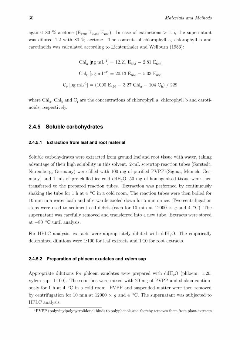
30 Materials and Methods
against 80 % acetone (E470, E646, E663). In case of extinctions > 1.5, the supernatant
was diluted 1:2 with 80 % acetone. The contents of chlorophyll a, chlorophyll b and
carotinoids was calculated according to Lichtenthaler and Wellburn (1983):
Chla [µg mL-1] = 12.21 E663 − 2.81 E646
Chlb [µg mL-1] = 20.13 E646 − 5.03 E663
Cr [µg mL-1] = (1000 E470 − 3.27 Chla − 104 Cb) / 229
where Chla, Chlb and Cr are the concentrations of chlorophyll a, chlorophyll b and caroti-
noids, respectively.
2.4.5 Soluble carbohydrates
2.4.5.1 Extraction from leaf and root material
Soluble carbohydrates were extracted from ground leaf and root tissue with water, taking
advantage of their high solubility in this solvent. 2-mL screwtop reaction tubes (Sarstedt,
Nuremberg, Germany) were filled with 100 mg of purified PVPP1(Sigma, Munich, Ger-
many) and 1 mL of pre-chilled ice-cold ddH2O. 50 mg of homogenised tissue were then
transferred to the prepared reaction tubes. Extraction was performed by continuously
shaking the tube for 1 h at 4 ◦C in a cold room. The reaction tubes were then boiled for
10 min in a water bath and afterwards cooled down for 5 min on ice. Two centrifugation
steps were used to sediment cell debris (each for 10 min at 12000 × g and 4 ◦C). The
supernatant was carefully removed and transferred into a new tube. Extracts were stored
at −80 ◦C until analysis.
For HPLC analysis, extracts were appropriately diluted with ddH2O. The empirically
determined dilutions were 1:100 for leaf extracts and 1:10 for root extracts.
2.4.5.2 Preparation of phloem exudates and xylem sap
Appropriate dilutions for phloem exudates were prepared with ddH2O (phloem: 1:20,
xylem sap: 1:100). The solutions were mixed with 20 mg of PVPP and shaken continu-
ously for 1 h at 4 ◦C in a cold room. PVPP and suspended matter were then removed
by centrifugation for 10 min at 12000 × g and 4 ◦C. The supernatant was subjected to
HPLC analysis.
1PVPP (polyvinylpolypyrrolidone) binds to polyphenols and thereby removes them from plant extracts

2.4 Physiological and analytical methods 31
2.4.5.3 HPLC analysis
Identification and quantification of soluble carbohydrates were carried out by High Pres-
sure Anion Exchange Chromatography with Pulsed Amperometric Detection (HPAE-
PAD) on a Dionex DX 500 HPLC system (Dionex, Sunnyvale, California, USA). The
system consisted of a GP 50 gradient pump and an ED 40 electrochemical detector. The
samples were injected into the system by an auto-sampler (model AS 3500, Thermo Sep-
aration Products, Fremont, California, USA). A guard column (CarboPac guard, 4 × 50
mm, Dionex) was installed upstream the analytical column to prevent contamination of
the analytical column. Thereby, carbohydrate separation was enhanced and a higher peak
resolution was achieved. As analytical column, a CarboPac PA1 (4 × 250 mm, Dionex)
was used.
The carbohydrates were isocratically eluted from the column with 56 mM NaOH. The
eluent was produced by the gradient pump from 200 mM NaOH (previously prepared from
50 % ultra-pure, HPLC grade sodium hydroxide, J. T. Baker, Deventer, Netherlands) and
ddH2O (ratio 28:72). The system was permanently kept free of air bubbles by degassing
both eluents with helium. The eluted carbohydrates were detected in the amperometry
cell of the ED 40. Detection was based on the oxidation of carbohydrates at the surface
of a gold electrode. The current generated by the oxidation was proportional to the
concentration of carbohydrate present in the eluent/sample mixture. The current was
analyzed by the ED 40. Data were recorded by the PeakNet software (version 5.1, Dionex,
Sunnyvale, California, USA).
The CarboPac PA1 is a general purpose column suitable for the analysis of mono-, di-
and some oligosaccharides including sugar alcohols like mannitol (Dionex, 2000, 2004).
Reliable detection of mannitol was crucial for the present study as it was present in con-
siderable amounts in tissue extracts of Fraxinus. In general, sugar alcohols like mannitol
are more difficult to analyse by HPAE-PAD because they are poorly retained on the
PA1 column due to the lower acidity as compared to the respective sugar counterparts.
However, sufficient resolution could be obtained for mannitol and another sugar alcohol,
inositol, with the configuration used (fig. 2.6).
2.4.5.4 Identification and quantification of soluble carbohydrates
The detected carbohydrates were identified and quantified by comparison with a standard
sugar solution. The standard contained inositol, mannitol, glucose, fructose and sucrose,
each at 100 µM. It was injected into the system at five different concentrations (20, 40,
60, 80, 100 µM). A sample chromatogram for a 80 µM standard is shown in fig. 2.6. From

32 Materials and Methods
0 5 10 15 20
010
2030
4050
Retention time (min)
PA
D r
espo
nse
(nC
)
Inositol
MannitolGlucose
Fructose Sucrose
●
●
●
●
●
●
0 20 40 60 80 100
0e+
001e
+06
2e+
063e
+06
4e+
065e
+06
6e+
06
Concentration (mM)
Pea
k A
rea
●
●
●
●
●
●
● InositolMannitolGlucoseFructoseSucrose
Figure 2.6: Analysis of soluble carbohydrates by HPAE-PAD. Left graph: typical chromatogram of asugar standard (in this example, 80 µM) after separation on a Dionex CarboPac PA1 column. Rightgraph: typical calibration curves for inositol, mannitol, glucose, fructose and sucrose. 10-µL aliquots of20, 40, 60, 80 and 100 µM standard solutions were injected into the HPLC system, and the obtainedpeak areas plotted against the respective concentration. Inositol, y = 47970x + 171306, r2 = 0.994;mannitol, y = 31859x + 75651, r2 = 0.981; glucose, y = 32681x + 5700, r2 = 0.998; fructose, y =25330x + 4423, r2 = 0.998; sucrose, y = 44676x – 77433, r2 = 0.984).
the different peak areas at the different concentrations, calibration curves were plotted.
These were linear for the given concentration range, r2 was > 0.984 (fig. 2.6).
Peak areas for standards and samples were obtained by interactive analysis of the HPLC
data with the PeakNet software (version 5.1, Dionex, Sunnyvale, California, USA).
2.4.6 Starch
Starch concentrations were determined in the context of the extraction of soluble carbo-
hydrates from samples (section 2.4.5.1). The pellet obtained in the last centrifugation
step was washed twice with 1 mL ddH2O. 5 U mL-1 amyloglucosidase (AGS) from As-
pergillus niger (Sigma-Aldrich, Munich, Germany) were dissolved in H2O. Aliquots of
1 mL were added to the pellet, and the mixture was continuously shaken for 1 h at 37 ◦C
(Thermo-Shaker, Stratagene, La Jolla, California, USA) to completely digest starch to
glucose. The digestion was stopped by boiling the extracts for 10 min in a water bath. Af-
ter cooling the sample on ice for 5 min, the samples were centrifuged (12000 × g , 10 min,
4 ◦C). A 1:10 dilution of the supernatant in H2O was used for HPLC analysis as described
above (section 2.4.5.3). As AGS contained small amounts of glucose for stabilization of
the enzyme, an aliquot of the AGS solution was subjected to HPLC analysis as well. The

2.4 Physiological and analytical methods 33
amount was subtracted from the samples’ glucose concentration. Starch concentration
was expressed as µmol glucose equivalents per g FW (µmol gluc. eq. g-1 FW).
2.4.7 ADH activity
The activity of alcohol dehydrogenase (ADH) was determined in fresh extracts of leaves,
roots and bark pieces. Extraction and enzyme assay were modified from Bouny and Saglio
(1996).
2.4.7.1 Total cell extracts from leaves
A healthy, fully developed leaf was removed from the tree (usually from a branch in the
upper third of the plant) using a razor blade. The petiole was discarded, and the leaf was
stored in a 7-mL screw top tube (Sarstedt, Nurnberg, Germany) on ice until all samples
were taken. A maximum of eight leaves were collected at a time in order to minimise
decay. 200 mg of the leaf were transferred to an ice-cold mortar. The plant material was
completely homogenised with a chilled pestle in 2 mL of ice-cold extraction buffer (50 mM
Tris-HCl pH 7.5, 10 mM Na2B4O7, 15 % v/v glycerol, 0.02 % triton, 1 mM PMSF, 5 mM
DTT, 5 % w/v PVPP). A spatula tip of fine quartz sand (Fluka, Buchs, Switzerland) was
added to enhance disintegration of tissue. The extract was transferred to a pre-chilled
2-mL reaction tube and centrifuged (12000 × g, 10 min, 4 ◦C). The supernatant was
transferred to a new reaction tube, and the centrifugation was repeated. The obtained
total cell extract was kept on ice and used fresh for the assay. An aliquot (10 µL) was
saved for the determination of soluble leaf proteins (section 2.4.8).
2.4.7.2 Total cell extracts from roots
The plant was carefully taken out of the pot in order to avoid injuries to the root system.
Fine roots of a diameter of up to 1 mm were collected from multiple points of the roots,
ensuring that the material was representative of the whole root system. The collected
roots were carefully cleaned under running tap water and quickly dried on paper tissue.
The roots were stored on ice in 2-mL reaction tubes (Eppendorf) until extraction. The
subsequent procedure was identical to the one described for leaves.

34 Materials and Methods
2.4.7.3 Total cell extracts of bark pieces
Bark sections including vascular cambium, phloem and periderm were excised from the
stem with a fresh scalpel. Remains of wood were discarded. The samples were stored on
ice in 2-mL Eppendorf tubes. The subsequent extraction procedure was identical as for
leaves except that 3 mL of extraction buffer were used for 100 mg of bark material.
2.4.7.4 Activity assay - principle
ADH catalyses the reversible oxidation of ethanol to acetaldehyde in the presence of
NAD+:
CH3CH2OH + NAD+ ADH /o CH3CHO + NADH + H+
In the assay used, ADH activity was monitored in the direction of ethanol oxidation.
Ethanol and NAD+ were added to an aliquot of the total cell extract, and the formation
of NADH was followed photometrically at 340 nm, representing the extinction maximum
of NADH. As the equilibrium of the reaction is shifted to the left side, it had to be
shifted completely to the right by using an excess of ethanol (100 mM). ADH activity is
expressed as µmol NADH formed min-1 which is equivalent to the definition of enzyme
units (U) for ADH. The specific ADH activity was thus calculated as:
ADH activity (U g-1 FW) =V[(∆E/∆t)sample − (∆E/∆t)blind
]v · d · ε · 10−6 · fdil · FW
(2.3)
where (∆E/∆t)sample is the change of extinction in the reaction with sample (min-1),
(∆E/∆t)blind is the change of extinction in the blind reaction (min-1), V is total assay
and v the sample volume (µL), d the light path (cm), ε the extinction coefficient of NADH
at the wavelength of 340 nm (6.3 · 10 -3 L mol-1 cm-1), fdil the dilution factor of the sample
and FW the fresh weight of the sample (g).
(∆E/∆t)sample and (∆E/∆t)blind were obtained from linear regression fits through the
data points of reaction and blind reaction, respectively (fig. 2.7).

2.4 Physiological and analytical methods 35
0 5 10 15
0.0
0.1
0.2
0.3
0.4
0.5
Reaction time (min)
Ext
inct
ion
●●●●●●●●●●●●●●●●●●●●●●●●●●●●●●●●●●●●●●●●●●●●●●●●●●●●●●●●●●●●●●●●●●●●●●●●●●●●●●●●●●●●●●●●●●●
● sample 1sample 2y == 0.001 x + 0.243; r2 == 0.284y == 0.015 x + 0.182; r2 == 0.996y == 0 x + 0.228; r2 == 0.291y == 0.014 x + 0.169; r2 == 0.996
Ethanoladdition
Figure 2.7: ADH assay: determination of slopes for blind reaction (broken lines) and reaction (solidlines) for two arbitrary samples. The arrow marks the addition of ethanol after recording the blindreaction for 5 min. This procedure corresponds to the protocol described for the plate reader; when thephotometer was used, blind reaction and reaction were measured in two separate assays.
2.4.7.5 Activity assay - use of the photometer
975 µL of ice-cold assay buffer (100 mM tricine pH 7.5, 6.8 mM NAD, 100 mM ethanol)
were pipetted into a disposable semi-micro cuvette (polystyrene 10 × 4 mm; Sarstedt,
Nurnberg, Germany). The cuvette was heated to 25 ◦C by placing the cuvette in the
tempered photometer slot for 15 min. 25 µL of fresh cell extract were then added to the
assay and mixed by inverting the cuvette that had been previously sealed with a double
layer of parafilm. The parafilm was removed, and the reaction was recorded for 10 min at
340 nm. Extinction was recorded at intervals of 10 s. The blind reaction was determined
in a parallel assay, containing H2O instead of ethanol.

36 Materials and Methods
2.4.7.6 Activity assay - use of the plate reader
100 µL of 2 × assay buffer (100 mM tricine pH 7.5, 6.8 mM NAD) and 40 µL of ddH2O
were transferred to the wells of a 96-well plate (Sarstedt, Nurnberg, Germany). The plate
was brought to 25 ◦C by inserting it into an appropriately tempered plate reader (Spectra
Rainbow; Tecan, Mannedorf, Switzerland) 10 min before starting the assay. 30 µL of fresh
cell extract were added to each well, and the blind reaction was recorded for 5 min at an
interval of 10 s (fig. 2.7). 30 µL of 670 mM ethanol were then added to the reaction mix,
and the change in extinction at 340 nm was recorded for 10 min. The different light paths
of blind (d = 0.6 cm) and main reaction (d = 0.7 cm), caused by the different reaction
volumes, were considered by using appropriate d in the calculations.
2.4.8 Soluble leaf proteins
The content of soluble leaf proteins was determined in total cell extracts from leaf tissue
(section 2.4.7.1) according to the method of Bradford (1976). 5 µL of protein extract
were transferred to a 96-well plate (Sarstedt, Nurnberg, Germany) and mixed with 200 µL
of Bradford reagent (Bio-Rad Protein Assay, diluted 1:5 with ddH2O; Bio-Rad, Munich,
Germany). After incubation for 10 min at RT, the extinction of the samples at λ = 595 nm
was determined with a plate reader (Spectra Rainbow; Tecan, Mannedorf, Switzerland).
A calibration curve was obtained from the extinction of a dilution series of a protein
standard (fig. 2.8).
2.4.9 Ethanol
2.4.9.1 Extraction from leaf and root material
Ethanol was extracted from homogenised leaf or root tissue with water as solvent. Stan-
dard reaction tubes (Eppendorf) were filled with 50 mg of purified PVPP and 0.5 mL
of ice cold ddH2O. 50 mg of frozen homogenised leaf or root material, respectively, were
transferred to the prepared tubes and immediately mixed by vortexing. The tubes were
permanently kept on ice. Ethanol was then extracted from the tissue powder by continu-
ous shaking for 20 min at 4 ◦C (cold room). Cell debris were removed by centrifugation
for 10 min at 12000 × g and 4 ◦C. The supernatant was transferred to a fresh reaction
tube, frozen in liquid N2 and stored at −80 ◦C until analysis.

2.4 Physiological and analytical methods 37
●
●
●
●
●
●
0 1 2 3 4 5
0.0
0.1
0.2
0.3
0.4
0.5
0.6
BSA concentration (µg µL−−1)
Net
ext
inct
ion
y == 0.123x −− 0.012; r2 = 0.994
Figure 2.8: Calibration curve for Bradford protein assay. A dilution series of a standard protein (bovineserum albumine, BSA; Sigma, Munich, Germany) at 0, 1, 2, 3, 4 and 5 µg µL-1 was prepared usingextraction buffer. After incubation of 5 µL of each dilution with 200 µL of Bradford reagent, the extinctionat λ = 595 nm was determined with a plate reader. Net extinction was obtained from extinction minuschemical blank (5 µL extraction buffer + 200 µL Bradford reagent). Results from linear regressionanalysis are shown. n = 3.
2.4.9.2 Preparation of xylem sap
Xylem sap samples were slowly thawed on ice in order to prevent evaporation of the con-
tained ethanol. Aliquots of 25 µL were transferred to standard reaction tubes (Eppendorf)
which had previously been filled with 20 mg of PVPP and 975 µL of ice cold ddH2O. Care
was taken to pipette the sample directly into the H2O, avoiding contact with the tube
wall. The mixture was then shaken for 20 min at 4 ◦C. After centrifugation (10 min,
12000 × g , 4 ◦C), the supernatant was pipetted into a new tube and stored at −80 ◦C
until analysis.

38 Materials and Methods
2.4.9.3 Enzymatic determination - principle
Ethanol concentrations were determined with a commercially available test kit (Roche,
Basel, Switzerland). Ethanol is oxidised to acetaldehyde in the presence of ADH and
NAD as an electron acceptor:
CH3CH2OH + NAD+ ADH /o CH3CHO + NADH + H+
The equilibrium of the reaction is quantitatively shifted towards acetaldehyde and NADH
by coupling the reaction to the ALDH-mediated oxidation of acetaldehyde to acetate:
CH3CHO + NAD+ ALDH /o CH3COOH + NADH + H+
The amount of ethanol is proportional to the amount of NADH produced in the reaction.
NADH (but not NAD) shows a strong extinction of light at the wavelength of 340 nm
which can be detected photometrically. This property was used in the assay.
2.4.9.4 Enzymatic determination - assay
The protocol followed the specifications of the manufacturer of the kit but with reagent
volumes adjusted for use with 96-well microtiter plates instead of 1-mL cuvettes. The
reaction mix (buffer + cosubstrates + coupling enzyme) was prepared by mixing 3 mL
of ready-made potassium diphosphate buffer, pH 9.0 (bottle 1) with a tablet containing
4 mg of NAD and 0.8 U of acetaldehyde (bottle 2). This amount of reaction mix was
sufficient for 15 samples and was made freshly for each measuring series. A microtiter
plate (Sarstedt, Nurnberg, Germany) was prepared by transferring 200 µL of the reaction
mix into each required well. Depending on the amount of ethanol, 5–10 µL of xylem
sap were transferred to the plate which was then inserted into the plate reader (Spectra
Rainbow, Tecan, Mannedorf, Switzerland) and mixed using the “quick shake” function.
The extinction was read at 340 nm (E1). 5 µL (22 U) of ADH suspension (bottle 3)
were added to start the reaction. After 10 min, the extinction was read again (E2). The
amount of ethanol in the sample was proportional to the extinction difference E2 - E1 and
was calculated on the basis of the Lambert-Beer law:
Concentration of ethanol (g L-1) =V ·MW ·∆Eε · d · v · n · 1000
(2.4)

2.5 Flap-feeding of U-13C-glucose 39
where V was the reaction volume, MW the molecular weight of ethanol (46.07 g mol-1),
ε the extinction coefficient of NADH at 340 nm (6.3 · 10-3 L mol-1 cm-1), d the light path
through the sample (0.5 cm), v the sample volume (5–10 µL), n the number of moles
NADH produced per moles ethanol oxidised (2) and ∆E E2 - E1 minus (E2 - E1)blank. The
blank reaction was measured once per plate with 10 µL of ddH2O in place of sample.
As control, an aliquot of ethanol standard solution (bottle 4, 0.06 g L-1) was measured in
the same way as the samples. The result for n = 6 measurements was 0.0598 ± 0.0040 g
L-1 (99.7 ± 6.8 %).
Recovery rates were determined by adding a defined amount of ethanol to extraction
assays before the shaking step. The amount of ethanol added (1 mM) was in the range
of ethanol present in the extraction assays (i.e. 0.1–2 mM). Of the 1 mM ethanol added
to the solutions, 0.85 to 0.97 mM were recovered in leaf (93 ± 5 %, n = 5), and 0.83 to
0.98 mM in root assays (91 ± 6 %, n = 5).
2.5 Flap-feeding of U-13C-glucose
2.5.1 Feeding procedure
U-13C-glucose (Cambridge Isotope Laboratories; Andover, MA, USA) was introduced into
leaves using the flap-feeding technique of Biddulph and Markle (1944). For this purpose,
an application tube was prepared by removing lid and upper third from a 0.5 mL PCR
tube (Eppendorf, Hamburg, Germany). This tube was filled with 75 µL of 100 mM U-13C-glucose and sealed with parafilm. A secondary vein from the middle of a healthy leaf
was cut at both longitudinal sides over a length of approx. 1 cm using a fresh razor blade.
The vein segment was isolated from the leaf by making a third cut through the vein close
to its connection to the primary vein. These cuts were made under water using a petri
dish, in order to prevent air from entering the vessels. The leaf was taken out of the water,
dried on soft paper, and the vein flap was immediately immersed into the feeding solution
(fig. 2.9). After 4–6 h, the application tube was taken off. The leaf including the petiole
was removed and frozen in liquid N2. The flap was stored in a separate tube. For the
recovery of 13C from the phloem, bark samples were taken from five stem segments of equal
length (fig. 2.10) and submitted to phloem exudation as described above (section 2.3.3.2).
In order to increase the amount of incorporated 13C, two flaps were used per plant. In
P. tremula and A. pseudoplatanus , these flaps were placed on the same leaf, while they
were on opposing leaflets in F. excelsior . Material from two application leaves was pooled.
This procedure was similar to the one described by Trip et al. (1965) who used three flaps

40 Materials and Methods
per plant.
A series of preliminary experiments was carried out in order to find suitable harvesting
times after application of the pulse. These were defined as the time when increased 13C
levels, and preferably a clear basipetal gradient, was detected in phloem exudates from
different heights of the stem. Up to four seedlings of each species were tested as described
above. Results indicated that harvest should be carried out four hours after pulsing in
poplar, and six hours after pulsing in ash and maple.
OH
13CHOH
13CHOHHOH
13C
HOH13C
H13C
13CHOH
Figure 2.9: Left: Illustration of flap-feeding method. A segment of a secondary vein was prepared fromthe leaf and immersed in 100 mM U-13C-glucose. As application vial, a cut PCR tube was used whichwas light enough to be hold only by the vein segment. Right: Chemical structure of U13C-glucose.
2.5.2 Determination of 13C derived
2.5.2.1 Sample preparation for elemental analysis
Leaves were transferred from −80 ◦C to a drying cabinet and desiccated for 5 days at
60 ◦C. For this purpose, the lids of the plastic tubes were removed. After drying, samples
were ground to fine powder for 2 min at 90 Hz with a ball mill (Retsch MM 2000, Retsch,
Haan, Germany). Approx. 0.5 mg of powder were transferred to a tin capsule (Tin
Capsules, CE Instruments, Milan, Italy).
For phloem exudates, 2 mL of the total volume (5 mL) were centrifuged for 10 min at
12000 × g in order to remove particulate material. 1.8 mL of the supernatant were
transferred into a new tube, from which H2O was completely evaporated for 24 h at 50◦C using a speed vac (Christ RVC 2-25, Christ, Osterode, Germany). The dried exudate

2.5 Flap-feeding of U-13C-glucose 41
segment 1
segment 2
segment 3
segment 4
segment 5
feeding leaf
Figure 2.10: Feeding experiment: Position of the fed leaf and the bark samples taken. U-13C-glucosewas incorporated into the leaf by flap-feeding. Bark samples were taken from five stem segments asindicated by arrows, and analysed for changes in δ13C. The total height of the plants was 80–120 cm,the height of each segment 15–20 cm. The flooding height was 15 cm above ground.
was resuspended in 50 µL of ddH2O, 10 µL of which were pipetted into a tin capsule (Tin
Capsules, CE Instruments, Milan, Italy).
2.5.2.2 13C/12C analysis
Total C and C isotope ratio (13C/12C) were determined on an isotope ratio mass spec-
trometer (IRMS; Delta Plus, ThermoQuest, Milan, Italy) connected to a C/N elemental
analyzer (NC 2500, ThermoQuest, Milan, Italy). Samples were placed on an auto-sampler
and successively injected into the C/N analyzer. At a temperature of approx. 1050 ◦C, the
material was quantitatively combusted in the presence of ultra-pure oxygen gas (99.995 %,
SWF, Fiedrichshafen, Germany). The oxidation products (H2O, CO2, N2 and NOx) were
transferred to the reduction reactor using ultra-pure helium (99.996 %, SWF) as a vec-
tor gas. In the reduction reactor, the NOx components were catalytically reduced to N2
(using pure copper as a catalyzer), combining all N molecules of the sample in the N2
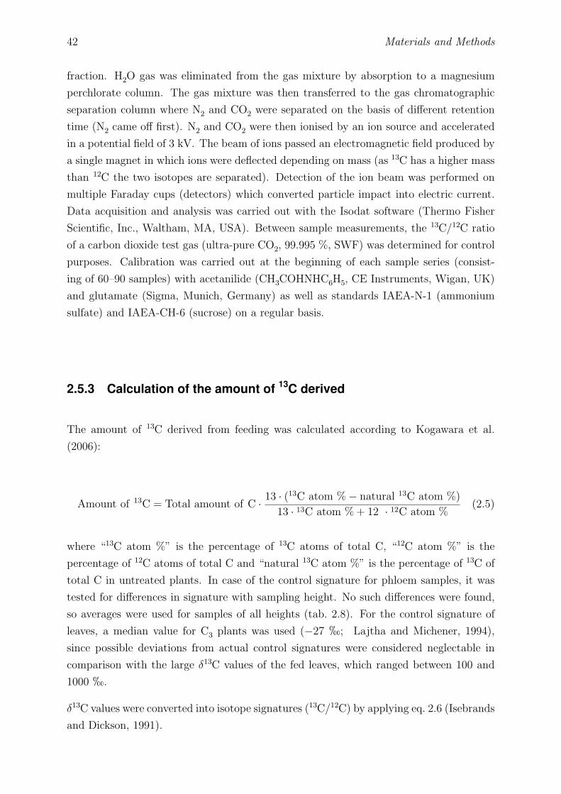
42 Materials and Methods
fraction. H2O gas was eliminated from the gas mixture by absorption to a magnesium
perchlorate column. The gas mixture was then transferred to the gas chromatographic
separation column where N2 and CO2 were separated on the basis of different retention
time (N2 came off first). N2 and CO2 were then ionised by an ion source and accelerated
in a potential field of 3 kV. The beam of ions passed an electromagnetic field produced by
a single magnet in which ions were deflected depending on mass (as 13C has a higher mass
than 12C the two isotopes are separated). Detection of the ion beam was performed on
multiple Faraday cups (detectors) which converted particle impact into electric current.
Data acquisition and analysis was carried out with the Isodat software (Thermo Fisher
Scientific, Inc., Waltham, MA, USA). Between sample measurements, the 13C/12C ratio
of a carbon dioxide test gas (ultra-pure CO2, 99.995 %, SWF) was determined for control
purposes. Calibration was carried out at the beginning of each sample series (consist-
ing of 60–90 samples) with acetanilide (CH3COHNHC6H5, CE Instruments, Wigan, UK)
and glutamate (Sigma, Munich, Germany) as well as standards IAEA-N-1 (ammonium
sulfate) and IAEA-CH-6 (sucrose) on a regular basis.
2.5.3 Calculation of the amount of 13C derived
The amount of 13C derived from feeding was calculated according to Kogawara et al.
(2006):
Amount of 13C = Total amount of C · 13 · (13C atom %− natural 13C atom %)
13 · 13C atom % + 12 · 12C atom %(2.5)
where “13C atom %” is the percentage of 13C atoms of total C, “12C atom %” is the
percentage of 12C atoms of total C and “natural 13C atom %” is the percentage of 13C of
total C in untreated plants. In case of the control signature for phloem samples, it was
tested for differences in signature with sampling height. No such differences were found,
so averages were used for samples of all heights (tab. 2.8). For the control signature of
leaves, a median value for C3 plants was used (−27 h; Lajtha and Michener, 1994),
since possible deviations from actual control signatures were considered neglectable in
comparison with the large δ13C values of the fed leaves, which ranged between 100 and
1000 h.
δ13C values were converted into isotope signatures (13C/12C) by applying eq. 2.6 (Isebrands
and Dickson, 1991).

2.5 Flap-feeding of U-13C-glucose 43
Table 2.8: Natural carbon isotope ratios used for computation of excess 13C derived from feeding.
Material / species Carbon isotope ratio (δ13C) (h) SourcePhloem exudate / ash −26.30 ± 0.37 Average of 6 samples from 2 plants
Phloem exudate / poplar −26.29 ± 0.51 Average of 6 samples from 2 plantsPhloem exudate / maple −29.35 ± 0.92 Average of 20 samples from 5 plants
Leaf / all species −27 Median value for leaves of C3 plants(Lajtha and Michener, 1994)
13C12C
= PDB +δ13C
1000· PDB (2.6)
where PDB is the Pee Dee Belemnite standard for δ13C (0.0112372).
“13C atom %” and “12C atom %”, required for eq. 2.5, were derived by eq. 2.7 (Isebrands
and Dickson, 1991).
13C atom % =13C12C· 100 12C atom % = 100− 13C atom % (2.7)
The total amount of C was calculated from the C mass percentage (obtained from MS
analysis), multiplied by the dry weight of the sample.
The following example demonstrates how the amount of 13C derived from feeding was
calculated for a leaf sample of 0.2 g DW. The C mass percentage and δ13C were determined
to be 55 % and +100 h, respectively. δ13C was converted to 13C atom % using eqs. 2.6
and 2.7. The result, 1.236, along with 12C atom % = 100–1.236 = 98.764 and natural 13C
atom % = 1.093 (corresponding to δ13C = −27 h; tab. 2.8), was used in eq. 2.5. The
amount of 13C derived from feeding was 0.170·10-3 g (0.013·10-3 mol). This amount was
related to the total amount of 13C incorporated by the plant which was known from the
volume of sugar solution taken up. 0.020·10-3 mol 13C were incorporated, thus 0.013·10-3
/ 0.020·10-3 = 0.655 = 65.5 % of incorporated 13C were found in the leaf.
For the phloem exudates, analogous calculations were carried out. The amount of 13C
derived from feeding was related to the DW of the bark piece and scaled to the dry
weight of the bark of the respective stem segment. Thereby, the amount of 13C derived
from feeding in the phloem sap of each stem segment was obtained.

44 Materials and Methods
2.6 Oxygen measurements within the stem
2.6.1 Principle
Oxygen within the stems of tree seedlings was determined with oxygen micro-optodes
(Presens GmbH, Regensburg, Germany). These miniaturised sensors have a tip diameter
of only 50 µm, allowing for measurements with high spatial resolution. The operation
principle is based on the quenching of luminescence of dye molecules in the presence of
molecular oxygen (Presens, 2002; Klimant et al., 1997). The dye molecules, a ruthenium
diimine complex, are applied on the tip of a fiber optic cable through which periodic (1
Hz) light signals of a wavelength of 505 nm are sent. The dye molecules are excited by
the light signal and emit some of the excitation energy as luminescence. The more oxygen
is present in the vicinity of the sensor tip, the greater is the portion of luminescence that
is quenched by the collision of oxygen molecules with dye molecules. The luminescence
signal is transferred back through the fiber cable and photometrically detected by an
oxygen meter (Microx TX2; Presens GmbH, Regensburg, Germany). The quenching
effect is quantified as the lifetime of luminescence which is shorter in the presence of
oxygen. The detection works equally well in gaseous and liquid phase and is independent
of pH, ions, salinity or viscosity (Presens, 2002).
2.6.2 Experimental setup
In the experiments, micro-optodes of the variant “needle-type” were used for O2 anal-
ysis (order no. NTH-L10-TF-NS120/0.8-Y). In this sensor type, the fragile sensor tip
is enclosed in the steel needle (length 120 mm, diameter 0.8 mm) of a plastic syringe
(fig. 2.11A). For the measurement in the wood, the tip was extended only to the end of
the diagonal cut of the cannula in order to avoid damage by contact with the wood.
In a preliminary experiment, it was tested if sufficient air convection occurred between
half-extended tip and environment to ensure a high temporal resolution of the measure-
ment. For this purpose, the sensor was transferred from air into a septum-sealed HPLC
vial filled with 1 M Na2SO3 (Na2SO3 was used to eliminate all oxygen from the solution
and the airspace above it). In this experiment, a reaction of the sensor was observed
within 30–60 s after insertion, compared to 5–10 s with the fully extended tip (data not
shown). This slightly larger response time was considered neglectable.
For insertion of the sensor, a hole of 0.9 mm diameter was drilled into the stem using a
drill machine. The hole was driven to a depth of approx. half of the stem diameter. After

2.6 Oxygen measurements within the stem 45
inserting the sensor, the hole was sealed with terostat (Teroson, Heidelberg, Germany;
fig. 2.11B). Externally, the sensor was fixed to a wooden staff (fig. 2.11A). Once inserted,
the tip of sensor was carefully extended, and recording was started after reaching steady
state concentrations (fig. 2.12). For data acquisition, the Oxyview software (version 4.16;
Presens, Regensburg, Germany) was used.
Stem-internal temperatures were required for temperature-corrected calculation of oxygen
concentrations. However, suitable sensors for this purpose were not available. Therefore,
temperatures were recorded using temperature sensors (Presens, Regensburg, Germany)
attached to the stem surface, which were assumed to approximate stem-internal temper-
atures (cf. Gansert, 2004).
Calibration of the sensors was performed using a two-point calibration according to the
manufacturer’s instructions.
A B
C
Figure 2.11: Stem-internal oxygen measurements. (A) syringes containing the sensor tip were fixatedon a scaffold made of bamboo sticks. (B) enlargement of (A) showing how the cannula was inserted intothe stem. The borehole was sealed with terostat (Teroson, Heidelberg, Germany). (C) oxygen meterMicrox TX2 (Presens, Regensburg, Germany). Oxygen sensor (left plug) and temperature sensor (rightplug) are connected to the device. For data acquisition, a notebook computer was used.

46 Materials and Methods
●
●● ●
● ● ●●
●● ● ● ● ● ● ● ● ● ● ●
● ● ●● ●
● ● ● ● ● ●● ● ● ●
● ● ● ● ●
4060
8010
012
0
Time (hh:mm)
[Oxy
gen]
(%
air
satu
ratio
n)
17:00 17:48 18:36 19:24
Sensor inserted
Figure 2.12: Oxygen measurements with needle-type micro-optode sensors (time of insertion markedby arrow). Approx. 30 min were required for the measured concentration to settle down to a stable level.Data were recorded every 5 min.
2.6.3 Manual calculation of the O2 concentration from raw data
The measured O2 concentrations were calculated directly by the Oxyview program. This
requires the calibration data for the respective sensor to be entered into the software
before measurements were started. However, this became impractical when sensors were
changed frequently, e.g. when measuring several trees in turn. In this case, it was more
convenient to use the raw data output, phase angle and temperature, and recalculate
the O2 concentrations manually. For this purpose, the formulas from the manufacturer’s
manual (Presens, 2002) were applied as specified in eq. 2.8.
O2 (% air saturation) =−b+
√b2 − 4ac
2a(2.8)
where a, b and c are defined as

2.6 Oxygen measurements within the stem 47
a =tan Φm,Tm
tan Φ0,Tm· 1
22.9·K2
SV,Tm
b =tan Φm,Tm
tan Φ0,Tm·KSV,Tm+
tan Φm,Tm
tan Φ0,Tm· 1
22.9·KSV,Tm−0.805· 1
22.9·KSV,Tm−KSV,Tm+0.805·KSV,Tm
c =tan Φm,Tm
tan Φ0,Tm− 1
tan Φm,Tm in these equations is the tangent of the phase angle Φ of the current measure-
ment (m) at the current temperature (Tm) and is defined as:
tan Φm,Tm = tan(Φ0,T0 ·Π
180) (2.9)
where tan Φ0,Tm is the tangent of the phase angle at 0 % oxygen as obtained from cali-
bration, extrapolated for Tm. Its definition is:
tan Φ0,Tm = tan(Φ0,T0 + (−0.08037 · (Tm − T0)) · Π
180(2.10)
KSV,Tm is the Stern-Vollmer constant for Tm which is derived from the Stern-Vollmer
constant for T100:
KSV,Tm = KSV,T100 + 3.83 · 10−4 · (Tm − T100) (2.11)
The Stern-Vollmer constant for T100, i.e. the temperature during calibration at 100 % O2
is derived as:
KSV,T100 =−B +
√B2 − 4AC
2A(2.12)
where A, B and C are defined as:
A =tan Φ100,T100
tan Φ0,T100· 1
22.9· [O2]
2
B =tan Φ100,T100
tan Φ0,T100· [O2] +
tan Φ100,T100
tan Φ0,T100· 1
22.9· [O2] + 0.805 · 1
22.9· [O2]− [O2] + 0.805 · [O2]
C =tan Φ100,T100
tan Φ0,T100− 1
In these equations, tan Φ100,T100 and tan Φ0,T100 are:
tan Φ100,T100 = tan(Φ100,T100 · Π180
)
tan Φ0,T100 = tan([Φ0,T0 + (−0.08037 · (T100 − T0))] · Π180
)

48 Materials and Methods
where Φ100,T100 and Φ0,T0 are phase angles at 100 % O2 and respective temperature and
at 0 % O2 and respective temperature, respectively.
Φ0,T0, Φ100,T100, T0 and T100 were obtained from calibration, Φm,Tm and Tm from the raw
data of the measurement.
2.7 Biometry
2.7.1 Stem height and diameter
Stem height was determined from the ground (upper pot rim) to the terminal bud of the
tree using a folding rule. The stem diameter was determined with a gauge, at a height
of 2 cm above the ground. Diameters at other heights were recorded as indicated in the
text.
2.7.2 Fresh and dry weight
Fresh weight of leaves, stems and roots was determined by weighing immediately after
harvest. For the determination of dry weight, the material was dried in paper bags at 60◦C until weight constancy (5–6 days).
2.7.3 Leaf area
Leaf area was determined using a leaf area meter (Delta T Devices Ltd, Cambridge, UK).
The contour of the leaf, which was positioned on a lightbox providing uniform background
illumination, was detected with a camera using the method of colour discrimination. The
detection threshold was manually adjusted as appropriate. From the area occupied by
the dark space, the leaf area was automatically calculated by the system. Calibration
was performed with paper rectangles of defined area at the beginning of each series of
measurements.
2.7.4 Leaf number
All living leaves were counted, irrespective of developmental stage or damages. Dead
leaves were not taken into account.

2.8 Statistical analysis 49
2.8 Statistical analysis
2.8.1 General data analysis and statistics
Unless otherwise stated, data of n multiple measurements (x) were expressed as mean (x)
± standard deviation based on a sample (SD, eq. 2.13).
SD =
√(x− x)2
n− 1(2.13)
Preparation of data for statistical analysis was performed with OpenOffice Calc (version
2.0 or higher, Sun Microsystems Inc., Santa Clara, California, USA). Large datasets
were stored in a MySQL database (version 5.0 or higher, MySQL AB, Uppsala, Sweden).
Statistical analyses as well as graphics were made with the software R, version 2.0 or higher
(R Development Core Team, 2006). Chemical structures were drawn with GChemPaint,
version 0.6.9 or higher (www.nongnu.org/gchempaint).
For testing statistical differences between two groups, Student’s two-sample t test was used
(R function t.test()). Differences between more than two groups were tested by analysis
of variance (ANOVA), using aov(). Multiple comparisons (post-hoc tests) were carried
out with Tukey’s Honest Significant Differences (HSD) test (TukeyHSD()). The latter
function possesses a compensation for mildly unbalanced data, making it applicable for
most of the datasets in the present study. Balanced designs were used in all experiments,
however, balance was lost in some cases due to missing observations.
Normal distribution and homogeneity of variances of data were tested using visual meth-
ods (index plots, histograms, QQ plots) as well as appropriate statistical tests (Pearson
χ2 test for normality, Bartlett test for homogeneity of variances). In case of violation of
any of these assumptions, data were either (1) transformed using an appropriate power
transformation or (2) subjected to non-parametric methods. (1) Transformation can
generally be applied to either predictor or response variable. However, as predictors
in the data of the present study were mostly categorical (e.g. treatment, species), the
only candidate for transformations was the response variable. For identifying suitable
power transformations, the suggestions of Fox (2002) were followed. Appropriate trans-
formations to normality and symmetry were identified using Box-Cox transformations
and related methods. (2) Non-parametric methods included the Wilcoxon rank sum test
(wilcox.test()) for testing differences between two groups and the Kruskal-Wallis rank
sum test (kruskal.test()) for more than two groups.

50 Materials and Methods
Unless otherwise specified, significant difference between two groups were marked with
asterisks, using standard significance codes, i.e. “*”, “**” or “***” for significant differ-
ences at the 5 %, 1 %, 0.1 % significance level, respectively. Letter notation (A, B, C,
. . . ) was used when more than two groups were compared, with different letters indicating
significant differences between the groups at the 5 % significance level. Letter output was
obtained using the R function multcompLetters() (package multcompView).
2.8.2 Analysis of light and CO2 response curves
Both light and CO2 response were fitted with the Mitscherlich model (eq. 2.14).
y = A[1− e−k(x−x0)] (2.14)
The use of the model was suggested by Potvin et al. (1990) as it includes three regression
coefficients, A, k and x0 which represent important physiological characteristics. In the
case of the light curves, A stands for the light-saturated assimilation rate, k for the
apparent quantum yield and x0 for the light compensation point. In the case of the CO2
curves, A represents CO2 saturated photosynthesis, k the increase of A with increasing
CO2 (A/CO2) and x0 the CO2 compensation point. x refers to the applied light or CO2
level, respectively. Thus, by fitting the model to the acquired light and CO2 curve data
(section 2.4.1.3), estimates for these physiological characteristics were obtained.
The model was used for two types of analyses. The purpose of the first type of analysis
was to fit individual response curves for each plant and treatment. Thereby, estimates
of the regression coefficients for each single response curve were obtained. On the basis
of the regression coefficients, regression lines could be drawn through the data points.
Confidence intervals of the three regression coefficients were also calculated, allowing for
pair-wise comparison of the parameters of two or more curves.
Functions used for this first type of analysis included nls() for fitting, nlsList() for fit-
ting multiple curves in one step, predict() to calculate regression lines and intervals()
for calculating confidence intervals of the regression parameters (all functions from the
package nlme).
As a criterion for the goodness of fit, the coefficient of determination for non-linear regres-
sions (r2nl) was calculated. The formula given by Sachs and Hedderich (2006) was used
(eq. 2.15).

2.8 Statistical analysis 51
r2nl =
1− ss∑y2 − 1
n(∑y)2
(2.15)
where ss is the residual sum of squares of the fit (obtained from nls()), y is the response
variable and n is the sample size.
Good fits were obtained for the photosynthetic response curves of ash, lime and wil-
low (figs. 3.32, 3.33). For oak, however, only low coefficients of determination were
yielded. Therefore, other models often used in physiological response curve analysis,
e.g. the Michaelis-Menten model (He et al., 1999), rectangular (Krauss et al., 2006) or
non-rectangular hyperbola (Ogren and Evans, 1993; Leverenz et al., 1990), were tested
alternatively but did not yield considerably better results.
In the second type of analysis, the Mitscherlich equation was used for setting up a non-
linear mixed effects model (NLME). The general approach was adopted from Peek et al.
(2002) but modified in several points to account for the different experimental design of
the present experiments. The model, as used by Peek et al. (2002), is given in eq. 2.16:
yij = f(φij, xij) + eij (2.16)
where f is a nonlinear function of an individual-specific parameter vector φij and the
predictor vector xij for the jth observation on the ith subject. eij is a vector of unknown
random errors. phiij was given by:
φij = Aijβ +Bijbi
where β is a vector of fixed population parameters and bi is a vector of random effects
of the ith individual (not varying with j). Aij and Bij are design matrices for the fixed
and random effects, respectively (notation according to Pinheiro and Bates (2000)). The
fixed effect design matrix (Aij) was specified by Peek et al. (2002) in accordance with
their experimental design which was 2x2 factorial (two species which were subjected to
two treatments). The random component Bij was specified in order to take into account
repeated measurements on the same leaves at different light levels. For f , Peek et al.
(2002) used the Mitscherlich model equation as already given above (eq. 2.14).
In the present experiments, two groups of plants, a control and a flooded group, were
measured at two dates (day 0 and day 14). Thus, two levels of repeated measurements
were present in the experiment: (1) multiple measurements on the same leaf of each plant

52 Materials and Methods
at different light (or CO2) levels, and (2) measurements of the same plants on day 0 and
day 14. In order to account for this two level grouping, model 2.16 was modified (eq. 2.17).
yijk = f(φijk, xijk) + eijk (2.17)
where i refers to the plant number, j to the day and k to the light (or CO2) level.
Accordingly, φijk was defined as:
φijk = Aijkβ +Bijkbi + Cijkcij
where Aijkβ and Bijkbi are defined analogously to the above terms, however, cij is a
random effects vector associated with the ith individual on the jth day, and Cijk is a
design matrix for the random effects of the second level.
Model 2.17 was fitted separately to the light and CO2 curve data of each species inves-
tigated (ash, lime, oak, willow), using the function nlme(). According to the model,
light (or CO2) level (x) was specified as primary covariate, treatment and day, and their
interaction, as covariates. Random effects were first included for all regression coefficients
(A, k and x0) but eliminated when there was no or little variation between individuals in
order to simplify the model (Pinheiro and Bates, 2000).
The results of nlme() included estimates for the 12 parameters (2 treatments × 2 days
× 3 parameters). In order to test if treatment, day or their interaction had a significant
effect on the parameters (A, k, or x0), Wald’s F test was carried out using the function
anova() with an appropriate specification of the model terms to be tested. For example,
a test for a significant effect of treat on A was specified as anova(model, test="F",
Terms="treat"). Accordingly, all other combinations of factors and parameters were
tested.
Multiple comparisons of the parameter estimates were performed by obtaining confi-
dence intervals for the parameters on the 95 % confidence levels using the function
intervals.lme(). Two groups were marked as significantly different when their con-
fidence intervals of the respective parameter did not overlap. Different letters were used
to denote these differences.

Chapter 3
Results
3.1 Experiment I: Effect of flooding on the C metabolism of
ash provenances “Alb”, “Rhine” and “BFor”
In order to characterise the impact of flooding on common ash, flooding experiments
with three-year-old seedlings were performed under semi-controlled conditions. In this
experiment, three provenances of common ash, “Alb”, “Rhine” and “BFor” were com-
pared regarding major features of C metabolism: photosynthesis, carbohydrate contents
of various tissues, and alcoholic fermentation in the roots.
3.1.1 Leaf gas exchange
3.1.1.1 Assimilation
Control plants showed light-saturated net assimilation rates (Amax) between 1.8 and 3.2
µmol m-2 s-1 (day 1) which increased from day 3 to 7 (4–6 µmol m-2 s-1) and thereafter
decreased again to values similar to day 1 (fig. 3.1). In contrast, Amax was initially
relatively high (7–7.5 µmol m-2 s-1) in flooded plants of all provenances and then showed
a decreasing trend with increasing flooding duration. As a consequence, Amax amounted
to only 1.5 to 2.4 µmol m-2 s-1 at the end of the experiment (day 42).
For better comparability, Amax of the flooded plants were expressed as percent of the
control (fig. 3.2). Generally, Amax on day 1 was 2 (“Rhine”) to 4 (“Alb”) times higher in
the flooded plants than in the controls, whereas on all other days Amax was lower or in

54 Results
Am
ax (µµ
mol
m−−2
s−−1
)
02
46
810
●
● ●
●
●
●
●
●
●
●● ● ●
● ●
* *
**
Alb
●
●●
●
● ●●
●
●●
●
● ●●
●●
*
*
Rhine
●
●
●
●
●
●
●
●
●
●
● ●●
●
*
**
BFor
ControlFlooded
●
●
Day of experiment
g s (m
mol
m−−2
s−−1
)
020
4060
8010
012
0
0 10 20 30 40
●
●●
●
●●
●
●
●
● ●
●
●
●
●
* *
* * *
0 10 20 30 40
● ●
●
●
●
●
●
●
●●
●
●
●
●
●
●
*
0 10 20 30 40
●●
● ●
●
●
●
●
●
●
●
●●
●
*
*
A
B
Figure 3.1: Effect of flooding on net assimilation (A) and stomatal conductance (B). Ash seedlingsof three provenances (“Alb”, “Rhine”, “BFor”) were flooded for the times indicated by horizontal barsand gas exchange was analysed as described in Materials and Methods. Points represent means offour plants (± SD). Asterisks indicate significant differences between the treatments as calculated byWilcoxon rank sum tests, using standard significance codes. In case of the omitted control measure-ments (days 28 and 42), results for the flooded plants were tested against the respective precedingcontrol day.
the same range as the controls. The difference on day 1 between “Alb” and “Rhine” was
statistically significant.
Continued flooding caused lower Amax in all provenances. For example, after three days of
flooding, “Alb” and “BFor” exhibited lower assimilation rates than the controls (71 and
41 % respectively) while “Rhine” (108 %) remained similar to the control. After 14 days
of treatment, Amax was significantly reduced in the flooded plants of “Alb” (35 % of the
control) and also reduced, albeit less pronounced, in “Rhine” (64 %) and “BFor” (80 %).
One week of recovery did not cause Amax to regenerate in “Alb” and “Rhine” as compared
to the controls, which remained on approximately the same low level of the last day of
the flooding treatment (59 and 66 %, respectively). “BFor”, however, showed a relatively
high A (215 %) after the recovery phase. The difference between “Alb”, “Rhine” and
“BFor” was statistically significant.

3.1 Experiment I: Effect of flooding on ash provenances “Alb”, “Rhine” and “BFor” 55
Day of experiment
g s (%
of c
ontr
ol)
Am
ax (%
of c
ontr
ol)
020
040
060
080
010
00
1 3 7 14 21 24 28 35 42
aab
b
a abb
a abb
ab ab
010
020
030
0
a
ab
b
a a
bAlbRhineBFor
A
B
Figure 3.2: Effect of flooding on net assimilation (A) and stomatal conductance (B) of ash seedlings.Trees were flooded for the times indicated by horizontal bars, and results for flooded seedlings wereexpressed as percent of the controls. Bars represent means of four plants (± SD). Different lettersindicate significant differences between the provenances as calculated by a one-way ANOVA, applyingTukey’s HSD post-hoc test at p < 0.05. In case of the omitted control measurements on days 28 and42 the preceding days were used for calculations.
Re-flooding caused a reduction of Amax for “Alb” (33 %) and “BFor” (61 %) whereas
“Rhine” remained unchanged (65 %). Surprisingly, prolonged flooding led to a slight
recovery of Amax in “Alb” (70 %) and “Rhine” (107 %) while “BFor” still remained at
65 % of the control levels. Seven days of a second recovery did not cause noticeably
changes to the previous measuring days in “Alb” (61 %) and “Rhine” (85 %), however,
in “BFor” a slight recovery to 117 % of the control level was observed. This increase in
“BFor”, even though on a smaller scale, resembled the increase after the first recovery

56 Results
period.
3.1.1.2 Stomatal conductance
Reduced Amax in response to flooding has been connected, among others, to reduced stom-
atal conductance (gs). Therefore, this parameter was studied in the flooding experiment
besides Amax. gs showed a high degree of variability, with relatively low values of 4 to
8 mmol m-2 s-1 in both controls and flooded trees on day 1, and higher values of 10–60
mmol m-2 s-1 in the further course of the experiment (fig. 3.1). Statistically significant
differences between the treatments were observed on days 1 and 3 in “Alb”, only on day 3
in “Rhine” and only on day 1 in “BFor” (in all cases, gs was higher in the flooded plants).
By contrast, significantly reduced gs values were found in the flooded plants of day 42 in
“Alb” and “BFor”.
Expressed as relative values (fig. 3.2), gs of the flooded plants amounted to 230–300 % of
the control plants on day 1 and even to 500–840 % on day 3. These high gs values were in
contrast to the relatively low assimilation rates on that day (same figure). After 14 days
of flooding, gs in the flooded plants was slightly increased in “BFor” (141 %) but lower in
“Alb” (52 %) and “Rhine” (86 %), with the difference between “Alb” and “BFor” being
statistically significant (p < 0.05). The recovery period did neither bring about a change
in gs of “Alb” (51 %) nor “Rhine” (66 %).
Re-flooding caused a slight, but not significant increase in gs in all provenances (122–
171 %), resembling the increase at the beginning of the first flooding period. After
prolonged flooding (day 35) as well as after the second recovery (day 42), however, gs
dropped again to values equal to or lower than the controls. On day 42, gs of the flooded
plants was significantly higher in “BFor” (92 %) as compared to “Rhine” (62 %).
3.1.1.3 Relationship between Amax and gs
Since assimilation rates under flood stress are often limited by a low stomatal aperture,
the relationship between Amax and gs was investigated by linear regression analysis. On
the basis of the data for the whole experiment, Amax showed only a poor connection to
gs, with r2 < 0.23 for all three provenances (fig. 3.3).

3.1 Experiment I: Effect of flooding on ash provenances “Alb”, “Rhine” and “BFor” 57
gs (mmol m−−2 s−−1)
Am
ax (µµ
mol
m−−2
s−−1
)
0
2
4
6
8
10
0 20 40 60 80
●
●●
●
●
●●
●
●
●
●
●
●
●
●
●
●
●
●●
●●
●●
●●
●
●
●●
●
●●
●
●
●
●
●
●
●●
●
●
● ●●
●
●
●
●●
●
●●
●
●
●
●●
●
●●
● ●
Alb
0 20 40 60 80
●
●●
●●
●
●
●
●
●
●
●
●
●
●
●
●
●
●
●
●●
●
●
●
●
●
●
●●
●
●
●
● ●●
●
●
●
●
●
●
●●
●
●
●
●
●●
●
●
●
●
●●
●
●
●●
●
●
●
●
●
●
●●
●
●
●
●●
Rhine
0 20 40 60 80
●●
●
●●
●
●
●
●
● ●
●●●
●
●
●
●
●
●●
●
●
●
●
●●
●
●
● ●
●
● ●
●
●
●●
●
●●
●●
● ●●
●
●
●
●
●●
●
●●
●
●●
●
●
BForControlFlooded
●
●
Figure 3.3: Analysis of the relationship between Amax and gs for experiment I. Data represent the leafgas exchange results of the whole experiment as previously shown (fig. 3.1). Linear regression linesare indicated for control (broken lines) and flooded plants (solid lines). “Alb” control: y = 0.0438x +1.4800, r2 = 0.163; “Alb” flooded: y = 0.0088x + 2.0948, r2 < 0.01; “Rhine” control: y = 0.0279x +2.4028, r2 = 0.098; “Rhine” flooded: y = 0.0511x + 1.3742, r2 = 0.226; “BFor” control: y = 0.0042x +2.2103, r2 < 0.01; “BFor” flooded: y = −0.0380x + 3.6962, r2 = 0.043.
3.1.2 Soluble carbohydrates
For a more comprehensive characterisation of flooding effects on C metabolism, contents
of soluble carbohydrates were determined for leaves, roots, phloem exudates and xylem
sap.
3.1.2.1 Leaves
The main soluble carbohydrates in leaves were mannitol, glucose, sucrose and fructose. In
the non-flooded trees, mannitol and glucose amounted to 11–16 and 11–23 µmol g-1 FW,
respectively, each contributing ≈45 % to total soluble carbohydrates (TSC, defined as the
sum of mannitol, fructose, glucose and sucrose). Sucrose and fructose contents amounted
to 0.9–4 µmol g-1 FW, each constituting ≈5 % of TSC. The TSC contents amounted to
15–45 µmol g-1 FW.
Flooding did not consistently change the TSC contents in comparison to the controls.
While decreased TSC concentrations were observed for some of the flooding durations
tested, e.g. on days 7 (48 %) and 21 (78 %) in “Rhine”, or on day 24 in “Alb” (58 %),
even prolonged flooding did not result in altered TSC concentrations, visible e.g. on day 35
for both “Rhine” (113 %) and “Alb” (96 %) (fig. 3.4). Similar results were obtained for the

58 Results
provenance “BFor”: three days after re-flooding, TSC contents were reduced significantly
(68 %), however, the two 14-day flooding periods did not result in a similar reduction
(102 %).
The observed reductions in TSC contents were in part not due to a uniform decrease of
all individual carbohydrate compounds, but to a differential reduction of its components.
For example, glucose and fructose contents on day 24 were significantly reduced in “Alb”
whereas mannitol and sucrose contents were not. Mannitol contents were not affected on
days 7 and 14 in “Rhine”, in contrast to sucrose and glucose which showed significant
reductions. On the contrary, the mannitol content was significantly reduced on day 21 in
the same provenance while contents of other carbohydrates were not affected.
In order to test if the flood-induced changes to TSC contents were different between the
provenances, TSC contents of the flooded plants were expressed as percent of the non-
flooded controls (fig. 3.5D). Differences between the provenances were only found for the
TSC contents on day 21 where TSC contents were somewhat increased in “Alb” (118 %)
and lower than the control in “Rhine” (78 %), with “BFor” being intermediate (99 %). On
all other days, changes, if present, did not differ between provenances. The analysis was
extended to glucose and fructose, summarised as “hexose” (fig. 3.5A), mannitol (fig. 3.5B)
and sucrose (fig. 3.5C). Provenance-specific differences were observed sporadically, how-
ever, without a clear connection to the flooding duration. For example, the relative hexose
content differed between provenances on day 24, whereas the relative mannitol content
differed on day 21.
3.1.2.2 Roots
Like in leaves, the primary carbohydrates in roots were mannitol, glucose, fructose and
sucrose. In unflooded roots, the TSC content amounted to 2.1 to 10.4 µmol g-1 FW.
Mannitol contents varied from 0.3 to 3.1 µmol g-1 FW, constituting up to 30 % of TSC.
Glucose contents varied from 0.5 to 2.7 µmol g-1 FW (18–41 %), sucrose contents from
0.7 to 3.4 µmol g-1 FW and fructose contents from 0.1–1.3 µmol g-1 FW (3–15 %).
The TSC content of the control plants of “Alb” and “Rhine” showed a remarkable decreas-
ing trend in the course of the experiment. For example, TSC contents in “Alb” decreased
from 6.0 on day 3 to 2.3 µmol g-1 FW on day 42. Such a decreasing tendency was not
observed in the flooded plants. Instead, TSC contents remained on the high initial level
or even increased, resulting in significant differences from the controls for many of the
flooding treatments studied (fig. 3.6). These increases amounted to 150–350 %. In the
provenance “BFor”, TSC contents remained constant in the control plants but increased
in the submerged trees. Statistically significant effects were observed after three and 14

3.1 Experiment I: Effect of flooding on ash provenances “Alb”, “Rhine” and “BFor” 59
Alb CF
CF
CF
CF
CF
CF
CF
CF
CF
13
714
2124
2835
42
nd
nd
nd
nd
0102030405060
Carbohydrate content (µµmol g−−1
FW)
Rhine CF
CF
CF
CF
CF
CF
CF
CF
CF
13
714
2124
2835
42
nd
nd
nd
BFor CF
CF
CF
CF
CF
CF
CF
CF
CF
13
714
2124
2835
42
nd
nd
nd
nd
nd
Suc
rose
Fru
ctos
eG
luco
seM
anni
tol
Tre
atm
ent /
Day
of e
xper
imen
t
13
714
2124
2835
421
37
1421
2428
3542
13
714
2124
2835
42Su
cr.
-*
*-
-*
--
Fruc
.**
--
--
-G
luc.
***
-*
*-
--
-M
ann.
-**
--
--
Tot
al*
-**
*-
-*
--
Figu
re3.
4:E
ffect
offlo
odin
gon
cont
ents
ofso
lubl
eca
rboh
ydra
tes
inle
aves
ofth
ree
prov
enan
ces
ofF.
exce
lsio
r.Tr
ees
wer
eflo
oded
fort
hetim
esin
dica
ted
byho
rizon
talb
ars,
and
carb
ohyd
rate
cont
ents
wer
ede
term
ined
inaq
ueou
sex
tract
sof
leav
esby
HP
LCan
alys
is.
Bar
sre
pres
entm
eans
(±S
D)
offo
urpl
ants
(nw
assm
alle
rin
afe
wca
ses
due
tosa
mpl
elo
ss).
Ast
eris
ks(*
)ind
icat
esi
gnifi
cant
diffe
renc
esbe
twee
ntre
atm
ents
fort
otal
and
sing
leca
rboh
ydra
tes,
resp
ectiv
ely,
asca
lcul
ated
byt
test
s,us
ing
stan
dard
sign
ifica
nce
code
s.C
,con
trol;
F,flo
oded
;nd,
noda
ta.

60 Results
Day of experiment
Car
bohy
drat
e co
nten
t (%
of C
O)
010
020
030
0
b
a
ab
Hexose
b
a
ab
Mannitol
1 3 7 14 21 24 28 35 42
b
a
a
Sucrose
1 3 7 14 21 24 28 35 42
010
020
030
0
b
a
ab
Total
AlbRhineBFor
A B
C D
Figure 3.5: Effect of flooding on contents of soluble carbohydrates in leaves of three provenancesof F. excelsior . Trees were flooded for the times indicated by horizontal bars, and leaf carbohydratecontents of flooded trees were expressed on a percent basis of controls. Results are shown for thesum of glucose and fructose (hexose, A), mannitol (B), sucrose (C) and total soluble carbohydrates(D). Bars represent means (± SD) for four plants. n was smaller in a few cases due to sample loss.Different letters indicate significant differences between provenances within each flooding duration andcarbohydrate type, as calculated by ANOVA with Tukey’s HSD (p < 0.05). Bars are missing when nodata were available.

3.1 Experiment I: Effect of flooding on ash provenances “Alb”, “Rhine” and “BFor” 61
days of flooding. Moreover, TSC contents remained tendentially increased after the first
recovery period (day 21).
The extent of TSC increase in response to flooding was significantly different between
the provenances. After 14 days of flooding, for example, the increase in “BFor” was
significantly higher than in “Alb”, and on day 28 the increase in the “Rhine” provenance
was significantly higher than in “Alb” (fig. 3.7D). On the other days, a clear temporal or
provenance-specific pattern was not observed.
In response to flooding, the provenances showed interesting differences in the accumulation
of mannitol. In the provenance “Alb”, mannitol increased continuously during the first
flooding period, dropped after reaeration and increased again in the course of the second
flooding period (fig. 3.7B). In contrast, the accumulation in “Rhine” was strongest during
the first days of flooding (3–7 days) and then decreased, a course observed for both flooding
periods. The diverging patterns in the two provenances led to a significant difference in
relative mannitol concentrations on day 42.
Provenance-specific differences were also indicated by different accumulations of sucrose.
Prolonged flooding resulted in a significantly stronger accumulation in the “Rhine” prove-
nance as compared to “Alb”, a phenomenon observed on days 14, 28 and 42 (fig. 3.7C).
By contrast, no clear differences between provenances were observed for the accumulation
of hexoses (fig. 3.7A).
3.1.2.3 Phloem exudates
TSC contents in phloem exudates of unflooded trees amounted to 0.7–2.3 (max. 4.6)
µmol g-1 bark FW and consisted of 40–60 % mannitol, 20–30 % glucose and 8–20 %
sucrose.
After three days of flooding, TSC contents were still unchanged (90 % in “Alb”) or lower
(61–65 % in both “Rhine” and “BFor”) than in the controls. Prolonged flooding for 14
days, however, resulted in an increase of TSC contents of 144–233 % of controls in all
provenances, though this effect was not in all cases statistically significant (fig. 3.8). Ten-
dentially elevated levels were measured on almost all subsequent days of the experiment,
mostly ranging between 130 and 190 % of controls. These increases were relatively homo-
geneous among provenances (fig. 3.9D); a significant difference was only present after day
7, with the increase in “Alb” (176 %) being significantly higher than in “Rhine” (106 %).
This significant difference applied for all individual carbohydrates, with the strongest dif-
ference observed for sucrose (600 % in “Alb” vs. 144 % in “Rhine”). In general, sucrose
seemed to accumulate stronger than hexoses (glucose, fructose) or mannitol (fig. 3.9A-C)

62 Results
AlbCF
CF
CF
CF
CF
CF
CF
CF
CF
13
714
2124
2835
42
nd
nd
0 2 4 6 8 10 12
Carbohydrate content (µµmol g−−1 FW)
RhineCF
CF
CF
CF
CF
CF
CF
CF
CF
13
714
2124
2835
42
nd
nd
BForCF
CF
CF
CF
CF
CF
CF
CF
CF
13
714
2124
2835
42
nd
nd
nd
nd
nd
nd
nd
Sucrose
Fructose
Glucose
Mannitol
Treatm
ent / Day of experim
ent
13
714
2124
2835
421
37
1421
2428
3542
13
714
2124
2835
42Sucr.
****
***
***
Fruc.*
**
***
*G
luc.*
**
**M
ann.*
**
**
**T
otal**
**
***
****
Figure3.6:
Effectofflooding
oncontents
ofsolublecarbohydrates
inroots
ofthreeprovenances
ofF.excelsior.Trees
were
floodedfor
thetim
esindicated
(horizontalbars),andcarbohydrate
contentsw
eredeterm
inedin
aqueousextracts
ofrootsusing
HP
LCanalysis.B
arsrepresentm
eans(±
SD
)offourplants(n
was
smallerin
afew
casesdue
tosam
pleloss).A
sterisks(*)indicate
significantdifferencesbetw
eentreatm
entsfortotaland
singlecarbohydrates,respectively,
ascalculated
byt
tests,usingstandard
significancecodes.
C,control;F,flooded;nd,no
data.

3.1 Experiment I: Effect of flooding on ash provenances “Alb”, “Rhine” and “BFor” 63
Day of experiment
Car
bohy
drat
e co
nten
t (%
of C
O)
020
040
060
080
010
00
a
abb
Hexose
a
b
Mannitol
1 3 7 14 21 24 28 35 42
a
bb
a
b
a
b
Sucrose
1 3 7 14 21 24 28 35 42
020
040
060
080
010
00a
aba a
b
Total
AlbRhineBFor
A B
C D
Figure 3.7: Effect of flooding on contents of soluble carbohydrates in roots of three provenances ofF. excelsior . Trees were flooded for the times indicated (horizontal bars), and root carbohydrate con-tents of flooded trees were expressed on a percent basis of controls. Results are shown for the sum ofglucose and fructose (hexose, A), mannitol (B), sucrose (C) and total soluble carbohydrates (D). Barsrepresent means (± SD) of four plants (n was smaller in a few cases due to sample loss). Differentletters indicate significant differences between provenances within each flooding duration and carbohy-drate type, as calculated by ANOVA with Tukey’s HSD (p < 0.05). Bars are missing when no data wereavailable.

64 Results
in response to flooding.
3.1.2.4 In xylem sap
TSC concentrations in the unflooded trees were relatively high at the beginning of the
experiment (2.5–4 mM) and decreased in the course of the experiment to much smaller
values (0.1–0.2 mM). In contrast, the decrease was less distinct in the flooded plants,
resulting in significantly increased concentrations compared to controls toward the end of
the experiment (fig. 3.10). For example, TSC concentrations on day 35 were increased in
the flooded plants by factors of 2.5 (“BFor”) to 4.3 (“Alb”).
Significant differences were observed between provenances, with “Alb” showing stronger
accumulations than “Rhine” and/or “BFor” after prolonged flooding (fig. 3.11D). Hex-
oses, mannitol and sucrose accumulated to a similar extent (fig. 3.11A–C).
3.1.3 ADH activity, ethanol contents and acetaldehyde exchange
3.1.3.1 Root ADH activity
Under normoxic conditions, activities of ADH in roots were relatively low with values
between 0.08 and 1.01 U g-1 FW in seedlings of the provenances “Alb” and “BFor”. For
the “Rhine” provenance, somewhat higher activities of up to 2.83 U g-1 FW were measured
in the non-flooded trees. Flooding caused a strong induction in ADH activity, reaching
values between 3 and 13 U g-1 FW (fig. 3.12). This corresponded to increases by factors
of 4–25.
The extent of increase was different for short and prolonged flooding durations. In “Alb”,
for example, 1-day flooding did not result in significantly increased activities (2.04 ± 0.86
U g-1 FW) whereas 3-day flooding caused a pronounced increase (4.87 ± 1.39 U g-1 FW).
Longer flooding periods did sometimes but not necessarily lead to further rises of ADH
activity. On day 28, for example, very high activities were observed (12.99 ± 0.92
U g-1 FW), being significantly higher than on day 3 (fig. 3.12). On day 35, however,
activities (6.93 ± 0.11 U g-1 FW) were in the same range as on day 3 and did not differ
statistically.
The course of ADH activity in the other provenances was generally similar as described
for “Alb”: flooding periods of longer than one day resulted in distinct, in most cases
statistically significant increases in activity. For the “Rhine” provenance, the increase
was in some cases statistically not significant, due to the relatively high activities of the

3.1 Experiment I: Effect of flooding on ash provenances “Alb”, “Rhine” and “BFor” 65
Alb CF
CF
CF
CF
CF
CF
CF
CF
CF
13
714
2124
2835
42
nd
nd
nd
0123456
Carbohydrate content (µµmol g−−1
FW)
Rhine CF
CF
CF
CF
CF
CF
CF
CF
CF
13
714
2124
2835
42
nd
nd
nd
BFor CF
CF
CF
CF
CF
CF
CF
CF
CF
13
714
2124
2835
42
nd
nd
nd
Suc
rose
Fru
ctos
eG
luco
seM
anni
tol
Tre
atm
ent /
Day
of e
xper
imen
t
13
714
2124
2835
421
37
1421
2428
3542
13
714
2124
2835
42Su
cr.
**
***
**
Fruc
.*
Glu
c.*
***
Man
n.*
**
Tot
al**
***
Figu
re3.
8:E
ffect
offlo
odin
gon
cont
ents
ofso
lubl
eca
rboh
ydra
tes
inph
loem
exud
ates
ofth
ree
prov
enan
ces
ofF.
exce
lsio
r.Tr
ees
wer
eflo
oded
for
the
times
indi
cate
d(h
oriz
onta
lbar
s),a
ndph
loem
exud
ates
wer
eco
llect
edan
dus
edfo
rcar
bohy
drat
ede
term
inat
ion
byH
PLC
anal
ysis
.B
ars
repr
esen
tmea
ns(±
SD
)of
four
plan
ts.n
was
smal
leri
na
few
case
sdu
eto
sam
ple
loss
.Ast
eris
ks(*
)ind
icat
esi
gnifi
cant
diffe
renc
esbe
twee
ntre
atm
ents
fort
otal
and
sing
leca
rboh
ydra
tes,
resp
ectiv
ely,
asca
lcul
ated
byt
test
s,us
ing
stan
dard
sign
ifica
nce
code
s.C
,con
trol;
F,flo
oded
;nd,
noda
ta.

66 Results
Day of experiment
Car
bohy
drat
e co
nten
t (%
of C
O)
020
040
060
080
010
00
a
b
Hexose
ab
Mannitol
1 3 7 14 21 24 28 35 42
a
b
Sucrose
1 3 7 14 21 24 28 35 42
020
040
060
080
010
00a
b
Total
AlbRhineBFor
A B
C D
Figure 3.9: Effect of flooding on contents of soluble carbohydrates in phloem exudates of three prove-nances of F. excelsior . Trees were flooded for the times indicated (horizontal bars), and carbohydratecontents of phloem exudates of flooded trees were expressed on a percent basis of controls. Resultsare shown for the sum of glucose and fructose (hexose, A), mannitol (B), sucrose (C) and total solublecarbohydrates (D). Bars represent means (± SD) of four plants. n was smaller in a few cases due tosample loss. Different letters indicate significant differences between provenances within each floodingduration and carbohydrate type, as calculated by ANOVA with Tukey’s HSD (p < 0.05). Missing bars:no data available.

3.1 Experiment I: Effect of flooding on ash provenances “Alb”, “Rhine” and “BFor” 67
Alb CF
CF
CF
CF
CF
CF
CF
CF
CF
13
714
2124
2835
42
nd
nd
nd
nd
nd
nd
nd
nd
0123456
Carbohydrate concentration (mM)
Rhine CF
CF
CF
CF
CF
CF
CF
CF
CF
13
714
2124
2835
42
nd
nd
nd
nd
nd
nd
nd
nd
BFor CF
CF
CF
CF
CF
CF
CF
CF
CF
13
714
2124
2835
42
nd
nd
nd
nd
nd
nd
nd
nd
nd
nd
Suc
rose
Fru
ctos
eG
luco
seM
anni
tol
Tre
atm
ent /
Day
of e
xper
imen
t
13
714
2124
2835
421
37
1421
2428
3542
13
714
2124
2835
42Su
cr.
***
***
****
Fruc
.*
**G
luc.
***
*M
ann.
***
***
*T
otal
****
***
*
Figu
re3.
10:
Effe
ctof
flood
ing
onco
nten
tsof
solu
ble
carb
ohyd
rate
sin
xyle
msa
pof
thre
epr
oven
ance
sof
F.ex
cels
ior.
Tree
sw
ere
flood
edfo
rth
etim
esin
dica
ted
(hor
izon
talb
ars)
and
xyle
msa
pw
aspr
epar
edby
the
Sch
olan
der
pres
sure
tech
niqu
e.X
ylem
sap
sam
ples
wer
esu
bmitt
edto
carb
ohyd
rate
anal
ysis
byH
PLC
.B
ars
repr
esen
tmea
ns(±
SD
)of
four
plan
ts.
nw
assm
alle
rin
afe
wca
ses
due
tosa
mpl
elo
ss.
Ast
eris
ks(*
)in
dica
tesi
gnifi
cant
diffe
renc
esbe
twee
ntre
atm
ents
fort
otal
and
sing
leca
rboh
ydra
tes,
resp
ectiv
ely,
asca
lcul
ated
byt
test
s,us
ing
stan
dard
sign
ifica
nce
code
s.C
,con
trol;
F,flo
oded
;nd,
noda
ta.

68 Results
Day of experiment
Car
bohy
drat
e co
nten
t (%
of C
O)
050
010
0015
00
Hexose
b
aa
b
a
ab
b b
a
Mannitol
1 3 7 14 21 24 28 35 42
b
a
a
b
a
ab
Sucrose
1 3 7 14 21 24 28 35 42
050
010
0015
00
b
aa
b
a
ab
b
aba
Total
AlbRhineBFor
A B
C D
Figure 3.11: Effect of flooding on contents of soluble carbohydrates in xylem sap of three provenancesof F. excelsior . Trees were flooded for the times indicated (horizontal bars), and carbohydrate contentsof xylem sap of flooded trees were expressed on a percent basis of controls. Results are shown for thesum of glucose and fructose (hexose, A), mannitol (B), sucrose (C) and total SC (D). Bars representmeans (± SD) for four plants. n was smaller in a few cases due to sample loss. Different letters indicatesignificant differences between provenances within each flooding duration and carbohydrate type, ascalculated by ANOVA with Tukey’s HSD (p < 0.05). Missing bars: no data available.

3.1 Experiment I: Effect of flooding on ash provenances “Alb”, “Rhine” and “BFor” 69
Day of experiment
AD
H a
ctiv
ity (
U g
−−1 F
W)
05
1015
20
0 10 20 30 40
●●
●● ● ●
●
●
●
●
●
●
●
●
●
●
a*
ac***
abc***
a
abc**
bc***
b**
abc*** ac
**
Alb
0 10 20 30 40
● ●
●●
●●
●
●
● ●
●●
●
●
●●
b
ab***
ab*
abab**
ab*
a**
ab
ab
Rhine
0 10 20 30 40
● ●● ●
●●
● ●
●
●
●
●
●
●
aa
ab*
b***
ab**ab
**
b***
ab***
BForControlFlooded
●
●
Figure 3.12: Effect of flooding on alcohol dehydrogenase (ADH) activity in roots of three provenancesof F. excelsior . Three-year-old seedlings were flooded for the times indicated (horizontal bars) andADH activity was biochemically determined as described in Materials and Methods. Points representmeans (± SD) of four plants each. Asterisks (*) indicate significant differences between flooded andcontrol treatments as calculated by t tests, using standard significance codes. Different letters denotesignificant differences between days of the flooded treatment within each provenance (ANOVA withTukey’s HSD test, p < 0.05).
controls. Statistically significant differences between the provenances were only observed
for “Alb” and “BFor” on days 3 and 28, when “BFor” exhibited lower activities than
“Alb” (tab. 3.1). Activities of the provenances “Alb” and “Rhine” did not differ in a
statistically firm manner on any of the days investigated.
Re-aeration for one week did not affect ADH activities. After the first recovery period,
for example, activities were unchanged (“Rhine”) or even higher (“Alb”, “BFor”) than at
the end of the flooding treatment. Similarly, the second reaeration period did not result
in a return of activities to the low levels observed for aerated plants.
3.1.3.2 Ethanol contents in roots
Concentrations of ethanol, the end product of alcoholic fermentation, were mostly below
the detection limit (≈10 µg g-1 FW) in normoxic as well as hypoxic roots (results not
shown).

70 Results
Table 3.1: Statistical analysis of ADH activity in roots of flooded ash seedlings. One-way ANOVAs withthe independent variable “provenance” (levels “Alb”, “Rhine”, “BFor”), were run separately for each dayof the experiment. Tukey’s HSD test was used to test for differences between the groups. Differentletters indicate significant differences between the provenances at p < 0.05.
Day df F p Multiple comparisonsAlb Rhine BFor
1 2 0.18 0.84 a a a3 2 6.48 0.02 ab a b7 1 0.74 0.42 - - -14 2 1.12 0.37 a a a21 2 1.68 0.24 a a a24 2 2.04 0.19 a a a28 2 4.05 0.06 b ab a35 2 0.62 0.56 a a a42 2 1.49 0.28 a a a
Leaf
EtO
H (
µµg g
−−1 F
W)
050
100
150
200
250
● ●
●
●
●
●
●
●
●
●●
●
Alb
●
●
●●
●●
●
●
●
●
●●
●
●
Rhine
●
●
●
●
●
● ●●
●
●
●●
●
BForControlFlooded
●
●
Day of experiment
Xyl
em E
tOH
(m
M)
0.0
0.5
1.0
0 10 20 30 40
●● ● ● ● ● ● ●
●
●
●
●
● ● ● ●●
**
*
*
* *
0 10 20 30 40
●
●
● ● ● ● ● ●
●
●●
●
● ●●
●
*
0 10 20 30 40
●
● ● ● ● ● ●
●
●●
● ●●
●
*
*
* *
A
B
Figure 3.13: Effect of flooding on leaf (A) and xylem (B) ethanol contents of three provenances ofF. excelsior . Trees were submerged for the times indicated by horizontal bars and ethanol content wasenzymatically determined as described in Materials and Methods. Points represent means (± SD) offour plants. Asterisks (*) indicate significant differences between flooded and control treatments forxylem ethanol as calculated by t tests, using standard significance codes. No statistical analysis wasperformed for leaf ethanol contents.

3.1 Experiment I: Effect of flooding on ash provenances “Alb”, “Rhine” and “BFor” 71
3.1.3.3 Ethanol contents in leaves
In contrast to the ethanol contents in roots, ethanol in leaves was present in well detectable
amounts between 50 and 230 µg g-1 FW in the non-flooded controls. In all provenances,
the content varied widely between individual plants. Flooding caused no changes in leaf
ethanol contents (fig. 3.13A), even on the days where increased contents might have been
expected due to the large amounts of ethanol transported in the xylem sap, e.g. day 1 in
“BFor”.
3.1.3.4 Ethanol concentrations in the xylem sap
Virtually no ethanol was detected in the xylem sap of normoxic controls. By contrast,
ethanol amounts of up to 1.2 mM were found after the trees had been subjected to
flooding (fig. 3.13B). In contrast to the pattern of ADH activity in the roots, ethanol
concentrations were significantly increased in all provenances immediately after initiation
of the flooding treatment, with concentrations between 0.1 (“Rhine”) and 0.5–0.6 mM
(“Alb”, “BFor”). Concentration remained increased in “Alb” and only dropped after
reaeration. By contrast, ethanol contents dropped already after three days in “Rhine”
and “BFor”. Surprisingly, re-flooding did not result in increased ethanol concentrations
which was in contrast to the response during the first flooding period.
3.1.3.5 Acetaldehyde exchange with the atmosphere
Acetaldehyde exchange was investigated in order to test if some of the xylem-transported
ethanol was converted to acetaldehyde and emitted into the atmosphere. Acetalde-
hyde exchange rates of non-flooded controls were generally low with values of max. 30
nmol m-2 min-1. Negative exchange rates, i.e. acetaldehyde uptake, of −50 nmol m-2 min-1
were also occasionally observed in the course of the experiment. In the flooded plants of
provenance “Alb”, exchange rates did not differ from the controls (fig. 3.14). In prove-
nance “Rhine”, emission rates increased slightly, though in a statistically not significant
manner, after two weeks of flooding (72.48 ± 96.06 nmol m-2 min-1) but not at longer
flooding periods. Emission rates in “BFor” were characterised by a single peak in re-
sponse to one day of flooding (281.74 ± 475.45 nmol m-2 min-1). This peak, however, did
not differ significantly from control levels either.

72 Results
Day of experiment
Exc
hang
e ra
te (
nmol
m−−2
min
−−1)
−20
0−
100
010
020
030
0
0 10 20 30 40
●
●
●● ●
●●
●●
●
●●
●●
●
●●
●
Alb
0 10 20 30 40
●
●
●●
● ●● ●
●
●
●
●
●
● ● ● ● ●
Rhine
0 10 20 30 40
●
●
●●
● ● ●
●
●
● ●●
●●
●●
BForControlFlooded
●
●
Figure 3.14: Effect of flooding on leaf acetaldehyde exchange of three provenances of F. excelsior .Trees were subjected to flooding for the times indicated (horizontal bars) and leaf acetaldehyde ex-change was determined using an open cuvette system with attached DNPH cartridges (Supelco, Mu-nich, Germany) in which leaf-emitted acetaldehyde was trapped (see Materials and Methods for de-tails). Points represent means (± SD) of four plants. A statistical analysis using Wilcoxon rank sumtests revealed no significant differences between flooding and control treatments.
3.1.4 Water content of leaf, root and stem
The water content of leaves of the non-flooded trees amounted to ≈80 % at the beginning
of the experiment, and decreased to ≈60 % towards the end of the experiment. This
decrease was likely due to leaf maturation during the experiment (mid May to end of
June). The flooding treatment caused no clear change to this general trend (fig. 3.15A).
Though significant differences were found for some treatment days, e.g. for “Alb” on
day 28 or for “BFor” on day 3, it was unclear if these differences reflected physiological
changes.
The water content of the stem including wood and bark also showed a decreasing tendency
in the course of the experiment. In the control plants, it decreased from ≈75 % to ≈50 %
in the provenance “Rhine” and “BFor”, whereas it was 5–10 % lower throughout the
whole experiment in the provenance “Alb”. Again, the flooded plants showed no clear
difference from their non-flooded counterparts (fig. 3.15B).
The water content of roots varied between 62 % and 83 % in the provenances “Rhine” and
“BFor”, while it was generally 5–10 % lower in the provenance “Alb”. As for leaves and
stems, there was a decreasing tendency in the roots during the course of the experiment,
though less pronounced than in the former. For “Rhine” and “BFor”, no statistical

3.1 Experiment I: Effect of flooding on ash provenances “Alb”, “Rhine” and “BFor” 73
differences were observed between flooded and control plants throughout the experiment
(fig. 3.15C). In “Alb”, statistically significant differences were observed on days 7 (flooded
trees higher) and 24 (control higher).
6070
80 ●
●
●
● ●●
●
●
●●
● ●
●●
●
●
**
Alb
●●
●
●
●
●
●●
●
●
●●
●●
●
●
*
Rhine
●
●
● ●
●
●
●
●
●
●
● ●
●●
*
**
BForControlFlooded
●
●
Wat
er c
onte
nt (
%)
4050
6070
80
●
● ●
●
●●
●
●
● ●
● ●
●● ●
●*
****
● ●
●●
●●
●
●
●●
●
●● ●
●
●
●
●
●
●●
●
●
●
●
●
●
●● ●
*
Day of experiment
6070
8090
0 10 20 30 40
● ●●
●
●
●
●
●
●● ●
●
● ●
●
**
0 10 20 30 40
●
● ●
●
●
●
●
●●
●
●
●
●●
●
0 10 20 30 40
● ●●
●
●
●
●
●
●
●
●●
●
A
B
C
Figure 3.15: Effect of flooding on the water content of leaves (A), stems (B) and roots (C) of threeprovenances of F. excelsior . Trees were subjected to flooding for the times indicated (horizontal bars)and water contents were calculated from the difference in FW and DW. Points represent means (± SD)of 4–5 plants. Asterisks denote significant differences between the treatments as determined by t testsat p < 0.05, using standard significance codes.
3.1.5 Stem height and diameter
Stem height and diameter were determined in additional plants that had been subjected
to both 2-week flooding periods. The measurements were made one week after removal

74 Results
of flooding water and included 31 flooded and 18 control plants of “Alb”, 77 flooded and
52 control plants of “Rhine” as well as 8 flooded and 11 control plants of “BFor”.
The mean diameter at the stem basis, 2 cm above the soil, was significantly increased
by the flooding treatment in the provenance “Rhine” (0.96 cm vs. 0.90 cm) (fig. 3.16,
A1). In contrast, no such change was observed for “Alb” or “BFor”. The comparatively
low diameter in “BFor” (0.69 cm and 0.75 cm, resp.) was due to lower age of the plants
compared to “Alb” and “Rhine” (see section 2.1.1). The diameter at a higher stem
position (approx. one third from the top) was also significantly increased in the provenance
“Rhine” (fig. 3.16, A2), an effect not observed in “Alb” or “BFor”.
Stem height did not differ between flooded and control plants (fig. 3.16, B1 and B2).
Diameter (cm)
0
0.2
0.4
0.6
0.8
1
1.2 *
0
0.2
0.4
0.6
0.8
1
1.2
Control
Flooded
*
Height (cm)
0
20
40
60
80
100
Alb Rhine BFor
0
20
40
60
80
100
Alb Rhine BFor
A1 A2
B1 B2
Figure 3.16: Effect of flooding on stem diameter (A1, A2) and stem height (B1, B2) of three prove-nances of F. excelsior . Tree seedlings were subjected to 2 × 2 weeks of flooding, and stem height anddiameter were determined. Stem diameter was determined at two positions, at the stem basis (A1) andat the lower end of the most recent stem segment (A2). The latter determination was carried out in orderto compensate for possible swelling/hypertrophied growth at the stem basis due to flooding. Besidestotal stem height (B1), the length of the most recent stem segment was determined. Bars representmeans (± SD). Asterisks (*) denote significant differences between treatments as calculated by t tests(p < 0.05).

3.1 Experiment I: Effect of flooding on ash provenances “Alb”, “Rhine” and “BFor” 75
3.1.6 Flood injuries and morphological adaptations
3.1.6.1 Leaf number
Partial or complete leaf loss in response to flooding was observed in many individual
plants. First signs of leaf loss were visible after 14 days of flooding, with more severe
effects becoming evident during the second flooding period. The average leaf number was
reduced from 33 to 15 in “Alb”, whereas no such reduction was observed in the provenances
“Rhine” or “BFor” (fig. 3.17A). Many plants of the provenance “Alb” exhibited complete
defoliation at the end of the experiment (fig. 3.18A).
After complete or partial defoliation, most plants were able to develop fresh leaves. These
fresh green leaves predominantly originated from terminal leaf buds (fig. 3.18, B+C).
However, the capacity to form fresh leaves was strongly reduced by the flooding treatment.
In “Alb”, only 2 % of the flooded plants had freshly budded leaves, as compared to 34 %
of the control plants. Similar (“BFor”) or less pronounced (“Rhine”) reductions were also
observed in the other provenances (fig. 3.17B).
Leaf number
0
5
10
15
20
25
30
35
40
45
50
Alb Rhine BFor
Control
Flooded
*
Percent
0
10
20
30
40
50
60
70
Alb Rhine BFor
A B
Figure 3.17: Effect of flooding on leaf number (A) and on the percentage of trees developing freshleaves (B) for three provenances of F. excelsior . Trees were subjected to 2 × 2 weeks flooding, andthe remaining number of leaves were counted. Furthermore, the percentage of trees developing freshleaves was determined. Bars in (A) represent means (± SD). The relatively high number of leaves inthe control plants of “Alb” was due to the fact that this provenance had more but smaller leaves. Therelatively low number in “BFor” was due to the lower age of these plants as compared to “Alb” and“Rhine”.

76 Results
A B
C
Figure 3.18: Leaf loss after flooding (A) and development of fresh leaves (B, C). The plants shown, allbelonging to the provenance “Alb”, had been subjected to 2 × 2 weeks of flooding.
3.1.6.2 Decay of fine roots
After 14 days of submergence, fine roots often showed a pronounced decay. Their colour
changed from bright white to gray. Particularly affected were the plants of the provenance
“Alb” which displayed much stronger root decay than “Rhine” or “BFor”, as shown in
fig. 3.19. However, the overall dry weight of the root system was not decreased in the
flooded plants (fig. 3.20).
A foul, sulfurous smell was often noted when harvesting the roots. It was particularly
noticeable after prolonged flooding.
3.1.6.3 Hypertrophied lenticels and adventitious roots
Development of hypertrophied lenticels (HL) was observed in the flooded portion of the
stem within approx. five days of flooding. HL appeared as white, mostly point-shaped
cell clusters (fig. 3.21, A) with diameters of approx. 0.5–1 mm. At wounded bark spots,
more extended growth was observed (fig. 3.21, B). Between the three provenances, there
were no differences in number or size of HL visible to the naked eye.
The formation of adventitious roots (AR) was not observed within the duration of the
experiment. However, in ash seedlings flooded for more than six weeks, AR formation
was observed. They were relatively few in numbers (3–5 roots per stem) and quite thick

3.1 Experiment I: Effect of flooding on ash provenances “Alb”, “Rhine” and “BFor” 77
Figure 3.19: Decay of fine roots after 14 days of flooding in the provenance “Alb” (right). By contrast,roots of the provenance “Rhine” were mostly considerably less affected (left).
Day of experiment
Dry
wei
ght (
g)
010
2030
0 10 20 30 40
●●
●
●
●
● ●
● ●●
●
●●
●●
Alb
0 10 20 30 40
●
● ●
●
●●
●
●
●
●
●●
●
●
●
Rhine
0 10 20 30 40
●●
●
●
●
●
●
●
●●
● ●
●
BForControlFlooded
●
●
Figure 3.20: Effect of flooding on the dry weight of roots in three provenances of F. excelsior . Treeswere flooded for the times indicated (horizontal bars) and dry weights of total roots were determined.Points represent means (± SD) of four plants. There were no statistical differences between floodedand control treatments, as calculated by Wilcoxon rank sum tests at p < 0.05.

78 Results
(diameter 2–3 mm) (fig. 3.22).
A B
Figure 3.21: Formation of hypertrophied lenticels. (A): Point-shaped hypertrophied lenticels in theflooded portion of the stem. (B): Hypertrophied cell growth along the edge of a bark wound (whitevertical stripe). A bark strip of approx. 2x0.5x0.1 cm was removed from the shown location for collectingcambial tissue.
Figure 3.22: Formation of adventitious roots (AR) in F. excelsior . The pictured plant of South Germanmountainous provenance area 81107 had been flooded continuously for six weeks until AR formationstarted.

3.2 Experiment II: Effect of flooding on C metabolism of
F. excelsior provenances “Alb” and “Rhine” as well as
F. angustifolia
3.2.1 Leaf gas exchange
3.2.1.1 Assimilation
Amax varied considerably between the provenances and between measurements within each
provenance. The control plants of “Alb” showed moderate Amax on day 3 (1.84 ± 1.10
µmol m-2 s-1) which decreased to 0.53 ± 0.42 µmol m-2 s-1 on day 10 (fig. 3.23). Similarly,
low values were observed on both days in the “Rhine” provenance (0.19–0.53 µmol m-2 s-1).
By contrast, F. angustifolia displayed considerably higher Amax than F. excelsior (4.95 ±2.82 µmol m-2 s-1). While short-term flooding caused no (“Alb”) or only little (“Rhine”)
reduction in Amax in F. excelsior , prolonged flooding reduced Amax by 87 % and 64 %
in comparison to the controls, respectively. The reduction in Amax was also observed in
F. angustifolia but it was less pronounced (38 %) than in F. excelsior . The differences
in reduction between the two F. excelsior provenances and F. angustifolia were, however,
statistically not significant (fig. 3.24).
3.2.1.2 Stomatal conductance
gs displayed a similar pattern as Amax (fig. 3.23). For “Alb”, relatively high values (25.29
± 10.45 mmol m-2 s-1) were observed in the control plants on day 3 and much lower
values on day 10 (7.69 ± 4.04 mmol m-2 s-1). In “Rhine”, gs was low on both days
(7.42–9.54 mmol m-2 s-1). F. angustifolia displayed considerably higher gs (41.66 ± 22.77
mmol m-2 s-1). Flooding caused a significant decrease in gs in both F. excelsior prove-
nances, but not in F. angustifolia. This reduction was strongest in “Alb” (66 %), com-
pared to 50 % in “Rhine” and 40 % in F. angustifolia (fig. 3.24). However, there were no
statistically firm differences between the F. excelsior provenances and F. angustifolia.
3.2.1.3 Comparison of Amax and gs between experiment I and II
A summary of the overlapping data of the two experiments is presented in tab. 3.2. The
three-day flooding treatment was carried in both years, allowing for a direct comparison.
The 14-day treatment in experiment I, however, was compared to the 10-day treatment

80 Results
Day of experiment
g s (m
mol
m−−2
s−−1
)A
max
(µµm
ol m
−−2 s
−−1)
02
46
8Alb Rhine Ang
020
4060
3 10 3 10 3 10
ControlFlooded
p=0.055
n.d.
n.d.
* **
A
B
Figure 3.23: Effect of flooding on net assimilation (A) and stomatal conductance (B) of “Alb”, “Rhine”and F. angustifolia. Trees were flooded for the time indicated and leaf gas exchange was measuredwith a portable photosynthesis system. Bars represent means of five different plants on each day (±SD). Asterisks indicate significant differences between flooding and control treatment as calculated byt tests, using standard significance codes. n.d., no data.
in experiment II.
For “Alb” and “Rhine”, three general trends were identified regarding Amax. (1) A strong
reduction in Amax was observed after 10/14 days of submergence. By contrast, short-
term flooding of three days caused no or only small decreases in Amax. (2) The reduction
in “Alb” was more pronounced than in “Rhine”, when compared within each experiment
(65 % in “Alb” vs. 36 % in “Rhine” in experiment I; 87 % in “Alb” vs. 64 % in “Rhine” in
experiment II). (3) The plants were more heavily affected by the long flooding treatment
in experiment II than in experiment I (“Alb”: 87 % in experiment II vs. 65 % in experiment
I; “Rhine”: 64 % in experiment II vs. 36 % in experiment I). A difference between the
experiments was observed regarding the reaction to short-term flooding: in “Alb”, there
was a reduction in Amax in experiment I but not in experiment II. “Rhine” contrarily
showed such a reduction in experiment II but not in experiment I.
Some general trends were also noticed for gs. (1) 10 or 14 days of flooding resulted in

3.2 Experiment II: Effect of flooding on “Alb”, “Rhine” and F. angustifolia 81
Day of experiment
Am
ax (%
of c
ontr
ol)
050
100
150
3 10
Day of experiment3 10
050
100
150Alb
RhineAng
g s (%
of c
ontr
ol)
a
a
a
A
A A
a
a a
A
A
A
A B
Figure 3.24: Effect of flooding on net assimilation (A) and stomatal conductance (B) of “Alb”, “Rhine”and F. angustifolia. Trees were flooded for the time indicated and Amax and gs were calculated on apercent basis of the controls. Bars represent means of five different plants per day (± SD). Differentletters indicate significant differences between provenances within each day and parameter (ANOVAwith Tukey’s HSD, p < 0.05). Results for F. angustifolia on day 3 were calculated on the basis of thecontrol plants of day 10.
reduced gs values whereas 3-day flooding did not. (2) The reduction on day 10 or 14,
respectively, was more distinct in “Alb” than in “Rhine” when compared within each
experiment (experiment I: 48 % in “Alb” vs. 14 % in “Rhine”; experiment II: 66 % in
“Alb” vs. 50 % in “Rhine”). The response of gs to the short flooding treatment, however,
was different between the experiments. While no change from control levels was observed
in experiment II, there was a significant increase in experiment I (“Alb”: 840 %, “Rhine”:
594 %).
3.2.2 Pigment contents
The content of total leaf pigments in unflooded control plants ranged from 2.65 to 3.19
mg g-1 FW for F. excelsior and from 3.07 to 3.84 mg g-1 FW for F. angustifolia. The
pigments were composed of approx. 63–69 % chlorophyll a, 15–18 % chlorophyll b and
16–21 % carotinoids (fig. 3.25). In the control plants, the total pigment content increased
from day 3 to day 10 by 10 % (“Alb”), 47 % (“Rhine”) and 25 % (F. angustifolia),
respectively. Such increases were not observed in the flooded trees. As a consequence, the
total pigment content on day 10 was tendentially (“Rhine”, F. angustifolia) or significantly
(“Alb”) reduced as compared to the controls. The reduction in “Alb” amounted to approx.
33 % and was due to decreased contents of both chlorophyll a (−34 %) and chlorophyll b

82 Results
Table 3.2: Comparison of leaf gas exchange results between experiments I and II. Data representmean assimilation rate (Amax) and stomatal conductance (gs) of four or five flooded plants per treatmentday, expressed as percent of the respective controls. Data compiled from figures 3.2 and 3.24. SD inbrackets.
Alb Rhine BFor F. ang.
exp. I exp. II exp. I exp. II exp. I exp. IIAmax (%) Day 3 71 106 108 63 46 82
(±25) (±51) (±57) (±15) (±22) (±29)Day 10/14 35 13 64 36 80 62
(±12) (±20) (±25) (±42) (±56) (±27)gs (%) Day 3 840 119 594 88 472 77
(±224) (±34) (±435) (±20) (±300) (±32)Day 10/14 52 34 86 50 141 60
(±20) (±2) (±39) (±10) (±39) (±30)
(−29 %).
01
23
4
CO FL CO FL CO FL CO FL CO FL CO FL
Day 3 Day 10 Day 3 Day 10 Day 3 Day 10
Alb Rhine Ang
Pig
men
t con
tent
(m
g g−−1
FW
)
Treatment / Day of experiment
Chl aChl bCr
*
*
*
Figure 3.25: Effect of flooding on leaf pigment content in “Alb”, “Rhine” and F. angustifolia. Trees weresubjected to flooding for the times indicated and leaf pigment content was determined photometricallyas described in Materials and Methods. Bars represent means (± SD) of five plants, with three leavesanalysed in each plant. Asterisks (*) indicate significant differences between flooded and control treat-ment (t test, p < 0.05). Chl a, chlorophyll a; Chl b, chlorophyll b; Cr, carotinoids; CO, Control; FL,Flooded.

3.2 Experiment II: Effect of flooding on “Alb”, “Rhine” and F. angustifolia 83
3.2.3 Contents of soluble leaf proteins
In unflooded plants, contents of soluble leaf proteins amounted to 37.32 to 41.02 mg g-1 FW
in F. excelsior and to considerably higher values (≈56 mg g-1 FW) in F. angustifolia.
While no changes to these concentrations were observed after three days of flooding in
F. angustifolia, the 10-day flooding treatment caused statistically significant reductions
of leaf protein contents in both F. excelsior and F. angustifolia (fig. 3.26). Among the
F. excelsior provenances, “Rhine” was more heavily affected (−59 %) than “Alb” (−35 %).
The effect on F. angustifolia was less distinct (−17 %). An analysis of variance revealed
significant differences in the relative protein content between the provenance “Rhine” on
the one hand, and “Alb” and F. angustifolia on the other hand (fig. 3.26).
Day of experiment
Pro
tein
con
tent
(m
g g−−1
FW
)
020
4060
3 10
Alb
3 10
Rhine
3 10
AngControlFlooded
****
*
n.d. n.d.
A
B
A
Figure 3.26: Effect of flooding on soluble leaf protein contents of two provenances of F. excelsior and ofF. angustifolia. Trees were submerged for the times indicated and leaf protein content was determinedusing the Bradford assay as described in Materials and Methods. Bars represent means (± SD) offive plants from each of which two leaves were sampled. Asterisks (*) above bars indicate significantdifferences between the treatments as calculated by t tests, using standard significance codes. Differentletters represent significant differences between the respective treatments as calculated by a one-wayANOVA with Tukey’s HSD at p < 0.05. n.d., no data.
3.2.4 Soluble carbohydrates and starch
3.2.4.1 Leaves
Like in 2004, the main soluble carbohydrates in leaf tissue were mannitol, glucose and su-
crose. In the non-flooded plants, mannitol contents amounted to 72.33 ± 9.6 µmol g-1 FW,

84 Results
constituting 54 ± 3 % of total soluble carbohydrates (TSC). Glucose contents amounted
to 49.30 ± 4.33 µmol g-1 FW (37 ± 4 %), sucrose to 11.1 ± 3.96 (8 ± 2 %). Fructose was
only present in minor amounts of max. 5 µmol g-1 FW (≈5 % of TSC). TSC amounted
to concentrations of 114 to 155 µmol g-1 FW, which was significantly higher than in ex-
periment I. This increase indicated a considerable difference in the C status of the plants
as compared to experiment I (see discussion).
Flooding caused a remarkable increase of leaf sugar contents in all provenances/species
(fig. 3.27A). This effect was visible already after three days of flooding, resulting, for
example, in an accumulation of TSC at 188 % of the control in F. angustifolia. Prolonged
flooding led to a similar increase, e.g. to 175 % of the control in the provenance “Rhine”.
Interestingly, provenances “Alb” and “Rhine” differed in their response to short-term
flooding: while no increase in TSC contents was observed in “Alb”, TSC contents sig-
nificantly increased in “Rhine” to 145 % of the control. F. angustifolia differed from
F. excelsior in its response to the long-term flooding as no difference in TSC contents
from the control (≈105 %) was observed.
Regarding individual carbohydrates, the contents of mannitol increased to 163–203 %
of the respective control group in response to flooding (tab. 3.3). This increase was
statistically significant when also a significant increase in TSC contents was observed.
Glucose contents increased to a similar extent as mannitol (151–173 %), however, with
fewer significant effects. Sucrose concentrations were tendentially increased on day 3 in all
plants (162–184 %) with the increase in F. angustifolia being statistically significant. On
day 10, however, sucrose contents were only increased in “Alb” (152 %) but significantly
decreased in “Rhine” (68 %) and tendentially decreased in F. angustifolia (77 %).
In order to test if the changes in carbohydrate contents of the flooded plants differed be-
tween provenances or species, respectively, analyses of variance were carried out with the
relative TSC concentrations. The results showed that the contents of TSC did not statis-
tically differ between provenances/species for any of the two flooding periods (tab. 3.3).
Mannitol on day 3 was significantly stronger increased in F. angustifolia than in “Alb”,
whereas the opposite was observed for day 10. The increase in glucose contents was signif-
icantly higher on day 3 in F. angustifolia as compared to both F. excelsior provenances,
whereas no significant differences were found for day 10. The relative sucrose contents
did not differ between groups.
3.2.4.2 Roots
TSC contents in unflooded roots ranged between 18 and 28 µmol g-1 FW. Mannitol and
glucose represented the biggest percentages with 34–49 % of TSC each. Sucrose was

3.2 Experiment II: Effect of flooding on “Alb”, “Rhine” and F. angustifolia 85
050
100
150
200
250
300
350
Alb Rhine Ang
*
*
**
*
*
*
*
**
**
**
**
nd
SucroseFructose
GlucoseMannitol
010
2030
4050
60
CO FL CO FL CO FL CO FL CO FL CO FL
Day 3 Day 10 Day 3 Day 10 Day 3 Day 10
Alb Rhine Ang
*
*
*
**
**
*
**
**
****
***nd
Treatment / Day of experiment
Car
bohy
drat
e co
nten
t (µµm
ol g
−−1 F
W)
A
B
Figure 3.27: Effect of flooding on contents of soluble carbohydrates in leaf (A) and root (B) of “Alb”,“Rhine” and F. angustifolia. Trees were flooded for the times indicated, and soluble carbohydrateswere extracted were from leaf and root tissues for determination by HPLC analysis (see Materials andMethods). Bars represent means (± SD) of five plants. Asterisks (*) indicate significant differencesbetween treatments for individual carbohydrates (* within bar segments) or total carbohydrate contents(* above bars), as calculated by (t test). Ang, F. angustifolia; CO, control; FL, flooded; nd, no data.
present in smaller amounts (16–25 %), fructose mostly constituted less than 4 % of TSC.
Like for the leaves, the TSC content was noticeably (up to four times) higher in experiment
II than in experiment I.
The effect of flooding on TSC contents differed for the two flooding durations studied and
also between provenances and species, respectively. Short-term flooding caused increases
in TSC contents in all plants, with statistically significant effects in “Alb” (193 % of con-
trol) and F. angustifolia (237 %) (fig. 3.27B). Ten-day flooding, however, did not change

86 Results
Table 3.3: Statistical analysis of soluble carbohydrate contents in flooded seedlings of “Alb”, “Rhine”and F. angustifolia. The percent values represent mean carbohydrate contents of flooded plants, ex-pressed as percent of the respective controls. Asterisks (*) indicate significant differences from therespective controls as calculated by t test, using standard significance codes; these are identical tothe ones shown in figs. 3.27 and 3.28. Different letters denote significant differences between prove-nance/treatment combinations within the different carbohydrates (ANOVA with Tukey’s HSD, p < 0.05).
Type Carbohydrate Day Alb (%) Rhine (%) F. ang. (%)Leaf Total 3 112.46 a 145.21 * ab 188.66 * a
10 175.02 * ab 153.38 * b 105.84 abMannitol 3 105.36 bc 170.71 ** ab 203.49 ** a
10 188.42 * a 163.13 * ab 83.19 cGlucose 3 101.16 a 105.12 a 172.98 * b
10 157.50 b 151.49 * ab 139.91 abSucrose 3 162.30 a 184.26 a 162.52 ** a
10 152.64 a 68.33 * a 76.83 a
Root Total 3 193.42 * ab 145.65 ab 237.14 * a10 101.04 b 140.78 ab 237.76 ** ab
Mannitol 3 326.81 ** a 295.10 * a 321.59 * a10 214.75 a 238.50 * a 286.32 * a
Glucose 3 127.74 a 65.85 * ab 133.62 a10 50.77 b 22.04 ** b 143.28 ** a
Sucrose 3 133.16 ab 82.84 a 217.83 * b10 58.62 a 131.25 ab 217.61 ** b
Phloem Total 3 126.52 a 146.34 a 150.93 * a10 325.51 *** b 241.28 ** ab 251.29 ** ab
Mannitol 3 108.47 b 162.41 ab 152.21 * ab10 241.00 *** a 241.09 ** a 208.59 * a
Glucose 3 210.53 − −10 − 143.81 458.24
Sucrose 3 205.74 a 320.11 a 141.63 a10 697.15 * ab 323.15 *** a 963.95 ** b
Xylem Total 3 296.39 a 101.94 a 177.54 a10 − 244.17 * a 186.69 * a
Mannitol 3 270.27 a 102.70 a 170.48 a10 − a 238.31 a 151.64 * a
Glucose 3 468.65 a 86.14 a 238.65 a10 − a 213.33 a 406.52 * a
Sucrose 3 349.6 * a 118.76 a 176.19 a10 − 421.75 ** a 404.35 *** a
TSC contents in “Alb” whereas otherwise slight (“Rhine”) and significant (F. angustifolia)
increases were observed.
A closer look at individual carbohydrates revealed differential responses of different com-
pounds to flooding. Prolonged flooding led to a remarkable increase in mannitol in both
F. excelsior (215–239 % of control) and F. angustifolia (286 %). By contrast, glucose
and sucrose in F. excelsior were decreased or unchanged as compared to the controls in

3.2 Experiment II: Effect of flooding on “Alb”, “Rhine” and F. angustifolia 87
response to flooding (tab. 3.3). In F. angustifolia, however, glucose and sucrose accumu-
lated significantly to 143 (glucose) and 218 % (sucrose) of the controls.
As a consequence, TSC contents in F. excelsior roots, flooded for ten days, changed in
favour of mannitol. The percentage of the latter rose from 39 % to 72 % in “Alb” and from
47 % to 79 % in “Rhine”. Accordingly, percentages of glucose and sucrose dropped from
together 61 % to 28 % in “Alb” and from 53 % to 21 % in “Rhine”. Due to the different
response pattern described for F. angustifolia, the change in carbohydrate composition
was less pronounced (see fig. 3.27B).
3.2.4.3 Phloem exudates
TSC contents in the phloem exudates of non-flooded plants ranged from 4.9 to 14.0
µmol g-1 FW. Mannitol constituted the major fraction (76–93 % of TSC), followed by
sucrose (5–18 %) and glucose (0–8 %). Flooding caused a dramatic increase of TSC
contents in all plants investigated. While the effect of short-term flooding was relatively
mild and only affected the TSC content of F. angustifolia in a statistically significant
manner (151 % of control), prolonged flooding affected all plants significantly (fig. 3.28A).
It resulted in increases by factors of 2.4 (“Rhine”, F. angustifolia) to 3.3 (“Alb”). These
relative TSC concentrations of the flooded plants, however, did not differ statistically
between the three groups (tab. 3.3).
Regarding the individual carbohydrates, mannitol contents increased on day 10 by factors
of 2.1 (F. angustifolia) to 2.4 (“Alb”, “Rhine”), with no statistical differences between the
three groups. In contrast, the increase of sucrose contents was much higher as compared
to that of mannitol in “Alb” (697 %) and F. angustifolia (963 %) but approx. equal in
“Rhine” (323 %). The difference between F. angustifolia and “Rhine” was statistically
significant (tab. 3.3).
3.2.4.4 Xylem sap
In xylem sap, TSC contents in non-flooded plants amounted to 6.1–15 mM in “Rhine”
and F. angustifolia, but was sometimes higher in “Alb” (up to 28.5 mM). Mannitol
constituted the major fraction (70–86 %), while glucose and sucrose each contributed
1–15 % to TSC. In comparison to experiment I, TSC contents were approx. 1.5 to 3-fold
higher in experiment II.
For “Alb”, the three-day flooding treatment caused a considerable (296 %), yet statisti-
cally insignificant increase in TSC contents. In contrast, no or only marginal increases

88 Results
010
2030
4050
60Alb Rhine Ang
Car
bohy
drat
e co
nten
t (µµm
ol g
−−1 F
W)
*
*
*
***
**
****
***
***
***
SucroseFructose
GlucoseMannitol
020
4060
8010
0
CO FL CO FL CO FL CO FL CO FL CO FL
Day 3 Day 10 Day 3 Day 10 Day 3 Day 10
Alb Rhine Ang
Car
bohy
drat
e co
ncen
trat
ion
(mM
)
*
**
***nd nd
Treatment / Day of experiment
A
B
Figure 3.28: Effect of flooding on contents of soluble carbohydrates in phloem exudates (A) and xylemsap (B) of “Alb”, “Rhine” and F. angustifolia. Trees were flooded for the times indicated, and solublecarbohydrates were extracted were from phloem exudates and xylem sap for determination by HPLCanalysis (see Materials and Methods). Bars represent means (± SD) of five plants. Asterisks (*)indicate significant differences between treatments for individual carbohydrates (* within bar segments)or total carbohydrate contents (* above bars), as calculated by (t test). Xylem sap data for “Alb”, day 10,are missing because xylem sap could not be obtained due to extremely negative stem water potentials(below −30 bars). Ang, F. angustifolia; CO, control; FL, flooded; nd, no data.
were observed in “Rhine” and F. angustifolia, respectively (fig. 3.28B). Prolonged flood-
ing, however, caused significantly increased TSC concentrations in both “Rhine” (244 %)
and F. angustifolia (187 %). For “Alb”, no results were available as xylem sap could not
be harvested due to extremely negative stem water potentials after 10 days of flooding
(below −30 bars).

3.2 Experiment II: Effect of flooding on “Alb”, “Rhine” and F. angustifolia 89
The accumulation effect on xylem sap TSC contents by flooding was similar for all com-
pounds studied. In response to 10-day flooding, mannitol increased by factors of 1.5
(F. angustifolia) to 2.4 (“Rhine”). Glucose increased by factors of 2.1 (“Rhine”) to 4.1
(F. angustifolia) and sucrose by factors of 4.0 (F. angustifolia) to 4.2 (“Rhine”). The
statistical comparison did not indicate differences between provenances and species, re-
spectively, for TSC and its components (tab. 3.3).
3.2.4.5 Starch in leaves
The starch content in leaves of unflooded control plants ranged between 24.18 and 48.83
µmol gluc. eq. g-1 FW, with the exception of “Alb” where considerably higher values were
found on day 10 (142.44 ± 78.90 µmol gluc. eq. g-1 FW). In flooded plants, starch contents
significantly increased at three days of flooding in “Alb” (223 % of the control) and
F. angustifolia (189 %) (fig. 3.29A). By contrast, there was no change compared to control
levels in “Rhine”. Prolonged flooding still maintained elevated starch levels in “Alb”
(215 %) but not in the other groups. Significant differences between the provenances and
species were only evident between the relatively high contents of “Alb” and F. angustifolia
on day 3 on the one hand, and the relatively low content of “Rhine” on day 10 on the
other hand (ANOVA with Tukey’s HSD at p < 0.05). At identical flooding durations, no
statistical differences were observed between provenances or species, respectively.
3.2.4.6 Starch in roots
In unflooded roots, starch contents ranged between 3.65 and 11.48 µmol gluc. eq. g-1
FW. In contrast to short-term flooding, which resulted in no significant changes in root
starch contents, prolonged flooding caused considerable decreases in starch contents in
“Alb” and F. angustifolia (fig. 3.29B). By contrast, the provenance “Rhine” showed a
significant increase in starch contents (283 % of the control). Within each provenance,
the relative starch contents of the flooded plants in comparison to the controls, did not
differ statistically between flooding durations (ANOVA with Tukey’s HSD at p < 0.05).
There were also no statistical differences between provenances at each flooding duration
(ANOVA with Tukey’s HSD at p < 0.05).

90 Results
Day of experiment
Sta
rch
cont
ent (
µµmol
glu
c. e
q. g
−−1 F
W)
010
020
030
0Alb Rhine Ang
05
1015
3 10 3 10 3 10
ControlFlooded
**
***
**
n.d.
n.d.
A
B
Figure 3.29: Effect of flooding on leaf (A) and root (B) starch contents of “Alb”, “Rhine” and F. angus-tifolia. Trees were flooded for three or ten days as indicated and starch contents were determined byenzymatic conversion to glucose and subsequent analysis by HPLC (see Materials and Methods). Barsrepresent means (± SD) of five plants. Asterisks (*) indicate significant differences between treatmentsas calculated by t tests, using standard significance codes. Ang, F. angustifolia; n.d., no data.
3.2.5 ADH activity, ethanol contents and acetaldehyde exchange
3.2.5.1 Root ADH activity
Similar to experiment I, ADH activities in roots of normoxic controls were low in all
plants investigated in experiment II (0.13–1.48 U g-1 FW). Activities increased in response
to flooding by a factor of up to 15 (fig. 3.30B). For F. excelsior provenance “Rhine”
and F. angustifolia, ADH activities were higher after prolonged flooding than after the
short, 3-day treatment. The contrary was observed for provenance “Alb”, which exhibited
relatively high activities after short (8.02 ± 6.89 U g-1 FW), but lower activities after
prolonged flooding (2.82 ± 2.05 U g-1 FW). Due to high variation between the individual
plants, however, there were no statistically firm differences among the flooded plants of
the three groups (fig. 3.30B).

3.2 Experiment II: Effect of flooding on “Alb”, “Rhine” and F. angustifolia 91
Day of experiment
AD
H a
ctiv
ity (
U g
−−1 F
W)
AD
H a
ctiv
ity (
U g
−−1 F
W)
0.0
0.5
1.0
1.5
2.0
2.5
3.0
Alb Rhine Ang0
510
15
3 10 3 10 3 10
ControlFlooded
n.d. n.d.
**
*
***
*
**
***A
AA
AA
A
A
B
Figure 3.30: Effect of flooding on leaf (A) and root (B) ADH activity in “Alb”, “Rhine” and F. angustifolia.Trees were subjected to three or ten days of flooding and ADH activity was determined biochemicallyin fresh leaf and root tissue, as described in Materials and Methods. Bars represent means (± SD)of five plants. Asterisks (*) indicate significant differences between treatments as calculated by t tests,using standard significance codes. Different letters for root ADH indicate significant differences betweenprovenances within the flooding treatment, as calculated by analysis of variance with Tukey’s HSD (p <0.05). n.d., no data.
3.2.5.2 Root ethanol content
Ethanol contents in non-flooded roots in experiment II were in the range of 10–60 µg g-1 FW
(fig. 3.31B) which was similar to the range of concentrations measured in experiment I.
Flooding caused no significant increase in root ethanol in provenance “Alb” and F. an-
gustifolia. In “Rhine”, however, significantly (approx. 5 times) more ethanol was present
in the submerged roots than in controls (57.54 ± 29.36 vs. 10.38 ± 15.94 µg g-1 FW). This
finding was in contrast to 2004 where no accumulation of ethanol in roots was observed.

92 Results
EtO
H c
onte
nt (
µµg g
−−1 F
W)
200
400
600
800
1000
Alb Rhine Ang
ControlFlooded
EtO
H c
onte
nt (
µµg g
−−1 F
W)
2040
6080
100
120
Day of experiment
EtO
H c
once
ntra
tion
(mM
)1
23
45
6
3 10 3 10 3 10
n.d. n.d. n.d.
n.d. n.d. n.d.
n.d.
*
*
***
**** *
A
B
C
Figure 3.31: Effect of flooding on ethanol contents in leaf (A), root (B) and xylem sap (C) in twoprovenances of F. excelsior and F. angustifolia. Trees were flooded for three or ten days, respectively,and ethanol concentration were enzymatically determined as described in Materials and Methods. Barsrepresent means (± SD) of five plants. Asterisks indicate significant differences between treatments,as calculated by t tests, using standard significance codes. Ang, F. angustifolia; n.d., no data.

3.2 Experiment II: Effect of flooding on “Alb”, “Rhine” and F. angustifolia 93
3.2.5.3 Leaf ADH activity
ADH activities in leaves of non-flooded plants ranged between 0.2 and 0.9 U g-1 FW.
Flooding did not cause an increase in activities in F. excelsior (fig. 3.12A). Prolonged
flooding even resulted in a significantly decreased ADH activity in the provenance “Alb”
(0.19 ± 0.04 U g-1 FW). By contrast, significantly increased activities were observed for
F. angustifolia in response to short-term (3 d) flooding (0.63 ± 0.12 U g-1 FW).
3.2.5.4 Leaf ethanol content
The amounts of ethanol in leaves of non-flooded trees were similar to the concentrations
measured in experiment I (190–315 µg g-1 FW). Concentrations were not altered in the
flooded trees, irrespective of the flooding duration (fig. 3.13A), thereby supporting the
findings of experiment I.
3.2.5.5 Ethanol concentrations in the xylem sap
While concentrations of ethanol in the xylem sap of control trees were very low (≤ 0.06
mM), flooding caused a strong increase of the concentrations (fig. 3.31C). After short-
term flooding, the concentration was relatively high in “Alb” (3.44 ± 2.46 mM) and
“Rhine” (2.36 ± 1.02 mM), while F. angustifolia showed a weaker increase (0.7 ± 0.46
mM). For the 10-day treatment, no data are available for “Alb” (see above). In “Rhine”
and F. angustifolia, 10-day flooding caused a similar increase of xylem ethanol contents
as on day 3 (1.34 ± 0.68 and 0.47 ± 0.24 mM, respectively).
3.2.5.6 Acetaldehyde exchange with the atmosphere
As no significant acetaldehyde emission rates were found in experiment I, emission rates
were exemplarily checked for only one of the F. excelsior provenances in experiment II
(“Rhine”). The measured emission rates were in the range of the blank controls (not
shown), supporting the low emission rates of experiment II. Consequently, measurements
for the remaining plants were omitted.


3.2 Photosynthetic performance of ash and three other species 95
3.3 Experiment III: Effect of flooding on the photosynthetic
performance of common ash and three other species of
varying flood tolerance
The previous experiments with different provenances of F. excelsior and with F. angusti-
folia showed differences in the response of CO2 assimilation to flooding. This experiment
was aimed at testing the photosynthetic performance of ash under flooding compared
to other species. For this purpose, the photosynthetic performance of three-year-old
seedlings of common ash, small-leaved lime (Tilia cordata Mill.), pedunculate oak (Quer-
cus robur L.) and purple willow (Salix purpurea L.) was investigated. The ash seedlings
in this experiment were from a South German mountainous area (HKG 81107), a region
including the previously characterised provenance areas “Alb” and “BFor”. Trees from
this region were assumed to represent a flood-sensitive ecotype.
Photosynthesis depends on numerous environmental conditions, including light intensity
and ambient CO2 concentration. The response of assimilation rates to varying ambient
conditions can be studied by recording photosynthetic light and CO2 response curves.
From the analysis of these curves, important photosynthetic parameters can be deduced,
which provide information about the processes limiting photosynthesis. These parameters
include light and CO2 saturated assimilation rates, apparent quantum yield and apparent
carboxylation efficiency as well as light and CO2 compensation points. The influence of a
14-day flooding treatment on these parameters was studied in the species indicated above.
3.3.1 Light response curves
Assimilation rate plotted against increasing light intensity yielded typical saturation
curves (fig. 3.32). Curve shapes differed between species, e.g. regarding the saturation
level (Amax). While Amax light was reached at relatively high light intensities of ≥1000
µmol m-2 s-1 in ash and willow, the same parameter was reached at much lower light
intensities in lime (200–400 µmol m-2 s-1) and oak (100–300 µmol m-2 s-1). The magnitude
of Amax light varied between 1.54 µmol m-2 s-1 in oak and 11.86 µmol m-2 s-1 in willow. Sim-
ilarly large differences were observed regarding the initial slope of the curves, representing
the apparent quantum yield of photosynthesis (Aqe). Aqe varied from low values in ash
(3.07 · 10-3) to high values in oak (20.6 · 10-3), visible as a relatively flat or steep initial
slope of the curves, respectively (fig. 3.32).
Flooding decreased Amax light markedly by 48 % from 5.60 µmol m-2 s-1 in the controls to

96 Results
Table 3.4: Summary of parameters obtained from light and CO2 curve analysis. Different letters of thesame case indicate significant differences between treatments within each species. See text for furtherexplanations. DOE, day of experiment; T, treatment; CO, control; FL, flooded.
Species DOE T Amax light Aqe (·103) LCP Amax CO2 ε (·103) CCP
Ash 3 CO 4.46 a 3.07 A −7.47 α 14.10 a’ 1.81 A’ 140.40 α’FL 3.59 a 3.17 A −17.48 α 15.82 a’ 1.28 A’ 129.10 α’
10 CO 5.60 a 4.78 AB 10.54 α 10.54 a’ 3.21 B’ 114.60 α’FL 2.93 a 7.57 B −3.92 α 12.40 a’ 1.38 A’ 137.30 α’
Lime 3 CO 3.98 a 9.43 A 18.26 α 7.69 a’ 2.85 A’ 109.10 α’FL 2.42 ab 11.97 A 26.32 α 6.47 a’ 2.85 A’ 159.60 α’
10 CO 2.95 ab 9.81 A 21.38 α 7.15 a’ 2.92 A’ 161.10 α’FL 1.56 b 5.40 A 33.73 α 4.59 a’ 2.85 A’ 119.10 α’
Oak 3 CO 2.29 a 12.27 A 6.96 α 7.88 a’ 0.69 A’ −10.96 α’FL 2.01 a 19.64 A 2.17 α 3.48 b’ 1.78 A’ −27.25 α’
10 CO 1.54 a 20.55 A 14.48 α 5.81 ab’ 0.70 A’ −126.10 α’FL 1.21 a 14.28 A 31.47 α 3.62 b’ 2.98 A’ 75.46 α’
Willow 3 CO 9.46 a 4.82 A 5.36 α 21.54 a’ 3.31 A’ 112.90 α’FL 8.58 a 5.76 A 24.15 α 24.94 a’ 2.66 A’ 114.50 α’
10 CO 11.86 a 3.91 A −1.94 α 20.63 a’ 4.78 A’ 155.40 αβ’FL 9.50 a 6.21 A 6.76 α 18.95 a’ 4.95 A’ 244.30 β’
2.93 µmol m-2 s-1 in the flooded plants. This difference, however, was statistically not
significant (see letter notation in fig. 3.32 and tab. 3.4). A similar difference between
flooded and control group was found for lime, which, however, was already present before
the flooding treatment. Amax light was otherwise not (oak) or only marginally (willow)
decreased. Thus, significant effects of flooding on Amax light were not observed.
Aqe increased by 54–59 % in ash and willow, whereas it decreased by 31 and 45 % in oak
and lime, respectively. However, none of these effects were statistically significant. Light
compensation points (LCP) were in the range of 10–30 µmol m-2 s-1 for lime and oak, and
in the range 0–10 µmol m-2 s-1 for ash and willow. In none of the species, the LCP was
altered significantly by the flooding treatment.
3.3.2 CO2 response curves
Similar to the light response curves, CO2 response curves showed clear differences between
the species. In the non-flooded plants, saturation levels were reached at CO2 concentra-
tions of 1000–1500 ppm in willow and lime, and at higher concentration in ash and oak
(>2000 ppm) (fig. 3.33). The initial slope of the curves, representing the apparent car-
boxylation efficiency (ε), also differed between species. ε was strikingly lower in control
plants of oak (0.69–0.70 mol m-2 s-1) as compared to control plants of ash (1.81–3.21
mol m-2 s-1), lime (2.85–2.92 mol m-2 s-1) and willow (3.31–4.78 mol m-2 s-1).
Flooding did not result in a significant change in CO2-saturated photosynthesis (Amax CO2)

3.3 Photosynthetic performance of ash and three other species 97
02
46
8
Day 0
●
●
●
●
●
●
●
●
● ● ●●
●
●
●
●
●
●
●
●●
●
●
●
02
46
8
y == 4.456 [1 −− e−−0.00307((x++7.466))]; r2 == 0.784y == 3.589 [1 −− e−−0.003169((x++17.48))]; r2 == 0.644
ash
Day 14
●
●
●
●
●●
●
●
●
●
●●
●
●
●
●
●
●
●
●
●●
●
●
y == 5.601 [1 −− e−−0.004779((x−−10.54))]; r2 == 0.691y == 2.929 [1 −− e−−0.007571((x++3.918))]; r2 == 0.909
●
ControlFlooded
02
46
8
●
●
●●
●
●
●
●
●●
●
●
●
●
●●
●
●●
● ●
●
02
46
8
y == 3.976 [1 −− e−−0.009431((x−−18.26))]; r2 == 0.778y == 2.424 [1 −− e−−0.01197((x−−26.32))]; r2 == 0.901
lime
●●
●
●
●●
● ●
● ●● ●
● ● ●
●●
●
●● ●
●
● ●
y == 2.945 [1 −− e−−0.009808((x−−21.38))]; r2 == 0.975y == 1.559 [1 −− e−−0.005401((x−−33.73))]; r2 == 0.888
02
46
8
●
●
● ●
●●
●
●
● ● ● ●
●
●
●
●
●●
●
●
● ●
●●
●
●
●
● ●●
02
46
8
y == 2.29 [1 −− e−−0.01227((x−−6.961))]; r2 == 0.421y == 2.013 [1 −− e−−0.01964((x−−2.169))]; r2 == 0.686
oak
●●
● ●●
●
●
●
●●
● ●
●
●
●
●
● ●
●
●●
● ● ●●
● ●●
●●
y == 1.542 [1 −− e−−0.02055((x−−14.48))]; r2 == 0.248y == 1.206 [1 −− e−−0.01428((x−−31.47))]; r2 == 0.169
05
1015
●
●
●
●
●
●
●
●
●
●
●
●
05
1015 y == 9.455 [1 −− e−−0.004816((x−−5.362))]; r2 == 0.935
y == 8.581 [1 −− e−−0.005758((x−−24.15))]; r2 == 0.75
0 200 400 600 800 1000
will
ow
●
●
●
● ●
●
●
●
● ●
●
●
●
● ●
●
●
●
●●
y == 11.86 [1 −− e−−0.003911((x++1.936))]; r2 == 0.876y == 9.503 [1 −− e−−0.006212((x−−6.76))]; r2 == 0.798
0 200 400 600 800 1000
Ane
t (µµm
ol m
−−2 s
−−1)
Incident PPFD (µµmol m−−2 s−−1)
a
a
A
A
a’
a’a
a
AB
B
a’
a’
a
a
A
A
a’
ab’ a
a
A
A
ab’
b’
a
a
A
A
a’
a’
a’
a’A
A
a
a
aa
a
A
A
a’
a’
a
A
A
a’
a’
Figure 3.32: Effect of flooding on light response curves in three-year-old seedlings of ash,lime, oak and willow. Assimilation rates at PPFDs of 0, 100, 200, 500 and 1000 µmol m-2 s-1
were recorded a first time before any flooding treatment was applied (day 0). After 14 days offlooding, a second set of light curves was recorded (day 14). Measurements were conductedfor an equal number of control plants. In both flooded and control groups, the same plantsused on day 0 and day 14. Points represent means for individual plants. For curve fitting,the Mitscherlich equation, y = Amax[1 − e−Aqe(x−LCP )], was used, providing parameterestimates for light saturated photosynthesis (Amax), apparent quantum yield (Aqe) and lightcompensation point (LCP). Different letters of the same case indicate significant differencesfor Amax (primed), Aqe (upper case) and LCP (lower case) within species, as calculated fromthe output of a nonlinear mixed effects model (see Materials and Methods).

98 Results
for any of the four species, though slight reductions of Amax CO2 were observed for oak
(−36 %) (fig. 3.33, tab. 3.4). In willow, Amax CO2 in the flooded plants decreased from
24.94 µmol m-2 s-1 on day 0 to 18.95 µmol m-2 s-1 on day 14 (−24 %), while the control
plants maintained a high Amax CO2. A significant decrease by 57 % in ε was only observed
in ash (1.38 vs. 3.21 mol m-2 s-1).
The CO2 compensation point (CCP) was not significantly affected by flooding, with the
exception of willow, where a shift towards higher CO2 concentrations was detected (244
vs. 155 ppm; tab. 3.4). However, in the latter case, only few data were available for
the CO2 concentration range below 375 ppm, resulting in potential inaccuracies in CCP
estimation.

3.3 Photosynthetic performance of ash and three other species 99
05
1015
20
Day 0
●
●
●
●
●
●
● ●
●
●
●
●
●
●
●
●
●●
●
●
05
1015
20 y == 14.1 [1 −− e−−0.001806((x−−140.4))]; r2 == 0.857y == 15.82 [1 −− e−−0.00128((x−−129.1))]; r2 == 0.946
ash
Day 14
●
●
●
●
●
●
●
●
●
●
●
●
●
●
●
●
●
●
●
●
y == 10.54 [1 −− e−−0.003208((x−−114.6))]; r2 == 0.884y == 12.4 [1 −− e−−0.001382((x−−137.3))]; r2 == 0.935
●
ControlFlooded
05
1015
20
●
●
● ● ●
●
●
●
●
● ●●
●
●
●
●●
●
●
●
●
●
●●
●
●
●
●●
●
05
1015
20 y == 7.694 [1 −− e−−0.002853((x−−109.1))]; r2 == 0.771y == 6.473 [1 −− e−−0.002859((x−−159.6))]; r2 == 0.721
lime
●
●
● ● ●●
●
●●
●●
●
●
●
●
●
●●
●
●
●
●
●●
y == 7.152 [1 −− e−−0.002915((x−−161.1))]; r2 == 0.792y == 4.589 [1 −− e−−0.002849((x−−119.1))]; r2 == 0.945
05
1015
20
● ● ●●
● ●● ●●
●●
●
●
●
●
●
●●
●
● ● ● ● ●
● ●●
●
●●
05
1015
20 y == 7.876 [1 −− e−−0.0006911((x++10.96))]; r2 == 0.719y == 3.483 [1 −− e−−0.001775((x++27.25))]; r2 == 0.243
oak
● ●● ● ●●
●
●
●
●●
●
●●
● ● ●
y == 5.81 [1 −− e−−0.000702((x++126.1))]; r2 == 0.796y == 3.622 [1 −− e−−0.002982((x−−75.46))]; r2 == 0.611
05
1015
2025
30
●
●
●
●
●
●
●
●
●
●
●
●
05
1015
2025
30 y == 21.54 [1 −− e−−0.003311((x−−112.9))]; r2 == 0.99y == 24.94 [1 −− e−−0.002658((x−−114.5))]; r2 == 0.917
0 500 1000 1500 2000
will
ow
●
●●
●
●
●
●
●●
●
● ●
y == 20.63 [1 −− e−−0.004779((x−−155.4))]; r2 == 0.823y == 18.95 [1 −− e−−0.004953((x−−244.3))]; r2 == 0.936
0 500 1000 1500 2000
Ane
t (µµm
ol m
−−2 s
−−1)
Ambient CO2 concentration (ppm)
a
a
A
A
a’
a’
a
a
B
A
a’
a’
a
a
A
A
a’
a’a
a
A
A
a’
a’
a
a
A
A
a’
b’
ab’
b’A
A
a
a
b
a
a
A
A
a’
a’
ab
A
A
a’
a’
Figure 3.33: Effect of flooding on CO2 response curves in ash, lime, oak and willow. Assimi-lation rates at CO2 concentrations of 140, 250, 375, 700, 1400 and 2000 ppm were recordeda first time before any flooding treatment was applied (day 0). After 14 days of flooding, asecond set of light curves was recorded (day 14). Measurements were conducted for anequal number of control plants. In both flooded and control groups, the same plants usedon day 0 and day 14. Points represent means for individual plants. For curve fitting, theMitscherlich equation, y = Amax[1−e−ε(x−CCP )], was used, providing parameter estimatesfor light saturated photosynthesis (Amax), apparent carboxylation efficiency (ε) and CO2 com-pensation point (CCP). Different letters of the same case indicate significant differences forAmax (primed), ε (upper case) and CCP (lower case) within species, as calculated from theoutput of a nonlinear mixed effects model (see Materials and Methods).


3.4 Experiment IV: Effect of flooding on phloem transport of leaf-fed 13C-glucose 101
3.4 Experiment IV: Effect of flooding on phloem transport
of leaf-fed 13C-glucose
The experiments with different ash provenances revealed considerable accumulation of
soluble carbohydrates in leaf as well as phloem tissue in response to flooding. These results
supported the idea of a reduced phloem transport of sugars in flooded trees. In this section,
results from a pulse-chase experiment are presented in which assimilate translocation
in flooded plants was studied in more detail. At the end of a 7-day flooding period,
isotopically labelled glucose (U-13C-glucose) was introduced into the leaves of different
species. The translocation of the label in the phloem was followed by collecting multiple
phloem exudate samples along the stem. The amount of 13C derived from feeding was
calculated from the 13C/12C isotope ratio of the phloem exudates. Non-flooded trees
served as controls. Besides ash, flood-sensitive sycamore maple (Acer pseudoplatanus L.)
and highly flood-tolerant American aspen (Populus tremula L.) were studied.
3.4.1 Feeding-derived 13C in the application leaf
In the control trees, the major portion of 13C derived from feeding remained in the ap-
plication leaves. In ash, the percentage amounted to 45.21 ± 30.98 %, in maple to
52.83 ± 46.44 % and in poplar to 69.75 ± 55.93 % (tab. 3.5). Seven-day flooding in-
creased the percentage of label retained in the application leaves. While in ash and maple
this increase amounted to only 20.5 and 20.2 %, respectively, as compared to the controls,
it was considerably more pronounced in poplar (52.3 %) (tab. 3.5).
3.4.2 Feeding-derived 13C in phloem exudates
The amount of label recovered from phloem exudates was much smaller in comparison
with the application leaves. Depending on species, max. 1 % of label was detected in
the phloem sap of the total stem section below the application leaf in non-flooded trees
(tab. 3.5, “Total bark”). A decreasing, basipetal gradient from stem segment 1 to segment
5 was found in all species. In the lowest segment (5), only very low amounts of feeding-
derived 13C of max. 0.05 % were detected. The remaining feeding-derived 13C, that was
neither detected in application leaves nor in phloem exudates, amounted to 29.41–54.57 %
(tab. 3.5, “Rest”).
Flooding resulted in a slight increase of the portions of fed 13C in the three middle stem
segments (2, 3 and 4) in ash and maple, in comparison to the respective controls (fig. 3.34).

102 Results
However, this effect was statistically significant only for segment 2 in ash (fig. 3.34). In
contrast to ash and maple, the amounts of label found in poplar in stem segments 2–4
were were not increased but tendentially lower than in the controls. Nevertheless, these
changes were not statistically significant either.
Table 3.5: Amounts of feeding solution and 13C taken up. A flap was cut into fully mature leaves of thespecies indicated. The table gives the total amount (µL) of solution taken up by the flap leaf from whichthe amount of 13C taken up was calculated. After 4–6 h of 13C application, five bark samples wereharvested along the stem and exudated. From the 13C signature of the phloem exudates, amounts of13C derived from feeding were calculated for five stem segments as described in Materials and Methods.Mean amounts (± SD) of feeding-derived 13C are indicated in µmol and in percent of total 13C takenup. Wilcoxon rank sum tests were carried to compare the feeding-derived amounts of 13C in applicationleaves and bark segments between treatments. Significant differences are indicated by asterisks (*),using standard significance codes. n = 6–8. T, treatment; CO, control; FL, flooded.
Species T Uptake13C-
glucose,mea-sured(µL)
Uptake13C,
calcu-lated(µmol)
13C derived from feeding
Appli-cation
leaf
Barkfromstemseg-ment
1
Barkfromstemseg-ment
2
Barkfromstemseg-ment
3
Barkfromstemseg-ment
4
Barkfromstemseg-ment
5
Totalbark
Rest
Ash CO 52.38 31.41 15.88 0.04 0.01 0.01 0.00 0.00 0.06 15.47
(±15.39) (±9.23) (±9.73) (±0.07) (±0.01) (±0.01) (±0.00) (±0.00) (±0.07) (±4.01)
=100% 45.21% 0.16% 0.02% 0.02% 0.01% 0.00% 0.22% 54.57%
FL 44.57 26.74 15.32 0.06 0.07** 0.01 0.00 0.00 0.14 11.28
(±14.11) (±8.45) (±8.07) (±0.10) (±0.13) (±0.01) (±0.00) (±0.00) (±0.16) (±4.56)
=100% 54.46% 0.17% 0.28% 0.05% 0.02% 0.00% 0.52% 45.02%
Maple CO 74.00 44.40 25.50 0.63 0.03 0.03 0.01 0.00 0.70 18.20
(±39.03) (±23.41) (±20.62) (±1.25) (±0.02) (±0.04) (±0.02) (±0.00) (±1.30) (±4.48)
=100% 52.83% 0.86% 0.06% 0.06% 0.02% 0.00% 1.00% 40.17%
FL 121.83 73.14 47.41 0.89 0.71 0.14 0.17 0.00 1.91 23.82
(±37.40) (±22.39) (±17.36) (±1.28) (±0.95) (±0.17) (±0.34) (±0.01) (±2.58) (±8.90)
=100% 63.48% 1.03% 0.82% 0.15% 0.20% 0.00% 2.20% 34.32%
Poplar CO 115.38 69.21 51.15 0.36 0.11 0.07 0.11 0.03 0.69 17.37
(±34.74) (±20.86) (±38.71) (±0.52) (±0.17) (±0.17) (±0.24) (±0.06) (±0.75) (±29.23)
=100% 69.75% 0.45% 0.13% 0.09% 0.13% 0.05% 0.84% 29.41%
FL 124.13 74.47 80.91 0.34 0.04 −0.01 −0.01 0.00 0.36 0
(±29.22) (±17.50) (±27.89) (±0.80) (±0.12) (±0.01) (±0.01) (±0.00) (±0.92) -
=100% 106.25% 0.40% 0.04% -0.01% -0.01% 0.00% 0.43% 0%

Average distance from feeding leaf (cm)
13C
allo
catio
n (%
of f
ed 13
C)
0.0
0.2
0.4
0.6
0.8
5 17 32 46 57
Ash
0.0
0.5
1.0
1.5
2.0
2.5
5 23 45 63 81
Maple
0.0
0.5
1.0
5 25 45 66 87
Poplar
ControlFlooded
**
Figure 3.34: Effect of flooding on the translocation of 13C in the phloem of ash, maple and poplarseedlings. Trees were flooded for seven days and fed with 13C-glucose via leaf flaps. Phloem transportof feeding-derived 13C was studied by sampling phloem sap from five different heights along the stem.From the 13C signature of the phloem exudates, the amount of 13C derived from feeding was calculatedfor five stem segments as described in Materials and Methods. The graph shows the amount of feeding-derived 13C present in the phloem sap of five equally spaced stem segments. The average distanceof each segment’s centre from the feeding leaf is indicated. Asterisks denote significant differencesbetween flooded and control treatments as calculated by Wilcoxon rank sum tests (**, p < 0.01).

104 Results

3.5 Experiment V: Effect of flooding on stem-internal oxygen concentrations 105
3.5 Experiment V: Effect of flooding on stem-internal oxy-
gen concentrations
The experiments described in this section were aimed at direct determination of O2 in
the stem as influenced by flooding. By means of miniaturized O2 sensors (micro-optodes)
implanted into the stem of tree seedlings, it was possible to track changes in O2 in real-
time. Measurements were carried out continuously over seven to ten days, involving a
flooding treatment of 3–4 days in the middle of this period. By this experimental design,
it was aimed to obtain information about the response of stem-internal O2 to flooding, the
status of O2 during flooding and the recovery from flooding. In addition to F. excelsior,
seedlings of two other species were investigated: pedunculate oak (Quercus robur) and
grey poplar (P. tremula × alba).
In a related experiment, ADH activities in bark samples were determined to test if changed
O2 concentrations in the stem affected the physiology of the trees.
3.5.1 O2 concentrations before flooding
Before the seedlings were subjected to the flooding treatment, stem-internal O2 was
recorded for 2–4 days under normoxic conditions. In ash seedlings, the average pre-
flooding O2 concentrations varied between 70 % and 86 % air saturation (% a.s.), in oak
between 75 % and 87 % a.s. and in poplar between 54 % and 81 % a.s. (tab. 3.6).
For ash and oak, it was tested if sensor implantation height had an influence on the pre-
flooding O2 concentrations. The results indicated a weak inverse-linear relationship for
ash (r2 = 0.73) whereas no such relationship was detected for oak (r2 = 0.02). However,
it is emphasised that these results are of preliminary character, since n was small (6 for
ash, 5 for oak). In poplar, all sensors were implanted at the same stem positions, so no
data were available for correlation analysis.
3.5.2 Response to flooding
Depending on tree species, seedlings showed a more less pronounced reduction of stem-
internal O2 concentrations in response to flooding. In ash and oak, stem-internal O2
concentrations decreased immediately after subjecting the plants to the flooding treatment
(fig. 3.35A+B). This drop took approx. 2 h until a new stable level was reached (fig. 3.36).
In ash, the reduction amounted to 23± 6 % a.s., or 6± 1 % a.s., respectively, depending on

106 Results
Table 3.6: Stem-internal O2 concentrations in ash, oak and poplar seedlings in response to flooding.Oxygen micro-optodes were implanted into the stems of three-year-old seedlings (stem diameter 1–2cm) to follow stem-internal O2 concentrations before, during and after flooding treatments of 5–8 days.Minimum (min), average (avg) and maximum (max) O2 concentrations during these phases (pre-flood,flood, post-flood) are given for each plant investigated. Bold figures additionally indicate average O2concentrations per species (±SD). All O2 concentrations in % air saturation (% a.s.). Depending onexperiment, trees were either equipped with one, or two different sensors at different stem heights, asindicated. In the particular case of ash trees 1 and 2, plants were first exposed to a flood height of 15cm (“full flood height”), that was reduced after four days to 5 cm (“reduced flood height”; cf. fig. 3.35A).Sens., sensor; hflood, flood height in cm above ground; hsens, sensor implantation height in cm aboveground; dsens, distance of sensor from water surface (=hsens−hflood); Reduction, difference between O2concentrations during, and before flooding (=[O2] flood)−([O2] pre-flood).
Plant/Sens.
hflood hsens dsens [O2] pre-flood [O2] flood Reduction [O2] post-flood
(cm) (cm) (cm) (% a.s.) (% a.s.) (% a.s.) (% a.s.)min avg max min avg max min avg max
Ash — below-water sensorsAsh 1/1 15 7 −8 71 77 82 2 6 16 −71 62 75 80Ash 2/1 15 5 −10 71 78 86 10 16 19 −62 77 79 84Ash 3/1 15 4 −11 82 86 92 7 11 16 −75 82 86 93Ash 4/1 15 3 −12 72 78 83 16 17 24 −61 67 73 80
80 13 −67 78(±4) (±5) (±7) (±6)
Ash — above-water sensors (full flood height)Ash 1/2 15 17 2 63 70 74 45 51 54 −19 67 75 83Ash 2/2 15 16 1 64 71 82 36 44 50 −27 69 81 84
71 48 −23 78(±1) (±5) (±6) (±4)
Ash — above-water sensors (reduced flood height)Ash 1/2 5 17 12 63 70 74 60 64 67 −6 67 75 83Ash 2/2 5 16 11 64 71 82 61 66 71 −5 69 81 84
71 65 −6 78(±1) (±1) (±1) (±4)
Oak (all sensors above water)Oak 1/1 5 8 3 81 87 90 68 72 77 −15 92 95 99Oak 1/2 5 17 12 73 80 81 75 76 78 −11 90 91 94Oak 2/1 4 10 6 80 83 86 64 68 71 −15 85 89 95Oak 3/1 2 11 9 76 80 81 75 77 78 −3 77 79 80Oak 3/2 2 27 25 70 75 77 66 69 72 −6 85 86 89Oak 4/1 4 8 4 78 80 82 58 60 61 −20 78 83 86
81 70 −11 87(±4) (±6) (±6) (±6)
Poplar (all sensors above water)Poplar 1/1 5 8 3 52 54 56 54 65 76 11 76 84 79Poplar 2/1 5 8 3 74 77 80 71 73 75 −4 75 85 90Poplar 3/1 5 8 3 76 79 81 73 78 85 −1 89 92 98Poplar 4/1 5 8 3 74 81 91 67 73 76 −8 78 85 95
73 72 −1 85(±13) (±5) (±8) (±5)

3.5 Experiment V: Effect of flooding on stem-internal oxygen concentrations 107
whether a full or a reduced flood height was applied (n = 2; tab. 3.6). In the flooded stem
section of ash, the decrease was considerably more pronounced, amounting to 67 ± 7 %
a.s. (n = 4; tab. 3.6). In oak, O2 concentrations were reduced by 11 ± 6 % a.s. (n =
6). In contrast to ash and oak, no clear response was observed in poplar (fig. 3.35C).
The concentrations during flooding (72 ± 5 % a.s., n = 4) were almost identical to those
before flooding (73 ± 13 % a.s.).
In ash and oak, the reduction in stem O2 concentrations was tendentially influenced by
the distance of the measuring position from the water surface, with tendentially larger
reductions near the surface (fig. 3.38). No such tendency was found for poplar.
3.5.3 Response to reaeration
O2 concentrations in ash and oak quickly recovered after termination of the flooding
treatment (fig. 3.36, A2+B2). Pre-flooded O2 concentrations were mostly restored within
2–3 h, i.e. in similar times as the preceding decline upon inundation. Poplar showed no
response to reaeration (fig. 3.36, C2).
In oak and poplar, higher O2 concentrations were detected after flooding compared to
pre-flooding values. O2 concentrations after flooding amounted to 87 ± 6 % a.s. in oak,
compared to 81 ± 4 % a.s. before inundation. In poplar, this response was more pro-
nounced than in oak, with O2 concentrations of 73 ± 13 % a.s. before, and 85 ± 5 % a.s.
after flooding (tab. 3.6).
3.5.4 Determination of sapflow
Sapflow densities were determined in parallel with O2 in all experiments in order to detect
a possible influence of sap stream on stem aeration. However, reliable data were only
obtained for two experiments, one with oak and one with poplar. In these two experiments,
no clear relationship between sapflow densities and stem-internal O2 concentrations were
observed. In oak, for example, sapflow densities decreased with progressing flooding
duration, whereas O2 concentrations remained on the same low level that was reached
at the beginning of the flooding treatment (fig. 3.39). A similar discrepancy between
O2 concentration, and sapflow course was found for poplar: O2 concentrations began to
increase approximately in the middle of the flooding treatment, however, the sapflow
pattern remained unchanged (fig. 3.40).

108 Results
3.5.5 ADH activity in bark tissue
ADH activity, determined as an indicator for anaerobiosis in the bark, was relatively
high in the controls, with specific activities in the range of 1 to 4 U g-1 FW (fig. 3.41).
These activities were comparable to those found for flooded ash roots (sections 3.1.3.1
and 3.2.5.1). Among the four tree species studied, the average activity was lowest in
pedunculate oak (1.6–1.9 U g-1 FW), intermediate in common ash (1.9–2.5 U g-1 FW)
and sycamore maple (2.1–2.5 U g-1 FW), and highest in gray poplar (2.9–3.3 U g-1 FW).
Flooding the trees for one week to a height of 15 cm above ground, did not significantly
increase ADH activities in any of the four species (fig. 3.41). This was true for bark
samples from the unflooded as well as from the flooded stem section. Only in sycamore
maple, activities in the flooded section showed a marked, albeit statistically not significant
increase (60 %).

FL (15 cm) FL (5 cm)0
2040
6080
100
Oxygen (7 cm)Oxygen (17 cm)Temp.
1020
3040
5060
FL (5 cm)
020
4060
8010
0
Oxy
gen
(% a
ir sa
tura
tion)
Oxygen (8 cm)Oxygen (17 cm)Temp.
1020
3040
5060
Tem
pera
ture
(°C
)
020
4060
8010
0
FL (5 cm)
020
4060
8010
0
0 2 4 6 8 10
Day of experiment
Oxygen (8 cm)Temp.
1015
2025
3035
40
A
B
C
Figure 3.35: Response of stem-internal O2 concentrations in ash (A), oak (B) and poplar (C) seedlingsto flooding. Three-year-old seedlings were flooded for the time indicated by dashed rectangles and O2concentration in the stem was recorded using implanted O2micro-optodes as described in Materialsand Methods. In ash and oak, two sensors were used each at the stem heights specified (see legends).The temperature course shown is that of the stem surface. Night periods from 22:00 to 07:00 h areshaded. For ash, the flooding height was reduced on day 7 from 15 to 5 cm. FL, flooding.

110 Results
●●
●
●
●
●
●
oxygen (7 cm)oxygen (17 cm)
7:00 8:00 9:00 10:00 11:00 12:00 13:00 14:00
Day of experiment
020
4060
8010
0
Oxy
gen
(% a
ir sa
tura
tion)
● ●●
●●
●●
●
●
oxygen (7 cm)oxygen (17 cm)
12:00 13:00 14:00 15:00 16:00 17:00 18:00 19:00
Day of experiment
020
4060
8010
0
Oxy
gen
(% a
ir sa
tura
tion)
●●
●●
●
●
oxygen (8 cm)oxygen (17 cm)
5:00 6:00 7:00 8:00 9:00 10:00 11:00 12:00
Day of experiment
020
4060
8010
012
0
Oxy
gen
(% a
ir sa
tura
tion)
● ●● ●
●
oxygen (8 cm)oxygen (17 cm)
5:00 6:00 7:00 8:00 9:00 10:00 11:00 12:00
Day of experiment
020
4060
8010
012
0
Oxy
gen
(% a
ir sa
tura
tion)
oxygen (8 cm)
10:00 11:00 12:00 13:00 14:00 15:00 16:00 17:00
Day of experiment
020
4060
8010
012
0
Oxy
gen
(% a
ir sa
tura
tion)
oxygen (8 cm)
10:00 11:00 12:00 13:00 14:00 15:00 16:00 17:00
Day of experiment
020
4060
8010
012
0
Oxy
gen
(% a
ir sa
tura
tion)
A1 A2
B1 B2
C1 C2
Figure 3.36: Responses of stem-internal O2 concentrations in ash (A1, A2), oak (B1, B2) and poplar(C1, C2) seedlings to flooding (left column) and reaeration (right column). Enlarged sections fromfig. 3.35. The flooding period is indicated by dashed lines. Sensor implantation heights are given in cmabove ground.

3.5 Experiment V: Effect of flooding on stem-internal oxygen concentrations 111
●
●
●
●
●
●
4 6 8 10 12 14 16
7075
8085
h
o2O
xyge
n (%
air
satu
ratio
n)
y == −0.79 x + 83.56 ; r2 == 0.7299
●
●
●
●
●
10 15 20 25
h76
7880
8284
86
Oxy
gen
(% a
ir sa
tura
tion)
y == 0.09 x + 79.71 ; r2 == 0.0238
Sensor implantation height (cm)
A B
Figure 3.37: Correlation between O2 concentration and sensor implantation height in ash (A) and oak(B). Data points represent average O2 concentrations before the flooding treatment on a per plantbasis (see tab. 3.6). Linear regression lines with corresponding regression equation and coefficient ofdetermination (r2) are shown. The results are of preliminary character, due to small n (6 for ash, 5 foroak).
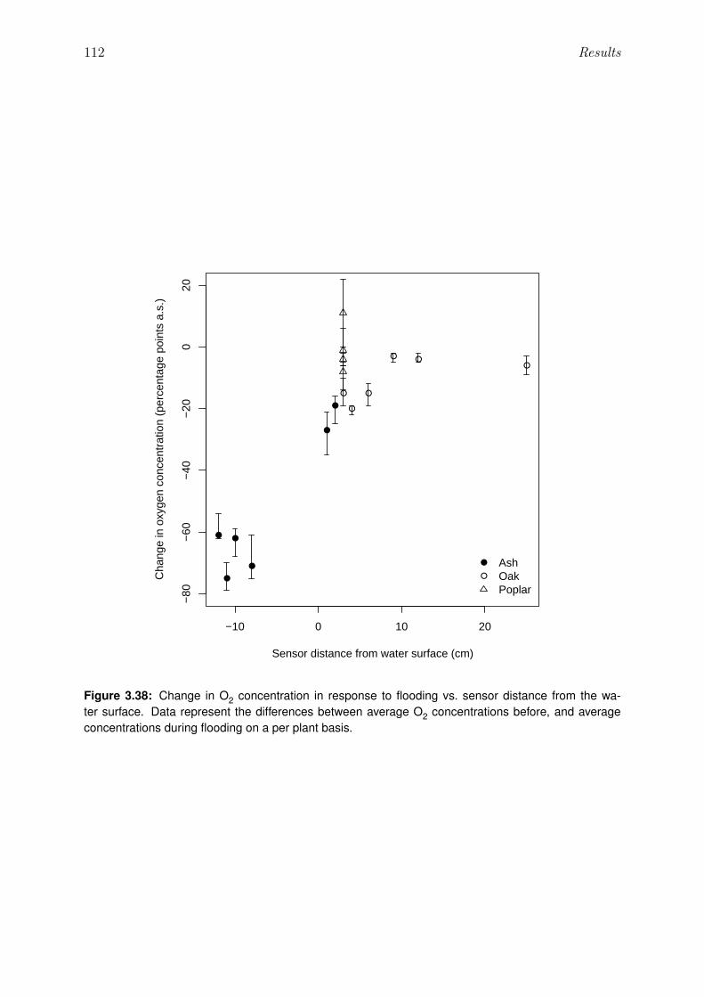
112 Results
−10 0 10 20
−80
−60
−40
−20
020
Sensor distance from water surface (cm)
Cha
nge
in o
xyge
n co
ncen
trat
ion
(per
cent
age
poin
ts a
.s.)
●
●
●
●
●
●
●
●
●
●
●
●
●
●
AshOakPoplar
Figure 3.38: Change in O2 concentration in response to flooding vs. sensor distance from the wa-ter surface. Data represent the differences between average O2 concentrations before, and averageconcentrations during flooding on a per plant basis.

3.5 Experiment V: Effect of flooding on stem-internal oxygen concentrations 113
40
50
60
70
80
90
100O
xyge
n (%
air
satu
ratio
n)
FL
0
1
2
3
4
5
6
Sap
flow
(g
h−−1 s
tem
−−1 )
10
12
14
16
18
20
Air
tem
p. (
°C)
0 2 4 6 8 10
Day of experiment
A
B
C
12:00 14:00 16:00 18:00
4050
6070
8090
100
5:00 7:00 9:00 11:00
4050
6070
8090
100
A1 A2
Figure 3.39: Effect of flooding on stem-internal O2 (A) and sapflow (B) in oak. A three-year-old Q. roburseedling was flooded for the time indicated (dashed rectangle), and within-stem O2 as well as sapflowwere determined as described in Materials and Methods. The O2 concentration was measured ata height of 8 cm above ground, sapflow a few cm above this position. The flood height was 4 cmabove ground. A1, A2, enlarged views of the responses of O2 concentration to flooding and reaeration,respectively. C, temperature of the stem surface. See fig. 3.35 for further explanations.

114 Results
40
50
60
70
80
90
100
Oxy
gen
(% a
ir sa
tura
tion)
FL
0
5
10
15
20
25
Sap
flow
(g
h−−1 s
tem
−−1 )
10
12
14
16
18
20
Air
tem
p. (
°C)
0 2 4 6 8 10
Day of experiment
A
B
C
10:00 12:00 14:00 16:00
020
4060
8010
012
0
10:00 12:00 14:00 16:00
020
4060
8010
012
0
A1 A2
Figure 3.40: Effect of flooding on stem-internal O2 (A) and sapflow (B) in poplar. C, temperature of thestem surface. See fig. 3.39 for further explanations.

3.5 Experiment V: Effect of flooding on stem-internal oxygen concentrations 115
Day of experiment
AD
H a
ctiv
ity (
U g
−−1 F
W)
01
23
4
Ash Maple Oak Poplar
above water
Ash Maple Oak Poplar
below waterControlFlooded
A B
Figure 3.41: Effect of flooding on ADH activity in bark of ash, maple, oak and poplar seedlings. Three-year-old seedlings were subjected to a one-week flooding treatment and ADH activity was determinedin bark samples, as described in Materials and Methods. The bark samples were harvested from twostem positions: above the water (A) and below the water (B), or from comparable positions in the controltrees, respectively. Bars represent means (± SD) of four plants. None of the differences between theflooded and control groups were statistically significant as calculated by t tests (p < 0.05).

116 Results

Chapter 4
Discussion
Common ash (F. excelsior) is one of the most abundant species of the European hardwood
alluvial forest, a habitat that is characterised by regular inundation events. However, the
physiological response of common ash to submergence has received little attention. In
the present study, seedlings of common ash were subjected to various controlled flood-
ing treatments, and hence oxygen depletion of the soil, resembling duration and cycling
of natural flooding regimes. As known from numerous studies (reviewed in Kozlowski,
1997), C metabolism of plants is profoundly altered by oxygen depletion of the soil, which
is reflected by various physiological parameters such as photosynthesis rates and tissue
carbohydrate contents. A range of these sensitive parameters was included in the present
study.
From a fundamental point of view, any adverse effect on C metabolism does in the long
run also affect growth, since anabolic processes are impaired. In the ash investigated
seedlings of the provenances “Alb”, “BFor” and “Rhine”, height and diameter growth was
determined after a total of four weeks of flooding, interrupted by one week of reaeration
which was expected to additionally cause post-anoxic stress. Reduced growth as a result
of this treatment was anticipated, since it covered approx. 30 % of the growing season and
constituted a flooding period that occurs in exceptional years only in the hardwood alluvial
forest. However, neither height nor diameter growth were decreased by this treatment
(fig. 3.16), suggesting that the seedlings adapted well to inundation. Such a conclusion
was supported by other parameters (see below). By contrast, flooding ash seedlings for
the whole growing season (April–September) has been reported to significantly reduce
height growth and biomass increase (Frye and Grosse, 1992; Iremonger and Kelly, 1988).
In the provenance “Rhine”, flooding even led to a significantly increased growth in diam-
eter (fig. 3.16). This may indicate the development of stem hypertrophy, a morphological

118 Discussion
adaptation to flooding that enhances stem-internal aeration (Kawase, 1981), as also ob-
served for F. excelsior by Frye and Grosse (1992). Since this phenomenon was only
observed in the provenance “Rhine”, originating from an alluvial forest, and not in “Alb”
and “BFor”, it may indicate a provenance-specific adaptation to its habitat.
Despite unchanged growth and the development of morphological adaptations such as
hypertrophied lenticels (sec. 3.1.6.3), the seedlings’ vitality was clearly weakened by root-
zone oxygen depletion. Visible damage that became apparent after two times two weeks
of flooding interrupted by one week of reaeration, included chlorophyll degradation, leaf
wilting, reduced leaf number and inhibited formation of new leaves (figs. 3.25 and 3.17).
Similar stress symptoms have been described for many species in response to root hypoxia,
including relatively flood-tolerant species like Ulmus americana (Angeles et al., 1986) and
even Populus deltoides (Cao and Conner, 1999). 30 days of inundation were sufficient to
cause necrosis and leaf shed in the former, while 42 days of flooding resulted in reduced
leaf size, leaf area, leaf number and inhibition of formation of new leaves in the latter
species. In comparison, the degree of injury in common ash did not appear extraordinary,
in particular for “Rhine” and “BFor” (fig. 3.17). By contrast, the provenance “Alb”
was more heavily affected, being the only provenance that showed more than 50 % leaf
shed (fig. 3.17) and also significant chlorophyll loss (fig. 3.25). This provided additional
evidence of a different flood tolerance among the provenances. Chlorophyll degradation
has been connected to diminished Mg2+ uptake from the flooded soil (Talbot et al., 1987).
Leaf wilting has been linked to decreased water absorption by the roots (see Else et al.,
2001).
In addition to leaf damage, root injury was observed after prolonged inundation (fig. 3.19).
Decay of fine roots has mainly been associated with Phytophthora infestation, a hypoxia-
tolerant fungus (Kozlowski, 1997) whose zoospores can be attracted to roots by or-
ganic compounds including ethanol (Tyler, 2002), which can be exudated from flooded
roots. Moreover, root damage may have been aggravated by H2S formation in the soil
(cf. sec. 3.1.6.2), because sulphide is a potent root toxin (Mendelssohn et al., 1981; Koch
and Mendelssohn, 1989). The provenance “Alb” evidently suffered more damage than
“Rhine” or “BFor”, with the roots of this provenance often completely rotten (fig. 3.19).
This supports the conclusion about the differences in flood resistance between the prove-
nances analysed. However, on biomass (FW) basis, such a difference was not confirmed
(fig. 3.20).
Increased diameter growth of the provenance “Rhine” on the one hand, and marked
damage in “Alb” on the other hand, suggested that differences between provenances may
also be reflected by the physiological parameters studied.

4.1 Anaerobic root metabolism 119
4.1 Anaerobic root metabolism
As a measure for anaerobic metabolism of the root, the activity of the enzyme alcohol
dehydrogenase (ADH) was determined. ADH is involved in the biochemical pathway
of ethanolic fermentation which describes the anaerobic conversion of the glycolytic end
product pyruvate to ethanol. In hypoxic plant roots, ethanol is the main product of
pyruvate metabolism while other pathways such lactic fermentation have only minor sig-
nificance (Good and Muench, 1993). In agreement with this, ADH in the most intensely
studied enzyme of anaerobic metabolism (Kennedy et al., 1992).
In the ash seedlings studied, increased activities of ADH were observed as soon as 24 h
after initiation of the flooding treatment (fig. 3.12). This fast induction of the enzyme
indicates that the ash roots became rapidly hypoxic (Sachs et al., 1996; Subbaiah and
Sachs, 2003). The quick response is in agreement with studies for maize roots, which
showed ADH transcript synthesis within 6 h of hypoxia (Andrews et al., 1994a).
Prolonged flooding resulted in a further increase of enzyme activities, reaching values of
4–15 U g-1 FW (figs. 3.12, 3.30). These were comparable to other tree species under
hypoxia, such as flood-tolerant Nyssa sylvatica, Taxodium distichum and Populus spec.
(Pezeshki, 1991; Angelov et al., 1996; Hauberg, 2008) but also flood-intolerant Quercus
species (Angelov et al., 1996; Parelle et al., 2006). Surprisingly, however, ADH activities
remained on this high level even after one week of reaeration. This was in contrast to
rice (Xie and Wu, 1989), the coastal grass Spartina patens (Burdick and Mendelssohn,
1990) and also tree species such as T. distichum (Angelov et al., 1996), all showing a
return of activities to control levels within hours or few days. A retardation may be
caused by poor drainage of soil, however, this did not apply in the present case. Hence,
the maintenance of high activity levels over periods where oxygen is available may be of
ecophysiological significance. In alluvial forests, the fluctuating hydrology may produce
series of oxygen deprivation and availability (Anderson and Pezeshki, 2001). Maintaining
a high expression of anaerobic proteins (ANPs) over periods where oxygen is available
may have the advantage that (1) anaerobic metabolism could commence immediately,
eliminating shortages in energy metabolism, and (2) energy-consuming re-synthesis of
proteins is avoided. Biochemically, this response resembles the “hypoxic pretreatment”
effect, which describes the enhanced anoxic survival of roots after preceding hypoxic
incubation (Andrews et al., 1994a; Bouny and Saglio, 1996; Subbaiah and Sachs, 2003).
In these root tips, ADH activity under anoxia was considerably higher in hypoxically pre-
treated (HPT) tips than in anoxically shocked ones (Saglio et al., 1988; Johnson et al.,
1989). Similarly, ADH activities in flooded ash roots were in part considerably higher
during the second than during the first flooding period. In the provenance “Alb”, for

120 Discussion
instance, activities were almost twice as high as before (fig. 3.12). HPT root tips showed
an overall enhanced tolerance to anoxia, due to higher higher adenylate energy charge
and an enhanced regulation of cytoplasmic pH (Bouny and Saglio, 1996, and references
therein). It may be speculated that similar responses also allowed F. excelsior roots to
adapt to prolonged flooding. This is partly supported by the relatively mild effect of the
second 14-day flooding period on leaf gas exchange and carbohydrate levels which were
less, or not more affected than at the end of the first flooding period.
Absence of provenance-specific differences in ADH activity
Neither the initial increase in ADH activity in response to flooding nor the maintenance
of high activities under prolonged flooding differed significantly among the provenances of
F. excelsior (tab. 3.1) or between F. excelsior and F. angustifolia (fig. 3.30). Therefore,
ADH activity did not seem to be a marker for trees’ flooding tolerance. This is in agree-
ment with manifold ADH responses described in literature (Benz et al., 2007). Originally,
it was assumed that flood-sensitive species responded to hypoxia with higher ADH ac-
tivities than tolerant species (Crawford, 1967; McManmon and Crawford, 1971). Several
studies supported this relationship (Pezeshki, 1991; Naidoo and Naidoo, 1992; Baruch,
1994; De Simone et al., 2002). However, many authors came to the opposite conclusion
(Mendelssohn et al., 1981; Parelle et al., 2006; Keeley, 1979).
The discrepancy in the literature about the relationship between flood tolerance and ADH
activity seems to be, at least, partially due to different flooding durations considered.
Short-term flooding (several days) often causes similar increases in activities in both
flood-tolerant and sensitive species. However, after long-term flooding (several weeks),
the flood-tolerant species sometimes show decreasing activities which is not observed in the
intolerant species (Pezeshki, 1991; Naidoo and Naidoo, 1992; Baruch, 1994; De Simone
et al., 2002; Benz et al., 2007). This can be due to enhanced aeration of root system
by formation of aerenchyma (De Simone et al., 2002; Benz et al., 2007). This activity
pattern of many flood-tolerant species was not reflected by F. excelsior which showed
rather higher than lower activities with prolonged flooding (fig. 3.12). Differences in this
respect between “Alb”, “BFor” and “Rhine” were not suggested by the present findings.
Fate of ethanol
Despite high ADH activities, ethanol, the product of the reaction catalysed by ADH,
mostly remained below the detection limit in flooded ash roots (sec. 3.1.3.2). Low con-
centrations of ≈10 µg g-1 FW have also been reported for relatively flood-tolerant Quer-

4.1 Anaerobic root metabolism 121
cus robur seedlings, whereas ethanol levels increased to 75 µg g-1 FW in Fagus sylvatica
(Schmull and Thomas, 2000). In general, flood-tolerant species seem to avoid ethanol
accumulation in the roots, whereas flood-sensitive species sometimes accumulate this po-
tential cell toxin (Crawford, 1967; McManmon and Crawford, 1971; Monk et al., 1984).
Moreover, build-up of more toxic acetaldehyde after reaeration is prevented (Crawford
and Braendle, 1996). The present findings suggest that ash rates among ethanol-avoiding
species, which may be of particular importance with respect to regular reaeration in al-
luvial environments.
Since ethanol did not accumulate in the roots, it must have been transported to other
tissues or exudated into the water. The results indicated that ethanol, to some degree,
moved up the shoot with the transpiration stream (figs. 3.13B, 3.31B). The concentra-
tions in the xylem sap in some cases exceeded 2 mM (fig. 3.31B) but mostly remained
< 1 mM (fig. 3.13B). In comparison, much higher concentrations have been reported for
Populus deltoides (5 mM; MacDonald and Kimmerer, 1991) and Populus tremula × alba
(> 30 mM; Kreuzwieser et al., 2000). This indicates substantial differences in ethanol
utilisation between flood-tolerant poplar and F. excelsior . In previous studies with Pop-
ulus (MacDonald and Kimmerer, 1993; Kreuzwieser et al., 1999), it has been shown that
the majority of the shoot-transported ethanol (> 95 %) is recycled in leaf C metabolism,
a feature regarded as a flood tolerance mechanism in poplar (Kreuzwieser et al., 1999).
Common ash may lack this feature, suggesting less efficient carbon utilisation under hy-
poxia.
In agreement with its low acropetal transport rates, ethanol did not accumulate in the
leaves (figs. 3.13A, 3.31A), did not cause induction of leaf ADH over constitutive levels
(fig. 3.30A) and was emitted in only small amounts (<100 nmol m-2 min-1) as acetaldehyde
(fig. 3.14). By comparison, emission rates of 350 nmol m-2 min-1 have been reported for
poplar (Kreuzwieser et al., 2000). In agreement with Kimmerer and MacDonald (1987),
constitutive leaf ADH activity was likely sufficient to cope with ethanol arriving at the
leaves.
Interestingly, ethanol transport in the xylem ceased completely after reflooding despite
unchanged or even higher ADH activity (fig. 3.13). This suggested a shift of ethanol
utilisation with repeated flooding, possibly towards increased exudation. The latter has
been shown to be the major path of ethanol removal from the roots flood-tolerant Pi-
nus contarta, Nyssa sylvatica (Hook et al., 1983) and Lotus corniculatus (Barta, 1984).
In general, efficient ethanol exudation has been especially associated with flood-tolerant
species (Barta, 1984), avoiding self-poisoning (McManmon and Crawford, 1971). In-
creased ethanol exudation with repeated flooding may represent an adaptive response,
resembling a certain phenomenon in maize roots. These roots showed efficient efflux of
122 Discussion
lactic acid, another fermentative end product, after hypoxic pretreatment, but not when
anoxically shocked (Xia and Saglio, 1992).
4.2 Photosynthesis
In general, CO2 assimilation was increasingly affected with prolonged periods of flooding.
The critical flood duration to cause clear reductions in light-saturated assimilation (Amax)
appeared to be in the range of four to ten days (figs. 3.1, 3.23). Submergence for up to
three days did not significantly impact photosynthesis (fig. 3.23), or even caused 2 to 4-fold
increases in Amax in comparison with the normoxic controls, a response that coincided with
an up to 8.5-fold increased gs (fig. 3.1). Especially the latter finding was not expected, since
assimilation rates usually decrease within few hours or days of inundation, as reported
for numerous tree species (Gomes and Kozlowski, 1980; Dreyer et al., 1991; Gravatt and
Kirby, 1998; Anderson and Pezeshki, 1999). In highly flood-tolerant F. pennsylvanica,
for instance, stomatal conductance was reduced by 50–75 % within three days of flooding
(Gomes and Kozlowski, 1980; Tang and Kozlowski, 1984). Therefore, it is more likely that
the plants suffered from drought stress in the time before the flooding treatment. This
was implied by the very low gs of less than 10 mmol m-2 s-1 before flooding (fig. 3.1). Upon
supply of the flood water, the stomata may have re-opened, suggesting that the normal
watering frequency was not sufficient to fulfil the high water requirement of common ash
seedlings (Besnard and Carlier, 1990; Carlier et al., 1992).
Longer flooding periods of 10–14 days exacerbated the repression of CO2 assimilation in all
provenances studied. In the provenance “Rhine”, for example, Amax was reduced by 36 %
to 64 % (tab. 3.2). In general, leaf gas exchange is more affected by root-zone hypoxia in
flood-intolerant, than in tolerant species (Pezeshki et al., 1996; Anderson and Pezeshki,
1999). In good agreement with this assumption, leaf gas exchange was tendentially more
reduced in the provenance “Alb” than in “Rhine”. Whilst this difference was statistically
not significant, it is still consistent with the above findings for growth as well as leaf and
root damage, as is the observation that the provenance “BFor” was not more affected
than “Rhine” (tab. 3.2). Furthermore, F. angustifolia was the least affected species,
corresponding well to its reportedly higher flood tolerance in comparison with F. excelsior .
In comparison to other species, the response of leaf gas exchange of F. excelsior resembled
those of flood-tolerant rather than flood-sensitive species. Flood-tolerant species like
Fraxinus pennsylvanica and Quercus nigra, for example, showed reductions in assimilation
by 55–60 %, after comparable flooding periods as in the present study (Gravatt and Kirby,
1998). In Quercus lyrata, a more sensitive species, assimilation was reduced by 75 %

4.2 Photosynthesis 123
(Pezeshki et al., 1996), in moderately tolerant Acer rubrum by around 65 % (Anella and
Whitlow, 2000), but even in highly flood-tolerant Taxodium distichum, assimilation was
still reduced by 30 % after two weeks of submergence (Pezeshki et al., 1996). However, the
apparently low reduction of leaf gas exchange of ash in comparison to other species was
not supported by the findings for other species in the present study (figs. 3.32, 3.33). As
expected, 14-day flooding had no significant effect on the photosynthetic performance of S.
purpurea, the most flood-tolerant of the species tested, as indicated by unchanged light and
CO2 saturated assimilation rates (Amax light, Amax CO2), unchanged apparent quantum yield
(Aqe) and carboxylation efficiency (ε) as well as unchanged light (LCP) and CO2 (CCP)
compensation points (figs. 3.32 and 3.33). By contrast, F. excelsior showed strongly
decreased Amax light (−50 %) and even significantly decreased ε (−57 %). Unexpectedly,
T. cordata, a species described as only slightly tolerant to flooding (Glenz et al., 2006),
displayed less interference of flooding with photosynthesis than F. excelsior (figs. 3.32,
3.33). The reason for this difference between lime and ash remained unclear, and requires
further investigation. The tendentially higher flood tolerance of Q. robur compared to
F. excelsior , again, was in agreement with a previous study of the two species (Vreugdenhil
et al., 2006).
Responses to reaeration and reflooding
Studying the effects of reaeration and reflooding on photosynthesis is of great ecological
importance, since hydrology undergoes strong fluctuations in alluvial forests (cf. An-
derson and Pezeshki, 1999). Flood-tolerant species like F. pennsylvanica (Gomes and
Kozlowski, 1980) or Populus deltoides (Regehr et al., 1975) are capable of recovering
stomatal conductance to pre-flooding levels within 3–5 days after reaeration of the soil.
By contrast, moderately tolerant Q. robur showed no clear recovery within one week of
flooding (Dreyer et al., 1991), a phenomenon attributed to a lack of recovery of root hy-
draulic conductance (Davies and Flore, 1986). For common ash, whose flood tolerance
resembles that of Q. robur , similar results were expected. However, neither of the prove-
nances “Alb” and “Rhine” showed increasing Amax after the flooding treatment (fig. 3.1).
Surprisingly, the opposite was observed for “BFor” (fig. 3.1), which clearly contradicted
the initial hypothesis that the alluvial provenance (“Rhine”) is best adapted to flooding.
Given the absence of a clear recovery in “Alb” and “Rhine”, leaf gas exchange was ex-
pected to be increasingly affected by repeated flooding. However, three days after re-
flooding, gs increased over control levels, similar to the response during the first flooding
period. This suggested that the plants were still able to profit from the enhanced water
availability. Moreover, 14 days after reflooding, photosynthesis rates in “Alb” (70 % of
control), “Rhine” (107 %) and “BFor” (67 %) were even less affected than on day 14 of

124 Discussion
the first flooding period. This indicates a good adaptation of leaf gas exchange to pro-
longed flooding. It may be speculated that the first flooding period had a similar effect
as described by Anderson and Pezeshki (2001) for flood-tolerant bald cypress (Taxodium
distichum). Seedlings of this species, subjected to multiple, short flooding events, main-
tained higher levels of stomatal conductance during subsequent continuous flooding than
plants directly exposed to continuous flooding. This effect was termed “flood hardening”
following the terms for cold or drought hardening (Anderson and Pezeshki, 2001) and
may also be responsible for the present observations with ash seedlings.
Similarly, stomatal adaptation to continuous oxygen deprivation at the roots has been
described for other tolerant species such as F. pennsylvanica (Gomes and Kozlowski,
1980) and Populus deltoides (Regehr et al., 1975). These tree species exhibited initially
depressed gs, but stomata re-opened with prolonged flooding. It may be assumed that
F. excelsior behaved similarly, even though it did not develop adventitious roots, which
seemed to be required for stomatal reopening in F. pennsylvanica (Gomes and Kozlowski,
1980). Surprisingly, all provenances performed equally well during the second flooding
period. A stronger impact on “Alb”, as may have been anticipated after the previous
results, was not observed.
Marigo et al. (2000) described that F. excelsior exhibits generally little control over stom-
atal aperture, resulting in relatively high gs under severe drought stress. This stomatal
behaviour is typical of “tolerators” (as opposed to “avoiders”; Ludlow, 1989) and might
have contributed to the maintenance of relatively high gs under prolonged flooding. It
may retain high CO2 assimilation rates, even when water uptake is limited by decreased
hydraulic conductivity of the hypoxic root (Else et al., 2001; Tournaire-Roux et al., 2003).
Factors limiting assimilation
The mostly parallel course of Amax and gs (fig. 3.1) suggested that Amax was mainly limited
by stomatal conductance. However, a plot of Amax vs. gs revealed only low correlations
between the two parameters (fig. 3.3). Thus, non-stomatal factors such as (1) leaf chloro-
phyll degradation, (2) reduced Rubisco contents and/or activity, (3) decreased leaf water
potential and (4) disturbed photosynthate transport were most probably also involved
(see Pezeshki et al., 1996). Significant chlorophyll degradation by around 30 % was found
for “Alb” after 10 days of flooding, which might explain the particularly strong decrease
in Amax after this flooding duration (13 % of control; fig. 3.24). Decreased Rubisco activ-
ity can also be assumed, since soluble leaf protein levels were reduced by 35 % (“Alb”)
to 59 % (“Rhine”) and Rubisco constitutes up to 50 % of total soluble leaf protein (see
Larcher, 2001). This was supported by the lower saturation level of the light response

4.3 Carbohydrate metabolism 125
curve (fig. 3.32) and the significantly reduced apparent carboxylation efficiency (fig. 3.33)
(Larcher, 2001). Reduced leaf water potential (Ψl) was indicated by incipient wilting, in
particular for “Alb” (cf. section 3.1.6.1). Accumulation of photoassimilates in the leaves
was also observed and will be discussed below.
4.3 Carbohydrate metabolism
Plant carbohydrate metabolism is crucially determined by rates of photosynthetic carbon
assimilation (source) on the one hand, and carbohydrate consumption in sink tissues on
the other hand. The present results showed that carbon fixation was strongly depressed
by root-zone oxygen depletion, suggesting decreased amounts of carbohydrates available
for respiration, growth and reserve build-up. At the same time, strongly elevated root
ADH levels as in the ash seedlings investigated, may result in accelerated glycolytic flux
and thereby accelerated assimilate consumption (known as “Pasteur effect”; Drew, 1992).
Flooding was therefore expected to alter assimilate partitioning on the whole-plant level.
Root carbohydrate metabolism
In the roots, soil oxygen depletion for 10–14 days mainly caused accumulation of solu-
ble sugars, as well as in the other plant parts studied (fig. 4.1). Such increased soluble
carbohydrate levels in flooded roots may surprise since accelerated channelling of sug-
ars into glycolysis often results in depletion of respirable substrates (Drew, 1992; Saglio
and Pradet, 1980; Vartapetian and Jackson, 1997, see Introduction). For tree species,
decreasing carbohydrate contents in response to flooding have been reported for roots of
flood-tolerant Picea mariana and Larix laricina (Islam and Macdonald, 2004) as well as
of non-tolerant Fagus sylvatica (Kreuzwieser et al., 2004). Also, isolated (“excised”) root
tips of maize, as well as intact roots of wheat survived longer periods of anoxia when
the incubation medium was supplemented with glucose, suggesting that the supply of
carbohydrates was critical for survival (Drew, 1997).
The observed increase in soluble sugars contents in flooded ash roots may imply either
(1) increased sugar import from the phloem, (2) increased starch reserve mobilisation,
(3) globally reduced consumption rates (growth, respiration), (4) reduced export into the
xylem or any combination of these causes. Increased photoassimilate import from the
phloem seemed unlikely, due to strongly depressed net assimilation, as well as restricted
carbon export from leaves (see below) of flooded trees. Accelerated mobilisation of root
starch reserves was indicated for “Alb” and F. angustifolia by starch content reductions

126 Discussion
Assimilation: 80 %
BFor
Phloem:HexSuc 133 %Mann 154 %
Leaf:HexSuc 62 %Mann 71 %Starch n.d.
Root:HexSuc 223 %Mann 358 %Starch n.d.
Xylem:HexSuc 138 %Mann 122 %
Assimilation: 13-35 %
Alb
Phloem:HexSuc 201-721 %Mann 236-241 %
Leaf:HexSuc 63-170 %Mann 90-188 %Starch 215 %
Root:HexSuc 60-78 %Mann 215-232 %Starch 27 %
Xylem:HexSuc 493 %Mann 514 %
Assimilation: 62 %
F. angustifolia
Phloem:HexSuc 781 %Mann 209 %
Leaf:HexSuc 114 %Mann 83 %Starch 107 %
Root:HexSuc 222 %Mann 286 %Starch 27 %
Xylem:HexSuc 406 %Mann 152 %
Assimilation: 36-64 %
Rhine
Phloem:HexSuc 236-242 %Mann 210-241 %
Leaf:HexSuc 98-150 %Mann 93-163 %Starch 56 %
Root:HexSuc 111-178 %Mann 193-238 %Starch 284 %
Xylem:HexSuc 101-289 %Mann 86-238 %
Figure 4.1: Alteration of carbohydrate contents by flooding. 10–14 days of root-zone oxygen deple-tion resulted in depressed net assimilation rates, while carbohydrate contents in leaf and root, as wellphloem exudates and xylem sap remained unchanged or increased. HexSuc, hexose+sucrose contentof flooded plants, expressed as percent of normoxic controls; Mann, mannitol content of flooded plants,expressed as percent of normoxic controls. Data compiled from figs. 3.5, 3.7, 3.9, 3.11 and tab. 3.3.
by each 63 % (fig. 3.29). By contrast, the provenance “Rhine” showed an almost three-fold
increase in starch contents (fig. 3.29). This observation for both the most flood-sensitive
provenance of F. excelsior (“Alb”) and the flood-tolerant F. angustifolia indicated that

4.3 Carbohydrate metabolism 127
starch utilisation in flooded ash roots was not related to flood tolerance. This contradicts
findings for other tree species, which suggested more efficient starch utilisation under
hypoxia in flood-tolerant compared to non-tolerant species (Gravatt and Kirby, 1998;
Kreuzwieser et al., 2004).
Decreased substrate consumption may occur under circumstances of reduced resource
demand, e.g. with diminished growth rates. A well characterised effect of flooding is
the rapid inhibition of root elongation, as demonstrated for flood-sensitive economic
plants such as wheat (Huang et al., 1997) and potato (Biemelt et al., 1999), but also
for flood-tolerant trees, e.g. bald cypress (Taxodium distichum; Pezeshki, 1991). Reduc-
tion of energy-consuming processes in hypoxic roots, such as biosynthesis of proteins and
structural carbohydrates, have been demonstrated (Saglio and Pradet, 1980; Barta, 1987;
Kogawara et al., 2006) and interpreted as the cause for carbohydrate accumulation in
flooded roots of numerous different species (Albrecht et al., 1993; Albrecht and Biemelt,
1998; Biemelt et al., 1999; Schlueter and Crawford, 2001). Similarly, growth of flooded
F. excelsior roots may have slowed or ceased in oxygen-depleted soils, leading to reduced
substrate demand and thereby to the observed accumulation of soluble carbohydrates.
Decreased root growth was strongly suggested by fine root decay (sec. 3.1.6.2), therefore
supporting this hypothesis.
Highly increased ADH levels and simultaneously reduced carbohydrate consumption are
not necessarily contradictory, as demonstrated for maize (Andrews et al., 1994b), potato
(Biemelt et al., 1999) and wheat (Albrecht et al., 2004). These studies showed that high
expression and in vitro activity of fermentative enzymes are not automatically paralleled
by increased glycolytic fluxes, and that enzymes of glycolysis and ethanolic fermentation
are not induced in equal measures but differentially. Similarly, glycolytic sugar break-
down in flooded ash roots may have remained on a low level despite high in vitro ADH
activity. However, more detailed biochemical investigations are needed to substantiate
this assumption.
Since starch played an unclear role as reserve carbohydrate under flooding, other reserve
compounds may be more important for flooded ash roots. Such a role was indicated
for the sugar alcohol mannitol. Among the carbohydrates analysed, the concentrations
of mannitol increased the strongest under oxygen depletion, resulting in a significant
change in the composition of soluble carbohydrates in the roots. The ratio of mannitol
to combined hexose and sucrose contents changed markedly from 0.51 to 2.59 in the
provenance “Alb”, from 0.87 to 3.71 in “Rhine” and from 0.92 to 1.36 in F. angustifolia
(cf. tab. 3.3). This change suggested that mannitol utilisation differed clearly from that
of sucrose or hexoses in flooded ash roots.
A possible biochemical basis for such a differential regulation is suggested by insights into
128 Discussion
carbohydrate metabolism of other mannitol-synthesising species such as celery (Apium
graveolens). This agricultural plant shows a strong accumulation of mannitol as soon
as transferred to high salinity (Stoop and Pharr, 1994), an effect due to specific down-
regulation of mannitol dehydrogenase (MTD), the enzyme catalysing mannitol breakdown
(Stoop and Pharr, 1993; Pharr et al., 1995). Since MTD is repressed by high sugar
concentrations (Pharr et al., 1995), sucrose is preferentially metabolised under normal
conditions, leaving sufficient mannitol reserves for possible stress situations (Stoop et al.,
1996). This pays off advantageously for plants due to mannitol’s property as a compatible
solute, which allows for tissue adaptation to salt stress by osmotic adjustment (Stoop
et al., 1996). Due to this regulation, mannitol reserves are saved until sucrose reserves
become exhausted (Stoop et al., 1996). A preferential use of sucrose over mannitol may
explain why, in the present study, mannitol concentrations remained on a high level even
when sucrose contents were slightly reduced, as occasionally observed in the flooded ash
seedlings (e.g. after 10-day flooding in “Alb” and “Rhine”; tab. 3.3).
Mannitol’s osmotic properties may be important under flood stress, just as they are under
conditions of high salinity. Hypoxia causes drastically decreased hydraulic conductivity of
roots (Else et al., 2001; Tournaire-Roux et al., 2003). Roots accumulate other compatible
solutes (e.g. amino acids) not only under salt (Ogawa and Yamauchi, 2006) but also under
drought stress (Parker and Pallardy, 1988). Osmotic adjustment is a common adaptation
to these circumstances, preventing water loss from tissue by increasing the cellular con-
centrations of osmolytes. In addition, an important role of mannitol in this process has
been demonstrated in several drought stress studies with F. excelsior (Guicherd et al.,
1997; Patonnier et al., 1999; Peltier and Marigo, 1999; Oddo et al., 2002).
The observation that mannitol accumulated to a similar extent in all provenances of F. ex-
celsior indicated that this response was no particular feature of flood-adapted ecotypes.
This is in agreement with osmotic adjustment representing a general response to various
environmental stress types (salt stress, drought stress), rather than a specific adaptation
to a particular stress such as oxygen deprivation (cf. Stoop et al., 1996). It is therefore
not surprising that “Alb” and “BFor” showed similarly increased mannitol contents upon
flooding as “Rhine”.
Carbohydrate concentrations in the xylem sap
Flooding did not only cause increased carbohydrate contents within the root system,
but apparently also increased sugar export into the xylem sap. In the xylem sap of
flooded trees, up to 8× higher TSC concentrations were found in comparison to well-
drained plants (figs. 3.11, 3.28B). The general amount of carbohydrates in the xylem

4.3 Carbohydrate metabolism 129
sap (corresponding to C contents of approx. 50–200 mM; fig. 3.28B) was comparable to
findings for Quercus robur seedlings (50–500 mM C) (Heizmann et al., 2001). In oak, the
carbohydrate composition is dominated by sucrose (Heizmann et al., 2001), whereas the
high percentage of mannitol (70–86 % of TSC) seemed to be ash-specific. This high portion
of xylem mannitol is in accordance with previous reports for F. excelsior (Patonnier et al.,
1999).
The role of sugars in the xylem sap has received little attention in flood tolerance research
(cf. Kreuzwieser et al., 2004). Higher sugar concentrations increase the osmolality of the
xylem sap (Jackson et al., 1996). It is well-known that trees secrete sugars into the
xylem sap via the contact parenchyma under ambient conditions of limited transpiration
stream, e.g. high air humidity (see Sitte et al., 1991, p. 200). This secretion enhances
the osmotic force of the xylem sap and thereby facilitates acropetal water flow. Increased
osmolyte concentrations originating from flooded roots can enhance the xylem flux in
hypoxic tomato plants (Jackson et al., 1996). Thus, increased sugar concentrations in
the xylem sap of F. excelsior seedlings possibly contributed to the maintenance of a
high transpiration stream, counteracting decreased stomatal conductance (fig. 3.1), and
potentially decreased root hydraulic conductance.
Apart from osmotic properties, carbohydrate in the xylem sap may represent a significant
portion of the shoot’s C pool (Heizmann et al., 2001). In pedunculate oak (Quercus
robur), for example, 8–91 % of leaf C did not stem from photosynthesis but from xylem
delivery of carbohydrates (Heizmann et al., 2001). This percentage was highest when
photosynthesis was low, e.g. during midday depression of assimilation. According to
these authors, C from the transpiration stream may supply leaves with low CO2 fixation
rates with sufficient amounts of substrates for respiration. Similarly, ash leaves with low
CO2 fixation rates due to flood stress, may have been supplied with additional C from
the xylem sap.
The high portion of mannitol in the xylem sap of F. excelsior has led to the speculation
that mannitol may be involved in root-to-shoot signalling, exerting control over stomatal
aperture (Patonnier et al., 1999). However, such a function could, in contrast to malate,
another important xylary constituent in ash, not be substantiated (Patonnier et al., 1999).
Thus, mannitol in the xylem sap of flooded plants may contribute to whole-plant C cycling
similar to sucrose (Heizmann et al., 2001).

130 Discussion
Leaves
The described effect of inundation on carbohydrate levels in the roots was accompanied by
either unchanged (fig. 3.4) or increased (fig. 3.23A) carbohydrate contents in the leaves.
This accumulation is in agreement with the above hypothesis that the roots’ sink strength
was weakened by flooding. Accumulation of photoassimilates may reflect reduced phloem
translocation of leaf sugars to sink tissues (Wample and Davis, 1983; Gravatt and Kirby,
1998). This was indicated by different physiological responses concerning leaf carbohy-
drate contents on the one hand, and root growth on the other hand, among tree species of
different flood tolerance. In flood tolerant Nyssa aquatica, for example, the maintenance
of active root growth coincided with the maintenance of low leaf carbohydrate levels,
whereas flood-sensitive Quercus alba showed reduced root growth and a comparatively
stronger leaf carbohydrate accumulation (Gravatt and Kirby, 1998).
In the present study, reduced assimilate transport from source leaves to sinks was sup-
ported by the finding of 13C accumulation in 13C-glucose fed leaves (tab. 3.5). 13C-glucose,
fed into source leaves via secondary vein flaps (Biddulph and Markle, 1944), was assumed
to be incorporated into the cytoplasmic C pool and exported as 13C-sucrose (or other
translocated sugars). The detection of 13C label in phloem exudates (fig. 3.34) supported
this assumption. Hence, accumulation of 13C in the leaves indicated that leaf export of
photoassimilates was inhibited by root-zone inundation.
Unexpectedly, this inhibition of leaf export was most clearly seen in flood-tolerant poplar,
while in flood-sensitive Acer pseudoplatanus as well as in F. excelsior , export rates were
obviously less affected (tab. 3.5). This contradicted the assumption that phloem trans-
port is less affected in flood-tolerant as compared to sensitive species (Gravatt and Kirby,
1998). Moreover, the finding was in contrast to the results of Kogawara et al. (2006), who
observed a failure to export assimilates in a flood-sensitive species (Eucalyptus camaldu-
lensis) but not in tolerant Melaleuca cajuputi. Possibly, the unexpected finding for poplar
was due to species-specific differences in age or developmental stage of the leaves between
poplar on the one hand, and ash and maple on the other hand. This assumption is based
on the fact that leaf age determines whether leaves are net carbon sources or net sinks
(Turgeon, 2006). The transition of leaves from from sink to source status occurs when
they are about approximately half grown (Turgeon, 2006). Poplar had a high number of
relatively small leaves, which likely exported less assimilates than the large, mature leaves
of ash and maple. This was supported by the high amount of 13C label remaining in leaves
of well-drained poplar, compared to leaves of well-drained ash and maple (tab. 3.5).
In ash, additionally to reduced sink demand from the hypoxic roots, substrate consump-
tion in other parts of the plants was possibly also weakened. Formation of new leaves, for

4.3 Carbohydrate metabolism 131
example, a process claiming a considerable portion of seedlings’ resources (see e.g. Ko-
gawara et al., 2006), was clearly inhibited (fig. 3.17). By contrast, an effect of flooding
on height growth was not observed (fig. 3.16). Also, an effect of flooding on respiration
of source leaves was not detected, as indicated by unchanged dark respiration rates of
the leaves (fig. 3.33). If leaf growth or maintenance metabolism had been significantly
affected by root-zone inundation, decreased respiration rates due to overall reduced ATP
demand would have been a possible consequence.
Apart from the unexpected findings for leaf assimilate export in P. tremula × alba, the
differences in carbohydrate accumulation between the provenances of F. excelsior are
in agreement with the hypothesis that the maintenance of low leaf carbohydrate levels
is an indicator for flood tolerance (Vu and Yelenosky, 1991; Gravatt and Kirby, 1998).
The provenance “Alb”, at least under the test conditions of experiment II, showed the
strongest accumulation in leaf carbohydrates of the three provenances after 10 days of
flooding, while “Rhine” showed intermediate and F. angustifolia no accumulation of car-
bohydrates (fig. 3.27). In addition, a considerable increase in leaf starch was only detected
in “Alb” (fig. 3.29). Together, this suggested that phloem transport was most disturbed
in “Alb”, and to lesser degrees in “Rhine” and F. angustifolia, which is in accordance
with the assumed flood tolerance ranking “Alb” < “Rhine” < F. angustifolia. However,
this assertion was not matched by the observations for short-term (3-day) flooding, where
F. angustifolia showed an accumulation of carbohydrates that was similar to that of “Alb”
and “Rhine” (fig. 3.27). This unexpected effect of short-term flooding indicated that fac-
tors other than the described sink effects must play a role in leaf assimilate accumulation.
One of these factors might be increased sugar import from the xylem, as already pointed
out above.
As a consequence of increased leaf photoassimilate levels, photosynthesis may be depressed
through mechanisms of feedback inhibition (Paul and Foyer, 2001). The maintenance of
low leaf assimilate contents may therefore be an important prerequisite for continued
carbon assimilation at high rates. Increased levels of photoassimilates in the leaves of
the flooded ash plants may have contributed to diminished photosynthesis rates (figs. 3.1,
3.23; see above). For the same reason, the relatively low assimilate levels after 10 days
of flooding in F. angustifolia may have allowed this species to retain higher assimilation
rates than F. excelsior (fig. 3.23). This property of F. angustifolia possibly contributes
to its higher flood tolerance in comparison with F. excelsior .

132 Discussion
Phloem
In the phloem, carbohydrates assimilated in photosynthetically active source leaves are
translocated over long distances to heterotrophic tissues, such as roots and developing
leaves. In well-drained plants, CO2 fixation rates were high, and photoassimilates were
loaded into the phloem at normal rates. By contrast, decreased photoassimilate export
from leaves of flooded plants implied that phloem loading rates were reduced in comparison
to the normoxic controls. Surprisingly, phloem carbohydrate levels were found to be
strongly increased in response to root-zone inundation (figs. 3.8, 3.28B; fig. 4.1). Since
phloem carbohydrate concentrations are modulated by the rate of loading on the one
hand, and (1) unloading rates, (2) transport velocity and (3) consumption for growth as
well as respiration on the other hand (Giaquinta, 1983; Lalonde et al., 2003), this result
indicated that at least one of these factors was more affected by flooding than assimilate
export from leaves.
As pointed out above, sink strength of roots was assumed to be reduced by flooding. Rates
of unloading of phloem carbohydrates to roots may have therefore decreased. Symplastic
unloading of sucrose requires a high concentration gradient between phloem path and
roots tips, which is normally maintained by active root metabolism (Lalonde et al., 2003).
However, if root metabolism is decelerated by hypoxia, unloading may be significantly
affected (Barta, 1987). Moreover, the disturbance of unloading may be aggravated by
hypoxia-induced damage to cell structures such as plasmodesmata (Saglio, 1985).
As far as the translocation velocity is concerned, several studies indicated that this may
also be affected by flooding. In the flooded section of the stem, access to atmospheric
oxygen is eliminated by the surrounding flood water, resulting in increasingly hypoxic
conditions in the phloem (cf. Dongen et al., 2003). Under these conditions, translocation
of solutes in the phloem can be strongly inhibited, at least for temporary periods as
shown for squash (Cucurbita melopepo torticollis Bailey; Sij and Swanson, 1973), sugar
beet (Beta vulgaris ; Cataldo et al., 1972) and Ricinus (Dongen et al., 2003). Therefore,
in the present study, inhibition of sugar translocation by hypoxia may have occurred in
the flooded section of the stem which covered approx. its lower 15 cm. In agreement with
this, phloem translocation of 13C was obviously diminished as indicated by accumulation
of feeding-derived 13C in the upper stem segments of ash (fig. 3.34). As expected, this
effect was not ash-specific but also affected maple seedlings (fig. 3.34). The latter may
have been expected to exhibit more retarded 13C translocation than F. excelsior , due to
its higher sensitivity to flooding. However, such differences between species are probably
very small and, thus, were impossible to detect in the present study, given the large
fluctuation of 13C translocation among specimens (see fig. 3.34).

4.3 Carbohydrate metabolism 133
Unexpectedly, carbohydrate accumulation in the phloem did not differ clearly between
the F. excelsior provenances or F. angustifolia (fig. 4.1). This indicated that the de-
scribed effects of hypoxia on sink and phloem path did not substantially differ between
the ash provenances and species, despite varying flood tolerance. One might argue that
these differences in flood tolerance are gradual and are not reflected sensitively enough
by the parameters tested. However, this is in contrast to other studies (e.g. Kogawara
et al., 2006), which found substantially different patterns of assimilate translocation be-
tween flood-tolerant and sensitive tree species. Therefore, it is concluded that F. excelsior
provenances and F. angustifolia do only marginally differ in parameters related to C sup-
ply to flooded roots. This indicates that physiological aspects other than the investigated
ones may be more important for determining the different degrees of flood tolerance ob-
served (see “Future research”).
Carbohydrate metabolism — methodological considerations
Range of carbohydrate concentrations in phloem exudates In comparison to other
studies, the total concentration of sugars in the phloem exudates was relatively low. For
poplar and beech, for example, 2–3 times higher concentrations were found (Herschbach
et al., 2005; Geßler et al., 2004). This difference is likely due to the different composition
of sugars translocated in common ash. Members of the genus Fraxinus are known to
translocate oligosaccharides of the raffinose family (RFOs) which occur in similarly high
concentrations as mannitol and sucrose (Zimmermann, 1957; Trip et al., 1963). RFOs
were not included in the sugar analysis of the present study (cf. sec. 2.4.5.3). Therefore,
the total concentration of soluble carbohydrates might have been two to four times higher
than determined in the present study, explaining the difference to species like poplar and
beech.
Presence of reducing sugars in phloem exudates The presence of glucose in consid-
erable amounts (up to 15 % of TSC; fig. 3.8) was surprising, since reducing sugars are
usually not rated among the translocated sugars (Hall and Baker, 1972). Also, Zimmer-
mann (1957) did not find hexoses in the phloem sap of Fraxinus. Their presence might
be the result of invertase activity which, originating from injured adjacent cells of the
phloem (Giaquinta, 1983), degrades sucrose to glucose and fructose. Although invertase
activity was previously not found under the experimental conditions used (Bartels, 2001;
Schulte, 1998), reducing sugars in concentrations of up to 5 % of TSC were also detected
in phloem exudates of beech (Geßler et al., 2004). A recent publication pointed out that
translocation of hexose sugars may not be as unusual as previously thought (van Bel and
Hess, 2008).
134 Discussion
Diverging carbohydrate concentration ranges in experiments I and II Considerably dif-
ferences in carbohydrate concentrations measured in experiments I and II were observed.
These were not due to technical issues as re-examination by HPLC analysis confirmed
the differences. Thus, (1) the different age of the plants, three years in experiment I
and four years in experiment II, might have played a role, although this assumption is
not supported by other studies (Donaldson et al., 2006). (2) Seasonal variation might
explain a certain variation since experiment I began in mid-May, four weeks earlier than
experiment II (cf. Schaberg et al., 2000; Wong et al., 2003). (3) Different experimental
conditions might have had the largest impact. Poor light supply in experiment I possibly
resulted in reduced CO2 assimilation and thereby lower carbohydrate concentrations in
general.
Flap feeding of 13C-glucose Flap feeding, a technique introduced by Biddulph and
Markle (1944), has been used extensively in studies of metabolism and translocation
of isotopically labelled sugars (Trip et al., 1965; Trip and Gorham, 1968; Goldsmith et al.,
1974; Bieleski and Redgwell, 1985). As external application of sugars to the surface of
intact leaves (Nelson and Gorham, 1957) was not an option because sugar uptake through
the cuticle obviously does not work for ash leaves (Trip et al., 1965), 13C-glucose was fed
through a cut flap. Photosynthesis under a 13CO2 atmosphere, as used by (Kogawara
et al., 2006), for example, was a worthwhile, though technically sophisticated alternative.
Moreover, flap feeding and 14CO2 assimilation were shown to deliver comparable results
in terms of range, composition and translocation of labelled sugars (Trip et al., 1965).
13C-glucose, used in the present study to follow the fate of photoassimilates, was readily
taken up by the leaves. It was assumed that it was converted to sucrose (and/or other
translocated carbohydrates) and loaded into the sieve tubes. Experimental evidence for
the occurrence of these conversions came from a previous translocation study (Saglio,
1985, and references therein). The fact that F. excelsior does not only translocate su-
crose but also mannitol and RFOs, while both maple and poplar appear to translocate
mainly sucrose (Zimmermann, 1957), raised the question whether 13C-glucose might be
differently metabolised among the three species. Trip et al. (1965) showed that a large
numbers of sugars are interconverted within the leaf. In particular, 14C-fructose was
partly converted to 14C-mannitol as well as 14C-RFOs. Moreover, mannitol has been sug-
gested to be synthesised from the cytoplasmic triose-P pool (Rumpho and Kennedy, 1983;
Loescher, 1987; Loescher et al., 1992). Therefore, in F. excelsior , glucose conversion to
translocatable carbohydrates other than sucrose could be assumed.

4.4 Stem-internal O2 concentrations 135
4.4 Stem-internal O2 concentrations
Previous studies with different species showed that root anoxia caused decreased O2 con-
centrations in the stem (del Hierro et al., 2002; Gansert, 2003). Diminished aeration of
the stem may on the one hand become critical for energy metabolism of the sapwood,
with possible consequences for growth and vitality of the tree (see Gansert, 2003; Spicer
and Holbrook, 2005). On the other hand, O2 diffusion through the stem has been shown
to be an important characteristic of flood-tolerant species, as it allows for O2 supply to
the flooded roots and thereby for aerobic respiration in a hypoxic environment (Arm-
strong, 1968; Hook and Brown, 1972; Colmer, 2003). As shown in the present study,
ash roots flooded for prolonged periods retained high fermentation rates, suggesting low
root aeration and the absence of morphological adaptations enhancing root O2 supply.
Stem-internal O2 concentrations were therefore investigated in ash and compared to an
equally (Q. robur) and a more flood-tolerant (P. tremula × alba) species.
For O2 detection, the relatively modern technology of O2 micro-optodes (Holst et al.,
1997; Klimant et al., 1997) was deployed in the present study. This approach has been
successfully used in several stem O2 studies (Gansert et al., 2001; Gansert, 2003; del
Hierro et al., 2002; Dongen et al., 2003; Spicer and Holbrook, 2005; Sorz and Hietz, 2006).
Due to its sensitivity, the method permits a high spatial and temporal resolution. Unlike
Clark-type micro-electrodes with similar sensitivity (Aguilar et al., 2003), it does not
consume O2 during the measurement. The latter feature was an essential prerequisite
for the present study, because O2 determinations were carried out for up to 12 days at
identical measuring positions. With such long measurements, Clark-type electrodes may
have produced technical artefacts.
The relatively simple method of inserting the sensor into the stem (see Materials and
Methods, sec. 2.6) appeared appropriate, as indicated by short adaptation (figs. 2.12) and
response times upon environmental changes (fig. 3.36). Technically similar approaches
have been applied by Spicer and Holbrook (2005) and Mancuso and Marras (2003).
Range of O2 concentrations
O2 concentrations in unflooded stems amounted to 70–95 % air saturation (a.s.). This
was comparable to ranges for seedlings of 5-year-old Betula pubescens (Gansert, 2003)
and 7-year-old Laurus nobilis (del Hierro et al., 2002). Considerably lower values (9–
35 % a.s.), however, were found in 4-year-old Olea europea trees (Mancuso and Marras,
2003). In adult trees, stem-internal O2 varies between concentrations of 9 % a.s. to 100 %

136 Discussion
a.s. (Eklund, 1990, 1993, 2000; Gansert et al., 2001; del Hierro et al., 2002; Spicer and
Holbrook, 2005) and is strongly influenced by seasonal fluctuations. In Quercus robur
and Acer platanoides, for instance, summer O2 concentrations (25–30 % a.s.) were two to
three times lower than concentrations in spring or autumn (75–80 % a.s.), likely due to
more intense sapwood metabolism (Eklund, 1993).
Effect of flooding on stem-internal O2 concentrations
Root submergence resulted in decreased stem O2 concentrations in ash and maple, but
not in poplar (fig. 3.35, tab. 3.6). In the literature, only few studies have investigated
the influence of root anoxia on stem O2 concentrations. For example, Betula pubescens
saplings showed a reduction in sapwood O2 concentrations from ≈80 to ≈30 % a.s. in
response to root-zone oxygen depletion (Gansert, 2003). Similarly, del Hierro et al. (2002)
managed to manipulate stem-internal O2 concentrations in Laurus nobilis by varying soil
water contents, with concentrations ≈20 % lower at high soil moisture. Whilst similar
reductions were found for ash and oak seedlings in the present study, the results are
difficult to compare, due to different age of specimens and different experimental setups.
Several studies provided evidence that stem-internal O2 concentrations are closely corre-
lated with sapflow velocity (Eklund, 1990, 1993; Eklund and Lavigne, 1995; Eklund, 2000;
Gansert et al., 2001; Gansert, 2003; Mancuso and Marras, 2003). Flooding is known to
reduce sapflow rates, due to diminished transpiration and root water uptake (Else et al.,
1996, 2001; Tournaire-Roux et al., 2003). In addition, the water in flooded soils contains
considerably less O2 than in aerated soils (Spicer and Holbrook, 2005).
Thus, the reduced O2 concentrations in ash and oak may be explained by less intense
O2 supply with the sapstream. Nevertheless, several observations indicated that the
influence of sapflow was limited. (1) The diurnal O2 concentration patterns of all plants
exhibited lower concentrations at day and higher ones at night (fig. 3.35). If xylem sap
was the dominant source of O2, one would expect the opposite, as indeed observed by
del Hierro et al. (2002) and Mancuso and Marras (2003). (2) O2 levels in the xylem
sap decrease with increasing stem height due to the passage through respiring sapwood
(Eklund, 2000). Such a correlation was very weak in ash and absent in oak (fig. 3.37),
although more experiments on this subject are necessary. (3) Sapflow, as determined with
the heat-balance method, showed no clear correlation with O2 concentrations in oak and
poplar (figs. 3.39, 3.40). (4) O2 concentrations in the flooded portion of the stem were
substantially more decreased than in the stem section above the water surface (fig. 3.35A,
tab. 3.6). If O2 was mainly delivered by the sapstream, then the drop in the lower stem
should not be higher than in the upper stem. Thus, the difference between the two stem

4.4 Stem-internal O2 concentrations 137
positions can only be explained with a significant radial O2 influx from the atmosphere.
Given such a strong influence of radial O2 diffusion, how can the impact of soil flooding
on O2 concentrations in the upper, unflooded stem sections be explained? (1) Xylem sap
passing through the flooded stem could be increasingly depleted in O2 due to consumption
by the wood parenchyma. Since there is no O2 diffusion from the atmosphere, all O2
requirements in this section must be served by the xylem sap. (2) The strong reduction
in the flooded stem portion might pose a sink for O2, causing O2 to diffuse from locations
of high concentrations (unflooded stem) to those of low concentrations (flooded stem).
Such basipetal O2 diffusion has been demonstrated for various wetland species (Hook and
Scholtens, 1978; Armstrong, 1968; Philipson and Coutts, 1978).
A problem with radial O2 diffusion from the atmosphere is that it requires a low radial
barrier to gas flow (Sorz and Hietz, 2006). Resistance to lateral diffusion is imposed by
bark, cambium and wood (Hook and Brown, 1972; Sorz and Hietz, 2006). In particular,
a porous vascular cambium seems to be a important prerequisite for radial gas diffusion
(Hook and Brown, 1972). However, cambium pores in significant numbers and sizes
are only found in wetland tree species like Nyssa aquatica and F. pennsylvanica (Hook
and Brown, 1972). By contrast, mesophytes do not permit free gas exchange across
the vascular cambium (Hook and Brown, 1972). This view of a relatively impermeable
cambium was supported by later works (Eklund, 2000; del Hierro et al., 2002; Gansert
et al., 2001; Gansert, 2003). Thus, intense O2 exchange with the atmosphere is surprising
for ash and maple. Possibly, morphological features like lenticels (sec. 3.1.6.3) facilitated
gas exchange (Hook et al., 1971; Grosse et al., 1992). Also, relatively rough bark like the
one of oak can decrease the resistance to lateral gas interchange (Sorz and Hietz, 2006).
A relatively free radial gas exchange allows for stem-internal aeration and thereby O2 sup-
ply to flooded roots (Armstrong, 1968; Philipson and Coutts, 1978). Good and Patrick
(1987) found that flood-tolerant F. pennsylvanica maintained higher root O2 and lower
CO2 concentrations than sensitive Quercus nigra. In contrast to F. pennsylvanica, F. ex-
celsior may not be able transport significant amounts of O2 to the roots, given the low O2
concentrations in the flooded stem measured in the present study (10–20 % a.s.). Such
a difference between F. pennsylvanica and F. excelsior may contribute to their widely
diverging flood tolerance.
Moreover, the increasing O2 concentrations in poplar (fig. 3.35C) may suggest enhanced
aeration of the stem in response to inundation. This may be due to incipient aerenchyma
formation in stem and root neck. In maize roots, aerenchyma formation was observed
within 2.5 days of hypoxia (Gunawardena et al., 2001), which is comparable to the time
point where O2 concentrations began to rise in poplar. More evidence, that such anatom-
ical adaptations can occur after short periods of time, were provided by own experiments

138 Discussion
with flood-tolerant Salix purpurea. This species formed adventitious roots, which often oc-
cur simultaneously with aerenchyma development (Armstrong et al., 1994), was observed
within 2–3 days of flooding. Increasing O2 levels were also observed for oak, possibly
indicating similar anatomical changes (fig. 3.35B). In contrast, the findings for ash did
not suggest enhanced stem aeration.
In the field, adult ash trees often show marked injuries to bark and cambium after pro-
longed flooding periods (FOWARA, 2006). These injuries include bark lesions of a length
of several centimetres, which may increase the risk of Phytophthora and other fungal in-
festations (Jung and Blaschke, 2004). Parts of the vascular cambium in these trees show
dieback, as indicated by black spots on stem cross sections in the particular year ring
(FOWARA, 2006). It may be speculated that such damage to the cambium is induced by
oxygen deficiency in the bark. However, anaerobic metabolism in the bark did not seem to
be affected by flooding, as indicated by unchanged ADH activities in both the unflooded
and flooded sections of the stem (fig. 3.41). ADH exhibited high activities of up to 3.3
U g-1 FW under normoxia, and high constitutive levels of anaerobic metabolism have also
been reported for the vascular cambium of Populus deltoides (Kimmerer and Stringer,
1988), as well as for the phloem of Ricinus (Dongen et al., 2003). These ADH levels may
have been sufficient to cope with diminished O2 availability under flooding. However, the
strong reduction of stem-internal O2 in the flooded stem section of ash indicated, that
cambium vitality may be severely affected with prolonged flooding periods.
4.5 Conclusions
Flood tolerance strategy of common ash
True wetland species develop morphological and anatomical adaptations to flooding, such
as hypertrophied lenticels, aerenchyma and adventitious roots, which enable them to
sustain growth under conditions of prolonged or permanent flooding (Crawford, 1967;
Naidoo et al., 1992; Vartapetian et al., 2003; Benz et al., 2007). By contrast, moderately
flood-tolerant species often rely on metabolic rather than morphological features that
provide a certain, though smaller degree of hypoxia tolerance. The ash seedlings studied
showed development of hypertrophied lenticels, and possibly stem hypertrophy in case of
the “Rhine” provenance, however, adventitious roots formed relatively late and only in
small numbers. Hence, for the tolerance strategy of common ash, metabolic adaptations
may be more important. One of these metabolic adaptations was possibly represented by
the accumulation of mannitol. A strategy of tolerance rather than avoidance (Ludlow,
1989; Vartapetian et al., 2003) appears plausible, considering corresponding reports for

4.5 Conclusions 139
the response of common ash to drought stress (Guicherd et al., 1997; Oddo et al., 2002;
Patonnier et al., 1999; Marigo et al., 2000).
Intraspecific variation of flood tolerance?
Three provenances of F. excelsior were analysed, in order to test the hypothesis that flood
resistance is higher in riparian populations than in trees originating from mountainous
areas. The impact of flooding on leaf gas exchange was stronger on plants originating
from the Swabian Jura (“Alb”) than on plants of the alluvial provenance “Rhine”, as
were chlorophyll loss, leaf shed and other visible injuries. Thus, when only comparing
“Alb” and “Rhine”, one could conclude that “Rhine” represents a flood-adapted ecotype.
However, results for the second mountainous provenance, “BFor”, restricted this con-
clusion since none of the parameters tested indicated a higher sensitivity in comparison
with “Rhine”. This is consistent with the findings of Weiser (1995) who described similar
long-term growth for two alluvial and two mountainous populations of F. excelsior , in-
dependent of the soil moisture regime tested. In Weiser’s study, the observed differences
in growth tended to be larger within alluvial and mountainous provenances, respectively,
than between these opposite provenance areas. Similarly, the flood tolerance of the prove-
nances tested in the present work may differ in a manner that is unrelated to the flood
frequency of the seed source area.
The results are in contrast to studies with other species, in which clearer evidence for ge-
netic adaptation to flooding was found. Distinct “flooding ecotypes” were demonstrated,
amongst others, for Nyssa sylvatica (Keeley, 1979), Acer rubrum (Anella and Whitlow,
2000) and Piriqueta caroliniana (Benz et al., 2007). However, in agreement with the
current results is a recent study on the genetic diversity of alluvial and non-alluvial pop-
ulations, which found no indications for the occurrence of genetic adaption to flooding in
common ash provenances (Dacasa-Rudinger et al., 2008). Therefore, the large ecological
amplitude of common ash (Marigo et al., 2000) may be ascribed to phenotypic plastic-
ity rather than genetic differentiation. However, such a conclusion must be validated by
investigating a larger number of ash provenances.
Consequences for cultivation of ash on flood-prone sites
Ash has become an important forestry tree in Europe (Pliura, 1999) due to its valu-
able timber (Hane, 2001) and easy establishment (Kerr and Cahalan, 2004). Ongoing
restoration of alluvial forests, and establishment of new forested water retention basins
(FOWARA, 2006; IRP, 2007), imply an increasing demand for flood-tolerant as well as eco-

140 Discussion
nomically profitable species. On the basis of the present knowledge (Siebel and Bouwma,
1998; Frye and Grosse, 1992; Iremonger and Kelly, 1988) and natural abundance of com-
mon ash in European hardwood alluvial forests (Volk, 2002), this species seems suitable
for forestry on flood-prone sites, as long as stagnant flooding is avoided (FOWARA, 2006).
The findings of this study support the view of common ash as a moderately flood-tolerant
tree species, and therefore do not argue against increased silvicultural use of common ash
on flood-prone sites.
A potentially crucial aspect of forest management is the choice of the right provenance
or ecotype for a given site. Current guidelines recommend ash from the upper Rhine
valley (provenance area 81105) for the cultivation in floodplain areas (FVA, 2004), based
on the concept of “near-natural” forest management. In this concept, local adaptedness
and preservation of genetic diversity are major goals. Although a specific adaptedness to
flooding of the “Rhine” provenance was relativised by the findings for “BFor”, the results
for “Alb” indicated that less flood-resistant ecotypes of F. excelsior exist, and must be
taken into consideration. Therefore, field studies with different ash provenances should
clarify which one is particularly suited for the site conditions (soil type, flooding frequency
etc.) of interest.
Moreover, measures of “flood-hardening” (Anderson and Pezeshki, 2001) may be taken
into consideration for enhancing the response of common ash seedlings to flooding. These
could be carried out in the form of control floodings which allow seedlings to stepwise
adapt to typical inundation regimes of a site. First experiences with “ecological floodings”
suggest that this practice may be a worthwhile strategy for enhancing success of forest
management in forested water retention areas (FOWARA, 2006).
Future research
Future investigations in F. excelsior should focus on the mechanisms that conveys flood
tolerance to this tree species. The present findings indicate that osmotic adjustment plays
a prominent role in the tolerance strategy of F. excelsior . Besides investigations of com-
patible solutes other than mannitol, e.g. malate (see Peltier et al., 1997; Patonnier et al.,
1999), a molecular characterisation of mannitol dehydrogenase (MTD) (Stoop and Pharr,
1993; Pharr et al., 1995), for example, could clarify if and how mannitol accumulation is
regulated. Similarly, cellular mannitol transporters could be studied, whose expression
seems to be an important determinant of mannitol contents (Conde et al., 2007).
Relatively clear differences between “Alb” and the other provenances were observed re-
garding visible flood injuries which, however, were not paralleled by correspondingly large

4.5 Conclusions 141
changes in the C metabolic parameters studied. Therefore, metabolic aspects apart from
C metabolism should receive more attention. For instance, nitrogen uptake (Kreuzwieser
et al., 2002), amino acid metabolism (Reggiani et al., 1988), sulphur nutrition (Herschbach
et al., 2005) or phosphate acquisition/allocation (Topa and Cheeseman, 1992) were all
shown to vary greatly among flood-tolerant and sensitive species. Consideration of these
parameters in future studies may help to reveal the metabolic basis for the diverging flood
tolerance among F. excelsior provenances.
Large provenance-specific differences in flood tolerance can also be caused by morpho-
logical differences. Benz et al. (2007), for instance, found that constitutive as well as
hypoxia-induced aerenchyma formation differed widely among genotypes of a single species
(Piriqueta caroliniana, Turneraceae). Therefore, morphological aspects should also be re-
garded more closely in future studies on flood tolerance of the genus Fraxinus.

142 Discussion

Summary
Common ash (Fraxinus excelsior L.), an autochthonous and abundant representative of
the Oleacea family of plants in Central Europe, is a characteristic member of the hard-
wood alluvial forest and, as such, exposed to moderate, but repeated inundation. Growth
and survival studies indicated an adaptation to oxygen deficits in compliance with this
habitat, whose physiological basis, however, has received little attention. Aim of the
present work was to characterise the flooding tolerance of common ash with respect to
central parameters of carbon metabolism. For this purpose, three-year-old ash seedlings
were exposed to controlled flooding treatments of 1–28 days. Photosynthesis, carbohy-
drate contents and parameters of anaerobic root metabolism were determined. Growth
parameters, as well as flood-induced leaf injuries were also acquired. Plants of three prove-
nances — Rhine floodplain, Swabian Jura, Black Forest — were compared in order to test
if regular flooding of the alluvial forest has resulted in the evolution of a flood-tolerant
ecotype. In addition, more detailed studies were carried out to compare common ash’s
photosynthetic performance and assimilate transport under hypoxia with that of other
tree species of lower and higher flooding tolerance.
These investigations yielded the following key results:
1. Biometric parameters and visible flood damage:
Neither height growth nor biomass development of the seedlings were affected by
the longest flooding treatment of a total of four weeks tested. However, partial leaf
shed occurred after 10–14 days of flooding, often extending into complete defoliation
with prolonged flooding. Formation of new leaves was inhibited. The provenance
from the Swabian Jura (“Alb”) suffered appreciably more damage than provenances
“Rhine” and Black Forest (“BFor”).
2. Photosynthesis:
While short-term (3 d) flooding did not influence photosynthesis rates, typical
hypoxia-related stress symptoms were indeed observed after 10–14 days of inunda-
tion. Light-saturated assimilation rates (Amax) dropped to values of between 80 %

144 Summary
and 30 % of normoxic controls, depending on provenance. “Alb” tendentially showed
the largest reduction of the three provenances whereas “BFor” was even slightly less
affected than “Rhine”. In seedlings of narrow-leaved ash (F. angustifolia L.) investi-
gated in parallel to F. excelsior , flooding produced the least effects, supporting the
reportedly higher flood tolerance of this species in comparison with F. excelsior . Re-
duction of Amax was obviously due to partial stomatal closure, however non-stomatal
factors such as reduced leaf chlorophyll contents (e.g. decreased by 33 % in “Alb”)
and reduced leaf protein contents (e.g. decreased by 59 % in “Rhine”) also played
a role. Reduced leaf protein contents suggested reduced amounts of Rubisco. Such
a conclusion was supported by the analysis of light and CO2 response curves of
photosynthesis, which, apart from ash, were recorded for oak (Quercus robur L.),
lime (Tilia cordata Mill.) and willow (Salix purpurea L.). After 14 days of flooding,
results for ash indicated 50 % and 57 % reductions in light-saturated assimilation
(Amax light) and apparent carboxylation efficiency (ε), respectively. In comparison
with ash, the other investigated species were less affected regarding the different
parameters. This was expected in the case of moderately flood-tolerant oak and
highly tolerant willow, but contradicted expectations in the case of flood-sensitive
lime.
3. Anaerobic root metabolism:
Increased activities of the enzyme alcohol dehydrogenase (ADH) were detected as
soon as 24 h after flooding, indicating a rapid switch of root metabolism from
aerobic to anaerobic pathways. With prolonged inundation, specific ADH activities
raised further to 3–13 U g-1 FW, corresponding to 4 to 25-fold normoxic levels.
Surprisingly, ADH activities remained unchangedly high even after one week of
reaeration, possibly indicating a specific adaptation to the periodic flooding regimes
of alluvial forests. Ethanol, end product of alcoholic fermentation and potential
cell toxin, did not accumulate in root tissue, which is typical of many flood-tolerant
species. Since its concentrations also remained low in the transpiration stream (max.
3.5 mM), ethanol was obviously hardly fed into metabolic recycling in the shoot, but
predominantly exudated into the surrounding medium. This trend was reinforced
upon reaeration and subsequent reflooding.
Despite high fermentation activities, substrate depletion as a consequence of a possi-
ble Pasteur effect did not occur. On the contrary, flooded roots showed tendentially
increased carbohydrate contents, indicating substantially metabolic activity, e.g. as
a consequence of diminshed growth. This was in agreement with the observed decay
of fine roots after prolonged hypoxia. There was no clear relationship between ADH
activity or root carbohydrate contents on the one hand, and flooding tolerance of
the investigated F. excelsior provenances and F. angustifolia on the other hand,

Summary 145
indicating that fermentative root metabolism did not substantially influence flood
resistance.
4. Translocation of photoassimilates:
Distinctly (1.5 to 2-fold) increased contents of soluble leaf sugars in ash seedlings
indicated reduced assimilate export from leaves. This conclusion was supported by
accumulation of 13C after feeding of 13C-glucose into the leaf. Moreover, phloem
sucrose contents increased 2 to 10-fold, suggesting that phloem unloading and/or
transport velocity were affected to a larger extent by flooding than phloem load-
ing. Regarding leaf sugar export, flood-sensitive maple (Acer pseudoplatanus L.)
behaved similar to ash, whereas flood-tolerant poplar (Populus tremula L.) surpris-
ingly exhibited complete inhibition as assimilate export.
5. Accumulation of mannitol:
In leaf and root tissue, as well as phloem exudates and xylem sap of flooded plants,
strongly (up to 8-fold) increased contents of the sugar alcohol mannitol were de-
tected. As mannitol in common ash is involved in osmotic adjustment of tissues
to decreased water contents, e.g. under drought stress, it may also have this func-
tion during flooding. Such a physiological role was supported by the finding that
mannitol contents in the roots increased stronger than soluble sugars, indicating
differential carbohydrate consumption.
6. Stem-internal oxygen concentrations:
Due to the high sensitivity of C metabolism for changes in O2 availability, deter-
minations of stem-internal O2 concentrations were carried out in addition to the
aforementioned investigations. In response to root flooding, O2 concentrations in
the stem ash seedlings dropped markedly from averagely 71 % air saturation (a.s.)
to 48 % a.s. Similar reductions were observed for oak (Quercus robur). In the
flooded stem section of ash, concentrations decreased unequally stronger to 13 %
a.s., indicating an important role of radial gas diffusion for stem aeration on the
one hand, and considerably hypoxic conditions in the stem base of ash on the other
hand. In contrast to ash and oak, stem-internal O2 concentrations in poplar were
not influenced by flooding.
To sum up, the “Rhine” provenance expectably proved to be more flood-tolerant than
the provenance “Alb”. By contrast, the relatively mild impact of flooding on “BFor” in
comparison with “Alb” was surprising and possibly due to different soil moisture regimes
of the two mountainous provenance areas. The present results indicated that selection
of suitable provenances may decisively influence the success of ash cultivation in, e.g.,
restoration of alluvial forests or afforestation of water retention basins.


German Summary
Die Gemeine Esche (Fraxinus excelsior L.), ein in Mitteleuropa autochthoner und weit
verbreiteter Vertreter der Olbaumgewachse (Oleaceae), ist ein charakteristisches Mit-
glied der Hartholzaue und somit moderaten, aber regelmaßigen Uberflutungen ausge-
setzt. Wachstums- und Uberlebensstudien zeigten eine diesem Habitat entsprechende
Anpassung an Sauerstoffmangel, deren physiologische Grundlage bislang jedoch kaum
untersucht wurde. Ziel der vorliegenden Arbeit war es, die Uberflutungstoleranz der
Gemeinen Esche im Hinblick auf zentrale Parameter des Kohlenstoffhaushalts zu charak-
terisieren. Dazu wurden dreijahrige Eschensamlinge kontrollierten Uberflutungen von 1–
28 Tagen ausgesetzt und Bestimmungen von Photosyntheseraten, Kohlenhydratgehalten
und Parametern des anaeroben Wurzelmetabolismus unterworfen. Ebenso wurden Wach-
stumsparameter und durch Uberflutung verursachte Blattschaden erfasst. Pflanzen dreier
Herkunfte — Rheinaue, Schwabische Alb und Schwarzwald — wurden verglichen, um
die Hypothese zu uberprufen, ob regelmaßige Uberflutungen des Auenwalds zur Aus-
bildung eines uberflutungstoleranten Okotypen gefuhrt haben. In vertiefenden Unter-
suchungen wurden außerdem Photosyntheseleistung und Assimilattransport der Esche
unter Uberflutungsbedingungen mit denen anderer Arten von geringerer und hoherer
Uberflutungstoleranz verglichen.
Diese Untersuchungen fuhrten zu den folgenden Schlusselergebnissen:
1. Biometrische Parameter und sichtbare Uberflutungsschaden:
Auch nach der langsten Uberflutungsbehandlung von insgesamt vier Wochen waren
weder Hohen- und Dickenwachstum, noch Biomasseentwicklung der Samlinge beein-
trachtigt. Allerdings traten nach 10–14 Tagen erster, mit fortschreitender Uberflut-
ung teilweise auch vollstandiger Blattabwurf auf. Die Bildung neuer Blatter war
verringert. Von diesen Schaden war die Herkunft “Alb” eindeutig starker betroffen
als “Rhein” und “Schwarzwald”.
2. Photosynthese:
Wahrend bei kurzzeitiger (3 d) Uberflutung keine Reduktion der Photosyntheser-

148 German Summary
aten zu beobachten war, traten nach 10 bis 14 Tagen typische, hypoxiebedingte
Stresssymptome auf. Die lichtgesattigte Assimilationsrate (Amax) sank je nach Her-
kunft auf Werte zwischen 80 % und 13 % der normoxischen Kontrollpflanzen. Die
Provenienz “Alb” wies tendenziell die großte Reduktion der drei Herkunfte auf,
wahrend “Schwarzwald” sogar etwas weniger betroffen war als “Rhein”. Bei paral-
lel untersuchten Samlingen der Schmalblattrigen Esche (F. angustifolia L.) zeigten
sich die geringsten Effekte, was gut mit der hoheren Uberflutungstoleranz dieser
Art ubereinstimmte. Die Verringerung von Amax war offenbar auf partiellen Stom-
ataschluss zuruckzufuhren, allerdings spielten auch nicht-stomatare Faktoren wie
verringerter Blattchlorophyllgehalt (z.B. in “Alb” um 33 % reduziert) und Blattpro-
teingehalt (z.B. in “Rhein” um 59 % reduziert) eine Rolle, wobei letzterer vermut-
lich mit verringerten Mengen des Enzyms Rubisco einherging. Einen solchen Schluss
legte auch die Analyse von Licht- und CO2-Response-Kurven der Photosynthese na-
he, die außer fur Esche auch fur Eiche (Quercus robur L.), Linde (Tilia cordata Mill.)
und Weide (Salix purpurea L.) aufgenommen wurden. Nach 14 Tagen Uberflutung
zeigte sich bei der Esche ein um 50 % reduziertes Lichtsattigungsniveau der Assimila-
tion (Amax light) sowie eine um 57 % verringerte apparente Carboxylierungseffizienz
(ε). Im Vergleich zur Esche zeigten die anderen untersuchten Arten eine deutlich
geringere Beeintrachtigung der verschiedenen Parameter, was den Erwartungen im
Falle der moderat bzw. sehr toleranten Eiche und Weide entsprach, im Falle der als
uberflutungssensitiv beschriebenen Linde aber uberraschte.
3. Anaerober Wurzelstoffwechsel:
Erhohte Aktivitaten des Enzyms Alkoholdehydrogenase (ADH) waren bereits 24 h
nach Uberflutungsbeginn detektierbar, was auf ein rasches Umschalten von aerobe
auf anaerobe Stoffwechselwege schließen ließ. Mit zunehmender Uberflutungsdauer
steigerte sich die spezifische ADH-Aktivitat auf 3–13 U g-1 FW, was dem 4 bis 25-
fachen der normoxischen Kontrollen entsprach. Uberraschenderweise blieb die ADH-
Aktivitat auch eine Woche nach Wiederbeluftung auf unverandert hohem Niveau,
was moglicherweise als Anpassung an die periodischen Uberflutungsbedingungen
des Auenwalds zu interpretieren ist. Ethanol, Endprodukt der alkoholischen Garung
und potenzielles Zellgift, zeigte trotz hoher ADH-Aktivitat keine Akkumulation im
Wurzelgewebe, was typisch fur viele uberflutungstolerante Arten ist. Da auch im
Transpirationsstrom nur geringe Ethanolkonzentrationen von max. 3.5 mM gefun-
den wurden, wurde Ethanol offenbar kaum einer metabolischen Wiederverwertung
im Spross zugefuhrt, sondern wahrscheinlich vorwiegend ins umgebende Medium
exudiert. Nach Wiederbeluftung und -uberflutung verstarkte sich dieser Trend noch
einmal.
Trotz starker Fermentationsaktivitat war, wie eventuell aufgrund eines Pasteur-

German Summary 149
Effekts zu erwarten, keine Verarmung, sondern tendenziell sogar eine Erhohung
loslicher Kohlenhydrategehalte im Wurzelgewebe feststellbar. Dies deutete auf ver-
ringerte Stoffwechselaktivitat z.B. durch eingeschranktes Wurzelwachstum hin, was
im Einklang mit dem beobachteten Feinwurzelverlust stand. Ein Zusammenhang
zwischen ADH-Aktivitat oder Kohlenhydratgehalt der Wurzel einerseits, und der
Uberflutungstoleranz der untersuchten F. excelsior -Herkunfte sowie F. angustifolia
andererseits war nicht klar erkennbar. Dies deutete darauf hin, dass der Garungs-
stoffwechsel der Wurzel die Uberflutungstoleranz nicht maßgeblich beeinflusste.
4. Translokation von Photoassimilaten:
Deutlich (1,5- bis 2-fach) erhohte Gehalte loslicher Blattzucker in uberfluteten Esch-
ensamlingen deuteten auf einen verringerten Assimilatexport aus dem Blatt hin.
Dieser Ruckschluss wurde durch die Akkumulation von 13C nach Einfutterung von13C-Glukose ins Blatt unterstutzt. Desweiteren kam es im Phloem zu 2- bis 10-
facher Akkumulation von Saccharose, was darauf hindeutete, dass Phloementladung
und/oder -transportgeschwindigkeit durch Uberflutung noch starker verringert wa-
ren als die Phloembeladung. In Bezug auf den Blattzuckerexport ergab sich fur
uberflutungssensitive Ahornsamlinge (Acer pseudoplatanus L.) ein ahnliches Bild
wie fur Esche, wahrend in uberflutungstoleranter Zitterpappel (Populus tremula L.)
der Assimilatexport uberraschenderweise komplett inhibiert war.
5. Akkumulation von Mannitol:
In Blatt- und Wurzelgewebe sowie in Phloemexudaten und im Xylemsaft fanden
sich stark (bis zu 8-fach) erhohte Gehalte des Zuckeralkohols Mannitol. Da Man-
nitol u.a. bei F. excelsior an der osmotischen Anpassung von Geweben an ver-
ringerte Wassergehalte, z.B. bei Trockenstress, beteiligt ist, kam ihm diese Funk-
tion moglicherweise auch bei Uberflutung zu. Fur eine besondere Rolle sprach, dass
Mannitol in der Wurzel starker akkumulierte als die loslichen Zucker, was auf dif-
ferentielle Kohlenhydratverwertung hindeutete.
6. Stamminterne Sauerstoffkonzentrationen:
Aufgrund der hohen Sensitivitat des C-Haushalts fur Veranderungen der O2-Verfug-
barkeit, wurden erganzend Bestimmungen der stamminternen O2-Konzentrationen
vorgenommen. In Reaktion auf Wurzeluberflutung verringerte sich die O2-Konzen-
tration im Stamm von Eschensamlingen von durchschnittlich 71 % Luftsattigung
(LS) deutlich auf 48 % LS. Ahnliche Reduktionen traten in der Eiche auf. Im
uberfluteten Stammabschnitt der Esche fiel die Konzentration ungleich starker auf
13 % LS, was einerseits auf eine wichtige Rolle von radialer Gasdiffusion fur die
Stammbeluftung hindeutete und andererseits auf stark hypoxische Verhaltnisse im
unteren Stammbereich der Esche hindeutete. Im Gegensatz zu Esche und Eiche,

150 German Summary
wurde die stamminterne O2-Konzentration bei der Pappel nicht durch Uberflutung
beeinflusst.
Zusammenfassend betrachtet, erwies sich die “Rhein”- gegenuber der “Alb”-Herkunft er-
wartungsgemaß als uberflutungstoleranter, wohingegen die im Vergleich zu “Alb” geringen
Uberflutungsauswirkungen auf die Herkunft “Schwarzwald” uberraschten und moglicher-
weise auf unterschiedlich feuchte Bodenverhaltnisse der beiden Gebirgsherkunfte zuruck-
zufuhren sind. Die Ergebnisse deuteten an, dass der Wahl der richtigen Eschenherkun-
ft eine große Bedeutung fur die forstliche Praxis, z.B. bei Auwaldrestaurationen oder
Bepflanzungen von Hochwasserruckhaltebecken, zukommt.

Bibliography
Aguilar, E. A., Turner, D. W., Gibbs, D. J., Armstrong, W., and Sivasithamparam, K.(2003). Oxygen distribution and movement, respiration and nutrient loading in bananaroots (Musa spp. L.) subjected to aerated and oxygen-depleted environments. Plantand Soil, 253(1):91–102.
Albrecht, G. and Biemelt, S. (1998). A comparative study on carbohydrate reservesand ethanolic fermentation in the roots of two wetland and non wetland species aftercommencement of hypoxia. Physiologia Plantarum, 104(1):81–86.
Albrecht, G., Kammerer, S., Praznik, W., and Wiedenroth, E. M. (1993). Fructan contentof wheat seedlings (Triticum aestivum L.) under hypoxia and following re-aeration. NewPhytologist, 123(3):471–476.
Albrecht, G., Mustroph, A., and Fox, T. C. (2004). Sugar and fructan accumulationduring metabolic adjustment between respiration and fermentation under low oxygenconditions in wheat roots. Physiologia Plantarum, 120:93–105.
Anderson, P. H. and Pezeshki, S. R. (1999). The effects of intermittent flooding onseedlings of three forest species. Photosynthetica, 37(4):543–552.
Anderson, P. H. and Pezeshki, S. R. (2001). Effects of flood pre-conditioning on responsesof three bottomland tree species to soil waterlogging. Journal of Plant Physiology,158(2):227–233.
Andrews, D. L., Drew, M. C., Johnson, J. R., and Cobb, B. G. (1994a). The responseof maize seedlings of different ages to hypoxic and anoxic stress - changes in inductionof ADH1 messenger-RNA, ADH activity, and survival of anoxia. Plant Physiology,105:53–60.
Andrews, D. L., Macalpine, D. M., Johnson, J. R., Kelley, P. M., Cobb, B. G., andDrew, M. C. (1994b). Differential induction of messenger-RNAs for the glycolyticand ethanolic fermentative pathways by hypoxia and anoxia in maize seedlings. PlantPhysiology, 106:1575–1582.
Anella, L. B. and Whitlow, T. H. (2000). Photosynthetic response to flooding of Acerrubrum seedlings from wet and dry sites. The American Midland Naturalist, 143(2):330–341.
Angeles, G., Evert, R. F., and Kozlowski, T. T. (1986). Development of lenticels andadventitious roots in flooded Ulmus americana seedlings. Canadian Journal of ForestResearch, 16:585–590.

152 BIBLIOGRAPHY
Angelov, M. N., Sung, S. J., Doong, R. L., Harms, W. R., Kormanik, P. P., and Black, J. C.(1996). Long- and short-term flooding effects on survival and sink-source relationshipsof swamp-adapted tree species. Tree Physiology, 16:477–484.
Armstrong, W. (1968). Oxygen diffusion from the roots of woody species. PhysiologiaPlantarum, 21:539–543.
Armstrong, W., Brandle, R., and Jackson, M. B. (1994). Mechanisms of flood tolerancein plants. Annals of Botany, 43:307–358.
Barta, A. L. (1984). Ethanol synthesis and loss from flooded roots of Medicago sativa L.and Lotus corniculatus L. Plant, Cell and Environment, 7:187–191.
Barta, A. L. (1987). Supply and partitioning of assimilates to roots of Medicago sativa L.and Lotus corniculatus L. under anoxia. Plant, Cell and Environment, 10(2):151–156.
Bartels, D. (2001). Untersuchungen zum Stickstoffhaushalt von Esche (Fraxinus excelsiorL.) und Stieleiche (Quercus robur L.) in einem Auenwald. PhD thesis, University ofFreiburg.
Baruch, Z. (1994). Responses to drought and flooding in tropical forage grasses. Plantand Soil, 164(1):87–96.
Battaglia, L. L., Keough, J. R., and Pritchett, D. W. (1995). Early secondary successionin a Southeastern US alluvial floodplain. Journal of Vegetation Science, 6(6):769–776.
Benz, B. R., Rhode, J. M., and Cruzan, M. B. (2007). Aerenchyma development andelevated alcohol dehydrogenase activity as alternative responses to hypoxic soils in thePiriqueta caroliniana complex. American Journal of Botany, 94(4):542.
Besnard, G. and Carlier, G. (1990). Potentiel hydrique et conductance stomatique desfeuilles de frene (Fraxinus excelsior L.) dans une foret alluviale du Haut-Rhone francais.Annals of Forest Science, 47:353–365.
Biddulph, O. and Markle, J. (1944). Translocation of radiophosphorus in the phloem ofthe cotton plant. American Journal of Botany, 31(2):65.
Bieleski, R. L. and Redgwell, R. J. (1985). Sorbitol versus sucrose as photosynthesisand translocation products in developing apricot leaves. Australian Journal of PlantPhysiology, 12:657–668.
Biemelt, S., Hajirezaei, M. R., Melzer, M., Albrecht, G., and Sonnewald, U. (1999).Sucrose synthase activity does not restrict glycolysis in roots of transgenic potato plantsunder hypoxic conditions. Planta, 210:41–49.
Binner, V., Bosch, T., Elling, W., Gulder, H. J., and Kolling, C. (2000). Gibt es eineNahrstoffmangelgrenze der Esche? AFZ/Der Wald, 5:220–222.
Bouny, J. M. and Saglio, P. H. (1996). Glycolytic flux and hexokinase activities in anoxicmaize root tips acclimated by hypoxic pretreatment. Plant Physiology, 111(1):187–194.
Bradford, M. M. (1976). A rapid and sensitive method for the quantitation of micro-gram quantities of protein utilizing the principle of protein-dye binding. AnalyticalBiochemistry, 72(1-2):248–254.

BIBLIOGRAPHY 153
Brammer, H. (1990a). Floods in Bangladesh: Geographical background to the 1987 and1988 floods. The Geographical Journal, 156(1):12–22.
Brammer, H. (1990b). Floods in Bangladesh: II. Flood mitigation and environmentalaspects. The Geographical Journal, 156(2):158–165.
Burdick, D. M. and Mendelssohn, I. A. (1990). Relationship between anatomical andmetabolic responses to soil waterlogging in the coastal grass Spartina patens . Journalof Experimental Botany, 41(2):223–228.
Cao, F. L. and Conner, W. H. (1999). Selection of flood-tolerant Populus deltoides clonesfor reforestation projects in China. Forest Ecology and Management, 117:211–220.
Carbiener, R. and Schnitzler, A. (1990). Evolution of major pattern models and processesof alluvial forest of the Rhine in the rift valley (France/Germany). Plant Ecology,88(2):115–129.
Carlier, G., Peltier, J. P., and Gielly, L. (1992). Comportement hydrique du frene (Fraxi-nus excelsior L) dans une formation montagnarde mesoxerophile. Annales des sciencesforestieres, 49(3):207–223.
Cataldo, D. A., Christy, A. L., and Coulson, C. L. (1972). Solution flow in the phloem.Plant Physiology, 49:690–695.
Colmer, T. D. (2003). Long-distance transport of gases in plants: a perspective on internalaeration and radial oxygen loss from roots. Plant, Cell and Environment, 26(1):17–36.
Conde, C., Silva, P., Agasse, A., Lemoine, R., Delrot, S., Tavares, R., and Geros, H.(2007). Utilization and transport of mannitol in Olea europaea and implications forsalt stress tolerance. Plant and Cell Physiology, 48(1):42–53.
Conner, W. H. (2001). Forested wetlands of the Southern United States: A bibliography.US Dept. of Agriculture, Forest Service, Southern Research Station.
Crawford, R. M. M. (1967). Alcohol dehydrogenase activity in relation to flooding toler-ance in roots. Journal of Experimental Botany, 18(3):458–464.
Crawford, R. M. M. (1992). Oxygen availability as an ecological limit to plant distribution.Advances in Ecological Research, 23:93–185.
Crawford, R. M. M. and Braendle, R. (1996). Oxygen deprivation stress in a changingenvironment. Journal of Experimental Botany, 47:145–159.
Cronk, J. K. and Fennessy, M. S. (2001). Wetland Plants: Biology and Ecology. CRCPress.
Cundall, E. P., Cahalan, C. M., and Connolly, T. (2003). Early results of ash (Fraxinusexcelsior L.) provenance trials at sites in England and Wales. Forestry, 76(4):385–400.
Dacasa-Rudinger, M. C. and Dounavi, A. (2008). Under-water germination potential ofcommon ash seeds (Fraxinus excelsior L.) originated from flooded and non flooded sites.Plant Biology.

154 BIBLIOGRAPHY
Dacasa-Rudinger, M. C., Glaeser, J., Hebel, I., and Dounavi, A. (2008). Genetic structuresof common ash (Fraxinus excelsior) populations in Germany at sites differing in waterregimes. Canadian Journal of Forestry.
Davies, F. S. and Flore, J. A. (1986). Flooding, gas exchange and hydraulic conductivityof highbush blueberry. Physiologia Plantarum, 67:545–551.
De Simone, O., Muller, E., Junk, W. J., and Schmidt, W. (2002). Adaptations of centralamazon tree species to prolonged flooding: root morphology and leaf longevity. PlantBiology (Stuttgart), 4:515–522.
del Hierro, A. M., Kronberger, W., Hietz, P., Offenthaler, I., and Richter, H. (2002). Anew method to determine the oxygen concentration inside the sapwood of trees. Journalof Experimental Botany, 53:559–563.
Dionex (2000). Analysis of carbohydrate by High Performance Anion Exchange Chro-matography with Pulsed Amperometric Detection (HPAE-PAD). Sunnyvale, California,USA.
Dionex (2004). Combined CarboPac product manual. Sunnyvale, California, USA.
Donaldson, J. R., Stevens, M. T., Barnhill, H. R., and Lindroth, R. L. (2006). Age-relatedshifts in leaf chemistry of clonal aspen (Populus tremuloides). Journal of ChemicalEcology, 32(7):1415–1429.
Dongen, J. T. v., Schurr, U., Pfister, M., and Geigenberger, P. (2003). Phloem metabolismand function have to cope with low internal oxygen. Plant Physiology, 131(4):1529–1543.
Drew, M. C. (1992). Soil aeration and plant root metabolism. Soil Science, 154:259–268.
Drew, M. C. (1997). Oxygen deficiency and root metabolism: Injury and acclimationunder hypoxia and anoxia. Annual Review of Plant Physiology and Plant MolecularBiology, 48:223–250.
Dreyer, E., Colin-Belgrand, M., and Biron, P. (1991). Photosynthesis and shoot waterstatus of seedlings from different oak species submitted to waterlogging. Annals ofForest Science, 48:205–214.
Eklund, L. (1990). Endogenous levels of oxygen, carbon dioxide and ethylene in stemsof Norway spruce trees during one growing season. Trees - Structur and Function,4:150–154.
Eklund, L. (1993). Seasonal variations of O2, CO2, and ethylene in oak and maple stems.Canadian Journal of Forest Research, 23:2608–2610.
Eklund, L. (2000). Internal oxygen levels decrease during the growing season and withincreasing stem height. Trees - Structur and Function, 14:177–180.
Eklund, L. and Lavigne, M. B. (1995). Restricted lateral gas movement in Pinus strobusbranches. Trees - Structur and Function, 10:83–85.
Ellenberg, H. (1996). Vegetation Mitteleuropas mit den Alpen in okologischer, dynamischerund historischer Sicht. E. Ulmer.

BIBLIOGRAPHY 155
Else, M. A., Coupland, D., Dutton, L., and Jackson, M. B. (2001). Decreased root hy-draulic conductivity reduces leaf water potential, initiates stomatal closure and slowsleaf expansion in flooded plants of castor oil (Ricinus communis) despite diminished de-livery of ABA from the roots to shoots in xylem sap. Physiologia Plantarum, 111(1):46–54.
Else, M. A., Hall, K. C., Arnold, G. M., Davies, W. J., and Jackson, M. B. (1995). Exportof abscisic acid, 1-aminocyclopropane-1-carboxylic acid, phosphate, and nitrate fromroots to shoots of flooded tomato plants. Plant Physiology, 107:377–384.
Else, M. A., Tiekstra, A. E., Croker, S. J., Davies, W. J., and Jackson, M. B. (1996). Stom-atal closure in flooded tomato plants involves abscisic acid and a chemically unidentifiedanti-transpirant in xylem sap. Plant Physiology, 112:239–247.
Farquhar, G. D., Caemmerer, S., and Berry, J. A. (1980). A biochemical model of photo-synthetic CO2 assimilation in leaves of C3 species. Planta, 149(1):78–90.
FOWARA (2006). FOWARA - forested water retention areas - guideline for decision mak-ers, forest managers and land owners. The FOWARA project, Freiburg i.Br., Germany.
Fox, J. (2002). An R and S-PLUS companion to applied regression. Sage.
Frye, J. and Grosse, W. (1992). Growth responses to flooding and recovery of deciduoustrees. Zeitschrift fur Naturforschung, 47c:683–689.
FVA (2004). Herkunftsempfehlungen fur forstliches Vermehrungsgut. Forstliche Versuchs-und Forschungsanstalt Baden-Wurttemberg.
Gansert, D. (2003). Xylem sap flow as a major pathway for oxygen supply to the sapwoodof birch (Betula pubescens Ehr.). Plant Cell and Environment, 26:1803–1814.
Gansert, D. (2004). A new type of cuvette for the measurement of daily variation of CO2
efflux from stems and branches in controlled temperature conditions. Trees - Structureand Function, V18(2):221–229.
Gansert, D., Burgdorf, M., and Losch, R. (2001). A novel approach to the in situ mea-surement of oxygen concentrations in the sapwood of woody plants. Plant Cell andEnvironment, 24:1055–1064.
Geigenberger, P. (2003). Response of plant metabolism to too little oxygen. CurrentOpinion in Plant Biology, 6:247–256.
Geßler, A., Rennenberg, H., and Keitel, C. (2004). Stable isotope composition of organiccompounds transported in the phloem of European beech - Evaluation of different meth-ods of phloem sap collection and assessment of gradients in carbon isotope compositionduring leaf-to-stem transport. Plant Biology (Stuttgart), 6:721–729.
Giaquinta, R. T. (1983). Phloem loading of sucrose. Annual Review of Plant Physiology,34(1):347–387.
Gibbs, J. and Greenway, H. (2003). Mechanisms of anoxia tolerance in plants. I. Growth,survival and anaerobic catabolism. Functional Plant Biology, 30:1–47.

156 BIBLIOGRAPHY
Gill, C. J. (1970). The flooding tolerance of woody species - a review. Forestry Abstracts,31(4):671–688.
Glenz, C., Schlaepfer, R., Iorgulescu, I., and Kienast, F. (2006). Flooding tolerance ofCentral European tree and shrub species. Forest Ecology and Management, 235(1-3):1–13.
Goldsmith, M. H. M., Cataldo, D. A., Karn, J., Brenneman, T., and Trip, P. (1974).The rapid non-polar transport of auxin in the phloem of intact Coleus plants. Planta,116(4):301–317.
Gomes, A. R. S. and Kozlowski, T. T. (1980). Growth responses and adaptations ofFraxinus pennsylvanica seedlings to flooding. Plant Physiology, 66(2):267–271.
Good, A. G. and Muench, D. G. (1993). Long-term anaerobic metabolism in root tissue(metabolic products of pyruvate metabolism). Plant Physiology, 101(4):1163–1168.
Good, B. J. and Patrick, W. H. (1987). Gas composition and respiration of water oak(Quercus nigra L.) and green ash (Fraxinus pennsylvanica Marsh.) roots after prolongedflooding. Plant and Soil, 97(3):419–427.
Gravatt, D. A. and Kirby, C. J. (1998). Patterns of photosynthesis and starch allocationin seedlings of four bottomland hardwood tree species subjected to flooding. TreePhysiology, 18:411–417.
Greenway, H. and Gibbs, J. (2003). Mechanisms of anoxia tolerance in plants. II. Energyrequirements for maintenance and energy distribution to essential processes. FunctionalPlant Biology, 30:999–1036.
Grosse, W., Frye, J., and Lattermann, S. (1992). Root aeration in wetland trees bypressurized gas transport. Tree Physiology, 10(3):285–295.
Guicherd, P., Peltier, J. P., Gout, E., Bligny, R., and Marigo, G. (1997). Osmotic ad-justment in Fraxinus excelsior L: malate and mannitol accumulation in leaves underdrought conditions. Trees - Structur and Function, 11:155–161.
Gunawardena, A. H., Pearce, D. M., Jackson, M. B., Hawes, C. R., and Evans, D. E.(2001). Characterisation of programmed cell death during aerenchyma formation in-duced by ethylene or hypoxia in roots of maize (Zea mays L.). Planta, 212(2):205–214.
Halkka, A. and Lappalainen, I. (2001). Insight into Europe’s forest protection. Technicalreport.
Hall, S. M. and Baker, D. A. (1972). The chemical composition of Ricinus phloem exudate.Planta, 106(2):131–140.
Hauberg, J. (2008). Molekulare und physiologische Untersuchungen zur Uberflutungstoler-anz von Pappeln (Populus tremula × alba): Die Bedeutung organspezifisch modulierterExpression des Alkoholdehydrogenase (ADH)- und Pyruvatdecarboxylase (PDC)-Gens.PhD thesis, Univerity of Freiburg, Germany.
He, J. B., Bogemann, G. M., van de Steeg, H. M., Rijnders, J., Voesenek, L., and Blom, C.(1999). Survival tactics of Ranunculus species in river floodplains. Oecologia, 118(1):1–8.

BIBLIOGRAPHY 157
Heizmann, U., Kreuzwieser, J., Schnitzler, J. P., Bruggemann, N., and Rennenberg, H.(2001). Assimilate transport in the xylem sap of pedunculate oak (Quercus robur)saplings. Plant Biology, 3:132–138.
Herschbach, C., Mult, S., Kreuzwieser, J., and Kopriva, S. (2005). Influence of anoxiaon whole plant sulphur nutrition of flooding-tolerant poplar (Populus tremula). Plant,Cell and Environment, 28:167–167.
Holst, G., Glud, R. N., Kuhl, M., and Klimant, I. (1997). A microoptode array for fine-scale measurement of oxygen distribution. Sensors and Actuators B, 38-39:122–129.
Hook, D. D. and Brown, C. L. (1972). Permeability of the cambium to air in trees adaptedto wet habitats. Botanical Gazette, 133:304–310.
Hook, D. D., Brown, C. L., and Kormanik, P. P. (1971). Inductive flood tolerance inswamp tupelo (Nyssa sylvatica var. biflora (Walt.) Sarg.). Journal of ExperimentalBotany, 22(1):78–89.
Hook, D. D., Debell, D. S., McKee, W. H., and Askew, J. L. (1983). Responses ofloblolly pine (mesophyte) and swamp tupelo (hydrophyte) seedlings to soil floodingand phosphorus. Plant and Soil, 71(1):387–394.
Hook, D. D. and Scholtens, J. R. (1978). Adaptations and flood tolerance of tree species.Plant life in anaerobic environments. Ann Arbor Science Publ. Ann Arbor, MI, EEUU,pages 299–331.
Huang, B., Johnson, J. W., Box, J. E., and Nesmith, D. S. (1997). Root characteristicsand hormone activity of wheat in response to hypoxia and ethylene. Crop science,37(3):812–818.
Hane, K. (2001). Die Esche (Fraxinus excelsior) ist Baum des Jahres 2001. Wald undHolz, 82:21–22.
IPCC (2007). Climate Change 2007: Synthesis Report. Contribution of Working Groups I,II and III to the Fourth Assessment Report of the Intergovernmental Panel on ClimateChange. IPCC, Geneva, Switzerland.
Iremonger, S. F. and Kelly, D. L. (1988). The responses of four Irish wetland tree speciesto raised soil water levels. New Phytologist, 109(4):491–497.
IRP (2007). Das Integrierte Rheinprogramm. Umweltministerium Baden-Wurttemberg.
Isebrands, J. G. and Dickson, R. E. (1991). Measuring carbohydrate production anddistribution: radiotracer techniques and applications. Techniques and Approaches inForest Tree Ecophysiology, pages 357–392.
Islam, M. A. and Macdonald, S. E. (2004). Ecophysiological adaptations of black spruce(Picea mariana) and tamarack (Larix laricina) seedlings to flooding. Trees - Structurand Function, 18:35–42.
Jackson, M. B. (2002). Long-distance signalling from roots to shoots assessed: the floodingstory. Journal of Experimental Botany, 53(367):175.

158 BIBLIOGRAPHY
Jackson, M. B., Davies, W. J., and Else, M. A. (1996). Pressure-flow relationships, xylemsolutes and root hydraulic conductance in flooded tomato plants. Annals of Botany,77:17–24.
Johnson, J., Cobb, B. G., and Drew, M. C. (1989). Hypoxic induction of anoxia tolerancein root tips of Zea mays . Plant Physiology, 91(3):837–841.
Jung, T. and Blaschke, M. (2004). Phytophthora root and collar rot of alders in Bavaria:distribution, modes of spread and possible management strategies. Plant Pathology,53(2):197–208.
Kashem, M. A. and Singh, B. R. (2001). Metal availability in contaminated soils: I.Effects of flooding and organic matter on changes in Eh, pH and solubility of Cd, NiandZn. Nutrient Cycling in Agroecosystems, 61(3):247–255.
Kawase, M. (1981). Anatomical and morphological adaptation of plants to waterlogging.HortScience, 16(1):30–34.
Keeley, J. E. (1979). Population differentiation along a flood frequency gradient: Physio-logical adaptations to flooding in Nyssa sylvatica. Ecological Monographs, 49(1):89–108.
Kennedy, R. A., Rumpho, M. E., and Fox, T. C. (1992). Anaerobic metabolism in plants.Plant Physiology, 100:1–6.
Kerr, G. (1995). Silviculture of ash in Southern England. Forestry, 68(1):63–70.
Kerr, G. and Cahalan, C. (2004). A review of site factors affecting the early growth ofash (Fraxinus excelsior L.). Forest Ecology and Management, 188(1-3):225–234.
Kimmerer, T. W. and MacDonald, R. C. (1987). Acetaldehyde and ethanol biosynthesisin leaves of plants 1. Plant Physiology, 84(4):1204–1209.
Kimmerer, T. W. and Stringer, M. A. (1988). Alcohol dehydrogenase and ethanol in thestems of trees: Evidence for anaerobic metabolism in the vascular cambium. PlantPhysiology, 87(3):693–697.
King, R. W. and Zeevaart, J. A. D. (1974). Enhancement of phloem exudation from cutpetioles by chelating agents. Plant Physiology, 53(1):96–103.
Klein, J. P., Maire, G., Exinger, F., Lutz, G., Perez, J. M. S., Tremolieres, M., and Junod,P. (1994). The restoration of former channels in the Rhine alluvial forest: The exampleof the Offendorf nature reserve (Alsace, France). Water Science & Technology, 29(3).
Kleinschmit, J., Svolba, J., Enescu, V., Franke, A., Rau, H. M., and Ruetz, W. (1996).Erste Ergebnisse des Eschen-Herkunftsversuches von 1982. Forstarchiv, 67:114–122.
Klimant, I., Kuhl, M., Glud, R. N., and Holst, G. (1997). Optical measurement of oxygenand temperature in microscale: strategies and biological applications. Sensors andActuators B, 38-39:29–37.
Koch, M. S. and Mendelssohn, I. A. (1989). Sulphide as a soil phytotoxin: differentialresponses in two marsh species. The Journal of Ecology, 77(2):565–578.

BIBLIOGRAPHY 159
Kogawara, S., Yamanoshita, T., Norisada, M., Masumori, M., and Kojima, K. (2006).Photosynthesis and photoassimilate transport during root hypoxia in Melaleuca ca-juputi, a flood-tolerant species, and in Eucalyptus camaldulensis, a moderately flood-tolerant species. Tree Physiology, 26:1413–1423.
Kozlowski, T. T. (1984). Plant responses to flooding of Soil. BioScience, 34(3).
Kozlowski, T. T. (1997). Responses of woody plants to flooding and salinity. Tree Phys-iology Monograph, 1:1–29.
Kozlowski, T. T. and Pallardy, S. G. (1979). Stomatal responses of Fraxinus pennsylvanicaseedlings during and after flooding. Physiologia Plantarum, 46:175–179.
Krauss, K. W., Twilley, R. R., Doyle, T. W., and Gardiner, E. S. (2006). Leaf gasexchange characteristics of three neotropical mangrove species in response to varyinghydroperiod. Tree Physiology, 26:959–968.
Kremer, D. and Cavlovic, J. (2005). Distribution of introduced North American ashspecies and their role in lowland forest management in Croatia. Journal of Forestry,103(6):309–313.
Kreuzwieser, J., Graus, M., Wisthaler, A., Hansel, A., Rennenberg, H., and Schnitzler,J. P. (2002). Xylem-transported glucose as an additional carbon source for leaf isopreneformation in Quercus robur . New Phytologist, 156(2):171–178.
Kreuzwieser, J., Kuhnemann, F., Martis, A., Rennenberg, H., and Urban, W. (2000). Di-urnal pattern of acetaldehyde emission by flooded poplar trees. Physiologia Plantarum,108(1):79–86.
Kreuzwieser, J., Papadopoulou, E., and Rennenberg, H. (2004). Interaction of floodingwith carbon metabolism of forest trees. Plant Biology (Stuttgart), 6:299–306.
Kreuzwieser, J., Scheerer, U., and Rennenberg, H. (1999). Metabolic origin of acetalde-hyde emitted by poplar (Populus tremula × alba) trees. Journal of ExperimentalBotany, 50:757–765.
Lajtha, K. and Michener, R. H., editors (1994). Stable isotopes in ecology and environ-mental science. Blackwell Scientific Publications.
Lalonde, S., Tegeder, M., Throne-Holst, M., Frommer, W. B., and Patrick, J. W. (2003).Phloem loading and unloading of sugars and amino acids. Plant, Cell and Environment,26(1):37.
Landolt, E. (1977). Okologische Zeigerwerte zur Schweizer Flora. Veroffentlichungendes Geobotanischen Instituts der Eidgenossischen Technischen Hochschule Stift Rubel,67:5–208.
Larcher, W. (2001). Okophysiologie der Pflanzen. Verlag Eugen Ulmer Stuttgart, 6.Auflage edition.
Leibundgut, H. (1956). Beitrag zur Rassenfrage bei der Esche. Schweizerische Zeitschriftfur Forstwesen, 107:165–174.

160 BIBLIOGRAPHY
Leverenz, J. W., Falk, S., Pilstrom, C. M., and Samuelsson, G. (1990). The effects ofphotoinhibition on the photosynthetic light-response curve of green plant cells (Chlamy-domonas reinhardtii). Planta, 182(2):161–168.
Lichtenthaler, H. K. and Wellburn, A. R. (1983). Determinations of total carotenoidsand chlorophylls a and b of leaf extracts in different solvents. Biochemical SocietyTransactions, 11(603):591–592.
Loescher, W. H. (1987). Physiology and metabolism of sugar alcohols in higher plants.Physiologia Plantarum, 70(3):553–557.
Loescher, W. H., Tyson, R. H., Everard, J. D., Redgwell, R. J., and Bieleski, R. L. (1992).Mannitol synthesis in higher plants - Evidence for the role and characterization of aNADPH-dependent mannose 6-phosphate reductase. Plant Physiology, 98:1396–1402.
Ludlow, M. M. (1989). Strategies of response to water stress. Structural and FunctionalResponses to Environmental Stresses: Water Shortage. SPB. La Haya, Holanda, pages269–281.
MacDonald, R. C. and Kimmerer, T. W. (1991). Ethanol in the stems of trees. PhysiologiaPlantarum, 82(4):582–588.
MacDonald, R. C. and Kimmerer, T. W. (1993). Metabolism of transpired ethanol byEastern cottonwood (Populus deltoides Bartr.). Plant Physiology, 102(1):173–179.
Mancuso, S. and Marras, A. M. (2003). Different pathways of the oxygen supply in thesapwood of young Olea europaea trees. Planta, 216:1028–1033.
Marigo, G., Peltier, J. P., Girel, J., and Pautou, G. (2000). Success in the demographicexpansion of Fraxinus excelsior L. Trees - Structure and Function, 15(1):1–13.
McManmon, M. and Crawford, R. M. M. (1971). A metabolic theory of flooding tolerance:The significance of enzyme distribution and behaviour. New Phytologist, 70(2):299–306.
Mendelssohn, I. A., McKee, K. L., and Patrick, W. H. (1981). Oxygen deficiency inSpartina alterniflora roots: metabolic adaptation to anoxia. Science, 214:439–441.
Michiels, H. G. and Aldinger, E. (2002). Forstliche Standortsgliederung in der BadischenRheinaue. AFZ/Der Wald, 15:811–815.
Middelkoop, H., Daamen, K., Gellens, D., Grabs, W., Kwadijk, J. C. J., Lang, H., Parmet,B., Schadler, B., Schulla, J., and Wilke, K. (2001). Impact of climate change onhydrological regimes and water resources management in the Rhine basin. ClimaticChange, 49(1):105–128.
Monk, L. S., Crawford, R. M. M., and Brandle, R. (1984). Fermentation rates and ethanolaccumulation in relation to flooding tolerance in rhizomes of monocotyledonous species.Journal of Experimental Botany, 35(5):738–745.
Munch, E. and Dieterich, V. (1925). Kalkeschen und Wassereschen. Silva, 13:129–135.
Naidoo, G., McKee, K. L., and Mendelssohn, I. A. (1992). Anatomical and metabolicresponses to waterlogging and salinity in Spartina alterniflora and S. patens (Poaceae).American Journal of Botany, 79(7):765–770.

BIBLIOGRAPHY 161
Naidoo, G. and Naidoo, S. (1992). Waterlogging responses of Sporobolus virginicus (L.)Kunth. Oecologia, 90(3):445–450.
Naylor, R. L., Goldburg, R. J., Mooney, H., Beveridge, M., Clay, J., Folke, C., Kautsky,N., Lubchenco, J., Primavera, J., and Williams, M. (1998). Nature’s subsidies to shrimpand salmon farming. Science, 282(5390):883.
Nelson, C. D. and Gorham, P. R. (1957). Uptake and translocation of C14-labelled sugarsapplied to primary leaves of soybean seedlings. Canadian Journal of Botany, 35(3):339–347.
Oddo, E., Saiano, F., Alonzo, G., and Bellini, E. (2002). An investigation of the seasonalpattern of mannitol content in deciduous and evergreen species of the Oleaceae growingin northern Sicily. Annals of Botany, 90:239–243.
Ogawa, A. and Yamauchi, A. (2006). Root osmotic adjustment under osmotic stress inmaize seedlings. 2. Mode of accumulation of several solutes for osmotic adjustment inthe root. Plant Production Science, 9(1):39–46.
Parelle, J., Brendel, O., Bodenes, C., Berveiller, D., Dizengremel, P., Jolivet, Y., andDreyer, E. (2006). Differences in morphological and physiological responses to water-logging between two sympatric oak species (Quercus petraea [Matt.] Liebl., Quercusrobur L.). Annals of Forest Science, 63:849–859.
Parker, W. C. and Pallardy, S. G. (1988). Leaf and root osmotic adjustment in drought-stressed Quercus alba, Q. macrocarpa, and Q. stellata seedlings. Canadian Journal ofForest Research, 18(1):1–9.
Patonnier, M. P., Peltier, J. P., and Marigo, G. (1999). Drought-induced increase inxylem malate and mannitol concentrations and closure of Fraxinus excelsior L. stomata.Journal of Experimental Botany, 50:1223–1229.
Paul, M. J. and Foyer, C. H. (2001). Sink regulation of photosynthesis. Journal ofExperimental Botany, 52(360):1383–1400.
Peek, M. S., Russek-Cohen, E., Wait, A. D., and Forseth, I. N. (2002). Physiologicalresponse curve analysis using nonlinear mixed models. Oecologia, 132(2):175–180.
Peltier, J. P., Marigo, D., and Marigo, G. (1997). Involvement of malate and mannitolin the diurnal regulation of the water status in members of Oleaceae. Trees - Structureand Function, 12(1):27–34.
Peltier, J. P. and Marigo, G. (1999). Drought adaptation in Fraxinus excelsior L.: Phys-iological basis of the elastic adjustment. Journal of Plant Physiology, 154:529–535.
Perata, P. and Alpi, A. (1993). Plant responses to anaerobiosis. Plant science, 93(1-2):1–17.
Pereira, J. S. and Kozlowski, T. T. (1977). Variations among woody angiosperms inresponse to flooding. Physiologia Plantarum, 41:184–192.
Pezeshki, S. R. (1991). Root responses of flood-tolerant and flood-sensitive tree speciesto soil redox conditions. Trees - Structure and Function, 5:180–186.

162 BIBLIOGRAPHY
Pezeshki, S. R., Pardue, J. H., and DeLaune, R. D. (1996). Leaf gas exchange and growthof flood-tolerant and flood-sensitive tree species under low soil redox conditions. TreePhysiology, 16(4):453–458.
Pfister, L., Kwadijk, J., Musy, A., Bronstert, A., and Hoffmann, L. (2004). Climatechange, land use change and runoff prediction in the Rhine-Meuse basins. River Re-search and Applications, 20(3):229–241.
Pharr, D. M., Stoop, J. M. H., Studer Feusi, M. E., Williamson, J. D., Massel, M. O.,and Conkling, M. A. (1995). Mannitol catabolism in plant sink tissues. Current Topicsin Plant Physiology, 13:180–194.
Philipson, J. J. and Coutts, M. P. (1978). The tolerance of tree roots to waterlogging.III. Oxygen transport in Lodgepole pine and Sitka spruce roots of primary structure.New Phytologist, 80(2):341–349.
Pinheiro, J. C. and Bates, D. M. (2000). Mixed-effects models in S and S-Plus. Springer.
Pliura, A. (1999). Ash (Fraxinus spp.) genetic resources conservation strategy. In Turok,J., Jensen, J., Palmberg-Lerche, C., Rusanen, M., Russel, K., Vries, S. d., and Lipman,E., editors, EUFORGEN Noble Hardwoods Network. Report of the 3rd meeting.
Ponnamperuma, F. N. (1972). The chemistry of submerged soils. Advances in Agronomy,24:29–96.
Ponnamperuma, F. N. (1984). Flooding and plant growth, chapter Effects of flooding onsoils, pages 9–45. Academic Press.
Potvin, C., Lechowicz, M. J., and Tardif, S. (1990). The statistical analysis of eco-physiological response curves obtained from experiments involving repeated measures.Ecology, 71(4):1389–1400.
Presens (2002). Microx TX2 - fiber-optic oxygen meter. Regensburg, Germany.
R Development Core Team (2006). R: A language and environment for statistical com-puting. Vienna, Austria.
Regehr, D. L., Bazzaz, F. A., and Boggess, W. R. (1975). Photosynthesis, transpira-tion and leaf conductance of Populus deltoides in relation to flooding and drought.Photosynthetica, 9:52–61.
Reggiani, R., Cantu, C. A., Brambilla, I., and Bertani, A. (1988). Accumulation andinterconversion of amino acids in rice roots under anoxia. Plant and Cell Physiology,29(6):981–987.
Rennenberg, H., Schneider, S., and Weber, P. (1996). Analysis of uptake and allocation ofnitrogen and sulfur compounds by trees in the field. Journal of Experimental Botany,47:1491–1498.
Rittershofer, B. (2001). Die Esche, ein vielseitiger Weltenbaum. AFZ/Der Wald, 24:1302–1307.

BIBLIOGRAPHY 163
Rumpho, M. E. and Kennedy, R. A. (1983). Anaerobiosis in Echinochloa crus-galli (Barn-yard grass) seedlings - 1. Intermediary metabolism and ethanol tolerance. Plant Phys-iology, 72(1):44–49.
Sachs, L. and Hedderich, J. (2006). Angewandte Statistik. Springer.
Sachs, M. M., Subbaiah, C. C., and Saab, I. N. (1996). Anaerobic gene expression andflooding tolerance in maize. Journal of Experimental Botany, 47(1):1.
Saglio, P., Drew, M., and Pradet, A. (1988). Metabolic acclimation to anoxia induced bylow (2-4 kPa partial pressure) oxygen pretreatment (hypoxia) in root tips of Zea mays .Plant Physiology, 86(1):61–66.
Saglio, P. H. (1985). Effect of path or sink anoxia on sugar translocation in roots of maizeseedlings. Plant Physiology, 77(2):285–290.
Saglio, P. H. and Pradet, A. (1980). Soluble sugars, respiration, and energy charge duringaging of excised maize root tips. Plant Physiology, 66(3):516–519.
Savill, P. S., Spencer, R., Roberts, J. E., and Hubert, J. D. (1999). Sixth year results fromfour ash (Fraxinus excelsior) breeding seedling orchards. Silvae Genetica, 48(2):92–100.
Schaberg, P. G., Snyder, M. C., Shane, J. B., and Donnelly, J. R. (2000). Seasonal patternsof carbohydrate reserves in red spruce seedlings. Tree Physiology, 20(8):549–555.
Scheller, H. (1977). Kritische Studien uber die kultivierten Fraxinus-Arten. Mitteilungender Deutschen Dendrologischen Gesellschaft, 69:49–162.
Schlueter, U. and Crawford, R. M. M. (2001). Long-term anoxia tolerance in leavesof Acorus calamus L. and Iris pseudacorus L. Journal of Experimental Botany,52(364):2213–2225.
Schmull, M. and Thomas, F. (2000). Morphological and physiological reactions of youngdeciduous trees (Quercus robur L., Q. petraea [Matt.] Liebl., Fagus sylvatica L.) towaterlogging. Plant and Soil, 225(1):227–242.
Schnitzler, A. (1994). European alluvial hardwood forests of large floodplains. Journal ofBiogeography, 21(6):605–623.
Scholander, P. F., Bradstreet, E. D., Hemmingsen, E. A., and Hammel, H. T. (1965). Sappressure in vascular plants: negative hydrostatic pressure can be measured in plants.Science, 148(3668):339–346.
Schulte, M. (1998). Der Einfluß von erhohtem atmospharischen CO2 auf den Kohlenstoff-,Stickstoff- und Schwefelhaushalt von Eichen. PhD thesis, University of Freiburg.
Siebel, H. N. and Bouwma, I. M. (1998). The occurrence of herbs and woody juvenilesin a hardwood floodplain forest in relation to flooding and light. Journal of VegetationScience, 9(5):623–630.
Siepe, A. (1994). Regeneration of floodplain biotopes on the upper Rhine–the ’PolderAltenheim’ case. Water Science Technology, 29:281–288.

164 BIBLIOGRAPHY
Siepe, A. (2006). Dynamische Uberflutungen am Oberrhein: Entwicklungs-Motor fur dieAuwald-Fauna. WSG Baden-Wurttemberg, 10:149–158.
Sij, J. W. and Swanson, C. A. (1973). Effect of petiole anoxia on phloem transport insquash. Plant Physiology, 51(2):368–371.
Sitte, P., Ziegler, H., Ehrendorfer, F., and A., B. (1991). Strasburger - Lehrbuch derBotanik. Fischer Verlag, Stuttgart, 33 edition.
Sorz, J. and Hietz, P. (2006). Gas diffusion through wood: implications for oxygen supply.Trees - Structure and Function, V20(1):34–41.
Spicer, R. and Holbrook, N. M. (2005). Within-stem oxygen concentration and sap flowin four temperate tree species: does long-lived xylem parenchyma experience hypoxia?Plant, Cell and Environment, 28:192–192.
Spath, V. (1988). Zur Hochwassertoleranz von Auenwaldbaumen. Natur und Landschaft,7:312–315.
Stoop, J. and Pharr, D. (1993). Effect of different carbon sources on relative growth rate,internal carbohydrates, and mannitol 1-oxidoreductase activity in celery suspensioncultures. Plant Physiology, 103(3):1001–1008.
Stoop, J. M. H. and Pharr, D. M. (1994). Mannitol metabolism in celery stressed byexcess macronutrients. Plant Physiology, 106(2):503.
Stoop, J. M. H., Williamson, J. D., and Mason Pharr, D. (1996). Mannitol metabolismin plants: a method for coping with stress. Trends in Plant Science, 1(5):139–144.
Stryer, L. (1996). Biochemie. Spektrum, Heidelberg, Berlin, Oxford, 4 edition.
Subbaiah, C. and Sachs, M. (2003). Molecular and cellular adaptations of maize toflooding stress. Annals of Botany, 91:119–127.
Talbot, R. J., Etherington, J. R., and Bryant, J. A. (1987). Comparative studies of plantgrowth and distribution in relation to waterlogging. XII. Growth, photosynthetic capac-ity and metal ion uptake in Salix caprea and S. cinerea ssp. oleifolia. New Phytologist,105(4):563–574.
Tang, Z. and Kozlowski, T. (1984). Water relations, ethylene production, and morpho-logical adaptation of Fraxinus pennsylvanica seedlings to flooding. Plant and Soil,77(2):183–192.
Topa, M. A. and Cheeseman, J. M. (1992). Carbon and phosphorus partitioning inPinus serotina seedlings growing under hypoxic and low-phosphorus conditions. TreePhysiology, 10(2):195–207.
Tournaire-Roux, C., Sutka, M., Javot, H., Gout, E., Gerbeau, P., Luu, D. T., Bligny,R., and Maurel, C. (2003). Cytosolic pH regulates root water transport during anoxicstress through gating of aquaporins. Nature, 425:393–397.
Trip, P. and Gorham, P. (1968). Translocation of sugar and tritiated water in squashplants. Plant Physiology, 43(11):1845–1849.

BIBLIOGRAPHY 165
Trip, P., Krotkov, G., and Nelson, C. D. (1963). Biosynthesis of mannitol-14C from 14CO2
by detached leaves of white ash and lilac. Canadian Journal of Botany, 41(7):1005–1010.
Trip, P., Nelson, C. D., and Krotkov, G. (1965). Selective and preferential translocationof C-labeled sugars in white ash and lilac. Plant Physiology, 40(4):740–747.
Turgeon, R. (2006). Phloem loading: how leaves gain their independence. BioScience,56(1):15–24.
Tyler, B. M. (2002). Molecular basis of recognition between Phytophthora pathogens andtheir hosts. Annual Review of Phytopathology, 40(1):137–167.
Ubysz, B. (2001). Assessing the vitality of common ash (Fraxinus excelsior L.) in standsafter the flood of 1997 on the Przytok forest district area. Sylwan, 4:4.
UNEP (2000). European forests and protected areas: gap analysis. Technical report.
van Bel, A. J. E. and Hess, P. H. (2008). Hexoses as phloem transport sugars: the end ofa dogma? Journal of Experimental Botany, 59(2):261–272.
Vartapetian, B., Andreeva, N., Generozova, P., Polyakova, I., Maslova, P., Dolgikh, I.,and Stepanova, U. (2003). Functional electron microscopy in studies of plant responseand adaptation to anaerobic stress. Annals of Botany, 91:155–172.
Vartapetian, B. B. and Jackson, M. B. (1997). Plant adaptations to anaerobic stress.Annals of Botany, 79 (Supplement A):3–20.
Visser, E. J. W., Voesenek, L. A. C. J., Vartapetian, B. B., and Jackson, M. B. (2003).Flooding and plant growth. Annals of Botany, 91:107–109.
Voesenek, L. A. C. J., Benschop, J. J., Bou, J., Cox, M. C. H., Groeneveld, H. W.,Millenaar, F. F., Vreeburg, R. A. M., and Peeters, A. J. M. (2003). Interactions betweenplant hormones regulate submergence-induced shoot elongation in the flooding-tolerantdicot Rumex palustris . Annals of Botany, 91:205–211.
Voesenek, L. A. C. J., Colmer, T. D., Pierik, R., Millenaar, F. F., and Peeters, A. J. M.(2006). How plants cope with complete submergence. New Phytologist, 170(2):213–226.
Volk, H. (2002). Zur Naturlichkeit der Esche (Fraxinus excelsior L.) in Flussauen Mit-teleuropas. Forstwissenschaftliches Centralblatt, 121(3):128–137.
Vreugdenhil, S. J., Kramer, K., and Pelsma, T. (2006). Effects of flooding duration, -frequency and -depth on the presence of saplings of six woody species in North-WestEurope. Forest Ecology and Management, 236(1):47–55.
Vu, J. C. V. and Yelenosky, G. (1991). Photosynthetic responses of citrus trees to soilflooding. Physiologia Plantarum, 81(1):7–14.
Wallander, E. and Albert, V. A. (2000). Phylogeny and classification of Oleaceae basedon rps16 and trnL-F sequence data. American Journal of Botany, 87(12):1827–1841.
Wample, R. L. and Davis, R. W. (1983). Effect of flooding on starch accumulation inchloroplasts of sunflower (Helianthus annuus L.). Plant Physiology, 73(1):195–198.

166 BIBLIOGRAPHY
Wardle, P. (1961). Fraxinus excelsior L. The Journal of Ecology, 49(3):739–751.
Weiser, F. (1995). Beitrag zur Existenz von Okotypen bei Gemeiner Esche (Fraxinusexcelsior L.). Forstarchiv, 66:251–257.
Wong, B. L., Baggett, K. L., and Rye, A. H. (2003). Seasonal patterns of reserve andsoluble carbohydrates in mature sugar maple (Acer saccharum). Canadian Journal ofBotany, 81(8):780–788.
WWF-International (2004). Living waters - conserving the source of life.
Xia, J. H. and Saglio, P. H. (1992). Lactic acid efflux as a mechanism of hypoxic accli-mation of maize root tips to anoxia. Plant Physiology, 100:40–46.
Xie, Y. and Wu, R. (1989). Rice alcohol dehydrogenase genes: anaerobic induction,organ specific expression and characterization of cDNA clones. Plant Molecular Biology,13(1):53–68.
Zimmermann, M. H. (1957). Translocation of organic substances in trees. - I. The natureof the sugars in the sieve tube exudate of trees. Plant Physiology, 32:288–291.
Ogren, E. and Evans, J. R. (1993). Photosynthetic light-response curves. Planta,189(2):182–190.

Acknowledgements
I am pleased to have the opportunity to express my gratitude to those people whose help
was indispensable for the success of the present thesis.
I would like to thank Prof. Rennenberg for the opportunity to work on an exciting stress-
physiological topic and for his guidance throughout the PhD project. To my supervisor,
Dr. Jurgen Kreuzwieser, I am deeply indebted for his advice and support. His insightful
comments and constructive criticism brought me to reconsider over and over the many
scientific questions and backgrounds relevant for the present work. This has undoubtedly
left its mark on the way I approach and judge scientific contexts. I also greatly appreciated
advice by Dr. Barbara Ehlting, Dr. Arthur Gessler and Dr. Andreas Peuke in manifold
scientific and statistical problems.
I am thankful to Monika Eiblmeier for readily sharing her professional lab knowledge and
her patience when work bench cleansing sometimes took a bit longer. . . I would also like
to thank Michael Rienks for his skillful technical support at numerous occasions. His help
with lifting those dreadful 25 kg-batteries onto stem heights of several meters is especially
acknowledged.
I am very grateful for the company of my great fellow PhD students, who never hesitated
to give a hand when needed. In particular, I thank Dr. Jost Hauberg for help with
countless small and big problems and his support in a special field mission (codename
“fine roots”). I thank Dr. Michael Nahm for interesting insights into climate change,
evolution theory and the music of Tom Waits.
I am also thankful to Dr. Peter Escher for his dedicated help with the mass spectrometer.
Thanks to Henriette Dietrich for providing me with (non-scientific) literature and music.
For their professional assistance with the “ash” experiments, I would like to thank the
following precious people (in alphabetical order): Dr. Cristian Cojocariu, Doris Fellner,
Ann-Kathrin Hofmann, Carmen Huglin, Ewa Lopacinska, Ursula Scheerer and Christiane
Steinki-Schwarz. Without your help, these experiments would have been simply unfeasi-
ble. To Carmen Huglin, Michael Nahm and Jost Hauberg I am additionally much obliged

168 Acknowledgements
for their support in seedling plantation in a thorny environment.
Moreover, I would like to say thank you to all partners of the FOWARA project. I greatly
enjoyed the friendly cooperation of the project, and the stimulating atmosphere at our
meetings.
Last but not least, I would like to thank my family and friends for their relentless support
and cheering during the last four years. There are no words to express my gratitude to
MariCarmen for her endless encouragement, patience and love.
April, 2008
Carsten Jaeger
Copyright © 2022 FDOKUMEN