Spitzer spectral line mapping of the HH211 outflow

Astronomy & Astrophysics manuscript no. HH211˙astro˙ph c© ESO 2014January 16, 2014

Spitzer spectral line mapping of the HH211 outflowO. Dionatos1,2, B. Nisini2, S. Cabrit3, L. Kristensen4, and G. Pineau des Forets5,3

1 Natural History Museum, University of Copenhagen, Øster Voldgade 5-7 1350 Copenhagen, Denmarke-mail: [email protected]

2 INAF - Osservatorio Astronomico di Roma, Via di Frascati, 33 00040 Monte Porzio Catone (RM), Italye-mail: [email protected]

3 LERMA, Observatoire de Paris, UMR 8112 du CNRS, 61 Avenue de Observatoire, 75014 Paris, Francee-mail: [email protected]

4 Leiden Observatory, Leiden University, Niels Bohrweg 2, 2300 CA Leiden, The Netherlandse-mail: [email protected]

5 Institut Astrophysique Spatiale (IAS), UMR 8617, CNRS, Universite Paris-Sud 11, Batiment 121, 91405 Orsay Cedex, Francee-mail: [email protected]

Preprint online version: January 16, 2014

ABSTRACT

Context. Jets from the youngest protostars are often detected only at mm wavelengths, through line emission of CO and SiO. However,it is not yet clear if such jets are mostly molecular or atomic, nor if they trace ejected gas or an entrained layer around an embeddedatomic jet.Aims. We investigate the warm gas content in the HH211 protostellar outflow to assess the jet mass-flux in the form of H2 and probefor the existence of an embedded atomic jet.Methods. We employ archival Spitzer slit-scan observations of the HH211 outflow over 5.2 – 37 µm obtained with the low resolutionIRS modules. Detected molecular and atomic lines are interpreted by means of emission line diagnostics and an existing grid ofmolecular shock models. The physical properties of the warm gas are compared against other molecular jet tracers and to the resultsof a similar study towards the L1448-C outflow.Results. We have detected and mapped the v=0–0 S(0) - S(7) H2 lines as well as fine-structure lines of S, Fe+, and Si+. The H2 isdetected down to 5′′ from the source and is characterized by a ”cool” T∼ 300K and a ”warm” T∼ 1000 ± 300 K component, with anextinctionAV ∼ 8 mag. The amount of cool H2 towards the jet agrees with that estimated from CO assuming fully molecular gas. Thewarm component is well fitted by C–type shocks with a low beam filling factor ∼ 0.01-0.04 and a mass-flux similar to the cool H2.The fine-structure line emission arises from dense gas with ionization fraction ∼ 0.5 − 5 × 10−3, suggestive of dissociative shocks.Line ratios to sulfur indicate that iron and silicon are depleted compared to solar abundances by a factor ∼ 10–50.Conclusions. Spitzer spectral mapping observations reveal for the first time a cool H2 component towards the CO jet of HH211consistent with the CO material being fully molecular and warm at ' 300 K. The maps also reveal for the first time the existence ofan embedded atomic jet in the HH211 outflow that can be traced down to the central source position. Its significant iron and silicondepletion excludes an origin from within the dust sublimation zone around the protostar. The momentum-flux seems insufficient toentrain the CO jet, although current uncertainties on jet speed and shock conditions are too large for a definite conclusion.

Key words. STARS: FORMATION, ISM: JETS AND OUTFLOWS, ISM: INDIVIDUAL OBJECTS: HH211-mm, INFRARED:ISM: LINES AND BANDS

1. Introduction

The process of mass accretion leading to the formation of lowmass protostars is always associated with ejection of materialin the form of well collimated high-velocity jets and/or widerslower bipolar outflows (Reipurth & Bachiller 1997; Arce et al.2007). Accretion and ejection phenomena are believed to be in-timately connected through the existence of a magnetized accre-tion disk around the forming protostar, but there is no consensusso far about the exact ejection mechanism (Pudritz et al. 2007;Shang et al. 2007; Ferreira et al. 2006). The study of the physicalproperties of jets (e.g. temperature, density, abundances, massflux) is therefore crucial to obtain indirect constraints on themass accretion and ejection processes, especially in the case ofprotostars in the earliest evolutionary stages - the so called Class

0 protostars - where the launching zone is heavily embedded ina dense cocoon of dust and gas.

Due to this high extinction, jets from the youngest Class 0sources cannot be seen in the optical and are mostly traced innear-IR H2 and in mm CO and SiO lines (Guilloteau et al. 1992;McCaughrean et al. 1994; Davis & Smith 1996). However, it isstill unclear whether the molecules trace a sheath of entrainedambient material around an unseen underlying atomic jet, or ifthey trace the primary jet material itself. In the latter case, thechemical composition of the jet (molecular vs. atomic fraction,dust depletion) holds crucial clues to the ejection zone, as thestrong UV flux generated by the accretion shock should destroydust grains and H2 molecules in the innermost regions of thedisk. A wind from such inner zones would be mostly atomic even

arX

iv:1

006.

0821

v1 [

astr

o-ph

.GA

] 4

Jun

201

0

2 O. Dionatos et al.: Spitzer spectral line mapping of the HH211 outflow

if CO and SiO are abundant — unless the mass flux is unusuallylarge (Ruden et al. 1990).

Mid-infrared spectroscopic observations are essential toprogress on these questions. A Spitzer study of the innermostjet regions of the Class 0 L 1448 outflow (Dionatos et al. 2009)revealed an underlying deeply embedded atomic/ionic compo-nent, not seen in the near-IR range, as well as mid-IR H2 emis-sion tracing the warm molecular content. Here we present a moreextensive Spitzer mapping study of the HH211 outflow, a partic-ularly interesting target that appears as a ”text-book” example ofjet-driven flow.

HH211 is located in the IC 348 complex in Perseus at adistance estimated to be between 250 pc (Enoch et al. 2006),adopted in the current paper, and ∼320 pc (Herbig 1998; Ladaet al. 2006). The driving source HH211-mm is detected in mmcontinuum emission (e.g. Gueth & Guilloteau 1999; Lee et al.2007), and has been classified as a low-mass and low-luminosityClass 0 young stellar object (Froebrich 2005).

The outflow was discovered by McCaughrean et al. (1994)in near-IR H2 emission tracing 2000 K hot, shocked gas in twobright symmetric bowshocks separated by 0.13pc with a faintchain of knots in between. A few compact knots of atomic emis-sion at optical and near-IR wavelengths (i.e. Hα, [SII]6730Åand [FeII]1.64µm) are also seen near the brightest H2 peaks(O’Connell et al. 2005; Caratti o Garatti et al. 2006; Walawenderet al. 2005, 2006).

The absence of any further shock structures on larger scalesmakes it the youngest outflow known so far, with a kinematicalage of only 1000 yr ×(V/100) km s−1 (Eisloffel et al. 2003a;Gueth & Guilloteau 1999).

Low velocity CO J=2-1 (Gueth & Guilloteau 1999) and COJ=3-2 (Lee et al. 2007) observations delineate the shape of abipolar swept-up cavity with its ends tracing the H2 bow-shocksand its flanks connecting back to the driving source, while thehigh-velocity components of the same transitions reveal an in-ner well-collimated CO jet extending out to ±25′′ from thesource. The CO jet is also traced in SiO through interferomet-ric observations of the J=1-0 (Chandler & Richer 2001), 5-4(Hirano et al. 2006) and 8-7 (Lee et al. 2007) transitions, andsingle-dish multi-transition studies (Gibb et al. 2004; Nisini et al.2002b). Excitation of such high J levels implies that the SiOjet is warmer and denser than the outflow cavity traced by low-velocity CO emission.

All observations reveal a highly bipolar structure, with blueand red-shifted lobes pointing southeast and northwest from thedriving source. The two lobes are well separated and such mor-phology combined with the low observed radial velocities (∼20km s−1, Gueth & Guilloteau 1999) implies that the inclination ofthe outflow is less than 10o from the plane of the sky (Gueth &Guilloteau 1999; Chandler & Richer 2001; Lee et al. 2007). Thissimple geometry is favorable to modelling. Indeed, the CO cav-ity shape is well fitted by a dynamical model of jet-driven bow-shock propagating into a medium of decreasing density (Gueth& Guilloteau 1999). This interpretation is supported by fittingthe near-IR line fluxes and morphologies at the apex of the red-shifted lobe with a series of bowshocks (O’Connell et al. 2005).A Spitzer map obtained at the tip the blue lobe indicates a higherexcitation 40 km/s dissociative shock on that side, with a sub-stantial UV flux (Tappe et al. 2008).

In this paper, we present archival Spitzer-IRS slit-scan ob-servations covering most of the HH211 flow with low spectralresolution (Section 3), which we analyse to address the physicalconditions and the molecular and dust content. In Section 4, thedetected rotational H2 transitions are employed as probes of the

10 20 30

0

0.05

0

0.5

1

1.5

0

0.5

ambient

outflow

on-source

Flu

x (J

y)

λ (μm)

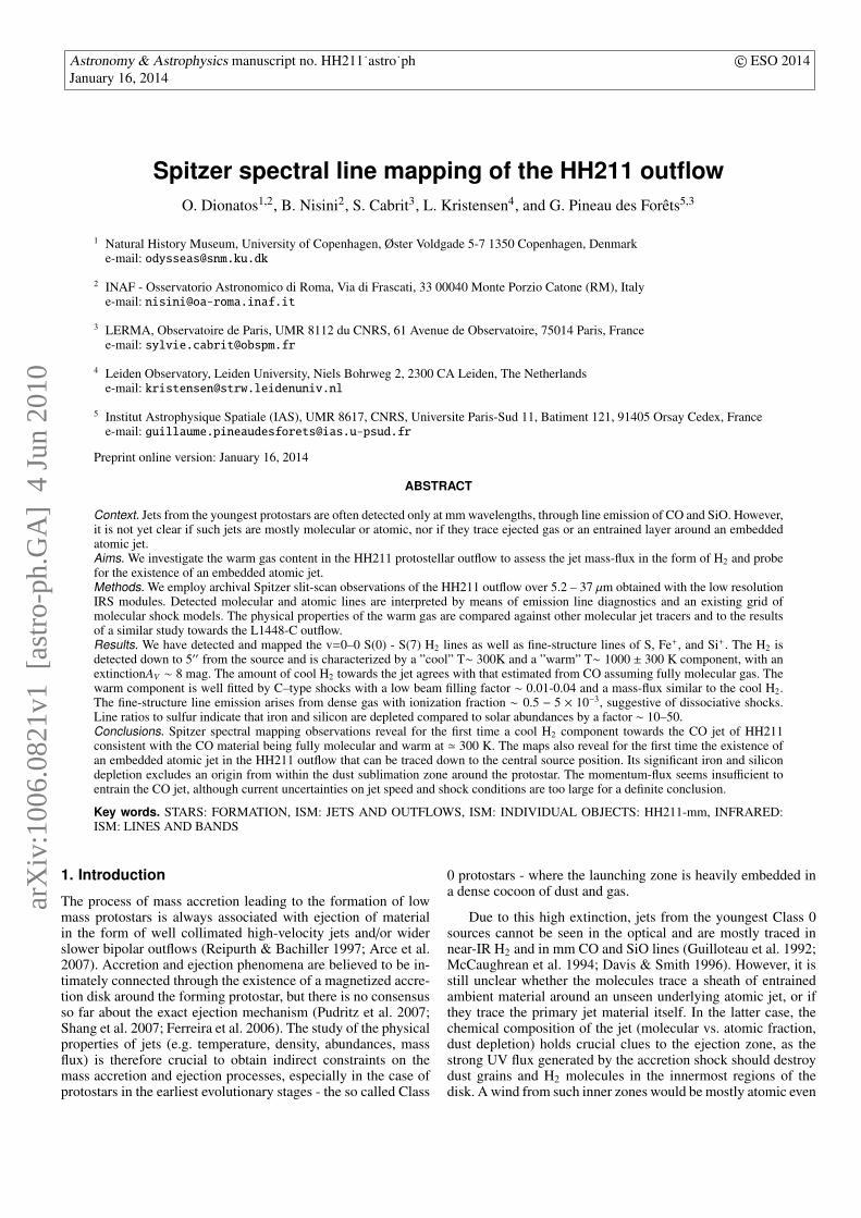
Fig. 1. Continuum subtracted spectrum, integrated over a regionof 612 square arcseconds covering the HH211 flow (middle),shown in comparison with a spectrum of the off-outflow regionof the same area (top). H2 emission from the 0–0 S(0)– S(7)lines is detected in the outflow, together with atomic emissionfrom the ground state transitions of [FeII],[SiII] and [SI]. TheH2 S(0) and S(1) lines are detected also in the off-outflow spec-trum, indicating the presence of a diffuse line emission compo-nent not related to the HH211 flow. Diffuse emission from PAHfeatures, such as the 11.3µm feature, is also evidenced. (Bottom:)On source spectrum extracted from an area equal to the LL pixelscale (110.25 square arcseconds), after removing the zodiacallight and ambient contribution presenting the intrinsic contin-uum emission from the outflow source.

physical conditions in the jet close to the driving source and theshocked gas further out, and compared with an existing grid of Cand J-type shock models. Atomic lines present in our spectra aretreated separately as probes for the existence of a deeply embed-ded atomic jet, and used to measure dust depletion. Mass-fluxesare inferred for the H2 and atomic components, and compared tothose measured in CO and SiO, as well as to a similar study ofthe inner jet of L1448. Our conclusions are presented in Section5.

2. Observations and data reduction

Observations were obtained with the Spitzer satellite (Werneret al. 2004) and retrieved from the Spitzer Public Data Archiveusing the Leopard software. They were performed as part of the”Shock dissipation in Nearby Star Forming Regions” programconducted by J. Bally (P.I.). In these, the low resolution modules(R∼60-130) of the Spitzer Infrared Spectrograph (IRS, Houcket al. 2004) were used in slit-scan mode to cover an area of57′′ × 73′′ and 157′′ × 168′′ for the Short Low (SL) and LongLow (LL) modules respectively, centered on the Class 0 sourceHH211-mm (αJ2000:03h43m56.5s, δJ2000:+32d00m51s). A per-pendicular scan step equal to the slit width of each module wasused, with a total integration time of 171 min. The combination

O. Dionatos et al.: Spitzer spectral line mapping of the HH211 outflow 3

H2 S(2) H2 S(4) H2 S(6)

H2 S(7)H2 S(5)H2 S(3)

+ + +

+++B1

R1 R2

B2B3

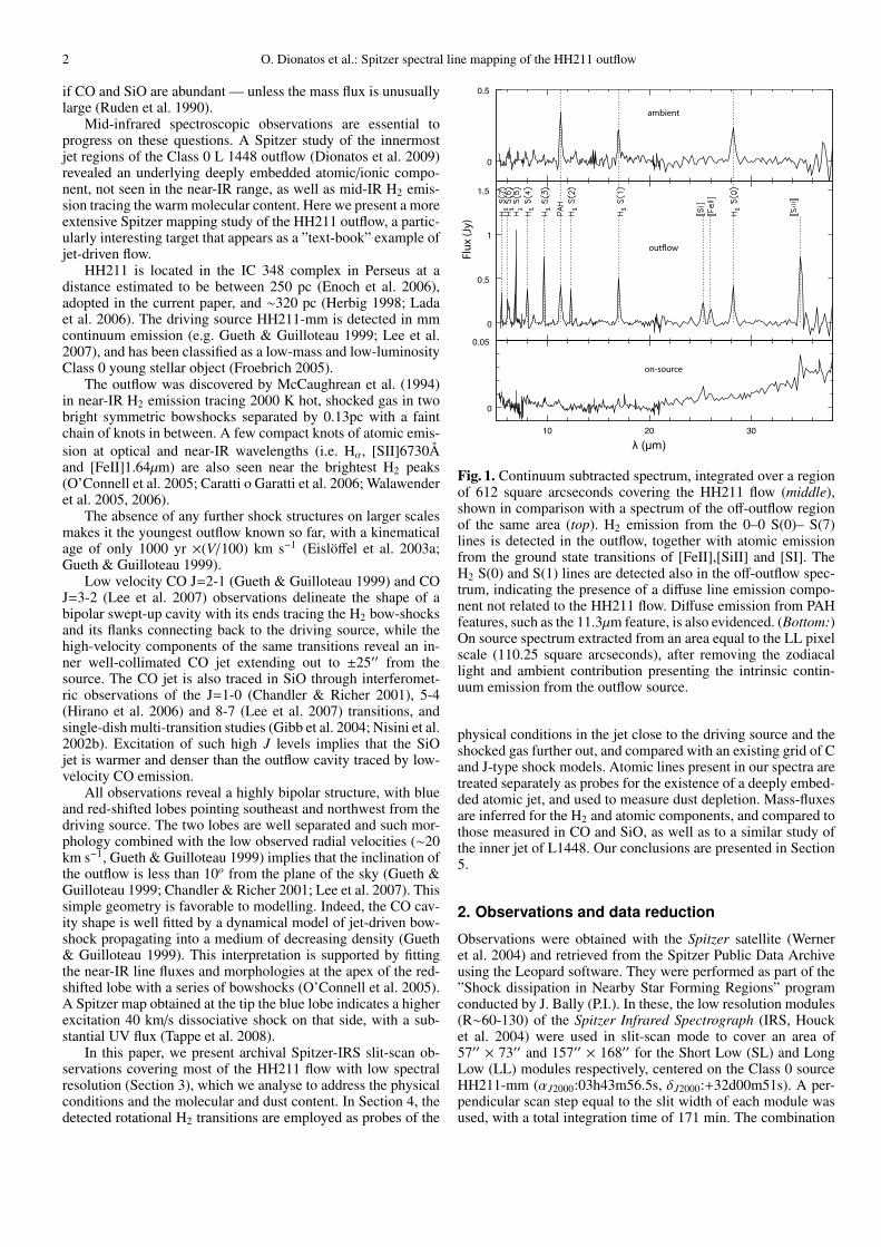
Fig. 2. H2 v=0–0 S(2) – S(7) line intensity maps of the HH211 flow observed with the Spitzer SL module, reconstructed with apixel scale of 3.5′′. Contours are from 10−12 W cm−2 sr−1 with an increment of 8 10−13 W cm−2 sr−1 for the para lines (even J),and from 2 10−12 W cm−2 sr−1 with an increment of 2.5 10−12 W cm−2 sr−1 for the ortho transitions (odd J). Crosses indicate thedriving source position at αJ2000:03h43m56.5s, δJ2000:+32d:00m:51s. In the H2 S(5) map, points B1-B3 and R1, R2 indicate peaksof emission, where AV and ortho to para ratio are estimated and excitation analysis is carried out.

of both IRS low resolution modules gives a complete wavelengthcoverage of 5.2 – 37.0 µm.

Initial data processing was performed at the Spitzer ScienceCenter using Version 15 of the processing pipeline. Spectraldata-cubes were built using the CUBISM software package(Smith et al. 2007) and bad/rogue pixels were masked throughvisual inspection.

Figure 1 presents the extracted continuum-subtracted spec-trum, integrated over a region encompassing the HH211 flow.The full series of H2 pure rotational lines (S(0)-S(7)) were de-tected, along with atomic and ionic lines from the fundamentaltransitions of [SI], [FeII], and [SiII] at 25µm, 26µm, and 35µmrespectively. For comparison, Fig. 1 shows also a spectrum of aregion encompassing the same area but in a direction perpendic-ular to the outflow. The H2 S(0) and S(1) lines are detected alsoin this off-outflow spectrum, indicating the presence of a diffuseline emission component not related to the HH211 flow. Diffuseemission from PAH features, such as the 11.3µm feature, is alsoevidenced. In Figure 1 we also plot the on source spectrum foran area equal to the LL pixel size, after subtracting the contribu-tion from an off-source, free of line-emission position. This onlyremoves zodiacal light and reveals the intrinsic mid-IR contin-uum from the central source, which is typical of low-luminosityClass 0 sources.

Subsequent analysis consisted in the construction of individ-ual line emission maps, using a home-built pipeline; in this, foreach spatial pixel of the data-cube, the brightness of each spec-tral line of interest was calculated by Gaussian fitting after sub-tracting a local second order polynomial baseline. The resultingline intensity maps have a square pixel of side equal to the slitwidth of the IRS module, namely 3.5′′ and 10.5′′ for the SL andLL modules respectively, while the diffraction limit of the tele-scope is 2.4′′ and 6.0′′ at λ=10µm and 25µm respectively. The

astrometric accuracy of the maps was found to be good withinthe limits imposed by the pixel size of each IRS module.

3. Spectral line maps

3.1. H2 emission

Figure 2 presents the emission line maps of the S(2) - S(7) ro-tational H2 lines observed with the SL - IRS modules with a3.5′′ sampling. Contours shape a characteristic bipolar outflowpattern, where the H2 emission is detected down to a projectedangular distance ∼ 5′′ from the driving source. Further down-wind, peaks of emission which can be attributed to shocked gasare observed. In the H2 S(5) map of Fig. 2 we label these peaksas B1-B3 in the southeast, blue-shifted lobe and R1-R2 in thenorthwest, red-shifted lobe, respectively.

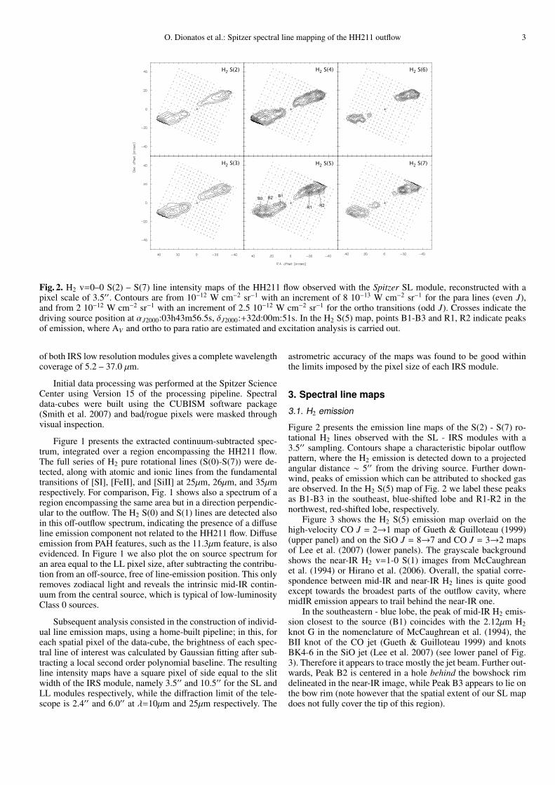
Figure 3 shows the H2 S(5) emission map overlaid on thehigh-velocity CO J = 2→1 map of Gueth & Guilloteau (1999)(upper panel) and on the SiO J = 8→7 and CO J = 3→2 mapsof Lee et al. (2007) (lower panels). The grayscale backgroundshows the near-IR H2 v=1-0 S(1) images from McCaughreanet al. (1994) or Hirano et al. (2006). Overall, the spatial corre-spondence between mid-IR and near-IR H2 lines is quite goodexcept towards the broadest parts of the outflow cavity, wheremidIR emission appears to trail behind the near-IR one.

In the southeastern - blue lobe, the peak of mid-IR H2 emis-sion closest to the source (B1) coincides with the 2.12µm H2knot G in the nomenclature of McCaughrean et al. (1994), theBII knot of the CO jet (Gueth & Guilloteau 1999) and knotsBK4-6 in the SiO jet (Lee et al. 2007) (see lower panel of Fig.3). Therefore it appears to trace mostly the jet beam. Further out-wards, Peak B2 is centered in a hole behind the bowshock rimdelineated in the near-IR image, while Peak B3 appears to lie onthe bow rim (note however that the spatial extent of our SL mapdoes not fully cover the tip of this region).


B1B1 R1R1B2B2

B1B1

B2B2B3B3R1R1

R2R2

B1B1 R1R1B2B2

Fig. 3. (Ipper panel) H2 v=0–0 S(5) map (green contours) su-perimposed over the high velocity CO J = 2–1 map of Gueth& Guilloteau (1999); (Lower panels) Inner part of the H2 v=0–0 S(5) map (green contours) superimposed on the SiO J = 8–7and the CO J = 3–2 maps of Lee et al. (2007). The grayscalebackgrounds show the H2 v=1–0 S(1) image from McCaughreanet al. (1994)(top panel) or Hirano et al. (2006)(lower panels).The slight S-shape pattern of the S(5) emission map follows thebrightness asymmetry of the cavity seen in the 2.12 µm image.In the blue-shifted jet lobe, point B1 is coincident with peak BIIin CO J=2-1 and BK4–6 in SiO.

Symmetrically on the redshifted side, the mid-IR H2 emis-sion close to the source forms an extended curving ”finger” trac-ing both the jet and the cavity wall north of it, as seen in the near-IR (see Fig. 3) and peak R1 coincides with the near-IR knot F ofMcCaughrean et al. (1994). However, peak R2 is again centeredon the cavity behind the bright bow rim traced in the near-IR.The spatial offset between B2 and R2 with respect to the near-IRcounterparts suggests that mid-IR emission in these broad re-gions may be tracing the outer bow-shock wings where gas isexpected to be in lower excitation conditions.

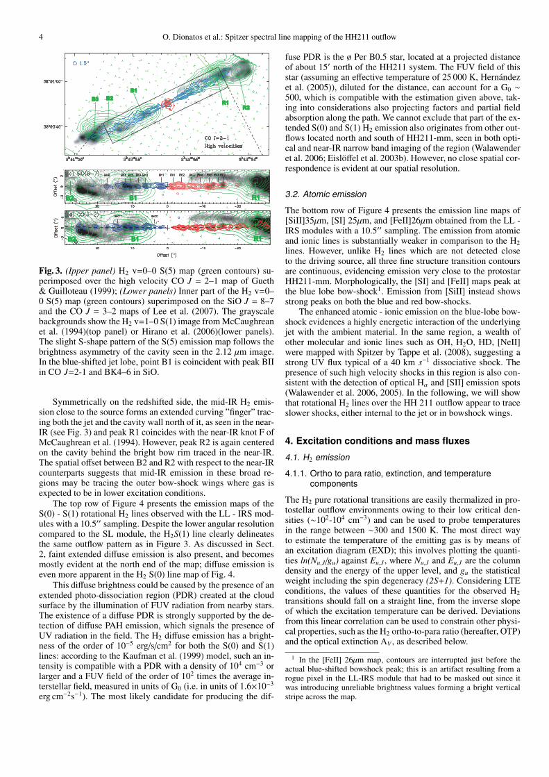
The top row of Figure 4 presents the emission maps of theS(0) - S(1) rotational H2 lines observed with the LL - IRS mod-ules with a 10.5′′ sampling. Despite the lower angular resolutioncompared to the SL module, the H2S(1) line clearly delineatesthe same outflow pattern as in Figure 3. As discussed in Sect.2, faint extended diffuse emission is also present, and becomesmostly evident at the north end of the map; diffuse emission iseven more apparent in the H2 S(0) line map of Fig. 4.

This diffuse brightness could be caused by the presence of anextended photo-dissociation region (PDR) created at the cloudsurface by the illumination of FUV radiation from nearby stars.The existence of a diffuse PDR is strongly supported by the de-tection of diffuse PAH emission, which signals the presence ofUV radiation in the field. The H2 diffuse emission has a bright-ness of the order of 10−5 erg/s/cm2 for both the S(0) and S(1)lines: according to the Kaufman et al. (1999) model, such an in-tensity is compatible with a PDR with a density of 104 cm−3 orlarger and a FUV field of the order of 102 times the average in-terstellar field, measured in units of G0 (i.e. in units of 1.6×10−3

erg cm−2s−1). The most likely candidate for producing the dif-

fuse PDR is the ø Per B0.5 star, located at a projected distanceof about 15′ north of the HH211 system. The FUV field of thisstar (assuming an effective temperature of 25 000 K, Hernandezet al. (2005)), diluted for the distance, can account for a G0 ∼

500, which is compatible with the estimation given above, tak-ing into considerations also projecting factors and partial fieldabsorption along the path. We cannot exclude that part of the ex-tended S(0) and S(1) H2 emission also originates from other out-flows located north and south of HH211-mm, seen in both opti-cal and near-IR narrow band imaging of the region (Walawenderet al. 2006; Eisloffel et al. 2003b). However, no close spatial cor-respondence is evident at our spatial resolution.

3.2. Atomic emission

The bottom row of Figure 4 presents the emission line maps of[SiII]35µm, [SI] 25µm, and [FeII]26µm obtained from the LL -IRS modules with a 10.5′′ sampling. The emission from atomicand ionic lines is substantially weaker in comparison to the H2lines. However, unlike H2 lines which are not detected closeto the driving source, all three fine structure transition contoursare continuous, evidencing emission very close to the protostarHH211-mm. Morphologically, the [SI] and [FeII] maps peak atthe blue lobe bow-shock1. Emission from [SiII] instead showsstrong peaks on both the blue and red bow-shocks.

The enhanced atomic - ionic emission on the blue-lobe bow-shock evidences a highly energetic interaction of the underlyingjet with the ambient material. In the same region, a wealth ofother molecular and ionic lines such as OH, H2O, HD, [NeII]were mapped with Spitzer by Tappe et al. (2008), suggesting astrong UV flux typical of a 40 km s−1 dissociative shock. Thepresence of such high velocity shocks in this region is also con-sistent with the detection of optical Hα and [SII] emission spots(Walawender et al. 2006, 2005). In the following, we will showthat rotational H2 lines over the HH 211 outflow appear to traceslower shocks, either internal to the jet or in bowshock wings.

4. Excitation conditions and mass fluxes

4.1. H2 emission

4.1.1. Ortho to para ratio, extinction, and temperaturecomponents

The H2 pure rotational transitions are easily thermalized in pro-tostellar outflow environments owing to their low critical den-sities (∼102-104 cm−3) and can be used to probe temperaturesin the range between ∼300 and 1500 K. The most direct wayto estimate the temperature of the emitting gas is by means ofan excitation diagram (EXD); this involves plotting the quanti-ties ln(Nu,J /gu) against Eu,J , where Nu,J and Eu,J are the columndensity and the energy of the upper level, and gu the statisticalweight including the spin degeneracy (2S+1). Considering LTEconditions, the values of these quantities for the observed H2transitions should fall on a straight line, from the inverse slopeof which the excitation temperature can be derived. Deviationsfrom this linear correlation can be used to constrain other physi-cal properties, such as the H2 ortho-to-para ratio (hereafter, OTP)and the optical extinction AV , as described below.

1 In the [FeII] 26µm map, contours are interrupted just before theactual blue-shifted bowshock peak; this is an artifact resulting from arogue pixel in the LL-IRS module that had to be masked out since itwas introducing unreliable brightness values forming a bright verticalstripe across the map.


+

++ + R1+R2LL2

LL1

B2+B3

+

H2S(1) H2S(0)

[SiII] [SI] [FeII]

Fig. 4. Intensity maps of the HH211 flow in the H2S(1) and S(0) lines (top row) and the atomic [SiII]35µm, [SI] 25µm, and[FeII]26µm lines (bottom row) obtained with the Spitzer IRS - LL module (pixel scale ∼10.5′′). Crosses mark the position ofthe driving source HH211-mm. The dashed circle in the H2 maps masks the area around a bright star (IC348 IR) where line inten-sity measurements are unreliable. In the [FeII] 26µm map, contours are interrupted just before the eastern bowshock peak due toa rogue pixel. Contour levels in the H2 S(1) map start from 10−12 W cm−2 sr−1 with 10−13 increments, and from 7 10 −13 W cm−2

sr−1 with 5× 10−14 increments for the S(0) map. Contours of the ionic line maps start at 10−13 W cm−2 sr−1 with 10−13 W cm−2 sr−1

steps for [SiII] and [FeII], and at 10−13 W cm−2 sr−1 with 2 × 10−13 W cm−2 sr−1 steps for [SI].

Deviations of the OTP from its LTE value are reflected asvertical displacements between the ortho and para transitionsin the EXD, forming a ”saw-tooth” pattern between the twoH2 species. The observed OTP was estimated by examining thealignment of the S(5) data point with the neighboring S(4) andS(6) transitions, following the method outlined in Wilgenbuset al. (2000); in all cases the spatial OTP variations are small,and values lie very close, within the statistical error limits, to thehigh-temperature LTE value of 3.

The H2 S(3) transition at 9.7 µm is sensitive to the amount ofdust along the line of sight, as it is located within a wide-band sil-icate absorption feature at the same wavelength; consequently avisual extinction value can be estimated by examining the align-ment of the S(3) point in comparison to the S(2) and S(4), havingpreviously corrected for any deviations of the OTP ratio from theequilibrium value. Visual extinction is then estimated assumingan A9.7/AV ratio equal to 0.087 (Rieke & Lebofsky 1985). AVis found to exhibit no regular pattern along the outflow and torange between 7 and 9 mag, being consistent with previous es-timates of 7–15 mag by McCaughrean et al. (1994); Caratti oGaratti et al. (2006)2 .

Considering an average value of AV equal to 8 mag acrossthe map, we have dereddened all the detected H2 lines falling inthe SL range (ie. S(2) to S(7)) using the extinction law of Rieke& Lebofsky (1985). Consequently, for all the points of the SLdata cube where at least 3 H2 lines are detected above 3-sigma,we have calculated the excitation temperature from the slope ofa least square fit on the dereddened data points in the EXD. An

2 O’Connell et al. (2005) reported a higher extinction of 25 mag in theredshifted lobe but considered it rather tentative given their observingconditions

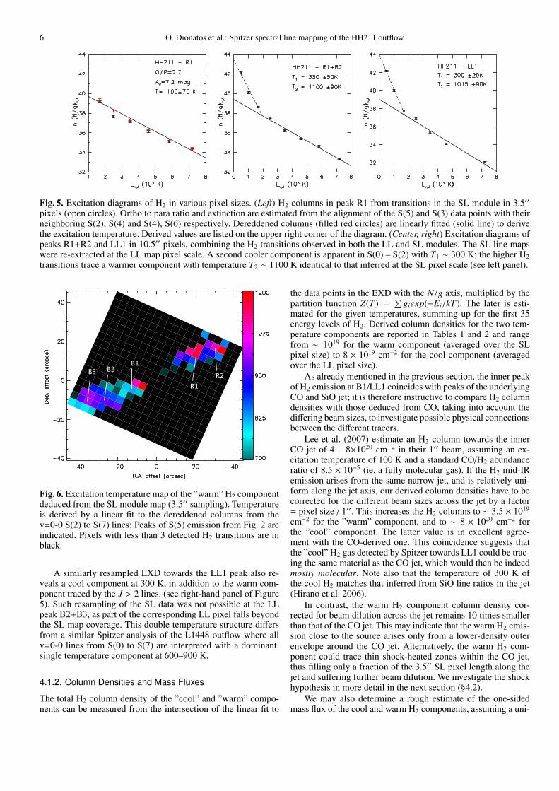
example of these operations is shown in the left panel of Fig. 5in the case of the R1 peak.

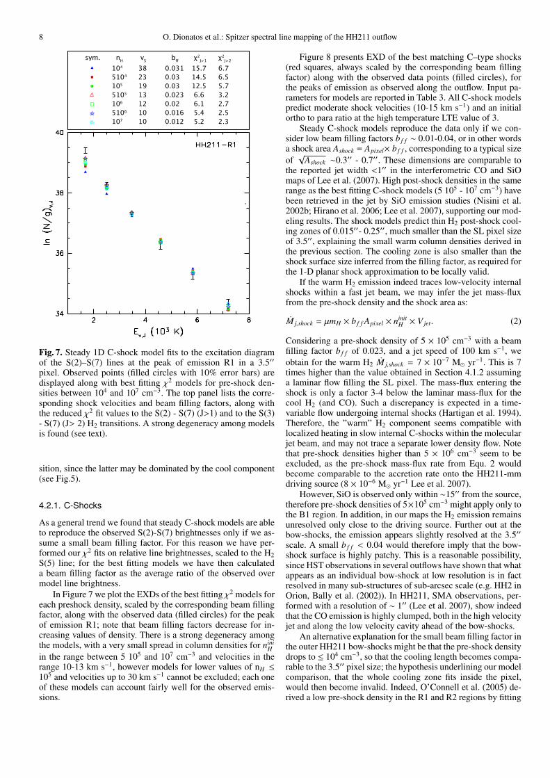
The results over the whole HH211 region are summarized inFig. 6 in the form of an excitation temperature map. Commonmorphological characteristics between the excitation tempera-ture map and the H2 S(2)-S(7) emissions are evident; peaks inexcitation temperature tend to coincide with peaks of emission.At those peaks, temperature reaches values up to 1200 K, whilein the more diffuse outflow regions the temperature is as low as700 K. In Table 1 we report the derived excitation temperatureswith this method for the peaks of the S(5) emission along theblue and the red lobes of the outflow.

In addition to the ”warm” H2 component at ' 1100 K indi-cated by the S(2)-S(7) lines, there is also evidence for a ”cool”component from the S(0) and S(1) lines detected in the LL mod-ule. This is illustrated in the central panel of Figure 5, whichpresent an EXD of the R1+R2 region in the LL 10.5′′ pixel, in-cluding the S(0) and S(1) datapoints. For consistency, the fluxesof S(2) to S(7) lines from the SL module were re-extracted atthe coarser LL module sampling. Due to the extended diffuseemission, the S(0) line flux was obtained after subtracting theambient contribution estimated in adjacent off-outflow regions.

While the resampled S(3) - S(7) emission keeps the same”warm” temperature ∼ 1100K, the data points for the S(0)-S(2)transitions show a steeper slope which is evidence for a ”cool”component at T∼ 300 K not probed by the higher J transitions.Another interesting result is that column densities obtained fromthe S(2)-S(7) lines in the LL pixel are smaller than in the SLpixel of 3.5′′, indicating that the warm component does not fillthe LL pixel.


Fig. 5. Excitation diagrams of H2 in various pixel sizes. (Left) H2 columns in peak R1 from transitions in the SL module in 3.5′′pixels (open circles). Ortho to para ratio and extinction are estimated from the alignment of the S(5) and S(3) data points with theirneighboring S(2), S(4) and S(4), S(6) respectively. Dereddened columns (filled red circles) are linearly fitted (solid line) to derivethe excitation temperature. Derived values are listed on the upper right corner of the diagram. (Center, right) Excitation diagrams ofpeaks R1+R2 and LL1 in 10.5′′ pixels, combining the H2 transitions observed in both the LL and SL modules. The SL line mapswere re-extracted at the LL map pixel scale. A second cooler component is apparent in S(0) – S(2) with T1 ∼ 300 K; the higher H2transitions trace a warmer component with temperature T2 ∼ 1100 K identical to that inferred at the SL pixel scale (see left panel).

B1

R2R1

B2B3

Fig. 6. Excitation temperature map of the ”warm” H2 componentdeduced from the SL module map (3.5′′ sampling). Temperatureis derived by a linear fit to the dereddened columns from thev=0-0 S(2) to S(7) lines; Peaks of S(5) emission from Fig. 2 areindicated. Pixels with less than 3 detected H2 transitions are inblack.

A similarly resampled EXD towards the LL1 peak also re-veals a cool component at 300 K, in addition to the warm com-ponent traced by the J > 2 lines. (see right-hand panel of Figure5). Such resampling of the SL data was not possible at the LLpeak B2+B3, as part of the corresponding LL pixel falls beyondthe SL map coverage. This double temperature structure differsfrom a similar Spitzer analysis of the L1448 outflow where allv=0-0 lines from S(0) to S(7) are interpreted with a dominant,single temperature component at 600–900 K.

4.1.2. Column Densities and Mass Fluxes

The total H2 column density of the ”cool” and ”warm” compo-nents can be measured from the intersection of the linear fit to

the data points in the EXD with the N/g axis, multiplied by thepartition function Z(T ) =

∑giexp(−Ei/kT ). The later is esti-

mated for the given temperatures, summing up for the first 35energy levels of H2. Derived column densities for the two tem-perature components are reported in Tables 1 and 2 and rangefrom ∼ 1019 for the warm component (averaged over the SLpixel size) to 8 × 1019 cm−2 for the cool component (averagedover the LL pixel size).

As already mentioned in the previous section, the inner peakof H2 emission at B1/LL1 coincides with peaks of the underlyingCO and SiO jet; it is therefore instructive to compare H2 columndensities with those deduced from CO, taking into account thediffering beam sizes, to investigate possible physical connectionsbetween the different tracers.

Lee et al. (2007) estimate an H2 column towards the innerCO jet of 4 − 8×1020 cm−2 in their 1′′ beam, assuming an ex-citation temperature of 100 K and a standard CO/H2 abundanceratio of 8.5 × 10−5 (ie. a fully molecular gas). If the H2 mid-IRemission arises from the same narrow jet, and is relatively uni-form along the jet axis, our derived column densities have to becorrected for the different beam sizes across the jet by a factor= pixel size / 1′′. This increases the H2 columns to ∼ 3.5 × 1019

cm−2 for the ”warm” component, and to ∼ 8 × 1020 cm−2 forthe ”cool” component. The latter value is in excellent agree-ment with the CO-derived one. This coincidence suggests thatthe ”cool” H2 gas detected by Spitzer towards LL1 could be trac-ing the same material as the CO jet, which would then be indeedmostly molecular. Note also that the temperature of 300 K ofthe cool H2 matches that inferred from SiO line ratios in the jet(Hirano et al. 2006).

In contrast, the warm H2 component column density cor-rected for beam dilution across the jet remains 10 times smallerthan that of the CO jet. This may indicate that the warm H2 emis-sion close to the source arises only from a lower-density outerenvelope around the CO jet. Alternatively, the warm H2 com-ponent could trace thin shock-heated zones within the CO jet,thus filling only a fraction of the 3.5′′ SL pixel length along thejet and suffering further beam dilution. We investigate the shockhypothesis in more detail in the next section (§4.2).

We may also determine a rough estimate of the one-sidedmass flux of the cool and warm H2 components, assuming a uni-


Table 1. Physical properties of the warm H2 component from H2 v=0–0 S(2) - S(7) lines extracted at the SL (3.5′′) scale

Position Offsets H2 0-0 S(5) T N(H2) Ma

(′′) (10−11 W cm−2 sr−1) (K) ( 1019 cm −2) (10−7 M� yr−1)

R1 [-20.1, 13.3] 3.3 1100±70 1.15 1.1R2 [-29.9, 17.0] 2.3 1050±75 1.3 1.2B1 [12.2, -4.7] 1.3 860±40 1.1 1.1B2 [26.9, -10.3] 2.0 950±70 1.5 1.4B3 [35.1, -10.6] 1.9 980±75 1.4 1.4

a M is proportional to (V jet/100 km s−1)×(3.5′′/lt) and is not corrected for postshock compression.

Table 2. Physical properties of the cool H2 component from H2 v=0–0 S(0) - S(2) lines extracted at the LL (10.5′′) scale

Position Offsets H2 0-0 S(1) T N(H2) Ma

(′′) (10−12 W cm−2 sr−1) (K) ( 1019 cm −2) (10−6 M� yr−1)

R1+R2 [-19.3, 15.1] 1.4 330±50 7.5 2.0LL1 [6.3, 2.0] 1.3 300±45 7.8 2.8

a M is proportional to (V jet/100 km s−1)×(10.5′′/lt) and is not corrected for postshock compression.

form laminar flow across the corresponding pixel, using the re-lationship from Dionatos et al. (2009):

M = 2µmH × 〈N(H2)A〉 × (Vt/lt) (1)

where µ =1.4 is the mean weight per gram of hydrogen, mH isthe proton mass, N(H2) the column density averaged over thearea A of the pixel, lt is the projected emitting length along theflow direction (assumed in Tables 1,2 to be equal to the pixellength), and Vt the tangential flow speed.

The value of Vt is quite uncertain. Taking into account radialvelocities in the range 5 - 20 km s−1 measured for the near-IR H2knots in the study of Salas et al. (2003), and assuming an inclina-tion angle between 5o and 10o (see §1), tangential velocities mayvary over 30 - 230 km s−1, introducing an absolute uncertainty ofa factor 3 either way in the inferred M values. In the following,we adopt Vt = 100 km s−1 for ease of comparison with earlierwork, bearing in mind that M values scale proportionally to theassumed velocity. In column 6 of Tables 1 and 2 we report theresulting M for the peaks of emission along the outflow, for bothtemperature components.

For the cool H2 gas component, the laminar mass-flux is∼ 20 − 28 × 10−7 M� yr−1. For comparison, the one-sided jetmass-loss rate based on CO(3-2) emission obtained by Lee et al.(2007) assuming the same velocity of 100 km s−1 and a com-pression factor of 3 is 3.5 − 7 × 10−7 M� yr−1. Adjusting theirestimations for Helium, and uncorrecting for compression, thelaminar mass flux of the CO jet rises to 15 − 30 × 10−7 M� yr−1;this is in excellent agreement with the cool H2 laminar mass fluxestimated here, again consistent with both tracing the same fullymolecular gas.

The warm H2 laminar mass-flux is 15-30 times lower at∼ 10−7M� yr−1 ×(Vt/100km s−1). Similar mass flux estimationswere obtained from the pure rotational H2 lines along the outflowof L1448 (Dionatos et al. 2009, 0.5− 1.4× 10−7M� yr−1), wheresimilar H2 columns were measured3. Note however that if thewarm H2 does not trace a laminar flow as assumed, but arises ina single shock within the pixel, then the relevant emitting lengthlt along the flow will be generally narrower than the SL pixel

3 Note that a typographical error was introduced in Table 2 ofDionatos et al. (2009); the values of N(H2) are ∼ 7 × 1018 cm−2 at CSand ∼ 1.5 − 3.8 × 1019 cm−2 for the other positions.

size, and the true mass flux will be higher than listed in Table 1.Mass-fluxes in the warm component in the shock hypothesis arepresented in the next section.

4.2. Shock models for the warm H2 component

As pointed out in §4.1, peaks of warm (J≥2) H2 emission coin-cide with peaks of temperature (Fig. 6) and possibly correspondto regions of shocked gas. In order to constrain the shock condi-tions in these regions, we employ the existing shock model griddescribed in the work of Kristensen et al. (2007) which is basedon the MHD-VODE multi-fluid steady shock code of Flower &Pineau des Forets (2003). The grid includes both continuous (C)and jump (J) type shocks and predicts the H2 lines brightness forvarious values of pre-shock density (nini

H ), shock velocity (V s),initial OTP ratio (otpini) and transverse magnetic field density(ϕ). The ranges of parameters investigated here are as follows:

– niniH = 104 to 107 cm −3 by alternating factors of 5 and 2.

– Vs = 10 - 50 km s−1 with a step of 1 km s−1

– otpini = 0.01, 1, 2, 3– ϕ(µG) = b ×

√nH (cm−3) where we fix b=1 for C and b=0

for J-type shocks.

The model is one-dimensional, considers 9 elements (H, He,C, O, N, S, Si, Mg and Fe) and 136 species connected with 1040reactions, and takes into account grain sputtering and erosion, aswell as a variety of cooling and heating processes. Initial chem-ical abundances are computed assuming no UV field and an H2cosmic ray ionization rate of 5×10−17 s−1, yielding an ionizationfraction ∼ 7×10−8(nini

H /104cm s−1)−0.5. The H2 level populationsand line brightnesses are integrated along the postshock coolingzone down to a temperature of 50 K, which is reached in a cool-ing time ∼ 100 (105 cm −3/ nH) yrs in C-shocks (much shorter inJ shocks). For more information on both the model and the griddata, the interested reader is referred to the articles of Flower &Pineau des Forets (2003) and Kristensen et al. (2007).

In the following, we have employed a χ2 fitting method tooptimally reproduce the observed H2 emission selecting the bestmatching C or J-type steady shock models from the grid. The χ2

- fitting is performed with and without considering the S(2) tran-


sym. nH vS bff χ2J>1 χ2

J>2

104 38 0.031 15.7 6.7 5104 23 0.03 14.5 6.5 105 19 0.03 12.5 5.7 5105 13 0.023 6.6 3.2 106 12 0.02 6.1 2.7 5106 10 0.016 5.4 2.5 107 10 0.012 5.2 2.3

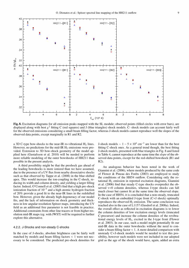
Fig. 7. Steady 1D C-shock model fits to the excitation diagramof the S(2)–S(7) lines at the peak of emission R1 in a 3.5′′pixel. Observed points (filled circles with 10% error bars) aredisplayed along with best fitting χ2 models for pre-shock den-sities between 104 and 107 cm−3. The top panel lists the corre-sponding shock velocities and beam filling factors, along withthe reduced χ2 fit values to the S(2) - S(7) (J>1) and to the S(3)- S(7) (J> 2) H2 transitions. A strong degeneracy among modelsis found (see text).

sition, since the latter may be dominated by the cool component(see Fig.5).

4.2.1. C-Shocks

As a general trend we found that steady C-shock models are ableto reproduce the observed S(2)-S(7) brightnesses only if we as-sume a small beam filling factor. For this reason we have per-formed our χ2 fits on relative line brightnesses, scaled to the H2S(5) line; for the best fitting models we have then calculateda beam filling factor as the average ratio of the observed overmodel line brightness.

In Figure 7 we plot the EXDs of the best fitting χ2 models foreach preshock density, scaled by the corresponding beam fillingfactor, along with the observed data (filled circles) for the peakof emission R1; note that beam filling factors decrease for in-creasing values of density. There is a strong degeneracy amongthe models, with a very small spread in column densities for nini

Hin the range between 5 105 and 107 cm−3 and velocities in therange 10-13 km s−1, however models for lower values of nH ≤

105 and velocities up to 30 km s−1 cannot be excluded; each oneof these models can account fairly well for the observed emis-sions.

Figure 8 presents EXD of the best matching C–type shocks(red squares, always scaled by the corresponding beam fillingfactor) along with the observed data points (filled circles), forthe peaks of emission as observed along the outflow. Input pa-rameters for models are reported in Table 3. All C-shock modelspredict moderate shock velocities (10-15 km s−1) and an initialortho to para ratio at the high temperature LTE value of 3.

Steady C-shock models reproduce the data only if we con-sider low beam filling factors b f f ∼ 0.01-0.04, or in other wordsa shock area Ashock = Apixel× b f f , corresponding to a typical sizeof√

Ashock ∼0.3′′ - 0.7′′. These dimensions are comparable tothe reported jet width <1′′ in the interferometric CO and SiOmaps of Lee et al. (2007). High post-shock densities in the samerange as the best fitting C-shock models (5 105 - 107 cm−3) havebeen retrieved in the jet by SiO emission studies (Nisini et al.2002b; Hirano et al. 2006; Lee et al. 2007), supporting our mod-eling results. The shock models predict thin H2 post-shock cool-ing zones of 0.015′′- 0.25′′, much smaller than the SL pixel sizeof 3.5′′, explaining the small warm column densities derived inthe previous section. The cooling zone is also smaller than theshock surface size inferred from the filling factor, as required forthe 1-D planar shock approximation to be locally valid.

If the warm H2 emission indeed traces low-velocity internalshocks within a fast jet beam, we may infer the jet mass-fluxfrom the pre-shock density and the shock area as:

M j,shock = µmH × b f f Apixel × ninitH × V jet. (2)

Considering a pre-shock density of 5 × 105 cm−3 with a beamfilling factor b f f of 0.023, and a jet speed of 100 km s−1, weobtain for the warm H2 M j,shock = 7 × 10−7 M� yr−1. This is 7times higher than the value obtained in Section 4.1.2 assuminga laminar flow filling the SL pixel. The mass-flux entering theshock is only a factor 3-4 below the laminar mass-flux for thecool H2 (and CO). Such a discrepancy is expected in a time-variable flow undergoing internal shocks (Hartigan et al. 1994).Therefore, the ”warm” H2 component seems compatible withlocalized heating in slow internal C-shocks within the molecularjet beam, and may not trace a separate lower density flow. Notethat pre-shock densities higher than 5 × 106 cm−3 seem to beexcluded, as the pre-shock mass-flux rate from Equ. 2 wouldbecome comparable to the accretion rate onto the HH211-mmdriving source (8 × 10−6 M� yr−1 Lee et al. 2007).

However, SiO is observed only within ∼15′′ from the source,therefore pre-shock densities of 5×105 cm−3 might apply only tothe B1 region. In addition, in our maps the H2 emission remainsunresolved only close to the driving source. Further out at thebow-shocks, the emission appears slightly resolved at the 3.5′′scale. A small b f f < 0.04 would therefore imply that the bow-shock surface is highly patchy. This is a reasonable possibility,since HST observations in several outflows have shown that whatappears as an individual bow-shock at low resolution is in factresolved in many sub-structures of sub-arcsec scale (e.g. HH2 inOrion, Bally et al. (2002)). In HH211, SMA observations, per-formed with a resolution of ∼ 1′′ (Lee et al. 2007), show indeedthat the CO emission is highly clumped, both in the high velocityjet and along the low velocity cavity ahead of the bow-shocks.

An alternative explanation for the small beam filling factor inthe outer HH211 bow-shocks might be that the pre-shock densitydrops to ≤ 104 cm−3, so that the cooling length becomes compa-rable to the 3.5′′ pixel size; the hypothesis underlining our modelcomparison, that the whole cooling zone fits inside the pixel,would then become invalid. Indeed, O’Connell et al. (2005) de-rived a low pre-shock density in the R1 and R2 regions by fitting


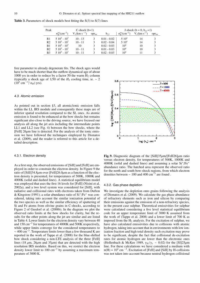
Fig. 8. Excitation diagrams for all emission peaks mapped with the SL module; observed points (filled circles with error bars), aredisplayed along with best χ2 fitting C (red squares) and J (blue triangles) shock models. C- shock models can account fairly wellfor the observed emissions considering a small beam filling factor, whereas J-shock models cannot reproduce well the slopes of theobserved data points, except marginally in R1 and R2.

a 3D C-type bow-shocks to the near-IR ro-vibrational H2 lines.However, no predictions for the mid-IR H2 emissions were pro-vided. Extension to 3D bow-shock geometry of the model ap-plied here (Gustafsson et al. 2010) will be needed to performmore reliable modeling of the outer bowshocks of HH211 thanpossible in the present analysis.

A third possibility might be that the preshock gas ahead ofthe leading bowshocks is more ionized than we have assumed,due to the presence of a UV flux from nearby dissociative shockssuch as that observed by Tappe et al. (2008) in the blue-shiftedapex. This would increase the ion-coupling in the C-shock, re-ducing its width and column density, and yielding a larger fillingfactor. Indeed, O’Connell et al. (2005) find that a high pre-shockionization fraction of 10−5 and a high atomic hydrogen fractionof 20% provide a good fit to the near-IR lines in the redshiftedbow. However, given the already high degeneracy of our modelfits, and the lack of information on shock geometry and thick-ness in low angular resolution Spitzer maps, introducing the UVfield as an additional free parameter is not feasible in practice.Additional constraints from other line tracers or from higher res-olution mid-IR maps (eg. with JWST) will be required to furtherexplore this alternative.

4.2.2. J-Shocks and non-steady C-shocks

In the case of J-shocks, absolute brightness can be fairly wellmatched by models and beam filling factors < 1 were not nec-essary to be considered. The predicted pre-shock densities for

J-shock models ∼ 1 − 5 × 104 cm−3 are lower than for the bestfitting C-shock ones. As a general trend though, the best fittingJ-shock models, presented with blue triangles in Fig. 8 and listedin Table 4, cannot reproduce at the same time the slope of the ob-served data points, except for the red-shifted bowshock (R1 andR2).

An analogous behavior has been noted in the work ofGiannini et al. (2006), where models produced by the same codeof Flower & Pineau des Forets (2003) are employed to studythe conditions of the HH54 outflow. Considering only the ro-tational H2 emission in reported excitation diagrams, Gianniniet al. (2006) find that steady C-type shocks overpredict the ob-served v=0 column densities, whereas J-type shocks can fallmuch closer but cannot fit at the same time the observed slope.In the case of HH54, it is concluded that a non-steady, truncatedC-shock with an embedded J-type front (C+J shock) optimallyreproduces the observed H2 emission. The same conclusion wasreached also in the case of L1157 (Gusdorf et al. 2008a). Indeed,the overall effect as reflected in excitation diagrams is to lowerthe column densities of low excitation energy levels (truncatedC-precursor) and increase the column densities of the rovibra-tional energy levels of H2, excited in the J-type front (Floweret al. 2003). In our case, such a model might potentially fit ourmid-IR data in the outer bowshocks without the need to con-sider a beam filling factor < 1. A more detailed comparison withunsteady C+J-shock models would be needed to test this pos-sibility, however such models were not included in our adoptedgrid as the age of the shock would have, again, added an extra


Table 3. Parameters of shock models best fitting the S(3) to S(7) lines

Peak C-shock (b=1) J-shock (b = 0, b f f =1)nini

H (cm−3) Vs(km s −1) oprini b f f niniH (cm−3) Vs(km s−1) oprini

R1 5 105 - 107 10 - 13 3 0.01 - 0.02 5 104 14 3R2 5 105 - 107 10 - 11 3 0.02 - 0.04 5 104 14 3B1 5 105 - 107 10 3 0.02 - 0.03 104 10 3B2 5 105 - 107 10 - 11 3 0.01 - 0.03 104 10 3B3 5 105 - 107 10 - 11 3 0.02 - 0.03 104 11 3

free parameter to already degenerate fits. The shock ages wouldhave to be much shorter than the outflow dynamical age of about1000 yrs in order to reduce by a factor 50 the warm H2 column(typically a shock age of 1/50 of the H2 cooling time, ie. ∼ 2(105 cm −3/ nH) yrs).

4.3. Atomic emission

As pointed out in section §3, all atomic/ionic emission fallswithin the LL IRS module and consequently these maps are ofinferior spatial resolution compared to the SL ones. As atomicemission is found to be enhanced at the bow shocks but remainssignificant also close to the driving source, we have focused ouranalysis all along the jet axis including the intermediate pointsLL1 and LL2 (see Fig. 4) between the bow shocks, where the[FeII] 26µm line is detected. For the analysis of the ionic emis-sion we have followed the techniques employed by Dionatoset al. (2009), and the reader is referred to this article for a de-tailed description.

4.3.1. Electron density

As a first step, the observed emissions of [SiII] and [FeII] are em-ployed in order to constrain the electron density. In Figure 9 theratio of [SiII]34.8µm over [FeII]26.0µm as a function of the elec-tron density is presented, for temperatures of 500K, 1000K and4000K (solid and dashed lines). A statistical equilibrium modelwas employed that uses the first 16 levels for [FeII] (Nisini et al.2002a), and a two level system was considered for [SiII], withradiative and collisional rates with electrons taken from Dufton& Kingston (1991); a solar abundance ratio of Si+/Fe+ was con-sidered, taking into account the similar ionization potential ofthe two species as well as the similar efficiency of sputtering ofSi and Fe atoms from olivine grains in C-shocks, according toFigure 2 of Gusdorf et al. (2008b). In the diagram we plot theobserved ratio limits at the bow shocks for clarity, but the re-sults for the other points along the jet are similar and are listedin Table 4. Lower limits for the electron density vary between 40and 150 cm−3 for temperatures of 4000K and 500K respectively,while upper limits converge for the considered temperatures to∼ 400 cm−3. Temperature limits lower than a few thousand K arereported in the work of Tappe et al. (2008) for the blue-shiftedbow shock considering a non-LTE analysis of the three [FeII]lines (18 µm, 26µm and 35µm) that are detected with the highresolution IRS modules. Based on this, we restrict the electrondensity lower limit to 100 cm−3 by assuming a maximum tem-perature of 3000 K.

Fig. 9. Diagnostic diagram of the [SiII]35µm/[FeII26]µm ratioversus electron density, for temperatures of 500K, 1000K and4000K (solid and dashed lines) and assuming a solar Si+/Fe+

abundance ratio. The hatched area represent the observed ratiofor the north and south bow-shock regions, from which electrondensities between ∼ 100 and 400 cm−3 are found .

4.3.2. Gas phase depletion

We investigate the depletion onto grains following the analysisof Dionatos et al. (2009). We calculate the gas phase abundanceof refractory elements such as iron and silicon by comparingtheir emissions against the emission of a non-refractory species,in the present case sulphur. Theoretical emissivities for sulphurwere calculated considering a five level statistical equilibriumcode for an upper temperature limit of 3000 K assumed fromthe work of (Tappe et al. 2008) and a lower limit of 700 K asimposed from the H2 analysis. For the excitation of sulphur, wehave also calculated emissivities due to collisions with atomichydrogen, taking into account that in environments with low ion-ization fraction and high total density such excitation may proveto be significant, despite the fact that collisional de-excitationrates for atomic hydrogen are lower than the electronic ones(Hollenbach & McKee 1989, γH/γe ∼ 0.02) for the [SI]25µmline. For these calculations we have considered a medium withn(H) = 104 cm −3. Excitation of [FeII] and [SiII] by H-collisionswas not taken into account because neutral hydrogen collisional


Table 4. Physical properties of the atomic/ionic line component

Position Offsets [SI] [FeII]/[SI] [SiII]/[FeII] M([SI])a,b nb,cH

(′′) (10−13 Watt cm−2 sr−1) (10−7 M� yr−1) (105 cm−3)

R1+R2 [-19.3, 15.1] 5.34 ± 0.13 0.92 ± 0.04 2.18 ± 0.51 0.4 - 3.4 0.21 - 1.61LL1 [-6.5, 8.6] 6.24 ± 0.16 0.60 ± 0.02 1.77 ± 0.82 0.4 - 4.1 0.24 - 1.88LL2 [6.3, 2.0] 7.49 ± 0.19 0.35 ± 0.01 1.95 ± 0.93 0.7 - 4.9 0.29 - 2.91

B2+B3 [31.9, -11.0] 16.1 ± 0.41 0.37 ± 0.01 2.14 ± 0.42 1.3 - 10.5 0.62 - 4.9

a M is proportional to (V jet/100 km s−1)×(10.5′′/lt) and is not corrected for postshock compression.b values calculated for collisions with electrons at T = 3000 K (lower value) and T = 700 K (upper value); including collisions with hydrogen for

n(H)=104 cm−3 would decrease the minimum and maximum values by a factor of ∼ 2 and 4 respectively.caverage proton density assuming an emitting volume of 10.5′′× 1′′× 1′′

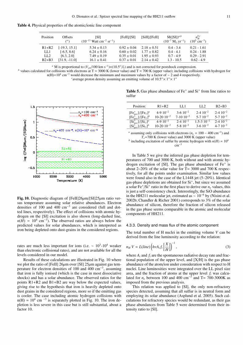
Fig. 10. Diagnostic diagram of [FeII]26µm/[SI]25µm ratio ver-sus temperature assuming solar relative abundances. Electrondensities of 100 and 400 cm−3 are considered (full and dot-ted lines, respectively). The effect of collisions with atomic hy-drogen on the [SI] excitation is also shown (long-dashed line,n(H) = 104 cm−3). The observed ratios are always below thepredicted values for solar abundances, which is interpreted asiron being depleted onto dust-grains in the considered regions.

rates are much less important for ions (i.e. ∼ 103-104 weakerthan electronic collisional rates), and are not available for all thelevels considered in our model.

Results of these calculations are illustrated in Fig. 10 wherewe plot the ratio of [FeII] 26µm over [SI] 25µm against gas tem-perature for electron densities of 100 and 400 cm−3, assumingthat iron is fully ionised (which is the case in most dissociativeshocks) and has a solar abundance. The observed ratios for thepoints R1+R2 and B1+B2 are way below the expected values,giving rise to the hypothesis that iron is heavily depleted ontodust grains in the considered regions, more so if the emitting gasis cooler. The case including atomic hydrogen collisions withn(H) = 104 cm −3 is separately plotted in Fig. 10. The iron de-pletion is less severe in this case but is still substantial, about afactor 10.

Table 5. Gas phase abundance of Fe+ and Si+ from line ratios tosulfur

Position: R1+R2 LL1 LL2 B2+B3

[Fe+gas]/[Fe�]a 4-9 10−2 3-6 10−2 2-4 10−2 2-4 10−2

[Fe+gas]/[Fe�]b 10-20 10−2 7-10 10−2 5-7 10−2 5-7 10−2

[Si+gas]/[Si�]a 4-9 10−2 2-4 10−2 1.5-3 10−2 2-4 10−2

[Si+gas]/[Si�]b 10-20 10−2 5-8 10−2 3-6 10−2 4-7 10−2

a assuming only collisions with electrons (ne = 100 − 400 cm−3) andTe=700 K (lower value) and 3000 K (upper value)

b including excitation of sulfur by atomic hydrogen with n(H) = 104

cm−3

In Table 5 we give the inferred gas phase depletion for tem-peratures of 700 and 3000 K, both without and with atomic hy-drogen excitation of [SI]. The gas phase abundance of Fe+ isabout 2–20% of the solar value for T= 3000 and 700 K respec-tively, for all the points under examination. Similar low valueswere found also in the case of the L1448 jet (5–20%). Identicalgas-phase depletions are obtained for Si+, but since we assumeda solar Fe+/Si+ ratio in the first place to derive our ne values, thisis just a self-consistency check. Interestingly, the SiO abundancein the HH211 molecular jet, estimated as ∼ 10−6 by (Nisini et al.2002b; Chandler & Richer 2001) corresponds to 3% of the solarabundance of silicon, therefore the fraction of silicon releasedin the gas phase seems comparable in the atomic and molecularcomponents of HH211.

4.3.3. Density and mass flux of the atomic component

The total number of H nuclei in the emitting volume V can bederived from the line luminosity according to the relation:

nH V = L(line)(hνAi fi

[ XH

])−1

, (3)

where Ai and fi are the spontaneous radiative decay rate and frac-tional population of the upper level, and [X/H] is the gas phaseabundance of the atom/ion under consideration with respect to Hnuclei. Line luminosities were integrated over the LL pixel sizearea, and the fraction of atoms at the upper level fi was calcu-lated for ne between 100 and 400 cm−3 and T= 700-3000K asimposed from the previous analysis.

This relation was applied to [SI], the only non-refractoryspecies detected, assuming that all sulfur is in neutral form andemploying its solar abundance (Asplund et al. 2005). Such cal-culations for refractory species would be redundant, as their gasphase abundances from Table 5 were determined from their in-tensity ratio to [SI].


Values of nH at individual positions are listed in column 7 ofTable 4 assuming an emitting volume in the LL pixel of 10.5′′×1′′× 1′′ (uniform narrow jet). The inferred nH depends stronglyon the adopted excitation conditions: it is about 0.2 − 0.6 × 105

cm−3 for T=3000 K, ne = 100 cm−3, and 8 times higher forT=700 K, ne = 400 cm−3. The ionisation fraction is then 1.6 −5×10−3 at 3000 K, or twice smaller at 700 K. Such an ionizationlevel seems to favor the upper temperature, and therefore thelower density range. If the fraction of H atoms is important withn(H) ' 104 cm−3, the nH values would be further reduced bya factor 2, down to a few 104 cm−3. In the case again, that theemission comes from a smaller volume, eg. a small 1′′ knot asobserved in the near-IR [FeII]1.64µm line, the density would riseup to 105 cm−3.

The mass flux in the atomic/ionic component assuming alaminar flow can also be derived applying the relationship givenin Nisini et al. (2005) as applied to the mid-IR lines in Dionatoset al. (2009):

M = µmH × (nH V) × (Vt/lt), (4)

where µ=1.4 is the mean weight per H nucleus, mH is the protonmass, nH V is the total number of protons in the emitting regionas given by Eq. 3, lt is the projected emitting length along theflow and Vt the tangential flow velocity.

Derived mass flux values at the various emission peaks arelisted in column 6 of Table 4 for a tangential speed of 100 kms−1 and lt = 10.5′′ (LL pixel size). Like nHV , they again dependstrongly on the adopted excitation conditions. From the ioniza-tion fraction considerations made above, we favor the high tem-perature, smaller M values of ∼ 0.4 − 1 × 10−7 M� yr−1. Theseare 20–50 times smaller than the cool H2 jet mass-flux, assumingthe same flow speed of 100 km s−1.

However, we stress again that M estimates assuming a lam-inar jet flow may be in error if the [SI] emission arises fromshocks, which is likely given the ionization fraction inferredabove. This is difficult to quantify without appropriate shockmodels.

The atomic/ionic emission appears to require higher excita-tion shocks than those producing the mid-IR H2 lines. The lowvelocity 10–15 km s−1 shock models that best fit the warm H2emission are unable to reproduce also the observed [FeII] and[SiII] line intensities unless the shocks are of J-type and theseatoms are essentially undepleted. As discussed in Section 4.3.2there is overwhelming evidence of depletion of these refractoryspecies, so [FeII] and [SiII] probably arise from faster shocksthan those dominating the mid-IR H2 lines. It is indeed likelythat the mid-IR atomic lines originates from the same dissocia-tive shocks at vs ≥ 30 km s−1 that give rise to the optical and NIRemission of Hα, [SII] and [FeII] (O’Connell et al. 2005; Carattio Garatti et al. 2006; Walawender et al. 2006, 2005).

Unfortunately, our shock models do not yet include ioniza-tion and dissociation by the shock UV flux, so we cannot explorethe relevant excitation range. However, we note that the J–shockmodels of Hollenbach & McKee (1989), which include UV flux,suggest that the [SI]25µm brightness is relatively independent ofshock speed over the range 30–100 km s−1 and is roughly pro-portional to nini

H . Our measured flux inside the LL 10.5′′ pixelwould suggest nini

H × b f f ' 100 − 1000 cm−3. From Eq. 2 wewould infer a preshock mass-flux of ∼ 0.5 − 5 × 10−7 M� yr−1,still smaller by a factor 4–40 than the cool H2 jet mass-flux.

These results would suggest that the atomic component inthe HH211 jet does not have enough momentum flux to entrainthe CO/SiO/H2 jet, if their velocities are comparable and the

shock compression in the cool H2/CO component does not ex-ceed a factor 3. The molecular jet would then have to trace mate-rial ejected from the accretion disk, while the atomic componentwould trace a separate ejection, e.g. from hotter more internalregions of the accretion disk. On the other hand, a higher com-pression factor in the cool H2/CO emitting zone, or a faster ionicjet would suffice to remove the discrepancy, therefore a definiteconclusion on whether the molecular jet is ejected or entrainedcannot be reached from the present data alone.

5. Conclusions

We have carried out Spitzer spectral mapping observationstowards the jet driven by the Class 0 source HH211-mm.Molecular lines (pure rotational H2) as well as fundamentalatomic and ionic lines ([SI], [SiII], [FeII]) were detected, andtheir maps follow the characteristic bipolar outflow pattern astraced by near-IR H2 and CO lines. H2 emission becomes im-portant only 5′′ away from the driving source while atomic andionic lines are detected very close to the driving source. In theinner part of the blue-shifted lobe, the H2 emission is spatiallycoincident with the high velocity jet observed in CO and SiO.

Analysis of the observed H2 lines reveal two temperaturecomponents: ”cool” gas at T∼ 300K dominating the mass, and”warm” gas at T∼ 700-1200K of 10 times smaller average col-umn density. Once corrected for beam dilution, the column den-sity of ”cool” H2 towards the CO jet is compatible with hydro-gen being mostly molecular. The warmer component traced bythe S(2) to S(7) lines is well fitted by C-shock models of highdensity ' 5 × 105 and a small shock cross section of 0.5′′, com-patible with the density and width of the CO jet quoted by Leeet al. (2007). The warm H2 emission could then trace thin layersof warm post-shock gas within the CO jet.

Similarly, high-density C-shock models can also account forthe brightness of the H2 mid-IR emission further downwind be-yond the CO and SiO jet, but the small shock surface filling fac-tor of 0.01-0.04 is not easy to reconcile with the spatial exten-sion visible in Spitzer maps, unless the bow-shock wings arevery clumpy. Lower density shocks of nH ≤ 104 cm−3 where thecooling zone spreads over several pixels and/or higher preshockionization may need to be considered in these regions, as previ-ously invoked to model near-IR H2 excitation in the red-shiftedbow-shock of HH211 (O’Connell et al. 2005).

The detected fine structure lines mapped very close to thedriving source signify the presence of an embedded atomic jet.Line ratio diagnostics indicate a gas-phase depletion of iron andsilicon of at least a factor 10, and lower excitation conditionsthan in optically visible jets. An atomic jet of similar proper-ties has been also detected by Spitzer in the outflow of L1448-C(Dionatos et al. 2009). As suggested in that case, the detectedatomic gas in the HH211-mm outflow may represent the equiv-alent for the Forbidden Emission Line (FEL) region observed inmore evolved ClassI/II sources. The gas depletion of iron and sil-icon indicates that dust grains have survived in the atomic flow,ruling out an origin from within the dust sublimation zone closeto the protostar. The excitation conditions require faster shocksthan those producing the H2 mid-IR lines.

Estimations of the molecular and atomic mass-flux rateshave been performed using both a laminar flow assumption andshock models. The cool H2 mass-flux is comparable to that in-ferred from CO observations, with a value uncorrected for com-pression of ∼ 2×10−6 M� yr−1 (V/100 km s−1); a similar value isfound for the warm H2 if it arises from dense C-shocks as sug-gested by best fit models. The atomic component mass-flux is


uncertain by a factor 8 due to its uncertain temperature, but con-siderations of ionization fraction as well as published dissocia-tive shock models suggest a mass-flux smaller than in the molec-ular jet. However, the momentum fluxes could become compa-rable if the atomic jet is faster than the molecular jet, or if thecool H2 and CO suffered shock compression. Given the uncer-tainties, it is still unclear whether the molecular CO jet is tracingambient gas entrained by the atomic jet, or if it has to be ejected,for example in a molecular MHD disk wind as recently modeledby Panoglou et al. (2010, A&A, submitted).

Acknowledgements. This work is based on archival data obtained with theSpitzer Space Telescope, which is operated by the Jet Propulsion Laboratory,California Institute of Technology under a contract with NASA. It was supportedin part by the European Community’s Marie Curie Actions - Human Resourceand Mobility within the JETSET (Jet Simulations, Experiments and Theory) net-work under contract MRTN-CT-2004 05592. Financial contribution from con-tract ASI I/016/07/0 is also acknowledged.

ReferencesArce, H. G., Shepherd, D., Gueth, F., et al. 2007, in Protostars and Planets V, ed.

B. Reipurth, D. Jewitt, & K. Keil, 245–260Asplund, M., Grevesse, N., & Sauval, A. J. 2005, in Astronomical Society of

the Pacific Conference Series, Vol. 336, Cosmic Abundances as Records ofStellar Evolution and Nucleosynthesis, ed. T. G. Barnes, III & F. N. Bash,25–+

Bally, J., Heathcote, S., Reipurth, B., et al. 2002, AJ, 123, 2627Caratti o Garatti, A., Giannini, T., Nisini, B., & Lorenzetti, D. 2006, A&A, 449,

1077Chandler, C. J. & Richer, J. S. 2001, ApJ, 555, 139Davis, C. J. & Smith, M. D. 1996, A&A, 309, 929Dionatos, O., Nisini, B., Garcia Lopez, R., et al. 2009, ApJ, 692, 1Dufton, P. L. & Kingston, A. E. 1991, MNRAS, 248, 827Eisloffel, J., Froebrich, D., Stanke, T., & McCaughrean, M. J. 2003a, ApJ, 595,

259Eisloffel, J., Froebrich, D., Stanke, T., & McCaughrean, M. J. 2003b, ApJ, 595,

259Enoch, M. L., Young, K. E., Glenn, J., et al. 2006, ApJ, 638, 293Ferreira, J., Dougados, C., & Cabrit, S. 2006, A&A, 453, 785Flower, D. R., Le Bourlot, J., Pineau des Forets, G., & Cabrit, S. 2003, MNRAS,

341, 70Flower, D. R. & Pineau des Forets, G. 2003, MNRAS, 343, 390Froebrich, D. 2005, ApJS, 156, 169Giannini, T., McCoey, C., Nisini, B., et al. 2006, A&A, 459, 821Gibb, A. G., Richer, J. S., Chandler, C. J., & Davis, C. J. 2004, ApJ, 603, 198Gueth, F. & Guilloteau, S. 1999, A&A, 343, 571Guilloteau, S., Bachiller, R., Fuente, A., & Lucas, R. 1992, A&A, 265, L49Gusdorf, A., Pineau Des Forets, G., Cabrit, S., & Flower, D. R. 2008a, A&A,

490, 695Gusdorf, A., Pineau Des Forets, G., Cabrit, S., & Flower, D. R. 2008b, A&A,

490, 695Gustafsson, M., Ravkilde, T., Kristensen, L. E., et al. 2010, A&A, 513, A5+Hartigan, P., Morse, J. A., & Raymond, J. 1994, ApJ, 436, 125Herbig, G. H. 1998, ApJ, 497, 736Hernandez, J., Calvet, N., Hartmann, L., et al. 2005, AJ, 129, 856Hirano, N., Liu, S.-Y., Shang, H., et al. 2006, ApJ, 636, L141Hollenbach, D. & McKee, C. F. 1989, ApJ, 342, 306Houck, J. R., Roellig, T. L., van Cleve, J., et al. 2004, ApJS, 154, 18Kaufman, M. J., Wolfire, M. G., Hollenbach, D. J., & Luhman, M. L. 1999, ApJ,

527, 795Kristensen, L. E., Ravkilde, T. L., Field, D., Lemaire, J. L., & Pineau Des Forets,

G. 2007, A&A, 469, 561Lada, C. J., Muench, A. A., Luhman, K. L., et al. 2006, AJ, 131, 1574Lee, C.-F., Ho, P. T. P., Palau, A., et al. 2007, ApJ, 670, 1188McCaughrean, M. J., Rayner, J. T., & Zinnecker, H. 1994, ApJ, 436, L189Nisini, B., Bacciotti, F., Giannini, T., et al. 2005, A&A, 441, 159Nisini, B., Caratti o Garatti, A., Giannini, T., & Lorenzetti, D. 2002a, A&A, 393,

1035Nisini, B., Codella, C., Giannini, T., & Richer, J. S. 2002b, A&A, 395, L25O’Connell, B., Smith, M. D., Froebrich, D., Davis, C. J., & Eisloffel, J. 2005,

A&A, 431, 223Pudritz, R. E., Ouyed, R., Fendt, C., & Brandenburg, A. 2007, in Protostars and

Planets V, ed. B. Reipurth, D. Jewitt, & K. Keil, 277–294

Reipurth, B. & Bachiller, R. 1997, in IAU Symposium, Vol. 170, IAUSymposium, ed. W. B. Latter, S. J. E. Radford, P. R. Jewell, J. G. Mangum,& J. Bally, 165–174

Rieke, G. H. & Lebofsky, M. J. 1985, ApJ, 288, 618Ruden, S. P., Glassgold, A. E., & Shu, F. H. 1990, ApJ, 361, 546Salas, L., Cruz-Gonzalez, I., & Rosado, M. 2003, Revista Mexicana de

Astronomia y Astrofisica, 39, 77Shang, H., Li, Z., & Hirano, N. 2007, in Protostars and Planets V, ed. B. Reipurth,

D. Jewitt, & K. Keil, 261–276Smith, J. D. T., Armus, L., Dale, D. A., et al. 2007, PASP, 119, 1133Tappe, A., Lada, C. J., Black, J. H., & Muench, A. A. 2008, ApJ, 680, L117Walawender, J., Bally, J., Kirk, H., et al. 2006, AJ, 132, 467Walawender, J., Bally, J., & Reipurth, B. 2005, AJ, 129, 2308Werner, M. W., Roellig, T. L., Low, F. J., et al. 2004, ApJS, 154, 1Wilgenbus, D., Cabrit, S., Pineau des Forets, G., & Flower, D. R. 2000, A&A,

356, 1010

Spitzer spectral line mapping of the HH211 outflow

Documents

Transcript of Spitzer spectral line mapping of the HH211 outflow