arX

iv:1

005.

1940

v1 [

astr

o-ph

.SR

] 1

1 M

ay 2

010

Disentangling protostellar evolutionary stages in clustered

environments using Spitzer-IRS spectra and comprehensive SED

modeling

Jan Forbrich1, Achim Tappe1, Thomas Robitaille1, August A. Muench1, Paula S. Teixeira2,

Elizabeth A. Lada3, Andrea Stolte4, & Charles J. Lada1

ABSTRACT

When studying the evolutionary stages of protostars that form in clusters, the role of anyintracluster medium cannot be neglected. High foreground extinction can lead to situationswhere young stellar objects (YSOs) appear to be in earlier evolutionary stages than they actuallyare, particularly when using simple criteria like spectral indices. To address this issue, we haveassembled detailed SED characterizations of a sample of 56 Spitzer-identified candidate YSOsin the clusters NGC 2264 and IC 348. For these, we use spectra obtained with the InfraredSpectrograph onboard the Spitzer Space Telescope and ancillary multi-wavelength photometry.The primary aim is twofold: 1) to discuss the role of spectral features, particularly those due toices and silicates, in determining a YSO’s evolutionary stage, and 2) to perform comprehensivemodeling of spectral energy distributions (SEDs) enhanced by the IRS data. The SEDs consistof ancillary optical-to-submillimeter multi-wavelength data as well as an accurate description ofthe 9.7 µm silicate feature and of the mid-infrared continuum derived from line-free parts ofthe IRS spectra. We find that using this approach, we can distinguish genuine protostars in thecluster from T Tauri stars masquerading as protostars due to external foreground extinction. Ourresults underline the importance of photometric data in the far-infrared/submillimeter wavelengthrange, at sufficiently high angular resolution to more accurately classify cluster members. Suchobservations are becoming possible now with the advent of the Herschel Space Observatory.

Subject headings: circumstellar matter — infrared: stars — open clusters and associations: individual(NGC 2264) — open clusters and associations: individual (IC 348)

1. Introduction

Finding and characterizing individual YoungStellar Objects (YSOs) in embedded clustered en-vironments is challenging because the observedYSO spectral energy distributions (SEDs) can eas-ily be influenced by dense material that is dis-tributed throughout the cluster, but physically un-

1Harvard-Smithsonian Center for Astrophysics, 60 Gar-

den Street, Cambridge, MA 02138, USA2European Southern Observatory, Karl-Schwarzschild-

Straße 2, D-85748 Garching bei Munchen, Germany3Department of Astronomy, University of Florida,

Gainesville, FL 32611, USA4I. Physikalisches Institut, Universitat zu Koln,

Zulpicher Str. 77, 50937 Koln, Germany

related to an individual YSO or its envelope. Inthat situation, the extra extinction can misleadthe observer since an affected source may appearto be in an earlier evolutionary stage than it ac-tually is. For example, the SED of a T Tauri starbehind foreground extinction can in some circum-stances look protostellar. In a more isolated envi-ronment, this situation would only occur in caseof edge-on disks, aggravated by the presence ofdisk flaring. To avoid confusion, Robitaille et al.(2006) proposed that sources be assigned designa-tions that refer to the actual evolutionary stages,rather than spectral classes defined by observa-tions, since the latter are affected by extinction.In most instances, the evolutionary stages (I, II,III) correspond to the SED classes. However, in

1

heavily extincted regions the SED classes may notalways correspond to the appropriate evolutionarystages. In embedded clustered environments, thedifference between YSO classes and evolutionarystages becomes particularly important.

Infrared spectroscopy allows us to go beyondprotostellar classifications based on photome-try. At near-infrared wavelengths, varying de-grees of veiling can be used to distinguish proto-stars from PMS stars (Casali & Matthews 1992;Greene & Lada 1996; White et al. 2007). At mid-infrared wavelengths, silicate dust and ices causetelltale spectral features that can be used to re-fine spectral classes. Many of these features oc-cur in the wavelength range that was accessiblewith the Infrared Spectrograph (IRS) onboardthe Spitzer Space Telescope (Houck et al. 2004).In the context of star formation, the power ofthis instrument has been shown most notably bystudies of T Tauri stars and protostars in Taurus,Chamaeleon, and Ophiuchus (Furlan et al. 2006,2008, 2009). Most recently, McClure et al. (2010)study an extensive sample of YSOs in Ophiuchus,using IRS data to determine their evolutionarystages.

To find out whether the effect of intracluster orexternal foreground extinction can be disentangledfrom the actual evolutionary stage of a YSO, wehave obtained IRS spectra and assembled detailedmulti-wavelength photometry for a sample of 56candidate YSOs in NGC 2264 and IC 348. Wethen use these data for comprehensive SEDmodel-ing with the primary aim of ascertaining the evolu-tionary stages for the sources in our sample. Thesecan then finally be compared to previous classifica-tion attempts that are mainly based on less broadmid-infrared wavelength coverage. For each of the56 sources, we have obtained mid-infrared spectrausing Spitzer-IRS. These data not only allow us tostudy spectral features that trace the evolutionarystage of a YSO (silicates and ices), but they alsoallow us to derive photometry from line-free partsof the spectrum to accurately reflect the underly-ing continuum. This technique also allows us toaccurately describe the main silicate spectral fea-ture by photometric data at selected wavelengths.Combined with ancillary photometric data span-ning optical to submillimeter wavelengths, the IRSdata thereby allow us to construct SEDs that aretailored toward the requirements of detailed mod-

eling. The accuracy of the modeling depends onthe SEDs not containing spectral lines that arenot part of the underlying model (e.g., PAH fea-tures); these features can fall into the band passesof broadband filters. Our IRS-derived photometryattempts to depict the continuum and the silicatefeatures. Compared to the usual approach of us-ing photometry from Spitzer-IRAC in SEDs forsubsequent modeling, we discard bands 3 and 4 ofthe IRAC data that we have for every source in fa-vor of corresponding line-free photometry derivedfrom the IRS data.

1.1. Source selection

We selected 56 candidate protostars in NGC2264 and IC348 – 40 in the former and 16 in thelatter region – from previous Spitzer photometricstudies of these regions by Muench et al. (2007)and Teixeira (2008). Our target sources are listedin Table 1.

NGC 2264 is a prominent, clustered star-forming region located at a distance of ∼913 pc(Baxter et al. 2009); for a recent review, seeDahm (2008). Here, we focus on the popula-tion of embedded protostars in the vicinity ofIRS 2 (Young et al. 2006) where we selected 40sources for Spitzer-IRS mid-infrared spectroscopicobservations. This region is one of the two mostprominent regions of ongoing star formation inNGC 2264, next to IRS 1. All selected sourcesare located in the Spokes cluster (Teixeira et al.2006). Figure 1 shows the selected sources ina mid-infrared view of the region. IC 348 is lo-cated in Perseus at a distance of ∼260 pc (e.g.,Lombardi et al. 2010); for a recent review, seeHerbst (2008). Muench et al. (2007) conducted aSpitzer census of this star-forming region. TheIC 348 sources discussed in this paper are amongthe most embedded in the cluster and are predom-inantly protostars in a narrow filamentary ridgelocated about 1 pc southwest of the central clus-ter. In Figure 2, we mark the selected sources ina mid-infrared view of the region.

A first comparison within our sample can beaccomplished by using the IRAC spectral in-dex αIRAC, as determined from a least-squaresfit to the photometry of all four IRAC bands(Lada et al. 2006); see section 2.2 for a discussionof the photometry. The sources in our NGC 2264subsample show diverse IRAC spectral indices,

2

ranging from α = −1.41 (source 27) to α = 4.21(source 45). Eighteen sources in this subsamplehave positive spectral indices. Sung et al. (2009)identify 37 out of the 40 sources as candidatecluster members in various stages, 20 of them arelisted as class I sources; their classification is in-cluded in Table 1. Note that while Sung et al.(2009) list no membership status for the threeremaining sources, our results suggest that theyare cluster members, too. In the IC 348 sample,the IRAC spectral indices range from α = −0.93(source 14) to α = 1.92 (source 6). The classifi-cation from Lada et al. (2006) and Muench et al.(2007) is listed in Table 1. Most of the sourcesin this subsample are class I objects. Since wedo not find significant differences between thesetwo cluster subsamples – both (unevenly) samplethe same YSO classes –, we will discuss them asone sample in the following, focusing more on adiscussion of evolutionary stages in general. Note,however, that the source table allows the readerto identify individual YSOs in both clusters.

In this paper, we first discuss the Spitzer-IRS observations and their data reduction. Wethen describe the ancillary multi-wavelength data,ranging from optical to submillimeter wave-lengths, and how we assembled composite SEDsfrom both IRS spectra and ancillary data. Sub-sequently, we perform comprehensive modeling ofthese SEDs before concluding with a discussionand summary of the results.

2. Observations and Data Reduction

2.1. Spectroscopic observations with Spitzer-IRS

IC 348 and NGC2264 were observed with theSpitzer Infrared Spectrograph (IRS) between 2006September 16 and 2007 October 30 (Spitzer pro-gram 30033). We mapped the majority of YSOsusing the IRS short-low (SL2/SL1, 5.2–8.7/7.4–14.5 µm, R = 64–128), short-high (SH, 9.9–19.6 µm, R = 600), and long-high (LH, 18.7–37.2 µm, R = 600 ) or long-low (LL, 14.0–38.0µm,R = 64–128) modules.

For IC 348, the sources are covered by individ-ual small maps of typically 2 by 3 dithered point-ings, i.e., three steps perpendicular and two stepsalong the slit, for both low and high resolutionmodules. We included separate high-resolution

background observations for each source. ForNGC2264, which shows a much higher degree ofsource clustering, we designed extended SL/LLmaps that cover a larger number of sources si-multaneously, with individual high-resolution 2 by3 dithered maps for the brightest sources. Forthe observations in NGC 2264, only a single high-resolution background observation was obtained;it is used for all NGC 2264 high-resolution maps.

All maps in this program are optimized fordata reduction with CUBISM1 v1.60 (Smith et al.2007), i.e., they were obtained with half slit-widthstepping perpendicular to the slit and additionaldithering along the slit direction in most cases,resulting in quadruple data redundancy for eachpixel in the map center. The individual steps ofour data reduction are as follows:

1. Acquisition of the BCDs (Basic CalibratedData) as provided by the Spitzer IRSpipeline S17.2 to S18.2

2. Importation of all sequential observationstaken at the same date into CUBISMprojects, separately for each module

3. Selection and subtraction of an averagebackground (dedicated for SH/LH; selectedfrom outrigger slit positions of the sameand/or other sources judged by variabilityof the background level in IRAC/MIPS (In-frared Array Camera, Multiband ImagingPhotometer for Spitzer) maps

4. Identification and excision of remainingbad pixels using CUBISM’s statistical al-gorithms

5. Construction of the data cube without us-ing CUBISM’s SLCF (Slit Loss CorrectionFunction), i.e., keeping the original IRSpipeline calibration (see §2.1.1)

6. Extraction of spectra for each source usinga square aperture of typically 4 by 4 mod-ule pixels (nominal pixel sizes for the IRSSL/LL/SH/LH modules are 1.8, 5.1, 2.3,and 4.5′′, respectively)

7. Conversion of spectra from the defaultMJysr−1 unit to Jy by multiplying by theaperture area in steradian

1http://ssc.spitzer.caltech.edu/archanaly/contributed/cubism/

3

8. Importation of spectra into SMART (Higdon et al.2004) for joining of the orders and scaling tomatch the MIPS 24µm photometry (used asreference, see below)

2.1.1. CUBISM

The Spitzer IRS pipeline is optimized for iso-lated stellar point sources. It is correcting for lightlosses due to the limited size of the slit and theextraction aperture compared to the point-spread-function. The flux calibration is accomplished byobserving standard stars and matching their spec-tra to stellar models. Hence, the pipeline flux cal-ibration is invalid if: a) the observed source is nota stellar point source, b) the slit is not centeredon the observed point source, or c), the defaultpipeline extraction apertures are changed. It ispossible to correct for items b) and c) by derivinga new calibration using the pipeline approach.

However, if the observed source is not a stel-lar or ‘true’ point source, e.g., a YSO with anaccretion disk and/or an extended envelope, wecannot expect the flux calibration to be correct.To make matters worse, the effects change withwavelength and also among the different IRS mod-ules because of their different sizes and the result-ing uneven coverage on an asymmetric, extendedsource. Since all YSOs have an individual anda priori unknown extended structure and, in ad-dition, slit coverage will change as a function ofdistance to the source, no reliable flux calibrationcan be derived from standards. Our approach tothis dilemma is to use CUBISM (see §2.1), which isoptimized for handling Spitzer IRS mapping dataof homogenous extended sources, and scale the re-sulting spectra to the measured MIPS-24µm pho-tometry of each source. As a consistency check ofthe photometric calibration, we have extracted2

color-correct magnitudes for IRAC bands 3 and4 from the IRS spectra in order to compare theresults with the IRAC aperture photometry. Forspectra that are not too noisy, the IRAC photome-try yields fluxes that are slightly higher than thosefrom the synthetic IRS photometry, with meanoffsets of 12% in band 3 and 18% in band 4, al-though offsets of up to a factor of two are occur-ring. While the two sets of photometry are equiv-

2using IDL code provided by the Spitzer Science Center at

http://ssc.spitzer.caltech.edu/dataanalysistools/cookbook/10/

alent in their spectral coverage, this comparisondoes not account for slit losses. Additionally, anysource variability would cause further differencessince the IRAC and IRS data were not obtainedsimultaneously. Given these limitations, the twosets of photometry thus appear to be consistent.

We compared the extracted spectra of CUBISMand SPICE for a representative, mapped YSO inour sample. This example, source 56, is shown inFigure 3. We selected this source since it is fairlybright and shows complex spectral structure dueto ices, silicate grains, H2 emission lines, and a ris-ing continuum due to the presence of an envelope.SPICE is the IRS data reduction tool supportedby the Spitzer Science Center, and it is optimizedfor single pointing (staring) observations of stellarpoint sources. The SPICE spectra were extractedby using only the map slits centered on the YSO,whereas the CUBISM spectra were extracted us-ing the approach described in §2.1. Reassuringly,both methods yield very similar spectral features,continuum shapes, and signal-to noise ratios. Inboth cases additional scaling is needed to join thespectral orders and match the MIPS photometry.The main advantages of CUBISM for reducing IRSmapping data of a large sample of diverse YSO’sare:

• The data reduction is greatly facilitated dueto integrated BCD bookkeeping, accurate vi-sualization and accounting of all slit point-ings, background subtraction, and statisticalbad pixel handling.

• The spatial maps cover all or a large fractionof an extended YSO and therefore minimizethe effects of uneven slit coverage or varyingslit orientation.

• There is no restriction on the size and shapeof the extraction aperture for the source andbackground spectra.

• The spatial maps provide increased data re-dundancy compared to single slit staring ob-servations.

The resulting spectra, concatenated from thedifferent modules, are shown in Figures 4 to 7,where they are sorted by evolutionary stage, as

4

informed by subsequent analysis3. Overall, theyrepresent a wide variety both in evolutionary stageas well an in the spectral features present.

2.1.2. Continuum and ice features

Many of the YSOs in our sample show promi-nent ice absorption features at 5–8 and 15 µm aswell as silicate absorption at 9.7 and 18 µm (see,e.g., Figure 3). In order to quantify and com-pare the ice and silicate features between differentsources, we measured the center optical depthsτλ of the 6.0 µm and 9.7 µm H2O ice and silicateabsorption features, respectively, and the inte-grated optical depth

∫τ dν of the 15 µm ice fea-

ture which is dominated by CO2 (Gerakines et al.1999) and has been described as a CO2:CO:H2Oblend (Pontoppidan et al. 2008). The lattercan be converted to a column density, Nice =A−1

ice

∫τ dν, where Aice is the ice band strength of

1.1× 10−17 cmmolecule−1 assuming pure CO2 ice(Gerakines et al. 1995; Pontoppidan et al. 2008).In order to convert the spectra to an optical depthscale, τλ = ln(Icont,λI

−1λ ), we determined the con-

tinuum by fitting a low-order polynomial on alog-log scale to the spectral regions below wave-lengths of about 5.8 µm and above 30 µm (seeFigure 3). These regions are least affected by ab-sorption features (see also Boogert et al. 2008).In addition, we determined a local continuum forthe 15 µm ice feature by fitting a low-order poly-nomial to the adjacent spectral continuum of thatfeature. A detailed analysis of the individual icefeature components is beyond the scope of thispaper. We note that the distribution of spectralfeature strengths is similar to previously publishedsurveys of other regions, even without taking intoaccount the different sets of criteria that were usedto define the various samples.

2.2. Ancillary optical, infrared, and sub-millimeter photometry

Our IRS spectra complement a wealth of ancil-lary photometric data that we use for subsequentcomprehensive SED modeling. For IC 348, we usedata compiled by Muench et al. (2007). The onlyexceptions are MIPS mid-infrared and SCUBA

3Note that sources 14 and 49 are not shown because nearby

bright sources blend with their data at longer wavelengths.

The SEDs of these sources therefore are not modeled at all.

submillimeter data where we have converted sev-eral flux densities for individual sources into upperlimits if there is any indication that several sourcescontribute to the flux density.

Our main source of optical UBVRI photom-etry for NGC 2264 is the ancillary data cat-alog compiled by Rebull et al. (2006). Thephotometry for the sources presented here isfrom various sources cited therein (Sung et al.1997; Flaccomio et al. 1999; Park et al. 2000;Rebull et al. 2002; Lamm et al. 2004). To resolveinconsistencies (for a given source, the UBVRI

photometry typically is from at least two differ-ent sources), the USNO-B1 catalog has been usedadditionally.

In the near-infrared, we use FLAMINGOS(Elston 1998) imaging data in JHK to surpassthe 2MASS catalog in sensitivity. The observa-tions were taken on 01 January 2005 when theinstrument was mounted to the 2.1m telescopeon Kitt Peak. In this data, all but seven of oursources in NGC 2264 are detected at least in K

band. For the undetected sources, the estimatedsensitivity limits of J = 19 mag, H = 18 mag,and K = 17.5 mag were assumed as upper lim-its. Aperture photometry was performed on theseimages with an aperture of five pixels or 1.5′′

with a surrounding annulus of five pixels widthto subtract the background. To avoid saturationproblems, we have used 2MASS photometry forthree bright sources (sources 17, 36, and 47).

In the mid-infrared range covered by Spitzer,we have obtained aperture photometry from IRACand PRF-fitting photometry from MIPS imagingdata. The IRAC data were obtained in March2006 (program ID 37) when both 0.6 sec and 12 secexposures were taken. Aperture photometry wasperformed with an aperture radius of five pixelsand a background annulus with inner and outerradii of 5 and 10 pixels. For all but two sources,we used the 12 sec exposures. Sources 20 and 47required correcting for saturation in the first twoIRAC channels. We used a comparison of IRACand longer-wavelength data to find obvious blendsof multiple objects and exclude the correspondingSEDs from modeling; this concerns sources 6+7 (ablend), 41, and 43. From the IRAC photometry, aspectral index αIRAC was determined from a least-squares fit to all four IRAC channels in λFλ. Toensure comparability within our full sample, the

5

same method was used to also determine spectralindices for the sources IC348, using the photomet-ric data from Muench et al. (2007).

In the submillimeter range, we use aper-ture photometry to estimate upper limits inSCUBA data (450 µm and 850 µm) obtained byWolf-Chase et al. (2003) for NGC 2264 in 1999and 2000. For NGC2264 and most of IC 348, wedecided to only use upper limits due the crowdingof the cluster relative to the angular resolution.In determining the photometry, we read out thepixel value at the source position (calibrated inJy/beam) and subsequently added five times therms of the surrounding 25 pixels. For the use inSED modeling, in order to use strict upper lim-its, we have doubled the upper limits that weredetermined in the mid-infrared (MIPS) and sub-millimeter bands.

2.3. Constructing photometric SEDs

As a preparation for the SED model fits, wehave constructed photometric SEDs for all ob-served sources using the ancillary photometricdata as well as the IRS observations. The SEDscover the optical (UBVRI), the near infrared(JHK), the mid-infrared (3µm up to 35µm fromIRAC and IRS) and the submillimeter ranges(450µm and 850µm). We have extracted pho-tometry from the IRS data to complement thebroadband data from the literature, using bandsthat characterize the continuum as well as the9.7 µm and 18 µm silicate features – these aretaken into account in the SED models that weuse – while being least affected by molecular oratomic lines and ice features that are not takeninto account in the model. The wavelengths forwhich photometry was derived using the IRS dataare 5.580, 7.650, 9.95, 12.93, 17.72, 24.28, 29.95,and 35.06 µm, where the first two bands replaceIRAC bands 3 and 4 since they are less affected byspectral features than these two IRAC bands. Thewidths of the IRS spectral windows that are con-verted into photometry are set to 2% of the centerwavelengths. In this process, a few photometrypoints were flagged and not taken into accountin the modeling if the IRS data were too noisy.Overall, fluxes from 21 separate wavelength bandswere used to construct the SEDs for individualsources.

3. Analysis

3.1. IRS spectra

3.1.1. Dust and ice features

In the following, we will focus on the silicate andice features and their correlation with the sources’infrared spectral indices while also noting the de-tection of PAH emission in only three sources inNGC2264, perhaps indicating the presence of rela-tively massive stars. The spectral analysis for thesources in our sample is summarized in Table 2,where the sources are already sorted by evolution-ary stage, as informed by subsequent SED mod-eling. The plots of the spectra in Figures 4 to 7are sorted in the same fashion. The detailed SEDmodeling that is required to sort the sources byevolutionary stage will be described subsequently.

For the purpose of comparing spectral featuresto an infrared spectral index as a more easily ob-servable source parameter, we use the IRAC spec-tral index simply because it is available for moresources in our sample than another frequently usedindex, spanning from the near-infrared K bandto 24 µm. Several, presumably deeply embeddedsources in our sample remain undetected in thenear-infrared wavelength range. We note, how-ever, that the trends discussed here are also ap-parent when using the K–24µm spectral index(not shown). We remind the reader that the IRACspectral index was calculated from all four IRACbands; to ensure the comparability with otherdatasets, it does not use any IRS data in replace-ment for IRAC channels. The scatter of the fourIRAC channels is reflected in the uncertainty ofthe spectral index, also derived from the fit.

We now discuss the relationship of the 9.7µmsilicate feature and the total ice column densitywith the IRAC spectral index. We also directlycompare silicate emission and ice absorption andcompare this relationship to the results of the c2dsurvey. In Fig. 8, we show the corresponding plotsin six panels that are described in more detail inthe following. As shown in Fig. 8a/b, a source witha positive spectral index tends to have strongersilicate absorption and ice features than a sourcewith a negative spectral index. Note that the sili-cate feature can appear in emission (indicative ofdisks) or in absorption, while the ice features al-ways are absorption features. Our discussion of

6

silicate features focuses on the prominent 9.7µmsilicate feature, but we note that the optical depthof the 18µm silicate features is correlated to theone at 9.7µm, even if any more detailed compari-son is limited by the uncertainties. The measuredfull-width half-maximum (FWHM) line widths ofthe 9.7µm silicate feature range from 1.8µm to3.6µm. Fig. 8c shows that the broader line widthscorrespond to negative silicate optical depths, i.e.,silicate emission, while the line width does notchange much for the silicate features in absorption.There is a tentative anti-correlation of the widthof the silicate feature with the IRAC spectral in-dex; the broadest lines are found in emission andin the sources with the lowest spectral indices (seeFig. 8d), possibly indicative of grain growth in thelater evolutionary stages. However, Sargent et al.(2009) and Watson et al. (2009) point out that theeffects of grain growth on the silicate feature aredifficult to observe unambiguously even for class IIsources where one might expect the effect to bemore discernible than in protostars. Finally, therealso appears to be a correlation between the op-tical depth of the 9.7µm silicate absorption fea-tures and the total ice column density (shownin Fig. 8e), similar to the results of Furlan et al.(2008, Fig. 29). As pointed out by Furlan et al.(2008), the silicate optical depth and the ice col-umn density are expected to be correlated sincea higher silicate optical depth should also provideshielding for ice mantles to grow. While gener-ally, sources with larger optical depths of the sili-cate feature tend to have stronger ice features, theclass I source 53 is the only source not followingthis trend; it has a much lower ice column densitythan what could be expected from this correlation,indicating that the central star might be able toevaporate the ice mantles.

None of the sources with silicate in emissionshow ice features. This probably indicates thatthe envelopes of these sources have dissipated andices are no longer observable. In Fig. 8f, we com-pare the silicate optical depth and the total icecolumn density from this study with results fromthe Spitzer c2d survey (Pontoppidan et al. 2008;Boogert et al. 2008). Again there is a correlationof large silicate optical depths and high ice columndensities even though there are two exceptionssimilar to source 53. These two sources (W33Aand W3 IRS 5) have high silicate optical depths,

but comparably low total ice column densities.W33A is an H II region and W3 IRS 5 is a massive-star–forming region. Possibly, both sources as wellas our source 53 produce strong enough radiationto evaporate the ice mantles.

A quantitative comparison of the spectral fea-tures with the literature is difficult since partic-ularly the methods used to determine the con-tinuum vary considerably. However, we can di-rectly compare our results with the c2d survey(Pontoppidan et al. 2008; Boogert et al. 2008).The range and distribution of the optical depthsof the silicate features (τ6µm and τ9.7µm) and ofthe total ice optical depth are very similar.

3.1.2. PAH and Gaseous Spectral Lines

As noted above, a detailed discussion of allspectral features that were observed in our sam-ple is beyond the scope of this paper. However, wewould like to point out the most important IRS re-sults beyond silicate and ice features. We detectedstrong PAH emission in sources 25, 36, and 42, allin NGC 2264. The emission is clearly associatedwith the YSOs, since the surrounding backgroundis devoid of extended PAH emission in all threecases. However, the Spitzer resolution does notpermit to resolve the origin of the PAH emissionwithin the YSO envelope/disk system. We can ex-clude extended PAH emission beyond the Spitzer

resolution limit for sources 25 and 42. In thesecases, the PAH emission is hence located within aradius of about 1000 AU from the YSO sources.In the case of source 36, the high luminosity aswell as blending of the PAH 6.2 µm feature withice features make the spatial PAH analysis uncer-tain. These three sources might represent the up-per end of the mass function in the Spokes clus-ter. We will later see that among these sourcesonly the SED of source 42 can be modeled reli-ably. The fit indeed suggests that source 42 isin the upper luminosity range among the objectswhose SEDs we have studied in more detail. Notethat even though NGC2264 IRS 2 is not includedin our spectral map, its immediate vicinity alsoshows strong PAH emission.

Within the Spokes cluster, Young et al. (2006)and Teixeira et al. (2007) discovered a dense clus-ter of protostars called the microcluster. This re-gion is included in our sample as two separateobjects, 41 and 43, each being a blend of several

7

sources that can be resolved in the near-infraredwavelength range. For these regions, we can takeadvantage of the spectral mapping capabilities ofSpitzer to characterize the region. Even thoughthe microcluster remains spatially unresolved atthe longer wavelengths, we can still study a varietyof spectral features in the region; this is shown inseveral panels in Fig. 9. The interpretation of thespatial features is complicated by the highly vari-able extinction across the region, most strongly af-fecting the near-IR wavelengths. In addition, theabsorption maps are constrained by the presenceof a background continuum source at the respec-tive wavelength, i.e., the absence of absorptiondoes not necessarily indicate the absence of theabsorbing species.

Fig. 9 (panel b) shows spatially extended H2

emission, which together with the detection of[Ne II] indicates outflow activity in the vicinity ofsources 41, 43, and 44. The H2 detection is consis-tent with the narrowband H2 (1–0) 2.12 µm imagepresented by Young et al. (2006). The 30 µm con-tinuum emission and the 15.2 µm ice absorption(Fig. 9, panel c) and f), respectively) are consis-tent with the positions of the protostars SMA–2, 3,5, and 6 reported by Teixeira et al. (2007), whentaking into account the larger Spitzer beam. Notethat SMA–5 and 6, the class 0 protostars with thehighest observed 230GHz flux in the microcluster,have no near-IR counterpart due to the high ex-tinction, but are detected in our longer wavelengthSpitzer maps.

The aim of a quantitative analysis of spectrallines is usually to determine the local physical con-ditions, primarily density and temperature of thegas, and to infer chemical abundances. Infraredemission lines are a useful gas diagnostic for op-tically obscured regions such as embedded YSOs.However, a detailed, quantitative analysis of in-frared emission lines in YSOs is hampered for thefollowing reasons:

• Typically, only a limited set of infrared linesis observed for a given source (probing cer-tain ionization stages and energy levels).

• Inadequate angular resolution results in lim-ited knowledge of the origin, physical geome-try, and location of the emissive region (out-flow shocks, an accretion disk, an envelope,etc., or a combination of those).

• Collisionally excited lines from an inhomoge-neous medium will be biased toward regionsof high temperature, where collisionally ex-cited emission lines will be strongest (e.g.,shocked gas).

• The UV radiation field (outflow shocks, diskand outflow cavity irradiation) and infraredcontinuum are hard to quantify, particularlyif the location of the emitting material is un-known.

• The line-of-sight extinction is difficult toquantify accurately.

In light of these difficulties, a meaningful dis-cussion of the relative line intensities of the sourcesin our sample is beyond the scope of this paperand would ideally require spatially resolved ob-servations. However, a qualitative assessment, inparticular of the presence or absence of infraredemission lines, can still give useful insights intothe physical characteristics of a given YSO. Ta-ble 4 shows an overview of the infrared emissionlines observed in our sample and lists importantatomic and molecular line parameters.

The last column in Table 4 gives the criticaldensity, ncrit,i =

∑j<i Aij/

∑j 6=i γij , where i is

the index for the initial level with energy Ei, j isthe final level, γ is the collisional rate coefficientout of level i, and A is the Einstein coefficient forspontaneous emission (Osterbrock 1989, eq. 3.31).If the gas density is much larger than the criti-cal density of a given energy level i, then colli-sional de-excitation dominates over spontaneousemission, and the infrared lines originating fromthis level get collisionally suppressed. If the den-sity is much smaller than the critical density, thesystem exhibits a non-LTE (local thermodynamicequilibrium) behavior, where line emission is thedominant de-excitation mechanism.

The initial energy level of a given infrared lineis usually populated by collisions with the mostabundant gas species (electrons, H, or H2, depend-ing on the conditions) and is depopulated eithervia spontaneous radiative emission giving rise tothe observed spectral line or via collisional de-excitation. The general conditions necessary foran infrared emission line to be strong are: a) alarge abundance of the species, b) a large popula-tion of the initial energy level (a kinetic gas tem-

8

perature similar or larger than Ei/kB), and c) alarge Einstein A coefficient for spontaneous emis-sion. Note that these are qualitative conditions,i.e., substantial populations and abundances cancompensate for small Einstein A-values (e.g., H2

pure rotational lines).

The most common infrared lines observed inour sample of 56 sources are pure rotational tran-sitions of H2 (17 sources, of which 10 sources showS(4) and higher) and atomic fine-structure tran-sitions of Ne+ (9 sources) and Fe+ (7 sources).Among these sources, there is no clear correlationbetween the detection of any one of these featureswith evolutionary stage, partly certainly due tothe low number of sources in each category. Forexample, out of the 17 sources with H2 transitions,four are in stage I, six are in stage II(ex), and threeare in stage II (while the stages of four sourceswere not conclusively determined).

The excited H2 lines trace the presence ofhot molecular gas, typically from slower, non-dissociating outflow shocks. Good examples aresources 41 and 43, which are part of the micro-cluster, an association of young sources with clearsigns of outflow activity (see above and Fig. 9).The [Ne II] 12.8 µm line is a good example of afine-structure line with a relatively large A-value,a low-lying energy level, and a large critical den-sity. In addition, neon is not depleted in the gasphase since it is not incorporated into dust grains.Therefore, Ne+ is abundant if sufficiently ener-getic UV photons are present to ionize neutralneon (λ ≤ 57 nm). This may be the case in the ir-radiated surface layers of accretion disks or in fastoutflow shocks that are strong enough to ionizeatomic hydrogen.

Iron is strongly depleted in the gas phase andtherefore it is typically observed in fast, dissocia-tive shocks, which destroy dust grains and liber-ate the iron into the gas phase (e.g., SNR shocksand fast protostellar outflows). Fe+ has a com-plex energy level structure and features both lowand high-lying energy levels, which makes it a veryuseful density and temperature diagnostic.

Combining all the information above, we at-tempt a simplified interpretation scheme:

H2 0–0 S(4) and higher traces a hot molecularenvironment (elevated gas temperature of afew 1000K or larger, low UV radiation, non-

dissociating shock).

[Ne II] 12.8 µm traces a high UV radiation en-vironment leading to high ionization and H2

photodissociation.

[Fe II] lines trace faster, dissociating shocks thatpartially destroy dust grains and produceUV radiation/ionization.

Of the eleven sources in our sample that show[Ne II] and/or [Fe II] lines, five show lines of bothspecies, four show only [Ne II] and two show only[Fe II]. The [Ne II] 12.8 µm emission in sourceswith no observed [Fe II] lines is unlikely to be dueto strong outflow shocks. These are probably casesof irradiated disks with little or no outflow shockactivity, consistent with the stage II/II(ex) clas-sification of three out of these sources (while wedid not determine a stage for the fourth source).The two sources with [Fe II] lines but no [Ne II]12.8 µm both seem to be young stage I sources,one of them being part of the microcluster, withstrong outflow shock activity.

Sources that show both [Ne II] and [Fe II] linesare probably due to irradiated disks and/or strongoutflow shocks. For example, source 41, which ispart of the microcluster and thus has no assignedstage due to source crowding, shows strong H2,[Fe II], and [Ne II]. It is unlikely that H2 and Ne+

coexist, and indeed our spectral mapping indicatesa spatial offset between the [Ne II] 12.8 µm andthe extended H2 emission, consistent with an ir-radiated disk and an outflow (see Fig. 9, panel b).Note as a caveat that the near-infrared imagingin the figure shows the complex, blended emissionin the microcluster and the clear limitations of thespatial resolution of our mid-infrared observations.An advantage is, however, that the longer wave-length observations penetrate the highly obscuredregion and show the deeply embedded protostellarsources.

3.2. SED Modeling

3.2.1. Procedure

The SEDs of all the sources were fit usingthe large set of model SEDs from Robitaille et al.(2006, hereafter R06) and the SED fitting toolfrom Robitaille et al. (2007, hereafter R07). Thesemodels were computed using the radiation trans-

9

fer code from Whitney et al. (2003b,a). The ba-sic model consists of a pre-main-sequence star sur-rounded by a flared accretion disk and a rotation-ally flattened envelope with cavities carved out bya bipolar outflow. Both scattering and reprocess-ing of the stellar radiation by dust, as well as thedisk accretion luminosity, are included. The setof models covers a large range of stellar masses(from 0.1 to 50M⊙) and evolutionary stages (fromdeeply embedded protostars to ‘anemic’ and ‘tran-sitional’ disks). In total, 14 parameters describethe stellar properties and the circumstellar dustgeometry, such as the stellar luminosity, temper-ature, disk mass, radius, inner radius, envelopeinfall rate, or bipolar cavity opening angle. Foreach set of parameters, SEDs were computed at10 different viewing angles. In total, 20,000 setsof parameters, and therefore 200,000 model SEDswere computed.

The R07 SED fitting tool fits each of the mod-els in the R06 model set to the data, allowing boththe distance and external foreground AV to be freeparameters (within specified ranges) and charac-terizes each fit by a χ2 value. By choosing a χ2

threshold for ‘good’ fits, one can then look at howwell constrained different parameters are.

For the fitting, we ignored models with view-ing angles i > 80◦ (i.e., edge-on). Model fitswith edge-on models tend to require unrealisticallyhigh stellar luminosities and seriously affect the re-sulting parameter ranges for many of the sources.However, if the sources in our sample are randomlyoriented, we would expect 56/9 ≈ 6 sources tohave i > 80◦. However, this number is an up-per limit because edge-on sources are fainter, andtherefore a flux-limited sample such as ours willbe biased towards non–edge-on sources. There-fore, while we may be incorrectly fitting a coupleof edge-on sources with non–edge-on models, weprevent the majority of the sources from being fitby edge-on models, which seriously skew the re-sulting parameter ranges.

In this paper, we define the goodness-of-fit cri-terion to be χ2 − χ2

best < 3× ndata. This criterionis identical to that chosen in R07, and is arbitrary,but models that fit better than this criterion gen-erally fit the data well. While this criterion is fairly‘loose’ in statistical terms, as described in R07,the coarse coverage of 14-dimensional parameterspace, intrinsic uncertainties in the models, and

variability all mean that adopting a stricter cri-terion would lead to over-interpretation. For thepurposes of the modeling, we allow the externalAV to vary between 0 and 40mag and the distanceto vary within 5% ranges of 913pc for NGC2264and 260 pc for IC 348.

The interstellar extinction from the sun to theouter ‘edge’ of the star forming regions is not likelyto exceed a magnitude of visual extinction. As willbe shown further on in this paper, the externalforeground (intracluster) extinction inside bothstar forming regions is what dominates the overallextinction toward most of the sources. Therefore,rather than assuming the same dust model as inR07, we choose to use a dust model with largergrains (M. Wolff, private communication, 2009).The dust model contains a mixture of astronomi-cal silicates and graphite in solar abundance, us-ing the optical constants of Laor & Draine (1993),and a size distribution derived from a maximumentropy method (Kim et al. 1994; Clayton et al.2003) to reproduce an RV value of 5.5. Such highRV values are more suited to dense star form-ing regions than the typical diffuse ISM value ofRV=3-3.5 (e.g., Cardelli et al. 1989). In order toassess the influence of the extinction law that weassume for the external foreground extinction onthe source classification, we have also used the twoobservational mid-infrared extinction laws derivedby McClure (2009). As noted in Table 3, we findthat only six to seven out of 44 sources would beclassified differently. There seems to be no system-atic effect on the number counts of the three differ-ent evolutionary stages since the changes largelycancel out. Conclusions concerning source pop-ulations are thus not significantly affected. Thechoice of extinction law does, however, alter theparameters derived for individual YSOs from theSED fits, but these are not considered in detail inthis paper.

Figures 10 to 12 show the SEDs of most of thesources along with the model fits. These sourcesare very well fit by the models, and the derived pa-rameters are reliable (within the framework of theassumed model geometry). On the other hand, forthe sources shown in Figure 13, the derived param-eters cannot be trusted. In the case of sources 8and 32, strong ice features in the 10 to 20 µm rangeand the lack of longer wavelength emission meansthat the model fits cannot be trusted. Sources

10

12, 16, 25, and 36 are not well fit by the models.In particular, source 25 is likely to be an edge-onsource. This source, which has strong PAH fea-tures, has a very similar overall SED and mid-infrared spectrum as Gomez’ Hamburger whichis a known edge-on disk (e.g., Bujarrabal et al.2008; Wood et al. 2008). Finally, in the case ofsources 6+7 (a blend), 41, and 43, the broadbandfluxes at most wavelengths contain contributionsfrom multiple sources. Therefore, while the SEDsappear well fit, the resulting parameters are notmeaningful.

Table 3 lists the lower and upper values of eachparameter of the good fits for each source. Thebest-fit value is not meaningful, and is thereforenot shown. Only sources with reliable parameters(as discussed above) are listed. The modeling re-sults are discussed in the next section. We notethat the fit results are generally compatible withadditional constraints from the literature (spectraltypes, X-ray–derived column densities); deviationsare not significant.

3.2.2. Results

One particularity about the R06 set of mod-els is that parameter space was not sampled in auniform way due to computational limitations. In-stead, the parameter space coverage was designedto include reasonable regions of parameter spacesuggested by observations and theory. Therefore,there exist intrinsic correlations between the pa-rameters in the set of models that need to betaken into account when using the models to lookfor trends (Robitaille 2008). For example, if inthis sample we were to find an inverse correlationbetween stellar temperature and envelope mass -which would make sense as one expects the stel-lar temperature to rise and the envelope mass todecrease as the source evolves - such a trend wasassumed in the R06 set of models and thereforethe result may just reflect this assumption ratherthan a real trend. We find no correlation betweenmodel parameters that is not likely to be due tothe assumptions built into the R06 models andtherefore in the remainder of this section we con-centrate on the determination of the evolutionarystage of the sources.

The sources in the present sample were orig-inally targeted as preferentially being candidateembedded protostars, based in part on the spectral

indices derived from Spitzer IRAC and MIPS pho-tometry. As shown in R06, while such a spectralindex provides a way of statistically estimating theevolutionary stage of sources in a sample, it is notnecessarily reliable on a source-by-source basis es-pecially in regions that can be expected to containlarge amounts of intersource extinction such asmassive, cluster-forming cloud cores. Therefore,some of the sources in this embedded cluster sam-ple may not actually be embedded protostars. Inthis section, we use the results of the SED model-ing along with information extracted from the IRSspectra and the spatial distribution of the sourcesto examine in detail the physical nature of each ofthe sources.

Based on the results of the broadband SEDmodeling, we separate the sources into sourcesthat require significant envelopes, and are there-fore are likely to be genuine protostars, and onesthat can be fit by disk-only models, and thereforemay be more evolved. We refer to the former asstage I sources and the latter as stage II sourcesas in R06, but define the separation between thetwo groups of sources differently to R06. We de-fine the genuine embedded sources (stage I) asthose which cannot be fit by models which haveenvelope masses less than 10−3M⊙, and the po-tentially more evolved sources (stage II) as thosethat can be fit with models that have envelopemasses below 10−3M⊙. Stage I sources are ex-pected to display class 0 or class I SEDs. Typ-ically, we would expect stage II sources to dis-play class II SEDs, but in the presence of signif-icant (unrelated) foreground extinction they candisplay class I-like SEDs. The same effect can becaused by flared disks that are seen edge-on, butthis should only affect a minor fraction of a givensample.

As can be seen in Table 3, some sources requirevery little external foreground extinction whileothers require at least 10 or 20 magnitudes ofsuch extinction in addition to the self-extinctionby the circumstellar dust. We therefore separatethe stage II sources into ones that require an ex-ternal extinction of at least 7mag (stage II(ex)),and sources that do not require an external AV ofmore than 7mag (stage II). Stage II(ex) sourcestypically display flat-spectrum/class I-like SEDswhile the stage II sources typically display moretraditional class II SEDs. The exact values to sep-

11

arate the sources into the three categories sourcesis fairly arbitrary, but there are only a few bor-derline cases. Most sources clearly fall into one ofthese categories. We note that some stage II(ex)sources have a minimum interstellar extinction ofless than 7mag: these are cases where only thestage I models require external extinctions below7mag, and all stage II models require higher ex-ternal extinctions.

Figure 14 shows the spatial distribution of thesources overlaid on a SCUBA 850 µm image foreach cluster. One striking result in NGC 2264is that the stage II sources clearly do not followthe same spatial distribution as the other sources,and are preferentially located to the West. Thestage I sources are preferentially associated withbrighter SCUBA 850 µm emission, while the stageII sources are preferentially associated with unde-tected or faint SCUBA 850 µm emission, with thestage II(ex) sources associated with intermediatebrightness sub-mm emission. The mean 850 µmfluxes associated with the sources and the cor-responding standard errors of these means are0.69±0.10, 0.34±0.06, and 0.14±0.06 Jy/beam forstages I, II(ex), and II respectively.

Taken together, these results suggest that thestage II sources are a population of T-Tauri-likestars that are in their protoplanetary disk phase,and furthermore are not deeply embedded in themolecular cloud, as they show fairly low extinc-tions. On the other hand, the sources in stageII(ex) require at least 7mag of external foregroundextinction and are spatially coincident with themassive dense SCUBA core in the East. This indi-cates that the sources in the East are more deeplyembedded in the cloud than those in the West.Both the fact that the stage II(ex) sources can befit by disk-dominated models and their lower as-sociated SCUBA 850 µm fluxes suggest that theseare in fact a similar population to stage II, butwith larger amounts of external foreground extinc-tion. Finally, the stage I sources are genuine em-bedded protostars.

4. Discussion

After the analysis of the IRS spectra and sub-sequent detailed SED modeling, we can character-ize the YSOs in our sample more accurately thanwhat was previously possible from YSO spectral

classes alone by assigning evolutionary stages nextto their SED classes. As we have seen, the compre-hensive SED modeling suggests that the sourcesfall into three classes: 1) genuine protostars (stageI), 2) disk sources behind high foreground extinc-tion (stage II(ex)), and 3) disk sources with lessexternal foreground extinction (stage II). Of the44 sources for which we determine evolutionarystages, 17 are stage I protostars. Most of thesewere already classified as class I in the literature(one, source 4, is a class 0 source, but a stage ear-lier than stage I has not been defined), with theexceptions of sources 28, 45, and 51 which have notbeen classified, or have been classified differently(source 35) in Sung et al. (2009). On the otherhand, as summarized in Table 1, the sample con-tains many previous class I sources that insteadappear to be in stage II(ex). Thus, a number ofsources appear to be in later evolutionary stagesthan what was previously suspected. Most previ-ously determined class II sources turn out to be instage II, although a few are in stage II(ex).

With regard to the use of spectral indices as anindicator of YSO class, our sample contains a fewobjects that can serve as instructive examples ofthe limits of using a single spectral index for theclassification of individual sources. Sources 3 and56 both have negative IRAC spectral indices, butit turns out that they are stage I protostars andwere classified as class I protostars in the litera-ture.

The IRS data are a significant help to constrainthe SEDs of these sources both by allowing us tomake use of spectral properties in YSO charac-terization, and by extending the SED wavelengthcoverage. The latter is further improved since theIRS data allow us to avoid spectral ranges contam-inated by unwanted line features for photometryand subsequent SED modeling. In particular, theyoungest sources show strong silicate and ice fea-tures in their mid-infrared spectra; both featuresare correlated with the sources’ spectral indices,both IRAC and K–24µm. A correlation of thesilicate optical depth at 9.7µm and the total icecolumn density is present, but has more scatterthan the correlations of the two features with theIRAC spectral index as a measure of evolutionarystage. The main exception appear to be objectswith high silicate optical depths but low total icecolumn densities. These might be more massive

12

stars with radiation fields able to evaporate the icemantles. A similar correlation is found in the c2ddata and by Furlan et al. (2008). We detect threesources with PAH emission (all in NGC 2264), asmall subset of our sample. Presumably, these aremore massive YSOs. For the crowded region ofthe microcluster of NGC 2264, we can make useof IRS spectral maps, for example to identify re-gions with jet activity.

Based on the IRS and modeling results, we cancheck whether the three evolutionary stages thatwere identified by SED modeling in turn have dis-tinctive features in their IRS spectra. We havetherefore marked the sources in Fig. 8 accordingto their evolutionary stage. Indeed, the stage Isources tend to have large optical depths of the sil-icate feature and strong ice features. Stage II(ex)sources have less strong silicate and ice featuresand stage II sources tend to show the silicate fea-ture in emission while not showing any ice fea-tures. It is interesting to note that the IRS spec-tral features also appear to be distinctly differ-ent when comparing stage II(ex) and stage IIsources. Fig. 8 shows that while virtually all stageII sources have the 9.7 µm in emission, indica-tive of disks, that is not the case for the stageII(ex) sources, presumably due to the additionalextinction which may ‘cancel out’ the emission.Also, none of the stage II sources show ice fea-tures, while stage II(ex) interestingly do show iceabsorption, although at smaller total column den-sities than the stage I sources. In our interpreta-tion, the stage II(ex) ice features would be relatedto the additional extinction by intracluster fore-ground material and not the sources themselves.In summary, while IRS data are of crucial impor-tance, they alone are not sufficient to distinguishthe evolutionary stages. For this purpose, detailedSED modeling is required.

We point out that in the context of our compre-hensive SED modeling, the archival submillime-ter data were very important for the separation ofthe sample into the different evolutionary stages.Dense dust and gas in an envelope manifest them-selves in submillimeter maps as concentrated emis-sion in contrast to more large-scale foreground ex-tinction. Future high-angular resolution observa-tions in the far-infrared/submillimeter wavelengthrange, as forthcoming from the Herschel SpaceObservatory, will be even better suited to help de-

termining the evolutionary stages in YSO samples.

Finally, we discuss the observable quantitiesthat correlate best with the different evolutionarystages. We have seen that this is certainly not aspectral index since the correlation of the evolu-tionary stages with spectral indices is not unam-biguous. The genuine protostars (stage I) all havesubmillimeter detections and the highest silicateoptical depths as well as the highest ice columndensities. The stage II sources are broadly char-acterized by a silicate feature in emission and noice features. The stage II(ex) sources lie betweenthese two extremes, but their SEDs can be eas-ily mistaken for class I sources (in fact, some werepreviously determined to be class I sources, seeabove); in particular, they do not show the sili-cate feature in emission. Once an individual SEDshape is well characterized, far-infrared and sub-millimeter continuum data are the most importantphotometric data to distinguish the different evo-lutionary stages.

5. Summary and Lessons Learned

We have combined Spitzer IRS spectra, SCUBAsubmillimeter, Spitzer mid-infrared, FLAMIN-GOS near-infrared and published UBVRI pho-tometry with detailed radiative transfer modelsto investigate the nature of the most embeddedmembers in the NGC2264 and IC 348 clusters.We summarize our results as follows:

• Empirical SED classes and mid-infraredspectral features do not provide unam-biguous identifications of YSO evolutionarystages in clustered environments.

• In particular, significant amounts of fore-ground extinction can transform a class IISED into a flat/class I SED and suppresssilicate emission characteristic of disks.

• SED modeling incorporating the silicate fea-tures and mm/submm photometry providesa more reliable measure of the evolutionarystage.

• In our sample of IC 348 sources, we identifythree stage I, six stage II(ex), and one stageII source. In our NGC2264 sample, coveringthe Spokes cluster, we identify 14 stage I, 9stage II(ex), and 11 stage II sources. Among

13

the previously known 20 class I sources inour NGC 2264 sample, we find 16 stage Isources whereas the reminder are classifiedas stage II(ex).

• Only in NGC2264, we identify three sourceswith PAH emission, potentially tracing theupper end of the mass function in this clus-ter.

• We find various YSOs with rotational H2

transitions as well as sources with neon andiron fine structure transitions, but for thesefeatures, we do not find a clear correlationwith evolutionary stage in our sample.

REFERENCES

Baxter, E. J., Covey, K. R., Muench, A. A., et al.2009, AJ, 138, 963

Bell, K. L. 2001, Journal of Physics B AtomicMolecular Physics, 33, 597

Boogert, A. C. A., Pontoppidan, K. M., Knez, C.,et al. 2008, ApJ, 678, 985

Bujarrabal, V., Young, K., & Fong, D. 2008, A&A,483, 839

Cardelli, J. A., Clayton, G. C., & Mathis, J. S.1989, ApJ, 345, 245

Casali, M. M. & Matthews, H. E. 1992, MNRAS,258, 399

Clayton, G. C., Wolff, M. J., Sofia, U. J., Gordon,K. D., & Misselt, K. A. 2003, ApJ, 588, 871

Dahm, S. E. 2008, The Young Cluster and StarForming Region NGC 2264, ed. B. Reipurth,966

Dufton, P. L. & Kingston, A. E. 1994, AtomicData and Nuclear Data Tables, 57, 273

Elston, R. 1998, in Society of Photo-Optical In-strumentation Engineers (SPIE) Conference Se-ries, Vol. 3354, Society of Photo-Optical Instru-mentation Engineers (SPIE) Conference Series,ed. A. M. Fowler, 404–413

Flaccomio, E., Micela, G., Sciortino, S., et al.1999, A&A, 345, 521

Furlan, E., Hartmann, L., Calvet, N., et al. 2006,ApJS, 165, 568

Furlan, E., McClure, M., Calvet, N., et al. 2008,ApJS, 176, 184

Furlan, E., Watson, D. M., McClure, M. K., et al.2009, ArXiv e-prints

Gerakines, P. A., Schutte, W. A., Greenberg,J. M., & van Dishoeck, E. F. 1995, A&A, 296,810

Gerakines, P. A., Whittet, D. C. B., Ehrenfreund,P., et al. 1999, ApJ, 522, 357

Greene, T. P. & Lada, C. J. 1996, AJ, 112, 2184

Griffin, D. C., Mitnik, D. M., & Badnell, N. R.2001, Journal of Physics B Atomic MolecularPhysics, 34, 4401

Herbst, W. 2008, Star Formation in IC 348, ed.B. Reipurth, 372

Higdon, S. J. U., Devost, D., Higdon, J. L., et al.2004, PASP, 116, 975

Houck, J. R., Roellig, T. L., van Cleve, J., et al.2004, ApJS, 154, 18

Kim, S.-H., Martin, P. G., & Hendry, P. D. 1994,ApJ, 422, 164

Lada, C. J., Muench, A. A., Luhman, K. L., et al.2006, AJ, 131, 1574

Lamm, M. H., Bailer-Jones, C. A. L., Mundt, R.,Herbst, W., & Scholz, A. 2004, A&A, 417, 557

Laor, A. & Draine, B. T. 1993, ApJ, 402, 441

Lombardi, M., Lada, C. J., & Alves, J. 2010, A&A,512, 67

McClure, M. 2009, ApJ, 693, L81

McClure, M. K., Furlan, E., Manoj, P., et al. 2010,ApJS, 188, 75

Muench, A. A., Lada, C. J., Luhman, K. L., Muze-rolle, J., & Young, E. 2007, AJ, 134, 411

Osterbrock, D. E. 1989, Astrophysics of gaseousnebulae and active galactic nuclei, ed. Oster-brock, D. E.

14

Park, B.-G., Sung, H., Bessell, M. S., & Kang,Y. H. 2000, AJ, 120, 894

Pontoppidan, K. M., Boogert, A. C. A., Fraser,H. J., et al. 2008, ApJ, 678, 1005

Ramsbottom, C. A., Hudson, C. E., Norrington,P. H., & Scott, M. P. 2007, A&A, 475, 765

Rebull, L. M., Makidon, R. B., Strom, S. E., et al.2002, AJ, 123, 1528

Rebull, L. M., Stauffer, J. R., Ramirez, S. V., et al.2006, AJ, 131, 2934

Robitaille, T. P. 2008, in Astronomical Society ofthe Pacific Conference Series, Vol. 387, MassiveStar Formation: Observations Confront The-ory, ed. H. Beuther, H. Linz, & T. Henning,290

Robitaille, T. P., Whitney, B. A., Indebetouw, R.,& Wood, K. 2007, ApJS, 169, 328

Robitaille, T. P., Whitney, B. A., Indebetouw, R.,Wood, K., & Denzmore, P. 2006, ApJS, 167,256

Ryter, C. E. 1996, Ap&SS, 236, 285

Sargent, B. A., Forrest, W. J., Tayrien, C., et al.2009, ApJS, 182, 477

Smith, J. D. T., Armus, L., Dale, D. A., et al.2007, PASP, 119, 1133

Sung, H., Bessell, M. S., & Lee, S.-W. 1997, AJ,114, 2644

Sung, H., Stauffer, J. R., & Bessell, M. S. 2009,AJ, 138, 1116

Tayal, S. S. 2004, ApJS, 153, 581

Teixeira, P. S. 2008, PhD thesis, Harvard-Smithsonian Center for Astrophysics,U.S.A. and University of Lisbon, Portugal

Teixeira, P. S., Lada, C. J., Young, E. T., et al.2006, ApJ, 636, L45

Teixeira, P. S., Zapata, L. A., & Lada, C. J. 2007,ApJ, 667, L179

Vuong, M. H., Montmerle, T., Grosso, N., et al.2003, A&A, 408, 581

Watson, D. M., Leisenring, J. M., Furlan, E., et al.2009, ApJS, 180, 84

White, R. J., Greene, T. P., Doppmann, G. W.,Covey, K. R., & Hillenbrand, L. A. 2007, Pro-tostars and Planets V, 117

Whitney, B. A., Wood, K., Bjorkman, J. E., &Cohen, M. 2003a, ApJ, 598, 1079

Whitney, B. A., Wood, K., Bjorkman, J. E., &Wolff, M. J. 2003b, ApJ, 591, 1049

Wolf-Chase, G., Moriarty-Schieven, G., Fich, M.,& Barsony, M. 2003, MNRAS, 344, 809

Wood, K., Whitney, B. A., Robitaille, T., &Draine, B. T. 2008, ApJ, 688, 1118

Wrathmall, S. A., Gusdorf, A., & Flower, D. R.2007, MNRAS, 382, 133

Young, E. T., Teixeira, P. S., Lada, C. J., et al.2006, ApJ, 642, 972

We would like to thank Grace Wolf-Chase, forproviding us with files of her submillimeter dataof NGC 2264, as well as the referee, Dan Wat-son, whose constructive comments led to improve-ments of this paper. This project is based, in largepart, on observations made with the Spitzer SpaceTelescope, which is operated by the Jet Propul-sion Laboratory, California Institute of Technol-ogy under a contract with NASA. Support for thiswork was provided by NASA through award no.1288815 issued by JPL/Caltech.

Facilities: Spitzer (IRS)

This 2-column preprint was prepared with the AAS LATEX

macros v5.2.

15

Table 1

Source list

ID RA Dec αIRAC αK−24 classa Stage(lit.) (this paper)

1 LRL 00245 03:43:45.17 +32:03:58.7 0.44 0.42 I II(ex)2 LRL 54362 03:43:50.97 +32:03:24.0 0.95 0.04 I I3 LRL 54361 03:43:51.03 +32:03:07.7 –0.83 n.a. I I4 LRL 57025 03:43:56.89 +32:03:03.4 n.a. n.a. 0 I5 LRL 00013 03:43:59.64 +32:01:54.2 –0.31 –0.27 thick II(ex)

6 LRL 54459 03:44:02.41 +32:02:04.5 1.92 n.a. I b

7 LRL 54460 03:44:02.62 +32:01:59.6 0.97 n.a. I b

8 LRL 01916 03:44:05.78 +32:00:28.5 –0.29 0.00 I9 LRL 04011 03:44:06.91 +32:01:55.4 –0.15 0.20 I II(ex)

10 LRL 00051 03:44:12.97 +32:01:35.4 0.37 0.42 thick II(ex)11 LRL 01889 03:44:21.35 +31:59:32.7 –0.01 0.58 I II(ex)12 LRL 00435 03:44:30.28 +32:11:35.3 0.47 0.51 flat13 LRL 01872 03:44:43.31 +32:01:31.6 0.40 0.76 I II(ex)14 LRL 01898 03:44:43.89 +32:01:37.4 –0.93 0.65 0/I c

15 LRL 00234 03:44:45.22 +32:01:20.0 –0.42 –0.32 I II16 LRL 00904 03:45:13.81 +32:12:10.1 1.20 0.53 I17 SSB 08807 06:40:39.34 +09:34:45.6 0.03 0.01 II,+ II18 SSB 08910 06:40:40.06 +09:35:02.9 –0.66 –0.58 II,+ II19 SSB 09077 06:40:41.15 +09:33:57.9 –1.02 –0.63 II,+ II20 SSB 10207 06:40:48.62 +09:35:57.7 –0.04 0.13 I,+ II(ex)21 SSB 10281 06:40:49.15 +09:37:36.4 –0.57 –0.24 pre-TD II22 SSB 10387 06:40:49.89 +09:36:49.5 –1.31 –0.89 II,+ II23 SSB 10455 06:40:50.29 +09:34:53.7 2.63 2.45 I I24 SSB 10587 06:40:51.06 +09:35:22.2 1.73 1.30 I I25 SSB 10710 06:40:51.91 +09:37:55.9 1.89 0.92 I26 SSB 10769 06:40:52.34 +09:34:57.7 1.75 1.60 I I27 SSB 10775 06:40:52.38 +09:34:31.4 –1.41 0.41 I II(ex)28 SSB 11017 06:40:54.19 +09:36:46.2 1.45 1.44 member? I29 SSB 11314 06:40:56.17 +09:36:31.0 –0.48 –0.42 II,+ II30 SSB 11347 06:40:56.40 +09:35:53.3 –1.16 –0.42 II,+ II31 SSB 11445 06:40:57.00 +09:33:01.4 0.52 –0.04 II,P II32 SSB 11592 06:40:57.98 +09:36:39.5 1.20 1.62 I,X33 SSB 11598 06:40:58.01 +09:36:14.6 –0.45 0.44 I,x II(ex)34 SSB 11802 06:40:59.14 +09:36:14.9 0.83 1.27 I II(ex)35 SSB 11825 06:40:59.27 +09:33:25.1 –0.48 0.07 pre-TD I36 SSB 11829 06:40:59.30 +09:35:52.4 –0.94 –0.61 II,X37 SSB 11847 06:40:59.37 +09:33:33.5 –1.22 –0.02 II,+ II38 SSB 12070 06:41:00.98 +09:32:44.5 –1.21 –0.89 II,+ II39 SSB 12208 06:41:01.83 +09:34:34.3 –0.35 0.53 I,x II(ex)40 SSB 12583 06:41:04.25 +09:34:59.7 –0.06 0.77 I I41 SSB 12780 06:41:05.56 +09:34:08.0 0.21 1.64 I,X42 SSB 12820 06:41:05.77 +09:35:29.6 0.62 0.36 I,X I43 SSB 12875 06:41:06.19 +09:34:08.8 0.33 1.53 I,x44 SSB 12893 06:41:06.29 +09:33:50.0 1.09 1.38 I I45 SSB 12913 06:41:06.42 +09:35:54.5 4.21 2.58 member? I46 SSB 12951 06:41:06.66 +09:33:57.8 –0.08 0.42 I,x II(ex)47 SSB 12966 06:41:06.74 +09:34:45.9 –0.38 0.05 II,+ II48 SSB 12968 06:41:06.77 +09:33:34.9 2.29 2.56 I I49 SSB 13069 06:41:07.40 +09:34:54.9 –0.98 0.20 II,x c

50 SSB 13111 06:41:07.67 +09:34:19.1 1.63 2.24 I,X I51 SSB 13238 06:41:08.61 +09:35:42.7 1.78 2.41 member? I52 SSB 13244 06:41:08.63 +09:36:03.4 –0.10 0.35 II II(ex)53 SSB 13427 06:41:09.90 +09:35:40.8 2.08 2.76 I I54 SSB 13499 06:41:10.43 +09:34:18.6 –0.35 0.06 II,X II(ex)55 SSB 13567 06:41:10.93 +09:34:08.3 –0.58 0.15 II,x II(ex)56 SSB 13696 06:41:11.84 +09:35:31.5 –0.47 0.43 I,X I

afor NGC 2264 from Sung et al. (2009) with the following symbols: + = Halpha emission star

16

with X-ray emission; X = X-ray emission star; x = X-ray emission candidate; P = X-ray emissionstar with strong Hα emission; for IC 348 from Lada et al. (2006, disk types) and Muench et al.(2007)

bSources 6 and 7 form a single blended source at most wavelengths, and are thus discussed assuch.

cDue to blending with nearby sources, insufficient photometry at longer wavelengths to warrantmodeling and further discussion.

17

Table 2

Spectral features and fit results

Source Stage τ6.0b τ9.7

b FWHM 9.7b Ntot(ice)b Commentsc

[ µm ] [×1018 cm−2]

2 I 1.01* 2.79* . . . 0.653 I 1.21* 3.00* . . . 2.08 H2 S(1)–S(7), [Ne II] 12.8, [Fe II] 17.9, 26.04 I . . . . . . . . . <3.64 H2 S(1)–S(2) , [Fe II] 17.9, 24.5, 26.0, 35.3, [S I] 25.2, [Si II] 34.8; no SL23 I 0.49 1.85 2.2 2.0224 I 1.61* 1.94* . . . . . . no LL/LH26 I 0.93 2.86 2.1 3.2528 I <0.75 1.89* 2.1 . . . no LL/LH35 I <0.14 <0.05 . . . <0.1540 I 0.31 1.36 2.6 0.8542 I . . . . . . . . . 0.78 PAH44 I 0.52 1.60 2.1 1.4145 I 1.41 5.93 2.0 5.2748 I 1.34 3.08 2.1 2.6550 I 0.92 3.87 2.1 4.4651 I <1.26 <1.58 . . . <0.42 H2 S(1)–S(2)53 I 1.94 6.27 1.8 1.7256 I 0.68* 1.28* 2.1 1.82 H2 S(2), S(5), [Ne II] 12.8, [Fe II] 17.9, 26.0, [Si II] 34.81 II(ex) <0.07 –0.35 3.0 <0.135 II(ex) 0.16 0.43 2.6 0.239 II(ex) <0.88 <0.50 . . . <2.66 H2 S(1)–S(5)10 II(ex) 0.13 1.48 2.3 0.3011 II(ex) 0.22* 0.83 2.8 0.7513 II(ex) 0.20 0.45 2.1 0.8120 II(ex) <0.05 <0.06 . . . <0.11 H2 S(1)–S(2), [Ne II] 12.827 II(ex) <1.08 <0.32 . . . . . . no LL/LH33 II(ex) <0.42 <0.54 . . . . . . H2 S(2)–S(7); no LL/LH34 II(ex) 0.35 1.27 2.3 0.56 H2 S(1)–S(3), [Ne II] 12.8, [Fe II] 17.9, 26.039 II(ex) 0.19* 0.38* 2.3 0.27*46 II(ex) 0.22* 0.68* 1.9 . . .52 II(ex) 0.51* 1.13* 2.2 . . . no LL/LH54 II(ex) 0.23* 0.51* 2.5 0.88* H2 S(1)–S(7)55 II(ex) <0.07 <0.50 . . . <0.33 H2 S(0)–S(5), [Si II] 34.815 II <0.20 0.54 . . . <0.5417 II <0.07 –0.25 3.6 <0.17 H2 S(0)–S(3), [Ne II] 12.818 II <0.08 –1.09 2.8 . . . no LL/LH19 II <0.21 <0.38 . . . . . . no LL/LH21 II <0.11 –0.54 2.8 <0.63 H2 S(0)–S(2), [Ne II] 12.822 II <0.06 –0.85 2.7 . . . H2 S(2)–S(3); no LL/LH29 II <0.08 –0.69 3.0 <0.1830 II <0.18 <0.14 . . . <0.5431 II <0.02 –0.53 3.0 <0.2537 II <0.32 –1.03 2.4 . . . no LL/LH38 II <0.08 –0.60 3.4 <0.2647 II <0.08 –0.34 2.8 <0.09

6+7 0.71 1.96 2.4 1.59 H2 S(1)–S(6), [Ne II] 12.88 0.23 1.00 2.6 1.3612 <0.78 <0.23 . . . <0.4214 1.11* 2.25* . . . <1.00 H2 S(1)–S(7), [Ne II] 12.8, [Ne III] 15.5, [Fe II] 17.9; no LL/LH16 <0.58 0.82 . . . <0.5925 <0.68 . . . . . . <0.19 PAH32 0.47 1.18* 2.1 1.7536 <0.12 <0.26 . . . 0.29 PAH41 0.60 1.60 1.9 1.72 H2 S(1)–S(7), [Ne II] 12.8, [Fe II] 5.3, 17.9, 26.0; part of microcluster43 0.97 2.66 2.4 2.19 H2 S(3)–S(7), [Fe II] 5.3, 17.9; part of microcluster49 0.19 0.77 2.1 . . . no LL/LH

18

Note.—Silicate optical depths and ice column densities are generally estimated to be accurate to ∼ 25% except for some cases, marked byasterisks, where the error is estimated to be ∼ 50%.

a(. . . ) = no silicate band or no data for FWHM fit; for ices: (. . . ) = no spectral data (e.g., SL or SH/LH only)

b(cotwo : CO : H2O)

cH2 transitions are H2(0–0) transitions.

19

Table 3

Ranges of parameters from the modeling with the R07 SED fitting tool.

Source External AV Total AV X-ray Av L⋆ T⋆ Sp. Type Menv Minfall Mdisk Stagea

(mag) (mag) (mag) (L⊙) (K) (M⊙) (M⊙/yr) (M⊙)

min max min max min max min max min max min max min max

2 36.8 40.0 52.9 78.5 0.1 0.5 2867 3106 3.3×10−3 1.4×10−1 5.0×10−7 1.2×10−5 3.2×10−6 1.9×10−3 I

3 20.8 39.7 50.2 52.0 0.2 0.2 2960 2960 4.1×10−2 4.1×10−2 4.6×10−6 4.6×10−6 6.5×10−3 6.5×10−3 I

4 0.0 40.0 481.9 700.2 1.2 2.5 2740 3537 1.7 4.4 5.0×10−5 1.1×10−4 7.7×10−5 1.9×10−3 I

23 b 37.0 40.0 55.9 65.4 1.6 2.3 2637 2894 9.1×10−3 4.3×10−2 7.2×10−7 1.6×10−6 2.5×10−4 1.5×10−2 I

24 7.3 40.0 43.7 462.6 0.4 3.8 2603 3886 4.2×10−3 8.2×10−1 6.5×10−7 6.8×10−5 7.7×10−6 1.6×10−2 I

26 0.2 0.2 77.4 77.4 1.3 1.3 2601 2601 1.4×10−1 1.4×10−1 5.2×10−6 5.2×10−6 7.6×10−3 7.6×10−3 I

28 34.2 40.0 50.0 70.8 0.4 0.9 2643 3193 4.2×10−3 9.7×10−2 6.8×10−7 5.8×10−6 1.2×10−4 6.4×10−3 I

35 0.9 3.3 4.5 15.2 5.9 16.8 3387 4470 1.1×10−2 1.4×10−1 1.4×10−6 4.2×10−6 1.5×10−3 3.6×10−2 I

40 23.7 36.9 30.8 37.1 20.6 117.5 4293 5867 3.0×10−3 5.3×10−1 1.4×10−7 1.2×10−5 4.5×10−5 6.8×10−2 I

42 10.6 23.0 19.0 24.5 16.85± 1.45 21.2 114.1 4222 5279 2.1×10−1 1.2×101 5.0×10−6 2.6×10−4 7.4×10−5 1.2×10−1 I

44 21.8 38.3 28.6 43.1 2.9 19.1 2803 4700 7.4×10−3 1.8 1.4×10−6 2.6×10−5 1.0×10−4 8.2×10−2 I

45 20.0 40.0 124.0 192.3 3.1 6.9 3039 3957 3.6×10−2 6.5×10−1 4.4×10−6 3.5×10−5 2.7×10−3 3.9×10−2 I

48 28.5 40.0 77.3 104.4 4.9 15.8 3449 4630 1.9×10−2 9.8 5.5×10−6 1.4×10−4 6.3×10−5 3.1×10−2 I

50 17.0 40.0 68.8 620.6 50.50± 5.75 3.7 15.5 2896 4351 6.5×10−2 3.6 5.4×10−6 9.9×10−5 1.5×10−4 3.5×10−2 I

51 0.0 40.0 476.3 2383.3 8.9 24.1 2651 4197 1.2×10−1 5.9×10−1 1.2×10−5 1.3×10−4 4.7×10−4 5.6×10−2 I

53 27.0 40.0 153.4 164.2 18.7 34.6 4245 4726 1.3×10−1 2.2×10−1 4.2×10−5 6.6×10−5 5.8×10−3 9.4×10−2 I

56 10.8 27.5 27.2 37.8 16.6 22.3 4202 4385 7.3×10−1 1.8 2.4×10−5 5.4×10−5 2.1×10−3 1.8×10−2 I

1 13.3 15.8 13.3 15.8 5.4 28.1 5013 9888 1.3×10−8 2.1×10−4 0 0 5.8×10−6 2.9×10−2 II(ex)

5 15.0 18.4 15.0 18.4 8.8 31.7 4197 7183 M0.5 1.2×10−6 3.6×10−2 0 8.3×10−7 3.0×10−5 1.1×10−1 II(ex)

9 8.7 10.1 8.7 10.1 0.0 0.0 3073 3074 1.9×10−9 2.1×10−8 0 0 6.7×10−6 2.0×10−5 II(ex)

10 b 1.4 16.0 16.0 40.2 1.3 14.1 2585 4504 7.4×10−4 5.3×10−2 1.1×10−7 1.4×10−6 4.8×10−3 5.5×10−2 II(ex)

11 24.7 30.3 24.7 30.3 1.2 6.6 3425 5714 2.8×10−9 4.2×10−3 0 2.7×10−7 2.3×10−4 3.4×10−2 II(ex)

13 22.7 34.0 23.9 34.2 5.8 42.0 3936 10731 3.8×10−9 4.4×10−1 0 1.1×10−5 1.4×10−5 1.1×10−1 II(ex)

20 8.7 11.3 9.8 11.4 4.90± 0.90 71.5 181.5 5724 13452 1.1×10−8 4.9×10−2 0 2.0×10−7 3.8×10−5 1.1×10−1 II(ex)

27 0.0 14.4 12.6 42.0 0.2 0.9 2684 3409 5.9×10−5 2.5×10−1 2.9×10−9 2.4×10−5 1.5×10−6 8.7×10−3 II(ex)

33 6.8 31.1 16.1 49.7 0.4 3.9 2654 5415 6.5×10−10 8.8×10−1 0 4.3×10−5 1.7×10−6 4.3×10−2 II(ex)

34 0.9 40.0 24.5 56.6 1.1 21.3 2585 7176 1.6×10−6 1.1×101 0 1.6×10−4 1.4×10−5 1.1×10−1 II(ex)

39 14.6 24.8 18.8 27.1 20.6 164.6 4335 13713 2.3×10−8 2.0×10−1 0 1.9×10−6 1.8×10−5 2.1×10−1 II(ex)

46 15.1 30.1 23.1 33.3 1.6 13.7 3280 5093 4.6×10−9 2.1 0 3.4×10−5 3.3×10−6 5.5×10−2 II(ex)

52 5.4 32.6 23.2 40.0 0.5 49.9 2716 9658 2.1×10−6 5.1×10−1 0 2.7×10−5 7.8×10−8 1.8×10−2 II(ex)

54 14.2 22.8 14.2 23.0 5.6 33.6 4041 10334 1.4×10−8 4.7×10−1 0 1.9×10−5 1.0×10−5 1.1×10−1 II(ex)

55 7.3 22.6 16.8 29.9 2.7 14.8 3776 7710 1.9×10−9 7.3×10−1 0 1.9×10−5 3.3×10−6 1.1×10−1 II(ex)

15 4.3 9.4 9.4 33.6 0.1 0.3 2883 3275 M5.75 7.3×10−10 6.9×10−3 0 9.6×10−7 2.0×10−5 7.9×10−3 II

17 5.1 7.0 5.1 7.0 25.2 86.4 4688 12157 K6 2.3×10−8 1.4×10−3 0 9.5×10−8 4.6×10−4 1.1×10−1 II

18 0.6 2.4 1.1 2.4 0.00± 0.10 3.9 8.5 4874 5912 K4IVe 6.5×10−9 1.8×10−5 0 0 9.7×10−6 1.6×10−2 II

19 0.2 4.0 0.2 4.0 0.9 9.0 3138 7468 K7 2.0×10−9 1.2×10−2 0 3.5×10−6 8.6×10−6 3.2×10−2 II

21 0.0 4.9 0.5 5.5 0.6 6.3 2790 4990 1.0×10−8 4.3×10−1 0 4.2×10−5 1.6×10−5 5.9×10−2 II

22 0.0 4.7 0.0 4.7 0.10± 0.30 1.4 48.5 3425 10610 K6/K1IVe 5.2×10−9 1.1×10−2 0 4.4×10−7 5.0×10−7 4.3×10−2 II

29 3.4 5.6 3.4 5.6 4.40± 0.75 13.3 60.0 4549 11533 K3 8.4×10−9 6.5×10−3 0 5.5×10−9 2.9×10−6 5.9×10−2 II

30 0.0 6.8 1.8 6.8 2.2 166.6 3538 13762 K3 1.3×10−8 5.7×10−1 0 2.8×10−5 1.4×10−8 3.7×10−2 II

31 0.0 9.5 4.8 13.7 1.45± 0.45 2.2 151.2 3514 13523 M3.5 1.0×10−8 2.3×10−1 0 5.5×10−6 5.6×10−8 9.4×10−3 II

37 0.0 3.7 2.5 13.3 0.50± 0.40 3.6 6.4 3930 5046 4.5×10−9 7.5×10−3 0 1.6×10−6 4.3×10−5 1.9×10−2 II

38 0.1 2.9 0.6 2.9 0.15± 0.15 8.7 31.9 4264 5978 K1 7.8×10−9 4.7×10−1 0 1.9×10−5 2.5×10−5 1.1×10−1 II

47 6.2 7.5 6.2 7.5 9.25± 1.30 84.9 759.7 7076 17926 G6 3.7×10−8 6.0×10−1 0 9.7×10−9 1.1×10−6 1.7×10−1 II

aThe fit results listed here, including the stages listed here were determined using an extinction law by M. Wolff, as described in the text. Using the two extinction laws derived by McClure (2009) leads tothe following differences: For the low-AK law, sources 23, 31, 40, and 44 become stage II(ex), and sources 10 and 27 become stage I; when using the high-AK law, almost the same changes occur, but source44 remains a stage I source.

bThe parameters for these sources should be treated with caution as the silicate absorption feature is not fit by the models

Note.—For each parameter, the minimum and maximum value are those of the models that provide a good fit (χ2 − χ2best < 3 × ndata). The X-ray AV has been estimated from the column densities that

were determined from spectral fits to NGC 2264 sources by the ANCHORS project (cxc.harvard.edu/ANCHORS), according to NH [cm−2]≈ 2 × 1021 × AV [mag] (Ryter 1996; Vuong et al. 2003). Spectraltypes are from SIMBAD.

20

Table 4

Data for gaseous infrared transitions observed in this work

Line ID λvac IEa Ei/kB Aij ncrit,ib

[ µm ] [eV] [K] [s−1] [cm−3]

H2 0–0 S(0) 28.22 . . . 510 2.9E-11 1H2 0–0 S(1) 17.03 . . . 1015 4.8E-10 13H2 0–0 S(2) 12.28 . . . 1682 2.8E-09 77H2 0–0 S(3) 9.66 . . . 2504 9.8E-09 279H2 0–0 S(4) 8.03 . . . 3474 2.6E-08 766H2 0–0 S(5) 6.91 . . . 4586 5.9E-08 1781H2 0–0 S(6) 6.11 . . . 5830 1.1E-07 3614H2 0–0 S(7) 5.51 . . . 7196 2.0E-07 6612

[Fe II] 25.99 7.9 554 2.1E-03 766535.35 7.9 961 1.6E-03 42745.34 7.9 2694 6.4E-05 297

17.94 7.9 3496 5.9E-03 1618524.52 7.9 4083 3.9E-03 10133

[Ne II] 12.81 21.6 1123 8.6E-03 311319[Ne III] 15.56 41.0 925 6.0E-03 113670

[S I] 25.25 . . . 570 1.4E-03 93131

[Si II] 34.82 8.2 413 2.1E-04 784

aionization energy needed to reach the respective ionizationstage

bcritical density of initial energy level i: using H–H2 collisionrates for H2 (Wrathmall et al. 2007), electron collision rates foratomic lines (Fe: Ramsbottom et al. 2007, NeII: Griffin et al.2001, NeIII: Bell 2001, SI: Tayal 2004, SiII: Dufton & Kingston1994), and a temperature of 2000K

21

Fig. 1.— Objects selected in NGC2264 for IRS survey, overlaid on a MIPS 24µm image. The boxes markthe location of spectral maps in the indicated modules. The large spectral map covers the Spokes cluster.The brightest source is NGC 2264 IRS 2, and it is not included in our sample.

Fig. 2.— Objects selected in IC348 for IRS survey, overlaid on a MIPS 24µm image.

22

�F

(erg

cm

s)

�

-2-1

�F

(erg

cm

s)

�

-2-1

Ice blend

Fig. 3.— Top: Spitzer IRS low and high resolutionspectrum of source 56: CUBISM (color) comparedto SPICE (grey/black) and IRAC/MIPS photom-etry (colored circles). No scalings have been ap-plied. Center: Continuum fit for Spitzer spectrumof source 26. The IRS low- and high-resolutionmodules have been scaled and merged. Verticaldashed lines mark the regions used for the con-tinuum fit. Bottom: Optical depth spectrum forsource 26.

23

Fig. 4.— IRS spectra of the 17 identified genuine protostars (stage I sources), in λFλ, with orders ofmagnitude indicated (in erg s−1 cm−2).

24

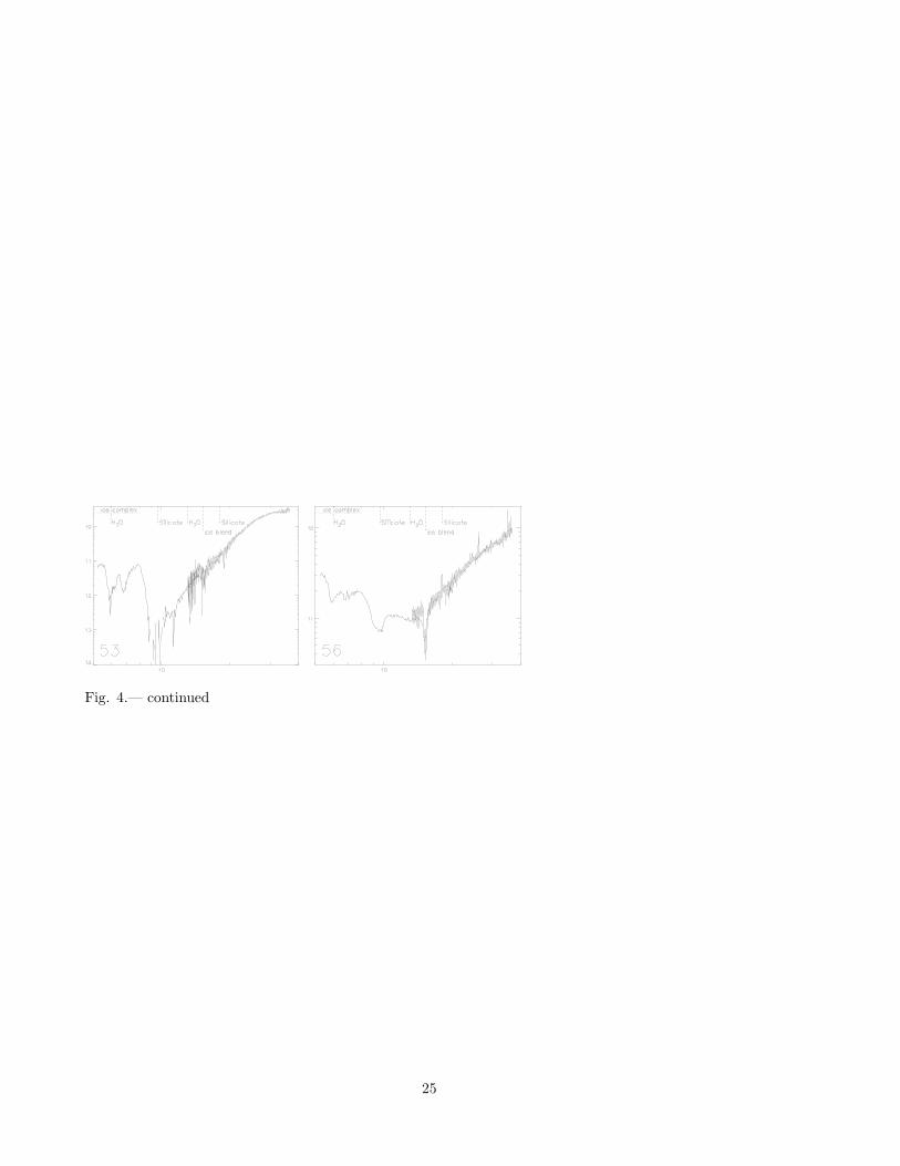
Fig. 4.— continued

25

Fig. 5.— IRS spectra of the 15 identified disk sources with high external foreground extinction (stage II(ex)sources).

26

Fig. 6.— IRS spectra of the 12 identified disk sources with low external foreground extinction (stage IIsources).

27

Fig. 7.— IRS spectra of sources where the modeling was found to be unreliable, for example due to blendingof several sources (see text).

28

-2

-1

0

1

2

3

4

5

6

7

8

-2 -1 0 1 2 3 4 5 6

τ Sil.

9.7

µm

αIRAC

a)

0

1

2

3

4

5

6

7

-2 -1 0 1 2 3 4 5 6

Nto

t(ice

ble

nd)

[1018

cm

-2]

αIRAC

b)

1

1.5

2

2.5

3

3.5

4

4.5

5

-2 -1 0 1 2 3 4 5 6 7 8

FW

HM

Sil.

9.7

[µm

]

τSil. 9.7µm

c)

1

1.5

2

2.5

3

3.5

4

4.5

5

-2 -1 0 1 2 3 4 5 6

FW

HM

Sil.

9.7

µm [µ

m]

αIRAC

d)

0

2

4

6

8

10

0 1 2 3 4 5 6 7 8

Nto

t(ice

ble

nd)

[1018

cm

-2]

τSil. 9.7µm

e)

0

2

4

6

8

10

0 1 2 3 4 5 6 7 8

Nto

t(ice

ble

nd)

[1018

cm

-2]

τSil. 9.7µm

f) c2d

Fig. 8.— a) Correlation of the IRAC spectral index and the optical depth of the 9.7µm silicate feature.Triangles indicate upper limits. b) Correlation of the IRAC spectral index and the total ice column density.Triangles indicate upper limits. c) Correlation of the optical depth and the FWHM linewidth of the 9.7µmsilicate feature. d) Correlation of the IRAC spectral index and the FWHM linewidth of the 9.7µm silicatefeature. e) Correlation of the optical depth of the 9.7µm silicate feature and the total ice column density,without upper limits. f) Correlation of the optical depth of the 9.7µm silicate feature and the total icecolumn density in the Spitzer c2d survey (Pontoppidan et al. 2008; Boogert et al. 2008), without upperlimits. In all color plots, red denotes stage I sources, green denotes stage II(ex) sources, blue denotes stageII, and black denotes sources where no evolutionary stage was determined.

29

Fig. 9.— Spectral maps for the microcluster region. Wavelength regions: a) Ks 2–2.3 µm (includes H2 (1–0)S(0)-S(2) and H I Brγ), b) H2 (0–0) S(7)+S(5)+S(3)+S(2), with [Ne II] 12.8 µm contour overlaid (5σ), c)30 minus 22 µm continuum emission, d) 6.0+6.7µm ice absorption (H2O and NH+

4 ), e) silicate 9.7 µm minusadjacent continuum, f) 15.2 µm ice absorption (CO2:CO:H2O). Boxes denote the original pixel size, i.e.,about the actual angular resolution, for the Spitzer data. In panel c, the submillimeter continuum is marked(5σ contour from Teixeira et al. 2006; note that only sources 41 and 43 were covered in that observation).

30

Fig. 10.— Observed SEDs of the 17 genuine protostars (stage I sources), with model SEDs providing a goodfit overplotted. The black circles show the observed fluxes, the triangles show upper limits, the black lineis the best fit model SED from R06, and the grey lines are other good model SED fits from R06 (where agood fit is defined as one with χ2 −χ2

best < 3× ndata). The dashed line shows the contribution of the stellarphotosphere, including the effect of foreground extinction. Note that the data points shown reflect the inputfor the fitting; upper limits therefore are not necessarily due to non-detections (see text).

31

Fig. 10.— continued

32

Fig. 11.— Observed SEDs of the 15 disk sources with high external foreground extinction (stage II(ex)sources), with model SEDs providing a good fit overplotted. The symbols and lines are as in Figure 10.

33

Fig. 12.— Observed SEDs of the 12 disk sources with low external foreground extinction (stage II sources),with model SEDs providing a good fit overplotted. The symbols and lines are as in Figure 10.

34

Fig. 13.— Observed SEDs of sources where the modeling results cannot be trusted, as described in thetext. Best fit results are only shown for guidance; note, for example, that good fits were obtained for theunresolved microcluster sources 41 and 43. The symbols and lines are as in Figure 10.

35

Fig. 14.— Position of the sources overplotted on 850 µm SCUBA maps of NGC 2264 (upper panel) andIC 348 (lower panel). The symbols denote stage I (circles), stage II(ex) (squares), and stage II (triangles)sources respectively. Grayscale steps are in steps of 0.2 Jy beam−1 up to 2 Jybeam−1.

36