Astronomy&Astrophysics

A&A 621, A76 (2019)https://doi.org/10.1051/0004-6361/201833537© ESO 2019

Characterizing young protostellar disks with the CALYPSOIRAM-PdBI survey: large Class 0 disks are rare?,??

A. J. Maury1,2, Ph. André1, L. Testi3,6, S. Maret4, A. Belloche5, P. Hennebelle1, S. Cabrit8,4, C. Codella6, F. Gueth7,L. Podio6, S. Anderl4, A. Bacmann4, S. Bontemps9, M. Gaudel1, B. Ladjelate10, C. Lefèvre7,

B. Tabone8, and B. Lefloch4

1 AIM, CEA, CNRS, Université Paris-Saclay, Université Paris Diderot, Sorbonne Paris Cité, 91191 Gif-sur-Yvette, Francee-mail: anaelle.maury@cea.fr

2 Harvard-Smithsonian Center for Astrophysics, Cambridge, MA 02138, USA3 ESO, Karl Schwarzschild Strasse 2, 85748 Garching bei München, Germany4 Université Grenoble Alpes, CNRS, IPAG, 38000 Grenoble, France5 Max-Planck-Institut für Radioastronomie, Auf dem Hügel 69, 53121 Bonn, Germany6 INAF – Osservatorio Astrofisico di Arcetri, Largo E. Fermi 5, 50125 Firenze, Italy7 Institut de Radioastronomie Millimétrique (IRAM), 38406 Saint-Martin-d’Hères, France8 LERMA, Observatoire de Paris, PSL Research University, CNRS, Sorbonne Université, UPMC Univ. Paris 06,

75014 Paris, France9 OASU/LAB-UMR5804, CNRS, Université Bordeaux, 33615 Pessac, France

10 Institut de RadioAstronomie Millimétrique (IRAM), Granada, Spain

Received 30 May 2018 / Accepted 16 October 2018

ABSTRACT

Context. Understanding the formation mechanisms of protoplanetary disks and multiple systems and also their pristine properties arekey questions for modern astrophysics. The properties of the youngest disks, embedded in rotating infalling protostellar envelopes,have largely remained unconstrained up to now.Aims. We aim to observe the youngest protostars with a spatial resolution that is high enough to resolve and characterize the progenitorsof protoplanetary disks. This can only be achieved using submillimeter and millimeter interferometric facilities. In the framework of theIRAM Plateau de Bure Interferometer survey CALYPSO, we have obtained subarcsecond observations of the dust continuum emissionat 231 and 94 GHz for a sample of 16 solar-type Class 0 protostars.Methods. In an attempt to identify disk-like structures embedded at small scales in the protostellar envelopes, we modeled the dustcontinuum emission visibility profiles using Plummer-like envelope models and envelope models that include additional Gaussiandisk-like components.Results. Our analysis shows that in the CALYPSO sample, 11 of the 16 Class 0 protostars are better reproduced by models including adisk-like dust continuum component contributing to the flux at small scales, but less than 25% of these candidate protostellar disks areresolved at radii >60 au. Including all available literature constraints on Class 0 disks at subarcsecond scales, we show that our resultsare representative: most (>72% in a sample of 26 protostars) Class 0 protostellar disks are small and emerge only at radii <60 au.We find a multiplicity fraction of the CALYPSO protostars .57% ± 10% at the scales 100–5000 au, which generally agrees with themultiplicity properties of Class I protostars at similar scales.Conclusions. We compare our observational constraints on the disk size distribution in Class 0 protostars to the typical disk propertiesfrom protostellar formation models. If Class 0 protostars contain similar rotational energy as is currently estimated for prestellar cores,then hydrodynamical models of protostellar collapse systematically predict a high occurrence of large disks. Our observations suggestthat these are rarely observed, however. Because they reduce the centrifugal radius and produce a disk size distribution that peaks atradii <100 au during the main accretion phase, magnetized models of rotating protostellar collapse are favored by our observations.

Key words. stars: formation – stars: protostars – radio continuum: ISM

1. Introduction

Understanding the first steps in the formation of protostars andprotoplanetary disks is a great unsolved problem of modern

? Based on observations carried out with the IRAM Plateau de BureInterferometer. IRAM is supported by INSU/CNRS (France), MPG(Germany), and IGN (Spain).?? The CALYPSO calibrated visibility tables and maps are publicly

available at http://www.iram-institute.org/EN/content-page-317-7-158-240-317-0.html

astrophysics. Observationally, the key to constraining protostarformation models lies in high-resolution studies of the youngestprotostars. Class 0 objects, which were originally discoveredat millimeter wavelengths, are believed to be the youngestknown accreting protostars (André et al. 1993). Because they areobserved only t . 4−9 × 104 yr after the formation of a centralhydrostatic protostellar object (Evans et al. 2009; Maury et al.2011) while most of their mass is still in the form of a densecore/envelope (Menv > M?), Class 0 protostars are believed to berepresentative of the main accretion phase of protostellar evolu-tion and are likely to retain detailed information on the initial

A76, page 1 of 44Open Access article, published by EDP Sciences, under the terms of the Creative Commons Attribution License (http://creativecommons.org/licenses/by/4.0),

which permits unrestricted use, distribution, and reproduction in any medium, provided the original work is properly cited.

A&A 621, A76 (2019)

conditions of protostellar collapse (see review by André et al.2000; Dunham et al. 2014).

High-resolution studies of Class 0 protostars are also key toconstraining theoretical models for the formation of protostel-lar disks. At the simplest level, the formation of circumstellardisks is a natural consequence of the conservation of angularmomentum during the collapse of rotating protostellar envelopesin the course of the main accretion phase (Cassen & Moosman1981; Terebey et al. 1984). Hydrodynamic simulations show thatin the absence of magnetic fields, rotationally supported disksform and quickly grow to reach large radii >100 au after a fewthousand years (Yorke & Bodenheimer 1999). These hydrody-namical disks are often massive enough to be gravitationallyunstable, and their fragmentation has been suggested to con-tribute to the formation of brown dwarfs and multiple stellarsystems (Stamatellos et al. 2007; Vorobyov 2010). On the otherhand, early ideal magnetohydrodynamics (MHD) numericalsimulations describing the protostellar collapse of magnetizedenvelopes had difficulties to form rotationally supported disksat scales r > 10 au because of strong magnetic braking: theincrease in magnetic energy as field lines are dragged inward dur-ing protostellar collapse (Galli et al. 2006; Hennebelle & Ciardi2009) reduces the envelope rotation and delays the formationof large disks. This so-called “magnetic braking catastrophe”was quickly mitigated, however, by including non-uniform ini-tial conditions such as a magnetic field that is misaligned withthe core rotation axis, transonic turbulent cores, or the treatmentof radiative transfer (Joos et al. 2012; Seifried et al. 2012; Bateet al. 2014; Machida et al. 2014). More realistic numerical simu-lations including non-ideal MHD physics that allows dissipatingand/or decoupling magnetic fields from the inner protostellarenvironment have recently been developed by several groups(Machida et al. 2011; Dapp et al. 2012; Masson et al. 2012; Liet al. 2014). Most numerical MHD studies now agree that includ-ing one or several resistive or dissipative effects (e.g., ambipolardiffusion, Ohmic dissipation, or the Hall effect) allows small(10 < r < 100 au) rotationally supported disks to be formedduring magnetized protostellar collapse (Machida et al. 2014;Tsukamoto et al. 2015; Masson et al. 2016). The exact ingredientsresponsible for early disk properties during the main accretionphase remain widely debated, however.

From the observational point of view, young stellar objects(YSOs) have been studied in great detail in recent years, showingthat large disks with radii &100 au are common in Class II (e.g.Andrews et al. 2009; Isella et al. 2009; Ricci et al. 2010; Spezziet al. 2013) and Class I objects (Wolf et al. 2008; Jørgensenet al. 2009; Takakuwa et al. 2012; Eisner 2012; Lee et al. 2016;Sakai et al. 2016). However, we still lack good constraints onthe properties of the progenitors of these disks during ear-lier phases of evolution: it has been difficult to observationallycharacterize the first stages of disk formation around Class 0protostars because emission from the protostellar envelope dom-inates at most scales that are probed by single-dish telescopes(Motte & André 2001) or early interferometric observations(Looney et al. 2000). Long-wavelength observations are requiredto image deeply embedded disks and peer through dense proto-stellar envelopes. Subarcsecond resolution is needed to matchthe disk sizes at the typical distances of nearby star-formingclouds (d ∼ 100–400 pc), as is high sensitivity to detect theweak fluxes of the youngest disks. Until recently, the small num-ber of Class 0 protostars in nearby clouds and their relativelyweak emission on small scales has restricted the millimeter inter-ferometric studies that are required to reach subarcsecond (or<∼100 au) resolution to the most extreme objects. For example,

a survey of bright Class 0 and Class I protostars with the Sub-Millimeter Array (SMA) by Jørgensen et al. (2009) attributed thedetection of compact dust continuum emission components, allunresolved at the ∼2′′ scales that these data probe, to the poten-tial presence of disks with masses between 0.002 and 0.5 Mduring the Class 0 phase. This simple interpretation was ques-tionable since modeling of the millimeter continuum emissionfrom Class 0 protostars sometimes indicates that an irregulardensity structure (e.g., complex envelope substructure or radialdensity enhancements at small scales) can lead to additionalcompact continuum emission in Class 0 protostars without theneed of a disk component (Chiang et al. 2008; Maury et al.2014).

Only the recent advent of powerful interferometric facilitieswith kilometer baselines at (sub)millimeter (submm) wave-lengths has allowed the inner envelopes of Class 0 protostarsto be explored at resolutions and sensitivities that are sufficientto distinguish envelope emission from resolved disk emission atthe relevant scales (20–200 au). A pilot high-resolution studyof five Class 0 protostars in Taurus and Perseus was carried outby Maury et al. (2010) with the IRAM Plateau de Bure Inter-ferometer (PdBI). No large r > 100 au disks or protobinarieswith separations 50 < a < 500 au were detected. Maury et al.(2010) concluded that the formation of protostellar disks andthe fragmentation of dense cores into multiple systems at scales50–500 au might be largely modified by magnetic fields duringthe main accretion phase. The apparent lack of large r > 100 auClass 0 disks could only be reproduced when magnetic-brakingeffects were included (Hennebelle & Teyssier 2008), while purehydrodynamical models produced too many large r > 100 audisks. Subsequently, Maury et al. (2014) showed that any diskcomponent in the NGC1333-IRAS2A protostar would need to be.40 au to reproduce the radial profile of the millimeter dust con-tinuum emission observed with the PdBI. Maret et al. (2014)modeled the kinematics observed in methanol emission linestoward the same source and found that no significant rotation pat-tern was detected on similar scales. This confirmed the absenceof a large disk in this Class 0 protostar.

The fast improvement of interferometric facilities such asALMA has recently allowed a few other high-resolution studiesto be made. A handful of Class 0 protostars have been pro-posed to have resolved disk-like rotation in their inner envelopes:while VLA 1623, HH212, and L1448-NB have been suggestedto harbor Keplerian-like kinematics at scales 40 < r < 100 au(Murillo et al. 2013; Codella et al. 2014a; Tobin et al. 2016a),the most convincing case for a resolved protostellar disk wasfound in the L1527 Class 0/I protostar, where Ohashi et al.(2014) found a transition from a rotating infalling envelopeto Keplerian motions in a disk at radii 50−60 au. On theother hand, Yen et al. (2015b) concluded that the disk in theClass 0 protostar B335 must have a radius r . 10 au to repro-duce the absence of a Keplerian pattern from the velocity fieldobserved with ALMA at subarcsecond scale in this edge-onsource.

To summarize, disks in young Class 0 protostars havelargely remained elusive up to now. The intrinsic difficulty indistinguishing individual components in envelope-dominatedobjects has precluded any statistical observational constraintson the distribution of disks sizes and masses. Only a survey pro-viding high angular resolution observations for a large sampleof Class 0 protostars can shed light on the controversy about thepristine characteristics of protostellar disks and ultimately onthe importance of magnetic fields in regulating disk formationduring protostellar formation (Li et al. 2014).

A76, page 2 of 44

A. J. Maury et al.: CALYPSO view of Class 0 protostellar disks

Table 1. CALYPSO sample of target protostars.

Protostar Distance Lint Menv Outflow PA References(pc) (L) (M) ()

[1] [2] [3] [4] [5] [6]

L1448-2A 235 3.0 1.2 −63 O’Linger et al. (1999)/Enoch et al. (2009)L1448-NB 235 2.5 3.1 −80 Curiel et al. (1990)/Sadavoy et al. (2014)L1448-C 235 7.0 1.3 −17 Anglada et al. (1989)/Sadavoy et al. (2014)IRAS2A 235 30 5.1 +205 Jennings et al. (1987)/Karska et al. (2013)SVS13B 235 2.0 1.8 +167 Grossman et al. (1987)/Chini et al. (1997)IRAS4A 235 3.0 7.9 +180 Jennings et al. (1987)/Sadavoy et al. (2014)IRAS4B 235 1.5 3.0 +167 Jennings et al. (1987)/Sadavoy et al. (2014)IRAM04191 140 0.05 0.5 +200 André et al. (1999)/André et al. (2000)L1521F 140 0.035 0.7–2 +240 Mizuno et al. (1994)/Tokuda et al. (2016)L1527 140 0.9 1.2 +60 Ladd et al. (1991)/Motte & André (2001)SerpM-S68N 415 10 10 −45 Casali et al. (1993)/Kaas et al. (2004)SerpM-SMM4 415 2 7 +30 Casali et al. (1993)/Kaas et al. (2004)SerpS-MM18 260 16 3 +188 Maury et al. (2011)/Maury et al. (2011)SerpS-MM22 260 0.2 0.5 +230 Maury et al. (2011)/Maury et al. (2011)L1157 250 2.0 1.5 163 Umemoto et al. (1992)/Motte & André (2001)GF9-2 200 0.3 0.5 0 Schneider & Elmegreen (1979)/Wiesemeyer (1997)

Notes. The sources are ordered by increasing right ascension of the targeted core (see phase centers of our observations in Table A.1). Column 1:name of the protostar. Column 2: distance of the cloud where the protostar lies. The Taurus distance is taken from a VLBA measurement estimatingdistances from 130 to 160 pc (Torres et al. 2009) depending on the location in the cloud: we adopt a mean value of 140 pc. The distance of Perseusis taken following recent VLBI parallax measurements that have determined a distance to the NGC 1333 region 235 ± 18 pc (Hirota et al. 2008)and a distance to the L1448 cloud of 232 ± 18 pc (Hirota et al. 2011). The distance of the Serpens Main cloud (SerpM sources) follows VLBImeasurements in Dzib et al. (2010), who have determined a distance of 415 pc for the Serpens Main core, while a distance 230–260 pc was widelyused before. Therefore, both Lint and Menv reported here are larger by a factor of 2.8 than those listed in the Bolocam and Spitzer literature before2011. The distance of Serpens South (SerpS sources) is still subject of debate, since no VLBI measurements toward the Serpens South filamentexist: for consistency, we use here the distance of 260 pc adopted in Maury et al. (2011) and in Herschel studies of Könyves et al. (2010, 2015).Column 3: internal luminosity of the protostar. The internal luminosities come from the analysis of Herschel maps obtained in the framework ofthe Gould Belt survey (HGBS, see, e.g., André et al. 2010 and Ladjelate et al., in prep.). Column 4: protostellar envelope mass from the literature(associated references in Col. 6). Column 5: position angle (PA of the blue lobe counted east of north) of the high-velocity emission from 12CO orSiO tracing the protostellar jet component, from our CALYPSO molecular line emission maps when detected. For some protostars, the blue andred lobes are not well aligned, and/or several jets are detected in our CALYPSO maps: in these cases, we report the PA of the blue lobe, originatingfrom the primary protostar position (see Table 3). Information on individual sources is reported in Appendix C, and the global jet properties in theCALYPSO sample will be provided in Podio & CALYPSO (in prep.). Column 6: references for values reported here: protostar discovery paper,then the reference for the envelope mass.

The Continuum And Lines in Young ProtoStellar Objects(CALYPSO1) IRAM Large Program is a survey of 16 Class 0protostars, carried out with the IRAM Plateau de Bure (PdBI)interferometer in three spectral setups (around 94, 219, and231 GHz). CALYPSO was crafted as an effort to make progressin our understanding of the angular momentum problem for starformation through high angular resolution observations (0.3′′,i.e., .100 au) of a significant sample of the youngest proto-stars. The main goals of the PdBI observations are to improveour understanding of (1) the formation of accretion disks andmultiple systems during protostellar collapse, (2) the role ofClass 0 jets and outflows in angular momentum extraction,and (3) the kinematics and structure of the inner protostellarenvironment. The 16 Class 0 objects of the CALYPSO sam-ple are among the youngest known solar-type protostars (Andréet al. 2000), with Menv ∼ 0.5–10 M, and internal luminosi-ties Lint ∼ 0.03–30 L (see Table 1). This sample comprisesmost of the pre-Herschel confirmed Class 0 protostars locatedin nearby (d < 420 pc) clouds that could be observed inshared tracks from the IRAM-PdBI location. Several papershave been published based on the CALYPSO survey and dis-cuss remarkable properties of individual protostars: IRAS2A

1 See http://irfu.cea.fr/Projets/Calypso/

(Maret et al. 2014; Codella et al. 2014b; Maury et al. 2014),IRAS4A (Santangelo et al. 2015), L1157 (Podio et al. 2016), orthe Class I protostar SVS13A (Lefèvre et al. 2017). Two anal-yses of the molecular line emission in CALYPSO subsampleshave also been carried out (Anderl et al. 2016; De Simone et al.2017).

This paper is the first of a series of statistical analyses(Belloche et al., in prep.; Maret et al., in prep.; Podio et al., inprep.; Gaudel et al., in prep.) that are carried out for the wholeCALYPSO sample. They address the three cornerstone questionsdescribed above that lie at the heart of the scientific motiva-tions of CALYPSO. This paper focuses on the inner densitystructure(s) of the CALYPSO Class 0 protostars, analyzing thedual-frequency dust continuum emission visibilities to probe thestructure of protostellar envelopes down to radii ∼30 au (for theTaurus sources) to ∼90 au (for the Serpens Main sources), withspecial emphasis on characterizing candidate protostellar disksand multiple systems. We show the dust continuum emissiondatasets, obtained at 1.37 and 3.18 mm, for the whole CALYPSOsample (see Table 1) in Sect. 2 and the dust continuum sourcesdetected in our maps in Sect. 3. Section 4 is dedicated to describ-ing the analysis of the dust continuum visibility dataset we per-formed to test whether candidate disk components are detected ineach of the primary targets of our sample. In Sect. 5.1 we discuss

A76, page 3 of 44

A&A 621, A76 (2019)

the occurrence and properties of the candidate embedded disksin Class 0 protostellar envelopes from our sample and the litera-ture. In Sect. 5.2 we explore current predictions from theoreticalmodels of protostellar collapse, and the constraints our resultsbring to these models. Finally, we briefly discuss in Sect. 5.3 themultiplicity of Class 0 protostars in our sample and in the litera-ture and compare them to the multiplicity properties of YSOs atmore advanced evolutionary stages.

2. Observations and data reduction

2.1. PdBI observations and calibration

Observations of the CALYPSO sources were carried out withthe IRAM PdBI between September 2010 and March 2013(see details in Table A.1). We adopted a multiple configura-tion strategy, using the six-antenna array in the most extendedconfiguration (A array) and in an intermediate antenna con-figuration (C array). This provided a fairly dense coverage ofthe uv-plane with 30 baselines ranging from 16 to 760 m. Weused the WideX2 correlator to cover a 3.8 GHz broadband spec-tral window for each of the three spectral setups, which wereobserved separately: at 1.29 mm for observations with a WideXcentral frequency of 231 GHz, at 1.37 mm for observations witha WideX central frequency of 219 GHz, and at 3.18 mm forobservations with a central WideX frequency of 94 GHz. Ahigher spectral resolution correlator was placed onto a handfulof molecular emission lines, but we present here only the analy-sis of the continuum emission extracted from the WideX dataset.The proximity of some of the sources on the sky allowed usto use common gain calibrators for several groups of sourcesand therefore to time-share a total of 37 tracks of ∼8 h on the16 sources. Each track was divided unequally among the sources,roughly in inverse proportion to the source luminosities so as toobtain the most homogeneous signal-to-noise ratios (S/N) in thesample. For each track, nearby amplitude and phase calibratorswere observed to determine the time-dependent complex antennagains. The calibration was performed in the GILDAS/CLIC3

environment. The correlator bandpass was calibrated on strongquasars (e.g., 3C273 and 3C454.3), while the absolute flux den-sity scale was usually derived from observations of MWC349and 3C84. The absolute flux calibration uncertainty is estimatedto be ∼10% at 94 GHz and ∼15% at 231 GHz.

For sources where the peak of the dust continuum emissionis detected at >40σ (roughly equivalent to all sources with peakflux >80 mJy beam−1 at 231 GHz; see Table 2), we also carriedout self-calibration of the continuum emission visibility datasetto improve the S/N at the longest baselines.

2.2. PdBI continuum emission maps

After a cross-check of the absolute flux calibration consistencyof the observing dates, the visibility datasets obtained with theA and C configuration were combined, for each of the three fre-quency setups independently. The continuum visibilities weregenerated from the WideX units, avoiding channels in whichline emission was detected at a level >5σ in the spectrum inte-grated over 2′′ around the peaks of the continuum emissionreported in Table 3. Examples of wide-band spectra are shownin Maury et al. (2014), while the analysis of the molecular con-tent of the whole sample will be presented in Belloche et al.

2 See www.iram.fr/widex3 www.iram.fr/IRAMFR/GILDAS/

Table 2. Properties of the PdBI continuum emission maps.

Field Synthesized beam FWHM (′′), PA () σ (mJy beam−1)231 GHz 94 GHz 231 GHz 94 GHz

L1448-2A 0.56 × 0.37, 36 1.41 × 0.93, 40 0.31 0.06L1448-NB 0.56 × 0.40, 38 1.42 × 0.97, 36 1.1 0.23L1448-C 0.58 × 0.36, 28 1.45 × 0.96, 43 0.6 0.09IRAS2A 0.62 × 0.45, 45 1.40 × 0.98, 38 0.97 0.14SVS13 0.54 × 0.33, 29 1.52 × 0.96, 24 1.0 0.17

IRAS4A 0.57 × 0.35, 29 1.53 × 0.98, 25 3.1 0.8IRAS4B 0.58 × 0.36, 30 1.52 × 0.99, 25 2.3 0.83

IRAM04191a 1.00 × 0.85, -160 1.90 × 1.57, 48 0.10 0.023L1521Fa 1.15 × 0.87, 25 2.19 × 1.90, 93 0.06 0.03L1527 0.53 × 0.35, 37 1.49 × 0.97, 33 0.45 0.07

SerpM-S68N 0.82 × 0.35, 22 1.84 × 1.11, 32 0.6 0.09SerpM-SMM4 0.74 × 0.33, 25 1.73 × 0.85, 28 1.5 0.25SerpS-MM18 0.74 × 0.33, 24 1.73 × 0.87, 27 1.3 0.2SerpS-MM22 0.88 × 0.35, 20 1.80 × 0.90, 27 0.39 0.05

L1157 0.51 × 0.40, 4 1.36 × 1.04, 64 0.6 0.09GF92a 0.85 × 0.68, 18 1.43 × 1.02, 66 0.14 0.025

Notes. (a)Maps of the weakest continuum emission sources in the sam-ple, IRAM04191, L1521F, and GF9-2, were produced using a naturalweighting to maximize the sensitivity to point sources, see text inSect. 2.2.

(in prep.). In order to produce images and visibility curves withoptimum sensitivity and best uv-coverage at 1.3 mm, we mergedthe continuum visibility data that were independently obtainedat 219 and 231 GHz: we used the spectral index computed fromthe shortest common baseline of our PdBI observations at 94and 231 GHz (α20kλ; see Col. 6 of Table 4) for each individualsource to scale the visibility amplitudes obtained at 219 GHzto 231 GHz. In the following, all 231 GHz fluxes, maps, andvisibility profiles stem from the combined data.

Imaging of the continuum visibility tables was carried outusing a robust scheme for weighting that allowed us to improvethe resolution and lower the side lobes without exceedinglydegrading the overall sensitivity. The robust (Briggs 1995)threshold we adopted was moderate (r = 0.34) and allowed usto reach a good compromise between imaging quality and sen-sitivity while enhancing the contribution of the high spatialfrequencies. This resulted in typical full widths at half-maximum(FWHMs) of the synthesized beams .0.5′′ at 231 GHz. Excep-tions were made for the low-luminosity sources IRAM 04191,L1521F, and GF9-2, where natural weighting was used to max-imize the sensitivity for these faint objects (producing synthe-sized beams ∼1.0′′ at 231 GHz). The maps were subsequentlycleaned using the Hogbom CLEAN algorithm provided in theGILDAS/MAPPING software, with a cleaning threshold set totwice the rms noise in the map. The properties of the resultingCLEANed maps (synthesized HPBWs, rms noises) are reportedin Table 2. The dust continuum emission maps obtained at 231and 94 GHz are shown in Figs. 1–3 for two of the Perseus sources(L1448-2A and SVS13B) and a Taurus source (L1527), whilethe remaining dust continuum maps for the 13 other fields in theCALYPSO sample are shown in Figs. B.1–B.13.

4 The robust parameter is set so that if the sum of natural weights in agiven uv cell is lower than this threshold, natural weights are kept; if it ishigher, the weight is set to this value. For more information on weightingschemes performed by the GILDAS/MAPPING software, see http://www.iram.fr/IRAMFR/IS/IS2002/html_1/node156.html.

A76, page 4 of 44

A. J. Maury et al.: CALYPSO view of Class 0 protostellar disks

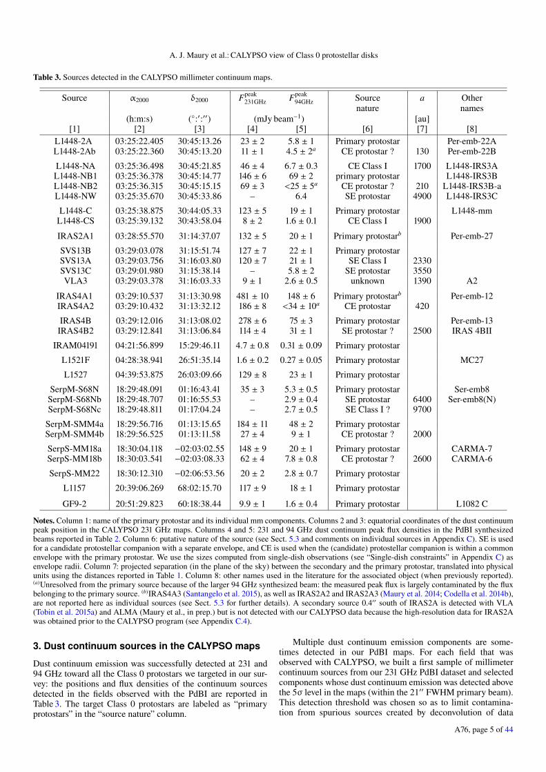
Table 3. Sources detected in the CALYPSO millimeter continuum maps.

Source α2000 δ2000 Fpeak231GHz Fpeak

94GHz Source a Othernature names

(h:m:s) (:′:′′) (mJy beam−1) [au][1] [2] [3] [4] [5] [6] [7] [8]

L1448-2A 03:25:22.405 30:45:13.26 23 ± 2 5.8 ± 1 Primary protostar Per-emb-22AL1448-2Ab 03:25:22.360 30:45:13.20 11 ± 1 4.5 ± 2a CE protostar ? 130 Per-emb-22B

L1448-NA 03:25:36.498 30:45:21.85 46 ± 4 6.7 ± 0.3 CE Class I 1700 L1448-IRS3AL1448-NB1 03:25:36.378 30:45:14.77 146 ± 6 69 ± 2 primary protostar L1448-IRS3BL1448-NB2 03:25:36.315 30:45:15.15 69 ± 3 <25 ± 5a CE protostar ? 210 L1448-IRS3B-aL1448-NW 03:25:35.670 30:45:33.86 – 6.4 SE protostar 4900 L1448-IRS3C

L1448-C 03:25:38.875 30:44:05.33 123 ± 5 19 ± 1 Primary protostar L1448-mmL1448-CS 03:25:39.132 30:43:58.04 8 ± 2 1.6 ± 0.1 CE Class I 1900

IRAS2A1 03:28:55.570 31:14:37.07 132 ± 5 20 ± 1 Primary protostarb Per-emb-27

SVS13B 03:29:03.078 31:15:51.74 127 ± 7 22 ± 1 Primary protostarSVS13A 03:29:03.756 31:16:03.80 120 ± 7 21 ± 1 SE Class I 2330SVS13C 03:29:01.980 31:15:38.14 – 5.8 ± 2 SE protostar 3550VLA3 03:29:03.378 31:16:03.33 9 ± 1 2.6 ± 0.5 unknown 1390 A2

IRAS4A1 03:29:10.537 31:13:30.98 481 ± 10 148 ± 6 Primary protostarb Per-emb-12IRAS4A2 03:29:10.432 31:13:32.12 186 ± 8 <34 ± 10a CE protostar 420

IRAS4B 03:29:12.016 31:13:08.02 278 ± 6 75 ± 3 Primary protostar Per-emb-13IRAS4B2 03:29:12.841 31:13:06.84 114 ± 4 31 ± 1 SE protostar ? 2500 IRAS 4BII

IRAM04191 04:21:56.899 15:29:46.11 4.7 ± 0.8 0.31 ± 0.09 Primary protostar

L1521F 04:28:38.941 26:51:35.14 1.6 ± 0.2 0.27 ± 0.05 Primary protostar MC27

L1527 04:39:53.875 26:03:09.66 129 ± 8 23 ± 1 Primary protostar

SerpM-S68N 18:29:48.091 01:16:43.41 35 ± 3 5.3 ± 0.5 Primary protostar Ser-emb8SerpM-S68Nb 18:29:48.707 01:16:55.53 – 2.9 ± 0.4 SE protostar 6400 Ser-emb8(N)SerpM-S68Nc 18:29:48.811 01:17:04.24 – 2.7 ± 0.5 SE Class I ? 9700

SerpM-SMM4a 18:29:56.716 01:13:15.65 184 ± 11 48 ± 2 Primary protostarSerpM-SMM4b 18:29:56.525 01:13:11.58 27 ± 4 9 ± 1 CE protostar ? 2000

SerpS-MM18a 18:30:04.118 −02:03:02.55 148 ± 9 20 ± 1 Primary protostar CARMA-7SerpS-MM18b 18:30:03.541 −02:03:08.33 62 ± 4 7.8 ± 0.8 CE protostar ? 2600 CARMA-6

SerpS-MM22 18:30:12.310 −02:06:53.56 20 ± 2 2.8 ± 0.7 Primary protostar

L1157 20:39:06.269 68:02:15.70 117 ± 9 18 ± 1 Primary protostar

GF9-2 20:51:29.823 60:18:38.44 9.9 ± 1 1.6 ± 0.4 Primary protostar L1082 C

Notes. Column 1: name of the primary protostar and its individual mm components. Columns 2 and 3: equatorial coordinates of the dust continuumpeak position in the CALYPSO 231 GHz maps. Columns 4 and 5: 231 and 94 GHz dust continuum peak flux densities in the PdBI synthesizedbeams reported in Table 2. Column 6: putative nature of the source (see Sect. 5.3 and comments on individual sources in Appendix C). SE is usedfor a candidate protostellar companion with a separate envelope, and CE is used when the (candidate) protostellar companion is within a commonenvelope with the primary protostar. We use the sizes computed from single-dish observations (see “Single-dish constraints” in Appendix C) asenvelope radii. Column 7: projected separation (in the plane of the sky) between the secondary and the primary protostar, translated into physicalunits using the distances reported in Table 1. Column 8: other names used in the literature for the associated object (when previously reported).(a)Unresolved from the primary source because of the larger 94 GHz synthesized beam: the measured peak flux is largely contaminated by the fluxbelonging to the primary source. (b)IRAS4A3 (Santangelo et al. 2015), as well as IRAS2A2 and IRAS2A3 (Maury et al. 2014; Codella et al. 2014b),are not reported here as individual sources (see Sect. 5.3 for further details). A secondary source 0.4′′ south of IRAS2A is detected with VLA(Tobin et al. 2015a) and ALMA (Maury et al., in prep.) but is not detected with our CALYPSO data because the high-resolution data for IRAS2Awas obtained prior to the CALYPSO program (see Appendix C.4).

3. Dust continuum sources in the CALYPSO maps

Dust continuum emission was successfully detected at 231 and94 GHz toward all the Class 0 protostars we targeted in our sur-vey: the positions and flux densities of the continuum sourcesdetected in the fields observed with the PdBI are reported inTable 3. The target Class 0 protostars are labeled as “primaryprotostars” in the “source nature” column.

Multiple dust continuum emission components are some-times detected in our PdBI maps. For each field that wasobserved with CALYPSO, we built a first sample of millimetercontinuum sources from our 231 GHz PdBI dataset and selectedcomponents whose dust continuum emission was detected abovethe 5σ level in the maps (within the 21′′ FWHM primary beam).This detection threshold was chosen so as to limit contamina-tion from spurious sources created by deconvolution of data

A76, page 5 of 44

A&A 621, A76 (2019)

Fig. 1. 1.3 mm (231 GHz, left panel) and3.3 mm (94 GHz, right panel) PdBI dustcontinuum emission maps of L1448-2A,corrected for primary beam attenuation.The ellipses in the bottom left corner showthe respective synthesized beam sizes. Thecontours are levels of −3σ (dashed), 5σ,and 10σ, then from 20σ in steps of 20σ(rms noise computed in the map before pri-mary beam correction, reported in Table 2).The blue and red arrows show the directionof the protostellar jet(s) either as found inour CALYPSO dataset or from the litera-ture (see Table 1).

Fig. 2. Same as Fig. 1 for the SVS13region. The dashed pink contour shows thePdBI primary beam at each frequency. Thecontours show levels of −3σ (dashed), 5σ,and 10σ, then from 20σ in steps of 20σ (seeTable 2). The blue and red arrows showthe direction of the protostellar jets fromour CALYPSO data for SVS13A/B (Podioet al., in prep.), while the SVS13C outflowPA stems from the CARMA map (Plunkettet al. 2013).

sampling only partially the uv-plane. We note that throughoutthis paper, we always report and use rms noises at phase cen-ter, but the maps we show and the fluxes we report are correctedfor the primary beam attenuation (the phase centers used in ourobservations are given in Table A.1). At the positions of the231 GHz continuum sources, we checked the PdBI 94 GHz mapsfor independent detection of a counterpart at lower frequency.All the sources detected in the CALYPSO 231 GHz maps have acounterpart detected at >3σ in the 94 GHz maps when it is pos-sible to resolve them (the synthesized beam of the 94 GHz datais 2.5 times larger than the beam of the 231 GHz data).

Moreover, since the PdBI 94 GHz maps have a larger primarybeam than the 231 GHz maps, four sources detected at >11′′from the main protostar in the 94 GHz map have no 231 GHzcounterpart since they fall outside the primary beam of thehigher frequency observations. In these cases (e.g., SVS13-C;see Fig. 2), the 94 GHz continuum source is reported only ifthe source was detected at another wavelength in the literature.Applying this method to all fields observed in the CALYPSO sur-vey, we detected a total of 30 dust continuum emission sources.We report the coordinates and peak flux densities in Table 3 anddiscuss their nature in Sect. 5.3.

4. Analysis of dust continuum source structures

4.1. Building a proper visibility dataset for each primarytarget protostar

Each secondary source reported in Table 3 was removed fromthe visibility data by subtracting a Gaussian source model with

FWHM at most twice the synthesized beam size (to removeonly compact components and avoid affecting the envelope emis-sion), or a point source if separated from the primary continuumcomponent by less than two synthesized beams. During this sub-traction process, the coordinates and peak fluxes of secondarycomponents were fixed to the values reported in Cols. 2 and3 of Table 3. Subtracting the visibilities that are due to sec-ondary components allowed us to perform a focused analysisof the continuum emission that originates from each main pro-tostar that was targeted by our observing program. We stress,however, that this operation does not preclude the possible pres-ence of tighter multiple components at scales that cannot beresolved with PdBI. For example, the real parts of the visi-bilities of L1448-NB, IRAS2A, and L1157 show oscillationsat long baselines in circularly averaged data, suggesting thatadditional structure or components (at a < 0.4′′) that are notcentered on the phase center may remain in these three sources.From now on, we discuss and analyze the millimeter continuumemission originating solely from the primary protostar in eachfield.

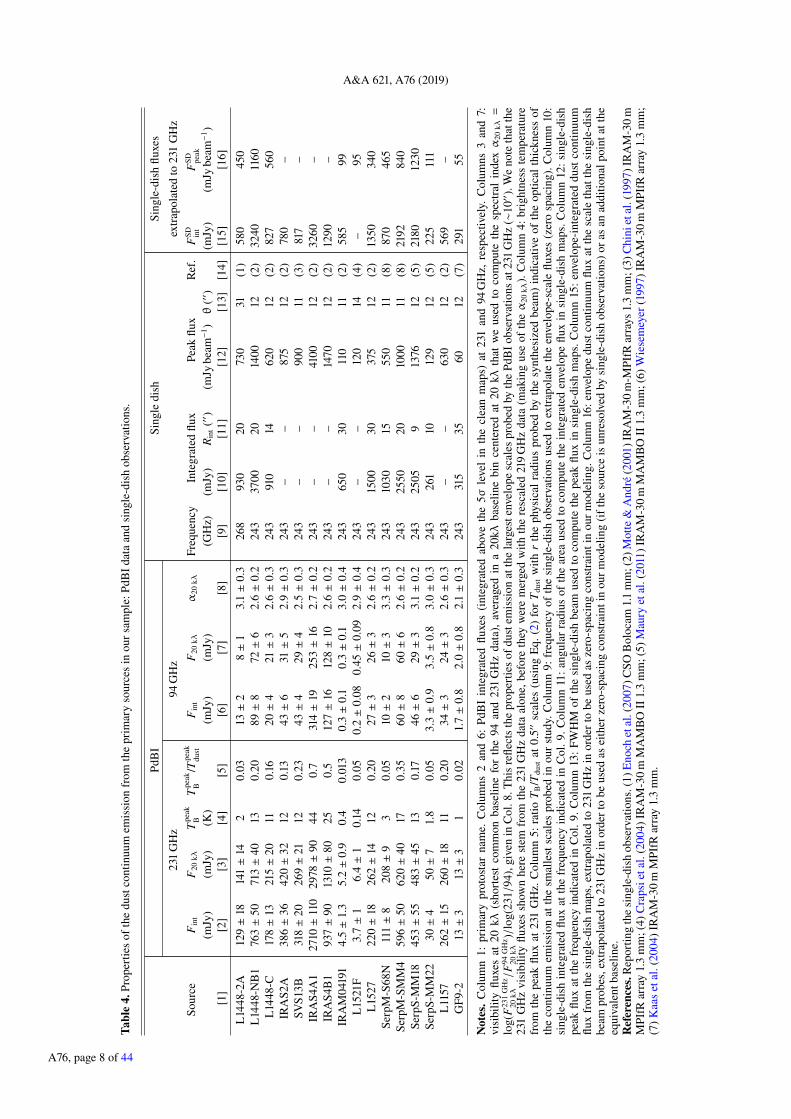
For all primary protostars targeted with CALYPSO, wereport the integrated flux densities (above a 5σ level) thatwe recovered with our PdBI observations in Table 4. Since thelargest scale sampled by the PdBI observations depends on thefrequency νobs and the shortest baseline in the array Bmin (max-imum recoverable scale MRS ∼ 0.6c/(νobs × Bmin), i.e., 14′′ at94 GHz and 6′′ at 231 GHz), we also report in Table 4 thematching visibility flux values, obtained at the shortest commonB = 20 kλ baseline (value averaged in a 10 kλ bin). We note

A76, page 6 of 44

A. J. Maury et al.: CALYPSO view of Class 0 protostellar disks

Fig. 3. Same as Fig. 1 for L1527. The con-tours show levels of −3σ, 5σ, and 10σ, andthen from 20σ in steps of 40σ (see Table 2).

that the shortest baseline sampled at 94 GHz is ∼8 kλ, so theintegrated fluxes from the 94 GHz maps can sometimes be sig-nificantly higher than the 20 kλ visibility flux values at 94 GHz.For the continuum data at 231 GHz, and especially for strongsources, the flux recovered in the CLEANed maps is sometimessignificantly lower than the flux measured at the 20 kλ baselines.This illustrates the difficulty of reliably reconstructing interfer-ometric maps from data with incomplete uv-coverage, and itjustifies our approach to carry out modeling in the uv-planerather than in the image plane.

4.2. Large-scale constraints from single-dish observationsof the dust continuum emission

We used a combination of PdBI configurations to observe thecontinuum emission down to baselines of 17 kλ at 231 GHz (8 kλat 94 GHz), probing spatial scales up to ∼6′′ at 231 GHz (14′′ at94 GHz). Protostellar envelopes typically extend to larger angu-lar scales at the distance of our sources (Motte & André 2001),and therefore cannot always be completely sampled using ourPdBI observations alone (see Fig. 4 for an example of IRAM-30 m intensity profiles for four of the protostars in our sample).We therefore collected information from the literature on single-dish continuum observations of the target protostars that probeenvelope scales &10′′, so as to better constrain the outer enve-lope density profiles through (i) dust continuum fluxes that areintegrated at envelope scales reported in Col. 8 of Table 4 and(ii) peak flux densities obtained with single-dish telescopes thattrace the material at the scales of the single-dish beam size,reported in Col. 10 of Table 4.

We can extrapolate the dust continuum fluxes found in theliterature, which are often obtained at slightly different frequen-cies than our PdBI setups, when we assume a simple power-lawdependence of the flux density on frequency by scaling the fluxby an average spectral index at envelope scales. We used thespectral index computed from the shortest common baseline ofour dual frequency PdBI observations at 20 kλ (see Col. 6 ofTable 4) for each individual source to extrapolate the single-dishfluxes to the frequency of our PdBI observations. When sec-ondary components were present in the field (see Table 3), wesubtracted their flux densities as estimated in the PdBI u–v planefrom the extrapolated single-dish flux of the primary sources.The resulting extrapolated total envelope fluxes and peak fluxdensities at 231 GHz are reported in Cols. 13 and 14 of Table 4,respectively, for the sources that are resolved by single-dishobservations. Values for the total fluxes at 94 GHz were obtained

(see Col. 6 of Table 4)for each individual source to extrapolate the single-dish fluxes tothe frequency of our PdBI observations. When secondary com-ponents were present in the field (see Table 3), we subtractedtheir flux densities as estimated in the PdBI u–v plane from theextrapolated single-dish flux of the primary sources. The result-ing extrapolated total envelope fluxes and peak flux densities at231 GHz are reported in Cols. 13 and 14 of Table 4, respectively,for the sources that are resolved by single-dish observations. Val-

Fig. 4. Examples of radial intensity profiles from single-dish mapsobtained at the IRAM-30 m telescope that are used as large-scale con-straint for the envelope modeling. These profiles were obtained from thedust continuum emission maps acquired using the IRAM-30 m and arepublished in Motte & André (2001) and Kaas et al. (2004).

by scaling the 231 GHz fluxes assuming the spectral indexindicated in Col. 6.

Because single-dish continuum observations are broadbandand the spectral index of the dust continuum emission in theenvelope at larger scales is not well constrained by our PdBIdual-frequency observations (since the minimum common base-line at 94 and 231 GHz only probes scales up to <∼6′′), thefluxes at baselines <10 kλ extrapolated from single-dish data areuncertain. When we used them in our modeling of the envelopeemission, we therefore allowed the total envelope flux to varywithin a range ±30%.

None of the four sources in NGC 1333 (IRAS2A, IRAS4A,IRAS4B, and SVS13B) is resolved by single-dish observations:the MAMBO bolometer-array studies by Motte & André (2001)and Chini et al. (1997) measured peak flux densities that areroughly equal to the integrated fluxes, integrated in areas twicethe beam size. We therefore constrained the envelope fluxes ofthese sources to match the single-dish peak fluxes (±40%) in anouter envelope radius smaller than or equal to the single-dishbeam (±40%). For L1521F, IRAM-30 m/MAMBO observationssuggest a total flux 500–1000 mJy in a radius 30′′ at 243 GHz(see Motte & André 2001; Tokuda et al. 2016) and a peak flux120 mJy in a 14′′ beam (similar to the value reported by Crapsiet al. 2004 in the nominal IRAM-30 m beam of 11′′). Although

A76, page 7 of 44

A&A 621, A76 (2019)

Tabl

e4.

Prop

ertie

sof

the

dust

cont

inuu

mem

issi

onfr

omth

epr

imar

yso

urce

sin

ours

ampl

e:Pd

BId

ata

and

sing

le-d

ish

obse

rvat

ions

.

PdB

ISi

ngle

dish

Sing

le-d

ish

fluxe

s

231

GH

z94

GH

zex

trap

olat

edto

231

GH

z

Sour

ceF

int

F20

kλT

peak

BT

peak

B/T

peak

dust

Fin

tF

20kλ

α20

kλFr

eque

ncy

Inte

grat

edflu

xPe

akflu

xR

ef.

FSD in

tF

SD peak

(mJy

)(m

Jy)

(K)

(mJy

)(m

Jy)

(GH

z)(m

Jy)

Rin

t(′′

)(m

Jybe

am−1

)θ

(′′)

(mJy

)(m

Jybe

am−1

)[1

][2

][3

][4

][5

][6

][7

][8

][9

][1

0][1

1][1

2][1

3][1

4][1

5][1

6]

L14

48-2

A12

9±

1814

1±

142

0.03

13±

28±

13.

1±

0.3

268

930

2073

031

(1)

580

450

L14

48-N

B1

763±

5071

3±

4013

0.20

89±

872±

62.

6±

0.2

243

3700

2014

0012

(2)

3240

1160

L14

48-C

178±

1321

5±

2011

0.16

20±

421±

32.

6±

0.3

243

910

1462

012

(2)

827

560

IRA

S2A

386±

3642

0±

3212

0.13

43±

631±

52.

9±

0.3

243

––

875

12(2

)78

0–

SVS1

3B31

8±

2026

9±

2112

0.23

43±

429±

42.

5±

0.3

243

––

900

11(3

)81

7–

IRA

S4A

127

10±

110

2978±

9044

0.7

314±

1925

3±

162.

7±

0.2

243

––

4100

12(2

)32

60–

IRA

S4B

193

7±

9013

10±

8025

0.5

127±

1612

8±

102.

6±

0.2

243

––

1470

12(2

)12

90–

IRA

M04

191

4.5±

1.3

5.2±

0.9

0.4

0.01

30.

3±

0.1

0.3±

0.1

3.0±

0.4

243

650

3011

011

(2)

585

99L

1521

F3.

7±

16.

4±

10.

140.

050.

2±

0.08

0.45±

0.09

2.9±

0.4

243

––

120

14(4

)–

95L

1527

220±

1826

2±

1412

0.20

27±

326±

32.

6±

0.2

243

1500

3037

512

(2)

1350

340

Serp

M-S

68N

111±

820

8±

93

0.05

10±

210±

33.

3±

0.3

243

1030

1555

011

(8)

870

465

Serp

M-S

MM

459

6±

5062

0±

4017

0.35

60±

860±

62.

6±

0.2

243

2550

2010

0011

(8)

2192

840

Serp

S-M

M18

453±

5548

3±

4513

0.17

46±

629±

33.

1±

0.2

243

2505

913

7612

(5)

2180

1230

Serp

S-M

M22

30±

450±

71.

80.

053.

3±

0.9

3.5±

0.8

3.0±

0.3

243

261

1012

912

(5)

225

111

L11

5726

2±

1526

0±

1811

0.20

34±

324±

32.

6±

0.3

243

––

630

12(2

)56

9–

GF9

-213±

313±

31

0.02

1.7±

0.8

2.0±

0.8

2.1±

0.3

243

315

3560

12(7

)29

155

Not

es.C

olum

n1:

prim

ary

prot

osta

rna

me.

Col

umns

2an

d6:

PdB

Iin

tegr

ated

fluxe

s(i

nteg

rate

dab

ove

the

5σle

vel

inth

ecl

ean

map

s)at

231

and

94G

Hz,

resp

ectiv

ely.

Col

umns

3an

d7:

visi

bilit

yflu

xes

at20

kλ(s

hort

est

com

mon

base

line

for

the

94an

d23

1G

Hz

data

),av

erag

edin

a20

kλba

selin

ebi

nce

nter

edat

20kλ

that

we

used

toco

mpu

teth

esp

ectr

alin

dexα

20kλ

=lo

g(F

231

GH

z20

kλ/F

94G

Hz

20kλ

)/lo

g(23

1/94

),gi

ven

inC

ol.8

.Thi

sre

flect

sth

epr

oper

ties

ofdu

stem

issi

onat

the

larg

este

nvel

ope

scal

espr

obed

byth

ePd

BIo

bser

vatio

nsat

231

GH

z(∼

10′′ )

.We

note

that

the

231

GH

zvi

sibi

lity

fluxe

ssh

own

here

stem

from

the

231

GH

zda

taal

one,

befo

reth

eyw

ere

mer

ged

with

the

resc

aled

219

GH

zda

ta(m

akin

gus

eof

theα

20kλ

).C

olum

n4:

brig

htne

sste

mpe

ratu

refr

omth

epe

akflu

xat

231

GH

z.C

olum

n5:

ratio

TB

/Tdu

stat

0.5′′

scal

es(u

sing

Eq.

(2)

for

Tdu

stw

ithr

the

phys

ical

radi

uspr

obed

byth

esy

nthe

size

dbe

am)

indi

cativ

eof

the

optic

alth

ickn

ess

ofth

eco

ntin

uum

emis

sion

atth

esm

alle

stsc

ales

prob

edin

our

stud

y.C

olum

n9:

freq

uenc

yof

the

sing

le-d

ish

obse

rvat

ions

used

toex

trap

olat

eth

een

velo

pe-s

cale

fluxe

s(z

ero

spac

ing)

.Col

umn

10:

sing

le-d

ish

inte

grat

edflu

xat

the

freq

uenc

yin

dica

ted

inC

ol.9

.Col

umn

11:a

ngul

arra

dius

ofth

ear

eaus

edto

com

pute

the

inte

grat

eden

velo

peflu

xin

sing

le-d

ish

map

s.C

olum

n12

:sin

gle-

dish

peak

flux

atth

efr

eque

ncy

indi

cate

din

Col

.9.C

olum

n13

:FW

HM

ofth

esi

ngle

-dis

hbe

amus

edto

com

pute

the

peak

flux

insi

ngle

-dis

hm

aps.

Col

umn

15:e

nvel

ope-

inte

grat

eddu

stco

ntin

uum

flux

from

the

sing

le-d

ish

map

s,ex

trap

olat

edto

231

GH

zin

orde

rto

beus

edas

zero

-spa

cing

cons

trai

ntin

our

mod

elin

g.C

olum

n16

:env

elop

edu

stco

ntin

uum

flux

atth

esc

ale

that

the

sing

le-d

ish

beam

prob

es,e

xtra

pola

ted

to23

1G

Hz

inor

dert

obe

used

asei

ther

zero

-spa

cing

cons

trai

ntin

ourm

odel

ing

(ift

heso

urce

isun

reso

lved

bysi

ngle

-dis

hob

serv

atio

ns)o

ras

anad

ditio

nalp

oint

atth

eeq

uiva

lent

base

line.

Ref

eren

ces.

Rep

ortin

gth

esi

ngle

-dis

hob

serv

atio

ns.(

1)E

noch

etal

.(20

07)C

SOB

oloc

am1.

1m

m;(

2)M

otte

&A

ndré

(200

1)IR

AM

-30

m-M

PIfR

arra

ys1.

3m

m;(

3)C

hini

etal

.(19

97)I

RA

M-3

0m

MPI

fRar

ray

1.3

mm

;(4)

Cra

psie

tal.

(200

4)IR

AM

-30

mM

AM

BO

II1.

3m

m;(

5)M

aury

etal

.(20

11)I

RA

M-3

0m

MA

MB

OII

1.3

mm

;(6)

Wie

sem

eyer

(199

7)IR

AM

-30

mM

PIfR

arra

y1.

3m

m;

(7)K

aas

etal

.(20

04)I

RA

M-3

0m

MPI

fRar

ray

1.3

mm

.

A76, page 8 of 44

A. J. Maury et al.: CALYPSO view of Class 0 protostellar disks

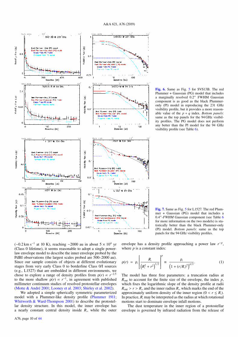
Fig. 5. Top panels: 1.3 mm (231 GHz) PdBI dust continuum emission visibility real parts as a function of baseline length (circularly averagedin 20 kλ bins) for L1448-2A. The left panel uses a linear scale, while the right panel shows the same data and models in logarithmic scaleto enhance the visibility of the long baseline points. The equivalent scales probed by the baselines in the image space are indicated at the topof each panel (computed as 0.6 × λ/b). In both panels, the plain lines show the best-fit Plummer-only envelope (Pl, black) and Plummer +Gaussian (PG, red) models we found to reproduce the visibility profile of the dust continuum emission in this source. The dashed lines showthe two components included in the best-fit PG model: the Plummer-envelope component in dashed light blue and the additional Gaussian compo-nent in dot-dashed dark blue (see Table 6 for more information on the two models). The Plummer + Gaussian (PG) model is not statistically betterthan the Plummer-only (Pl) for L1448-2A. Bottom panels: same as the top panels for the 94 GHz visibility profiles.

the L1521F envelope was resolved with MAMBO, the total fluxis somewhat uncertain as the observations were affected by rel-atively strong sky noise. We therefore only fixed the peak fluxin our model fit, allowing the total integrated flux to vary byup to ±50% around the single-dish value. For GF9-2 we usedthe IRAM-30 m fluxes from Wiesemeyer (1997): 60 mJy beam−1

peak flux and 315 mJy integrated up to a radius 35′′ at 240 GHz,extrapolated to our frequencies. Using a spectral index α20 kλ =2.1 between 94 and 231 GHz (see Table 4), we expect an inte-grated flux of 291 mJy at 231 GHz (55 mJy peak flux) and44 mJy at 94 GHz (8 mJy peak flux). Since these extrapo-lated envelope-scale fluxes are quite uncertain, we let them quiteloose during the fitting process with an error bar of 50% at bothfrequencies.

4.3. Comparison to protostellar envelope models

From the continuum visibility dataset constructed for each pri-mary protostar (see Sect. 4.1), we extracted the flux density ofthe protostellar dust continuum emission as a function of spatialfrequency by averaging the real parts of the observed visibilitiesin bins of baseline lengths (bin widths of 20 kλ at 231 GHz, andbin widths of 10 kλ at 94 GHz). We obtained visibility curvessampling baselines [20–590] kλ at 231 GHz and [10–240] kλat 94 GHz. Error bars on visibility amplitudes were estimatedfrom the individual weights (wi) of the interferometric visibilityamplitudes (yi), which were then averaged in bins of uv-distance:the error bar is the error on the mean value in an individual bin(yerr = Σ(w2

i × (yi −wmean)2)/(Σwi)2 and wmean = Σ(yi ×wi)/Σwi).

The continuum visibility curves for two of the Perseus sources(L1448-2A and SVS13B) and a Taurus source (L1527) are shownin Figs. 5–7, while the visibility curves of the other sources of thesample can be found in Figs. C.3–C.17. Our PdBI visibility pro-files probe the radial distribution of the dust continuum emissionfrom spatial scales θ = 0.35′′ to θ = 12′′. The envelope emissionat larger scales is constrained by the single-dish dust contin-uum profiles, which are mostly obtained with the IRAM-30 mtelescope (beam FWHM 11′′ at 1.3 mm).

We compared these dust continuum emission visibilitycurves to simple models of protostellar envelopes in a waysimilar to what was carried out in Maury et al. (2014) to analyzethe preliminary CALYPSO data for the NGC 1333 IRAS2Aprotostar. The envelope models considered here and the resultsof their comparison with the dust continuum observations aredescribed below.

4.3.1. Parameterized envelope models

For protostars in which a hydrostatic core has formed at thecenter, self-similar collapse solutions (Shu 1977; Whitworth &Summers 1985) suggest that the radial density profile of theenvelope at large radii r > Ri is expected to range betweenρ(r) ∝ r−3/2 in the inner dynamical free-fall region (in sphericalsimilarity solutions) and ρ(r) ∝ r−2 in the outer region wherethe initial conditions found in prestellar cores would have beenconserved, where Ri can be the centrifugal radius if a disk devel-ops or the radius of an inner cavity in the envelope. Since theradius of the expansion wavefront grows at the sound speed

A76, page 9 of 44

A&A 621, A76 (2019)

Fig. 6. Same as Fig. 5 for SVS13B. The redPlummer + Gaussian (PG) model that includesa marginally resolved 0.2′′ FWHM Gaussiancomponent is as good as the black Plummer-only (Pl) model in reproducing the 231 GHzvisibility profile, but it provides a more reason-able value of the p + q index. Bottom panels:same as the top panels for the 94 GHz visibil-ity profiles. The PG model does not performany better than the Pl model for the 94 GHzvisibility profile (see Table 6).

Fig. 7. Same as Fig. 5 for L1527. The red Plum-mer + Gaussian (PG) model that includes a0.4′′-FWHM Gaussian component (see Table 6for more information on the two models) is sta-tistically better than the black Plummer-only(Pl) model. Bottom panels: same as the toppanels for the 94 GHz visibility profiles.

(∼0.2 km s−1 at 10 K), reaching ∼2000 au in about 5 × 104 yr(Class 0 lifetime), it seems reasonable to adopt a single power-law envelope model to describe the inner envelope probed by thePdBI observations (the largest scales probed are 500–2000 au).Since our sample consists of objects at different evolutionarystages from very early Class 0 to borderline Class 0/I sources(e.g., L1527) that are embedded in different environments, wechose to explore a range of density profiles from ρ(r) ∝ r−2.5

to the more shallow ρ(r) ∝ r−1, in agreement with publishedmillimeter continuum studies of resolved protostellar envelopes(Motte & André 2001; Looney et al. 2003; Shirley et al. 2002).

We adopted a simple spherically symmetric parameterizedmodel with a Plummer-like density profile (Plummer 1911;Whitworth & Ward-Thompson 2001) to describe the protostel-lar density structure. In this model, the inner envelope hasa nearly constant central density inside Ri, while the outer

envelope has a density profile approaching a power law r−p,where p is a constant index:

ρ(r) = ρi

Ri(R2

i + r2)1/2

p

≡ ρi(1 + (r/Ri)2

)p/2 . (1)

The model has three free parameters: a truncation radius atRout to account for the finite size of the envelope, the index p,which fixes the logarithmic slope of the density profile at radiiRout > r > Ri, and the inner radius Ri, which marks the end of theapproximately uniform density of the inner region (0 < r ≤ Ri).In practice, Ri may be interpreted as the radius at which rotationalmotions start to dominate envelope infall motions.

The dust temperature in the inner region of a protostellarenvelope is governed by infrared radiation from the release of

A76, page 10 of 44

A. J. Maury et al.: CALYPSO view of Class 0 protostellar disks

gravitational energy of the material that accretes onto the centralobject. We ignore here the contribution of the interstellar radia-tion field, which mostly contributes to heating the outer layers ofthe envelope, although this contribution may be significant in thevery low luminosity objects IRAM04191 and L1521F. We notethat the dust continuum emission tracing the inner envelopes inour sample is optically thin at the two wavelengths we probed,as checked from the peak and integrated brightness temperaturesfrom our PdBI maps (see Cols. 4 and 5 of Table 4), except forIRAS4A where the emission is partially optically thick at ∼0.5′′scales. Following Butner et al. (1990) and Terebey et al. (1993),the dust temperature distribution T (r) in the power-law envelopeat radii r > Ri that is due to the central heating of the protostellarenvelope may be approximated as follows in the case of opticallythin dust continuum emission:

T (r) = 60( r13 400 au

)−q(

Lint

105 L

)q/2

K, (2)

where r represents the radius from the central source of lumi-nosity Lint. We varied the index q of the power-law temperaturedependence (T (r) ∝ r−q) between q = 0.3 and q = 0.5 in ourmodel fits.

The emerging intensity distribution of the envelope resultsfrom the combination of the dust density and temperature distri-butions of Eqs. (1) and (2). For instance, in the Rayleigh–Jeansregime, the radial intensity distribution of a power-law enve-lope is expected to scale as I(r) ∝ r−(p+q−1) (cf. Adams 1991). Inpractice, we therefore considered the following model intensitydistribution:

I(r) =I0(

1 + (r/Ri)2)(p+q−1)/2 , (3)

where I0 is the intensity from radii r < Ri and r represents theprojected radius. Considering the combination of likely densityand temperature distributions presented above, we let our modelspan a range from p + q = 1.3 to p + q = 2.9 between Ri and Rout.

4.3.2. Fitting the dust continuum emission visibilities withenvelope models

To model our interferometric observations, we converted theintensity distribution of the Plummer envelope model into a 1Dvisibility curve as a function of baseline b =

√u2 + v2 using a

Hankel transform (corresponding to the 2D Fourier transform ofa circularly symmetric function, see Bracewell 1965; Berger &Segransan 2007) :

V(b) = 2π∫ ∞

0Iν(rb)J0 (2πrbb) rbdrb, (4)

where J0 is the zeroth-order Bessel function,

J0(z) =1

2π

∫ 2π

0exp (−iz cos θ) dθ. (5)

For example, this interferometric transform turns a sphericallysymmetric power-law intensity distribution I(r) ∝ r−(p+q−1) intoa power-law visibility distribution as a function of u-v distance,V(b) ∝ bp+q−3, solely determined by the power-law indices ofthe temperature and density profiles p and q in the envelope atr > Ri.

We performed a least-squares fit of the observed visibilitydata with the interferometric transform of the parameterized

envelope model described by Eqs. (1) and (2). The envelopepower-law index (p + q) and the inner cavity radius Ri wereleft as free parameters within the previously mentioned ranges,when we adjusted the observed profiles. The estimated param-eter uncertainties were computed from the covariance matrix(see the description of the mpcurvefit in Markwardt 2009). Thebest-fit set of envelope parameters that reproduces the PdBIcontinuum visibility distribution for each of the 16 CALYPSOClass 0 sources is reported in Table 6. The modeled envelopevisibility profiles are shown for three sources of our sample asa black curve overlaid on the observed visibilities in Figs. 5–7,while the models for other sources of the sample are shown inFigs. C.3–C.17.

The radial distributions of the millimeter dust continuumemission of 10 of the 16 Class 0 protostars in our sam-ple (L1448-2A, IRAS2A, SVS13B, IRAS4A1, IRAM04191,L1521F, SerpM-S68N, SerpS-MM18, SerpS-MM22, and L1157)can be satisfactorily reproduced with models of Plummer-likeprotostellar envelopes with reduced χ2 values ≤3 (see the modelparameters and reduced χ2 values reported in the first two linesof Table 6 for each source) in the two continuum bands that areprobed in CALYPSO observations. Moreover, the model enve-lope sizes and power-law indices p + q for these 10 sources thatwe report in Table 6 show a good agreement in the two contin-uum bands (within 15%). This validates our choice of not fittingthe two visibility profiles at the two frequencies jointly, and itshows that when a Plummer envelope model is satisfactory, thereis no need to fix the envelope parameters to reproduce the dustcontinuum emission distribution at the longest baselines that areonly probed by the 231 GHz data.

4.4. Comparison with envelope models including a disk-likecomponent

For three protostars in our sample (L1448-C, L1448-NB1, andL1527; see Table 6), no single Plummer envelope model was ableto satisfactorily reproduce the continuum emission data at both231 and 94 GHz (reduced χ2 > 3). At these two frequencies, thecurvature of the radial intensity profile for these sources does notfollow a simple power-law trend, or at uv-distances longer than100 kλ, their PdBI visibility curve does not decrease quicklyenough to be reproduced by one envelope model alone. In addi-tion, while the 94 GHz visibility profiles of IRAS4B and GF92are satisfactorily described by single-envelope models, their231 GHz visibility profiles are inconsistent with single Plummer-like envelope models. This suggests that emission at baselinesprobed only by the 231 GHz data (250–550 kλ) differs fromthe best-fit envelope model we found to reproduce the 94 GHzcontinuum emission. Finally, while the 231 GHz profile canbe modeled quite satisfactorily by a Plummer model (reducedχ2 ≤ 3) for SerpM-SMM4, this does not hold for the 94 GHzprofile.

The failure to reproduce one or both of the visibility profilesusing circularly symmetric Plummer-like envelope models mayreflect the presence in the source of either (i) asymmetric fea-tures in the envelope structure or (ii) an additional density ortemperature component at small scales that is not properlymodeled, such as a protostellar disk that is embedded in theenvelope5. To check whether the visibility profiles of these

5 Note that our approximation to model the envelope contribution witha single power-law Plummer profile is not expected to affect our detec-tion of disk-like structures from the visibility curves at long baselinessince a flatter inner density power law index produces a steeper visibilitycurve.

A76, page 11 of 44

A&A 621, A76 (2019)

six objects could include an additional continuum emission com-ponent originating from a disk that is embedded in the envelope,we also fit the visibility profile of each CALYPSO protostar witha two-component model consisting of a Plummer-like envelope(cf. Eq. (1)) and an additional compact circular Gaussian com-ponent located at phase center, whose flux FGauss and FWHMΘGauss were left as free parameters (hereafter PG model forPlummer + Gaussian model). For these sources where the Gaus-sian component is spatially resolved, the value of Ri is enforcedto be higher than the value of ΘGauss during the minimizationprocess. The visibility function of the Gaussian disk componentwas calculated as

V(b) ∝ exp(−π × ΘGauss × b2/4ln 2). (6)

The parameters of the best-fit PG models are reported inTable 6. Figures C.3–C.17 show the Pl and PG models over the231 and 94 GHz visibility curves of all the sources in our sample.

We performed a Fisher6 statistical test (later referred to asan F-test) to decide which of the best-fit Plummer-only model(Pl) and the best Plummer + Gauss (PG) models we obtained foreach source in our sample was better. The goal was to avoid over-modeling the visibility profiles of sources with complex structureusing a model that reproduced the observations better only coin-cidentally, because it includes two additional free parameters,such as the PG model. The results of the F-test (computingP values from the F distribution to test if the PG models arestatistically better than the Pl models despite their two addi-tional free parameters), which compared the best-fit Pl and PGmodels we obtained for each protostar are reported in Col. 10of Table 6: we indicate a “yes” if the F-test suggests that thePG model is statistically better than the Pl model, and a “no”otherwise.

For all 10 sources that have satisfactory (reduced χ2 < 3) Plmodels at the two frequencies (231 and 94 GHz), none of thePG models provided a better fit for the two frequencies, exceptfor SerpS-MM22. However, for five out of the six sources withunsatisfactory Pl models, the F-test suggests at either 231 GHz(L1448-C, L1527, IRAS4B, and GF92) or 94 GHz (L1448-C,L1527 and SerpM-SMM4) that the PG models reproduce themillimeter dust continuum visibility profiles significantly betterthan the Pl models.

For three protostars in our sample that are better repro-duced with PG models at the two frequencies (L1527, SerpM-SMM4, and SerpS-MM22), our modeling suggests an additionalGaussian component is detected, that is well resolved in our231 GHz PdBI data. While the inclusion of a Gaussian compo-nent significantly improved the minimization at both frequenciesfor two other protostars (L1448-C and GF9-2), the FWHMs ofthese components are very similar to the scale probed by ourlongest baseline (570 kλ, i.e., probing radii down to 0.26′′). Thisindicates that the additional Gaussian components suggested byour modeling are at best marginally resolved considering theincrease in phase noise at the longest baselines, and that theirsizes are therefore highly uncertain (see Table 6). For IRAS4B,the inclusion of a large and bright Gaussian component signif-icantly improves the minimization for the 231 GHz visibilityprofile, which was unsatisfactorily modeled with a single Plum-mer envelope, but does not improve the modeling of our 94 GHzdata. For five protostars that are well modeled at both frequenciesusing Pl models (SVS13B, IRAM04191, L1521F, SerpS-MM18,and L1157), the inclusion of unresolved Gaussian components6 For more information on the Fisher test, see for example Donaldson(1968) and references therein.

in the PG models allows obtaining a significantly better mini-mization at 231 GHz, where we reach the best angular resolution,but does not improve the modeling of the 94 GHz visibilityprofiles. When we consider the null flux level dependence atthe longest baselines in our PdBI observations, the decreas-ing slope of such low fluxes with increasing baseline at thelongest baselines is questionable, and we therefore conserva-tively assume that these Gaussian components are detected butunresolved.

Finally, none of the models we attempted performed verywell for L1448-NB1 (with reduced χ2 values always higher thanor equal to 3), probably because the emission at long base-lines (>200 kλ) shows wiggles that cannot be reproduced witha simple model such as we adopted here. In the specific caseof this protostar, other models centered either on L1448-NB2 orin between the two millimeter sources L1448-NB1 and L1448-NB2 were attempted. They tentatively suggested the presence ofan additional circumbinary structure (see Appendix C.2).

Figures 5–8 show examples of Plummer-only (Pl, blackcurve) and Plummer + Gauss (PG, red curve) model fits forfour sources of our sample: L1448-2A, L1157, and SVS13B,which are satisfactorily described by an envelope-only model,and L1527, for which the inclusion of an additional centralGaussian source allows us to reproduce the visibility profilebetter than an envelope-only model.

4.5. Characterization of disk-like components in the sample

For a 2D Gaussian distribution, most of the radiation (90%)is emitted from within a radius r < FWHM, thus we conser-vatively defined the candidate disk radius to be the estimatedFWHM size of the additional Gaussian component when the PGmodel provided a better model than the Pl model (as suggestedby the F-test, see previous section and Col. 10 of Table 6).

For sources where the Pl model reproduces the visibilityprofile better at both frequencies (L1448-2A, IRAS4A, SerpM-S68N, and SerpS-MM18), we performed a new minimization ofthe PG model with fixed envelope parameters from the best-fit Plmodel (PGf models in Appendix C). The Gaussian parametersof this PGf model were compared to the Gaussian parameters ofthe best-fit PG model (with free envelope parameters): the high-est values provide upper limits to the disk size and flux in thesource. For sources for which the PG model reproduces the twothe visibility profiles better (L1448-C, L1527, SerpM-SMM4,SerpS-MM22, and GF9-2), the parameters of the Gaussian com-ponent at 231 GHz (best angular resolution) are taken as thecandidate disk size and disk flux in the source (or upper limitsif the Gaussian component in the PG model is unresolved). Forsources for which only the 231 GHz visibility profile (probingthe smallest spatial scales) is better reproduced by a PG model(SVS13B, IRAS4B, IRAM04191, L1521F, and L1157), we usedthe properties of the Gaussian component of the PG231 model(see Table 6) as candidate disk size and flux, or upper limitsif the Gaussian component is unresolved. IRAS2A is the onlysource in the sample that is better reproduced by the PG modelat 94 GHz, but not at 231 GHz. However, the Pl model at 94 GHzis also satisfactory (reduced chi square of 0.9) and the Gaussiancomponent of the PG model is unresolved: hence, we consider itlikely that an unresolved candidate disk is detected in our 94 GHzdata and report the candidate disk as unresolved in Table 5, withthe upper limits on its size and flux stemming from the best-fit PG model at 231 GHz (consistent with the parameters ofthe best-fit PG model at 94 GHz). Following this method, wereport in Table 5 the detection of candidate protostellar disk-like

A76, page 12 of 44

A. J. Maury et al.: CALYPSO view of Class 0 protostellar disks

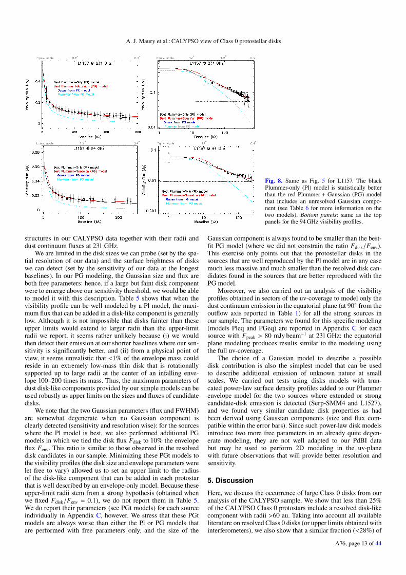
Fig. 8. Same as Fig. 5 for L1157. The blackPlummer-only (Pl) model is statistically betterthan the red Plummer + Gaussian (PG) modelthat includes an unresolved Gaussian compo-nent (see Table 6 for more information on thetwo models). Bottom panels: same as the toppanels for the 94 GHz visibility profiles.

structures in our CALYPSO data together with their radii anddust continuum fluxes at 231 GHz.

We are limited in the disk sizes we can probe (set by the spa-tial resolution of our data) and the surface brightness of diskswe can detect (set by the sensitivity of our data at the longestbaselines). In our PG modeling, the Gaussian size and flux areboth free parameters: hence, if a large but faint disk componentwere to emerge above our sensitivity threshold, we would be ableto model it with this description. Table 5 shows that when thevisibility profile can be well modeled by a Pl model, the maxi-mum flux that can be added in a disk-like component is generallylow. Although it is not impossible that disks fainter than theseupper limits would extend to larger radii than the upper-limitradii we report, it seems rather unlikely because (i) we wouldthen detect their emission at our shorter baselines where our sen-sitivity is significantly better, and (ii) from a physical point ofview, it seems unrealistic that <1% of the envelope mass couldreside in an extremely low-mass thin disk that is rotationallysupported up to large radii at the center of an infalling enve-lope 100–200 times its mass. Thus, the maximum parameters ofdust disk-like components provided by our simple models can beused robustly as upper limits on the sizes and fluxes of candidatedisks.

We note that the two Gaussian parameters (flux and FWHM)are somewhat degenerate when no Gaussian component isclearly detected (sensitivity and resolution wise): for the sourceswhere the Pl model is best, we also performed additional PGmodels in which we tied the disk flux Fdisk to 10% the envelopeflux Fenv. This ratio is similar to those observed in the resolveddisk candidates in our sample. Minimizing these PGt models tothe visibility profiles (the disk size and envelope parameters werelet free to vary) allowed us to set an upper limit to the radiusof the disk-like component that can be added in each protostarthat is well described by an envelope-only model. Because theseupper-limit radii stem from a strong hypothesis (obtained whenwe fixed Fdisk/Fenv = 0.1), we do not report them in Table 5.We do report their parameters (see PGt models) for each sourceindividually in Appendix C, however. We stress that these PGtmodels are always worse than either the Pl or PG models thatare performed with free parameters only, and the size of the

Gaussian component is always found to be smaller than the best-fit PG model (where we did not constrain the ratio Fdisk/Fenv).This exercise only points out that the protostellar disks in thesources that are well reproduced by the Pl model are in any casemuch less massive and much smaller than the resolved disk can-didates found in the sources that are better reproduced with thePG model.

Moreover, we also carried out an analysis of the visibilityprofiles obtained in sectors of the uv-coverage to model only thedust continuum emission in the equatorial plane (at 90 from theoutflow axis reported in Table 1) for all the strong sources inour sample. The parameters we found for this specific modeling(models Pleq and PGeq) are reported in Appendix C for eachsource with Fpeak > 80 mJy beam−1 at 231 GHz: the equatorialplane modeling produces results similar to the modeling usingthe full uv-coverage.

The choice of a Gaussian model to describe a possibledisk contribution is also the simplest model that can be usedto describe additional emission of unknown nature at smallscales. We carried out tests using disks models with trun-cated power-law surface density profiles added to our Plummerenvelope model for the two sources where extended or strongcandidate-disk emission is detected (Serp-SMM4 and L1527),and we found very similar candidate disk properties as hadbeen derived using Gaussian components (size and flux com-patible within the error bars). Since such power-law disk modelsintroduce two more free parameters in an already quite degen-erate modeling, they are not well adapted to our PdBI databut may be used to perform 2D modeling in the uv-planewith future observations that will provide better resolution andsensitivity.

5. Discussion

Here, we discuss the occurrence of large Class 0 disks from ouranalysis of the CALYPSO sample. We show that less than 25%of the CALYPSO Class 0 protostars include a resolved disk-likecomponent with radii >60 au. Taking into account all availableliterature on resolved Class 0 disks (or upper limits obtained withinterferometers), we also show that a similar fraction (<28%) of

A76, page 13 of 44

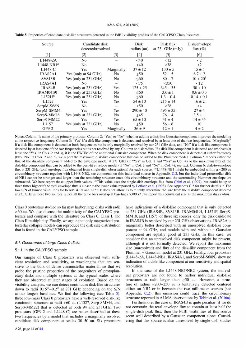
A&A 621, A76 (2019)

Table 5. Properties of candidate disk-like structures detected in the PdBI visibility profiles of the CALYPSO Class 0 sources.

Source Candidate disk Disk Disk flux Disk/envelopedetected/resolved radius (au) at 231 GHz (mJy) flux (%)

[1] [2] [3] [4] [5] [6]L1448-2A No – <40 <12 <2

L1448-NB1a No – <40 <38 <2L1448-C Yes Marginally 37 ± 12 130 ± 5 15 ± 5IRAS2A1 Yes (only at 94 GHz) No .50 52 ± 5 6.7 ± 2SVS13B Yes (only at 231 GHz) No .60 80 ± 7 10 ± 20b

IRAS4A1 No – <75 <350 <12IRAS4B Yes (only at 231 GHz) Yes 125 ± 25 645 ± 35 50 ± 10

IRAM04191c Yes (only at 231 GHz) No .60 3.6 ± 1 0.6 ± 0.3L1521Fc Yes (only at 231 GHz) No .60 1.3 ± 0.4 0.14 ± 0.1L1527 Yes Yes 54 ± 10 215 ± 14 16 ± 2

SerpM-S68N No – <50 <28 <4SerpM-SMM4 Yes Yes 290 ± 40 595 ± 35 27 ± 4SerpS-MM18 Yes (only at 231 GHz) No .45 76 ± 4 3.5 ± 1SerpS-MM22 Yes Yes 65 ± 10 31 ± 4 14 ± 35

L1157 Yes (only at 231 GHz) No .50 56 ± 6 10GF9-2 Yes Marginally 36 ± 9 12 ± 1 4 ± 2

Notes. Column 1: name of the primary protostar. Column 2: “Yes” or “No”: whether adding a disk-like Gaussian component improves the modelingat the respective frequency. Column 3: “Yes” if a disk-like component is detected and resolved by at least one of the two frequencies, “Marginally”if a disk-like component is detected at both frequencies but is only marginally resolved by our 231 GHz data, and “No” if a disk-like component isdetected by at least one of the two frequencies but is not resolved by any. Column 4: disk radius. If a disk-like component is detected and resolved (atleast one “Yes” in Cols. 2 and 3), it is the FWHM of the additional Gaussian component. When no disk component is detected at either frequency(two “No” in Cols. 2 and 3), we report the maximum disk-like component that can be added to the Plummer model. Column 5 reports either theflux of the disk-like component added to the envelope model at 231 GHz (if “Yes” in Col. 2 and “Yes” in Col. 4) or the maximum flux of thedisk-like component that can be added to the best-fit envelope model (if “No” in Col. 2 and “No” in Col. 4), see text. Column 6: disk-to-envelopeflux at 231 GHz (total envelope flux obtained from single-dish observations) for each source. (a)L1448-NB1 might be embedded within a ∼200 aucircumbinary structure together with L1448-NB2, see comments on this individual source in Appendix C.2, but the individual protostellar diskof NB1 cannot be stronger and larger than the remaining structure once this circumbinary structure and the surrounding Plummer envelope aresubtracted. We here report these upper-limit values. (b)This value uses the single-dish envelope flux from Chini et al. (1997), but could be up tothree times higher if the total envelope flux is closer to the lower value reported by Lefloch et al. (1998). See Appendix C.5 for further details. (c)Thelow S/N of binned visibilities for IRAM04191 and L1521F does not allow us to reliably determine the size from the disk-like component detectedat 231 GHz in these two sources. Since all the error bars overlap at baselines >300 kλ, we report this equivalent size as the maximum disk radius.

Class 0 protostars studied so far may harbor large disks with radii>60 au. We also discuss the multiplicity of the CALYPSO pro-tostars and compare with the literature on Class 0, Class I, andClass II multiplicity. Finally, we argue that only magnetized pro-tostellar collapse models can reproduce the disk size distributionthat is found in the CALYPSO sample.

5.1. Occurrence of large Class 0 disks

5.1.1. In the CALYPSO sample

Our sample of Class 0 protostars was observed with suffi-cient resolution and sensitivity, at wavelengths that are sen-sitive to the bulk of dense circumstellar material, so that weprobe the pristine properties of the progenitors of protoplan-etary disks and multiple systems at the typical scales wherethey are observed at later stages of evolution. Based on thevisibility analysis, we can detect continuum disk-like structuresdown to radii 0.15′′−0.2′′ at 231 GHz depending on the S/Nat our longest baselines. We find the following (see Table 5):three low-mass Class 0 protostars have a well-resolved disk-likecontinuum structure at radii >60 au (L1527, Serp-SMM4, andSerpS-MM22) that is detected at both 94 and 231 GHz. Twoprotostars (GF9-2 and L1448-C) are better described at thesetwo frequencies by a model that includes a marginally resolvedcandidate disk component at scales 30–50 au. Six protostars

have indications of a disk-like component that is only detectedat 231 GHz (IRAS4B, SVS13B, IRAM04191, L1521F, SerpS-MM18, and L1157): of these six sources, only the disk candidatein IRAS4B is resolved by our 231 GHz observations. IRAS2A ismarginally better described with an unresolved disk-like com-ponent at 94 GHz, and models with and without a Gaussiancomponent are equally good at 231 GHz. In this case, weconsider that an unresolved disk component might be present,although it is not formally detected. We report the maximumsize (unresolved) and flux of the disk-like component from thePlummer + Gaussian model at 231 GHz. Finally, four protostars(L1448-2A, L1448-NB1, IRAS4A1, and SerpM-S68N) show noindication of a disk-like component at our sensitivity and spatialresolution.

In the case of the L1448-NB1/NB2 system, the individ-ual protostars are not found to harbor individual disk-likestructures at radii larger than &50 au. However, a struc-ture of radius ∼200−250 au is tentatively detected centeredeither on NB2 or in between the two millimeter sources (seeAppendix C.2): this emission could trace the circumbinarystructure reported in ALMA observations by Tobin et al. (2016a).

Furthermore, the case of IRAS4B is quite peculiar: if we donot constrain the total envelope flux to contain at least half thesingle-dish peak flux, then the PdBI visibilities of this sourceseem well described by a Gaussian component alone. Consid-ering that this source is also unresolved by single-dish studies

A76, page 14 of 44

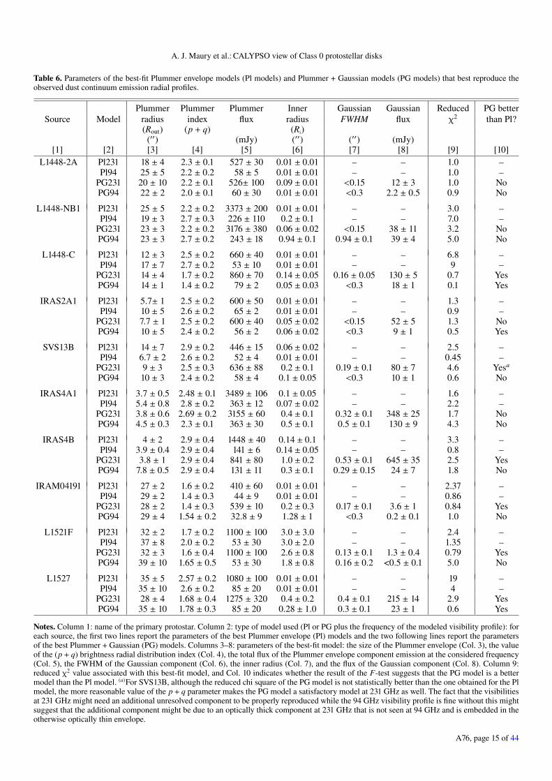
A. J. Maury et al.: CALYPSO view of Class 0 protostellar disks

Table 6. Parameters of the best-fit Plummer envelope models (Pl models) and Plummer + Gaussian models (PG models) that best reproduce theobserved dust continuum emission radial profiles.

Plummer Plummer Plummer Inner Gaussian Gaussian Reduced PG betterSource Model radius index flux radius FWHM flux χ2 than Pl?

(Rout) (p + q) (Ri)(′′) (mJy) (′′) (′′) (mJy)

[1] [2] [3] [4] [5] [6] [7] [8] [9] [10]L1448-2A Pl231 18 ± 4 2.3 ± 0.1 527 ± 30 0.01 ± 0.01 – – 1.0 –

Pl94 25 ± 5 2.2 ± 0.2 58 ± 5 0.01 ± 0.01 – – 1.0 –PG231 20 ± 10 2.2 ± 0.1 526± 100 0.09 ± 0.01 <0.15 12 ± 3 1.0 NoPG94 22 ± 2 2.0 ± 0.1 60 ± 30 0.01 ± 0.01 <0.3 2.2 ± 0.5 0.9 No

L1448-NB1 Pl231 25 ± 5 2.2 ± 0.2 3373 ± 200 0.01 ± 0.01 – – 3.0 –Pl94 19 ± 3 2.7 ± 0.3 226 ± 110 0.2 ± 0.1 – – 7.0 –

PG231 23 ± 3 2.2 ± 0.2 3176 ± 380 0.06 ± 0.02 <0.15 38 ± 11 3.2 NoPG94 23 ± 3 2.7 ± 0.2 243 ± 18 0.94 ± 0.1 0.94 ± 0.1 39 ± 4 5.0 No

L1448-C Pl231 12 ± 3 2.5 ± 0.2 660 ± 40 0.01 ± 0.01 – – 6.8 –Pl94 17 ± 7 2.7 ± 0.2 53 ± 10 0.01 ± 0.01 – – 9 –

PG231 14 ± 4 1.7 ± 0.2 860 ± 70 0.14 ± 0.05 0.16 ± 0.05 130 ± 5 0.7 YesPG94 14 ± 1 1.4 ± 0.2 79 ± 2 0.05 ± 0.03 <0.3 18 ± 1 0.1 Yes

IRAS2A1 Pl231 5.7± 1 2.5 ± 0.2 600 ± 50 0.01 ± 0.01 – – 1.3 –Pl94 10 ± 5 2.6 ± 0.2 65 ± 2 0.01 ± 0.01 – – 0.9 –

PG231 7.7 ± 1 2.5 ± 0.2 600 ± 40 0.05 ± 0.02 <0.15 52 ± 5 1.3 NoPG94 10 ± 5 2.4 ± 0.2 56 ± 2 0.06 ± 0.02 <0.3 9 ± 1 0.5 Yes

SVS13B Pl231 14 ± 7 2.9 ± 0.2 446 ± 15 0.06 ± 0.02 – – 2.5 –Pl94 6.7 ± 2 2.6 ± 0.2 52 ± 4 0.01 ± 0.01 – – 0.45 –

PG231 9 ± 3 2.5 ± 0.3 636 ± 88 0.2 ± 0.1 0.19 ± 0.1 80 ± 7 4.6 Yesa

PG94 10 ± 3 2.4 ± 0.2 58 ± 4 0.1 ± 0.05 <0.3 10 ± 1 0.6 No

IRAS4A1 Pl231 3.7 ± 0.5 2.48 ± 0.1 3489 ± 106 0.1 ± 0.05 – – 1.6 –Pl94 5.4 ± 0.8 2.8 ± 0.2 363 ± 12 0.07 ± 0.02 – – 2.2 –

PG231 3.8 ± 0.6 2.69 ± 0.2 3155 ± 60 0.4 ± 0.1 0.32 ± 0.1 348 ± 25 1.7 NoPG94 4.5 ± 0.3 2.3 ± 0.1 363 ± 30 0.5 ± 0.1 0.5 ± 0.1 130 ± 9 4.3 No

IRAS4B Pl231 4 ± 2 2.9 ± 0.4 1448 ± 40 0.14 ± 0.1 – – 3.3 –Pl94 3.9 ± 0.4 2.9 ± 0.4 141 ± 6 0.14 ± 0.05 – – 0.8 –

PG231 3.8 ± 1 2.9 ± 0.4 841 ± 80 1.0 ± 0.2 0.53 ± 0.1 645 ± 35 2.5 YesPG94 7.8 ± 0.5 2.9 ± 0.4 131 ± 11 0.3 ± 0.1 0.29 ± 0.15 24 ± 7 1.8 No

IRAM04191 Pl231 27 ± 2 1.6 ± 0.2 410 ± 60 0.01 ± 0.01 – – 2.37 –Pl94 29 ± 2 1.4 ± 0.3 44 ± 9 0.01 ± 0.01 – – 0.86 –

PG231 28 ± 2 1.4 ± 0.3 539 ± 10 0.2 ± 0.3 0.17 ± 0.1 3.6 ± 1 0.84 YesPG94 29 ± 4 1.54 ± 0.2 32.8 ± 9 1.28 ± 1 <0.3 0.2 ± 0.1 1.0 No

L1521F Pl231 32 ± 2 1.7 ± 0.2 1100 ± 100 3.0 ± 3.0 – – 2.4 –Pl94 37 ± 8 2.0 ± 0.2 53 ± 30 3.0 ± 2.0 – – 1.35 –

PG231 32 ± 3 1.6 ± 0.4 1100 ± 100 2.6 ± 0.8 0.13 ± 0.1 1.3 ± 0.4 0.79 YesPG94 39 ± 10 1.65 ± 0.5 53 ± 30 1.8 ± 0.8 0.16 ± 0.2 <0.5 ± 0.1 5.0 No

L1527 Pl231 35 ± 5 2.57 ± 0.2 1080 ± 100 0.01 ± 0.01 – – 19 –Pl94 35 ± 10 2.6 ± 0.2 85 ± 20 0.01 ± 0.01 – – 4 –

PG231 28 ± 4 1.68 ± 0.4 1275 ± 320 0.4 ± 0.2 0.4 ± 0.1 215 ± 14 2.9 YesPG94 35 ± 10 1.78 ± 0.3 85 ± 20 0.28 ± 1.0 0.3 ± 0.1 23 ± 1 0.6 Yes

Notes. Column 1: name of the primary protostar. Column 2: type of model used (Pl or PG plus the frequency of the modeled visibility profile): foreach source, the first two lines report the parameters of the best Plummer envelope (Pl) models and the two following lines report the parametersof the best Plummer + Gaussian (PG) models. Columns 3–8: parameters of the best-fit model: the size of the Plummer envelope (Col. 3), the valueof the (p + q) brightness radial distribution index (Col. 4), the total flux of the Plummer envelope component emission at the considered frequency(Col. 5), the FWHM of the Gaussian component (Col. 6), the inner radius (Col. 7), and the flux of the Gaussian component (Col. 8). Column 9:reduced χ2 value associated with this best-fit model, and Col. 10 indicates whether the result of the F-test suggests that the PG model is a bettermodel than the Pl model. (a)For SVS13B, although the reduced chi square of the PG model is not statistically better than the one obtained for the Plmodel, the more reasonable value of the p + q parameter makes the PG model a satisfactory model at 231 GHz as well. The fact that the visibilitiesat 231 GHz might need an additional unresolved component to be properly reproduced while the 94 GHz visibility profile is fine without this mightsuggest that the additional component might be due to an optically thick component at 231 GHz that is not seen at 94 GHz and is embedded in theotherwise optically thin envelope.

A76, page 15 of 44

A&A 621, A76 (2019)

Table 6. continued.

Plummer Plummer Plummer Inner Gaussian Gaussian Reduced PG betterSource Model radius index flux radius FWHM flux χ2 than Pl?

(Rout) (p + q) (Ri)(′′) (mJy) (′′) (′′) (mJy)

[1] [2] [3] [4] [5] [6] [7] [8] [9] [10]SerpM-S68N Pl231 15 ± 2 2.28 ± 0.1 800 ± 80 0.01 ± 0.01 – – 1.67 –

Pl94 22 ± 5 2.56 ± 0.2 35 ± 10 0.03 ± 0.03 – – 1.2 –PG231 13.9 ± 3 2.1 ± 0.2 800 ± 80 0.1 ± 0.1 0.11 ± 0.1 28 ± 11 2.1 NoPG94 15 ± 2 2.08 ± 0.2 35 ± 10 0.5 ± 0.1 0.5 ± 0.1 6.5 ± 1 3.4 No

SerpM-SMM4 Pl231 25 ± 5 2.8 ± 0.4 1700 ± 200 0.06 ± 0.05 – – 2.7 –Pl94 15 ± 4 2.8 ± 0.4 105 ± 6 0.01 ± 0.01 – – 3.7 –

PG231 22 ± 5 1.8 ± 0.5 1305 ± 500 0.70 ± 0.1 0.70 ± 0.2 595 ± 35 0.14 YesPG94 25 ± 5 1.6 ± 0.3 103 ± 20 0.6 ± 0.1 0.62 ± 0.1 61 ± 3 0.39 Yes

SerpS-MM18 Pl231 16 ± 2 2.24 ± 0.2 2208 ± 190 0.01 ± 0.01 – – 1.8 –Pl94 20 ± 5 2.4 ± 0.2 114 ± 20 0.015 ± 0.05 – – 0.87 –

PG231 15.5 ± 6 2.17 ± 0.2 2327 ± 55 0.13 ± 0.07 0.128 ± 0.08 76 ± 4 0.68 YesPG94 11 ± 2 2.24 ± 0.2 114 ± 20 0.04 ± 0.02 <0.1 ± 0.1 <1 ± 0.5 2.78 No

SerpS-MM22 Pl231 11 ± 2 2.56 ± 0.2 135 ± 30 0.01 ± 0.01 – – 1.8 –Pl94 25 ± 5 2.7 ± 0.3 10 ± 5 0.01 ± 0.01 – – 1.16 –

PG231 10 ± 4 2.0 ± 0.3 148 ± 9 0.26 ± 0.08 0.25 ± 0.08 31 ± 4 1.1 YesPG94 19 ± 3 1.98 ± 0.3 10 ± 5 0.31± 0.07 0.31± 0.07 3.2 ± 0.5 0.59 Yes

L1157 Pl231 12 ± 10 2.68 ± 0.2 520 ± 170 0.01 ± 0.01 – – 1.29 –Pl94 16 ± 5 2.65 ± 0.2 61 ± 10 0.01 ± 0.01 – – 1.4 –

PG231 6.8 ± 2 2.5 ± 0.2 494 ± 35 0.05 ± 0.04 <0.1 ± 0.1 56 ± 6 0.76 YesPG94 8.2 ± 2 2.24 ± 0.3 61 ± 10 0.05 ± 0.04 <0.3 ± 1 9 ± 1 2.5 No

GF9-2 Pl231 40 ± 7 2.36 ± 0.2 179 ± 20 0.01 ± 0.01 – – 5 –Pl94 40 ± 10 2.2 ± 0.2 27 ± 7 0.01 ± 0.01 – – 1.8 –

PG231 37 ± 3 1.67 ± 0.3 407 ± 80 0.18 ± 0.05 0.18 ± 0.05 11.8 ± 2 0.55 YesPG94 34 ± 5 1.71 ± 0.3 39 ± 20 0.15 ± 0.07 <0.3 ± 0.1 1.3 ± 0.5 0.45 Yes

(and our modeling suggests a very compact envelope structure,if any), its Class 0 nature may be questioned and it may be moretypical of the Class I stage (as, e.g., SVS13A) still embeddedin its native cloud (resolved out by our interferometric observa-tions, hence the Gaussian-like profile). It is also possible that the231 GHz dust emission at PdBI scales is optically thick, but thisis not suggested by either (i) the temperature brightness of the231 GHz PdBI dust continuum emission peak or (ii) the sim-ilarly small envelope size found when modeling the opticallythin 94 GHz dust continuum profile. Finally, we stress that theremarkably large size of the disk-like component in Serp-SMM4(290 au) is quite intriguing and calls for further analysis of thekinematics at these scales to characterize the nature of the dustcontinuum emission, which does not follow a standard envelopepower-law radial distribution.

When we assume that all resolved continuum structureswe detected in our sample trace protostellar disks, the frac-tion of candidate protostellar disks with radii >60 au is 4 outof 16 (IRAS4B, L1527, SerpS-MM22, and SerpM-SMM4), i.e.∼25%. Moreover, our modeling shows that the candidate diskradii are <100 au in 14 out of 16 Class 0 protostars. Sincethese disk-like continuum structures need to be confirmed kine-matically, the analysis of the dust continuum emission in theCALYPSO sample provides an upper limit to the occurrenceof large (with radii &60 au) disks of ≤25% during the mainaccretion phase. Our results show that most Class 0 proto-stars have embedded disks (75% of the sources in our sampleare better described when a disk component is included), but

most of these young protostellar disks are small in size andflux.

5.1.2. Comparison with other works

Several groups have recently tried to characterize the propertiesof disks around Class 0 protostars. For example, Segura-Coxet al. (2016, 2018) used the VANDAM 8 mm continuum VLAsurvey of 43 Class 0 and Class 0/I protostars in Perseus. Theyfound that only 15 of these Class 0 and 0/I sources are resolvedat 15 au, and the candidate disks of only 10 of the VANDAMClass 0 protostars are resolved at radii >12 au. All of these10 disk Class 0 candidates have radii r < 45 au, and the diskcomponent is not resolved in 67% of the VANDAM protostarsat a 12 au scale. When the VANDAM and CALYPSO samplesare combined, only 4 out of 52 Class 0 and 0/I protostars, thatis, ≤8%, appear to have dust continuum circumstellar disks withradii &60 au. We did not include these disk sizes in our statis-tics for Class 0 protostars: as stated by the authors themselves,they may only represent lower limits because the 8 mm dust con-tinuum emission size could be biased by a population of largedust grains that drift inward. We note that our CALYPSO results,which are obtained at shorter wavelengths, are less strongly sub-ject to dust property limitations7, but we nevertheless also find

7 The 1.3 mm dust continuum emission remains optically thin at mostradii we probe here, and was never shown to be preferentially trac-ing large grains, although grain growth at scales <500 au cannot beexcluded.

A76, page 16 of 44

A. J. Maury et al.: CALYPSO view of Class 0 protostellar disks

that most Class 0 disks have small radii r < 60 au, with radiusvalues consistent for the sources in common to both samples.

Other recent results for the quest of rotationally supportedcircumstellar disks in Class 0 protostars include L1527 (Ohashiet al. 2014, ALMA), which has a centrifugal radius of ∼60 au,and VLA 1623 (Murillo et al. 2013), which was suggestedto show Keplerian disk motions up to r ∼ 189 au. The latterrequires confirmation, however, because the model that was usedis complex. In the HH212 protostar, Lee et al. (2018a) founda candidate Keplerian disk at radius ∼40 au that is embeddedin a dusty disk-like structure at radius ∼60 AU. Recent SMAobservations of the Class 0 protostar BHR7 suggest a compactdust continuum component at r ∼ 120 au, although the kinemat-ics obtained within the same dataset do not confirm Keplerianrotation at similar scales (Tobin et al. 2018). Gerin et al. (2017)analyzed ALMA 0.8 mm dust continuum observations of twoClass 0 protostars, B1b-N and B1b-S. They found that compactdisk-like components could only contribute to the intensityprofiles at scales .50 au. The 0.87 mm ALMA observationsby Tokuda et al. (2017) enabled the detection of a small 10 auradius disk in L1521F. For the B335 protostar, observations ofthe kinematics in the inner envelope with ALMA provided anupper limit to the disk radius of B335 <15 au (Yen et al. 2015b).The two Class 0 protostars IRAS16253 and IRAS15398 havebeen observed with ALMA by Yen et al. (2017), who found acandidate disk radius of 20 au in IRAS15398 and an upper-limitdisk radius of 6 au in IRAS16253. The Class 0 L1455 IRS1 wasobserved with the SMA, and the size of its protostellar disk wasconstrained to <200 AU (Chou et al. 2016). The HH211 Class 0protostar was observed with ALMA, and its disk radius wasconstrained to .10 au (Lee et al. 2018b). Finally, in an SMAsurvey of envelope kinematics toward a sample of 14 Class 0protostars, Yen et al. (2015a) found that three sources (L1448-NB, Per-emb 9, and IRAS 03292+3039) harbored kinematicsthat were consistent with rotational motions dominating infallingmotions in their inner envelopes at scales ∼100−200 au. TwoClass 0 protostars of their sample, L1527 and HH212, show rota-tionally dominated motions close to Keplerian at radii 50–80 au:rotationally supported disks with radii ∼40−60 au have indeedbe confirmed by other groups in these two sources. The remain-ing 8 Class 0 protostars of the Yen et al. (2015a) sample do notshow any indication of rotationally dominated motions at scalessampled by the SMA observations (1.5′′–5′′ synthesized beams,and heterogeneous source distances). Our CALYPSO analysistriples the number of Class 0 protostars that are analyzed at highangular resolution to seek for disk-like structures at wavelengthsthat probe the bulk of circumstellar material (<3 mm). When wecombine the CALYPSO sample with the recent ALMA resultsthat probe radii .60 au, only 5–7 out of 26 Class 0 protostars,that is, <28%, show either confirmed or candidate disks at radii>60 au. The disk radii as a function of the protostellar bolomet-ric luminosity for all Class 0 disks that are characterized withmillimeter-wavelength observations that probe scales &60 aufrom CALYPSO and the literature are shown as red symbolsin Fig. 9.

The main caveat in characterizing candidate disk structuresfrom continuum visibilities stems from the uncertain estimate ofthe large-scale envelope contribution. We stress that we left theenvelope parameters free to vary in our modeling to account forthe variety of envelopes that is observed in Class 0 protostars. Wealso emphasize that all of our best-fit models suggest envelopeparameters that are physically reasonable. If the large-scale enve-lope deviates from the spherical symmetry assumed here, the

) (Baren-feld et al. 2017). Individual studies of Class I disks that are char-acterized by either dust or molecular lines observations between0.7 mm and 2.7 mm with a spatial resolution better than 50 auinclude SVS13A, R-CrA, L1551NE, L1551-IRS1, L1455-IRS1,Lupus3-MMS, L1489, IRS43, IRS63, TMR1, TMC1, TMC1A,and L1536 (Lindberg et al. 2014; Yen et al. 2017; Takakuwaet al. 2014; Aso et al. 2015; Harsono et al. 2014), Elias29, WL12(Miotello et al. 2014), and the ten Taurus Class I from Sheehan& Eisner (2017). They are shown in Figure 9 as black stars. Westress that some radii are estimated based on the kinematics ofmolecular lines (centrifugal radius), while some are determined

Fig. 9. Protostellar disk radii Rdisk as a function of the protostellar bolo-metric luminosity Lbol for all Class 0 (red circles) and Class I (blackstars) protostars observed between 0.7 and 2.7 mm with a spatial reso-lution better than 50 au from the CALYPSO sample and the literature.The Class 0 disks shown here are from the CALYPSO sample (filledcircles) and those characterized in the literature (contour circles, see textfor names and references). When only upper limits on disk sizes couldbe estimated, the upper-limit values are indicated with arrows pointingdown. The dotted red box shows the location of the ten Class 0 diskradii from the 8mm continuum observations of the VANDAM sample(Segura-Cox et al. 2018). The individual Class I disks shown are thosedescribed in the text of Sect. 5.1.3. The dashed lines show the mediandisk radii: in red from the sample of 25 Class 0 disks with R0 <50 au(including upper limit radii), and in black the median radius from thesample of 25 Class I disks with RI = 115 au.

estimated properties of the candidate disks may change slightly.However, the spherical envelope model has the advantage ofsimplicity and accurately reproduces the observed visibilities atshort baselines. Our additional modeling, which used only theequatorial dust continuum profiles, suggests that the possibleasymmetry of the envelope structure does not significantly affectour results.

We also acknowledge that the full extent of rotationally sup-ported disks may be larger than the extent seen in millimeter dustcontinuum emission. We stress, however, that this is not the casein L1527, for example, where our estimate of the disk radius fromdust continuum emission (56 ± 10 au) agrees with the radiusthat was determined from the molecular gas (centrifugal radius∼54–74 au; Ohashi et al. 2014; Aso et al. 2017) based on an anal-ysis of the CO kinematics at an angular resolution similar to ourCALYPSO data. We note, however, that Keplerian motions weretentatively detected up to rc ∼ 90 au in the SO emission of L1527(CALYPSO data; Maret et al., in prep.).

Our study suggests that many Class 0 disks still remainuncharacterized because they lie at small scales that are notyet probed by current surveys in the (sub)millimeter regime,where the structure of Class 0 objects is best characterized.In the future, it will be of paramount importance to obtainaccurate disk size and disk mass distributions at scales that areyet unexplored by most observational studies to make progressin our understanding of the formation and early evolution ofstars and protoplanetary disks. Such studies will allow us toprobe the disk kinematics and ultimately constrain the centralprotostellar mass and track its growth against the evolution ofthe envelope + disk system.

A76, page 17 of 44

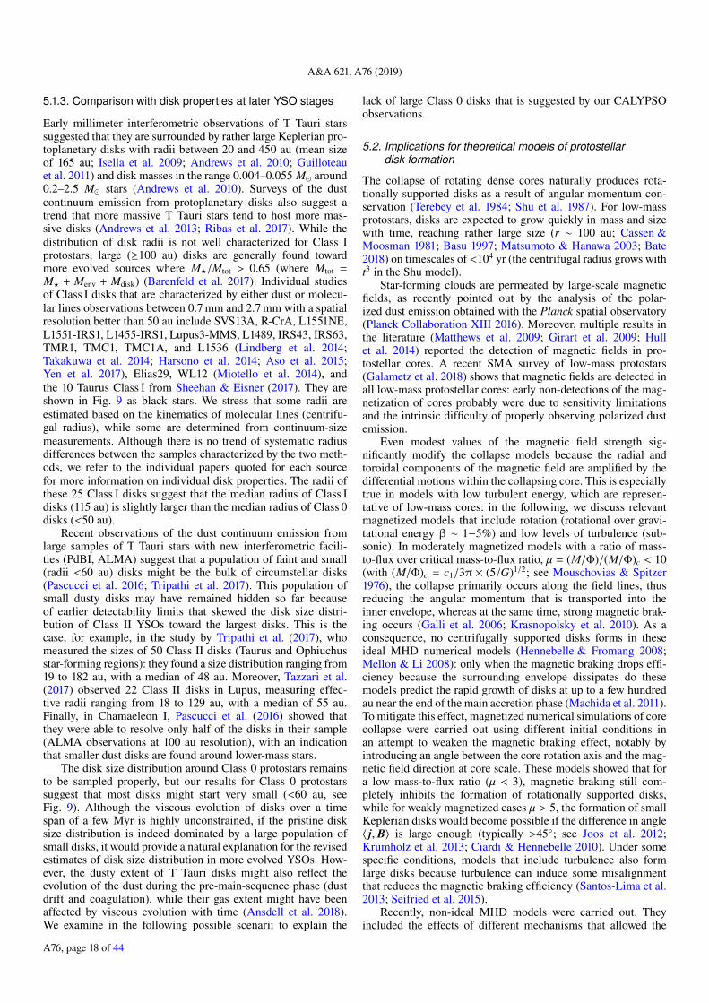
A&A 621, A76 (2019)

5.1.3. Comparison with disk properties at later YSO stages

Early millimeter interferometric observations of T Tauri starssuggested that they are surrounded by rather large Keplerian pro-toplanetary disks with radii between 20 and 450 au (mean sizeof 165 au; Isella et al. 2009; Andrews et al. 2010; Guilloteauet al. 2011) and disk masses in the range 0.004–0.055 M around0.2–2.5 M stars (Andrews et al. 2010). Surveys of the dustcontinuum emission from protoplanetary disks also suggest atrend that more massive T Tauri stars tend to host more mas-sive disks (Andrews et al. 2013; Ribas et al. 2017). While thedistribution of disk radii is not well characterized for Class Iprotostars, large (≥100 au) disks are generally found towardmore evolved sources where M?/Mtot > 0.65 (where Mtot =M? + Menv + Mdisk) (Barenfeld et al. 2017). Individual studiesof Class I disks that are characterized by either dust or molecu-lar lines observations between 0.7 mm and 2.7 mm with a spatialresolution better than 50 au include SVS13A, R-CrA, L1551NE,L1551-IRS1, L1455-IRS1, Lupus3-MMS, L1489, IRS43, IRS63,TMR1, TMC1, TMC1A, and L1536 (Lindberg et al. 2014;Takakuwa et al. 2014; Harsono et al. 2014; Aso et al. 2015;Yen et al. 2017), Elias29, WL12 (Miotello et al. 2014), andthe 10 Taurus Class I from Sheehan & Eisner (2017). They areshown in Fig. 9 as black stars. We stress that some radii areestimated based on the kinematics of molecular lines (centrifu-gal radius), while some are determined from continuum-sizemeasurements. Although there is no trend of systematic radiusdifferences between the samples characterized by the two meth-ods, we refer to the individual papers quoted for each sourcefor more information on individual disk properties. The radii ofthese 25 Class I disks suggest that the median radius of Class Idisks (115 au) is slightly larger than the median radius of Class 0disks (<50 au).

Recent observations of the dust continuum emission fromlarge samples of T Tauri stars with new interferometric facili-ties (PdBI, ALMA) suggest that a population of faint and small(radii <60 au) disks might be the bulk of circumstellar disks(Pascucci et al. 2016; Tripathi et al. 2017). This population ofsmall dusty disks may have remained hidden so far becauseof earlier detectability limits that skewed the disk size distri-bution of Class II YSOs toward the largest disks. This is thecase, for example, in the study by Tripathi et al. (2017), whomeasured the sizes of 50 Class II disks (Taurus and Ophiuchusstar-forming regions): they found a size distribution ranging from19 to 182 au, with a median of 48 au. Moreover, Tazzari et al.(2017) observed 22 Class II disks in Lupus, measuring effec-tive radii ranging from 18 to 129 au, with a median of 55 au.Finally, in Chamaeleon I, Pascucci et al. (2016) showed thatthey were able to resolve only half of the disks in their sample(ALMA observations at 100 au resolution), with an indicationthat smaller dust disks are found around lower-mass stars.

The disk size distribution around Class 0 protostars remainsto be sampled properly, but our results for Class 0 protostarssuggest that most disks might start very small (<60 au, seeFig. 9). Although the viscous evolution of disks over a timespan of a few Myr is highly unconstrained, if the pristine disksize distribution is indeed dominated by a large population ofsmall disks, it would provide a natural explanation for the revisedestimates of disk size distribution in more evolved YSOs. How-ever, the dusty extent of T Tauri disks might also reflect theevolution of the dust during the pre-main-sequence phase (dustdrift and coagulation), while their gas extent might have beenaffected by viscous evolution with time (Ansdell et al. 2018).We examine in the following possible scenarii to explain the

lack of large Class 0 disks that is suggested by our CALYPSOobservations.

5.2. Implications for theoretical models of protostellardisk formation

The collapse of rotating dense cores naturally produces rota-tionally supported disks as a result of angular momentum con-servation (Terebey et al. 1984; Shu et al. 1987). For low-massprotostars, disks are expected to grow quickly in mass and sizewith time, reaching rather large size (r ∼ 100 au; Cassen &Moosman 1981; Basu 1997; Matsumoto & Hanawa 2003; Bate2018) on timescales of <104 yr (the centrifugal radius grows witht3 in the Shu model).

Star-forming clouds are permeated by large-scale magneticfields, as recently pointed out by the analysis of the polar-ized dust emission obtained with the Planck spatial observatory(Planck Collaboration XIII 2016). Moreover, multiple results inthe literature (Matthews et al. 2009; Girart et al. 2009; Hullet al. 2014) reported the detection of magnetic fields in pro-tostellar cores. A recent SMA survey of low-mass protostars(Galametz et al. 2018) shows that magnetic fields are detected inall low-mass protostellar cores: early non-detections of the mag-netization of cores probably were due to sensitivity limitationsand the intrinsic difficulty of properly observing polarized dustemission.

Even modest values of the magnetic field strength sig-nificantly modify the collapse models because the radial andtoroidal components of the magnetic field are amplified by thedifferential motions within the collapsing core. This is especiallytrue in models with low turbulent energy, which are represen-tative of low-mass cores: in the following, we discuss relevantmagnetized models that include rotation (rotational over gravi-tational energy β ∼ 1−5%) and low levels of turbulence (sub-sonic). In moderately magnetized models with a ratio of mass-to-flux over critical mass-to-flux ratio, µ = (M/Φ)/(M/Φ)c < 10(with (M/Φ)c = c1/3π × (5/G)1/2; see Mouschovias & Spitzer1976), the collapse primarily occurs along the field lines, thusreducing the angular momentum that is transported into theinner envelope, whereas at the same time, strong magnetic brak-ing occurs (Galli et al. 2006; Krasnopolsky et al. 2010). As aconsequence, no centrifugally supported disks forms in theseideal MHD numerical models (Hennebelle & Fromang 2008;Mellon & Li 2008): only when the magnetic braking drops effi-ciency because the surrounding envelope dissipates do thesemodels predict the rapid growth of disks at up to a few hundredau near the end of the main accretion phase (Machida et al. 2011).To mitigate this effect, magnetized numerical simulations of corecollapse were carried out using different initial conditions inan attempt to weaken the magnetic braking effect, notably byintroducing an angle between the core rotation axis and the mag-netic field direction at core scale. These models showed that fora low mass-to-flux ratio (µ < 3), magnetic braking still com-pletely inhibits the formation of rotationally supported disks,while for weakly magnetized cases µ > 5, the formation of smallKeplerian disks would become possible if the difference in angle〈 j, B〉 is large enough (typically >45; see Joos et al. 2012;Krumholz et al. 2013; Ciardi & Hennebelle 2010). Under somespecific conditions, models that include turbulence also formlarge disks because turbulence can induce some misalignmentthat reduces the magnetic braking efficiency (Santos-Lima et al.2013; Seifried et al. 2015).

Recently, non-ideal MHD models were carried out. Theyincluded the effects of different mechanisms that allowed the

A76, page 18 of 44

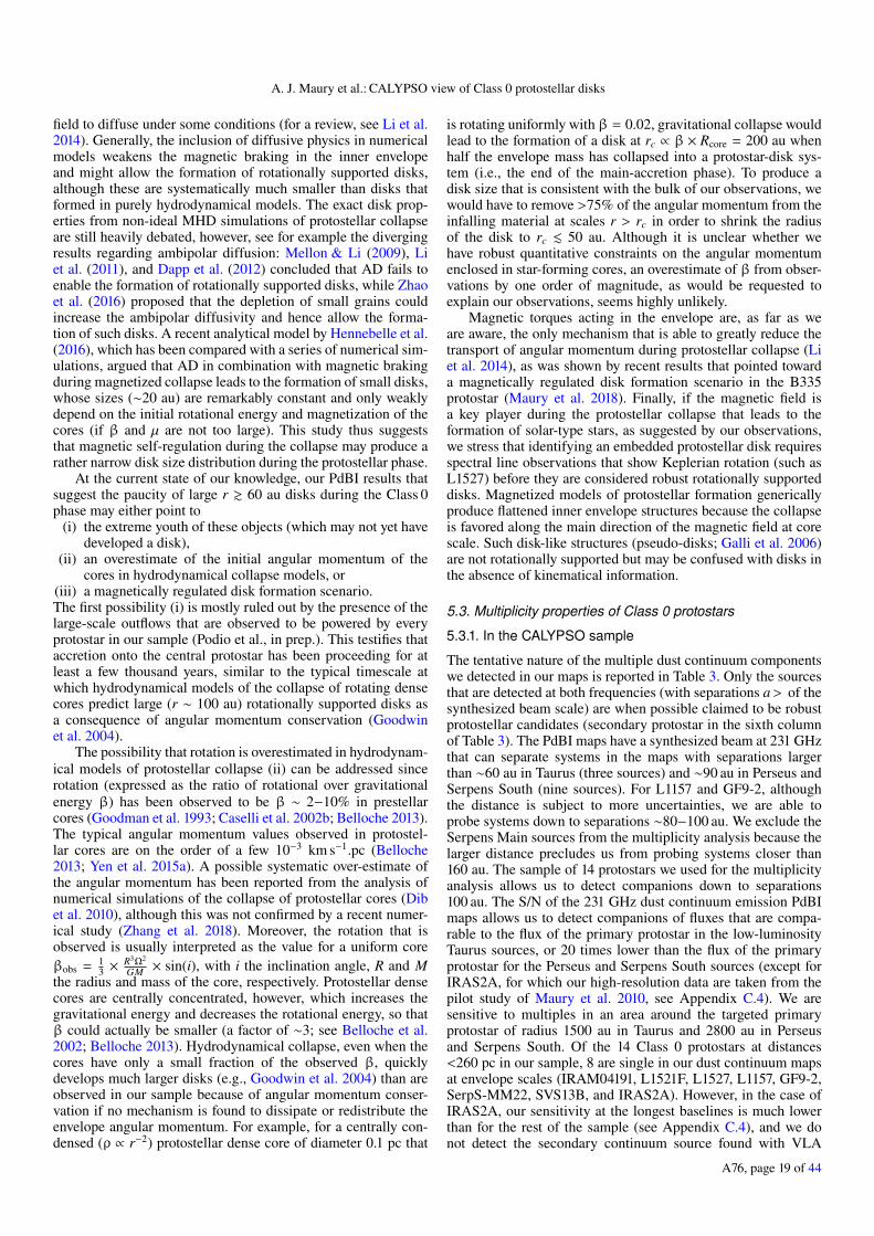
A. J. Maury et al.: CALYPSO view of Class 0 protostellar disks

field to diffuse under some conditions (for a review, see Li et al.2014). Generally, the inclusion of diffusive physics in numericalmodels weakens the magnetic braking in the inner envelopeand might allow the formation of rotationally supported disks,although these are systematically much smaller than disks thatformed in purely hydrodynamical models. The exact disk prop-erties from non-ideal MHD simulations of protostellar collapseare still heavily debated, however, see for example the divergingresults regarding ambipolar diffusion: Mellon & Li (2009), Liet al. (2011), and Dapp et al. (2012) concluded that AD fails toenable the formation of rotationally supported disks, while Zhaoet al. (2016) proposed that the depletion of small grains couldincrease the ambipolar diffusivity and hence allow the forma-tion of such disks. A recent analytical model by Hennebelle et al.(2016), which has been compared with a series of numerical sim-ulations, argued that AD in combination with magnetic brakingduring magnetized collapse leads to the formation of small disks,whose sizes (∼20 au) are remarkably constant and only weaklydepend on the initial rotational energy and magnetization of thecores (if β and µ are not too large). This study thus suggeststhat magnetic self-regulation during the collapse may produce arather narrow disk size distribution during the protostellar phase.

At the current state of our knowledge, our PdBI results thatsuggest the paucity of large r & 60 au disks during the Class 0phase may either point to

(i) the extreme youth of these objects (which may not yet havedeveloped a disk),

(ii) an overestimate of the initial angular momentum of thecores in hydrodynamical collapse models, or

(iii) a magnetically regulated disk formation scenario.The first possibility (i) is mostly ruled out by the presence of thelarge-scale outflows that are observed to be powered by everyprotostar in our sample (Podio et al., in prep.). This testifies thataccretion onto the central protostar has been proceeding for atleast a few thousand years, similar to the typical timescale atwhich hydrodynamical models of the collapse of rotating densecores predict large (r ∼ 100 au) rotationally supported disks asa consequence of angular momentum conservation (Goodwinet al. 2004).

The possibility that rotation is overestimated in hydrodynam-ical models of protostellar collapse (ii) can be addressed sincerotation (expressed as the ratio of rotational over gravitationalenergy β) has been observed to be β ∼ 2−10% in prestellarcores (Goodman et al. 1993; Caselli et al. 2002b; Belloche 2013).The typical angular momentum values observed in protostel-lar cores are on the order of a few 10−3 km s−1.pc (Belloche2013; Yen et al. 2015a). A possible systematic over-estimate ofthe angular momentum has been reported from the analysis ofnumerical simulations of the collapse of protostellar cores (Dibet al. 2010), although this was not confirmed by a recent numer-ical study (Zhang et al. 2018). Moreover, the rotation that isobserved is usually interpreted as the value for a uniform coreβobs = 1

3 × R3Ω2

GM × sin(i), with i the inclination angle, R and Mthe radius and mass of the core, respectively. Protostellar densecores are centrally concentrated, however, which increases thegravitational energy and decreases the rotational energy, so thatβ could actually be smaller (a factor of ∼3; see Belloche et al.2002; Belloche 2013). Hydrodynamical collapse, even when thecores have only a small fraction of the observed β, quicklydevelops much larger disks (e.g., Goodwin et al. 2004) than areobserved in our sample because of angular momentum conser-vation if no mechanism is found to dissipate or redistribute theenvelope angular momentum. For example, for a centrally con-densed (ρ ∝ r−2) protostellar dense core of diameter 0.1 pc that

is rotating uniformly with β = 0.02, gravitational collapse wouldlead to the formation of a disk at rc ∝ β × Rcore = 200 au whenhalf the envelope mass has collapsed into a protostar-disk sys-tem (i.e., the end of the main-accretion phase). To produce adisk size that is consistent with the bulk of our observations, wewould have to remove >75% of the angular momentum from theinfalling material at scales r > rc in order to shrink the radiusof the disk to rc . 50 au. Although it is unclear whether wehave robust quantitative constraints on the angular momentumenclosed in star-forming cores, an overestimate of β from obser-vations by one order of magnitude, as would be requested toexplain our observations, seems highly unlikely.

Magnetic torques acting in the envelope are, as far as weare aware, the only mechanism that is able to greatly reduce thetransport of angular momentum during protostellar collapse (Liet al. 2014), as was shown by recent results that pointed towarda magnetically regulated disk formation scenario in the B335protostar (Maury et al. 2018). Finally, if the magnetic field isa key player during the protostellar collapse that leads to theformation of solar-type stars, as suggested by our observations,we stress that identifying an embedded protostellar disk requiresspectral line observations that show Keplerian rotation (such asL1527) before they are considered robust rotationally supporteddisks. Magnetized models of protostellar formation genericallyproduce flattened inner envelope structures because the collapseis favored along the main direction of the magnetic field at corescale. Such disk-like structures (pseudo-disks; Galli et al. 2006)are not rotationally supported but may be confused with disks inthe absence of kinematical information.

5.3. Multiplicity properties of Class 0 protostars

5.3.1. In the CALYPSO sample

The tentative nature of the multiple dust continuum componentswe detected in our maps is reported in Table 3. Only the sourcesthat are detected at both frequencies (with separations a> of thesynthesized beam scale) are when possible claimed to be robustprotostellar candidates (secondary protostar in the sixth columnof Table 3). The PdBI maps have a synthesized beam at 231 GHzthat can separate systems in the maps with separations largerthan ∼60 au in Taurus (three sources) and ∼90 au in Perseus andSerpens South (nine sources). For L1157 and GF9-2, althoughthe distance is subject to more uncertainties, we are able toprobe systems down to separations ∼80−100 au. We exclude theSerpens Main sources from the multiplicity analysis because thelarger distance precludes us from probing systems closer than160 au. The sample of 14 protostars we used for the multiplicityanalysis allows us to detect companions down to separations100 au. The S/N of the 231 GHz dust continuum emission PdBImaps allows us to detect companions of fluxes that are compa-rable to the flux of the primary protostar in the low-luminosityTaurus sources, or 20 times lower than the flux of the primaryprotostar for the Perseus and Serpens South sources (except forIRAS2A, for which our high-resolution data are taken from thepilot study of Maury et al. 2010, see Appendix C.4). We aresensitive to multiples in an area around the targeted primaryprotostar of radius 1500 au in Taurus and 2800 au in Perseusand Serpens South. Of the 14 Class 0 protostars at distances<260 pc in our sample, 8 are single in our dust continuum mapsat envelope scales (IRAM04191, L1521F, L1527, L1157, GF9-2,SerpS-MM22, SVS13B, and IRAS2A). However, in the case ofIRAS2A, our sensitivity at the longest baselines is much lowerthan for the rest of the sample (see Appendix C.4), and we donot detect the secondary continuum source found with VLA

A76, page 19 of 44

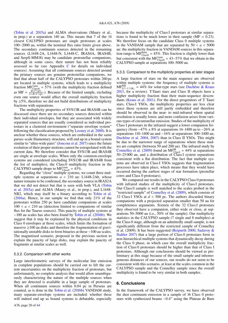
A&A 621, A76 (2019)

(Tobin et al. 2015a) and ALMA observations (Maury et al.,in prep.) at a separation 140 au. This means that 7 of the 14closest CALYPSO protostars are single protostars at scales100−2000 au, within the nominal flux ratio limits given above.The secondary continuum sources detected in the remainingsources (L1448-2A, L1448-N, L1448-C, IRAS4A, IRAS4B,and SerpS-MM18) may be candidate protostellar companions,although in some cases, their nature has not been reliablyassessed so far (see Appendix C for details on individualsources). Assuming that all continuum sources detected aroundthe primary sources are genuine protostellar companions, wefind that about half of the CALYPSO protostars within 260 pcare located in multiple systems, which leads to a multiplicityfraction MF1mm

Class0 = 57% (with the multiplicity fraction definedas MF =

B+T+Q+·S +B+T+Q+· ). Because of the limited sample, excluding

even one source would affect the overall multiplicity fractionby &5%, therefore we did not build distributions of multiplicityfractions with separations.

The multiplicity properties of SVS13B and IRAS4B can bediscussed since there are no secondary sources detected withintheir individual envelopes, but they are associated with widelyseparated sources that are usually considered as individual pro-tostars in a clustered environment (“separate envelope system”following the classification proposed by Looney et al. 2000). It isunclear whether these sources, which are embedded in the sameparsec-scale filamentary structure, will end up in a bound systemsimilar to “ultra-wide pairs” (Joncour et al. 2017) since the futureevolution of their proper motions cannot be extrapolated with thecurrent data. We therefore consider that SVS13B and IRAS4Bare single at envelope scales. When only the common-envelopesystems are considered (excluding SVS13B and IRAS4B fromthe list of multiples), the Class 0 multiplicity fraction in theCALYPSO sample drops to MF1mm

Class0 = 43%.Regarding the “close” multiple systems, we count three mul-

tiple systems at separations a < 210 au: L1448-2Ab, whosenature remains to be confirmed, the secondary source in IRAS2Athat we did not detect but that is seen with both VLA (Tobinet al. 2015a) and ALMA (Maury et al., in prep.), and L1448-NB2, which may itself be a binary according to Tobin et al.(2016a). Hence, in our sample we find that only 21% of theprotostars within 250 pc have candidate companions at scales100 < a < 210 au (detection limited to companions of similarflux for the Taurus sources). This paucity of multiple systems at∼100 au scales has also been found by Tobin et al. (2016b). Wesuggest that it may be explained by the physical conditions inClass 0 envelopes at those scales, which limits the formation ofmassive &100 au disks and therefore the fragmentation of gravi-tationally unstable disks to form binaries at these ∼100 au scales.The magnetized scenario, proposed in the previous section toexplain the paucity of large disks, may explain the paucity offragments at similar scales as well.

5.3.2. Comparison with other works

Large interferometric surveys of the molecular line emissionin complete populations should be carried out to lift the cur-rent uncertainties on the multiplicity fraction of protostars, butunfortunately, no complete analysis that would allow unambigu-ously characterizing the nature of the multiple sources whenthey are detected is available in a large sample of protostars.When all continuum sources within 0.04 pc in Perseus arecounted, as is done in the Tobin et al. (2016b) VANDAM study,many separate-envelope systems are included: whether thesewill indeed end up as bound systems is debatable, especially

because the multiplicity of Class I protostars at similar separa-tions is found to be much lower in their sample (MF = 0.23).We therefore focus on the candidate Class 0 multiple systemsin the VANDAM sample that are separated by 50 < a < 5000au: the multiplicity fraction in VANDAM sources in this separa-tion range is MF8mm

Class0 = 45%. This fraction is slightly lower thanbut consistent with the MF1mm

Class0 = 43−57% that we obtain in theCALYPSO sample at separations 100–5000 au.

5.3.3. Comparison to the multiplicity properties at later stages

A large fraction of stars on the main sequence are observedwithin multiple systems: the frequency of multiple systems isMFMS

0.7−1.3 M = 44% for solar-type stars (see Duchêne & Kraus2013, for a review). T-Tauri stars and Class II objects have ahigher multiplicity fraction than their main-sequence descen-dants (Kraus et al. 2011). For the direct progenitors of T Tauristars, Class I YSOs, the multiplicity properties are less clearsince these systems are still partly embedded and thereforeshould be observed in the near- to mid-infrared where spatialresolution is usually lower, and more confusion arises from vari-ous types of circumstellar emission. Studies of the multiplicity ofClass I protostars in the infrared suggest a lower companion fre-quency (from ∼47% ± 8% at separations 14–1400 au to ∼26% atseparations 110–1400 au and ∼16% at separations 300–1400 au;Duchêne et al. 2004, 2007) than in Class II YSOs. This mightbe due to the narrower range of separations where these stud-ies are complete (between 50 and 200 au). The infrared study byConnelley et al. (2009) found an MFIR

ClassI = 44% at separations50–25 000 au, and a distribution of Class I system separationsconsistent with a flat distribution. The fact that multiple sys-tems are observed in Class I YSOs suggests that fragmentationprocesses have taken place, which means that they would haveoccurred during the earliest stages of star formation (prestellarcores and Class 0 protostars).

We compared our results in the CALYPSO Class 0 protostarswith infrared studies of the multiplicity of Class I protostars.Our Class 0 sample is well matched to the scales probed in the“restricted sample” of Connelley et al. (2009), which consists of32 Class I YSOs at d < 500 pc. The authors discarded binarycompanions with a projected separation smaller than 50 au forcompleteness arguments. Sixteen of the 32 Class I protostarsthey observed have a companion, either wide or close, at sep-arations 50–5000 au (i.e., 50% of the sample). Our multiplicitystatistics in the CALYPSO sample (7 single and 8 multiples) atthe Class 0 stage, although on an admittedly small sample, is notsignificantly different from the restricted sample of Connelleyet al. (2009). It has been suggested (Reipurth 2000; Sadavoy &Stahler 2017) that a large portion of Class 0 protostars form innon-hierarchical multiple systems that dynamically decay duringthe Class 0 phase, in which case the overall multiplicity frac-tion of Class 0 protostars should be higher than that of Class Iprotostars. Although our conclusions should be viewed as pre-liminary at this stage because of the small sample and inhomo-geneous distances of our sources, our results do not seem to beconsistent with this scenario, at least at the scales common in theCALYPSO sample and the Connelley sample since the overallmultiplicity is found to be very similar in both samples.

6. Conclusions

In the framework of the CALYPSO survey, we have observedthe dust continuum emission in a sample of 16 Class 0 proto-stars with synthesized beams ∼0.4′′ using the Plateau de Bure

A76, page 20 of 44

A. J. Maury et al.: CALYPSO view of Class 0 protostellar disks

interferometer at IRAM (50–150 au at the distances of oursources). We performed an analysis of the dust continuum visi-bility data using models of Plummer envelopes and explored therange of parameters for envelope properties. Six of these 16 pro-tostars cannot be satisfactorily described by a single circularlysymmetric envelope model over the whole range of spatial scales(40–1000 au) sampled by our observations at either 1.3 mm or3 mm. We thus modeled the visibility profiles including an addi-tional Gaussian component for all sources in our sample in orderto test whether adding a disk-like component would explain theproperties of some of the CALYPSO protostars at long baselines.The main results of our study are listed below.1. For 11 of the 16 protostellar profiles we analyzed, the inclu-

sion of disk-like components improves the description ofthe 231 GHz continuum visibility profiles at the longestbaselines we probed.

2. However, only four protostars in our sample require a candi-date disk structure resolved with radii >60 au to reproducetheir dust continuum visibility profiles (IRAS4B, L1527,Serpens South MM22, and Serpens Main SMM4). Twoother protostars (L1448-C and GF9-2) are better reproducedwhen an additional disk-like component is included; they aremarginally resolved by our data at radii .60 au. In one closemultiple system (L1448-NB1/2), an additional circumbinarystructure with radius ∼200 au may be present, while thetwo individual protostars do not show evidence of individualdisks resolved by our observations.

3. Four out of the 16 protostars in the CALYPSO sample arelikely to harbor large, well-resolved individual protostellardisks at radii >60 au. Our observations suggest that whilemost Class 0 protostars show evidence of embedded disks,most (>75%) Class 0 continuum disks are small. When wecombined all the recent 0.8–1 mm interferometric obser-vations of Class 0 protostars that probed the bulk of theenvelope emission down to radii ∼50 au, only 5–7 out of 26Class 0 protostars, that is <28%, show either confirmed orcandidate large disks at radii &60 au. This upper limit on theoccurrence of large disks at the Class 0 stage confirms ourearlier results (Maury et al. 2010) and suggests that Class 0disks are small on average.

4. From a theoretical point of view, if Class 0 protostars containsimilar rotational energy as currently estimated in prestellarcores, only magnetized models of protostellar collapse canreproduce such a large population of small disks during themain accretion phase.

5. The multiplicity fraction in the CALYPSO sample is foundto be ∼43−57% ± 5% at scales 100–5000 au, which isslightly larger than but in general agreement with previousstudies of Class 0 multiplicity.

Our results suggest that the formation of disks and multi-ple systems during the Class 0 phase could occur at smallerscales than predicted by hydrodynamical models of rotatingprotostellar collapse. However, we stress that confirming theproperties of the embedded protostellar structures requires addi-tional spectral line analysis that either traces rotationally sup-ported motions to robustly identify disk components, or confirmsthe protostellar nature of the systems at ∼50 au scales.

Acknowledgements. We thank the IRAM staff for their support in carrying outthe CALYPSO observations, and the anonymous referee for a detailed readingthat significantly helped us to improve the paper. We thank Kees Dullemond,Ralf Klessen, Sandrine Bottinelli, Benoit Commercon, and Ralf Launhardt fortheir participation to the preparation of the CALYPSO project. We thank theINSU “Action Spécifique ALMA” for their financial support to the CALYPSOcollaboration. This work has benefited from the support of the EuropeanResearch Council under the European Union’s Seventh Framework Programme

(Advanced Grant ORISTARS with grant agreement No. 291294 and StartingGrant MagneticYSOs with grant agreement No. 679937).

References

Adams, F. C. 1991, ApJ, 382, 544Anderl, S., Maret, S., Cabrit, S., et al. 2016, A&A, 591, A3André, P., Ward-Thompson, D., & Barsony, M. 1993, ApJ, 406, 122André, P., Motte, F., & Bacmann, A. 1999, ApJ, 513, L57André, P., Ward-Thompson, D., & Barsony, M. 2000, Protostars and Planets IV

(Tucson, AZ: University of Arizona Press), 59André, P., Men’shchikov, A., Bontemps, S., et al. 2010, A&A, 518, L102Andrews, S. M., Wilner, D. J., Hughes, A. M., Qi, C., & Dullemond, C. P. 2009,

ApJ, 700, 1502Andrews, S. M., Wilner, D. J., Hughes, A. M., Qi, C., & Dullemond, C. P. 2010,

ApJ, 723, 1241Andrews, S. M., Rosenfeld, K. A., Kraus, A. L., & Wilner, D. J. 2013, ApJ, 771,

129Anglada, G., Rodriguez, L. F., Torrelles, J. M., et al. 1989, ApJ, 341, 208Ansdell, M., Williams, J. P., Trapman, L., et al. 2018, ApJ, 859, 21Aso, Y., Ohashi, N., Saigo, K., et al. 2015, ApJ, 812, 27Aso, Y., Ohashi, N., Aikawa, Y., et al. 2017, ApJ, 849, 56Barenfeld, S. A., Carpenter, J. M., Sargent, A. I., Isella, A., & Ricci, L. 2017,

ApJ, 851, 85Basu, S. 1997, ApJ, 485, 240Bate, M. R. 2018, MNRAS, 475, 5618Bate, M. R., Tricco, T. S., & Price, D. J. 2014, MNRAS, 437, 77Belloche, A. 2013, EAS Pub. Ser., 62, 25Belloche, A., & André, P. 2004, A&A, 419, L35Belloche, A., André, P., Despois, D., & Blinder, S. 2002, A&A, 393, 927Berger, J. P., & Segransan, D. 2007, New Astron. Rev., 51, 576Bontemps, S., André, P., Terebey, S., & Cabrit, S. 1996, A&A, 311, 858Bracewell, R., in The Fourier Transform and Its Applications, ed. R. Bracewell

(Pennsylvania: McGraw-Hill Science, 1965)Briggs, D. S. 1995, BAAS, 27,1444Butner, H. M., Evans, II, N. J., Harvey, P. M., et al. 1990, ApJ, 364, 164Casali, M. M., Eiroa, C., & Duncan, W. D. 1993, A&A, 275, 195Caselli, P., Benson, P., Myers, P., & Tafalla, M. 2002a, ApJ, 572, 238Caselli, P., Walmsley, C., Zucconi, A., et al. 2002b, ApJ, 565, 331Cassen, P., & Moosman, A. 1981, Icarus, 48, 353Chen, X., Arce, H. G., Dunham, M. M., & Zhang, Q. 2012, ApJ, 747, L43Chiang, H.-F., Looney, L. W., Tassis, K., Mundy, L. G., & Mouschovias, T. C.

2008, ApJ, 680, 474Ching, T.-C., Lai, S.-P., Zhang, Q., et al. 2016, ApJ, 819, 159Chini, R., Reipurth, B., Sievers, A., et al. 1997, A&A, 325, 542Choi, M., Tatematsu, K., Park, G., & Kang, M. 2007, ApJ, 667, L183Choi, M., Tatematsu, K., & Kang, M. 2010, ApJ, 723, L34Chou, H.-G., Yen, H.-W., Koch, P. M., & Guilloteau, S. 2016, ApJ, 823, 151Ciardi, A., & Hennebelle, P. 2010, MNRAS, 409, L39Ciardi, D. R., Telesco, C. M., Williams, J. P., et al. 2003, ApJ, 585, 392Codella, C., Cabrit, S., Gueth, F., et al. 2014a, A&A, 568, L5Codella, C., Maury, A. J., Gueth, F., et al. 2014b, A&A, 563, L3Connelley, M. S., Reipurth, B., & Tokunaga, A. T. 2009, AJ, 138, 1193Crapsi, A., Caselli, P., Walmsley, C. M., et al. 2004, A&A, 420, 957Curiel, S., Raymond, J. C., Moran, J. M., Rodriguez, L. F., & Canto, J. 1990,

ApJ, 365, L85Dapp, W. B., Basu, S., & Kunz, M. W. 2012, A&A, 541, A35De Simone, M., Codella, C., Testi, L., et al. 2017, A&A, 599, A121Dib, S., Hennebelle, P., Pineda, J. E., et al. 2010, ApJ, 723, 425Donaldson, T. S. 1968, J. Am. Stat. Assoc., 63, 322Duchêne, G., & Kraus, A. 2013, ARA&A, 51, 269Duchêne, G., Bouvier, J., Bontemps, S., André, P., & Motte, F. 2004, A&A, 427,

651Duchêne, G., Bontemps, S., Bouvier, J., et al. 2007, A&A, 476, 229Dunham, M. M., Stutz, A. M., Allen, L. E., et al. 2014, Protostars and Planets IV

(Tucson, AZ: University of Arizona Press), 195Dzib, S., Loinard, L., Mioduszewski, A. J., et al. 2010, ApJ, 718, 610Eisner, J. A. 2012, ApJ, 755, 23Enoch, M. L., Young, K. E., Glenn, J., et al. 2006, ApJ, 638, 293Enoch, M. L., Glenn, J., Evans, II, N. J., et al. 2007, ApJ, 666, 982Enoch, M. L., Evans, N. J., Sargent, A. I., & Glenn, J. 2009, ApJ, 692, 973Enoch, M. L., Corder, S., Duchêne, G., et al. 2011, ApJS, 195, 21Evans, N. J., Dunham, M. M., Jørgensen, J. K., et al. 2009, ApJS, 181, 321Furuya, R. S., Kitamura, Y., Wootten, H. A., Claussen, M. J., & Kawabe, R. 2001,

ApJ, 559, L143Furuya, R. S., Kitamura, Y., Wootten, A., Claussen, M. J., & Kawabe, R. 2003,

ApJS, 144, 71

A76, page 21 of 44

A&A 621, A76 (2019)

Furuya, R. S., Kitamura, Y., & Shinnaga, H. 2006, ApJ, 653, 1369Furuya, R. S., Kitamura, Y., & Shinnaga, H. 2014, ApJ, 793, 94Galametz, M., Maury, A., Girart, J. M., et al. 2018, A&A, 616, A139Galli, D., Lizano, S., Shu, F. H., & Allen, A. 2006, ApJ, 647, 374Gerin, M., Pety, J., Commerçon, B., et al. 2017, A&A, 606, A35Girart, J. M., Rao, R., & Estalella, R. 2009, ApJ, 694, 56Goodman, A., Benson, P., Fuller, G., & Myers, P. 1993, ApJ, 406, 528Goodwin, S. P., Whitworth, A. P., & Ward-Thompson, D. 2004, A&A, 423,

169Grossman, E. N., Masson, C. R., Sargent, A. I., et al. 1987, ApJ, 320, 356Guilloteau, S., Dutrey, A., Piétu, V., & Boehler, Y. 2011, A&A, 529, A105Harsono, D., Jørgensen, J. K., van Dishoeck, E. F., et al. 2014, A&A, 562, A77Harvey, P., Merín, B., Huard, T. L., et al. 2007, ApJ, 663, 1149Hennebelle, P., & Ciardi, A. 2009, A&A, 506, L29Hennebelle, P., & Fromang, S. 2008, A&A, 477, 9Hennebelle, P., & Teyssier, R. 2008, A&A, 477, 25Hennebelle, P., Commerçon, B., Chabrier, G., & Marchand, P. 2016, ApJ, 830,

L8Hirano, N., Ho, P. P. T., Liu, S.-Y., et al. 2010, ApJ, 717, 58Hirota, T., Bushimata, T., Choi, Y. K., et al. 2008, PASJ, 60, 37Hirota, T., Honma, M., Imai, H., et al. 2011, PASJ, 63, 1Hull, C. L. H., Plambeck, R. L., Kwon, W., et al. 2014, ApJS, 213, 13Isella, A., Carpenter, J. M., & Sargent, A. I. 2009, ApJ, 701, 260Jennings, R. E., Cameron, D. H. M., Cudlip, W., & Hirst, C. J. 1987, MNRAS,

226, 461Joncour, I., Duchêne, G., & Moraux, E. 2017, A&A, 599, A14Joos, M., Hennebelle, P., & Ciardi, A. 2012, A&A, 543, A128Jørgensen, J. K., Harvey, P. M., Evans, II, N. J., et al. 2006, ApJ, 645, 1246Jørgensen, J. K., Johnstone, D., Kirk, H., & Myers, P. C. 2007, ApJ, 656, 293Jørgensen, J. K., van Dishoeck, E. F., Visser, R., et al. 2009, A&A, 507, 861Kaas, A. A., Olofsson, G., Bontemps, S., et al. 2004, A&A, 421, 623Karska, A., Herczeg, G. J., van Dishoeck, E. F., et al. 2013, A&A, 552, A141Könyves, V., André, P., Men’shchikov, A., et al. 2010, A&A, 518, L106Könyves, V., André, P., Men’shchikov, A., et al. 2015, A&A, 584, A91Krasnopolsky, R., Li, Z.-Y., & Shang, H. 2010, ApJ, 716, 1541Kraus, A. L., Ireland, M. J., Martinache, F., & Hillenbrand, L. A. 2011, ApJ, 731,

8Kristensen, L. E., van Dishoeck, E. F., van Kempen, T. A., et al. 2010, A&A, 516,

A57Krumholz, M. R., Crutcher, R. M., & Hull, C. L. H. 2013, ApJ, 767, L11Kwon, W., Looney, L. W., Crutcher, R. M., & Kirk, J. M. 2006, ApJ, 653, 1358Kwon, W., Fernández-López, M., Stephens, I. W., & Looney, L. W. 2015, ApJ,

814, 43Ladd, E. F., Adams, F. C., Fuller, G. A., et al. 1991, ApJ, 382, 555Lee, K. I., Dunham, M. M., Myers, P. C., et al. 2015, ApJ, 814, 114Lee, C.-F., Hwang, H.-C., & Li, Z.-Y. 2016, ApJ, 826, 213Lee, C.-F., Li, Z.-Y., Codella, C., et al. 2018a, ApJ, 856, 14Lee, C.-F., Li, Z.-Y., Hirano, N., et al. 2018b, ApJ, 863, 94Lefèvre, C., Cabrit, S., Maury, A. J., et al. 2017, A&A, 604, L1Lefloch, B., Castets, A., Cernicharo, J., Langer, W. D., & Zylka, R. 1998, A&A,

334, 269Li, Z.-Y., Krasnopolsky, R., & Shang, H. 2011, ApJ, 738, 180Li, Z.-Y., Banerjee, R., Pudritz, R. E., et al. 2014, Protostars and Planets IV

(Tucson, AZ: University of Arizona Press), 173Lindberg, J. E., Jørgensen, J. K., Brinch, C., et al. 2014, A&A, 566, A74Looney, L., Mundy, L., & Welch, W. 2000, ApJ, 529, 477Looney, L., Mundy, L., & Welch, W. 2003, ApJ, 592, 255Machida, M. N., Inutsuka, S.-I., & Matsumoto, T. 2011, PASJ, 63, 555Machida, M. N., Inutsuka, S.-I., & Matsumoto, T. 2014, MNRAS, 438, 2278Maret, S., Belloche, A., Maury, A. J., et al. 2014, A&A, 563, L1Markwardt, C. B. 2009, in Astronomical Data Analysis Software and Systems

XVIII, eds. D. A. Bohlender, D. Durand, & P. Dowler, ASP Conf. Ser., 411,251

Masson, J., Teyssier, R., Mulet-Marquis, C., Hennebelle, P., & Chabrier, G. 2012,ApJS, 201, 24

Masson, J., Chabrier, G., Hennebelle, P., Vaytet, N., & Commerçon B. 2016,A&A, 587, A32

Matsumoto, T., & Hanawa, T. 2003, ApJ, 595, 913Matthews, B. C., McPhee, C. A., Fissel, L. M., & Curran, R. L. 2009, ApJS, 182,

143Maury, A. J., André, P., Hennebelle, P., et al. 2010, A&A, 512, A40Maury, A. J., André, P., Men’shchikov, A., Könyves, V., & Bontemps, S. 2011,

A&A, 535, A77Maury, A. J., Belloche, A., André, P., et al. 2014, A&A, 563, L2Maury, A., André, P., Maret, S., et al. 2015, IAU General Assembly, 22, 2254840Maury, A. J., Girart, J. M., Zhang, Q., et al. 2018, MNRAS, 477, 2760

McMullin, J. P., Mundy, L. G., Wilking, B. A., Hezel, T., & Blake, G. A. 1994,ApJ, 424, 222

Mellon, R. R., & Li, Z.-Y. 2008, ApJ, 681, 1356Mellon, R. R., & Li, Z.-Y. 2009, ApJ, 698, 922Miotello, A., Testi, L., Lodato, G., et al. 2014, A&A, 567, A32Mizuno, A., Onishi, T., Hayashi, M., et al. 1994, Nature, 368, 719Motte, F., & André, P. 2001, A&A, 365, 440Mouschovias, T., & Spitzer, Jr. L. 1976, ApJ, 210, 326Murillo, N. M., Lai, S.-P., Bruderer, S., Harsono, D., & van Dishoeck E. F. 2013,

A&A, 560, A103Ohashi, N., Saigo, K., Aso, Y., et al. 2014, ApJ, 796, 131O’Linger, J., Wolf-Chase, G., Barsony, M., & Ward-Thompson, D. 1999, ApJ,

515, 696Ortiz-León, G. N., Loinard, L., Mioduszewski, A. J., et al. 2015, ApJ, 805, 9Pascucci, I., Testi, L., Herczeg, G. J., et al. 2016, ApJ, 831, 125Planck Collaboration XIII. 2016, A&A, 586, A13Plummer, H. C. 1911, MNRAS, 71, 460Plunkett, A. L., Arce, H. G., Corder, S. A., et al. 2013, ApJ, 774, 22Plunkett, A. L., Fernández-López, M., Arce, H. G., et al. 2018, A&A, 615, A9Podio, L., Codella, C., Gueth, F., et al. 2016, A&A, 593, L4Reipurth, B. 2000, AJ, 120, 3177Ribas, Á., Espaillat, C. C., Macías, E., et al. 2017, ApJ, 849, 63Ricci, L., Testi, L., Natta, A., et al. 2010, A&A, 512, A15Rodríguez, L., Anglada, G., & Curiel, S. 1999, ApJS, 125, 427Sadavoy, S. I., & Stahler, S. W. 2017, MNRAS, 469, 3881Sadavoy, S. I., Francesco, J. D., André, P., et al. 2014, ApJ, 787, L18Sakai, N., Oya, Y., López-Sepulcre, A., et al. 2016, ApJ, 820, L34Santangelo, G., Codella, C., Cabrit, S., et al. 2015, A&A, 584, A126Santos-Lima, R., de Gouveia Dal Pino, E. M., & Lazarian, A. 2013, MNRAS,

429, 3371Schneider, S., & Elmegreen, B. G. 1979, ApJS, 41, 87Segura-Cox, D. M., Harris, R. J., Tobin, J. J., et al. 2016, ApJ, 817, L14Segura-Cox, D. M., Looney, L. W., Tobin, J. J., et al. 2018, ApJ, 866, 161Seifried, D., Banerjee, R., Pudritz, R. E., & Klessen, R. S. 2012, MNRAS, 423,

L40Seifried, D., Banerjee, R., Pudritz, R. E., & Klessen, R. S. 2015, MNRAS, 446,

2776Sheehan, P. D., & Eisner, J. A. 2017, ApJ, 851, 45Shirley, Y. L., Evans, II, N. J., & Rawlings, J. M. C. 2002, ApJ, 575, 337Shu, F. 1977, ApJ, 214, 488Shu, F., Adams, F., & Lizano, S. 1987, ARA&A, 25, 23Spezzi, L., Cox, N. L. J., Prusti, T., et al. 2013, A&A, 555, A71Stamatellos, D., Hubber, D., & Whitworth, A. 2007, MNRAS, 382, L30Straižys, V., Cernis, K., & Bartašiute. , S. 2003, A&A, 405, 585Takakuwa, S., Saito, M., Lim, J., et al. 2012, ApJ, 754, 52Takakuwa, S., Saito, M., Saigo, K., et al. 2014, ApJ, 796, 1Tazzari, M., Testi, L., Natta, A., et al. 2017, A&A, 606, A88Terebey, S., Shu, F., & Cassen, P. 1984, ApJ, 286, 529Terebey, S., Chandler, C., & Andre, P. 1993, ApJ, 414, 759Tobin, J. J., Dunham, M. M., Looney, L. W., et al. 2015a, ApJ, 798, 61Tobin, J. J., Looney, L. W., Wilner, D. J., et al. 2015b, ApJ, 805, 125Tobin, J. J., Kratter, K. M., Persson, M. V., et al. 2016a, Nature, 538, 483Tobin, J. J., Looney, L. W., Li, Z.-Y., et al. 2016b, ApJ, 818, 73Tobin, J. J., Bos, S. P., Dunham, M. M., Bourke, T. L., & van der Marel, N. 2018,

ApJ, 856, 164Tokuda, K., Onishi, T., Matsumoto, T., et al. 2016, ApJ, 826, 26Tokuda, K., Onishi, T., Saigo, K., et al. 2017, ApJ, 849, 101Torres, R. M., Loinard, L., Mioduszewski, A. J., & Rodríguez, L. F. 2009, ApJ,

698, 242Tripathi, A., Andrews, S. M., Birnstiel, T., & Wilner, D. J. 2017, ApJ, 845, 44Tsukamoto, Y., Iwasaki, K., Okuzumi, S., Machida, M. N., & Inutsuka, S. 2015,

ApJ, 810, L26Umemoto, T., Iwata, T., Fukui, Y., et al. 1992, ApJ, 392, L83Vorobyov, E. I. 2010, ApJ, 723, 1294Whitworth, A., & Summers, D. 1985, MNRAS, 214, 1Whitworth, A., & Ward-Thompson, D. 2001, ApJ, 547, 317Wiesemeyer, H. 1997, Ph.D. thesis, Institut de Radio Astronomie MillimétriqueWolf, S., Schegerer, A., Beuther, H., Padgett, D. L., & Stapelfeldt, K. R. 2008,

ApJ, 674, L101Yen, H.-W., Koch, P. M., Takakuwa, S., et al. 2015a, ApJ, 799, 193Yen, H.-W., Takakuwa, S., Koch, P. M., et al. 2015b, ApJ, 812, 129Yen, H.-W., Koch, P. M., Takakuwa, S., et al. 2017, ApJ, 834, 178Yorke, H. W., & Bodenheimer, P. 1999, ApJ, 525, 330Zhang, S., Hartmann, L., Zamora-Avilés, M., & Kuznetsova, A. 2018, MNRAS,

480, 5495Zhao, B., Caselli, P., Li, Z.-Y., et al. 2016, MNRAS, 460, 2050

A76, page 22 of 44

A. J. Maury et al.: CALYPSO view of Class 0 protostellar disks

Appendix A: Details of CALYPSO observations

Table A.1. Fields observed with CALYPSO, grouped by shared observing tracks.

Fielda Phase center Central frequency of WideX observationsα2000 δ2000 231 GHz 219 GHz 94 GHz

Track1Observation dates

L1448-2A 03:25:22.4 +30:45:12 2010 Jan. 23-24 2010 Dec. 11-12 2010 Nov. 2-3L1448-C 03:25:38.9 +30:44:05 2010 Nov. 18-19 2011 Jan. 24-25 2011 Jan. 27-28L1521F 04:28:38.9 +26:51:36 2012 Nov. 15-16 2011 Apr. 5-13

Track2Observation dates

SVS13B 03:29:03.7 +31:15:52 2011 Feb. 5 2011 Nov. 13-14 2011 Nov. 11-12IRAS4A 03:29:10.5 +31:13:31 2011 Oct. 15 2012 Feb. 4 2011 Nov. 18-20IRAS4B 03:29:11.9 +31:13:08 2012 Feb. 12-13 2013 Jan. 24 2012 Feb. 6-7L1527 04:39:53.9 +26:03:10 2012 Nov. 7-8 2013 Feb. 16

Track3Observation dates

L1448-N 03:25:36.3 +30:45:15 2008 Feb. 09b 2010 Dec. 04-05 2010 Nov. 06-07IRAS2A 03:28:55.6 +31:14:37 2010 Nov. 07-08-21-22 2010 Dec. 04-05 2010 Nov. 06-07

IRAM04191 04:21:56.9 +15:29:46 2011 Jan. 25/Feb. 01 2011 Jan. 29-30Track4

Observation datesSerpM-S68N 18:29:48.10 +01:16:43.6 2011 Feb. 08 2011 Nov. 13-14-16 2011 Nov. 09-11-12

SerpM-SMM4 18:29:56.70 +01:13:15.0 2011 Mar. 25 2012 Feb. 04-21-25 2012 Feb. 12SerpS-MM18 18:30:03.86 −02:03:04.9 2012 Feb. 02 2013 Feb. 16 2012 Mar. 01SerpS-MM22 18:30:12.34 −02:06:52.4 2012 Nov. 16

Track5Observation dates

L1157 20:39:06.3 +68:02:15 2011 Feb. 04-06-07 2011 Nov. 08-10-11-12-13 2011 Nov. 07GF9-2 20:51:30.1 +60:18:39 2011 Mar. 20 2012 Feb. 11-17-18 2012 Feb. 08

2012 Oct.30 2013 Jan. 12

Notes. (a)The region mapped by a given field is limited by the PdBI primary beam: 20′′ at 231 GHz, 23′′ at 219 GHz, and 54′′ at 94 GHz. (b)Identifiesobservations from the pilot observing program R068 (Maury et al. 2010).

Appendix B: CALYPSO dust continuum maps

Fig. B.1. 1.3 mm (231 GHz) and 3.3 mm (94 GHz) PdBI dust continuum emission maps of L1448-N. The ellipses in the bottom left corner showthe respective synthesized beam sizes. The contours are levels of −3σ (dashed) and 5σ, then in steps of 10σ from 10σ to 100σ, and finally insteps of 20σ beyond (rms noise computed in the map before primary beam correction as reported in Table 2). The maps have been corrected forprimary beam attenuation. The blue and red arrows show the direction of the protostellar jet(s) associated with the millimeter sources in the field,see Table 1 for further details.

A76, page 23 of 44

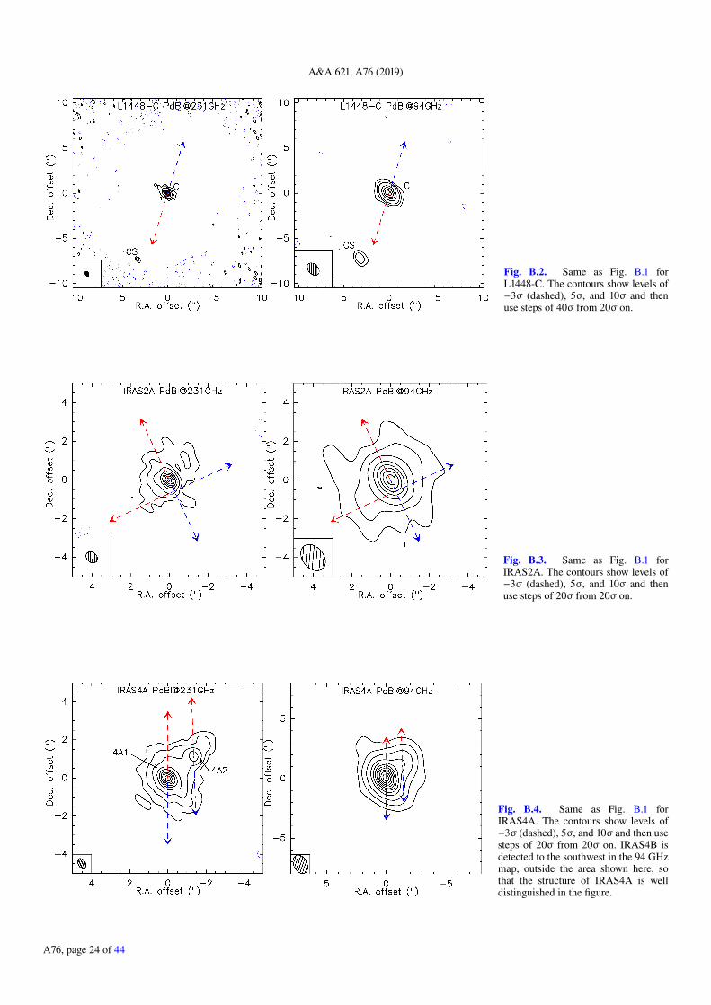
A&A 621, A76 (2019)

Fig. B.2. Same as Fig. B.1 forL1448-C. The contours show levels of−3σ (dashed), 5σ, and 10σ and thenuse steps of 40σ from 20σ on.

Fig. B.3. Same as Fig. B.1 forIRAS2A. The contours show levels of−3σ (dashed), 5σ, and 10σ and thenuse steps of 20σ from 20σ on.

Fig. B.4. Same as Fig. B.1 forIRAS4A. The contours show levels of−3σ (dashed), 5σ, and 10σ and then usesteps of 20σ from 20σ on. IRAS4B isdetected to the southwest in the 94 GHzmap, outside the area shown here, sothat the structure of IRAS4A is welldistinguished in the figure.

A76, page 24 of 44

A. J. Maury et al.: CALYPSO view of Class 0 protostellar disks

Fig. B.5. Same as Fig. B.1 forIRAS4B. The contours show levels of−3σ (dashed), 5σ, and 10σ and then usesteps of 30σ from 20σ on. The flux den-sity in the maps has been corrected forprimary beam attenuation (the primarybeam FWHM is shown as a pink dashedcircle in the 94 GHz map).

Fig. B.6. Same as Fig. B.1 forIRAM04191. The contours show levelsof −3σ and 5σ and then use steps of 10σfrom 10σ on.

Fig. B.7. Same as Fig. 1 for L1521F.The contours show levels of −3σ and 5σand then use steps of 10σ from 10σ on.

A76, page 25 of 44

A&A 621, A76 (2019)

Fig. B.8. Same as Fig. B.1 for SerpM-S68N. The contours show levels of −3σand 5σ and then use steps of 10σ from10σ on. The dashed pink contour in the94 GHz continuum emission map showsthe PdBI primary beam.

Fig. B.9. Same as Fig. B.1 for SerpM-SMM4. The contours show levels of−3σ, 5σ, and 10σ and then use steps of20σ from 20σ on.

Fig. B.10. Same as Fig. B.1 for SerpS-MM18. The contours show levels of−3σ and 5σ and then use steps of 20σfrom 10σ on. The dashed pink contourshows the PdBI primary beam.

A76, page 26 of 44

A. J. Maury et al.: CALYPSO view of Class 0 protostellar disks

Fig. B.11. Same as Fig. B.1 for SerpS-MM22. The contours show levels of−3σ and 5σ and then use steps of 10σfrom 10σ on.

Fig. B.12. Same as Fig. B.1 for L1157.The contours show levels of −3σ and 5σand then use steps of 30σ from 20σ on.

Fig. B.13. Same as Fig. B.1 for GF9-2.The contours show levels of −3σ, 5σ,and 10σ and then use steps of 20σ from20σ on.

A76, page 27 of 44

A&A 621, A76 (2019)

Appendix C: Comments on individual sources

C.1. L1448-2A

Single-dish constraints. We used the 268 GHz Bolocam fluxesreported in Enoch et al. (2006), and subtracted the 15 mJyfrom L1448-2Ab, which was removed from the PdBI visibilities.We used the dual-frequency PdBI spectral index at 20 kλ (seeTable 4) to extrapolate the flux from 268 to 231 GHz. The uncer-tainties on the 231 GHz extrapolated fluxes are ±30%. The samemethod was followed to extrapolate the 94 GHz envelope fluxes(integrated flux and peak flux), with estimated uncertainties of±40%.

Multiplicity. L1448-2A is the only millimeter source detectedin the field, see Fig. 1, but an extension is also detected westof the millimeter peak position. The coordinates of this sec-ondary source, L1448-2Ab, are reported in Table 3. L1448-2Abwas detected with the VLA (Tobin et al. 2016b) with a peak fluxdensity 0.151 Jy at 8mm, but was never previously detected athigher frequencies, including in the 1.3 mm CARMA map at0.3′′ resolution published by Tobin et al. (2015b). Its location inthe equatorial plane of L1448-2A (as estimated from the jet posi-tion angle from L1448-2A), detection in independent datasetsat different millimeter wavelengths, and 1.3 mm peak flux halfof the flux toward the primary protostar make it a robust proto-stellar companion candidate. Moreover, we tentatively detect twodistinct jets from L1448-2A in our CALYPSO maps of the high-velocity 12CO(2-1) emission (blue and red jets are misaligned;Podio et al., in prep.). The exact nature of L1448-2Ab needs tobe further characterized with observations at higher angular res-olution, but we consider it a candidate protostellar companion inour multiplicity analysis.

Candidate disk. The visibility profiles at 231 and 94 GHz areshown in Figs. 5 and C.1 together with the best Plummer-only(Pl) and Plummer + Gauss (PG) models. When all the dustcontinuum visibilities are used, the best-fit model to reproducethe continuum emission visibility profiles of L1448-2A is thePlummer-only model for both frequencies (see main text andTable 6). The best-fit PG model for the 231 GHz visibilityprofile includes a 12 mJy Gaussian source with an unresolvedFWHM <0.15′′. The upper limits on the parameters for thisGaussian component are reported as upper limits on the diskproperties in Table 5. Similarly, the best-fit PG model that repro-duces the 94 GHz visibilities includes the minimum (size andflux) Gaussian component allowed in the fitting procedure (seeTable 6). When only the equatorial visibilities are used (i.e., onlythe visibilities at PA −80 ± 30 are selected), we find that thebest-fit model is still the Plummer-only model (see models Pleqand PGeq in Table C.1). It is therefore clear from our analy-sis of the CALYPSO data that the continuum structure aroundL1448-2A traces the inner part of the envelope, and no resolvedcontinuum disk-like emission is detected at scales 50–500 au.

C.2. L1448-NB

Single dish constraints. We used the data from IRAM-30 mMAMBO observations reported in Motte & André (2001), andsubtracted the fluxes from the sources that were removed fromthe PdBI visibilities, that is, L1448-NA and the secondary west-ern source NB2. To extrapolate the MAMBO 243 GHz fluxesto our observing frequencies, we used the large-scale spectralindex computed directly from our PdBI dual-frequency visibilityamplitudes at 20 kλ (see Table 4). While the integrated flux over

Fig. C.1. Visibility profiles of the 231 GHz (black dots) and 94 GHz(gray triangles) continuum emission from L1448-2A. In each visibil-ity curve, we show the best-fit Plummer-only model (Pl, black curve)and the best-fit Plummer + Gauss (PG, red curve) model. In the case ofL1448-2A, the F-test suggests that the PG models are not statisticallybetter than the Plummer-only (Pl) models, although the presence ofan unresolved (radius <0.15′′) disk-like component cannot be robustlyexcluded.

4200 au is 2.1 Jy in Motte & André (2001; MA01), we wouldexpect a total envelope flux 1.79 Jy in a 14′′ radius (the distanceadopted in MA01 was 300 pc). However, the modeled Rout of10 000 au in Motte & André (2001) for L1448-NB suggests alarger radius (20′′ at 300 pc) than the radius in which they reportthis integrated flux. From their map, we computed the flux inan area of radius 20′′, obtaining an integrated flux 3.7 Jy, whichtranslates into a 3.24 Jy total envelope flux at 231 GHz. Sim-ilarly, we used the MA01 peak flux to complete our visibilityprofile at 9 kλ (for a 20′′ radius source in a 11′′ beam). Theestimated uncertainties on the 231 GHz extrapolated fluxes are±30%. The same method was followed to extrapolate the 94 GHzenvelope fluxes (integrated and peak fluxes), and the estimateduncertainties are ±40%.

Multiplicity. L1448-NB is the strongest millimeter source in thefield, see Fig. B.1. The secondary source L1448-NA, located1500 au away, was previously detected at both infrared and mil-limeter wavelengths and is classified as a Class I protostar (Ciardiet al. 2003; Kwon et al. 2006). It drives an outflow whose red-shifted lobe was detected by Lee et al. (2015) at a PA 218. Thesource L1448-NW was also previously detected in the BIMA andSMA surveys (Looney et al. 2000; Lee et al. 2015), although it issometimes referred to as L1448-IRS3C: it is associated with two8 mm sources, might not be gravitationally bound to the NA/NBsystem, and seems to drive an outflow (Lee et al. 2015), but itsnature is not precisely determined.

At smaller scales, NB is resolved into two components, NB1and NB2. NB1 is the strongest millimeter source, and the westernsecondary component L1448-NB2 was previously detected inthe 1.3 mm dust continuum emission with the PdBI and ALMAmaps (Maury et al. 2015; Tobin et al. 2016a) and with the VLAat 8 mm (Lee et al. 2015). It is tentatively resolved into two com-ponents called IRS3B-a and IRS3B-b with ALMA and VLA. Itslocation along the axis of the collimated jet driven by L1448-NB1 (projected onto the plane of the sky) and its flat spectralindex (possibly due to free-free emission) would naively suggestthat this source is due to interaction between the jet and the

A76, page 28 of 44

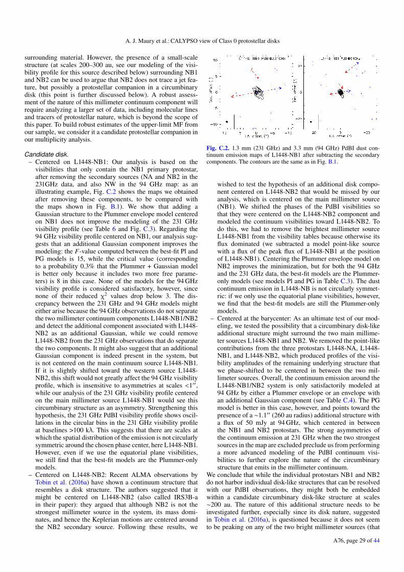
A. J. Maury et al.: CALYPSO view of Class 0 protostellar disks

surrounding material. However, the presence of a small-scalestructure (at scales 200–300 au, see our modeling of the visi-bility profile for this source described below) surrounding NB1and NB2 can be used to argue that NB2 does not trace a jet fea-ture, but possibly a protostellar companion in a circumbinarydisk (this point is further discussed below). A robust assess-ment of the nature of this millimeter continuum component willrequire analyzing a larger set of data, including molecular linesand tracers of protostellar nature, which is beyond the scope ofthis paper. To build robust estimates of the upper-limit MF fromour sample, we consider it a candidate protostellar companion inour multiplicity analysis.

Candidate disk.– Centered on L1448-NB1: Our analysis is based on the

visibilities that only contain the NB1 primary protostar,after removing the secondary sources (NA and NB2 in the231GHz data, and also NW in the 94 GHz map: as anillustrating example, Fig. C.2 shows the maps we obtainedafter removing these components, to be compared withthe maps shown in Fig. B.1). We show that adding aGaussian structure to the Plummer envelope model centeredon NB1 does not improve the modeling of the 231 GHzvisibility profile (see Table 6 and Fig. C.3). Regarding the94 GHz visibility profile centered on NB1, our analysis sug-gests that an additional Gaussian component improves themodeling: the F-value computed between the best-fit Pl andPG models is 15, while the critical value (correspondingto a probability 0.3% that the Plummer + Gaussian modelis better only because it includes two more free parame-ters) is 8 in this case. None of the models for the 94 GHzvisibility profile is considered satisfactory, however, sincenone of their reduced χ2 values drop below 3. The dis-crepancy between the 231 GHz and 94 GHz models mighteither arise because the 94 GHz observations do not separatethe two millimeter continuum components L1448-NB1/NB2and detect the additional component associated with L1448-NB2 as an additional Gaussian, while we could removeL1448-NB2 from the 231 GHz observations that do separatethe two components. It might also suggest that an additionalGaussian component is indeed present in the system, butis not centered on the main continuum source L1448-NB1.If it is slightly shifted toward the western source L1448-NB2, this shift would not greatly affect the 94 GHz visibilityprofile, which is insensitive to asymmetries at scales <1′′,while our analysis of the 231 GHz visibility profile centeredon the main millimeter source L1448-NB1 would see thiscircumbinary structure as an asymmetry. Strengthening thishypothesis, the 231 GHz PdBI visibility profile shows oscil-lations in the circular bins in the 231 GHz visibility profileat baselines >100 kλ. This suggests that there are scales atwhich the spatial distribution of the emission is not circularlysymmetric around the chosen phase center, here L1448-NB1.However, even if we use the equatorial plane visibilities,we still find that the best-fit models are the Plummer-onlymodels.

– Centered on L1448-NB2: Recent ALMA observations byTobin et al. (2016a) have shown a continuum structure thatresembles a disk structure. The authors suggested that itmight be centered on L1448-NB2 (also called IRS3B-ain their paper): they argued that although NB2 is not thestrongest millimeter source in the system, its mass domi-nates, and hence the Keplerian motions are centered aroundthe NB2 secondary source. Following these results, we

Fig. C.2. 1.3 mm (231 GHz) and 3.3 mm (94 GHz) PdBI dust con-tinuum emission maps of L1448-NB1 after subtracting the secondarycomponents. The contours are the same as in Fig. B.1.

wished to test the hypothesis of an additional disk compo-nent centered on L1448-NB2 that would be missed by ouranalysis, which is centered on the main millimeter source(NB1). We shifted the phases of the PdBI visibilities sothat they were centered on the L1448-NB2 component andmodeled the continuum visibilities toward L1448-NB2. Todo this, we had to remove the brightest millimeter sourceL1448-NB1 from the visibility tables because otherwise itsflux dominated (we subtracted a model point-like sourcewith a flux of the peak flux of L1448-NB1 at the positionof L1448-NB1). Centering the Plummer envelope model onNB2 improves the minimization, but for both the 94 GHzand the 231 GHz data, the best-fit models are the Plummer-only models (see models Pl and PG in Table C.3). The dustcontinuum emission in L1448-NB is not circularly symmet-ric: if we only use the equatorial plane visibilities, however,we find that the best-fit models are still the Plummer-onlymodels.

– Centered at the barycenter: As an ultimate test of our mod-eling, we tested the possibility that a circumbinary disk-likeadditional structure might surround the two main millime-ter sources L1448-NB1 and NB2. We removed the point-likecontributions from the three protostars L1448-NA, L1448-NB1, and L1448-NB2, which produced profiles of the visi-bility amplitudes of the remaining underlying structure thatwe phase-shifted to be centered in between the two mil-limeter sources. Overall, the continuum emission around theL1448-NB1/NB2 system is only satisfactorily modeled at94 GHz by either a Plummer envelope or an envelope withan additional Gaussian component (see Table C.4). The PGmodel is better in this case, however, and points toward thepresence of a ∼1.1′′ (260 au radius) additional structure witha flux of 50 mJy at 94 GHz, which centered in betweenthe NB1 and NB2 protostars. The strong asymmetries ofthe continuum emission at 231 GHz when the two strongestsources in the map are excluded preclude us from performinga more advanced modeling of the PdBI continuum visi-bilities to further explore the nature of the circumbinarystructure that emits in the millimeter continuum.

We conclude that while the individual protostars NB1 and NB2do not harbor individual disk-like structures that can be resolvedwith our PdBI observations, they might both be embeddedwithin a candidate circumbinary disk-like structure at scales∼200 au. The nature of this additional structure needs to beinvestigated further, especially since its disk nature, suggestedin Tobin et al. (2016a), is questioned because it does not seemto be peaking on any of the two bright millimeter sources (that

A76, page 29 of 44

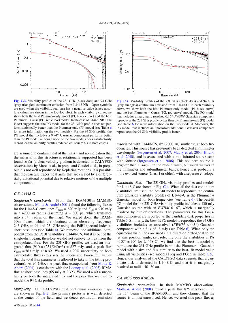
A&A 621, A76 (2019)

ra-dius on the map). We scaled down the IRAM-30m fluxes,which are obtained at an observing frequency 243 GHz, to94 GHz and 231 GHz using the PdBI spectral index at shortbaselines (see Table 4). We removed one additional compo-

Fig. C.3. Visibility profiles of the 231 GHz (black dots) and 94 GHz(gray triangles) continuum emission from L1448-NB1. Open symbolsare used when the visibility real part has a negative value (since abso-lute values are shown in the log–log plot). In each visibility curve, weshow both the best Plummer-only model (Pl, black curve) and the bestPlummer + Gauss (PG, red curve) model. In the case of L1448-NB1, theF-test suggests that the PG model for the 231 GHz profile does not per-form statistically better than the Plummer-only (Pl) model (see Table 6for more information on the two models). For the 94 GHz profile, thePG model that includes a 0.94′′ Gaussian component performs betterthan the Pl model, although none of the two models does satisfactorilyreproduce the visibility profile (reduced chi square >3 in both cases).

are assumed to contain most of the mass), and no indication thatthe material in this structure is rotationally supported has beenfound so far (a clear velocity gradient is detected in CALYPSOobservations by Maret et al., in prep., and Gaudel et al., in prep.,but it is not well reproduced by Keplerian rotation). It is possiblethat the structure traces tidal arms that are created by a differen-tial gravitational potential due to relative motions of the multiplecomponents.

C.3. L1448-C

Single-dish constraints. From their IRAM-30 m MAMBOobservations, Motte & André (2001) found the following fluxesfor the L1448-C envelope: Fpeak = 620 mJy and Fint = 910 mJyin a 4200 au radius (assuming d = 300 pc, which translatesinto a 14′′ radius on the map). We scaled down the IRAM-30 m fluxes, which are obtained at an observing frequency243 GHz, to 94 and 231 GHz using the PdBI spectral index atshort baselines (see Table 4). We removed one additional com-ponent from the PdBI visibilities: L1448-CS, but it is out of thesingle-dish beam, therefore we did not remove its flux from theextrapolated flux. For the 231 GHz profile, we used an inte-grated flux (910 × (231/240)2.5) = 827 mJy, and a peak fluxFpeak = 563 mJy, at 8 kλ. We used a 20% uncertainty on bothextrapolated fluxes (this sets the upper- and lower-limit valuesthat the total flux parameter is allowed to take in the fitting pro-cedure). At 94 GHz, the peak flux extrapolated from Motte &André (2001) is consistent with the Looney et al. (2003) BIMAflux at short baselines (65 mJy at 2 kλ). We used a 40% uncer-tainty on both the integrated flux and the peak flux we used tomodel the 94 GHz profile.

Multiplicity. Our CALYPSO dust continuum emission mapsare shown in Fig. B.2. The primary protostar is well detectedat the center of the field, and we detect continuum emission

Fig. C.4. Visibility profiles of the 231 GHz (black dots) and 94 GHz(gray triangles) continuum emission from L1448-C. In each visibilitycurve, we show both the best Plummer-only model (Pl, black curve)and the best Plummer + Gauss (PG, red curve) model. The PG modelthat includes a marginally resolved 0.16′′-FWHM Gaussian componentreproduces the 231 GHz profile better than the Plummer-only (Pl) model(see Table 6 for more information on the two models). Moreover, thePG model that includes an unresolved additional Gaussian componentreproduces the 94 GHz visibility profile better.

associated with L1448-CS, 8′′ (2000 au) southeast, at both fre-quencies. This source has previously been detected at millimeterwavelengths (Jørgensen et al. 2007; Maury et al. 2010; Hiranoet al. 2010), and is associated with a mid-infrared source seenwith Spitzer (Jørgensen et al. 2006). This southern source isbrighter than L1448-C in the mid-infrared, but much weaker inthe millimeter and submillimeter bands: hence it is probably amore evolved source (Class I or older), with a separate envelope.

Candidate disk. The 231 GHz visibility profiles and modelsfor L1448-C are shown in Fig. C.4. When all the dust continuumvisibilities are used, the best-fit model to reproduce the contin-uum emission visibility profiles of L1448-C is the Plummer +Gaussian model for both frequencies (see Table 6). The best-fitPG model for the 231 GHz visibility profile includes a 130 mJyGaussian source with an FWHM 0.16′′, which is marginallyresolved by our observations. The parameters for this Gaus-sian component are reported as the candidate disk properties inTable 5. Similarly, the best-fit PG model to reproduce the 94 GHzvisibilities includes an unresolved (FWHM < 0.3′′) Gaussiancomponent with a flux of 18 mJy (see Table 6). When only theequatorial visibilities are used (in a direction orthogonal to thejet axis position angle, i.e., selecting only the visibilities at PA−107 ± 30 for L1448-C), we find that the best-fit model toreproduce the 231 GHz profile is still the Plummer + Gaussianmodel with a size and flux similar to the best- fit model valueusing all visibilities (see models Pleq and PGeq in Table C.5).Hence, our analysis of the CALYPSO data suggests that a can-didate disk is detected in L1448-C, and that it is marginallyresolved at radii ∼40−50 au.

C.4. NGC1333 IRAS2A

Single-dish constraints. In their MAMBO observations,Motte & André (2001) found a peak flux 875 mJy beam−1 inthe 11′′ beam of the IRAM-30 m, and they claimed that thesource is almost unresolved. Hence, we used this peak flux as

A76, page 30 of 44

A. J. Maury et al.: CALYPSO view of Class 0 protostellar disks

Fig. C.5. Same as Fig. C.4 for IRAS2A. The Plummer-only model isthe best-fit model to reproduce the 231 GHz profile. The PG model,which includes an unresolved additional Gaussian component, performsmarginally better than the Pl model for the 94 GHz visibility profile.

the envelope-integrated flux for IRAS2A. Using the 20 kλ spec-tral index from our dual-frequency continuum visibilities (seeTable 4), we scaled this value down to our frequencies to obtainthe total envelope fluxes at 231 and 94 GHz. We left the sourcesize quite loose in our fitting and allowed values for Rout ∼ 6 ±4′′ since it is unresolved by the single-dish observations. Theuncertainty on the total flux was set to 30%.

Multiplicity. In our CALYPSO maps, shown in Fig. B.3, a sin-gle protostar is detected. The two continuum sources IRAS2A2and IRAS2A3, reported in Maury et al. (2014) and Codellaet al. (2014b), are now shown to originate from an envelopestructure that is detected by the interferometer: our improveddataset after self-calibration (which improved the rms noise andthe imaging fidelity) allows us to recover the lower surfacebrightness emission that surrounds them, and they are found toreconnect with the main source envelope emission. This sug-gests that, similar to what was proposed in Santangelo et al.(2015) for IRAS4A, these sources represent the dust contin-uum emission from envelope structures that are detected by theinterferometer when only a restricted range of spatial scalesis sampled. They are therefore no longer considered as robustcompact continuum emission components. Recent VLA (Tobinet al. 2015b) and ALMA observations (not yet published, Mauryet al., in prep.) of IRAS2A have revealed the presence of asecondary millimeter dust continuum source located 0.4′′ fromthe main millimeter source. Although the nature of this sec-ondary component remains to be investigated, it is likely thatIRAS2A is a close (≤100−200 au) binary system (two sepa-rate jets are detected; Podio & CALYPSO, in prep.). This sourceis not separated from the main millimeter source in our PdBImaps, although a slight extension is detected at its location.Our highest angular resolution data for IRAS2A (configura-tion A of the PdBi at 231 GHz) was obtained as part of thepilot R068 project (Maury et al. 2010): the lower sensitivityof these earlier observations (obtained before the installationof the WideX correlator) explains the non-detection of a sepa-rated compact source at the secondary position. To build robustestimates of the upper-limit MF from our sample, and consid-ering that a secondary source is detected with ALMA and theVLA, we count IRAS2A as a binary system in our multiplicityanalysis.

Candidate disk. The 231 GHz visibility profiles and modelsare shown in Fig. C.5 for IRAS2A. When all the dust continuumvisibilities are used, the best-fit model to reproduce the contin-uum emission visibility profiles of IRAS2A is the Plummer-onlymodel for the 231 GHz profile (see main text and Table 6). Thebest-fit PG model for the 231 GHz visibility profile that satisfac-torily reproduces the visibility profile but is not better than thePlummer-only model includes a 52 mJy Gaussian source thatis unresolved with an FWHM 0.01′′ (the smallest size allowedin our fitting procedure). The upper limits on the parameters forthis Gaussian component are reported as upper limits on the diskproperties in Table 5. The PG model performs marginally bet-ter than the Pl model at reproducing the 94 GHz visibilities (acomparison of the two models produces an F-value of 11, whilethe critical value of F is 8. Above this, the probability that thePG model is better only by chance is <0.3%). It includes anunresolved Gaussian with a flux of 9 mJy (see Table 6). Whenonly the equatorial visibilities are used (in a direction orthogonalto the jet axis position angle, i.e., selecting only the visibili-ties at PA −65 ± 30), we find that the best-fit model is stillthe Plummer-only model for the 231 GHz profile (see modelsPleq and PGeq in Table C.6). Our analysis of the CALYPSO datatherefore suggests that no resolved disk-like emission is detectedat scales 50–500 au.

We also tested the effect of removing a point source fromthe flux of the secondary source that is resolved with theALMA 1.3 mm observations (14 mJy at 230 GHz; Mauryet al., in prep.) from the PdBI visibilities and shifting thephase center to the position of the main millimeter source at(03:28:55.569;31:14:36.952) to model the 231 GHz PdBI visibil-ities anew. For the sake of clarity and brevity, we do not reportthis model here, but the best-fit model is still the Plummer-onlymodel, with very similar parameters as were found as best fits forthe whole visibility dataset, which is reported in Table 6.

C.5. SVS13B

Single-dish constraints. Fluxes obtained using the MAMBObolometer array on the IRAM-30 m telescope are reported inChini et al. (1997): Fpeak = 900 mJy and Fint = 1180 mJy. How-ever, Lefloch et al. (1998) reported a peak flux for SVS13Bof only 320 mJy beam−1, with the same instrument and tele-scope. We used the Chini et al. (1997) peak flux as the envelopeintegrated flux in a source the size of the MAMBO beam (11′′-FWHM), and we used the Lefloch et al. (1998) value as the lowerlimit allowed for the total envelope flux for the minimization. Weused the peak flux as an integrated flux in the MAMBO beambecause contamination from the surrounding filament, and moreespecially, from the nearby SVS13A, precluded obtaining robustintegrated fluxes for SVS13B alone at radii larger than 6′′. Wescale these fluxes down using the 20 kλ spectral index from ourdual-frequency continuum visibilities (see Table 4). We also letthe source size quite loose in the minimization procedure, allow-ing radii from 4′′ to 14′′. The uncertainty on the total envelopeflux was set to 40%.

Multiplicity. SVS13B is in a large-scale multiple system (sepa-rate envelopes) with SVS13A, a Class I protostar located 3500 auaway, and SVS13C, whose nature is as yet undetermined, andwhich lies 4500 au away. These three sources are detected inour 94 GHz dust continuum emission map shown in Fig. 2. Afourth source, VLA3 detected previously at centimeter wave-lengths with the VLA by Rodríguez et al. (1999), is also detectedin both our maps (although not at the 10σ level in our 231 GHz

A76, page 31 of 44

A&A 621, A76 (2019)

from the jet axis found inthe CALYPSO data, Podio et al. in prep), we find that thebest-fit model is still the Plummer-only model at 231 GHz

Fig. C.6. Same as Fig. C.4 for SVS13B. The Plummer-only models arethe best-fit models to reproduce the two profiles, although at 231 GHz,a more reasonable (p + q) index is found in the PG model that includesa 0.19′′ FWHM Gaussian component (flux 80 mJy).

data). A millimeter counterpart to VLA3 was also previouslytentatively detected in the BIMA maps of Looney et al. (2000) asan extension from the SVS13A source at 110 GHz (they namedit A2). The primary Class 0 protostar in the field, SVS13B, doesnot exhibit any sign of further multiplicity down to the scales of∼50 au that are probed by our data. A single protostellar jet fromSVS13B is detected in our CALYPSO maps of molecular lineemission at a PA +167 (Podio & CALYPSO, in prep.).

Candidate disk. When all the dust continuum visibilities areused, the best-fit model to reproduce the continuum emissionvisibility profiles of SVS13B is the Plummer-only model forboth frequencies (see main text and Table 6). However, the bestPlummer-only model to reproduce the 231 GHz visibility pro-file is found to have p + q = 2.9 which seems excessively high.Although we do not exclude that such a value might be phys-ically possible, we stress that including a Gaussian componentallows reducing this slope index to p + q = 2.5, which is a morestandard value that is expected in protostellar envelopes (Looneyet al. 2003; also found p + q = 2.4 at short <40 kλ baselinesin their 3 mm BIMA data). This best-fit PG model for the 231GHz visibility profile includes a 80 mJy Gaussian source withan FWHM 0.19′′: although this model is not statistically betterthan the Plummer-only model, we have to keep these facts inmind about SVS13B. In Table 5 we report these values as upperlimits for the candidate disk component. The F-test shows thatthe best-fit model to reproduce the 94 GHz visibilities is also thePlummer-only model (see Table 6 and Figs. 6 and C.6), with asatisfactorily reduced χ2 value that is only slightly lower thanthat of the Plummer + Gaussian model, but has two free param-eters less. When only the equatorial visibilities are used (in adirection orthogonal to the jet axis position angle, i.e., selectingonly the visibilities at PA −103 ± 30 from the jet axis foundin the CALYPSO data; Podio et al., in prep.), we find that thebest-fit model is still the Plummer-only model at 231 GHz with ahigh index p + q = 2.9 (see models Pleq and PGeq in Table C.7).Our analysis of the CALYPSO data therefore suggests that thecontinuum emission from SVS13B is better reproduced by anenvelope model down to scales 50 au, but we cannot exclude thepresence of a .60 au candidate disk which in addition producesmore reasonable p + q values.

Fig. C.7. Same as Fig. C.4 for IRAS4A1. The Plummer-only models arethe best-fit models to reproduce the two visibility profiles.

C.6. NGC1333 IRAS4A1

Single-dish constraints. Motte & André (2001) reported thatthe NGC1333 IRAS4A envelope is unresolved in their IRAM-30 m observations (12′′-FWHM beam). The peak flux is Fpeak =4.1 Jy in the IRAM-30 m beam, which we used as the total enve-lope flux in a 6′′ source. We removed the contribution fromIRAS4A2 and rescaled the MAMBO flux that was obtained ata central frequency of 243 GHz to obtain extrapolated fluxes atboth 94 and 231 GHz (using the spectral index at large scalesfrom our dual-frequency PdBI data, see Table 4). We used a 20%uncertainty on the single-dish flux, and let the outer enveloperadius vary between 3′′ and 9′′.

Multiplicity. The IRAS4A system is resolved by our CALYPSOobservations: see Fig. B.4. The secondary protostar IRAS4A2was extensively discussed by Santangelo et al. (2015) and drivesits own high-velocity jet. The continuum emission associatedwith the component IRAS4A3 reported in Santangelo et al.(2015) disappears when robust weighting is used. This confirmsthe suggestion made in Santangelo et al. (2015) that this tracesa structure of dust continuum emission that is produced by theoutflow interaction with the envelope, and is not a compactcomponent associated with a true protostellar source.

Candidate disk. The models and visibility profiles ofIRAS4A1 are shown in Fig. C.7. When all the dust continuumvisibilities are used, the best-fit model to reproduce the contin-uum emission visibility profiles of IRAS4A1 is the Plummer-only model for both the 231 and 94 GHz visibility profiles (seemain text and Table 6). The best-fit PG model for the 231 GHzvisibility profile includes a 348 mJy Gaussian source with anFWHM 0.3′′, but does not perform better than the Plummer-onlymodel (slightly larger reduced χ2, but two additional free param-eters). The upper limits on the parameters for this Gaussiancomponent are reported as upper limits on the disk propertiesin Table 5. When only the equatorial visibilities are used (inthe direction of the C17O(3–2) velocity gradient that is shownin the SMA map by Ching et al. (2016) at the 4′′ core scale, i.e.,selecting only the visibilities at PA −62 ± 30), we find that thebest-fit model is still the Plummer-only model for the 231 GHzprofile (see models Pleq and PGeq in Table C.6). It is thereforeclear from our analysis of the CALYPSO data that the continuumstructure around NGC 1333 IRAS4A1 can be well described

A76, page 32 of 44

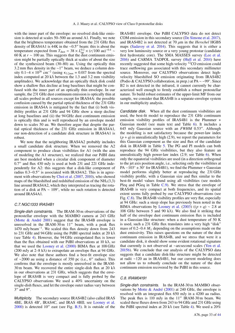
A. J. Maury et al.: CALYPSO view of Class 0 protostellar disks

with the inner part of the envelope: no resolved disk-like emis-sion is detected at scales 50–500 au around A1. Finally, we notethat the brightness temperature obtained from the 231 GHz fluxdensity of IRAS4A1 is 44K in the ∼0.5′′ beam: this is about thetemperature expected from Tdust = 38 × L0.2

int × (r/100 au)−0.4 ∼60 K at r ∼ 100 au. This suggests that the dust continuum emis-sion might be partially optically thick at scales of about the sizeof the synthesized beam (30–80) au. Using the optically thin3.2 mm flux density in the ∼1′′ beam, we deduce a column den-sity 0.1−4 × 1026 cm−2 (using κ3.2mm = 0.017 from the spectralindex computed at 20 kλ between the 1.3 and 3.2 mm visibilityamplitudes). We acknowledge that an optically thick disk couldshow a shallow flux decline at long baselines that might be con-fused with the inner part of an optically thin envelope. In oursample, the 231 GHz dust continuum emission is optically thin atall scales probed in all sources except for IRAS4A: the possibleconfusion caused by the partial optical thickness of the 231 GHzemission in IRAS4A is mitigated by the fact that (i) both vis-ibility profiles at 231 GHz and 94 GHz show a steep declineat long baselines and (ii) the 94 GHz dust continuum emissionis optically thin and is well reproduced by an envelope modeldown to scales 50 au. We therefore argue that despite the par-tial optical thickness of the 231 GHz emission in IRAS4A1,our non-detection of a candidate disk structure in IRAS4A1 isrobust.

We note that the neighboring IRAS4A2 probably includesa small candidate disk structure. When we removed the A2component to produce clean visibilities for A1 (with the aimof modeling the A1 structure), we realized that our PdBI dataare best modeled when a circular disk component of diameter0.7′′ and flux 430 mJy is used at both 231 and 221 GHz inde-pendently for A2: this suggests that a disk-like component ofradius 0.3−0.5′′ is associated with IRAS4A2. This is in agree-ment with observations by Choi et al. (2007, 2010), who showedmaps of the blueshifted and redshifted emission of the NH3(3,3)line around IRAS4A2, which they interpreted as tracing the rota-tion of a disk at PA ∼ 109, while no such rotation is detectedaround IRAS4A1.

C.7. NGC1333 IRAS4B1

Single-dish constraints. The IRAM-30 m observations of theprotostellar envelope with the MAMBO camera at 243 GHz(Motte & André 2001) suggest that the IRAS4B envelope isunresolved in the IRAM-30 m 11′′ beam, with a peak flux1470 mJy beam−1. We scaled this flux density down from 243to 231 GHz and 94 GHz using the PdBI spectral index at 20 kλ(see Table 4). However, the 94 GHz extrapolated flux is lowerthan the flux obtained with our PdBI observations at 10 kλ, sothat we used the Looney et al. (2000) BIMA flux at 108 GHz(200 mJy at 2–8 kλ) to extrapolate an envelope flux at 94 GHz.We also note that these authors find a best-fit envelope sizeof ∼2000 au using a distance of 350 pc (i.e., 6′′ radius). Thisconfirms that the envelope is mostly unresolved in the IRAM-30 m beam. We recovered the entire single-dish flux at 20 kλin our observations at 231 GHz, which suggests that the enve-lope of IRAS4B is very compact and is fully probed by theCALYPSO observations We used a 40% uncertainty on thesingle-dish fluxes, and let the envelope outer radius vary between3′′ and 9′′.

Multiplicity. The secondary source IRAS4B2 (also called IRAS4BE, IRAS 4B′, IRAS4C, and IRAS 4BII; see Looney et al.2000) is detected 10′′ east (see Fig. B.5). It is outside of the

IRAS4B1 envelope. Our PdBI CALYPSO data do not detectCOM emission in this secondary source (De Simone et al. 2017),and IRAS4B2 is not detected at 70 µm in the Herschel HGBSmaps (Sadavoy et al. 2014). This suggests that it is either avery low luminosity source or a very young protostar (candidatefirst hydrostatic core). The SMA MASSES survey (Lee et al.2016) and CARMA TADPOL survey (Hull et al. 2014) haverecently suggested that some high-velocity 12CO emission couldtrace outflowing gas associated with this secondary millimetersource. Moreover, our CALYPSO observations detect high-velocity blueshifted SO emission originating from IRAS4B2(Podio & CALYPSO collaboration, in prep.) at PA∼−99. SinceB2 is not detected in the infrared, it cannot currently be char-acterized well enough to firmly establish a robust protostellarnature. To build robust estimates of the upper-limit MF from oursample, we consider that IRAS4B is a separate-envelope systemin our multiplicity analysis.

Candidate disk. When all the dust continuum visibilities areused, the best-fit model to reproduce the 231 GHz continuumemission visibility profiles of IRAS4B1 is the Plummer +Gaussian model (see main text and Table 6). It includes a645 mJy Gaussian source with an FWHM 0.53′′. Althoughthe modeling is not satisfactory because the power-law index(p + q) is unrealistically high (2.9), we report the parameters forthis Gaussian component as the size and flux of the candidatedisk in IRAS4B in Table 5. The PG and Pl models can bothreproduce the 94 GHz visibilities, but they also feature anunrealistically high power-law index (2.9; see Table 6). Whenonly the equatorial visibilities are used (in a direction orthogonalto the jet axis position angle, i.e., selecting only the visibilities atPA −103 ± 30 for IRAS4B1), we find the Plummer + Gaussianmodel performs slightly better at reproducing the 231 GHzvisibility profile, with a Gaussian size and flux similar to thebest-fit model values found using all visibilities (see modelsPleq and PGeq in Table C.9). We stress that the envelope ofIRAS4B is very compact at both frequencies, and its spatialextent seems fully probed by our CALYPSO observations (seeFig. C.8). The IRAS4B visibility profiles are very flat, especiallyat 94 GHz: such a steep slope has previously been noted in theBIMA observations by Looney et al. (2003) ((p + q) ∼ 2.8 at108 GHz between 5 and 90 kλ). We also find it striking thathalf of the envelope dust continuum emission flux is includedin a Gaussian-like structure: when a dust temperature of 50 Kis used, such a 231 GHz flux translates into a very high “disk”mass of 0.2−0.4 M depending on the assumptions made on thedust emissivity. This raises questions on the nature of the dustcontinuum emission in IRAS4B, and we stress that were it acandidate disk, it should show some evident rotational signaturethat currently is not observed at ∼arcsecond scales (Yen et al.2015b). We conclude that our analysis of the CALYPSO datasuggests that a candidate disk-like structure might be detectedat radii ∼120 au in IRAS4B1, but our current modeling doesnot allow us to robustly conclude on the nature of the dustcontinuum emission recovered by the PdBI in this source.

C.8. IRAM04191

Single-dish constraints. In the IRAM-30 m MAMBO obser-vations by Motte & André (2001) at 240 GHz, the envelope isresolved with an integrated flux 650 mJy in a 4200 au radius.The peak flux is 110 mJy in the 11′′ IRAM-30 m beam. Wescaled these fluxes down from 243 to 94 GHz and 231 GHz usingthe PdBI spectral index at 20 kλ (see Table 4). We used a 20%

A76, page 33 of 44

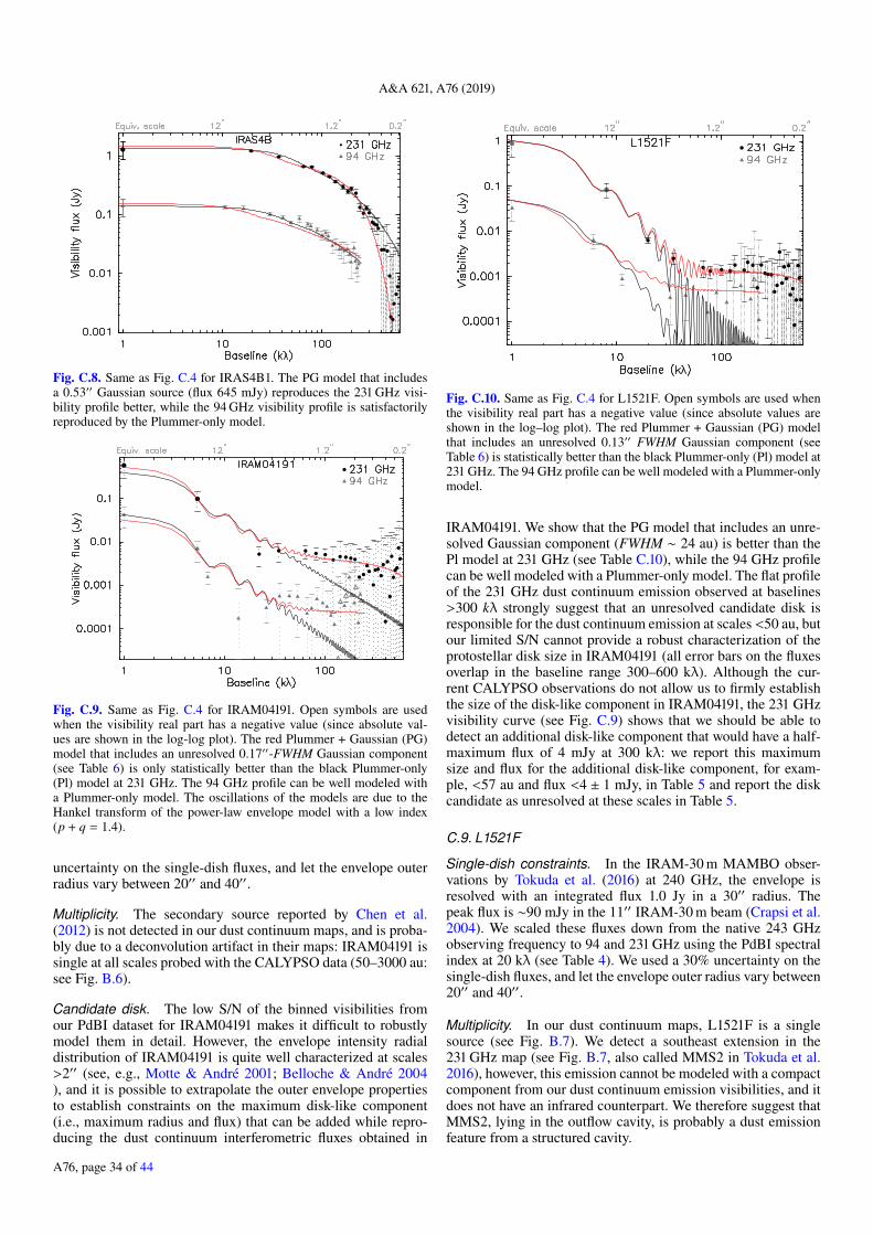
A&A 621, A76 (2019)

(see Table 4). We used a 20% un-

certainty on the single-dish fluxes, and let the envelope outerradius vary between 20

Fig. C.8. Same as Fig. C.4 for IRAS4B1. The PG model that includesa 0.53′′ Gaussian source (flux 645 mJy) reproduces the 231 GHz visi-bility profile better, while the 94 GHz visibility profile is satisfactorilyreproduced by the Plummer-only model.

certainty on the single-dish fluxes, and let the envelope outerradius vary between 20

Fig. C.9. Same as Fig. C.4 for IRAM04191. Open symbols are usedwhen the visibility real part has a negative value (since absolute val-ues are shown in the log-log plot). The red Plummer + Gaussian (PG)model that includes an unresolved 0.17′′-FWHM Gaussian component(see Table 6) is only statistically better than the black Plummer-only(Pl) model at 231 GHz. The 94 GHz profile can be well modeled witha Plummer-only model. The oscillations of the models are due to theHankel transform of the power-law envelope model with a low index(p + q = 1.4).

uncertainty on the single-dish fluxes, and let the envelope outerradius vary between 20′′ and 40′′.

Multiplicity. The secondary source reported by Chen et al.(2012) is not detected in our dust continuum maps, and is proba-bly due to a deconvolution artifact in their maps: IRAM04191 issingle at all scales probed with the CALYPSO data (50–3000 au:see Fig. B.6).

Candidate disk. The low S/N of the binned visibilities fromour PdBI dataset for IRAM04191 makes it difficult to robustlymodel them in detail. However, the envelope intensity radialdistribution of IRAM04191 is quite well characterized at scales>2′′ (see, e.g., Motte & André 2001; Belloche & André 2004), and it is possible to extrapolate the outer envelope propertiesto establish constraints on the maximum disk-like component(i.e., maximum radius and flux) that can be added while repro-ducing the dust continuum interferometric fluxes obtained in

Fig. C.10. Same as Fig. C.4 for L1521F. Open symbols are used whenthe visibility real part has a negative value (since absolute values areshown in the log–log plot). The red Plummer + Gaussian (PG) modelthat includes an unresolved 0.13′′ FWHM Gaussian component (seeTable 6) is statistically better than the black Plummer-only (Pl) model at231 GHz. The 94 GHz profile can be well modeled with a Plummer-onlymodel.

IRAM04191. We show that the PG model that includes an unre-solved Gaussian component (FWHM ∼ 24 au) is better than thePl model at 231 GHz (see Table C.10), while the 94 GHz profilecan be well modeled with a Plummer-only model. The flat profileof the 231 GHz dust continuum emission observed at baselines>300 kλ strongly suggest that an unresolved candidate disk isresponsible for the dust continuum emission at scales <50 au, butour limited S/N cannot provide a robust characterization of theprotostellar disk size in IRAM04191 (all error bars on the fluxesoverlap in the baseline range 300–600 kλ). Although the cur-rent CALYPSO observations do not allow us to firmly establishthe size of the disk-like component in IRAM04191, the 231 GHzvisibility curve (see Fig. C.9) shows that we should be able todetect an additional disk-like component that would have a half-maximum flux of 4 mJy at 300 kλ: we report this maximumsize and flux for the additional disk-like component, for exam-ple, <57 au and flux <4 ± 1 mJy, in Table 5 and report the diskcandidate as unresolved at these scales in Table 5.

C.9. L1521F

Single-dish constraints. In the IRAM-30 m MAMBO obser-vations by Tokuda et al. (2016) at 240 GHz, the envelope isresolved with an integrated flux 1.0 Jy in a 30′′ radius. Thepeak flux is ∼90 mJy in the 11′′ IRAM-30 m beam (Crapsi et al.2004). We scaled these fluxes down from the native 243 GHzobserving frequency to 94 and 231 GHz using the PdBI spectralindex at 20 kλ (see Table 4). We used a 30% uncertainty on thesingle-dish fluxes, and let the envelope outer radius vary between20′′ and 40′′.

Multiplicity. In our dust continuum maps, L1521F is a singlesource (see Fig. B.7). We detect a southeast extension in the231 GHz map (see Fig. B.7, also called MMS2 in Tokuda et al.2016), however, this emission cannot be modeled with a compactcomponent from our dust continuum emission visibilities, and itdoes not have an infrared counterpart. We therefore suggest thatMMS2, lying in the outflow cavity, is probably a dust emissionfeature from a structured cavity.

A76, page 34 of 44

A. J. Maury et al.: CALYPSO view of Class 0 protostellar disks

Fig. C.11. Same as Fig. C.4 for L1527. The two visibility profilesare better reproduced with models that include an additional Gaussiansource whose FWHM is 0.4′′ at 231 GHz.

Candidate disk.. The low S/N of the binned visibilities fromour PdBI dataset for L1521F make it difficult to robustly modelthem in detail, but it is possible to extrapolate the outer enve-lope properties to establish constraints on the maximum disk-likecomponent (i.e., maximum radius and flux) that can be addedwhile reproducing the dust continuum interferometric fluxesobtained in L1521F. The 231 GHZ profile is best modeled usinga PG model that includes an unresolved Gaussian component(FWHM 0.13′′; see Fig. C.10): this suggests that a candidate diskof radius ∼<20 au and flux ∼1.3 ± 0.4 mJy may be detected inL1521F. However, as in the case of IRAM04191, we are limitedby the S/N <3 at long (>300 kλ) baselines for L1521F, so that thesize of the Gaussian component that can be added to the Plum-mer envelope model is subject to high uncertainties. To remainrobust in our characterization of a potential protostellar disk inL1521F, we report in Table 5 that a candidate disk-like compo-nent might contribute a flux 1.3 mJy at scales <57 au (300 kλ).We also note that 0.87 mm ALMA observations by Tokuda et al.(2017) reported the detection of a small 10 au disk in L1521F,which is consistent with our upper-limit size and flux at 1.3 mm.

C.10. L1527

Single-dish constraints. In the IRAM-30 m observations byMotte & André (2001) with MAMBO at 240 GHz, the L1527envelope is resolved with an integrated flux 1500 mJy in a4200 au radius. The peak flux is 375 mJy in the 11′′ IRAM-30 m beam. We scaled these fluxes down from 243 to 94 GHz and231 GHz using the PdBI spectral index at 20 kλ (see Table 4). Weused a 20% uncertainty on the extrapolated single-dish fluxes,and let the envelope outer radius vary between 25′′ and 35′′.

Multiplicity. In our dust continuum maps, L1527 is a singlesource (see Fig. 3).

Candidate disk. The models and the visibility profiles ofL1527 are shown in Fig. 7 in the text and in Fig. C.11 here. Whenall the dust continuum visibilities are used, the best-fit model toreproduce the continuum emission visibility profiles of L1527 isthe Plummer + Gaussian model for both frequencies (see maintext and Table 6). The best-fit PG model for the 231 GHz visi-bility profile includes a 215 mJy Gaussian source with FWHM0.4′′. The parameters for this Gaussian component are reported

as the candidate disk properties in Table 5. Similarly, the best-fit PG model to reproduce the 94 GHz visibilities includes amarginally resolved Gaussian component with FWHM = 0.3′′and flux 23 mJy (see Table 6). When only the equatorial vis-ibilities are used (in a direction orthogonal to the jet axisposition angle, i.e., selecting only the visibilities at PA 19 ± 30for L1527), we find that the Plummer + Gaussian model per-forms better at reproducing the 231 GHz visibility profile, with aGaussian size and flux similar to the best-fit model values foundusing all visibilities (see models Pleq and PGeq in Table C.12).Our analysis of the CALYPSO data therefore suggests that acandidate disk-like structure is detected at radii ∼50−70 auin L1527.

C.11. Serpens Main S68N

Single-dish constraints. SerpM-S68N (McMullin et al. 1994)is also known as SMM 9 (Casali et al. 1993) or Ser-emb 8 (Enochet al. 2011), and is located in the Serpens Main cluster. Twoprotostars are located within the FWHM of the Bolocam coreSer-emb 8 associated with S68N, but the envelope associatedwith S68N can be clearly identified in the IRAM-30 m observa-tions by Kaas et al. (2004) at better angular resolution. Based onthe MAMBO map, we estimate an integrated flux 1030 mJy in a15′′ radius area, and a peak flux 550 mJy in the 11′′ IRAM-30 mbeam. We scaled these fluxes down from the MAMBO centralfrequency of 243 to 94 GHz and 231 GHz using the PdBI spec-tral index at 20 kλ (see Table 4). We used a 15% uncertaintyon the extrapolated single-dish fluxes, and let the envelope outerradius vary between 8′′ and 22′′.

Multiplicity. SerpM-S68N (S68N in the following) is singlein the 231 GHz PdBI primary beam area (21′′ FWHM; seeFig. B.8). Our PdBI 94 GHz map indicates a compact sourceat the position of S68N, and two additional sources ∼12′′ and∼20′′ to the northeast. This is consistent with the CARMA230 GHz sources found by Enoch et al. (2011). While the regionis crowded and it is difficult to robustly associate sources at dif-ferent wavelengths with different resolutions, it seems that thesecondary source S68Nb has no Spitzer MIPS counterpart at24 µm, while S68Nc has an associated Spitzer IRAC source at8 µm (Enoch et al. 2009; Harvey et al. 2007): it is classified as aClass I protostar. The three sources (S68N, S68Nb, and S68Nc)are embedded in a common parsec-scale filamentary structureseen in the single-dish maps of the dust continuum emission, butthey have separate envelopes.

Candidate disk. When all the dust continuum visibilities areused, the Plummer model is as good a model as the PG modelto reproduce the continuum emission visibility profiles of S68Nat both frequencies (see main text and Table 6). The best-fitPG model for the 231 GHz visibility profile includes an unre-solved Gaussian source with an FWHM 0.11′′ and flux 28 mJy.The parameters for this Gaussian component are reported as theupper-limit values for any disk in S68N in Table 5, although ourobservations do not hint at the presence of a disk in S68N. Whenonly the equatorial visibilities are used (in a direction orthogonalto the jet axis position angle, i.e., selecting only the visibilitiesat PA 45 ± 30 for S68N), we find that the Plummer model per-forms as well as the Plummer + Gaussian model to reproduce the231 GHz visibility profile, with a Gaussian size and flux similarto the best-fit model values found using all visibilities (see mod-els Pleq and PGeq in Table C.12). Our analysis of the CALYPSOdata therefore suggests that no disk-like structure is resolved in

A76, page 35 of 44

A&A 621, A76 (2019)

Fig. C.12. Same as Fig. C.4 for S68N. The Plummer-only models arethe best-fit models to reproduce both visibility profiles.

S68N at our spatial resolution, and any disk can only be presentat radii <50 au.

C.12. Serpens Main SMM4

Single-dish constraints. The envelope associated with SerpM-SMM4 (SMM4 in the following) can be clearly identified inthe IRAM-30 m observations by Kaas et al. (2004): based onthe MAMBO map, we estimate an integrated flux 2350 mJyin a 20′′ radius area (background subtracted), and a peak flux1000 mJy in the 11′′ IRAM-30 m beam. We removed the con-tribution from MM4b that is included in the 11′′ beam, andscaled these fluxes down from the MAMBO central frequencyof 243 to 94 GHz and 231 GHz (using the PdBI spectral indexat 20 kλ, see Table 4). We used a 20% uncertainty on theextrapolated single-dish fluxes, and let the envelope outer radiusvary between 15′′ and 25′′.

Multiplicity. In both our dust continuum maps at 231 and94 GHz, we detect a secondary component, SMM4b, about 7′′southwest of the strongest millimeter source (see Fig. B.9).This is the first time that this secondary component is detected,and its nature is therefore unclear. However, it seems thatthe Herschel/PACS emission peaks toward SMM4b and nottoward the main protostar. Moreover, a water maser was detectedat (18:29:56.51, 01:13:11.6, equ. J2000) with the VLA, seeFuruya et al. (2003): this position is closer to the position ofMM4b than to the position of MM4a. Finally, the methanol out-flow detected in Kristensen et al. (2010) was not found to peakon the millimeter emission peak reported in the literature. Basedon these pieces of evidence, we suggest that SMM4b is probablythe driving source of the jet or outflow, while the more quiescentSMM4a dominates the millimeter dust continuum emission. Amore detailed analysis of the jet properties and chemical contentfor these two sources will be proposed by Podio & CALYPSO(in prep.) and Belloche & CALYPSO (in prep.).

Candidate disk. When all the dust continuum visibilities areused, the best-fit model to reproduce the continuum emissionvisibility profiles of SMM4a is the Plummer + Gauss modelfor both frequencies (see main text and Table 6). The best-fitPG model for the 231 GHz visibility profile includes a Gaussiansource with an FWHM 0.7′′ and flux 595 mJy. The parametersfor this Gaussian component are reported as the values for the

to the southwest(see Fig. B.10). At a distance of 250 pc for Serpens South,these two sources are separated by 2600 au. We note thatOrtiz-León et al. (2015) argued that Serpens Main and W40are at a same distance, about 430 pc, based on their VLA par-allax measurements of seven sources in both clouds. WhileW40 and Serpens South seem to belong to the same extinc-tion wall (Straižys et al. 2003), it is not yet clear at which dis-tance the Serpens South filament is located (Könyves et al.2015). For consistency with previous studies, we use herethe value of 250 pc but acknowledge that the distance mightbe twice larger, and the physical separation between MM18aand MM18b could thus be up to 5000 au. MM18b was orig-inally detected in Maury et al. (2011), then with CARMA

Fig. C.13. Same as Fig. C.4 for SMM4. Open symbols are used whenthe visibility real part has a negative value (since absolute values areshown in the log-log plot). The PG models are the best-fit modelsto reproduce the two CALYPSO visibility profiles: at 231 GHz, theadditional Gaussian component has an FWHM 0.7′′ and flux 595 mJy.

properties of the candidate disk in SMM4a in Table 5. Hence, ouranalysis of the CALYPSO data suggests that continuum emissionthat is not accounted for by circular-symmetric Plummer-likeenvelope models may trace a disk-like structure in SMM4a thatis resolved with our observations with a radius ∼300 au. If thiscontinuum emission indeed traces a disk structure, the disk fluxat 231 GHz accounts for ∼30% of the total envelope flux fromsingle-dish observations (obtained within a 20′′ radius), which isvery unusual for Class 0 protostars. Based on the internal lumi-nosity of SMM4a in the HGBS (2 L; see Table 1), we wouldexpect a dust temperature ∼20−30 K at the 200 kλ scale, turningthe 231 GHz disk flux into a disk mass >0.3 M. Such a highdisk mass is surprising: a more complete analysis of SMM4awith 2D modeling of interferometric data that cover a larger spa-tial dynamic range is needed to better understand the nature ofthis source.

C.13. Serpens South MM18

Single-dish constraints. The envelope associated withSerpens South MM18 (SerpS-MM18 in the following) hasbeen mapped with MAMBO on the IRAM-30 m telescope(Maury et al. 2011): based on the MAMBO map, we estimate anintegrated flux 2505 mJy in a 18′′ FWHM source, and a peakflux 1376 mJy in the 11′′ IRAM-30 m beam. We removed thecontribution from MM18b and scaled these fluxes down fromthe MAMBO central frequency of 243 to 94 GHz and 231 GHz(using the PdBI spectral index at 20 kλ; see Table 4). We used a20% uncertainty on the extrapolated single-dish fluxes, and letthe envelope outer radius vary between 10′′ and 20′′.

Multiplicity. SerpS-MM18 is separated into two sources in ourCALYPSO maps: MM18a the primary protostar (dominatingthe millimeter continuum emission) and a secondary sourceMM18b, weaker and more compact, 10′′ to the southwest (seeFig. B.10). At a distance of 250 pc for Serpens South, these twosources are separated by 2600 au. We note that Ortiz-León et al.(2015) argued that Serpens Main and W40 are at a same dis-tance, about 430 pc, based on their VLA parallax measurementsof seven sources in both clouds. While W40 and Serpens Southseem to belong to the same extinction wall (Straižys et al. 2003),

A76, page 36 of 44

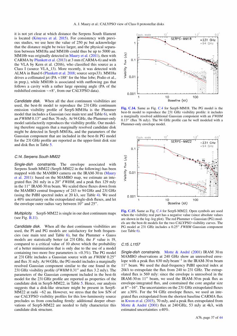
A. J. Maury et al.: CALYPSO view of Class 0 protostellar disks

it is not yet clear at which distance the Serpens South filamentis located (Könyves et al. 2015). For consistency with previ-ous studies, we use here the value of 250 pc but acknowledgethat the distance might be twice larger, and the physical separa-tion between MM18a and MM18b could thus be up to 5000 au.MM18b was originally detected in Maury et al. (2011), then withCARMA by Plunkett et al. (2013) at 3 mm (CARMA-6) and withthe VLA by Kern et al. (2016), who classified this source as aClass I (source VLA_13). More recently, it was detected withALMA in Band 6 (Plunkett et al. 2018; source serps33). MM18adrives a collimated jet (PA +188 for the blue lobe; Podio et al.,in prep.), while MM18b is associated with outflowing gas thatfollows a cavity with a rather large opening angle (PA of theredshifted emission ∼+8, from our CALYPSO data).

Candidate disk. When all the dust continuum visibilities areused, the best-fit model to reproduce the 231 GHz continuumemission visibility profile of SerpS-MM18a is the Plummermodel that includes a Gaussian (see main text and Table 6), withan FWHM 0.13′′ and flux 76 mJy. At 94 GHz, the Plummer-onlymodel satisfactorily reproduces the visibility profile. Our model-ing therefore suggests that a marginally resolved candidate diskmight be detected in SerpS-MM18a, and the parameters of theGaussian component that are included in the best-fit PG modelfor the 231 GHz profile are reported as the upper-limit disk sizeand disk flux in Table 5.

C.14. Serpens South MM22

Single-dish constraints. The envelope associated withSerpens South MM22 (SerpS-MM22 in the following) has beenmapped with the MAMBO camera on the IRAM-30 m (Mauryet al. 2011): based on the MAMBO map, we estimate an inte-grated flux 261 mJy in a 20′′ FWHM, and a peak flux 129 mJyin the 11′′ IRAM-30 m beam. We scaled these fluxes down fromthe MAMBO central frequency of 243 to 94 GHz and 231 GHz(using the PdBI spectral index at 20 kλ, see Table 4). We useda 40% uncertainty on the extrapolated single-dish fluxes, and letthe envelope outer radius vary between 10′′ and 25′′.

Multiplicity. SerpS-MM22 is single in our dust continuum maps(see Fig. B.11).

Candidate disk. When all the dust continuum visibilities areused, the Pl and PG models are satisfactory for both frequen-cies (see main text and Table 6), but the Plummer + Gaussmodels are statistically better (at 231 GHz, the F value is 19,compared to a critical value of 10 above which the probabilityof a better minimization that is only due to the use of a modelcontaining two more free parameters is <0.3%). The PG modelat 231 GHz includes a Gaussian source with an FWHM 0.25′′and flux 31 mJy. At 94 GHz, the PG model includes a marginallyresolved Gaussian component similar to the one found in the231 GHz visibility profile (FWHM 0.31′′ and flux 3.2 mJy). Theparameters of the Gaussian component included in the best-fitmodel for the 231 GHz profile are reported as properties of thecandidate disk in SerpS-MM22, in Table 5. Hence, our analysissuggests that a disk-like structure might be present in SerpS-MM22 at radii ∼62 au. However, we stress that the low S/N ofour CALYPSO visibility profiles for this low-luminosity sourceprecludes us from concluding firmly: additional deeper obser-vations of SerpS-MM22 are needed to fully characterize thiscandidate disk structure.

Fig. C.14. Same as Fig. C.4 for SerpS-MM18. The PG model is thebest-fit model to reproduce the 231 GHz visibility profile: it includesa marginally resolved additional Gaussian component with an FWHM0.13′′ (flux 76 mJy). The 94 GHz profile can be well modeled with aPlummer-only envelope model.

Fig. C.15. Same as Fig. C.4 for SerpS-MM22. Open symbols are usedwhen the visibility real part has a negative value (since absolute valuesare shown in the log–log plot). The red Plummer + Gaussian (PG) mod-els are the best-fit models for the two CALYPSO visibility curves. ThePG model at 231 GHz includes a 0.25′′ FWHM Gaussian component(see Table 6).

C.15. L1157

Single-dish constraints. Motte & André (2001) IRAM 30 mMAMBO observations at 240 GHz show an unresolved enve-lope with a peak flux 630 mJy beam−1 in the IRAM-30 m beam11′′ beam. We used the dual-frequency PdBI spectral index at20kλ to extrapolate the flux from 240 to 231 GHz. The extrap-olated flux is 569 mJy: since the envelope is unresolved in theIRAM-30 m 11′′ beam, we used the IRAM-30 m peak flux asenvelope-integrated flux, and constrained the core angular sizeat 8′′−16′′. The uncertainties on the 231 GHz extrapolated fluxesare ±30%. For the 94 GHz envelope fluxes, we used an inte-grated flux extrapolated from the shortest baseline CARMA fluxin Kwon et al. (2015), 70 mJy, and a peak flux extrapolated fromMotte & André (2001) flux at 240 GHz, 53 mJy at 4kλ, withestimated uncertainties ±40%.

A76, page 37 of 44

A&A 621, A76 (2019)

Fig. C.16. Same as Fig. C.16 for L1157. The red Plummer + Gaussian(PG) model that includes an unresolved Gaussian component (seeTable 6 for more informations on both models) is statistically better thanthe black Plummer-only (Pl) model at 231 GHz. At 94 GHz, the best-fitmodel is the Plummer-envelope model.

Multiplicity. We find no evidence of multiplicity in L1157 downto the 0.4′′ scales probed by our longest baselines. Kwon et al.(2015) suggested that multiple jets originate from the L1157inner envelope, but the detection of a unique resolved high-velocity jet with CALYPSO observations (Podio et al. 2016)rather suggests L1157 is indeed a single protostar at scales70−1000 au.

Candidate disk. The models that reproduce the visibilityprofile for L1157 are shown in Fig. 8. When all the dustcontinuum visibilities are used, the best-fit model to repro-duce the continuum emission visibility profiles of L1157 isthe PG model for the 231 GHz data (see main text andTable 6): it includes an unresolved 56 ± 6 mJy Gaussian source.The F-value obtained when the best-fit Pl and best-fit PGmodel are compared is 9 for the 231 GHz dataset, which isslightly above the critical value (the critical value of F abovewhich the probability of a coincidental better minimization dueto two additional parameters is 8). The parameters for thisGaussian component are reported in Table 5. The best-fit modelto reproduce the 94 GHz visibilities is the Pl model.

When only the equatorial visibilities are used (in a directionorthogonal to the jet axis position angle, i.e., selecting only thevisibilities at PA +73 ± 30), we find that the PG model per-forms slightly better than the Pl model as well (see models Pleqand PGeq in Table C.17). Our analysis of the CALYPSO datatherefore suggests that the continuum structure around L1157 isdominated by emission from the inner part of the envelope, andan unresolved candidate disk only contributes at scales <50 auto the long-baseline 231 GHz fluxes.

C.16. GF9-2

Single-dish constraints. The envelope associated with GF9-2is quite unconstrained, and this core has been little studied so

Fig. C.17. Same as Fig. C.4 for GF9-2. The 231 GHz visibility profile isshown with black dots and the 94 GHz visibility profile with gray trian-gles. The red Plummer + Gaussian (PG) model that includes a Gaussiancomponent (0.18′′ FWHM for the 231 GHz and unresolved at 94 GHz) isstatistically better than the black Plummer-only (Pl) model. See Tables 6and C.18 for more information on the models.

far. It is also known as L1082C (Bontemps et al. 1996; Caselliet al. 2002a). Located at 200 pc, it has been shown to be asso-ciated with an infrared source (Furuya et al. 2006, 2014), anda maser was detected to be associated with the core (Furuyaet al. 2001). In Helmut Wiesemeyer’s Ph.D. thesis (Wiesemeyer1997), where the NH3 emission maps are used as a temperatureprobe at an arcminute scale, the envelope mass is estimated tobe ∼0.3 M. We note that a virial analysis that uses the C18Oline width at similar scales suggests an envelope mass 1 M,while Furuya et al. (2006) found an envelope mass 0.6 Mbased on the dust continuum maps at 350 µm within a 5400 auarea.

We used the IRAM-30 m observations by Wiesemeyer(1997) with the MPIfR bolometer to constrain the large-scaleenvelope properties. Based on these data, we estimate an inte-grated flux 315 mJy in an area 20′′ in radius, and a peak flux60 mJy beam−1 in a 12′′ beam. We scaled these fluxes down fromthe original central frequency of 243 to 94 GHz and 231 GHz(using the PdBI spectral index at 20 kλ; see Table 4). We useda 40% uncertainty on the extrapolated single-dish fluxes, and letthe envelope outer radius vary between 20′′ and 40′′.

Multiplicity. We find no evidence of multiplicity in GF9-2 at thescales probed by our CALYPSO observations (50–5000 au).

Candidate disk. For the two visibility profiles at 231 and94 GHz, models that include an additional Gaussian componentare statistically better at reproducing the intensity radial distri-bution. Therefore, we conclude that the GF9-2 core seems toinclude a small-scale disk-like component whose size is ∼36 ±10 au and whose flux is 12 mJy at 231 GHz. We stress that thefluxes in the two visibility profiles obtained with the PdBI aresurprisingly flat (see Fig. C.17), even at the shortest baselineswe probed (10 kλ at 94 GHz): no clear envelope-like profile

A76, page 38 of 44

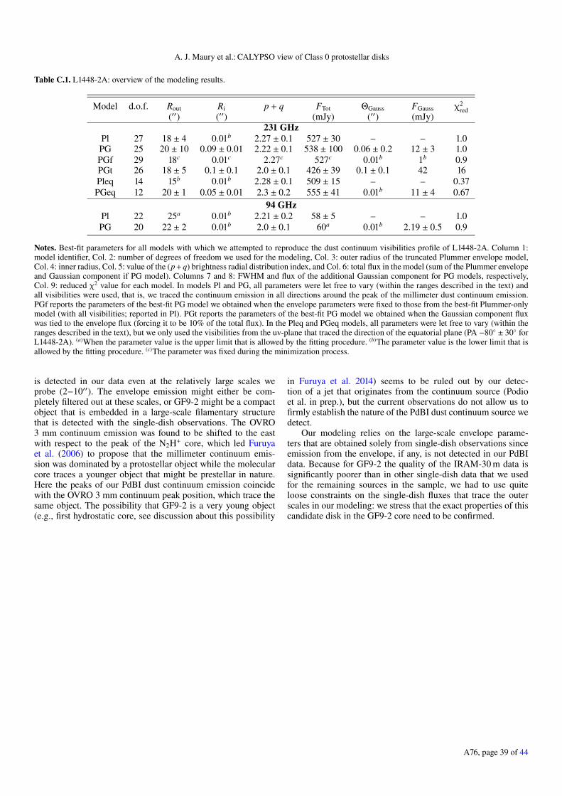
A. J. Maury et al.: CALYPSO view of Class 0 protostellar disks

Table C.1. L1448-2A: overview of the modeling results.

Model d.o.f. Rout Ri p + q FTot ΘGauss FGauss χ2red

(′′) (′′) (mJy) (′′) (mJy)231 GHz

Pl 27 18 ± 4 0.01b 2.27 ± 0.1 527 ± 30 – – 1.0PG 25 20 ± 10 0.09 ± 0.01 2.22 ± 0.1 538 ± 100 0.06 ± 0.2 12 ± 3 1.0PGf 29 18c 0.01c 2.27c 527c 0.01b 1b 0.9PGt 26 18 ± 5 0.1 ± 0.1 2.0 ± 0.1 426 ± 39 0.1 ± 0.1 42 16Pleq 14 15b 0.01b 2.28 ± 0.1 509 ± 15 – – 0.37PGeq 12 20 ± 1 0.05 ± 0.01 2.3 ± 0.2 555 ± 41 0.01b 11 ± 4 0.67

94 GHzPl 22 25a 0.01b 2.21 ± 0.2 58 ± 5 – – 1.0PG 20 22 ± 2 0.01b 2.0 ± 0.1 60a 0.01b 2.19 ± 0.5 0.9

Notes. Best-fit parameters for all models with which we attempted to reproduce the dust continuum visibilities profile of L1448-2A. Column 1:model identifier, Col. 2: number of degrees of freedom we used for the modeling, Col. 3: outer radius of the truncated Plummer envelope model,Col. 4: inner radius, Col. 5: value of the (p + q) brightness radial distribution index, and Col. 6: total flux in the model (sum of the Plummer envelopeand Gaussian component if PG model). Columns 7 and 8: FWHM and flux of the additional Gaussian component for PG models, respectively,Col. 9: reduced χ2 value for each model. In models Pl and PG, all parameters were let free to vary (within the ranges described in the text) andall visibilities were used, that is, we traced the continuum emission in all directions around the peak of the millimeter dust continuum emission.PGf reports the parameters of the best-fit PG model we obtained when the envelope parameters were fixed to those from the best-fit Plummer-onlymodel (with all visibilities; reported in Pl). PGt reports the parameters of the best-fit PG model we obtained when the Gaussian component fluxwas tied to the envelope flux (forcing it to be 10% of the total flux). In the Pleq and PGeq models, all parameters were let free to vary (within theranges described in the text), but we only used the visibilities from the uv-plane that traced the direction of the equatorial plane (PA −80 ± 30 forL1448-2A). (a)When the parameter value is the upper limit that is allowed by the fitting procedure. (b)The parameter value is the lower limit that isallowed by the fitting procedure. (c)The parameter was fixed during the minimization process.

is detected in our data even at the relatively large scales weprobe (2−10′′). The envelope emission might either be com-pletely filtered out at these scales, or GF9-2 might be a compactobject that is embedded in a large-scale filamentary structurethat is detected with the single-dish observations. The OVRO3 mm continuum emission was found to be shifted to the eastwith respect to the peak of the N2H+ core, which led Furuyaet al. (2006) to propose that the millimeter continuum emis-sion was dominated by a protostellar object while the molecularcore traces a younger object that might be prestellar in nature.Here the peaks of our PdBI dust continuum emission coincidewith the OVRO 3 mm continuum peak position, which trace thesame object. The possibility that GF9-2 is a very young object(e.g., first hydrostatic core, see discussion about this possibility

in Furuya et al. 2014) seems to be ruled out by our detec-tion of a jet that originates from the continuum source (Podioet al. in prep.), but the current observations do not allow us tofirmly establish the nature of the PdBI dust continuum source wedetect.

Our modeling relies on the large-scale envelope parame-ters that are obtained solely from single-dish observations sinceemission from the envelope, if any, is not detected in our PdBIdata. Because for GF9-2 the quality of the IRAM-30 m data issignificantly poorer than in other single-dish data that we usedfor the remaining sources in the sample, we had to use quiteloose constraints on the single-dish fluxes that trace the outerscales in our modeling: we stress that the exact properties of thiscandidate disk in the GF9-2 core need to be confirmed.

A76, page 39 of 44

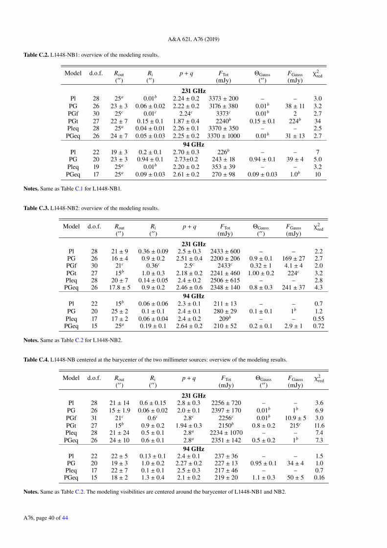
A&A 621, A76 (2019)

Table C.2. L1448-NB1: overview of the modeling results.

Model d.o.f. Rout Ri p + q FTot ΘGauss FGauss χ2red

(′′) (′′) (mJy) (′′) (mJy)

231 GHzPl 28 25a 0.01b 2.24 ± 0.2 3373 ± 200 – – 3.0PG 26 23 ± 3 0.06 ± 0.02 2.22 ± 0.2 3176 ± 380 0.01b 38 ± 11 3.2PGf 30 25c 0.01c 2.24c 3373c 0.01b 2 2.7PGt 27 22 ± 7 0.15 ± 0.1 1.87 ± 0.4 2240b 0.15 ± 0.1 224b 34Pleq 28 25a 0.04 ± 0.01 2.26 ± 0.1 3370 ± 350 – – 2.5PGeq 26 24 ± 7 0.05 ± 0.03 2.25 ± 0.2 3370 ± 1000 0.01b 31 ± 13 2.7

94 GHzPl 22 19 ± 3 0.2 ± 0.1 2.70 ± 0.3 226b – – 7PG 20 23 ± 3 0.94 ± 0.1 2.73±0.2 243 ± 18 0.94 ± 0.1 39 ± 4 5.0

Pleq 19 25a 0.01b 2.20 ± 0.2 353 ± 39 – – 3.2PGeq 17 25a 0.09 ± 0.03 2.61 ± 0.2 270 ± 98 0.09 ± 0.03 1.0b 10

Notes. Same as Table C.1 for L1448-NB1.

Table C.3. L1448-NB2: overview of the modeling results.

Model d.o.f. Rout Ri p + q FTot ΘGauss FGauss χ2red

(′′) (′′) (mJy) (′′) (mJy)

231 GHzPl 28 21 ± 9 0.36 ± 0.09 2.5 ± 0.3 2433 ± 600 – – 2.2PG 26 16 ± 4 0.9 ± 0.2 2.51 ± 0.4 2200 ± 206 0.9 ± 0.1 169 ± 27 2.7PGf 30 21c 0.36c 2.5c 2433c 0.32 ± 1 4.1 ± 4 2.0PGt 27 15b 1.0 ± 0.3 2.18 ± 0.2 2241 ± 460 1.00 ± 0.2 224c 3.2Pleq 28 20 ± 7 0.14 ± 0.05 2.4 ± 0.2 2506 ± 615 – – 2.8PGeq 26 17.8 ± 5 0.9 ± 0.2 2.46 ± 0.6 2348 ± 140 0.8 ± 0.3 241 ± 37 4.3

94 GHzPl 22 15b 0.06 ± 0.06 2.3 ± 0.1 211 ± 13 – – 0.7PG 20 25 ± 2 0.1 ± 0.1 2.4 ± 0.1 280 ± 29 0.1 ± 0.1 1b 1.2Pleq 17 17 ± 2 0.06 ± 0.04 2.4 ± 0.2 209b – – 0.55PGeq 15 25a 0.19 ± 0.1 2.64 ± 0.2 210 ± 52 0.2 ± 0.1 2.9 ± 1 0.72

Notes. Same as Table C.2 for L1448-NB2.

Table C.4. L1448-NB centered at the barycenter of the two millimeter sources: overview of the modeling results.

Model d.o.f. Rout Ri p + q FTot ΘGauss FGauss χ2red

(′′) (′′) (mJy) (′′) (mJy)

231 GHzPl 28 21 ± 14 0.6 ± 0.15 2.8 ± 0.3 2256 ± 720 – – 3.6PG 26 15 ± 1.9 0.06 ± 0.02 2.0 ± 0.1 2397 ± 170 0.01b 1b 6.9PGf 31 21c 0.6c 2.8c 2256c 0.01b 10.9 ± 5 3.0PGt 27 15b 0.9 ± 0.2 1.94 ± 0.3 2150b 0.8 ± 0.2 215c 11.6Pleq 28 21 ± 24 0.5 ± 0.1 2.8a 2234 ± 1070 – – 7.4PGeq 26 24 ± 10 0.6 ± 0.1 2.8a 2351 ± 142 0.5 ± 0.2 1b 7.3

94 GHzPl 22 22 ± 5 0.13 ± 0.1 2.4 ± 0.1 237 ± 36 – – 1.5PG 20 19 ± 3 1.0 ± 0.2 2.27 ± 0.2 227 ± 13 0.95 ± 0.1 34 ± 4 1.0

Pleq 17 22 ± 7 0.1 ± 0.1 2.5 ± 0.3 217 ± 46 – – 0.7PGeq 15 18 ± 2 1.3 ± 0.4 2.1 ± 0.2 219 ± 20 1.1 ± 0.3 50 ± 5 0.16

Notes. Same as Table C.2. The modeling visibilities are centered around the barycenter of L1448-NB1 and NB2.

A76, page 40 of 44

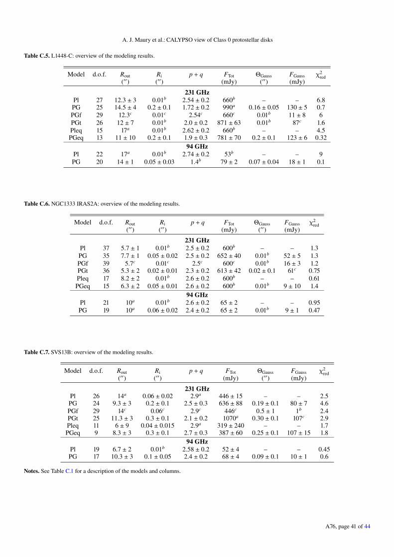
A. J. Maury et al.: CALYPSO view of Class 0 protostellar disks

Table C.5. L1448-C: overview of the modeling results.

Model d.o.f. Rout Ri p + q FTot ΘGauss FGauss χ2red

(′′) (′′) (mJy) (′′) (mJy)

231 GHzPl 27 12.3 ± 3 0.01b 2.54 ± 0.2 660b – – 6.8PG 25 14.5 ± 4 0.2 ± 0.1 1.72 ± 0.2 990a 0.16 ± 0.05 130 ± 5 0.7PGf 29 12.3c 0.01c 2.54c 660c 0.01b 11 ± 8 6PGt 26 12 ± 7 0.01b 2.0 ± 0.2 871 ± 63 0.01b 87c 1.6Pleq 15 17a 0.01b 2.62 ± 0.2 660b – – 4.5PGeq 13 11 ± 10 0.2 ± 0.1 1.9 ± 0.3 781 ± 70 0.2 ± 0.1 123 ± 6 0.32

94 GHzPl 22 17a 0.01b 2.74 ± 0.2 53b – – 9PG 20 14 ± 1 0.05 ± 0.03 1.4b 79 ± 2 0.07 ± 0.04 18 ± 1 0.1

Table C.6. NGC1333 IRAS2A: overview of the modeling results.

Model d.o.f. Rout Ri p + q FTot ΘGauss FGauss χ2red

(′′) (′′) (mJy) (′′) (mJy)

231 GHzPl 37 5.7 ± 1 0.01b 2.5 ± 0.2 600b – – 1.3PG 35 7.7 ± 1 0.05 ± 0.02 2.5 ± 0.2 652 ± 40 0.01b 52 ± 5 1.3PGf 39 5.7c 0.01c 2.5c 600c 0.01b 16 ± 3 1.2PGt 36 5.3 ± 2 0.02 ± 0.01 2.3 ± 0.2 613 ± 42 0.02 ± 0.1 61c 0.75Pleq 17 8.2 ± 2 0.01b 2.6 ± 0.2 600b – – 0.61PGeq 15 6.3 ± 2 0.05 ± 0.01 2.6 ± 0.2 600b 0.01b 9 ± 10 1.4

94 GHzPl 21 10a 0.01b 2.6 ± 0.2 65 ± 2 – – 0.95PG 19 10a 0.06 ± 0.02 2.4 ± 0.2 65 ± 2 0.01b 9 ± 1 0.47

Table C.7. SVS13B: overview of the modeling results.

Model d.o.f. Rout Ri p + q FTot ΘGauss FGauss χ2red

(′′) (′′) (mJy) (′′) (mJy)

231 GHzPl 26 14a 0.06 ± 0.02 2.9a 446 ± 15 – – 2.5PG 24 9.3 ± 3 0.2 ± 0.1 2.5 ± 0.3 636 ± 88 0.19 ± 0.1 80 ± 7 4.6PGf 29 14c 0.06c 2.9c 446c 0.5 ± 1 1b 2.4PGt 25 11.3 ± 3 0.3 ± 0.1 2.1 ± 0.2 1070a 0.30 ± 0.1 107c 2.9Pleq 11 6 ± 9 0.04 ± 0.015 2.9a 319 ± 240 – – 1.7PGeq 9 8.3 ± 3 0.3 ± 0.1 2.7 ± 0.3 387 ± 60 0.25 ± 0.1 107 ± 15 1.8

94 GHzPl 19 6.7 ± 2 0.01b 2.58 ± 0.2 52 ± 4 – – 0.45PG 17 10.3 ± 3 0.1 ± 0.05 2.4 ± 0.2 68 ± 4 0.09 ± 0.1 10 ± 1 0.6

Notes. See Table C.1 for a description of the models and columns.

A76, page 41 of 44

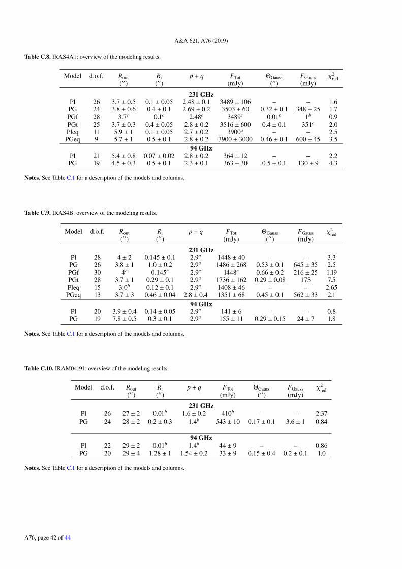
A&A 621, A76 (2019)

Table C.8. IRAS4A1: overview of the modeling results.

Model d.o.f. Rout Ri p + q FTot ΘGauss FGauss χ2red

(′′) (′′) (mJy) (′′) (mJy)

231 GHzPl 26 3.7 ± 0.5 0.1 ± 0.05 2.48 ± 0.1 3489 ± 106 – – 1.6PG 24 3.8 ± 0.6 0.4 ± 0.1 2.69 ± 0.2 3503 ± 60 0.32 ± 0.1 348 ± 25 1.7PGf 28 3.7c 0.1c 2.48c 3489c 0.01b 1b 0.9PGt 25 3.7 ± 0.3 0.4 ± 0.05 2.8 ± 0.2 3516 ± 600 0.4 ± 0.1 351c 2.0Pleq 11 5.9 ± 1 0.1 ± 0.05 2.7 ± 0.2 3900a – – 2.5PGeq 9 5.7 ± 1 0.5 ± 0.1 2.8 ± 0.2 3900 ± 3000 0.46 ± 0.1 600 ± 45 3.5

94 GHzPl 21 5.4 ± 0.8 0.07 ± 0.02 2.8 ± 0.2 364 ± 12 – – 2.2PG 19 4.5 ± 0.3 0.5 ± 0.1 2.3 ± 0.1 363 ± 30 0.5 ± 0.1 130 ± 9 4.3

Notes. See Table C.1 for a description of the models and columns.

Table C.9. IRAS4B: overview of the modeling results.

Model d.o.f. Rout Ri p + q FTot ΘGauss FGauss χ2red

(′′) (′′) (mJy) (′′) (mJy)

231 GHzPl 28 4 ± 2 0.145 ± 0.1 2.9a 1448 ± 40 – – 3.3PG 26 3.8 ± 1 1.0 ± 0.2 2.9a 1486 ± 268 0.53 ± 0.1 645 ± 35 2.5PGf 30 4c 0.145c 2.9c 1448c 0.66 ± 0.2 216 ± 25 1.19PGt 28 3.7 ± 1 0.29 ± 0.1 2.9a 1736 ± 162 0.29 ± 0.08 173 7.5Pleq 15 3.0b 0.12 ± 0.1 2.9a 1408 ± 46 – – 2.65PGeq 13 3.7 ± 3 0.46 ± 0.04 2.8 ± 0.4 1351 ± 68 0.45 ± 0.1 562 ± 33 2.1

94 GHzPl 20 3.9 ± 0.4 0.14 ± 0.05 2.9a 141 ± 6 – – 0.8PG 19 7.8 ± 0.5 0.3 ± 0.1 2.9a 155 ± 11 0.29 ± 0.15 24 ± 7 1.8

Notes. See Table C.1 for a description of the models and columns.

Table C.10. IRAM04191: overview of the modeling results.

Model d.o.f. Rout Ri p + q FTot ΘGauss FGauss χ2red

(′′) (′′) (mJy) (′′) (mJy)

231 GHzPl 26 27 ± 2 0.01b 1.6 ± 0.2 410b – – 2.37PG 24 28 ± 2 0.2 ± 0.3 1.4b 543 ± 10 0.17 ± 0.1 3.6 ± 1 0.84

94 GHzPl 22 29 ± 2 0.01b 1.4b 44 ± 9 – – 0.86PG 20 29 ± 4 1.28 ± 1 1.54 ± 0.2 33 ± 9 0.15 ± 0.4 0.2 ± 0.1 1.0

Notes. See Table C.1 for a description of the models and columns.

A76, page 42 of 44

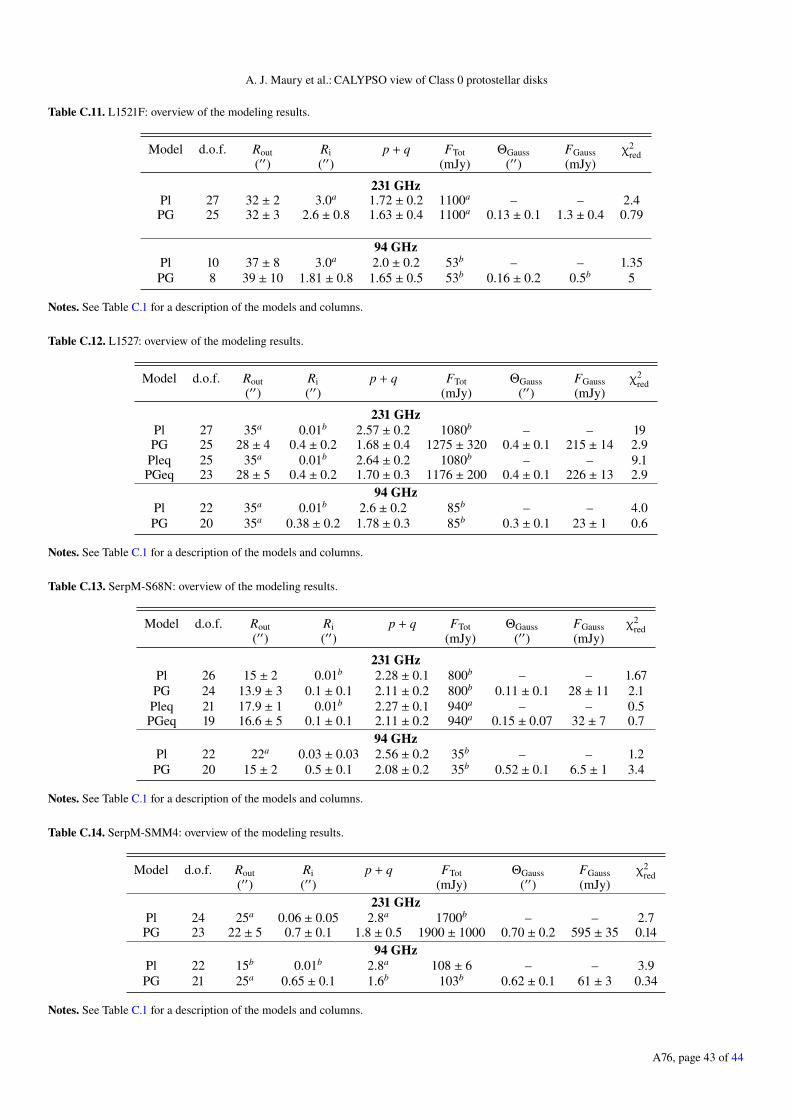
A. J. Maury et al.: CALYPSO view of Class 0 protostellar disks

Table C.11. L1521F: overview of the modeling results.

Model d.o.f. Rout Ri p + q FTot ΘGauss FGauss χ2red

(′′) (′′) (mJy) (′′) (mJy)

231 GHzPl 27 32 ± 2 3.0a 1.72 ± 0.2 1100a – – 2.4PG 25 32 ± 3 2.6 ± 0.8 1.63 ± 0.4 1100a 0.13 ± 0.1 1.3 ± 0.4 0.79

94 GHzPl 10 37 ± 8 3.0a 2.0 ± 0.2 53b – – 1.35PG 8 39 ± 10 1.81 ± 0.8 1.65 ± 0.5 53b 0.16 ± 0.2 0.5b 5

Notes. See Table C.1 for a description of the models and columns.

Table C.12. L1527: overview of the modeling results.

Model d.o.f. Rout Ri p + q FTot ΘGauss FGauss χ2red

(′′) (′′) (mJy) (′′) (mJy)

231 GHzPl 27 35a 0.01b 2.57 ± 0.2 1080b – – 19PG 25 28 ± 4 0.4 ± 0.2 1.68 ± 0.4 1275 ± 320 0.4 ± 0.1 215 ± 14 2.9Pleq 25 35a 0.01b 2.64 ± 0.2 1080b – – 9.1PGeq 23 28 ± 5 0.4 ± 0.2 1.70 ± 0.3 1176 ± 200 0.4 ± 0.1 226 ± 13 2.9

94 GHzPl 22 35a 0.01b 2.6 ± 0.2 85b – – 4.0PG 20 35a 0.38 ± 0.2 1.78 ± 0.3 85b 0.3 ± 0.1 23 ± 1 0.6

Notes. See Table C.1 for a description of the models and columns.

Table C.13. SerpM-S68N: overview of the modeling results.

Model d.o.f. Rout Ri p + q FTot ΘGauss FGauss χ2red

(′′) (′′) (mJy) (′′) (mJy)

231 GHzPl 26 15 ± 2 0.01b 2.28 ± 0.1 800b – – 1.67PG 24 13.9 ± 3 0.1 ± 0.1 2.11 ± 0.2 800b 0.11 ± 0.1 28 ± 11 2.1

Pleq 21 17.9 ± 1 0.01b 2.27 ± 0.1 940a – – 0.5PGeq 19 16.6 ± 5 0.1 ± 0.1 2.11 ± 0.2 940a 0.15 ± 0.07 32 ± 7 0.7

94 GHzPl 22 22a 0.03 ± 0.03 2.56 ± 0.2 35b – – 1.2PG 20 15 ± 2 0.5 ± 0.1 2.08 ± 0.2 35b 0.52 ± 0.1 6.5 ± 1 3.4

Notes. See Table C.1 for a description of the models and columns.

Table C.14. SerpM-SMM4: overview of the modeling results.

Model d.o.f. Rout Ri p + q FTot ΘGauss FGauss χ2red

(′′) (′′) (mJy) (′′) (mJy)231 GHz

Pl 24 25a 0.06 ± 0.05 2.8a 1700b – – 2.7PG 23 22 ± 5 0.7 ± 0.1 1.8 ± 0.5 1900 ± 1000 0.70 ± 0.2 595 ± 35 0.14

94 GHzPl 22 15b 0.01b 2.8a 108 ± 6 – – 3.9PG 21 25a 0.65 ± 0.1 1.6b 103b 0.62 ± 0.1 61 ± 3 0.34

Notes. See Table C.1 for a description of the models and columns.

A76, page 43 of 44

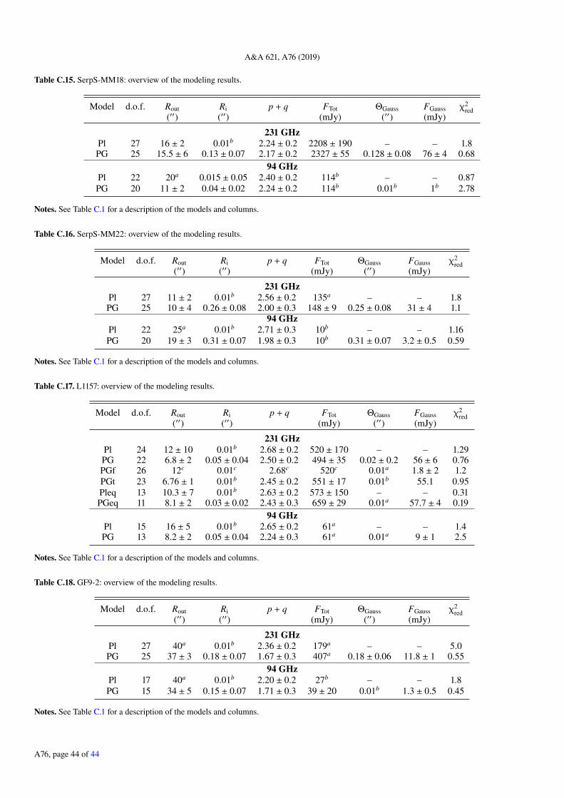
A&A 621, A76 (2019)

Table C.15. SerpS-MM18: overview of the modeling results.

Model d.o.f. Rout Ri p + q FTot ΘGauss FGauss χ2red

(′′) (′′) (mJy) (′′) (mJy)

231 GHzPl 27 16 ± 2 0.01b 2.24 ± 0.2 2208 ± 190 – – 1.8PG 25 15.5 ± 6 0.13 ± 0.07 2.17 ± 0.2 2327 ± 55 0.128 ± 0.08 76 ± 4 0.68

94 GHzPl 22 20a 0.015 ± 0.05 2.40 ± 0.2 114b – – 0.87PG 20 11 ± 2 0.04 ± 0.02 2.24 ± 0.2 114b 0.01b 1b 2.78

Notes. See Table C.1 for a description of the models and columns.

Table C.16. SerpS-MM22: overview of the modeling results.

Model d.o.f. Rout Ri p + q FTot ΘGauss FGauss χ2red

(′′) (′′) (mJy) (′′) (mJy)

231 GHzPl 27 11 ± 2 0.01b 2.56 ± 0.2 135a – – 1.8PG 25 10 ± 4 0.26 ± 0.08 2.00 ± 0.3 148 ± 9 0.25 ± 0.08 31 ± 4 1.1

94 GHzPl 22 25a 0.01b 2.71 ± 0.3 10b – – 1.16PG 20 19 ± 3 0.31 ± 0.07 1.98 ± 0.3 10b 0.31 ± 0.07 3.2 ± 0.5 0.59

Notes. See Table C.1 for a description of the models and columns.

Table C.17. L1157: overview of the modeling results.

Model d.o.f. Rout Ri p + q FTot ΘGauss FGauss χ2red

(′′) (′′) (mJy) (′′) (mJy)

231 GHzPl 24 12 ± 10 0.01b 2.68 ± 0.2 520 ± 170 – – 1.29PG 22 6.8 ± 2 0.05 ± 0.04 2.50 ± 0.2 494 ± 35 0.02 ± 0.2 56 ± 6 0.76PGf 26 12c 0.01c 2.68c 520c 0.01a 1.8 ± 2 1.2PGt 23 6.76 ± 1 0.01b 2.45 ± 0.2 551 ± 17 0.01b 55.1 0.95Pleq 13 10.3 ± 7 0.01b 2.63 ± 0.2 573 ± 150 – – 0.31PGeq 11 8.1 ± 2 0.03 ± 0.02 2.43 ± 0.3 659 ± 29 0.01a 57.7 ± 4 0.19

94 GHzPl 15 16 ± 5 0.01b 2.65 ± 0.2 61a – – 1.4PG 13 8.2 ± 2 0.05 ± 0.04 2.24 ± 0.3 61a 0.01a 9 ± 1 2.5

Notes. See Table C.1 for a description of the models and columns.

Table C.18. GF9-2: overview of the modeling results.

Model d.o.f. Rout Ri p + q FTot ΘGauss FGauss χ2red

(′′) (′′) (mJy) (′′) (mJy)

231 GHzPl 27 40a 0.01b 2.36 ± 0.2 179a – – 5.0PG 25 37 ± 3 0.18 ± 0.07 1.67 ± 0.3 407a 0.18 ± 0.06 11.8 ± 1 0.55

94 GHzPl 17 40a 0.01b 2.20 ± 0.2 27b – – 1.8PG 15 34 ± 5 0.15 ± 0.07 1.71 ± 0.3 39 ± 20 0.01b 1.3 ± 0.5 0.45

Notes. See Table C.1 for a description of the models and columns.

A76, page 44 of 44